1.differential equations for engineers. wei-chau xie. cambridge university press 978-0-511-77622-9...
TRANSCRIPT


1. Differential equations for engineers. Wei-Chau Xie. Cambridge University Press 978-0-511-77622-9
2. Differential Equations with Applications and Historical Notes. Second edition. Simmons
3. Differential Equations, third edition. Shepley L. Ross
4. Differential Equations. Linear, Nonlinear, Ordinary, Partial. A.C. King, J. Billingham and S.R. Otto 0521016878
5. Ordinary and Partial Differential Equations. Agarwal & Regan. 0387791450

I. Ecuaciones diferenciales de primer orden1. Teoría básica y métodos de solución. 2. Breviario de aplicaciones físicas.
II. Ecuaciones diferenciales de segundo orden1. Ecuaciones homogéneas de coeficientes constantes. 2. Ecuación de Euler-Cauchy. 3. Ecuaciones heterogénea y métodos de solución.
Coeficientes indeterminados y variación de parámetros. 4. Solución en series de potencias. 5. Ecuaciones diferenciales de Bessel, Legendre, Hermite y Laguerre 6. Solución usando transformada de Fourier.7. Funciones especiales: gamma y error.
III. Introducción a las ecuaciones en derivadas parciales1. Ecuaciones lineales y separación de variables. 2. Problemas de condición de frontera, valores propios y funciones
propias. 3. Ecuaciones especiales: de difusión, de onda y de Laplace. 4. Solución en series de Fourier.

1 1 1
2 2 2
1 2 1 2 1 2
1
, , ,
, , , .
y P x y Q x y x
y a y a
y b y b
P Q a b
Resolver
con las condiciones a la frontera
Las funciones son continuas en
Las cantidades , , , , , son constantes reales.
Suponemos que 1
2 2
y no son cero ambas,
y suponemos que y no son cero ambas.
La letra es un parámetro arbitrario.

1 2, 0 0.x
Se dice que el problema es homogéneo si
y
En caso contrario es inhomogéneo o
no homogéneo.
1 1 1
2 2 2
, , ,y P x y Q x y x
y a y a
y b y b
Resolver
con las condiciones a la frontera

2
2
0
10
0 0 0.
10.
2
t
d I t dI tRI t t t t t
dt L dt LC
dI tI t
dt
R
LLC
Resolver el problema de valores iniciales,
;
con y
Suponemos que

2
2
0
10
10 0 0. 0.
2t
d I t dI tRI t t t t t
dt L dt LC
dI t RI t
dt LLC
Resolver el problema de valores iniciales,
;
con y Suponemos que
, ,2
,
Rb neper frequency
Lattenuation
Definimos la frecuencia is called the or
and is a measure of how fast the transient response
of the circuit will die away after the stimulus has been removed.
Definimo
0
1
LC
I t y t
s que es la frecuencia angular de resonancia.
Asociamos

2202
0
0
2 0
0 0 0.
0.
t
d y t dy tb y t t t t t
dt dt
dy ty t
dt
b
Resolver el problema de valores iniciales,
;
con
y
Suponemos que
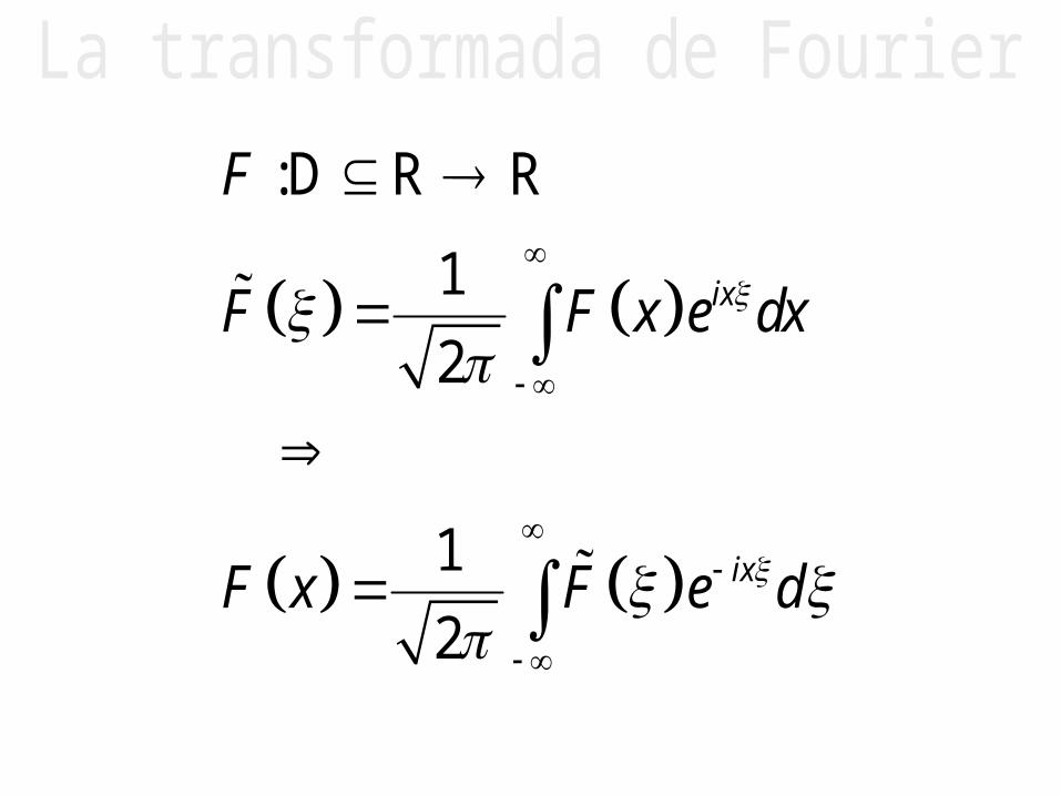
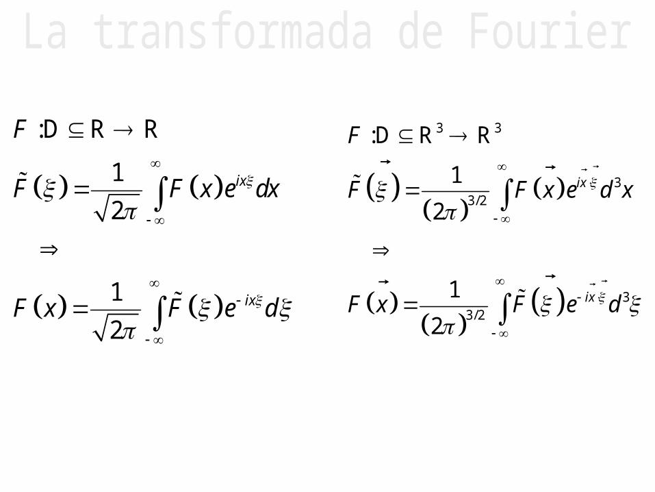
:
1
2
1
2
ix
ix
F
F F x e dx
F x F e d
D R R

2202
2202
2
2
d y t dy tb y t t t
dt dt
d y t dy tb y t t t
dt dt
F F
F F F F
2202
0
2 0
0 0 0t
d y t dy tb y t t t t t
dt dt
dy ty t
dt
Resolver el problema de valores iniciales,
;
con
y

:
1 1
2 2ix ix
F
F F x e dx F x F e d
D R R
n
n
n
d f xi f x
dx
F F

1 1
2 2i t i tt t t t e dt e
F
:
1
2
1
2
ix
ix
F
F F x e dx
F x F e d
D R R

2 20
2 20
2 20
12
21
22
1
22
i t
i t
i t
y ib y y e
ib y e
ey
ib
2
202
2d y t dy t
b y t t tdt dt
F F F F
2202
0
2 0
0 0 0t
d y t dy tb y t t t t t
dt dt
dy ty t
dt
;
y

2202
2 20
2
1
22
i t
d y t dy tb y t t t
dt dt
ey
ib
F F F F
2202
0
2 0
0 0 0t
d y t dy tb y t t t t t
dt dt
dy ty t
dt
;
y
2 20
2 20
1 1
22 2
1
2 2
i ti t
i t t
ey t e d
ib
e d
ib

02 20
10
2 2
i t te dy t b
ib
;
2 2 2 2 2 2 2 20 0 0 0
i t t iz t te d e d
ib b ib b z ib b z ib b
( )
k
f z
D
z
C
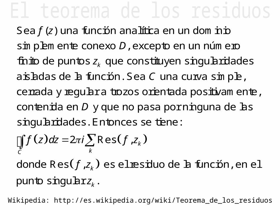
Sea una función analítica en un dominio
simplemente conexo , excepto en un número
finito de puntos que constituyen singularidades
aisladas de la función. Sea una curva simple,
cerrada y re
gular
2 ,
,
kkC
k
D
f z dz i f z
f z
z
a trozos orientada positivamente,
contenida en y que no pasa por ninguna de las
singularidades. Entonces se tiene:
Res
donde Res es el residuo de la función, en el
punto singular .k
Wikipedia: http://es.wikipedia.org/wiki/Teorema_de_los_residuos

0
0
0
1,
2
( )
C
f z f z dz
f z z z
i
C
R
z
Se denomina residuo de una función analítica
en una singularidad aislada al número
Res
donde representa una circunferencia de centro
y radio en cuyo interior no hay pu
ntos
0.z
singulares
de la función salvo
Wikipedia: http://es.wikipedia.org/wiki/Residuo_(análisis_complejo)

0
0
0
1,
2
( )
C
f z f z dz Ci
R
f z z z
z
Se denomina residuo de una función analítica en una singularidad aislada
al número Res donde representa una circunferencia de centro
y radio en cuyo interior no hay
pun 0.ztos singulares de la función salvo
Wikipedia: http://es.wikipedia.org/wiki/Residuo_(análisis_complejo)
0
0
0
0
1
0 01
( )
( , ) 0
( )
1( , )
1 !limN
N
Nz z
f z z
f z
f z N z
df z z z f z
N dz
Si tiene una singularidad evitable en , el residuo es
Res .
Si tiene un polo de orden en , entonces el residuo
se puede calcular como:
Res
Si e 0
0
,
.
.
1
z
z
l punto es una singularidad esencial el residuo se
calcula desarrollando la función en serie de Laurent en torno a
El residuo es el coeficiente correspondiente a la potencia de
exponente


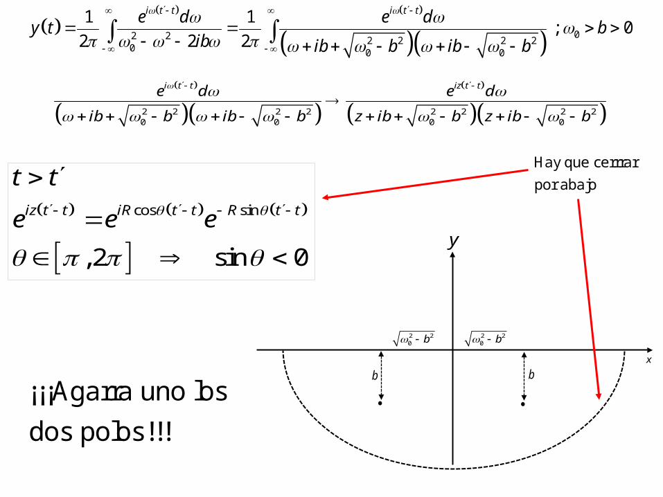
02 20
10
2 2
i t te dy t b
ib
;
2 2 2 2 2 2 2 20 0 0 0
i t t iz t te d e d
ib b ib b z ib b z ib b
b b
2 20 b 2 2
0 b
x
y
cos sin
0, sin 0
iz t t iR t t R t t
t t
e e e
Hay que cerrrar
por arriba
0y t
02 2 2 2 2 20 0 0
1 10
2 2 2
i t t i t te d e dy t b
ib ib b ib b
;
2 2 2 2 2 2 2 20 0 0 0
i t t iz t te d e d
ib b ib b z ib b z ib b
b b
2 20 b 2 2
0 b
x
y
Hay que cerrrar
por abajo
¡¡¡Agarra uno los
dos polos!!!
cos sin
, 2 sin 0
iz t t iR t t R t t
t t
e e e

2 2 2 20 0
2 2 2 20 0
2 2 2 22 2 2 20 00 0
2 22 2
i t t ib b i t t ib biz t t iz t t
z ib b z ib b
e d e e d e
z ibz z ibzb b
Res ; Res
02 2 2 2 2 20 0 0
1 10
2 2 2
i t t i t te d e dy t b
ib ib b ib b
;
b b
2 20 b 2 2
0 b
x
y
02 2 2 2 2 20 0 0
1 10
2 2 2
i t t i t te d e dy t b
ib ib b ib b
;
b b
2 20 b 2 2
0 b
x
y
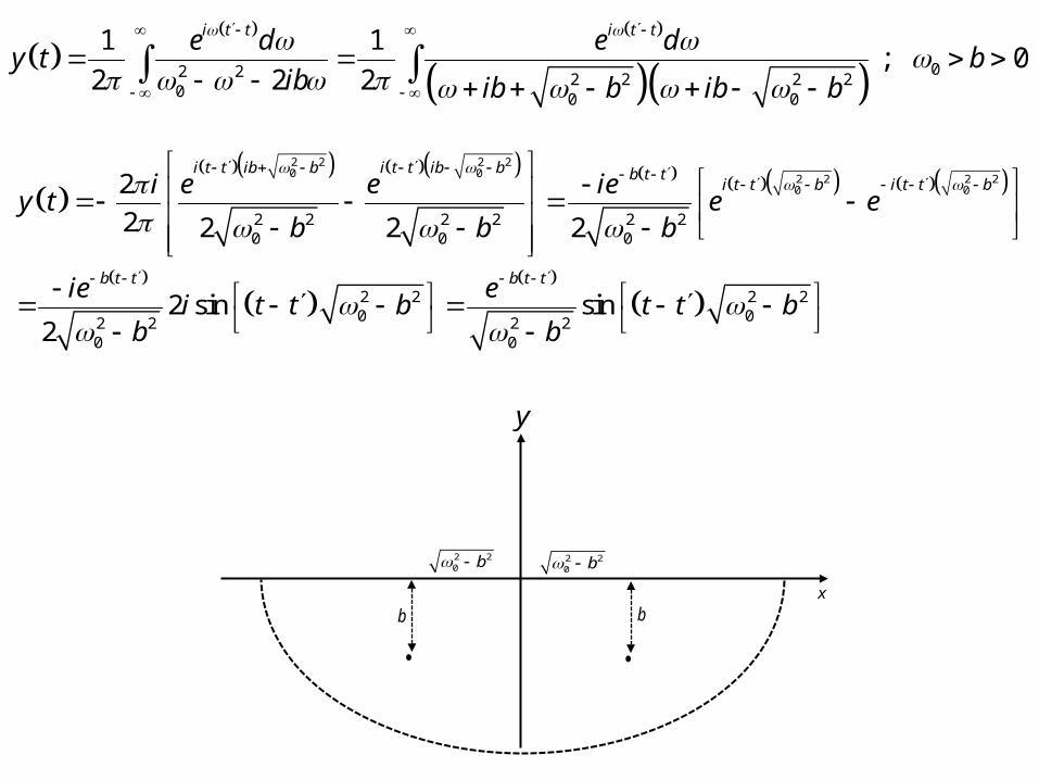
2 2 2 20 0 2 2 2 2
0 0
2 2 2 2 2 20 0 0
2 2 2 20 02 2 2 2
0 0
2
2 2 2 2
2 sin sin2
i t t ib b i t t ib b b t ti t t b i t t b
b t t b t t
i e e iey t e e
b b b
ie ei t t b t t b
b b

2 20
0
sinb t t
t t
y t t te t t
b
2202
0
2 0
0 0 0t
d y t dy tb y t t t t t
dt dt
dy ty t
dt
;
y

2
2
0
10
10 0 0, 0
2t
d I t dI tRI t t t t t
dt L dt LC
dI t RI t
dt LLC
;
con y
2
2
0
sin
1 4
2
Rt t
L
t t
I t t te t t
LR
L C

2
sinRt t
Lt t
I t e
250 0.06 3.5
0.02
R L C
t
, H, F
s
I (A)
t (s)

2202
0
2 0
0 0
0
0 0 0t
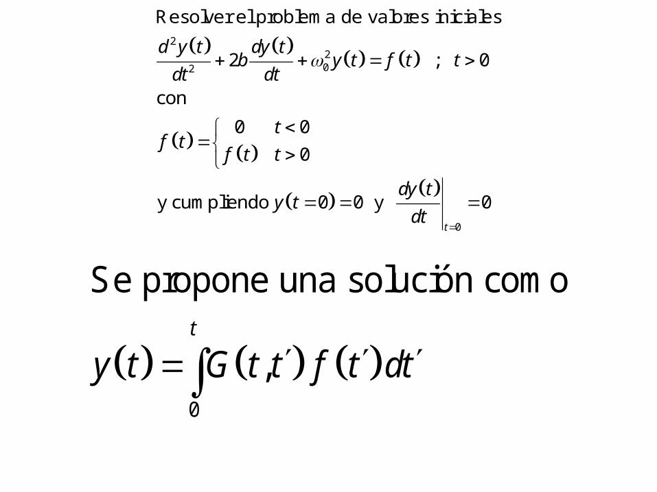
d y t dy tb y t f t t
dt dt
tf t
f t t
dy ty t
dt
Resolver el problema de valores
iniciales
;
con
y cumpliendo y
2202
0
2 0
0 0
0
0 0 0t
d y t dy tb y t f t t
dt dt
tf t
f t t
dy ty t
dt
Resolver el problema de valores iniciales
;
con
y cumpliendo y
0
,t
y t G t t f t dt
Se propone una solución como

2202
0 0 0
2202
0 0 0
2202
0
, 2 , ,
, ,2 ,
, ,2 ,
t t t
t t t
t
d dG t t f t dt b G t t f t dt G t t f t dt f t
dt dt
d G t t dG t tf t dt b f t dt G t t f t dt f t
dt dt
d G t t dG t tb G t t f t dt f t
dt dt
2202
0
2 0
0 0
0
0 0 0t
d y t dy tb y t f t t
dt dt
tf t
f t t
dy ty t
dt
Resolver el problema de valores iniciales
;
con
y cumpliendo y
0
,t
y t G t t f t dt Se propone

2202
0
, ,¡¡¡¡ 2 , !!!!
t
d G t t dG t tb G t t t t
dt dt
t t f t dt f t
f t f t
Si
y
2202
0
2202
0
2 0
,
, ,2 ,
t
t
d y t dy tb y t f t t
dt dt
y t G t t f t dt
d G t t dG t tb G t t f t dt f t
dt dt
;
Se propone

0
2 20
sintb t t t t
y t e f t dt
b
2202
0
2 0
0 0
0
0 0 0t
d y t dy tb y t f t t
dt dt
tf t
f t t
dy ty t
dt
Resolver el problema de valores iniciales
;
con
y cumpliendo y
0
2202
,
, ,2 ,
t
y t G t t f t dt
d G t t dG t tb G t t t t
dt dt
sin, b t t t t
G t t e
Del problema anterior

2202
0
2 0
0 0
0
0 0 0t
d y t dy tb y t f t t
dt dtt
f tf t t
dy ty t
dt
;
y

2202
2 20
2 20
2 0
2
2
d y t dy tb y t f t t
dt dt
y ib y y f
fy
ib
;

12 20 2
fy t
ib
F
2202
2 20
2 0
2
d y t dy tb y t f t t
dt dt
fy
ib
;

12 *
*
.
f g f t g t
f t g t f g t d
f g
donde
es la convolución de y
F
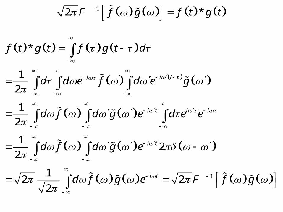
1
*
1
2
1
2
12
2
12 2
2
i ti
i t i i
i t
i t
f t g t f g t d
d d e f d e g
d f d g e d e e
d f d g e
d f g e f g
F
12 *f g f t g t F
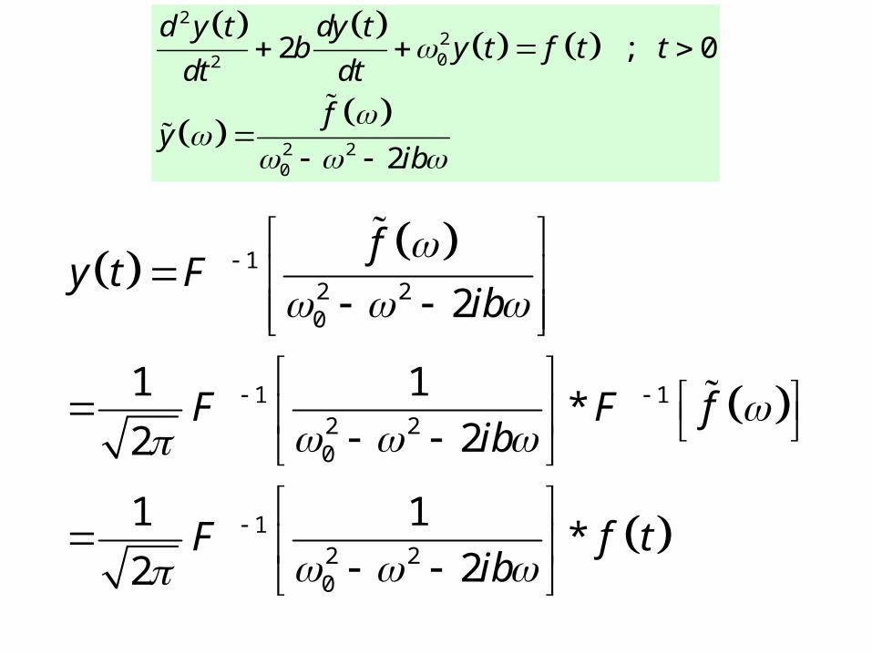
12 20
1 12 20
12 20
2
1 1*
22
1 1*
22
fy t
ib
fib
f tib
F
F F
F
2202
2 20
2 0
2
d y t dy tb y t f t t
dt dt
fy
ib
;

12 20
1*
2y t f t
ib
F
12 2 2 20 0
2 20
1 1
2 22
0 0
sin2 0
i t
bt
ed
ib ib
t
te t
b
F
2202
2 20
2 0
2
d y t dy tb y t f t t
dt dt
fy
ib
;

0
2 20
sintb t t t t
y t e f t dt
b
2202
2 20
2 0
2
d y t dy tb y t f t t
dt dt
fy
ib
;
12 20
12 20
1*
2
0 01
sin2 2 0bt
y t f tib
t
tib e t
F
F

2
2
0
0
10
10 0 0, 0
2
0 0
sin 0
t
f
d I t dI tRI t V t t t
dt L dt LC
dI t RI t
dt LLC
tV t
V t t
;
con y

2
2
0
0
10
10 0 0, 0
2
0 0
cos 0
t
f f
d I t dI tRI t V t t t
dt L dt LC
dI t RI t
dt LLC
tV t
V t t
;
con y
2
0
2
sin
1 4
2
t Rt t
Lt t
I t e V t dt
LR
L C
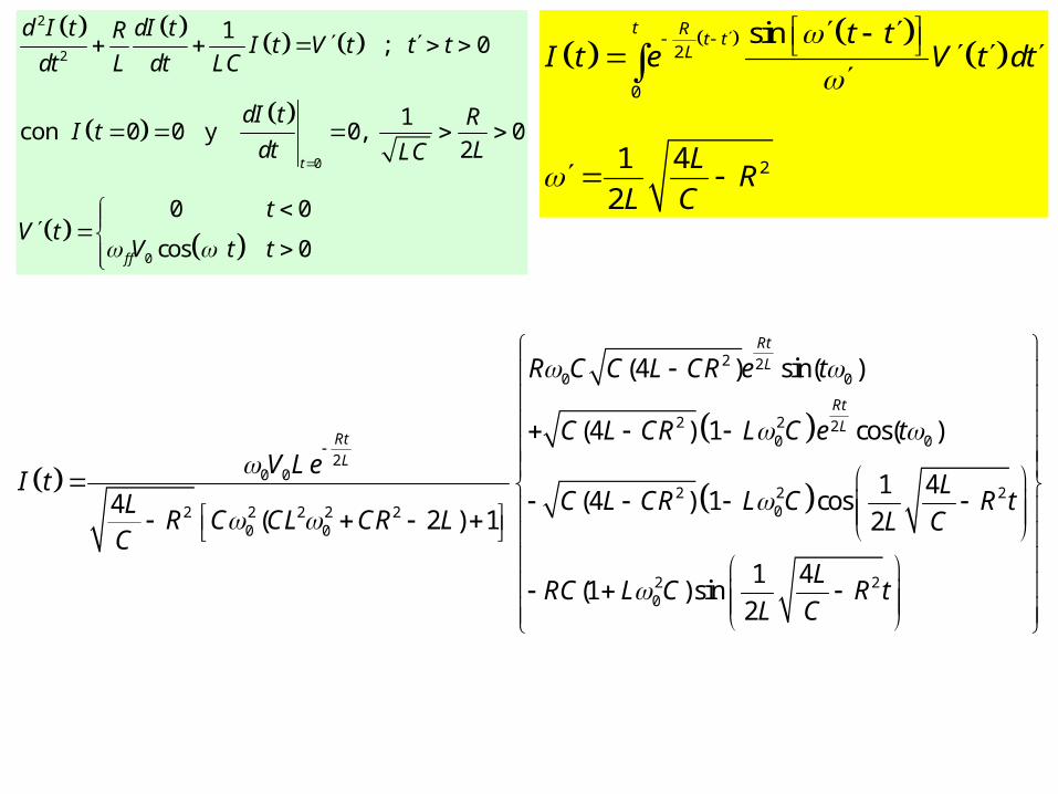
2 20 0
2 2 20 0
20 0
2 2 202 2 2 2 2
0 0
2 20
(4 ) sin( )
(4 ) 1 cos( )
4(
14 ) 1 cos4
( 2 ) 1 2
1 4(1 )sin
2
Rt
L
Rt
LRt
L
R C L CR e t
C L CR L e tV Le
I t LC L CR L R tL
R C CL CR L L CC
L
C
RCC
C
t
C
CL RL
2
2
0
0
10
10 0 0, 0
2
0 0
cos 0
t
f f
d I t dI tRI t V t t t
dt L dt LC
dI t RI t
dt LLC
tV t
V t t
;
con y
2
0
2
sin
1 4
2
t Rt t
Lt t
I t e V t dt
LR
L C

0 0250 0.06 3.5 60 110R L C V , H, F, Hz, V
I (A)
t (s)


2 , , , ,
, , , ,
x y z f x y z
x y z g x y z
en
en
D
D

2
2
0
0
h p
h
p p
g
f
donde
en , en
y donde
en , en
D D
D D
2 , , , ,
, , , ,
x y z f x y z
x y z g x y z
en
en
D
D
:
1
2
1
2
ix
ix
F
F F x e dx
F x F e d
D R R
3 3
33/2
33/2
:
1
2
1
2
ix
ix
F
F F x e d x
F x F e d
D R R

3 3
3 3
2
2 3 3
3 3
i x i x
ii xx
x
e d f e d
d fe e d
R R
R R
3 3
3 33/2 3/2
1 1
2 2i x i xx e d f x f e d
;
R R
2 f

2 2 22
2 2 2
2 2 2
2 2 2
2 2 2
2
exp
exp exp exp
exp
i xx x y z
x y z x y z x y z
x y z x y z
i x
e i x y zx y z
i x y z i x y z i x y z
x y z
i x y z
e
3 3
2 3 3i xx
i xd f e de
R R
22x

3 3
2 3 3i xx
i xd f e de
R R
2 f
3 3
3 3
2
2i i xxd f e d
f
e
R R

3
3 3
3 3
3 3
33/2 2
3 33/2 2 3/2
3 33 2
3 33 2
1
2
1 1 1
2 2
1 1
2
1
2
i x
i i x
i i x
i x
fx e d
f e d e d
f e e d d
ef d d
R
R R
R R
R R
22 f f

3 3
3 33 2
1
2
i xex f d d
R R 2
2
f
f
3 3
cos2 3
3 2
1sin
2
ir xex f r drd d d
r
R R

3
2coscos2
20 0 0
sin sinir x
ir xer drd d dr d e d
r
R
I
cos
0 0
2 sin ir xdr d e
I
2
0
2d
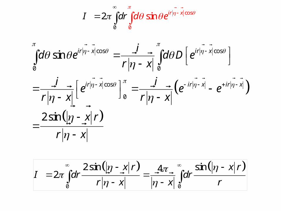
cos cos
0 0
cos
0
sin
2sin
ir x ir x
ir x ir x ir x
id e d D e
r x
i ie e e
r x r x
x r
r x
cos
00
2 sin ir xd d er
I
0 0
2sin sin42
x r x rdr dr
r x x r
I

0
sin4 x rdr
x r
I
0
sin 1 sin 1Im
2 2
ied d d
p.v. p.v.
0 0 0 0
sin sin sin sinqd d dq d
q

ied
p.v.


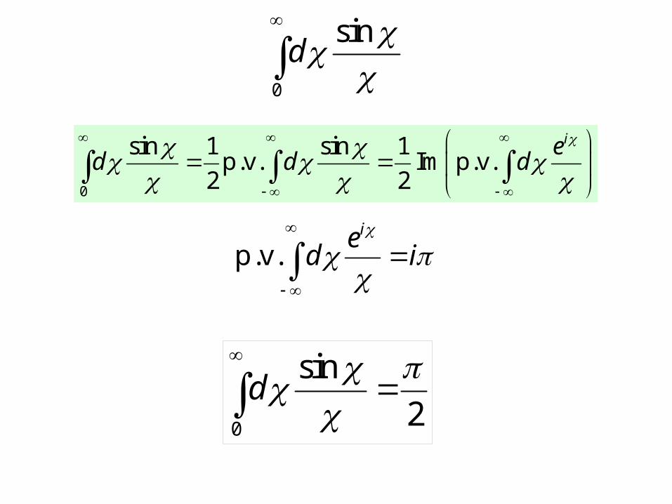
0
sind
0
sin 1 sin 1Im
2 2
ied d d
p.v. p.v.
ied i
p.v.
0
sin
2d

0 0
sin4 sin
2
x rdr d
x r
; I
22
x
I

3 3
cos2 3
3 2
1sin
2
ir xex f r drd d d
r
R R
3
cos 22
2
2sin
ir xer drd d
r x
R
2
2
f
f
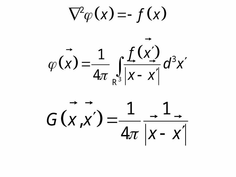
3
31
4
fx d
x
R
3
2
31
4
x f x
f xx d x
x x
R
1 1,
4G x x
x x

3
2
31
4
x f x
f xx d x
x x
R
1 1,
4G x x
x x
3
2 2
11. , ,
4
2. , ,
3. , 0
x x
x x
x xG x x G x x x x
x x
G x x G x x x x
G x x x x
,
, para y para

3
2
3,
x f x
x f x G x x d x
R
1 1,
4G x x
x x
3 3
3
2
2
2
2 3 3
2 3
2
,
,
,
,
,
x
x
x
x
x
x
G x x x x
f x G x x f x x x
f x G x x f x x x
f x G x x d x f x x x d x
f x G x x d x f x
x f x
R R
R