2 integration - birkbeck, university of londonecon109.econ.bbk.ac.uk/brad/advcalc/notes 2...
TRANSCRIPT
Advanced Calculus Chapter 2 Integration 18
2 Integration
2.1 Methods of Integration
Recall that integration is the reverse process of differentiation,and is consequently sometimes referred to as anti-differentiation.More specifically, if f is a function of one variable x then an integralof f is a function F such that dF
dx= f(x). We write
F (x) =
∫f(x) dx.
For any constant c, since ddx
(c) = 0, we have ddx
(F (x) + c) = f(x).
Thus there are infinitely many possibilities for
∫f(x) dx. This does
not usually cause a problem as we always add a constant to anyintegral derived. An alternative approach is to include limits in theintegral and write
F (x) =
∫ x
a
f(x) dx.
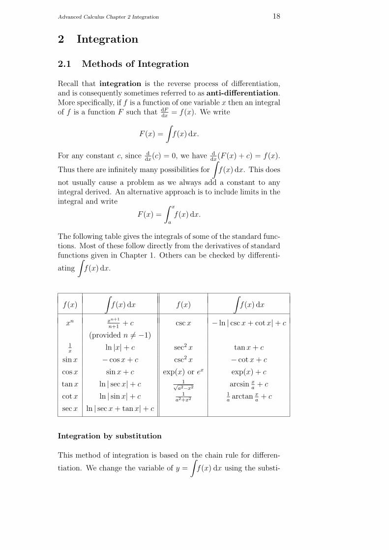
The following table gives the integrals of some of the standard func-tions. Most of these follow directly from the derivatives of standardfunctions given in Chapter 1. Others can be checked by differenti-
ating
∫f(x) dx.
f(x)
∫f(x) dx f(x)
∫f(x) dx
xn xn+1
n+1+ c csc x − ln | csc x + cot x|+ c
(provided n 6= −1)1x
ln |x|+ c sec2 x tan x + c
sin x − cos x + c csc2 x − cot x + c
cos x sin x + c exp(x) or ex exp(x) + c
tan x ln | sec x|+ c 1√a2−x2 arcsin x
a+ c
cot x ln | sin x|+ c 1a2+x2
1aarctan x
a+ c
sec x ln | sec x + tan x|+ c
Integration by substitution
This method of integration is based on the chain rule for differen-
tiation. We change the variable of y =
∫f(x) dx using the substi-

Advanced Calculus Chapter 2 Integration 19
tution x = g(u). Then, since integration is the reverse of differen-
tiation, we havedy
dx= f(x). Thus by the chain rule
dy
du=
dy
dx
dx
du
= f(x)dx
du
= f(g(u))dx
du
So integrating the final expression for dydu
, with respect to u, we get
y =
∫f(g(u))
dx
dudu. Comparing the two expressions for y we get
∫f(x) dx =
∫f(g(u))
dx
dudu.
When evaluating a definite integral, if we use a substitution tochange the variable from x to a function u of x, it is usually easiestto change the limits of integration from x values to u values. (Thissaves having to convert back to x again after integrating.)
Specifically, if u = u(x), then
∫ b
a
f(x) dx =
∫ u(b)
u(a)
f(u)dx
dudu.
Integration by Parts
If u and v are functions of x then the product rule for differentiationgives:
∫u
dv
dxdx = uv −
∫vdu
dxdx.
This is the formula for integration by parts.
Integration by parts is useful for integrating products where onefactor (u) will differentiate to give a simpler function, and where it
is possible to integrate the other factor
(dv
dx
).
Exercises 2.1
1. Integrate the following expressions with respect to x.
Advanced Calculus Chapter 2 Integration 20
(a) 3x5 − 2x2 + 3x− 2; (b) 4x3 − 5
x5 ; (c) x3+3x2
x+1;
(d) (3x + 1)5; (e) sin(3x− 2); (f) 2x(x2 + 7)8;
(g) xe 2x2; (h) sin7 x cos x; (i) tan x;
(j) x+3x2+4
; (k) x cos x; (l) x(x + 1)10;
(m) x sin 2x; (n) xe−x; (o) x2ex;
(p) arctan x; (q) ln x; (q) arccos x.
2. Evaluate each of the following integrals using the given sub-stitution.
(a)
∫dx
x ln x, u = ln x.
(b)
∫4x
(3− 2x)2dx, u = 3− 2x.
(c)
∫sec5 x tan x dx, u = sec x.
(d)
∫2e2x
1 + e4xdx, u = e2x.
(e)
∫5 sin7 x dx, u = cos x.
(f)
∫14x2
√1 + x dx, x = u2 − 1.
(g)
∫ √1− x2 dx, x = sin u.
2.2 Integrals with infinite limits
It is sometimes possible to evaluate a definite integral that has one,or both, of its limits equal to infinity or negative infinity. We define
∫ ∞
a
f(x) dx = limX→∞
∫ X
a
f(x) dx.
If the limit exists then the definite integral exists and its value isthe limit; otherwise the definite integral does not exist.
When evaluating limits to infinity we make use of the following
results: (i) limX→∞
g(X) = limX→0
g
(1
X
); (ii) lim
X→∞A−X = 0, for all
real numbers A, with A > 1.
Advanced Calculus Chapter 2 Integration 21
Example 1 Evaluate
∫ ∞
1
dx
x3.
∫ ∞
1
dx
x3= lim
X→∞
∫ X
1
dx
x3,
= limX→∞
∫ X
1
x−3 dx,
= limX→∞
[−1
2x−2
]X
1
,
= limX→∞
[− 1
2x2
]X
1
,
= limX→∞
(− 1
2X2+
1
2
),
= limX→0
(−1
2X2 +
1
2
),
=1
2.
Example 2 Let a ∈ R. Evaluate
∫ ∞
a
e−x dx.
∫ ∞
a
e−x dx = limX→∞
∫ X
a
e−x dx,
= limX→∞
[−e−x]X
a,
= limX→∞
(−e−X + e−a),
= e−a.
Exercises 2.2
1. Where possible, evaluate the following integrals:
(a)
∫ ∞
0
e−5x dx;
(b)
∫ ∞
1
dx√x
dx;
(c)
∫ ∞
0
dx
1 + x2dx;
(d)
∫ ∞
0
e−x cos x dx.
2. Determine all of the real numbers s for which
∫ ∞
1
xs dx is
defined.
Advanced Calculus Chapter 2 Integration 22
3. Let f : (a, b] → R be a continuous function with
limx→a
f(x) = ∞. Suggest how you could define
∫ b
a
f(x) dx.
(Recall that (a, b] = {r ∈ R : a < r ≤ b}.)Use your suggestion to evaluate the following integrals:
(a)
∫ 1
0
dx√x
;
(b)
∫ 10
1
dx
(x− 1)23
.
2.3 Double integrals over rectangular regions
Let f : R2 → R. We want to find the volume enclosed betweenthe surface z = f(x, y), the xy-plane and the planes x = a, x = b,y = c and y = d.
Example 3 Find the volume enclosed between the surface of
z = 8x3y + 3x2y2
and the planes z = 0, x = 2, x = 3, y = 1 and y = 2.
The required volume is given by the double integral
∫ 2
1
∫ 3
2
(8x3y + 3x2y2) dx dy =
∫ 2
1
[2x4y + x3y2
]3
2dy,
=
∫ 2
1
(162y + 27y32− 32y − 8y2
)dy,
=
∫ 2
1
(130y + 19y2
)dy,
=
[65y2 +
19
3y3
]2
1
,
= 65× 4 +19
3× 8− 65− 19
3= 2391
3.
Exercises 2.3
1. Evaluate
∫ 3
1
∫ 2
0
x2y dx dy.
2. Evaluate
∫ π4
0
∫ π4
0
sin(x + y) dx dy.

Advanced Calculus Chapter 2 Integration 23
2.4 Non-rectangular regions of integration
We now consider the problem of evaluating a double integral overa non-rectangular region D. We write this as
∫ ∫
D
f(x, y) dx dy.
As given, we are integrating first with respect to x. In this case thelimits of the inner integral are (possibly constant) functions of yand the limits of the outer integral are constants. When evaluatinga double integral the final answer represents a volume and so shouldnot involve either of the variables of integration; if your final answerdoes involve either variable then you should check your limits.
Example 4 Find the volume beneath the surface of z = xy overthe region of the (x, y)-plane enclosed by the y-axis, y = x andy = 2.
Here we require
∫ ∫
D
xy dx dy where D is the region of the (x, y)-
plane enclosed by the y-axis, y = x and y = 2.
We start by sketching the region of integration.
y
1.5
2
1
0
0.5
2.50 1.51 2
x
0.5
The region D
Since we are integrating with respect to x first we need to find thelimits of the inner integral as functions of y. To do this we draw aline parallel to the x-axis passing through D. Where the line crossesthe left hand side of D gives the lower limit (x = 0) and where itcrosses the right hand side of D gives the upper limit (x = y). Thelimits of the outer integral are then just the minimum (y = 0) and
Advanced Calculus Chapter 2 Integration 24
maximum (y = 2) values of y over D. Thus we get:∫ ∫
D
xy dx dy =
∫ 2
0
∫ y
0
xy dx dy,
=
∫ 2
0
[1
2x2y
]y
0
dy,
=
∫ 2
0
1
2y3 dy,
=
[1
8y4
]2
0
= 2.
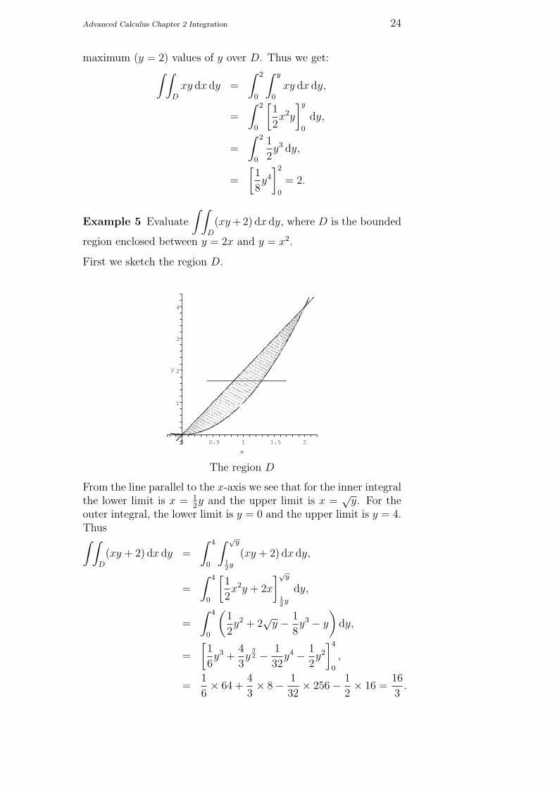
Example 5 Evaluate
∫ ∫
D
(xy +2) dx dy, where D is the bounded
region enclosed between y = 2x and y = x2.
First we sketch the region D.
y
3
4
2
01.50 21
x
0.5
1
The region D
From the line parallel to the x-axis we see that for the inner integralthe lower limit is x = 1
2y and the upper limit is x =
√y. For the
outer integral, the lower limit is y = 0 and the upper limit is y = 4.Thus∫ ∫
D
(xy + 2) dx dy =
∫ 4
0
∫ √y
12y
(xy + 2) dx dy,
=
∫ 4
0
[1
2x2y + 2x
]√y
12y
dy,
=
∫ 4
0
(1
2y2 + 2
√y − 1
8y3 − y
)dy,
=
[1
6y3 +
4
3y
32 − 1
32y4 − 1
2y2
]4
0
,
=1
6× 64 +
4
3× 8− 1
32× 256− 1
2× 16 =
16
3.

Advanced Calculus Chapter 2 Integration 25
Splitting the integral
So far we have been able to determine the limits of the inner integralof a double integral a single functions of y. However, this is notalways possible. In such cases we have to split the integral intotwo, or more, integrals.
Example 6 Evaluate
∫ ∫
D
xy2 dx dy, where D is triangle with ver-
tices at (0, 0), (3, 1) and (0, 3).
First we sketch the region D.
y
2.5
0.5
3
2
1
2.500
10.5 2 31.5
x
1.5
The region D
From the lines parallel to the x-axis we see that the limits of theinner integral depend on whether y < 1 or y > 1. Thus we split theintegral into two integrals where the limits of the outer integralsare 0 and 1, and 1 and 3, respectively. Doing this, and working outthe limits of the inner integrals as before gives:∫ ∫
D
xy2 dx dy =
∫ 1
0
∫ 3y
0
xy2 dx dy +
∫ 3
1
∫ 32(3−y)
0
xy2 dx dy,
=
∫ 1
0
[1
2x2y2
]3y
0
dy +
∫ 3
1
[1
2x2y2
] 32(3−y)
0
dy,
=
∫ 1
0
9
2y4 dy +
∫ 3
1
9
8(3− y)2y2 dy,
=
∫ 1
0
9
2y4 dy +
∫ 3
1
9
8(y4 − 6y3 + 9y2) dy,
=9
2
[1
5y5
]1
0
+9
8
[1
5y5 − 3
2y4 + 3y3
]3
1
,
=9
10+
9
8
(1
5× 243− 3
2× 81 + 3× 27− 1
5+
3
2− 3
),
=9
10+
9
8× 62
5= 8 1
10.
Advanced Calculus Chapter 2 Integration 26
Exercises 2.4
1. Evaluate
∫ ∫
D
(x + y) dx dy, where
D = {(x, y) : 0 ≤ y ≤ 1, y ≤ x ≤ 1 + 2y}.
2. Evaluate
∫ ∫
D
(x − y)2 dx dy, where D is the region enclosed
between x = 3, y = 1 and y = x2.
3. Evaluate
∫ ∫
D
xy dx dy, where D is the square with vertices
at (1, 0), (0, 1), (1, 2) and (2, 1).
4. Evaluate
∫ ∫
P
xy dx dy, where P is the pentagon with vertices
at (0, 0), (0, 2), (1, 2), (2, 1) and (2, 0).
5. Explain why
∫ ∫
D
dx dy gives the area of D. Use this result
to find the area of the region enclosed between the curvesx = 7y − xy2 and x = y2 + 3.
2.5 Changing the order of integration
In the examples considered so far, we have always integrated firstwith respect to x. This is not necessary, and there is no reasonwhy we should not choose to integrate first with respect to y. Intwo particular cases, it can be advantageous, or even necessary, tochange the order of integration. These cases are:
• to avoid having to split the integral into two, or more, regions;
• when it is difficult, or not possible, to integrate f(x, y) withrespect to x.

Advanced Calculus Chapter 2 Integration 27
As an example of the first case, consider again Example 6, but thistime we integrate first with respect to y.
y
2.5
0.5
3
2
1
2.500
10.5 2 31.5
x
1.5
To find the limits of the inner integral we draw a line through theregion parallel to the y-axis; where the line crosses the region at thelowest point (y = 1
3x) gives the lower limit, and where it crosses
the highest point (y = 3 − 23x) gives the upper limit. The limits
of the outer integral are just the minimum (x = 0) and maximum(x = 3) values of x. Thus we get:∫ ∫
D
xy2 dx dy =
∫ ∫
D
xy2 dy dx,
=
∫ 3
0
∫ 3− 23x
13x
xy2 dy dx,
=
∫ 3
0
[1
3xy3
]3− 23x
13x
dx,
=
∫ 3
0
(1
3x(3− 2
3x)3 − 1
81x4
)dx,
=
∫ 3
0
(1
3x(27− 18x + 4x2 − 8
27x3)− 1
81x4
)dx,
=
∫ 3
0
(1
3x(27− 18x + 4x2 − 8
27x3)− 1
81x4
)dx,
=
∫ 3
0
(9x− 6x2 +
4
3x3 − 1
9x4
)dx,
=
[9
2x2 − 2x3 +
1
3x4 − 1
45x5
]3
0
,
=9
2× 9− 2× 27 +
1
3× 81− 1
45,
= 8 110
.
The following two examples illustrate the case when we change theorder of integration because it is difficult, or impossible, to evaluate
Advanced Calculus Chapter 2 Integration 28
the integral in the order given.
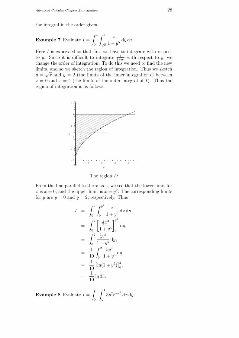
Example 7 Evaluate I =
∫ 4
0
∫ 2
√x
x
1 + y5dy dx.
Here I is expressed so that first we have to integrate with respectto y. Since it is difficult to integrate 1
1+y5 with respect to y, wechange the order of integration. To do this we need to find the newlimits, and so we sketch the region of integration. Thus we sketchy =
√x and y = 2 (the limits of the inner integral of I) between
x = 0 and x = 4 (the limits of the outer integral of I). Thus theregion of integration is as follows.
y
2
0
2.5
1.5
0.5
2 430
x
1
1
The region D
From the line parallel to the x-axis, we see that the lower limit forx is x = 0, and the upper limit is x = y2. The corresponding limitsfor y are y = 0 and y = 2, respectively. Thus
I =
∫ 2
0
∫ y2
0
x
1 + y5dx dy,
=
∫ 2
0
[ 12x2
1 + y5
]y2
0
dy,
=
∫ 2
0
12y4
1 + y5dy,
=1
10
∫ 2
0
5y4
1 + y5dy,
=1
10
[ln(1 + y5)
]2
0,
=1
10ln 33.
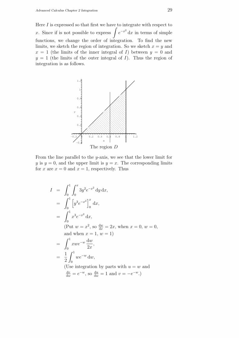
Example 8 Evaluate I =
∫ 1
0
∫ 1
y
3y2e−x2
dx dy.
Advanced Calculus Chapter 2 Integration 29
Here I is expressed so that first we have to integrate with respect to
x. Since if is not possible to express
∫e−x2
dx in terms of simple
functions, we change the order of integration. To find the newlimits, we sketch the region of integration. So we sketch x = y andx = 1 (the limits of the inner integral of I) between y = 0 andy = 1 (the limits of the outer integral of I). Thus the region ofintegration is as follows.
y
1
0.2
1.2
0.8
0.4
-0.2
0.80
1.20.4 0.60.2 10
x
0.6
-0.2
The region D
From the line parallel to the y-axis, we see that the lower limit fory is y = 0, and the upper limit is y = x. The corresponding limitsfor x are x = 0 and x = 1, respectively. Thus
I =
∫ 1
0
∫ x
0
3y2e−x2
dy dx,
=
∫ 1
0
[y3e−x2
]x
0dx,
=
∫ 1
0
x3e−x2
dx,
(Put w = x2, so dwdx
= 2x, when x = 0, w = 0,
and when x = 1, w = 1)
=
∫ 1
0
xwe−w dw
2x,
=1
2
∫ 1
0
we−w dw,
(Use integration by parts with u = w anddvdw
= e−w, so dudw
= 1 and v = −e−w.)
Advanced Calculus Chapter 2 Integration 30
=1
2
[−we−w +
∫e−wdw
]1
0
,
=1
2
[−we−w − e−w]1
0,
= −1
2
[e−w(w + 1)
]1
0,
= −1
2(2e−1 − 1),
=1
2− e−1.
Exercises 2.5
1. For each of the following double integrals:
(i) evaluate the integral as given;
(ii) sketch the region of integration;
(iii) change the order of integration, and re-evaluate the in-tegral.
(a)
∫ 3
0
∫ y
0
(x2 + y2) dx dy.
(b)
∫ 2
0
∫ 4−2x
0
xy dy dx.
(c)
∫ 1
0
∫ √y
y
y2x dx dy.
2. Evaluate the following double integrals.
(a)
∫ 1
0
∫ 2
2y
6y√
1 + x3 dx dy;
(b)
∫ 2
1
∫ 1y
12
x3 cos(x2y) dx dy.
3. Evaluate
∫ 2
0
∫ 2y
y
sin(πy
x
)dx dy +
∫ 4
2
∫ 4
y
sin(πy
x
)dx dy.
2.6 Unbounded regions of integration
It is possible to perform some double integrals over an unboundedregion. In such cases, one or more of the limits is infinite.
Example 9 Evaluate
∫ ∫
D
e−(x+y) dx dy, where D = {(x, y) ∈ R2 :
0 ≤ y ≤ 1, y ≤ x}.
Advanced Calculus Chapter 2 Integration 31
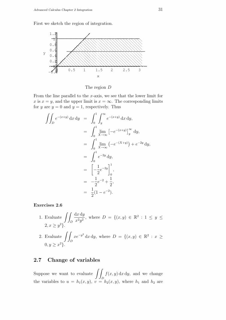
First we sketch the region of integration.
y
1
0.2
1.2
0.8
0.4
-0.20
0310.5 1.5 2.5
x
2
0.6
The region D
From the line parallel to the x-axis, we see that the lower limit forx is x = y, and the upper limit is x = ∞. The corresponding limitsfor y are y = 0 and y = 1, respectively. Thus
∫ ∫
D
e−(x+y) dx dy =
∫ 1
0
∫ ∞
y
e−(x+y) dx dy,
=
∫ 1
0
limX→∞
[−e−(x+y)]∞y
dy,
=
∫ 1
0
limX→∞
(−e−(X+y))
+ e−2y dy,
=
∫ 1
0
e−2y dy,
=
[−1
2e−2y
]1
0
,
= −1
2e−2 +
1
2,
=1
2(1− e−2).
Exercises 2.6
1. Evaluate
∫ ∫
D
dx dy
x2y2, where D = {(x, y) ∈ R2 : 1 ≤ y ≤
2, x ≥ y2}.
2. Evaluate
∫ ∫
D
xe−y2
dx dy, where D = {(x, y) ∈ R2 : x ≥0, y ≥ x2}.
2.7 Change of variables
Suppose we want to evaluate
∫ ∫
D
f(x, y) dx dy, and we change
the variables to u = h1(x, y), v = h2(x, y), where h1 and h2 are
Advanced Calculus Chapter 2 Integration 32
invertible on D. Such a change of variables transforms the integralover D in the (x, y)-plane to an integral over ∆ in the (u, v)-plane.It remains to transform the function to a function in u and v, beingintegrated with respect to u and v. To do this, first note that sinceh1 and h2 are invertible on D, there are invertible functions g1 andg2 on ∆ such that x = g1(u, v) and y = g2(u, v). Now we define theJacobean by
∂(x, y)
∂(u, v)= det
(∂x∂u
∂x∂v
∂y∂u
∂y∂v
).
Then
Recall that if A =(
a bc d
)
then det A = ad− bc.
∫ ∫
D
f(x, y) dx dy =
∫ ∫
∆
f(g1(u, v), g2(u, v))
∣∣∣∣∂(x, y)
∂(u, v)
∣∣∣∣ du dv.
If it is difficult to express x and y in terms of u and v then we canuse the fact that
∂(x, y)
∂(u, v)=
1∂(u,v)∂(x,y)
.
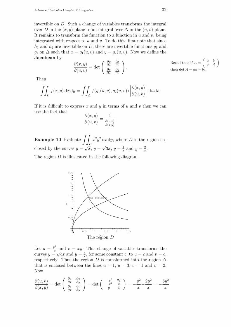
Example 10 Evaluate
∫ ∫
D
x2y2 dx dy, where D is the region en-
closed by the curves y =√
x, y =√
3x, y = 1x
and y = 2x.
The region D is illustrated in the following diagram.
The region D
y
2
0
2.5
1.5
x
20
0.5
1
0.5 1 2.51.5
The region D
Let u = y2
xand v = xy. This change of variables transforms the
curves y =√
cx and y = cx, for some constant c, to u = c and v = c,
respectively. Thus the region D is transformed into the region ∆that is enclosed between the lines u = 1, u = 3, v = 1 and v = 2.Now
∂(u, v)
∂(x, y)= det
(∂u∂x
∂u∂y
∂v∂x
∂v∂y
)= det
(− y2
x22yx
y x
)= −y2
x−2y2
x= −3y2
x.
Advanced Calculus Chapter 2 Integration 33
Thus ∣∣∣∣∂(x, y)
∂(u, v)
∣∣∣∣ =1∣∣∣∂(u,v)
∂(x,y)
∣∣∣=
x
3y2.
Thus∫ ∫
D
x2y2 dx dy =
∫ ∫
∆
x2y2
∣∣∣∣∂(x, y)
∂(u, v)
∣∣∣∣ du dv,
=
∫ 2
1
∫ 3
1
(x2y2)
(x
3y2
)du dv,
=
∫ 2
1
∫ 3
1
1
3
v2
udu dv,
=
∫ 2
1
1
3
[v2 ln u
]3
1dv,
=
∫ 2
1
1
3v2 ln 3 dv,
=
(1
3ln 3
)[1
3v3
]2
1
,
=1
9ln 3(8− 1),
=7
9ln 3.
Example 11 Evaluate
∫ ∫
D
y2 cos(y
x
)dx dy, where D is the re-
gion enclosed by the curves y = ax, y = bx, y = ax
and y = bx,
where a, b ∈ R with a > b > 0.
Let u = yx
and v = xy. This change of variables transforms thecurves y = cx and y = c
x, for some constant c, to u = c and v = c,
respectively. Thus the region D is transformed into the region ∆that is enclosed between the lines u = b, u = a, v = b and v = a.Now
∂(u, v)
∂(x, y)= det
(∂u∂x
∂u∂y
∂v∂x
∂v∂y
)= det
( − yx2
1x
y x
)= − y
x2x−y
x= −2
y
x.
Thus ∣∣∣∣∂(x, y)
∂(u, v)
∣∣∣∣ =1∣∣∣∂(u,v)
∂(x,y)
∣∣∣=
x
2y.
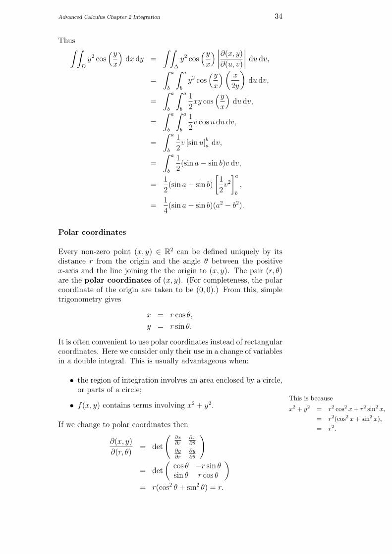
Advanced Calculus Chapter 2 Integration 34
Thus∫ ∫
D
y2 cos(y
x
)dx dy =
∫ ∫
∆
y2 cos(y
x
) ∣∣∣∣∂(x, y)
∂(u, v)
∣∣∣∣ du dv,
=
∫ a
b
∫ a
b
y2 cos(y
x
) (x
2y
)du dv,
=
∫ a
b
∫ a
b
1
2xy cos
(y
x
)du dv,
=
∫ a
b
∫ a
b
1
2v cos u du dv,
=
∫ a
b
1
2v [sin u]ba dv,
=
∫ a
b
1
2(sin a− sin b)v dv,
=1
2(sin a− sin b)
[1
2v2
]a
b
,
=1
4(sin a− sin b)(a2 − b2).
Polar coordinates
Every non-zero point (x, y) ∈ R2 can be defined uniquely by itsdistance r from the origin and the angle θ between the positivex-axis and the line joining the the origin to (x, y). The pair (r, θ)are the polar coordinates of (x, y). (For completeness, the polarcoordinate of the origin are taken to be (0, 0).) From this, simpletrigonometry gives
x = r cos θ,
y = r sin θ.
It is often convenient to use polar coordinates instead of rectangularcoordinates. Here we consider only their use in a change of variablesin a double integral. This is usually advantageous when:
• the region of integration involves an area enclosed by a circle,or parts of a circle;
• f(x, y) contains terms involving x2 + y2.This is because
x2 + y2 = r2 cos2 x + r2 sin2 x,
= r2(cos2 x + sin2 x),= r2.
If we change to polar coordinates then
∂(x, y)
∂(r, θ)= det
(∂x∂r
∂x∂θ
∂y∂r
∂y∂θ
)
= det
(cos θ −r sin θsin θ r cos θ
)
= r(cos2 θ + sin2 θ) = r.

Advanced Calculus Chapter 2 Integration 35
When changing variables from rectangular to polar coordinates you
may quote the fact that∂(x, y)
∂(r, θ)= r without going through the
above derivation.
Example 12 Find
∫ ∫
D
x2y dx dy, where
D = {(x, y) ∈ R2 : x ≥ 0, y ≥ 0 x2 + y2 ≤ a2}, for some a ∈ R.
Changing variables to polar coordinates we get:
∫ ∫
D
x2y dx dy =
∫ π2
0
∫ a
0
(r2 cos2 θ)(r sin θ)r dr dθ,
=
∫ π2
0
∫ a
0
r4 cos2 θ sin θ dr dθ,
=
∫ π2
0
[r5
5
]a
0
cos2 θ sin θ dr dθ,
=a5
5
∫ π2
0
cos2 θ sin θ dr dθ,
=a5
5
[−cos3 θ
3
]π2
0
=a5
5
1
3=
1
15a5.
Example 13 Evaluate
∫ ∫
D
xy dx dy, where D is the interior of
the circle of radius 1, centre (1, 1).
Here we first make the change of variable u = x− 1, v = y − 1. It
is easy to check that∂(u, v)
∂(x, y)= 1 and the region of integration ∆ is
the interior of the circle of radius 1, centre (0, 0). Thus
∫ ∫
D
xy dx dy =
∫ ∫
∆
(u + 1)(v + 1) du dv.
Now we change to polar coordinates with u = r cos θ and v = r sin θ.
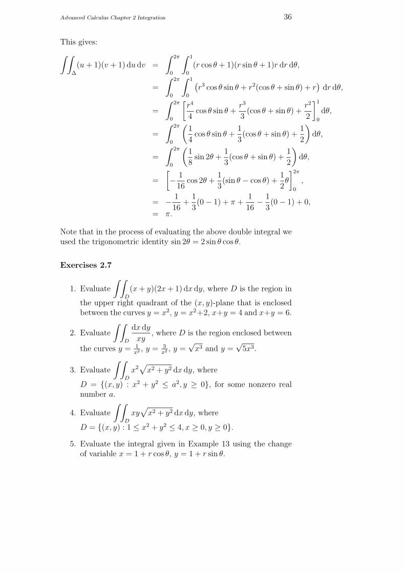
Advanced Calculus Chapter 2 Integration 36
This gives:
∫ ∫
∆
(u + 1)(v + 1) du dv =
∫ 2π
0
∫ 1
0
(r cos θ + 1)(r sin θ + 1)r dr dθ,
=
∫ 2π
0
∫ 1
0
(r3 cos θ sin θ + r2(cos θ + sin θ) + r
)dr dθ,
=
∫ 2π
0
[r4
4cos θ sin θ +
r3
3(cos θ + sin θ) +
r2
2
]1
0
dθ,
=
∫ 2π
0
(1
4cos θ sin θ +
1
3(cos θ + sin θ) +
1
2
)dθ,
=
∫ 2π
0
(1
8sin 2θ +
1
3(cos θ + sin θ) +
1
2
)dθ,
=
[− 1
16cos 2θ +
1
3(sin θ − cos θ) +
1
2θ
]2π
0
,
= − 1
16+
1
3(0− 1) + π +
1
16− 1
3(0− 1) + 0,
= π.
Note that in the process of evaluating the above double integral weused the trigonometric identity sin 2θ = 2 sin θ cos θ.
Exercises 2.7
1. Evaluate
∫ ∫
D
(x + y)(2x + 1) dx dy, where D is the region in
the upper right quadrant of the (x, y)-plane that is enclosedbetween the curves y = x2, y = x2+2, x+y = 4 and x+y = 6.
2. Evaluate
∫ ∫
D
dx dy
xy, where D is the region enclosed between
the curves y = 1x2 , y = 3
x2 , y =√
x3 and y =√
5x3.
3. Evaluate
∫ ∫
D
x2√
x2 + y2 dx dy, where
D = {(x, y) : x2 + y2 ≤ a2, y ≥ 0}, for some nonzero realnumber a.
4. Evaluate
∫ ∫
D
xy√
x2 + y2 dx dy, where
D = {(x, y) : 1 ≤ x2 + y2 ≤ 4, x ≥ 0, y ≥ 0}.5. Evaluate the integral given in Example 13 using the change
of variable x = 1 + r cos θ, y = 1 + r sin θ.