20. alfven waves - stanford...

Phys780: Plasma Physics Lecture 20. Alfven Waves. 1

20. Alfven waves

([3], p.233-239; [1], p.202-237; Chen, Sec.4.18, p.136-144)

We have considered two types of waves in plasma:

1. electrostatic Langmuir waves and ion-sound waves: oscillations of

electrons and ions relative to each other

2. electromagnetic waves - high-frequency waves affected by motions

of electrons in plasma in the oscillating electric field of the waves

and in the stationary magnetic field (we assumed that ions are

heavy and don’t move)

The third types of waves are MHD waves in which plasma oscillates as

a single fluid.

These waves are described by using single-fluid plasma equations and

Maxwell equations.


Consider Maxwell equations:

∇× ~E = −1

c

∂ ~B

∂t

∇× ~B =1

c

∂ ~E

∂t︸︷︷︸

displacement current

+4π

c~j

∇ · ~B = 0

∇ · ~E = 4πq = 0

We derive equation for ~E by applying operator ∇× to the first

equation and substituting ∇× ~B from the second equation:

∇× (∇× ~E) = −1

c

∂∇× ~B

∂t= −

1

c2∂2 ~E

∂t2−

4π

c2∂~j

∂t

Using

∇× (∇× ~E) = ∇(∇·) ~E − (∇ · ∇) ~E = −∇2 ~E


we obtain

∇2 ~E =1

c2∂2 ~E

∂t2+

4π

c2∂~j

∂t

where ~j is determined from Ohm’s law (lecture 13):

~E +~v × ~B

c=

~j

σ+

1

en

[~j × ~B

c−∇pe

]

+me

e2n

∂~j

∂t

Previously, we considered only slow processes and neglected the last

term. However, for high-frequency electromagnetic waves with

frequencies close to plasma frequency this term significant.

Plasma velocity ~v is determined from the equation of motion

ρd~v

dt= −∇p+

1

c(~j × ~B),

and pressure is determined from the continuity and energy equations:

∂ρ

∂t+∇(ρ~v) = 0


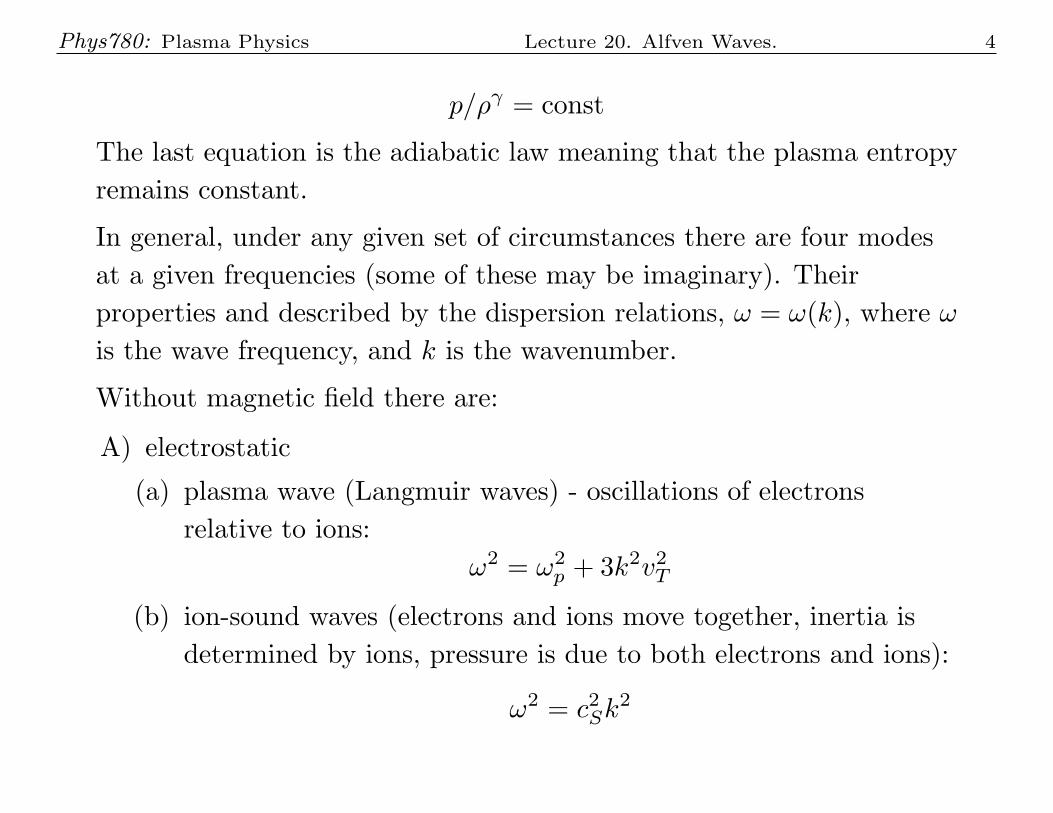
p/ργ = const

The last equation is the adiabatic law meaning that the plasma entropy

remains constant.

In general, under any given set of circumstances there are four modes

at a given frequencies (some of these may be imaginary). Their

properties and described by the dispersion relations, ω = ω(k), where ω

is the wave frequency, and k is the wavenumber.

Without magnetic field there are:

A) electrostatic

(a) plasma wave (Langmuir waves) - oscillations of electrons

relative to ions:

ω2 = ω2p + 3k2v2T

(b) ion-sound waves (electrons and ions move together, inertia is

determined by ions, pressure is due to both electrons and ions):

ω2 = c2Sk2


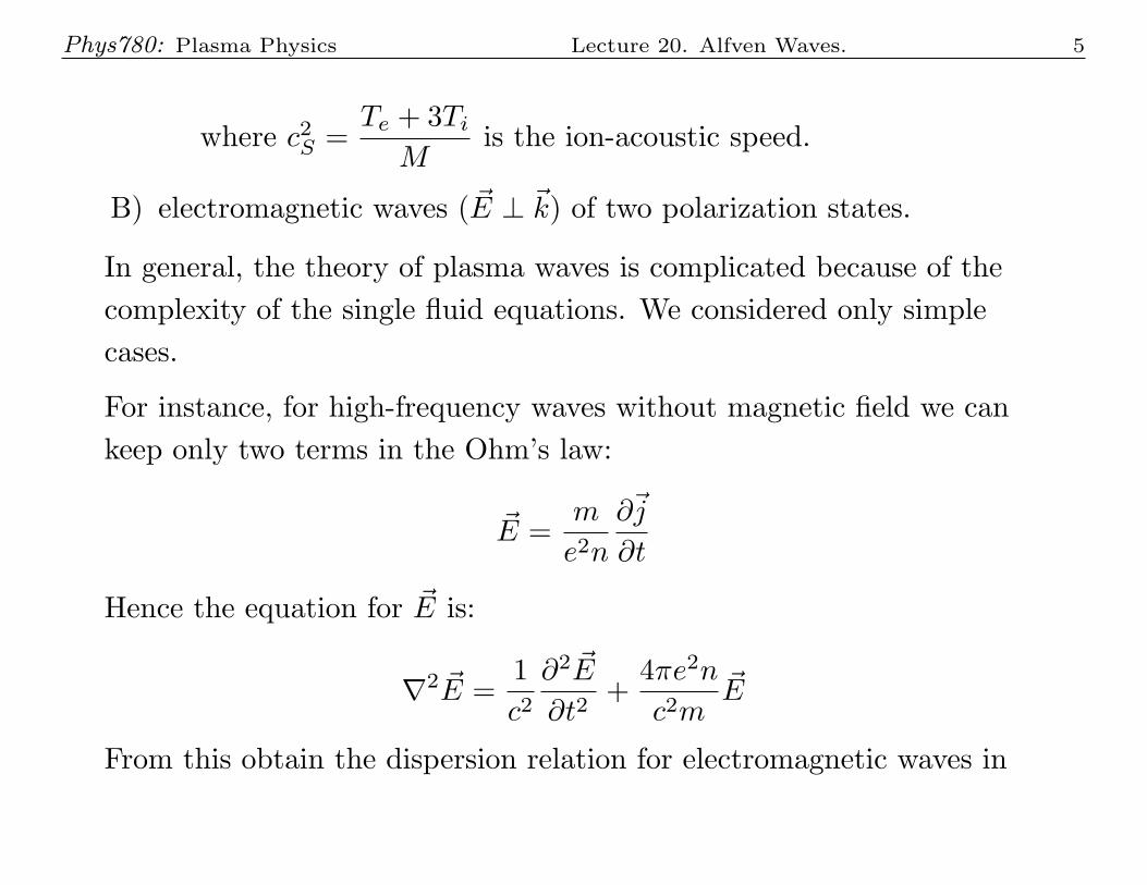
where c2S =Te + 3Ti

Mis the ion-acoustic speed.

B) electromagnetic waves ( ~E ⊥ ~k) of two polarization states.

In general, the theory of plasma waves is complicated because of the

complexity of the single fluid equations. We considered only simple

cases.

For instance, for high-frequency waves without magnetic field we can

keep only two terms in the Ohm’s law:

~E =m

e2n

∂~j

∂t

Hence the equation for ~E is:

∇2 ~E =1

c2∂2 ~E

∂t2+

4πe2n

c2m~E

From this obtain the dispersion relation for electromagnetic waves in


plasma:

ω2

c2= k2 +

ω2p

c2.

In general, a wave in a magnetic field involves both electric and

magnetic forces. A high-frequency wave is a combination of

electromagnetic wave with a longitudinal electrostatic wave. Density

gradients may produce coupling between different types of waves.

With magnetic field, for electromagnetic waves traveling along the field

lines there are two wave modes:

• R-waves (with right circular polarization):

c2k2

ω2= 1−

ω2p

ω(ω − ωe)

where ωe =eB

mcis the electron cyclotron frequency.


• L-waves (with left circular polarization):

c2k2

ω2= 1−

ω2p

ω(ω + ωe)

In the first case, the wave polarization vector ( ~E) rotates in the same

direction is the gyration of electrons. This gives rise to a low-frequency

whistler mode (electron-cyclotron wave) with the frequency below the

electron cyclotron frequency (Lecture 17). Previously, we considered

ions as stationary.

When motion of ions is taken into account then the R- and L-wave

modes are modified, and new type of hydromagnetic waves appear at

low frequencies smaller than the ion cyclotron frequency ω < ωci.

In this case the dispersion relations for the R- and L-waves are the

following:


• R-waves (with right circular polarization):

c2k2

ω2= 1−

ω2p

(ω + ωi)(ωe − ω)

where ωi =eB

Mcis the ion cyclotron frequency.

• L-waves (with left circular polarization):

c2k2

ω2= 1−

ω2p

(ω − ωi)(ω + ωe)

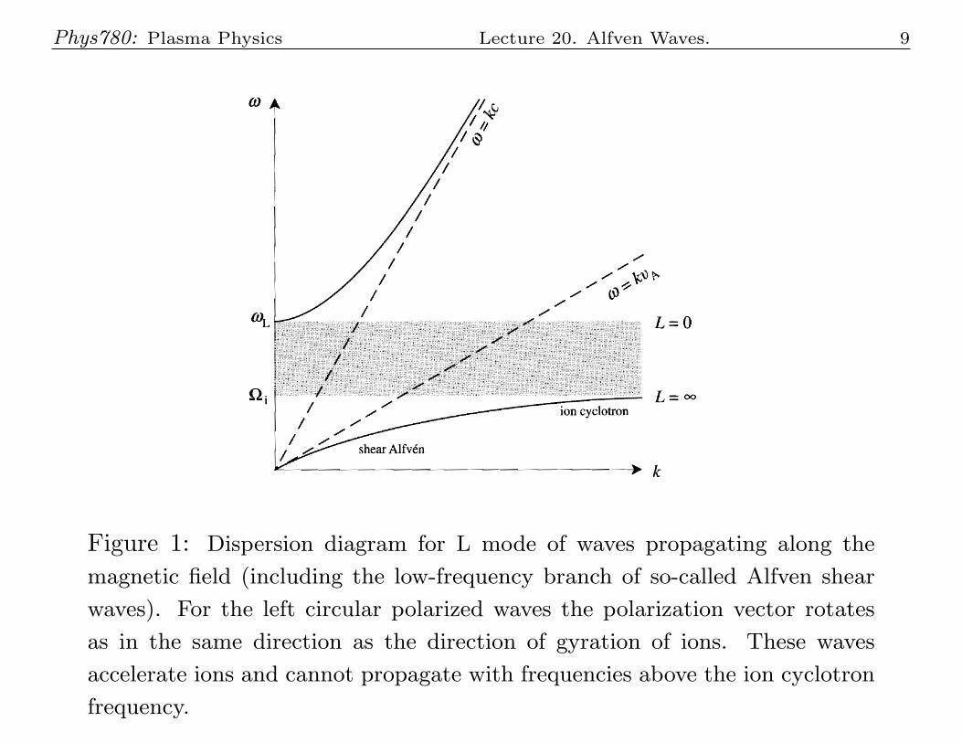
The additional mode (ion cyclotron wave) appears in the L-wave case

because the polarization electric field vector rotates in the same

direction as the gyration of ions (Figure 1).


Figure 1: Dispersion diagram for L mode of waves propagating along the

magnetic field (including the low-frequency branch of so-called Alfven shear

waves). For the left circular polarized waves the polarization vector rotates

as in the same direction as the direction of gyration of ions. These waves

accelerate ions and cannot propagate with frequencies above the ion cyclotron

frequency.


Figure 2: Dispersion diagram for R mode. For the right circular polarized

waves the polarization vector rotates as in the same direction as the direction

of gyration of electrons. At low frequencies, for waves traveling perpendicular

to magnetic field lines a compressible Alfven wave mode (also called fast MHD

wave) appears (we’ll consider this wave in the next lecture).


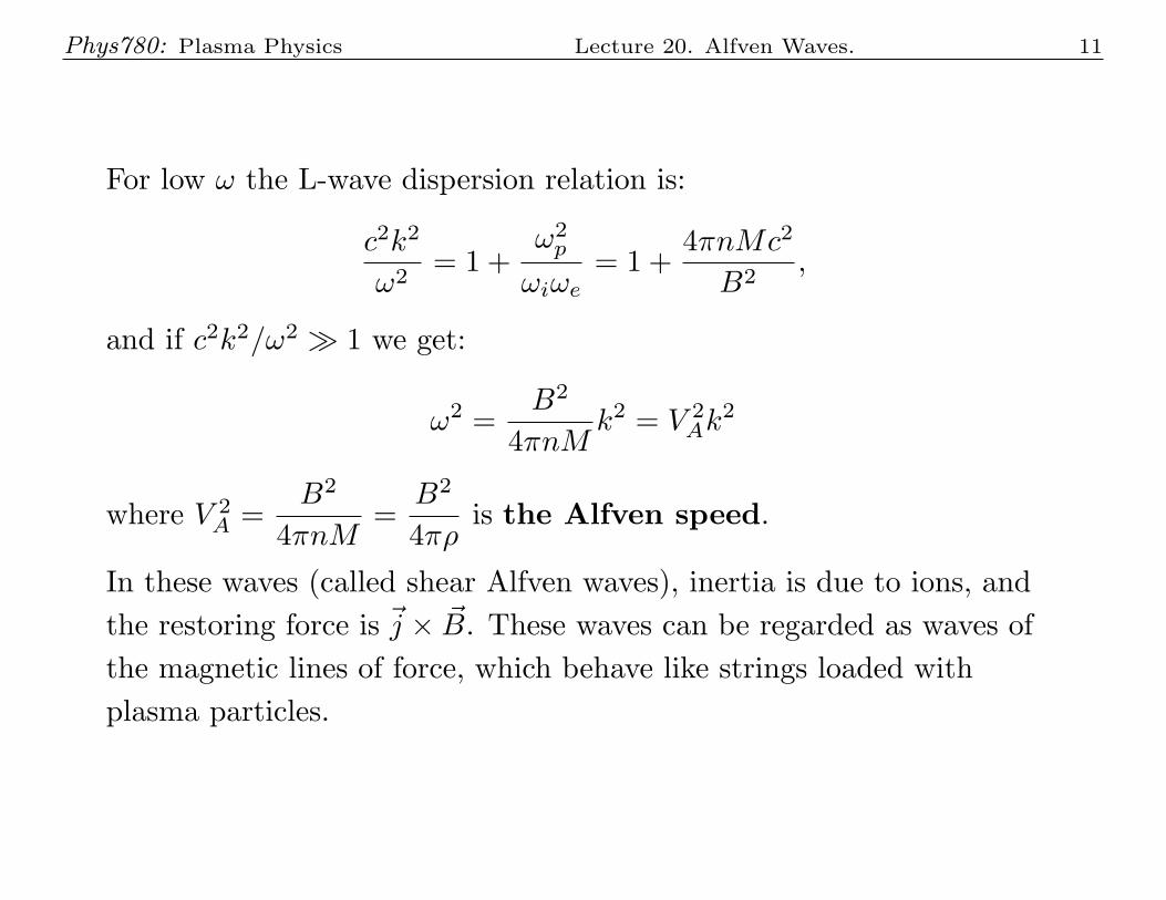
For low ω the L-wave dispersion relation is:

c2k2

ω2= 1 +

ω2p

ωiωe

= 1 +4πnMc2

B2,

and if c2k2/ω2 ≫ 1 we get:

ω2 =B2

4πnMk2 = V 2

Ak2

where V 2A =

B2

4πnM=

B2

4πρis the Alfven speed.

In these waves (called shear Alfven waves), inertia is due to ions, and

the restoring force is ~j × ~B. These waves can be regarded as waves of

the magnetic lines of force, which behave like strings loaded with

plasma particles.


Alfven waves

Let us consider now the low-frequency hydromagnetic waves.

In we neglect the displacement current, Hall effect, pressure gradient,

and compressibility. Then, the equations have the following form:

∇2 ~E =4π

c2∂~j

∂t

ρ∂~v

∂t=

1

c~j × ~B

If~B = (0, 0, B0)

~v = (vx, 0, 0)

~E = (0, Ey, 0)

~j = (0, jy, 0)


Figure 3: Geometry of an Alfven wave propagating along ~B0.


then

ρ∂vx∂t

=1

cjyB0

Ey −1

cvxB0 = 0

∂2Ey

∂z2=

4π

c2∂jy∂t

vx =cEy

B0

jy =cρ

B0

∂vx∂t

=c2ρ

B20

∂Ey

∂t

∂2Ey

∂z2=

4πρ

B20

∂2Ey

∂t2

Thus, the dispersion relation of these waves (Alfven waves) is

ω2 =B2

0

4πρk2 = V 2

a k2


where

V 2A =

B20

4πρ

is the Alfven speed.

Consider basic properties of Alfven waves. If

Ey = E0 sinω

(

t−z

VA

)

then

jy =c2ρE0ω

B20

cosω

(

t−z

VA

)

vx =cE0

B0

sinω

(

t−z

VA

)

We find the oscillating magnetic field of the wave from the Maxwell

equation

∇× ~B =4π

c~j


the y-component of which has the following form

∂Bx

∂z=

4π

cjy

Hence∂Bx

∂z=

4πcρ

B20

∂Ey

∂t

Substituting Ey and integrating over z we get

Bx = −cE0

VA

sinω

(

t−z

VA

)

We see that vx and Bx oscillate in antiphase. We can calculate the

kinetic and magnetic energy densities averaged over the wave period,

taking into account that:⟨

sin2 ω

(

t−z

VA

)⟩

=1

2⟨ρv2x2

⟩

=ρc2E2

0

4B20


⟨B2

x

8π

⟩

=c2E2

0ρ

4B20

Thus, the kinetic and magnetic energies of Alfven waves are equal.

For the relative amplitudes of velocity and magnetic field oscillations

we obtain|vx|

VA

=|Bx|

B0

=cE0

B0VA

If vx is large then Bx is also large. Hence Alfven waves can amplify the

initial magnetic field and transport it to large distances. However, the

condition of incompressibility requires that the Alfven speed is much

smaller than the speed of sound VA ≪ cs.

Consider now the equation for the magnetic lines of force:

dx

Bx

=dz

B0

dx

dz=

Bx

B0

= −cE0

B0VA

sinω(t− z/VA)


The general solution for the lines of force displacement is:

x = x0 +cE0

B0ωcosω(t− z/VA)

The corresponding velocity of the line of force is:

dx

dt= −

cE0

B0

sinω(t− z/VA) = vx

Hence the magnetic field lines are “frozen” into the plasma.

When the electrical resistivity of plasma is zero (σ = ∞) the waves are

non-dissipative, otherwise the Alfven waves dissipate.

We can calculate the averaged over the period Joule dissipation and the

corresponding change of the wave energy:

dW

dt== −

1

T

∫ T

0

j2

σdt


where

W =1

T

∫ T

0

(1

2ρv2x +

B2x

8π

)

dt

We obtain

W =ρc2E2

0

2B20

⟨j2⟩=

c4ρ2E20ω

2

2B40

=Wω2ρc2

B20

dW

dt= −

Wω2ρc2

σB20

= −Wω2c2

4πσV 2A

= −W

τ

where

τ =2πσV 2

A

c2ω2=

V 2A

2ω2νm=

L2

νm

Here

νm =c2

4πσ


is called “magnetic viscosity”,

L =VA

ω=

λ

2π

is a “characteristic size” of variations in plasma, λ = 2π/k = 2πVA/ω is

the wavelength.

The dissipation rate relative to the wave period is

τ/P = τω/2π =V 2A

4πωνm=

1

2π

VAL

νm=

1

2πRem

where

Rem =VAL

νm

is the magnetic Reynolds number. It determines the relative time scale

of the Joule dissipation compared to the dynamic time scale.


Magnetic Reynolds number

It plays a fundamental role in the plasma MHD theory. Consider the

equation for the magnetic field evolution in the presence of Joule

dissipation

∇× ~B =4π

c~j

~j = σ

(

~E +1

c~v × ~B

)

∇× ~E = −1

c

∂ ~B

∂t

~E =~j

σ−

(~v × ~B)

c

~j =c

4π∇× ~B


Finally, we obtain

∂ ~B

∂t= ∇× (~v × ~B)−∇×

[c2

4πσ(∇× ~B)

]

The magnetic Reynolds number determines the relative role of the two

terms in the right-hand side: magnetic field advection and dissipation.

The relative importance of these terms for a process of a characteristic

scale L, velocity v is determined by the magnetic Reynolds number:

RM =vBL

c2

4πσBL2

=4πσLv

c2.

For typical coronal conditions: T = 106K, σ = 1012 s−1, L = 108 cm,

v = 107 cm/s,

RM ∼ 105 >> 1.

For uniform σ the last term can be simplified:

∇× (∇× ~B) = ∇(∇ · ~B)−∇2 ~B = −∇2 ~B.


∂ ~B

∂t= ∇× (~v × ~B) +

c2

4πσ∇2 ~B

Then, if ~v = 0 we get a diffusion equation:

∂ ~B

∂t= D∇2 ~B,

where

D =c2

4πσis a diffusion coefficient for magnetic field.

Exercises:

1. Estimate the characteristic scale of dissipation of magnetic field in

solar flares. The duration of solar flares is 103 sec.

L ∼

√

c2t

4πσ∼ 105cm = 1km.

This is smaller than the observed flare structure. What does that

mean?


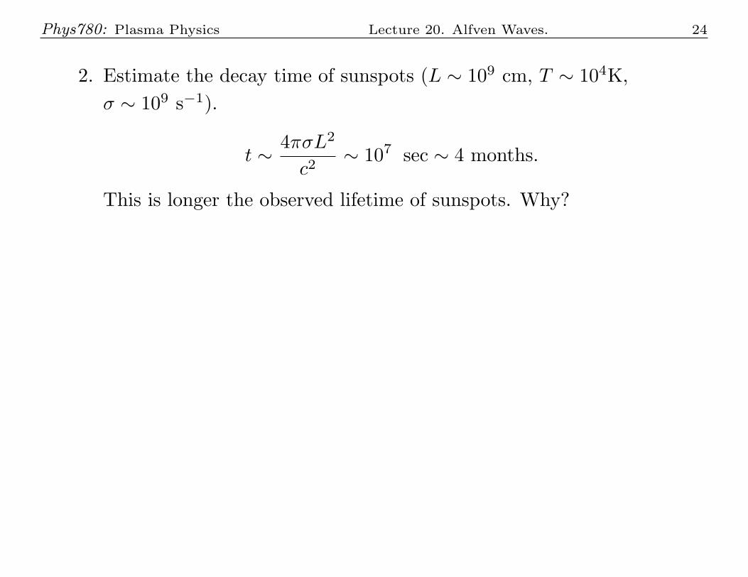
2. Estimate the decay time of sunspots (L ∼ 109 cm, T ∼ 104K,

σ ∼ 109 s−1).

t ∼4πσL2

c2∼ 107 sec ∼ 4 months.

This is longer the observed lifetime of sunspots. Why?

20. alfven waves - stanford...

Documents