Montréal Mai 2004

© 2004 Eric Ghysels, Pedro Santa-Clara, Rossen Valkanov. Tous droits réservés. All rights reserved. Reproduction partielle permise avec citation du document source, incluant la notice ©. Short sections may be quoted without explicit permission, if full credit, including © notice, is given to the source.

Série Scientifique Scientific Series

2004s-20

The MIDAS Touch: Mixed Data Sampling Regression

Models

Eric Ghysels, Pedro Santa-Clara, Rossen Valkanov

CIRANO

Le CIRANO est un organisme sans but lucratif constitué en vertu de la Loi des compagnies du Québec. Le financement de son infrastructure et de ses activités de recherche provient des cotisations de ses organisations-membres, d’une subvention d’infrastructure du ministère de la Recherche, de la Science et de la Technologie, de même que des subventions et mandats obtenus par ses équipes de recherche.

CIRANO is a private non-profit organization incorporated under the Québec Companies Act. Its infrastructure and research activities are funded through fees paid by member organizations, an infrastructure grant from the Ministère de la Recherche, de la Science et de la Technologie, and grants and research mandates obtained by its research teams.

Les organisations-partenaires / The Partner Organizations PARTENAIRE MAJEUR . Ministère du développement économique et régional et de la recherche [MDERR] PARTENAIRES . Alcan inc. . Axa Canada . Banque du Canada . Banque Laurentienne du Canada . Banque Nationale du Canada . Banque Royale du Canada . Bell Canada . BMO Groupe Financier . Bombardier . Bourse de Montréal . Caisse de dépôt et placement du Québec . Développement des ressources humaines Canada [DRHC] . Fédération des caisses Desjardins du Québec . GazMétro . Hydro-Québec . Industrie Canada . Ministère des Finances du Québec . Pratt & Whitney Canada Inc. . Raymond Chabot Grant Thornton . Ville de Montréal . École Polytechnique de Montréal . HEC Montréal . Université Concordia . Université de Montréal . Université du Québec à Montréal . Université Laval . Université McGill . Université de Sherbrooke ASSOCIE A : . Institut de Finance Mathématique de Montréal (IFM2) . Laboratoires universitaires Bell Canada . Réseau de calcul et de modélisation mathématique [RCM2] . Réseau de centres d’excellence MITACS (Les mathématiques des technologies de l’information et des systèmes complexes)

ISSN 1198-8177

Les cahiers de la série scientifique (CS) visent à rendre accessibles des résultats de recherche effectuée au CIRANO afin de susciter échanges et commentaires. Ces cahiers sont écrits dans le style des publications scientifiques. Les idées et les opinions émises sont sous l’unique responsabilité des auteurs et ne représentent pas nécessairement les positions du CIRANO ou de ses partenaires. This paper presents research carried out at CIRANO and aims at encouraging discussion and comment. The observations and viewpoints expressed are the sole responsibility of the authors. They do not necessarily represent positions of CIRANO or its partners.

The MIDAS Touch: Mixed Data Sampling Regression Models*

Eric Ghysels†, Pedro Santa-Clara‡, Rossen Valkanov§

Résumé / Abstract

Nous introduisons des modèles de régression MIDAS (Mixed Data Sampling). Ce sont des modèles de régression avec des séries temporelles échantillonées à différentes fréquences. Nous analysons les liens avec les modèles à retards échelonnés.

Mots clés : retards échelonnés, aliasing, biais de discrétisation.

We introduce Mixed Data Sampling (henceforth MIDAS) regression models. The regressions involve time series data sampled at different frequencies. Technically speaking MIDAS models specify conditional expectations as a distributed lag of regressors recorded at some higher sampling frequencies. We examine the asymptotic properties of MIDAS regression estimation and compare it with traditional distributed lag models. MIDAS regressions have wide applicability in macroeconomics and finance.

Keywords: distributed log models, aliasing, discretization bias.

* We thank Arthur Sinko for able research assistance and Tim Bollerslev, Mike Chernov, Rob Engle, David Hendry, Nour Meddahi, Eric Renault, Neil Shephard as well as seminar participants at Oxford, the Research Triangle Conference, UNC and USC for helpful comments. † Department of Economics, University of North Carolina and CIRANO, Gardner Hall CB 3305, Chapel Hill, NC 27599-3305, phone: (919) 966-5325, e-mail: eghysels@unc.edu. ‡ The Anderson School, UCLA.Los Angeles, CA 90095-1481, phone: (310) 206-6077, e-mail: pedro.santa-clara@anderson.ucla.edu. § The Anderson School, UCLA, Los Angeles, CA 90095-1481, phone: (310) 825-7246, e-mail: rossen.valkanov@anderson.ucla.edu.

1 Introduction

A typical time series regression model involves data sampled at the same frequency. The

idea to construct regression models that combine data with different sampling frequencies

is relatively unexplored. We discuss various ways to construct such regressions. We

call the regression framework a Mi(xed) Da(ta) S(ampling) regression (henceforth MIDAS

regression). At a general level, the interest in MIDAS regressions addresses a situation often

encountered in practice where the relevant information is high frequency data, whereas the

quantity of interest is a low frequency process. For example, with macroeconomic data

one often has series sampled monthly, like price series and monetary aggregates, and series

sampled quarterly or annually, typically real activity series like GDP and its components.

In many circumstances one wants to find, say the relationship between inflation and growth,

and hence combine monthly and quarterly data. Another prime example relates to models

of stock market volatility. The low frequency variable is for example a quadratic variation or

other volatility process over some long future horizon corresponding to the time to maturity

of an option, whereas the high frequency data set is past market information potentially at

the tick-by-tick level. Another example of such a situation is Value-at-Risk which attempts to

forecast likely future losses using quantiles of the (conditional) portfolio return distribution.

The horizon is usually 10 days, the information is again market-driven and abundant.

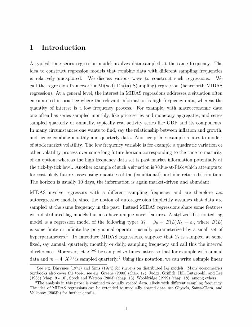
MIDAS involve regressors with a different sampling frequency and are therefore not

autoregressive models, since the notion of autoregression implicitly assumes that data are

sampled at the same frequency in the past. Instead MIDAS regressions share some features

with distributed lag models but also have unique novel features. A stylized distributed lag

model is a regression model of the following type: Yt = β0 + B(L)Xt + εt, where B(L)

is some finite or infinite lag polynomial operator, usually parameterized by a small set of

hyperparameters.1 To introduce MIDAS regressions, suppose that Yt is sampled at some

fixed, say annual, quarterly, monthly or daily, sampling frequency and call this the interval

of reference. Moreover, let X (m) be sampled m times faster, so that for example with annual

data and m = 4, X (4) is sampled quarterly.2 Using this notation, we can write a simple linear

1See e.g. Dhrymes (1971) and Sims (1974) for surveys on distributed lag models. Many econometricstextbooks also cover the topic, see e.g. Greene (2000) (chap. 17), Judge, Griffith, Hill, Lutkepohl, and Lee(1985) (chap. 9 - 10), Stock and Watson (2003) (chap. 13), Wooldridge (1999) (chap. 18), among others.

2The analysis in this paper is confined to equally spaced data, albeit with different sampling frequency.The idea of MIDAS regressions can be extended to unequally spaced data, see Ghysels, Santa-Clara, andValkanov (2003b) for further details.

1

MIDAS regression: Yt = β0 + B(L1/m) X(m)t + ε

(m)t where B(L1/m) =

∑jmax

j=0 B(j)Lj/m is a

polynomial of length jmax (possibly infinite) in the L1/m operator, and Lj/mX(m)t =X

(m)t−j/m.

In other words, the Lj/m operator produces the value of X(m)t lagged by j/m periods. The

annual/quarterly example would imply that the above equation is a projection of annual this

year’s Yt onto a data set quarterly data X(m)t up to jmax quarterly lags back.3

There are differences and similarities between distributed lag models and MIDAS regressions.

Our goal is to present a general discussion of model specification and estimation in mixed

sampling frequency settings, starting with a comparison of MIDAS and distributed lag

models and then proceeding with more general MIDAS models. On the surface the

econometric estimation issues appear straightforward, since MIDAS regression models

involve (nonlinear) least squares or related procedures. However, when it is recognized that

any sampling frequency can be mixed with any other, and that potential approximation

errors may come into play, one faces some challenging econometric issues. Some of these

issues are addressed, others remain open questions. For example, MIDAS regressions relate

to temporal aggregation issues. The mathematical structure commonly adopted to study

aggregation is one that assumes that the underlying stochastic processes evolve in continuous

time and data are collected at equi-distant discrete points in time. Formulating a model in

continuous time has the appeal of a priori imposing a structure on discretely observed data

that is independent of the sampling interval. It is this appeal that explains the considerable

literature on continuous time models, a very partial list of papers studying various aspects

of such models includes Bergstrom (1990), Chambers (1991), Comte and Renault (1996),

Geweke (1978), Hansen and Sargent (1983), Hansen and Sargent (1991a), Hansen and

Sargent (1991b), McCrorie (2000), Phillips (1959), Phillips (1972), Phillips (1973), Phillips

(1974), Robinson (1977) and Sims (1971). We provide new results in the context of MIDAS

regressions, showing that under certain conditions, the aggregation bias disappears when Yt

remains sampled at a fixed rate and only X(m)t is sampled more frequently. In the traditional

distributed lag literature it was always assumed that both Yt and Xt were sampled more

frequently (see in particular Geweke (1978)). Data collection limitations prevent us often

from sampling all series more frequently, hence the interest in MIDAS regressions and the

interest in knowing what happens to discretization biases when only independent variables

can be sampled more frequently. We show that the discretization bias in distributed lag

models and in MIDAS regression both converge to zero as m → 0 both in a local and global

3MIDAS regressions are obviously also not constrained to be either linear or univariate. Such extensionswill also be discussed in the paper.

2

sense. This result is of significance as for instance regressions involving macroeconomic

variables and financial series are usually confined to monthly, quarterly or annual regressions

due to the availability of macro series. The results show that one can use the finer sampling of

financial series to alleviate the discretization bias despite the unavailability of high frequency

data for Yt.

We also study the asymptotic distribution of estimators in the context of MIDAS regressions

and compare them with distributed lag models. MIDAS regression parameter estimation

using feasible GLS is compared with the feasible GLS in distributed lag regressions using

the same information set. We show that MIDAS regressions are clearly at a disadvantage in

terms of asymptotic efficiency as the lack of sampling Yt more frequently generally results in

efficiency losses. We also discuss various extensions of MIDAS to nonlinear and multivariate

settings.

The paper is organized as follows. In section 2 we motivate the study of MIDAS regressions

and discuss some of the outstanding issues. In section 3 we compare MIDAS and distributed

lag models, emphasizing similarities and differences. First we revisit aggregation bias and

aliasing. We are concerned with consistency, or absence of discretization bias as we sampled

regressor at ever increasing frequency and show that both distributed lag and MIDAS

regressions share the same properties, namely the discretization bias is eventually eliminated.

The analysis only deals with OLS estimators and does not address any efficient estimation

methods. Next we study the asymptotics of MIDAS regression parameter estimation using

feasible GLS and comparing it with the feasible GLS in distributed lag regressions. We show

that under some special circumstances, there no losses of efficiency when MIDAS regressions

are compared with distributed lag models. The section concludes with a discussion of some

similarities regarding model selection and parameterization. Section 4 deals exclusively with

MIDAS models and discusses various aspects of large sample theory. The paper concludes

with section 5 discussing possible extensions and future work.

2 Why MIDAS regressions?

MIDAS regressions are essentially tightly parameterized reduced form regressions that

involve processes sampled at different frequencies. In this section we explain why we are

3

interested in such a setup. Consider the simple linear MIDAS regression:

Yt = β0 + β1B(L1/m)X(m)t−1 + ε

(m)t (2.1)

where B(L1/m) =∑jmax

j=0 B(j)Lj/m is a polynomial of length jmax in the L1/m operator, and

Lj/mxt=xt−j/m. In other words, the Lj/m operator produces the value of xt lagged by j/m

periods.4 Specification (2.1) is kept as simple as possible for clarity of exposition. Later

sections will present more general MIDAS regressions, allowing for other regressors with

different sampling frequencies, as well as multivariate and possibly non-linear relationships.

The order of the polynomial B(L1/m) is assumed here for simplicity to be finite. However,

even if the number of parameters bk’s in the polynomial B(L1/m) is finite, it might be quite

large. To capture daily fluctuations in the process over the last, say, 6 months, we would

need 6 × 22, or 132 bk’s parameters to estimate (assuming 22 trading days a month). To

account for daily data over the last year, we would need approximately 264 parameters. It

becomes rapidly clear that one must impose some structure upon the bk’s in order to get

sensible results.

In empirical work, a direct treatment of mixed data samples is typically circumvented by

first aggregating the highest frequency data in order to reduce all data to the same frequency

and then in a second step estimate a standard regression model. This amounts to imposing

some a priori restrictions on the parameters of the B(L1/m) polynomial and by the same

token not fully exploiting all the information available.

The above remarks lead us to an obvious conclusion: we face a trade-off. The mixed data

sampling regression exploits a much larger information set and is more flexible. The cost is

parameter proliferation, as a suitable polynomial B(L1/m) might involve many lags of the

X(m)t−j/m data and thus many parameters to estimate. Ideally, we want to preserve most of

the information in the MIDAS regression, while decreasing the number of parameters to

estimate. While there are several ways of reducing the parameter space, we use an approach

that is both simple to use, and also is likely to suit many applications. Our approach has

its roots in an old literature on distributed lag models with new twists, a subject to which

we turn in the next section.

One may still wonder whether it is necessary to use polynomials like the ones presented in

(2.1). In some cases one can indeed formulate a time series model for the data sampled at

4To identify the parameter β1 we assume that the weights of the polynomial B(L1/m) sum to one.

4

frequency 1/m and compute the implied MIDAS regression, an exercise we shall call reverse

engineering. To conclude this section we will go through such an exercise and show that it is

feasible in some very special cases, but in general it appears like an impractical alternative.

Showing the complexity of reverse engineering will also clarify the appeal of the route we

advocate to take.

We consider an example drawn from the volatility literature, in part to emphasize the

versatility of MIDAS regressions. Indeed, the idea of MIDAS regressions has been applied

already in a number of settings involving volatility dynamics.5

To set the stage let us reconsider equation (2.1) and assume that both Yt and X(m)t are

generated by a weak GARCH(1,1) process.6 More specifically, consider the so called GARCH

diffusion which yields exact weak GARCH(1,1) discretizations which are represented by the

following equations:

ln Pt − ln Pt−1/m = r(m)t = σ(m),tz

(m)t

σ2(m),t = φ(m) + α(m)[r

(m)t−1/m]2 + β(m)σ

2(m),t−1/m

(2.2)

where z(m)t is Normal i.i.d. (0, 1) and r

(m)t is the returns process sampled at frequency 1/m.7

Suppose we run regression (2.1) between the (monthly or daily) sum of squared returns and

(daily or intradaily) squared returns, i.e. we estimate

m∑

j=1

[r(m)t+j/m]2 = β0 + β1B(L1/m)[r

(m)t ]2 + εt (2.3)

5A number of applications to date have been mostly related to volatility modeling. Ghysels, Santa-Clara, and Valkanov (2002) show that MIDAS regressions for volatility provide a versatile and powerfultool to study the risk-return trade-off and improve upon existing models of volatility. See also Wang (2003)for a Bayesian model comparison which includes MIDAS regression specifications for the risk-return trade-off. Brown and Ferreira (2003), Ghysels, Santa-Clara, and Valkanov (2003a), among others, use variousMIDAS regressions to predict future volatility. The relationship between various recently introduced high-frequency data estimators, see e.g. Andersen, Bollerslev, Diebold, and Labys (2003) and Barndorff-Nielsenand Shephard (2003), and MIDAS regression is also discussed in Ghysels, Santa-Clara, and Valkanov (2003a).

6The terminology of weak GARCH originated with the work of Drost and Nijman (1993) and refersto volatility predictions involving only linear functionals of past returns and squared returns. Obviously,many ARCH-type models involve nonlinear functions of past (daily) returns. It would be possible to studynonlinear functions involving distributed lags of high frequency returns. This possibility is explored later inthe paper.

7The GARCH parameters of (2.2) are related to the GARCH diffusion via formulas appearing inCorollary 3.2 of Drost and Werker (1996). Likewise, Drost and Nijman (1993) derive the mappings between

GARCH parameters corresponding to processes with r(m)t sampled with different values of m.

5

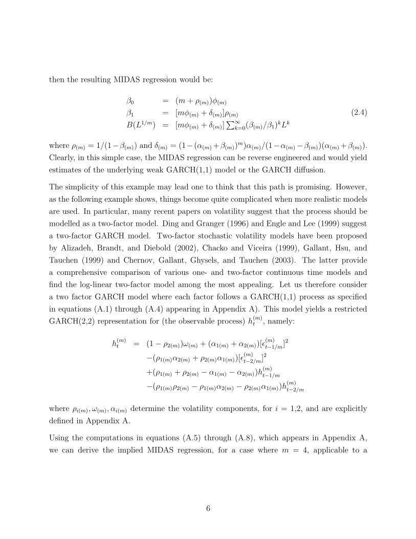
then the resulting MIDAS regression would be:

β0 = (m + ρ(m))φ(m)

β1 = [mφ(m) + δ(m)]ρ(m)

B(L1/m) = [mφ(m) + δ(m)]∑∞

k=0(β(m)/β1)kLk

(2.4)

where ρ(m) = 1/(1−β(m)) and δ(m) = (1− (α(m) +β(m))m)α(m)/(1−α(m)−β(m))(α(m) +β(m)).

Clearly, in this simple case, the MIDAS regression can be reverse engineered and would yield

estimates of the underlying weak GARCH(1,1) model or the GARCH diffusion.

The simplicity of this example may lead one to think that this path is promising. However,

as the following example shows, things become quite complicated when more realistic models

are used. In particular, many recent papers on volatility suggest that the process should be

modelled as a two-factor model. Ding and Granger (1996) and Engle and Lee (1999) suggest

a two-factor GARCH model. Two-factor stochastic volatility models have been proposed

by Alizadeh, Brandt, and Diebold (2002), Chacko and Viceira (1999), Gallant, Hsu, and

Tauchen (1999) and Chernov, Gallant, Ghysels, and Tauchen (2003). The latter provide

a comprehensive comparison of various one- and two-factor continuous time models and

find the log-linear two-factor model among the most appealing. Let us therefore consider

a two factor GARCH model where each factor follows a GARCH(1,1) process as specified

in equations (A.1) through (A.4) appearing in Appendix A). This model yields a restricted

GARCH(2,2) representation for (the observable process) h(m)t , namely:

h(m)t = (1 − ρ2(m))ω(m) + (α1(m) + α2(m))[ε

(m)t−1/m]2

−(ρ1(m)α2(m) + ρ2(m)α1(m))[ε(m)t−2/m]2

+(ρ1(m) + ρ2(m) − α1(m) − α2(m))h(m)t−1/m

−(ρ1(m)ρ2(m) − ρ1(m)α2(m) − ρ2(m)α1(m))h(m)t−2/m

where ρi(m), ω(m), αi(m) determine the volatility components, for i = 1,2, and are explicitly

defined in Appendix A.

Using the computations in equations (A.5) through (A.8), which appears in Appendix A,

we can derive the implied MIDAS regression, for a case where m = 4, applicable to a

6

monthly/weekly MIDAS regression setting. The intercept of the MIDAS regression is:

β0 = (1 − ρ2(m))ω(m)(4 − (ρ1(m) + ρ2(m)) − ρ1(m)ρ2(m) − (ρ1(m) + ρ2(m))2

−ρ1(m)ρ2(m) − (ρ1(m) + ρ2(m))ρ1(m)ρ2(m) − (ρ1(m) + ρ2(m))3 − 2(ρ1(m) + ρ2(m))×

ρ1(m)ρ2(m) − (ρ1(m) + ρ2(m))2ρ1(m)ρ2(m) − (ρ1(m)ρ2(m))

2 − (ρ1(m) + ρ2(m))4

−3(ρ1(m) + ρ2(m))2ρ1(m)ρ2(m) − (ρ1(m)ρ2(m))

2 − (ρ1(m) + ρ2(m))3ρ1(m)ρ2(m)

−2(ρ1(m) + ρ2(m))(ρ1(m)ρ2(m))2)

(2.5)

Despite the simplicity of the model and the low value of m we find that the implied MIDAS

polynomial is extremely complex and impractical, it appears in the Appendix as formula

(A.9).

The two examples in this section show that reverse engineering is not a practical solution,

except in some very limited circumstances. It should also be noted that this analysis

is confined to MIDAS regressions involving a pure time series setting without additional

regressors. All of this, leads us to fully explore in the rest of the paper an approach built on

polynomials parameterized parsimoniously. This implies that we need to draw comparison

with distributed lag models, a topic we address in the next section.

3 MIDAS and distributed lag models: A comparison

In this section we compare MIDAS and distributed lag models. Although we discussed

a volatility-related example in the previous section, for the purpose of comparison with

distributed lag models we focus mostly on linear models and we emphasis the differences

and similarities between the two approaches. We begin with a setup where we leave

unspecified the parameterization of the polynomials (both for MIDAS and the distributed

lag specification. In a first subsection we revisit aliasing and discretization biases. The

second subsection is devoted to asymptotic efficiency comparisons. A final subsection deals

with similarities between MIDAS and distributed lag regression models.

3.1 Aggregation Bias and Aliasing Revisited

When data of different sampling frequencies are mixed, one invariably deals with temporal

aggregation. To study aggregation issues it is convenient to assume that the underlying

7

stochastic processes evolve in continuous time and data are collected at discrete points in

time. Such a setting has the appeal of imposing a priori a structure on discretely observed

data that is independent of the sampling interval. This is most convenient not only to

study temporal aggregation but also to introduce a formal discussion of MIDAS models.

Throughout the paper we shall use the convention that processes in discrete time sampled at

equidistant points separated by a step size of 1/m, are denoted by Y(m)t whereas continuous

time processes are denoted by y(t). With this convention, observations of processes in discrete

time with sampling frequency 1/m are:

Y(m)k/m = y(k/m) and X

(m)k/m = x(k/m) k ∈ . . . ,−1, 0, 1, . . . (3.1)

where y(t) and x(t) = (x1(t), . . . , xN(t))′, or more formally y(t, ω) and x(t, ω) =

(x1(t, ω), . . . , xN(t, ω))′, are realizations of covariance stationary processes in continuous time

governed by a probability space (Ω, A, P ).8 The above case covers a point sampling scheme.

Alternatively,

Y(m)k/m =

∫ k/m

(k−1−a)/my(τ)dτ and X

(m)k/m =

∫ k/m

(k−1−a)/mx(τ)dτ (3.2)

where typically a = 0, though it can be positive if some type of filtering occurs (to be

discussed later). The case of m = 1 corresponds to the discrete time representation usually

studied. The superscript will often be dropped in such a case, namely Yk refers to Y(1)k .

To discuss many issues ranging from parameterization and approximations to discretization

biases let us start with the continuous time setting:

y(t) = b ∗ x(t) + u(t) (3.3)

=

∫ ∞

−∞

x(t − s)b(s)ds + u(t)

where the symbol ∗ denotes the convolution operator. The errors in equation (3.3) are not

necessarily i.i.d. Identification of b in equation (3.3) rests on the assumption that the x

process is, up to second moments, truly exogenous, i.e. E[x(t)u(s)] = 0, ∀ s and t.

Sims (1971) and Geweke (1978) examine equations like (3.3) and study the relationship

between inference drawn from discrete time models and the parameters of the continuous

8Further technical assumption will need to be imposed on the stochastic processes, but for the momentwe shall proceed without the technical details.

8

time convolution.9 We will consider a single regressor (as in Sims (1971)) while focusing on

the limiting behavior of the discretely sampled model, as in Geweke (1978).10

A discrete time distributed lag model corresponding to (3.3) would be as follows:

Y(m)t/m =

1

m

∞∑

s=−∞

B(m)(s

m)X

(m)(t−s)/m + U

(m)t/m (3.4)

where both y and x are sampled at frequency 1/m.11 The topic of discretization bias in

distributed lag models, i.e. the difference between an estimator B(m) and b for any given

m, has been extensively studied, see for instance Sims (1971), Geweke (1978), Hansen and

Sargent (1983), Hansen and Sargent (1991b), Phillips (1972), Phillips (1973) and Phillips

(1974), among others.

MIDAS regressions involve processes with various sampling frequencies. More specifically,

we study projections of Y sampled with m = 1 and X (m) sampled with m > 1. MIDAS

regression models are therefore:

Yt =1

m

∞∑

s=−∞

B(m)(s

m)X

(m)(t−s)/m + Ut (3.5)

Notice the differences between the two equations (3.4) and (3.5). The former has a projection

of Y(m)t/m onto the x process sampled discretely at frequency 1/m whereas the latter has a

projection of Y(1)t onto the same information set.

In this section we revisit the convergence of parameter estimators B(m) to b in equation (3.3)

for m increasing in the context of a MIDAS regression model (3.5). It is important to note

that we only deal with OLS estimators, and therefore are not interested at this stage with

efficiency issues. The latter will be the topic of the next section. Hence, we examine OLS

estimators B(m) in distributed lag models, similar to Sims (1971) andGeweke (1978), and

OLS estimators B(m) in MIDAS regressions.

9Equation (3.3) subsumes special cases like one-sided projections or solutions to stochastic differentialequations, see e.g. Geweke (1978)

10The case of multivariate regression is a straightforward extensions omitted here to avoid the cost ofcumbersome notation.

11The normalization of equation (3.4) by a factor 1/m is, as Geweke (1978) notes, necessary as the numberof parameters in any set

[

B(m)(s/m) : s ∈ [t1, t2]]

increases approximately in proportion with n and eachindividual coefficient in (3.4) will approach zero with increasing m.

9

To do so, let us recall first what happens when a distributed lag model is considered.

Following Sims (1972) the least squares estimator of B(m) in (3.4) minimizes the following

criterion:∫ πm

−πm

|B(m)(ω) − b(ω)|2Fm[Sx](ω) (3.6)

where Sx is the spectral density of the continuously sampled process x(t) and the spectral

density of the discretely sampled process x(t−s)/m, denoted S(m)x ≡ Fm[Sx], is expressed in

terms of the folding operator (see e.g. Fishman (1969), p. 38) Fm[g](ω) =∑∞

k=−∞ g(ω +

2mπk). Finally, B(m) and b are the Fourier transforms of B(m) and b respectively. Moreover,

the discretely sampled distributed lag regression yields the OLS estimator:

B(m) = Fm[Sxb]/Fm[Sx] = Fm[Syx]/Fm[Sx] (3.7)

where Syx is the co-spectrum of continuously sampled y(t) and x(t). Both equations (3.6)

and (3.7) suggest that MIDAS regressions may have properties regarding discretization bias

reduction similar to those of distributed lag models. Equation (3.6) tells us that the least

squares estimator minimizes a least squares distance between the Fourier transform of the

continuous sampling convolution polynomial and its discrete sampling fit weighted by Fm[Sx].

With MIDAS regressions we do have Fm[Sx] available.

Equation (3.7) also suggests that MIDAS regressions may resemble distributed lag models

in terms of discretization bias, yet it also brings us to a first technical issue that needs to

be discussed. So far we did not make a distinction between discrete data driven by a point-

sampling scheme, as in (3.1), or a flow aggregation as in (3.2). Usually in distributed lag

models the distinction is not important. A well known result often exploited in the literature

on seasonality tells us that as long as yt and xt as filtered with the same filter, there should be

no concern regarding bias.12 In the context of MIDAS regressions, point sampling is the most

straightforward case to discuss and will therefore be treated first. When flow variables are

considered one would indeed expect to see yt =∫ t

(t−1−a)y(τ)dτ and xk/m =

∫ k/m

(k−1−a)/mx(τ)dτ,

which amounts to unbalanced filtering on both sides of the MIDAS regression and therefore

a potential source of bias. It is for this reason that we proceed first with the point sampling

case.

To proceed with the intuition why equation (3.7) also suggests that MIDAS regressions may

12The same filter means that a is the same in (3.2). See Sims (1974) and Wallis (1974) for the originalwork on the topic and Ghysels and Osborn (2001) for the most recent literature.

10

resemble distributed lag models in terms of discretization bias, it is important to note that

what matters, besides Fm[Sx], is the covariance Fm[Syx]. In a MIDAS regression, assuming

stationarity and point sampling of y and x it is clear that ultimately we recover the covariance

between yt and any lag of xt. In this regards we are in a situation similar to a distributed

lag model where the sampling frequency increases. There is another way to explain why

distributed lag models and MIDAS regressions share similar properties with regards to

discretization bias. In the previous section we noted that MIDAS regressions appear like

skip-sampled distributed lag models (again thinking of the point sampling case). The skip

sampling causes autocorrelated residuals, yet this does not preclude OLS to be consistent

and feature the same bias properties as distributed lag models. To elaborate further on this

topic we discuss the technical issues in the remainder of this section.

There is both a local and a global dimension to the bias issue, the former being point-

wise limm→∞ Bm(s) = b(s), whereas the latter is concerned how Bm(s) approximates b(s)

as a function in the limit. It is convenient to use spectral analysis, as mean square

convergence in the frequency domain is L2 convergence in the time domain, whereas L1

convergence in the spectral domain corresponds to point-wise convergence in the time

domain. Regarding global convergence properties, Geweke (1978) (Theorem 3) shows

that limm→∞

∑∞

s=−∞[Bm(s/m) − b(s/m)]′[Bm(s/m) − b(s/m)] = 0. To state the result in

general terms for MIDAS regressions we consider multivariate regressions as in the original

formulation of Geweke (1978). The following result can be stated as an extension of Geweke

(1978) (Theorems 3 and 4):

Theorem 3.1 Let Assumptions B.1 through B.4 appearing in Appendix B hold. Moreover,

consider the MIDAS regression (3.5) with data discretely point-sampled as in (3.1), then:

limm→∞

∞∑

s=−∞

[Bm(s/m) − b(s/m)]′[Bm(s/m) − b(s/m)] = 0 (3.8)

and for each point t there exists a sequence of intervals Sm = (t − tm, t + tm) such that

limm→∞

(2tm)−1∑

s/m∈T m

Bmi (s/m) =

1

2limε→0

[bi(t − ε) + bi(t − ε)] i = 1, . . . , N (3.9)

The proof of Theorem 3.1 appears in Appendix C. Regressions involving macroeconomic

variables and financial series are usually confined to monthly, quarterly or annual regressions

11

due to the availability of macro series. The results appearing in this section show that one

can use the finer sampling of financial series to alleviate the discretization bias.

So far we only dealt with point sampled processes and noted that flow variables are likely to be

more cumbersome in the case of MIDAS regressions since mixed sampling frequencies lead to

different flow aggregations. Recall that the cause of the problem is the unbalanced filtering yt

=∫ t

(t−1−a)y(τ)dτ and xk/m =

∫ k/m

(k−1−a)/mx(τ)dτ. There is, however, a fairly simple - although

somewhat unorthodox - solution to the bias induced by unbalanced filtering. It suffices to

project yt onto xk/m =∫ k/m

(k/m−1−a)x(τ)dτ, which amounts to a balanced filtering on both

sides of the MIDAS regression. This scheme yields a MIDAS regression where for example

quarterly GNP growth is projected on monthly sampled 3-month inflation growth rates.

Likewise, in the case of volatility applications this scheme would amount to projecting daily

increments in quadratic variation onto five-minute sampled daily increments in quadratic

variation (assuming a 24-hour market cycle).13

To conclude this section we would like to draw attention to the dimensionality of aliasing,

as discussed in Hansen and Sargent (1983). In the case of rational polynomial lags

Hansen and Sargent (1983) (Theorem 1) show that in general there will only be finite

number of observationally equivalent models due to aliasing (though in general the class

of observationally equivalent models given equispaced discrete time series observations is

uncountable). Their result readily applies to MIDAS regressions as well.

3.2 Asymptotic Efficiency

The asymptotic analysis in the previous section was one of continuous records and the

emphasis was consistency, or absence of discretization bias as we sampled regressor at ever

increasing frequency. We showed that both distributed lag and MIDAS regressions feature

the desirable property of approximating b both locally and a globally. Moreover, the analysis

in the previous section only dealt with OLS estimators and did not address any efficient

estimation methods. In this section we turn our attention to efficient estimation. To do so,

we turn our attention to the conventional asymptotic analysis where the span of the data

set T expands asymptotically with a fixed sampling frequency m. Distributed lag models

will have sample sizes mT whereas the corresponding sample sizes for MIDAS regressions

13Such a scheme has been considered in the context of volatility estimation by Andreou and Ghysels (2002)as a rolling sample estimator of increments of quadratic variation.

12

will be T. Obviously, with m = 1 both are equivalent and MIDAS regressions turn into

distributed lag models. Consequently, distributed lag models involve more ’data’ as the

number of observations is mT, yet as far as information set is concerned, both distributed

lag and MIDAS regressions are on equal footing since they both involve the same regressors.

What we are interested in is what happens as T → ∞ so that both samples are large and

involve the same regressors.

We begin our analysis with linear models, which build directly on the discussions appearing

in the previous section. Linear models are covered in a first subsection. Next, we move

to partial linear models which feature nonlinearities separable from a linear projection and

therefore share many properties with linear models. A third and final section deals with

general nonlinear models.

3.2.1 Linear regression models

As in the previous section, it is not surprising that we will rely on spectral estimation

and in particular examine estimators due to Hannan (1963a) and Hannan (1963b) that are

asymptotically normal and efficient. The frequency domain GLS achieves asymptotically the

Gauss-Markov efficiency bound under general smoothness conditions on the residual spectral

density.

Consider again the discrete time distributed lag model like (3.4) where both y and x are

sampled at a fixed frequency 1/m. Hence, we consider equation

Y(m)t/m =

1

m

∞∑

s=−∞

b(m)(s

m)X

(m)(t−s)/m + u

(m)t/m (3.10)

where b(m) is the pseudo-true value associated with the fixed m.14 We try to obtain an

efficient estimator which we will denote BmH given a data set of size mT for both Y (m) and

X(m).

14Note the two differences between equations (3.4) and (3.10). The latter uses pseudo-true parameters

b(m) and residuals u(m)t/m, whereas the former was expressed in terms of OLS estimator B(m) and estimated

residuals U(m)t/m.

13

Before discussing the asymptotic distribution for BmH we introduce the MIDAS regression:

Yt =1

m

∞∑

s=−∞

b(m)(s

m)X

(m)(t−s)/m + ut (3.11)

where b(m) is again the pseudo-true value associated with the fixed m in analogy with equation

(3.10). The efficient estimator for the above MIDAS regression, which we will denote BmM

given a data set of size T for Y and X (m) has the following properties. The efficient estimator

for the above MIDAS regression, which we will denote BmM given a data set of size T for Y and

X(m) has the following properties, in comparison with the distributed lag model estimator

BmH :

Theorem 3.2 Let Assumptions B.1 through B.6 appearing in Appendix B hold. Then, the

Hannan feasible estimator is defined as:

B(m)H = [

km∑

j=−km+1

S(m)X (ωj)S

(m)U (ωj)

−1]−1[

k∑

j=−k+1

S(m)XY (ωj)S

(m)U (ωj)

−1] (3.12)

for ωj = mπj/km and where the spectral density estimators and bandwidth are defined in

(B.10) appearing in Appendix B. Likewise, the Hannan feasible estimator for a MIDAS

regression is:

B(m)M = [

km∑

j=−km+1

S(m)X (ωj)S

(1)U (ωj)

−1]−1[

k∑

j=−k+1

S(m)XY (ωj)S

(1)U (ωj)

−1] (3.13)

The estimator (3.12) has the following asymptotic distribution:

√mT (B

(m)H − b(m)) → N(0, 2π

∫ mπ

−mπ

Fm[Sx(ω)](Fm[Su(ω)])−1dω−1) (3.14)

whereas estimator (3.13) has the following asymptotic distribution:

√T (B

(m)M − b(m)) → N(0, 2π

∫ π

−π

Fm[Sx(ω)](F1[Su(ω)])−1dω−1) (3.15)

Provided, b(m) and b(m) are equal, the two estimators are asymptotically equivalent if Fm[Su]

is constant, i.e. U (m) is white noise.

14

The proof of the above theorem appears in Appendix D. Note that the pseudo-true values

b(m) and b(m) might differ, although the results of the previous section warrant to assume

that such a difference would be negligible for sufficiently large m. In the remainder of our

analysis we will proceed as if this is the case.

Let us first further elaborate on why the asymptotic efficiency of distributed lag and MIDAS

regressions differ. To do this it will be helpful to consider a slight variation of equation (3.3).

Often the equation is obtained from a so called rational distributed lag:

b2 ∗ y(t) = b1 ∗ x(t) + v(t) (3.16)

where identification of b1 and b2 is achieved by assuming that v is serially uncorrelated as

well as uncorrelated with x.

Equations (3.16) and (3.3) are related via the relationship b ≡ b−2 ∗ b1 where b−2 is the inverse

under convolution. Consequently, the serial dependence of the residuals in (3.3) is determined

by v(t) = b−2 ∗ u(t). A discrete time distributed lag model corresponding to (3.16) would be

as follows:

Y(m)t/m =

1

m

∞∑

s=−∞

b(m)1 (

s

m)(b

(m)2 (

s

m))−X

(m)(t−s)/m + u

(m)t/m

A simple strategy that leads to efficient estimation is to prefilter the equation by b2 :

Y(m)t/m =

∞∑

s=−∞

(b(m)2 (

s

m))Y

(m)(t−s−1)/m +

∞∑

s=−∞

b(m)1 (

s

m)X

(m)(t−s)/m + v

(m)t/m

where the availability of lagged Y(m)t/m allows us to apply the polynomial b2. In a MIDAS

regression this strategy is infeasible due to the lack of high frequency Y(m)t/m . Consequently,

the errors remain correlated and the estimator has to settle with an autocorrelation structure

that cannot be further unravelled. The clear advantage of distributed lag models is the

availability of the additional information about Y (m).

The result in theorem 3.2 tells us that uncorrelated errors in the distributed lag equation

are a situation where the advantage of distributed lag models is not of any consequence as

there is no need to prefilter. This observation is valid for models that are not determined by

rational polynomials as well, the case of rational polynomials is one where the results can

be presented in a transparent way. It is important to note, however, that theorem 3.2 does

not state that white noise is both necessary and sufficient. Indeed, there are cases whether

15

the two estimators are asymptotically equally efficient despite the fact that Fm[Su] is not

constant, i.e. U (m) is autocorrelated. A simple case would be where U (m) is an MA(q) process

with q < m. In such situations, there is correlation in U (m) but U (1) is uncorrelated as the

original process has memory shorter than the temporal aggregation. The Hannan efficient

estimator of the distributed lag model picks up the autocorrelation up to lag q, whereas the

MIDAS regression is asymptotically efficient without such a correction.

Hannan’s estimation procedure requires the choice of a bandwidth km, and an unsuitable

bandwidth selection can produce poor estimates. Robinson (1991) discusses frequency

domain inference with data-based bandwidth selection and proposed a commonly used

spectral estimator based on a weighted average of periodogram estimates of the fundamental

frequencies, or:

B(m)R = [

mT/2∑

j=−mT/2+1

I(m)X (ωj)S

(m)U (ωj)

−1]−1[

mT/2∑

j=−mT/2+1

I(m)XY (ωj)S

(m)U (ωj)

−1] (3.17)

The above estimator B(m)R is first order equivalent to the original estimator proposed by

Hannan. It is not difficult to show that the results in this section extend to such alternative

estimators when MIDAS and distributed lag regressions are compared in terms of asymptotic

efficiency. One outstanding issue, beyond the scope of the present paper is how higher-order

approximations for the coefficient estimates in MIDAS and distributed lag models compare.

Xiao and Phillips (1998) discuss such expansions for H(m)R . We leave such analysis for future

research.

To conclude it should be noted that simultaneous equations linear MIDAS regressions can

also be studied and compared with systems of linear distributed lag regressions. Indeed, the

analysis in this section, using the Hannan efficient estimation procedure, has multivariate

extensions. In particular, Hannan (1968) studies the circumstances under which least squares

are asymptotically efficient for the estimation of in systems of linear regressions and provides

a theorem which can be used to extend the result in Theorem 3.2 to multivariate settings.15

15The multivariate setting raises issues such as testing for Granger causality. Those are discussed at lengthin Ghysels, Santa-Clara, and Valkanov (2003a).

16

3.2.2 Partial linear models

The analysis in this section is inspired by Phillips, Guo, and Xiao (2002) who consider:

Y(m)t/m =

1

m

∞∑

s=−∞

b(m)(s

m)X

(m)(t−s)/m + g(Z

(m)t/m) + u

(m)t/m (3.18)

where the above equation is an adaptation of (3.10) to include a nonlinear functional g.16

Hence, in this model the response is assumed to be linearly related to X(m)t/m and nonlinearly to

Z(m)t/m (without lags). Partial linear models have been studied extensively and Phillips, Guo,

and Xiao (2002) provide an elaborate list of papers on the subject. Following early work

by Robinson (1988), a Nadaraya-Watson kernel estimator is used to eliminate the unknown

nonlinear function in a first step. Robinson (1988) assumed i.i.d. errors and showed that a

second stage least squares estimator for the linear regression part is√

mT consistent and

asymptotically normal. Phillips, Guo, and Xiao (2002) extends this to general autocorrelated

residuals and use a spectral density approach like in the previous section. Consider the

following MIDAS partial linear regression:

Yt =1

m

∞∑

s=−∞

b(m)(s

m)X

(m)(t−s)/m + g(Z

(m)t/m) + ut (3.19)

Taking expectations conditional on Z(m)t/m in both equations (3.18) and (3.19) and subtracting

the result from the original equations yields:

Y(m)t/m =

1

m

∞∑

s=−∞

b(m)(s

m)X

(m)(t−s)/m + u

(m)t/mYt =

1

m

∞∑

s=−∞

b(m)(s

m)X

(m)(t−s)/m + ut

where Y(m)t/m = Y

(m)t/m - E[Y

(m)t/m |Z(m)

t/m], Yt = Yt - E[Yt|Z(m)t ], and X

(m)t/m = X

(m)t/m - E[X

(m)t/m|Z(m)

t/m].

Note that Yt is still conditional on the same Z(m) process as Y(m)t/m . If the conditional

expectations were known, the above regression would simply be respectively a linear

distributed lag and MIDAS regression. In partial linear models the quantities Y(m)t/m , Yt and

X(m)t/m involve nonparametric estimation using a standard Nadaraya-Watson kernel estimator.

The analysis of Robinson (1988) and Phillips, Guo, and Xiao (2002) allows us to extend

16To be precise Phillips, Guo, and Xiao (2002) consider a regression such as (3.18) with a general regressorwhich we have specialized to the distributed lag setting.

17

theorem 3.2 to partial linear MIDAS models.17

3.3 Some similarities

The most striking similarity between MIDAS regressions and distributed lag models is the

fact that lag polynomials need to be tightly parameterized. In this respect there are similar

issues that emerge. Various parameterizations have been suggested in the distributed lag

literature, see e.g. Judge, Griffith, Hill, Lutkepohl, and Lee (1985) for further discussion.18

This common theme between distributed lag and MIDAS regressions generates similarities

with regards to estimation. Take for example a ”rational” polynomial lag structure, as

appearing in equation (3.16). Often such a rational polynomial is thought of as an

approximation for the function b(s) in (3.3). Therefore, model selection issues and asymptotic

misspecification errors are relevant for both MIDAS and distributed lag regressions and there

is no new ’theory’ as far as MIDAS is concerned. Spectral estimation typically amounts to

fixing the model size deterministically as a function of the sample size (see Sims (1974)

for further discussion). In a different approach, due to Akaike (1973) and many subsequent

refinements such as Schwarz (1978), among many others, a model fitting information criterion

function is used. We do not further explore this area here, except for noting that there is

a large literature already on the subject that can be applied in the context of MIDAS

regressions.

4 General MIDAS models

It will be convenient to start from a conventional asymptotic analysis. Let us consider a

general multivariate MIDAS regression setting, namely:

Yt+1 = B0 + f(

K∑

i=1

L∑

j=1

Bij(L1/mi)g(X

(mi)t )) + εt+1 (4.1)

17It should be noted, however, that the technical assumptions appearing in Appendix B require somestrengthening, see Phillips, Guo, and Xiao (2002) for details.

18Ghysels, Santa-Clara, and Valkanov (2003a) introduce a distributed lag based on the beta function,which is to the best of our knowledge novel to the literature and has proven to be very useful. The lagstructure can take many shapes and is determined only by two parameters.

18

and we collect all the parameters controlling the polynomials into the parameter vector b. As

noted in the previous section, the polynomials Bij(L1/mi) can be two-sided and the functions

f and/or g can involve unknown parameters. When unconstrained estimation is considered

this parameter space is potentially infinite. In the context of MIDAS regression models the

parameter vector b is a function of hyperparameters θ, hence the notation b(θ). To separate

the hyperparameter vector θ controlling the polynomials from the other parameters we denote

γ = (β ′ θ′)′. Therefore unconstrained estimation involves the possibly infinite parameter

space (β ′ b′)′, which is replaced in a MIDAS regression by (β ′ b(θ)′)′, or (β ′ θ′)′. At first

we will assume fixed mi, i = 1, . . . , K, and show that for such cases we can estimate MIDAS

regression with the usual asymptotic tools. Hence, for all practical purposes one can do the

estimation with standard software using conventional econometric methods.

The asymptotic analysis becomes slightly more involved when we let at least one mi go to

infinity, implying a continuous record conditioning set of regressors. In a first subsection

we present the conventional asymptotic analysis and then in a second subsection we turn to

MIDAS regressions with continuous record observations.

4.1 Fixed and Finite Sampling Frequencies

We consider the general class of extremum estimators. This class, which maximizes some

objective function that depends on the data and sample size, includes maximum likelihood

(MLE), nonlinear least squares (NLS) and generalized method of moments (GMM)

estimators which are the three types of estimators we would like to consider. An estimator

γT is an extremum estimator if there is an objective function MT (γ), given a sample size T

such that θT maximizes MT (γ) subject to θ ∈ Γ. The MLE estimator corresponds to

MT (γ) ≡ T−1T

∑

t=1

l(εt|γ) (4.2)

where l is the log likelihood based on distributional assumptions on the error process in (4.1).

As for the NLS estimator, the objective function is

MT (γ) ≡ −T−1T

∑

t=1

εt(γ)2 (4.3)

19

where εt+1(γ) ≡ [yt+1 - B0 - f(∑K

i=1

∑Lj=1 Bij(L

1/mi)g(X(mi)t ))]. Finally for the GMM

estimator the objective function

MT (γ) ≡ −[T−1T

∑

t=1

gt(γ)]′WT [T−1T

∑

t=1

gt(γ)] (4.4)

where gt(γ) ≡ υt × Zt−1 where Zt−1 is an instrument vector.19

One of the standard regularity conditions for consistency is that the parameter space is

compact, which in most cases is achieved by assuming a finite dimensional closed and

bounded parameter space. More specifically, Γ ⊂ Rq and Γ is compact. MIDAS regressions

therefore assume the standard environment in terms of parameter spaces. A second critical

assumption to establish consistency is identification, which can be written as:

Assumption 4.1 Given the information set It ≡ X(mi)τ , τ < t, i = 1, . . . , K, there exists a

function b(θ0) with dim(θ0) finite (small) and a parameter β0 such that

E[εt+1(β′0, b(θ0))

′)|It] = 0

for a unique γ0 = (β ′0, θ

′0)

′ ∈ Γ ⊂ Rq and Γ is compact.

This assumption is critical as it ensures the correct specification of the MIDAS polynomials.

When this assumption replaces the usual identification assumption we obtain the usual

asymptotic results, provided all other standard regularity conditions apply. More specifically,

the MLE, NLS and GMM estimators are consistent and asymptotically normal under

suitable regularity conditions appearing for instance in Gallant and White (1988), among

many others. Note that the asymptotics is for fixed mi, i = 1, . . . , K, and T going to infinity.

4.2 Continuously sampled regressors

In the remainder of this section we devote our attention to cases where at least one mi in

(4.1) goes to infinity, implying a continuous record conditioning set of regressors. Hence, we

ultimately estimate a functional approximation with a continuum of past observations rather

19Recall that when autoregressive augmentations appear in MIDAS regressions we know that the laggeddependent variable may not be a valid instrument, as discussed earlier.

20

than a polynomial lag of a MIDAS regression. To discuss this case we focus on a univariate

single regressor model without intercept and slope:

Yt+1 = B(L1/m)X(m)t + ε

(m)t+1 (4.5)

where B(L1/m) = b0 + b1L1/m + b2L

2/m+ . . . +bjmaxLjmax/m.20 Suppose now that we take

the limit of m → ∞ with jmax/m → κ. Hence, we are essentially sampling a continuum of

data between t and t− κ, allowing possibly κ to be infinite. With a continuum of data (4.5)

becomes the following convolution equation:

Yt+1 = β0 + β1

∫ κ

j=0

bj(θ)X(∞)t−j dj + ε

(∞)t+1 (4.6)

The MLE and NLS estimators of a correctly specified MIDAS regression, that is one

satisfying Assumption 4.1, are again standard provided we can compute the integral in (4.6)

without numerical approximation error. Note that now εt+1(θ) ≡ yt+1 −∫ κ

j=0bj(θ)x

(∞)t−j dj.

The GMM estimator requires more discussion because the choice of moment conditions and

instruments is not so straightforward. Recall that the GMM estimator specializes to

MT (θ) ≡ −[T−1T

∑

t=1

[(yt+1−∫ κ

j=0

bj(θ)x(∞)t−j dj)Zt−1]

′WT [T−1T

∑

t=1

[(yt+1−∫ κ

j=0

bj(θ)x(∞)t−j dj)Zt−1]]

(4.7)

and in principle any x ∈ I(∞)t,t−κ is a valid instrument so that one can exploit all possible

moment conditions that arise from the cross-product of errors and regressors in the MIDAS

regression polynomial. This ultimately yields a continuum of moment conditions, with a

finite parameter space. The fact that we approach a continuum of moments implies that

the moment conditions in (4.7) become more correlated and in the limit their covariance

matrix (and hence the inverse of the optimal GMM weighting matrix) approaches singularity.

This problem has been recognized by Carrasco and Florens (2000), who propose a so called

C − GMM estimator in situations of a limit continuum of moment conditions.

The C − GMM estimator is based on the arbitrary set of moment conditions:

Eθ0ht(τ ; θ0) = 0 (4.8)

20For simplicity we also assume that the polynomial to be one-sided.

21

where ht+1 (τ ; θ) ≡ [yt+1 −∫ κ

j=0bj(θ)x

(∞)t−j dj]x

(∞)t−τ , with τ ∈ R+. We will refer to ht(τ ; θ0) as a

moment function.21 Let hT (τ ; θ0) =∑T

t=1 ht(τ ; θ0)/T denote the sample mean of the moment

functions. The most convenient way to work with such infinite set is to impose a Hilbert

space structure. Carrasco and Florens introduce a space L2 (π) to which ht(.; θ0) belongs as

a function of τ. The inner product in this space is defined as

〈f, g〉 =

∫

f (τ) g (τ) π (τ) dτ (4.9)

where π is a probability density usually selected to be Gaussian. The norm corresponding

to the inner product is ‖ f ‖2= 〈f, f〉 . Similar to the standard GMM setup, one can prove

the central limit result for the sample mean of moment functions:

√T hT (τ ; θ0)

L⇒ N (0, K) (4.10)

Since hT is an element of Hilbert space, N is understood as a Gaussian random element of

the same space with variance 〈Kf, f〉, where the covariance operator K satisfies:

〈Kf, g〉 = Eθ0 [〈f, ht(θ0)〉 〈g, ht(θ0)〉] (4.11)

Note that K is an integral operator that can be written as

Kf (τ1) =

∫

k (τ1, τ2) f (τ2)π (τ2) dτ2 (4.12)

with k (τ1, τ2) = Eθ0(

ht (τ1; θ0) ht(τ2;θ0)

)

. The function k is called the kernel of the integral

operator K.

One way to implement the C-GMM estimator is to minimize the objective function:

minθ

v′ (θ)[

IT − C[

αT IT + C2]−1

C]

v (θ) (4.13)

where C is a T × T−matrix with the eigenvalues identical to those of KT and with (t, l)

21We continue here with the special case of a single regressor. Multi-regressor or multivariate extensionsare straightforward extensions.

22

element ctl/ (T − q), t, l = 1, ..., T, IT is the T × T identity matrix, v = [v1, ..., vT ]′ with

vt (θ) =⟨

hT (τ ; θ) , ht

(

τ ; θ1T

)⟩

,

ctl =⟨

hl

(

τ ; θ1T

)

, ht

(

τ ; θ1T

)⟩

.

where θ1T is a first step estimator which consistent (as in the usual GMM setting).

The above estimator, when Assumption 4.1 which guarantees that the MIDAS regression

is asymptotically correctly specified, has the standard properties of GMM estimators:

consistency, asymptotic normality and optimality. The following result is stated without

proof, as details appear in Carrasco and Florens (2000) and Carrasco, Chernov, Ghysels,

and Florens (2002):

Proposition 4.1 Let Assumption 4.1 hold and all other regularity conditions for the C-

GMM appearing in Carrasco and Florens (2000) hold as well. Moreover, let B be a bounded

linear operator defined on L2 (π) or a subspace of L2 (π) and BT a sequence of random

bounded linear operators converging to B. The C-GMM estimator θT = argminθ

∥

∥

∥BT hT (θ)

∥

∥

∥

has the following properties:

1. θT is consistent and asymptotically normal such that

√T

(

θT − θ0

)

L→ N(

0, V −11 × V2 × V −1

1

)

where V1 =⟨

BEθ0 (∇θh) , BEθ0 (∇θh)⟩

and V2 =⟨

BEθ0 (∇θh) , (BKB∗) BEθ0 (∇θh)⟩

.

2. Among all admissible weighting operators B, there is one yielding an estimator with

minimal variance. It is equal to K−1/2, where K is the covariance operator defined in

(4.12).

Carrasco, Chernov, Ghysels, and Florens (2002) extend this to the case of weakly dependent

processes. If it is a weakly dependent process then, ht is replaced by Uht in vt and ctl, see

Carrasco, Chernov, Ghysels, and Florens (2002) for a definition of Uht and further details.

This estimator, like the usual GMM, also involves a two-step procedure and a HAC-type

estimator of the covariance operator.

It is important to stress that in the above analysis the sample size T drives the asymptotics.

This is perhaps not surprising since the left hand side of a MIDAS regression determines the

23

data accumulation rate in terms of the reference interval of time. In this regard, our analysis

differs from recent developments such as Barndorff-Nielsen and Shephard (2003), who study

a multivariate covariance and regressions framework and consider ”filling in” of data x(m)

over fixed time intervals and obtain non-Gaussian asymptotic distributions. Along these lines

one could consider letting the sampling interval of Yt and X(m)t shrink at appropriate rates

to yield a continuous record data sample. We leave this question open for future research.

Once a continuum of moments approach is considered one can also wonder what the most

efficient choice of instruments would be. Carrasco, Chernov, Ghysels, and Florens (2002)

consider so called double index moment functions where τ in (4.8) is multidimensional, that

is τ = (τ1 τ2) ∈ R2.22 In particular, consider the set of moment conditions:

ht+1 (τ ; θ) ≡ [yt+1 −∫ θ

j=0

bj(θ)x(∞)t−j dj]Z(τ1, x

(∞)t−τ2) (4.14)

where Z(τ1, x(∞)t−τ2) is some ’optimal’ instrument choice. Using results in Carrasco, Chernov,

Ghysels, and Florens (2002) one can compute the asymptotic variance of θT , namely one can

compute(⟨

Eθ0 (∇θh) , Eθ0 (∇θh)⟩

K

)−1. To establish conditions under which this variance

coincides with the Cramer Rao efficiency bound, consider S, the linear space spanned by

h (τ, yt; θ0) and S be its closure. The results in Carrasco, Chernov, Ghysels, and Florens

(2002) imply that double-index C-GMM estimator based on (4.14) is efficient when the score

belongs to the span of the moment conditions. Intuitively, such a choice of instrument should

be clear. Since we can not construct the optimal instrument in, we can span it via a set of

basis functions. The choice of functions Z(τ1, x(∞)t−τ2) is closely related with the choice of test

functions to construct consistent conditional moment test, see Bierens (1990) as well as M.

and White (1998) and references therein. In particular, using the results of M. and White

(1998), Z(τ1, x(∞)t−τ2) could be based on any analytic functions but the polynomials. One

choice would be to consider the set of base functions Z(τ1, x(∞)t−τ2) = exp τ1x

(∞)t−τ2 , with τ1 ∈ R

and τ2 ∈ R+. The utilization of the continuum of moment conditions is precisely what allows

one to perform this spanning. Needless to say that imposing a distributional assumption

on υt yields an efficient MLE estimator that can be implemented straightforwardly as well.

The issue of efficient estimation also needs further exploration.

22We continue here again with the special case of a single regressor. Multi-regressor or multivariateextensions are straightforward extensions.

24

5 Conclusions

We introduced MIDAS regression models which involve time series data sampled at

different frequencies. MIDAS regressions are essentially tightly parameterized reduced form

regressions that involve processes sampled at different frequencies. At a general level, the

interest in MIDAS regressions addresses a situation often encountered in practice where

the relevant information is high frequency data, whereas the quantity of interest is a low

frequency process. In empirical work, a direct treatment of mixed data samples is typically

circumvented by first aggregating the highest frequency data in order to reduce all data

to the same frequency and then in a second step estimate a standard regression model.

We examined the features MIDAS regressions share with distributed lag models but also

emphasized their unique novel features.

While we discussed a large variety of issues, we clearly indicated some areas that remain

unresolved. These areas pertain to estimation and specification errors as well as the

treatment of long memory, seasonality and other common time series themes like (fractional)

co-integration.

25

References

Akaike, H., 1973, “Information theory and an extension of the maximum likelihood

principle,” in Second International Symposium on Information Theory, ed. by B. Petrov,

and F. Csaki, pp. 267–281. Akademia Kiado (Budapest).

Alizadeh, S., M. W. Brandt, and F. X. Diebold, 2002, “Range-based estimation of stochastic

volatility models,” Journal of Finance, 57(3), 1047–1091.

Andersen, T., T. Bollerslev, F. X. Diebold, and P. Labys, 2003, “Modeling and Forecasting

Realized Volatility,” Econometrica.

Andreou, E., and E. Ghysels, 2002, “Rolling-Sample Volatility Estimators: Some New

Theoretical, Simulation and Empirical Results,” Journal of Business and Economic

Statistics, 20, 363–376.

Barndorff-Nielsen, O., and N. Shephard, 2003, “Econometric analysis of realised covariation:

high frequency based covariance, regression and correlation in financial economics,”

Econometrica.

Bergstrom, A., 1990, Continuous Time Econometric Modelling. Oxford University Press,

Oxford.

Bierens, H., 1990, “A consistent conditional moment test of functional form,” Econometrica,

58, 1443–1458.

Brown, D. P., and M. A. F. Ferreira, 2003, “The Information in the Idiosyncratic Volatility

of Small Firms,” Working paper, Univesrity of Wisconsin and ISCTE.

Carrasco, M., M. Chernov, E. Ghysels, and J. Florens, 2002, “Efficient estimation of

jump diffusions and general dynamic models with a continuum of moment conditions,”

Discussion Paper.

Carrasco, M., and J. P. Florens, 2000, “Generalization of GMM to a continuum of moment

conditions,” Econometric Theory, 16, 797–834.

Chacko, G., and L. Viceira, 1999, “Spectral GMM estimation of continuous-time processes,”

Working paper, Harvard Business School.

26

Chambers, M., 1991, “Discrete models for estimating general continuous time systems,”

Econometric Theory, 7, 531–542.

Chernov, M., A. R. Gallant, E. Ghysels, and G. Tauchen, 2003, “Alternative Models for

Stock Price Dynamics,” Journal of Econometrics, 116, 225–257.

Comte, F., and E. Renault, 1996, “Noncausality in continuous time models,” Journal of

Econometrics, 73, 101–149.

Dhrymes, P., 1971, Distributed lags: Problems of Estimation and Formulation. Holden-Day,

San Francisco.

Ding, Z., and C. Granger, 1996, “Modeling Volatility Persistence of Speculative Returns: A

New Approach,” Journal of Econometrics, 73, 185–215.

Drost, F. C., and T. Nijman, 1993, “Temporal Aggregation of GARCH Processes,”

Econometrica, 61, 909–727.

Drost, F. C., and B. M. J. Werker, 1996, “Closing the GARCH Gap: Continuous Time

GARCH Modeling,” Journal of Econometrics, 74, 31–57.

Engle, R., and G. Lee, 1999, “A long-run and short-run component model of stock return

volatility,” in Cointegration, Causality and Forecasting - A Festschrift in Honour of Clive

W. J. Granger, ed. by R. F. Engle, and H. White. Oxford University Press, Oxford.

Fishman, G., 1969, Spectral Methods in Econometrics. Harvard University Press, Cambridge.

Gallant, A., and H. White, 1988, A Unified Theory of Estimation and Inference for Nonlinear

Dynamic Models. Basil Blackwell, Oxford.

Gallant, A. R., C.-T. Hsu, and G. Tauchen, 1999, “Using daily range data to calibrate

volatility diffusions and extract the forward integrated variance,” Review of Economic

Statistics, 81, 617–631.

Geweke, J., 1978, “Temporal Aggregation in the Multiple Regression Model,” Econometrica,

46, 643–661.

Ghysels, E., and D. Osborn, 2001, The Econometric Analysis of Seasonal Time Series.

Cambridge University Press, Cambridge.

27

Ghysels, E., P. Santa-Clara, and R. Valkanov, 2002, “There is a risk-return tradeoff after

all,” Working paper, UNC and UCLA.

, 2003a, “Predicting volatility: getting the most out of return data sampled at

different frequencies,” Working paper, UNC and UCLA.

, 2003b, “Variations on the Theme of MIDAS regressions,” Working paper, UNC and

UCLA.

Greene, W., 2000, Econometic Analysis. Prentice Hall.

Hannan, E., 1963a, “Regression for Time Series,” in Proceedings of a Symposium on Time

Series Analysis, ed. by M. Rosenblatt. John Wiley.

, 1963b, “Regression for Time Series with Errors of Measurement,” Biometrika, 50,

293–302.

, 1968, “Least-squares Efficiency for Vector Time Series,” Journal of the Royal

Statistical Society. Series B, 30, 490–498.

Hansen, L., and T. Sargent, 1983, “The Dimensionality of the Alliasing Problem with

Rational Spectral Densities,” Econometrica, 51, 377–387.

, 1991a, “Identification of continuous time rational expectations from discrete data,”

in Rational Expectations Econometrics, ed. by L. Hansen, and T. Sargent, pp. 219–235.

Westview Press, Boulder.

, 1991b, “Two difficulties in interpreting vector autoregressions,” in Rational

Expectations Econometrics, ed. by L. Hansen, and T. Sargent, pp. 77–119. Westview Press,

Boulder.

Judge, G., W. Griffith, R. Hill, H. Lutkepohl, and T. Lee, 1985, The theory and Practice of

Econometrics - Second Edition. John Wiley & Sons.

M., S., and H. White, 1998, “Consistent specification testing with nuisance parameters

present only under the alternative,” Econometric Theory, 14, 295–325.

McCrorie, J., 2000, “Deriving the exact discrete analog of a continuous time system,”

Econometric Theory, 16, 998–1015.

28

Phillips, A., 1959, “The estimation of parameters in systems of stochastic differential

equations,” Biometrika, 46, 67–76.

Phillips, P., 1972, “The Structural Estimation of a Stochastic Differential Equation System,”

Econometrica, 40, 1021–1041.

, 1973, “The Problem of Identification in Finite Parameter Continuous Time Models,”

Journal of Econometrics, 1, 351–362.

, 1974, “The Estimation of some Continuous Time Models,” Econometrica, 42, 803–

824.

Phillips, P., B. Guo, and Z. Xiao, 2002, “Efficient regression in time series partial linear

models,” Cowles Foundation Discussion paper No. 1363.

Robinson, P., 1977, “The construction and estimation of continuous time models and discrete

approximations in econometrics,” Journal of Econometrics, 6, 173–198.

, 1988, “Root-N-Consistent Semiparametric Regression,” Econometrica, 56, 931–954.

, 1991, “Automatic frequency domain inference on semiparametric and nonparametric

models,” Econometrica, 59, 755–786.

Schwarz, G., 1978, “Estimating the dimension of a model,” Annals of Statistics, 6, 461–464.

Sims, C., 1971, “Discrete Approximations to Continuous Time Distributed Lags in

Econometrics,” Econometrica, 39, 545–563.

, 1972, “The role of approximate prior restrictions in distributed lag estimation,”

Journal of American Statistical Association, 67, 169–175.

, 1974, “Distributed lags,” in Frontiers of Quantitative Economics II, ed. by M. D.

Intrilligator, and D. A. Kendrick. North-Holland, Amsterdam.

Stock, J., and M. Watson, 2003, Introduction to Econometrics. Addison-Wesley.

Wallis, K., 1974, “Seasonal adjustment and relations between variables,” Journal of

American Statistical Association, 69, 618–626.

Wang, L., 2003, “On the Intertemporal Risk-Return Relation: A Bayesian Model

Comparison Perspective,” Working paper, Wharton.

29

Wooldridge, J., 1999, Introductory Econometrics: A Modern Approach. South-Western.

Xiao, Z., and P. Phillips, 1998, “Higher-order approximations for frequency domain time

series regression,” Journal of Econometrics, 86, 297–336.

30

A Reverse engineering MIDAS regressions: A two-

factor model example

We consider a two factor GARCH model appearing in section ??, namely:

h(m)t = h

(m)1t + h

(m)2t (A.1)

with the components as follows:

h(m)1t = ω(m) + ρ1(m)h

(m)1t−1/m + α1(m)µ

(m)t−1/m (A.2)

and

h(m)2t = ρ2(m)h

(m)2t−1/m + α2(m)µ

(m)t−1/m (A.3)

where µ(m)t = [ε

(m)t ]2 − h

(m)t and returns are written as:

r(m)t = a(m) + ε

(m)t (A.4)

where ε(m)t = σ

(m)t z

(m)t and z

(m)t is i.i.d. (0, 1) while h

(m)t = [σ

(m)t ]2. The component GARCH model

implies a restricted GARCH(2,2) representation for (the observable process) h(m)t specified in 2.5.

Using this representation we can compute t he following:

EL[h(m)t+1/m|Ih(m)

t ] = (1 − ρ2(m))ω(m)(1 − (ρ1(m) + ρ2(m)) − ρ1(m)ρ2(m)) + (ρ1(m) + ρ2(m))h(m)t

+ρ1(m)ρ2(m)h(m)t−1/m

− (ρ1(m) + ρ2(m) − α1(m) − α2(m))µt

+(ρ1(m)ρ2(m) − ρ1(m)α2(m) − ρ2(m)α1(m))µt−1/m

(A.5)

EL[h(m)t+2/m|Ih(m)

t ] = (1 − ρ2(m))ω(m)(1 − (ρ1(m) + ρ2(m))2 − ρ1(m)ρ2(m) − (ρ1(m) + ρ2(m))×

ρ1(m)ρ2(m)) + ((ρ1(m) + ρ2(m))2 + ρ1(m)ρ2(m))h

(m)t + (ρ1(m) + ρ2(m))×

ρ1(m)ρ2(m)h(m)t−1/m − ((ρ1(m) + ρ2(m))(ρ1(m) + ρ2(m) − α1(m) − α2(m))

+(ρ1(m)ρ2(m) − ρ1(m)α2(m) − ρ2(m)α1(m)))µt

+ρ1(m)ρ2(m)(ρ1(m)ρ2(m) − ρ1(m)α2(m) − ρ2(m)α1(m))µt−1/m

(A.6)

31

EL[h(m)t+3/m|Ih(m)

t ] = (1 − ρ2(m))ω(m)(1 − (ρ1(m) + ρ2(m))3 − 2(ρ1(m) + ρ2(m))ρ1(m)ρ2(m)

−(ρ1(m) + ρ2(m))2ρ1(m)ρ2(m) − (ρ1(m)ρ2(m))

2) + ((ρ1(m) + ρ2(m))3

+2(ρ1(m) + ρ2(m))ρ1(m)ρ2(m))h(m)t + ((ρ1(m) + ρ2(m))

2ρ1(m)ρ2(m)

+(ρ1(m)ρ2(m))2)h

(m)t−1/m − ((ρ1(m) + ρ2(m))

2(ρ1(m) + ρ2(m) − α1(m) − α2(m))

−ρ1(m)ρ2(m)(ρ1(m) + ρ2(m) − α1(m) − α2(m))

+(ρ1(m) + ρ2(m))(ρ1(m)ρ2(m) − ρ1(m)α2(m)

−ρ2(m)α1(m)))µt + ((ρ1(m) + ρ2(m))2(ρ1(m)ρ2(m)

−ρ1(m)α2(m) − ρ2(m)α1(m)) + ρ1(m)ρ2(m)×(ρ1(m)ρ2(m) − ρ1(m)α2(m) − ρ2(m)α1(m)))µt−1/m

(A.7)

EL[h(m)t+4/m|Ih(m)

t ] = (1 − ρ2(m))ω(m)(1 − (ρ1(m) + ρ2(m))4 − 3(ρ1(m) + ρ2(m))

2ρ1(m)ρ2(m)

−(ρ1(m)ρ2(m))2 − (ρ1(m) + ρ2(m))

3ρ1(m)ρ2(m) − 2(ρ1(m) + ρ2(m))(ρ1(m)ρ2(m))2)

+((ρ1(m) + ρ2(m))4 + 3(ρ1(m) + ρ2(m))

2ρ1(m)ρ2(m) + (ρ1(m)ρ2(m))2)h

(m)t

+((ρ1(m) + ρ2(m))3ρ1(m)ρ2(m) + 2(ρ1(m) + ρ2(m))(ρ1(m)ρ2(m))

2)h(m)t−1/m

−((ρ1(m) + ρ2(m))3(ρ1(m) + ρ2(m) − α1(m) − α2(m))

+(ρ1(m) + ρ2(m))2(ρ1(m)ρ2(m) − ρ1(m)α2(m) − ρ2(m)α1(m))

−2(ρ1(m) + ρ2(m))ρ1(m)ρ2(m)(ρ1(m) + ρ2(m) − α1(m)

−α2(m)) + ρ1(m)ρ2(m)(ρ1(m)ρ2(m) − ρ1(m)α2(m) − ρ2(m)α1(m)))µt

+((ρ1(m) + ρ2(m))3 + 2(ρ1(m) + ρ2(m))ρ1(m)ρ2(m)(ρ1(m)ρ2(m)

−ρ1(m)α2(m) − ρ2(m)α1(m)))µt−1/m

(A.8)

Then the MIDAS projection equation has the following expression:

β1B(L1/m) = ((ρ1(m) + ρ2(m)) + (ρ1(m) + ρ2(m))2 + ρ1(m)ρ2(m) + (ρ1(m)+

ρ2(m))3 + 2(ρ1(m) + ρ2(m))ρ1(m)ρ2(m)

+(ρ1(m) + ρ2(m))4 + 3(ρ1(m) + ρ2(m))

2ρ1(m)ρ2(m) + (ρ1(m)ρ2(m))2)

+(ρ1(m)ρ2(m) + (ρ1(m) + ρ2(m))ρ1(m)ρ2(m) + (ρ1(m) + ρ2(m))2ρ1(m)ρ2(m)

+(ρ1(m)ρ2(m))2 + (ρ1(m) + ρ2(m))

3ρ1(m)ρ2(m)

+2(ρ1(m) + ρ2(m))(ρ1(m)ρ2(m))2)L1/m

+((ρ1(m)ρ2(m) − ρ1(m)α2(m) − ρ2(m)α1(m)) − (ρ1(m) + ρ2(m))×

32

(ρ1(m) + ρ2(m) − α1(m) − α2(m)) − (ρ1(m) + ρ2(m) − α1(m) − α2(m))

−(ρ1(m) + ρ2(m))2(ρ1(m) + ρ2(m) − α1(m) − α2(m))

−ρ1(m)ρ2(m)(ρ1(m) + ρ2(m) − α1(m) − α2(m))

+(ρ1(m) + ρ2(m))(ρ1(m)ρ2(m) − ρ1(m)α2(m) − ρ2(m)α1(m))

+(ρ1(m) − ρ2(m))3(ρ1(m) + ρ2(m) − α1(m) − α2(m)) + (ρ1(m)

+ρ2(m))2(ρ1(m)ρ2(m) − ρ1(m)α2(m) − ρ2(m)α1(m))

−2(ρ1(m) + ρ2(m))ρ1(m)ρ2(m)(ρ1(m) + ρ2(m) − α1(m) − α2(m))

+ρ1(m)ρ2(m)(ρ1(m)ρ2(m) − ρ1(m)α2(m) − ρ2(m)α1(m)))×(1 − (ρ1(m) + ρ2(m))L

1/m + ρ1(m)ρ2(m)L2/m)/

(1 − (ρ1(m) + ρ2(m) − α1(m) − α2(m))L1/m + (ρ1(m)ρ2(m) − ρ1(m)α2(m) − ρ2(m)α1(m))L

2/m)

+((ρ1(m)ρ2(m) − ρ1(m)α2(m) − ρ2(m)α1(m)) + ρ1(m)ρ2(m)×(ρ1(m)ρ2(m) − ρ1(m)α2(m) − ρ2(m)α1(m))+

(ρ1(m) + ρ2(m))2(ρ1(m)ρ2(m) − ρ1(m)α2(m) − ρ2(m)α1(m)) + ρ1(m)ρ2(m)(ρ1(m)ρ2(m)

−ρ1(m)α2(m) − ρ2(m)α1(m)) + (ρ1(m) + ρ2(m))3

+2(ρ1(m) + ρ2(m))ρ1(m)ρ2(m)(ρ1(m)ρ2(m) − ρ1(m)α2(m) − ρ2(m)α1(m)))×(1 − (ρ1(m) + ρ2(m))L

1/m + ρ1(m)ρ2(m)L2/m)L1/m/

(1 − (ρ1(m) + ρ2(m) − α1(m) − α2(m))L1/m + (ρ1(m)ρ2(m) − ρ1(m)α2(m) − ρ2(m)α1(m))L

2/m)

(A.9)

B Regularity Conditions

It is worth recalling equation (3.3), namely:

y(t) = b ∗ x(t) + u(t)

=

∫ ∞

−∞

x(t − s)b(s)ds + u(t)

where the errors are not necessarily i.i.d. In addition, the following technical conditions are assumed

to hold:

Assumption B.1 The continuous time processes y(t), x(t) and u(t) are covariance stationary with

spectral densities Sy, Sx, Su and co-spectrum Sxy.

Assumption B.2 To ensure identification of b in equation (3.3) rests on the assumption that the

x process is, up to second moments, truly exogenous, i.e. E[x(t)u(s)] = 0, ∀ s and t ∈ R.

33

So far, we did not distinguish single regressor and multiple regressor cases. In the main body of

the paper we treated the single regressor case for ease of presentation. The following technical

conditions cover the general multiple regression case.

Assumption B.3 b(s) in (3.3) is an N -dimensional vector of absolutely integrable functions of

bounded total variation.

Assumption B.4 The eigenvalues of the spectral density matrix of x(t) are strictly bounded

away from zero on every finite frequency interval and that in the auxiliary regressions: xi(t) =∫ ∞

−∞xj(t − s)′bij(s)ds + εij(t) all bij are ordinary absolutely integrable functions.

In order to define the Hannan efficient estimators studied in section 3 we consider the spectral

densities Fm[Sx], Fm[Sx] and co-spectrum Fm[Syx], and define the estimators:

S(m)Z (λ) =

1

2πm

km∑

s=−km

K(s

km)R

(m)Z (s) exp(−isλ) (B.10)

for Z(m) equal to X(m) or U (m), where km is a bandwidth parameter, K is a kernel function and

R(m)Z (s) is the autocovariance function of Z (m). Equation (B.10) can be straightforwardly modified

to deal with the co-spectrum Fm[Syx] as well. The following conditions are assumed to hold:

Assumption B.5 The bandwidth km = o(√

mT ) and the kernel K(x) is an even, bounded function

for x ∈ [−1, 1] with k(0) = 1 and k(x) = 0 for x /∈ [−1, 1].

In addition, the following assumption is made regarding the error processes and autocovariances:

Assumption B.6 The error processes u(m)t/m and ut in equations (3.10) and (3.11) respectively,

are linear processes with absolute summable Wold decomposition moving average representations.

Moreover, the autocovariances appearing in Assumption B.5, R(m)Z (s) satisfy:

∑∞s=−∞ |s|‖R(m)

Z (s)‖< ∞.

C Proof of Theorem 3.1

We start from the observation in Sims (1972) that the least squares estimator of B (m) in (3.4)

minimizes the following criterion:

∫ πm

−πm|B(m)(ω) − b(ω)|2Fm[Sx](ω) (C.11)

34

When all processes are point-sampled, the residuals of the MIDAS regression (3.5) are skip-sampled

versions of the residuals in (3.4). Consequently, the least squares estimator minimizes the criterion

(C.11) subject to frequency folding:

∞∑

j=−∞

∫ π

−π|B(m)(ω + 2πj) − b(ω + 2πj)|2Fm[Sx](ω + 2πj) (C.12)

Since it is assumed that the spectral density matrix is strictly positive the minimizations in (C.11)

and (C.12) yield the same minimand B(m).

Another way of obtaining the equivalence between B (m) in (3.4) and B(m) in (3.5) is to note

that Sims (1971) shows the following relationship between continuous sampled b in (3.3) and the

discretely sampled distributed lag estimator B (m) in (3.4):

B(m) =

∫ ∞

−∞

r(m)x b(s)ds (C.13)

r(m)x (t) =

∞∑

s=−∞

R−∗

X(m)(s)Rx(t − s)

where RX(m)(s) is the autocovariance function of x(t) and R−∗

X(m)(s) is the inverse under convolution

of RX(m)(s).23 From equation (C.13) Sims (1971) notes (p. 548) that B (m) is obtained from b by

first smoothing b using the filter Rx ∗ RX(m) since another way of writing the above equation is

B(m) = b(s) * Rx(t − s) * R−∗

X(m) . Clearly, this filter only involves X (m) and therefore the same

relationship holds for B(m).

The remainder of the proof follows Geweke (1978), following the same steps to show that (3.8)

holds for MIDAS regressions. Likewise, to establish that (3.9) holds it is also straightforward to

follow the proof in Geweke (1978).

D Proof of Theorem 3.2

In this section we present the proof of theorem 3.2. The result of the MIDAS regression estimator

appearing in equation (3.13) is a straightforward application of the original result in Hannan (1963a)

and Hannan (1963b) who imposes Assumptions B.1 through B.5 (with some slight modifications

that are of no consequence here). In particular the MIDAS regression is viewed as a regression

projection of Y onto X (m) in the context of the Hannan procedure. The result for the distributed

23Equation (C.13) is derived for multivariate regressions in Geweke (1978).

35

lag estimator is similar to that appearing in Hannan (1963a) and Hannan (1963b), yet modified for

the sampling at frequency 1/m. The asymptotic distributions appearing in(3.14) and (3.15) follow

as well.

We are interested in the efficiency comparison and therefore focus on the difference between the

distribution of√

T (B(m)M − b(m)) versus that of

√mT (B

(m)H − b(m)) (ignoring, as noted in the main

body of the paper the potential differences in discretization biases with fixed m). First we re-scale

the latter such that the asymptotic distribution is in terms of√

T , yielding the covariance matrices:

2π

m∫ mπ

−mπFm[Sx(ω)](Fm[Su(ω)])−1dω−1)

and

2π∫ π

−πFm[Sx(ω)](F1[Su(ω)])−1dω−1)

Assuming that Fm[Su] is constant, i.e. U (m) is white noise, leads to the above being equal to:

2π

m∫ mπ

−mπFm[Sx(ω)](

σ2u

2πm)−1dω−1)

and

2π∫ π

−πFm[Sx(ω)](

σ2u

2π)−1dω−1)

which are equivalent.

36