2012 federal forecasters conference - u.s. … · 2012 federal forecasters conference forecasting...
TRANSCRIPT

The 19th Federal Forecasters Conference The Value of Government Forecasts
September 27, 2012 at the Bureau of Labor Statistics
Sponsoring Agencies Bureau of Labor Statistics Bureau of Transportation Statistics Department of Labor Department of Veterans Affairs Economic Research Service Internal Revenue Service International Trade Administration National Center for Education Statistics U.S. Census Bureau U.S. Energy Information Administration U.S. Geological Survey
Partnering Organization Research Program on Forecasting The George Washington University
www.federalforecasters.org

2012 Federal Forecasters Conference Paper and Proceedings
Announcement The 20th
Federal Forecasters Conference FFC2014
Will be held
April 24, 2014
in
Washington, DC
2012 Federal Forecasters Conference Paper and Proceedings
Contents Announcements ........................................................................................................................... Inside Cover
Table of Contents ........................................................................................................................................... i
Editor Page ................................................................................................................................................... iii
Federal Forecasters Consortium Board ........................................................................................................ iv
Foreword ...................................................................................................................................................... vi
Acknowledgements ..................................................................................................................................... vii
2012 Federal Forecasters Conference Forecasting Contest Winners ......................................................... viii
2011 Best Conference Paper Awards ........................................................................................................... ix
Scenes from the Conference ......................................................................................................................... x
Morning Session
Panel Discussion ..................................................................................................................................... 1
Energy Forecasts in Volatile Times Adam Sieminski, U.S. Department of Energy........................................................................................ 2
Forecasting Supply and Demand at USDA Joseph Glauber, U.S. Department of Agriculture ................................................................................... 2
Demographic Projections: Why Should Anyone Listen to Us? Howard Hogan, U. S. Census Bureau .................................................................................................... 3
Concurrent Sessions I
The Value of Case Studies
Article Abstracts ..................................................................................................................................... 4
The Role of Forecasting in the Federal Judiciary John Golmant, James Woods, Kevin Scott Administrative Office of U.S. Courts ................................ 5
Evaluating Government Forecasts
Article Abstracts ................................................................................................................................... 14
Improving Forecasts
Article Abstracts ................................................................................................................................... 15
Modeling and Forecasting Methodology
Article Abstracts ................................................................................................................................... 16
Benchmarking and Forecasting: A Top-Down Approach for Combining Forecasts at Multiple Frequencies Michele A. Trovero, Ed Blair, and Michael J. Leonard, SAS Institute Inc .......................................... 17
i
2012 Federal Forecasters Conference Paper and Proceedings
Concurrent Sessions II
Forecast Process
Article Abstracts ................................................................................................................................... 24
A Simple Model for Potential Output Maggie Woodward, Bureau of Labor Statistics ................................................................................... 25
Surveys and Forecasting
Article Abstracts ................................................................................................................................... 34
Compensation and Health Expenditures
Article Abstracts ................................................................................................................................... 35
Estimating the Impact of Reform on National Health Expenditures: An Impartial Outlook for Policymakers, Researchers, and the Public Andrea Sisko, Office of the Actuary, Centers for Medicare & Medicaid Services .............................. 36
Long-Term Projections
Article Abstracts ................................................................................................................................... 44
Projecting Net International Migration of the Foreign Born: 2012 to 2060 David Armstrong and Jennifer Ortman, Population Division, U.S. Census Bureau ............................ 45
ii

2012 Federal Forecasters Conference Paper and Proceedings
The 19th Federal Forecasters Conference — 2012
Edited and Prepared by
Kellie Schelach U.S. Department of Veterans Affairs
Veterans Health Administration Milwaukee, WI
iii

2012 Federal Forecasters Conference Paper and Proceedings
2012 Federal Forecasters Consortium Board
Adjemian, Michael Economic Research Service U.S. Department of Agriculture
Busse, Jeffrey U.S. Geological Survey U.S. Department of the Interior
Byun, Kathryn Bureau of Labor Statistics U.S. Department of Labor
Graham, Richard Bureau of Labor Statistics U.S. Department of Labor
Hussar, William National Center for Education Statistics U.S. Department of Education
Joutz, Frederick Research Program on Forecasting The George Washington University
Lane, Erin Bureau of Labor Statistics U.S. Department of Labor
MacDonald, Stephen Economic Research Service U.S. Department of Agriculture
Mallik, Arup U.S. Energy Information Administration U.S. Department of Energy
Matthews, Marybeth Veterans Health Administration U.S. Department of Veterans Affairs
Memmott, Jeff Bureau of Transportation Statistics U.S. Department of Transportation
Mosheim, Roberto Economic Research Service U.S. Department of Agriculture
Notis, Ken Bureau of Transportation Statistics U.S. Department of Transportation
Ortman, Jennifer U.S. Census Bureau U.S. Department of Commerce
Sinclair, Tara Research Program on Forecasting The George Washington University
Singh, Dilpreet Veterans Health Administration U.S. Department of Veterans Affairs
Sloboda, Brian W. Office of Regulatory and Programmatic Policy U.S. Department of Labor
Vincent, Grayson U.S. Census Bureau U.S. Department of Commerce
Waddington, David U.S. Census Bureau U.S. Department of Commerce
Weyl, Leann Internal Revenue Service U.S. Department of the Treasury
Young, Peg Bureau of Transportation Statistics U.S. Department of Transportation
iv

2012 Federal Forecasters Conference Paper and Proceedings
FFC Board
Front Row: (left to right) Kathryn Byun, Bureau of Labor Statistics; Arup Mallik, U.S. Energy Information Administration; Erin Lane, Bureau of Labor Statistics; Jennifer Ortman, U.S. Census Bureau.
Back Row: (left to right) Frederick Joutz, The George Washington University; Grayson Vincent, U.S. Census Bureau; Stephen MacDonald, Economic Research Service; Jeffrey Busse, U.S. Geological Survey.
v

2012 Federal Forecasters Conference Paper and Proceedings
Foreword
The 19th Federal Forecasters Conference (FFC2012) was held September 27, 2012 in Washington, DC. This meeting continues a series of conferences that began in 1988 and have brought wide recognition to the importance of forecasting as a major statistical activity within the Federal Government and among its partner organizations. Over the years, these conferences have provided a forum for practitioners and others interested in the field to organize, meet, and share information on forecasting data and methods, the quality and performance of forecasts, and major issues impacting federal forecasts.
The theme of FFC2012, “The Value of Government Forecasts,” was addressed from a variety of perspectives by a distinguished panel.
Adam Sieminski, Administrator, Energy Information Administration, U. S. Department of Energy, spoke about the volatility of energy forecasts, their view of what the future energy mix will be, and how to be intelligent consumers of energy forecasts.
Joseph Glauber, Chief Economist, Office of the Chief Economist, U. S. Department of Agriculture discussed the volatility of agricultural commodity prices, forecast security in the context of past security breaches and in the context of 24/7 financial market trading, as well as the challenge of making good forecasts within budget constraints.
Howard Hogan, Chief Demographer, Office of the Director, U. S. Census Bureau, discussed the variety of uses for census data as well as the challenges in producing population projections in terms of resources and data quality.
The papers and presentations in this FFC2012 proceedings volume cover a range of topics. The panel highlighted how to be an intelligent consumer of Federal forecasts. The concurrent afternoon sessions educated attendees in how to adapt forecasting techniques to particular challenges within the Federal Judiciary, Defense, the Federal Reserve Board, and a wide variety of other settings.
vi

2012 Federal Forecasters Conference Paper and Proceedings
Acknowledgements
Many individuals contributed to the success of the 19th Federal Forecasters Conference (FFC2012). First and foremost, without the support of the cosponsoring agencies and the dedication of the Federal Forecasters Consortium Board, FFC2012 would not have been possible.
Grayson Vincent of the U.S. Census Bureau opened the morning program, introducing John Galvin, Acting Commissioner of the Bureau of Labor Statistics, who gave the welcoming remarks. Brian Sloboda of the U. S. Department of Labor announced the winners of the 2012 forecasting contest. Frederick Joutz of the George Washington University announced the FFC2011 Best Conference Paper Awards. Jeffrey Busse of the U.S. Geological Survey presented award certificates. Christine Klucsarits, of the U.S. Census Bureau took photographs. Jennifer Ortman of the U.S. Census Bureau moderated the morning session’s panel discussion.
Erin Lane of the Bureau of Labor Statistics (BLS) organized the afternoon sessions. William Hussar of the National Center of Education Statistics prepared the papers from the afternoon sessions for inclusion in this publication. All members of the Federal Forecasters Board worked hard to provide support for the various aspects of the conference, making it the success it was.
Many thanks to the afternoon session chairs, who voluteered to organize and moderate the afternoon presentations. The session chairs are listed within these proceedings.
Special thanks go to Tara Sinclair and Frederick Joutz of the George Washington University for reviewing the papers presented at the 18th Federal Forecasters Conference and selecting the winners of the Best Conference Paper Awards for FFC2012.
Special thanks go to Erma McCray of the Economic Research Service, for staffing the registration desk.
FFC2012 was hosted by the BLS at their conference and training facility. The contributions of a number of BLS staff helped make this so successful. Foremost, were Erin Lane and Kathryn Byun who oversaw the overall preparation and clean up. Drew Liming designed and prepared the graphics for the conference poster, program, and proceedings cover. Additionally, special thanks also go to the staff of the BLS Conference and Training Center, who once again helped to make the day go smoothly.
Marybeth Matthews and Kellie Schelach of U.S. Department of Veterans Affairs produced the conference program, and this publication, which is an invaluable contribution.
Finally, we thank all of the attendees, discussants, and presenters whose participation made FFC2012 a successful conference.
vii

2012 Federal Forecasters Conference Paper and Proceedings
2012 Federal Forecasters Conference
2012 Forecasting Contest Winners
Winner:
Tom Garin U. S. Department of Veterans Affairs
First Runner Up:
Gregory J. Cepluch U.S. Census Bureau
Samuel Greenblatt
Bureau of Labor Statistics
Second Runner Up:
Roger Moncarz Bureau of Labor Statistics
viii

2012 Federal Forecasters Conference Paper and Proceedings
FFC2011 – 18th Federal Forecasters Conference
Best Paper Awards
Winner
Direct Marketing Strategies and Internet Connectivity Timothy Park and Shawn Wozniak
Economic Research Service
Honorable Mention
Forecasters vs. Models: A Horse Race on Monthly Indicator Releases David Payne
Office of the Chief Economist, Economics and Statistics Administration, Department of Commerce
Long Term Medicare Spending Projections Gregory Y. Won
Air Traffic Organization Office of Safety, Federal Aviation Administration
ix

2012 Federal Forecasters Conference Paper and Proceedings
The 19th Federal Forecasters Conference
FFC2012
Scenes from the Conference
Photos by Christine Klucsarits U.S. Census Bureau
U.S. Department of Commerce
x

2012 Federal Forecasters Conference Paper and Proceedings
Grayson Vincent, FFC Chair, opens the 2012 Federal Forecasters Conference.
John Galvin, Acting Commissioner of the Bureau of Labor Statistics, welcomes the FFC 2012 participants.
Brian Sloboda, FFC Board Member, announces the winners of the Forecasting Contest.
Frederick Joutz, FFC Board Member, announces winners of the Best Paper Contest.
xi

2012 Federal Forecasters Conference Paper and Proceedings
Jennifer Ortman, FFC Board Member, introduces the morning panelists.
Adam Sieminski, morning panelist and U.S. Energy Information Administration Administrator, presents.
Joseph Glauber, morning panelist and Chief Economist at USDA, presents.
Howard Hogan, morning panelist and Chief Demographer at the U.S. Census Bureau, presents.
xii
2012 Federal Forecasters Conference Paper and Proceedings
Panel Discussion
The Value of Government Forecasts
Government forecasts are necessary and valuable for understanding the fiscal tradeoffs and implications of different policies to the public and private sector. The President, Congress, and policy analysts rely on forecasts for allocating government resources and budgets. Federal forecasters make projections across a broad array of issues including population, the labor force, defense requirements, medical costs, agricultural programs, energy supply and demand, tax revenues, pollution, transportation, infrastructure investments, social insurance, and regulatory programs. They provide this critical input using analytical and quantitative models under varying degrees of uncertainty.
The 2012 Federal Forecasters Conference will examine how government forecasters face these challenges and how policy-makers and other decision-makers use forecasts to make decisions.
Moderator
Jennifer Ortman, Ph.D. U.S. Census Bureau
U.S. Department of Commerce
Panelists
Adam Sieminski Administrator
Energy Information Administration U.S. Department of Energy
Joseph Glauber, Ph.D. Chief Economist
Office of the Chief Economist U.S. Department of Agriculture
Howard Hogan, Ph.D. Chief Demographer
Office of the Director U.S. Census Bureau
1

2012 Federal Forecasters Conference Paper and Proceedings
Adam Sieminski Administrator
Energy Information Administration U.S. Department of Energy
Energy Forecasts in Volatile Times
The Energy Information Administration (EIA) was formed after the 1973 oil embargo to provide U.S. policymakers with independent statistics and forecasts on domestic and global energy markets. By law, EIA’s data, analyses, and forecasts are independent of approval by any other office or employee of the U.S. government. EIA produces several high-profile, forward-looking products of varying frequency on energy prices, changes in energy mix and the impact of policy proposals on energy use, price, and energy-related emissions. A key challenge EIA faces is providing the necessary context to consumers of our forecasts in order to understand the inherent complexity and volatility of energy forecasts. After nearly four months at the head of EIA, Adam Sieminski will provide some insights into assessing the values of our forecasts and the challenge of explaining this complexity to policymakers and the public.
Joseph Glauber, Ph.D. Chief Economist
Office of the Chief Economist U.S. Department of Agriculture
Forecasting Supply and Demand at USDA
The global grain shortages in the early 1970s exposed significant flaws in how USDA organized and analyzed market information. Agencies within USDA often produced different estimates which led to conflicting advice to policymakers. In 1973, the Outlook and Situation Board was charged with integrating the market intelligence of the Department to provide a consensus view to the public on agricultural markets. The first report published in September 1973 provided detailed forecasts for US feed grain, soybean, wheat and cotton crops. Over the years, the World Agricultural Supply and Demand Estimates report has grown to include detailed forecasts for US and major foreign suppliers and importers of crops as well as forecasts for livestock, dairy and poultry markets. Reports are closely watched by market traders and provide important information for policymakers. Challenges facing USDA include how to maintain a gold standard forecasting system given budget constraints and declining data resources, growing complexity of global markets and increasing concerns over data security given 24/7 trading in financial markets.
2

2012 Federal Forecasters Conference Paper and Proceedings
Howard Hogan, Ph.D. Chief Demographer
Office of the Director U.S. Census Bureau
Demographic Projections: Why Should Anyone Listen to Us?
The U.S. Census Bureau produces population projections for the nation on a regular basis. The projected size and structure of the population is important to public and private interests, both socially and economically. There are many different consumers and uses of population forecasts. Population forecasts never turn out to be precisely accurate and often they miss huge shifts and changes in trends. This presentation will examine failures in population projections, why consumers continue to rely on government population forecasts, and their overall value. The variety of uses and consumers will also be addressed, as well as the challenges in producing population projections in terms of resources and data quality.
3

2012 Federal Forecasters Conference Paper and Proceedings
Concurrent Sessions I
The Value of Case Studies
Session Chair: Jeffrey Busse, U.S. Geological Survey, U.S. Department of the Interior
The Role of Forecasting in the Federal Judiciary John Golmant, Jim Woods, and Kevin Scott, Administrative Office of the U.S. Courts
The federal judiciary must be able to process its business efficiently and efficaciously. Having a sense of how much work can be expected in the future can help the judiciary plan its budgetary and staffing requirements. To accomplish this, the Administrative of the US Courts regularly produces forecasts of future court caseloads, the main determinants of workload. The forecasts of caseloads are formulated using data-based statistical time series models. The models accommodate changes in law, the economy, and Executive Branch policy. The effectiveness of the forecasting models is assessed annually.
Application of Unobserved Component Model to Monitor Monthly Return Count Data in Real Time Jeff Matsuo, IRS Office of Research
IRS download data containing the number of returns filed by form type, and by geographical locations on a monthly interval. It is essential to ensure that the data is accurate and reliable in order to produce the most dependable forecast for the IRS workload planning and resource allocations. It is also important to detect any unusual patterns as soon as the data are available, in order to investigate and research any relevant information surrounding the data, well before the publication deadline. In this presentation, the author presents the forecasts produced by the Unobserved Component Model and compares the results to the actual monthly data, to identify any “unexpected” data points in the historical time series.
The Who, When, Why, and How of Retail Food Price Forecasting at the USDA Economic Research Service Richard Volpe, USDA Economic Research Service
The Food Markets Branch of the Economic Research Service (ERS) maintains a topic page providing retail food price forecasts for major categories of the Consumer Price Index (CPI). Since 2007, when food prices began a string of volatility that continues to today, these forecasts have received much attention through the media, academia, and the government. This paper provides the motivation for analyzing food prices, an overview of the forecasting methodology used by ERS, the plans in place to expand and improve upon the forecasting process, and the ways these forecasts have been used by customers of ERS in recent years.
4

2012 Federal Forecasters Conference Paper and Proceedings
The Role of Forecasting in the Federal Judiciary By John Golmant, James Woods, Kevin Scott1
Administrative Office of U.S. Courts
Abstract
The federal judiciary must be able to process its business efficiently and efficaciously. Having a sense of how much work can be expected in the future can help the judiciary plan its budgetary and staffing requirements. To accomplish this, the Administrative Office of the U.S. Courts (AO) regularly produces forecasts of future court caseloads, the main determinants of workload. The forecasts of caseloads are formulated using data-based statistical time series models. The models accommodate changes in law, the economy, and Executive Branch policy. The effectiveness of the forecasting models is assessed annually. 1 Introduction
The three branches of federal government-- the Executive Branch, the Legislative Branch, and the Judicial Branch--work together to ensure that every citizen is protected under the Constitution. Simply put, the Legislative Branch writes the laws and provides funding for government operatives; the Executive Branch implements and enforces the laws; and the Judicial Branch interprets the laws and determines their constitutionality. The federal judiciary, sometimes referred to as the Third Branch, is comprised of the Supreme Court, 12 circuit courts of appeals, the federal circuit court of appeals, 94 district courts, 90 bankruptcy courts, the Court of International Trade, the Court of Federal Claims, and various support offices. The Judicial Conference of the United States2 and the
1 1 The views and opinions expressed within this paper are solely those of the authors and do not represent official policy of the Judicial Conference of the United States or the Administrative Office of the U.S. Courts.
2 As a direct result of Congressional action in 1922, the Judicial Conference was created to serve as the
AO3 play key roles in the daily operation of the federal judiciary. The practical business of the judiciary includes administering justice in civil, criminal, and bankruptcy matters, providing probation and pretrial services, and ensuring the availability of legal representation in criminal cases for defendants in criminal matters. The work of the federal courts is largely determined by outside sources. The judiciary itself does not create the work, nor does it have influence over the type of work presented before it. For example, during the 1980s and 1990s, consumer attitudes toward credit, coupled with the financial industry=s willingness to lend, created a society encumbered with record levels of personal debt.4 One practical result of this phenomenon was that millions of consumers filed for personal bankruptcy protection through the federal
policymaking body to govern the administration of the United States Courts.
3 The AO was created in 1939 to serve the federal judiciary in carrying out its constitutional mission to provide equal justice under law. The AO provides a wide range of administrative, legal, financial, management, program, and information technology services to the federal courts. The AO provides support and staff counsel to the Judicial Conference and its committees, and it implements and executes Judicial Conference policies, as well as applicable federal statutes and regulations. The AO facilitates communications within the federal judiciary and with Congress, the Executive Branch, and the public on behalf of the federal judiciary. The current director, Judge Thomas F. Hogan, was appointed October 17, 2011. The Director is the chief administrative officer for the federal courts and secretary to the Judicial Conference of the United States.
4 In 1980, total consumer credit reached approximately 352 billion dollars. By 2000, total consumer credit hit 1,717 billion—a 388 percent increase over 1980 levels. Source: US Board of Governors of the Federal Reserve System; Consumer Credit Report, Report G-19.
5

2012 Federal Forecasters Conference Paper and Proceedings
courts.5 During the 1990s and 2000s, in part because of an expanding U.S. economy, many foreigners entered the U.S. illegally or overstayed their temporary work visas. Enforcement of immigration law resulted in tens of thousands of immigration cases entering the federal judicial system.6
The judiciary cannot influence what laws are created, nor can it determine how the laws are enforced. Nevertheless, it must prepare a budget that takes into account the type and amount of work it expects to have. To accomplish this, the AO prepares forecasts of annual counts of bankruptcy filings, civil filings, criminal filings, appeals filings, petit and grand jury activity, probation and pretrial services caseload, and Criminal Justice Act (federal defender and panel attorney) representations.
These forecasts are used in a variety of ways, but by far the most important is in the judiciary’s annual budget submission to Congress. The forecasts (used to prepare the budget submission) are computed at the national aggregate level with one-, two-, and three-year forecast horizons. The forecasts are translated into future budget requirements. Other forecasts are used in determining future courthouse construction requirements and long-range planning requirements. The focus of this paper, however, will be how forecasts are used in the annual budget submission.
5 In 1980, 210,364 bankruptcy petitions were filed. In 2000, 1,282,102 petitions were filed---a 509 percent increase. Source: Annual Report of the Director of the Administrative Office of the US Courts, F-Series tables. 6 In 1990, 3,063 immigration defendants were brought to the federal courts; in 1995, 4,471 immigration defendants were brought to the courts; in 2000, 13,052 immigration defendants went to court; and in 2005, 18,322 immigration defendants were brought court. Source: Annual Report of the Director of the Administrative Office of the US Courts, Table D-3.
The Budget Process7
The budget process can be broken down into two phases formulation and execution. Budget formulation refers to the set of processes used to develop and present the judiciary=s national funding requirements for a specific fiscal year to the Congress to secure an appropriation. Budget execution refers to all processes concerned with allocating, allotting, reprogramming, obligating, expending, disbursing, and accounting for the funds made available under the appropriations act for the operating requirements for the current fiscal year. Budget formulation is a critical phase of the national budget process. The judiciary transmits budget requests to Congress to fulfill its authority to conduct judicial business throughout the country. Budget formulation for the judiciary involves an extensive 19-month planning process that starts with actions initiated by the Judicial Conference. Each spring, the Director of the AO, in accordance with 28 U.S.C. ' 605, submits the judiciary=s budget request to the Office of Management and Budget (OMB) in October for inclusion in the President=s budget request to Congress. By law (31 U.S.C. ' 1105), OMB can comment on, but not make changes to, the judiciary=s Congressional budget submission (known as the Yellow Book). Divisional program offices within the AO use the current year=s financial plan as a basis for estimating the funding requirements necessary to maintain the current level of operations for the fiscal year under consideration. The court support staffing requirements of the current year=s financial plan are adjusted to reflect workload changes projected by the AO=s Statistics Division. The workload projections are used in work measurement staffing formulas that calculate the number of supporting personnel necessary for court support offices. Each court program (appellate, district, bankruptcy, and probation and pretrial services offices) has a
7 The following discussion on the budget process comes directly from Court Budget Operating Manual published by the AO, April 2012.
6

2012 Federal Forecasters Conference Paper and Proceedings
unique staffing formula with multiple factors, such as case filings, divisional office support, information technology, and credits for financial and various other administrative functions.8 Caseload Projections
The budget formulation process for the judiciary is highly dependent on accurate counts of future caseload. To accomplish this, the AO=s Statistics Division (SD) regularly produces forecasts of the number of cases entering the federal courts (at the national aggregate level). Different types of cases account for different types of work. For example, a bankruptcy filing is very different from a criminal filing in terms of the type and amount of work needed to resolve the case. Table 1 provides a listing of the various case types (and other work factors) for which SD prepares forecasts. Table 1. Work Factors Bankruptcy Filings Appellate Court Filings District Court Filings Civil Filings Criminal Filings
Persons Serving Under Supervision (Probation) Pretrial Services Petit Jurors Grand Jurors Criminal Justice Act Representations Within a particular case type, subcomponents are examined. Each subcomponent has a unique contribution to the overall workload. For example, different types of bankruptcy cases have different work requirements. SD produces forecasts of chapter 7 filings, chapter 11 filings, 8 While the overwhelming majority of funding for the judiciary stems from appropriations from Congress, additional funding is derived from a portion of the filing fees collected by the clerks of court. For example, a civil case filing fee is $250 (per 28 U.S.C. § 1914). A chapter 7 (debt liquidation) bankruptcy filing fee is $245 (per 28 USC § 1930). In addition, user fees are collected for electronic access to case filings.
chapter 12 filings, and chapter 13 filings.9 Chapter 7 filings account for roughly 70 percent of overall bankruptcy filings, but generally require the least amount of work relative to other chapter types. By contrast, chapter 11 filings account for a much smaller percentage of overall bankruptcy filings, but generally require much more work by judges and court staff. Table 2 provides a listing of the subcomponents for each of the major case types. Table 2. Subcomponents for Selected Work Factors Bankruptcy Filings Appellate Filings Total Bankruptcies Chapter 7 Chapter 11 Chapter 12 Chapter 13 Adversary Proceedings Adversary Terminations
Total Appeals Civil Appeals Criminal Appeals Other Appeals
Civil Filings Criminal Filings Total Civil Filings US Plaintiff Recoveries Social Security Filings Prisoner Petitions Diversity Filings Other Filings Non-prisoner Pro Se Filings
Total Cases Total Defendants Drug Defendants Immigration Defendants Other Defendants Felony Defendants
Some work is indirectly related to the number of cases entering the federal courts. The number of grand jurors and petit jurors called for service, the number of persons using probation and pretrial services, and the number of public
9 The different chapter designations refer
to the corresponding chapters of the Bankruptcy Code. A chapter 7 bankruptcy petition calls for debt forgiveness and liquidation of unprotected assets. A chapter 11 bankruptcy petition requests a court-managed debt restructuring for large corporations. A chapter 12 filing provides a family farmer with court-managed debt restructuring. A chapter 13 petition calls for debt-restructuring for a consumer or small business. For more information on bankruptcy, see Bankruptcy Basics at http://www.uscourts.gov/FederalCourts/Bankruptcy/BankruptcyBasics.aspx.
7

2012 Federal Forecasters Conference Paper and Proceedings
defender representations are dependent, to various degrees, on the number of filings entering the federal courts. Forecast Methodology
Data-based statistical time series models are employed to project future caseload. More specifically, SD employs Autoregressive Integrated Moving Average (ARIMA) models and dynamic regression models (a regression model with ARIMA errors) to compute projections.10 A data-based approach offers an objective, impartial means of producing estimates of future workload. This approach can also accommodate changing laws, changing law enforcement policies, and a changing economy. With respect to the SD budget submission forecasts, monthly data are employed in most of the time series models. For many case types, monthly data are available from 1980 onward.11 Projected estimates are formulated at the monthly level and then aggregated to the annual level. Estimates for each subcomponent for each case type are computed three times during the
10 The general form of the dynamic regression models is:
Φ(B)(F(Yt) - ∑βnXnt ) = θ(B)εt where
• Yt is the dependent variable (i.e., the variable of interest) at time t,
• F is a Box-Cox transformation (if necessary),
• X1t, X2t, ..., Xnt are values of independent variables at time t,
• εt is the amount of white noise at time t, • Φ(B) is short-hand notation for
autoregressive parameters, • β1, β2, ... , βn are regression parameters, • θ(B) is short-hand notation for moving
average parameters, and • B is a backwards difference operator.
11 The models formulated for bankruptcy, appeals filings, and civil filings employ data back to 1980; the models formulated for criminal filings and juror usage use monthly data going back to 1990; the models for defender representations, back to 1994; and the models of probation and pretrial, back to 1992.
year. The first forecast includes a projection for each of three forecast horizons-- the current business year (the 12-month period ending June 30), the next business year, and the business year after that.12 This forecast uses data through the most recent calendar year (the 12-month period ending December 31). This forecast is typically available in early spring. The second forecast horizon typically corresponds to the forecast that is used in developing the Judiciary’s initial budget estimates.
The second forecast includes the same three forecast horizons but uses data through March. This forecast is typically available in late spring. The last forecast is available in the fall and includes the latter two forecast horizons. By and large, the forecasts associated with first of these two horizons are the ones used to develop the estimates for the final budget submission to Congress.
After each set of forecasts is formulated, SD formally presents the forecasts to the users, AO divisional offices. The presentation itself includes written documentation, discussion of the forecasting methodology, an exchange of information regarding the major influences on the case types, and an opportunity for the users to comment on particular sets of forecasts.
Case Studies
The following two examples illustrate how statistical time series models are applied. These examples also illustrate how the judiciary’s workload can be impacted by outside forces, e.g., legislative acts or executive branch policy. Bankruptcies – Chapter 7
Chapter 7 (debt liquidation) filings account for roughly 70 percent of overall bankruptcy filings. During the 12-month period model June 30, 2012, 914,015 chapter 7 petitions were filed. Figure 1 depicts monthly chapter 7 filings for the January 1994 through June 2012. A number of characteristics are worth noting. First, chapter
12 Juror services and defender representations use forecast horizons that are based on the fiscal year (the 12-month period ending September 30).
8

2012 Federal Forecasters Conference Paper and Proceedings
7 filings are highly seasonal, with March and April being the high-water months. Chapter 7 petitions have increased across time and have an increasing month-to-month variation. They were affected greatly by the passage and implementation of the Bankruptcy Abuse Prevention and Consumer Protection Act of 2005, as evidenced by the huge spike and subsequent drop-off in filings during 2005. Lastly, chapter 7 filings are cyclical. The cyclical nature roughly corresponds to the cyclical behavior of consumer debt, as Figure 2 suggests. The latest model designation used to forecast chapter 7 filings was a (2,1,0)(0,1,1) ARIMA model with regression components to account for outliers (both additive and temporary change), holiday effects, and cyclicality (via distributive lag models using debt-to-income and debt service ratios). A log transformation to account for non-stationarity of the variance is applied to chapter 7 filings.
Figure 3 shows the forecasts calculated for the 12-month period ending June 30, 2012. The longest forecast horizon corresponds to a forecast calculated using monthly data through September 2010, the next longest forecast horizon used monthly data through September 2011, and the shortest forecast horizon used data through March 2012. The three forecast horizons correspond to the forecasts, 1,076,700 filings, 944,700 filings, and 918,700 filings, respectively.13 As expected, the accuracy of the forecasts reflects the length of the forecast horizon, i.e., the shortest forecast horizon produced the most accurate forecast.
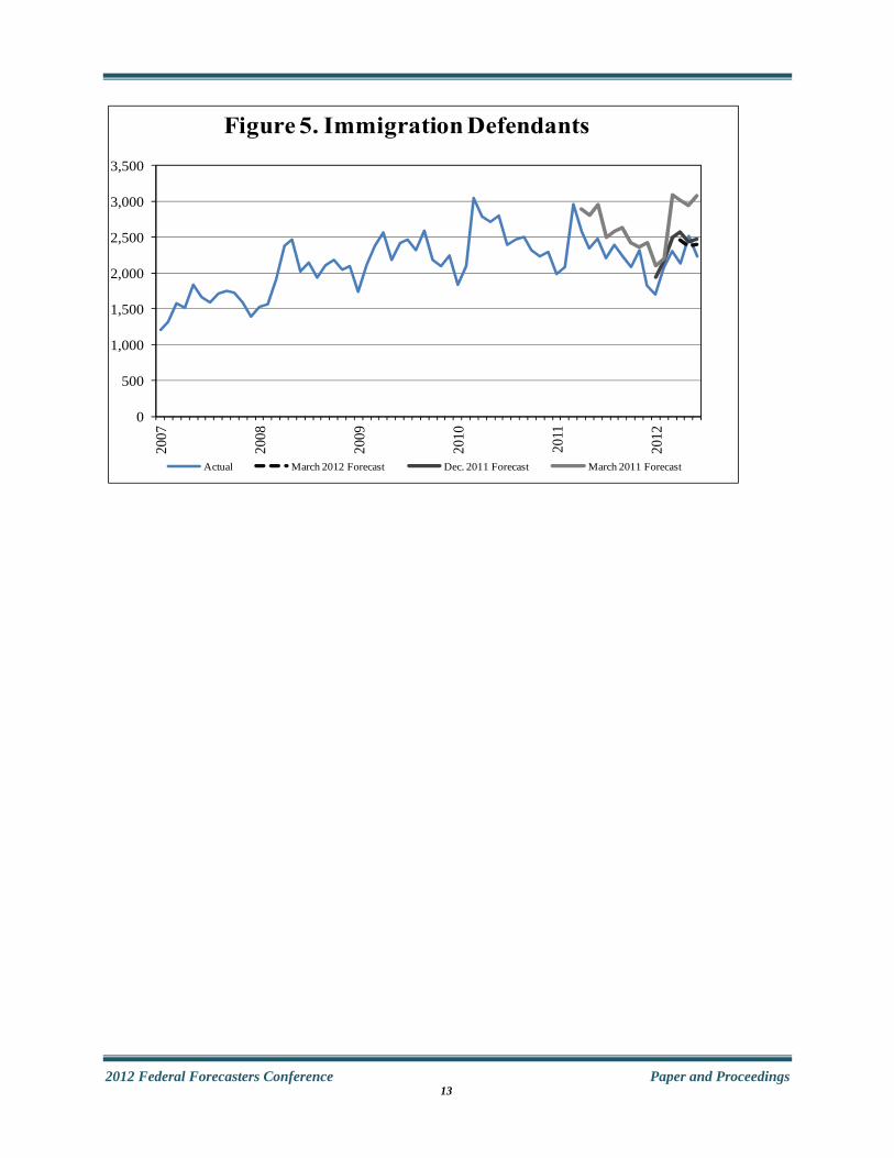
Criminal Filings – Illegal Immigration Defendants
SD’s forecasts of criminal filings include forecasts of drug defendants, illegal immigration defendants, and other defendants. During the 12-month period ending June 30, 2012, the overall number of criminal defendants entering the
13 The second estimate, 944,700 filings, was used in the final formulation of the Judiciary’s 2012 Congressional budget submission.
federal courts reached 96,915; the number of drug defendants was 30,719; the number of immigration defendants was 26,074; and the number of other defendants was 40,122. Figure 4 depicts annual criminal filings for the years 1993 through 2012 (based on the 12-month period ending June 30). This figure shows that overall criminal filings have been increasing over this period, and the rising trend is primarily the result of a rise in illegal immigration defendants. This increase was principally influenced by Executive Branch policy in terms of its enforcement of illegal immigration laws, but, as mentioned, an expanding economy during this period also played a role.14 The latest model designation to forecast illegal immigration defendants was a (2,1,0)(0,1,2) ARIMA model with regression components to account for outliers (additive and temporary change). Figure 5 shows the forecasted values for three forecast horizons. The longest corresponds to a forecast calculated using monthly data through the March 2010, the next longest used monthly data through September 2011, and the shortest forecast horizon used data through March 2012. The three forecast horizons correspond to the forecasts--37,300 defendants, 27,300 defendants, and 26,400 defendants, respectively.15 Forecast Evaluation
Every forecast is an estimate, and therefore every forecast has an error associated with it. Every year, SD publishes the error rates for all its forecasts. It presents the error rates to AO senior staff to promote the transparency and credibility of the forecasting process. Transparency is achieved through an ongoing discussion of the forecasting process with divisional offices. Credibility is achieved because the forecast errors are generally
14 See, e.g., the Department of Homeland Security Fact Sheet, http://www.dhs.gov/news/2011/10/04/fact-sheet- smart-effective-border-security-and-immigration- enforcement. 15 The second estimate, 27,300 defendants, was used in the development of the Judiciary’s 2012 Congressional budget submission.
9

2012 Federal Forecasters Conference Paper and Proceedings
reasonable, and whenever a particular forecast error is abnormally large, an explanation is offered.
The forecast errors are presented in three ways—the raw error, the percent error, and the mean absolute percent error (MAPE). The error measures are posted for each case type and forecast horizon. The raw error is the estimate minus the actual. The percent error is the raw error divided by the actual. The MAPE is the average of all percent errors (in absolute terms) across time for a particular case type and forecast horizon. Another measure, the mean percent error (MPE), is also calculated and shared when requested. The MPE is the average of all percent errors across time for a particular case type and forecast horizon.16 Both the MAPE and MPE can inform the forecasting process. For example, an MPE at or near zero implies that the forecasts have likely underestimated as often as they overestimated, i.e., systemic bias is likely not present. A small MAPE would imply that, historically, forecasts have been very accurate.
Table 3 presents the MAPEs and MPEs for select case types. It is notable that the MPEs are generally very close to zero. Also notable is that some case types have smaller MAPEs than others. The probation forecasts have the lowest error rates, which reflects generally well-behaved and consistent time series (i.e., easy to predict time series).
Table 3. Forecast Error Rates
Case Type Error Type
Forecast Horizon
Current Year
Budget Submission
Year
Third Year
Appeals MAPE MPE
1.5 -0.5
4.1 1.1
6.0 1.6
Criminal MAPE MPE
2.2 0.9
4.8 1.1
7.6 1.1
Civil MAPE MPE
2.1 -0.6
5.5 -0.4
8.3 0.5
Bankruptcy MAPE MPE
1.4 -0.2
5.8 0.2
14.2 2.0
Petit Jury MAPE 1.6 4.4 8.0
16 For most case types, 26 years of error data were used in the calculation of the MAPE and MPE.
MPE 0.4 2.7 4.7
Grand Jury MAPEMPE
1.8 0.5
4.2 2.4
5.5 3.3
Probation MAPEMPE
0.7 0.0
1.9 0.8
2.4 1.2
Concluding Remarks
The work of the federal judiciary is largely determined by legislative, administrative, and economic forces outside of its control. Nevertheless, the judiciary must anticipate its workload to help plan its budget and manage its resources. The number of cases entering the federal courts is a large determinant of workload, so accurately projecting future caseload can help the judiciary formulate its budget. SD produces forecasts for nine main work factors, three times a year, and each of these work factors has subcomponents that must also be projected. Statistical time series models are used to compute the forecasts. The forecasting process is transparent, and its credibility is objectively evaluated every year.
10

2012 Federal Forecasters Conference Paper and Proceedings
0
50,000
100,000
150,000
200,000
250,000
1990
1991
1992
1993
1994
1995
1996
1997
1998
1999
2000
2001
2002
2003
2004
2005
2006
2007
2008
2009
2010
2011
2012
Figure 1. Chapter 7 Filings
Recession Actual Trend
0
30,000
60,000
90,000
120,000
150,000
180,000
210,000
10
12
14
16
18
20
22
24
Deb
t--P
erce
nt
Figure 2. Consumer Debt
Debt Service Ratio Debt-to-Income Ratio Chapter 7 Chapter 7 SA
Bankruptcies
11

2012 Federal Forecasters Conference Paper and Proceedings
0
20,000
40,000
60,000
80,000
100,000
120,000
140,000
2007
2008
2009
2010
2011
2012
Figure 3. Chapter 7 Filings
Actual March 2012 Forecast September 2011 Forecast September 2010 Forecast
0
20,000
40,000
60,000
80,000
100,000
120,000
1993
1998
2003
2008
2012
Figure 4. Criminal Defendants
Total Immigration Drugs Other
12
2012 Federal Forecasters Conference Paper and Proceedings
0
500
1,000
1,500
2,000
2,500
3,000
3,50020
07
2008
2009
2010
2011
2012
Figure 5. Immigration Defendants
Actual March 2012 Forecast Dec. 2011 Forecast March 2011 Forecast
13
2012 Federal Forecasters Conference Paper and Proceedings
Evaluating Government Forecasts
Session Chair: Dilpreet Singh, Veterans Health Administration, U.S. Department of Veterans Affairs
IRS Practitioner Mandate Effect on Total Individual Electronic Filing (e-file) Michelle Chu and Leann Weyl, IRS Office of Research
In 1998, the Internal Revenue Service (IRS) received more than 64 million individual tax returns electronically (about 53%). Under the Internal Revenue Service Restructuring and Reform Act of 1998 (RRA98), IRS’ goal was to have at least 80% of all such returns filed electronically by the year 2007. In 2008, more than 87 million (about 60%) individual tax returns were received electronically. Thus, IRS launched an initiative to improve the electronic filing rate, resulting in an e-file mandate on tax return preparers, introduced and passed in November 2009. The mandate requires preparers who expect to file more than ten individual tax returns (including forms 1040, 1040A, 1040EZ, and 1041) to file them electronically beginning in CY 2011. The 80% goal was to include both business and individual tax forms. However, this analysis only focuses on the individual form 1040 series and attached schedules.
Detecting and Quantifying Biases in Government Forecasts of the U.S. Gross Federal Debt Neil R. Ericsson, Federal Reserve Board
Government debt has attracted considerable attention during the recent financial crisis and Great Recession. Building on Martinez (2011), this paper analyzes one-year-ahead forecasts of the U.S. gross Federal debt by the CBO, OMB, and APB over 1984–2011. Standard tests do not detect biases in these forecasts. However, a recently developed technique—impulse indicator saturation (IIS)—detects highly significant time-varying biases in all three agencies’ forecasts, particularly for 1990, 2001, 2008, 2009, and 2011. Biases differ across different agencies’ forecasts. IIS defines a generic procedure for examining forecast properties, and it explains why standard tests failed to detect bias.
Evaluating the Economic Forecasts of FOMC Members Xuguang (Simon) Sheng, Department of Economics, American University
This paper provides a detailed analysis of individual members’ real GDP and inflation forecasts of the Federal Open Market Committee (FOMC) during 1992-2001. We find a substantial diversity of participants’ views regarding likely outcomes for output growth and inflation rate. We notice a general tendency for FOMC participants to underpredict real GDP and overpredict inflation during the sample period. Despite those, we find the evidence that the Committee members have considerable information about inflation and output growth beyond what is known to commercial forecasters. We also notice systematic differences in forecast accuracy between the governors and the regional bank presidents.
14

2012 Federal Forecasters Conference Paper and Proceedings
Improving Forecasts
Session Chair: Arup Mallik, U.S. Energy Information Administration, U.S. Department of Energy
HRSA’s New Clinician Supply and Demand Models: The Quest for Transparency, User-Friendliness, and Utility for Policy Jennifer Nooney, Ph.D, National Center for Health Workforce Analysis, Health Resources and Services Administration
The Health Resources and Services Administration (HRSA) has recently redesigned a key forecasting system to project the supply and demand for physicians, physician assistants, and advanced practiced nurses. The redesign incorporates structural improvements to the models as well as additional functionality for modeling scenarios. This paper describes the structure of the models, their improved user interfaces, and the scenario-building capabilities that make them useful for policy. The opportunities and challenges around public release of the new models are discussed, as well as methods for making the model structure more transparent in our publically-available workforce projections reports.
Interpreting Employment Projections in Light of the Recession Michael Wolf, Bureau of Labor Statistics
BLS produces employment projections every two years to help workers, educators, and policy makers understand changes in the US labor market. The most recent set of projections, covering 2010-20, were produced right after large job losses during the recession, which poses a problem for interpreting the projections: many occupations and industries projected to gain jobs are just recovering from job losses during the recession, and understanding the difference between these jobs and jobs in fields that are experiencing long-run structural growth is important. This paper presents the projections and several methods of interpreting the data to help understand these differences.
Adjustment Strategies for Forecast Smoothing: A Soybean Production Forecasts Case Study Stephen MacDonald, Economic Research Service, USDA and Olga Isengildina-Massa, Clemson University
Recent research indicates that U.S. Department of Agriculture monthly commodity forecasts are smoothed. Revisions to U.S. supply and demand forecasts for a number of important agricultural commodities are positively correlated with previous month revisions, an inefficiency with potentially large impact during a period of high price volatility. Adjustment strategies to correct this problem will have to take into account the accounting and economic relationships between the USDA forecasts, and the institutional characteristics of USDA’s forecasting process. This paper uses USDA’s monthly soybean production forecasts during 1998-2010 to demonstrate the impact of several correction strategies on forecast efficiency and accuracy.
15

2012 Federal Forecasters Conference Paper and Proceedings
Modeling and Forecasting Methodology
Session Chair: Peg Young, Bureau of Transportation Statistics, U.S. Department of Transportation
An Overview of Regression Effects in the X-12-ARIMA Method “Tammy” Wilma S. Jackson, SAS Institute
Regression effects in the X-12-ARIMA method have 2 important roles in the method: they are used in the regARIMA model to prior adjust and extend the series and they identify effects to be included in the various components. How are effects specified? How do they affect the regARIMA model and the series to be seasonally adjusted? How are the effects used in the decomposition? Although the answers to these questions can be found elsewhere in the existing literature, this talk will attempt to organize and classify this information for users.
Multi-Step Ahead Forecasting of Vector Time Series Tucker McElroy, U.S. Census Bureau and Michael McCracken, Federal Reserve Bank of St. Louis
This paper develops the theory of multi-step ahead forecasting for vector time series that exhibit temporal nonstationarity and co-integration. We treat the case of a semi-infinite past, developing the forecast filters and the forecast error filters explicitly, and also provide formulas for forecasting from a finite-sample of data. This latter application can be accomplished by the use of large matrices, which remains practicable when the total sample size is moderate. Expressions for Mean Square Error of forecasts are also derived, and can be implemented readily. Three diverse data applications illustrate the flexibility and generality of these formulas: forecasting Euro Area DGP, CPI, and UR; backcasting fertility rates by racial category; and forecasting regional housing starts using a seasonally co-integrated model.
(Regression) Models Behaving Badly Keith Ord, Georgetown University
Building a good regression model for forecasting purposes is an arduous task, even with the many diagnostic tools we have available. However, standard practice does not always stand us in good stead. Even when a model is well-specified “business as usual” can lead to problems, such as biased forecasts and inadequate prediction intervals. We examine some alternative approaches that can help to avoid these difficulties.
Benchmarking and Forecasting: A Top-Down Approach for Combining Forecasts at Multiple Frequencies Michele A. Trovero, Ed Blair, and Michael J. Leonard, SAS Institute Inc
Forecasters often deal with data accumulated at different time intervals (for example, monthly data and daily data). A common practice is to generate the forecasts at the two time intervals independently so as to choose the best model for each series. That practice can result in forecasts that do not agree. This paper shows how the lower-frequency forecasts can be used as a benchmark to adjust the higher-frequency forecasts, thus taking the best advantage of both forecasts. An example is presented in which this method leads to improvements in the high-frequency forecasts, especially when the data exhibit intermittent behavior.
16

2012 Federal Forecasters Conference Paper and Proceedings
Benchmarking and Forecasting: a Top-Down Approach for Combining Forecasts at Multiple Frequencies Michele A. Trovero, Ed Blair, and Michael J. Leonard SAS Institute Inc. Abstract
Forecasters often deal with data accumulated at different time intervals (for example, monthly data and daily data). A common practice is to generate the forecasts at the two time intervals independently so as to choose the best model for each series. That practice can result in forecasts that do not agree. This paper shows how the SAS® High-Performance Forecasting HPFTEMPRECON procedure uses the lower frequency forecast as a benchmark to adjust the higher-frequency forecast to take the best advantage of both forecasts. Key Words: Forecasting; Benchmarking; Multiple Frequencies; SAS/HPF; PROC HPFTEMPRECON. 1. Introduction
Forecasters often need to produce forecasts for a certain time series at more than one frequency. For example, a company that provides warranty repairs for appliances might want to forecast the number of daily calls for staffing and operational planning, such as ordering supplies. The company might also want to forecast service calls at a monthly frequency to plan long-term expansion and to plan for financial concerns such as the purchase of more vehicles or the hiring of new staff. This paper deals with the problem of forecasting one time series at different frequencies, with a focus on stock variables. For a stock variable, the low-frequency series is the temporal aggregation of the high-frequency series. The term accumulation indicates temporal aggregation, and thus distinguishes it from other forms of aggregation, such as the aggregation of series within a subclass that can take place in a hierarchical forecasting context. The problem of forecasting at multiple frequencies is easily solved in an ideal world where data are plentiful, series are well behaved (meaning they have mostly nonzero values and are easily transformed to a covariance stationary series), and the correct model is chosen for each series. In this case, the accumulation of the high-frequency
forecasts is at least as efficient as the forecasts generated by modeling the low-frequency series, in the sense that the mean squared error of the h-step-ahead prediction of the former is less than or equal to the mean squared error of the h-step-ahead prediction of the latter. A formal outline of this argument for seasonal ARIMA processes can be found in Wei (1990, Chapter 16). The idea is simple: a forecast (prediction) is the linear projection onto the Hilbert space generated by the observed series. The space spanned by the low-frequency data is a subset of the space spanned by the high-frequency data. Therefore, the accumulation of the projection on the finer space generated by the high-frequency data is at least as “close” to the actual future value as the projection on the coarser space spanned by the low-frequency data. Another way to express the same concept that is simpler and does not require any mathematical jargon is that the accumulation process is a form of compression that involves loss of information. The original high-frequency data cannot be regenerated using only the accumulated data. Therefore, forecasts generated with the restricted information contained in the accumulated data cannot be better than forecasts generated with full information of the non-accumulated data. Reality, however, rarely comes in textbook format. Consider the following real-life examples (the name of the companies are retained for confidentiality reasons): Example 1. The spare-parts branch of a large company operates nationwide and manages more than 40,000 spare parts. Three-months-ahead daily forecasts are needed for each ZIP code for replenishing the repair trucks and for making staffing decisions. Very few parts are needed with regularity. Approximately only 10% of the parts show a somewhat regular demand for each ZIP code. For the remaining parts, the daily demand is almost always zero. Long-term monthly forecasts are needed for part production, hiring purposes, and long-term investments. Example 2. A large retail store chain collects POS (point-of-sale) data in each store. Hourly forecasts
17
2012 Federal Forecasters Conference Paper and Proceedings
are needed in the medium term for staffing purposes. The hourly data are kept for three months, after which they are discarded due to the cost of storing such a large amount of data. Only data accumulated at daily intervals are kept. Long-term monthly forecasts are needed for expansion and financial planning. In both examples, forecasts are needed at different frequencies for different purposes. However, there are good reasons to believe that the accumulation of the high-frequency forecasts will not lead to good forecasts for the low-frequency data. In the first example, most series show intermittent behavior. Intermittent series consist mostly of a single value, usually zero. Models for intermittent data, such as the popular Croston (1972) model, cannot capture important features such as trend, seasonality, and dependency on events or other external variables. Additionally, multiple seasonal components might be present in the high-frequency data, whether they are intermittent or not. Modeling and estimating multiple seasonal components simultaneously can be complex and computationally intensive. In the second example, the duration of the hourly (high-frequency) data is not sufficient to produce monthly (low-frequency) forecasts of any value. Indeed, you can reasonably argue that the information contained in the longer history of the daily data can be used with benefit to forecast the hourly data. For example, when making staffing decisions about the very important winter holiday season, the retailer should use the information contained in the daily data, which covers the previous holiday seasons, and not rely solely on the hourly data forecasts which are based only on the previous three months. In practice, the forecasts for the two or more frequencies of interest are often derived independently from each other by selecting at each frequency a model that provides the best results according to criteria, such as minimizing the MAPE (mean absolute percentage error). However, when the forecasts are derived independently, the accumulation of the high-frequency forecasts is generally different from the forecasts generated by the model for the low-frequency data. Additionally, as in Example 2, you might want to use the low-frequency forecasts to improve the high-frequency forecasts. This paper shows a method for revising the high-frequency forecasts such that their accumulation at
the low frequency is equal to the forecasts generated by the model selected for the low-frequency data. The first section details the method. The second section introduces the HPFTEMPRECON procedure in SAS® High Performance Forecasting and shows how it can reconcile monthly forecasts to daily forecasts for the Box and Jenkins’ airline data. The third section presents the results of applying the method to a data set that consists of several time series that exhibit intermittent behavior. Finally, the last section draws the conclusions. 2. Method
The combination of a series of high-frequency data with a series of more reliable but less frequent data is seen often in business statistics. For example, surveys are conducted at quarterly intervals on a subsample of the population of interest to determine the interannual variations, while comprehensive surveys on the whole population are conducted only on a yearly basis. The process of adjusting the more frequent data to match the less frequent but more reliable data is known in the literature as benchmarking. Denton (1971) provided the first general framework for benchmarking based on minimizing a quadratic function. A recent and comprehensive review on the topic can be found in Dagum and Cholette (2006). The lower-frequency forecasts are also referred to as the benchmark forecasts. The higher-frequency forecasts are also referred to as the indicator forecasts. Benchmarking procedures can be applied more generally to any two series that are measured at different time intervals. Therefore, this paper more generally refers to the benchmark series and indicator series to indicate the forecasts involved in the benchmarking. Denote the indicator series by with 1,… , , where t is associated with a date. Denote the benchmark series by , 1,… , . The benchmarks have a starting date ; and ending date ; , such that 1 ; ; . You want to find an optimal benchmarked series , 1,… , such that the accumulation of benchmarked series at the frequency of the lower-frequency forecasts is equal to the benchmark series. That is,
;
;
18

2012 Federal Forecasters Conference Paper and Proceedings
For 1,… , . The bias is defined as the expected discrepancy between the benchmark and the indicator series. You can decide whether to adjust the original indicator series to account for the bias. Denote the bias-adjusted indicator series by . When no adjustment for bias is performed, . The additive bias correction is given by:
∑ ∑ ∑ ;
;
∑ ∑ 1;
;
In this case, the bias-adjusted indicator is
The multiplicative bias correction is given by: ∑
∑ ∑ ;
;
In this case, the bias adjusted-series is . Note that the multiplicative bias is not defined when the denominator is zero. Let , … , ′ be the vector of the bias-corrected indicator series, and let , … , ′ be the vector of its reconciled values. Let D be the T x T diagonal matrix whose main-diagonal elements are , | | , 1, … , . Indicate by V the tridiagonal symmetric matrix whose main-diagonal elements are , , 1 and
, 1 , 2,… , 1, and whose sub- and super-diagonal elements are , , , 1,… , 1. Define ∶ and ∶ , where indicates the Moore-Penrose
pseudo-inverse of The benchmarked (reconciled) series is given by the values ,
1,… , , that minimize the quadratic function
; , 12
′ ′
under the constraints :
;
, 1, … ,
where 0 1 and ∈ are parameters that you select. When does not contain zeros, the target function is equivalent to the one proposed by Quenneville et al. (2006). Two issues are considered when benchmarking. The first one is to preserve the movement in the high-frequency series as much as possible (movement preservation). The second is to account
for the timeliness of the benchmarks, in the sense that the benchmark for the last period might not be available if the indicator series extends beyond the last benchmark value. Bias correction is a way to improve the timeliness of the benchmark in that it attempts to reduce the expected discrepancies between the benchmark and the indicator function. The parameter is a smoothing parameter that controls the movement preservation. The closer is to one, the more the original series movement is preserved. The parameter usually takes values 0, 0.5, or 1. For 0, you have an additive benchmarking model. For 0.5 and 0, you have a prorating benchmarking model. In the traditional application of benchmarking, the goal is to regain the additivity of some seasonal adjusted series with respect to the benchmark. In the context of this paper, the goal is to find the optimal forecasts for the high-frequency series that respect the accumulation constraint. Therefore, it is suggested that you select the bias correction and values of the parameters and in such a way as to optimize the selection criteria that was originally used to select the models for the high-frequency data. For example, if the model for the high-frequency data was selected by minimizing MAPE, likewise the parameters , , and the bias correction should be chosen to minimize MAPE for the benchmarked forecasts. When 0 1, the constrained minimization problem can be derived from the constrained regression problem
1, … , 1, … ,
:
;
, 1, … ,
where is a white-noise process with variance , and are weights proportional to | | . Therefore, when 0, the minimization problem is equivalent to a constrained regression problem where the error between the bias-adjusted indicator and the benchmarked series follows an AR(1) process with an autoregressive parameter proportional to . Let , , … . , ′ . The constraint equation can be rewritten as
19

2012 Federal Forecasters Conference Paper and Proceedings
where is a matrix of zeros and ones such that is the accumulation of the benchmarked series at the frequency of the benchmark. The solution of the minimization problem then becomes
′ ′ where is a diagonal matrix whose main-diagonal elements are , and is the covariance matrix of
. When benchmarking can be interpreted as a regression problem, it is also possible to derive the covariance of the reconciled forecasts. See Quenneville et al. (2006) for the details. A further interpretation of this method is as a way to combine the forecasts at the two frequencies to produce forecasts for the higher frequency. The weights for the combination are derived using the solution of the minimization problem. The lower-frequency forecasts are assigned unit weights since they provide the right-hand side of the constraint equations. 3. The HPFTEMPRECON Procedure
Using the method outlined in the preceding section, the HPFTEMPRECON procedure reconciles high-frequency forecasts to low-frequency forecasts in such a way that the accumulation of the reconciled high-frequency forecasts is equal to the low-frequency forecasts. PROC HPFTEMPRECON reconciles forecasts for the same item at two different time frequencies whose intervals are nested in one another. In other words, it reconciles a two-level hierarchy of forecasts in the time dimension. For example, it reconciles monthly forecasts for the Box and Jenkins airline passenger data (in the Sashelp.Air data set) to the quarterly forecasts for the same series. For this reason, the HPFTEMPRECON procedure not only requires two input data sets for the predictions, but also it requires that the two frequencies of the forecasts be specified in two separate statements: the ID statement for the high-frequency data, and the BENCHID statement for the low-frequency data. SAS High Performance Forecasting procedures are used to generate the forecasts at monthly and quarterly frequencies. These forecasts become the inputs to PROC HPFTEMPRECON. A full
discussion about the SAS High Performance Forecasting system is outside the scope of this paper. Details can be found in SAS High-Performance Forecasting: User’s Guide. First, the HPFESMSPEC procedure generates an exponential smoothing model specification which is then selected by the HPFSELECT procedure: proc hpfesmspec rep=work.repo specname=myesm; esm; run; proc hpfselect rep=work.repo name=myselect; spec myesm; run; Then, forecasts are generated with PROC HPFENGINE at the monthly and the quarterly frequencies using the selected model specification: proc hpfengine data=Sashelp.Air rep=work.repo globalselection=myselect out=OutMon outfor=OutForMon outmodelinfo=OutMod; id date interval=month; forecast air; run; proc hpfengine data=Sashelp.Air rep=work.repo globalselection=myselect out=OutQtr outfor=OutForQtr outmodelinfo=OutModQrt; id date interval=qtr accumulate=total; forecast air; run; Note that the variable air appears in the FORECAST statement of both PROC HPFENGINE instances. The INTERVAL= option in the ID statements are different. In the first instance, the time ID interval is month; in the
20

2012 Federal Forecasters Conference Paper and Proceedings
second instance, it is quarter. The monthly forecasts are stored in the PREDICT variable of the OutForMon data set, and the quarterly forecasts are stored in the PREDICT variable of the OutForQtr data set. Finally, the monthly forecasts are reconciled to the quarterly forecasts using PROC HPFTEMPRECON: proc hpftemprecon data=OutForMon benchdata=OutForQtr outfor=BenFor outstat=BenStat exp=0.5 smooth=0.5; id date interval=month; benchid date interval=qtr; run; First, notice that the data set of the monthly forecasts is the argument of the DATA= option in the HPFTEMPRECON statement, and the quarterly forecasts data set is the argument of the BENCHDATA= option. Second, notice that there are two statements to specify the frequency of the data, one for each input data set that contains the predictions. The ID statement is associated with the DATA= data set and specifies the variable that contains the time index of the indicator predictions and its relative frequency (interval). The BENCHID statement is associated with the BENCHDATA= data set and specifies the variable that contains the time index of the benchmark predictions and its relative frequency. Remember that the interval of the ID variable needs to be fully nested in the interval of the BENCHID variable. For example, months are fully nested in quarters. On the contrary, weeks are not fully nested in months, since a week can span two months. Therefore, the frequency of the indicator series cannot be weekly when the benchmark series has a monthly frequency. The and parameters are set by the EXP= and SMOOTH= options, respectively, in the HPFTEMPRECON statement. You can vary the reconciled forecasts by selecting the values of the SMOOTH= and EXP= options. Figure 3-1 shows
the original forecasts versus the reconciled forecasts when both parameters are equal to 0.5. 4. Data Analysis
This section applies the method discussed in the preceding sections to a data set of real data that consists of several time series, most of which show intermittent behavior. The data represent six years of monthly demand for 753 parts at the British Royal Air Force (RAF), between July 1992 and June 1998, for a total of 72 observations. Demand for spare parts is a typical example in which intermittent demand is usually encountered. And, indeed, a majority of the series in this collection exhibit intermittent behavior. First, forecasts are generated independently at the monthly and quarterly intervals. Two years of data are used to fit the model. One year is used for out-of-sample model selection. After model selection, the model parameters are estimated again to use the full three years of data. That leaves two years of data for evaluation of the performance of the forecasts. SAS Forecast Server is used to perform model selection. The full details of the model selection procedure it uses can be found in Leonard (2002). RMSE is chosen as selection criterion because it can be computed unequivocally regardless of the value of the series. The most common selection criterion in the forecasting practice, the mean absolute percentage error (MAPE), is not meaningful with intermittent series. Figure 4-2 and Figure 4-3 display the model family selected for the monthly and the quarterly data, respectively. You can see that for approximately 50% of the monthly series, a model for intermittent data is selected. This proportion is dramatically reduced for the quarterly data. Figure 4-2. Model Family Distribution for Monthly Data.
21

2012 Federal Forecasters Conference Paper and Proceedings
Figure 4-3. Model Family Distribution for Quarterly Data.
The monthly forecasts are reconciled to the quarterly forecasts for a grid of values of and , with ∈ 0, 0.1, 0.2, … , 0.9, 1 and ∈ 0, 0.5, 1 . For each series the set of values of and is selected as those that minimize the out-of-sample RMSE in the selection interval. Finally, the RMSE of the reconciled forecasts is compared to the RMSE of the original model forecasts in the two-year evaluation period. The RMSE of the reconciled monthly forecasts for the selected values of and is improved for 562 of the 753 series when compared to the original model RMSE. The average improvement for these 562 series is 52%. 5. Conclusions
This paper presents a method for reconciling higher-frequency forecasts to lower-frequency forecasts for a time series accumulated in a hierarchy of time intervals. The method is a based on the minimization of a quadratic loss function subject to the constraint that the reconciled lower-frequency forecasts accumulate to the higher-frequency intervals. Under certain circumstances, the problem can also be interpreted as a regression
problem. This method is implemented in the SAS HPFTEMPRECON procedure. The target function depends on two parameters whose selection can depend on the same criteria that are used to select the models for the forecasts at the two frequencies. The application of this method can lead to more accurate forecasts when the data at higher frequency are mostly intermittent and therefore are not suitable for models that include features such as input variables, events, and seasonal components. References
Box, G. E. P. and Jenkins, G. M. (1976), Time Series Analysis: Forecasting and Control, Revised Edition, San Francisco: Holden-Day. Croston, J. D. (1972), “Forecasting and Stock Control for Intermittent Demands,” Operations Research Quarterly, 23, No. 3. Dagum, E. B. and Cholette, P. A. (2006), Benchmarking, Temporal Distribution, and Reconciliation Methods for Time Series, volume 186 of Lecture Notes in Statistics, Springer Verlag. Denton, F. (1971), “Adjustment of Monthly or Quarterly Series to Annual Totals: An Approach Based on Quadratic Minimization,” Journal of the American Statistical Association, 82, 99–102. Leonard, M. J. (2002), “Large Scale Automatic Forecasting: Millions of Forecasts,” paper presented at the International Symposium of Forecasting. Quenneville, B., Fortier, S., Chen, Z.-G., and Latendresse, E. (2006), “Recent Developments in Benchmarking to Annual Totals in X-12-ARIMA and at Statistics Canada,” in Proceedings of the Eurostat Conference on Seasonality, Seasonal Adjustment, and Their Implications for Short-Term Analysis and Forecasting, Luxembourg. Wei, W. W. S. (1990), Time Series Analysis: Univariate and Multivariate Methods, Redwood: Addison-Wesley.
22

2012 Federal Forecasters Conference Paper and Proceedings
Figure 3-1. Original versus Reconciled Forecasts, . , .
Figure 4-1. Model Selection and Evaluation.
23
2012 Federal Forecasters Conference Paper and Proceedings
Concurrent Sessions II
Forecast Processes
Session Chair: Stephen MacDonald, Economic Research Service, U.S. Department of Agriculture
Forecasting in a Changing World: Behavioral Responses to Environmental Changes Jeff Matsuo, Ahmad Qadri, and Michael Sebastiani, IRS Office of Research
Historically, U.S. tax form volumes remain relatively stable over time. Major tax changes don’t often occur. However, stimulus programs following the U.S. economic crisis were administered largely through the tax system. More recently, the IRS has been directed to implement new information reporting requirements. In such instances, taxpayer behaviors change in response to these new filing requirements. Tax changes such as these are becoming more frequent, making historical time series analysis on taxpayer filing behaviors more difficult. Forecasts of tax filing volumes inherently assume taxpayer responses to these external changes. It is commonly assumed that taxpayers behave in ways to benefit themselves. Forecasts are based upon those basic assumptions. Yet, taxpayers don’t always behave expected ways; sometimes they appear to not support their own self interests. In this paper, we examine recent behavioral anomalies, and examine whether there are any lessons to be applied to future forecasting efforts.
A Simple Model for Potential Output Maggie Woodward, Bureau of Labor Statistics
Underlying their 10 year employment projections, The Bureau of Labor Statistics (BLS) assumes that the economy will reach its full-employment level in the projection year. In conjunction with the full employment assumption, GDP is expected to be at or very near its potential level. To provide a point of comparison to the GDP model solution from the Macroeconomic Advisers software, development of an independent model for potential output has been undertaken. Using a growth model based on the Cobb-Douglas production function, and incorporating BLS’ labor force projections, output for the non-farm business sector was estimated and then expanded to the full economy. The discussion concludes with an evaluation of the model in relation to others, as well as components for future elaboration.
A Pilot Macroeconometric Model in Making Effective Policy Decisions in the Republic of Azerbaijan Fakhri Hasanov and Frederick Joutz, The George Washington University
This is a preliminary report of a macroeconometric and forecasting model developed by Hasanov and Joutz during his Fulbright Fellow visit at the Research Program on Forecasting in the Department of Economics at the George Washington University. Please do not quote without permission of the authors. They are continuing to work on the model improving its coverage, testing the model properties, robustifying the forecasts, and documentation.
24

2012 Federal Forecasters Conference Paper and Proceedings
A Simple Model for Estimating Potential Output Maggie Woodward
Division of Industry Employment Projections, U.S. Bureau of Labor Statistics Abstract
Underlying their 10 year employment projections, The Bureau of Labor Statistics (BLS) assumes that the economy will reach its full-employment level in the projection year. In conjunction with the full employment assumption, GDP is expected to be at or very near its potential level. To provide a point of comparison to the GDP model solution from the Macroeconomic Advisers software, development of an independent model for potential output has been undertaken. Using a growth model based on the Cobb-Douglas production function, and incorporating BLS’ labor force projections, output for the non-farm business sector was estimated and then expanded to the full economy. The discussion concludes with an evaluation of the model in relation to others, as well as components for future elaboration. Introduction
Potential GDP (or “potential output”) is an estimate of the maximum level of output that can be sustained by the economy given a steady rate of inflation. When a positive output gap exists, the actual level of output in the economy may exceed its potential, causing inflation to accelerate due to the pressures put on capacity constraints. At other times, actual output may fall below the potential level creating a negative output gap, leading to disinflation. When the economy is at its potential level, the unemployment rate is equal to the non-accelerating inflation rate of unemployment (NAIRU), the unemployment rate associated with a steady rate of inflation. The economy is considered to be at its full-employment level when the actual unemployment rate is equal to the NAIRU. The Division of Industry Employment Projections (DIEP) at the Bureau of Labor Statistics publishes estimates for employment in industries and occupations at a ten-year horizon. These estimates are published primarily through the Occupational Outlook Handbook (OOH), which provides information to its users about the growth of careers in many fields, as well as how to prepare for them.
Given the long-term outlook of the OOH and the goal of preparing the future workforce, the macroeconomic projections that underlie the occupational employment projections are focused on determining the long-run trend of the economy, rather than forecasting shocks or cyclical changes. The macroeconomic projections published by DIEP are based upon a model produced by Macroeconomic Advisers (MA). The macro model is a complex system of equations and contains over 700 variables. The software provided by MA allows BLS to incorporate their own assumptions about certain key variables, most importantly the demographic measures. Therefore, BLS arrives at a unique solution based on the framework provided by MA. In the target year, the macroeconomic projections assume a full-employment economy. This assumption directs the model results toward the long-run trend in the economy. However, given the importance of the projected GDP to the detailed employment projections and the complexity of the macro model, it is desirable to have external measures of potential output with which the macro model can be compared. This paper will briefly explore the possible methodologies for constructing such an estimate and then, after selecting one, provide details on the inputs used for the chosen methodology, followed by a discussion of the outcomes. Approaches in the Literature
Numerous methods have been used to estimate potential GDP, each with its own advantages and drawbacks (Mishkin, 2007; St-Amant & van Norden, 1997; Congressional Budget Office [CBO], 2004; International Monetary Fund, 2009). One approach is to use a statistical filter, such as a Kalman or Hodrick-Prescott filter. Such filters separate the cyclical and permanent components of a series. By treating the output gap as the cyclical element of real GDP, isolating it leaves the trend component, which is potential output. A major shortcoming of such methods when used in forecasting is the end-of-sample problem. The
25

2012 Federal Forecasters Conference Paper and Proceedings
filters take into account values prior to and after a given point when estimating the trend at that point. Toward the end of a sample, lacking future data points to balance out a shock, the filter becomes more responsive to temporary fluctuations in the data. Given the high level of volatility in the recent economic past, this is especially problematic. Another option for modeling potential output is presented by Vector Auto Regressions (VARs) and other types of multivariate time series. While these more complex models allow for the consideration of more factors which may influence potential output, the relationships between the variables are embedded in the modeling process, and don’t necessarily take advantage of economic theory. Furthermore, in the resulting estimates, it is difficult to tell which of the variables may be driving any changes observed in the trend. A third commonly-employed method for estimating potential GDP is growth accounting. By combining labor, capital, and total factor productivity estimates through a production function, growth accounting provides a simple, transparent framework for estimation. Each input variable is independently adjusted to its potential level to arrive at an estimate for potential GDP. Through this method, it is easy to discern which of the input variables are driving trends in the growth of potential GDP. An additional benefit of using growth accounting is that the smoothed explanatory variables can be used as a further check on the output from the macro model. For these reasons, a growth accounting framework was adopted for this project. The production function utilized here begins with a simple Cobb-Douglass basis, where output is a function of capital, labor, and total factor productivity. The capital and labor inputs are weighted by their historical average shares of compensation in value added, equal to .3 and .7, respectively. Converted into its linear form, the equation is as follows:
ln(Y) =.7 ln(L) +.3 ln(K) + ln(A)
where:
Y = real GDP
A = total factor productivity L = total hours worked K = capital input
Utilizing growth accounting as the methodology for calculating potential GDP requires a decision to be made about the methods used to adjust the input data to their respective potential levels. A univariate filter could be used to extract the trend components of each input, but the filters present the same end-of-sample problem as discussed earlier. Alternatively, regressions can be used to de-cyclicize the input data. In a method similar to that used by the Congressional Budget Office (2001), piecewise linear regressions were employed to construct a historical series of potential levels for the input variable when necessary. These regressions are based upon Okun’s Law, which describes the inverse relationship between the unemployment gap (the difference between the actual unemployment rate and the NAIRU) and the output gap (Knotek, 2007). The unemployment gap can therefore be used to gauge how far from potential the economy may be. The regressions are first solved with the unemployment gap as an independent variable, and the variable to be adjusted as the dependent variable. After the coefficients and intercept for the regression equation have been obtained, the unemployment gap is set to zero and the equation is re-solved to obtain the de-cyclicized history. The slope of the regression line is allowed to vary at each business cycle peak, meaning that growth rates in the smoothed variable are constant across each business cycle, but can vary from cycle to cycle if called for by the data. The National Bureau of Economic Research’s business cycle dates in a quarterly format were used to mark each business cycle peak, necessitating quarterly data for each input. The Labor Input
The potential labor input is equal to total hours worked, which is dependent upon average weekly hours, the NAIRU, labor force participation rates, and population growth:
∗ ∗ 1 ∗ where:
26

2012 Federal Forecasters Conference Paper and Proceedings
l* = potential labor input awh* = potential average weekly hours NAIRU = non-accelerating inflation rate of
unemployment Lfpr* = potential labor force
participation rate cnp = civilian noninstitutional
population Estimates for the civilian non-institutional populations are not adjusted to potential because they already amount to their maximum possible contribution to output. Labor force participation rates and average weekly hours estimates were adjusted to potential using the piecewise linear regression process described above. Projections of these data are made internally by DIEP. Historical estimates for the CNP and LFPR come from the Current Population Survey, while the AWH estimates are provided by the Current Employment Statistics program at BLS. BLS does not publish an explicit estimate of the NAIRU. For its projections, DIEP relies on research and guidance from the macro model to set targets for the unemployment rate in the full-employment economy. Particularly since the recession that ended in 2009, there has been discussion about whether or not there have been structural changes in our nation’s economy that may have raised the NAIRU above previously estimated levels (Daly, Hobjin, Sahin, & Valletta, 2011). An elevated NAIRU could be influenced by changes such as a higher level mismatch between the skills possessed by members of the labor force and available job openings, perhaps caused in large part by the decline of manufacturing, or erosion of skills in the long-term unemployed17 (Tasci and Burgen, 2011; Ball and Mankiw, 2002). Additional considerations include the possibility that the NAIRU was influenced during the recession and recovery by the federally-funded extensions to unemployment compensation programs and the generally high level of uncertainty that has persisted in the economy, leading businesses to be more reluctant to hire workers (Kudlyak and Schwartzman, 2012). Published research supported
17 The long-term unemployed consist of those who have been unemployed for greater than 26 weeks.
the estimate of NAIRU assumed in the macro model, therefore it was determined to be appropriate for use in the potential GDP calculations. It should be noted that AWH data come from the CES program and consist of total private employment. The potential employment level yielded by the equation above was not adjusted in any manner, such as subtracting government and agricultural employment, and therefore represents total employment, a higher figure than nonfarm business employment. However, since the primary concern is with the percent change in the total hours worked, it was deemed acceptable to proceed with the estimate for the initial stages of this project. The Capital Input
For the capital input, a measure of capital services is preferable to an estimate of capital stocks for several reasons. Capital stock estimates measure the value of the assets themselves, which is not as important when measuring growth. Rather, it is the contributions of capital to the production process that should be considered. Such a measure is provided by a capital services index (Schreyer, 2004). There are several other factors that make measures of capital services flows a preferable alternative to capital stocks when estimating the production function (Organisation for Economic Co-operation and Development [OECD], 2001). Neither gross nor net capital stocks effectively account for the efficiency of stocks as they age. Gross capital stocks value all assets as if they are new, which assumes that older assets are equally productive as newer ones. Net capital stocks use current market prices to value capital, often undervaluing the capital because prices decrease much more rapidly than the efficiency of the capital. This is corrected for in the calculation of a capital services index by applying an age-efficiency profile to the stocks, converting them into standard efficiency units before aggregating them into an index. Additionally, by weighting each asset by its value (new or current market), gross and net capital stocks imply that equally valued assets make equal contributions to production. Instead, a capital services index weights assets by their contribution to total capital
27

2012 Federal Forecasters Conference Paper and Proceedings
income. Finally, measuring the capital input as a stock and the labor input (and output itself) as a flow introduces inconsistency of the variables into the model. Stock variables are valued at a fixed point in time, whereas flow variables are measured across a period of time. The variables therefore have different units (for example, dollars versus dollars per year) and cannot be accurately compared.
Despite being a preferable estimate of potential capital availability, measures of the flow of capital services are not as readily available as capital stock data. Constructing such a series requires a great deal of information, including rental and depreciation rates for different types of capital. These complexities made it necessary to seek out an existing estimate rather than creating a new one for this project. The Multifactor Productivity Program (MFP) at BLS publishes an index of capital services for a variety of manufacturing industries as well as the private non-farm business sector and private business sector as a whole. However, the series are limited in that the data are only available on an annual basis and only extend back as far as 1987. The CBO also publishes an annual index of capital services as part of their potential GDP projections. DIEP’s macro model contains a capital services index which exhibits similar growth to those of the CBO and BLS’ MFP program. This series was selected for use in this project because it affords DIEP the most information about the construction of the series and the ability to customize the estimate over the projection period. It should be noted that the capital input represents the total potential flow of services from capital, which is assumed to be in constant proportion to the capital stocks (OECD, 2001). This input is therefore not subjected to smoothing via piecewise linear regression. Variations in the rate of capital utilization are instead captured by the total factor productivity estimate because of its nature as a residual measure (see below). Total Factor Productivity
Total factor productivity (TFP) is a residual measure that accounts for the changes in output that do not result from changes in either the labor or capital inputs. TFP growth is often attributed to
technical progress, but serves to incorporate a wide variety of changes to production processes, such as the influence of economies of scale or changes to human capital. Estimates from the multifactor productivity program at BLS have the same disadvantages as the capital services index from the same source, namely that the time series is limited to 1987 through present day, and data are published on an annual basis only. TFP estimates from the BLS, CBO, and DIEP’s macro model were largely in agreement, as would be expected. For ease of implementation and to enhance comparability, the estimate from the macro model was used in calculating potential GDP. Over the projection period, growth in TFP is set to its long-run average growth rate. Potential Output for the Nonfarm Business Sector and the Economy as a Whole
Data for TFP and capital services, though available for the nonfarm business (NFB) sector, were more difficult to obtain as estimated for the entire economy. Due to these limitations on the availability of input data, potential output for only the NFB sector was calculated initially. After calculating potential NFB output, a ratio was used to adjust the estimate to a full-economy basis. The NFB sector composes approximately seventy-five percent of total GDP, a share which has been increasing over time. The trend of the historical ratio of the NFB sector to total GDP was obtained through a piecewise linear regression, very similar to the process used to de-cyclicize the input variables. The potential output estimate for the NFB sector was then divided by the smoothed ratio to obtain an estimate for the economy was a whole. Results and Discussion
Historical and projected estimates for potential GDP are shown in chart 1 along with historical estimates of GDP from the Bureau of Economic Analysis. A straight line was used to connect the published projection from BLS for the year 2020 to the historical data for 2010 from BEA, as BLS does not publish projections for the interim years. The calculated potential GDP from the growth accounting method produced a result very close to the BLS projection for the target year, though the projection is slightly higher. It is important to note that these estimates were not made simultaneously;
28

2012 Federal Forecasters Conference Paper and Proceedings
the BLS projection was finalized in mid-2011, while the potential GDP calculations were made later and benefit from the inclusion of additional months of data. The recovery from the recession ending in June 2009 has been slow, which is likely acting as a drag on potential growth, the influence of which could not yet be seen in the most recent round of projections. The resulting estimate of potential GDP shows good historical agreement with those of the IMF and the CBO. (See chart 2.) In the years since the most recent business cycle peak in December of 2007, the estimate calculated here is somewhat lower than that of the CBO, a difference that appears to be driven by CBO’s assumption of a lower NAIRU. (See chart 3.) Estimated growth in potential output across the 10-year projections period is roughly equal, however, with the estimate from CBO having average annual growth of 2.07 percent and the procedure described above resulting in an average annual growth rate of 2.12 percent.18 Though the results are similar to other published estimates, having an in-house method of estimating potential GDP is still of value to DIEP. Rather than relying on the assumptions of other agencies and bodies, DIEP can incorporate its own expectations into the model, including the particularly important labor force figures. Part of the usefulness of the simplicity of the growth accounting framework is that it allows for the easy incorporation of improvements in the underlying components. One such improvement would be to develop in-house estimates for NAIRU and TFP. Though using the same inputs as the macro model ensures that the assumptions underlying the macro model and the potential output model are consistent, it would be even more beneficial to estimate these data independently as a further check on the macro model itself. Another improvement would be to estimate employment in the NFB sector explicitly. To do so, it would be necessary to subtract out public sector and agricultural employment, as well as employment in households and non-profit institutions. These data
18 Like the potential GDP estimated here, the CBO projections benefit from additional months of data which were not available when the BLS projections for 2020 were made.
come from different sources, and the feasibility of obtaining and combining the data for these adjustments will hopefully be explored in the near future.19 The potential GDP model is a work in progress, and stands to benefit from continued improvement in the future. References
Ball, L., Mankiw, G. (2002). The NAIRU in Theory and Practice. Journal of Economic Perspectives, 16 (4), 115-136.
Congressional Budget Office. (2001). CBO’s
Method for Estimating Potential Output: An Update. Washington, D.C.
Congressional Budget Office. (2004) A Summary
of Alternative Methods for Estimating Potential GDP. Washington, D.C.
Daly, M., Hobjin, B. Sahin, A. Valletta, R. A
Rising Natural Rate of Unemployment: Transitory or Permanent? Federal Reserve Bank of San Francisco Working Paper Series, 2011-05.
Knotek, Edward S. (2007). How Useful is Okun’s
Law?. Economic Review, Federal Reserve Bank of Kansas City, 73-103.
Kudlyak, M., Schwartzman, F. (2012). Accounting
for Unemployment in the Great Recession: Nonparticipation Matters. Federal Reserve Bank of Richmond Working Paper Series, 12-04.
International Monetary Fund. (2009). U.S.
Potential Growth in the Aftermath of the Crisis. IMF Country Report No. 09/229.
Mishkin, F.S. (2007). Estimating Potential Output.
Speech from the Conference on Price
19 Estimates for employment in government are made by the Current Employment Statistics program, while data for household, agricultural, and non-profit workers are collected by the Current Population Survey. Furthermore, non-profit employment estimates have only been collected for a short amount of time, and are unpublished.
29
2012 Federal Forecasters Conference Paper and Proceedings
Measurement for Monetary Policy. Federal Reserve Bank of Dallas, Dallas, TX.
Organisation for Economic Co-operaton and
Development. (2001). Measuring Capital: A Manual on the Measurement of Capital Stocks, Consumption of Fixed Capital and Capital Services. Paris.
Sahin, A., Song, J., Topa, G., Violante, G. (2012).
Mismatch Unemployment. NBER Working Paper Series, 18265.
Schreyer, P. (2004). Capital Stocks, Capital
Services and Multi-Factor Productivity Measures. OECD Economic Studies, 2003 (2), 163-182.
St-Amant, P., van Norden, S. (1997) Measurement
of the Output Gap: A Discussion of Recent Research at the Bank of Canada. Technical Report 79. Bank of Canada, Ottawa.
Tasci, M. and Burgen, E. (2011). Beyond the
Unemployment Rate: Long-term Unemployment. Federal Reserve Bank of Cleveland : Economic Trends. Retrieved from http://www.clevelandfed.org/research/trends/2012/0812/01labmar.cfm?DCS.nav=RSS
30

2012 Federal Forecasters Conference Paper and Proceedings
Source: Bureau of Economic Analysis; U.S. Bureau of Labor Statistics Note: For each projections cycle, BLS publishes an estimate of GDP for the target year only. The dashed line in the above graph connects historical GDP data from BEA with the published BLS projection for 2020 and is not necessarily representative of the expected path of the economy in the intervening years.
4000
6000
8000
10000
12000
14000
16000
1800019
77
197
9
198
1
198
3
198
5
198
7
198
9
199
1
199
3
199
5
199
7
199
9
200
1
200
3
200
5
200
7
200
9
201
1
201
3
201
5
201
7
201
9
Bill
ion
s o
f ch
ain
ed 2
005
do
llars
Chart 1: Historical real GDP and calculated GDP*, 1977-2020
Calculated GDP* BLS Projection Measured GDP
31

2012 Federal Forecasters Conference Paper and Proceedings
Source: “An Update to the Budget and Economic Outlook: Fiscal Years 2012 to 2022”, Congressional Budget Office; World Economic Outlook Database, International Monetary Fund. Note: The published IMF data end in 2017, at which point the output gap is projected to be essentially zero.
4000
6000
8000
10000
12000
14000
16000
1800019
77
197
9
198
1
198
3
198
5
198
7
198
9
199
1
199
3
199
5
199
7
199
9
200
1
200
3
200
5
200
7
200
9
201
1
201
3
201
5
201
7
201
9
Bill
ion
s o
f ch
ain
ed 2
005
do
llars
Chart 2: Historical and projected estimates for GDP*, 1977-2020
Calculated GDP* CBO's GDP* IMF GDP*
32

2012 Federal Forecasters Conference Paper and Proceedings
Source: “An Update to the Budget and Economic Outlook: Fiscal Years 2012 to 2022”, Congressional Budget Office; World Economic Outlook Database, International Monetary Fund; U.S. Bureau of Labor Statistics Note: For each projections cycle, BLS publishes an estimate of GDP for the target year only. The dashed line in the above graph connects historical GDP data from BEA with the published BLS projection for 2020 and is not necessarily representative of the expected path of the economy in the intervening years. Additionally, the published IMF data end in 2017, at which point the output gap is projected to be essentially zero.
12000
13000
14000
15000
16000
17000
18000
200
4
200
5
200
6
200
7
200
8
200
9
201
0
201
1
201
2
201
3
201
4
201
5
201
6
201
7
201
8
201
9
202
0
Bill
ion
s o
f ch
ain
ed 2
005
do
llars
Chart 3: Comparison of estimates of potential GDP for recent and projected years
Calculated GDP* CBO's GDP* IMF GDP*
Measured GDP BLS Projection
33
2012 Federal Forecasters Conference Paper and Proceedings
Surveys and Forecasting
Session Chair: Howard Hogan, U.S. Census Bureau, U.S. Department of Commerce
How Have the Distributions of Fed and Private Sector Forecast Errors Evolved Over Time? Edward N. Gamber, Julie K. Smith, Department of Economics and Jeffery P. Liebner, Department of Mathematics, Lafayette College
Christina and David Romer (2000) showed that the Federal Reserve was more accurate than the private sector at forecasting output growth and inflation over the period 1965 – 1991. Using more recent data, Gamber and Smith (2009) showed that the Fed is still more accurate than the private sector, but the gap between private sector and Fed forecast errors has declined since the early 1990s. Both of the above studies compare the accuracy of the Fed’s Greenbook forecasts with the accuracy of the mean or median of a group of private sector forecasters (Survey of Professor Forecasts and Blue Chip economic indicators). In this paper we explore the entire distribution of forecast errors and forecasters in order to test whether there are individual forecasters that consistently beat the Fed. Using a bootstrapping technique, we test whether superior forecast accuracy on the part of the Fed, or a group of private sector forecasters, is due to good luck, or good forecasting.
Measuring Disagreement in Qualitative Survey Data Frieder Mokinski, Centre for European Economic Research (ZEW), Germany, Xuguang (Simon) Sheng, Department of Economics, American University, and Jingyun Yang, The Methodology Center, Pennsylvania State University
We propose new methods to measuring disagreement among survey respondents in qualitative data. Our first measure is based on Carlson and Parkin (1975)’s method and gives the extent of disagreement in predicting a single variable. Using a dynamic factor model, our second method measures overall disagreement for the economy from individual sectors, states or countries. Our third measure takes advantage of individual responses in the survey and uses the multi-rater kappa coefficient, a measure of disagreement regularly employed in medical and psychological studies. Using monthly directional forecasts from the ZEW survey during 1991-2012, we find that the proposed disagreement measures closely match the disagreement calculated from the point forecasts of the ECB’s Survey of Professional Forecasters.
Examining Federal Reserve Behavior Over Time Using An Augmented Reaction Function and Real Time Economic Data Paul Sundell, USDA Economic Research Service (Retired)
The paper examines econometrically how monetary policy has evolved over time since the mid 1980s by estimating a time varying, partial adjustment, forward looking Taylor rule. The partial adjustment Taylor rule includes inflation and the output gap and other current information variables that impacts monetary policy directly and through its influence on perceived macroeconomic and policy risk. Risk management allows for policy adjustments when economic risks are greater than normal or when risks are perceived to be nonsymmetrical in nature. Among the variables included in the reaction function are real credit growth, real credit quality spreads, foreign economic conditions, and the probability of near term United States recession.
34

2012 Federal Forecasters Conference Paper and Proceedings
Compensation and Health Expenditures
Session Chair: Ken Notis, Bureau of Transportation Statistics, U.S. Department of Transportation
Compensation Policy and Retention of Special Operations Forces in the Army, Navy, and Air Force Carol S. Moore, PhD and Brandeanna Sanders, PhD Office of the Secretary of Defense
In recent years, the Department of Defense has offered retention bonuses, up to $150K, to retirement-eligible special operations forces. We examine the responsiveness of military members to the bonus with respect to retention decisions.
Estimating the Impact of Reform on National Health Expenditures: An Impartial Outlook for Policymakers, Researchers, and the Public Andrea Sisko, Office of the Actuary, Centers for Medicare & Medicaid Services
The short-run National Health Expenditure projections from the CMS Office of the Actuary (OACT) have informed researchers, policymakers, and the public on the outlook for nearly one-fifth of the economy, including an accompanying article that frequently ranks among Health Affairs’ most read. This presentation will cover OACT’s initial projected impacts on health spending related to the Patient Protection and Affordable Care Act of 2010, and why those estimates were particularly unique and relevant. We will also highlight notable enhancements made to our reform model over time, discuss our latest estimates, and quantitatively analyze observed differences between the initial and current sets of projections.
Improving the Military Retirement Program Michael R. Strobl, PhD, Department of Defense, Cost Analysis and Program Evaluation
This paper examines the intertemporal decisions facing thousands of military service members each year as they choose between different military retirement programs. Due to differences in intertemporal valuations, the cost of military retirement programs to the government can exceed their value to the military service members. Forecasts reveal that temporal reallocations of money in the Defense Department’s military retirement programs could save the government more than $600 million per year while making military service members no worse off.
35

2012 Federal Forecasters Conference Paper and Proceedings
Estimating the Impact of Reform on National Health Expenditures: An Impartial Outlook for Policymakers, Researchers, and the Public
Andrea M. Sisko, Office of the Actuary, Centers for Medicare & Medicaid Services The statements and estimates provided here are those of the Office of the Actuary and do not represent an official position of the Department of Health and Human Services or the Administration. Abstract
The short-run (11-year) National Health Expenditure projections from the Centers for Medicare & Medicaid Services’ (CMS) Office of the Actuary (OACT), including an accompanying article that frequently ranks among Health Affairs’ most read, inform researchers, policymakers, and the public on the outlook for nearly one-fifth of the economy. This paper covers OACT’s initial projected impacts on health spending related to the Patient Protection and Affordable Care Act of 2010 and explains why those estimates were particularly unique and relevant. The paper also highlights notable enhancements made to OACT’s reform model over time, discusses the latest estimates, and quantitatively analyzes observed differences between the initial and current sets of projections. Introduction
The short-run National Health Expenditure (NHE) projections from the Office of the Actuary (OACT) at the Centers for Medicare & Medicaid Services (CMS), including an accompanying article that frequently ranks among Health Affairs’ most read, inform researchers, policymakers, and the public on the outlook for nearly one-fifth of the economy. Since September 2010, the projections have included the spending and enrollment impacts of the Patient Protection and Affordable Care Act (ACA), as amended, using the Office of the Actuary Health Reform Model (OHRM). This model was produced as part of OACT’s role as an impartial advisor to the Administration and Congress and was used to produce legislative cost estimates during the national health reform debate of 2009 and 2010. This paper describes OACT’s mission, its role in estimating health reform impacts, and its unique contribution to the reform debate; provides a brief
overview of the mechanics of the OHRM; analyzes the methods used to adapt the OHRM for use in the NHE projections; and reviews key innovations in estimating the effect of health reform implemented since 2010. The paper also briefly discusses the major findings from the latest NHE projections, which cover 2011-2021, and a supplemental analysis that compared the initial NHE projections inclusive of the effects of health reform (published in 2010) to the current NHE projections. The Office of the Actuary and Its Contribution to the Health Reform Debate
The mission of OACT is to provide timely, impartial, and authoritative actuarial, economic, and statistical estimates and analysis of health care financing and expenditures. In keeping with this mission and precedent set during the health reform debate of the early 1990s, OACT staff developed the OHRM to provide Congress and the Administration with federal cost, enrollment, and national health expenditure impact estimates associated with health reform proposals. Richard Foster, the CMS Chief Actuary, disseminated the results in a series of memoranda, which were prepared for cost estimates covering H.R. 3200 (Ways and Means Committee version), H.R. 3962 (as passed by the House), H.R. 3590 (Senate bill, as proposed by the Senate Majority Leader and as passed), and finally, the Patient Protection and Affordable Care Act as amended.20 OACT’s health reform cost estimates are unique and relevant for two reasons. First, they are the only federal estimates that examine the impact of health reform legislation on national health expenditures, as well as the impact on health insurance coverage and the Federal Budget. Second, the estimates provide another independent view that can be compared and combined with the work of the Congressional Budget Office (CBO) and others to provide a range of estimated impacts 20 These memoranda are available online at http://www.cms.gov/Research-Statistics-Data-and Systems/Research/ActuarialStudies/HealthCareReform.html
36

2012 Federal Forecasters Conference Paper and Proceedings
of health reform proposals for policymaker consideration. Additional analysis was considered to be particularly useful given the substantial uncertainty surrounding the financial and coverage effects of key reform provisions, many of which are novel or have not yet been implemented at the national level (Foster, 2010). Technical Description of the Office of the Actuary Health Reform Model (OHRM)
In brief, the OHRM estimates the Federal Budget, health insurance enrollment, and NHE impacts of ACA provisions through a combination of a microsimulation model and actuarial cost estimates (Exhibit 1). The microsimulation model reflects assumptions on possible behavioral changes associated with ACA coverage expansions on the part of individuals and employers. The spending and enrollment impacts from the model are combined with actuarial cost estimates of the ACA’s many non-expansion-related provisions, such as those affecting Medicare, Medicaid, and the Children’s Health Insurance Program, as well as immediate reforms in the law, such as the expansion of coverage to dependents under age 26 and the Pre-Existing Condition Health Insurance Plan. In addition, the model includes the estimated impact (where applicable) of provisions that might be associated with “bending the cost curve” of overall health spending (hereinafter referred to as “trend” proposals).21 The source data for the OHRM, as used in the 2009-2010 memoranda, consist of a two-part database. The first dataset comprises Medical Expenditure Panel Survey (MEPS) data on household characteristics and health care spending (MEPS-HC for 2003-2005), together with health insurance premiums (MEPS-IC for 2006). The health spending data were controlled to the latest 21 Such provisions include those related to prevention and wellness, comparative effectiveness research, fraud and abuse prevention, and administrative simplification. Only comparative effectiveness research was estimated to slightly reduce national health expenditures over the projection period (2010-2019); other provisions were found no have no impact due a lack of consensus in the literature (e.g., prevention and wellness) or were not estimated due to a lack of specificity in the legislative specification (Foster, 2010).
available NHE projection for 2010. The second database consists of employer characteristics from the 2008 Kaiser/Health Research & Educational Trust Employer Survey that are summarized into three industry groupings and four firm size groupings. These data are linked to the households by workers by industry and by firm size. Updated and extended NHE projections were employed as the baseline for health spending.22 Assumptions related to the major coverage provisions of the ACA are then applied to the households and employers in the OHRM database. These major provisions include the expansion of Medicaid coverage to families with incomes under 138 percent of the federal poverty level, the individual mandate to purchase health insurance, and subsidies for eligible persons to purchase health insurance through health insurance exchanges and/or to partially offset cost sharing required under exchange plans.23 Also included are employer-related provisions, such as the subsidies for small employers to offer insurance and penalties for those employers with more than 50 employees who do not offer it. These assumptions are used to estimate the number of people who will enroll in or shift to different types of coverage, whether through Medicaid, exchanges, or employers, and to anticipate employer decisions whether to offer insurance. Induction factors24 are applied to baseline health spending for these persons commensurate with the change in insurance coverage status. The output of this process is the impact of the ACA’s coverage provisions on spending by payer and coverage, as well as federal government revenue associated with individual and employer penalties and subsidies, all aggregated in 2010. Transition assumptions are then used to phase into the ultimate impact over several years. These
22 For more information on the updated and extended NHE projections, please see the memorandum by Foster & Heffler (2009). See references for URL. 23 An insurance choice model within the OHRM facilitates the estimates of exchange coverage enrollment. This model was developed based on Marquis & Long (1995). 24 Induction factors were developed based on Hadley, Holahan, Coughlin, & Miller (2008) and CBO (1993).
37

2012 Federal Forecasters Conference Paper and Proceedings
impacts are combined with the “trend” proposals and non-expansion-related Medicare and Medicaid provision effects, resulting in the final impacts of the ACA on health spending by payer, health insurance coverage, and federal government revenue associated with individual and employer penalties and subsidies for 2010-2019. Quantifying the Impact of Reform in the National Health Expenditure Projections
With the passage of the ACA, the NHE projections methodology required modification to capture the new current-law specifications that were outside the scope and macroeconomic relationships established by the existing NHE projections model.25 As a result, the OHRM process described in the prior section was applied to the NHE projections methodology, and the existing model was retained for generating baseline health spending projections (e.g., health spending in the absence of the ACA). The OHRM continues to be used to generate ACA enrollment and spending impacts. The estimates generated by the two models are then summed to reflect health spending under current law. Since 2010, OACT staff has implemented a number of notable improvements and refinements to the NHE projections model and OHRM (Exhibit 2). The most expansive was the addition of health reform impacts by type-of-service throughout, in addition to the existing impacts by payer. Impacts by service for the 2014 coverage expansion were implemented using detail from the OHRM dataset. Impacts associated with the newly covered or those shifting coverage were split using service distributions for those who have existing coverage with similar demographic and health characteristics. Estimates of government administrative costs were also incorporated for the first time into the OHRM.
25 The NHE projections model is an econometric model that is largely based on the long-run relationship between health spending and disposable personal income. For more information, please see the NHE projections methodology paper, which is available at http://www.cms.gov/Research-Statistics-Data-and-Systems/Statistics-Trends-and-Reports/NationalHealth ExpendData/Downloads/projections-methodology.pdf.
Such impacts include estimated new Health and Human Services and CMS program administration expenses, estimated exchange administrative costs, and estimated spending for numerous “line item” provisions in the law, such as the Prevention and Public Health Trust, new research initiatives including the Patient-Centered Outcomes Research Institute, and funding for community health centers/federally qualified health centers. Projections by sponsor of health care were also added to the NHE projections model. This important view of future health spending was in development prior to the passage of the ACA and has been available in the historical NHE for several years. Projections by sponsor are critical to understanding the changes in health care financing applied under the ACA because the financing of exchange coverage can vary substantially. Depending on the family income of those persons choosing such coverage, the plan premium (and cost sharing, at certain income levels for the individual or family) can be subsidized to varying degrees by the federal government. This distinction is critical in understanding the relative financing responsibility for health care over the next decade. The current OHRM also reflects updated source data. MEPS-HC data employed for households now reflect 2006-2008, and health spending in the household database is now controlled to the NHE projection for 2014; accordingly, the coverage expansion-related impacts are aggregated in 2014 prior to the application of the transition assumptions. Major Findings from the National Health Expenditure Projections, 2011-2021; Analysis of Differences between April 2010 and June 2012 Projections
As shown in Exhibit 3 and discussed in Keehan, Cuckler, Sisko, Madison, Smith, Lizonitz et al. (2012), NHE growth is projected to be 5.7 percent per year, on average, over the projection period (2011-2021). Without the effect of the ACA, projected NHE average annual growth would be 5.6 percent. The effect of the ACA on projected NHE, therefore, is 0.1 percentage point per year,
38

2012 Federal Forecasters Conference Paper and Proceedings
on average, or $478 billion cumulatively over the period. OACT’s June 2012 projections release included a supplemental analysis that compared projected 2019 spending levels, as estimated in the April 2010 memorandum on the financial, enrollment, and national health expenditure impacts of the ACA, and those spending levels estimated in the current projections (CMS, 2012). Major results of this analysis are presented in Exhibit 4.26 Based on this analysis, projected national health expenditures for 2019, as estimated in June 2012, are $4.207 trillion, $509 billion lower than the $4.717 trillion projected in April 2010. Changes associated with the baseline projection (as opposed to the estimate of the effect of the ACA) almost entirely explain this difference; the estimate of the ACA effect is $15 billion higher in June 2012 than in April 2010. Among the primary factors contributing to this increase are updates and refinements to underlying estimates of the uninsured population, as well as estimates of the costs of administering the ACA, which were not included in the April 2010 estimates. Four major factors explain the change in projected baseline spending. The first two are related to the depth and severity of the recent recession. Actual health spending levels during the recession period were lower than had been projected in April 2010 and account for $68 billion of the $509-billion difference. Similarly, macroeconomic assumptions used in the current NHE projections reflected lower expectations for income and price growth than anticipated in April 2010. This change in assumptions accounts for $59 billion of the difference. The third major factor—lower growth assumptions for Medicaid, Medicare, and other government payers and programs unrelated to the ACA— accounts for $262 billion of the difference. These growth assumptions largely reflect a changing economic and policy environment that affects
26 For more information, please see the full analysis document, which is available online. See references for URL.
Medicaid per enrollee trends and enrollment, as well as lower expected growth in Medicare spending for hospital and prescription drugs. Other non-ACA related factors that are difficult to estimate separately account for the remaining $134 billion of the $509-billion difference. These factors include changes in non-personal health care spending paid for by other private revenues and the net cost of private health insurance, model changes, and re-estimated equations based on updated data, research, and assumptions. Conclusion
In keeping with its role as an impartial advisor to policymakers, researchers, and the public, the Office of the Actuary has offered its best technical estimates for consideration during the recent national health reform efforts, as well as its latest annual projections of national health expenditures over the next decade. This paper documents the evolution of the Office of the Actuary Health Reform Model and the National Health Expenditure projections to take into account current law under the Affordable Care Act, the latest outlook for health care spending, and comparisons of the current and April 2010 projections published just after the passage of the ACA. References
CBO (1993). “Behavioral Assumptions for Estimating the Effects of Health Care Proposals.” Congressional Budget Office. Retrieved October 24, 2012, from http://www.cbo.gov/ publication/41278
CMS (2012). Analysis of Factors Leading to Changes in Projected 2019 National Health Expenditure Estimates: A Comparison of April 2010 Projections and June 2012 Projections. Retrieved October 16, 2012, from http://www.cms.gov/ Research-Statistics-Data-and-Systems/Statistics-TrendsandReports/NationalHealth ExpendData/Downloads/ProjectionsRevision Analysis.pdf
39
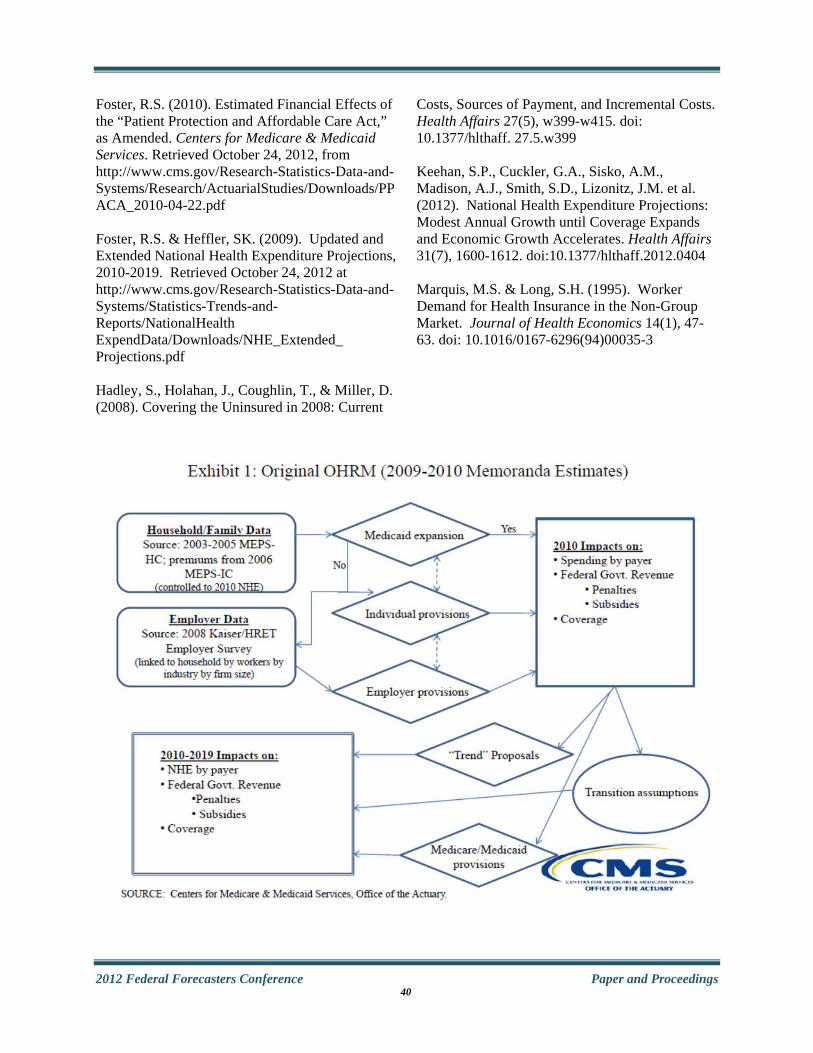
2012 Federal Forecasters Conference Paper and Proceedings
Foster, R.S. (2010). Estimated Financial Effects of the “Patient Protection and Affordable Care Act,” as Amended. Centers for Medicare & Medicaid Services. Retrieved October 24, 2012, from http://www.cms.gov/Research-Statistics-Data-and-Systems/Research/ActuarialStudies/Downloads/PPACA_2010-04-22.pdf Foster, R.S. & Heffler, SK. (2009). Updated and Extended National Health Expenditure Projections, 2010-2019. Retrieved October 24, 2012 at http://www.cms.gov/Research-Statistics-Data-and-Systems/Statistics-Trends-and-Reports/NationalHealth ExpendData/Downloads/NHE_Extended_ Projections.pdf Hadley, S., Holahan, J., Coughlin, T., & Miller, D. (2008). Covering the Uninsured in 2008: Current
Costs, Sources of Payment, and Incremental Costs. Health Affairs 27(5), w399-w415. doi: 10.1377/hlthaff. 27.5.w399 Keehan, S.P., Cuckler, G.A., Sisko, A.M., Madison, A.J., Smith, S.D., Lizonitz, J.M. et al. (2012). National Health Expenditure Projections: Modest Annual Growth until Coverage Expands and Economic Growth Accelerates. Health Affairs 31(7), 1600-1612. doi:10.1377/hlthaff.2012.0404 Marquis, M.S. & Long, S.H. (1995). Worker Demand for Health Insurance in the Non-Group Market. Journal of Health Economics 14(1), 47-63. doi: 10.1016/0167-6296(94)00035-3
40

2012 Federal Forecasters Conference Paper and Proceedings
41

2012 Federal Forecasters Conference Paper and Proceedings
42
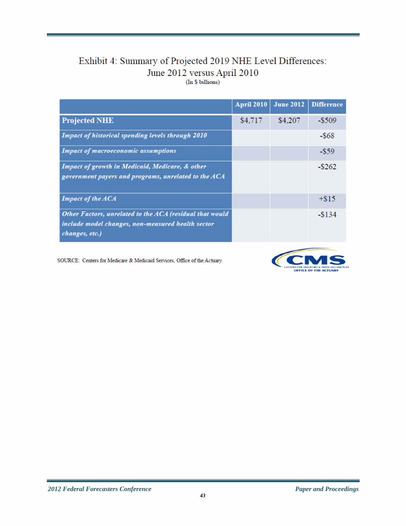
2012 Federal Forecasters Conference Paper and Proceedings 43

2012 Federal Forecasters Conference Paper and Proceedings
Long-Term Projections
Session Chair: Rose Woods, Bureau of Labor Statistics, U.S. Department of Labor
Sources of Difficulties and Uncertainties in Developing Long-Term Commodity Projections of China’s Agriculture Imports Jim Hansen, USDA Economic Research Service
Problems in developing accurate agriculture commodity import projections by China are presented. China leads the world in agriculture imports for soybeans and cotton and increasingly importing more corn. USDA Economic Research Service develops and maintains a large-scale China agriculture economic model for developing USDA’s annual long-term commodity projections, used in budget and policy analysis. This research identifies variables, factors, policies, uncertainties and problems in developing accurate and consistent projections of import demand for major commodities by China. USDA’s 10 year commodity projections for China are compared to actual data. Agriculture data problems, uncertainties and causes are identified for China.
Long Term Projections and Structural Modeling within a Committee Context Uthra Raghunathan and Jerry Cessna, USDA Agricultural Market Service, Dairy Programs
Each year, USDA publishes 10-year annual conditional supply, use, and price projections for agricultural commodities. The USDA Dairy Interagency Commodity Estimates Committee determines projections through a combination of econometric modeling and judgments of the committee members. The purpose of this paper is to explain our methods for (1) producing a set of long-term projections that reflect a composite of econometric results and judgment-based analyses, and (2) using those projections as a baseline for analyzing the impacts of economic shocks and policy changes.
Projecting the Net International Migration of the Foreign-Born: 2012 to 2060 David M. Armstrong and Jennifer M. Ortman, Population Division, U.S. Census Bureau
In this paper, we present four series of projections of the net international migration of the foreign-born to the United States. Net international migration of the foreign-born is estimated and projected as two components: immigration and emigration. The projections of foreign-born immigration are based on two time-series of estimates, the first is derived from administrative records and the second is based on census and survey data. The base series of foreign-born immigration are projected to 2060 using a stepwise autoregressive model with a linear trend. Net international migration of the foreign-born is projected separately by sex, race, and Hispanic origin.
44
2012 Federal Forecasters Conference Paper and Proceedings
Projecting Net International Migration of the Foreign Born: 2012 to 2060 Presented at the Federal Forecasters Conference, Washington, DC, September 27, 2012
David Armstrong and Jennifer Ortman, Population Division, U.S. Census Bureau
This paper is released to inform interested parties of ongoing research and to encourage discussion of work in progress. Any views expressed on statistical, methodological, technical, or operational issues are those of the authors and not necessarily those of the U.S. Census Bureau. ABSTRACT
In this paper, we present four series of projections of net international migration of the foreign-born to the United States. Net international migration of the foreign-born is estimated and projected as two components: immigration and emigration. Three series of foreign-born immigration projections were produced. The first is derived from administrative records, the second is based on census and survey data, and the third is based on rates of emigration from sending countries. Foreign-born emigration is projected by applying rates of emigration to projections of the foreign-born population. Net foreign-born migration is projected by subtracting the emigrants from the immigrants. We evaluate the projected level of net foreign-born migration across series and the race and Hispanic origin distributions of the projected foreign-born migrants. INTRODUCTION
This paper presents preliminary results of ongoing research by U.S. Census Bureau analysts on projecting net foreign-born migration for use in projecting the U.S. resident population. We evaluate two approaches to projecting immigration.27 The first is based on the extrapolation of past trends in immigration to the United States and the second models future immigration to the United States based on rates of emigration from sending countries. We present results for the total number of projected immigrants, net migrants, and the race and Hispanic origin distribution of each migration scenario. 27 The terms immigration, emigration, and migration in this paper refer to the movement of the foreign-born.
DATA AND METHODS
Our research on projecting immigration has resulted in two approaches, representing two different perspectives from which to project future immigration to the United States. Past Trends Approach
The first approach is termed the “past trends” approach, which bases projections of future levels of immigration on past trends in composition and size of the flows. This approach is grounded in the perspective of the receiving country, in this case the United States, and does not incorporate information on the trends in population in sending countries. For the “past trends” approach, we have developed two series of immigration estimates. The first is based on administrative records from the Department of Homeland Security on persons obtaining legal permanent resident status for the period from 1973 to 2010. Information on year of arrival derived from the administrative records was used to estimate immigration for the period. As the administrative data do not include immigrants of all legal statuses – just those who obtained legal permanent resident status – the estimates can be viewed as a theoretical minimum estimate of annual immigration. The national projections released in 2008 were based on these estimates of immigration. Our second series of immigration estimates is based on census and American Community Survey (ACS) data. Information on year of entry for the foreign-born population was used to generate estimates of immigration for the period from 1980 to 2010. Estimates for 1980 to 1999 are based on 1990 census data. Census 2000 data was used for the 1990 to 1999 period and single-year ACS files from 2000 through 2010 were used to create estimates for the 2000 to 2010 period. We produced one immigration projection scenario using the administrative records data and two using
45

2012 Federal Forecasters Conference Paper and Proceedings
the census and ACS data. The projections were created based on a linear extrapolation of the trends in immigration from these series. Emigration from Sending Country Groups Approach
The second approach, which we call the “emigration from sending country groups” approach, shifts the perspective to the source countries by projecting emigration rates for four sending groups, which are then projected forward. All countries were grouped into four broad groups: Europe and the Middle East, Asia, Africa and the non-Spanish Caribbean, and the Spanish Caribbean and Latin America. These groupings were devised to place migrants into categories that correspond to the race and Hispanic origin groups for which we produce population projections. We developed rates of emigration from these sending country groups to the United States using the Census/ACS-based series of immigration estimates and population estimates for the sending country groups from the Census Bureau’s International Data Base (IDB). The Census Bureau’s International Programs Center produces estimates and projections of population in other countries, which are compiled into the IDB and are available to the public on the Census Bureau’s website.28 The IDB projections are available through 2050. To extend the series to 2060, we extrapolated the populations from 2050 to 2060 by assuming that the growth rates for that period would decline at the same rate as in the 2040 to 2050 period. The extrapolation was performed within each of the four country-of-birth groupings. Emigration rates for each of the four country-of-birth groupings were calculated by dividing the number of immigrants to the United States, from our census/ACS-based estimates of immigration, by the estimated population in that grouping. Rates were produced for the years 1980 through 2010 using this method. The emigration rates were projected into the future by assuming the current rates will move toward an ultimate rate that can be
28 http://www.census.gov/population/international
thought of as a weighted average of the observed rates. The projected rates are then applied to the projected populations of the sending country groups to derive the projected number of immigrants from each sending country group. Foreign-Born Emigration from the United States
We projected emigration of the foreign-born population from the United States by first estimating a set of emigration rates and then applying those rates to the foreign-born population. Emigration rates are estimated using a residual methodology and are held constant for all projected years. The rates are produced and applied by age, sex, Hispanic origin, and arrival cohort. Three arrival cohorts are used: (1) immigrants who arrived in the past 0 to 9 years, (2) immigrants who arrived in the past 10-19 years, and (3) immigrants who arrived 20 or more years ago. The residual rates are estimated using Census 2000 as the base population and the 2010 ACS as the target population. A residual estimate is calculated by adding half of the annual immigrants to the initial population, surviving that population forward to the next year, and then adding the immigrants for that period.29 This process is reiterated until the target date of July 1, 2010 is reached. The result is the expected population, from which the target population provided by the 2010 ACS is subtracted to provide a residual estimate of emigration. This estimate of emigration is converted into a rate by dividing the annual estimate by the number of person years lived during the period. The rates are smoothed using penalized least squares.
29 Due to the continuous nature of migration, with migrants arriving throughout the year rather than all at one point in time, migrants are not at risk of dying for the full year. If we were to add in all of the immigrants at the beginning of the interval and survive them forward by subtracting out deaths to the group, we would overestimate the number of deaths for the immigrant arrivals in that year. Instead, we add half of the immigrants at the beginning of the period and survive them forward to the end of the interval by subtracting out deaths. We then add in the other half of the immigrants, which were not subjected to mortality.
46

2012 Federal Forecasters Conference Paper and Proceedings
Emigration was projected by applying the emigration rates to the foreign-born population. The same set of rates, by age, sex, and Hispanic origin, were used for all projected years. For example, to estimate emigration between 2010 and 2011, the emigration rates were applied to the foreign-born population from the 2010 ACS. To project emigration between 2011 and 2012, the foreign-born population is projected for 2011 by aging the foreign-born population from the 2010 ACS forward one year, subtracting out deaths and emigrants, and adding the projected number of immigrants for that year. The residual rates are then applied to the projected foreign-born population for 2011. This process is repeated each year until 2060. The projections of emigration from the United States are subtracted from the immigration projections to create the projected number of net migrants for each year to 2060. RESULTS
Past Trends Approach
Figure 1 shows the two series of immigration estimates and the projection scenarios we produced based on each series for the “past trends” approach. The y-axis represents the number of immigrants and the x-axis represents the year of the estimate or projection. The administrative records scenario is the blue line and projects immigration to be about 1.9 million in 2060. This series is notably lower than the estimates and projections based on census and ACS data because it includes only immigrants who are legal permanent residents. The first census/ACS scenario is based on the full time series of data from 1980 through 2010 and is referred to as the 2010 “jump off” scenario. It represents the trajectory that would be expected if past trends, including the recent downturn in immigration, were to continue into the future. This scenario projects about 2.3 million immigrants in 2060. The second census/ACS scenario is referred to as the 2007 jump off scenario because the observed data for that series were restricted to just the years 1980 through 2007. This scenario illustrates what future trends in immigration might be if the trends prior to the recession in the late 2000s were to continue. It projects the level of immigration to be about 2.8 million in 2060.
Figure 2 presents the projections of net migration for the three “past trends” scenarios. These projections were produced by subtracting our projections of emigration from each of the three “past trends” scenarios. To promote consistency between the National Projections and the National Population Estimates, we control the 2011 values of net migration to the values used to produce the current vintage of estimates. We then interpolate between the controlled 2011 values and the projected values for 2060 to produce the annual projected values. The value of net migration used in the current population estimates was about 723 thousand. The projected level of net migration in 2060 is around 1.3 million in the administrative records scenario and just under 2 million in the 2007 jump off scenario. The 2010 jump off scenario falls in between at more than 1.5 million. In addition to the overall level of net migration, we are interested in the projected composition of the future migrant flows. Figure 3 presents the distribution of the estimates for 2011 and projections for 2060 for each of the three scenarios of net migrants by race and Hispanic origin. There are four blocks of data, each representing a different race and Hispanic origin group. Within each block, the gray column represents the category’s percentage of the total net migration estimate for 2011. The colored columns represent the category’s percentage for each projection scenario in 2060. The blue columns represent the administrative records scenario, the red column represents the 2010 jump off scenario, and the green column represents the 2007 jump off scenario. In all three scenarios, the percent non-Hispanic White is projected to increase from 16.9 percent in 2011 to account for over 20 percent of net migration in 2060. The percent non-Hispanic Black is projected to increase from 8.5 percent to 13.4 percent in the administrative records scenario. There is no change in the 2010 jump off scenario and a slight decrease in the 2007 jump off scenario. The percent non-Hispanic Asian is projected to increase slightly in two scenarios, rising to 30.5 percent in the administrative records scenario and 28.3 percent in the 2010 jump off scenario. In contrast, the percent non-Hispanic Asian is
47
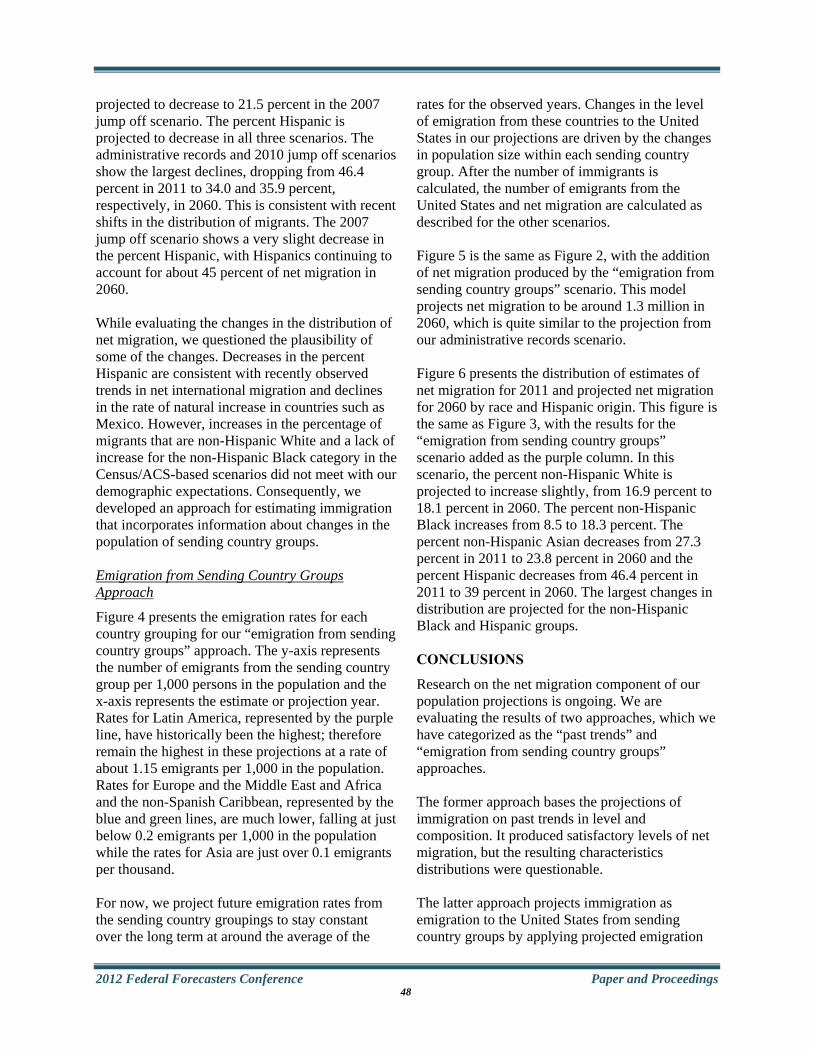
2012 Federal Forecasters Conference Paper and Proceedings
projected to decrease to 21.5 percent in the 2007 jump off scenario. The percent Hispanic is projected to decrease in all three scenarios. The administrative records and 2010 jump off scenarios show the largest declines, dropping from 46.4 percent in 2011 to 34.0 and 35.9 percent, respectively, in 2060. This is consistent with recent shifts in the distribution of migrants. The 2007 jump off scenario shows a very slight decrease in the percent Hispanic, with Hispanics continuing to account for about 45 percent of net migration in 2060. While evaluating the changes in the distribution of net migration, we questioned the plausibility of some of the changes. Decreases in the percent Hispanic are consistent with recently observed trends in net international migration and declines in the rate of natural increase in countries such as Mexico. However, increases in the percentage of migrants that are non-Hispanic White and a lack of increase for the non-Hispanic Black category in the Census/ACS-based scenarios did not meet with our demographic expectations. Consequently, we developed an approach for estimating immigration that incorporates information about changes in the population of sending country groups. Emigration from Sending Country Groups Approach
Figure 4 presents the emigration rates for each country grouping for our “emigration from sending country groups” approach. The y-axis represents the number of emigrants from the sending country group per 1,000 persons in the population and the x-axis represents the estimate or projection year. Rates for Latin America, represented by the purple line, have historically been the highest; therefore remain the highest in these projections at a rate of about 1.15 emigrants per 1,000 in the population. Rates for Europe and the Middle East and Africa and the non-Spanish Caribbean, represented by the blue and green lines, are much lower, falling at just below 0.2 emigrants per 1,000 in the population while the rates for Asia are just over 0.1 emigrants per thousand. For now, we project future emigration rates from the sending country groupings to stay constant over the long term at around the average of the
rates for the observed years. Changes in the level of emigration from these countries to the United States in our projections are driven by the changes in population size within each sending country group. After the number of immigrants is calculated, the number of emigrants from the United States and net migration are calculated as described for the other scenarios. Figure 5 is the same as Figure 2, with the addition of net migration produced by the “emigration from sending country groups” scenario. This model projects net migration to be around 1.3 million in 2060, which is quite similar to the projection from our administrative records scenario. Figure 6 presents the distribution of estimates of net migration for 2011 and projected net migration for 2060 by race and Hispanic origin. This figure is the same as Figure 3, with the results for the “emigration from sending country groups” scenario added as the purple column. In this scenario, the percent non-Hispanic White is projected to increase slightly, from 16.9 percent to 18.1 percent in 2060. The percent non-Hispanic Black increases from 8.5 to 18.3 percent. The percent non-Hispanic Asian decreases from 27.3 percent in 2011 to 23.8 percent in 2060 and the percent Hispanic decreases from 46.4 percent in 2011 to 39 percent in 2060. The largest changes in distribution are projected for the non-Hispanic Black and Hispanic groups. CONCLUSIONS
Research on the net migration component of our population projections is ongoing. We are evaluating the results of two approaches, which we have categorized as the “past trends” and “emigration from sending country groups” approaches. The former approach bases the projections of immigration on past trends in level and composition. It produced satisfactory levels of net migration, but the resulting characteristics distributions were questionable. The latter approach projects immigration as emigration to the United States from sending country groups by applying projected emigration
48

2012 Federal Forecasters Conference Paper and Proceedings
rates to projected populations for those groups. The projected net migration resulting from this method is largely driven by changes in the populations of the sending country groups making it very appealing from a demographic methods point of view. While we hold rates of emigration from sending countries constant over time in this application of the method, we plan to undertake research to evaluate the feasibility of expanding the model to project changes in rates over time based on changes in demographic characteristics of the sending country, such as the age structure of the population, and economic developments. We are in the process of finalizing the projections of net international migration for the 2012 National Projections. At this time, the preferred method is a slightly modified version of the “emigration from sending country groups” scenario. We hope to finalize this very soon and begin to produce the population projections. These projections are planned for release in December 2012.
49

2012 Federal Forecasters Conference Paper and Proceedings 50

2012 Federal Forecasters Conference Papers and Proceedings
51
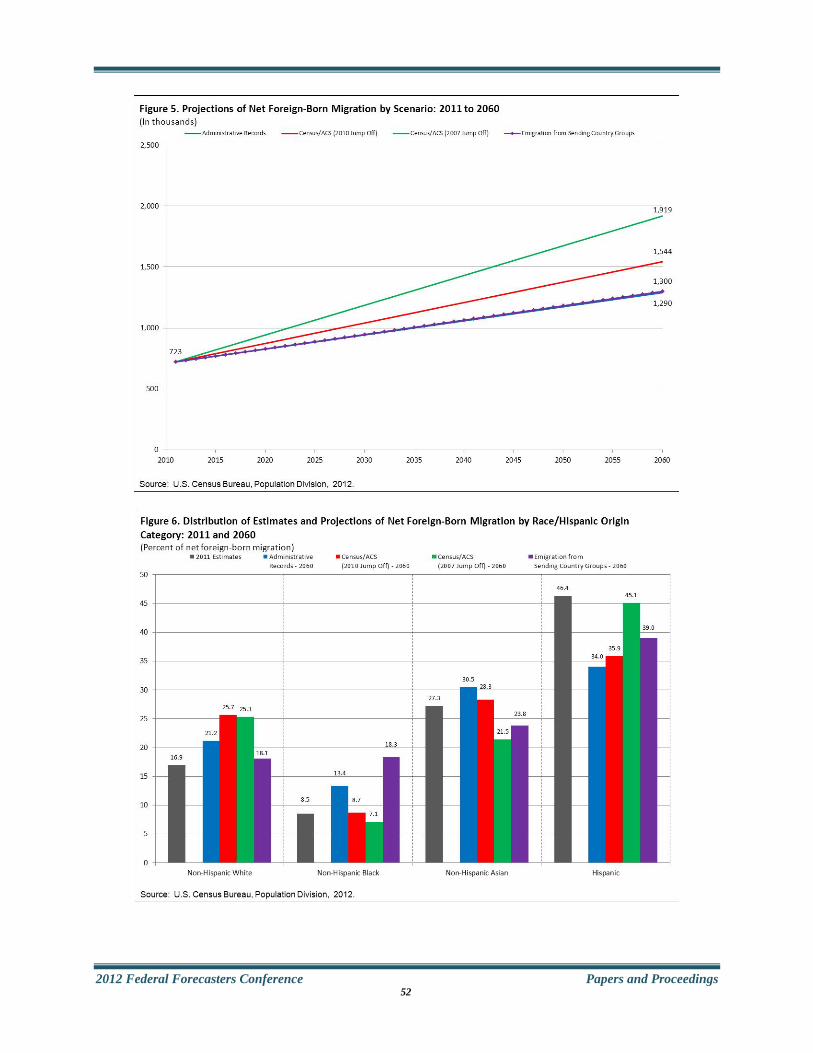
2012 Federal Forecasters Conference Papers and Proceedings
52