2012 pb vi trajectory plots for transmission line models evaluation

Copyright 2012 Piero Belforte November 20th 2012

1

V-I trajectory plots for Transmission Line models evaluation

A comparative analysis between an exact distributed model and the

equivalent LC lumped model of a transmission line (TL) is shown. In a

previous paper the comparison is made using Worst Case Eye Diagrams

https://docs.google.com/file/d/0BxZqV10CSiNS1JwTnc1NVIyTWs/edit.

Here a method based on the Voltage/Current (V-I) trajectories at line

ports is presented.

The reference test circuit is the following:

Fig.1 Comparative test circuit


2

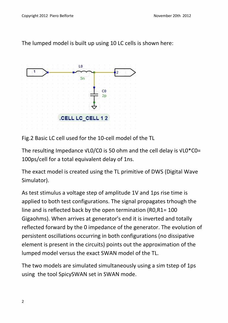
The lumped model is built up using 10 LC cells is shown here:

Fig.2 Basic LC cell used for the 10-cell model of the TL

The resulting Impedance √L0/C0 is 50 ohm and the cell delay is √L0*C0=

100ps/cell for a total equivalent delay of 1ns.

The exact model is created using the TL primitive of DWS (Digital Wave

Simulator).

As test stimulus a voltage step of amplitude 1V and 1ps rise time is

applied to both test configurations. The signal propagates trhough the

line and is reflected back by the open termination (R0,R1= 100

Gigaohms). When arrives at generator's end it is inverted and totally

reflected forward by the 0 impedance of the generator. The evolution of

persistent oscillations occurring in both configurations (no dissipative

element is present in the circuits) points out the approximation of the

lumped model versus the exact SWAN model of the TL.

The two models are simulated simultaneously using a sim tstep of 1ps

using the tool SpicySWAN set in SWAN mode.


3

Here the SWAN netlist extracted from the test circuit :

Fig.3 SWAN (DWS) netlist extracted form the circuit of fig.1

Simulation results are shown here as a multiplot:

Fig. 4 Multiplot of sim results coming from circuit of fig. 1


4

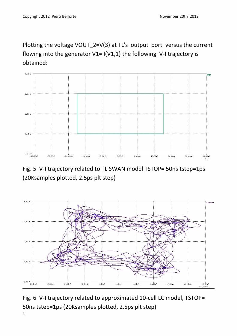
Plotting the voltage VOUT_2=V(3) at TL's output port versus the current

flowing into the generator V1= I(V1,1) the following V-I trajectory is

obtained:

Fig. 5 V-I trajectory related to TL SWAN model TSTOP= 50ns tstep=1ps

(20Ksamples plotted, 2.5ps plt step)

Fig. 6 V-I trajectory related to approximated 10-cell LC model, TSTOP=

50ns tstep=1ps (20Ksamples plotted, 2.5ps plt step)


5

Increasing the simulation time window the following trajectory is

obtained:

Fig. 7 V-I trajectory related to approximated 10-cell LC model, TSTOP=

500ns tstep=1ps (.5Megasamples calculated, 20Ksamples plotted, 2.5ps

plt step)


6

Comparing previous results using the same scale the result shown in the

following fig.8 is obtained.

Fig.8 Comparative images showing the V-I trajectories related to circuit

LC_CHAIN_TL plotted with the same I and V scales.

In the previous fig.8 in yellow the inner area of trajectory envelope is

highlighted. This area is perfectly rectangular in the ideal case (SWAN

model of TL). For the 10 LC-cell model this area is no more rectangular

and becomes smaller because waveform distortion increases increasing

the time window of the analysis.


7

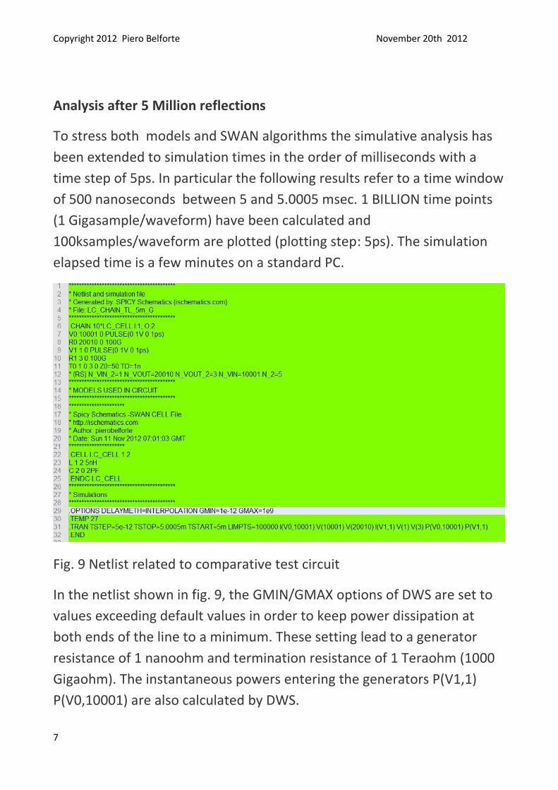
Analysis after 5 Million reflections

To stress both models and SWAN algorithms the simulative analysis has

been extended to simulation times in the order of milliseconds with a

time step of 5ps. In particular the following results refer to a time window

of 500 nanoseconds between 5 and 5.0005 msec. 1 BILLION time points

(1 Gigasample/waveform) have been calculated and

100ksamples/waveform are plotted (plotting step: 5ps). The simulation

elapsed time is a few minutes on a standard PC.

Fig. 9 Netlist related to comparative test circuit

In the netlist shown in fig. 9, the GMIN/GMAX options of DWS are set to

values exceeding default values in order to keep power dissipation at

both ends of the line to a minimum. These setting lead to a generator

resistance of 1 nanoohm and termination resistance of 1 Teraohm (1000

Gigaohm). The instantaneous powers entering the generators P(V1,1)

P(V0,10001) are also calculated by DWS.


8

Fig. 10 Simulated waveforms related to netlist of fig 9

The power at generator V1 port has peak values of 19.95mW that means

50uW less than the value exchanged with the line at the first reflections.

After about 5Million reflections 50uW is the power loss due to GMIN and

GMAX settings and dissipated at non ideal (zero and infinite) line

terminations.


9

Fig 11 V-P (Voltage-Power) plots related to LC_CHAIN_TL test circuit

after 5msec from the start (5 Million back and forth reflections).

From V-P plots of fig. 11 it can be pointed out a still near ideal

rectangular diagram for SWAN TL (the 50uW dissipated power is

negligible at this scale). The random oscillations of power exchanged in LC

model have still a behavior similar to that of the beginning of oscillations

because also in this time window the power dissipated at terminations is

still negligible.


10

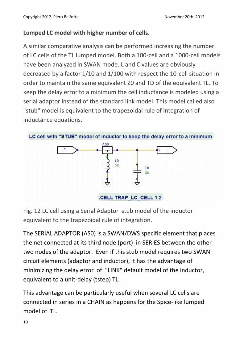
Lumped LC model with higher number of cells.

A similar comparative analysis can be performed increasing the number

of LC cells of the TL lumped model. Both a 100-cell and a 1000-cell models

have been analyzed in SWAN mode. L and C values are obviously

decreased by a factor 1/10 and 1/100 with respect the 10-cell situation in

order to maintain the same equivalent Z0 and TD of the equivalent TL. To

keep the delay error to a minimum the cell inductance is modeled using a

serial adaptor instead of the standard link model. This model called also

"stub" model is equivalent to the trapezoidal rule of integration of

inductance equations.

Fig. 12 LC cell using a Serial Adaptor stub model of the inductor

equivalent to the trapezoidal rule of integration.

The SERIAL ADAPTOR (AS0) is a SWAN/DWS specific element that places

the net connected at its third node (port) in SERIES between the other

two nodes of the adaptor. Even if this stub model requires two SWAN

circuit elements (adaptor and inductor), it has the advantage of

minimizing the delay error of "LINK" default model of the inductor,

equivalent to a unit-delay (tstep) TL.

This advantage can be particularly useful when several LC cells are

connected in series in a CHAIN as happens for the Spice-like lumped

model of TL.


11

Fig. 13 IV trajectories related to several implementations of the lumped

model Transmission Line (SWAN).


12

As can be pointed out by the differences among the V-I plots of fig. 13,

increasing the number of cascaded cells, the trajectories approach the

ideal line RECTANGULAR shape, but from the 1,000 cell up no significant

advantage is obtained if the number of cells is increased to 2,000 or even

4,000 cells using a simulation time step of 1ps.

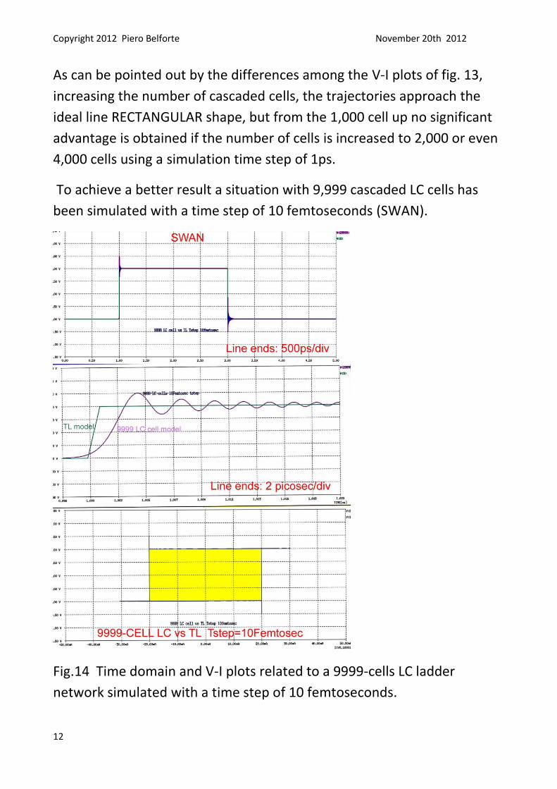
To achieve a better result a situation with 9,999 cascaded LC cells has

been simulated with a time step of 10 femtoseconds (SWAN).

Fig.14 Time domain and V-I plots related to a 9999-cells LC ladder

network simulated with a time step of 10 femtoseconds.


13

This last circuit required the calculation of .5 Million points

(Megasample/waveform) for a network containing about 30,000

elements (including series adaptors). As can be pointed out from the plots

of Fig. 13, only in this situation a good agreement with TL distributed

model is obtained at the expense of a huge simulation effort that only

SWAN can afford with simulation times in the order of minutes.

A residual rise time increase of about 500fs and some ringing still affect

the output waveform with respect TL distributed model.

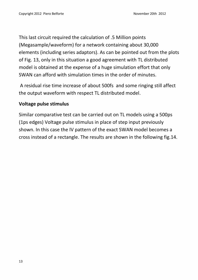
Voltage pulse stimulus

Similar comparative test can be carried out on TL models using a 500ps

(1ps edges) Voltage pulse stimulus in place of step input previously

shown. In this case the IV pattern of the exact SWAN model becomes a

cross instead of a rectangle. The results are shown in the following fig.14.


14

Fig. 14 Comparative model tests using a 500ps Voltage pulse stimulus

Spice models of TL

Spice-derived simulators have several problems dealing with TL models.

Being based on resolution of NA (Nodal Analysis) equations, these

simulators assume no propagation of signals inside the circuit under

analysis. Variable time step control adds further problems in dealing with

fixed delays. To avoid these issues, very often TLs are approximated with

LC networks leading to signal distortions typical of this Kind of models as

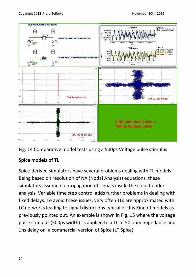
previously pointed out. An example is shown in Fig. 15 where the voltage

pulse stimulus (500ps width) is applied to a TL of 50 ohm impedance and

1ns delay on a commercial version of Spice (LT Spice)


15

Fig. 15 Results of LT Spice simulation of TL version of circuit of fig.14

(Yellow: Line input pulse, Violet: signal at the Line end )

In fig.15 the reflected pulses are affected by heavy progressive

distortions typical of a lumped model. The pulse edges slow down

progressively and overshoots/undershoots appear.

Some simulators, like MicroCap, use more accurate TL models and can

can work at fixed time steps, but the simulation times are order of

magnitudes higher than those of SWAN/DWS.

Even the simulation of lossless LC ladder networks are not so easy with

Spice. To keep the error to a minimum a very short fixed time step (10fs-

1ps) should be used also in this case. A comparison between SWAN and

MC10 simulation times are shown here:

http://www.youtube.com/watch?v=pTMBnvUChog

and here: http://www.youtube.com/watch?v=xJnA5ioAwb4

Even for this simple 10-cell test circuit the speedup factor of SWAN vs

MC10 is in the order of 70-100 at same accuracy level (differences less

than 1mV between the waveforms coming from the two simulators,

fig.16). This speedup increases if the number of cascaded cells increases.


16

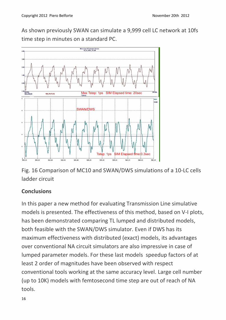
As shown previously SWAN can simulate a 9,999 cell LC network at 10fs

time step in minutes on a standard PC.

Fig. 16 Comparison of MC10 and SWAN/DWS simulations of a 10-LC cells

ladder circuit

Conclusions

In this paper a new method for evaluating Transmission Line simulative

models is presented. The effectiveness of this method, based on V-I plots,

has been demonstrated comparing TL lumped and distributed models,

both feasible with the SWAN/DWS simulator. Even if DWS has its

maximum effectiveness with distributed (exact) models, its advantages

over conventional NA circuit simulators are also impressive in case of

lumped parameter models. For these last models speedup factors of at

least 2 order of magnitudes have been observed with respect

conventional tools working at the same accuracy level. Large cell number

(up to 10K) models with femtosecond time step are out of reach of NA

tools.

2012 pb vi trajectory plots for transmission line models evaluation

Technology