Trajectory Planning and Sliding-Mode Control Based

Trajectory-Tracking for Cybercars

Razvan Solea and Urbano Nunes 1

Institute of Systems and Robotics, University of Coimbra, Polo II, 3030-290 Coimbra, Portugal

Tel: +351 239 796200; Fax: +351 239 406672; E-mail: {razvan, urbano} @isr.uc.pt

Abstract

Fully automatic driving is emerging as the approach to dramatically improve efficiency

(throughput per unit of space) while at the same time leading to the goal of zero accidents.

This approach, based on fully automated vehicles, might improve the efficiency of road travel in

terms of space and energy used, and in terms of service provided as well. For such automated

operation, trajectory planning methods that produce smooth trajectories, with low level asso-

ciated accelerations and jerk for providing human comfort, are required. This paper addresses

this problem proposing a new approach that consists of introducing a velocity planning stage

in the trajectory planner. Moreover, this paper presents the design and simulation evaluation

of trajectory-tracking and path-following controllers for autonomous vehicles based on sliding

mode control. A new design of sliding surface is proposed, such that lateral and angular er-

rors are internally coupled with each other (in cartesian space) in a sliding surface leading to

convergence of both variables.

1 Introduction

The number of accidents generated by road transport is a dramatic social problem requiring urgent

and effective solutions. Improvements in vehicle quality have helped to increase safety and capacity,

but as vehicle safety and traffic engineering has improved, the proportion of accidents due to driver

error has increased with a result that automotive engineering has focused on accident mitigation

rather than avoidance. The introduction of safer vehicles has sometimes been associated with greater

accident frequency, particularly involving vehicle-pedestrian conflicts where drivers are encouraged to

take greater risks as a result of their perceived invulnerability. It is now recognized that the limiting

factor for further improvement is the poor performance of the human driver. Fully automatic driving

is emerging as the approach to dramatically improve efficiency while at the same time leading to

the goal of zero accidents. In this context, a new approach for mobility providing an alternative to

the private passenger car, by offering the same flexibility but with much less nuisances, is emerging,

based on fully automated vehicles, named cybercars [9], [4].

Although motion planning of mobile robots and autonomous vehicles has been thoroughly studied

in the last decades, the requisite of producing trajectories with low associated accelerations and jerk

is not easily traceable in the technical literature. This paper addresses this problem proposing an

approach that consists of introducing a velocity planning stage to generate adequate time sequences

to be used in the interpolating curve planners. In this context, we generate speed profiles (linear

1Corresponding author.

1

Integrated Computer-aided Engineering, Int. Journal,IOS Press, vol.14, n.1, pp.33-47, 2007.

and angular) that lead to trajectories respecting human comfort. The need of having travel comfort

in autonomous vehicle’ applications, like in cybercars [4], motivated our research on the subject of

this paper.

Additionally, trajectory tracking control strategies are here proposed using sliding mode control

(SMC) techniques.

Trajectory tracking control means tracking reference trajectories predefined or given by path

planners. It has been widely studied and various effective methods and tracking controllers have

been developed (e.g. [1], [2], [5], [11], [13]). The model-based tracking control approaches can be

divided into kinematic and dynamic based methods.

According to different control theories, a more elaborate category in the sense of kinematic

methods can be grouped in five sets [13]: (1) sliding mode based approaches, (2) input-output

linearization based approaches, (3) fuzzy based approaches, (4) neural network based approaches,

and (5) backstepping based approaches. Among all of these kinematic-based methods, considering

the stability of tracking control laws, the hardware computation load and the maneuverability in

practice, tracking control law designed by sliding mode technology has been proved one of the best

solutions.

Sliding mode control (SMC) is a special discontinuous control technique applicable to various

practical systems [12]. The main advantages of using SMC include fast response, good transient and

robustness with respect to system uncertainties and external disturbances. Therefore, it is attractive

for many highly nonlinear uncertain systems [10].

Aguilar et al. [1] determined a variable structure control with sliding mode to stabilize the

vehicle’s motion around the reference path (path-following control). Yang and Kim [11] proposed

a sliding mode control law for solving trajectory tracking problems of nonholonomic mobile robots

in polar coordinates. A new SMC kinematic controller defined in polar coordinates, for trajectory-

tracking in the content of wheeled mobile robots, is described in [2]. In the proposed method,

two controllers are designed to asymptotically stabilize the tracking errors in position and heading

direction, respectively.

2 Trajectory Planning

Trajectory planning for passenger’s transport vehicles must generate smooth trajectories with low

associated accelerations and jerk. Lateral and longitudinal accelerations depend on the linear speed:

aT =dv

dt(1)

aL =dθ

dt· v = k · v2 (2)

thus, the trajectory planning must perform not only the planning of the curve (spatial dimension)

but also the speed profile (temporal dimension).

The ISO 2631-1 standard [8] (Table 1) relates comfort with the overall r.m.s. acceleration, acting

on the human body, defined as:

aw =√

k2x · a2

wx + k2y · a2

wy + k2z · a2

wz (3)

2

where awx, awy, awz, are the r.m.s. accelerations on x, y, z axes respectively, and kx, ky, kz, are

multiplying factors. For a seated person kx = ky = 1.4, kz = 1. For motion on the xy-plane, awz = 0.

The vehicle frame is chosen so that the x−axis and y−axis are aligned with the longitudinal and

lateral directions of the trajectory, respectively.

Using Table 1 and equation (3), for ”not uncomfortable” accelerations, the longitudinal and

lateral r.m.s. accelerations must be less than 0.24 m/s2. This value allows defining the reference

speeds, and consequently the time values. The reference velocity at the final point of a segment k

(defined by two consecutive waypoints i and i + 1), can be calculated as

vi+1 = vi ± awx · tk, awx ≤ 0.24m/s2 (4)

tk = ti+1 − ti =

√2 · sk

awx

(5)

where sk is the length of the segment. A path between the initial and the final point is formed as a

series of curves (each curve connects two consecutive waypoints). We choose for (5) the maximum

value of awx (awx = 0.24m/s2) to obtain a minimal value for tk.

Table 1: ISO 2631-1 STANDARD.Overall Consequence

Acceleration

aw < 0.315m/s2 Not uncomfortable

0.315 < aw < 0.63m/s2 A little uncomfortable

0.5 < aw < 1m/s2 Fairy uncomfortable

0.8 < aw < 1.6m/s2 Uncomfortable

1.25 < aw < 2.5m/s2 Very uncomfortable

aw > 2.5m/s2 Extremely uncomfortable

The problem: Given a set of waypoints, find control inputs v(t), ω(t) such that the vehicle

starting from an arbitrary initial extended state:

pa = [xa ya]T

= [x(0) y(0)]T; θa = θ(0);

va = v(0); va = v(0);ωa = ω(0); ωa = ω(0);

reaches the arbitrary final extended state:

pw = [xw yw]T

= [x(tfin) y(tfin)]T; θw = θ(tfin);

vw = v(tfin); vw = v(tfin);ωw = ω(tfin); ωw = ω(tfin).

crossing all the given waypoints. The comfort of human body constraint

aw < 0.4m/s2 (6)

is to be satisfied.

The algorithm:

• Step 1: Determine a path connecting pa (start point) with pw (final point)

pk(u) =

[xk(u)

yk(u)

]=

[c0k + c1k · u + c2k · u2 + . . .

d0k + d1k · u + d2k · u2 + . . .

](7)

3

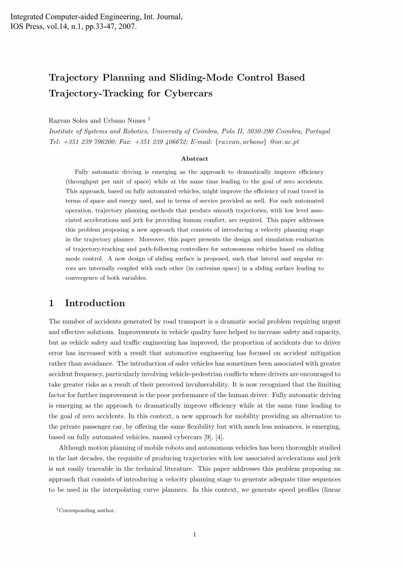
Figure 1: A possible velocity planning for one curve

were u ∈ [0, 1], and cik and dik, i = 0, 1, . . . are constants to be found function of the type of

the curve (e.g. cubic splines, trigonometric splines or quintic splines).

Determine the length sk for each curve,

sk(u) =

∫ 1

0

‖pk(ξ)‖ · dξ (8)

and the curvature kck(u) for each curve,

kck(u) =xk(u) · yk(u) − xk(u) · yk(u)√

x2k(u) + y2

k(u)(9)

• Step 2: Each vk(t) are generated with five properly joined spline curves (j = 1, 2, . . . 5) like in

[6]:

vj(t) = a1j + 2a2j · t + 3a3j · t2, t ∈ [0, tj ],

5∑j=1

tj = tk (10)

where coefficients aij are defined in [3]. The generated velocity is C1 and strictly positive for

any t ∈ [0, tk]. The number of curves is suggested by practical reasons (the smoothness of the

velocity profile increases with the number of curves). An example of the velocity profile (for

one curve) is shown in Fig. 1.

• Step 3: The angular velocity functions ωk(t) ∈ C1 are defined according to:

ωk(t) := vk(t) · kk(sk)|sk(t)=

∫t

0

vk(ξ)dξ(11)

where kk(sk) is the curvature expressed as a function of the arc length sk(t).

• Step 4: Calculate the r.m.s. acceleration awk for each curve using equations (1), (2) and (3).

IF awk > 0.4m/s2 THEN change the time for that segment (curve) and go to step 2.

If the r.m.s. acceleration is not under 0.4m/s2 for a given curve the time for that segment is

increased (an increase of 10 % has been used). Using the proposed algorithm (summarized in Table

2) a path, respecting comfort of human body, is obtained.

4

Table 2: Trajectory planning algorithm.

1. calculate xk(u) and yk(u) for each curve (eq. 7).

2. calculate the curve length sk(u) for each curve (eq. 8).

3. calculate the curvature for each curve (eq. 9).

4. calculate the time tk for each curve (eq. 5).

5. calculate velocity at each waypoint vi (eq. 4).

6. repeat (for each curve)

(a) calculate the curvature, kk(sk(t))

(b) calculate vk(t)

(b1) if min(vk(t)) < 0 then decrease the final velocity vi+1

and go to (b).

(c) calculate the angular velocity ωk(t) (eq. 10).

(d) find the overall rms acceleration awk (eq. 3).

(e) if awk > 0.4m/s2 then increase the time (tk).

7. until awk < 0.4m/s2.

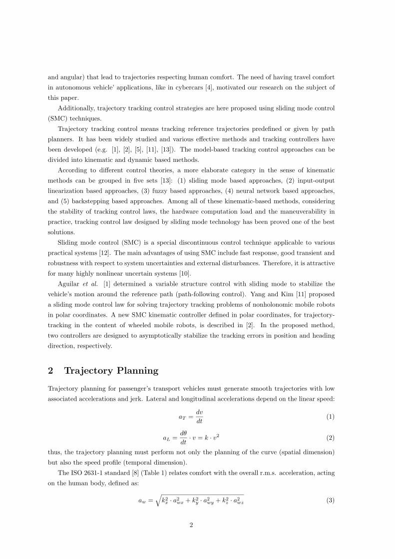
0 10 20 30 40 50 60

0

10

20

30

40

50

60

a(3,7,0)b(20,7,0)

c(22,9,pi/2)

d(24,18,pi/2)

e(24,20,0)

f(38,20,0)

g(40,22,pi/2)

h(40,31.2,pi/2)i(42,34,pi/8)

j(47,42,pi/2)

k(38,51,pi)

l(30,46,−3*pi/4)

m(27.2,44,pi)

n(4,44,pi)

o(2,42,−pi/2)

p(2,20,−pi/2)

Path [m]

Figure 2: Path planning example using quintic polynomial curves

Consider the example depicted in Fig. 2 where the larger circles represent waypoints (a, b, ..., p).

Each waypoint is defined by a position, in meters, and an orientation, in radians.

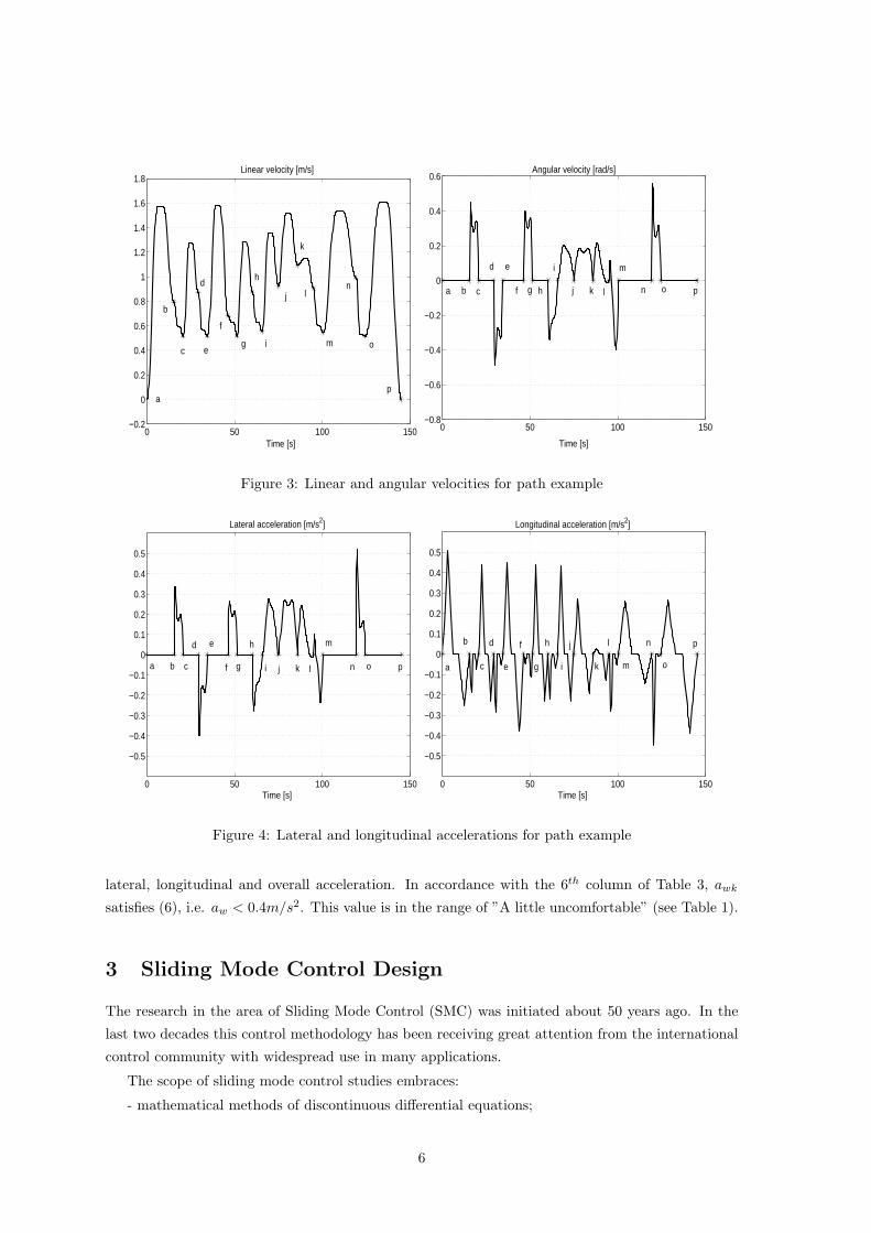
Figs. 2-4 show results of the application of the proposed trajectory planning algorithm satisfying

the comfort condition (6). From Fig. 4 we observe that the maximum absolute value for lateral

acceleration is below 0.51m/s2 and the maximum absolute value for longitudinal acceleration is

below 0.51m/s2.

Table 3 summarizes the results of the applied trajectory planning algorithm: length, time and

r.m.s. acceleration values for each curve (segment). Three acceleration components are considered:

5

0 50 100 150−0.2

0

0.2

0.4

0.6

0.8

1

1.2

1.4

1.6

1.8Linear velocity [m/s]

Time [s]

b

c

d

e

f

g

h

i

j

k

l

m

n

o

p a

0 50 100 150−0.8

−0.6

−0.4

−0.2

0

0.2

0.4

0.6Angular velocity [rad/s]

Time [s]

a b c

d e

f g

i

j k l

m

n o ph

Figure 3: Linear and angular velocities for path example

0 50 100 150

−0.5

−0.4

−0.3

−0.2

−0.1

0

0.1

0.2

0.3

0.4

0.5

Lateral acceleration [m/s2]

Time [s]

pon

m

lkji

h

gf

ed

cba

0 50 100 150

−0.5

−0.4

−0.3

−0.2

−0.1

0

0.1

0.2

0.3

0.4

0.5

Longitudinal acceleration [m/s2]

Time [s]

p

o

n

m

l

k

j

i

h

g

f

e

d

c

b

a

Figure 4: Lateral and longitudinal accelerations for path example

lateral, longitudinal and overall acceleration. In accordance with the 6th column of Table 3, awk

satisfies (6), i.e. aw < 0.4m/s2. This value is in the range of ”A little uncomfortable” (see Table 1).

3 Sliding Mode Control Design

The research in the area of Sliding Mode Control (SMC) was initiated about 50 years ago. In the

last two decades this control methodology has been receiving great attention from the international

control community with widespread use in many applications.

The scope of sliding mode control studies embraces:

- mathematical methods of discontinuous differential equations;

6

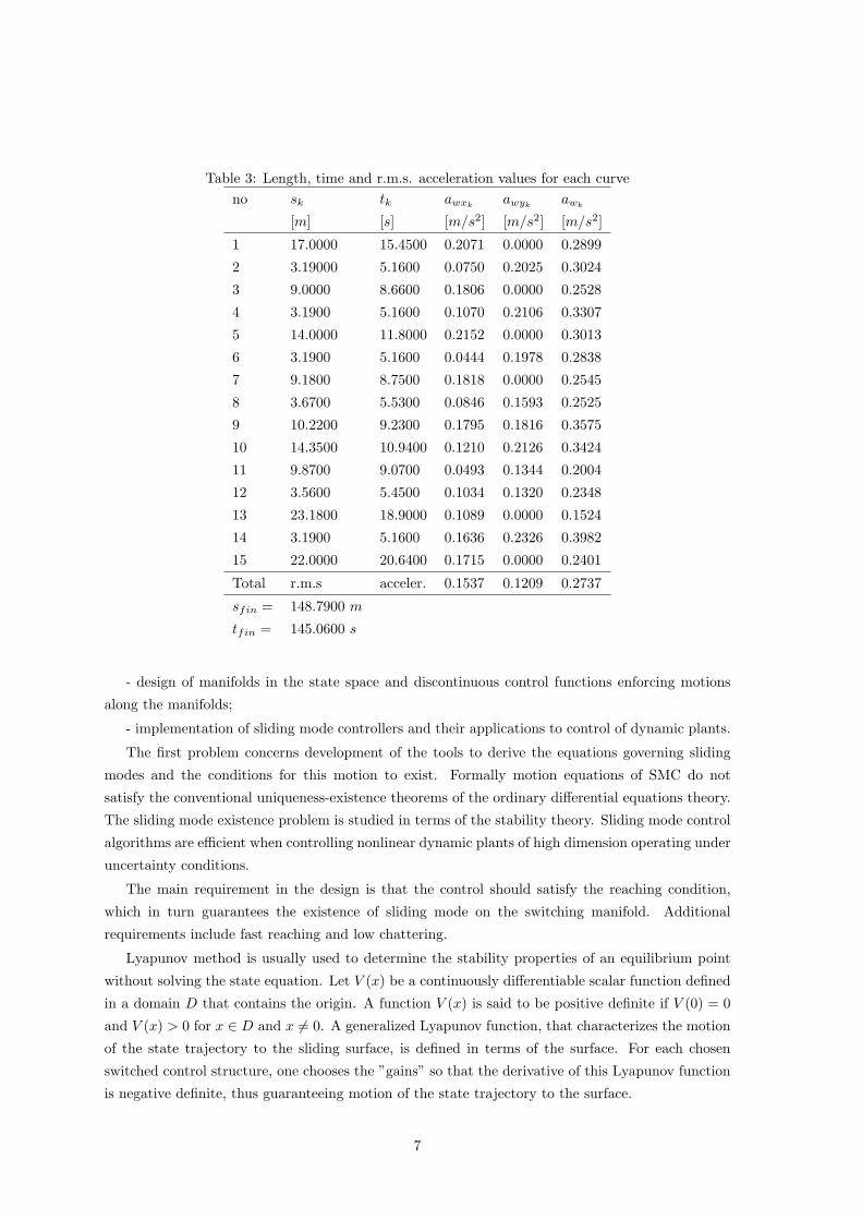
Table 3: Length, time and r.m.s. acceleration values for each curve

no sk tk awxkawyk

awk

[m] [s] [m/s2] [m/s2] [m/s2]

1 17.0000 15.4500 0.2071 0.0000 0.2899

2 3.19000 5.1600 0.0750 0.2025 0.3024

3 9.0000 8.6600 0.1806 0.0000 0.2528

4 3.1900 5.1600 0.1070 0.2106 0.3307

5 14.0000 11.8000 0.2152 0.0000 0.3013

6 3.1900 5.1600 0.0444 0.1978 0.2838

7 9.1800 8.7500 0.1818 0.0000 0.2545

8 3.6700 5.5300 0.0846 0.1593 0.2525

9 10.2200 9.2300 0.1795 0.1816 0.3575

10 14.3500 10.9400 0.1210 0.2126 0.3424

11 9.8700 9.0700 0.0493 0.1344 0.2004

12 3.5600 5.4500 0.1034 0.1320 0.2348

13 23.1800 18.9000 0.1089 0.0000 0.1524

14 3.1900 5.1600 0.1636 0.2326 0.3982

15 22.0000 20.6400 0.1715 0.0000 0.2401

Total r.m.s acceler. 0.1537 0.1209 0.2737

sfin = 148.7900 m

tfin = 145.0600 s

- design of manifolds in the state space and discontinuous control functions enforcing motions

along the manifolds;

- implementation of sliding mode controllers and their applications to control of dynamic plants.

The first problem concerns development of the tools to derive the equations governing sliding

modes and the conditions for this motion to exist. Formally motion equations of SMC do not

satisfy the conventional uniqueness-existence theorems of the ordinary differential equations theory.

The sliding mode existence problem is studied in terms of the stability theory. Sliding mode control

algorithms are efficient when controlling nonlinear dynamic plants of high dimension operating under

uncertainty conditions.

The main requirement in the design is that the control should satisfy the reaching condition,

which in turn guarantees the existence of sliding mode on the switching manifold. Additional

requirements include fast reaching and low chattering.

Lyapunov method is usually used to determine the stability properties of an equilibrium point

without solving the state equation. Let V (x) be a continuously differentiable scalar function defined

in a domain D that contains the origin. A function V (x) is said to be positive definite if V (0) = 0

and V (x) > 0 for x ∈ D and x �= 0. A generalized Lyapunov function, that characterizes the motion

of the state trajectory to the sliding surface, is defined in terms of the surface. For each chosen

switched control structure, one chooses the ”gains” so that the derivative of this Lyapunov function

is negative definite, thus guaranteeing motion of the state trajectory to the surface.

7

3.1 Sliding Mode Trajectory-Tracking Control

It is supposed that a feasible desired trajectory for the vehicle is pre-specified by a trajectory

planner. The problem is to design a robust controller so that the vehicle will correctly track the

desired trajectory under a large class of disturbances.

We consider as a motion model of a vehicle the following simplified nonholonomic system:⎧⎪⎪⎨⎪⎪⎩

xr(t) = vr(t) · cosθr(t)

yr(t) = vr(t) · sinθr(t)

θr(t) = vr

l· tanφr(t)

(12)

where (see Fig. 5) xr and yr are the Cartesian coordinates of the rear axle midpoint, vr is the

velocity of this midpoint, θr is the vehicle’s heading angle, l is the inter-axle distance, and φr the

front wheel angle, which is the control variable to steer the vehicle.

In this paper, the kinematic bicycle model is considered (see Figs. 5 - 7). The trajectory tracking

errors can be described by (xe, ye, θe). The aim is to design a stable controller with commands (vc,

φc).

Figure 5: Bicycle model (12)

The error vector for trajectory-tracking is easily obtained from Figs. 5 and 6,⎡⎢⎢⎣

xe

ye

θe

⎤⎥⎥⎦ =

⎡⎢⎢⎣

cosθd sinθd 0

−sinθd cosθd 0

0 0 1

⎤⎥⎥⎦ ·

⎡⎢⎢⎣

xr − xd

yr − yd

θr − θd

⎤⎥⎥⎦ (13)

where (xd, yd, θd) denotes the virtual car pose. The corresponding error derivatives are⎧⎪⎪⎨⎪⎪⎩

xe = −vd + vr · cosθe + ye ·vd

l· tanφd

ye = vr · sinθe − xe ·vd

l· tanφd

θe = vr

l· tanφr −

vd

l· tanφd

(14)

where vd and φd are the heading speed and desired front wheel angle, respectively.

8

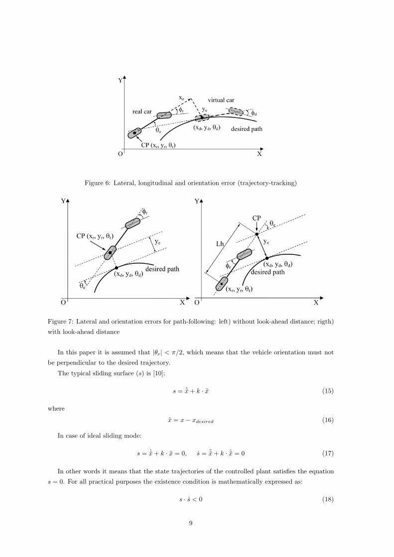
Figure 6: Lateral, longitudinal and orientation error (trajectory-tracking)

Figure 7: Lateral and orientation errors for path-following: left) without look-ahead distance; rigth)

with look-ahead distance

In this paper it is assumed that |θe| < π/2, which means that the vehicle orientation must not

be perpendicular to the desired trajectory.

The typical sliding surface (s) is [10]:

s = ˙x + k · x (15)

where

x = x − xdesired (16)

In case of ideal sliding mode:

s = ˙x + k · x = 0, s = ¨x + k · ˙x = 0 (17)

In other words it means that the state trajectories of the controlled plant satisfies the equation

s = 0. For all practical purposes the existence condition is mathematically expressed as:

s · s < 0 (18)

9

In physical sense it means that sliding mode exists if in the vicinity of the switching line s = 0,

the tangent or the velocity vector of the state trajectory points towards the switching line.

A new design of sliding surface is proposed, such that lateral error, ye, and angular error, θe, are

internally coupled with each other in a sliding surface leading to convergence of both variables. For

that purpose the following sliding surfaces are proposed:

s1 = xe + k1 · xe (19)

s2 = ye + k2 · ye + k0 · sgn(ye) · θe (20)

In trajectory-tracking exist three variables (xe, ye, θe) and just two control variables, which

implies that we have only two sliding surfaces. We chose to couple ye and θe in one sliding surface.

The condition under which the state will move toward and reach a sliding surface is called a reaching

condition. A practical general form of the reaching law is

s = −Q · g(s) − P · sgn(s) (21)

where

Q =

[q1 0

0 q2

], qi > 0, P =

[p1 0

0 p2

], pi > 0, i = 1, 2.

sgn(s) =

[sgn(s1)

sgn(s2)

], g(s) =

[g1(s1)

g2(s2)

], si · gi(si) > 0, gi(0) = 0

Various choices of Q and P specify different rates for s and yield different structures in the

reaching law.

Three practical special cases of (21) are given below:

1. constant rate reaching

s = −P · sgn(s) (22)

This law forces the switching variable s to reach the switching manifold at a constant rate

|si| = −pi, i = 1, 2.

2. constant plus proportional rate reaching

s = −Q · s − P · sgn(s) (23)

By adding the proportional rate term −Q · s, the state is forced to approach the switching

manifolds faster when s is large.

3. power rate reaching

s = −Q · |s|α· sgn(s), 0 < α < 1. (24)

This reaching law increases the reaching speed when the state is far away from the switching

manifold, but reduces the rate when the state is near the manifold.

10

In this work the second reaching law (23) was selected. From the time derivative of (19) and

(20) and using (23), results

s1 = xe + k1 · xe = −q1 · s1 − p1 · sgn(s1) (25)

s2 = ye + k2 · ye + k0 · sgn(ye) · θe = −q2 · s2 − p2 · sgn(s2) (26)

From (14), (25) and (26), and after some mathematical manipulation, we get the commands:

vc =1

cosθe

· (−q1 · s1 − p1 · sgn(s1) − k1 · xe − ωd · ye − ωd · ye + vr · θe · sinθe + vd) (27)

φc = arctan( lvr

· ωd + lvr·(vr·cosθe+k0·sgn(ye)) · (−q2s2 − p2sgn(s2)−

−k2 · ye − vr · sinθe + ωd · xe + ωd · xe))

(28)

Let us define V = 12 · sT · s as a Lyapunov function candidate, therefore its time derivative is

V = s1 · s1 + s2 · s2

= s1 · (−q1 · s1 −p1 · sgn(s1)) + s2 · (−q2 · s2 − p2 · sgn(s2))

= −sT · Q · s − p1 · |s1| − p2 · |s2|

For V to be negative semi-definite, it is sufficient to choose qi and pi such that qi, pi > 0.

3.2 Sliding Mode Path-Following Control

In path-following, the control objective is to ensure that the vehicle will correctly follow the reference

path. For this purpose, both the lateral error, ye, and the orientation error, θe, must be minimized.

It is supposed that a feasible desired path for the vehicle is pre-specified by a trajectory planner.

For the path-following without look-ahead (Lh = 0) (see Fig. 7) the error vector is:

[ye

θe

]=

[−sinθd cosθd 0

0 0 1

]·

⎡⎢⎢⎣

xr − xd

yr − yd

θr − θd

⎤⎥⎥⎦ (29)

The lateral error, ye, is defined as the distance between the vehicle control point (CP) and the closest

point along the desired trajectory. The corresponding error derivatives are:{ye = vr · sinθe

θe = θr = vr

l· tanφr

(30)

Defining the control point CP (see Fig. 7) at a distance Lh �= 0 in front of the vehicle (called

look-ahead distance), (29) becomes:

[ye

θe

]=

[−sinθd cosθd 0

0 0 1

]·

⎡⎢⎢⎣

xr − xd + Lh · cosθr

yr − yd + Lh · sinθr

θr − θd

⎤⎥⎥⎦

11

and {ye = vr · sinθe + Lh · vr

l· tanφr · cosθe

θe = θr = vr

l· tanφr

(31)

In this paper it is assumed that |θe| < π/2, which means that the vehicle orientation must not

be perpendicular to the desired trajectory.

We propose a new design of sliding surface such that lateral error, ye, and angular variable, θe

are internally coupled with each other in a sliding surface leading to convergence of both variables.

For that purpose the following sliding surface is proposed:

s = ye + k · ye + k0 · sgn(ye) · θe (32)

In path-following exist two variables (ye, θe) and just one control variable, which implies that we

have only one sliding surface. We chose to couple ye and θe in one sliding surface.

By choosing the second reaching law (23),

s = ye + k · ye + k0 · sgn(ye) · θe = −Q · s − P · sgn(s) (33)

From (31) and (33), the steering control law is obtained as

φc = arctan

(l

vr

·−Qs − Psgn(s) − kvrsinθe

vr · cosθe + k0 · sgn(ye)

)(34)

For the case of using look-ahead Lh:

φc = l·cos2(φr)vr·Lh·cosθe

· (−Q · s − P · sgn(s) − k · ye − vr · θe · cosθe+

+Lh · θ2e · sinθe − k0 · sgn(ye) · θe)

(35)

Let us define V = 12 · s2 as a Lyapunov function candidate, therefore its time derivative is

V = s · s

= s · (ye + k · ye + k0 · sgn(ye) · θe)

= s · (−Q · s − P · sgn(s))

= −Q · s2 − P · s2

|s|

For V to be negative semi-definite, it is sufficient to choose Q and P such that Q, P ≥ 0.

4 Simulation Results

In this section, simulation results of the proposed methods are presented. The simulation model

block diagram is shown in Fig. 8. The following transfer functions were employed:

Hφ =φr

φc

=ω2

n

s2 + 2 · D · ωn · s + ω2n

; Hv =vr

vc

=1

0.25 · s + 1(36)

with D = 0.7 and ωn = 2π · 5Hz.

The reference trajectory was generated using the trajectory planner, described in Section 1 (we

considered the example illustrated in Fig. 2). Design parameters of (19), (20), (25), (26), (32) and

12

Figure 8: Simulation model block diagram

(33) are k0 = 0.05, k1 = 0.25, k = k2 = 0.5, p1 = 1, p2 = 1, q1 = 1 and q2 = 1. The signum

functions in the control inputs (25), (26) and (33) and sliding surfaces (25), (26) and (33) were

replaced by saturation functions with ±0.5 thresholds, to reduce the chattering phenomenon. Also,

input disturbances were chosen to be Gaussian random noise with zero mean and variance 0.05. The

look-ahead distance for path-following control is Lh = 1.5 m.

Figs. 9-11 show the results for trajectory-tracking control without initial pose error where it is

shown that the achieved linear velocity follows the reference velocity, both accelerations (lateral and

longitudinal) follow the reference accelerations, and the tracking errors converge to zero.

0 50 100 1500

0.2

0.4

0.6

0.8

1

1.2

1.4

1.6

1.8

2Linear velocity [m/s]

Time [s]

desiredreal

0 50 100 150−60

−40

−20

0

20

40

60Steering [deg]

Time [s]

desiredreal

Figure 9: Linear velocity and steering angle for trajectory-tracking controller without initial pose

error

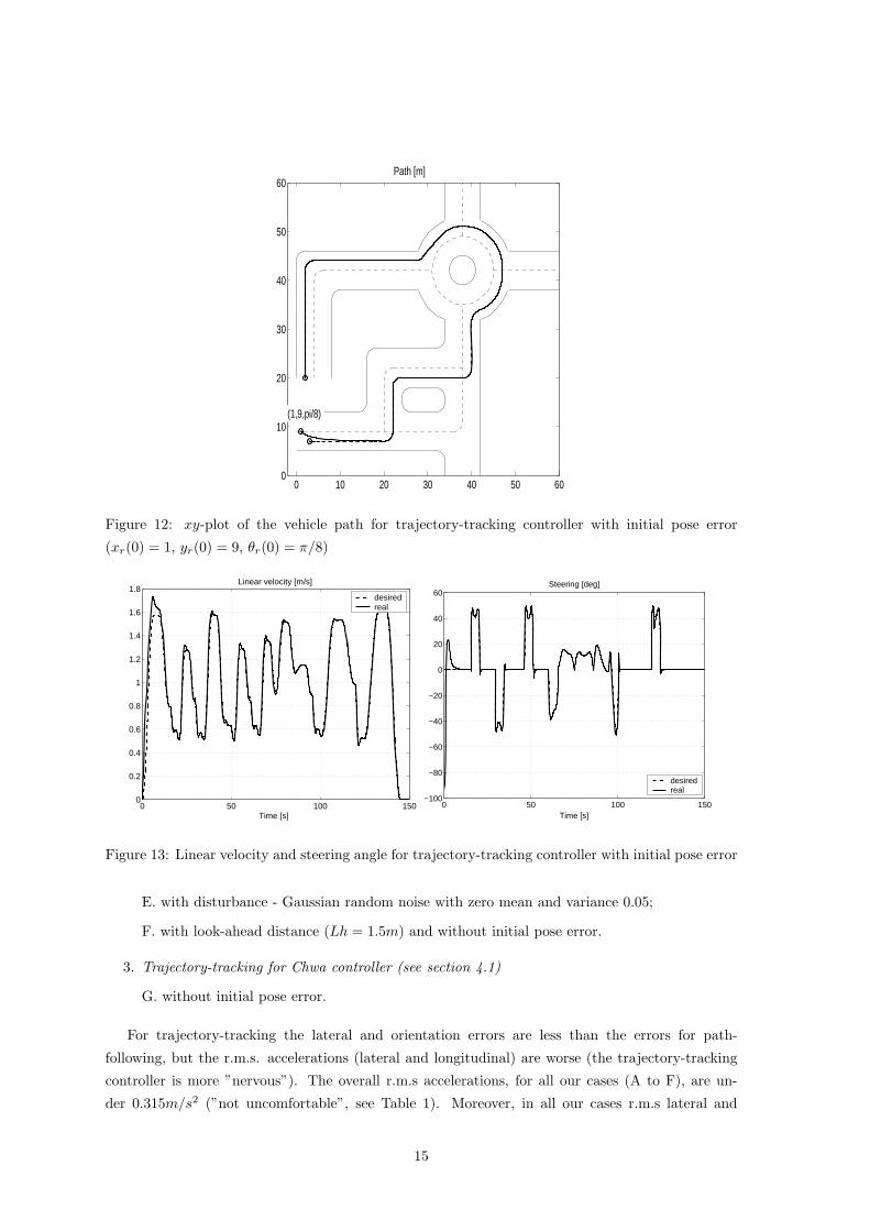
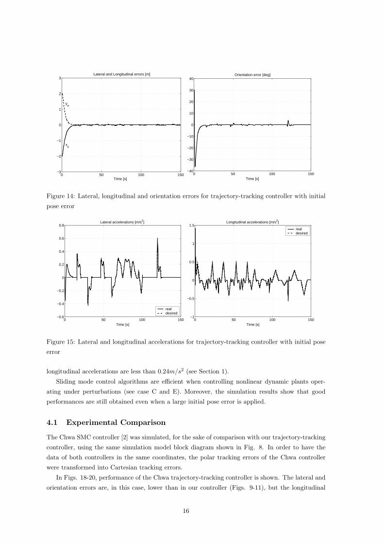
Figs. 12-15, for trajectory-tracking control with initial pose error (xr(0) = 1, yr(0) = 9, θr(0) =

π/8), show that the car retrieve the initial difference (xe = −2, ye = 2) quickly (Δt ≈ 20s), and

that the tracking errors converge to zero. The trajectory-tracking task must perform not only

the tracking of the curve (spatial dimension) but also doing it following a specified speed profile

(temporal dimension).

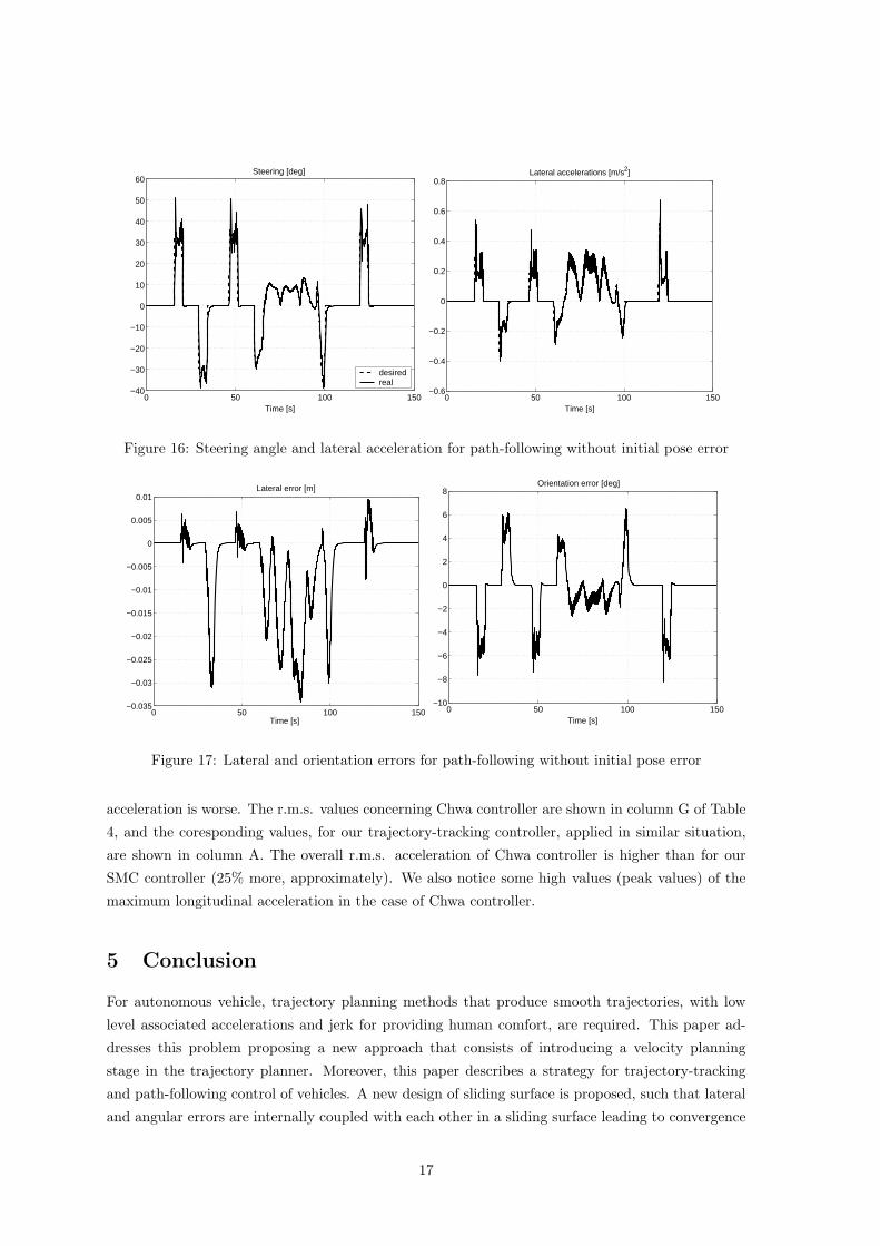
Figs. 16-17 show that path-following performance for reference trajectory (see Fig. 2) is sat-

13

0 50 100 150−0.05

−0.04

−0.03

−0.02

−0.01

0

0.01

0.02

0.03

0.04Lateral and Longitudinal errors [m]

Time [s]

xe

ye

0 50 100 150−3

−2

−1

0

1

2

3

4Orientation error [deg]

Time [s]

Figure 10: Lateral, longitudinal and orientation errors for trajectory-tracking controller without

initial pose error

0 50 100 150−0.6

−0.4

−0.2

0

0.2

0.4

0.6

0.8Lateral accelerations [m/s2]

Time [s]

realdesired

0 50 100 150−0.8

−0.6

−0.4

−0.2

0

0.2

0.4

0.6Longitudinal accelerations [m/s2]

Time [s]

realdesired

Figure 11: Lateral and longitudinal accelerations for trajectory-tracking controller without initial

pose error

isfactory. The lateral and orientation errors also converge to zero. In the path-following task, the

lateral error, ye, is defined as the distance between the vehicle control point and the closest point

along the vehicle desired trajectory as illustrated in Fig. 7.

Table 4 summarizes results of simulations for the following cases:

1. Trajectory-tracking

A. without initial pose error;

B. with initial pose error (xr(0) = 1, yr(0) = 9, θr(0) = π/8);

C. with disturbance - Gaussian random noise with zero mean and variance 0.05.

2. Path-following

D. without initial pose error;

14

0 10 20 30 40 50 600

10

20

30

40

50

60Path [m]

(1,9,pi/8)

Figure 12: xy-plot of the vehicle path for trajectory-tracking controller with initial pose error

(xr(0) = 1, yr(0) = 9, θr(0) = π/8)

0 50 100 1500

0.2

0.4

0.6

0.8

1

1.2

1.4

1.6

1.8Linear velocity [m/s]

Time [s]

desiredreal

0 50 100 150−100

−80

−60

−40

−20

0

20

40

60Steering [deg]

Time [s]

desiredreal

Figure 13: Linear velocity and steering angle for trajectory-tracking controller with initial pose error

E. with disturbance - Gaussian random noise with zero mean and variance 0.05;

F. with look-ahead distance (Lh = 1.5m) and without initial pose error.

3. Trajectory-tracking for Chwa controller (see section 4.1)

G. without initial pose error.

For trajectory-tracking the lateral and orientation errors are less than the errors for path-

following, but the r.m.s. accelerations (lateral and longitudinal) are worse (the trajectory-tracking

controller is more ”nervous”). The overall r.m.s accelerations, for all our cases (A to F), are un-

der 0.315m/s2 (”not uncomfortable”, see Table 1). Moreover, in all our cases r.m.s lateral and

15

0 50 100 150−3

−2

−1

0

1

2

3Lateral and Longitudinal errors [m]

Time [s]

ye

xe

0 50 100 150−40

−30

−20

−10

0

10

20

30

40Orientation error [deg]

Time [s]

Figure 14: Lateral, longitudinal and orientation errors for trajectory-tracking controller with initial

pose error

0 50 100 150−0.6

−0.4

−0.2

0

0.2

0.4

0.6

0.8Lateral accelerations [m/s2]

Time [s]

realdesired

0 50 100 150−1

−0.5

0

0.5

1

1.5Longitudinal accelerations [m/s2]

Time [s]

realdesired

Figure 15: Lateral and longitudinal accelerations for trajectory-tracking controller with initial pose

error

longitudinal accelerations are less than 0.24m/s2 (see Section 1).

Sliding mode control algorithms are efficient when controlling nonlinear dynamic plants oper-

ating under perturbations (see case C and E). Moreover, the simulation results show that good

performances are still obtained even when a large initial pose error is applied.

4.1 Experimental Comparison

The Chwa SMC controller [2] was simulated, for the sake of comparison with our trajectory-tracking

controller, using the same simulation model block diagram shown in Fig. 8. In order to have the

data of both controllers in the same coordinates, the polar tracking errors of the Chwa controller

were transformed into Cartesian tracking errors.

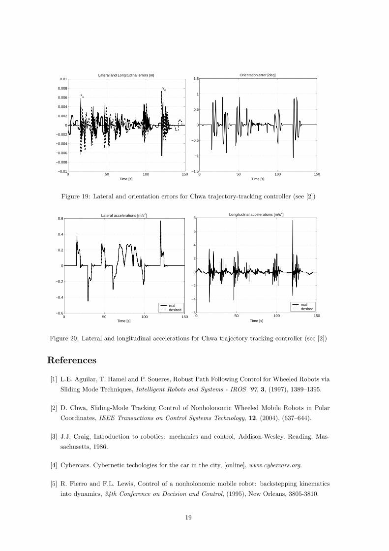
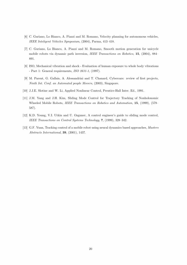
In Figs. 18-20, performance of the Chwa trajectory-tracking controller is shown. The lateral and

orientation errors are, in this case, lower than in our controller (Figs. 9-11), but the longitudinal

16

0 50 100 150−40

−30

−20

−10

0

10

20

30

40

50

60Steering [deg]

Time [s]

desiredreal

0 50 100 150−0.6

−0.4

−0.2

0

0.2

0.4

0.6

0.8Lateral accelerations [m/s2]

Time [s]

Figure 16: Steering angle and lateral acceleration for path-following without initial pose error

0 50 100 150−0.035

−0.03

−0.025

−0.02

−0.015

−0.01

−0.005

0

0.005

0.01Lateral error [m]

Time [s]0 50 100 150

−10

−8

−6

−4

−2

0

2

4

6

8Orientation error [deg]

Time [s]

Figure 17: Lateral and orientation errors for path-following without initial pose error

acceleration is worse. The r.m.s. values concerning Chwa controller are shown in column G of Table

4, and the coresponding values, for our trajectory-tracking controller, applied in similar situation,

are shown in column A. The overall r.m.s. acceleration of Chwa controller is higher than for our

SMC controller (25% more, approximately). We also notice some high values (peak values) of the

maximum longitudinal acceleration in the case of Chwa controller.

5 Conclusion

For autonomous vehicle, trajectory planning methods that produce smooth trajectories, with low

level associated accelerations and jerk for providing human comfort, are required. This paper ad-

dresses this problem proposing a new approach that consists of introducing a velocity planning

stage in the trajectory planner. Moreover, this paper describes a strategy for trajectory-tracking

and path-following control of vehicles. A new design of sliding surface is proposed, such that lateral

and angular errors are internally coupled with each other in a sliding surface leading to convergence

17

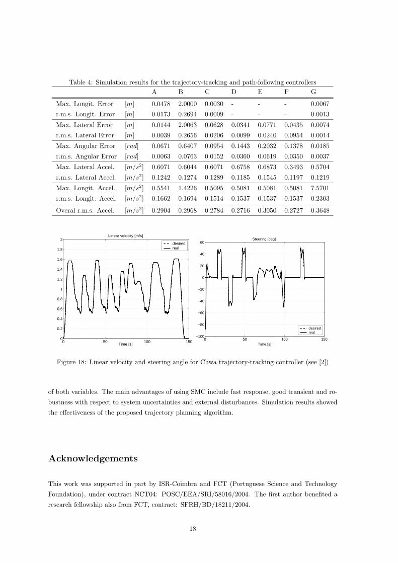
Table 4: Simulation results for the trajectory-tracking and path-following controllers

A B C D E F G

Max. Longit. Error [m] 0.0478 2.0000 0.0030 - - - 0.0067

r.m.s. Longit. Error [m] 0.0173 0.2694 0.0009 - - - 0.0013

Max. Lateral Error [m] 0.0144 2.0063 0.0628 0.0341 0.0771 0.0435 0.0074

r.m.s. Lateral Error [m] 0.0039 0.2656 0.0206 0.0099 0.0240 0.0954 0.0014

Max. Angular Error [rad] 0.0671 0.6407 0.0954 0.1443 0.2032 0.1378 0.0185

r.m.s. Angular Error [rad] 0.0063 0.0763 0.0152 0.0360 0.0619 0.0350 0.0037

Max. Lateral Accel. [m/s2] 0.6071 0.6044 0.6071 0.6758 0.6873 0.3493 0.5704

r.m.s. Lateral Accel. [m/s2] 0.1242 0.1274 0.1289 0.1185 0.1545 0.1197 0.1219

Max. Longit. Accel. [m/s2] 0.5541 1.4226 0.5095 0.5081 0.5081 0.5081 7.5701

r.m.s. Longit. Accel. [m/s2] 0.1662 0.1694 0.1514 0.1537 0.1537 0.1537 0.2303

Overal r.m.s. Accel. [m/s2] 0.2904 0.2968 0.2784 0.2716 0.3050 0.2727 0.3648

0 50 100 1500

0.2

0.4

0.6

0.8

1

1.2

1.4

1.6

1.8

2Linear velocity [m/s]

Time [s]

desiredreal

0 50 100 150−100

−80

−60

−40

−20

0

20

40

60Steering [deg]

Time [s]

desiredreal

Figure 18: Linear velocity and steering angle for Chwa trajectory-tracking controller (see [2])

of both variables. The main advantages of using SMC include fast response, good transient and ro-

bustness with respect to system uncertainties and external disturbances. Simulation results showed

the effectiveness of the proposed trajectory planning algorithm.

Acknowledgements

This work was supported in part by ISR-Coimbra and FCT (Portuguese Science and Technology

Foundation), under contract NCT04: POSC/EEA/SRI/58016/2004. The first author benefited a

research fellowship also from FCT, contract: SFRH/BD/18211/2004.

18

0 50 100 150−0.01

−0.008

−0.006

−0.004

−0.002

0

0.002

0.004

0.006

0.008

0.01Lateral and Longitudinal errors [m]

Time [s]

xe

ye

0 50 100 150−1.5

−1

−0.5

0

0.5

1

1.5Orientation error [deg]

Time [s]

Figure 19: Lateral and orientation errors for Chwa trajectory-tracking controller (see [2])

0 50 100 150−0.6

−0.4

−0.2

0

0.2

0.4

0.6Lateral accelerations [m/s2]

Time [s]

realdesired

0 50 100 150−6

−4

−2

0

2

4

6

8Longitudinal accelerations [m/s2]

Time [s]

realdesired

Figure 20: Lateral and longitudinal accelerations for Chwa trajectory-tracking controller (see [2])

References

[1] L.E. Aguilar, T. Hamel and P. Soueres, Robust Path Following Control for Wheeled Robots via

Sliding Mode Techniques, Intelligent Robots and Systems - IROS ’97, 3, (1997), 1389–1395.

[2] D. Chwa, Sliding-Mode Tracking Control of Nonholonomic Wheeled Mobile Robots in Polar

Coordinates, IEEE Transactions on Control Systems Technology, 12, (2004), (637–644).

[3] J.J. Craig, Introduction to robotics: mechanics and control, Addison-Wesley, Reading, Mas-

sachusetts, 1986.

[4] Cybercars. Cybernetic techologies for the car in the city, [online], www.cybercars.org.

[5] R. Fierro and F.L. Lewis, Control of a nonholonomic mobile robot: backstepping kinematics

into dynamics, 34th Conference on Decision and Control, (1995), New Orleans, 3805-3810.

19

[6] C. Guriano, Lo Bianco, A. Piazzi and M. Romano, Velocity planning for autonomous vehicles,

IEEE Inteligent Vehicles Symposium, (2004), Parma, 413–418.

[7] C. Guriano, Lo Bianco, A. Piazzi and M. Romano, Smooth motion generation for unicycle

mobile robots via dynamic path inversion, IEEE Transactions on Robotics, 15, (2004), 884–

891.

[8] ISO, Mechanical vibration and shock - Evaluation of human exposure to whole body vibrations

- Part 1: General requirements, ISO 2631-1, (1997).

[9] M. Parent, G. Gallais, A. Alessandrini and T. Chanard, Cybercars: review of first projects,

Ninth Int. Conf. an Automated people Movers, (2003), Singapore.

[10] J.J.E. Slotine and W. Li, Applied Nonlinear Control, Prentice-Hall Inter. Ed., 1991.

[11] J.M. Yang and J.H. Kim, Sliding Mode Control for Trajectory Tracking of Nonholonomic

Wheeled Mobile Robots, IEEE Transactions on Robotics and Automation, 15, (1999), (578–

587).

[12] K.D. Young, V.I. Utkin and U. Ozguner, A control engineer’s guide to sliding mode control,

IEEE Transactions on Control Systems Technology, 7, (1999), 328–342.

[13] G.F. Yuan, Tracking control of a mobile robot using neural dynamics based approaches, Masters

Abstracts International, 39, (2001), 1437.

20