2013 u.s. veterinary workforce study: modeling capacity utilization€¦ · · 2013-04-232013...
TRANSCRIPT

Proposal for PhRMA Economic Burden of PD Study
2013 U.S. Veterinary Workforce
Study: Modeling Capacity
Utilization
Final Report For:
American Veterinary Medical Association
April 16, 2013

i
Acknowledgement The study team received guidance and subject matter expertise from a Workforce Advisory Group
(WAG). While WAG members provided insights and guidance to the study team, the views
expressed in this report do not necessarily reflect the views of specific WAG members or the
institutions that they represent.
Workforce Advisory Group Members
Link Welborn, DVM, DABVP (Chair). President, Tampa Bay Veterinary Medical Group, Tampa, FL
Jane Brunt, DVM. Executive Director, CATalyst Council, Inc., Annapolis, MD.
Margaret Coffey, DVM, MBA. Director, Veterinary Teaching Hospital, LSU, Baton Rouge, LA
David Gersholowitz, MBA. Chief Operating Officer, BluePearl Veterinary Partners, New York, NY.
Eleanor Green, DVM, DACVIM, DABVP. Carl B. King Dean of Veterinary Medicine, College of Veterinary Medical & Biomedical Sciences, Texas A&M University, College Station, TX
Jeffrey Klausner, DVM, DACVIM. Chief Medical Officer and Senior Vice President, Banfield Pet Hospital, Portland, OR
Roger Saltman, DVM, MBA. Group Director, Cattle-Equine Technical Services, Zoetis, Cazenovia, NY
Carin Smith, DVM. President, Smith Veterinary Consulting, Inc., Peshastin, WA
Scott Spaulding, DVM. President , Badger Veterinary Hospital. Janesville, WI.
Michael Thomas, DVM. President, Noah’s Animal Hospitals, Indianapolis, IN.
Karl Wise, PhD. Associate Executive Vice President, AVMA, Schaumburg, IL
AVMA Staff Consultant
Michael Dicks, PhD. Director, Veterinary Economics Division, AVMA, Schaumburg, IL
Study Authors
IHS Healthcare & Pharma1 Center for Health Workforce Studies2
Timothy M. Dall, MS Gaetano J. Forte, BA
Michael V. Storm, BA Margaret H. Langelier, MS
Paul Gallo, BS
Ryan M. Koory, BS
James W. Gillula, PhD
1 1150 Connecticut Ave. NW, Suite 401, Washington, DC. 20036. 2 SUNY School of Public Health.
University at Albany. One University Place. Rensselaer, NY 12144

ii
Contents
Executive Summary .................................................................................................................................. vi
I. Background .......................................................................................................................................... 1
A. Key Study Concepts and Definitions .......................................................................................... 2
B. Theoretical Framework for Veterinary Workforce Assessment and Literature Review ..... 3
C. Defining Current National Demand and Measuring Excess Capacity/Shortfall ................. 8
II. Estimating and Projecting Veterinarian Supply ...................................................................... 18
A. Estimated Current Supply .......................................................................................................... 19
B. New Entrants to the U.S. Veterinarian Workforce .................................................................. 24
C. Workforce Attrition ..................................................................................................................... 27
D. Hours Worked .............................................................................................................................. 29
E. Supply Projections ....................................................................................................................... 33
III. Estimating and Projecting Demand for Veterinarians ............................................................ 37
A. Data and Methods ........................................................................................................................ 37
B. Projections of State and National Demand for Veterinarians ................................................ 48
IV. Conclusion .................................................................................................................................... 57
A. National Projections of Adequacy of Supply and Discussion ............................................... 57
B. Study Strengths and Limitations ............................................................................................... 59
C. Areas for Future Research........................................................................................................... 60
D. Summary ....................................................................................................................................... 62
Appendix A: Results from the 2012 Workforce Survey...................................................................... 64
A. Survey Design ............................................................................................................................... 64
B. Survey Results .............................................................................................................................. 75
Appendix B: Regression Results ............................................................................................................ 78
Appendix C: Modeling Approach Used to Forecast Future U.S. Production of Food Animals ... 83
References ………………….………………………………………………………………………..…. 86

iii
Exhibits
Exhibit 1. Wait Time to Obtain Appointment for Last Veterinarian Visit for Pet (% distribution
by wait time) ............................................................................................................................................... 6
Exhibit 2. Supply, Demand, and Price .................................................................................................... 7
Exhibit 3. Average Annual Earnings of Veterinarians in Clinical Practice ........................................ 9
Exhibit 4. Percent of Veterinary Medical School Seniors with at Least One Offer for Employment
or Further Education, and Average Number of Offers ...................................................................... 11
Exhibit 5. Perceptions of Local Market Areas ...................................................................................... 12
Exhibit 6. Assessment of Practice Productivity among Respondents Engaged in Individual or
Group/Herd Animal Health Care ......................................................................................................... 12
Exhibit 7. Potential Productivity Growth ............................................................................................. 13
Exhibit 8. Estimated Current Excess Capacity by State and Practice Type ..................................... 15
Exhibit 9. Estimated Current Excess Capacity of Veterinary Services: Small Animal Practice .... 16
Exhibit 10. Estimated Current Excess Capacity of Veterinary Services: Equine Practice .............. 16
Exhibit 11. Estimated Current Excess Capacity of Veterinary Services: Food Animal Practice ... 17
Exhibit 12. Estimated Current Excess Capacity of Veterinary Services: Mixed Animal Practice . 17
Exhibit 13. Microsimulation Model of Veterinarian Supply .............................................................. 18
Exhibit 14. Veterinarian Age Distribution and Initial Supply Refinement ...................................... 21
Exhibit 15. Veterinarian Age and Gender Distribution ...................................................................... 22
Exhibit 16. State Estimates of Veterinarian Supply: 2012 ................................................................... 23
Exhibit 17. Total Graduates from U.S. Colleges of Veterinary Medicine: 1980 to 2012 ................. 24
Exhibit 18. Estimates of New Veterinarians Entering the U.S. Workforce ...................................... 25
Exhibit 19. Past and Projected U.S. Baccalaureate Graduates (across all academic fields)............ 26
Exhibit 20. Age Distribution of New Graduates from Veterinary Medical Schools ....................... 27
Exhibit 21. Veterinarian Workforce Attrition Patterns ....................................................................... 28
Exhibit 22. Average Hours Worked per Week..................................................................................... 31
Exhibit 23. Full-Time Equivalent Scalars .............................................................................................. 31
Exhibit 24. Average Annual Hours Worked for Men: 2002-2012 ...................................................... 32
Exhibit 25. Average Annual Hours Worked for Women: 2002-2012 ................................................ 32
Exhibit 26. Projections of Active and “2012 Equivalent” Supply: 2012-2030 (Baseline Scenario) 35

iv
Exhibit 27. Alternative Supply Scenarios: 2012-2030 .......................................................................... 36
Exhibit 28. State Projections of Total Small Animals and Household-Owned Equine, 2012 ........ 41
Exhibit 29. Distribution of Time Spent By Practice Type ................................................................... 43
Exhibit 30. Food Animal Veterinarian Workforce, 2012 ..................................................................... 45
Exhibit 31. Projected Growth in Food Animal Supply ....................................................................... 46
Exhibit 32. Veterinary Workforce in Federal Employment, 2012 ...................................................... 47
Exhibit 33. Total FTE Demand for Veterinarians in the U.S., 2012 ................................................... 50
Exhibit 34. Total FTE Demand for Veterinarians in the U.S., 2025 ................................................... 50
Exhibit 35. State Estimates of Total FTE Demand for Small Animal Veterinarians ....................... 51
Exhibit 36. State Estimates of Total FTE Demand for Equine Veterinarians ................................... 52
Exhibit 37. State Estimates of Total FTE Demand for Food Animal Veterinarians ........................ 53
Exhibit 38. State Projections of % and FTE Demand Growth for Small Animal Veterinarians:
2012-2025 ................................................................................................................................................... 54
Exhibit 39. State Estimates of Demand for Food Animal Veterinarians: 2012 ................................ 55
Exhibit 40. State Projections of % and FTE Demand Growth for Food Animal Veterinarians:
2012-2025 ................................................................................................................................................... 55
Exhibit 41. Baseline Demand Projections: 2012-2025 .......................................................................... 56
Exhibit 42. Alternative Supply Scenarios vs. Baseline Demand Projections 2012-2025 ................. 58
Exhibit 43. Employment Sector Groups ................................................................................................ 65
Exhibit 44. Population Cross-Classification and Subgroup Counts ................................................. 66
Exhibit 45. Sample Subgroup Counts .................................................................................................... 67
Exhibit 46. Survey Response by Gender ............................................................................................... 68
Exhibit 47. Survey Response by Employment Sector ......................................................................... 68
Exhibit 48. Survey Response by Age and AVMA Professional Activity Status .............................. 69
Exhibit 49. Survey Response by Geographic Location ....................................................................... 69
Exhibit 50. Survey Response by Employment Sector, Geographic Location, Professional Activity
Status, Age, and Gender.......................................................................................................................... 70
Exhibit 51. Respondent Group Cross-Classification ........................................................................... 71
Exhibit 52. Survey Response Rate Difference Weights ....................................................................... 72
Exhibit 53. Sampling Design Adjustment ............................................................................................. 74
Exhibit 54. Respondent Demographics: Gender and Age .................................................................. 75

v
Exhibit 55. Respondent Demographics: Employment Sector ............................................................ 76
Exhibit 56. Age when Became Permanently Inactive in Veterinary Medicine ................................ 76
Exhibit 57. Reported Plans for Becoming Permanently Inactive in Veterinary Medicine ............. 77
Exhibit 58. Age when Plan to Become Permanently Inactive in Veterinary Medicine .................. 77
Exhibit 59. Rate Ratios from Poisson Regression for Pet Ownership ............................................... 78
Exhibit 60. Rate Ratios from Poisson Regression for Dog Services ................................................... 79
Exhibit 61. Rate Ratios from Poisson Regression for Cat Services .................................................... 81
Exhibit 62. IHS Global Insight Agricultural Forecasting Model ....................................................... 84

vi
Executive Summary
The American Veterinary Medical Association (AVMA) contracted with IHS Healthcare &
Pharma (IHS) and the Center for Health Workforce Studies (CHWS) to conduct a study on the
current and future adequacy of supply of veterinary medical services and veterinarians. The
purpose of this study is to help inform strategies to ensure the economic viability of veterinary
medicine as the profession works to attract and retain highly qualified professionals. This study
was designed to produce information regarding the number and employment sector mix of
veterinarians the nation needs to train to ensure a balanced supply (both geographically and
over time) as the profession works to fulfill its social mission. The primary goals of this study,
therefore, were to:
1. Identify and quantify key trends and factors related to veterinary workforce decisions,
demand for veterinary services, economic viability of practice, and care delivery;
2. Quantify the degree to which there is under- or- over capacity in veterinary services at
the national, state, and employment sector levels
3. Identify gaps in the workforce research and areas requiring further research; and
4. Develop a Veterinarian Workforce Simulation Model that over time would be
maintained and enhanced by AVMA’s new Economics Division.
Methods used to collect information and produce the findings presented in this report include:
(1) a review of the published and gray literature; (2) interviews with subject matter experts and
key stakeholders; (3) empirical analysis of surveys and data collected by AVMA, the federal
government, and other institutions; (4) fielding of a 2012 Veterinary Workforce Survey; and (5)
development of the Veterinarian Workforce Simulation Model for projecting future supply and
demand.
Key findings regarding the current state of the veterinary workforce include:
Market indicators suggest excess capacity at the national level to supply veterinary
services. Recent trends include falling incomes of veterinarians, falling rates of
productivity (using various measures), and increased difficulty for new graduates to
find employment.
Respondents to the 2012 Veterinary Workforce Survey who indicated that they were
engaged in clinical practice were asked to characterize their local market areas and their
practices’ capacity and productivity. Almost half of the respondents reported
perceptions of too many veterinarians and too many veterinary practices. A similar
percentage also reported perceptions of just the right number of both veterinarians and
veterinary practices. Slightly more than half of the respondents indicated that their
practices were not working at full capacity.

vii
Based on survey responses to the question of how much productivity could be increased
if (a) there are no changes in the way the practice is organized, (b) there are no changes
in the number of veterinarians or support staff, and (c) there is an unlimited supply of
clients and patients, we calculate excess capacity for veterinary services were highest for
equine practice (23% excess capacity), followed by small animal (18%), food animal
(15%), and mixed practices (13%). These numbers reflected that 42% of veterinarians
who reported on the capacity status of their practice (i.e., did not respond “don’t
know/not sure”) reported that their practice was already working at full capacity. We
assume that in 2012 the demand for veterinarians employed in government, academia,
industry, and “other” (tax exempt and municipalities) sectors is equal to supply (i.e.,
there is no shortfall or surplus at the national level).
Key supply-related findings include:
We estimate the current supply of active veterinarians at the beginning of 2012 is
approximately 90,200. This estimate is roughly equivalent to the estimate in the recent
National Academy of Sciences report that cites 92,000 professionals in 2010 based on
AVMA data, but makes adjustments for what appears to be an overestimate of active
veterinarians age 65 and older in the AVMA data.1
The number of new college of veterinary medicine graduates entering the US over the
next decade is unknown, but estimates based on North American Veterinary Licensing
Exam (NAVLE) data are that approximately 3,457 graduates (from accredited and non-
accredited) colleges of veterinary medicine completed their education in 2012.
Enrollment data allows us to project the likely number of new CVM graduates through
2016, and we model alternative supply scenarios with different rates of growth
assumptions ranging from no increases in graduates after 2016 to 4% annual growth in
new graduates after 2016. These scenarios reflect announced growth in enrollment at
existing CVMs, as well as the potential for continued expansion if historical rates
continue.
Supply projections are presented based on alternative assumptions regarding number of
new graduates, hours worked patterns, and retirement patterns.
We define a “2012 equivalent” veterinarian as someone who works 2,313 hours per year
in professional activities—which is the national average across veterinarians of all age
groups and gender. Under the Baseline Scenario with assumed 2% annual growth in
number of CVM graduates, the national supply of 90,200 veterinarians in 2012 is
projected to grow to approximately 95,400 by 2020, 100,400 by 2025, and 108,900 by 2030.
1 National Academy of Sciences. Workforce Needs in Veterinary Medicine. 2012. http://dels.nas.edu/resources/static-assets/materials-based-on-reports/reports-in-brief/Vet-Med-Report-Brief-Final.pdf.

viii
These future year projections are in terms of 2012 equivalents that take into
consideration the changing age and gender composition of the veterinarian workforce.
Women constitute approximately 50% of the current workforce, but will likely grow to
71% of the workforce by 2030. Women constitute 78% of new graduates, whereas the
older workforce nearing traditional retirement age is predominantly male.
Key demand-related findings include:
Based on estimates of excess capacity among veterinarians in clinical practice (calculated
from the 2012 Veterinarian Workforce Survey) and the assumption of balance between
supply and demand for veterinarians in non-clinical practice, we calculate national
demand for veterinarians equals 78,950 in 2012. Comparison to supply suggests national
excess capacity of 12.5% at current price levels for services (equivalent to the services of
approximately 11,250 veterinarians).
The Baseline Demand Scenario models current trends—accounting for changing
household demographics, trends in livestock and food animal consumption patterns,
and demand drivers in other employment sectors. Therefore, this scenario represents
our best estimate of future demand under the status quo. Under this scenario, total
demand is projected to grow to 88,100 in 2025 (or by 12% relative to 2012).
Future adequacy of supply findings include:
Comparison of the Baseline supply and demand scenarios (with the Baseline scenario
reflecting informed assumptions about the continuation of current trends) suggests that
the magnitude of the surplus capacity will range from 11% and 14% between 2012 and
2025 (equivalent to approximately 9,300 to 12,300 veterinarians).
We model the sensitivity of the supply projections to different assumptions regarding
number of veterinarians trained, hours worked patterns, and retirement patterns. Under
every scenario the supply projections exceed demand through 2025. Given the high debt
load of new students and stagnating incomes seen in recent years among veterinarians,
it is unlikely that veterinarians will reduce average hours worked or retire earlier than
current and historical patterns. Consequently, there is greater potential for the supply
projections to exceed the baseline estimates rather than fall short of the baseline
estimates.
The report discusses research gaps that if filled could help inform strategies to ensure adequate
access to veterinary services and the economic viability of veterinary practice:
Develop more objective measures of demand for veterinary services.
Develop early warning indicators of imbalances between supply and demand (similar to
the Aggregate Demand Index developed by the Pharmacy Manpower Project).
Conduct research on the price sensitivity of pet and animal owners.

ix
Monitor the careers of new veterinarians by selecting a sample each year for
participation in a long term follow-up study that seeks to explore the career trajectories
of individuals who become veterinarians in the current supply/demand environment.
Acquire additional information on the average amount of time veterinarians spend
providing specific types of services to simulate the demand implications of changing
mix of services demanded and implementation of alternative care delivery models.
In summary, it appears that at the national level there is current excess capacity to provide
direct animal care services. In percentage terms, the level of excess capacity appears to be
largest for equine practices, followed by small animal practices, food production practices, and
mixed animal practices. This excess capacity is likely to persist for the foreseeable future even if
veterinary schools were to curtail expansion of enrollment. However, this excess capacity could
potentially be reduced or eliminated if veterinarians were able to increase demand for
veterinary services through outreach programs to educate pet owners or by removing access
barriers or reducing the cost to purchase services to spur greater volume of services.

1
I. Background
The American Veterinary Medical Association contracted with IHS Healthcare & Pharma
(IHS) and the Center for Health Workforce Studies (CHWS) to conduct a study on the
current and future adequacy of supply of veterinary medical services and veterinarians. The
purpose of this study was to help inform strategies to ensure the economic viability of
veterinary medicine as the profession works to attract and retain highly qualified
professionals. This study was designed to produce information regarding the number and
employment sector mix of veterinarians the nation needs to train to ensure a balanced
supply (both geographically and over time) as the profession strives to fulfill its social
mission. The primary goals of this study, therefore, were:
1. To identify and quantify the implications of key trends and factors related to
veterinary workforce decisions, demand for veterinary services, economic viability
of practice, and care delivery;
2. To estimate the degree to which there is under- or- over capacity in veterinary
services at the national and state level by employment sector; and
3. To identify gaps in the workforce research and identify areas requiring further
research.
The information in this report was obtained using four data collection strategies:
1. Empirical analysis of survey and other data. We analyzed data collected by the
American Veterinary Medical Association (AVMA), federal agencies, and other
organizations. AVMA’s database of veterinarians (which contains information on
veterinarians who are not members of AVMA as well as members) was a primary
source for the current supply of veterinarians. Multiple years of the Biennial
Economic Survey, Pet Demographic Study, and Graduating Senior Survey were
analyzed. We also analyzed the U.S. Census Bureau’s American Community Survey
(ACS). These sources are described later in more detail.
2. Literature review. We conducted a review of the peer-reviewed literature on the
veterinary workforce, as well as industry and government reports. The review
focused on the literature published since the KPMG (1999) veterinary workforce
study.1
3. Phone interviews with key stakeholders and subject matter experts.
Approximately two dozen phone interviews were conducted with members of the
study Workforce Advisory Group, key stakeholder groups, and subject matter
experts recommended by members of the advisory group.
4. New workforce survey of veterinarians. From September to October 2012, we
conducted a survey with a sample of veterinarians to collect information on

2
retirement patterns and intentions, perceptions of local adequacy of veterinary
supply capacity, and other workforce-related information. This survey is described
later, with a detailed description provided in Appendix A.
A key component of this study was the development of a Veterinary Workforce Computer
Simulation Model that over time will be refined, updated, and used by AVMA’s new Veterinary
Economics Division. The supply and demand components of this workforce model were
designed to be flexible to simulate the implications of changes in trends affecting supply and
demand for veterinary services. This report, therefore, is the first in a planned series of regular
reports and analyses that will be sponsored or published by AVMA’s economic analysis team.
A. Key Study Concepts and Definitions
Throughout this report we refer to the following economic, workforce-related, and other
terms:
Employment sector. Veterinarians work in a variety of settings, with a large majority
in private clinical practice. Others work in industry/commercial, federal
government, academia, or “other” settings (e.g., tax-exempt organizations and
municipal governments). Veterinarians in clinical practice are often differentiated by
whether they are predominantly small animal practices, small/large mixed animal
practices, equine practices, or food animal practices.
Supply of veterinary services. This term generally refers to the provision of
veterinary services to animals—regardless of whether these services are provided by
veterinarians, veterinary technicians or assistants, or other support staff.
Active supply of veterinarians. Veterinarians were considered part of the active
supply if they self-reported working in veterinary medicine.
Full-time equivalent (FTE) supply. While most veterinarians work full time, some
are employed part time. We defined one FTE based on the average annual hours
(2,313) worked across all active veterinarians (part time and full time) in 2012.
Supply was defined as the number of veterinary service hours veterinarians reported
as being at work or working and thus, assumedly, available and able to supply
services. The FTE concept allowed us to compare current supply to future supply,
and compare supply to demand using a standardized unit.
Demand for veterinary services. In this report, the technique for measuring demand
varied across employment sectors. The main driver of demand for veterinarians in
small animal, equine, and mixed animal practices reflected the willingness to pay for
veterinary services as measured by national patterns of veterinary visits by animal
owners. Demand for food animal veterinarians and many government veterinarians
reflected changes in populations of livestock. The Baseline Demand Scenario that
was modeled assumed that the ratio of livestock to veterinarians, with the ratio
varying by type of livestock, remains constant over the projection horizon. Demand
for veterinarians in academia reflected growth in schools and assumed the same

3
ratio of academic veterinarians to students. Demand for veterinarians in industry
and other sectors reflected projected growth in a variety of sectors of the economy.
Need for veterinary services. Whereas the term “demand” reflected consumers’
willingness to pay for veterinary services given the price of services, the term “need”
referred to an assessment of services that were warranted. Veterinarians may have
expressed their clinical judgment that animals should receive certain services (e.g.,
preventive care), but if animal owners are unwilling to pay for such services at
prevailing prices or are unaware of the need for such services, then the need goes
unmet (for lack of demand). Need also referred to someone expressing a desire for
veterinarians to serve in some geographic area or career path/niche. For example, in
many rural areas animal owners desire improved access to veterinary services but
the level of demand is insufficient to make veterinary practice financially viable.
While there is an expressed need for veterinarians, there is insufficient demand.
Likewise, in some career paths (e.g., public health) there may be unfilled positions. A
group may have expressed that they “need” more veterinarians in public health or
desire a “surge capacity” in the event of emergencies, but if government agencies cut
positions, do not create jobs, or are unable to offer competitive salaries for such
services, then this need does not translate to demand.
Supply capacity. We defined capacity as the ability to provide services. Capacity
generally referred to the ability of veterinarians to supply services in a specific
geographic area and employment sector. On an individual level, capacity was the
total amount of services a veterinarian was able to provide based on available
resources.
Excess capacity. This term referred to the ability to provide services in excess of the
quantity demanded at a price that consumers are willing to pay. Excess capacity
means that veterinarians in a particular geographic area and/or employment sector
are underutilized. This underutilization can take the form of unemployment, but
more often takes the form of reduced productivity because either (1) the veterinarian
does not have sufficient demand for services to keep busy, or (2) the veterinarian is
keeping busy by providing services that could be provided by a technician or other
staff member with less training.
B. Theoretical Framework for Veterinary Workforce Assessment and
Literature Review
Veterinary workforce planning is the process to help ensure that the nation has the right
number and mix of veterinary service providers in the right places to provide access to
services at affordable prices that support economically viable veterinary practices. Over the
past several decades, numerous reports and articles have been published on the topic of
whether the United States has the right number and mix of veterinarians to meet the
country’s current and future needs. Some of these studies found current and projected
excess capacity within the veterinary workforce—including work by Arthur D. Little, Inc. in

4
19782, Wise and Kushman in 19853, Getz in 19974, and Brown and Silverman (KPMG) in
1999.1
Other studies suggested there is a shortfall of veterinarians in select careers (namely, food
animal production and public health), in rural areas, or in research (i.e., receiving PhD
training). These included studies by the AAVMC (2006)5, Sterner (2006)6, Andrus et al.
(2006)7, Funk and Bartlett (2008)8, GAO (2009)9, Jarman et al. (2011)10, and National
Academy of Sciences (2012)11. The National Academy of Sciences report stated that they
found little evidence of workforce shortages in most fields of veterinary medicine and
expressed concern that “an unsustainable economic future is confronting the profession (p.
207)” due to the large number of veterinarians being trained and the high debt levels of new
graduates. 11
Often, studies that reported a shortage confused the terms “need” and “demand.” They
found, for example, that the U.S. and the world might need more veterinarians in a public
health capacity to improve social good (e.g., to help combat animal spread diseases such as
West Nile fever and to help prevent outbreaks of SARS, monkey pox, bovine spongiform
encephalopathy, and highly pathogenic avian influenza) or to help ensure the safety of food
supply, if governments or other institutions were unable to fund positions or to pay
competitive wages to attract and retain veterinarians, then the demand for veterinary services
was not present. As defined previously, demand for services was based on a price point (in
this case, compensation levels), and it would have been inefficient and a disservice to train
people for positions that were unfunded or for which compensation levels were non-
competitive.
Likewise, the nation might need more veterinarians to work in food production—especially
in rural areas. However, if there is insufficient demand to make veterinary practices in these
areas financially viable then these areas will have difficulty attracting and retaining
veterinarians despite the abundance of veterinarians in the workforce. As noted by the
National Academy of Sciences report: “Regions that formerly supported a veterinarian can
no longer do so. This is not a sign of a shortfall in the supply of veterinarians but rather of a
shortfall in employment opportunities (p. 204).”11
Effective planning, therefore, requires answers to the following questions:
1. What is the right number and mix of care providers?
2. What is considered “adequate” access to services?
3. What prices are affordable to purchasers of services while still supporting
economically viable veterinary practices?
Answering these questions is made complicated by the dearth of research conducted on
these topics.
5
What is the right number and mix of veterinary services providers?
From an economic perspective, the right number and mix of veterinary providers is the
number of veterinarians and support staff (technicians, assistants, etc.) that allows for the
most efficient delivery of services at prices that consumers are willing to pay. Efficient
delivery of veterinary services starts with each occupation operating at the top of their
license. That is, veterinarians do the work that only they are trained to do. Veterinary
technicians, assistants, and other support staff do the work that they are trained to do. In an
efficient system, veterinarians minimize the amount of work they do that can instead be
done by a person with less training.
What is considered “adequate” access to services?
Having too few veterinary service providers means that some demand for services may go
unmet—despite pet or animal owners’ willingness to pay for services at prevailing prices.
Perceived shortages have long existed in many medical fields. Some physician specialties have
reported long, average wait times for new patients to obtain an appointment or for existing
patients to obtain a return appointment. The American Academy of Neurology reported that in
2012 the average wait time was 35 business days for a new patient to see an adult neurologist
and 30 days wait for existing patients to obtain follow-up visits.12 A 2009 survey of physician
appointment wait times by Merritt Hawkins and Associates found that the average wait time
for new patients to see a neurosurgeon was 24 days, for family practice 20 days, for orthopedic
surgery 17 days, and for cardiology 15 days.13 The Children’s Hospital Association also found
long wait times to see a pediatric specialist were common, with an average wait time of 45
business days for patients to obtain a clinic visit with a pediatric neurologist.14
In contrast, the AVMA 2012 Pet Ownership Survey asked questions regarding wait time to
obtain an appointment with a veterinarian.15 The majority of pet owners reported that they
were able to obtain a visit that same day or the next day with the veterinarian practice, with
approximately 85% of owners able to obtain an appointment within three days of calling to
schedule (Exhibit 1). These findings were relatively consistent across owners of dogs, cats,
horses, and birds. For owners who waited longer than three days for an appointment, it was
unclear if the length of time was due to the veterinarian practice being unable to accommodate
the patient because the practice was booked, whether the visit fell on a holiday or weekend, or
whether the wait time was to better accommodate the schedule of the pet owner.

6
Exhibit 1. Wait Time to Obtain Appointment for Last Veterinarian Visit for Pet
(% distribution by wait time)
Wait Time Dog Cat Horse Bird
Same day 28% 27% 29% 29%
Next day 27% 27% 25% 29%
2-3 days 30% 30% 26% 25%
3-5 days 9% 10% 11% 10%
1-2 weeks 5% 5% 7% 5%
More than 2 weeks 1% 1% 2% 2%
Total 100% 100% 100% 100%
When there are too few providers, employers experience abnormally long wait times to fill
vacant positions. A 2012 survey by the Children’s Hospital Association, for example,
reported that more than one-quarter of children’s hospitals reported vacancies of 12 months
or longer for pediatric providers in many pediatric specialties.14 When there is excess
capacity, then large numbers of applicants vie for available job openings and vacancies were
filled quickly. GAO (2009) reported that over a five-year period the vacancy rate for
veterinarian positions in slaughter plants varied by location and year, ranging from no
vacancy to a high of 35% of positions vacant.9
A challenge for workforce planning is to better understand the extent to which high vacancy
rates are local and/or associated with inadequate compensation, versus the degree to which
high vacancy rates are widespread and associated with inadequate supply capacity. In the
case of veterinary medicine, there were no widespread indicators of inability for consumers
to access veterinary services and ample indicators that consumers are able to obtain access
to veterinary services if they are willing to pay current prevailing market prices.
What prices are affordable to purchasers of services while still supporting economically
viable veterinary practices?
While research on this topic falls outside the scope of this study, the “price” to purchase
veterinary services can be thought of as the costs that consumers pay to obtain veterinary
services for their pet or animal. For employment sectors where veterinarians are hired as
employees, however, the price of services can be thought of as compensation levels required
to attract and retain veterinarians.
Consider Exhibit 2, which illustrates the relationship between supply of veterinary services,
demand for services, and price. As illustrated in Figure A, in a competitive market, supply
and demand interact to produce what economists define as a “market clearing price.” That
is, in a competitive market the price (P*) is determined such that the quantity of veterinary
services supplied will be equal to the quantity (Q*) of services demanded. If the supply of

7
services grows faster than demand, then supply shifts to the right—as illustrated by
beginning supply (S1) and ending supply (S2) in Figures B and C. If prices adjust (Figure B),
then the market clearing price will fall from P1 to P2 and the quantity of services demanded
will increase from Q1 to Q2 such that supply and demand are again in equilibrium. If prices
fail to adjust (as illustrated in Figure C), then at the prevailing price the quantity of services
that veterinarians are willing to supply (Q2) exceeds the quantity that consumers are willing
to purchase (Q1) creating excess capacity (Q2-Q1). When supply grows faster than demand,
then average incomes of veterinarians will fall because either, (1) the prices they charge for
their services will decline, or (2) the volume of services that they provide will decline
because the same aggregate volume of services is being distributed over a larger number of
providers.
If supply grows slower than demand, then the opposite phenomenon occurs with prices
rising or the quantity of services demanded falling until supply and demand are again in
equilibrium, and veterinarian incomes rise.
Exhibit 2. Supply, Demand, and Price
Pric
e o
f V
ete
rin
ary S
ervic
es
Quantity Veterinary Services
Supply
Demand
P*
Q*
Pric
e o
f V
ete
rin
ary S
ervic
es
Quantity Veterinary Services
Demand
P1
P2
Q2Q1
S1
S2
Pric
e o
f V
ete
rin
ary S
ervic
es
Quantity Veterinary Services
Demand
P1
Q2Q1
S1
S2
Excess Capacity
Figure B Figure C
Figure A

8
C. Defining Current National Demand and Measuring Excess
Capacity/Shortfall
Numerically, the national demand for veterinarians can be thought of as the current supply
minus (plus) any current excess capacity (shortage). Mathematically,
or
In labor markets where workers are predominately employees (rather than self-employed),
demand for workers is calculated as the number of positions that have been adequately
funded (i.e., current employed workers plus the number of vacancies for which firms are
actively recruiting and for which compensation should be adequate to attract applicants).a
When vacancy rates are low (reflecting normal time delays to fill positions when people
change employment or retire), then demand is largely filled and supply is equal to the
number of workers currently employed plus those unemployed workers who are actively
seeking employment in the field.
Results of our 2012 workforce survey (Appendix A) suggested that 41% of veterinarians
were owners/partners, 43% were associates/employees, and 16% reported their status as
“other.” Estimating demand for workers is more complicated in professions such as
veterinary medicine (or employment sectors within a profession) where a substantial
number of workers are self-employed or are compensated in large part based on
performance—e.g., compensated based on amount of revenues generated. The
measurement challenge is that self-employed people, by definition, are not unemployed.
Rather, they adjust their number of hours worked to meet workload (or demand) or their
productivity per hour changes. When demand for services is low, these individuals work
fewer hours and/or provide fewer services per hour worked, and when demand is high,
they work more hours and/or provide more services per hour worked. A challenge with
using hours worked as a metric for demand for services is that many factors influence the
amount of hours worked—ranging from demand for services to personal issues (health and
family) to economic considerations.
As discussed later, using AVMA data we were able to estimate current state and national
supply of veterinarians by employment sector. While we could not directly measure
demand for services, we could estimate the degree to which supply capacity exceeded or fell
short of demand. To do so, we looked for indicators of a shortfall or excess of capacity. In
a As indicated previously, positions that remained vacant because the offered salary was below market rates was not considered part of demand.

9
many geographic areas, veterinarians in direct animal care were experiencing indicators
consistent with excess capacity, such as short wait times for animal owners to obtain an
appointment (Exhibit 1), declining or stagnating incomes (Exhibit 3), declining
productivitya, increased difficulty of new graduates to find employment (Exhibit 4),
perceptions that supply exceeded demand (Exhibit 5), and the ability and willingness to
provide more services if the demand was present (Exhibit 6).
Our analysis of the 2006 through 2012 AVMA Biennial Economic Surveys suggested
declining average income (in 2012 dollars) of veterinarians in clinical practice, with the
decline especially pronounced for veterinarians in equine practice.17
Exhibit 3. Average Annual Earnings of Veterinarians in Clinical Practice
Source: Analysis of the 2006 through 2012 Biennial Economic Survey.
In 2012, approximately 38.5% of veterinary medical school seniors did not have an offer for
employment or further education (internship or residency) at the time of the survey (Exhibit
4). The proportion of seniors without an offer was relatively constant (between 10.4% and
a A report by Bayer Healthcare LLC, indicated a consistent decline in median new clients/FTE veterinarian (slide 21), median active clients/FTE veterinarian between 2001 and 2009 (slide 22), declining in median transactions/FTE veterinarian (slide 23), and decline in patients/veterinarian/week (slide 24).16
$80,000
$85,000
$90,000
$95,000
$100,000
$105,000
$110,000
$115,000
2006 2008 2010 2012
Ave
rage
An
nu
al E
arn
ings
Year
Total Small Animal Food Animal Equine Mixed

10
8.3%) from 2003 to 2008, before there was a large increase to 20.5% in 2009 and to 38.5% in
2012. Survey results showed a consistent decline in the average number of offers (both overall
and conditional on having at least one offer). While there was an uptick in 2008, in general
there was a consistent decline in (1) average offers per senior, and (2) average offers per senior
with at least one offer. In 2003, there were 2.23 offers per senior, and this number declined to
1.01 offers per senior by 2012. The large number of offers garnered by some seniors illustrated
that regardless of the state of the economy or the state of the veterinary labor market, some
seniors (presumably top seniors from highly respected schools) had little difficulty finding
employment upon graduation. On the other hand, the survey indicated that a growing
number of students had no offers in hand as they neared graduation.
Still, an AAVMC survey of recent DVM graduates of schools and colleges of veterinary
medicine in the US finds that at six months post graduation only 2.1% of year 2012
graduates report being unemployed (with the remaining 97.9% employed in veterinary
medicine, some other field, or enrolled in a graduate program). a Among year 2011
graduates, only 1.6% report being unemployed at six months post graduation.
a Survey of Recent DVM Graduates of Schools and Colleges of Veterinary Medicine in the United States [Internet]. Washington, DC: Association of American Veterinary Medical Colleges; 2013 Feb p. 1–9. Available from: http://www.aavmc.org/Public-Data/Survey-of-Recent-US-DVM-Graduates.aspx

11
Exhibit 4. Percent of Veterinary Medical School Seniors with at Least One Offer for
Employment or Further Education, and Average Number of Offers
Source: Analysis of the 2003 through 2012 Graduating Senior Survey. Note: This survey was administered electronically to students in accredited schools of veterinary medicine, starting approximately one month prior to graduation and was open until time of graduation. Prior to 2008, the survey was distributed as a paper questionnaire that schools disseminated to seniors within a few weeks of graduation. Moving to an electronic format for data collection increased the response rate from approximately 70-75% per year to over 90% per year.
Respondents to the 2012 Veterinary Workforce Survey (see Appendix A) who indicated that
they were engaged in clinical practice were asked to characterize their local market areas
and their practices’ capacity and productivity. Almost half of the respondents reported
perceptions of too many veterinarians and too many veterinary practices (Exhibit 5). A
similar percentage also reported perceptions of just the right number of both veterinarians
and veterinary practices. Slightly more than half of the respondents indicated that their
practices were not working at full capacity (Exhibit 6).
0%
5%
10%
15%
20%
25%
30%
35%
40%
45%
0.0
0.5
1.0
1.5
2.0
2.5
3.0
2003 2004 2005 2006 2007 2008 2009 2010 2011 2012
% S
enio
rs W
ith
ou
t an
Off
er
Ave
rage
# O
ffe
rs
Year
# offers per senior with offer # offers per senior % seniors without an offer

12
Exhibit 5. Perceptions of Local Market Areas
How would you characterize the number of
veterinarians currently serving the same
animal population?
How would you characterize the number of
veterinary practices currently serving the
same animal population?
Exhibit 6. Assessment of Practice Productivity among Respondents Engaged in
Individual or Group/Herd Animal Health Care

13
For those who reported their practice was working at less than full capacity, two follow-up
questions were posed about the quantity of potential productivity available under two
scenarios.
In the first scenario, respondents were asked to assume the following:
There are no changes in the way the practice is organized.
There are no changes in the number of veterinarians or support staff.
There is an unlimited supply of clients and patients.
In the second scenario, respondents were asked to assume the following:
There is an unlimited supply of clients and patients.
This supply of clients and patients enables you to hire additional good technicians
and support staff.
The staff is well trained in providing great medical care.
About one-third of these respondents reported potential productivity gains of greater than
25% under the first scenario (Exhibit 7). Respondents reported greater potential for
productivity increases under the second scenario—indicating the potential to expand the
provision of veterinary services through greater use of support staff. Under the second
scenario, about two-thirds of respondents reported potential productivity gains of greater
than 25%.
Exhibit 7. Potential Productivity Growth
In the absence of objective metrics to define excess capacity, veterinarians themselves were
called upon to judge (based on their perceptions) whether they had the ability and
willingness to increase the level of services provided given their current practice resources
and at prevailing prices for services. The survey sample size was sufficient to analyze
responses to the excess capacity questions for more populous states and for each

14
employment sector, but was of insufficient size to jointly estimate responses by state and
employment sector (especially for less populous states).
We used ordered logistic regression analysis—which imposes simplifying assumptions on
the distribution of responses across states and employment sectors—to estimate the
magnitude of current excess capacity by state and employment sector. The dependent
variable was whether the respondent indicated their practice was (1) working at full
capacity, or potential productivity increased (2) 1-10%, (3) 11-25%, (4) 26-50%, (5) 51-75%, or
(6) >75%. The explanatory variables in the regression were employment sector and state. We
applied the estimated ordered logistic prediction equations to each state and employment
sector to calculate the probability veterinarians would indicate the above responses (1)
through (6). For responses (2) through (6), we used the midpoint of each range (e.g., 5% is
the midpoint of the 1-10% range) as an indicator of excess capacity. Using this information,
we estimated that nationally there was 17% excess capacity for veterinary services in private
clinical practice (under Scenario 1). National estimates of excess capacity for veterinary
services were highest for equine practice (23% excess capacity), followed by small animal
(18%), food animal (15%), and mixed practices (13%). These numbers reflected that 42% of
veterinarians who reported on the capacity status of their practice (i.e., did not respond
“don’t know/not sure”) reported that their practice was already working at full capacity.
A table of the estimated excess capacity in veterinary practices by state and practice is
provided in Exhibit 8, and maps of the state estimates of excess capacity for small animal
practice, equine practice, food animal practice and mixed animal practice is presented in
Exhibit 9 through Exhibit 12, respectively.
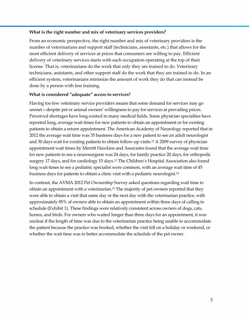
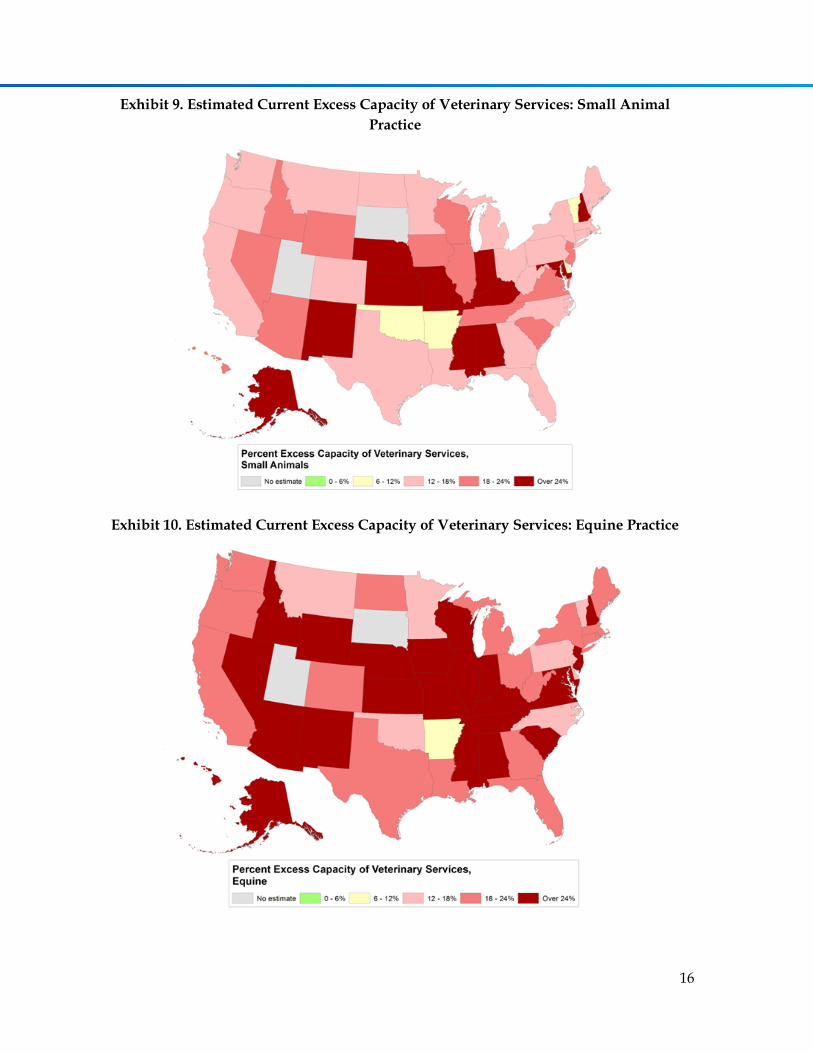
For small animal practices, the Midwest and South regions of the U.S. appeared to have the
largest average excess capacity (Exhibit 9). Estimates of excess capacity for individual states
(especially less populous states) were subject to small sample size, and therefore were less
precise estimates of the actual magnitude of excess capacity as compared to regional or
national totals. In part because of the regression approach used, geographic variation in
patterns of excess capacity was similar across practice types. Estimates were unavailable for
South Dakota and Utah due to lack of survey respondents in those states.

15
Exhibit 8. Estimated Current Excess Capacity by State and Practice Type
State Food Animal Small Animal Equine Mixed
Alabama 21% 24% 31% 19%
Alaska 25% 28% 35% 22%
Arizona 18% 21% 28% 16%
Arkansas 6% 7% 10% 5%
California 12% 15% 20% 11%
Colorado 12% 14% 20% 11%
Connecticut 13% 15% 21% 11%
Delaware 10% 12% 17% 8%
Florida 15% 18% 24% 13%
Georgia 15% 17% 23% 13%
Hawaii 19% 23% 29% 17%
Idaho 18% 21% 27% 16%
Illinois 18% 21% 28% 16%
Indiana 25% 29% 36% 23%
Iowa 16% 19% 25% 14%
Kansas 22% 25% 32% 20%
Kentucky 23% 26% 33% 21%
Louisiana 11% 14% 19% 10%
Maine 11% 13% 18% 9%
Maryland 21% 25% 31% 19%
Massachusetts 11% 13% 18% 10%
Michigan 14% 16% 22% 12%
Minnesota 10% 12% 17% 9%
Mississippi 31% 35% 42% 28%
Missouri 21% 24% 31% 19%
Montana 11% 13% 18% 9%
Nebraska 34% 38% 45% 31%
Nevada 20% 24% 30% 18%
New Hampshire 28% 32% 39% 26%
New Jersey 17% 20% 26% 15%
New Mexico 30% 34% 41% 28%
New York 14% 16% 22% 12%
North Carolina 10% 12% 17% 9%
North Dakota 15% 18% 24% 13%
Ohio 12% 15% 20% 11%
Oklahoma 8% 10% 14% 7%
Oregon 15% 17% 23% 13%
Pennsylvania 10% 12% 17% 9%
Rhode Island 12% 15% 20% 11%
South Carolina 19% 22% 28% 17%
South Dakota NA NA NA NA
Tennessee 16% 19% 25% 15%
Texas 13% 15% 21% 11%
Utah NA NA NA NA
Vermont 9% 11% 16% 8%
Virginia 16% 19% 25% 14%
Washington 12% 15% 20% 11%
West Virginia 13% 16% 21% 12%
Wisconsin 16% 19% 25% 15%
Wyoming 20% 23% 30% 18%
U.S. 15% 18% 23% 13%
NA=estimate not available because no veterinary respondents in the state.
16
Exhibit 9. Estimated Current Excess Capacity of Veterinary Services: Small Animal
Practice
Exhibit 10. Estimated Current Excess Capacity of Veterinary Services: Equine Practice

17
Exhibit 11. Estimated Current Excess Capacity of Veterinary Services: Food Animal
Practice
Exhibit 12. Estimated Current Excess Capacity of Veterinary Services: Mixed Animal
Practice

18
II. Estimating and Projecting Veterinarian Supply
Projections of the future active supply of veterinarians were based on a microsimulation
model that simulated career choices of individual veterinarians.a The projections started
with a database that contained information on each veterinarian in the current workforce,
added new graduates entering the veterinary workforce from accredited and non-accredited
colleges of veterinary medicine (CVM), and subtracted veterinarians who left the workforce
(Exhibit 13). Adjusting for patterns in hours worked allowed for calculating a “2012
equivalent” supply—where a 2012 equivalent was defined by the average hours worked by
veterinarians in 2012 (2,313 hours) including veterinarians of all ages, gender, and full-
time/part-time status. By definition, active supply and 2012 equivalent supply were
identical in 2012, but could differ slightly by state and over time depending on the age and
gender composition of the workforce and the expected work hours by age and gender. All
the supply estimates and projections presented in this report are in terms of 2012
equivalents unless labeled as active.
Exhibit 13. Microsimulation Model of Veterinarian Supply
a Note: While microsimulation modeling has been used extensively by public and private organizations for forecasting and policy analysis, only recently has microsimulation modeling been used for health workforce modeling. The federal Bureau of Health Professions, Health Resources and Services Administration, recently adopted the use of microsimulation modeling for all its health profession supply and demand modeling.
Starting year # veterinarians
New entrants
Attrition
Ending year # veterinarians
Veterinarian Active Supply
Scope of practice
Workforce participation
Supply of Veterinary
Medical Services

19
Major data sources for modeling supply and career behavior included:
AVMA Veterinarian Database. This file contains data on AVMA members and non-
members as of January 1, 2012. It contains demographic and professional
information on 124,876 individuals—including retired veterinarians and those likely
practicing outside the U.S. This file served as the basis for estimates of the 2012
supply of veterinarians and also informed the analysis of new and recent graduates.
Biennial Economic Survey of Veterinarians. Every two years AVMA conducts a
survey of self-employed veterinarians who own their practice, and a survey of
veterinarians who are employees. The file contained information on salary, hours
worked, graduation year, employment sector, and other demographic information.
While the number of veterinarians sampled in each survey differs, the 2012 survey
contained records from 4,099 veterinarians.
AVMA Graduating Senior Survey. Data for years 2003 to 2012 were analyzed to
better understand availability of job offers and preferences for employment sector.
The 2012 survey contained approximately 2,500 responses for key questions
analyzed.
American Community Survey (ACS). This annual survey is conducted by the U.S.
Census Bureau. Each year contains approximately 3 million individuals in 1 million
households. We combined the 2006 through 2010 surveys to increase sample size,
resulting in a file with 4,553 veterinarians of which 4,398 reported being active in the
workforce. The file contained demographic, employment, location, income,
household, and other information. These data were analyzed primarily to model
workforce behavior (e.g., hours worked) as a function of demographic, economic,
and other factors.
Veterinarian Workforce Survey. An electronic survey conducted in September and
October 2012 collected information on workforce behavior for 3,497 participants
(adjusted response rate of 34.8%). Additional information from this survey and key
findings are summarized in an Appendix. Pertinent information from the survey
included information on retirement patterns and estimates of veterinarian
perception of excess capacity in veterinary supply.
In subsequent sections, we summarize the data, methods, and assumptions used to estimate
current supply, new entrants to the U.S. veterinarian workforce, attrition from the workforce,
and patterns of hours worked. Subsequently, we present national and state projections of
supply.
A. Estimated Current Supply
Current supply was estimated from AVMA files that contain information on both AVMA
members and non-members. Approximately 98,900 veterinarians were listed as active in
20
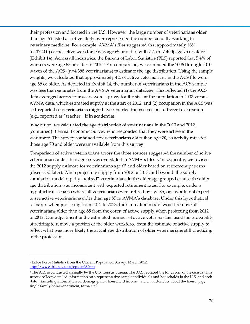
their profession and located in the U.S. However, the large number of veterinarians older
than age 65 listed as active likely over-represented the number actually working in
veterinary medicine. For example, AVMA’s files suggested that approximately 18%
(n 17,400) of the active workforce was age 65 or older, with 7% (n 7,400) age 75 or older
(Exhibit 14). Across all industries, the Bureau of Labor Statistics (BLS) reported that 5.4% of
workers were age 65 or older in 2010.a For comparison, we combined the 2006 through 2010
waves of the ACS b(n=4,398 veterinarians) to estimate the age distribution. Using the sample
weights, we calculated that approximately 4% of active veterinarians in the ACS file were
age 65 or older. As depicted in Exhibit 14, the number of veterinarians in the ACS sample
was less than estimates from the AVMA veterinarian database. This reflected (1) the ACS
data averaged across four years were a proxy for the size of the population in 2008 versus
AVMA data, which estimated supply at the start of 2012, and (2) occupation in the ACS was
self-reported so veterinarians might have reported themselves in a different occupation
(e.g., reported as “teacher,” if in academia).
In addition, we calculated the age distribution of veterinarians in the 2010 and 2012
(combined) Biennial Economic Survey who responded that they were active in the
workforce. The survey contained few veterinarians older than age 70, so activity rates for
those age 70 and older were unavailable from this survey.
Comparison of active veterinarians across the three sources suggested the number of active
veterinarians older than age 65 was overstated in AVMA’s files. Consequently, we revised
the 2012 supply estimate for veterinarians age 65 and older based on retirement patterns
(discussed later). When projecting supply from 2012 to 2013 and beyond, the supply
simulation model rapidly “retired” veterinarians in the older age groups because the older
age distribution was inconsistent with expected retirement rates. For example, under a
hypothetical scenario where all veterinarians were retired by age 85, one would not expect
to see active veterinarians older than age 85 in AVMA’s database. Under this hypothetical
scenario, when projecting from 2012 to 2013, the simulation model would remove all
veterinarians older than age 85 from the count of active supply when projecting from 2012
to 2013. Our adjustment to the estimated number of active veterinarians used the probability
of retiring to remove a portion of the older workforce from the estimate of active supply to
reflect what was more likely the actual age distribution of older veterinarians still practicing
in the profession.
a Labor Force Statistics from the Current Population Survey. March 2012. http://www.bls.gov/cps/cpsaat03.htm b The ACS is conducted annually by the U.S. Census Bureau. The ACS replaced the long form of the census. This survey collects detailed information on a representative sample individuals and households in the U.S. and each state—including information on demographics, household income, and characteristics about the house (e.g., single family home, apartment, farm, etc.).

21
This adjustment removed 8,195 individuals, and resulted in a current supply estimate of
90,705 active veterinarians. This supply estimate was slightly lower than the estimate of
92,000 professionals (in 2010) reported by the recent National Academy of Sciences which
cited AVMA data based on workforce activity status in the AVMA database.11 Of the active
veterinarians, approximately 9,100 (10%) were age 65 or older— a number more consistent
with other estimates and which suggested that veterinarians tend to retire later than the
national average.
Exhibit 14. Veterinarian Age Distribution and Initial Supply Refinement
Source: Analysis of AVMA’s Veterinarian Database, the ACS (2006 to 2010 combined files), and the Biennial Economic Survey of Veterinarians (2010 and 2012 combined files).
As illustrated in Exhibit 15, younger veterinarians were disproportionately women.
Consequently, women will constitute a growing portion of the workforce as a substantial
portion of the men are expected to retire in the next one to two decades.
-
500
1,000
1,500
2,000
2,500
3,000
3,500
18 21 24 27 30 33 36 39 42 45 48 51 54 57 60 63 66 69 72 75 78 81 84 87 90 93 96 99
Act
ive
Ve
teri
nar
ian
s
Veterinarian Age
Original 2012 AVMA Data
Revised 2012 Data
American Community Survey
(2006-2010)
2010 & 2012 Economic Survey

22
Exhibit 15. Veterinarian Age and Gender Distribution
Source: Analysis of AVMA’s Veterinarian Database.
The size and characteristics of the veterinary workforce varied by state (Exhibit 16).
Massachusetts had the highest percentage of the workforce that was female (65%) compared
to the national average (50%). Iowa, Idaho, and Montana were tied for largest percentage of
the workforce age 55 or older (40%) compared to the national average (32%).
-
200
400
600
800
1,000
1,200
1,400
1,600
1,800
2,000
25 30 35 40 45 50 55 60 65 70 75 80
FTE
Sup
ply
Veterinarian Age
Women
Men

23
Exhibit 16. State Estimates of Veterinarian Supply: 2012
Total Employment sector
State Active
%
Women
% Age
55+
Private Clinical
Practice
Industry/
Commercial Government Academia Other
AK 230 63 34 180 <10 20 10 10
AL 1,440 40 35 1,090 40 80 210 40
AR 710 33 39 600 30 60 20 20
AZ 1,680 52 32 1,470 50 50 60 40
CA 7,980 52 35 6,460 270 250 610 290
CO 2,730 53 31 2,150 80 140 250 100
CT 1,100 54 31 910 80 20 60 20
DC 140 54 33 70 <10 50 10 10
DE 210 59 30 160 20 10 10 10
FL 5,060 47 32 4,390 90 160 280 160
GA 2,780 51 26 2,170 120 170 280 60
HI 280 50 37 230 <10 20 <10 10
IA 1,700 34 40 1,260 90 130 180 40
ID 670 38 40 580 30 30 30 20
IL 3,310 52 28 2,810 100 80 220 120
IN 1,720 44 36 1,380 90 60 160 30
KS 1,480 38 39 1,110 120 70 150 50
KY 1,370 41 30 1,190 30 70 80 20
LA 1,200 47 29 1,000 20 40 120 30
MA 2,010 65 28 1,570 90 40 200 60
MD 2,170 56 31 1,520 80 370 120 70
ME 520 54 35 460 10 10 20 10
MI 2,800 53 34 2,230 150 100 220 80
MN 2,060 49 34 1,640 90 80 190 50
MO 2,000 43 34 1,620 100 70 170 50
MS 840 41 29 670 20 60 110 10
MT 580 40 40 510 10 20 10 10
NC 3,170 56 26 2,490 160 170 290 60
ND 240 46 31 210 <10 10 20 <10
NE 840 33 37 690 30 70 50 20
NH 550 61 28 490 10 10 30 10
NJ 1,950 52 30 1,600 160 40 90 50
NM 640 53 38 530 20 30 30 20
NV 630 46 27 570 20 20 30 10
NY 4,090 52 30 3,420 100 110 320 140
OH 3,230 51 30 2,700 110 110 240 70
OK 1,400 39 37 1,170 30 80 110 30
OR 1,670 56 31 1,390 40 50 110 60
PA 3,570 54 29 2,910 160 100 310 80
RI 250 61 26 220 <10 10 10 10
SC 1,090 52 26 930 30 50 60 40
SD 370 35 37 310 10 20 20 10
TN 1,860 50 27 1,580 40 70 150 40
TX 6,280 44 33 5,300 180 310 380 160
UT 520 33 34 450 10 30 30 10
VA 2,880 58 28 2,330 80 170 200 80
VT 370 55 35 320 10 10 20 <10
WA 2,600 56 33 2,120 70 100 200 90
WI 2,540 47 33 2,110 100 100 190 50
WV 400 50 29 350 10 30 20 10
WY 290 41 38 240 10 20 20 10
U.S. 90,230 50 32 73,860 3,200 4,000 6,690 2,480
Notes: Numbers might not sum to totals because of rounding. Veterinarians whose employment sector was unknown were distributed across employment categories based on each state’s distribution of veterinarians whose employment sector was known.

24
B. New Entrants to the U.S. Veterinarian Workforce
The career of veterinarians often spans 30 or 40 years, so the number and age distribution of
new veterinarians trained each year has profound implications for the future supply with
the impact compounding year after year.
The estimated number of new graduates entering the workforce in 2012 was taken from the
number of candidates passing the North American Veterinary Licensing Exam (NAVLE)
who applied through U.S. licensing boards in 2011/2012. Since the number of candidates
passing the NAVLE in future years is unknown, the best available data were used to
calculate the number of new entrants in the future. Data on enrollments in AVMA
accredited schools in the U.S. were combined with data on enrollments of American
students in AAVMC member (AVMA accredited and non-accredited) schools outside of the
U.S. for the classes of 2013-2016. The growth rate of enrollment was then applied to the
initial estimate from the NAVLE to get the number of new graduates through 2016
(reflecting that the new student class would experience some attrition during the first year).
Scenarios estimating the impact of increased seats in current schools and in new schools are
addressed later (page 33) under “Supply Projections.” According to the AAVMC, overall
growth in graduates from U.S. veterinary schools was flat from the mid-1980s through the
1990s, but increased markedly over the last decade and thus has averaged approximately
2% per year for the last 30 years (Exhibit 17).
Exhibit 17. Total Graduates from U.S. Colleges of Veterinary Medicine: 1980 to 2012
Source: American Association of Veterinary Medical Colleges
1746
2012
2138
2219
2020
2165
2216
2466
2687
1200
1400
1600
1800
2000
2200
2400
2600
2800
3000
3200
Nu
mb
er
of
Gra
du
ate
s
Year of Graduation
Total Number of Graduates from US Colleges of Veterinary Medicine
AAVMC Internal Data Reports1980-2012
25
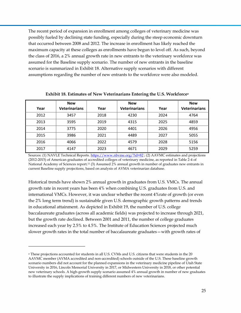
The recent period of expansion in enrollment among colleges of veterinary medicine was
possibly fueled by declining state funding, especially during the steep economic downturn
that occurred between 2008 and 2012. The increase in enrollment has likely reached the
maximum capacity at these colleges as enrollments have begun to level off. As such, beyond
the class of 2016, a 2% annual growth rate in new entrants to the veterinary workforce was
assumed for the Baseline supply scenario. The number of new entrants in the baseline
scenario is summarized in Exhibit 18. Alternative supply scenarios with different
assumptions regarding the number of new entrants to the workforce were also modeled.
Exhibit 18. Estimates of New Veterinarians Entering the U.S. Workforcea
Year New
Veterinarians Year New
Veterinarians Year New
Veterinarians
2012 3457 2018 4230 2024 4764
2013 3595 2019 4315 2025 4859
2014 3775 2020 4401 2026 4956
2015 3986 2021 4489 2027 5055
2016 4066 2022 4579 2028 5156
2017 4147 2023 4671 2029 5259
Sources: (1) NAVLE Technical Reports. https://www.nbvme.org/?id=82 ; (2) AAVMC estimates and projections (2012-2015) of American graduates of accredited colleges of veterinary medicine, as reported in Table 2-4 of National Academy of Sciences report.11 (3) Assumed 2% annual growth in number of graduates new entrants in current Baseline supply projections, based on analysis of AVMA veterinarian database.
Historical trends have shown 2% annual growth in graduates from U.S. VMCs. The annual
growth rate in recent years has been 4% when combining U.S. graduates from U.S. and
international VMCs. However, it was unclear whether the recent 4%rate of growth (or even
the 2% long term trend) is sustainable given U.S. demographic growth patterns and trends
in educational attainment. As depicted in Exhibit 19, the number of U.S. college
baccalaureate graduates (across all academic fields) was projected to increase through 2021,
but the growth rate declined. Between 2001 and 2011, the number of college graduates
increased each year by 2.5% to 4.5%. The Institute of Education Sciences projected much
slower growth rates in the total number of baccalaureate graduates—with growth rates of
a These projections accounted for students in all U.S. CVMs and U.S. citizens that were students in the 20 AAVMC member (AVMA accredited and non-accredited) schools outside of the U.S. These baseline growth scenario numbers did not account for the planned expansions in the veterinary medicine pipeline of Utah State University in 2016, Lincoln Memorial University in 2017, or Midwestern University in 2018, or other potential new veterinary schools. A high-growth supply scenario assumed 4% annual growth in number of new graduates to illustrate the supply implications of training different numbers of new veterinarians.

26
1% to 2% between 2013 and 2021. The growth trend for master’s degree and PhD graduates
was slightly higher—with growth rates falling from 2.5% in 2013 to 1.5% by 2021.
Exhibit 19. Past and Projected U.S. Baccalaureate Graduates (across all academic fields)
Source: Historical data and projections of future college graduates from the Institute of Education Sciences, National Center for Education Statistics, Table 33. Published January 2013. http://nces.ed.gov/programs/projections/projections2021/tables.asp
Using AVMA data on the year of graduation, we identified veterinarians who graduated
between 2008 and 2011 to calculate the gender and age distribution of new graduates. In
recent years, the percentage of new female graduates has remained relatively stable at
around 78%. Most new graduates were between age 26 and 30, and 25% of new graduates
were age 26 (Exhibit 20).
0
500,000
1,000,000
1,500,000
2,000,000
2,500,000
0.0%
0.5%
1.0%
1.5%
2.0%
2.5%
3.0%
3.5%
4.0%
4.5%
5.0%
1997 1999 2001 2003 2005 2007 2009 2011 2013 2015 2017 2019 2021
Tota
l Co
lle
ge G
rad
uat
es
% G
row
th in
Nu
mb
ne
r o
f C
oll
ege
Gra
du
ate
s
Year
Growth Rate

27
Exhibit 20. Age Distribution of New Graduates from Veterinary Medical Schools
Source: Analysis of AVMA’s Veterinarian Database.
The microsimulation approach used to model future supply created an artificial cohort of
new graduates each year, with each new graduate assigned an age and gender based on the
probability distributions observed among graduates during the past four years.
C. Workforce Attrition
Our review of the literature and analysis of existing data sources found little information on the
retirement patterns of veterinarians. While analysis of membership type in AVMA’s database
provided some indication of retirement patterns, the decision to survey the veterinary
workforce (see Appendix A) was determined in part by the need to have better information
about workforce attrition patterns.
The two survey questions used to provide information on attrition patterns asked currently
active veterinarians at what age they planned to become permanently inactive in the workforce
and asked currently inactive veterinarians at what age they became permanently inactive. These
responses were combined to create estimates of workforce attrition for males and females by
0%
5%
10%
15%
20%
25%
30%
20 25 30 35 40 45 50 55
Pro
po
rtio
n o
f Ne
w V
ete
rin
aria
ns
Veterinarian Age
Age=26

28
age. Estimates of retirement patterns were combined with mortality rates from the Centers
for Disease Control and Prevention to estimate overall workforce attrition rates, and
mortality rates took into consideration that people in professional occupations tend to have
lower mortality rates through age 65 as compared to national average mortality rates for
men and women. Johnson et al. found that age-adjusted mortality rates for professional and
technical occupations were approximately 25% lower than national rates for men and 15%
lower for women. 18
Applying these rates to veterinarians suggested that for every 1,000 men and 1,000 women
who entered the veterinary workforce, approximately 437 men and 335 women were active
past age 65 (Exhibit 21). Approximately 104 men and 80 women remained active past age 70.
Exhibit 21. Veterinarian Workforce Attrition Patterns
Source: Analysis of AVMA 2012 Veterinary Workforce Survey.
The approach we used to model future supply of veterinarians differed from the approach used
in the recent National Academy of Sciences (NAS) study.11 The NAS estimated annual number
0
100
200
300
400
500
600
700
800
900
1000
22 24 26 28 30 32 34 36 38 40 42 44 46 48 50 52 54 56 58 60 62 64 66 68 70 72 74 76 78 80 82 84
Re
mai
nin
g A
ctiv
e F
rom
Ori
gin
al 1
00
0
Veterinarian Age
Men
Women

29
of retirements by dividing (1) size of the current workforce by (2) length of veterinarians’ career
span (which was assumed to be 35 years for most veterinarians but only 30 years for
veterinarians in food-animal practice because of the physical and strenuous nature of the
work).a The approach used by NAS, however, failed to reflect the current and projected future
age distribution of the workforce. Furthermore, retirement patterns can change over time based
on social norms and policies (e.g., increasing the eligibility age for Social Security and Medicare),
economic conditions and their impact on retirement assets, ability to sell one’s veterinary
practice, and work-life balance decisions. The BLS, for example, reported that many older
workers were delaying retirement and this pattern of delayed retirements was expected to
continue even after the economy recovers.19 Among the population age 65 and older, labor
force participation rates grew slightly from 11.8% in 1990 to 12.9% in 2000. There was a
substantial increase to 17.4% in 2010, and in 2020, the BLS projected that 22.6% of
individuals age 65 and older would be part of the labor force.
The NAS reported “anecdotal evidence from practitioners suggests that a high percentage of
new graduates leave equine practice within 5 to 10 years” for reasons including long hours
and limited time for personal life (p. 49).11 The large majority of these younger veterinarians
leaving equine practice (as well as those leaving mixed animal practices) were likely to
transition to other employment sectors—such as small animal practice, academia,
government, or industry.
Alternative supply scenarios presented in this report include whether older veterinarians
accelerated or delayed retirement compared to historic patterns.
D. Hours Worked
Projections of the future supply of veterinary services took into consideration trends and
factors that may influence future levels of effort as defined by work hours. Trends with
implications for total hours worked included: (1) the growing portion of the workforce that
is female, (2) shifts in the age distribution of the workforce, (3) generational shifts in work-
life balance expectations, (4) industry consolidation that could lead to a growing proportion
of the workforce that is employed rather than self-employed, (5) imbalances between supply
and demand for veterinary services, (6) changes in the economics of veterinary practice, and
(7) changes in technology and care delivery patterns that could affect office and on-call
hours for veterinarians who provide animal care.
Our analyses were designed to address many of the above trends. Findings from our
analysis of AVMA’s Biennial Economic Survey (2002 to 2012) and the Census Bureau’s 2010
a During the interviews, informants suggested that there might be some validity to the belief that veterinarians in food animal practice departed practice a few years earlier than companion animal veterinarians, but that it might not be such an issue going forward. The nature of food animal practice has changed and the physical effort required of the veterinarian might not be as constant as in the past. Some of that work is now being accomplished by other technical personnel in food animal production facilities and feed lots.

30
ACS provided insights and were incorporated into the supply projections presented later.
To generate a complete sample of veterinarians in the Biennial Economic Survey, we
combined the Owners and Non-owners components of the survey. As illustrated in Exhibit
22, in 2012 the average number of hours worked for both men and women tended to decline
with age. This was true for both part-time and full-time workers. Among the 1,989 men in
the survey, the average hours worked per week was 48.2, while for the 1,905 women in the
survey the average was 45.1 hours. Veterinarians younger than age 30 worked the most
hours per week, with men working 55.2 hours and women working 52.8 hours. Conversely,
veterinarians age 65 and older worked the fewest hours, with men working 41.1 hours and
women working 33.1 hours.
While there was little gender difference in average hours worked when controlling for self-
reported full-time versus part-time status, 18% of women reported working part time versus
11% for men. There were also differences by age and gender in average weeks worked per
year (47.5 weeks for men and 46.0 weeks for women) and temporary departures from the
workforce (3% for men and 4% for women). Taken together, we observed that men age 30 to
39 tended to work approximately 15% more hours than the industry average, while women
age 60 to 64 tended to work the fewest hours at approximately 37% less than the average
(Exhibit 23). Using this information, we calculated FTE scalars which we applied to the
projections of future active supply to account for the impact of demographic shifts on
average hours worked. Under a Baseline supply scenario, where future workforce
participation patterns were similar to today’s patterns, we counted men age 30 to 39 as 1.15
FTE, and women age 60 to 64 as 0.63 FTE.
Combining the 2002 through 2012 waves of the Biennial Economic Survey, we investigated
whether there was evidence of generational shifts in average hours worked. We found no
evidence of a generational shift. Among men, we did observe an increase in hours for those
age 30-45 versus those younger than age 30, and a slight downward shift in hours across
most age groups over time (Exhibit 24). Hours worked in 2012 were slightly below the
average from 2002 to 2012, while hours for 2004 were near the lowest across years and hours
for 2008 and similar to 2006. We observed similar patterns of hours worked by women
between 2002 and 2012, with downward shifts over time (Exhibit 25). These shifts toward
lower average hours worked appeared to affect all the age groups, so this could be
indicative of market conditions rather than generational shifts. High levels of student debta
made it unlikely that younger veterinarians would work fewer hours than historical
patterns suggested, and hours worked would likely rise if there was sufficient demand.
a Shepherd and Pikel (2011) reported that the average student debt of new veterinarian graduates was $142,613 in 2011, a 6.5% increase from 2010 levels.20
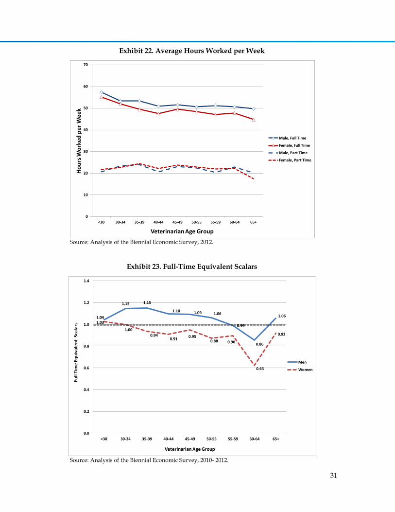
31
Exhibit 22. Average Hours Worked per Week
Source: Analysis of the Biennial Economic Survey, 2012.
Exhibit 23. Full-Time Equivalent Scalars
Source: Analysis of the Biennial Economic Survey, 2010- 2012.
0
10
20
30
40
50
60
70
<30 30-34 35-39 40-44 45-49 50-55 55-59 60-64 65+
Ho
urs
Wo
rke
d p
er
We
ek
Veterinarian Age Group
Male, Full Time
Female, Full Time
Male, Part Time
Female, Part Time
1.04
1.15 1.15
1.10 1.09 1.06
0.99
0.86
1.06
1.03
1.00
0.94 0.91
0.95 0.88 0.90
0.63
0.92
0.0
0.2
0.4
0.6
0.8
1.0
1.2
1.4
<30 30-34 35-39 40-44 45-49 50-55 55-59 60-64 65+
Full
Tim
e E
qu
ival
en
t S
cala
rs
Veterinarian Age Group
Men
Women

32
Exhibit 24. Average Annual Hours Worked for Men: 2002-2012
Source: Analysis of the Biennial Economic Survey, 2002-2012.
Exhibit 25. Average Annual Hours Worked for Women: 2002-2012
Source: Analysis of the Biennial Economic Survey, 2002-2012.
1,500
1,700
1,900
2,100
2,300
2,500
2,700
2,900
<30 30-34 35-39 40-44 45-49 50-54 55-59 60-64 65+
An
nu
al H
ou
rs W
ork
ed
Veterinarian Age Group
2002
2004
2006
2008
2010
2012
Average
1,500
1,700
1,900
2,100
2,300
2,500
2,700
2,900
<30 30-34 35-39 40-44 45-49 50-54 55+
An
nu
al H
ou
rs W
ork
ed
Veterinarian Age Group
2002
2004
2006
2008
2010
2012
Average
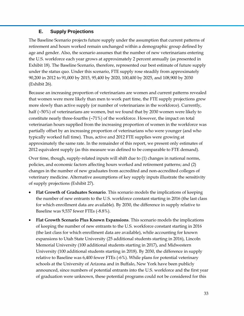
33
E. Supply Projections
The Baseline Scenario projects future supply under the assumption that current patterns of
retirement and hours worked remain unchanged within a demographic group defined by
age and gender. Also, the scenario assumes that the number of new veterinarians entering
the U.S. workforce each year grows at approximately 2 percent annually (as presented in
Exhibit 18). The Baseline Scenario, therefore, represented our best estimate of future supply
under the status quo. Under this scenario, FTE supply rose steadily from approximately
90,200 in 2012 to 91,000 by 2015, 95,400 by 2020, 100,400 by 2025, and 108,900 by 2030
(Exhibit 26).
Because an increasing proportion of veterinarians are women and current patterns revealed
that women were more likely than men to work part time, the FTE supply projections grew
more slowly than active supply (or number of veterinarians in the workforce). Currently,
half ( 50%) of veterinarians are women, but we found that by 2030 women were likely to
constitute nearly three-fourths ( 71%) of the workforce. However, the impact on total
veterinarian hours supplied from the increasing proportion of women in the workforce was
partially offset by an increasing proportion of veterinarians who were younger (and who
typically worked full time). Thus, active and 2012 FTE supplies were growing at
approximately the same rate. In the remainder of this report, we present only estimates of
2012 equivalent supply (as this measure was defined to be comparable to FTE demand).
Over time, though, supply-related inputs will shift due to (1) changes in national norms,
policies, and economic factors affecting hours worked and retirement patterns; and (2)
changes in the number of new graduates from accredited and non-accredited colleges of
veterinary medicine. Alternative assumptions of key supply inputs illustrate the sensitivity
of supply projections (Exhibit 27).
Flat Growth of Graduates Scenario. This scenario models the implications of keeping
the number of new entrants to the U.S. workforce constant starting in 2016 (the last class
for which enrollment data are available). By 2030, the difference in supply relative to
Baseline was 9,537 fewer FTEs (-8.8%).
Flat Growth Scenario Plus Known Expansions. This scenario models the implications
of keeping the number of new entrants to the U.S. workforce constant starting in 2016
(the last class for which enrollment data are available), while accounting for known
expansions to Utah State University (25 additional students starting in 2016), Lincoln
Memorial University (100 additional students starting in 2017), and Midwestern
University (100 additional students starting in 2018). By 2030, the difference in supply
relative to Baseline was 6,400 fewer FTEs (-6%). While plans for potential veterinary
schools at the University of Arizona and in Buffalo, New York have been publicly
announced, since numbers of potential entrants into the U.S. workforce and the first year
of graduation were unknown, these potential programs could not be considered for this

34
scenario. Likewise, additional enrollment growth in international schools such as Ross
University was unknown and therefore not included in this scenario.
High Growth Rate Scenario (4% annual growth). The growth rate in number of U.S.
citizens graduating from U.S. and international schools combined has been
approximately 4% average annual growth in recent years. This hypothetical scenario
illustrated the implications if recent growth trends continued. Whereas the baseline
scenario assumed that each year the number of graduates grows by 80-95 between 2016
and 2025, this high growth scenario assumed that the number of new graduates grows
by 160 to 220 each year between 2016 and 2025. Under this scenario with 4% annual
growth in new graduates, by 2030 the supply was 11,500 FTEs higher than under the
Baseline scenario which assumed 2% annual growth in number of new graduates.
Delayed or Earlier Retirement Scenarios. Over time, veterinarians could delay
retirement to reflect, for example, changes in Medicare eligibility age or improved health
that prolongs careers. Or, veterinarians might decide to retire earlier because of work-
life balance choices. These scenarios model retirement patterns that shift to reflect (1)
retiring two years earlier, and (2) retiring two years later, on average, relative to current
retirement patterns. By 2030, the difference in supply relative to Baseline was roughly
4,000 FTEs ( 4%).
Change in Total Hours Worked Scenarios. The Baseline projections reflect the changing
demographics of the veterinarian workforce. However, total average hours worked
could change to reflect changes in desired work-life balance and a need to work more
hours due to high educational debt. If average hours decreased by 10% (from
approximately 47.8 hours/week to 43.0 hours/week), for example, then there would be
an immediate 10% shift down in FTE supply. Likewise, if average hours worked
increased by 10% (rising to 52.6 hours/week) then there would be an immediate 10%
shift up in FTE supply. By 2030, the difference in supply relative to Baseline was 10,900
FTEs ( 10%).
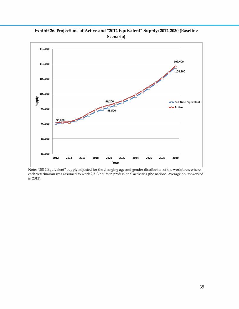
35
Exhibit 26. Projections of Active and “2012 Equivalent” Supply: 2012-2030 (Baseline
Scenario)
Note: “2012 Equivalent” supply adjusted for the changing age and gender distribution of the workforce, where each veterinarian was assumed to work 2,313 hours in professional activities (the national average hours worked in 2012).
90,200
95,500
108,900
96,200
109,400
80,000
85,000
90,000
95,000
100,000
105,000
110,000
115,000
2012 2014 2016 2018 2020 2022 2024 2026 2028 2030
Sup
ply
Year
Full Time Equivalent
Active

36
Exhibit 27. Alternative Supply Scenarios: 2012-2030
The downward shift in average hours worked during the past decade (across all age groups
and controlling for gender) could be the result of insufficient demand for services among
veterinarians in private clinical practice. If so, this suggests that the potential supply of
veterinarian services was greater than actual supply, and that average hours worked would
rise if there was a better balance between market supply and demand.
Changes to retirement patterns could increase or decrease supply, with a two-year swing in
retirement patterns changing future supply by approximately the same impact as one
graduating class of new veterinarians. If, as anticipated by the BLS, many older workers
delay retirement even after the current economic downturn recovers, then the future supply
of veterinarians will likely be higher than the baseline projections. 19
Changing the number of new veterinarians trained has significant long-term implications on
supply, with the impact accumulating over time. FTE supply has flexibility to shift up or
down quickly to accommodate short-term fluctuations in demand (although economic
pressures and the need to pay off educational debt could prevent hours from falling).
80,000
85,000
90,000
95,000
100,000
105,000
110,000
115,000
120,000
125,000
2012 2014 2016 2018 2020 2022 2024 2026 2028 2030
FTE
Ve
teri
nar
ian
s
Year
Increased Hours (+10%)
High Growth Scenario
Delayed Retirement (2 yrs)
Baseline Supply
Earlier Retirement (2 years)
No Increase Except Utah
State, Lincoln Memorial, and MidwesternNo Increase in New
Graduates After 2016
Reduced Hours (-10%)

37
III. Estimating and Projecting Demand for Veterinarians
The demand component of the Veterinary Workforce Model was designed to forecast pet
ownership and food animal populations, demand for veterinary services, and the derived
demand for veterinarians through 2025 by employment sector. Demand was projected at the
state level for the small animal, equine, and food animal sectors, but calculated at the
national level for industry, academia, government, and the “other” employment due to lack
of state-level data and the regional nature of these employment sectors.
A. Data and Methods
Major data sources for modeling demand and animal populations include:
2012 Veterinary Workforce Survey. A sample drawn from the AVMA database of
veterinarians (including active and retired, and AVMA members and non-members)
collected information on perceptions of the adequacy of veterinarian supply in one’s
local geographic area and employment sector, and perception of level of excess
capacity within one’s own veterinary practice. An appendix provides more detail on
this survey and findings.
AVMA Pet Demographic Survey (PDS).15 Data from the 2007 and 2012 surveys
were used to analyze the number and type of pets owned in a household.
Additionally, the survey measured the number of visits to a veterinarian in the past
year and the type of service performed during a visit.
Biennial Economic Survey of Veterinarians.17 Every two years AVMA conducts a
survey of self-employed veterinarians who own their practice and a survey of
veterinarians who are employees. Information on the proportion of time worked by
animal type and employment sector was used in the demand analysis. The 2012
survey contained records from 4,099 veterinarians.
American Community Survey (ACS).21 This annual survey conducted by the U.S.
Census Bureau contains information on approximately 3 million individuals in 1
million households representative of the population in each state in 2010. The file
contains demographic, employment, location, income, household, and other
information. These data were combined with the PDS data to model the estimated
number of pets and veterinary services provided to pets in each state as a function of
demographic, economic, and other household characteristics.
Census Bureau Population Projections.22, 23 We used state and national projections
of the population to forecast change in the number and characteristics of households
through 2030.
IHS Food Animal Projection Model. This model, developed by IHS’s Agricultural
team, predicts the U.S. population of food animals, including beef and dairy cows,
swine, poultry, and sheep.
38
In subsequent sections, we summarize the data, methods, and assumptions used to estimate
current demand, and changes in employment sector. Then, we present projections of the
national demand for veterinary services and veterinarians.
Small Animal Practice and Household-Owned Equine
Projecting demand for small animal veterinarians at the state level and into the future starts
with projecting pet ownership, from which we calculated the demand for veterinary
services and veterinarians. Demand for services was defined as the number and mix of
veterinary services that households were anticipating to use as a function of pet needs, price
of services, and households’ ability and willingness to pay for services.
To forecast demand for small animals (separately for dogs, cats, birds, and “all other”) and
household equine (i.e., excluding horses not owned by individual households), we first
developed forecasting equations that related propensity to own pets as a function of
household characteristics. (Demand for equine veterinarians is discussed in more detail in a
later section). These forecasting equations were then applied to a database containing
characteristics of a representative sample of households in each state for 2010 through 2025.
The 2010 ACS contains approximately 1,283,700 households that are representative of the
approximately 100 million households in the U.S., with household sample weights
developed for 2011 through 2025 to reflect Census Bureau population projections.
Approximately 98,200 households were sampled in the combined 2007 and 2012 Pet
Demographic Study to gauge pet ownership. Of these households, approximately 58,900
owned at least one pet. In these pet-owning homes there are 62,623 dogs, 71,283 cats, 9,322
birds, 5,541 horses, and 13,566 other pets.
For households with dogs, the mean was 1.7 dogs/household, but the number ranged from
1 to 100. We used Poisson regression to quantify the likely number of dogs in each
household as a function of household characteristics (Exhibit 59). Factors used to predict
dog ownership include household demographics, such as number of children and the age,
race, and marital status of the head of household; household socioeconomic characteristics,
including job status and highest educational attainment of head of household and total
household income; home type (e.g., single family home, apartment); region of the country;
and whether the head of household reported their occupation as farmer. Selection of
explanatory variables was based on hypothesized factors related to pet ownership, but
restricted to variables presented in both the Pet Demographic Study and the ACS. Separate
but similar Poisson regressions were estimated to model household demand for cats, birds,
horses, and “all other” pets. We used logistic regression (with the same explanatory
variables) to estimate households’ probability of pet ownership.
The regression results for dogs and cats are presented in Appendix B and are reported as
rate ratios that reflect the rate of pet ownership for a household with a particular
characteristic relative to the “comparison” group. A household whose head was age 65 or

39
older, for example, owned dogs at 1.52 times the rate of ownership for households headed
by a person younger than age 25. Dog, cat, and bird ownership was most likely in
households with a head age 45-54, whereas horse ownership was more likely for households
with a head age 55-64 (all else being equal). Pet ownership tended to rise with age of head of
household through age mid-40s and 50s, before declining among the elderly. Other findings
showed the impact of specific characteristics, controlling for other characteristics:
There were significant regional differences in rates of pet ownership
Propensity to own a pet varied significantly by race
Having more children was associated with increased rates of pet ownership
Higher educational attainment (which was correlated with household income) was
associated with lower rates of pet ownership
Being unmarried was associated with higher ownership of dogs and cats
Cat and bird ownership tended to decline with higher household income, while
horse ownership tended to rise with household income
Living in a mobile home was associated with the highest rate of pet ownership,
while living in an apartment, condominium, or duplex was associated with lower
rates of pet ownership
Farmers were significantly more likely to own dogs, cats, and horses, but less likely
to own birds as pets relative to non-farmers.
Using PDS data, we used Poisson regression to quantify the relationship between dog
owners’ number of visits to a veterinarian during the year and household characteristics
(including number of dogs). We modeled annual visits to the veterinarian for 10 categories
of services (with some groupings in the PDS combined because of small sample size). The 10
categories are 1) general exam, 2) vaccines, 3) emergency care, 4) laboratory tests, 5) drugs,
6) flea/worm medication, 7) surgery, 8) behavior, 9) euthanization, and 10) “other.”a Each of
the 10 regressions was calculated separately for dogs, cats, birds, horses, and “other”
animals.
The household characteristics included in these regressions were the same characteristics
used to model demand for pets (Appendix B). In general, higher household income was
associated with greater propensity to obtain veterinary services, while having more children
in the household was associated with lower propensity to obtain veterinary services. There
was substantial regional variation in propensity to seek services, with pet owners in the
New England region often more likely to obtain veterinary services compared to pet owners
in other regions. Many of these findings were consistent with previous work, such as Wolf
a Emergency care combined the survey categories of emergency, hospitalization, and x-ray. The number of services provided will exceed the number of visits to a veterinarian, as multiple services might be provided during one visit.
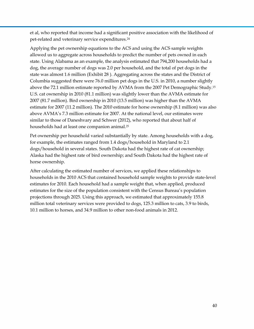
40
et al, who reported that income had a significant positive association with the likelihood of
pet-related and veterinary service expenditures.24
Applying the pet ownership equations to the ACS and using the ACS sample weights
allowed us to aggregate across households to predict the number of pets owned in each
state. Using Alabama as an example, the analysis estimated that 794,200 households had a
dog, the average number of dogs was 2.0 per household, and the total of pet dogs in the
state was almost 1.6 million (Exhibit 28 ). Aggregating across the states and the District of
Columbia suggested there were 76.0 million pet dogs in the U.S. in 2010, a number slightly
above the 72.1 million estimate reported by AVMA from the 2007 Pet Demographic Study.15
U.S. cat ownership in 2010 (81.1 million) was slightly lower than the AVMA estimate for
2007 (81.7 million). Bird ownership in 2010 (13.5 million) was higher than the AVMA
estimate for 2007 (11.2 million). The 2010 estimate for horse ownership (8.1 million) was also
above AVMA’s 7.3 million estimate for 2007. At the national level, our estimates were
similar to those of Daneshvary and Schwer (2012), who reported that about half of
households had at least one companion animal.25
Pet ownership per household varied substantially by state. Among households with a dog,
for example, the estimates ranged from 1.4 dogs/household in Maryland to 2.1
dogs/household in several states. South Dakota had the highest rate of cat ownership;
Alaska had the highest rate of bird ownership; and South Dakota had the highest rate of
horse ownership.
After calculating the estimated number of services, we applied these relationships to
households in the 2010 ACS that contained household sample weights to provide state-level
estimates for 2010. Each household had a sample weight that, when applied, produced
estimates for the size of the population consistent with the Census Bureau’s population
projections through 2025. Using this approach, we estimated that approximately 155.8
million total veterinary services were provided to dogs, 125.3 million to cats, 3.9 to birds,
10.1 million to horses, and 34.9 million to other non-food animals in 2012.
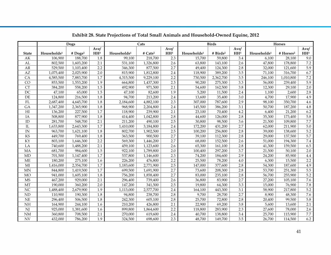
41
Exhibit 28. State Projections of Total Small Animals and Household-Owned Equine, 2012
Dogs Cats Birds Horses
State Households1 # Dogs2
Ave/ HH3 Households1 # Cats2
Ave/ HH3 Households1 # Birds2
Ave/ HH3 Households1 # Horses2
Ave/ HH3
AK 106,900 188,700 1.8 99,100 218,700 2.3 15,700 59,800 3.4 6,100 28,100 9.0
AL 802,500 1,603,200 2.1 531,100 1,326,800 2.6 63,800 143,100 2.6 47,800 178,800 7.2
AR 529,500 1,103,400 2.2 346,300 877,500 2.7 49,400 124,300 2.8 32,000 121,600 5.9
AZ 1,075,400 2,025,900 2.0 815,900 1,812,800 2.4 118,900 389,200 3.5 71,100 316,700 6.7
CA 4,585,500 7,883,700 1.7 4,315,500 9,229,100 2.2 730,500 2,362,700 3.5 246,100 1,010,800 7.2
CO 853,500 1,553,200 1.9 664,800 1,437,300 2.3 90,200 275,300 3.3 56,000 239,400 5.9
CT 384,200 558,200 1.5 492,900 971,500 2.1 54,600 162,500 3.8 12,300 29,100 2.0
DC 47,100 65,000 1.5 47,100 82,600 1.9 5,200 11,500 2.4 1,100 2,600 2.8
DE 124,800 216,500 1.8 94,700 213,200 2.4 13,600 35,400 3.0 4,700 17,900 4.9
FL 2,687,400 4,645,700 1.8 2,184,600 4,882,100 2.3 307,000 787,600 2.9 98,100 350,700 4.6
GA 1,347,200 2,365,900 1.8 968,900 2,204,800 2.4 145,500 386,200 3.1 50,700 187,200 4.8
HI 136,200 227,500 1.7 118,900 239,900 2.1 23,100 70,400 4.2 6,400 21,200 6.2
IA 508,800 877,900 1.8 414,400 1,042,800 2.8 44,600 126,000 2.8 35,300 173,400 5.8
ID 281,700 548,700 2.1 211,200 490,100 2.5 30,800 98,500 3.6 21,500 109,800 7.7
IL 1,633,800 2,643,300 1.7 1,410,000 3,184,800 2.4 172,200 431,200 2.7 62,000 211,900 5.0
IN 963,700 1,621,100 1.8 802,700 1,902,500 2.5 100,200 256,800 2.8 39,000 138,600 5.2
KS 449,700 769,400 1.8 363,500 900,500 2.7 39,100 112,300 2.8 29,000 137,500 5.7
KY 803,100 1,646,300 2.2 569,300 1,446,200 2.7 68,000 152,500 2.6 51,000 194,300 7.4
LA 740,600 1,488,200 2.1 459,100 1,123,600 2.6 65,300 161,100 2.8 41,300 159,500 6.5
MA 681,700 984,600 1.5 922,100 1,789,800 2.0 100,400 297,200 3.7 21,500 50,100 2.0
MD 701,500 1,147,400 1.7 537,800 1,146,600 2.3 74,200 184,600 2.9 24,200 85,900 4.4
ME 180,200 275,100 1.6 226,200 476,800 2.2 25,500 78,200 4.0 6,300 15,500 2.2
MI 1,416,000 2,354,700 1.7 1,183,600 2,771,900 2.5 147,000 377,600 2.8 54,300 187,600 4.9
MN 844,800 1,419,500 1.7 699,500 1,691,900 2.7 73,600 208,300 2.8 53,700 251,300 5.5
MO 941,000 1,605,100 1.8 756,200 1,858,400 2.7 83,000 235,100 2.8 56,700 255,900 5.2
MS 467,200 929,000 2.1 296,400 739,400 2.6 36,800 83,900 2.7 27,200 105,100 7.6
MT 190,000 360,200 2.0 147,200 341,500 2.5 19,800 64,300 3.3 15,000 76,900 7.8
NC 1,488,400 2,679,900 1.9 1,113,000 2,577,700 2.4 164,100 443,300 3.1 58,900 217,800 5.2
ND 110,900 190,300 1.8 94,800 238,700 2.8 9,700 28,700 2.7 8,900 48,300 7.6
NE 296,400 506,500 1.8 242,300 605,100 2.8 25,700 72,800 2.8 20,400 99,500 5.8
NH 164,900 244,100 1.6 210,200 426,800 2.1 22,900 69,200 3.8 5,600 13,600 2.1
NJ 925,000 1,381,600 1.6 899,800 1,864,600 2.2 118,800 283,900 2.3 27,600 78,000 2.6
NM 360,800 708,500 2.1 270,000 619,600 2.4 40,700 138,800 3.4 25,700 115,900 7.7
NV 432,000 786,200 1.9 324,500 698,600 2.3 48,700 149,700 3.5 26,700 114,500 6.2

42
Dogs Cats Birds Horses
State Households1 # Dogs2
Ave/ HH3 Households1 # Cats2
Ave/ HH3 Households1 # Birds2
Ave/ HH3 Households1 # Horses2
Ave/ HH3
NY 1,893,900 2,818,300 1.6 1,992,600 4,050,400 2.1 262,000 624,400 2.3 56,100 154,300 2.6
OH 1,665,800 2,745,400 1.7 1,409,900 3,272,900 2.5 172,300 432,800 2.8 63,100 219,400 4.9
OK 706,000 1,508,000 2.2 464,700 1,189,100 2.7 65,800 178,900 2.7 44,300 168,200 6.8
OR 610,100 1,064,200 1.8 595,700 1,319,200 2.3 91,000 289,800 3.3 34,800 152,000 7.0
PA 1,512,700 2,317,000 1.6 1,503,700 3,205,400 2.2 191,300 453,500 2.3 47,500 141,000 2.8
RI 115,400 169,600 1.6 152,000 302,800 2.1 17,200 51,500 3.7 3,600 8,300 2.0
SC 691,300 1,234,200 1.9 510,000 1,173,500 2.4 75,200 198,800 3.1 26,600 100,500 5.2
SD 135,600 238,500 1.8 113,300 296,100 2.9 11,900 36,900 2.8 11,300 62,100 7.7
TN 1,115,900 2,235,600 2.1 773,800 1,934,300 2.6 91,400 204,400 2.6 66,600 242,100 6.7
TX 4,152,800 8,604,900 2.2 2,730,600 6,759,300 2.7 399,300 1,022,500 2.9 248,900 915,400 6.1
UT 421,100 807,000 2.0 312,800 703,400 2.4 46,100 150,000 3.7 30,300 146,400 6.8
VA 1,122,300 1,920,900 1.8 858,100 1,905,900 2.3 119,600 307,800 2.9 42,200 153,800 4.6
VT 82,600 125,100 1.6 105,800 221,400 2.2 11,500 35,000 4.0 3,000 7,700 2.4
WA 1,041,000 1,807,000 1.7 995,400 2,172,200 2.3 152,800 487,900 3.4 59,000 254,900 7.1
WI 861,800 1,412,400 1.7 752,500 1,747,900 2.5 88,400 220,300 2.7 35,300 128,700 5.5
WV 324,900 599,700 1.9 252,800 601,800 2.5 37,300 98,400 3.0 13,100 48,300 4.6
WY 105,500 201,700 2.0 79,300 180,900 2.4 10,900 34,300 3.4 8,200 41,600 7.9
U.S. Total (2012) 43,821,100 77,414,000 1.8 36,436,900 82,470,800 2.4 4,972,500 13,689,000 3.0 2,137,800 8,289,700 5.8
AVMA4
(2007) 43,021,000 72,114,000 1.7 37,460,000 81,721,000 2.2 4,453,000 11,199,000 2.5 2,087,000 7,295,000 3.5 1 Estimated households with a pet, based on logistic regression. 2 Estimated number of pets, based on Poisson regression. 3 Average number of pets of that type per household with a pet. 4American Veterinary Medical Association. 2007. U.S. Pet Ownership & Demographics Sourcebook. https://www.avma.org/KB/Resources/Statistics/Pages/Market-research-statistics-US-pet-ownership.aspx
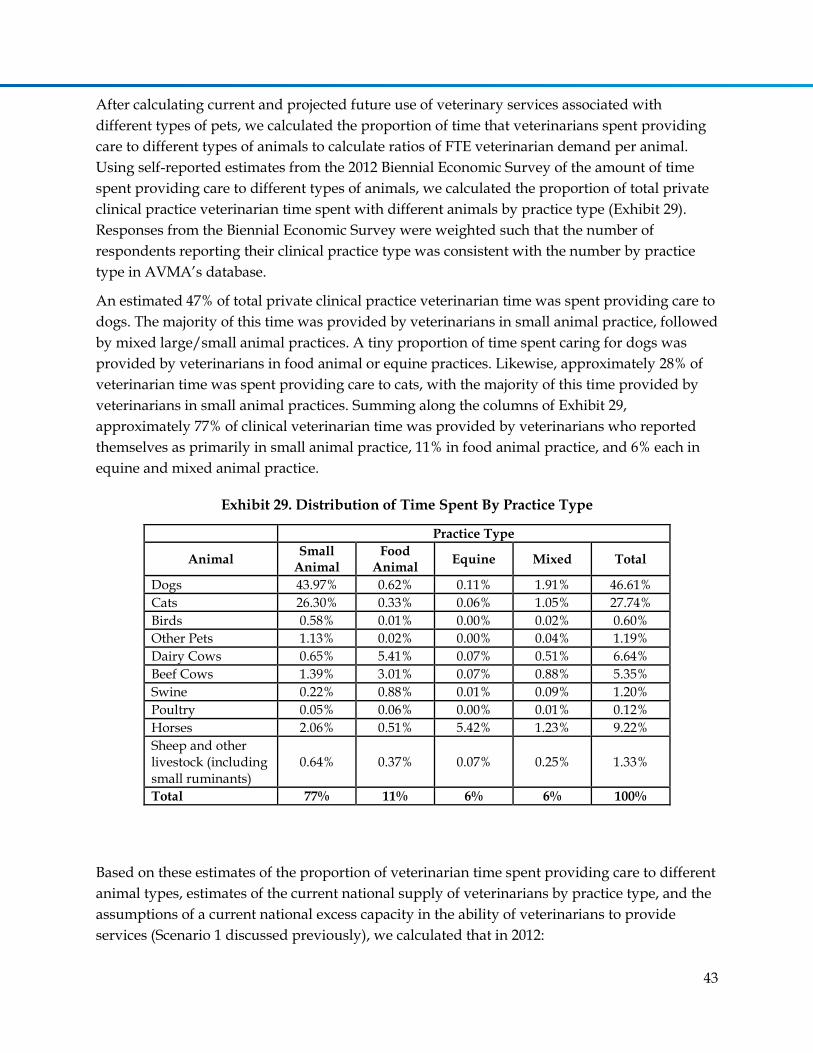
43
After calculating current and projected future use of veterinary services associated with
different types of pets, we calculated the proportion of time that veterinarians spent providing
care to different types of animals to calculate ratios of FTE veterinarian demand per animal.
Using self-reported estimates from the 2012 Biennial Economic Survey of the amount of time
spent providing care to different types of animals, we calculated the proportion of total private
clinical practice veterinarian time spent with different animals by practice type (Exhibit 29).
Responses from the Biennial Economic Survey were weighted such that the number of
respondents reporting their clinical practice type was consistent with the number by practice
type in AVMA’s database.
An estimated 47% of total private clinical practice veterinarian time was spent providing care to
dogs. The majority of this time was provided by veterinarians in small animal practice, followed
by mixed large/small animal practices. A tiny proportion of time spent caring for dogs was
provided by veterinarians in food animal or equine practices. Likewise, approximately 28% of
veterinarian time was spent providing care to cats, with the majority of this time provided by
veterinarians in small animal practices. Summing along the columns of Exhibit 29,
approximately 77% of clinical veterinarian time was provided by veterinarians who reported
themselves as primarily in small animal practice, 11% in food animal practice, and 6% each in
equine and mixed animal practice.
Exhibit 29. Distribution of Time Spent By Practice Type
Practice Type
Animal Small
Animal Food
Animal Equine Mixed Total
Dogs 43.97% 0.62% 0.11% 1.91% 46.61%
Cats 26.30% 0.33% 0.06% 1.05% 27.74%
Birds 0.58% 0.01% 0.00% 0.02% 0.60%
Other Pets 1.13% 0.02% 0.00% 0.04% 1.19%
Dairy Cows 0.65% 5.41% 0.07% 0.51% 6.64%
Beef Cows 1.39% 3.01% 0.07% 0.88% 5.35%
Swine 0.22% 0.88% 0.01% 0.09% 1.20%
Poultry 0.05% 0.06% 0.00% 0.01% 0.12%
Horses 2.06% 0.51% 5.42% 1.23% 9.22%
Sheep and other livestock (including small ruminants)
0.64% 0.37% 0.07% 0.25% 1.33%
Total 77% 11% 6% 6% 100%
Based on these estimates of the proportion of veterinarian time spent providing care to different
animal types, estimates of the current national supply of veterinarians by practice type, and the
assumptions of a current national excess capacity in the ability of veterinarians to provide
services (Scenario 1 discussed previously), we calculated that in 2012:

44
4,449 services for dogs= 1 FTE veterinarian
6,013 services for cats= 1 FTE veterinarian
8,648 services for birds= 1 FTE veterinarian
38,854 services for other pets= 1 FTE veterinarian
Note that very few services were provided to pets in the “other” category, so while there was
less reliability in this estimate of services per FTE veterinarian, this category of pets had little
impact on the overall demand for veterinary services. Also, as discussed previously, services
were not equivalent to visits as multiple services might be provided during one visit. This
analysis did not take into consideration that some services were more veterinarian-time
intensive than other services. Additional information on the relative time resource intensity of
each service could improve the projections of future veterinarian demand to the extent that
growth in demand for services differs slightly for the different types of services. Better
information on the amount of time spent providing specific types of services could improve the
ability to simulate the demand implications of alternative models of care delivery (e.g., greater
use of non-veterinarian staff).
Overall, this translated into 2012 FTE demand for 35,029 dog veterinarians, 20,846 cat
veterinarians, 454 bird veterinarians, and 897 “other” animal veterinarians—recognizing that
each FTE was actually made up of multiple veterinarians providing care to a variety of pet
types.
Equine Practice
The American Horse Council reported 9.2 million horses in the U.S. including:a
845,000 for racing
2.7 million for showing
3.9 million for recreation
1.75 million for other activities
Based on the proportion of private clinical practice veterinarian time spent with different types
of animals (Exhibit 29), and taking into account estimates of the current excess capacity in the
ability of veterinarians to provide services (Exhibit 7), we calculated demand for equine
veterinarians at 5,640 in 2012. This translated to approximately 1,630 horses cared for per FTE
veterinarian (with the majority of this care provided by equine veterinarians). From Exhibit 29 we
estimated that 59% of care provided to horses was provided by veterinarians in equine practice,
22% of care was provided by veterinarians who described their practice as predominantly small
a AHC defines “other” activities to include: farm and ranch work, rodeo, carriage horses, polo, police work, informal competitions, etc. http://www.horsecouncil.org/national-economic-impact-us-horse-industry

45
animal practicea, 13% of care was provided by veterinarians in mixed practices, and the
remaining care was provided by veterinarians in food animal (3%) practices. For veterinarians
in equine practice, approximately 94% of their time was spent caring for horses, with the
remaining 6% caring for a variety of small and large animals.
The Pet Demographic Study included households that captured a portion of horse ownership.
Based on the survey sample weights, the households in this survey accounted for close to 8.3
million horses in 2012 (or 90% of horses in the U.S.). The demand projections included in this
report modeled growth in demand for horses overall as a function of the projected growth in
demand for horses by households.
Food Animal Practice
The demand for non-government food animal veterinarians was linked to the U.S. population of
food animals. To estimate the demand for food animal veterinarians, we used the food animal
population projections generated by the IHS Agricultural Forecasting Model. A summary of this
model is provided in Appendix C. This model does not forecast aquaculture stocks, so growth in
aquaculture veterinary services was an omitted component of this analysis.
Using the clinical time distribution reported in Exhibit 29 for food animals, we first estimated the
number of FTE veterinarians caring for food animals by animal type: dairy cows, beef cattle, swine,
broilers and layers, sheep, and other livestock (Exhibit 30). The other livestock category included
turkeys, “other swine,” and less common food animals. We compared these FTE estimates against
current food animal production estimates to calculate FTE-to-animal ratios. Using the surplus
estimates discussed earlier (Exhibit 7), we calculated what the FTE-to-animal ratios would be if food
animal veterinarians were working at full capacity. Compared to current supply of 11,060 FTEs, we
calculated demand for 9,550 FTEs, if food animal veterinarians were all working at full capacity.
Exhibit 30. Food Animal Veterinarian Workforce, 2012
Animal Type Total Food Animal Supply (millions)
FTE Veterinarian Animals per FTE Veterinarian
Supply Demand Current Removing Excess
Capacity
Dairy cows 9.2 4,990 4,330 1,800 2,100
Beef cattle 81.5 4,020 3,490 20,300 23,400
Swine 64.8 900 780 72,000 83,100
Broilers and layers 7,896.4 90 80 87,738,000 98,705,300
Sheep 5.4 780 680 6,900 7,900
Other livestock 310.6 220 190 1,411,800 1,634,700
Total NA 11,060 9,550 NA NA
a Analysis of the 2012 Biennial Economic Survey (weighted using information in AVMA’s database of veterinarians) found that veterinarians who reported their work as predominantly small animal practice reported spending approximately 2.7% of their time, on average, providing equine care.

46
From the forecasting model, between 2012 and 2025 we projected growth in the supply of
broilers and layers (22%), turkeys (14%), swine (10%), and beef cattle (3%) (Exhibit 31). We
projected a small decline in supply of dairy cattle (-2%) and sheep (-6%).
Exhibit 31. Projected Growth in Food Animal Supply
2012 2015 2018 2021 2025
FTE Veterinarians
Food Animal
% Change (relative to 2012)
FTE Veterinarians
Food Animal
% Change (relative to 2012)
FTE Veterinarians
Food Animal
% Change (relative to 2012)
FTE Veterinarians
Food Animal
% Change (relative to 2012)
FTE Veterinarian
s
Food Animal
% Change (relative to 2012)
Dairy Cows 4,991 0.00% 4,950 -0.83% 4,970 -0.42% 4,936 -1.11% 4,906 -1.70%
Beef Cattle 4,019 0.00% 3,943 -1.87% 4,005 -0.34% 4,044 0.63% 4,134 2.87%
Swine 901 0.00% 923 2.45% 935 3.73% 960 6.58% 990 9.93%
Poultry 89 0.00% 98 9.73% 102 13.82% 104 16.69% 108 20.89%
Sheep and all other ruminants 780 0.00% 770 -1.25% 759 -2.60% 747 -4.13% 730 -6.40%
Turkeys 221 0.00% 232 4.56% 236 6.78% 244 10.43% 249 12.57%
Industry/Commercial
Veterinarians working in industry conduct a wide variety of services. Some of the major areas
of focus include pharmaceutical and biotechnology companies that work on drug discovery for
human health; animal health companies that produce veterinary pharmaceuticals,
biotechnology, and diagnostics; and animal feed companies that define nutritional
requirements.a Due to limited information on the current demand for veterinarians working in
industry, we used the assumption that the current supply (FTE=3,210) and demand for 2012
were in equilibrium.
To project future demand for veterinarians working in industry, we used information from a
recent survey conducted by the National Academy of Sciences. The survey contacted 118
companies from around the industry sector that were known to employ veterinarians. Of the
118 companies contacted, there were 59 respondents that collectively employed 1,527
veterinarians in 2007 (which represented approximately 49% of the 3,125 AVMA reported
industry veterinarians for the same year).b Of these respondents, companies anticipated a total
of 463 new positions opening between 2008 and 2016, representing a 30% growth. This equated
to a 3.75% average annual growth rate between 2008 and 2016. Additionally, the 59 respondents
a http://www.nap.edu/openbook.php?record_id=13413&page=90 b http://www.nap.edu/openbook.php?record_id=13413&page=92
47
reported that 15.7% of currently employed veterinarians would reach or exceed age 65 by the
year 2016. This equated to an additional 240 vacancies in anticipated hiring needs. It was
important to note that at the time of the survey, the industry sector, like other areas of
veterinary medicine, had been affected by the economic recession and it was likely that many
veterinarians would delay retirement and therefore weaken the demand for replacements.a For
modeling, we assumed that 3.75% annual growth in industry veterinary positions would
continue through 2016, but then the growth in demand would slow to approximately half this
rate (or 1.9%annually) from 2017 through 2025. Cumulatively, these annual growth rates
amounted to a 37% increase in demand between 2012 and 2025.
Government Veterinarians
To accurately measure the demand for veterinarians working in government in both clinical
and non-clinical roles, we separated the population into two distinct groups: (1) veterinarians
working with the Department of Defense, and (2) veterinarians working for all other
government agencies. The second group was the largest of the two, and included veterinarians
working for the Department of Agriculture and Department of Health and Human Services
(Exhibit 32).
Exhibit 32. Veterinary Workforce in Federal Employment, 2012
Employer # Employed Veterinarians
Department of Defense 987
Department of Homeland Security 15
Department of Agriculture 1,753
Department of Interior 37
Department of Health and Human Services 328
Food and Drug Administration 113
Centers for Disease Control and Prevention 93
National Institutes of Health 92
U.S. Public Health Service Commissioned Corps 22
Other 8
Total 3,120
Veterinarians working for these agencies provided many services centered around, but not
limited to, the U.S. food animal population. This included enforcing meat and poultry
inspection procedures, regulating animal medications, and researching animal diseases. As
many of these veterinarians provided services related to food supply animals, we linked
demand for veterinarians in these agencies to the projected growth in supply of food animals.
a http://www.nap.edu/openbook.php?record_id=13413&page=98
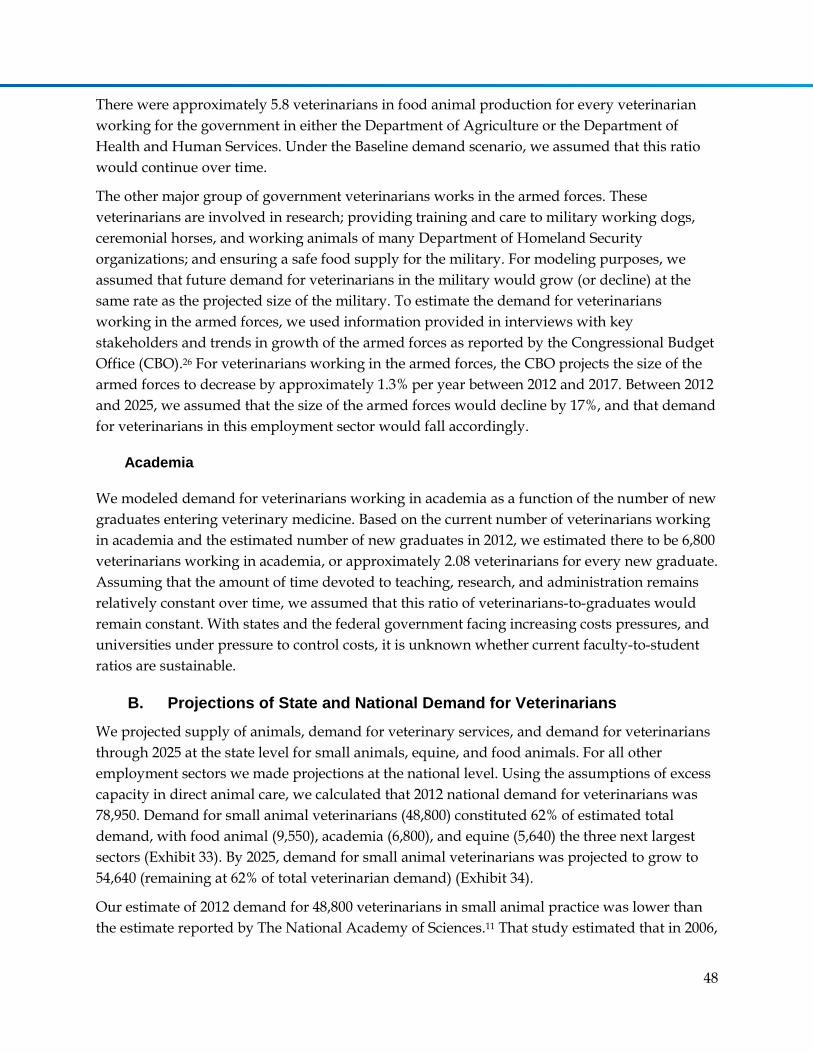
48
There were approximately 5.8 veterinarians in food animal production for every veterinarian
working for the government in either the Department of Agriculture or the Department of
Health and Human Services. Under the Baseline demand scenario, we assumed that this ratio
would continue over time.
The other major group of government veterinarians works in the armed forces. These
veterinarians are involved in research; providing training and care to military working dogs,
ceremonial horses, and working animals of many Department of Homeland Security
organizations; and ensuring a safe food supply for the military. For modeling purposes, we
assumed that future demand for veterinarians in the military would grow (or decline) at the
same rate as the projected size of the military. To estimate the demand for veterinarians
working in the armed forces, we used information provided in interviews with key
stakeholders and trends in growth of the armed forces as reported by the Congressional Budget
Office (CBO).26 For veterinarians working in the armed forces, the CBO projects the size of the
armed forces to decrease by approximately 1.3% per year between 2012 and 2017. Between 2012
and 2025, we assumed that the size of the armed forces would decline by 17%, and that demand
for veterinarians in this employment sector would fall accordingly.
Academia
We modeled demand for veterinarians working in academia as a function of the number of new
graduates entering veterinary medicine. Based on the current number of veterinarians working
in academia and the estimated number of new graduates in 2012, we estimated there to be 6,800
veterinarians working in academia, or approximately 2.08 veterinarians for every new graduate.
Assuming that the amount of time devoted to teaching, research, and administration remains
relatively constant over time, we assumed that this ratio of veterinarians-to-graduates would
remain constant. With states and the federal government facing increasing costs pressures, and
universities under pressure to control costs, it is unknown whether current faculty-to-student
ratios are sustainable.
B. Projections of State and National Demand for Veterinarians
We projected supply of animals, demand for veterinary services, and demand for veterinarians
through 2025 at the state level for small animals, equine, and food animals. For all other
employment sectors we made projections at the national level. Using the assumptions of excess
capacity in direct animal care, we calculated that 2012 national demand for veterinarians was
78,950. Demand for small animal veterinarians (48,800) constituted 62% of estimated total
demand, with food animal (9,550), academia (6,800), and equine (5,640) the three next largest
sectors (Exhibit 33). By 2025, demand for small animal veterinarians was projected to grow to
54,640 (remaining at 62% of total veterinarian demand) (Exhibit 34).
Our estimate of 2012 demand for 48,800 veterinarians in small animal practice was lower than
the estimate reported by The National Academy of Sciences.11 That study estimated that in 2006,

49
a total of 48,158 FTE veterinarians were providing companion animal care (with companion
care equivalent to our small animal sector—which included the portion of time spent providing
small animal care by veterinarians in other employment sectors such as mixed animal
practices). The National Academy of Sciences predicted demand in 2016 would be between
50,805 and 65,950 FTEs (depending on productivity levels of veterinarians). To reach the
midpoint of these estimates (58,378) suggested demand was increasing by about 1,022
veterinarians per year between 2006 and 2016—reaching 54,300 FTEs in 2012 (or 11% higher
than our estimate of current demand). The National Academy of Sciences demand estimate
(interpolated to estimate demand for 2012) was approximately equivalent to current supply and
would approximate demand under the assumption of no current excess capacity in the
companion animal sector.
We projected that the demand for small animal veterinarians would grow by 12% (approximately
450 FTEs per year) between 2012 and 2025 as a function of population growth and changing
household characteristics (including modest growth in average household income). This projected
growth rate over a 13-year period (about 0.9% average, annual growth) was substantially lower
than the 1.3% average annual growth rate projected by KPMG (1999) for the period 1997 to 2015.1
Demand for food animal veterinarians was projected to grow only 1% between 2012 and 2025—
reflecting very little growth in supply of dairy cows and beef cattle that together accounted for 83%
of veterinarians involved in food production. Furthermore, industry consolidation and improved
productivity could contribute to an actual decline in demand for food animal veterinarians. These
findings were similar to the KPMG study, which estimated a 1.7% decline (between 1997 and 2015)
in FTE veterinarians working in large animal practice.1 State level estimates of the total FTE demand
for small animal veterinarians, equine veterinarians, and food animal veterinarians are provided in
Exhibits 35, 36, and 37 respectively.

50
Exhibit 33. Total FTE Demand for Veterinarians in the U.S., 2012
Exhibit 34. Total FTE Demand for Veterinarians in the U.S., 2025
Equine5,640
7%
Small Animal48,800
62%
Industry/ Commercial3,210
4%
Food Animal9,550 12%
Government (civilian)2,130
3%
Government (military)990 1%
Academia6,800
9%
Other1,840
2%
Equine6,960
8%
Small Animal54,640
62%
Industry/ Commercial4,390
5%
Food Animal9,650 11%
Government (civilian)2,150
2%
Government (military)920 1%
Academia7,630
9%
Other1,720
2%
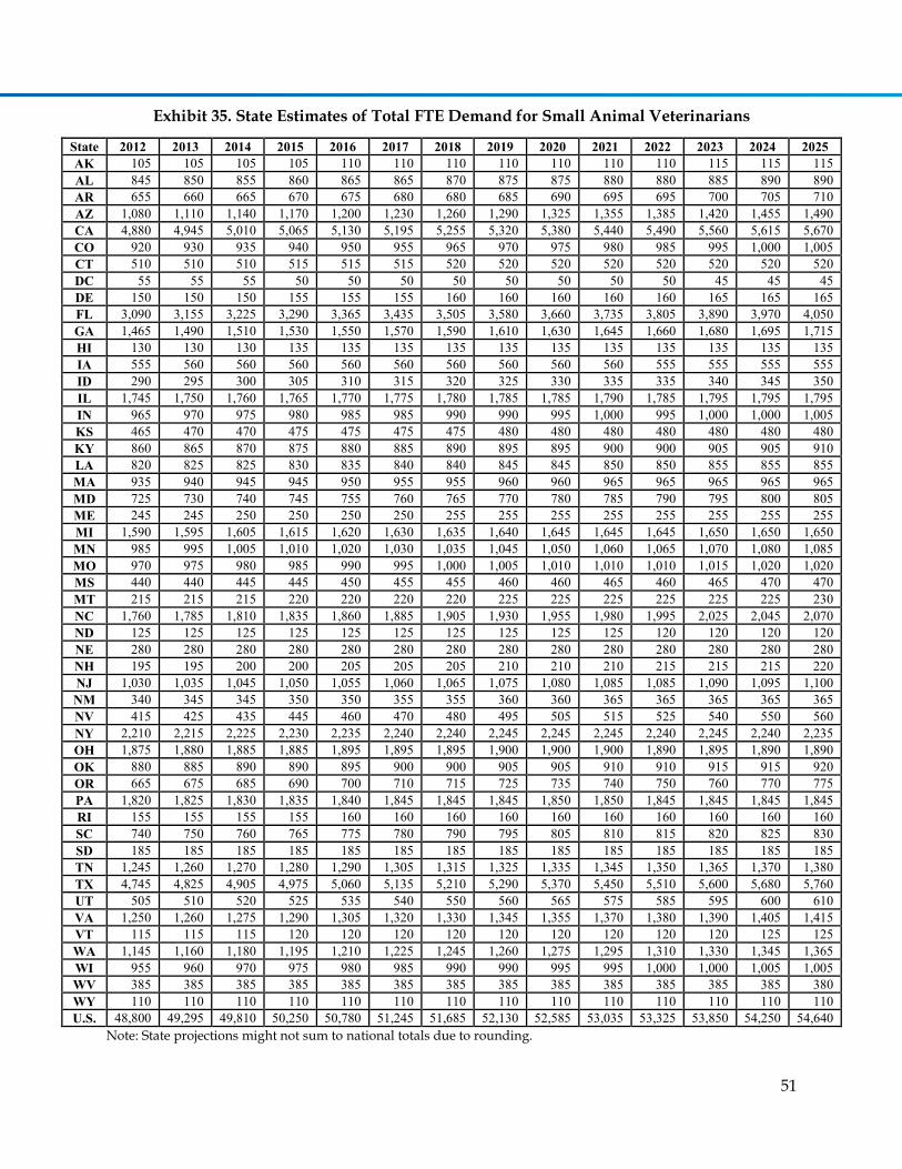
51
Exhibit 35. State Estimates of Total FTE Demand for Small Animal Veterinarians
State 2012 2013 2014 2015 2016 2017 2018 2019 2020 2021 2022 2023 2024 2025
AK 105 105 105 105 110 110 110 110 110 110 110 115 115 115
AL 845 850 855 860 865 865 870 875 875 880 880 885 890 890
AR 655 660 665 670 675 680 680 685 690 695 695 700 705 710
AZ 1,080 1,110 1,140 1,170 1,200 1,230 1,260 1,290 1,325 1,355 1,385 1,420 1,455 1,490
CA 4,880 4,945 5,010 5,065 5,130 5,195 5,255 5,320 5,380 5,440 5,490 5,560 5,615 5,670
CO 920 930 935 940 950 955 965 970 975 980 985 995 1,000 1,005
CT 510 510 510 515 515 515 520 520 520 520 520 520 520 520
DC 55 55 55 50 50 50 50 50 50 50 50 45 45 45
DE 150 150 150 155 155 155 160 160 160 160 160 165 165 165
FL 3,090 3,155 3,225 3,290 3,365 3,435 3,505 3,580 3,660 3,735 3,805 3,890 3,970 4,050
GA 1,465 1,490 1,510 1,530 1,550 1,570 1,590 1,610 1,630 1,645 1,660 1,680 1,695 1,715
HI 130 130 130 135 135 135 135 135 135 135 135 135 135 135
IA 555 560 560 560 560 560 560 560 560 560 555 555 555 555
ID 290 295 300 305 310 315 320 325 330 335 335 340 345 350
IL 1,745 1,750 1,760 1,765 1,770 1,775 1,780 1,785 1,785 1,790 1,785 1,795 1,795 1,795
IN 965 970 975 980 985 985 990 990 995 1,000 995 1,000 1,000 1,005
KS 465 470 470 475 475 475 475 480 480 480 480 480 480 480
KY 860 865 870 875 880 885 890 895 895 900 900 905 905 910
LA 820 825 825 830 835 840 840 845 845 850 850 855 855 855
MA 935 940 945 945 950 955 955 960 960 965 965 965 965 965
MD 725 730 740 745 755 760 765 770 780 785 790 795 800 805
ME 245 245 250 250 250 250 255 255 255 255 255 255 255 255
MI 1,590 1,595 1,605 1,615 1,620 1,630 1,635 1,640 1,645 1,645 1,645 1,650 1,650 1,650
MN 985 995 1,005 1,010 1,020 1,030 1,035 1,045 1,050 1,060 1,065 1,070 1,080 1,085
MO 970 975 980 985 990 995 1,000 1,005 1,010 1,010 1,010 1,015 1,020 1,020
MS 440 440 445 445 450 455 455 460 460 465 460 465 470 470
MT 215 215 215 220 220 220 220 225 225 225 225 225 225 230
NC 1,760 1,785 1,810 1,835 1,860 1,885 1,905 1,930 1,955 1,980 1,995 2,025 2,045 2,070
ND 125 125 125 125 125 125 125 125 125 125 120 120 120 120
NE 280 280 280 280 280 280 280 280 280 280 280 280 280 280
NH 195 195 200 200 205 205 205 210 210 210 215 215 215 220
NJ 1,030 1,035 1,045 1,050 1,055 1,060 1,065 1,075 1,080 1,085 1,085 1,090 1,095 1,100
NM 340 345 345 350 350 355 355 360 360 365 365 365 365 365
NV 415 425 435 445 460 470 480 495 505 515 525 540 550 560
NY 2,210 2,215 2,225 2,230 2,235 2,240 2,240 2,245 2,245 2,245 2,240 2,245 2,240 2,235
OH 1,875 1,880 1,885 1,885 1,895 1,895 1,895 1,900 1,900 1,900 1,890 1,895 1,890 1,890
OK 880 885 890 890 895 900 900 905 905 910 910 915 915 920
OR 665 675 685 690 700 710 715 725 735 740 750 760 770 775
PA 1,820 1,825 1,830 1,835 1,840 1,845 1,845 1,845 1,850 1,850 1,845 1,845 1,845 1,845
RI 155 155 155 155 160 160 160 160 160 160 160 160 160 160
SC 740 750 760 765 775 780 790 795 805 810 815 820 825 830
SD 185 185 185 185 185 185 185 185 185 185 185 185 185 185
TN 1,245 1,260 1,270 1,280 1,290 1,305 1,315 1,325 1,335 1,345 1,350 1,365 1,370 1,380
TX 4,745 4,825 4,905 4,975 5,060 5,135 5,210 5,290 5,370 5,450 5,510 5,600 5,680 5,760
UT 505 510 520 525 535 540 550 560 565 575 585 595 600 610
VA 1,250 1,260 1,275 1,290 1,305 1,320 1,330 1,345 1,355 1,370 1,380 1,390 1,405 1,415
VT 115 115 115 120 120 120 120 120 120 120 120 120 125 125
WA 1,145 1,160 1,180 1,195 1,210 1,225 1,245 1,260 1,275 1,295 1,310 1,330 1,345 1,365
WI 955 960 970 975 980 985 990 990 995 995 1,000 1,000 1,005 1,005
WV 385 385 385 385 385 385 385 385 385 385 385 385 385 380
WY 110 110 110 110 110 110 110 110 110 110 110 110 110 110
U.S. 48,800 49,295 49,810 50,250 50,780 51,245 51,685 52,130 52,585 53,035 53,325 53,850 54,250 54,640
Note: State projections might not sum to national totals due to rounding.

52
Exhibit 36. State Estimates of Total FTE Demand for Equine Veterinarians
State 2012 2013 2014 2015 2016 2017 2018 2019 2020 2021 2022 2023 2024 2025
AK 15 15 15 15 15 20 20 20 20 20 20 20 20 20
AL 105 105 105 110 110 110 110 115 115 115 115 120 120 120
AR 75 80 80 80 80 85 85 85 85 85 85 90 90 90
AZ 205 210 215 220 230 240 250 255 265 270 275 290 300 310
CA 675 690 695 710 725 745 755 770 785 790 800 825 840 850
CO 180 180 180 185 190 190 195 195 200 200 200 205 210 210
CT 30 30 30 30 30 30 30 30 30 30 30 30 30 30
DC <5 <5 <5 <5 <5 <5 <5 <5 <5 <5 <5 <5 <5 <5
DE 15 15 15 15 15 15 15 15 15 15 15 15 15 15
FL 265 275 280 285 295 310 315 325 335 340 345 365 375 385
GA 140 140 140 145 150 155 155 160 160 165 165 170 175 175
HI 15 15 15 15 15 15 15 15 15 15 15 15 15 15
IA 110 110 110 110 115 115 115 115 120 120 115 120 120 120
ID 60 65 65 65 70 70 75 75 75 75 80 80 85 85
IL 160 160 160 165 165 170 170 170 170 170 170 175 180 180
IN 90 90 95 95 95 95 100 100 100 100 100 105 105 105
KS 85 85 85 85 90 90 90 90 90 90 90 95 95 95
KY 110 110 110 110 115 115 115 115 120 120 120 120 125 125
LA 95 95 100 100 100 105 105 105 105 105 105 110 110 110
MA 50 50 50 50 50 50 50 50 50 50 50 55 55 55
MD 65 65 70 70 70 70 70 75 75 75 75 75 80 80
ME 15 15 15 15 15 15 15 15 15 15 15 15 15 15
MI 145 145 145 150 150 155 155 155 160 160 160 160 165 165
MN 180 180 185 185 190 195 195 200 205 205 205 210 215 215
MO 160 160 160 160 165 170 170 170 175 175 175 180 180 185
MS 55 55 55 55 60 60 60 60 60 60 60 65 65 65
MT 50 50 50 50 55 55 55 55 55 55 55 60 60 60
NC 165 170 170 175 180 185 185 190 195 195 195 205 210 215
ND 30 30 30 30 30 30 30 30 30 30 30 30 30 30
NE 55 55 55 55 55 55 55 60 60 60 60 60 60 60
NH 10 10 10 10 10 10 10 15 15 15 15 15 15 15
NJ 70 70 70 70 75 75 75 75 75 75 75 80 80 80
NM 65 65 65 65 70 70 70 70 75 75 75 75 75 75
NV 75 75 80 80 85 90 90 95 95 100 100 105 110 110
NY 140 140 140 140 140 145 145 145 145 145 145 150 150 150
OH 170 170 170 175 175 180 180 180 185 180 180 185 185 190
OK 105 110 110 110 110 115 115 115 120 120 115 120 125 125
OR 100 100 105 105 110 110 115 115 120 120 120 125 125 130
PA 125 125 125 125 130 130 130 135 135 135 135 135 140 140
RI 10 10 10 10 10 10 10 10 10 10 10 10 10 10
SC 70 70 70 70 75 75 75 80 80 80 80 80 85 85
SD 45 45 45 45 45 50 50 50 50 50 50 50 50 50
TN 150 150 150 155 160 160 165 165 170 170 170 175 180 180
TX 555 565 575 585 605 625 635 650 665 670 680 705 725 735
UT 115 115 120 120 125 130 130 135 135 140 140 145 150 150
VA 120 120 120 125 125 130 130 135 135 135 135 140 145 145
VT 5 5 5 5 5 5 10 10 10 10 10 10 10 10
WA 175 180 185 185 190 195 200 205 210 210 215 220 225 230
WI 95 95 95 95 100 100 100 100 105 105 105 105 110 110
WV 35 35 35 35 35 35 35 35 35 35 35 35 40 40
WY 25 25 25 25 25 30 30 30 30 30 30 30 30 30
U.S. 5,645 5,730 5,790 5,885 6,030 6,185 6,270 6,370 6,480 6,520 6,550 6,750 6,880 6,965
Note: State projections might not sum to national totals due to rounding.

53
Exhibit 37. State Estimates of Total FTE Demand for Food Animal Veterinarians
State 2012 2013 2014 2015 2016 2017 2018 2019 2020 2021 2022 2023 2024 2025
AK <5 <5 <5 <5 <5 <5 <5 <5 <5 <5 <5 <5 <5 <5
AL 430 430 435 435 435 435 435 430 425 425 420 420 415 415
AR 510 505 500 495 485 475 465 455 440 430 415 405 395 380
AZ 50 50 50 50 50 50 50 50 55 55 55 55 55 55
CA 245 240 240 235 235 235 235 235 235 235 235 235 235 235
CO 130 125 120 115 115 115 115 115 110 110 110 105 105 105
CT <5 <5 <5 <5 <5 <5 <5 <5 <5 <5 <5 <5 <5 <5
DC <5 <5 <5 <5 <5 <5 <5 <5 <5 <5 <5 <5 <5 <5
DE 90 85 85 85 80 80 75 75 70 70 65 65 60 60
FL 80 75 70 65 65 65 65 65 60 60 60 60 60 60
GA 575 580 590 595 595 595 590 585 580 575 570 570 565 560
HI 5 5 5 5 5 5 5 5 5 5 5 5 5 5
IA 940 940 940 955 975 985 995 1,005 1,020 1,035 1,055 1,065 1,080 1,095
ID 95 95 95 95 95 100 100 100 100 100 105 105 105 105
IL 220 215 210 205 205 200 200 195 195 190 190 185 185 180
IN 160 155 155 155 155 150 150 145 145 145 145 145 140 140
KS 305 300 295 290 290 290 290 290 290 290 290 290 290 290
KY 250 260 275 285 300 310 325 335 345 355 370 380 395 405
LA 125 130 140 145 155 160 170 180 185 195 200 210 220 225
MA <5 <5 <5 <5 <5 <5 <5 <5 <5 <5 <5 <5 <5 <5
MD 115 115 115 115 115 115 115 115 110 110 110 110 105 105
ME 5 <5 <5 <5 <5 <5 <5 <5 <5 <5 <5 <5 <5 <5
MI 90 85 85 85 85 85 85 85 85 85 85 85 85 85
MN 435 435 435 440 445 450 455 460 465 475 485 490 495 500
MO 365 360 355 355 355 350 350 350 345 345 340 340 340 335
MS 320 320 325 330 330 330 330 330 330 325 325 325 325 325
MT 120 115 115 115 115 115 115 115 115 115 115 115 115 115
NC 730 720 715 715 715 710 700 695 685 680 675 670 665 655
ND 75 75 70 70 70 70 70 65 65 65 65 65 65 65
NE 330 320 310 305 305 305 300 300 300 295 295 295 295 290
NH <5 <5 <5 <5 <5 <5 <5 <5 <5 <5 <5 <5 <5 <5
NJ <5 <5 <5 <5 <5 <5 <5 <5 <5 <5 <5 <5 <5 <5
NM 55 55 55 55 50 50 50 50 50 50 50 50 50 50
NV 20 20 20 20 20 20 20 20 20 20 20 20 20 20
NY 65 60 60 60 60 60 60 60 60 55 55 55 55 55
OH 140 135 135 135 140 140 140 140 145 145 145 150 150 150
OK 430 450 455 465 480 490 500 510 525 535 545 555 565 580
OR 60 60 60 55 55 55 55 55 55 55 55 55 55 55
PA 185 185 185 185 185 185 185 185 185 185 185 185 190 190
RI <5 <5 <5 <5 <5 <5 <5 <5 <5 <5 <5 <5 <5 <5
SC 115 115 115 115 120 120 120 120 120 120 120 125 125 125
SD 240 235 230 225 225 225 220 220 220 220 215 215 215 215
TN 85 80 80 75 75 75 75 75 75 75 75 75 75 75
TX 820 830 825 820 825 830 835 840 840 840 845 845 850 855
UT 85 85 85 85 85 85 85 85 85 85 90 90 90 90
VA 165 160 160 160 155 155 150 150 145 145 145 140 140 135
VT 10 10 10 10 10 10 10 10 10 10 10 10 10 10
WA 50 45 45 45 45 45 45 45 45 45 45 45 45 45
WI 150 145 140 140 135 135 135 135 135 130 130 130 130 130
WV 15 15 15 15 15 15 15 15 15 15 15 15 15 15
WY 70 65 65 60 60 60 60 60 55 55 55 55 55 55
U.S. 9,550 9,510 9,480 9,475 9,515 9,540 9,555 9,570 9,570 9,580 9,595 9,610 9,630 9,650
Note: State projections might not sum to national totals due to rounding.

54
Exhibit 38 depicts the percent change in demand for small animal and equine veterinarians.
Two regions that saw the largest increase in demand for veterinarians were the Southeast and
the Western U.S. Unsurprisingly, the two states with the largest growth, Arizona and Florida,
fell within these geographic regions. Conversely, both North Dakota and West Virginia would
experience a minor reduction in demand for veterinarians between 2012 and 2025. The
projected growth for North Dakota was low, possibly, given the economic growth seen in the
state in recent years as a result of the oil industry (this growth was not captured in the latest
state-level population projections produced by the U.S. Census Bureau).a
Exhibit 38. State Projections of % and FTE Demand Growth for Small Animal Veterinarians:
2012-2025
Demand for food animal veterinarians was concentrated in the Midwest and Southern states
(Exhibit 39). Between 2012 and 2025, demand was projected to decline in the New England
region and in many states, while demand was projected to increase (in percentage terms) across
many of the southern states (Exhibit 40).
The Baseline Scenario projects future demand under the assumption that current patterns of pet
ownership will remain largely unchanged but will reflect changing household demographics
(e.g., age, race/ethnicity); the supply of food animals will grow as projected by IHS’s
Agricultural Forecasting Model; that patterns of care delivery for pets, horses, and food animals
will remain largely unchanged; and that demand for veterinarians in academia, government,
and industry will reflect recent trends in their respective demand drivers. The baseline scenario
also assumes a current national 17% excess capacity of veterinarians in small animal, equine,
a While the oil boom has increased the population in North Dakota, much of that increase has been from unaccompanied male workers who are living in man camps. It is extremely difficult to find housing for families in the Bakken oil reserve. It is unknown how long this boom period will persist.

55
and food animal practice veterinarians. The Baseline Scenario, therefore, represented our best
estimate of future demand under the status quo. Under this scenario, total demand grew 12%—
from approximately 78,950 in 2012 to 88,070 in 2025 (Exhibit 41). Veterinarians in small animal
and equine care constituted the largest portion of total demand, with food animal and academia
reflecting the second and third largest employment sectors, respectively.
Exhibit 39. State Estimates of Demand for Food Animal Veterinarians: 2012
Exhibit 40. State Projections of % and FTE Demand Growth for Food Animal Veterinarians:
2012-2025

56
Exhibit 41. Baseline Demand Projections: 2012-2025
Practice 2012 2013 2014 2015 2016 2017 2018 2019 2020 2021 2022 2023 2024 2025
Equine 5,640 5,730 5,790 5,880 6,030 6,180 6,270 6,370 6,480 6,520 6,550 6,750 6,880 6,960
Small Animal 48,800 49,300 49,810 50,250 50,780 51,250 51,690 52,130 52,590 53,040 53,320 53,850 54,250 54,640
Industry/ Commercial
3,210 3,330 3,450 3,580 3,720 3,790 3,860 3,930 4,000 4,080 4,150 4,230 4,310 4,390
Food Animal 9,550 9,510 9,480 9,480 9,520 9,540 9,560 9,570 9,570 9,580 9,600 9,610 9,630 9,650
Government (civilian)
2,130 2,120 2,110 2,120 2,130 2,130 2,130 2,130 2,130 2,140 2,140 2,150 2,150 2,150
Government (military)
990 970 960 950 940 920 920 920 920 920 920 920 920 920
Academia 6,800 7,190 7,340 7,480 7,630 7,630 7,630 7,630 7,630 7,630 7,630 7,630 7,630 7,630
Other 1,840 1,830 1,820 1,810 1,800 1,790 1,780 1,770 1,770 1,760 1,750 1,740 1,730 1,720
Total 78,950 79,970 80,760 81,560 82,540 83,240 83,840 84,460 85,100 85,660 86,070 86,880 87,500 88,070
Note: Totals may not add to the sum of column values due to rounding.
57
The Baseline Scenario suggested that at the national level demand for veterinarians would grow
by 11-12% between 2012 and 2025. The growth in demand was driven primarily by demand for
small animal practice (which would continue to constitute approximately 62% of FTE
veterinarian demand). Study projections suggested higher than average percentage growth in
demand in the industry/commercial, equine, and academia employment sectors—although
projections for each of these sectors had important caveats. For industry, there was little
information on which to base trends in demand and the demand growth assumptions relied
heavily on an industry survey conducted during the middle of the economic downturn. The
equine sector has experienced turbulent times during the economic downturn and diminished
demand in the racing sector. The projected growth in this sector reflected (in part) the observed
relationship that older people have a greater propensity to own horses. To the extent that this
relationship was generational rather than an age relationship, then the rising elderly population
might not own horses at the same level as the current elderly. While we projected modest
growth in demand for veterinarians in academia, university and government, budget pressures
and vagueness regarding the number of new veterinarians who would be trained, created some
uncertainty in these projections. Slow growth in the government and other (tax-exempt
institutions and municipalities) sectors reflected anticipated budget pressures that would
restrain hiring. Slow growth in the food animal sector reflected projections of slow or negative
growth in the nation’s stocks of beef cattle, dairy cattle, sheep, and swine, despite substantial
growth in demand for poultry (which requires a relatively small veterinary workforce to
oversee the large volumes of poultry produced).
IV. Conclusion
This section reviews the main findings of this study, discusses study strengths and limitations,
identifies potential areas for future research, and provides summary conclusions.
A. National Projections of Adequacy of Supply and Discussion
We estimated that the supply for veterinarians (90,200) in the U.S. in 2012 exceeded demand for
veterinarians (78,950) by approximately 11,250 (or excess capacity of 12.5%) at the current levels
of prices for services. Because a large proportion of veterinarians were self-employed and
unemployment rates for veterinarians were low, this excess capacity took the form of under-
employment rather than unemployment. Between 2012 and 2025, under a baseline scenario we
projected that both supply and demand would grow by about 11% (reaching demand of 88,100
and supply of 100,400 by 2025). Comparison of the baseline supply and demand scenarios
suggest that the magnitude of the excess capacity ranges from 11% to 14% between 2012 and
2025 (ranging from 9,300 to 12,300 FTEs each year between 2012 and 2025). If veterinary
practices were to staff using a greater proportion of veterinary technicians and other supply
staff, then the excess capacity among the veterinarian workforce could be even higher.
We modeled the sensitivity of the supply projections to different assumptions regarding the
number of veterinarians trained, patterns of hours worked, and retirement patterns. Under

58
every scenario the supply projections exceeded demand through 2025 (Exhibit 42). Given the
high debt load of new students and stagnating incomes seen in recent years among
veterinarians, it was deemed unlikely that veterinarians would reduce average hours worked or
retire earlier than current and historical patterns. If veterinarians worked more hours, fewer
veterinarians would be required to provide the same level of services. Consequently, there was
a greater potential for the supply projections to exceed the baseline estimates rather than to fall
short of the baseline estimates. It was unlikely that veterinarians would reduce hours worked
because of economic pressures to maintain practice and household income. Likewise, it was
unlikely that veterinarians would retire earlier than historical patterns because of a combination
of economic pressures, changes in federal policies such as delaying eligibility age for Medicare,
and the general overall improvement in population health that allows people to live longer and
remain healthier.
Exhibit 42. Alternative Supply Scenarios vs. Baseline Demand Projections 2012-2025
70,000
75,000
80,000
85,000
90,000
95,000
100,000
105,000
110,000
115,000
120,000
2012 2014 2016 2018 2020 2022 2024
FTE
Ve
teri
nar
ian
s
Year
Increased Hours (+10%)
Delayed Retirement (2 yrs)
High Growth
Baseline Supply
No Increase Except Utah State, Lincoln Memorial, and MidwesternNo Increase in New Graduates After 2016
Earlier Retirement (2 years)
Reduced Hours (-10%)
Baseline Demand
Supply Scenarios
Demand Scenario

59
B. Study Strengths and Limitations
The supply and demand projections presented in this report were based on microsimulation
models that took into consideration many factors shown to be associated with supply and
demand for veterinary services. Most of the data used were from the most recent AVMA
surveys, Census Bureau population estimates and projections, and other key data sources.
Where data were lacking, assumptions were necessitated. For this reason, the projection models
were designed to be updated as new information or data sources become available.
Whereas traditional workforce models often start with the assumption that supply and demand
are in equilibrium in the base year, this study relied on a survey with 3,497 respondents who
provided their assessment of the adequacy of veterinary supply in their local geographic area
and employment sector. These veterinarians also provided insight on the amount of excess
capacity (if any) in their practices. This information allowed us to quantify a measure of excess
capacity by state and employment sector (for those sectors providing direct animal care where a
substantial portion of veterinarians are self-employed or owners of veterinary practices).
Data limitations contributed to several study limitations that were potential areas for future
research.
1. The estimates of excess capacity in 2012 were based on the self-reported perceptions of
veterinarians as to whether their local supply of veterinarians was adequate, and the
degree of excess capacity within their practice. Development of more objective measures
of both physical and human excess capacity in veterinary practices would improve the
accuracy of the results. Still, the perceptions of excess capacity were consistent with
other evidence, such as stagnating or falling incomes of veterinarians, increased
difficulty of new graduates finding employment, and trends in declining productivity.
2. The modeling of demand for veterinary services was made complicated by the large
variation in types of work provided by veterinarians. This was true especially in food
animal production where veterinary services differed substantially by animal type. A
more detailed analysis of how much time was spent providing specific veterinary
services would improve the estimates of the demand for veterinary FTEs—especially as
the mix of services would likely change over time.
3. Our analysis covered the major food animal types with the exception of aquaculture
veterinary practice. Future research might model the growth in aquaculture and also
separate out animal types included in the “all other” category used in this analysis.
4. There was little information to model growth trends in demand for veterinarians in
industry. Our analysis relied on survey data collected during the middle of an economic
downturn that asked industry representatives their plans for hiring.
5. Additional research is needed to better understand trends in horse ownership by type of
owner and horse use (households owning horses for leisure, racing horses, etc.). Our
analysis found a correlation between age of head of household and propensity to own
horses, but additional research is required to better understand if this is an age effect or

60
a generational effect (with the future elderly owning fewer horses per capita than the
current elderly).
6. The supply projections assumed that new graduates from veterinary medical colleges
would locate in states and employment sectors with the least excess capacity. That is,
new veterinarians would gravitate to geographic areas and employment sectors where
there are the greatest career and employment opportunities. The current supply
projection model did not take into account that some veterinarians would move
geographically or change employment sectors during their career (e.g., switching from
equine or food animal to government or research). Consequently, projections of
imbalances between veterinary supply and demand would be less accurate for specific
states or employment sectors as compared to the national projections.
7. The demand analysis took into consideration changes in the racial/ethnic composition
of the U.S. population. However, there may be additional diversity or cultural
differences that warrant additional research. For example, within the non-Hispanic
“other” demographic group, there were people from Asia, the Middle East, and many
other regions where different cultural norms exist as to providing veterinary care for
companion animals.
C. Areas for Future Research
The data limitations and research gaps described above highlight potential areas where
additional research could improve understanding of trends affecting the veterinary workforce.
The workforce simulation models developed for this study were built to be updated and refined
as research gaps are filled, and an important component of this study was identification of
unanswered questions. We suggest the following as areas where additional research is needed
or where data collection efforts might be implemented.
1. Develop more objective measures of demand for veterinary services. For this analysis, current demand was estimated by adding current supply plus estimates of current excess capacity. Another approach is benchmarking. For this approach one would identify communities where there appears to be a good balance between supply and demand for services. That is, consumers in that area do not experience abnormally long wait times or difficulty to access veterinary services, veterinarians are able to earn compensation levels consistent with their expectations, and veterinary practices are efficient in terms of how workload is divided between veterinarians and support staff. Findings from these case studies could then be extrapolated to other communities to assess adequacy of supply.
2. Develop early warning indicators of imbalances between supply and demand. AVMA might consider developing a measurement system similar to the Aggregate Demand Index developed by the Pharmacy Manpower Project.a This index was based on monthly input
a http://www.pharmacymanpower.com/

61
collected across different geographic areas on the assessment of balance between supply and demand and levels of difficulty hiring new pharmacists. Consistent and frequent collection of metrics could provide baseline trends and early indicators of changes in the balance between supply and demand. Potential indicators include:
Indicators regarding availability of veterinarian jobs
o Number of job openings for veterinarians advertised
o Number of vacancies for veterinarians
o Ratio of applicants per veterinarian job opening
o Average length of time to fill a veterinarian job opening
Indicators regarding veterinary practices
o Practice profitability
o Frequency of organizational changes in practices
(selling/merging/consolidating)
o Numbers of services provided and ratio of revenue per service provided
o Perceptions of the extent to which practice works at peak
efficiency/productivity
o Perceptions of adequacy of supply in an area
o Average wait times for non-emergency appointments
Indicators regarding veterinarians’ income and workforce behavior
o Veterinarian income and per hour equivalent
o Plans to leave veterinary medicine for another career and reasons why
o Age when a veterinarian becomes permanently inactive
Indicators such as those above can be collected through existing data collection efforts at the
AVMA. Periodic collection of these data and monitoring of changes in these indicators would
help AVMA recognize when shifts in the relationship between supply and demand for
veterinarians occur. Moreover, as these indicators are collected over time, AVMA could begin to
analyze the relationship between these indicators and the results of the supply and demand
projection model.
3. Conduct research on the price sensitivity of pet and animal owners. The current excess capacity among veterinary practices providing direct animal care could be influenced through efforts to increase the volume of services used. Research is needed to better understand the degree to which reducing the price of services will increase volume of such services. If services are “price elastic,” then small reductions in price of some services could translate to substantially higher volume. On the other hand, if services are “price inelastic,” then changes in price will have little effect on volume of services.
4. Monitor the careers of new veterinarians. With the estimation that a current surplus of more than 11,000 veterinarians exists and is projected to persist into the future, it is important to understand what the ramifications of this imbalance will be for new veterinarians. New veterinarians could be identified as they successfully complete the NAVLE examination each year. From that group, a sample could be selected each year for participation in a long-term, follow-up study that seeks to explore the career trajectories of individuals who

62
become veterinarians in the current supply/demand environment. Of importance would be observing:
how do these new professionals fare in the job market?
is there a threshold of how long they will unsatisfactorily pursue a career as a
veterinarian and will there develop a large exodus of new veterinarians at some point in
the future?
will there be effects on their willingness to start new practices or buy existing practices
from retiring veterinarians?
While, some have already speculated about these questions, it will be important to collect the
data to confirm or dispute these speculations and understand how the new veterinarians’
careers play out over time.
5. Acquire additional information on the average amount of time veterinarians spend providing specific types of services. Such information could improve the ability to simulate the demand implications of the changing mix of services demanded, and implementation of alternative care delivery models such as greater use of non-veterinarian staff.
6. Continue to update model inputs and refine model components, parameters, and assumptions. The model developed for this project is sophisticated and contains a large number of data inputs, parameters, and assumptions. As the future unfolds, the underlying data inputs of the models will become outdated and need to be recompiled for the models to remain useful over time. Related to this is periodic updating of the model parameters. Periodically, the model parameters should be revisited and changed as necessary as additional research is conducted and our understanding of the drivers of supply and demand for veterinarians changes. Moreover, as has been pointed out in the previous section, there are a number of refinements that will improve the granularity of the model’s projections, including improving the equine demand module of the model and improved understanding of the drivers of new veterinarian geographic distribution. Supply inputs that could be updated periodically in the model include current supply, number of new graduates, hours worked patterns, and retirement patterns. Demand inputs that would require periodic updating include new Census Bureau population estimates/projections for each state, and evolving patterns of pet ownership and use of veterinary services.
7. Evaluate demand projection assumptions. The demand projections presented here assumed that care delivery patterns would remain comparatively unchanged relative to current patterns. If veterinarians make greater use of veterinary technicians or other staff, then all else being equal, there would be fewer veterinarians needed to supply the same level of services.
D. Summary
In summary, it appears that at the national level there is current excess capacity to provide
direct animal care services. In percentage terms, the level of excess capacity appeared to be
largest for equine practices, followed by small animal practices, food production practices, and
mixed animal practices. This excess capacity is projected to persist for the foreseeable future in
the absence of reduced growth in the number of new veterinarians trained and/or efforts to
expand the use of veterinary services.

63
While at the national level there appears to be excess capacity in veterinary clinical practice, in
certain geographic areas and for certain skill sets (e.g., research) there may be pockets where
there is insufficient capacity to meet demand for services. Despite the increased difficulty that
new veterinarian graduates are having finding employment, the large number of employment
offers made to some new graduates demonstrates that top students at well regarded CVMs may
have little difficulty finding employment.
Why is it important to have supply and demand in balance? From a societal perspective the
nation’s resources should be put to their most efficient use. Training too many veterinarians
uses educational and financial resources that might be put to other uses, but more important, it
reduces the average productivity of veterinarians over the course of their 30- to 40-year career.
Excess capacity reduces the financial viability of veterinary medicine, placing a financial burden
on veterinarians and their families—especially new veterinarians entering practice with high
levels of educational debt. As articulated by Getz (1997): “As long as the excess supply
continues…a number of persons trained to be veterinarians seem likely to be disappointed in
their economic circumstance.”4
Training too few veterinarians also has costs. If that were to be the case, then services needed by
animals may not be provided—even if the owners of these pets and animals were able and
willing to pay prevailing prices for services. National shortages tend to exacerbate geographic
inadequacies in supply, with the available workforce gravitating towards metropolitan and
higher income areas. However, while there may be a rationale to refocus the training of some
veterinarians (e.g., away from animal practice and towards research), the indicators are that the
nation is producing more veterinarians than are required to meet the demand for veterinary
services at prevailing prices for all types of veterinary services.
Also, data collection systems might be put in place to provide early warning signals of changes
in veterinary workforce supply and demand imbalances. Projections of future supply and
demand for veterinary services and veterinarians should be periodically updated to incorporate
the latest trends in supply and demand determinants.
Market forces create “signals” regarding whether the nation is producing too many or too few
veterinarians. The signals being broadcast by the market for veterinary services are declining
veterinarian productivity, stagnating and declining incomes, and increasing difficulty of new
graduates to find employment. These signals are consistent with veterinarian perceptions that
there is excess capacity in clinical practice and that veterinarians are under-employed and could
increase productivity if there were more demand for services. The supply and demand
projections presented here using the most recent trends in supply and demand determinants
suggest that the excess capacity is likely to persist for the foreseeable future.
64
Appendix A: Results from the 2012 Workforce Survey
In July 2012, upon submission of the first draft report to the Work Advisory Group (WAG) and
subsequent discussion of gaps and uncertainties in several of the supply model parameters, it
was decided that a primary data collection effort be undertaken to fill the data gaps. The
identified gaps included data on the perceived degree of excess capacity in providing veterinary
services; current professional activity status of veterinarians; work effort across gender, age, and
employment sector distribution; likelihood and timing of moving across employment sectors;
and likelihood and timing of permanently leaving veterinary medicine. The data were to be
collected from veterinarians in all employment sectors, those actively working in the profession,
as well as those who had already become permanently inactive in the profession.
A. Survey Design
During the month of August, project staff worked with the WAG to develop a survey capable of
collecting the desired data. The survey questions were drawn from a number of sources,
including previously conducted surveys of human medicine physicians, the AVMA biennial
economic survey, and a survey conducted earlier in 2012 by the Veterinary Information
Network. In September, WAG members pilot tested the survey instrument. Upon gathering
their feedback, the survey was finalized. The final survey instrument comprised 17 numbered
questions. The number of questions posed and answered by respondents, however, was
conditional on the responses to certain questions on the survey. For example, respondents who
reported that they were permanently inactive in veterinary medicine were not asked questions
about their current veterinary medical practice, but rather were asked questions regarding their
decision to become permanently inactive.
Population Data Source, Sampling Frame, and Sample
In September 2012, the Center for Health Workforce Studies (CHWS) worked with AVMA’s
membership department to select a sample of veterinarians from the AVMA’s database of
veterinarians. This sampling frame numbered 104,235 veterinarians and included veterinarians
who were not members of the AVMA and retired veterinarians. Because the survey was to be
conducted online with email solicitations as the only means of requesting participation in the
effort, only veterinarians for whom the AVMA database had valid emails were eligible to be
part of the sampling frame.
The sampling frame was characterized across four dimensions: age, gender, employment sector,
and professional status. Age was distinguished across two groups (age 50 and older/younger
than age 50), employment sector across five groups (see Exhibit 43), and professional status
across two groups (active in veterinary medicine/not active). The cross-classification of these
dimensions yielded 30 subgroups (see Exhibit 44).
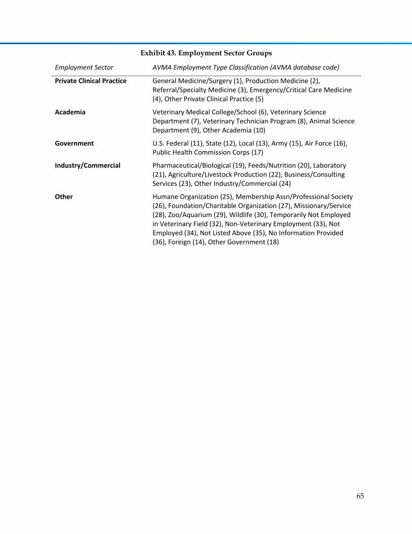
65
Exhibit 43. Employment Sector Groups
Employment Sector AVMA Employment Type Classification (AVMA database code)
Private Clinical Practice General Medicine/Surgery (1), Production Medicine (2), Referral/Specialty Medicine (3), Emergency/Critical Care Medicine (4), Other Private Clinical Practice (5)
Academia Veterinary Medical College/School (6), Veterinary Science Department (7), Veterinary Technician Program (8), Animal Science Department (9), Other Academia (10)
Government U.S. Federal (11), State (12), Local (13), Army (15), Air Force (16), Public Health Commission Corps (17)
Industry/Commercial Pharmaceutical/Biological (19), Feeds/Nutrition (20), Laboratory (21), Agriculture/Livestock Production (22), Business/Consulting Services (23), Other Industry/Commercial (24)
Other Humane Organization (25), Membership Assn/Professional Society (26), Foundation/Charitable Organization (27), Missionary/Service (28), Zoo/Aquarium (29), Wildlife (30), Temporarily Not Employed in Veterinary Field (32), Non-Veterinary Employment (33), Not Employed (34), Not Listed Above (35), No Information Provided (36), Foreign (14), Other Government (18)

66
Exhibit 44. Population Cross-Classification and Subgroup Counts
Active Veterinarians Age 50 and Older
Employment Sector Female Male
Private Clinical Practice 11,129 25,757
Academia 1,272 2,892
Government 708 2,380
Industry/Commercial 626 1,827
Other 6,006 7,685
Total 19,741 40,541
Active Veterinarians Younger than Age 50
Employment Sector Female Male
Private Clinical Practice 20,444 9,520
Academia 1,641 830
Government 517 254
Industry/Commercial 418 304
Other 6,438 2,527
Total 29,458 13,435
Retired Veterinarians
Employment Sector Female Male
Private Clinical Practice 53 699
Academia 10 69
Government 4 42
Industry/Commercial 7 55
Other 17 103
Total 91 968
Within each of the subgroups, veterinarians were randomly selected for inclusion in the sample
in sufficient number to achieve a target margin of error rate of +/-3% for each of the subgroups.
This target yielded a total sample size of 11,443 veterinarians. The subgroup distributions are
shown in Exhibit 45.

67
Exhibit 45. Sample Subgroup Counts
Active Veterinarians Age 50 and Older
Employment Sector Female Male
Private Clinical Practice 747 776
Academia 491 627
Government 380 595
Industry/Commercial 386 523
Other 706 725
Total 2,710 3,246
Active Veterinarians Younger than Age 50
Employment Sector Female Male
Private Clinical Practice 770 738
Academia 538 408
Government 314 193
Industry/Commercial 275 221
Other 712 608
Total 2,609 2,168
Retired Veterinarians
Employment Sector Female Male
Private Clinical Practice 38 437
Academia 12 48
Government 3 33
Industry/Commercial 4 46
Other 13 76
Total 70 640
Survey Distribution Details
Data collection began on September 11, 2012 with an email sent to each veterinarian selected
into the sample. Reminder emails were sent to non-respondent veterinarians on September 17
September 30, October 11, and October 28. The online survey remained open through
November 2, 2012, at which point data collection was closed.

68
Response Rate Analysis
In all, 3,497 responses were collected from the 11,443 veterinarians sampled, for an unadjusted
response rate of 30.6% (3,497 ÷ 11,443). The unadjusted response rate was a biased indicator of
the actual level of response to the survey because it did not take into account that some portion
of the sampled veterinarians never received the invitation or follow-up emails due to outdated
or incorrect email address information from the AVMA database or because the emails were
rejected by a spam filter or other software system that blocks potentially unwanted email
automatically. Among the 11,443 veterinarians sampled, 1,138 of the email addresses in the
database were undeliverable and 264 yielded a response that the email could not be delivered
because it was considered spam. Taking these responses into account, the adjusted sample size
was 10,041. The adjusted response rate, then, was 34.8% (3,497 ÷ 10,041).
Exhibit 46 through Exhibit 50 present the findings of an analysis of the response rates for select
sample subgroups. The tables include the response rate, the figures used to calculate the rate, as
well as statistics to determine whether the rates were different.
Exhibit 46. Survey Response by Gender
Gender Rate N Responses F p
Male 33.7% 5,224 1,761 4.234 < 0.040
Female 35.7% 4,817 1,718
In terms of gender, response levels among male and female veterinarians varied statistically (F
= 4.234; p < 0.040). Female veterinarians were slightly more likely to respond (35.7%) than male
veterinarians (33.7%).
In terms of employment sector, response levels in the five categories varied statistically (F =
50.035; p < 0.001). Veterinarians in the government employment sector were the most likely to
respond to the survey (44.1%), followed closely by those in academia (41.8%) and in the
industry/commercial sector (40.8%). Veterinarians in the private clinical practice and other
employment sectors were least likely to respond to the survey (29.0% and 28.7%, respectively).
Exhibit 47. Survey Response by Employment Sector
Employment Sector Rate N Responses F p
Private clinical practice 29.0% 3,275 949
50.035 < 0.001
Academia 41.8% 1,845 772
Government 44.1% 1,259 555
Industry/Commercial 40.8% 1,253 511
Other 28.7% 2,409 692
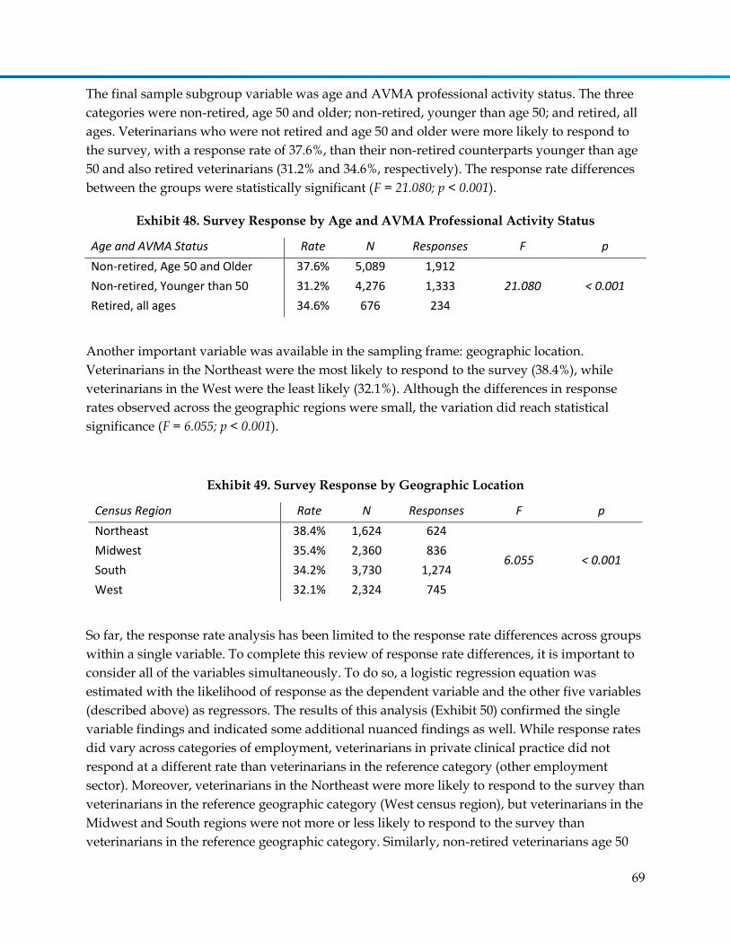
69
The final sample subgroup variable was age and AVMA professional activity status. The three
categories were non-retired, age 50 and older; non-retired, younger than age 50; and retired, all
ages. Veterinarians who were not retired and age 50 and older were more likely to respond to
the survey, with a response rate of 37.6%, than their non-retired counterparts younger than age
50 and also retired veterinarians (31.2% and 34.6%, respectively). The response rate differences
between the groups were statistically significant (F = 21.080; p < 0.001).
Exhibit 48. Survey Response by Age and AVMA Professional Activity Status
Age and AVMA Status Rate N Responses F p
Non-retired, Age 50 and Older 37.6% 5,089 1,912
21.080 < 0.001 Non-retired, Younger than 50 31.2% 4,276 1,333
Retired, all ages 34.6% 676 234
Another important variable was available in the sampling frame: geographic location.
Veterinarians in the Northeast were the most likely to respond to the survey (38.4%), while
veterinarians in the West were the least likely (32.1%). Although the differences in response
rates observed across the geographic regions were small, the variation did reach statistical
significance (F = 6.055; p < 0.001).
Exhibit 49. Survey Response by Geographic Location
Census Region Rate N Responses F p
Northeast 38.4% 1,624 624
6.055 < 0.001 Midwest 35.4% 2,360 836
South 34.2% 3,730 1,274
West 32.1% 2,324 745
So far, the response rate analysis has been limited to the response rate differences across groups
within a single variable. To complete this review of response rate differences, it is important to
consider all of the variables simultaneously. To do so, a logistic regression equation was
estimated with the likelihood of response as the dependent variable and the other five variables
(described above) as regressors. The results of this analysis (Exhibit 50) confirmed the single
variable findings and indicated some additional nuanced findings as well. While response rates
did vary across categories of employment, veterinarians in private clinical practice did not
respond at a different rate than veterinarians in the reference category (other employment
sector). Moreover, veterinarians in the Northeast were more likely to respond to the survey than
veterinarians in the reference geographic category (West census region), but veterinarians in the
Midwest and South regions were not more or less likely to respond to the survey than
veterinarians in the reference geographic category. Similarly, non-retired veterinarians age 50
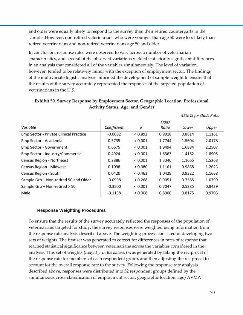
70
and older were equally likely to respond to the survey than their retired counterparts in the
sample. However, non-retired veterinarians who were younger than age 50 were less likely than
retired veterinarians and non-retired veterinarians age 50 and older.
In conclusion, response rates were observed to vary across a number of veterinarian
characteristics, and several of the observed variations yielded statistically significant differences
in an analysis that considered all of the variables simultaneously. The level of variation,
however, tended to be relatively minor with the exception of employment sector. The findings
of the multivariate logistic analysis informed the development of sample weight to ensure that
the results of the survey accurately represented the responses of the targeted population of
veterinarians in the U.S.
Exhibit 50. Survey Response by Employment Sector, Geographic Location, Professional
Activity Status, Age, and Gender
95% CI for Odds Ratio
Variable Coefficient p Odds Ratio Lower Upper
Emp Sector - Private Clinical Practice -0.0082 < 0.892 0.9918 0.8814 1.1161
Emp Sector - Academia 0.5735 < 0.001 1.7744 1.5604 2.0178
Emp Sector - Government 0.6675 < 0.001 1.9494 1.6884 2.2507
Emp Sector - Industry/Commercial 0.4924 < 0.001 1.6363 1.4162 1.8905
Census Region - Northeast 0.2886 < 0.001 1.3346 1.1665 1.5268
Census Region - Midwest 0.1098 < 0.080 1.1161 0.9868 1.2623
Census Region - South 0.0420 < 0.463 1.0429 0.9322 1.1668
Sample Grp – Non-retired 50 and Older -0.0998 < 0.268 0.9051 0.7585 1.0799
Sample Grp – Non-retired > 50 -0.3500 < 0.001 0.7047 0.5885 0.8439
Male -0.1158 < 0.008 0.8906 0.8175 0.9703
Response Weighting Procedures
To ensure that the results of the survey accurately reflected the responses of the population of
veterinarians targeted for study, the survey responses were weighted using information from
the response rate analysis described above. The weighting process consisted of developing two
sets of weights. The first set was generated to correct for differences in rates of response that
reached statistical significance between veterinarians across the variables considered in the
analysis. This set of weights (weight_r in the dataset) was generated by taking the reciprocal of
the response rate for members of each respondent group, and then adjusting the reciprocal to
account for the overall response rate to the survey. Following the response rate analysis
described above, responses were distributed into 32 respondent groups defined by the
simultaneous cross-classification of employment sector, geographic location, age/AVMA

71
professional status, and gender (Exhibit 51). The specific weights and calculations used to
develop them are presented in Exhibit 52.
Exhibit 51. Respondent Group Cross-Classification
Group ID Gender Region Sample Group Employment Sector
1 Male Northeast Non-Retired 50 and Older & Retired Private Clinical & Other
2 Male Northeast Non-Retired 50 and Older & Retired Academia
3 Male Northeast Non-Retired 50 and Older & Retired Government
4 Male Northeast Non-Retired 50 and Older & Retired Industry/Commercial
5 Male Midwest & South & West Non-Retired 50 and Older & Retired Private Clinical & Other
6 Male Midwest & South & West Non-Retired 50 and Older & Retired Academia
7 Male Midwest & South & West Non-Retired 50 and Older & Retired Government
8 Male Midwest & South & West Non-Retired 50 and Older & Retired Industry/Commercial
9 Male Northeast Non-Retired Younger than 50 Private Clinical & Other
10 Male Northeast Non-Retired Younger than 50 Academia
11 Male Northeast Non-Retired Younger than 50 Government
12 Male Northeast Non-Retired Younger than 50 Industry/Commercial
13 Male Midwest & South & West Non-Retired Younger than 50 Private Clinical & Other
14 Male Midwest & South & West Non-Retired Younger than 50 Academia
15 Male Midwest & South & West Non-Retired Younger than 50 Government
16 Male Midwest & South & West Non-Retired Younger than 50 Industry/Commercial
17 Female Northeast Non-Retired 50 and Older & Retired Private Clinical & Other
18 Female Northeast Non-Retired 50 and Older & Retired Academia
19 Female Northeast Non-Retired 50 and Older & Retired Government
20 Female Northeast Non-Retired 50 and Older & Retired Industry/Commercial
21 Female Midwest & South & West Non-Retired 50 and Older & Retired Private Clinical & Other
22 Female Midwest & South & West Non-Retired 50 and Older & Retired Academia
23 Female Midwest & South & West Non-Retired 50 and Older & Retired Government
24 Female Midwest & South & West Non-Retired 50 and Older & Retired Industry/Commercial
25 Female Northeast Non-Retired Younger than 50 Private Clinical & Other
26 Female Northeast Non-Retired Younger than 50 Academia
27 Female Northeast Non-Retired Younger than 50 Government
28 Female Northeast Non-Retired Younger than 50 Industry/Commercial
29 Female Midwest & South & West Non-Retired Younger than 50 Private Clinical & Other
30 Female Midwest & South & West Non-Retired Younger than 50 Academia
31 Female Midwest & South & West Non-Retired Younger than 50 Government
32 Female Midwest & South & West Non-Retired Younger than 50 Industry/Commercial
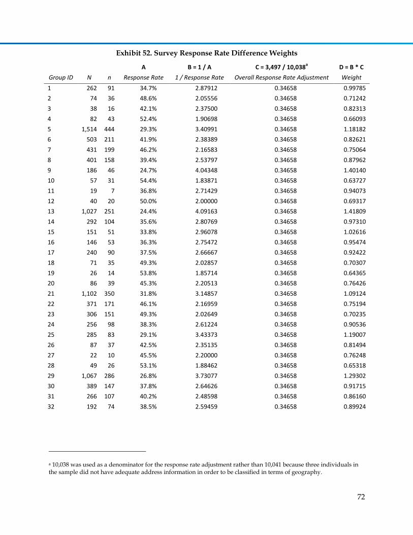
72
Exhibit 52. Survey Response Rate Difference Weights
A B = 1 / A C = 3,497 / 10,038a D = B * C
Group ID N n Response Rate 1 / Response Rate Overall Response Rate Adjustment Weight
1 262 91 34.7% 2.87912 0.34658 0.99785
2 74 36 48.6% 2.05556 0.34658 0.71242
3 38 16 42.1% 2.37500 0.34658 0.82313
4 82 43 52.4% 1.90698 0.34658 0.66093
5 1,514 444 29.3% 3.40991 0.34658 1.18182
6 503 211 41.9% 2.38389 0.34658 0.82621
7 431 199 46.2% 2.16583 0.34658 0.75064
8 401 158 39.4% 2.53797 0.34658 0.87962
9 186 46 24.7% 4.04348 0.34658 1.40140
10 57 31 54.4% 1.83871 0.34658 0.63727
11 19 7 36.8% 2.71429 0.34658 0.94073
12 40 20 50.0% 2.00000 0.34658 0.69317
13 1,027 251 24.4% 4.09163 0.34658 1.41809
14 292 104 35.6% 2.80769 0.34658 0.97310
15 151 51 33.8% 2.96078 0.34658 1.02616
16 146 53 36.3% 2.75472 0.34658 0.95474
17 240 90 37.5% 2.66667 0.34658 0.92422
18 71 35 49.3% 2.02857 0.34658 0.70307
19 26 14 53.8% 1.85714 0.34658 0.64365
20 86 39 45.3% 2.20513 0.34658 0.76426
21 1,102 350 31.8% 3.14857 0.34658 1.09124
22 371 171 46.1% 2.16959 0.34658 0.75194
23 306 151 49.3% 2.02649 0.34658 0.70235
24 256 98 38.3% 2.61224 0.34658 0.90536
25 285 83 29.1% 3.43373 0.34658 1.19007
26 87 37 42.5% 2.35135 0.34658 0.81494
27 22 10 45.5% 2.20000 0.34658 0.76248
28 49 26 53.1% 1.88462 0.34658 0.65318
29 1,067 286 26.8% 3.73077 0.34658 1.29302
30 389 147 37.8% 2.64626 0.34658 0.91715
31 266 107 40.2% 2.48598 0.34658 0.86160
32 192 74 38.5% 2.59459 0.34658 0.89924
a 10,038 was used as a denominator for the response rate adjustment rather than 10,041 because three individuals in the sample did not have adequate address information in order to be classified in terms of geography.
73
The second set of weights was generated to allow for a national-level benchmark to be
developed for each question on the survey. Because the sample was selected in a
disproportionate manner in order to produce accurate estimates within subgroups defined by
the strata variables of the population of veterinarians targeted for use in developing supply and
demand model parameters, the strata characteristics in the sample were not distributed in the
same manner as they were in the targeted population of veterinarians in the U.S. Thus, in the
aggregate, they did not represent the targeted population of veterinarians. To correct for the
differences in the distribution of these characteristics, the reciprocal of the sampling fraction
(adjusted for the total response rate) was used as the basis for the sampling design adjustment
factor (Exhibit 53).
The final step in creating the national-level benchmark weight was to correct for the identified
response rate differences identified in Exhibit 50. The adjustment was made by multiplying the
sampling design adjustment factor values (weightb) by the weights presented in Exhibit 51
(weight_r). This second set of weights was labeled weight_bmark_final in the dataset. This set of
weights should only be used to generate national-level population benchmarks.

74
Exhibit 53. Sampling Design Adjustment
Gender
Sample Group A B C = B / A D = 1 / C E = 10,041 / 104,234 F = D * E
Employment Sector Population Sample Sampling fraction
1 / Sampling fraction
Total Sampling Fraction Adjustment
Sampling Design
Adjustment
Male
Non-retired, Age 50 and Older
Private Clinical Practice 25,757 714 0.0277 36.0742 0.0963 3.4750
Academia 2,892 532 0.1840 5.4361 0.0963 0.5237
Government 2,380 438 0.1840 5.4338 0.0963 0.5234
Industry/Commercial 1,827 442 0.2419 4.1335 0.0963 0.3982
Other 7,685 570 0.0742 13.4825 0.0963 1.2988
Non-retired, Younger than Age 50
Private Clinical Practice 9,520 684 0.0718 13.9181 0.0963 1.3407
Academia 830 349 0.4205 2.3782 0.0963 0.2291
Government 254 170 0.6693 1.4941 0.0963 0.1439
Industry/Commercial 304 186 0.6118 1.6344 0.0963 0.1574
Other 2,527 529 0.2093 4.7769 0.0963 0.4602
Retired, All ages
Private Clinical Practice 699 419 0.5994 1.6683 0.0963 0.1607
Academia 69 46 0.6667 1.5000 0.0963 0.1445
Government 42 31 0.7381 1.3548 0.0963 0.1305
Industry/Commercial 55 41 0.7455 1.3415 0.0963 0.1292
Other 103 73 0.7087 1.4110 0.0963 0.1359
Female
Non-retired, Age 50 and Older
Private Clinical Practice 11,129 694 0.0624 16.0360 0.0963 1.5448
Academia 1,272 431 0.3388 2.9513 0.0963 0.2843
Government 708 329 0.4647 2.1520 0.0963 0.2073
Industry/Commercial 626 338 0.5399 1.8521 0.0963 0.1784
Other 6,006 601 0.1001 9.9933 0.0963 0.9627
Non-retired, Younger than Age 50
Private Clinical Practice 20,444 728 0.0356 28.0824 0.0963 2.7052
Academia 1,641 476 0.2901 3.4475 0.0963 0.3321
Government 517 288 0.5571 1.7951 0.0963 0.1729
Industry/Commercial 418 242 0.5789 1.7273 0.0963 0.1664
Other 6,438 624 0.0969 10.3173 0.0963 0.9939
Retired
Private Clinical Practice 53 36 0.6792 1.4722 0.0963 0.1418
Academia 11 11 1.0000 1.0000 0.0963 0.0963
Government 4 3 0.7500 1.3333 0.0963 0.1284
Industry/Commercial 7 4 0.5714 1.7500 0.0963 0.1686
Other 17 12 0.7059 1.4167 0.0963 0.1365

75
B. Survey Results
The survey responses presented in this section have been weighted to account for the response
rate variations and sampling design. Survey respondents were distributed relatively evenly by
gender, with women making up 48% of the respondents and men making up 52% (Exhibit 54).
The median age of a respondent was 54 years of age. Among women, the median age was 45
years of age, and among men, the median age was 60 years of age.
Exhibit 54. Respondent Demographics: Gender and Age
Gender Number of
Respondents Percentage of Respondents
Female 1,671 48%
Male 1,808 52%
Age Category Number of
Respondents Percentage of Respondents
Younger than 30 years of age 176 5%
30 to 39 years of age 646 19%
40 to 49 years of age 642 18%
50 to 59 years of age 900 26%
60 to 69 years of age 718 21%
70 years of age and older 398 11%
Age Category Female Percentage Male Percentage
Younger than 30 years of age 159 10% 17 1%
30 to 39 years of age 438 26% 208 12%
40 to 49 years of age 411 25% 231 13%
50 to 59 years of age 492 29% 408 23%
60 to 69 years of age 147 9% 571 32%
70 years of age and older 25 1% 372 21%
Nearly two-thirds (65%) of the respondents were associated with the private clinical practice
employment sector (Exhibit 55). Respondents from the “other” sector made up the next largest
group of respondents at slightly less than one-quarter (22%) of the total respondents.
Respondents from the academia, government, and industry/commercial sector made up about
6%, 4%, and 3%, respectively, of respondents.
The youngest respondents were found in the private clinical practice sector with a median age
of 53 years of age. Respondents from the academic, government, and industry/commercial
sectors had a median age of 57 years of age.

76
Exhibit 55. Respondent Demographics: Employment Sector
Employment Sector Number of
Respondents Percentage of Respondents Median Age
Private Clinical Practice 2,250 65% 53
Academia 226 6% 57
Government 132 4% 57
Industry/Commercial 110 3% 57
Other 762 22% 56
A total of 381 respondents reported being permanently inactive in veterinary medicine (Exhibit
56). Among them, the median age at which respondents become permanently inactive was 62
years of age. Looking at the distribution of the reported age at the time of becoming
permanently inactive revealed that there was a rate of attrition among young veterinarians. Of
the veterinarians who reported being permanently inactive in veterinary medicine, just over
one-quarter (26%) left the workforce before age 60. This did not imply, however, that one-
quarter of veterinarians would retire by age 60. For example, if older veterinarians had died
then their ages at leaving the workforce were unknown.
Exhibit 56. Age when Became Permanently Inactive in Veterinary Medicine
Age Category (Age when became permanently inactive)
Number of Respondents
Percentage of Respondents
Younger than 30 years of age 3 1%
30 to 39 years of age 14 4%
40 to 49 years of age 20 6%
50 to 59 years of age 53 15%
60 to 64 years of age 113 32%
65 to 69 years of age 76 22%
70 to 74 years of age 35 10%
75 years of age and older 37 11%
Of the respondents who reported being active in veterinary medicine or being temporarily
inactive, 45% reported an age at which they planned to become permanently inactive, 24%
reported that they had no specific plans to become permanently inactive, but indicated plans to
reduce the amount of time they spend in veterinary medicine at a specified age, and 31%
reported that they had no plans to become permanently inactive (Exhibit 57).

77
Exhibit 57. Reported Plans for Becoming Permanently Inactive in Veterinary Medicine
Among those respondents who reported an age at which they planned to become permanently
inactive in veterinary medicine, the median age reported was 65 years of age. Exhibit 58
presents the distribution of responses across age categories. More than one-third (34%) of
respondents reported plans to remain active in veterinary medicine until at least 70 years of age.
Note that findings from Exhibit 58 (anticipated age at retirement) are not directly comparable to
findings from Exhibit 56 (age distribution of those who have retired). Some departures from the
workforce are unplanned (e.g., departure for health problems, or departure for unanticipated
career change influenced by job opportunities). Also, the large influx of new graduates over the
past two decades means that a large portion of veterinarians have not reached traditional
retirement age so the data on inactive veterinarians has a disproportion number of people who
have left the workforce before traditional retirement age.
Exhibit 58. Age when Plan to Become Permanently Inactive in Veterinary Medicine
Age Category (Age when plan to become perm. inactive)
Number of Respondents
Percentage of Respondents
Younger than 50 years of age 12 1%
50 to 59 years of age 83 7%
60 to 64 years of age 235 19%
65 to 69 years of age 503 40%
70 to 74 years of age 275 22%
75 years of age and older 146 12%
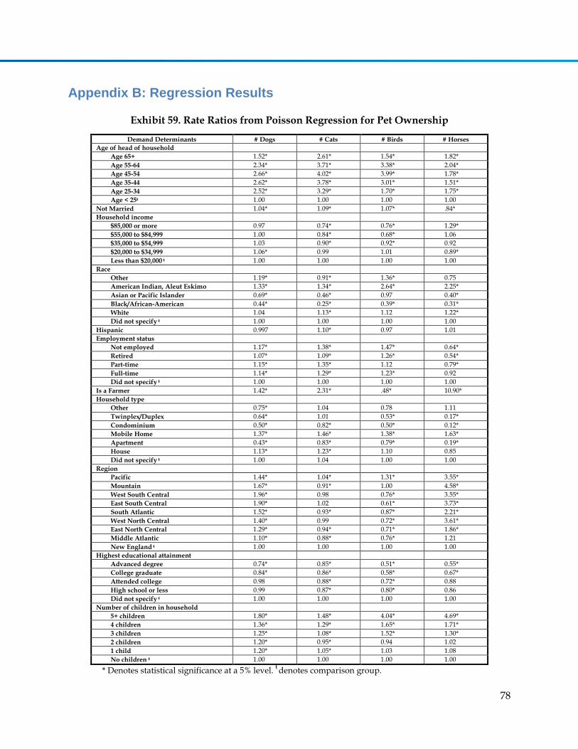
78
Appendix B: Regression Results
Exhibit 59. Rate Ratios from Poisson Regression for Pet Ownership
Demand Determinants # Dogs # Cats # Birds # Horses
Age of head of household
Age 65+ 1.52* 2.61* 1.54* 1.82*
Age 55-64 2.34* 3.71* 3.38* 2.04*
Age 45-54 2.66* 4.02* 3.99* 1.78*
Age 35-44 2.62* 3.78* 3.01* 1.51*
Age 25-34 2.52* 3.29* 1.70* 1.75*
Age < 25ŧ 1.00 1.00 1.00 1.00
Not Married 1.04* 1.09* 1.07* .84*
Household income
$85,000 or more 0.97 0.74* 0.76* 1.29*
$55,000 to $84,999 1.00 0.84* 0.68* 1.06
$35,000 to $54,999 1.03 0.90* 0.92* 0.92
$20,000 to $34,999 1.06* 0.99 1.01 0.89*
Less than $20,000 ŧ 1.00 1.00 1.00 1.00
Race
Other 1.19* 0.91* 1.36* 0.75
American Indian, Aleut Eskimo 1.33* 1.34* 2.64* 2.25*
Asian or Pacific Islander 0.69* 0.46* 0.97 0.40*
Black/African-American 0.44* 0.25* 0.39* 0.31*
White 1.04 1.13* 1.12 1.22*
Did not specify ŧ 1.00 1.00 1.00 1.00
Hispanic 0.997 1.10* 0.97 1.01
Employment status
Not employed 1.17* 1.38* 1.47* 0.64*
Retired 1.07* 1.09* 1.26* 0.54*
Part-time 1.15* 1.35* 1.12 0.79*
Full-time 1.14* 1.29* 1.23* 0.92
Did not specify ŧ 1.00 1.00 1.00 1.00
Is a Farmer 1.42* 2.31* .48* 10.90*
Household type
Other 0.75* 1.04 0.78 1.11
Twinplex/Duplex 0.64* 1.01 0.53* 0.17*
Condominium 0.50* 0.82* 0.50* 0.12*
Mobile Home 1.37* 1.46* 1.38* 1.63*
Apartment 0.43* 0.83* 0.79* 0.19*
House 1.13* 1.23* 1.10 0.85
Did not specify ŧ 1.00 1.04 1.00 1.00
Region
Pacific 1.44* 1.04* 1.31* 3.55*
Mountain 1.67* 0.91* 1.00 4.58*
West South Central 1.96* 0.98 0.76* 3.55*
East South Central 1.90* 1.02 0.61* 3.73*
South Atlantic 1.52* 0.93* 0.87* 2.21*
West North Central 1.40* 0.99 0.72* 3.61*
East North Central 1.29* 0.94* 0.71* 1.86*
Middle Atlantic 1.10* 0.88* 0.76* 1.21
New England ŧ 1.00 1.00 1.00 1.00
Highest educational attainment
Advanced degree 0.74* 0.85* 0.51* 0.55*
College graduate 0.84* 0.86* 0.58* 0.67*
Attended college 0.98 0.88* 0.72* 0.88
High school or less 0.99 0.87* 0.80* 0.86
Did not specify ŧ 1.00 1.00 1.00 1.00
Number of children in household
5+ children 1.80* 1.48* 4.04* 4.69*
4 children 1.36* 1.29* 1.65* 1.71*
3 children 1.25* 1.08* 1.52* 1.30*
2 children 1.20* 0.95* 0.94 1.02
1 child 1.20* 1.05* 1.03 1.08
No children ŧ 1.00 1.00 1.00 1.00
* Denotes statistical significance at a 5% level. ŧ denotes comparison group.

79
Exhibit 60. Rate Ratios from Poisson Regression for Dog Services
Exams Vaccines
Emergency Care
Lab Work Drugs Flea/Worm Surgery Behavior Euthanized Other
Age of head of household
Age 65+ 0.96 0.99 1.00 1.30* 1.18* 1.35* 0.95 0.73 2.13* 0.99
Age 55-64 0.95 1.02 0.92 1.27* 1.19* 1.15 0.87 0.59 2.07* 0.90
Age 45-54 0.96 1.03 0.91 1.16 1.13 1.15 0.85 0.58 1.56 0.84*
Age 35-44 0.96 1.01 0.90 1.10 1.07 1.06 0.80 0.41* 1.66* 0.79*
Age 25-34 0.98 1.05 0.83 1.02 0.99 1.14 0.80 0.76 0.98 0.85*
Age < 25ŧ 1.00 1.00 1.00 1.00 1.00 1.00 1.00 1.00 1.00 1.00
Not Married 1.01 0.98 0.98 1.02 0.99 0.97 1.02 1.05 0.92 1.05
Household income
$85,000 or more 1.27* 1.11* 1.04 1.65* 1.22* 1.01 1.13 1.01 0.91 1.57*
$55,000 to $84,999 1.26* 1.14* 1.05 1.59* 1.20* 1.01 1.00 0.75 0.93 1.28*
$35,000 to $54,999 1.23* 1.14* 0.97 1.42* 1.20* 1.00 1.00 0.76 0.95 1.15*
$20,000 to $34,999 1.14* 1.10* 1.02 1.16* 1.09 1.02 0.97 0.90 0.97 1.12
Less than $20,000 ŧ 1.00 1.00 1.00 1.00 1.00 1.00 1.00 1.00 1.00 1.00
Race
Other 1.06 0.95 1.19 1.29 0.99 0.92 1.07 1.86 1.11 1.25
American Indian, Aleut Eskimo 1.06 1.05 1.09 0.91* 0.98 1.23 1.10 0.00 0.37 1.07
Asian or Pacific Islander 1.03 0.96 0.97 1.13 0.84 1.07 1.11 4.80* 1.72 1.12
Black/African-American 0.97 0.95 0.96 0.77 0.74 1.04 0.87 2.07 0.55 1.38*
White 1.08 0.98 0.93 1.21 1.10* 0.94 1.04 2.18 1.05 0.99
Did not specify ŧ 1.00 1.00 1.00 1.00 1.00 1.00 1.00 1.00 1.00 1.00
Hispanic 1.00 0.99 0.91* 0.98 1.00 1.02 0.90 0.90 1.03 0.90*
Employment status
Not employed 1.10* 1.07 0.91 1.14 1.26* 1.01 0.56* 0.32* 0.67* 0.96
Retired 1.09* 1.05 1.00 1.19 1.31* 1.05 0.73* 0.48* 0.89 1.10
Part-time 1.08 1.03 0.84 1.03 1.20* 0.99 0.70* 0.47* 0.81 1.05
Full-time 1.06 1.04 0.88 1.07 1.18* 0.99 0.71* 0.58* 0.83 0.92
Did not specify ŧ 1.00 1.00 1.00 1.00 1.00 1.00 1.00 1.00 1.00 1.00
Is a Farmer 0.56* 0.77* 1.21* 0.79* 0.68* 1.31 1.09 0.00 0.92 0.73
Household type
Other 1.01 0.96 1.19 1.11 1.00 0.80 1.79 1.61 1.13 1.13
Twinplex/Duplex 1.06 0.86 0.93 1.04 1.03 0.76 1.45 0.76 0.99 1.06
Condominium 1.09 0.96 1.06 1.11 1.04 0.73* 1.32 1.48 1.02 1.18

80
Exams Vaccines
Emergency Care
Lab Work Drugs Flea/Worm Surgery Behavior Euthanized Other
Mobile Home 0.98 0.94 0.94 0.85 0.99 0.92 0.82 0.51 0.79 0.74*
Apartment 1.11 1.00 0.90 0.90 1.05 0.84 1.00 1.57 0.87 1.03
House 1.03 0.96 0.97 0.91 1.06 0.83 1.18 1.13 1.23 0.86
Did not specify ŧ 1.00 1.00 1.00 1.00 1.00 1.00 1.00 1.00 1.00 1.00
Region
Pacific 0.82* 0.92 0.87 0.65* 0.78* 0.56* 1.51* 1.01 0.71* 0.99
Mountain 0.94 0.99 0.82* 0.65* 0.80* 0.28* 1.41* 0.99 0.67* 1.05
West South Central 0.86* 1.03 0.68* 0.65* 0.92 1.00 1.11 0.72 0.54* 1.18
East South Central 0.87* 0.99 0.67* 0.74* 0.95 1.13 0.99 0.40* 0.50* 1.27*
South Atlantic 0.95 1.02 0.67* 0.86* 0.98 1.07 1.09 0.81 0.59* 1.09
West North Central 0.89* 1.01 0.66* 0.75* 0.89 0.84* 1.20 0.57 0.73* 1.24*
East North Central 0.98 1.01 0.71* 0.84* 0.96 0.90 1.20 0.53 0.77 1.06
Middle Atlantic 1.03 1.00 0.84* 0.80* 0.94 0.81* 1.11 1.01 0.70* 0.92
New England ŧ 1.00 1.00 1.00 1.00 1.00 1.00 1.00 1.00 1.00 1.00
Highest educational attainment
Advanced degree 1.09 0.97 1.06 1.06 1.14 1.04 1.52 0.71 1.16 1.08
College graduate 1.09 1.01 1.03 0.96 1.07 0.99 1.41 0.64 1.16 0.97
Attended college 1.05 1.00 1.04 0.94 1.03 0.99 1.40 0.59 1.20 0.90
High school or less 0.95 0.96 0.94 0.74* 0.90 0.98 1.31 0.38* 0.91 0.75*
Did not specify ŧ 1.00 1.00 1.00 1.00 1.00 1.00 1.00 1.00 1.00 1.00
Number of children in household
5+ children 0.62* 0.80 0.77 0.43* 0.47* 0.87 0.95 0.00 0.00 0.38*
4 children 0.97 1.05 1.11 0.78* 0.74* 1.02 0.91 0.92 0.65 0.94
3 children 0.94 1.01 0.87 0.74* 0.70* 1.00 0.75* 0.39* 0.65* 0.78*
2 children 0.98 1.05 0.83* 0.79* 0.77* 1.05 0.74* 0.66 0.90 0.86*
1 child 1.01 1.01 0.94 0.91* 0.94* 1.01 0.93 1.19 0.91 0.93
No children ŧ 1.00 1.00 1.00 1.00 1.00 1.00 1.00 1.00 1.00 1.00
Number of dogs 0.99 0.99 1.04* 1.01 1.02* 1.00 1.04* 1.05* 1.04* 0.99
* Denotes statistical significance at a 5% level. ŧ denotes comparison group.

81
Exhibit 61. Rate Ratios from Poisson Regression for Cat Services
Exams Vaccines
Emergency Care
Lab Work Drugs Flea/Worm Surgery Behavior Euthanized Other
Age of head of household
Age 65+ 0.87* 0.83* 1.18 0.95 1.04 1.00 0.99 0.61 1.32 1.53*
Age 55-64 0.91 0.89* 1.07 0.92 1.07 0.99 0.80 0.59 1.15 1.60*
Age 45-54 0.90 0.90 1.12 0.91 0.98 1.02 0.90 0.54 1.16 1.25
Age 35-44 0.91 0.89 1.06 0.95 0.94 0.97 0.81 0.84 1.10 1.04
Age 25-34 0.95 0.91 1.07 0.92 0.98 0.94 1.01 0.86 0.96 0.63
Age < 25ŧ 1.00 1.00 1.00 1.00 1.00 1.00 1.00 1.00 1.00 1.00
Not Married 1.00 0.95* 1.00 1.04 1.06 0.97 0.92 0.92 1.03 1.05
Household income
$85,000 or more 1.36* 1.20* 1.20* 1.69* 1.28* 0.75* 1.06 1.57 1.45 1.02
$55,000 to $84,999 1.36* 1.22* 1.19* 1.60* 1.36* 0.80* 1.21 1.09 1.22 1.16*
$35,000 to $54,999 1.32* 1.18* 1.08 1.47* 1.35* 0.89 0.94 1.02 1.15 1.05
$20,000 to $34,999 1.19* 1.10* 1.07 1.22* 1.21* 0.95 0.93 1.47 1.02 0.92
Less than $20,000 ŧ 1.00 1.00 1.00 1.00 1.00 1.00 1.00 1.00 1.00 1.00
Race
Other 1.17 1.18 0.88 1.16 1.18 1.12 1.63 0.50 1.33* 0.37
American Indian, Aleut Eskimo 1.11 1.17 0.91 1.36 1.43 1.19 1.65 0.79 1.12 0.28
Asian or Pacific Islander 1.12 1.02 0.94 1.28 1.15 0.97 0.84 0.78 1.43 0.75
Black/African-American 1.01 1.01 0.94 0.79 0.85 1.07 1.30 0.48 1.22 0.66
White 1.15 1.11 0.86 1.22 1.21 1.10 1.54 0.42* 0.93 0.91
Did not specify ŧ 1.00 1.00 1.00 1.00 1.00 1.00 1.00 1.00 1.00 1.00
Hispanic 0.83* 0.85* 1.04* 0.82* 0.74 1.15 0.86 1.32 0.98 1.49*
Employment status
Not employed 1.18* 1.19* 0.92 1.29* 1.32* 0.97 0.73 0.73 0.91* 1.70
Retired 1.17* 1.20* 0.91 1.15 1.15 1.17 0.71 1.05 0.97 1.71
Part-time 1.14* 1.13 1.03 1.17 1.28* 1.12 0.78 1.26 0.93 1.45
Full-time 1.10- 1.12 0.86 1.10 1.09 1.04 0.79 0.82 0.94 1.89
Did not specify ŧ 1.00 1.00 1.00 1.00 1.00 1.00 1.00 1.00 1.00 1.00
Is a Farmer 0.49* 0.60* 0.52 0.59 0.53* 1.08 0.25 1.59 0.69 0.00
Household type
Other 1.10 1.25 1.00 1.17 1.18 0.63 0.78 0.40 0.77 1.43
Twinplex/Duplex 1.06 1.18 1.45 0.96 1.30 0.79 0.87 0.79 0.90 1.57
Condominium 1.10 1.16 1.33 1.18 1.19 0.52* 1.14 0.87 1.00 1.70
Mobile Home 0.94 1.14 1.33 0.75 1.05 0.86 1.06 0.35 0.54 1.19

82
Exams Vaccines
Emergency Care
Lab Work Drugs Flea/Worm Surgery Behavior Euthanized Other
Apartment 1.10 1.19 1.27 1.02 1.25 0.87 1.23 0.93 0.87 1.40
House 1.01 1.18 1.26 0.87 1.07 0.85 0.86 0.69 0.68 1.39
Did not specify ŧ 1.00 1.00 1.00 1.00 1.00 1.00 1.00 1.00 1.00 1.00
Region
Pacific 0.81* 0.75* 0.94 0.95 1.02 0.85 1.52* 1.24 0.80 1.04*
Mountain 0.87* 0.85* 0.76* 0.81* 0.85 0.34* 1.30 0.74 0.74 1.04*
West South Central 0.81* 0.87* 0.79* 0.87 1.03 0.89 1.04 0.94 0.67 1.00
East South Central 0.86* 0.93 0.66* 0.76* 1.03 1.14 1.09 0.50 0.64* 0.62*
South Atlantic 0.94 0.96 0.82* 1.02 1.17* 1.17* 1.15 0.98 0.85 0.82*
West North Central 0.87* 0.93 0.76* 0.81* 0.95 0.83 1.08 0.87 0.79 0.98
East North Central 0.94 0.87* 0.80* 0.97 1.21* 0.80* 1.23 1.42 0.74 1.08*
Middle Atlantic 1.03 0.96 1.01 1.02 1.14 0.92 0.99 1.45 0.87 1.04
New England ŧ 1.00 1.00 1.00 1.00 1.00 1.00 1.00 1.00 1.00 1.00
Highest educational attainment
Advanced degree 1.05 1.10 1.13 0.94 0.89 0.84 0.50* 1.10 1.02 2.19
College graduate 1.03 1.10 1.04 0.83 0.85 0.78 0.46* 0.70 0.82 2.15
Attended college 0.96 1.05 1.04 0.76 0.87 0.73* 0.46* 0.65 0.73* 2.28*
High school or less 0.83* 0.95 0.94 0.62* 0.70* 0.72* 0.43* 0.62 0.61* 1.46*
Did not specify ŧ 1.00 1.00 1.00 1.00 1.00 1.00 1.00 1.00 1.00 1.00
Number of children in household
5+ children 0.47* 0.66* 0.96 0.43* 0.26* 0.53 0.30 0.00 0.12 0.93*
4 children 0.82* 0.92 0.74* 0.63* 0.70* 1.27 0.98 0.68 0.55 0.63*
3 children 0.82* 0.88* 0.78* 0.57* 0.71* 1.15 0.84 0.12* 0.60 0.65*
2 children 0.88* 0.98 0.79* 0.74* 0.77 0.99 0.86 0.72 0.58 0.76*
1 child 0.94* 0.97 0.96 0.92 0.94 0.97 0.98 1.28 0.85 0.85*
No children ŧ 1.00 1.00 1.00 1.00 1.00 1.00 1.00 1.00 1.00 1.00
Number of cats 0.99* 0.98* 1.04* 1.03* 1.04* 1.02* 1.04* 1.03* 1.02* 1.04*
* Denotes statistical significance at a 5% level. ŧ denotes comparison group.

83
Appendix C: Modeling Approach Used to Forecast Future U.S.
Production of Food Animals
The U.S. state-level inventory forecast produced by the IHS Agricultural Services group utilizes
a global agricultural modeling complex incorporating a dynamic simultaneous structural partial
equilibrium modeling methodology similar to methods used by the University of Missouri
Food and Agricultural Policy Research Institute (FAPRI), the United States Department of
Agriculture (USDA), and the Food and Agriculture Organization of the United Nations (FAO).
The modeling complex consists of 10 partial equilibrium models covering the following sectors
(Exhibit 62):
U.S. Crops and Biofuels
U.S. Livestock
U.S. Dairy
International Livestock
International Grains
International Oilseeds
Oils and Meals, International Cotton
International Sugar
International Rice
International Biofuels
The above were used in conjunction with other independent and more recursive models
covering Global Cost of Production, Farm Income (for select countries), and Global Caloric
Consumption. Each model leveraged sector-relevant macroeconomic, energy, and exogenous
cost variable forecasts produced by other IHS groups in addition to industry-relevant
exogenous variable forecasts produced from other forecast models developed and maintained
by IHS Agricultural Services.
Each of the partial equilibrium models that made up the global agricultural modeling complex
consisted of linear structural equations, which simulated specific behaviors at the country and
global region level for both the supply and demand sides of various agricultural markets. The
equations applied elasticity-based slope coefficients to behavior specific independent variables
in order to solve for the optimal pricing solution for the market. Optimization from the livestock
and meat industry perspective was achieved by maximizing current year net returns based on
the returns from meat production relative to the cost of producing additional animals in a given
year. Demand side optimization was achieved by simulating utility maximization given the
utility derived from the relative cost incurred in acquiring an additional unit of a commodity.
This was done by applying elasticity slope coefficients to the price of the given commodity, the
prices of its relevant substitutes, and average per capita income. The elasticity slope coefficients
simulated the average consumer’s rate of substitution between two goods given relative price
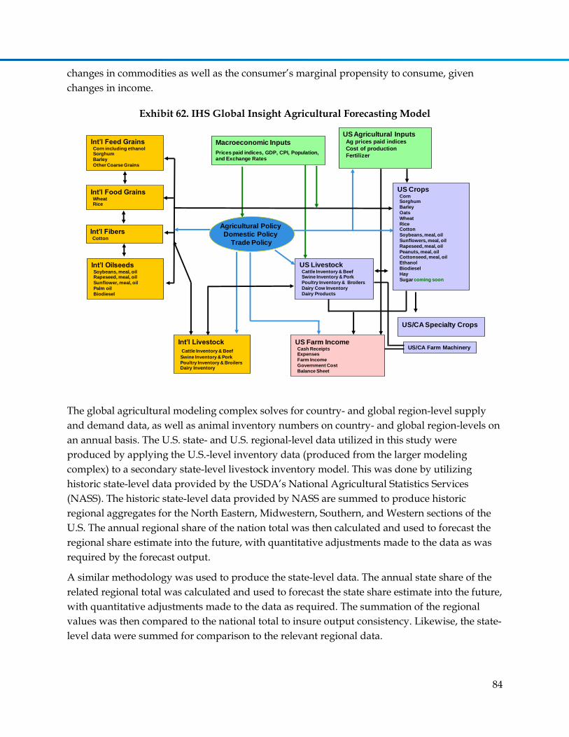
84
changes in commodities as well as the consumer’s marginal propensity to consume, given
changes in income.
Exhibit 62. IHS Global Insight Agricultural Forecasting Model
The global agricultural modeling complex solves for country- and global region-level supply
and demand data, as well as animal inventory numbers on country- and global region-levels on
an annual basis. The U.S. state- and U.S. regional-level data utilized in this study were
produced by applying the U.S.-level inventory data (produced from the larger modeling
complex) to a secondary state-level livestock inventory model. This was done by utilizing
historic state-level data provided by the USDA’s National Agricultural Statistics Services
(NASS). The historic state-level data provided by NASS are summed to produce historic
regional aggregates for the North Eastern, Midwestern, Southern, and Western sections of the
U.S. The annual regional share of the nation total was then calculated and used to forecast the
regional share estimate into the future, with quantitative adjustments made to the data as was
required by the forecast output.
A similar methodology was used to produce the state-level data. The annual state share of the
related regional total was calculated and used to forecast the state share estimate into the future,
with quantitative adjustments made to the data as required. The summation of the regional
values was then compared to the national total to insure output consistency. Likewise, the state-
level data were summed for comparison to the relevant regional data.
Int’l Feed Grains Corn including ethanolSorghum
Barley
Other Coarse Grains
Int’l OilseedsSoybeans, meal, oil Rapeseed, meal, oil
Sunflower, meal, oil
Palm oil
Biodiesel
Int’l FibersCotton
Int’l Food GrainsWheatRice
Int’l Livestock
Cattle Inventory & Beef
Swine Inventory & Pork
Poultry Inventory & BroilersDairy Inventory
US Crops CornSorghum
Barley
Oats
Wheat
RiceCotton
Soybeans, meal, oil
Sunflowers, meal, oil
Rapeseed, meal, oil
Peanuts, meal, oilCottonseed, meal, oil
Ethanol
Biodiesel
Hay
Sugar coming soon
US Livestock Cattle Inventory & BeefSwine Inventory & Pork
Poultry Inventory & Broilers
Dairy Cow Inventory
Dairy Products
US Farm Income Cash ReceiptsExpenses
Farm Income
Government Cost
Balance Sheet
US Agricultural Inputs Ag prices paid indices
Cost of production
Fertilizer
Macroeconomic Inputs
Prices paid indices, GDP, CPI, Population, and Exchange Rates
US/CA Farm Machinery
US/CA Specialty Crops
Agricultural Policy
Domestic Policy
Trade Policy

85
The modeling framework produced annual estimates of national-, regional-, and state-level
inventories of cattle (including specific breakouts for beef and dairy cows), hogs (including a
specific breakout for hogs used for breeding purposes), the number of broiler-type chicks
placed, total sheep and lamb inventories, and the total inventory of turkeys raised for slaughter.
The cattle inventory forecast was for January first-spot inventory values. This was due to the
annual dynamics of the cattle inventory. The actual number of cattle that live within a given
year was neither available nor necessary for measuring the U.S. beef and dairy industry. As
cattle go through predictable gestational and life cycles, an annual spot inventory number was
sufficient for determining the likely path of either expansion or retraction for the herd during a
given year.
December first-inventory numbers were used as an appropriate proxy for the hog industry, for
reasons similar to those stated above for the cattle industry. Although hogs have a shorter
gestational period, as well as a shorter time span from farrowing to slaughter, the period was
long enough and predictable enough that the annual inventory numbers could sufficiently
determine the industry’s path of expansion or retraction during a given time period. The same
was true for the sheep and lamb inventories, which were recorded as the January first number,
similar to cattle.
The inventory data for the turkey and broiler industries were different from the other three
categories, as these industries were able to move at a faster pace than the other industries. The
greater flexibility of the poultry industry rendered spot inventory forecast less accurate, as
inventory numbers could be quickly retracted and then repopulated within a calendar year. Thus,
in order to determine the size and direction of the two poultry industry sectors, annual livestock
production figures were used. The broiler industry was measured by the number of broiler type
chicks placed on feed during a given year, while the turkey industry was measured by the number
of turkeys raised for slaughter in a given year. The two metrics were similar in that both measure
the volume of animals that moved through the industry during a given year. The significant
difference between the two data types was that the broiler inventory was measured at the
beginning of the production process, while the turkey inventory was measured at the end of the
production process.

86
Reference List
1. Brown JP, Silverman JD. The current and future market for veterinarians and veterinary medical services in the United States. J Am Vet Med Assoc 1999;215(2):161-183.
2. Arthur D Little I. Summary of U.S. veterinary medical manpower needs: 1978-1990. J Am Vet Med Assoc 1978;173:369-372.
3. Wise JK, Kushman JE. Synopsis of US veterinary medical manpower study: demand and supply from 1980 to 2000. J Am Vet Med Assoc 1985;187(4):358-361.
4. Getz M. Veterinary Medicine in Economic Transition. Iowa State University Press; 1997.
5. Association of American Veterinary Medical Colleges. Veterinarians step up to the nation's public health needs. Washington, DC: AAVMC; 2006.
6. Sterner KE. An invited perspective on the shortage of veterinarians in food supply veterinary medicine. Journal of the American Veterinary Medical Association 2006;229(1):30-32.
7. Andrus D, Gwinner K, Prince J. Food Supply Veterinary Medicine Coalition: Estimating FSVM Demand and Maintaining the Availability of Veterinarians for Careers in Food Supply Related Disciplines in the United States and Canada. Schaumburg, IL: American Veterinary Medical Association; 2006.
8. Funk JA, Bartlett PC. Public health education at Michigan State University. J Vet Med Educ 2008;35(2):199-202.
9. US Government Accountability Office. Veterinarian Workforce: Actions Are Needed to Ensure Sufficient Capacity for Protecting Public and Animal Health. Washington, DC: US Government Accountability Office; 2009.
10. Jarman DW, Liang JL, Luce RR, Wright JG, Stennies GM, Bisgard KM. Veterinary public health capacity in the United States: opportunities for improvement. Public Health Rep 2011;126(6):868-874.
11. National Academy of Sciences. Workforce Needs in Veterinary Medicine. National Academy of Sciences, 2012 (Accessed June 26, 2012 http://dels.nas.edu/resources/static-assets/materials-based-on-reports/reports-in-brief/Vet-Med-Report-Brief-Final.pdf).
12. American Academy of Neurology. 2012 Medical Economics Issues Survey. American Academy of Neurology, 2012.
13. Survey of Physician Appointment Wait Times. Merritt Hawkins and Associates, 2009http://www.merritthawkins.com/pdf/mha2009waittimesurvey.pdf).

87
14. Children's Hospital Association. Pediatric Specialist Physician Shortages Affect Access to Care. Children's Hospital Association, 2012http://www.childrenshospitals.net/AM/Template.cfm?Section=Surveys&Template=/CM/ContentDisplay.cfm&ContentID=63293).
15. American Veterinary Medical Association. U.S. Pet Ownership & Demographic Sourcebook. 2012.
16. Bayer Healthcare LLC. Bayer Veterinary Care Usage Study. 2011
17. American Veterinary Medical Association. Biennial Economic Surveys, 2006-2012. 2012
18. Johnson NJ, Sorlie PD, Backlund E. The impact of specific occupation on mortality in the U.S. National Longitudinal Mortality Study. Demography 1999;36(3):355-367.
19. Toossi M. Labor Force Projections to 2010: A More Slowly Growing Workforce. Monthly Labor Review 2012;(January):43-64.
20. Shepherd AJ, Pikel L. Employment, starting salaries, and educational indebtedness of year-2011 graduates of US veterinary medical colleges. Journal of the American Veterinary Medical Association 2011;239(7):953-957.
21. U.S.Census Bureau. 2010 American Community Survey. 2011
22. U.S.Census Bureau. Interim State Population Projections 2000-2030 based on Census 2000. http://www census gov/population/www/projections/stproj html, 2005 (Accessed March 2, 2013 .
23. U.S.Census Bureau. National Population Projections 2012 to 2060 (based on 2010 Census). 2012
24. Wolf CA, Lloyd JW, Black JR. An examination of US consumer pet-related and veterinary service expenditures, 1980--2005. J Am Vet Med Assoc 2008;233(3):404-413.
25. Daneshvary N, Schwer KR. The Nature of Demand for Companion Pet Health Care. Journal of Applied Business Research 2012;9(4).
26. Congressional Budget Office. Long-Term Implications of the 2013 Future Years Defense Program. Congressional Budget Office, 2012