2015 transport sip appendix d

Appendix D

Transport Assessment for the 0.075 ppm Ozone NAAQS This section contains a detailed discussion of the comprehensive transport assessment analyses conducted by ARB staff. This assessment includes a discussion of modeling uncertainties, emission control programs, assessment of meteorological model performance, and an evaluation of modeling receptors identified by draft U.S. EPA photochemical modeling. Modeling Challenges Related to Western States Modeling of interstate transport of ozone in the western U.S. is challenging due to the widespread presence of complex terrain and limited availability of monitoring data to validate models. Complex terrain has a significant influence on vertical transport,1 promotes multiple scales of transport and subsequently, creates a situation in which, as noted in Huang et al. (2013) “different scales of transport (e.g., trans-Pacific, stratospheric intrusions, and interstate) can be dynamically and chemically coupled and simultaneously affect O3 in the mountain states when the meteorological conditions are favorable.”2 Further, the widespread presence of complex terrain promotes routine boundary layer entrainment of free tropospheric air which is composed of air derived from many sources including long-range transport and the stratosphere.3 In the free troposphere, these air parcels containing ozone and ozone precursors derived from long-range transport and the stratosphere are typically observed in ozone sonde or aircraft profiles as filamentous layers, which are challenging to replicate in atmospheric models.4

1 Kim, D.; Stockwell, W. R. An online coupled meteorological and air quality modeling study of the effect of complex terrain on the regional transport and transformation of air pollutants over the Western United States. Atmospheric Environment, v. 41, n. 11, 2007 2 Huang, M. et al. Impact of Southern California anthropogenic emissions on ozone pollution in the mountain states: Model analysis and observational evidence from space. Journal of Geophysical Research: Atmospheres, v. 118, n. 22, 2013 3 Fine, R. et al. Variability and sources of surface ozone at rural sites in Nevada, USA: Results from two years of the Nevada Rural Ozone Initiative. Science of The Total Environment, v. 530–531, 2015; Lin, M. et al. Transport of Asian ozone pollution into surface air over the western United States in spring. Journal of Geophysical Research: Atmospheres, v. 117, n. D21, 2012a; Lin, M. et al. Springtime high surface ozone events over the western United States: Quantifying the role of stratospheric intrusions. Journal of Geophysical Research: Atmospheres, v. 117, n. D21, 2012b 4 Lin, 2012a, op.cit.; Yates, E. L. I., L. T. Roby, M. C. Pierce, R. B. Johnson, M. S. Reddy, P. J. Tadic, J. M. Loewenstein, M. Gore, W. Airborne observations and modeling of springtime stratosphere-to-

D-1

Uncertainty in resolving the exchange between the free troposphere and the surface boundary layer remains an issue in modeling analyses.5 Kim and Stockwell (2007)6 note that the “impact of complex terrain on the transport of air pollutants is significant and it may be crucial for the long-range air pollutants transport on both regional and global scales.” Without accurate representations of transport, creating effective interstate management plans will be significantly challenging. Wildfire Emissions

Although emissions generated by wildfires are episodic, numerous studies have reported that ozone concentrations can be enhanced, sometimes significantly, during wildfires.7 Using surface measurements combined with a global chemistry climate model, Pfister et al.8 found that during periods of elevated fire activity, 8-hour ozone concentrations increase by an average of 10 ppb.

Recent studies have indicated that NOx emissions from wildfires can mix with regional emissions and impact ozone concentrations downwind of the fire. The nitrogen content of biomass ranges from 0.2 to 4 percent but may be enhanced due to deposition of anthropogenic nitrogen pollution, particularly near urban areas.9 In terms of ozone production, wildfire plumes are generally NOx limited. Very close to the point of emission, loss of ozone can occur due to titration with NO. The production of ozone in a plume will generally increase downwind but can vary as the plume ages, travels downwind, undergoes physical and chemical changes, and entrains emissions from other sources.10

troposphere transport over California. Atmos. Chem. Phys. Discuss., v. 13, n. 4, 2013; Trickl, T. et al. How stratospheric are deep stratospheric intrusions? Atmos. Chem. Phys. Discuss., v. 14, n. 10, 2014 5 Dolwick 6 Kim, op.cit. 7 e.g. Langford, A. O.; Pierce, R. B.; Schultz, P. J. Stratospheric intrusions, the Santa Ana winds, and wildland fires in Southern California. Geophysical Research Letters, v. 42, n. 14, 2015; Singh, H. B. et al. Interactions of fire emissions and urban pollution over California: Ozone formation and air quality simulations. Atmospheric Environment, v. 56, n. 0, 2012; Pfister, G. G.; Wiedinmyer, C.; Emmons, L. K. Impacts of the fall 2007 California wildfires on surface ozone: Integrating local observations with global model simulations. Geophysical Research Letters, v. 35, n. 19, 2008 8 Pfister, et.al, op.cit. 9 Jaffe, D. A.; Wigder, N. L. Ozone production from wildfires: A critical review. Atmospheric Environment, v. 51, n. 0, 2012, and references therein. 10 e.g. Bytnerowicz, A. et al. Analysis of the effects of combustion emissions and Santa Ana winds on ambient ozone during the October 2007 southern California wildfires. Atmospheric Environment, v. 44, n. 5, 2010; Jaffe, op.cit.

D-2

The Significance of Transport in Western States

U.S. EPA identified upwind states that made significant contributions to downwind nonattainment and maintenance areas using photochemical modeling analyses. An upwind state was linked to a downwind nonattainment or maintenance area if U.S. EPA’s modeling projected that, absent new emission reductions, the upwind state’s contribution to the downwind receptor would exceed one percent of the 0.075 ppm 8-hour ozone NAAQS. An analysis of the contribution estimates reported by U.S. EPA was conducted to determine the utility of applying a uniform one percent threshold given the different variables involved in transport in the western states including: geography, complex pollutant sources, and large distances between western states and receptor sites. The results are presented in the following table as well as the subsequent series of maps. In terms of geography, there are many differences. The CSAPR states are an average of 60,735 square miles whereas the average western state covers 103,443 square miles and is characterized by widespread complex terrain. As discussed in the staff report and elsewhere in this document, complex terrain can slow or impede the transit of an air mass allowing more time for physical and chemical transformations. In the West, identified receptors are primarily impacted by local emissions and transport is responsible for a much smaller portion of total impact from all sources. Table D.1 compares the contributions in the western states as compared to themselves and as compared to the CSAPR states. In the West, local contributions dominate contributions from other sources by a factor of 8:1. In contrast, what is seen in the East is that local contributions show a much lower impact resulting in a factor of 1:2. This is an indication of a major difference between the contributions that interstate transport makes to the local ozone problem in the two areas of the country. Figure D.1 shows the local contribution from the state where the receptor is located and provides further documentation as to the differences regarding transport. As shown by the large circles dominating in the western states, local contributions dominate. In contrast, the local contribution is much smaller in the east, with some differences noted for the southwestern CSAPR states.

D-3

Table D.1: Nationwide Receptor Contribution Analysis

Contribution at Receptor Sites

State Local % of Total

Other States

% of Total

Initial/ Boundary

% of Total

Western States Arizona 31.57 42% 4.21 6% 33.9 45% California 40.47 48% 1.22 1% 31.55 37% Colorado 26.79 35% 7.11 9% 35.36 47% Average 32.94 4.18 33.60 CSAPR States Connecticut 6.83 9% 46.10 60% 16.45 21% Kentucky 21.90 29% 24.61 33% 20.34 27% Maryland 23.87 31% 29.88 39% 16.15 21% Michigan 11.76 16% 34.31 46% 17.91 24% New Jersey 9.39 13% 40.43 55% 15.72 21% New York 10.38 13% 40.94 53% 16.76 22% Ohio 16.72 22% 32.83 43% 17.48 23% Pennsylvania 22.56 30% 26.36 35% 18.96 25% Texas 34.49 45% 10.12 13% 22.04 29% Wisconsin 12.22 16% 40.11 52% 14.91 19% Average 17.01 32.57 17.67

Western Ratio of Local Contributions to Other States Contributions 8:1 Ratio of Local and Boundary to Other States Contributions 16:1 CSAPR States Ratio of Local Contributions to Other States Contributions 1:2

Ratio of Local and Boundary to Other States Contributions 1:1 Western/CSAPR Ratio of Local Contributions 2:1 Ratio of Other States Contributions 1:8 Ratio of Initial/Boundary Contributions 2:1

D-4

Figure D.1: Local Contribution (ppb) to Each Site

D-5

In CSAPR states there are often multiple upwind states impacting any individual receptor. Figure D.2 shows the number of upwind states that are characterized as source areas for a particular receptor site (i.e. meeting the one percent threshold criteria established by CSAPR). Receptor sites in the CSAPR states are impacted by a greater number of surrounding states than receptor sites in the West. Finally, Figure D.3 shows the average contribution to a receptor site from upwind states that contribute more than one percent of the NAAQS. The number of states and the average contribution from each state to receptor sites is much higher in CSAPR states than in the West.

Figure D.2: Count of States Contributing More Than 1 Percent to Receptor

D-6

Additionally, a January 22, 2015 memo from U.S. EPA11 stated the following with regards to the use of the one percent threshold in western states:

“CSAPR and its predecessor transport rules, the NOx SIP Call and CAIR, were designed to address the collective contributions from the 37 states in the Eastern U.S. and were not formally evaluated for applicability to the 11 states in the Western U.S. The EPA’s preliminary modeling indicates that most western states contribute less than 1 percent to downwind nonattainment or maintenance receptors, a level the EPA considered to not need further evaluation for actions to address transport in CSAPR. There are a few receptors in the West where 1 to 3 western states may contribute amounts potentially exceeding the 1 percent threshold. Due to the possibility that additional considerations may impact the EPA’s and state’s evaluation of transport from these potentially linked states in the Western U.S., we expect that the EPA and states will continue to evaluate these western transport linkages (not included in the attachment) on a case-by-case basis.”

11 Page, Stephen D., U.S. EPA, Memorandum to Regional Air Directors, January 22, 2015, http://www3.epa.gov/airtransport/GoodNeighborProvision2008NAAQS.pdf

Figure D.3: Average Contribution (ppb) from States Contributing More Than 1 Percent

D-7

There are fundamental differences between the transport regimes in western states and CSAPR and criteria is needed to account for these fundamental differences in order to effectively address transport in each region of the country. U.S. EPA has recognized these differences by specifying that transport will be addressed on a “case-by-case basis” in the West

California Emission Control Programs

Mobile sources remain California’s largest emission source sector. However, due to the diverse nature of sources in the State, ARB and the air pollution control districts have developed and implemented comprehensive rules addressing emissions from all sectors. In addition, California has regulated consumer products, an important area source category, since 1989. California’s consumer products program directly benefits air quality in other states in two ways. First, it reduces California emissions. Second, many products sold across the nation are formulated to meet California’s more stringent limits. In terms of mobile sources, since 1967, California has developed regulatory initiatives and new emission control technologies that in turn often have served as models for elements of the federal mobile source emission control program. For decades, vehicles

first sold in California were certified and maintained to the more stringent emission levels of California in contrast to their counterparts first sold in other states. Therefore, even though emission standards applicable to many classes of motor vehicles have been harmonized nationally, California’s legacy programs continue to have a current and future beneficial impact both within California and neighboring states as these vehicles travel both in and out of California. ARB continues to implement new emission controls aimed at all segments of California’s motor vehicle fleet. To expedite air quality benefits from mobile sources with harmonized California and national emission standards, California has adopted and implemented “fleet rules” for heavy-duty trucks, buses, and construction equipment. These rules accelerate deployment of the cleanest available emission control technologies, thereby bringing forward emission reductions sooner than they would have otherwise occurred. The latest round of U.S. EPA modeling for the interstate transport portion of the infrastructure SIP takes into consideration many of the existing control programs and shows a marked improvement between the base year of 2011 and the future year 2017. Emissions of oxides of Nitrogen (NOx) decrease by 445 tons per day (tpd) between 2011 and 2017, while Reactive Organic Gas (ROG) emissions decrease by 277 tpd between those same years. In addition to the rules taken into consideration for this modeling run, there are additional reductions already achieved and planned for the future that will continue to provide substantial emission reductions to downwind states. Table D.2 lists an additional 29 rules that have To expedite air quality benefits from mobile sources with harmonized California and national emission standards, California has adopted and implemented “fleet rules” for heavy-duty trucks, buses, and construction equipment. These rules accelerate deployment of the cleanest available emission control technologies, thereby bringing forward emission reductions sooner than they would have otherwise occurred. In 2000, ARB adopted a voluntary low-NOx emissions standard for heavy-duty engines to help engine technology move forward to even cleaner levels. To support this effort, the State has funded incentive programs to further reduce emissions from the legacy fleet and has pursued numerous advanced mobile source technologies. For California’s ozone nonattainment areas to attain the 0.075 8-hour ozone NAAQS, the State and the U.S. EPA have recognized that transformational change is needed, such as transitioning to largely zero and near-zero emissions vehicle technologies. Additionally, California is undertaking a comprehensive review of its goods movement

D-8

system with the goal to release a sustainable freight plan in July 2016. ARB staff is currently considering new measure concepts in support of attainment for the 0.075 ppm ozone NAAQS. Table D.2 contains a list of local air district rules which have been adopted and are not included in the latest round of modeling by U.S. EPA. These are the latest in several rounds of increasingly stringent requirements applicable to all levels of stationary and area-wide sources. These measures show California’s continuing commitment to achieve reductions across all sectors.

Table D.2 List of California Local Air District Rules for Ozone

D-9

Rule Description

Pollutant or Precursor Emission Controlled

Rule/Regulation Number**

Federal Register

(FR) Citation

Architectural Coatings– limit the VOC content of architectural coatings used in the District or to allow the averaging of such coatings, as specified, so their actual emissions do not exceed the allowable emissions if all the averaged coatings had complied with the specified limits.

VOC South Coast AQMD, Rule 1113

78 FR 18244

Graphic Arts– limit ink, coating, fountain solution, or solvent containing Reactive Organic Compounds (ROC) above a certain amount from being applied, manufactured, or supplied for use in a graphic arts operation in the District.

ROC Ventura County APCD, Rule 74.19

78 FR 58459

Organic Material Composting Operations– limit emissions of volatile organic compounds (VOC) from composting operations.

VOC San Joaquin Valley Unified APCD, Rule 4566

77 FR 71130

Emissions Reductions from Greenwaste Composting Operations– reduce fugitive emissions of VOC and ammonia occurring during greenwaste composting operations.

VOC, NH3 South Coast AQMD, Rule 1133.3

77 FR 71129

Automotive, Mobile Equipment and Associated Parts and Components– limit the emission of VOC into the atmosphere from coatings and solvents associated with the coating of motor vehicles, mobile equipment and associated parts and components.

VOC Sacramento Metropolitan AQMD, Rule 459

77 FR 47536

Graphic Arts Operations– limit the emissions of VOC from continuous web or single sheet fed graphic arts printing, processing, laminating or drying operations and digital printing operations.

VOC San Diego County APCD, Rule 67.16

77 FR 58313

Natural Gas-Fired Fan-Type Central Furnaces and Small Water Heaters– limit oxides of nitrogen from any natural gas-fired fan-type central furnaces or water heaters manufactured, supplied, sold, offered for sale, installed, or solicited for installation within the District.

NOx Santa Barbara County APCD, Rule 352

78 FR 21543

Rule Description



Federal Register

(FR) Citation

Wood Products Coating Operations– limit VOC from all new wood products coating operations.

VOC San Diego County APCD, Rule 67.11

78 FR 21537

Surface Coating of Aerospace Vehicles and Components–limit reactive organic compounds (ROC) as applicable to any person who manufactures any aerospace vehicle coating or aerospace component coating for use within the District, as well as any person who uses, applies, or solicits the use or application of any aerospace vehicle or component coating or associated solvent within the District.

ROC Santa Barbara County APCD, Rule 337

78 FR 21537

Polyester Resin Operations– limit VOC from solvent cleaning machines and operations, coating of metal parts and products and polyester resin operations.

VOC Santa Barbara County APCD, Rule 349

79 FR 4821

Adhesives and Sealants– limit VOC from adhesives and sealants and is applicable to any person who supplies, sells, offers for sale, distributes, manufactures, solicits the application of, or uses any adhesive product, sealant product, or associated solvent for use within the District.

VOC Santa Barbara County APCD, Rule 353

78 FR 53680

Gasoline Transfer and Dispensing– limit VOC and oxides of nitrogen emissions from gas-fired fan-type central furnaces, small water heaters, and the transfer and dispensing of gasoline. This rule applies to the transfer of gasoline from any tank truck, trailer, or railroad tank car into any stationary storage tank or mobile fueler, and from any stationary storage tank or mobile fueler into any mobile fueler or motor vehicle fuel tank.

VOC, NOx South Coast AQMD, Rule 461

78 FR 21543

Adhesives– limit emissions of VOC from the application of commercial and industrial adhesive or sealant products, and from related solvents and strippers.

VOC Placer County APCD, Rule 235

78 FR 53680

Graphic Arts Operations– limit the emissions of VOC from graphic arts operations.

VOC Placer County APCD, Rule 239

79 FR 14178

Liquefied Petroleum Gas Transfer and Dispensing– reduce emissions of VOC associated with the transfer and dispensing of liquefied petroleum gas (LPG).


79 FR 364

Large Water Heaters and Small Boilers– regulate emissions of oxides of nitrogen (NOx) and carbon monoxide (CO) from natural gas fired water heaters, boilers, steam generators, and process heaters.

NOx, CO Ventura County APCD, Rule 74.11.1

79 FR 28613

Boilers, Water Heaters and Process Heaters– regulate emissions of oxides of nitrogen (NOx) and carbon monoxide (CO) from boilers, steam generators, and process heaters.

NOx, CO Ventura County APCD, Rule 74.15.1

79 FR 28613

D-10

Rule Description



Federal Register

(FR) Citation

Aerospace Assembly and Component Manufacturing Operations– establish ROC limits for industrial sites engaged in the manufacturing, assembling, coating, masking, bonding, paint stripping, and surface cleaning of aerospace components and the cleanup of equipment associate with these operations. It also describes related recordkeeping requirements and test methods.


79 FR 37222

Marine Coating Operations– establish ROC limits for application, use, and supply of coatings for marine and fresh water vessels, drilling vessels, and navigational aids, and their parts or components, including any parts subjected to unprotected shipboard conditions. It also includes requirements for add-on control equipment, surface preparation and cleanup solvents, recordkeeping, and test methods.


79 FR 37222

SIP Credit for Emission Reductions Generated Through Incentive Programs– provide an administrative mechanism for the District to receive credit towards State Implementation Plan requirements for emission reductions achieved in the San Joaquin Valley Air Basin through incentive programs administered by the District, NRCS, or ARB.

Varies by plan San Joaquin Valley Unified APCD, Rule 9610

80 FR 19020

Surface Preparation and Clean-up Solvents– limit the emissions of VOC from surface preparation and clean-up, and from the storage and disposal of materials used for surface preparation and clean-up.

VOC Feather River AQMD, Rule 3.14

80 FR 22646

Vehicle and Mobile Equipment Coating Operations– establish limits on the emission of VOC from vehicle and mobile equipment coating operations (VMECO).


80 FR 33195

Wood Products Coating Operation– To establish limits on the emission of VOC from coatings and strippers used on wood products.


80 FR 22646

Petroleum Refinery Coking Operations– reduce emissions from atmospheric venting of coke drums. This rule applies to all petroleum refineries equipped with delayed coking units.


80 FR 2609

Solvent Cleaning and Degreasing– reduce VOC emission from operations associated with solvent cleaning and degreasing. It is also designed to reduce VOC emission from operations associated with the use of organic solvents. It also regulates the disposal and evaporation of photochemically reactive organic solvents or compounds into the atmosphere. And lastly, it limits VOC emissions from operations associated with solvent degreasing.

VOC Yolo Solano AQMD, Rule 2.31

80 FR 23449

D-11

Rule Description



Federal Register

(FR) Citation

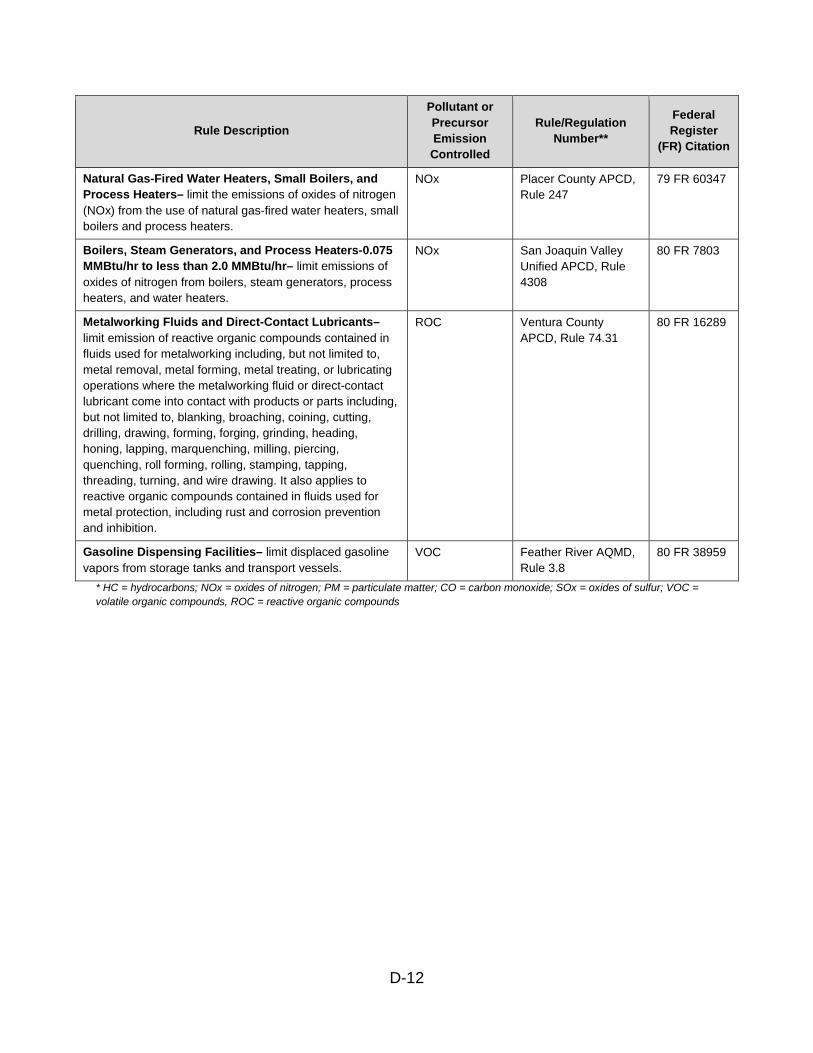
Natural Gas-Fired Water Heaters, Small Boilers, and Process Heaters– limit the emissions of oxides of nitrogen (NOx) from the use of natural gas-fired water heaters, small boilers and process heaters.

NOx Placer County APCD, Rule 247

79 FR 60347

Boilers, Steam Generators, and Process Heaters-0.075 MMBtu/hr to less than 2.0 MMBtu/hr– limit emissions of oxides of nitrogen from boilers, steam generators, process heaters, and water heaters.

NOx San Joaquin Valley Unified APCD, Rule 4308

80 FR 7803

Metalworking Fluids and Direct-Contact Lubricants– limit emission of reactive organic compounds contained in fluids used for metalworking including, but not limited to, metal removal, metal forming, metal treating, or lubricating operations where the metalworking fluid or direct-contact lubricant come into contact with products or parts including, but not limited to, blanking, broaching, coining, cutting, drilling, drawing, forming, forging, grinding, heading, honing, lapping, marquenching, milling, piercing, quenching, roll forming, rolling, stamping, tapping, threading, turning, and wire drawing. It also applies to reactive organic compounds contained in fluids used for metal protection, including rust and corrosion prevention and inhibition.


80 FR 16289

Gasoline Dispensing Facilities– limit displaced gasoline vapors from storage tanks and transport vessels.


80 FR 38959

* HC = hydrocarbons; NOx = oxides of nitrogen; PM = particulate matter; CO = carbon monoxide; SOx = oxides of sulfur; VOC = volatile organic compounds, ROC = reactive organic compounds

D-12

Potential Receptor Evaluation Arizona The U.S EPA modeling identified one potential maintenance receptor in Arizona. This is the North Phoenix monitoring site located in the Phoenix-Mesa nonattainment area which contains portions of Maricopa and Pinal Counties. The Phoenix-Mesa area is currently classified as a marginal nonattainment area. However, U.S. EPA recently proposed to reclassify the area to moderate, because of failing to attain the standard by the 2014 ozone season.12 As of 2010, the Phoenix nonattainment area contained a population of 3.8 million. The Phoenix-Mesa-Scottsdale Core Based Statistical Area (CBSA) is located in central Arizona, at an elevation of approximately 1,100 feet, in what is also referred to as the “Valley of the Sun.” The Phoenix Metropolitan Area is mostly flat, but is surrounded by multiple mountain chains of varying heights. To the southwest of Phoenix are the Sierra Estrella Mountains extending up to roughly 4,500 feet in elevation at the highest peak; to the west are the White Tank Mountains reaching 4,100 feet; to the north and northeast are the Bradshaw Mountains and multiple other ridges ranging from 6,000 to 8,000 feet at the highest peaks; and to the east are the Superstition Mountains, with peaks up to nearly 8,000 feet. The southern side of the metropolitan area is bounded by South Mountain, which extends up to 2,300 feet, and to the southeast is desert that gradually slopes up in elevation. As a result, the Phoenix region is within a large topographic bowl and the terrain significantly limits the flow of air through the area during non-stormy periods. Situated in the northeast portion of the Sonoran Desert, the Phoenix area experiences mostly clear skies, warm to hot temperatures, and very little rainfall during most of the year. In the summer months, upper-level high pressure systems over the western U.S., typically centered over the Four Corners region, produce temperatures easily over 100° F on most days, limit cloud formation, and generally lead to light winds in the Phoenix region. Local wind flow patterns are dominated by differential heating across the area and can be quite variable, but due to constraints by the mountain chains around the region, air masses within the Phoenix area tend to flow from west to east in the afternoon and stay within the “bowl.” Cooling in the evening also allows the air to flow back downslope from east to west at night, transporting the day’s emissions and pollutants back into the metropolitan area.

12 Determinations of Attainment by the Attainment Date, Extensions of the Attainment Date, and Reclassification of Several Areas Classified as Marginal for the 2008 Ozone National Ambient Air Quality Standards,80 FR 51992, August 27, 2015

D-13

One key weather pattern that does impact the Phoenix region is the summer monsoon, which transports clouds and moisture from the south/southeast, often leading to the formation of thunderstorms, heavy rains, and very strong winds that can produce major dust storms. Because of the monsoon, more rain falls during the summer months than during the rest of the year. These conditions also inhibit the formation and buildup of ozone in Phoenix on the many days each year with active monsoon weather. Other than during the monsoon period, the generally dry climate in Arizona allows for strong, shallow temperature inversions to form on most nights, trapping emissions and pollutants near the ground or in a residual layer aloft. However, afternoon temperatures are often very hot, especially during the month of July. As a result, mixing heights in Phoenix can be several thousand feet, thus allowing the atmosphere to mix deeply. As was the case in 2015, the three highest ozone concentration days, based on preliminary data, occurred in June and the fourth highest was in August, when average temperatures tend to be slightly lower than in July. Four of the top five high days in 2014 were in June, with the remaining day in September. In all cases, the monitoring sites with the highest ozone concentrations were to the east of the Phoenix Metropolitan area, indicating that clear skies, hot temperatures (about 103-108 °F), and calm/variable winds in the morning and light-to-moderate westerly winds in the afternoon produce ideal conditions for high ozone in central Arizona.

Figure D.4: Arizona Nonattainment Area Reference Map

D-14

U.S. EPA’s interstate transport modeling for 2017 showed that all sites in Arizona would meet the 0.075 ppm ozone standard. However, modeling indicated that the North Phoenix site in the Phoenix-Mesa nonattainment area (Site ID 04-013-1004) would be near enough to the ozone standard to be considered maintenance.

Table D.3: Ozone Receptor in the State of Arizona 8-Hr Design Value Approximate

County Site Name AQS ID (ppm) Receptor

Type

Distance to California

Border (miles)

2011 2012 2013

Maricopa North Phoenix 04-013-1004 77 81 81 Maintenance 128 Modeled Maintenance Receptor in Arizona North Phoenix The North Phoenix receptor site is located in the center of the Phoenix-Mesa NA Area and is located in the central portion of Maricopa County. It is located roughly eight miles north of downtown Phoenix, at the foot of the Phoenix Mountains. The monitor has an elevation of roughly 1,249 feet. The Phoenix Mountains run northwest to southeast through the center of the Phoenix metropolitan area. Figure D.5 is a map of North Phoenix’s location in comparison to Phoenix and the Phoenix Mountains. Figure D.6 shows the design value trend at the potential receptor site from 2003 to 2013. From 2003 to 2009, design values trended down each year with an average annual reduction of 1.8 percent and a total reduction of 2.4 percent for the twelve year period. The most significant reductions were seen in 2008 to 2009, which coincided with a national recession. Since 2009, the design values have been increasing each year by an average of 1.6 percent.

D-15

Figure D.5: 2008 Ozone NAAQS Receptor in the State of Arizona

Figure D.6: Ozone 8-Hour Design Values, North Phoenix Receptor

D-16

Model Performance and Impacts on Model Results ARB acknowledges that based on consideration of distance (less than 200 miles) and meteorology, a transport pathway does exist between Southern California and Phoenix, Arizona. Research studies have attempted to examine these transport impacts. However, large uncertainties remain as to the frequency and magnitude of these transport contributions, particularly on high ozone days that drive compliance considerations. Given the model performance issues discussed below, there is uncertainty as to whether transport contributions from California exceed a one percent threshold or if it is of a sufficient magnitude or frequency to interfere with maintenance of the 0.075 ppm ozone NAAQS at the receptor site in Phoenix. Issues with model performance may hinder assessments of contributions from upwind states. In any modeling exercise, a high correspondence between the days with the highest modeled ozone values and the days with the highest measured ozone values is desirable. The tables below show the extent of this correspondence in 2011 at the Phoenix, Arizona maintenance receptor site. Concentrations listed in these tables are for measured values on those days.

Table D.4: Model Derived Top 10 Daily Maximum 8-hour Ozone Days in 2011 with Measured Concentrations on those Days

Rank Date Measured 8-hour Ozone Daily Maximum (ppb)

1 8/23/2011 67 2 6/21/2011 60 3 9/4/2011 67 4 8/24/2011 68 5 6/22/2011 73 6 9/7/2011 65 7 9/8/2011 64 8 6/9/2011 90 9 9/20/2011 56

10 6/10/2011 81 Average measured daily maximumdays

8-hour value for top 10 modeled 69.1

Average measured daily maximum 8-hour value for eight top 10 modeled days not in common with top 10 monitored days 65

D-17

Table D.5: Measured Top 10 Daily Maximum 8-hour Ozone Days in 2011 with Measured Concentrations on those Days

Rank Date Measured 8-hour Ozone Daily Maximum (ppb)

1 6/9/2011 90 2 9/1/2011 83 3 5/25/2011 82 4 8/25/2011 82 5 6/10/2011 81 6 7/8/2011 77 7 8/4/2011 77 8 8/17/2011 77 9 5/24/2011 75

10 6/3/2011 74 Average measured daily days

maximum 8-hour value for top 10 monitored 79.8

Average measured daily maximum 8-hour value for eight top 10 monitored days not in common with top 10 modeled days 78.4

We note that only two of the 10 days with the highest monitored 8-hour ozone values in 2011 are among days with the top 10 modeled ozone values. One could expect the meteorology to be completely different between the monitored highest days and the modeled highest days. Instead, 8 of the 10 days with the highest monitored ozone levels – and when conditions may not have been conducive for ozone transport from California – were not among the top 10 modeled days. Also, the average concentration of the eight highest modeled days that were not in the top 10 monitored days was 65 ppb, well below the ozone standard. Given the relatively low concentrations measured on those eight modeled days, conditions most conducive to development of high ozone were not present at the North Phoenix site. These may have been days with less stagnant conditions and more ventilation, under which conditions a small ozone contribution from California may have occurred. Such low ozone days are not representative of that site’s design value conditions, which would occur under different meteorological conditions. Thus this modeling may not appropriately reflect the contribution of California emissions on days that comprise the design value. Additionally, it is important to note that the 2017 modeling does take into account the 29 stationary source measures recently adopted by local air districts in California, the benefits of California’s consumer products program in other states and California’s continuing incentive investments.

D-18

Arizona Summary Based on the analyses described above, the intervening terrain, and the effect of local meteorological conditions conducive to the formation of ozone, we believe it is reasonable to conclude that emissions from California do not significantly interfere with maintenance of the 0.075 ppm 8-hour ozone NAAQS at this receptor Colorado

The Denver-Boulder-Greeley-Ft Collins-Loveland nonattainment area was originally classified as a marginal nonattainment area in 2012 with an attainment deadline of 2014. U.S. EPA recently proposed that the classification be changed to moderate by 2016 due to a failure to attain by the required deadline. As of 2010, the Denver nonattainment area contained a population of 3.4 million people. The nonattainment area contains the counties of Adams, Arapahoe, Boulder, Broomfield, Clear Creek, Denver, Douglas, Elbert, Gilpin, Jefferson, and Park, as well as portions of Larimer and Weld counties. Geographically the Denver-Aurora-Lakewood CBSA is located at the base of the Front Range, or the eastern edge of the Rocky Mountains on a generally flat plateau at approximately 5,200 feet. With the Front Range running north-to-south and extending up to an altitude of 8,000 feet, it forms an abrupt barrier to air flow on the western side of the metropolitan area. The southern and southeastern end of the CBSA is bound by more gradually rising mountains, still reaching up to nearly 6,500 feet and also forming a significant barrier to air flow. To the east and north of the Denver area, there are gradually rising hills that rise a couple hundred feet above the city center elevation, but the region is generally open to air flow in those directions. During the summer months, upper-level high pressure systems over the Rocky Mountains and Central Plains produce mostly sunny skies, temperatures around 90-95° F, and light winds in the Denver region, causing local wind flow patterns to be dominated by terrain and differential heating across the area. These conditions are conducive for the accumulation of local emissions and the formation of ozone. Ideal ozone formation conditions involve surface high pressure to the east-northeast of the Denver area, which produce light east-northeasterly winds and push emissions into the foothill areas to the west-southwest portions of the region, which is where the National Renewable Energy Labs and Chatfield ozone monitoring sites are located. These monitoring sites typically have the highest ozone concentrations in the region. These sites are also located anywhere from 300 feet to 800 feet in elevation above

D-19

Denver, putting them higher in the mixed layer of the atmosphere and away from most of the primary emission sources that can scavenge ozone from the air. This feature allows ozone concentrations to remain higher for more hours, leading to higher 8-hour averages. Another local feature that can develop under broad high pressure days is upslope and downslope flow in the foothill regions where the two monitoring sites are located. During the day, heating of the foothills can lead to upslope winds that draw air from the metropolitan area toward the monitoring sites. At night, the air in the less populated and less developed foothill areas and over the mountain slopes cools and drains back into the metropolitan area. This recirculation pattern allows emissions and ozone concentrations to build up over multi-day periods, similar to what was seen from June 20-23, 2015, when the two highest ozone days of the summer occurred. During the four days, 8-hour average ozone concentrations peaked at 93 ppb on June 21 and reached 91 ppb on June 23, based on preliminary data. The flow from the northeast pushed the air far enough into the Front Range gaps on June 23, that even the Aspen Park monitoring site, over 21 miles to the southwest of Denver, reached 1-hour concentrations of 95 ppb and 98 ppb on consecutive hours during the middle of the afternoon. Modeled Receptors in Colorado U.S. EPA’s modeling showed impact from California at greater than the one percent threshold at four receptor sites in Colorado (Figure D.7). Following is location information, receptor characterization, as well as 8-hour design values for 2011-2013, the base year design values used in projections for 2017, for each of the receptors listed in Table D.6.

D-20

Figure D.7: Denver-Boulder-Greeley-Ft Collins-Loveland, CO Nonattainment Area

D-21

Table D.6: Ozone Receptors in the State of Colorado

County Site Name AQS ID

8-Hr Design Value (ppm) Receptor

Type

Approximate Distance to California

Border 2011 2012 2013 (miles)

Jefferson Rocky Flats - North 08-059-0006 78 80 83 Nonattainment 618 Douglas Chatfield State Park 08-035-0004 77 82 83 Nonattainment 611 Jefferson Natl Renew Energy 08-059-0011 75 79 82 Maintenance 612 Arapahoe Highland Reservoir 08-005-0002 74 77 79 Maintenance 618

Modeled Nonattainment Receptors in Colorado

Rocky Flats North

Rocky Flats North is located towards the western portion of the Denver nonattainment area and is located in the very northern part of Jefferson County. Roughly five miles from the foot of the Rocky Mountains, the monitor has an elevation of about 5,900 feet. Additionally, the site is located about 16 miles northwest of the City of Denver. The Rocky Mountains run northwest to southeast through Jefferson County.

Jefferson County has the third highest population in the Denver nonattainment area. The neighboring counties are Boulder to the north, Arapahoe and Denver to the east, and Douglas to the southeast. Chatfield State Park Chatfield State Park is located in the southern portion of the Denver nonattainment area and roughly four miles from the foot of the Rocky Mountains at an elevation of about 5,500 feet. Additionally, the site is located about 15 miles south of the city of Denver. The Rocky Mountains run northwest to southeast through Douglas County. Douglas County has the seventh highest population in the Denver nonattainment area. The neighboring counties are Jefferson to the west and Arapahoe to the north. Modeled Maintenance Receptors in Colorado National Renewable Energy Labs (NREL) NREL is located towards the western portion of the Denver nonattainment area and is located in the northern portion of Jefferson County. NREL is located roughly three miles from the foot of the Rocky Mountains at an elevation of about 6,000 feet. Additionally, the site is located about 10 miles west of the city of Denver. The Rocky Mountains run northwest to southeast through Jefferson County. Jefferson County has the third highest population in the Denver nonattainment area. The neighboring counties are Boulder to the north, Arapahoe and Denver to the east, and Douglas to the southeast. Highland Reservoir Highland Reservoir is located towards the southern portion of the Denver nonattainment area and is located in the southwestern part of Arapahoe County. It is located roughly 10 miles from the foot of the Rocky Mountains at an elevation of about 5,700 feet. Additionally, the site is located about 12 miles south of the City of Denver. Arapahoe County has the second highest population in the Denver nonattainment area. The neighboring counties are Adams to the north, Denver and Jefferson to the west, and Douglas to the south.

D-22

Of these sites, both Chatfield and NREL are located to the west-southwest of the Denver area, which is where emissions typically get pushed due to east-northeasterly winds on days with meteorology conducive to ozone formation. These sites are also located anywhere from 300 to 800 feet in elevation above the Denver city area, putting them higher in the mixed layer of the atmosphere and away from most of the primary emission sources that can scavenge ozone from the air. This feature allows ozone concentrations to remain higher for more hours, leading to higher 8-hour average concentrations. Trajectory Analysis of Impact from California to Colorado Due to the large distance between California and Colorado and the widespread presence of complex terrain, ARB staff conducted a trajectory analysis. The goal of the trajectory analysis was to evaluate the potential for transport of ozone or ozone precursors from California to Colorado. In this analysis, ARB staff used the National Oceanic and Atmospheric Administration (NOAA) Hybrid Single Particle Lagrangian Integrated Trajectory (HYSPLIT) model13 for computing trajectories. The HYSPLIT model is an analytical tool that calculates the path of an air parcel either backwards or forward in time. In addition, this tool allows one to examine air parcel movement from various altitudes above the ground. The web based version of the model was used for this analysis (Available at: http://ready.arl.noaa.gov/HYSPLIT.php). Trajectory analysis cannot confirm transport but can provide insight on the potential for transport and the potential frequency of transport. Moreover, trajectory models represent movement of air parcels through space but do not confirm transport of emissions. Even if a parcel of air passed through a particular location, emissions intercepted by the parcel can vary markedly depending on chemical and physical properties of the local environment and the air parcel. ARB staff computed backward trajectories from four potential Colorado receptor sites for days when measured concentrations exceeded the 0.075 ppm 8-hour ozone standard in June and July of 2011 and 2012. June and July were chosen by ARB staff because these months have most of the high ozone days. North American Mesoscale Forecast System (NAM) 12 km meteorological data were used for each trajectory run. Nine individual back trajectories were modeled for each site exceedance day corresponding to three altitude levels for the beginning hour, middle hour, and end hour of the daily maximum 8-hour ozone concentration. Trajectories were initiated from 10, 1000, and 2000 meters above ground level and the duration was 96 hours. For back

13 Draxler, R.R. and Rolph, G.D., 2015. HYSPLIT (HYbrid Single-Particle Lagrangian Integrated Trajectory) Model access via NOAA ARL READY Website (http://ready.arl.noaa.gov/HYSPLIT.php). NOAA Air Resources Laboratory, Silver Spring, MD, last accessed: November 13, 2015

D-23

trajectories that reached from Colorado back to California, ARB staff noted whether the height of the beginning point in Colorado and the ending point in California were above or within the mixed layer, as determined by the HYSPLIT model. As defined by NOAA, “..the mixed layer is the part of the atmosphere that easily exchanges heat and momentum with the surface. It is well mixed due to the wind turbulence introduced by frictional effects of the surface and the surface heating induced thermals. Pollutants become well dispersed in this layer. It is usually capped by a temperature inversion (temperature increases with height at the top of the boundary layer limiting mixing)”.14 In total, 477 back trajectories were modeled for the 53 site exceedance days. A breakdown of the exceedance days and back trajectories by receptor site is presented in Table D.7. Table D.7: Colorado Receptor Trajectory Summary

Receptor Site Name

Number of Site 8-hour Ozone Exceedance Days

Number of Back

Trajectories

Number of Occurrences of Back Trajectories

within the Mixed Layer at CO and CA

Chatfield 13 117 3 Highland Reservoir 7 63 2 NREL 16 144 4 Rocky Flats 17 153 2 Total 53 477 11

Of the 477 back trajectories, only 11 initiated from within the mixed layer in Colorado reached back into the mixed layer within a California air basin. As a result, the percentage of trajectories that had the potential to travel from the mixed layer at the Colorado receptor sites to the mixed layer within a California air basin was extremely low (two percent). For the 11 back trajectories that were initiated from the mixed layer in Colorado and reached within the mixed layer in California, forward trajectories from California were run, starting at 10 meters above the ground. The objective of the 10 meter forward trajectory was to confirm that source emissions near the surface would be intercepted by the mixed layer at the receptor sites, thus verifying the backwards trajectory. The duration of the forward trajectories was 96 hours. For those trajectories that reached a Colorado receptor site, it was noted whether the trajectory end point was above or within the mixed layer and whether the forward trajectory was similar in duration to the backward trajectory. Only 1 of the 11 forward trajectories from the mixed layer in

14 Page, op.cit.

D-24

California reached the mixed layer at a Colorado receptor site, suggesting that the complexity of the physical environment between California and Colorado limits the reproducibility of modeled transport and that considerable multi-faceted analyses would be necessary to explore transport mechanisms through areas of complex terrain. An additional product of the HYSPLIT model is the vertical cross-section profile of the back trajectory path. For days with back trajectories that travelled from within the mixed layer at a Colorado receptor site to within the mixed layer at a California air basin, most of the back trajectories had paths that were at the surface for a portion of time and aloft the remainder of time.

Also, ARB staff reviewed NOAA 500 millibar charts and found that upper-level weather patterns and winds on days leading up to and on the days the back trajectories reached California were generally supportive and consistent. Generally, the patterns on the start day of the back trajectory were a Great Basin or Midwest high pressure combined with a western U.S. trough or trough off the western U.S. coast. Winds aloft during these patterns are generally from the southwest from California to Colorado, but may also curl in a clockwise direction when over the Great Basin. Subsequent days prior to the back trajectory start day, upper-level pressure patterns were located a bit further west each day back in time.

However, despite the upper-level weather patterns supporting flow along a path from California to Colorado for many of the trajectory days, the key finding was that the air was almost always above the mixed-layer over California, Colorado, or both, meaning the air at the surface was decoupled from the aloft air. Without vertical mixing of the air between the mixed layer near the ground and the upper-level, little-to-no impact from transport of emissions or pollutants would be expected at the surface. In summary, the trajectory analysis indicated that transport from California emission source areas to Colorado is possible, but is extremely unlikely on high ozone days at the four receptor sites in Colorado. In terms of frequency or establishing a firm understanding of mechanisms, there were very low percentages of back and forward trajectories where an air parcel within the mixed layer at the Colorado receptor sites had a trajectory back to the mixed layer within California. Given the distance (over 800 miles), complex terrain, and entrainment of ozone and precursors from other source regions along trajectory paths, there would be significant physical and chemical processing of transported air masses during transit. Thus, considerable multi-faceted analyses would be necessary to more accurately and confidently quantify California’s contribution, if any, to ozone concentrations measured in Colorado, especially on exceedance days.

D-25

Potential Wildfire Impacts

Figure D.8: Close-up of Receptor Sites in Colorado

D-26

The four receptor sites in Colorado (Figure D.8), while displaying some variability in the design value over the past decade, have an overall downward trend from 2003 to 2010, with an average decrease of 10 ppb over the eight year period. However, that trend changes starting with 2011 where the design value increases from a low of 0.072 ppm in 2010 to 0.083 ppm in 2013. Table D.8 documents wildfire activity which may be one of the contributing factors to the increase in design value trends.

Table D.8: Colorado Wildfire Acreage Burned

State Fire Acreage Burned/Year Type 2009 2010 2011 2012 2013

CO Wildland 50,456 44,020 161,167 246,445 195,145 Prescribed 25,674 29,377 29,331 8,775 16,321 Total 76,130 73,397 190,498 255,220 211,466

Figure D.9: Design Value Trends vs Wildfire Acreage Burned

D-27

The wildfire contribution in the U.S. EPA modeling for Colorado was estimated to be between 0.32 and 0.74 ppb for the four receptor sites. However, the only contributions solely attributed to wildfires are when emissions of NOx and VOCs from wildfires interact to form ozone. If NOx from wildfires reacts with VOCs from anthropogenic sources, then the ozone formed is attributed to the anthropogenic sources (the same is true for VOCs from wildfires and NOx from anthropogenic sources). This methodology for estimating wildfire impacts therefore underestimates the impact of wildfires. Additionally, for the years captured in the five-year average design value (2009-2013), both 2012 and 2013 had significant wildfire activity, which could have resulted in elevated ozone levels in 2012 and 2013, impacting the design value. The 2012 wildfire season in Colorado was of a catastrophic nature. The State of Colorado documented some of these wildfire impacts and flagged data in AQS as having potential wildfire impacts. Table D.9 below lists the top ten highest 8-hour ozone concentrations for 2012 at the Rocky Flats site and the contribution to the 8-hour ozone maximum concentration that the State attributed to the wildfire (termed Residual) using their air quality forecasting regression program.

Table D.9: 2012 Days in the Top 10 Maximum 8-Hour Ozone Concentrations at Rocky Flats (AQS ID 08-059-0006)

Date Max 8-hour Ozone (ppb) Flag

Wildfire Impact Residual (ppb)

Bias Adjusted Max 8-hour Ozone (ppb)

22 June 101 RT 34 67 04 July 92 RT 20 72 05 July 88 RT 18 70

09 August 84 RT 16 68 13 July 82 02 July 81 RT Not Given

21 August 80 RT 14 66 25 August 80 RT 17 63 21 June 79 11 July 79

Below are the descriptions of the wildfire events that Colorado entered into AQS, which ARB staff accessed on November 3, 2015. The comments are found in the raw data to support the flagging of the data and the request to exclude the data (RT or “Wildfire-U.S.”, Regional Concurrence Requested). These days would have included the (five-year) base year design values used in modeling. June 22 at Rocky Flats

GOES visible satellite imagery provide evidence that a plume of smoke from the High Park Fire in Larimer County was entrained into an area of limited planetary boundary layer depth along the Northern Front Range from west of Denver northward. Ozone forecast regression models showed a 25 ppb positive residual at the Fort Collins West site and a 34 ppb positive residual at the at the Rocky Flats North site. The wildfire and associated meteorological conditions are not controllable.

Jul 4 2012 at Rocky Flats

MODIS Terra and Aqua and GOES satellite imagery showed a large mass or plume of smoke from fires burning in Wyoming, Montana, and South Dakota (on July 3) entering northeastern Colorado behind a cool front that crossed into Colorado during the morning hours. The presence of smoke was also verified by surface PM2.5 concentrations, surface visibility observations, AIRS satellite carbon monoxide measurements, and MODIS aerosol optical depth products. This smoke was trapped within the surface mixed layer from the Denver area north to the Wyoming border and east of the Front Range. Ozone forecast

D-28

regression models showed positive residuals of 20 ppb, 20 ppb, and 9 ppb at Rocky Flats North, Weld County Tower, and Ft. Collins West, respectively. The plume did not appear to cover RMNP. The wildfires and associated meteorological conditions are not controllable.

July 5 at Rocky Flats

MODIS Terra imagery and aerosol optical depth products showed that the smoke from Wyoming, Montana, and South Dakota that entered the region on July 4 continued across much of the Front Range region on July 5 from Colorado Springs through Denver north to Weld and Larimer Counties (the smoke did not appear to affect RMNP). Ozone forecast regression models showed positive residuals of 18 ppb, 3 ppb, and 13 ppb at Rocky Flats North, Weld County Tower, and Ft. Collins West, respectively. The wildfires and associated meteorological conditions are not controllable.

Aug 9 at Rocky Flats

MODIS Terra and Aqua satellite imagery, aerosol optical depth products, NOAA smoke and fire products, and AIRS CO products showed a large area of smoke from fires burning in Utah, Nevada, Idaho, Oregon, California, and Montana covering much of the West including eastern Colorado. Ozone forecast regression models showed positive residuals of 16 ppb, 5 ppb, and 16 ppb at Rocky Flats North, Weld County Tower, and Ft. Collins West, respectively. The wildfires and associated meteorological conditions are not controllable.


MODIS Terra and Aqua satellite imagery, aerosol optical depth products, NOAA smoke and fire products, and AIRS CO products showed an extensive area of smoke from fires burning in western and northwestern states covering much of the West including northeastern Colorado. Ozone forecast regression models showed residuals of +14 ppb, +1 ppb, and +4 ppb at Rocky Flats North, Weld County Tower, and Ft. Collins West, respectively. The wildfires and associated meteorological conditions are not controllable.

D-29


MODIS Terra and Aqua satellite imagery and aerosol optical depth products showed an extensive area of smoke from fires burning in western and northwestern states covering much of the West including northeastern Colorado. Ozone forecast regression models showed residuals of +17 ppb, -5 ppb, and -1 ppb at Rocky Flats North, Weld County Tower, and Ft. Collins West, respectively. The wildfires and associated meteorological conditions are not controllable.

Photochemical Modeling As mentioned above, wildfire impacts in 2011-2013 may well have elevated design values in this nonattainment area. To the extent the wildfires of 2011-2013 resulted in higher design values for 2011, 2012 and 2013, those wildfires also resulted in elevated predictions of future year design values for the Denver area in 2017. This has air quality planning consequences and could have attendant regulatory consequences. ARB staff has commented to U.S. EPA on the inclusion of wildfire emissions when performing future year modeling. The base year of 2011 was used in U.S. EPA modeling to project a design value in 2017. That modeled base year had significant wildfire activity, which U.S. EPA included in model projections for 2017. ARB staff has commented that the magnitude of wildfire emissions included in the model can mask the benefits of emission reductions from regulations. Consequently, the model may not be adequately responsive to emission reductions when projecting ozone levels. In addition, impacts of wildfires in 2012 and 2013 played a large role in determining future year design values. When determining whether a nonattainment area meets the ozone standard in a future year, U.S. EPA guidance calls for averaging the measurement-based design values for 2011, 2012 and 2013. This enables modeling, which is performed for only one year, to represent conditions that occurred in other years -- such as milder or more severe meteorology, or impacts of new emission controls. This averaged base year design value weights air quality data from individual years differently. Data from 2009 and 2013 is weighted once, data from 2010 and 2012 is weighted twice, and data from 2011 is weighted three times. As noted earlier, wildfires in 2011-2013 may have resulted in elevated ozone measurements. Due to the weighting used, two-thirds of the years used to project the 2017 design value are years potentially heavily impacted by wildfires. This raises the potential that future year design values may be artificially elevated.

D-30

The same potential exists regarding U.S. EPA’s modeling methodology for determining maintenance areas. Here, the single highest design value (rather than the average one) is used in projecting future year levels. A future year design value for 2013 is based on three years (2011-2013) with unusually high levels of acreage burned in wildfires. While the exceptional events process can be used to remove the impacts of wildfires and other events on air quality data, a case-by-case solution for modeling purposes may be achieved more directly by considering current weighting of years used by U.S. EPA when constructing modeled base year design values. In each case, consideration would need to be made based on wildfire impacts in each year and each state. ARB staff would welcome the opportunity to collaborate with U.S. EPA staff on weighting years when constructing base year design values for transport-related nonattainment and maintenance projections. Colorado Summary Based on the above-described analyses, the distances from California, the intervening terrain, the effect of local topology, the impact of local meteorological conditions conducive to the formation of ozone, and modeling base year design values that do not address wildfire impact, we believe it is reasonable to assume that emissions from California do not significantly interfere with the maintenance or contribute to the nonattainment of the 2008 8-hour ozone NAAQS at these receptors.

Summary Draft modeling performed by U.S. EPA projected 2017 design values in neighboring western states that were below the standard, with the exception of four areas in Colorado and one area in Arizona that are currently designated nonattainment. This element of the good neighbor SIP evaluated U.S. EPA’s modeling to determine whether it accurately represents transport between California and other western states by employing a weight of evidence approach. The nature of transport relationships among CSAPR and western states is fundamentally different. Additional dialog and collaborative work among U.S. EPA and western states is needed in order to identify a technical basis for determining the appropriate level for significant transport contribution in the western U.S.

D-31

There are a number of model performance issues that lend uncertainty to the quantification of significant transport in U.S. EPA’s draft modeling. These uncertainties have to do with how the current modeling addresses complex terrain, wildfire impacts, distances between sources and receptors, and the frequency and magnitude of impacts on high ozone days that drive compliance. Consequently, there are uncertainties in projected design values as well as whether contributions exceeded a one percent threshold. Due to the large distance and complex terrain between Colorado and California, ARB conducted a trajectory analysis. This trajectory analysis indicated that transport from California emission source areas to Colorado is possible, but given the distance, complex terrain, entrainment of ozone and precursors from other source regions along trajectory paths, there would be significant physical and chemical processing of transported air masses during transit. Thus, considerable multi-faceted analyses would be necessary to more accurately and confidently quantify California’s contribution, if any, to ozone concentrations measured in Colorado, especially on exceedance days. Although the distance between Southern California and Phoenix supports a transport pathway, there is insufficient evidence at this time to determine whether transport is significant on high ozone days and whether transport will impact maintenance of the Phoenix receptor. Given these uncertainties, ARB concludes that California does not have a significant transport impact on maintenance or nonattainment receptors in Arizona and Colorado for the 0.075 ppm 8-hour ozone NAAQS. This conclusion, combined with strategies already in place, as well as 29 new rules adopted since the modeling base year, and ARB’s current and ongoing emission control programs will yield additional benefits to downwind states. The steps California is taking to ensure its emissions continue to decline will help nonattainment areas in neighboring states, projected to meet the ozone standard in 2017, maintain clean air. The comprehensive assessment presented here demonstrates that ozone from California does not contribute significantly to nonattainment or maintenance receptors in other states, and particularly to those in Colorado and Arizona.

D-32

2015 transport sip appendix d

Documents