21 Testing Problems

Testing is certainly another fundamental problem of inference. It is interestingly

different from estimation. The accuracy measures are fundamentally different and

the appropriate asymptotic theory is also different. Much of the theory of testing has

revolved somehow or other on the Neyman-Pearson lemma, which has led to a lot

of ancillary developments in other problems in mathematical statistics. Testing has

ledto the useful idea of local alternatives, and like maximum likelihood in estimation,

likelihood ratio, Wald, and Rao score tests have earned the status of default methods,

with a neat and quite unified asymptotic theory. Because of all these reasons,

a treatment of testing is essential. We discuss the asymptotic theory of likelihood

ratio, Wald, and Rao score tests in this chapter. Principal references for this chapter

are Bickel and Doksum (2001), Ferguson (1996), and Sen and Singer (1993). Many

other specific references are given in the sections.

21.1 Likelihood Ratio Tests

The likelihood ratio test is a general omnibus test applicable, in principle, in most

finite dimensional parametric problems. Thus, let X(n) = (X1, . . . , Xn) be the

observed data with joint distribution P nθ ¿ µn, θ ∈ Θ, and density fθ(x

(n)) =

dP nθ /dµn. Here, µn is some appropriate σ-finite measure on Xn, which we assume

to be a subset of an Euclidean space. For testing H0 : θ ∈ Θ0 vs. H1 : θ ∈ Θ − Θ0,

the likelihood ratio test (LRT) rejects H0 for small values of

Λn =supθ∈Θ0

fθ(x(n))

supθ∈Θ fθ(x(n))

The motivation for Λn comes from two sources:

(a) The case where H0, H1 are each simple, a most powerful (MP) test is found

from Λn by the Neyman-Pearson lemma.

(b) The intuitive explanation that for small values of Λn we can better match

the observed data with some value of θ outside of Θ0.

LRTs are useful because they are omnibus tests and because otherwise optimal

tests for a given sample size n are generally hard to find outside of the exponential

family. However the LRT is not a universal test. There are important examples

where the LRT simply cannot be used, because the null distribution of the LRT test

statistic depends on nuisance parameters. Also, the exact distribution of the LRT

319

statistic is very difficult or impossible to find in many problems. Thus, asymptotics

become really important. But the asymptotics of the LRT may be nonstandard

under nonstandard conditions.

Although we only discuss the case of a parametric model with a fixed finite di-

mensional parameter space, LRTs and their useful modifications have been studied

when the number of parameters grows with the sample size n, and in nonparamet-

ric problems. See, e.g., Portnoy(1988),Fan,Hung and Wong(2000), and Fan and

Zhang(2001).

We start with a series of examples, which illustrate various important aspects of the

likelihood ratio method.

21.2 Examples

Example 21.1. Let X1, X2, . . . , Xniid∼ N(µ, σ2) and consider testing

H0 : µ = 0 vs.H1 : µ 6= 0.

Let θ = (µ, σ2). Then,

Λn =supθ∈Θ0

(1/σn) exp(− 1

2σ2

∑i(Xi − µ)2

)supθ∈Θ(1/σn) exp

(− 12σ2

∑i(Xi − µ)2

) =

(∑i(Xi − Xn)2∑

i X2i

)n/2

by an elementary calculation of mles of θ under H0 and in the general parameter

space. By another elementary calculation, Λn < c is seen to be equivalent to t2n > k

where

tn =

√nXn√

1n−1

∑i(Xi − Xn)

2

is the t-statistic. In other words, the t-test is the LRT. Also, observe that,

t2n =nX

2

n

1n−1

∑i(Xi − Xn)

2

=

∑i X

2i − ∑

i(Xi − Xn)2

1n−1

∑i(Xi − Xn)

2

=(n − 1)

∑i X

2i∑

i(Xi − Xn)2 − (n − 1)

= (n − 1)Λ−2/nn − (n − 1)

320

This implies,

Λn =

(n − 1

t2n + n − 1

)n/2

⇒ log Λn =n

2log

n − 1

t2n + n − 1

⇒ −2 log Λn = n log

(1 +

t2nn − 1

)

= n

(t2n

n − 1+ op

(t2n

n − 1

))L−→ χ2

1

under H0 since tnL−→ N(0, 1) under H0.

Example 21.2. Consider a multinomial distribution MN(n, p1, · · · , pk). Consider

testing

H0 : p1 = p2 = · · · = pk vs. H1 : H0 is not true.

Let n1, · · · , nk denote the observed cell frequencies. Then by an elementary calcu-

lation,

Λn = Πki=1

(n

kni

)ni

⇒ − log Λn = n(logk

n) +

k∑i=1

ni log ni

The exact distribution of this is a messy discrete object and so asymptotics will be

useful. We illustrate the asymptotic distribution for k = 2. In this case,

− log Λn = n log 2 − n log n + n1 log n1 + (n − n1) log(n − n1)

Let Zn = (n1 − n/2)/√

n/4. Then,

− log Λn = n log 2 − n log n

+n +

√nZn

2log

n +√

nZn

2+

n −√nZn

2log

n −√nZn

2

= −n log n +n +

√nZn

2log(n +

√nZn) +

n −√nZn

2log(n −√

nZn)

=n +

√nZn

2log(1 +

Zn√n

) +n −√

nZn

2log(1 − Zn√

n)

=n +

√nZn

2

(Zn√

n− Z2

n

2n+ op

(Z2

n

n

))

321

+n −√

nZn

2

(− Zn√

n− Z2

n

2n+ op

(Z2

n

n

))

=Z2

n

2+ op(1).

Hence −2 log ΛnL−→ χ2

1 under H0 as ZnL−→ N(0, 1) under H0.

Remark: The popular test in this problem is the Pearson chi-square test which

rejects H0 for large values of ∑ki=1(ni − n/k)2

n/k

Interestingly this test statistic too has an asymptotic χ21 distribution as does the

LRT statistic.

Example 21.3. This example shows that the chi-square asymptotics of the LRT

statistic fail when parameters have constraints or somehow there is a boundary phe-

nomenon.

Let X1, X2, . . . , Xniid∼ N2(θ, I) where the parameter space is restricted to Θ = {θ =

(θ1, θ2) : θ1 ≥ 0, θ2 ≥ 0}. Consider testing

H0 : θ = 0 vs. H1 : H0 is not true.

We would write the n realizations as xi = (x1i, x2i)T and the sample average would

be denoted by x = (x1, x2). The mle of θ is given by,

θ =

(x1 ∨ 0

x2 ∨ 0

)

Therefore by an elementary calculation,

Λn =exp(−∑

i x21i/2 − ∑

i x22i/2)

exp(−∑i(x1i − x1 ∨ 0)2/2 − ∑

i(x2i − x2 ∨ 0)2/2)

Case 1: x1 ≤ 0, x2 ≤ 0. In this case Λn = 1 and −2 log Λn = 0.

Case 2: x1 > 0, x2 ≤ 0. In this case −2 log Λn = nx21.

Case 3: x1 ≤ 0, x2 > 0. In this case −2 log Λn = nx22.

322

Case 4: x1 > 0, x2 > 0. In this case −2 log Λn = nx21 + nx2

2.

Now, under H0 each of the above four cases has a probability 1/4 of occurrence.

Therefore, under H0,

−2 log ΛnL−→ 1

4δ{0} +

1

2χ2

1 +1

4χ2

2,

in the sense of the mixture distribution being its weak limit.

Example 21.4. In bio-equivalence trials, a brand name drug and a generic are

compared with regard to some important clinical variable, such as average drug

concentration in blood over a 24 hour time period. By testing for a difference, the

problem is reduced to a single variable, often assumed to be normal. Formally, one

has X1, X2, . . . , Xniid∼ N(µ, σ2) and the bio-equivalence hypothesis is:

H0 : |µ| ≤ ε for some specified ε > 0.

Inference is always significantly harder if known constraints on the parameters are

enforced. Casella and Strawderman(1980) is a standard introduction to the normal

mean problem with restrictions on the mean; Robertson,Wright and Dykstra (1988)

is an almost encyclopedic exposition.

Coming back to our example, to derive the LRT, we need the restricted mle and

the non-restricted mle. We will assume here that σ2 is known. Then the MLE under

H0 is

µH0 = X if |X| ≤ ε

= εsign(X) if |X| > ε.

Consequently, the LRT statistic Λn satisfies,

−2 log Λn = 0 if |X| ≤ ε

=n

σ2(X − ε)2 if X > ε

=n

σ2(X + ε)2 if X < −ε.

Take a fixed µ. Then,

Pµ(|X| ≤ ε) = Φ

(√n(ε − µ)

σ

)+ Φ

(√n(ε + µ)

σ

)− 1

Pµ(X < −ε) = Φ

(−√

n(ε + µ)

σ

)

323

and

Pµ(X > ε) = 1 − Φ

(√n(ε − µ)

σ

)From these expressions we get:

Case 1: If −ε < µ < ε then Pµ(|X| ≤ ε) → 1 and so −2 log ΛnL−→ δ{0}.

Case 2.a: If µ = −ε then each of Pµ(|X| ≤ ε) and Pµ(X < −ε) converges to 1/2. In

this case, −2 log ΛnL−→ 1

2δ{0}+ 1

2χ2

1, i.e., the mixture of a point mass and a chisquare

distribution.

Case 2.b: Similarly if µ = ε then again, −2 log ΛnL−→ 1

2δ{0} + 1

2χ2

1.

Case 3: If µ > ε then Pµ(|X| ≤ ε) → 0 and Pµ(X > ε) → 1. In this case,

−2 log ΛnL−→ NCχ2(1, (µ − ε)2/σ2)), a noncentral chisquare distribution.

Case 4: Likewise, if µ < −ε then −2 log ΛnL−→ NCχ2(1, (µ + ε)2/σ2)).

So, unfortunately, even the null asymptotic distribution of − log Λn depends on the

exact value of µ.

Example 21.5. Consider the Behrens-Fisher problem with

X1, X2, . . . , Xmiid∼ N(µ1, σ

21)

Y1, Y2, . . . , Yniid∼ N(µ2, σ

22)

and all m + n observations are independent. We want to test

H0 : µ1 = µ2 vs. H1 : µ1 6= µ2.

Let µ, σ21, σ

22 denote the restricted mle of µ, σ2

1 and σ22 respectively, under H0. They

satisfy the equations,

σ21 = (X − µ)2 +

1

m

∑i

(Xi − X)2

σ22 = (Y − µ)2 +

1

n

∑j

(Yj − Y )2

0 =m(X − µ)

σ21

+n(Y − µ)

σ22

324

This gives,

−2 log Λn =

( 1m

∑(Xi − X)2

1m

∑(Xi − X)2 + (X − µ)2

)m2

( 1n

∑(Yj − Y )2

1n

∑(Yj − Y )2 + (Y − µ)2

)n2

However, the LRT fails as a matter of practical use because its distribution depends

on the nuisance parameter σ21/σ

22, which is unknown.

Example 21.6. In point estimation, the mles in nonregular problems behave fun-

damentally differently with respect to their asymptotic distributions. For exam-

ple, limit distributions of mles are not normal (see Chapter 16). It is interesting,

therefore, that limit distributions of −2 log Λn in nonregular cases still follow the

chi-square recipe, but with different degrees of freedom.

As an example, suppose X1, X2, . . . , Xniid∼ U [µ − σ, µ + σ] and suppose we want to

test H0 : µ = 0. Let W = X(n) − X(1) and U = max(X(n),−X(1)). Under H0, U

is complete and sufficient and W/U is an ancillary statistic. Therefore, by Basu’s

theorem (Basu (1955)), under H0, U and W/U are independent. This will be useful

shortly to us. Now, by a straightforward calculation,

Λn =

(W

2U

)n

⇒ −2 log Λn = 2n(log 2U − log W )

Therefore, under H0,

Eeit(−2 log Λn) = Ee2nit(log 2U−log W ) =Ee2nit(− log W )

Ee2nit(− log 2U)

by the independence of U and W/U . This works out, on doing the calculation, to

Eeit(−2 log Λn) =n − 1

n(1 − 2it) − 1→ 1

1 − 2it

Since (1− 2it)−1 is the characteristic function of the χ22 distribution, it follows that

−2 log ΛnL−→ χ2

2.

Thus inspite of the nonregularity, −2 log Λn is asymptotically chi-square, but we

gain a degree of freedom! This phenomenon holds more generally in nonregular

cases.

325

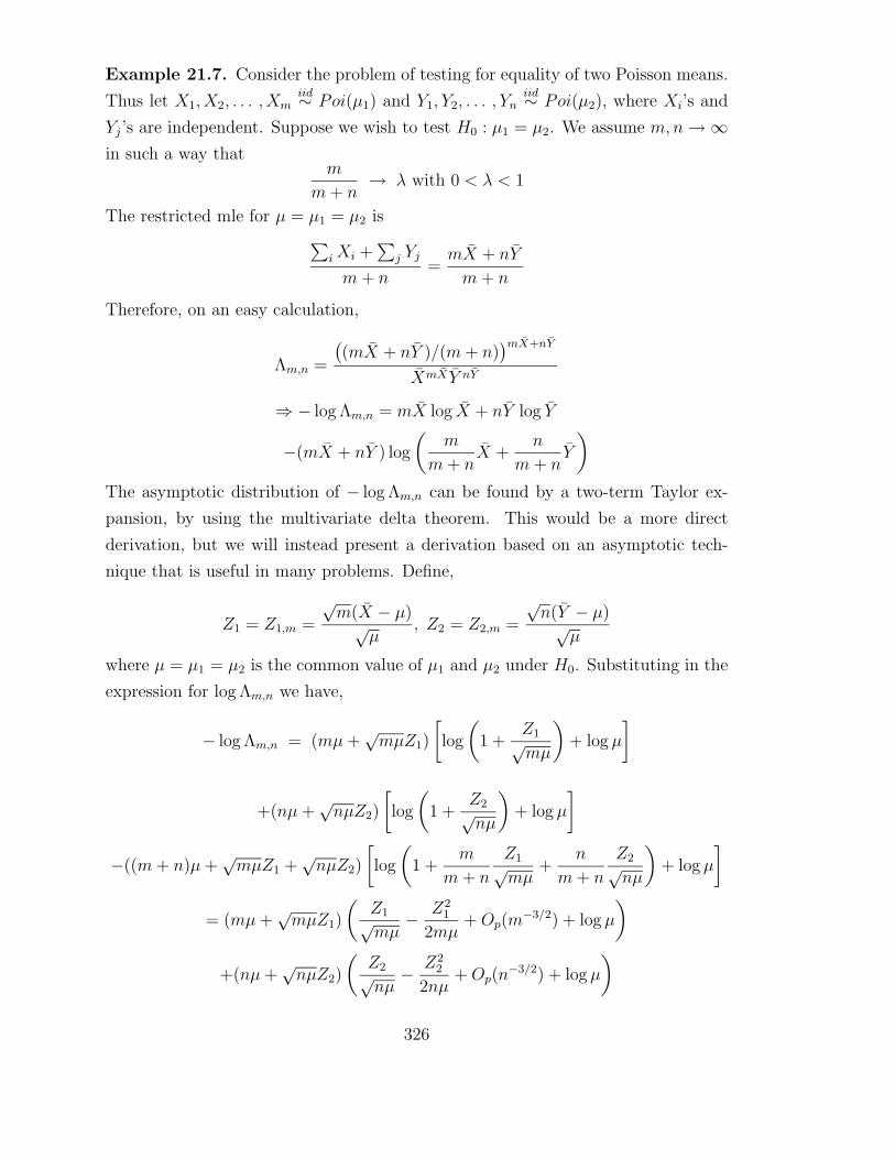
Example 21.7. Consider the problem of testing for equality of two Poisson means.

Thus let X1, X2, . . . , Xmiid∼ Poi(µ1) and Y1, Y2, . . . , Yn

iid∼ Poi(µ2), where Xi’s and

Yj’s are independent. Suppose we wish to test H0 : µ1 = µ2. We assume m,n → ∞in such a way that

m

m + n→ λ with 0 < λ < 1

The restricted mle for µ = µ1 = µ2 is∑i Xi +

∑j Yj

m + n=

mX + nY

m + n

Therefore, on an easy calculation,

Λm,n =

((mX + nY )/(m + n)

)mX+nY

XmX Y nY

⇒ − log Λm,n = mX log X + nY log Y

−(mX + nY ) log

(m

m + nX +

n

m + nY

)The asymptotic distribution of − log Λm,n can be found by a two-term Taylor ex-

pansion, by using the multivariate delta theorem. This would be a more direct

derivation, but we will instead present a derivation based on an asymptotic tech-

nique that is useful in many problems. Define,

Z1 = Z1,m =

√m(X − µ)√

µ, Z2 = Z2,m =

√n(Y − µ)√

µ

where µ = µ1 = µ2 is the common value of µ1 and µ2 under H0. Substituting in the

expression for log Λm,n we have,

− log Λm,n = (mµ +√

mµZ1)

[log

(1 +

Z1√mµ

)+ log µ

]

+(nµ +√

nµZ2)

[log

(1 +

Z2√nµ

)+ log µ

]

−((m + n)µ +√

mµZ1 +√

nµZ2)

[log

(1 +

m

m + n

Z1√mµ

+n

m + n

Z2√nµ

)+ log µ

]

= (mµ +√

mµZ1)

(Z1√mµ

− Z21

2mµ+ Op(m

−3/2) + log µ

)

+(nµ +√

nµZ2)

(Z2√nµ

− Z22

2nµ+ Op(n

−3/2) + log µ

)

326

−((m + n)µ +√

mµZ1 +√

nµZ2)(m

m + n

Z1√mµ

+n

m + n

Z2√nµ

− m

(m + n)2

Z21

2µ− n

(m + n)2

Z22

2µ

−√

mn

(m + n)2

Z1Z2

µ+ Op(min(m,n)−3/2) + log µ)

On further algebra, from above, by breaking down the terms, and on cancellation,

− log Λm,n = Z21

(1

2− m

2(m + n)

)+ Z2

2

(1

2− n

2(m + n)

)

−√

mn

m + nZ1Z2 + op(1)

Assuming that m/(m + n) → λ, it follows that,

− log Λm,n =1

2

(√n

m + nZ1 −

√m

m + nZ2

)2

+ op(1)

L−→ 1

2(√

1 − λN1 −√

λN2)2

where N1, N2 are independent N(0, 1). Therefore, −2 log Λm,nL−→ χ2

1, since√

1 − λN1−√λN2 ∼ N(0, 1).

Example 21.8. This example gives a general formula for the LRT statistic for test-

ing about the natural parameter vector in q-dimensional multiparameter exponential

family. What makes the example special is a link of the LRT to the Kullback-Leibler

divergence measure in the exponential family.

Suppose X1, X2, . . . , Xniid∼ p(x|θ) = eθ′T (x)c(θ)h(x)(dµ). Suppose we want to test

θ ∈ Θ0 vs. H1 : θ ∈ Θ − Θ0 where Θ is the full natural parameter space. Then, by

definition,

−2 log Λn = −2 logsupθ∈Θ0

c(θ)n exp(θ′∑

i T (xi))

supθ∈Θ c(θ)n exp(θ′∑

i T (xi))

= −2 supθ0∈Θ0

[n log c(θ0) + nθ′0T ] + 2 supθ∈Θ

[n log c(θ) + nθ′T ]

= 2n supθ∈Θ

infθ0∈Θ0

[(θ − θ0)′T + log c(θ) − log c(θ0)]

on a simple rearrangement of the terms. Recall now (see Chapter 2) that the

Kullback-Leibler divergence, K(f, g) is defined to be,

327

K(f, g) = Ef logf

g=

∫log

f(x)

g(x)f(x)µ(dx)

It follows that,

K(pθ, pθ0) = (θ − θ0)′EθT (X) + log c(θ) − log c(θ0)

for any θ, θ0 ∈ Θ. We will write K(θ, θ0) for K(pθ, pθ0). Recall also that in the

general exponential family, the unrestricted mle θ of θ exists for all large n and

furthermore, θ is a moment estimate given by Eθ=θ(T ) = T . Consequently,

−2 log Λn = 2n supθ∈Θ

infθ0∈Θ0

[(θ − θ0)′Eθ(T ) + log c(θ) − log c(θ0)+

(θ − θ)′Eθ(T ) + log c(θ) − log c(θ)]

= 2n supθ∈Θ

infθ0∈Θ0

[K(θ, θ0) + (θ − θ)′Eθ(T ) + log c(θ) − log c(θ)]

= 2n infθ0∈Θ0

K(θ, θ0) + 2n supθ∈Θ

[(θ − θ)′T n + log c(θ) − log c(θ)]

The second term in the above vanishes as the the supremum is attained at θ = θ.

Thus we ultimately have the identity,

−2 log Λn = 2n infθ0∈Θ0

K(θ, θ0)

The connection is beautiful. Kullback-Leibler divergence being a measure of dis-

tance, infθ0∈Θ0 K(θ, θ0) quantifies the disagreement between the null and the esti-

mated value of the true parameter θ, when estimated by the mle. The formula says

that when the disagreement is small one should accept H0.

The link to the K-L divergence is special for the exponential family; for example, if

pθ(x) =1√2π

e−12(x−θ)2 ,

then, for any θ, θ0, K(θ, θ0) = (θ − θ0)2/2 by a direct calculation. Therefore,

−2 log Λn = 2n infθ0∈Θ0

1

2(θ − θ)2 = n inf

θ0∈Θ0

(X − θ0)2

If H0 is simple, i.e., H0 : θ = θ0, then the above expression simplifies to −2 log Λn =

n(X − θ0)2, just the familiar chisquare statistic.

328

21.3 Asymptotic Theory of Likelihood Ratio Test Statistics

Suppose X1, X2, . . . , Xniid∼ f(x|θ), densities with respect to some dominating mea-

sure µ. We present the asymptotic theory of the LRT statistic for two types of null

hypothesis.

Suppose θ ∈ Θ ⊆ Rq for some 0 < q < ∞, and suppose as an affine subspace of R

q,

dim Θ = q. One type of null hypothesis we consider is H0 : θ = θ0 (specified). A sec-

ond type of null hypothesis is that for some 0 < r < q, and functions h1(θ), . . . hr(θ),

linearly independent,

h1(θ) = h2(θ) = · · · = hr(θ) = 0.

For each case, under regularity conditions to be stated below, the LRT statistic

is asymptotically a central chi-square under H0 with a fixed degree of freedom,

including the case where H0 is composite.

Example 21.9. Suppose X11, . . . , X1n1

iid∼ Poisson (θ1), X21, . . . , X2n2

iid∼ Poisson

(θ2) and X31, . . . , X3n3

iid∼ Poisson (θ3) where 0 < θ1, θ2, θ3 < ∞, and all observations

are independent. An example of H0 of the first type is H0 : θ1 = 1, θ2 = 2, θ3 = 1.

An example of H0 of the second type is H0 : θ1 = θ2 = θ3. The functions h1, h2 may

be chosen as h1(θ) = θ1 − θ2, h2(θ) = θ2 − θ3.

In the first case, −2 log Λn is asymptotically χ23 under H0 and in the second case

it is asymptotically χ22 under each θ ∈ H0. This is a special example of a theorem

originally stated by Wilks (1938); also see Lawley (1956). The degree of freedom

of the asymptotic chi-square distribution under H0 is the number of independent

constraints specified by H0; it is useful to remember this as a general rule.

Theorem 21.1. Suppose X1, X2, . . . , Xniid∼ fθ(x) = f(x|θ) = dPθ

dµfor some domi-

nating measure µ. Suppose θ ∈ Θ, an affine subspace of Rq of dimension q. Suppose

that the conditions required for asymptotic normality of any strongly consistent se-

quence of roots θn of the likelihood equation hold (see Chapter 16). Consider the

problem H0 : θ = θ0 against H1 : θ 6= θ0. Let

Λn =

n∏i=1

f(xi|θ0)

l(θn),

where l(·) denotes the likelihood function. Then −2 log ΛnL−→ χ2

q under H0.

The proof can be seen in Ferguson (1996), Bickel and Doksum (2001), or Sen and

329

Singer (1993).

Remark: As we have seen in our illustrative examples earlier in this chapter, the

theorem can fail if the regularity conditions fail to hold. For instance, if the null

value is a boundary point in a constrained parameter space, then the result will fail.

Remark: This theorem is used in the following way. To use the LRT with an exact

level α, we need to find cn,α such that PH0(Λn < cn,α) = α. Generally, Λn is so

complicated as a statistic that one cannot find cn,α exactly. Instead we use the test

that rejects H0, when

−2 log Λn > χ2α,q.

The theorem above implies that P (−2 log Λn > χ2α,q) → α and so P (−2 log Λn >

χ2α,q) − P (Λn < cn,α) → 0 as n → ∞.

Under the second type of null hypothesis the same result holds with the degree of

freedom being r. Precisely, the following holds:

Theorem 21.2. Assume all the regularity conditions in the previous theorem. De-

fine Hq×r = H(θ) =(

∂∂θi

hj(θ))

1≤i≤q1≤j≤r

; it is assumed that the required partial deriva-

tives exist. Suppose for each θ ∈ Θ0, H has full column rank. Define

Λn =

supθ:hj(θ)=0,1≤j≤r

l(θ)

l(θn).

Then, −2 log ΛnL−→ χ2

r under each θ in H0.

A proof can be seen in Sen and Singer(1993).

21.4 Distribution under Alternatives

To find the power of the test that rejects H0 when −2 log Λn > χ2α,d for some d,

one would need to know the distribution of −2 log Λn at the particular θ = θ1 value

where we want to know the power. But the distribution under θ1 of −2 log Λn for a

fixed n is also generally impossible to find. So we may appeal to asymptotics.

However, there cannot be a nondegenerate limit distribution on [0,∞) for −2 log Λn

under a fixed θ1 in the alternative. The following simple example illustrates this

difficulty.

330

Example 21.10. Suppose X1, X2, . . . , Xniid∼ N(µ, σ2), µ, σ2 both unknown, and

we wish to test H0 : µ = 0 vs. H1 : µ 6= 0. We saw earlier that

Λn =

(∑(Xi − X)2∑

X2i

)n/2

=

( ∑(Xi − X)2∑

(Xi − X)2 + nX2

)n/2

.

⇒ −2 log Λn = n log

(1 +

nX2∑(Xi − X)2

)= n log

(1 +

X2

1n

∑(Xi − x)2

)

Consider now a value µ 6= 0. Then X2 a.s−→ µ2(> 0) and 1n

∑(Xi − X)2 a.s−→ σ2.

Therefore, clearly −2 log Λna.s−→ ∞ under each fixed µ 6= 0. There cannot be a bona

fide limit distribution for −2 log Λn under a fixed alternative µ.

However, if we let µ depend on n and take µn = ∆√n

for some fixed but arbitrary

∆, 0 < ∆ < ∞, then −2 log Λn still has a bona fide limit distribution under the

sequence of alternatives µn.

Sometimes alternatives of the form µn = ∆√n

are motivated by arguing that one wants

the test to be powerful at values of µ close to the null value. Such a property would

correspond to a sensitive test. These alternatives are called Pitman alternatives.

The following result holds. We present the case hi(θ) = θi for notational simplicity.

Theorem 21.3. Assume the same regularity conditions as in the previous theo-

rems. Let θq×1 = (θ1, η)′ where θ1 is r × 1 and η is (q − r) × 1, a vector of nuisance

parameters. Let H0 : θ1 = θ10 (specified) and let θn = (θ10 + ∆√n, η). Let I(θ)

be the Fisher Information matrix, with Iij(θ) = −E(

∂2

∂θi∂θjlog f(X|θ)

). Denote

V (θ) = I−1(θ) and Vr(θ) the upper (r × r) principal submatrix in V (θ). Then

−2 log ΛnL−→

Pθn

NCχ2(r, ∆′V −1r (θ0, η)∆) where NCχ2(r, δ) denotes the noncentral χ2

distribution with r degrees of freedom and noncentrality parameter δ.

Remark: The theorem is essentially proved in Sen and Singer (1993). The the-

orem can be restated in an obvious way for the testing problem H0 : g(θ) =

(gi(θ), . . . , gr(θ)) = 0.

Example 21.11. Let X1, . . . , Xn be iid N(µ, σ2). Let θ = (µ, σ2) = (θ1, η), where

θ1 = µ and η = σ2. Thus q = 2 and r = 1. Suppose we want to test H0 : µ = µ0 vs.

H1 : µ 6= µ0. Consider alternatives θn = (µ0 + ∆√n, η). By a familiar calculation,

I(θ) =

(1η

0

0 12η2

)⇒ V (θ) =

(η 0

0 2η2

)and Vr(θ) = η.

331

Therefore, by the above theorem −2 log ΛnL−→

Pθn

NCχ2(1, ∆2

η) = NCχ2(1, ∆2

σ2 )

Remark: One practical use of this theorem is in approximating the power of a test

that rejects H0 if −2 log Λn > c.

Suppose we are interested in approximating the power of the test when θ1 = θ10 + ε.

Formally, set ε = ∆√n⇒ ∆ = ε

√n. Use NCχ2(1, nε2

Vr(θ10,η)) as an approximation to

the distribution of −2 log Λn at θ = (θ10+ε, η). Thus the power will be approximated

as P (NCχ2(1, nε2

Vr(θ10,η)) > c).

21.5 Bartlett Correction

We saw that under regularity conditions −2 log Λn has asymptotically a χ2(r) distri-

bution under H0 for some r. Certainly, −2 log Λn is not exactly distributed as χ2(r).

In fact, even the expectation is not r. It turns out that E(−2 log Λn) under H0 admits

an expansion of the form r(1 + an

+ o(n−1)). Consequently, E(

−2 log Λn

1+ an

+Rn

)= r where

Rn is the remainder term in E(−2 log Λn). Moreover, E(

−2 log Λn

1+ an

)= r + O(n−2).

Thus we gain higher order accuracy in the mean by rescaling −2 log Λn to −2 log Λn

1+ an

.

For the absolutely continuous case, the higher order accuracy even carries over to

the χ2 approximation itself, i.e.

P

(−2 log Λn

1 + an

≤ c

)= P (χ2(r) ≤ c) + O(n−2);

Due to the rescaling, the 1n

term that would otherwise be present has vanished. This

type of rescaling is known as the Bartlett correction. See Bartlett(1937),Wilks(1938),

McCullagh and Cox(1986), and Barndorff-Nielsen and Hall(1988) for detailed treat-

ment of Bartlett corrections in general circumstances.

21.6 The Wald and Rao Score Tests

Competitors to the LRT are available in the literature. They are general and can

be applied to a wide selection of problems. Typically, the three procedures are

asymptotically first order equivalent. See Wald(1943),and Rao(1948) for the first

introduction of these procedures.

We define the Wald and the score statistics first. We have not stated these definitions

under the weakest possible conditions. Also note that establishing the asymptotics

332

of these statistics will require more conditions than are needed for just defining

them.

Definition 21.1. Let X1, X2, . . . , Xn be iid f(x|θ) = dPθ

dµ, θ ∈ Θ ⊆ Rq, µ a σ-finite

measure. Suppose the Fisher information matrix I(θ) exists at all θ. Consider

H0 : θ = θ0. Let θn be the MLE of θ. Define QW = n(θn − θ0)′I(θn)(θn − θ0). This

is the Wald test statistic for H0 : θ = θ0.

Definition 21.2. Let X1, X2, . . . , Xn be iid f(x|θ) = dPθ

dµ, θ ∈ Θ ⊆ Rq, µ a σ-finite

measure. Consider testing H0 : θ = θ0. Assume that f(x|θ) is partially differen-

tiable with respect to each coordinate of θ for every x, θ, and the Fisher information

matrix exists and is invertible at θ = θ0. Let Un(θ) =n∑

i=1

∂∂θ

log f(xi|θ). Define

QS = 1nU ′

n(θ0)I−1(θ0)Un(θ0); QS is the Rao score test statistic for H0 : θ = θ0.

Remark: As we have seen in Chapter 16, the MLE θn is asymptotically multivariate

normal under the Cramer-Rao regularity conditions. Therefore, n(θn−θ0)′I(θn)(θn−

θ0) is asymptotically a central chisquare, provided I(θ) is smooth at θ0. The Wald

test rejects H0 when QW = n(θn − θ0)′I(θn)(θn − θ0) is larger than a chisquare per-

centile.

On the other hand, under simple moment conditions on the score function ∂∂θ

log f(xi|θ),by the CLT Un(θ)√

nis asymptotically multivariate normal, and therefore the Rao score

statistic QS = 1nU ′

n(θ0)I−1(θ0)Un(θ0) is asymptotically a chisquare. The score test

rejects H0 when QS is larger than a chisquare percentile. Notice that in this case of

a simple H0, the χ2 approximation of QS holds under less assumptions than would

be required for QW or −2 log Λn. Note also that to evaluate QS, computation of θn

is not necessary, which can be a major advantage in some applications. Here are the

asymptotic chisquare results for these two statistics. A version of the two parts of

the theorem below is proved in Serfling (1980) and in Sen and Singer (1993). Also

see van der Vaart (1998).

Theorem 21.4.

(a) If f(x|θ) can be differentiated twice under the integral sign, I(θ0) exists and

is invertible, and {x : f(x|θ) > 0} is independent of θ, then under H0 : θ =

θ0, QSL−→ χ2

q, where q = dimension of Θ.

(b) Assume the Cramer-Rao regularity conditions for the asymptotic multivariate

normality of the MLE, and assume that the Fisher information matrix is con-

333

tinuous in a neighborhood of θ0. Then, under H0 : θ = θ0, QWL−→ χ2

q, with

q as above.

Remark: QW and QS can be defined for composite nulls of the form H0 : g(θ) =

(g1(θ), . . . , gr(θ)) = 0 and once again, under appropriate conditions, QW and QS

are asymptotically χ2r for any θ ∈ H0. However, now the definition of QS requires

calculation of the restricted MLE θn,H0 under H0.

Again, consult Sen and Singer(1993) for a proof.

Comparisons between the LRT, the Wald test and Rao’s score test have been

made using higher order asymptotics. See Mukerjee and Reid(2001), in particular.

21.7 Likelihood Ratio Confidence Intervals

The usual duality between testing and confidence intervals says that the acceptance

region of a test with size α can be inverted to give a confidence set of coverage

probability at least (1− α). In other words, suppose A(θ0) is the acceptance region

of a size α test for H0 : θ = θ0 and define S(x) = {θ0 : x ∈ A(θ0)}. Then

Pθ0(S(x) 3 θ0) ≥ 1 − α and hence S(x) is a 100(1 − α)% confidence set for θ.

This method is called the inversion of a test. In particular, each of the LRT, the

Wald test, and the Rao score test can be inverted to construct confidence sets that

have asymptotically a 100(1 − α)% coverage probability.

The confidence sets constructed from the LRT, the Wald test,and the score test are

respectively called the likelihood ratio, Wald and score confidence sets. Of these, the

Wald and the score confidence sets are ellipsoids because of how the corresponding

test statistics are defined. The likelihood ratio confidence set is typically more

complicated. Here is an example.

Example 21.12. Suppose Xiiid∼ Bin(1, p), 1 ≤ i ≤ n. For testing H0 : p = p0 vs.

H1 : p 6= p0, the LRT statistic is

Λn =px

0(1 − p0)n−x

supp

px(1 − p)n−xwhere x =

n∑i=1

Xi

=px

0(1 − p0)n−x

(xn)x(1 − (x

n))n−x

=px

0(1 − p0)n−xnn

xx(n − x)n−x

Thus the LR confidence set is of the form SLR(x) := {p0 : Λn ≥ k} = {p0 :

px0(1 − p0)

n−x ≥ k∗} = {p0 : x log p0 + (n − x) log(1 − p0) ≥ log k∗}.

334

The function x log p0 + (n − x) log(1 − p0) is concave in p0 and therefore SLR(x)

is an interval. The interval is of the form [0, u] or [l, 1] or [l, u] for 0 < l, u < 1.

However, l, u cannot be written in closed form; see Brown, Cai, DasGupta (2001)

for asymptotic expansions for them.

Next, QW = n(p − p0)2I(p), where p = x

nis the MLE of p and I(p) = 1

p(1−p)is

the Fisher information function. Therefore

QW = n(x

n− p0)

2

p(1 − p).

The Wald confidence interval is SW = {p0 : n(p−p0)2

p(1−p)≤ χ2

α} = {p0 : (p − p0)2 ≤

p(1−p)n

χ2α} = {p0 : |p − p0| ≤ χα√

n

√p(1 − p)} = [p − χα√

n

√p(1 − p), p + χα√

n

√p(1 − p)]

This is the textbook confidence interval for p.

For the score test statistic, we need Un(p) =n∑

i=1

∂∂p

log f(xi|p) =n∑

i=1

∂∂p

[xi log p +

(1 − xi) log(1 − p)] = x−npp(1−p)

. Therefore, QS = 1n

(x−np0)2

p0(1−p0)and the score confidence

interval is SS = {p0 : (x−np0)2

np0(1−p0)≤ χ2

α} = {p0 : (x − np0)2 ≤ nχ2

αp0(1 − p0)} = {p0 :

p20(n

2 + nχ2α)− p0(2nx + nχ2

α) + x2 ≤ 0} = [lS, uS], where lS, uS are the roots of the

quadratic equation p20(n

2 + nχ2α) − p0(2nx + nχ2

α) + x2 = 0.

These intervals all have the property

limn→∞

Pp0(S 3 p0) = 1 − α.

See Brown, Cai, DasGupta (2001) for a comparison of their exact coverage proper-

ties; they show that the performance of the Wald confidence interval is extremely

poor, and the score and the likelihood ratio intervals perform much better.

335

21.8 Exercises

For each of the following problems 1 to 18, derive the LRT statistic and find its

limiting distribution under the null, if there is a meaningful one :

Exercise 21.1. . X1, X2, . . . , Xniid∼ Ber(p), H0 : p = 1

2vs.H1 : p 6= 1

2. Is the LRT

statistic a monotone function of |X − n2| ?

Exercise 21.2. . X1, X2, . . . , Xniid∼ N(µ, 1), H0 : a ≤ µ ≤ b,H1 : not H0.

Exercise 21.3. . *X1, X2, . . . , Xniid∼ N(µ, 1), H0 : µ is an integer, H1 : µ is not an

integer.

Exercise 21.4. . * X1, X2, . . . , Xniid∼ N(µ, 1), H0 : µ is rational, H1 : µ is irra-

tional.

Exercise 21.5. . X1, X2, . . . , Xniid∼ Ber(p1), Y1, Y2, . . . , Ym

iid∼ Ber(p2), H0 : p1 =

p2, H1 : p1 6= p2; assume all m + n observations are independent.

Exercise 21.6. . X1, X2, . . . , Xniid∼ Ber(p1), Y1, Y2, . . . , Ym

iid∼ Ber(p2); H0 : p1 =

p2 = 12, H1 : not H0; all observations are independent.

Exercise 21.7. . X1, X2, . . . , Xniid∼ Poi(µ), Y1, Y2, . . . , Ym

iid∼ Poi(λ), H0 : µ = λ =

1, H1 : not H0; all observations are independent.

Exercise 21.8. . * X1, X2, . . . , Xniid∼ N(µ1, σ

21), Y1, Y2, . . . , Ym

iid∼ N(µ2, σ22), H0 :

µ1 = µ2, σ1 = σ2, H1 : not H0 (i.e., test that two normal distributions are identical);

again, all observations are independent.

Exercise 21.9. . X1, X2, . . . , Xniid∼ N(µ, σ2), H0 : µ = 0, σ = 1, H1 : not H0.

Exercise 21.10. . X1, X2, . . . , Xniid∼ BV N(µ1, µ2, σ1, σ2, ρ), H0 : ρ = 0, H1 : ρ 6=

0.

Exercise 21.11. . X1, X2, . . . , Xniid∼ MV N(µ, I), H0 : µ = 0, H1 : µ 6= 0.

Exercise 21.12. . * X1, X2, . . . , Xniid∼ MV N(µ, Σ), H0 : µ = 0, H1 : µ 6= 0.

Exercise 21.13. . X1, X2, . . . , Xniid∼ MV N(µ, Σ), H0 : Σ = I,H1 : Σ 6= I.

Exercise 21.14. . * Xijindep.∼ U [0, θi], j = 1, 2, . . . , n, i = 1, 2, . . . , k,H0 : θi are

equal, H1 ; not H0.

Remark: : Notice the EXACT chisquare distribution.

336

Exercise 21.15. . Xijindep.∼ N(µi, σ

2), H0 : µi are equal, H1 : not H0.

Remark: : Notice that you get the usual F test for ANOVA.

Exercise 21.16. . * X1, X2, . . . , Xniid∼ c(α)Exp[−|x|α], where c(α) is the normal-

izing constant, H0 : α = 2, H1 : α 6= 2.

Exercise 21.17. . (Xi, Yi), i = 1, 2, . . . , niid∼ BV N(µ1, µ2, σ1, σ2, ρ), H0 : µ1 =

µ2, H1 : µ1 6= µ2.

Remark: : This is the paired t test.

Exercise 21.18. . X1, X2, . . . , Xniid∼ N(µ1, σ

21), Y1, Y2, . . . , Ym

iid∼ N(µ2, σ22), H0 :

σ1 = σ2, H1 : σ1 6= σ2; assume all observations are independent.

Exercise 21.19. * Suppose X1, X2, . . . , Xn are iid from a two component mixture

pN(0, 1) + (1 − p)N(µ, 1), where p, µ are unknown.

Consider testing H0 : µ = 0 vs.H1 : µ 6= 0. What is the LRT statistic ? Simulate

the value of the LRT by gradually increasing n and observe its slight decreasing

trend as n increases.

Remark: : It has been shown by Jon Hartigan that in this case −2 log Λn → ∞.

Exercise 21.20. * Suppose X1, X2, . . . , Xn are iid from a two component mixture

pN(µ1, 1) + (1 − p)N(µ2, 1), and suppose we know that |µi| ≤ 1, i = 1, 2. Consider

testing H0 : µ1 = µ2 vs.H1 : µ1 6= µ2, when p, 0 < p < 1 is unknown.

What is the LRT statistic ? Simulate the distribution of the LRT under the null

by gradually increasing n.

Remark: : The asymptotic null distribution is nonstandard, but known.

Exercise 21.21. *For each of Exercises 1, 6, 7, 9, 10, 11, simulate the exact dis-

tribution of −2 log Λn for n = 10, 20, 40, 100 under the null, and compare its visual

match to the limiting null distribution.

Exercise 21.22. *For each of Exercises 1, 5, 6, 7, 9, simulate the exact power of

the LRT at selected alternatives, and compare it to the approximation to the power

obtained from the limiting nonnull distribution, as indicated in text.

Exercise 21.23. * For each of Exercises 1, 6, 7, 9, compute the constant a of the

Bartlett correction of the likelihood ratio, as indicated in text.

337

Exercise 21.24. * Let X1, X2, . . . , Xniid∼ N(µ, σ2). Plot the Wald and the Rao

score confidence sets for θ = (µ, σ) for a simulated data set. Observe the visual

similarity of the two sets by gradually increasing n.

Exercise 21.25. Let X1, X2, . . . , Xniid∼ Poi(µ). Compute the likelihood ratio,

Wald, and Rao score confidence intervals for µ for a simulated data set. Observe

the similarity of the limits of the intervals for large n.

Exercise 21.26. * Let X1, X2, . . . , Xniid∼ Poi(µ). Derive a two-term expansion for

the expected lengths of the Wald and the Rao score intervals for µ. Plot them for

selected n and check if either one is usually shorter than the other interval.

Exercise 21.27. Consider the linear regression model E(Yi) = β0 + β1xi, i =

1, 2, . . . , n, with Yi being mutually independent, distributed as N(β0 + β1xi, σ2), σ2

unknown. Find the likelihood ratio confidence set for (β0, β1).

21.9 References

Barndorff-Nielsen,O. and Hall,P.(1988).On the level error after Bartlett adjustment

of the likelihood ratio statistic,Biometrika,75,374-378.

Bartlett,M.(1937).Properties of sufficiency and statistical tests,Proc.Royal Soc.London,

Ser A,160,268-282.

Bickel,P.J. and Doksum,K.(2001).Mathematical Statistics,Basic Ideas and Se-

lected Topics,Prentice Hall,Upper Saddle River,NJ.

Brown,L.,Cai,T., and DasGupta,A.(2001).Interval estimation for a binomial pro-

portion, Statist.Sc.,16,2,101-133.

Casella,G. and Strawderman,W.E.(1980). Estimating a bounded normal mean,

Ann.Stat., 9,4,870-878.

Fan,J.,Hung,H., and Wong,W.(2000).Geometric understanding of likelihood ra-

tio statistics,JASA,95,451,836-841.

Fan,J. and Zhang,C.(2001).Generalized likelihood ratio statistics and Wilks’ phe-

nomenon, Ann.Stat.,29,1,153-193.

Ferguson,T.S.(1996).A Course in Large Sample theory,Chapman and Hall,London.

338

Lawley,D.N.(1956).A general method for approximating the distribution of like-

lihood ratio criteria,Biometrika,43,295-303.

McCullagh,P. and Cox,D.(1986).Invariants and likelihood ratio statistics,Ann.Stat.,

14,4,1419-1430.

Mukerjee,R. and Reid,N.(2001).Comparison of test statistics via expected lengths

of associated confidence intervals,Jour.Stat.Planning and Inf.,97,1,141-151.

Portnoy,S.(1988).Asymptotic behavior of likelihood methods for Exponential

families when the number of parameters tends to infinity,Ann.Stat.,16,356-366.

Rao,C.R.(1948).Large sample tests of statistical hypotheses concerning several

parameters with applications to problems of estimation,Proc.Cambridge Philos.

Soc.,44,50-57.

Robertson,T.,Wright,F.T. and Dykstra,R.L.(1988). Order Restricted Statistical

Inference,John Wiley,New York.

Sen,P.K. and Singer,J.(1993).Large Sample Methods in Statistics,An Introduc-

tion with Applications,Chapman and Hall,New York.

Serfling, R. (1980). Approximation Theorems of Mathematical Statistics, Wiley,

New York.

van der Vaart, A. (1998). Asymptotic Statistics, Cambridge University Press,

Cambridge.

Wald,A.(1943).Tests of statistical hypotheses concerning several parameters when

the number of observations is large,Trans.Amer.Math.Soc.,5,426-482.

Wilks,S.(1938).The large sample distribution of the likelihood ratio for testing

composite hypotheses,Ann.Math.Statist.,9,60-62.

339