1

2534 Lecture 9: Bayesian Games, Mechanism Design and AuctionsWrap up (quickly) extensive form/dynamic gamesMechanism Design

• Bayesian games, mechanisms, auctions (a bit)• will focus on Shoham and Leyton-Brown for next couple of classes• today: Ch.6.3, main parts of Ch.10 • next week: auctions (skim Ch.11), topics in mechanism design

Announcements• Problem Set 2 due next week• Project Proposals due today (unless pre-proposal was “approved”)

will return next week with final feedback• Projects Due on Dec.17

CSC 2534 Lecture Slides (c) 2011-14, C. Boutilier

Games with Incomplete Information

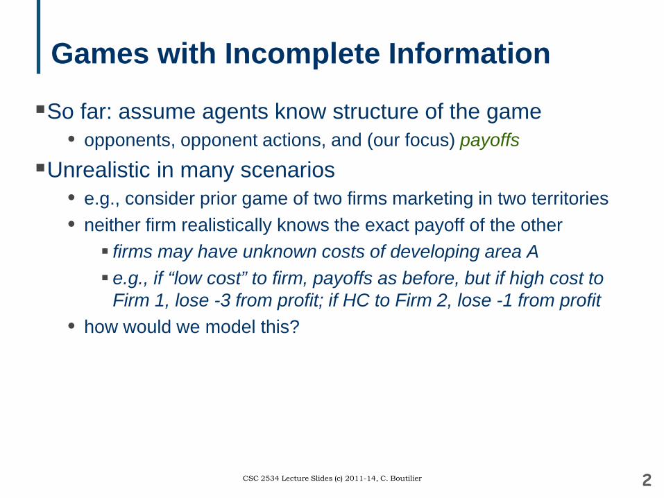
So far: assume agents know structure of the game• opponents, opponent actions, and (our focus) payoffs

Unrealistic in many scenarios• e.g., consider prior game of two firms marketing in two territories• neither firm realistically knows the exact payoff of the other

firms may have unknown costs of developing area A e.g., if “low cost” to firm, payoffs as before, but if high cost to

Firm 1, lose -3 from profit; if HC to Firm 2, lose -1 from profit• how would we model this?

2CSC 2534 Lecture Slides (c) 2011-14, C. Boutilier

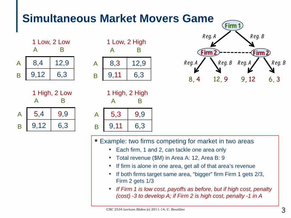
Simultaneous Market Movers Game

3CSC 2534 Lecture Slides (c) 2011-14, C. Boutilier

8,4 12,99,12 6,3

A

B

A B

Firm 1

Firm 2 Firm 2

Reg. A Reg. B

8, 4 12, 9 9, 12 6, 3

Reg. A Reg. BReg. A Reg. B

Example: two firms competing for market in two areas• Each firm, 1 and 2, can tackle one area only• Total revenue ($M) in Area A: 12, Area B: 9• If firm is alone in one area, get all of that area’s revenue• If both firms target same area, “bigger” firm Firm 1 gets 2/3,

Firm 2 gets 1/3• If Firm 1 is low cost, payoffs as before, but if high cost, penalty

(cost) -3 to develop A; if Firm 2 is high cost, penalty -1 in A

8,3 12,99,11 6,3

A

B

A B1 Low, 2 Low 1 Low, 2 High

5,4 9,99,12 6,3

A

B

A B

5,3 9,99,11 6,3

A

B

A B1 High, 2 Low 1 High, 2 High

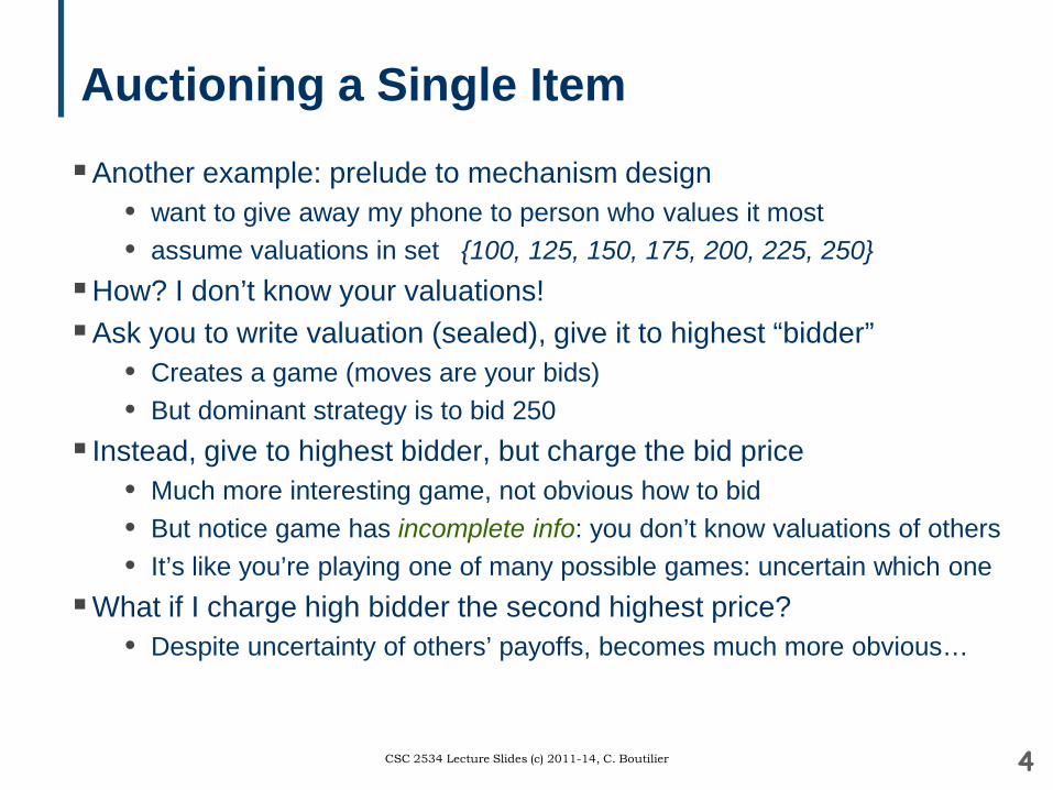
Auctioning a Single ItemAnother example: prelude to mechanism design

• want to give away my phone to person who values it most• assume valuations in set {100, 125, 150, 175, 200, 225, 250}

How? I don’t know your valuations!Ask you to write valuation (sealed), give it to highest “bidder”

• Creates a game (moves are your bids)• But dominant strategy is to bid 250

Instead, give to highest bidder, but charge the bid price• Much more interesting game, not obvious how to bid• But notice game has incomplete info: you don’t know valuations of others• It’s like you’re playing one of many possible games: uncertain which one

What if I charge high bidder the second highest price?• Despite uncertainty of others’ payoffs, becomes much more obvious…

4CSC 2534 Lecture Slides (c) 2011-14, C. Boutilier

Bayesian Games

A Bayesian game (of incomplete information)• set of agents (or players) i = {1, … N}• action set Ai for each agent i, with joint actions A = X Ai• type space Θi for each agent i, with joint type space Θ = X Θi

• utility functions ui : A X Θi →R ui(a,θi) is utility of action a to agent i when type is θi ∈ Θi

• common prior distribution P over ΘType represents private information i has about the game

• usually, we’ll speak of i’s type as its “utility function” since this is what dictates i’s utility for any joint action

• i is assumed to know its type (it is revealed before action taken) also reveals partial info about others’ types (conditioning)

• game is common knowledge

5CSC 2534 Lecture Slides (c) 2011-14, C. Boutilier

Simultaneous Market Movers Game

6CSC 2534 Lecture Slides (c) 2011-14, C. Boutilier

8,4 12,99,12 6,3

A

B

A B

8,3 12,99,11 6,3

A

B

A B1 Low, 2 Low 1 Low, 2 High

5,4 9,99,12 6,3

A

B

A B

5,3 9,99,11 6,3

A

B

A B1 High, 2 Low 1 High, 2 High

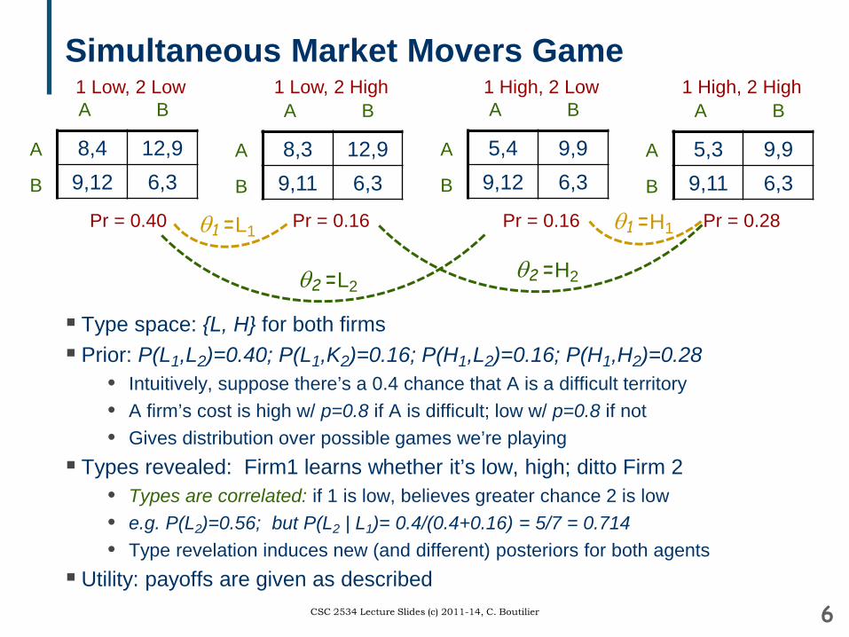
Type space: {L, H} for both firms Prior: P(L1,L2)=0.40; P(L1,K2)=0.16; P(H1,L2)=0.16; P(H1,H2)=0.28

• Intuitively, suppose there’s a 0.4 chance that A is a difficult territory• A firm’s cost is high w/ p=0.8 if A is difficult; low w/ p=0.8 if not• Gives distribution over possible games we’re playing

Types revealed: Firm1 learns whether it’s low, high; ditto Firm 2 • Types are correlated: if 1 is low, believes greater chance 2 is low• e.g. P(L2)=0.56; but P(L2 | L1)= 0.4/(0.4+0.16) = 5/7 = 0.714• Type revelation induces new (and different) posteriors for both agents

Utility: payoffs are given as described

Pr = 0.40 Pr = 0.16 Pr = 0.16 Pr = 0.28θ1 =L1 θ1 =H1

θ2 =L2θ2 =H2

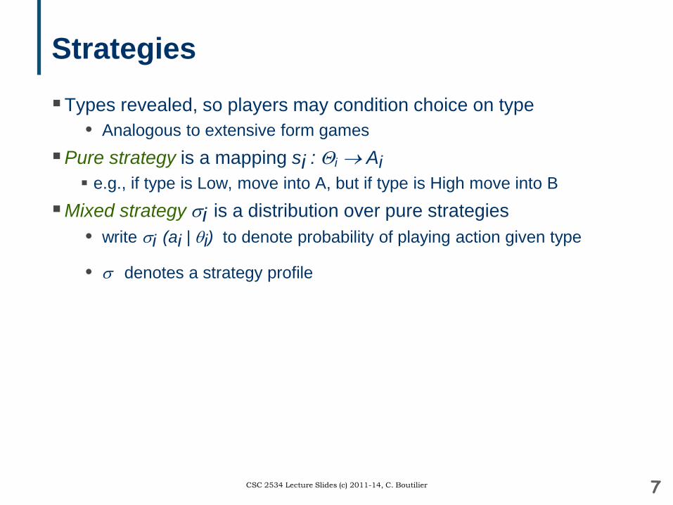
StrategiesTypes revealed, so players may condition choice on type

• Analogous to extensive form gamesPure strategy is a mapping si : Θi → Ai e.g., if type is Low, move into A, but if type is High move into B

Mixed strategy σi is a distribution over pure strategies • write σi (ai | θi) to denote probability of playing action given type

• σ denotes a strategy profile

7CSC 2534 Lecture Slides (c) 2011-14, C. Boutilier

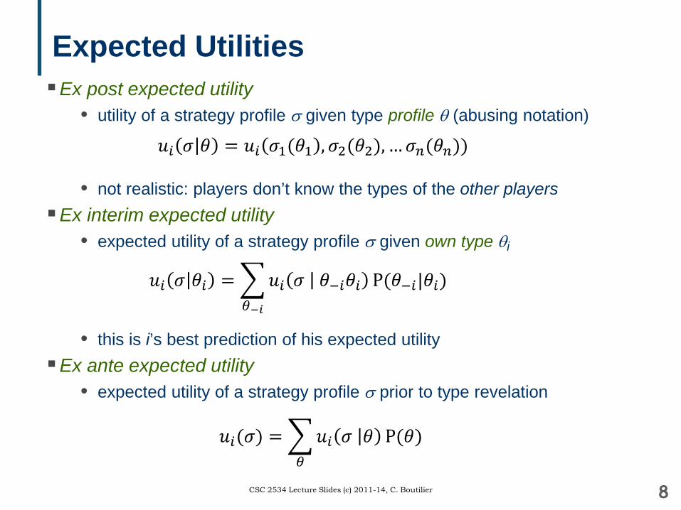
Expected UtilitiesEx post expected utility

• utility of a strategy profile σ given type profile θ (abusing notation)

• not realistic: players don’t know the types of the other playersEx interim expected utility

• expected utility of a strategy profile σ given own type θi

• this is i’s best prediction of his expected utilityEx ante expected utility

• expected utility of a strategy profile σ prior to type revelation

8CSC 2534 Lecture Slides (c) 2011-14, C. Boutilier

𝑢𝑢𝑖𝑖 𝜎𝜎 𝜃𝜃 = 𝑢𝑢𝑖𝑖 𝜎𝜎1(𝜃𝜃1 , 𝜎𝜎2(𝜃𝜃2), … 𝜎𝜎𝑛𝑛(𝜃𝜃𝑛𝑛))

𝑢𝑢𝑖𝑖 𝜎𝜎 𝜃𝜃𝑖𝑖 = �𝜃𝜃−𝑖𝑖

𝑢𝑢𝑖𝑖 𝜎𝜎 𝜃𝜃−𝑖𝑖𝜃𝜃𝑖𝑖 P(𝜃𝜃−𝑖𝑖|𝜃𝜃𝑖𝑖)

𝑢𝑢𝑖𝑖(𝜎𝜎) = �𝜃𝜃

𝑢𝑢𝑖𝑖 𝜎𝜎 𝜃𝜃 P(𝜃𝜃)

Best Responses

A best response for i to profile σ-i is any strategy σisatisfying ui(σi ∙σ-i) ≥ ui(σ’i ∙σ-i) for all σ’i

Note: this doesn’t prevent i from optimizing choice for each of its possible types: Given σ-i , the strategy that maximizes ex ante utility will map each possible type θi to the choice that maximizes ex interim utility for θi

Note: given fixed strategies of others, a player reasons about the (conditional) predicted types of others, and how this will lead to probabilities of various actions being played

9CSC 2534 Lecture Slides (c) 2011-14, C. Boutilier

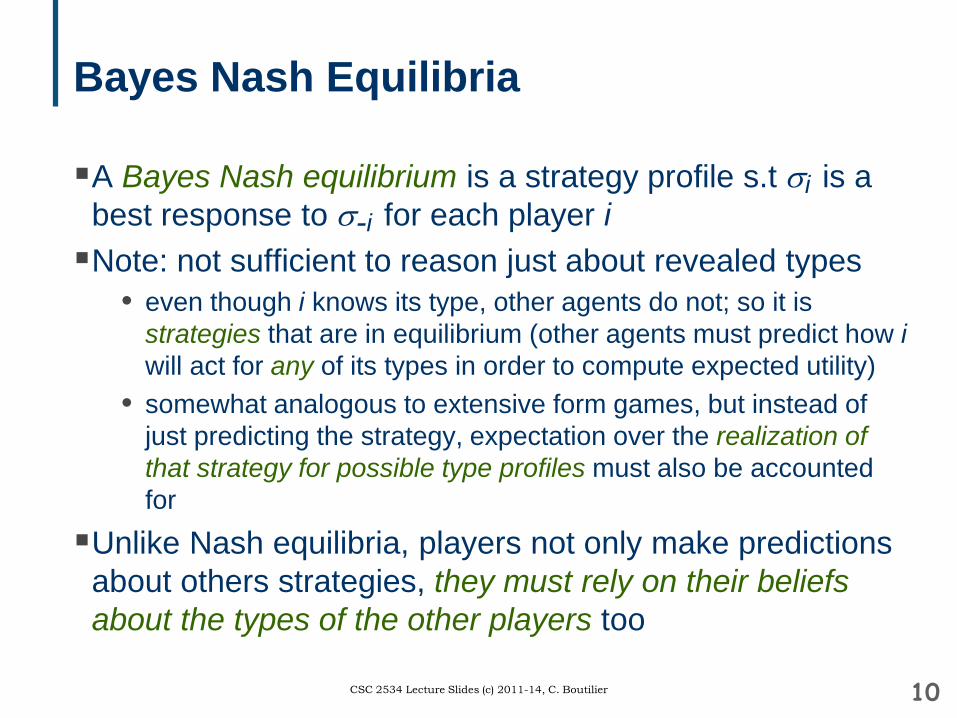
Bayes Nash Equilibria

A Bayes Nash equilibrium is a strategy profile s.t σi is a best response to σ-i for each player iNote: not sufficient to reason just about revealed types

• even though i knows its type, other agents do not; so it is strategies that are in equilibrium (other agents must predict how iwill act for any of its types in order to compute expected utility)

• somewhat analogous to extensive form games, but instead of just predicting the strategy, expectation over the realization of that strategy for possible type profiles must also be accounted for

Unlike Nash equilibria, players not only make predictions about others strategies, they must rely on their beliefs about the types of the other players too

10CSC 2534 Lecture Slides (c) 2011-14, C. Boutilier

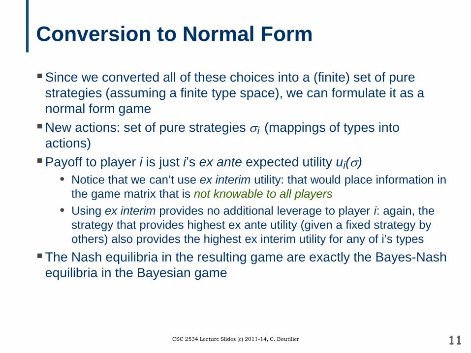
Conversion to Normal Form

Since we converted all of these choices into a (finite) set of pure strategies (assuming a finite type space), we can formulate it as a normal form gameNew actions: set of pure strategies σi (mappings of types into

actions)Payoff to player i is just i’s ex ante expected utility ui(σ)

• Notice that we can’t use ex interim utility: that would place information in the game matrix that is not knowable to all players

• Using ex interim provides no additional leverage to player i: again, the strategy that provides highest ex ante utility (given a fixed strategy by others) also provides the highest ex interim utility for any of i’s types

The Nash equilibria in the resulting game are exactly the Bayes-Nash equilibria in the Bayesian game

11CSC 2534 Lecture Slides (c) 2011-14, C. Boutilier

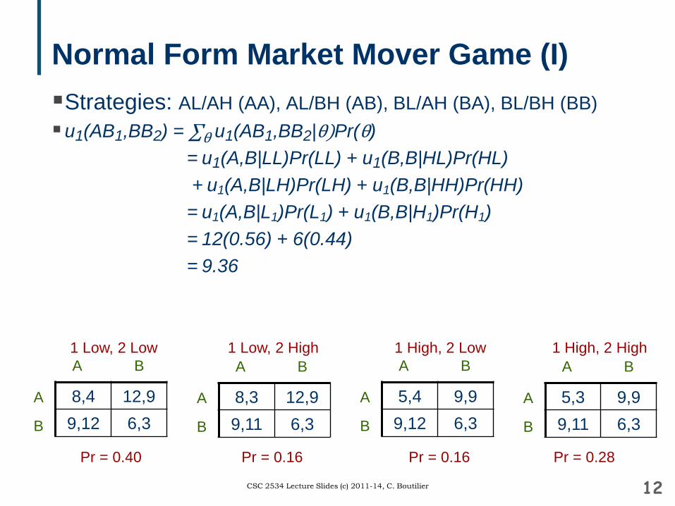
Normal Form Market Mover Game (I)Strategies: AL/AH (AA), AL/BH (AB), BL/AH (BA), BL/BH (BB)u1(AB1,BB2) = ∑θ u1(AB1,BB2|θ)Pr(θ)

= u1(A,B|LL)Pr(LL) + u1(B,B|HL)Pr(HL)+ u1(A,B|LH)Pr(LH) + u1(B,B|HH)Pr(HH)= u1(A,B|L1)Pr(L1) + u1(B,B|H1)Pr(H1) = 12(0.56) + 6(0.44) = 9.36

12CSC 2534 Lecture Slides (c) 2011-14, C. Boutilier

8,4 12,99,12 6,3

A

B

A B

8,3 12,99,11 6,3

A

B

A B1 Low, 2 Low 1 Low, 2 High

5,4 9,99,12 6,3

A

B

A B

5,3 9,99,11 6,3

A

B

A B1 High, 2 Low 1 High, 2 High

Pr = 0.40 Pr = 0.16 Pr = 0.16 Pr = 0.28

Normal Form Market Mover Game (II)Strategies: AL/AH (AA), AL/BH (AB), BL/AH (BA), BL/BH (BB)u1(AA1,BB2) = ∑θ u1(AA1,BB2|θ)Pr(θ)

= u1(A,B|LL)Pr(LL) + u1(A,B|HL)Pr(HL)+ u1(A,B|LH)Pr(LH) + u1(A,B|HH)Pr(HH)= u1(A,B|L1)Pr(L1) + u1(A,B|H1)Pr(H1) = 12(0.56) + 9(0.44) = 10.68

13CSC 2534 Lecture Slides (c) 2011-14, C. Boutilier

8,4 12,99,12 6,3

A

B

A B

8,3 12,99,11 6,3

A

B

A B1 Low, 2 Low 1 Low, 2 High

5,4 9,99,12 6,3

A

B

A B

5,3 9,99,11 6,3

A

B

A B1 High, 2 Low 1 High, 2 High

Pr = 0.40 Pr = 0.16 Pr = 0.16 Pr = 0.28

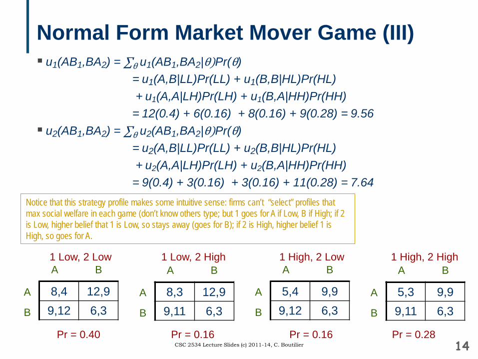
Normal Form Market Mover Game (III) u1(AB1,BA2) = ∑θ u1(AB1,BA2|θ)Pr(θ)

= u1(A,B|LL)Pr(LL) + u1(B,B|HL)Pr(HL)+ u1(A,A|LH)Pr(LH) + u1(B,A|HH)Pr(HH)

= 12(0.4) + 6(0.16) + 8(0.16) + 9(0.28) = 9.56 u2(AB1,BA2) = ∑θ u2(AB1,BA2|θ)Pr(θ)

= u2(A,B|LL)Pr(LL) + u2(B,B|HL)Pr(HL) + u2(A,A|LH)Pr(LH) + u2(B,A|HH)Pr(HH)

= 9(0.4) + 3(0.16) + 3(0.16) + 11(0.28) = 7.64

14CSC 2534 Lecture Slides (c) 2011-14, C. Boutilier

8,4 12,99,12 6,3

A

B

A B

8,3 12,99,11 6,3

A

B

A B1 Low, 2 Low 1 Low, 2 High

5,4 9,99,12 6,3

A

B

A B

5,3 9,99,11 6,3

A

B

A B1 High, 2 Low 1 High, 2 High

Pr = 0.40 Pr = 0.16 Pr = 0.16 Pr = 0.28

Notice that this strategy profile makes some intuitive sense: firms can’t “select” profiles that max social welfare in each game (don’t know others type; but 1 goes for A if Low, B if High; if 2 is Low, higher belief that 1 is Low, so stays away (goes for B); if 2 is High, higher belief 1 is High, so goes for A.

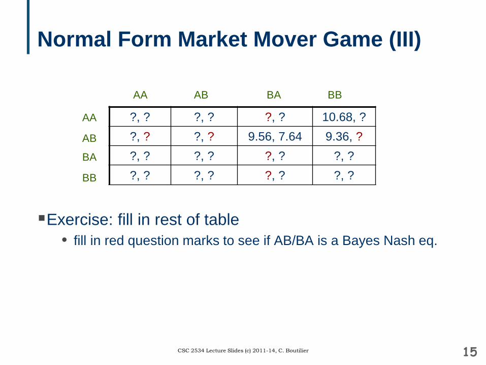
Normal Form Market Mover Game (III)

Exercise: fill in rest of table• fill in red question marks to see if AB/BA is a Bayes Nash eq.

15CSC 2534 Lecture Slides (c) 2011-14, C. Boutilier

?, ? ?, ? ?, ? 10.68, ??, ? ?, ? 9.56, 7.64 9.36, ??, ? ?, ? ?, ? ?, ??, ? ?, ? ?, ? ?, ?

AA

AB

AA AB BA BB

BA

BB

Other Incomplete Information

Harsanyi (1967) argued that other forms of uncertainty in structure can be modeled using payoff uncertainty

• uncertainty in player actions; e.g., can player P1 do A,B or A,B,C include action C as a move in all games, but create type(s) for P1

that gives C such low payoff that it would never choose that action assign probability to that type equal to 1 – Pr(C exists)

• uncertainty about players; e.g., is P1 in the game? include player P1 in all games, but create new type corresponding

to non-existence and an action that is dominant for P1 under that type such that payoffs for other players are as if P1 is not present assign probability to this type equal to 1-Pr(P1 exists)

16CSC 2534 Lecture Slides (c) 2011-14, C. Boutilier

Stronger Equilibrium NotionsDominant Strategy Equilibrium

• σi is dominant for player i if it has max expected utility no matter what strategies other players play

• DSE: a profile in which each player plays a dominant strategy• concept applies to normal form games too (Prisoners dilemma)• very robust: does not rely on predictions about behavior of opponents,

nor on accurate beliefs about other’s typesEx Post Equilibrium

• profile σ is an EPE if, for all i: ui(σi ∙σ-i | θ) ≥ ui(σ’i ∙σ-i | θ) for all θ, σ’i• no matter what i learns about your type, would not deviate from σi

• different than dominant: depends on prediction about others’ strategies• still quite robust: does not rely on accurate beliefs about types of others,

only predictions of strategies (much like regular Nash equilibrium)Both notions important in mechanism design

17CSC 2534 Lecture Slides (c) 2011-14, C. Boutilier

Return to the Second Price Auction

I want to give away my phone to person values it most• in other words, I want to maximize social welfare• but I don’t know valuations, so I decide to ask and see who’s

willing to pay: use 2nd-price auction formatBidders submit “sealed” bids; highest bidder wins, pays

price bid by second-highest bidder• also known as Vickrey auctions• special case of Groves mechanisms, Vickrey-Clarke-Groves

(VCG) mechanisms

2nd-price seems weird but is quite remarkable• truthful bidding, i.e., bidding your true value, is a dominant

strategy

To see this, let’s formulate it as a Bayesian game

18CSC 2534 Lecture Slides (c) 2011-14, C. Boutilier

Second-Price Auction: Bayesian Game

n players (bidders)Types: each player k has value vk ∊ [0,1] for itemstrategies/actions for player k: any bid bk between [0,1]outcomes: player k wins, pays price p (2nd highest bid)

• outcomes are pairs (k,p), i.e., (winner, price)payoff for player k:

• if k loses: payoff is 0• if k wins, payoff depends on price p: payoff is vk – p

Prior: joint distribution over values (will not specify for now)• we do assume that values (types) are independent and private• i.e., own value does not influence beliefs about value of other bidders

Note: action space and type space are continuous

19CSC 2534 Lecture Slides (c) 2011-14, C. Boutilier

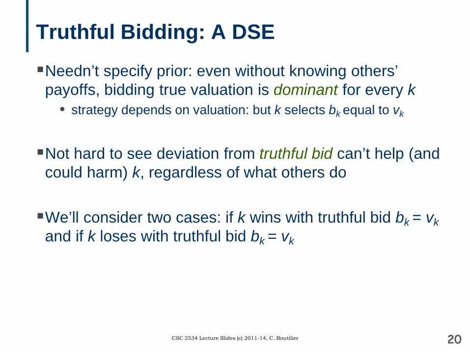
Truthful Bidding: A DSENeedn’t specify prior: even without knowing others’

payoffs, bidding true valuation is dominant for every k• strategy depends on valuation: but k selects bk equal to vk

Not hard to see deviation from truthful bid can’t help (and could harm) k, regardless of what others do

We’ll consider two cases: if k wins with truthful bid bk = vkand if k loses with truthful bid bk = vk

20CSC 2534 Lecture Slides (c) 2011-14, C. Boutilier

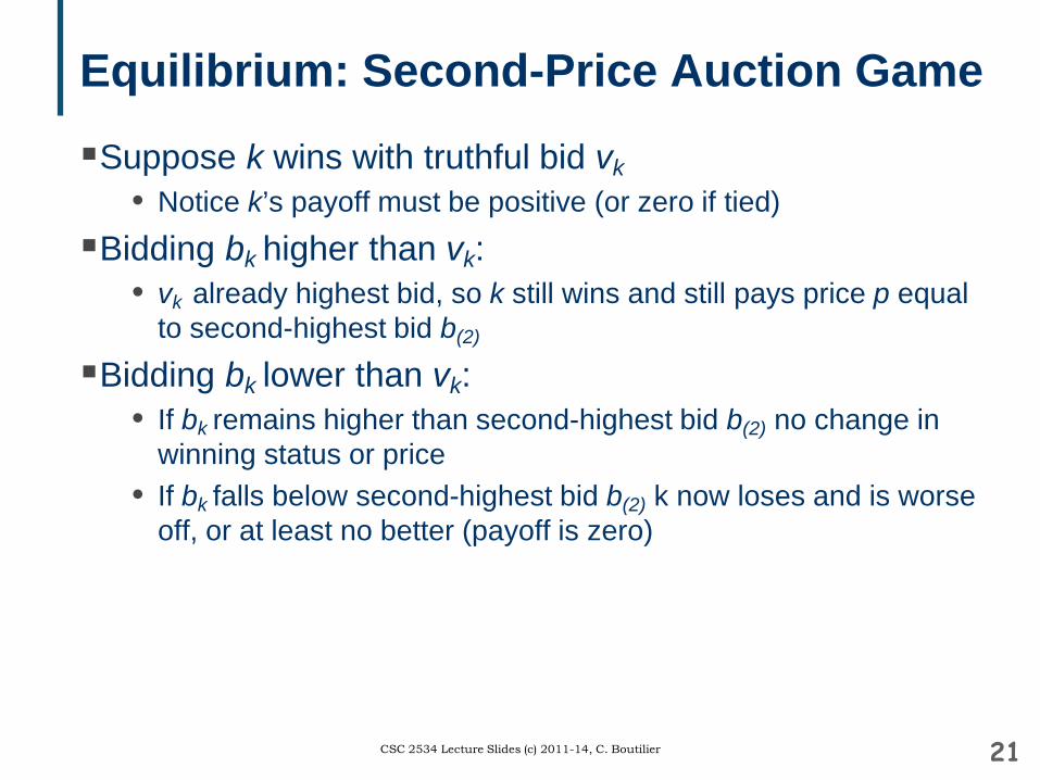
Equilibrium: Second-Price Auction GameSuppose k wins with truthful bid vk

• Notice k’s payoff must be positive (or zero if tied)Bidding bk higher than vk:

• vk already highest bid, so k still wins and still pays price p equal to second-highest bid b(2)

Bidding bk lower than vk:• If bk remains higher than second-highest bid b(2) no change in

winning status or price• If bk falls below second-highest bid b(2) k now loses and is worse

off, or at least no better (payoff is zero)

21CSC 2534 Lecture Slides (c) 2011-14, C. Boutilier

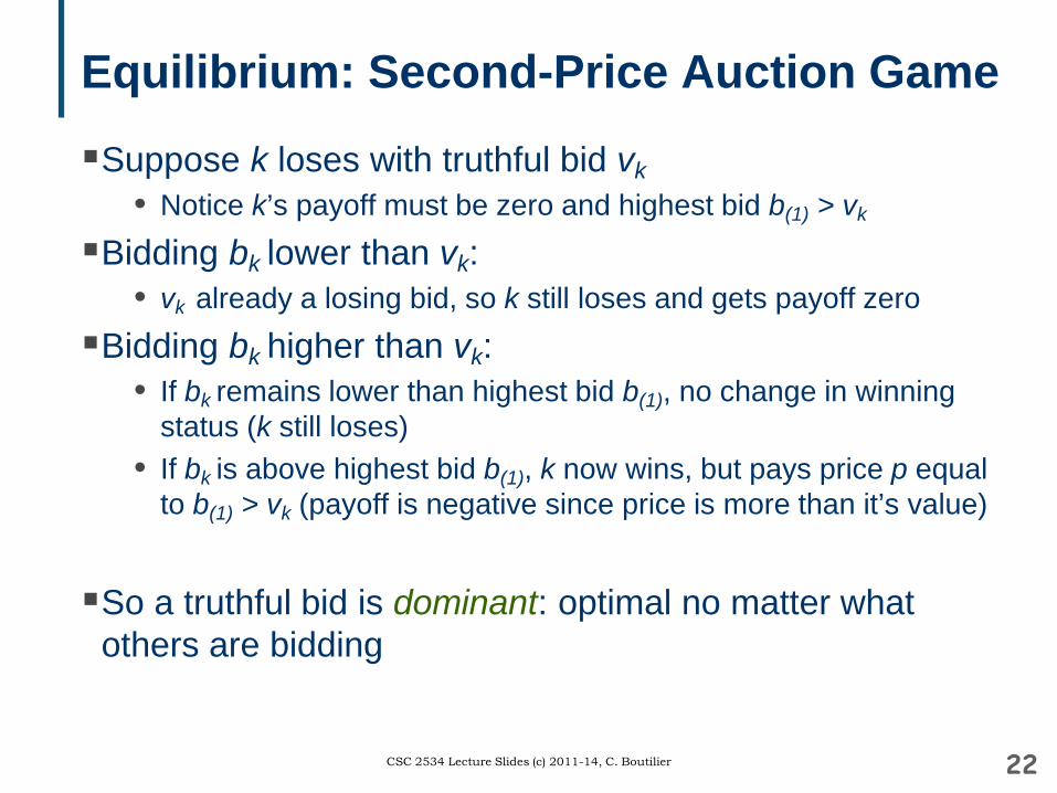
Equilibrium: Second-Price Auction GameSuppose k loses with truthful bid vk

• Notice k’s payoff must be zero and highest bid b(1) > vk

Bidding bk lower than vk:• vk already a losing bid, so k still loses and gets payoff zero

Bidding bk higher than vk:• If bk remains lower than highest bid b(1), no change in winning

status (k still loses)• If bk is above highest bid b(1), k now wins, but pays price p equal

to b(1) > vk (payoff is negative since price is more than it’s value)

So a truthful bid is dominant: optimal no matter what others are bidding

22CSC 2534 Lecture Slides (c) 2011-14, C. Boutilier

Truthful Bidding in Second-Price Auction

Consider actions of bidder 2• Ignore values of other

bidders, consider only their bids. Their values don’t impact outcome, only bids do.

What if bidder 2 bids:• truthfully $105?

loses (payoff 0)• too high: $120

loses (payoff 0)• too high: $130

wins (payoff -20)• too low: $70

loses (payoff 0)23CSC 2534 Lecture Slides (c) 2011-14, C. Boutilier

b1 = $125

v2 = $105b2 = ???

b3 = $90

b4 = $65

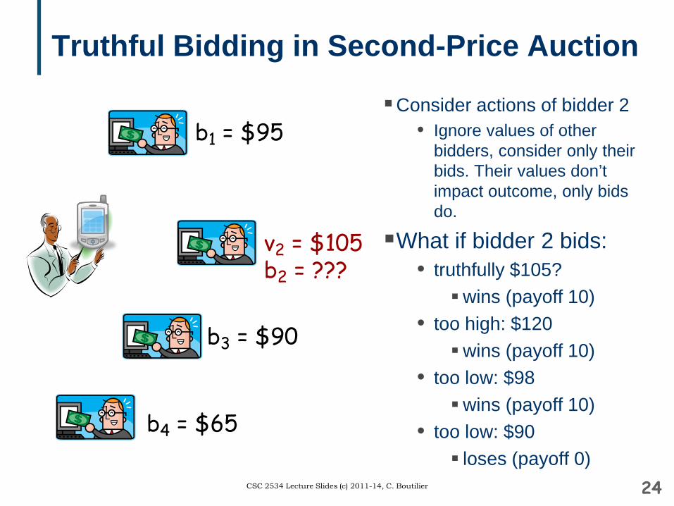
Truthful Bidding in Second-Price Auction

Consider actions of bidder 2• Ignore values of other

bidders, consider only their bids. Their values don’t impact outcome, only bids do.

What if bidder 2 bids:• truthfully $105?

wins (payoff 10)• too high: $120

wins (payoff 10)• too low: $98

wins (payoff 10)• too low: $90

loses (payoff 0)24CSC 2534 Lecture Slides (c) 2011-14, C. Boutilier

b1 = $95

v2 = $105b2 = ???

b3 = $90

b4 = $65

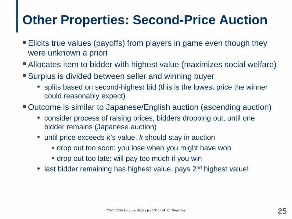
Other Properties: Second-Price AuctionElicits true values (payoffs) from players in game even though they

were unknown a prioriAllocates item to bidder with highest value (maximizes social welfare)Surplus is divided between seller and winning buyer

• splits based on second-highest bid (this is the lowest price the winner could reasonably expect)

Outcome is similar to Japanese/English auction (ascending auction)• consider process of raising prices, bidders dropping out, until one

bidder remains (Japanese auction)• until price exceeds k’s value, k should stay in auction

drop out too soon: you lose when you might have won drop out too late: will pay too much if you win

• last bidder remaining has highest value, pays 2nd highest value!

25CSC 2534 Lecture Slides (c) 2011-14, C. Boutilier

Mechanism Design

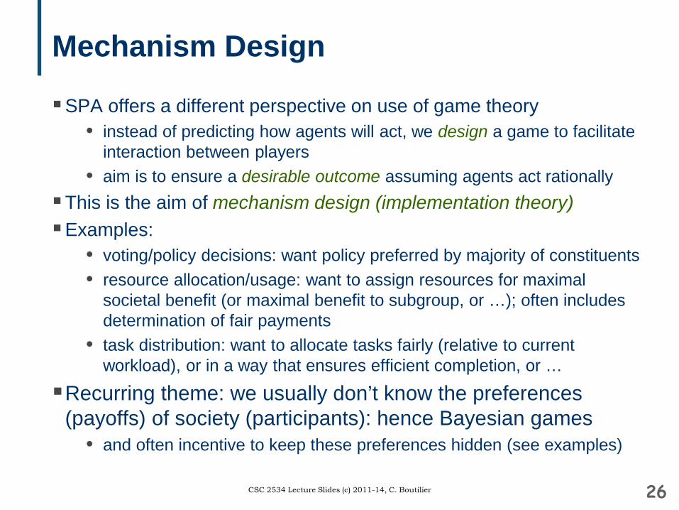
SPA offers a different perspective on use of game theory• instead of predicting how agents will act, we design a game to facilitate

interaction between players• aim is to ensure a desirable outcome assuming agents act rationally

This is the aim of mechanism design (implementation theory)Examples:

• voting/policy decisions: want policy preferred by majority of constituents• resource allocation/usage: want to assign resources for maximal

societal benefit (or maximal benefit to subgroup, or …); often includes determination of fair payments

• task distribution: want to allocate tasks fairly (relative to current workload), or in a way that ensures efficient completion, or …

Recurring theme: we usually don’t know the preferences (payoffs) of society (participants): hence Bayesian games

• and often incentive to keep these preferences hidden (see examples)

26CSC 2534 Lecture Slides (c) 2011-14, C. Boutilier

Mechanism Design: Basic SetupSet of possible outcomes On players, with each player k having:

• type space Θk

• utility function uk : O X Θk →R uk(o,θk) is utility of outcome o to agent k when type is θk ∈ Θk

think of θk as an encoding of k’s preferences (or utility function) (Typically) a common prior distribution P over ΘA social choice function (SCF) C: Θ → O

• intuitively C(θ) is the most desirable option if player preferences are θ• can allow “correspondence”, social “objectives” that score outcomes

Examples of social choice criteria:• make majority “happy”; maximize social welfare (SWM); find “fairest”

outcome; make one person as happy as possible (e.g., revenue max’ztn in auctions), make least well-off person as happy as possible…

• set up for SPA: types: values; outcomes: winner-price; SCF: SWM

27CSC 2534 Lecture Slides (c) 2011-14, C. Boutilier

A Mechanism

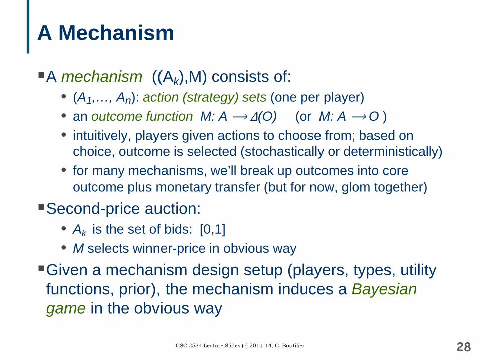
A mechanism ((Ak),M) consists of:• (A1,…, An): action (strategy) sets (one per player) • an outcome function M: A ⟶ Δ(O) (or M: A ⟶ O ) • intuitively, players given actions to choose from; based on

choice, outcome is selected (stochastically or deterministically)• for many mechanisms, we’ll break up outcomes into core

outcome plus monetary transfer (but for now, glom together)Second-price auction:

• Ak is the set of bids: [0,1]• M selects winner-price in obvious way

Given a mechanism design setup (players, types, utility functions, prior), the mechanism induces a Bayesian game in the obvious way

28CSC 2534 Lecture Slides (c) 2011-14, C. Boutilier

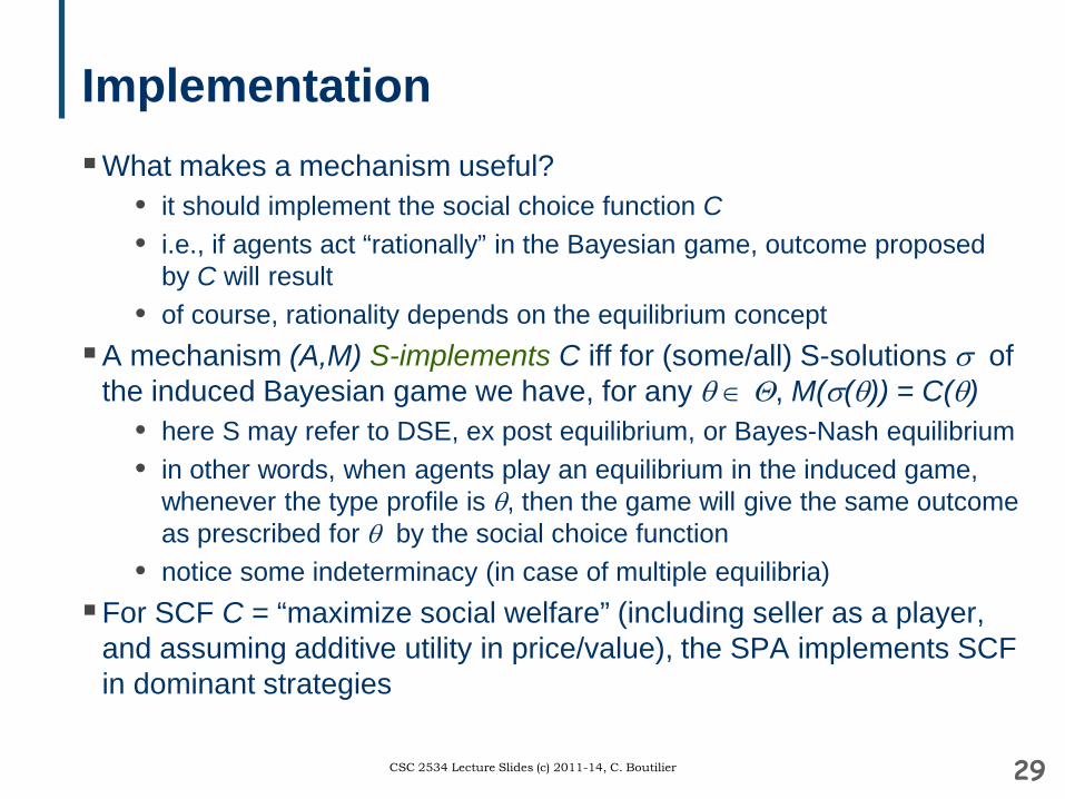
ImplementationWhat makes a mechanism useful?

• it should implement the social choice function C• i.e., if agents act “rationally” in the Bayesian game, outcome proposed

by C will result• of course, rationality depends on the equilibrium concept

A mechanism (A,M) S-implements C iff for (some/all) S-solutions σ of the induced Bayesian game we have, for any θ ∈ Θ, M(σ(θ)) = C(θ)

• here S may refer to DSE, ex post equilibrium, or Bayes-Nash equilibrium• in other words, when agents play an equilibrium in the induced game,

whenever the type profile is θ, then the game will give the same outcome as prescribed for θ by the social choice function

• notice some indeterminacy (in case of multiple equilibria)For SCF C = “maximize social welfare” (including seller as a player,

and assuming additive utility in price/value), the SPA implements SCF in dominant strategies

29CSC 2534 Lecture Slides (c) 2011-14, C. Boutilier

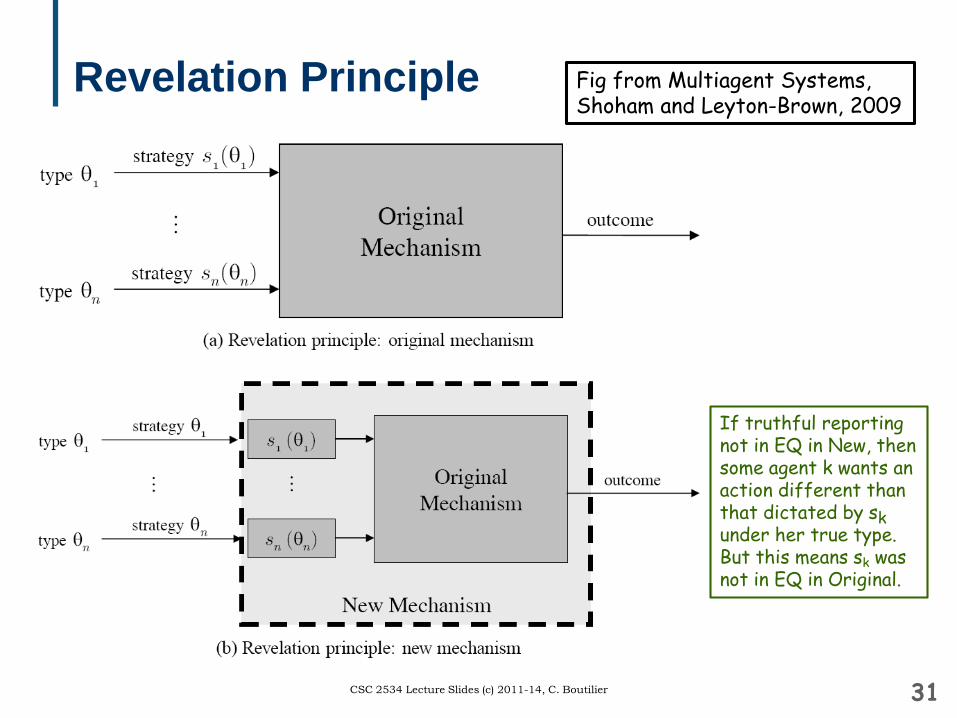
Revelation Principle

Given SCF C, how could one even begin to explore space of mechanisms?

• actions can be arbitrary, mappings can be arbitrary, …Notice that SPA keeps actions simple: “state your value”

• it’s a direct mechanism: Ak = θk (i.e., actions are “declare your type”)• …and stating values truthfully is a DSE• Turns out this is an instance of a broad principle

Revelation principle: if there is an S-implementation of SCF C, then there exists a direct, mechanism that S-implements C and is truthful

• intuition: design new outcome function M’ so that when agents report truthfully, the mechanism makes the choice original M would have realized in the S-solution

Consequence: much work in mechanism design focuses on direct mechanisms and truthful implementation

30CSC 2534 Lecture Slides (c) 2011-14, C. Boutilier

Revelation Principle

31CSC 2534 Lecture Slides (c) 2011-14, C. Boutilier

Fig from Multiagent Systems,Shoham and Leyton-Brown, 2009

If truthful reportingnot in EQ in New, thensome agent k wants anaction different thanthat dictated by skunder her true type.But this means sk wasnot in EQ in Original.

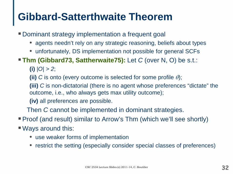
Gibbard-Satterthwaite TheoremDominant strategy implementation a frequent goal

• agents needn’t rely on any strategic reasoning, beliefs about types• unfortunately, DS implementation not possible for general SCFs

Thm (Gibbard73, Sattherwaite75): Let C (over N, O) be s.t.:(i) |O| > 2; (ii) C is onto (every outcome is selected for some profile θ); (iii) C is non-dictatorial (there is no agent whose preferences “dictate” the outcome, i.e., who always gets max utility outcome); (iv) all preferences are possible.

Then C cannot be implemented in dominant strategies.Proof (and result) similar to Arrow’s Thm (which we’ll see shortly)Ways around this:

• use weaker forms of implementation• restrict the setting (especially consider special classes of preferences)

32CSC 2534 Lecture Slides (c) 2011-14, C. Boutilier

Groves MechanismsDespite GS theorem, truthful implementation in DS is possible for an

important class of problems• assume outcomes allow for transfer of utility between players• assume agent preferences over such transfers are additive• auctions are an example (utility function in SPA)

Quasi-linear mechanism design problem (QLMD)• extend outcome space with “monetary” transfers

outcomes: O x T, where T is set of vectors of form (t1, … tn)• quasi-linear utility: uk((o,t),θk) = vk(o,θk) + tk• SCF is SWM (i.e., maximization of social welfare SW(o,t,θ) )

Assumptions:• value for “concrete” outcomes and transfer commensurate• players are risk neutral

In SPA, utility is valuation less price paid (negt’v transfer to winner), or price paid (pos’tv transfer to seller) (see formalization on slide 3)

33CSC 2534 Lecture Slides (c) 2011-14, C. Boutilier

Groves MechanismsA Groves mechanism (A,M) for QLMD problem is:

• Ak = θk = Vk : agent k announces values v*k for outcomes• M(v*) = (o, t1, … tn) where:

o = argmaxo∊O ∑k v*k(o) tk(v*k) = ∑j≠k v*j(o) – hk(v*-k), where hk is an arbitrary function

Intuition is simple:• choose SWM-outcome based on declared values v*• then transfer to k: the declared welfare of chosen outcome to the other

agents, less some “social cost” function hk which depends on what others said (but critically, not on what k reports)

Some notes:• in fact, a family of mechanisms, for various choices of hk

• if agents reveal true values, i.e., v*k = vk for all k, then it maximizes SW• SPA: is an instance of this

34CSC 2534 Lecture Slides (c) 2011-14, C. Boutilier

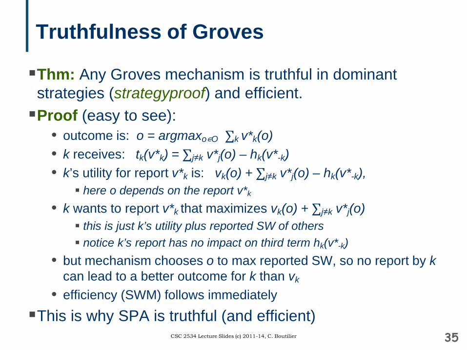
Truthfulness of Groves

Thm: Any Groves mechanism is truthful in dominant strategies (strategyproof) and efficient.Proof (easy to see):

• outcome is: o = argmaxo∊O ∑k v*k(o)• k receives: tk(v*k) = ∑j≠k v*j(o) – hk(v*-k) • k’s utility for report v*k is: vk(o) + ∑j≠k v*j(o) – hk(v*-k),

here o depends on the report v*k

• k wants to report v*k that maximizes vk(o) + ∑j≠k v*j(o) this is just k’s utility plus reported SW of others notice k’s report has no impact on third term hk(v*-k)

• but mechanism chooses o to max reported SW, so no report by kcan lead to a better outcome for k than vk

• efficiency (SWM) follows immediatelyThis is why SPA is truthful (and efficient)

35CSC 2534 Lecture Slides (c) 2011-14, C. Boutilier

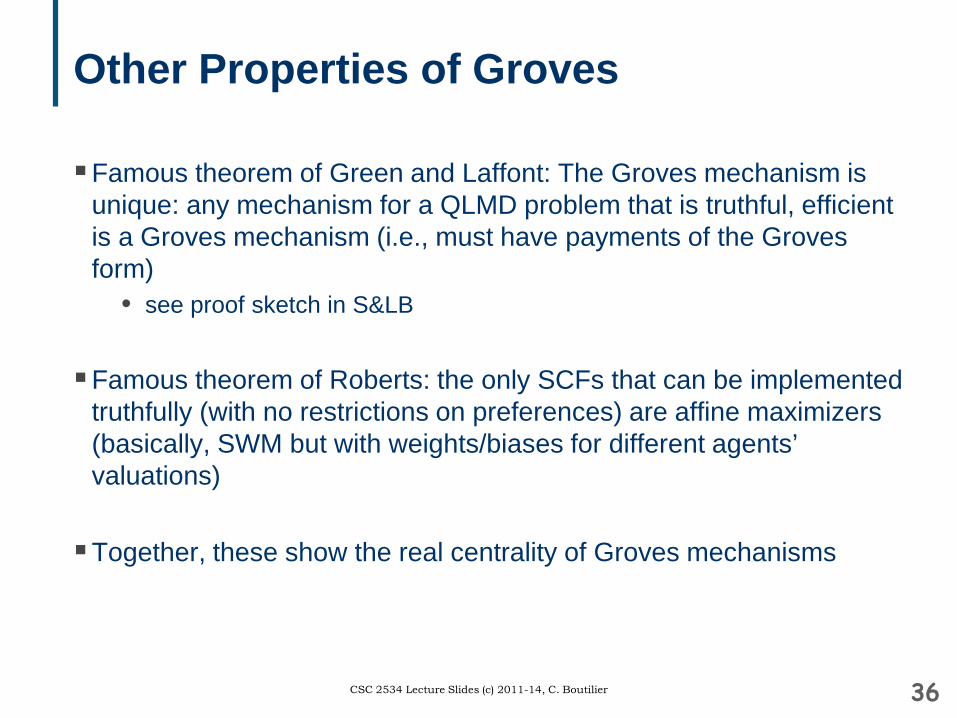
Other Properties of Groves

Famous theorem of Green and Laffont: The Groves mechanism is unique: any mechanism for a QLMD problem that is truthful, efficient is a Groves mechanism (i.e., must have payments of the Groves form)

• see proof sketch in S&LB

Famous theorem of Roberts: the only SCFs that can be implemented truthfully (with no restrictions on preferences) are affine maximizers(basically, SWM but with weights/biases for different agents’ valuations)

Together, these show the real centrality of Groves mechanisms

36CSC 2534 Lecture Slides (c) 2011-14, C. Boutilier

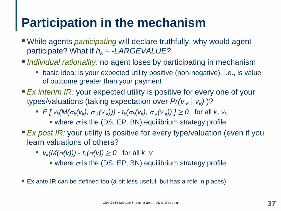
Participation in the mechanismWhile agents participating will declare truthfully, why would agent

participate? What if hk = -LARGEVALUE? Individual rationality: no agent loses by participating in mechanism

• basic idea: is your expected utility positive (non-negative), i.e., is value of outcome greater than your payment

Ex interim IR: your expected utility is positive for every one of your types/valuations (taking expectation over Pr(v-k | vk) )?

• E [ vk(M(σk(vk), σ-k(v-k))) - tk(σk(vk), σ-k(v-k)) ] ≥ 0 for all k, vk

where σ is the (DS, EP, BN) equilibrium strategy profileEx post IR: your utility is positive for every type/valuation (even if you

learn valuations of others?• vk(M(σ(v))) - tk(σ(v)) ≥ 0 for all k, v

where σ is the (DS, EP, BN) equilibrium strategy profile

Ex ante IR can be defined too (a bit less useful, but has a role in places)

37CSC 2534 Lecture Slides (c) 2011-14, C. Boutilier

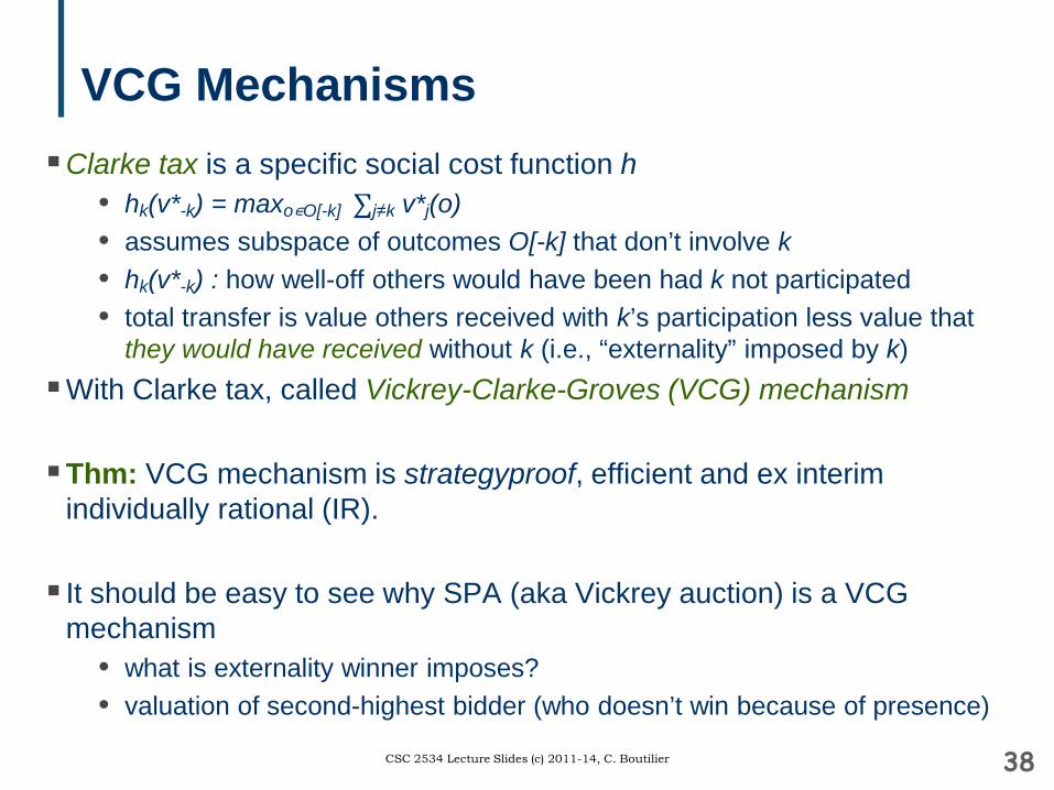
VCG MechanismsClarke tax is a specific social cost function h

• hk(v*-k) = maxo∊O[-k] ∑j≠k v*j(o)• assumes subspace of outcomes O[-k] that don’t involve k• hk(v*-k) : how well-off others would have been had k not participated• total transfer is value others received with k’s participation less value that

they would have received without k (i.e., “externality” imposed by k)With Clarke tax, called Vickrey-Clarke-Groves (VCG) mechanism

Thm: VCG mechanism is strategyproof, efficient and ex interim individually rational (IR).

It should be easy to see why SPA (aka Vickrey auction) is a VCG mechanism

• what is externality winner imposes?• valuation of second-highest bidder (who doesn’t win because of presence)

38CSC 2534 Lecture Slides (c) 2011-14, C. Boutilier

Other IssuesBudget balance: transfers sum to zero

• transfers in VCG need not be balanced (might be OK to run a surplus; but mechanism may need to subsidize its operation)

• general impossibility result: if type space is rich enough (all valuations over O), can’t generally attain efficiency, strategy proofness, and budget balance

• some special cases can be achieved (e.g., see “no single-agent effect”, which is why VCG works for very general single-sided auctions), or the dAGVA mechanism (BNE, ex ante IR, budget-balanced)

Implementing other choice functions• we’ll see this when we discuss social choice (e.g., maxmin fairness)

Ex post or BN implementation• e.g., the dAGVA mechanism

39CSC 2534 Lecture Slides (c) 2011-14, C. Boutilier

Issues with VCGType revelation

• revealing utility functions difficult; e.g., large (combinatorial) outcomes privacy, communication complexity, computation

• can incremental elicitation work? sometimes: e.g., descending (Dutch auction)

• can approximation work? in general, no; but sometime yes… we’ll discuss more in a bit…

Computational approximation• VCG requires computing optimal (SWM) outcomes

not just one optimization, but n+1 (for all n “subeconomies”) often problematic (e.g., combinatorial auctions) focus of algorithmic mechanism design

• But approximation can destroy incentives and other properties of VCG

40CSC 2534 Lecture Slides (c) 2011-14, C. Boutilier

Issues with VCGFrugality

• VCG transfers may be more extreme than seems necessary e.g., seller revenue, total cost to buyer we’ll see an example in combinatorial auctions

• a fair amount of study on design of mechanisms that are “frugal” (e.g., that try to minimize cost to a buyer) in specific settings (e.g., network and graph problems)

Collusion• many mechanisms are susceptible to collusion, but VCG is largely

viewed as being especially susceptible (we’ll return to this: auctions)

Returning revenue to agents• an issue studied to some extent: if VCG extracts payments over and

above true costs (e.g., Clarke tax for public projects), can some of this be returned to bidders (in a way that doesn’t impact truthfulness)?

41CSC 2534 Lecture Slides (c) 2011-14, C. Boutilier

Combinatorial Auctions

Already discussed 2nd price auctions in depth, 1st price auctions a bit (and will return in a few slides to auctions in general)

Often sellers offer multiple (distinct) items, buyers need multiple items• buyer’s value may depend on the collection of items obtained

Complements: items whose value increase when combined• e.g., a cheap flight to Siena less valuable if you don’t have a hotel room

Substitutes: items whose value decrease when combined• e.g., you’d like the 10AM flight or the 7AM flight; but not both

If items are sold separately, knowing how to bid is difficult• bidders run an “exposure” risk: might win item whose value is

unpredictable because unsure of what other items they might win

42CSC 2534 Lecture Slides (c) 2011-14, C. Boutilier

We Will Continue Mechanism Design Next Week…

43CSC 2534 Lecture Slides (c) 2011-14, C. Boutilier