2+m``2migl2m` hgl2irq`fb *qmpqhmibqm hgl2m`...

NPFL114, Lecture 6

Convolutional Neural Networks III,

Recurrent Neural NetworksMilan Straka

April 08, 2019

Charles University in Prague Faculty of Mathematics and Physics Institute of Formal and Applied Linguistics

unless otherwise stated

Fast R-CNN

Figure 1 of paper "Fast R-CNN", https://arxiv.org/abs/1504.08083.

2/41NPFL114, Lecture 6 Refresh ImageSegmentation FPN FocalLoss TransferLearning GroupNorm RNN LSTM

Fast R-CNN

The bounding box is parametrized as follows. Let be center coordinates and

width and height of the RoI, and let be parameters of the bounding box. We

represent them as follows:

Usually a loss, or Huber loss, is employed for bounding box parameters

The complete loss is then

x , y ,w ,h r r r r

x, y,w,h

t x

t w

= (x − x )/w ,r r

= log(w/w ),r

t y

t h

= (y − y )/h r r

= log(h/h )r

smooth L 1

smooth (x) =L 1 {0.5x2

∣x∣ − 0.5if ∣x∣ < 1otherwise

L( , , c, t) =c t L ( , c) +cls c λ[c ≥ 1] smooth ( −i∈{x,y,w,h}

∑ L 1 ti t ).i


Fast R-CNN

Intersection over unionFor two bounding boxes (or two masks) the intersection over union (IoU) is a ration of theintersection of the boxes (or masks) and the union of the boxes (or masks).

Choosing RoIs for trainingDuring training, we use images with RoIs each. The RoIs are selected so that have

intersection over union (IoU) overlap with ground-truth boxes at least 0.5; the others arechosen to have the IoU in range .

Choosing RoIs during inferenceSingle object can be found in multiple RoIs. To choose the most salient one, we perform non-maximum suppression -- we ignore RoIs which have an overlap with a higher scoring RoI of thesame type, where the IoU is larger than a given threshold (usually, 0.3 is used). Higher scoringRoI is the one with higher probability from the classification head.

2 64 25%

[0.1, 0.5)


Object Detection Evaluation

Average PrecisionEvaluation is performed using Average Precision (AP).

We assume all bounding boxes (or masks) produced by a system have confidence values whichcan be used to rank them. Then, for a single class, we take the boxes (or masks) in the orderof the ranks and generate precision/recall curve, considering a bounding box correct if it hasIoU at least 0.5 with any ground-truth box. We define AP as an average of precisions for recalllevels .

Figure 6 of paper "The PASCAL Visual Object Classes (VOC) Challenge",http://homepages.inf.ed.ac.uk/ckiw/postscript/ijcv_voc09.pdf.

Figure 6 of paper "The PASCAL Visual Object Classes (VOC) Challenge",http://homepages.inf.ed.ac.uk/ckiw/postscript/ijcv_voc09.pdf.

0, 0.1, 0.2, … , 1


Faster R-CNN

For Fast R-CNN, the most time consuming part is generating the RoIs.

Therefore, Faster R-CNN jointly generates regions of interest using a region proposal networkand performs object detection.

Figure 2 of paper "Faster R-CNN: Towards Real-Time Object Detection with Region Proposal Networks", https://arxiv.org/abs/1506.01497


Mask R-CNN

Figure 1 of paper "Mask R-CNN", https://arxiv.org/abs/1703.06870.


Mask R-CNN

RoIAlignMore precise alignment is required for the RoI in order to predict the masks. Therefore, insteadof max-pooling used in the RoI pooling, RoIAlign with bilinear interpolation is used.



Mask R-CNN

Masks are predicted in a third branch of the object detector.

Usually higher resolution is needed ( instead of ).

The masks are predicted for each class separately.The masks are predicted using convolutions instead of fully connected layers.


14 × 14 7 × 7


Mask R-CNN

Table 2 of paper "Mask R-CNN", https://arxiv.org/abs/1703.06870.


Mask R-CNN – Human Pose Estimation


Testing applicability of Mask R-CNN architecture.

Keypoints (e.g., left shoulder, right elbow, …) are detected as independent one-hot masks ofsize with output function.

Table 4 of paper "Mask R-CNN", https://arxiv.org/abs/1703.06870.

56 × 56 softmax


Feature Pyramid Networks

(a) Featurized image pyramid

predict

predict

predict

predict

(b) Single feature map

predict

(d) Feature Pyramid Network

predict

predict

predict

(c) Pyramidal feature hierarchy

predict

predict

predict

Figure 1 of paper "Feature Pyramid Networks for Object Detection", https://arxiv.org/abs/1612.03144.



predict

predict

predict

predict




2x up

1x1 conv +

pre dic t

pre dic t

pre dic t




image test-dev test-std

method backbone competition pyramid [email protected] AP APs APm APl [email protected] AP APs APm APl

ours, Faster R-CNN on FPN ResNet-101 - 59.1 36.2 18.2 39.0 48.2 58.5 35.8 17.5 38.7 47.8

Competition-winning single-model results follow:

G-RMI† Inception-ResNet 2016 - 34.7 - - - - - - - -

AttractioNet‡ [10] VGG16 + Wide ResNet§ 2016 53.4 35.7 15.6 38.0 52.7 52.9 35.3 14.7 37.6 51.9

Faster R-CNN +++ [16] ResNet-101 2015 55.7 34.9 15.6 38.7 50.9 - - - - -

Multipath [40] (on minival) VGG-16 2015 49.6 31.5 - - - - - - - -

ION‡ [2] VGG-16 2015 53.4 31.2 12.8 32.9 45.2 52.9 30.7 11.8 32.8 44.8

Table 4 of paper "Feature Pyramid Networks for Object Detection", https://arxiv.org/abs/1612.03144.


Focal Loss

0 0.2 0.4 0.6 0.8 1

probability of ground truth class

0

1

2

3

4

5

loss

= 0 = 0.5

= 1 = 2

= 5

we ll- c la s s ifie de x a mple s

we ll- c la s s ifie de x a mple s

CE(pt) = − log(pt)

FL(pt) = −(1− pt)γ log(pt)

Figure 1 of paper "Focal Loss for Dense Object Detection", https://arxiv.org/abs/1708.02002.

For single-stage object detectionarchitectures, class imbalance has beenidentified as the main issue preventing toobtain performance comparable to two-stage detectors. In a single-stage detector,there can be tens of thousands of anchors,with only dozens of useful trainingexamples.

Cross-entropy loss is computed as

Focal-loss (loss focused on hard examples)is proposed as

L =cross-entropy − log p (y∣x).model

L =focal-loss −(1 − p (y∣x)) ⋅modelγ log p (y∣x).model


Focal Loss

0 .2 .4 .6 .8 1

fraction of foreground examples

0

0.2

0.4

0.6

0.8

1

cu

mu

lative

no

rma

lize

d lo

ss

= 0

= 0.5

= 1

= 2

0 .2 .4 .6 .8 1

fraction of background examples

0

0.2

0.4

0.6

0.8

1

cu

mu

lative

no

rma

lize

d lo

ss

= 0

= 0.5

= 1

= 2

Figure 4. Cumulative distribution functions of the normalized loss for positive and negative samples for different values of γ for a converged

model. The effect of changing γ on the distribution of the loss for positive examples is minor. For negatives, however, increasing γ heavily

concentrates the loss on hard examples, focusing nearly all attention away from easy negatives.



RetinaNet

RetineNet is a single-stage detector, using feature pyramid network architecture. Built on top ofResNet architecture, the feature pyramid contains levels through , with each having

256 channels and resolution lower than the input. On each pyramid level , we consider 9

anchors for every position, with 3 different aspect ratios ( , , ) and with 3 different

sizes ( ). The classification and boundary regression heads do not share

parameters and are fully convolutional, generating sigmoids and

bounding boxes per position.

c la s s+bo x s u bne ts c la s s

s u bne t

bo x s u bne t

W×H×2 5 6

W×H×2 5 6

W×H×4 A

W×H×2 5 6

W×H×2 5 6

W×H×K A×4

×4

+

+

c la s s+bo x s u bne ts

c la s s+bo x s u bne ts

(a ) R e sNe t (b) fe a tu re py ra mid ne t (c ) c la s s s u bne t (to p) (d) bo x s u bne t (bo tto m)


P 3 P 7 P l

2l P l

1 1 : 2 2 : 1{2, 2 , 2 } ⋅1/3 2/3 4 ⋅ 2l

anchors ⋅ classes anchors


RetinaNet

During training we assign anchors to ground-truth object boxes if IoU is at least 0.5; tobackground if IoU with any ground-truth region is at most 0.4 (the rest of anchors are ignoredduring training). The classification head is trained using focal loss with (but according to

the paper, all values in range works well); the boundary regression head is trained using

loss as in Fast(er) R-CNN.

During inference, we consider at most 1000 objects with at least 0.05 probability from everypyramid level, merging the top predictions from all levels using non-maximum suppression with0.5 threshold.

backbone AP AP50 AP75 APS APM APL

Two-stage methods

Faster R-CNN+++ [16] ResNet-101-C4 34.9 55.7 37.4 15.6 38.7 50.9

Faster R-CNN w FPN [20] ResNet-101-FPN 36.2 59.1 39.0 18.2 39.0 48.2

Faster R-CNN by G-RMI [17] Inception-ResNet-v2 [34] 34.7 55.5 36.7 13.5 38.1 52.0

Faster R-CNN w TDM [32] Inception-ResNet-v2-TDM 36.8 57.7 39.2 16.2 39.8 52.1

One-stage methods

YOLOv2 [27] DarkNet-19 [27] 21.6 44.0 19.2 5.0 22.4 35.5

SSD513 [22, 9] ResNet-101-SSD 31.2 50.4 33.3 10.2 34.5 49.8

DSSD513 [9] ResNet-101-DSSD 33.2 53.3 35.2 13.0 35.4 51.1

RetinaNet (ours) ResNet-101-FPN 39.1 59.1 42.3 21.8 42.7 50.2

RetinaNet (ours) ResNeXt-101-FPN 40.8 61.1 44.1 24.1 44.2 51.2

Table 2 of paper "Focal Loss for Dense Object Detection", https://arxiv.org/abs/1708.02002.

γ = 2[0.5, 5]

smooth L 1


Transfer Learning

In many situations, we would like to utilize a model trained on a different dataset – generally,this cross-dataset usage is called transfer learning.

In image processing, models trained on ImageNet are frequently used as general featureextraction models.

The easiest scenario is to take a ImageNet model, drop the last classification layer, and use theresult of the global average pooling as image features. The ImageNet model is not modifiedduring training.

For efficiency, we may precompute the image features once and reuse it later many times.


Transfer Learning – Finetuning

After we have successfully trained a network employing an ImageNet model, we may improveperformance further by finetuning – training the full network including the ImageNet model,allowing the feature extraction to adapt to the current dataset.

The laters after the ImageNet models must be already trained to convergence.

Usually a smaller learning rate is necessary (for example one tenth of the original one, i.e.,0.0001 for Adam).

We have to think about batch normalization, data augmentation or other regularizationtechniques.


Normalization

Batch NormalizationNeuron value is normalized across the minibatch, and in case of CNN also across all positions.

Layer NormalizationNeuron value is normalized across the layer.

H, W

C N

Batch Norm

H, W

C N

Layer Norm

H, W

C N

Instance Norm

H, W

C N

Group Norm

Figure 2 of paper "Group Normalization", https://arxiv.org/abs/1803.08494.


Group Normalization

Group Normalization is analogous to Layer normalization, but the channels are normalized ingroups (by default, ).

H, W

C N

Batch Norm

H, W

C N

Layer Norm

H, W

C N

Instance Norm

H, W

C N

Group Norm


2481632

batch size (images per worker)

22

24

26

28

30

32

34

36

erro

r (%

)

Batch Norm

Group Norm


G = 32


Group Normalization

0 10 20 30 40 50 60 70 80 90 100

epochs

20

25

30

35

40

45

50

55

60

erro

r (%

)

train error

Batch Norm (BN)

Layer Norm (LN)

Instance Norm (IN)

Group Norm (GN)

BNLN

IN

GN

0 10 20 30 40 50 60 70 80 90 100

epochs

20

25

30

35

40

45

50

55

60

erro

r (%

)

val error

Batch Norm (BN)

Layer Norm (LN)

Instance Norm (IN)

Group Norm (GN)

BN

LN

IN

GN

Figure 4. Compar ison of er ror curves with a batch size of 32 images/GPU. We show the ImageNet training error (left) and validation

error (right) vs. numbers of training epochs. The model is ResNet-50.

0 10 20 30 40 50 60 70 80 90 100

epochs

20

25

30

35

40

45

50

55

60

erro

r (%

)

Batch Norm (BN)

BN, 32 ims/gpu

BN, 16 ims/gpu

BN, 8 ims/gpu

BN, 4 ims/gpu

BN, 2 ims/gpu

0 10 20 30 40 50 60 70 80 90 100

epochs

20

25

30

35

40

45

50

55

60

erro

r (%

)

Group Norm (GN)

GN, 32 ims/gpu

GN, 16 ims/gpu

GN, 8 ims/gpu

GN, 4 ims/gpu

GN, 2 ims/gpu

Figure 5. Sensitivity to batch sizes: ResNet-50’s validation error of BN (left) and GN (right) trained with 32, 16, 8, 4, and 2 images/GPU.

Figures 4 and 5 of paper "Group Normalization", https://arxiv.org/abs/1803.08494.


Group Normalization

Tables 4 and 5 of paper "Group Normalization", https://arxiv.org/abs/1803.08494.


Recurrent Neural Networks




Single RNN cell

input

output

state

Unrolled RNN cells

input 1

output 1

state

input 2

output 2

state

input 3

output 3

state

input 4

output 4

state


Basic RNN Cell

input

previous state

output = new state

Given an input and previous state , the new state is computed as

One of the simplest possibilities is

x(t) s(t−1)

s =(t) f(s ,x ; θ).(t−1) (t)

s =(t) tanh(Us +(t−1) V x +(t) b).


Basic RNN Cell

Basic RNN cells suffer a lot from vanishing/exploding gradients (the challenge of long-termdependencies).

If we simplify the recurrence of states to

we get

If has eigenvalue decomposition of , we get

The main problem is that the same function is iteratively applied many times.

Several more complex RNN cell variants have been proposed, which alleviate this issue to somedegree, namely LSTM and GRU.

s =(t) Us ,(t−1)

s =(t) U s .t (0)

U U = QΛQ−1

s =(t) QΛ Q s .t −1 (0)


Basic RNN Applications

Sequence Element ClassificationUse outputs for individual elements.

input 1

output 1

state

input 2

output 2

state

input 3

output 3

state

input 4

output 4

state

Sequence RepresentationUse state after processing the whole sequence (alternatively, take output of the last element).


Basic RNN Applications

Sequence PredictionDuring training, predict next sequence element.

BOS

x(0)

x(0)

x(1)

x(1)

x(2)

x(2)

x(3)

x(3)

EOS

During inference, use predicted elements as further inputs.

BOS

x(0)

x(1)

x(2)

x(3)

EOS


Long Short-Term Memory

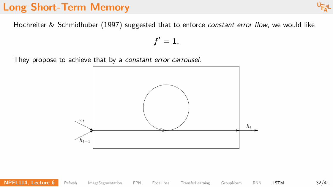
Hochreiter & Schmidhuber (1997) suggested that to enforce constant error flow, we would like

They propose to achieve that by a constant error carrousel.

xt

ht−1

ht

f =′ 1.



xt

ht−1

httanh

σ

xt ht−1

tanh

σ

xt ht−1

ct

They also propose an input and output gates which control the flow of information into and outof the carrousel (memory cell ).c t

i t

o t

c t

h t

← σ(W x + V h + b )it

it−1

i

← σ(W x + V h + b )ot

ot−1

o

← c + i ⋅ tanh(W x + V h + b )t−1 ty

ty

t−1y

← o ⋅ tanh(c )t t



xt

ht−1

httanh

σ

xt ht−1

tanh

σ

xt ht−1

ct

σ

ht−1xt

Later in Gers, Schmidhuber & Cummins (1999) a possibility to forget information from memorycell was added.c t

i t

f t

o t

c t

h t

← σ(W x + V h + b )it

it−1

i

← σ(W x + V h + b )ft

ft−1

f

← σ(W x + V h + b )ot

ot−1

o

← f ⋅ c + i ⋅ tanh(W x + V h + b )t t−1 ty

ty

t−1y

← o ⋅ tanh(c )t t



http://colah.github.io/posts/2015-08-Understanding-LSTMs/img/LSTM3-SimpleRNN.png



http://colah.github.io/posts/2015-08-Understanding-LSTMs/img/LSTM3-chain.png



http://colah.github.io/posts/2015-08-Understanding-LSTMs/img/LSTM3-C-line.png



http://colah.github.io/posts/2015-08-Understanding-LSTMs/img/LSTM3-focus-i.png



http://colah.github.io/posts/2015-08-Understanding-LSTMs/img/LSTM3-focus-f.png



http://colah.github.io/posts/2015-08-Understanding-LSTMs/img/LSTM3-focus-C.png



http://colah.github.io/posts/2015-08-Understanding-LSTMs/img/LSTM3-focus-o.png


2+m``2migl2m` hgl2irq`fb *qmpqhmibqm hgl2m`...

Documents