2nd order methods dsbvp jcam gaurav

8/6/2019 2nd Order Methods DSBVP JCAM Gaurav

http://slidepdf.com/reader/full/2nd-order-methods-dsbvp-jcam-gaurav 1/23

Second Order Methods for Doubly SingularBoundary Value Problems

R.K. Pandey∗ and G. K. Gupta†

Department of Mathematics, Indian Institute of Technology, Kharagpur, 721302, India.

Abstract

In this work we develop three numerical methods of second order accuracy fordoubly singular boundary value problems

( p(x)y(x)) = q(x)f (x, y), 0 < x ≤ 1

with boundary conditions y(0) = A(or y(0) = 0 or limx→0

p(x)y(x) = 0) and αy(1) +

βy (1) = γ , where α(> 0), β(≥ 0), γ and A are finite constants. Here p(0) = 0 andq(x) is unbounded near x = 0. The convergence of the methods is established underquite general conditions which are verified by two examples.

Keywords: Doubly singular boundary value problems, Finite difference method, Chawla’s

identity, Thomas-Fermi equation.MSC : 65L10, 65L12, 34B16

1 Introduction

Consider the following class of singular two point boundary value problems

Ly ≡ ( p(x)y) = q(x)f (x, y), 0 < x ≤ 1, (1)

with boundary conditions

y (0) = A, αy (1) + βy

(1) = γ (2)

or, y

(0) = 0(or limx→0

p(x)y(x) = 0), αy (1) + βy

(1) = γ, (3)

∗Corresponding author. E-mail: [email protected]†E-mail: [email protected]

1



where α > 0, β ≥ 0 and A, γ are finite constants. Here p(0) = 0 and q(x) is unboundednear x = 0. The condition p(0) = 0 says that the problem is singular and as q(x) isunbounded near x = 0, so the problem is doubly singular ([1]). Let p(x), q(x) and f (x, y)

satisfy the following conditions:

(A − 1): (i) p(0) = 0, p(x) > 0 in (0, 1],(ii) p(x) ∈ C [0, 1] ∩ C 1(0, 1] ,(iii) p(x) = xb0g(x), (0 ≤ b0 < 1), g(x) > 0 and(iv) G ∈ C 3[0, 1] and Giv(x) exists on (0, 1),where G(x) = 1/g(x) on [0, 1].

(A − 2): (i) q(x) > 0 in (0, 1], q(x) is unbounded near x = 0,(ii) q(x) ∈ L1(0, 1),(iii) q(x) = xa0H (x), H (0) > 0 with (a0 > −1),(iv) H (x) ∈ C 3[0, 1] and H iv(x) exists on (0, 1) and

(v) 1 + a0 − b0 ≥ 0.

(A − 3): f (x, y) is continuous on {[0, 1] ×R}, ∂f ∂y

exists, continuous and ∂f ∂y

≥ 0 forall 0 ≤ x ≤ 1 and for all real y.

Thomas [16] and Fermi [8] independently derived a boundary value problem for deter-mining the electrical potential in an atom. The analysis leads to the nonlinear singularsecond order problem

y = x−1/2y3/2

with a set of boundary conditions. The following are of our interest.

(i) the neutral atom with Bohr radius b given by y(0) = 1, by(b) − y(b) = 0;

(ii) the ionized atom given by y(0) = 1, y(b) = 0.

Furthermore, Chan and Hon [4] have considered the generalized Thomas-Fermi equation

(xby) = cq(x)ye, y(0) = 1, y(a) = 0

for parameter values 0 ≤ b < 1, c > 0, d > −2, e > 1 and q(x) = xb+d.Such singular problems have been the concern of researchers [2,3,7,9]. The existence-

uniqueness of the solution of the boundary value problem (1) with boundary condition

(2) or (3) is established in [1, 6,12, 13, 14, 17]. Bobisud [1] has mentioned that in caselimx→0+

q(x)

p(x)= 0, the condition y(0) = 0 is quite severe, i.e., it is sufficient but not necessary

for forcing the solution to be differentiable at x = 0. In fact if limx→0+

p(x)y(x) = 0, then

limx→0+

y(x) = limx→0+

q(x)

p(x)· limx→0+

f (x, y(x)).

2



Thus limx→0+

y(x) = 0 if either limx→0+

q(x)

p(x)= 0 or f (0, y(0)) = 0. But lim

x→0+

q(x)

p(x)= 0 if q(x)

has discontinuity at x = 0; thus it is natural to consider the weaker boundary condition

limx→0+ p(x)y

(x) = 0.

There is a considerable literature on numerical methods for q(x) = 1 but to the bestof our knowledge very few numerical methods are available to tackle doubly singularboundary value problems. Reddien [15] has considered the linear form of (1) and derivednumerical methods for q(x) ∈ L2[0, 1] which is stronger assumption than (A − 2)(ii).

Chawla and Katti [5] have developed three second order accuracy methods M 1, M 2and M 3 for differential equation (1) with q(x) = 1, p(x) = xα, 0 ≤ α < 1 and boundaryconditions y(0) = A, y(1) = B. The method M 1 is based on nonuniform mesh andone evaluation of the function f (x, y) while methods M 2 and M 3 are based on uniformmesh and three evaluations of the function f (x, y). They claimed that the method M 3based on uniform mesh is superior than other methods. Furthermore, the methods M 1based on nonuniform mesh and M 2 based on uniform mesh have been extended in [11] fornonnegative function p(x) satisfying (A − 1)(i − iii) with G(x) analytic at singular pointx0 and q(x) = p(x).

In this paper we extend all the three methods M 1, M 2 and M 3 to doubly singular dif-ferential equation (1) with boundary conditions (2) or (3). All the methods are developedfor both uniform as well as appropriate nonuniform mesh. The second order convergenceof the methods are established under quite general conditions on p(x), q(x) and f (x, y).For p(x) = 1, q(x) = 1, the methods M 1 and M 2 both reduce to the classical secondorder method based on one evaluation of the function f (x, y). For nonuniform mesh

the conditions on the function f (x, y) are weaker than that of uniform mesh. Thus themethods based on nonuniform mesh can tackle wider class of doubly singular problems.The method M 3 based on nonuniform mesh is superior to the other methods which iscorroborated through numerical examples.

2 Finite difference methods

This section is divided in two parts (i) Description of the methods and (ii) Constructionof the methods. All coefficients not specified explicitly in this section are specified in theappendix.

2.1 Description of the Methods

In this section we first state the methods; their detailed construction process is given insection 2.2.

For positive integer N ≥ 2, we consider the mesh wh = {xk}N k=0 over [0, 1]: 0 = x0 <

x1 < x2 < · · · xN = 1, h = 1N . Let r(x) := f (x, y(x)) (y(x) is the solution), yk = y(xk)

3



etc. Now we approximate the differential operator Ly on the grid wh by the followingdifference operators

(Lhy)k = yk−1/J k−1 − (1/J k + 1/J k−1)yk + yk+1/J k, k = 1(1)(N − 1), (4)

(Lhy)N = yN −1/J N −1 − (1/J N −1 + α/(βGN ))yN + γ/(βGN ), (5)

for boundary value problem (1)-(2). In the case of boundary condition (3) the operatoris approximated by

(Lhy)1 = −y1/J 1 + y2/J 1. (6)

Here y = (yk) denotes the approximate solution, yk ≈ yk, Gk = G(xk), and

J k =

xk+1

xk

( p(τ ))−1dτ. (7)

Note that the functions p(x) and G(x) are defined in assumption (A − 1).We now state three different methods to solve the singular boundary value problem (1)

with boundary conditions (2) or (3).Method M 1The first method M 1 for boundary value problem (1)-(2) is given by

(Lhy)k = aM 10,k rk, k = 1(1)(N − 1), (8)

(Lhy)N = aM 10,N rN . (9)

In the case of boundary condition (3) the modified equation for k = 1 is

(Lhy)1 = aM 10,1 r1 + aM 1

1,1 r2. (10)

Method M 2The second method M 2 for boundary value problem (1)-(2) is given by

(Lhy)k = aM 20,k rk + aM 2

1,k rk+1 − aM 2−1,krk−1, k = 1(1)(N − 1), (11)

(Lhy)N = aM 20,N rN . (12)


(Lhy)1 = aM 20,1 r1 + aM 21,1 r2. (13)

Method M 3The third method M 3 for boundary value problem (1)-(2) is given by

(Lhy)k = aM 30,k rk + aM 3

1,k rk+1 − aM 3−1,krk−1, k = 1(1)(N − 1), (14)

(Lhy)N = aM 30,N rN − aM 3

−1,N rN −1. (15)

4




(Lhy)1 = aM 20,1 r1 + aM 2

1,1 r2. (16)

The coefficients aM ii,j are specified in the appendix.

All the three methods are developed for both uniform mesh (with mesh point xk =

kh, h = 1N

) and nonuniform mesh (with mesh point xk = (kh)1

(1−b0) ).

2.2 Construction of the methods

In this section we describe the derivation of method M 1 and the derivation of othermethods follows in a similar manner. Local truncation errors are mentioned withoutproof.

2.2.1 Method M 1

With z (x) = p (x) y(x) the differential equation (1) becomes z = q(x)f (x, y(x)). Thenan approximation for the differential operator Ly on the mesh wh is obtained as follows:Integrating z = q(x)f (x, y(x)) twice, first from xk to x and then from xk to xk+1 andchange the order of integration to get the following

yk+1 − yk = zkJ k +

xk+1 xk

xk+1 t

( p (τ ))−1 dτ

q (t) r (t) dt, (17)

where zk = z(xk), r(x) := f (t, y(x)) and J k = xk+1

xk ( p (τ ))

−1

dτ . In an analogous manner,we get

yk − yk−1 = zkJ k−1 −

xk xk−1

t xk−1

( p (τ ))−1 dτ

q (t) r (t) dt. (18)

Eliminating zk from (17) and (18) we obtain the Chawla’s identity

yk+1 − ykJ k

−yk − yk−1

J k−1=

I +kJ k

+I −k

J k−1, k = 1 (1) (N − 1), (19)

where

I +k =

xk+1 xk

xk+1 t

( p (τ ))−1 dτ q(t)r (t) dt,

I −k =

xk xk−1

t xk−1

( p (τ ))−1 dτ

q(t)r (t) dt.

5



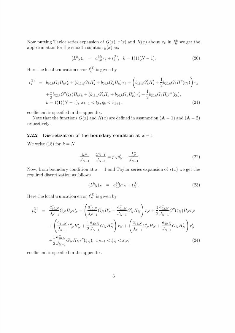
Now putting Taylor series expansion of G(x), r(x) and H (x) about xk in I ±k we get theapproximation for the smooth solution y(x) as:

(Lhy)k = aM

10,k rk + t(1)k , k = 1(1)(N − 1). (20)

Here the local truncation error t(1)k is given by

t(1)k = b10,kGkH krk + (b10,kGkH k + b01,kG

kH k) rk +

b11,kG

kH k +1

2b20,kGkH (ηk)

rk

+1

2b02,kG(ζ k)H krk + (b11,kG

kH k + b20,kGkH k) rk +1

2b20,kGkH kr(ξk),

k = 1(1)(N − 1), xk−1 < ξk, ηk < xk+1; (21)

coefficient is specified in the appendix.

Note that the functions G(x) and H (x) are defined in assumption (A − 1) and (A − 2)respectively.

2.2.2 Discretization of the boundary condition at x = 1

We write (18) for k = N

yN

J N −1−

yN −1

J N −1= pN y

N −

I −N

J N −1. (22)

Now, from boundary condition at x = 1 and Taylor series expansion of r(x) we get the

required discretization as follows

(Lhy)N = aM 10,N rN + t

(1)N . (23)

Here the local truncation error t(1)N is given by

t(1)N =

a−10,N

J N −1GN H N r

N +

a−10,N

J N −1GN H N +

a−01,N

J N −1G

N H N

rN +

1

2

a−02,N

J N −1G(ζ N )H N rN

+

a−11,N

J N −1G

N H N +1

2

a−20,N

J N −1GN H N

rN +

a−11,N

J N −1G

N H N +a−20,N

J N −1GN H N

rN

+1

2

a−20,N

J N −1GN H N r

(ξ−N ), xN −1 < ξ−N < xN ; (24)

coefficient is specified in the appendix.

6



2.2.3 Discretization of the boundary condition at x = 0

Integrating the differential equation (1) twice, first from x1 to x; then from x1 to x2 and

interchanging the order of integration we get

y2 − y1 = J 1

x1 0

q(t)r(t)dt +

x2 x1

x2 t

( p(τ ))−1dτ

q(t)r(t)dt.

Now, using Taylor series expansion of r(x), H (x) and G(x) about x = x1 we get thefollowing discretization for k = 1

(Lhy)1 = aM 10,1 r1 + aM 1

1,1 r2 + t(1)1 , (25)

t(1)1 =

a+11,1

J 1G

1H 1 +1

2

a+02,1

J 1G

1H 1 +x3+a01

ψ(3)

H 1 +1

2

a+20,1

J 1G1H 1 r1

+

2x3+a0

1

ψ(3)H 1 +

a+20,1J 1

G1H 1 +a+11,1

J 1G

1H 1

r1

+

x3+a01

ψ(3)+

1

2

a+20,1

J 1G1H 1

r(ξ1), 0 < ξ1 < x2. (26)

Here t(1)1 is the local truncation error; coefficient is specified in the appendix. The functions

G(x) and H (x) are defined in assumption (A − 1) and (A − 2).The methods M 2 and M 3 can be obtained by using central difference and forward differenceapproximations for rk respectively.

2.2.4 Computation of y0

To compute y0 we use the following:

y0 = y1 +x2+a0−b01

(1 + a0)(2 + a0 − b0)H 1G1r1 + x3+a0−b0

1

−

1

(1 + a0)(2 − b0)

+1

(2 + a0 − b0)(3 + a0 − b0)+

1

(2 − b0)(3 + a0 − b0)

G

1H 1r1

+−1

(1 + a0)(2 + a0)+

1

(3 + a0 − b0)G1H 1r1+x2+a0−b0

1

−

1

(1 + a0)(2 + a0)+

1

(3 + a0 − b0)

(r2 − r1)

+O(h4+a0−b0). (27)

which can be obtained by integrating ( py) = q(x)r(x) first from 0 to x, then from 0 tox1.

7



3 Convergence of the methods

In this section we show that under suitable conditions methods M 1 and M 2 are of second

order accuracy on uniform mesh as well as nonuniform mesh. The convergence analysis forthe method M 3 follows in a similar manner. For convergence analysis we first introducethe matrix notations.

Let Y = (y1,..., yN )T , R(Y ) = (r1,..., rN )

T , Q = (q1,...,qN )T and T = (t1,...,tN )

T ,then the finite difference methods (M 1, M 2 and M 3) can be expressed in matrix form as

BY + P R(Y ) = Q, (28)

and for smooth Y = (y1,...,yN )T , the methods can be written as

BY + P R(Y ) + T = Q, (29)

where B = (bij) and P = ( pij) are (N × N ) tridiagonal matrices.

Let E = Y − Y = (e1,...eN )T , then from Mean Value Theorem R(Y ) − R(Y ) = ME ,M = diag{U 1,...,U N } (U k = ∂f k

∂yk≥ 0), then from equation (28) and (29) we get the error

equation as

(B + P M )E = T. (30)

We recall that by the notation Z ≥ 0 we mean that all components zi of the vector Z satisfy zi ≥ 0. Similarly by B ≥ 0 we mean all the elements bij of the matrix B satisfybij ≥ 0.

From Corollary of Theorem 7.2 and Theorem 7.4 ([10]) a tridiagonal matrix B ismonotone if

bk,k+1 ≤ 0, bk,k−1 ≤ 0 and

N j=1

bk,j ≥ 0, k = 1, 2,...,N > 0, for at least one i.

Furthermore, from Theorem 7.3 ([10]), B−1 exists and the elements of B−1 are nonneg-ative. Now, if B + P M is monotone and B + P M ≥ B, then from from Theorem 7.5([10])

(B + P M )−1 ≤ B−1. (31)

Let vector norm E and matrix norm B be defined by

E = max1≤k≤N

|ek| and B = max1≤k≤N

N

j=1 |bkj |,

then from (30) we get

E = (B + P M )−1|T |. (32)

Furthermore, if B + P M ≥ B and B is also monotone matrix, then from (31) we get

E ≤ B−1|T |. (33)

8



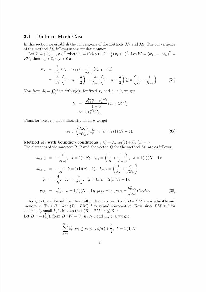
3.1 Uniform Mesh Case

In this section we establish the convergence of the methods M 1 and M 2. The convergence

of the method M 3 follows in the similar manner.Let V = (v1, . . . , vN )T where v j = (2β/α) + 2 − 1

2 (x j + 1)2. Let W = (w1, . . . , wN )T =

BV , then w1 > 0, wN > 0 and

wk =1

J k(vk − vk+1) −

1

J k−1(vk−1 − vk) ,

=h

J k

1 + xk +

h

2

−

h

J k−1

1 + xk −

h

2

≥ h

1

J k−

1

J k−1

. (34)

Now from J k = xk+1

xkx−b0G(x)dx, for fixed xk and h → 0, we get

J k = x

1−b0

k+1 − x

1−b0

k1 − b0

Gk + O(h2)

∼ hx−b0k Gk.

Thus, for fixed xk and sufficiently small h we get

wk >

b0h

2Gk

xb0−1k , k = 2 (1) (N − 1). (35)

Method M 1 with boundary conditions y(0) = A, αy(1) + βy (1) = γ The elements of the matrices B, P and the vector Q for the method M 1 are as follows:

bk,k−1 = −1

J k−1, k = 2(1)N ; bk,k =

1

J k+

1

J k−1

, k = 1(1)(N − 1);

bk,k+1 = −1

J k, k = 1(1)(N − 1); bN,N =

1

J N +

α

βGN

;

q1 =A

J 0, qN =

γ

βGN , qk = 0, k = 2(1)(N − 1);

pk,k = aM 10,k , k = 1(1)(N − 1); pk±1 = 0, pN,N =

a−00,N

J N −1GN H N . (36)

As J k > 0 and for sufficiently small h, the matrices B and B + P M are irreducible and

monotone. Thus B−1 and (B + P M )−1 exist and nonnegative. Now, since P M ≥ 0 forsufficiently small h, it follows that (B + P M )−1 ≤ B−1.

Let B−1 = ( bij), from B−1W = V , w1 > 0 and wN > 0 we get

N −1 j=2

bk,jwk ≤ v j < (2β/α) +3

2, k = 1 (1) N.

9



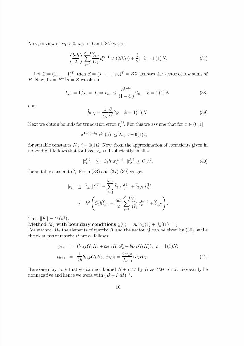
Now, in view of w1 > 0, wN > 0 and (35) we get

b0h

2 N −1

j=2 bk,jGk x

b0−1

k < (2β/α) +

3

2 , k = 1 (1) N. (37)

Let Z = (1, · · · , 1)T , then S = (s1, · · · , sN )T = BZ denotes the vector of row sums of

B. Now, from B−1S = Z we obtain

bk,1 = 1/s1 = J 0 ⇒ bk,1 ≤h1−b0

(1 − b0)G0, k = 1 (1) N (38)

and

bk,N =

1

sN

β

αGN , k = 1(1) N. (39)

Next we obtain bounds for truncation error t(1)k . For this we assume that for x ∈ (0, 1]

x1+a0−b0|r(i)(x)| ≤ N i, i = 0(1)2,

for suitable constants N i, i = 0(1)2. Now, from the approximation of coefficients given inappendix it follows that for fixed xk and sufficiently small h

|t(1)k | ≤ C 1h3xb0−1

k , |t(1)N | ≤ C 1h2, (40)

for suitable constant C 1. From (33) and (37)-(39) we get

|ei| ≤ bk,1|t(1)1 | +

N −1 j=2

bk,j |t(1) j | + bk,N |t

(1)N |

≤ h2

C 1h bk,1 +

b0h

2

N −1 j=1

bk,jGk

xb0−1k + bk,N

.

Thus E = O (h2) .Method M 2 with boundary conditions y(0) = A, αy(1) + βy (1) = γ For method M 2 the elements of matrix B and the vector Q can be given by (36), whilethe elements of matrix P are as follows:

pk,k = (b00,kGkH k + b01,kH kGk + b10,kGkH k) , k = 1(1)N ;

pk±1 =1

2hb10,kGkH k, pN,N =

a−00,N

J N −1GN H N . (41)

Here one may note that we can not bound B + P M by B as P M is not necessarily benonnegative and hence we work with (B + P M )−1.

10



Let Z = (1, · · · , 1)T then S ∗ = (s∗1, · · · , s∗N )T = (B + P M )Z denotes the vector of row

sums of B + P M . From S ∗ = (B + P M )Z , it is easy to see that

s∗1 >1

2J 0 , s∗N >α

βGN , and s∗k > hH kxa0k , k = 1(1)(N − 1).

Now, for fixed xk and sufficiently small h, from (B + P M )−1S ∗ = Z we get

(B + P M )−1k,1 ≤1

s∗1≤

2h1−b0

G1(1 − b0), (B + P M )−1k,N ≤

1

J N −1s∗N

≤βh1−b0

α, and

(B + P M )−1k,j ≤1

min2≤ j≤N −1 s∗ j, j = 1(1)(N − 1) ≤

1

hH kxa0k

. (42)

The local truncations errors t(2)k and t

(2)N are given as

t(2)k =

b11,kG

kH k +1

2b20,kGkH (ηk) +

1

2b02,kG(ζ k)H k

rk + (b11,kG

kH k + b20,kGkH k) rk

+1

2b20,kGkH kr(ξk) −

h2

6b10,kGkH kr(σk), k = 1(1)(N − 1), xk−1 < ξk < xk,

t(2)N =

a−10,N

J N −1GN H N r

N +

a−10,N

J N −1GN H N +

a−01,N

J N −1G

N H N

rN +

1

2

a−02,N

J N −1G(ζ N )H N rN

+

a−11,N

J N −1G

N H N +1

2

a−20,N

J N −1GN H N

rN +

a−11,N

J N −1G

N H N +a−20,N

J N −1GN H N

rN

+12

a

−

20,N J N −1

GN H N r(ξN ), xN −1 < ξN < xN . (43)

Next we obtain bounds for truncation error t(2)k . For this we assume that for x ∈ (0, 1]

|r(i)(x)| ≤ N i, i = 0(1)2,

for suitable constants N i, i = 0(1)2. Now, from the approximation of coefficients given inappendix it follows that, for fixed xk and sufficiently small h

|t(2)k | ≤ C 1h3xa0

k , k = 1(1)(N − 1); |t(2)N | ≤ C 3h2, (44)

where C 1 and C 3 are suitable constants. Now, since ||E || ≤ ||(B + P M )−1

T ||, with thehelp of (42) and (44) we obtain ||E || = O(h2).

3.2 Nonuniform Mesh Case

In this section also we establish the second order convergence for the methods M 1, M 2and the analysis for the method M 3 follows in similar manner.

11



Let V = (v1, . . . , vN )T where v j = (2β/α) + 2 − 1

2 (x j + 1)2. Let W = (w1, . . . , wN )T =

BV , then

wk =1

J k (vk − vk+1) −1

J k−1 (vk−1 − vk) ,

=h

J k

1 + xk +

h

2

−

h

J k−1

1 + xk −

h

2

≥ h

1

J k−

1

J k−1

. (45)

Now, from J k = xk+1

xkx−b0G(x)dx, for fixed xk(= (kh)

11−b0 ) and h → 0, we get

J k =x1−b0k+1 − x1−b0

k

1 − b0Gk + O(h2)

∼h

1 − b0Gk.

Thus for fixed xk and sufficiently small h we get

wk >

b0h

(1 − b0) Gk

x2b0−1k , k = 2 (1) (N − 1). (46)

Method M 1 with boundary conditions y(0) = A, αy(1) + βy (1) = γ For this method the elements of the matrices B, P and the vector Q are given by (36). AsJ k > 0 then for sufficiently small h we get that the matrices B and B +P M are irreducibleand monotone. Furthermore, in view of P M ≥ 0 we conclude that B−1, (B + P M )−1

exist, nonnegative and (B + P M )−1 ≤ B−1.Since

Let B−1 = ( bij), from from B−1W = V , w1 > 0 and wN > 0 we get

N −1 j=2

bk,jwk ≤ v j < (2β/α) +3

2, k = 1 (1) N.

Now in view of w1 > 0, wN > 0 and (46) we getb0h

(1 − b0)

N −1 j=2

bk,jGk

x2b0−1k < (2β/α) +

3

2, k = 1 (1) N. (47)

To obtain the bounds for the truncation error t(1)

k and t(1)

N , we assume that for x ∈ (0, 1]

|x1+a0+b0r(i)(x)| ≤ N i, i = 0(1)2,

for suitable constants N i, i = 0(1)2, then from sufficiently small h

|t(1)k | ≤ C 1

h3

12(1 − b0)3Gkx2b0−1k , |t

(1)N | ≤ C 4

h2

12(1 − b0)3GN

12



and

|t(1)1 | ≤ C 5h2 xb0

1

(1 − b0)3

,

where C 1 and C 4 and C 5 are suitable constants. Now following the analysis of uniformmesh case we get that ||E || = O(h2).Method M 2 with boundary conditions y(0) = A, αy(1) + βy (1) = γ For the method M 2 the elements of the matrix B and the vector Q are given by (36) andelements of matrix P are given by (41).

To obtain the bounds for the truncation error t(2)k and t

(2)N , we assume that for x ∈ (0, 1]

|x2b0r(i)(x)| ≤ N i, i = 0(1)2,

for suitable constants N i, i = 0(1)2. Then for sufficiently small h

|t(2)k | ≤ C 1

h3

(1 − b0)3xa0+b0k , |t

(2)N | ≤ C 6h2,

where C 1 and C 6 are suitable constants. Now following the analysis of uniform mesh casewe get that ||E || = O(h2).

Thus we have established the following result.

Theorem 3.1 Assume that p(x), q(x) and f (x, y) satisfy assumptions given in (A − 1),(A − 2) and (A − 3) respectively. Let r(x) := f (x, y(x)), then the method M 1 is of second order accuracy for sufficiently small mesh size h provided

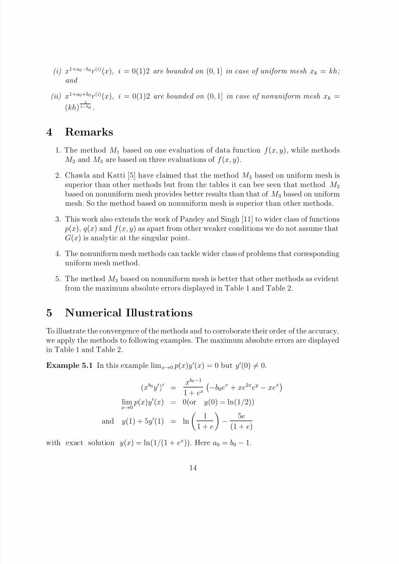
(i) x1+a0−b0r(i)(x), i = 0(1)2 are bounded on (0, 1] in case of uniform mesh xk = kh;and

(ii) x1+a0+b0r(i)(x), i = 0(1)2 are bounded on (0, 1] in case of nonuniform mesh xk =

(kh)1

1−b0 .


(i) r(i)(x), i = 0(1)2 are bounded on (0, 1] in case of uniform mesh xk = kh; and

(ii) x2b0r(i)(x), i = 0(1)2 are bounded on (0, 1] in case of nonuniform mesh xk =

(kh)1

1−b0 .


13



(i) x1+a0−b0r(i)(x), i = 0(1)2 are bounded on (0, 1] in case of uniform mesh xk = kh;and

(ii) x1+a0+b0

r(i)

(x), i = 0(1)2 are bounded on (0, 1] in case of nonuniform mesh xk =(kh)

11−b0 .

4 Remarks

1. The method M 1 based on one evaluation of data function f (x, y), while methodsM 2 and M 3 are based on three evaluations of f (x, y).

2. Chawla and Katti [5] have claimed that the method M 3 based on uniform mesh issuperior than other methods but from the tables it can bee seen that method M 3

based on nonuniform mesh provides better results than that of M 3 based on uniformmesh. So the method based on nonuniform mesh is superior than other methods.

3. This work also extends the work of Pandey and Singh [11] to wider class of functions p(x), q(x) and f (x, y) as apart from other weaker conditions we do not assume thatG(x) is analytic at the singular point.

4. The nonuniform mesh methods can tackle wider class of problems that correspondinguniform mesh method.

5. The method M 3 based on nonuniform mesh is better that other methods as evidentfrom the maximum absolute errors displayed in Table 1 and Table 2.

5 Numerical Illustrations

To illustrate the convergence of the methods and to corroborate their order of the accuracy,we apply the methods to following examples. The maximum absolute errors are displayedin Table 1 and Table 2.

Example 5.1 In this example limx→0 p(x)y(x) = 0 but y(0) = 0.

(xb0y) =xb0−1

1 + ex −b0ex + xe2xey − xexlim

x→0 p(x)y(x) = 0(or y(0) = ln(1/2))

and y(1) + 5y(1) = ln

1

1 + e

−

5e

(1 + e)

with exact solution y(x) = ln(1/(1 + ex)). Here a0 = b0 − 1.

14



Example 5.2 In this example G(x) = (1 + x3.5). Thus G(x) ∈ C 3[0, 1] and Giv(x) existson (0, 1), but G(x) is not an analytic function.

xb0 11 + x3.5

y = (3.5 − b0)(1 + x3.5)(4 + x3.5−b0)

(3.5 − b0)x5.5−b0ey+

−2.5x2 +

3.5x5.5

(1 + x3.5)

y(0) = 0(or y(0) = ln(1/4))

and y(1) + 5y(1) = ln(1/5) − (3.5 − b0)

with exact solution y(x) = ln(1/(4 + x3.5−b0)). Here a0 = −0.5.

All the three methods M 1, M 2 and M 3 are applied on the both the examples for b0 =

0.2, 0.5. Maximum absolute errors and order of accuracy for Example 5.1 and Example5.2 are displayed in Table 1 and Table 2 respectively.

5.1 Numerical Results for Uniform/Nonuniform Mesh Case

Table 1: Maximum absolute errors and order of the methods for Example 5.1

N b0 = 0.2 Order b0 = 0.5 Order b0 = 0.2 Order b0 = 0.5 OrderUniform Mesh:y(0) = ln(1/4) Nonuniform Mesh:y(0) = ln(1/4)

Method M 1

512 1.37(−6)a

3.71(-6) 5.40(-7) 7.84(-7)1024 3.72(-7) 1.88 9.99(-7) 1.90 1.35(-7) 2.00 1.96(-7) 2.002048 1.01(-7) 2.68(-7) 3.39(-8) 4.90(-8)4096 2.70(-8) 1.90 7.14(-8) 1.91 8.55(-9) 2.00 1.22(-8) 2.00

Method M 2512 1.40(-7) 3.30(-7) 2.05(-7) 1.17(-6)

1024 3.50(-8) 2.00 8.25(-8) 2.00 5.11(-8) 2.00 2.91(-7) 2.002048 8.77(-9) 2.06(-8) 1.28(-8) 7.29(-8)4096 2.20(-9) 2.00 5.14(-9) 2.00 3.20(-9) 2.00 1.82(-8) 2.00

Method M 3512 4.96(-8) 1.04(-7) 6.28(-9) 2.57(-8)

1024 1.24(-8) 2.00 2.59(-8) 2.00 1.57(-9) 2.00 6.41(-9) 2.002048 3.09(-9) 6.47(-9) 3.91(-10) 1.60(-9)4096 7.62(-10) 2.00 1.63(-9) 2.00 9.23(-11) 2.08 4.00(-10) 2.00

15



N b0 = 0.2 Order b0 = 0.5 Order b0 = 0.2 Order b0 = 0.5 OrderUniform Mesh:lim

x→0 p(x)y(x) = 0 Nonuniform Mesh:lim

x→0 p(x)y(x) = 0

Method M 1512 1.38(-6) 2.28(-6) 1.63(-6) 8.43(-7)

1024 3.70(-7) 1.88 7.80(-7) 1.89 4.08(-7) 2.00 2.10(-7) 2.002048 9.73(-8) 2.10(-7) 1.02(-7) 5.25(-8)4096 2.56(-8) 1.90 5.55(-8) 1.91 2.55(-8) 2.00 1.31(-8) 2.00

Method M 2512 6.81(-7) 7.37(-7) 8.87(-7) 2.44(-6)

1024 1.68(-7) 2.02 1.84(-7) 2.00 2.22(-7) 2.00 6.10(-7) 2.002048 4.19(-8) 4.61(-8) 5.56(-8) 1.52(-7)4096 1.05(-8) 2.00 1.15(-8) 2.00 1.39(-8) 2.00 3.82(-8) 2.00

Method M 3

512 4.97(-8) 1.04(-7) 6.28(-9) 2.57(-8)1024 1.24(-8) 2.00 2.59(-8) 2.00 1.57(-9) 2.00 6.41(-9) 2.002048 3.09(-9) 6.47(-9) 3.91(-10) 1.60(-9)4096 7.62(-10) 2.02 1.61(-9) 2.00 9.23(-11) 2.08 4.01(-10) 2.00

a1.37(−6) = 1.37 × 10−6

Table 2: Maximum absolute errors and order of the methods for Example 5.2

N b0 = 0.2 Order b0 = 0.5 Order b0 = 0.2 Order b0 = 0.5 OrderUniform Mesh:y(0) = ln(1/4) Nonuniform Mesh:y(0) = ln(1/4)

Method M 1512 8.01(-7) 1.53(-6) 6.53(-7) 9.76(-7)

1024 2.00(-7) 2.00 3.82(-7) 2.00 1.64(-7) 2.00 2.45(-7) 2.002048 5.01(-8) 9.55(-8) 4.09(-8) 6.13(-8)4096 1.25(-8) 2.00 2.38(-8) 2.00 1.02(-8) 2.00 1.53(-8) 2.00

Method M 2512 4.13(-7) 5.02(-7) 4.45(-7) 7.94(-7)

1024 1.03(-7) 1.99 1.26(-7) 2.00 1.11(-7) 2.00 1.97(-7) 2.002048 2.58(-8) 3.16(-8) 2.78(-8) 4.92(-8)4096 6.45(-9) 2.00 7.78(-9) 2.00 6.91(-9) 2.00 1.23(-8) 2.00

Method M 3512 3.11(-7) 4.43(-7) 3.42(-8) 4.11(-7)

1024 7.76(-8) 2.00 1.11(-7) 2.00 8.51(-9) 2.00 1.04(-7) 2.002048 1.94(-8) 2.76(-8) 2.12(-9) 2.62(-8)4096 4.83(-9) 2.00 6.77(-9) 2.00 5.24(-10) 2.01 6.59(-9) 2.00

16



N b0 = 0.2 Order b0 = 0.5 Order b0 = 0.2 Order b0 = 0.5 Order

Uniform Mesh:y(0) = 0 Nonuniform Mesh:y(0) = 0Method M 1

512 2.47(-6) 6.13(-6) 3.42(-6) 1.80(-6)1024 9.69(-7) 1.64 1.92(-6) 1.68 8.67(-7) 1.98 4.52(-7) 1.992048 3.05(-7) 5.50(-7) 2.18(-7) 1.13(-7)4096 8.76(-8) 1.81 1.49(-7) 1.89 5.41(-8) 2.01 2.84(-8) 2.00

Method M 2512 9.14(-6) 9.07(-6) 3.11(-7) 2.58(-6)

1024 1.99(-6) 2.20 1.95(-6) 2.21 6.70(-8) 2.21 6.40(-7) 1.992048 4.43(-7) 4.34(-7) 1.54(-8) 1.59(-7)4096 1.01(-7) 2.12 9.96(-8) 2.12 3.85(-9) 2.00 3.97(-8) 2.00

Method M 3

512 3.06(-7) 3.97(-7) 3.43(-8) 1.04(-7)1024 7.71(-8) 1.99 1.05(-7) 1.92 8.51(-9) 2.01 2.62(-8) 1.992048 1.93(-8) 2.69(-8) 2.12(-9) 6.59(-9)4096 4.83(-9) 2.00 6.69(-9) 2.01 5.24(-10) 2.02 1.65(-9) 2.00

A Appendix

Here we mention the truncation errors which are not mentioned in the previous sections.The coefficients involved in the methods and their approximations are also mentioned.

Truncation errors for methods M 2 and M 3

t(2)

1 = a+11,1J 1 G

1H

1 +

1

2

a+02,1J 1 G

(ζ 1)H 1 f 1

+

x3+a01

(1 + a0)(2 + a0)(3 + a0)H (η1) +

1

2

a+20,1J 1

G1H (η1)

f 1

+

2x3+a0

1

(1 + a0)(2 + a0)(3 + a0)H 1 +

a+20,1J 1

G1H 1 +a+11,1

J 1G

1H 1

f 1

+

x3+a01

(1 + a0)(2 + a0)(3 + a0)+

1

2

a+20,1

J 1G1H 1

f (σ1), t

(3)1 = t

(2)1 ,

t(3)k =

b11,kG

kH k +1

2b20,kGkH (ηk) +

1

2b02,kG(zetak)H k

f k

+ (b11,kGkH k + b20,kGkH k) f k

+

1

2b20,k −

h

2

a+10,kJ k

+h

2

a−10,kJ k−1

GkH kf (ξk), k = 1(1)(N − 1),

t(3)N =

1

2

a−02,N

J N −1G(ζ N )H N f N +

a−11,N

J N −1G

N H N +1

2

a−20,N

J N −1GN H (ηN )

f N

17



+

a−11,N

J N −1G

N H N +a−20,N

J N −1GN H N

f N +

1

2

a−20,N

J N −1GN H N f (ξN ).

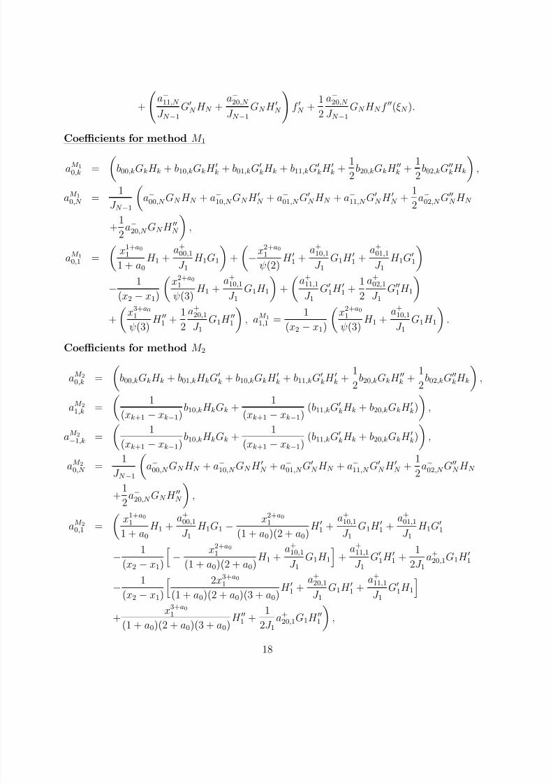
Coefficients for method M 1

aM 10,k =

b00,kGkH k + b10,kGkH k + b01,kG

kH k + b11,kGkH k +

1

2b20,kGkH k +

1

2b02,kG

kH k

,

aM 10,N =

1

J N −1

a−00,N GN H N + a−10,N GN H N + a−01,N G

N H N + a−11,N G

N H N +

1

2a−02,N G

N H N

+1

2a−20,N GN H N

,

aM 10,1 =

x1+a01

1 + a0H 1 +

a+00,1J 1

H 1G1+

−

x2+a01

ψ(2)H 1 +

a+10,1J 1

G1H 1 +a+01,1

J 1H 1G

1−

1

(x2 − x1)

x2+a01

ψ(3)H 1 +

a+10,1J 1

G1H 1

+a+11,1

J 1G

1H 1 +1

2

a+02,1J 1

G1H 1

+

x3+a01

ψ(3)H 1 +

1

2

a+20,1J 1

G1H 1

, aM 1

1,1 =1

(x2 − x1)

x2+a01

ψ(3)H 1 +

a+10,1J 1

G1H 1

.


aM 20,k =

b00,kGkH k + b01,kH kG

k + b10,kGkH k + b11,kGkH k +

1

2b20,kGkH k +

1

2b02,kG

kH k

,

a

M 2

1,k = 1

(xk+1 − xk−1) b10,kH kGk +

1

(xk+1 − xk−1) (b11,kG

kH k + b20,kGkH

k) ,

aM 2−1,k =

1

(xk+1 − xk−1)b10,kH kGk +

1

(xk+1 − xk−1)(b11,kG

kH k + b20,kGkH k)

,

aM 20,N =

1

J N −1


N H N + a−11,N G

N H N +

1

2a−02,N G

N H N

+1

2a−20,N GN H N

,

aM 20,1 =

x1+a01

1 + a0H 1 +

a+00,1J 1

H 1G1 −x2+a01

(1 + a0)(2 + a0)H 1 +

a+10,1J 1

G1H 1 +a+01,1

J 1H 1G

1

− 1(x2 − x1)

− x2+a01

(1 + a0)(2 + a0)H 1 + a+10,1

J 1G1H 1+ a+11,1

J 1G

1H 1 + 12J 1

a+20,1G1H 1

−1

(x2 − x1)

2x3+a01

(1 + a0)(2 + a0)(3 + a0)H 1 +

a+20,1J 1

G1H 1 +a+11,1

J 1G

1H 1

+x3+a01

(1 + a0)(2 + a0)(3 + a0)H 1 +

1

2J 1a+20,1G1H 1

,

18



aM 21,1 =

1

(x2 − x1)

−

x2+a01

(1 + a0)(2 + a0)H 1 +

a+10,1J 1

G1H 1

+1

(x2 − x1)

+

2x3+a01

(1 + a0)(2 + a0)(3 + a0)H 1 +

a+20,1J 1

G1H 1 +a+11,1

J 1G

1H 1

.


aM 30,k =

b00,kGkH k + b01,kH kG

k + b10,kGkH k −1

(xk+1 − xk)

a+10,kJ k

GkH k + b11,kGkH k

+1

2b20,kGkH k +

1

2b02,kG

kH k −1

(xk+1 − xk)

a+11,k

J kG

kH k +a+20,k

J kGkH k

− 1(xk+1 − xk)

a+

11,k

J k− 1

(xk+1 − xk)a−

11,k

J k−1G

kH k − 1(xk+1 − xk)

a+

20,k

J kGkH k

+1

(xk − xk−1)

a−11,kJ k−1

GkH k +

a−20,kJ k−1

GkH k

+

1

(xk − xk−1)

a−10,kJ k−1

GkH k

+1

(xk − xk−1)

a−20,kJ k−1

GkH k

,

aM 31,k =

1

(xk+1 − xk)

a+10,k

J kGkH k +

a+11,kJ k

GkH k +

a+20,k

J kGkH k

,

aM 3−1,k =

1

(xk − xk−1)

a−10,kJ k−1

GkH k +a−11,kJ k−1

GkH k +

a−20,kJ k−1

GkH k

,

aM 3−1,N =

1

(xN − xN −1)

a−10,N GN H N + a−11,N G

N H N + a−20,N GN H N

,

aM 30,N =

1

J N −1


N H N +

a−10,,N

(xN − xN −1)GN H N

+a−11,N GN H N +

a−11,N

(xN

− xN −1)

GN H N +

a−20,N

(xN

− xN −1)

GN H N +1

2a−02,N G

N H N

+1

2a−20,N GN H N

,

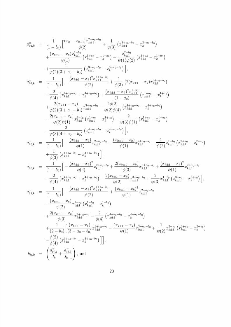
where

a±00,k =1

(1 − b0)

−

(x2+a0−b0k±1 − x2+a0−b0

k )

φ(2)+

xk±1

ψ(1)

x1+a0k±1 − x1+a0

k

,

19



a±01,k =1

(1 − b0)

(xk − xk±1)x2+a0−b0k±1

φ(2)+

1

φ(3)

x3+a0−b0k±1 − x3+a0−b0

k

+

(xk±1 − xk)x1−b0k±1

ψ(1) x1+a

0k±1 − x1+a

0k −x2−b0k±1

ψ(1)ϕ(2) x1+a

0k±1 − x1+a

0k +

1

ϕ(2)(3 + a0 − b0)

x3+a0−b0k±1 − x3+a0−b0

k

,

a±02,k =1

(1 − b0)

−

(xk±1 − xk)2x2+a0−b0k±1

φ(2)+

1

φ(3)

2(xk±1 − xk)x3+a0−b0

k±1

−

2

φ(4)

x4+a0−b0k±1 − x4+a0−b0

k

+

(xk±1 − xk)2x1−b0k±1

(1 + a0)

x1+a0k±1 − x1+a0

k

+

2(xk±1 − xk)

ϕ(2)(3 + a0 − b0)x3+a0−b0k±1 −

2φ(2)

ϕ(2)φ(4) x4+a0−b0k±1 − x4+a0−b0

k

−

2(xk±1 − xk)ϕ(2)ψ(1)

x2−b0k±1

x1+a0k±1 − x1+a0

k

+2

ϕ(3)ψ(1)

x1+a0k±1 − x1+a0

k

−2

ϕ(3)(4 + a0 − b0)

x4+a0−b0k±1 − x4+a0−b0

k

,

a±10,k =1

(1 − b0)

−

(xk±1 − xk)

φ(1)x2+a0−b0k±1 +

(xk±1 − xk)

ψ(1)x2+a0−b0k±1 −

1

ψ(2)x1−b0k±1

x2+a0k±1 − x2+a0

k

+

1

φ(3)

x3+a0−b0k±1 − x3+a0−b0

k

,

a±20,k =1

(1 − b0)−(xk±1 − xk)2

φ(2)

x2+a0−b0k±1 +

2(xk±1 − xk)

φ(3)

x3+a0−b0k±1 +

(xk±1 − xk)2

ψ(1)

x2+a0−b0k±1

−2

φ(4)

x4+a0−b0k±1 − x4+a0−b0

k

−

2(xk±1 − xk)

ψ(2)x3+a0−b0k±1 +

2

ψ(3)x1−b0k±1

x3+a0k±1 − x3+a0

k

,

a±11,k =1

(1 − b0)

−

(xk±1 − xk)2x2+a0−b0k±1

φ(2)+

(xk±1 − xk)2

ψ(1)x2+a0−b0k±1

−(xk±1 − xk)

ψ(2)x1−b0k±1

x1−b0k±1 − x1−b0

k

+

2(xk±1 − xk)

φ(3)x3+a0−b0k±1 −

2

φ(4)

x4+a0−b0k±1 − x4+a0−b0

k

+

1

(2 − b0) (xk±1 − xk)

(3 + a0 − b0)x3+a0−b0k±1 −

(xk±1 − xk)

ψ(1) x3+a0−b0k±1 +

1

ψ(2)x2−b0k±1 x

2+a0k±1 − x

2+a0k

−φ(2)

φ(4)

x4+a0−b0k±1 − x4+a0−b0

k

,

bij,k =

a+ij,kJ k

+a−ij,kJ k−1

, and

20



φ(i) =i

j=2

( j + a0 − b0), ψ(i) =i

j=1

( j + a0), ϕ(i) =i

j=2

( j − b0).

Approximations of the coefficients for uniform mesh caseFor uniform mesh xk = kh, k = 0(1)N and h = 1

N then for fixed xk as h → 0, we getthe following approximations for the coefficients

b00,k ∼hxa0

k

Gk, b01,k ∼ (a0 − 2b0)

h3xa0−1k

4Gk, b02,k ∼

h3xa0k

2Gk

b11,k ∼h3xa0

k

4Gk, b10,k ∼ (2a0 − 3b0)

h3xa0−1k

12Gk, b20,k ∼

h3xa0k

6Gk.

Furthermore, for sufficiently small h we get

|a−00,N | <h2

2, |a−11,N | <

h4

4, |a−20,N | <

h4

6, |a−01,N | <

2h3

3, |a−02,N | <

h4

6, |a−10,N | <

h3

3.

Approximations of the coefficients for nonuniform mesh case

For nonuniform mesh xk = (kh)1

1−b0 , k = 0(1)N, k = 0(1)N , and h = 1N

then forfixed xk as h → 0, we get the following approximations for the coefficients

b00,k ∼hxa0+b0

k

(1 − b0)Gk, b01,k ∼ (a0 + 2b0)

h3x3b0+a0−1k

4(1 − b0)3Gk, b10,k ∼ (2a0 + 3b0)

h3x3b0+a0−1k

12(1 − b0)3Gk

b11,k ∼h3x3b0+a0

k

4(1 − b0)3Gk

, b20,k ∼h3x3b0+a0

k

6(1 − b0)3Gk

, b02,k ∼h3x3b0+a0

k

(1 − b0)32Gk

.

Furthermore, for sufficiently small h we get

|a−00,N | <h2

2(1 − b0), |a−01,N | <

2h3

3(1 − b0)3, |a−10,N | <

h3

3(1 − b0)3,

|a−11,N | <h4

4(1 − b0)3, |a−20,N | <

h4

6(1 − b0)3, |a−02,N | <

h4

2(1 − b0)4.

AcknowledgementsWe are thankful to the referee for valuable suggestions. The work is supported by

Department of Science and Technology, New Delhi, India.

References

[1] Bobisud L. E., Existence of solutions for nonlinear singular boundary value problems,Applicable Analysis, 35 (1990) 43–57.

21



[2] Bobisud L. E., O’Regan D., Royalty W. D., Singular boundary value problems, Ap-plicable Analysis 23 (1986) 233–243.

[3] Bobisud L. E., O’Regan D. and Royalty W. D., Solvability of some nonlinear bound-ary value problems, Nonlinear Analysis: Theory Methods & Applications, 12 (1988)855–869.

[4] Chan C. Y., Hon Y. C., A constructive solution for a generalized Thomas-Fermitheory of ionized atoms, Qutr. Appl. Math., 45 (1987) 591–599.

[5] Chawla M. M. and Katti C. P., Finite difference methods and their convergence fora class of singular two point boundary value problems, Numer. Math., 39 (1982)341–350.

[6] Dunninger D. R. and Kurtz J. C., Existence of solutions for some nonlinear singular

boundary value problems, J. Math Anal. Appl., 115 (1986) 396–405.

[7] Einar Hille, Some aspects of the Thomas-Fermi equation, Journal d’Analyse Math-matique , 23 (1) (1970) 147–170.

[8] Fermi E., Un methodo statistico per la determinazione di alcune proprieta dell’atomo,Rend. Accad. Naz. del Lincei. Cl. sci. fis., mat. enat., 6 (1927) 602–607.

[9] Granas A., Guenther R. B. and Lee J. W., Nonlinear boundary value problems forordinary differential equations, Dissertationes Mathematcae, Warsaw, 1985.

[10] Henrici P., Discrete variable methods in ordinary differential equations, John Wiley

& Sons, N. Y. (1962).

[11] Pandey R. K. and Singh A. K., On the convergence of a finite difference methodfor weakly regular singular boundary value problems , J. Comp. Appl. Math., 205(2007) 496–478.

[12] Pandey R. K. and Verma A. K., Existence-uniqueness results for a class of singularboundary value problems arising in physiology , Nonlinear Analysis: Real World Appl., 9 (2008) 40–52.

[13] Pandey R. K. and Verma A. K., A note in existence-uniqueness results for a classof doubly singular boundary value problems, Nonlinear Analysis: Theory Methods & Applications, 71 (2009) 3477–3487.

[14] Pandey R. K. and Verma A. K., On solvability of derivative dependent doubly sin-gular boundary value problems, J. Appl. Math. Comp., to appear.

[15] Reddien G. W., Projection Methods and Singular Two Point Boundary Value Prob-lems Numer Math., 21 (1973) 193–205.

22



[16] Thomas L. H., The calculation of atomic fields, Proc. Camb. Phil. Soc., 23 (1927)542–548.

[17] Zhang Y. A note on solvability of singular boundary value problems, Nonnlinear Analysis: Theory Methods & Applications, 26 (10) (1996) 1605–1609.

23

2nd order methods dsbvp jcam gaurav

Documents