32 1 init val probs

8/13/2019 32 1 Init Val Probs

http://slidepdf.com/reader/full/32-1-init-val-probs 1/19

Contentsontents Numerical

Initial Value Problems

32.1 Initial Value Problems 2

32.2 Linear Multistep Methods 20

32.3 Predictor-Corrector Methods 39

32.4 Parabolic PDEs 45

32.5 Hyperbolic PDEs 69

Learning

In this Workbook you will learn about numerical methods for approximating solutions

relating to a certain type of application area. Specifically you will see methods that

approximate solutions to differential equations.

outcomes

http://www.ebookcraze.blogspot.com/



Initial Value Problems

32.1

Introduction

Many engineering applications describe the evolution of some process with time. In order to definesuch an application we require two distinct pieces of information: we need to know what the processis and also when or where the application started.

In this Section we begin with a discussion of some of these so-called initial value problems. Thenwe look at two numerical methods that can be used to approximate solutions of certain initial valueproblems. These two methods will serve as useful instances of a fairly general class of methods whichwe will describe in Section 32.2.

Prerequisites

Before starting this Section you should . . .

• revise the trapezium method forapproximating integrals in 31.2

• review the material concerningapproximations to derivatives in 31.3

Learning Outcomes

On completion you should be able to . . .

• recognise an initial value problem

• implement the Euler and trapezium

method to approximate the solutions of certain initial value problems

2 HELM (2005):Workbook 32: Numerical Initial Value Problems




1. Initial value problemsIn 19.4 we saw the following initial value problem which arises from Newton’s law of cooling

dθ

dt = −k(θ − θs), θ(0) = θ0.

Here θ = θ(t) is the temperature of some liquid at time t, θ0 is the initial temperature at t = 0 andθs is the surrounding temperature. The constant of proportion k has units s−1 and depends on theproperties of the liquid.

This initial value problem has two parts: the differential equation dθ

dt = −k(θ − θs), which models

the physical process, and the initial condition θ(0) = θ0.

Key Point 1

An initial value problem may be made up of two components

1. A mathematical model of the process , stated in the form of a differential equation.

2. An initial value, given at some value of the independent variable.

It should be noted that there are applications in which initial value problems do not model processesthat are time dependent, but we will not dwell on this fact here.

The initial value problem above is such that we can write down an exact or analytic solution (it isθ(t) = θs + (θ0 − θs)e−kt) but there are many applications where it is impossible or undesirable toseek such a solution. The aim of this Section is to begin to describe numerical methods that can beused to find approximate solutions of initial value problems.

Rather than using the application-specific notation given above involving θ we will consider thefollowing initial value problem in this Section. We seek y = y(t) (or an approximation to it) thatsatisfies the differential equation

dy

dt = f (t, y), (t > 0)

and which is subject to the initial condition

y(0) = y0,

a known quantity.

Some of the examples we will consider will be such that an analytic solution is readily available, andthis fact can be used as a check on the accuracy of the numerical methods that follow.

HELM (2005):Section 32.1: Initial Value Problems

3




2. Numerical solutions

We suppose that the initial value problem

dy

dt = f (t, y) y(0) = y0

is such that we are unable (or unwilling) to seek a solution analytically (that is, by hand) and that weprefer to use a computer to approximate y instead. We begin by asking what we expect a numericalsolution to look like.

Numerical solutions to initial value problems discussed in this Workbook will be in the form of asequence of numbers approximating y(t) at a sequence of values of t. The simplest methods choosethe t-values to be equally spaced, and we will stick to these methods. We denote the commondistance between consecutive t-values as h.

Key Point 2

A numerical approximation to the initial value problem

dy

dt = f (t, y), y(0) = y0

is a sequence of numbers y0, y1, y2, y3, . . . .The value y0 will be exact, because it is defined by the initial condition.

For n ≥ 1, yn is the approximation to the exact value y(t) at t = nh.

In Figure 1 the exact solution y(t) is shown as a thick curve and approximations to y(nh) are shownas crosses.

y0

y1

y2y3

t1 = h t2 = 2h t3 = 3ht

Figure 1





The general idea is to take the given initial condition y0 and then use it together with what we knowabout the physical process (from the differential equation) to obtain an approximation y1 to y(h).We will have then carried out the first time step.

Then we use the differential equation to obtain y2, an approximation to y(2h). Thus the second

time step is completed.And so on, at the nth time step we find yn, an approximation to y(nh).

Key Point 3

A time step is the procedure carried out to move a numerical approximation one increment forwardin time.

The way in which we choose to “use the differential equation” will define a particular numericalmethod, and some ways are better than others. We begin by looking at the simplest method.

3. An explicit method

Guided by the fact that we only seek approximations to y(t) at t-values that are a distance h apart wecould use a forward difference formula to approximate the derivative in the differential equation.

This leads toy(t + h) − y(t)

h ≈ f (t, y)

and we use this as the inspiration for the numerical method

yn+1 − yn = hf (nh,yn)

For clarity we denote f (nh,yn) as f n. The procedure for implementing the method (called Euler’smethod - pronounced “Oil-er’s method” - is summarised in the following Key Point.


5




Key Point 4

Euler’s method for approximating the solution of

dydt

= f (t, y), y(0) = y0

is as follows. We choose a time step h, then

y(h) ≈ y1 = y0 + hf (0, y0)

y(2h) ≈ y2 = y1 + hf (h, y1)

y(3h) ≈ y3 = y2 + hf (2h, y2)

y(4h) ≈ y4 = y3 + hf (3h, y3)...

In general, y(nh) is approximated by yn = yn−1 + hf n−1 .

This is called an explicit method, but the reason why will be clearer in a page or two when weencounter an implicit method. First we look at an Example.

Example 1Suppose that y = y(t) is the solution to the initial value problem

dy

dt = −1/(t + y)2, y(0) = 0.9

Carry out two time steps of Euler’s method with a step size of h = 0.125 so as toobtain approximations to y(0.125) and y(0.25).

Solution

In general, Euler’s method may be written yn+1 = yn + hf n and here f (t, y) = −1/(t + y)2.For the first time step we require f 0 = f (0, y0) = f (0, 0.9) = −1.23457 and therefore

y1 = y0 + hf 0 = 0.9 + 0.125 × (−1.23457) = 0.745679

For the second time step we require f 1 = f (h, y1) = f (0.125, 0.745679) = −1.31912 and therefore

y2 = y1 + hf 1 = 0.745679 + 0.125 × (−1.31912) = 0.580789

We conclude that

y(0.125) ≈ 0.745679 y(0.25) ≈ 0.580789

where these approximations are given to 6 decimal places.





The simple, repetitive nature of this process makes it ideal for computational implementation, butthis next exercise can be carried out by hand.

Taskask

Suppose that y = y(t) is the solution to the initial value problem

dy

dt = −y2, y(0) = 0.5

Carry out two time steps of Euler’s method with a step size of h = 0.01 so as toobtain approximations to y(0.01) and y(0.02).

Your solution

AnswerFor the first time step we require f 0 = f (0, y0) = f (0, 0.5) = −(0.5)2 = −0.25 and therefore

y1 = y0 + hf 0 = 0.5 + 0.01 × (−0.25) = 0.4975

For the second time step we require f 1 = f (h, y1) = f (0.01, 0.4975) = −(0.4975)2 = −0.24751and therefore

y2 = y1 + hf 1 = 0.4975 + 0.01 × (−0.24751) = 0.495025

We conclude that

y(0.01) ≈ 0.497500 y(0.02) ≈ 0.495025 to six decimal places.

The following Task involves the so-called logistic approximation that may be used in modellingpopulation dynamics.


7




Taskask

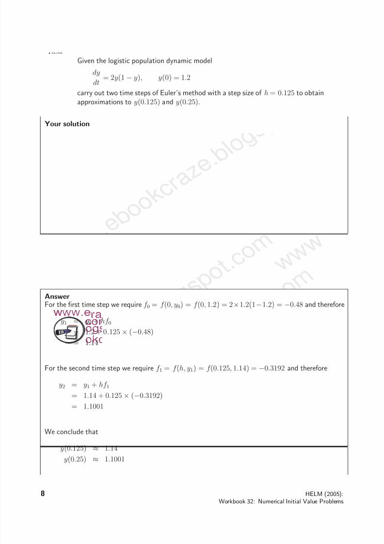
Given the logistic population dynamic model

dy

dt = 2y(1 − y), y(0) = 1.2

carry out two time steps of Euler’s method with a step size of h = 0.125 to obtainapproximations to y(0.125) and y(0.25).

Your solution

AnswerFor the first time step we require f 0 = f (0, y0) = f (0, 1.2) = 2×1.2(1−1.2) = −0.48 and therefore

y1 = y0 + hf 0

= 1.2 + 0.125 × (−0.48)

= 1.14

For the second time step we require f 1 = f (h, y1) = f (0.125, 1.14) = −0.3192 and therefore

y2 = y1 + hf 1

= 1.14 + 0.125 × (−0.3192)

= 1.1001

We conclude that

y(0.125) ≈ 1.14

y(0.25) ≈ 1.1001





Taskask

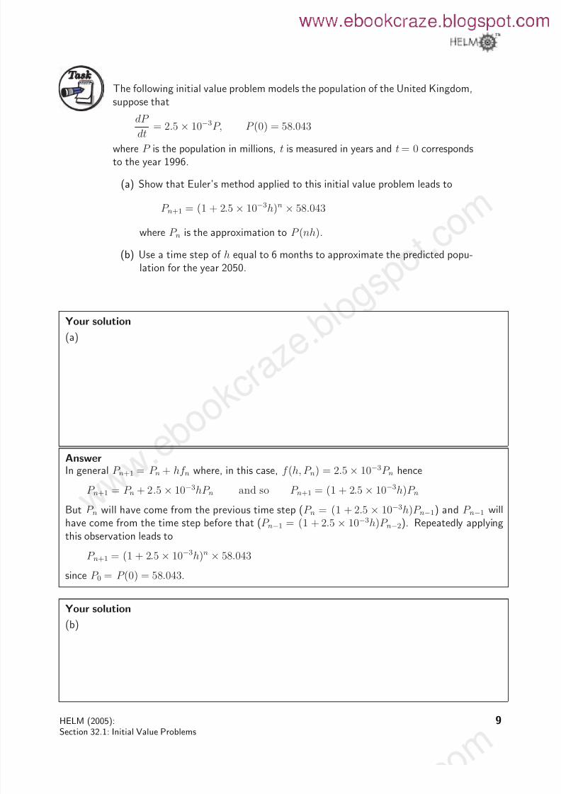
The following initial value problem models the population of the United Kingdom,suppose that

dP

dt = 2.5 × 10−3P, P (0) = 58.043

where P is the population in millions, t is measured in years and t = 0 correspondsto the year 1996.

(a) Show that Euler’s method applied to this initial value problem leads to

P n+1 = (1 + 2.5 × 10−3h)n × 58.043

where P n is the approximation to P (nh).

(b) Use a time step of h equal to 6 months to approximate the predicted popu-

lation for the year 2050.

Your solution

(a)

AnswerIn general P n+1 = P n + hf n where, in this case, f (h, P n) = 2.5 × 10−3P n hence

P n+1 = P n + 2.5 × 10−3hP n and so P n+1 = (1 + 2.5 × 10−3h)P n

But P n will have come from the previous time step (P n = (1 + 2.5 × 10−3h)P n−1) and P n−1 willhave come from the time step before that (P n−1 = (1 + 2.5 × 10−3h)P n−2). Repeatedly applying

this observation leads toP n+1 = (1 + 2.5 × 10−3h)n × 58.043

since P 0 = P (0) = 58.043.

Your solution

(b)


9




AnswerFor a time step of 6 months we take h = 1

2 (in years) and we require 108 time steps to cover the

54 years from 1996 to 2050. Hence

UK population (in millions) in 2050 ≈ P (54) ≈ P 108 = (1 + 2.5 × 10−3 × 12

)108 × 58.043 =

66.427

where this approximation is given to 3 decimal places.

Accuracy of Euler’s method

There are two issues to consider when concerning ourselves with the accuracy of our results.

1. How accurately does the differential equation model the physical process?

2. How accurately does the numerical method approximate the solution of the differential equa-tion?

Our aim here is to address only the second of these two questions.Let us now consider an example with a known solution and consider just how accurate Euler’s methodis. Suppose that

dy

dt = y y(0) = 1.

We know that the solution to this problem is y(t) = et, and we now compare exact values with thevalues given by Euler’s method. For the sake of argument, let us consider approximations to y(t) att = 1. The exact value is y(1) = 2.718282 to 6 decimal places. The following table shows results to6 decimal places obtained on a spreadsheet program for a selection of choices of h.

h Euler approximation Difference between exactto y(1) = 2.718282 value and Euler approximation

0.2 y5 = 2.488320 0.2299620.1 y10 = 2.593742 0.124539

0.05 y20 = 2.653298 0.0649840.025 y40 = 2.685064 0.033218

0.0125 y80 = 2.701485 0.016797

Notice that the smaller h is, the more time steps we have to take to get to t = 1. In the tableabove each successive implementation of Euler’s method halves h. Interestingly, the error halves

(approximately) as h halves. This observation verifies something we will see in Section 32.2, thatis that the error in Euler’s method is (approximately) proportional to the step size h. This sort of behaviour is called first-order, and the reason for this name will become clear later.

Key Point 5

Euler’s method is first order. In other words, the error it incurs is approximately proportional to h.





4. An implicit method

Another approach that can be used to address the initial value problem

dy

dt = f (t, y), y(0) = y0

is to consider integrating the differential equation

dy

dt = f (t, y)

from t = nh to t = nh + h. This leads to

y(t)

t=nh+h

t=nh

=

(n+1)h

nh

f (t, y) dt

that is,

y(nh + h) − y(nh) =

(n+1)h

nh

f (t, y) dt

and the problem now becomes one of approximating the integral on the right-hand side.

If we approximate the integral using the simple trapezium rule and replace the terms by their approx-imations we obtain the numerical method

yn+1 − yn = 12h (f n + f n+1)

The procedure for time stepping with this method is much the same as that used for Euler’s method,but with one difference. Let us imagine applying the method, we are given y0 as the initial conditionand now aim to find y1 from

y1 = y0 + h

2 (f 0 + f 1)

= y0 + h

2{f (0, y0) + f (h, y1)}

And here is the problem: the unknown y1 appears on both sides of the equation. We cannot, ingeneral, find an explicit expression for y1 and for this reason the numerical method is called animplicit method.

In practice the particular form of f may allow us to find y1 fairly simply, but in general we have toapproximate y1 for example by using the bisection method, or Newton-Raphson. (Another approachthat can be used involves what is called a predictor-corrector method, in other words, a “guessand improve” method, and we will discuss this again later in this Workbook.)

And then, of course, we encounter the problem again in the second time step, when calculating y2.And again for y3 and so on. There is, in general, a genuine cost in implementing implicit methods,but they are popular because they have desirable properties, as we will see later in this Workbook.


11




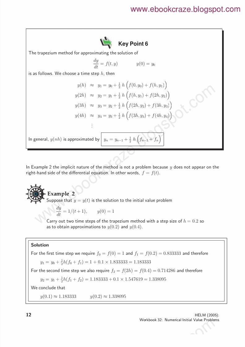
Key Point 6

The trapezium method for approximating the solution of

dydt

= f (t, y) y(0) = y0

is as follows. We choose a time step h, then

y(h) ≈ y1 = y0 + 12 hf (0, y0) + f (h, y1)

y(2h) ≈ y2 = y1 + 12 hf (h, y1) + f (2h, y2)

y(3h) ≈ y3 = y2 + 12 hf (2h, y2) + f (3h, y3)

y(4h) ≈ y4 = y3 +

1

2 hf (3h, y3) + f (4h, y4)

...

In general, y(nh) is approximated by yn = yn−1 + 12 hf n−1 + f n

In Example 2 the implicit nature of the method is not a problem because y does not appear on theright-hand side of the differential equation. In other words, f = f (t).


dy

dt = 1/(t + 1), y(0) = 1

Carry out two time steps of the trapezium method with a step size of h = 0.2 soas to obtain approximations to y(0.2) and y(0.4).

Solution

For the first time step we require f 0 = f (0) = 1 and f 1 = f (0.2) = 0.833333 and therefore

y1 = y0 + 12h(f 0 + f 1) = 1 + 0.1 × 1.833333 = 1.183333

For the second time step we also require f 2 = f (2h) = f (0.4) = 0.714286 and therefore

y2 = y1 + 12h(f 1 + f 2) = 1.183333 + 0.1 × 1.547619 = 1.338095

We conclude that

y(0.1) ≈ 1.183333 y(0.2) ≈ 1.338095





Example 3 has f dependent on y, so the implicit nature of the trapezium method could be a problem.However in this case the way in which f depends on y is simple enough for us to be able to rearrangefor an explicit expression for yn+1.


dy

dt = 1/(t2 + 1) − 2y, y(0) = 2

Carry out two time steps of the trapezium method with a step size of h = 0.1 soas to obtain approximations to y(0.1) and y(0.2).

Solution

The trapezium method is yn+1 = yn + h

2(f n + f n+1) and in this case yn+1 will appear on both sides

because f depends on y. We have

yn+1 = yn + h

2

1

t2n

+ 1 − 2yn

+

1

t2n+1 + 1

− 2yn+1

= yn + h

2{g(tn) − 2yn + g(tn+1) − 2yn+1}

where g(t) ≡

1

(t2 + 1) which is the part of f that depends on t. On rearranging to get all yn+1

terms on the left, we get

(1 + h)yn+1 = yn + 12hg(tn) − 2yn + g(tn+1)

In this case h = 0.1.

For the first time step we require g(0) = 1 and g(0.1) = 0.990099 and therefore

1.1y1 = 2 + 0.05(1 − 2 × 2 + 0.990099)

Hence y1 = 1.726823, to six decimal places.

For the second time step we also require g(2h) = g(0.2) = 0.961538 and therefore

1.1y2 = 1.726823 + 0.05(0.990099 − 2 × 1.726823 + 0.961538)

Hence y2 = 1.501566. We conclude that y(0.1) ≈ 1.726823 and y(0.2) ≈ 1.501566 to 6 d.p.


13




Taskask

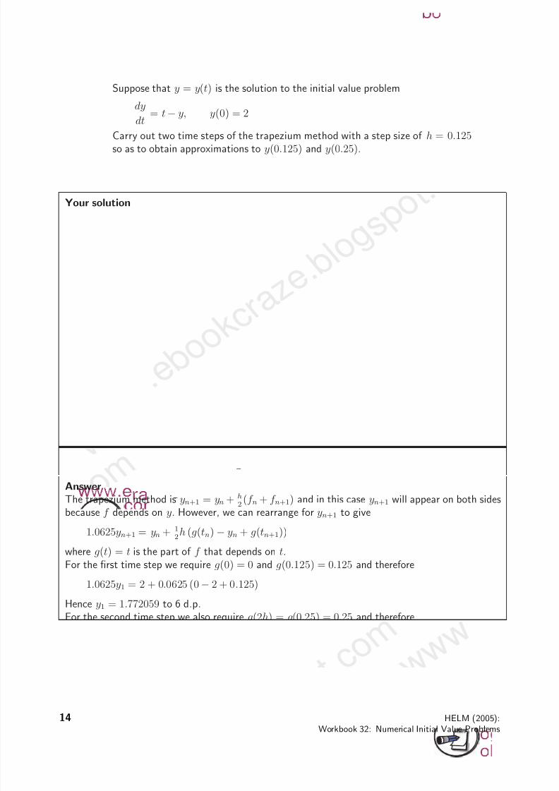
Suppose that y = y(t) is the solution to the initial value problem

dy

dt = t− y, y(0) = 2

Carry out two time steps of the trapezium method with a step size of h = 0.125so as to obtain approximations to y(0.125) and y(0.25).

Your solution

Answer

The trapezium method is yn+1 = yn + h

2(f n + f n+1) and in this case yn+1 will appear on both sides

because f depends on y. However, we can rearrange for yn+1 to give

1.0625yn+1

= yn + 1

2h (g(tn) − yn + g(tn

+1))

where g(t) = t is the part of f that depends on t.For the first time step we require g(0) = 0 and g(0.125) = 0.125 and therefore

1.0625y1 = 2 + 0.0625 (0− 2 + 0.125)

Hence y1 = 1.772059 to 6 d.p.For the second time step we also require g(2h) = g(0.25) = 0.25 and therefore

1.0625y2 = 1.772059 + 0.0625 (0.125 − 1.772059 + 0.25)

Hence y2 = 1.58564, to 6 d.p.





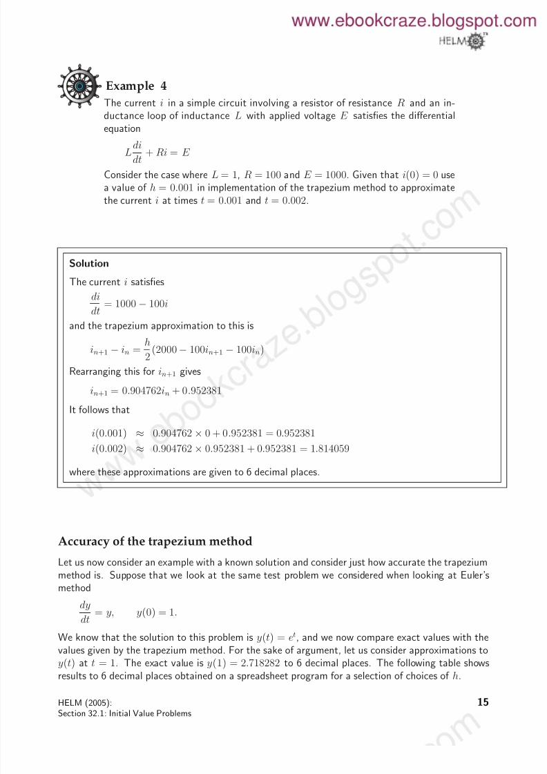
Example 4

The current i in a simple circuit involving a resistor of resistance R and an in-ductance loop of inductance L with applied voltage E satisfies the differential

equation

Ldi

dt + Ri = E

Consider the case where L = 1, R = 100 and E = 1000. Given that i(0) = 0 usea value of h = 0.001 in implementation of the trapezium method to approximatethe current i at times t = 0.001 and t = 0.002.

Solution

The current i satisfies

di

dt = 1000 − 100i

and the trapezium approximation to this is

in+1 − in = h

2(2000− 100in+1 − 100in)

Rearranging this for in+1 gives

in+1 = 0.904762in + 0.952381It follows that

i(0.001) ≈ 0.904762 × 0 + 0.952381 = 0.952381

i(0.002) ≈ 0.904762 × 0.952381 + 0.952381 = 1.814059

where these approximations are given to 6 decimal places.

Accuracy of the trapezium method

Let us now consider an example with a known solution and consider just how accurate the trapeziummethod is. Suppose that we look at the same test problem we considered when looking at Euler’smethod

dy

dt = y, y(0) = 1.

We know that the solution to this problem is y(t) = et, and we now compare exact values with thevalues given by the trapezium method. For the sake of argument, let us consider approximations toy(t) at t = 1. The exact value is y(1) = 2.718282 to 6 decimal places. The following table showsresults to 6 decimal places obtained on a spreadsheet program for a selection of choices of h.


15




h Trapezium approximation Difference between exactto y(1) = 2.718282 value and trapezium approximation

0.2 y5 = 2.727413 0.0091310.1 y10 = 2.720551 0.002270

0.05 y20 = 2.718848 0.000567

0.025 y40 = 2.718423 0.0001420.0125 y80 = 2.718317 0.000035

Notice that each time h is reduced by a factor of 12

, the error reduces by a factor of (approximately) 14

.This observation verifies something we will see in Section 32.2, that is that the error in the trapeziumapproximation is (approximately) proportional to h2. This sort of behaviour is called second-order.

Key Point 7

The trapezium approximation is second order. In other words, the error it incurs is approximatelyproportional to h2.





Exercises

1. Suppose that y = y(t) is the solution to the initial value problem

dy

dt

= t + y y(0) = 3

Carry out two time steps of Euler’s method with a step size of h = 0.05 so as to obtainapproximations to y(0.05) and y(0.1).


dy

dt = 1/(t2 + 1) y(0) = 2

Carry out two time steps of the trapezium method with a step size of h = 0.1 so as to obtainapproximations to y(0.1) and y(0.2).


dy

dt = t2 − y y(0) = 1.5

Carry out two time steps of the trapezium method with a step size of h = 0.125 so as to obtainapproximations to y(0.125) and y(0.25).

4. The current i in a simple circuit involving a resistor of resistance R, an inductance loop of inductance L with applied voltage E satisfies the differential equation

Ldidt

+ Ri = E

Consider the case where L = 1.5, R = 120 and E = 600. Given that i(0) = 0 use a value of h = 0.0025 in implementation of the trapezium method to approximate the current i at timest = 0.0025 and t = 0.005.


17




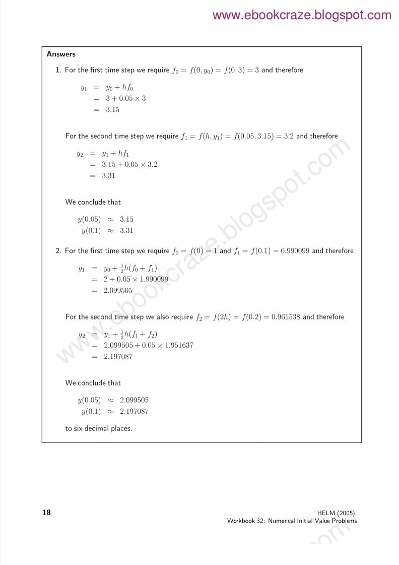
Answers

1. For the first time step we require f 0 = f (0, y0) = f (0, 3) = 3 and therefore

y1 = y0 + hf 0

= 3 + 0.05 × 3

= 3.15

For the second time step we require f 1 = f (h, y1) = f (0.05, 3.15) = 3.2 and therefore

y2 = y1 + hf 1

= 3.15 + 0.05 × 3.2

= 3.31

We conclude that

y(0.05) ≈ 3.15

y(0.1) ≈ 3.31

2. For the first time step we require f 0 = f (0) = 1 and f 1 = f (0.1) = 0.990099 and therefore

y1 = y0 + 12h(f 0 + f 1)

= 2 + 0.05 × 1.990099

= 2.099505

For the second time step we also require f 2 = f (2h) = f (0.2) = 0.961538 and therefore

y2 = y1 + 12h(f 1 + f 2)

= 2.099505 + 0.05 × 1.951637

= 2.197087

We conclude that

y(0.05) ≈ 2.099505

y(0.1) ≈ 2.197087

to six decimal places.





Answers

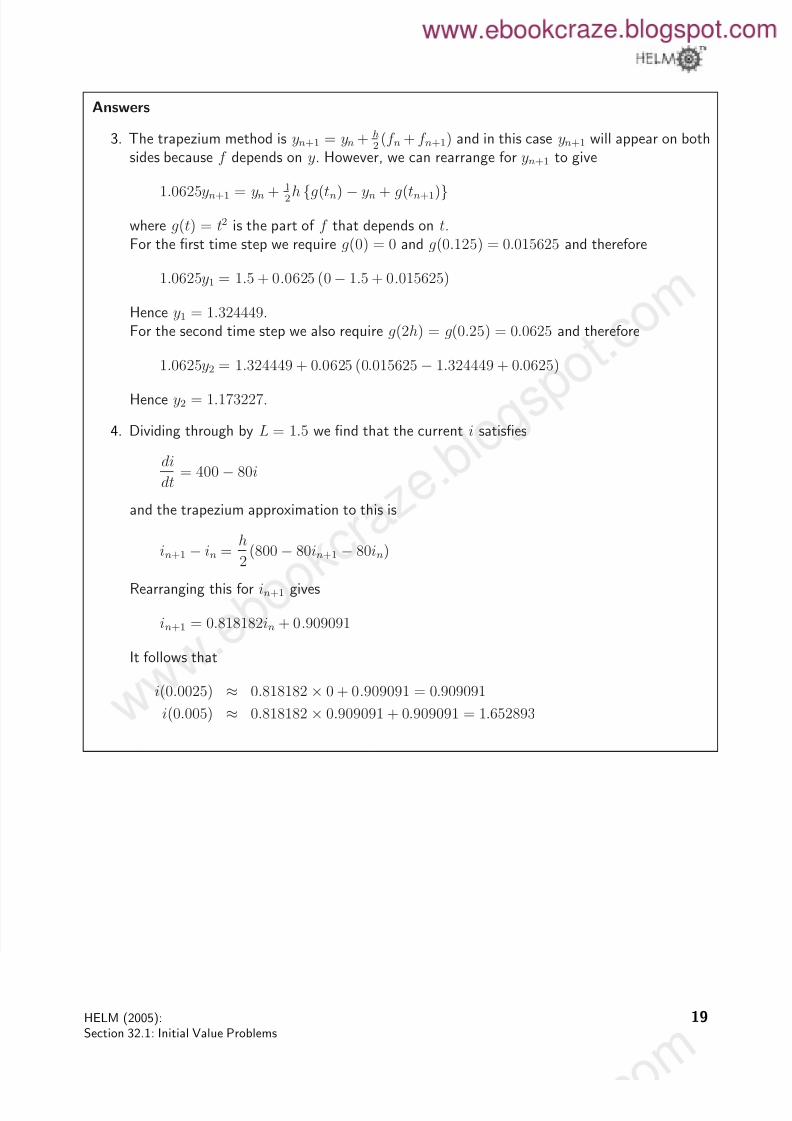
3. The trapezium method is yn+1 = yn + h

2(f n + f n+1) and in this case yn+1 will appear on both

sides because f depends on y. However, we can rearrange for yn+1 to give

1.0625yn+1 = yn + 12h {g(tn) − yn + g(tn+1)}

where g(t) = t2 is the part of f that depends on t.For the first time step we require g(0) = 0 and g(0.125) = 0.015625 and therefore

1.0625y1 = 1.5 + 0.0625 (0− 1.5 + 0.015625)

Hence y1 = 1.324449.For the second time step we also require g(2h) = g(0.25) = 0.0625 and therefore

1.0625y2 = 1.324449 + 0.0625 (0.015625 − 1.324449 + 0.0625)

Hence y2 = 1.173227.

4. Dividing through by L = 1.5 we find that the current i satisfies

di

dt = 400 − 80i

and the trapezium approximation to this is

in+1 − in = h

2(800 − 80in+1 − 80in)

Rearranging this for in+1 gives

in+1 = 0.818182in + 0.909091

It follows that

i(0.0025) ≈ 0.818182 × 0 + 0.909091 = 0.909091

i(0.005) ≈ 0.818182 × 0.909091 + 0.909091 = 1.652893

HELM (2005): 19


32 1 init val probs

Documents