350 oil & hydrocarbon spills, modelling, analysis & control · mapinfo called vertical...

An oil spill model for Cook Inlet and Shelikof

Strait, Alaska

Bryan PearcePearce Engineering, Orono, Maine, 04473, USADoug JonesCoastline Engineering, Anchorage, Alaska. 99504, USA

Howard McllvainePearce Engineering, Orono, Maine, 04473, USA

Abstract

The Cook Inlet Regional Citizens Advisory Committee (CIRCAC) and thePrince William Sound Regional Citizens Advisory Committee (PWSRCAC)have jointly produced an oil spill model that entirely encompasses Cook Inlet aswell as Shelikof Straight and a small part of the Gulf of Alaska. The modeledregion is approximately 400 Km by 400 Km. Cook Inlet is a resonant basin withtidal ranges in some areas on the order of 10 meters with extensive areas that godry at low tide and currents in excess of 5 Kts. Because of the large currents andcurrent variations in Cook Inlet it was necessary to place considerable emphasison a flow model to construct an oil spill model.

The model allows the user to specify the location of the oil spill, time, date,duration of the spill as well as other parameters. The model has an interactivegraphical interface. To aid in this interactive process, displays of the path andshape of the oil spill are included as well as water velocity, date and time. Theuser can update wind speed and direction as desired. The model will allow theuser to update a spill location if field data becomes available. Other usefulfeatures of the model include the location of land impacts, and a trace facility.The trace facility displays a history of the spill trajectory.

Transactions on Ecology and the Environment vol 20, © 1998 WIT Press, www.witpress.com, ISSN 1743-3541

350 Oil & Hydrocarbon Spills, Modelling, Analysis & Control

Introduction

The tides and currents in Cook Inlet are extreme. Spring tides in theupper reaches of Cook Inlet in Knik and Turn agin Arms (Figure 1) canexceed 30 feet and Cook Inlet currents can be over 5 Knots. Thefrequently used assumption that tidal currents are small compared to winddriven currents does not apply in Cook Inlet. In 1996 The Cook InletRegional Citizens Advisory Committee (CIRCAC) established arequirement for an oil spill model for Cook Inlet, Alaska. The model wasto be used for education, public relations, training, and possibly spill

tracking in the event of a spill.

Because of the nature of the oceanographic environment in the inlet, themodel must account for the extreme current regime in Cook Inlet. Inaddition to the requirement of modeling the currents in the inlet, themodel was to have a simple interface and be coded in Visual Basic. TheVisual Basic requirement allowed CIRCAC personnel access to themodel and the have ability to make changes, updates, and modificationsas needed. The final requirement was that the model be inexpensive.Thus the model was assembled using best available information as it wasnot possible to spend large sums on data taking or analysis.

Two versions of the model have now been completed, Phase I andPhase II. Phase I covers Cook Inlet only and the Phase II version of themodel increases the coverage to include Shelikof Strait as shown inFigure 1. To accomplish this increased coverage, the user interface forPhase II has been changed, and provides the user with a "window" to themodel, which will be discussed later. The model also queries theresolution of the host machine and adapts accordingly without requiringactive changes by the user. Additional features include conversionbetween Lat/Long and state plane coordinate Systems. Because of thecomplexities of the calculations, the water velocities for the model arecalculated for a mean tidal cycle and stored as a lookup table for themodel. These velocities are then "stretched" or interpolated toapproximately account for the spring and neap variations in the tide. Themodel does onboard tidal predictions and the interpolations are based onthe predicted elevations at Seldovia in Katchemak Bay.


Oil & Hydrocarbon Spills, Modelling, Analysis & Control 351

Figure 1 - Cook Inlet and Shelikof Strait

Bathymetry

The ocean boundaries for the two models (Phase I and Phasell) areshown in Figure 1. The initial step in assembling the model was to obtainthe bathymetry for the region. Some of the data was obtained fromNOAA electronically, but there were substantial dropouts, or areas where



no data was available. These were mostly areas where the existing chartswere produced before the data was archived electronically. In TurniganArm with its' extensive mudflats, even with the NOAA charts, it becamenecessary to make a best estimate of the depths. The data for theremaining areas were digitized from NOAA charts. The assembled datarepresented several million data points. The outstanding DOGS (DigitalOptimization of Grid Systems) (Gait, 1996) program from NOAAHAZMAT was used to reduce this very large set into a useable set.

DOGS is one of several tools available from NOAA HAZMAT that can

assist in oil spill modeling and analysis. DOGS reduces the number ofdata points needed to construct an accurate grid.

The depth data from all sources were combined using MAPINFO andAlaska State Plane coordinates as shown in Figure 2. By using stateplane rather than latitude and longitude we could easily require all gridsto be the same size. The numerical grid was created using an extension of

Depth Meters

310.1 - 278.2

278.2 - 246.4

;gg 246.4 - 214.6

-~] 214.6-182.7

"] 182.77-150.9

J 150.94- 119.1

"-] 119.1 -87.2

T] 87.2 - 55.4

H 55.4 - 23.6

m 23.6 - -8.2

[Figure 2 Bathymetry (Meters

Wow MLLW))



Cell dimensions 2KM x 2KM

MAPINFO called VerticalMapper. Vertical Mapperuses a variety of schemes for

grid creation for this case alinear interpolation was usedwith a constraint of abouttwo grid widths. Once thegrid is created it must betrimmed to accuratelydescribe the coastline andislands. A region based onthe actual coastline wascreated (approximately theregion in Figure 2) that wasthen used as a template totrim the cells to the correctcoastline. The final grid forthe Phase I model was 121Cells (North/South) X 106Cells (East/West) with a 833in grid spacing and for thePhase II grid there were 221 Cells (North/South) X 182 Cells(East/West) with square girds at 2 kilometer spacing. The final grid forPhase II is shown in Figure 3.

Currents

Figure 3 - Phase II Grid

Numerical models were used to calculate the currents in Cook Inlet basedon the phase and magnitude of the tides at the boundaries. The modelused for Phase I of the study was the Princeton Ocean Model (POM).(Blumberg and Mellor 1987) POM was originally developed for use inoffshore areas and does not allow for grid elements to be included andexcluded from the computation as the water rises and falls. Cook Inlet isa resonant basin. Tides are extreme in the upper arms, and large areas ofmudflats are exposed at low tide. The consequence of the limitation inPOM is that the model "crashed" when it attempted to divide by a depthof zero. To obtain a reasonable solution it became necessary to modifyPOM to dynamically add and delete grid elements according to thechanging depths. After POM was modified to allow each grid element toflood and dry, the model agreed with available tide data to within about



15 centimeters. The code to add flooding and drying to POM isavailable to anyone interested in using POM for intertidal areas.

For Phase II, the currents were calculated using TRIMS (Cheng, et al1993) by Ralph Chen of USGS. The TRIMS model uses an implicitscheme and provides accurate solutions more quickly and with fewer

stability problems than POM. While the currents in Cook Inlet proper aredominated by the tides, the currents in the Shelikof Strait also show a netdrift to the south that varies from 0 to 50 cm/s. This is undoubtedly due tothe Alaska Current. It is impossible to predict these currents and anaverage condition, of about 30 cm/s has been modeled by imposing a tiltin the ocean boundary conditions.

Lagrangian Model

The oil spill model uses a Lagrangian, or random walk, approach. Withthis method, the oil spill is characterized as a large group of autonomousparticles. Each particle, once released into the model, behaves as directedby a set of rules. After each time step, a particle will move to a newlocation. The new location is based on the current speed at that locationand time, the wind speed, and a random motion based on the turbulentviscosity. It has been shown that in the limit of a large number ofparticles, this process produces the same result as the familiarconvection/diffusion equation if the random step is based on the turbulent

viscosity.

The use of the random walk presumes that the spreading oil has reached astage where the physical processes in the ocean such as wind, waves andcurrents are more important than the flow of oil governed by gravity andmolecular viscosity. The dynamics of wind and wave driven oilmovement are complicated. It is easier to discuss the processes than toquantify them. (Delvigne, 1993) (Overstreet and Gait, 1995) Some oilparticles become entrained by waves and once entrained, because ofbuoyancy, slowly return to the surface. At this point some particles are atthe top of the wind generated surface layer while other particles aredeeper. This results in the particles moving horizontally at differentspeeds. Since the net result of the wind generated boundary layer andwave entrainment is to usually move the particles from about 1% to about4% of the wind speed. To provide a conservative estimate of the rangeof movement of the spilled oil we have adopted a scheme used by NOAA



HAZMAT, where

each particle israndomly assigned aspeed of between 1and 4 percent of the

wind speed.

Following thedirective to keep themodel as simple as

possible, we haveprovided a simplelinear decay to accountfor oil weathering.When a particle triesto "jump" onto theland it is either stuckto the beach orreturned to thesimulation based onthe probability that itwill stick to the beach. Figure 4-Primary Interface Dialog

This parameter can becontrolled by the user and is set to a default value of 50 percent.

Graphical Interface

In the Phase I model, the user interface had a single window. In Phase IIthe interface has been modified so that it can fit on any screen size. Theprimary interface Dialog is a schematic of Cook Inlet and Shelikof Straitas shown in Figure 4. When the model starts it checks the screenresolution of the host computer and adjusts the resolution of the image tofit the screen. Normally, the lowest resolution is 640x480 Pixels.CIRCAC requested the feature so that the model would be available to a

larger user base

Due to hardware limitations the entire high resolution image can not bedisplayed. To keep the necessary resolution, the user is provided with awindow with which to view a portion of the model. There are twomethods of navigation within the model. The first are scroll bars.Second, a low resolution image of the entire model has been placed in the



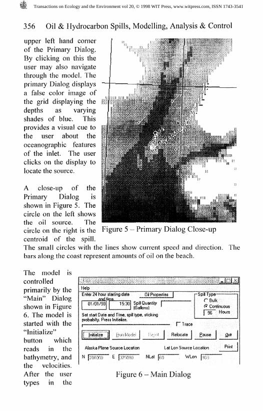
upper left hand cornerof the Primary Dialog.By clicking on this theuser may also navigatethrough the model. Theprimary Dialog displays

a false color image ofthe grid displaying thedepths as varyingshades of blue. Thisprovides a visual cue tothe user about theoceanographic features

of the inlet. The userclicks on the display tolocate the source.

A close-up of the

Primary Dialog isshown in Figure 5. Thecircle on the left showsthe oil source. Thecircle on the right is the Figure 5 - Primary Dialog Close-up

centroid of the spill.The small circles with the lines show current speed and direction. Thebars along the coast represent amounts of oil on the beach.

The model iscontrolledprimarily by the"Main" Dialogshown in Figure6. The model isstarted with the"Initialize"button whichreads in thebathymetry, andthe velocities.After the usertypes in the

' :'< f <JIH' ' *''«£ '/*£/'HelpEnter 24 hour

and01/01/98

Set start Dateprobabilty. Pn'i initialize

Alaska Plan

N | 700000

%%:; J;<;rW

stalling datetime

15:30

and Time, sp>ss Initialize.

]| jjunWc

e Source loc

E I'Snoc

V .v , - </k%%.<- -;< "':-:%%&

OH Properties |Spill Quantity I(Gallons) '

ill type, sticking

del | ttoj'-i j Relocate

ation Lat Lon Source

0 NLat p5 WLc

~SpiH Type-r Bulk(T Cont| 96

Pause |

.ocation

^ (Too

Llnlxl

inuousHours

Sffi |

Print I

Figure 6 - Main Dialog



TideatShelakof Coordinates Start Date and Time101/01/98 | 15:30

Simulation Time|l/i/98 ' |' 18:53

Spfll Center|346834, 624849

Figure 7 - Status and Tide Dialogs

starting date, starting time and spill quantity, the model is ready to run.The user may also choose whether the spill is bulk or continuous. Before

running the model the user must choose a spill location and then may

click on a number oflocations to providefor a graphicaldisplay of the watervelocities. Byclicking on the "Run

Model" button theuser begins thesimulation. Themodel has beenupdated to includeboth Alaska Stateplane and Lat/Longcoordinates for thesource location. The"Relocate" buttonbrings up the Relocate Dialog which allows the users to translate the oilspill by typing in the new location of the spill in either Lat/Long or StatePlane coordinates. Once the model is running, the user may specify thewind, as before, using the Wind Control Dialog. The Status Dialog isshown in Figure 7. The Status Dialog displays the instantaneous depth

and current at the cursor location. It also displays the cursor location, thetide at Seldovia, and model time. Two important additions to the Phase IImodel include Print and Properties. The Print feature allows the user to

create a black and whiteline drawing that maybe easily faxed. Theuser accesses the PrintDialog via the Printbutton on the MainDialog. The printDialog is shown inFigure 8 and allows theuser to select eithercolor or black and whiteand generates the linedrawing.The Properties Dialog

Flint PieviewGet Image

EPSON Stylus COLOAcrobat PDFWriter

y/

Figure 8 - Print Dialog



allows the user to input simple oil properties. The properties are decaydue to weathering and probability that an oil particle will adhere to theshore. These parameters will have minimal effect and thus for mostsimulations the default values are adequate. By clicking with the rightmouse button anywhere over an area representing water, the minimumand maximum tide are displayed. The tide at the current time is

displayed using a red bar as shown in Figure 7.

Conclusions & Continuing Development

An oil spill model using currents from detailed flow models has been

created at low cost to provide a straight forward and easy to use model ofan area with extreme oceanographic conditions. Because of the dynamicnature of Cook Inlet, the next step in providing a real improvement in themodel will be to include the flow model in real time.

Bibliography

Blumberg, A.F., and G.L. Mellor, 1987, "A Description of a three-dimensional coastal ocean circulation model, Three-Dimensional CoastalOcean Models, Vol 4. N. Heaps, Ed., American Geophysical Union

Cheng, R.T., V. Casulli, and J.W. Gartner, 1993, "Tidal, Residual,Intertidal, Mudflat (TRIM) model and its applications to San FranciscoBay, California", Estuarine, Coastal, and Shlef Science VO1. 36, pp.235-280

Delvigne, G. 1993. "Natural dispersion of oil by different sources ofturbulence". Proceedings of the 16*** Arctic and Marine Oil SpillProgram Technical Seminar^ Calgary, Alberta, June 7-9, 1993, Ottawa,Ontario: Environment Canada, pp 415-419

J. A. Gait, 1996, Private Communication

R. Overstreet and J.A. Gait, "Physical Processes Affecting the Movementand Spreading of Oils in Inland Waters", HAZMAT'Report 95-7, NOAAIHazardous Materials Response and Assessment Division, September1995, Seattle, Washington.


350 oil & hydrocarbon spills, modelling, analysis & control · mapinfo called vertical...

Documents