3d autoencoder algorithm for lithological mapping using zy

3D autoencoder algorithm for lithological mappingusing ZY-1 02D hyperspectral imagery:

a case study of Liuyuan region

Junchuan Yu ,a,* Liang Zhang,b Qiang Li,c Yichuan Li,a Wei Huang,a

Zhiwei Sun,d Yanni Ma,a and Peng HeaaChina Aero Geophysical Survey and Remote Sensing Center for Land and Resources,

Beijing, ChinabChina University of Geosciences, Beijing, China

cShenyang Geotechnical Investigation and Surveying Research Institute Co., Ltd.,Shenyang, China

dBeijing GEOWAY Spatial Co., Ltd., Beijing, China

Abstract. A hyperspectral image (HSI) contains hundreds of spectral bands, which providedetailed spectral information, thus offering an inherent advantage in classification. The success-ful launch of the Gaofen-5 and ZY-1 02D hyperspectral satellites has promoted the need forlarge-scale geological applications, such as mineral and lithological mapping (LM). In recentyears, following the success of computer vision, deep learning methods have shown their ad-vantage in solving the problem of hyperspectral classification. However, the combination of deeplearning and HSI to solve the problem of geological mapping is insufficient. We propose a new3D convolutional autoencoder for LM. A pixel-based and cube-based 3D convolutional neuralnetwork architecture is designed to extract spatial–spectral features. Traditional and machinelearning methods are employed as competing methods, trained on two real hyperspectral data-sets, and evaluated according to the overall accuracy, F1 score, and other metrics. Results indi-cate that the proposed method can provide convincing results for LM applications on the basis ofthe hyperspectral data provided by the ZY-1 02D satellite. Compared with traditional methods,the combination of deep learning and hyperspectral can provide more efficient and highly accu-rate results. The proposed method has better robustness than supervised learning methods andshows great promise under small sample conditions. As far as we know, this work is the firstattempt to apply unsupervised spatial–spectral feature learning technology in LM applications,which is of great significance for large-scale applications. © The Authors. Published by SPIE under aCreative Commons Attribution 4.0 International License. Distribution or reproduction of this work inwhole or in part requires full attribution of the original publication, including its DOI. [DOI: 10.1117/1.JRS.15.042610]

Keywords: deep learning; lithological mapping; autoencoder; hyperspectral; small sample;ZY-1 02D.

Paper 210344SS receivedMay 31, 2021; accepted for publication Sep. 7, 2021; published onlineSep. 20, 2021.

1 Introduction

As one of the hottest topics in the remote sensing field, hyperspectral technology plays a sig-nificant role in Earth observation. Hyperspectral image (HSI) contains hundreds of spectralbands, which provide detailed spectral information, and thus has an inherent advantage ingeological applications. Generally, most minerals and rocks have obvious spectral characteristicsin the range of 400 to 2500 nm.1 Spectral analysis of typical rocks and minerals and building aspectral database establish a good foundation for lithological mapping (LM).2,3 Differentgeological bodies and formations, which vary in terms of mineral composition, weathering char-acteristics, alteration, and tectonic setting, also lead to a different spectral signature in hyper-spectral data.4,5 Therefore, richer spectral information and higher spatial resolution correspond to

*Address all correspondence to Junchuan Yu, [email protected]

Journal of Applied Remote Sensing 042610-1 Oct–Dec 2021 • Vol. 15(4)

Downloaded From: https://www.spiedigitallibrary.org/journals/Journal-of-Applied-Remote-Sensing on 23 Feb 2022Terms of Use: https://www.spiedigitallibrary.org/terms-of-use

https://orcid.org/0000-0003-2987-0504

https://doi.org/10.1117/1.JRS.15.042610

https://doi.org/10.1117/1.JRS.15.042610

https://doi.org/10.1117/1.JRS.15.042610

https://doi.org/10.1117/1.JRS.15.042610

https://doi.org/10.1117/1.JRS.15.042610

mailto:[email protected]




its greater advantage in expressing of different types of geological bodies. Although geologicalmapping based on airborne hyperspectral has been performed for many years, the high cost ofdata acquisition has made the application and promotion of this technology more difficult.Benefiting from the development of hyperspectral satellite technology, Gaofen-5,6,7 ZY-102D8 has been successfully launched, thus providing sufficient data guarantee for large-scaleLM.9 Both Gaofen-5 and ZY-1 02D have a width of 60 km, a spatial resolution of 30 m, andhundreds of spectral bands, which are helpful for developing accurate, efficient, and low-costgeological mapping applications.

In the past few decades, various methods based on HIS have been proposed for geologicalmapping. Traditional lithology and mineral mapping methods can be summarized into threecategories: image enhancement methods, spectral feature analysis methods, and object-ori-ented-based methods. Image enhancement methods such as minimum noise fraction rotation(MNF),10,11 principal component analysis (PCA),12 and band ratio13,14 method aim to enhancethe relevant feature of litho-units through transformation processing such as dimensionalityreduction. Such methods are simple and effective, but they are mainly used to enhance theexpression of lithology-related features and cannot directly achieve classification. Spectral fea-ture analysis methods can be further subdivided into two types, spectral feature extraction (SFE)methods15–17 and spectral matching (SM) methods.18,19 As a method with clear physical mean-ing, the SFE method is based on the analysis of the diagnostic spectral features of typical mineralor litho-units and artificially identifies rules to achieve LM. However, because the algorithmmainly uses manual identification rules to implement LM, it is less efficient when appliedto large-scale, multiple targets, and complex scenarios.20 In the definition of the SM methods,rock types are distinguished by comparing the consistency of the target spectrum with that of thereference spectrum. Typical SM methods, such as spectral angle mapper (SAM)21,22 and spectralinformation divergence (SID)23 are the most commonly used. The unmixing method can also beregarded as an extension of this type of method.24 Compared with the SFE methods, it is easier toimplement, but it is not sensitive enough to minor diagnostic spectral signatures,25 and the choiceof reference spectrum is also important to accuracy. Object-wise methods should apply super-pixel segmentation,26,27 such as simple linear iterative clustering to the target images. Althoughthis kind of method overcomes the salt-and-pepper effect to some extent, the recognition accu-racy is still affected by the initial super-pixel precision and the insufficient utilization of spectralfeatures. The above-mentioned traditional methods have their own advantages, but the problemsof insufficient spatial–spectral feature combination, weak feature extraction ability, and low effi-ciency are difficult to avoid.

With advances in machine learning technology, a series of learning-based methods have beenproposed for LM, such as support vector machine28,29 and random forest.30 Compared with tradi-tional methods, the learning-based methods can capture more effective features through super-vised learning, thereby overcoming the problem of artificial threshold setting in complex scenes.In recent years, deep learning technology has achieved remarkable progress in hyperspectralapplication.4,31,32 However, few application cases of LM using deep learning methods combinedwith HSI. As shown in Refs. 27 and 33, a convolutional neural network (CNN) was used toaddress LM problems based on HSI in the supervised scenario, thereby providing a good casefor the application of deep learning in LM. Considering that the accuracy of supervision-basedclassification algorithms is constrained by the amount and representativeness of training samplesand that applying locally trained models to large-scale and complex scenarios is difficult, webelieve that using self-learning methods to solve LM problem is a better choice. Most recently,the autoencoder-like architecture has been developed in hyperspectral unmixing and became anew trend in self-learning methods. In Refs. 34–36, denoising and sparseness autoencoder areintroduced to estimate the abundance of endmembers. In Refs. 37 and 38, the 3D-CNN autoen-coders are further employed for hyperspectral unmixing to improve the classification accuracy.Inspired by these autoencoder applications, we introduce a novel end-to-end 3D convolutionalautoencoder for LM. The encoder with pixel-based or cube-based CNNs is proposed to explorethe spatial–spectral contextual features of HSI, and the decoder is designed to estimate the end-member of the litho-units. The novelty of this method lies in the use of a 3D autoencoder, whichimplements LM through self-learning and avoids the use of large training sets. In our experi-ments, SAM, SID, and a simple CNN network are used as competing methods on the same data

Yu et al.: 3D autoencoder algorithm for lithological mapping using ZY-1 02D hyperspectral imagery. . .



set and trained using the same parameter settings as the proposed method. Overall accuracy,F1-score, and other metrics are employed to evaluate the performance. As far as we know, thiswork is the first attempt to apply unsupervised spatial–spectral feature learning technology inLM application based on HSI.

The remainder of this paper is organized as follows: The proposed method is described inSec. 2. The working area and data are described in Sec. 3. Experiments and results are presentedin Sec. 4, and the conclusion and discussions are presented in Sec. 5.

2 Proposed Methods

2.1 Problem Formulation

Geological bodies and formations formed in diverse geological environments show differencesin mineral composition, weathering characteristics, and alteration, thereby leading to distinctspectral signatures in hyperspectral data. Reasonably, the LM problem can be considered asan unmixing problem, which aims to estimate the proportions of each spectral endmember thatrepresenting certain litho-units. The formula can be expressed as

EQ-TARGET;temp:intralink-;e001;116;525M ¼ ΨðEAÞ þ N; (1)

in whichM is indicative of a mixture pixel of reflectance, E represents the endmembers of litho-units, A denotes their proportions, N is the additive vector, and Ψ represents the implicit non-linear function applied to the linear transform. The problem investigated in this paper is theestimation of the proportion matrix A by given the endmembers matrix E. It is worth notingthat the proportion non-negative and sum-to-one constrain are two physical constraints39 thatrestrict the model from estimating the correct result following the physical rules. The formerdemonstrates all elements of the estimation result, which indicates that the proportions of eachlitho-unit must be nonnegative, and the latter requires that the sum of proportion in each pixelequals one.

Autoencoder is an unsupervised training network composed of an encoder and a decoder,which can learn the data patterns and reconstruct input information with a minimum reconstruc-tion error. Under certain constraints, the decoder part can be regarded as a reconstruction of HSIbased on pure litho-units matrix and their proportions matrix. Hence, given the spectral end-members of typical litho-units as the weight of the reconstructed layer, the proportion matrixof each litho-unit can be estimated as the activations of the last hidden layer for each inputspectrum.

2.2 3D-CNN Autoencoder

Compared with other remote sensing data, hyperspectral data contains richer information inchannel dimension. Thus, we used 3D convolution in hyperspectral data processing, which canbe expressed as

EQ-TARGET;temp:intralink-;e002;116;229vxyzlf ¼ σ

Xm

XHk−1

h¼0

XWk−1

w¼0

XCk−1

d¼0

whwdlfmv

ðxþhÞðyþwÞðzþdÞðl−1Þm

!þ blf; (2)

in which vxyzlf represents the value of a unit at position ðx; y; zÞ on the f’th feature map in the l’thlayer;m indexes the sets of the feature map in the preceding layer ðl − 1Þ;Hk,Wk, Ck denote theheight, width, and channel of the kernel, respectively; whwd

lfm stands for the weight at positionðh; w; dÞ connected to the f’th feature map; and b and σ are the bias and the activation function,respectively.

Inspired by the application of autoencoder for spectral unmixing problems, we introduce apixel-based 3D convolutional autoencoder (PBA) and a cube-based 3D convolutional autoen-coder (CBA). The main architectures of PBA and CBA are the same, but the inputs are different.The PBA takes a spectrum vector at each pixel as input, whereas the CBA takes the hyperspectral




cube ðS × S × CÞ as input data to obtain joint spatial–spectral information, where S denotes thespatial window size and C is the number of spectral bands. In theory, the size of S is not fixed, itcan be set according to the size of the data. In this case, S is set to 5. Generally, as an end-to-endnetwork, the input and output of the autoencoder are the same, as in PCA. However, the output ofthe CBA is the central pixel of the input hyperspectral cube, as shown in Fig. 1. Similarly, thenumber of convolutional layers of the model’s encoder is also changeable. The focus of thispaper is to use the autoencoder to solve the LM problem, which is why a general encoder archi-tecture is adopted in this case. Considering that several high-computational-cost fully connectedlayers (FC layers) are present in the network, we adopted five 3D convolutional layers as theencoder in this case, which can maintain sufficient feature extraction capabilities withoutincreasing the computational burden as much as possible.

As shown in Fig. 2, an encoder with five 3D convolutional layers is designed to extract thespatial and spectral information of HSI. For the decoder part, we first use two FC layers toincrease the nonlinearity of the model, and then use another FC layer to reconstruct the inputspectrum. To follow the non-negative and sum-to-one constrain mentioned earlier, the absolutetransformation (Abs in Table 1) and softmax activation is added before the final FC layer of thedecoder. The detailed parameters of CBA are shown in Table 1.

2.3 Comparison Model

SAM and SID, which are two traditional spectral feature analysis methods, are employed ascomparison methods. A supervised model with a basic CNN architecture is also used to evaluatethe performance of the proposed model. Through a comparison of the angle difference betweenthe spectrum of each pixel and the pure litho-units, the closest one is selected as the classificationresult. For the supervised model of deep learning in this paper, we use a basic CNN structure toobtain the probability of each category. The architecture is shown in Table 2. The network is

M

Encoder Decoder

EA

M

input

Central pixel

loss function (SID)

loss function (SID)

HSI

CBA

PBA

input

H×W× C

HSIH×W× C

5×5× C

1×1× C

1×1× C

Reconstructedspectrum

Fig. 1 Schematic diagram of autoencoder with cube-base and pixel-based input spectrum.

Feature layer 3D Conv FlattenHSI cube

3×3×(C-2)1×1×(C-4) 1×1×(C-6)

1×1×(C-8) 1×1×(C-10)

Flatten

abs

A A

C

2565×5×CH×W×C

3×3×33×3×3

CubeHSI

1×1×3 1×1×31×1×3

f f f ff =32 =64 =128 =256=16

Fig. 2 Architecture of the proposed 3D-CNN autoencoder.




mainly composed of two convolution layers and two FC layers. The former is responsible forextracting the image feature and the latter is responsible for flattening the feature to 1D.Moreover, the dropout technique is utilized to prevent overfitting.

2.4 Loss Function

We use SID as the loss function of our unsupervised methods and use categorical cross-entropyas the supervised methods’ loss function. SID measures the difference between the input spec-trum vector and the reconstructed spectrum by the decoder. It is a measure of the similarityevaluation of two spectral curves by using the relative entropy of spectral information. TheSID of input spectrum x and reconstructed spectrum y can be expressed as

EQ-TARGET;temp:intralink-;e003;116;353SIDðx; yÞ ¼ DðxkyÞ þDðykxÞ: (3)

Cross-entropy is used to evaluate the difference between the predicted result and the refer-ence ground truth (GT) in the supervised methods. The formula can be expressed as

EQ-TARGET;temp:intralink-;e004;116;297L ¼ 1

N

Xi

Li ¼ −1

N

Xi

XMc¼1

yic logðpicÞ; (4)

Table 2 The architecture of the basic CNN model.

Model Layer Kernel size Filters Activation Feature size

CNN Conv3D-1 (3, 3) 32 ReLU (5, 5, 32)

Conv3D-2 (3, 3) 64 ReLU (5, 5, 64)

Dropout (0.25) — — — (5, 5, 64)

Flatten — — — (1600,)

Dense-1 — 60 ReLU (60,)

Dropout (0.5) — — — (60,)

Dense-2 — 5 Softmax (5,)

Table 1 The architecture of the proposed CBA model.

Model Layer Kernel size Filters Activation Feature size

CBA (5 × 5 × C) Conv3D-1 (3, 3, 3) 16 ReLU (3, 3, C-2, 16)

Conv3D-2 (3, 3, 3) 32 ReLU (1, 1, C-4, 32)

Conv3D-3 (1, 1, 3) 64 ReLU (1, 1, C-6, 64)

Conv3D-4 (1, 1, 3) 128 ReLU (1, 1, C-8, 128)

Conv3D-5 (1, 1, 3) 256 ReLU (1, 1, C-10, 256)

Flatten — — — (C-10)×256

FC-layer-1 — 256 ReLU 256

FC-layer-2 — N — N

Abs — — Softmax N

FC-layer-3 — C ReLU C




in which N represents the number of samples, M represents the number of categories, and yic isan indicator variable (0 or 1), which is 1 if the category c is the same as the category ofsample i and 0 otherwise. pic denotes the predicted probability that the sample i belongs tocategory c.

2.5 Evaluation

The performance of the proposed model is quantitatively measured according to the agreementsand differences between the predicted results and GTs. The most common metrics overall accu-racy, recall, F1-score, and precision were used as the evaluation index to evaluate the comparedmethods. For reference, a general analysis of the accuracy metrics for classification tasks can befound in Ref. 40. These metrics are defined as follows:

EQ-TARGET;temp:intralink-;e005;116;591Precision ¼ TPTPþ FP

; (5)

EQ-TARGET;temp:intralink-;e006;116;537Recall ¼ TPTPþ FN

; (6)

EQ-TARGET;temp:intralink-;e007;116;504Overall Accuracy ¼ TPþ TNTPþ TN þ FPþ FN

; (7)

EQ-TARGET;temp:intralink-;e008;116;471F1 score ¼ 21

Recallþ 1

Precision

; (8)

where TP, TN, FP, and FN represent true positive, true negative, false positive, and false negative,respectively.

3 Working Area and Data

3.1 Working Area

The study area is located in Liuyuan town, northwestern Gansu Province, which is located in themiddle east of the Dongtianshan-Beishan metallogenic belts, the southern margin of the CentralAsian Orogenic Belt. In its long history of geological development, the Liuyuan area has expe-rienced complex tectonic movements and magmatic activities and has excellent metallogenicconditions. The geological composition of the study area is relatively simple. According to the1:50000 geological map, the main litho-units of the working area can be divided into five cat-egories. Hercynian acidic intrusive rocks with different compositions occupy 50% of the studyarea. The Ordovician Huaniushan Formation is the main strata in the study area, which is mainlycomposed of plagioclase, basalt, and metamorphic sandstone. However, due to the small scaleof the reference geological map, it cannot accurately reflect the edge of the geological bodies.With the aid of the high spatial-resolution and high spectral-resolution of ZY-1 02D’s images, theboundaries of different geological bodies can be observed in true-color images (Fig. 3). Further,in the HSI after MNF transformation, the difference between litho-units is enhanced and can bebetter distinguished through color and texture. Finally, in reference to the geological map, thefinal GT is labeled through manual interpretation based on MNF-transformed data. Five typicallitho-unit’s spectrum were collected as the endmember matrix for the extraction of the proportionmatrix.

3.2 Data Acquisition

We apply our method to two hyperspectral datasets with GT to evaluate the performance ofthe proposed method.

The Urban dataset is an airborne HSI obtained by HYDICE and is widely used in classi-fication research. It contains 307 × 307 pixels and 210 bands in the range from 0.4 to 2.5 μm.




Forty-eight bad bands are removed, and the remaining 162 bands are used for classification. Thedata contain six endmembers, namely, asphalt, grass, tree, roof, metal, and dirt.

ZY-1 02D was launched on September 12, 2019, and is China’s first self-built commercialhyperspectral satellite. ZY-1 02D will play an important role in large-scale monitoring and quan-titative application by virtue of its wide spectrum range and high spatial and spectral resolutioncharacteristics. ZY-1 02D carries a visible and near-infrared (VNIR) multi-spectral imager and ahyperspectral sensor. As shown in Table 3, it covers a range of 0.4 to 2.5 μm and has 166 spectralbands. The spectral resolution is 10 nm for VNIR and 20 nm for shortwave infrared (SWIR). Thespatial resolution is 30 m and the swash width is 60 km.

3.3 Data Processing

The experimental ZY-1 02D images were obtained in the Liuyuan area of Gansu Province onFebruary 7, 2020. Generally, before the mineral information extraction step, the original hyper-spectral data needs to be processed into reflectance data. The preprocessing of ZY-1 02D mainlyincludes the following steps:

1. Removal of bad bands and overlapping bands.2. Conversion of DN to radiance by using the absolute calibration coefficient.3. Strip noise removal by using spectral moment matching methods.4. Correction of radiance data to reflectance by using the FLAASH atmospheric correc-

tion model.5. Geometric correction and orthorectification.

4 Experiments and Results

4.1 Experimental Setting

The Urban and the ZY-1 02D datasets with GT are used in this experiment to evaluate the clas-sification performance of different methods. To test and verify the robustness of the proposedmethod, we randomly select 1/10, 1/50, and 1/100 of the original data to construct three datasetswhile considering the balance of the sample number of each category. In each dataset, 70% of

Table 3 Technical specifications of ZY-1 02D hyperspectral sensor.

Sensor Module Spectral range (nm) Bandwidth (nm) Spatial resolution (m) Bands

ZY-1 02D VNIR 395 to 1040 ∼10 30 76

SWIR 1005 to 2510 ∼20 30 90

(a)

(c) (d)

(b)

Fig. 3 (a) HSI of the working area; (b) the 1:50000 geological map; (c) the MNF-transformedHIS of the working area; (d) the GT labeled through manual interpretation.




these data is used as training data, and 30% is used as validation data. The experiment wasperformed in a TensorFlow (1.13.1) framework on an NVIDIATesla V100 GPU and optimizedby the adaptive moment estimation (Adam) algorithm (initial learning rate as 0.001). Duringthe training process, the SID objective function is used in the CBA and PBA models, whereasthe categorical cross-entropy objective function is used in the basic CNN model. Moreover,30 epochs are sufficient for training, and the batch size was set to 32.

4.2 Results

4.2.1 Urban

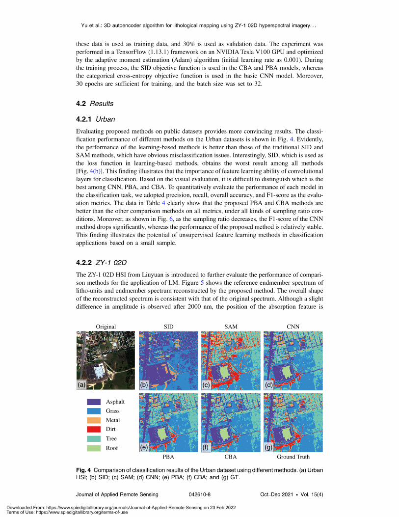
Evaluating proposed methods on public datasets provides more convincing results. The classi-fication performance of different methods on the Urban datasets is shown in Fig. 4. Evidently,the performance of the learning-based methods is better than those of the traditional SID andSAM methods, which have obvious misclassification issues. Interestingly, SID, which is used asthe loss function in learning-based methods, obtains the worst result among all methods[Fig. 4(b)]. This finding illustrates that the importance of feature learning ability of convolutionallayers for classification. Based on the visual evaluation, it is difficult to distinguish which is thebest among CNN, PBA, and CBA. To quantitatively evaluate the performance of each model inthe classification task, we adopted precision, recall, overall accuracy, and F1-score as the evalu-ation metrics. The data in Table 4 clearly show that the proposed PBA and CBA methods arebetter than the other comparison methods on all metrics, under all kinds of sampling ratio con-ditions. Moreover, as shown in Fig. 6, as the sampling ratio decreases, the F1-score of the CNNmethod drops significantly, whereas the performance of the proposed method is relatively stable.This finding illustrates the potential of unsupervised feature learning methods in classificationapplications based on a small sample.

4.2.2 ZY-1 02D

The ZY-1 02D HSI from Liuyuan is introduced to further evaluate the performance of compari-son methods for the application of LM. Figure 5 shows the reference endmember spectrum oflitho-units and endmember spectrum reconstructed by the proposed method. The overall shapeof the reconstructed spectrum is consistent with that of the original spectrum. Although a slightdifference in amplitude is observed after 2000 nm, the position of the absorption feature is

CBA

Original SID SAM CNN

PBA Ground Truth

(a) (b) (c) (d)

(e) (f) (g)Tree

Roof

Dirt

Metal

Grass

Asphalt

Fig. 4 Comparison of classification results of the Urban dataset using different methods. (a) UrbanHSI; (b) SID; (c) SAM; (d) CNN; (e) PBA; (f) CBA; and (g) GT.




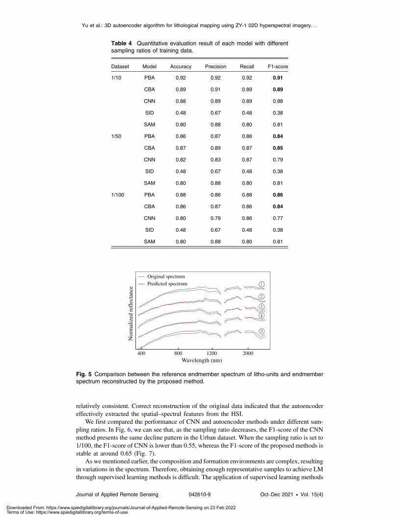
relatively consistent. Correct reconstruction of the original data indicated that the autoencodereffectively extracted the spatial–spectral features from the HSI.

We first compared the performance of CNN and autoencoder methods under different sam-pling ratios. In Fig. 6, we can see that, as the sampling ratio decreases, the F1-score of the CNNmethod presents the same decline pattern in the Urban dataset. When the sampling ratio is set to1/100, the F1-score of CNN is lower than 0.55, whereas the F1-score of the proposed methods isstable at around 0.65 (Fig. 7).

As we mentioned earlier, the composition and formation environments are complex, resultingin variations in the spectrum. Therefore, obtaining enough representative samples to achieve LMthrough supervised learning methods is difficult. The application of supervised learning methods

Table 4 Quantitative evaluation result of each model with differentsampling ratios of training data.

Dataset Model Accuracy Precision Recall F1-score

1/10 PBA 0.92 0.92 0.92 0.91

CBA 0.89 0.91 0.89 0.89

CNN 0.88 0.89 0.89 0.88

SID 0.48 0.67 0.48 0.38

SAM 0.80 0.88 0.80 0.81

1/50 PBA 0.86 0.87 0.86 0.84

CBA 0.87 0.89 0.87 0.85

CNN 0.82 0.83 0.87 0.79

SID 0.48 0.67 0.48 0.38

SAM 0.80 0.88 0.80 0.81

1/100 PBA 0.88 0.86 0.88 0.86

CBA 0.86 0.87 0.86 0.84

CNN 0.80 0.79 0.86 0.77

SID 0.48 0.67 0.48 0.38

SAM 0.80 0.88 0.80 0.81

Nor

mal

ized

ref

lect

ance

400

Original spectrumPredicted spectrum

800Wavelength (nm)

1200 2000

Fig. 5 Comparison between the reference endmember spectrum of litho-units and endmemberspectrum reconstructed by the proposed method.




to small data is more likely to lead to overfitting, thereby leading to difficulty in maintainingrobustness in larger and more complex scenarios.

Table 5 shows that when the sampling ratio is set to 1:50, the classification results of theproposed method are nearly equal to the results of the CNN method. However, CNN has obviousmisclassification in the prediction of categories with a small volume of samples [Fig. 8(d)].Figure 9 shows that the prediction accuracy of the CNN method differs for each category,whereas the CBA model has relatively good robustness in the prediction of all categories.

In this case of LM, the performance of CBA is slightly better than that of PBA (Table 5,Fig. 9) because CBA takes the HSI cube as input to obtain more spatial information. We believethat CBA is more suitable for scenes with larger classification targets; otherwise, there is noguarantee that its performance will be better than that of PBA (Table 4). Although the proposedmethod still has room for improvement in classification accuracy due to the inaccuracy ofmanual labeling, it has better robustness than the supervised learning method. Combined with

0.70

0.75

0.80

0.85

0.90

0.95

1/10 1/50 1/1000.50

0.55

0.60

0.65

0.70

0.75

0.80

1/10 1/50 1/100

F1-s

core

Sampling ratio of Urban Sampling ratio of ZY-1 02D

F1-s

core

(a) (b)PBA CBA CNN PBA CBA CNN

Fig. 7 F1-Score with different sampling ratios of the Urban dataset and the ZY-1 02D dataset.(a) F1-score of the Urban dataset and (b) F1-score of the ZY-1 02D dataset.

Table 5 Performance of different methods for LM with 1/50 sampling ratio of training data.

Model Accuracy Precision Recall F1-score

PBA 0.64 0.65 0.64 0.64

CBA 0.64 0.67 0.64 0.65

CNN 0.65 0.76 0.64 0.65

SID 0.24 0.41 0.24 0.25

SAM 0.39 0.61 0.39 0.37

PBA

CB

AC

NN

1/10 1/50 1/100

Fig. 6 LM results with different sampling ratio for LM of the working area.




the high-quality HSI of ZY-1 02D, the proposed method shows great potential in the large-scaleapplications under small sample conditions.

5 Conclusion

In this work, we present a new 3D convolutional autoencoder for LM. The pixel-based and cube-based 3D convolutional architecture is designed as an encoder to extract spatial–spectral fea-tures. An FC layer with non-negative and sum-to-one constrain is employed to extract the end-member of the litho-units. The traditional methods SAM and SID and machine learning methodsCNN are employed as competing methods and trained on both airborne and spaceborne hyper-spectral datasets. The experimental results indicate that the proposed method can provide con-vincing results for LM applications on the basis of hyperspectral data provided by the ZY-1 02Dsatellite. Compared with traditional methods, the combination of deep learning and hyperspectraldata can provide more efficient and highly accurate results. The proposed method has betterrobustness than the supervised learning methods and shows great promise under small sample

SID SAM

CBA CNN

PBA GT

(f)

(a) (b)

(d)(c)

(e)

Fig. 8 Comparison of classification results for LM of the working area at 1/50 sampling ratio.(a) SID; (b) SAM; (c) CBA; (d) CNN; (e) PBA; and (f) GT.

Type 2

0.00

0.30

0.60

0.90

CNN

F1-S

core

PBA CBA

Type 1 Type 3 Type 4 Type 5

Fig. 9 Comparison of F1-score of each type of litho-units predicted by different models with 1/50sampling ratio.




conditions, which is of great significance for large-scale applications based on newly spaceborneHSI payloads.

Acknowledgments

This work was funded in part by the National Key Research and Development Program of Chinaunder Grant No. 2016YFB0501401 and jointly by the Advance Research Project of Civil SpaceTechnology.

References

1. G. R. Hunt et al., “Visible and near infrared spectra of minerals and rocks. IX. Basic andultrabasic igneous rocks” (1974).

2. R. Kokaly et al., “USGS spectral library version 7: US geological survey data series 1035”(2017).

3. I. Longhi et al., “Spectral analysis and classification of metamorphic rocks from laboratoryreflectance spectra in the 0.4 − 2.5 μm interval: a tool for hyperspectral data interpretation,”Int. J. Remote Sens. 22(18), 3763–3782 (2001).

4. R. N. Clark and T. L. Roush, “Reflectance spectroscopy: quantitative analysis techniques forremote sensing applications,” J. Geophys. Res. Solid Earth 89(B7), 6329–6340 (1984).

5. R. N. Clark, “Chapter1: Spectroscopy of rocks and minerals, and principles of spectros-copy,” in Manual of Remote Sensing, Remote Sensing for the Earth Sciences, A. N. Rencz,Ed., Vol. 3, pp. 3–58, John Wiley and Sons, New York (1999).

6. Y. Liu et al., “Development of visible and short-wave infrared hyperspectral imager onboardGaoFen-5 satellite,” J. Remote Sens. 24, 333–344 (2020).

7. Y. Yang et al., “A temperature and emissivity separation algorithm for Chinese Gaofen-5satellite data,” in IEEE Int. Geosci. and Remote Sens. Symp., pp. 2543–2546 (2018).

8. Y. Zhong et al., “Advances in spaceborne hyperspectral remote sensing in China,” Geo-spat.Inf. Sci. 24(1), 95–120 (2021).

9. J. Yu et al., “An effective cloud detection method for Gaofen-5 images via deep learning,”Remote Sens. 12(13), 2106 (2020).

10. A. A. Green et al., “A transformation for ordering multispectral data in terms of imagequality with implications for noise removal,” IEEE Trans. Geosci. Remote Sens. 26(1),65–74 (1988).

11. M. Black et al., “Automated lithological mapping using airborne hyperspectral thermalinfrared data: a case study from Anchorage Island, Antarctica,” Remote Sens. Environ.176, 225–241 (2016).

12. A. Alberti et al., “Landsat TM data processing for lithological discrimination in the Caracolearea (Namibe Province, SW Angola),” J. African Earth Sci. 17(3), 261–274 (1993).

13. S. Dasgupta and S. Mukherjee, “Remote sensing in lineament identification: examples fromwestern India,” in Developments in Structural geology and Tectonics, pp. 205–221, Elsevier(2019).

14. M. W. Mwaniki, M. S. Matthias, and G. Schellmann, “Application of remote sensing tech-nologies to map the structural geology of central Region of Kenya,” IEEE J. Sel. Top. Appl.Earth Obs. Remote Sens. 8(4), 1855–1867 (2015).

15. G. R. Hunt, “Spectral signatures of particulate minerals in the visible and near infrared,”Geophysics 42(3), 501–513 (1977).

16. R. P. Gupta, Remote Sensing Geology, Springer (2017).17. C. Carli, G. Serventi, and M. Sgavetti, “VNIR spectral characteristics of terrestrial igneous

effusive rocks: mineralogical composition and the influence of texture,” Geol. Soc. LondonSpecial Publ. 401(1), 139–158 (2015).

18. N. Xu et al., “Mineral information extraction for hyperspectral image based on modifiedspectral feature fitting algorithm,” Spectrosc. Spectral Anal. 31(6), 1639–1643 (2011).

19. R. Jain and R. U. Sharma, “Airborne hyperspectral data for mineral mapping in southeasternRajasthan, India,” Int. J. Appl. Earth Obs. Geoinf. 81, 137–145 (2019).




https://doi.org/10.1080/01431160010006980

https://doi.org/10.1029/JB089iB07p06329

https://doi.org/10.11834/jrs.20209196

https://doi.org/10.1109/IGARSS.2018.8517701

https://doi.org/10.1080/10095020.2020.1860653

https://doi.org/10.1080/10095020.2020.1860653

https://doi.org/10.3390/rs12132106

https://doi.org/10.1109/36.3001

https://doi.org/10.1016/j.rse.2016.01.022

https://doi.org/10.1016/0899-5362(93)90072-X

https://doi.org/10.1109/JSTARS.2015.2395094


https://doi.org/10.1190/1.1440721

https://doi.org/10.1144/SP401.19

https://doi.org/10.1144/SP401.19

https://doi.org/10.3964/j.issn.1000-0593(2011)06-1639-05

https://doi.org/10.1016/j.jag.2019.05.007

20. A. Ghulam, R. Amer, and T. M. Kusky, “Mineral exploration and alteration zone mapping inEastern Desert of Egypt using ASTER data,” in ASPRS Annu. Conf. (2010).

21. X. Zhang and P. Li, “Lithological mapping from hyperspectral data by improved use ofspectral angle mapper,” Int. J. Appl. Earth Obs. Geoinf. 31, 95–109 (2014).

22. C. Hecker et al., “Assessing the influence of reference spectra on synthetic SAMclassification results,” IEEE Trans. Geosci. Remote Sens. 46(12), 4162–4172 (2008).

23. C.-I. Chang, “An information-theoretic approach to spectral variability, similarity, anddiscrimination for hyperspectral image analysis,” IEEE Trans. Inf. Theory 46(5),1927–1932 (2000).

24. J. B. Adams, M. O. Smith, and P. E. Johnson, “Spectral mixture modeling: A new analysisof rock and soil types at the Viking Lander 1 site,” J. Geophys. Res. Solid Earth 91(B8),8098–8112 (1986).

25. J. Yu and B. Yan, “Efficient solution of large-scale domestic hyperspectral data processingand geological application,” in Int. Workshop Remote Sens. Intell. Process., pp. 1–4(2017).

26. W. Wang et al., “Deep learning based lithology classification using dual-frequency Pol-SARdata,” Applied Sciences 8(9), 1513 (2018).

27. Y. Vasuki et al., “An interactive image segmentation method for lithological boundarydetection: a rapid mapping tool for geologists,” Comput. Geosci. 100, 27–40 (2017).

28. M. Chakouri et al., “Geological and mineralogical mapping in Moroccan central Jebiletusing multispectral and hyperspectral satellite data and machine learning,” Int. J. Adv.Trends Comput. Sci. Eng. 9(4), 5772–5783 (2020).

29. N. Rani, V. R. Mandla, and T. Singh, “Performance of image classification on hyperspectralimagery for lithological mapping,” J. Geol. Soc. India 88(4), 440–448 (2016).

30. M. Belgiu and L. Drăguţ, “Random forest in remote sensing: a review of applications andfuture directions,” ISPRS J. Photogramm. Remote Sens. 114, 24–31 (2016).

31. X. Wang et al., “Caps-TripleGAN: GAN-assisted CapsNet for hyperspectral image classi-fication,” IEEE Trans. Geosci. Remote Sens. 57(9), 7232–7245 (2019).

32. X. Wang et al., “CVA 2 E: a conditional variational autoencoder with an adversarial trainingprocess for hyperspectral imagery classification,” IEEE Trans. Geosci. Remote Sens. 58(8),5676–5692 (2020).

33. B. Ye et al., “Application of lithological mapping based on advanced hyperspectralimager (AHSI) imagery onboard Gaofen-5 (GF-5) satellite,” Remote Sensing 12(23), 3990(2020).

34. O. Savas, K. Berk, and A. G. Bozdagi, “EndNet: sparse autoencoder network for endmem-ber extraction and hyperspectral unmixing,” IEEE Trans. Geosci. Remote Sens. 57, 482–496(2017).

35. Y. Qu and H. Qi, “uDAS: an untied denoising autoencoder with sparsity for spectral unmix-ing,” IEEE Trans. Geosci. Remote Sens. 57, 1698–1712 (2019).

36. Y. Su et al., “DAEN: deep autoencoder networks for hyperspectral unmixing,” IEEE Trans.Geosci. Remote Sens. 57, 4309–4321 (2019).

37. X. Zhang et al., “Hyperspectral unmixing via deep convolutional neural networks,” IEEEGeosci. Remote Sens. Lett. 15, 1755–1759 (2018).

38. F. Khajehrayeni and H. Ghassemian, “Hyperspectral unmixing using deep convolutionalautoencoders in a supervised scenario,” IEEE J. Sel. Top. Appl. Earth Obs. RemoteSens., 13, 567–576 (2020).

39. D. C. Heinz and C.-I. Chang, “Fully constrained least squares linear spectral mixture analy-sis method for material quantification in hyperspectral imagery,” IEEE Trans. Geosci.Remote Sens. 39(3), 529–545 (2002).

40. M. Sokolova and G. Lapalme, “A systematic analysis of performance measures forclassification tasks,” Inf. Process. Manage. 45, 427–437 (2009).

Junchuan Yu received his PhD from China University of Geosciences in 2013. He currentlyworks in the Department of Satellite Application Research at China Aero Geophysical Surveyand Remote Sensing Center for Natural Resources. His research interests include hyperspectralremote sensing, deep learning, and geological application.




https://doi.org/10.1016/j.jag.2014.03.007

https://doi.org/10.1109/TGRS.2008.2001035

https://doi.org/10.1109/18.857802

https://doi.org/10.1029/JB091iB08p08098

https://doi.org/10.1109/RSIP.2017.7970774

https://doi.org/10.3390/app8091513

https://doi.org/10.1016/j.cageo.2016.12.001

https://doi.org/10.30534/ijatcse/2020/234942020

https://doi.org/10.30534/ijatcse/2020/234942020

https://doi.org/10.1007/s12594-016-0507-5

https://doi.org/10.1016/j.isprsjprs.2016.01.011



https://doi.org/10.3390/rs12233990





https://doi.org/10.1109/LGRS.2018.2857804

https://doi.org/10.1109/LGRS.2018.2857804



https://doi.org/10.1109/36.911111

https://doi.org/10.1109/36.911111

https://doi.org/10.1016/j.ipm.2009.03.002

Liang Zhang received his BS degree from the China University of Geosciences, Beijing, in2019. He is currently pursuing a PhD in surveying and mapping in China University ofGeosciences, Beijing. His research interests include intelligent processing of remote sensingimages using deep learning methods and neural network algorithm.

Qiang Li received his MS degree from Wuhan University. He currently working in ShenyangGeotechnical Investigation and Surveying Research Institute Co., Ltd. At present, he mainlyengaged in photogrammetry and remote sensing.

Yichuan Li received his PhD from China University of Geosciences in 2015. She currentlyworking in China Aero Geophysical Survey and Remote Sensing Center for Natural Resources,engaged in hyperspectral remote sensing and deep learning.

Wei Huang is a computer engineer who works in China Aero Geophysical Survey and RemoteSensing Center for Natural Resources. His major research activities include parallel computingand computer architecture.

Zhiwei Sun graduated from Lanzhou Jiaotong University with a master’s degree in cartographyand geographic information system. At present, he mainly engaged in photogrammetry andremote sensing.

Yanni Ma graduated from China University of Geosciences (Beijing) with a bachelor’s degreein GIS and a master’s degree in surveying and mapping. At present, she works in the China AeroGeophysical Survey and Remote Sensing Center for Natural Resources, engaged in deeplearning and remote sensing image information extraction.

Peng He is a PhD student at China University of Geosciences in structural geology. She cur-rently works in the China Aero Geophysical Survey and Remote Sensing Center for NaturalResources. Her research interests are remote sensing of environment and geological disasters.




3d autoencoder algorithm for lithological mapping using zy

Documents