4.3 draft 5/27/04 1 · type of ﬁnite element analysis (fea). the practical advantages of fea in...

Chapter 1

INTRODUCTION

1.1 Finite Element Methods

The goal of this text is to introduce finite element methods from a rather broadperspective. We will consider the basic theory of finite element methods as utilized as anengineering tool. Likewise, example engineering applications will be presented toillustrate practical concepts of heat transfer, stress analysis, and other fields. Today thesubject of error analysis for adaptivity of finite element methods has reached the pointthat it is both economical and reliable and should be considered in an engineeringanalysis. Finally, we will consider in some detail the typical computational proceduresrequired to apply modern finite element analysis, and the associated error analysis. Inthis chapter we will begin with an overview of the finite element method. We close itwith consideration of modern programming approaches and a discussion of how thesoftware provided differs from the author’s previous implementations of finite elementcomputational procedures.

In modern engineering analysis it is rare to find a project that does not require sometype of finite element analysis (FEA). The practical advantages of FEA in stress analysisand structural dynamics have made it the accepted tool for the last two decades. It is alsoheavily employed in thermal analysis, especially in connection with thermal stressanalysis.

Clearly, the greatest advantage of FEA is its ability to handle truly arbitrarygeometry. Probably its next most important features are the ability to deal with generalboundary conditions and to include nonhomogeneous and anisotropic materials. Thesefeatures alone mean that we can treat systems of arbitrary shape that are made up ofnumerous different material regions. Each material could have constant properties or theproperties could vary with spatial location. To these very desirable features we can add alarge amount of freedom in prescribing the loading conditions and in the postprocessingof items such as the stresses and strains. For elliptical boundary value problems the FEAprocedures offer significant computational and storage efficiencies that further enhance itsuse. That class of problems include stress analysis, heat conduction, electrical fields,magnetic fields, ideal fluid flow, etc. FEA also gives us an important solution techniquefor other problem classes such as the nonlinear Navier - Stokes equations for fluiddynamics, and for plasticity in nonlinear solids.

4.3 Draft− 5/27/04 © 2004 J.E. Akin 1

2 J. E. Akin

Here we will show what FEA has to offer and illustrate some of its theoreticalformulations and practical applications. A design engineer should study finite elementmethods in more detail than we can consider here. It is still an active area of research.The current trends are toward the use of error estimators and automatic adaptive FEAprocedures that give the maximum accuracy for the minimum computational cost. This isalso closely tied to shape modification and optimization procedures.

(e)

(b)

(e)

(b)

U ( x, y )

Figure 1.2.1 Piecewise approximation of a scalar function

4.3 Draft− 5/27/04 © 2004 J.E. Akin. All rights reserved.

Finite Elements, Introduction 3

1.2 Capabilities of FEA

There are many commercial and public-domain finite element systems that areavailable today. To summarize the typical capabilities, several of the most widely usedsoftware systems have been compared to identify what they hav e in common. Often wefind about 90% of the options are available in all the systems. Some offer veryspecialized capabilities such as aeroelastic flutter or hydroelastic lubrication. Themainstream capabilities to be listed here are found to be included in the majority of thecommercial systems. The newer adaptive systems may have fewer options installed butthey are rapidly adding features common to those given above. Most of these systems areavailable on engineering workstations and personal computers as well as mainframes andsupercomputers. The extent of the usefulness of a FEA system is directly related to theextent of its element library. The typical elements found within a single system usuallyinclude membrane, solid, and axisymmetric elements that offer linear, quadratic, andcubic approximations with a fixed number of unknowns per node. The new hierarchicalelements have relatively few basic shapes but they do offer a potentially large number ofunknowns per node (up to 81 for a solid). Thus, the actual effective element library sizeis extremely large.

In the finite element method, the boundary and interior of the region are subdividedby lines (or surfaces) into a finite number of discrete sized subregions or finite elements.A number of nodal points are established with the mesh. The size of an element isusually associated with a reference length denoted byh. It, for example, may be thediameter of the smallest sphere that can enclose the element. These nodal points can lieanywhere along, or inside, the subdividing mesh, but they are usually located atintersecting mesh lines (or surfaces). The elements may have straight boundaries andthus, some geometric approximations will be introduced in the geometric idealization ifthe actual region of interest has curvilinear boundaries. These concepts are graphicallyrepresented in Fig. 1.2.1.

The nodal points and elements are assigned identifying integer numbers beginningwith unity and ranging to some maximum value. The assignment of the nodal numbersand element numbers will have a significant effect on the solution time and storagerequirements. The analyst assigns a number of generalized degrees of freedom to eachand every node. These are the unknown nodal parameters that have been chosen by theanalyst to govern the formulation of the problem of interest. Common nodal parametersare displacement components, temperatures, and velocity components. The nodalparameters do not have to hav e a physical meaning, although they usually do. Forexample, the hierarchical elements typically use the derivatives up to order six as themidside nodal parameters. This idealization procedure defines the total number ofdegrees of freedom associated with a typical node, a typical element, and the totalsystem. Data must be supplied to define the spatial coordinates of each nodal point. It iscommon to associate some code to each node to indicate which, if any, of the parametersat the node have boundary constraints specified. In the new adaptive systems the numberof nodes, elements, and parameters per node usually all change with each new iteration.

Another important concept is that ofelement connectivity, (or topology) i.e., the listof global node numbers that are attached to an element. The element connectivity datadefines the topology of the (initial) mesh, which is used, in turn, to assemble the system


4 J. E. Akin

Definegeometry,

materials, axes

Generatemesh

Type ofcalculation

?

Define pressure,gravity, loads, ...

Define heat flux,heat generation

Generate and assemble elementand boundary matrices

Apply essential boundary conditions,solve algebraic equations,recover system reactions

Average nodal fluxes,post-process elements,estimate element errors

Adapt mesh

Prescribedtemperature

data

Prescribeddisplacement

data

Erroracceptable

?

Thermal Stress

No StopYes

Figure 1.2.2 Typical stages in a finite element analysis



algebraic equations. Thus, for each element it is necessary to input, in some consistentorder, the node numbers that are associated with that particular element. The list of nodenumbers connected to a particular element is usually referred to as the element incidentlist for that element. We usually associate a material code, or properties, with eachelement.

Finite element analysis can require very large amounts of input data. Thus, mostFEA systems offer the user significant data generation or supplementation capabilities.The common data generation and validation options include the generation and/orreplication of coordinate systems, node locations, element connectivity, loading sets,restraint conditions, etc. The verification of such extensive amounts of input andgenerated data is greatly enhanced by the use of computer graphics.

In the adaptive methods we must also compute the error indicators, error estimators,and various energy norms. All these quantities are usually output at 1 to 27 points ineach of thousands of elements. The most commonly needed information in anengineering analysis is the state of temperatures, or displacements and stresses. Thus,almost every system offers linear static stress analysis capabilities, and linear thermalanalysis capabilities for conduction and convection that are often needed to providetemperature distributions for thermal stress analysis. Usually the same mesh geometry isused for the temperature analysis and the thermal stress analysis. Of course, some studiesrequire information on the natural frequencies of vibration or the response to dynamicforces or the effect of frequency driven excitations. Thus, dynamic analysis options areusually available. The efficient utilization of materials often requires us to employnonlinear material properties and/or nonlinear equations. Such resources require a moreexperienced and sophisticated user. The usual nonlinear stress analysis features in largecommercial FEA systems include buckling, creep, large deflections, and plasticity. Thoseadvanced methods will not be considered here.

There are certain features of finite element systems which are so important from apractical point of view that, essentially, we cannot get along without them. Basically we

Table 1.1 Typical unknown variables in finite element analysis

Application Primary Associated Secondary

Stress analysis Displacement, Force, Stress,Rotation Moment Failure criterion

Error estimates

Heat transfer Temperature Flux Interior fluxError estimates

Potential flow Potential function Normal velocity Interior velocityError estimates

Navier-Stokes Velocity Pressure Error estimates


6 J. E. Akin

Table 1.2 Typical given variables and corresponding reactions

Application Given Reaction

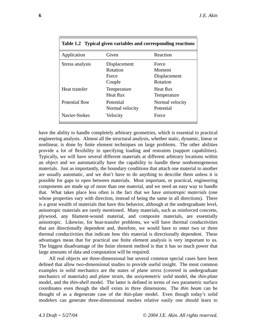
Stress analysis Displacement ForceRotation MomentForce DisplacementCouple Rotation

Heat transfer Temperature Heat fluxHeat flux Temperature

Potential flow Potential Normal velocityNormal velocity Potential

Navier-Stokes Velocity Force

have the ability to handle completely arbitrary geometries, which is essential to practicalengineering analysis. Almost all the structural analysis, whether static, dynamic, linear ornonlinear, is done by finite element techniques on large problems. The other abilitiesprovide a lot of flexibility in specifying loading and restraints (support capabilities).Typically, we will have sev eral different materials at different arbitrary locations withinan object and we automatically have the capability to handle these nonhomogeneousmaterials. Just as importantly, the boundary conditions that attach one material to anotherare usually automatic, and we don’t hav e to do anything to describe them unless it ispossible for gaps to open between materials. Most important, or practical, engineeringcomponents are made up of more than one material, and we need an easy way to handlethat. What takes place less often is the fact that we haveanisotropic materials(onewhose properties vary with direction, instead of being the same in all directions). Thereis a great wealth of materials that have this behavior, although at the undergraduate level,anisotropic materials are rarely mentioned. Many materials, such as reinforced concrete,plywood, any filament-wound material, and composite materials, are essentiallyanisotropic. Likewise, for heat-transfer problems, we will have thermal conductivitiesthat are directionally dependent and, therefore, we would have to enter two or threethermal conductivities that indicate how this material is directionally dependent. Theseadvantages mean that for practical use finite element analysis is very important to us.The biggest disadvantage of the finite element method is that it has so much power thatlarge amounts of data and computation will be required.

All real objects are three-dimensional but several common special cases have beendefined that allow two-dimensional studies to provide useful insight. The most commonexamples in solid mechanics are the states ofplane stress(covered in undergraduatemechanics of materials) andplane strain, the axisymmetric solidmodel, thethin-platemodel, and thethin-shellmodel. The latter is defined in terms of two parametric surfacecoordinates even though the shell exists in three dimensions. Thethin beamcan bethought of as a degenerate case of the thin-plate model. Even though today’s solidmodelers can generate three-dimensional meshes relative easily one should learn to



approach such problems carefully. A well planned series of two-dimensionalapproximations can provide important insight into planning a good three-dimensionalmodel. They also provide good "ballpark" checks on the three-dimensional answers. Ofcourse, the use of basic handbook calculations in estimating the answer beforeapproaching a FEA system is also highly recommended.

The typical unknown variables in a finite element analysis are listed in Table 1.1 anda list of related action-reaction variables are cited in Table 1.2. Figure 1.2.2 outlines as aflow chart the major steps needed for either a thermal analysis or stress analysis. Notethat these segments are very similar. One of the benefits of developing a finite elementapproach is that most of the changes related to a new field of application occur at theelement level definitions and usually represent less than 5 percent of the totalprogramming effort.

1.3 Outline of Finite Element Procedures

From the mathematical point of view the finite element method is an integralformulation. Modern finite element integral formulations are usually obtained by eitherof two different procedures:weighted residualor variational formulations. Thefollowing sections briefly outline the common procedures for establishing finite elementmodels. It is fortunate that all these techniques use the same bookkeeping operations togenerate the final assembly of algebraic equations that must be solved for the unknowns.

The generation of finite element models by the utilization of weighted residualtechniques is increasingly important in the solution of differential equations for non-structural applications. The weighted residual method starts with the governingdifferential equation to be satisfied in a domainΩ :

(1.1)L(φ ) = Q ,

where L denotes a differential operator acting on the primary unknown,φ , andQ is asource term. Generally we assume an approximate solution, sayφ * , for the spatialdistribution of the unknown, say

(1.2)φ (x) ≈ φ * =n

iΣ hi (x) Φ*

i ,

where the hi (x) are spatial distributions associated with the coefficientΦ*i . That

assumption leads to a corresponding assumption for the spatial gradient of the assumedbehavior. Next we substitute these assumptions on spatial distributions into thedifferential equation. Since the assumption is approximate, this operation defines aresidual error term,R, in the differential equation

(1.3)L(φ * ) − Q = R ≠ 0 .

Although we cannot force the residual term to vanish, it is possible to force a weightedintegral, over the solution domain, of the residual to vanish. That is, the integral of theproduct of the residual term and some weighting function is set equal to zero, so that

(1.4)I i =Ω∫ R wi dΩ = 0

leads to the same number of equations as there are unknownΦ*i values. Most of the time


8 J. E. Akin

0 0 0 0 0 1 00 0 0 1 0 0 0=

(b)

(e)

Elements

Mesh

Nodes

Positions

Unknowns

1 3 5 7 6 4 2

x1 x 3 x 5 x 7 x6 x 4 x 2

D1 D3 D5 D 7 D6 D 4 D2

(1) (a) … (b) (6)

1 2

(e)

D1

D2

D3

D4

D5

D6

D7

D1

D2

(a)

D1

D2

(b)

x1

x2

x3

x4

x5

x6

x7

x1

x2

(a)

(b)

C1

C2

C3

C4

C5

C6

C7

C1

C2

(a)

(b)x1

x2

C1

C2

Gather geometryfor Se, Ce

Gather answersto post-process

Scatter element vectorsfor assembly of C

xe = x(e)

De = D(e)

C = Cee

S D = C

Figure 1.3.1 Gather and scatter concepts for finite elements

we will find it very useful to employ integration by parts on this governing integral.Substituting an assumed spatial behavior for the approximate solution,φ * , and the

weighting function,w, results in a set of algebraic equations that can be solved for theunknown nodal coefficients in the approximate solution. This is because the unknowncoefficients can be pulled out of the spatial integrals involved in the assembly process.

The choice of weighting function defines the type of weighted residual techniquebeing utilized. The Galerkin criterion selects

(1.5)wi = hi (x) ,

to make the residual error "orthogonal" to the approximate solution. Use of integrationby parts with the Galerkin procedure (i.e., the Divergence Theorem) reduces thecontinuity requirements of the approximating functions. If a Euler variational procedure



exists, the Galerkin criterion will lead to the same element matrices.A spatial interpolation, or blending function is assumed for the purpose of relating

the quantity of interest within the element in terms of the values of the nodal parametersat the nodes connected to that particular element. For both weighted residual andvariational formulations, the following restrictions are accepted for establishingconvergence of the finite element model as the mesh refinement increases:

1. The element interpolation functions must be capable of modeling any constantvalues of the dependent variable or its derivatives, to the order present in thedefining integral statement, in the limit as the element size decreases.

2. The element interpolation functions should be chosen so that at element interfacesthe dependent variable and its derivatives, of one order less than those occurring inthe defining integral statement, are continuous.

Through the assumption of the spatial interpolations, the variables of interest andtheir derivatives are uniquely specified throughout the solution domain by the nodalparameters associated with the nodal points of the system. The parameters at a particularnode directly influence only the elements connected to that particular node. The domainwill be split into a mesh. That will require that we establish some bookkeeping processesto keep up with data going to, or coming from a node or element. Those processes arecommonly called gather and scatter, respectively. Figure 1.3.1 shows some of theseprocesses for a simple mesh with one scalar unknown per node,ng = 1, in a one-dimensional physical space. There the system node numbers are shown numbered in anarbitrary fashion. To establish the local element space domain we must usually gather thecoordinates of each of its nodes. For example, for elementb(= 5) it gathers the data forsystem node numbers 6 and 4, respectively, so that the element length,L(5) = x6 − x4, canbe computed. Usually we also have to gather some data on the coefficients in thedifferential equation (material properties usually). If the coefficients vary over space theymay be supplied as data at the nodes that must also be gathered to form the elementmatrices.

After the element behavior has been described by spatial assumptions, then thederivatives of the space functions are used to approximate the spatial derivatives requiredin the integral form. The remaining fundamental problem is to establish the elementmatrices,Se and Ce. This involves substituting the approximation space functions andtheir derivatives into the governing integral form and moving the unknown coefficients,De, outside the integrals. Historically, the resulting matrices have been called the elementstiffness matrix and load vector, respectively.

Once the element equations have been established the contribution of each elementis added, using its topology (or connectivity), to form the system equations. The systemof algebraic equations resulting from FEA (of a linear system) will be of the formS D = C. The vectorD contains the unknown nodal parameters, and the matricesS andCare obtained by assembling the known element matrices,Se andCe, respectively. Figure1.3.1 shows how the local coefficients of the element source vector,Ce, are scattered andadded into the resultant system source,C. That illustration shows a conversion of localrow numbers to the corresponding system row numbers (by using the elementconnectivity data). An identical conversion is used to convert the local and system


10 J. E. Akin

column numbers needed in assemblying eachSe into S. In the majority of problemsSe,and thus,S, will be symmetric. Also, the system square matrix,S, is usually bandedabout the diagonal or at leastsparse. If S is unsymmetric its upper and lower triangleshave the same sparsity.

After the system equations have been assembled, it is necessary to apply theessential boundary constraintsbefore solving for the unknown nodal parameters. Themost common types of essential boundary conditions (EBC) are (1) defining explicitvalues of the parameter at a node and (2) defining constraint equations that are linearcombinations of the unknown nodal quantities. The latter constraints are often referred toin the literature asmulti-point constraints(MPC). An essential boundary conditionshould not be confused with a forcing condition of the type that involves a flux or tractionon the boundary of one or more elements. These element boundary source, or forcing,terms contribute additional terms to the governing integral form and thus to the elementsquare and/or column matrices for the elements on which the sources were applied.Thus, although these (Neumann-type, and Robinor mixed-type) conditions do enter intothe system equations, their presence may not be obvious at the system level. Whereveressential boundary conditions do not act on part of the boundary, then at such locations,source terms from a lower order differential equation automatically apply. If one doesnot supply data for the source terms, then they default to zero. Such portions of theboundary are said to be subject to natural boundary conditions (NBC). The naturalboundary condition varies with the integral form, and typical examples will appear later.

The initial sparseness (the relative percentage of zero entries) of the square matrix,S, is an important consideration since we only want to store non-zero terms. If weemploy a direct solver then many initially zero terms will become non-zero during thesolution process and the assigned storage must allow for that. The "fill-in" depends onthe numbering of the nodes. If the FEA system being employed does not have anautomatic renumbering system to increase sparseness, then the user must learn how tonumber nodes (or elements) efficiently. After the system algebraic equations have beensolved for the unknown nodal parameters, it is usually necessary to output the parameters,D. For every essential boundary condition onD, there is a corresponding unknownreaction term inC that can be computed afterD is known. These usually have physicalmeanings and should be output to help check the results.

In rare cases the problem would be considered completed at this point, but in mostcases it is necessary to use the calculated values of the nodal parameters to calculate otherquantities of interest. For example, in stress analysis we use the calculated nodaldisplacements to solve for the strains and stresses. All adaptive programs must do a verylarge amount of postprocessing to be sure that the solution,D, has been obtained to thelevel of accuracy specified by the analyst. Figure 1.3.1 also shows that the gatheroperation is needed again for extracting the local results,De, from the total results,D, sothey can be employed in special element post-processing and/or error estimates.

Usually the postprocessing calculations involve determining the spatial derivativesof the solution throughout the mesh. Those gradients are continuous within each elementdomain, but are discontinuous across the inter-element boundaries. The true solutionusually has continuous derivatives so it is desirable to somehow average the individualelement gradient estimates to create continuous gradient estimate values that can be



reported at the nodes. Fortunately, this addition gradient averaging process also providesnew information that allows the estimate of the problem error norm to be calculated.That gradient averaging process will be presented in Chapter 2.

In the next chapter we will review the historical approach of the method of weightedresiduals and its extension to finite element analysis. The earliest formulations for finiteelement models were based on variational techniques. This is especially true in the areasof structural mechanics and stress analysis. Modern analysis in these areas has come torely on FEA almost exclusively. Variational models find the nodal parameters that yield aminimum (or stationary) value of an integral known as a functional. In most cases it ispossible to assign a physical meaning to the integral. For example, in solid mechanics theintegral represents thetotal potential energy, whereas in a fluid mechanics problem itmay correspond to the rate of entropy production. Most physical problems withvariational formulations result in quadratic forms that yield algebraic equations for thesystem which are symmetric and positive definite. The solution that yields a minimumvalue of the integral functional and satisfies the essential boundary conditions isequivalent to the solution of an associated differential equation. This is known as theEuler theorem.

Compared to the method of weighted residuals, where we start with the differentialequation, it may seem strange to start a variational formulation with an integral form andthen check to see if it corresponds to the differential equation we want. However, fromEuler’s work more than two centuries ago we know the variational forms of most evenorder differential equations that appear in science, engineering, and applied mathematics.This is especially true for elliptical equations. Euler’s Theorem of Variational Calculusstates that the solution,u, that satisfies the essential boundary conditions and rendersstationary the functional

(1.6)I =Ω∫ f

x, y, z,φ ,

∂φ∂x

,∂φ∂y

,∂φ∂z

dΩ +Γ∫

qφ + aφ 2 / 2

d Γ

also satisfies the partial differential equation

(1.7)∂ f

∂φ−

∂∂x

∂ f

∂ ( ∂φ / ∂x )−

∂∂y

∂ f

∂ ( ∂φ / ∂y )−

∂∂z

∂ f

∂ ( ∂φ / ∂z )= 0

in Ω, and satisfies the natural boundary condition that

(1.8)nx∂ f

∂ ( ∂φ / ∂x )+ ny

∂ f

∂ ( ∂φ / ∂y )+ nz

∂ f

∂ ( ∂φ / ∂z )+ q + aφ = 0

on Γ that is not subject to an essential boundary. Herenx, ny, nz are the components ofthe normal vector on the boundary,Γ. Note that this theorem also defines the naturalboundary condition, as well as the corresponding differential equation. In Chapter 7 wewill examine some common Euler variational forms and their extensions to finite elementanalysis.


12 J. E. Akin

1.4 Assembly into the System Equations1.4.1 Introduction

An important but often misunderstood topic is the procedure forassemblyingthesystem equations from the element equations and any boundary contributions. Hereassemblying is defined as the operation of adding the coefficients of the elementequations into the proper locations in the system equations. There are various methodsfor accomplishing this but most are numerically inefficient. The numerically efficientdirect assemblytechnique will be described here in some detail. We begin by reviewingthe simple but important relationship between a set of local (nodal point, or element)degree of freedom numbers and the corresponding system degree of freedom numbers.

The assembly process, introduced in part in Fig. 1.3.1, is graphically illustrated inFig. 1.4.1 for a mesh consisting of six nodes (nm = 6), three elements (ne = 3). It has afour-node quadrilateral and two three-node triangles, with one generalized parameter pernode (ng = 1). The top of the figure shows the nodal connectivity of the three elementsand a cross-hatching to define the source of the various coefficients that are occurring inthe matrices assembled in the lower part of the figure. The assembly of the systemS andC matrices is graphically coded to denote the sources of the contributing terms but nottheir values. A hatched area indicates a term that was added in from an element that hasthe same hash code. For example, the load vector term C(6), coming from the onlyparameter at node 6, is seen to be the sum of contributions from elements 1 and 2, whichare hatched with horizontal (-) and vertical (|) lines, respectively. The connectivity tableimplies the same thing since node 6 is only connected to those two elements. By way ofcomparison, the term C(1) has a contribution only from element 2. The connectivitytable shows only that element is connected to that corner node.

Note that we have to setS = 0 to begin the summation. Referring to Fig. 1.4.1 wesee that 10 of the coefficients inS remain initially zero. So that example is initially about27 % sparse. (This will changed if a direct solution process is used.) In practicalproblems the assembled matrix may initially be 90 % sparse, or more. Special equationsolving techniques take advantage of this feature to save memory space and to reduceoperation counts.

1.4.2 Computing the Equation Index

There are a number of ways to assign the equation numbers of the algebraic systemthat results from a finite element analysis procedure. Here we will select one that has asimple equation that is valid for most applications. Consider a typical nodal point in thesystem and assume that there areng parameters associated with each node. Thus, at atypical node there will beng local degree of freedom numbers (1≤ J ≤ ng) and acorresponding set of system degree of freedom numbers. IfI denotes the system nodenumber of the point, then theng corresponding system degrees of freedom,Φk have theirequation number,k assigned as

(1.9)k (I , J) = ng * ( I − 1 ) + J 1 ≤ I ≤ nm , 1 ≤ J ≤ ng ,

wherenm is the maximum node number in the system. That is, they start at 1 and rangeto ng at the first system node then at the second node they range from (ng + 1) to (2ng)



5

4

62

1

3

Element Topology1 2, 6, 3, 12 6, 4, 3, 03 5, 3, 4, 0local 1, 2, 3, 4

1

3

2

1 2 3 4 5 6

1

2

3

4

5

6

1

2

3

4

5

6

D1

D2

D3

D4

D5

D6

* =

Global

Global Assembly: S * D = C

1

1

1

2

2

2

4

3

3

3

0 0 0 0 0 10 0 0 1 0 00 0 1 0 0 0

2 =

Figure 1.4.1 Graphical illustration of matrix assembly


14 J. E. Akin

FUNCTION GET_INDEX_AT_PT (I_PT) RESULT (INDEX) ! 1! * * * * * * * * * * * * * * * * * * * * * * * * * * ! 2! DETERMINE DEGREES OF FREEDOM NUMBERS AT A NODE ! 3! * * * * * * * * * * * * * * * * * * * * * * * * * * ! 4Use System_Constants ! for N_G_DOF ! 5

IMPLICIT NONE ! 6INTEGER, INTENT(IN) :: I_PT ! 7INTEGER :: INDEX (N_G_DOF) ! 8INTEGER :: J ! implied loop ! 9

!10! N_G_DOF = NUMBER OF PARAMETERS (DOF) PER NODE !11! I_PT = SYSTEM NODE NUMBER !12! INDEX = SYSTEM DOF NOS OF NODAL DOF !13! INDEX (J) = N_G_DOF*(I_PT - 1) + J !14

!15INDEX = (/ (N_G_DOF*(I_PT - 1) + J, J = 1, N_G_DOF) /) !16

END FUNCTION GET_INDEX_AT_PT !17

FUNCTION GET_ELEM_INDEX (LT_N, ELEM_NODES) RESULT(INDEX) ! 1! * * * * * * * * * * * * * * * * * * * * * * * * * * * ! 2! DETERMINE DEGREES OF FREEDOM NUMBERS OF ELEMENT ! 3! * * * * * * * * * * * * * * * * * * * * * * * * * * * ! 4Use System_Constants ! for N_G_DOF ! 5

IMPLICIT NONE ! 6INTEGER, INTENT(IN) :: LT_N, ELEM_NODES (LT_N) ! 7INTEGER :: INDEX (LT_N * N_G_DOF) ! OUT ! 8INTEGER :: EQ_ELEM, EQ_SYS, IG, K, SYS_K ! LOOPS ! 9

!10! ELEM_NODES = NODAL INCIDENCES OF THE ELEMENT !11! EQ_ELEM = LOCAL EQUATION NUMBER !12! EQ_SYS = SYSTEM EQUATION NUMBER !13! INDEX = SYSTEM DOF NUMBERS OF ELEMENT DOF NUMBERS !14! INDEX (N_G_DOF*(K-1)+IG) = N_G_DOF*(ELEM_NODES(K)-1) + IG !15! LT_N = NUMBER OF NODES PER ELEMENT !16! N_G_DOF = NUMBER OF GENERAL PARAMETERS (DOF) PER NODE !17

!18DO K = 1, LT_N ! LOOP OVER NODES OF ELEMENT !19

SYS_K = ELEM_NODES (K) ! SYSTEM NODE NUMBER !20DO IG = 1, N_G_DOF ! LOOP OVER GENERALIZED DOF !21

EQ_ELEM = IG + N_G_DOF * (K - 1) ! LOCAL EQ !22EQ_SYS = IG + N_G_DOF * (SYS_K - 1) ! SYSTEM EQ !23IF ( SYS_K > 0 ) THEN ! VALID NODE !24

INDEX (EQ_ELEM) = EQ_SYS !25ELSE ! ALLOW MISSING NODE !26

INDEX (EQ_ELEM) = 0 !27END IF ! MISSING NODE !28

END DO ! OVER DOF !29END DO ! OVER LOCAL NODES !30

END FUNCTION GET_ELEM_INDEX !31

Figure 1.4.2 Computing equation numbers for homogeneous nodal dof



Element Topology Equations

1 1, 3 1, 2, 5, 62 3, 4 5, 6, 7, 83 4, 2 7, 8, 3, 4

1 2 3 4 5 6

1

234

56

1

234

56

D1

D2

D3

D4

D5

D6

* =

Global

Global Assembly: S * D = C

(1) (2) (3)

1 3 4 2

7 8

7

8

7

8D7

D8

(e)

j k

u kvk

ujv j

1

234

1

234

1

234

5

678

1

256

7

834

1 2 5 6 5 6 7 8 7 8 3 4

(1) (2) (3)

Element Square Matrices:

Mesh:

Global

Local

Figure 1.4.3 Assemblying two unknowns per node


16 J. E. Akin

SUBROUTINE STORE_COLUMN (N_D_FRE, N_EL_FRE, INDEX, C, CC) ! 1! * * * * * * * * * * * * * * * * * * * * * * * * * * * * ! 2! STORE ELEMENT COLUMN MATRIX IN SYSTEM COLUMN MATRIX ! 3! * * * * * * * * * * * * * * * * * * * * * * * * * * * * ! 4Use Precision_Module ! Defines DP for double precision ! 5

IMPLICIT NONE ! 6INTEGER, INTENT(IN) :: N_D_FRE, N_EL_FRE ! 7INTEGER, INTENT(IN) :: INDEX (N_EL_FRE) ! 8REAL(DP), INTENT(IN) :: C (N_EL_FRE) ! 9REAL(DP), INTENT(INOUT) :: CC (N_D_FRE) !10INTEGER :: I, J !11

!12! N_D_FRE = NO DEGREES OF FREEDOM IN THE SYSTEM !13! N_EL_FRE = NUMBER OF DEGREES OF FREEDOM PER ELEMENT !14! INDEX = SYSTEM DOF NOS OF THE ELEMENT DOF !15! C = ELEMENT COLUMN MATRIX !16! CC = SYSTEM COLUMN MATRIX !17

!18DO I = 1, N_EL_FRE ! ELEMENT ROW !19

J = INDEX (I) ! SYSTEM ROW NUMBER !20IF ( J > 0 ) CC (J) = CC (J) + C (I) ! SKIP INACTIVE ROW !21

END DO ! OVER ROWS !22END SUBROUTINE STORE_COLUMN !23

SUBROUTINE STORE_FULL_SQUARE (N_D_FRE, N_EL_FRE, S, SS, INDEX) ! 1! * * * * * * * * * * * * * * * * * * * * * * * * * * * * * * ! 2! STORE ELEMENT SQ MATRIX IN FULL SYSTEM SQ MATRIX ! 3! * * * * * * * * * * * * * * * * * * * * * * * * * * * * * * ! 4Use Precision_Module ! Defines DP for double precision ! 5

IMPLICIT NONE ! 6INTEGER, INTENT(IN) :: N_D_FRE, N_EL_FRE ! 7INTEGER, INTENT(IN) :: INDEX (N_EL_FRE) ! 8REAL(DP), INTENT(IN) :: S (N_EL_FRE, N_EL_FRE) ! 9REAL(DP), INTENT(INOUT) :: SS (N_D_FRE, N_D_FRE) !10INTEGER :: I, II, J, JJ !11

!12! N_D_FRE = TOTAL NO OF SYSTEM DEGREES OF FREEDOM !13! N_EL_FRE = NO DEGREES OF FREEDOM PER ELEMENT !14! INDEX = SYSTEM DOF NOS OF ELEMENT PARAMETERS !15! S = FULL ELEMENT SQUARE MATRIX !16! SS = FULL SYSTEM SQUARE MATRIX !17

!18DO I = 1, N_EL_FRE ! ELEMENT ROW !19

II = INDEX (I) ! SYSTEM ROW NUMBER !20IF ( II > 0 ) THEN ! SKIP INACTIVE ROW !21

DO J = 1, N_EL_FRE ! ELEMENT COLUMN !22JJ = INDEX (J) ! SYSTEM COLUMN !23IF ( JJ > 0 ) SS (II, JJ) = SS (II, JJ) + S (I, J) !24

END DO ! OVER COLUMNS !25END IF !26

END DO ! OVER ROWS !27END SUBROUTINE STORE_FULL_SQUARE !28

Figure 1.4.4 Assembly of element arrays into system arrays

and so on through the mesh. These elementary calculations are carried out by subroutineGET_INDEX_AT_PT. The program assignsng storage locations for the vector, sayINDEX, containing the system degree of freedom numbers associated with the specifiednodal point — see Tables 1.4.1 and 1.4.2 for the related details.



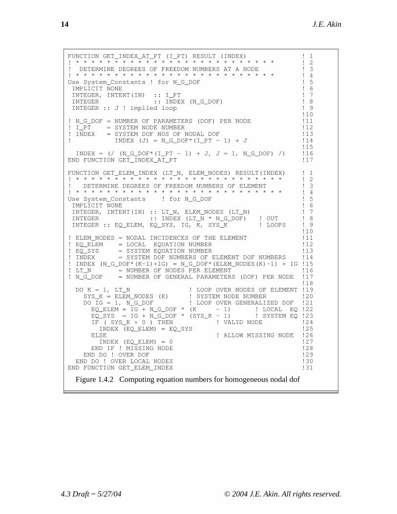
A similar expression defines the local equation numbers in an element or on aboundary segment. The difference is that thenI corresponds to a local node number andhas an upper limit ofnn or nb, respectively. In the latter two cases the local equationnumber is the subscript for theINDEX array and the corresponding system equationnumber is the integer value stored inINDEX at that position. In other words, Eq. 1.9 isused to find local or system equation numbers andJ always refers to the specific dof ofinterest andI corresponds to the type of node number (I S for a system node,I E for alocal element node, orI B for a local boundary segment node). For a typical element typesubroutine GET_ELEM_INDEX, Fig. 1.4.2, fills the above elementINDEX vector forany standard or boundary element. In that subroutine storage locations are likewiseestablished for thenn element incidences (extracted by subroutine GET_ELEM_NODES)and the correspondingni = nn × ng system degree of freedom numbers associated withthe element, in vectorINDEX.

Figure 1.4.3 illustrates the use of Eq. 1.9 for calculating the system equationnumbers forng = 2 andnm = 4. TheD vector in the bottom portion shows that at eachnode we count its dof before moving to the next node. In the middle section the cross-hatched element matrices show the 4 local equation numbers to the left of the squarematrix, and the corresponding system equation numbers are shown to the right of thesquare matrix, in bold font. Noting that there areng = 2 dof per node explains why thetop left topology list (element connectivity withnn = 2) is expanded to the systemequation number list with 4 columns.

Once the system degree of freedom numbers for the element have been stored in avector, sayINDEX, then the subscripts of a coefficient in the element equation can bedirectly converted to the subscripts of the corresponding system coefficient to which it isto be added. This correspondence between local and system subscripts is illustrated inFig. 1.4.5. The expressions for these assembly, or scatter, operations are generally of theform

(1.10)CI = CI + Cei , SI , J = SI , J + Se

i, j

where i and j are the local subscripts of a coefficient in the element square matrix,Se,and I , J are the corresponding subscripts of the system equation coefficient, inS, towhich the element contribution is to be added. The direct conversions are given byI = INDEX(i), J = INDEX( j ), where theINDEX array for element,e, is generated fromEq. 1.1 by subroutine GET_ELEM_INDEX.

Figure 1.4.2 shows how that index could be computed for a node or element for thecommon case where the number of generalized degrees of freedom per node isev erywhere constant. For a single unknown per node (ng = 1), as shown in Fig. 1.4.1,then the nodal degree of freedom loop (at lines 16 and 21 in Fig. 1.4.2) simply equatesthe equation number to the global node number. An example where there are twounknowns per node is illustrated in Fig. 1.4.3. That figure shows a line element mesh withtwo nodes per element and two dof per node (such as a standard beam element). In thatcase it is similar to the assembly of Fig. 1.4.1, but instead of a single coefficient we areadding a set of smaller square sub-matrices intoS. Figure 1.4.4 shows how the assemblycan be implemented for column matrices (subroutine STORE_COLUMN) and full (non-sparse) square matrices (STORE_FULL_SQUARE) if one has an integer index that


18 J. E. Akin

Table 1.4.1 Degree of freedom numbers at system nodeI s

Local System†

1 INDEX(1)2 INDEX(2). .. .. .J INDEX(J). .. .. .ng INDEX(ng)

† INDEX(J) = ng * ( I s − 1 ) + J

Table 1.4.2 Relating local and system equation numbers

Element degree of freedom numbersLocal Parameter Systemnode number node Local System

I L J IS = node( I L ) ng * ( I L − 1 ) + J ng * ( I S − 1 ) + J

1 1 node(1) 1 ng * [ node(1)−1] + 11 2 node(1) 2. . .. . . . .1 ng node(1) . .2 1 node(2) . .. . .. . .. . .K Jg node(K ) ng * ( K−1) + Jg ng * [ node(K )−1] + Jg. . .. . . . .nn 1 node(nn) . .. . . . .. . .nn ng node(nn) nn * ng ng * [ node(nn)−1] + ng



relates the local element degrees of freedom to the system dof.

1.4.3 Example Equation Numbers

Consider a two-dimensional problem (ns = 2) inv olving 400 nodal points (nm = 400)and 35 elements (ne = 35). Assume two parameters per node (ng = 2) and let theseparameters represent the horizontal and vertical components of some vector. In a stressanalysis problem, the vector could represent the displacement vector of the node, whereasin a fluid flow problem it could represent the velocity vector at the nodal point. Assumethe elements to be triangular with three corner nodes (nn = 3). The local numbers ofthese nodes will be defined in some consistent manner, e.g., by numbering counter-clockwise from one corner. This mesh is illustrated in Fig. 1.4.5.

By utilizing the above control parameters, it is easy to determine the total number ofdegrees of freedom in the system,nd, and associated with a typical element,ni are:nd = nm * ng = 400 * 2 = 800, andni = nn * ng = 3 * 2 = 6, respectively. In addition tothe total number of degrees of freedom in the system, it is important to be able to identifythe system degree of freedom number that is associated with any parameter in the system.Table 1.4.2 or subroutine GET_DOF_INDEX, provides this information. This relationhas many practical uses. For example, when one specifies that the first parameter (J = 1)at system node 50 (I S = 50) has some given value what one is indirectly saying is thatsystem degree of freedom numberDOF = 2 * (50 − 1) + 1 = 99 has a given value. In asimilar manner, we often need to identify the system degree of freedom numbers that

1

23

4

9

261

270

310

11

400

397

380

1

23

2135

Figure 1.4.5 Mesh for assembly equation number calculations


20 J. E. Akin

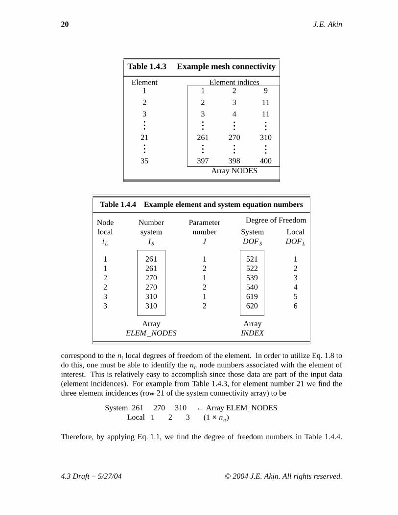
Table 1.4.3 Example mesh connectivity

Element Element indices1 1 2 9

2 2 3 11

3 3 4 11... ... ... ...21 261 270 310... ... ... ...35 397 398 400

Array NODES

Table 1.4.4 Example element and system equation numbers

Node Number Parameter Degree of Freedom

local system number System Locali L I S J DOFS DOFL

1 261 1 521 11 261 2 522 22 270 1 539 32 270 2 540 43 310 1 619 53 310 2 620 6

Array ArrayELEM_NODES INDEX

correspond to theni local degrees of freedom of the element. In order to utilize Eq. 1.8 todo this, one must be able to identify thenn node numbers associated with the element ofinterest. This is relatively easy to accomplish since those data are part of the input data(element incidences). For example from Table 1.4.3, for element number 21 we find thethree element incidences (row 21 of the system connectivity array) to be

System 261 270 310 ← Array ELEM_NODESLocal 1 2 3 (1× nn)

Therefore, by applying Eq. 1.1, we find the degree of freedom numbers in Table 1.4.4.



The element arrayINDEX has many programming uses. Its most important applicationis to aid in the assembly (scatter) of the element equations to form the governing systemequations. We see from Fig. 1.4.2 that the element equations are expressed in terms oflocal degree of freedom numbers. In order to add these element coefficients into thesystem equations one must identify the relation between the local degree of freedomnumbers and the corresponding system degree of freedom numbers. ArrayINDEXprovides this information for a specific element. In practice, the assembly procedure is asfollows. First the system matricesS andC are set equal to zero. Then a loop over all theelements if performed. For each element, the element matrices are generated in terms ofthe local degrees of freedom. The coefficients of the element matrices are added to thecorresponding coefficients in the system matrices. Before the addition is carried out, theelement arrayINDEX is used to convert the local subscripts of the coefficient to thesystem subscripts of the term in the system equations to which the coefficient is to beadded. That is, we scatter

(1.11)Sei , j

+→ SI, J , Ce

i

+→ CI

where I S = INDEX ( i L ) and JS = INDEX ( j L ) are the corresponding row and columnnumbers in the system equations,i L , j L are the subscripts of the coefficients in terms of

the local degrees of freedom, and+→ reads "is added to". Considering all of the the

terms in the element matrices for element 21 in the previous example, one finds sixtypical scatters from theSe andCe arrays are

Se1, 1

+→ S521, 521 Ce

1+→ C521

Se2, 3

+→ S522, 539 Ce

2

+→ C522

Se3, 4

+→ S539, 540 Ce

3+→ C539

Se4, 5

+→ S540, 620 Ce

4+→ C540

Se5, 6

+→ S619, 620 Ce

5

+→ C619

Se1, 6

+→ S521, 620 Ce

6+→ C620 .

1.5 Error Concepts

Part of the emphasis of this book will be on error analysis in finite element studies.Thus this will be a good point to mention some of the items that will be of interest to uslater. We will always employ integral forms. Denote the highest derivative occurring inthe integral by the integerm. Assume all elements have the same shape and use the sameinterpolation polynomial. Let the characteristic element length size be the real valueh,and assume that we are using a complete polynomial of integer degreep. Later we willbe interested in the asymptotic convergence rate, in some norm, as the element size


22 J. E. Akin

0 1 2 3 4 5 60

1

2

3

4

5

6

XY

FE Mesh Geometry: 346 Elements, 197 Nodes (3 per element)

Figure 1.5.1 Relating element size to expected gradients

approaches zero,h → 0. Here we will just mention the point wise error that provides theinsight into creating a good manual mesh or a reasonable starting point for an adaptivemesh. For a problem with a smooth solution the local finite element error is proportionalto the product of them − th derivative at the point and the element size,h, raised to thep − th power. That is,

(1.12)e(x) ∝ hp ∂mu(x) / ∂xm .

This provides some engineering judgement in establishing an initial mesh. Whereyou expect the gradients (them − th derivative) to be high then make the elements verysmall. Conversely, where the gradients will be zero or small we can have large elementsto reduce the cost. These concepts are illustrated in Fig. 1.5.1 where the stresses around ahole in a large flat plate are shown. There we see linear three noded triangles (sop = 1)in a quarter symmetry mesh. Later we will show that the integral form contains the firstderivatives (gradient, som = 1). Undergraduate studies refer to this as a stressconcentration problem and show that the gradients rapidly increase by a factor of about 3over a very small region near the top of the hole. Thus we need small elements there. Atthe far boundaries the tractions are constant so the gradients displacement are nearly zerothere and the elements can be big. Later we will automate estimating local errorcalculations and the associated element size changes needed for an accurate and costeffective solution.

1.6 Exercises

1. Assume (unrealistically) that all the entries in an element square matrix andcolumn vector are equal to the element number. Carry out the assembly of the system inFig. 1.4.1 to obtain the final numerical values for each coefficient in theS andC matrices.



Hint: manually loop over each element and carry out the line by line steps given inGET_ELEM_INDEX, and then those inSTORE_COLUMN, and finally those inSTORE_FULL_SQUAREbefore going to the next element.

2. Assume (unrealistically) that all the entries in an element square matrix and columnvector are equal to the element number. Carry out the assembly of the system inFig. 1.4.3 to obtain the final numerical values for each coefficient in theS andC matrices.

3. In Fig. 1.4.3 assume that the global nodes are numbered consecutively from 1 to 4(from left to right). Write the element index vector for each of the three elements.

4. List the topology (connectivity data) for the six elements in Fig. 1.3.1.

5. Why does theββ Boolean array in Fig. 1.3.1 have two rows and seven columns?

6. What is the Boolean array,ββ , for elementa(= 2) in Fig. 1.3.1?

7. What is the percent of sparsity of theS matrix in Fig. 1.4.3?

8. What is the Boolean array,ββ , for element 3 in Fig. 1.4.1?

9. What is the size of the Boolean array,ββ , for any element in Fig. 1.4.3? Explain why.

10. What is the Boolean array,ββ , for element 1 in Fig. 1.4.3?

11. Referring to Fig. 1.4.1, multiply the given 6× 1D array by the 3× 6 Boolean array,ββ , for the second element to gather its corresponding localDe local dof.

12. In a FEA stress analysis where a translational displacement is prescribed the reactionnecessary for equilibrium is _____: a) heat flux, b) force vector, c) pressure, d)temperature, e) moment (couple) vector.

13. In a FEA stress analysis where a rotational displacement is prescribed the reactionnecessary for equilibrium is ____: a) heat flux, b) force vector, c) pressure, d)temperature, e) moment (couple) vector.

14. In a FEA thermal analysis where a temperature is prescribed the reaction necessaryfor equilibrium is _____: a) heat flux, b) force vector, c) pressure, d) temperature, e)moment (couple) vector.

15. A material that is the same at all points is ___: a) homogeneous, b) non-homogeneous, c) isotropic, d) anisotropic, e) orthotropic.

16. A material that is the same in all directions at a point is ___: a) homogeneous, b)non-homogeneous, c) isotropic, d) anisotropic, e) orthotropic.

17. A material that is the same at all points is ___: a) homogeneous, b) non-homogeneous, c) isotropic, d) anisotropic, e) orthotropic.

18. A material that is the same in all directions at a point is ___: a) homogeneous, b)non-homogeneous, c) isotropic d) anisotropic, e) orthotropic.


24 J. E. Akin

19. Define a scalar, vector, and tensor quantity to have zero, one, and two subscripts,respectively. Identify which of the above describe the following items: _____ mass,_____ time, _____ position, _____ centroid, _____ volume, _____ surface area, _____displacement, _____ temperature, _____ heat flux, _____ heat source, _____ stress,_____ moment of inertia, _____ force, _____ moment, _____ velocity.

20. In a finite element solution at a node, the _____: a) primary variable is most accurate,b) primary variable is least accurate, c) secondary variable is most accurate, d) secondaryvariable is least accurate.

21. Interior to an element in an FEA solution, the _____: a) primary variable is mostaccurate, b) primary variable is least accurate, c) secondary variable is most accurate, d)secondary variable is least accurate.

1.7 Bibliography

[1] Adams, V. and Askenazi, A.,Building Better Products with Finite Element Analysis,Santa Fe: Onword Press (1999).

[2] Akin, J.E., Finite Elements for Analysis and Design, London: AcademicPress (1994).

[3] Akin, J.E. and Singh, M., "Object-Oriented Fortran 90 P-Adaptive Finite ElementMethod," pp. 141−149 inDevelopments in Engineering Computational Technology,ed. B.H.V. Topping, Edinburgh: Civil_Comp Press (2000).

[4] Bathe, K.J.,Finite Element Procedures, Englewood Cliffs: Prentice-Hall (1996).[5] Becker, E.B., Carey, G.F., and Oden, J.T.,Finite Elements − An Introduction,

Englewood Cliffs: Prentice-Hall (1981).[6] Cook, R.D., Malkus, D.S., and Plesha, N.E.,Concepts and Applications of Finite

Element Analysis, New York: John Wiley (1989).[7] Cook, R.D., Malkus, D.S., Plesha, N.E., and Witt, R.J.,Concepts and Applications

of Finite Element Analysis, New York: John Wiley (2002).[8] Desai, C.S. and , T. Kundu,Introduction to the Finite Element Method, Boca Raton:

CRC Press (2001).[9] Gupta, K.K and Meek, J.L.,Finite Element Multidisciplinary Analysis, Reston:

AIAA (2000).[10] Huebner, K.H., Thornton, E.A., and Byrom, T.G.,Finite Element Method for

Engineers, New York: John Wiley (1994).[11] Hughes, T.J.R., The Finite Element Method, Englewood Cliffs:

Prentice-Hall (1987).[12] Norrie, D.H. and DeVries, G.,Finite Element Bibliography, New York: Plenum

Press (1976).



[13] Pironneau, O.,Finite Element Methods for Fluids, New York: John Wiley (1991).[14] Rao, S.S.,The Finite Element Method in Engineering, Boston : Butterworth

Heinemann (1999).[15] Segerlind, L.J.,Applied Finite Element Analysis, New York: John Wiley (1987).[16] Silvester, P.P. and Ferrari, R.L.,Finite Elements for Electrical Engineers,

Cambridge: Cambridge University Press (1996).[17] Smith, I.M. and Griffiths, D.V.,Programming the Finite Element Method,3rd

Edition, Chichester: John Wiley (1998).[18] Szabo, B. and Babuska, I.,Finite Element Analysis, New York: John Wiley (1991).[19] Whiteman, J.R., A Bibliography of Finite Elements, London: Academic

Press (1975).[20] Zienkiewicz, O.C. and Taylor, R.L.,The Finite Element Method,4th Edition, New

York: McGraw-Hill (1991).


4.3 draft 5/27/04 1 · type of ﬁnite element analysis (fea). the practical advantages of fea in...

Documents