480w data acquisition - university of san...

480W Data Acquisition

Quinn Pratt

ver. 1.7

Abstract

This document serves to describe the data acquisition methodsfor experiments performed in the advanced laboratory course (PHYS480W). Data acquisition routines are an essential feature of modernphysics experiments. We explore acquisition through industry stan-dard programs such as MATLAB and National Instruments’ LabView.

Contents

1 Introduction 1

2 Hardware 32.1 NI myDAQ . . . . . . . . . . . . . . . . . . . . . . . . . . . . 32.2 NI USB-6343 . . . . . . . . . . . . . . . . . . . . . . . . . . . 4

3 MatLab 43.1 MATLAB .m file to control MyDAQ . . . . . . . . . . . . . . 5

4 LabView 8

5 Appendix I: MATLAB Programming Acquisition Notes 11

6 Appendix II: Basic G-Coding 14

7 LabView Data Acquisition 15

1

Pratt of 17

1 Introduction

For the purposes of this course, we will focus more on the utility end ofdata acquisition, as opposed to delving into the nitty-gritty programmingconcepts surrounding Data Acquisition devices (DAQs). Regardless of theexperiment, data acquisition can be pictured roughly as shown in fig 1.

Note: although the data acquisition hardware we will be using has thecapability to output analog signals (hardware → actuator), we will not beusing this functionality.

We can adapt the diagram above to reflect our system:

• Sensor: One example of a data acquisition system sensor would bea thermocouple, a pressure gauge, an ammeter, etc. In our case, the’sensor’ will usually be a voltage reading across a resistor.

• Signal Conditioning: this refers to the ability to include filters, volt-age dividers, amplifiers, or other post-sensor analog or digital instru-ments.

• Acquisition Hardware: In our case, this will exclusively be NationalInstruments DAQ hardware. examples used in this course will be theNI myDAQ, or the NI USB-DAQ 6343. Acquisition hardware differsfrom a sensor in that these are special types of hardware which havethe ability to communicate with a computer (through a driver).

• Software: We will cover two software methods for acquisition, Mat-Lab and LabView. Furthermore, both of these programs make use ofthe DAQmx driver, however, MatLab additionally requires the DataAcquisition Toolkit.

Although prior experience with MatLab hardware-programming is notrequired for using the data acquisition routines outlined in this document itis important to note that the scripts and user interfaces are not the wholestory, even after acquisition, additionally post processing and analysis willbe required, and to that end, basic MatLab competency will be crucial.

2 Hardware

In this section we will discuss the National Instruments hardware whichmakes computer-automated data acquisition possible. Although data can

Pratt of 17

Figure 1: DAQ hardware is a software controlled apparatus that receivesinput data from a transducer or sensor which is causally connected to thephysical phenomena one wants to measure somehow. DAQ hardware permitsthe extraction of a data stream produced by the sensor, issuing in a file which,through post processing, becomes a graph in ones research paper or report.

be collected through a variety of instruments such as digital storage oscillo-scopes (DSO’s), the advantage of the NI hardware is that it is designed tobe controlled by the computer.

2.1 NI myDAQ

This device is a small, USB-powered data acquisition board. These boards wedesigned by NI to be easy-to-use academic DAQ hardware, meaning that theyare meant to be used by students to probe circuits, attach accelerometers,thermocouples, digital switches and controls, etc. They can only handleinput voltages of ±10V, and they have a maximum sample rate of 200kS/s.

Figure 2 is a shot of the NI myDAQ. Note the plug-in terminals alongthe right side

We have fitted each of these boards with a BNC-add on (figure 3). Thisconverts the plug-in ports on the side of the DAQ to industry-standard coax-ial BNC ports. There are 4 BNC ports on the myDAQ, each of them hasbeen hard-wired for single-ended measurements with a ground-reference di-rectly above the ports. the two ports on the left are analog-out (AO), whilethe ports on the right are the analog-in (AI).

Pratt of 17

Figure 2: NI myDAQ device. We will use 2 such devices this semester, onelabeled Eric and the other Quinn

Figure 3: Use of myDAQ is made considerably easier with a BNC connectorextension board which snaps into the DAQ.

Pratt of 17

Figure 4: The NI USB-6343 has 4 analog outputs and 23 analog inputs, witha maximum digitization rate of 500ks/s.

2.2 NI USB-6343

While the myDAQ is a very versatile instrument, some experiments require amore sophisticated data acquisition board. This is the NI USB-6343, shownin figure 4, which is used to send and receive analog and digital signals. Ithas a maximum sample rate of 500kS/s and is much more power than themyDAQ. It has 23 Analog-In BNC inputs as well as many screw-terminalsand 4 Analog-Out BNC terminals.

This device also connects to the computer through USB and can be pro-grammatically controlled through either MatLab or LabView.

3 MatLab

This section demonstrates the use of the NI Hardware in conjunction withMatLab and the MatLab Data Acquisition Toolbox (DAQ Toolbox). We willalso cover the Graphical User Interface (GUI) which was developed with theintention of simplifying data acquisition in MatLab.

3.1 MATLAB .m file to control MyDAQ

This subsection describes how to use the graphical user interface which wasdeveloped to make Data Acquisition even more user-friendly. The GUI places

Pratt of 17

Figure 5: MATLAB data acquisition toolbox generated generic GUI thatcontrols MyDAQ.

a veil over the actual code which is being executed as the user fills out thevalues and pushes buttons in the separate window. While the details of thecode are important, we limit ourselves here to the use of the GUI itself. WithMATLAB running, ones opens and runs myDAQ_480W.m.

Note: This GUI is only compatible with the NI myDAQ hardware.

When the GUI is executed, a small window will appear (figure 5); thiswindow shows several editable-text boxes as well as a large, empty plot.

To use the GUI, the user should follow the following steps:

1. Select whether the experiment required two channels of data, or onechannel.

2. Type in the desired Rate for acquisition an example of a moderate ratewould be 10,000 samples/second. The NI myDAQ is limited to 200,000samples/second.

Note: The user should type these parameters in the form of numbersONLY, i.e. do not type 10,000; instead type 10000.

Pratt of 17

Figure 6: Here, a two channel GUI has been selected, with a digitization rateof 104#/sec, and a duration of a tenth of a second.

3. Type in the desired acquisition Duration. Another important quantityis the Rate × Duration, which tells the user how many samples will begathered. For example, if the user inputs 10,000 as the rate, and 0.1as the duration, the acquisition session will collect 1000 samples.

4. Once the properties have been configured, the user can click the ‘Ac-quire’ push-button. Each time the button is pushed, the session isexecuted with the user-inputted properties, and the data is plotted.The user is free to adjust the properties and re-acquire. Note: theuser cannot change between 1-channel and 2-channel freely, this willgenerate an error.

5. When ready, the user can save the data by typing an appropriate file-name in the editable-textbook at the bottom of the window, and hit thesave pushbutton. The save button will produce a .csv file in the currentMatLab directory. It is not necessary to include the file extension inthe file name, the .csv extension is appended afterward.

For Two-channel sessions it might look like what is shown in figure 6.

Pratt of 17

Once the user has acquired the data he/she wants, and they have savedthe data to a .csv file, the functionality of this GUI has reached its end.That is to say, this GUI environment was not designed for additional postprocessing. The first step of any post-processing routine should be to usethe MatLab code: csvread(’YourFileNameHere.csv’) to input theirdata as a MatLab array.

The .csv files generated will be of a specific form. The Data Acquisitionwill place the signals in a samples-by-channel array. where samples are rows,and each channel adds another column. For example, if one were to save thesine wave from the one-channel example, they would see a cdv file with onecolumn (representing the one channel) and 1000 rows (representing the 1000samples collected). In the two-channel example, the resulting .csv file wouldbe 1000-by-2 with the second column containing the triangle wave data.

4 LabView

Although all of the newest data acquisition protocols rely on MatLab, wemake use of the National Instruments’ graphical programming environment“LabView” for some of the labs. The analogous thing in LabView to the Mat-lab GUI is the ’instrument.vi’ which mimics the data acquisition instrumentunder control of LabView software. A screen shot of Grab Trace 480w.viis shown in figure 7, a simple .vi file which was written to mimic the utilityof a generic 4 channel digital storage oscilloscope.

LabView is often credited as the industry standard for automation anddata acquisition. There is a reason why we use National Instruments hard-ware (myDAQ and the USB-6343). LabView is the software to go along withthe hardware. The traditional data bus for software instrument control hasbeen the IEEE 488 standard or the general purpose interface bus, or gpip.Most pc installations have a gpib card installed in the pc and instrumentshave been typically connected to the pc with gpip cables. There are now’gpib to usb’ connectors to obviate the need for the gpib card to be phys-ically installed inside the pc box or lap top. This data circuit is shown infigure reffig:labviewcontrol. The urgent point here is that one could controla DSO or a function generator or a lockin amplifier, power supply, pulsegenerator, or DAQ board in this fashion.

Like the Matlab GUI, the virtual instrument, or .vi file is really the result

Pratt of 17

Figure 7: A generic ’virtual instrument’ front panel as it would appear in awindow generated when the .vi file is launched, which simulates a 4 channelDSO. In the spirit of full disclosure, the actual gpib address (7 instrumentsare readily addressable) is hardwired with a string constant in the back panelof the .vi file.

Figure 8: Instruments such as the DSO can acquire data using the signalprocessing present in the instrument itself, and be controlled by LabViewsoftware via the pc through the gpib bus, using the hardware shown above.Gpib cabling is generally required.

Pratt of 17

of graphical coding which can be created and edited in the so-called backpanel of the GUI. LabView uses a graphical language, meaning functionsand variables are represented not by words but by little images which can bemanipulated on the so-called ’front panel’. It’s the front panel that is codedto look like the physical device one is taking data with. There is a whole lotmore too it, and that discussion is deferred to the appendix.

Let’s consider how to use the virtual instrument to take data, the use ofwhich is predicated on the prior use of a 4 channel digital storage oscilloscope(TEKTRONICS TDS2014, in our case) to acquire the data. One will wantto become familiar with the use of the scope first and configure inputs, scalesensitivities, triggering, and the time base so as to acquire the signal in thefirst place.

Then,

1. Select which two channels of data from the scope one wants to acquireusing the knob controls on the front panel of vi.

2. The details of the digitization rate are determined by the scope settings.In particular, the time base of the scope determines the digitizationrate: 2500 points are collected per 10 units of time. So, for instance, ifone chooses a time base of 10 sec/box, one has then chosen a digitizationat rate of 25 acquisitions/sec.

3. Then one fills in the complete path name of the file to write the fileinto the appropriate directory.

4. To execute the data capture from the controlled instrument (yes Lab-View can control lots of different instruments), simply click the arrowbutton in the toolbar of the vi. The grid pattern on the front panelgoes blank and arrow button turns a funny shape, and you wait, andget bored, and then it comes back (the front panel grid pattern) witha graph. Now the odd thing is that it’s not always clear which datarecord forces the auto scale, and you will note that the graph isn’tscaled in X or Y as the oscilloscope is, so NB: please record PLEASERECORD the scope parameters for each data file. Or, mess aroundwith G-Programming to hardwire in the scale factors on the displayedgraph. You will do something like this in post-processing, probably inMATLAB

Pratt of 17

(a) (b)

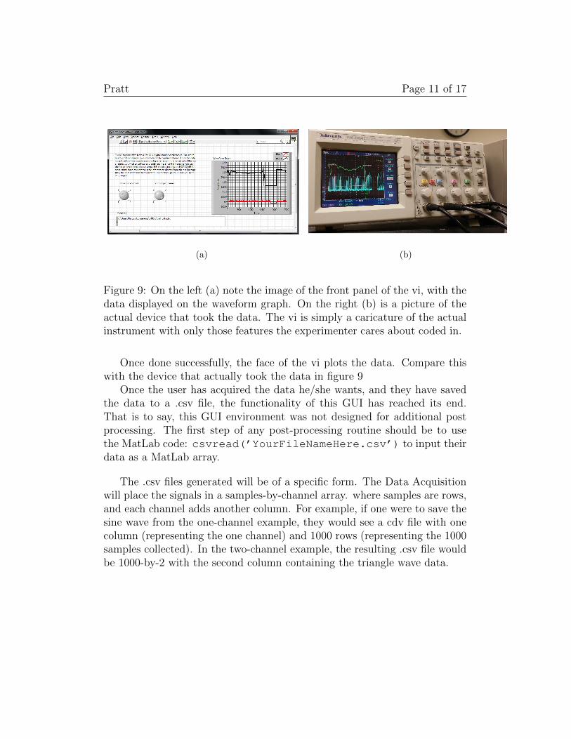
Figure 9: On the left (a) note the image of the front panel of the vi, with thedata displayed on the waveform graph. On the right (b) is a picture of theactual device that took the data. The vi is simply a caricature of the actualinstrument with only those features the experimenter cares about coded in.

Once done successfully, the face of the vi plots the data. Compare thiswith the device that actually took the data in figure 9

Once the user has acquired the data he/she wants, and they have savedthe data to a .csv file, the functionality of this GUI has reached its end.That is to say, this GUI environment was not designed for additional postprocessing. The first step of any post-processing routine should be to usethe MatLab code: csvread(’YourFileNameHere.csv’) to input theirdata as a MatLab array.

The .csv files generated will be of a specific form. The Data Acquisitionwill place the signals in a samples-by-channel array. where samples are rows,and each channel adds another column. For example, if one were to save thesine wave from the one-channel example, they would see a cdv file with onecolumn (representing the one channel) and 1000 rows (representing the 1000samples collected). In the two-channel example, the resulting .csv file wouldbe 1000-by-2 with the second column containing the triangle wave data.

Pratt of 17

5 Appendix I: MATLAB Programming Ac-

quisition Notes

Although the GUI is very useful, it is also important to understand how itworks. The GUI places a veil over the actual code which is being executedas the user fills out the values and pushes buttons in the separate window.

To understand the background code which communicates with the my-DAQ and subsequently gathers data, we must first discuss the relevant func-tions and properties.

This compatibility between the myDAQ would not be possible withoutthe Data Acquisition Toolbox. This toolbox allows the user to avoid usingthe more advanced DAQmx C-scripts by bundling the commands into a setcompact MatLab functions.

Examples of said functions are:

• createSession(...)

• addAnalogInputChannel(...)

• startForeground(...)

In addition to simply collecting data we must also configure certain prop-erties of our acquisition, examples of configureable properties are:

• Rate

• DurationInSeconds

• Name

• IsContinuous

These functions and configureable properties are the core of MatLab dataacquisition. However, we have not yet addressed how to call these functions,or how to configure the properties of a session.

MatLab is an object-oriented programming language, simply put, thismeans that the user must create virtual ‘objects’ in the computer’s memory,then the user can modify said ‘objects’ using functions. In the realm of dataacquisition this means that we must create a virtual object to represent the

Pratt of 17

action of collecting analog data through a driver... this virtual object is calleda session.

Sessions in MatLab are objects, just like a matrix, a variable, a figure,a function handle, etc. Any experience the user may have plotting data inMatLab will find this very familiar. Just as with a plot the user can configurewhether there’s a legend, what the axis limits are, whether the grid is visibleor not, etc. The user can configure a session to fit their acquisition needs.

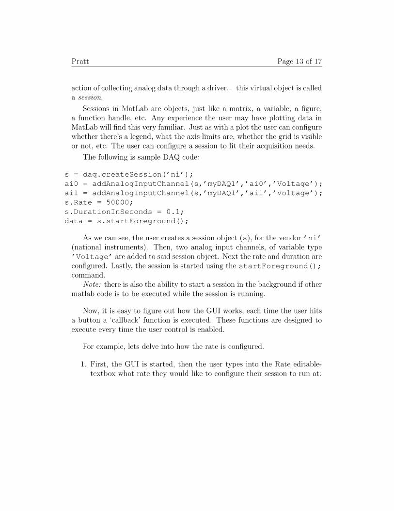
The following is sample DAQ code:

s = daq.createSession(’ni’);ai0 = addAnalogInputChannel(s,’myDAQ1’,’ai0’,’Voltage’);ai1 = addAnalogInputChannel(s,’myDAQ1’,’ai1’,’Voltage’);s.Rate = 50000;s.DurationInSeconds = 0.1;data = s.startForeground();

As we can see, the user creates a session object (s), for the vendor ’ni’(national instruments). Then, two analog input channels, of variable type’Voltage’ are added to said session object. Next the rate and duration areconfigured. Lastly, the session is started using the startForeground();command.

Note: there is also the ability to start a session in the background if othermatlab code is to be executed while the session is running.

Now, it is easy to figure out how the GUI works, each time the user hitsa button a ‘callback’ function is executed. These functions are designed toexecute every time the user control is enabled.

For example, lets delve into how the rate is configured.

1. First, the GUI is started, then the user types into the Rate editable-textbox what rate they would like to configure their session to run at:

Pratt of 17

2. As soon as the rate is written the callback function is executed:

function Rate Callback(hObject, eventdata, handles)

textrate = get(handles.Rate,’string’);

ratedouble = str2double(textrate);

handles.rate = ratedouble;

guidata(hObject,handles);

This bit of code shows how when the function is called, the preallocatedvalue handles.rate is updated to the user-inputted value. Then,the global data structure is refreshed with the guidata(...) func-tion. Data structures are used to pass this value to the acquire-buttoncallback function.

3. Once the user presses the acquire button (after giving the GUI a dura-tion), the Acquire callback function is called. This function reads as:

function Acquire Callback(hObject, eventdata, handles)

s duplicate = handles.session;

s duplicate.DurationInSeconds = handles.duration;

s duplicate.Rate = handles.rate;

data = s duplicate.startForeground();

handles.data = data;

guidata(hObject,handles);

Pratt of 17

Here we see that the acquire button grabs the preallocated data acqui-sition session (which is initially configured in the startup function), setsthe duration, sets the rate, then starts the session in the foreground.Additionally it saves the data to the handles structure and refreshesthe global structure. We save the data to the structure in order to usethe csvwrite(...) function when the save button is pressed.

This example is meant to show how the data acquisition functions havebeen interwoven into the GUI script. The underlying concept here is thatof data structures, which can be passed from callback to callback in thebackground of the GUI.

6 Appendix II: Basic G-Coding

When programming in LabView, one does not write scripts (m-files), insteadone creates a virtual instrument, or .vi-file. Virtual Images have two mainparts, a front panel and a back panel. In the front panel, one configures usercontrols, be that graphs, indicators, sliders, virtual thermometers and gauges,etc. In the back panel, the programmer must use function blocks and otherprogramming tools to string all the indicators/graphs to their data sourcesand so forth.

A LabView .vi is very much like the GUI described above in MatLab. Infact, a ‘perfect’ .vi would work like a GUI, wherein the user would never haveto see the back panel. Unfortunately we do not live in a perfect world, andtherefore as users it is important to understand how a LabView back paneloperates.

Information, be that strings, doubles, integers, file paths, error codes,etc., flow around multicolored wires in the back panel, from block to block.Common coding structures like for loops, while loops, if-statements and soforth are represented as physical structures... here is a simple example toshow how different graphical coding is compared to normal, textual language.

• Textual:

for i = 1:100

display(rand);

pause(1);

end

Pratt of 17

• Graphical:

It is easy read along with the textual language and see that it will display arandom number 100 times, pausing for 1 second between each iteration. Thegraphical language is a bit harder to follow as it has no definite sequence.This is perhaps the hardest part about LabView’s language, it is entirelyatemporal.

The blue ‘100’ in the top left shows that the loop will run 100 times, therandom number primitive function block will generate a random number andput said number into an indicator so the user can see it in the front panel,meanwhile the wait function will make the loop wait for 1000ms (1 second).One difference in the LabView code is that the user has the ability to togglea button on the front panel to stop the loop (bottom right corner).

7 LabView Data Acquisition

LabView has, essentially, three types of sub-vi’s, or ’blocks’ to be used indata acquisition:

• Primitive Functions: These are the most basic form of blocks inLabView. They appear with a somewhat yellowish tint, and they gen-erally perform more low-level computational tasks. e.g. ’build array’,’concatenate string’, ’add’, ’bundle’...etc. Data Acquisition was madepossible using the ’GPIB Write’ block in the program: “Grab Trace480w’.vi’.

Here is an example of a primitive data acquisition function:

Pratt of 17

Note: These Low-level blocks do NOT use the DAQ, they use thecomputer’s own GPIB card to communicate with instruments.

• Mid-Level Sub-VI’s: These are slightly more advanced blocks. Thesegenerally appear white and can perform more complicated tasks. ex-amples of these include: ’Read/Write Spreadsheet’, ’Numeric Inte-gration’...etc. Data Acquisition is made possible using the mid-levelSub-Vi’s under the ‘Measurement I/O’ tab, in the ‘NI-DAQmx’ menu.These functions can be used to control the DAQmx driver on a moreintimate level than the next form of block.

Here is an example of a mid-level data acquisition function, this onespecifically is the ’create channel’ block:

• Express VI’s: These are by far the easiest blocks to use, but theyallow for the least user-customization. In my opinion they are sort of agimmick. These blocks are hardly blocks at all, they appear rectangu-lar and pale-blue. The data acquisition express vi is called the ‘DAQAssistant’. When using the daq assistant, an entire new GUI opens upand the user is prompted to configure the data acquisition all at once...giving it a very limited range of flexibility. This express .vi works verywell if the user only wants to output one type of signal, or only wantsto collect data once and display it, for our higher-level lab needs theexpress .vi is not ideal.

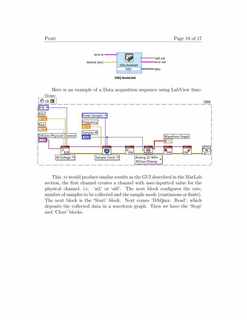
Here is what the express .vi for data acquisition (DAQ Assistant) lookslike:

Pratt of 17

Here is an example of a Data acquisition sequence using LabView func-tions:

This .vi would produce similar results as the GUI described in the MatLabsection, the first channel creates a channel with user-inputted value for thephysical channel, i.e. ‘ai1’ or ‘ai0’. The next block configures the rate,number of samples to be collected and the sample mode (continuous or finite).The next block is the ‘Start’ block. Next comes ‘DAQmx: Read’, whichdeposits the collected data in a waveform graph. Then we have the ‘Stop’and ‘Clear’ blocks.

480w data acquisition - university of san...

Documents