5-dmdw5-supervised learning 2cursuri.cs.pub.ro/~radulescu/dmdw/dmdw-nou/dmdw5.pdfclassification...
TRANSCRIPT

Supervised LearningSupervised Learning
- Part 2 -
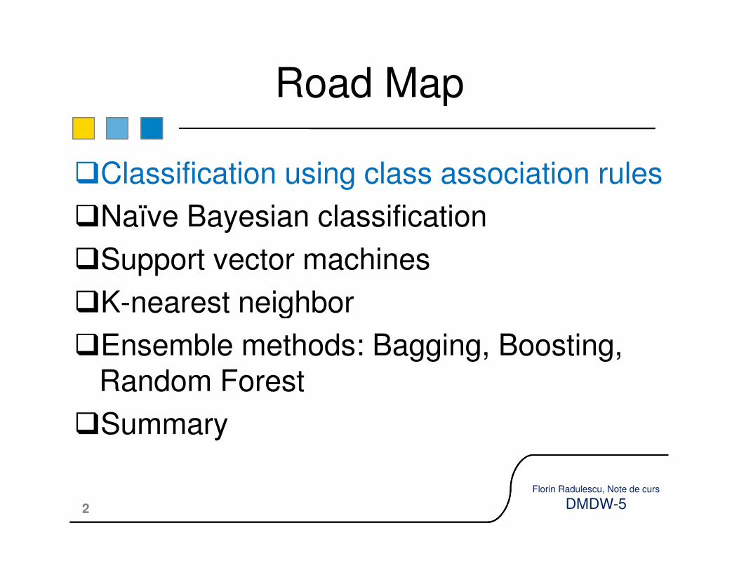
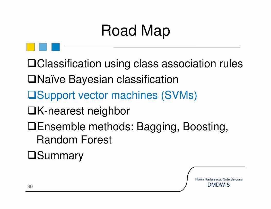
�Classification using class association rules
�Naïve Bayesian classification
�Support vector machines
K-nearest neighbor
Road Map
2
Florin Radulescu, Note de curs
DMDW-5
�K-nearest neighbor
�Ensemble methods: Bagging, Boosting, Random Forest
�Summary
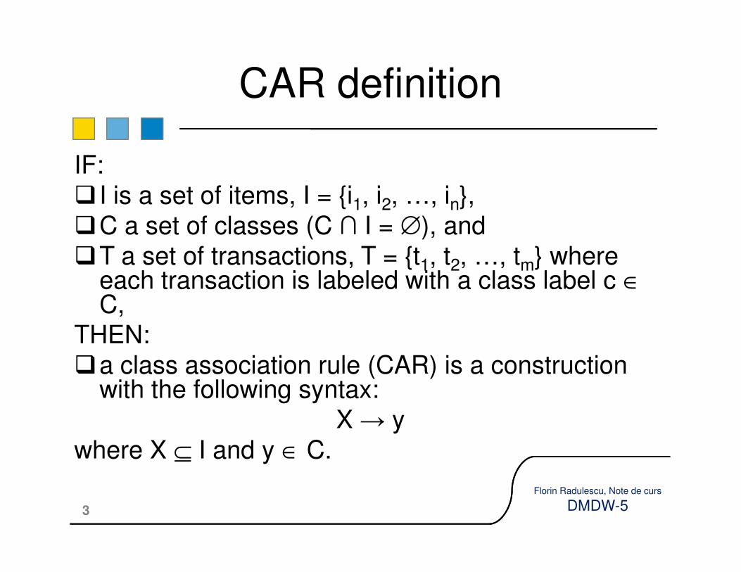
IF:
� I is a set of items, I = {i1, i2, …, in},
�C a set of classes (C ∩ I = ∅), and
�T a set of transactions, T = {t1, t2, …, tm} where each transaction is labeled with a class label c ∈
CAR definition
3
Florin Radulescu, Note de curs
DMDW-5
each transaction is labeled with a class label c ∈C,
THEN:
�a class association rule (CAR) is a construction with the following syntax:
X → y
where X ⊆ I and y ∈ C.
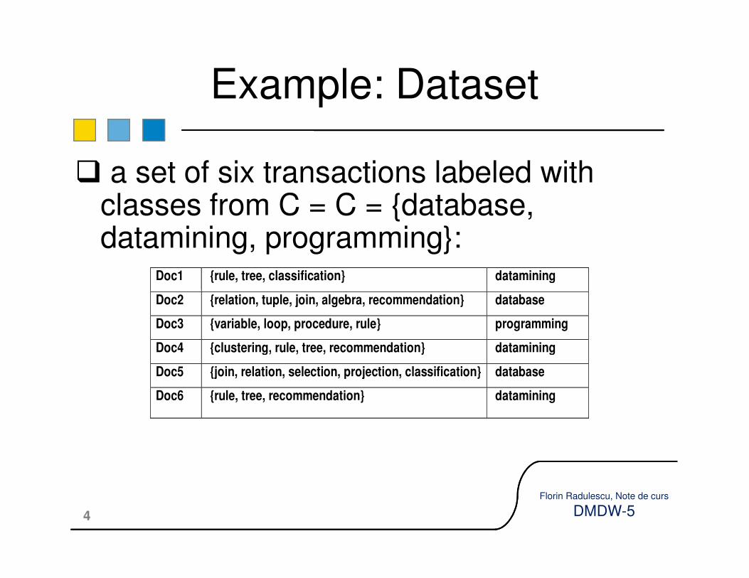
� a set of six transactions labeled with classes from C = C = {database, datamining, programming}:
Example: Dataset
Doc1 {rule, tree, classification} datamining
4
Florin Radulescu, Note de curs
DMDW-5
Doc2 {relation, tuple, join, algebra, recommendation} database
Doc3 {variable, loop, procedure, rule} programming
Doc4 {clustering, rule, tree, recommendation} datamining
Doc5 {join, relation, selection, projection, classification} database
Doc6 {rule, tree, recommendation} datamining

� The following constructions are valid CARs:
rule → datamining;
recommendation → database
�For each CAR the support and confidence may
Support and confidence
5
Florin Radulescu, Note de curs
DMDW-5
�For each CAR the support and confidence may
be computed:

Example: support and confidence
Doc1 {rule, tree, classification} datamining
Doc2 {relation, tuple, join, algebra, recommendation} database
Doc3 {variable, loop, procedure, rule} programming
Doc4 {clustering, rule, tree, recommendation} datamining
Doc5 {join, relation, selection, projection, classification} database
Doc6 {rule, tree, recommendation} datamining
6
Florin Radulescu, Note de curs
DMDW-5
Using these expressions:
�sup(rule → datamining) = 3/6 = 50%, and
�conf(rule → datamining) = 3/4 = 75%.
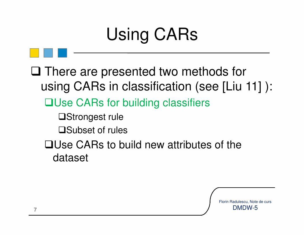
� There are presented two methods for using CARs in classification (see [Liu 11] ):
�Use CARs for building classifiers
�Strongest rule
Using CARs
7
Florin Radulescu, Note de curs
DMDW-5
�Strongest rule
�Subset of rules
�Use CARs to build new attributes of the
dataset

� In this case after CARs are obtained by data mining (as described in chapter 3) the CARs set is used for classifying new examples:
� For each new example the strongest rule that covers that example is chosen for classification (its class will be assigned to the test example.
� Strongest rule means rule with the highest confidence and/or
Strongest rule
8
Florin Radulescu, Note de curs
DMDW-5
� Strongest rule means rule with the highest confidence and/or support. There are also other measures for rule strength (chi-square test from statistics for example).
� This is the simplest method to use CARs for classifications: Rules are ordered by their strength and for each new test example the ordered rule list is scanned and the first rule covering the example is picked up.
� A CAR covers an example if the example contains the left side of the rule (the transaction contains all the items in rule left side).

�For example if we have an ordered rule list:
rule → datamining;
variable → programming
recommendation → database
Strongest rule: example
9
Florin Radulescu, Note de curs
DMDW-5
recommendation → database
�Then the transaction
will be labeled with class ‘datamining’ because
of the first rule-strongest than the other rules.
Doc-ex {rule, variable, loop, recommendation} ?

This method is used in Classification Based on
Associations (CBA). In this case, having a training dataset D and a set of CARs R, the objectives are:
A. to order R using their support and
Subset of rules
10
Florin Radulescu, Note de curs
DMDW-5
A. to order R using their support and confidence, R = {r1, r2, …, rn}:1. First rules with highest confidence2. For the same confidence use the support to
order the rules3. For the same support and confidence order by
rule generation-time (rules generated first are ‘greater’ than rules generated later).

B. to select a subset S of R covering D:1. Start with an empty set S
2. Consider ordered rules from R in sequence: for each rule r�If r covers at least an example in D add r to S and
Subset of rules
11
Florin Radulescu, Note de curs
DMDW-5
�If r covers at least an example in D add r to S and remove covered examples from D
3. Stop when D is empty
4. Add the majority class as default classification.
The result is:
Classifier = <ri1, ri2, …, rik, majority-class>

� There are presented two methods for using CARs in classification (see [Liu 11] ):
�Use CARs for building classifiers
�Strongest rule
Using CARs
12
Florin Radulescu, Note de curs
DMDW-5
�Strongest rule
�Subset of rules
�Use CARs to build new attributes of the
dataset
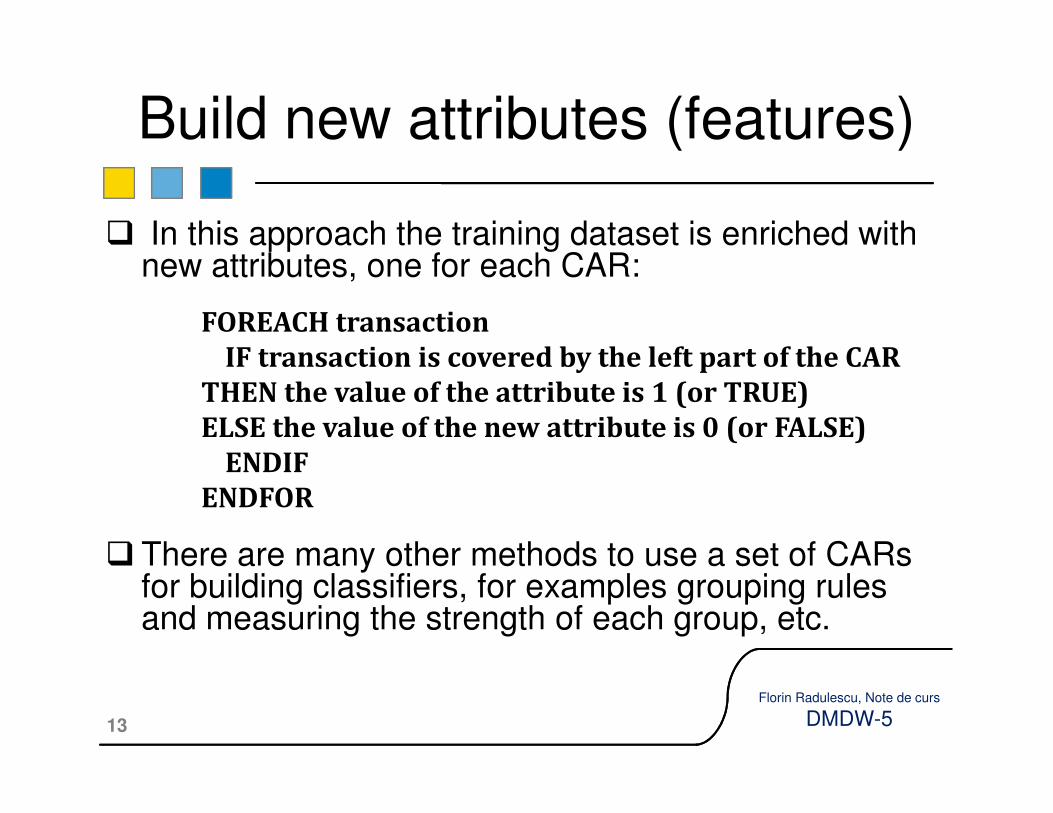
� In this approach the training dataset is enriched with new attributes, one for each CAR:
FOREACH transaction
IF transaction is covered by the left part of the CAR
THEN the value of the attribute is 1 (or TRUE)
Build new attributes (features)
13
Florin Radulescu, Note de curs
DMDW-5
THEN the value of the attribute is 1 (or TRUE)
ELSE the value of the new attribute is 0 (or FALSE)
ENDIF
ENDFOR
� There are many other methods to use a set of CARs for building classifiers, for examples grouping rules and measuring the strength of each group, etc.

� Usual association rules may be also used in recommendation systems:
�The rules are ordered by their confidence and support and then may be used, considering them in this order, for labeling new examples
Use of association rules
14
Florin Radulescu, Note de curs
DMDW-5
them in this order, for labeling new examples
� Labels are not classes but other items (recommendations).
�For example, based on a set of association rules containing books, the system may recommend new books to customers based on their previous orders.

�Classification using class association rules
�Naïve Bayesian classification
�Support vector machines
K-nearest neighbor
Road Map
15
Florin Radulescu, Note de curs
DMDW-5
�K-nearest neighbor
�Ensemble methods: Bagging, Boosting, Random Forest
�Summary

� This approach is a probabilistic one.
�The algorithms based on Bayes theorem compute for each test example not a single class but a probability of each class in C (the set of classes).
� If the dataset has k attributes, A1, A2, …, Ak, the objective is to compute for each class c ∈ C = {c ,
Naïve Bayes: Overview
16
Florin Radulescu, Note de curs
DMDW-5
� If the dataset has k attributes, A1, A2, …, Ak, the objective is to compute for each class c ∈ C = {c1, c2, …, cn) the probability of the test example (a1, a2, …, ak) to belong to the class c:
Pr(Class = c | A1 = a1, …, Ak = ak)
� If classification is needed, the class with the highest probability may be assigned to that example.
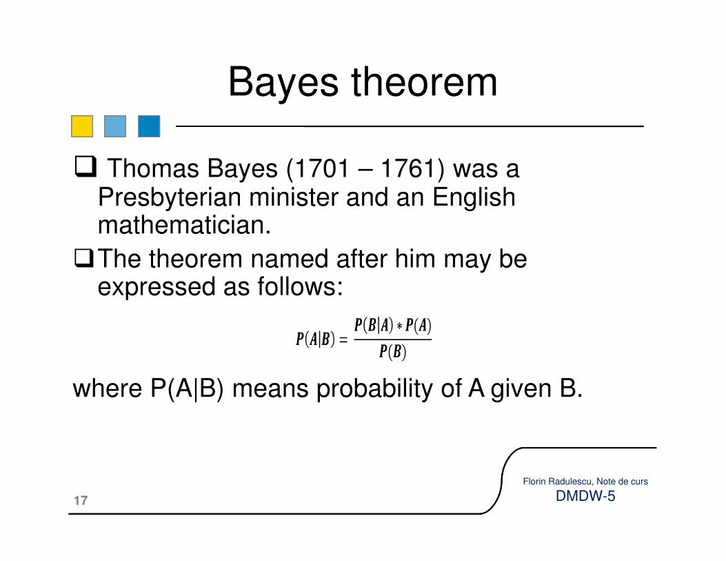
� Thomas Bayes (1701 – 1761) was a Presbyterian minister and an English mathematician.
�The theorem named after him may be expressed as follows:
Bayes theorem
17
Florin Radulescu, Note de curs
DMDW-5
expressed as follows:
where P(A|B) means probability of A given B.

� “Students in EC101 are 30% from the ABD M.Sc. module and 70% from other modules.
� 20% of the students are placed in the first 5 rows of seats but for ABD this percent is
Example
18
Florin Radulescu, Note de curs
DMDW-5
5 rows of seats but for ABD this percent is 40%.
� When the dean enters the class and sits somewhere in the first 5 rows, near a student, compute the probability that its neighbor is from ABD?”

�So:
Solution
19
Florin Radulescu, Note de curs
DMDW-5
�So:

� The objective is to compute
Pr(Class = c | A1 = a1, …, Ak = ak).
�Applying Bayes theorem:
Building classifiers
Pr(C = cj | A1 = a1, …, Ak = ak) =
20
Florin Radulescu, Note de curs
DMDW-5
Pr(C = cj | A1 = a1, …, Ak = ak) =
=

� Making the following assumption: “all attributes are conditionally independent given the class C=cj” then:
Building classifiers
21
Florin Radulescu, Note de curs
DMDW-5
�Because of this assumption the method is called “naïve”.
�Not in all situations the assumption is valid.
�The practice shows that the results obtained using this simplifying assumption are good enough in most of the cases.
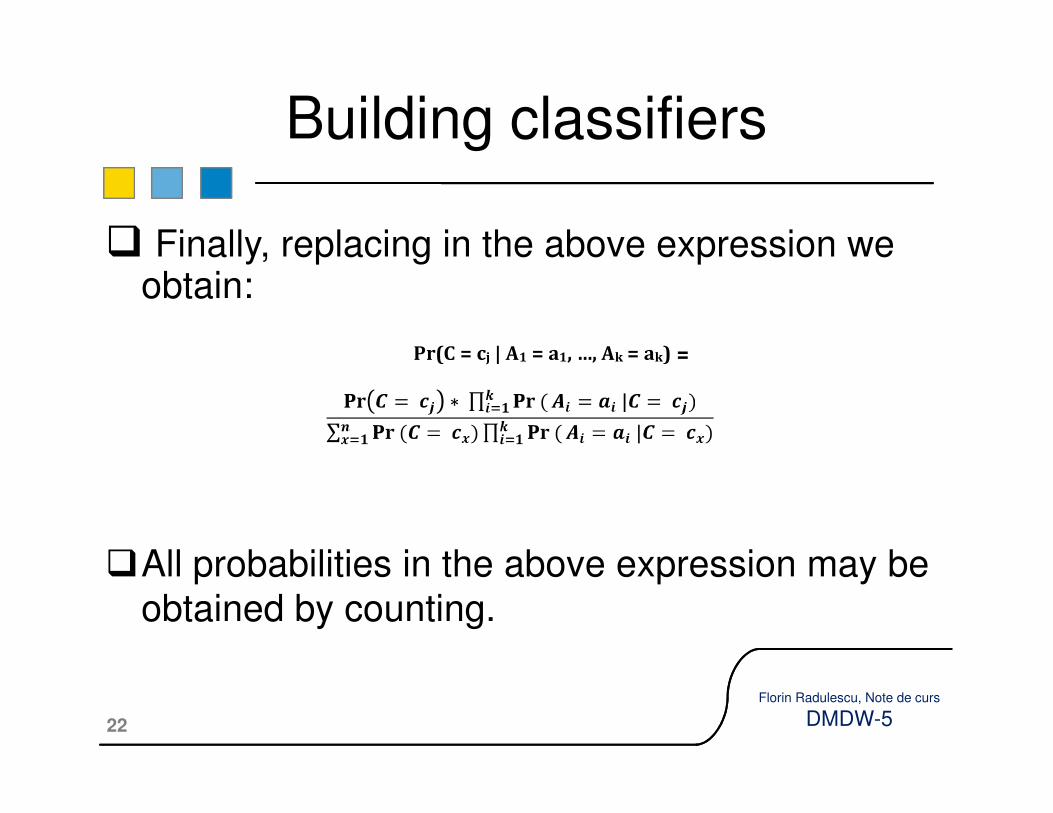
� Finally, replacing in the above expression we obtain:
Building classifiers
Pr(C = cj | A1 = a1, …, Ak = ak) =
22
Florin Radulescu, Note de curs
DMDW-5
�All probabilities in the above expression may be
obtained by counting.
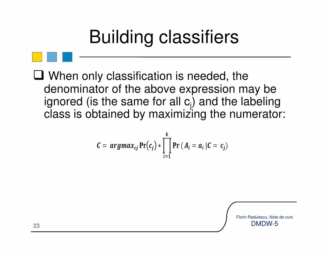
� When only classification is needed, the denominator of the above expression may be ignored (is the same for all cj) and the labeling class is obtained by maximizing the numerator:
Building classifiers
23
Florin Radulescu, Note de curs
DMDW-5

� Consider a simplified version of the PlayTennis table :
Example
Outlook Wind Play Tennis
Overcast Weak Yes
Overcast Strong Yes
24
Florin Radulescu, Note de curs
DMDW-5
Overcast Strong Yes
Overcast Absent No
Sunny Weak Yes
Sunny Strong No
Rain Strong No
Rain Weak No
Rain Absent Yes

Pr(Yes) = 4/8 Pr(No) = 4/8
Pr(Overcast | C = Yes) = 2/4 Pr(Weak | C = Yes) = 2/4
Pr(Overcast | C = No) = 1/4 Pr(Weak | C = No) = 1/4
Pr(Sunny | C = Yes) = 1/4 Pr(Strong| C = Yes) = 1/4
Pr(Sunny | C = No) = 1/4 Pr(Strong| C = No) = 2/4
Example
25
Florin Radulescu, Note de curs
DMDW-5
Pr(Sunny | C = No) = 1/4 Pr(Strong| C = No) = 2/4
Pr(Rain | C = Yes) = 1/4 Pr(Absent| C = Yes) = 1/4
Pr(Rain | C = No) = 2/4 Pr(Absent| C = No) = 1/4
� If the test example is:
Sunny Absent ???
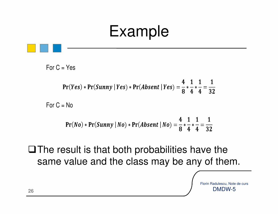
Example
For C = Yes
For C = No
26
Florin Radulescu, Note de curs
DMDW-5
�The result is that both probabilities have the
same value and the class may be any of them.
For C = No
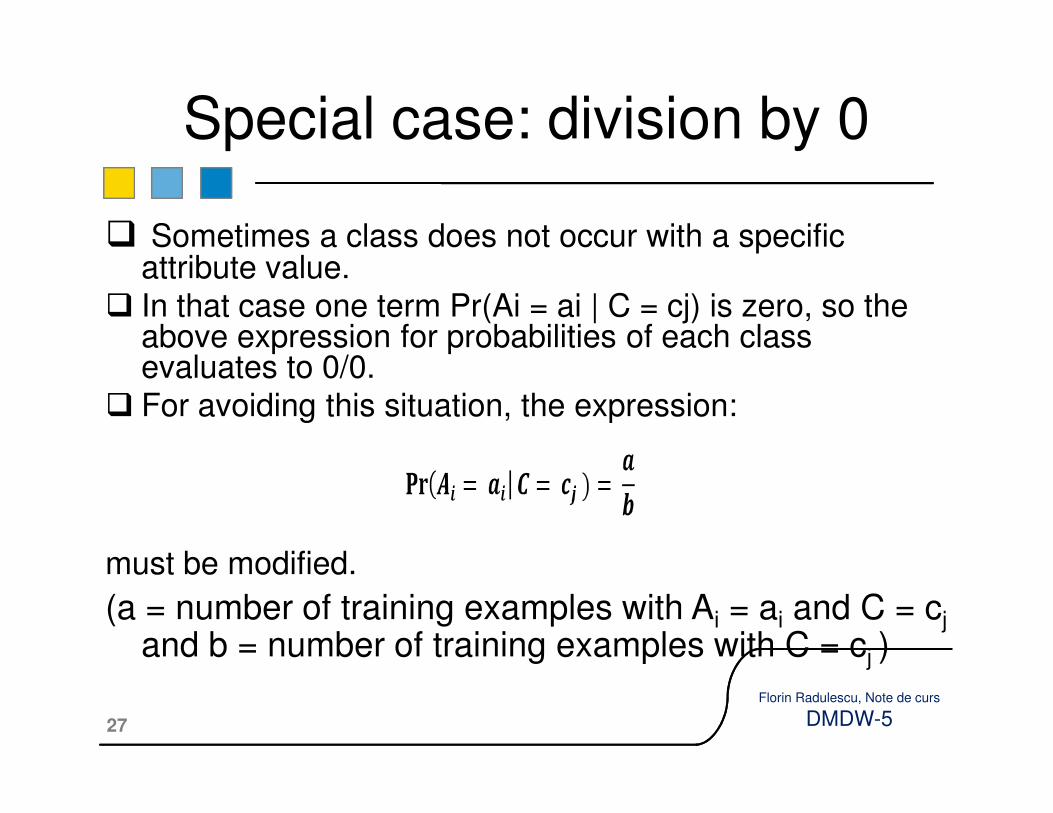
� Sometimes a class does not occur with a specific attribute value.
� In that case one term Pr(Ai = ai | C = cj) is zero, so the above expression for probabilities of each class evaluates to 0/0.
� For avoiding this situation, the expression:
Special case: division by 0
27
Florin Radulescu, Note de curs
DMDW-5
� For avoiding this situation, the expression:
must be modified.
(a = number of training examples with Ai = ai and C = cj
and b = number of training examples with C = cj )
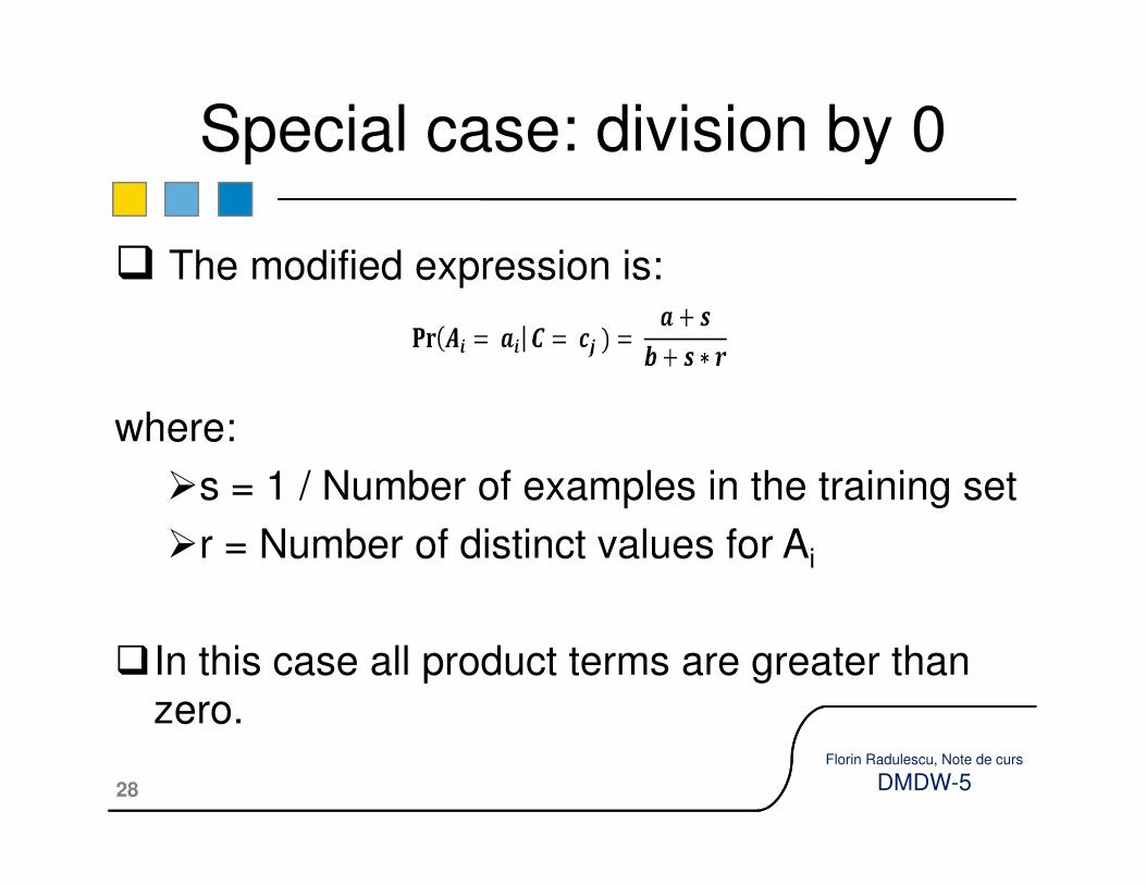
� The modified expression is:
where:
Special case: division by 0
28
Florin Radulescu, Note de curs
DMDW-5
where:
�s = 1 / Number of examples in the training set
�r = Number of distinct values for Ai
�In this case all product terms are greater than
zero.
Non-categorical values or absent values:
�All non-categorical attributes must be discretized (replaced with categorical ones).
Special case: values
29
Florin Radulescu, Note de curs
DMDW-5
ones).
�Also, if some attributes have a missing value, these values are ignored.
�Classification using class association rules
�Naïve Bayesian classification
�Support vector machines (SVMs)
K-nearest neighbor
Road Map
30
Florin Radulescu, Note de curs
DMDW-5
�K-nearest neighbor
�Ensemble methods: Bagging, Boosting, Random Forest
�Summary
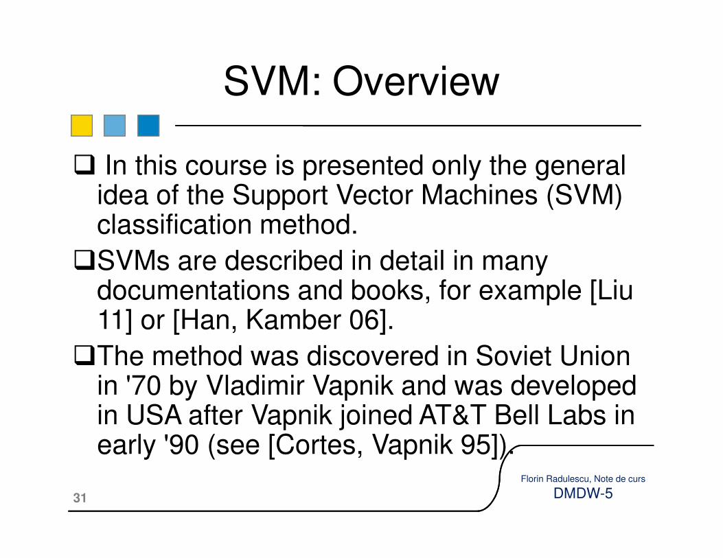
� In this course is presented only the general idea of the Support Vector Machines (SVM) classification method.
�SVMs are described in detail in many documentations and books, for example [Liu
SVM: Overview
31
Florin Radulescu, Note de curs
DMDW-5
documentations and books, for example [Liu 11] or [Han, Kamber 06].
�The method was discovered in Soviet Union in '70 by Vladimir Vapnik and was developed in USA after Vapnik joined AT&T Bell Labs in early '90 (see [Cortes, Vapnik 95]).
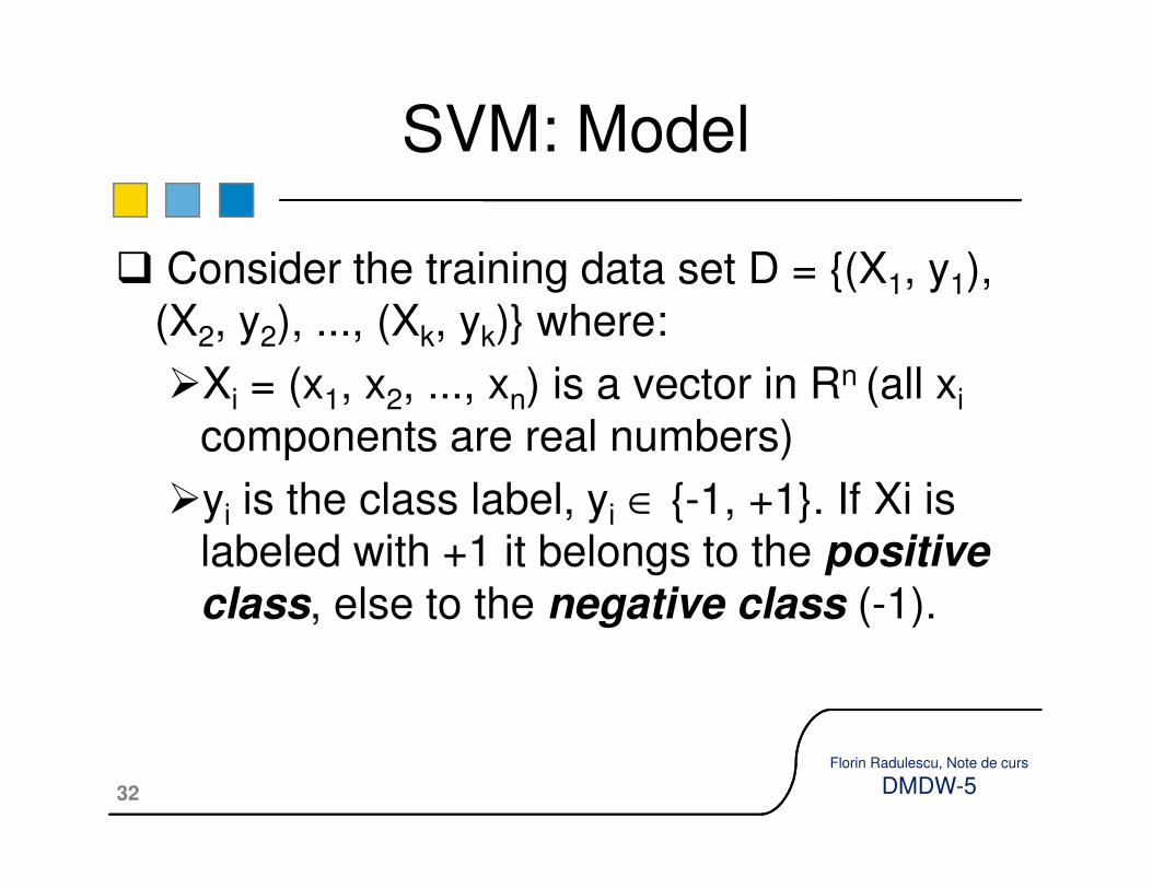
� Consider the training data set D = {(X1, y1),
(X2, y2), ..., (Xk, yk)} where:
�Xi = (x1, x2, ..., xn) is a vector in Rn (all xi
components are real numbers)
SVM: Model
32
Florin Radulescu, Note de curs
DMDW-5
components are real numbers)
�yi is the class label, yi ∈ {-1, +1}. If Xi is labeled with +1 it belongs to the positive
class, else to the negative class (-1).

�A possible classifier is a linear function:
f(X) = <w ⋅ X> + b
such as:
SVM: Model
33
Florin Radulescu, Note de curs
DMDW-5
where:
�w is a weight vector,
�<w ⋅ X> is the dot product of vectors w and X,
�b is a real number and
�w and b may be scaled up or down as shown below.

�The meaning of f is that the hyperplane
< w ⋅ X> + b = 0
separates the points of the training set D in two:
�one half of the space contains the positive
SVM: Model
34
Florin Radulescu, Note de curs
DMDW-5
�one half of the space contains the positive
values and
�the other half the negative values in D (like
hyperplanes H1 and H2 in the next figure).
�All test examples can now be classified using f:
the value of f gives the label for the example.

Figure 1
35
Florin Radulescu, Note de curs
DMDW-5
� Source: Wikipedia

� SVM tries to find the ‘best’ hyperplane of that form.
�The theory shows that the best plane is the one maximizing the so-called margin (the minimum orthogonal distance between a positive and
Best hyperplane
36
Florin Radulescu, Note de curs
DMDW-5
orthogonal distance between a positive and negative point from the training set – see next figure for an example.

Figure 2
37
Florin Radulescu, Note de curs
DMDW-5
� Source: Wikipedia

� Consider X+ and X- the nearest positive and negative points for the hyperplane
<w ⋅ X> + b = 0
� Then there are two other parallel hyperplanes, H+ and H- passing through X+ and X- and their expression is:H : <w ⋅ X> + b = 1
The model
38
Florin Radulescu, Note de curs
DMDW-5
H+ : <w ⋅ X> + b = 1
H- : <w ⋅ X> + b = -1
� These two hyperplanes are with dotted lines in Figure 1. Note that w and b must be scaled such as:<w ⋅ Xi> + b ≥ 1 for yi = 1
<w ⋅ Xi> + b ≤ -1 for yi = -1

�The margin is the distance between these two planes and may be computed using vector space algebra obtaining:
The model
39
Florin Radulescu, Note de curs
DMDW-5
�Maximizing the margin means minimizing the value of
�The points X+ and X- are called support vectorsand are the only important points from the dataset.
� When positive and negative points are linearly
separable, the SVM definition is the following:
� Having a training data set D = {(X1, y1), (X2, y2), ..., (Xk, yk)}
� Minimize the value of expression (1) above
� With restriction: yi (<w ⋅ Xi> + b) ≥ 1, knowing the value of yi: +1
Definition: separable case
40
Florin Radulescu, Note de curs
DMDW-5
� With restriction: yi (<w ⋅ Xi> + b) ≥ 1, knowing the value of yi: +1 or -1
� This optimization problem is solvable by rewriting the
above inequality using a Lagrangian formulation and
then finding solution using Karush-Kuhn-Tucker (KKT)
conditions.
� This mathematical approach is beyond the scope of this
course.
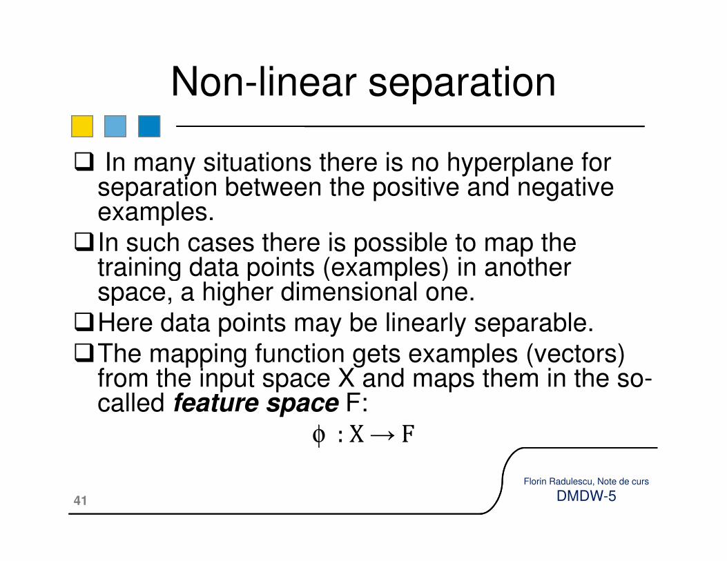
� In many situations there is no hyperplane for separation between the positive and negative examples.
�In such cases there is possible to map the training data points (examples) in another space, a higher dimensional one.
Non-linear separation
41
Florin Radulescu, Note de curs
DMDW-5
training data points (examples) in another space, a higher dimensional one.
�Here data points may be linearly separable.
�The mapping function gets examples (vectors) from the input space X and maps them in the so-called feature space F:
φ : X → F

�Each point X is mapped in φ(X). So, after
mapping the whole D there is another training
set, containing vectors from F and not from X,
with dim(F) ≥ n = dim(X):
Non-linear separation
42
Florin Radulescu, Note de curs
DMDW-5
D = {(φ(X1), y1), (φ(X2), y2), ..., (φ(Xk), yk)}
�For an appropriate φ, these points are linearly
separable.
�An example is the next figure.
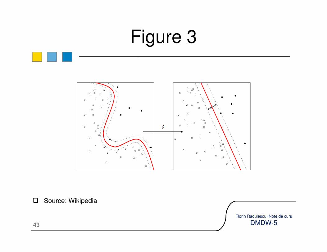
Figure 3
43
Florin Radulescu, Note de curs
DMDW-5
� Source: Wikipedia

• But how can we find this mapping function?
• In solving the optimization problem for finding the linear separation hyperplane in the new feature space F all terms containing training examples are only of the form φ (Xi) ⋅ φ(Xj).
• By replacing this dot product with a function in both X
Kernel functions
44
Florin Radulescu, Note de curs
DMDW-5
• By replacing this dot product with a function in both Xiand Xj the need for finding φ disappears. Such a function is called a kernel function:
K(Xi, Xj) = φ (Xi) ⋅ φ(Xj)
• For finding the separation hyperplane in F we must only replace all dot products with the chosen kernel function and then proceed with the optimization problem like in separable case.

Some of the most used kernel functions are:
�Linear kernel
K(X, Y) = <X ⋅ Y> + b
�Polynomial Kernel
Kernel functions
45
Florin Radulescu, Note de curs
DMDW-5
�Polynomial Kernel
K(X, Y) = (a * <X ⋅ Y> + b)p
�Sigmoid Kernel
K(X, Y) = tanh(a * <X ⋅ Y> + b)
� SVM deals with continuous real values for attributes. �When categorical attributes exists in the training
data a conversion to real values is needed.
�When more than two classes are needed
Other aspects concerning SVMs
46
Florin Radulescu, Note de curs
DMDW-5
�When more than two classes are needed SVM can be used recursively. �First use separates one class; the second use
separates the second class and so on. For N classes N-1 runs are needed.
�SVM are a very good method in hyper dimensional data classification.
�Classification using class association rules
�Naïve Bayesian classification
�Support vector machines
K-nearest neighbor (kNN)
Road Map
47
Florin Radulescu, Note de curs
DMDW-5
�K-nearest neighbor (kNN)
�Ensemble methods: Bagging, Boosting, Random Forest
�Summary
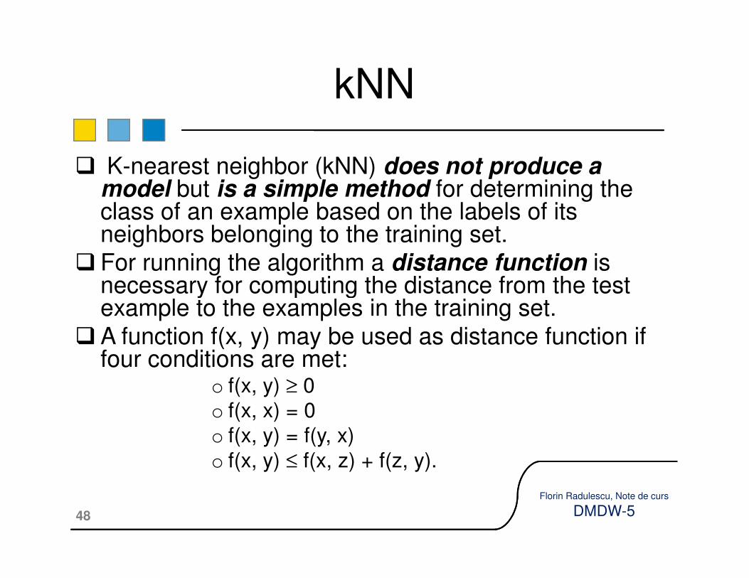
� K-nearest neighbor (kNN) does not produce a model but is a simple method for determining the class of an example based on the labels of its neighbors belonging to the training set.
� For running the algorithm a distance function is necessary for computing the distance from the test
kNN
48
Florin Radulescu, Note de curs
DMDW-5
necessary for computing the distance from the test example to the examples in the training set.
�A function f(x, y) may be used as distance function if four conditions are met:
o f(x, y) ≥ 0o f(x, x) = 0
o f(x, y) = f(y, x)
o f(x, y) ≤ f(x, z) + f(z, y).
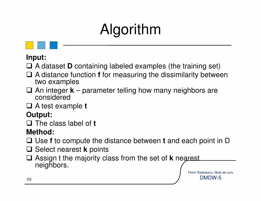
Input:� A dataset D containing labeled examples (the training set)
� A distance function f for measuring the dissimilarity between two examples
� An integer k – parameter telling how many neighbors are considered
Algorithm
49
Florin Radulescu, Note de curs
DMDW-5
considered
� A test example tOutput:� The class label of tMethod:� Use f to compute the distance between t and each point in D
� Select nearest k points
� Assign t the majority class from the set of k nearest neighbors.
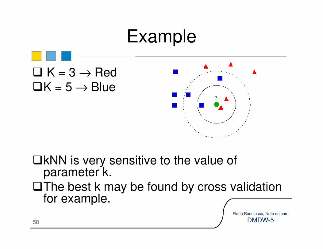
� K = 3 → Red
�K = 5 → Blue
Example
50
Florin Radulescu, Note de curs
DMDW-5
�kNN is very sensitive to the value of parameter k.
�The best k may be found by cross validation for example.

�Classification using class association rules
�Naïve Bayesian classification
�Support vector machines
K-nearest neighbor (kNN)
Road Map
51
Florin Radulescu, Note de curs
DMDW-5
�K-nearest neighbor (kNN)
�Ensemble methods: Bagging, Boosting, Random Forest
�Summary
� Ensemble methods combine multiple classifiers to obtain a better one.
�Combined classifiers are similar (use the same learning method) but the training
Ensemble methods
52
Florin Radulescu, Note de curs
DMDW-5
same learning method) but the training datasets or the weights of the examples in them are different.

� The name Bagging comes from Bootstrap Aggregating.
� As presented in the previous lesson bootstrap method is part of resampling
Bagging
53
Florin Radulescu, Note de curs
DMDW-5
bootstrap method is part of resampling methods and consists in getting a training set from the initial labeled data by sampling with replacement.
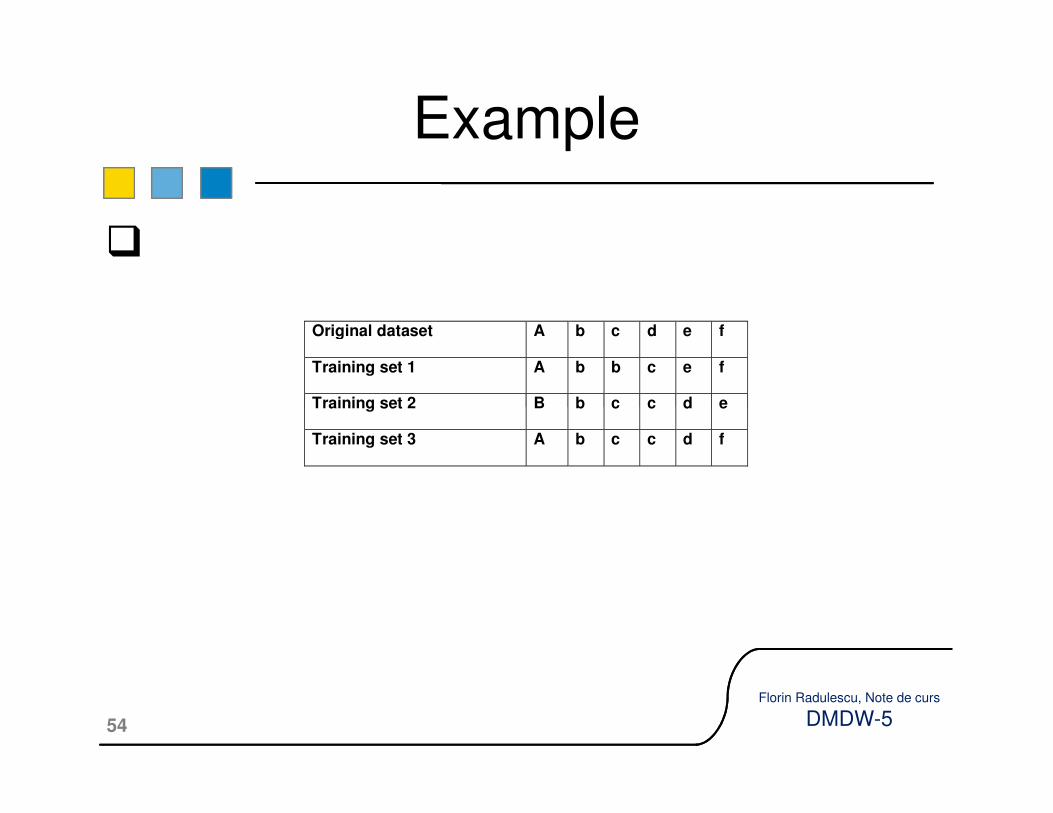
�
Example
Original dataset A b c d e f
Training set 1 A b b c e f
Training set 2 B b c c d e
54
Florin Radulescu, Note de curs
DMDW-5
Training set 2 B b c c d e
Training set 3 A b c c d f

Bagging consists in:
�Starting with the original dataset, build n training datasets by sampling with replacement (bootstrap samples)
� For each training dataset build a classifier using the same learning algorithm (called weak classifiers).
Bagging
55
Florin Radulescu, Note de curs
DMDW-5
same learning algorithm (called weak classifiers).
� The final classifier is obtained by combining the results of the weak classifiers (by voting for example).
�Bagging helps to improve the accuracy for unstable learning algorithms: decision trees, neural networks.
� It does not help for kNN, Naïve Bayesian classification or CARs.

• Boosting consists in building a sequence of weak classifiers and adding them in the structure of the final strong classifier.
• The weak classifiers are weighted based on the weak learners' accuracy.
Boosting
56
Florin Radulescu, Note de curs
DMDW-5
the weak learners' accuracy.
• Also data is reweighted after each weak classifier is built such as examples that are incorrectly classified gain some extra weight.
• The result is that the next weak classifiers in the sequence focus more on the examples that previous weak classifiers missed.

� Random forest is an ensemble classifier consisting in a set of decision trees The final classifier output the modal value of the classes output by each tree.
� The algorithm is the following:1. Choose T - number of trees to grow.2. Choose m - number of variables used to split each node. m << M,
where M is the number of input variables.
Random forest
57
Florin Radulescu, Note de curs
DMDW-5
where M is the number of input variables.3. Grow T trees. When growing each tree do the following:
� Construct a bootstrap sample from training data with replacement and grow a tree from this bootstrap sample.
� When growing a tree at each node select m variables at random and use them to find the best split.
� Grow the tree to a maximal extent. There is no pruning. 4. Predict new data by aggregating the predictions of the trees (e.g.
majority votes for classification, average for regression).

This course presented:
�Classification using class association rules: CARs for building classifiers and using CARs for building new attributes (features) of the training dataset.
�Naïve Bayesian classification: Bayes theorem, Naïve Bayesian algorithm for building classifiers.
Summary
58
Florin Radulescu, Note de curs
DMDW-5
Bayesian algorithm for building classifiers.
�An introduction to support vector machines (SVMs): model, definition, kernel functions.
�K-nearest neighbor method for classification
�Ensemble methods: Bagging, Boosting, Random Forest
�Next week: Unsupervised learning – part 1

[Liu 11] Bing Liu, 2011. Web Data Mining, Exploring Hyperlinks, Contents, and Usage Data, Second Edition, Springer, chapter 3.
[Han, Kamber 06] Jiawei Han, Micheline Kamber, Data Mining: Concepts and Techniques, Second Edition, Morgan Kaufmann Publishers, 2006
[Cortes, Vapnik 95] Cortes, Corinna; and Vapnik, Vladimir N.;
References
59
Florin Radulescu, Note de curs
DMDW-5
[Cortes, Vapnik 95] Cortes, Corinna; and Vapnik, Vladimir N.; "Support-Vector Networks", Machine Learning, 20, 1995. http://www.springerlink.com/content/k238jx04hm87j80g/
[Wikipedia] Wikipedia, the free encyclopedia, en.wikipedia.org