530 ieee transactions on visualization and computer ...mcmains/pubs... · 530 ieee transactions on...

Performing Efficient NURBS ModelingOperations on the GPU

Adarsh Krishnamurthy, Rahul Khardekar, Sara McMains, Kirk Haller, and Gershon Elber

Abstract—We present algorithms for evaluating and performing modeling operations on NURBS surfaces using the programmable

fragment processor on the Graphics Processing Unit (GPU). We extend our GPU-based NURBS evaluator that evaluates NURBS

surfaces to compute exact normals for either standard or rational B-spline surfaces for use in rendering and geometric modeling. We

build on these calculations in our new GPU algorithms to perform standard modeling operations such as inverse evaluations, ray

intersections, and surface-surface intersections on the GPU. Our modeling algorithms run in real time, enabling the user to sketch on

the actual surface to create new features. In addition, the designer can edit the surface by interactively trimming it without the need for

retessellation. Our GPU-accelerated algorithm to perform surface-surface intersection operations with NURBS surfaces can output

intersection curves in the model space as well as in the parametric spaces of both the intersecting surfaces at interactive rates. We

also extend our surface-surface intersection algorithm to evaluate self-intersections in NURBS surfaces.

Index Terms—NURBS, GPU, inverse evaluation, sketching, interactive trimming, SSI, intersection curves, self-intersection, prefix sum.

Ç

1 INTRODUCTION

INDUSTRIAL design of products has shifted from using boxyshapes with straight edges to incorporate curved free-form

surfaces. Non Uniform Rational B-Spline (NURBS) surfacesprovide a convenient and compact representation of suchcurved surfaces that has become the representation of choicein mechanical CAD systems. Hence, real-time interactionwith NURBS surfaces is essential for any CAD package.However, since evaluation of a NURBS surface is inherently acomputation-intensive process, commercial CAD packagesdeal with it by preprocessing NURBS surfaces, usuallytessellating them and using the triangulated model fordisplay as well as certain modeling operations like selection.With the advent of programmable graphics hardware, theneed for tessellating the NURBS surface in the CPU fordisplay was obviated, since the GPU can be used for theevaluation and direct display of the surfaces [1], [2], [3], [4].However, CAD packages still perform modeling operationsusing the CPU with either the tessellated surfaces oranalytically using NURBS definitions. This reduces theinteractivity for the user when designing these free-formsurfaces, since operations like sketching on the NURBSsurface or fast evaluation of intersection curves are notpossible. Leading commercial CAD packages do not allowthe designer to sketch directly on the NURBS surface; instead,

they restrict the user to sketching on a tangent plane. Becauseof this, the designer has to wait until the operation iscompleted to get visual feedback.

The process of finding the surface coordinates ðx; y; zÞ forgiven parameter values ðu; vÞ is called evaluation. Inverseevaluation is the process of finding the parameter valuesðu; vÞ given any point on the surface. We have developed aparallel algorithm for fast inverse evaluations of NURBSsurfaces on the GPU. This algorithm forms the basis of manymodeling operations like selection (ray-surface intersection),sketching on the surface, and interactive trimming (see Fig. 1).Moreover, since these algorithms exploit the parallelism ofthe GPU, these operations can now be performed atinteractive speeds, making immediate visual feedback tothe designer possible for the first time. We demonstrate theuse of our fast inverse evaluation algorithm to directly sketchon the surface, which makes certain operations like inter-active trimming intuitive to the designer.

Designers are usually trained to work with curves onsurfaces, such as silhouette curves and intersection curves.Thus, they would like to see real-time changes in thesecurves as the underlying surfaces are edited, which requiresan efficient algorithm to compute intersection curves offree-form surfaces. Finding the intersection curve is, ingeneral, a very complex operation, since two NURBSsurface equations of arbitrary degree have to be solvedsimultaneously. Many commercial CAD packages usemarching methods, where the algorithm uses a numericalroot-finding technique to first find a single intersectionpoint. The algorithm then finds another point along theintersection curve that is close to the first intersection point.This process is repeated and ultimately a completepiecewise linear approximation of the intersection curve iscalculated. However, since this technique is inherentlyserial, it cannot be parallelized for efficient evaluation onthe GPU. We have developed a GPU-accelerated parallelalgorithm to evaluate the intersection curves using boundson the evaluated surface points. This algorithm is both fastand guaranteed to find the intersection curves within auser-defined tolerance.

530 IEEE TRANSACTIONS ON VISUALIZATION AND COMPUTER GRAPHICS, VOL. 15, NO. 4, JULY/AUGUST 2009

. A. Krishnamurthy, R. Khardekar, and S. McMains are with theDepartment of Mechanical Engineering, University of California, Berkeley,Berkeley, CA 94720. E-mail: {adarsh, rahul, mcmains}@me.berkeley.edu.

. K. Haller is with SolidWorks Corporation, 300 Baker Avenue, Concord,MA 01742. E-mail: [email protected].

. G. Elber is with the Department of Computer Science, Technion, IsraelInstitute of Technology, Haifa 32000, Israel.E-mail: [email protected].

Manuscript received 24 July 2008; revised 21 Nov. 2008; accepted 7 Jan. 2009;published online 5 Feb. 2009.Recommended for acceptance by H. Qin.For information on obtaining reprints of this article, please send e-mail to:[email protected], and reference IEEECS Log NumberTVCGSI-2008-07-0107.Digital Object Identifier no. 10.1109/TVCG.2009.29.

1077-2626/09/$25.00 � 2009 IEEE Published by the IEEE Computer Society

Authorized licensed use limited to: Univ of Calif Berkeley. Downloaded on January 4, 2010 at 00:57 from IEEE Xplore. Restrictions apply.

In this paper, we present GPU-based algorithms toperform modeling operations efficiently on NURBS sur-faces. Our main contributions include:

. A new unified method to calculate exact deriva-tives and exact normals of arbitrary-degree NURBSsurfaces on the GPU. Our method is designed soas to not require separate fragment programs forevaluating surfaces of different degrees.

. An efficient algorithm to perform inverse evalua-tion of NURBS surfaces on the GPU. Thisalgorithm finds the parametric ðu; vÞ coordinategiven any ðx; y; zÞ coordinate on the NURBSsurface within an arbitrary user-defined tolerance.

. A novel method to interactively trim and sketchon a NURBS surface in real time. This is possiblebecause our fast inverse evaluation algorithmenables us to sketch in the model space, not justin the parametric space, with the correspondencetracked simultaneously.

. A GPU-accelerated algorithm to perform fast androbust NURBS surface-surface intersections. Theintersection curve, like the sketch curve above, issimultaneously output in the model space as well asin the parametric spaces of the two NURBS surfaces.The GPU is used to accelerate the operation byfinding points on the intersection curves and theactual intersection curves are calculated from thesepoints on the CPU.

. An extension of the surface-surface intersectionalgorithm to evaluate self-intersections in NURBSsurfaces. This algorithm can be used to detect self-intersections and output the intersection curves ifthe surface is self intersecting.

We summarize our approach to evaluating and renderingNURBS surfaces on the GPU in Section 2; for more details,refer to [1]. We then discuss the evaluation of first and secondderivatives of the NURBS surfaces (Section 3) and then usethese to compute bounding boxes for NURBS surfaces(Section 4). Then, we describe how these bounds are usedto perform inverse evaluations (Section 5) and computeintersection curves (Section 6). Fig. 2 shows these connectionsbetween the different parts of our algorithms; each of theseoperations are described in detail in the sections indicated.

2 PREVIOUS WORK

One of the main prerequisites for performing fast modeling

operations on NURBS is to have a fast NURBS evaluator. We

present a short outline of our algorithm to evaluate NURBSsurfaces on the GPU that was explained in detail in [1]. Themain idea of our algorithm was to use a fragment program toevaluate a NURBS surface in several passes. One advantageof our approach is that we have two correspondingrepresentations of the NURBS surface as four-componentvectors—ðx; y; z; wÞ coordinates—in space as well as theircorresponding parametric values—ðu; vÞ coordinates. Weexploit this correspondence during modeling operations likeinverse evaluation and evaluation of intersection curves.

In our algorithm, we first evaluate the basis functionvalues on the GPU in parallel for all the parameter positionswhere we want to evaluate the surface coordinates. Theparameter positions can be chosen arbitrarily by the user; wechose an equally spaced grid of points to make theimplementation simpler. For example in this paper, we chosea starting grid size of 1; 024� 1; 024 and refined it based on theuser-specified tolerances. We parallelize the de Boor evalua-tion algorithm [5] so that it runs efficiently on the GPU. Weuse the de Boor evaluation method because B-spline basisfunctions of any degree can be evaluated using the samefragment program. Other NURBS evaluations on the GPUeither require different fragment programs for differentdegrees [2] or are restricted to cubic polynomials [3]. Weperform the basis function evaluation separately for theu andv parametric directions on the GPU and store these values astextures. We multiply these basis function values with thecorresponding control points to obtain the surface point

KRISHNAMURTHY ET AL.: PERFORMING EFFICIENT NURBS MODELING OPERATIONS ON THE GPU 531

Fig. 1. Modeling operations like (a) sketching, (b) ray intersection, (c) trimming, and (d) surface-surface intersection performed directly on trimmed

NURBS models.

Fig. 2. Graphic showing the links between different parts of our modeling

algorithms. The results of the GPU evaluations are stored in separate

textures.


coordinates. We can restrict the multiplication to the submeshof the control points that affect a particular surface pointbecause of the local support property of NURBS (Fig. 3). Weperform the multiplication operation in parallel for all thesurface coordinates using another fragment program. Thesurface point coordinates thus calculated are stored directlyin a texture on the GPU using the RGBA channels. Whilerendering, we interpret these values stored in the texture asvertex coordinates using a Vertex Buffer Object (VBO). Wethus avoid the slow operation of reading back the computeddata from the GPU to the CPU, directly rendering the NURBSsurface on the screen.

Previous work that used GPUs to render NURBS curvesor surfaces focused only on efficient evaluation of thesurface coordinates and/or normals by the authors of [2],[3], [6], [7]. They did not use GPUs to perform modelingoperations like inverse evaluations and intersection curveevaluations. Previous work on inverse evaluation of NURBSsurfaces mainly focused on ray tracing NURBS surfaces.Ray tracing was performed on parametric and rationalsurfaces by solving for the ray-surface intersection pointusing numerical methods [8], [9], [10]. There has also beenprevious work on ray tracing using the GPU, whichincludes [4], [11], [12], [13]. Another application of inverseevaluation of NURBS is solving for geometric constraints. Amethod to solve geometric constraints by using multivariatesplines was given in [14], which can be used to solve severalrelated problems like ray traps and sweep envelopes.Inverse evaluation has also been used for haptic renderingto find the parametric ðu; vÞ coordinates of a given point ona NURBS surface [15]. Inverse evaluation was used in thiscase to solve for the contact point of a haptic probe withtrimmed NURBS surfaces in a virtual environment.

Carr et al. [13] also presented a GPU algorithm to find theindexes of the rendered texels in a texture, a subproblemfor our GPU algorithm for intersection calculations. Thissubproblem falls under the class of stream reduction, theprocess of removing unwanted elements from a stream ofvalues and reducing it to a smaller list containing therequired output. General Purpose computing on the GPU(GPGPU) uses stream reduction to remove defunct elementsfrom the output of a previous pass before sending it as inputfor the next pass. Since the positions of the output elementsdo not have any fixed correspondence with the positions ofthe input, the stream reduction process is considered

nonuniform. A parallel Oðkþ lognÞ algorithm, where k isthe output size, for nonuniform stream reduction based onprefix sums was given in [16]. However, standard graphicscards do not have the capability to perform a scatteroperation (random writes to different memory locations),which was an essential step in the algorithm given in [16].Another algorithm has been presented in [17] for nonuniformstream reduction on the GPU that runs in Oðn lognÞ, not asefficient due to workarounds required because of lack ofscatter. A stream reduction algorithm specifically for 2Dtextures on the GPU was proposed in [18], which used thefragment processor to perform other operations whileperforming the scatter operation, thereby hiding the latency.Recently, an OðnÞ GPU stream reduction algorithm wasproposed in [19], also using prefix sums, that relies on thelatest NVIDIA CUDA architecture for its scatter function-ality. We propose a similar OðnÞ stream reduction algorithmbased on computing a parallel prefix sum, but implement itusing the standard GPGPU framework so that it is bothcompatible with older hardware and not limited to a singlebrand of GPU.

Several approaches to collision detection on the GPUhave been proposed. Occlusion queries on graphics hard-ware were used in [20] to detect collisions of polygonalmeshes in large environments. Collisions between particleswere calculated in [21], [22] to simulate large scale particlesystems on the GPU. Recently, a method to detect collisionsbetween deformable parameterized surfaces using GPUswas presented by Greß et al. [18]. They solve the collisiondetection problem by generating a bounding box hierarchyfor the surface and then detecting collisions by checkingoverlap between the bounding boxes.

Evaluation of intersection curves is a fundamentaloperation in computer-aided geometric design and solidmodeling [23], [24]. There have been several attempts tosolve the problem, since it is hard to achieve all the desiredcharacteristics of robustness, accuracy, and efficiency. Acomprehensive survey of surface-surface intersection algo-rithms was summarized in [25]. A more recent algebraicalgorithm for efficient surface intersection using lowerdimensional formulations was given by Krishnan andManocha [26]. They also classified the conventionalmethods for evaluating the intersection curves as analyticalmethods, lattice evaluations, subdivision methods, andmarching methods. Many commercial CAD softwarepackages use the numerical marching method outlined in[27], [28] to evaluate intersection curves.

3 DERIVATIVES OF NURBS SURFACES

To perform geometric operations on NURBS surfaces, wenot only require the surface point coordinates themselvesbut also the first and second partial derivatives with respectto the two parameter directions u and v at the surfacepoints. As a very fast first-degree approximation, we canuse the evaluated point coordinates to estimate the firstderivatives using central differencing. However, thisapproach gives rise to artificial discontinuities at patchboundaries and at rational parts of the surface. Moreover,second derivatives estimated from these first derivatives inthe same manner have larger errors associated with them.One way to overcome this issue is to evaluate the normals


Fig. 3. Graphic showing our NURBS evaluation algorithm on the GPU.The control mesh of size m� n and the evaluation mesh are made offour-component vectors stored as RGBA textures. The surface patch isof order ku in the u direction and kv in the v direction. The multiplication isrestricted to the submesh of size ku � kv.


of the surface exactly at each surface point, similar to theevaluation of the surface coordinates. Since we alreadyevaluate the higher order basis functions from lower orderbasis-functions, we can directly calculate the derivatives ofthe basis functions within the same framework as our basisfunction evaluation algorithm, and then use the basisfunction derivatives to evaluate the derivatives of theNURBS surface precisely, to within machine precision.

3.1 Differential Geometry for B-Spline Surfaces

In this section, we present a concise version of the equations

that are required for computing derivatives of NURBS

surfaces, adapted from [29]. We present the exact equationsfor a Non-Uniform B-Spline (NUBS) surface first and then

extend the derivation to include rational surfaces. For a

NUBS surface, Sðu; vÞ, given by (1), the derivatives can be

computed by multiplying the control points (Pijs) with the

derivatives of the basis functions. The variables Npi s and

Nqj s are the B-spline basis functions of degrees p and q,

respectively, as a function of the knots uis and vis,

respectively ((2) and (3)); the Pijs are the NUBS control

points defined as a quadrilateral mesh.

Sðu; vÞ ¼Xni¼0

Xmj¼0

Npi ðuÞN

qj ðvÞPij; ð1Þ

Npi ðuÞ ¼

u� uiuiþp � ui

Np�1i ðuÞ þ uiþpþ1 � u

uiþpþ1 � uiþ1Np�1iþ1 ðuÞ; ð2Þ

N0i ðuÞ ¼

1; if ui � u < uiþ1;0; otherwise:

�ð3Þ

The derivative of the basis function of degree p withrespect to u is given by (4). To evaluate the derivative of abasis function of degree p, the basis function of degree p� 1needs to be computed. We use the indicial notation N;u todenote the derivative with respect to u. Note that p� 1 inthe numerator of (4) arises due to the fact that the B-splinebasis function of degree p that we are differentiating is apiecewise polynomial of degree p in u.

Npi;uðuÞ ¼

p� 1

uiþp � uiNp�1i ðuÞ � p� 1

uiþpþ1 � uiþ1Np�1iþ1 ðuÞ: ð4Þ

The derivatives of the B-spline basis functions, N;u andN;v, are then multiplied by the control points Pij to get thederivative along the u or vparametric direction on the surfaceas given in (5) and (6), respectively. We can then calculate thesurface normalNðu; vÞ of the NUBS surface (Fig. 4) by takingthe cross product of the u and v partial derivatives (7). Itshould be noted that Nðu; vÞ is not a unit vector field but it iswell defined as long as S is a regular surface.

S;uðu; vÞ ¼Xni¼0

Xmj¼0

Npi;uðuÞN

qj ðvÞPij; ð5Þ

S;vðu; vÞ ¼Xni¼0

Xmj¼0

Npi ðuÞN

qj;vðvÞPij; ð6Þ

Nðu; vÞ ¼ S;uðu; vÞ � S;vðu; vÞ: ð7Þ

3.2 Rational Derivatives

The derivatives of NURBS surfaces are not as straightfor-ward to evaluate as in the NUBS case [30]. This is becausethe derivatives have to be evaluated using the chain ruledue of the existence of the rational component. The NURBSsurface coordinates are evaluated as the four-componentvector shown in (8) and (9). Since we evaluate the four-component vectors without performing the rational divi-sion on the GPU, we can effectively use this data to evaluatethe surface derivatives.

Sðu; vÞ ¼�X

w; �X ¼

xyz

0@

1A; ð8Þ

xyzw

0BB@

1CCA ¼

Pni¼0

Pmj¼0 N

pi ðuÞN

qj ðvÞxijPn

i¼0

Pmj¼0 N

pi ðuÞN

qj ðvÞyijPn

i¼0

Pmj¼0 N

pi ðuÞN

qj ðvÞzijPn

i¼0

Pmj¼0 N

pi ðuÞN

qj ðvÞwij

0BBB@

1CCCA; ð9Þ

S;uðu; vÞ ¼�X;uw� �Xw;u

w2; ð10Þ

x;uy;uz;uw;u

0BB@

1CCA ¼

Pni¼0

Pmj¼0 N

pi;uðuÞN

qj ðvÞxijPn

i¼0

Pmj¼0 N

pi;uðuÞN

qj ðvÞyijPn

i¼0

Pmj¼0 N

pi;uðuÞN

qj ðvÞzijPn

i¼0

Pmj¼0 N

pi;uðuÞN

qj ðvÞwij

0BBB@

1CCCA: ð11Þ

The partial derivative with respect to u (10) is derivedusing the quotient rule (in turn derived using the chainrule). It can be calculated by first evaluating the product ofthe derivatives of the basis functions and the correspondingcontrol points as a four-component vector (11), and thenperforming the required rational division operations. Thepartial derivative of the surface with respect to v can also beevaluated in a similar manner. In this work, we assume allthe weights (w) are positive, and hence, no poles can occurin S or its partial derivatives.

3.3 GPU Implementation

The GPU implementation of the evaluation of surfacederivatives is a direct extension of the evaluation of thesurface coordinates as explained in Section 2. The GPU


Fig. 4. Calculation of surface normal from the u and v partial derivatives.


evaluation consists of four steps as given below. The firstthree steps are similar to the method for evaluation of thesurface coordinates. We give the steps for evaluating thesurface derivatives with respect to u; the steps for findingthe derivative with respect to v are similar, exchanging uand v in step 2:

1. Locate the submesh of control points that influencethe evaluation point coordinates.

2. Compute the basis functions and the derivatives ofthe basis functions along the two-parameter direc-tions, respectively.

a. Compute the nonzero basis function derivativeswith respect to u.

b. Compute the nonzero basis functions withrespect to v.

3. Multiply the nonzero basis functions and the basisfunction derivatives with their corresponding con-trol points from the submesh and sum the results.

4. Evaluate the rational derivatives as given in (10)using the evaluated surface coordinates and surfacederivatives from the previous step.

One notable feature of this algorithm is that step 1 and step2b are already performed while evaluating the surfacecoordinates using our NURBS evaluation algorithm. More-over, computing the u derivative in step 2a is different fromevaluating the B-spline basis function only in the final step ofthe evaluation. Since we are using the de Boor evaluationalgorithm, evaluating the B-spline basis function of order k aswell as its derivative requires the evaluation of the B-splinebasis function of order k� 1. In practice, since we are alreadycomputing the B-spline basis function of order k� 1, we storethis intermediate result as a texture on the GPU. We then usethis as input for evaluating both the B-spline basis function oforder k as well as its derivative.

We evaluate the derivatives of the basis functions withrespect to each parameter direction separately and storethem in separate textures on the GPU. Once the derivativeswith respect to the u and v directions are calculated as four-component vectors, the surface normals are calculated. Thisis performed using a separate fragment program that takesthe rational surface derivatives as input and then evaluatestheir cross product to calculate the surface normal (7).Thus, the process of evaluating the NURBS surfaces as wellas their normals can be performed efficiently within a singleframework using our method.

4 BOUNDING BOXES FOR NURBS SURFACES

We make use of axis-aligned bounding boxes (AABB) forthe NURBS surfaces to perform modeling operations usingthe GPU. With the help of such bounding boxes, severalqueries such as ray-surface intersections and surface-surface intersections can be efficiently answered, whichthen form the building blocks for more complex operationslike sketching on the surface and intersection curvecalculations. There are different methods to constructbounding boxes for free-form surfaces. One method is tofit bounding boxes that enclose the control points thatdefine the surface. This method, however, does not produce

very tight bounding boxes and makes the bounding boxesindependent of the user-defined tolerance values. Anotherapproximate method is to construct bounding boxesenclosing sets of four adjacent points evaluated on thesurface. In [18], the bounding boxes for use in collisiondetection were constructed from sets of four adjacent pointson a parameterized surface, after ensuring that theirapproximation of the surface is within the given toleranceby very finely subdividing the surface. However, thismethod does not guarantee that the surface will becompletely enclosed by the bounding box and it canpotentially miss some intersections. We overcome theseissues by evaluating the NURBS surface in a regular gridand then expand the bounding boxes based on thecurvature of the surface so that they are guaranteed toenclose the surface. Another advantage of this method isthat the bounding boxes automatically become tighter whenwe evaluate the surface at a finer resolution.

The analytical expression for the factor that can be used toexpand the bounding boxes based on the surface curvature isgiven by Filip et al. [31]. They show that if a parametric C2

surface is evaluated at ðnþ 1Þ � ðmþ 1Þ grid of points, thedeviation of the surface from the piecewise linear approx-imation cannot exceed a constant K defined by (12)-(15):

K ¼ 1

8

1

n2M1 þ

2

nmM2 þ

1

m2M3

� �; ð12Þ

M1 ¼ max8ðu;vÞ

max@2x

@u2

��; @

2y

@u2

��; @

2z

@u2

��

� �� ; ð13Þ

M2 ¼ max8ðu;vÞ

max@2x

@u@v

��; @2y

@u@v

��; @2z

@u@v

��

� �� ; ð14Þ

M3 ¼ max8ðu;vÞ

max@2x

@v2

��; @

2y

@v2

��; @

2z

@v2

��

� �� : ð15Þ

To compute the bounding boxes for a NURBS surface,we first evaluate the surface Sðu; vÞ in a grid of points usingour NURBS evaluator on the GPU. We also evaluate theprecise first derivatives of the surface, @S=@u and @S=@v, atthese points as explained in Section 3. We approximate thesecond partial derivatives of the surface by central differen-cing (explained below in Section 4.1). We then find thevalue of K for the surface using (12). The bounding boxesthemselves are constructed by constructing boxes thatenclose sets of four adjacent surface points and thenexpanding this box by K, which ensures that no part ofthe surface penetrates out of the bounding box.

4.1 Curvature Evaluation

Evaluating the exact curvature of the surfaces along the twoparameter directions can be performed in a similar manner toevaluating the first derivatives. However, the number ofadditional calculation steps (16 passes for a bicubic surface)required for this operation is prohibitively many and there-fore cannot be completed in a real-time setting. Nevertheless,since we have exact derivatives along the two parameterdirections, we can approximate the second derivatives to a



reasonable accuracy (error< Oð1=n2Þ forn evaluation points)by evaluating them using central differencing.

The central differencing formula for evaluating thesecond derivatives is given in (16). The value of h is 1=n

for the u direction and 1=m in the v direction since thesurface is evaluated on a ðnþ 1Þ � ðmþ 1Þ grid of evalua-tion points. Three second-derivative values have to becalculated for each surface point: the second derivativeswith respect to each parameter direction (@2S=@u2 and@2S=@v2) and one mixed second derivative (@2S=@u@v).However, we can use our same fragment program writtento perform the central differencing operation to evaluate thesecond derivatives with different first derivative textures asinput. For example, (17) shows how to calculate the secondderivative with respect to u using the first derivative asinput using central differencing:

@F ðxÞ@x

¼ F ðxþ hÞ � F ðx� hÞ2h

; ð16Þ

@2S

@u2¼@ @Sðu;vÞ

@u

� @u

¼@Sðuþh;vÞ

@u � @Sðu�h;vÞ@u

2h; h ¼ 1

n: ð17Þ

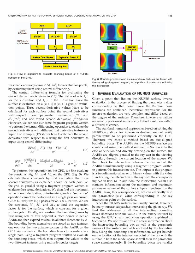
To perform this operation on the GPU, we first evaluatethe constants M1, M2, and M3 on the GPU (Fig. 5). Wecalculate these constants by first evaluating the threesecond-derivatives as explained above for each point onthe grid in parallel using a fragment program written toevaluate the second derivatives. We then find the maximumvalue of each derivative; unfortunately, such a “reduction”operation cannot be performed in a single pass on currentGPUs but requires logn passes for an n� n texture. We usethe constants, M1, M2, and M3, to find the expansionfactor K for the surface, which is constant for a givensurface patch. Finally, we construct the bounding boxes byfirst using sets of four adjacent surface points to get anAABB and then expand this box in all three directions by K.The bounding boxes themselves are stored as two textures,one each for the two extreme corners of the AABB, on theGPU. We evaluate all the bounding boxes for a surface in asingle pass using a fragment program written to evaluatethe bounding boxes, which then outputs the values to thetwo different textures using multiple render targets.

5 INVERSE EVALUATION OF NURBS SURFACES

Given a point that lies on the NURBS surface, inverseevaluation is the process of finding the parameter valuescorresponding to that point. Since the B-spline basisfunctions are nonlinear, theoretical expressions for theinverse evaluation are very complex and differ based onthe degree of the surfaces. Therefore, inverse evaluationsare usually performed numerically to find a solution withina desired tolerance.

The standard numerical approaches based on solving theNURBS equations for inverse evaluation are not easilyparallelizable to be performed efficiently on the GPU.Therefore, we chose a method based on axis-alignedbounding boxes. The AABBs for the NURBS surface areconstructed using the method outlined in Section 4. In thecase of selection and directly drawing on the surface, theAABBs are aligned parallel to the ray cast in the viewingdirection, through the current location of the mouse. Wethen check for intersection between the ray and all theAABBs simultaneously using a fragment program writtento perform this intersection test. The output of this programis a two-dimensional array of binary values with the value1, indicating the intersection of the ray with the correspond-ing AABB (Fig. 6). In addition, the intersecting AABB alsocontains information about the minimum and maximumparameter values of the surface subpatch enclosed by theAABB. Using this correspondence, we can efficiently findthe parametric ðu; vÞ value corresponding to the rayintersection point on the surface.

Since the NURBS surfaces are usually curved, there canbe many surface subpatches intersecting the given ray. Wefind the addresses of all the intersecting boundingboxes (locations with the value 1 in the binary texture) byusing the GPU stream reduction operation explained inSection 5.1. We use this address to access information aboutthe intersecting bounding box as well as the parametricranges of the surface subpatch enclosed by the boundingbox. Using the bounding box information, we get boundson the location of the intersection point of the ray with thesurface in both the model space as well as in the parametricspace simultaneously. If the bounding boxes are smaller


Fig. 5. Flow of algorithm to evaluate bounding boxes of a NURBS

surface on the GPU.Fig. 6. Bounding-boxes stored as min and max textures are tested with

the ray using a fragment program; its output is a binary texture indicating

the intersection.


than the required tolerance, we can take the midpoint of thebounding box as the intersection point of the ray withthe surface. Once all the ray intersection points on thesurface are found, we output only the point that is closestto the view plane by evaluating the distance of all the rayintersection points from the view plane on the CPU andchoosing the point with the smallest distance value.

5.1 GPU Stream Reduction

An essential operation in our inverse evaluation algorithmis to find the addresses of all the bounding boxes thatintersect with a particular ray so that we can use thisaddress to access information about the intersectingbounding box. In this operation, we find the indexes(location) of the texels in the texture that have the givenvalue (in this case, 1). This corresponds to a class ofproblems known as non-uniform stream reduction. Streamreduction is usually considered a serial operation since thenumber of elements in the output is not known, and hence,the whole input has to be operated upon to output thecorrect result. We build on previous work that developedparallel algorithms based on parallel prefix sum for thisoperation, which we summarized in Section 2. Implement-ing this parallel prefix sum on standard graphics hardwareis not straightforward, however, due to the lack of scatterfunctionality on standard programmable GPUs.

We first explain briefly the parallel stream reduction

operation described in [16]. It consists of three main steps: up-

sweep, down-sweep, and scatter. The up-sweep operation

computes a hierarchy of logn levels, where each element at a

higher level is obtained as a sum of two elements in the lower-

level (Algorithm 1). An example of the up-sweep operation isshown using an eight-element 1D array (Fig. 7). The last

element at the end of the operation gives the total number of

elements with the value 1 in the input array. After performing

this operation, we obtain a binary tree with the last element as

the root node and the original array as the leaf nodes; eachnode of this tree represents the sum of all the values in the

subtree of that node.

The down-sweep operation given by Algorithm 2, per-formed on the array resulting from Algorithm 1, computesthe exclusive prefix sum of the original input array. Theexclusive prefix sum of an array is defined as the sum of all thevalues preceding a particular position in the array notincluding the value in the position itself. Fig. 8 gives anexample of the down-sweep operation performed on theoutput shown in Fig. 7 in order to calculate the exclusiveprefix sum for the original input given in Fig. 7. The first stepof the down-sweep operation is to replace the last element(root element) in the array obtained after the up-sweepoperation with the value 0. Then in the consecutive steps, theparent element at each subarray is copied to the left element ofthe child array and the right element of the child array iscalculated as the sum of the old left element and the parentelement. In effect, every element now contains the sum of allthe elements to the left of itself in the tree structure.

The value of the exclusive prefix sum at the positionswhere the value of the input array is 1, gives the address towhich that particular input value has to be scattered toperform the stream reduction. The final step, after the up-sweep and down-sweep are completed, is the scatteroperation in which this address is used to reduce the inputstream such that the elements with value 1 are collected atthe front of the array.

However, we cannot directly use this stream reductionalgorithm on the GPU due to three issues. The first issue isthat the original algorithm was developed for one-dimen-sional arrays, and hence, has to be adapted to operate on atwo-dimensional texture. The second issue is that thetraditional GPGPU model based on OpenGL or DirectXdoes not allow the scatter operation, which is the last step ofthe stream reduction algorithm. Finally, the original


Fig. 7. Example of the up-sweep operation performed on a 1D array

given in the first row. The inputs indicated are summed at each step.

Fig. 8. Example of the down-sweep operation performed on the original

1D array given in Fig. 7. The elements corresponding to the values of 1

in the original input are highlighted in the result; these are the addresses

where those values are to be scattered.


formulation in [16] computed the prefix sum in situ bymodifying the input array. This is not possible using thestandard GPGPU framework since we cannot read andwrite to the same location simultaneously.

We solve the first problem by first assuming that each rowof the texture is a separate array and compute the first part ofthe up-sweep operation until each row array is reduced to asingle element. Now we again perform the up-sweepoperation on the array formed by concatenating all thesingle elements in a column along the column direction. Inthe example shown in Fig. 9b, we perform the up-sweepoperation on each row until we end up with the values incolumn 7. Then we perform the up-sweep operation oncolumn 7 and output the results to column 8. As shown in theexample, to overcome the restriction of reading and writingto the same memory location, we maintain a hierarchy of theinput texture. This method uses only twice the storage as theoriginal texture used, and a single fragment program writtento perform the summation can be repeatedly used. Wecompute the up-sweep operation in OðlognÞ passes.

We then perform the down-sweep operation in a similarmanner but in reverse order, by first performing theoperation along the columns and then extending it to therows to obtain the exclusive prefix sum of the input. Inthe example shown in Fig. 9c, each bold box contains theexclusive prefix sum of the corresponding bold box in Fig. 9b.

Once we have the output from the down-sweep operation,we extract the address of only those texels thathave the value1in the input texture (Fig. 9d). We reinterpret this texture as a

VBO and use a vertex program, written to output theaddressesof the inputvalueswithvalue1as (x; y) coordinates,to write to two separate channels of the output texture. Thesize of the output texture varies based on the number ofelements with value 1 in the input texture; it is equal to the firstsquare number larger than the number of elements with value1 in the input. This output texture is then directly used by theinverse evaluation and the surface-surface intersectionapplications for further processing.

5.2 GPU Implementation of Inverse Evaluation

The algorithm used for performing the full inverseevaluation is given pictorially in Fig. 11. The three stepsin the top row of Fig. 11—evaluating the surface, construct-ing bounding boxes, and finding intersecting boxes—areperformed on the GPU. The data corresponding to theselected bounding box are read back from the GPU. Wethen check on the CPU whether the ranges in the parametricdomain of the surface as well as the size of the boundingbox are within the required tolerance; for example, we canuse an absolute tolerance of 10�6 in the parametric spaceand a relative tolerance of 10�3 in the model space. If thetolerance conditions are met, we output the midpoint of theparametric range as the output of the inverse evaluation. Ifnot, we reevaluate the NURBS surface at a finer resolutionwithin the previously output parametric range(s). Thesetolerances are usually met within two or three iterationssince we evaluate the surface at a high resolution(1; 024� 1; 024) during each iteration.

5.3 Applications of Inverse Evaluation

We can build different modeling operations using theinverse evaluation algorithm as the basic module. Theseoperations include ray intersections, direct sketching onNURBS surfaces, and interactive trimming. Fig. 10a showsan example where we compute all the intersection points(two in this case, marked with red crosses) of a particularray with the surfaces of a toy model. By aligning the raydirection perpendicular to the view plane, we can use thesame algorithm for selecting a particular surface from agiven set of NURBS surfaces.

One of the most important advantages of a real-timealgorithm to perform inverse evaluation is the ability tosketch directly on the NURBS surface. The advantage comesfrom the fact that the curve is simultaneously sketched bothin the three-dimensional model space as well as in the two-dimensional parameter space. This helps in performing


Fig. 9. Different steps of the GPU stream reduction algorithm. (a) Input,

(b) Up sweep, (c) Down sweep, and (d) Scatter using VBO.

Fig. 10. Different NURBS modeling applications using inverse evaluation. (a) Ray intersection, (b) sketching directly on the surface, and

(c) interactive trimming: the eyes of the model were trimmed interactively.


modeling operations like extrusions and trimming, wherethe parameter space sketches are typically used for definingthese operations. Fig. 10b shows a curve sketched on aNURBS model and the curve in the parametric domain isshown in the inset.

By combining our sketching interface with the algorithmthat renders trimmed NURBS surfaces in real time, we canperform interactive trimming operations (Fig. 10c). Usingour interactive trimming application, the designer getsimmediate feedback on the result of the trimming opera-tion, unlike current commercial CAD systems.

6 NURBS INTERSECTION CURVE EVALUATION

Calculating the intersection curve of a surface-surfaceintersection is a frequently encountered operation in CADsystems. It forms an essential part of important CADoperations like trimming, filleting, and b-rep generationfrom Boolean operations. However, since it is a slowoperation, it is usually performed in the background, andthus, the user does not get real-time feedback except in thesimplest of cases. We present a GPU-accelerated surface-surface intersection algorithm to calculate intersectioncurves both in the model space as well as in the parametricspaces of both the surfaces.

We now give a broad overview of our surface-surfaceintersection algorithm. Our algorithm makes use of boundingbox hierarchies to accelerate the intersection operation. Weevaluate both intersecting surfaces using the GPU and thenuse the method described in Section 4 to construct the AABBsfor the surfaces, using the same coordinate frame. Weconstruct a hierarchy of bounding boxes by combining fourbounding boxes at one level to construct a single boundingbox in the next level. To find the intersection curve, we thentraverse along the hierarchy simultaneously for both thesurfaces and find the intersecting bounding boxes inthe lowest level using the GPU. At the same time, we alsoget the ranges in the parametric domain corresponding to theintersecting surface patches. We then check if the sizes of thebounding boxes as well as the parametric ranges are within auser-defined tolerance. Once the tolerance conditions aremet, we get a better estimate of the point on the intersectioncurve by intersecting the linearized surface patch within theintersecting bounding boxes.

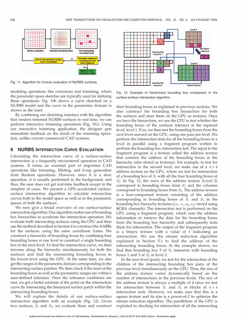
We will explain the details of our surface-surfaceintersection algorithm with an example (Fig. 12). Giventwo surfaces, S1 and S2, we evaluate them and construct

their bounding boxes as explained in previous sections. Wealso construct the bounding box hierarchies for boththe surfaces and store them on the GPU as textures. Oncewe have the hierarchies, we use the CPU to test whether thebounding boxes of the surfaces intersect at the topmostlevel, level 1. If so, we then test the bounding boxes from thenext level onward on the GPU, using one pass per level. Weperform the intersection tests for all the bounding boxes in alevel in parallel using a fragment program written toperform the bounding box intersection test. The input to thefragment program is a texture called the address texturethat contains the address of the bounding boxes in thehierarchy (also stored as textures). For example, to test forintersection in the second level, we make use of a 4� 4address texture on the GPU, where we test for intersectionof a bounding box of S1 with all the four bounding boxes ofS2. In Fig. 12, the rows of the address texture (Level 2)correspond to bounding boxes from S1 and the columnscorrespond to bounding boxes from S2. The address textureis a four-component texture consisting of the addresscorresponding to bounding boxes of S1 and S2 in thebounding box hierarchy textures (ðu1; v1; u2; v2Þ stored usingRGBA channels). The intersection test is performed on theGPU using a fragment program, which uses the addressinformation to retrieve the data for the bounding boxesfrom the bounding box hierarchy and subsequently teststhem for intersection. The output of the fragment programis a binary texture with a value of 1 indicating anintersection. We use the stream reduction algorithmexplained in Section 5.1 to find the address of theintersecting bounding boxes. In the example shown, wefind that bounding box 3 of S1 intersects with boundingboxes 1 and 3 of S2 at level 2.

In the next level (pass), we test for the intersection of thechildren of the intersecting bounding box pairs of theprevious level simultaneously on the GPU. Thus, the size ofthe address texture varies dynamically based on thenumber of intersections in the previous levels. The size ofthe address texture is always a multiple of 4 since we testfor intersection between S1 and S2 in blocks of 4� 4intersection tests. However, we make sure that this is asquare texture and its size is a power-of-2 to optimize thestream reduction algorithm. The parallelism of the GPU isexploited in checking for intersection of all the intersecting


Fig. 11. Algorithm for inverse evaluation of NURBS surfaces.

Fig. 12. Example of hierarchical bounding box comparison in the

surface-surface intersection algorithm.


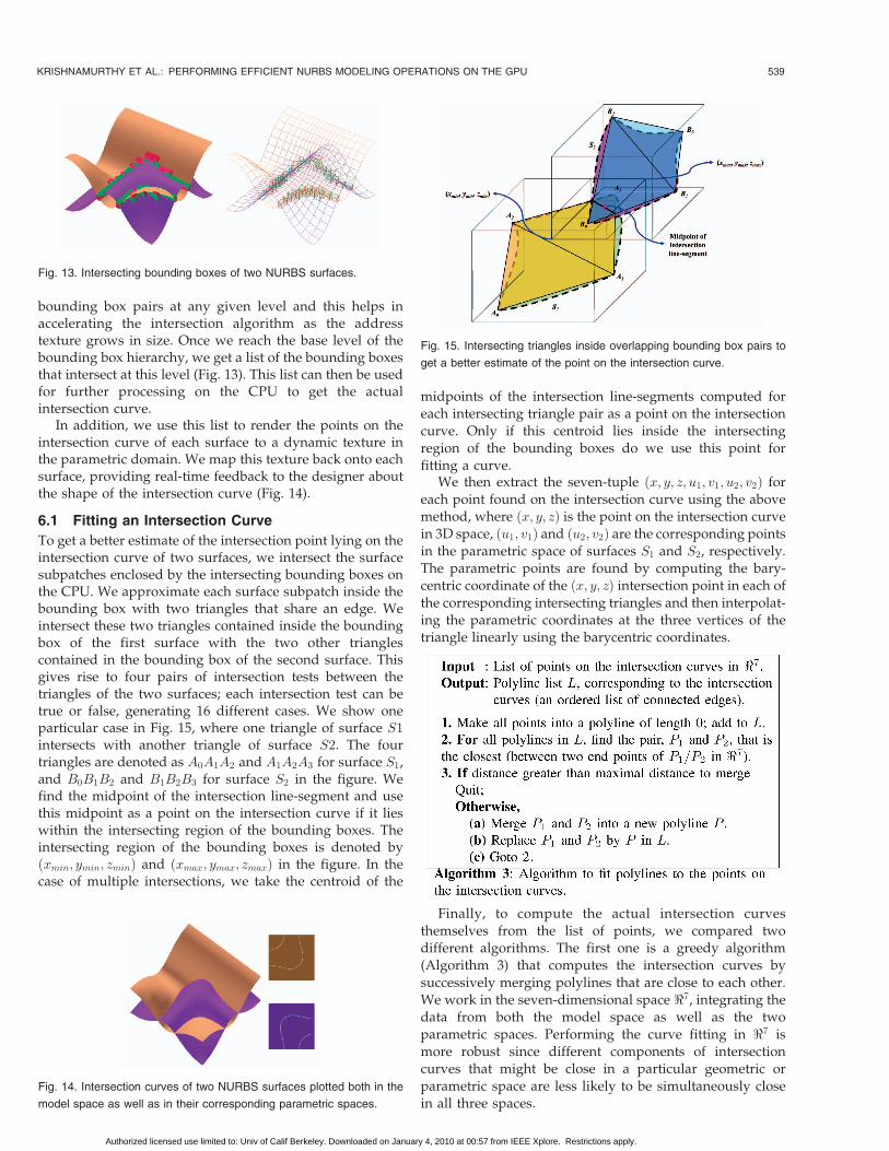
bounding box pairs at any given level and this helps inaccelerating the intersection algorithm as the addresstexture grows in size. Once we reach the base level of thebounding box hierarchy, we get a list of the bounding boxesthat intersect at this level (Fig. 13). This list can then be usedfor further processing on the CPU to get the actualintersection curve.

In addition, we use this list to render the points on theintersection curve of each surface to a dynamic texture inthe parametric domain. We map this texture back onto eachsurface, providing real-time feedback to the designer aboutthe shape of the intersection curve (Fig. 14).

6.1 Fitting an Intersection Curve

To get a better estimate of the intersection point lying on theintersection curve of two surfaces, we intersect the surfacesubpatches enclosed by the intersecting bounding boxes onthe CPU. We approximate each surface subpatch inside thebounding box with two triangles that share an edge. Weintersect these two triangles contained inside the boundingbox of the first surface with the two other trianglescontained in the bounding box of the second surface. Thisgives rise to four pairs of intersection tests between thetriangles of the two surfaces; each intersection test can betrue or false, generating 16 different cases. We show oneparticular case in Fig. 15, where one triangle of surface S1intersects with another triangle of surface S2. The fourtriangles are denoted as A0A1A2 and A1A2A3 for surface S1,and B0B1B2 and B1B2B3 for surface S2 in the figure. Wefind the midpoint of the intersection line-segment and usethis midpoint as a point on the intersection curve if it lieswithin the intersecting region of the bounding boxes. Theintersecting region of the bounding boxes is denoted byðxmin; ymin; zminÞ and ðxmax; ymax; zmaxÞ in the figure. In thecase of multiple intersections, we take the centroid of the

midpoints of the intersection line-segments computed foreach intersecting triangle pair as a point on the intersectioncurve. Only if this centroid lies inside the intersectingregion of the bounding boxes do we use this point forfitting a curve.

We then extract the seven-tuple ðx; y; z; u1; v1; u2; v2Þ foreach point found on the intersection curve using the abovemethod, where ðx; y; zÞ is the point on the intersection curvein 3D space, ðu1; v1Þ and ðu2; v2Þ are the corresponding pointsin the parametric space of surfaces S1 and S2, respectively.The parametric points are found by computing the bary-centric coordinate of the ðx; y; zÞ intersection point in each ofthe corresponding intersecting triangles and then interpolat-ing the parametric coordinates at the three vertices of thetriangle linearly using the barycentric coordinates.

Finally, to compute the actual intersection curvesthemselves from the list of points, we compared twodifferent algorithms. The first one is a greedy algorithm(Algorithm 3) that computes the intersection curves bysuccessively merging polylines that are close to each other.We work in the seven-dimensional space <7, integrating thedata from both the model space as well as the twoparametric spaces. Performing the curve fitting in <7 ismore robust since different components of intersectioncurves that might be close in a particular geometric orparametric space are less likely to be simultaneously closein all three spaces.


Fig. 13. Intersecting bounding boxes of two NURBS surfaces.

Fig. 14. Intersection curves of two NURBS surfaces plotted both in the

model space as well as in their corresponding parametric spaces.

Fig. 15. Intersecting triangles inside overlapping bounding box pairs to

get a better estimate of the point on the intersection curve.


The second algorithm (Algorithm 4) uses the fact that theintersection points we find are enclosed by AABBs that arepart of a regular grid. We can thus fit a polyline by connectinga point to the closest point whose enclosing bounding box is aneighbor to the enclosing bounding box of the current point,limiting our search to the one-ring neighborhood of boundingboxes. We still find the closest point in <7. After adding theclosest point in the one-ring neighborhood to the polyline, werepeat our search to find another point that is the closest to thepoint just added. Since the starting point can be in the middleof an intersection curve, we have to grow the polyline in bothdirections. This algorithm can be compared to a depth-firstsearch on a list to find all the connected components andhence takes OðnÞ time. However, if there is more than oneremaining adjacent bounding box with unmerged intersec-tion points, some points may not be merged into the polylineand will be output as polylines of length 1 (Fig. 16). Thesepolylines can then either be discarded or merged at the correctposition of the longer polylines by making an additional pass.

The time taken to fit a polyline using Algorithm 3 dependson an efficient closest neighbor query. Currently, we performthis operation through an exhaustive search that takes

Oðn2Þ time, which could be optimized by using more efficientsearch techniques, but we would still expect it to be slowerthan the OðnÞ time Algorithm 4. For the example shown inFig. 14, the polyline fitting for over 7,000 points takes0.20 seconds on a 2-GHz PC for a tolerance value of2� 10�3. On the other hand, the time taken by a single passof Algorithm 4 was 0.02 seconds for the same input andtolerance value. However, 320 single-point polylines werealso produced by Algorithm 4, which were discarded. From atolerant geometry point of view, discarding these points doesnot reduce the overall tolerance achieved compared toAlgorithm 3.

Since our input list of points on the intersection curve issufficiently dense, a polyline that passes through thesepoints can be directly used for further modeling operations.If a more compact representation is required, we can fit aNURBS curve of any required order that approximates thepoints on the intersection curve using standard curve-fittingtechniques. Since the intersection points obtained from ouralgorithm are enclosed within their corresponding bound-ing boxes both in the model space and in the parametricspace, we can guarantee a required bound on the results. Inaddition, if the arbitrary user-defined bounds are smallenough, we are guaranteed not to miss any portion of theintersection curve. Since we also give instantaneous visualfeedback to the user, the user will immediately know ifthere are any features missing and can reduce the toleranceto obtain the desired result.

One of the main limitations of both our algorithms forfitting a polyline is that they will fail to recreate the correcttopology when two unrelated intersection curves are veryclose on both surfaces. This can happen when an intersec-tion curve splits into two branches or when the two surfacesare locally flat and are touching each other. A method thatensures the topology of the intersection set is to be sought,possibly at the CPU level, using the GPU only to find thesimple intersection curves. Such a method will also help inbalancing the load between the CPU and the GPU.

6.2 Self-Intersection Evaluation

We extended our surface-surface intersection algorithm todetect and evaluate self-intersections in NURBS surfaces. Toperform the self-intersection test, we create two instances ofthe bounding box hierarchy for the surface on the GPU. Wethen test for intersection between these two surfaceinstances using the same GPU algorithm we use to performsurface-surface intersections. The output of this algorithm isa list of bounding box pairs at the lowest level of thehierarchy that overlap each other. We then remove fromthis list all the pairs which correspond to the same surfacesubpatch. Finally, if there are any bounding box pairs whichbelong to different surface subpatches left in the list, thenthe surface is self-intersecting.

Once we find a surface to be self-intersecting, we performtriangle-triangle intersection of the triangles containedwithin the intersecting bounding box pairs. Similar to thesurface-surface intersection algorithm, we find points on theself-intersection curve and then fit a polyline through thisself intersection curve. However, the main limitation of thealgorithm is that a self intersection smaller than the tolerancewill be rejected. This can occur in a local self-intersection due


Fig. 16. Example showing the possible generation of single-point

polyline by Algorithm 4. (a) The one-ring of bounding boxes (shaded).

(b) The point marked in red is not merged and is output as a single-point

polyline if it is not the closest point in <7.


to curvature in an offset surface, and a complete intersectionloop will be difficult to evaluate since the tolerance needs tobe infinitesimally small in this case. Fig. 17 shows twoexamples where we detect and evaluate self-intersectioncurves in NURBS surfaces. The example shown in Fig. 17btook 0.42 seconds to compute the self-intersection curves to atolerance value of 2� 10�3, while the more complicatedexample shown in Fig. 17a took 0.97 seconds.

6.3 Intersection Timing

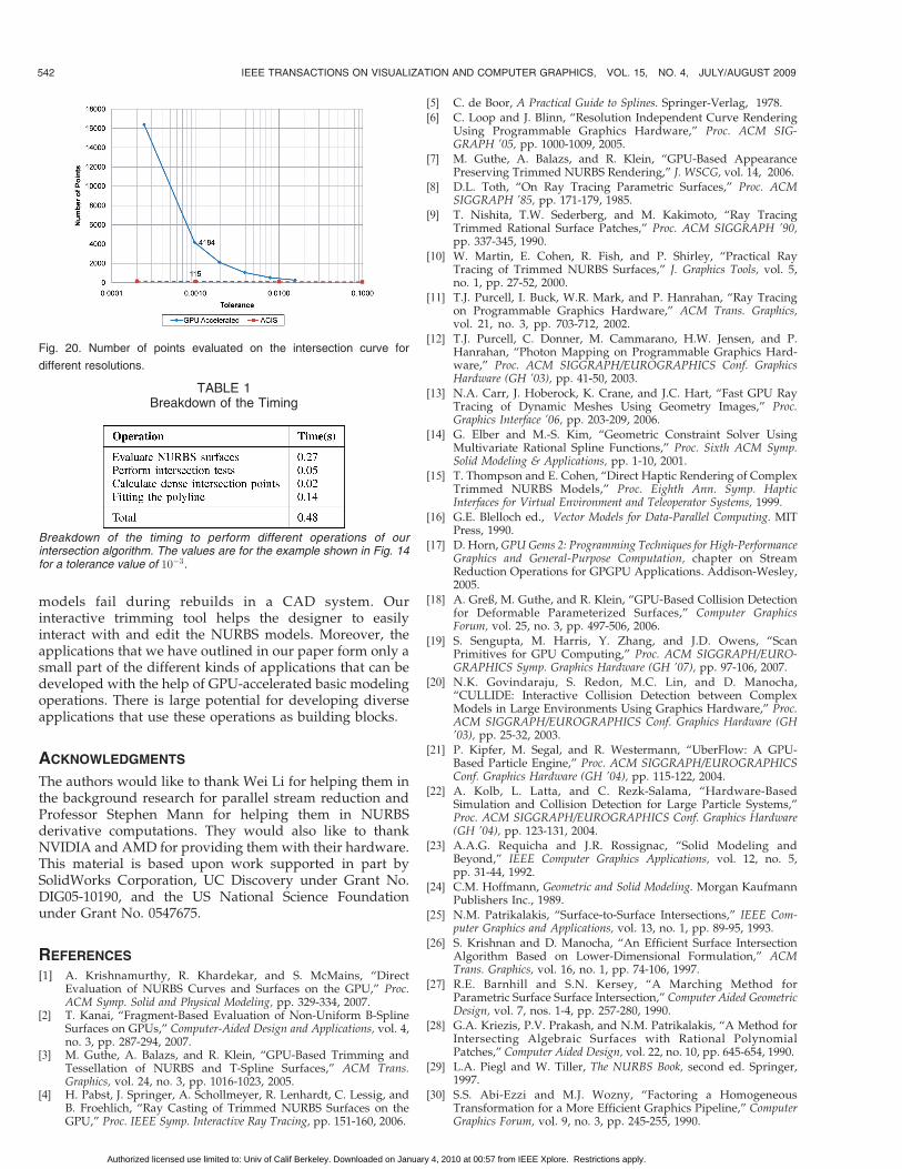
We timed our GPU-accelerated algorithm for evaluating theintersection curves on a 3-GHz CPU with 2 GB of RAMequipped with a NVIDIA Quadro FX4500 GPU with 512 MBgraphics memory running Windows XP. We performed asurface-surface intersection of the two NURBS surfacesshown in Fig. 18. The surfaces were bicubic NURBS with403� 199 and 298� 313 control points, respectively. Weused Algorithm 4 to fit the polylines during the timing. Wecompare our timings to evaluate the intersection curves tothe required user-defined tolerance with those of thecommercial solid modeling kernel ACIS (v18).

Fig. 19 compares the time for evaluating the intersectioncurves by varying the tolerance values. Our GPU-acceleratedevaluation is more than 40 times faster than ACIS incomputing the intersection curves to the standard toleranceof 10�3 used in ACIS. The output from ACIS is an interpolatedpolyline where the points on the polyline are within the user-defined tolerance value from the exact intersection curve.ACIS does not guarantee any tolerance on the piecewiselinear line segments that make up the polyline [32]. On theother hand, we evaluate dense intersection points with theirspacing adjusted based on the tolerance to achieve a

guaranteed tolerance on the piecewise linear segments ofthe polyline as well. We compute almost 40 times as manypoints on the intersection curve as ACIS does for the standardACIS tolerance value of 10�3 (Fig. 20).

Table 1 gives the breakdown of the timing of ourintersection algorithm for evaluating the intersectioncurves, shown in Fig. 14, for a tolerance value of 10�3.The evaluation of the NURBS surfaces is a large fraction ofthe total time. Note that we do not require such high-tolerance values for giving visual feedback; hence, it can beperformed at interactive rates.

7 CONCLUSIONS

We present fast algorithms to perform interactive modelingoperations on NURBS surfaces. Our algorithms do notrequire the latest graphics cards and are backward compa-tible with any graphics card that has basic programmingcapabilities. This is essential for the actual adoption of ouralgorithms in commercial CAD systems. We expect theperformance of our algorithms to only improve with theadvent of new and faster graphics cards.

Both our GPU algorithm to sketch on NURBS surfaces aswell as our GPU-accelerated algorithm to calculate inter-section curves give real-time feedback to the designer aboutthe shape of the curves in the parametric space. This gives adirect handle for the designer to check for inconsistency if


Fig. 17. Detection and evaluation of self-intersections in NURBS surfaces.

Fig. 18. NURBS surfaces used for timing the evaluation of intersection

curves.

Fig. 19. Time taken for evaluating the intersection curves of the two

NURBS surfaces shown in Fig. 18 with different resolutions. Note that

we are evaluating many more points on the intersection curve for a given

resolution (Fig. 20).


models fail during rebuilds in a CAD system. Ourinteractive trimming tool helps the designer to easilyinteract with and edit the NURBS models. Moreover, theapplications that we have outlined in our paper form only asmall part of the different kinds of applications that can bedeveloped with the help of GPU-accelerated basic modelingoperations. There is large potential for developing diverseapplications that use these operations as building blocks.

ACKNOWLEDGMENTS

The authors would like to thank Wei Li for helping them inthe background research for parallel stream reduction andProfessor Stephen Mann for helping them in NURBSderivative computations. They would also like to thankNVIDIA and AMD for providing them with their hardware.This material is based upon work supported in part bySolidWorks Corporation, UC Discovery under Grant No.DIG05-10190, and the US National Science Foundationunder Grant No. 0547675.

REFERENCES

[1] A. Krishnamurthy, R. Khardekar, and S. McMains, “DirectEvaluation of NURBS Curves and Surfaces on the GPU,” Proc.ACM Symp. Solid and Physical Modeling, pp. 329-334, 2007.

[2] T. Kanai, “Fragment-Based Evaluation of Non-Uniform B-SplineSurfaces on GPUs,” Computer-Aided Design and Applications, vol. 4,no. 3, pp. 287-294, 2007.

[3] M. Guthe, A. Balazs, and R. Klein, “GPU-Based Trimming andTessellation of NURBS and T-Spline Surfaces,” ACM Trans.Graphics, vol. 24, no. 3, pp. 1016-1023, 2005.

[4] H. Pabst, J. Springer, A. Schollmeyer, R. Lenhardt, C. Lessig, andB. Froehlich, “Ray Casting of Trimmed NURBS Surfaces on theGPU,” Proc. IEEE Symp. Interactive Ray Tracing, pp. 151-160, 2006.

[5] C. de Boor, A Practical Guide to Splines. Springer-Verlag, 1978.[6] C. Loop and J. Blinn, “Resolution Independent Curve Rendering

Using Programmable Graphics Hardware,” Proc. ACM SIG-GRAPH ’05, pp. 1000-1009, 2005.

[7] M. Guthe, A. Balazs, and R. Klein, “GPU-Based AppearancePreserving Trimmed NURBS Rendering,” J. WSCG, vol. 14, 2006.

[8] D.L. Toth, “On Ray Tracing Parametric Surfaces,” Proc. ACMSIGGRAPH ’85, pp. 171-179, 1985.

[9] T. Nishita, T.W. Sederberg, and M. Kakimoto, “Ray TracingTrimmed Rational Surface Patches,” Proc. ACM SIGGRAPH ’90,pp. 337-345, 1990.

[10] W. Martin, E. Cohen, R. Fish, and P. Shirley, “Practical RayTracing of Trimmed NURBS Surfaces,” J. Graphics Tools, vol. 5,no. 1, pp. 27-52, 2000.

[11] T.J. Purcell, I. Buck, W.R. Mark, and P. Hanrahan, “Ray Tracingon Programmable Graphics Hardware,” ACM Trans. Graphics,vol. 21, no. 3, pp. 703-712, 2002.

[12] T.J. Purcell, C. Donner, M. Cammarano, H.W. Jensen, and P.Hanrahan, “Photon Mapping on Programmable Graphics Hard-ware,” Proc. ACM SIGGRAPH/EUROGRAPHICS Conf. GraphicsHardware (GH ’03), pp. 41-50, 2003.

[13] N.A. Carr, J. Hoberock, K. Crane, and J.C. Hart, “Fast GPU RayTracing of Dynamic Meshes Using Geometry Images,” Proc.Graphics Interface ’06, pp. 203-209, 2006.

[14] G. Elber and M.-S. Kim, “Geometric Constraint Solver UsingMultivariate Rational Spline Functions,” Proc. Sixth ACM Symp.Solid Modeling & Applications, pp. 1-10, 2001.

[15] T. Thompson and E. Cohen, “Direct Haptic Rendering of ComplexTrimmed NURBS Models,” Proc. Eighth Ann. Symp. HapticInterfaces for Virtual Environment and Teleoperator Systems, 1999.

[16] G.E. Blelloch ed., Vector Models for Data-Parallel Computing. MITPress, 1990.

[17] D. Horn, GPU Gems 2: Programming Techniques for High-PerformanceGraphics and General-Purpose Computation, chapter on StreamReduction Operations for GPGPU Applications. Addison-Wesley,2005.

[18] A. Greß, M. Guthe, and R. Klein, “GPU-Based Collision Detectionfor Deformable Parameterized Surfaces,” Computer GraphicsForum, vol. 25, no. 3, pp. 497-506, 2006.

[19] S. Sengupta, M. Harris, Y. Zhang, and J.D. Owens, “ScanPrimitives for GPU Computing,” Proc. ACM SIGGRAPH/EURO-GRAPHICS Symp. Graphics Hardware (GH ’07), pp. 97-106, 2007.

[20] N.K. Govindaraju, S. Redon, M.C. Lin, and D. Manocha,“CULLIDE: Interactive Collision Detection between ComplexModels in Large Environments Using Graphics Hardware,” Proc.ACM SIGGRAPH/EUROGRAPHICS Conf. Graphics Hardware (GH’03), pp. 25-32, 2003.

[21] P. Kipfer, M. Segal, and R. Westermann, “UberFlow: A GPU-Based Particle Engine,” Proc. ACM SIGGRAPH/EUROGRAPHICSConf. Graphics Hardware (GH ’04), pp. 115-122, 2004.

[22] A. Kolb, L. Latta, and C. Rezk-Salama, “Hardware-BasedSimulation and Collision Detection for Large Particle Systems,”Proc. ACM SIGGRAPH/EUROGRAPHICS Conf. Graphics Hardware(GH ’04), pp. 123-131, 2004.

[23] A.A.G. Requicha and J.R. Rossignac, “Solid Modeling andBeyond,” IEEE Computer Graphics Applications, vol. 12, no. 5,pp. 31-44, 1992.

[24] C.M. Hoffmann, Geometric and Solid Modeling. Morgan KaufmannPublishers Inc., 1989.

[25] N.M. Patrikalakis, “Surface-to-Surface Intersections,” IEEE Com-puter Graphics and Applications, vol. 13, no. 1, pp. 89-95, 1993.

[26] S. Krishnan and D. Manocha, “An Efficient Surface IntersectionAlgorithm Based on Lower-Dimensional Formulation,” ACMTrans. Graphics, vol. 16, no. 1, pp. 74-106, 1997.

[27] R.E. Barnhill and S.N. Kersey, “A Marching Method forParametric Surface Surface Intersection,” Computer Aided GeometricDesign, vol. 7, nos. 1-4, pp. 257-280, 1990.

[28] G.A. Kriezis, P.V. Prakash, and N.M. Patrikalakis, “A Method forIntersecting Algebraic Surfaces with Rational PolynomialPatches,” Computer Aided Design, vol. 22, no. 10, pp. 645-654, 1990.

[29] L.A. Piegl and W. Tiller, The NURBS Book, second ed. Springer,1997.

[30] S.S. Abi-Ezzi and M.J. Wozny, “Factoring a HomogeneousTransformation for a More Efficient Graphics Pipeline,” ComputerGraphics Forum, vol. 9, no. 3, pp. 245-255, 1990.


Fig. 20. Number of points evaluated on the intersection curve for

different resolutions.

TABLE 1Breakdown of the Timing

Breakdown of the timing to perform different operations of ourintersection algorithm. The values are for the example shown in Fig. 14for a tolerance value of 10�3.


[31] D. Filip, R. Magedson, and R. Markot, “Surface Algorithms UsingBounds on Derivatives,” Computer Aided Geometric Design, vol. 3,no. 4, pp. 295-311, 1987.

[32] J. Corney and T. Lim, 3D Modeling with ACIS. Saxe-Coburg, 2001.

Adarsh Krishnamurthy received the bachelorsand masters degrees in mechanical engineeringfrom the Indian Institute of Technology, Madras.He is currently working toward the PhD degree inthe Department of Mechanical Engineering at theUniversity of California, Berkeley. His researchinterests include computer aided Design (CAD),solid modeling, GPU algorithms, computationalgeometry, and ultrasonic nondestructive testing.

Rahul Khardekar received the PhD degree inmechanical engineering from the University ofCalifornia, Berkeley. He is currently a 3D graphicsengineer in Align Technology, Inc. His researchinterests include computational geometry, com-puter graphics, and computer-aided design andmanufacturing.

Sara McMains received the PhD degree fromU.C. Berkeley in computer science. She iscurrently an associate professor of mechanicalengineering at the University of California,Berkeley. Her research interests include geo-metric design for manufacturing (DFM) feed-back, geometric and solid modeling, CAD/CAM,GPU algorithms, computer-aided process plan-ning, layered manufacturing, and virtual reality.

Kirk Haller received the degree from the University of Wisconsin—Ma-dison. He is currently a director of research at Dassault SystemesSolidWorks Corp., the leader in 3D CAD technology. The SolidWorks’Research Group is focused on advancing science and technology inorder to provide better tools for engineers, designers, and other creativeprofessionals. Prior to joining SolidWorks, he was an assistant professorat the University of Waterloo and a research assistant at DalhousieUniversity.

Gershon Elber received the BSc degree incomputer engineering and the MSc degree incomputer science from the Technion, Israel,in 1986 and 1987, respectively, and the PhDdegree in computer science from the Universityof Utah, in 1992. He is currently a professor in theComputer Science Department, Technion, Israel.His research interests include computer aidedgeometric designs and computer graphics. He isa member of the ACM and IEEE. He has served

on the editorial board of the Computer Aided Design, Computer GraphicsForum, the Visual Computer, and the International Journal of Computa-tional Geometry & Applications and has served in many conferenceprogram committees including Solid Modeling, Shape Modeling, Geo-metric Modeling and Processing, Pacific Graphics, Computer GraphicsInternational, and SIGGRAPH. He was one of the paper chairs of SolidModeling 2003 and Solid Modeling 2004, and will be the conference chairof Solid Modeling 2010. He has published over 150 papers in internationalconferences and journals and is one of the authors of a book titledGeometric Modeling with Splines—An Introduction.

. For more information on this or any other computing topic,please visit our Digital Library at www.computer.org/publications/dlib.



530 ieee transactions on visualization and computer ...mcmains/pubs... · 530 ieee transactions on...

Documents