Graph Mining

1

Graph Mining Graphs

Model sophisticated structures and their interactions

Chemical Informatics

Bioinformatics

Computer Vision

Video Indexing

Text Retrieval

Web Analysis

Social Networks

Mining frequent sub-graph patterns Characterization, Discrimination, Classification and Cluster Analysis,

building graph indices and similarity search

2

Mining Frequent Subgraphs Graph g

Vertex Set – V(g) Edge set – E(g) Label function maps a vertex / edge to a label Graph g is a sub-graph of another graph g’ if there exists a graph iso-

morphism from g to g’ Support(g) or frequency(g) – number of graphs in D = {G1, G2,..Gn} where

g is a sub-graph Frequent graph – satisfies min_sup

3

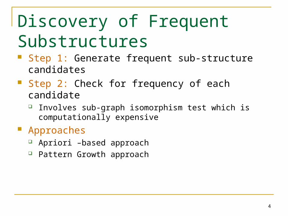
Discovery of Frequent Substructures Step 1: Generate frequent sub-structure candidates Step 2: Check for frequency of each candidate

Involves sub-graph isomorphism test which is computationally expensive

Approaches Apriori –based approach Pattern Growth approach

4

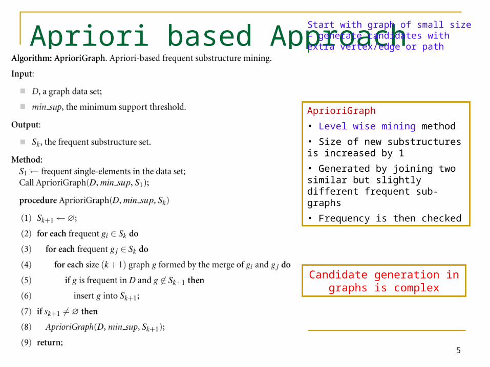
Apriori based Approach

5

Start with graph of small size – generate candidates with extra vertex/edge or path

AprioriGraph

• Level wise mining method

• Size of new substructures is increased by 1

• Generated by joining two similar but slightly different frequent sub-graphs

• Frequency is then checked

Candidate generation in graphs is complex

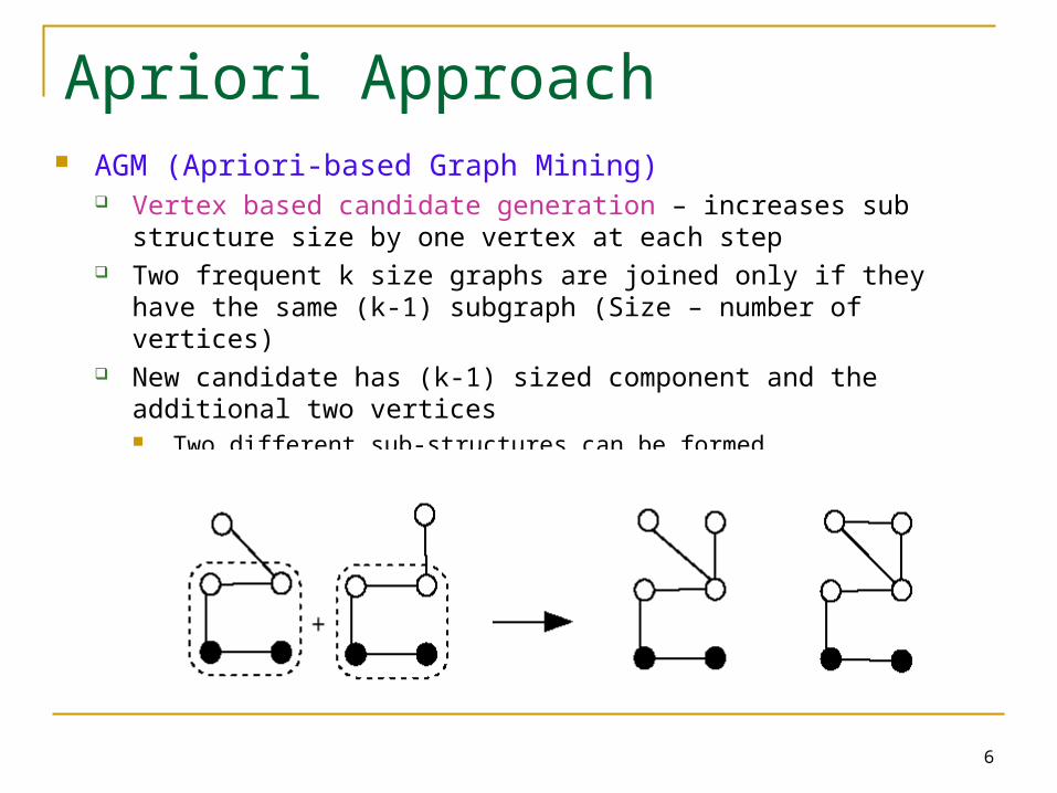
Apriori Approach AGM (Apriori-based Graph Mining)

Vertex based candidate generation – increases sub structure size by one vertex at each step

Two frequent k size graphs are joined only if they have the same (k-1) subgraph (Size – number of vertices)

New candidate has (k-1) sized component and the additional two vertices Two different sub-structures can be formed

6

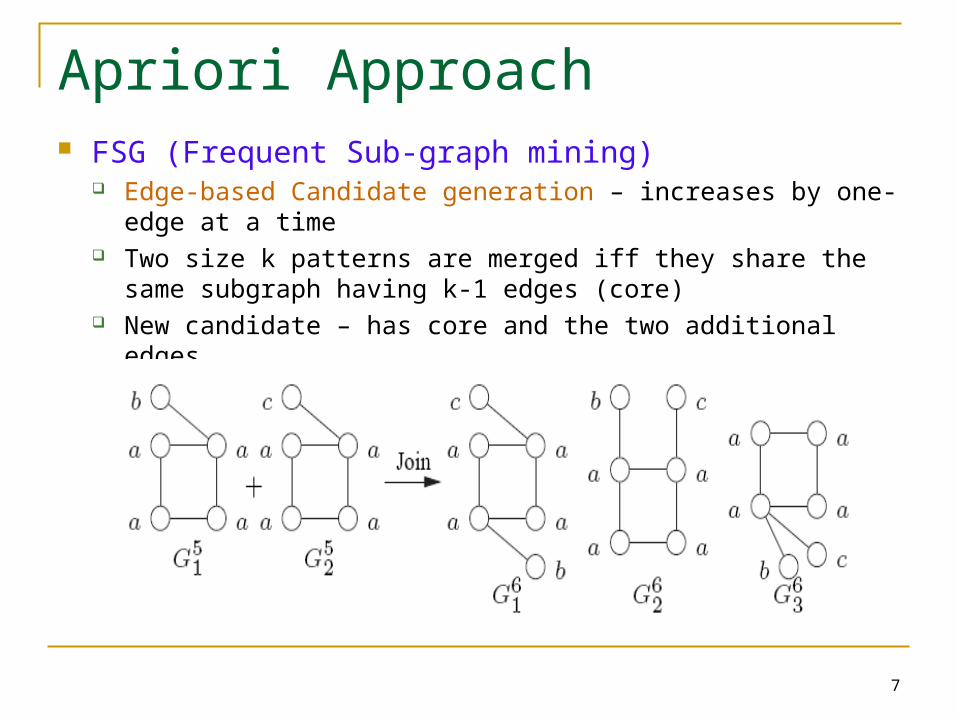
Apriori Approach FSG (Frequent Sub-graph mining)

Edge-based Candidate generation – increases by one-edge at a time

Two size k patterns are merged iff they share the same subgraph having k-1 edges (core)

New candidate – has core and the two additional edges

7

Apriori Approach

Edge disjoint path method

Classify graphs by number of disjoint paths they have

Two paths are edge-disjoint if they do not share any common edge

A substructure pattern with k+1 disjoint paths is generated by joining sub-structures with k disjoint paths

Disadvantage of Apriori Approaches

Overhead when joining two sub-structures

Uses BFS strategy : level-wise candidate generation

To check whether a k+1 graph is frequent – it must check all of its size-k sub graphs

May consume more memory

8

Pattern-Growth Approach Uses BFS as well as DFS

A graph g can be extended by adding a new edge e. The newly formed graph is denoted by g x e.

Edge e may or may not introduce a new vertex to g.

If e introduces a new vertex, the new graph is denoted by g xf e, otherwise, g xb e, where f or b indicates that the extension is in a forward or backward direction.

Pattern Growth Approach

For each discovered graph g performs extensions recursively until all frequent graphs with g are found

Simple but inefficient

Same graph is discovered multiple times – duplicate graph

9

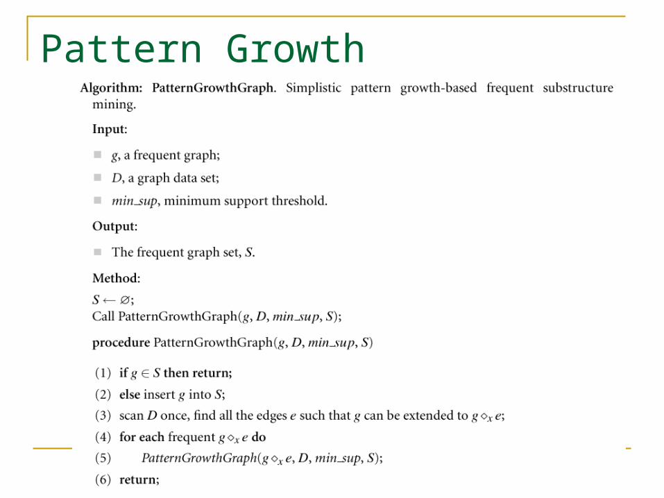
Pattern Growth

10

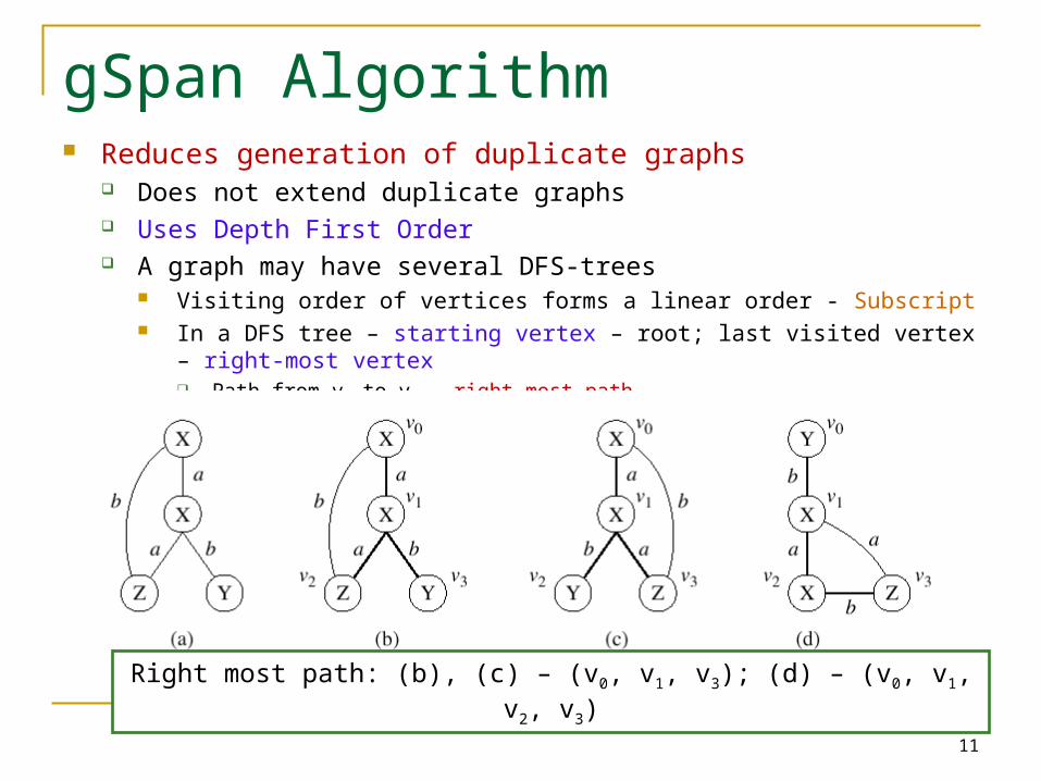
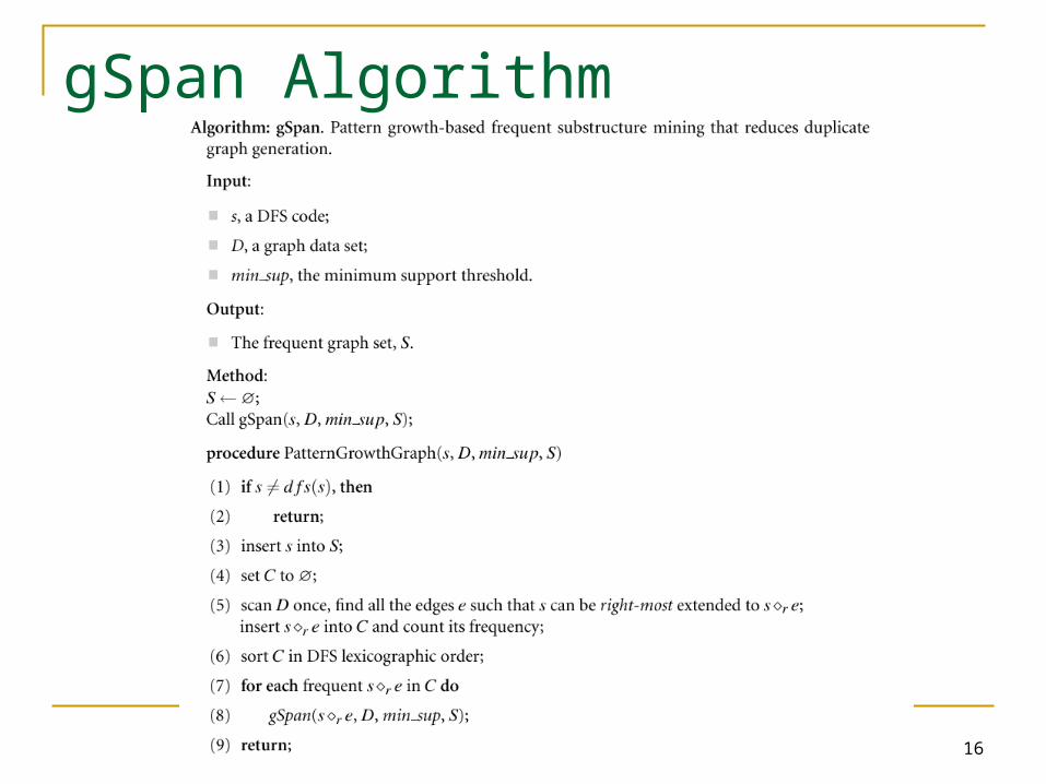
gSpan Algorithm Reduces generation of duplicate graphs

Does not extend duplicate graphs Uses Depth First Order A graph may have several DFS-trees

Visiting order of vertices forms a linear order - Subscript In a DFS tree – starting vertex – root; last visited vertex – right-most vertex

Path from v0 to vn – right most path

11

Right most path: (b), (c) – (v0, v1, v3); (d) – (v0, v1, v2, v3)

gSpan Algorithm gSpan restricts the extension method

A new edge e can be added between the right-most vertex and another vertex on the right-most path (backward

extension); or it can introduce a new vertex and connect to a vertex on the right-most path (forward

extension)

Right-most extension, denoted by G r e

12

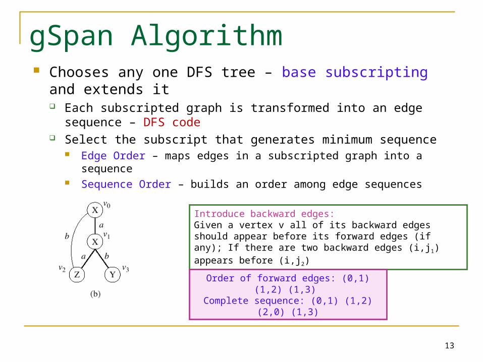
gSpan Algorithm Chooses any one DFS tree – base subscripting and

extends it Each subscripted graph is transformed into an edge sequence –

DFS code Select the subscript that generates minimum sequence

Edge Order – maps edges in a subscripted graph into a sequence Sequence Order – builds an order among edge sequences

13

Introduce backward edges: Given a vertex v all of its backward edges should appear before its forward edges (if any); If there are two backward edges (i,j1) appears before (i,j2)

Order of forward edges: (0,1) (1,2) (1,3) Complete sequence: (0,1) (1,2) (2,0) (1,3)

gSpan Algorithm

14

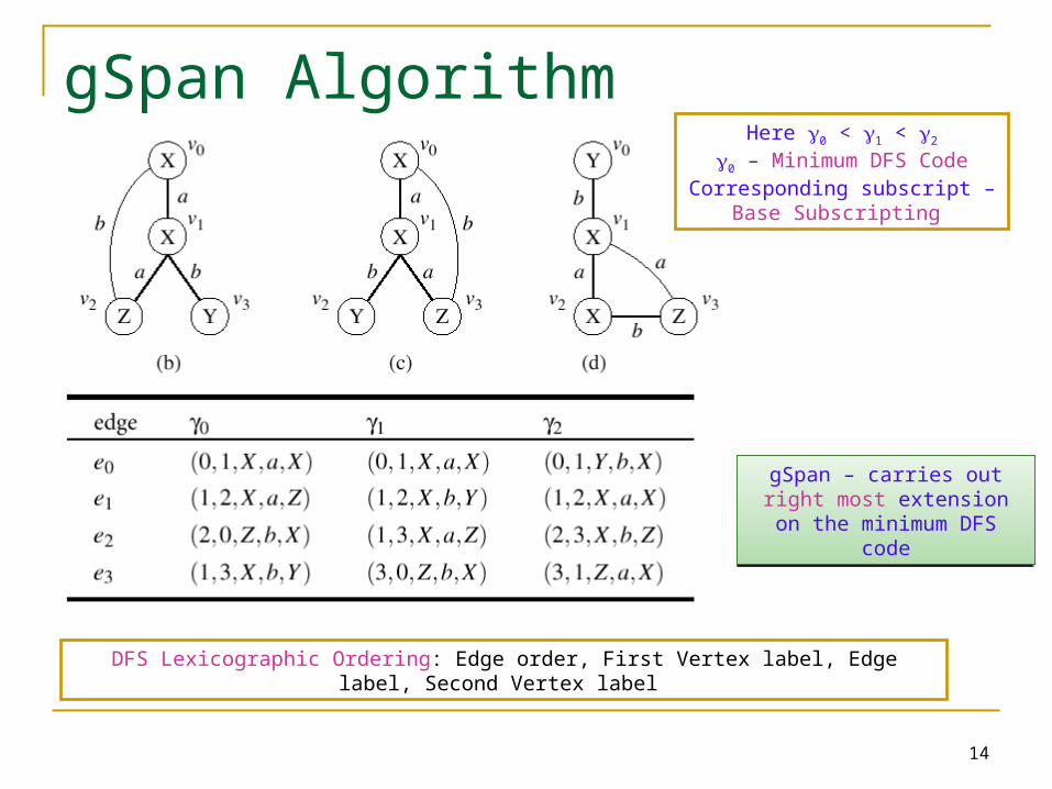
DFS Lexicographic Ordering: Edge order, First Vertex label, Edge label, Second Vertex label

Here 0 < 1 < 2

0 – Minimum DFS CodeCorresponding subscript – Base

Subscripting

gSpan – carries out right most extension on the minimum

DFS code

gSpan – carries out right most extension on the minimum

DFS code

gSpan Algorithm

Root – Empty code Each node is a DFS code encoding a graph Each edge – rightmost extension from a (k-1) length DFS code to a

k-length DFS code If codes s and s’ encode the same graph – search space s’ can be safely

pruned

15

gSpan Algorithm

16

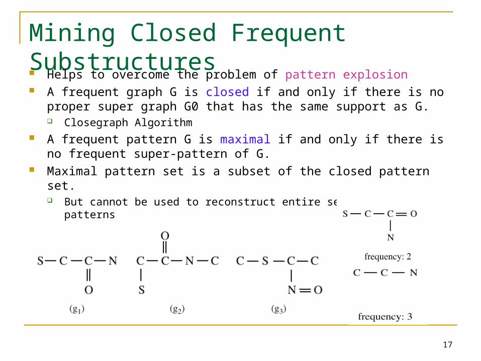
Mining Closed Frequent Substructures Helps to overcome the problem of pattern explosion A frequent graph G is closed if and only if there is no proper super graph G0

that has the same support as G. Closegraph Algorithm

A frequent pattern G is maximal if and only if there is no frequent super-pattern of G.

Maximal pattern set is a subset of the closed pattern set. But cannot be used to reconstruct entire set of frequent patterns

17

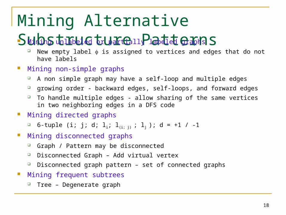
Mining Alternative Substructure Patterns Mining unlabeled or partially labeled graphs

New empty label is assigned to vertices and edges that do not have labels

Mining non-simple graphs A non simple graph may have a self-loop and multiple edges growing order - backward edges, self-loops, and forward edges To handle multiple edges - allow sharing of the same vertices in two neighboring

edges in a DFS code

Mining directed graphs 6-tuple (i; j; d; li; l(i; j) ; lj ); d = +1 / -1

Mining disconnected graphs Graph / Pattern may be disconnected Disconnected Graph – Add virtual vertex Disconnected graph pattern – set of connected graphs

Mining frequent subtrees Tree – Degenerate graph

18

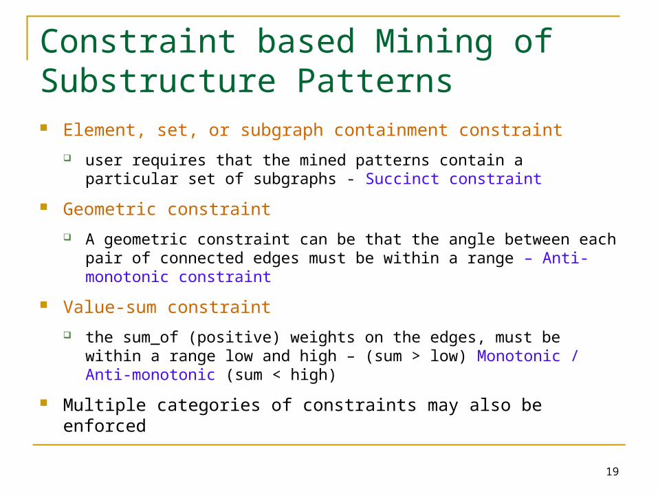
Constraint based Mining of Substructure Patterns Element, set, or subgraph containment constraint

user requires that the mined patterns contain a particular set of subgraphs - Succinct constraint

Geometric constraint

A geometric constraint can be that the angle between each pair of connected edges must be within a range – Anti-monotonic constraint

Value-sum constraint

the sum_of (positive) weights on the edges, must be within a range low and high – (sum > low) Monotonic / Anti-monotonic (sum < high)

Multiple categories of constraints may also be enforced

19

Mining Approximate Frequent Substructures Approximate frequent substructures allow slight structural variations

Several slightly different frequent substructures can be represented using one approximate substructure

SUBDUE – Substructure discovery system

based on the Minimum Description Length (MDL) principle

adopts a constrained beam search

SUBDUE performs approximate matching

20

Mining Coherent and Dense Sub structures A frequent substructure G is a coherent sub graph if the mutual information

between G and each of its own sub graphs is above some threshold Reduces number of patterns mined Application: coherent substructure mining selects a small subset of features that have high

distinguishing power between protein classes.

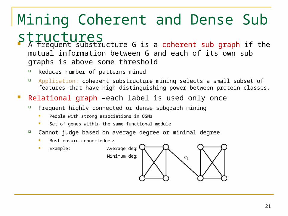
Relational graph –each label is used only once Frequent highly connected or dense subgraph mining

People with strong associations in OSNs

Set of genes within the same functional module

Cannot judge based on average degree or minimal degree Must ensure connectedness

Example: Average degree: 3.25

Minimum degree 3

21

Mining Dense Substructures Dense graphs defined in terms of Edge Connectivity

Given a graph G, an edge cut is a set of edges Ec such that E(G) - Ec is disconnected. A minimum cut is the smallest set in all edge cuts.

The edge connectivity of G is the size of a minimum cut.

A graph is dense if its edge connectivity is no less than a specified minimum cut threshold

Mining Dense substructures Pattern-growth approach called Close-Cut (Scalable)

starts with a small frequent candidate graph and extends it until it finds the largest super graph with the same support

Pattern-reduction approach called Splat (High performance) directly intersects relational graphs to obtain highly connected graphs

A pattern g discovered in a set is progressively intersected with subsequent components to give g’

Some edges in g may be removed

The size of candidate graphs is reduced by intersection and decomposition operations.

22

Applications – Graph Indexing Indexing is essential for efficient search and query processing Traditional approaches are not feasible for graphs

Indexing based on nodes / edges / sub-graphs Path based Indexing approach

Enumerate all the paths in a database up to maxL length and index them Index is used to identify all graphs with the paths in query Not suitable for complex graph queries

Structural information is lost when a query graph is broken apart

Many false positives maybe returned

gIndex – considers frequent and discriminative substructures as index features A frequent substructure is discriminative if its support cannot be approximated by the intersection of the

graph sets

Achieves good performance at less cost

23

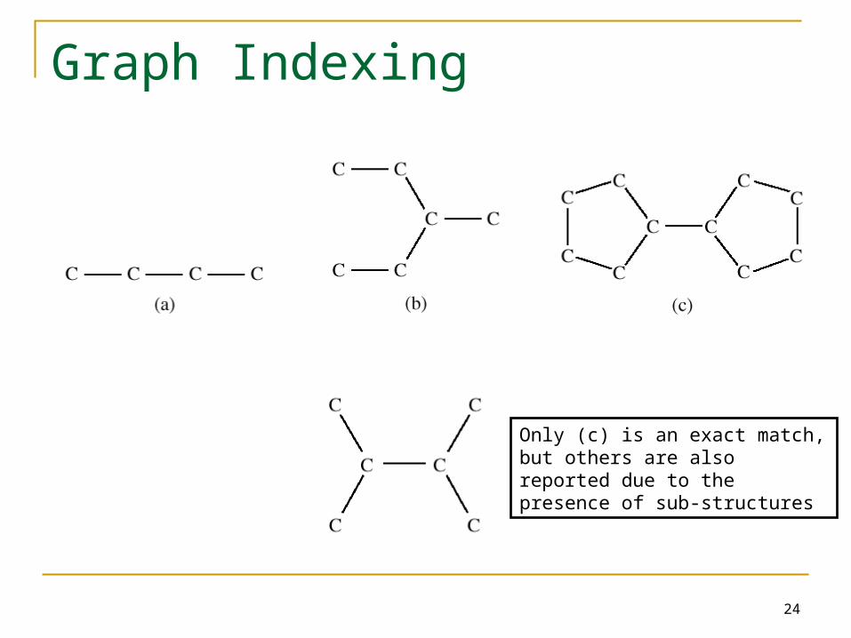
Graph Indexing

24

Only (c) is an exact match, but others are also reported due to the presence of sub-structures

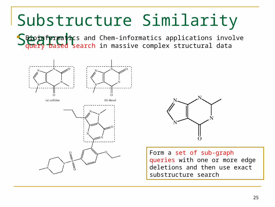
Substructure Similarity Search Bioinformatics and Chem-informatics applications involve query

based search in massive complex structural data

25

Form a set of sub-graph queries with one or more edge deletions and then use exact substructure search

Substructure Similarity Search Grafil (Graph Similarity Filtering)

Feature based structural filtering Models each query graph as a set of features

Edge deletions – feature misses Too many features – reduce performance Multi-filter composition strategy

Feature Set - group of similar features

26

Classification and Cluster Analysis using Graph Patterns Graph Classification

Mine frequent graph patterns Features that are frequent in one class but less in another – Discriminative

features – Model construction Can adjust frequency, connectivity thresholds SVM, NBM etc are used

Cluster Analysis Cluster Similar graphs based on graph connectivity (minimal cuts) Hierarchical clusters based on support threshold Outliers can also be detected

Inter-related process

27