localized methods in graph mining

Localized methods in !graph mining

David F. Gleich!Purdue University!

Joint work with Kyle Kloster @"Purdue & Michael Mahoney @ Berkeley supported by "NSF CAREER CCF-1149756 David Gleich · Purdue 1

David Gleich · Purdue 2

STORY TIME •  Simple theme •  Many pictures!


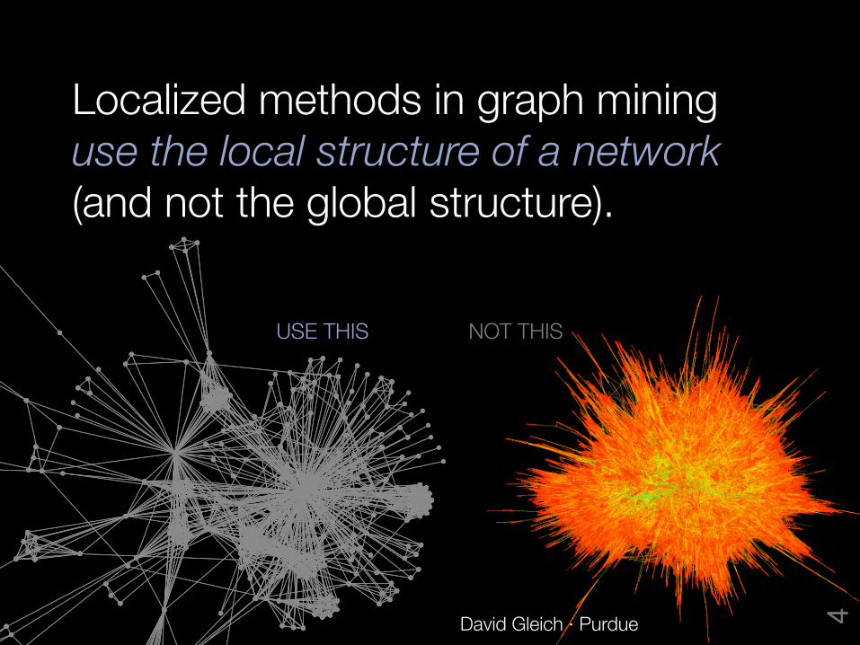
Localized methods in graph mining "use the local structure of a network !(and not the global structure).

USE THIS NOT THIS


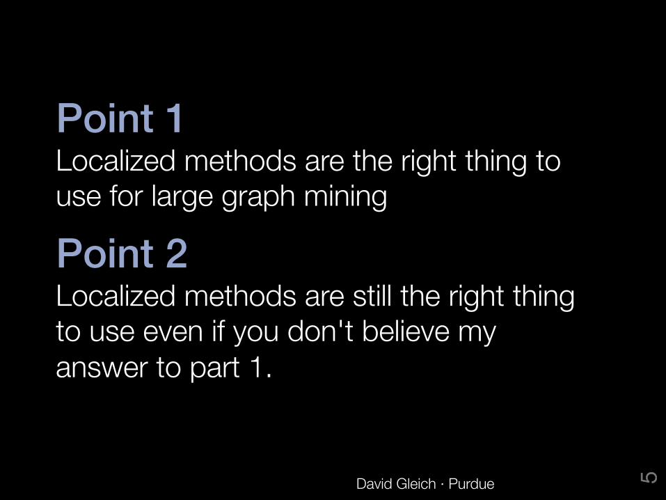
Point 1 "Localized methods are the right thing to use for large graph mining

Point 2 "Localized methods are still the right thing to use even if you don't believe my answer to part 1.


Some graphs have global structure


Image by R. Rossi from our paper"on clique detection for "

Temporal Strong-Components

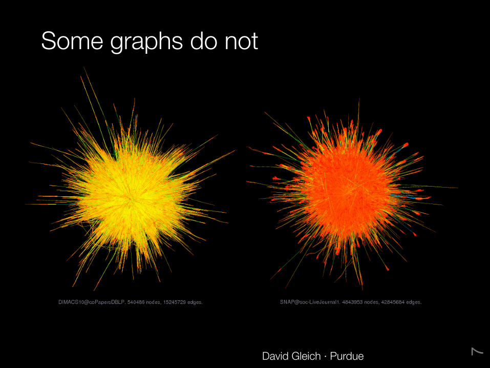
Some graphs do not


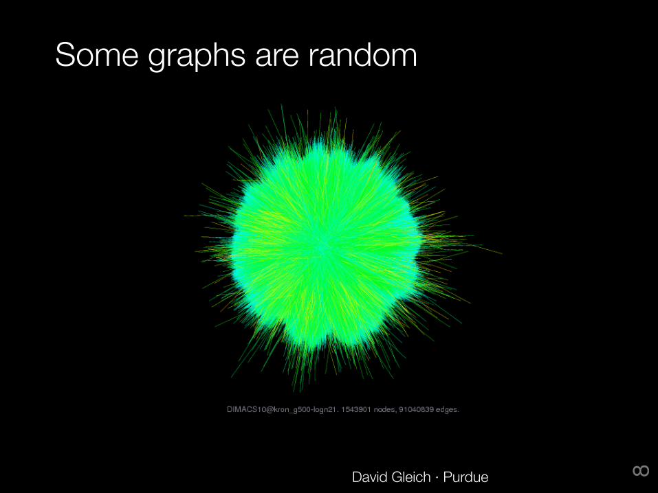
Some graphs are random


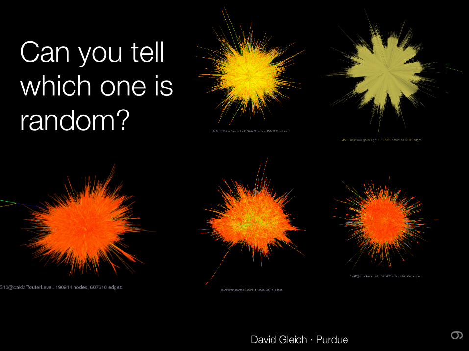
Can you tell which one is random?


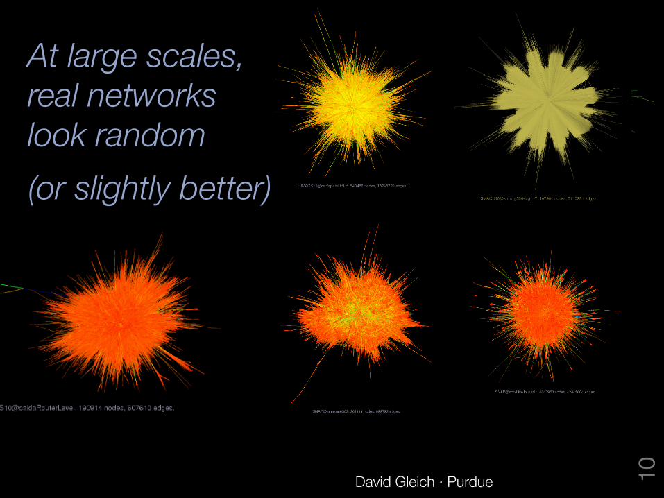
At large scales, !real networks !look random (or slightly better)


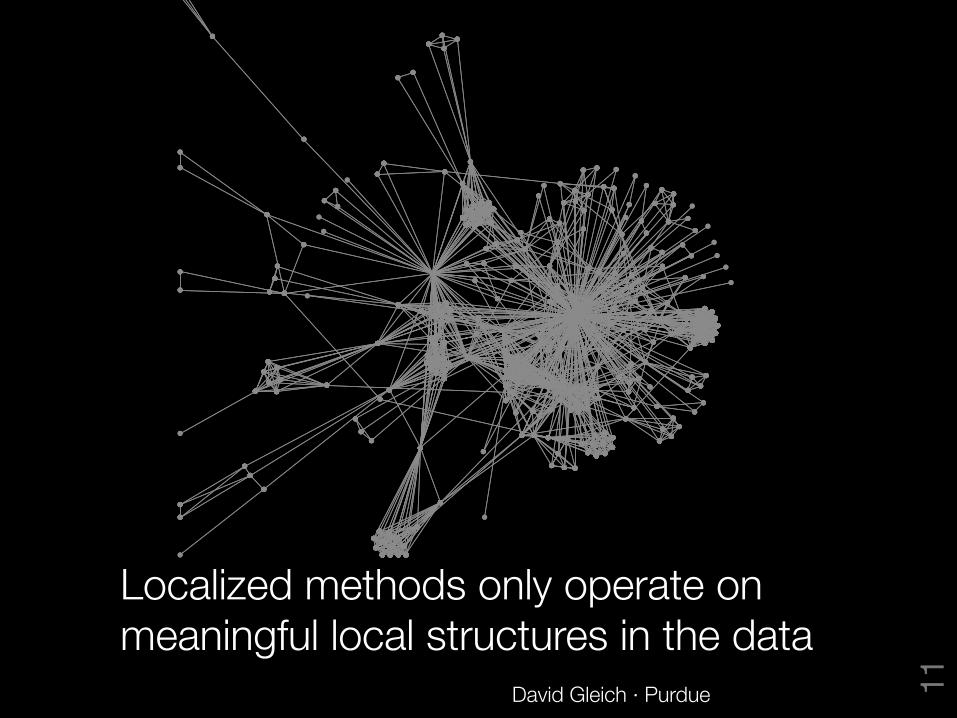
Localized methods only operate on meaningful local structures in the data


CAVEATS There are large-scale global structures. BUT They don’t look like what your small-scale intuition would predict. Continents exist in Facebook, but they don’t look small scale structures

Leskovec, Lang, Dasgupta, Mahoney. Internet Math, 2009. Ugander, Backstrom, WSDM (2013) Jeub, Balachandran, Porter, Mucha, Mahoney. Phys Rev E 2015.


Point 1 "Localized methods are the right thing to use for large graph mining

Point 2 "Localized methods are still the right thing to use even if you don't believe my answer to part 1.


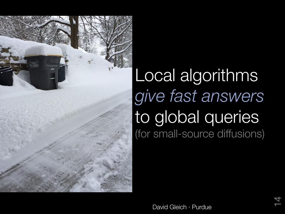
Local algorithms give fast answers to global queries "(for small-source diffusions)


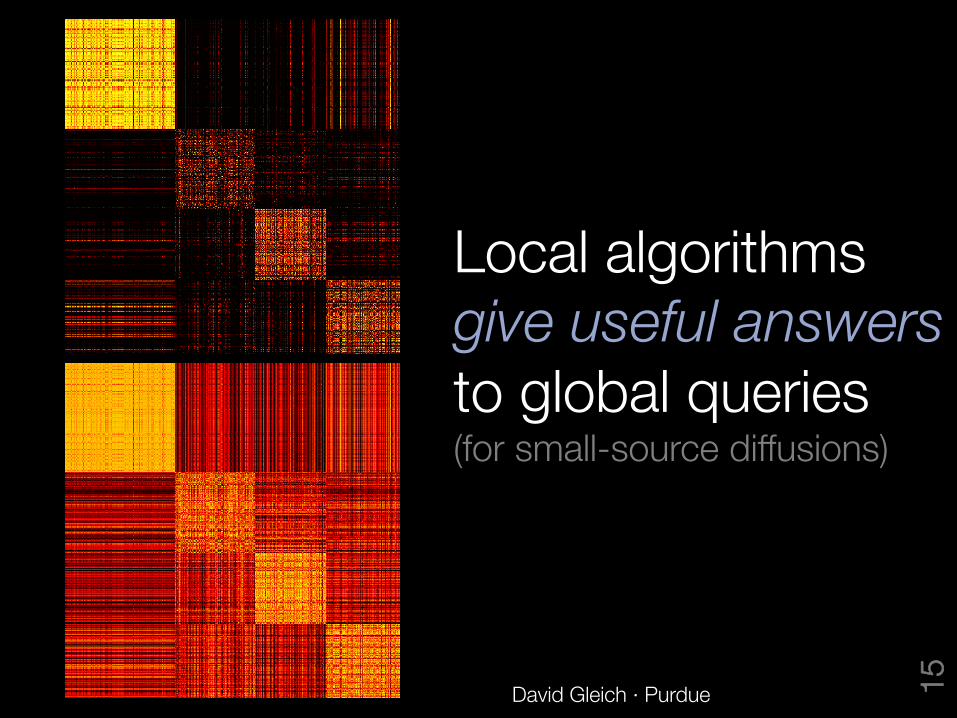
Local algorithms give useful answers to global queries "(for small-source diffusions)


Pictures from Sparse Matrix Respository (David & Hu) www.cise.ufl.edu/research/sparse/matrices/


Graph diffusions


34

feature

X R D S • S P R I N G 2 0 1 3 • V O L . 1 9 • N O . 3

damentally limited); the second type models a diffusion of a virtual good (think of sending links or a virus spread-ing on a network), which can be copied infinitely often. Google’s celebrated PageRank model uses a conservative diffusion to determine importance of pages on the Web [4], whereas those studying when a virus will continue to propagate found the eigenvalues of the non-conservative diffusion determine the answer [5]. Thus, just as in scientific computing, marrying the method to the model is key for the best scientific computing on social networks.

Ultimately, none of these steps dif-fer from the practice of physical sci-entific computing. The challenges in creating models, devising algorithms, validating results, and comparing models just take on different chal-lenges when the problems come from social data instead of physical mod-els. Thus, let us return to our starting question: What does the matrix have to do with the social network? Just as in scientific computing, many inter-esting problems, models, and meth-ods for social networks boil down to matrix computations. Yet, as in the expander example above, the types of matrix questions change dramatical-ly in order to fit social network mod-els. Let’s see what’s been done that’s enticingly and refreshingly different from the types of matrix computa-tions encountered in physical scien-tific computing.

EXPANDER GRAPHS AND PARALLEL COMPUTING Recently, a coalition of folks from aca-demia, national labs, and industry set out to tackle the problems in parallel computing and expander graphs. They established the Graph 500 benchmark (http://www.graph500.org) to measure the performance of a parallel com-puter on a standard graph computa-tion with an expander graph. Over the past three years, they’ve seen perfor-mance grow by more than 1,000-times through a combination of novel soft-ware algorithms and higher perfor-mance parallel computers. But, there is still work left in adapting the soft-ware innovations for parallel comput-ing back to matrix computations for social networks.

Figure 1. In a standard scientific computing problem, we find the steady state heat distribution of a plate with a heat-source in the middle. This scientific problem is solved via a linear system. In a social diffusion problem, we are trying to find people who like the movie (labeled in dark orange) instead of people who don’t like the movie (labeled in dark purple). By solving a different linear system, we can determine who is likely to enjoy the movie (light orange).

Problem

Diffusionin a plate

Movie interest indiffusion

Equations

�

�

�

�

Figure 2. The network, or mesh, from a typical problem in scientific computing resides in a low dimensional space—think of two or three dimensions. These physical spaces put limits on the size of the boundary or “surface area” of the space given its volume. No such limits exist in social networks and these two sets are usually about the same size. A network with this property is called an expander network.

Size of set ≈ Size of boundary

Size of set » Size of boundary

“Networks” from PDEs are usuallyphysical

Social networksare expanders

high

low

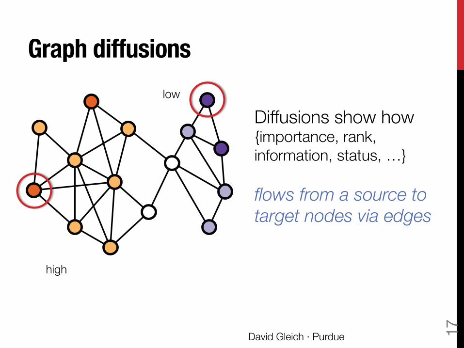
Diffusions show how {importance, rank, information, status, …} flows from a source to target nodes via edges

Graph diffusions


f =1X

k=0

↵k Pk s

34

feature






Problem

Diffusionin a plate


Equations

�

�

�

�






high

low

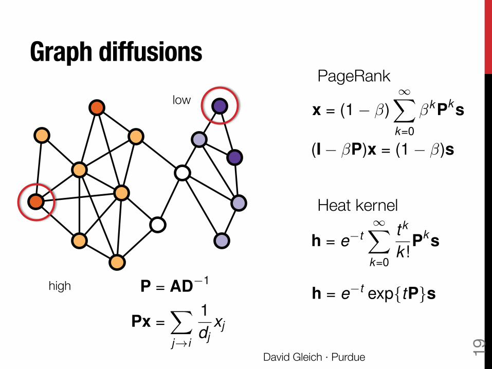
A – adjacency matrix!D – degree matrix!P – column stochastic operator s – the “seed” (a sparse vector) f – the diffusion result 𝛼k – the path weights

P = AD

�1

Px =X

j!i

1d

j

x

j

Graph diffusions help: 1.  Attribute prediction 2.  Community detection 3.  “Ranking” 4.  Find small conductance sets 5.  Graph label propagation

Graph diffusions


34

feature






Problem

Diffusionin a plate


Equations

�

�

�

�






high

low

h = e�t1X

k=0

tk

k !Pk s

h = e�texp{tP}s

PageRank

Heat kernel

x = (1 � �)1X

k=0

�kP

ks

(I � �P)x = (1 � �)s

P = AD

�1

Px =X

j!i

1d

j

x

j

Graph diffusions


h = e�t1X

k=0

tk

k !Pk s

h = e�texp{tP}s

PageRank

Heat kernel

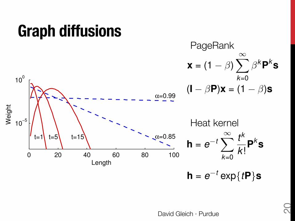
0 20 40 60 80 100

10−5

100

t=1 t=5 t=15 α=0.85

α=0.99

Weig

ht

Length

x = (1 � �)1X

k=0

�kP

ks

(I � �P)x = (1 � �)s

TwitterRank GeneRank IsoRank MonitorRank BookRank TimedPage-Rank

CiteRank AuthorRank PopRank FactRank ObjectRank FolkRank ItemRank

BuddyRank TwitterRank HostRank DirRank TrustRank BadRank VisualRank

PAGERANK BEYOND THE WEB 15

Fig. 4.2. PageRank vectors of the symbolic image, or Ulam network, of the Chirikov typical mapwith ↵ = 0.9 and uniform teleportation. From left to right, we show the standard PageRank vector,the weighted PageRank vector using the unweighted cell in-degree count as the weighting term, andthe reverse PageRank vector. Each node in the graph is a point (x, y), and it links to all other points(x, y) reachable via the map f (see the text). The graph is weighted by the likelihood of the transition.PageRank, itself, highlights both the attractors (the bright regions), and the contours of the transientmanifold that leads to the attractor. The weighted vector looks almost identical, but it exhibits aninteresting stippling e↵ect. The reverse PageRank highlights regions of the phase-space that are exitedquickly, and thus, these regions are dark or black in the PageRank vector. The solution vectors werescaled by the cube-root for visualization purposes. These figures are incredibly beautiful and showimportant transient regions of these dynamical systems.

winner networks. The intuitive idea underlying these rankings is that of a randomfan that follows a team until another team beats them, at which point they pickup the new team, and periodically restarts with an arbitrary team. In the Govanet al. [2008] construction, they corrected dangling nodes using a strongly preferentialmodification, although, we note that a sink preferential modification may have beenmore appropriate given the intuitive idea of a random fan. Radicchi [2011] usedPageRank on a network of tennis players with the same construction. Again, this wasa weighted network. PageRank with ↵ = 0.85 and uniform teleportation on the tennisnetwork placed Jimmy Conors in the best player position.

4.7. PageRank in literature: BookRank. PageRank methods help with threeproblems in literature. What are the most important books? Which story paths inhypertextual literature are most likely? And what should I read next?

For the first question, Jockers [2012] defines a complicated distance metric betweenbooks using topic modeling ideas from latent Dirichlet allocation [Blei et al., 2003].Using PageRank as a centrality measure on this graph, in concert with other graphanalytic tools, allows Jockers to argue that Jane Austin and Walter Scott are the mostoriginal authors of the 19th century.

Hypertextual literature contains multiple possible story paths for a single novel.Among American children of similar age to me, the most familiar would be the Chooseyour own adventure series. Each of these books consists of a set of storylets; at theconclusion of a storylet, the story either ends, or presents a set of possibilities forthe next story. Kontopoulou et al. [2012] argue that the random surfer model forPageRank maps perfectly to how users read these books. Thus, they look for the mostprobable storylets in a book. For this problem, the graphs are directed and acyclic,the stochastic matrix is normalized by outdegree, and we have a standard PageRankproblem. They are careful to model a weakly preferential PageRank system thatdeterministically transitions from a terminal (or dangling) storylet back to the start of

PAGERANK BEYOND THE WEB 5

Fig. 2.1. An illustration of the empirical properties of localized PageRank vectors with teleporta-tion to a single node in an isolated region. In the graph at left, the teleportation vector is the singlecircled node. The PageRank vector is shown as the node color in the right figure. PageRank valuesremain high within this region and are nearly zero in the rest of the graph. Theory from Andersenet al. [2006] explains when this property occurs.

theory. Instead, we’ll state this a bit informally. Suppose that we solve a localizedPageRank problem in a large graph, but the nodes we select for teleportation lie ina region that is somehow isolated, yet connected to the rest of the graph. Then thefinal PageRank vector is large only in this isolated region and has small values on theremainder of the graph. This behavior is exactly what most uses of localized PageRankwant: they want to find out what is nearby the selected nodes and far from the restof the graph. Proving this result involves spectral graph theory, Cheeger inequalities,and localized random walks – see Andersen et al. [2006] for more detail. Instead, weillustrate this theory with Figure 2.1.

Next, we will see some of the common constructions of the matrices P and P̄ thatarise when computing PageRank on a graph. These justify that PageRank is also asimple construction.

3. PageRank constructions. When a PageRank method is used within anapplication, there are two common motivations. In the centrality case, the input isa graph representing relationships or flows between a set of things – they may bedocuments, people, genes, proteins, roads, or pieces of software – and the goal is todetermine the expected importance of each piece in light of the full set of relationshipsand the teleporting behavior. This motivation was Google’s original goal in craftingPageRank. In the localized case, the input is also the same type of graph, but thegoal is to determine the importance relative to a small subset of the objects. Ineither case, we need to build a stochastic or sub-stochastic matrix from a graph. Inthis section, we review some of the common constructions that produce a PageRankor pseudo-PageRank system. For a visual overview of some of the possibilities, seeFigures 3.1 and 3.2.

Notation for graphs and matrices. Let A be the adjacency matrix for a graphwhere we assume that the vertex set is V = {1, . . . , n}. The graph could be directed,in which case A is non-symmetric, or undirected, in which case A is symmetric. Thegraph could also be weighted, in which case Ai,j gives the positive weight of edge (i, j).Edges with zero weight are assumed to be irrelevant and equivalent to edges that arenot present. For such a graph, let d be the vector of node out-degrees, or equivalently,the vector of row-sums: d = Ae. The matrix D is simply the diagonal matrix with don the diagonal. Weighted graphs are extremely common in applications when the

PageRank beyond the Web http://arxiv.org/abs/1407.5107

(I � ↵P)x = (1 � ↵)x

by Jessica Leber

Fast Magazine

21

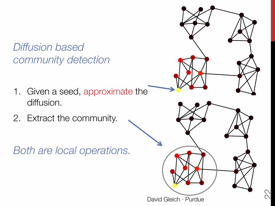
Diffusion based !community detection 1.  Given a seed, approximate the

diffusion. 2.  Extract the community.

Both are local operations.


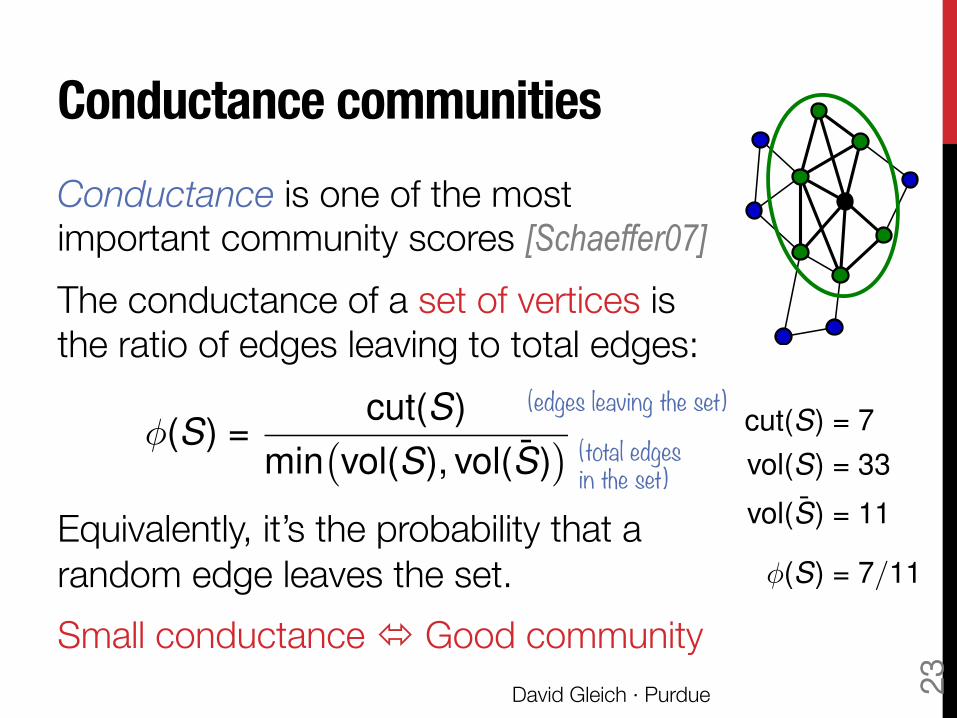
Conductance communities Conductance is one of the most important community scores [Schaeffer07] The conductance of a set of vertices is the ratio of edges leaving to total edges: Equivalently, it’s the probability that a random edge leaves the set. Small conductance ó Good community

�(S) =

cut(S)

min

�vol(S), vol(

¯S)

�(edges leaving the set)

(total edges in the set)

David Gleich · Purdue

cut(S) = 7

vol(S) = 33

vol(

¯S) = 11

�(S) = 7/11

23

Andersen-Chung-Lang!personalized PageRank community theorem![Andersen et al. 2006]![Ghosh et al. 2014, KDD]

Informally Suppose the seeds are in a set of good conductance, then a sweep-cut on a diffusion will find a set with conductance that’s nearly as good. … also, it’s really fast.


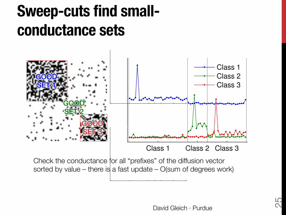
Sweep-cuts find small-conductance sets

594595596597598599600601602603604605606607608609610611612613614615616617618619620621622623624625626627628629630631632633634635636637638639640641642643644645646647

(a) The adjacencystructure of our samplewith the threeunbalanced classesindicated.

Class 1 Class 2 Class 3

Class 1

Class 2

Class 3


Class 1

Class 2

Class 3


Class 1

Class 2

Class 3

(b) Zhou (3 labels) (c) Andersen-Lang (3 labels) (d) Joachims (3 labels)


Class 1

Class 2

Class 3


Class 1

Class 2

Class 3


Class 1

Class 2

Class 3

(e) Zhou (15 labels) (f) Andersen-Lang (15 labels) (g) Joachims (15 labels)

Figure 4: A study of the paradoxical e↵ects of value-based rounding on di↵usion-based learning in asimple environment. With three labels, only Zhou et al.’s di↵usion has correct predictions, whereaswith 15 labels, none of the methods correctly predict the three classes. See the text for more aboutthe nature of the plots.

has 60 nodes. Class 1 has 30 nodes, class 2 has 10 nodes, and class 3 has 20 nodes. Thus, eachprediction matrix Y has three columns corresponding to each of the three classes. The remainingsubfigures show the matrix Y from the di↵usion-based learning methods we study: Zhou et al. (b, e);the Andersen-Lang weighting variation (c, f); and Joachims’s method (d, g). The top panel in each ofthe remaining subfigures shows the case of 3 labeled nodes (b, c, d), while the bottom panel in eachof the remaining subfigures shows the case of 15 labeled nodes (e, f, g). In each figure, note that eachcolumn of Y is displayed as a separate line, color-coded according to one of the three class label.

Let’s consider the top row with one labeled node from each class, i.e., that corresponding to using 3labeled nodes. The spikes in each vector represent the e↵ect of the labeled node on each di↵usion,while the values on the remaining nodes are the value of the di↵usion for that node. Note thatonly Zhou’s di↵usion with three labels and value-based rounding will correctly classify this simpleexample, agreeing with the simple intuition. The Andersen-Lang variation su↵ers from a degree-bias(in this simple case, it just weights Zhou’s di↵usion with the degree of the labeled node). Joachims’sdi↵usion misclassifies class 3 as class 1 because the near-clique like structure in class 1 dominates thedi↵usion e↵ects and the negative labels in class three are not enough to recover. Thus, the negativelabels have the e↵ect of changing the weight of each di↵usion.

When we move to 15 labels, we label one node from each class as before and the remaining 12 labelsare chosen uniformly at random. None of the methods classify the examples correctly and they alluniformly predict class 1. This occurs because there are more nodes randomly selected from class1, and it receives a higher overall weight. We make two observations here. First, there are a varietyof very reasonable and well-motivated heuristic corrections that would eliminate these e↵ects andrestore the performance of value based rounding, and the introduction of these heuristics is common.Second, the rank-based rounding has good performance in all these cases, regardless of the particulardi↵usion employed. To see this, look at the ranking (essentially, fix a color, and move along the Yaxis from the top, and observe which nodes are “hit”) on each color in the bottom panel of each ofthese subfigures. All of the di↵usion show raised levels for the correct class, and these correct classesare revealed by the rank-based rounding scheme, thus yielding far more robust predictions.

C USPS digits

Next, we move on to USPS digits example.

12

594595596597598599600601602603604605606607608609610611612613614615616617618619620621622623624625626627628629630631632633634635636637638639640641642643644645646647

(a) The adjacencystructure of our samplewith the threeunbalanced classesindicated.


Class 1

Class 2

Class 3


Class 1

Class 2

Class 3


Class 1

Class 2

Class 3

(b) Zhou (3 labels) (c) Andersen-Lang (3 labels) (d) Joachims (3 labels)


Class 1

Class 2

Class 3


Class 1

Class 2

Class 3


Class 1

Class 2

Class 3

(e) Zhou (15 labels) (f) Andersen-Lang (15 labels) (g) Joachims (15 labels)

Figure 4: A study of the paradoxical e↵ects of value-based rounding on di↵usion-based learning in asimple environment. With three labels, only Zhou et al.’s di↵usion has correct predictions, whereaswith 15 labels, none of the methods correctly predict the three classes. See the text for more aboutthe nature of the plots.

has 60 nodes. Class 1 has 30 nodes, class 2 has 10 nodes, and class 3 has 20 nodes. Thus, eachprediction matrix Y has three columns corresponding to each of the three classes. The remainingsubfigures show the matrix Y from the di↵usion-based learning methods we study: Zhou et al. (b, e);the Andersen-Lang weighting variation (c, f); and Joachims’s method (d, g). The top panel in each ofthe remaining subfigures shows the case of 3 labeled nodes (b, c, d), while the bottom panel in eachof the remaining subfigures shows the case of 15 labeled nodes (e, f, g). In each figure, note that eachcolumn of Y is displayed as a separate line, color-coded according to one of the three class label.

Let’s consider the top row with one labeled node from each class, i.e., that corresponding to using 3labeled nodes. The spikes in each vector represent the e↵ect of the labeled node on each di↵usion,while the values on the remaining nodes are the value of the di↵usion for that node. Note thatonly Zhou’s di↵usion with three labels and value-based rounding will correctly classify this simpleexample, agreeing with the simple intuition. The Andersen-Lang variation su↵ers from a degree-bias(in this simple case, it just weights Zhou’s di↵usion with the degree of the labeled node). Joachims’sdi↵usion misclassifies class 3 as class 1 because the near-clique like structure in class 1 dominates thedi↵usion e↵ects and the negative labels in class three are not enough to recover. Thus, the negativelabels have the e↵ect of changing the weight of each di↵usion.

When we move to 15 labels, we label one node from each class as before and the remaining 12 labelsare chosen uniformly at random. None of the methods classify the examples correctly and they alluniformly predict class 1. This occurs because there are more nodes randomly selected from class1, and it receives a higher overall weight. We make two observations here. First, there are a varietyof very reasonable and well-motivated heuristic corrections that would eliminate these e↵ects andrestore the performance of value based rounding, and the introduction of these heuristics is common.Second, the rank-based rounding has good performance in all these cases, regardless of the particulardi↵usion employed. To see this, look at the ranking (essentially, fix a color, and move along the Yaxis from the top, and observe which nodes are “hit”) on each color in the bottom panel of each ofthese subfigures. All of the di↵usion show raised levels for the correct class, and these correct classesare revealed by the rank-based rounding scheme, thus yielding far more robust predictions.

C USPS digits

Next, we move on to USPS digits example.

12

GOOD !SET 1!

Check the conductance for all “prefixes” of the diffusion vector sorted by value – there is a fast update – O(sum of degrees work)

GOOD !SET 2!

GOOD !SET 3!


Diffusions are localized "and we have algorithms to find their local regions


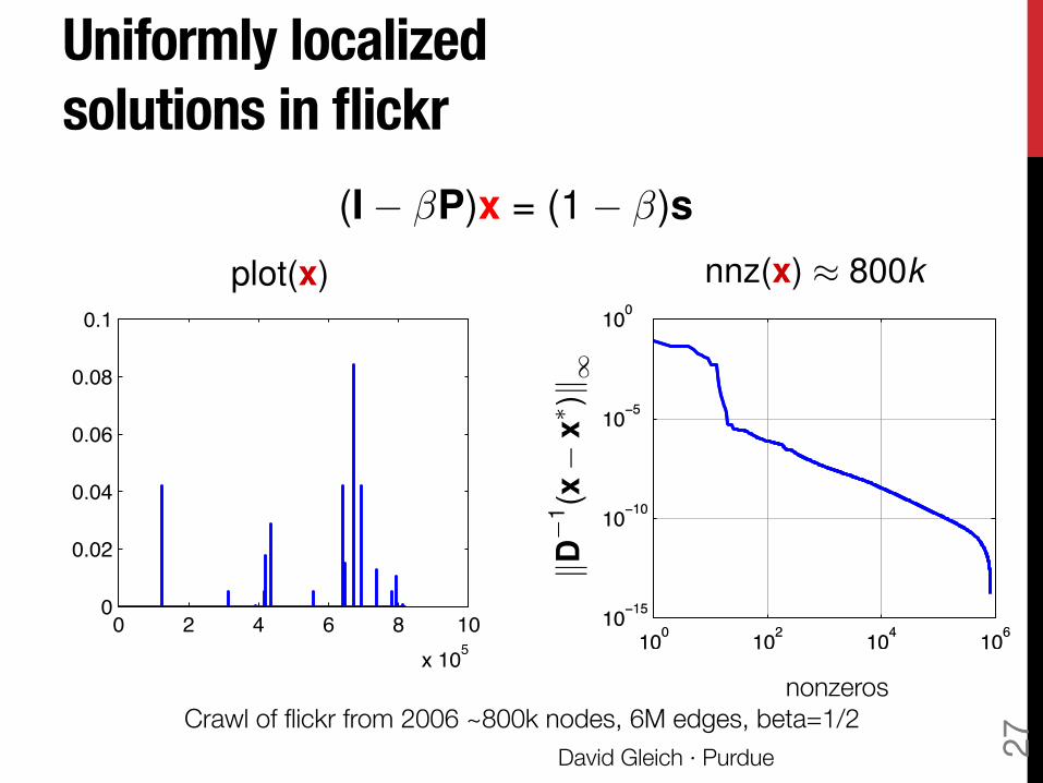
Uniformly localized !solutions in flickr

plot(x)


0 2 4 6 8 10x 105

0

0.02

0.04

0.06

0.08

0.1

100 102 104 10610−15

10−10

10−5

100

100 102 104 10610−15

10−10

10−5

100

nonzeros Crawl of flickr from 2006 ~800k nodes, 6M edges, beta=1/2

(I � �P)x = (1 � �)snnz(x) ⇡ 800k

kD�

1 (x�

x

⇤ )k 1

"

Our mission!Find the solution with work "roughly proportional to the "localization, not the matrix.


Our Point"The push procedure gives "localized algorithms for diffusions "in a pleasingly wide variety of settings.

Our Results"New empirical and theoretical insights into why and how “push” is so effective


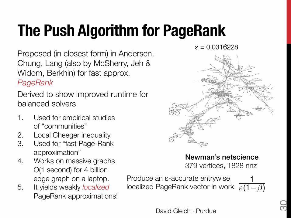
The Push Algorithm for PageRank Proposed (in closest form) in Andersen, Chung, Lang (also by McSherry, Jeh & Widom, Berkhin) for fast approx. PageRank Derived to show improved runtime for balanced solvers


1.  Used for empirical studies of “communities”

2.  Local Cheeger inequality. 3.  Used for “fast Page-Rank

approximation” 4.  Works on massive graphs

O(1 second) for 4 billion edge graph on a laptop.

5.  It yields weakly localized PageRank approximations!

Newman’s netscience!379 vertices, 1828 nnz Produce an ε-accurate entrywise

localized PageRank vector in work 1

"(1��)

Gauss-Seidel and !Gauss-Southwell


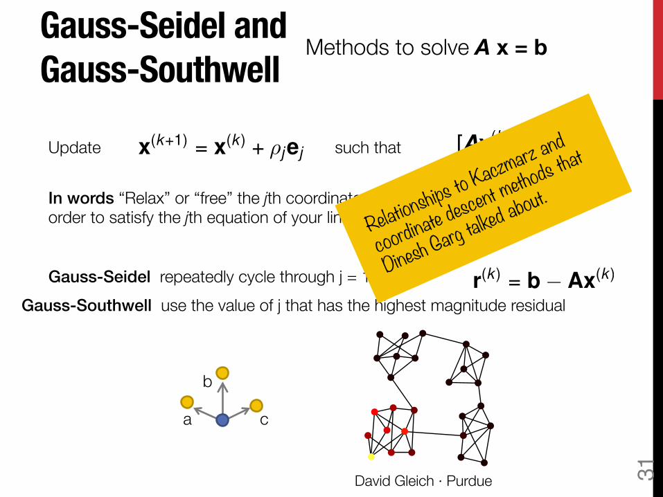
Methods to solve A x = b

x

(k+1) = x

(k ) + ⇢jej [Ax

(k+1)]j = [b]jUpdate such that

In words “Relax” or “free” the jth coordinate of your solution vector in order to satisfy the jth equation of your linear system.

Gauss-Seidel repeatedly cycle through j = 1 to n Gauss-Southwell use the value of j that has the highest magnitude residual

r

(k ) = b � Ax

(k )

a

b

c

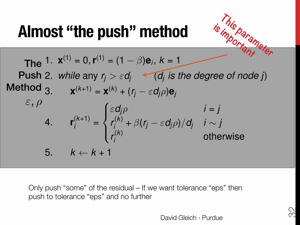
Almost “the push” method The

Push Method!


1. x

(1)

= 0, r

(1)

= (1� �)e

i

, k = 1

2. while any r

j

> "dj

(d

j

is the degree of node j)

3. x

(k+1)

= x

(k )

+ (r

j

� "dj

⇢)e

j

4. r

(k+1)

i

=

8><

>:

"dj

⇢ i = j

r

(k )

i

+ �(r

j

� "dj

⇢)/d

j

i ⇠ j

r

(k )

i

otherwise

5. k k + 1

", ⇢

Only push “some” of the residual – If we want tolerance “eps” then push to tolerance “eps” and no further

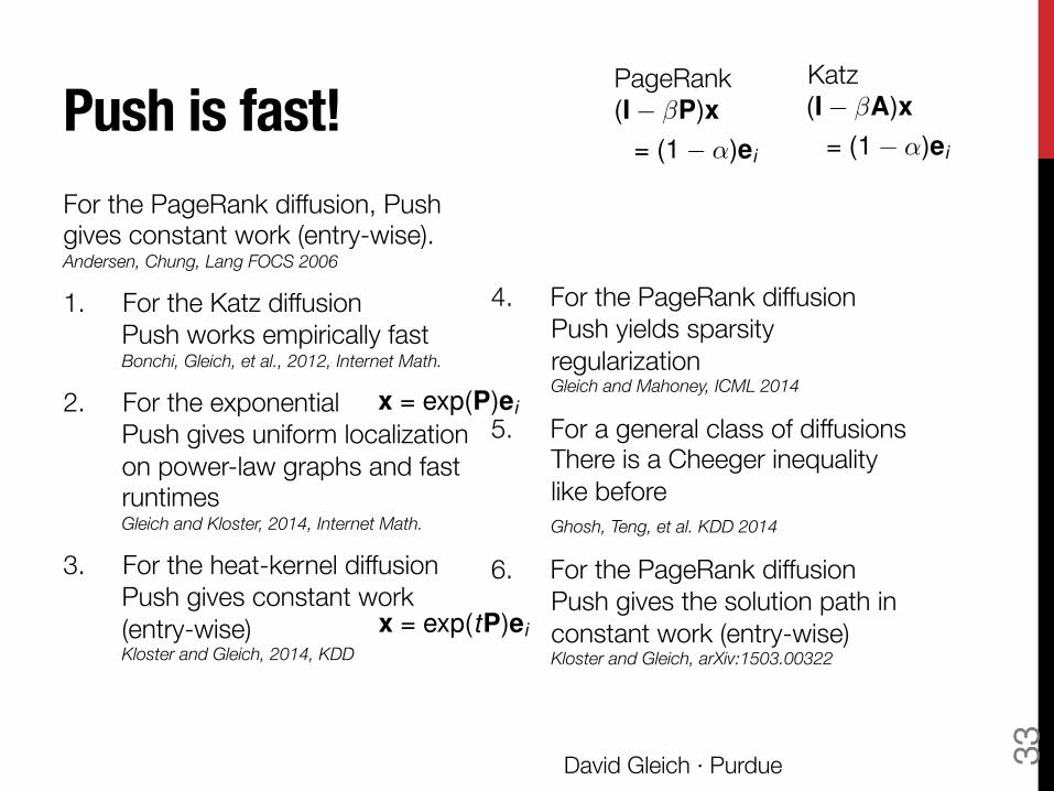
Push is fast! For the PageRank diffusion, Push gives constant work (entry-wise)."Andersen, Chung, Lang FOCS 2006 1.  For the Katz diffusion"

Push works empirically fast "Bonchi, Gleich, et al., 2012, Internet Math.

2.  For the exponential"Push gives uniform localization on power-law graphs and fast runtimes"Gleich and Kloster, 2014, Internet Math.

3.  For the heat-kernel diffusion "Push gives constant work (entry-wise)"Kloster and Gleich, 2014, KDD

4.  For the PageRank diffusion "Push yields sparsity regularization"Gleich and Mahoney, ICML 2014

5.  For a general class of diffusions "There is a Cheeger inequality like before"Ghosh, Teng, et al. KDD 2014

6.  For the PageRank diffusion "Push gives the solution path in constant work (entry-wise)"Kloster and Gleich, arXiv:1503.00322

x = exp(tP)ei

x = exp(P)ei

(I � �P)x= (1 � ↵)ei

(I � �A)x= (1 � ↵)ei

PageRank Katz


Push is useful! 1.  Push implicitly regularizes semi-

supervised learning"Gleich and Mahoney, submitted

2.  Push gives state of the art results for overlapping community detection "Whang, Gleich, Dhillon, CIKM 2013!Whang, Gleich, Dhillon, In prep.

3.  Push for overlapping clusters decrease communication in parallel solutions"Andersen, Gleich, Mirrokni, WSDM 2012


F1 F20.1

0.12

0.14

0.16

0.18

0.2

0.22

0.24DBLP

demonbigclamgraclus centersspread hubsrandomegonet

Student Version of MATLAB

F1 F2

0.15

0.2

0.25

0.3

0.35

0.4

0.45

0.5

0.55

0.6

Amazon



Figure 3: F1 and F2 measures comparing our algorithmic communities to ground truth – a higher barindicates better communities.

Amazon DBLP0

1

2

3

4

5

6

7

8Run time

Run

tim

e (h

ours

)



Figure 4: Runtime on Amazon and DBLP – Theseed set expansion algorithm is faster than Demonand Bigclam.

5.4 Comparison of running timesFinally, we compare the algorithms by runtime. Figure 4

and Table 5 show the runtime of each algorithm. We runthe single thread version of Bigclam for HepPh, AstroPh,CondMat, DBLP, and Amazon networks, and use the multi-threaded version with 20 threads for Flickr, Myspace, andLiveJournal networks.

As can be seen in Figure 4, the seed set expansion meth-ods are much faster than Demon and Bigclam on DBLP andAmazon networks. On small networks (HepPh, AstroPh,CondMat), our algorithm with “spread hubs” is faster thanDemon and Bigclam. On large networks (Flickr, LiveJour-nal, Myspace), our seed set expansion methods are muchfaster than Bigclam even though we compare a single-threadedimplementation of our method with 20 threads for Bigclam.

6. DISCUSSION AND CONCLUSIONWe now discuss the results from our experimental investi-

gations. First, we note that our seed set expansion methodwas the only method that worked on all of the problems.Also, our method is faster than both Bigclam and Demon.

Our seed set expansion algorithm is also easy to parallelizebecause each seed can be expanded independently. Thisproperty indicates that the runtime of the seed set expan-sion method could be further reduced in a multi-threadedversion. Also, we can use any other high quality partition-ing scheme instead of Graclus including those with paralleland distributed implementations [25]. Perhaps surprisingly,the major di↵erence in cost between using Graclus centersfor the seeds and the other seed choices does not result fromthe expense of running Graclus. Rather, it arises becausethe personalized PageRank expansion technique takes longerfor the seeds chosen by Graclus and spread hubs. When thePageRank expansion method has a larger input set, it tendsto take longer, and the input sets we provide for the spreadhubs and Graclus seeding strategies are the neighborhoodsets of high degree vertices.Another finding that emerges from our results is that us-

ing random seeds outperforms both Bigclam and Demon.We believe there are two reasons for this finding. First, ran-dom seeds are likely to be in some set of reasonable conduc-tance as also discussed by Andersen and Lang [5]. Second,and importantly, a recent study by Abrahao [2] showed thatpersonalized PageRank clusters are topologically similar toreal-world clusters [2]. Any method that uses this techniquewill find clusters that look real.Finally, we wish to address the relationship between our

results and some prior observations on overlapping commu-nities. The authors of Bigclam found that the dense regionsof a graph reflect areas of overlap between overlapping com-munities. By using a conductance measure, we ought tofind only these dense regions – however, our method pro-duces much larger communities that cover the entire graph.The reason for this di↵erence is that we use the entire ver-tex neighborhood as the restart for the personalized PageR-ank expansion routine. We avoid seeding exclusively insidea dense region by using an entire vertex neighborhood as aseed, which grows the set beyond the dense region. Thus, thecommunities we find likely capture a combination of commu-nities given by the egonet of the original seed node. To ex-pand on this point, in experiments we omit due to space, wefound that seeding solely on the node itself – rather than us-

Proposed Algorithm

Seed Set ExpansionCarefully select seedsGreedily expand communities around the seed sets

The algorithmFiltering PhaseSeeding PhaseSeed Set Expansion PhasePropagation Phase

Joyce Jiyoung Whang, The University of Texas at Austin Conference on Information and Knowledge Management (8/44)

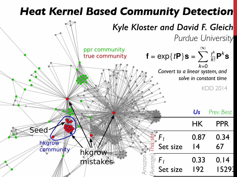
HK PPR

F1 0.87 0.34Set size 14 67

F1 0.33 0.14Set size 192 15293Am

azon

(Ave

rage

)

Us! Prev. Best

This

set

Heat Kernel Based Community Detection

KDD 2014

Kyle Kloster and David F. Gleich!Purdue University

f = exp{tP}s =

1X

k=0

tk

k !

Pk s

Convert to a linear system, and solve in constant time

Heat kernel localization General recipe!1.  Take problem X, "

convert into a linear system

2.  Apply “push” to that linear system

3.  Analyze and bound total work

David Gleich ·∙ Purdue 36

Heat kernel recipe!1.  Convert into "

""

2.  Apply “push” 3.  Analyze work bound "

x = exp(tP)ei2

6666664

III�tP/1 III

�tP/2. . .. . . III

�tP/N III

3

7777775

2

6666664

v0v1......

vN

3

7777775=

2

6666664

ei0......0

3

7777775

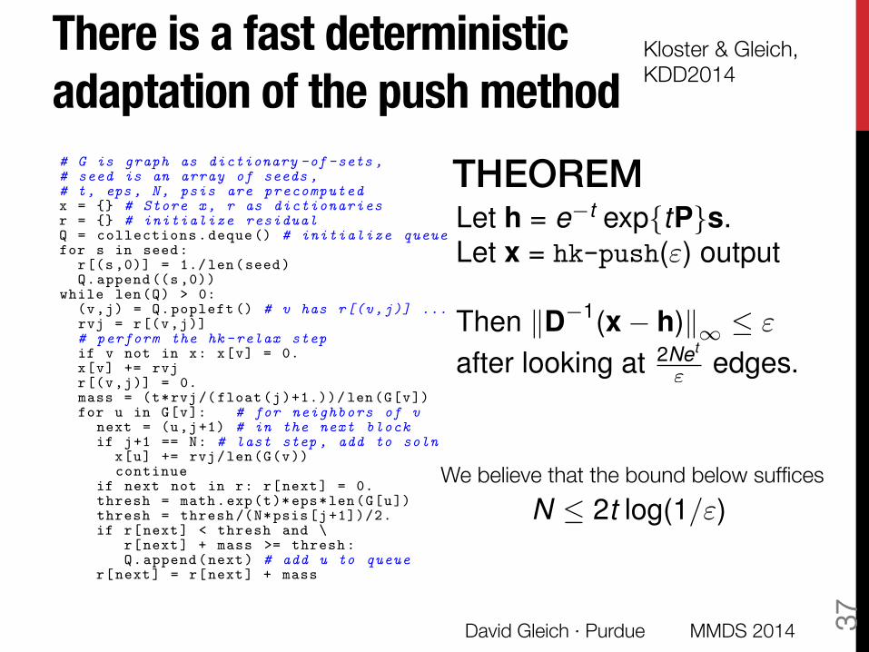
There is a fast deterministic adaptation of the push method


Kloster & Gleich, KDD2014

These polynomials k(t) are closely related to the � functionscentral to exponential integrators in ODEs [37]. Note that 0 = TN .

To guarantee the total error satisfies the criterion (3) then,it is enough to show that the error at each Taylor termsatisfies an 1-norm inequality analogous to (3). This isdiscussed in more detail in Section A.

4.3 Deriving a linear systemTo define the basic step of the hk-relax algorithm and to

show how the k influence the total error, we rearrange theTaylor polynomial computation into a linear system.

Denote by vk the k

th term of the vector sum TN (tP)s:

TN (tP)s = s+ t1Ps+ · · ·+ tN

N !PNs (7)

= v0 + v1 + · · ·+ vN . (8)

Note that vk+1 = tk+1

(k+1)!Pk+1 = t

(k+1)Pvk. This identityimplies that the terms vk exactly satisfy the linear system

2

6

6

6

6

6

6

4

I�t1 P I

�t2 P

. . .

. . . I�tN P I

3

7

7

7

7

7

7

5

2

6

6

6

6

6

6

4

v0

v1

...

...vN

3

7

7

7

7

7

7

5

=

2

6

6

6

6

6

6

4

s0......0

3

7

7

7

7

7

7

5

. (9)

Let v = [v0;v1; · · · ;vN ]. An approximate solution v̂ to(9) would have block components v̂k such that

PNk=0 v̂k ⇡

TN (tP)s, our desired approximation to e

th. In practice, weupdate only a single length n solution vector, adding allupdates to that vector, instead of maintaining the N + 1di↵erent block vectors v̂k as part of v̂; furthermore, the blockmatrix and right-hand side are never formed explicitly.

With this block system in place, we can describe the algo-rithm’s steps.

4.4 The hk-relax algorithmGiven a random walk transition matrix P, scalar t > 0,

and seed vector s as inputs, we solve the linear system from(9) as follows. Denote the initial solution vector by y and theinitial nN ⇥ 1 residual by r(0) = e1 ⌦ s. Denote by r(i, j) theentry of r corresponding to node i in residual block j. Theidea is to iteratively remove all entries from r that satisfy

r(i, j) � e

t"di

2N j(t). (10)

To organize this process, we begin by placing the nonzeroentries of r(0) in a queue, Q(r), and place updated entries ofr into Q(r) only if they satisfy (10).

Then hk-relax proceeds as follows.1. At each step, pop the top entry of Q(r), call it r(i, j),

and subtract that entry in r, making r(i, j) = 0.2. Add r(i, j) to yi.3. Add r(i, j) t

j+1Pej to residual block rj+1.4. For each entry of rj+1 that was updated, add that entry

to the back of Q(r) if it satisfies (10).Once all entries of r that satisfy (10) have been removed,

the resulting solution vector y will satisfy (3), which weprove in Section A, along with a bound on the work requiredto achieve this. We present working code for our methodin Figure 2 that shows how to optimize this computationusing sparse data structures. These make it highly e�cientin practice.

# G is graph as dictionary -of-sets ,

# seed is an array of seeds ,

# t, eps , N, psis are precomputed

x = {} # Store x, r as dictionaries

r = {} # initialize residual

Q = collections.deque() # initialize queue

for s in seed:

r[(s,0)] = 1./len(seed)

Q.append ((s,0))

while len(Q) > 0:

(v,j) = Q.popleft () # v has r[(v,j)] ...

rvj = r[(v,j)]

# perform the hk-relax step

if v not in x: x[v] = 0.

x[v] += rvj

r[(v,j)] = 0.

mass = (t*rvj/(float(j)+1.))/ len(G[v])

for u in G[v]: # for neighbors of v

next = (u,j+1) # in the next block

if j+1 == N: # last step , add to soln

x[u] += rvj/len(G(v))

continue

if next not in r: r[next] = 0.

thresh = math.exp(t)*eps*len(G[u])

thresh = thresh /(N*psis[j+1])/2.

if r[next] < thresh and \

r[next] + mass >= thresh:

Q.append(next) # add u to queue

r[next] = r[next] + mass

Figure 2: Pseudo-code for our algorithm as work-ing python code. The graph is stored as a dic-tionary of sets so that the G[v] statement re-turns the set of neighbors associated with vertexv. The solution is the vector x indexed by ver-tices and the residual vector is indexed by tuples(v, j) that are pairs of vertices and steps j. Afully working demo may be downloaded from githubhttps://gist.github.com/dgleich/7d904a10dfd9ddfaf49a.

4.5 Choosing NThe last detail of the algorithm we need to discuss is how

to pick N . In (4) we want to guarantee the accuracy ofD�1 exp {tP} s � D�1

TN (tP)s. By using D�1 exp {tP} =exp

�

tPT

D�1 andD�1TN (tP) = TN (tPT )D�1, we can get

a new upperbound on kD�1 exp {tP} s�D�1TN (tP)sk1 by

noting

k expn

tPTo

D�1s� TN (tPT )D�1sk1

k expn

tPTo

� TN (tPT )k1kD�1sk1.

Since s is stochastic, we have kD�1sk1 kD�1sk1 1.From [34] we know that the norm k exp

�

tPT

�TN (tPT )k1is bounded by

ktPT kN+11

(N + 1)!(N + 2)

(N + 2� t) t

N+1

(N + 1)!(N + 2)

(N + 2� t). (11)

So to guarantee (4), it is enough to choose N that impliestN+1

(N+1)!(N+2)

(N+2�t) < "/2. Such an N can be determined e�-ciently simply by iteratively computing terms of the Taylorpolynomial for et until the error is less than the desired errorfor hk-relax. In practice, this required a choice of N nogreater than 2t log( 1" ), which we think can be made rigorous.

Let h = e�texp{tP}s.

Let x = hk-push(") output

Then kD

�1

(x � h)k1 "

after looking at

2Net

" edges.

We believe that the bound below suffices N 2t log(1/")

MMDS 2014

THEOREM!

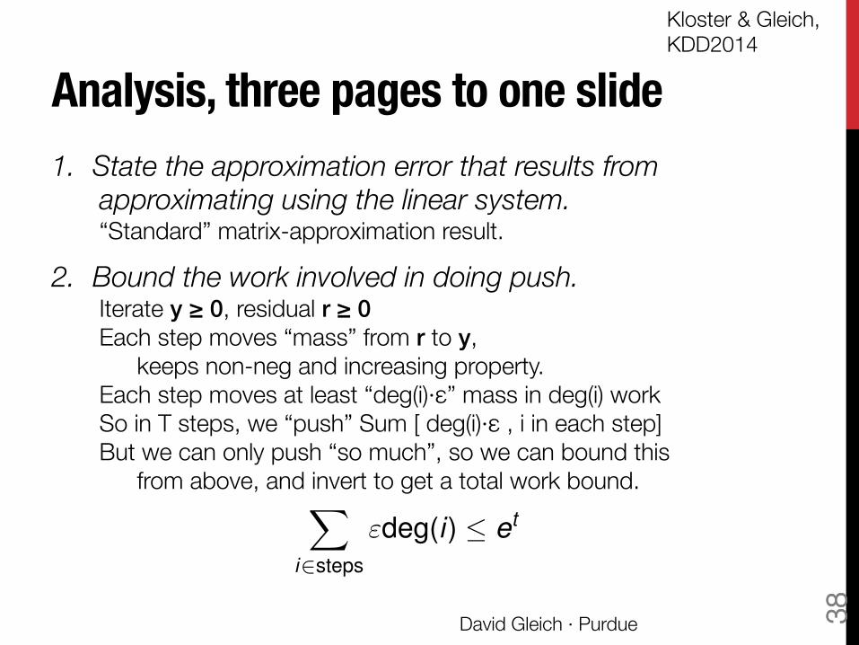
Analysis, three pages to one slide 1.  State the approximation error that results from

approximating using the linear system.!“Standard” matrix-approximation result.

2.  Bound the work involved in doing push. !Iterate y ≥ 0, residual r ≥ 0 "Each step moves “mass” from r to y, "

keeps non-neg and increasing property."Each step moves at least “deg(i)·ε” mass in deg(i) work"So in T steps, we “push” Sum [ deg(i)·ε , i in each step]"But we can only push “so much”, so we can bound this

from above, and invert to get a total work bound.


Kloster & Gleich, KDD2014

X

i2steps

"deg(i) et

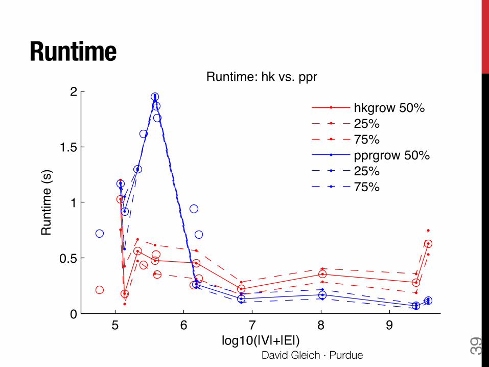
Runtime

David Gleich · Purdue 39 5 6 7 8 9

0

0.5

1

1.5

2Runtime: hk vs. ppr

log10(|V|+|E|)

Run

time

(s)

hkgrow 50%25%75%pprgrow 50%25%75%

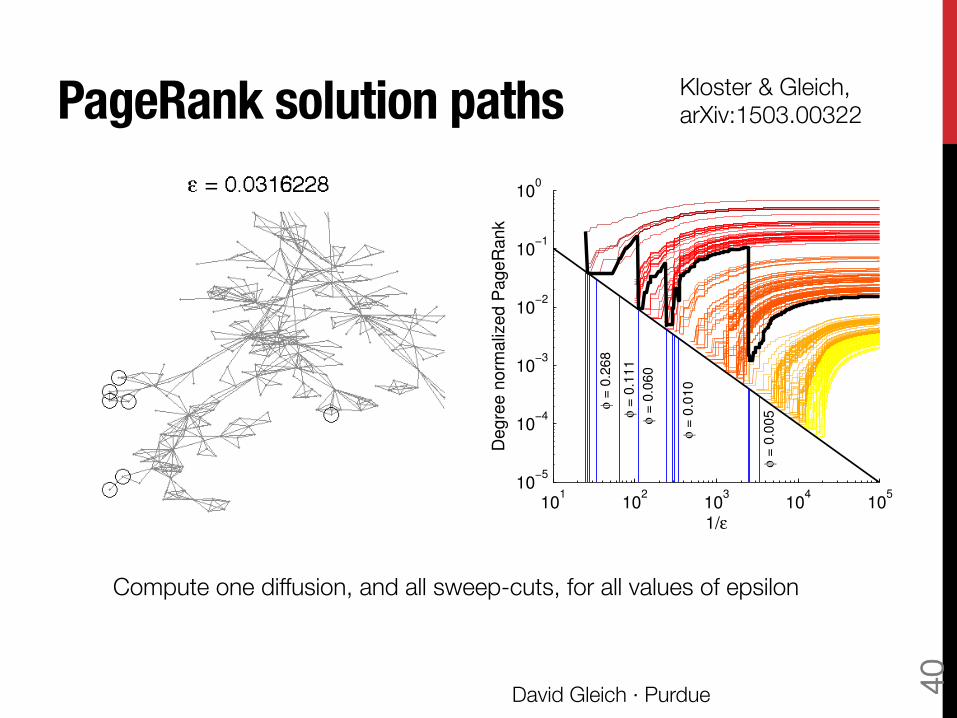
PageRank solution paths

101

102

103

104

105

10−5

10−4

10−3

10−2

10−1

100

1/ε

De

gre

e n

orm

aliz

ed

Pa

ge

Ra

nk

φ =

0.0

05

φ =

0.0

10

φ =

0.0

60

φ =

0.1

11

φ =

0.2

68


Compute one diffusion, and all sweep-cuts, for all values of epsilon

Kloster & Gleich, arXiv:1503.00322

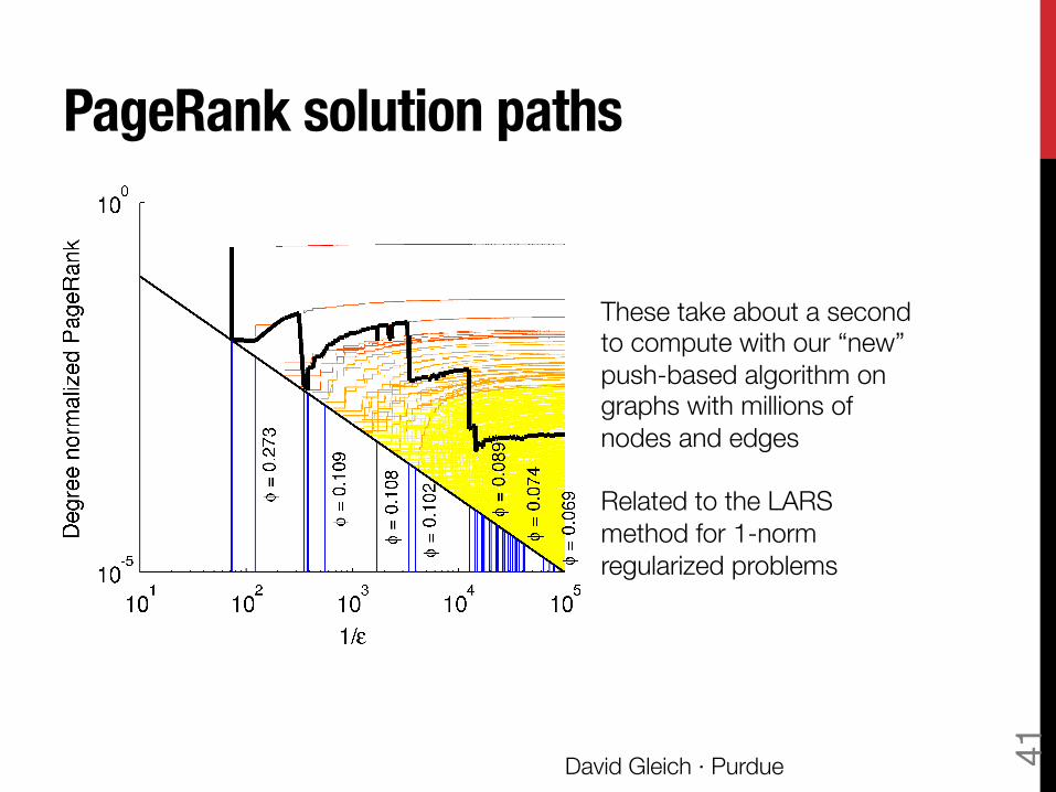
PageRank solution paths


These take about a second to compute with our “new” push-based algorithm on graphs with millions of nodes and edges Related to the LARS method for 1-norm regularized problems

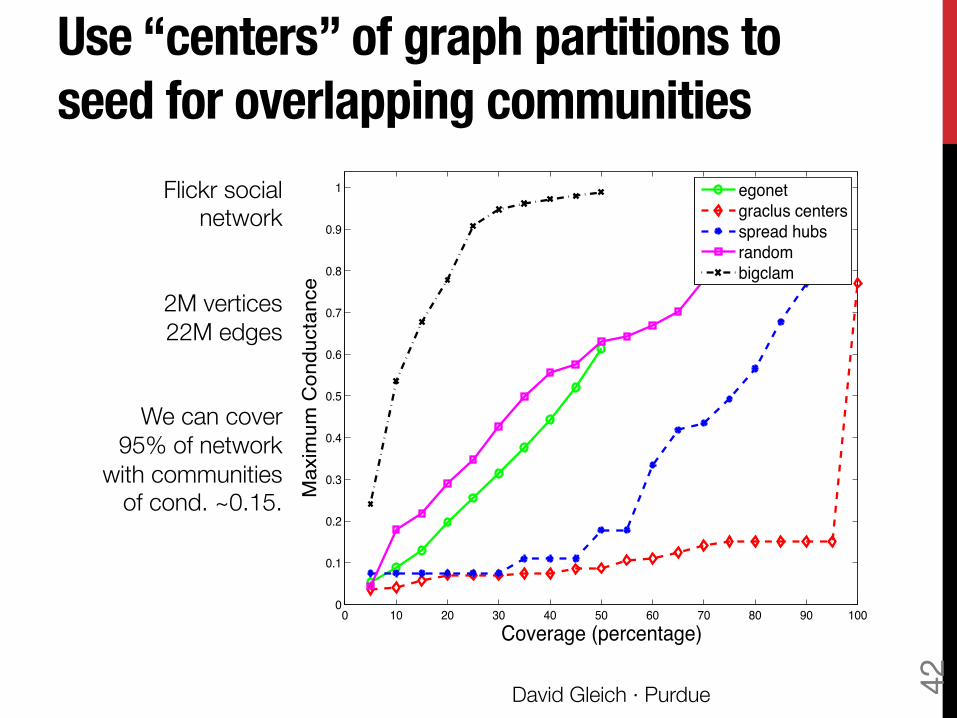
Use “centers” of graph partitions to seed for overlapping communities


Table 4: Returned number of clusters and graph coverage of each algorithm

Graph random egonet graclus ctr. spread hubs demon bigclam

HepPh coverage (%) 97.1 72.1 100 100 88.8 62.1no. of clusters 97 241 109 100 5,138 100

AstroPh coverage (%) 97.6 71.1 100 100 94.2 62.3no. of clusters 192 282 256 212 8,282 200

CondMat coverage (%) 92.4 99.5 100 100 91.2 79.5no. of clusters 199 687 257 202 10,547 200

DBLP coverage (%) 99.9 86.3 100 100 84.9 94.6no. of clusters 21,272 8,643 18,477 26,503 174,627 25000

Amazon coverage (%) 99.9 100 100 100 79.2 99.2no. of clusters 21,553 14,919 20,036 27,763 105,828 25,000

Flickr coverage (%) 76.0 54.0 100 93.6 - 52.1no. of clusters 14,638 24,150 16,347 15,349 - 15,000

LiveJournal coverage (%) 88.9 66.7 99.8 99.8 - 43.9no. of clusters 14,850 34,389 16,271 15,058 - 15,000

Myspace coverage (%) 91.4 69.1 100 99.9 - -no. of clusters 14,909 67,126 16,366 15,324 - -

0 10 20 30 40 50 60 70 80 90 1000

0.1

0.2

0.3

0.4

0.5

0.6

0.7

0.8

0.9

Coverage (percentage)

Max

imum

Con

duct

ance

egonetgraclus centersspread hubsrandomdemonbigclam


(a) AstroPh

0 10 20 30 40 50 60 70 80 90 1000

0.1

0.2

0.3

0.4

0.5

0.6

0.7

0.8

0.9


Max

imum

Con

duct

ance



(b) HepPh

0 10 20 30 40 50 60 70 80 90 1000

0.1

0.2

0.3

0.4

0.5

0.6

0.7

0.8

0.9


Max

imum

Con

duct

ance



(c) CondMat

0 10 20 30 40 50 60 70 80 90 1000

0.1

0.2

0.3

0.4

0.5

0.6

0.7

0.8

0.9

1


Max

imum

Con

duct

ance

egonetgraclus centersspread hubsrandombigclam


(d) Flickr

0 10 20 30 40 50 60 70 80 90 1000

0.1

0.2

0.3

0.4

0.5

0.6

0.7

0.8

0.9

1


Max

imum

Con

duct

ance

egonetgraclus centersspread hubsrandombigclam


(e) LiveJournal

0 10 20 30 40 50 60 70 80 90 1000

0.1

0.2

0.3

0.4

0.5

0.6

0.7

0.8

0.9


Max

imum

Con

duct

ance

egonetgraclus centersspread hubsrandom


(f) Myspace

Figure 2: Conductance vs. graph coverage – lower curve indicates better communities. Overall, “gracluscenters” outperforms other seeding strategies, including the state-of-the-art methods Demon and Bigclam.

Flickr social network

2M vertices"22M edges

We can cover

95% of network with communities

of cond. ~0.15.

References and ongoing work Gleich and Kloster – Relaxation methods for the matrix exponential, J. Internet Math "Kloster and Gleich – Heat kernel based community detection KDD2014 Gleich and Mahoney – Algorithmic Anti-differentiation, ICML 2014 "Gleich and Mahoney – Regularized diffusions, Submitted Whang, Gleich, Dhillon – Seeds for overlapping communities, CIKM 2013 www.cs.purdue.edu/homes/dgleich/codes/nexpokit!www.cs.purdue.edu/homes/dgleich/codes/l1pagerank •  Improved localization bounds for functions of matrices •  Asynchronous and parallel “push”-style methods •  Localized methods beyond conductance


Supported by NSF CAREER 1149756-CCF www.cs.purdue.edu/homes/dgleich

localized methods in graph mining

Technology

datadavid gleich purdue

notdavid gleich purdue

betterdavid gleich purdue

thisdavid gleich purdue

randomdavid gleich purdue

purdue university

purdue michael mahoney

localized methods