5f. work unit number 7. performing organization …
TRANSCRIPT

REPORT DOCUMENTATION PAGE " Public reporting burden for this collection of information is estimated to average 1 hour per response, including the time for reviewing instruc AFRL-SR-AR- 1JV-U2-
the data needed, and completing and reviewing this collection of information. Send comments regarding this burden estimate or any other < reducing this burden to Department of Defense, Washington Headquarters Services, Directorate for Information Operations and Reports (07 VA 22202-4302. Respondents should be aware that notwithstanding any other provision of law, no person shall be subject to any penalty f display a currently valid OMB control number. PLEASE DO NOT RETURN YOUR FORM TO THE ABOVE ADDRESS. (n^i- 1. REPORT DATE (DD-MM-YYYY) 31 - 05 - 2002
2. REPORT TYPE Final Technical Report
4. TITLE AND SUBTITLE
Electromagnetic Scattering from Multiple Scale Geometries
6. AUTHOR(S)
Maria Z Caponi Alain Sei
7. PERFORMING ORGANIZATION NAME(S) AND ADDRESS(ES) AND ADDRESS(ES)
TRW Space and Electronics Group 1, Space Park, MS Rl-1008 Redondo Beach, CA 90278
9. SPONSORING / MONITORING AGENCY NAME(S) AND ADDRESS(ES) USAF, AFMC Air Force Office of Scientific Research 801 North Randolph St, Room 732 Arlington, VA 22203-1977
%/. fcSJ-\ I
01 Mar 1999 to 3-1 ■May 300» 5a. CONTRACT NUMBER "3-^6^Ax Öl- F49620-99-C-0014
5b. GRANT NUMBER
5c. PROGRAM ELEMENT NUMBER
5d. PROJECT NUMBER FQ8671-9900630 G550/00
5e. TASK NUMBER
5f. WORK UNIT NUMBER
8. PERFORMING ORGANIZATION REPORT NUMBER
1A570-0001-UT-01
10. SPONSOR/MONITOR'S ACRONYM(S)
20020702 040 12. DISTRIBUTION / AVAILABILITY STATEMENT
A - Approved for public release; distribution unlimited
13. SUPPLEMENTARY NOTES
14. ABSTRACT This final technical report describes the development, implementation, numerical validation and potential exploitation of an accurate and efficient scattering solvers to compute the horizontal (TE mode) and vertical (TM mode) polarization returns from multi-scale surfaces. This modeling effort was motivated by a large number of remote sensing applications that require the characterization by means of radar scattering measurements of the scattering surface configuration or variations in the surface patterns for detection or environmental purposes. The nature of the relevant scattering surfaces and the measured scattered fields drives the need for an extremely accurate scattering solver able to deal with multi-scale surfaces in an efficient manner. This objective was achieved by using a combination of perturbation and asymptotic expansions and an innovative and careful implementation of these expansions for full double precision accuracy. The Fourier series representations used in this problem allowed for very efficient computations due the relatively small order of these series in typical cases. HH and W polarization have been implemented and allow the rigorous investigation of critical remote sensing problems.
15. SUBJECT TERMS Electromagnetic Scattering, Rough Surface, Ocean scattering, Numerical Methods, High Frequency 16. SECURITY CLASSIFICATION OF: UNCLASSIFIED
a. REPORT UNCLASSIFIED
b. ABSTRACT UNCLASSIFIED
c. THIS PAGE UNCLASSIFIED
17. LIMITATION OF ABSTRACT
UL
18. NUMBER OF PAGES
19a. NAME OF RESPONSIBLE PERSON
19b. TELEPHONE NUMBER (include area code)
Standard Form 298 (Rev. 8-98) Prescribed by ANSI Std. Z39.18

Electromagnetic Scattering from Multiple Scale Geometries
Executive Summary
This final report describes the development, implementation, numerical validation and potential
exploitation of a highly accurate and efficient scattering solver to compute the horizontal (TE
mode) and vertical (TM mode) polarized returns from multi-scale surfaces for ocean remote
sensing applications. A large number of remote sensing applications require the
characterization by means of radar scattering measurements of the scattering surface
configuration or variations in the surface patterns for detection or environmental purposes. In
particular, for applications associated with ocean remote sensing appropriate exploitation of the
experimental measurements requires a detailed knowledge of the relation between the
characteristics of surface waves and their variation with environmental parameters, and the
properties of observables, such as polarized return power and Doppler spectrum. Relevant
ocean geometries include more than one dominant scale and recent results have shown that
the number of scales included in the problem and the accuracy of the computation can strongly
affect the prediction of modeled polarized radar backscattering returns cf. [Sei et al, 1999]. The
standard models used to predict ocean backscatter returns usually resort to simplified two-scale
model and zero or first order computations [Valenzuela, 1978]. These models are unable to
predict recent significant experimental results demonstrating that horizontally (TE mode)
polarized radar backscatter returns can intermittently exceed vertical (TM mode) polarized
returns at low grazing angles. Furthermore, the experimental measurements of the normalized
backscattered returns are generally in the -60-dB to -100-dB range [Lee et al, 1997b],
demonstrating the need for a scattering model with a relative accuracy of at least 10 digits.
These requirements, the complexity and multitude of scales present on the application of
interest as well as the absence of satisfactory scattering algorithms in the existing literature
motivated this project and an approach that emphasizes the use of high order methods to
achieve accurate and fast, versatile and user-friendly computations. The successful approach to
the solution of such a numerical challenge is based on innovative mathematical methods as well
as their very careful implementations to obtain double precision accuracy. The mathematical
methods developed for this problem are based on a combination of high order asymptotic and
perturbation methods and their implementation is based on the development of libraries for the
manipulation of Taylor-Fourier series. This final report provides a complete description of the
mathematical methods and their implementation as well as their potential exploitation for ocean
remote sensing. Technical details will often be referred to already publish work. Finally the
source code as well as a guide for its compilation and implementation is provided in the
accompanying floppy disk.

1.1 Introduction
A large number of remote sensing applications entail the characterization by means of
radar scattering measurements of the scattering surface configuration or variations in the
surface patterns for detection or environmental purposes. In particular, appropriate exploitation
of sensor measurements for ocean remote sensing applications require an in depth knowledge
of the relation between the characteristics of surface waves and their variation with
environmental parameters, and the properties of observables, such as polarized return power
and Doppler spectrum. The electromagnetic scattering from multiple scale geometries (ESMSG)
project detailed in this report focuses on the development, implementation and numerical
validation of highly accurate and efficient scattering solvers to compute the horizontal (TE
mode) and vertical (TM mode) polarization returns from multi-scale surfaces for utilization in
ocean radar remote sensing applications as well as potential extensions to terrain remote
sensing. Specific ocean radar remote sensing applications of interest include ocean spectrum
characterization for wind speed and direction prediction, ship wake detection and ocean bottom
topography and or internal current determination.
Ocean specific pattern variations can occur when internal waves created by submerged
objects or bottom topography interact with the ocean surface waves modifying the surface
roughness. In turn, the wind generates short surface waves (of the order of cm) that are
modulated by and superimposed on a continuum of longer waves ranging from 50 cm to 100's
of meters. Depending on the wind and ocean currents, these waves can travel in various
directions creating a complex 3-dimensional surface or approach a simpler 2- dimensional-like,
but still multi-scale geometry. Although the centimeter-scale waves are mainly responsible for
backscattering microwave radar signals, recent experiments have shown that specific
characteristics of the finite amplitude long waves strongly affect the properties of the polarized
backscattering radar return; bistatic returns are expected to be affected similarly. In general, the
ocean surface backscattering cross sections are very low, resulting in ratios of radar return
power to radar input power of the order of -80dB. Further, the time series measurements show
spikes in the polarization ratios TE/TM (HH/W) that can reach values larger than 1 for small
grazing angles. Experimental analysis of the data indicates that the spikes are associated with
the presence of asymmetric, large amplitude, long waves. These results cannot be explained
with the currently used composite surface models because these models lack the accuracy
necessary for quantitative predictions and neglect multipath effects. Further, these models
strongly depend on an arbitrary separation of scales on the surface and therefore do not yield
genuine results. Other scattering models that have been used to describe the experimental
data are either not sufficiently accurate or can only model specific length scales or profiles.
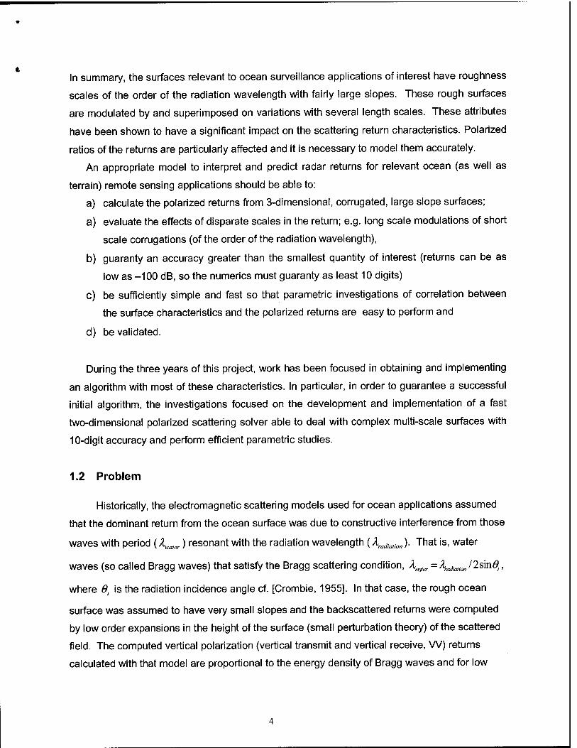
In summary, the surfaces relevant to ocean surveillance applications of interest have roughness
scales of the order of the radiation wavelength with fairly large slopes. These rough surfaces
are modulated by and superimposed on variations with several length scales. These attributes
have been shown to have a significant impact on the scattering return characteristics. Polarized
ratios of the returns are particularly affected and it is necessary to model them accurately.
An appropriate model to interpret and predict radar returns for relevant ocean (as well as
terrain) remote sensing applications should be able to:
a) calculate the polarized returns from 3-dimensional, corrugated, large slope surfaces;
a) evaluate the effects of disparate scales in the return; e.g. long scale modulations of short
scale corrugations (of the order of the radiation wavelength),
b) guaranty an accuracy greater than the smallest quantity of interest (returns can be as
low as -100 dB, so the numerics must guaranty as least 10 digits)
c) be sufficiently simple and fast so that parametric investigations of correlation between
the surface characteristics and the polarized returns are easy to perform and
d) be validated.
During the three years of this project, work has been focused in obtaining and implementing
an algorithm with most of these characteristics. In particular, in order to guarantee a successful
initial algorithm, the investigations focused on the development and implementation of a fast
two-dimensional polarized scattering solver able to deal with complex multi-scale surfaces with
10-digit accuracy and perform efficient parametric studies.
1.2 Problem
Historically, the electromagnetic scattering models used for ocean applications assumed
that the dominant return from the ocean surface was due to constructive interference from those
waves with period {Xwmer) resonant with the radiation wavelength (\adiation). That is, water
waves (so called Bragg waves) that satisfy the Bragg scattering condition, /^ =\adia,ioJ2smßi,
where 0t is the radiation incidence angle cf. [Crombie, 1955]. In that case, the rough ocean
surface was assumed to have very small slopes and the backscattered returns were computed
by low order expansions in the height of the surface (small perturbation theory) of the scattered
field. The computed vertical polarization (vertical transmit and vertical receive, W) returns
calculated with that model are proportional to the energy density of Bragg waves and for low

grazing (high incidence) angles they are always much larger than the horizontal (horizontal
transmit and horizontal receive, HH) returns. For example, it can be shown cf. [Valenzuela,
1978] that the ratio HH/W goes to 0 at 90 degrees incidence for a perfect conductor.
Late 70's experimental measurements demonstrated that short surface waves (~ 30 cm)
could image long patterns (~ 1 Km) that could be associated with the ocean bottom topography.
(Cf. Figure 1B). This result was interpreted as the modulation of the resonant (Bragg) short
waves spatial distribution energy density by the long surface current gradients. Thus, in order to
understand the experimental results it was necessary to include in the model the variation in the
Bragg resonant waves due to the long wave tilt and composite models were developed to take
this effect into account. These models also predicted large vertical to horizontal return ratios
(W/HH»1) for small grazing angles. In addition the maximum of the Doppler spectra (power
(A)

FRANCE DUNKERQUE OOSTENDE
BELGIUM
y' 2°E
2°30' E /
CONTOURS IN METERS CURRENT SPEEDS IN METERS PER SECOND
/^51°N
(B)
Figure 1: Land Sat images of the English Channel. L band: 30-cm.
A) Radar image - B) Bottom topography contours.
New experimental results obtained during the early to mid 90's sparked a renewed interest in
appropriate scattering models to interpret polarized radar data. For example, experimental
observations with the TRW X-band radar mounted on the bow of a boat in a Loch Lihnne
experiment [Lee et al, 1995, 1996] as well as complementary laboratory experiments [Lee et al,
1997a, 1997b] showed that for low grazing angles the horizontal returns could be larger than the
vertical returns. Further, the regions where these events or spikes (HH/W >1) occurred were of
an intermittent nature and the result of very low scattering returns, of the order of -60 to -100
dB range (See Figure 2 below). The measured Doppler spectra, also demonstrated that as the

grazing angle decreased, the maxima associated with the HH returns, moved towards faster
velocities that no longer could be associated with Bragg waves. (See Figure 2A and 2B).
24 26 30 32 34 36
Time from start of run (sec)
(A)
'. Ö( = j!1, upwind loot .LOW j*„
-3 0 0 -2 0 0 -ICO 0 100 200 300
(B)
Figure 2: (A) A short sample of time-resolved, band-pass-filtered backscattered echoes at X-
Band (B) Time-integrated Doppler spectra of wind waves (see [Lee et al, 1995] for details).
The paradigm was further complicated by differences in the vertical and horizontal radar images
obtained under different weather conditions. For example, the JUSREX'92 experimental results
[Gasparovic and Etkin, 1994] indicated that internal waves are well imaged by HH and W for a
stable boundary layer (longer wave spectrum), whereas they are not well imaged in W for an
unstable boundary layer (short wave spectrum). The short waves mask long wave patterns in
W but not in HH (cf. Fig. 3). These and other similar experimental results resulted in a different
understanding of the dominant scattering mechanisms from ocean surfaces:
a) returns are associated with the modulation of short waves (of the order of 1 - 30cm) by
finite amplitude long waves (.5m - 3m) and/or the generation of large amplitude short
waves in the front faces of almost breaking long waves;
b) the strong horizontal polarization scattering returns are due mainly to "Non-Bragg
mechanism" that are most likely dominated by specular and multibounce or multipath
interference from incipient braking waves;
c) the multi-scale nature of the ocean surfaces plays a dominant role for the horizontal
returns;

d) the difference between horizontal and vertical returns yields an additional insight in the
interpretation of radar measurements.
w
Figure 3: Radar images taken the JUSREX'92 experiment under (a) stable and (b) unstable
boundary layer conditions (see [Churyumov and Kravtsov, 2000] for details).
Most important, the results also pointed out the need for an appropriate scattering model
that could take into account the multi-scale nature of the surface, the larger slopes and could
deal with the very low returns. Composite models using low order expansions or generally
models with low accuracy or failing to take into account the large range of contributing scales
will fail to predict the experimental results.
From a computational point of view the task of developing such a model (multi-scale, at
least 10 digit accuracy, includes both TE and TM polarizations) seems rather formidable. In the
following sections a description is given of the method employed in this project to successfully
address this computational challenge. Section 1.3 summarizes the mathematical model.
Section 1.4 discusses some of the problems encounter in its implementation and in Section 1.5
validation results are summarized. Potential exploitations of this algorithm are described in
Section 1.6. More detailed descriptions of the points discussed in those sections are given in
the Appendices as well as in the associated publications. A diskette with the algorithm and
documentation is included with this Final report.
1.3 Mathematical model
The problem of evaluating scattering returns from rough surfaces is rather challenging —
owing to the multiple-scale nature of rough scatterers, whose spectra may span a wide range of
length-scales cf. [Valenzuela, 1978]. A number of techniques have been developed to treat
limiting cases of this problem. For example, the high frequency case, in which the wavelength X
of the incident radiation is much smaller than the characteristic surface length-scales, has been
treated by means of low order asymptotic expansions, such as the Kirchhoff approximation. On
the other hand, resonant problems where the incident radiation wavelength is of the order of the
roughness scale have been treated by perturbation methods, typically first or second order
expansions in the height h of the surface cf. [Rice, 1951; Mitzner, 1964; Shmelev, 1972;
Voronovich, 1994]. However, when a multitude of scales is present on the surface none of these
techniques is adequate, and attempts to combine them in so-called two-scale approaches have
been given cf. [Kuryanov, 1963; McDaniel and Gorman, 1983; Voronovich, 1994; Gil'man et al,
1996]. The results provided by these methods are not always satisfactory, owing to the
limitations imposed by the low orders of approximation used in both, the high frequency and the
small perturbation methods.
A new approach to multi-scale scattering, based on use of expansions of very high order
in both parameters X and h, has been proposed recently cf. [Bruno et al, 2000]. These
combined methods, which are based on complex variable theory and analytic continuation,
require nontrivial mathematical treatments; the resulting approaches, however, do expand
substantially on the range of applicability over low order methods, and can be used in some of
the most challenging cases arising in applications. Perturbation series of very high-order in h
have been introduced and used elsewhere to treat resonant problems — in which the
wavelength of radiation is comparable to the surface length-scales cf. [Bruno and Reitich, 1993;
Seietal, 1999].
This new method does not require separation of the surface length-scales into large and
small, but instead it is able to deal with a continuum of scales on the surface. Indeed the high
order expansions presented below have a common "overlap" region in the (h,X) plane where
both components are highly accurate. More precisely, there is a range of surface heights and
incident wavelengths for which both methods produce results with machine accuracy. Therefore
by dividing the scales of a surface at wavelength (or scale) in the overlap region we obtain a
general method which is applicable to surfaces containing a continuum of length-scales —
which is ideal for evaluation of scattering from surfaces with spectral distributions of oceanic
type.

We consider surfaces containing a continuum of scales but, as mentioned above, the
existence of an overlap allows us to solve the complete multiple-scale problem by expressing an
arbitrary surface
y = S(x)
as a sum
y = So(x) + F(x)
where S0(x) contains wavenumbers less than Ns, and F(x) contains the complementary set of
wavenumbers greater then Ns. Thus, our method uses a dichotomy in wave numbers but it does
not assume a separation of scales. This feature is essential in the study of oceanic waves since
many studies show that the wave spectrum spans a large range of wavenumbers (see for
instance [Pierson and Moskowitz, 1964]).
The discussion here is restricted to the particular case of an HH configuration in two
dimensions since the W case can be treated similarly. The modifications necessary to treat the
W case will be pointed out as needed. The scattered field created by an incident H polarized
plane wave impinging on the rough surface solves the Helmholtz equation with a Dirichlet
boundary condition. Our approach to the solution of the general problem with rough surface y=
S(x) proceeds as follows:
• We consider the surface S(x,8) = S0 (x) + 5F(x), which will be used as a basis for a
perturbative method in the parameter 8.
• The solution u = u(x,8) associated with the surface S(x,8) is obtained by perturbation
theory around 8 = 0.
• The solution for the surface S(x) is then recovered by setting 8=1. (This evaluation
usually leads to divergent series whose re-summation requires appropriate analytic
continuation.)
In detail, writing:
(1)
+ OO fil
u(x,z,S) = Y, u (x,z)
u (x,z)
m = 0
dmu
m ml
(x,z,S = 0)
10

The fact that, for every value of 8 the field u(x,z,S) solves the Helmholtz equation
Au(x,z;S) + k2u(x,z;S) = 0
(2)
u(x,S(x,S);S) = -uinc(x,S(x,S))
implies that, for index m we have
Aum(x,z)+ k2um(x,z) = 0
(3) um(x,S0(x)) = G[F,«0,«!,..., um_l](x,S0(x))
The interest in this equation arises from the fact that, although the right hand side in the
boundary condition for um is highly oscillatory, the surface S0 itself is not. We therefore have
reduced a problem on a highly oscillatory surface to a sequence of problems on a non-
oscillatory surface. For example the zeroth, first and second order Taylor coefficients u0, ui and
u2 in the expansion of u(x,z,8) solve the following scattering problems:
(5)
AM,(X,Z) + k2ux(x,z) = 0
t/jCx^oO)) = -F(x) dun du —- +
inc \
dz (x,S0(x))
(4)
Au0(x,z) + k2u0(x,z) = 0
u0(x,S0(x)) = -uinc (x,S0(x))
(6)
Au2(x,z) + k u2(x,z) = 0 f*2
u2(x,S0(x)) =-F (x) d2un d u 2.. inc ^\
dz' dz2 j (x,S0(x))
-2F(x)^-(x,50(x)) dz
The general boundary condition for umin equation (3) (denoted by G[F, u0, Ui, ...,um.
iKx.SoCx))) can be computed by differentiation of order m with respect to 5 of the exact
boundary condition of equation (2). Note the boundary term for um involve all the previous Taylor
coefficients Uj j=0...m-1. This is already obvious on equation (5) and (6).
11

From equation (4), (5) and (6), it is clear that the computation of each Taylor coefficients
um involves solving a high frequency problem on a smooth surface. Typically uinc is a plane
wave with wave number k=2n/X and S0 is a surface with characteristic length d much greater
than X. The characteristic length in our approach is the period of the surface as we have chosen
a Fourier description of the surface. We are then faced with solving very accurately a high-
frequency scattering problem.
Also equations (4), (5) and (6) show that the computation of the boundary condition
involves z-derivatives of high-order of the previous Taylor coefficients. The simplest example is
the boundary condition for ui involves the z-derivative of u0. Since we know u0 on the surface
(from equation (4)) knowing the z-derivative is equivalent to knowing the normal derivative on
the surface. This involves therefore the computation of the Dirichlet to Neumann map. So the
two main components of the algorithm are
• A High-frequency solver
• A Dirichlet to Neumann Map code
We give below an overview of each component. A detailed description of the high-frequency
solver can be found in [Bruno et al., 2002].
1.3.1 High-Frequency Solver
1.3.1.1 Background
Our approach to the high-frequency problem uses an integral equation formulation,
whose solution v(x) is sought and obtained in the form of an asymptotic expansion
(7) v(x,k) = ei-^fj1^
with p=-1 for TM polarization and p=0 for TE polarization. This expansion is similar in form to
the geometrical optics
(8) u(x,z,k) = e^^fd'^^
where S=S(x,z) is the unknown phase of the scattered field. Note that the phase of the density
v(x) of (7) is determined directly from the geometry and the incident field and, unlike that in the
geometrical optics field, it is not an unknown of the problem. In particular, the present approach
12

does not require solution of an eikonal equation (cf. [Vidale, 1988; VanTrier and Symes, 1991;
Fatemi et al, 1995; Benamou, 1999], and it bypasses the complex nature of the field of rays,
caustics, etc.
The validity of the expansion (8) has been extensively studied [Friedlander, 1946;
Lüneburg, 1949a; Lüneburg, 1949b; Van Kampen, 1949; Lüneburg, 1964]; in particular, it is
known that equation (8) needs to be modified in the presence of singularities of the scattering
surface. To treat edges and wedges, for example, an expansion containing powers of k1/2
[Lüneburg, 1949b; Van Kampen, 1949; Keller, 1958; Lewis and Boersma, 1969; Lewis and
Keller, 1964] must be used; caustics and creeping waves also lead to similar modified
expansions [Kravtsov, 1964; Brown, 1966; Ludwig, 1966; Lewis et al, 1967; Ahluwalia et al,
1968]. Proofs of the asymptotic nature of expansion (8) were given in cases where no such
singularities occur [Miranker, 1957; Bloom and Kazarinoff, 1976]. In practice only expansions (8)
of very low orders (one, or, at most two) have been used, owing in part to the substantial
algebraic complexity required by high order expansions [Bouche et al, 1997]. First order
versions of the expansion (7), on the other hand were treated in [Lee, 1975; Chaloupka and
Meckelburg, 1985; Ansorge 1986,1987].
The region of validity of our expansion (7) the other hand corresponds to configurations where
no shadowing occurs. At shadowing the wave vector of the incident plane wave is tangent to the
surface at some point, which causes certain integrals to diverge; see [Bruno et al, 2002] for
details. Thus, a different kind of expansion, in fractional powers of 1/k, should be used to treat
shadowing configurations: a first order version of such an expansion was discussed in [Hong,
1967]; see [Friedlander and Keller, 1955; Lewis and Keller, 1964; Brown 1966; Duistermaat,
1992] for the ray-tracing counterpart.
In [Bruno et al, 2002] we show that high order summations of expansion (7) can indeed
be used to produce highly accurate results for surfaces and wavelengths of interest in
applications for both TE and TM polarization. Results with machine precision accuracy, which
were obtained from computations involving expansions of order as high as 20, are presented.
Our algorithm is based on systematic use and manipulation of certain Taylor-Fourier series
representations, which are discussed in detail in [Bruno et al, 2002],
1.3.1.2 Integral Equation
The scattered field u=u(x,z) induced by an incident plane wave impinging on the rough
surface y=S0(x) under TE polarization is the solution of the Helmholtz equation with a Dirichlet
boundary condition. As is known [Voronovich, 1994] the field u(x,z) can be computed as an
13

integral involving a surface density v(x,k) and the Green's function G(x,z,x',z') for the Helmholtz
equation
dG (9) u(x,z) = \ v{^k)^(x,z,^S^))4\ + S'^)2d^
where v(x,k) satisfies the boundary integral equation
(10) H|S+ J v(^k)^(xMx)^S0(^ÜX^d^ = -eim-ißs^x)
with cc=k sin(6inc), ß=k cos(einc) and k=2n/X is the wavenumber. 9inc is the incidence angle
measured counter-clockwise from the vertical axis. A useful form of the integral equation (10)
results as we factor out the rapidly oscillating phase function
(11) ju(x,k) + jju({,k)|^(x,S0(*),£S0(£)K^>^o«-*o(0)Ji + s'0(tfdS = -2
ju(x,k) = e-iax+ißs°(x)v(x,k)
which cancels the fast oscillations in all non-integrated terms, and thus suggests use of an
expansion of the form (7). Substitution of the expansion (7) into equation (11) then yields:
(12) E^to-^c*,*), -2
dG (13) /"(*,*) = J v„^^(x)50(x),^50©)e-^)+^w-s«(f)Vl + 5;(^)2^
To solve equation (12) we use asymptotic expansions for the integrals ln(x,k), collect coefficients
of each power of 1/k, and then determine, recursively, the coefficients vn(x). We obtain in
[Bruno et al, 2002], an expansion which gives ln(x,k) in terms of derivatives of vn(x).
(14) K q=Q K
/;w=S^F^w
14

where the functions Bq.^(x) are determined from the profile and incidence angle only. We then
find a recursion which gives vn(x) as a linear combination of derivatives of the previous
coefficients vn-i-q(x).
V0(*) = -2
(15) n-\
^ q=0
1.3.2 Dirichlet to Neumann Map
1.3.2.1 Reduction to first-order normal derivative
The boundary condition for an arbitrary order um(x,z) can be derived by differentiating to
order m the boundary condition for u(x,y,S) and then setting 8=0. In detail we find for the TE
case
(16) um(x,S0(x)) = - ~\m„inc m
dz"
y m\Fp(x) opum_p^
/*=i p\{m-p)\ dz1 (x,S0(x))
and for the TM case
(17) ^(x,S0(x))- on
\m+l„.inc
Fm(x)^—^—+y m\Fp{x) op+lum_p
ozman f^p\(m-p)\ ozpon (x,S0(x))
The formulas above show that differentiation of high order is required. However using an
argument similar to the one used in the proof of the Cauchy-Kowalesky theorem [Hadamard,
1964; Courant and Hilbert, 1962], we can set up the calculation recursively so that at any given
stage only the Dirichlet and Neumann data are required.
For example in the TE case, the boundary condition for u2(x,z) given in formula (6),
requires the second order derivative of u0(x,z) evaluated on the surface z=S0(x) with respect to
z. That quantity can be computed if u0(x, S0(x)) and 3uo/3z(x, S0(x)) are known on the surface
(18) 'A(x)=u0(x,S0(x))
B(x)=^(x,S0(x)) oz
z=So(x). Differentiating with respect to x (tangential derivative) we find
15

^"W=^(x,50(x)) + 2^(x)^(x,50(x)) + (50(x))2^(x,1S0(x)) + 50'(x)^(x,50(x)) dx dzdx dzdz dz
B\x) = P^(x,S0(x)) + S'0(x)^(x,S0(x)) dzdx dzdz
Using Helmholtz equation on the boundary yields
p± (x, S0 (x)) = -^ (x, S0 (x)) - k\ (x, S0 (x)) axax azaz
And finally
(19) °-^(x,S0(x)) =—7~t(Ä'(x) + k2A(x)-S'0(x)B(x) + 2S0(x)B\x)) &&v' ov" l + (sof
Note that only x derivatives (that is tangential derivatives) are involved as long we known the
first z-derivative (or normal derivative). This is a classical result of the theory of characteristics
[Hadamard, 1949, chap 7].
To compute the mth derivative of uo with respect to z, the same calculation can be
repeated with
a un A(x) = ^-^(x,S0(x)) dz t\m-l
B(x)=^-^(x,S0(x)) dz
Therefore by keeping two of the successive z derivatives of Uo (resp up in general) we can
compute the z-derivative of u0 (resp up) to any order. The main remaining question is therefore
the computation of the z (or normal) derivative of Uo (resp up) given the Dirichlet data Uo(x,So(x))
(resp up(x, S0(x))).
1.3.2.2 Evaluation of the first-order normal derivative
Our integral representation (9) of the scattered field Uo (resp up) does not allow the
calculation of 3uo/3n(x,z) for z= So(x) by differentiation under the integral sign since it gives rise
to non integrable terms. A detailed analysis of the origin of the non-integrable terms showed that
they arose from the logarithmic behavior of the Green's function at the origin. So the main
difficulty reduces to computing the normal derivative in the case where Green's function is the
16

logarithm. This corresponds to Laplace's equation, that is Helmholtz's equation with k=0. So we
consider a "scattered" field of the form:
u(x,z) = \v^)^-\og{r{x,z,^S^)))^ + Sl&d^ dn
r(x,z,Z,S0(Z)) = [(x-Z)2 +(z-S0&y 1/2
Using the analyticity of the logarithm, the Cauchy-Riemann equations relate tangential and
normal derivatives of the logarithm and its conjugate function.
In detail we have
'3log_a0 dn, dtg
30 _ d log 0(x,z,^) = tan !
*-5 -
Therefore we can write:
u(x, z) = +JV(«f) J- 6(x, z, £ S0 (£))Jl + S'0(Z)2dZ
Noting that
dt, ■0(x,z,£,So(£)) =
1 d
Vi+W* 0(x,z,Z,So(&)
After integration by parts, we obtain
i(x,z)= l^-0(x,z,Z,SQ(g))dt M
This expression can now be differentiated under the integral sign with respect to the normal at x
du , , 7dv(£)30 dn.
-(x,z)= J J d% dn
av(^aiog -\ dE, dt
(x,z,$,S0(g))dZ
(x,z,Z,S0<£))d£
and finally
du, , a 7a v(fl (x,z) = -^- \°^-\og{x,z^S^))d^ atr
J oc X -co ^
17

Therefore the normal derivative of a double layer potential has been expressed as the tangential
derivative of a single layer (with a different density). The normal derivative on the surface can
then be obtained by taking the limit when z tends to S0(x).
For the general case where k*0, after isolating the logarithmic part of the Green's
function, the remainder of the Green's function (which is the Hankel function minus the
logarithm) is treated by differentiation under the integral sign, as it does not give rise to singular
terms.
1.4 Implementation issues
Taylor-Fourier algebra
The implementation of the high-frequency solver as well as the Dirichlet to Neumann
map is done without discretization points on the surface. Instead we represent the unknown
coefficients of the various current densities of equation (7) as Fourier series. Therefore the
densities themselves are Taylor-Fourier series that is Taylor series in 1/k whose coefficients are
Fourier series. Thus, a Taylor-Fourier series f(x,t) is given by an expression of the form
ipx fM=ZfÄxy /„(*)= 5Xe
«=0
The manipulations required by our methods include sum, products, composition and as well as
algebraic and functional inverses. These operations need to be implemented with care, as we
show in what follows.
Compositions and inverses of Taylor-Fourier series require consideration of
multiplication and addition, so we discuss the latter two operations first. Additions do not pose
difficulties: naturally, they result from addition of coefficients. Multiplication and division of
Taylor-Fourier series, on the other hand, could in principle be obtained by means of Fast Fourier
Transforms [Press et al, 1992]. Unfortunately such procedures are not appropriate in our
context. Indeed, as shown below, the very rapid decay of the Fourier and Taylor coefficients
arising in our calculations is not well captured through convolutions obtained from FFTs. Since
an accurate representation of this decay is essential in our method — which, based on high
order differentiation of Fourier-Taylor series, greatly magnifies high frequency components —
an alternate approach needs to be used.
Before describing our accurate algorithms for manipulation of Taylor-Fourier series we
present an example illustrating the difficulties associated with use of FFTs in this context. We
thus consider the problem of evaluating the subsequent derivatives of the function
18

*w=!s^ ^«=0 ö
through multiplication and differentiation of Fourier series. For comparison purposes we note
that S actually admits the closed form:
S(x) = 1 + 2- acos(x)-l
a2 -2acos(x) + l
The value a=10 is used in the following tests. Table 1 below shows the errors resulting in the
evaluation of a sequence of derivatives of the function S at x=0 through two different methods:
FFT and direct summation of the convolution expression. (Here errors were evaluated by
comparison with the corresponding values obtained from direct differentiation of the expression
by means of an algebraic manipulator).
Differentiation Oder
Exact value at x=0 20 modes 30 modes 40 modes FFT Conv FFT Conv FFT Conv
2 -7.376924249352232e-01 13e-12 5.4e-16 1.7e-ll 2.76-16 1.0e-ll 2.7e-16 10 4361708943655447e+03 8.8e-07 1.2e-09 l.le-03 6.9e-16 3.8e-03 6.9e-16
20 1.220898732494702e+12 3.1e-02 5.0e-05 1.4e+03 2.2e-ll 1.3e+05 8.2e-16
Table 1: Values of the derivatives of the function S(x) at x=0 for various orders of differentiation.
The columns marked 20 Modes, 30 Modes and 40 Modes list the relative errors of the
derivatives computed by summing differentiated Fourier series truncated at 20, 30 and 40
Modes, respectively. Columns FFT and Conv. resulted from use of Fourier coefficients obtained
through FFTs and direct convolution, respectively.
We see that, as mentioned above, use of Fourier series obtained from FFTs lead to
substantial accuracy losses. Indeed, FFTs evaluate the small high-order Fourier coefficients of a
product through sums and differences of "large" function values, and thus, they give rise to
large relative errors in the high-frequency components. These relative errors are then magnified
by the differentiation process, and all accuracy is lost in high order differentiations: note the
increasing loss of accuracy that results from use of larger number of Fourier modes in the FFT
procedure. The direct convolution, on the other hand, does not suffer from this difficulty.
Indeed, direct convolutions evaluate a particular Fourier coefficient an of a product of series
through sums of terms of the same order of magnitude as an. The result is a series whose
coefficients are fully accurate in relative terms, so that subsequent differentiations do not lead to
accuracy losses. We point out that full double precision accuracy can be obtained for derivatives
19

of orders 20 and higher provided sufficiently many modes are used in the method based on
direct convolutions.
In addition to sums and multiplications, our approach requires use of algorithms for
composition and as well as algebraic and functional inverses of Taylor-Fourier series. In view of
the previous considerations, a few comments will suffice to provide a complete prescription.
Compositions result from iterated products and sums of Fourier series, and thus they do not
present difficulties. As is known from the theory of formal power series [Cartan, 1963], functional
inverses of a Taylor-Fourier series with f0 =0 results quite directly once the algebraic inverse of
the Fourier series fi(x) * 0 is known. We may thus restrict our discussion to evaluation of
algebraic inverses of Fourier series. As in the case of the product of Fourier series, two
alternatives can be considered for the evaluation of algebraic inverses. One of them involves
point evaluations and FFTs; in view of our previous comments it is clear such an approach
would not lead to accurate numerics. An alternative approach, akin to use of a direct convolution
in evaluation of products, requires solution of a linear system of equations for the Fourier
coefficients of the algebraic inverse. In view of the decay of the Fourier coefficients of smooth
functions, such linear systems can be truncated and solved to produce the coefficients of
inverses with high accuracy.
In sum, manipulations of Taylor-Fourier series should not use point-value discretizations if
accurate values of functions and their derivatives are to be obtained. The approach described
in this section calls, instead, for operations performed fully in Fourier space. In practice we have
found the procedures described here produce full double precision accuracies for all operations
between Taylor-Fourier series and their subsequent high-order derivatives in very short
computing times.
1.5 Validation of the Code
1.5.1 High-Frequency Solver
In this section we present the results produced by our algorithm for the energy radiated
in the various scattering directions. We use the periodic Green's function G of period d [Petit,
1980]
G(x,z) = —y£—-— an=a + n-j ßn=4k 1 2 a:
to obtain from the Rayleigh series for the scattered field
20

-|-oo
ianx+ißnz (20) K(*,Z)=XV
Here, the coefficients Bn are "Rayleigh amplitudes", which are given in TE polarization by
2öfJ0 ß„ and in TM polarization by
1 d
B =^—[v{x,k)e-ia"x-ißMx)dx " 2idßn{
The required integrals were computed by means of the trapezoidal rule, which for the periodic
functions under consideration is spectrally accurate, and can be computed very efficiently by
means of the FFT. Our numerical results show values and errors corresponding to the
"scattering efficiencies" en, see [Petit, 1980], which are defined by
and which give the fraction of the energy which is scattered in each one of the (finitely many)
scattering directions. To test the accuracy of our numerical procedures the high-frequency (HF)
results were compared to those of the method of variation boundaries [Bruno and Reitich, 1993]
(MVB) in an "overlap" wavelength region — in which both algorithms are very accurate.
Additional results, in regimes beyond those that can be resolved by the boundary variation
method are also presented in [Bruno et al, 2002].
Note that the HF and MVB methods are substantially different in nature: one is a high
order expansion in 1/k whereas the other is a high order expansion in the height h of the profile.
In the examples that follow we list relative errors for the computed values of scattered energies
in the various scattering directions.
The results below show examples of accuracies reached by our high frequency solver.
The scattering surface, the polarization and angle of the incident field and height to period ratio
as well as the wavelength to period ratio are indicated above the table of results. Note the
double precision accuracies reached with expansion of the order of 15. The order zero
calculation corresponds to the classical Kirchhoff approximation (or tangent plane
approximation). Note the substantial gain in accuracy provided by our solver over this classical
approximation.
21

Scattering surface TE Polarization Normal Incidence
h/d
Scattering Direction #
= 0.025
Scattered Energy Order 0 Order 1
A/d = 0.025
Order 3 Order 5 Order 9 Order 11
0 4.843033211037387e-02 1.9e-3 4.8e-6 1.9e-8 4.2e-ll 1.6e-15 0.0e-16 1 4.533269321280629e-02 2.3e-3 2.4e-6 8.3e-9 2.4e-ll 1.8e-15 0.0e-16 2 8.263582066556663e-02 8.3e-4 3.0e-6 1.3e-8 3.5e-ll 3.4e-16 0.0e-16 3 1.032017750281185e-03 1.8e-2 7.4e-5 3.7e-8 1.3e-10 9.7e-15 1.0e-15 4 1.019744820363490e-01 1.0e-3 1.3e-6 7.1e-10 1.6e-12 0.0e-16 0.0e-16 5 1.396970992023250e-01 1.2e-4 3.4e-6 5.1e-9 8.7e-12 0.0e-16 0.0e-16 6 7.578492663719054e-02 7.9e-4 6.5e-6 1.3e-8 2.6e-l 1 3.7e-16 0.0e-16 7 2.36186703037868 le-02 1.3e-3 1.0e-5 2.3e-8 5.5e-ll 8.8e-16 0.0e-16
The run time for the calculation of order 11 was 3 seconds on a Dec Alpha 600MHz.
Scattering surface TM Polarization Normal Incidence
h/d =0.025 A/d = 0.0251
Scattering Direction #
Scattered Enerev Order 0 Order 1 Order 3 Order 5 Order 9 Orderll
0 4.626620392423562e-02 9.3e-5 3.3e-7 2.5e-10 2.0e-13 0.0e-16 0.0e-16
1 4.784012804881663e-02 l.le-4 2.0e-7 1.7e-10 5.6e-14 0.0e-16 0.0e-16
2 8.098026673047228e-02 7.2e-5 4.4e-7 3.6e-10 2.5e-14 0.0e-16 0.0e-16
3 1.530238230277614e-03 2.3e-5 9.3e-9 2.5e-12 1.7e-15 0.0e-16 0.0e-10
4 1.044707459140400e-01 l.le-4 1.3e-7 2.6e-10 2.5e-13 0.0e-16 0.0e-16
5 1.392864901043021e-01 1.9e-5 4.4e-8 2.6e-10 2.6e-13 0.0e-16 0.0e-16
6 7.439074834360192e-02 6.0e-5 2.0e-7 4.9e-ll 4.5e-14 0.0e-16 0.0e-16
7 2.290107975972599e-02 3.0e-5 1.3e-7 2.3e-ll 3.7e-14 6.9e-18 0.0e-16
The run time for the calculation of order 11 was 3 seconds on a Dec Alpha 600MHz.
Scattering surface TE Polarization Normal Incidence
h/d = 0.04 M = 0.0251
Scatterine Direction #
Scattered Energy Order 0 Order 1 Order 5 Order 9 Order 11 Order 15
0 1.9837028748538606-01 1.4e-3 6.7e-6 6.3e-10 1.8e-13 5.0e-15 0.0e-16
1 2.125625186015414e-02 4.3e-3 7.3e-6 8.6e-10 4.6e-14 4.9e-16 0.0e-16
2 5.109656298137152e-02 4.2e-3 5 3e-6 1.3e-9 35e-14 6 9e-15 0.0e-16
3 1 350594564861170e-01 1 1e-3 3 0e-6 1 8e-10 5 1*-14 6 9e-16 0 0r,-16 4 1.670755436364386e-02 4.3e-3 9.0e-6 l.5e-9 1.8e-13 1.0e-14 0 0e-16
'S 1 041839113172000e-01 8.7e-4 1 1e-5 47e-10 3 8^-14 OOP-16 0 0e-16
6 3.029977474761340e-02 7.6e-4 1 1e-5 4 8e-10 1 0e-1 5 ?..0e-15 0.0f-16 7 2.828409217693459e-02 2.5e-3 3.2e-5 1.8e-9 3.5e-14 4.6e-15 6.1e-16
22

The run time for the calculation of order 15 was 6 seconds on a Dec Alpha 600MHz.
Scattering surface TMPolarization Normal Incidence
h/d=0.04 A/d= 0.0251
Scattering Direction #
Scattered Energy Order 0 Order 1 Order 5 Order 9 Orderll Order 15
0 1.985778821348800e-01 2.6e-4 2.1e-6 l.le-11 1.8e-15 1.0e-15 1.2e-15
1 2.203189065423 864e-02 9.4e-5 1.3e-7 1.9e-13 4.5e-16 4.9e-16 4.7e-16
2 4.989624245086630e-02 1.5e-4 5.8e-7 6.8e-12 3.4e-16 4.2e-16 4.9e-16
3 1.363942224141270e-01 1.5e-4 4.1e-7 9.1e-12 1.5e-15 9.2e-16 9.2e-16
4 1.685456723960805e-02 7.2e-5 2.9e-7 2.5e-12 4.6e-16 2.5e-16 2.3e-16
5 1.040033802018770e-01 9.3e-5 1.0e-7 8.7e-12 3.1e-16 2.1e-16 3.1e-16
6 2.994981016528542e-02 2.3e-5 4.6e-8 5.6e-12 4.2e-17 3.2e-16 2.9e-16
7 2.795532080716518e-02 7.0e-5 4.3e-7 3.5e-13 9.0e-17 3.1e-17 4.1e-17
The run time for the calculation of order 15 was 5 seconds on a Dec Alpha 600MHz.
1.5.2 Dirichlet to Neumann Map
To test the accuracy of the Dirichlet to Neumann map, the Rayleigh expansion (20) of
the scattered field was used again. Here we choose surfaces for which the Rayleigh hypothesis
holds that is surfaces for which the Rayleigh expansion (20) is uniformly convergent up to the
surface itself cf. [Petit and Cadilhac, 1966; Millar, 1969; Kyurkchan et al, 1996]. In that case the
Rayleigh series can be differentiated with respect to the normal and the results from the
Rayleigh series and the integral formulation described in section 1.3.2 can be compared. Just
as in the previous section the coefficient Bn are obtained from the method of variation of
boundary. In detail, since the normal derivative of the field on the surface is a periodic function
of the tangential variable x, we compared the Fourier coefficient ofthat function as produced by
the differentiation of the Rayleigh series and the methods of section 1.3.2. The results
presented below show the absolute error for the first 9 Fourier coefficients of this function for
two different surfaces. The agreement is quite satisfactory given that the accuracy of the
coefficient Bn is 15-16 digits but they are multiplied by k=2rc/?i= 2n/0.025 ~ 251.
So for example the relative error on the first (and largest) coefficient is 1.4e-12/251=5.6e-15.
23
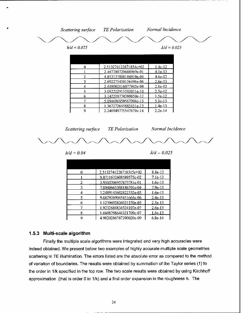
Scattering surface TE Polarization Normal Incidence
h/d = 0.025 A/d= 0.025
^^^^^^^^^^^^^1 0 2.513274122871854e+02 1.4e-12 1 2.467789729688969e-01 4.1e-13 2 4.853137888184910e-04 4.6e-12 3 2.692275458156496e-06 2.6e-13 4 2.418002116077943e-08 2.1e-12 5 3.012222915203911e-10 2.5e-12 6 3.142218774380850e-12 1.5e-12 7 5.094686950567004e-13 5.1e-13 8 1.367272645883451e-13 1.4e-13 9 2.246949775547679e-14 2.2e-14
Scattering surface TE Polarization Normal Incidence
h/d=0.04 A/d = 0.025
^^^^■^^^^^■^H 0 2.5132741228718315e+02 8.8e-13
1 9.8711672408589575e-02 7.1e-13 2 3.9503306957875781e-01 1.6e-13
3 7.0040665308186701e-04 7.9e-13 4 1.2489143602822332e-03 1.6e-13 5 9.6829269045451665e-06 2.4e-13
6 1.1239693826031570e-05 2.5e-13 7 1.9232684834524107e-07 2.6e-13
8 1.6608798644321709e-07 1.6e-13 9 4.9820286787390020e-09 6.8e-14
1.5.3 Multi-scale algorithm
Finally the multiple scale algorithms were integrated and very high accuracies were
indeed obtained. We present below two examples of highly accurate multiple scale geometries
scattering in TE illumination. The errors listed are the absolute error as compared to the method
of variation of boundaries. The results were obtained by summation of the Taylor series (1) to
the order in 1/k specified in the top row. The two scale results were obtained by using Kirchhoff
approximation (that is order 0 in 1/k) and a first order expansion in the roughness h. The
24

difference between the two scale column and the Order 1 column comes from the fact that we
used an expansion of order 20 in the high-frequency solver for Order 1 as opposed to order 0
for the two scale case.
h/d= 0.0252 Scattering surface A/d= 0.025
vwvwww Scattering
Direction # Scattered Energy
Two Scale Order 1 Order 2 Order 4 Order 6 Order 8
0 4.833824308716315e-02 1.8e-4 9.2e-5 2.1e-8 2.3e-12 5.8e-14 6.0e-15
1 4.524676580264179e-02 2.0e-5 8.7e-5 2.0e-8 2.0e-12 4.0e-14 2.3e-15
2 8.248342098822989E-02 2.3e-4 1.6e-4 3.2e-8 3.2e-12 6.6e-14 8.8e-15
3 1.053390492569949E-03 1.7e-5 2.0e-6 2.2e-8 3.4e-12 8.9e-15 8.8e-16
4 0.101853442231311 8.7e-5 1.9e-4 2.3e-8 6.0e-12 3.0e-14 5.5e-15
5 0.139564830538028 2.8e-4 2.6e-4 6.3e-8 1.3e-ll 2.7e-14 8.8e-15
6 7.574080330783492E-02 2.0e-4 1.4e-4 6.0e-8 l.le-11 1.5e-14 8.9e-15
7 2.357615851308177E-02 7.5e-5 4.4e-5 8.6e-9 8.1e-13 2.4e-14 1.5e-14
The scattering surface was in that case defined by z=0.025(cos(2jtx)+0.01cos(20ro<)). The
calculation of order 8, which yielded 14 digits of accuracy, took 1 hour 9 minutes 54 seconds on
a 600 MHz machine. A result with 12 digits of accuracy was obtained for order 4 and took 5
minutes and 51 seconds on the same machine. The large difference in timing is due mainly to a
reduction in number of Fourier modes used. Whereas 30 modes suffice for 12-digit accuracy,
100 modes are necessary for 15-digit accuracy.
h/d= 0.0101 Scattering surface
\j ^ w ■V/XJ
A/d= 0.025
Scattering Direction #
Scattered Energy
Two Scale Order 1 Order 2 Order 4 Order 6
0 0.198901761348164 2.1e-4 6.1e-5 4.3e-8 l.le-12 3.5e-14
1 2.118863974374862E-02 8.4e-5 6.5e-6 4.9e-9 1.2e-13 3.1e-15
2 5.064428936060158E-02 2.3e-4 1.5e-5 3.4e-9 8.2e-13 2.4e-14
3 0.135474001366087 l.le-4 4.1e-5 3.3e-9 8.2e-13 3.7e-14
4 1.614783623594695E-02 6.5e-5 5.0e-6 4.2e-9 9.9e-13 5.7e-14
5 0.104163054003108 1.2e-4 3.2e-5 8.1e-10 5.6e-14 2.6e-14
6 3.084758570010842E-02 3.2e-5 9.3e-6 4.2e-8 8.5e-13 1.9e-13 7 2.782604772500211E-02 7.8e-5 8.5e-6 3.2e-8 7.4e-13 6.3e-14
In this next example, the scattering surface was defined by
Z=0.01*(COS(27CX)+COS(4TCX)+0.025COS(20JTX)). The calculation of order 6, which yielded 14 digits
25

of accuracy, took 55 minutes and 34 seconds on a 600 MHz machine. A result with 12 digits of
accuracy obtained for order 4 took 13 minutes and 17 seconds on the same machine.
1.6 Exploitation and Follow on
A natural transition program is to correlate polarized radar backscattering returns to
relevant surface characteristics, with specific focus on ocean surfaces, through the utilization of
an appropriately validated highly efficient and accurate algorithm specially designed for the
solution of scattering problems from multiple scale surfaces. The overall objective is to improve
the interpretation and predictive capabilities from radar remote sensing returns.
1.6.1 Modeling of Doppler spectrum
The time evolution of the polarized scattering returns is of great use in analyzing the
distribution and evolution of scatterers on the ocean surface. Indeed, the power spectrum of the
polarized backscattered returns, also known as the Doppler spectrum, is routinely used in
experiments for diagnostic and analysis of the distribution and speed of the scatterers on the
moving surface, cf. [Lee et al, 1997a; Rozenberg et al, 1996; Lee et al, 1996; Lee et al, 1997b;
Liu et al, 1998; Lee et al, 1995; Ja et al, 2001; Duncan et al, 1999].
TRW's Ocean technology department, a world-renown center of excellence for ocean
hydrodynamics, has developed many ocean simulation tools based on the formulations
described in [Longuet-Higgins and Cokelet, 1976] and [Zhakarov, 1968]. These algorithms are
design to model the hydrodynamic evolution of a variety of scales on the water surface. The
coupling of these hydrodynamic models to the TRW high-order high frequency multi-scale
electromagnetic numerical solver will provide a powerful, efficient and extremely accurate
algorithm for the modeling and analysis of Doppler spectra. The high accuracy delivered by the
scattering solver is necessary due to the range of scattering returns typically observed to be
between -60 dB to -100 dB. This means that to compute reliably simulation results, an
accuracy of 10 digits is necessary at the very least.
Once the Doppler spectrum code is implemented, a series of hypothesis regarding the
cause and nature of the HH/VV ratio intermittent spiking can be addressed. In particular, the
broadening of the velocity distribution introduced by the scattering process can be analyzed.
Indeed, since the propagation of water waves will be performed numerically the distribution of
velocities at every point along the profile can be evaluated as a function of time. The power
spectrum of this distribution of velocities can then be compared to the power spectrum of the
scattering returns for each polarization (the Doppler spectrum). To our knowledge, the basic
26

understanding of the relationship between the distribution of velocities on the water surface and
the associated Doppler spectrum for HH and W polarization obtained from the scattering
returns has never been undertaken. It will be of immediate interest to the ocean scattering and
remote-sensing communities that seeks to interpret measured Doppler spectra in terms of
surface characteristics.
1.6.2 Return from statistically described rough surfaces
The computational speed of our multi-scale algorithm allows the investigation of the
surface configuration mechanisms responsible for distinct radar return signatures. In particular,
detailed parametric studies can be performed about the dependence of the scattering returns on
the surface statistical characteristics such as their spectral distribution cf. [Pierson and
Moskowitz, 1964; Donelan and Pierson, 1987; Jahne and Riemer, 1990; Apel, 1994 and
Elfouhaily et al, 1997]. One outstanding, yet unsolved, problem in that field concerns the
retrieval of wind speed and direction from radar measurements. A number of empirical models
have been proposed cf. [Apel, 1994] and more recent measurements have been made cf.
[Chaudry and Moore, 1984; Masuko et al, 1986; Woiceshyn et al, 1986; Carswell et al, 1994].
However the establishment of a reliable empirical relationship between radar cross
section and wind speed and direction remains elusive cf. [Rufenach, 1998; Phillips, 1988]. The
discrepancy can be attributed to two main factors. First the computations of the radar cross
section are all based on two-scale models. These models rely on the distribution of short
"Bragg" waves, which spectrum is still a matter of active research cf. [Pierson and Moskowitz,
1964; Donelan and Pierson, 1987; Jahne and Riemer, 1990; Apel, 1994 and Elfouhaily et al,
1997]. Of course, the interpretation of measured data and the retrieval of wind characteristics
require a model of the dependence of the radar returns on the wind characteristics.
We propose to alleviate the errors introduced by the two-scale scattering model by
replacing the scattering module by our highly accurate solver. The expected outcome ofthat
study is the evaluation of current ocean spectra with full electromagnetic account of all scales
on the surface at X-band. Furthermore accurate scattering computations will permit to test the
current functional forms of the backscattered cross section as a function of wind speed and to
determine their range of validity. This will help the wind retrieval (inverse) problem, which is
poorly understood at this point cf. [Rufenach, 1998].
It is of interest to note here that the recent studies we carried out with a simplified
version of our algorithm, for periodic surfaces with slopes in the range 0.01-0.3, have already
yielded results not expected from the predictions of classical theories cf. [Sei et al., 1999]. In
27

particular, these results provide the first rigorous theoretical evidence of anomalous absorption
of polarized EM radiation. This result is potentially of strong relevance to the ocean scattering
community. Our results show that significant effects on the backscattering polarization ratio
(HH/W or TE/TM) can arise from modulated short waves, that is, corrugated surfaces with
features similar to those abundant in ocean surfaces (cf. Figure 4 and [Sei et al., 1999]). The
effects depend on incidence angle, dielectric constant and specific configuration characteristics.
Figure 2 shows an instance of the results we have obtained. It illustrates the increase in
the ratio of HH/W, obtained for the specific wavetrain of Figure 4, for a particular region of
slope values (ka = n h/d, where h is the height and d the period of the wavetrain). The figure
also shows the constant, and orders of magnitude smaller, value of HH/W that would have
been predicted by either first order theories or the classical theory of Rice. These results are all
the more relevant in view of the recent experimental measurements that have demonstrated the
strong contribution to the radar return from incipient or actively breaking water waves cf. [Lee et
al, 1997; Liu et al, 1998].
These waves are nonlinear by nature, with large slopes (ka ~ .1) consisting of
wavetrains of different scales and can be directionally modulated. The experimental results
show "sea spikes" in potential agreement with our calculation. The "sea spikes" are regions of
large HH/W polarization ratios and sporadically high HH returns for near grazing angles in
direct contradiction with first order perturbation theories.
Figure 4. Periodic modulated wave train
Incidence Angte = TO Dsg - HH ,•' W
t First Order ;
■ / ^^
-
: i
Figure 5. Simulated scattering returns for surface shown in Fig. 4
and comparison with first order and classical theories.
28

1.7 Bibliography
M. Abramowitz and I. Stegun, Handbook of mathematical functions with formulas, graphs, and
mathematical tables, US Dept Commerce, June, 1964.
D. S. Ahluwalia, R. M. Lewis and J. Boersma, Uniform asymptotic theory of diffraction by a plane
screen, SIAM J. Appl. Math., 16 (4), 783-807, 1968.
J. R. Apel, An improved model for the ocean surface wave vector spectrum and its effects on radar
backscatter, J. Geophys. Res., 99, 16,269-26,291, 1994.
H. Ansorge, Electromagnetic reflection from a curved dielectric interface, IEEE Trans. Ant. Prop.,
34,842-845, 1986.
H. Ansorge, First order corrections to reflection and transmission at a curved dielectric interface with
emphasis on polarization properties, Radio science, 22, 993-998, 1987.
J. D. Benamou, Direct computations of multivalued phase space solutions for Hamilton-Jacobi equations,
Comm. Pure Appl. Math., 52, 1443-1475, 1999.
N. Bleistein and R. A. Handelsman, Asymptotic expansions of integrals, Dover Publications, New York,
1986.
C. O. Bloom and N. D. Kazarinoff, Short wave radiation problems in inhomogeneous media: asymptotic
solutions, Lecture Notes in Mathematics 522, Springer-Verlag, Berlin, 1976.
D. Bouche, F. Molinet and R. Mittra, Asymptotic methods in electromagnetics, Springer-Verlag, Berlin,
1997.
W. P. Brown, On the asymptotic behavior of electromagnetic fields from convex cylinders near grazing
incidence, J. of Math. Anal, and App., 15, 355-385, 1966.
O. Bruno and F. Reitich, Numerical solution of diffraction problems: a method of variation of boundaries
I, II, III, J. Opt. Soc. A 10, 1168-1175, 2307-2316, 2551-2562, 1993.
O. Bruno, A. Sei and M. Caponi, Rigorous multi-scale solver for rough-surface scattering problems:
high-order-high-frequency and variation of boundaries, Proceedings of the NATO Sensors and
Electronics Technology (SET) Symposium on '"Low Grazing angle clutter: Its Characterization,
Measurement, and Application", JHU/APL, Laurel, MD, April 25-27 2000.
29

O. Bruno, A. Sei and M. Caponi, High-order high-frequency solutions of rough surface scattering
problems, to appear in Radio Science, 2002. See also Appendix Al.
J. R. Carswell, S. C. Carson, R. E. Mclntosh, K. K. Li, G. Neumann, D. J. Mclaughlin, J. C. Wilkerson, P.
G. Black and V. Nghiem, Airborne scatterometers: Investigating ocean backscatter under low- and
high-wind conditions, Proc. IEEE, 82, 1835-1860, 1994.
H. Cartan, Elementary theory of analytic functions of one or several complex variables, Addison-Wesley,
Reading, Mass., 1963.
H. Chaloupka and H. J. Meckelburg Improved high-frequency current approximation for curved
conducting surfaces, AEU, Arch. Elektron. Ubertragungstech, 39, 245-250, 1985.
A. H. Chaudhry and R. K. Moore, Tower-based backscatter measurements of the sea, IEEE J. Ocean.
Eng., OE-9, 309-316, 1984.
A. N. Churyumov and Y.A. Kravtsov, Microwave backscatter from mesoscale breaking waves on the sea
surface, Waves in Random media, 10, 1-15, 2000.
R. Courant and D. Hilbert, Methods of Mathematical Physics, Interscience Publishers, 1962.
D.D. Crombie, Doppler spectrum of sea echo at 13.6 Mc/s, Nature, 175, 681-682, 1955.
M. A. Donelan and W. J. Pierson, Radar scattering and equilibrium ranges in wind-generated waves with
application to scatterometry, J. Geophys. Res., 92, 4971-5029, 1987.
J. J. Duistermaat, Huygens' principle for linear partial differential equations, Huygens' principle, 1690-
1990: theory and applications, H. BlokEd, Elsevier, 1992.
J.H. Duncan, H. Qiao, V. Philomin and A. Wentz, Gentle spilling breakers: Crest profile evolution, J.
Fluid Mech.. 379, 191-222, 1999.
T. Elfouhaily, B. Chapron and K. Katsaros, A unified directional spectrum for long and short wind-driven
waves, J. Geophys. Res., 102, 15,781-15,796, 1997.
E. Fatemi, B. Engquist and S. Osher, Numerical solution of the high frequency asymptotic expansion for
the scalar wave equation, J. Comp. Phys., 120, 145-155, 1995.
F. G. Friedlander, Geometrical Optics and Maxwell's equations, Proc. Cambridge Philos. Soc, 43 (2),
284-286, 1946.
F. G. Friedlander and J. B. Keller, Asymptotic expansion of solutions of (A + k2) u - 0, Comm. Pure Appl.
Math., 8, 387-394, 1955.
30

R.F. Gasparovic and V.S. Etkin, An overview of the joint US/Russia internal wave remote sensing
experiment, Proc. IGARSS'94, 741-743, 1994.
M. A. Gil'Man, A. G. Mikheyev and T. L. Tkachenko, The two-scale model and other methods for the
approximate solution of the problem of diffraction by rough surfaces, Comp. Maths Math. Phys., 36,
1429-1442, 1996.
J. Hadamard, La theorie des equations aux derivees partielles, Editions Scientifiques, Pekin, 1964.
J. Hadamard, Lecons sur la propagation des ondes et les equations de l'hydrodynamique, Chelsea
Publishing Company, New-York, 1949.
S. Hong, Asymptotic theory of electromagnetic and acoustic diffraction by smooth convex surfaces of
variable curvature, J. Math. Phys., 8, 1223-1232, 1967.
M.C. Hutley, Diffraction gratings, Academic Press, San Diego, Calif., 1982.
S.J. Ja, J.C. West, H. Qiao and J.H. Duncan, Mechanisms of low-grazing-angle scattering from spilling
breaker water waves, Radio Science, 36, 981-998, 2001.
B. Jahne and K. S. Riemer, Two-dimensional wave number spectra of small-scale water surface waves, J.
Geophys. Res., 95, 11,531-11546, 1990.
J. B. Keller, A geometric theory of diffraction, AMS Calculus of variations and its applications, L.M.
Graves ed., McGraw-Hill, New York, 1958.
B. Kinsman, Wind waves, their generation and propagation on the ocean surface, Englewood Cliffs, New
Jersey, Prentice-Hall, 1965.
Y. A. Kravtsov, A modification of the geometric optics method, Radiofizika, 7, 664-673, 1964.
B. F. Kuryanov, The scattering of sound at a rough surface with two types of irregularity, Soviet Physics-
Acoustic, 8 (3), 252-257, Jan. 1963.
A.G. Kyurkchan, B.Y. Sternin and V.E. Shatalov, Singularities of continuation of wave fields, Physics-
Uspekhi, 30 (12), 1221-1242, 1996.
P. Lee, J.D. Barter, K.L. Beach, C.L. Hindman, B.M. Lake and H. Rungaldier, X-band microwave
backscatteringfrom ocean waves, J. Geo. Res. 100, 2591-2611, 1995.
P. Lee, J.D. Barter, E. Caponi, M. Caponi, C.L. Hindman, B.M. Lake and H. Rungaldier, Wind-speed
dependence of small grazing angle microwave backscatter from sea surfaces, IEEE Trans. Ant. Prop.
44, 333-340, 1996.
31

P. Lee, J.D. Barter, K.L. Beach, C.L. Hindman, B.M. Lake, H.R. Thompson and R. Yee, Experiments on
Bragg and non-Bragg scattering using single-frequency and chirped radars, Radio. Sei. 32, 1725-
1744, 1997a.
P. H. Y. Lee, J. D. Barter, K. L. Beach et al, Scattering from breaking waves without wind, IEEE Trans.
Ant. Prop., 46 (1), 14-26, 1997b.
S. W. Lee, Electromagnetic reflection from a conducting surface: geometrical optics solution, IEEE
Trans. Ant. Prop., 23, 184-191, 1975.
R. M. Lewis and J. Boersma, Uniform theory of edge diffraction, J. Math. Phys., 10 (12), 2291-2305,
1969.
R. M. Lewis and J. B. Keller, Asymptotic methods for partial differential equations: The reduced wave
equation and Maxwell's equations, Research Report EM-194, New York University, 1964. (Reprinted
in Surveys in Applied Mathematics, Vol. 1, 1-82, Plenum Press, New York, 1995).
R. M. Lewis, N. Bleistein and D. Ludwig, Uniform asymptotic theory of creeping waves, Comm. Pure
Appl. Math., 20, 295-320, 1967.
Yong Liu, Stephen J. Frazier, and Robert E. Mclntosh, Measurement and Classification of Low-Grazing-
Angle Radar Sea Spikes, IEEE Transactions on Antennas and Propagation 46 (1), 27-40, 1998.
M. S. Longuet-Higgins and E. D. Cokelet, The deformation of steep surface waves on water I: A
numerical method of computation, Proc. R. Soc. A., 350, 1-26, 1976.
R. K. Lüneburg, Mathematical theory of Optics, Brown University, 1944. (Reprinted by University of
California Press, Berkeley, 1964).
R. K. Lüneburg, Asymptotic expansion of steady state electromagnetic fields, Research Report EM-14,
New York University, July 1949.
R. K. Lüneburg, Asymptotic evaluation of diffraction integrals, Research Report EM-15, New York
University, October 1949.
D. Ludwig, Uniform asymptotic expansion at a caustic, Comm. Pure Appl. Math., 19, 215-250, 1966.
S. T. McDaniel and A. D. Gorman, An examination of the composite-roughness scattering model, J.
Acoust. Soc. Am., 73, 1476-1486, 1983.
H. Masuko, K. Okamoto, M. Shimada and S. Niwa, Measurement of microwave backscattering
signatures of the ocean surface using X-Band and Ka-Band airborne scatterometers, J. Geophys.
Res., 91, 13,065-13,083, 1986.
32

R.F. Millar, On the Rayleigh assumption in scattering by a periodic surface, Proc. Camb. Phil. Soc, 65,
773-791, 1969.
W. L. Miranker, Parametric theory of Au + h?u, Arch. Ratl. Mech. Anal, 1, 139-152, 1957.
K. M. Mitzner, Effect of small irregularities on electromagnetic scattering from an interface of arbitrary
shape, J. Math. Phys., 5, 1776-1786, 1964.
R. K. Moore and A. K. Fung, Radar determination of winds at sea, P. IEEE, 67 (11), 1504-1521, 1979.
O. M. Phillips, Remote sensing of the sea surface, Ann. Rev. Fluid Mech., 20, 80-109, 1988.
R. Petit, Electromagnetic theory of Gratings, Springer-Verlag, Berlin, 1980.
R. Petit and M. Cadilhac, Sur la diffraction dune onde plane par un reseau infiniment conducteur, C. R.
Acad. Sei. Paris, Ser A-B, 262, 468-471, 1966.
WJ. Pierson and L. Moskowitz, A proposed spectral form for fully developed wind seas based on the
similarity theory of S.A. Kitaigorodskii, J. Geo. Res. 69, 5181—5190, 1964.
W. H. Press, S. A. Teukolsky, W. T. Vetterling and B. P. Flannery, Numerical Recipes, Cambridge
University Press, 1992.
S. O. Rice, Reflection of electromagnetic waves from slightly rough surfaces, Comm. Pure Appl. Math.,
4,351-378, 1951.
A. D. Rozenberg, D. C. Quigley, and W. Kendall Melville, Laboratory Study of Polarized Microwave
Scattering by Surface Waves at Grazing Incidence: The Influence of Long Waves, IEEE Transactions
on Geoscience and Remote Sensing 34 (6), 1331-1342,1996.
C. Rufenach, Comparison of four ERS-1 scatterometer wind retrieval algorithms with buoy
measurements, J. Atmos. Oceanic Technol., 15, 304-313, 1998.
A. Sei, O. P. Bruno and M. Caponi, Study of polarization scattering anomalies with application to
oceanic scattering, Radio Science, 34 (2), 385-411, 1999.
A. B. Shmelev, Wave scattering by statistically uneven surfaces, Soviet Physics uspekhi, 15 (2), 173-183,
Sept. 1972.
G.R. Valenzuela, Theories for the interaction of electromagnetic and oceanic waves - A review,
Boundary-layer Meteor. 13, 61-85, 1978.
N. G. Van Kampen, An asymptotic treatment of diffraction problems, Physical4 (9), 575-589, January
1949.
33

J. Vidale, Finite difference calculation oftraveltimes, B. Seismol. Am., 78, 2062-2076, 1988.
A. G. Voronovich, Wave scattering from rough surfaces, Springer-Verlag, Berlin, 1994.
J. VanTrier and W. W. Symes, Upwind finite- difference calculation oftraveltimes, Geophysics, 56, 812-
821, 1991.
P. M. Woiceshyn, M. G. Wurtele, D. H Boggs, L. F. McGoldrick and S. Peteherych, The necessity for a
new parametrization of an empirical model for wind/ocean scatterometry, J. Geophys. Res., 91,
2273-2288, 1986.
V. E. Zhakarov, Stability of periodic waves of finite amplitude on the surface of a deep fluid, J. Appl.
Mech. Tech. Phys. (Engl. Transl.), 9, 190-194, 1968.
34

APPENDICES
The appendices list the published work in the course of this project, the patent application filed
with the US Patent office as a result of this work and the annual progress reports produced in
the course of this project.
Appendix Al:
High-Order High Frequency solutions of rough surface scattering problem, to appear in
Radio Science, 2002.
Appendix A2:
Polarization ratios anomalies of 3D rough surface scattering as second order effects,
IEEE AP-S International symposium, Boston, Massachusetts, July 2001.
Appendix A3:
Rigorous multi-scale solver for rough-surface scattering problems: high-order-high-
frequency and variation of boundaries, Proceedings of the NATO Sensors and
Electronics Technology (SET) Symposium on "Low Grazing angle clutter: Its
Characterization, Measurement, and Application", JHU/APL, Laurel, MD, April 2000.
Appendix A4:
High-Order High Frequency solutions of rough surface scattering problem, Fifth
International Conference on Mathematical and Numerical Aspects of Wave Propagation,
Santiago de Compostella, Spain, July 2000.
Appendix A5:
An innovative high-order method for electromagnetic scattering form rough surfaces,
National Radio Science Meeting, Boulder, Colorado, January 2000.
35

Appendix Bl:
US Patent application: High-Order High-Frequency rough surface scattering solver
Appendix Cl: Progress report for 03/01/1999 - 07/31/1999
Appendix C2: Progress report for 07/31/1999 - 07/31/2000
Appendix C3: Progress report for 07/31/2000 - 07/31/2001
Appendix C4: Progress report for 07/31/2001 - 12/31/2001
36

Appendix Al:
High-Order High Frequency solutions of rough surface scattering problem, to appear in
Radio Science, 2002.

High-Order High-Frequency Solutions of Rough Surface
Scattering Problems
Oscar P. Bruno Applied Mathematics, California Institute of Technology, Pasadena Ca, 91125
Alain Sei Ocean Technology Department, TRW, 1 Space Park. Redondo Beach. Ca. 90278
Maria Caponi Ocean Technology Department, TRW, 1 Space Park. Redondo Beach. Ca. 90278

2
Abstract. A new method is introduced for the solution of problems of scattering
by rough surfaces in the high-frequency regime. It is shown that high order
summations of expansions in inverse powers of the wavenumber can be used
within an integral equation framework to produce highly accurate results for
surfaces and wavelengths of interest in applications. Our algorithm is based on
systematic use and manipulation of certain Taylor-Fourier series representations
and explicit asymptotic expansions of oscillatory integrals. Results with machine
precision accuracy are presented which were obtained from computations involving
expansions of order as high as twenty.

1. Introduction
Computations of electromagnetic scattering from rough surfaces play important roles in a wide
range of applications, including remote sensing, surveillance, non destructive testing, etc. The
problem of evaluating such scattering returns is rather challenging — owing to the multiple-scale
nature of rough scatterers, whose spectra may span a wide range of length-scales [Valenzuela,
1978].
A number of techniques have been developed to treat limiting cases of this problem. For
example, the high frequency case, in which the wavelength A of the incident radiation is much
smaller than the characteristic surface length-scales, has been treated by means of low order
asymptotic expansions, such as the Kirchhoff approximation. On the other hand, resonant
problems where the incident radiation wavelength is of the order of the roughness scale have
been treated by perturbation methods, typically first or second order expansions in the height h
of the surface [Rice, 1951; Shmelev, 1972; Mitzner, 1964; Voronovich, 1994]. However, when a
multitude of scales is present on the surface none of these techniques is adequate, and attempts to
combine them in a so-called two-scale approaches have been given [Kuryanov, 1963; McDaniel
and Gorman, 1983; Voronovich, 1994; Gil'Man et al. 1996]. The results provided by these
methods are not always satisfactory, owing to the limitations imposed by the low orders of
approximation used in both, the high-frequency and the small perturbation methods.
A new approach to multi-scale scattering, based on use of expansions of very high order in
both parameters A and h, has been proposed recently [Bruno et al., 2000]. These combined
methods, which are based on complex variable theory and analytic continuation, require nontriv-
ial mathematical treatments; the resulting approaches, however, do expand substantially on the
range of applicability over low order methods, and can be used in some of the most challenging

4
cases arising in applications. Perturbation series of very high-order in h have been introduced
and used elsewhere to treat resonant problems — in which the wavelength of radiation is com-
parable to the surface length-scales [Bruno and Reitich, 1993; Sei et al., 1999]. In this paper
we focus on our high-order perturbation series in the wavelength A, which, as we shall show,
exhibits excellent convergence in the high-frequency, small wavelength regime. The combined
(h, A) perturbation algorithms for multiscale surfaces, which require as a main component the
accurate high frequency solvers presented in this paper, are described in [Bruno et al, 2000].
Our approach to the present high-frequency problem uses an integral equation formulation,
whose solution u is sought and obtained in the form of an asymptotic expansion
+oo . / \ u(x,k) = e--W(^^), (!)
n=p K
with p = — 1 for TM polarization and p = 0 for TE polarization. This expansion is similar in
form to the geometrical optics series [Lewis and Keller, 1964]
+00
n=0
where S = S(x, y) is the unknown phase of the scattered field. Note that the phase of the
density v of (1) is determined directly from the geometry and the incident field and, unlike that
in the geometrical optics field, it is not an unknown of the problem. In particular, the present
approach does not require solution of an eikonal equation [Vidale, 1988; VanTrier and Symes,
1991; Fatemi et al., 1995; Benamou, 1999], and it bypasses the complex nature of the field of
rays, caustics, etc.
The validity of the expansion (2) has been extensively studied [Friedlander, 1946; Lüneburg,
1949a; Lüneburg, 1949b; Van Kampen, 1949; Lüneburg, 1964]; in particular, it is known that
equation (2) needs to be modified in the presence of singularities of the scattering surface.
+00 I \
u(x,y,k) = e**(*..0 £ *ÜM, (2)

5
To treat edges and wedges, for example, an expansion containing powers of k~1/2 [Lüneburg,
1949b; Van Kampen, 1949; Keller, 1958; Lewis and Boersma, 1969; Lewis and Keller, 1964] must
be used; caustics and creeping waves also lead to similar modified expansions [Kravtsov, 1964;
Brown, 1966; Ludwig, 1966; Lewis et al., 1967; Ahluwalia et al, 1968]. Proofs of the asymptotic
nature of expansion (2) were given in cases where no such singularities occur [Miranker, 1957;
Bloom and Kazarinoff, 1976]. In practice only expansions (2) of very low orders (one, or, at most
two) have been used — owing in part to the substantial algebraic complexity required by high
order expansions [Bouche et al., 1997]. First order versions of the expansion (1), on the other
hand were treated in [Lee, 1975; Chaloupka and Meckelburg, 1985; Ansorge, 1986; Ansorge,
1987].
The region of validity of our ansatz (1), on the other hand, corresponds to configurations where
no shadowing occurs. At shadowing the wave vector of the incident plane wave is tangent to the
surface at some point, which causes certain integrals to diverge; see Section 4. Thus, a different
kind of expansion, in fractional powers of 1/k. should be used to treat shadowing configurations:
a first order version of such an expansion was discussed in [Hong. 1967]; see [Friedlander
and Keller, 1955; Lewis and Keller, 1964; Brown, 1966; Duistermaat. 1992] for the ray-tracing
counterpart.
In this paper we show that high order summations of expansion (1) can indeed be used to
produce highly accurate results for surfaces and wavelengths of interest in applications for both
TE and TM polarizations; in Section 7, for example, we present results with machine precision
accuracy, which were obtained from computations involving expansions of order as high as 20.
Our algorithm is based on systematic use and manipulation of certain Taylor-Fourier series
representations, which we discuss in Section 5. Operations such as product, composition and

6
inversion of Taylor-Fourier series lie at the core of our algebraic treatment; as shown in Section
5 certain numerical subtleties associated with these operations require a careful treatment for
error control.
In order to streamline our discussion we first treat, in sections 2 to 5, the complete formalism
in the TE case; the changes necessary for the TM case are then described in Section 6. In
detail, in Section 2 we present our basic recursive formula for the evaluation of the coefficients
un{x) of equation (1) for the TE case. These coefficients depend on certain explicit asymptotic
expansions of integrals, which we present in Sections 3 and 4. A discussion of the Taylor-Fourier
algebra then ensues in Section 5. As we said, the modifications necessary for the TM case are
discussed in Section 6. A variety of numerical results for both TE and TM polarizations, finally,
are presented in Section 7.
2. High-Frequency Integral Equations — TE case
The scattered field u = u(x,y) induced by an incident plane wave impinging on the rough
surface y = f(x) under TE polarization is the solution of the Helmholtz equation with a Dirichlet
boundary condition. As is known [Voronovich, 1994] the field u(x,y) can be computed as
an integral involving a surface density v(x,k) and the Green's function G(x,y,x',y') for the
Helmholtz equation
u(x',k) —(x,y,x'J(x'))Jl + (f>(x>))2dx' (3)
where v satisfies the boundary integral equation
^^ + fl ^(xj(x),x'j(x'))^/l + (f'(x'))2u(x',k)dx' = -ete-WW. (4)

In what follows we will use the relations
dG ^(xJ(x),x'J(x'))^l + (f'(x'))2 = -l-h(kr)g(x^x') dn
r = ^{x'-x)2 + (f{x')-f{x)y h(t) = tH\{t) H\ Hankel function
gM = /(*0-/(*)-(*'-*)/V) a = ksm{e) 6 = Acos(fl))
where 9 is the incidence angle measured counter-clockwise from the vertical axis, and k = 2n/\
is the wavenumber.
A useful form of the integral equation (4) results as we factor out the rapidly oscillating phase
function e^-W(*)
(e-(i°>*-ißf(x))vfakj\ _ 1 f+0° h(kr)g(x,x') (e^iax-iß^x))u(x'.k)) dx! = -2, (5) ^ ' 2i J — oo
which cancels the fast oscillations in all non-integrated terms, and thus suggests use of an ansatz
of the form
u(x,k) = e"*-W(*)£^2. (6)
Substitution of the ansatz (6) into equation (5) then yields
£^(^)-^"(^)) = -2 (J)
where
p(x,k) = f+°° /l(fcr)&(x,a;,)ei0l(s'"x)~'/3(/(l')"/(l))^(^')^'• ■/ —00
To solve equation (7) we use asymptotic expansions for the integrals In(x. k). collect coefficients
of each power of 1/fc, and then determine, recursively, the coefficients vn{x). In detail, we obtain
in Section 3 an expansion which gives In{x, k) in terms of derivatives of un(x)
*"(*,*) = l+f1-^1 where W = f^B^x) (8) %=o ft fco ox

where the functions Bq-t{x) are determined from the profile and incidence angle only. (We
point out, however, that our algebraic treatment yields an expression for I*(x) which, although
equivalent to that of (8), is different in form; see Remark 1 and equation (25).) From (7) and (8)
we then find a recursion which gives un(x) as a linear combination of derivatives of the previous
coefficients i/n_i_g(a;)
u0(x) = -2
(9)
Use of the Taylor-Fourier algebra of Section 5 allows us to perform accurately the high order
differentiations required by our high-order expansions; the needed expansion (8) of the integral
In, in turn, is the subject of the next section.
3. Asymptotic expansion of In(x,k)
We first split the integral In as a sum In = II +1\ where
n{x,k) = f h(kr)g{x,xyaW-x)-ißVV)-Hx))Mx')d*' J—oo
I%{x,k) = f+^h(kr)g(x,x^x'-x^iß^x'^f^un(x')dx' Jx
We evaluate in detail the asymptotic expansion for i+(x, k); the corresponding expansion for i"™
then follows analogously.
Using t = x' — x we obtain
Il{x,k) = f+0° h(k<l>+(x,t))g{x,x + t)eiat-ißMx+Q-fWun(x + t)dt (10) Jo
where
4>+{x,t) = yJt* + U{x + t)-f{x)Y

For the treatment presented here, f(x) is assumed to satisfy the condition
4>'Ax,t) = d(f>+(x,t)
at >o for t > 0 (11)
so that the map t H-> <f>+(x, t) is invertible. (This condition is generally satisfied by rough surfaces
considered in practice: for a sinusoidal profile f{x) = acos(x), for example, the inequality (11)
holds as long as a < 1.) Then setting
u = <ß+(x,t) t = (bAix.u)
equation (10) becomes
r+oo I$(x,k) = / h(k-
Jo
+0° L/,..^g(3;.a; + ^+1(a;»U)). ,n(x + ^-1(a;,u))eia*+I(x',')-1'3(/(a:+*+1(x>,'))-/(x))du.
Calling
F${x,u) g(x,x + (f)+
l(x,u))
4?+(x,<l>1l{x,u)) vn(x + (f>+ (x,u))
(12)
ip+(x,u) = (f{x + 4>+l{x,u)) -/(z)) cos(0) -(/)+
l(x.u)sin(9),
I+(x,k) reduces to
r+oo lVx,k) = / F^{x,u)h{ku)e-lk^x'^du.
Jo
Remark 1 The unknown vn{x) is contained as a factor in the function F+(x, u). Notation (12)
is useful in that it helps present the integrand as a product of two distinct factors: a non-
oscillatory component F+(x,u) and an oscillatory component h(ku)e~lkxll+(x'uy
In addition to (11) we assume the profile y = f(x) is an analytic function — so that the map
u (->• F™(x,u) is analytic as well. Using the Taylor series
FUx,u) = +g dmFZ(x,0)um _ +2? + Z-j F,„m m| _ 2^ Pn,m\x) dum
m=0 m=0
U ml
(13)

10
the integral I+(x,k) takes the form
+00 r+00 ~rl-*J /*-rOO
I»(x,k) = Y.<rn{x)jQ Umh(ku)e-ik*+^du
m=0
(14)
to km+1 * Thus, the \/k expansion of 7" results from the corresponding expansions of the integrals
A+(k,m,x) = [+°° vmh(v)e-ikjp+^^dv. (15) Jo
These non-convergent integrals must be re-interpreted by means of analytic continuation — in a
manner similar to that used in the definition and manipulation of Mellin transforms [Bleistein
and Handelsman, 1986]. An explicit expansion of A+(k, m,x) is given in the following section.
3.1. Expansion of the integrals 7" and 7™
+°° „,m
m\
the identity ip+(x, 0) = 0, expansion of the function exp(—i(kip+(x, |) — ipf(x)v)) leads to the
-t-°° um Using the Taylor expansion of ip+(x,u) = ]P ipm(x)—T m tne variable u together with
m=0
(-i(hnh+(T. t\ -il&l
expression +00 n „+
e-i*0+(s,|) = e-ii>U*» U + g fc-» £ ^Än+A (16) V n=l e=i /
for certain (function) coefficients a~ln(x). Then, defining
A+(p,x) = / «P/»(«) e"W (^»rf« (17) Jo
and
A+(m,:r) = £^^4+(m + n-Ks) (18)
we obtain
e=o
A+(k,m,x) = A+(m,x) + £ ^^, (19) n=l

11
and the series +00 / q \
i$(x,k) = E E4M+(?-^)p"H (2°) q=0 \i=0 )
for I™ results. We see that this expansion is given in terms of the integrals (17) which, like
those of the previous section, are non-convergent and require analytic continuation. An explicit
expression for this integral as a function of p and x is given in Section 4.
The case of J" (x, k) can be treated similarly: we use t = x — x' and the definitions
</>-(*, t) = \A2+ (/(*-*)-/(*))'
g{x,x-4>_l{x,u))^ (ir_ik-\,
(j)'_{x,4>Zl{x,u)) pn{XiU) = yy+ r-.'vnix-^fru))
if> (x.u) = (f(x-(f)_l(x,u))-f(x))cos(6) — (f)_l(x,u)sin(9).
Then, letting ajn(x) be the coefficients in the expansion of e~lk^ (x'%^
e-iktl>-{x,%) _ c-i1>-(x)v (1 , J2k-nJ2at>n(X\ri+l\
n=l i=l
calling
Aö(p,x)= f °0vph(v)e-i*iWvdv Jo
and defining the functions A~(m,x) by
A-(m,x) = X!~^7i—A^(m + n + £,x). (=o
we obtain the expansion for the integral II:
(21)
+oo / q \
In_(x,k) = E &^j(?-^) U-H. (22) 9=0 V=0 /

12
3.2. A simplified expression for the integral In(x,k)
The expansions for I^(x,k) and P{x,k) can be combined into an expression which depends
only on the functions p^e(x), afn{x) and
S(q,x) = A+(q,x) + (-1)M0-(Q,X). (23)
Indeed, using the identity (f>~(x,t) = (p+(x, -t) we find
^-(x) = (-l)^l(x), ajjx) = (-l)^a+Jx), and p"f(x) = (-ifp+^x). (24)
The 1/fc-expansion of In(x,k) now follows from (20), (22) and (24)
In(x,k) = n(x,k) + I!L{x,k)
+00 / q
£ (j2P^-l^W(9-i,x)+p-ill_/(x)A7(q-tx)) k-"-1
9=o \e=o
= E !>*.,-<(*) (Af(q-£,x) + (-l)"-fAy{q-Lx)) k-"-1
q=0e=o
Using (18), (21) and (24) we thus obtain our key formula
+2?/"(x)
9=0
(25)
fcO \j=0 ^
As we have seen, the function S(rn, x) is defined by divergent integrals; an explicit expression
for this function is given in the following section. The coefficients ajrn and p^m, in turn, are
defined as products, quotients, compositions and inverses of certain power series expansions;
accurate methods for such manipulations of power series are given in Section 5. Note that

13
a+e(x) and S(q + j, x) depend on the scattering profile and incidence angle only; the coefficient
p+ depends on the geometry and the derivatives of the coefficient vn of order < m.
4. Computation of S(q,x).
Interestingly, a closed form expression can be given for the function S(q,x). Indeed, since
ipi(x) = ip'i(x) we may write
S(q,x) = A+(q,x) + (-l)*Aö(q,x).
or.
S(q,x) = <
j °C'v"h(v) (e-^t^ + (-ijV^M») dv,
r+oo 2 vq+iHl(v)cos{t/}f(x)v)dv q
Jo even
r+oo ~2i vq+1Hl(v)sin(4>?{x)v)dv q odd.
Jo Using formulae (11.4.19) and (11.4.16) in [Abramowitz and Stegun, 1964] together with the
Taylor expansion of sin(x) and cos (re), we then obtain the closed form expression
S{q,x) = <
2k + q + 3
2<1+2^(_1)k(MM)lr(—2—}
hi} (»)' r(1-2fc-g)
q even
(26)
„.2k + q + 4
_2 29+2 ?(_^Mwr r(^~} q odd Zi
Thus S(q,x) is a series in powers of ip±(x), whose coefficients can be evaluated explicitly in
terms of the T function.
Remark 2 It is easy to see that the radius of convergence of the power series in equation (26)
is 1, and that the series actually diverges for ipf = 1. This condition has an interesting physical

14
interpretation; since
s f'(x)cos(0)-sin(0) Y\ \x) — I ;
the condition ipi{x) = 1 is equivalent to
f'(x) = -cot(ö)
or, equivalently, that some rays in the incident plane wave are tangent to the scattering surface.
Alternatively, using the asymptotic expansion
H\(v) ~ ,/Xe'V Tj V TTV
we see that the oscillatory term in AQ(P,X) is e^1_^i (x))v; which becomes non-oscillatory for
ipi(x) = 1, and thus causes the integral to diverge. Therefore, as mentioned in the introduction,
the present algorithm applies only to configurations for which no shadowing occurs. Extension
of these methods to configurations including shadowing are forthcoming.
Remark 3 In addition to the infinite series (26), the function S admits a finite closed form
representation, namely:
s(q,i>) = (i-V'2r(9+3/2)w)
where Pq{x) is a polynomial of degree equal to the integer part ofq/2. These polynomials can. be
computed easily and efficiently through a Taylor expansion of the product S(q.ip)(l — if>2)(i+3'2>.

15
For example, the first few values of q we have
5(0» = (l-V2)_3/2-2
5(l,</>) = (l-^2)-5/2-(-6)
S(2,ij>) = (1 - V2)"7/2-(-6 + 24V')
5(3, V) = (l-V2)_9/2-(90 + 120^)
5(4, i/>) = (l-V2)"u/2-(90 + 1080^ + 720^)
5(5, V») = (l-^2)~13/2.(-3150- 12600</> - 5040?/>2)
5. Computation of p^q_e and a+e: Taylor-Fourier algebra
As indicated previously, the functions vX,q-i an<^ a%i m equations (12), (13) and (16) can
be obtained through manipulations of Taylor-Fourier series, which we define, quite simply, as
Taylor series whose coefficients are Fourier series. Thus, a Taylor-Fourier series f(x,t) is given
by an expression of the form
+oo oo
f(x, t) = J2 fn(x)tn fn(x) = J2 fnt eUx (27)
The manipulations required by our methods include sum, products, composition and as well as
algebraic and functional inverses. These operations need to be implemented with care, as we
show in what follows.
Compositions and inverses of Taylor-Fourier series require consideration of multiplication and
addition, so we discuss the latter two operations first. Additions do not pose difficulties: nat-
urally, they result from addition of coefficients. Multiplications and divisions of Taylor-Fourier
series, on the other hand, could in principle be obtained by means of Fast Fourier Trans-
forms [Press et al., 1992]. Unfortunately such procedures are not appropriate in our context.
Indeed, as we show below, the very rapid decay of the Fourier and Taylor coefficients arising

16
in our calculations is not well captured through convolutions obtained from FFTs. Since an
accurate representation of this decay is essential in our method — which, based on high or-
der differentiations of Fourier-Taylor series, greatly magnifies high frequency components — an
alternate approach needs to be used.
Before describing our accurate algorithms for manipulation of Taylor-Fourier series we present
an example illustrating the difficulties associated with use of FFTs in this context. We thus
consider the problem of evaluating the subsequent derivatives of the function
\k=—oo
through multiplication and differentiation of Fourier series. For comparison purposes we note
that S actually admits the closed form
„, \ f- acos(:r) — 1 \ S(x) = 1 + 2 K ' : 28
V a2 -2acos(x) + 1/
the value a = 10 is used in the following tests.
In Table 1 below we present the errors resulting in the evaluation of a sequence of deriva-
tives of the function S at x = 0 through two different methods: FFT and direct summation of
the convolution expression. (Here errors were evaluated by comparison with the corresponding-
values obtained from direct differentiation of the expression (28) by means of an algebraic ma-
nipulator.) We see that, as mentioned above, use of Fourier series obtained from FFTs lead to
substantial accuracy losses. Indeed, FFTs evaluate the small high-order Fourier coefficients of a
product through sums and differences of "large" function values, and thus, they give rise to large
relative errors in the high-frequency components. These relative errors are then magnified by the
differentiation process, and all accuracy is lost in high order differentiations: note the increasing-
loss of accuracy that results from use of larger number of Fourier modes in the FFT procedure.

17
The direct convolution, on the other hand, does not suffer from this difficulty. Indeed, direct
convolutions evaluate a particular Fourier coefficient an of a product of series through sums of
terms of the same order of magnitude as an. The result is a series whose coefficients are fully
accurate in relative terms, so that subsequent differentiations do not lead to accuracy losses. We
point out that full double precision accuracy can be obtained for derivatives of orders 20 and
higher provided sufficiently many modes are used in the method based on direct convolutions.
In addition to sums and multiplications, our approach requires use of algorithms for compo-
sition and as well as algebraic and functional inverses of Taylor-Fourier series. In view of the
previous considerations, a few comments will suffice to provide a complete prescription. Com-
positions result from iterated products and sums of Fourier series, and thus they do not present
difficulties. As is known from the theory of formal power series [Cartan, 1963], functional in-
verses of a Taylor-Fourier series (27) with /o = 0 results quite directly once the algebraic inverse
of the Fourier series f\ (x) ^ 0 is known. We may thus restrict our discussion to evaluation of
algebraic inverses of Fourier series.
As in the case of the product of Fourier series, two alternatives can be considered for the
evaluation of algebraic inverses. One of them involves point evaluations and FFTs; in view
of our previous comments it is clear such an approach would not lead to accurate numerics.
An alternative approach, akin to use of a direct convolution in evaluation of products, requires
solution of a linear system of equations for the Fourier coefficients of the algebraic inverse. In
view of the decay of the Fourier coefficients of smooth functions, such linear systems can be
truncated and solved to produce the coefficients of inverses with high accuracy.
In sum, manipulations of Taylor-Fourier series should not use point-value discretizations if
accurate values of functions and their derivatives are to be obtained. The approach described
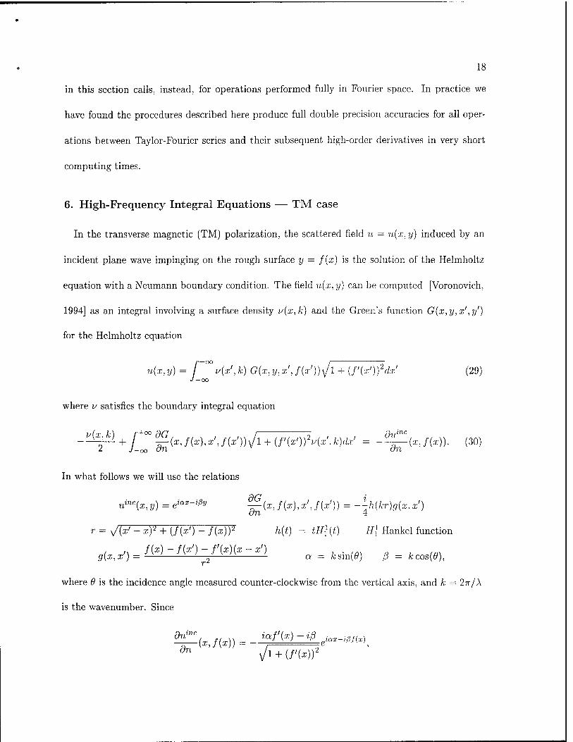
18
in this section calls, instead, for operations performed fully in Fourier space. In practice we
have found the procedures described here produce full double precision accuracies for all oper-
ations between Taylor-Fourier series and their subsequent high-order derivatives in very short
computing times.
6. High-Frequency Integral Equations — TM case
In the transverse magnetic (TM) polarization, the scattered field u = u(x,y) induced by an
incident plane wave impinging on the rough surface y = f(x) is the solution of the Helmholtz
equation with a Neumann boundary condition. The field u(x, y) can be computed [Voronovich,
1994] as an integral involving a surface density u(x,k) and the Green's function G(x,y,x',y')
for the Helmholtz equation
u(x,y) = r°°v(x',k) G(x,y,x',f(x'))yjl + (f'(x'))2dx' (29)
where v satisfies the boundary integral equation
v{x,k) , f+°°dG, ,, . , ,. ,.. / , .... m2 , , MJ., du inc
2 ' J -oo dn WM J yj,),u, ,J\J>) ) V L n
what follows we will ise the relations
umc(x,y) = „iax -ißy dG dn{i
r = yj{x' - x)2 + (W )-f(x))2
g(x.x') f(x) ■ -/(a: ')-f'(x)(x -x>)
r2
On ■(x,f(x)). (30)
■(xj(x),x',f(x')) = --h(kr)g(x,x')
h(t) = tHl{t) H{ Hankel function
a = A;sin(0) ß = kcos(9),
where 9 is the incidence angle measured counter-clockwise from the vertical axis, and k = 2n/\
is the wavenumber. Since
—0c fix)) = -™f!M+iLei<*x-ißf(x)

19
calling ü(x, k) = v(x, k)Jl + (f'(x)) we can rewrite equation (30) as follows:
i>(x,k) /+O0
i>(x',k)h(kr)g(x,x')dx' = {iaf'{x) + iß)eiax~ißs^ (31) -oo
As in Section 2, a useful form of the integral equation (31) results as we factor out the rapidly
oscillating phase function eiax~lßf{x)
(e-«°x-ißf{*))üfak)) 2J-
+oo h(kr)g(x,x') (e-(iax-ißf(x»v(x',k)) dx' = 2(iaf'(x) +iß),
(32)
which cancels the fast oscillations in all non-integrated terms. Using an expansion for the
function v(x, k) similar to (6)
ü(x,k) iax-ißf(x) +00
Un (33) n=-\
in (32) then yields
+0° 1 / i \ E ■jp;{*n(x)--ln(x,k)) = 2k(i8m(9)f'(x)+icos(9)) (34)
n= —1
where
/-hOO
h(kr)g(x,x')eia(x'-x)-ißVW-Kx»i>n{x')dx'. -oo
The solution of equation (34) requires asymptotic expansions for the integrals In(x,k). These
expansions are obtained, as in the TE case, by the methods of Section 3. In particular we obtain
the following expressions for the coefficients vn(x):
v-i{x) = 2(*sin(0)/'(a:) + *'cos(0))
(35)
Vn\X)

20
7. Numerical results
Our numerical method proceeds to obtain the integral densities u(x, k) through equation (6)
in TE polarization and equation (33) in TM polarization, with coefficients vn and vn obtained
from (9) and (35) respectively, and with 1% given by (25). The Taylor-Fourier expansions
required in equation (12) for the functions 0+1 and g/<j>'+ are precomputed. as they depend
only on the profile / and they are independent of wave numbers, incidence angles, etc. The
precomputation time was 0.5 seconds for the profile of Figure 1(a) and Figure 1(b) and 0.7
seconds for the profile of Figure 1(c). (This and all subsequent calculations were performed
in a DEC Alpha workstation (600MHz)). Once the density has been obtained all field related
quantities can be evaluated easily from equation (3) in the TE case and equation (29) in the
TM case.
In this section we present the results produced by our algorithm for the energy radiated in
the various scattering directions. To do this, we use the periodic Green's function G of period
d [Petit et al., 1980]
1 +°° ßiOinX + ißnV 2lT I ö(x,y) = — Y, ß ' an = a + n —, ßn = <Jk2-a2
n n=—oo "n
to obtain from (3) (TE) or from (29) (TM), the Rayleigh series for the scattered field
+oo
u(x,y)= Y, Bne^x+^y. n=—oo
Here, the coefficients Bn are "Rayleigh amplitudes", which are given in TE polarization by
Bn = h[{~l + itf,{x))v{x* k^ianX~lßnf{x)dx:
and in TM polarization by
2idßn Jo

21
The required integrals were computed by means of the trapezoidal rule, which for the periodic
functions under consideration is spectrally accurate, and can be computed very efficiently by
means of the FFT.
Our numerical results show values and errors corresponding to the "scattering efficiencies" e„,
see [Petit et al., 1980], which are defined by
e - Pn.\B I2 cn — o \-°n\ j
and which give the fraction of the energy which is scattered in each one of the (finitely many)
scattering directions. To test the accuracy of our numerical procedures we compare our high-
frequency (HF) results to those of the method of variation boundaries [Bruno and Reitich,
1993] (MVB) in an "overlap" wavelength region — in which both algorithms are very accurate;
additional results, in regimes beyond those that can be resolved by the boundary variation
method are also presented. Note that the HF and MVB methods are substantially different in
nature: one is a high order expansion in l/k whereas the other is a high order expansion in
the height h of the profile. In the examples that follow we list relative errors for the computed
values of scattered energies in the various scattering directions. The figures given in the columns
denoted by Order 0-19 are the relative errors for the values of the scattered energy calculated
from the high frequency code to orders 0-19 in the corresponding scattering direction. In all
cases errors were evaluated through comparison with a highly accurate reference solution; in
Tables 2 to 8 the reference solution was produced by means of the boundary variations code
mentioned above; in Tables 9 and 10, the reference solution was obtained through a higher-
order application of our high frequency algorithm (Order 15). The first term in the high-
frequency expansion happens to coincide with the classical Kirchhoff approximation. Note that
the Kirchhoff approximation can also be obtained as the zeroth order term of the Neumann

22
series for equation (4). We emphasize, however, that the high-frequency method used in this
paper is of a completely different nature to that arising from use of Neumann series.
Our first example, presented in Table 2, corresponds to the profile in Figure 1(a) illuminated
by a TE polarized plane wave with h = 0.025, A = 0.025 and an incidence angle 9 = 30°. The
run time was 10 seconds for the calculation of order 17; we see that, as claimed, the present
approach produces results with full double precision accuracy in short computing times.
The results for the profile in Figure 1(a) under TM polarization are given in Table 3. Here
we take h — 0.025, A = 0.0251, with an incidence angle 9 = 30°. Our choice of wavelength
in the present TM case, which is slightly different from the value A = 0.025 we used in the
TE case, was made to avoid the Wood anomaly [Hutley, 1982] that occurs at the latter value,
for which the test boundary variation code fails. Our high-frequency method however does not
suffer from that drawback and results for the profile in Figure 1(a) with //, = 0.025, A = 0.025
and an incidence angle 9 = 30° are given in Table 4. The reference solution in this case is the
high-order high-frequency solution of order 21. The convergence of our expansion in this case is
similar to the convergence observed to the previous case where X/d = 0.0251. Again, full double
precision accuracies are reached in a 10 second calculation.
Our method is not restricted to sinusoidal surfaces, of course. In Table 5. for instance we
present results corresponding to the profile of Figure 1(b) with h = 0.01, A = 0.025 and 0 = 0°
in TE polarization. The run time was 5 seconds for the order 11 calculation. Table 6 shows
results for the same profile under TM polarization with h = 0.01, A = 0.0251 and 9 = 0°. The
run time was 4 seconds for the order 11 calculation.
We next consider the third order "Stokes" wave [Kinsman, 1965] shown in Figure 1(c). The
results presented in Table 7 assumed the parameter values h = 0.02, A = 0.04 and 9 = 0° and TE

23
polarization. The run time in this case was 27 seconds for the calculation of order 19. Table 8
shows the results for TM polarization and h = 0.02, A = 0.041 and 9 = 0°. The run time was
23 seconds for the order 19 calculation.
Table 9, presents results for a low grazing angle example for the profile of Figure 1(a) with
h = 0.025, A = 0.001 and 9 = 70° (20° grazing) in TE polarization. As mentioned above, for
reference in this case we used the high-frequency solution of order 15. The run time for the order
9 calculation was 12 seconds. The results for the profile of Figure 1(a) under TM polarization
with h = 0.025, A = 0.0011 and 9 = 70° are given in Table 10. The run time was 19 seconds for
the order 9 calculation.
A final remark concerning the order of the Fourier series used in the examples above is now
in order. For the examples given in Tables 2-8 no more than 30 Fourier modes were used.
The number of Fourier modes needed depends on the incidence angle, height of the profile, the
order of the high-frequency expansion used and the accuracy required; in the cases considered
in Tables 9 and 10, for example, it was necessary to use 45 Fourier coefficients to achieve the
accuracies reported.
8. Conclusions
We have shown that high order summations of expansions of the type (1) can be used to
produce highly accurate results for problems of scattering by rough surfaces in the high-frequency
regime in TE and TM polarizations. Our algorithm is based on analytic continuation of divergent
integrals and careful algebraic manipulation of Taylor-Fourier series representations. Our results
show accuracies which improve substantially over those given by classical methods such as the
Kirchhoff approximation. As shown recently [Sei et al., 1999], such accuracies are needed to

24
capture important aspects of rough surface scattering involving very low scattering returns and
occurrences of unusual polarization ratios. Further, the results of [Bruno and Reitich, 1993]
clearly suggest that a multiscale perturbation algorithm of the type proposed in [Bruno et al,
2000] should yield the required accuracies for multiscale surfaces provided an accurate high-
frequency solver, such as the one presented in this paper, is used. This paper thus extends the
range of applicability of classical asymptotic methods producing a versatile, highly accurate and
efficient high-frequency numerical solver.

25
(a)
(b)
c _
Figure 1. Various profiles considered in the text:
(a) f(x) = -COS(2TTX)
(b) f(x) = -(COS(27TX) + cos(47ra;))
(c) f[x) = ^(-cos(27ra;) +0.35cos(47rar) - Ü.Ü35cos(67nr))

26
Table 1. Values of the derivatives of the function S{x) at x = 0 for various orders of differentiation. The columns marked 20 Modes, 30 Modes and 40 Modes list the relative errors of the derivatives computed by summing differentiated Fourier series truncated at 20, 30 and 40 Modes, respectively. Columns FFT and Conv. resulted from use of Fourier coefficients obtained through FFTs and direct convolution, re- spectively.
Order Exact value at 0 20 Modes 30 Modes 40 Modes
FFT Conv. FFT Conv. FFT Conv.
2 -7.376924249352232e-01 1.3e-12 5.4e-16 1.7e-ll 2.7e-16 1.0e-ll 2.7e-16
4 2.377008924791275e+00 6.8e-ll 3.0e-14 4.2e-09 2.9e-15 9.8e-10 2.9e-15
6 -1.702966504696142e+01 5.5e-10 1.8e-12 4.6e-07 0.0e-00 1.7e-07 0.0e-00
8 2.184589621949499e+02 2.7e-08 5.8e-ll 2.9e-05 2.3e-15 4.1e-05 2.3e-15
10 -4.361708943655447e+03 8.8e-07 1.2e-09 l.le-03 6.9e-16 3.8e-03 6.9e-16
12 1.248619506829422e+05 1.4e-05 1.7e-08 3.1e-02 0.0e-00 2.2e-01 8.0e-16
14 -4.844671808314213e+06 1.4e-04 1.8e-07 6.5e-01 6.0e-15 8.7e+00 1.0e-15
16 2.445839768254340e+08 l.le-03 1.5e-06 1.0e+01 1.3e-13 2.7e+02 1.6e-15
18 -1.557531553377787e+10 6.5e-03 9.4e-06 1.3e+02 1.9e-12 6.6e+03 0.0e-00
20 1.220898732494702e+12 3.1e-02 5.0e-05 1.4e+03 2.2e-ll 1.3e+05 8.2e-16

27
Table 2. Results for the profile of Figure 1(a) in TE polarization with h = 0.025, A = 0.025 and incidence angle 0 = 30°. The run time was 10 seconds for the calculation of order 17.
Efficiency
#
Scattered
Energy Order 0 Order 1 Order 5 Order 11 Order 17
0 7.538669511479800e-04 3.8e-02 6.3e-05 l.le-08 5.0e-12 2.4e-13
1 1.194293110668300e-01 2.0e-04 3.1e-06 4.9e-09 2.8e-13 2.2e-14
2 4.713900020760300e-03 1.5e-02 1.7e-05 2.7e-08 6.5e-13 3.3e-14
3 9.472951023686101e-02 2.4e-03 5.8e-05 1.7e-09 1.2e-13 4.0e-15
4 1.606247510782500e-01 1.2e-04 8.9e-05 2.8e-10 7.3e-14 8.6e-15
5 8.121747375826800e-02 1.5e-03 1.3e-04 2.3e-08 3.5e-14 7.9e-15
6 2.068175899532900e-02 2.7e-03 1.9e-04 1.2e-08 3.1e-13 4.4e-15
7 3.171379802403400e-03 3.9e-03 2.5e-04 3.5e-08 1.5e-13 5.3e-15

28
Table 3. Results for the profile of Figure 1(a) in TM polarization with h = 0.025, A = 0.0251 and incidence angle 9 = 30°. The run time was 10 seconds for the calculation of order 17.
Efficiency
#
Scattered
Energy Order 0 Order 1 Order 5 Order 11 Order 17
0 1.148002904781718e-03 3.1e-02 3.4e-05 2.6e-09 7.2e-13 4.0e-13
1 1.196487185464779e-01 1.5e-04 l.le-05 2.2e-ll 1.8e-14 3.3e-14
2 3.930863630633380e-03 1.6e-02 2.9e-05 2.8e-10 l.oe-13 l.le-13
3 9.729981709870275e-02 2.4e-03 2.3e-05 2.6e-10 4.3e-14 3.7e-14
4 1.603959300090739e-01 1.4e-04 4.0e-05 3.6e-10 1.9e-14 2.4e-14
5 7.991729015156721e-02 1.5e-03 6.5e-05 2.8e-10 1.3e-14 6.9e-15
6 2.011674295356339e-02 2.7e-04 9.8e-05 3.4e-10 4.0e-14 1.3e-14
7 3.052813099869383e-03 3.9e-03 1.4e-04 2.5e-09 4.4e-14 9.6e-14
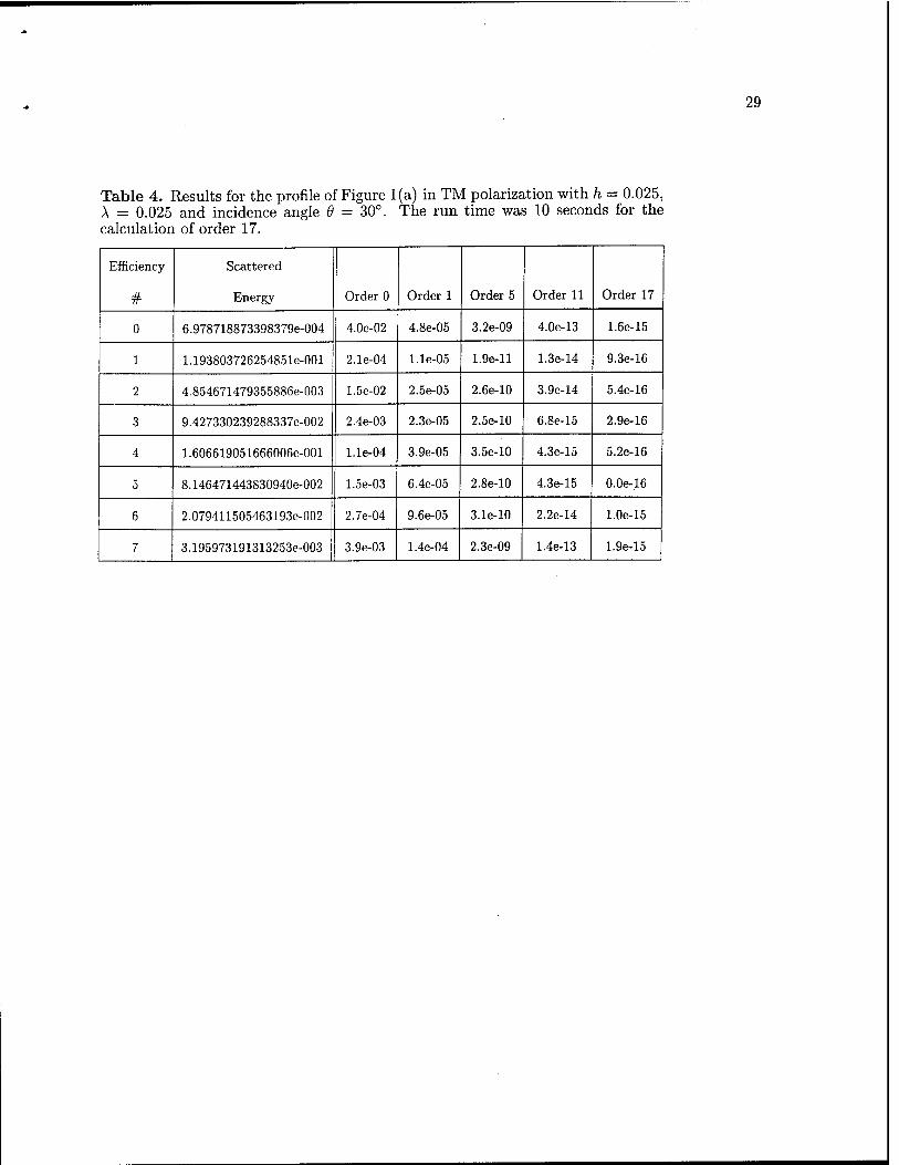
29
Table 4. Results for the profile of Figure 1(a) in TM polarization with h = 0.025, A = 0.025 and incidence angle 9 = 30°. The run time was 10 seconds for the calculation of order 17.
Efficiency
#
Scattered
Energy Order 0 Order 1 Order 5 Order 11 Order 17
0 6.978718873398379e-004 4.0e-02 4.8e-05 3.2e-09 4.0e-13 1.6e-15
1 1.193803726254851e-001 2.1e-04 l.le-05 1.9e-ll 1.3e-14 9.3e-16
2 4.854671479355886e-003 1.5e-02 2.5e-05 2.6e-10 3.9e-14 5.4e-16
3 9.427330239288337e-002 2.4e-03 2.3e-05 2.5e-10 6.8e-15 2.9e-16
4 1.606619051666006e-001 l.le-04 3.9e-05 3.5e-10 4.3e-15 5.2e-16
5 8.146471443830940e-002 1.5e-03 6.4e-05 2.8e-10 4.3e-15 0.0e-16
6 2.079411505463193e-002 2.7e-04 9.6e-05 3.1e-10 2.2e-14 1.0e-15
7 3.195973191313253e-003 3.9e-03 1.4e-04 2.3e-09 1.4e-13 1.9e-15

30
Table 5. Results for the profile of Figure 1(b) in TE polarization with h = 0.01, A = 0.025 and 9 = 0°. The run time was 5 seconds for the order 11 calculation.
Efficiency
#
Scattered
Energy Order 0 Order 1 Order 5 Order 9 Order 11
0 1.983702874853860e-01 1.4e-03 6.7e-06 6.3e-10 1.8e-13 9.8e-16
1 2.125625186015414e-02 4.3e-03 7.3e-06 8.6e-10 4.6e-14 1.5e-14
2 5.109656298137152e-02 4.2e-03 5.3e-06 1.3e-09 3.5e-14 l.le-14
3 1.350594564861170e-01 l.le-03 3.0e-06 1.8e-10 5.1e-14 6.6e-15
4 1.670755436364386e-02 4.3e-03 928e-06 1.5e-09 1.8e-13 2.7e-15
5 1.041839113172000e-01 8.7e-04 l.le-05 4.7e-10 3.8e-14 2.9e-15
6 3.029977474761340e-02 7.6e-04 l.le-05 4.8e-10 1.0e-15 9.0e-15
7 2.828409217693459e-02 2.5e-03 3.2e-05 1.8e-09 3.5e-14 9.4e-15

31
Table 6. Results for the profile of Figure 1(b) in TM polarization with h = 0.01, A = 0.025 and 6 = 0°. The run time was 4 seconds for the order 11 calculation.
Efficiency
#
Scattered
Energy Order 0 Order 1 Order 5 Order 9 Order 11
0 1.985778821348800e-01 1.3e-03 l.le-05 5.6e-ll 9.1e-15 5.0e-15
1 2.203189065423864e-02 4.3e-03 6.1e-06 8.5e-12 2.0e-14 2.2e-14
2 4.989624245086630e-02 4.2e-03 1.2e-05 1.3e-10 6.8e-15 8.3e-15
3 1.363942224141270e-01 l.le-03 3.0e-06 6.6e-ll l.le-14 6.7e-15
4 1.685456723960805e-02 4.3e-03 1.7e-05 1.5e-10 2.7e-14 1.5e-14
5 1.040033802018770e-01 8.9e-04 9.9e-07 8.4e-ll 2.9e-15 2.0e-15
6 2.994981016528542e-02 7.8e-04 1.5e-06 1.9e-10 1.4e-15 1.0e-14
7 2.795532080716518e-02 2.5e-03 1.5e-05 1.2e-ll 3.2e-15 l.le-15

32
Table 7. Results for the profile of Figure 1(c) in TE polarization with h = 0.02, A = 0.04 and 0 = 0°. The run time was 27 seconds for the calculation of order 19.
Efficiency
#
Scattered
Energy Order 0 Order 1 Order 5 Order 11 Order 19
0 2.762105662320035e-01 1.9e-3 1.6e-5 7.4e-9 6.5e-14 2.4e-15
1 5.735818584364873e-02 3.1e-3 2.0e-5 1.9e-8 1.3e-12 6.0e-16
2 9.154897389472935e-02 3.7e-3 5.1e-6 8.2e-9 1.4e-12 6.7e-15
3 1.051875097051952e-01 4.6e-4 5.1e-6 1.6e-9 1.0e-12 9.2e-16
4 6.713521833646909e-02 1.7e-3 2.7e-5 1.4e-ll 3.6e-12 2.1e-16
5 2.830374622545111e-02 3.9e-3 7.3e-5 1.4e-8 2.2e-13 6.7e-15
6 9.270117932865375e-03 5.9e-3 1.3e-4 3.2e-8 l.le-11 3.0e-15
7 2.435385416440963e-03 7.9e-3 2.2e-4 8.4e-8 4.1e-12 1.8e-16

33
Table 8. Results for the profile of Figure 1(c) in TM polarization with h = 0.02, A = 0.041 and 0 = 0°. The run time was 23 seconds for the calculation of order 19.
Efficiency
#
Scattered
Energy Order 0 Order 1 Order 5 Order 11 Order 19
0 1.291589358261453e-01 2.2e-03 1.6e-05 2.7e-10 2.1e-12 9.5e-14
1 1.662663939465338e-01 1.7e-03 5.1e-05 2.8e-10 1.6e-12 4.1e-14
2 3.920583564991646e-03 8.5e-03 5.3e-06 7.0e-09 1.3e-ll 6.2e-13
3 1.878743087516774e-02 1.5e-02 2.7e-06 2.6e-09 6.9e-12 1.5e-13
4 7.416580102755271e-02 3.7e-03 2.8e-05 4.6e-09 6.7e-12 9.4e-15
5 7.840714643630796e-02 2.4e-04 2.0e-05 6.5e-09 6.6e-13 2.4e-14
6 5.345392880491968e-02 2.6e-03 1.6e-05 6.5e-09 9.6e-12 4.9e-14
7 2.611186407051911e-02 5.1e-03 6.8e-05 4.3e-09 8.6e-13 5.1e-14

34
Table 9. Results for the profile of Figure 1(a) in TE polarization with h = 0.025, A = 0.001 and 9 = 70°. The run time was 12 seconds for the order 9 calculation.
Efficiency
#
Scattered
Energy Order 0 Order 1 Order 3 Order 7 Order 9
0 9.405896918172547e-03 9.1e-06 2.3e-07 1.2e-10 1.7e-14 6.1e-16
1 4.691450406852652e-03 1.2e-05 l.le-07 8.4e-ll 2.3e-16 2.2e-16
2 4.977619850889408e-03 1.2e-05 1.3e-07 7.3e-ll 7.5e-15 9.1e-17
3 8.970028199252082e-03 l.le-05 2.1e-07 1.8e-10 5.5e-15 3.6e-16
4 1.591650541515982e-03 8.4e-06 4.2e-08 2.5e-ll 5.2e-17 3.9e-16
5 1.151449525094811e-02 6.0e-06 2.7e-07 2.7e-10 3.8e-15 5.7e-17
6 1.509705192413105e-04 2.8e-06 4.9e-09 8.3e-13 1.2e-15 2.0e-16
7 1.232860573339191e-02 6.3e-07 2.9e-07 3.5e-10 4.2e-15 7.6e-16
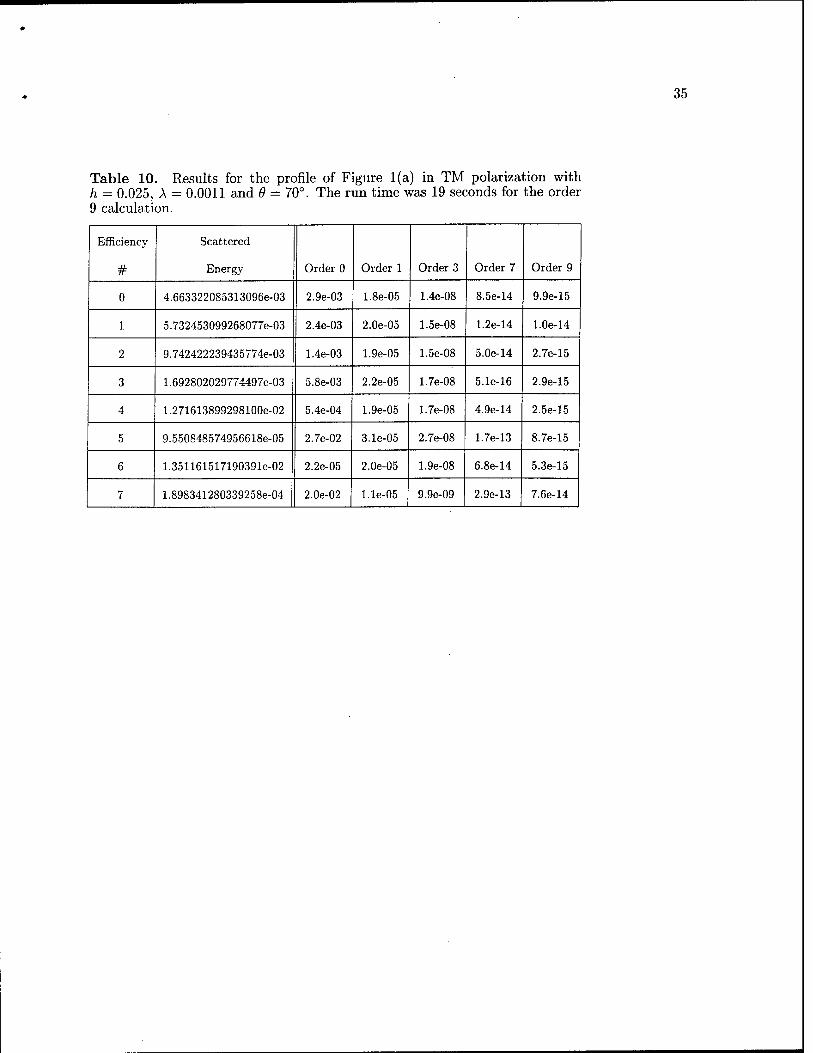
35
Table 10. Results for the profile of Figure 1(a) in TM polarization with h = 0.025, A = 0.0011 and 0 = 70°. The run time was 19 seconds for the order 9 calculation.
Efficiency
#
Scattered
Energy Order 0 Order 1 Order 3 Order 7 Order 9
0 4.663322085313096e-03 2.9e-03 1.8e-05 1.4e-08 8.5e-14 9.9e-15
1 5.732453099268077e-03 2.4e-03 2.0e-05 1.5e-08 1.2e-14 1.0e-14
2 9.742422239435774e-03 1.4e-03 1.9e-05 1.5e-08 5.0e-14 2.7e-15
3 1.692802029774497e-03 5.8e-03 2.2e-05 1.7e-08 5.1e-16 2.9e-15
4 1.271613899298100e-02 5.4e-04 1.9e-05 1.7e-08 4.9e-14 2.5e-15
5 9.550848574956618e-05 2.7e-02 3.1e-05 2.7e-08 1.7e-13 8.7e-15
6 1.351161517190391e-02 2.2e-05 2.0e-05 1.9e-08 6.8e-14 5.3e-15
7 1.898341280339258e-04 2.0e-02 l.le-05 9.9e-09 2.9e-13 7.6e-14

36
Acknowledgment and Disclaimer: Effort sponsored by DARPA/AFOSR under contract
number F49620-99-C-0014, the Air Force Office of Scientific Research, Air Force Materials Com-
mand. USAF, under grant numbers F49620-99-1-0010 and F49620-99-1-0193. and through NSF
contracts No. DMS-9523292 and DMS-9816802). The US Government is authorized to repro-
duce and distribute reprints for governmental purposes notwithstanding any copyright notation
thereon. The views and conclusions contained herein are those of the authors and should not
be interpreted as necessarily representing the official policies or endorsements, either expressed
or implied, of the Air Force Office of Scientific Research or the US Government.
References
M. Abramowitz and I. Stegun, Handbook of mathematical functions with formulas, graphs, and mathematical
tables, US Dept Commerce, June, 1964.
D. S. Ahluwalia, R. M. Lewis and J. Boersma. Uniform asymptotic theory of diffraction by a plane screen, SIAM
J. Appl. Math., 16 (4), 783-807, 1968.
H. Ansorge, Electromagnetic reflection from a curved dielectric interface. IEEE Trans. Ant. Prop., 34, 842-845,
1986.
H. Ansorge, First order corrections to reflection and transmission at a curved dielectric interface with emphasis
on polarization properties, Radio science. 22, 993-998, 1987.
J. D. Benamou, Direct computations of multivalued phase space solutions for Hamilton-,lacobi equations, Comm.
Pure Appl. Math., 52, 1443-1475, 1999.
N. Bleistein and R. A. Handelsman, Asymptotic expansions of integrals. Dover Publications, New York, 1986.
C. O. Bloom and N. D. Kazarinoff, Short wave radiation problems in mhomogeneous media : asymptotic solutions,
Lecture Notes in Mathematics 522, Springer-Verlag, Berlin, 1976.
D. Bouche, F. Molinet and R. Mittra, Asymptotic methods in electromagnetics, Springer-Verlag, Berlin, 1997.
W. P. Brown, On the asymptotic behavior of electromagnetic fields from convex cylinders near grazing incidence,
J. of Math. Anal, and App., 15, 355-385, 1966.
0. Bruno and F. Reitich, Numerical solution of diffraction problems: a method of variation of boundaries I, II,
III J. Opt. Soc. A 10, 1168-1175, 2307-2316, 2551-2562, 1993.

37
O. Bruno, A. Sei and M. Caponi, Rigorous multi-scale solver for rough-surface scattering problems: high-order-
high-frequency and variation of boundaries, To appear in the Proceedings of the NATO Sensors and Electronics
Technology (SET) Symposium on "Low Grazing angle clutter: Its Characterization, Measurement, and Appli-
cation", JHU/APL, Laurel, MD, April 25-27 2000.
H. Cartan, Elementary theory of analytic functions of one or several complex variables, Addison-Wesley, Reading,
Mass., 1963.
H. Chaloupka and H. J. Meckelburg, Improved high-frequency current approximation for curved conducting sur-
faces, AEU, Arch. Elektron. Ubertragungstech, 39, 245-250, 1985.
J. J. Duistermaat, Huygens' principle for linear partial differential equations, Huygens' principle, 1690-1990 :
theory and applications, H. Blok Ed, Elsevier, 1992.
E. Fatemi, B. Engquist and S. Osher, Numerical solution of the high frequency asymptotic expansion for the scalar
wave equation, J. Comp. Phys., 120, 145-155, 1995.
F. G. Friedlander, Geometrical Optics and Maxwell's equations, Proc. Cambridge Philos. Soc, 43 (2), 284-286,
1946.
F. G. Friedlander and J. B. Keller, Asymptotic expansion of solutions of (V2 + k2)u = 0, Comm. Pure Appl.
Math., 8, 387-394, 1955.
M. A. Gil'Man, A. G. Mikheyev and T. L. Tkachenko, The two-scale model and other methods for the approximate
solution of the problem of diffraction by rough surfaces, Comp. Maths Math. Phys., 36, 1429-1442, 1996.
S. Hong, Asymptotic theory of electromagnetic and acoustic diffraction by smooth convex surfaces of variable
curvature, J. Math. Phys., 8, 1223-1232, 1967.
M.C. Hutley Diffraction gratings, Academic Press, San Diego, Calif., 1982.
J. B. Keller, A geometric theory of diffraction, AMS Calculus of variations and its applications, L.M. Graves ed.,
McGraw-Hill, New York, 1958.
B. Kinsman, Wind waves, their generation and propagation on the ocean surface, Englewood Cliffs, N.J., Prentice-
Hall, 1965.
Y. A. Kravtsov, A modification of the geometric optics method, Radiofizika, 7, 664-673, 1964.
B. F. Kuryanov, The scattering of sound at a rough surface with two types of irregularity, Soviet Physics-Acoustic,
8 (3), 252-257, Jan. 1963.
S. W. Lee, Electromagnetic reflection from a conducting surface: geometrical optics solution, IEEE Trans. Ant.
Prop., 23, 184-191, 1975.

38
R. M. Lewis and J. Boersma, Uniform theory of edge diffraction, J. Math. Phys., 10 (12), 2291-2305, 1969.
R. M. Lewis and J. B. Keller, Asymptotic methods for partial differential equations: The reduced wave equation and
Maxwell's equations, Research Report EM-194, New York University, 1964. (Reprinted in Surveys in Applied
Mathematics, 1-82, Plenum Press, New York, 1995).
R. M. Lewis, N. Bleistein and D. Ludwig, Uniform asymptotic theory of creeping waves, Comm. Pure Appl. Math..
20, 295-320, 1967.
R. K. Lüneburg, Mathematical theory of Optics, Brown University, 1944. (reprinted by Univeristy of California
Press, Berkeley, 1964).
R. K. Lüneburg, Asymptotic expansion of steady state electromagnetic fields, Research Report EM-14, New York
University, July 1949.
R. K. Lüneburg, Asymptotic evaluation of diffraction integrals, Research Report EM-15, New York University,
October 1949.
D. Ludwig, Uniform asymptotic expansion at a caustic, Comm. Pure Appl. Math.. 19. 215-250, 1966.
S. T. McDaniel and A. D. Gorman, An examination of the composite-roughness scattering model, J. Acoust. Soc.
Am., 73, 1476-1486, 1983.
W. L. Miranker, Parametric theory of Au + k'2u, Arch. Ratl. Mech. Anal., 1, 139-152. 1957.
K. M. Mitzner, Effect of small irregularities on electromagnetic scattering from an interface of arbitrary shape, J.
Math. Phys., 5, 1776-1786, 1964.
R. Petit, ed. Electromagnetic theory of Gratings, Springer-Verlag, Berlin, 1980.
W. H. Press, S. A. Teukolsky, W. T. Vetterling and B. P. Flannery, Numerical Recipes, Cambridge University
Press, 1992.
S. O. Rice, Reflection of electromagnetic waves from slightly rough surfaces, Comm. Pure Appl. Math., 4, 351-378,
1951.
A. Sei, O. P. Bruno and M. Caponi, Study of polarization scattering anomalies with application to oceanic scattering
Radio Science, 34 (2), 385-411, March 1999.
A. B. Shmelev, Wave scattering by statistically uneven surfaces, Soviet Physics uspekhi, 15 (2), 173-183, Sept.
1972.
G.R. Valenzuela, Theories for the interaction of electromagnetic and oceanic waves - A review, Boundary-layer
Meteor. 13, 61-85, 1978.
N. G. Van Kampen, An asymptotic treatment of diffraction problems, Physica 14 (9), 575-589, January 1949.

39
J. Vidale, Finite difference calculation of traveltimes, B. Seismol. Am., 78, 2062-2076, 1988.
A. G. Voronovich, Wave scattering from rough surfaces, Springer-Verlag, Berlin, 1994.
J. Van Trier and W. W. Symes, Upwind finite- difference calculation of traveltimes, Geophysics, 56, 812-821, 1991.
(Received.
Copyright 2001 by the American Geophysical Union.
Paper number .

Appendix A2:
Polarization ratios anomalies of 3D rough surface scattering as second order effects,
IEEE AP-S International symposium, Boston, Massachusetts, July 2001.
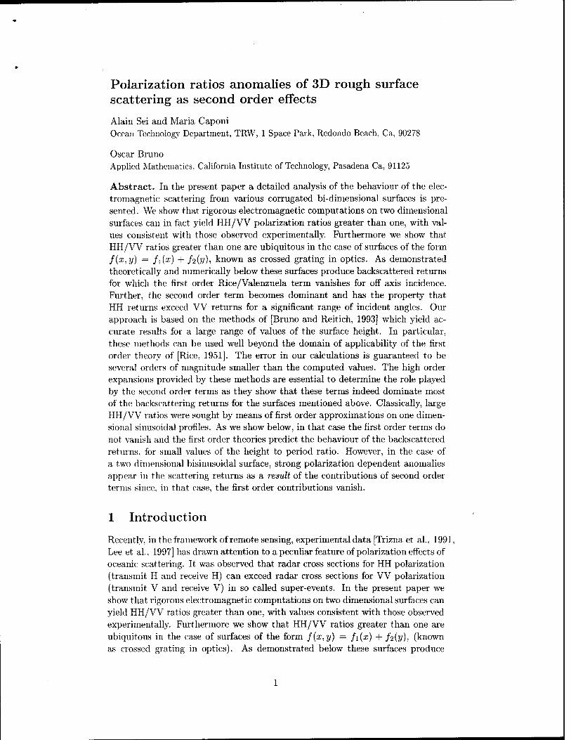
Polarization ratios anomalies of 3D rough surface scattering as second order effects
Alain Sei and Maria Caponi Ocean Technology Department, TRW, 1 Space Park, Redondo Beach, Ca, 90278
Oscar Bruno Applied Mathematics, California Institute of Technology, Pasadena Ca. 91125
Abstract. In the present paper a detailed analysis of the behaviour of the elec- tromagnetic scattering from various corrugated bi-dimensional surfaces is pre- sented. We show that rigorous electromagnetic computations on two dimensional surfaces can in fact yield HH/VV polarization ratios greater than one, with val- ues consistent with those observed experimentally. Furthermore we show that HH/VV ratios greater than one are ubiquitous in the case of surfaces of the form f{x.y) = fi(x) + f-iiy), known as crossed grating in optics. As demonstrated theoretically and numerically below these surfaces produce backscattered returns for which the first order Rice/Valenzuela term vanishes for off axis incidence. Further, the second order term becomes dominant and has the property that HH returns exceed VV returns for a significant range of incident angles. Our approach is based on the methods of [Bruno and Reitich, 1993] which yield ac- curate results for a large range of values of the surface height. In particular, these methods can be used well beyond the domain of applicability of the first order theory of [Rice, 1951]. The error in our calculations is guaranteed to be several orders of magnitude smaller than the computed values. The high order expansions provided by these methods are essential to determine the role played by the second order terms as they show that these terms indeed dominate most of the backscattering returns for the surfaces mentioned above. Classically, large HH/VV ratios were sought by means of first order approximations on one dimen- sional sinusoidal profiles. As we show below, in that case the first order terms do not vanish and the first order theories predict the behaviour of the backscattered returns, for small values of the height to period ratio. However, in the case of a two dimensional bisinusoidal surface, strong polarization dependent anomalies appear in the scattering returns as a result of the contributions of second order terms since, in that case, the first order contributions vanish.
1 Introduction
Recently, in the framework of remote sensing, experimental data [Trizna et al., 1991, Lee et al., 1997] has drawn attention to a peculiar feature of polarization effects of oceanic scattering. It was observed that radar cross sections for HH polarization (transmit H and receive H) can exceed radar cross sections for VV polarization (transmit V and receive V) in so called super-events. In the present paper we show that rigorous electromagnetic computations on two dimensional surfaces can yield HH/VV ratios greater than one, with values consistent with those observed experimentally. Furthermore we show that HH/W ratios greater than one are ubiquitous in the case of surfaces of the form f{x,y) = f\(x) + /2O./), (known as crossed grating in optics). As demonstrated below these surfaces produce

backscattered returns for which the first order (Rice/Valenzuela) term vanishes for off axis incidence. Further, the second order term becomes dominant and has the property that HH returns exceed VV returns for a significant range of
incident angles.
2 Perturbation expansions
We consider a time harmonic incident plane wave impinging on the doubly peri- odic surface z = f(x,y). with x-axis period dx and y-axis period dy. We have: f(x + dx,y + dy) — f(x.y). The incident electric field with wave vector k is :
Em<: = A exp [i{ax + iiy - jz)} (1)
where the vector A = (A[, .42, A*) specifies the state of polarization of the inci- dent wave and k is determine from the incident angles -ip and 0 as follows:
/ a = kcos(ip) sin(O) k = ji = k sin(t/>) sin(0) | (2)
\ -7 = -kvos(0)
The angle 9 is the angle between the vector k and the z-axis and the angle »/> is the angle between the projection of the vector k and the x-axis and k = |k| = 2TT/A
where A is wavelength of the incident radiation. The time harmonic Maxwell's equations for the scattered electric field E reduce to the following equations in the case of a perfect conductor:
AE(JT. y, z) + k2E(x. y, z) = 0 V • EU-. y, z) = 0
(3) n x E{x,y,f{x,y)) = -n x E'"c(x.y. f{x.y))
where n is the normal to the surface z = f(x.y). To derive a perturbation series for the solution of this scattering problem we introduce the surface fg(x.y) = Sf(x.y) where S is a complex number, see [Bruno and Reitich. 1993]. The scat- tered field E(x,y.z:S) associated to the surface fd(x.y) can be written and com- puted as a Taylor series expansion in powers of 6. as follows:
E{x: y, z: 6) = E(x. y, z; 0) + Ed(x. y, z: 0)6 + Ew(:/.\ y, z: 0) -- + ... (4)
Solving the scattering problem for the surface z = f(x.y) then amounts to eval- uating the series (4) at 6 — 1.
As is known, see [Petit, 1980], the field scattered from a bi-periodic surface can be represented outside the groove region (that is for z > max f(x. y)) as a sum of outgoing plane waves with certain amplitudes Bp-(/ as follows E(x,y, z) = ]TBM e^+MiV-yr-«' where M
at = a + IKX fim = ß + mKy yLm = \/A:2 - at - ßm (5)
and where the surface z = f{x,y) is given by its Fourier series:

The outgoing (p,q) plane wave etapx+'l^y+lp'qZ will contribute backscatering re- turns if the following 3D Bragg conditions are satisfied:
av = —a ßa = -ß lp,q — 7 (6)
From the definitions (2) and (5), the conditions (6) are equivalent to the following:
A 2sin(0)
p2 +
tan(^) = 1 df P dy
(7)
For a given incidence {6,ip). for which p and q satisfy (7), it can be shown that the first order backscattered field is given by:
Es(x,y,z,;0) =
( 2i(7A] + 2aA3) 2i(^A2+2ßA3)
A3
-2i{aAl + ßA2) + Ai—{a2 + ß2)
\
f p Jp,q c iapz+i3qy^*t,,,qz
(8)
3 Numerical Results - Perfectly conducting surfaces
We consider the simplest two dimensional surface namely a bisinusoid surface with periods dx — dy = 1 and height h defined by:
f(x,y) — — (cos(27ra:) + cos(27ry)) (9)
The fact that the surface f{x,y) is of the form f{x,y) — fi{x) + f2(y) implies that the Fourier coefficients fejn of f(x,y) are such that fPtq = 0 for p ■ q ^ 0. In this case, formula (8) shows that unless p = 0 or q = 0, that is unless ip = 0
or '</•; 7T —, the first order backscattered field vanishes. When the incident field is 2
7T aligned with the x or y axis, that is when tj) — 0 or if> = —, then the ratio of HH
to VV backscattered returns turns out to be:
*HH(0,0) = crHHJO^m = f cos(0)2
(TVV{0,0) avv(9,ir/2) ll + sin(0)2 (10)
which is the classical first order result found in [Valenzuela, 1978] for a perfect conductor (take the limit e -¥ +oo in formulas 4.10 and 4.11 on page 211). When
ip z£ 0 or ip ^ —, that is for p ■ q ^ 0, the first order term vanishes (since fv^q =
0 for p-q 7^ 0) and the second order term becomes dominant. This is illustrated in Figure 1 where the second order calculation is compared to a high order (21) converged reference solution (see [Bruno and Reitich, 1993, Sei et al., 1999] for details on the accuracy of the numerical algorithm used). Most interestingly, the second order term has the striking feature that HH returns exceed VV retiuns for a large range of incidence angles as illustrated in Figure 2, in sharp contrast to the first order returns. As expected from formula (8) the fact that the second order term is dominant is not a special feature of the bisinusoid surface (9); similar results were obtained for arbitrary surfaces of the form f(x, y) = f\{x) + J2[y)-

(a) (b)
Figure 1: Comparison of the second order calculation to the exact high order calculation for the surface (9) with h = 0.03, if> = 45° and 30° < 0 < 89°. (a) HH polarization, (b) VV Polarization.
(b)
0.03. Figure 2: HH and VV backscattered returns for the surface (9) with h ip = 45° and 30° < 0 < 89° (a). Corresponding HH to VV ratios (b). Acknowledgements: The authors gratefully acknowledge support from TRW internal research fund.
References [Bruno and Reitich, 1993] O. Bruno and F. Reitich. Numerical-solution of
diffraction problems HI - a method of variation' of boundaries .3. doubly periodic gratings, J. Opt. Soc. A 10. 2551-2562. 1993.
[Lee et al., 1997] P. Lee. J.D. Barter. K.L. Beach. C.L. Hindinan. B.M. Lake. H.R. Thompson and R. Yee Experiments on Drag!/ "n(1 non-Bragg scattering using single-frequency and chirped radars, Radio. Sei. 32. 1725-1744. 1997.
[Petit, 1980] R. Petit. Electromagnetic theory of gratings. Springer-Verlag, 1980.
[Rice, 1951] S.O. Rice. Reflection of electromagnetic waves front slightly rough surfaces.. Comm. Pure Appl. Math. 4, 351-378. 1951.
[Sei et al., 1999] A. Sei. O.P. Bruno and M. Caponi, Study of polarization de- pendent scattering anomalies with application to oceanic scattering. Radio Science, 34, 385-411. 1999.
[Triznaet al., 1991] D.B Trizna, J.P. Hansen, P. Hwang and J. Wu. Laboratory studies of radar sea spikes at low grazing angles. J. Geo. Res. 96, 12529- 12537, 1991.
[Valenzuela, 1978] G.R. Valenzuela, Theories for the interaction of electromag- netic and oceanic waves - A review. Boundary-layer Meteor. 13. 61-85, 1978.

Appendix A3:
Rigorous multi-scale solver for rough-surface scattering problems: high-order-high-
frequency and variation of boundaries, Proceedings of the NATO Sensors and
Electronics Technology (SET) Symposium on "Low Grazing angle clutter: Its
Characterization, Measurement, and Application", JHU/APL, Laurel, MD, April 2000.

o <0
I Q. s
I
o
RTO-MP-60 AC/323(SET)TP/12
NORTH ATLANTIC TREATY ORGANIZATION
RESEARCH AND TECHNOLOGY ORGANIZATION
BP 25. 7 RUE ANCELLE. F-92201 NEUILLY-SUR-SEINE CEDEX. FRANCE
RTO MEETING PROCEEDINGS 60
Low Grazing Angle Clutter: Its Characterization, Measurement and Application (le Fouillis ä incidence rasante, caracterisation. mesure et application)
Papers presented at the RTO Sensors and Electronics Technology Panel (SETI Symposium, held in Laurel. Maryland. USA. 25-27 April 2000.
This document should be announced and supplied only to NATO. Government Agencies of NATO nations and their bona fide contractors, and to other recipients approved by the RTO National Coordinators.
Ce document ne doit etre notifie et disthbue qu'ä TOTAN. qu'aux instances gouvernementales des pays de TOTAN et a lews organismes dependants, ainsi qu'ä leurs contractants dument hahilites et au.x out res demandeurs agrees par les Coordonnateurs Nationau.x pour la RTO.
OFFICIAL INFORMATION Published October 2000
NO PUBLIC RELEASE
NATO UNCLASSIFIED

NATO UNCLASSIFIED RTO-MP-60 13-1 AC/323(SET)TP/12
Rigorous Multi-scale Solver for Rough-surface Scattering Problems: High-order-high-frequency and Variation of Boundaries
Oscar Bruno Applied Mathematics 217-50, Caltech, Pasadena, CA 91125, USA
Alain Sei Ocean Technology Department, TRW, Building Rl/Rm 1008
Redondo Beach, CA 90278, USA
Maria Caponi Ocean Technology Department, TRW, Building Rl/Rm 1008
Redondo Beach, CA 90278, USA
1 Introduction
The electromagnetic scattering from the surface of the ocean plays an important role in a wide range of applications, including SAR imaging, remote sensing, detection, etc. The analysis of the scattering pro- cesses involved in these applications poses a rather challenging scientific problem as it requires descrip- tion and understanding of diffraction by complicated surfaces [1]. Computationally, the main difficulty arises from the multiple-scale nature of the scatter- ing surfaces, whose spectrum spans a wide range of lengthscales. A number of techniques have been de- veloped to treat associated limiting cases. For exam- ple, the high frequency case, in which the wavelength A of the incident radiation is much smaller than the surface lengthscales, can be handled by asymptotic methods such as geometrical optics or physical op- tics approximations. On the other hand, resonant problems where the incident radiation is of the order of the surface scale are treated by perturbation meth- ods, typically first or second order expansions in the height h of the surface (cf. [2,3,35]).
However, when a multitude of scales is present on the surface none of the techniques above is adequate, and attempts to combine them in a so-called two- scale approaches [2,4,5] have been given. The two- scale models imply a splitting of the surface into a large and small scale, see e.g. [5,6], where typically
a first order approximation in wavelength (Kirch- hoff approximation) is used to treat smooth compo- nents of a surface and a first order in surface height (Rayleigh-Rice method [35]) is used to deal with the rough components of the surface. The results pro- vided by these methods are not always satisfactory — precisely as a result of the limitations imposed by the low orders of approximation used in both, the high-frequency approximation and the small pertur- bation methods. (See e.g. [5] where the loss of accu- racy of the two-scale model at low grazing angles is demonstrated.)
To alleviate these drawbacks, our approach to multi-scale scattering is based on use of expansions of very high order in both parameters A and h — which leads to algorithms based on complex variable theory and analytic continuation. The resulting approach expands substantially on the range of applicability over low order methods, and can be used in some of the most challenging cases arising in practice. Fur- thermore, as demonstrated below, this new method does not require separation of the length-scales in the surface into large and small, but instead it is able to deal with a continuum of scales on the surface. In- deed the high order expansions presented below have a common "overlap" region in the (X,h) plane where both components are highly accurate. More precisely, there is a range of surface heights and incident wave- lengths for which both methods produce results with
Paper presented at the RTO SET Symposium on "Low Grazing Angle Clutter: Its Characterization. Measurement and Application ". held in Maryland, USA, 25-27 April 2000, and published in RTO MP-60.

13-2 RTO-MP-60 AC/323(SET)TP/12
NATO UNCLASSIFIED
machine accuracy. Therefore by dividing the scales of a surface at a point in the overlap region we ob- tain a general method which is applicable to surfaces containing a continuum of length-scales — which is ideal for evaluation of scattering from surfaces with spectral distributions of oceanic type.
High accuracy as is exhibited by our algorithms is essential in a wide range of important oceanic appli- cations — whose return losses are typically in the -60 dB to -100 dB range. In particular, in order to pro- vide credible results numerical methods must be able to insure accuracies of the order of up to 10 digits in some cases; see [37] for a case in point.
In the present paper we provide a description of our general approach, and we focus on the two basic ele- ments of the general method, namely the high-order perturbation expansion in the wavelength A and the high-order perturbation in height h. For simplicity we restrict our theoretical discussion to problems of scattering from a perfectly conducting rough surface of a transverse electric polarized wave (HH Polariza- tion); numerical results will be given for both trans- verse electric and transverse magnetic polarizations, for three-dimensional problems, and for low to very low grazing angles. In particular we present results for a surface obtained from a Longuet-Higgins hy- drodynamic code, for which our solver produced full double precision accuracy for grazing angles as low as 1°.
2 Multi-scale solver
Our multi-scale solver is based on the method of variation of boundaries [14-17]. We consider sur- faces containing a continuum of scales but, as men- tioned above, the existence of an overlap allows us to solve the complete multiple-scale problem by ex- pressing an arbitrary surface y = S(x) as a sum y = So(x) + F(x) where SQ(X) contains wave num- bers < Ns, and F(x) contain the complementary set of wave numbers > Ns- Thus, our method uses a dichotomy in wave numbers but it does not assume a separation of scales. This feature is essential in the study of oceanic waves since many studies show that the wave spectrum spans a large range of wavenum-
ber (see for instance [33]). As mentioned above, we restrict our presentation
to the particular case of an HH configuration in two dimensions; the scattered field created by an incident plane wave impinging on the rough surface thus solves the Helmholtz equation with a Dirichlet boundary condition. Our approach to the solution of the gen- eral problem with rough surface y = S{x) proceeds as follows:
1. We consider the surface S(x, 6) = So(x) +5F{x), which will be used as a basis for a perturbative method in the parameter 5.
2. The solution u = u(x, 6) associated with the sur- face S(x,6) is obtained by perturbation theory around S = 0.
3. The solution for the surface S(x) is then recov- ered by setting 6 = 1. (As explained in Sec- tion 4 below, this evaluation usually leads to di- vergent series whose re-sumation requires appro- priate methods of analytic continuation.)
In detail, writing
(1)
+0O
u{x,z;6) = Y] um(x,z) — ' * 777.'
ro=0
dmu
mi
the fact that, for every fixed value of S the field u(x, z; 6) solves the Helmholtz equation
(2) Au(x, z; 6) + k2u(x, z;6) = 0
u(x,S(x,6);6) = -utnc{x,S{x,6))
then tells us that, for every fixed value of m we have
Aum(x,z) + k2um(x,z) = 0
um(x, S0{x)) = G [F,uinc, ■ ■ • ,um_i] {x, S0{x)) (3) The interest in this equation arises from the fact that, although the right hand side in the boundary condi- tion for um is highly oscillatory, the surface SQ itself

NATOUNCLASSIFIED
■'-/■i.-^T^—^M^^^Ä^--
RTO-MP-60 13-3 A0323(SEDTP/12
is not We therefore have reduced a problem on a highly oscillatory surface to a sequence of problems on a non-oscillatory surface. For example the zeroth and first order coefficient in the expansion of u{x, z; S) solve the following scattering problems:
(4)
and
Au0(x, z) + fc2uo(x, z) = 0
uQ(x,So(x)) = -uinc(x,S0(x)).
Ait! (x, z) + k2Ui (x, z) = 0
Ul(x,S0(x)) = F(x) (^ + I*) (x,5o(x)).
(5) The general boundary condition of (3) can be com- puted up to any order by differentiation with respect to 5 of the boundary condition of (2), as in equa- tion (5), and the general solution to arbitrary order can be found.
3 Variation of boundaries - previous work
In the particular case where the surface y = SQ{X) is a plane, which allows for exact solution of each of the scattering problems (3), this perturbation method has been studied in detail [15-17]. Earlier uses of per- turbation theory in these contexts had been limited to low-order methods; the new high order perturba- tion theory on the other hand, relies on expansions of very high order in powers of a deviation parameter, denoted here by 5, and techniques of analytic con- tinuation in the complex J-plane. Specifically, Taylor series for the field quantities are obtained through differentiation of the Maxwell system with respect to 6. The possible (and common) divergence of the re- sulting series is handled through re-summation tech- niques that exploit the analytic structure of the so- lution.
The resulting algorithms can resolve scattering re- turns with accuracies that are several orders of mag- nitude better than those given by classical meth- ods [15-17]. Such accuracies can play an important
role in applications. For instance the fine resolution provided by our algorithms has recently helped set- tle a long-standing controversy relating to polarized back-scattering returns from rough surfaces —which amount to very small fractions of the incident en- ergy [37].
As shown in the various papers cited in this sec- tion, this solver is extremely accurate for a wide range of surface heights and incidence angles. Thus, the accuracy of the multi-scale method proposed in the previous section is determined by the corresponding accuracy of the high-frequency solutions for equa- tion (3). Such an accurate solver for high-frequency problems, in turn, is provided in the following sec- tion. The performance of both the boundary varia- tion and high-frequency methods is studied numeri- cally in Section 5.
4 High-order-high-frequency method
The scattered field can be computed from the surface current density v induced on the surface f(x) by the incident plane wave [2]. The function v solves the integral equation
v(x, k)-U h(kMM')g(x, x')v(x', k)dx' = ■ A/-0O
Oiotx-ißf(x)
(6) where
MM' h(t)
g(x,x') a
y/{x'-xF +(/{*)-f{x))* tH[{t) Hi Hankel function (/(*')-/(*)-(s'-z)/'(z'))/MM'2
Jtsin(ö) ß = fccos(0).
To solve this equation we use an asymptotic expan- sion of high order around k = co. Our asymptotic expansion results from the geometrical optics type ansatz
(7) u(x, k) = e +oo i -.
iax-ißf(x) V^ un(X)
n=0 fc"

13-4 RTO-MP-60 NATO UNCLASSIFIED AC/323(SET)TP/12
Prom equations (6) and (7) we obtain with
W l^kr "nW- 27 (*»*)) = ~2 <£+(x,^+ (x,u)) n=0 ^ '
*P+(x,u) = (f(x + <i>^(x,u))-f(x))cos(e) where - ^(x.ujsin^)
,+co (10) /n(x,ifc) = / Ä(JfcAfM')5(x,s,)e"<*(s,*')i/n(ar')«fa/ We can now use the Taylor series of u ^ F+{x,u)
J-oo around u = 0 V'(x,i/) = sin(0)(x' - x) - cos(0)(/(x') - /(*))
E+oc SmF+(x 01 um i2? ° rn (X,V)U _ yr +
,^ v^uu.» ,nr, rv u™.,, ,„vu>.w ».>, 8um ml Z^fn,mK ) r T_ / i\. r-i/7 m=0 m=0
asymptotic expansion of In[x,k) in powers of 1/fc. i <9mF+(x, 0) To do this we use two separate integration regions Pn,m{x) = ^y g^ and we define
to express I"(x, fc) in the form
H{x,k)= fh{kMM')g{x,x')e-ik^x'x^un{x')dx' +«> +0o
V^oo i? (x, *) = £ p£m (*) / umh{ku)e-ik^ (».«)rfu Il(x,k) = h(kMM')g(x,x')e-ik^x'x'^un(x')dx' m=o -Jo
We focus first on an asymptotic expansion for m=o Jo
I+(x, k). Using t = x' —x we can write _r^ tWJ+,, ,.
m=0
i?(x, *) = jf W+(*,*))^,x+t)^(-^-(x+*)* S2L we have set
(9) , ,+oo
where cf>+(x,t) = ^/P + (f{x + t)- /(x))2 and (12) A+(k,m,x) = / vmh(v)e-ik+ l''&dv ip(x,t) = sm(9)t - cos(0)(/(x + t) - /(x)) For the ^ simplest treatment we present here we assume that (These non-convergent integrals must be re- f(x) satisfies the condition interpreted by means of analytic continuation —
in a manner similar to that use in the definition 0' fx^ t\ _ "»*+ (x> *) > Q for £ > o anc^ manipulation of Mellin transforms. We do not
dt ~ provide details about this analytic continuation , , ,, , , procedure here; see [7] for a complete treatment in
so that the map t -+ <j>+ (x, t) is mvertible; this condi- the cage of the Mdlin transform-)
tion is generally satisfied by rough surfaces relevant To complete our expansion of ™( fc) we need to
to the applications under consideration. Then setting _„J„__ 0 „„„,.„„„„„ J; • r *u ±-4. r b produce a corresponding expansion of the quantity ., , A+(k,m,x) in powers of 1/fc. With e = Ilk we call
u = 4>+{x,t) <=> i = 0+(x,u)
„m_ .. .. ,m • +u . A+(e,m,x) = A+(ifc,m,x) = / wm/i(u)e ^ ^"^di; we can rewrite equation (9) in the form v ' ' ' Jn (13)
mr M f+c° un. \n<+, ^ -ikri>+(x u)j B? evaiuation of the successive derivatives of /+(*,*) = / h(ku)F^(x,u)e 'k«> <->du. Ä+(£,m,x) with respect to s at e = 0 it is easy

NATO UNCLASSIFIED RTO-MP-60 AC/323(SET)TP/12
13-5
to check that the coefficients of the Taylor series of Ä+(e, m, x) with respect to e can be obtained directly if all the integrals in the sequence
Ä+(m,x) = [+?rh(v)e-iS£(x'0)dv, Jo
are known; for example, the first derivative is given
by (with ip+(x) = -J^-{x,u = 0)) dun
dÄ+(e,m,x) de
,$"(*) Ä+{m + 2,x)
E=0
Using equations (11) and (13) the expansion for I£ (x, Jfe) results; clearly, the expansion of I" (x, k) can be obtained through a similar derivation. The com- bined expansion for In(x, k) involves combinations of quantities such as p+m(x), $"(ar), Pn,m(x)i $t (x)> Ä+{m,x),Ä-{m,x). It can be shown that all of these quantities — and therefore the integrals ı(m,x) for all m— can be obtained from the integrals
high frequency code to orders 0-21 in the scattering direction listed.
We start with a classical test example: a sinusoidal
profile f(x) = -COS(27TX). In this example we have h = 0.025, A = 0.025 and an incidence angle of 40°. The errors given in this table were computed through comparison with the results given by the boundary variations code. The convergence of the high frequency method is nicely illustrated by this example which, in fact, validates both the high frequency and the boundary variations calculation. We note that an approximation of order 21 in powers of 1/fc is accurate to machine precision.
I L
•+0O
vm+lH[ (v) cos(av)dv
m+1Hl(v)sm(av)dv
if m even
if m odd
for which closed form formulas are available [8].
5 Numerical results
To test the accuracy of our numerical procedures we compare our results for the high-frequency and boundary variation methods in an "overlap" wave- length region — in which, as we show, both algo- rithms are very accurate. Note that these two meth- ods are substantially different in nature: one is a high order expansion in A whereas the other is a high order expansion in the height h of the profile. In the ex- amples that follow we list relative errors for the com- puted values of the corresponding scattered energy (efficiency) shown; the results given in the columns denoted by Order 0-21 are the relative errors for the values of the scattered energy calculated from the
Scattering Direction # Order 0 Order 5 Order 15 Order 21
0 2.0e-4 8.5e-10 4.1e-13 1.3e-14
1 3.1e-4 3.6e-9 1.6e-13 4.0e-15
2 2.5e-4 7.5e-9 8.7e-14 2.9e-16
3 2.6e-4 3.0e-9 1.8e-14 2.9e-16
4 1.8e-4 l.le-10 4.6e-15 9.2e-16
5 2.1e-4 4.2e-10 5.6e-15 5.6e-16
6 1.4e-4 2.9e-9 1.6e-14 3.3e-16
Our next example corresponds to the same profile as above with h = 0.025, A = 0.001 and an incidence angle of 70° (that is, 20° from grazing). This high frequency problem lies outside the domain of applica- bility of the method of variation of boundaries. Our errors here were computed through comparison with a calculation of higher order (Order 15). Again we see that the accuracy of the method is excellent in this case as well.
Scattering Direction # Order 0 Order 3 Order 7 Order 11
0 9.7e-4 1.3e-8 4.0e-13 3.7e-16
1 2.5e-3 1.8e-8 5.6e-14 1.8e-16
2 2.4e-3 1.5e-8 5.4e-13 5.2e-16
3 1.2e-3 2.0e-8 9.1e-14 5.8e-16
4 5.3e-3 1.6e-8 9.5e-13 2.3e-15
5 5.2e-4 2.4e-8 5.8e-14 4.5e-16
6 1.9e-2 6.0e-9 3.4e-12 5.3e-15
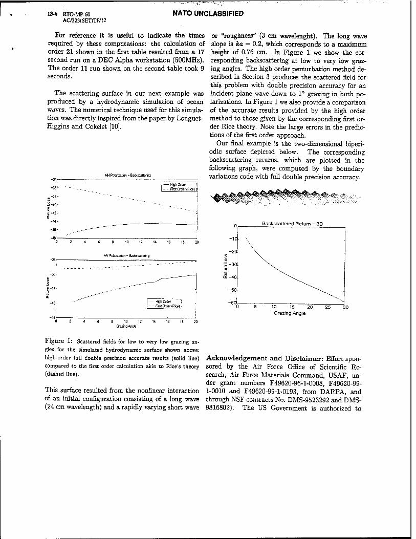
13-6 RTO-MP-60 AC/323(SET)TP/12
NATO UNCLASSIFIED
For reference it is useful to indicate the times required by these computations: the calculation of order 21 shown in the first table resulted from a 17 second run on a DEC Alpha workstation (500MHz). The order 11 run shown on the second table took 9 seconds.
The scattering surface in our next example was produced by a hydrodynamic simulation of ocean waves. The numerical technique used for this simula- tion was directly inspired from the paper by Longuet- Higgins and Cokelet [10].
-34 r- HH Polarization - Backscattering
-36 h
„-38J- « ■3-40H E |-42r z
-441-
-46'
— High Order
- - Frst Order (Rice) r
W Polarization - Badcscattering
-30 H
0 -i E -35r 3 «
,_ —"'"'" -—-
-4Q> — High Order i 1 - - Frst Order (Rice) i |
-45' .
j 10 12
Grazing Angle
Figure 1: Scattered fields for low to very low grazing an-
gles for the simulated hydrodynamic surface shown above:
high-order full double precision accurate results (solid line)
compared to the first order calculation akin to Rice's theory
(dashed line).
This surface resulted from the nonlinear interaction of an initial configuration consisting of a long wave (24 cm wavelength) and a rapidly varying short wave
or "roughness" (3 cm wavelenght). The long wave slope is ka = 0.2, which corresponds to a maximum height of 0.76 cm. In Figure 1 we show the cor- responding backscattering at low to very low graz- ing angles. The high order perturbation method de- scribed in Section 3 produces the scattered field for this problem with double precision accuracy for an incident plane wave down to 1° grazing in both po- larizations. In Figure 1 we also provide a comparison of the accurate results provided by the high order method to those given by the corresponding first or- der Rice theory. Note the large errors in the predic- tions of the first order approach.
Our final example is the two-dimensional biperi- odic surface depicted below. The corresponding backscattering returns, which are plotted in the following graph, were computed by the boundary variations code with full double precision accuracy.
!.#.* W^W<:
Backscatlered Return ■
10 15 20 Grazing Angle
Acknowledgement and Disclaimer: Effort spon- sored by the Air Force Office of Scientific Re- search, Air Force Materials Command, USAF, un- der grant numbers F49620-96-1-0008, F49620-99- 1-0010 and F49620-99-1-0193, from DARPA, and through NSF contracts No. DMS-9523292 and DMS- 9816802). The US Government is authorized to

T NATO UNCLASSIFIED RTO-MP-60 AC/323(SET)TP/12
13-7
reproduce and distribute reprints for governmen- tal purposes notwithstanding any copyright notation thereon. The views and conclusions contained herein are those of the authors and should not be interpreted as necessarily representing the official policies or en- dorsements, either expressed or implied, of the Air Force Office of Scientific Research or the US Govern- ment.
References
[1] G. R. Valenzuela, Theories for the interaction of electromagnetic and oceanic waves - A review, Boundary-layer Meteor. 13 (1978), 61-85.
[2] A.G. Voronovich, Wave scattering from rough surfaces, Springer-Verlag, Berlin, 1994.
[3] A.B. Shmelev, Wave scattering by statistically uneven surfaces, Soviet Physics uspekhi, Vol 15, 2, pp 173-183, Sept. 1972.
[4] B.F. Kuryanov, The scattering of sound at a rough surface with two types of irregularity, So- viet Physics-Acoustic, Vol 8, 3, pp 252-257, Jan. 1963.
[5] S.T. McDaniel and A.D. Gorman An exam- ination of the composite-roughness scattering model, J. Acoust. Soc. Am., Vol 73, 5, pp 1476- 1486, 1983.
[6] Galybin N.N., Backscattering of sound by a dis- turbed sea surface, Soviet Physics-Acoustic, Vol 22, pp 193-197, 1976.
[7] N. Bleistein and R.A. Handelsman, Asymptotic expansions of integrals, Dover Publications, New York, 1986.
[8] M. Abramowitz and I. Stegun Handbook of mathematical functions with formulas, graphs, and mathematical tables, US Dept Commerce, June, 1964.
[9] B. Kinsman, Wind waves, their generation and propagation on the ocean surface, Englewood Cliffs, N.J., Prentice-Hall, 1965.
[10] M.S. Longuet-Higgins and E.D. Gokelet The de- formation of steep surface waves on water: I a numerical method of computation, Proc. R. Soc. Lond. A, 350, (1976), 1-26.
[11] G. V. Anand and M. K. George, Normal mode sound propagation in an ocean with sinusoidal surface waves, J. Acoust. Soc. Am. 80 (1986), 238-243.
[12] G. V. Anand and M. K. George, Normal mode sound propagation in an ocean with random narrow-band surface waves, J. Acoust. Soc. Am. 94 (1993), 279-292.
[13] G. A. Baker and P. Graves-Morris, Pade" Approximants, 2nd edition, Encyclo- pedia of Mathematics and its Applications 59, Cambridge University Press, Cambridge (1996).
[14] O. P. Bruno and F. Reitich, Solution of a bound- ary value problem for Helmholtz equation via variation of the boundary into the complex do- main,, Proc. Roy. Soc. Edinburgh 122A (1992), 317-340.
[15] 0. P. Bruno and F. Reitich, Numerical solution of diffraction problems: a method of variation of boundaries, J. Opt. Soc. Amer. A 10 (1993), 1168-1175.
[16] O. P. Bruno and F. Reitich, Numerical solution of diffraction problems: a method of variation of boundaries II. Dielectric gratings, Pade approx- imants and singularities, J. Opt. Soc. Amer. A 10 (1993), 2307-2316.
[17] O. P. Bruno and F. Reitich, Numerical solution of diffraction problems: a method of variation of boundaries III. Doubly periodic gratings, J. Opt. Soc. Amer. A 10 (1993), 2551-2562.
[18] O. P. Bruno and F. Reitich, Approximation of analytic functions: a method of enhanced con- vergence, Math. Comp. 63 (1994), 195-213.
[19] J. J. Greffet, Scattering of electromagnetic waves by rough dielectric surfaces, Phys. Rev. B 37 (1988), 6436-6441.

13-8 RTO-MP-60 AC/323(SET)TP/12
NATO UNCLASSIFIED
[20] J. J. Greffet, C. Baylard and P. Versaevel, Diffraction of electromagnetic waves by crossed gratings: a series solution, Opt. Lett. 17 (1992), 1740-1742.
[21] J. J. Greffet and Z. Maassarani, Scattering of electromagnetic waves by a grating: a numeri- cal evaluation of the iterative-series solution, J. Opt. Soc. Am. A 7 (1990), 1483-1493.
[22] E. Y. Harper and F. M. Labianca, Perturbation theory for scattering of sound from a point source by a moving rough surface in the presence of re- fraction, J. Acoust. Soc. Am. 57 (1975), 1044- 1051.
[23] E. Y. Harper and F. M. Labianca, Scattering of sound from a point source by a rough surface progressing over an isovelocity ocean, J. Acoust. Soc. Am. 58 (1975), 349-364.
[24] D. R. Jackson, D. P. Winebrenner and A. Ishi- maru, Comparison of perturbation theories for rough-surface scattering, J. Acoust. Soc. Am. 83 (1988), 961-969.
[25] W. A. Kuperman and F. Ingenito, Attenuation of the coherent component of sound propagat- ing in shallow water with rough boundaries, J. Acoust. Soc. Am. 61 (1977), 1178-1187.
New York (1968).
[30] D. Maystre, and M. Neviere, Electromagnetic theory of crossed gratings, J. Optics 9 (1978), 301-306.
[31] A. H. Nayfeh and O. R. Asfar, Parallel-plate waveguide with sinusoidally perturbed bound- aries, J. Appl. Phys. 45 (1974), 4797-4800.
[32] W. H. Peake, Theory of radar return from ter- rain, IRE Nat'l Conv. 7 (1959), 27-41.
[33] W.J. Pierson and L. Moskowitz A proposed spec- tral form for fully dev eloped wind seas based on the similarity theory of S.A. Kitaigorodskii, J. Geo. Res. 69 (1964), 5181-5190.
[34] Lord Rayleigh, The theory of sound, Vol. 2, Dover, New York (1945).
[35] S. O. Rice, Reflection of electromagnetic waves from slightly rough surfaces, Comm. Pure Appl. Math. 4 (1951), 351-378.
[36] J. Roginsky, Derivation of closed-form ex- pressions for the T matrices of Rayleigh-Rice and extinction-theorem perturbation theories, J. Acoust. Soc. Am. 90 (1991), 1130-1137.
[37] A. Sei, O. Bruno and M. Caponi, Study of polar- ization dependent scattering anomalies with ap- plications to oceanic scattering, Radio Sei. 34 (1999) 385-411.
[26] Y. Liu, S. J. Frasier and R. E Mclntosh, Mea- ßg] N. C. Skaropoulos and D. P. Chrissoulidis, Gen- surement and classification of low-grazing-angle erai perturbative solution to wave scattering from radar sea spikes, IEEE Trans. Ant. Prop. 46 a soft random cylindrical surface, J. Acoust. Soc. (1998), 27-40. Amer. 106 (1999), 596-604.
[27] C. Lopez, F. J. Yndurain and N. Garcia, Itera- [39] Talbot, D., Titchener, J. B. and Willis, J. R., tive series for calculating the scattering of waves 77^ reflection of electromagnetic waves from from hard corrugated surfaces, Phys. Rev. B 18 very rough interfaces, Wave Motion 12 (1990), (1978), 970-972. 245-260.
[28] A. A. Maradudin, Iterative solutions for elec- tromagnetic scattering by gratings, J. Opt. Soc. Am. 73 (1983), 759-764.
[29] D. Maystre, Rigorous vector theories of diffrac- tion gratings, in Progress in Optics, E. Wolf ed., North Holland, Amsterdam (1984), 3-67.
[40] A. Wirgin, Scattering from hard and soft cor- rugated surfaces: Rerative corrections to the Kirchhoff approximation through the extinction theorem, J. Acoust. Soc. Am. 85 (1989), 670- 679.

Appendix A4:
High-Order High Frequency solutions of rough surface scattering problem, Fifth
International Conference on Mathematical and Numerical Aspects of Wave Propagation,
Santiago de Compostella, Spain, July 2000.

FIFTH INTERNATIONAL CONFERENCE ON
MATHEMATICAL AND
NUMERICAL ASPECTS
OF WAVE PROPAGATION
Edited by Alfredo Bermüdez, Dolores Gomez, Christophe Hazard, Patrick Joly, and Jean E. Roberts
lajn. IN R.IA

High Order High Frequency Solutions of Rough Surface Scattering Problems
Oscar Bruno Applied Mathematics, Caltech. Pasadena. California
Alain Sei Ocean Technology Department, TRW, Redondo Beach, California
Maria Caponi Ocean Technology Department, TRW, Redondo Beach, California
1 Introduction Pie electromagnetic scattering from the surface of the ocean and other rough surfaces plays an important ,"o'le in a wide range of applications, including SAR imaging, remote sensing, scattering from terrain, non ,'lrstructive testing in optics, etc. The analysis of the scattering processes involved in these applications „oses a rather challenging scientific problem as it requires description and understanding of diffraction by implicated multiple-scales surfaces [1]. Computationally, the main difficulty arises from the multiple- -ralo nature of the scattering surfaces, whose spectrum spans a wide range of lengthscales. In fact, known techniques have been developed to treat limiting cases. For example, the high frequency case, in which the wavelength A of the incident radiation is much smaller than the surface lengthscales, can !,e handled bv asvmptotic methods such as geometrical optics or the Kirchhoff approximation. On the „riiei hand, resonant problems where the incident radiation is of the order of the surface scale are treated bv perturbation methods, typically first or second order expansions in the height, h of the surface (cf. 2. 31). However, when a multitude of scales is present on the surface none of the techniques above; is adequate, and attempts to combine them in a so-called two-scale approaches ([■!, 2]) have been given. The lesults provided by these methods are not always satisfactory — precisely as a result of the limitations imposed by the low orders of approximation used in both, the high-frequency approximation and the
Miiall perturbation methods. Our approach to multi-scale scattering is based on use of expansions of very high order in both
parameters A and h. Such extensions require rather complex mathematical treatments, including complex variable theory and analytic continuation. The resulting approach expands substantially on the range of applicability over low order methods, and can be used in some of the most challenging cases arising in applications. In this paper we focus on one of our high order expansions, namely a high-order perturbation .xpansion in the wavelength A. Perturbation series of very high-order in h. have been introduced and used elsewhere ([6, 7J): the combined algorithms are currently under development.
The presentation in this paper focuses on the two-dimensional problem of scattering from a perfectly conducting rough surface of a transverse electric polarized wave (TE). The scattered field created by an incident plane wave impinging on the rough surface solves Helmholtz's equation with a Dirichlet boundary i otulition. As is known [2J the scattered field can be computed from the surface current density v induced nil the surface f{x) by the incident plane wave. The function v solves the integral equation
r + oc v{s-k) -i f h(kMM')g(x.x')v(x',k)dx' = -e'"
2 4 ./_«,
477

I
where
MM' = v/(x'-x)2 + (/(x')-/(x))2 h(t) = tH}(t) H{ Hankel function
*(*.*') = f{Xl)'f{X)m%~X)f'{X,) * = *-inWne) 0 = *COs(*ine).
To solve this equation we use an asymptotic expansion of high order around k = co. Our asymptoti expansion results from the ansatz
+00 , ,
(2) V(x,k) = e««x-«/(«) ^ f^£l n=0
From equations (1) and (2) we obtain
+00 . / v
(3) £77: (un(x)~l-r{x,k)) = -2 n=0 ' ^ '
where
yi(W/A/')5(x.i')e'0'I'"x)_i3(/(l')"/(I1Vn(x')rf3:' ■'DO
To obtain the coefficients vn{x) we must produce the asymptotic expansion of Inlx. k) in powers of 1/k To do this we use two separate integration regions and we define
I1(x,k) = I h{kMM')gix.x')elaix'-z)-,ßif^">-f^)un{x')dx'
r+oo
Il{x,k) = / h{kM\I')g{x,x')e'a{x'-x)-,ßu(x,)-{{xV!vn(xr)dx'
2 Asymptotic expansion of I"(x. k) We focus first on an asymptotic expansion for I"(x. k). Using t — x' - x we can write
r-rca
(4) I+(x,k) = / h(k<p+(x,t))g(x,x + 0e",t-"5(/(x+t)-/(l,,J'„(x + t)dt Jo
where
0+(x,o = sjf- + u{x + t)-f{x)y.
11 For the simplest treatment we present here we assume that /(i) satisfies the condition
4>+(x.t) = —+ - > 0 for t > 0 at ~
so that the map t >-> <f>+(x. t) is invertible; this condition is generally satisfied by rough surfaces considered in practice. Then setting
u = <p+(x.t) <=> t = ^(x.u)
we can rewrite equation (4) in the form
Jo 0+{x,4>+ (i,uj)

479 or, calling
v+i \ 9(x,x + <l>-l{x,u)) , .
**(i.«) = (/(* + *;'(i,»))-/W)cos(«mc)-#;'(I,„)si„(«m(.|j
/■+00
Jo
We can now use the Taylor series of the map u M- F+{X,U) around u = 0
to dum ml to Pn'mi) ' m\ du-
to express I^{x,k) in the form
+°° r+io
/£(*,*) = J^Ptmix) [ °°umh(ku)e-'k"+(*^du
m=0 * J0 ^-n fc"^1 ^ ' 171=0
(6 foe ^_
, m,x) m=o ,v -»o *— rT'
where we have set
("' A+(k,m,x) = f vmh(v)e-ik*T(J!^dv. Jo
(These non-convergent integrals must be re-interpreted by means of analytic continuation - in a manner similar to that use in the definition and manipulation of Mellin transforms. We do not provide details about this analytic continuation procedure here; see [8] for a complete treatment in the case of the Mellin transform.)
To complete our expansion of /»(*, k) we need to produce a corresponding expansion of the quantity A^(k, m,x) m powers of 1/k. With e = \/k we call
(8) r +' XJ
A+(e,m,x) = A+(k:m,x) = / vmh(v)e~'v+lx-v
Jo }/idv.
By evaluation of the successive derivatives of Ä+(s,m.x) with respect to s at e = 0 it is easv to check that the coefficients of the Taylor series of A+(e,m.x) with respect to c can be obtained directly if all the integrals in the sequence
Ä+(0,m,x) = / vmh(v)e-'^'^dv . Jo
are known; for example, the first two such derivatives are given by (with h>+(x) = d"U+ (x u = 0)) " du" '
dÄ+(e,m.x)
de
<92.I + (<r.?n.x)
= ^t(x)-[+ 2 (0,m + 2,x)
d£2 ~ 3 -i^(0,n, + 3,x)-i!ffl.4+(oil„+41x). lf=U - 4
Using equations (6) and (8) the expansion for I«(x,k) results; clearly, the expansion of/»(*,*) can be obtained through a s.milar derivation. The combined expansion for /»(*,*) involves combinations of

48U
quantities such as p^,m(i), ^f(x), p^,m{x), $J{x), Ä+(Q,m,x), Ä (0,m,x). It can be shown that all o,_~' these quantities — and therefore the integrals A* (0, m, x) for all m— can be obtained from the integrals
r i:
vm Hi (v) cos(av)dv if m even
vm+lH\ (i>) sin{av)dv if m odd
for which closed form formulas are available [5].
3 Numerical results To test the accuracy of our numerical procedure we compared our results to a highly accurate boundary variation code (cf. [6]) in a region (in wavelength) where the two algorithms were very accurate as shown below. Note that these two methods are substantially different in nature: one is a high order expansion in A whereas the other is a high order expansion in the height h of the profile.
All our results are for normal incidence illumination. The results listed in the columns Order 0-17 are the relative errors for each scattered energy (efficiency) listed.
We start with the simplest example namely a sinusoidal profile f(x) = - cos(27rz). In this example
we have h = 0.025 and A = 0.025.
Scattering Direction #
Scattered Energy Order 0 Order 1 Order 3 Order 5 Order 9 Order 11
0 4.843033211037387e-02 1.9e-3 4.8e-6 1.9e-8 4.2e-ll 1.6e-15 0.0e-16 1 4.533269321280629e-ü2 2.3e-3 2.4e-6 8.3e-9 2.4e-ll 1.8e-15 0.0e-16 2 8.263582066556663e-02 8.3e-4 3.0e-6 1.3e-8 3.5e-ll 3.4e-16 0.0e-16
3 1.032017750281185e-03 1.8e-2 7.4e-5 3.7e-8 1.3e-10 9.7e-15 1.0e-15 4 1.019744820363490e-01 1.0e-3 1.3e-6 7.1e-10 1.6e-12 0.0e-16 0.0e-16
5 1.396970992023250e-01 1.2e-4 3.4e-6 5.1e-9 8.7e-12 0.0e-16 0.0e-16 6 7.578492663719054e-02 7.9e-4 6.5e-6 1.3e-8 2.6e-ll 3.7e-16 0.0e-16 7 2.361867030378681e-02 1.3e-3 1.0e-5 2.3e-8 5.5e-ll 8.8e-16 0.0e-16
Our next example is given by the profile f(x) = -(COS(2TTX) + cos(4?rx)). In this example we have
h = 0.01 and A = 0.025.
Scattering Direction #
Scattered Energy Order 0 Order 1 Order 5 Order 9 Order 11 Order 15
0 1.983702874853860e-01 1.4e-3 6.7e-6 6.3e-10 1.8e-13 5.0e-15 0.0e-16
1 2.125625186015414e-02 4.3e-3 7.3e-6 8.6e-10 4.6e-14 4.9e-16 0.0e-16 2 5.109656298137152e-02 4.2e-3 5.3e-6 1.3e-9 3.5e-14 6.9e-15 0.0e-16
3 1.350594564861170e-01 l.le-3 3.0e-6 1.8e-10 5.1e-14 6.9e-16 0.0e-16 4 1.670755436364386e-02 4.3e-3 928e-6 1.5e-9 1.8e-13 0.0e-14 0.0e-16
5 1.041839113172000e-01 8.7e-4 l.le-5 4.7e-10 3.8e-14 0.0e-16 0.0e-16
6 3.029977474761340e-02 7.6e-4 l.le-5 4.8e-10 1.0e-15 2.0e-15 0.0e-16
7 2.828409217693459e-02 2.5e-3 3.2e-5 1.8e-9 3.5e-14 4.6e-15 6.1e-16
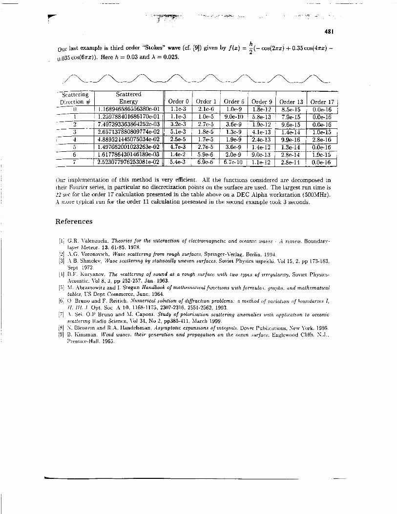
r "-•Jö««M!jg»v
481
Our last example is third order "Stokes" wave (cf. [9]) given by /(x) = -(-COS(2TTX) + 0.35 cos(47rx)
^OSocos^Trz)). Here h = 0.03 and A = 0.025.
"""Scattering Direction #
Scattered Energy Order 0 Order 1 Order 5 Order 9 Order 13 Order 17
" 0 1.168946586556380e-01 l.le-3 2.1e-6 1.0e-9 1.8e-12 8.5e-15 0.0e-16 ] 1 1.259788401686170e-01 l.le-3 1.0e-5 9.0e-10 5.8e-13 7.9e-15 0.0e-16 2 7.407393363864252e-03 3.2e-3 2.7e-5 3.6e-9 1.9e-12 9.6e-15 0.0e-lC i 3 2.657137880809774e-02 ö.le-3 1.8e-5 1.3e-9 4.1e-13 1.4e-14 1.0e-15 4 4.889524445075034e-02 2.5e-5 1.7e-5 1.9e-9 2.4e-13 9.9e-16 2.8e-16 D 1.497662001023263e-02 4.7e-3 2.7e-5 3.6e-9 1.4e-12 1.3e-14 0.0e-16 j 6 1.617786430146189e-03 1.4e-2 5.9e-6 2.0e-9 9.0e-13 2.8e-14 1.9e-15 < 2.523077976253081e-02 5.4e-3 6.9e-6 6.7e-10 l.le-12 2.8e-14 0.0e-16
Our implementation of this method is very efficient. All the functions considered are decomposed in their Fourier series, in particular no discretization points on the surface are used. The largest run time is 22 sec for the order 17 calculation presented in the table above on a DEC Alpha workstation (500MHz). A more typical run for the order 11 calculation presented in the second example took 3 seconds.
References
[2] [3]
HI
[6]
[8]
G.R. Yalenzuela, Theories for the interaction of electromagnetic and oceanic waves - A review. Boundary- layer Meteor. 13, 61-85, 1978. A.C. Voronovich, Wave scattering from rough surfaces, Springer-Verlag, Berlin, 1994. A.B. Shmclev, Wave scattering by statiscally uneven surfaces. Soviet Physics uspekhi. Yol 15, 2, pp 173-183, Sept. 1972. B.F. Kuryanov, The scattering of sound at a rough surface with two types of irregularity, Soviet Physics- Acoustic, Vol 8, 3, pp 252-257, Jan. 1963. M. Abramowitz and I. Stegun Handbook of mathematical functions with formulas, graphs, and mathematical tables, US Dept Commerce, June, 1964. O. Bruno and F. Reiticli. Numerical solution of diffraction problems: a method of variation of boundaries I, II. III. .1. Opt. Soc. A 10, 1168-1175, 2307-2316, 2551-2562, 1993. A Sei. O.P Bruno and M. Caponi. Study of polarization scattering anomalies with application to oceanic scattering Radio Science, Vol 34, No 2, pp385-411, March 1999. N. Bleistein and R.A. Handelsman, Asymptotic expansions of integrals. Dover Publications. New York, 1986. B. Kinsman. Wind waves, their generation and propagation on the ocean surface. Englcwood Cliffs, N.J., Prentice-Hall, 1965.

Appendix A5:
An innovative high-order method for electromagnetic scattering form rough surfaces,
National Radio Science Meeting, Boulder, Colorado, January 2000.

NATIONAL ACADEMIES OF SCIENCES AND ENGINEERING
NATIONAL RESEARCH COUNCIL
of the
UNITED STATES OF AMERICA
UNITED STATES NATIONAL COMMITTEE
International Union of Radio Science
^^
National Radio Science Meeting
4-8 January 2000
Sponsored by USNC/URSI
University of Colorado Boulder, Colorado
U.S.A.
^«Äa--
BIF2 We.PM
B/F2-6 AN INNOVATIVE HIGH-ORDER METHOD FOR ELECTRO- 15:00 MAGNETIC SCATTERING FROM ROUGH SURFACES
Oscar Bruno Caltech Pasadena, CA 91125 Maria Caponi TRW Redondo Beach, CA 90278 Alain Sei* TRW Redondo Beach, CA 90278
We present an innovative algorithm for the computation of electromag- netic scattering from rough surfaces, with emphasis on ocean scattering ap- plications. Our new method couples a high-order boundary variation method with an approach based on high-order, high-frequency asymptotic expansions of singular integrals.
To solve a scattering problem on a rough surface — composed of a smooth swell of general shape underlying a rough, highly oscillatory layer — we view the roughness as perturbation of the swell. The boundary variations method, used extensively in previous studies (Sei et al, Radio Science, 34, 385-411. 1999, Bruno O. and Reitich F., J. Opt. Soc. A., 10, 2551-2562, 1993). allows us to evaluate the scattered field from such rough surfaces by means of analytic continuation of an associated perturbation series of high order (Bruno O. and Reitich F., Proc. R. Soc. Edinburgh. A, 122, 317-340, 1992).
The evaluation of each one of the coefficients in this perturbation ex- pansion requires the solution of a scattering problem on a smooth surface with highly oscillatory boundary conditions. The solution of this notoriously difficult problem is computed efficiently and accurately by means of a new, high-order, high-frequency asymptotic expansion for the surface currents. Our high-frequency solver, which is designed to apply in the small wavelength regime — in which geometrical optics and the Kirchoff approximation are fre- quently used —, should be applicable to a wide range of scattering problems. Unlike the geometrical optics type expansions where amplitudes can become unbounded (at caustics), our high frequency algorithm is entirely rigorous and highly accurate.
This presentation will describe our approach to the general rough surface problem with a detailed discussion on the high-frequency solver. Numerical results in a variety of cases will be presented, demonstrating the accuracy and computational efficiency of our new methods.

Appendix Bl:
US Patent application: High-Order High-Frequency rough surface scattering solver

. ,<W Docket No. 11-1151
CERTIFICATE OF MAILING Express Mail Mailing Label No. EK745231604US Date of Deposit September 29 . 2000 I hereby certify that this paper or fee is being deposited with the United States Postal Service "Express Mail Post Office to Addressee" service under 37CFR1.10 on the date indicated above and is addressed to the Assistant Commissioner of Patents and Trademarks, Washington, DC 20231. Mailer Lynn E« Cabiles
(print) Maiier s-WA~^fc. o^lJJLu-^.
(signature)
HIGH-ORDER HIGH-FREQUENCY ROUGH SURFACE
SCATTERING SOLVER
This invention was made with Government support under F49620-99-C-
0014 awarded by AFOSR/DARPA. The Government has certain rights in this
invention.
BACKGROUND OF THE INVENTION
5 1. Field of the Invention
The present invention relates generally to scattering processes, and in
particular to computation of electromagnetic scattered fields from multiple scale
geometries.
2. Discussion of the Related Art
10 Electromagnetic scattering from rough surfaces such as the surface of the
ocean plays an important role in a wide range of applications including imaging,
remote sensing, and detection. The analysis of the scattering processes
involved in these applications poses a rather challenging scientific problem that
-1-

TRW Docket No. 11-1151
requires description and understanding of diffraction by complicated surfaces.
Computationally, the main difficulty arises from the multiple-scale nature of the
scattering surfaces, whose spectrum spans a wide range of lengthscales. A
number of techniques have been developed to treat associated limiting cases.
5 For example, the high frequency case, in which the wavelength, X, of the incident
radiation is much smaller than the surface lengthscales can be handled by
asymptotic methods such as geometrical optics or physical optics
approximations. On the other hand, resonant problems where the incident
radiation is of the order of the surface scale are treated by perturbation methods,
10 typically first or second or expansions in the height, h, of the surface.
However, when a multitude of scales is present on the surface, none of
the techniques described above either alone or in combination in so-called two-
scale approaches is adequate. The two-scale models imply a splitting of the
surface into a large scale and a small scale. Typically, a first order
15 approximation in wavelength is used to treat the smooth components of the
surface, and a first order in surface height is used to deal with the rough
components of the surface. The results provided by these methods are not
satisfactory precisely as a result of limitations imposed by the low orders of
approximation used in both, the high-frequency approximation method and the
20 small perturbation method.
-2-
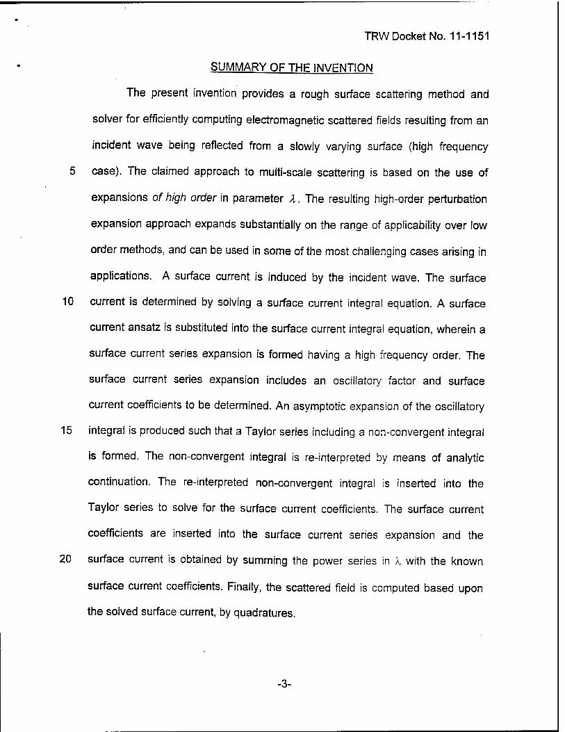
TRW Docket No. 11-1151
SUMMARY OF THE INVFNTION
The present invention provides a rough surface scattering method and
solver for efficiently computing electromagnetic scattered fields resulting from an
incident wave being reflected from a slowly varying surface (high frequency
5 case). The claimed approach to multi-scale scattering is based on the use of
expansions of high order in parameter X. The resulting high-order perturbation
expansion approach expands substantially on the range of applicability over low
order methods, and can be used in some of the most challenging cases arising in
applications. A surface current is induced by the incident wave. The surface
10 current is determined by solving a surface current integral equation. A surface
current ansatz is substituted into the surface current integral equation, wherein a
surface current series expansion is formed having a high frequency order. The
surface current series expansion includes an oscillatory factor and surface
current coefficients to be determined. An asymptotic expansion of the oscillatory
15 integral is produced such that a Taylor series including a non-convergent integral
is formed. The non-convergent integral is re-interpreted by means of analytic
continuation. The re-interpreted non-convergent integral is inserted into the
Taylor series to solve for the surface current coefficients. The surface current
coefficients are inserted into the surface current series expansion and the
20 surface current is obtained by summing the power series in k with the known
surface current coefficients. Finally, the scattered field is computed based upon
the solved surface current, by quadratures.
-3-

TRW Docket No. 11-1151
For a more complete understanding of the invention, its objects and
advantages, reference may be had to the following specification and to the
accompanying drawings.
5 BRIEF DESCRIPTION OF THE DRAWINGS
Figure 1 illustrates a flow diagram of a method for computing scattered
fields in accordance with the teachings of the invention; and
Figure 2 illustrates a transverse electric polarized wave (TE) impinging on
a rough surface.
10 DETAILED DESCRIPTION OF THE PREFERRED EMBODIMENT
Referring to Figure 1, a method of computing a scattered field according to
the present invention is shown. The method is based on the use of expansions
of high order in the parameter X. Such extensions require rather complex
mathematical treatments, including complex variable theory and analytic
15 continuation. The resulting approach expands substantially on the range of
applicability over low order methods, and can be used in some of the most
challenging cases arising in applications. Here, we focus on a high-order
perturbation expansion in the wavelength X.
1. Introduction
20 With additional reference to Figure 2, a transverse electric polarized wave
(TE) 12, with electric field, E, pointing out of the figure, impinging on a rough
surface 10 is illustrated. The method is particularly suitable for two-dimensional
-4-

TRW Docket No. 11-1151
problems of scattering from a perfectly conducting rough surface 10 of a
transverse electric polarized wave (TE) 12. A scattered field created by the
incident plane wave 12 impinging on the rough surface 10 solves Helmholtz's
equation with a Dirichlet boundary condition. The scattered field can be
5 computed from the surface current density, v, 14 induced on the rough surface
f(x) 10 by the incident plane wave 12 by integrating the solved surface current
against the Green's function. See, Wave scattering from rough surfaces, by A.G.
Voronovich, Springer-Verlag, Berlin, 1994, which is hereby incorporated by
reference. The function v solves the integral equation:
10 (1) ifc^Li rh(kMM')g(x,x')v{x',k)ck'=-eiax-l/¥{x\ step 20, 9 A J-oo
where
MM' = J(x'-x)2+(f{x')-f(x)f h{t) = tH\if) H\ Hankel function
MM
15 To solve this equation, an asymptotic expansion of high order around k = co is
used. The asymptotic expansion results from the ansatz
-5-

TRW Docket No. 11-1151
From equations (1) and (2) we obtain the following equation for the surface
current coefficients;
(3) 2j7\ v» (*K'"M)]*-2, step 24. M»O k v * /
where
/" (JC, k) = £h(kMM')g(x, x')e»**'-*)-'M*')-f(*\ (x')dx'
To obtain the coefficients vn(x) we produce the asymptotic expansion of I"(x,k),
an oscillatory integral, in powers of \/k, step 26. To do this we use two separate
integration regions which we define below. However using a single integration
region or multiple integration regions is within the scope of the invention.
10 r.(x,k)= f h(kMM')g(x,xyal*-xhlM*M*\(x')dx'
/; (JC, k)=Jf h(kMM')g(x, JC»)e'«(',-H/>(/(*1h/(Jr))Vfl ^^
-6-

TRW Docket No. 11-1151
2. Asymptotic expansion of I"(x,k)
We focus on an asymptotic expansion for Il(x,k). Using t = x-x we can
write
(4) /+" (x, *) = f° h(k</> + (x, t))g(x, x + t)e ia,-'Mx+l hf{x\ (x + t)dt
5 where
t + (x,t)=Jt2+(f(x + t)-f(x)
For the simplest treatment we present here we assume that f{x) satisfies the
condition
v ' dt
10 so that the map t\->0 + (x,t) is invertible; this condition is generally satisfied by
rough surfaces considered in practice. Then setting
U = (j) + {x,t) <=> t=0+](x,lt)
we can rewrite equation (4) in the form
-7-

TRWDocketNo. 11-1151
<P+\x,0+ {x,u))
or, calling
^+(x,<z>+ (x,w)j
(5)
^ + (x, K) = (/(x + £' (x,«))- /(x))cos(0/;,c)- ^ (x, «)sin(^),
/; (x, k)=f h(ku)F; (x, u)e -**♦(*•" V«.
We can now use the Taylor series of the map u i-> F* (x,u) around u = 0
,„=o 0H /w! m+0 /«! du
to express /"(x,A) in the form
»1=0
+00
(6)
-8-
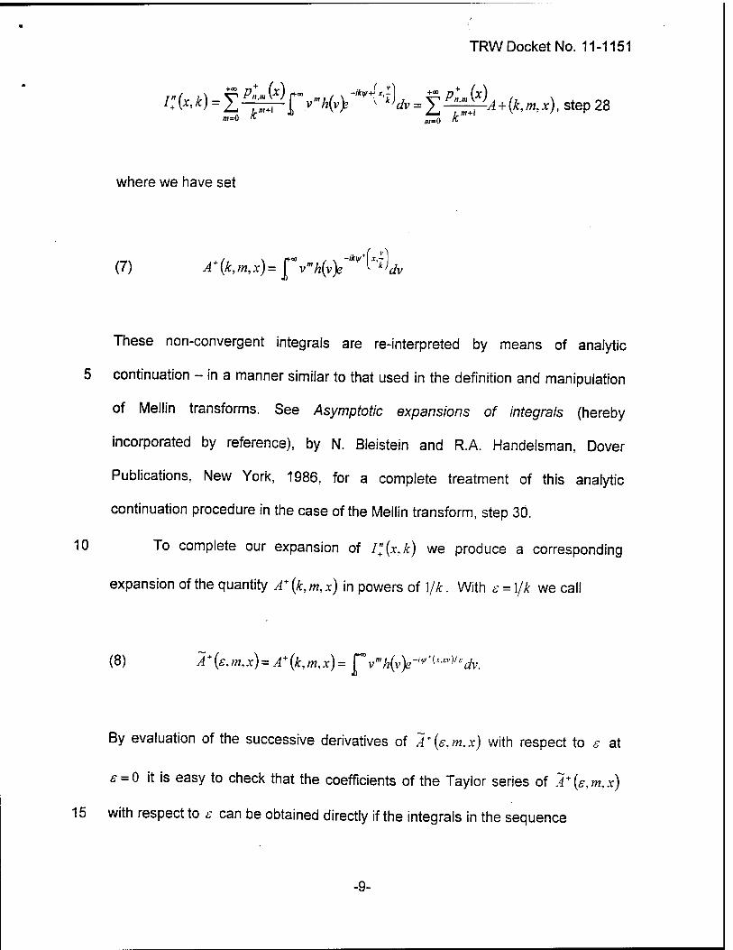
TRW Docket No. 11-1151
/»-o * m=0 K
where we have set
(7) A+(k,m,x)=fv»h(vyik^dv
These non-convergent integrals are re-interpreted by means of analytic
5 continuation - in a manner similar to that used in the definition and manipulation
of Mellin transforms. See Asymptotic expansions of integrals (hereby
incorporated by reference), by N. Bleistein and R.A. Handelsman, Dover
Publications, New York, 1986, for a complete treatment of this analytic
continuation procedure in the case of the Mellin transform, step 30.
10 To complete our expansion of I"{x,k) we produce a corresponding
expansion of the quantity A+(k,m,x) in powers of \/k. With s = l/k we call
(8) A + (e,m,x) = A+(k,m,x)= J"v"Ä(v>-,>*(r-w)/*rfv.
By evaluation of the successive derivatives of A*{e,m.x) with respect to e at
£ = 0 it is easy to check that the coefficients of the Taylor series of A+{s,m,x)
15 with respect to s can be obtained directly if the integrals in the sequence
-9-
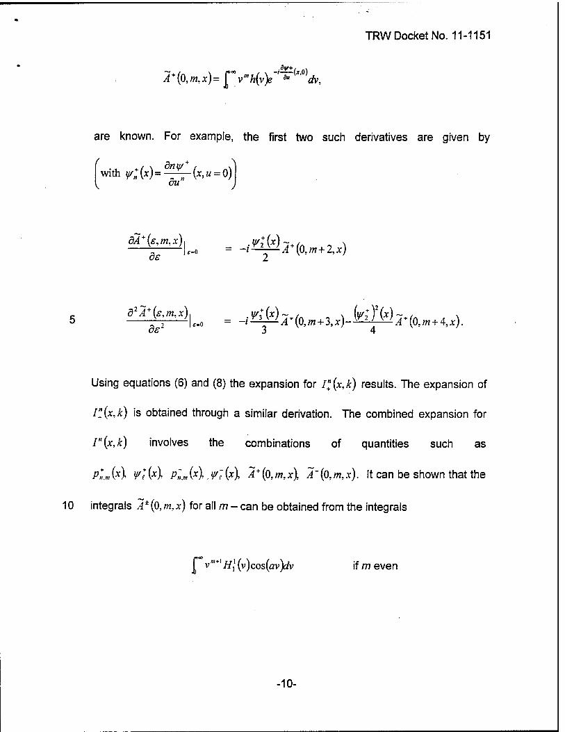
TRW Docket No. 11-1151
^(O.m.il^fv-Afv^W
are known. For example, the first two such derivatives are given by
with<(x)=-^(x,« = 0) du
dA+ (s, m, x) | w+ (x) ~ / N
de 2
_ d2A + (s,m,x), wt(x\~J./ \ wZ)(x)~ / N 5 rr-M~o = -i!^A + (0,m + 3,x)-W2)
A V V (0,m + 4,x).
of" 3 4
Using equations (6) and (8) the expansion for /;(*,£) results. The expansion of
I"(x,k) is obtained through a similar derivation. The combined expansion for
I"(x,k) involves the combinations of quantities such as
Pn.„Xx\ Vtix\ Pi,.m(x\.^t{x), A + (0,m,x), A~(0,m,x). It can be shown that the
10 integrals 2* (0, m, x) for all m - can be obtained from the integrals
| v ",+l Hi (v) cos(av)dv if m even
-10-

TRW Docket No. 11-1151
fvm+]Hl(v)sin{av)dv if m odd
for which closed form formulas are available in Handbook of mathematical
functions with formulas, graphs, and mathematical tables, by M. Abramowitz and
5 I. Stegun, US Dept Commerce, June, 1964, which is hereby incorporated by
reference, step 32.
Next, the high frequency order for the computation is selected, step 34.
The scope of the invention includes a high frequency order that is 2 or greater.
Those skilled in the art will readily recognize that selection of the high frequency
10 order involves a trade-off between computation speed and accuracy which will
vary depending on the particular application.
Finally, having determined the surface current coefficients, the surface
current is computed with formula (2) for, and the scattered field is computed by
integrating the solved surface current against Green's function, step 36.
15 3. Numerical results
To test the accuracy of the procedure we compared our results to a highly
accurate boundary variation code in a region (in wavelength) where the two
algorithms were very accurate as shown below. See, Numerical solution of
diffraction problems: a method of variation of boundaries I, II, III, by O. Bruno and
20 F. Reitich, J. Opt. Soc. A 10, 1168-1175, 2307-2316, 2551-2562, 1993. Note
that these two methods are substantially different in nature: ours is a high order
-11-
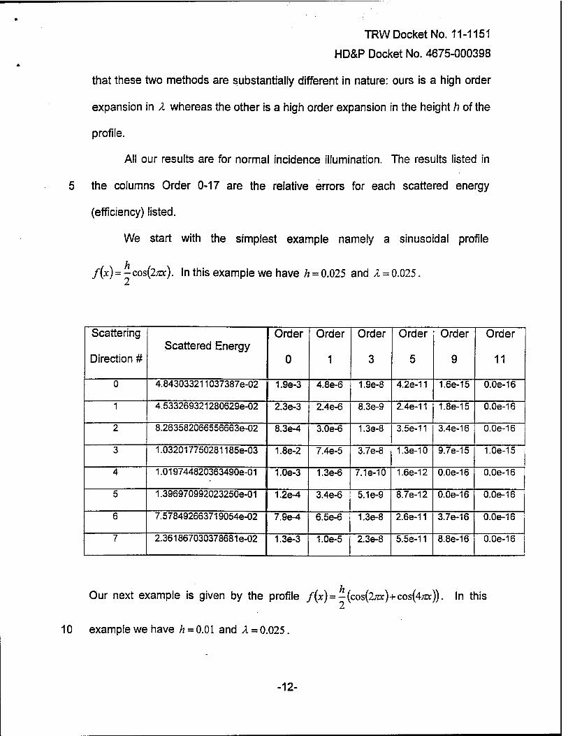
TRW Docket No. 11-1151
HD&P Docket No. 4675-000398
that these two methods are substantially different in nature: ours is a high order
expansion in X whereas the other is a high order expansion in the height h of the
profile.
All our results are for normal incidence illumination. The results listed in
the columns Order 0-17 are the relative errors for each scattered energy
(efficiency) listed.
We start with the simplest example namely a sinusoidal profile
f(x)=-cos(2;zx). In this example we have h = 0.025 and X = 0.025.
Scattering
Direction # Scattered Energy
Order
0
Order
1
Order
3
Order
5
Order
9
Order
11
0 4.843033211037387e-02 1.9e-3 4.8e-6 1.9e-8 4.2e-11 1.6e-15 0.0e-16
1 4.533269321280629e-02 2.3e-3 2.4e-6 8.3e-9 2.4e-11 1.8e-15 0.0e-16
2 8.263582066556663e-02 8.3e-4 3.0e-6 1.38-8 3.56-11 3.4e-16 0.0e-16
3 1.032017750281185e-03 1.8e-2 7.4e-5 3.7e-8 1.3e-10 9.7e-15 1.0e-15
4 1.019744820363490e-01 1.0e-3 1.3e-6 7.1e-10 1.6e-12 0.0e-16 0.0e-16
5 1.3969709920232508-01 1.2e-4 3.4e-6 5.1e-9 8.7e-12 0.0e-16 0.0e-16
6 7.578492663719054e-02 7.9e-4 6.5e-6 1.3e-8 2.6e-11 3.7e-16 0.0e-16
7 2.361867030378681e-02 1.3e-3 1.0e-5 2.3e-8 5.5e-11 8.8e-16 0.0e-16
Our next example is given by the profile /(x)=-(cos(2^c)+cos(4^r)). In this
10 example we have /z = 0.01 and X = 0.025.
-12-

TRW Docket No. 11-1151
HD&P Docket No. 4675-000398
Scattering
Direction # Scattered Energy
Order
0
Order
1
Order
5
Order
9
Order
11
Order
15
0 1.9837028748538606-01 1.4e-3 6.7e-6 6.3e-10 1.8e-13 5.0e-15 0.0e-16
1 2.125625186015414e-02 4.3e-3 7.3e-6 8.6e-10 4.6e-14 4.9e-16 0.0e-16
2 5.109656298137152e-02 4.2e-3 5.3e-6 1.3e-9 3.5e-14 6.9e-15 0.0e-16
3 1.3505945648611706-01 1.1e-3 3.0e-6 1.8e-10 5.1e-14 6.9e-16 0.0e-16
4 1.670755436364386e-02 4.3e-3 928e-6 1.5e-9 1.8e-13 0.0e-14 0.0e-16
5 1.041839113172000e-01 8.7e-4 1.1e-5 4.76-10 3.8e-14 0.0e-16 0.0e-16 |
6 3.029977474761340e-02 7.6e-4 1.1e-5 4.8e-10 1.0e-15 2.06-15 0.0e-16
7 2.828409217693459e-02 2.5e-3 3.2e-5 1.8e-9 3.5e-14 4.6e-15 6.1e-16
Our last example is a third order "Stokes" wave (cf. [9]) given by
/W=-(-cos(2^r)+0.35cos(4^:)-0.035cos(6^c)). Here h = 0.Q3 and A = 0.025.
Scattering
Direction # Scattered Energy
Order
0
Order
1
Order
5
Order
9
Order
13
Order
17
0 1.168946586556380e-01 1.16-3 2.1e-6 1.0e-9 1.8e-12 8.5e-15 0.0e-16
1 1.259788401686170e-01 1.1e-3 1.0e-5 9.0e-10 5.8e-13 79e-15 0.0e-16
2 7.407393363864252e-03 3.2e-3 2.7e-5 3.6e-9 1.9e-12 9.6e-15 0.0e-16
3 2.657137880809774e-02 5.1e-3 1.8e-5 1.3e-9 4.1e-13 1.4e-14 1.0e-15
4 4.889524445075034e-02 2.5e-5 1.7e-5 1.9e-9 2.4e-13 9.9e-16 2.8e-16
5 1.497662001023263e- 02 4.7e-3 2.7e-5 3.6e-9 1.4e-12 1.3e-14 0.0e-16
6 1.617786430146189e-03 1.4e-2 5.9e-6 2.0e-9 9.0e-13 2.8e-14 1.9e-15
7 2.523077976253081e-02 5.4e-3 6.9e-6 6.7e-10 1.1e-12 2.8e-14 0.0e-16
-13-

TRW Docket No. 11-1151
Our implementation of this method is very efficient. All the functions
considered are decomposed in their Fourier series. The largest run time is 22
sec for the order 17 calculation presented in the table above on a DEC Alpha
workstation (600MHz). A more typical run for the order 11 calculation presented
5 in the second example took 3 seconds.
Thus it will be appreciated from the above that as a result of the present
invention, a method for computing a scattered field resulting from an incident
wave being reflected from a rough surface is provided by which the principal
objectives, among others, are completely fulfilled. It will be equally apparent and
10 is contemplated that modification and/or changes may be made in the illustrated
embodiment without departure from the invention. Accordingly, it is expressly
intended that the foregoing description and accompanying drawings are
illustrative of preferred embodiments only, not limiting, and that the true spirit and
scope of the present invention will be determined by reference to the appended
15 claims and their legal equivalent.
-14-

TRW Docket No. 11-1151
CLAIMS
What is claimed is:
1 1. A method of computing a scattered field resulting from an incident
2 wave being reflected from a rough surface, a surface current being induced by
3 the incident wave, comprising the steps of:
4 representing the surface current as high-order high-frequency
5 expansion;
6 substituting a surface current ansatz into the surface current
7 integral equation, wherein a surface current series expansion is formed having a
8 high frequency order, the surface current series expansion including an
9 oscillatory integral and surface current coefficients;
10 producing an asymptotic expansion of the oscillatory integral;
11 evaluating the asymptotic expansion for the surface current
12 coefficients;
13 inserting the surface current coefficients into the surface current
14 series expansion;
15 evaluating the surface current series expansion for the surface
16 current; and
17 computing the scattered field based upon the solved surface
18 current.
-15-
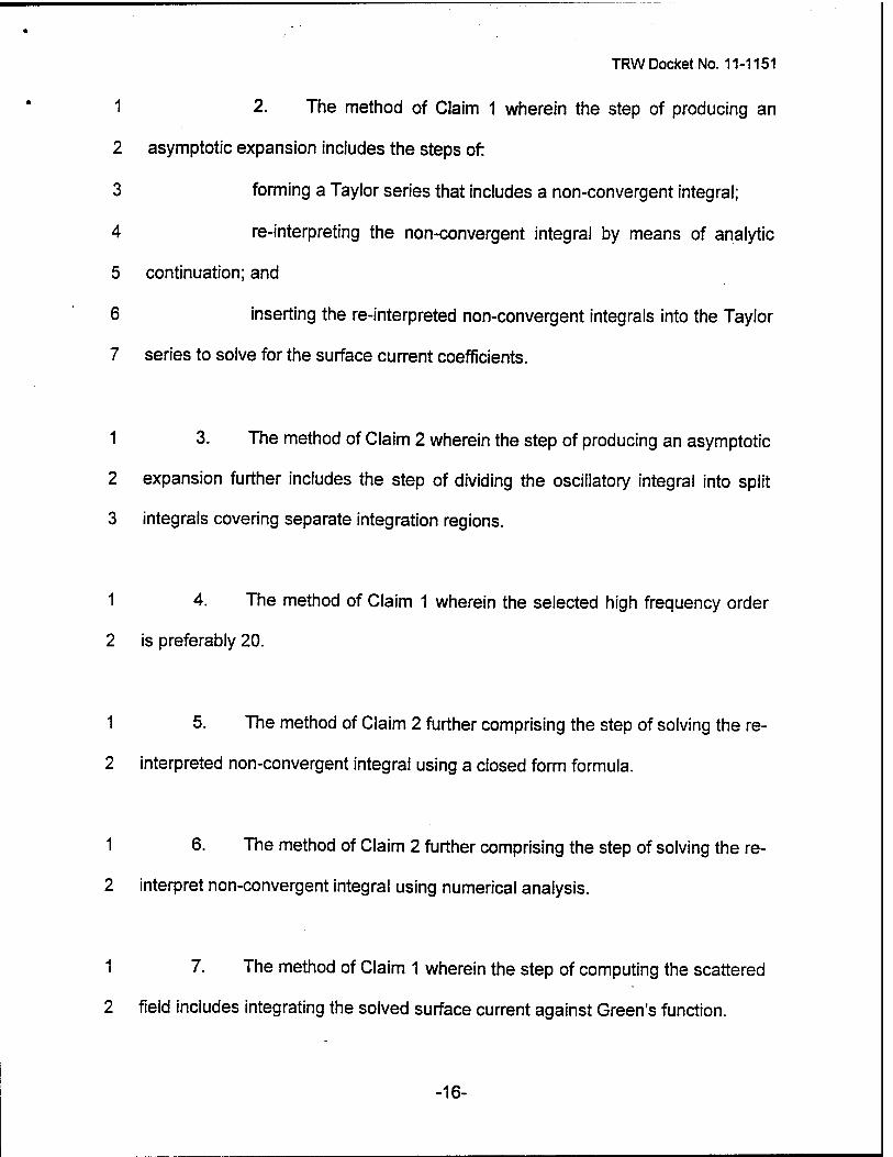
TRW Docket No. 11-1151
1 2. The method of Claim 1 wherein the step of producing an
2 asymptotic expansion includes the steps of:
3 forming a Taylor series that includes a non-convergent integral;
4 re-interpreting the non-convergent integral by means of analytic
5 continuation; and
6 inserting the re-interpreted non-convergent integrals into the Taylor
7 series to solve for the surface current coefficients.
1 3. The method of Claim 2 wherein the step of producing an asymptotic
2 expansion further includes the step of dividing the oscillatory integral into split
3 integrals covering separate integration regions.
1 4. The method of Claim 1 wherein the selected high frequency order
2 is preferably 20.
1 5. The method of Claim 2 further comprising the step of solving the re-
2 interpreted non-convergent integral using a closed form formula.
1 6. The method of Claim 2 further comprising the step of solving the re-
2 interpret non-convergent integral using numerical analysis.
1 7. The method of Claim 1 wherein the step of computing the scattered
2 field includes integrating the solved surface current against Green's function.
■16-

TRW Docket No. 11-1151
1 8. The method of Claim 1 wherein the oscillatory integral is
2 /"(*,*)= J£h(kMM')g(x, x')e '^'-'HM^/M)^ (^ _
3 where; MM'=J(x'-xf + (f(x')-f(x)f h(t) = tH\(t) H\ Hankel function
^yjWH^m a = ksin(ffJ flmkm(ßj.
1 9. The method of Claim 2 wherein the Taylor series is
2 i:(x,k)=j:^A + (k,m,x) m=0 k"
1 10. A method of computing a scattered field resulting from an incident
2 wave being reflected from a rough surface having a characteristic lengthscale, a
3 surface current being induced by the incident wave, the incident wave having a
4 wavelength less than the rough surface lengthscale, comprising the steps of:
5 representing the surface current as a high-order high-frequency
6 expansion;
7 substituting a surface current ansatz into the surface current
8 integral equation, wherein a surface current series expansion is formed having a
9 high frequency order, the surface current series expansion including an
10 oscillatory integral and surface current coefficients;
-17-

TRW Docket No. 11-1151
11 producing an asymptotic expansion of the oscillatory integral such
12 that a Taylor series including a non-convergent integral is formed;
13 re-interpreting the non-convergent integral by means of analytic
14 continuation;
15 inserting the re-interpreted non-convergent integrals into the Taylor
16 series to solve for the surface current coefficients;
17 inserting the surface current coefficients into the surface current
18 series expansion;
19 evaluating the surface current series expansion for the surface
20 current; and
21 integrating the solved surface current against Green's function,
22 whereby the scattered field is determined.
1 11. The method of Claim 10 wherein the step of producing an
2 asymptotic expansion further includes the step of dividing the oscillatory integral
3 into split integrals covering separate integration regions.
1 12. The method of Claim 10 wherein the high frequency order is at
2 least about three.
1 13. The method of Claim 10 further comprising the step of solving the
2 re-interpreted non-convergent integral using a closed form formula.
-18-

TRW Docket No. 11-1151
1 14. The method of Claim 10 wherein the Taylor series is
1 15. The method of Claim 10 further comprising the step of solving the
2 re-interpreted non-convergent integral using a closed form formula.
1 16. The method of Claim 15 wherein the closed form formula is
2 | vm+lHi (v)cos(av)fv if m even
3 and
4 I" vm+lHi (v)sin(av)/v if m odd.
1 17. A solver for computing a scattered field resulting from an incident
2 wave being reflected from a rough surface having a characteristic lengthscale, a
3 surface current being induced by the incident wave, the incident wave having a
4 wavelength less than the rough surface lengthscale, comprising:
5 means for representing the surface current as a high-order high-
6 frequency expansion;
7 means for substituting a surface current ansatz into the surface
8 current integral equation, wherein a surface current series expansion is formed
9 having a high frequency order, the surface current series expansion including an
10 oscillatory integral and surface current coefficients;
-19-

TRW Docket No. 11-1151
11 means for producing an asymptotic expansion of the oscillatory
12 integral such that a Taylor series including a non-convergent integral is formed;
13 means for re-interpreting the non-convergent integral by means of
14 analytic continuation;
15 means for inserting the re-interpreted non-convergent integrals into
16 the Taylor series to solve for the surface current coefficients;
17 means for inserting the surface current coefficients into the surface
18 current series expansion;
19 means for evaluating the surface current series expansion for the
20 surface current; and
21 means for integrating the solved surface current against Green's
22 function, whereby the scattered field is determined.
1 18. The solver of Claim 17 wherein the high frequency order is at least
2 about three.
1 19. The solver, of Claim 17 further comprising means for dividing the
2 oscillatory integral into split integrals covering separate integration regions.
-20-

TRW Docket No. 11-1151
HIGH-ORDER HIGH-FREQUENCY ROUGH SURFACE SCATTERING SOLVER
ABSTRACT OF THE DISCLOSURE
The present invention provides a rough surface scattering method and
solver for efficiently computing electromagnetic scattered fields resulting from an
incident wave (12) being reflected from a surface slowly varying on the scale of
the wavelength (10). The wavelength claimed approach to high-frequency
5 scattering is based on the use of expansions of high order in parameter X,
wavelength of the incident radiation. The resulting high-order expansion
approach expands substantially on the range of applicability over low order
methods, and can be used in some of the most challenging cases arising in
applications. The surface current (14) induced by the incident wave (12) is
10 represented as a high-order high-frequency expansion (20). The surface current
ansatz is substituted into the surface current integral equation (22), wherein a
surface current series expansion is formed (24) having a high frequency order.
The surface current series expansion includes an oscillatory integral and surface
current coefficients. An asymptotic expansion of the oscillatory integral is
15 produced having a Taylor series (26). The Taylor series is evaluated and the
surface current coefficients (32) determined. The surface current coefficients are
inserted into the surface current series expansion. The surface current series
expansion is evaluated to yield the surface current (36). Finally, the scattered
field is computed based upon the solved surface current (36).
-21-

20
Determining the surface current from the surface current integral equation
Substituting a surface current ansatz into the surface current integral equation
22
24 Forming a surface current series expansion having a high frequency order
and including an oscillatory integral and surface current coefficients
Producing an asymptotic expansion of the oscillatory integral
Forming a Taylor series having a non-convergent integral
Re-interpreting the non-convergent integral
Solving for the surface current coefficients
Selecting the high frequency order
Solving for the surface current and scattered field
FIG. 1
26
28
30
32
34
36
I

\\\\\\ \\\
CM
Appendix Cl
Electromagnetic Scattering from Multiple Scale Geometries
Contract Number: F49620-99-C-0014 Progress Report for the period: March 01-99 - July 31-99
PI: Maria Caponi Email: [email protected]
Phone: 310-812-0079 Fax: 310-814-2359
TRW, Inc; Ocean Technology Department
Rl-1008 Redondo Beach, California 90278

2 Program Objectives:
The statement of work objectives for the first year of this program is:
Development and initial implementation of a new approach to calculate scattering from multiple
scale surfaces containing large curvature and small-scale corrugations.
Initial numerical calculations for simple 2-D two scale geometries relevant to ocean applications.
Objective 1 includes:
1 .a Development of a very accurate algorithm to solve high-frequency scattering problems
on a smooth non-planar surface.
1 .b Development of the integrated algorithm that treats the short scale surface variations
(roughness) as perturbations of the long scale modulations.
3. Status of effort:
A new algorithm has been developed and implemented, and is currently being tested to
calculate the scattering return from smooth, slowly varying, arbitrary surfaces (the high-
frequency scattering problem) (Objective 1 .a). The algorithm relies on an integral equation
formulation and makes use of an innovative high-order high-frequency rigorous asymptotics
expansion of the singular integrals. The method includes all multiple scattering terms with no
iterations of the integral equation. The initial calculations to third order have been validated by
comparison with a previous developed boundary variation method in the overlap region of
validity. The results show an improvement of 5 orders of magnitude over Kirchhoff (0th order).
Higher order calculations are currently being implemented. The integrated algorithm to
calculate the scattering from short scale roughness on long scale swell surfaces (Objectivel .b)
has been formulated. Initial implementation will start once the high-frequency algorithm is
validated to arbitrary orders.
4. Accomplishments/New Findings
During the initial 5 months of this project the following significant research has been
accomplished:
The innovative algorithm proposed at the beginning of this project to compute the scattering
return from multi-scale surfaces has been formulated in detail. The algorithm consists of two
main elements: A) A boundary variation method that reduces the multi-scale problem to a
sequence of high-frequency scattering problems on a smooth surface. B) A new high-order,
high frequency method.
The high-frequency part of this algorithm, which entails the highly accurate calculation of the
scattering return from surfaces with characteristics scales larger than the radiation wavelength
has been implemented and successfully validated to third order. Results that are 5 orders of

magnitude more accurate than Kirchhoff (0th order) have been obtained, demonstrating the
advantages of the new method.
The implementation of the high- frequency algorithm is based on an ingenious asymptotic
expansion of the highly singular integrals and on the analytic continuation of the divergent
integrals. A numerically efficient version of the algorithm was found to compute accurately these
expansions to all orders. High accuracy is crucial for this method since it will be used
repeatedly to solve the general problem.
These initial results are critical to an accurate calculation of the scattering return from multiple
scale surfaces, in particular for ocean surveillance applications. For example, recent
experimental results have shown polarization losses of the order of-80 dB for high horizontal to
vertical polarization ratios (HH/W>1) that can not be predicted with standard scattering models.
The algorithm developed in this program will have enough accuracy to predict those large
losses. Further, once validated, this algorithm will be able to predict radar returns not only for
ocean but also for terrain relevant missions where multi-scale surfaces play a dominant role in
the characteristics of the return.
5 Personnel Supported:
Dr. Alain Sei, TRW: (supported by this program ~ 65% of his time); Dr. Maria Caponi, TRW:
(supported by this program <5% of her time); Dr. Oscar Bruno, MathSys and Caltech (Technical
services, supporter by this program <10% of his time)
6 Publications: None on current contract period. 7 Interactions/Transitions:
Participation/presentation: Poster and VG at ACMP DARPA PI meeting. S.F. June 30-July1,
1999.
Transitions: the algorithm being developed is planned to be used in conjunction with the TRW
hydrodynamic codes to obtain a predictive model of ocean radar returns. The results from this
combination code will be relevant to Navy applications.
8 New Discoveries: A new method to solve the high-frequency scattering problem with high accuracy (16 digits) 9 Honors/Awards: None during current contract period

Appendix C2
Electromagnetic Scattering from Multiple Scale Geometries
Contract Number: F49620-99-C-0014 Progress Report for the period: July 31- 99 - July 31- 00
PI: Maria Caponi Email: [email protected]
Phone: 310-812-0079 Fax: 310-814-2359
TRW, Inc; Ocean Technology Department
Rl-1008 Redondo Beach, California 90278

2. Program Objectives:
The statement of work objectives for the second year of this program were:
Parametric investigations with 2-D multi-scale code for surfaces relevant to ocean remote
sensing applications
Development and initial implementation of new approach to 3-D surfaces.
These objectives have been revised to:
Validation of the 2-D high-order high-frequency code for large scale surfaces and its use in
parametric investigations relevant to ocean remote sensing applications.
Formulation and implementation of the 2-D multi-scale algorithm.
Objective 1 includes
1.a. Efficient implementation of the high-frequency algorithm to arbitrary order.
Objective 2 includes:
2.a. Development of coupling between the high frequency and the boundary variation methods,
including innovative use of Cauchy-Kowalesky argument for computation of high order normal
derivatives.
2.b. Treatments of high-order normal derivatives through the use of Helmholtz's equation
second order normal derivatives and high-order tangential derivatives to avoid hyper-singular
integrals.
The revision of the objectives was due in part to the need for a more efficient and accurate
implementation of the high-frequency algorithm than the one carried out during the first year of
this contract. The original implementation was not easily amenable to very high order
expansions therefore limiting the range and accuracy of application of the method. However,
the repeated use of the high-frequency code in the final multiple scale algorithm requires double
digit accuracy to arbitrary orders. The new implementation uses subtle and intensive algebraic
treatments that result in a very efficient and innovative algorithm, currently being considered for
a patent application. However, this revised implementation delayed the coding of the final multi-
scale algorithm. Further delay also resulted from extensive validations of the results.
3. Status of effort:
The new high-order-high frequency algorithm has been extended to arbitrary order and
accuracy. This extension relies on the development of a library of subroutines for the efficient
algebraic treatment of infinite Taylor-Fourier series. The code has been validated by
comparison with the method of variation of boundaries in the overlap region in wavelengths
where both methods are valid. The code has been exercised for numerous configurations,
machine precision accuracy was reached in cpu times of seconds in all cases (Rev. objective
1). A detailed formulation of the multiple-scale algorithm including an innovative coupling of the

new high-order high frequency method and the boundary variation method has been completed
and implemented. The details of the method have been documented. The complete Fortran
implementation of the integrated algorithm is expected in the next few weeks. Currently, each
segment of the Fortran code is being carefully tested and verified (Rev. objective 2).
Afterwards, careful parametric investigations relevant to ocean remote sensing will be
performed.
4. Accomplishments/New Findings
During the last year the following significant accomplishments have been reached in this project: 1 A library of subroutines for the efficient algebraic treatment of infinite Taylor-Fourier
series was completed. These series were introduced specifically by us to meet the
accuracy and efficiency demands of this project.
2 Full double precision agreement was obtained between the high-order high-frequency
method and the boundary variation method for numerous and varied examples
throughout the overlap region in wavelengths where both methods are valid. Computing
times of the order of seconds on a 600MHz desktop workstation were achieved in all
cases. The high-frequency code was also validated and exercised in the high-frequency
regime (wavelength < surface scale length) for configurations of interest to ocean
remote sensing where the boundary variation code failed.
3 The details of this highly innovative high-frequency algorithm are currently being
considered by TRW for a patent application.
4 The high frequency algorithm has been integrated with the method of variation of
boundaries to yield a highly accurate and efficient multiple-scale solver. The high order
nature of the algorithm requires an inventive use of the Cauchy-Kowalevsky argument.
A method has been derived for the evaluation of the necessary high-order normal
derivatives, (which would normally give rise to hyper-singular integrals) through the use
of the Helmholtz equation, the second normal derivative and the high-order tangential
derivatives. These tangential derivatives, in turn, are computed through an application
of the Taylor-Fourier algebra mentioned in 1 above. The second normal derivative is
computed directly by manipulations of the kernel singularities.
This integrated code, currently being tested, is expected to be the most efficient and
accurate solver for the computation of scattered waves from multi-scale rough surfaces. A
code with these characteristics is necessary for current ocean and terrain remote sensing
applications, given the small scattering returns relative to the incident field.
5. Personnel Supported:
Dr. Alain Sei, TRW: (supported by this program - 65% of his time);
Dr. Maria Caponi, TRW: (supported by this program < 5% of her time);

6 Publications:
The results of these investigations are documented in the following papers:
O. Bruno, A. Sei, and M. Caponi; "High order, high frequency solvers for rough surface
scattering problems". In Proceedings of the 2001 IEEE AP-S International symposium and
USNC/URSI National Radio Science meeting, July 2001, Boston, Massachusetts, USA.
A. Sei, M. Caponi and O. Bruno, "Polarization Ratios Anomalies of 3D Rough Surface
Scattering as Second Order Effects". in Proceedings of the 2001 IEEE AP-S International
symposium and USNC/URSI National Radio Science meeting, July 2001, Boston,
Massachusetts, USA.
7 Interactions/Transitions:
Participation/presentation:
Participation in the AFOSR Electromagnetic workshop, San Antonio, Jan 2001.
Presentation to DARPA PI meeting Washington D.C., April 2001.
Transitions:
A detailed study of polarization anomalies has been performed in 3D using the previously
developed method of variation of boundaries. This study is still on-going and a statistical study
similar to the one performed last year in two dimensions is envisioned. This study is of interest a
particular Navy customer.
Discussion with the government are on going for application of these methods to problems of
interest to the Navy, this is expected to result in a transition follow on project. This follow on
project will include the use of the numerical code in conjunction with the TRW hydrodynamic
codes to calculate the time evolution of radar return from evolving relevant ocean surfaces and
the appropriate calculation of the associate Doppler spectrum in both the TE (H) and the TM (V)
polarization. In addition experimental validation of the algorithm will be carried out using the
TRW testing facilities.
8 New Discoveries:
A new method to solve multi-scale scattering problems under TE polarization has been
developed implemented and validated.
A new method to solve high-frequency scattering problems under TM polarization with machine
precision accuracy has been implemented and validated.
9 Honors/Awards:
^ None this year.

Dr. Oscar Bruno, MathSys and Caltech (Technical services, supported by this program < 10%
of his time)
6. Publications:
The investigations and results of this program are documented in the following papers:
O. Bruno, M. Caponi and A. Sei; "An innovative high-order method for electromagnetic
scattering from rough surfaces." In Proceedings of the National Radio Science Meeting, 4-8
January, 2000, Univ. of Colorado, Boulder, USA
O. Bruno, A. Sei and M. Caponi," Rigorous multi-scale solver for rough-surface
scattering problems: high-order-high-frequency and variation of boundaries". To appear in
Proceedings of the NATO meeting on Low Grazing Angle Clutter: Its characterization,
measurement and application. April 2000, Laurel, Maryland, USA.
O. Bruno, A. Sei, and M. Caponi; "High order, high frequency solution of rough surface
scattering problems". In Proceedings of the fifth international conference on mathematical and
numerical aspects of wave propagation, Santiago de Compostella, Spain, July 2000, pp. 477-
481.
O. Bruno, A. Sei and M. Caponi; "High order high frequency solutions of rough surface
scattering problem", in final preparation, to be send for publication to Radio Science, Aug. 2000.
A claim has been recently sent to the TRW lawyers (July 2000) to obtain permission to
file a patent on the invention of the high frequency high order algorithm for solution of rough
surface scattering problems.
7. Interactions/Transitions:
Participation/presentation:
Poster presentation in AFOSR San Antonio Electromagnetic Workshop, Jan. 2000.
Presentation to DARPA PI meeting Washington D.C., April 2000.
Transitions: the algorithm being developed is intended to be used in conjunction with the TRW
hydrodynamic codes to obtain a predictive model of ocean radar returns. The results from this
combined code will be extremely relevant to Navy applications. In the mean time, a tailored
version of the boundary variation method code has been used to perform a statistical study of
the polarized backscattering returns associated with ocean spectra characteristic of near
breaking long waves for a particular Navy customer. This study, still ongoing, will be extended to
larger spectral bandwidths once the multi-scale code is completely implemented and validated.
8. New Discoveries:
A new method to compute the high-frequency scattering problem to arbitrary orders with
machine precision has been implemented.

A new method to solve the multi-scale scattering problems has been developed and
implemented.
9. Honors/Awards:
Dr A. Sei chaired the three sessions on scattering at the fifth international conference the
mathematical and numerical aspects of wave propagation, Santiago de Compostella, Spain,
July 2000.

Appendix C3
Electromagnetic Scattering from Multiple Scale Geometries
Contract Number: F49620-99-C-0014 Progress Report for the period: July 31- 00 - July 31- 01
PI: Maria Caponi Email: [email protected]
Phone: 310-812-0079 Fax: 310-814-2359
TRW, Inc; Ocean Technology Department
Rl-1008 Redondo Beach, California 90278

2. Program Objectives:
The statement of work objectives for the third year of this program were:
Detailed parametric investigations for 3-D surfaces relevant to applications of interest. (E.g. 2
and 3 scale modulated wave geometries with different modulations and/or scales in each
dimension).
For the first half of the third year, these objectives have been revised to:
Implementation and validation of the 2-D TE multi-scale code for surfaces including a range of
scales and its use in parametric investigations relevant to ocean remote sensing applications.
Formulation of the 2-D TM multi-scale algorithm.
The goal for the rest of the third year of this program is to implement the TM multiscale
algorithm and exercise it in conjunction with the multiscale TE
Objective 2 includes
2. 1. Formulation and implementation of the high-frequency algorithm to arbitrary order under
TM polarization.
2. 2. Development of coupling between the high frequency and the boundary variation methods,
including innovative use of Cauchy-Kowalesky argument for computation of high order normal
derivatives in the TM case.
2.3. Treatment of high-order normal derivatives through the use of Helmholtz's equation,
second order normal derivatives and high-order tangential derivatives to avoid hyper-singular
integrals. This involves implementing the Neumann to Dirichlet map and its tangential
derivatives.
2.4. Integration of previous modules for a general fully accurate TM multi-scale scattering code
and parametric studies relevant to oceanic scattering.
The revision of the objectives was a requirement for a more efficient and accurate
implementation of the high-frequency algorithm. The original implementation was not amenable
to very high order expansions therefore limiting the range and accuracy of application of the
method. However, the repeated use of the high-frequency code in the final multiple scale
algorithm requires double digit accuracy to arbitrary orders.
3. Status of effort:
The essential modules for the TE multi-scale algorithm (high-order high-frequency solver,
Dirichlet to Neumann map implementation) have been integrated to yield a highly accurate and
efficient code. Extensive optimization and validation of the code have been done by comparison
with the method of variation of boundaries in the overlap region in wavelengths where both
methods yield accurate results. The code has been exercised for numerous configurations,
machine precision accuracy was reached in cpu times of minutes in all cases (objective 1). A

detailed formulation of the high-order high frequency solver in the TM case has been
documented and implemented. This solver has been optimized and extensively validated by
comparison with the method of variation of boundaries in the overlap region in wavelengths
where both methods yield accurate results. In all cases CPU times of the order of seconds yield
full double precision accuracy (objective 2.1).
The multiscale TM algorithm, involving the coupling between the high-frequency TM
algorithm and the boundary variation methods as well as the treatment of high-order normal
derivatives (and its crucial part the Neumann to Dirichlet map) have been formulated and
documented (objective 2.2 and 2.3). The Fortran implementation of the integrated algorithm is
expected to be completed in the next few months. By the end of this third year the code will be
exercised and careful parametric investigations relevant to ocean remote sensing will be
performed.
4. Accomplishments/New Findings
During the last year the following significant accomplishments have been reached in this project: 5 Full double precision agreement was obtained between our new multi-scale method
under TE polarization and the boundary variation method for numerous and varied
examples throughout the overlap region in wavelengths where both methods are valid.
Computing times of the order of minutes on a 600MHz desktop workstation were
achieved in all cases.
6 The high-order high frequency algorithm has been formulated and implemented for the
TM case. The code was validated by comparison with the method of variation of
boundary (in the region of overlapping validity) for numerous examples. On a 600MHz
desktop workstation, full double precision accuracy was achieved in CPU times of
seconds.
Our current TE multi-scale solver (as well as the shortly expected TM multi-scale solver) is
the most efficient and accurate solver for the computation of scattered waves from multi-scale
rough surfaces. A code with such high accuracy requirements (full double precision) and speed
is a necessary tool for the study of current ocean and terrain remote sensing applications, given
the small scattering returns relative to the incident field.
The formulation of the multiscale TM algorithm has been completed and is in the process
of implementation.
5 Personnel Supported:
Dr. Alain Sei, TRW: (supported by this program - 70% of his time);
Dr. Maria Caponi, TRW: (supported by this program < 1% of her time);
Dr. Oscar Bruno, MathSys and Caltech (Technical services, supported by this program < 10%
of his time)

Appendix C4
Electromagnetic Scattering from Multiple Scale Geometries
Contract Number: F49620-99-C-0014 Progress Report for the period: July 31- 01 - December 31- 01
PI: Maria Caponi Email: [email protected]
Phone: 310-812-0079 Fax: 310-814-2359
TRW, Inc; Ocean Technology Department
Rl-1008 Redondo Beach, California 90278

/
2. Program Objectives:
The statement of work objectives for the third year of this program were modified in the progress
report for the period 07/31/00 - 07/31/01 (see appendix below). They consisted of the two
following objectives:
Implementation and validation of the 2-D TE multi-scale code for surfaces including a range of
scales and its use in parametric investigations relevant to ocean remote sensing applications.
Formulation of the 2-D TM multi-scale algorithm.
The goal for the rest of the third year of this program is to implement the TM multiscale
algorithm and exercise it in conjunction with the multiscale TE
Objective 2 includes
2. 1. Formulation and implementation of the high-frequency algorithm to arbitrary order
under TM polarization.
2. 2. Development of coupling between the high frequency and the boundary variation
methods, including innovative use of Cauchy-Kowalesky argument for computation of high order
normal derivatives in the TM case.
2.3. Treatment of high-order normal derivatives through the use of Helmholtz's equation,
second order normal derivatives and high-order tangential derivatives to avoid hyper-singular
integrals. This involves implementing the Neumann to Dirichlet map and its tangential
derivatives.
2.4. Integration of previous modules for a general fully accurate TM multi-scale scattering
code and parametric studies relevant to oceanic scattering.
3. Status of effort:
The objectives 1, 2.1 and 2.2 were accomplished last year. In the period August 1st 2001,
December 31st 2001 objectives 2.2 and 2.3 were implemented and tested. The implementation
of the Neumann to Dirichlet map (similar to the implementation of the Dirichlet to Neumann
map) yielded full double precision agreement with the method of variation of boundaries. The
tests used a shallow surface where Rayleigh hypothesis holds. This meant that the Rayleigh
series expansion (Plane wave expansion) of the scattered field converged uniformly and
absolutely on the surface. Therefore the Neumann to Dirichlet map could be computed by direct
differentiation of the Rayleigh series.
The derivation and implementation of the general right hand side for an arbitrary order was
then tested first in the case of a plane to arbitrary high order, where the method of variation of
boundaries yielded the reference solution in closed form. Then the general right hand side was
tested for orders up to 5 by comparison of the numerical results from our code to an algebraic

manipulator (Maple). Again in this case full double precision agreement was obtained
(Objective 2.3). The integration of the Neumann to Dirichlet module, the computation of the
general right hand side and the high frequency solver was then the final step towards a general
multiscale scattering solver in TM polarization. The implementation was completed and testing
showed that accuracy of 9 to 10 digits was achieved in configuration similar to those tested in
the TE case (Objective 2.4). The testing and debugging of the code however had to be
interrupted in December due to lack of funding.
4. Accomplishments/New Findings
During the last six months of this project, the following significant accomplishments have been
reached:
7 Full double precision agreement of the computation of the Neumann to Dirichlet map
was obtained between our method based on single layer potentials and the Rayleigh
series expansion.
8 The general right hand side for the general high frequency problem in TM polarization
was successfully tested against the method of variation of boundary (in the case of a
plane) and against an algebraic manipulator (Maple) for a general configuration up to
order 5.
9 The general multi-scale solver in TM polarization was integrated and gave results with
accuracy of 9 to 10 digits in general configurations in CPU times of minutes. Further
improvement in the accuracy had to stop however due to lack of funding.
5 Personnel Supported:
Dr. Alain Sei, TRW: (supported by this program ~ 70% of his time);
Dr. Maria Caponi, TRW: (supported by this program < 1% of her time);
Dr. Oscar Bruno, MathSys and Caltech (Technical services, supported by this program < 10%
of his time)
6 Publications:
None this period
7 Interactions/Transitions:
None this period
8 New Discoveries:
A new method to solve multi-scale scattering problems under TM polarization has been
developed implemented and validated.
9 Honors/Awards: None this year.