6 stability analysis
DESCRIPTION
hiTRANSCRIPT
Module 6
Stability Analysis
Objectives: To understand the various notions of stability and Lyapunov based analysis
in establishing them.
Lesson objectives
This module helps the reader in
– understanding the various notions of nonlinear stability such as stability, asymptotic
stability, global asymptotic stability and exponential statbility
– the use of Lyapunov stability theory in proving stability of equilibrium points
– estimating the region of attraction of an equilibrium point
– the use of La Salle’s invariance principle to infer asymptotic stability
– establishing the stability of linear systems by computing the eigen-spectrum of the
linearized system matrix
– establishing the stability of linear systems by solving the Lyapunov equation
– instability result.
96
NPTEL-Electrical Engineering - Nonlinear Control System
Suggested reading
• Nonlinear System Analysis: M. Vidyasagar
• Nonlinear Systems: H. K. Khalil
• Linear Systems Theory: Joao P. Hespanha
Joint Initiative of IITs and IISc
–Funded by MHRD
97
Lecture-28
Stability definitions
Consider a system described by
xxx = f(x) (28.1)
where x ∈ IRn, f : D −→ IRn is locally Lipschitz in x on D, and D ⊂ IRn is a domain
that contains the origin x = 0. Let xe ∈ D be an equilibrium point, that is, f(xe) = 0.
Without loss of generality, we assume xe = 0, the origin. We next state the various
notions of stability for the system (28.1).
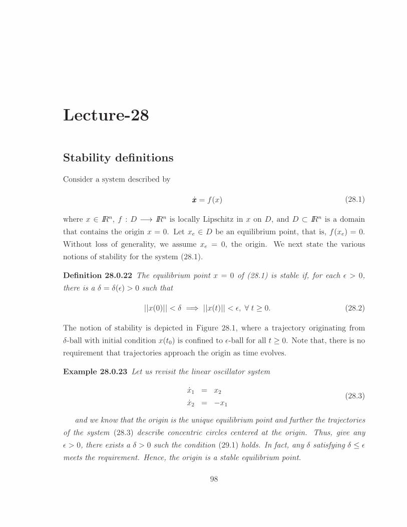
Definition 28.0.22 The equilibrium point x = 0 of (28.1) is stable if, for each ǫ > 0,
there is a δ = δ(ǫ) > 0 such that
||x(0)|| < δ =⇒ ||x(t)|| < ǫ, ∀ t ≥ 0. (28.2)
The notion of stability is depicted in Figure 28.1, where a trajectory originating from
δ-ball with initial condition x(t0) is confined to ǫ-ball for all t ≥ 0. Note that, there is no
requirement that trajectories approach the origin as time evolves.
Example 28.0.23 Let us revisit the linear oscillator system
x1 = x2
x2 = −x1(28.3)
and we know that the origin is the unique equilibrium point and further the trajectories
of the system (28.3) describe concentric circles centered at the origin. Thus, give any
ǫ > 0, there exists a δ > 0 such the condition (29.1) holds. In fact, any δ satisfying δ ≤ ǫ
meets the requirement. Hence, the origin is a stable equilibrium point.
98
NPTEL-Electrical Engineering - Nonlinear Control System
xe
x1t
E
x(t0) x(t0)
x(t)
x2x2 x1
Eδ
δ
Figure 28.1: Stability: Evolution of trajectory
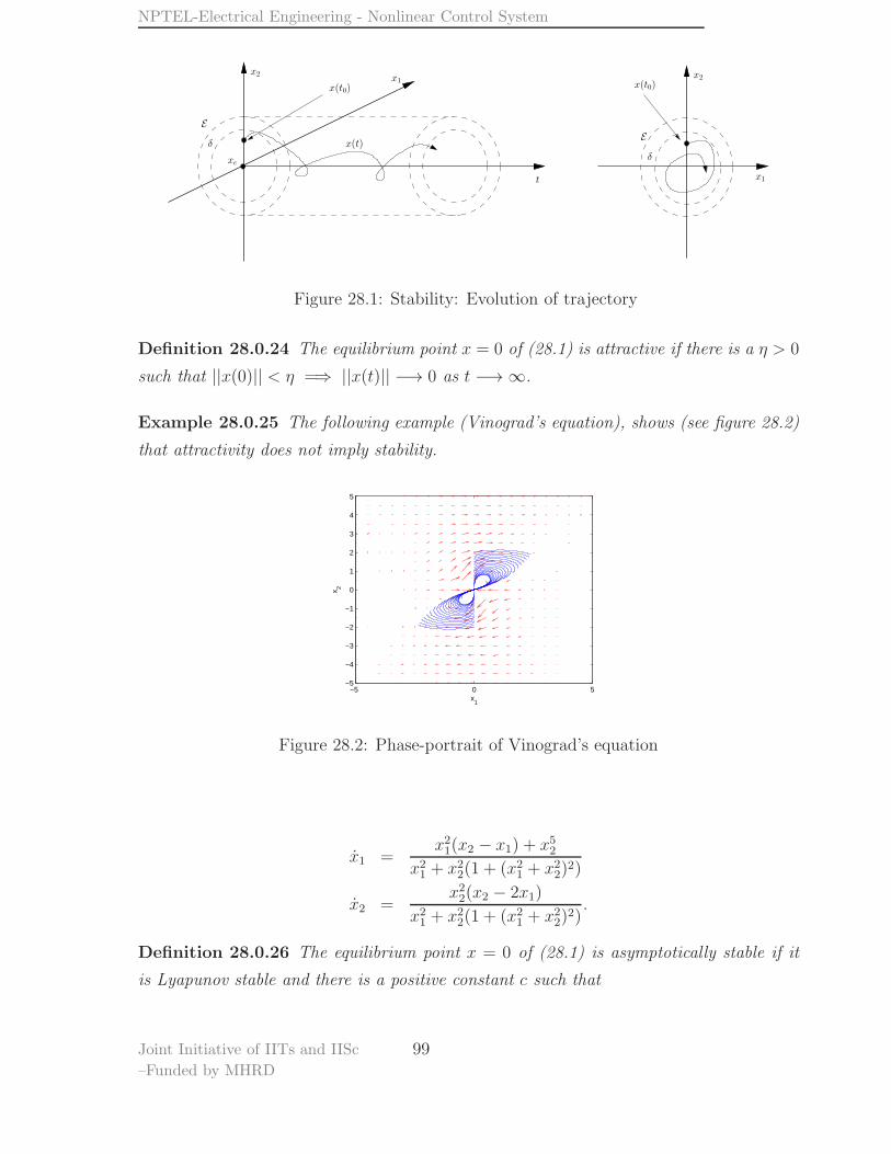
Definition 28.0.24 The equilibrium point x = 0 of (28.1) is attractive if there is a η > 0
such that ||x(0)|| < η =⇒ ||x(t)|| −→ 0 as t −→ ∞.
Example 28.0.25 The following example (Vinograd’s equation), shows (see figure 28.2)
that attractivity does not imply stability.
−5 0 5−5
−4
−3
−2
−1
0
1
2
3
4
5
x1
x 2
Figure 28.2: Phase-portrait of Vinograd’s equation
x1 =x21(x2 − x1) + x52
x21 + x22(1 + (x21 + x22)2)
x2 =x22(x2 − 2x1)
x21 + x22(1 + (x21 + x22)2).
Definition 28.0.26 The equilibrium point x = 0 of (28.1) is asymptotically stable if it
is Lyapunov stable and there is a positive constant c such that
Joint Initiative of IITs and IISc
–Funded by MHRD
99
NPTEL-Electrical Engineering - Nonlinear Control System
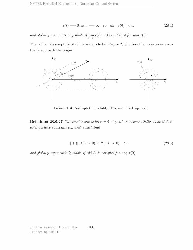
x(t) −→ 0 as t −→ ∞, for all ||x(0)|| < c. (28.4)
and globally asymptotically stable if limt→∞
x(t) = 0 is satisfied for any x(0).
The notion of asymptotic stability is depicted in Figure 28.3, where the trajectories even-
tually approach the origin.
x(t)
x1t
E
x(t0) x(t0)x2x2 x1
Eδ
δ
xe
Figure 28.3: Asymptotic Stability: Evolution of trajectory
Definition 28.0.27 The equilibrium point x = 0 of (28.1) is exponentially stable if there
exist positive constants c, k and λ such that
||x(t)|| ≤ k||x(0)||e−λ t, ∀ ||x(0)|| < c (28.5)
and globally exponentially stable if (28.5) is satisfied for any x(0).
Joint Initiative of IITs and IISc
–Funded by MHRD
100
Lecture-29
We next present Lyapunov’s stability theorem concerning the stability of the equilibrium
point x = 0 of (28.1).
Theorem 29.0.28 Let V : D −→ IR be a continuously differentiable function such that
V is positive-definite on D and V ≤ 0 in D. Then x = 0 is stable. Further if V < 0 in
D \ 0, then x = 0 is asymptotically stable.
Proof:
We have to establish a δ-Ball such that for all initial conditions in it, the corresponding
trajectories of (28.1) are bounded by ǫ for all t ≥ 0. Choose r ∈ (0, ǫ] such that Br=
x ∈ IRn : ||x|| ≤ r ⊂ D. Let α = min||x||=r
V (x). Since V (x) > 0 for x 6= 0, α > 0. Take
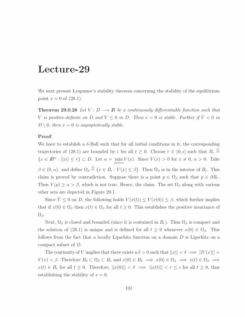
β ∈ (0, α). and define Ωβ= x ∈ Br : V (x) ≤ β. Then Ωβ is in the interior of Br. This
claim is proved by contradiction. Suppose there is a point p ∈ Ωβ such that p ∈ ∂Br.
Then V (p) ≥ α > β, which is not true. Hence, the claim. The set Ωβ along with various
other sets are depicted in Figure 29.1.
Since V ≤ 0 on D, the following holds V (x(t)) ≤ V (x(0)) ≤ β, which further implies
that if x(0) ∈ Ωβ then x(t) ∈ Ωβ for all t ≥ 0. This establishes the positive invariance of
Ωβ .
Next, Ωβ is closed and bounded (since it is contained in Br). Thus Ωβ is compact and
the solution of (28.1) is unique and is defined for all t ≥ 0 whenever x(0) ∈ Ωβ . This
follows from the fact that a locally Lipschitz function on a domain D is Lipschitz on a
compact subset of D.
The continuity of V implies that there exists a δ > 0 such that ||x|| < δ =⇒ ||V (x)|| =V (x) < β. Therefore Bδ ⊂ Ωβ ⊂ Br and x(0) ∈ Bδ =⇒ x(0) ∈ Ωβ =⇒ x(t) ∈ Ωβ =⇒x(t) ∈ Br for all t ≥ 0. Therefore, ||x(0)|| < δ =⇒ ||x(t)|| < r ≤ ǫ for all t ≥ 0, thus
establishing the stability of x = 0.
101
NPTEL-Electrical Engineering - Nonlinear Control System
r
D
B
Bδ
Ω β
Figure 29.1: Geometric representation of sets in a plane
−0.2
−0.1
0
0.1
0.2
−3−2
−10
12
30
0.02
0.04
0.06
0.08
0.1
x1
x2
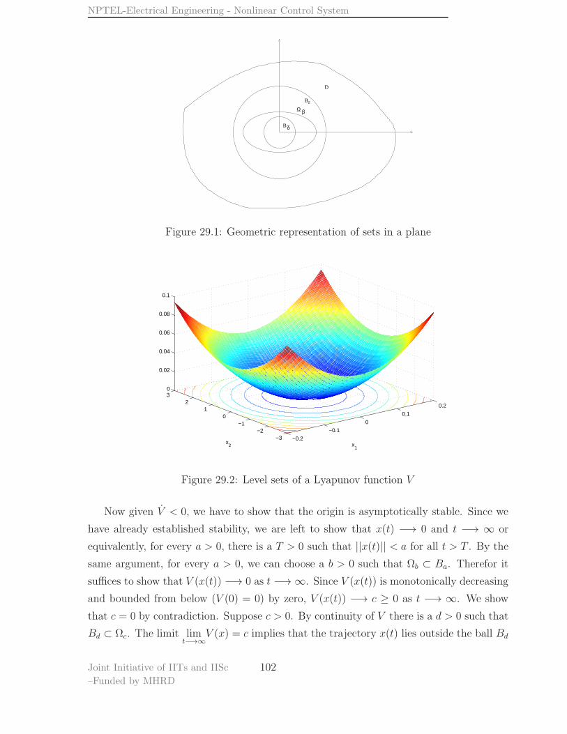
Figure 29.2: Level sets of a Lyapunov function V
Now given V < 0, we have to show that the origin is asymptotically stable. Since we
have already established stability, we are left to show that x(t) −→ 0 and t −→ ∞ or
equivalently, for every a > 0, there is a T > 0 such that ||x(t)|| < a for all t > T . By the
same argument, for every a > 0, we can choose a b > 0 such that Ωb ⊂ Ba. Therefor it
suffices to show that V (x(t)) −→ 0 as t −→ ∞. Since V (x(t)) is monotonically decreasing
and bounded from below (V (0) = 0) by zero, V (x(t)) −→ c ≥ 0 as t −→ ∞. We show
that c = 0 by contradiction. Suppose c > 0. By continuity of V there is a d > 0 such that
Bd ⊂ Ωc. The limit limt−→∞
V (x) = c implies that the trajectory x(t) lies outside the ball Bd
Joint Initiative of IITs and IISc
–Funded by MHRD
102
NPTEL-Electrical Engineering - Nonlinear Control System
for all t ≥ 0. Let −γ = maxd≤||x||≤r
V (x). The existence of γ is ensured because of the fact that
a continuous function (V ) on a compact set (x : d ≤ ||x|| ≤ r) achieves its maximum and
minimum. Since V < 0, −γ < 0. Since V (x(t)) = V (x(0))+∫ t
0V (x(τ))dτ ≤ V (x(0))−γt,
V (x(t)) will eventually become negative and hence contradicts V (x(t)) −→ c ≥ 0. Thus
c = 0. 2
Remark 29.0.29 Stability of the equilibrium is also referred to as stability in the sense
of Lyapunov or simply Lyapunov stable.
Joint Initiative of IITs and IISc
–Funded by MHRD
103
Lecture-30
The use of Lyapunov’s theorem 29.0.28 will be shown through the following examples.
The theorem provides only sufficient conditions under which stability holds. It means that
if the conditions are not met, then one cannot infer anything about the stability result and
further investigation is required to arrive at a Lyapunov function. Even in the plane, the
search for Lyapunov functions is nontrivial and several methods like the variable gradient,
have been proposed to provide a way of arriving at a Lyapunov function. If the energy
of the system is known, then it serves as the candidate Lyapunov function as can be seen
through the simple pendulum example.
Example 30.0.30 Consider the simple pendulum system
x1 = x2
x2 = −a sin x1(30.1)
Consider the candidate Lyapunov function V = a(1 − cosx1) + x22/2. Then V = 0.
Therefore the lower equilibrium point (0, 0) is Lyapunov stable. If friction is considered
in the model, then the equations of motion are
x1 = x2
x2 = −a sin x1 − bx2(30.2)
where, b = kl and k being the friction co-efficient. If we use the same V , then V = −bx22 ≤0, that is V is negative semi-definite. Therefore, we cannot infer about the asymptotic
stability of the origin, which the system possesses from the physics of the system or from
the phase-portrait. Hence, we search for candidate Lyapunov function such that V is
negative-definite. Consider V (x) = 12x⊤Px+ a(1 − cosx1), where P = P⊤ > 0 should be
selected in a manner that V < 0. The derivative of V along the trajectories of (30.2) is
given by
V = a(1− p22)x2 sin x1 − ap12x1 sin x1 + (p11 − p12b)x1x2 + (p12 − p22b)x22.
104
NPTEL-Electrical Engineering - Nonlinear Control System
To eliminate the sign indefinite terms, we set p22 = 1 and p11 = p12b. To retain the
sign-definite terms, let p12 = bp222. Then V = −ab
2x1 sin x1 − b
2x22 < 0 in D
= x ∈ IR2 :
x1 ∈ (−π, π). The corresponding V = x⊤
[
b2 b2
b2
1
]
x + a(1 − cosx1) > 0 in D. Thus
the origin is locally asymptotically stable.
Example 30.0.31
x1 = x2
x2 = −x31 − x32(30.3)
Clearly (0, 0) is the unique equilibrium point. Consider the candidate Lyapunov function
V =x41
4+
x22
2. Then V = −x42 ≤ 0. Therefore V is a Lyapunov function and the origin is
Lyapunov stable.
Example 30.0.32
x1 = x2
x2 = −h1(x1)− x2 − h2(x3)
x3 = x2 − x3.
(30.4)
where, h1 and h2 are locally Lipschitz functions that satisfy hi(0) = 0 and zhi(z) > 0,
i=1,2, for all z 6= 0. Clearly (0, 0, 0) is the unique equilibrium point. Consider the
candidate Lyapunov function V =∫ x1
0h1(z)dz +
∫ x3
0h2(z)dz +
x22
2. Then V = h1x1 +
h2x3 +x2x2 = −x22 −x3h2(x3) ≤ 0. Therefore V is a Lyapunov function and the origin is
Lyapunov stable.
The construction of Lyapunov function is not straightforward for nonlinear systems,
especially when the system does not possess energy-like function. A few approaches to
constructing Lyapunov functions are variable gradient method, Krasovski’s, Zubov’s and
Energy-Casimir methods. We focus on the variable gradient method.
Joint Initiative of IITs and IISc
–Funded by MHRD
105
Lecture-31
Variable gradient method
In this method, we assume a structure for the gradient ∂V∂x
and fix its components to
render V < 0. Let V be the candidate Lyapunov function whose gradient we assumed to
have the form
∂V
∂x
⊤= g(x)
where, g(x) = [g1(x) g2(x) . . . gn(x)]⊤. Poincare Lemma gives us the condition under
which a given vector is a gradient of some scalar function.
Lemma 31.0.33 Given a smooth vector field v(x), v : IRn −→ IRn, there exists a smooth
function h(x), h : IRn −→ IR such that ∇xh = v(x) if and only if ∇xv = (∇xv)⊤.
The construct g(x) is such that V is negative definite on a domain D. Finally, the
Lyapunov function V is extracted from the line integral
V (x) =
∫ x
0
g⊤(s)ds =
∫ x
0
n∑
i=1
gi(s)dsi. (31.1)
Using the fact that the line integral of a gradient vector g : IRn −→ IRn is path inde-
pendent, the line integration in (31.1) can be taken along any path joining the origin to
x. Choosing the path made up of line segments parallel to the coordinates axes, (31.1)
becomes
V (x) =
∫ x1
0
g1(s1, 0, 0, . . . , 0)ds1 +
∫ x2
0
g2(x1, s2, 0, . . . , 0)ds2
+ . . .+
∫ xn
0
gn(x1, x2, x3, . . . , sn)dsn.
This method is illustrated through the following pendulum-like example.
106
NPTEL-Electrical Engineering - Nonlinear Control System
Example 31.0.34
x1 = x2
x2 = −h(x1)− ax2, a > 0(31.2)
where, h( · ) is locally Lipschitz, h(0) = 0 and yh(y) > 0 for all y ∈ (−b, c) for some
b, c > 0. Assume
g(x) =
[
x1α(x) + x2β(x)
x1γ(x) + x2δ(x)
]
Thus, the Jacobian of g(x) is symmetric iff
∂g1∂x2
=∂g2∂x1
which yields
β(x) + x2∂β(x)
∂x2+ x1
∂α(x)
∂x2= γ(x) + x1
∂γ(x)
∂x1+ x2
∂δ(x)
∂x1(31.3)
Now the derivative of V along the trajectories of (31.2) is
V = g(x)⊤f(x) = α(x)x1x2 + β(x)x22 − h(x1)x1γ(x)− h(x1)x2δ(x)− ax1x2γ(x)− ax22δ(x).(31.4)
To eliminate the sign-indefinite terms in (31.4), we set
α(x)x1 − h(x1)δ(x)− ax1γ(x) = 0 (31.5)
and (31.4) reduces to
V = β(x)x22 − h(x1)x1γ(x)− ax22δ(x).
Now fix δ(x) = δ > 0, β(x) = β and γ(x) = γ > 0, as constants. Then the symmetry
condition (31.3) reduces to β + x1∂α(x)∂x2
= γ which implies that α(x) = α(x1) and β = γ.
Next,
V = γh(x1)x1 − x22(aδ − γ)
is negative-definite for 0 < γ < aδ and x1 ∈ (−b, c). Finally, we extract V as
V =
∫ x
0
(δh(y1) + aγy1)dy1 + (γy1 + δy2)dy2
=
∫ x1
0
(δh(y1) + aγy1)dy1 +
∫ x2
0
(γx1 + δy2)dy2
= δ
∫ x1
0
h(y1)dy1 +aγ
2y21 + γx1x2 +
δ
2y22
= δ
∫ x1
0
h(y1)dy1 +1
2x⊤
[
aγ γ
γ δ
]
︸ ︷︷ ︸
>0
x.
Joint Initiative of IITs and IISc
–Funded by MHRD
107
NPTEL-Electrical Engineering - Nonlinear Control System
It is clear that V is positive-definite in D= x : x1 ∈ (−b, c) and as already claimed V
is negative-definite. Hence the origin is asymptotically stable.
Joint Initiative of IITs and IISc
–Funded by MHRD
108
Lecture-32
Global asymptotic stability
The existence of a Lyapunov function V (x) which proves the origin to be asymptotically
stable does not guarantee that all trajectories originating from D will converge to the
origin. For the origin to be globally asymptotically stable the Lyapunov function should
be ‘radially unbounded’.The Lyapunov function V (x) is said to be radially unbounded if
V (x) → ∞ as x→ ∞, uniformly in x.
Define level sets of V (x) as Ωc = x ∈ D : V (x) ≤ c. If Ωc is closed and bounded
for any c > 0 (assured by radial unboundedness) and if D = Rn then the origin x = 0 is
globally asymptotically stable. Note that the notion of GAS is applicable only to systems
with isolated unique equilibrium point.
Region/Domain of attraction
Definition 32.0.35 Let Φ(t, x0) be the flow associated with a system.Then the region/domain
of attraction RA is defined as
RA = x : Φ(t, x) is defined for all t > 0 and Φ(t, x) = 0 as t→ ∞
Lemma 32.0.36 The set RA is open, connected and positive invariant. Moreover, the
boundary of RA is formed by trajectories.
Example 32.0.37 Consider the system
x1 = x2
x2 = 4(x1 + x2)− h(x1 + x2)(32.1)
109
NPTEL-Electrical Engineering - Nonlinear Control System
where h(0) = 0 and h(p)p ≥ 0 ∀ |p| ≤ 1. The origin (0, 0) is the unique equilibrium point
of the system. We will show that it is asymptotically stable and estimate the region of
attraction. Consider V (x) = x⊤Px where P =
[
2 1
1 1
]
> 0. The derivative of V along
the trajectories of (32.1) is
V = −x⊤[
8 6
6 6
]
x− 2h(x1 + x2)(x1 + x2)
6 −x⊤[
8 6
6 6
]
x.
It is clear that V is negative definite on D= x : |(x1 + x2)| ≤ 1. Hence (0, 0) is
asymptotically stable. From the phase portrait it can be seen that any trajectory within
the strip |(x1 + x2)| 6 1 converges to the origin.
Finding the exact region of attraction is an onerous task even for second-order systems.
However, an estimate of the region of attraction still provides guaranteed stability. One
way of obtaining the estimate is to use the closed and bounded level sets of the Lyapunov
function itself. A closed form solution for the estimates can be found when the Lyapunov
function is quadratic in x.
Joint Initiative of IITs and IISc
–Funded by MHRD
110
Lecture-33
Estimate of RA for quadratic Lyapunov functions
Let the quadratic Lyapunov function for a system be given as V = x⊤Px;P = P⊤ > 0.
Further, it is assumed that ∂V∂xf(x) < 0 in D. We can estimate the region/domain of
attraction for such systems depending on the constraints on D.
Case 1: For constraints of the form Ωc ⊆ D= x ∈ Rn :‖ x ‖2< r choose
c < min‖x‖=r
x⊤Px = λmin(P )r2
where λmin(P ) is the minimum eigen value of P .
Case 2: For constraints of the form Ωc ⊆ D , x ∈ Rn : |b⊤x|2 6 r, choose
c < min|b⊤x|6r
x⊤Px
which can be solved using the necessary conditions for optimality. Setting the cost function
as L = x⊤Px + λ(b⊤x)2 − r2 where λ ∈ IR is the Lagrange multiplier. The necessary
conditions for optimality are ∂L∂x
= 0 and ∂L∂λ
= 0. Now,
∂L
∂x= 2Px+ 2λ(b⊤x)b = 0
⇒ Px = −λ(b⊤x)b (33.1)
∂L
∂λ= (b⊤x)2 − r2
⇒ b⊤x = ±r. (33.2)
111
NPTEL-Electrical Engineering - Nonlinear Control System
Solving (33.1) and (33.2), we obtain the optimum values as x∗ and λ∗ as
x∗ = ± rP−1b
b⊤P−1b; λ∗ =
−1
b⊤P−1b.
Hence J∗ = x∗⊤Px∗ = r2
b⊤P−1band we choose c < J∗. If the set D is characterized by
multiple constraints, the optimization problem becomes min|b⊤i x|6ri
x⊤Px for i = 1 to m. It is
a known fact that J = min(Ji, ..., Jm) where Ji =r2i
b⊤i P−1bi.
Example 33.0.38 Consider the system
x1 = −x1(1− (x21 + x22))
x2 = −x2(1− (x21 + x22)).(33.3)
We need to first show that the origin is asymptotically stable. Taking V (x) =x21+x2
2
2results
in V (x) = −(x21 + x22)(1− (x21 + x22)). Thus V < 0 in D= (x1, x2) : x21 + x22 < 1. Hence
(0, 0) is asymptotically stable and an estimate of the domain of attraction is given by
x ∈ IR2 : x21 + x22 ≤ 1.
Example 33.0.39 Consider the system
x1 = x2
x2 = −x1 − x2 − (2x2 + x1)(1− x22)(33.4)
It is required to show that the origin is asymptotically stable and estimate its region of
attraction. The asymptotic stability of the origin is established by considering V (x) =
x⊤
[
5 1
1 2
]
x and noting that V < 0 in D= x ∈ IR2 : |x2| ≤ 1. The estimate of the
domain of attraction is given by Ωc = x ∈ IR2 : V (x) ≤ c, where
c <1
[0 1]
[
5 1
1 2
]−1
[0 1]⊤
=9
5
.
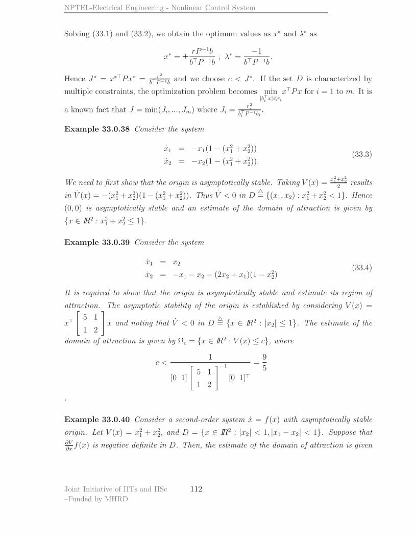
Example 33.0.40 Consider a second-order system x = f(x) with asymptotically stable
origin. Let V (x) = x21 + x22, and D = x ∈ IR2 : |x2| < 1, |x1 − x2| < 1. Suppose that∂V∂xf(x) is negative definite in D. Then, the estimate of the domain of attraction is given
Joint Initiative of IITs and IISc
–Funded by MHRD
112
NPTEL-Electrical Engineering - Nonlinear Control System
by Ωc = x ∈ IR2 : V (x) ≤ c, where c < min(c1, c2) with
c1 =12
[1 − 1]
[
1 0
0 1
]−1
[1 − 1]⊤
=1
2
c2 =12
[10 1]
[
1 0
0 1
]−1
[0 1]⊤
= 1.
The estimate is x21 + x22 ≤ r2 where r = 1√2as shown Figure 33.1.
r
x1
x 2
1
−1
1
1
−
Figure 33.1: Estimate of the domain of the attraction of the origin
Joint Initiative of IITs and IISc
–Funded by MHRD
113
Lecture-34
Example 34.0.41 Consider the system
x1 = x1 − x31 + x2
x2 = 3x1 − x2(34.1)
a. Find all equilibrium points of the system.
b. Using linearization, study the stability of the each equilibrium point.
c. Using a quadratic Lyapunov function, estimate the region of attraction of each
asymptotically stable equilibrium point. Try to make your estimate as large as pos-
sible.
d. Construct the phase-portrait of the system and show on it the exact regions of at-
traction as well as your estimates.
Solution:
The system has three equilibrium points given by E = (x1, x2) : (0, 0), (2, 6), (−2,−6).The linearization about each of these equilibrium points is given by x = Aix, i = 1, 2, 3
where, the matrices A1, A2 and A3 are given by
A1 =
[
1 1
3 −1
]
;A2 =
[
−11 1
3 −1
]
;A3 =
[
−11 1
3 −1
]
The corresponding eigenvalue are given by eig(A1) = 2,−2, eig(A1) = eig(A2) =
−11.2915,−0.7085. Therefore, the equilibrium point (0, 0) is a saddle and equilibrium
points (2, 6) and (−2,−6) are stable nodes.
Next, we perform a coordinate change so that the equilibrium point (2, 6) is the origin
of the new coordinate system and the objective is establish the stability using a quadratic
114
NPTEL-Electrical Engineering - Nonlinear Control System
Lyapunov function. Define z1 = x1 − 2, z2 = x2 − 6, then the resulting equations (34.1)
in the new coordinates is given by
z1 = −11z1 + z2 − 6z21 − z31
z2 = 3z1 − z2(34.2)
The equilibrium points are transformed as follows in z-coordinates.
(2, 6) 7→ (0, 0)
(0, 0) 7→ (−2,−6)
(−2,−6) 7→ (−4,−12)
Now consider a quadratic candidate Lyapunov function V (z) = 12z⊤Pz, where
P =
[
p11 p12
p12 p22
]
> 0.
The derivative of V along the trajectories of (34.2) is given by
V = z21(−11p11 + 3p12) + z1z2(p11 − 12p12 + 3p22) + z22(p12 − p22)
−p11z41 − 6p11z31 − p12z2z
31 − 6p12z
21z2.
(34.3)
To eliminate the sign-indefinite terms, we set p12 = 0. Then (34.3) can be expressed as
V = −z⊤Q(z1)z (34.4)
where,
Q(z1) =
[
p11(z21 + 6z1 + 11) (p11+3p22)
2(p11+3p22)
2p22
]
.
It is easy to see that for p11, p22 > 0, the matrix Q(z1) is locally positive-definite around
z1 = 0. Fix, p11 = 3, p22 = 1 (see subsection 34.0.41 ). Then Q(z1) > 0 in the set
D1= (z1, z2) : z1 ∈ (−2,∞). Thus V < 0 in D1 and it follows that (z1, z2) = (0, 0) is
asymptotically stable.
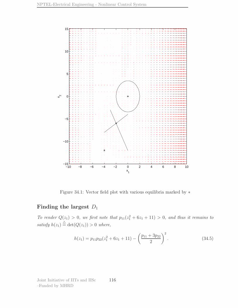
To compute the region of attraction RA and compare it with the estimate of the domain
of attraction Ωc, we plot the vector field plot of (34.2) as shown in Figure 34.1. A local
analysis about the saddle point shows that the stable eigenvectors satisfy z2 − z1 = 0
and the unstable eigenvectors satisfy 3z1 + z2 = 0. The region of attraction is given by
RA = (z1, z2) ∈ IR2 : 3z1 + z2 > 0. The estimate of the domain of attraction of the
origin (z1 = 0, z2 = 0) is given by Ωc= (z1, z2) ∈ (3z1+z2 > 0)∩D1 : 3z
21+z
22 ≤ c, c > 0
is compact.
Joint Initiative of IITs and IISc
–Funded by MHRD
115
NPTEL-Electrical Engineering - Nonlinear Control System
−10 −8 −6 −4 −2 0 2 4 6 8 10−15
−10
−5
0
5
10
15
x1
x 2
Figure 34.1: Vector field plot with various equilibria marked by ∗
Finding the largest D1
To render Q(z1) > 0, we first note that p11(z21 + 6z1 + 11) > 0, and thus it remains to
satisfy h(z1)= det(Q(z1)) > 0 where,
h(z1) = p11p22(z21 + 6z1 + 11)−
(p11 + 3p22
2
)2
. (34.5)
Joint Initiative of IITs and IISc
–Funded by MHRD
116
NPTEL-Electrical Engineering - Nonlinear Control System
The function h(z1) has minima at z1 = −3 for all values of p11 and p22. So by substituting
z1 = −3 in (34.5)
h(−3) = p11p22(9− 18 + 11)−(p11 + 3p22
2
)2
= −p211 − 9p222 + 2p11p22.
In order to render Q(z1) > 0, the det(Q(z1)) > 0, this implies h(−3) > 0, hence
−p211 − 9p222 + 2p11p22 > 0.
Let us set the minimum value of h(z1) = 0, thus
−p211 − 9p222 + 2p11p22 = 0
⇒(p11p22
)2
− 2
(p11p22
)
+ 9 = 0. (34.6)
Substituting p11p22
= y, we obtain imaginary roots of (34.6), thus for no positive real values
of p11 and p22 the function h(z1) can achieve a positive minima. Further, by putting
z1 = −2 in (34.5) and solving we get
h(−2) = p11p22(4− 12 + 11)−(p11 + 3p22
2
)2
= −p211 − 9p222 + 6p11p22
hence for f(−2) > 0,
−p211 − 9p222 + 6p11p22 > 0.
Let us set the minimum value of h(z1) = 0, thus
−p211 − 9p222 + 6p11p22 = 0
⇒(p11p22
)2
− 6
(p11p22
)
+ 9 = 0. (34.7)
Again, substituting p11p22
= y and solving we get roots of (34.7) as y = 3, 3 which are real,
positive and equal. Thus for z1 6 −2, h(z1) cannot have positive minima for all positive
real values of p11 and p22. Hence we have p11p22
= y = 3 ⇒ p22 = 1, p11 = 3.
Joint Initiative of IITs and IISc
–Funded by MHRD
117
Lecture-35
La Salle’s invariance principle
In many problems, it is easy to establish the negative semi-definiteness of V rather than the
negative definite property. In such a case, Lyapunov’s theorem only establishes stability
and nothing can be said about asymptotic stability. La Salle’s invariance principle aids
in establishing asymptotic stability property of the origin even when V is negative semi-
definite.
Theorem 35.0.42 Consider the system x = f(x) and let Ω be a compact set that is
invariant with respect to this system. Let V : D → R be continuously differentiable such
that V ≤ 0 in Ω. Let E be the set of points in Ω such that V = 0. Further let M be the
largest invariant set in E. Then every solution starting in Ω converges to M as t→ ∞.
Note that in theorem 35.0.42, the only requirement on V is that it be continuously differ-
entiable and V ≤ 0 on a compact set Ω. Since we deal with positive-definite V , the choice
Ω = Ωc ensures the compactness of Ω, at least for sufficiently small c > 0. The extension
of La Salle’s invariance principle to systems that possess a positive definite V is stated in
the following Corollary, also called as the theorem of Barbashin and Krasovskii. The La
Salle’s invariance principle is illustrated through the following examples.
Corollary 35.0.43 Consider the system x = f(x) and let x = 0 be the equilibrium point.
Let V : D → R be continuously differentiable that is positive definite and V ≤ 0 on D.
Let S = x ∈ Ωc : V = 0. If no solution of x = f(x) can stay identically in S except the
trivial solution x(t) = 0 then the origin is asymptotically stable.
Example 35.0.44 For the pendulum system
118
NPTEL-Electrical Engineering - Nonlinear Control System
x1 = x2
x2 = −a sin x1 − bx2(35.1)
Take V (x) = a(1 − cos x1) +x22
2> 0 on D = (x1, x2) : x1 ∈ (−π, π). It is seen that
V = −bx22 6 0 ⇒ is negative semi-definite. Let S = x ∈ Ωc, V = 0. Then
x(t) ∈ S ⇒ x2 ≡ 0 ⇒ x2 ≡ 0 ⇒ sin x1 ≡ 0 ⇒ x1 ≡ 0
Hence (0, 0) being the only point in M , is asymptotically stable.
Example 35.0.45
x1 = x2
x2 = −x31 − x32(35.2)
Taking V (x) =x41
4+
x22
2, V = −x42 which is negative semi-definite. Let S = x ∈ Ωc, V =
0. Then x(t) ∈ S ⇒ x2 ≡ 0 ⇒ x2 ≡ 0 ⇒ −x31 − x32 ≡ 0 ⇒ x1 ≡ 0 ⇒M = (0, 0). Hence
the origin is asymptotically stable.
Example 35.0.46
x1 = x2
x2 = −x1 − x2 − x2|x2|(35.3)
Taking V (x) =x21+x2
2
2yields V = −x22(1 + |x2|) 6 0. Let S = x ∈ Ωc, V = 0. Then
x(t) ∈ S ⇒ x2 ≡ 0 ⇒ x2 ≡ 0 ⇒ x1 ≡ 0 ⇒ x1 ≡ 0, thereby proving the asymptotic stability
of the origin.
Example 35.0.47
x1 = x2
x2 = −h1(x1)− x2 − h2(x3)
x3 = x2 − x3
(35.4)
where hi(u)u > 0; i = 1, 2. Taking V (x) =x1∫
0
h1(z)dz +x2∫
0
h2(z)dz we get V = −x22 −h2(x3)x3 which is negative semi-definite. Then
x(t) ∈ S ⇒ x2 ≡ 0 ⇒ x2 ≡ 0 ⇒ x3 ≡ 0 ⇒ x3 ≡ 0
Hence, the origin (0, 0, 0) is asymptotically stable.
Joint Initiative of IITs and IISc
–Funded by MHRD
119
Lecture-36
Stability of Linear systems
Consider the linear system given by x = Ax and a corresponding V (x) = x⊤Px where
P⊤ = P > 0. Then,
V = x⊤Px+ x⊤P x
= x⊤A⊤Px+ x⊤PAx
= x⊤(A⊤P + PA)x
Hence for asymptotic stability we get the Lyapunov equation given by
A⊤P + PA = −Q
for some Q > 0.
Definition 36.0.48 A Matrix A is said to be Hurwitz if all its eigen values satisfy
Re(λi) < 0.
Theorem 36.0.49 A matrix ‘A’ is Hurwitz and only if given any positive definite matrix
Q, there exists a symmetric, positive definite matrix P such that A⊤P +PA = −Q holds.
Moreover the matrix P is unique.
Example 36.0.50 Consider the system
x =
[
0 −1
1 −1
]
x (36.1)
120
NPTEL-Electrical Engineering - Nonlinear Control System
Choosing P =
[
P11 P12
P12 P22
]
and Q =
[
1 0
0 1
]
, solving the Lyapunov equation we obtain
0 2 0
−1 −1 1
0 2 2
P11
P12
P22
=
−1
0
1
⇒
P11
P12
P22
=
32
−12
1
P =
[32
−12
−12
1
]
is symmetric, positive definite and unique. From Theorem 36.0.49
A =
[
0 −1
1 −1
]
is Hurwitz and hence (0, 0) is stable.
Lyapunov’s indirect method
Theorem 36.0.51 Consider a system
x = f(x), x ∈ IRn, (36.2)
Let x = 0 be the equilibrium point i.e f(0) = 0. Further assume f : D → Rn is contin-
uously differentiable on a domain D in the neighbourhood of the origin. Let A = ∂f∂x|x=0.
If the linearized system (36.2) is exponentially stable, then there exists a ball B ⊂ D and
constants c, λ > 0 such that for every solution x(t) to the nonlinear system (36.2) that
starts at x(0) ∈ B, we have
‖ x(t) ‖≤ ce−λ(t) ‖ x(0) ‖, ∀ t ≥ 0. (36.3)
For proving the above theorem we require the following results:
1. If Q is positive definite then the following inequality holds
λmin(Q) ‖ x ‖226 x⊤Qx 6 λmax(Q) ‖ x ‖22
Lemma 36.0.52 Comparison Lemma Let V : IRn → IR be a differentiable func-
tion such that ∂V∂x
⊤f(x) ≤ µV (x) for some constant µ ∈ IR. Then V (x(t)) ≤
eµ(t)V (x(0)), ∀ t ≥ 0.
Joint Initiative of IITs and IISc
–Funded by MHRD
121
NPTEL-Electrical Engineering - Nonlinear Control System
The proof of the main theorem now follows.
Proof : Since f in (36.2) is twice differentiable, we know from Taylor’s theorem that
r(x) , f(x)−(f(xe) + Ax
)= f(x)− Ax = O(‖ x ‖2).
which means that there exists a constant c and a ball B around x = 0 for which
‖ r(x) ‖≤ c ‖ x ‖2, ∀x ∈ B. (36.4)
Since the linearized system is exponentially stable, there exists a positive-definite-matrix
P for which
A′P + PA = −I.
Define a real-valued continuously differentiable function
V , x⊤Px
and its derivative along trajectories of (37.1) is given by
V = f(x)⊤Px+ x⊤Pf(x)
=(Ax+ r(x)
)⊤Px+ x⊤P
(Ax+ r(x)
)
= x⊤(A⊤P + PA)x+ 2x⊤Pr(x)= − ‖ x ‖2 +2x⊤Pr(x)
≤ − ‖ x ‖2 +2 ‖ P ‖ ‖ x ‖ ‖ r(x) ‖ .
(36.5)
Let ǫ > 0 be sufficiently small so that the ellipsoid centered at x = 0 satisfies the following:
•E , x ∈ IRn : x⊤Px ≤ ǫ ⊂ B.
•1− 2c ‖ P ‖ ‖ x ‖≥ 1
2=⇒ ‖ x ‖≤ 1
4 c ‖ P ‖ .
Thus, for x ∈ E ,V ≤ − ‖ x ‖2 +2c ‖ P ‖ ‖ x ‖3
= −(1− 2c ‖ P ‖ ‖ x ‖
)‖ x ‖2
= −12‖ x ‖2
< 0, x 6= 0.
(36.6)
For this choice of ǫ, the set E is positively invariant and the origin is asymptotically stable.
Further, from (36.6) and the fact that x⊤Px ≤ ‖ P ‖ ‖ x ‖2, it follows that if x(0) starts
Joint Initiative of IITs and IISc
–Funded by MHRD
122
NPTEL-Electrical Engineering - Nonlinear Control System
B (inside E)
xe
B (from Taylor’s Theorem)
E (inside B)
≤ 14 c ‖P‖
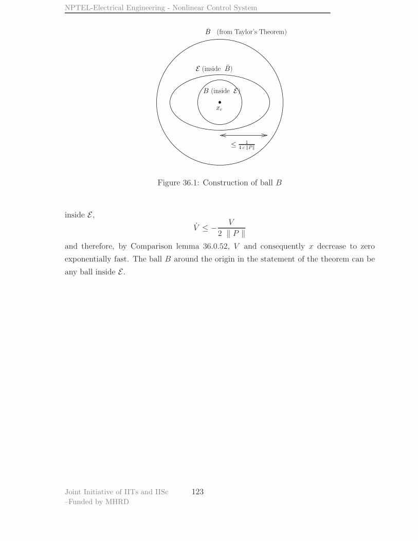
Figure 36.1: Construction of ball B
inside E ,V ≤ − V
2 ‖ P ‖and therefore, by Comparison lemma 36.0.52, V and consequently x decrease to zero
exponentially fast. The ball B around the origin in the statement of the theorem can be
any ball inside E .
Joint Initiative of IITs and IISc
–Funded by MHRD
123
Lecture-37
Instability
An equilibrium is unstable if it is not stable. There are several results establishing insta-
bility, but we shall use the result by Chetayev, which is stated as follows.
Theorem 37.0.53 Let x = 0 be an equilibrium point of x = f(x). Let V : D −→ IR be a
continuously differentiable function such that V (0) = 0 and V (x0) > 0 for some x0 with
arbitrarily small ||x0||. Define a set U = x ∈ Br : V (x) > 0, where Br = x ∈ D :
||x|| ≤ r and suppose that V (x) > 0 in U . Then x = 0 is unstable.
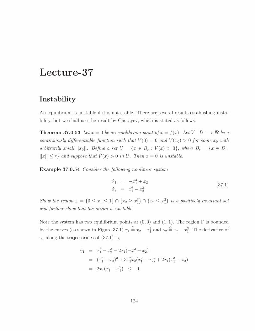
Example 37.0.54 Consider the following nonlinear system
x1 = −x31 + x2
x2 = x61 − x32(37.1)
Show the region Γ = 0 ≤ x1 ≤ 1 ∩ x2 ≥ x31 ∩ x2 ≤ x21 is a positively invariant set
and further show that the origin is unstable.
Note the system has two equilibrium points at (0, 0) and (1, 1). The region Γ is bounded
by the curves (as shown in Figure 37.1) γ1= x2 − x21 and γ2
= x2 − x31. The derivative of
γ1 along the trajectorioes of (37.1) is,
γ1 = x61 − x32 − 2x1(−x31 + x2)
= (x21 − x2)3 + 3x21x2(x
21 − x2) + 2x1(x
31 − x2)
= 2x1(x31 − x21) ≤ 0
124
NPTEL-Electrical Engineering - Nonlinear Control System
Hence, the direction of the vector field f on the curve γ1 points into Γ. Similarly, the
derivative of γ2 along trajectories of (37.1) is,
γ2 = x61 − x32 − 3x21(−x31 + x2)
= (x21 − x2)3 + 3x21x2(x
21 − x2) + 3x21(x
31 − x2)
= (x21 − x2)3 + 3x21x2(x
21 − x2) ≥ 0
Hence, the direction of the vector field f on the curve γ2 also points into Γ. Thus all the
trajectories eminating from a neighbourhood of Γ are trapped in it, that is, Γ is positively
invariant set.
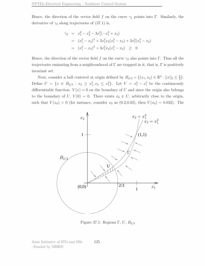
Next, consider a ball centered at origin defined by B2/3 = (x1, x2) ∈ R2 : ||x||2 ≤ 2
3.
Define U = x ∈ B2/3 : x2 ≥ x31, x2 ≤ x21. Let V = x21 − x31 be the continuously
differentiable function. V (x) = 0 on the boundary of U and since the origin also belongs
to the boundary of U , V (0) = 0. There exists x0 ∈ U , arbitrarily close to the origin,
such that V (x0) > 0 (for instance, consider x0 as (0.2,0.02), then V (x0) = 0.032). The
12/3
U
(1,1)1
(0,0)
ΓB2/3
x1
x2 = x21
x2 = x31x2
Figure 37.1: Regions Γ, U , B2/3
Joint Initiative of IITs and IISc
–Funded by MHRD
125
NPTEL-Electrical Engineering - Nonlinear Control System
derivative of V along the trajectories of (37.1) is,
V = 2x1(−x31 + x2)− 3x21(−x31 + x2)
= (x2 − x31)x1(2− 3x1) ≥ 0 for all x ∈ U.
All the hypothesis of Chetayev’s theorem hold, thereby proving the origin to be unstable.
Joint Initiative of IITs and IISc
–Funded by MHRD
126
Exercise problems
1. Use a quadratic Lyapunov function candidate to show that the origin is asymptoti-
cally stable:
a.
x1 = −x1 + x1x2
x2 = −x2
b.
x1 = x2(1− x21)
x2 = −(x1 + x2)(1− x21)
2. Euler equations for a rotating rigid spacecraft are given by
Jω + ω × Jω = u
or
J1ω1 = (J2 − J3)ω2ω3 + u1
J2ω2 = (J3 − J1)ω1ω3 + u2
J3ω3 = (J1 − J2)ω1ω2 + u3
(37.2)
where ω1, ω2, ω3 are the components of the angular velocity vector ω along the
principal axes, u1, u2, u3 are the torque inputs applied about the principal axes, and
J1 > J2 > J3 > 0 are the principal moments of inertia. The rotational kinetic
energy of the spacecraft is given by T (ω) = 12(J1ω
21 + J2ω
22 + J3ω
23) while the total
angular momentum of the body is given by P (ω) =√
J21ω
21 + J2
2ω22 + J2
3ω23.
a. Find all the equilibria of the rotational dynamics.
127
NPTEL-Electrical Engineering - Nonlinear Control System
b. Compute T and P along the trajectories of (37.2). What can you conclude
about stability?
c. Show that with ui = 0, i = 1, 2, 3, the origin ω = 0 is stable. Is it asymptotically
stable?
d. Use the Lyapunov function V (ω) = (T (ω)−T (ωe))2+[(P (ω))2− (P (ωe))
2]2 to
show that every equilibrium of the form ωe = [Ω 0 0]⊤ is Lyapunov stable.
e. Repeat the above step for the equilibria of the form ωe = [0 0 Ω]⊤.
f. Use the function V (ω) = ω1ω3 to show that every equilibrium point of the form
ωe = [0 Ω 0]⊤ is unstable. The result can be proved as follows. Define the
states as (x1, x2, x3) = (ω1, ω2−Ω, ω3). Then the rotating rigid body dynamics
can be written as
x1 = 1J1(J2 − J3)(x2x3 + x3Ω)
x2 = 1J2(J3 − J1)(x1x3)
x3 = 1J3(J1 − J2)(x1x2 + x1Ω)
(37.3)
The derivative of smooth function V = x1x3 along the trajectories of (37.3) is
given by
V =(J2 − J3)
J1(x2x
23 + Ωx22) +
(J1 − J2)
J3(x21x2 + Ωx21) > 0 ∀ x2 > 0.
Let U be a closed ball of radius r around the origin and define the region D1
in U as D1 = x ∈ U : x1x3 > 0, x2 > 0. The boundary of D1 is the surface
V (x) = 0 and the sphere ||x|| = r. Since V (0) = 0, the origin lies on the
boundary of D1. Further, in D1, both V and V > 0. By Chetayev’s theorem,
the origin is unstable.
g. Suppose that the torque inputs apply the feedback control ui = −k1ωi, where
ki, i = 1, 2, 3 are positive constants. Show that the origin of the closed-loop
system is globally asymptotically stable.
3. Consider the system
x1 = x2
x2 = −(x1 + x2)− h(x1 + x2)
where h is continuously differentiable and zh(z) > 0 ∀ z ∈ IR. Using the variable
gradient method, find a Lyapunov function that shows that the origin is globally
asymptotically stable.
Joint Initiative of IITs and IISc
–Funded by MHRD
128
NPTEL-Electrical Engineering - Nonlinear Control System
4. Show that the origin of
x1 = x2
x2 = −x31 − x32
is globally asymptotically stable.
5. Consider the linear system x = (A−BR−1B⊤P )x, where P = P⊤ > 0 and satisfies
the Riccati equation
PA+ A⊤P +Q− PBR−1B⊤P = 0
where, R = R⊤ > 0, and Q = Q⊤ ≥ 0. Using V (x) = x⊤Px as a Lyapunov function
candidate, show that the origin is globally asymptotically stable when
(1) Q > 0.
(2) Q = C⊤C and the pair (A,C) is observable.
6. Consider the tunnel diode circuit as shown in figure 1. The tunnel diode has a
nonlinear voltage-controlled constitutive relationship that contains the region of
negative resistance. This characteristic made it possible to construct bistable circuits
which were used in switching or memory elements in early computers. The circuit
equations are given by
LI = E −RI − V
CV = I − I(V ).
Using the Lyapunov function,
P (I, V ) =C
2(E − RI − V )2 +
L
2(I − I(V ))2 + λ[
1
2RI2 − EI
+IV −∫ V
0
Ig(Vg)dVg]
where λ ∈ IR is free, find conditions on λ for asymptotic stability. Also find the
condition on the steepness of slope of the negative resistance region of the tunnel
diode.
7. Consider the following system
x1 = (x2 − 1)x31
x2 = − x41(1 + x21)
2− x2
(1 + x22)
(a) Show that the origin is asymptotically stable. (b) Is V radially unbounded ?
Joint Initiative of IITs and IISc
–Funded by MHRD
129
NPTEL-Electrical Engineering - Nonlinear Control System
8. Consider the system
x1 = x1 − x31 + x2
x2 = 3x1 − x2
c. Using a quadratic Lyapunov function, show that the equilibrium point (−2,−6)
is asymptotically stable. Clearly define the set D where V < 0.
d. On the plane, show the region of attraction RA as well as the estimate of the
region of attraction Ωc.
9. Show that the origin of the system x = Ax, where A =
[
−2 3
−1 −4
]
is asymptoti-
cally stable using the Lyapunov equation A⊤P + PA = −Q, where Q > 0.
10. The dynamics of a Spring-mass system with viscous and Coulomb friction and zero
external force is given by
My =Mg − ky − c1y − c2y|y|
where, M is the mass, k is the spring constant, c1, c2 > 0 are friction coefficients and
y is the displacement of the mass from a reference position. Show that the origin is
globally asymptotically stable.
Joint Initiative of IITs and IISc
–Funded by MHRD
130