Proceedings of the

6th International Workshop on the

Implementation of Logics

Christoph Benzmuller, Bernd Fischer, Geoff Sutcliffe

Held at

The 13th International Conference on

Logic for Programming, Artificial Intelligence and Reasoning

Phnom Penh, Cambodia

13th - 17th November 2006

The 6th International Workshop

on the Implementation of Logics

Christoph Benzmuller1, Bernd Fischer2, Geoff Sutcliffe3

1 Universitat des Saarlandes, Germany, chris@ags.uni-sb.de2 University of Southampton, England, b.fischer@ecs.soton.ac.uk

3 University of Miami, geoff@cs.miami.edu

The IWIL workshop series brings together developers and users of systems that

implement reasoning in logic, to share information about successful implementation

techniques for automated reasoning systems and similar programs. Systems of all types

(automated, interactive, etc), and for all logics (classical, non-classical, all orders, etc)

are of interest to the workshop. Contributions that help the community to understand

how to build useful and powerful reasoning systems in practice are of particular interest.

Two invited papers, and six research papers selected from the submissions (by the

program committee listed below), will be presented. A panel discussion will enable

all attendees to participate in open discussion. Previous IWIL workshops include the

5th IWIL (Montevideo, Uruguay), 4th IWIL (Almati, Kazakhstan), 3rd IWIL (Tbilisi,

Georgia), 2nd IWIL (Havana, Cuba), and 1st IWIL (Reunion Island).

Journal Publication

The Journal of Algorithms in Applied Logic, Artificial Intelligence and Computer Science

has agreed to a special issue based around around the topic of the IWIL workshop. The

special issue targets IWIL participants, but will also also accept submissions from the

broader community.

Program Committee

Wolfgang Ahrendt (Chalmers University of Technology, Sweden)

Anbulagan (National ICT Australia, Australia)

Serge Autexier (Universitat des Saarlandes, Germany)

Chad Brown (Universitt des Saarlandes, Germany)

Hans de Nivelle (Max-Planck Institut fr Informatik, Germany)

Alexander Fuchs (University of Iowa, USA)

Thomas Hillenbrand (Max-Planck Institut fur Informatik, Germany)

Boris Konev (University of Liverpool, England)

Konstantin Korovin (University of Manchester, England)

Albert Oliveras (Technical University of Catalonia, Spain)

Brigitte Pientka (McGill University, Canada)

Stephan Schulz (Technische Universitat Mnchen, Germany)

Volker Sorge (University of Birmingham, England)

Alwen Tiu (Australian National University, Australia)

Ullrich Hustadt (University of Liverpool, England)

Presentation Schedule

Session 1:

9:00-10:00 Invited Talk: Algorithms and Data Structures for First-Order

Equational Deduction

Stephan Schulz

Session 2:

10:30-11:00 Term Indexing for the LEO-II Prover

Frank Theiß and Christoph Benzmuller

11:00-11:30 Integrating External Deduction Tools with ACL2

Matt Kaufmann, J Strother Moore, Sandip Ray and Erik Reeber

11:30-12:00 Efficiently Checking Propositional Resolution Proofs in Isabelle/HOL

Tjark Weber

Session 3:

14:00-15:00 Invited Talk: Implementing an Instantiation-based Theorem Prover

for First-order Logic

Konstantin Korovin

Session 4:

15:30-16:00 Tableau Decision Procedure for Propositional Intuitionistic Logic

Guido Fiorino, Alessandro Avellone and Ugo Moscato

16:00-16:30 LIFT-UP: Lifted First-Order Planning Under Uncertainty

Steffen Holldobler and Olga Skvortsova

16:30-17:00 Multiple Preprocessing for Systematic SAT Solvers

Anbulagan and John Slaney

17:00-18:00 Panel Interrogation: Experts on the implementation of

logics will answer questions from the workshop attendees

Anbulagan, Martin Giese, Konstantin Korovin, Stephan Schulz

Acknowledgements

We wish to thank the following for their contribution to the success of this confer-

ence: Air Force Office of Scientific Research, Asian Office of Aerospace Research and

Development.

Algorithms and Data Structures

for

First-Order Equational Deduction

(extended abstract)

Stephan Schulz

Technische Universitat Munchen

schulz@eprover.org

1 Introduction

First-order logic with equality is one of the most widely used logics. While there is alarge number of different approaches to theorem proving in this logic, the field has beendominated by saturation-based systems using some variant of the superposition calcu-lus [BG90, BG94, BG98, NR01], i.e. systems that employ paramodulation, restrictedby ordering constraints and possibly literal selection, as the main inference mechanism,and rewriting and subsumption as the main redundancy elimination techniques. Manysystems complement equational reasoning with explicit resolution for non-equationalliterals. Examples of provers based on the combination of paramodulation, rewritingand (possibly) resolution include SPASS [WBH+02], Vampire [RV01], Otter [MW97],its successor Prover9, and E [Sch02, Sch04b].

The power of a saturating prover depends on four different, but interrelated aspects:

• The calculus (What inferences are necessary and possible?)

• The inference engine (How are they implemented?)

• The search organization (How is the the proof state organized and which invariantsare maintained?)

• The heuristic control of the search (Which subset of inferences is performed andin what order?)

In this talk I will discuss the basic concepts of the given clause saturation algorithmand its implementation. In particular, I will describe the behaviour of the DISCOUNTloop version of this algorithm on practical examples, and discuss how this affected thechoice of algorithms and data structures for E. I will try point out some low-hangingfruit, where a lot of performance can be gained for relatively modest investment in codecomplexity, as well as some more advanced techniques that have a significant pay-off.

1

2 Rewrite-Based Theorem Proving

Superposition is a refutational calculus. It attempts to make the potential unsatisfiabil-ity of a formula (consisting of axioms and negated conjecture) explicit using saturation.The search state is represented by a set of first-order clauses (disjunctions of literalsover terms). The proof search employs two different mechanisms. First, new clauses areadded to the proof state by generating inference rules, using existing clauses as premises.Secondly, simplifying or contracting inference rules are used to remove clauses or to re-place them by simpler ones. The proof is successful if this process eventually producesthe empty clause, i.e. an explicit contradiction.

While the generating inferences are crucial to establish the theoretical completenessof the calculus, extensive use of contracting inferences has turned out to be indispensablefor actually finding proofs.

The practical difficulty of implementing a high-performance theorem prover resultsmostly from the fact that the proof state grows extremely fast with the depth of theproof search. A successful implementation has to be able to handle large data sets,efficiently find potential inference partners, and in particular, be able to quickly identifyclauses that can be simplified or removed.

While the number of inference and simplification rules can be much larger, in nearlyall cases only three rules are critical from a performance point of view:

• Superposition (including resolution as a special case) or a similar restricted formof paramodulation is by far the most prolific generating inference rule. Typically,between 95% and 99% of clauses in a non-trivial proof search are generated bya paramodulation inference. Paramodulation can essentially be described as acombination of instantiation (guided by unification) and lazy conditional rewriting.For superposition, this inference is further restricted by ordering constraints (asmaller term cannot be replaced by a larger term) and literal selection (only certainliterals need to be considered as applicable or as targets of the application).

• Unconditional rewriting allows the simplification of a clause by replacing a termwith an equivalent, but simpler term. In contrast to superposition, no instantiationof the rewritten clause takes place, and a term is always replaced by a smallerone. As a consequence, this is a simplifying inference, and the original of therewritten clause can be discarded. Practical experience has shown that in mostcases rewriting drastically improves the search behaviour of a prover.

• Subsumption allows the elimination of clauses if a more general clause already isknown. As such, it helps to reduce the search space explosion typical for saturatingprovers. However, finding subsumption relations between clauses can be veryexpensive.

For completeness, it is necessary to eventually consider all combinations of non-redundant clauses as premises for generating inferences. To avoid the overhead of keep-ing track of each possible combination, the given-clause algorithms splits the proofstate into two distinct subsets, the set P of processed (or active) clauses, and the setU of unprocessed (or passive) clauses, and maintains the invariant that all necessary

2

inferences between clauses in P have been performed. On the most abstract level, thealgorithm picks a clause from U , performs all inferences with this clause and clausesfrom P (adding the resulting newly deduced clauses to U), and puts it into P . Thisprocess is repeated until either the empty clause is deduced, the set U runs empty (inwhich case there is not proof), or some time or resource limit has been reached (in whichcase the prover terminates without a useful result). The major heuristic decision in thisalgorithm is in which order clauses from U are picked for processing.

The two main variants of the given clause algorithm differ in how they integratesimplification into this basic loop. The Otter loop maintains the whole proof state ina fully simplified (or interreduced) state. It uses all unit equations for rewriting andall clauses for subsumption attempts. The DISCOUNT loop, on which E is built, onlymaintains this invariant for the set P of processed clauses. It simplifies newly generatedclauses once (to weed out obviously redundant clauses and to aid heuristic evaluation,but it does not use them for rewriting or subsumption until they are actually selectedfor processing. It thus trades reduced simplification for a higher rate of iterations of themain loop. Opinions differ on which of the two designs is more efficient (see e.g. [RV03]).

3 Representing the Proof State

Analysis of the behavior of provers over a large set of examples has shown that the size ofU typically grows about quadratically with the size of P . Therefore for non-trivial proofproblems, the vast majority of clauses is in U , and unprocessed clauses are responsiblefor most of the resources used by the prover. The overall proof state can easily reachmillions clauses, with a corresponding number of literals and terms as their constituents.

Surprisingly, with naive implementations much of the CPU time can be taken upwith seemingly trivial operations. In the first version of DISCOUNT [ADF95, DKS97]we found to our surprise that assumedly complex operations like first-order unificationwere negligible, while linear time operations like the naive insertion of clauses into U

(organized as a linear list sorted by heuristic evaluation) took up around half of thetotal search time.

The first and most basic data type for a first-order prover is the term. Simple,direct implementations realize terms as ordered trees, with each node labeled by afunction or variable symbol, and with the subterms of a term as successor nodes inthe tree. Alternatives to this basic design are either increasingly optimized for size, asflat-terms, string terms, and eventually implicit terms (reconstructed on demand) as inthe Waldmeister prover [GHLS03], or they try to store more and more precomputedinformation at the term nodes to speed up repetitive operations. This is particularlysuccessful if sets of terms are not represented as sets of trees, but as a shared directedacyclic graph, with repeated occurrences of any given term or subterm only representedonce. This approach has been followed in E. We found sharing factors varying from 5-15in the unit equational case, up to several 1000 in the general non-Horn case.

3

4 Rewriting

Shared terms do not only allow a reduction in memory consumption, they also allowthe sharing of (some) term-related inferences. In particular, they allow the sharing ofrewrite operations and, even more importantly, normal form information among terms.For any rewritten term, we can add a link pointing to the result of the rewrite operation.If we encounter the same term again in the future, we can just follow this link insteadof performing a real search for matching and applicable rewrite rules. Less glorious, butnot less effective, is the sharing of information about non-rewritability. In either versionof the given clause algorithm, the set of potential rewrite rules changes over time, andthe strength of the rewrite relation grows monotonically. If a term is in normal formwith respect to all rules at a given time, no older rule has to be ever considered again forrewriting this term. This criterion can be integrated into indexing techniques to furtherspeed up normal form computation.

5 Subsumption

A single rewriting step is usually cheap to perform. The high cost of rewriting comesfrom the large number of term positions and rules to consider. For subsumption, onthe other hand, even a single clause-clause check can be very expensive, as the problemis known to be NP-complete [KN86]. Unless reasonable care is taken, the exponentialworst case can indeed be encountered, and with clauses that are large enough that thishurts performance significantly1.

To overcome this problem, a number of strategies can be implemented. First, pre-sorting of literals with a suitable ordering stable under substitutions can greatly reducethe number of permutations that need to be considered. Secondly, a number of requiredconditions for subsumption can be tested rather cheaply. If any of these tests fail, thefull subsumption test becomes superfluous.

Feature vector indexing [Sch04a] arranges several of these tests in a way that theycan be performed not only for single clauses, but for sets of clauses at a time.

6 Conclusion

Engineering a modern first-order theorem prover is part science, part craft, and partart. Unfortunately, there is no single exposition of the necessary knowledge available atthe moment - something that the community should aim to rectify.

References

[ADF95] J. Avenhaus, J. Denzinger, and M. Fuchs. DISCOUNT: A System for Dis-tributed Equational Deduction. In J. Hsiang, editor, Proc. of the 6th RTA,Kaiserslautern, volume 914 of LNCS, pages 397–402. Springer, 1995.

1This is an understated version of “The prover stops cold”.

4

[BG90] L. Bachmair and H. Ganzinger. On Restrictions of Ordered Paramodulationwith Simplification. In M.E. Stickel, editor, Proc. of the 10th CADE, Kai-serslautern, volume 449 of LNAI, pages 427—441. Springer, 1990.

[BG94] L. Bachmair and H. Ganzinger. Rewrite-Based Equational Theorem Prov-ing with Selection and Simplification. Journal of Logic and Computation,3(4):217–247, 1994.

[BG98] L. Bachmair and H. Ganzinger. Equational Reasoning in Saturation-BasedTheorem Proving. In W. Bibel and P.H. Schmitt, editors, Automated De-duction — A Basis for Applications, volume 9 (1) of Applied Logic Series,chapter 11, pages 353–397. Kluwer Academic Publishers, 1998.

[DKS97] J. Denzinger, M. Kronenburg, and S. Schulz. DISCOUNT: A Dis-tributed and Learning Equational Prover. Journal of Automated Reasoning,2(18):189–198, 1997. Special Issue on the CADE 13 ATP System Competi-tion.

[GHLS03] J.M. Gaillourdet, Th. Hillenbrand, B. Lochner, and H. Spies. The NewWaldmeister Loop At Work. In F. Bader, editor, Proc. of the 19th CADE,Miami, volume 2741 of LNAI, pages 317–321. Springer, 2003.

[KN86] D. Kapur and P. Narendran. NP-Completeness of the Set Unification andMatching Problems. In J.H. Siekmann, editor, Proc. of the 8th CADE,Oxford, volume 230 of LNCS, pages 489–495. Springer, 1986.

[MW97] W.W. McCune and L. Wos. Otter: The CADE-13 Competition Incarna-tions. Journal of Automated Reasoning, 18(2):211–220, 1997. Special Issueon the CADE 13 ATP System Competition.

[NR01] R. Nieuwenhuis and A. Rubio. Paramodulation-Based Theorem Proving. InA. Robinson and A. Voronkov, editors, Handbook of Automated Reasoning,volume I, chapter 7, pages 371–443. Elsevier Science and MIT Press, 2001.

[RV01] A. Riazanov and A. Voronkov. Vampire 1.1 (System Description). InR. Gore, A. Leitsch, and T. Nipkow, editors, Proc. of the 1st IJCAR, Siena,volume 2083 of LNAI, pages 376–380. Springer, 2001.

[RV03] A. Riazanov and A. Voronkov. Limited resource strategy in resolution the-orem proving. Journal of Symbolic Computation, 36(1–2):101–115, 2003.

[Sch02] S. Schulz. E – A Brainiac Theorem Prover. Journal of AI Communications,15(2/3):111–126, 2002.

[Sch04a] S. Schulz. Simple and Efficient Clause Subsumption with Feature VectorIndexing. In G. Sutcliffe, S. Schulz, and T. Tammet, editors, Proc. ofthe IJCAR-2004 Workshop on Empirically Successful First-Order TheoremProving, Cork, Ireland, ENTCS. Elsevier Science, 2004. (to appear).

5

[Sch04b] S. Schulz. System Description: E 0.81. In D. Basin and M. Rusinowitch,editors, Proc. of the 2nd IJCAR, Cork, Ireland, volume 3097 of LNAI, pages223–228. Springer, 2004.

[WBH+02] Christoph Weidenbach, Uwe Brahm, Thomas Hillenbrand, Enno Keen,Christian Theobald, and Dalibor Topic. Spass version 2.0. In A. Voronkov,editor, Proc. of the 18th CADE, Copenhagen, volume 2392 of LNAI, pages275–279. Springer, 2002.

6

Term Indexing for the LEO-II Prover

Frank Theiß1

Christoph Benzmuller2

1FR Informatik, Universitat des Saarlandes, Saarbrucken, Germanylime@ags.uni-sb.de

2Computer Laboratory, The University of Cambridge, UKchris@ags.uni-sb.de

Abstract

We present a new term indexing approach which shall support e!cient auto-mated theorem proving in classical higher order logic. Key features of our indexingmethod are a shared representation of terms, the use of partial syntax trees tospeedup logical computations and indexing of subterm occurrences. For the im-plementation of explicit substitutions, additional support is o"ered by indexing ofbound variable occurrences. A preliminary evaluation of our approach shows someencouraging first results.

1 Introduction

Term indexing has become standard in first order theorem proving and is applied inall major systems in this domain [RV02, Sch02, WBH+02]. An overview on first orderterm indexing is given in [RSV01] and [NHRV01] presents an evaluation of di"erenttechniques. Comparably few term indexing techniques have been developed and studiedfor higher order logic. An example is Pientka’s work on higher order substitution treeindexing [Pie03].

In this paper we present a new approach to higher order term indexing developed forthe higher order resolution prover LEO-II1, the successor of LEO [BK98]. Our approachis motivated by work presented in [TSP06], which studies the application of indexingtechniques for interfacing between theorem proving and computer algebra.

Pientka’s approach is based on substitution tree indexing and relies on unification oflinear higher order patterns. While higher order pattern unification is a comparativelyhigh level operation, the approach we present here is based on coordinate and pathindexing [Sti89] and thus relies on lower level operations, for example, operations onhashtables. Apart from indexing and retrieval of terms, we particularly want to speedupbasic operations such as replacement of (sub-)terms and occurs checks.

1The LEO-II project at Cambridge University has just started (in October 2006). The project isfunded by EPSRC under grant EP/D070511/1.

7

2 Terms in de Bruijn Notation

LEO (and its successor LEO-II under development) is based on Church’s simple typetheory, that is, a logic built on top of the simply typed !-calculus [Chu40]. In contrastto LEO, our new term data structure for LEO-II uses de Bruijn [dB72] indices for theinternal representation of bound variables. In this paper, de Bruijn indices have the formxi, where x is a nameless dummy and i the actual index. Constants and free variablesin LEO-II, called symbols in the remainder of this paper, have named representations.Due to Currying, applications have only one argument term in LEO-II.2

Terms in LEO-II are thus defined as follows:

• Symbols are either constant symbols (taken from an alphabet #) or (free, existen-tial) variable symbols (taken from an alphabet V). Every symbol is a term.

• Bound variables, represented by de Bruijn indices xi for some index i ! {1, 2, . . .},are terms.

• If s and t are terms, then the application s@t is a term.

• If t is a term, then the abstraction !.t is a term.

For bound variables xi, the de Bruijn index i denotes the distance between thevariable and its binder in terms of scopes. Scopes are limited by occurrences of !-binders,thus the index i is determined by the number of occurrences of !-binders between thevariable and its binder.

For instance, the term

!a.!b.(b = ((!c.(cb))a))

translates to

!!.(x0 = ((!.(x0x1))x1))

in de Bruijn notion. While de Bruijn indices ease the treatment of "-conversion inthe implementation, they are less intuitive. As it can be seen in the above example,di"erent occurrences of the same bound variable may have di"erent de Bruijn indices.This is the case here for b, which translates to both x0 and x1. Vice versa, di"erentoccurrences of the same de Bruijn index may refer to di"erent !-binders. This is the casefor x0, which relates to both the bound variable b (first occurrence of x0) and the boundvariable c (second occurrence of x0). Similarly, x1 is related to the bound variables band the bound variable a.

2Alternative representations, for example, spine notation [CP97], offer at first sight shorter paths toterm parts that are relevant for a number of operations. The difference is primarily the order in whichthe parts of a term can be accessed. In the case of the spine notation, for example, the head symbol ofa term can be directly accessed. In our approach we try to offer these shortcuts by representing indexedterms in a graph structure. This allows to adopt additional ways of accessing (sub-)terms by introducingadditional graph edges. For instance, the head symbol of each term and its position are indexed in ourdata structure.

8

The presentation of LEO-II’s type system (simple types) is omitted here. Withrespect to LEO-II’s term indexing, typing only provides an additional criterion for thedistinction between terms, for example, di"erent occurrences of the same de Bruijnindex may have di"erent types. Apart from this, typing has no further impact on theindexing mechanism. Overall correctness is ensured outside the index structure, that is,by indexing only terms in #$ normal form.

3 The Index

The indexing mechanism we describe here supports fast access to indexed terms and itssubterms. The index will be used in LEO-II to store intermediate results (consistingof clauses, literals, and terms in literals) of LEO-II’s resolution based proof procedure.The idea is that these intermediate results are always kept in #$ normal form (that is, $short and # normal; for example, the term (!.(!.(x1x0))))((!.gx0)c) has the #$ normalform (gc)). Hence, #$ normalisation is an invariant of our approach and we assume thatwe never insert non-normal terms to an index.

Key features of our indexing mechanism are a shared representation of terms (seeSection 3.1), the use of partial syntax trees to speedup logical computations (see Sec-tion 3.2) and the indexing of subterm occurrences (see Section 3.3). For the imple-mentation of explicit substitutions [FKP96, ACCL90], additional support is o"ered byindexing of bound variable occurrences (see Section 3.4).

Partial syntax trees are used to index occurrences of symbols and subterms within aterm. They help to avoid occurs checks and to early prune superfluous branches in theimplementation of operations like replacement, substitution or #-reduction. Checkingwhether or not a symbol occurs within a term or in a given branch of its syntax treerequires only constant time.

The implementation of the index is furthermore based on the use of cascaded hashta-bles, for example, to index application terms according to their function or argumentterm. This allows requests for terms in a style similar to SQL [Ame92]. For example,indexing of applications is realised similar to an SQL table Applications featuring thecolumns appl for application terms, func for their respective function terms and arg fortheir argument terms. Retrieval of terms is similar to SQL queries like “select appl

from Applications where func=t”, which returns terms whose function term is t.

3.1 Shared Representation of Terms

Terms in LEO-II have a perfectly shared representation, that is, all occurrences ofsyntactically equal terms (in de Bruijn notation) are represented by a single instance. Anexception are bound variables, where instances of the same variable may have di"erentde Bruijn indices. The treatment of bound variables is described further in Section 3.4.

Terms are represented as term nodes. Term nodes are numbered by n ! {1, 2, . . .} inthe order they are created. In the following, term nodes are referred to either by theirnumber or by their graph representation, which is defined as follows:

• For each symbol s ! # occurring in some term, a term node symbol(s) is created.

• For each bound variable xi occurring in some term, a term node bound(i) is created.

9

• If an application s@t occurs in some term, where s is represented by term node iand t by term node j, a term node application(i, j) is created.

• If an abstraction !t occurs in some term, where t is represented by term node i, aterm node abstraction(i) is created.

This graph representation of terms is implemented using hashtables:

• Hashtable abstr with scope : IN " IN is used to lookup abstractions with agiven scope i.

• Hashtable appl with func : IN " IN " IN is used to lookup an application witha given function i and argument j.

• Hashtable appl with arg : IN " IN " IN is used to lookup an application witha given argument j and function j. This is similar to appl with func, but thehashtable keys are used here in reversed order.

This hashtable system can be employed to retrieve term nodes in a similar way asin a relational database. It can be used to retrieve single terms as well as sets of terms,for example, all application term nodes whose function term is represented by node i.

3.2 Partial Syntax Trees

Term indexing in LEO-II is based on partial syntax trees (PST), a concept that isnewly introduced in this paper. Partial syntax trees are used to indicate positions of asymbol or a particular subterm within a term. PSTs are called partial because they onlyrepresent relevant parts of a term. Examples are PSTs recording symbol occurrencesin a term, where relevant part means, that the term part in question actually containsan occurrence of that symbol. Such PSTs allow for early detection of branches in aterm’s syntax tree with no occurrences of a specific symbol, since these branches are notrepresented in the PST for this symbol.

In LEO-II’s term system (remember that this is based on simply typed !-calculuswith Currying) a term position is defined as follows:

• While symbol nodes and bound variable nodes have no children in a term’s syn-tax tree, abstraction nodes respectively application nodes have exactly one childrespectively exactly two children. The relative position of these children to theirparent node is described by either abstr (the relation between an abstractionnode and its scope), func or arg (the relation between an application node andits function term respectively its argument term).

• A position is defined as a (possibly empty) sequence of relative positions. Startingfrom the top position in a term, each entry of the sequence describes one traversalstep in the term’s syntax tree.

• An empty sequence of relative positions represents the root position or emptyposition, which is the topmost position in a term.

10

Consider, for example, the term (!.x0)@(f@a). Its subterms occur at the followingpositions:

(!.x0)@(f@a) : []!.x0 : [func]x0 : [func; arg]f@a : [arg]f : [arg; func]a : [arg; arg]

Based on this notion of positions, we introduce the notion of partial syntax trees.As an example3, consider the term a = 0 · a, which translates in Curried form to(= @a)@((·@0)@a). The example term’s syntax tree is given by:

@

@ @

= a @ a

· 0

A partial syntax tree (PST) is a tree of nodes corresponding to positions in a term.Each term position which occurs in a PST is represented as a node which

• has up to three child trees4 (these children are partial syntax trees which corre-spond to the terms at one of the relative positions abstr, func or arg), and

• may be annotated by some data.

A partial syntax tree t is denoted by pst(tabstr , tfunc , targ ), where tabstr is the PST ofthe scope of t if t is an abstraction, and where tfunc and targ are the PSTs of the functionterm and the argument term of t if t is an application. If no position in a branch ofthe syntax tree is annotated by some data, this branch is empty and is denoted by anunderscore ( ).

The PST corresponding to the whole term in the above example and its annotationsis thus given by:

3We present a simple first order example here, since the the treatment of bound variables is specialand is described later in Section 3.4.

4The data structure of PSTs can not only be partial, its structure can also exceed the syntax tree ofterms as defined in Section 2 if all three children of a node are nonempty. This may be the case whenusing PSTs to represent coordinates, that is term positions which occur in some term. This is used whenbuilding the index as described in Section 3.3, which is similar to Stickel’s path indexing and coordinateindexing methods [Sti89, McC92].

11

p1 = pst( , p2, p5)p2 = pst( , p3, p4)p3 = pst( , , ) with annotation =p4 = pst( , , ) with annotation ap5 = pst( , p6, p9)p6 = pst( , p7, p8)p7 = pst( , , ) with annotation ·p8 = pst( , , ) with annotation 0p9 = pst( , , ) with annotation a

When the term is added to the index, however, not the PST of the entire term isrecorded, but the PSTs of each of the occurring symbols (and subterms). For example,the PST of all occurrences of the symbol a in a = 0 · a is given by:

@

@ @

a a

PST for a

If a symbol occurs at a term position, the corresponding PST entry is annotated bythat symbol. If a branch of a term’s syntax tree has no occurrences of the symbol inquestion, the PST contains no entry for this branch. The PST for occurrences of symbola in the above example is thus given by:

pa1 = pst( , pa2, pa4)pa2 = pst( , , pa3)pa3 = pst( , , ) with annotation apa4 = pst( , , pa5)pa5 = pst( , , ) with annotation a

Similarly, the PSTs for the remaining symbols are recorded:

@

@

=

@

@

@

·

@

@

@

0

PST for = PST for · PST for 0

If the PST of all occurrences of a symbol (or subterm) t′ in a given term t is available,this provides a basis for speeding up replacements of t′. Also a costly occurs check isavoided, since the existence or non-existence of a PST for a symbol can be used as

12

criterion. The nodes of the PST for t′ determine the nodes in t that have to be modifiedwhen performing the replacement operation, and all nodes in t that are not representedin the PST for t′ remain unchanged (i.e., the recursion over the term structure forreplacement operations is pruned early).

When replacing a by (f@b) in the above example, the operation proceeds as follows:

• The operations starts at root position with term (= @a)@((·@0)@a) and with thecorresponding PST for a, pa1 = pst( , pa2, pa4). As both the function child pa2

and the argument child pa3 of the PST are nonempty, the replacement operationrecurses over both the function term (= @a) and the argument term ((·@0)@a):

[(f@b)/a](= @a)@((·@0)@a) # ([(f@b)/a](= @a))@([(f@b)/a]((·@0)@a))

• To replace a in (= @a) with corresponding PST pa2 = pst( , , pa3), only theargument term has to be processed. The child PST corresponding to the functionterm in pa2 is empty, indicating that there are no further occurrences of a in thisterm. Thus we have:

[(f@b)/a](= @a) # (= @([(f@b)/a]a))

and analogously for ((·@0)@a)) and pa4 = pst( , , pa5), where again processingthe function term (·@0) is avoided:

[(f@b)/a]((·@0)@a)) # ((·@0)@([(f@b)/a]a))

• Finally a is replaced in the term a with corresponding PST pa3 respectively pa5.Both pa3 and pa5 have no child nodes and are annotated with a, so the result isin both cases the replacement term (f@b):

[(f@b)/a]a # (f@b)

The result of this operation is thus:

[(f@b)/a](= @a)@((·@0)@a) # (= @(f@b))@((·@0)@(f@b))

During the operation, only those branches of the syntax tree with an actual oc-currence of a are processed and branches with no occurrences of a, here the terms =and (·@0), are avoided. In this example, only five out of nine term nodes have to beprocessed due to the guidance provided by the PST.

As a probably useful indicator for the speedup for replacements obtainable this waywe therefore investigate the ratio of term size to PST size counted in nodes of the tree,that is, the number of abstractions, applications, symbols and bound variables. As isillustrated above, this ratio is a measure for the speedup which we expect for replacementoperations.

In the above example, the term size is 9 (we have 9 nodes), which gives the followingrates for the occurring symbols:

13

Symbol PST size PST/term sizea 5 0.56= 3 0.33· 4 0.440 4 0.44

We examined an excerpt of Jutting’s Automath encoding of Landau’s book Grund-lagen der Analysis [vBJ77, Lan30] with over 900 definitions and theorems (see Section 4for details) and found an average PST size/term size rate of 0.21 for symbol occur-rences. When indexing nonprimitive terms, too (that is, applications and abstractions),this rate dropped to 0.12.

3.3 Building the Index

The index records whether and at which positions a subterm5 occurs in a term. Similarto relational databases, both subterms occurring in a given term and terms in whicha given subterm occurs are indexed. Thus, the index can be used to find terms in thedatabase with occurrences of particular subterms and also to speed up logical operationssuch as substitution by avoiding occurs checks.

The index is built recursively, starting from symbols, which are the leaf nodes ina term’s syntax tree. The only term which occurs in a symbol is the symbol itself atroot position. Nonprimitive terms, that is abstractions and applications are built up asfollows:

• The subterms occurring in an abstraction are all subterms which occur in the scopeof the abstraction. For a symbol whose occurrences in a term A are recorded inthe PST t′, its occurrences in the abstraction !.A are given by t = pst(t′, , ).

• The subterms occurring in an application are all subterms which occur in itsfunction term or in its argument term. For a symbol whose occurrences in thefunction and argument term are recorded in the PSTs t′func and t′arg , the PST trecording its occurrences in the application is given by t = pst( , t′func , t

′

arg ). If theterm occurs only in the argument respectively in the function of an application,tfunc respectively targ is empty.

Furthermore each primitive and nonprimitive term is recorded to occur as a subtermof itself at root position.

The result is a PST for each subterm of the term to be indexed, describing the oc-currences of this subterm. These PSTs are added to the hashtable occurrences. Addi-tionally, terms are indexed according to their subterms in a second hashtable occurs in.A third hashtable is occurrs at, which is used to index terms according to subtermsat a given term position. Thus the core of the index consists of:

5In the current implementation, both occurring symbols and nonprimitive subterms are indexed.However, we plan to further evaluate the tradeoff between the speedup gained this way and the costfor maintenance of the index. Depending on this evaulation, we may want to restrict the nonprimitivesubterms to be indexed, for example, by using their size as a criterion. Similar ideas have been examinedby McCune [McC92], for example, the effect of limitations on the length of paths used in path indexing.

14

• Hashtable occurrences : IN " IN " PST indexes occurrences of subterms (thesecond key) in a given term (the first key). The indexed value is a PST of thepositions where the subterm occurs. If a subterm does not occur, then there is noentry in the hashtable.

• Hashtable occurs in : IN " IN∗ is used to index a list of all terms in which agiven subterm (the key) occurs.

• Hashtable occurrs at : pos " IN " IN∗ is a hashtable to index all terms in whicha given subterm (the second key) occurs at a given position (the first key).

For example, occurrences of symbol a in the example term (= @a)@((·@0)@a) areindexed by the following hashtable updates (we assume that a is represented by termnode i and (= @a)@((·@0)@a) by term node j):

• add psta with first key j and second key i in occurrences

• add j with key i in occurs in

• add j to the set hashed in occurs at with first key [func; arg] and second key i;if no such set exists in the hashtable, add the singleton {j}

• add j to the set hashed in occurs at with first key [arg; arg] and second key i; ifno such set exists in the hashtable, add the singleton {j}

The basic operations of adding a term to the index take constant time (except forrehashing). The indexing of a term of length n takes time O(n).

3.4 Bound Variables

Bound variables play a special role in the term system. To see this, remember ourexample from the beginning, that is, the term !a.!b.((= b)((!c.(cb))a)) or, with deBruijn indices, !!.((= x0)((!.(x0x1))x1)). This example shows that two occurrences ofthe same bound variable may have syntactically di"erent de Bruijn indices and that thede Bruijn indices of occurrences of di"erent variables may be syntactically equal. It isdesirable to provide quick access to all variables bound by a given binder to speedup#-reduction and related operations such as raising or lowering of bound variable indices.We will now illustrate our solution to this issue. Remember that indexed terms arealways kept in #$ normal form, hence, normalisation is mandatory after instantiationof existential variables or expansion of defined constants (if the modified terms shall beindexed again).

The syntax tree of our example term in de Bruijn notation is

15

!

!

@

@ @

= x0 ! x1

@

x0 x1

In this case the bound variable b has two instances which are denoted by x0 andx1, while x0 (resp. x1) can denote both c or b (resp. b or a). Since bound variablesare indexed as described in Section 3.3, this gives a somewhat scattered informationon where to find the variables that are bound by one particular !-binder. This kindof information, however, is important in practice, for example, to support e!cient #-reduction. We therefore once more employ PSTs to describe the occurrences of variablesbound by one and the same !-binder:

!1

!2

@

@

x1

!1

!2

@

@ @

x0 !3

@

x1

!1

!2

@

@

!3

@

x0

Variables bound by !1 Variables bound by !2 Variables bound by !3

For example, the PST indicating occurrences of variables bound by !2 in the aboveexample is given by:

p1 = pst(p2, , )p2 = pst(p3, , )p3 = pst( , p4, p6)p4 = pst( , , p5)p5 = pst( , , ) with annotation 0p6 = pst( , p7, )p7 = pst(p8, , )p8 = pst( , , p9)p9 = pst( , , ) with annotation 1

16

The explicit notation of variables bound by !2 and !3 is analogous and thereforeomitted here.

This list of PSTs is also recorded in LEO-II’s index, in the order shown above. EachPST is assigned a scope number, where the scopes are defined by the occurrence of !-binders. When traversing the syntax tree, the PST recording occurrences of variablesbound by the first !-binder is assigned scope number 1, the PST related to the second!-binder has scope number 2 and so on.

While the term !((!.x0) = ((!.(x0x1))x1)) is closed, that is, all de Bruijn indexedvariables are bound by a !-binder within the term, this is not always true for its sub-terms. Unbound variables occur, for example, in !.(x0x1), where x1 refers to a binderoutside the term. In particular, all primitive terms consisting only of de Bruijn vari-ables refer to a binder outside this term. While the PSTs for bound variables can beconstructed as shown above, the determination of the scope numbers deserves a specialtreatment in case of loose bound variables, that is bound variables without a binder inthe given subterm. If a term has occurrences of loose bound variables, their de Bruijnindex allows to determine the distance to their (virtual) binder measured in scopes up-wards from the term’s root position. PSTs for loose bound variables are assigned ascope number s $ 0. The PST to denote all occurrences of x1 in itself is consequentlyassigned the scope number %1, and the PST denoting the occurrence of x1 in !.(x0x1)is assigned scope number 0.

Indexing of bound variable occurrences in a term is used to speedup #-reduction.For each !-binder the positions of variables bound by this binder are known, thus,only the parts of the term that actually are modified have to be processed. In thecontext of explicit substitutions [FKP96, ACCL90], the implementation of shift and liftoperators can furthermore be reduced to recalculation of the o"set and elimination ofbound variable PSTs from the list.

3.5 Using the Index

3.5.1 Adding and Retrieving Terms:

Terms are added to and retrieved from an index in a similar way as in coordinate or pathindexing [Sti89]. When a term t is added to the index, the PSTs of symbol occurrencesare constructed as described in Section 3.3. Then the following hashtables are updated:

• In occurrences, the PSTs of the occurring symbols (or subterms) are added.

• For each occurring symbol (or subterm), t is added to the set of terms which isrecorded for that symbol in occurs in. If there is no such entry in occurs in,the singleton {t} is added.

• For each term position in t, t is indexed in occurs at in the same way with theposition as first key and the the subterm as second key.

Furthermore, the PSTs for bound variables are constructed as described in Sec-tion 3.4 and are added to the hashtable boundvars.

For each occurrence of a subterm at a given position in a query term, a set of candi-date terms is retrieved from hashtable occurs at. Sets of candidate terms can further-more be retrieved from hashtable occurrences for subterms occurring at unspecified

17

positions. The result of the query is the intersection of all candidate sets obtained thisway.

3.5.2 Speeding up Computation:

Using the index, e!cient occurs checks are reduced to single hashtable lookups. E!cientreplacement of a symbol or subterm t is furthermore supported by PSTs recorded in theindex (in hashtable occurrences), since these PSTs make it possible to avoid processingof term parts with no occurrences of t. Fast #-reduction is supported by the PSTsrecorded in hashtable boundvars.

3.5.3 Explicit Substitutions:

Our approach can also support explicit substitutions. Note that subterm occurrencesin a term t can be quickly determined as described above. Similarly, the occurrences ofa subterm s in the result of applying a substitution % to a term t can be determinedusing our indexing technique. To determine occurrences of s in %t where % = [b/a],occurrences of s and a in t are looked up from the index, as well as occurrences of s inb. Thus we get three PSTs psts/t, psta/t and psts/b. To find all occurrences of s in %t,all positions annotated by a in psta/t are replaced by a new sub PST pst s/b, and theresult is merged with psts/t. For %1%2 . . . %nt, this operation is cascaded.

4 Preliminary Evaluation

Full evaluation of the indexing method presented here is still work in progress. This isbecause the implementation of LEO-II is still at its very beginning, so that we cannotpursue an empirical evaluation within theorem proving applications with LEO-II atthe current stage of development. A purely theoretical examination is di!cult andfurthermore questionable, as the computational complexity can be expected to heavilydepend on the structure of the application domains [NHRV01].

However, we were able to undertake some first experiments which may give us an im-pression of the e!ciency gain we may expect for LEO-II (for example, in comparison toLEO and other higher order theorem provers that do not use term indexing techniques).

In order to get a realistic impression of the structural characteristics of real worldterm sets, we indexed a sample selection of 900 theorems and definitions from a HOTPTP[GS06] version of Jutting’s Automath encoding of Landau’s book Grundlagen der Anal-ysis [vBJ77, Lan30]. An overview on the results of this experiment is given in Figure 1.We will now discuss these results.

In our study, we determined, for example, the rate of term sharing, which is theaverage number of parent nodes per node and the average number of terms a givennode occurs in. At first sight the average number of parent nodes of 1.68 appears tobe relatively low, an impression which is underlined by the high number of nodes withno or one parent node (about 90%). For nodes which are deeply buried in a term’sstructure, however, the sharing rate multiplies along the path up to root position, sothe average number of terms a node occurs in (33.5) relativises this impression. Ourexperiments indicate furthermore an increase of the sharing rate by operations like

18

Number of indexed terms 977Number of created term nodes 11618Average term size 54Number of nodes with no parent nodes 904Number of nodes with one parent node 9633Number of nodes with two more more parent nodes 1083Maximum number of parent nodes 2778 (symbol &)Average number of parent nodes 1.68Average number of terms a node occurs in 33.5-”-(for symbols) 493.9-”-(for nonprimitive term nodes) 24Average PST/term size for symbol occurrences 0.21Average PST/term size for bound variable occurrences 0.33Average PST/term size for all term nodes 0.12

Figure 1: Structure of the Landau sample.

replacement, substitution and #-reduction, due to the reuse of already indexed subterms.Additionally, the maintenance of the index is supported by data already existing in theindex. As most logical operations on terms reuse parts of these terms, the cost tomaintain the index is less than indexing a set of terms starting from an empty index,as required for instance, when initially loading a mathematical theory to memory.

An indicator for the term retrieval performance is the average number of terms anode occurs in. With an average number of occurrences of 33.5 and a total of 11618 termnodes, a theoretical average of 99.7% of candidate nodes for retrieval can be excluded bychecking occurrences of subterms only (compared to a naive approach). By specifyingthe position of the subterm’s occurrence, the set of retrieved terms is further restricted.

The use of shared terms is responsible for a further improvement of performancesimilar to the transition from coordinate indexing to path indexing [Sti89]. While bothmethods employ a common underlying idea, path indexing is substantially faster. In theformer approach terms are discriminated by occurrences of single symbols at specifiedpositions (or coordinates, hence the name). The criterion in the latter is the occurrenceof a path, that is the occurrence of a sequence of specified symbols in a descendingpath in the syntax tree. The retrieval of candidates for one path of length n is thuscorresponding to n passes of retrieval in coordinate indexing. We expect a similar e"ectin our approach due to shared representation of terms, since terms are indexed accordingto the occurrence of nonprimitive term structures, too. This assumption is supportedby the increase of the exclusion rate of 95.7% for symbol occurrences only (with anaverage number of 493.9 superterms per node) to 99.8% for nonprimitive terms (withan average of 24 superterms per node). This rise corresponds to a theoretical speedupby factor 20.

We can also predict a significant performance improvement of operations, such asreplacement, substitution and occurs check. They all are critical in theorem proving.The indexing method we present here supports occurs checks in constant time, based

19

on simple hashtable lookup. This applies not only to symbols, but also to nonprimitiveterms. This also supports global replacement of defined terms (for example, a = b) bytheir definiendum (for example, &P.Pa # Pb).

A measure of the e!ciency improvement for replacement operations is the PST/termsize rate. The value is 0.21 for symbols, which is relevant, for example, for variable sub-stitution, and which corresponds to a theoretical speedup by factor 5. The value forbound variables, which is relevant for #-reduction, is 0.33, corresponding to a theoret-ical speedup by factor 3. The probably least common operation is the replacement ofnonprimitive terms, as discussed above.

We are aware of the fact that the results shown here are based on a theoreticaljuggling with average values. These results may thus di"er strongly from the behaviourwhen used in a realistic application in theorem proving as we intend. This is due toseveral factors: First we expect the structure of the set of indexed terms to changeduring operation. In general the basic operations of a theorem prover will increase thesharing rate of some symbols and subterms. This makes occurrences of these terms a lessdiscriminating criterion, on the other hands it decreases the cost of maintenance of theindex. The tradeo" of these two factors will be subject to further examination. Second,the evaluation of average values does most likely not correspond to index operationsequences as they actually occur in a realistic theorem proving application.

5 Conclusion and Future Work

The main features of the new higher order term indexing method we presented in thispaper are shared term representation, relational indexing of subterm occurrences andthe use of partial syntax trees. Occurrences of subterms are indexed in several waysand can be flexibly combined to design customised procedures for term retrieval andheuristics. Our method furthermore provides support for potentially costly operationssuch as global unfolding of defined terms. Our indexing method is based on simplehashtable operations, so there is little computational overhead in term retrieval andmaintenance of the index. Indexing of subterm occurrences allows furthermore for anoccurs check in constant time. Additionally, the performance is improved by the use ofPSTs. Finally, a shared representation of terms helps to keep the costs for maintainingthe index low and improves the performance of retrieval operations.

The indexing technique presented in this paper has been implemented in OCaml[LDG+05]. A proper evaluation of the approach within a real theorem proving contextis still work in progress. However, first experiments are promising.

The preliminary evaluation in this paper is based on some statistical data we com-puted for 900 example terms from an encoding of Landau’s textbook. To what extendour predictions on e!ciency gain are realistic will be examined in future work.

Furthermore, as the experience from first order term indexing shows, most successfulsystems employ a combination of various indexing methods which are used complemen-tarily. We will thus also evaluate which aspects of our indexing method result in a realperformance gain and which do not. Our evaluation will be done with the LEO-II proveras soon as a first version of its resolution loop is available. In the LEO-II context weare particularly interested in the fast determination of clauses (resp. literals and terms

20

in clauses) with respect to certain filter criteria. In the extreme case, these criteria maybe based on complex operations such as higher order pattern unification [PP03] or evenfull higher order unification [Hue75, SG89].

Our approach di"ers from Pientka’s work, which has a stronger emphasis on termretrieval. Pientka’s method is based on high level operations such as unification of linearhigher order patterns to construct substitution trees, while our method relies mainly onsimpler low level operations and makes strong use of hashtables. Both methods appearcomplementary to some extend, which motivates the study of a combination of both.

Future work also includes the investigation of alternative term representation tech-niques, such as suspension calculus [Nad02], spine representation [CP97] and explicitsubstitutions [FKP96, ACCL90] in the context of our term indexing approach. We areespecially interested in the combination of aspects from di"erent representation tech-niques within a single graph structure.

References

[ACCL90] Martın Abadi, Luca Cardelli, Pierre-Louis Curien, and Jean-Jacques Levy.Explicit substitutions. In Conference Record of the Seventeenth AnnualACM Symposium on Principles of Programming Languages, San Francisco,California, pages 31–46. ACM, 1990.

[Ame92] American National Standards Institute. American national standard for in-formation systems: database language — SQL: ANSI X3.135-1992. Amer-ican National Standards Institute, pub-ANSI:adr, 1992. Revision and con-solidation of ANSI X3.135-1989 and ANSI X3.168-1989, Approved October3, 1989.

[BK98] Christoph Benzmuller and Michael Kohlhase. LEO – a higher-order theo-rem prover. In Claude Kirchner and Helene Kirchner, editors, Proceedingsof the 15th International Conference on Automated Deduction (CADE-15),number 1421 in LNAI, pages 139–143, Lindau, Germany, 1998. Springer.

[Chu40] Alonzo Church. A formulation of the simple theory of types. Journal ofSymbolic Logic, 5:56–68, 1940.

[CP97] Iliano Cervesato and Frank Pfenning. A linear spine calculus. TechnicalReport CMU-CS-97-125, Pittsburgh, PA, 1997.

[dB72] N.G. de Bruijn. Lambda-calculus notation with nameless dummies: a toolfor automatic formula manipulation with application to the Church-Rossertheorem. Indag. Math., 34(5):381–392, 1972.

[FKP96] Maria C. F. Ferreira, Delia Kesner, and Laurence Puel. Lambda-calculi withexplicit substitutions and composition which preserve beta-strong normal-ization. In Algebraic and Logic Programming, pages 284–298, 1996.

[GS06] Allen Van Gelder and Geo" Sutcli"e. Extending the tptp language to higher-order logic with automated parser generation. In Proceedings of IJCAR,2006.

21

[Hue75] G. Huet. A unification algorithm for typed !-calculus. Theoretical ComputerScience, 1:27–57, 1975.

[Lan30] Edmund Yehezkel Landau. Grundlagen der Analysis. Erstvero", Leipzig,first edition, 1930.

[LDG+05] Xavier Leroy, Damien Doligez, Jacques Garrigue, Didier Remy, and JeromeVouillon. The Objective Caml system, release 3.09, October 2005.

[McC92] William McCune. Experiments with discrimination-tree indexing and pathindexing for term retrieval. Journal of Automated Reasoning, 9(2):147–167,1992.

[Nad02] G. Nadathur. The suspension notation for lambda terms and its use inmetalanguage implementations, 2002.

[NHRV01] R. Nieuwenhuis, T. Hillenbrand, A. Riazanov, and A. Voronkov. On theevaluation of indexing techniques for theorem proving. In Proceedings ofIJCAR 2001, volume 2083 of LNAI, pages 257–271. Springer Verlag, 2001.

[Pie03] Brigitte Pientka. Higher-order substitution tree indexing. In CatusciaPalamidessi, editor, ICLP, volume 2916 of Lecture Notes in Computer Sci-ence, pages 377–391. Springer, 2003.

[PP03] B. Pientka and F. Pfenning. Optimizing higher-order pattern unification,2003.

[RSV01] I. V. Ramakrishnan, R. C. Sekar, and Andrei Voronkov. Term indexing. InJohn Alan Robinson and Andrei Voronkov, editors, Handbook of AutomatedReasoning, pages 1853–1964. Elsevier and MIT Press, 2001.

[RV02] A. Riazanov and A. Voronkov. The design and implementation of Vampire.AICOM, 15(2-3):91–110, jun 2002.

[Sch02] S. Schulz. E – A Brainiac Theorem Prover. Journal of AI Communications,15(2/3):111–126, 2002.

[SG89] W. Snyder and J. Gallier. Higherorder unification revisited: Complete setsof transformations. Journal of Symbolic Computation, 8(2):101–114, 1989.

[Sti89] M. Stickel. The path-indexing method for indexing terms. Technical Report473, Artificial Intelligence Center, SRI International, 333 Ravenswood Ave.,Menlo Park, CA 94025, 1989.

[TSP06] Frank Theiß, Volker Sorge, and Martin Pollet. Interfacing to computeralgebra via term indexing. In Proceedings of Calculemus. Elsevier, 2006.

[vBJ77] L.S. van Benthem Jutting. Checking Landau’s ”Grundlagen” in the Au-tomath system. PhD thesis, Technische Hogeschool Eindhoven, StichtingMathematisch Centrum, 1977. See also: [Lan30].

22

[WBH+02] Ch. Weidenbach, U. Brahm, T. Hillenbrand, E. Keen, Ch. Theobald, andD. Topic. SPASS version 2.0. In Proceedings of CADE 2002, pages 275–279,2002.

23

Integrating External Deduction Tools with ACL2 ∗

Matt Kaufmann, J Strother Moore, Sandip Ray, Erik ReeberDepartment of Computer Sciences

University of Texas at AustinAustin, TX 78712, USA

{kaufmann,moore,sandip,reeber}@cs.utexas.eduhttp://www.cs.utexas.edu/users/{kaufmann,moore,sandip,reeber}

Abstract

We present an interface connecting the ACL2 theorem prover with external de-duction tools. The logic of ACL2 contains several constructs intended to facilitatestructuring of interactive proof development, which complicates the design of suchan interface. We discuss some of these complexities and develop a precise specifica-tion of the requirements from external tools for sound connection with ACL2. Wealso develop constructs within ACL2 to enable the developers of external tools tosatisfy our specifications.

1 Introduction

Recent years have seen rapid advancement in the capacity of automatic reasoning tools,most notably for decidable theories such as propositional calculus and Presburger arith-metic. For instance, modern BDD packages and Boolean satisfiability solvers can auto-matically solve problems with tens of thousands of variables and have been successfullyused to reason about commercial hardware system implementations. This advancementhas sparked significant interest in the general-purpose, interactive theorem proving com-munity to improve the efficiency and automation in theorem provers by providing aconnection with state-of-the-art automatic reasoning tools. In this paper, we present ageneral mechanism we are building to connect deduction tools, external to the ACL2theorem prover, with that prover.

ACL2 [KMM00, KM06] is an industrial-strength interactive theorem proving sys-tem. It consists of an efficient programming interface based on an applicative sub-set of Common Lisp [KM94], and a first-order, inductive theorem prover for a logicof recursive functions. The ACL2 theorem prover supports several deduction mech-anisms such as congruence-based conditional rewriting, well-founded induction, sev-eral decision procedures, and generalization. The theorem prover has been particu-larly successful in the verification of microprocessors and hardware designs such as

∗This material is based upon work supported by DARPA and the National Science Foundation underGrant No. CNS-0429591, by the National Science Foundation under Grant No. ISS-0417413, and byDARPA under Contract No. NBCH30390004.

24

the floating point multiplication, division, and square root algorithms of AMD proces-sors [MLK98, Rus98, RF00, FKR+02], microcode for the Motorola CAP DSP [BH97],separation properties for the Rockwell Collins AAMP7TM processor [GRW04], and anon-trivial pipelined machine with interrupts, exceptions, and speculative instructionexecution [SH97]. However, the applicability of ACL2 (as in fact that of any theoremprover) is often limited by the amount of user expertise required to drive the theoremprover; indeed, the verification projects referenced above represent many man-years ofeffort. Yet, a significant number of lemmas proven in the process, in particular manyproofs exhibiting invariance of predicates over executions of hardware design implemen-tations, can be expressed in a decidable theory and automatically dispatched by anautomatic decision procedure for the theory.

On the other hand, it is not trivial to connect ACL2 with an external deduction tool.The logic of ACL2 is complicated by the presence of several constructs intended to facili-tate effective proof structuring [KM01]. It is therefore imperative (i) to determine underwhat logical constraints a conjecture certified by a combination of the theorem proverand other tools can be claimed to be a valid theorem, and (ii) to provide mechanismsso that a tool implementor might be able to meet the logical constraints so determined.

In this paper, we propose a general interface for connecting external tools with ACL2.The user can instruct ACL2 to use external deduction tools for reducing a goal formulaC to a list of formulas LC during a proof attempt. The claim is that provability of eachformula in LC implies the provability of C. We present a sufficient condition expressiblein ACL2 guaranteeing this claim, and discuss the soundness requirements on the toolimplementor. We also propose a modest augmentation of the logical guarantees providedby ACL2, in order to facilitate connection with certain types of tools (cf. Section 5).

We distinguish between two classes of external tools, namely (i) tools verified bythe ACL2 theorem prover, and (ii) unverified but trusted tools. A verified tool mustbe formalized in the logic of ACL2 and the sufficient condition alluded to above mustbe formally established by the theorem prover. An unverified tool can be defined usingthe ACL2 programming interface, and can invoke arbitrary executable programs usingcalls to the underlying operating system via a system call interface. An unverified toolis introduced with a “tag” acknowledging that the validity of the formulas proven usingthe tool depends on the correctness of the tool.

The interface for unverified tools enables us to invoke Boolean Satisfiability solvers,BDD packages, etc., for simplifying ACL2 subgoals. Why might verified tools be ofinterest? The formal language of ACL2 is a programming language, based on an ap-plicative subset of Common Lisp. The close connection with Lisp makes it possible towrite efficiently executable programs in the ACL2 logic [KM94]. In fact, most of theACL2 source code is implemented in this language. We believe it will be handy toprovide facilities to the ACL2 user to control proofs by (i) implementing customizeddomain-specific reasoning code, (ii) verifying with ACL2 that the code is sound, and(iii) invoking the code for proving theorems in the target domain. In fact, ACL2 cur-rently provides a way for users to augment its built-in term simplifier with their owncustomized reasoning code, via the so-called “meta rules” [BM81]. However, such rulesessentially augment the reasoning engine of ACL2 without providing the user control tomanipulate a specific subgoal arising during a proof. Furthermore, meta rules only allowreducing a term to one that is provably equivalent—they do not allow generalization.

25

With our interface, an ACL2 user can invoke directly a customized, verified reasoningtool to replace a subgoal by a collection of possibly more general subgoals.

The remainder of the paper is organized as follows. In Section 2 we provide a briefoverview of the ACL2 system. In Sections 3 through 5 we present our interface forconnecting verified and unverified external tools with ACL2, touching upon the logicalunderpinnings involved. We discuss related work in Section 6 and conclude in Section 7.No previous familiarity with ACL2 is assumed in this presentation; the relevant featuresof the logic and the theorem prover are discussed in Section 2.

2 ACL2

The name “ACL2” stands for “A Computational Logic for Applicative Common Lisp”.The name is used to denote (i) a programming language based on an applicative subsetof Common Lisp, (ii) a first-order logic of recursive functions with induction, and (iii) atheorem prover for the logic. In this section, we provide a brief overview of ACL2. Thereview is not complete, but only intended to lay the foundation for our work. Readersinterested in learning ACL2 are referred to the ACL2 Home Page [KM06] which containsextensive hypertext documentation together with references to several books and papers.

2.1 The logic

The kernel of the ACL2 logic consists of a formal syntax, some rules of inference, andsome axioms. Kaufmann and Moore [KM97] provide a precise description of the kernellogic. The logic supported by the theorem prover is an extension of the kernel logic.

The kernel syntax describes terms composed of variables, constants, and functionsymbols applied to a fixed number of argument terms. The kernel logic introduces “for-mulas” as composed of equalities between terms and the usual propositional connectives.

The syntax of ACL2 is the prefix-normal syntax of Lisp; thus, the application of abinary function f on arguments a and b is represented by (f a b) rather than the moretraditional f(a, b). However, in this paper we will use the formal syntax only when it isrelevant for the associated discussion. In particular we will write (x× y) instead of (*x y) and (if x then y else z) instead of (if x y z).

The axioms of ACL2 describe the properties of certain Common Lisp primitives. Forexample, the following are axioms about the primitives equal and if:

Axioms.x = y ⇒ equal(x, y) = Tx 6= y ⇒ equal(x, y) = NILx = NIL ⇒ (if x then y else z) = zx 6= NIL ⇒ (if x then y else z) = y

Notice that the kernel syntax is quantifier-free and each formula is implicitly universallyquantified over all the free variables in the formula. Furthermore, the use of functionsymbols equal and if make it possible to embed propositional calculus and equality intothe term language. When we write a term τ in place of a formula, it stands for theformula τ 6= NIL. Thus, in ACL2, the following term is an axiom relating the Lispfunctions cons, car, and equal.

26

Axiom.equal(cons(car(x, y)), x)

This axiom stands for the formula equal(car(cons(x, y)), x) 6= NIL, which is provablyequivalent to car(cons(x, y)) = x. With this convention, we will feel free to interchangeterms and formulas. We will similarly feel free to apply logical connectives to a term orformula. Thus when we write ¬τ , where τ is a term, we mean the term (or formula bythe above convention) obtained by applying the function symbol not to τ , where not isaxiomatized as:

Axiom.not(x) = if x then NIL else T

The convention above enables us to interpret an ACL2 theorem as follows. If theterm τ (when interpreted as a formula) is a theorem then for all substitutions σ of freevariables in τ to objects in the ACL2 universe the (ground) term τ/σ evaluates to anon-NIL value. This alternative view will be critical in deriving sufficient conditions forcorrectness of external tools integrated with ACL2.

The kernel logic includes axioms that characterize the primitive Lisp functions overnumbers, characters, strings, symbols, and ordered pairs. These objects together makeup the ACL2 standard universe; but “non-standard” ACL2 universes may contain otherobjects. Lists are represented as ordered pairs, so that the list (1 2 3) is representedas cons(1, cons(2, cons(3, NIL))). For brevity, we will write list(x, y, z) as an abbrevia-tion for cons(x, cons(y, cons(z, NIL))). Another convenient data structure built out ofordered pairs is the association list (or alist) which is essentially a list of pairs, e.g.,list(cons("a", 1), cons("b", 2)). We often use alists for describing finite mappings; theabove alist can be thought as a mapping that associates the strings "a" and "b" with 1and 2, respectively.

In addition to propositional calculus and equality the rules of inference of ACL2 in-clude instantiation, together with first-order induction over ε0 (see below). For instance,the formula car(cons(2, x)) = 2 is provable by instantiation from the above axiom relat-ing car, cons, and equal.

The ACL2 theorem prover initializes with a boot-strapping (first-order) theory calledthe Ground Zero theory (GZ for short). In the sequel, whenever we mention an ACL2theory, we mean a theory obtained by extending GZ via the extension principles ex-plained below. The theory GZ contains the axioms of the kernel logic. In addition,it also contains a well-founded first-order induction principle, by way of an embeddingof ordinals below ε0. In particular, GZ is assumed to be inductively complete, thatis, it is assumed implicitly to contain all the first-order well-founded induction axiomsexpressible using formulas φ in the language of GZ:

(∀y < ε0)[((∀x < y)φ/{y := x}) ⇒ φ(y)] ⇒ (∀y < ε0)φ(y)

2.1.1 Extension Principles

ACL2 also provides several extension principles that allow the user to extend a theoryby introducing new function symbols and axioms about them. Two extension principlesthat are particularly relevant to us are (i) the definitional principle to introduce total

27

functions, and (ii) the encapsulation principle to introduce constrained functions,1 andwe discuss them in some detail. Note that whenever we say (below) that a theory isextended by axiomatizing new function symbols we implicitly assume that the resultingtheory is also inductively complete, that is, all the induction axioms in the language ofthe extended theory are also introduced together with the axioms explicitly specified.

Definitional Principle:

The definitional principle allows the user to extend a theory by axiomatizing new total(recursive) functions. For example, one can use this principle to introduce the unaryfunction symbol fact axiomatized as follows, which returns the factorial of its argument.

Definitional Axiom.fact(n) = if natp(n) ∧ (n > 0) then n× fact(n− 1) else 1

Here, natp(n) is axiomatized in GZ to return T if n is a natural number, and NILotherwise. To ensure that the extended theory is consistent, ACL2 first proves that therecursion terminates. This is achieved by exhibiting some measure m that maps theset of function arguments to some well-founded structure derived from the embeddingof ordinals below ε0. For the axiom above, an appropriate measure is nfix(n) which isaxiomatized in GZ to return n if n is a natural number, otherwise 0.

Encapsulation Principle:

The encapsulation principle allows the extension of the ACL2 logic with functions intro-duced with constraints rather than full definitions. This principle, for instance, allowsus to extend a theory by introducing a new unary function foo with only the followingaxiom that merely posits that foo always returns a natural number:

Encapsulation Axiom.natp(foo(x))

The encapsulation axioms are also referred to as constraints, and the functions intro-duced via this principle are called constrained functions. To ensure the consistency ofthe resulting theory, one must show that there exist (total) functions satisfying the al-leged constraints; such functions are called witnesses to the constraints. For foo above,an appropriate witness is the constant function that always returns 1.

For a constrained function f the only axioms known are the constraints. Therefore,any theorem proved about f is also valid for a function f ′ that also satisfies the con-straints. More precisely, call the conjunction of the constraints on f the formula φ. Forany formula θ, let θ′ be the formula obtained by replacing the function symbol f by thefunction symbol f ′. Then a derived rule of inference, functional instantiation, specifiesthat if φ′ and ψ are theorems then ψ′ is also a theorem. Consider, for example, the con-stant function of one argument that returns 10. This function satisfies the constraintfor foo; thus if bar(foo(x)) is provable for some function bar then functional instantiationcan be used to prove bar(10). .

1Other extension principles include the introduction of Skolem (choice) functions and specificationof a formula as an axiom. The latter is discouraged since one can introduce unsoundness by addingarbitrary axioms. For this paper, we will ignore the possibility of introducing arbitrary axioms.

28

2.2 The Theorem Prover

As a theorem prover, ACL2 is an automated, interactive proof assistant. It is automatedin the sense that no user input is expected once the theorem prover has embarked on thesearch for the proof of a conjecture. It is interactive in the sense that the proof searchis largely determined by the previously proven lemmas in its database at the beginningof a proof attempt; the user essentially programs the theorem prover by stating lemmasfor it to prove, to use automatically in subsequent proofs. There is also a goal-directedinteractive loop (called the “proof-checker”), similar in nature to what is offered byLCF-style provers; but it is much less frequently used and not relevant to the discussionbelow.

Interacting with the ACL2 theorem prover principally proceeds as follows. The usercreates a relevant theory (extending GZ) using the extension principles to model someartifact of interest. Then she poses some conjecture about the functions in the theoryand instructs the theorem prover to prove the conjecture, possibly providing hints onhow to proceed in the proof search. For instance, if the artifact is the factorial functionabove, an appropriate conjecture might be the following formula, which says that factalways returns a natural number.

Theorem fact-is-natp:natp(fact(x)) = T

The theorem prover attempts to prove such a conjecture by applying a sequence oftransformations to it, replacing each goal (initially, the conjecture) with a list of sub-goals. ACL2 provides a hint mechanism that enables the user to instruct the theoremprover on how to proceed with its proof search at any goal or subgoal. For instance, theuser can instruct the theorem prover to begin its proof search by inducting on x.

Once a theorem is proven, the theorem prover stores it in a database, for use insubsequent derivations. This database groups theorems into various rule classes, whichaffects how the theorem prover will automatically apply them. The default rule classis rewrite, which causes the theorem prover to replace instances of the left-hand-sideof an equality with its corresponding right-hand-side. If the conjecture fact-is-natpabove is a rewrite rule, then subsequently whenever ACL2 encounters a term of the formnatp(fact(τ)) in the course of a proof attempt, it rewrites the term to T.

ACL2 users interact with the theorem prover primarily by issuing a sequence of eventcommands for introducing new functions and proving theorems with appropriate ruleclasses. For example, fact-is-natp is the name of the above theorem event. Duringproof development the user typically records events in a file, often referred to as a book.Once the desired theorems have been proven, the user instructs ACL2 to certify sucha book in order to facilitate the use of the events in other projects. A book can becertified once and then included during a subsequent ACL2 session without rerunningthe associated proofs. To facilitate structured proof development, the user is permittedto mark some of the events in a book as local events. For instance, to prove some relevanttheorem the user might introduce several auxiliary functions and intermediate lemmasthat are not generally useful; such events are typically marked to be local. When abook is included in a subsequent proof project, only the non-local events in the bookare accessible, thus preventing unwanted clutter in the database of the theorem prover.

29

The presence of local events complicates the soundness claims for ACL2. Notefrom above that local events in a book might include commands for introducing newfunctions (thus extending an ACL2 theory with new axioms), which are not availablein the subsequent sessions where the book is loaded. Yet, in order to prove some non-local theorem in the book ACL2 might have used some of these local axioms. Onemust therefore answer under what condition it is legitimate to mark an axiomatic eventin a book as local, and what formal soundness claims can be provided for an ACL2session in which such a pre-certified book is loaded. Such questions have been answeredby Kaufmann and Moore [KM01]: if a formula φ is proven as a theorem in an ACL2session, then φ is in fact first-order derivable (with induction) from the axioms of GZtogether with (hereditarily) only the axiomatic events in the session that involve thefunction symbols in φ. (In particular, every ACL2 session corresponds to a theorythat is a conservative extension of GZ.) Thus, any definition or theorem that does notinvolve the function symbols in the non-local events of a book can be marked local. Toimplement this requirement, book certification involves two passes. In the first pass,ACL2 proves each theorem (and admits each axiomatic event) sequentially. In thesecond pass, it skips proofs, and makes a so-called local incompatibility check, checkingprimarily that each axiomatic event involved in any non-local theorem in the book isalso non-local.

2.3 The ACL2 Programming Environment

ACL2 is closely tied with Common Lisp. The formal syntax of the logic is essentiallythe syntax of Lisp, and the axioms in GZ for the primitive Lisp functions are carefullycrafted so that the return value of a function as predicted by the axioms matches withthe value specified in the Common Lisp Manual on arguments in the intended domainof its application. Furthermore, events corresponding to functions introduced using thedefinitional principle are essentially Lisp definitions. For instance, consider the factorialfunction fact described above. The formal event introducing the definitional axiom offact is written in ACL2 as follows.

(defun fact (n) (if (and (natp n) (> n 0)) (* n (fact (- n 1))) 1))

This is essentially a Lisp definition of the function! The connection with Common Lispenables the users of ACL2 to execute formal definitions by using the underlying Lispevaluator. Since Lisp is an ANSI-standard, efficient functional programming language,ACL2 users often make use of the connection to implement formally defined yet efficientcode. Indeed, the theorem prover itself makes use of this connection for simplifyingground terms during proof search; for instance, ACL2 will simplify fact(3) to 6 byevaluation in the underlying Lisp.

In order to facilitate efficient code development, ACL2 also provides a logic-freeprogramming environment. A user can implement any applicative Lisp function andmark it to be in program mode. No proof obligation is generated for such functions.ACL2 can evaluate such functions using the Lisp evaluator, although no logical guarantee(including termination) is provided. Furthermore, ACL2 provides an interface to theunderlying operating system, which enables the user to invoke arbitrary executable code(and operating system commands) from inside an ACL2 session.

30

2.4 Evaluators

ACL2 provides a convenient notation for defining an evaluator for a fixed set of functions.Evaluators are used to support meta reasoning [BM81]. We will not consider metareasoning in this paper, but we briefly mention evaluators since they will be useful incharacterizing the correctness of external tools.

A proof search involves applying transformations to reduce a goal to a collectionof subgoals. Internally, ACL2 stores each goal as a clause represented as an objectin the ACL2 universe. For instance, when ACL2 attempts to prove a theorem of theform τ1 ∧ τ2 ∧ . . . ∧ τn ⇒ τ , it represents the proof goal internally as a list of terms,(¬τ1 ... ¬τn τ), which can be thought of as the disjunction of its elements (literals).When ACL2 works on any subgoal, the transformation procedures work on the internalrepresentation of the subgoal, called the current clause. Since this representation is anACL2 object, we can define functions over such objects.

An evaluator makes explicit the connection between terms and their internal repre-sentations. Assume that f1, . . . , fn are functions axiomatized in some ACL2 theory T .A function ev, also axiomatized in T is called an evaluator for f1, . . . , fn, if the axiomsassociated with ev can be viewed as specifying an evaluation semantics for the internalrepresentation of terms composed of f1, . . . , fn that is consistent with the definitions ofthese functions; such axioms are then referred to as evaluator axioms. A precise char-acterization of all the evaluator axioms is described in the ACL2 Manual [KM06] underthe documentation topic defevaluator; here we only mention one for illustration, whichcorresponds to the evaluation of the m-ary function symbol fi:

An Evaluator Axiom.ev(list(′fi,′ τ1, ...,′ τm), a) = fi(ev(′τ1, a), . . . , ev(′τm, a))

Here ’fi is assumed to be the internal representation of fi and ’τj is the internalrepresentation of τj , for 1 ≤ j ≤ m. It is convenient to think of a as an associationlist that maps the (internal representation of the) free variables in τ1, . . . , τm to ACL2objects. Then the axiom specifies that the evaluation of the list (’fi ’τ1 ... ’τm)(which corresponds to the internal representation of fi(τ1, . . . , τm)) under some mappingof free variables to objects is the same as the function fi applied to the evaluation ofeach τj under the same mapping.

3 Verified External Tools

In this section, we discuss verified external tools. We consider verified tools first sincethey are amenable to perhaps a simpler understanding than unverified ones. The ideasand infrastructure we develop in this section will be extended successively in the nexttwo sections to support connections with unverified tools.

We will refer to external deduction tools as clause processors. Recall that ACL2internally represents terms as clauses, so that a subgoal of the form τ0∧τ1∧ . . .∧τn ⇒ τis represented as a disjunction by the list (¬τ0 ¬τ1 ... ¬τn τ). Our interface enablesthe user to transform the current clause with custom code. More precisely, a clauseprocessor is a function that takes a clause C (together with possibly other arguments)

31

disjoin(C) = if ¬consp(C) then ∗NIL∗ else list(if, car(C), ∗T∗, disjoin(cdr(C)))conjoin(LC) = if ¬consp(LC) then ∗T∗ else list(if, disjoin(car(LC)), conjoin(cdr(LC)), ∗NIL∗)

Figure 1: Axioms to support clause processors in GZ. Here *T* and *NIL* are assumedto be the internal representation of T and NIL respectively. The predicate consp isdefined in GZ such that consp(x) returns T if x is an ordered pair, and NIL otherwise.

and returns a list of clauses LC .2 The intention is that if each clause in LC is a theoremof the current ACL2 theory then so is C. In the remainder of the paper, when we talkabout clause processors, we will mean such clause manipulation functions.

Our interface for verified external tools constitutes the following components.

• A new rule class for installing clause processors. Suppose the user has defined afunction tool0 that she desires to use as a clause processor. She can then provea specific theorem about tool0 (described below) and attach this rule class to thetheorem. The effect is to install tool0 in the ACL2 database as a clause processorfor use in subsequent proof attempts.

• A new hint for using clause processors. Once tool0 has been installed as a clauseprocessor it can be invoked via this hint to transform a conjecture during a sub-sequent proof attempt. If the user instructs ACL2 to use tool0 to help provesome goal G, then ACL2 transforms G into the collection of subgoals generatedby executing tool0 on (the clause representation of) G.

We now explain the theorem alluded to above for installing a function tool0 as a clauseprocessor. Recall that one way to interpret a formula proven by ACL2 is via an evalu-ation semantics; that is, a formula Φ is a theorem if, for every substitution σ mappingeach free variable of Φ to some object, Φ/σ does not evaluate to NIL. Our formal proofobligation for installing functions as clause processors is based on this evaluation se-mantics. Let C be a clause whose disjunction is the term τ , and let tool0, with C as itsargument, produce the list (C1 ... Cn) whose respective disjunctions are the termsτ1, . . . , τn. Informally, we want to ensure that if τ/σ evaluates to NIL for some substitu-tion σ then there is some σ′ and i such that τi/σ′ also evaluates to NIL. This conditioncan be made precise in the logic of ACL2 by extending the notion of evaluators discussedin Section 2.4 from terms to clauses. Before describing the extension, we will assumethat the ACL2 ground zero theory GZ contains two functions disjoin and conjoin axiom-atized as shown in Figure 1. Informally, the axioms specify how to interpret objectsrepresenting clauses and clause lists. For instance, the function disjoin specifies that theinterpretation of a clause (τ0 τ1 τ2) is the same as the interpretation of (if τ0 T (ifτ1 T (if τ2 T NIL)))), which represents the disjunctions of the terms τ0, τ1, and τ2.

Based on these axioms, we can formalize the correctness of clause processors bydefining an evaluation semantics for clauses. In particular, assume that ev is an eval-uator for the single function if. Thus ev(list(if, τ0, τ1, τ2), a) stipulates how the term“if τ0 then τ1 else τ2” can be evaluated. For any theory T (obtained by extending GZ

2The formal definition of a clause processor is somewhat more complex. In particular, it can optionallytake as argument the current ACL2 state among others, and return, in addition to the list of clauses,an error message and possibly a new ACL2 state. We will ignore such details in this paper.

32

term-listp(C) ∧ alistp(a) ∧ (ev(disjoin(C), a) = ∗NIL∗)⇒

ev(conjoin(tool0(args, C)), tool0-env(args, C, a)) = ∗NIL∗

Figure 2: Correctness condition for clause processors. Here ev is assumed to be anevaluator for if, and args represents the remaining arguments of tool0 (in additionto clause C). The predicates term-listp and alistp are axiomatized in GZ such that(i) term-listp(x) returns a Boolean, which is T if and only if x is an object in the ACL2universe representing a well-formed list of terms (and hence a clause), and (ii) alistp(a)returns a Boolean, which is T if and only if a is a well-formed association list.

via the extension principles), a clause processor function tool0(args, C) will be said tobe legal in T if there exists a function tool0-env in T such that the formula shown inFigure 2 is a theorem. The function tool0-env returns an association list like σ′ in our in-formal example above: it potentially modifies the original association list to respect anygeneralization being performed by tool0. Note that a weaker theorem would logicallysuffice, replacing the use of the association list tool0-env(args, c, a) by an existentiallyquantified variable.

A theorem of the form shown in Figure 2 can be tagged with the new rule classfor clause processors, instructing ACL2 to use the function tool0 as a new verifiedexternal tool. Theorem 1 below, based on the “Essay on Correctness of Meta Reasoning”comment in the ACL2 sources, guarantees that the above condition is sufficient for thesoundness of using tool0 to transform goal conjectures.

Theorem 1 Let T be an ACL2 theory for which tool0 is a legal clause processor, andlet tool0 return a list LC of clauses given an input clause C. If each clause in LC isprovable in T , then C is also provable in T .

Proof: The theorem is a simple consequence of the following lemma, given the correct-ness condition shown in Figure 2.

Lemma 1 Let τ be a term with free variables v0, . . . , vn, ev an evaluator for the functionsymbols in τ , and e a list of cons pairs of the form (〈’v0, ’τ0〉 ... 〈’vn, ’τn〉),where ’vi and ’τi are internal representation of vi and τi respectively. Let σ be asubstitution mapping each vi to τi, and let ’τ be the internal representation of the termτ . Then the following formula is a theorem: ev(′τ , e) = τ/σ.

Proof: An easy induction on the structure of term τ .

The simplicity of the above proof might belie some of the subtleties involved. Forinstance, recall that each ACL2 theory T is a conservative extension of GZ. Furthermore,note that theorems whose proofs use an invocation of tool0 often do not involve thefunction symbols occurring in the definition of the function tool0 itself. For instance,assume that tool0 is a simple clause generalizer that replaces each occurrence of a specificsubterm in a clause by a free variable not present in the original clause. Such a functioncan be invoked for generalization in the proof of a formula Φ although Φ might not

33

contain any occurrence of tool0. On the completion of a successful proof of Φ, canwe then mark tool0 as local? The answer is in general “no”, since Theorem 1 onlyguarantees provability of the clause input to the clause processor from those returnedin the theory in which the clause processor is legal. In particular such a theory mustcontain the definitions of the function symbols being manipulated by tool0, and for thisit suffices that tool0 not be marked local. In fact a soundness bug in a previous but veryrecent release of ACL2 occurred in an analogous context for meta rules, due to ACL2’sprevious inability to track the fact that the theory in which such rules are applied indeedincluded the definitions supporting the corresponding evaluators.

4 Basic Unverified External Tools

Verified clause processors are useful when the user intends to augment the reasoningengine of ACL2 with mechanically checked code for customized clause manipulation.However, more often, we want to manipulate goal conjectures using a tool that is externalto the theorem prover, for instance a state-of-the-art Boolean satisfiability solver ormodel checker. In this section, we will consider an extension of the mechanisms toincorporate such tools. In the next section we will present additional constructs tofacilitate integration with more general tools.

Our interface for unverified tools involves extending the theorem prover with a newevent that enables ACL2 to recognize some function tool1 defined by the user as anunverified clause processor. Here the function tool1 might be implemented using programmode and might also invoke arbitrary executable code using ACL2’s system call interface(cf. Section 2.3). The effect of the event in subsequent proof search with ACL2 is thesame as if tool1 were introduced as a verified clause processor: hints can be used toinvoke the function for manipulating terms arising during proofs.

Suppose an unverified tool tool1 simplifies a clause in the course of proving somegoal conjecture. What guarantees should an implementor of tool1 provide (and mustthe user trust) in order to claim that the goal conjecture is indeed a theorem? In thissimple case, a sufficient guarantee is that there is a theory T containing the definitionof tool1 and appropriate evaluators such that the formula analogous to the one shownin Figure 2 in the previous section for tool1 is a theorem of T . The soundness of theuse of tool1 then follows from Theorem 1.

Since the invocation of an unverified tool for simplifying ACL2 conjectures carries alogical burden, the event introducing such tools provides two constructs, namely (i) atag for the user of the tool to acknowledge this burden, and (ii) a concept of supportersfor the tool developer to implement the tool in a way as to be able to guarantee thatthe logical restrictions are met. We now explain these two constructs.

The tag associated with an event installing an unverified tool tool1 is a symbol (thedefault value being the name of the tool itself), which must be used to acknowledgethat the soundness of any theorem proven by an application of tool1 depends on theimplementor of tool1 satisfying the logical guarantees above. The certification of anybook that contains an event installing an unverified clause processor (or hereditarilyincludes such a book, even locally) requires the user to tag the certification commandwith the name of the tags introduced with the event. Note that technically the mere act

34

of installing an unverified tool does not introduce any unsoundness; the logical burdenexpressed above pertains to the use of the tool. Nevertheless, our decision to insist thatthe certification of any book with an installation of an unverified tool (whether subse-quently used or not) to be tagged is governed by implementation convenience. Recallthat the local incompatibility check (that is, the second pass of a book certification) skipsproofs, and thereby ignores the hints provided during the proof process. By “tracking”the installation rather than the application of an unverified clause processor, we disallowthe possibility of a user certifying a book that locally introduces an unverified tool anduses it for simplifying some formulas, without acknowledging the application of the tool.

Finally we turn to supporters. This construct enables a tool developer to providethe guarantee outlined above in the presence of local events. To understand why thisconstruct is necessary, consider the following scenario. Suppose a developer createsa book (say, book1) in which the function f is introduced locally with the followingdefinitional axiom:

Local Definitional Axiom.f(x) = x

Suppose further that book1 also installs an unverified clause processor tool1. Assumethat the definition of tool1 does not involve invocation of f , but it replaces terms of theform f(τ) with τ ; thus the correctness of tool1 depends on the intended definition of f .However, if an ACL2 session is extended by including book1, then the extended sessioncontains the definition of tool0 tagged as an unverified clause processor, but does notcontain the (local) definition of f . Thus we can write another book (say, book2) thatincludes book1 and then provides a new definition of f , for instance the following:

Definitional Axiom.f(x) = cons(x, x)

We now are working in a theory in which tool1 may be used to perform term manipu-lations that are completely unjustified by the current definition of f , thus invalidatingany guarantee provided by the implementor of tool1.

In general, then, suppose that a tool has built-in knowledge about some functionsymbols. The tool implementor cannot meet the logical burden expressed above un-less the user of the tool is required to include the axioms that have been introducedfor those function symbols. The supporters construct of the event installing unverifiedclause processors provides a way for the implementor to insist that such axioms arepresent, by listing the names of axiomatic events (typically function symbols that nametheir definitions, e.g., f in the example above). We will refer to these events as the sup-porting events for the clause processor. Whenever ACL2 encounters an event installinga function tool1 as an unverified clause processor with a non-empty list of supporters,it will check that tool1 and all of the supporting event names are already defined.

5 Templates and Generalized External Tools

The view above of unverified tools is that if a clause processor replaces some clause witha list of clauses then the provability of the resulting clauses implies the provability of theoriginal clause. A clause processor is thus an efficient procedure for assisting in proofs

35

of theorems that could, in principle, have been proven from the axiomatic events of thecurrent theory. This simple view is sufficient in most situations; for instance, one canuse it to connect ACL2 with a Boolean satisfiability solver that checks if a propositionalformula is a tautology. However, some ACL2 users have found the necessity to use moresophisticated tools that implement their own theory. We will now discuss an extensionto the ACL2 logic that facilitates connection with such tools.

To motivate the need for such tools, assume that we wish to prove a theorem aboutsome hardware design. Most such designs are written in a Hardware Description Lan-guage (HDL) such as VHDL or Verilog. One way of formalizing such designs is todefine a semantics of the HDL in ACL2, possibly by defining a formal interpreter forthe language. However, defining such an interpreter is typically extremely complex andlabor-intensive. On the other hand, there are several model checkers available whichcan parse designs written in VHDL or Verilog. An alternative is merely to constrainsome properties of the interpreter and use a combination of theorem proving and modelchecking in the following manner:

• Establish low-level properties of parts of a design using model checkers or otherdecision procedures.

• Use the theorem prover to compose the properties proven by the model checkertogether with the constrained properties of the interpreter to establish the cor-rectness of the design.

The above approach has shown promise in scaling formal verification to industrial de-signs. For instance, Sawada and Reeber [SR06] have recently verified an industrialVHDL floating-point multiplier using a combination of ACL2 and an IBM internal ver-ification tool called SixthSense [MBP+04]. They introduce two functions, sigbit andsigvec, with the following assumed semantics:

• sigbit(e, s, n, p) returns a bit corresponding to the value of bit signal s of a VHDLdesign e at cycle n and phase p.

• sigvec(e, s, l, h, n, p) returns a bit vector corresponding to the bit-range between land h of s for design e at cycle n and phase p.

In ACL2 these two functions are constrained only to return a bit and bit-vector respec-tively. The key properties of the different multiplier stages are proven using SixthSense.For instance, one of the properties proven is that sigvec when applied to (i) a constantC representing the multiplier design, (ii) a specific signal s of the design, (iii) two spe-cific values lb and hb corresponding to the bit-width of s, and (iv) a specific cycle andphase, returns the sum of two other bit vectors at the previous cycle; this correspondsto one stage of the Wallace-tree decomposition implemented by the multiplier. All suchtheorems are then composed by ACL2 to verify that the multiplier, when provided twovectors of the right size, produces their product after 5 cycles.

How do we support this verification approach? Note that the property above is notprovable from the constraints on the associated functions alone (namely sigvec returnsa bit vector). Thus if we use encapsulation to constrain sigvec and posit the propertyas a theorem then functional instantiation can derive an inconsistency. The problem

36

is that the property is provable from the constraints together with axioms about sigvecthat are unknown to ACL2 but assumed to be accessible to SixthSense.

Our solution to the above is to extend the extension principles of ACL2 with anew principle called encapsulation templates (or simply templates). Function symbolsintroduced via templates are constrained functions just like those introduced via theencapsulation principle, and the soundness of extending an ACL2 theory is analogouslyguaranteed by exhibiting a local witness satisfying the constraints. However, there is onesignificant distinction between encapsulation principle and templates: the constraintsintroduced are marked incomplete, acknowledging that they might not encompass allthe constraints on the functions. ACL2 therefore disallows functional instantiation oftheorems by substituting for functions introduced via templates.

The use of template events facilitates integration of ACL2 with tools like SixthSenseabove. Suppose that we wish to connect ACL2 with an unverified tool tool1 that im-plements a theory that we do not wish to define explicitly in ACL2. We then use atemplate event to introduce the function symbols (say f and g) regarding which thetheory of the clause processor contains additional axioms. Finally we introduce tool1 asan unverified clause processor, marking f and g as supporting events.

We now explain the logical burden for the developer of such a connection. Assumethat an ACL2 theory T is extended by a template event E, and suppose that thesupporting events for tool1 mention some function introduced by E. Then the developerof tool1 must guarantee that it is possible, in principle, to introduce f and g via theencapsulation principle (which we will refer to as the “promised” encapsulation EP ofthe functions) such that the following conditions hold:

1. The constraints in EP include the constraints in E.

2. EP does not introduce any additional function symbols other than those intro-duced by E.

3. EP is admissible in theory T .

4. For any extension T0 of T together with the constraints in EP , if one can invoketool1 to reduce some clause C to a list of clauses LC then if each clause of LC isfirst-order provable (with induction) in T0 then C must be provable in T0.

Furthermore, in order to make logical guarantees regarding ACL2 sessions that containevents corresponding to several unverified external tools, ACL2 enforces the following“disjointness condition”: a template event may not be extended to a promised encap-sulate by two different clause processors. Thus, when an unverified clause processorinstallation event has a supporting event name, f , such that f is a function symbol thathad been introduced by a template, it is required that no unverified clause processorhas been previously installed in the current ACL2 session that has a supporting eventname that is a function symbol introduced in the same template. This makes it possibleto view the event as essentially the (unique) promised encapsulation whose existence isguaranteed by the implementor of the tool. Note that condition 2 above is necessaryfor this purpose to preclude the possibility that the theory implemented by differentexternal tools might have conflicting implicit axioms in their promised encapsulationsfor function symbols not introduced by the template.

37

With these conditions, we can make the following informal claim for an ACL2 sessionwhich includes templates together with the use of unverified clause processors:

Perform the following transformation in sequence to each template eventE in the session. If there is a tool tool1 whose supporting events mentiona function symbol introduced by E then replace E with the encapsulationEP promised by the developer of tool1. Otherwise extend E to an arbitraryadmissible encapsulate. (Note that at least one such extension exists, namelyone in which no additional constraint is introduced.) Then every allegedtheorem in the session is in fact derivable in first-order logic (with induction)from the axiomatic events in the session produced after this transformation.

The informal claim above can be made precise by formalizing the notion of an ACL2session. Kaufmann and Moore [KM01] describe such a formalization where a validsession is modeled as a chronology, inductively defined as a sequence of events that iseither (i) the empty sequence, or (ii) constructed from a sequence by introducing oneof the legal ACL2 events such as commands for introducing new functions, and provingtheorems. We omit that description here and refer the reader to their paper [KM01] fordetails. For this paper, we point out that given a careful inductive characterization ofa session as a chronology, it is easy to see that an ACL2 session transformed as abovereally corresponds to a chronology. The basic observation is that for any chronologyin which no function introduced by an encapsulation is functionally instantiated, theencapsulation may be strengthened and the result is still a chronology. The proof is byinduction on the formation of chronologies, and each proof obligation encountered inthe inductive step is discharged against the possibly stronger theory.

6 Related Work

The importance of allowing the hooking up of external tools has been widely recognizedin the theorem proving community. Some early ideas for connecting different theoremprovers are discussed in a proposal for so-called “interface logics” [Gut91], with thegoal to connect automated reasoning tools by defining a single logic L such that thelogics of the individual tools can be viewed as sub-logics of L. More recently, withthe success of model checkers and Boolean satisfiability solvers, there has been signifi-cant work connecting such tools with interactive theorem proving. The PVS theoremprover provides connections with several decision procedures such as model checkersand SAT solvers [RSS95, Sha01]. The Isabelle theorem prover [Pau] uses unverifiedexternal tools as oracles for checking formulas as theorems during a proof search; thismechanism has been used to integrate model checkers and arithmetic decision proce-dures with Isabelle [MN95, BF00]. Oracles are also used in the HOL family of higherorder logic theorem provers [GM93]; for instance, the PROSPER project [DCN+00] usesthe HOL98 theorem prover as a uniform and logically-based coordination mechanismbetween several verification tools. The most recent incarnation of this family of theo-rem provers, HOL4, uses an external oracle interface to decide large Boolean formulasthrough connections to state-of-the-art BDD and SAT-solving libraries [Gor02], and alsouses that oracle interface to connect HOL4 with ACL2 as discussed in the next section.

38

The primary basis for interfacing external tools with theorem provers for higher-order logic (specifically HOL and Isabelle) involves the concept of “theorem tagging”,introduced by Gunter for HOL90 [Gun98]. The idea is to introduce a tag in the logicfor each oracle and view a theorem certified by the oracle as an implication with the tagcorresponding to the certifying oracle as a hypothesis. This approach enables trackingof dependencies on unverified tools at the level of individual theorems. In contrast,our approach is designed to track such dependencies at the level of files, that is, ACL2books. Our coarser level of tracking is at first glance unfortunate: if a book containssome events that depend on such tools and others that do not, then the entire bookis “tainted” in the sense that its certification requires an appropriate acknowledgementfor the tools. We believe that this will not prove to be an issue in practice, as ACL2users typically find it easy to move events between books. On the positive side, it issimpler to track a single event introducing an external tool rather than uses of suchan event, especially since hints are ignored when including previously certified books.As an aside, we note that a very general tagging mechanism is under development forACL2, serving as a foundation in particular for tagging of unverified clause processors.

There has also been work on using an external tool to search for a proof that canthen be checked by the theorem prover without assistance from the tool. Hurd [Hur02]describes such an interface connecting HOL with first-order logic. McCune and Shum-sky [MS00] present a system called Ivy which uses Otter to search for first-order proofsof equational theories and then invokes ACL2 to check such proof objects. Meng andPaulson [MP04] interface Isabelle with a resolution theorem prover.

Several ACL2 users have integrated external tools with ACL2; but without thedisciplined mechanisms of this paper, such integration has essentially involved imple-mentation hacks on the ACL2 source code. Ray, Matthews, and Tuttle integrate ACL2with SMV [RMT03]. Reeber and Hunt connect ACL2 with the Zchaff satisfiabilitysolver [RH06], and Sawada and Reeber provide a connection with SixthSense [SR06].Manolios and Srinivasan connect ACL2 with UCLID [MS04, MS05].

7 Conclusion and Future Work

Different deduction tools bring in different capabilities to formal verification. A strengthof general purpose theorem provers compared to many tools based on decision proceduresis in the expressive power of the logic, which enables succinct definitions. Automaticdecision procedures provide more automated proof procedures for decidable theories.Several ACL2 users have requested ways to connect ACL2 with automated decisionprocedures. We believe that the mechanisms described in this paper will provide a dis-ciplined way of using ACL2 with other tools with a clear specification of the expectationsfrom the tool in order to guarantee soundness of the ACL2 session. Furthermore, webelieve that verified clause processors will provide a way for the user to control a proofmore effectively without relying on ACL2’s heuristics.

We have presented an approach to connecting ACL2 with external deduction tools,but we have merely scratched the surface. It is well-known that developing an effectiveinterface between two or more deduction tools is a complicated exercise [KM92]. Itremains to be seen how to effectively decompose theorem proving problems so as to

39

make effective use of clause processors to provide the requisite automation.Some researchers have criticized our interface on the grounds that developing a con-

nection with an external tool requires significant knowledge of the ACL2 logic. Whilewe acknowledge that our interface requires understanding of that logic, including theterm representation, we believe that such requirement is necessary for any developerinterested in developing connections between formal tools. A connection between differ-ent formal tools must involve a connection between two logics, and the builder of suchconnection must understand both the logics, including the legal syntax of terms, andthe axioms and rules of inferences. It should be noted that the logic of ACL2 is perhapsmore complex than many others, principally because it offers proof structuring mecha-nisms by enabling the user to mark events as local. This complexity manifests itself inthe interface; constructs such as supporters are provided essentially to enable the toolimplementor to provide logical guarantees in the presence of local events. However, webelieve that with these constructs it will be possible for the tool developers to implementconnections with ACL2 with reasonable understanding of the theorem prover.

Finally, note that the restrictions for the tool developers that we have outlinedpreclude certain external deduction tools. For instance, there has been recent workconnecting HOL with ACL2 [GHKR06a, GHKR06b]; the approach there has been for aHOL user to make use of ACL2’s proof automation and fast execution capabilities. Itmight be of interest to the ACL2 user to take advantage of HOL’s expressive power aswell. We are working on extending the logical foundations of ACL2 to facilitate sucha connection. The key idea is that the ACL2 theorem prover might be viewed as atheorem prover for the HOL logic. If the view is accurate then it will be possible forthe user of ACL2 to prove some formulas in HOL and use them in an ACL2 session,claiming that the session essentially reflects a HOL session mirrored in ACL2.

Acknowledgements

The authors thank Peter Dillinger, Robert Krug, Pete Manolios, John Matthews, andRob Sumners for comments and feedback.

References

[BF00] D. Basin and S. Friedrich. Combining WS1S and HOL. In D. M. Gabbayand M. de Rijke, editors, Frontiers of Combining Systems 2, pages 39–56.Research Studies Press/Wiley, Baldock, Herts, UK, February 2000.

[BH97] B. Brock and W. A. Hunt, Jr. Formally Specifying and Mechanically Ver-ifying Programs for the Motorola Complex Arithmetic Processor DSP. InProceedings of the 1997 International Conference on Computer Design:VLSI in Computers & Processors (ICCD 1997), pages 31–36, Austin, TX,1997. IEEE Computer Society Press.

[BM81] R. S. Boyer and J S. Moore. Metafunctions: Proving them Correct andUsing Them Efficiently as New Proof Procedure. In R. S. Boyer and J S.Moore, editors, The Correctness Problem in Computer Science. AcademicPress, London, UK, 1981.

40

[DCN+00] L. A. Dennis, G. Collins, M. Norrish, R. Boulton, K. Slind, G. Robinson,M. Gordon, and T. F. Melham. The PROSPER toolkit. In S. Graf andM. Schwartbach, editors, Proceedings of the 6th International Conferenceon Tools and Algorithms for Constructing Systems (TACAS 2000), volume1785 of LNCS, pages 78–92, Berlin, Germany, 2000. Springer-Verlag.

[FKR+02] A. Flatau, M. Kaufmann, D. F. Reed, D. Russinoff, E. W. Smith, andR. Sumners. Formal Verification of Microprocessors at AMD. In M. Sheeranand T. F. Melham, editors, 4th International Workshop on Designing Cor-rect Circuits (DCC 2002), Grenoble, France, April 2002.

[GHKR06a] M. J. C. Gordon, W. A. Hunt, Jr., M. Kaufmann, and J. Reynolds. Anembedding of the ACL2 logic in HOL. In P. Manolios and M. Wilding,editors, 6th International Workshop on the ACL2 Theorem Prover and ItsApplications (ACL2 2006), Seattle, WA, August 2006.

[GHKR06b] M. J. C. Gordon, W. A. Hunt, Jr., M. Kaufmann, and J. Reynolds. Anintegration of HOL and ACL2. In A. Gupta and P. Manolios, editors,Proceedings of the 6th International Conference on Formal Methods inComputer-Aided Design (FMCAD 2006), San Jose, CA, November 2006.Springer-Verlag.

[GM93] M. J. C. Gordon and T. F. Melham, editors. Introduction to HOL: ATheorem-Proving Environment for Higher-Order Logic. Cambridge Uni-versity Press, 1993.

[Gor02] M. J. C. Gordon. Programming combinations of deduction and BDD-based symbolic calculation. LMS Journal of Computation and Mathemat-ics, 5:56–76, 2002.

[GRW04] D. A. Greve, R. Richards, and M. Wilding. A Summary of Intrinsic Par-titioning Verification. In M. Kaufmann and J S. Moore, editors, 5th In-ternational Workshop on the ACL2 Theorem Prover and Its Applications(ACL2 2004), Austin, TX, November 2004.

[Gun98] E. L. Gunter. Adding External Decision Procedures to HOL90 Securely.Lecture Notes in Computer Science, 1479:143–152, 1998.

[Gut91] J. D. Guttman. A Proposed Interface Logic for Verification Environments.Technical Report M-91-19, The Mitre Corporation, March 1991.

[Hur02] J. Hurd. An LCF-Style Interface between HOL and First-Order Logic. InA. Voronkov, editor, Proceedings of the 18th International Conference onAutomated Deduction (CADE 2002), volume 2392 of LNCS, pages 134–138.Springer-Verlag, 2002.

[KM92] M. Kaufmann and J S. Moore. Should We Begin a Stanrdization Processfor Interface Logics? Technical Report 72, Computational Logic Inc. (CLI),January 1992.

41

[KM94] M. Kaufmann and J S. Moore. Design Goals of ACL2. Technical Report101, Computational Logic Incorporated (CLI), 1717 West Sixth Street,Suite 290, Austin, TX 78703, 1994.

[KM97] M. Kaufmann and J S. Moore. A Precise Description of theACL2 Logic. See URL http://www.cs.utexas.edu/users/moore/-publications/km97.ps.gz, 1997.

[KM01] M. Kaufmann and J S. Moore. Structured Theory Development for aMechanized Logic. Journal of Automated Reasoning, 26(2):161–203, 2001.

[KM06] M Kaufmann and J S. Moore. ACL2 home page, 2006. See URL http://-www.cs.utexas.edu/users/moore/acl2.

[KMM00] M. Kaufmann, P. Manolios, and J S. Moore. Computer-Aided Reasoning:An Approach. Kluwer Academic Publishers, Boston, MA, June 2000.

[MBP+04] H. Mony, J. Baumgartner, V. Paruthi, R. Kanzelman, and A. Kuehlmann.Scalable Automated Verification via Exper-System Guided Transforma-tions. In A. J. Hu and A. K. Martin, editors, Proceedings of the 5thInternational Conference on Formal Methods in Computer-Aided Design(FMCAD 2004), volume 3312 of LNCS, pages 217–233. Springer-Verlag,2004.

[MLK98] J S. Moore, T. Lynch, and M. Kaufmann. A Mechanically Checked Proofof the Kernel of the AMD5K86 Floating-point Division Algorithm. IEEETransactions on Computers, 47(9):913–926, September 1998.

[MN95] O. Muller and T. Nipkow. Combining Model Checking and Deduction ofI/O-Automata. In E. Brinksma, editor, Proceedings of the 1st InternationalWorkshop on Tools and Algorithms for the Construction and Analysis ofSystems (TACAS 1995), volume 1019 of LNCS, Aarhus, Denmark, May1995. Springer-Verlag.

[MP04] J. Meng and L. C. Paulson. Experiments on Supporting Interactive ProofUsing Resolution. In D. A. Basin and M. Rusinowitch, editors, Proceedingsof the 2nd International Joint Conference on Computer-Aided Reasoning(IJCAR 2004), volume 3097 of LNCS, pages 372–384, 2004.

[MS00] W. McCune and O. Shumsky. Ivy: A Preprocessor and Proof Checker forFirst-Order Logic. In P. Manlolios, M. Kaufmann, and J S. Moore, editors,Computer-Aided Reasoning: ACL2 Case Studies, pages 217–230. KluwerAcademic Publishers, Boston, MA, June 2000.

[MS04] P. Manolios and S. Srinivasan. Automatic Verification of Safety and Live-ness of XScale-Like Processor Models Using WEB Refinements. In De-sign, Automation and Test in Europe (DATE 2004), pages 168–175, Paris,France, 2004. IEEE Computer Society Press.

42

[MS05] P. Manolios and S. Srinivasan. Refinement Maps for Efficient Verificationof Processor Models. In Design, Automation and Test in Europe (DATE2005), pages 1304–1309, Munich, Germany, 2005. IEEE Computer SocietyPress.

[Pau] L. Paulson. The Isabelle Reference Manual. See URL http://www.cl.-cam.ac.uk/Research/HVG/Isabelle/dist/Isabelle2003/doc/ref.pdf.

[RF00] D. Russinoff and A. Flatau. RTL Verification: A Floating Point Multiplier.In M. Kaufmann, P. Manolios, and J S. Moore, editors, Computer-AidedReasoning: ACL2 Case Studies, pages 201–232, Boston, MA, June 2000.Kluwer Academic Publishers.

[RH06] E. Reeber and W. A. Hunt, Jr. A SAT-Based Decision Procedure for theSubclass of Unrollable List Formulas in ACL2 (SULFA). In U. Furbach andN. Shankar, editors, Proceedings of the 3rd International Joint Conferenceon Computer-Aided Reasoning (IJCAR 2006), volume 4130 of LNAI, pages453–467, 2006.

[RMT03] S. Ray, J. Matthews, and M. Tuttle. Certifying Compositional ModelChecking Algorithms in ACL2. In W. A. Hunt, Jr., M. Kaufmann, andJ S. Moore, editors, 4th International Workshop on the ACL2 TheoremProver and Its Applications (ACL2 2003), Boulder, CO, July 2003.

[RSS95] S. Rajan, N. Shankar, and M. K. Srivas. An Integration of Model-Checkingwith Automated Proof Checking. In P. Wolper, editor, Proceedings of the8th International Conference on Computer-Aided Verification (CAV ’95),volume 939 of LNCS, pages 84–97. Springer-Verlag, 1995.

[Rus98] D. Russinoff. A Mechanically Checked Proof of IEEE Compliance of aRegister-Transfer-Level Specification of the AMD-K7 Floating-point Mul-tiplication, Division, and Square Root Instructions. LMS Journal of Com-putation and Mathematics, 1:148–200, December 1998.

[SH97] J. Sawada and W. A. Hunt, Jr. Trace Table Based Approach for PipelinedMicroprocessor Verification. In O. Grumberg, editor, Proceedings of the9th International Conference on Computer-Aided Verification (CAV 1997),volume 1254 of LNCS, pages 364–375. Springer-Verlag, 1997.

[Sha01] N. Shankar. Using Decision Procedures with Higher Order Logics. In R. J.Boulton and P. B. Jackson, editors, Proceedings of the 14th InternationalConference on Theorem Proving in Higher-Order Logics (TPHOLS 2001),volume 2152 of LNCS, pages 5–26. Springer-Verlag, 2001.

[SR06] J. Sawada and E. Reeber. ACL2SIX: A hint used to integrate a theoremprover and an automated verification tool. In A. Gupta and P. Manolios,editors, Proceedings of the 6th International Conference on Formal Methodsin Computer-Aided Design (FMCAD 2006), San Jose, CA, November 2006.Springer-Verlag.

43

E!ciently Checking Propositional Resolution Proofs inIsabelle/HOL

Tjark Weber1

1Institut fur Informatik, Technische Universitat MunchenBoltzmannstr. 3, D-85748 Garching b. Munchen, Germany

webertj@in.tum.de

Abstract

This paper describes the integration of zCha! and MiniSat, currently two leadingSAT solvers, with Isabelle/HOL. Both SAT solvers generate resolution-style proofsfor (instances of) propositional tautologies. These proofs are verified by the theoremprover. The presented approach significantly improves Isabelle’s performance onpropositional problems, and exhibits counterexamples for unprovable conjectures.It is shown that an LCF-style theorem prover can serve as a viable proof checker evenfor large SAT problems. An e"cient representation of the propositional problem inthe theorem prover turns out to be crucial; several possible solutions are discussed.

1 Introduction

Interactive theorem provers like PVS [ORS92], HOL [GM93] or Isabelle [Pau94] tradi-tionally support rich specification logics. Proof search and automation for these logicshowever is di"cult, and proving a non-trivial theorem usually requires manual guidanceby an expert user. Automated theorem provers on the other hand, while often designedfor simpler logics, have become increasingly powerful over the past few years. New algo-rithms, improved heuristics and faster hardware allow interesting theorems to be provedwith little or no human interaction, sometimes within seconds.

By integrating automated provers with interactive systems, we can preserve therichness of our specification logic and at the same time increase the degree of automa-tion [Sha01]. This is an idea that goes back at least to the early nineties [KKS91].However, to ensure that a potential bug in the automated prover does not render thewhole system unsound, theorems in Isabelle, like in other LCF-style [Gor00] provers,can be derived only through a fixed set of core inference rules. Therefore it is not su"-cient for the automated prover to return whether a formula is provable, but it must alsogenerate the actual proof, expressed (or expressable) in terms of the interactive system’sinference rules.

Formal verification is an important application area of interactive theorem prov-ing. Problems in verification can often be reduced to Boolean satisfiability (SAT), andrecent SAT solver advances have made this approach feasible in practice. Hence theperformance of an interactive prover on propositional problems may be of significant

44

practical importance. In this paper we describe the integration of zCha! [MMZ+01]and MiniSat [ES04], two leading SAT solvers, with the Isabelle/HOL [NPW02] prover.

We have shown earlier [Web05a, Web05b] that using a SAT solver to prove theo-rems of propositional logic dramatically improves Isabelle’s performance on this class offormulae, even when a rather naive (and unfortunately, as we will see in Section 3, inef-ficient) representation of propositional problems is used. Furthermore, while Isabelle’sprevious decision procedures simply fail on unprovable conjectures, SAT solvers are ableto produce concrete counterexamples. In this paper we focus on recent improvementsof the proof reconstruction algorithm in Isabelle/HOL, which cause a speedup by sev-eral orders of magnitude. In particular the representation of the propositional problemturns out to be crucial for performance. While the implementation in [Web05a] was stilllimited to relatively small SAT problems, the recent improvements now allow to checkproofs with millions of resolution steps in reasonable time. This shows that, somewhatcontrary to common belief, e"cient proof checking in an LCF-style system is feasible.

The next section describes the integration of zCha! and MiniSat with Isabelle/HOLin more detail. In Section 3 we evaluate the performance of our approach, and reporton experimental results. Related work is discussed in Section 4. Section 5 concludesthis paper with some final remarks and points out directions for future research.

2 System Description

To prove a propositional tautology ! in the Isabelle/HOL system with the help of zCha!or MiniSat, we proceed in several steps. First ! is negated, and the negation is convertedinto an equivalent formula !! in conjunctive normal form. !! is then written to a filein DIMACS CNF format [DIM93], the standard input format supported by most SATsolvers. zCha! and MiniSat, when run on this file, return either “unsatisfiable”, or asatisfying assignment for !!.

In the latter case, the satisfying assignment is displayed to the user. The assignmentconstitutes a counterexample to the original (unnegated) conjecture. When the solverreturns “unsatisfiable” however, things are more complicated. If we have confidence inthe SAT solver, we can simply trust its result and accept ! as a theorem in Isabelle.The theorem is tagged with an “oracle” flag to indicate that it was proved not throughIsabelle’s own inference rules, but by an external tool. In this scenario, a bug in theSAT solver could potentially allow us to derive inconsistent theorems in Isabelle/HOL.

The LCF-approach instead demands that we verify the solver’s claim of unsatisfia-bility within Isabelle/HOL. While this is not as simple as the validation of a satisfyingassignment, the increasing complexity of SAT solvers has before raised the question ofsupport for independent verification of their results, and in 2003 zCha! has been ex-tended by L. Zhang and S. Malik [ZM03] to generate resolution-style proofs that can beverified by an independent checker. (This issue has also been acknowledged by the an-nual SAT Competition, which has introduced a special track on certified unsat answersin 2005.) More recently, a proof-logging version of MiniSat has been released [ES06],and John Matthews has extended this version to produce human-readable proofs thatare easy to parse [Mat06], similar to those produced by zCha!. Hence our main taskboils down to using Isabelle/HOL as an independent checker for the resolution proofs

45

Inputformula Preprocessing

Counterexample

Model

Isabelle

Theorem reconstructionProof

DIMACS CNF

satisfiable?

SAT Solver

yes no

Proof Trace

Figure 1: Isabelle – SAT System Architecture

found by zCha! and MiniSat.Both solvers store their proof in a text file that is read in by Isabelle, and the

individual resolution steps are replayed in Isabelle/HOL. Section 2.1 briefly describesthe necessary preprocessing of the input formula, and details of the proof reconstructionare explained in Section 2.2. The overall system architecture is shown in Figure 1.

2.1 Preprocessing

Isabelle/HOL o!ers higher-order logic (on top of Isabelle’s meta logic), whereas mostSAT solvers only support formulae of propositional logic in conjunctive normal form(CNF). Therefore the (negated) input formula ! must be preprocessed before it can bepassed to the solver.

Two di!erent CNF conversions are currently implemented: a naive encoding thatmay cause an exponential blowup of the formula, and a Tseitin-style encoding [Tse83]that may introduce (existentially quantified) auxiliary Boolean variables, cf. [Gor01].The technical details can be found in [Web05a]. More sophisticated CNF conversions,e.g. from [NRW98], could be implemented as well. The main focus of our work howeveris on e"cient proof reconstruction, less on transformations of the input formula: thebenchmark problems used for evaluation in Section 3 are already given in CNF anyway.

Note that it is not su"cient to convert ! into an equivalent formula !! in CNF.Rather, we have to prove this equivalence inside Isabelle/HOL. The result is not a sin-gle formula, but a theorem of the form ! ! = !!. The fact that our CNF transformationmust be proof-producing leaves some potential for optimization. One could implementa non proof-producing (and therefore much faster) version of the same CNF transfor-mation, and use it for preprocessing instead. Application of the proof-producing versionwould then be necessary only if the SAT solver has in fact shown a formula to be un-satisfiable. The total runtime on provable formulae would increase slightly, as the CNF

46

transformation needed to be done twice – first without, later with proofs. Preprocessingtimes for unprovable formulae however should improve.

!! is written to a file in DIMACS CNF format, and the SAT solver is invoked onthis input file.

2.2 Proof Reconstruction

When zCha! and MiniSat return “unsatisfiable”, they also generate a resolution-styleproof of unsatisfiability and store the proof in a text file [ZM03, Mat06]. While theprecise format of this file di!ers between the solvers, the essential proof technique is thesame. Both SAT solvers use propositional resolution to derive new clauses from existingones:

P ∨ x Q ∨ ¬xP ∨Q

It is well-known that this single inference rule is sound and complete for propositionallogic. A set of clauses is unsatisfiable i! the empty clause is derivable via resolution.(For the purpose of proof reconstruction, we are only interested in the proof returnedby the SAT solver, not in the techniques and heuristics that the solver uses internallyto find this proof. Therefore the integration of zCha! and MiniSat is quite similar –minor di!erences in their proof trace format aside –, and further SAT solvers capableof generating resolution-style proofs could be integrated with Isabelle in the exact samemanner.)

We assign a unique identifier – simply a non-negative integer, starting with 0 –to each clause of the original CNF formula. Further clauses derived by resolution areassigned identifiers by the solver. Often we are not interested in the clause obtained byresolving just two existing clauses, but only in the result of a whole resolution chain,where two clauses are resolved, the result is resolved with yet another clause, and soon. Consequently, we define an ML [MTHM97] type of propositional resolution proofsas a pair whose first component is a table mapping integers (to be interpreted as theidentifiers of clauses derived by resolution) to lists of integers (to be interpreted as theidentifiers of previously derived clauses that are part of the defining resolution chain).The second component of the proof is just the identifier of the empty clause.

type proof = int list Inttab.table * int

This type is merely intended as an internal format to store the information containedin a resolution proof. There are many restrictions on valid proofs that are not enforcedby this type. For example, it does not ensure that its second component indeed denotesthe empty clause, that every resolution step is legal, or that there are no circular depen-dencies between derived clauses. It is only important that every resolution proof canbe represented as a value of type proof, not conversely. The proof returned by zCha!or MiniSat is translated into this internal format, and passed to the actual proof recon-struction algorithm. This algorithm will either generate an Isabelle/HOL theorem, orfail in case the proof is invalid (which should not happen unless the SAT solver containsa bug).

47

2.2.1 zCha! ’s Proof Trace Format

The format of the proof trace generated by zCha! has not been documented before.Therefore a detailed description of the format and its interpretation, although not themain focus of this paper, seems in order.

The proof file generated by zCha! consists of three sections, the first two of whichare optional (but present in any non-trivial proof). The first section defines clausesderived from the original problem by resolution. A typical line would be “CL: 7 <= 23 0”, meaning that a new clause was derived by resolving clauses 2 and 3, and resolvingthe result with clause 0. In this example, the new clause is assigned the identifier 7,which may then be used in further lines of the proof file. Clauses of the original CNFformula are implicitly assigned identifiers starting from 0, in the order they are given inthe DIMACS file. When converting zCha!’s proof into our internal format, the clauseidentifiers in a CL line can immediately be added to the table which constitutes theproof’s first component, with the new identifier as the key, and the list of resolvents asthe associated value.

The second section of the proof file records variable assignments that are implied bythe first section, and by other variable assignments. As an example, consider “VAR: 3L: 2 V: 0 A: 1 Lits: 4 7”. This line states that variable 3 must be false (i.e. itsvalue must be 0; zCha! uses “V: 1” for variables that must be true) at decision level 2,the antecedent being clause 1. The antecedent is a clause in which every literal exceptfor the one containing the assigned variable must evaluate to false because of variableassignments at lower decision levels (or because the antecedent is already a unit clause).The antecedent’s literals are given explicitly by zCha!, using an encoding that multiplieseach variable by 2 and adds 1 for negative literals. Hence “Lits: 4 7” correspondsto the clause x2 ∨ ¬x3. Our internal proof format does not allow to record variableassignments directly, but we can translate them by observing that they correspond tounit clauses. For each variable assignment in zCha!’s trace, a new clause identifier isgenerated (using the number of clauses derived in the first section as a basis, and thevariable itself as o!set) and added as a key to the proof’s table. The associated list ofresolvents contains the antecedent, and is otherwise obtained from the explicitly givenliterals: for each literal’s variable (except for the one that is being assigned), a similarunit clause must have been added to the table before; its identifier computed accordingto the same formula. We ignore both the value and the level information in zCha!’strace. The former is implicit in the derived unit clause (which contains the variableeither positively or negatively), and the latter is implicit in the overall proof structure.

The last section of the proof file consists of just one line which specifies the conflictclause, a clause which has only false literals: e.g. “CONF: 3 == 4 6”. Literals areencoded in the same way as in the second section, so clause 3 would be x2 ∨ x3 in thiscase. We translate this line into our internal proof format by generating a new clauseidentifier i which is added to the proof’s table, with the conflict clause itself and theunit clause for each of the conflict clause’s variables as associated resolvents. Finally,we set the proof’s second component to i.

48

2.2.2 MiniSat’s Proof Trace Format

The proof-logging version of MiniSat originally generated proof traces in a rather com-pact (and again undocumented) binary format, for which we have not implemented aparser. John Matthews [Mat06] however has extended this version with the ability toproduce readable proof traces in ASCII format, similar to those produced by zCha!.We describe the precise proof trace format, and its translation into our internal proofformat.

MiniSat’s proof traces, unlike zCha!’s, are not divided into sections. They containfour di!erent types of statements: “R” to reference original clauses, “C” for clausesderived via resolution, “D” to delete clauses that are not needed anymore, and “X” toindicate the end of proof. Aside from “X”, which must appear exactly once and at theend of the proof trace, the other statements may appear in any number and (almost)any order.

MiniSat does not implicitly assign identifiers to clauses in the original CNF formula.Instead, “R” statements, e.g. “R 0 <= -1 3 4”, are used to establish clause identifiers.This particular line introduces a clause identifier 0 for the clause ¬x1∨x3∨x4, which musthave been one of the original clauses in this example. (Note that MiniSat, unlike zCha!,uses the DIMACS encoding of literals in its proof trace.) Since our internal proof formatuses di!erent identifiers for the original clauses, the translation of MiniSat’s proof traceinto the internal format becomes parameterized by a renaming R of clause identifiers.An “R” statement does not a!ect the proof itself, but it extends the renaming. Thegiven literals are used to look up the identifier of the corresponding original clause, andthe clause identifier introduced by the “R” statement is mapped to the clause’s original(internal) identifier.

New clauses are derived from existing clauses via resolution chains. A typical linewould be “C 7 <= 2 5 3 4 0”, meaning that a new clause with identifier 7 was derivedby resolving clauses 2 and 3 (with x5 as the pivot variable), and resolving the result withclause 0 (with x4 as the pivot variable). In zCha!’s notation, this would correspondto “CL: 7 <= 2 3 0”. We add this line to the proof’s table just like for zCha!, butwith one di!erence: MiniSat’s clause identifiers cannot be used directly. Instead, wegenerate a new internal clause identifier for this line, extend the renaming R by mappingMiniSat’s clause identifier (7 in this example) to the newly generated identifier, andapply R to the identifiers of resolvents as well.

Clauses that are not needed anymore can be indicated by a “D” statement, followedby a clause identifier. Currently such statements are ignored. Making beneficial use ofthem would require not only a modified proof format, but also a di!erent algorithm forproof reconstruction.

Finally a line like “X 0 42” indicates the end of proof. The numbers are the mini-mum and maximum, respectively, identifiers of clauses used in the proof. We ignore thefirst identifier (which is usually 0 anyway), and use the second identifier, mapped fromMiniSat’s identifier scheme to our internal one by applying R, as the identifier of theempty clause, i.e. as the proof’s second component.

There is one significant di!erence between MiniSat’s and zCha!’s proof traces thatshould have become apparent from the foregoing description. MiniSat, unlike zCha!,records the pivot variable for each resolution step in its trace, i.e. the variable that occurs

49

positively in one clause partaking in the resolution, and negatively in the other. Thisinformation is redundant, as the pivot variable can always be determined from those twoclauses: If two clauses containing more than one variable both positively and negativelywere to be resolved, the resulting clause would be tautological, i.e. contain a variable andits negation. Both zCha! and MiniSat are smart enough not to derive such tautologicalclauses in the first place. We have decided to ignore the pivot information in MiniSat’straces, since proof reconstruction for zCha! requires the pivot variable to be determinedanyway, and using MiniSat’s pivot data would need a modified internal proof format.This however leaves some potential for optimization wrt. replaying MiniSat proofs.

2.2.3 Proof Reconstruction

We now come to the core of this paper. The task of proof reconstruction is to deriveFalse from the original clauses, using information from a value of type proof (whichrepresents a resolution proof found by a SAT solver). This can be done in various ways.In particular the precise representation of the problem as an Isabelle/HOL theorem (ora collection of Isabelle/HOL theorems) turns out to be crucial for performance.

Naive HOL Representation In an early implementation [Web05a], the whole prob-lem was represented as a single theorem ! (!! =⇒ False) =⇒ (!! =⇒ False), where!! was completely encoded in HOL as a conjunction of disjunctions. Step by step, thistheorem was then modified to reduce the antecedent !! =⇒ False to True, which wouldeventually prove ! !! =⇒ False.

This was extremely ine"cient for two reasons. First, every resolution step requiredmanipulation of the whole (possibly huge) problem at once. Second, and just as im-portant, SAT solvers treat clauses as sets of literals, making implicit use of associa-tivity, commutativity and idempotence of disjunction. Likewise, CNF formulae aretreated as sets of clauses, making implicit use of the same properties for conjunction.The encoding in HOL however required numerous explicit rewrites (with theorems like! (P ∨Q) = (Q ∨ P )) to reorder clauses and literals before each resolution step.

Separate Clauses Representation A better representation of the CNF formula wasdiscussed in [FMM+06]. In order to understand it, we need to look at the ML datatypeof theorems that Isabelle uses internally. Every theorem encodes a sequent # ! !, where! is a single formula, and # is a finite set of formulae (implemented as an ordered listof terms, although this detail doesn’t matter to us). The intended interpretation isthat ! holds when every formula in # is assumed as a hypothesis. So far we have onlyconsidered theorems where # = ∅, written ! ! for short. This was motivated by thenormal user-level view on theorems in Isabelle, where assumptions are encoded usingimplications =⇒ , rather than hypotheses. Isabelle’s inference kernel however providesrules that let us convert between hypotheses and implications as we like:

{!} ! !Assume

# ! "

# \ ! ! ! =⇒ "impI

# ! ! =⇒ " #" ! !

# ∪ #" ! "impE

Let us use [[A1; . . . ;An]] =⇒ B as a short hand for A1 =⇒ . . . =⇒ An =⇒ B (withimplication associating to the right). In [FMM+06], each clause p1 ∨ . . .∨ pn is encoded

50

as an implication p1 =⇒ . . . =⇒ pn =⇒ False (where pi denotes the negation normalform of ¬pi, for 1 ≤ i ≤ n), and turned into a separate theorem

{p1 ∨ . . . ∨ pn} ! [[p1; . . . ; pn]] =⇒ False.

This allows resolution to operate on comparatively small objects, and resolving twoclauses # ! [[p1; . . . ; pn]] =⇒ False and #" ! [[q1; . . . ; qm]] =⇒ False, where ¬pi = qj

for some i and j, essentially becomes an application of the cut rule. The first clauseis rewritten to # ! [[p1; . . . ; pi#1; pi+1; . . . ; pn]] =⇒ ¬pi. A derived Isabelle tactic thenperforms the cut to obtain

# ∪ #" ! [[q1; . . . ; qj#1; p1; . . . ; pi#1; pi+1; . . . ; pn; qj+1; . . . ; qm]] =⇒ False

from the two clauses. Note that this representation, while breaking apart the givenclauses into separate theorems allows us to view the CNF formula as a set of clauses,still does not allow us to view each individual clause as a set of literals. Some reorderingof literals is necessary before cuts can be performed, and after each cut, duplicate literalshave to be removed from the result.

Sequent Representation We can further exploit the fact that Isabelle’s inferencekernel treats a theorem’s hypotheses as a set of formulae, by encoding each clause usinghypotheses only. Consider the following representation of a clause p1 ∨ . . . ∨ pn as anIsabelle/HOL theorem:

{p1 ∨ . . . ∨ pn, p1, . . . , pn} ! False.

Resolving two clauses p1 ∨ . . . ∨ pn and q1 ∨ . . . ∨ qm, where ¬pi = qj , now starts withtwo applications of the impI rule to obtain theorems

{p1 ∨ . . . ∨ pn, p1, . . . , pi#1, pi+1, . . . , pn} ! ¬pi =⇒ False

and{q1 ∨ . . . ∨ qm, q1, . . . , qj#1, qj+1, . . . , qm} ! pi =⇒ False.

We then instantiate a previously proven theorem

! (P =⇒ False) =⇒ (¬P =⇒ False) =⇒ False

(where P is an arbitrary proposition) with pi for P . Instantiation is another basicoperation provided by Isabelle’s inference kernel. Finally two applications of impE yield

{p1∨. . .∨pn, p1, . . . , pi#1, pi+1, . . . , pn}∪{q1∨. . .∨qm, q1, . . . , qj#1, qj+1, . . . , qm} ! False.

This approach requires no explicit reordering of literals anymore. Furthermore,duplicate literals do not need to be eliminated after resolution. This is all handled bythe inference kernel now; the sequent representation is as close to a SAT solver’s view ofclauses as sets of literals as possible in Isabelle. With this representation, we do not relyon derived tactics anymore to perform resolution, but we can give a precise descriptionof the implementation in terms of (five, as we see above) applications of core inferencerules.

51

CNF Sequent Representation The sequent representation has the disadvantagethat each clause contains itself as a hypothesis. Since hypotheses are accumulatedduring resolution, this leads to larger and larger sets of hypotheses, which will eventuallycontain every clause used in the resolution proof. Forming the union of these setstakes the kernel a significant amount of time. It is therefore faster to use a slightlydi!erent clause representation, where each clause contains the whole CNF formula !!

as a hypothesis. Let !! ≡∧k

i=1 Ci, where k is the number of clauses. Using the Assumerule, we obtain a theorem {

∧ki=1 Ci} !

∧ki=1 Ci. Repeated elimination of conjunction

(with the help of two theorems, namely ! P ∧ Q =⇒ P and ! P ∧ Q =⇒ Q) yields alist of theorems {

∧ki=1 Ci} ! C1, . . . , {

∧ki=1 Ci} ! Ck. Each of these theorems is then

converted into the sequent form described above, with literals as hypotheses and Falseas the theorem’s conclusion. This representation increases preprocessing times slightly,but throughout the entire proof, the set of hypotheses for each clause now consists of∧k

i=1 Ci and the clause’s literals only. It is therefore much smaller than before, whichspeeds up resolution. Furthermore, memory requirements do not increase: the term∧k

i=1 Ci needs to be kept in memory only once, and can be shared between di!erentclauses. This can also be exploited when the union of hypotheses is formed (assumingthat the inference kernel and the underlying ML system support it): a simple pointercomparison is su"cient to determine that both theorems contain

∧ki=1 Ci as a hypothesis

(and hence that the resulting theorem needs to contain it only once); no lengthy termtraversal is required.

We should mention that this representation of clauses, despite its superior practicalperformance, has a small downside. The resulting theorem always has every givenclause as a premise, while the theorem produced by the sequent representation only hasthose clauses as premises that were actually used in the proof. If the logically strongertheorem is needed, it can be obtained by analyzing the resolution proof to identify theused clauses beforehand, and filtering out the unused ones before proof reconstruction.

We still need to determine the pivot literal (i.e. pi and ¬pi in the above example)before resolving two clauses. This could be done by directly comparing the hypothesesof the two clauses, and searching for a term that occurs both positively and negatively.It turns out to be slightly faster however (and also more robust, since we make fewerassumptions about the actual implementation of hypotheses in Isabelle) to use our owndata structure. With each clause, we associate a table that maps integers – one for eachliteral in the clause – to the Isabelle term representation of a literal. The table is aninverse of the mapping from literals to integers that was constructed for translation intoDIMACS format, but restricted to the literals that actually occur in a clause. Positiveintegers are mapped to positive literals (atoms), and negative integers are mapped tonegative literals (negated atoms). This way term negation simply corresponds to integernegation. The table associated with the result of a resolution step is the union of thetwo tables that were associated with the resolvents, but with the entry for pi (¬pi,respectively) removed from the table associated with the first (second, respectively)clause.

Another optimization, related not to the representation of individual clauses, butto the overall proof structure, is perhaps more obvious and has been present in ourimplementations since the beginning. zCha! and MiniSat, during proof search, maygenerate many clauses that are ultimately not needed to derive the empty clause. Instead

52

of replaying the whole proof trace in chronological order, we perform “backwards” proofreconstruction, starting with the identifier of the empty clause, and recursively provingthe required resolvents using depth-first search.

While some clauses may not be needed at all, others may be used multiple timesin the resolution proof. It would be highly ine"cient to prove these clauses over andover again. Therefore all clauses proved are stored in an array, which is allocatedat the beginning of proof reconstruction (with a size big enough to possibly hold allclauses derived during the proof). Initially, this array only contains clauses presentin the original CNF formula, still in their original format as a disjunction of literals.Whenever an original clause is used as a resolvent, it is converted into the sequent formatdescribed above. (Note that this avoids converting original clauses that are not usedin the proof at all.) The converted clause, along with its literal table, is stored in thearray instead of the original (unconverted) clause. Each clause obtained as the result ofa resolution chain is stored as well. Reusing a previously proved clause merely causesan array lookup.

For this reason, it could be beneficial to analyze the resolution chains in more detail:sometimes very similar chains occur in a proof, di!ering only in a clause or two. Commonparts of resolution chains could be stored as additional lemmas (which only need tobe derived once), thereby reducing the total number of resolution steps. A detailedevaluation of this idea is beyond the scope of this paper.

2.3 A Simple Example

In this section we illustrate the proof reconstruction using a small example. Considerthe following input formula

! ≡ (¬x1 ∨ x2) ∧ (¬x2 ∨ ¬x3) ∧ (x1 ∨ x2) ∧ (¬x2 ∨ x3).

Since ! is already in conjunctive normal form, preprocessing simply yields the theorem! ! = !. The corresponding DIMACS CNF file, aside from its header, contains one linefor each clause in !:

-1 2 0-2 -3 01 2 0

-2 3 0

zCha! and MiniSat easily detect that this problem is unsatisfiable. zCha! creates atext file with the following data:

CL: 4 <= 2 0VAR: 2 L: 0 V: 1 A: 4 Lits: 4VAR: 3 L: 1 V: 0 A: 1 Lits: 5 7CONF: 3 == 5 6

We see that first a new clause, with identifier 4, is derived by resolving clause 2,x1 ∨ x2, with clause 0, ¬x1 ∨ x2. The pivot variable which occurs both positively (inclause 2) and negatively (in clause 0) is x1; this variable is eliminated by resolution.

53

¬x2 ∨ x3

x1 ∨ x2 ¬x1 ∨ x2x2

x3

¬x2 ∨ ¬x3

x1 ∨ x2 ¬x1 ∨ x2x2

¬x3

⊥

Figure 2: Resolution Proof found by zCha!

Now the value of x2 (VAR: 2) can be deduced from clause 4 (A: 4). x2 must betrue (V: 1). Clause 4 contains only one literal (Lits: 4), namely x2 (since 4÷2 = 2),occuring positively (since 4 mod 2 = 0). This decision is made at level 0 (L: 0), beforeany decision at higher levels.

Likewise, the value of x3 can then be deduced from clause 1, ¬x2 ∨¬x3. x3 must befalse (V: 0).

Finally clause 3 is our conflict clause. It contains two literals, ¬x2 (since 5÷ 2 = 2,5 mod 2 = 1) and x3 (since 6 ÷ 2 = 3, 6 mod 2 = 0). But we already know that bothliterals must be false, so this clause is not satisfiable.

In Isabelle, the resolution proof corresponding to zCha!’s proof trace is constructedbackwards from the conflict clause. A tree-like representation of the proof is shown inFigure 2. Note that information concerning the level of decisions, the actual value ofvariables, or the literals that occur in a clause is redundant in the sense that it is notneeded by Isabelle to validate zCha!’s proof. The clause x2, although used twice in theproof, is derived only once during resolution (and reused the second time), saving oneresolution step in this little example.

The proof trace produced by MiniSat for the same problem happens to encode adi!erent resolution proof:

R 0 <= -1 2R 1 <= -2 -3R 2 <= 1 2R 3 <= -2 3C 4 <= 3 3 1C 5 <= 0 2 4C 6 <= 2 2 4C 7 <= 5 1 6X 0 7

The first four lines introduce clause identifiers for all four clauses in the originalproblem, in their original order as well (e!ectively making the renaming R from Mini-Sat’s clause identifiers to internal clause identifiers the identity in this case). The nextfour lines define four new clauses (one clause per line), derived by resolution. Clause 4 isthe result of resolving clause 3 (¬x2∨x3) with clause 1 (¬x2∨¬x3), where x3 is used aspivot literal. Hence clause 4 is equal to ¬x2. Likewise, clause 5 is the result of resolvingclauses 0 and 4, and clause 6 is obtained by resolving clauses 2 and 4. Finally resolvingclauses 5 and 6 yields the empty clause, which is assigned clause identifier 7. The proofis shown in Figure 3. Again one resolution step is saved in the Isabelle implementationbecause clause ¬x2 is proved only once.

54

¬x1 ∨ x2

¬x2 ∨ x3 ¬x2 ∨ ¬x3¬x2

¬x1

x1 ∨ x2

¬x2 ∨ x3 ¬x2 ∨ ¬x3¬x2

x1

⊥

Figure 3: Resolution Proof found by MiniSat

Problem Representation Proof Reconstruction (zCha!)Naive HOL 726.5Separate Clauses 7.8Sequent 1.2CNF Sequent 0.5

Table 1: Runtimes (in seconds) for MSC007-1.008

3 Evaluation

In [Web05a], we compared the performance of our approach, using the naive HOLproblem representation, to that of Isabelle’s existing automatic proof procedures onall 42 problems contained in version 2.6.0 of the TPTP library [SS98] that have arepresentation in propositional logic. The problems were negated, so that unsatisfiableproblems became provable. The benchmarks were run on a machine with a 3 GHz IntelXeon CPU and 1 GB of main memory.

19 of these 42 problems are rather easy, and were solved in less than a second each byboth the existing procedures and the SAT solver approach. On the remaining 23 prob-lems, zCha! proved to be clearly superior to Isabelle’s built-in proof procedures. zCha!solved all problems in less than a second, and proof reconstruction in Isabelle/HOL tooka few seconds at most for all but one problem: with the naive HOL representation, theproof for problem MSC007-1.008 was reconstructed in just over 12 minutes.

To give an impression of the e!ect that the di!erent clause representations discussedin Section 2.2.3 have on performance, Table 1 shows the di!erent times required toprove problem MSC007-1.008. The proof found by zCha! for this problem has 8,705resolution steps. MiniSat finds a proof with 40,790 resolution steps for the same problem,which is reconstructed in about 3.8 seconds total with the sequent representation, andin 1.1 seconds total with the CNF sequent representation. The times to prove the otherproblems from the TPTP library have decreased in a similar fashion and are well belowone second each now.

This enables us to evaluate the performance on some significantly larger problems,taken from the SATLIB library [HS00]. These problems do not only push Isabelle’sinference kernel to its limits, but also other parts of the prover. While the smaller TPTPproblems were converted to Isabelle’s input syntax by a Perl script, this approach turnsout to be infeasible for the larger SATLIB problems. The Perl script still works fine, butIsabelle’s parser (which was mainly intended for small, hand-crafted terms) is unableto parse the resulting theory files, which are several megabytes large, in reasonabletime. Also, the prover’s user interface is unable to display the resulting formulae. Wehave therefore implemented our own little parser, which builds ML terms directly from

55

Problem Variables Clauses zChaff (s) Proof (s) Resolutions Total (s)c7552mul.miter 11282 69529 73 70 252200 1456pipe 15800 394739 167 321 268808 5126pipe 6 ooo 17064 545612 308 2575 870345 31797pipe 23910 751118 495 1132 357136 1768

Table 2: Runtimes (in seconds) for SATLIB problems, zCha!

Problem Variables Clauses MiniSat (s) Proof (s) Resolutions Total (s)c7552mul.miter 11282 69529 25 49 908231 1066pipe 15800 394739 x — — —6pipe 6 ooo 17064 545612 x — — —7pipe 23910 751118 x — — —

Table 3: Runtimes (in seconds) for SATLIB problems, MiniSat

DIMACS files, and we work entirely at the system’s ML level, avoiding the usual userinterface, to prove unsatisfiability.

Statistics for four unsatisfiable SATLIB problems (chosen among those that wereused to evaluate zCha!’s performance in [ZM03]) are shown in Tables 2 and 3, for zCha!and MiniSat respectively. The first column shows the time in seconds that it takes theSAT solver to find a proof of unsatisfiability. The second column, “Proof”, shows thetime in seconds required to replay the proof’s resolutions steps in Isabelle/HOL, usingthe CNF sequent representation of clauses. The third column shows the number ofresolution steps performed during proof replay. The last column, “Total”, finally showsthe total time to prove the problem unsatisfiable in Isabelle, including SAT solvingtime, proof replay, parsing of input and output files, and any other intermediate pre-and postprocessing. These timings were obtained on an AMD Athlon 64 X2 Dual CoreProcessor 3800+ with 4 GB of main memory. An x indicates that the solver ran out ofmemory, or that the proof trace file exceeded a size of 2 GB. Needless to say that noneof these problems can be solved automatically by Isabelle’s built-in proof procedures.

It seems that proof checking in Isabelle/HOL, despite all optimizations that we haveimplemented, is sometimes about an order of magnitude slower than proof verificationwith an external checker written in C++ [ZM03]. From Table 2 we conclude that provingunsatisfiability in Isabelle/HOL is by a factor of roughly 2 to 10 slower than using zCha!alone. This additional overhead was to be expected: it is the price that we have to payfor using Isabelle’s LCF-style kernel, which is not geared towards propositional logic.However, we also see that proof reconstruction in Isabelle scales quite well with ourlatest implementation, and that it remains feasible even for large SAT problems.

Comparing the runtimes for problem c7552mul.miter on the proofs found by zCha!and MiniSat, we see that the time taken to reconstruct a proof does not solely depend onthe number of resolutions steps. In particular our algorithm for resolving two clauses,as described in Section 2.2.3, is linear in the length (i.e. number of literals) of thoseclauses. The average length of a clause is about 31.0 for the MiniSat proof, and about98.6 for the proof found by zCha!. This explains why the zCha! proof, despite itssmaller number of resolution steps, takes longer to reconstruct.

56

4 Related Work

Michael Gordon has implemented HolSatLib [Gor01], a library which is now part of theHOL 4 theorem prover. This library provides functions to convert HOL 4 terms intoCNF, and to analyze them using a SAT solver. In the case of unsatisfiability however, theuser only has the option to trust the external solver. No proof reconstruction takes place,“since there is no e"cient way to check for unsatisfiability using pure Hol98 theoremproving” [Gor01]. A bug in the SAT solver could ultimately lead to an inconsistency inHOL 4.

Perhaps closer related to our work is the integration of automated first-order provers,in the context of Isabelle recently further explored by Joe Hurd [Hur99, Hur02], JiaMeng [Men03], and Lawrence Paulson [MP04, MP06]. Proofs found by the automatedsystem are either verified by the interactive prover immediately [Hur99], or translatedinto a proof script that can be executed later [MP04]. Also Andreas Meier’s TRAMP sys-tem [Mei00] transforms the output of various automated first-order provers into naturaldeduction proofs. The main focus of their work however is on the necessary translationfrom the interactive prover’s specification language to first-order logic. In contrast ourapproach is so far restricted to instances of propositional tautologies, but we have fo-cused on performance (rather than on di"cult translation issues), and we use a SATsolver, rather than a first-order prover. Other work on combining proof and modelsearch includes [dNM06].

A custom-built SAT solver has been integrated with the CVC Lite system [BB04]by Clark Barrett et al. [BBD03]. While this solver produces proofs that can be checkedindependently, our work shows that it is possible to integrate existing, highly e"cientsolvers with an LCF-style prover: the information provided by recent versions of zCha!and MiniSat is su"cient to produce a proof object in a theorem prover, no custom-builtsolver is necessary.

An earlier version of this work was presented in [Web05a], and improved by AlwenTiu et al. [FMM+06]. Furthermore Hasan Amjad [Amj06b] has recently integrated aproof-generating version of the MiniSat solver with HOL 4 in a similar fashion. Inthis paper we have discussed our most recent implementation, which is based on anovel clause representation and constitutes a significant performance improvement whencompared to earlier work.

5 Conclusions and Future Work

The SAT solver approach dramatically outperforms the automatic proof procedures thatwere previously available in Isabelle/HOL. With the help of zCha! or MiniSat, manyformulae that were previously out of the scope of Isabelle’s built-in tactics can now beproved – or refuted – automatically, often within seconds. Isabelle’s applicability as atool for formal verification, where large propositional problems occur in practice, hasthereby improved considerably.

Furthermore, using the data structures and optimizations described in this paper,proof reconstruction for propositional logic scales quite well even to large SAT problemsand proofs with several hundred thousand resolution steps. The additional confidencegained by using an LCF-style prover to check the proof obviously comes at a price (in

57

terms of runtime), but it’s not nearly as expensive as one might have expected afterearlier implementations.

While improving the performance of our implementation, we confirmed an almostself-evident truth: use profiling to see which functions take a lot of time, and focus onimproving them – this is were the greatest benefits lie. This was an iterative process.A better implementation would allow us to tackle larger SAT problems, which in turnwould uncover new performance bottlenecks. More importantly, we discovered someine"ciencies in the implementation of the Isabelle kernel. (Instantiating a theorem witha term, for example, was linear in the size of the term, rather than in constant time.)These ine"ciencies played no important role as long as the kernel only had to deal withrelatively small terms, but in our context, where formulae sometimes consist of millionsof literals, they turned out to have a negative impact on performance. Subsequently thekernel implementation was modified, and these ine"ciencies were removed.

Tuning an implementation to the extend presented here requires a great deal offamiliarity with the underlying theorem prover. Nevertheless our results are applica-ble beyond Isabelle/HOL. Other interactive provers for higher-order logic, e.g. HOL 4and HOL-Light, use very similar data structures to represent their theorems. HasanAmjad has confirmed that the CNF sequent representation works equally well in theseprovers [Amj06b].

We have already mentioned some possible directions for future work. There is prob-ably not very much potential left to optimize the implementation of resolution itselfat this point. However, to further improve the performance of proof reconstruction, itcould be beneficial to analyze the resolution proof found by the SAT solver in moredetail. Merging similar resolution chains may reduce the overall number of resolutionsrequired, and re-sorting resolutions may help to derive shorter clauses during the proof,which should improve the performance of individual resolution steps. Some preliminaryresults along these lines are reported in [Amj06a].

The approach presented in this paper has applications beyond propositional reason-ing. The decision problem for richer logics (or fragments thereof) can be reduced toSAT [ABC+02, Str02, MS05, RH06]. Consequently, proof reconstruction for proposi-tional logic can serve as a foundation for proof reconstruction for other logics. Basedon our work, only a proof-generating implementation of the reduction is needed to inte-grate the more powerful, yet SAT-based decision procedure with an LCF-style theoremprover. This has already been used to integrate haRVey, a Satisfiability Modulo Theo-ries (SMT) prover, with Isabelle [Hur06]. haRVey, like other SMT systems, uses variousdecision procedures (e.g. congruence closure for uninterpreted functions) on top of aSAT solver.

Acknowledgments. The author would like to thank Markus Wenzel for severalgood ideas and his extensive help with tuning the implementation, and Hasan Amjadfor more good ideas and the challenge that he posed. The clause representations usedin this paper were suggested to me by various people, including Hasan Amjad, JohnHarrison, John Matthews, and Markus Wenzel.

58

References

[ABC+02] G. Audemard, P. Bertoli, A. Cimatti, A. Kornilowicz, and R. Sebastiani. ASAT based approach for solving formulas over Boolean and linear math-ematical propositions. In Andrei Voronkov, editor, Proceedings of the18th International Conference on Automated Deduction (CADE-18), vol-ume 2392 of Lecture Notes in Artificial Intelligence, pages 195–210, Copen-hagen, Denmark, July 2002. Springer.

[Amj06a] Hasan Amjad. Compressing propositional refutations. In Stephan Merzand Tobias Nipkow, editors, Sixth International Workshop on AutomatedVerification of Critical Systems (AVOCS ’06) – Preliminary Proceedings,pages 7–18, 2006.

[Amj06b] Hasan Amjad. A HOL/MiniSat interface. Personal communication, Septem-ber 2006.

[BB04] Clark Barrett and Sergey Berezin. CVC Lite: A new implementation ofthe cooperating validity checker. In Proceedings of the 16th InternationalConference on Computer Aided Verification (CAV 2004), Boston, Mas-sachusetts, USA, July 2004.

[BBD03] Clark Barrett, Sergey Berezin, and David L. Dill. A proof-producingBoolean search engine. In Proceedings of the Workshop on Pragmaticsof Decision Procedures in Automated Reasoning (PDPAR 2003), Miami,Florida, USA, July 2003.

[DIM93] DIMACS satisfiability suggested format, 1993. Available online at ftp://dimacs.rutgers.edu/pub/challenge/satisfiability/doc.

[dNM06] Hans de Nivelle and Jia Meng. Geometric resolution: A proof procedurebased on finite model search. In Ulrich Furbach and Natarajan Shankar,editors, Automated Reasoning – Third International Joint Conference, IJ-CAR 2006, Seattle, WA, USA, August 2006, Proceedings, volume 4130 ofLecture Notes in Artificial Intelligence, pages 303–317, 2006.

[ES04] Niklas Een and Niklas Sorensson. An extensible SAT-solver. In En-rico Giunchiglia and Armando Tacchella, editors, Theory and Applicationsof Satisfiability Testing, 6th International Conference, SAT 2003. SantaMargherita Ligure, Italy, May 5-8, 2003 Selected Revised Papers, volume2919 of Lecture Notes in Computer Science, pages 502–518. Springer, 2004.

[ES06] Niklas Een and Niklas Sorensson. MiniSat-p-v1.14 – A proof-logging ver-sion of MiniSat, September 2006. Available online at http://www.cs.chalmers.se/Cs/Research/FormalMethods/MiniSat/.

[FMM+06] Pascal Fontaine, Jean-Yves Marion, Stephan Merz, Leonor Prensa Nieto,and Alwen Tiu. Expressiveness + automation + soundness: Towards com-bining SMT solvers and interactive proof assistants. In Holger Hermanns

59

and Jens Palsberg, editors, Tools and Algorithms for the Construction andAnalysis of Systems, 12th International Conference, TACAS 2006 Held asPart of the Joint European Conferences on Theory and Practice of Software,ETAPS 2006, Vienna, Austria, March 25 - April 2, 2006, Proceedings, vol-ume 3920 of Lecture Notes in Computer Science, pages 167–181. Springer,2006.

[GM93] M. J. C. Gordon and T. F. Melham, editors. Introduction to HOL: Atheorem proving environment for higher order logic. Cambridge UniversityPress, 1993.

[Gor00] M. J. C. Gordon. From LCF to HOL: A short history. In G. Plotkin, Colin P.Stirling, and Mads Tofte, editors, Proof, Language, and Interaction. MITPress, 2000.

[Gor01] M. J. C. Gordon. HolSatLib documentation, version 1.0b, June 2001. Avail-able online at http://www.cl.cam.ac.uk/$mjcg/HolSatLib/HolSatLib.html.

[HS00] Holger H. Hoos and Thomas Stutzle. SATLIB: An online resource for re-search on SAT. In Ian Gent, Hans van Maaren, and Toby Walsh, ed-itors, SAT 2000, pages 283–292. IOS Press, 2000. Available online athttp://www.satlib.org/.

[Hur99] Joe Hurd. Integrating Gandalf and HOL. In Yves Bertot, Gilles Dowek,Andre Hirschowitz, Christine Paulin, and Laurent Thery, editors, TheoremProving in Higher Order Logics, 12th International Conference, TPHOLs’99, volume 1690 of Lecture Notes in Computer Science, pages 311–321,Nice, France, September 1999. Springer.

[Hur02] Joe Hurd. An LCF-style interface between HOL and first-order logic. InAndrei Voronkov, editor, Proceedings of the 18th International Conferenceon Automated Deduction (CADE-18), volume 2392 of Lecture Notes inArtificial Intelligence, pages 134–138, Copenhagen, Denmark, July 2002.Springer.

[Hur06] Clement Hurlin. Proof reconstruction for first-order logic and set-theoreticalconstructions. In Stephan Merz and Tobias Nipkow, editors, Sixth Inter-national Workshop on Automated Verification of Critical Systems (AVOCS’06) – Preliminary Proceedings, pages 157–162, 2006.

[KKS91] R. Kumar, T. Kropf, and K. Schneider. Integrating a first-order automaticprover in the HOL environment. In M. Archer, J. J. Joyce, K. N. Levitt,and P. J. Windley, editors, Proceedings of the 1991 International Workshopon the HOL Theorem Proving System and its Applications, pages 170–176,Davis, California, USA, August 1991. IEEE Computer Society Press, 1992.

[Mat06] John Matthews. ASCII proof traces for MiniSat. Personal communication,August 2006.

60

[Mei00] Andreas Meier. TRAMP: Transformation of machine-found proofs intonatural deduction proofs at the assertion level. In David A. McAllester, ed-itor, Automated Deduction – CADE-17, 17th International Conference onAutomated Deduction, Pittsburgh, PA, USA, June 17-20, 2000, Proceed-ings, volume 1831 of Lecture Notes in Artificial Intelligence, pages 460–464.Springer, 2000.

[Men03] Jia Meng. Integration of interactive and automatic provers. In Manuel Carroand Jesus Correas, editors, Second CologNet Workshop on ImplementationTechnology for Computational Logic Systems, FME 2003, September 2003.

[MMZ+01] M. Moskewicz, C. Madigan, Y. Zhao, L. Zhang, and S. Malik. Cha!: Engi-neering an e"cient SAT solver. In Proceedings of the 38th Design Automa-tion Conference, Las Vegas, June 2001.

[MP04] Jia Meng and Lawrence C. Paulson. Experiments on supporting interac-tive proof using resolution. In David Basin and Michael Rusinowitch, edi-tors, Automated Reasoning: Second International Joint Conference, IJCAR2004, Cork, Ireland, July 4-8, 2004, Proceedings, volume 3097 of LectureNotes in Artificial Intelligence, pages 372–384. Springer, 2004.

[MP06] Jia Meng and Lawrence C. Paulson. Translating higher-order problems tofirst-order clauses. In Geo! Sutcli!e, Renate Schmidt, and Stephan Schulz,editors, ESCoR: Empirically Successful Computerized Reasoning, volume192 of CEUR Workshop Proceedings, pages 70–80, 2006.

[MS05] Andreas Meier and Volker Sorge. Applying SAT solving in classification offinite algebras. Journal of Automated Reasoning, 35(1–3):201–235, October2005.

[MTHM97] Robin Milner, Mads Tofte, Robert Harper, and David MacQueen. TheDefinition of Standard ML - Revised. MIT Press, May 1997.

[NPW02] Tobias Nipkow, Lawrence C. Paulson, and Markus Wenzel. Isabelle/HOL –A Proof Assistant for Higher-Order Logic, volume 2283 of Lecture Notes inComputer Science. Springer, 2002.

[NRW98] Andreas Nonnengart, Georg Rock, and Christoph Weidenbach. On generat-ing small clause normal forms. In Claude Kirchner and Helene Kirchner, ed-itors, Automated Deduction – CADE-15, 15th International Conference onAutomated Deduction, Lindau, Germany, July 5-10, 1998, Proceedings, vol-ume 1421 of Lecture Notes in Computer Science, pages 397–411. Springer,1998.

[ORS92] S. Owre, J. M. Rushby, and N. Shankar. PVS: A prototype verification sys-tem. In Deepak Kapur, editor, 11th International Conference on AutomatedDeduction (CADE), volume 607 of Lecture Notes in Artificial Intelligence,pages 748–752, Saratoga, NY, June 1992. Springer.

61

[Pau94] Lawrence C. Paulson. Isabelle: A Generic Theorem Prover, volume 828 ofLecture Notes in Computer Science. Springer, 1994.

[RH06] Erik Reeber and Warren A. Hunt, Jr. A SAT-based decision procedurefor the subclass of unrollable list formulas in ACL2 (SULFA). In UlrichFurbach and Natarajan Shankar, editors, Automated Reasoning – ThirdInternational Joint Conference, IJCAR 2006, Seattle, WA, USA, August2006, Proceedings, volume 4130 of Lecture Notes in Artificial Intelligence,pages 453–467, 2006.

[Sha01] Natarajan Shankar. Using decision procedures with a higher-order logic.In Richard J. Boulton and Paul B. Jackson, editors, Theorem Proving inHigher Order Logics, 14th International Conference, TPHOLs 2001, Ed-inburgh, Scotland, UK, September 3-6, 2001, Proceedings, volume 2152 ofLecture Notes in Computer Science, pages 5–26. Springer, 2001.

[SS98] Geo! Sutcli!e and Christian Suttner. The TPTP problem library: CNFrelease v1.2.1. Journal of Automated Reasoning, 21(2):177–203, 1998. Avail-able online at http://www.cs.miami.edu/$tptp/.

[Str02] Ofer Strichman. On solving Presburger and linear arithmetic with SAT. InM. D. Aagaard and J. W. O’Leary, editors, Formal Methods in Computer-Aided Design: 4th International Conference, FMCAD 2002, Portland, OR,USA, November 6-8, 2002, Proceedings, volume 2517 of Lecture Notes inComputer Science, pages 160–169. Springer, 2002.

[Tse83] G. S. Tseitin. On the complexity of derivation in propositional calculus. InJ. Siekmann and G. Wrightson, editors, Automation Of Reasoning: Clas-sical Papers On Computational Logic, Vol. II, 1967-1970, pages 466–483.Springer, 1983. Also in Structures in Constructive Mathematics and Math-ematical Logic Part II, ed. A. O. Slisenko, 1968, pp. 115–125.

[Web05a] Tjark Weber. Integrating a SAT solver with an LCF-style theorem prover.In A. Armando and A. Cimatti, editors, Proceedings of PDPAR’05 – ThirdInternational Workshop on Pragmatical Aspects of Decision Procedures inAutomated Reasoning, Edinburgh, UK, July 2005.

[Web05b] Tjark Weber. Using a SAT solver as a fast decision procedure for proposi-tional logic in an LCF-style theorem prover. In Joe Hurd, Edward Smith,and Ashish Darbari, editors, Theorem Proving in Higher Order Logics –18th International Conference, TPHOLs 2005, Oxford, UK, August 2005,Emerging Trends Proceedings, pages 180–189, Oxford, UK, August 2005.Oxford University Computing Laboratory, Programming Research Group.Research Report PRG-RR-05-02.

[ZM03] Lintao Zhang and Sharad Malik. Validating SAT solvers using an indepen-dent resolution-based checker: Practical implementations and other appli-cations. In Design, Automation and Test in Europe (DATE 2003), pages10880–10885. IEEE Computer Society, 2003.

62

Implementing an Instantiation-based Theorem Prover

for First-order Logic

Konstantin Korovin

The University of Manchester, England

korovink@cs.man.ac.uk

The basic idea behind instantiation-based theorem proving is to combine clever gen-eration of instances of clauses with satisfiability checking of ground formulas. There area number of approaches developed and implemented in recent years: Ordered SemanticHyper Linking of Plaisted and Zhu, Disconnection Calculus of Letz and Stenz imple-mented in DCTP, Model Evolution Calculus of Baumgartner and Tinelli implementedin Darwin, and instantiation approach of Claessen implemented in Equinox.

One of the distinctive features of the approach we have been developing is a mod-ular combination of ground reasoning with instantiation. In particular, this approachallows us to employ any off-the-shelf propositional satisfiability solver in a general con-text of first-order reasoning. In our previous work (together with Harald Ganzinger)we developed a theoretical background for this instantiation method and have showncompleteness results together with general criteria for redundancy elimination. In orderto evaluate the practical applicability, we implemented our method in iProver.

This talk focuses on implementation issues of an instantiation-based theorem prover,based upon our experience with iProver. We show how our abstract framework canbe turned into a concrete implementation. We discuss how well-studied technologyof implementing resolution theorem provers can be adapted for implementing iProverand issues specific to instantiation. We show some concrete redundancy criteria forinstantiation and how they are implemented in iProver. Finally, we discuss some futuredirections.

63

A Tableau Decision Procedure for PropositionalIntuitionistic Logic

Alessandro Avellone, Guido Fiorino, Ugo MoscatoDipartimento di Metodi Quantitativi per l’Economia,

Universita Milano-Bicocca,Piazza dell’Ateneo Nuovo, 1, 20126 Milano, Italy{alessandro.avellone,guido.fiorino,ugo.moscato}@unimib.it

November 3, 2006

Abstract

The contribution of this paper consists in some techniques to bound the proofsearch space in propositional intuitionistic logic. These techniques are justified byKripke semantics and they are the backbone of a tableau based theorem prover(PITP) implemented in C++ language. PITP and some known theorem proversare compared by the formulas of ILTP v1.1.1 benchmark library. It turns out thatPITP is, at the moment, the propositional prover that solves most formulas of thelibrary.

1 Introduction

The development of e!ective theorem provers for intuitionistic and constructive logicsis of interest both for the investigations and applications of such logics to formal soft-ware/hardware verification and program synthesis (see i.e. [ML84, Con86, ES99, Men00,FFO02, BC04, AFF+06]).

In this paper we present a strategy and an implementation based on a tableaucalculus for propositional intuitionistic logic. Our decision procedure implements thetableau calculus of [AFM04] (this calculus is an enhancement of the calculus given in[Fit69] and it is related to the tableau and sequent calculi of [MMO97, Hud93, Dyc92]).

We introduce some new techniques utilized by our decision procedure to narrow thesearch space and the width of the proofs. The PSPACE-completeness of intuitionistic va-lidity ([Sta79]) suggests that backtracking and branching cannot be eliminated. In orderto improve the time e"ciency of the implementations and make them usable, strategieshave to be developed to bound backtracking and branching as much as possible.

The optimizations we present are explained by the Kripke semantics for intuitionisticlogic. Such semantical techniques are related to the fact that tableau calculi are strictlyjoined to the semantics of the logic at hand. Loosely speaking, a tableau proof for aformula is the attempt to build a model satisfying the formula. The construction of sucha model proceeds by increasing, step by step, the information necessary to define sucha model (thus, step by step the accuracy of the model increases). If the proof ends ina contradiction, then there is no model for the formula. Otherwise, a model satisfying

64

the formula is immediately derived from the proof. With this machinery at hand, firstwe provide a su"cient condition allowing us to stop a tableau proof without loosingthe completeness. Then we describe a technique to bound branching on the formulaswhich only contain conjunctions and disjunctions. Finally we present a technique todeduce the satisfiability of a set of formulas S, when the satisfiability of a set S! anda permutation ! such that S = !(S!) are known. Such a technique allows us to boundbacktracking. Our technique to bound backtracking is di!erent from the semanticaltechnique provided in [Wei98].

Besides the strategy and its completeness, in the final part of the paper we presentsome experimental results on the implementation PITP. PITP is written in C++ andit is tested on the propositional part of ILTP v1.1.1 benchmark library ([ROK06]). Of274 propositional benchmarks contained in ILTP v1.1.1, PITP decides 215 formulasincluding 13 previously unsolved problems within the time limit of ten minutes. Togive the reader more elements to evaluate PITP strategies, comparisons with di!erentversions of PITP are provided.

2 Notation and Preliminaries

We consider the propositional language L based on a denumerable set of propositionalvariables or atoms PV and the logical connectives ¬,!,",#. (Propositional) Kripkemodels are the main tool to semantically characterize (propositional) intuitionistic logicInt (see [CZ97] and [Fit69] for the details). A Kripke model for L is a structure K =$P,%, ", !&, where $P,%, "& is a poset with minimum " and ! is the forcing relation, abinary relation between elements # of P and p of PV such that # ! p and # % $ implythat $ ! p. The forcing relation is extended in a standard way to arbitrary formulas ofL as follows:

1. # ! A !B i! # ! A and # ! B;

2. # ! A "B i! # ! A or # ! B;

3. # ! A # B i!, for every $ ' P such that # % $, $ ! A implies $ ! B;

4. # ! ¬A i! for every $ ' P such that # % $, $ ! A does not hold.

We write # ! A when # ! A does not hold.It is easy to prove that for every formula A, if # ! A and # % $, then $ ! A. A

formula A is valid in a Kripke model K = $P,%,",!& if and only if " ! A. It is wellknown that Int coincides with the set of formulas valid in all Kripke models.

If we consider Kripke models K = $P,%,",!& such that |P | = 1 we get classical mod-els for (propositional) classical logic Cl. Classical models are usually seen as functions% from PV to {true, false}. Given a formula A and a model %, we use % |= A withthe usual meaning of satisfiability. Finally, given a set S, the set PV(S) denotes theelements of PV occurring in S.

In the following presentation, we give a brief overview of the tableau calculus Tab of[AFM04] which is implemented by our decision procedure. The rules of the calculus aregiven in Table 1. The calculus works on signed well formed formulas (sw! for short),

65

where a sw! is a (propositional) formula prefixed with a sign T, F or Fc. Given aKripke model K = $P,%,",!&, a world # ' P , a formula A and a set of sw!s S, themeaning of the signs is as follows:

• # ! TA (# realizes TA) i! # ! A;

• # ! FA i! # ! A;

• # ! FcA i! # ! ¬A;

• # ! S i! # realizes every sw! in S.

• K ! S i! " ! S.

A proof table (or proof tree) for S is a tree, rooted with S and obtained by the subsequentapplication of the rules of the calculus. As an example, let # = {T(A ! B),T(B !C),F(A " B)}. With “ rule T! applies to # taking H ( T(A ! B) as main sw!” wemean that T! applies to # as !

!\{T(A"B)},TA,TBT!. If no confusion arises we say thata rule applies to # or equivalently a rule applies to H. Finally with Rule(H) we meanthe rule related to H (in our example Rule(T(A !B)) is T!).

For every proof table for S, the depth and the number of symbols occurring in thenodes is linearly bounded in the number of symbols occurring in S (see [AFM04] forfurther details). This is the key feature to implement a depth-first decision procedurewhose space complexity is O(n lg n) (as a matter of fact, it is well known that to generateall the proof tables in the search space and to visit them with a depth-first strategy, itis su"cient to have a stack containing, for every node of the visited branch, the indexof the main sw! and a bit to store if the leftmost branch has been visited [Hud93]).

We emphasize that the sign Fc is introduced to give a specialized treatment of thenegated formulas. In this sense the rules for the formulas signed with Fc could berewritten replacing in the Fc-rules every occurrence of the sign Fc with T¬.

Given a set of sw!s S, the signed atoms of S are the elements of the set &S ={H|H ' S and H is a signed atom}. We say that S contains a complementary pair i!{TA,FA} ) S or {TA,FcA} ) S. Given &S , we denote with %!S the (classical) modeldefined as follows: if Tp ' &S , then %!S (p) = true, %!S (p) = false otherwise.

Given a classical model %, (i) %!TH i! % |= H; (ii) %!FH and %!FcH i! % *|= H.Given a set of sw!s S, a sw! H (respectively a set of sw!s S!) and the set of signedatoms &S defined as above, we say that &S realizes H (respectively &S realizes S!), andwe write &S ! H (respectively &S ! S!), i! there exists a classical model % fulfilling thefollowing conditions:

(i) % ! H (respectively % ! H ! for every H ! ' S!).

(ii) if Tp ' &S , then %(p) = true;

(iii) if Fp ' &S or Fcp ' &S , then %(p) = false

In other words, the relation ! between &S and a signed formula H holds if there existsa classical model % both realizing &S and H. If {Tp,Fcp,Fp} + S = , then there is nocondition on the truth value that % gives to p.

66

S,T(A !B)S,TA,TB

T! S,F(A !B)S,FA|S,FB

F! S,Fc(A !B)Sc,FcA|Sc,FcB

Fc!

S,T(A "B)S,TA|S,TB

T" S,F(A "B)S,FA,FB

F" S,Fc(A "B)S,FcA,FcB

Fc"

S,TA,T(A # B)S,TA,TB

T # Atom, with A an atom

S,F(A # B)Sc,TA,FB

F # S,Fc(A # B)Sc,TA,FcB

Fc #

S,T(¬A)S,FcA

T¬ S,F(¬A)Sc,TA

F¬ S,Fc(¬A)Sc,TA

Fc¬

S,T((A !B) # C)S,T(A # (B # C))

T # ! S,T(¬A # B)Sc,TA|S,TB

T # ¬

S,T((A "B) # C)S,T(A # p),T(B # p),T(p # C)

T # "

S,T((A # B) # C)Sc,TA,Fp,T(p # C),T(B # p)|S,TC

T ##

where Sc = {TA|TA ' S} - {FcA|FcA ' S} andp is a new atom

Table 1: the Tab calculus

We say that a w! or a sw! is classically evaluable (cle-w! and cle-sw! for short) i!conjunctions and disjunctions are the only connectives occurring in it. Finally, a set Sof sw!s is contradictory if at least one of the following conditions holds:

1. S contains a complementary pair;

2. S contains a cle-sw! H such that &S " H;

3. &S " S and for every propositional variable p occurring in S, Tp ' S or Fcp ' S.

Proposition 2.1 If a set of sw!s S is contradictory, then for every Kripke model K =$P,%,",!&, " " S.

Proof: If S is contradictory because the first condition holds, then for some formulaA, {TA,FA} ) S or {TA,FcA} ) S holds. By the meaning of the signs and thedefinition of the forcing relation in Kripke models, the claim immediately follows. IfS is contradictory because the second condition holds, then &S " H. Thus, there isno classical model realizing both the signed atoms of S (that is &S) and H. Since H

67

is a cle-sw!, its classical and intuitionistic realizability coincide, thus no Kripke modelrealizes S. If S is contradictory because the third condition holds, then let us supposethere exists a Kripke model K = $P,%,",!& such that "!S. Then for every p ' PV(S)," ! p or " ! ¬p and this means that every world in K forces the same propositionalvariables occurring in S, that is for every #, $ ' P and for every p ' PV(S), # ! pi! $ ! p. Let ' ' P be a maximal state in the poset $P,%, "&. Since ' behaves as aclassical model, by hypothesis, ' " S. Then, since every world of K forces the samepropositional variables of S we deduce that " " S. ./

A closed proof table is a proof table whose leaves are all contradictory sets. A closedproof table is a proof of the calculus: a formula A is provable if there exists a closedproof table for {FA}. For every rule of the calculus it is easy to prove that if thereexists a Kripke model K = $P,%,",!& and # ' P such that # realizes the premise ofthe rule, then there exists (a possibly di!erent) Kripke model K ! = $P !,%!, "!,!!& and$ ' P ! such that $ realizes the conclusion. This is the main step to prove the soundnessof the calculus:

Theorem 2.2 (Soundness) Let A be a w!. If there exists a closed proof table startingfrom {FA}, then A is valid.

3 The optimizations and the proof search algorithm

Below we describe a recursive procedure Tab(S) which given a set S of sw!s, returnseither a closed proof table for S or NULL (if there exists a Kripke model realizing S).

To describe Tab we use the following notation. Let S be a set of sw!s, let H ' Sand let S1 or S1 | S2 be the nodes of the proof tree obtained by applying to S the ruleRule(H) corresponding to H. If Tab1 and Tab2 are closed proof tables for S1 and S2

respectively, then S

Tab1Rule(H) or S

Tab1 | Tab2

Rule(H) denote the closed proof table for

S defined in the obvious way. Moreover, Ri(H) (i = 1, 2) denotes the set containing thesw!s of Si which replaces H. For instance:R1(T(A !B)) = {TA,TB },R1(T(A "B)) = {TA}, R2(T(A "B)) = {TB},R1(T((A # B) # C)) = {TA,Fp,T(B # p),T(p # C) },R2(T((A # B) # C)) = {TC}.

As stated in the introduction, Tab uses substitutions. For our purposes, the onlysubstitutions we are interested in are permutations from PV to PV. Given a substitution! and a sw! H (respectively, a set of sw!s S and tableau T ) !(H) (respectively, !(S)and !(T )) means the sw! (respectively, the set of sw!s and the tableau) obtained byapplying the substitution in the obvious way.

The procedure Tab divides the formulas in six groups according to their behaviorwith respect to branching and backtracking:C1 = {T(A!B), F(A"B), Fc(A"B), T(¬A), T(p # A) with p an atom, T((A!B) #C), T((A "B) # C)};C2 = {T(A "B), F(A !B);C3 = {F(¬A), F(A # B)};

68

C4 = {T((A # B) # C), T(¬A # B)};C5 = {Fc(A # B), Fc(¬A)};C6 = {Fc(A !B)}.We call Ci-sw!s (i = 1, . . . , 6), respectively Ci-rules, the sw!s of the group Ci, respectivelythe rules related to Ci-sw!s.

The intuition behind these groups can be explained as follows. It is well known thatin classical logic the order in which the rules are applied does not a!ect the completenessof the decision procedure: if a proof exists it is found independently of the order inwhich the rules are applied. Thus the search space consists of a single proof tree whosebranches have to be visited by the decision procedure. The rules having two conclusionsgive rise to branches. Rules of this kind are T" and F!. In intuitionistic logic theorder in which the rules are applied is relevant and a!ect the completeness. Given aset #, there are many ways to go on with the proof (that is many sw!s can be chosenas main sw!). Since the order is relevant, if the choice of a sw! as main sw! does notgive a closed proof table, we have to backtrack and try with another sw! as main sw!.This means that in intuitionistic logic there is a space of proof tables to be visited bybacktracking. Rules requiring backtracking are, i.e., F #, T ##. In order to boundtime consumption, Tab applies the rules not requiring branching and backtracking first,then the rules not requiring backtracking, finally the rules requiring backtracking. In theCompleteness Lemma (Lemma 4.1, page 11) we prove that we do not lose completenessif C5 and C6-rules are applied only when no other rule applies. Thus the application ofC5 and C6-rules is invertible and no backtracking is required. On the other hand, to getcompleteness, backtracking is unavoidable when C3 and C4-rules are applied.

Now we come to the optimizations. First we discuss two checks that allow us tobound the depth of the proofs. Let S be a set such that %!S ! S. Thus the Kripkemodel coinciding with the classical model %!S realizes S and we do not need to go onwith the proof. The second check is related to Point 3 in the definition of contradictoryset. If &S " S and every propositional variable occurring in S occurs in S as sw! signedT or Fc, then there is no Kripke model realizing S and we do not need to proceedwith the proof. Although these checks could be performed after every rule application,our strategy performs it when neither a C1 nor a C2-rule applies to S (in Section 5 thisoptimization is referred as opt1).

In order to bound branching, Tab treats in a particular way the cle-sw!s in S, thatis the sw!s in which only ! and " occur (in other words sw!s whose intuitionistic truthcoincides with classical truth). When Tab treats C2-sw!s (Point 3 of the algorithmgiven below), first of all Tab checks if in S there exists a cle-sw! H such that &S " H.If S fulfills this condition, then S is not realizable, as we pointed out in Proposition 2.1.Otherwise, if in S a cle-sw! H occurs, such that %!S does not satisfy H, the splittingrule Rule(H) is applied (we recall that %!S is the classical model defined from S bytaking as true the atoms p such that Tp ' S). Thus the cle-sw!s of S, satisfyingthe underlying model, are never applied. Despite this, from the realizability of oneamong (S \ {H})-R1(H) and (S \ {H})-R2(H) we have enough information to provethe realizability of S. In other words, we consider only the cle-sw!s of C2 that arenot realized by the model underlying S (see Point 3 and Completeness Lemma for the

69

details). As an example consider

S = { F(P0 ! P2),F(P0 ! P4),F(P2 ! P4),F(P1 ! P3),F(P1 ! P5),F(P3 ! P5),T(P0 " P1),T(P2 " P3),T(P4 " P5) }.

Since %!S realizes the F-sw!s in S but %!S does not realize any of the T-sw!s of S, thenTab chooses one of them, let us suppose H = T(P0 " P1). The rule T" is appliedto S and S1 = (S \ {H}) - {TP0} and S2 = (S \ {H}) - {TP1} are the subsequentsets of S. Now consider S1. Since %!S1

realizes TP0 and all the F-sw!s in S1, but %!S1

realizes neither T(P2 " P3) nor T(P4 " P5), Tab chooses one of them, let us supposeH = T(P2 " P3). The rule T" is applied to S1 and S3 = (S1 \ {H}) - {TP2} andS4 = (S1 \ {H}) - {TP3} are the subsequent sets of S1. Since &S3 does not realizeF(P0 ! P2) we deduce that S3 is contradictory. Similarly for the other sets. Weemphasize that at every step, the C2-rules applicable to Si are only the ones where therelated sw!s are not realized by %!Si

. Without this strategy a huge closed proof tablecould arise (in Section 5 this optimization is referred as opt2).

To bound the search space, [Wei98] describes a decision procedure in which back-tracking is bounded by a semantical technique inspired by the completeness theorem.The completeness theorem proves the satisfiability (realizability in our context) of aset S under the hypothesis that S does not have any closed proof table. As an ex-ample, let S = {F(A # B),T((A # B) # C),FC,TD}. From S we can de-fine the Kripke model K(S) = $P,%,",!& such that P = {"} and " ! D. Notethat K(S) realizes TD but K(S) does not realize S. To prove the realizability ofS, the realizability of S1 = {TA,FB,T((A # B) # C),TD} and one betweenS2 = {TA,Fp,T(B # p),T(p # C),TD} and S3 = {F(A # B),TC,FC,TD}have to be proved. Since S3 is not realizable, the realizability of S1 and S2 mustbe proved. From S1 we define the Kripke model K(S1) = ${#},%,#,!&, where # % #,# ! D and # ! A such that K(S1) ! S1. If we glue K(S1) above K(S) we get anew Kripke model K = ${",#},%,",!& where " % ", " % #, # % #, " ! D,# ! Dand # ! A. Since K ! S, we do not need to apply T ## to S in order to obtainS2 = {TA,Fp,T(B # p),T(B # C),TD} (from S2 a Kripke model K(S2) is defin-able; K(S2) glued above K(S) gives rise to a Kripke model realizing S). In this case thework on S2 is spared. In the general case, see [Wei98], the information collected fromnon closed proof tables built from a set S is used to build a Kripke model K. As a mat-ter of fact, let S be a set such that no C1 or C2-rule is applicable. Let {H1, . . . ,Hu} ) Sthe C3 and C4-sw!s of S. If there exists a Hj such that K " Hj , then Rule(Hj) haveto be applied. If a closed proof table is found, then S is not realizable, otherwise theKripke model K can be extended in a new one, Kj satisfying Hj . The procedure of[Wei98] continues until a closed proof table or a Kripke model Ki, 1 % i % u, such thatKi ! {H1, . . . ,Hu} is found. The procedure prunes the search space, since in S not allthe sw!s requiring backtracking are considered, but only the sw!s which, when checked,are not realized from the Kripke model at hand.

Now, consider S = {F(A # B),F(C # D)}. From S we can define the Kripke modelK(S) = $P,%,",!& such that P = {"} and ! is the empty set. K(S) does not realizeS. By applying F # to S with F(A # B) as the main formula we get S1 = {TA,FB}.The underlying model is K(S1) = ${#},%,#,!& with # ! A. K(S1) glued above K(S)gives rise to a model that does not realize F(C # D). Thus we must backtrack. We

70

apply F # to S with F(C # D) as the main formula. We get S2 = {TC,FD}. Theunderlying model is K(S2) = ${$},%,$,!& such that $ % $ and $ ! C realizes S2. Bygluing K(S1) and K(S2) above K(S) the resulting model K = ${",#,$},%,",!& suchthat

" % #, " % $, " % ",# % #, $ % $, # ! A and $ ! C

realizes S. But by a permutation ! : PV # PV such that !(C) = A and !(D) = B,!(S2) = S1 and we can build K(S2) = $P,%,!!, ", & from K(S1) as follows: K(S2) hasthe same poset as K(S1) and !! is: for every # ' P and for every p ' PV, # !! p i!# ! !(p). In other words, K(S1) can be translated into K(S2) via ! and we can avoidbacktracking on S. As another example consider

S = { T(((P0 # (P1 " P2)) # (P1 " P2))),T(((P2 # (P1 " P0)) # (P1 " P0))),T(((P1 # (P2 " P0)) # (P2 " P0))),F((P1 " (P2 " P0))) },

where only a few steps are needed to obtain S starting from {FH}, where H is theaxiom schema

!2i=0

"(Pi #

#j #=i Pj) #

#j #=i Pj

$#

#2i=0 Pi characterizing the logic of

binary trees (a logic in the family of k-ary trees logics, [CZ97], also known as Gabbay-deJongh logics). From S we can define the model K(S) = $P,%,",!& such that P = {"}and ! is the empty set. K(S) does not realize S. By applying T ## to S withH = T(((P0 # (P1 " P2)) # (P1 " P2))) we get S1 = (S \ {H}) - R2(H) andS2 = (S \ {H})c -R1(H). Since S1 is not realizable, to prove the realizability of S wehave to prove the realizability of S2. S2 defines the Kripke model K(S2) = ${#},%,#,!&,where # % # and # ! P0. Thus K(S2) ! S2 holds. Now, if we glue K(S2) above K(S)we get a new model K !(S) = ${",#},%,",!&, where " % ", " % #, # % # and # ! P0.K !(S) does not realize S. Thus we must backtrack twice:

(i) by applying T ## to S with H = T(((P2 # (P1 " P0)) # (P1 " P0))) we get,S3 = (S \ {H})c -R1 and S4 = (S \ {H}) -R2(H);

(ii) by applying T ## to S with H = T(((P1 # (P2 " P0)) # (P2 " P0))) we getS5 = (S \ {H}) -R2(H) and S6 = (S \ {H})c -R1(H).

In a few steps we find that S4 and S6 are not realizable. From S3 we define the Kripkemodel K(S3) = ${$},%,$,!& where $ % $ and $ ! P2. K(S3) ! S3. From S5 we definethe Kripke model K(S5) = ${(},%,(,!& where ( % ( and ( ! P1. K(S5) ! S5. Thusby gluing K(S2),K(S3) and K(S5) above K(S) we get a model K realizing S. Since wecan define the permutations !1 and !2 such that !1(S3) = S2 and !2(S5) = S2 we canavoid backtracking. Thus no proof of realizability of S3 or S5 is needed and the Kripkemodels realizing S3 and S5 can be obtained by applying the permutations on the forcingrelation of the Kripke model for S2.

Thus to avoid backtracking Tab builds a permutation ! between sets of sw!s. LetH be C3-sw!. Before applying Rule(H) we check if there exists a permutation ! fromPV(S) to PV(S) such that !((S \ {H})c -R1(H)) = (S \ {H !})c -R1(H !). We alreadyknow that the set (S \ {H !})c -R1(H !) obtained treating H ! is realizable by a Kripkemodel K !. Since we have a permutation ! , then the set (S \{H})c-R1(H) is realized bythe Kripke model K having the same poset as K ! and such that for every world # and

71

every propositional variable p, # !K! p i! # !K !(p). This means that the permutation! allows us to go from K ! to K (and the permutation !$1 allows us to go from K to K !).In particular, ! and !$1 translate the forcing relation between the models. Analogouslyif H is a C4-sw!. We emphasize that given a Kripke model K, a permutation ! and asw! H, K ! H does not imply K ! !(H). Thus we have taken a di!erent route withrespect to [Wei98], where the realizability of !(H) is checked on K that realizes H andthe two methods work in di!erent situations. We emphasize that both methods imply acertain computational cost. The method of [Wei98] implies checking the realizability ona Kripke model, which is time consuming for sw!s of the kind T(A # B). Our methodcan be time consuming if we perform a search of a permutation among the Pv(S)!possible permutations. However, as we describe in Section 5, the procedure searches ina small subset of all possible permutations (in Section 5, this optimization is referred asopt3).

Finally, we could also define a permutation to prove that a set is not realizable. As amatter of fact, if S is not realizable and there exists a permutation ! such that !(S) = S!,then S! is not realizable. Thus, given a set S and a C2 or C6-sw! H ' S, if (S \ {H}) -R1(H) is closed and there exists a permutation ! such that !((S \ {H}) - R1(H)) =(S \ {H}) -R2(H) then (S \ {H}) -R2(H) is not realizable and the tableau proof for(S \ {H}) -R1(H) can be translated via ! in a tableau proof for (S \ {H}) -R2(H)(see Points 3 and 6 of Tab). As a trivial application, consider a valid w! H(p), wherep = {p1, . . . , pn} are all the propositional variables occurring in H. To prove that{F(H(p) ! H(q))} is closed, it is su"cient to prove, by an application of F!, that{FH(p)} is closed and there exists a permutation such that {FH(p)} = !({FH(q)}).

To save work space, we describe Tab in natural language. The algorithm is dividedin seven main points. We recall that the input of Tab is a set S of sw!s. If S isrealizable, then Tab returns NULL, otherwise Tab returns a closed proof table for S. Inthe following description, given a set V of sw!s, Tab (V) is the recursive call to Tabwith actual parameter V . Some instructions ’return NULL’ are labeled with r1,. . . , r6.In the Completeness Lemma we refer to such instructions by means of these labels.Function Tab (S)1. If S contains a complementary pair, then Tab returns the proof S;

2. If a C1-rule applies to S, then let H be a C1-sw!. If Tab((S \ {H})-R1(H)) returns

a proof ), then Tab returns the proof S)

Rule(H), otherwise Tab returns NULL (r1);

3. If a C2-rule applies to S, then if there exists a C2-sw! H such that H is a cle-sw!and &S " H, then Tab returns (the proof) S. Otherwise, let H be a cle-sw! such that%!S " H, if there is any, otherwise let H be a C2-sw!. Let )1 = Tab(S \ {H}-R1(H)).If )1 is NULL, then Tab returns NULL. If there exists a permutation ! such that (S \{H})-R1(H) = !(S \{H})-R2(H)), then Tab returns the proof S

)1 | !$1()1)Rule(H).

If such a permutation does not exist, then let )2 = Tab(S \ {H} -R2(H)). If )2 is a

proof, then Tab returns the proof S

)1 | )2

Rule(H), otherwise ()2 is NULL) Tab returns

NULL;

4. If a C3 or C4-rule applies to S, then Tab proceeds as follows: if %!S ! S, then Tab

72

returns NULL (r2). If for every p ' PV(S), Tp ' S or Fcp ' S, then Tab returns S.If the previous points do not apply, then Tab carries out the following Points 4.1 and4.2:4.1 Let {H1, . . . Hn} be all the C3-sw!s in S. For i = 1, . . . , n, the following instructionsare iterated: if there is no sw! Hj (j ' {1, . . . , i 0 1}) and a permutation ! such that(S \{Hj})c-R1(Hj) = !((S\{Hi})c-R1(Hi)), then let ) = Tab((S \{Hi})c-R1(Hi)).

If ) is a proof, then Tab returns the proof S)

Rule(Hi);4.2 Let {H1, . . . Hn} be all the C4-sw!s in S. For i = 1, . . . , n, the following Points (4.2.1)and (4.2.2) are iterated.(4.2.1) If there is neither sw! Hj (j ' {1, . . . , i 0 1}) nor a permutation ! such that(S\{Hj})-R2(Hj) = !((S\{Hi})-R2(Hi)), then let )2,i = Tab((S\{Hi})-R2(Hi)). If)2,i is NULL, then Tab returns NULL (r3). If there is neither sw! Hj , with j ' {1, . . . , i01}, nor a permutation ! such that (S \{Hj})c-R1(Hj) = !((S \{Hi})c-R1(Hi)), then

if Tab((S \{Hi})c-R1(Hi)) returns a proof )1, Tab returns the proof S

)1 | )2,i

Rule(Hi).

(4.2.2) If Point (4.2.1) does not hold, then there exists a permutation ! and a sw! Hj

(j ' {1, . . . , i01}) such that (S\{Hj})-R2(Hj) = !((S\{Hi})-R2(Hi)). If there is nosw! Hu, with u ' {1, . . . , i01}, and a permutation ! such that (S \{Hu})c-R1(Hu) =!((S \ {Hi})c - R1(Hi)), then if Tab((S \ {Hi})c - R1(Hi)) returns a proof )1, Tab

returns the proof S

)1 | !$1()2,j)Rule(Hi).

If in Points (4.1) and (4.2) Tab does not find any closed proof table, then Tab returnsNULL (r4).

5. If a C5-rule applies to S, then let H be a C5-sw!. If Tab((S \{H})c-R1(H)) returns

a proof ), then Tab returns the proof S)

Rule(H), otherwise Tab returns NULL;

6. If a C6-rule applies to S, then let H be a C6-sw!. Let )1 = Tab((S \{H})c-R1(H)).If )1 is NULL, then Tab returns NULL. If there exists a permutation ! such that (S \{H})c-R1(H) = !((S\{H})c-R2(H)), then Tab returns the proof S

)1 | !$1()1)Rule(H).

If such a permutation does not exist, then let )2 = Tab((S \ {H})c -R2(H)). If )2 is a

proof, then Tab returns S

)1 | )2

Rule(H), otherwise ()2 is NULL) Tab returns NULL (r5);

7. If none of the previous points apply, then Tab returns NULL (r6).

end function Tab.Point 4 deserves some comments. If the classical model %!S realizes S (condition

“%!S ! S”) then such a model is a Kripke model realizing S. If for every propositionalvariable p ' Pv(S), Tp ' S or Fcp ' S holds, then the subsequent sets of S do notcontain more information than S and from %!S " S we deduce &S " S. Since &S " S,then S is not realizable (see Proposition 2.1). The iteration in Points 4.1 and 4.2 canbe summarized as follows: a proof for S is searched: for every C3 or C4-sw! H in S,Rule(H) is applied to S. If no proof is found, then S is realizable. Now consider C3-sw!s.If for a previous iteration j the set obtained by applying Rule(Hj) to S is realizableand can be translated via a permutation ! in (S \ {Hi})c -R(Hi), then Tab does not

73

apply Rule(Hi) to S. The permutation ! and the realizability of (S \ {Hj})c -R(Hj)imply the realizability of (S \ {Hi})c - R(Hi) (see Case 4 in Completeness Lemma).Tab applies the same idea in Point 4.2 to C4-sw!s of S. This point is more complexbecause C4-rules have two conclusions.

4 Completeness

In order to prove the completeness of Tab, we prove that given a set of sw!s S, if thecall Tab(S) returns NULL, then we have enough information to build a countermodelK = $P,%,",!& such that " ! S. To prove the proposition we need to introduce thefunction deg defined as follows:

• if p is an atom, then deg(p) = 0;

• deg(A !B) = deg(A) + deg(B) + 2;

• deg(A "B) = deg(A) + deg(B) + 3;

• deg(A # B) = deg(A) + deg(B)+ (number of implications occurring in A) + 1;

• deg(¬A) = deg(A) + 1;

• deg(S) =%

H%S deg(H).

It is easy to show that if S! is obtained from a set of sw!s S by an application of a ruleof Tab, then deg(S!) < deg(S).

Lemma 4.1 (Completeness) Let S be a set of sw!s and suppose that Tab(S) returnsthe NULL value. Then, there is a Kripke model K = $P,%,",!& such that " ! S.

Proof: The proof goes by induction on the complexity of S, measured with respect tothe function deg(S).Basis: if deg(S) = 0, then S contains atomic sw!s only. Tab(S) carries out the in-struction labeled (r6). Moreover, S does not contain sets of the kind {Tp,Fp} and{Tp,Fcp}. Let K = $P,%,",!& be the Kripke model such that P = {"} and " ! p i!Tp ' S. It is easy to show that " ! S.

Step: Let us assume by induction hypothesis that the proposition holds for all sets S!

such that deg(S!) < deg(S). We prove that the proposition holds for S by inspectingall the possible cases where the procedure returns the NULL value.Case 1: the instruction labeled r1 has been performed. By induction hypothesis thereexists a Kripke model K = $P,%,",!& such that "!(S \{H})-R1(H), with H ' C1. Weprove " ! H by proceeding according to the cases of H. If H is of the kind T(A ! B),then by induction hypothesis " ! {TA,TB}, thus " ! A and " ! B, and therefore" ! A !B. This implies " ! T(A !B). The other cases for H ' C1 are similar.Case 2: the instruction labeled r2 has been performed. Thus %!S ! S holds. We use %!S

to define a Kripke model K with a single world " such that " ! p i! %(p) = true. Since" behaves as a classical model, " ! S holds.Case 3: the instruction labeled r3 has been performed. By induction hypothesis there

74

exists a model K such that "! (S \{Hi})-R2(Hi), where Hi ' C4. Let us suppose thatH is of the kind T((A # B) # C), thus " ! TC and this implies " ! Hi. The proofgoes similarly if Hi is of the kind T(¬A # B).Case 4: the instruction labeled r4 has been performed. This implies that: (i) for ev-ery H ' S + C3, we have two cases: (ia) Tab((S \ {H})c - R1(H)) = NULL, thusby induction hypothesis there exists a Kripke model KH = $PH ,%H , "H , !H& suchthat "H ! (S \ {H})c - R1(H); (ib) there exists a permutation ! from PV(S) toPV(S) and a sw! H ! ' S + C3 such that Tab((S \ {H !})c - R1(H !)) = NULL and(S\{H !})c-R1(H !) = !((S\{H})c-R1(H)). Thus by Point (a) applied to H !, there ex-ists a Kripke model KH! = $PH! ,%H! , "H! , !H!& such that "H! !(S\{H !})c-R1(H !). Byusing ! we can translate KH! into a model KH = $PH ,%H , "H ,!H&, where PH = PH! ,%H=%H! , "H = "H! and for every world # ' PH , if p ' PV(S), then # !H !(p)i! # !H! p. By definition of KH , it follows KH ! (S \ {H})c - R1(H)); (ii) for ev-ery H ' S + C4, we have two cases: (iia)Tab((S \ {H})c - R1(H)) = NULL, thusby induction hypothesis there exists a Kripke model KH = $PH ,%H , "H , !H& suchthat "H ! (S \ {H})c - R1(H). (iib) there exist a permutation ! from PV(S) toPV(S) and a sw! H ! ' S + C4 such that Tab((S \ {H !})c - R1(H !)) = NULL and(S\{H !})c-R1(H !) = !((S\{H})c-R1(H)). Thus by Point (a) applied to H !, there ex-ists a Kripke model KH! = $PH! ,%H! , "H! , !H!& such that "H! !(S\{H !})c-R1(H !). Byusing ! we can translate KH! into a model KH = $PH ,%H , "H ,!H&, where PH = PH! ,%H=%H! , "H = "H! and for every world # ' PH , if p ' PV(S), then # !H !(p) i!# !H! p. By definition of KH , it follows KH !(S\{H})c-R1(H)). Let K = $P,%, ", !&be a Kripke model defined as follows:

P =&

H%S&(C3SC4) PH - {"};

%=&

H%S&(C3SC4) %H -{(",#)|# ' P};

! =&

H%S&(C3SC4) !H -{(", p)|Tp ' S}.

By construction of K, " ! SCase 5: the instruction labeled r5 has been performed. We point out that S + C1 =S + C2 = S + C3 = S + C4 = S + C5 = ,. By induction hypothesis there exists a modelKH = $PH ,%H , "H ,!H& such that "H ! (S \ {H})c -R2(H), where H ' C6. Let K =$P,%, ", !& be a Kripke defined as follows: P = PH - {"}, % = %H -{(",#)|# ' P},! =!H -{(", p)|Tp ' S}. By the construction of K, " ! S, in particular, by inductionhypothesis "H ! ¬B and therefore "H ! ¬(A !B). This implies " ! Fc(A !B).Case 6: the instruction r6 has been carried out. In this case S contains atomic sw!sand sw!s of the kind T(p # A) and with Tp /' S. Let K = $P,%,",!& be the Kripkemodel such that P = {"} and " ! p i! Tp ' S. It is easy to show that " ! S. As amatter of fact, if T(p # A) ' S, since Tp /' S, " ! p therefore " ! p # A. ./

By Lemma 4.1 we immediately get the completeness of Tab.

Theorem 4.2 (Completeness) If A ' Int, then Tab({FA}) returns a closed prooftable starting from FA.

75

5 Implementation and Results

We have implemented Tab as an iterative procedure in C++ language. At presentthere are some features that are missing. First, there is no any kind of lexical nor-malization. This feature, together with backjumping ([Bak95]) and BCP ([Fre95]),only to give a partial list of the possible optimization techniques, is typical in the-orem provers and will be one of the changes in the new version of the implementa-tion. Moreover, when PITP applies C3 and C4-rules, the search for a permutation pro-ceeds as follows: let S be a set of sw!s and let H and H ! be C3-sw!s in S. PITPdoes not perform a full search among the Pv(S)! possible permutations. PITP triesto build a permutation ! such that H = !(H !) and ! = !$1. If such a ! fulfills(S \ {H})c -R1(H) = !((S \ {H !})c -R1(H !)), then ! is used. Otherwise PITP con-siders that no permutation exists and solves (S \ {H !})c - R1(H !). Analogously forC4-sw!s. Since our search is narrow, many permutations are disregarded. This problemis made worse by the fact that conjunctions and disjunctions are not implemented aslists of formulas. Thus at present this optimization is applied only to two families offormulas of ILTP v1.1.1 library. Finally PITP does not implement the search for apermutation in Points 3 and 6 of Tab. Despite the fact that some optimizations are

ft Prolog ft C LJT STRIP PITPsolved 188 199 175 202 215(%) 68.6 72.6 63.9 73.7 78.5proved 104 106 108 119 128refuted 84 93 67 83 87solved after:

0-1s 173 185 166 178 1901-10s 5 6 4 11 10

10-100s 6 7 2 11 9100-600s 4 1 3 2 6

(>600s) 86 75 47 43 58errors 0 0 52 29 1

Table 2: ft Prolog, ft C, LJT, STRIP and PITP on ILTP v1.1.1 formulas

SYJ202+1 SYJ205+1 SYJ206+1 SYJ207+1 SYJ208+1 SYJ209+1 SYJ211+1 SYJ212+1provable provable provable refutable refutable refutable refutable refutable

ft Prolog 07 (516.55) 08 (60.26) 10 (144.5) 07 (358.05) 08 (65.41) 10 (543.09) 04 (66.62) 20 (0.01)ft C 07 (76.3) 09 (85.84) 11 (481.98) 07 (51.13) 17 (81.41) 10 (96.99) 04 (17.25) 20 (0.01)LJT 02 (0.09) 20 (0.01) 05 (0.01) 03 (2.64) 08 (0.18) 10 (461.27) 08 (546.46) 07 (204.98)STRIP 06 (11.28) 14 (267.39) 20 (37.64) 04 (9.3) 06 (0.24) 10 (132.55) 09 (97.63) 20 (36.79)PITP 09 (595.79) 20 (0.01) 20 (4.07) 04 (11.11) 08 (83.66) 10 (280.47) 20 (526.16) 11 (528.08)

Table 3: ILTP v1.1.1 formulas solved by classes

missing, results in Table 2 (this table is taken from http://www.iltp.de/download/-ILTP-v1.1.1-prop-comparison.txt) shows that PITP outperforms the known theo-rem provers on ILTP v1.1.1 library. Within 10 minutes PITP decides 215 out of 274formulas of ILTP v1.1.1 The library divides the formulas in several families. Everyfamily contains formulas sharing the same pattern of increasing complexity. In Table 3

76

SYJ201+1 SYJ202+1 SYJ207+1 SYJ208+1 SYJ209+1 SYJ211+1 SYJ212+1PITP none 20 (1.29) 03 (0.01) 04 (43.77) 04 (2.50) 10 (596.55) 20 (526.94) 11 (527.72)PITP -opt1 20 (0.03) 08 (44.59) 04 (44.76) 08 (93.60) 10 (325.93) 20 (558.11) 11 (548.01)PITP -opt2 20 (1.67) 03 (0.01) 04 (12.18) 04 (2.37) 10 (311.37) 19 (293.34) 10 (88.92)PITP -opt3 20 (0.03) 08 (44.21) 04 (11.36) 08 (94.30) 10 (591.68) 19 (291.18) 10 (92.05)PITP ALL 20 (0.03) 08 (45.30) 04 (12.74) 08 (90.11) 10 (297.83) 19 (313.11) 10 (93.18)

Table 4: Comparison between PITP optimizations

(this table is taken from http://www.iltp.de/) for every family (some families of ILTPv1.1.1 are missing because they are decided within 1s by all provers) we report the indexof the largest formula which every prover is able to decide within 600s CPU time and inparenthesis the CPU time necessary to solve such a formula. PITP solves all the formu-las in three families and it is the best prover in three families (SYJ202+1, SYJ206+1,SYJ211+1), ft-C solves all the formulas of SYJ212+1 and it is the best prover in fourfamilies (SYJ207+1, SYJ208+1, SYJ210+1, SYJ212+1), finally STRIP solves all theformulas in two families but in no class is it the best prover. Finally we run PITP on ourXeon 3.2GHz machine to evaluate the e!ect of using the optimizations described above.It is well known to people working in ATP that an optimization can be e!ective forone class of formulas and be negative for other classes. In Table 4 we compare di!erentoptimizations and give the results of their use on some classes of ILTP v1.1.1 formulas.First, PITP without optimizations outperforms the other versions of PITP on the fam-ilies SYJ211+1 and SYJ212+1. To give an idea of the overhead of the optimizations onformulas where such optimizations do not apply, PITP without optimizations solves the19th formula of SYJ211+1 in 247.19 seconds and the 10th formula of SYJ212+1 in 76.55seconds. Among the optimizations the most important seems opt2. When opt2 is notactive the performances decrease. Thus even if this optimization can be used only onparticular classes of formulas, it dramatically influences the performances (in our opin-ion this gives an idea of the great importance of bounding branching in propositionalintuitionistic logic). With regard to the other optimizations, there are some advantagesin some classes and disadvantages in others. In table 5 we provide the results of thecomparison between PITP and STRIP on twelve thousand random formulas with threehundred connectives (since the performance of ft-C was worse than STRIP and PITP,table 5 lacks of ft-C). Given the time limit of five minutes, STRIP does not decide 780formulas, PITP does not decide 16 formulas.

References

[AFF+06] A. Avellone, M. Ferrari, C. Fiorentini, G. Fiorino, and U. Moscato. Esbc: anapplication for computing stabilization bounds. ENTCS, 153(1):23–33, 2006.

[AFM04] A. Avellone, G. Fiorino, and U. Moscato. A new O(n lg n)-space deci-sion procedure for propositional intuitionistic logic. In Andrei VoronkovMatthias Baaz, Johann Makowsky, editor, LPAR 2002: Short Contributions,CSL 2003: Extended Posters, volume VIII of Kurt Godel Society, CollegiumLogicum, 2004.

77

[Bak95] A. B. Baker. Intelligent Backtracking on Constraint Satisfaction Problems:Experimental and Theoretical Results. PhD thesis, University of Oregon,1995.

[BC04] Yves Bertot and P. (Pierre) Casteran. Interactive theorem proving and pro-gram development: Coq’Art: the calculus of inductive constructions. Textsin theoretical computer science. Springer-Verlag, pub-SV:adr, 2004.

[Con86] R. Constable. Implementing Mathematics with the Nuprl Proof DevelopmentSystem. Prentice–Hall, Englewood Cli!s, New Jersey, 1986.

[CZ97] A. Chagrov and M. Zakharyaschev. Modal Logic. Oxford University Press,1997.

[Dyc92] R. Dyckho!. Contraction-free sequent calculi for intuitionistic logic. Journalof Symbolic Logic, 57(3):795–807, 1992.

[ES99] Uwe Egly and Stephan Schmitt. On intuitionistic proof transformations,their complexity, and application to constructive program synthesis. Fundam.Inform., 39(1-2):59–83, 1999.

[FFO02] M. Ferrari, C. Fiorentini, and M. Ornaghi. Extracting exact time boundsfrom logical proofs. In A. Pettorossi, editor, Logic Based Program Synthesisand Transformation, 11th International Workshop, LOPSTR 2001, SelectedPapers, volume 2372 of Lecture Notes in Computer Science, pages 245–265.Springer-Verlag, 2002.

[Fit69] M.C. Fitting. Intuitionistic Logic, Model Theory and Forcing. North-Holland,1969.

[Fre95] Jon William Freeman. Improvements to propositional satisfiability searchalgorithms. PhD thesis, University of Pennsylvania, 1995.

[Hud93] J. Hudelmaier. An O(n log n)-space decision procedure for intuitionisticpropositional logic. Journal of Logic and Computation, 3(1):63–75, 1993.

[Men00] M. Mendler. Timing analysis of combinational circuits in intuitionistic propo-sitional logic. Formal Methods in System Design, 17(1):5–37, 2000.

[ML84] P. Martin-Lof. Intuitionistic Type Theory. Studies in Proof Theory. Bib-liopolis, Napoli, 1984.

[MMO97] P. Miglioli, U. Moscato, and M. Ornaghi. Avoiding duplications in tableausystems for intuitionistic logic and Kuroda logic. Logic Journal of the IGPL,5(1):145–167, 1997.

[ROK06] Thomas Raths, Jens Otten, and Christoph Kreitz. The ILTP problem libraryfor intuitionistic logic. release v1.1. To appear in Journal of Automated Rea-soning, 2006.

78

provable0-1s 1-10s 10-200s 200-300s

STRIP 200 19 15 0PITP 192 36 11 2

unprovable0-1s 1-10s 10-200s 200-300s

STRIP 10139 404 394 49PITP 11663 49 27 4

> 300sSTRIP 780PITP 16

Table 5: PITP and STRIP on random generated formulas

[Sta79] R. Statman. Intuitionistic logic is polynomial-space complete. TheoreticalComputer Science, 9(1):67–72, 1979.

[Wei98] Klaus Weich. Decision procedures for intuitionistic propositional logic byprogram extraction. In TABLEAUX, pages 292–306, 1998.

79

LIFT-UP: Lifted First-Order Planning Under Uncertainty

Ste!en Holldobler and Olga SkvortsovaInternational Center for Computational Logic

Technische Universitat Dresden, Dresden, Germany{sh,skvortsova}@iccl.tu-dresden.de

Abstract

We present a new approach for solving first-order Markov decision processescombining first-order state abstraction and heuristic search. In contrast to existingsystems, which start with propositionalizing the decision process and then performstate abstraction on its propositionalized version we apply state abstraction directlyon the decision process avoiding propositionalization. Secondly, guided by an ad-missible heuristic, the search is restricted to those states that are reachable fromthe initial state. We demonstrate the usefulness of the above techniques for solv-ing first-order Markov decision processes within a domain dependent system calledFluCaP which participated in the probabilistic track of the 2004 InternationalPlanning Competition. Working toward a domain independent implementation wepresent novel approaches to !-subsumption involving literal and object contexts.

1 Introduction

We are interested in solving probabilistic planning problems, i. e. planning problems,where the execution of an action leads to the desired e!ects only with a certain proba-bility. For such problems, Markov decision processes have been adopted as a representa-tional and computational model in much recent work, e.g., by [BBS95]. They are usuallysolved using the so-called dynamic programming principle [BDH99] employing a valueiteration algorithm. Classical dynamic programming algorithms explicitly enumeratethe state space and are thus exponenetial. In recent years several methods have beendeveloped which avoid an explicit enuration of the state space. The most prominent arestate abstraction [BDH99], heuristic search (e. g. [BBS95, DKKN95]) and a combinationof both as used, for example, in symbolic LAO! [FH02].

A common feature of these approaches is that a Markov decision process is proposi-tionalized before state abstraction techniques and heuristic search algorithms are appliedwithin a value iteration algorithm. Unfortunately, the propositionalization step itselfmay increase the problem significantly. To overcome this problem, it was first proposedin [BRP01] to solve first-order Markov decision processes by applying a first-order valueiteration algorithm and first-order state abstraction techniques. Whereas this sym-bolic dynamic programming approach was rooted in a version of the Situation Calculus[Rei91], we have reformulated and extended these ideas in a variant of the fluent cal-culus [HS04]. In this system, which is now called LIFT-UP, lifted first-order planningunder uncertainty can be performed.

80

In the LIFT-UP system, states and actions are expressed in the language of thefluent calculus [HS90], which is slightly extended to handle probabilities. In addition,value functions and policies are represented by constructing first-order formulas whichpartition the state space into clusters, referred to as abstract states. Then, value iter-ation can be performed on top of these clusters, obviating the need for explicit stateenumeration. This allows the solution of first-order Markov decision processes withoutrequiring explicit state enumeration or propositionalization. In addition, heuristics areused to guide the search and normalization techniques are applied to eliminate redun-dant states. The LIFT-UP approach can thus be viewed as a first-order generalizationof symbolic LAO! or, alternatively, as symbolic dynamic programming enhanced byheuristic search and state space normalization.

To evaluate the LIFT-UP system we have developed a domain-dependent implemen-tation called FluCaP. It can solve probabilistic blocksword problems as they appeared,for example, in the colored blocksworld domain of the 2004 International PlanningCompetition. FluCaP is quite successful and outperforming other systems on trulyfirst-order problems. On the other hand and working towards a domain-independentimplementation we have studied !-subsumption algorithms. !-subsumption problemsarise at various places in the LIFT-UP system: The normalization process requires tocheck whether one abstract state subsumes another one; the check whether an action isapplicable to some abstract state and the computation of set of the successor or prede-cessor states also requires subsumption. One should observe that the latter applicationrequires to compute a complete set of substitutions.

In this paper we give an overview of the LIFT-UP approach.

2 First-order Markov Decision Processes

A Markov decision process, is a tuple (Z,A,P,R, C), where Z is a finite set of states,A is a finite set of actions, and P : Z ! Z ! A " [0, 1], written P(z"|z, a), specifiestransition probabilities. In particular, P(z"|z, a) denotes the probability of ending up atstate z" given that the agent was in state z and action a was executed. R : Z " R isa real-valued reward function associating with each state z its immediate utility R(z).C : A " R is a real-valued cost function associating a cost C(a) with each action a. Asequential decision problem consists of a Markov decision process and is the problemof finding a policy " : Z " A that maximizes the total expected discounted rewardreceived when executing the policy " over an infinite (or indefinite) horizon. A Markovdecision process is said to be first-order if the expressions used to define Z, A and Pare first-order.

The value V!(z) of a state z with respect to the policy " is defined as

V!(z) = R(z) + C("(z)) + #!

z!#ZP(z"|z, "(z))V!(z"),

where 0 # # # 1 is a discount factor. We take # equal to 1 for indefinite-horizonproblems only, i. e. when a goal is reached the system enters an absorbing state in whichno further rewards or costs are accrued. A value function V is set to be optimal if it

81

satisfiesR(z) + max

a#A{C(a) + #

!

z!#ZP(z"|z, a)V !(z")} ,

for each z $ Z; in this case the value function is usually denoted by V !(z). The optimalpolicy is extracted from the optimal value function.

We assume that planning problems meet the following requirements:

1. Each problem has a goal statement, identifying a set of absorbing goal states.

2. A positive reward is associated with each action ending in a goal state; otherwiseit is 0.

3. A cost is associated with each action.

4. A “done” action is available in all states.

The “done” action can be used to end any further accumulation of reward. Together,these conditions ensure that an MDP model of a planning problem is a positive boundedmodel as described by [Put94]. Such planning problems are also often called stochasticshortest path problems.

3 Probabilistic Fluent Calculus

States, actions, transition probabilities, cost and reward function are specified in aprobabilistic and sorted extension of the fluent calculus [HS90, Thi98].

Fluents and States Let " denote a set of function symbols containing the binaryfunction symbol % and the nullary function symbol 1. % is an AC1-symbol with 1 asunit element. Let "$ = " \ {%, 1}. Non-variable "$-terms are called fluents. Letf(t1, . . . , tn) be a fluent. The terms ti, 1 # i # n are called objects. A state is a finiteset of ground fluents. Let D be the set of all states.

Fluent Terms and Abstract States Fluent terms are defined inductively as follows:1 is a fluent term; each fluent is a fluent term; if G1 and G2 are fluent terms, then so isG1 % G2. Let F be the set of all fluent terms. We assume that each fluent term obeysthe singularity condition: each fluent may occur at most once in a fluent term. Becauseof the latter, there is a bijection ·M between ground fluent terms and states. Somecare must be taken when instantiating a non-ground fluent term F by a substitution !because F! may violate the singularity condition. A substitution ! is allowed for fluentterm F if F! meets the singularity condition.

Abstract states are expressions of the form F or F %X, where F is a fluent term andX is a variable of sort fluent term. Let S denote the set of abstract states. Abstractstates denote sets of states as defined by the mapping ·I : S " 2D: Let Z be an abstractstate. Then

[Z]I = {[Z!]M | ! is an allowed grounding substitution for Z}.

82

(c)(d)

(b)

(a)

Figure 1: The interpretations of the abstract states (a) Z1 = on(X1, a) % on(a, table),(b) Z2 = on(X2, a) % on(a, table) % Y2, (c) Z3 = on(X3, a) % on(a, table) % clear(X3) and(d) Z4 = on(X4, a) % on(a, table) % clear(X4) %Y4, where a is an object denoting a block,table is an object denoting a table, X1, X2, X3 and X4 are variables of sort object, Y2

and Y4 are variables of sort fluent term, on(Xi, a), i = 1 . . . 4, is a fluent denoting thatsome block Xi is on a and clear(Xi), i = 3, 4, is a fluent denoting that block Xi is clear.

This is illustrated in Figure 1. In other words, abstract states are characterized bymeans of positive conditions that must hold in each ground instance thereof and, thus,they represent clusters of states. In this way, abstract states embody a form of statespace abstraction, which is called first-order state abstraction.

As a running example, we consider problems taken from the colored Blocksworldscenario, which is an extension of the classical Blocksworld scenario in the sense thatalong with the unique identifier, each block is now assigned a specific color. Thus, astate description provides an arrangement of colors instead of an arrangement of blocks.For example, a state Z defined as a fluent term:

Z = red(X0) % green(X1) % blue(X2) % red(X3) % red(X4)%red(X5) % green(X6) % green(X7) % Tower(X0, . . . , X7) ,

specifies a tower that is comprised of eigth colored blocks.

Subsumption Let Z1 and Z2 be abstract states. Then Z1 is subsumed by Z2, insymbols Z1 & Z2, if there exists an allowed substitution ! such that Z2! =AC1 Z1.Intuitively, Z1 is subsumed by Z2 i! ZI

1 ' ZI2 . In the LIFT-UP system we are often

concerned with the problem of finding a complete set of allowed substitutions solvingthe AC1-matching problem Z2! =AC1 Z1.

For example, consider the abstract states mentioned in Figure 1. Then, Z1 & Z2

with ! = {X2 (" X1, Y2 (" 1}, Z3 & Z2 with ! = {X2 (" X3, Y2 (" clear(X3)}. However,Z1 )& Z3 and Z3 )& Z1.

Actions Let "a denote a set of action names, where "a*" = +. An action space A isa set of expressions of the form (a(X1, . . . , Xn), C, E), where a $ "a, Xi, 1 # i # n, arevariables or constants, C $ F called precondition and E $ F called e!ect of the actiona(X1, . . . , Xn). E.g., a pickup-action in the blockworld can be specified by

(pickup (X, Y ), on(X, Y ) % clear(X) % empty, holding(X) % clear(Y )),

where empty denotes that the robot arm is empty and holding(X) that the block Xis in the gripper. For simplicity, we will often supress parameters, preconditions ande!ects of an action (a(X1, . . . , Xn), C, E) and refer to it as a instead.

83

Nature’s Choice and Probabilities In analogy to the approach in [BRP01] stochas-tic actions are decomposed into deterministic primitives under nature’s control, referredto as nature’s choices. It can be modelled with the help of a binary relation symbolchoice as follows: Consider the action pickup (X, Y ):

choice (pickup (X, Y ), a) , (a = pickupS (X, Y ) - a = pickupF (X, Y )),

where pickupS and pickupF define two nature’s choices for action pickup , viz., that itsucceeds or fails. For simplicity, we denote the set of nature’s choices of an action a asCh (a) := {aj |choice (a, aj)}.

For each of nature’s choices aj associated with an action a we define the probabilityprob (aj , a, Z) denoting the probability with which one of nature’s choices aj is chosenin a state Z. For example,

prob (pickupS (X, Y ), pickup (X, Y ), Z) = .75

states that the probability for the successful execution of the pickup action in state Zis .75. We require that for each action the probabilities of all its nature’s choices sumup to 1.

Rewards and Costs Reward and cost functions are defined for abstract states usingthe unary relation symbols reward and cost. For example, we might want to give areward of 500 to all states in which some block X is on block a and 0, otherwise:

reward (Z) = 500 , Z & (on(X, a), +),reward (Z) = 0 , Z )& (on(X, a), +).

In other words, the state space is divided into two abstract states depending on whetheror not, a block X is on block a. Likewise, value functions can be specified with respectto the abstract states only. Action costs can be analogously defined. E. g., with

cost(pickup (X, Y )) = 3

the execution of the pickup -action is penalized with 3.

Forward and Backward Application of Actions An action (a(X1, . . . , Xn), C, E)is forward applicable with ! to an abstract state Z $ S, denoted as forward (Z, a, !), if(C % U)! =AC1 Z, where U is a new variable of sort fluent term and ! is an allowedsubstitution. If applicable, then the action progresses to or yields the state (E %U)!. Inthis case, (E % U)! is called successor state of Z and denoted as succ(Z, a, !).

An action (a(X1, . . . , Xn), C, E) is backward applicable with ! to an abstract stateZ $ S, denoted as backward (Z, a, !), if (E % U)! =AC1 Z, where U is a new variable ofsort fluent term and ! is an allowed substitution. If applicable, then the action regressesto the state (C %U)!. In this case, (C %U)! is called predecessor state of Z and denotedas pred(Z, a, !).

One should observe that the AC1-matching problems involved in the application ofactions are subsumption problems, viz. Z & (C % U) and Z & (E % U). Moreover, inorder to determine all possible successor or predecessor states of some state with respectto some action we have to compute complete sets of allowed substitutions solving thecorresponding subsumption problems.

84

policyExpansion(!,S0, G)E := F := "from := S0

repeatto :=

S

Z!from

S

aj!Ch(a){succ(Z, aj , ")},

where (a, ") := !(Z)F := F # (to $ G)E := E # fromfrom := to % G $ Euntil (from = ")E := E # FG := G # Freturn (E, F, G)

FOVI(E,A, prob, reward, cost, #, V )repeatV " := Vloop for each Z & Eloop for each a & Aloop for each " such that forward (Z, a, ")Q(Z, a, ") := reward(Z) + cost(a)+

#P

aj!Ch(a)prob(aj , a, Z) · V "(succ(Z, aj , "))

end loopend loopV (Z) := max

(a,!)Q(Z, a, ")

end loopV := normalize(V )r := 'V $ V "'until stopping criterion! := extractPolicy(V )return (V, !, r)

FOLAO#(A, prob, reward, cost, #,S0, h, $)V := hG := "For each Z & S0, initialize ! with an arbitrary actionrepeat

(E, F, G) := policyExpansion(!,S0, G)(V, !, r) := FOVI(E,A, prob, reward, cost, #, V )

until (F = ") and r ( $return (!, V )

Figure 2: LIFT-UP algorithm.

4 LIFT-UP Algorithm

In order to solve first-order MDPs, we have developed a new algorithm that combinesheuristic search and first-order state abstraction techniques.

Our algorithm, referred to as LIFT-UP, can be seen as a generalization of the sym-bolic LAO! algorithm by [FH02]. Given an initial state, LIFT-UP uses an admissibleheuristic to focus computation on the parts of the state space that are reachable fromthe initial state. Moreover, it specifies MDP components, value functions, policies, andadmissible heuristics using a first-order language of the Probabilistic Fluent Calculus.This allows LIFT-UP to manipulate abstract states instead of individual states. Thealgorithm itself is presented in Figure 2.

As symbolic LAO!, LIFT-UP has two phases that alternate until a complete solutionis found, which is guaranteed to be optimal. First, it expands the best partial policy andevaluates the states on its fringe using an admissible heuristic function. Then it performsdynamic programming on the states visited by the best partial policy, to update theirvalues and possibly revise the current best partial policy. We note that we focus onpartial policies that map a subcollection of states into actions.

In the policy expansion step, we perform reachability analysis to find the set F ofstates that have not yet been expanded, but are reachable from the set S0 of initial

85

states by following the partial policy ". The set of states G contains states that havebeen expanded so far. By expanding a partial policy we mean that it will be defined fora larger set of states in the dynamic programming step.

In symbolic LAO!, reachability analysis is performed on propositional algebraic de-cision diagrams (ADDs). Therefore, an additional preprocessing of a first-order MDPis required at the outset of any solution attempt. This preprocessing involves propo-sitionalization of the first-order structure of an MDP, viz., instantiation of the MDPcomponents with all possible combinations of domain objects. Whereas, LIFT-UP re-lies on the lifted first-order reasoning, that is, computations are kept on the first-orderlevel avoiding propositionalization. In particular, action applicability check and compu-tation of successors as well as predecessors are accomplished on abstract states directly.

In the dynamic programming step of LIFT-UP, we employ a modified first-ordervalue iteration algorithm (FOVI) that computes the value only on those states whichare reachable from the initial states. More precisely, we call FOVI on the set E of statesthat are visited by the best current partial policy. In this way, we improve the e#ciencyof the original FOVI algorithm by [HS04] by using symbolic dynamic programmingtogether with reachability analysis.

Given a FOMDP and a value function represented in PFC, FOVI returns the bestpartial value function V , the best partial policy " and the residual r. In order to updatethe values of the states Z in E, we assign the values from the current value functionto the successors of Z. We compute successors with respect to all nature’s choices aj .The residual r is computed as the absolute value of the largest di!erence between thecurrent and the newly computed value functions V " and V , respectively. We note thatthe newly computed value function V is taken in its normalized form, i.e., as a result ofthe normalize procedure that will be described in Section 4.2.1. Extraction of a bestpartial policy " is straightforward: One simply needs to extract the maximizing actionsfrom the best partial value function V .

As with symbolic LAO!, LIFT-UP converges to an $-optimal policy when threeconditions are met: (1) its current policy does not have any unexpanded states, (2) theresidual r is less than the predefined threshold $, and (3) the value function is initializedwith an admissible heuristic. The original convergence proofs for LAO! and symbolicLAO! by [HZ01] carry over in a straightforward way to LIFT-UP.

When calling LIFT-UP, we initialize the value function with an admissible heuristicfunction h that focuses the search on a subset of reachable states. A simple way to createan admissible heuristic is to use dynamic programming to compute an approximatevalue function. Therefore, in order to obtain an admissible heuristic h in LIFT-UP, weperform several iterations of the original FOVI. We start the algorithm on an initialvalue function that is admissible. Since each step of FOVI preserves admissibility, theresulting value function is admissible as well. The initial value function assigns the goalreward to each state thereby overestimating the optimal value, since the goal reward isthe maximal possible reward.

Since all computations in LIFT-UP are performed on abstract states instead ofindividual states, FOMDPs are solved avoiding explicit state and action enumerationand propositionalization. Lifted first-order reasoning leads to better performance ofLIFT-UP in comparison to symbolic LAO!, as shown in Section 5.2.

86

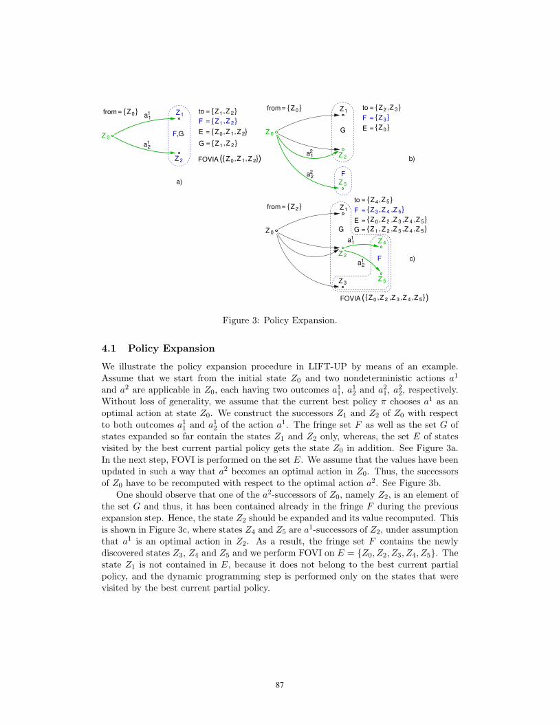
Z0 Z 2

Z0 Z1 Z 2

Z1 Z 2

Z0 Z 1 Z 2

a11

a12

a)

E = { , , }F Z 1

( )

Z 0

1

Z 2

Z

FOVIA

,G

= {from } to = { , }F = { }Z1 Z 2,

G = { , }

{ , , }

Z1

Z 0

Z 3

a12

Z4

Z 3 Z 4

Z1

1a2

Z2 Z 3

G

2a2

1a1

{ }Z0

Z 5

Z1

b)

c)

Z 5Z 2

Z0 Z 2 Z 3 Z 4 Z 5, , , ,{ }

Z0 Z 2 Z 3 Z 4 Z 5, , , ,{ }=from

E =

to = { }

F

}G = { , , , ,G

FOVIA ( )

E =

to = { , }F =

=from

F

Z0

Z 2

Z 3

{ }Z3

F = { , , }Z3 Z 4 Z 5

Z 2

Z 5

Z 4

{ }Z0

{ }Z2,

Figure 3: Policy Expansion.

4.1 Policy Expansion

We illustrate the policy expansion procedure in LIFT-UP by means of an example.Assume that we start from the initial state Z0 and two nondeterministic actions a1

and a2 are applicable in Z0, each having two outcomes a11, a1

2 and a21, a2

2, respectively.Without loss of generality, we assume that the current best policy " chooses a1 as anoptimal action at state Z0. We construct the successors Z1 and Z2 of Z0 with respectto both outcomes a1

1 and a12 of the action a1. The fringe set F as well as the set G of

states expanded so far contain the states Z1 and Z2 only, whereas, the set E of statesvisited by the best current partial policy gets the state Z0 in addition. See Figure 3a.In the next step, FOVI is performed on the set E. We assume that the values have beenupdated in such a way that a2 becomes an optimal action in Z0. Thus, the successorsof Z0 have to be recomputed with respect to the optimal action a2. See Figure 3b.

One should observe that one of the a2-successors of Z0, namely Z2, is an element ofthe set G and thus, it has been contained already in the fringe F during the previousexpansion step. Hence, the state Z2 should be expanded and its value recomputed. Thisis shown in Figure 3c, where states Z4 and Z5 are a1-successors of Z2, under assumptionthat a1 is an optimal action in Z2. As a result, the fringe set F contains the newlydiscovered states Z3, Z4 and Z5 and we perform FOVI on E = {Z0, Z2, Z3, Z4, Z5}. Thestate Z1 is not contained in E, because it does not belong to the best current partialpolicy, and the dynamic programming step is performed only on the states that werevisited by the best current partial policy.

87

N Number of states Time, msec Runtime, msec Runtime w/o norm, msecSupdate Snorm Update Norm

0 9 6 144 1 145 1441 24 14 393 3 396 5932 94 23 884 12 896 22193 129 33 1377 16 1393 132934 328 39 2079 46 2125 775145 361 48 2519 51 2570 8057536 604 52 3268 107 3375 n/a7 627 54 3534 110 3644 n/a8 795 56 3873 157 4030 n/a9 811 59 4131 154 4285 n/a

Table 1: Representative timing results for the first ten iterations of the first-order valueiteration with the normalization procedure switched on or o!.

4.2 First-order Value Iteration

The first-order value iteration algorithm (FOVI) produces a first-order representation ofthe optimal value function and policy by exploiting the logical structure of a first-orderMDP. Thus, FOVI can be seen as a first-order counterpart of the classical value iterationalgorithm by [Bel57].

In LIFT-UP, the first-order value iteration algorithm serves two purposes: First,we perform several iterations of FOVI in order to create an admissible heuristic h inLIFT-UP. Second, in the dynamic programming step of LIFT-UP, we apply FOVI onthe states visited by the best partial policy in order to update their values and possiblyrevise the current best partial policy.

4.2.1 Normalization

It was already mentioned by several authors that value iteration adds a dramatic compu-tational overhead to a solution technique for first-order MDPs if no care about redundantcomputations is taken [BRP01, HS04].

Recently, there have been proposed an automated normalization procedure that,given a state space, delivers an equivalent one that contains no redundancy [HS04].This procedure, referred to as normalize in the LIFT-UP algorithm, is always calledbefore the value function is transmitted to the next iteration step, thereby preventing thepropagation of redundancy to the next computation steps. The technique employs thenotion of the subsumption relation defined in Section 3. Informally, given two abstractstates Z1 and Z2 such that Z1 & Z2 and the values associated to states are identical, Z1

can be easily removed from the state space because it contains redundant information.Table 1 illustrates the importance of the normalization algorithm by providing some

representative timing results for the first ten iterations of the first-order value iteration.The experiments were carried out on the problem taken from the colored Blocksworldscenario consisting of ten blocks. Even on such a relatively simple problem FOVI withthe normalization switched o! does not scale beyond the sixth iteration.

The results in Table 1 demonstrate that the normalization during some iterationof FOVI dramatically shrinks the computational e!ort during the next iterations. The

88

columns labelled Supdate and Snorm show the size of the state space after performingthe value updates and the normalization, respectively. For example, the normalizationfactor, i.e., the ratio between the number Supdate of states obtained after performing oneupdate step and the number Snorm of states obtained after performing the normalizationstep, at the seventh iteration is 11.6. This means that more than ninety percent ofthe state space contained redundant information. The fourth and fifth columns inTable 1 contain the time Update and Norm spent on performing value updates and onthe normalization, respectively. The total runtime Runtime, when the normalization isswitched on, is given in the sixth column. The seventh column labelled Runtime w/onorm depicts the total runtime of FOVI when the normalization is switched o!. If wewould sum up all values in the seventh column and the values in the sixth columnup to the sixth iteration inclusively, subtract the latter from the former and dividethe result by the total time Norm needed for performing normalization during the firstsix iterations, then we would obtain the normalization gain of about three orders ofmagnitude.

5 The Planning System FluCaP

To evaluate the LIFT-UP approach we have developed a domain-dependent implementa-tion called FluCaP. It can solve probabilistic Blocksworld problems as they appeared,for example, in the colored Blocksworld domain of the 2004 International PlanningCompetition.

5.1 Domain-dependent Optimizations

So far, we have presented a general theory of LIFT-UP for finding solutions in uncertainplanning environments which are represented as first-order MDPs. However, severaldomain-driven optimizations or relaxations have been posed on the general theory. Asa result, FluCaP has demonstrated a competitive computational behaviour.

Action Applicability Since in the Blocksworld domain, all states were fully specified,abstract states were described as fluent terms only. This allows to relax the forwardand backward action applicability conditions. Since the cases are symmetric, we willconcentrate on the forward action applicability condition that was initially defined as:An action (a(X1, . . . , Xn), C, E) is forward applicable with ! to an abstract state Z $ S,denoted as forward (Z, a, !), if (C % U)! =AC1 Z, where U is a new variable of sortfluent term and ! is an allowed substitution. Since C and Z are fluent terms under thesingularity condition, the aforementioned AC1-matching problem can be transformedinto the !-subsumption problem [Rob65].

Moreover, we optimize the obtained !-subsumption problem further. Since a statedescription in a colored Blocksworld represents a number of towers, we compare towersof blocks and their color distributions instead of matching respective fluent terms. Theexperiments have shown that it is much faster to manipulate with towers rather thanwith fluent terms. For example, assume that an action precondition contains a fluentclear(X). Let a state describe three towers of blocks. By inspecting the uppermostblocks in the towers, we conclude that there are only three blocks, which satisfy the

89

precondition. It would be interesting to check whether this optimization technique canbe successfully applied in other planning domains as well.

Meanwhile, in Section 6, we present some results towards e#cient domain-independentsolution methods for the !-subsumption problem.

Normalization The similar situation occurs in the case of normalization which relieson the subsumption relation defined in Section 3. The AC1-matching problem underly-ing the subsumption relation reduces to the !-subsumption problem.

Again, it is much faster to operate on towers rather than on fluent terms. For exam-ple, assume that one state describes two towers of four and three blocks, respectively.Another state also describes two towers but of five and two blocks, respectively. In orderto decide, whether one state subsumes another one we try to match the correspondingtowers and their color distributions. As experiments have shown, this optimizationspeeds up the normalization immensely.

5.2 Experimental Evaluation

We demonstrate the advantages of combining the heuristic search together with first-order state abstraction on a FluCaP system, that has successfully entered the domain-dependent track of the probabilistic part of the 2004 International Planning Competition(IPC’2004). The experimental results were all obtained using RedHat Linux running ona 3.4GHz Pentium IV machine with 3GB of RAM.

In Table 2, we present the performance comparison of FluCaP together with sym-bolic LAO! on examples taken from the colored Blocksworld (BW) scenario. Our mainobjective was to investigate whether first-order state abstraction using logic could im-prove the computational behaviour of a planning system for solving FOMDPs. Thecolored BW problems were our main interest since they were the only ones representedin first-order terms and hence the only ones that allowed us to make use of the first-orderstate abstraction.

At the outset of solving a colored BW problem, symbolic LAO! starts by proposi-tionalizing its components, namely, the goal statement and actions. Only after that,the abstraction using propositional ADDs is applied. In contrast, FluCaP performsfirst-order abstraction on a colored BW problem directly, avoiding unnecessary ground-ing. In the following, we show how an abstraction technique a!ects the computation ofa heuristic function. To create an admissible heuristic, FluCaP performs twenty itera-tions of FOVI and symbolic LAO! performs twenty iterations of an approximate valueiteration algorithm similar to APRICODD by [SAHB00]. The columns labelled H.timeand NAS show the time needed for computing a heuristic function and the number ofabstract states it covers, respectively. In comparison to FluCaP, symbolic LAO! needsto evaluate fewer abstract states in the heuristic function but takes considerably moretime. One can conclude that abstract states in symbolic LAO! enjoy more complexstructure than those in FluCaP.

We note that, in comparison to FOVI, FluCaP restricts the value iteration to asmaller state space. Intuitively, the value function, which is delivered by FOVI, covers alarger state space, because the time that is allocated for the heuristic search in FluCaPis now used for performing additional iterations in FOVI. The results in the column

90

Problem Total av. reward Total time, sec. H.time, sec. NAS NGS, !103 %

B C LAO

*

Flu

CaP

FO

VI

Flu

CaP

–

LAO

*

Flu

CaP

FO

VI

Flu

CaP

–

LAO

*

Flu

CaP

LAO

*

Flu

CaP

FO

VI

LAO

*

Flu

CaP

Flu

CaP

4 494 494 494 494 22.3 22.0 23.4 31.1 8.7 4.2 35 410 1077 0.86 0.82 2.75 3 496 495 495 496 23.1 17.8 22.7 25.1 9.5 1.3 34 172 687 0.86 0.68 2.1

2 496 495 495 495 27.3 11.7 15.7 16.5 12.7 0.3 32 55 278 0.86 0.66 1.9

4 493 493 493 493 137.6 78.5 261.6 285.4 76.7 21.0 68 1061 3847 7.05 4.24 3.16 3 493 492 493 492 150.5 33.0 119.1 128.5 85.0 9.3 82 539 1738 7.05 6.50 2.3

2 495 494 495 496 221.3 16.6 56.4 63.3 135.0 1.2 46 130 902 7.05 6.24 2.0

4 492 491 491 491 1644 198.1 2776 n/a 757.0 171.3 143 2953 12014 65.9 23.6 3.57 3 494 494 494 494 1265 161.6 1809 2813 718.3 143.6 112 2133 7591 65.9 51.2 2.4

2 494 494 494 494 2210 27.3 317.7 443.6 1241 12.3 101 425 2109 65.9 61.2 2.0

4 n/a 490 n/a n/a n/a 1212 n/a n/a n/a 804.1 n/a 8328 n/a n/a 66.6 4.18 3 n/a 490 n/a n/a n/a 598.5 n/a n/a n/a 301.2 n/a 3956 n/a n/a 379.7 3.0

2 n/a 492 n/a n/a n/a 215.3 1908 n/a n/a 153.2 n/a 2019 7251 n/a 1121 2.3

15 3 n/a 486 n/a n/a n/a 1809 n/a n/a n/a 1733 n/a 7276 n/a n/a 1.2 · 107 5.7

17 4 n/a 481 n/a n/a n/a 3548 n/a n/a n/a 1751 n/a 15225 n/a n/a 2.5 · 107 6.1

Table 2: Performance comparison of FluCaP (denoted as FluCaP) and symbolic LAO!

(denoted as LAO*), where the cells n/a denote the fact that a planner did not deliver asolution within the time limit of one hour. NAS and NGS are number of abstract andground states, respectively.

labelled % justify that the harder the problem is (that is, the more colors it contains), thehigher the percentage of runtime spent on normalization. Almost on all test problems,the e!ort spent on normalization takes three percent of the total runtime on average.

In order to compare the heuristic accuracy, we present in the column labelled NGSthe number of ground states which the heuristic assigns non-zero values to. One cansee that the heuristics returned by FluCaP and symbolic LAO! have similar accuracy,but FluCaP takes much less time to compute them. This reflects the advantage ofthe plain first-order abstraction in comparison to the marriage of propositionalizationwith abstraction using propositional ADDs. In some examples, we gain several ordersof magnitude in H.time.

The column labelled Total time presents the time needed to solve a problem. Duringthis time, a planner must execute 30 runs from an initial state to a goal state. A one-hourblock is allocated for each problem. We note that, in comparison to FluCaP, the timerequired by heuristic search in symbolic LAO! (i.e., di!erence between Total time andH.time) grows considerably faster in the size of the problem. This reflects the potentialof employing first-order abstraction instead of abstraction based on propositional ADDsduring heuristic search.

The average reward obtained over 30 runs, shown in column Total av. reward, isthe planner’s evaluation score. The reward value close to 500 (which is the maximumpossible reward) simply indicates that a planner found a reasonably good policy. Eachtime the number of blocks B increases by 1, the running time for symbolic LAO! increasesroughly 10 times. Thus, it could not scale to problems having more than seven blocks.This is in contrast to FluCaP which could solve problems of seventeen blocks. We

91

B Total av. reward, "500 Total time, sec. H.time, sec. NAS NGS ! 1021

20 489.0 137.5 56.8 711 1.722 487.4 293.8 110.2 976 1.1 ! 103

24 492.0 757.3 409.8 1676 1.0 ! 106

26 482.8 817.0 117.2 1141 4.6 ! 108

28 493.0 2511.3 823.3 2832 8.6 ! 1011

30 491.2 3580.4 1174.0 4290 1.1 ! 1015

32 476.0 3953.8 781.8 2811 7.4 ! 1017

34 475.6 3954.1 939.4 3248 9.6! 1020

36 n/a n/a n/a n/a n/a

Table 3: Performance of FluCaP on larger instances of one-color Blocksworld problems,where the cells n/a denote the fact that a planner did not deliver a solution within thetime limit.

note that the number of colors C in a problem a!ects the e#ciency of an abstractiontechnique. In FluCaP, as C decreases, the abstraction rate increases which, in turn, isreflected by the dramatic decrease in runtime. The opposite holds for symbolic LAO!.

In addition, we compare FluCaP with two variants. The first one, denoted asFOVI, performs no heuristic search at all, but rather, employs FOVI to compute the $-optimal total value function from which a policy is extracted. The second one, denotedas FluCaP–, performs ‘trivial’ heuristic search starting with an initial value functionas an admissible heuristic. As expected, FluCaP that combines heuristic search andFOVI demonstrates an advantage over plain FOVI and trivial heuristic search. Theseresults illustrate the significance of heuristic search in general (FluCaP vs. FOVI) and theimportance of heuristic accuracy, in particular (FluCaP vs. FluCaP–). FOVI and FluCaP–

do not scale to problems with more than seven blocks.Table 3 presents the performance results of FluCaP on larger instances of one-color

BW problems with the number of blocks varying from twenty to thirty four. We believethat FluCaP does not scale to problems of larger size because the implementation isnot yet well optimized. In general, we believe that the FluCaP system should not beas sensitive to the size of a problem as propositional planners are.

Our experiments were targeted at the one-color problems only because they are,on the one hand, the simplest ones for us and, on the other hand, the bottleneck forpropositional planners. The structure of one-color problems allows us to apply first-order state abstraction in its full power. For example, for a 34-blocks problem FluCaPoperates on about 3.3 thousand abstract states that explode to 9.6 ! 1041 individualstates after propositionalization. A propositional planner must be highly optimized inorder to cope with this non-trivial state space.

We note that additional colors in larger instances (more than 20 blocks) of BWproblems cause dramatic increase in computational time, so we consider these prob-lems as being unsolved. One should also observe that the number of abstract statesNAS increases with the number of blocks non-monotonically because the problems aregenerated randomly. For example, the 30-blocks problem happens to be harder thanthe 34-blocks one. Finally, we note that all results that appear in Tables 2 and 3 wereobtained by using the new version of the evaluation software that does not rely on propo-sitionalization in contrast to the initial version that was used during the competition.

92

The competition domains and results are available in [YLWA05].

6 Domain-independent Methods for !-subsumption

Given two fluent terms Z1 and Z2 under singularity condition, Z1 !-subsumes Z2, writtenZ1 .AC1

" Z2, i! there exists an allowed substitution ! such that (Z1 % U)! =AC1 Z2.Initially, !-subsumption was defined on clauses. Given two clauses C and D, C

!-subsumes D i! there exists a substitution ! such that C! ' D [Rob65]. In general,!-subsumption is np-complete [KN86]. In the domain-dependent implementation ofthe LIFT-UP approach, that was described in the previous section, we have employeddomain-driven optimization techniques that have allowed to reduce the complexity of!-subsumption. This section is devoted to the e#cient domain-independent solutionmethods for !-subsumption which cope with its np-completeness.

One approach to cope with the np-completeness of !-subsumption is deterministicsubsumption. A state is said to be determinate if there is an ordering of fluents, suchthat in each step there is a fluent which has exactly one match that is consistent withthe previously matched fluents [KL94]. However, in practice, there may be only fewfluents, or none at all, that can be matched deterministically. Recently, in [SHW96],it was developed another approach, which we refer to as literal context, LitCon, forshort, to cope with the complexity of !-subsumption. The authors propose to reducethe number of matching candidates for each fluent by using the contextual information.The method is based on the idea that fluents may only be matched to those fluents thatpossess the same relations up to an arbitrary depth in a clause. As a result, a certainsuperset of determinate states can be tested for subsumption in polynomial time.

Unfortunately, as it was shown in [KRS06], LitCon does not scale very well up tolarge depth. Because in some planning problems, the size of state descriptions can berelatively large, it might be necessary to compute the contextual information for largevalues of the depth parameter. Therefore, we are strongly interested in a technique thatscales better than LitCon. In this section, we present an approach, referred to as objectcontext, ObjCon, for short, which demonstrates better computational behaviour thanLitCon. Based on the idea of ObjCon, we develop a new !-subsumption algorithmand compare it with the LitCon-based approach.

6.1 Object Context

In general, a fluent f in a state Z1 can be matched with several fluents in a state Z2, thatare referred to as matching candidates of f . LitCon is based on the idea that fluentsin Z1 can be only matched to those fluents in Z2, the context of which include thecontext of the fluents in Z1 [SHW96]. The context is given by occurrences of identicalobjects (variables Vars (Z) and constants Const (Z)) or chains of such occurrences andis defined up to some fixed depth. In e!ect, matching candidates that do not meetthe above context condition can be e!ortlessly pruned. In most cases, such pruningresults in deterministic subsumption, thereby considerably extending the tractable classof states.

The computation of the context itself is dramatically a!ected by the depth parame-ter: The larger the depth is, the longer the chains of objects’ occurrences are, and thus,

93

more e!ort should be devoted to build them. Unfortunately, LitCon does not scalevery well up to large depth [KRS06]. For example, consider a state

Z = on(X, Y ) % on(Y, table) % r(X) % b(Y ) % h(X) % h(Y ) % w(X) % l(Y )

that can be informally read as: A block X is on the block Y which is on the table,and both blocks enjoy various properties, like color (red r or blue b) or weight (heavyh or light l), they can be wet w. Z contains eight fluents and only three objects. InLitCon, the context should be computed for each of eight fluents in order to keep trackof all occurrences of identical objects. What if we were to compute the context for eachobject instead? In our running example, we would need to perform computations onlythree times, in this case.

Herein, we propose a more e#cient approach, referred to as ObjCon, for computingthe contextual information and incorporate it into a new context-based !-subsumptionalgorithm. More formally, we build the object occurrence graph GZ = (V,E, %) for a stateZ, where vertices are objects of Z, denoted as Obj (Z), and edges E = {(o1,"1, f, "2, o2)|Z contains f(t1, . . . , tn) and o1 = t!1 and o2 = t!2} with o1, o2 $ Obj (Z), f(t1, . . . , tn)being a fluent and "1,"2 being positions of objects o1, o2 in f . The labeling function%(o) = {f |Z contains f(o)} associates each object o with a unary fluent name f thisobject belongs to. The object occurrence graph for the state Z from our running examplewill contain three vertices X, Y and table with labels {r, h, w}, {b, h, l} and {}, resp.,and two edges (X, 1, on, 2, Y ) and (Y, 1, on, 2, table).

The object context ObjCon(o, Z, d) of depth d > 0 is defined for each object o of a

state Z as a chain of labels: %(o)!11 ·f1·!1

2/" %(o1)!21 ·f2·!2

2/" . . .!d1 ·fd·!d

2/" %(od) $ObjCon(o, Z, d)

i! o!11 ·f1·!1

2/" o1!21 ·f2·!2

2/" . . .!d1 ·fd·!d

2/" od is a path in GZ of length d starting at o. In ourrunning example, ObjCon(X, Z, 1) of depth 1 of the variable X in Z contains one chain{{r, h, w} 1·on·2/" {b, h, l}}.

Following the ideas of [SHW96], we define the embedding of object contexts for statesZ1 and Z2, which serves as a pruning condition for reducing the space of matching can-didates for Z1 and Z2. Briefly, let OC1 =ObjCon(o1, Z1, d), OC2 =ObjCon(o2, Z2, d).Then OC1 is embedded in OC2, written OC1 ! OC2, i! for every chain of labels in OC1

there exists a chain of labels in OC2 which preserves the positions of objects in fluentsand the labels for each object in OC1 are included in the respective labels in OC2 upto the depth d. Finally, if ObjCon(X, Z1, d) )! ObjCon(o, Z2, d) then there exists no! such that (Z1 % U)µ! =AC1 Z2, where µ = {X (" o} and U is a new variable of sortfluent term. In other words, a variable X in Z1 cannot be matched against an object oin Z2 within a globally consistent match, if the variable’s context cannot be embeddedin the object’s context. Therefore, the substitutions that meet the above condition canbe e!ortlessly pruned from the search space. For any context depth d > 0, the contextinclusion is an additional condition that reduces the number of candidates, and hencethere exists more often at most one remaining matching candidate.

Based on the idea of the object context, we describe a new !-subsumption algorithmin Algorithm 1. Please note that this algorithm provides a complete set of all allowedsubstitutions which is used later on for determining the set of all possible successors orpredecessors of some state with respect to some action. Due to the lack of space, we

94

Input: Two fluent terms Z1, Z2.Output: A complete set of substitutitons θ such that Z1 #AC1

" Z2.

1. Deterministically match as many fluents of Z1 as possible to fluents of Z2. Substitute Z1 withthe substitution found. If some fluent of Z1 does not match any fluent of Z2, decide Z1 !AC1

" Z2.

2. ObjCon-based deterministically match as many fluents of Z1 as possible to fluents of Z2.Substitute Z1 with the substitution found. If some fluent of Z1 does not match any fluent of Z2,decide Z1 !AC1

" Z2.

3. Build the substitution graph (V, E) for Z1 and Z2 with nodes v = (µ, i) $ V , where µ is amatching candidate for Z1 and Z2, i.e., matches some fluent at position i in Z1 to some fluent inZ2 and i % 1 is referred to as a layer of v. Two nodes (µ1, i1) and (µ2, i2) are connected with anedge i! µ1µ2 = µ2µ1 and i1

&= i2. Delete all nodes (µ, i) with Xµ = o, for some X $ Vars (Z1)

and o $ Obj (Z2), and ObjCon(X, Z1, d)&! ObjCon(o, Z2, d) for some d. Find all cliques of size

|Z1| in (V, E).

Algorithm 1: ObjCon-alltheta.

omit the algorithm for computing all cliques in a substitution graph. However, it canbe found in [KRS06].

6.2 Experimental Evaluation

Figure 4 depicts the comparison timing results between the LitCon-based subsumptionreasoner, referred to as AllTheta, and its ObjCon-based opponent, referred to asFluCaP. The results were obtained using RedHat Linux running on a 2.4GHz PentiumIV machine with 2GB of RAM.

We demonstrate the advantages of exploiting the object-based context informationon problems that stem from the colored Blocksworld and Pipesworld planning scenar-ios. The Pipesworld domain models the flow of oil-derivative liquids through pipelinesegments connecting areas, and is inspired by applications in the oil industry. Liquidsare modeled as batches of a certain unit size. A segment must always contain a certainnumber of batches (i.e., it must always be full). Batches can be pushed into pipelinesfrom either side, leading to the batch at the opposite end “falling” into the incidentarea. Batches have associated product types, and batches of certain types may neverbe adjacent to each other in a pipeline. Moreover, areas may never have constraints onhow many batches of a certain product type they can hold.

For each problem, there have been done 1000 subsumption tests. The time limitof 100 minutes has been allocated. The results show that FluCaP scales better thanAllTheta. It is best to observe on the problems of forteen-, twenty-, and thirty-blocks. As empirical results demonstrate, the optimal value of the depth parameter forBlocksworld and Pipesworld is four.

The main reason for the computational gain of FluCaP is that it is less sensitiveto the growth of the depth parameter. Under the condition that the number of objectsin a state is strictly less than the number of fluents and other parameters are fixed,the amount of object-based context information is strictly less than the amount of theliteral-based context information. Moreover, on the Pipesworld problems, FluCaPrequires two orders of magnitude less time than AllTheta.

95

0 5

10 15 20 25 30 35 40

5 4 3 2

Subs

umpt

ion

time,

ms

Context depth

10 blocks

FluCaPAllTheta

0 5

10 15 20 25 30 35 40

5 4 3 2

Subs

umpt

ion

time,

ms

Context depth

12 blocks

FluCaPAllTheta

0 5

10 15 20 25 30 35 40

5 4 3 2

Subs

umpt

ion

time,

ms

Context depth

14 blocks

FluCaPAllTheta

0 5

10 15 20 25 30 35 40

5 4 3 2

Subs

umpt

ion

time,

ms

Context depth

20 blocks

FluCaPAllTheta

0 5

10 15 20 25 30 35 40

5 4 3 2

Subs

umpt

ion

time,

ms

Context depth

30 blocks

FluCaPAllTheta

1

10

100

1000

5 4 3 2

Subs

umpt

ion

time,

ms

Context depth

4 Areas

FluCaPAllTheta

1

10

100

1000

10000

5 4 3 2

Subs

umpt

ion

time,

ms

Context depth

6 Areas

FluCaPAllTheta

1

10

100

1000

10000

100000

5 4 3 2

Subs

umpt

ion

time,

ms

Context depth

8 Areas

FluCaPAllTheta

1

10

100

1000

10000

100000

1e+06

5 4 3 2

Subs

umpt

ion

time,

ms

Context depth

10 Areas

FluCaPAllTheta

Figure 4: Comparison timing results for FluCaP and AllTheta. The results presentthe average time needed for one subsumption test. Please note that the plots forPipesworld are shown in logscale. Therefore small di!erences in the plot may indicatea substantial di!erence on runtimes.

7 Related Work

We follow the symbolic dynamic programming (SDP) approach within Situation Calcu-lus (SC) of [BRP01] in using first-order state abstraction for FOMDPs. In the courseof first-order value iteration, a state space may contain redundant abstract states thatdramatically a!ect the algorithm’s e#ciency. In order to achieve computational savings,normalization must be performed to remove this redundancy. However, in the originalwork by [BRP01] this was done by hand. To the best of our knowledge, the preliminaryimplementation of the SDP approach within SC uses human-provided rewrite rules forlogical simplification. In contrast, [HS04] have developed an automated normalizationprocedure for FOVI brings the computational gain of several orders of magnitude. An-other crucial di!erence is that our algorithm uses heuristic search to limit the numberof states for which a policy is computed.

The ReBel algorithm by [KvOdR04] relates to LIFT-UP in that it also uses a rep-resentation language that is simpler than Situation Calculus. This feature makes thestate space normalization computationally feasible.

All the above algorithms can be classified as deductive approaches to solving FOMDPs.They can be characterized by the following features: (1) they are model-based, (2) theyaim at exact solutions, and (3) logical reasoning methods are used to compute ab-stractions. We should note that FOVI aims at exact solution for a FOMDP, whereasLIFT-UP, due to the heuristic search that avoids evaluating all states, seeks for an ap-proximate solution. Therefore, it would be more appropriate to classify LIFT-UP as an

96

approximate deductive approach to FOMDPs.In another vein, there is some research on developing inductive approaches to solving

FOMDPs, e.g., by [FYG03]. The authors propose the approximate policy iteration(API) algorithm, where they replace the use of cost-function approximations as policyrepresentations in API with direct, compact state-action mappings, and use a standardrelational learner to learn these mappings. A recent approach by [GT04] proposes aninductive policy construction algorithm that strikes a middle-ground between deductiveand inductive techniques.

8 Conclusions

We have proposed a new approach that combines heuristic search and first-order stateabstraction for solving first-order MDPs more e#ciently. In contrast to existing systems,which start with propositionalizing the decision problem at the outset of any solutionattempt, we perform lifted reasoning on the first-order structure of an MDP directly.However, there is plenty remaining to be done. For example, we are interested in thequestion of to what extent the optimization techniques applied in modern propositionalplanners can be combined with first-order state abstraction.

Acknowledgements

We thank anonymous reviewers for their comments on the previous versions of thispaper. We also thank Zhengzhu Feng for fruitful discussions and for providing us withthe executable of the symbolic LAO! planner. Olga Skvortsova was supported by agrant within the Graduate Programme GRK 334 “Specification of discrete processes andsystems of processes by operational models and logics” under auspices of the DeutscheForschungsgemeinschaft (DFG).

References

[BBS95] A. G. Barto, S. J. Bradtke, and S. P Singh. Learning to act using real-timedynamic programming. Artificial Intelligence, 72(1-2):81–138, 1995.

[BDH99] C. Boutilier, T. Dean, and S. Hanks. Decision-theoretic planning: Struc-tural assumptions and computational leverage. Journal of Artificial Intel-ligence Research, 11:1–94, 1999.

[Bel57] R. E. Bellman. Dynamic programming. Princeton University Press, Prince-ton, NJ, USA, 1957.

[BRP01] C. Boutilier, R. Reiter, and B. Price. Symbolic Dynamic Programmingfor First-Order MDPs. In Bernhard Nebel, editor, Proceedings of the Sev-enteenth International Conference on Artificial Intelligence (IJCAI’2001),pages 690–700. Morgan Kaufmann, 2001.

[DKKN95] T. Dean, L. Kaelbling, J. Kirman, and A. Nicholson. Planning under timeconstraints in stochastic domains. Artificial Intelligence, 76:35–74, 1995.

97

[FH02] Z. Feng and E. Hansen. Symbolic heuristic search for factored MarkovDecision Processes. In R. Dechter, M. Kearns, and R. Sutton, editors,Proceedings of the Eighteenth National Conference on Artificial Intelligence(AAAI’2002), pages 455–460, Edmonton, Canada, 2002. AAAI Press.

[FYG03] A. Fern, S. Yoon, and R. Givan. Approximate policy iteration with a policylanguage bias. In S. Thrun, L. Saul, and B. Scholkopf, editors, Proceedingsof the Seventeenth Annual Conference on Neural Information ProcessingSystems (NIPS’2003), Vancouver, Canada, 2003. MIT Press.

[GT04] C. Gretton and S. Thiebaux. Exploiting first-order regression in inductivepolicy selection. In M. Chickering and J. Halpern, editors, Proceedings of theTwentieth Conference on Uncertainty in Artificial Intelligence (UAI’2004),Ban!, Canada, July 2004. Morgan Kaufmann.

[HS90] S. Holldobler and J. Schneeberger. A new deductive approach to planning.New Generation Computing, 8:225–244, 1990.

[HS04] S. Holldobler and O. Skvortsova. A Logic-Based Approach to DynamicProgramming. In Proceedings of the Workshop on “Learning and Planningin Markov Processes–Advances and Challenges” at the Nineteenth NationalConference on Artificial Intelligence (AAAI’04), pages 31–36, San Jose,CA, July 2004. AAAI Press.

[HZ01] E. Hansen and S. Zilberstein. LAO*: A heuristic search algorithm thatfinds solutions with loops. Artificial Intelligence, 129:35–62, 2001.

[KL94] J.-U. Kietz and M. Lubbe. An e#cient subsumption algorithm for inductivelogic programming. In Proceedings of the Eleventh International Conferenceon MAchine Learning, pages 130–138, 1994.

[KN86] D. Kapur and P. Narendran. NP-completeness of the set unification andmatching problems. In J.H.Siekman, editor, Proceedings of the Conferenceon Automated Deduction, pages 489–495. Springer, Berlin, 1986. LectureNotes in Computer Science 230.

[KRS06] E. Karabaev, G. Ramme, and O. Skvortsova. E#cient symbolic reason-ing for first-order MDPs. In Proceedings of the Workshop on ”Planning,Learning and Monitoring with Uncertainty and Dynamic Worlds” at theSeventeenth European Conference on Artificial Intelligence (ECAI’2006),Riva del Garda, Italy, 2006. To appear.

[KvOdR04] K. Kersting, M. van Otterlo, and L. de Raedt. Bellman goes relational. InC. E. Brodley, editor, Proceedings of the Twenty-First International Con-ference in Machine Learning (ICML’2004), pages 465–472, Ban!, Canada,July 2004. ACM.

[Put94] M. L. Puterman. Markov Decision Processes - Discrete Stochastic DynamicProgramming. John Wiley & Sons, Inc., New York, NY, 1994.

98

[Rei91] R. Reiter. The Frame Problem in the Situation Calculus: A Simple Solution(Sometimes) and a Completeness Result for Goal Regression. In VladimirLifschitz, editor, Artificial Intelligence and Mathematical Theory of Com-putation: Papers in Honor of John McCarthy, pages 359–380. AcademicPress, San Diego, CA, 1991.

[Rob65] J.A. Robinson. A machine-learning logic based on the resolution principle.Journal of the Association for Computing Machinery, 12(1):23–41, 1965.

[SAHB00] R. St-Aubin, H. Hoey, and C. Boutilier. APRICODD: Approximate policyconstruction using decision diagrams. In T. K. Leen, T. G. Dietterich,and V. Tresp, editors, Proceedings of the Fourteenth Annual Conferenceon Neural Information Processing Systems (NIPS’2000), pages 1089–1095,Denver, 2000. MIT Press.

[SHW96] T. Sche!er, R. Herbrich, and F. Wysotzki. E#cient !-subsumption basedon graph algorithms. In Proceedings of the 6th International Workshop onInductive Logic Programming, pages 212–228, Berlin, August 1996. volume1314 of LNAI.

[Thi98] M. Thielscher. Introduction to the fluent calculus. Electronic Transactionson Artificial Intelligence, 2(3-4):179–192, 1998.

[YLWA05] H.L.S. Younes, M.L. Littman, D. Weissman, and J. Asmuth. The firstprobabilistic track of the International Planning Competition. Journal ofArtificial Intelligence Research, 24:851–887, 2005.

99

Multiple Preprocessing for Systematic SAT Solvers

Anbulagan1, John Slaney1,2

1Logic and Computation Program, National ICT Australia Ltd.2Computer Sciences Laboratory, Australian National University

{anbulagan, john.slaney}@nicta.com.au

Abstract

High-performance SAT solvers based on systematic search generally use eitherconflict driven clause learning (CDCL) or lookahead techniques to gain e!ciency.Both styles of reasoning can gain from a preprocessing phase in which some formof deduction is used to simplify the problem. In this paper we undertake an empir-ical examination of the e"ects of several recently proposed preprocessors on bothCDCL and lookahead-based SAT solvers. One finding is that the use of multiplepreprocessors one after the other can be much more e"ective than using any one ofthem alone, but that the order in which they are applied is significant. We intendour results to be particularly useful to those implementing new preprocessors andsolvers.

1 Introduction

In the last decade, the propositional satisfiability (SAT) has become one of the mostinteresting research problems within artificial intelligence (AI). This tendency can beseen through the development of a number of powerful SAT solvers, based on eithersystematic search or stochastic local search (SLS), for solving various hard combinato-rial search problems such as automatic deduction, hardware and software verification,planning, scheduling, and FPGA routing.

The power of contemporary systematic SAT solvers derives not only from the un-derlying Davis-Putnam-Logemann-Loveland (DPLL) algorithm but also from enhance-ments aimed at increasing the amount of unit propagation, improving the choices ofvariables for splitting or making backtracking more intelligent. Two of the most impor-tant such enhancements are conflict driven clause learning (CDCL), made practicable ona large scale by the watched literal technique, and one-step lookahead. These two tendto exclude each other: the most successful solvers generally incorporate one or the otherbut not both. The benefits they bring are rather di"erent too, as is clear from the resultsof recent SAT competitions. For problems in the “industrial” category, CDCL, as im-plemented in MINISAT [ES03, SE05], siege [Rya04] and zCha" [MMZ+01, ZMMM01] iscurrently the method of choice. On random problems, however, lookahead-based solverssuch as Dew Satz [AS05], Kcnfs [DD01] and March dl [HvM06] perform better.

Lookahead, of course, is expensive at every choice node, while clause learning isexpensive only at backtrack points. Since half of the nodes (plus one) in any binarytree are leaves, this di"erence is significant for lookahead-based solvers which process

100

nodes relatively slowly and gain, if at all, by reducing the search tree size. Lookingahead is an investment in at-node processing which can pay o" only if it results in moreinformed choices with an impact on the total number of nodes visited. Where learntclauses prune the tree at least as e"ectively as complex choice heuristics, CDCL mustwin. This seems to be the case in many classes of highly structured problems such as the“industrial” ones in the SAT competitions. We have no clearer definition than anyoneelse of “structure”, but are interested to find ways in which lookahead-based solversmight detect and exploit it as well as the clause learners do.

A noteworthy feature of many recent systems is a preprocessing phase, often usinginference by some variant of resolution, to transform problems prior to the search.One suggestion we wish to make and explore is that such transformations may helplookahead-based solvers to discover useful structure. That is, much of the reasoning doneby nogood inference might be done cheaply “up-front”, provided that the subsequentvariable choice heuristics are good enough to exploit it. In what follows, we are thereforeconcerned mainly with the e"ects of preprocessing, including those of using multiplepreprocessors in series, on the performance of a lookahead-based solver Dew Satz onproblems where it does poorly in comparison with a clause learning solver (MINISAT). Wealso include some results and remarks on benefits to be gained in the opposite direction,where MINISAT is helped by preprocessing to attack problems to which Dew Satz is moresuited.

In this paper we propose a multiple preprocessing technique to boost the performanceof systematic SAT solvers. The motivation for applying multiple preprocessors prior tothe systematic search process is clear: each preprocessor uses a di"erent strategy inobjective to simplify clause sets derived from real-world problems that exhibit a greatdeal structure such as symmetries, variable dependencies, clustering, and the like. Ourinitial observation showed that each strategy works well for simplifying the structureof some problems, at most of the time, from hard to easy. When a problem exhibitsdi"erent kinds of structure, then a single preprocessor has di!culty to simplify thestructures. In this case, we need to run multiple preprocessors one after the other.

We report performance statistics for the two solvers, Dew Satz and MINISAT, withand without combinations of five (and for one problem set, six) of the best contemporarySAT preprocessors when solving parity, planning, bounded model checking and FPGArouting benchmark problems from SATLIB and the recent SAT competitions. Onefinding is that the use of multiple preprocessors one after the other can be much moree"ective than using any one of them alone, but that the order in which they are appliedis significant. We intend our results to be particularly useful to those implementing newpreprocessors and solvers.

The rest of the paper is organized as follows: section 2 addresses the related work.In sections 3 and 4, we briefly describe the preprocessors and solvers examined in ourstudy. The main part of the paper consists of experimental results, and we concludewith a few remarks and suggestions.

101

2 Related Work

Resolution-based SAT preprocessors for CNF formula simplification have a dramaticimpact on the performance of even the most e!cient SAT solvers on many benchmarkproblems [LMS01]. The simplest preprocessor consists of just computing length-boundedresolvents and deleting duplicate and subsumed clauses, as well as tautologies and anyduplicate literals in a clause.

There are two most directly related works. The first one is that of Anbulaganet al. [APSS06] which examined the integration of five resolution-based preprocessorsalone or the combination of them with stochastic local search (SLS) solvers. Theirexperimental results show that SLS solvers benefit the present of resolution-based pre-processing and multiple preprocessing techniques. And the second one is that of Lynceand Marques-Silva [LMS01]. They only evaluated empirically the impact of some pre-processors developed before 2001 including 3-Resolution, without considering multiplepreprocessing, on the performance of systematic SAT solvers. In recent years, manyother preprocessors, which are sophisticated, have been applied to modern propositionalreasoners. Among them are 2-SIMPLIFY [Bra01], the preprocessor in Lsat [OGMS02]for recovering and exploiting Boolean gates, HyPre [Bac02, BW04], Shatter [ASM03]for dealing with symmetry structure, NiVER [SP05] and SatELite [EB05]. We considersome of these preprocessors plus 3-Resolution in our study.

3 SAT Preprocessors

We describe briefly the six SAT preprocessors used in the experiments. The firstfive are all based on resolution and its variants such as hyper-resolution. Resolu-tion [Qui55, DP60, Rob65] itself is widely used as a rule of inference in first orderautomated deduction, where the clauses tend to be few in number and contain few lit-erals, and where the reasoning is primarily driven by unification. As a procedure forpropositional reasoning, however, resolution is rarely used on its own because in prac-tice it has not been found to lead to e!cient algorithms. The sixth preprocessor is aspecial-purpose tool for symmetry detection, which is important for one problem classin the experiments.

3.1 3-Resolution

k-Resolution is just saturation under resolution with the restriction that the parentclauses are of length at most k. The special cases of 2-Resolution and 3-Resolutionare of most interest. 3-Resolution has been used in a number of SAT solvers, notablySatz [LA97] and the SLS solver R+AdaptNovelty+ [APSS05] which won the satisfiablerandom problem category in the SAT2005 competition. Since it is the preprocessoralready used by Satz, we expect it to work well with Dew Satz.

3.2 2-SIMPLIFY

2-SIMPLIFY [Bra01] constructs an implication graph from all binary clauses in theproblem. Where there is an implication chain from a literal X to X, X can be deduced

102

as a unit which can be propagated. The method also collapses strongly connectedcomponents, propagates shared implications, or literals implied in the graph by everyliteral in a clause, and removes some redundant binary clauses. Experimental results[Bra01, Bra04] show that systematic search benefits markedly from 2-SIMPLIFY on awide range of problems.

3.3 HyPre

HyPre [BW04] also reasons with binary clauses, but incorporates full hyper-resolution,making it more powerful than 2-SIMPLIFY. In addition, unit reduction and equalityreduction are incrementally applied to infer more binary clauses. It can be costly interms of time, but since it is based explicitly on hyper-resolution it avoids the spaceexplosion of computing a full transitive closure. HyPre has been used in the SAT solver,2CLS+EQ [Bac02], and we consider it a very promising addition to many other solvers.It is generally useful for exploiting implicational structure in large problems.

3.4 NiVER

Variable Elimination Resolution (VER) is an ancient inference method consisting ofperforming all resolutions on a chosen variable and then deleting all clauses in whichthat variable occurs, leaving just the resolvents. It is easy to see that this is a completedecision procedure for SAT problems, and almost as easy to see that it is not practicablebecause of exponential space complexity. Recently, Subbarayan and Pradhan [SP05]proposed NiVER (Non increasing VER) which restricts the variable elimination to thecase in which there is no increase in the number of literals after elimination. This showspromise as a SAT preprocessor, improving the performance of a number of solvers [SP05].

3.5 SatELite

Een and Biere [EB05] proposed the SatELite preprocessor, which extends NiVER witha rule of Variable Elimination by Substitution. Several additions including subsumptiondetection and improved data structures further improved performance in both space andtime. SatELite was combined with MINISAT to form SatELiteGTI, the system whichdominated the SAT2005 competition on the crafted and industrial problem categories.Since we use MINISAT for our experiments, it is obvious that SatELite should be one ofthe preprocessors we consider.

3.6 Shatter

It is clear that eliminating symmetries is essential to solving realistic instances of manyproblems. None of the resolution-based preprocessors does this, so for problems thatinvolve a high degree of symmetry we added Shatter [AMS03] which detects symmetriesand adds symmetry-breaking clauses. These always increase the size of the clause setand for satisfiable problems they remove some of the solutions, but they typically makethe problem easier by pruning away isomorphic copies of parts of the search space.

103

4 SAT Solvers

As noted in Section 1, we concentrate on just two solvers: MINISAT, which relies onclause learning, and Dew Satz, which uses lookahead.

4.1 MINISAT

Sorensson and Een [ES03, SE05] released the MINISAT solver in 2005. Its design is basedon Cha", particularly in that it learns nogoods or “conflict clauses” and accesses themduring the search by means of two watched literals in each clause. MINISAT is quitesmall (a few hundred lines of code) and easy to use either alone or as a module of alarger system. Its speed in comparison with similar solvers such as zCha" comes from aseries of innovations of which the most important are an activity-decay schedule whichproceeds by frequent small reductions rather than occasional large ones, and an inferencerule for reducing the size of conflict clauses by introducing a restricted subsumption test.The cited paper contains a brief but informative description of these ideas.

4.2 Dew Satz

The solver Dew Satz [AS05] is a recent version of the Satz solver [LA97]. Like its parentSatz, it gains e!ciency by a restricted one-step lookahead scheme which rates some ofthe neighbouring variables every time a choice must be made for branching purposes. Itslookahead is more sophisticated than the original one of Satz, adding a DEW (dynamicequality weighting) heuristic to deal with equalities. This enables the variable selectionprocess to avoid duplicating the work of weighting variables detected to be equivalentto those already examined. Thus, while the solver has no special inference mechanismfor propositional equalities, it does deal tolerably well with problems containing them.

5 Experimental Results

We present results on four benchmark problem sets chosen to present challenges for oneor other or both of the SAT solvers. The experiments were conducted on a cluster of 16AMD Athlon 64 processors running at 2 GHz with 2 GB of RAM. Ptime in the tablesrepresents preprocessing time, while Stime represents solvers runtime without includingPtime. The timebound of Stime is 15,000 seconds per problem instance. It is worthnoting that in our study the results of SatELiteGTI, the solver which dominated theSAT2005 competition on the crafted and industrial problem categories, are representedby the results of SatELite+MINISAT.

5.1 The 32-bit Parity Problem

The 32-bit parity problem was listed by Selman et al. [SKM97] as one of ten challengesfor research on satisfiability testing. The ten instances of the problem are satisfiable.The first response to this challenge was by Warners and van Maaren [WvM98] whosolved the par32-*-c problem (5 instances) using a special-purpose preprocessor todeal with equivalency conditions. Two years later, Li [Li00] solved the ten par32*instances by enhancing Satz’s search process with equivalency reasoning. Ostrowski et

104

Instance Prep. #Vars/#Cls/#Lits Ptime Dew Satz MINISAT

Stime #BackT Stime #Conflict

par32-1 Orig 3176/10227/27501 n/a >15,000 n/a >15,000 n/a3Res 2418/7463/19750 0.08 12,873 17,335,530 >15,000 n/aHyp+3Res 1313/6193/17203 0.50 9,513 17,391,333 >15,000 n/aNiv+3Res 1315/5948/16707 0.46 6,858 13,476,105 >15,000 n/a3Res+Hyp 1313/5495/15810 0.11 9,655 17,335,492 >15,000 n/aSat+3Res 849/5245/18660 0.37 14,729 34,569,968 >15,000 n/a

par32-2 Orig 3176/10253/27405 n/a >15,000 n/a 5,364 9,125,8213Res 2392/7387/19550 0.08 5,171 9,341,185 6,205 10,492,612Hyp+3Res 1301/5975/16719 0.36 3,831 8,186,883 >15,000 n/aNiv+3Res 1303/5730/16223 0.29 1,518 3,889,345 >15,000 n/a

par32-3 Orig 3176/10297/27581 n/a >15,000 n/a >15,000 n/a3Res 2395/7437/19738 0.07 6,124 9,711,576 >15,000 n/aHyp+3Res 1323/5961/16779 0.23 3,673 9,708,520 >15,000 n/aNiv+3Res 1325/5716/16283 0.22 4,470 9,710,552 >15,000 n/aSat+3Res 848/5284/18878 0.37 3,647 2,206,369 >15,000 n/a

par32-4 Orig 3176/10313/27645 n/a >15,000 n/a >15,000 n/a3Res 2385/7433/19762 0.08 10,425 10,036,154 >15,000 n/aSat 849/5160/18581 0.21 12,820 18,230,746 >15,000 n/aHyp+3Res 1331/6055/16999 0.36 9,001 17,712,997 >15,000 n/a3Res+Hyp 1331/5567/16026 0.11 5,741 10,036,146 >15,000 n/aNiv+3Res 1333/5810/16503 0.34 6,099 10,036,154 >15,000 n/a3Res+Niv 1290/5297/15481 0.10 14,003 25,092,756 >15,000 n/a3Res+Sat 850/5286/18958 0.35 3,552 7,744,986 >15,000 n/aSat+3Res 849/5333/19052 0.38 3,563 7,744,986 >15,000 n/aSat+2Sim 848/5154/18565 0.26 12,862 18,230,746 >15,000 n/a

par32-5 Orig 3176/10325/27693 n/a >15,000 n/a >15,000 n/aNiv 1978/7864/22535 0.03 10,651 27,165,469 >15,000 n/a

par32-1-c Orig 1315/5254/15390 n/a >15,000 n/a >15,000 n/a3Res 1315/5957/16738 0.35 11,068 25,920,943 >15,000 n/aHyp+3Res 1313/6193/17203 0.48 7,419 8,931,149 >15,000 n/a

par32-2-c Orig 1303/5206/15246 n/a >15,000 n/a >15,000 n/a3Res 1303/5739/16254 0.23 428 345,680 >15,000 n/aHyp+3Res 1301/5975/16719 0.32 7,402 8,166,758 >15,000 n/a

par32-3-c Orig 1325/5294/15510 n/a >15,000 n/a >15,000 n/a3Res 1325/5725/16314 0.15 4,482 9,462,205 >15,000 n/aHyp 1323/5589/16094 0.04 11,745 19,947,965 >15,000 n/aHyp+3Res 1323/5961/16779 0.22 4,375 9,462,245 >15,000 n/aNiv+3Res 1321/5708/16266 0.24 7,361 16,265,438 >15,000 n/aSat+3Res 802/5335/19335 0.33 5,407 7,280,963 >15,000 n/a

par32-4-c Orig 1333/5326/15606 n/a >15,000 n/a >15,000 n/a3Res 1333/5819/16534 0.24 7,097 8,440,212 >15,000 n/aHyp+3Res 1331/6055/16999 0.32 5,175 9,669,012 >15,000 n/aNiv+3Res 1329/5802/16486 0.55 10,495 21,738,376 >15,000 n/aSat+3Res 806/5357/19443 0.32 10,110 8,013,977 >15,000 n/a

par32-5-c Orig 1339/5350/15678 n/a 10,949 22,878,571 >15,000 n/aNiv+3Res 1335/5728/16362 0.28 >15,000 n/a 7,363 16,189,524

Table 1: Dew Satz and MINISAT performance, before and after preprocessing, on par32problem.

105

al. [OGMS02], solved the problems with Lsat, which performs a preprocessing step torecover and exploit the logical gates of a given CNF formula and then applies DPLLwith a Jeroslow-Wang branching rule. The challenge has now been met convincingly byHeule et al. [HvM04] with their March eq solver, which combines equivalency reasoningin a preprocessor with a lookahead-based DPLL and which solves all of the par32*instances in seconds. Dew Satz is one of the few solvers to have solved any instances ofthe 32-bit parity problem without special-purpose equivalency reasoning [AS05].

Table 1 shows the results of running the lookahead-based solver Dew Satz and theCDCL-based solver MINISAT on the ten par32 instances, with and without preprocess-ing. As preprocessors we used 3-Resolution, HyPre, NiVER and SatELite alone andfollowed by 3-Resolution for the last three. We eliminated 2-SIMPLIFY from this testas it aborted the resolution process of the first five par32* instances presented in theTable 1. We experimented also with all combination of two preprocessors for the prob-lems par32-1 and par32-4. Where lines are omitted from the table (e.g. there is noline for HyPre on par32-1 and for SatELite+3-Resolution on par32-2), this is becauseno single solver produced a solution for those simplified instances.

It is evident from the table that these problems are seriously hard for both solvers.Even with preprocessing, MINISAT times out on all of them except for par32-2 andpar32-5-c. Curiously, on par32-2 instance, preprocessing with 3-Resolution makes itsperformance degrade a little. This is not a uniform e"ect: Table 4 below shows ex-amples in which MINISAT benefits markedly from 3-Resolution. Without preprocessing,Dew Satz times out on nine of ten par32 instances, but in every case except par32-5and par32-5-c 3-Resolution su!ces to help it find a solution, and running multiplepreprocessors improves its performance.

In general, Table 1 shows that multiple preprocessing contributes significantly toenhance the performance of Dew Satz and the preprocessor 3-Resolution dominates thecontribution through either single or multiple preprocessing.

5.2 A Planning Benchmark Problem

The ferry planning benchmark problems, taken from SAT2005 competition, are all easyfor MINISAT, which solves all of them in about one second without needing preprocessors.Dew Satz, however, is challenged by them. The problems are satisfiable. We show theDew Satz and MINISAT results on the problems in Table 2. Clearly the original problemscontain some structure that CDCL is able to exploit but which is uncovered by one-steplookahead. It is therefore interesting to see which kinds of reasoning carried out in apreprocessing phase are able to make that same structure available to Dew Satz. Moststrikingly, reasoning with binary clauses in the manner of the 2-SIMPLIFY preprocessorreduces runtimes by upwards of four orders of magnitude in some cases. HyPre, NiVERand SatELite, especially HyPre, are also e"ective on these planning problems. In mostcases the number of backtracks reduces from million to less than 100 or even zero forferry8 v01a, ferry9 v01a, and ferry10 ks99a instances which means that the inputformula is solved at the root node of the search tree.

106

Instance Prep. #Vars/#Cls/#Lits Ptime Dew Satz MINISAT

Stime #BackT Stime #Conflict

ferry7 ks99i Orig 1946/22336/45706 n/a 2,828 10,764,261 0.13 4,2663Res 1930/22289/45621 0.09 >15,000 n/a 0.11 3,707Hyp 1881/32855/66732 0.21 1,672 1,204,321 0.03 417Niv 1543/21904/45243 0.01 >15,000 n/a 0.10 3,469Sat 1286/21601/50644 0.33 >15,000 n/a 0.07 2,763Sat+2Sim 1279/56597/120318 0.49 0.41 28 0.05 1,096

ferry7 v01i Orig 1329/21688/50617 n/a >15,000 n/a 0.05 1,8583Res 1329/21681/50505 0.14 >15,000 n/a 0.05 1,858Sat 1286/21609/50803 0.17 >15,000 n/a 0.18 6,309Sat+2Sim+3Res 1286/64472/136299 0.95 4.28 824 0.05 1,018Sat+2Sim+Hyp+3Res 1272/62208/131357 1.26 3.30 580 0.10 2,398

ferry8 ks99a Orig 1259/15259/31167 n/a 574 1,869,995 0.01 03Res 1241/15206/31071 0.08 654 2,074,794 0.01 0Sat 813/14720/34687 0.24 810 1,040,528 0.01 381Sat+2Sim 813/35008/75263 0.35 0.11 4 0.02 295

ferry8 ks99i Orig 2547/32525/66425 n/a >15,000 n/a 0.22 6,6153Res 2529/32472/66329 0.12 >15,000 n/a 0.14 3,495Hyp 2473/48120/97601 0.32 >15,000 n/a 0.07 1,030Sat 1696/31589/74007 0.49 >15,000 n/a 0.41 10,551Sat+2Sim 1683/83930/178217 0.76 9.38 3,255 0.20 5,105

ferry8 v01a Orig 854/14819/34624 n/a 13,162 39,153,348 0.01 2773Res 854/14811/34480 0.11 >15,000 n/a 0.01 277Hyp 846/38141/81268 0.18 6.11 570 0.02 226Hyp+Sat 813/38044/81364 0.36 29.66 2,749 0.02 277Hyp+Sat+3Res 813/38028/81196 0.70 0.71 15 0.02 277Hyp+Sat+2Sim 813/36583/78442 0.50 0.17 0 0.02 233

ferry8 v01i Orig 1745/31688/73934 n/a >15,000 n/a 0.55 12,9353Res 1745/31680/73790 0.20 >15,000 n/a 0.55 12,935Sat 1696/31598/74202 0.25 >15,000 n/a 0.25 7,869Sat+2Sim+3Res 1696/96092/202904 1.50 268 68,681 4.06 28,690

ferry9 ks99a Orig 1598/21427/43693 n/a >15,000 n/a 0.01 03Res 1578/21368/43586 0.10 >15,000 n/a 0.01 0Hyp 1542/29836/60522 0.21 >15,000 n/a 0.02 278Niv 1244/21046/43264 0.01 >15,000 n/a 0.01 29Sat 1042/20765/48878 0.33 >15,000 n/a 0.02 3502Sim 1569/20563/41976 0.02 >15,000 n/a 0.04 1,359Hyp+Sat 1056/26902/72553 0.88 33.73 22,929 0.03 609Sat+2Sim 1042/50487/108322 0.50 0.18 5 0.03 261

ferry9 v01a Orig 1088/20878/48771 n/a >15,000 n/a 0.01 1813Res 1088/20869/48591 0.16 >15,000 n/a 0.01 181Hyp 1079/55371/117757 0.28 0.42 0 0.03 187Hyp+Sat 1042/55256/117861 0.49 70.83 5,080 0.03 181Hyp+Sat+2Sim 1042/53394/114135 0.72 0.39 2 0.03 234

ferry10 ks99a Orig 1977/29041/59135 n/a >15,000 n/a 0.03 7103Res 1955/28976/59017 0.13 >15,000 n/a 0.03 827Hyp 1915/40743/82551 0.29 >15,000 n/a 0.04 563Niv 1544/28578/58619 0.02 >15,000 n/a 0.01 0Sat 1299/28246/66432 0.44 >15,000 n/a 0.03 9092Sim 1945/27992/57049 0.05 >15,000 n/a 0.05 1,565Sat+2Sim 1299/69894/149728 0.69 0.28 1 0.04 4193Res+2Sim+Niv 1793/21099/43369 0.43 0.08 0 0.06 1,278Niv+Hyp+2Sim+3Res 1532/24524/50463 0.54 5.19 3,949 0.02 454

ferry10 v01a Orig 1350/28371/66258 n/a >15,000 n/a 0.02 1913Res 1350/28361/66038 0.23 >15,000 n/a 0.02 191Hyp 1340/77030/163576 0.40 4.90 550 0.04 401Hyp+Sat+3Res 1299/76874/163442 1.56 1,643 118,635 0.04 343Hyp+Sat+2Sim 1299/74615/159134 1.00 1.78 61 0.04 459

Table 2: Dew Satz and MINISAT performance, before and after preprocessing, on ferryplanning problem.

107

Instance Prep. #Vars/#Cls/#Lits Ptime Dew Satz MINISAT

Stime #BackT Stime #Conflict

bmc-ibm-3 Orig 14930/72106/189182 n/a >15,000 n/a 0.39 1,738Hyp 5429/32038/89471 3.72 113 2,327 0.06 379Niv 10591/62966/176261 0.47 >15,000 n/a 0.36 2,0883Res 11940/56736/148383 0.41 >15,000 n/a 0.37 2,374Sat 6486/44239/137653 1.32 >15,000 n/a 0.21 1,744Hyp+3Res 5429/30517/79041 3.98 19.67 68 0.04 206

bmc-galileo-8 Orig 58073/294821/767187 n/a >15,000 n/a 0.37 462Hyp 9613/85311/202625 416 67.92 0 0.06 2Niv 30788/240141/685499 1.06 >15,000 n/a 0.42 1,1483Res 43962/182261/456906 5.91 >15,000 n/a 0.46 1,182Sat 20593/135076/414093 6.46 >15,000 n/a 0.19 762Hyp+3Res 9613/82572/188966 417 120 0 0.05 2Sat+3Res 20561/134793/413048 10.12 19.00 1 0.18 799

bmc-galileo-9 Orig 63623/326999/852078 n/a >15,000 n/a 0.54 1,186Hyp 8802/70198/170970 407 90.50 0 0.06 2Niv 33872/267378/763037 1.17 >15,000 n/a 0.42 1,1483Res 49400/208310/523628 6.56 >15,000 n/a 0.46 1,060Sat 23381/155837/477951 7.47 >15,000 n/a 0.24 1,009Hyp+3Res 8802/67042/155884 408 57.57 0 0.04 2

bmc-ibm-10 Orig 59056/323700/854093 n/a >15,000 n/a 1.77 4,277Hyp 2259/10831/29155 47.28 0.30 0 0.01 0Niv 40530/285198/797443 1.19 >15,000 n/a 0.90 3,5323Res 32377/154730/400447 4.70 >15,000 n/a 1.32 3,276Sat 14956/116772/404199 5.53 >15,000 n/a 0.49 2,502

bmc-ibm-11 Orig 32109/150027/394770 n/a >15,000 n/a 2.01 6,422Hyp 7342/40802/106327 13.84 4.73 1 0.05 160Niv 22927/130058/365568 0.96 >15,000 n/a 1.33 5,6073Res 22709/98066/252495 1.46 >15,000 n/a 2.44 7,875Sat 10071/62668/200137 2.58 >15,000 n/a 0.77 5,481

bmc-ibm-12 Orig 39598/194778/515536 n/a >15,000 n/a 8.41 11,887Hyp 12205/87082/228241 91.61 >15,000 n/a 0.74 1,513Niv 27813/168440/476976 0.69 >15,000 n/a 4.46 8,7023Res 32606/160555/419341 2.77 >15,000 n/a 6.77 10,243Sat 15176/109121/364968 4.50 >15,000 n/a 2.37 6,219Niv+Hyp+3Res 12001/100114/253071 85.81 106 6 0.76 1,937

bmc-ibm-13 Orig 13215/65728/174164 n/a >15,000 n/a 1.84 8,088Hyp 5010/27248/78059 3.16 >15,000 n/a 0.13 1,018Niv 9226/57332/161962 0.35 >15,000 n/a 1.72 9,1813Res 10426/49594/129998 0.49 >15,000 n/a 13.17 30,687Sat 4549/34273/110676 1.27 >15,000 n/a 1.25 9,3243Res+Niv+Hyp+3Res 3529/22589/62633 2.90 1,575 4,662,067 0.03 150

bmc-alpha- Orig 663443/3065529/7845396 n/a >15,000 n/a 6.64 50225449 Sat 12408/76025/247622 129 6.94 7 0.06 1

Sat+Hyp 9091/61789/203593 566 7.82 2 0.10 109Sat+Niv 12356/75709/246367 130 4.48 2 0.06 1Sat+3Res 12404/77805/249192 130 8.84 1 0.06 1Sat+2Sim 10457/71128/229499 131 6.37 10 0.10 133

bmc-alpha- Orig 1080015/3054591/7395935 n/a >15,000 n/a 5,409 587,7554408 Sat 23657/112343/364874 47.22 >15,000 n/a 1,266 820,043

Sat+Hyp 13235/88976/263053 56.13 >15,000 n/a 8,753 4,916,981Sat+Niv 22983/108603/351369 49.34 >15,000 n/a 2,137 1,294,590Sat+3Res 23657/117795/380389 48.18 >15,000 n/a 946 618,853Sat+2Sim 17470/129245/375444 51.55 >15,000 n/a 804 561,529Sat+2Sim+3Res 16837/98726/305057 52.89 >15,000 n/a 571 510,705

Table 3: Dew Satz and MINISAT performance, before and after preprocessing, on hardBMC instances.

108

Instance Prep. #Vars/#Cls/#Lits Ptime Dew Satz MINISAT

Stime #BackT Stime #Conflict

01-k10 Orig 9275/38802/98468 n/a 18.96 1,472 0.08 313Hyp n/a 1.27 n/a n/a n/a n/aNiv 6662/33394/90715 0.16 4.12 366 0.07 3273Res 6498/27318/70158 0.24 26.38 2,860 0.07 282Sat 3418/19648/62925 0.84 3.46 140 0.03 2622Sim 4379/59765/133585 3.41 0.24 1 0.05 135

01-k15 Orig 11524/48585/123966 n/a >15,000 n/a 0.49 3,7433Res+Sat+Niv+Hyp 3382/25936/79364 4.65 1,420 130,013 0.06 6823Res+Hyp+Niv+3Res 4203/23731/60639 4.33 190 13,449 0.06 4303Res+Hyp+3Res 4732/24972/63133 4.17 262 19,701 0.04 243Hyp 4889/27056/71819 3.94 2,937 178,245 0.06 603Niv 8068/41368/113317 0.19 >15,000 n/a 0.49 3,5483Res 9403/40059/103137 0.27 >15,000 n/a 0.66 3,783Sat 5198/30697/97961 1.13 >15,000 n/a 0.32 3,655

01-k20 Orig 15069/63760/163081 n/a >15,000 n/a 4.95 16,6583Res+Hyp+Niv+3Res 6382/34846/89807 6.94 513 29,629 0.20 1,261Hyp 7323/39150/104635 6.40 >15,000 n/a 0.95 5,182Niv 10533/54293/149192 0.25 >15,000 n/a 0.28 2,0693Res 12948/55490/142966 0.37 >15,000 n/a 1.58 9,341Sat 7179/42837/136537 1.52 >15,000 n/a 1.11 8,7052Sim 9370/93921/217635 1.91 >15,000 n/a 0.35 1,977

26-k70 Orig 346561/1752741/4579945 n/a >15,000 n/a 8,382 2,654,6143Res 346561/1756001/4588705 150 21.32 1 1.02 10Hyp 243461/1569549/4182061 338 >15,000 n/a 1.22 642Niv 155221/1354556/4075072 479 >15,000 n/a 1.07 492Sat 132670/1300914/4980854 109 >15,000 n/a 2,325 1,503,271

26-k75 Orig 371091/1877066/4904440 n/a >15,000 n/a 8,540 2,880,3763Res 371091/1880536/4913780 161 22.81 1 1.06 11Hyp 260621/1680704/4477966 364 >15,000 n/a 1.20 654Niv 166195/1450679/4364543 4.95 >15,000 n/a 1.41 474Sat 141870/1392526/5327557 117 >15,000 n/a 3,896 2,067,948

26-k85 Orig 420151/2125716/5553430 n/a >15,000 n/a >15,000 n/a3Res 420151/2129606/5563930 183 25.43 1 1.21 10Hyp 294941/1903014/5069776 417 >15,000 n/a 1.55 747Niv 187631/1641901/4941437 5.69 >15,000 n/a 1.37 535Sat 160270/1576770/6039510 132 >15,000 n/a 4,472 2,308,225

26-k90 Orig 444681/2250041/5877925 n/a >15,000 n/a >15,000 n/aNiv+3Res 198605/2208074/6624608 121 13.21 1 1.77 5Hyp+3Res 312101/1979389/5187311 600 46.53 1 1.39 53Res 444681/2254141/5889005 195 26.99 1 1.26 10Hyp 312101/2014169/5365681 446 >15,000 n/a 1.55 583Niv 198605/1738024/5230908 5.91 >15,000 n/a 1.38 429Sat 169470/1669436/6402318 140 >15,000 n/a 8,240 3,311,629

Table 4: Dew Satz and MINISAT performance, before and after preprocessing, onSAT2005 IBM-FV-* instances.

109

5.3 Bounded Model Checking Problems

Another domain providing benchmark problem sets which appear to be easy for MINISAT

but sometimes hard for Dew Satz is bounded model checking. In Table 3 we reportresults on five of eleven BMC-IBM problems, two BMC-galileo problems and two of fourBMC-alpha problems. All other benchmark problems in the BMC-IBM class are easy forboth solvers and so are omitted from the table. The other two BMC-alpha instancesare harder than the two reported even for MINISAT before and after preprocessing. Theproblems presented in Table 3 are satisfiable.

Each of these bounded model checking problems is brought within the range ofDew Satz by some form of preprocessing. In general, HyPre and 3-Resolution are thebest for this purpose, especially when used together, though on problem BMC-IBM-13they are ine"ective without the additional use of NiVER. The column showing thenumber of times Dew Satz backtracks is worthy of note. In many cases, preprocessingreduces the problem to one that can be solved without backtracking. Solving “with-out backtracking” has to be interpreted with care here, of course, since a nontrivialamount of lookahead may be required in a “backtrack-free” search. The results forBMC-galileo-9 furnish a good example of this: HyPre takes 407 seconds to refine theproblem, following which Dew Satz spends 90 seconds on lookahead reasoning whileconstructing the first (heuristic) branch of its search tree, but then that branch leadsdirectly to a solution. Adding 3-Resolution to the preprocessing step does not changethe number of variables, and only slightly reduces the number of clauses, but it roughlyhalves the time subsequently spent on lookahead.

The instance BMC-alpha-4408 is hard for Dew Satz even after preprocessing. WhileMINISAT with multiple preprocessing solves the problem instance with an order of mag-nitude faster. We can also observe that HyPre brings more benefit than SatELite,

Table 4 shows results for both solvers on a related problem set consisting of formalverification problems taken from the SAT2005 competition. The IBM-FV-01 problemsare satisfiable except for the problem IBM-FV-01-k10; the IBM-FV-26 problems areunsatisfiable. Most of these satisfiable problems are easy for MINISAT, but the unsatisfi-able cases show that the SatELite preprocessor (with which MINISAT was paired in thecompetition) is by far the least e"ective of the four we consider for MINISAT on theseproblems. The preprocessor HyPre proved the unsatisfiability of IBM-FV-01-k10 in 1.27seconds. 2-SIMPLIFY was not used to simplify the IBM-FV-26 problems, because it islimited for input formula with maximum 100,000 variables. Again there are cases inwhich Dew Satz is improved from a 15,000 second timeout to a one-branch proof of un-satisfiability. Note that the numbers of clauses in these cases are actually increased bythe preprocessor 3-Resolution, confirming that the point of such reasoning is to exposestructure rather than to reduce problem size.

5.4 A Highly Symmetrical Problem

FPGA routing problem is a higly symmetrical problem that model the routing of wires inthe channels of field-programmable integrated circuits [AMS03]. The problem instancesused in the experiment, which were artificially designed by Fadi Aloul, are taken fromSAT2002 competition.

110

Without preprocessing to break symmetries, many of the FPGA routing problemsare hard—harder for CDCL solvers than for lookahead-based ones. Not only do theyhave many symmetries, but the clause graphs are also disconnected. Lookahead tech-niques with neighbourhood variables ordering heuristic seem able to choose inferenceswithin one graph component before moving to another, whereas MINISAT jumps fre-quently between components. Table 5 shows performances of both solvers on FPGArouting problem set. Of 21 selected satisfiable (bart) problems, MINISAT solves 8 insome 2 hours. It manages better with the unsatisfiable (homer) instances, solving 14 of15 in a total time of around 6 hours. Dew Satz solves all of the bart problems in 17.5seconds and the homer ones in 45 minutes.

The detailed results for two of the satisfiable problems and two unsatisfiable ones(Table 6) are interesting. The resolution-based preprocessors do not give any mod-ification to the size of the input formula except when using SatELite. The Shatterpreprocessor, which removes certain symmetries, is tried on its own and in combinationwith the five resolution-based preprocessors. It should be noted that the addition ofsymmetry-breaking clauses increases the sizes of the problems, but of course it greatlyreduces the search spaces in most cases.

The performance of Dew Satz after preprocessing is often worse in terms of timethan it was before, though there is always a decreases in the size of its search tree. Thisis because of the increase in the problem size which increases the amount of lookaheadprocess. MINISAT, by contrast, sometimes speeds up by several orders of magnitudeafter preprocessing.

Instance Dew Satz MINISAT

#Solved Stime #BackT #Solved Stime #Conflictbart (21 SAT) 21 17.52 1,536,966 8 7,203 119,782,466homer (15 UNSAT) 15 2,662 109,771,200 14 22,183 143,719,166

Table 5: Dew Satz and MINISAT performance, without preprocessing, on FPGA routingproblems.

5.5 Order of Preprocessors

Table 7 illustrates the di!culty of selecting the order in which to apply multiple prepro-cessors. It shows results on just two sample problems. The first is the bounded modelchecking problem BMC-IBM-12, which Dew Satz attempted with the three preprocessorsHyPre, NiVER and 3-Resolution in di"erent orders. Only one order, NiVER followed byHyPre followed by 3-Resolution, renders the problem feasible for Dew Satz. With thepreprocessors in that order, it is solved in less than 2 minutes; with any other order itcannot be solved in more than four hours. The second problem, ferry10 ks99a, showsthe range of di"erent outcomes produced by varying the order of four preprocessors. Ifwe get it right, we get a solution in 5 seconds, but we know of no simple rule for gettingit right in such a case. Neither running NiVER first nor running 3-Resolution last issu!cient. Even with NiVER, HyPre and 3-Resolution in the right order, putting 2-SIMPLIFY first rather than third changes the runtime from 5 seconds to several hours.The third experiment illustrates the e"fect of alternating two preprocessors. Simplifying

111

Instance Prep. #Vars/#Cls/#Lits Ptime Dew Satz MINISAT

Stime #BackT Stime #Conflict

bart28 Orig 428/2907/7929 n/a 0.00 0 >15,000 n/aSat 413/2892/11469 0.06 0.02 0 >15,000 n/aSha 1825/8407/27003 0.37 0.06 9 198 775,639Sha+3Res 1764/7702/24400 0.46 0.04 1 2,458 7,676,459Sha+Hyp 1764/8349/26138 0.41 0.05 20 >15,000 n/aSha+Niv 1781/8358/26759 0.38 0.05 6 5.46 53,683Sha+Sat 1728/8254/30422 0.53 0.10 0 115 684,272Sha+2Sim 1750/7892/24682 0.39 0.05 17 19.12 150,838

bart30 Orig 485/3617/9954 n/a 0.31 20,160 >15,000 n/aSat 468/3600/14544 0.08 0.03 0 >15,000 n/aSha 2017/9649/30874 0.49 0.11 96 >15,000 n/aSha+3Res 1945/8686/27492 0.60 0.12 224 4,149 7,594,231Sha+Hyp 1945/9348/29218 0.54 11,729 28,270,212 >15,000 n/aSha+Niv 1969/9599/30625 0.50 0.06 1 >15,000 n/aSha+Sat 1776/8830/33533 0.77 0.12 1 >15,000 n/aSha+2Sim 1919/8758/27287 0.51 0.05 9 >15,000 n/a

homer19 Orig 330/2340/4950 n/a 473 19,958,400 10,233 51,960,410Sat 300/2310/8400 0.04 >15,000 n/a 5,621 54,469,568Sha 1460/6764/20242 0.16 2,345 4,828,639 2.26 33,492Sha+3Res 1388/5748/16914 0.23 3,231 7,189,966 1.14 21,669Sha+Hyp 1387/6547/18865 0.20 4,179 9,611,768 1.90 30,418Sha+Niv 1412/6715/19993 0.17 2,570 5,202,084 3.15 45,484Sha+Sat 1201/5846/19288 0.34 4,071 6,236,966 1.48 26,517Sha+2Sim 1348/5639/16110 0.17 307 678,425 0.70 14,682

homer20 Orig 440/4220/8800 n/a 941 19,958,400 >15,000 n/aSat 400/4180/15200 0.08 1,443 6,982,425 11,448 57,302,582Sha 1999/10340/29988 0.28 369 350,610 1.83 22,950Sha+3Res 1907/8793/25027 0.37 362 405,059 1.41 18,273Sha+Hyp 1905/10527/29129 0.34 1,306 1,451,567 1.10 13,927Sha+Niv 1941/10276/29671 0.29 379 349,842 0.91 13,543Sha+Sat 1723/9420/30986 0.54 822 300,605 1.00 13,831Sha+2Sim 1879/9419/26188 0.31 114 120,297 0.40 6,612

Table 6: Dew Satz and MINISAT performance, before and after preprocessing, on selectedFPGA routing instances.

Instance Prep. #Vars/#Cls/#Lits Ptime Stime #BackT

bmc-ibm-12 Hyp+3Res+Niv 10805/83643/204679 96.11 >15,000 n/aNiv+Hyp+3Res 12001/100114/253071 85.81 106 63Res+Hyp+Niv 10038/82632/221890 89.56 >15,000 n/a3Res+Niv+Hyp 11107/99673/269405 58.38 >15,000 n/a

ferry10 ks99a 2Sim+Niv+Hyp+3Res 1518/32206/65806 0.43 >15,000 n/aNiv+3Res+2Sim+Hyp 1532/25229/51873 0.49 11,345 17,778,4833Res+2Sim+Niv+Hyp 1793/20597/42365 0.56 907 1,172,964Niv+Hyp+2Sim+3Res 1532/24524/50463 0.54 5.19 3,949

ferry10 ks99a 2Sim+Niv 1518/27554/56565 0.08 >15,000 n/a2Sim+Niv+2Sim 1518/18988/39433 0.27 3,197 6,066,2412Sim+Niv+2Sim+Niv 1486/18956/39429 0.29 129 290,8712Sim+Niv+2Sim+Niv+2Sim 1486/23258/48033 0.48 7,355 8,216,100

Table 7: Dew Satz’s performance on instances with preprocessor ordering.

112

with 2-SIMPLIFY followed by NiVER is insu!cient to allow solution before the timeout.Simplifying again with 2-SIMPLIFY brings the runtime down to under an hour; addingNiVER again brings it down again to a couple of minutes; repeating 2-SIMPLIFY, farfrom improving matters, causes the time to blow out to two hours.

6 Conclusions

We performed an empirical study of the e"ects of several recently proposed SAT prepro-cessors on both CDCL and lookahead-based SAT solvers. We describe several outcomesfrom this study as follow.

1. High-performance SAT solvers, whether they depend on clause learning or onlookahead, benefit greatly from preprocessing. Improvements of four orders ofmagnitude in runtimes are not uncommon.

2. It is unlikely to equip a SAT solver with just one preprocessor of the kind con-sidered in this paper. Very di"erent preprocessing techniques are appropriate todi"erent problem classes.

3. There are frequently benefits to be gained from running two or more preprocessorsin series on the same problem instance.

4. Both clause learning and lookahead need to be enhanced with techniques specificto reasoning with binary clauses, in order to exploit dependency chains, and withtechniques for equality reasoning.

5. Lookahead-based solvers also benefit greatly from resolution between longer clauses,as in the 3-Resolution preprocessor. This seems to capture ahead of the searchsome of the inferences which would be achieved during it by learning clauses.CDCL solvers can also benefit from 3-Resolution preprocessor—dramatically incertain instances—but the e"ects are far from uniform.

6.1 Future work

The following lines of research are open:

1. It would, of course, be easy if tedious to extend the experiments to more problemsets, more preprocessors and especially to more solvers. We shall probably lookat some more DPLL solvers, but do not expect the results to add much morethan detail to what is reported in the present paper. One of the more importantadditions to the class of solvers will be a non-clausal (Boolean circuit) reasoner.We have not yet experimented with such a solver. We have already investigatedpreprocessing for several state of the art SLS (stochastic local search) solvers, butthat is such a di"erent game that we regard it as a di"erent experiment and donot report it here.

2. The more important line of research is to investigate methods for automaticallychoosing among the available preprocessors for a given problem instance, and

113

for automaticallly choosing the order in which to apply successive preprocessors.Machine learning may help here, though it would be better, or at least moreinsightful, to be able to base decisions on a decent theory about the interaction ofreasoning methods.

3. Another interesting project is to combine preprocessors not as a series of separatemodules but as a single reasoner. For example, it would be possible to satu-rate under 3-Resolution and hyper-resolution together, in the manner found inresolution-based theorem provers. Whether this would be cost-e"ective in termsof time, and whether the results would di"er in any worthwhile way from thoseobtained by ordering separate preprocessors, are unknown at this stage.

As SAT solvers are increasingly applied to real-world problems, we expect deductivereasoning by preprocessors to become increasingly important to them.

Acknowledgments

This work was funded by National ICT Australia (NICTA). National ICT Australia isfunded through the Australian Government’s Backing Australia’s Ability initiative, inpart through the Australian Research Council.

References

[AMS03] Fadi A. Aloul, Igor L. Markov, and Karem A. Sakallah. Shatter: E!-cient symmetry-breaking for boolean satisfiability. In Design AutomationConference, pages 836–839. ACM/IEEE, 2003.

[APSS05] Anbulagan, Duc Nghia Pham, John Slaney, and Abdul Sattar. Old reso-lution meets modern SLS. In Proceedings of 20th AAAI, pages 354–359,2005.

[APSS06] Anbulagan, Duc Nghia Pham, John Slaney, and Abdul Sattar. BoostingSLS performance by incorporating resolution-based preprocessor. In Pro-ceedings of Third International Workshop on Local Search Techniques inConstraint Satisfaction (LSCS), in conjunction with CP-06, pages 43–57,2006.

[AS05] Anbulagan and John Slaney. Lookahead saturation with restriction for SAT.In Proceedings of 11th CP, pages 727–731, 2005.

[ASM03] Fadi A. Aloul, Karem A. Sakallah, and Igor L. Markov. E!cient symmetrybreaking for boolean satisfiability. In Proceedings of 18th IJCAI, Mexico,2003.

[Bac02] Fahiem Bacchus. Enhancing Davis Putnam with extended binary clause rea-soning. In Proceedings of 18th AAAI, pages 613–619, Edmonton, Canada,August 2002. AAAI Press.

114

[Bra01] Ronen I. Brafman. A simplifier for propositional formulas with many binaryclauses. In Proceedings of 17th IJCAI, pages 515–522, 2001.

[Bra04] Ronen I. Brafman. A simplifier for propositional formulas with many binaryclauses. IEEE Transactions on Systems, Man, and Cybernetics, Part B,34(1):52–59, 2004.

[BW04] Fahiem Bacchus and Jonathan Winter. E"ective preprocessing with hyper-resolution and equality reduction. In Revised Selected Papers of SAT 2003,LNCS 2919 Springer, pages 341–355, 2004.

[DD01] Olivier Dubois and Gilles Dequen. A backbone-search heuristic for e!cientsolving of hard 3-SAT formulae. In Proceedings of 17th IJCAI, pages 248–253, Seattle, Washington, USA, 2001.

[DP60] M. Davis and H. Putnam. A computing procedure for quantification theory.Journal of the ACM, 7:201–215, 1960.

[EB05] Niklas Een and Armin Biere. E"ective preprocessing in SAT through vari-able and clause elimination. In Proceedings of 8th SAT, LNCS Springer,2005.

[ES03] Niklas Een and Niklas Sorensson. An extensible SAT-solver. In Proceedingsof 6th SAT, 2003.

[HvM04] Marijn Heule and Hans van Maaren. Aligning CNF- and equivalence-reasoning. In Proceedings of 7th SAT, Vancouver, Canada, 2004.

[HvM06] Marijn Heule and Hans van Maaren. March dl: Adding adaptive heuristicsand a new branching strategy. Journal on Satisfiability, Boolean Modelingand Computation, (2):47–59, 2006.

[LA97] Chu Min Li and Anbulagan. Look-ahead versus look-back for satisfiabilityproblems. In Proceedings of 3rd CP, pages 341–355, Schloss Hagenberg,Austria, 1997.

[Li00] Chu Min Li. Integrating equivalency reasoning into Davis-Putnam pro-cedure. In Proceedings of 17th AAAI, pages 291–296, USA, 2000. AAAIPress.

[LMS01] I. Lynce and J. Marques-Silva. The interaction between simplification andsearch in propositional satisfiability. In Proceedings of CP’01 Workshop onModeling and Problem Formulation, 2001.

[MMZ+01] M. W. Moskewicz, C. F. Madigan, Y. Zhao, L. Zhang, and S. Malik. Cha":Engineering an e!cient SAT solver. In Proceedings of DAC, pages 530–535,2001.

[OGMS02] Richard Ostrowski, Eric Gregoire, Bertrand Mazure, and Lakhdar Sais.Recovering and exploiting structural knowledge from CNF formulas. InProceedings of 8th CP, pages 185–199, 2002.

115

[Qui55] W. V. Quine. A way to simplify truth functions. American MathematicalMonthly, 62:627–631, 1955.

[Rob65] J. A. Robinson. A machine-oriented logic based on the resolution principle.Journal of the ACM, 12:23–41, 1965.

[Rya04] Lawrence O. Ryan. E!cient Algorithms for Clause Learning SAT Solvers.PhD thesis, Simon Fraser University, Burnaby, Canada, 2004.

[SE05] Niklas Sorensson and Niklas Een. MINISAT v1.13 - A SAT solver withconflict-clause minimization. In 2005 International SAT Competitionwebsite: http://www.lri.fr/∼simon/contest05/results/descriptions/solvers/minisat static.pdf,2005.

[SKM97] Bart Selman, Henry Kautz, and David McAllester. Ten challenges in propo-sitional reasoning and search. In Proceedings of 15th IJCAI, pages 50–54,Nagoya, Aichi, Japan, 1997.

[SP05] Sathiamoorthy Subbarayan and Dhiraj K. Pradhan. NiVER: Non increasingvariable elimination resolution for preprocessing SAT instances. In RevisedSelected Papers of SAT 2004, LNCS 3542 Springer, pages 276–291, 2005.

[WvM98] Joost P. Warners and Hans van Maaren. A two-phase algorithm for solvinga class of hard satisfiability problems. Operations Research Letters, 23:81–88, 1998.

[ZMMM01] L. Zhang, C. F. Madigan, M. W. Moskewicz, and S. Malik. E!cient con-flict driven learning in a Boolean satisfiability solver. In Proceedings ofInternational Conference on Computer Aided Design ICCAD2001, 2001.

116