2014.02.11.

1

7. Atmospheric flows

Dr. Gergely KristófDept. of Fluid Mechanics, BME

April, 2012.

Energy balance of a moving volume of air in the atmosphere

Te atmosphere feels colder at the top of high mountain.Cold air does not flows down to sea level. Why?

The cold air flow would warm up due to the increasing pressure.(We cannot observe this phenomenon in any laboratory experiments.)

:wδ work due to:- reversible compression;- viscous dissipation.

:qδ heating due to:- turbulent transport,- radiation,- latent heat release

(phase change).

wqdu δδ += change of the internal energyof a unit mass of air.

The change of the thermodynamic state in a rapid vertical flow of dry air is dominated by the reversible compression work, therefore it is isentropic.

The potential temperature: Θ1

0

1

00

−−

=

=

κκ

κ

ρ

ρ

p

p

T

TFor isentropic flows:

pp

vp

c

R

c

cc=

−=

−

κ

κ 1

in which κ is the ratio of specific heats, thus

pc/R

pT

=

Pa105

Θ

The potential temperature of the atmospheric air in a point characterized by

temperature T and pressure p is defined as:

Θ would be the temperature if the air parcel would taken down to sea level.

2014.02.11.

2

Stable and unstable stratifications

Θ

zStableUnstable

On the basis of the potential temperature profile we can analyze the atmospheric stability:

Neutral

Vertical flows

z

Θ

Θ0Τ0

z

T

p0

z

Hydrostatics

gz

pρ−=

∂

∂

In order to solve this we need to find relation between p and ρ.

( )pf=ρ

Barotrophic relation:

const.=ρ homogenous atm.

const.00

== T,TR

pρ isothermal atm.

const.0

0 =

= m,

p

pm

ρρ polytrophic atm.

e.g. Θ=const.

( )zfT,TR

p==ρ

2014.02.11.

3

Problem #7.1

Please, calculate the pressure profile for a given (linear) temperature profile:

const.=∂

∂−=

z

Tγ

zTT γ−= 0

in which

,

.

To the solution

Assume, that in z=0: T=T0 and p=p0 !

The dry adiabatic temperature gradient

pc

R

p

p

T

T

=

00

The adiabatic relation:

p

.adiab

c

R

g

R=

γBy comparing the exponents:

km

K89

1000

89.

.

c

g

p.adiab ==== Γγwe obtain the adiabatic

temperature gradient:

We compare the T(p) relation of a linear temperature model with those of an adiabatic model.

g

R

p

p

T

T

γ

=

00

From the linear T profil of γ gradient we obtained:

γγ R

g

T

zTpp

−=

0

00

Thus the dry adiabatic T profile is a linear profile of Γ gradient.

Aha! T(z) must be also linear for an adiabatic

profile!

The standard atmosphere

Troposphere

Stratosphere

ΘT

T,Θ

z

11 km

km

K56.=γ

Standard (average)tropospherictemperature gradient:

K15.288T0 =

Pa1001325.1p 5

0 ⋅=

Referencevalues:

Γ

γ

Γ<

2014.02.11.

4

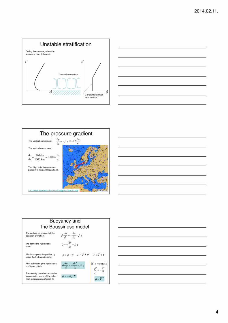
Unstable stratification

z

Θ

z

Θ

During the summer, when the surface is heavily heated:

Thermal convection:

Constant potential temperature.

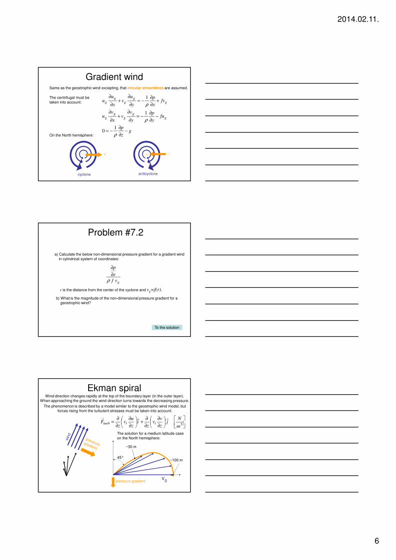
The pressure gradient g

z

pρ−=

∂

∂

m

Pa12−≅The vertical component:

The vertical component:

m

Pa00260

km 1000

hPa 26.

x

p==

∂

∂

http://www.weatheronline.co.uk/map/vor/euro/d.htm

This high anisotropy causes problem in numerical solutions.

Buoyancy and the Boussinesq model

gz

p

dt

dwρρ −

∂

∂−=

The vertical component of theequation of motion:

gz

pρ−

∂

∂−=0We define the hydrostatic

state:

'ppp += 'ρρρ += 'TTT +=We decompose the profiles by using the hydrostatic state:

'T' βρρ −=The density perturbation can beexpressed in terms of the cubic heat expansion coefficient β:

g'z

'p

dt

dwρρ −

∂

∂−=

After subtracting the hydrostaticprofile we obtain:

T

'T'−=

ρ

ρ

1−= Tβ

:p constIf =

2014.02.11.

5

Acoustic filteringThe density need to depend on the pressure, but

we need to eliminate the acoustic waves. (Acoustic effects require very small time stepping.)

)z(ρρ ≅

0=⋅∇ )v( ρ

0=∂

∂+

∂

∂+

∂

∂+

∂

∂

z

w

y

v

x

u

t

ρρρρThe continuity equation for compressible fluid:

Since the average density is a function of the altitude, this is a more complex continuity equation we normally use in incompressible flow models.

Coriolis force

x

y

N

S

Ω

wvu

kji

vC zyx ΩΩΩΩ 22 −=×−=

xyz

zxy

yzx

vuC

uwC

wvC

ΩΩ

ΩΩ

ΩΩ

22

22

22

−=

−=

−=

0≅

−=

≅

z

y

x

C

fuC

fvC φΩ sinf 2=in which

)sin(

)cos(

z

y

x

φΩΩ

φΩΩ

Ω

=

=

= 0

φ the geographic latitude

Inertial forces in a rotating frame:- Centrifugal force- Coriolis force

― Taken into account in g.

― Effects only moving bodies.

the average of w is 0.

the buoyancy forceprevails in vertical

flows

Geostrophic wind

0=∂

∂+

∂

∂

y

pv

x

pu gg 0=∇⋅ pvg

rthus

Steady flow with the assumptions below:

gz

p

fuy

p

fvx

p

g

g

−∂

∂−=

−∂

∂−=

+∂

∂−=

ρ

ρ

ρ

10

10

10 No convective acceleration:

streamlines are approximated with parallel lines. Strain stresses are neglected.

Hydrostatic equilibrium in z direction.

On the North hemisphere:

The pressure gradient is perpendicular to the direction of the equilibrium flow.

... self-consistent specification of the boundary conditions.

2014.02.11.

6

Gradient windSame as the geostrophic wind excepting, that circular streamlines are assumed.

+__ +

cyclone anticyclone

On the North hemisphere:g

z

p

fuy

p

y

vv

x

vu

fvx

p

y

uv

x

uu

gg

gg

g

gg

gg

g

−∂

∂−=

−∂

∂−=

∂

∂+

∂

∂

+∂

∂−=

∂

∂+

∂

∂

ρ

ρ

ρ

10

1

1The centrifugal must be taken into account:

Problem #7.2

a) Calculate the below non-dimensional pressure gradient for a gradient windin cylindrical system of coordinates:

gvf

r

p

ρ∂

∂

r is the distance from the center of the cyclone and vg=f(r).

b) What is the magnitude of the non-dimensional pressure gradient for a geostrophic wind?

To the solution

Ekman spiral

The phenomenon is described by a model similar to the geostrophic wind model, butforces rising from the turbulent stresses must be taken into account:

∂

∂

∂

∂+

∂

∂

∂

∂=

3m

Nj

z

vv

zi

z

uv

zF ttturb

rrr

45°

vgpressure gradient

~30 m

~100 m

Wind direction changes rapidly at the top of the boundary layer (in the outer layer).When approaching the ground the wind direction turns towards the decreasing pressure.

The solution for a medium latitude caseon the North hemisphere:

2014.02.11.

7

Velocity magnitude in the boundary layer

The Monyin-Obuhovprofile:

+=

L

z

z

zln

u

uβ

κ 0*

1z0: roughness height;κ: Von Kármán const;L: M-O scale.

pc

H

uL

ρκ 0

2*

T

g−=

H0: heat flux(H0 ~ -dΘ/dz)

+ _

Two important effects must be taken into account: surface roughness and thermal stratification.

=

νκ*

*

91 uzln

u

u

The profile of a constant density flow past a flat plate for comparison:

We can note that, the Reynolds number does not count in atmospheric flows.

Summary

• Thermal stratification;• Adiabatic compression and expansion

due to vertical flows;• Variation of density in vertical flows

due to the hydrostatic pressure;• Coriolis force;• Turbulence in stratified medium;• Moisture transport and phase

changes;• Surface energy balance involving the

radiation heat transport, the heat storage and a number of other complex phenomena.

We

have

touc

hed

upon

thes

e to

pics

Most important atmospheric flow related physical phenomena beyond the scope of basic level fluid mechanics:

CFD based atmospheric simulations

Gergely Kristóf Ph.D., Miklós Balogh, Norbert Rácz29-th March 2009.

2014.02.11.

8

model conversion interface

Advantages of a CFD based model

grid refinement

• Either the surface geometry isdescribed in high details or (alternatively) meso-scaleeffects are taken into account.

• Bidirectional interface is a source of numerical errors eg.it can cause partial reflection.

Meso scale model

CFD

CFD(with some changes)

• Higher accuracy• No limits on geometrical precision• Flexible meshing • Advanced turbulent models• Easy customization• Advanced pre- and post

processing tools

Methodology

ANSYS FLUENT + transformation system

+ customized source terms

Mathematical description

z~,~,p~,T~

,~ vρTransformed variables

0=⋅∇ v~

( ) ( ) ( ) Fgτvvv +−+⋅∇+−∇=⊗⋅∇+∂

∂000 ρρρρ ~p~~~~

t

( ) ( ) ( ) Ttpp ST~

KT~

c~T~

ct

+∇⋅∇=⋅∇+∂

∂00 ρρ v

( ) ( ) kbkk

t SGGkk~kt

+−++

∇⋅∇=⋅∇+

∂

∂ερ

σ

µρρ 000 v

( ) ( ) ++

−+

∇⋅∇=⋅∇+

∂

∂

εν

ερερε

σ

µερερ

ε kCSC~

t

t2

201000 v

( )000 TT~~ −−= βρρρ

εεεε

SGCk

C b ++ 31

Customized volume sources

2014.02.11.

9

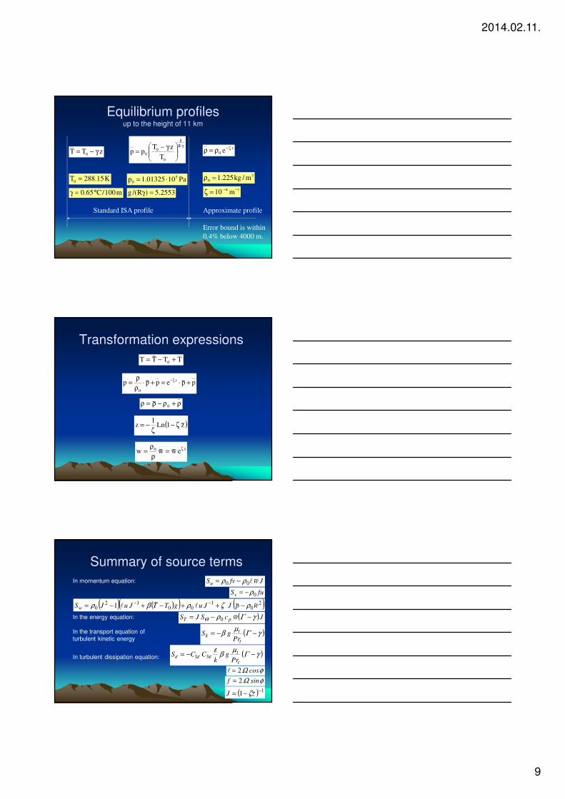
zTT 0 γ−=γ

γ−=

R

g

0

00

T

zTpp

z

0 e ζ−ρ=ρ

m100/C65.0 °=γ

K15.288T0 = Pa1001325.1p 5

0 ⋅=3

0 m/kg225.1=ρ

2553.5)R/(g =γ14 m10 −−=ζ

Standard ISA profile Approximate profile

Error bound is within

0.4% below 4000 m.

Equilibrium profiles up to the height of 11 km

TTT~

T 0 +−=

ρ+ρ−ρ=ρ 0~

( )z~1Ln1

z ζ−ζ

−=

z0 ew~w~wζ=

ρ

ρ=

Transformation expressions

pp~epp~p z

0

+⋅=+⋅ρ

ρ= ζ−

Summary of source terms

In the energy equation:

In the transport equation of turbulent kinetic energy

In turbulent dissipation equation:

In momentum equation: Jw~fvSu l00 ρρ −=

fuSv 0ρ−=

φΩ sinf 2=

φΩ cos2=l

( ) ( )( ) ( )20

100

120 1 w~p~JJugTT

~JuJSw ρζρβρ −++−+−= −−

ll

( )Jw~cSJS pT γΓρΘ −−= 0

( )γΓµ

β −−=t

tk

PrgS

( )γΓµ

βε

εεε −−=t

t

Prg

kCCS 31

( ) 11

−−= z~J ζ

2014.02.11.

10

Related publications[1] Kristóf G, Rácz N, Balogh M: Adaptation of Pressure Based CFD Solvers for Mesoscale Atmospheric Problems,

Boundary-Layer Meteorol, 2008.[2] N.Rácz, G.Kristóf, T.Weidinger, M.Balogh: Simulation of gravity waves and model validation to laboratory

experiments, CD, Urban Air Quality Conf. Cyprus, 2007.[3] G.Kristóf, N.Rácz, M.Balogh: Adaptation of pressure based CFD solvers to urban heat island convection

problems, CD, Urban Air Quality Conf. Cyprus, 2007.

[4] G.Kristóf, N.Rácz, Tamás Bányai, Norbert Rácz: Development of computational model for urban heat island convection using general purpose CFD solver, ICUC6, 6-th Int.Conf.on Urban Climate, Göteborg, pp. 822-825., 2006.

[5] G. Kristóf, T. Weidinger, T. Bányai, N. Rácz, T.Gál, J.Unger: A városi hősziget által generált konvekció modellezése általános célú áramlástani szoftverrel - példaként egy szegedi alkalmazással, III. Magyar Földrajzi Konferencia, Budapest, 2006., Bp, CD

[6] Kristóf G., Rácz N., Bányai T., Gál T., Unger J., Weidinger T.: A városi hősziget által generált konvekció modellezése általános célú áramlástani szoftverrel− összehasonlítás kisminta kísérletekkel A 32. Meteorológiai Tudományos Napok előadásai. Országos Meteorológiai Szolgálat, Bp., 2006

[7] Dr. Lajos T., Dr. Kristóf G., Dr. Goricsán I., Rácz N.: Városklíma vizsgálatok a BME Áramlástan Tanszékén, hősziget numerikus szimulációja VAHAVA projekt (A globális klímaváltozás: hazai hatások és válaszok) zárókonferenciája Bp. CD, 2006

[8] Rácz N. és Kristóf G.: Hősziget cirkuláció kisminta méréseinek összehasonlítása saját fejlesztésű LES modellel Egyetemi Meteorológiai Füzetek No. 20 ELTE Meteorológiai Tanszék, Bp. 173-176, 2006.

[9] M. Balogh, G. Kristóf:Automated Grid Generation for Atmospheric Dispersion Simulations, pp.1-6., MICROCAD konferencia, Miskolc, 2007.

Two validation examples

Comparison with the results of water tank experiments

Experimetal setup

Uniformly stratified salt water:ρ= 1.03- 1.00 g/cm3

Typical towing speeds:U = 1-15 cm/s

Brunt-Vaisala frequency range:N= 1.09-1.55 1/s

Reexp ≈ 102-103

Studied obstacle heights:h= 20mm, 40mm

Gyüre, B. and Jánosi, I.M., 2003. Stratified flow over asymmetric and double bell-shaped obstacles. Dynamics of Atmospheres and Oceans 37, 155-170.

z

gN

∂

ρ∂

ρ−=

2014.02.11.

11

z(x) = a exp(-b|x|2γ )different parameterset for positive andnegative x

Numerical mesh

U/Nh = 1.4

U/Nh = 0.3

Gravity wavesGyüre, B. and Jánosi, I.M., 2003. Stratified flow over asymmetric and double bell-shaped obstacles. Dynamics of Atmospheres and Oceans 37, 155-170.

Simulation vs. experimental data

Wave length Amplitude

2014.02.11.

12

A.Cenedese, P.Monti: Interaction between an Inland Urban Heat Island and a Sea-Breeze Flow: A Laboratory Study, 2003.

Experimental setup

920 k prismatic cells

Streamlines colored byvelocity magnitude

Fine structure of the thermal boundary layer

Large eddy simulation in FLUENT

PIV results(Cenedese &Monti 2003)

CFD results

Thermal convectionA.Cenedese, P.Monti: Interaction between an Inland Urban

Heat Island and a Sea-Breeze Flow: A Laboratory Study, 2003.

2014.02.11.

13

Comparison of velocity and temperature profiles

PIV

CFD

PIV

CFD

Some more application examples

Full scale simulations

Meso scale atmospheric dispersion

Orography of Pilis mountain

Evolution of surface concentration

2014.02.11.

14

Wind speed: 3m/sInjection velocity: 5 m/s

Chimney height 180 mStandard (stable) temperature profile

Micro-scale atmospheric dispersionStreamlines colored by temperature

Kelvin-Helmholtz instability

Com domain: 25 km x 5.5 kmTemperature difference 20 °C

Satellite image about Guadalupe island

First CFD results

Von Kármán vortices behind a volcanic island

2014.02.11.

15

Targeted application areas• Local circulation modeling:

– Urban heat island convection, ventilation of cities;

– See breeze;– Valley breeze.

• Power generation and pollution control:– Assessment of wind power potential,

optimization of wind farms;– Plumes emitted by cooling towers

and chimneys;– Dispersion of pollutant in the urban

atmosphere.• Research of meteorological phenomena:

– Gravity waves;– Cloud formation;– Flow around high mountain.

• Simulation of disasters:– Large scale fires (e.g. in forest

fires or town fires);– Volcanic plumes.