7. gaining insight - agsm | unsw business school · 7. gaining insight the product of ... anal y...
TRANSCRIPT

7. Gaining Insight
The product of any anal ysis should be new insights whichclarify a course of action.
>

7. Gaining Insight
The product of any anal ysis should be new insights whichclarify a course of action. The process of evaluation has threepar ts: (See Clemen, Pac kage.)
>

7. Gaining Insight
The product of any anal ysis should be new insights whichclarify a course of action. The process of evaluation has threepar ts: (See Clemen, Pac kage.)
7. 1 De t erminis tic evaluation
➣ Sensitivity analysis
➣ Tornado diagrams
7.2 Probabilis tic evaluation
➣ Cumulative probability distr ibution
➣ Sensitivity to probability
7.3 Expect ed Value of Infor mation
➣ Expect ed Value of Per fect Infor mation (VPI)
➣ Expect ed Value of imper fect infor mation
>

Lecture 9 UNSW © 2009 Page 2
7. 1 Det erminis tic Ev aluation
Det erminis tic ev aluation may be closes t to the way mos tanal yses are per for med outside decision analysis.
Sensitivity analysis provides the ability to det ermine themos t impor tant fact ors which affect either the decision orthe value (“the bott om line”). We can then use the Tornadodiag ram to illus trat e the relative sensitivities of eachvariable.
< >

Lecture 9 UNSW © 2009 Page 2
7. 1 Det erminis tic Ev aluation
Det erminis tic ev aluation may be closes t to the way mos tanal yses are per for med outside decision analysis.
Sensitivity analysis provides the ability to det ermine themos t impor tant fact ors which affect either the decision orthe value (“the bott om line”). We can then use the Tornadodiag ram to illus trat e the relative sensitivities of eachvariable.
Variables for Glix:P r o b a b i l i t i e s
10 50 90
Market size (Gigag rams) 0.2 1 2
Market share (%) 15 20 25
Mfg. Costs ($/kg) 1 1.5 2
Mktg. Costs ($/kg) 0.5 0.75 1
↑baseline
< >

Lecture 9 UNSW © 2009 Page 3
Conducting sensitivity analysis on uncertainties:
St ep 1:
< >

Lecture 9 UNSW © 2009 Page 3
Conducting sensitivity analysis on uncertainties:
St ep 1: Build a deter ministic value model which uses theuncer tainties identified in the frame and calculatesaccording to the decision crit erion.
St ep 2:
< >

Lecture 9 UNSW © 2009 Page 3
Conducting sensitivity analysis on uncertainties:
St ep 1: Build a deter ministic value model which uses theuncer tainties identified in the frame and calculatesaccording to the decision crit erion.
St ep 2: Choose a low (10th percentile — a 10% chance of thevariable falling below X ), base (50%), and high (90%)value for each uncertain event.
St ep 3:
< >

Lecture 9 UNSW © 2009 Page 3
Conducting sensitivity analysis on uncertainties:
St ep 1: Build a deter ministic value model which uses theuncer tainties identified in the frame and calculatesaccording to the decision crit erion.
St ep 2: Choose a low (10th percentile — a 10% chance of thevariable falling below X ), base (50%), and high (90%)value for each uncertain event.
St ep 3: Run the model with all uncertainties set at their basevalues, and record the calculated value.
St ep 4:
< >

Lecture 9 UNSW © 2009 Page 3
Conducting sensitivity analysis on uncertainties:
St ep 1: Build a deter ministic value model which uses theuncer tainties identified in the frame and calculatesaccording to the decision crit erion.
St ep 2: Choose a low (10th percentile — a 10% chance of thevariable falling below X ), base (50%), and high (90%)value for each uncertain event.
St ep 3: Run the model with all uncertainties set at their basevalues, and record the calculated value.
St ep 4: Run the model swinging each var iable from its 10t hpercentile to its 90th, while holding all other var iablesat their base values. Record the calculated value ateach setting.
St ep 5:
< >

Lecture 9 UNSW © 2009 Page 3
Conducting sensitivity analysis on uncertainties:
St ep 1: Build a deter ministic value model which uses theuncer tainties identified in the frame and calculatesaccording to the decision crit erion.
St ep 2: Choose a low (10th percentile — a 10% chance of thevariable falling below X ), base (50%), and high (90%)value for each uncertain event.
St ep 3: Run the model with all uncertainties set at their basevalues, and record the calculated value.
St ep 4: Run the model swinging each var iable from its 10t hpercentile to its 90th, while holding all other var iablesat their base values. Record the calculated value ateach setting.
St ep 5: Plot a Tor nado diag ram using the data.
< >

Lecture 9 UNSW © 2009 Page 4
Building the value model
The value model for Glix:
Fixed inputs:Discount rat e = 10% p.a.Tax rat e = 40%Glix price/k g = $5.00Project length = 10 year s
< >

Lecture 9 UNSW © 2009 Page 4
Building the value model
The value model for Glix:
Fixed inputs:Discount rat e = 10% p.a.Tax rat e = 40%Glix price/k g = $5.00Project length = 10 year s
NPV of Glix = (Revenue − Cost)× Discount Fact or for eachyear
Revenue = Price × Volume
Volume = Market Size × Market Share
Cos t = (Manufactur ing Cos t + Market Cost) × Volume
< >

Lecture 9 UNSW © 2009 Page 5
Base case value for Glix:
Revenue = $5.00 × 1,000,000 kg × 20%
Cos ts → ($1.50 + $0.75) × 1,000,000
→ $1,000,000 − $450,000
→ $550,000/year × (1−0.40) after tax
→ $330,000 × 10 year s × 10%
< >

Lecture 9 UNSW © 2009 Page 5
Base case value for Glix:
Revenue = $5.00 × 1,000,000 kg × 20%
Cos ts → ($1.50 + $0.75) × 1,000,000
→ $1,000,000 − $450,000
→ $550,000/year × (1−0.40) after tax
→ $330,000 × 10 year s × 10%
∴ Profit = $1,209,525
< >

Lecture 9 UNSW © 2009 Page 5
Base case value for Glix:
Revenue = $5.00 × 1,000,000 kg × 20%
Cos ts → ($1.50 + $0.75) × 1,000,000
→ $1,000,000 − $450,000
→ $550,000/year × (1−0.40) after tax
→ $330,000 × 10 year s × 10%
∴ Profit = $1,209,525
ValueModel
Discount rat e
Tax rat e
Glix Price
What you want< >

Lecture 9 UNSW © 2009 Page 6
Plot the Tor nado using graph paper or softw are.
St ep 1:
< >

Lecture 9 UNSW © 2009 Page 6
Plot the Tor nado using graph paper or softw are.
St ep 1: Calculat e the swing of each var iable, from the 10t h tothe 90t h percentile.
St ep 2:
< >

Lecture 9 UNSW © 2009 Page 6
Plot the Tor nado using graph paper or softw are.
St ep 1: Calculat e the swing of each var iable, from the 10t h tothe 90t h percentile.
St ep 2: Rank in order the swings in value from larges t tosmalles t.
St ep 3:
< >

Lecture 9 UNSW © 2009 Page 6
Plot the Tor nado using graph paper or softw are.
St ep 1: Calculat e the swing of each var iable, from the 10t h tothe 90t h percentile.
St ep 2: Rank in order the swings in value from larges t tosmalles t.
St ep 3: Dr aw a hor izontal line and deter mine an appropr iatevalue scale.
St ep 4:
< >

Lecture 9 UNSW © 2009 Page 6
Plot the Tor nado using graph paper or softw are.
St ep 1: Calculat e the swing of each var iable, from the 10t h tothe 90t h percentile.
St ep 2: Rank in order the swings in value from larges t tosmalles t.
St ep 3: Dr aw a hor izontal line and deter mine an appropr iatevalue scale.
St ep 4: Dr aw a ver tical line which cuts the horizont al line atthe base case value.
St ep 5:
< >

Lecture 9 UNSW © 2009 Page 6
Plot the Tor nado using graph paper or softw are.
St ep 1: Calculat e the swing of each var iable, from the 10t h tothe 90t h percentile.
St ep 2: Rank in order the swings in value from larges t tosmalles t.
St ep 3: Dr aw a hor izontal line and deter mine an appropr iatevalue scale.
St ep 4: Dr aw a ver tical line which cuts the horizont al line atthe base case value.
St ep 5: Dr aw hor izontal bars for each uncertainty relative totheir swings in value.
< >

Lecture 9 UNSW © 2009 Page 7
The Tor nado Diag ram.
Base Case Value $1,209,525
Market Size:
Market Share:
Manufactur ing Cos ts:
Marketing Costs:
See Clemen (Reading 18) and Skinner (Reading 20) forfur ther discussion.
< >

Lecture 9 UNSW © 2009 Page 8
Simplifying the model:
Tornado diagrams provide insight into the key uncer taintiesaf fecting the decision.
< >

Lecture 9 UNSW © 2009 Page 8
Simplifying the model:
Tornado diagrams provide insight into the key uncer taintiesaf fecting the decision.
The decision model can then be simplified using the insightsgained from the sensitivity analysis. This is very impor tantfor large models with man y uncer tainties.
With project Glix, the most impor tant uncertainty is MarketSize, and the least impor tant is Marketing Costs, from theTornedo Diagram above.
Impor tant : alw ays str ive to simplify your Influence Diagrams:use Tor nado diag rams and your intuition to reduce thedeg ree of comple xity of the ID — they are much more usefulwhen simple!
< >

Lecture 9 UNSW © 2009 Page 9
Influence Diagram of Glix Decision
NPV of Glix
Revenue
Cos ts
Volume
Market
Size
Market
Share
Manufactur ing
Cos ts
Launch
Glix
< >

Lecture 9 UNSW © 2009 Page 10
7.2 Probabilis tic Ev aluation
Det erminis tic uncer tainty is impor tant for identifying keyvariables but does not provide insight into the likelihood ofany scenar io.
< >

Lecture 9 UNSW © 2009 Page 10
7.2 Probabilis tic Ev aluation
Det erminis tic uncer tainty is impor tant for identifying keyvariables but does not provide insight into the likelihood ofany scenar io.
The cumulative probability distr ibution provides a graphicalrisk profile for the project or each alter native.
(This is more technical: see David C. Skinner, Introduction toDecision Analysis (Gainesville, Fl., 2nd. ed., 1999), pp.11 2−113, 218−220.)
But see Laura’s decision below.
< >

Lecture 9 UNSW © 2009 Page 11
Another alter native? Selling the Glix project.
In addition to launching Glix, the company also want ed toev aluat e the alt ernatives of selling and/or licensing theproduct.
< >

Lecture 9 UNSW © 2009 Page 11
Another alter native? Selling the Glix project.
In addition to launching Glix, the company also want ed toev aluat e the alt ernatives of selling and/or licensing theproduct.
The influence diagram for selling Glix to another company:
NPV of GlixSell
Glix
Selling Costs
Sales Price
Large Company
Of fer
Small Company
Of fer Probability of
Large Offer
The EMV of Selling = $320,000.< >

Lecture 9 UNSW © 2009 Page 12
Or Licensing Glix:
The company could license Glix and receive roy alties fromthe sales.
NPV of Glix
License
Glix
Revenue
Volume
Market Size
Market Share
Royalty
Rate
Licensing
Cos ts
< >

Lecture 9 UNSW © 2009 Page 12
Or Licensing Glix:
The company could license Glix and receive roy alties fromthe sales.
NPV of Glix
License
Glix
Revenue
Volume
Market Size
Market Share
Royalty
Rate
Licensing
Cos ts
The EMV of Licensing = $1,135,000< >

Lecture 9 UNSW © 2009 Page 13
Compar ing alt ernatives
We can compare each alter native on a consis t ent basis,thereby full y examining the risk and opportunity of eachalt ernative.
< >

Lecture 9 UNSW © 2009 Page 13
Compar ing alt ernatives
We can compare each alter native on a consis t ent basis,thereby full y examining the risk and opportunity of eachalt ernative.
Choosing wisely:
Dominance—
➣
< >

Lecture 9 UNSW © 2009 Page 13
Compar ing alt ernatives
We can compare each alter native on a consis t ent basis,thereby full y examining the risk and opportunity of eachalt ernative.
Choosing wisely:
Dominance—
➣ Dominance can be de t erminis tic or stoc hastic
➣
< >

Lecture 9 UNSW © 2009 Page 13
Compar ing alt ernatives
We can compare each alter native on a consis t ent basis,thereby full y examining the risk and opportunity of eachalt ernative.
Choosing wisely:
Dominance—
➣ Dominance can be de t erminis tic or stoc hastic
➣ Allows infer ior alt ernatives to be eliminat ed
➣ Is alway s bett er than the other alter natives
It turns out, with fur ther analysis, that none of the threealt ernatives shows complet e dominance over the other two.
The “sell” alter native, however, is less attractive, based onan EMV of $320,455.
< >

Lecture 9 UNSW © 2009 Page 14
Sensitivity to probability :
Sensitivity to probability is similar to det erminis tic sensitivityanal ysis in that the aim is to identify var iables which wouldchange the decision.
< >

Lecture 9 UNSW © 2009 Page 14
Sensitivity to probability :
Sensitivity to probability is similar to det erminis tic sensitivityanal ysis in that the aim is to identify var iables which wouldchange the decision.
Having said that any subjective probability whichincor porat es the exper t’s available knowledge, beliefs,exper iences, and data is cor rect, we need to know howsensitive the decision is to any par ticular probability. Thiswill help us choose between launching or licensing Glix.
It turns out that we should launch if we are confident thatlaunc hing has a great er than 40% chance of success.
< >

Lecture 9 UNSW © 2009 Page 15
Games Agains t Nature: Gaining Insight —The Value of Infor mation
Today’s topics:
1. The Value of Per fect Infor mation
a. For Laura
b. For Glix
2. Probabilis tic Sensitivity Analysis
a. For Laura
3. The Value of Imper fect Infor mation
a. For Laura
b. For Glix
< >

Lecture 9 UNSW © 2009 Page 16
1. The Value of Infor mation
We can deter mine the value of gat hering additionalinfor mation before spending time or money to gat her it.
The Value of Per fect Infor mation is the easiest to calculat e,and provides an upper boundary as to the mos t we shouldever spend on new infor mation.
Mos t companies over-inves t in infor mation, spending more thanit is worth to them.
The Value of Per fect Infor mation (VPI) is the mos t that weshould spend for new infor mation which is not 100% reliable.
We would only value Per fect Infor mation if it changed ourdecisions, other wise not.
< >

Lecture 9 UNSW © 2009 Page 17
1a. Laura’s Case — The Expected Value of Per fectInfor mation (VPI)
Laur a could reduce uncertainty through infor mationgathering:
➣
< >

Lecture 9 UNSW © 2009 Page 17
1a. Laura’s Case — The Expected Value of Per fectInfor mation (VPI)
Laur a could reduce uncertainty through infor mationgathering:
➣ Laur a could employ a market-research firm to tes t for theacceptance and demand for Retro.
➣
< >

Lecture 9 UNSW © 2009 Page 17
1a. Laura’s Case — The Expected Value of Per fectInfor mation (VPI)
Laur a could reduce uncertainty through infor mationgathering:
➣ Laur a could employ a market-research firm to tes t for theacceptance and demand for Retro.
➣ If tot all y reliable (no errors), then
— if “Retro is definit ely a Goer”, then a retur n of$2 40k, less the price of the Trial
—
< >

Lecture 9 UNSW © 2009 Page 17
1a. Laura’s Case — The Expected Value of Per fectInfor mation (VPI)
Laur a could reduce uncertainty through infor mationgathering:
➣ Laur a could employ a market-research firm to tes t for theacceptance and demand for Retro.
➣ If tot all y reliable (no errors), then
— if “Retro is definit ely a Goer”, then a retur n of$2 40k, less the price of the Trial
— if the Trial indicates Retro is a “Fizzer,” thenchoose a net retur n of $200k with Trad, less thepr ice of the Trial
< >
Lecture 9 UNSW © 2009 Page 18
Laura has two decisions to make:
1.
< >

Lecture 9 UNSW © 2009 Page 18
Laura has two decisions to make:
1. Whet her or not to Trial, which is relat ed to the priceof the Trial.
For a given price, should she Trial?
If not, then the decision is as before: Trad or Retro?
2.
< >

Lecture 9 UNSW © 2009 Page 18
Laura has two decisions to make:
1. Whet her or not to Trial, which is relat ed to the priceof the Trial.
For a given price, should she Trial?
If not, then the decision is as before: Trad or Retro?
2. If she buys the Trial, what’s the most she should payfor it?
To answer this, we need to examine her best choicewit h the Trial: Trad or Retro?
The expect ed value of infor mation is the difference betweenLaur a’s expect ed retur ns wit h the Trial and wit hout the Trial.
< >

Lecture 9 UNSW © 2009 Page 19
Laur a’s Influence Diagram: To Trial or Not?
Market
Tr ial
Market
demand
Tr ial or
Tr ad or
Retro?
Tr ad or
Retro?
Payoff
The arrow from the Market Trial chance node to Laur a’ssecond decision represents the infor mation (per fect or not)that she receives from the Trial.
That infor mation in turn is influenced (perfectl y or not) bythe actual Market Demand.
If the Trial is 100% reliable, then there is no uncer tainty afterthe Trial, and hence no arrow from the Market Demanduncer tainty to the Pay off: all uncertainty is resol ved beforethe Trad/R etro decision is made.
< >

Lecture 9 UNSW © 2009 Page 20
Laur a: the VPI
What Laura would like to know is what a specific piece ofinfor mation implies for the eventual market demand forRetro, that is:
Probability (Retro is a Goer, given that Trial says “Goer” )
With per fect infor mation, this probability is 1.
< >

Lecture 9 UNSW © 2009 Page 20
Laur a: the VPI
What Laura would like to know is what a specific piece ofinfor mation implies for the eventual market demand forRetro, that is:
Probability (Retro is a Goer, given that Trial says “Goer” )
With per fect infor mation, this probability is 1.
Q: What is Laura’s estimat e of the probability that theClair voy ant will say: “Goer”?
< >

Lecture 9 UNSW © 2009 Page 21
The new decision tree, including the tes t marketing decision:
L
L N
$200N
$150$2 40
L L
N $200
$2 40
$200 N
$150
No Trial
Tr adRetro
Goer
0.4
Fizzer
0.6
Tr ial
“Goer” “Fizzer”
Retro Tr ad
Goer
1.0
T R
Fizzer
1.0
< >

Lecture 9 UNSW © 2009 Page 21
The new decision tree, including the tes t marketing decision:
L
L N
$200N
$150$2 40
L L
N $200
$2 40
$200 N
$150
No Trial
Tr adRetro
Goer
0.4
Fizzer
0.6
Tr ial
“Goer” “Fizzer”
Retro Tr ad
Goer
1.0
T R
Fizzer
1.0
$186
Tr ad
$200
✘
$240 $150
< >

Lecture 9 UNSW © 2009 Page 21
The new decision tree, including the tes t marketing decision:
L
L N
$200N
$150$2 40
L L
N $200
$2 40
$200 N
$150
No Trial
Tr adRetro
Goer
0.4
Fizzer
0.6
Tr ial
“Goer” “Fizzer”
Retro Tr ad
Goer
1.0
T R
Fizzer
1.0
$186
Tr ad
$200
✘
$240 $150
Retro
$2 40
✘ Tr ad
$200
✘
0.4 0.6
$216
Tr ial✘
The Shoe Decision with Per fect Infor mation
(R emember : the Trial is 100% accurat e.)
< >

Lecture 9 UNSW © 2009 Page 22
The new decision tree has four decision nodes :
1. whet her or not to tes t,
2. which range to choose without tes ting,
3. which range to choose if the tes t says “Goer,” and
4. which range to choose if the tes t says “Fizzer.”
< >

Lecture 9 UNSW © 2009 Page 22
The new decision tree has four decision nodes :
1. whet her or not to tes t,
2. which range to choose without tes ting,
3. which range to choose if the tes t says “Goer,” and
4. which range to choose if the tes t says “Fizzer.”
The second, third, and four th decision nodes are trivial:
2. Choose Tr ad if Laur a chooses not to tes t. (W ithouttesting, Trad pay s $200k, which is better than the $186kexpect ed from Retro.)
3. choose Retro if the tes t says it’s a “Goer”,
4. other wise choose Trad,
< >

Lecture 9 UNSW © 2009 Page 23
How many chance nodes ?
➣ Possibl y three: the outcome of the tes t, and the 2outcomes if she chooses Retro.
➣ But if the tes t is 100% reliable, it would rule out anyuncer tainty about Retro, one way or the other, and so thesecond and third chance nodes disappear.
< >

Lecture 9 UNSW © 2009 Page 24
Ques tion: What is Laura’s estimat e of the probability of the100%-reliable tes t coming up with Retro as a “Goer”?
< >

Lecture 9 UNSW © 2009 Page 24
Ques tion: What is Laura’s estimat e of the probability of the100%-reliable tes t coming up with Retro as a “Goer”?
Well, her “prior” that Retro will be a Goer is probability =0.4.
< >

Lecture 9 UNSW © 2009 Page 24
Ques tion: What is Laura’s estimat e of the probability of the100%-reliable tes t coming up with Retro as a “Goer”?
Well, her “prior” that Retro will be a Goer is probability =0.4.And consis tency dict ates that this is also her belief thattesting will give the result that Retro is a “Goer”.
➣
< >

Lecture 9 UNSW © 2009 Page 24
Ques tion: What is Laura’s estimat e of the probability of the100%-reliable tes t coming up with Retro as a “Goer”?
Well, her “prior” that Retro will be a Goer is probability =0.4.And consis tency dict ates that this is also her belief thattesting will give the result that Retro is a “Goer”.
➣ Laur a’s expect ed retur n from the Trial:
$2 40k × 0.4(t he Tr ial indicated that Retro is a “Goer” and Laurachooses Retro)
+ $200k × 0.6(t he Tr ial indicated that Retro will “Fizz” and Laurachooses Trad)
= $216k
< >

Lecture 9 UNSW © 2009 Page 25
Laur a’s Expect ed VPI
➣ Her expect ed retur n of No Trial = $200k from choosingTr ad(which is higher than the expect ed retur n of $186k ofchoosing Retro),
∴
< >

Lecture 9 UNSW © 2009 Page 25
Laur a’s Expect ed VPI
➣ Her expect ed retur n of No Trial = $200k from choosingTr ad(which is higher than the expect ed retur n of $186k ofchoosing Retro),
∴ The maximum Laura would be prepared to pay for the Trialis:
$216k − $200k = $16k .
This is the Expect ed Value of Per fect Infor mation in thisdecision;
The expect ed value of imper fect infor mation would be lessthan $16k .
For an on-line applet for simple calculations of EVPI, seehttp://www.cs.usask.ca/content/resources/tutorials/csconcepts/1999_6/Tutorial/Java/EVPIApp/evpi.html
< >

Lecture 9 UNSW © 2009 Page 26
1b. Calculating the VPI of the Glix case
VPI is calculated by placing the uncertainty you want toev aluat e before the decision. Then, recalculat e the expect edvalue.Focus on Market Size (MS) uncertainty :L = 200k, M = 1m, H = 2m.
Or iginal tree: EMV = $1,310,910
Launch
$1.310m
License
$1.135m
Sell
$320k
$3.237m$1.209m−$413k
0.25
MS: 2m
0.5
MS: 1m
0.25
MS: 200k
✘ ✘Launch
$1.310m
< >

Lecture 9 UNSW © 2009 Page 27
Plot the Tree wit h Perfect Infor mation
Tr ee wit h per fect infor mation: EMV = $1,697,866
$1.698m
Launch
$3.237m
Launch
$1.209m
License
$1.135m
0.25
MS: 2m
0.5
MS: 1m
0.25
MS: 200kClair voy ant :
< >

Lecture 9 UNSW © 2009 Page 27
Plot the Tree wit h Perfect Infor mation
Tr ee wit h per fect infor mation: EMV = $1,697,866
$1.698m
Launch
$3.237m
Launch
$1.209m
License
$1.135m
0.25
MS: 2m
0.5
MS: 1m
0.25
MS: 200kClair voy ant :
∴ VPI = $1,697,866 − $1,310,910 = $386,956
< >

Lecture 9 UNSW © 2009 Page 28
2. Probabilis tic Sensitivity Analysis — Laura
Laur a’s belief in the probability p of Retro’s being a Goer =0.4
At what (cross-over) prior probability p̂ would Laura chooseRetro wit h No Trial?
< >

Lecture 9 UNSW © 2009 Page 28
2. Probabilis tic Sensitivity Analysis — Laura
Laur a’s belief in the probability p of Retro’s being a Goer =0.4
At what (cross-over) prior probability p̂ would Laura chooseRetro wit h No Trial?
What would the expect ed value of a complet ely accur ateTr ial be then?
If Laura’s probability that Retro is a Goer is p, then thatmus t be her best guess as to the probability of the event thatthe Trial says Retro is a “Goer”.
To be consis t ent, what else could she believe?
If she’s uncer tain about Retro’s success, then she cannot becer tain that a 100%-reliable Trial would say that Retrowould, or would not, be a “success”.
< >

Lecture 9 UNSW © 2009 Page 29
Laura’ s Decision Tree wit h Perfect Infor mation:
L
L N
$200N
$150$2 40
L L
N $200
$2 40
$200 N
$150
No Trial
Tr adRetro
Goer
p
Fizzer
(1−p)
Tr ial
“Goer”
p
“Fizzer”
(1−p)
Retro Tr ad
Goer
1.0
Fizzer
1.0
< >

Lecture 9 UNSW © 2009 Page 29
Laura’ s Decision Tree wit h Perfect Infor mation:
L
L N
$200N
$150$2 40
L L
N $200
$2 40
$200 N
$150
No Trial
Tr adRetro
Goer
p
Fizzer
(1−p)
Tr ial
“Goer”
p
“Fizzer”
(1−p)
Retro Tr ad
Goer
1.0
Fizzer
1.0
$150+90p
< >

Lecture 9 UNSW © 2009 Page 29
Laura’ s Decision Tree wit h Perfect Infor mation:
L
L N
$200N
$150$2 40
L L
N $200
$2 40
$200 N
$150
No Trial
Tr adRetro
Goer
p
Fizzer
(1−p)
Tr ial
“Goer”
p
“Fizzer”
(1−p)
Retro Tr ad
Goer
1.0
Fizzer
1.0
$150+90p
$240
Retro
$2 40
✘
< >

Lecture 9 UNSW © 2009 Page 29
Laura’ s Decision Tree wit h Perfect Infor mation:
L
L N
$200N
$150$2 40
L L
N $200
$2 40
$200 N
$150
No Trial
Tr adRetro
Goer
p
Fizzer
(1−p)
Tr ial
“Goer”
p
“Fizzer”
(1−p)
Retro Tr ad
Goer
1.0
Fizzer
1.0
$150+90p
$240
Retro
$2 40
✘
$150
Tr ad
$200
✘
$200+40p
< >

Lecture 9 UNSW © 2009 Page 29
Laura’ s Decision Tree wit h Perfect Infor mation:
L
L N
$200N
$150$2 40
L L
N $200
$2 40
$200 N
$150
No Trial
Tr adRetro
Goer
p
Fizzer
(1−p)
Tr ial
“Goer”
p
“Fizzer”
(1−p)
Retro Tr ad
Goer
1.0
Fizzer
1.0
$150+90p
$240
Retro
$2 40
✘
$150
Tr ad
$200
✘
$200+40p
Tr ial✘
The Shoe Decision with Per fect Infor mation
(i.e. a 100%-reliable tes t)
< >

Lecture 9 UNSW © 2009 Page 30
The expect ed value of choosing Retro in the absence of aTr ial:
$150 + 90p,
< >

Lecture 9 UNSW © 2009 Page 30
The expect ed value of choosing Retro in the absence of aTr ial:
$150 + 90p,
compared with the unchanged value of $200 of choosingTr ad.
∴ the cross-over probability p̂ is 0.556.
< >

Lecture 9 UNSW © 2009 Page 30
The expect ed value of choosing Retro in the absence of aTr ial:
$150 + 90p,
compared with the unchanged value of $200 of choosingTr ad.
∴ the cross-over probability p̂ is 0.556.
On the Trial side of the tree, to be consis t ent the probabilityof the tes t indicating that Retro will be a “Goer” must be p,and a “Fizzer” 1 − p.
The expect ed value of choosing Trial =200 + 40p.
< >

Lecture 9 UNSW © 2009 Page 31
Plotting these expect ed values as a function of the priorprobability p of Goer:
Pr ior probability of Goer, p
EM
V $
0 0.25 0.5 0.75 10
50
100
150
200
250
•
•
•
$186
$200
$216
< >

Lecture 9 UNSW © 2009 Page 31
Plotting these expect ed values as a function of the priorprobability p of Goer:
Pr ior probability of Goer, p
EM
V $
0 0.25 0.5 0.75 10
50
100
150
200
250
•
•
•
$186
$200
$216
Tr ad= $200
< >

Lecture 9 UNSW © 2009 Page 31
Plotting these expect ed values as a function of the priorprobability p of Goer:
Pr ior probability of Goer, p
EM
V $
0 0.25 0.5 0.75 10
50
100
150
200
250
•
•
•
$186
$200
$216
Tr ad= $200
Retro= $150+90p
< >

Lecture 9 UNSW © 2009 Page 31
Plotting these expect ed values as a function of the priorprobability p of Goer:
Pr ior probability of Goer, p
EM
V $
0 0.25 0.5 0.75 10
50
100
150
200
250
•
•
•
$186
$200
$216
Tr ad= $200
Retro= $150+90p
Sensitivity Diagram: Expected Value agains t Prior Probability pof Goer
< >

Lecture 9 UNSW © 2009 Page 32
The Expected Value of Per fect Infor mation (VPI)— Laur a
The or ange line: the expect ed value with the Trial.
∴ the minimum ver tical dis tance down from the or ange lineto green or red line is the Expected Value of Per fectInfor mation at any probability of Goer p.
At p = 0.4 ➣ the expect ed value of Retro is $186,
➣ the value of Trad is $200,
➣ and the value with Trial is $216,
The Expected VPI = the improv ement in expect ed value withthe Trial,
= the difference between the or ange line and the nexthighes t value, whether Tr ad or Retro.
= $216k − $200k = $16,000 when p = 0.4
< >

Lecture 9 UNSW © 2009 Page 33
Cer tainty and the Expected VPI
When Laura is cer tain about the outcome with Retro, thevalue of reducing uncertainty is zero.
< >

Lecture 9 UNSW © 2009 Page 33
Cer tainty and the Expected VPI
When Laura is cer tain about the outcome with Retro, thevalue of reducing uncertainty is zero.
She is certain twice: when she
➣ knows that Retro is a Goer ( p = 1.0), or
➣ is certain that Retro is a Fizzer ( p = 0.0).
< >

Lecture 9 UNSW © 2009 Page 33
Cer tainty and the Expected VPI
When Laura is cer tain about the outcome with Retro, thevalue of reducing uncertainty is zero.
She is certain twice: when she
➣ knows that Retro is a Goer ( p = 1.0), or
➣ is certain that Retro is a Fizzer ( p = 0.0).
The cross-over probability p̂ at which choosing Retro has ahigher expect ed value than choosing Trad is 0.556.
Probability p̂ cor responds to the highest expect ed VPI, andoccur s when her decision is most sensitive to the probabilityp of Goer.
Highes t expect ed VPI (@ p̂ = 0.556) = $22,240.
< >

Lecture 9 UNSW © 2009 Page 34
Which var iables are mos t cr ucial? — Laur a
We hav e considered the decision’s sensitivity to a singlevariable: the probability that Retro is a Goer.
But there might be some uncertainty about the payoffs ofTr ad and Retro under the two possibilities.
Whic h is the most critical variable on which to per for m asensitivity analysis?
Holding all other var iables at their most likel y values, one byone each var iable be taken from its lowest likel y value to itshighes t, and the effect of this on the optimand (the var iablebeing maximised or minimised) be plott ed.
A Tornado plot, wit h the var iable wit h the great es t ef fect ontop and that with the least on the bott om.
Those var iables which can push the maximand lowest arethe ones that should be subject to a sensitivity analysis.
< >

Lecture 9 UNSW © 2009 Page 35
3a. Laura’s Case: The Expected Value ofImper fect Infor mation
But what if the Trial is not 100%-reliable?
< >

Lecture 9 UNSW © 2009 Page 35
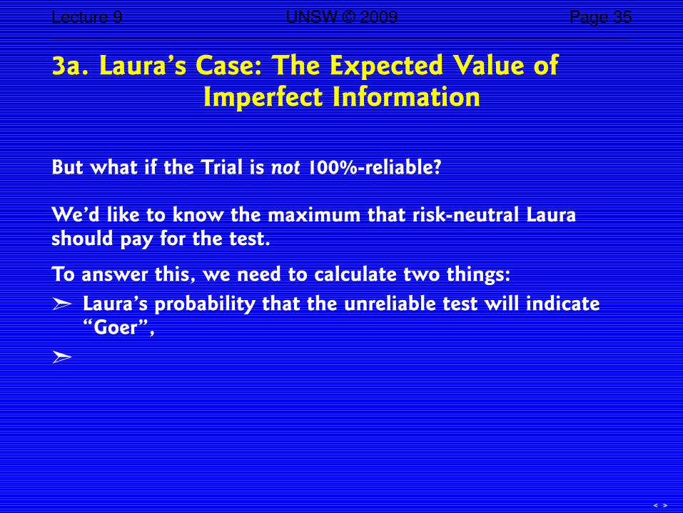
3a. Laura’s Case: The Expected Value ofImper fect Infor mation
But what if the Trial is not 100%-reliable?
We ’d like to know the maximum that risk-neutr al Laur ashould pay for the tes t.
To answer this, we need to calculat e two things:
➣
< >
Lecture 9 UNSW © 2009 Page 35
3a. Laura’s Case: The Expected Value ofImper fect Infor mation
But what if the Trial is not 100%-reliable?
We ’d like to know the maximum that risk-neutr al Laur ashould pay for the tes t.
To answer this, we need to calculat e two things:
➣ Laur a’s probability that the unreliable tes t will indicate“Goer”,
➣
< >

Lecture 9 UNSW © 2009 Page 35
3a. Laura’s Case: The Expected Value ofImper fect Infor mation
But what if the Trial is not 100%-reliable?
We ’d like to know the maximum that risk-neutr al Laur ashould pay for the tes t.
To answer this, we need to calculat e two things:
➣ Laur a’s probability that the unreliable tes t will indicate“Goer”,
➣ and the Conditional Probability of Retro being a Goer ifthe tes t indicat es “Goer”.
(W ith a 100%-reliable tes t, the for mer probability is 0.4 andthe latt er is 1.0.)
< >

Lecture 9 UNSW © 2009 Page 36
The following tree modelsLaur a’s decision:
L
L N
$200N
$150$2 40
L L
N $200
$2 40 $150
$200 N
$2 40 $150
No Trial
Tr adRetro
Goer
.4
Fizzer
.6
80%-R eliable
Tr ial
“Goer”
?
“Fizzer”
?
Retro Tr ad
Goer
?
Fizzer
?
T R
G
?
F
?
< >

Lecture 9 UNSW © 2009 Page 36
The following tree modelsLaur a’s decision:
L
L N
$200N
$150$2 40
L L
N $200
$2 40 $150
$200 N
$2 40 $150
No Trial
Tr adRetro
Goer
.4
Fizzer
.6
80%-R eliable
Tr ial
“Goer”
?
“Fizzer”
?
Retro Tr ad
Goer
?
Fizzer
?
T R
G
?
F
?
$186
< >

Lecture 9 UNSW © 2009 Page 36
The following tree modelsLaur a’s decision:
L
L N
$200N
$150$2 40
L L
N $200
$2 40 $150
$200 N
$2 40 $150
No Trial
Tr adRetro
Goer
.4
Fizzer
.6
80%-R eliable
Tr ial
“Goer”
?
“Fizzer”
?
Retro Tr ad
Goer
?
Fizzer
?
T R
G
?
F
?
$186
Tr ad
$200
✘
< >

Lecture 9 UNSW © 2009 Page 36
The following tree modelsLaur a’s decision:
L
L N
$200N
$150$2 40
L L
N $200
$2 40 $150
$200 N
$2 40 $150
No Trial
Tr adRetro
Goer
.4
Fizzer
.6
80%-R eliable
Tr ial
“Goer”
?
“Fizzer”
?
Retro Tr ad
Goer
?
Fizzer
?
T R
G
?
F
?
$186
Tr ad
$200
✘
What probabilities do the ques tion mark s represent?
To answer this ques tion we need to flip a smaller probabilitytree to calculat e the conditional probabilities.
< >

Lecture 9 UNSW © 2009 Page 37
Laur a and the Shoe Decision (cont.)
Laur a decides to employ the Acme Marketing Company.Unfortunat ely, they are onl y 80% reliable:
➣ given that Retro is a Fizzer, Acme will say “Goer” 20% ofthe time (a false positive), and
➣ given that Retro is a Goer, Acme will say “Fizzer” 20% ofthe time (a false negative).
NNature →
Events →Pr ior Probabilities →
AAAcme →
Indications →Reliabilities →
Joint Events → G & “F”G & “G” F & “G” F & “F”
Fizzer
0.6
Goer
0.4
“Goer”
.8
“Fizzer”
.2 “Goer”
0.2
“Fizzer”
0.8
∴ Joint Probs →G & “F”
0.08
G & “G”
0.32
F & “G”
0.12
F & “F”
0.48
Market Tes ting — a probability tree< >

Lecture 9 UNSW © 2009 Page 38
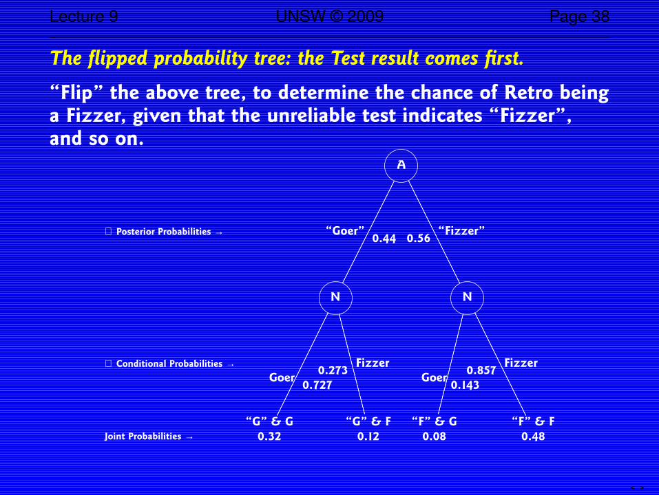
The flipped probability tree: the Tes t result comes first.
“Flip” the above tree, to det ermine the chance of Retro beinga Fizzer, given that the unreliable tes t indicat es “Fizzer”,and so on.
A
NN
“F” & G
0.08
“G” & G
0.32
“G” & F
0.12
“F” & F
0.48Joint Probabilities →
“Fizzer”“Goer”
Goer
Fizzer
Goer
Fizzer
< >

Lecture 9 UNSW © 2009 Page 38
The flipped probability tree: the Tes t result comes first.
“Flip” the above tree, to det ermine the chance of Retro beinga Fizzer, given that the unreliable tes t indicat es “Fizzer”,and so on.
A
NN
“F” & G
0.08
“G” & G
0.32
“G” & F
0.12
“F” & F
0.48Joint Probabilities →
“Fizzer”“Goer”
Goer
Fizzer
Goer
Fizzer
∴ Posterior Probabilities →0.560.4 4
< >
Lecture 9 UNSW © 2009 Page 38
The flipped probability tree: the Tes t result comes first.
“Flip” the above tree, to det ermine the chance of Retro beinga Fizzer, given that the unreliable tes t indicat es “Fizzer”,and so on.
A
NN
“F” & G
0.08
“G” & G
0.32
“G” & F
0.12
“F” & F
0.48Joint Probabilities →
“Fizzer”“Goer”
Goer
Fizzer
Goer
Fizzer
∴ Posterior Probabilities →0.560.4 4
∴ Conditional Probabilities →
0.727
0.273
0.143
0.857
< >

Lecture 9 UNSW © 2009 Page 39
Market Tes ting
Fr om the flipped probability tree:
➣
< >

Lecture 9 UNSW © 2009 Page 39
Market Tes ting
Fr om the flipped probability tree:
➣ the conditional probability of Retro being a Goer giventhat Acme says it’s a “Fizzer” is 0.08
0.08+0.48= 1
7= 0.1 43;
➣
< >

Lecture 9 UNSW © 2009 Page 39
Market Tes ting
Fr om the flipped probability tree:
➣ the conditional probability of Retro being a Goer giventhat Acme says it’s a “Fizzer” is 0.08
0.08+0.48= 1
7= 0.1 43;
➣ the conditional probability of Retro being a Goer giventhat Acme says it’s a “Goer” is 0.32
0.32+0.12= 8
11= 0.727.
➣ based upon Laura’s prior belief that Retro is a Goer with aprobability of 40%, she expects that with probability 0.32+ 0.1 2 = 0.4 4 Acme will say “Goer”.
We can now replace the ques tion mark s in the decision treeabove, which allows us to sol ve the decision problem, withexpect ed values.(Tree flipping gives the same results for conditionalprobability as using Bayes’ Theorem.)
< >

Lecture 9 UNSW © 2009 Page 40
Expect ed Value of Imperfect Infor mation — Laura
Fr om the sensitivity graph above, p = 0.4 4 is less than the the cross-ov er probability p̂:
∴
< >

Lecture 9 UNSW © 2009 Page 40
Expect ed Value of Imperfect Infor mation — Laura
Fr om the sensitivity graph above, p = 0.4 4 is less than the the cross-ov er probability p̂:
∴ If Acme says “Goer”, which Laura expects will happen withprobability of 0.44, then she will choose Retro.
&
< >

Lecture 9 UNSW © 2009 Page 40
Expect ed Value of Imperfect Infor mation — Laura
Fr om the sensitivity graph above, p = 0.4 4 is less than the the cross-ov er probability p̂:
∴ If Acme says “Goer”, which Laura expects will happen withprobability of 0.44, then she will choose Retro.
& Her expect ed payoff is (150 + 90p) × 1000 = $21 5,430, with theconditional probability that Retro is a Goer, given that Acme said
“Goer”, p = 811
= 0.727.
∴
< >
Lecture 9 UNSW © 2009 Page 40
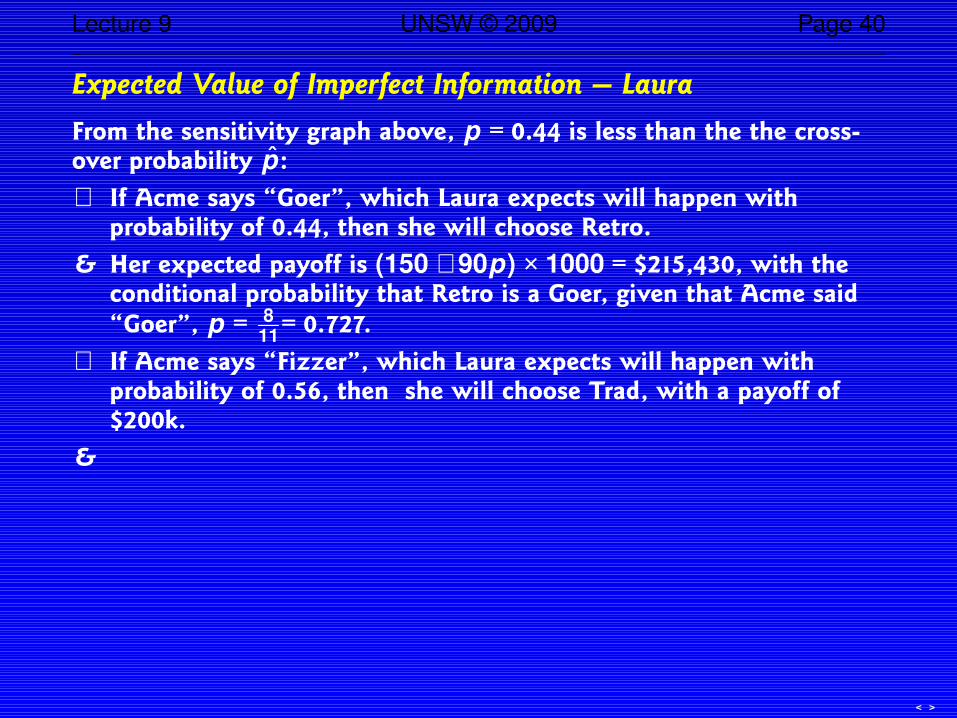
Expect ed Value of Imperfect Infor mation — Laura
Fr om the sensitivity graph above, p = 0.4 4 is less than the the cross-ov er probability p̂:
∴ If Acme says “Goer”, which Laura expects will happen withprobability of 0.44, then she will choose Retro.
& Her expect ed payoff is (150 + 90p) × 1000 = $21 5,430, with theconditional probability that Retro is a Goer, given that Acme said
“Goer”, p = 811
= 0.727.
∴ If Acme says “Fizzer”, which Laura expects will happen withprobability of 0.56, then she will choose Trad, with a pay off of$200k .
&
< >

Lecture 9 UNSW © 2009 Page 40
Expect ed Value of Imperfect Infor mation — Laura
Fr om the sensitivity graph above, p = 0.4 4 is less than the the cross-ov er probability p̂:
∴ If Acme says “Goer”, which Laura expects will happen withprobability of 0.44, then she will choose Retro.
& Her expect ed payoff is (150 + 90p) × 1000 = $21 5,430, with theconditional probability that Retro is a Goer, given that Acme said
“Goer”, p = 811
= 0.727.
∴ If Acme says “Fizzer”, which Laura expects will happen withprobability of 0.56, then she will choose Trad, with a pay off of$200k .
& Her expect ed payoff wit h Acme ’s imper fect infor mation is thus0.56 × $200k + 0.44 × $215,430 = $206,789.
➣
< >

Lecture 9 UNSW © 2009 Page 40
Expect ed Value of Imperfect Infor mation — Laura
Fr om the sensitivity graph above, p = 0.4 4 is less than the the cross-ov er probability p̂:
∴ If Acme says “Goer”, which Laura expects will happen withprobability of 0.44, then she will choose Retro.
& Her expect ed payoff is (150 + 90p) × 1000 = $21 5,430, with theconditional probability that Retro is a Goer, given that Acme said
“Goer”, p = 811
= 0.727.
∴ If Acme says “Fizzer”, which Laura expects will happen withprobability of 0.56, then she will choose Trad, with a pay off of$200k .
& Her expect ed payoff wit h Acme ’s imper fect infor mation is thus0.56 × $200k + 0.44 × $215,430 = $206,789.
➣ Her expect ed payoff wit hout this infor mation is $200k, since shechooses Trad.
∴
< >

Lecture 9 UNSW © 2009 Page 40
Expect ed Value of Imperfect Infor mation — Laura
Fr om the sensitivity graph above, p = 0.4 4 is less than the the cross-ov er probability p̂:
∴ If Acme says “Goer”, which Laura expects will happen withprobability of 0.44, then she will choose Retro.
& Her expect ed payoff is (150 + 90p) × 1000 = $21 5,430, with theconditional probability that Retro is a Goer, given that Acme said
“Goer”, p = 811
= 0.727.
∴ If Acme says “Fizzer”, which Laura expects will happen withprobability of 0.56, then she will choose Trad, with a pay off of$200k .
& Her expect ed payoff wit h Acme ’s imper fect infor mation is thus0.56 × $200k + 0.44 × $215,430 = $206,789.
➣ Her expect ed payoff wit hout this infor mation is $200k, since shechooses Trad.
∴ The expect ed value to Laur a of 80%-reliable infor mation is$206,789 − $200,000 = $6,789.
< >

Lecture 9 UNSW © 2009 Page 41
Af ter tree-flipping:
➣ Laur a’s conditional probability that Retro is a Goer, giventhat Acme has states that it will be a “Goer,” is 8
11or
0.727.
➣
< >

Lecture 9 UNSW © 2009 Page 41
Af ter tree-flipping:
➣ Laur a’s conditional probability that Retro is a Goer, giventhat Acme has states that it will be a “Goer,” is 8
11or
0.727.
➣ Laur a’s probability that Acme will state that Retro is a“Goer” is 0.44.
Laur a’s fulldecision tree:
L
L N
$200N
$150$2 40
L L
N $200
$2 40 $150
$200 N
$2 40 $150
No Trial
Tr adRetro
Goer
.4
Fizzer
.6
80%-R eliable
Tr ial
“Goer”
.4 4
“Fizzer”
.56
R T
Goer
.727
Fizzer
.273
T R
G F
< >

Lecture 9 UNSW © 2009 Page 42
So the following tree models Laura’s decision:
L
L N
$200N
$150$2 40
L L
N $200
$2 40 $150
$200 N
$2 40 $150
No Trial
Tr adRetro
Goer
.4
Fizzer
.6
80%-R eliable
Tr ial
“Goer”
0.4 4
“Fizzer”
0.56
Retro Tr ad
Goer
0.727
Fizzer
.273
T R
G
.1 43
F
0.857
< >

Lecture 9 UNSW © 2009 Page 42
So the following tree models Laura’s decision:
L
L N
$200N
$150$2 40
L L
N $200
$2 40 $150
$200 N
$2 40 $150
No Trial
Tr adRetro
Goer
.4
Fizzer
.6
80%-R eliable
Tr ial
“Goer”
0.4 4
“Fizzer”
0.56
Retro Tr ad
Goer
0.727
Fizzer
.273
T R
G
.1 43
F
0.857
$186
< >

Lecture 9 UNSW © 2009 Page 42
So the following tree models Laura’s decision:
L
L N
$200N
$150$2 40
L L
N $200
$2 40 $150
$200 N
$2 40 $150
No Trial
Tr adRetro
Goer
.4
Fizzer
.6
80%-R eliable
Tr ial
“Goer”
0.4 4
“Fizzer”
0.56
Retro Tr ad
Goer
0.727
Fizzer
.273
T R
G
.1 43
F
0.857
$186
Tr ad
$200
✘
$215
Retro
$215
✘
$163
Tr ad
$200
✘
$206.8
80%-R eliable
Tr ial
$206.8
✘
EV with the 80%-tes t = $206,790EV without the tes t = $200k
∴ EV of the 80%-reliable infor mation = $6,790< >

Lecture 9 UNSW © 2009 Page 43
3b. Value of Imper fect Infor mation of Glix:
We know the Value of Per fect Infor mation is $386,956.
What if we could conduct a market surve y for $300,000?
Would it be wor th the investment?
First, we mus t creat e a new influence diagram.
No tice that the Surve y is influenced by Market Size rat herthan vice ver sa. This is to preser ve the state of nature.
Recall: there are three possibilities for Market Size:
Low = 200,000Medium = 1,000,000High = 2,000,000
< >

Lecture 9 UNSW © 2009 Page 44
Glix’s Launch? — Surve y Influence Diagram.
NPV of Glix
Revenue
Cos ts
Volume
Market
Size
Market
Share
Marketing
Cos ts
Manufactur ing
Cos ts
Launch
Glix
Market
Sur vey
< >

Lecture 9 UNSW © 2009 Page 45
Glix: The Value of Imper fect Infor mation —Reversing or Flipping the Tree
In order to calculat e the value of imper fect infor mation, wemus t flip the tree, to obt ain the conditional probabilities,
< >

Lecture 9 UNSW © 2009 Page 45
Glix: The Value of Imper fect Infor mation —Reversing or Flipping the Tree
In order to calculat e the value of imper fect infor mation, wemus t flip the tree, to obt ain the conditional probabilities, suchas Prob (MS = 200k | the surve y indicat es “L”), which iscor rect.
< >

Lecture 9 UNSW © 2009 Page 45
Glix: The Value of Imper fect Infor mation —Reversing or Flipping the Tree
In order to calculat e the value of imper fect infor mation, wemus t flip the tree, to obt ain the conditional probabilities, suchas Prob (MS = 200k | the surve y indicat es “L”), which iscor rect.Assume: if the surve y is incorrect, then the two wrongindications are equall y likel y.
Prior tree: Glix
N
H: 2mM: 1mL: 200k
0.7
“H”
0.175
0.15
“M”
0.0375
0.15
“L”
0.0375
0.1
“H”
0.05
0.8
“M”
0.4
0.1
“L”
0.05
0.25
“H”
0.0625
0.25
“M”
0.0625
0.5
“L”
0.125
0.250.5
0.25 ← Priors
← Events
← Unreliabilities← Indications← ∴ Joints
< >

Lecture 9 UNSW © 2009 Page 46
The Pos t erior tree (flipped)
N
“H”“M”“L”
0.61
H
0.175
0.17
M
0.05
0.22
L
0.0625
0.075
H
0.0375
0.8
M
0.4
0.125
L
0.0625
0.17
H
0.0375
0.2 4
M
0.05
0.59
L
0.125
0.28750.5
0.2125 ← Posteriors
← Indications
← Conditionals← Events← Joints
< >

Lecture 9 UNSW © 2009 Page 46
The Pos t erior tree (flipped)
N
“H”“M”“L”
0.61
H
0.175
0.17
M
0.05
0.22
L
0.0625
0.075
H
0.0375
0.8
M
0.4
0.125
L
0.0625
0.17
H
0.0375
0.2 4
M
0.05
0.59
L
0.125
0.28750.5
0.2125 ← Posteriors
← Indications
← Conditionals← Events← Joints
The posterior tree indicates that the Surve y assessment iscor rect 70% of the time (the joint probabilities sum to 0.70):p(L&“L”) + p(M&“M”) + p(H&“H”)= 0.125 + 0.4 + 0.175 =0.70
We seek the Conditional Probabilities: given an Indication,how likel y is the Event?
< >

Lecture 9 UNSW © 2009 Page 47
The flipped (posterior) tree also reveals:
1.
< >

Lecture 9 UNSW © 2009 Page 47
The flipped (posterior) tree also reveals:
1. If the Surve y indicat es “L”, then
pL = 0.59, pM = 0.2 4, pH = 0.17,
which means (from p. 9-13) the EMV(Launch | “L”) =$596.8k
< >

Lecture 9 UNSW © 2009 Page 47
The flipped (posterior) tree also reveals:
1. If the Surve y indicat es “L”, then
pL = 0.59, pM = 0.2 4, pH = 0.17,
which means (from p. 9-13) the EMV(Launch | “L”) =$596.8k
→ Licence = $1,135k should be chosen.
2.
< >

Lecture 9 UNSW © 2009 Page 47
The flipped (posterior) tree also reveals:
1. If the Surve y indicat es “L”, then
pL = 0.59, pM = 0.2 4, pH = 0.17,
which means (from p. 9-13) the EMV(Launch | “L”) =$596.8k
→ Licence = $1,135k should be chosen.
2. If the Surve y indicat es “M”, then
pL = 0.1 25, pM = 0.8, pH = 0.075,
which means the EMV(Launch | “M”) = $1,158.4k >Licence,
so choose Launch instead of Licence.
3.
< >

Lecture 9 UNSW © 2009 Page 47
The flipped (posterior) tree also reveals:
1. If the Surve y indicat es “L”, then
pL = 0.59, pM = 0.2 4, pH = 0.17,
which means (from p. 9-13) the EMV(Launch | “L”) =$596.8k
→ Licence = $1,135k should be chosen.
2. If the Surve y indicat es “M”, then
pL = 0.1 25, pM = 0.8, pH = 0.075,
which means the EMV(Launch | “M”) = $1,158.4k >Licence,
so choose Launch instead of Licence.
3. If the Surve y indicat es “H”, then
pL = 0.22, pM = 0.17, pH = 0.61,
which means the EMV(Launch | “H”) = $2,089k >Licence,
so choose Launch instead of Licence. < >

Lecture 9 UNSW © 2009 Page 48
∴ The Value of the Surve y for Glix:
The unconditional EMV with the Surve y
= 0.2125 × $1.135m + 0.5 × $1.158 4m + 0.2875 ×$2.089m = $1.420m
< >

Lecture 9 UNSW © 2009 Page 48
∴ The Value of the Surve y for Glix:
The unconditional EMV with the Surve y
= 0.2125 × $1.135m + 0.5 × $1.158 4m + 0.2875 ×$2.089m = $1.420m
∴ The value of the Surve y = $1.420m − $1.310m = $11 0k,
which is the maximum that should be paid for the Surve y.
< >

Lecture 9 UNSW © 2009 Page 49
Summar y of Sensitivity Analysis and Value ofInfor mation
Decision analysis provides tremendous insight into the valueof all the different alter natives, and can help to creat e newalt ernatives.
<

Lecture 9 UNSW © 2009 Page 49
Summar y of Sensitivity Analysis and Value ofInfor mation
Decision analysis provides tremendous insight into the valueof all the different alter natives, and can help to creat e newalt ernatives.
Sensitivity analysis is impor tant in identifying the fact orswhich affect the decision: the Tor nado diag ram.
Sensitivity to probability can help identify the var iance thatwould cause you to change your decision.
The value of gat hering additional infor mation can becalculat ed before gather ing the infor mation.
Remember to consider the feasibility and reliability ofgather ing additional infor mation. Jus t because you cancalculat e the value does not mean that you can either findthe infor mation or obtain it.
(R eading: Clemen, Reading 18 in the Pac kage)<