)

N 6Z 55173

C)

U

NATIONAL ADVISORY COMMITTEE

FOR AERONAUTICS

TECHNICAL NOTE 3173

A STUDY OF HYPERSONIC SMALL-DISTURBANCE THEORY

By Milton D. Van Dyke

Ames Aeronautical Laboratory Moffett Field, Calif.

777

Washington

May 1954

C) TOP

ow or'

T on w< now

r

, M,

1.

p

S

https://ntrs.nasa.gov/search.jsp?R=19930083893 2018-05-21T09:58:21+00:00Z

NATIONAL ADVISORY COMMITTEE FOR AERONAUTICS

TECHNICAL NOTE 3173

A STUDY OF HYPERSONIC SMALL-DISTURBANCE THEORY

By Milton D. Van Dyke

SUMMARY

A systematic study is made of the approximate inviscid theory of thin bodies moving at such high supersonic speeds that nonlinearity is an essential feature of the equations of flow. The first-order small-disturbance equations are derived for three-dimensional motions involv-ing shock waves, and estimates are obtained for the order of error involved in the approximation. The hypersonic similarity rule of Tsien and Hayes, and Hayes' unsteady analogy appear in the course of the devel-opment.

It is shown that the hypersonic theory can be interpreted so that it applies also in the range of linearized supersonic flow theory. Hence, a single small-disturbance theory, and associated similarity rule, apply at all supersonic speeds above the transonic zone.

Several examples are solved according to the small-disturbance theory, and compared with the full solutions when available. These include flow past a wedge and cone, and determination of the initial gradients at the tip of plane and axially symmetric ogives. For the axially symmetric ogive it is shown that further terms can be found only by using Lighthill's technique of rendering solutions uniformly valid., and thus the initial curvature of the pressure distribution is calculated. It is concluded that on a body of revolution described by a power series, the pressure distribution and shock wave are also given by power series.

A brief discussion is given of various additional approximations from existing theories. -

INTRODUCTION

Aerodynamic shapes are ordinarily most efficient when they cause the least flow disturbance. For this reason, simplified theories based upon the assumption of small disturbances due to thin bodies have proved

LH

2 NACA TN 3173

to be of practical value in analyzing incompressible, subsonic, tran-sonic, and supersonic flows.' For flows at Mach numbers large compared with unity, however, the pressure disturbances may no longer be small (compared with the static pressure) even for thin shapes, so that in this sense it has been said that no small-disturbance theory exists (ref. 1). However, if viscosity can be neglected, the velocity disturb-ances remain small compared with the speed of flight (though not compared with the speed of sound), and even the pressure changes are small if com-pared with the dynamic pressure. In this sense, therefore, a small-disturbance theory exists, and the assumption of such small disturbances leads to a useful simplification of the equations for compressible flow at arbitrarily high Mach numbers.

Viscosity and heat conduction must be neglected in order to have a small-disturbance theory. Otherwise, for example, the viscous no-slip condition would introduce velocity disturbances equal to the speed of flight. In many cases this simplification does not destroy the essential features of the flow. In other cases, the inviscid theory may serve as a basis for including viscosity and heat conduction. Thus, recent studies of the hypersonic boundary layer (refs. 2 and 3), which indicate that vis-cous effects become essential at extreme Mach numbers (say, greater than 17), replace the boundary layer by a fictitious solid surface and then utilize inviscid theory of the sort considered here.

At sufficiently high Mach numbers, inviscid flow past any given thin object requires nonlinear equations for its description. We take this as the definition of hypersonic flow: Supersonic flow past a thin body is termed hypersonic if the Mach number is so great that nonlinearity becomes an essential feature. Thus, the definition of hypersonic flow stands on an equal footing with the generally accepted meaning of transonic flow at the other extreme of the supersonic range; that is, flow at a Mach number so close to unity that nonlinearity (of a different sort) is an essential feature. These two terms - transonic and hypersonic - are most meaningful when defined (as here) only for thin shapes. They then describe two quite distinct regimes which are, moreover, separated by a consider-able range of "ordinary supersonic" flow in which the transonic and hyper-sonic nonlinearities are unimportant, so that linearized theory can account for all significant features of the flow. If one attempts to extend the terms to thick bodies, the two separate regimes tend to merge, so that one must concede that a flow field can be simultaneously tran-sonic and hypersonic.

It should be noted that the term hypersonic has occasionally been used in the literature with other meanings than that adopted here. Flows are sometimes called hypersonic if the free-stream Mach number is simply large compared with unity (say, 10 or 5, or even 3). This is not strictly

'Throughout, "thin" is used to refer to any body whose streainwise slope is small, and so applies to slender fusiform objects as well as flat shapes such as airfoils.

NACA TN 3173 3

equivalent to the present definition because, in principle, at any given Mach number a body can always be chosen so thin that nonlinearity is insignificant. However, such extreme thinness does not arise in prac-tice, so that the two definitions are equivalent for practical purposes. Again, Oswatitsch has defined hypersonic flow as the limiting condition for a given body as the free-stream Mach number tends to infinity (ref. Ii-). This Is a limiting case of the present definition and, indeed, Oswatitsch's similarity rules for thin bodies are simply special cases of the more general rules.

Associated with each of the various small-disturbance theories is a similarity rule which connects flows at different speeds past affinely related shapes. In the case of linearized subsonic and supersonic theory, the similarity rule was fully understood only long after the small-disturbance theory was in common use. On the other hand, the tran-sonic similarity rule was developed concurrently with the small-disturbance theory. For hypersonic flows, the simplified theory and associated similarity rule were first given by Tsien (ref. 5), but were restricted to irrotational flows (and to plane or axially symmetric shapes). This is a severe limitation because strong curved shock waves and consequent entropy gradients and flow rotation are. essential features of nearly all hypersonic flow problems. This restriction was removed by Hayes, who indicated in a brief note (ref. 6) that Tsien t s similarity rule is valid for rotational flows and for general three-dimensional shapes. The rule was further extended to unsteady motion by Hamaker and Wong (ref. 7).

As a result of this circuitous development, there exists a gap in the hypersonic theory. The similarity rule Is known for full three-dimensional flows with curved shock waves, but the underlying small-disturbance theory has never been written down. (To be sure, however, its form is known from the analogy with nonsteady flow in one less dimension, which was pointed out by Hayes.) For the special case of plane flow, and for Mach numbers which are not arbitrarily large, this gap has recently been closed by Goldsworthy (ref. 8). The published examples of applications of the theory are limited to the few special cases which are strictly irrotational (e.g., the wedge and cone) or are assumed to be approximately so.

The present paper undertakes a systematic study of the small-disturbance theory for hypersonic flow. First, the small-disturbance problem Is derived by reduction of the full equations of motion, bound-ary conditions, and shock-wave relations. The similarity rule and unsteady analogy appear in the course of this development. This portion of the paper may be regarded as an elucidation of Hayes' note, with esti-mates obtained for the order of error. Next, it is pointed out that to within terms of the order neglected, the hypersonic similarity theory can be written in the form of the similarity theory for linearized super-sonic flow, so that a single theory and associated similarity rule cover

11. NACA TN 3173

both regimes. Then, a number of special problems are solved according to the small-disturbance theory and are compared with the full solutions when they exist.

The symbols' used in the text are defined in Appendix A.

HYPERSONIC SMALL-DISTURBANCE THEORY

Basic Assumptions

Consider a three-dimensional body fixed in a steady uniform stream. Viscosity and heat conduction are neglected, which implies that shock waves will be approximated by abrupt discontinuities.

The body is assumed to be thin, in the sense that the streamwise slope of its surface is everywhere small compared with unity. The degree of thinness will be measured by the small parameter 'r which may, for example, be taken to be the maximum slope of the body, 2 or its thickness ratio. However, for inclined shapes T must be identified with the angle of attack if it is considerably greater than the body thickness.

The free-stream Mach number M is assumed to be so high that the flow is hypersonic. That is, linearized theory is inadequate for pre-dicting the essential features of the flow. It is known that linearized theory yields an adequate approximation if the maximum body slope is small compared with the slope of the free-stream Mach cone, that is,

if T<<l where 3 = JM2_l. As this ratio approaches unity, linear-ized theory grows increasingly inaccurate. Therefore the flow is hyper-sonic if the ratio PT is not small compared with unity. Since i - is small, this means that 0 and, therefore, also N will be large in the hypersonic range, so that 0 is nearly equal to M. Thus, the criterion for hypersonic small-disturbance flow may be written

T<<1 with MT or >>l (1) M>> 1 J

From a mathematical point of view, it is convenient to regard all the small-disturbance theories as being asymptotic forms of the full theory

2If the slope is high in some small region of the body, as at a

slightly blunt leading edge, it may be presumed that the small-disturbance theory remains valid except locally. In this case T might be taken to be the thickness ratio.

x

LI -

NACA TN 3173 5

for vanishingly thin bodies. Thus, the criterion for hypersonic flow may be expressed more formally as:

-o(i)1TO MT as (2) jM4

We introduce a Cartesian coordi-nate system with the positive x axis aimed with the free-stream direction (sketch (a)). Let the surface of the body be described by c B(x,y,z) = 0, and the complete system of shock waves by S(x,y ) z) = 0, where the function S is not, of course, known at the outset.

Sketch (a) . - Notation for hyper-

sonic flow past thin body.

Full Problem

Consider the problem of determing the three velocity components u, v, w, pressure p, and density p throughout the flow field in the vicinity of the body. The mathematical system required is the differen-tial equations of motion (which govern the flow except at discontinuities), the Rankine-Hugoniot relations across shock discontinuities, and boundary conditions at the surface of the body and far from the body.

Equations of motion. - The differential equations of motion, which express the principles of conservation of mass, momentum, and energy, are

(continuity) (pu) + (v) + ( pw ) = 0 (3a)

(x momentum) uu + vuy + uz + p/p = 0 (3b)

3llere the order symbols are used in the conventional sense: f(T) = 0(i) as T —> 0 means that 1(T) remains bounded as 'r—> 0; and 1(T) = 0(g[T]) means f(T)/g(T) is 0(1); similarly, 1(T) = 0(1) means. f(T) vanishes as T—>O.

6 NACA TN 3173

(y momentum) uv + vv + wv + Py/p = 0 (3c)

(z momentum) UWX + vw + wwz + = 0 (3d)

(energy) u(p/p7) + v(/ Y ) + w(p/pY ) = 0 (3e)

(See, e.g., ref. 9, ch. 1.) Here subscripts indicate differentiation, and y is the adiabatic exponent of the gas. The last equation actually expresses the fact that the entropy is constant along streamlines, which for steady flow is equivalent to the conservation of energy (ref. 9, pp. 15-16).

Boundary conditions. At the body the normal component of velocity must vanish. The unit normal vector at the surface is proportional to grad B, so that the condition becomes

q • grad B = 0

where q is the velocity vector, or

(tangency) uBx + vBy + WBz = 0 at B = 0

(!)

The other boundary condition, which implies that the body is flying into still air, may be taken in various equivalent forms. For present purposes it is convenient to require that all disturbances vanish far ahead of the body:

u-4u03

(upstream) v and w —Oas x —-.o (5)

p —.p0

P

Shock-wave relations.- At a shock wave, conservation of tangential momentum leads to the requirement that the velocity component tangent to the shock surface be continuous. The tangential velocity component

(sketch(b)) is given by qt = (n x q) x n, where the unit normal

NACA TN 3173 7

vector n is proportional to grad S. It is convenient to use brackets to denote the jump in a flow quantity across a shock wave so that, for example, [u] is the increase in u through the shock. With this nota-tion, the condition of conservation of tangential momentum becomes

/ -

(tangential momentum)

jJ. = .L!J. = .11 at s = o (6a) Sx Sy Sz Sketch (b).- Components of

velocity at shock wave.

This imposes two independent scalar conditions at the shock wave, as physical considerations clearly indicate that it should. For plane flow, say, in the x-y plane, the last term becomes indeterminate and should, of course, be dropped.

The remaining shock-wave relations express the conservation of nor-mal momentum, mass, and energy across the shock. The magnitude of the velocity component normal to the shock is (sketch (b)).

> uS+vS - f-wS q . fl =

I Sx+Sy+Sz

Consequently, the other three shock relations are found to be (ref. 9, P- 300), using the jump notation,

(mass) [P(uSx+vSy+wSz)J = 0 (6b)

(normal momentum) [P(uS-i-vS-i-wS) 2 + ( S2+S2+S2 )p] = 0 at 3=0 (6c)

(energy) 1(US2x+vsy+wS)2 + (3x2+3y2^5z2)J = 0 (6d)

So far, these relations are quite symmetrical, remaining unchanged if the brackets are taken to denote the change upstream rather than down-stream through the shock. A definite sense of flow direction is

NACA TN 3173

provided only by the second law of thermodynamics, which requires that the entropy shall not decrease across each shock wave, so that

(2nd law of thermo.) [_]> 0 at S = 0 (6e)

For later use we record Bernoulli's law

(u-i-v+w) + _Z_ £ = const. (7) y-1 P

which holds, with the same constant, throughout the flow field.

First-Order Problem

The full problem is now to be simplified by discarding all but lead-ing terms in the body thickness T. This will give a first-order hyper-sonic small-disturbance theory, which can be expected to provide aclose approximation for thin shapes.

The reduction is conveniently carried out by introducing new inde-pendent variables which are of order unity throughout the flow field. The form of this transformation is suggested by simple examples and limiting cases. For example, the approximate solution for a thin plane wedge at very high Mach number has been given several times. Pertinent results are that the lateral extent of the flow field is some moderate multiple of the wedge thickness, that the density never exceeds (y+i)/(y-i) times its free-stream value, and that the relative streamwise velocity disturbance and the pressure coefficient are of the order of the square of the surface slope. Again, the Newtonian impact theory, modified to include effects of centrifugal force, which yields the limit-ing solution for M = and y = 1, shows pressure coefficients propor-tional to the square of the thickness. The tangency condition suggests that, in general, all cross-wind velocities vary directly with the thick-ness. Such considerations suggest introducting new (barred) independent and dependent variables, and redefining the functions describing the body and shock-wave surfaces, as follows:

y= ;i: y (8a)

1 Z =- z

T

NkCA TN 3173

U = u [1+i-

V = UT v(,y)

W = UT (8b)

p = POO (3T,)

P = p00

B =(8c)

S =

The new dependent variables are dimensionless, and the others may be regarded as dimensionless if the body is of unit length.

We tentatively assume that all the new dependent variables (iI,V, etc.) and the new functions B and are 0(1) as 7 4 0 for fixed MT, and that the reciprocals of the new independent variables (i/i, etc.) are likewise 0(1). The correctness of this assumption is suggested by examples such as those discussed above; its justification will come from the consistency of the resulting theory.

It is important to realize that the notation V = 0(1) includes the possibility that in the limit 7 becomes arbitrarily small as well as the possibility that it approaches a constant nonzero value; only the possibility of its growing arbitrarily large is ruled out. For example, the reduced velocity components ii, V, and 7 will be identically zero in the region ahead of the body. On the other hand, it is definitely implied here that in at least some portion of the flow field the reduced quantities will not vanish in the limit as T +O. 4 To be sure, they ,may not all be of order of magnitude unity in the intuitive physical sense; for example, for flow past a thin flat wing ü • and V will be moderate multiples of unity, but V will be numerically much smaller.

Reduced problem.- This transformation of variables is now intro-duced into the full problem of equations (3) to (6). If we discard terms which contain T2 explicitly; such as T 2pU in the continuity equation, the differential equations become

(x momentum) ü- + + ü- + i-/p = 0 (9) x y z

4 That is, f(7) = 0(T) implies that f(T) is not identically 0(7).

10 NACA TN 3173

(continuity) P3j + () + () = 0 (ba)

(y momentum) + + +p P = a (lob)

(z momentum) + + Wi + p-/p = 0 (lOc)

( energy- ) (/p_y) + (/p) + W(P/) Z = a (lod)

the boundary conditions become

(tangency) + + = a at i = 0 (ii)

(upstream) , , 7W - 0

l/7M-r2 as - (12)

P--l.

and the jump conditions at the shock waves become

(tangential momentum) [ii.) = [ j =

-- - x y z

(mass) [(++)]=o

(normal - -- --momentum) [ (s- + vS + wS)2 + (2 + 2)] = 0 at S=0 (13)

(energy)1 2

.(s_ + VS- + wS-)2 + J_ (_2 + _2) !.

I = 0

x y z y-1 Y Z

(2nd law r of thermo.) _o

The parameters- M and T of the full problem enter this reduced problem only in the combination NT, which appears only in the upstream condition on 5 (eq. (12)). In the hypersonic range, where l/Wr=0(l),

NACA TN 3173

11

the reduced problem possesses complete internal consistency. This is most readily understood by considering first the case where it does not.

In the range of linearized theory, where 5 MT <<1, equation (12) presents a contradiction. It was assumed at the outset that f is 0(1), but its value upstream, (1/M2r2), is then not 0(1). This inconsistency is an automatic warning that the reduction breaks down in the range of linearized theory. Indeed, it will be seen later that the assumed orders of reduced quantities are then actually incorrect, and that the reduced equations fail to describe linearized supersonic flow.

In the hypersonic range no such inconsistencies arise. Hence, the tentative assumptions regarding orders of reduced quantities are justified a posteriori, as are the simplifications effected by discarding terms that

involve 72 explicitly.

Order of error.- Because terms of order ¶2 have been omitted in the reduction, first-order quantities will differ from their exact values by 0(72). For the special case of plane flow, an analysis similar to the preceding hasbeen given by Goldsworthy (ref. 8), who considers only a single bow wave; 6 he furthermore confines attention to the range MT "l (which, to be sure, may be the range of most practical importance) and finds the error to be 0(l/M 2 ). This is equivalent to the present result in that range. However, the present result is more general, holding for arbitrarily large values of the similarity parameter (assuming, of course, that the assumption of a continuum flow remains valid). For example, at infinite free-stream Mach number, the error in first-order theory is correctly 0(r2).

It is interesting to note that the error in the various first-order small-disturbance theories decreases progressively from 0(72/3) in tran-sonic flow to 0(T) in linearized supersonic flow to 0(72) in hypersonic flow. Therefore, under the plausible assumption (confirmed by later examples) that these mathematical order estimates give a reasonable indi-cation of the actual physical magnitude of error, the practical need for a second-order solution is seen to be greatest for transonic flow and least at hypersonic speeds.

Unsteady analogy.- A significant feature of the reduced problem is that the problem for the streamwise velocity a has been uncoupled from that for the other variables. Equations (10) to (13) constitute a com-plete problem for v, w, p, and p, which can be solved independent of u.

5 More precisely, where MT = 0(1) as T->0.

6 1t seems important to consider multiple shocks, because it is not at all obvious that subsequent-shocks have the same status as the bow shock; in particular, at M = Co the upstream Mach number is infinite for the bow shock, but has moderate supersonic values for the subsequent shocks.

12 NACA TN 3173

Thereafter, (if required) can be determined from Bernoulli's law:

7 1 -1- - — = const. (1)-i-) (y-1)M2T2

Consequently, equation (9) and the first terms of equations (12) and ( 13a) are superfluous and can henceforth be disregarded.

As pointed out by Hayes (ref. 6), this first-order, problem is com-pletely equivalent to a full problem for unsteady flow in one less space dimension. The reduced problem of equations (10) to (13) is precisely the full problem of unsteady motion In the plane due to a moving solid boundary described by = 0, where 2 is interpreted as the time, and all other barred variables as the actual physical quan-tities. 7 The outline of the moving boundary is given by the trace of the original thin shape in a cross-stream plane which moves downstream with the free-stream velocity (sketch (c)). For example, the problem of steady hypersonic flow past a slender pointed body of revolution is

equivalent to the problem of unsteady planar motion due to a circular

- - cylinder whose radius varies with UM time, growing from zero at time

= 0. Hayes has given a physical explanation of this analogy.

Sketch (c).- Plane of unsteady analogy.

It may be noted that the analogy is similar to that arising in the slender-body theory of linearized compressible flow, as exemplified by the work of Jones (ref. 10) and Ward (ref. ii). There, however, the time-dependent analogue is incompressible, whereas here it Is definitely com-pressible.

Similarity rule.- The parameters M and T appear in the reduced problem only in the combination MT, which is the hypersonic similarity parameter of Tsien. This means that for bodies derivable from one another by uniform contraction or expansion of all dimensions normal to the stream, the flow fields are related if the corresponding Mach

7The undisturbed fluid has density =l and pressure =1/7M2T2.

NACA TN 3173 13

numbers are such that the similarity parameter MT IS the same in each case. The nature of this relationship is simply that the reduced flow quantities, as functions of the reduced coordinates, are the same in each flow. All distinctive flow surfaces, such as the body itself and the shock-wave system, have identical descriptions in terms of the reduced coordinates. This is the hypersonic similarity rule of Tsien, which was extended to rotational and three-dimensional flow by Hayes. Its implica-tions with regard to pressure and force coefficients will be summarized later, after the hypersonic rule has been combined with that for ordinary supersonic flow.

Extension to unsteady flow.- For simplicity, the preceding discussion has been restricted to steady flow. It can readily be extended to unsteady motions involving small time-dependent oscillations of a thin body exposed to a steady uniform stream (or, from another point of view, flying through still air executing slight time-dependent variations from a mean steady rectilinear flight). The full problem is obtained by replacing the sub-stantial derivative u6/6x + v6/6y + w6/6z wherever it appears in equa-tions (3) to (6) by its unsteady counterpart a/at + u6/6x + v6/6y + w6/6z. Correspondingly, if a reduced time t is introduced according to

= ut

('5)

then the unsteady small-disturbance problem is obtained from the steady problem of equations (9) to (13) by adding /t throughout to the operator /i + + ô/. For example, the reduced continuity equation (eq. (i)) becomes, for unsteady motion

E ++ () + () = 0 (16)

The problem for ü remains uncoupled from the problem for the other variables. 8 Furthermore, in the remaining problem the and t deriv-atives appear only in the combination 616E + This means that the number of independent variables can be reduced by one by adopting the viewpoint of an observer who is moving with the free stream (or, to put it another way, who is fixed in still air with the body moving past). Thus, introducing "still-air" coordinates

X , =x-ut x' =x - ut

- - tt=t

(17) tt=t

8llowever, ü can no longer be found immediately in terms of the solution of the remaining problem, because in unsteady motion there is no useful counterpart of the Bernoulli equation (eq. (iii. )); fortunately, u is seldom actually required.

/

14 NACA TN 3113

reduces the unsteady small-disturbance problem to exactly the form of the steady problem (eqs. (9) to (13)), with t replaced by t'. This means that Hayes' analogy remains valid for unsteady motion if account is taken of the actual variation of the contour with time as well as the apparent variation due to relative motion depicted in sketch (c). This result was first given by Hamaker and Wong (ref. 7). Recently, Lighthill has analyzed oscillating airfoils at hypersonic speeds from this point of view (ref. 12).

If the body oscillates so rapidly or with such large amplitude that _ is much greater than f., the error remains of 0(T 2 ) only if T is

taken to be the maximum instantaneous slope of particle paths at the sur-face of the body.

Unified Supersonic-hypersonic small-disturbance theory. - It would be advantageous if the hypersonic small-disturbance theory included linearized supersonic theory as a special case. Then the awkward ques-tion of what is the lower limit of hypersonic flow would not arise. A single theory, and corresponding similarity rule, would hold for all supersonic speeds above the transonic range.

In the case of transonic small-disturbance theory, a unification of this sort is known to arise quite naturally (ref. 13, P . 9). In its original form (with p2 not replaced by 2(M-1)) transonic theory embraces linearized theory as a special case, so that it furnishes effectively a unified subsonic-transonic-supersonic theory giving a first approximation at all speeds below the hypersonic range.

In the case of hypersonic flow, a connection with the adjoining supersonic range can likewise be effected (ref. 14), but the reason therefor is much less straightforward. An immediate obstacle is the faät that the approximations leading to the hypersonic theory and those leading to linearized theory are mutually exclusive. The difficulty arises in the continuity equation (eq. (3a)) which in the hypersonic case was shown to reduce to

u p + (pv) y + (pw) z = 0 (18a)

but in linearized theory reduces instead to

+P.Ux + P( Vy + w ) = 0 (18b)

The term P0,Px must be retained in linearized theory, whereas it must be neglected in hypersonic theory in order to achieve similitude. It would therefore appear Impossible to give a small-disturbance theory which is general enough to describe both hypersonic and ordinary super-sonic flows, and yet simplified enough to retain the corresponding similitudes. It must be regarded as a coincidence that this can, nevertheless, be accomplished.

NACA TN 3173 15

It is shown in Appendix B that the hypersonic theory covers the ordinary supersonic range if it is reinterpreted in accordance with the similarity rule for linearized theory (ref. 15). It is found that solu- tions of hypersonic small-disturbance theory remain valid at small values of the parameter MT (which is the domain of linearized theory), provided that MT is replaced by OT and the results are reinterpreted in terms of physical variables according to

U = u,[l + T2U X 13T)]

V = ui r)

w = ur(19a)

P = p {i + 7M2T2 [P(Y; T)- 7T2

] } = p (7M2,.22

-

P = PW {l +T) - 1 ] } =.(

M2

P-

rather than according to equation (8). The pressure coefficient is given by

1( = 1 2 - T p -l9b)

Since the error is 0(T 2 ) in the hypersonic theory and 0 ('r113 ) in the linearized theory, the error in this unified theory is 0(T 2 ) or 0(T/J3), whichever is the greater.

The flow quantities of chief aerodynamic interest are the pressure coefficient and the various force and moment coefficients derived from it by integration. If the hypersonic small-disturbance problem has been solved to find Cp/T 2 as a function of the reduced coordinates and the parameter MT, the result is rendered valid also in the ordinary supersonic range simply by replacing MT by 3r.

Unified similarity rule.- The unified supersonic-hypersonic similar-ity rule may be summarized as follows:

For steady flow past thin bodies derivable from one another by uni-form contraction or expansion of all dimensions normal to the stream,

9For slender shapes such as thin bodies of revolution the error - is only 0(T 2/t32 ) in the linearized theory and, hence, 0(T) or

0(T2/ 2 ) in the combined theory.

16

NACA TN 3173

the flow fields are related if the corresponding Mach numbers are such that the similarity parameter 13T is the same in each case (i- being any measure of thickness). The relationship is such that the flow fields are identical when expressed in terms of the reduced flow quan-tities

u-u .L, L, 00 or --- m M21'2 P T2 M2PCO

as functions of the reduced coordinates

, 1•' •T

When the body oscillates slightly, the same is true with the addition of ut to the reduced coordinates, provided that the time history of oscil-lation in terms of reduced coordinates is the same for each body.

From the rule for pressures follows the equality of the reduced force and moment coefficients

CD CL Cm -, etc.

1^k T

7 .

Here k = 1 if some plan-form area is taken for reference and k = 0 if some cross-sectional area Is used. The connection between the simi-larity rules for forces and moments is contained in the statement that the center of pressure is constant in terms of the reduced coordinates.

An unlimited number of equivalent forms of the reduced variables can be produced, for example, by multiplying by any power of the simi-larity parameter. However, the forms given here are the most useful ones in the hypersonic range, because they involve functions of order unity. In the supersonic range no forms have this advantage, except in the special case of plane flow, where it would be convenient to use

13

(u — 1)and

It should be noted that in the hypersonic and combined similarity rules the adiabatic exponent 7 must remain fixed, whereas its magni-tude is arbitrary in the supersonic case (since it does not appear in the linearized problem).

NACA TN 3173

17

TYPICAL APPLICATIONS OF HYPERSONIC SMALL-DISTURBANCE THEORY

Several problems will now be solved according to hypersonic small-disturbance theory. These examples will illustrate possible methods of solution, and demonstrate the degree of simplification resulting from the assumption of small disturbances. Comparison with the corresponding solutions of the full equations (when available) will indicate the accuracy to be anticipated when the theory is applied to more elaborate problems.

Plane and Axially Symmetric Flows

The examples to be considered are either plane or axially symmetric flows. Accordingly, it is convenient to introduce coordinates x,r where in the case of plane flow r is the Cartesian coordinate y. Henceforth, v will denote the velocity component in the r direction, which is the radial velocity fo± axially symmetric flows.

Equations of motion.- In these coordinates, the hypersonic small-disturbance equations of motion (eqs. (10) . ) become

+ ()- + a = 0 (2Oa)

x r r

(2Ob) X r

- 7 G/ ) + v(p/p ) = 0 (20c)

The distinction between two and three dimensions arises only in the continuity equation, where a = 0 for plane flow and a = 1 for axially symmetric flow.

=

Boundary and shock conditions.- rr s(x)

Let the surface of the body be described by r = 'rb(x), as indi- cated in sketch (d). Then the U

tangency condition of equation (11) _____

becomes

= b'(i) at = b() (21)

The upstream conditions are given Sketch (d).- Notation for plane by equation (12). or axially symmetric body.

18

NACA TN 3173

The examples to be considered will involve only a single bow shock wave, which may be described by r = rs(x). The shock-wave conditions are given by equations (13), but in this case it is easier to take advan-tage of the convenient relations which are listed in reference 16. Equations (136), (128), and (129) of reference 16, when reduced to hyper-sonic small-disturbance form, give

- 2 K2-1 v=—

K2

- 27K2 - (y-i) s'2 (i) at E = s() (22) p=

= ( y-i-i) K2

2 + (7-1) K2

where K = MTs'() is the hypersonic similarity parameter based on the local shock-wave slope.

Stream function.- The continuity equation (eq. (20a)) may be accounted for by introducing a stream function, setting

r p = r (23)

=

so that

- x v= --r

(21)

=

Then equation (20c) states that / p is a function only of *, as is clear from the fact that entropy is constant along streamlines between shock waves. Substituting into the momentum equation (20b) gives

7+1 for plane (74-- + (A)(2) flow (25a)

- 2 111 " 11'- +11r 2 -

r xx xTrxr x7+1 for

rJ 7&)( )+te_2J axially (25b) L \ rr / r symmetric

flow

NACA TN 3173

where

The pressure is given by

19

-- = p/7p (25c)

(26) - _7 p = wp =w(r/r)

Plane Wedge

As a simple introductory example, consider hypersonic flow past a thin wedge of semivertex angle 5. Here, and in the examples to follow, the solution is most readily carried out by assuming a given shock wave and Mach number and calculating the corresponding body shape. It is therefore convenient to identify the thickness parameter T with the shock-wave angle rather than the wedge angle. This is quite permissible at hypersonic speeds, where they are of the same order; it is also per-missible in the ordinary supersonic range, where they are not, provided that b rather than 7 is used in the error estimates. Let b = be the ratio of wedge to shock angles.

The flow field is conical (velocities constant along rays), so that the stream function has the form

-

*(x,r) = f(e) (27)

where U is a conical variable, defined by

(28)

TX 5i

which varies from b at the wedge to unity at the shock wave. Thus, equation (25a) becomes

f U [f2 - 7W f 1(7 = 0 (29a)

where, from equations (22) and (25c)

W27K2-(y-l) 2+( 7 l) I 2 7

=7(7+1)2 (y+l)2

° I (29b) 0

- with K = MT. The shock-wave conditions of equation (22) give (since s'=l)

f(l)=l -

ft (1)(7+l)

° 2 (30)

- = 2 + (7-1)t2

20 NACA TN 3173

The solution of this problem, which corresponds to f" = 0, is

(y+i) K 2 e - 2(K02 .1)

f(0) =2

(31) 2 + ( y_i) Ko

Requiring f to vanish at the surface gives the ratio of wedge to shock angles

b -- 2(I 02 - 1)

T (7+1) 2

The auxiliary hypersonic parameter K 0 = Mr can now be eliminated in favor of M8, with the result that

S - b -

+ J(l)2 + M252 (33)

Then from equations (26) and (27) the pressure coefficient at the wedge (or anywhere between the wedge and shock wave) is found to be

= 2+ f( 2 + 1 (3k)

P[

J'\2 M252J

(32)

These results were first given by Linnell (ref.. 17) . Numerical values of pressure coefficient are com-pared in sketch (e) with the exact results for wedges of various thick-nesses. Here S has been taken to be the tangent of the wedge angle, though within the scope of the small-disturbance theory it might equally well have been identified with the sine of the angle, the angle itself, etc.

8bz tan -'R'

cp R

4

SM

theory

WE .33 .5 I

M R

Sketch (e).- Wedge pressure according to hypersonic small-disturbance theory.

12 rb = T(bx + cx + ... (36)

NACA TN 3173 21

Unified supersonic-hypersonic result.- Replacing the parameter M by 06 renders the solution valid in the ordinary supersonic range as well:

2 _ C = 52 [, +) + 22 J (35)

This result is again compared with the full solutions in sketch (f). 8 The advantage of the unified result is obvious. In all subsequent examples the results will be pre-sented only in this form.

It is interesting to note that this formula has been proposed by Ivey and Cline (ref. 18) for pre-dicting the surface pressure on any 0 supersonic airfoil. They obtained .333

it by seeking an interpolation formula connecting Ackeret's linear- Sketch (f).- Wedge pressure accord-ized theory with the hypersonic ing to unified supersonic-result of Linnell (eq. (31)) for a hypersonic small-disturbance tangent wedge. theory.

Initial Gradients for Plane Ogive

Using the full equations, Crocco first determined the initial gra-dients of flow quantities at the tip of a plane ogive by perturbing the solution for a wedge (ref. 19) . His analysis has been repeated and elaborated upon by Schfer (ref. 20) and others. This problem provides a good test of the small-disturbance theory in a case involving shock-wave curvature. Let b be the ini-tial ratio of body slope to shock-wave slope, and 1 the cprrespond-ing ratio of radii of curvature. Then in physical coordinates the body (sketch (g)) may be described by iLg__ ____br 9ø_

2oIisturbance theory

.5BR:,1 CD

and the shock wave by

r5 = T(x + icx2 + ...) ( 37)

Sketch (g).- Plane or axially symmetric ogive.

22 NACA TN 3173

Here c will be negative for the convex shapes usually encountered in

practice.

Shock-wave conditions.- Conditions just behind the shock wave are found from equations (22) to be given by

2( K 0 I (7_1)I04+(7+5)I02-2 -

[2+(7-1)Kl+ lcx+

2+(7-1)K J (K 0 2_1) 2] ...}

(38a)

(7+1)K021+ ________ lc + ...]

( 38b)

2+(7-1)K 7 [2+(7_l)2

= NOY- 27 2_(y_l) r2+(y_1)021

-+

7(y+1)2 L (7+12 J {

_ - Zcx + (38c)

[272_(7_l)] [2+(y_l)2] ... }

where K = MT is the auxiliary hypersonic similarity parameter based upon the initial shock-wave angle.

Equations of motion.- The flow behind the shock wave will consist of a uniform field upon which is superimposed a perturbation field due to body curvature. Hence, along each ray from the vertex the flow quan-tities will have constant values associated with the initial slope of the body plus linear variations proportional to the initial curvature (together with higher variations which need not be considered in evalu-ating initial gradients). Thus, the stream function of equation (25a) can be written in the form

= f(6) - zc 2 g(e) + ... (39)

Along the shock wave

* = F = :5 +

NACA TN 3113

23

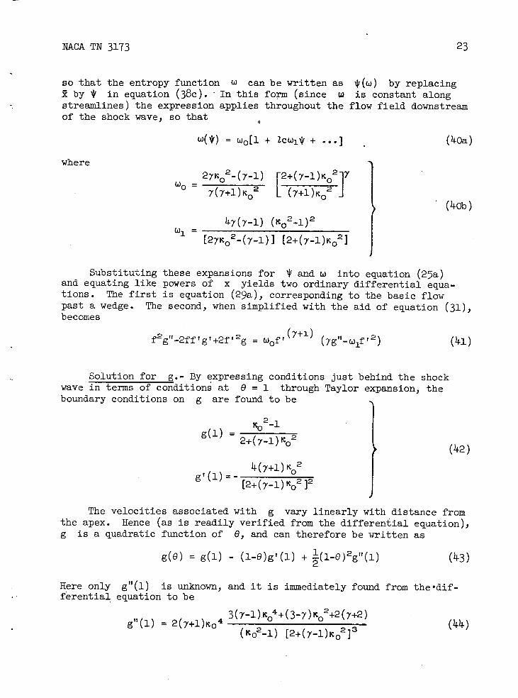
so that the entropy function () can be written as r(c) by replacing by \ in equation (38c). In this form (since w is constant along

streamlines) the expression applies throughout the flow field downstream of the shock wave, so that

= w-jl + lc,* + ...] (oa)

where2yi02-(y_1) [2+(y_1)Io217

0 7(i+1)2 L (7+1)K02 1

(kwh)

47(7]) (K2_1)2 (A)1 =

[27I02_(7_1)] [2+(y_l)o2]

Substituting these expansions for and W into equation (25a) and equating like powers of x yields two. ordinary differential equa-tions. The first is equation (29a), corresponding to the basic flow past a wedge. The second, when simplified with the aid of equation (31), becomes

2 (y--i) f g"-2ff'g'+2f' 2g = (A)of! 019"-w1f '

2 ) (i)

Solution for g.- By expressing conditions just behind the shock wave in terms of conditions at 0 = 1 through Taylor expansion, the boundary conditions on g are found to be

g(l) = 2+(71)2. (2)

[2+(-/-l) K02]2

The velocities associated with g vary linearly with distance from the apex. Hence (as is readily verified from the differential equation), g is a quadratic function of e, and can therefore be written as

g(0) = g(i) - (1-0)g'(l) +1(1_e)2gtl(1) (43)

Here only g"(1) is unknown, and it is immediately found from the dif- ferential equation to be

3(7_1)i04+(3_7)I02+2(7+2) g"(l) = 2(y+l)K 0 4 (44) 23 (K 0 2-l) [2+(7-1)K0 ]

21. NACA TN 3173

Curvature ratio and surface pressure.- The body curvature and pres-sure gradient can be expressed in terms of the values of g(0) and its derivative at e = b. From equations (42) to (44) it is found that

______ 2(27-l)1c04+(y+5)K02-(y-l)

g(b) = (y+1)(K02-l) [2+(y-l)K02]

2Pto2(3Ko2+1) gt(b) = - (K

2-l) [2+(7-1)K 0 2]

The surface of the body is determined by the vanishing of the stream function. Thus it is found that the ratio of shock-wave curvature to body curvature is given by

fl(b) - (y+1)22(2_l)(14.6)

2g(b) - 2 [2(27-1)o+(7+5)o2(71)]

The initial pressure gradient on the surface of the body is given by

6C P b = -yw1r'(b)7 g'(b) T 2 ax I g(b)

so that in terms of the initial slope B 0 ' = bT and curvature R0 " = CT

of the body

(11.7)

(7+1)02(3K02+1) [27K 02_(7_1)]

pi b (KO 2_1) [2(27_1)K0+(7+5)02(71)]R0 'B0 " ( 48)

-

Although these results have been expressed in terms of the auxiliary parameter Ko = MT, they can be given explicitly in terms of Mach number and apex angle (in the combination MR 0 ' = Mbr) with the aid of equa-tion (33). In this respect the small-disturbance solution is superior to the full solution, which yields no such explicit results. Replacing

MRo' by 3R0 ' renders these results applicable at all supersonic speeds.

S 15 (Ref. 21)

Small-disturbance theory

333 . BR

.8

1.

.4

0.25

4

ac, Small-disturbance theory

a(Rn:x)

2

Y . R.x . kR:5....

0L. .25 .333 .5

$ R

NACA TN 3173

25

The small-disturbance result for the curvature ratio is compared in sketch (h) with the full solution for various vertex angles, taken from the convenient tabulation of reference 21. Sketch (i) gives the corresponding comparison for the initial pressure gradient.

Sketch (h).- Initial ratio of shock to body curvature for plane ogive.

Sketch (i).- Initial pressure gradient on plane ogive.

Circular Cone

Consider flow past a slender circular cone of semivertex angle 6. (sketch (j)) . Again it Is conven-ient to regard the Mach number and shock-wave angle as given, and to solve for the corresponding cone angle. Thus let the shock-wave angle be i- and the cone angle = br, where again b is a con-

stant less than unity that is to be determined. Sketch (j) . - Notation for cone.

Equation of motion.- The flow field is conical so that all flow quantities are constant along rays. This means that the stream function of equatipn (25b) has the form

r r() = 2r( e), = =

It follows that the equation of motion (eq. (25b)) becomes the nonlinear ordinary differential equation

('+) f2f't- 2ff'2=7o f'

(

f'

e(7_1)(o)

0 )

26 NACA TN 3173

Here wo is the constant value of /7 behind the shock wave, given by equation ( li-Ob), and K o = MT IS again the auxiliary hypersonic simi-larity parameter based upon shock-wave angle.

Boundary-conditions.- The shock-wave conditions of equation (22), together with equation (49), combine to give

1 f -.

(51) fT(l)

(7+1) KO I

= I 2+(7-1)K02 j

The condition of tangent flow at the cone requires that the stream function vanish at the surface:

f(b) = 0

(52)

Numerical integration.- The nonlinear equation for f, equation (50), can be readily integrated numerically. Choosing a value of the auxiliary similarity parameter i, we calculate w o from equation (40b) and the initial values of f and f' from equations (51), and then integrate step by step inward from the shock wave until f vanishes, which deter-mines the cone surface. With the ratio of cone angle to shock-wave angle /T = b thus determined, the results can be re-expressed in terms of the similarity parameter based upon cone angle. Eight or ten intervals between shock wave and body yield ample numerical accuracy, provided that in each step the predicted values of f and its deriva-tives are corrected by averaging and iterating before proceeding to the next step. (For values of rc near unity, the first few intervals near the shock wave must be taken smaller than the others.)

The pressure coefficient is obtained in terms of the first deriva-tive of the stream function according to

1 62 Lb 2 e) yM22

where the similarity parameter M5 of the hypersonic problem is to be reinterpreted as P6 so that the result is applicable throughout the entire supersonic range.

Computations have been carried out for 7 = 1.1.05, in order to com-pare with the full solutions tabulated by Kopal (ref. 22). The chosen values of the parameters are listed in the following table, together with certain of the results:

(53)

NACA TN 3173

27

MT 8/i- 05 ft(b)/b C/82

1.014 0.3620 0.3765 1.217 3.183 1.19 .5545 .6599 1.522 2.646 1.8 .7281 1.150 2.207 2.333 2.87 .86o4 2.469 3.925 2.154. 14 . 14.7 .8921 3.988 14.973 2.116

.9114. 0 6.149 2.091

The small-disturbance result for surface pressure is compared with the full results (from ref. 22) in sketch (k). The differences between the full solution and the small- 4 disturbance limit are closely pro-portional to the square of the thickness, in accordance with the estimate of the error as 0(82) or 0(82/32). It is noteworthy that 3

the fractional differences are in fact very nearly equal to 62. The same is true of surface pres-sures in the previous examples. CP, 2 This suggests that the mathematical R'O

order estimate may be relied upon to give a quantitative prediction of the error in the small-disturbance approximation. I

This approximate solution for cones was previously sought by Shen (ref. 23), whose result is also shown in sketch (k). It appears that his solution, which involves more involved computa-tions, must contain errors. Sketch (k).- Surface pressure

on cone.

Initial Gradients on Ogive of Revolution

Consider the axially symmetric counterpart of Croccots problem: the determination of the initial gradients of flow quantities at the tip of an ogival body of revolution. This problem has recently been considered for the full equations by Cabannes (ref. 24) and by Shen and Lin (ref. 25). It will be seen that the small-disturbance solution serves as a useful guide to the full solution. In particular, it clar-ifies the behavior of the solution near the surface, which was glossed over by Cabannes and in Shen and Lin's work was misconstrued to

o .333

]-disturbance theory

(Ref. 23)

Full solution

tanR

.5

a

ffel

NACA TN 3173

indicate a singularity which implied wrongly that the initial pressure gradient at the tip of an ogive is infinite.

As in the plane problem, let the body be described in physical coordinates by

1 2 rb = T(bX + cx + ...) (511.)

and the shock wave by

r3 = T(x + 1 Zcx2 ()

(sketch (g)). Conditions just behind the shock wave are given by equa-tion (38), with and 4r replaced by - 4r /i and

Equations of motion. - Again along each ray the flow quantities have constant values corresponding to the initial slope plus linear variations proportional to the initial curvature (together with higher variations which are considered later). Hence, the stream function may be written in the form

= 2) - c 3g(e) + ... (56)

Along the shock wave

= l2 = 12 + ••• 2 2

so that an expression for the entropy function cj throughout the flow field downstream of the shock wave is obtained by replacing R with ..[V in equation (38c). Hence,

L(1]J) = wo [i + ZC(A)1 + ...] ( 57)

where W j and w, are given by equation (40b).

Substituting these expansions into equation (25b) and equating like powers of 2 yields for f the nonlinear ordinary differential equa-tion already treated in the problem of the cone (eq. (5 0 )), and for g the linear equation

Dg" = A + Bg + Cg' (58a)

whose coefficients depend upon f according to

NACA TN 3173 29

(y+i) ________ ____ - ( - t)] A=0w1 f' fi

[ (7-1)

B = 12ff"

f?(7+1)[7+2(78b)

C = 7w&(7-')

- (+i) ] - 8ff'

D = 'yWo f - 2

As in the plane problem, initial conditions on g are found by expressing conditions just behind the shock wave in terms of conditions at e = 1 through Taylor series expansions:

2_ 0 g(1) = _________

2+(7_1)1c02

(59)

g'( .l)- K02 (7-1)K02+2(27+3Y

Behavior of solution near body surface.- Just as conditions at the curved shock wave have been related to those at 0 = 1, so with the present coordinate system it is necessary to relate conditions at the surface of the body to those on the initially tangent cone 0 b. However, the solution is nonanalytic near the surface, which means that Taylor series expansions do not exist. It is therefore necessary to examine the nature of the solution in the vicinity of the body.

The function f associated with the basic conical flow is analytic near the surface (and vanishes at 0 = b), so that it has a Taylor series expansion:

f(0) = (0-b) f(b) + ... 0[(o-b) 2 ] (60)

It follows from equations (78b) and (60) that near the surface the coefficients of the differential equation for g behave like

A". (0-b)- 112

B (0-b)(61)

D. 1

NACA TN 3173

Therefore the point 0 = b is a singular point of equation (58a), but is an ordinary (nonsingular) point of the homogeneous equation obtained by deleting A (see ref. 26, p. 73). Therefore the general solution of the homogeneous equation is analytic and can be taken to have the form

n

=a(0-b) (62)

0

where all higher coefficients an can be expressed in terms of the two arbitrary constants a 0 and a 1 by means of the differential equation. Then the procedure for calculating a particular integral (ref. 26, p. 122) shows that the nonhomogeneous equation (58a) has a particular integral of the form

(e-) L cn(0-b)n

(63)

0

where the coefficients en can all be determined. Here the 3/2-power branch point arises from the fact that the pencil of fluid striking the tip of the ogive is spread thin over the entire surface, and the linear entropy gradient at the tip due to a curved shock wave is thus intensi-fied to a square-root gradient normal to the surface elsewhere. The complete solution of equation (58) is the sum of gj and gp

In treating the full problem in reference 25, Shen and Lin claimed to have found a logarithmic singularity at 0 = b, which considerably complicated their analysis. Because of this singularity, their solu-tion was restricted to concave bodies (although they conjectured that it might be extended to convex bodies). The singularity also led to the conclusion that for an analytic body shape the shock wave is non-analytic, and vice versa. Furthermore, the singularity would -imply that the initial pressure gradient on an analytic body of revolution is infinite, although numerical solutions by the method of characteristics give no indication of this.

The present solution shows no such singularity. It seems unlikely that a singularity could have disappeared as a result of making the small-disturbance approximation, since this would imply that the approx-imate model does not retain the essential features of the full problem. The alternative conclusion is that the singularity does not actually exist in the full problem. This has subsequently been confirmed by the authors of reference 2510 who find that the singularity is, in fact, only apparent in the sense of reference 26, page 406.

'01n a private communication; see also Addendum No. 1 to ref. 25.

NACA TN 3173 31

It may be noted that Cabaimes, in treating the full problem, has completely ignored the nonanalytic nature of the solution, and simply extrapolated his numerical solution to the surface of the body (ref. 24). His results may not be seriously in error, because the effect of the nonanalyticity is small.

Numerical integration. - The differential equation for g has been integrated numerically for the six values of the similarity parameter chosen previously for the cone. The integration was carried out step by step starting from the known values at the shock wave and using the same intervals as for the cone. This step-by-step solution was joined at the two points nearest the surface with the series expansion about e = b given by equations (62) and (63): -

g(e) = 22fT(b)3/2(e_b)3/2

+ €_(970_ 12

37 32) + •..] +

g(b) [1 + 27€ - A(1+27\)€4 + ...] +

g'(b) (e-b) (1+ € - +

+ ...)(6a)

where(7-1) -1

?\=[7wO

f' (b) 1

(64b) L ' b

(Values from the step-by-step integration and the series expansion were also compared at the third point from the surface as a check.) Because they are based upon the previous solution for a cone, the computations were carried out with 7 = 1.405.

Curvature ratio and pressure gradient. - Because the nonanalyticity appears only in higher terms of the series, surface values of g and its first derivative (but no higher derivatives) can be expressed in terms of values at e = b. The surface of the body is determined by the vanishing of the stream function. Thus the ratio of shock-wave curvature to body curvature is found to be given by

f'(b)(67)

2g(b)

Proceeding as in the plane case, it is found that the initial pressure gradient is expressed in terms of the initial slope R 0 ' = bT and curv-ature H0 t' = CT of the body by

Small-disturbance theo 4

ac, a(RRx)

2 i

r . R,x + iR:x2 +

<I,

32

NACA TN 3173

= f'(b) 7 [-g'(b)]RQ 'R0 " ( 66)

lb M2R0,2b g(b)

Numerical values of g(b) and g'(b) are listed in the following table, together with the resulting values for the curvature ratio 2 and surface pressure gradient:

PRO I (b) '(b) 2 1

b 0.3765 5.170 -8.502 0.011.26 5.532

.6599 1.800 -3.60 .2311.6 4.662 1.150 1.573 -.073 .5106 4.5111. 2.469 2.101 -6.820 .8039 3.988 2.487 -8.638 .8921 4.8o2

2.931 -10.76 .9586 11..929

The curvature ratio is plotted in sketch (l),and the initial pres-sure gradient in sketch (in). The. curvature ratios calculated from the

6

/

83O •-' (Ref. 25)

100

- - - - -

J Small-disturbance theory

.8

.4

.333 .5 'S 0 IR0 .333 .5 I

B R,

Sketch (Z)._ Initial ratio of Sketch (m).- Initial pressure shock to body curvature for gradient on ogive of revo-ogive of revolution. lution.

full equations by Shen and Lin are also shown in sketch (i) for com-parison, because the error introduced by incorrect treatment of the solution near the body is probably small.

NACA TN 3173

33

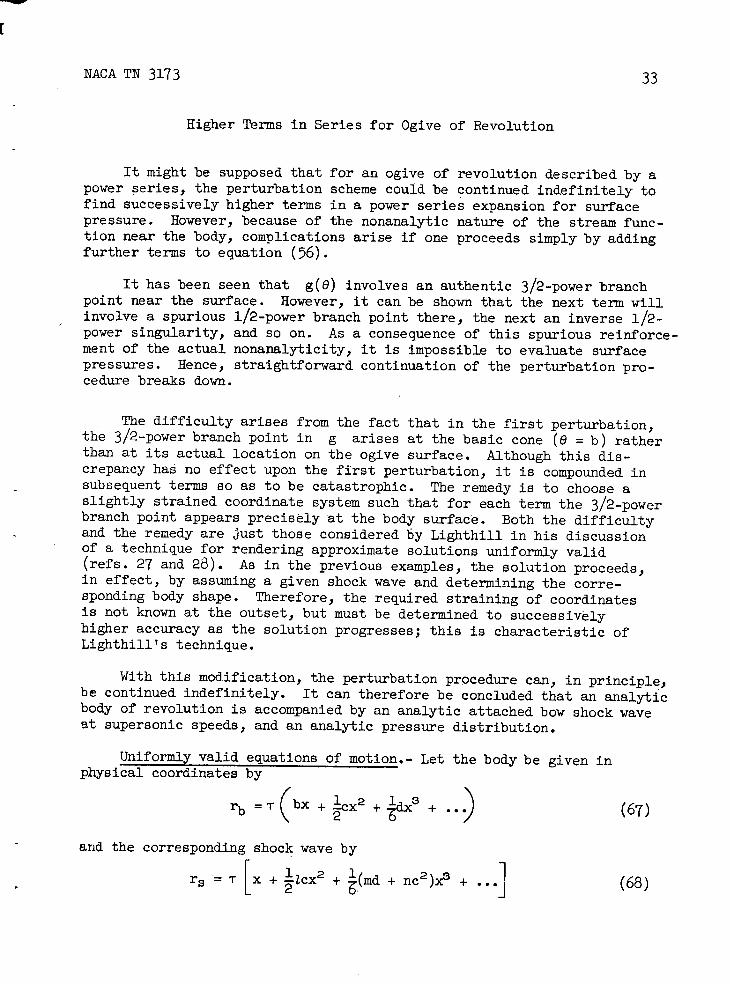
Higher Terms in Series for Ogive of Revolution

It might be supposed that for an ogive of revolution described by a power series, the perturbation scheme could be continued indefinitely to find successively higher terms in a power series expansion for surface pressure. However, because of the nonanalytic nature of the stream func-tion near the body, complications arise if one proceeds simply by adding further terms to equation (56).

It has been seen that g(0) involves an authentic 3/2-power branch point near the surface. However, it can be shown that the next term will involve a spurious 1/2-power branch point there, the next an inverse 1/2-power singularity, and so on. As a consequence of this spurious reinforce-ment of the actual nonanalyticity, it is impossible to evaluate surface pressures. Hence, straightforward continuation of the perturbation pro-cedure breaks down.

The difficulty arises from the fact that in the first perturbation, the 3/2-power branch point in g arises at the basic cone (e = b) rather than at its actual location on the ogive surface. Although this dis-crepancy has no effect upon the first perturbation, it is compounded in subsequent terms so as to be catastrophic. The remedy Is to choose a slightly strained coordinate system such that for each term the 3/2-power branch point appears precisely at the body surface. Both the difficulty and the remedy are just those considered by Lighthill in his discussion of a technique for rendering approximate solutions uniformly valid (ref's. 27 and 28). As In the previous examples, the solution proceeds, in effect, by assuming a given shock wave and determining the corre-sponding body shape. Therefore, the required straining of coordinates is not known at the outset, but must be determined to successively higher accuracy as the solution progresses; this is characteristic of Lighthill' s technique.

With this modification, the perturbation procedure can, In principle, be continued indefinitely. It can therefore be concluded that an analytic body of revolution is accompanied by an analytic attached bow shock wave at supersonic speeds, and an analytic pressure distribution.

Uniformly valid equations of motion.- Let the body be given in physical coordinates by

rb = T (bx + cx2 +dx + ...)

(6)

- and the corresponding shock wave by

r3 T [x + ILZCX2 + (md + nc2)x3 + ...]

(68)

34

NACA TN 3173

Now introduce a slightly strained radial coordinate such that the body surface is given byr = bx. The simplest choice is

(69)

The procedure which led to equation (57) gives for the entropy function behind the shock wave

= {1+ i zcI + [ w1 (md+nc2 ) + w2 1 2c2 ] + ...

}

( 70a)

where C. 0 and ( 1 are given by equation ( ifOb), and

11.

(7+1) = (A)1 (70b)

(o2_1)[2+(7_l)Ko2]

The stream function has the form

4 = 2f.() - cx g8) - x [c2(0) + ' d()J + ... (71)

where V is the nearly conical coordinate The differential equations which result from substituting this series into the equation of motion are simplified by setting

= zg() --f'()

() =nth( ' ) -f'() (72)

= zi() + nh( ' ) + zg'() - If ,, ( 6 )

(The functions g, h, and j thus introduced are those which would appear in place of g, h, and j if no straining of the coordinate system had been undertaken.) Then the differential equations (and boundary conditions) for f and g, as functions of the strained variable , are (as implied by the common notation) found to be just those solved in the previous sections, where f and g were functions of the unstrained variable 0. The differential equations for the new functions h and j are -

Dh" = E + Fh + Gh'

Dj't = I + Fj + Gj'

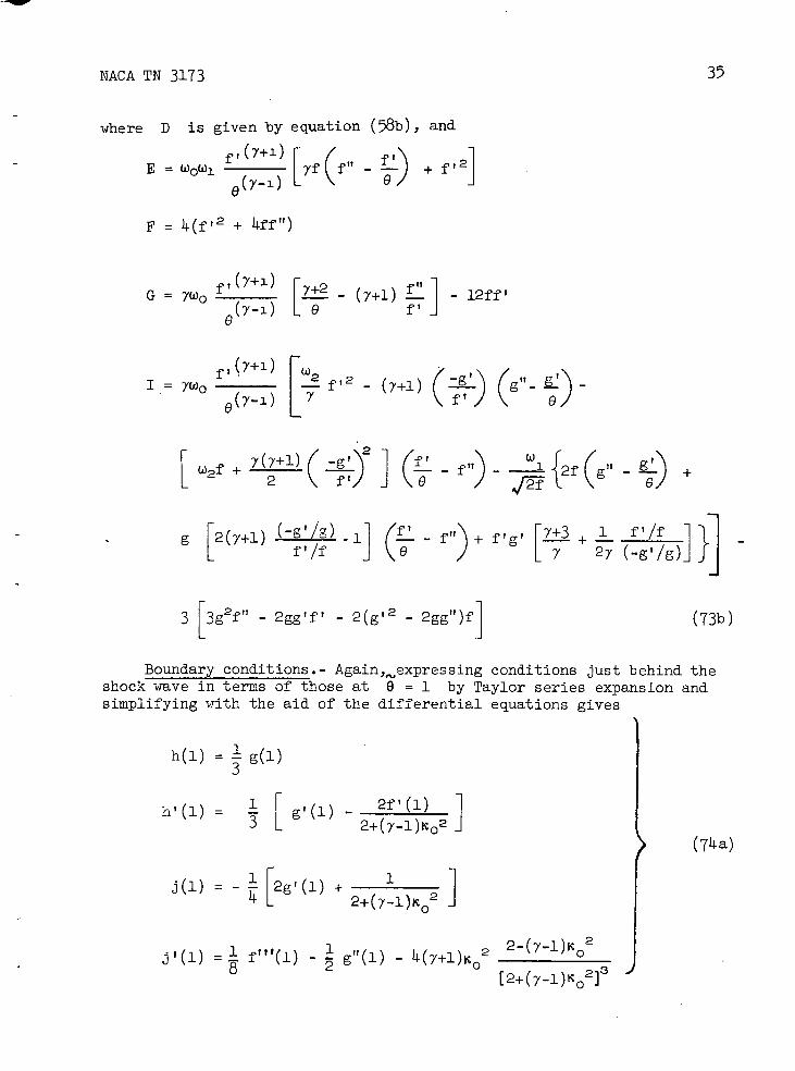
35 NACA TN 3173

where D is given by equation (58b), and ft(7+1) [ I ft'\

E=W0W1 Yf e(7_1) 1 ' 0/

F = 14 (f t 2 + li-ff")

f,(7+1) IL+G = 7W0 2 - (7+1) - 12ff' e ft J

fI(7+1)

f2 e(71 )

[W2

7 () (gti) I = _______

w2f +

[ C g 2(y+1)

I f'/f

3 [3g2f ti - 2gg'f'

\2 /WI (g"( f" - 2f g + f!J - ) -2f 0)

L 11 ( - ftt)+ f' r + ft/f 1 L 27 (-g'/g)]

g' }j

- 2(g'2 - 2ggtt)f] ()

Boundary conditions.- Again,,expressing conditions just behind the shock wave in terms of those at 8 = 1 by Taylor series expansion and simplifying with the aid of the differential equations gives

h(1) = g(i)

g'(l) - 2f1(l) ht ( l ) = L 2^(7_l)2(7Iia)

j(1) = - 2g'(1) +2 ] 2+(y-l)i

j'(l) f"'(1)- g"(l) - (7+1)2 2-(7-1)K02

[2+(7-1) K 0 2]3

36

NACA TN 3173

where f l (l) is given by equation (51b), g(l) and g'(l) by equation (9),' and

(7_1)2

2+(7-1)K02 I

f lot - 2K02[272_(7_1)] [2+(37+1)K02] (7+1)(l2_1) [2+(7_1)I2]2

g"(l) = I

K 2 (7_1)(27+3)+(2y3+372+5)K02_3(7_1)72+(67+1)Ko4+2(y_1)(57+3)Ko8f

0(Ko [2+(y-J)KO )

Behavior near body surface.- The fact that f( ') is analytic

at = b implies that the full solution for h is also analytic, and that the solution of the homogeneous equation for j is analytic. The

Coefficient I is proportional to ( - b) -3/2 , so that a particular

integral for j is proportional to ( - b) ''2. For purposes of computa-tion it is important to separate the regular part of I from the singu-lar part, because either may predominate for the closest practical approach to the singularity, depending upon the value of the similarity parameter. Furthermore, the accuracy of joining the step-by-step solu-tion for j to the series is increased by treating not j itself but the combination j + g 1 /2z. Hence, the series employed is

(,) 1/2

- +

g t ___

...] 2) 21 7 b

gb 9br 1 + € +7 + ...] + b' L 2.tJ

j(b) [l+2€2+€3+ ...] +

j'(b)(-b) 11 + € - ++ ...] (75a)

where fb f(b), etc., ? and € are defined by equation (64b), and

NACA TN 317337

= b (-gb')

gb

(75b) 2 N/ 2 W2 (bfb312

37 gb )

Numerical integration. - The differential equations for h and j have been integrated numerically in the manner outlined previously, with v = 1.405. Because h represents actually (like g) only a first perturbation of the basic conical flow 11 and is furthermore regular near the body, it is readily determined with ample accuracy. On the other hand, in the equation for j, the coefficient I is so strongly singu-lar that it was found necessary to replace simple step-by-step integra-tion by the more laborious five-term procedure of Milne (ref. 29, p. 12). The coefficients and boundary values are also considerably more difficult to calculate, so the integration of j has been limited to three values of the similarity parameter, on h has been found for four values.

The accuracy of the solution for j suffers from the facts that it depends upon the accuracy of the preceding solution for g, that one coefficient in the differential equation is strongly singular, and that the results of physical interest are found as differences of nearly equal quantities. Consequently, although results derived from the functions f, g, and h are probably reliable to three or four significant figures, those derived from j are perhaps not reliable to more than two.

Body shape and pressure distribution.- The parameters m and n, which relate the shape of the shock wave to that of the body, are found, by requiring the stream function to vanish at the surface, to be given by

m I

(76)

n = - 1 Zg' - )

The surface pressure coefficient is given by

-2 (' - 11 (77) T2 7K02 L r) j

b

11 It corresponds to a pointed body with zero initial curvature;

compare reference 24, part III.

38 NACA TN 3173

Thus it is found that on the surface of a body described in actual coordinates by

r R0 t x + + 1 B+ ... (78)

the pressure coefficient is given by

3C p 2 /Cr \\ ______ _____ __________ n2 2Cp

Pb = R'

RoT2) + R0tR0" 16(RO'Ro"x) ] X + fRO [2(RttX)2 ] +

R01R01" k(RoI x)6(Ro"'x) I I x2 + ... (79a)

where

Cp EW 21

°0

L(fb'bI - R 2

Cp 7w fb'\7 = b (\T) (\gb)

(79b)

2 No, (' (-b'

(R0'x)(R0"x) 3 b b / "ib

62C ib'\7(Y-1 gb' b' 2 hb\

_ _ 2n— -21 (RttX)2 = 2?w0 b) gb2 - 3b

Numerical values of h(b), h'(b), j(b), and j'(b) are listed in the following table, together with the resulting values of the parameters m and n which relate the shape of the shock wave to that of the body, and the two functions which give the initial curvature of the surface pressure distribution.

NACA TN 3173 39

R0 ' h(b) h1(b) j(b) j'(b) m n P 2cp

(Ro"x) 2 (R0 'x) (R0"x)

0.3765 14.34 36.11.0 0.0051 - - - - - - 5.6911. .6599 1.752 -5.401 -7 . 34 43.7 .0803 0.583 4.04 4.736 1.150 .9341 -3.665 1.911. 5.30 .2867 .868 5.20 4.561

1.166 -6.948 7.63 -27.4 .8031 -.901 13.7 5.332

The two pressure-curvature functions are plotted in sketches (n) and (o). (Curves have been faired through the three calculated points by analogy with the results of the cone-expansion approximation discussed in the following section.)

15 1I I 6

10

at a(R:x)2

Small-disturbance 5

0' I

.333

Sketch (n).- First term in ini-tial pressure curvature on ogive of revolution.

Small-disturbance theor1

826p 8(Rx) a(Rx)

2

0 .333 .5 I

B R

Sketch (o).- Second term in ini-tial pressure curvature on ogive of revolution.

Further Approximations

The theory discussed heretofore is the simplest which retains all the essential features of hypersonic flow, so that its solutions approach exactness as the thickness tends toward zero. Further approximations, although desirable for facilitating solution, will introduce errors whose nature may be more obscure. In the case of plane flow, however, further approximations exist which are so simple and accurate that the problem may be considered solved for practical purposes (cases (6) and (7) below). These and other approximations will now be considered for three-dimensional shapes, in comparison with the solutions already given.

-

Most of these approximations are useful outside the limits of hyper-sonic small-disturbance theory. However, we shall consider them here only as they are reduced to small-disturbance form, so that they actually

- -

Second-order

disturbance

- >-Lees Hype:sonic small.

Newtonian

anR

R?

4

3

o I-.333 .5

OD

B

1.o NACA TN 3173

represent approximations beyond those already made. For example, the well-known shock-expansion method will be considered only in its hyper-sonic small-disturbance form (ref. 17).

The following additional approximations will be considered:

(1) Linearized theory, second-order theory, etc. (2) Newtonian impact theory (3) Newtonian theory plus centrifugal forces (1) y1 (5) Cone-expansion approximation (6) Tangent-cone approximation (7) Compression-layer approximation

Linearized theory, etc.- The breakdown of linearized theory serves almost as a definition of hypersonic flow. Hence, the most that can be expected of linearized theory, second-order theory, etc., is that they penetrate somewhat into the lower end of the hypersonic range.

For plane flow Donov (ref. 30, pp. 90-91 ) has determined the fourth-order solution. Reduced to hypersonic small-disturbance form, his result for surface pressure coefficient on a single airfoil may be written as

M2C = 2K+ 7± K2 +Z K04 +

37777233 (7+l)2(37_5) K< K + K0tx +

96 128(80)

where K is the local similarity parameter (M times local surface slope), K0 its value at the lead-ing edge, and Ko l its initial rate of change. Even in this reduced form nothing is known of the range of convergence of the series or, indeed, whether it converges at all. However, for a single wedge the solution is known in closed form from equation (34). Hence, it IS seen that in this special case the series is convergent for K E m5:5 Il./(y+l), which is 1.67 for air.

For cones the linearized and second-order solutions (ref 31, p. ii), as reduced to hypersonic small-disturbance form, are shown

Sketch (p).- Further approximations in sketch (p). to hypersonic small-disturbance theory; pressure on cone, y=1.405.

NACA TN 3173

Newtonian impact theory- Assuming that fluid particles lose their normal momentum on impact with the surface leads to a prediction of pres-sures proportional to the square of the sine of the angle of inclination or, in the small-disturbance approximation

-=2 (81)

wherever the slope is positive, and zero elsewhere. According to equa-tion (34) the actual value for a wedge falls only to 2.11 at infinite Mach number (with 7 = 7/5), so that the approximation is poor for plane flow. It is more satisfactory for fusiform shapes such as a cone (sketch (p)), for which the actual value at M = co (with 7 = 7/5) is 2.09.

Newtonian plus centrifugal forces.- Newtonian impact theory has been improved by including the centrifugal pressure gradient through the layer of fluid streaming over the body (rem. 32 and 33). The result is pre-cisely the limit of the full theory as M-> oo and 7— 1. In the small-disturbance approximation (ref. 33), it gives for plane flow

= 2(R' 2 + BR") (82)

In both cases it is to be understood that negative values are to be replaced by zero. Sketch (q) shows that the improvement due to includ-ing centrifugal effects is appreci-able for the initial pressure gradi-ent on an ogive of revolution.

7 = 1.- It has just been seen that on fusiform shapes near M = so, the surface pressure is insensitive to the value of 7. At the other end of the hypersonic range, linearized theory is inde-pendent of 7. These two extremes suggest that a close approximation throughout the hypersonic range may be found by setting 7 = 1 (and this is particularly true since in a real gas 7

-S I

"_T

-.5

Tangent-cone

Cone- \ Newtonian + centrifugal

Hypersonic small-disturbance theory

Newtonian

.333 • I

Sketch (q).- Further approxi-mations to hypersonic small-disturbance theory; initial pressure gradient on ogive of revolution, 7 = 1.405.

and for axially symmetric flow 8

Cp = 2R' 2 + BR" (83)6

ac, a(RR:s)

4

2

0

NACA TN 3173

approaches 1 at high temperatures). This choice simplifies the theory by rendering it effectively isentropic; that is, although shock waves produce entropy jumps, entropy does not appear in the pressure-density relation and is therefore absent from the problem.

This approximation has been tested by computing the hypersonic small-disturbance solution for a cone with y = 1. The results corresponding to those tabulated on page 27 are shown in the following table (including the known value at M = co).

Mi- E/T I3 f'(b)/b Cp/2

l.04 0.3912 0.4069 1.255 3.076 1.17 .7609 .6450 1.546 2.627 1 .50 .7647 1.147 2.498 2.277

1 00 00 2

Sketch (p) shows close agreement with the results for 7 = 1.405, the discrepancy being, indeed, less than that due to the thickness of a 100 seinivertex angle (cf. sketch (k)).

"Cone-expansion" approximation. - The shock-expansion method for plane flow, which neglects disturbances reflected from the bow wave, has recently been shown to yield good accuracy at all supersonic speeds away from the transonic zone (ref. 34).

A more surprising discovery is that an analogous procedure yields a reasonable approximation for certain three-dimensional shapes in hyper-sonic flow. In this "cone-expansion" method the flow behind the tip of a pointed body is approximated by a Prandtl-Meyer expansion (refs. 35 and 36). The accuracy of this approximation is indicated by the compar-ison shown in sketch (q) for the initial pressure gradient on an ogive of revolution.

Tangent-cone approximation. - Newtonian impact theory predicts pres-sures depending only upon the local slope. This suggests approximating the pressure at each point of a body by that on a locally tangent cone or wedge at the same Mach number. For plane flow this gives equation (35), which yields good accuracy. For bodies of revolution, sketch (q) gives an indication of the accuracy obtainable.

Compression-layer approximation.- In the upper end of the hypersonic range the bow shock lies close to the body (if the body slope is posi-tive). This suggests making an approximation somewhat analogous to that of the Prandtl boundary-layer theory, assuming that the layer of com-pressed fluid between the body and shock is very thin.

For example, assume that the shock wave lies so close to a circular cone that a linear variation is adequate to describe the stream function.

NACA TN 3113

113

Then according to equation (51) the stream function is given by

j•(y+l),2

= - - (i-e) (84) 2+(7-1)K 0

2

Requiring this to vanish at the surface gives as the ratio of cone angle to shock-wave angle

b = = (7+3)K2_2

T 2(y,l)I2

This result has been derived by Lees (ref. 37). At infinite Mach num-ber with y = 1.405 it gives 0.916 compared with the true value of 0.914, and Lees shows that it is accurate even in the lower end of the hyper-sonic range. However, for the corresponding surface pressure coeffi-cient, the range of good approximation is much smaller, as shown in sketch (p).

Ames Aeronautical Laboratory National Advisory Committee for Aeronautics

Moffett Field, Calif., Mar. 18, 1954

(85)

NACA TN 3173

APPENDIX A

PRINCIPAL SYMBOLS

A,B,C,D,E, coefficients of differential equations. (See eqs. (58) F,G,H,I and (73).)

B(x,y,z) function defining body shape

o(x) reduced radius (or ordinate) of axially symmetric (or plane) body

b,c,d coefficients in series expansion for radius (or ordinate) of body (See eqs. (36) and (67).)

CP- pressure coefficient, (

p p 0)

1. 2 —puco

f,g,h,j functions in series expansion for stream function (See eqs. (39) and (72).)

2 initial ratio of shock-wave curvature to body curvature

m,n coefficients relating shapes of shock wave and body (See eq. (68).)

M free-stream Mach number

p pressure

R(x) radius (or ordinate) of axially symmetric (or plane) ogive

r radius (or ordinate) in cylindrical (or plane Cartesian) coordinates

S(x,y,z) function defining shape of system of shock waves

S(X) radius (or ordinate) of shock wave attached to axially symmetric (or plane) body

t time

u,v,w velocity components in Cartesian or cylindrical coordinates

NACA TN 3173 45.

x,y,z Cartesian coordinates with x in streamwise direction

dM2_i

adiabatic exponent

5 semivertex angle of wedge or cone

(e - b) b

0 conical variable, r x

auxiliary hypersonic similarity parameter based upon local slope of shock wave, MTSt(x)

[WI

K 02 b(7+1JJ

b(_gl)

gb

2fj (bfb') 3,y gb

P density

a constant which is zero for plane flow, unity for axially symmetric flow

T thickness parameter of body; in examples, initial slope of shock wave

stream function for plane or axially symmetric flow (See eq. (23).)

entropy function (See eq. (25).)

terms in series expansion for u(See eqs. (40) and (ro).)

{ ] denote jump in quantity through shock wave

16 NACA TN 3173

() reduced form (See eqs. (8).)

() form associated with strained coordinates. (See eqs. (69) and (71.))

( )' derivative with respect to argument

( ) value at tip of pointed body

( ) value at surface of body (or at = b)

( ) value at shock wave

( ) value in free stream

NACA TN 3173 47

APPENDIX B

CONNECTION BETWEEN HYPERSONIC AND LINEARIZED

SUPERSONIC SIMILITUDE

The similitude for linearized supersonic flow is now well understood, having been first correctly stated by Gthert in reference 15 (for the analogous case of linearized subsonic flow). This similarity rule implies that the reduced coordinates 3F,Y, and T of equation (8a) may again be Introduced, and that then the reduced flow quantities,

T 2 ucc j

T U00 (Bla)

T U

l (p 7M2 T 2 V) 00 -

1

p2 (^p (Bib)

M2 oo )

depend only on the reduced coordinates and the supersonic similarity parameter f3T. 12 The error, in the theory and associated similarity rule is O(T/13), in general. It may be emphasized that here, as in all the similarity rules, the choice of reduced variables is by no means unique; an unlimited number of equivalent forms can be. produced, for example, by multiplying each reduced variable by, or adding to it, any constant multiple of powers of the similarity parameter. The particular forms adopted here were chosen to correspond as closely as possible to their hypersonic counterparts in equation (8b), so as to facilitate the follow-ing argument.

For Mach numbers so large that M is effectively equal to 3, these results agree with those for the hypersonic case, 13 and this was pointed out by Tsien (ref. 5). However, it is more fruitful to reverse

12 Here, in contrast with the hypersonic case, the reduced variables and are definitely not 0(i) as T—O (for fixed M).

13 With 7 = 1 + and (yMr2)1

NACA TN 3173

the argument, and observe that the hypersonic similitude, just as it stands, is entirely consistent with the linearized similitude. This is immediately apparent for the reduced velocities ii, V, and which (as implied by the common notation) have identical forms in the two cases. They differ only in depending upon different parameters, but In hyper-sonic flow M and 13 are Interchangeable to within the accuracy 0(T2) of the theory, so that MT can be replaced by 13T to complete the correspondence.. For the pressure and density, the hypersonic theory (eq. (8b)) shows that

1 (-L - 1) = P_ 1

7M212 - 7MT

E! I (^^_f 132

) =

- i) M2

Again utilizing the fact that M and 13 are interchangeable in the hypersonic range, these can be rewritten

1 /D - 1 =

i -=---li =p— =p 7M2T2 \p )

- p=

=P-1 =

M2 \ ,1

(B2a)

(B2b)

where the final forms depend upon the parameter 13T and are therefore (as implied by the notation) identical with their linearized counter-parts in equation (21b). Thus the correspondence is complete.

This means that the hypersonic small-disturbance theory, when properly interpreted according to.the linearized supersonic similitude, yields a first-order solution at all speeds above the transonic zone. The reduced problem of equations (10) to (13) is solved for a given value of the parameter MT, and then with MT replaced by 13T is interpreted, in terms of physical variables according to

U = u [1 + T 2u(x,y,z; 13T)]

V = UOO

W = ucc, TW

p = p [i + 7M2r2 ( -713T2)

= p. (fl2T2 - 1)

M2 1 P =p [i + (- i)J

= p( _)

(B3)

NACA TN 3173

11.9

REFERENCES

1. Lin, C. C., Reissner, E., and Tsien, H. S.: On Two-dimensional Non-steady Motion of a Slender Body in a Compressible Fluid. Jour. Math. and Phys., vol. 27, no. 3, Oct. 1948, pp. 220-231.

2. Lees, L., and Probstein, R. F.: Hypersonic Viscous Flow Over a Flat Plate. Princeton Univ., Aero. Eng. Lab. Rep. 195, 1952.

3. Lees, Lester: On the Boundary-Layer Equations in Hypersonic Flow and Their Approximate Solutions. Jour. Aero.Sci., vol. 20, no. 2, Feb. 1953, pp. 111.3145.

11. Oswatitsch, Klaus: Ahnhichkeitsgesetze fir Hyperscha1lstr3muiag. ZAMP, vol. 2, no. 4, July 1951, pp. 249_2611..

5. Tsien, H. S.: Similarity Laws of Hypersonic Flows. Jour. Math. and Phys., vol. 25, no. 3, Oct. 1946, pp. 247-251.

6. Hayes, Wallace D.: On Hypersonic Similitude. Quart. Appl. Math., vol. 5, no. 1, Apr. 1947, pp. 105-106.

7. Hainaker, Frank M., and Wang, Thomas J.: The Similarity Law for Nonsteady Hypersonic Flows and Requirements for the Dynamical Similarity of Related Bodies in Free Flight. NASA TN 2631, 1952.

8. Goldsworthy, F. A.: Two-dimensional Rotational Flow at High Mach Number Past Thin Aerofoils. Quart. Jour. Mech. and Appl. Math., vol. 5, pt. 1, Mar. 1952 , pp. 54-63.

9. Courant, H., and Friedrichs, K. 0.: Supersonic Flow and Shock Waves. Interscience Publishers, Inc., 1948.

10. Jones, R. T.: Properties of Low-Aspect-Ratio Pointed Wings at Speeds below and above the Speed of Sound. NACA Rep. 835, 1946.

11. Ward, G. N.: Supersonic Flow Past Slender Pointed Bodies. Quart. Jour. Mech. and Appi. Math., vol. 2, pt. 1. Mar. 1949, pp. 75-97.

12. Lighthill, M. J.: Oscillating Airfoils at High Mach Number. Jour. Aero. Sci., vol. 20, no. 6, June 1953, pp. 402-406.

13. Spreiter, John R.: On the Application of Transonic Similarity Rules. NACA TN 2726, 1952.

14. Van Dyke, Milton D.: The Combined Supersonic-Hypersonic Similarity Rule. Jour. Aero. Sci., vol. 18, no. 7, July 1951, pp. 499-5OO.

FM

NACA TN 3173

15. Gthert, B.: Ebene und. ratimliche Strmung bei hohen Unterschallge-schwindigkeiten (Erweiterung der Prandtlscben Regel). Lilienthal Gesellschaft 127. (Available in English trans. as NACA TN 1107.)

16. Staff of the Ames Aeronautical Laboratory: Equations, Tables, and Charts for Compressible Flow. NACA Rep. 1135, 1953 . ( Supersedes NACA TN 1428)

17. Linnell, Richard D.: Two-dimensional Airfoils in Hypersonic Flows. Jour. Aero. Sc., vol. 16, no. 1, Jan. 1949, pp. 22-30.

18. Ivey, H. Reese, and Cline, Charles W.: Effect of Heat-Capacity Lag on the Flow Through Oblique Shock Waves. NACA TN 2196, 1950.

19. Crocco, Luigi: Singolarita della Corrente Gassosa Iperacustica nell'Intorno dl una Prora a Diedro. L'Aerotecnica, vol. 17, no. 6, June 1937, pp. 519534.

20. Schafer, M.: The Relation Between Wall Curvature and Shock Front Curvature in Two-Dimensional Gas Flow. AF, Air Materiel Command, Wright-Patterson Air Force Base, Intelligence Dept., Tech. Rep. F-TS-1202-IA, 1949, Brown Univ., (Providence R.I.) Graduate Div. of Applied Mathematics. (Trans.) A9-T-9. From: PeenemUnde (Heeresversuchsanstalt) Archly 44/8. Techniache Hochschule Dresden, Lehrstuhl fir Technische Mechanik, Oct. 20, 1942.

21. Kraus, Samuel: An Analysis of Supersonic Flow in the Region of the Leading Edge of Curved Airfoils, Including Charts for Determing Surface-Pressure Gradient and Shock-Wave Curvature. NACA TN 2729, 1952.

22. Mass. Inst. of Tech., Dept. of Elect. Engr., Center of Analysis. Tables of Supersonic Flow Around Cones, by the Staff of the Com-puting Section, Center of Analysis, under the direction of Zdenek Kopal. Tech. Rep. No. 1, Cambridge, 1947.

23. Shen, S. F.: Hypersonic Flow Over a Slender Cone. Jour. Math. and Phys., vol. 27, no. 1, Apr. 1918, pp. 56-66.

24. Ca1annes, Henri: Etude de 1 1 0nde de Choc Attache dans les Ecoulernents de Revolution. Premiere Partie: Cas dtun Obstacle Terming par une Ogive. La Recherche Aronautique, no. 24, 1951, pp. 17-23.

25. Shen, S. F., and Lin, C. C.: On the Attached Curved Shock in Front of a Sharp-nosed Axially Symmetrical Body Placed in a Uniform Stream. NACA TN 2505, 1951-

26. Ince, E. L.: Ordinary Differential Equations. First American ed. Dover Publications.

NACA TN 3173 51

27. Ligbthill, M. J.: A Technique for Rendering Approximate Solutions to Physical Problems Uniformly Valid. Philos. Mag., Ser. 7, vol. 240, Dec. 199, pp. 1179-1201.

23. Lighthill, M. J.: Higher-Order Approximations. Section E of vol. V, General Theory of High-Speed Aerodynamics, High-Speed Aerodynamics and Jet Propulsion. Princeton Univ. Press. (In press)

29. Milne, William Edmund: Numerical Ca1cu1us. Princeton Univ. Press, 1949.

30. Kochin, N. E., Kiebel, I. A., and Roze, N. V.: Teoreticheskaya Gidromekhanika. Third ed., Leningrad-Moscow Ogiz, 1948.

31. Van Dyke, Milton D.: Practical Calculation of Second-Order Super-sonic Flow Past Nonlifting Bodies of Revolution. NACA TN 2744, 1952.

32. Busemann, A.: F1issigkeits- und Gasbewegung. Handwrterbuch der Naturwissenschaften, Zweite Auflage (Gustav Fischer, Jena), 1933, pp. 275-277.

33. Ivey, H. Reese, Klunker, E. Bernard, and Bowen, Edward N.: A Method for Determining the Aerodynamic Characteristics of Two- and Three-Dimensional Shapes at Hypersonic Speeds. NACA TN 1613, 1948.

34. Eggers, A. J., Jr., and Syvertson, Clarence A.: Inviscid Flow About Airfoils at High Supersonic Speeds. NACA TN 2646, 1952.

35. Eggers, A. J., Jr., and Savin, Raymond C.: Approximate Methods for Calculating the Flow About Nonhifting Bodies of Revolution at High Supersonic Airspeeds. NACA TN 2579, 1951.

36. Eggers, A. J., Jr.: On the Calculation of Flow About Objects Traveling at High Supersonic Speeds. NACA TN 2811, 1952.

37. Lees, Lester: Note on the Hypersonic Similarity Law for an Unyawed Cone. Jour. Aero. Sci., vol. 18, no. 10, Oct. 1951, pp. 700-702.

NACA-Langley - 5-28-54 - 1000