8. kinetic monte carlo - acclab.helsinki.fiknordlun/mc/mc8nc.pdf · kinetic monte carlo ... per...

8. Kinetic Monte Carlo

[Duane Johnsons notes in web; Per Stoltze: Simulation methods in atomic-scale physics; Fichthorn, Weinberg: J. Chem. Phys. 95 (1991)

1090; Bortz, Kalos, Lebowitz, J. Computational Physics 17 (1975) 10]

Basics of Monte Carlo simulations, Kai Nordlund 2006 JJ J � I II × 1

8.1. Introduction

Above, we saw how simple random walks can be used to simulate movement processes. They work

fine per se, but if we want to obtain a physical time scale for the simulated processes, we need to

know the average jump time.

Let us now think about how realistic it is to expect we could know it in a microscopic process.

• Consider e.g. any kind of defect in a solid, the emission of a photon in a crystal, or a

change in the geometry of a polymer.

• In many, probably most, cases these are activated processes, i.e. they start when the

internal energy exceeds some barrier.

Schematically:


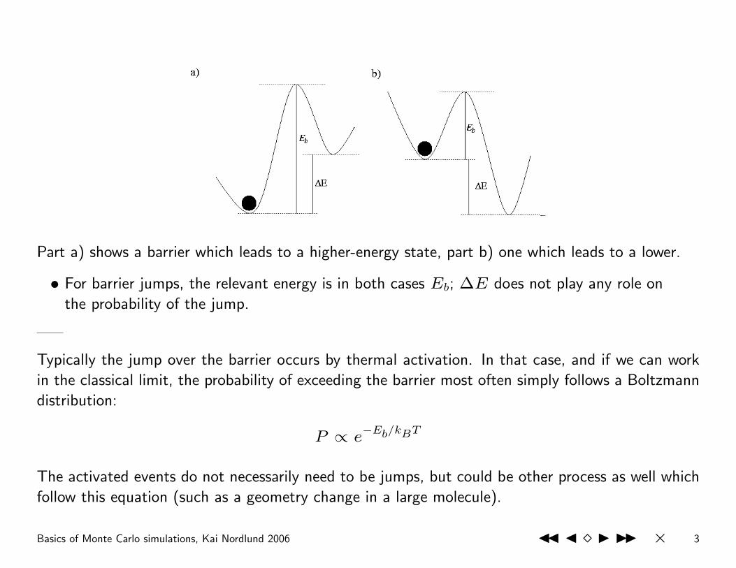
Part a) shows a barrier which leads to a higher-energy state, part b) one which leads to a lower.

• For barrier jumps, the relevant energy is in both cases Eb; ∆E does not play any role on

the probability of the jump.

Typically the jump over the barrier occurs by thermal activation. In that case, and if we can work

in the classical limit, the probability of exceeding the barrier most often simply follows a Boltzmann

distribution:

P ∝ e−Eb/kBT

The activated events do not necessarily need to be jumps, but could be other process as well which

follow this equation (such as a geometry change in a large molecule).


By introducing a proportionality constant we can write the event frequency as

event rate(T) = w = w0e−Eb/kBT

(1)

where w0 can be interpreted as an “attempt frequency” telling how often an attempt is made to

exceed the barrier.

• In case Eb = 0, or T = ∞, we see that every attempt would be successful.

In solids it is easy to understand the attempt frequency: it is simply the vibration frequency of the

atom. It can often be predicted to good accuracy when the atom vibration (elastic and sound)

properties of the lattice are well known. Typically it is of the order of 1/(100 fs).

• As a good approximation, w0 is independent of T , at least in solids, basically because the

elastic constants are almost independent of T .

In section we show that the probability density for a transition to occur is

f(t) = re−rt


Hence the use of an average transition time in the random walk discussed in the previous section is

a quite crude approximation.

• If there is only one transition rate, the approximation may not be too bad.

• But if we want to simulate processes which involve many different kinds of transitions

occurring at different rates, it is rather clear it is not justifiable to ignore the real,

exponential time dependence.

– Moreover, if we use Eq. 1 to derive the event probability in our simulations, we get

the added advantage that we can do simulations at any temperature realistically, even

if the temperature keeps changing during the modeling.

One can now think of 3 basic approaches to simulate a system with multiple rates:


1. Use a short ∆t. For every step, go through all particles i, and use wi to randomly choose

whether it will move at this particular time interval. This approach has the advantage that it

is intuitively clear, and that it is perfectly clear what the real time is. The disadvantage is that

to preserve the ratios between different rates, one has to have ∆t � 1/wmax, where wmax

is the fastest event rate in the system. This makes this approach very slow and inefficient,

as many time steps will be spent when nothing or only a few particles move, even though all

particles have to be gone through at every step.

2. Pick a particle i randomly. Then let it jump according to a probability e−Eb/kBT . This works

fine, and in fact is a special case of the Metropolis algorithm discussed later on during the

course. The downside for this is that it is often not clear how to derive the real time scale from

the number of Monte Carlo steps.

3. Pick a particle at random, but with a probability proportional to its jump rate. This clearly

makes the routine efficient, as every step produces a jump. Since the method combines

efficiency and real time, it is close to perfect for simulation of activated processes.

Approach 3 is the essence of the kinetic Monte Carlo method.


8.2. The kinetic Monte Carlo algorithm

For the kinetic Monte Carlo simulations, we consider a system with a set of transitions Wi from a

state xa into other possible states xb

Wi(xa → xb)

For each Wi there is a transition probability per unit time, i. e. rate ri. i loops over all possible

transitions. The rate is typically given by Eq. 1.

The Kinetic Monte Carlo method can be used to simulate these processes provided:

1◦ The transitions are Poisson processes

2◦ The different processes are independent, i.e. not correlated

3◦ The time increments between successful steps are calculated properly

• Point 1◦ is explained below in section .

• There we will also prove the equation which calculates the time increments needed for

step 3◦ .


• Requirement 2◦ has been discussed above, but to restate this: we require that one event

is only dependent on the previous state of the system, but is not dependent on how any

previous event occurred.

In addition to these, some theorists add a requirement

4◦ The transition probabilities follow a so-called “dynamical hierarchy” which obeys detailed

balance

This requirement may be necessary when one uses the simulations to examine the static and dynamic

properties of the Hamiltonian describing the system. However, it is perfectly possible and quite

commong to use KMC to model systems which are constantly out of equilibrium and do not satisfy

criterion 4◦ .

An example of such systems is so called “driven systems” where some external factor (irradiation,

high pressure) keeps the system out of reaching thermodynamic equilibrium. Since criterion 4◦ is

not necessary to fulfill to use KMC, we will not discuss it in detail.

Without any further ado, I will present the usual KMC algorithm.


0◦ Set the time t = 0

1◦ Form a list of all the rates ri of all possible transitions Wi in the system

2◦ Calculate the cumulative function Ri =

iXj=1

rj for i = 1, . . . , N where N is the total

number of transitions. Denote R = RN

3◦ Get a uniform random number u ∈ [0, 1]

4◦ Find the event to carry out i by finding the i for which

Ri−1 < uR ≤ Ri

5◦ Carry out event i

6◦ Find all Wi and recalculate all ri which may have changed due to the transition

7◦ Get a new uniform random number u ∈ [0, 1]

8◦ Update the time with t = t + ∆t where:

∆t = −log u

R(2)

9◦ Return to step 1


• This algorithm is known as the residence-time algorithm or the n-fold way or the

Bortz-Kalos-Liebowitz (BKL) algorithm or the kinetic Monte Carlo (KMC) algorithm.

– I would recommend using “residence-time algorithm”, since this is nowadays in quite

common use.

• Strictly speaking, any algorithm which uses equation log uR to calculate time can be called a

KMC method. The above algorithm is thus the “residence time algorithm” implementation

of KMC.

• An interesting thing to note is that the time scale could also be calculated as 1/R without

the random number, and one would obtain exactly the same long-time average of the time

scale.

– This is because the average of log u for u in the interval [0, 1] is exactly -1.

– However, including the random number gives a better description of the stochastic

nature of the Poisson processes, which obviously will not occur at even time intervals.


8.2.0.1. History of Kinetic Monte Carlo

The history of kinetic Monte Carlo is somewhat murky.

– In contrast to the Metropolis method which is well defined to have begun with a single

paper from 1953.

The Metropolis method gave no time scale, so it is obvious people would start to try to obtain it

once that method was out.

• One of the first works in the direction of kinetics was by Flinn and McManus [Phys. Rev.

124 (1961) 54] who considered transition probabilities and rates in vacancy motion. But

they did not derive any explicit time scale, so this does not really count as KMC.

• Apparently the first publication which described the basic features of the above KMC

method (using a cumulative function to select an event and a time scale calculation of

the form 1/R) was by Young and Elcock, Proc. Phys. Soc 89 (1966) 735.

• Bortz, Kalos and Lebowitz [J. Computational Physics 17 (1975) 10] developed a KMC

algorithm for simulating an Ising Spin system, and described in detail the most algorithm

described above, which they called the “n-fold way”.

– They also derived the log u/R form of the time calculation


– But strangely enough, they did not cite the Young and Elcock paper at all

Perhaps because of these murky origins, the KMC method is still not described in most MC

textbooks, even though it is widely used.

• A good modern reference to the theory of the method is [Fichthorn and Weinberg, J.

Chem. Phys. 95 (1991) 1090].

8.2.0.2. Notes on efficiency

The algorithm is clearly O(N), since at least step 2◦ has a sum over N elements. This sounds

good, but remember that this means that we need N operations for every event, and probably want

to simulate millions or billions of events.

In case this is the bottleneck in terms of efficiency, it is possible to remake the algorithm to achieve

below-N scaling for every event, even down to O(log2 N), using so called binning methods and

recursive tree searches.

• The basic idea of binning methods [Maksym, Semicond. Sci. Technol. 3 (1988) 594] is

rather obvious: one can place all possible events with the same rate ri into the same bin

j, then select events first from the bins j and then from one bin select randomly one of

the events i.


– If there are numerous objects with the same rates, this can give easily substantial time

savings.

We will not present these in detail here, since they belong more to the realm of computer science

than physics, but if you start doing KMC with many event or object types, it is best to look into it.

We will now first look at what the central idea behind the selection scheme is (steps 2◦ – 5◦ ),

then motivate and derive the time advancing equation in step 8◦ .

8.2.1. Motivation for the basic approach

Say we have a system with 3 objects

A1, A2, A3

The system state xa is then the list of objects {A1, A2, A3}. The possible transitions are that

each object may change into another object, i.e.

A1 A2 A3

↓ or ↓ or ↓B1 B2 B3

Then we have three transition rates. Let us arbitrarily say that they are

r1 = 0.1, r2 = 0.3, r3 = 1.2


which would give the cumulative function Ri as

R1 = 0.1, R2 = 0.4, R3 = 1.6

We can now plot the ri as regions and Ri as points on a line as follows:

0 0.1 0.4 1.6

r1 r2 r3

If we now generate a random number u between 0 and 1, and multiply it by R = 1.6, this number

uR will correspond to some point on the line. It is clear from the figure that the probability of e.g.

obtaining point 2 is

0.1 < uR < 0.4

i.e. proportional to r2/R. So we will get the different events with a probability which corresponds

to their rate. This is exactly what we wanted from the beginning.

8.2.2. Motivation of equation for time

To motivate eq. 2, we consider the activated processes discussed above, for which the jump

frequency is

jump rate(T) = w(T ) = w0e−Eb/kBT

Now consider a fixed T . We then have jumps occurring at a rate r = w(T ).


If further the probability of a jump to occur is independent of the previous history, and the same

at all times (both quite reasonable assumptions), the transition probability is a uniform function of

time. Then the process is a so called Poisson process, which are quite well known in the theory of

stochastic processes [Fichthorn, J. Chem. Phys. 95, 1090, and references therein].

To derive the functional form of the time dependence, consider a single object with a uniform

transition probability r. Call f the transition probability density, which gives the probability rate

that the transition occurs at time t. The change of f(t) over some short time interval dt is

proportional to r, dt and f because f gives the probability density that particles still remain at

time t. I.e.

df(t) = −rf(t)dt =⇒df

dt= −rf

and the solution is

f(t) = Ae−rt

By using the boundary condition f(0) = r we get

f(t) = re−rt

A useful feature of Poisson processes is that a large number N of Poisson processes, with rates ri,

will behave as another large Poisson process with the same properties of a single process. Hence for

this process one can write the probability density as

F (t) = Re−Rt

(3)


with

R =

NXi=1

ri. (4)

F (t) now gives directly the transition probability density for the whole system.

We know from section 4 how to generate random numbers in any distribution; the integral function

is now e−Rt and we get the inverse from

e−Rt

= u =⇒ t = −ln u

R(5)

where u is a uniform random number. This is exactly Eq. 2 above!

We can now also do a consistency check by calculating the average time between jumps < t > in

the composite system in two different ways. First we obtain < t > by integrating equation 3

< t >=

Z ∞

0

Rte−Rt

dt = Rt−1

Re−Rt

˛∞0

−Z ∞

0

R−1

Re−Rt

dt = − R−1

R

−1

Re−Rt

˛∞0

=1

R

But we can also obtain the average assuming Eq. 5 is valid, by obtaining the average of ln u over


all random numbers between 0 and 1, i.e.Z 1

0

ln udu = −1

Hence < t > from Eq. 5 is also 1/R, so everything is really consistent here.

8.2.3. Some analysis of the algorithm

8.2.3.1. Advantages

With some thought, we can see several interesting features in the KMC algorithm. One is that

there is nothing in the algorithm which requires thermodynamic equilibrium; we can start with any

set of transitions, and as long as they fulfill the basic criteria given above, we can use this method.

• In fact the algorithm only deals with rates, so it could actually be used to simulate anything

with a set of known rates, even if the system has nothing to do with thermodynamics!

– E.g. nuclear decay with known half-lifes.

Moreover, because the ri and Wi and the list of them are recalculated on every iteration (steps 1◦

, 2◦ and 6◦ ), the objects simulated can change character at every step.


• They can for instance react with each other to form reaction products, which can be

entirely new objects, vanish from the system by some form of recombination, or an object

may split up into several new objects.

• If this kind of non-preservation of objects occurs, the method has another major advantage.

Since R is recalculated every step depending on which objects are present, the time scale

∆t of the steps will follow the system evolution automatically.

• So, if we initially for instance have a set of very fast-moving objects, which after some

time have reacted so that there are only slow-moving objects left, the time scale will

automatically get longer after the fast objects are gone.

• And this also works the other way: if a slow object breaks up and emits a fast-moving

object, the method will immediately switch to shorter time scales.

• Thanks to this feature, KMC can be used to model systems where the initial time scale

is of the order of fs, and the final one of the order of minutes, hours or sometimes even

years.

8.2.3.2. Disadvantages

The major physical disadvantage with KMC is that all possible rates ri and reactions have to be

known in advance.


• The method itself can do nothing about predicting them!

• Instead, they have to be obtained from experimental data, or derived from other

simulation methods, typically electronic structure calculations or molecular dynamics

(MD) simulations.

• This is a clear and strong contrast to MD simulations. These can, based on (hopefully)

well motivated interatomic force models, predict transition rates, and sometimes even find

entirely new kinds of transitions and reactions. But they are limited to short timescales,

at most µs:s.

Another minor disadvantage from a computational efficiency point of view is forming all the lists

and recalculating the ri (steps 1◦ , 2◦ and 7◦ ). Especially recalculating all ri may be quite slow.

• But since every step only carries out one event ie, and thus usually only affects a small

subset of all objects, it is probably in most applications possible to deduce and update

those ri which may have been affected by the ie event.


• In fact, in complex systems with many different kinds of objects and events possible, the

major effort in writing a KMC program tends to be in constructing the binning method,

and finding and implementing data structures and bookkeeping algorithms which allow for

efficient updating, rather than on the physics side.


8.3. Applications

The presentation above was intentionally kept on an as abstract and general level as possible, to

emphasize the fairly general character of the method. Now we will, to hopefully give a better idea

of how this can work in practice, first list a few examples of where KMC has been used, then go

through one real-life example of considerable practical importance in detail.

8.3.1. Examples

[Duane Johnsons article]

KMC has been at least used in simulations of the following physical systems:

1. Surface diffusion

2. Molecular beam epitaxy (MBE) growth

3. Chemical vapor deposition (CVD) growth

4. Vacancy diffusion in alloys

5. Compositional patterning in alloys driven by irradiation

6. Polymers: topological constraints vs. entanglements


7. Coarsening of domain evolution

8. Dislocation motion

9. Defect mobility and clustering in irradiated solids

In the following, we will discuss the last example, especially for the case of Si.

8.3.2. Point defects in Si

[Own knowledge, but see e.g. Mayer-Lau, Electronic Materials Science For Integrated Circuits in Si and GaAs, MacMillan 1990, and Chason et

al., J. Appl. Phys 81 (1997) 6513]

When a solid material is irradiated with ions, neutrons or electrons of sufficiently high energy (∼100 eV for ions or neutrons, more than 100 keV for electrons), they produce damage in the material.

If the material is crystalline, this damage can as a first approximation be described as consisting of

empty lattice sites (=vacancies), and extra atoms between lattice sites (=interstitials).

The reason to this is simply that when the energetic particle collides with a lattice atom, it can kick

it out from its own site, after which the atom most probably ends up in an interstitial site.

In reality, there is often also significant defect clustering going on, and in metals the clusters often


in fact dominate the behaviour. But in Si it turns out that the simple vacancy-interstitial picture

can be used as the starting point for studying defect migration with good results.

So we now consider Si only. During the manufacturing of Si computer chips (the very ones which

are inside every present-day computer) ion irradiation is routinely used to introduce dopant atoms

into silicon. In present-day chips the irradiation goes a few hundred nm deep in the Si. The depth

is of the same order of magnitude as the linewidth of the central components in the chip, which

today (2006) is 90 nm in top-of-the-line Intel and AMD processors.

During this irradiation the doses are so large that a very high defect concentration forms in the Si,

and usually it in fact amorphizes.

• Since the chip only works for crystalline Si, the Si wafer is raised to a very high temperature,

∼ 1000 K for furnace anneals, ∼ 1300 K for light-induced so called “rapid thermal”

anneals, to recrystallize the amorphized region.

When the amorphized region recrystallizes, it will initially have a very high concentration of vacancies

and interstitials.


• These will start migrating, many of the vacancies and interstitials will recombine, some

will reach the surface where they essentially vanish, some will escape into the bulk of the

Si, and some cluster with other defects of the same type to form vacancy and interstitial

clusters.

• The clusters can also break up and emit new point defects.

Understanding this process is crucial for further miniaturization of the chip components, and KMC

can be the crucial tool for this, as it can simulate all of the processes described above.

For instance, a few years ago a major problem appeared when it turned out that there was an

anomalous, so called “transient-enhanced” diffusion (TED) process driving boron dopant atoms

much deeper in than they should be for the chip to work properly.

• Understanding of what was going on was achieved by a combination of KMC simulations

and experiments, which eventually revealed that Si interstitials were enhancing the mobility

of the boron atoms.

Right now an additional, related problem is that there is no known easy way in which the B doping

can be carried out shallower than 20 nm from the surface, since the required B concentrations will

be so high that a boronization-enhanced diffusion will always drive the B in to at least this depth.


• If this problem is not solved, the further miniaturization of Si chips (as predicted by

Moore’s law with a time constant of 18 months) may stop completely sometime around

2010. Whatever the solution may be, it is likely KMC simulations will be somehow

involved in obtaining it.


8.4. KMC simulation of point defects in Si

For educational purposes, and to make the rather abstract algorithm given above more concrete, I

will now describe in detail how to simulate a stripped model of defect migration in Si.

• I will only consider the two basic defect types, the interstitial and vacancy, and ignore

clustering completely.

• But I will include the most basic defect reaction: recombination. It is self-evident that if

a vacancy and interstitial come sufficiently close to each other, the extra interstitial atom

will fill in the vacant lattice site, and only perfect Si lattice will remain. So this is a true

case of the simulated objects vanishing.

To simulate this process, the defect migration coefficients need to be known. They are actually notknown to very good accuracy, and at low temperatures subject to controversy even in the order of

magnitude. For high temperatures some sort of agreement on the values does exist.

We will use the values reported in 1996 by Tang et al. [Phys. Rev. B. 55 (1997) 14279], giving the

migration properties as

jump rate(T) = w = wde−Em/kBT

where wd is the defect jump rate prefactor and Em the migration activation energy. The values


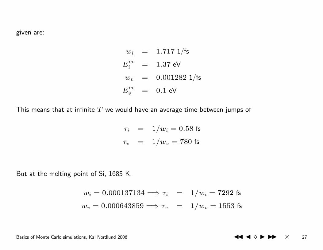
given are:

wi = 1.717 1/fs

Emi = 1.37 eV

wv = 0.001282 1/fs

Emv = 0.1 eV

This means that at infinite T we would have an average time between jumps of

τi = 1/wi = 0.58 fs

τv = 1/wv = 780 fs

But at the melting point of Si, 1685 K,

wi = 0.000137134 =⇒ τi = 1/wi = 7292 fs

wv = 0.000643859 =⇒ τv = 1/wv = 1553 fs


so at all realistic temperatures the vacancy in this model moves faster than the interstitial because

of the lower activation energy.

The jump length is set to the nearest-neighbour atom distance in Si, 2.35 A, since this corresponds

to the known migration mechanisms. Moreover, the KMC simulations in Si are usually performed as

if the defect motion in it would occur in a random medium (so you can ignore the lattice structure).

Recombination is described simply by assuming that if an interstitial and vacancy are within 4 A

from each other, they will immediately recombine. This is a quite realistic assumption, except that

the exact value of the recombination distance may vary.

So in our model system, there are 3 possible processes:

1. A vacancy jumps by 2.35 A in a random direction

2. An interstitial jumps by 2.35 A in a random direction

3. If a vacancy and interstitial are within 4 A from each other, they will immediately recombine and

vanish from the system.

So now the possible transitions Wi are just the defect jumps 1 and 2, and there is only one possible

transition per defect. So the array of events will simply coincide with the array of defects.


Process 3 is not activated, so it is treated as a step which is not part of the actual residence-time

algorithm.

Assuming we only simulate at constant temperature, here is description of how we can simulate this

problem with KMC:


0 a◦ Set the time t = 0. Set initial positions of all N defects xj for j = 1, . . . , N and their types tj. Set thetemperature T and recombination radius rrec = 4.0 A. Set Niter = 0 and select Nitermax

0 b◦ Go through all defects and for each defect find whether any defect of the opposite type is closer than rrec toit. If so, remove both from the tables xj and tj, set N = N − 2

0 c◦ Calculate the jump rate for interstitials from T: wi = wie−Em

i /kBTand same for vacancies v

1◦ Set rj = wd where d = i or d = v, depending on the defect type tj for all j = 1, . . . , N

2◦ Calculate the cumulative function Rj =

jXk=1

rk for j = 1, . . . , N . Denote R = RN

3◦ Get a uniform random number u ∈ [0, 1]

4◦ Find the defect to move j out by finding the j for which

Rj−1 < uR ≤ Rj

5◦ Carry out jump j by displacing defect j in a random direction in 3D by 2.35 A

6◦ For defect j, find whether any defect of the opposite type is closer than rrec to it. If so, remove both fromthe tables xj, tj and rj, set N = N − 2.

7◦ Get a new uniform random number u ∈ [0, 1]

8◦ Update the time with t = t + ∆t where:

∆t = −log u

R

9◦ Set Niter = Niter + 1. If Niter < Nitermax return to step 1.

10◦ Analyze for desired properties and print results


In the exercises you get to code this for yourself to get a good feeling of it.

8.4.0.1. Sample application

We now use this method to study the following question. During ion irradiation, the defects induced

by a single incoming ion are as a rough first approximation produced in Gaussian distributions. The

average depth of the interstitials is slightly deeper in than the vacancies (simply because the ions

tend to kick the atoms deeper in on average). Let us say the defect profiles would be two Gaussians

with means of 100 A and 105 A and the same standard deviations of 30 A:


We want to simulate what happens in this system at different temperatures, especially what fraction

of the defects recombine and where the rest end up (the surface or the bulk).

The irradiation is carried out on a very wide area (mm’s or cm’s), which we can not possibly

simulate. But when we are interested in a section in the middle of the irradiation region, we can

simply pick a small section of the Si, and apply periodic boundaries on the sides in x and y (i.e. let

the defects move and interact over the boundary to the other side of the simulation cell). The size

has to be clearly larger than the jump length or recombination radius, and large enough to contain

a substantial amount of defects.

The surface is a perfect sink for defects, i.e. any defect which goes above z = 0 vanishes from the

system. The size inside the cell is assumed to be infinite (in reality it typically is ∼ 1 mm, large

enough that we will never reach it with 2.35 A jumps in our simulations).

So the simulation geometry is as follows, in a 2D projection:


I slightly modified the algorithm above to simulate this; the additions are just the periodic boundaries

and sink at the surface (note that in the exercise you need neither of these!).

The atomic density in Si is 0.050 atoms/A3. So if we choose the xy cell size as 20 A, and consider

that 68 % of the defects will be within 1 standard deviation (now 30 A) of the average, the relation

between the simulated number of defects of each type N and the defect concentration ρ in the


central region will be

ρ =0.68N

202 × 30× 0.05= 0.0000567N

So to get a typical defect concentration of e.g. 1%, we need to have 176 defects of each type, i.e.

352 in total.

After running the simulation, we can plot the time dependence of the numbers of defects and

reactions as follows. This is for 1000 K, a typical “furnace annealing” temperature:


So what happens is that there is almost immediately some recombination, as closeby vacancies and

interstitials recombine. After that the more mobile vacancies tend to vanish at the surface, and keep

on recombining. At about 1010 fs the last vacancy is gone, the simulation speeds up significantly,

and the interstitials start moving. In the very end, at about 1013 fs (0.01 s), only a few interstitials

remain.

Here is a sequence of picture illustrating what is going on initially: The red dots are vacancies, the

purple ones interstitials. The plotting region is 0-20 A in the x direction, 0-300 A in the z direction

(the labels in the figure are misleading). The surface z = 0 is to the left.


The interstitials do not move essentially at all in this phase, so what happens is just that the

vacancies vanish by recombination and at the surface. But a few vacancies go deep into the bulk.

But on longer time scales, these vacancies have a chance to come back to the interstitial layer and

recombine. This is what happens. Here is a plot of the state at 1 µs (note that the z scale is now

extended from 0 to 10000 A):


So the vacancies are indeed quite far from the interstitials, but from the time dependence plot we

see that they do eventually recombine. Here is then the final state at almost 2× 1013 fs = 0.02 s:

On even longer time scales, the interstitials would most probably eventually reach the surface. The

total number of defect steps simulated in this run was about 56 million.


At higher temperatures, 1300 K (a typical rapid thermal anneal temperature), the picture changes

somewhat because the interstitials and vacancies are mobile on comparable time scales. Hence the

relative time scale difference on the number of i’s and v’s is considerably less:

The total time scale here is much less than at 1000 K, as expected for higher temperatures. In this

case the simulation ended when all particles had vanished.

If we look at a clearly lower temperature, say 600 K, everything of course is slower still, and there

is no interstitial mobility at all on the time scales when the vacancies move:


Note the huge difference in time scales here: the vacancies vanish completely in 0.16 ms, while the

interstitials only start moving on time scales of seconds, and subsequently vanish on timescales of

hours! This illustrates well the power of KMC to simulate widely disparate timescales.

There is also very little recombination now; apparently the recombination is significant primarily

when the interstitials are mobile on time scales comparable to the vacancy. In additional tests as a

function of temperature, I found that there was very little recombination even at 800 K, and only

at temperatures close to 900 K and above did it become significant.


Now that we have seen the results, did it matter that the interstitials were 5 A deeper in than the

vacancies? Almost certainly not, since each step was 2.35 A, and the number of steps taken very

large, so the 5 A difference probably got washed out completely.

But the difference could be of consequence if the difference was much larger than the step size and

average number of steps before recombination.

• I tested this having mean ranges of 1000 A for vacancies, and 1100 A for interstitials, and

standard deviations of 100 A for both.

• The initial distributions still overlap significantly, but after some minor annealing, there is

no overlap at all.

So we have produced a defect zone with only vacancies, and another one with only interstitials:


This is the concept behind concept of a “vacancy implanter”, which actually has been built and

may provide a solution to the TED problem mentioned above (not that this information belongs

would belong to this course).

Note that in these examples, we still had a fairly small number of objects to study. If this were

a serious study, one would of course have to repeat the simulations for different seed numbers


and larger system sizes to ensure that the non-physical simulation parameters do not affect the

conclusions drawn.

• And include the defect clustering reactions...

But still, the models used were not entirely unrealistic, and the qualitative results actually do

correspond to reality.


8. kinetic monte carlo - acclab.helsinki.fiknordlun/mc/mc8nc.pdf · kinetic monte carlo ... per...

Documents