Computer Science and Software Engineering

University of Wisconsin - Platteville

Computer Science and Software Engineering

University of Wisconsin - Platteville

8. Machine Learning

CS 3030 Lecture Notes

Yan Shi

UW-Platteville

Read: Textbook Chapter 10

Common ML Problems

Classification: data is labeled (assigned a class).

— e.g., spam/non-spam, fraud/non-fraud

Regression: data is labeled with a real value

— e.g., predict stock price

Clustering: data is not labeled, but can be divided into groups based on similarity

— e.g., social network

ML Strategies

Supervised Learning— The computer is presented with example inputs and their

desired outputs, given by a "teacher", and the goal is to learn a general rule that maps inputs to outputs.

Unsupervised Learning— no labels are given to the learning algorithm, leaving

it on its own to find structure in its input. Unsupervised learning can be a goal in itself (discovering hidden patterns in data).

Reinforcement Learning— Learning systems are given a positive feedback when

they classify data correctly, and negative feedback when they classify data incorrectly.

Training

Learning problems usually involve classifying inputs into a set of classifications.— Learning is only possible if there is a relationship between the

data and the classifications.— That is, can identify a function f : data → classification

Training involves — providing the system with data which has been manually

classified— system learn from the training data how to classify unseen data.

Training data:— usually more than one variable— can be of different types

Concept Learning

Concept learning involves determining a mapping: a set of input variables a Boolean value.— Such methods are known as inductive learning

methods.

If a function can be found which maps training data to correct classifications, then it will also work well for unseen data – hopefully!— This process is known as generalization.

Example

safe(Speed, Weather, CarDist, SleepHours, TimeOfDay, Temp)

— Speed: slow, medium, fast

— Weather: wind, rain, snow, sun

— CarDist: integer giving feet: 10, 20, 30, 40, 50, 60

— SleepHours: hours of sleep over last 24 hours

— TimeOfDay: morning, afternoon, evening, night

— Temp: cold, warm, hot

Hypotheses

A hypothesis is a vector of variables:h1 = <slow, wind, 30, 8, evening, cold>

In concept learning, a training hypothesis is either a positive or negative (true or false) one.

A ? is used to indicate that any value will be suitable.— h2 = <fast, rain, 100, 3, ?, ?> : negative

A Ø is used to indicate that no value will be suitable.— h3 = <fast, rain, 100, 3, Ø, Ø>

Concept learning: examine set of positive, negative training examples; identify set of patterns that completely classifies data

General to Specific Ordering

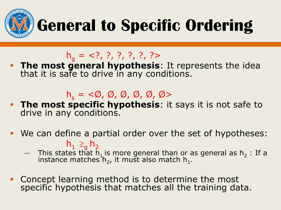
hg = <?, ?, ?, ?, ?, ?> The most general hypothesis: It represents the idea

that it is safe to drive in any conditions.

hs = <Ø, Ø, Ø, Ø, Ø, Ø> The most specific hypothesis: it says it is not safe to

drive in any conditions.

We can define a partial order over the set of hypotheses:h1 g h2

— This states that h1 is more general than or as general as h2 : If a instance matches h2, it must also match h1.

Concept learning method is to determine the most specific hypothesis that matches all the training data.

Simple Learning Algorithm

start from the most specific hypothesis hs

for each training case, — if hypothesis does not cover the case, then replace the

attributes in the hypothesis with the next most general value that does match:

Example:Given training hypotheses— safe(slow, wind, 30, 8, evening, cold) — safe(slow, rain, 20, 8, evening, warm) — safe(slow, snow, 30, 8, afternoon, cold)

Algorithm Issues:— only one solution: most specific one (may not be optimal)— does not allow for negative examples — does not handle inconsistent data

Version Space

A version space is the set of hypotheses that correctly map all the training data to their categories.

A simplistic learning method would be to start from a version space of all hypotheses and to systematically remove all the ones that do not match the training data.

Clearly this would not be an efficient learning method!

Based on the similar idea, we can use candidate elimination to learn.

Candidate Elimination Algorithm

Goal: Derive one hypothesis which matches all training data.

Initial sets:hg = set with predicate matching all cases hs = set with predicate matching no cases

For each positive training example p: —remove all elements of hg that fail to match p —if x in hs does not match p, replace x by the set of

items Y where each element in Y is minimally more general than x but still matches p

—delete from hs any hypothesis more general than some other hypothesis in hs

—delete from hs any hypothesis more general than some hypothesis in hg

Candidate Elimination Algorithm

(Continued)

For each negative training example n: — remove all elements of hs that match n — if x in hg matches n, replace x by the set of items

Y where each element in Y is minimally more specific than x but does not match n

— delete from hg any hypothesis more specific than some other hypothesis in hg

— delete from hg any hypothesis more specific than some hypothesis in hs

If end result is empty, then there is no concept that matches all positive cases and no negative cases;

if it is a singleton then you have found your concept

Example

learn simplified form of safe:safe(Speed, Weather, SleptRecently)

where— Speed: slow, medium, fast— Weather: rain, sun— SleptRecently = at least 5 hours in last 24: yes, no

Training data:— positive: safe(slow, rain, yes) — negative: safe(fast, rain, no) — positive: safe(medium, rain, yes) — negative: safe(fast, sun, no) — positive: safe(fast, sun, yes)

Training case hg hs

Initially: { safe(_, _, _) } { safe(none, none, none) }

positive: safe(slow, rain, yes) { safe(_, _, _) } { safe(slow, rain, yes) }

negative: safe(fast, rain, no)

{ safe(slow, _, _), safe(medium, _, _),safe(_, sun, _), safe(_, _, yes) }

{ safe(slow, rain, yes) }

positive: safe(medium, rain, yes) { safe(medium, _, _), safe(_, _, yes) }

{ safe(_, rain, yes) }

negative: safe(fast, sun, no) { safe(medium, _, _), safe(_, _, yes) }

{ safe(_, rain, yes) }

If next item is...

positive: safe(fast, sun, yes) { safe(_, _, yes) } { safe(_, _, yes) } - done

On the other hand, if next item is...

positive: safe(slow, rain, no) { } { safe(_, rain, _) } - fail

Inductive Bias

All learning methods have an inductive bias. The inductive bias of a learning method is the set

of restrictions on the learning method.

Bias in Candidate Elimination algorithm: — Assume the solution can be expressed as a

conjunction of concepts.— Does not allow more complex expressions there

might be some solutions we cannot explore.

Inductive bias is necessary: without it, a learning method could not learn to generalize.— rote learning: just learning set of facts

Decision Tree

Will a film be a box-office success?

Decision Tree Induction

A decision tree takes an input and gives a Boolean output.— Version space: only conjunctions

— Decision tree: conjunctions and disjunctions

Decision tree induction involves creating a decision tree from a set of training data that can be used to correctly classify the training data.— Classics algorithm: ID3 (Quinlan, 1980s)— This has been improved upon, but at cost of more complexity

ID3 builds the decision tree from the top down, selecting the features from the training data that provide the most information at each stage.

Entropy and Information Gain

Entropy: H(S) = - p1 log2 p1 - p0 log2 p0P1:the proportion of the training data which are positive p0 is the proportion which are negative

The entropy of S is zero when all the examples are positive, or when all the examples are negative.

The entropy reaches its maximum value of 1 when exactly half of the examples are positive, and half are negative.

Information Gain of a feature: — original entropy - weighted sum of entropies of each category.

H(S) - wiH(Si)— Weight is the proportion of the training data that fell into that

category.

Example

Example (Continued)

H = 1 (half are box-office success) H(USA) = -(3/4)log2(3/4) – (1/4)log2(1/4) = 0.811 H(Europe) = 1 H(Rest of World) = 0 Gain(Country) = H – 0.4H(USA) – 0.4H(Europe) – 0.2H(Rest of

World) = 0.276 … Gain(Big star) = 0.01 Gain(Genre) = 0.17 We should pick “Country of Origin” as the top node.

Repeat this process until we build the entire decision tree. If entire training set is of the same category/same result, a

leaf node is reached.

Artificial Neural Network

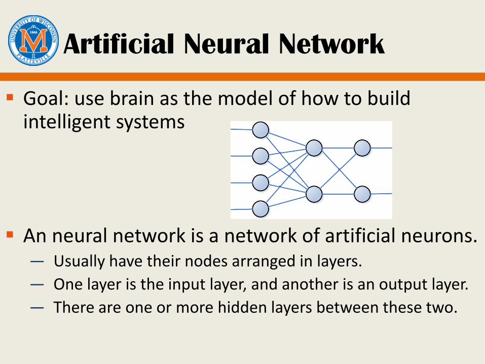
Goal: use brain as the model of how to build intelligent systems

An neural network is a network of artificial neurons.— Usually have their nodes arranged in layers.

— One layer is the input layer, and another is an output layer.

— There are one or more hidden layers between these two.

22

Biological Neurons

The human brain is made up of billions of simple processing units – neurons.

Inputs are received on dendrites, and if the input levels are over a threshold, the neuron fires, passing a signal through the axon to the synapse which then connects to another neuron.

Artificial Neurons

Each neuron in the network receives one or more inputs.

An activation function is applied to the inputs, which determines the output of the neuron –the activation level.

What should be the activation function?

— Focus on many research works

Common Activation Functions

linear function: easy to understand, hard to interpret output

step function: easier to interpret output, hard to learn with

sigmoid function: Y = 1/(1 + e-x) most common solution

Perceptron

A perceptron is a single neuron that classifies a set of inputs into one of two categories (usually 1 or 0).

The perceptron usually uses a step function, which returns 1 if the weighted sum of inputs exceeds a threshold, and –1 otherwise.

Training a Perceptron

Training process: adjust the weights!— First, inputs are given random weights (usually

between –0.5 and 0.5).

— An item of training data is presented. If the perceptron mis-classifies it, the weights are modified as:

— e is the size of the error, 0 if correct, positive if the output is too low and negative if the output is too high.

— a is the learning rate, between 0 and 1.

Example: learning logical OR

We use t = 0, a = 0.2 Randomly initial weights as:

w1 = -0.2, w2 = 0.4

First example: 1, 1 1X = -0.2*1 + 0.4*1 = 0.2, Y = 1, correct

Second example: 1, 0 1X = -0.2, Y = 0, incorrect, e = y-Y = 1w1 = -0.2 + 0.2*1*1 = 0, w2 = 0.4 + 0.2*0*1 = 0.4

Third example: 0, 1 1X = 0.4, Y = 1, correct

Fourth example: 0, 0 1X = 0, Y = 0, correct. FIRST ITERATION(EPOCH) DONE.

Continue this process until all four examples are classified correctly!

x1 x2 y

1 1 1

1 0 1

0 1 1

0 0 0

Limitation of Perceptron

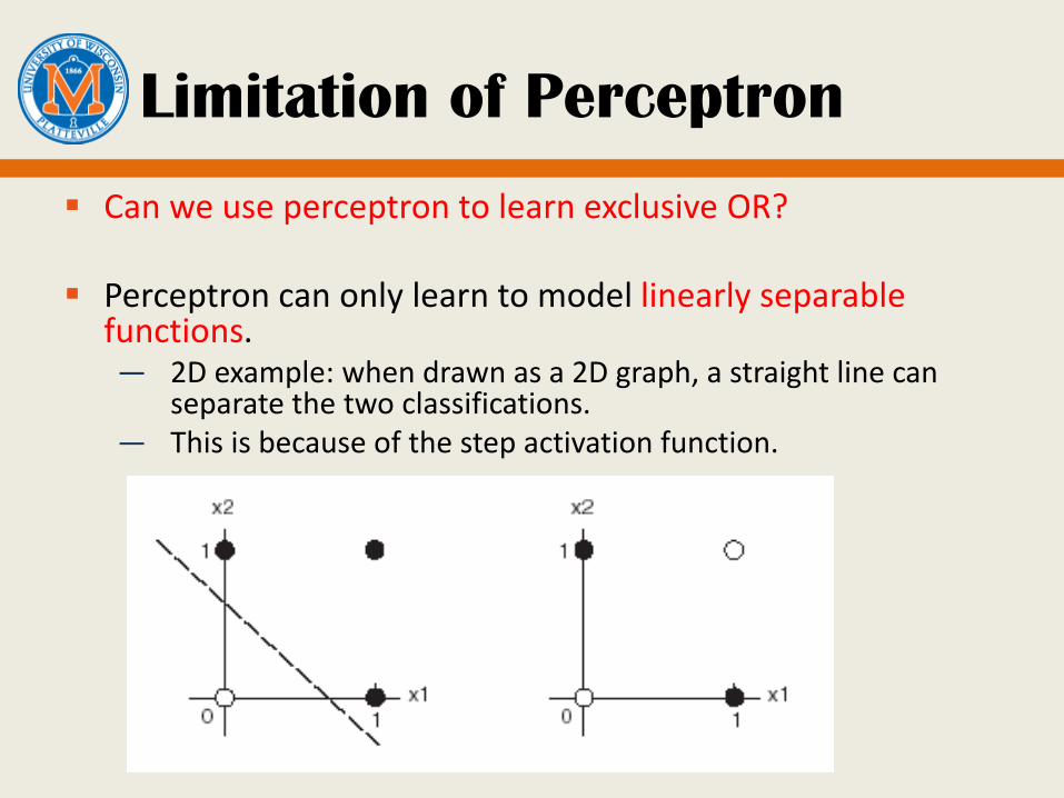
Can we use perceptron to learn exclusive OR?

Perceptron can only learn to model linearly separable functions.— 2D example: when drawn as a 2D graph, a straight line can

separate the two classifications.— This is because of the step activation function.

Multilayer Neural Network

Multilayer neural networks learn in the same way as perceptron.

Feed-forward network: Input layer simply pass the

input signal to the hidden layer. Output layer combines and

sends out output signals. Hidden layers do the real work. There are many more

weights to learn, and it is important to assign credit (or blame) correctly when changing weights.

Backpropagation Network

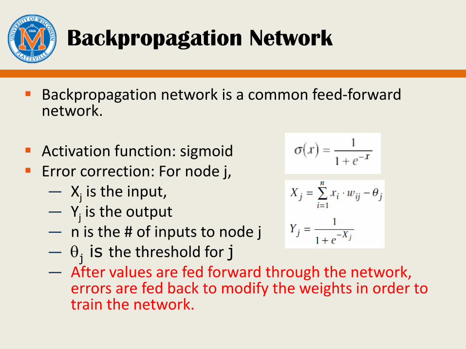
Backpropagation network is a common feed-forward network.

Activation function: sigmoid Error correction: For node j,

— Xj is the input,— Yj is the output— n is the # of inputs to node j— j is the threshold for j— After values are fed forward through the network,

errors are fed back to modify the weights in order to train the network.

For each node, we calculate an error gradient : the error value for this node multiplied by the derivative of the activation function.

Output layer node k has(ek is the error)

Hidden layer node j has

The weights are updated as

The training stops when the sum of the squares of the errors in an epoch is less than some threshold.

Backpropagation Network

Notes on BP Network

The method used in BP is known as gradient descent: — follow the steepest path down the surface that

represents the error function to attempt to find the minimum in the error space.

BP doesn’t mimic the human brain.

It is slow. — May take thousands of iterations(epochs) to reach a

satisfactorily low level of error.— How to improve? See Ch 11.4.2

BP in action: http://selene.science.ru.nl/backprop.html

Evaluating a Learning Algorithm

Split examples into training set and validation set Train on (often smaller) training set, then use

validation set to check results

Possible Issues:— noisy inputs: errors from noisy sensors/misinterpreted

inputs— classification noise: misclassified examples— Overfitting: no generalization

For NN, don't want more hidden units than inputs and outputs must have more test cases than number of weights (often at

least 10 times as many tests as weights)

Summary

Common ML Problems

Three types of ML

Concept learning

— Candidate elimination

— Decision tree

ANN

— Perceptron

— BP