a 3d high-order aeroacoustics model for turbomachinery fan
TRANSCRIPT
A 3D High-Order Aeroacoustics Modelfor Turbomachinery Fan Noise
Propagation
by
Matthew Morgan Cand
Department of Mechanical Engineering
Imperial College London / University of London
A thesis submitted for the degree of
Doctor of Philosophy
June 2005
1
Abstract
This study investigates computational tools to predict forward-arcfan noise from aero-engines. Efficient computational procedures areneeded to model sound propagating in the intermediate zone betweenthe fan assembly and the intake surroundings, where boundary-elementmethods can then propagate it to the ground level. A high-ordermethod that is able to fully simulate the intake geometry’s non-axisymmetric nature, while remaining faster than traditional meth-ods, is investigated.
Following a review of the literature, a code solving the linearised Eulerequations, using a time-domain finite difference scheme, is developed.For the solid wall boundary condition, an immersed boundary tech-nique designed for aeroacoustics, with a careful extrapolation of valuesfrom the fluid, allows a regular Cartesian grid to be used in the wholedomain. A novel 3D formulation of this method, suitable for theaeroacoustics problems considered, was developed, and the algorithmis described in detail.
This scheme is first applied to a series of standard benchmark cases,of increasing complexity, for validation purposes. Some more repres-entative 3D inlet cases are then simulated: a simple model of theJT15D bellmouth turbofan and an elliptic profile. Finally, the effectof an asymmetric inlet geometry on modal propagation is investig-ated. Comparisons are made with results from a 2D aeroacousticscode, and from a traditional computational fluid dynamic scheme,evaluating the benefit of using the current approach. It is shown thata high-order scheme is more computationally efficient than low-ordertechniques, by at least one order of magnitude. But the wall bound-ary condition is shown to be excessively dissipative in 3D, and furtherwork is needed to improve its accuracy.
2
Acknowledgements
I would like to address heartfelt thanks to my supervisors, Pr. MehmetImregun and Dr. Abdulnaser Sayma. First, for directing me towardsthis research subject, but mostly for their patience, their supernaturalability to point me in the right direction every time, and their constantavailability despite a busy schedule.
For providing ACTRAN solutions for comparison, as well as guidance,the help and efforts of Dr. Naoki Tsuchiya and Prof. Jeremy Astley,from the Institute of Sound and Vibration, University of Southamp-ton, U.K., are gratefully acknowledged.
Thanks also to those, too numerous to mention all, who providedfriendly advice and guidance when we met. Amongst them: BrianTester, Francois Moyroud, Alexander Wilson, Joaquim Peiro, SpencerSherwin, Fred Perie, Pr. Hirsch . . .
I am grateful for the essential financial support of the Fondation del’Ecole Polytechnique and the OECD.
Many thanks to the delightful colleagues which made working muchnicer: Dr. Enrique Gutierrez, Dr. Hugo Elizalde, Sen Huang, Dario DiMaio, Gabriel Saiz and Marija Nikolic, Dr. Ibrahim Sever Dr. SureshPerinpanayagam, and all the italian Erasmus students in the office;Mehdi Vahdati, Michael Kim and Luca Di Mare in the UTC. I willhave many fond memories of discussions around (essential) cups ofstrong coffee.
My parents are to thank for many things, and I will limit myselfhere to acknowledging, with great affection, their total support andconfidence during these long years of study. The same goes for mydarling Robyn, the little London bird that I neglected too much inthe last 4 years. You made it all worthwhile.
3

4
Contents
Nomenclature 15
1 Introduction 191.1 Background . . . . . . . . . . . . . . . . . . . . . . . . . . . . . . 19
1.1.1 The place of noise in civil aviation . . . . . . . . . . . . . . 191.1.2 The importance of fan noise . . . . . . . . . . . . . . . . . 20
1.2 Problem statement . . . . . . . . . . . . . . . . . . . . . . . . . . 241.2.1 The need for computational models . . . . . . . . . . . . . 241.2.2 Computational aeroacoustics . . . . . . . . . . . . . . . . . 241.2.3 The mid-field domain . . . . . . . . . . . . . . . . . . . . . 26
1.3 Scope and aims of the thesis . . . . . . . . . . . . . . . . . . . . . 27
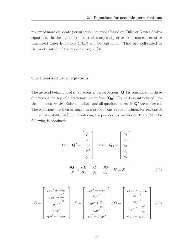
2 Model and discretisation 312.1 Equations for acoustic perturbations . . . . . . . . . . . . . . . . 31
2.1.1 Partition of variables . . . . . . . . . . . . . . . . . . . . . 322.1.2 Nature of the model . . . . . . . . . . . . . . . . . . . . . 322.1.3 Formulation . . . . . . . . . . . . . . . . . . . . . . . . . . 332.1.4 Possible extensions . . . . . . . . . . . . . . . . . . . . . . 36
2.2 Literature survey: spatial and temporal discretisation . . . . . . . 372.2.1 Spatial discretisation . . . . . . . . . . . . . . . . . . . . . 382.2.2 Temporal discretisation . . . . . . . . . . . . . . . . . . . . 512.2.3 Stability . . . . . . . . . . . . . . . . . . . . . . . . . . . . 532.2.4 Implementation . . . . . . . . . . . . . . . . . . . . . . . . 54
2.3 Boundary conditions . . . . . . . . . . . . . . . . . . . . . . . . . 552.3.1 Sound radiation . . . . . . . . . . . . . . . . . . . . . . . . 552.3.2 Solid walls . . . . . . . . . . . . . . . . . . . . . . . . . . . 572.3.3 In-duct boundary condition . . . . . . . . . . . . . . . . . 58
3 Three-dimensional wall treatment for noise propagation 613.1 Literature survey . . . . . . . . . . . . . . . . . . . . . . . . . . . 61
3.1.1 Wall boundary condition and finite difference . . . . . . . 61
5
3.1.2 Immersed boundary methods . . . . . . . . . . . . . . . . 633.1.3 Cartesian-grid preserving method for aeroacoustics . . . . 65
3.2 3D algorithm for CAA . . . . . . . . . . . . . . . . . . . . . . . . 663.2.1 Description of the 3D immersed boundary algorithm . . . 663.2.2 Discretisation errors . . . . . . . . . . . . . . . . . . . . . 773.2.3 Computational issues . . . . . . . . . . . . . . . . . . . . . 803.2.4 Artificial dissipation . . . . . . . . . . . . . . . . . . . . . 81
3.3 Locally concave geometry cases . . . . . . . . . . . . . . . . . . . 82
4 Validation cases 854.1 Free-field Propagation . . . . . . . . . . . . . . . . . . . . . . . . 86
4.1.1 2D propagation . . . . . . . . . . . . . . . . . . . . . . . . 864.1.2 Non-uniform mean flow effects . . . . . . . . . . . . . . . . 924.1.3 3D propagation . . . . . . . . . . . . . . . . . . . . . . . . 94
4.2 Wall boundary in 2D . . . . . . . . . . . . . . . . . . . . . . . . . 954.2.1 Straight wall boundaries . . . . . . . . . . . . . . . . . . . 954.2.2 Curved wall boundaries . . . . . . . . . . . . . . . . . . . . 994.2.3 Flow around the wall surface . . . . . . . . . . . . . . . . . 102
4.3 Wall boundary in 3D . . . . . . . . . . . . . . . . . . . . . . . . . 1064.3.1 Scattering from a sphere . . . . . . . . . . . . . . . . . . . 1064.3.2 Mean flow effects . . . . . . . . . . . . . . . . . . . . . . . 111
5 Study of representative industrial cases 1155.1 Preliminary study . . . . . . . . . . . . . . . . . . . . . . . . . . . 116
5.1.1 Simple plane wave propagation . . . . . . . . . . . . . . . 1165.1.2 Spinning modes of an infinite cylinder . . . . . . . . . . . . 119
5.2 First case study: JT15D inlet . . . . . . . . . . . . . . . . . . . . 1215.2.1 Description . . . . . . . . . . . . . . . . . . . . . . . . . . 1215.2.2 Azimuthal modes . . . . . . . . . . . . . . . . . . . . . . . 1235.2.3 Plane wave cases . . . . . . . . . . . . . . . . . . . . . . . 135
5.3 Second case study: elliptic inlet models . . . . . . . . . . . . . . . 1465.3.1 Axisymmetric inlet . . . . . . . . . . . . . . . . . . . . . . 1465.3.2 Scarfed inlet . . . . . . . . . . . . . . . . . . . . . . . . . . 153
5.4 Concluding remarks . . . . . . . . . . . . . . . . . . . . . . . . . . 157
6 Conclusions and further work 1596.1 Conclusions . . . . . . . . . . . . . . . . . . . . . . . . . . . . . . 1596.2 Recommendations for further work . . . . . . . . . . . . . . . . . 163
References 165
6
List of Figures
1.1 Approximate diagram of the noise radiation patterns from a typicalmodern high-bypass aeroengine [1]. . . . . . . . . . . . . . . . . . 21
1.2 Description of the mid-field region in a typical modern aeroengine. 271.3 Outline of the thesis. . . . . . . . . . . . . . . . . . . . . . . . . . 30
2.1 2D slice (constant z plane) of the grid used to model plane wavepropagation, shown here for the 10 PPW resolution. . . . . . . . . 39
2.2 Plane wave computation with a low-order scheme. . . . . . . . . . 402.3 Popular high-order accurate spatial discretisations for CAA. In
grey, chosen scheme for this study. . . . . . . . . . . . . . . . . . . 422.4 Comparison of different finite difference schemes. — : exact solu-
tion, · · ·: standard 4th order,−−−: 6th order, − · −: DRP scheme. 462.5 Representative shifted finite difference stencils in a corner region. 472.6 Schematic of shifted stencil accuracy derivation. . . . . . . . . . . 492.7 Non-dimensional dispersion error δx with N=20. Solid line: case
A, - ·· -: case B, - · -: case C, · · ·: case D, - - -: case E. . . . . . . 502.8 Same as Fig. 2.7, with N=45. . . . . . . . . . . . . . . . . . . . . 50
3.1 Finite difference stencils next to a straight wall. . . . . . . . . . . 623.2 Ghost points and the corresponding normal vectors behind a smooth,
slightly curved wall. The extrapolation procedure is schematisedin bold. . . . . . . . . . . . . . . . . . . . . . . . . . . . . . . . . 65
3.3 Typical situations in the 2D algorithm of Ref. [2]. . . . . . . . . . 683.4 Typical situations in the 2D algorithm of Ref. [2] and correspond-
ing normal. . . . . . . . . . . . . . . . . . . . . . . . . . . . . . . 703.5 Examples of double intersection situation. . . . . . . . . . . . . . 713.6 Examples of 3D type 1 situation around a ghost point G (general
case of a triangular facet). . . . . . . . . . . . . . . . . . . . . . . 733.7 Examples of 3D type 2 situation around a ghost point G (general
case of a triangular facet). . . . . . . . . . . . . . . . . . . . . . . 743.8 Examples of 3D type 3 situation around a ghost point G (general
case of a triangular facet). . . . . . . . . . . . . . . . . . . . . . . 74
7
3.9 The OAB triangle with interpolation parameters. . . . . . . . . . 75
3.10 Plot of Eη for a sphere as a function of the radius. . . . . . . . . . 78
3.11 Curvature and discretisation (the curvature is exaggerated here). . 79
3.12 Fortran data structure for A (and its inverse). . . . . . . . . . . . 80
3.13 Fortran data structure for C. The additional array column is forthe ghost value index, f in Eq. (3.11). . . . . . . . . . . . . . . . 81
3.14 Locally concave surface situation. . . . . . . . . . . . . . . . . . . 83
3.15 Extrapolation along the normal direction (in 2D). . . . . . . . . . 84
4.1 Validation of simple linear scheme with a Gaussian pulse. M = 0.Cut along y=0. —: exact solution, + +: OAB scheme with ∆t =0.05. . . . . . . . . . . . . . . . . . . . . . . . . . . . . . . . . . . 87
4.2 Same as Fig. 4.1, with —: exact solution, +: OAB ∆t = 0.1,×: 4-stage LDDRK ∆t = 0.7, �: 5-stage LDDRK ∆t = 1.1. . . . 87
4.3 Validation of simple linear scheme with a Gaussian pulse. Mx =+0.5. Cut along y=0. . . . . . . . . . . . . . . . . . . . . . . . . . 88
4.4 Propagation of an acoustic monopole source in 2D (λ = 7) placedat the domain’s center. + : OAB scheme with ∆t = 0.05, — :analytical solution. Cut along y = 0 line. . . . . . . . . . . . . . . 89
4.5 Same as Fig. 4.4, with —: exact solution, +: OAB with ∆t = 0.1,×: 4-stage LDDRK with ∆t = 0.5, �: 5-stage LDDRK with ∆t =1.0. . . . . . . . . . . . . . . . . . . . . . . . . . . . . . . . . . . . 90
4.6 Monopole oscillator (T=15) in center of computational domain.Mx = +0.3. Pressure contours: 0, ±5 10−3, ±2 10−3. Negativecontours are in dotted lines. . . . . . . . . . . . . . . . . . . . . . 91
4.7 Simple shear flow used as a mean flow input. . . . . . . . . . . . . 92
4.8 Shear flow (Ms = 0.125) modifying a monopole’s radiation. Pres-sure contours: 0, ±5 10−3, ±2 . 10−3. Negative contours are indotted lines. . . . . . . . . . . . . . . . . . . . . . . . . . . . . . . 93
4.9 Propagation of an acoustic monopole source (dimensionless wavelengthλ = 7) placed at the domain’s center in 3D. Plot along x = y = 0line, —: analytical solution, + + +: computed solution. . . . . . 94
4.10 Interference pattern created by a wall (x = 0) next to an oscillatingmonopole (x = 50), with a wavelength of λ = 7. Contours ofpressure: 0 and ±0.01, — computed value, - - reference solution. . 96
4.11 Sound pressure levels for the result of Fig. 4.10. . . . . . . . . . . 97
4.12 Reflection of an acoustic pulse by a wall along the left boundary.Mean flow Mach number My = 0.5. a) and b): Density contours,—: 10−3, 8.10−4, 5.10−4, 2.5.10−4 and - - -: −10−4,−3.10−4,−4.10−4. 98
8
4.13 Monopole oscillator scattering on an infinite cylinder, α ≃ 18.8 contours of pressure between ±10−3. Negative contours are indotted lines. . . . . . . . . . . . . . . . . . . . . . . . . . . . . . . 100
4.14 Sound pressure levels of the computed solution of Fig. 4.13. . . . . 101
4.15 Cut along the y = 0 line of a source of λ = 7 at x = 30, scatteredby a cylinder of radius a = 20. — : analytical solution; computedsolution: + + + with optimal dissipation, × × × with large Rw
∆
coefficient. . . . . . . . . . . . . . . . . . . . . . . . . . . . . . . . 101
4.16 Effect of the of a Mach 0.2 flow around the cylinder. 10 contoursof pressure between ±5 10−3. Negative contours are in dotted lines. 103
4.17 Effect of the Mach 0.2 flow around the cylinder on the SPL. . . . 104
4.18 Plot along y = 0 of the solution of Fig. 4.16: −−×−−, and thecomputation with double resolution: —+—. . . . . . . . . . . . . 105
4.19 3D scattering of a source (z = 34, wavelength of λ = 10) by asphere of radius a = 20. Plot in the y = 0 plane, of acousticpressure contours: ±10−4, the dashed lines represent negative values.107
4.20 3D scattering of a Gaussian monopole source by a sphere. Plotat time t = 100, along the z axis. — computed values, −−−analytical solution. . . . . . . . . . . . . . . . . . . . . . . . . . . 108
4.21 3D scattering of a Gaussian monopole source (z = 30, wavelengthof λ = 7) by a sphere of radius a = 20: α = 17.9. Plot at timet = 100. — computed values, −−− analytical solution. . . . . . 109
4.22 Computation with several resolutions of the 3D scattering by thesphere. Same parameters as Fig. 4.21 with λ = 15. . . . . . . . . . 110
4.23 Effect of the of a Mach 0.2 flow around the sphere. 10 contours ofpressure between ±4 10−3. Negative contours are in dotted lines. . 112
5.1 Plane wave propagation, acoustic pressure plot along centerline.Comparison of the different AU3D solutions, the 7 PPW HOPresult and an analytical solution. . . . . . . . . . . . . . . . . . . 117
5.2 Acoustic pressure plot along centerline for 30 PPW case, with:—— 3 Newton iterations per time step, - - - 1 Newton iteration. 118
5.3 Simplified schematic of the geometry of the JT15D static inlet.Approximate measurements are in cm. . . . . . . . . . . . . . . . 122
5.4 Convergence of the solution to a periodic state, for the (8,1) mode(3150 Hz). . . . . . . . . . . . . . . . . . . . . . . . . . . . . . . . 124
5.5 Pressure contours (unit modal amplitude) in a symmetry plan forthe (8,1) mode at 3150Hz. . . . . . . . . . . . . . . . . . . . . . . 127
5.6 Pressure contours (unit modal amplitude) in a symmetry plan forthe (4,1) mode at 1855.55Hz. . . . . . . . . . . . . . . . . . . . . 128
9
5.7 Directivity plot for the (8,1) mode with λ = 10.6 cm and 12 cm,and the (4,1) mode with λ = 18 cm. . . . . . . . . . . . . . . . . . 129
5.8 Pressure contours in a symmetry plan for the (13,1) mode at3150Hz (unit modal amplitude). . . . . . . . . . . . . . . . . . . . 131
5.9 Directivity plot for the (13,1) mode at 3150Hz, with and withoutmean flow (M=0.18), HOP and ACTRAN computations. . . . . . 132
5.10 Computed mean flow with M=0.18 at the fan-face, streamlinescolor-coded with the Mach number values. . . . . . . . . . . . . . 132
5.11 Pressure contours in a symmetry plan for the (13,1) mode at3150Hz (unit modal amplitude), with the steady flow of Fig. 5.10. 133
5.12 Solution for the (8,1) mode at 3150 Hz, full geometry. . . . . . . . 1345.13 2D-section of the grid used in the low-order sound propagation
calculation, y = 0 plane. Coarsely meshed case with ∆=1.0 cm. . 1365.14 Propagation of the (0,0) mode with λ = 10.6 cm. Contours of
non-dimensional acoustic pressure in a symmetry plane. . . . . . . 1385.15 Propagation of the (0,0) mode with λ = 10.6 cm. Acoustic pressure
along centerline for HOP with 8.84 PPW, and AU3D with severalresolutions. . . . . . . . . . . . . . . . . . . . . . . . . . . . . . . 139
5.16 Propagation of the (0,0) mode with λ = 13.2 cm, contours of non-dimensional acoustic pressure. . . . . . . . . . . . . . . . . . . . . 141
5.17 Propagation of the (0,0) mode with λ = 30cm, contours of non-dimensional acoustic pressure. . . . . . . . . . . . . . . . . . . . . 142
5.18 Same as Fig. 5.15, with λ = 13.2 cm. . . . . . . . . . . . . . . . . 1435.19 Same as Fig. 5.15, with λ = 30 cm. . . . . . . . . . . . . . . . . . 1435.20 (0,0) mode with λ = 30 cm: boundary conditions investigations. . 1445.21 Description of the elliptic inlet geometry. . . . . . . . . . . . . . . 1475.22 2D-section of the grid used in the low-order sound propagation
calculation. Coarsely meshed case with ∆=0.1. . . . . . . . . . . 1485.23 Propagation of the (0,0) mode with λ = 1. Contours of non-
dimensional acoustic pressure in a symmetry plane, scaled for com-parison. . . . . . . . . . . . . . . . . . . . . . . . . . . . . . . . . 150
5.24 (0,0) mode with λ = 1, acoustic pressure along centerline for theHOP solution (10 PPW) and AU3D solutions. . . . . . . . . . . . 151
5.25 Same as Fig. 5.24 with λ = 2. . . . . . . . . . . . . . . . . . . . . 1515.26 Propagation of the (0,0) mode with λ = 2. Contours of unsteady
pressure (arbitrary amplitude) in a symmetry plane. . . . . . . . . 1525.27 Description of the negatively scarfed inlet model, and its effect on
radiated sound. . . . . . . . . . . . . . . . . . . . . . . . . . . . . 1535.28 3D scarfed elliptic inlet surface, overlayed with the intersections
with the Cartesian grid. . . . . . . . . . . . . . . . . . . . . . . . 1555.29 Mid-field SPL plot for the plane wave mode with λ = 9, angle=θ. 156
10
5.30 Mid-field SPL plot for the modes of Table 5.5. . . . . . . . . . . . 157
11

12

List of Tables
2.1 Non-dimensional dispersion error δx with N=45 . . . . . . . . . . 492.2 Maximum time steps, using the DRP spatial scheme, to have sta-
bility and sufficiently low dispersion/dissipation. . . . . . . . . . . 54
4.1 Summary of the main validations cases used in this chapter. . . . 113
5.1 Computational times for the simple plane wave case, scaled fordirect comparison, and accuracy obtained. . . . . . . . . . . . . . 118
5.2 Modal parameters for the modes studied. . . . . . . . . . . . . . . 1255.3 Computational times for the fully 3D JT15D plane wave cases. . . 1375.4 Computational times for the plane wave computations with the 3D
elliptic inlet. . . . . . . . . . . . . . . . . . . . . . . . . . . . . . . 1495.5 Theoretical cut-off ratios ξ for the modes considered. . . . . . . . 156
13

14
Nomenclature
Latin
a Characteristic length scale of the problem.Anmµ Amplitude of the (n,m, µ) mode.
A, C Arrays used in the Cartesian wall boundary condition method.aj Finite difference coefficient.b Half-width of gaussian profile.
b Intermediate, pre ghost-value vector.bj Optimised Adams-Bashforth scheme coefficients.c Speed of sound.cg A wave’s group velocity.(~er, ~eθ, ~eϕ) Basis vectors of the spherical coordinate system.E,F ,G Pseudo-conservative flux vectors (LEE).H Main flow inhomogeneities vector (LEE).F(Q) Right-hand side or “residual” vector, for the variable set Q.i
√−1
Jm, Ym Bessel function of the first and second kind, of order m.(l,m, n) Discrete indexes of a Cartesian mesh point.M Mach number.(m,µ) Acoustic modal indexes (azimuthal, radial).Ng Number of ghost points.p Pressure.pg Vector of ghost pressure values.Q Unknowns vector (total).Qn Unknowns at discretised time level n.Q ′ Unknowns vector (perturbations).Q0 Unknowns vector (mean flow).R∆ Artificial selective dissipation Reynolds number.ℜ Takes the real part of a complex number.rw Wall radius in the inlet duct.S Acoustic source vector (LEE).
15
s Number of Runge-Kutta stages per time step.t Time.T Temporal period of the signal.~v = (u, v, w) Velocity vector and 3D Cartesian components.~V = (Vx, Vy, Vz) General vector and 3D Cartesian components.(x, y, z) Cartesian coordinates.
Greek
α Wavenumber.αmµ Radial wavenumber for mode (m,µ).αx,mµ Axial wavenumber for mode (m,µ).α Computed wavenumber.α Reduced wavenumber, or Helmholtz number.βj Runge-Kutta coefficients.γ Ratio of specific heats of the gas.∆g Elementary spacing of discretised variable g (∆t, ∆x...)~η Normal vector.θ Polar angle.κi Optimised extrapolation weights.λ Wavelength.Λa, Λb Interpolation parameters.ν Frequency.ρ Density.σ Dissipation coefficient for the absorbtion zone (amplitude σm).τ Scarfing ratio.ϕ Azimuthal angle.ω Circular frequency.ζ Annular mode coefficient.
Abbreviations
1D 1-dimensional.2D 2-dimensional.2.5D 3D problem reduced to 2D using simplifying assumptions.3D 3-dimensional.BPF Blade Passing Frequency.CAA Computational Aero-Acoustics.CAD Computer Assisted Design.
16
CFD Computational Fluid Dynamics.CFL Courant-Friedrichs-Lewy number c(1 + M)∆t/∆x.DNS Direct Numerical Simulation.DRP Dispersion Relation Preserving.ENO Essentially Non-Oscillatory.FW-H Ffowcs-Williams and Hawkings.HOP High Order Propagation computational code.LEE Linearised Euler Equations.LES Large Eddy Simulation.LDDRK Low-Dispersion and Dissipation Runge-Kutta scheme.OAB Optimised Adams-Bashforth time integration scheme.PML Perfectly Matching Layer.PPW Points Per Wavelength.RANS Reynolds-Averaged Navier-Stokes.RHS Right-Hand Side (of an equation).RMS Root-Mean-Square.SPL Sound Pressure Level.
17

18
Chapter 1
Introduction
1.1 Background
1.1.1 The place of noise in civil aviation
The last 50 years have seen a dramatic evolution of the civil aeronautical sector,
with a constant increase in air traffic all around the world, by a factor of more
than 20 since the sixties. In that time, airplane noise has changed from a source of
wonder to a nuisance [1], as the zones surrounding airports are densely populated,
and it is now a major concern for the aeronautics industry. In 1969 the USA in-
troduced the first set of aircraft noise regulations: Federal Aviation Regulations
part 36. This was followed by several international agreements under the Inter-
national Civil Aviation Organisation (ICAO), the most relevant currently being
ICAO Chapter 4, requiring high bypass ratio engines for all new aircrafts to be
certified from January 2006 [3]. Regulations are becoming increasingly stringent,
and local regulations, such as the ones in effect in the London airports, are often
more demanding.
In an industry where large time scales are involved to get a return on invest-
ment, any major civil aircraft design must be able to comply with regulations
over a long period of time. These constraints are of far-reaching strategic im-
portance: noise significantly restricted usage of the Concorde supersonic aircraft
in the USA, which led to an unexpectedly bad commercial performance. A 1997
European regulation on “hush-kits” (adapting older aircrafts to more demanding
19
1. INTRODUCTION
noise regulations) led to a 5-year cross-atlantic trade dispute.
Since the mid-sixties, significant progress has been made, and noise produced
by aircraft engines has been reduced overall by around 20dB: a reduction of two
orders of magnitude in the radiated acoustic energy, and a fourfold reduction in
perceived noise. This reduction in individually emitted noise has compensated
the effect of the increase in traffic. However, trends indicate that this might cease
to be the case in the next 10 to 20 years if usage increases at the same rate and sig-
nificant progress is not made in the acoustic performance of modern aircraft. This
is why noise is today one of the main design considerations. Indeed, the point has
been reached where performance and economics need to be compromised in order
to comply with noise requirements [4]. However, in the future, concerns about
climate change may put the reduction of greenhouse effect-causing emissions to
the top of the environmental agenda [3].
Because of the nature of civil aviation, the aeronautics industry is of course
conservative and risk-averse, operating in a competitive environment demanding
high investment costs; therefore in the near- to mid-term there will probably not
be any revolutionary modifications of the current classic turbofan airplane engine
design. A radical re-thinking of the civilian aircraft, driven by sustainability
concerns [5] is for the long-term. Therefore a lot of effort will be concentrated on
relatively small modifications of the existing engine design.
1.1.2 The importance of fan noise
Noise emitted by civil aircrafts can be classified [1, 6] into external noise, caused
by the flow around the aircraft and the jet exhaust, and internal engine noise
radiating outside. In the latter category, sound mainly originates from the rotor
and stator blades in the different compressor and turbine stages, and from the
fuel combustion. Jet noise is mainly caused by turbulence occurring as the high-
speed exhaust flow mixes with the surrounding air [7], and by the shocks present
in under-expanded supercritical jets [8].
The dramatic progress in noise reduction described above has mostly been
due to a transition (driven by the need for fuel economy) from pure turbojet
engines to turbofans. In the latter, a large fan stage, powered by a highly efficient
20
1.1 Background
compressor/turbine core, pushes a relatively slow and cold flow into a secondary
surrounding bypass duct. This allows the exhaust jet velocity to be reduced, for
the same thrust, which dramatically reduces the noise created by the exhaust jet,
whose intensity is mostly proportional to the 8th power of the flow velocity. The
noise from the fan does increase because of the additional loading, but is more
amenable to design techniques, whereas jet noise is difficult to reduce without
altering the exhaust speed [1, 7, 9].
This has led to a greater emphasis on the study of blade-related noise. In
modern engines this mainly comes from the large main fan, as it interacts with
various flow features and blocks a lot of the sound from the compressor and
turbine. It is now a dominant source of flyover noise in the critical takeoff and
approach flight phases, when the aircraft has a relatively slow speed [10, 11]. It
is also during those phases, when the airplane is the closest to the ground level,
that the impact of noise on the community is the most significant. Therefore
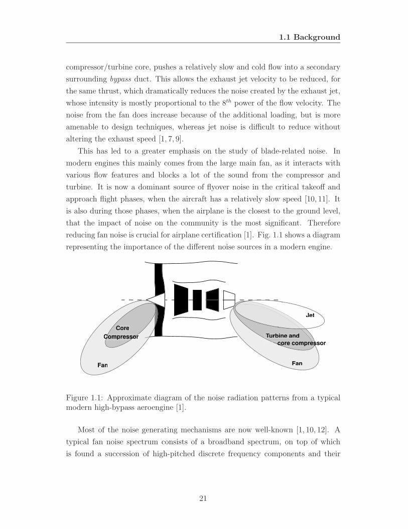
reducing fan noise is crucial for airplane certification [1]. Fig. 1.1 shows a diagram
representing the importance of the different noise sources in a modern engine.
Fan
CompressorCompressorCompressor
Fan
Turbine and Tu
ompressor core compressorompressorompressor core compressorompressorompressor core compressorompressor
Core
Jet
Figure 1.1: Approximate diagram of the noise radiation patterns from a typicalmodern high-bypass aeroengine [1].
Most of the noise generating mechanisms are now well-known [1, 10, 12]. A
typical fan noise spectrum consists of a broadband spectrum, on top of which
is found a succession of high-pitched discrete frequency components and their
21
1. INTRODUCTION
harmonics. The first part is called broadband noise, generated by internal tur-
bulence impinging on structures, and the latter is tone noise: this loud whine
is composed of frequencies which are multiples of the engine rotation frequency
(engine orders). Tyler and Sofrin [13] have identified this turbine noise as ori-
ginating from forward and backward interactions between rotor and stator blade
rows: the main fan and associated guiding vanes, and the internal compressor
and turbine. The propagation of the associated “spinning” modes in the inlet
ducts is very complex [9, 12].
When the fan blade tips are supersonic, shocks are produced. This creates a
sound spectrum rich in discrete frequencies, often called “Multiple Pure Tone”
noise. Furthermore, the complex interaction of these N-waves amplifies blade-
to-blade variability, which adds low engine order components to the pure-tone
ones: “buzz-saw” noise [14]. This high-amplitude, relatively low-frequency noise
is highly disturbing because it is poorly attenuated by the cabin walls and by the
atmosphere.
When the mean flow coming in the inlet is not circumferentially uniform,
distortion noise can also be produced. This may occur when wind is blowing on
the side of the engine, or if an intake droop is disturbing the inflow. The blades,
in their rotating frame of reference, perceive this perturbation periodically, which
can produce a low engine-order (and therefore low-frequency) sound.
“Lined” walls, porous surfaces with resonant cavities, can absorb a large part
of the generated noise spectrum through absorbtion and dissipation mechanisms,
as illustrated in Ref. [1]. They were one of the earliest features used to reduce
fan noise [6], and are now systematically found in commercial aeroengine inlets.
Their design and tuning is delicate, but their presence is critical to the sonic
performance of the engine. However, there are limits to this approach, and some
other recent fan noise reduction techniques, investigated at the NASA [10] and
in European programs devoted to aeroacoustics [4, 15], include:
Fan design: lowering the tip speed or modifying the blade shape can reduce
shock strength.
Wake management consists of ensuring that the flow immediately downstream
22
1.1 Background
of blades is as smooth as possible to avoid strong noise-generating turbu-
lence.
Optimising the number of blades/bypass vanes: the nature of the modes
generated by rotor/stator interaction is related to the number of blades [13].
By carefully adjusting their relative numbers, it is possible to control which
modes are generated.
Increasing the rotor/stator distance to make use of the natural decay of
wakes.
Using swept/leaned guide vanes as opposed to straight ones, can effectively
reduce interaction effects in some cases.
An inversely scarfed inlet: traditionally, engine inlets are scarfed so that the
upper lip is longer, for aerodynamical reasons. However, negatively-scarfed
intakes are being investigated: the extended lower lip is intended to reflect
most of the sound away from the ground.
Active control: this regroups all methods trying to cancel out sound by the
means of diverse actuators or generators, responding to the noise levels
through a carefully designed feedback chain.
It should be noted that many of these modifications involve complex, strongly
3-dimensional effects. More importantly, many are also strongly linked to aero-
dynamic or aeroelastic aspects of the engine design [16]: concerns such as blade
vibration and robustness, the power regime and efficiency of the engine, etc. For
example, a negatively scarfed inlet might cause inflow distortion, and might also
affect the wing’s lift or create drag.
Because of progress in materials and techniques, fan blades are getting lighter;
this means higher vibrations, and aeroelastic interactions with the acoustic and
unsteady flow when there is a match (in shape and frequency) between struc-
tural and acoustic modes. Vahdati et al. [17], and later Wu et al. [18], examined
the influence of inlet acoustics on the fan blades’ “flutter”, or self-excited vi-
brations. Both domains of expertise, aeroelasticity and aeroacoustics, are now
closely linked, while the requirements for quieter engines get at the same time
23
1. INTRODUCTION
more important and more difficult to meet. This challenge demands an integrated
design solution.
1.2 Problem statement
1.2.1 The need for computational models
Analytical solutions of acoustic equations are complex, even in the simplest
cases [19]. In most realistic situations, a solution is out of reach, unless some
strongly simplifying assumptions are made, and the effects of the underlying flow
are rarely taken into account. Ozyoruk [9] presents a review of early fan noise
modelling methods; for example, Nayfeh presented several models [6]. More
recently, the multi-scales propagation model for slowly varying ducts of Rien-
stra [20], or in the case of high frequencies, ray theory [21, 22], have been used
to study propagation inside the duct, and the diffraction at the lip, for relat-
ively simple geometries. Empirical methods are also widely used in the industry;
several examples in the current domain of interest can be found in the literat-
ure [12, 23]. But these simple models have their limits.
On the other hand, experiments on aeroengines are very costly and lengthy to
set up [9]. Therefore, it is important to develop predictive computational models
to simulate these phenomena, for use in the design phase. A computed solution
is known over the whole domain of study, compared to experiments that can only
give a limited set of measurement points. This allows a better understanding of
the physical mechanisms underpinning certain behaviours. For example, numer-
ical experiments by Tam and Kurbatskii [24] have precisely identified the mech-
anisms providing sound dissipation through vortex shedding in certain acoustic
liners.
1.2.2 Computational aeroacoustics
As aeroacoustics is a particular branch of fluid mechanics, it is theoretically pos-
sible to use a traditional Computational Fluid Dynamics (CFD) code to study
noise. In the last 30 years this area of research has matured, and very efficient
24
1.2 Problem statement
and robust CFD methods have been developed, and validated for a variety of
applications [25]. To include the effect of turbulence in viscous fluids, a Dir-
ect Numerical Simulation (DNS) approach can be taken, or a less computation-
ally expensive modelling of turbulence through Large Eddy Simulation (LES) or
Reynolds-Averaged Navier-Stokes (RANS) approaches [25].
A typical example is the AU3D code: it can solve the RANS equations with
a second-order accurate finite volume formulation on hybrid (structured and un-
structured) grids. A mix of adaptive Jameson second and fourth order dissipation
combined with a pressure sensor prevents odd-even oscillation, while preserving
accuracy in the smooth regions and reverting to first order near shocks. It ad-
vances the solution in time using a second-order backwards implicit formulation,
with dual time-stepping [26–28].
The fan region is home to many strongly non-linear noise-generating phe-
nomena, where vorticity, turbulence, solid-fluid interaction, shear layers, viscous
effects, etc. play a large part. A traditional CFD, viscid or inviscid solver can,
in principle, model sound generated by these effects, and propagate it over a
short distance. Rumsey et al. [29] describe the use of a similar code, CFL3D, de-
veloped in the NASA Langley Research Center, to model tone noise in a realistic
3D ducted-fan aeroengine geometry.
As many researchers have pointed out [9, 30–33], and as will be explained in
Chapter 2, traditional CFD codes cannot cope well with the nature of sound
signals. This is because they employ low-order discretisation schemes, for their
relative ease of development and coding. These schemes also do not require
highly accurate boundary conditions, grid metrics, or expensive computations
at each discretisation point; they are quite robust and have effectively modelled
many fluid phenomena. But when it comes to propagating the generated sound
waves, it became apparent that, unless a very fine spatial resolution is used (at
prohibitive computational cost), or large wavelengths are studied [17], important
phase and amplitude errors appear. Often, the waves, already of low amplitude
relatively to the ambient flow, are numerically dissipated after a few wavelengths.
The disparity between the length scales of the problem and the short acoustic
wavelengths is also a major problem. This explains the considerable interest in
dedicated, efficient numerical methods, and the relatively recent emergence of the
25
1. INTRODUCTION
field of Computational Aero-Acoustics (CAA) [30].
Although general CAA principles and methods are now starting to be well-
established, there still is a need for efficient techniques to model sound scattering
from complex geometries, while still retaining a high order of accuracy. Over-
all, two main approaches can be found: using unstructured grids, or using a
structured body-fitted grid mapped to a regular computational domain. These
techniques and the related discretisation schemes will be reviewed in Chapter 2
and 3. Curved grids, and to a lesser extent unstructured grids, are problematic
to generate, of poor quality except in the simplest cases, and can be the source of
numerical instability and distortions. In the current work, an alternative struc-
tured approach will be investigated, using techniques that allow the use of regular,
uniform grid in the whole domain. This means that strongly non-uniform prob-
lems would be difficult to model, but in most of the domain a discretisation with
good isotropy and resolution characteristics, adapted to acoustics, will be used,
avoiding the meshing problems outlined above.
1.2.3 The mid-field domain
A traditional CFD method can be used in the internal region of the engine (as
shown in the centre of Fig. 1.2), to simulate the aerodynamic and aeroelastic
behaviour of the forward region of the engine. This includes the generation of
sound and its accurate propagation in this limited region, where a fine grid can
be used. On the other hand, integral methods, described in Section 2.1.3, can
take, as input, the sound on a certain surface and propagate it to the far-field
very efficiently; however, they do not model acoustic/aerodynamic interactions
or the effects of propagation through complex non-uniform mean flows [9, 34].
There is therefore a need for methods that propagate sound in the mid-field :
between the near-field where the sources of sound reside, and the zone where the
flow is uniform; it must be able to model the complex refraction and wavelength-
shifting effects caused by non-trivial flows in the transition zone between the
internal and the external regions of the engine, as represented in Fig. 1.2. Work
of this type has been done, for complex 3D situations, by Ozyoruk [9, 35, 36] and
Stanescu [37–39]. Also of note is the 2D model of Breard [40], and early studies
26
1.3 Scope and aims of the thesis
made by assuming an irrotational flow [41].
It might also be interesting to use the method developed for the mid-field
domain in the bypass duct zone downstream of the main fan and the stator vanes.
Noise propagation is affected by the complex flow, and the geometry is curved,
and non-axisymmetric because of the presence of obstacles like the support pylon.
Bypass duct
Bypass duct
Compressor
and turbine Mean Flow
Mid-Field
zone
Figure 1.2: Description of the mid-field region in a typical modern aeroengine.
1.3 Scope and aims of the thesis
This work originated in the need for developing an integrated computational
design tool, combining well-established aerodynamic and aeroelastic models with
acoustic prediction capabilities. Linking both of these aspects of the design of
modern aeroengines would shorten the long feedback process that is now necessary
given the preponderance of noise concerns.
It is necessary, in such a complex environment, to focus on certain aspects of
the noise problem. This study is concerned with the front half of the aeroengine,
27
1. INTRODUCTION
as aeroelastic design mainly deals with the blades of the large low-pressure fan
and of the first stages of the compressor. This domain was studied for example by
Ozyoruk [9] and Keith [22]. The paramount importance of fan noise in modern
engine design has been stressed in this chapter. It was decided to focus on tone
noise, as broadband noise is of smaller magnitude in most cases, and, by its nature,
is less suited to direct numerical simulation. Given the importance of N-waves
caused by supersonic fan rotation and the resulting buzz-saw noise, the methods
described should also be considered for their ability to model these phenomena.
In the context of noise certification, the most important flight phases are takeoff
and approach, because of the proximity to the affected communities. This means
that the airplane is at relatively low speed, and the mean flow on which the
sound propagates will be of low Mach number (M< 0.3) [11]. The propagation
of these acoustic signals should be designed to be run in parallel to the aero-
elastic/dynamic computations, which would then provide the sound source. This
hybrid approach would be well-suited to the problem, allowing the use of methods
adapted to each part of the problem [34].
The current work concentrates on efficient schemes which are needed to propag-
ate sound in the mid-field region. They must be able to handle the great differ-
ence in amplitude between these acoustic perturbation and the flow on which
they propagate. The influence of the latter is of great importance, in the zone
of interest, since the complex effect this has on sound propagation is the main
reason simple models cannot be used. Crucially, the method must provide a great
level of accuracy in the resolved sound waves, up to the limit of the computa-
tional zone, where integral methods can take over. At the same time it must
be able to be used in realistic situations, to solve complex engineering problems.
Therefore issues such as implementation and the computational resources used
are critical. Finally, the overall scheme, no matter how refined, must be faster
than what would be obtained by simply using a traditional CFD scheme with a
very fine resolution.
Fully asymmetric inlet geometries, such those found in modern aeroengines,
need to be modelled. Furthermore, as has been pointed out above, many of
the noise generation mechanisms (like distortion noise) are highly 3-dimensional
but cannot be modelled by the many efficient 2D models that exist already.
28
1.3 Scope and aims of the thesis
Therefore, not only must the simulations be fully 3D, but an efficient way to
represent complex 3D wall surfaces must also be found. The methods developed
here might also be used for other problems with similar requirements.
Outline of the thesis
In Chapter 2, an appropriate set of equations to model the problem at hand is
presented, after having separated the acoustic part. The next step is to discretise
these equations both in space and time: a review of popular CAA schemes is
presented. A finite difference method is implemented, following the requirements
described above. The importance, for the correct resolution of acoustic waves,
of the scheme’s order of accuracy is investigated in detail. This is followed by
some notes on implementation and stability, and a quick overview of the correct
boundary conditions to be used with this scheme.
In Chapter 3, the need for an efficient way to model complex wall boundaries
in the context of CAA is described, preserving the high order of accuracy of the
solution. One of the main contributions of the current work is the development
of a novel systematic method to deal with 3D wall boundaries. The associated
algorithmic and computational issues are addressed.
In Chapter 4, a validation of the code against benchmark results is presented.
The basic model and computational scheme, in 2D and 3D, are first considered.
Then, the treatment of the wall boundary condition is investigated in detail, first
by replicating basic 2D test cases, and then by validating the new 3D approach
against a standard benchmark. It is found that the performance of the 3D method
is inferior to the 2D one. The effects of complex mean flows are studied in both
cases, but instability is observed in the presence of mean flows with important
Mach numbers.
In Chapter 5, some more complex situations, of the type commonly en-
countered in studies of aero-engine noise, are investigated. This includes asym-
metric situations. The current scheme performs efficiently overall, but some im-
portant dissipation is found to be present close to the wall boundary.
This outline is summarised in Fig. 1.3.
29
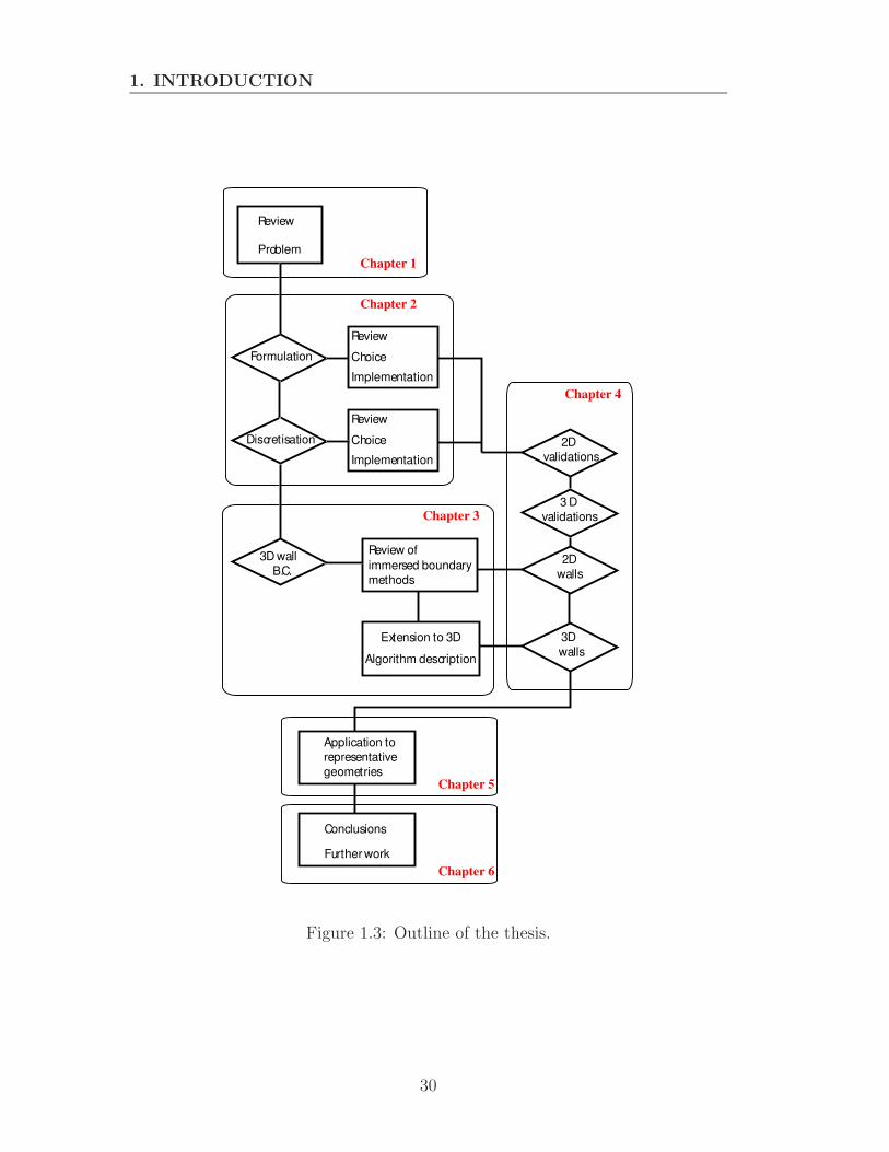
1. INTRODUCTION
Problem
Review
Formulation
Discretisation Choice
Implementation
Review
Choice
Implementation
Review
immersed boundary
methods
Review of 3D wall
B.C.
2D
validations
3 D
validations
2D
walls
3D
wallsExtension to 3D
Algorithm description
Application to
representative
geometries
Conclusions
Further work
Chapter 1
Chapter 2
Chapter 3
Chapter 4
Chapter 5
Chapter 6
Figure 1.3: Outline of the thesis.
30
Chapter 2
Model and discretisation
In this chapter, a numerical model is chosen to efficiently solve the problem
described in Chapter 1: the complexity of time-accurate sound propagation over
arbitrary non-uniform flows must be represented in 3D. First, an appropriate set
of equations is considered to this effect, given some acceptable hypotheses. If the
acoustic part of the fluid behaviour is treated separately, it is then possible to
use dedicated numerical CAA techniques, a review of which is made. Spatial and
temporal discretisation schemes are considered, as well as their stability. In both
cases, the advantages of using high-order accurate formulations become apparent.
Because of their nature, particular attention must be devoted to the boundary
conditions of the problem. The treatment of wall boundaries is delicate in this
context, and will be investigated in more detail in Chapter 3.
2.1 Equations for acoustic perturbations
It is necessary to find a model for the mid-field propagation: between the near-
field where the sources of sound reside (close to the turbine blades and the fan),
and the zone where the flow is uniform (away from the engine). The objective is
to propagate the interaction tone sound, and possibly the N-waves of buzz-saw
noise, while including the complex effects caused by non-uniform flows in the
transition zone between the internal and the external regions of the engine.
31
2. MODEL AND DISCRETISATION
2.1.1 Partition of variables
Essentially, sound consists of the unsteady, propagating perturbations Q ′ of a
quasi-permanent fluid state Q0. The latter is often called the mean flow. The
unknowns are the density ρ, the velocity components u, v and w, and the pressure
p. The total solution Q is then separated as:
Q = Q0 + Q ′ (2.1)
Not only is this consistent with the intuitive definition above, but it allows
decoupling of the two behaviours, and treating each part with methods best
adapted to their intrinsic characteristics. The perturbations often have amplitude
of several orders of magnitude less than that of the mean flow quantities, so
considering them separately avoids rounding-off errors. This also means that a
linear approximation is made possible by neglecting terms of second order or
more in Q ′.
In cases of interest for aeroengine acoustic certification, the mean flow is
considered steady, and given as an input. This allows a hybrid system, with a
traditional CFD program computing the steady flow while the propagation of the
acoustic perturbations is computed separately by a CAA code [34].
2.1.2 Nature of the model
The generation of the sound is an area of research in its own right, separate
from the propagation. For the problem considered, sound is generated by the
complex, often non-linear, interaction phenomena around the fan region outlined
in Chapter 1. This can be given by a CFD program, solving the full viscous
equations in the near-field region. In this case, to obtain a total design solution,
the programs computing the source and the propagation should both run in par-
allel. This is why a time-domain implementation is chosen for the latter, as in
Ozyoruk’s work [9]; this treatment allows multiple modes and frequencies to be
considered at the same time. However, frequency-domain models can be very
useful to study the propagation of a single mode or frequency once it has been
isolated, and the effect of a specific inlet configuration. For example, see the study
32
2.1 Equations for acoustic perturbations
of Lan, Guo and Breard [42]. Furthermore, the implementation of porous wall
boundary condition is much more straightforward in the frequency domain, as
described in Section 2.3.2. On the other hand, a time-domain formulation allows
for the possibility of a straightforward implementation of the full non-linear equa-
tions, for further extensions (see Section 2.1.4); although there has been recently
investigations into non-linear frequency-domain methods [40].
Ray theory provides a good model of high frequency sound propagation [21],
but implementing complex geometries is mathematically very complex [22]; fur-
thermore, most of the acoustic energy is contained in the lower harmonics [1, 9].
From now on, as in the majority of similar sound scattering or propagation
studies referenced therein, the perturbations Q ′ are assumed to behave in an
inviscid manner. It is possible to consider the effects of viscosity and temper-
ature gradients, but they are not important in most studies of scattering and
propagation (except for very long distances, when dissipation becomes appar-
ent). Viscous effects are fundamental in some of the noise generation mechanism,
especially from turbulence, like in jet noise studies [7, 43, 44] or broad-band noise
effects [1]. In small-scale studies of unsteady vortex-shedding or when unsteady
boundary layer effects are important, the viscous terms should be considered, as
in Refs. [45] and [24], but this will not be done here. The perturbation equations
can however take as input a fully viscous mean flow, without needing to change
them [46].
2.1.3 Formulation
The need for a complete model
Many of the existing methods used to predict forward noise propagation from
engine inlets use simplifying assumptions that will not capture the more complex
wave phenomena induced by the mean flow, aerodynamic/acoustic couplings, etc.
When the mean flow is perfectly still, and the acoustics are assumed linear,
inviscid and isentropic, the problem can be reduced to a traditional wave propaga-
tion problem [47, 48]. This is also true for a uniformly convective flow (constant
mean flow velocity ~v0 = [u0 v0 w0] everywhere), after an appropriate Galilean
coordinate transformation [9]. These equations are solved with Green’s functions,
33
2. MODEL AND DISCRETISATION
and an integral representation of the solution can be found, depending only on
the time history of the variables on a certain control surface. The sound field at
any distance is obtained from a very computationally efficient surface quadrat-
ure. This is the basis of the widely used integral or Boundary Element Methods
(BEM), of which Lyrintzis presents a review [34]. There are no dispersion or dis-
sipation errors introduced during the propagation and the accuracy only depends
on that of the source.
The Kirchhoff method, modified to allow for a moving control surface [49], is
often used to propagate sound to an arbitrary distance in the far-field (for ex-
ample see Ozyoruk [9, 36] and Rumsey [29]). The porous surface Ffowcs-Williams
Hawking method [50, 51], with the quadrupole source term neglected, is equival-
ent, but it might be preferable for reasons of reduced sensitivity to the quality and
linearity of the input solution. It is also less sensitive to vorticity disturbances,
and therefore well adapted to exhaust noise problems [52, 53].
In both cases the control surface must include all regions of sound generation,
non-linear behaviour, and inhomogeneous flow. The flow going in the inlet mouth
of a typical aero-engine is highly non-uniform, and aerodynamic/acoustic coup-
lings occur: refraction, wavelength modifications or more complex effects. These
phenomena are rarely taken into account by analytical or empirical models: it is
in those cases that a full computational assessment is most useful.
It is possible to include all these effects while still using the BEM approach: by
re-arranging the Navier-Stokes equations, a wave-type equation can be obtained,
with the noise generation and flow effects appearing as a source term. This is the
basis of the “acoustic analogies”, the equations of Lighthill and Lilley and their
modifications or simplifications [7, 54]. But a Green’s function is still assumed to
be found, so this approach can be only used in certain wall-bounded problems,
and only for simple mean flows. Lilley’s equation has the advantage of separating
the mean flow effects from the source term, but, as a third order differential
equation, it is difficult to solve numerically. These formulations are mostly used
to evaluate noise generated by turbulence.
Many early CAA studies used perturbed potential equations, which assume
that the mean flow is irrotational [41, 55]. But this limits the type of input flows
that may be used upstream of the fan. Redonnet [46] presents a comprehensive
34
2.1 Equations for acoustic perturbations
review of more elaborate perturbation equations based on Euler or Navier-Stokes
equations. In the light of the current study’s objectives, the non-conservative
Linearised Euler Equations (LEE) will be considered. They are well-suited to
the modelisation of the mid-field region [34].
The linearised Euler equations
The inviscid behaviour of small acoustic perturbations (Q ′) is considered in three
dimensions, on top of a stationary mean flow (Q0). Eq. (2.1) is introduced into
the non-conservative Euler equations, and all quadratic terms in Q ′ are neglected.
The equations are then arranged in a pseudo-conservative fashion, for reasons of
numerical stability [46], by introducing the pseudo-flux vectors E, F and G. The
following is obtained:
Let: Q ′ =
ρ ′
u ′
v ′
w ′
p ′
and: Q0 =
ρ0
u0
v0
w0
p0
∂Q ′
∂t+
∂E
∂x+
∂F
∂y+
∂G
∂z+ H = S (2.2)
E =
ρ0u′ + ρ ′u0
u0u′ +
p ′
ρ0
u0v′
u0w′
u0p′ + γp0u
′
, F =
ρ0v′ + ρ ′v0
v0u′
v0v′ +
p ′
ρ0
v0w′
v0p′ + γp0v
′
, G =
ρ0w′ + ρ ′w0
w0u′
w0v′
w0w′ +
p ′
ρ0
w0p′ + γp0w
′
(2.3)
35
2. MODEL AND DISCRETISATION
S represents a possible source term. H = 0 if the mean flow is uniform. Other-
wise [46, 56]:
H =
0
u ′
(
∂u0
∂x−∇~v0
)
+1
(ρ0)2
(
ρ ′∂p0
∂x+ p ′
∂ρ0
∂x
)
v ′
(
∂v0
∂y−∇~v0
)
+1
(ρ0)2
(
ρ ′∂p0
∂y+ p ′
∂ρ0
∂y
)
w ′
(
∂w0
∂z−∇~v0
)
+1
(ρ0)2
(
ρ ′∂p0
∂z+ p ′
∂ρ0
∂z
)
(γ − 1)[
p ′∇~v0 − ~v ′∇p0
]
(2.4)
2.1.4 Possible extensions
Using conservative variables generally leads to more robust numerical schemes for
CFD [46]; however, the author has not encountered a study that directly proves
the necessity of such a formulation for the type of applications considered here.
Tam [57] notes that they should be used in cases of strong shocks to correctly
assess the shock’s velocity. In computational acoustics [30], the important met-
ric is the accuracy of the phase and amplitude of the propagated waves, and not
the numerical conservation of the variables. Furthermore, with a non-conservative
formulation, the equations are expressed in terms of the primitive variables (dens-
ity, velocity, pressure) [7, 33, 40, 52, 54]. This will allow a direct implementation
of the solid wall boundary condition using the pressure values (see Chapter 3).
The partition into mean flow and fluctuations does not imply that the per-
turbations are small; indeed some researchers have investigated equations where
the non-linear terms are retained. Morris et al. [58] described the “non-linear
disturbances equations”, and Long [59] derived a non-conservative formulation.
This treatment has many advantages over using the Euler equations for the total
variable Q: as described above, adapted methods can be used for each part, with
a much more efficient result. This is useful because sometimes the propagation
is non-linear: high sound pressure levels are often present in aero-engine inlets
(more than 160dB). In this case, the small perturbation assumption is not valid,
and wave-steepening effects can occur. This is the case for N-waves produced by
supersonic fan blade tips (and buzz-saw noise). Also, in cases where the mean
36
2.2 Literature survey: spatial and temporal discretisation
flow is highly sheared (such as those found in the aft zone of the engine), neg-
lecting the non-linear effects can lead to instability [54], unless some of the LEE
terms are suppressed [52, 56].
A linear scheme is investigated here: this can represent a very good approx-
imation of the propagation of an N-wave if its amplitude has decayed sufficiently.
This depends on the point where the mid-field zone is set to start; usually half-
way up the inlet is satisfactory. This means neglecting the interaction of the
harmonic components of the wave as it progresses. It is probably overall much
less computationally expensive to extend the non-linear CFD region up to the
right point than to perform a full non-linear treatment of the propagation. Not
only must the non-linear terms be added to the equations, and conservative vari-
ables used, but also specific shock-capturing schemes are needed to handle the
discontinuities of the solution, as will be explained in Section 2.2.1.
2.2 Literature survey: spatial and temporal dis-
cretisation
The chosen set of acoustic equations must now be discretised, in order to solve it
numerically. The inefficiency of traditional CFD codes in propagating sound over
several wavelengths will be illustrated with a simple example in the following
pages. Using very fine grids with a traditional, low-order scheme, to obtain
the accuracy needed for acoustics computations, is impractical, so the choice of
integration scheme is really important. There is now a large body of work [30, 31,
33, 60, etc.] showing that high-order accurate discretisations capture the waves
much more accurately, for a lower overall computational effort.
Some commonly used methods will be reviewed. Several workshops on bench-
mark computational acoustics problems have provided a very interesting platform
for the direct comparison of different methods, and their resolution of several typ-
ical CAA problems [33, 60, 61].
Intuitively, using a low-order discretisation is equivalent to building a solution
with a piecewise linear function; this is badly suited to the oscillating nature of
acoustic signals. High-order methods use more elaborate representations, which
37
2. MODEL AND DISCRETISATION
are more appropriate for these problems, hence their efficiency. One problem
is that unless filtering or dissipative mechanisms are used, instability will occur
next to discontinuities because of the creation of spurious high-frequency waves.
This is similar to Gibb’s phenomenon, which occurs when trying to approximate
a discontinuous function with a truncated Fourier series [62].
2.2.1 Spatial discretisation
Overview
The crucial part of the numerical treatment resides in the spatial discretisation
of the equations. Many different methods are adapted for this purpose, and some
well-known methods have been re-designed specifically for CAA purposes. They
will be examined in this study, considering that a computationally economic 3-
dimensional method is needed, to replace low-order CFD schemes.
A good metric to characterise how efficient the scheme performs is the number
of Points-per-Wavelength (PPW ) required to propagate sound accurately over
several wavelengths, allowing a certain maximal error in phase (dispersion) and
amplitude (dissipation).
Rumsey et al. [29] refer to results indicating that the CFL3D code, from
NASA Langley Research Center, needs resolutions of around 25 PPW in each
spatial direction to propagate sound correctly in the near-field. This is typical
of traditional, low-order CFD codes, and even more would be needed to cover
longer distances. Lockard [63] shows that, to have less than 10% relative phase
and amplitude error, for a propagation over 20 wavelength, a second-order central
difference scheme needs 91PPW. He also points out that, for a given distance,
increasing the frequency leads to surprisingly large PPW requirements because it
represents a propagation of several more wavelengths, which requires even more
stringent criteria to avoid numerical errors.
A simple study of propagation using a low-order discretisation was made us-
ing the AU3D code described in Section 1.2.2. Originally designed to study
aero-elasticity in axial turbomachinery, it can model many viscous or inviscid
fluid mechanics problems, and has been used successfully in some low-frequency
38
2.2 Literature survey: spatial and temporal discretisation
acoustic cases [17, 18]. A simple plane wave, of wavelength λ = 49 cm, is im-
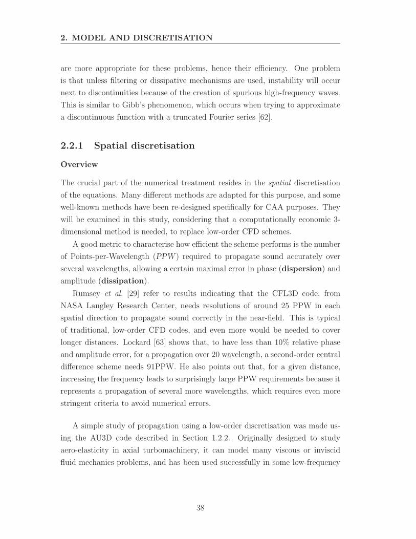
posed at one end of a hexahedral 3D domain, of dimensions 10 m×1 m×1 m, to
propagate along the ~x axis in the negative direction. On half the domain (x from
0 to -5 m), the grid is fine, with uniform grid spacing along ~x of size ∆, and 15
grid-points in both the ~y and ~z directions. In the rest of the domain (x from -5 m
to -10 m), the grid becomes increasingly stretched in the x direction to prevent
artificial reflections, as shown in Fig. 2.1.
x
y
-10 -8 -6 -4 -2 0
-3
-2
-1
0
1
2
3
4
5
Figure 2.1: 2D slice (constant z plane) of the grid used to model plane wavepropagation, shown here for the 10 PPW resolution.
The mean flow is considered at rest. A symmetric boundary condition is
imposed on all boundaries parallel to ~x, and the two other boundaries have 1-D
non-reflecting boundary conditions using a characteristics method, which allows
the imposition of an incoming wave at x = 0. It was decided, after numerical
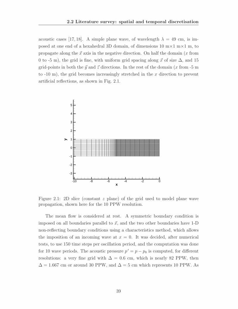
tests, to use 150 time steps per oscillation period, and the computation was done
for 10 wave periods. The acoustic pressure p ′ = p− p0 is computed, for different
resolutions: a very fine grid with ∆ = 0.6 cm, which is nearly 82 PPW, then
∆ = 1.667 cm or around 30 PPW, and ∆ = 5 cm which represents 10 PPW. As
39
2. MODEL AND DISCRETISATION
with all following AU3D results, p ′ is non-dimensional, normalised by a reference
pressure of pref = 10000 Pascals. The resulting acoustic pressure, along the
centerline, is shown in Fig. 2.2, along with an exact solution.
-0.06
-0.04
-0.02
0
0.02
0.04
0.06
-4 -3.5 -3 -2.5 -2 -1.5 -1 -0.5 0
Pre
ssur
e
x
Exact solution10 PPW
30 PPW82 PPW
Figure 2.2: Plane wave computation with a low-order scheme.
The results very clearly show the strong numerical dissipation and dispersion
that arise when a coarse mesh is used. For 10 PPW the wave is very quickly
damped and becomes more than half a wavelength out of phase. Even when
the wave is not strongly dissipated (30 PPW), an increasing phase error appears
as the wave propagates (up to 6% of the wavelength): as Lockard pointed out,
dispersion errors are much more important than dissipation ones for low-order
discretisations [63]. Using even 30 PPW is impractical in demanding aeroacous-
tics cases, where the Helmholtz number α = αa = 2πa/λ can go up to 20 or more
(where a is a length scale of the problem, for example the duct radius, and α the
wavenumber).
It is therefore necessary to investigate more efficient methods for realistic CAA
computations. Typically, high-order methods permit using less than 10PPW, and
even with this resolution, large problems remain quite a challenge. When directly
40
2.2 Literature survey: spatial and temporal discretisation
computing the noise generated by turbulence, for example from LES computa-
tions, a very high level of accuracy is needed to resolve the length-scales all the
way to the limits of the sub-grid model; this means typically a 7th order or more
scheme capable of resolving 4 PPW [64, 65]. But in this project, the objective is
to get overall more efficiency than a low-order scheme; a good compromise seems
to be around 7 to 10 PPW.
The order of accuracy can be raised by increasing the number of points used to
compute the derivative, or by using, in an implicit fashion, the values from neigh-
bouring points. Another approach is to construct the solution using more complex
and appropriate “test” functions. These methods introduce many mathematical,
algorithmic and numerical difficulties, and the resulting schemes are often less
robust than their low-order counterparts, so careful work is needed.
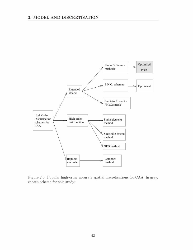
Commonly used schemes (as summarised in Fig. 2.3) will now be reviewed:
Explicit finite difference: this is the most straightforward formulation, based
on a truncated Taylor series. To extend the order of accuracy, more points are in-
cluded in the derivations stencil [25]. However, the resulting extended stencils can
be the source of many new algorithmic difficulties, near boundaries mostly. They
also prohibit the use of unstructured meshes. Those schemes will be described in
more detail below.
MacCormack schemes: integrate equations both in space and time using an
extended asymmetric stencil and a predictor-corrector method. High-order ac-
curate versions were used in early CAA applications [66], but they were found
to perform less well than some finite difference methods [67], and they are not
commonly used in recent CAA applications.
Compact scheme: an implicit finite difference scheme. The derivative at each
point is expressed proportionally to the derivatives on the immediately neigh-
bouring points [68]. After solving the resulting tridiagonal linear system, a very
accurate representation is obtained (even for resolutions as low as 4 PPW). Fur-
thermore, a 3-point stencil can be used, hence the name. This means that mesh-
ing techniques used with low-order schemes can be retained, and the algorithmic
41
2. MODEL AND DISCRETISATION
High OrderDiscretisationschemes forCAA
High ordertest function
"McCormack"Predictor/corrector
Extendedstencil
E.N.O. schemes
Finite elementsmethod
Spectral elementsmethod
Finite Differencemethods
Optimised
GFD method
Implicitmethods
Compactmethod
Optimised:
DRP
Figure 2.3: Popular high-order accurate spatial discretisations for CAA. In grey,chosen scheme for this study.
42
2.2 Literature survey: spatial and temporal discretisation
difficulties associated with large stencils are avoided. This type of scheme has
been used with success to model downstream propagation in axisymmetric en-
gine noise problems [52]. However, inverting the tri-diagonal matrix comes at
a computational cost; Redonnet showed that using implicit finite difference is
2.5 times more costly, per spatial direction, than a similar explicit scheme, and
that, for a given frequency, the marginal gain in PPW used does not compensate
this [46]. So, in 3D cases, when the grid is not fixed but a specific wavelength
must be resolved, an explicit scheme will be more computationally efficient, and
should be used unless the problems introduced by large stencils are deemed to be
more important.
Essentially Non-Oscillating (ENO) methods: specifically designed to rep-
resent shocks and discontinuities accurately; by reverting to a low-order approx-
imation of the solution near them, while retaining a high-order accuracy in most
of the domain [69], they avoid the oscillations associated with other high-order
schemes. They have been specifically adapted for use in CAA [63, 70], and re-
cently, more accurate “weighted” formulations have been developed [71]; but
flux-splitting and an evaluation of the solution is required at each point in order
to build an appropriate reconstruction polynomial, and this will come at a certain
computational cost [30].
Finite or spectral elements: such elements are popular in CFD because they
lead to robust and compact schemes that can be used, with finite volume formula-
tions, to discretise complex geometries using unstructured grids [25]. It is possible
to obtain a high-order accuracy with such schemes by increasing the order of the
test functions inside each element. For example, wave envelope methods were
widely used in early CAA studies [9, 55, 72]. But implicit finite element methods
are computationally expensive to extend to 3D because of the quadrature process,
resulting in large matrices that are very costly to invert [9]. There is however
ongoing research on quadrature-free methods [73], and explicit methods such as
the discontinuous-Galerkin techniques are increasingly popular.
The spectral-element method supersedes traditional spectral methods, which
were only capable of handling simple geometries [37, 74]. Highly accurate acous-
43
2. MODEL AND DISCRETISATION
tic scattering computations are then possible [37, 38, 75]. Stanescu [39] uses a
parallelized spectral element code to compute the 3D scattering of tone noise
by an airplane’s engine inlet and wing. Difficulties with traditional tetrahedral-
based unstructured grids has led to the development of spectral/hp element meth-
ods [76].
Other methods: The GFD scheme is a recently developed method that uses
Green’s functions, local solutions of the wave equation, as test functions for the
discretisation [77]. By writing compatibility equations for all the points in the
domain, a unique solution is found. Because the test functions are so well adapted
to the problem, the resolution can be as low as 3 PPW. There is an ongoing
research effort to adapt this scheme for inlet wave propagation problems [78].
The CIP scheme [79], developed for convection problems, seems very adapted,
but its efficacy in a CAA context has not been evaluated yet.
Scheme choice
In this work, it was decided to assess the use of an explicit finite differ-
ence scheme. Computational efficiency is crucial, since the goal is to compute
propagation in the mid-field faster than low-order schemes with a very fine res-
olution. Compact and implicit finite element methods were excluded, as they
generally become relatively more expensive when extended to 3D. Finite differ-
ence schemes are associated with structured methods, and a uniform grid, with
good resolution characteristics, can be retained in the whole domain. In the next
chapter this approach will be explained in more detail, based on the fact that
grid quality considerations become crucial for high-order accurate CAA prob-
lems. Finite difference schemes appear efficient and versatile [33, 60], and it is
the main technique used for many complex, demanding 2D [8, 42, 54, 80] and 3D
models [7, 9, 35, 43, 53, 58].
The first derivative of a function f along the x axis is expressed, at a point
x0, as [25]:
∂f
∂x(x0) ≃
1
∆x
3∑
j=−3
ajf(x0 + j∆x) (2.5)
44
2.2 Literature survey: spatial and temporal discretisation
for a 7-point stencil. The aj coefficients are determined through a Taylor ex-
pansion by specifying the order of the truncation error (in this case {aj} =
{− 160
, 320
,−34, 0, 3
4,− 3
20, 1
60}).
Finite-element treatment of fully 3D CAA problems can be computed more
easily thanks to parallel computation, for example see Ref. [39]. Finite difference
schemes can also be sped up in the same way: this was studied in detail by
Ozyoruk [9]. Morris and Shieh [81] computed a 3D scattering test problem using
the following method: the hexahedral domain is separated in “slices”, each of
which is assigned to a different processor. Both of these studies show that the
computations scale well with the number of processors.
Optimised finite difference
In the context of acoustic applications, it is more illuminating to examine the
wavenumber resolution characteristics of the scheme instead of focussing on the
order of the truncation error [31, 32, 46, 68]. A Fourier transform of Eq. (2.5) can
be used to show when the theoretical wavenumber α differs from the computed
one α [32]:
α ≃ −i
∆x
3∑
j=−3
aj eijα∆x = α (2.6)
If the group velocity cg is not accurately resolved, then the waves will be
predicted to propagate at the wrong speed. This means that the slope dαdα
also
has to be very accurate [30]:
dα
dα=
M∑
j=−N
jaj eijα∆x ≃ 1 (2.7)
A significant resolution gain can be obtained by designing the aj coefficients
for an optimal accuracy over a certain wavenumber range, by relaxing the order
constraint. More specifically, the widely-used “Dispersion-Relation Preserving”
(DRP) scheme [30, 32] is employed in this study. It is a 7-point stencil method,
optimised over a certain range, while only being formally 4th-order accurate in
terms of truncation error. The range is usually taken to be |α∆x| ≤ 1.1 after
45
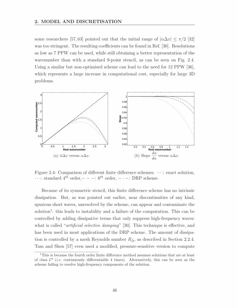
2. MODEL AND DISCRETISATION
some researchers [57, 63] pointed out that the initial range of |α∆x| ≤ π/2 [32]
was too stringent. The resulting coefficients can be found in Ref. [30]. Resolutions
as low as 7 PPW can be used, while still obtaining a better representation of the
wavenumber than with a standard 9-point stencil, as can be seen on Fig. 2.4.
Using a similar but non-optimised scheme can lead to the need for 12 PPW [36],
which represents a large increase in computational cost, especially for large 3D
problems.
0 0.5 1 1.5 2 2.5 30
0.5
1
1.5
2
2.5
3
Real wavenumber
Co
mp
ute
d w
aven
um
ber
(a) α∆x versus α∆x.
0.2 0.4 0.6 0.8 1 1.2 1.40.82
0.84
0.86
0.88
0.9
0.92
0.94
0.96
0.98
1
Real wavenumber
Slo
pe
(b) Slopedα
dαversus α∆x.
Figure 2.4: Comparison of different finite difference schemes. — : exact solution,· · ·: standard 4th order,−−−: 6th order, − · −: DRP scheme.
Because of its symmetric stencil, this finite difference scheme has no intrinsic
dissipation. But, as was pointed out earlier, near discontinuities of any kind,
spurious short waves, unresolved by the scheme, can appear and contaminate the
solution1: this leads to instability and a failure of the computation. This can be
controlled by adding dissipative terms that only suppress high-frequency waves:
what is called “artificial selective damping” [30]. This technique is effective, and
has been used in most applications of the DRP scheme. The amount of dissipa-
tion is controlled by a mesh Reynolds number R∆, as described in Section 2.2.4.
Tam and Shen [57] even used a modified, pressure-sensitive version to compute
1This is because the fourth order finite difference method assumes solutions that are at leastof class C4 (i.e. continuously differentiable 4 times). Alternatively, this can be seen as thescheme failing to resolve high-frequency components of the solution.
46
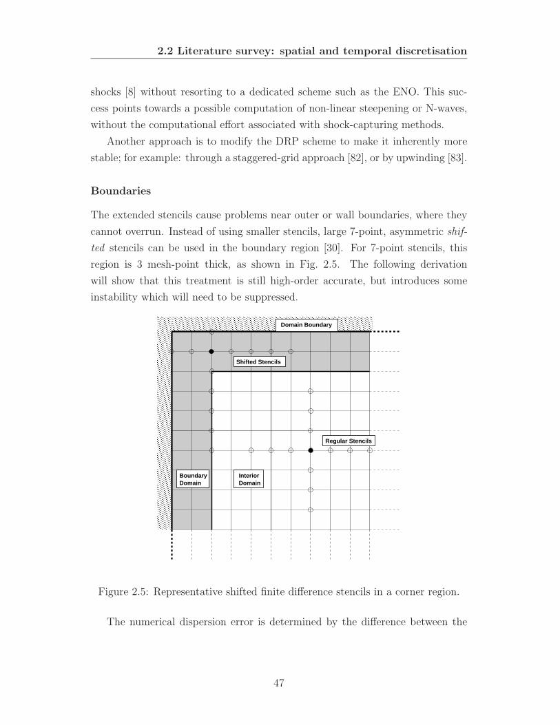
2.2 Literature survey: spatial and temporal discretisation
shocks [8] without resorting to a dedicated scheme such as the ENO. This suc-
cess points towards a possible computation of non-linear steepening or N-waves,
without the computational effort associated with shock-capturing methods.
Another approach is to modify the DRP scheme to make it inherently more
stable; for example: through a staggered-grid approach [82], or by upwinding [83].
Boundaries
The extended stencils cause problems near outer or wall boundaries, where they
cannot overrun. Instead of using smaller stencils, large 7-point, asymmetric shif-
ted stencils can be used in the boundary region [30]. For 7-point stencils, this
region is 3 mesh-point thick, as shown in Fig. 2.5. The following derivation
will show that this treatment is still high-order accurate, but introduces some
instability which will need to be suppressed.
���������������������������������������������������������������������������������������������������������������������������������������������������������������������
���������������������������������������������������������������������������������������������������������������������������������������������������������������������
���������������������������������������������������������������������������������������������������������������������������������������
���������������������������������������������������������������������������������������������������������������������������������������
Domain Boundary
Regular Stencils
DomainInteriorBoundaryDomain
Shifted Stencils
Figure 2.5: Representative shifted finite difference stencils in a corner region.
The numerical dispersion error is determined by the difference between the
47
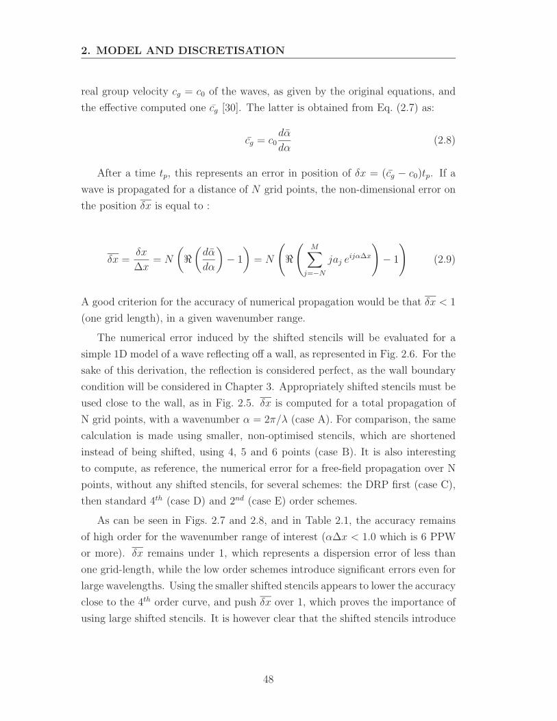
2. MODEL AND DISCRETISATION
real group velocity cg = c0 of the waves, as given by the original equations, and
the effective computed one cg [30]. The latter is obtained from Eq. (2.7) as:
cg = c0dα
dα(2.8)
After a time tp, this represents an error in position of δx = (cg − c0)tp. If a
wave is propagated for a distance of N grid points, the non-dimensional error on
the position δx is equal to :
δx =δx
∆x= N
(
ℜ(
dα
dα
)
− 1
)
= N
(
ℜ(
M∑
j=−N
jaj eijα∆x
)
− 1
)
(2.9)
A good criterion for the accuracy of numerical propagation would be that δx < 1
(one grid length), in a given wavenumber range.
The numerical error induced by the shifted stencils will be evaluated for a
simple 1D model of a wave reflecting off a wall, as represented in Fig. 2.6. For the
sake of this derivation, the reflection is considered perfect, as the wall boundary
condition will be considered in Chapter 3. Appropriately shifted stencils must be
used close to the wall, as in Fig. 2.5. δx is computed for a total propagation of
N grid points, with a wavenumber α = 2π/λ (case A). For comparison, the same
calculation is made using smaller, non-optimised stencils, which are shortened
instead of being shifted, using 4, 5 and 6 points (case B). It is also interesting
to compute, as reference, the numerical error for a free-field propagation over N
points, without any shifted stencils, for several schemes: the DRP first (case C),
then standard 4th (case D) and 2nd (case E) order schemes.
As can be seen in Figs. 2.7 and 2.8, and in Table 2.1, the accuracy remains
of high order for the wavenumber range of interest (α∆x < 1.0 which is 6 PPW
or more). δx remains under 1, which represents a dispersion error of less than
one grid-length, while the low order schemes introduce significant errors even for
large wavelengths. Using the smaller shifted stencils appears to lower the accuracy
close to the 4th order curve, and push δx over 1, which proves the importance of
using large shifted stencils. It is however clear that the shifted stencils introduce
48
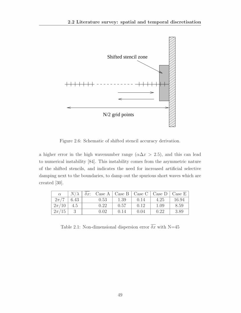
2.2 Literature survey: spatial and temporal discretisation
����������������������������
����������������������������
N/2 grid points
Shifted stencil zone
Figure 2.6: Schematic of shifted stencil accuracy derivation.
a higher error in the high wavenumber range (α∆x > 2.5), and this can lead
to numerical instability [84]. This instability comes from the asymmetric nature
of the shifted stencils, and indicates the need for increased artificial selective
damping next to the boundaries, to damp out the spurious short waves which are
created [30].
α N/λ δx: Case A Case B Case C Case D Case E2π/7 6.43 0.53 1.39 0.14 4.25 16.942π/10 4.5 0.22 0.57 0.12 1.09 8.592π/15 3 0.02 0.14 0.04 0.22 3.89
Table 2.1: Non-dimensional dispersion error δx with N=45
49
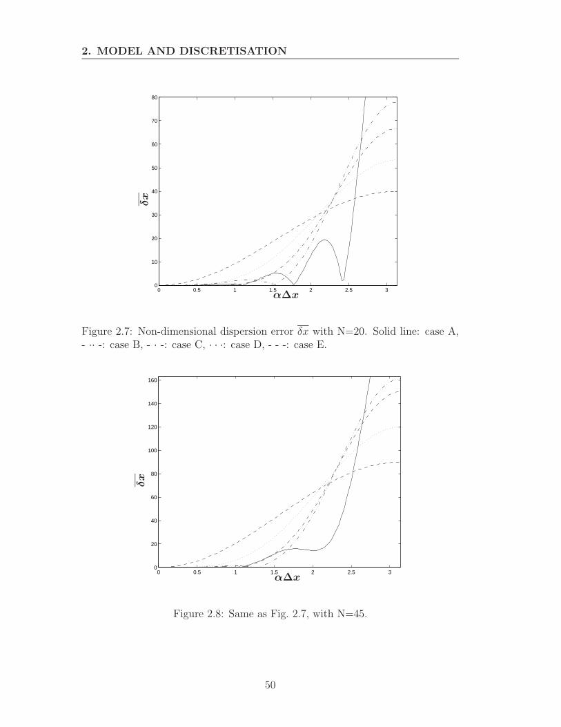
2. MODEL AND DISCRETISATION
0 0.5 1 1.5 2 2.5 30
10
20
30
40
50
60
70
80
α∆x
δx
Figure 2.7: Non-dimensional dispersion error δx with N=20. Solid line: case A,- ·· -: case B, - · -: case C, · · ·: case D, - - -: case E.
0 0.5 1 1.5 2 2.5 30
20
40
60
80
100
120
140
160
α∆x
δx
Figure 2.8: Same as Fig. 2.7, with N=45.
50
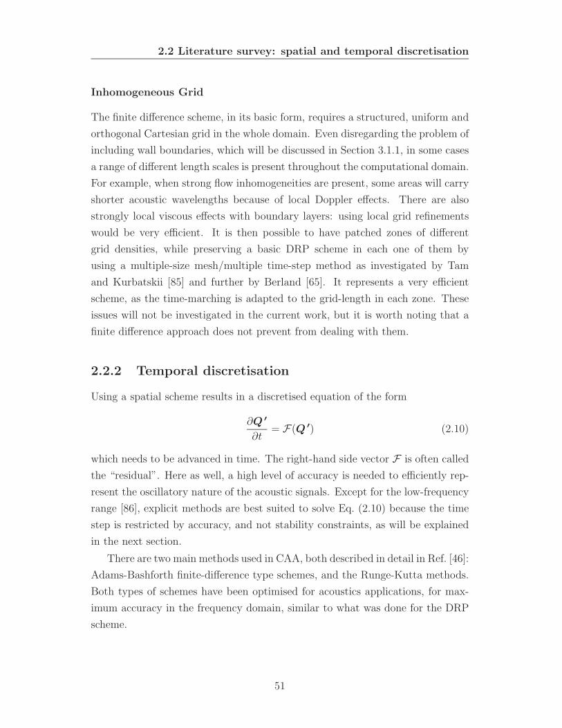
2.2 Literature survey: spatial and temporal discretisation
Inhomogeneous Grid
The finite difference scheme, in its basic form, requires a structured, uniform and
orthogonal Cartesian grid in the whole domain. Even disregarding the problem of
including wall boundaries, which will be discussed in Section 3.1.1, in some cases
a range of different length scales is present throughout the computational domain.
For example, when strong flow inhomogeneities are present, some areas will carry
shorter acoustic wavelengths because of local Doppler effects. There are also
strongly local viscous effects with boundary layers: using local grid refinements
would be very efficient. It is then possible to have patched zones of different
grid densities, while preserving a basic DRP scheme in each one of them by
using a multiple-size mesh/multiple time-step method as investigated by Tam
and Kurbatskii [85] and further by Berland [65]. It represents a very efficient
scheme, as the time-marching is adapted to the grid-length in each zone. These
issues will not be investigated in the current work, but it is worth noting that a
finite difference approach does not prevent from dealing with them.
2.2.2 Temporal discretisation
Using a spatial scheme results in a discretised equation of the form
∂Q ′
∂t= F(Q ′) (2.10)
which needs to be advanced in time. The right-hand side vector F is often called
the “residual”. Here as well, a high level of accuracy is needed to efficiently rep-
resent the oscillatory nature of the acoustic signals. Except for the low-frequency
range [86], explicit methods are best suited to solve Eq. (2.10) because the time
step is restricted by accuracy, and not stability constraints, as will be explained
in the next section.
There are two main methods used in CAA, both described in detail in Ref. [46]:
Adams-Bashforth finite-difference type schemes, and the Runge-Kutta methods.
Both types of schemes have been optimised for acoustics applications, for max-
imum accuracy in the frequency domain, similar to what was done for the DRP
scheme.
51
2. MODEL AND DISCRETISATION
The Optimised Adams-Bashforth (OAB) four levels time-marching scheme
was described by Tam and Webb [32]. It uses, at the time level n, the residual
values of the 3 preceding time steps:
Q ′n+1 = Q ′n + ∆t3∑
j=0
bj F(Q ′n−j) (2.11)
where ∆t is the time step chosen, and bj are the optimised coefficients. This
means that the three previous values of the residual need to be stored in memory.
A linearised version of the Runge-Kutta algorithm allows a low-storage imple-
mentation, while retaining its accuracy for linear problems. Hu et al. [87] designed
optimised versions of these algorithms: “Low-Dissipation and -Dispersion Runge-
Kutta” (LDDRK). If s is the number of Runge-Kutta stages, at each time step
the quantities
Kj = ∆t F(Q ′n + βj Kj−1) (2.12)
for j = {1 . . . s} are computed (with β1 = 0). The optimised {βj}j=2...s coefficients
can be found in Ref. [87]. Then the final step is:
Q ′n+1 = Q ′n + Ks (2.13)
In this study, s = 4 and s = 5 will be used. The unused Kj can be overwritten, so
only two levels of storage are needed. For large 3D problems this might provide
a significant gain. It should be noted that Stanescu [88] and Berland [65] have
studied similar schemes that retain their high accuracy for non-linear problems.
The LDDRK integration has greater stability, lower memory usage and higher
resolution than the modified Adams-Bashforth scheme, but needs s computations
of the equation residuals per time step, whereas the latter only needs one. So,
compared to the scheme above, this will a priori represent a gain in computational
time only if the greater stability and accuracy allow time steps more than s times
larger.
52
2.2 Literature survey: spatial and temporal discretisation
2.2.3 Stability
In this subsection, both the temporal and spatial discretisation are combined. For
a uniform underlying flow, Redonnet [46] shows that once the scheme is space-
accurate and time-accurate, the overall solution is accurate and the evolution
of the variables in time will give the correct solution. In other words, if the
wavenumber and the frequency are well approximated, then the wave will be
correctly simulated.
The combinations of the optimised Adams-Bashforth and the LDDRK schemes
with the DRP scheme are studied respectively in Refs. [32] and [87]. A theoretical
study of their resolution of the simple one-dimensional wave equation is made:
this gives an indication of their performance and stability. For the whole range of
wavenumbers represented by the DRP scheme (α∆x < 1.65, cf. Fig. 2.4(a)) the
temporal integration is stable if the time step is smaller than a certain value ∆tst.
But in both cases, a smaller time step ∆tac is needed for an accurate evaluation
of the frequency for the range of wavenumbers resolved by the scheme (7 PPW
or more). ∆tac is calculated by allowing, for the first scheme, a maximum error
on the amplitude of 0.5dB for a propagation of 100 mesh spacings, and, for the
LDDRK, a 10−3 maximum relative error for phase and amplitude.
The computed values of those limits are presented in Table 2.2. M represents
the Mach number of the convective flow, if present. For the OAB scheme, the
derivation of Ref. [32] was modified to take into account the new wavenumber
optimisation range of ±1.1 (cf. Section 2.2.1). The limits of the LDDRK scheme
are given in Ref. [87] as function of the the Courant-Friedrichs-Lewy number
CFL= c(1 + M)∆t/∆x. To compare how effective the different schemes are, the
accuracy limit is divided by the number of stages s, which gives the number of
residual evaluations per time step.
It is clear that the accuracy constraint on the time step (∆t < ∆tac) is more
demanding than the stability constraint (∆t < ∆tst) [9]. The large time steps
allowed by implicit methods will not be needed, which justifies the choice of ex-
plicit time-marching. Furthermore, implicit methods have a larger computational
cost, and often introduce a large numerical distortion for large time-steps [9].
In theory, to resolve a given wavenumber, all other considerations being equal,
53
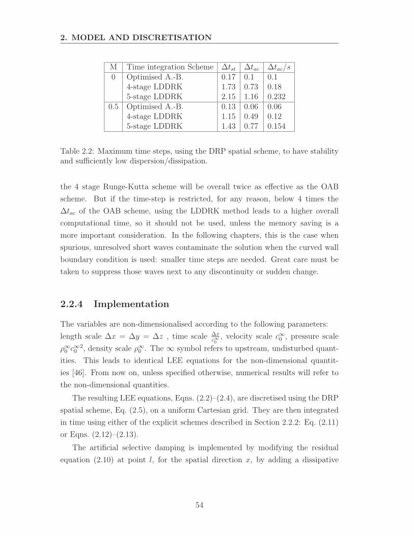
2. MODEL AND DISCRETISATION
M Time integration Scheme ∆tst ∆tac ∆tac/s0 Optimised A.-B. 0.17 0.1 0.1
4-stage LDDRK 1.73 0.73 0.185-stage LDDRK 2.15 1.16 0.232
0.5 Optimised A.-B. 0.13 0.06 0.064-stage LDDRK 1.15 0.49 0.125-stage LDDRK 1.43 0.77 0.154
Table 2.2: Maximum time steps, using the DRP spatial scheme, to have stabilityand sufficiently low dispersion/dissipation.
the 4 stage Runge-Kutta scheme will be overall twice as effective as the OAB
scheme. But if the time-step is restricted, for any reason, below 4 times the
∆tac of the OAB scheme, using the LDDRK method leads to a higher overall
computational time, so it should not be used, unless the memory saving is a
more important consideration. In the following chapters, this is the case when
spurious, unresolved short waves contaminate the solution when the curved wall
boundary condition is used: smaller time steps are needed. Great care must be
taken to suppress those waves next to any discontinuity or sudden change.
2.2.4 Implementation
The variables are non-dimensionalised according to the following parameters:
length scale ∆x = ∆y = ∆z , time scale ∆xc∞0
, velocity scale c∞0 , pressure scale
ρ∞
0 c∞02, density scale ρ∞
0 . The ∞ symbol refers to upstream, undisturbed quant-
ities. This leads to identical LEE equations for the non-dimensional quantit-
ies [46]. From now on, unless specified otherwise, numerical results will refer to
the non-dimensional quantities.
The resulting LEE equations, Eqns. (2.2)–(2.4), are discretised using the DRP
spatial scheme, Eq. (2.5), on a uniform Cartesian grid. They are then integrated
in time using either of the explicit schemes described in Section 2.2.2: Eq. (2.11)
or Eqns. (2.12)–(2.13).
The artificial selective damping is implemented by modifying the residual
equation (2.10) at point l, for the spatial direction x, by adding a dissipative
54
2.3 Boundary conditions
term [30]:
∂Ql′
∂t= F(Ql
′) − c∞∆xR∆
3∑
j=−3
dj Q ′
l+j (2.14)
with the artificial Reynolds number R∆ controlling the amount of dissipation. The
same is done for y and z. As Tam and Shen showed [57], although this is designed
to eliminate the spurious short waves, there will still be a small effect on the
frequencies of interest, and at length this might affect the quality of the solution
by adding some numerical dissipation and dispersion. Therefore the amount of
dissipation must be chosen as low as stability will allow. A low background
value (typically R∆ = 0.01) is used in the whole domain, adding a Gaussian
distribution (typically of amplitude R∆ = 0.15 and half-width 8) near the edge
of the computational domain [33, 60].
2.3 Boundary conditions
Boundary conditions are a very important aspect of CAA problems, because
they need to have the same high fidelity as the numerical schemes used to solve
the problem in the main domain [30, 68]. Additionally, any error or spurious
reflection will propagate in the main domain with little dissipation. There is
often no universal solution functioning in every case, although a large amount of
research is done in this area. The external boundaries must be able to let outgoing
waves exit the computational domain, and, because of the engine geometries being
studied, the modelling of solid walls and of the in-duct interface must also be
considered.
2.3.1 Sound radiation
It is particularly crucial to implement the Sommerfeld condition: outgoing wave
radiating towards infinity. Numerical simulations need to be run on a finite
domain, but the outer limits must be transparent to outgoing waves, as if the
domain extended to infinity. If wrongly expressed, artificial reflections occur at
the boundaries. In the case of finite element methods, infinite elements [38, 55] can
provide an appropriate boundary treatment. Otherwise, three main approaches
55
2. MODEL AND DISCRETISATION
are found in the CAA literature [30]:
Characteristics analysis is a popular approach in traditional steady-state
CFD, rarely used in CAA investigations. It uses the propagational speed ei-
genvalues of the governing equations near the boundary (see Thompson [89] or
Giles [90]). In practice, it is seldom used in a fully 3-dimensional implementation,
and this can cause significant reflections when waves are not exactly normal to
the boundary [9, 30].
Absorbing boundary layers prevent reflections by damping out any wave
reaching the boundary. This can be done by stretching the grid in a “sponge
zone”, or by progressively reducing the order of the spatial discretisation (Redon-
net [46]). But this can create instability, and introduce low-frequency, parasite
waves. A suitable progressive damping can be introduced: Bogey [7]. Zhang [52]
implemented a similar “buffer zone”, using an explicit damping formulation, as
did Stanescu [37, 39].
Another method in this category is the Perfectly Matched Layer (PML) [91].
This method, developed for computational electrodynamics, consists of adding, in
the absorbtion zone, a dissipative term to the main equations after they have been
split along all spatial directions. It avoids reflections at the interface by matching
the eigensolutions in both domains. It has been used in many applications, for
example Ref. [43]. However, Tam et al. [92] among others have shown that
in certain cases in which the main flow is normal to the boundary, instability
phenomena can generate parasite waves. Particularly, inside a duct with non-
zero flow, the PML condition can actually amplify waves. There is an ongoing
research on how to transform the PML equations to obtain unconditional stability,
even for non-trivial mean flows [93].
Asymptotic boundary conditions: presented by Bayliss and Turkel [94],
and Tam and Webb [32], they assume that the boundaries are far enough from
all sources of sound (in the center of the domain) for an asymptotic form of the
equations to be used. They were later extended to non-homogeneous mean flows
by Tam and Dong [95]. It is also possible to formulate a non-linear version of the
56
2.3 Boundary conditions
asymptotic conditions, as done by Tam and Shen [8].
They are fully three-dimensional, and were found to be efficient in many
applications [7, 9, 33, 35, 96] with less than a few percent reflections at most. They
come in two forms: “radiation” and “outflow”, with the former allowing acoustic
waves to exit, while the latter is found downstream of the mean flow in cases
where convected entropy and vorticity modes of excitation need to exit as well.
The 3D formulation of the radiation condition is given by Bogey [7] as:
1
cg
∂Q ′
∂t+ (
∂
∂r+
1
r)Q ′ = 0
With: cg = ~v0.~er +√
c20 − (~v0.~eθ)2 − (~v0. ~eϕ)2
(2.15)
where r is the radial distance and (~er, ~eθ, ~eϕ) the unit vectors of the spherical
coordinate system centered in the approximate location of the sources.
The efficiency of this asymptotic approximation depends on the distance
between the sources of sound and the boundaries, although Tam and Webb [32]
show that they still give good results if the source is 20 grid-lengths from the
boundary. Using a larger domain leads to an increased computational effort, so
for certain problems, absorbing boundary conditions might be more efficient in
that respect [43, 91]. One solution would be to combine an asymptotic treatment
with a damping layer, as it was necessary to do in some jet noise cases, where
strong vortical disturbances are convected downstream [7, 96]. Some instability
problems for long-time integration have also been reported [37], due to the spuri-
ous waves created by the presence of the boundary, but this can be remedied
by the use of artificial selective damping [30]. In the following, the asymptotic
radiation condition will be implemented.
2.3.2 Solid walls
Since the perturbations are assumed to be inviscid, the slip boundary condition
needs to be enforced close to the wall. If the normal direction is indicated by ~η,
the condition is:
~v ′.~η =∂p ′
∂η= 0 (2.16)
57
2. MODEL AND DISCRETISATION
The difficulties involved in numerically enforcing this condition will be examined
in Chapter 3.
As described in Section 1.1.2, using porous, absorbing walls is a major tech-
nique of noise reduction. These liners can be modelled by a frequency-dependant
impedance, often obtained experimentally. This makes their implementation in
time-domain schemes difficult. Popular approaches include using z-transforms [35],
differential equations [97] or a 1D model of the liner cavity [98]. Because of time
constraints, none of these has been implemented in the current work, but the wall
boundary condition described in chapter 3 will be assessed for compatibility with
these models.
2.3.3 In-duct boundary condition
An important problem is how to numerically impose an incoming wave on the
boundary situated inside the duct. This “matching plane” is the principal source
of sound for the problem considered. It must therefore be accurate, and also allow
scattered waves to exit the computational domain. The latter come from the
reflections at the inlet mouth of the different acoustic modes, occurring because
of the impedance mismatch between the inside of the duct and the free-field
domain. This is more important close to cut-off conditions [99]. The modes
can be obtained by a modal decomposition technique, such as that developed by
Ovenden and Rienstra [100]. If the modes considered are not strongly cut-on,
artificial reflections can occur if the incoming waves are simply imposed on the
boundary, through a Riemann problem [37] or simply by imposing the values
directly on the surface [9].
An alternative approach is to apply an appropriate radiation boundary condi-
tion to the outgoing waves only: by subtracting from the main unknowns vector
Q ′ the desired incoming solution Q ′
in, the desired treatment is then applied to
Q ′
out = Q ′ − Q ′
in, as in Ref. [95]. Dong [101] proved that, in a perfectly thin
cylindrical duct of finite length, aligned with the x axis, carrying a simple flow of
Mach number M , the condition:
[
∂
∂t+ (M − 1)
∂
∂x
]
Q ′
out = 0 (2.17)
58
2.3 Boundary conditions
allows incoming modes to enter and reflected modes to exit. It is accurate to
the order of the square of the cut-off ratio. It has been used for example by
Li et al. [96] with good results. Other researchers use a 1-D formulation of the
asymptotic boundary conditions, on the matching surface, which is very close to
Eq. (2.17) [102].
Zhang [52] studied different methods to be used in this fashion for the gener-
ation of modes in an annular duct for the downstream radiation of internal tone
noise. Amongst these was an implicit formulation, which introduces a progressive
damping, whilst generating the correct acoustic input Q ′
in. For each time step,
the solution vector Q ′ is damped, at the end of the time integration process, to
obtain the final vector Q ′
e through the following formulation:
Q ′
e = Q ′ − σ(Q ′ − Q ′
in) (2.18)
The absorbtion coefficient σ is given by
σ = σm
( |x − L|L
)β
(2.19)
where σm is the amplitude of the dissipation, L the length of the absorbtion
zone and β a power coefficient. It compares favorably to several other absorbing
boundary conditions, including PML and implicit formulations, generating very
little spurious reflections over a large variety of wave angles [52]. It has already
been pointed out that the PML formulation, applied inside a duct will lead to
instability in the presence of mean flow, unless group velocities are carefully
adjusted [92, 93].
A fully accurate, non-reflecting boundary condition for acoustics in bounded
flows is still an open topic of research, and partial solutions often involve a com-
plex analysis of all in- and out-going modes, with non-local treatments in space
or time [103, 104], which will lead be computationally expensive.
59

2. MODEL AND DISCRETISATION
60
Chapter 3
Three-dimensional wall
treatment for noise propagation
Free-field sound propagation has been described in Chapter 2 but the accurate
representation of wall boundaries is more delicate, and represents a major topic
of research in CAA. The use of high-order discretisation schemes introduces many
difficulties, mainly because they are very sensitive to the properties of the dis-
cretisation grid used, particularly compared to overly diffusive low-order methods.
In this chapter, popular practices are reviewed, focusing on structured immersed
boundary techniques, which allow the use of a uniform Cartesian grid. One of
the main contribution of this research work is described: a novel algorithm to
systematically treat immersed wall boundaries in 3D, specifically designed for
acoustic problems.
3.1 Literature survey
3.1.1 Wall boundary condition and finite difference
Tam and Dong [105] described a well-posed way of enforcing the inviscid wall
boundary condition: a row of virtual pressure values (called ghost values) is
added just behind the wall, as shown in Fig. 3.1. They are only included in the
stencils used to compute pressure derivatives, and their value is determined so as
to enforce the condition of zero normal velocity on the wall surface, through the
61
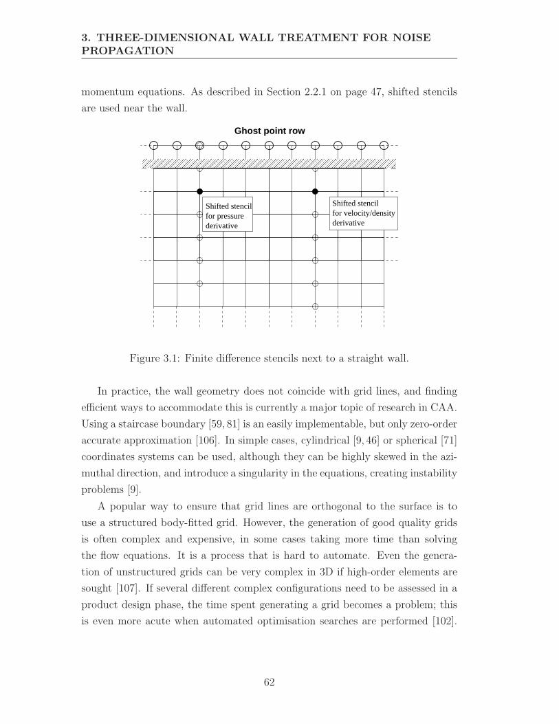
3. THREE-DIMENSIONAL WALL TREATMENT FOR NOISEPROPAGATION
momentum equations. As described in Section 2.2.1 on page 47, shifted stencils
are used near the wall.
����������������������������������������������������������������������������������������������������������������
Ghost point row
Shifted stencilfor pressure derivative
Shifted stencilfor velocity/densityderivative
Figure 3.1: Finite difference stencils next to a straight wall.
In practice, the wall geometry does not coincide with grid lines, and finding
efficient ways to accommodate this is currently a major topic of research in CAA.
Using a staircase boundary [59, 81] is an easily implementable, but only zero-order
accurate approximation [106]. In simple cases, cylindrical [9, 46] or spherical [71]
coordinates systems can be used, although they can be highly skewed in the azi-
muthal direction, and introduce a singularity in the equations, creating instability
problems [9].
A popular way to ensure that grid lines are orthogonal to the surface is to
use a structured body-fitted grid. However, the generation of good quality grids
is often complex and expensive, in some cases taking more time than solving
the flow equations. It is a process that is hard to automate. Even the genera-
tion of unstructured grids can be very complex in 3D if high-order elements are
sought [107]. If several different complex configurations need to be assessed in a
product design phase, the time spent generating a grid becomes a problem; this
is even more acute when automated optimisation searches are performed [102].
62
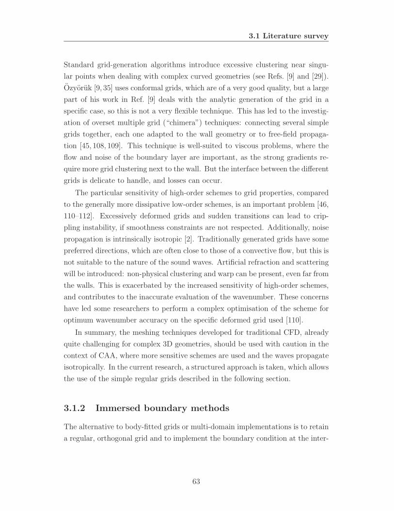
3.1 Literature survey
Standard grid-generation algorithms introduce excessive clustering near singu-
lar points when dealing with complex curved geometries (see Refs. [9] and [29]).
Ozyoruk [9, 35] uses conformal grids, which are of a very good quality, but a large
part of his work in Ref. [9] deals with the analytic generation of the grid in a
specific case, so this is not a very flexible technique. This has led to the investig-
ation of overset multiple grid (“chimera”) techniques: connecting several simple
grids together, each one adapted to the wall geometry or to free-field propaga-
tion [45, 108, 109]. This technique is well-suited to viscous problems, where the
flow and noise of the boundary layer are important, as the strong gradients re-
quire more grid clustering next to the wall. But the interface between the different
grids is delicate to handle, and losses can occur.
The particular sensitivity of high-order schemes to grid properties, compared
to the generally more dissipative low-order schemes, is an important problem [46,
110–112]. Excessively deformed grids and sudden transitions can lead to crip-
pling instability, if smoothness constraints are not respected. Additionally, noise
propagation is intrinsically isotropic [2]. Traditionally generated grids have some
preferred directions, which are often close to those of a convective flow, but this is
not suitable to the nature of the sound waves. Artificial refraction and scattering
will be introduced: non-physical clustering and warp can be present, even far from
the walls. This is exacerbated by the increased sensitivity of high-order schemes,
and contributes to the inaccurate evaluation of the wavenumber. These concerns
have led some researchers to perform a complex optimisation of the scheme for
optimum wavenumber accuracy on the specific deformed grid used [110].
In summary, the meshing techniques developed for traditional CFD, already
quite challenging for complex 3D geometries, should be used with caution in the
context of CAA, where more sensitive schemes are used and the waves propagate
isotropically. In the current research, a structured approach is taken, which allows
the use of the simple regular grids described in the following section.
3.1.2 Immersed boundary methods
The alternative to body-fitted grids or multi-domain implementations is to retain
a regular, orthogonal grid and to implement the boundary condition at the inter-
63
3. THREE-DIMENSIONAL WALL TREATMENT FOR NOISEPROPAGATION
sections between the grid and the surface. The boundary is said to be immersed
inside the grid system. There has been recent interest in this type of method, for
example in the field of biological fluid mechanics. This was driven by the need
to handle complex and even moving geometries, like blood vessels, without the
need for a lengthy meshing procedure [113].
Various methods can be regrouped under the “immersed boundary” label:
they use a reconstruction of the solution at the boundary of the solid surface,
overlayed on a fixed regular grid. Virtual “ghost” points, situated close to the
solid surface, exert a force determined to induce the desired boundary condi-
tion [106, 113–116]. “Cut-cell” methods are similar, but typically used with finite
volume discretisations. They take into account the way the surface intersects the
Cartesian cells to form smaller, irregular ones. This necessitates merging those
smaller cells with the main ones, to avoid the small time steps associated with
the former [117, 118].
These schemes were not designed to solve CAA problems, and use low-order
spatial discretisations, with almost invariably the equivalent of a simple linear
interpolation to estimate the values on the boundary from those in the surround-
ing fluid. For example, Fadlun et al. [106] use a linear interpolation between
the desired boundary velocity and the surrounding known quantities. The res-
ulting solution is correct because the global second-order accuracy is preserved,
as is the case for many Cartesian boundary treatments [119]. Tran and Udayku-
mar [114] describe an immersed boundary method associated with a high-order
ENO scheme. They use low-order extrapolation along the normal direction to
determine the values of the ghost points. The order of the scheme is reduced
locally by the boundary treatment, but a high order scheme is retained in most
of the domain, so they claim an overall good accuracy should be maintained.
Lombard and Piraux [120] briefly review the immersed interface methods
which are used to model acoustic behaviour in inhomogeneous media, and present
a method designed specifically to deal with the discontinuities involved with in-
homogeneous, solid/fluid interfaces. A Cartesian grid is used throughout and a
polynomial reconstruction is made near the surface, to obtain a stable and overall
second-order accurate solution.
64
3.1 Literature survey
3.1.3 Cartesian-grid preserving method for aeroacoustics
For the treatment of acoustic propagation problems, the relevant consideration
is the spatial resolution needed to accurately represent the wavenumber of the
acoustic signals [30]. It is important to retain a high-order accuracy to maintain
small levels of dissipation and dispersion errors, and perform more efficiently than
low-order schemes. With this in mind, Kurbatskii [121] designed an immersed
boundary method for aeroacoustics that preserves the Cartesian grid in the whole
domain. The method uses a description of how the surface intersects with the
grid lines. A systematic algorithm determines on which segment of the boundary
to implement the boundary condition, using an exhaustive classification of the
different geometrical situations around the ghost points [2]. The result, in a
typical situation, is represented in Fig. 3.2.
Fluid
Ghost Point
Inside the wall
Extrapolation
Extrapolation
Figure 3.2: Ghost points and the corresponding normal vectors behind a smooth,slightly curved wall. The extrapolation procedure is schematised in bold.
65
3. THREE-DIMENSIONAL WALL TREATMENT FOR NOISEPROPAGATION
Pressure gradient values are extrapolated, from inside the fluid, to the en-
forcement point on the surface to determine ghost values of pressure. Tam and
Kurbatskii [84] found that it is necessary to use an optimised high-order extrapol-
ation scheme, to obtain good accuracy for the desired wavenumber range, and to
suppress the instability caused by spurious short wavelengths. This wavenumber-
optimised approach performs better than a traditional B-Spline method [109].
3.2 3D algorithm for CAA
Modelling 3D walls is a challenge but it is important because few real intake or
bypass ducts are axisymmetric, for aerodynamic or acoustic design reasons, and
it was pointed out in Section 1.1.2 that many noise generation and propagation
mechanisms are three-dimensional, so an axisymmetric analysis can be insuf-
ficient. Additionally, the explicit finite difference method then has a distinct
advantage over implicit schemes for which the computational effort increases dra-
matically when going from 2D to 3D.
A 3D cut-cell method was developed by Yang et al. [117], but it approximates
the discretised surface with quadrilaterals to obtain an estimate of the normals
and the volume fraction of solid/liquid in each cut cell, which might be too
inaccurate. Casalino [78] has taken a 3D immersed boundary approach, but
in conjunction with the GFD method. Complex, moving 3D boundaries can be
represented by a level set method, together with an immersed boundary approach,
although obtaining the level set representation can be complex [79]. The method
of Fadlun et al. [106] is also 3D, but like most of schemes of this type found in
the literature, uses a low-order local reconstruction of the solution near the wall.
Because of the demands of acoustic problems, a higher order of accuracy would
be needed, so in this section an algorithm for 3D wall geometries is presented,
developed for CAA as part of the present research.
3.2.1 Description of the 3D immersed boundary algorithm
The method developed in this work is based on an extension of Kurbatskii’s
2D method described above, involving some additional challenges because of the
66
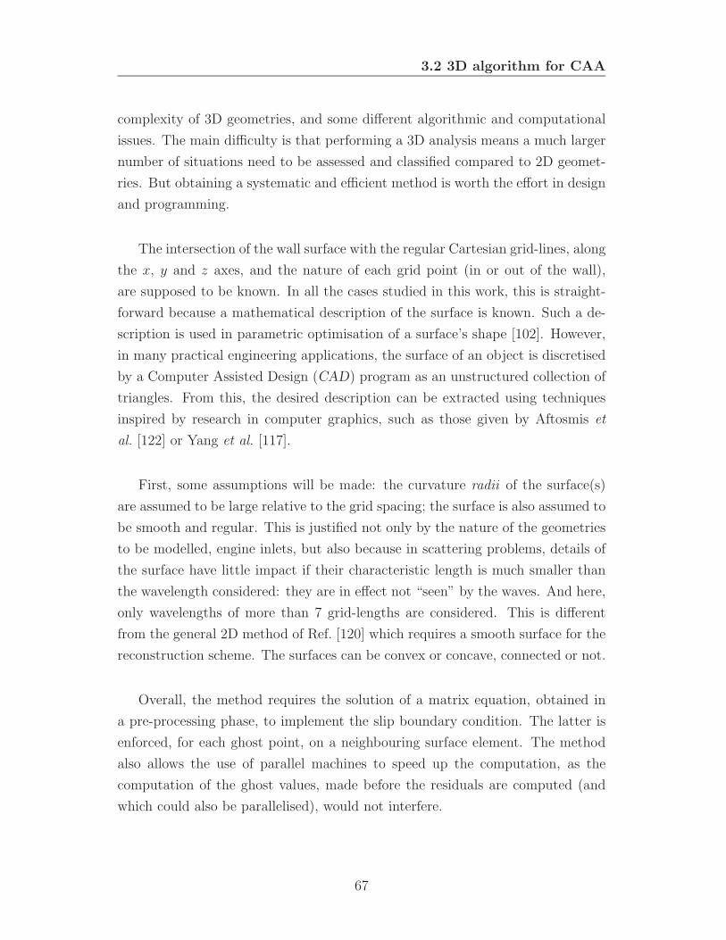
3.2 3D algorithm for CAA
complexity of 3D geometries, and some different algorithmic and computational
issues. The main difficulty is that performing a 3D analysis means a much larger
number of situations need to be assessed and classified compared to 2D geomet-
ries. But obtaining a systematic and efficient method is worth the effort in design
and programming.
The intersection of the wall surface with the regular Cartesian grid-lines, along
the x, y and z axes, and the nature of each grid point (in or out of the wall),
are supposed to be known. In all the cases studied in this work, this is straight-
forward because a mathematical description of the surface is known. Such a de-
scription is used in parametric optimisation of a surface’s shape [102]. However,
in many practical engineering applications, the surface of an object is discretised
by a Computer Assisted Design (CAD) program as an unstructured collection of
triangles. From this, the desired description can be extracted using techniques
inspired by research in computer graphics, such as those given by Aftosmis et
al. [122] or Yang et al. [117].
First, some assumptions will be made: the curvature radii of the surface(s)
are assumed to be large relative to the grid spacing; the surface is also assumed to
be smooth and regular. This is justified not only by the nature of the geometries
to be modelled, engine inlets, but also because in scattering problems, details of
the surface have little impact if their characteristic length is much smaller than
the wavelength considered: they are in effect not “seen” by the waves. And here,
only wavelengths of more than 7 grid-lengths are considered. This is different
from the general 2D method of Ref. [120] which requires a smooth surface for the
reconstruction scheme. The surfaces can be convex or concave, connected or not.
Overall, the method requires the solution of a matrix equation, obtained in
a pre-processing phase, to implement the slip boundary condition. The latter is
enforced, for each ghost point, on a neighbouring surface element. The method
also allows the use of parallel machines to speed up the computation, as the
computation of the ghost values, made before the residuals are computed (and
which could also be parallelised), would not interfere.
67
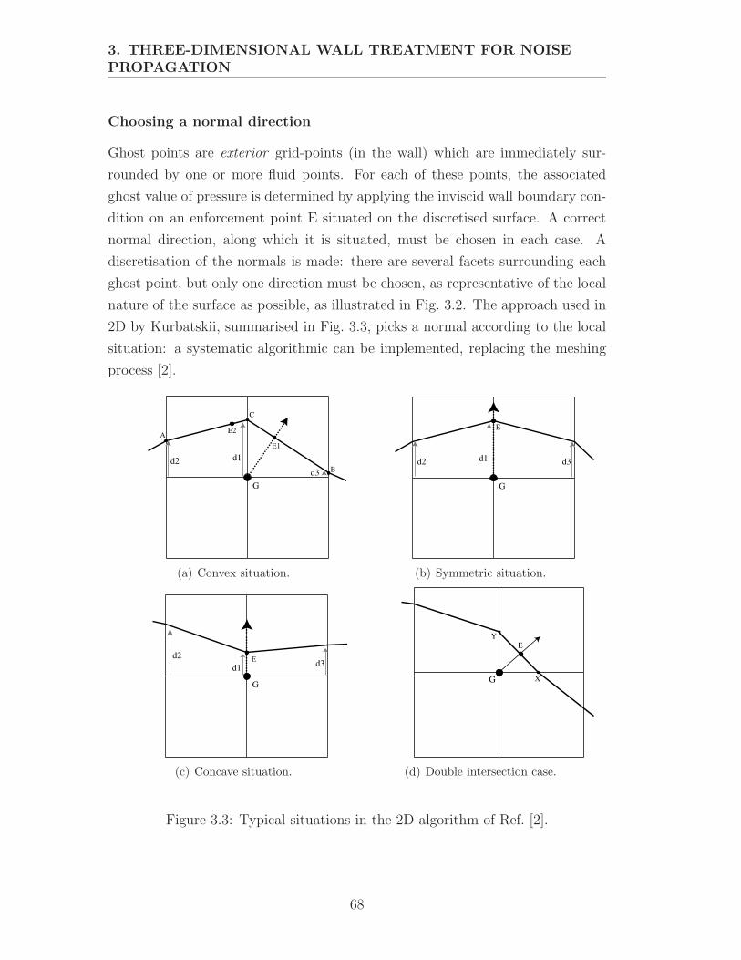
3. THREE-DIMENSIONAL WALL TREATMENT FOR NOISEPROPAGATION
Choosing a normal direction
Ghost points are exterior grid-points (in the wall) which are immediately sur-
rounded by one or more fluid points. For each of these points, the associated
ghost value of pressure is determined by applying the inviscid wall boundary con-
dition on an enforcement point E situated on the discretised surface. A correct
normal direction, along which it is situated, must be chosen in each case. A
discretisation of the normals is made: there are several facets surrounding each
ghost point, but only one direction must be chosen, as representative of the local
nature of the surface as possible, as illustrated in Fig. 3.2. The approach used in
2D by Kurbatskii, summarised in Fig. 3.3, picks a normal according to the local
situation: a systematic algorithmic can be implemented, replacing the meshing
process [2].
E1
E2
C
A
B
G
d2 d1
d3
(a) Convex situation.
E
G
d2 d1 d3
(b) Symmetric situation.
E
G
d2d3
d1
(c) Concave situation.
E
Y
XG
(d) Double intersection case.
Figure 3.3: Typical situations in the 2D algorithm of Ref. [2].
68
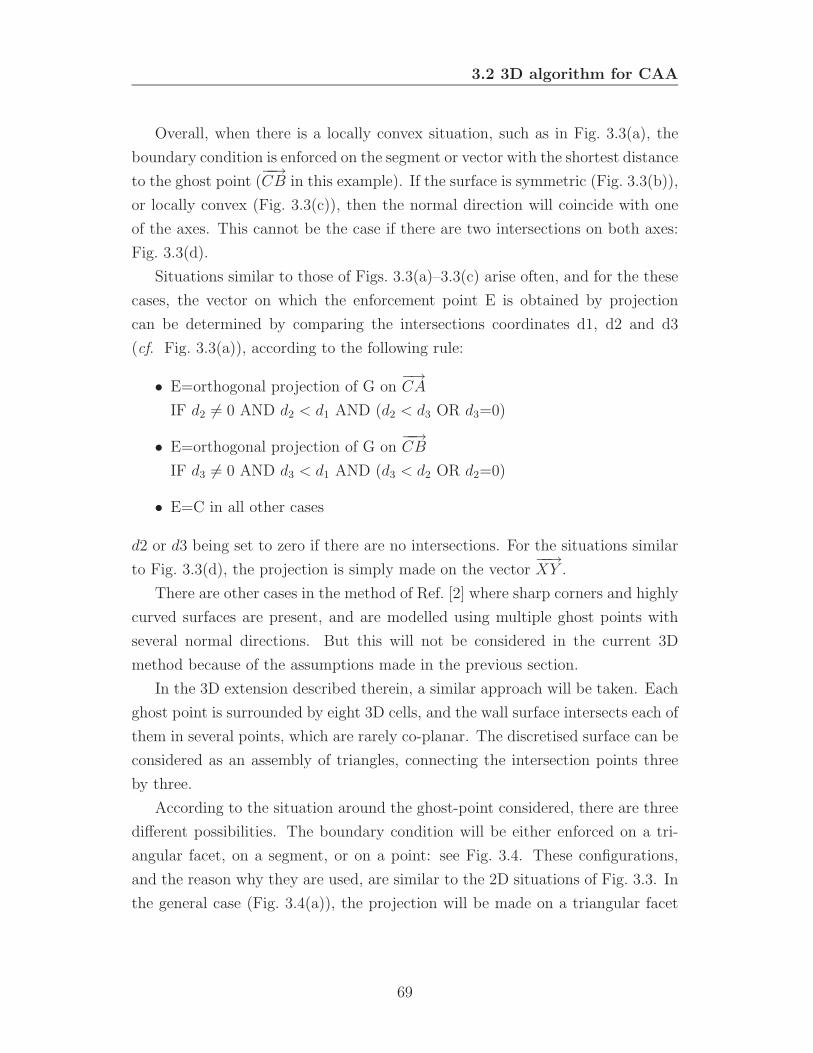
3.2 3D algorithm for CAA
Overall, when there is a locally convex situation, such as in Fig. 3.3(a), the
boundary condition is enforced on the segment or vector with the shortest distance
to the ghost point (−−→CB in this example). If the surface is symmetric (Fig. 3.3(b)),
or locally convex (Fig. 3.3(c)), then the normal direction will coincide with one
of the axes. This cannot be the case if there are two intersections on both axes:
Fig. 3.3(d).
Situations similar to those of Figs. 3.3(a)–3.3(c) arise often, and for the these
cases, the vector on which the enforcement point E is obtained by projection
can be determined by comparing the intersections coordinates d1, d2 and d3
(cf. Fig. 3.3(a)), according to the following rule:
• E=orthogonal projection of G on−→CA
IF d2 6= 0 AND d2 < d1 AND (d2 < d3 OR d3=0)
• E=orthogonal projection of G on−−→CB
IF d3 6= 0 AND d3 < d1 AND (d3 < d2 OR d2=0)
• E=C in all other cases
d2 or d3 being set to zero if there are no intersections. For the situations similar
to Fig. 3.3(d), the projection is simply made on the vector−−→XY .
There are other cases in the method of Ref. [2] where sharp corners and highly
curved surfaces are present, and are modelled using multiple ghost points with
several normal directions. But this will not be considered in the current 3D
method because of the assumptions made in the previous section.
In the 3D extension described therein, a similar approach will be taken. Each
ghost point is surrounded by eight 3D cells, and the wall surface intersects each of
them in several points, which are rarely co-planar. The discretised surface can be
considered as an assembly of triangles, connecting the intersection points three
by three.
According to the situation around the ghost-point considered, there are three
different possibilities. The boundary condition will be either enforced on a tri-
angular facet, on a segment, or on a point: see Fig. 3.4. These configurations,
and the reason why they are used, are similar to the 2D situations of Fig. 3.3. In
the general case (Fig. 3.4(a)), the projection will be made on a triangular facet
69
3. THREE-DIMENSIONAL WALL TREATMENT FOR NOISEPROPAGATION
defined by 2 vectors ~a =−→OA and ~b =
−−→OB, as described in Fig. 3.4(b). The relev-
ant triangle is the one closest to G. The enforcement point E is the projection of
the ghost point G on the facet, and this defines the normal direction. In the case
of Fig. 3.4(c), one of the vectors (~a or ~b) is null, and the triangle reduces to a line.
In the last case (Fig. 3.4(d)), both vectors are null and the triangle is reduced to
the single point O, the normal direction coinciding with a coordinate axis.
G
EEEE
(a) Enforcement on a triangular facet.
����
��
��
��
O
A
GB
��E
~a
~b
~xc
~η
δ
(b) Parameters in the general case.
G
E
(c) Enforcement on a segment.
G
E
(d) Enforcement on a point.
Figure 3.4: Typical situations in the 2D algorithm of Ref. [2] and correspondingnormal.
The subsequent interpolation and extrapolations used to obtain the pressure
gradient at point E will be described below, but first, the systematic algorithm
which determines vectors ~a and ~b (or their absence) will be outlined in the fol-
70
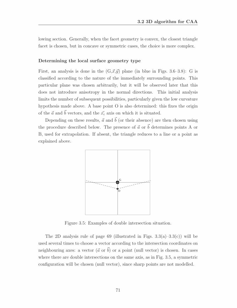
3.2 3D algorithm for CAA
lowing section. Generally, when the facet geometry is convex, the closest triangle
facet is chosen, but in concave or symmetric cases, the choice is more complex.
Determining the local surface geometry type
First, an analysis is done in the (G,~x,~y) plane (in blue in Figs. 3.6–3.8): G is
classified according to the nature of the immediately surrounding points. This
particular plane was chosen arbitrarily, but it will be observed later that this
does not introduce anisotropy in the normal directions. This initial analysis
limits the number of subsequent possibilities, particularly given the low curvature
hypothesis made above. A base point O is also determined: this fixes the origin
of the ~a and ~b vectors, and the ~xc axis on which it is situated.
Depending on these results, ~a and ~b (or their absence) are then chosen using
the procedure described below. The presence of ~a or ~b determines points A or
B, used for extrapolation. If absent, the triangle reduces to a line or a point as
explained above.
G
O
Figure 3.5: Examples of double intersection situation.
The 2D analysis rule of page 69 (illustrated in Figs. 3.3(a)–3.3(c)) will be
used several times to choose a vector according to the intersection coordinates on
neighbouring axes: a vector (~a or ~b) or a point (null vector) is chosen. In cases
where there are double intersections on the same axis, as in Fig. 3.5, a symmetric
configuration will be chosen (null vector), since sharp points are not modelled.
71
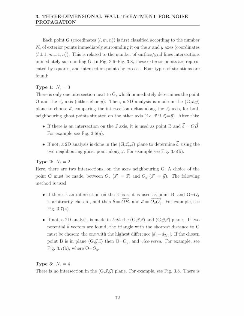
3. THREE-DIMENSIONAL WALL TREATMENT FOR NOISEPROPAGATION
Each point G (coordinates (l,m, n)) is first classified according to the number
Ne of exterior points immediately surrounding it on the x and y axes (coordinates
(l± 1,m± 1, n)). This is related to the number of surface/grid lines intersections
immediately surrounding G. In Fig. 3.6–Fig. 3.8, these exterior points are repres-
ented by squares, and intersection points by crosses. Four types of situations are
found:
Type 1: Ne = 3
There is only one intersection next to G, which immediately determines the point
O and the ~xc axis (either ~x or ~y). Then, a 2D analysis is made in the (G,~x,~y)
plane to choose ~a, comparing the intersection deltas along the ~xc axis, for both
neighbouring ghost points situated on the other axis (i.e. ~x if ~xc=~y). After this:
• If there is an intersection on the ~z axis, it is used as point B and ~b =−−→OB.
For example see Fig. 3.6(a).
• If not, a 2D analysis is done in the (G,~xc,~z) plane to determine ~b, using the
two neighbouring ghost point along ~z. For example see Fig. 3.6(b).
Type 2: Ne = 2
Here, there are two intersections, on the axes neighbouring G. A choice of the
point O must be made, between Ox (~xc = ~x) and Oy (~xc = ~y). The following
method is used:
• If there is an intersection on the ~z axis, it is used as point B, and O=Ox
is arbitrarily chosen , and then ~b =−−→OB, and ~a =
−−−→OxOy. For example, see
Fig. 3.7(a).
• If not, a 2D analysis is made in both the (G,~x,~z) and (G,~y,~z) planes. If two
potential ~b vectors are found, the triangle with the shortest distance to G
must be chosen: the one with the highest difference |d1−d2/3|. If the chosen
point B is in plane (G,~y,~z) then O=Oy, and vice-versa. For example, see
Fig. 3.7(b), where O=Oy.
Type 3: Ne = 4
There is no intersection in the (G,~x,~y) plane. For example, see Fig. 3.8. There is
72
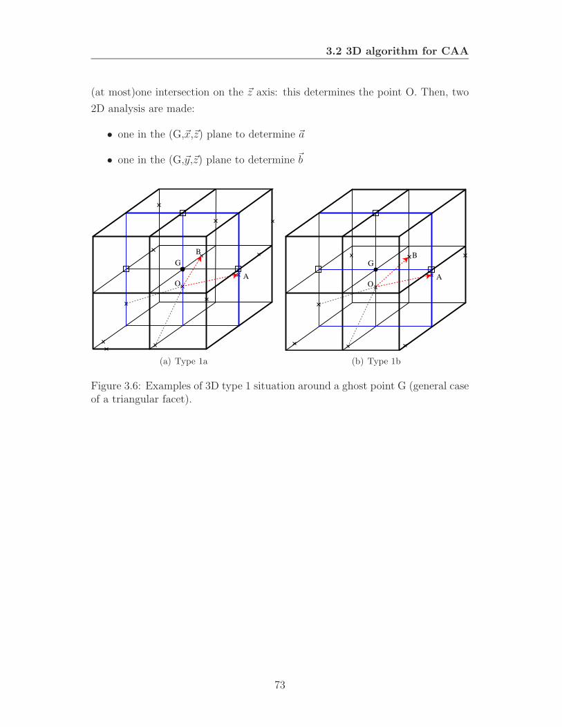
3.2 3D algorithm for CAA
(at most)one intersection on the ~z axis: this determines the point O. Then, two
2D analysis are made:
• one in the (G,~x,~z) plane to determine ~a
• one in the (G,~y,~z) plane to determine ~b
G
AO
B
(a) Type 1a
G
AO
B
(b) Type 1b
Figure 3.6: Examples of 3D type 1 situation around a ghost point G (general caseof a triangular facet).
73
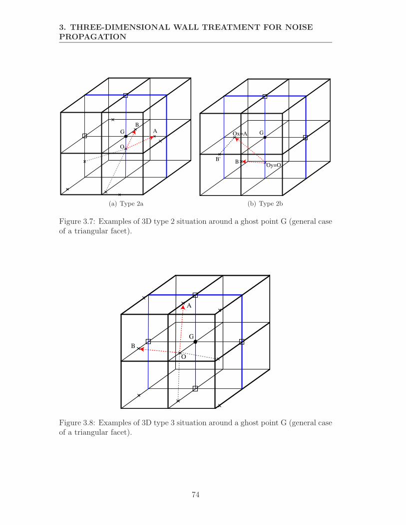
3. THREE-DIMENSIONAL WALL TREATMENT FOR NOISEPROPAGATION
G A
O
B
(a) Type 2a
GOx=A
Oy=OBB'
(b) Type 2b
Figure 3.7: Examples of 3D type 2 situation around a ghost point G (general caseof a triangular facet).
G
A
O
B
Figure 3.8: Examples of 3D type 3 situation around a ghost point G (general caseof a triangular facet).
74
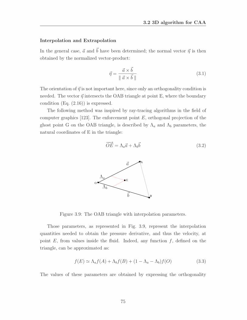
3.2 3D algorithm for CAA
Interpolation and Extrapolation
In the general case, ~a and ~b have been determined; the normal vector ~η is then
obtained by the normalized vector-product:
~η =~a ×~b
‖ ~a ×~b ‖(3.1)
The orientation of ~η is not important here, since only an orthogonality condition is
needed. The vector ~η intersects the OAB triangle at point E, where the boundary
condition (Eq. (2.16)) is expressed.
The following method was inspired by ray-tracing algorithms in the field of
computer graphics [123]. The enforcement point E, orthogonal projection of the
ghost point G on the OAB triangle, is described by Λa and Λb parameters, the
natural coordinates of E in the triangle:
−−→OE = Λa~a + Λb
~b (3.2)
O
B
E
A~a
~b
Λa
Λb
Figure 3.9: The OAB triangle with interpolation parameters.
Those parameters, as represented in Fig. 3.9, represent the interpolation
quantities needed to obtain the pressure derivative, and thus the velocity, at
point E, from values inside the fluid. Indeed, any function f , defined on the
triangle, can be approximated as:
f(E) ≃ Λaf(A) + Λbf(B) + (1 − Λa − Λb)f(O) (3.3)
The values of these parameters are obtained by expressing the orthogonality
75
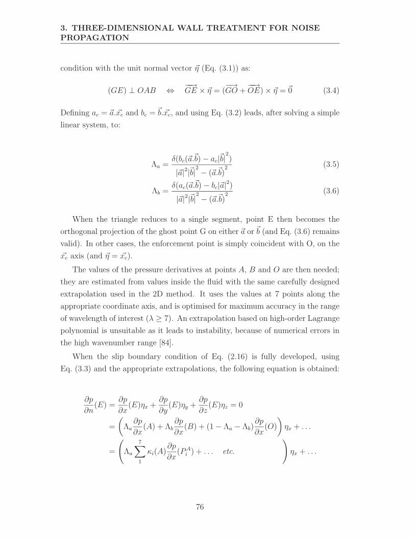
3. THREE-DIMENSIONAL WALL TREATMENT FOR NOISEPROPAGATION
condition with the unit normal vector ~η (Eq. (3.1)) as:
(GE) ⊥ OAB ⇔ −−→GE × ~η = (
−→GO +
−−→OE) × ~η = ~0 (3.4)
Defining ac = ~a.~xc and bc = ~b. ~xc, and using Eq. (3.2) leads, after solving a simple
linear system, to:
Λa =δ(bc(~a.~b) − ac|~b|
2)
|~a|2|~b|2 − (~a.~b)2 (3.5)
Λb =δ(ac(~a.~b) − bc|~a|2)|~a|2|~b|2 − (~a.~b)
2 (3.6)
When the triangle reduces to a single segment, point E then becomes the
orthogonal projection of the ghost point G on either ~a or ~b (and Eq. (3.6) remains
valid). In other cases, the enforcement point is simply coincident with O, on the
~xc axis (and ~η = ~xc).
The values of the pressure derivatives at points A, B and O are then needed;
they are estimated from values inside the fluid with the same carefully designed
extrapolation used in the 2D method. It uses the values at 7 points along the
appropriate coordinate axis, and is optimised for maximum accuracy in the range
of wavelength of interest (λ ≥ 7). An extrapolation based on high-order Lagrange
polynomial is unsuitable as it leads to instability, because of numerical errors in
the high wavenumber range [84].
When the slip boundary condition of Eq. (2.16) is fully developed, using
Eq. (3.3) and the appropriate extrapolations, the following equation is obtained:
∂p
∂n(E) =
∂p
∂x(E)ηx +
∂p
∂y(E)ηy +
∂p
∂z(E)ηz = 0
=
(
Λa∂p
∂x(A) + Λb
∂p
∂x(B) + (1 − Λa − Λb)
∂p
∂x(O)
)
ηx + . . .
=
(
Λa
7∑
1
κi(A)∂p
∂x(PA
i ) + . . . etc.
)
ηx + . . .
76

3.2 3D algorithm for CAA
where {PAi }i=1→7 are the extrapolation points related to point A, with the corres-
ponding optimised extrapolation weights κi [84]. For each of these, the derivative∂p∂xj
(Pi) is expressed with the adequate DRP discretisation stencil, according to
their proximity to the boundaries. These stencils mostly include points in the
fluid, but also sometimes ghost points. Therefore the different ghost values are
interdependent, and this will lead to a linear system that should be expressed in
matrix form. By putting all the terms involving ghost values on the Left-Hand
Side (LHS) of the equation, and all the other terms on the Right-Hand Side
(RHS), the following is obtained:
A pg = b (3.7)
The matrix A represents the interdependence of the ghost values of pressure pg.
The vector b is related to the pressure values in the fluid surrounding the wall
surface through the array C (see Section 3.2.3). A only needs to be inverted once,
at the start, and then the vector pg = A−1 b is calculated at each time step, giving
the values of the pressure at all the ghost points. The implementation of arrays
A and C will be described in Section 3.2.3.
3.2.2 Discretisation errors
Before the overall resulting accuracy obtained by the current method is assessed,
in the next chapter, through numerical experiments, it is interesting to verify if
the surface normal is correctly evaluated by the above algorithm. If the norm
‖~V ‖ of a vector is defined as√
V 2x + V 2
y + V 2z , the maximum error, over all ghost
points, on the normal vector ~η is computed as:
Eη = max(‖−−→ηreal −−−−→ηcomp.‖) (3.8)
For a sphere of radius a = 20∆x, Eη = 3.2 × 10⁻² is obtained; this represents
(at most) an angle of less than 1◦ between the true normal direction and the
computed one. Furthermore, as can be seen in Fig. 3.10, this error decreases
strongly as the sphere radius increases. This shows that the 3D algorithm used
to pick the appropriate triangle is effective, and does converge towards a correct
77
3. THREE-DIMENSIONAL WALL TREATMENT FOR NOISEPROPAGATION
estimation of the normal, as a function of the curvature radius. Furthermore,
an examination of the errors and the normals, over the whole surface, showed
that starting with an analysis in the (~x,~y) plane does not introduce an artificial
asymmetry in this computation.
0.01
0.02
0.03
0.04
0.05
0.06
0.07
0.08
0.09
5 10 15 20 25 30 35 40 45 50 55
Err
or o
n no
rmal
vec
tor
Sphere radius
Figure 3.10: Plot of Eη for a sphere as a function of the radius.
It is possible to estimate the error introduced by the triangular discretisation
of the real curved surface, in the same fashion as was done by Kurbatskii in
2D [121]. It should be noted that this type of error is common to most numerical
discretisation schemes, except for some finite element formulations that take into
account the surface’s curvature. In a grid cell of dimension ∆, the worst case
scenario, shown in Fig. 3.11, is considered. The osculating sphere S, of radius
R=CP, the local curvature radius, is tangential to the surface considered at point
P. The ratio ∆R
has been assumed to be small. So it is possible to obtain an estim-
ation of the distance δ = PE between the point where the boundary condition
should be applied (P) and the point where it actually is (E).
Some simple trigonometry gives:
δ = PE ≈ 1
6
∆2
R(3.9)
78

3.2 3D algorithm for CAA
E
P
C
R
∆
∆
Figure 3.11: Curvature and discretisation (the curvature is exaggerated here).
This is slightly larger than the 2D case, where the ratio was 1/8. For a wave
function of wavelength λ, the average error on amplitude over a period [121] is:
Edisc =1
2
2π
λδ ≃ π
6
∆
λ
∆
R(3.10)
In the case of the maximum resolution of the DRP scheme (∆λ
= 1/7), and a typ-
ical curvature of R∆
= 10, Edisc ≈ 0.0075. Therefore intrinsic discretisation errors
can be expected to be slightly larger than in the 2D case, where Edisc ≈ 0.0056
for the same conditions.
Apart from these issues, the main source of error comes from the extrapolation
and interpolation schemes. It will be observed in chapters 4 and 5 that, in 3D,
the errors become too important. A high-order 7-point extrapolation is used, but
for most ghost points, three will need to be done, instead of two maximum in 2D,
and errors can accumulate. Additionally, a linear interpolation is used within
79
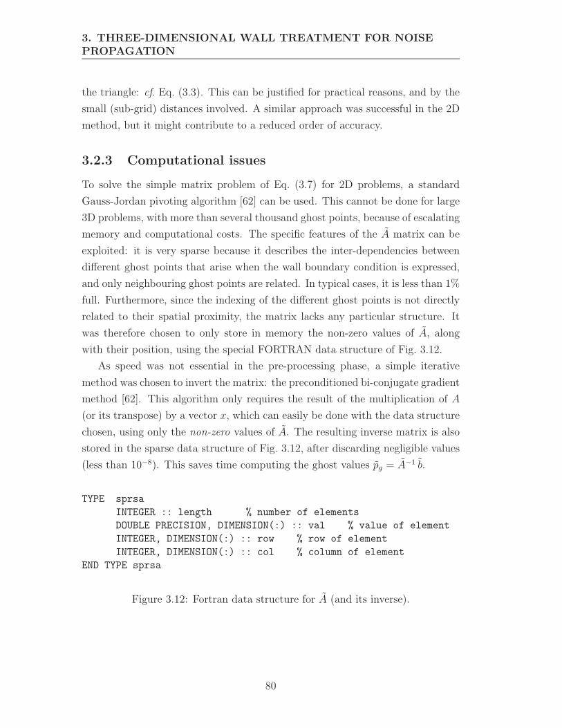
3. THREE-DIMENSIONAL WALL TREATMENT FOR NOISEPROPAGATION
the triangle: cf. Eq. (3.3). This can be justified for practical reasons, and by the
small (sub-grid) distances involved. A similar approach was successful in the 2D
method, but it might contribute to a reduced order of accuracy.
3.2.3 Computational issues
To solve the simple matrix problem of Eq. (3.7) for 2D problems, a standard
Gauss-Jordan pivoting algorithm [62] can be used. This cannot be done for large
3D problems, with more than several thousand ghost points, because of escalating
memory and computational costs. The specific features of the A matrix can be
exploited: it is very sparse because it describes the inter-dependencies between
different ghost points that arise when the wall boundary condition is expressed,
and only neighbouring ghost points are related. In typical cases, it is less than 1%
full. Furthermore, since the indexing of the different ghost points is not directly
related to their spatial proximity, the matrix lacks any particular structure. It
was therefore chosen to only store in memory the non-zero values of A, along
with their position, using the special FORTRAN data structure of Fig. 3.12.
As speed was not essential in the pre-processing phase, a simple iterative
method was chosen to invert the matrix: the preconditioned bi-conjugate gradient
method [62]. This algorithm only requires the result of the multiplication of A
(or its transpose) by a vector x, which can easily be done with the data structure
chosen, using only the non-zero values of A. The resulting inverse matrix is also
stored in the sparse data structure of Fig. 3.12, after discarding negligible values
(less than 10−8). This saves time computing the ghost values pg = A−1 b.
TYPE sprsa
INTEGER :: length % number of elements
DOUBLE PRECISION, DIMENSION(:) :: val % value of element
INTEGER, DIMENSION(:) :: row % row of element
INTEGER, DIMENSION(:) :: col % column of element
END TYPE sprsa
Figure 3.12: Fortran data structure for A (and its inverse).
80
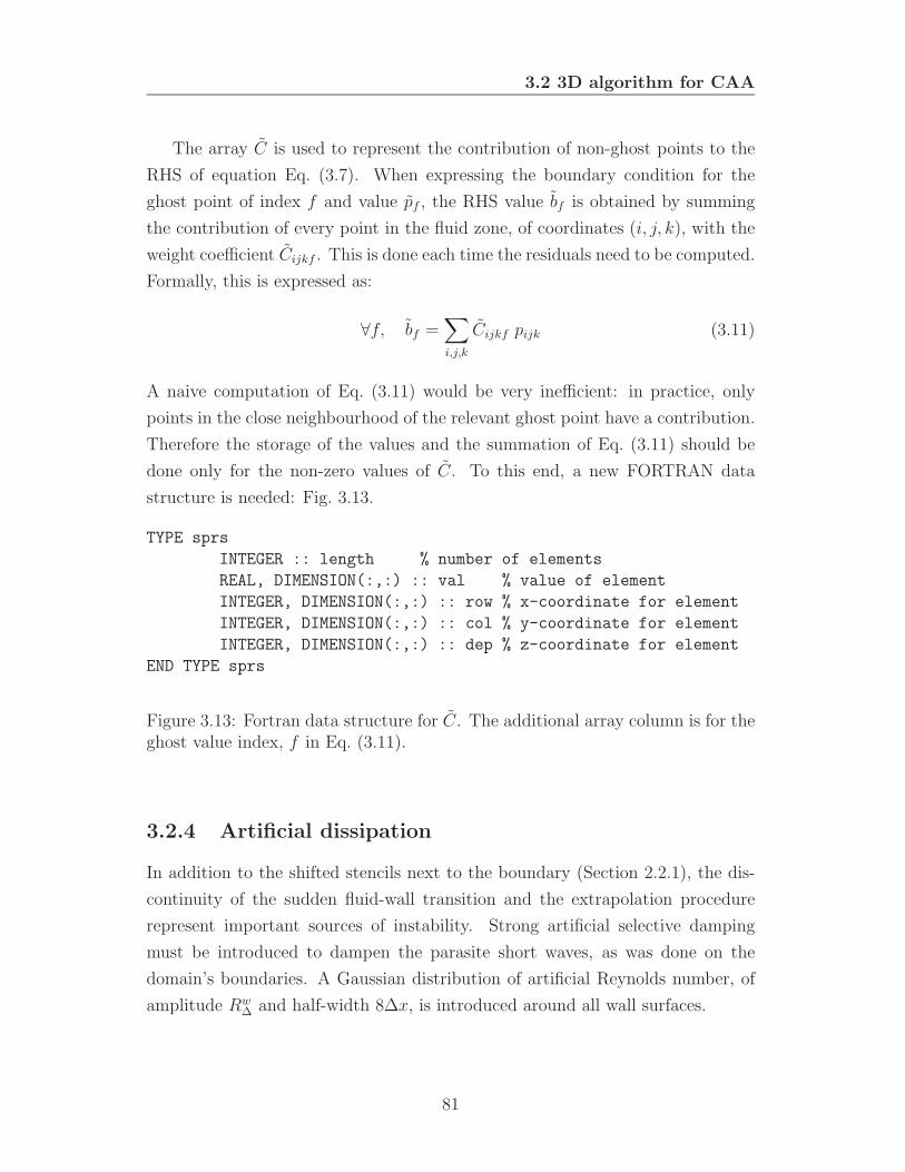
3.2 3D algorithm for CAA
The array C is used to represent the contribution of non-ghost points to the
RHS of equation Eq. (3.7). When expressing the boundary condition for the
ghost point of index f and value pf , the RHS value bf is obtained by summing
the contribution of every point in the fluid zone, of coordinates (i, j, k), with the
weight coefficient Cijkf . This is done each time the residuals need to be computed.
Formally, this is expressed as:
∀f, bf =∑
i,j,k
Cijkf pijk (3.11)
A naive computation of Eq. (3.11) would be very inefficient: in practice, only
points in the close neighbourhood of the relevant ghost point have a contribution.
Therefore the storage of the values and the summation of Eq. (3.11) should be
done only for the non-zero values of C. To this end, a new FORTRAN data
structure is needed: Fig. 3.13.
TYPE sprs
INTEGER :: length % number of elements
REAL, DIMENSION(:,:) :: val % value of element
INTEGER, DIMENSION(:,:) :: row % x-coordinate for element
INTEGER, DIMENSION(:,:) :: col % y-coordinate for element
INTEGER, DIMENSION(:,:) :: dep % z-coordinate for element
END TYPE sprs
Figure 3.13: Fortran data structure for C. The additional array column is for theghost value index, f in Eq. (3.11).
3.2.4 Artificial dissipation
In addition to the shifted stencils next to the boundary (Section 2.2.1), the dis-
continuity of the sudden fluid-wall transition and the extrapolation procedure
represent important sources of instability. Strong artificial selective damping
must be introduced to dampen the parasite short waves, as was done on the
domain’s boundaries. A Gaussian distribution of artificial Reynolds number, of
amplitude Rw∆ and half-width 8∆x, is introduced around all wall surfaces.
81
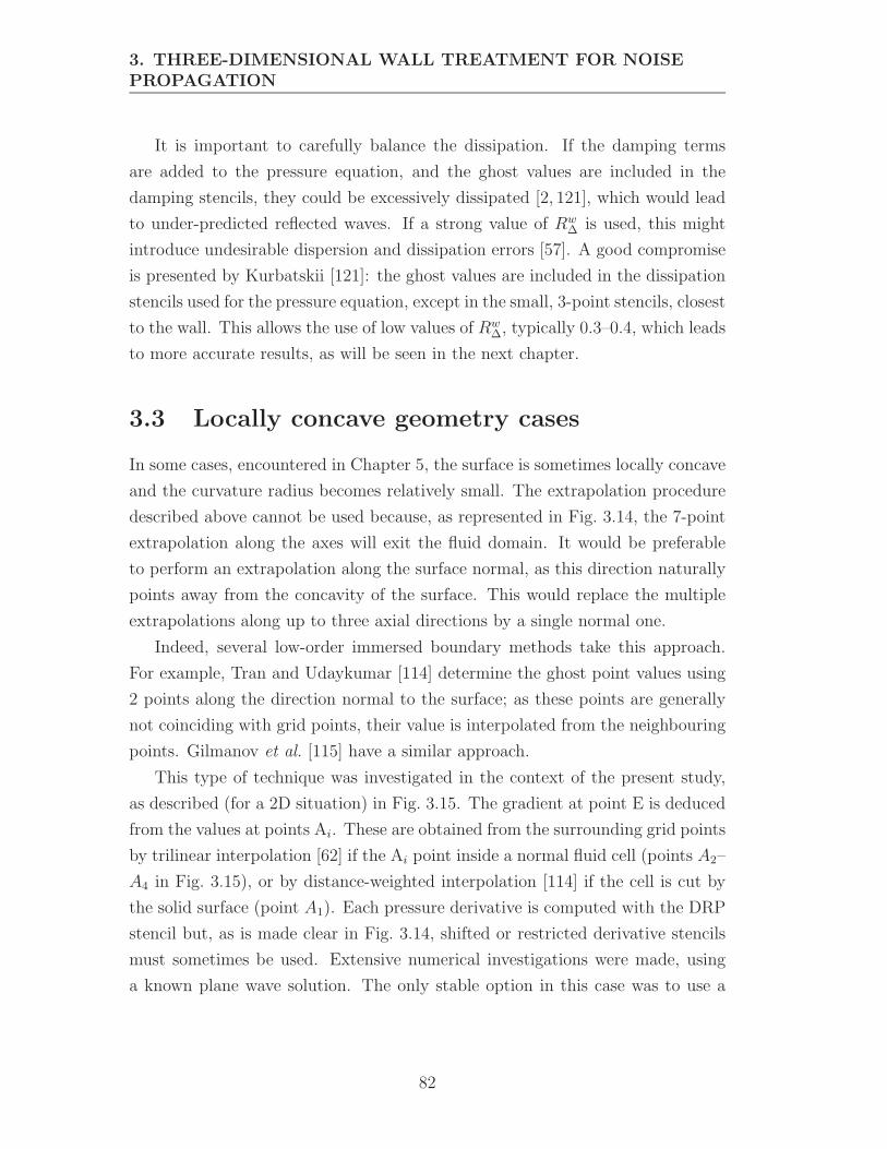
3. THREE-DIMENSIONAL WALL TREATMENT FOR NOISEPROPAGATION
It is important to carefully balance the dissipation. If the damping terms
are added to the pressure equation, and the ghost values are included in the
damping stencils, they could be excessively dissipated [2, 121], which would lead
to under-predicted reflected waves. If a strong value of Rw∆ is used, this might
introduce undesirable dispersion and dissipation errors [57]. A good compromise
is presented by Kurbatskii [121]: the ghost values are included in the dissipation
stencils used for the pressure equation, except in the small, 3-point stencils, closest
to the wall. This allows the use of low values of Rw∆, typically 0.3–0.4, which leads
to more accurate results, as will be seen in the next chapter.
3.3 Locally concave geometry cases
In some cases, encountered in Chapter 5, the surface is sometimes locally concave
and the curvature radius becomes relatively small. The extrapolation procedure
described above cannot be used because, as represented in Fig. 3.14, the 7-point
extrapolation along the axes will exit the fluid domain. It would be preferable
to perform an extrapolation along the surface normal, as this direction naturally
points away from the concavity of the surface. This would replace the multiple
extrapolations along up to three axial directions by a single normal one.
Indeed, several low-order immersed boundary methods take this approach.
For example, Tran and Udaykumar [114] determine the ghost point values using
2 points along the direction normal to the surface; as these points are generally
not coinciding with grid points, their value is interpolated from the neighbouring
points. Gilmanov et al. [115] have a similar approach.
This type of technique was investigated in the context of the present study,
as described (for a 2D situation) in Fig. 3.15. The gradient at point E is deduced
from the values at points Ai. These are obtained from the surrounding grid points
by trilinear interpolation [62] if the Ai point inside a normal fluid cell (points A2–
A4 in Fig. 3.15), or by distance-weighted interpolation [114] if the cell is cut by
the solid surface (point A1). Each pressure derivative is computed with the DRP
stencil but, as is made clear in Fig. 3.14, shifted or restricted derivative stencils
must sometimes be used. Extensive numerical investigations were made, using
a known plane wave solution. The only stable option in this case was to use a
82
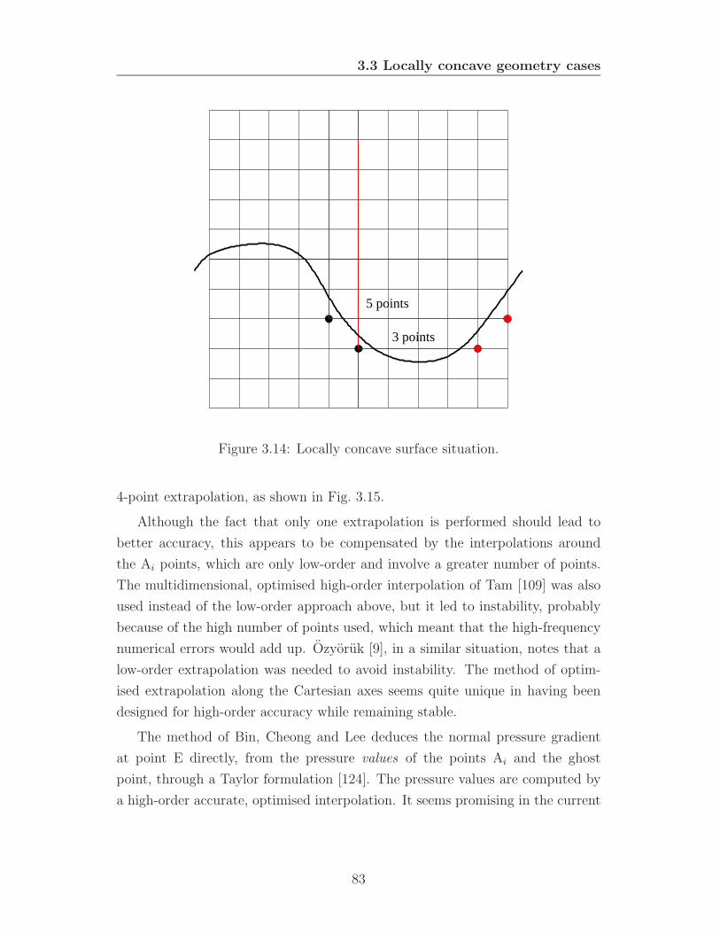
3.3 Locally concave geometry cases
5 points
3 points
Figure 3.14: Locally concave surface situation.
4-point extrapolation, as shown in Fig. 3.15.
Although the fact that only one extrapolation is performed should lead to
better accuracy, this appears to be compensated by the interpolations around
the Ai points, which are only low-order and involve a greater number of points.
The multidimensional, optimised high-order interpolation of Tam [109] was also
used instead of the low-order approach above, but it led to instability, probably
because of the high number of points used, which meant that the high-frequency
numerical errors would add up. Ozyoruk [9], in a similar situation, notes that a
low-order extrapolation was needed to avoid instability. The method of optim-
ised extrapolation along the Cartesian axes seems quite unique in having been
designed for high-order accuracy while remaining stable.
The method of Bin, Cheong and Lee deduces the normal pressure gradient
at point E directly, from the pressure values of the points Ai and the ghost
point, through a Taylor formulation [124]. The pressure values are computed by
a high-order accurate, optimised interpolation. It seems promising in the current
83
3. THREE-DIMENSIONAL WALL TREATMENT FOR NOISEPROPAGATION
context, but its results could not be replicated in the present study for lack of
time.
G
d2 E
d1
A1
A2
A3
A4
Figure 3.15: Extrapolation along the normal direction (in 2D).
Concluding remarks
A new immersed boundary algorithm was developed to meet the challenge of
representing 3D wall boundaries without the need for any meshing techniques,
while retaining a large order accuracy throughout most of the domain. This was
done by extending an existing 2D method, designing an appropriate systematic
algorithm to deal with all possible geometries (with some assumptions on the
curvature of the surface). This posed several computational problems which were
dealt with. For ghost points in locally concave areas, an alternative, low-order
normal extrapolation is used. This method will be validated in chapter 4 on
simple benchmark cases, and applied to more complex geometries in Chapter 5.
84
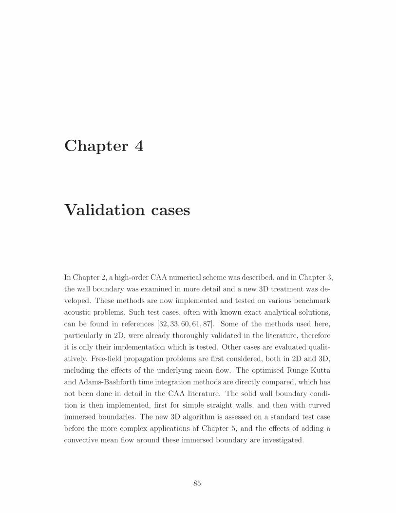
Chapter 4
Validation cases
In Chapter 2, a high-order CAA numerical scheme was described, and in Chapter 3,
the wall boundary was examined in more detail and a new 3D treatment was de-
veloped. These methods are now implemented and tested on various benchmark
acoustic problems. Such test cases, often with known exact analytical solutions,
can be found in references [32, 33, 60, 61, 87]. Some of the methods used here,
particularly in 2D, were already thoroughly validated in the literature, therefore
it is only their implementation which is tested. Other cases are evaluated qualit-
atively. Free-field propagation problems are first considered, both in 2D and 3D,
including the effects of the underlying mean flow. The optimised Runge-Kutta
and Adams-Bashforth time integration methods are directly compared, which has
not been done in detail in the CAA literature. The solid wall boundary condi-
tion is then implemented, first for simple straight walls, and then with curved
immersed boundaries. The new 3D algorithm is assessed on a standard test case
before the more complex applications of Chapter 5, and the effects of adding a
convective mean flow around these immersed boundary are investigated.
85
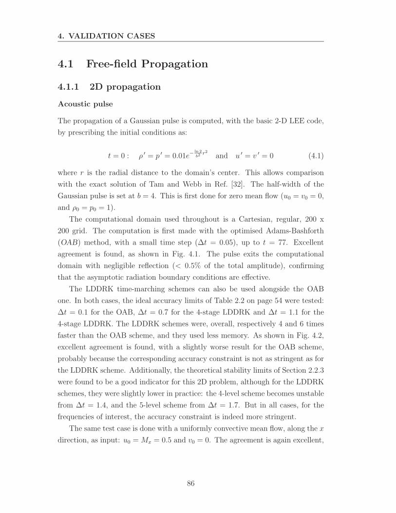
4. VALIDATION CASES
4.1 Free-field Propagation
4.1.1 2D propagation
Acoustic pulse
The propagation of a Gaussian pulse is computed, with the basic 2-D LEE code,
by prescribing the initial conditions as:
t = 0 : ρ ′ = p ′ = 0.01e−ln 2
b2r2
and u ′ = v ′ = 0 (4.1)
where r is the radial distance to the domain’s center. This allows comparison
with the exact solution of Tam and Webb in Ref. [32]. The half-width of the
Gaussian pulse is set at b = 4. This is first done for zero mean flow (u0 = v0 = 0,
and ρ0 = p0 = 1).
The computational domain used throughout is a Cartesian, regular, 200 x
200 grid. The computation is first made with the optimised Adams-Bashforth
(OAB) method, with a small time step (∆t = 0.05), up to t = 77. Excellent
agreement is found, as shown in Fig. 4.1. The pulse exits the computational
domain with negligible reflection (< 0.5% of the total amplitude), confirming
that the asymptotic radiation boundary conditions are effective.
The LDDRK time-marching schemes can also be used alongside the OAB
one. In both cases, the ideal accuracy limits of Table 2.2 on page 54 were tested:
∆t = 0.1 for the OAB, ∆t = 0.7 for the 4-stage LDDRK and ∆t = 1.1 for the
4-stage LDDRK. The LDDRK schemes were, overall, respectively 4 and 6 times
faster than the OAB scheme, and they used less memory. As shown in Fig. 4.2,
excellent agreement is found, with a slightly worse result for the OAB scheme,
probably because the corresponding accuracy constraint is not as stringent as for
the LDDRK scheme. Additionally, the theoretical stability limits of Section 2.2.3
were found to be a good indicator for this 2D problem, although for the LDDRK
schemes, they were slightly lower in practice: the 4-level scheme becomes unstable
from ∆t = 1.4, and the 5-level scheme from ∆t = 1.7. But in all cases, for the
frequencies of interest, the accuracy constraint is indeed more stringent.
The same test case is done with a uniformly convective mean flow, along the x
direction, as input: u0 = Mx = 0.5 and v0 = 0. The agreement is again excellent,
86
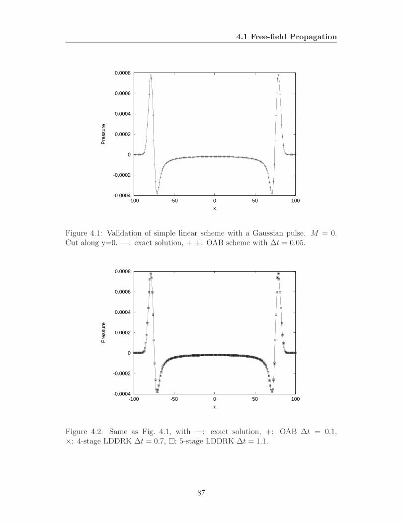
4.1 Free-field Propagation
-0.0004
-0.0002
0
0.0002
0.0004
0.0006
0.0008
-100 -50 0 50 100
Pre
ssur
e
x
Figure 4.1: Validation of simple linear scheme with a Gaussian pulse. M = 0.Cut along y=0. —: exact solution, + +: OAB scheme with ∆t = 0.05.
-0.0004
-0.0002
0
0.0002
0.0004
0.0006
0.0008
-100 -50 0 50 100
Pre
ssur
e
x
Figure 4.2: Same as Fig. 4.1, with —: exact solution, +: OAB ∆t = 0.1,×: 4-stage LDDRK ∆t = 0.7, �: 5-stage LDDRK ∆t = 1.1.
87
4. VALIDATION CASES
as shown in Fig. 4.3. The presence of the flow does reduce the stability and
accuracy limits, as predicted in Section 2.2.3.
-0.0006
-0.0004
-0.0002
0
0.0002
0.0004
0.0006
0.0008
0.001
-100 -50 0 50 100
Den
sity
(di
men
sion
less
)
X position / dx
ComputedExact
Figure 4.3: Validation of simple linear scheme with a Gaussian pulse. Mx = +0.5.Cut along y=0.
Acoustic oscillating source
Fig. 4.4 shows the propagation of a monopole acoustic source: the term of the
source vector S (in Eq. (2.2) on page 35) related to the pressure equation is an
oscillating term with a smooth Gaussian distribution of amplitude:
S4 = −0.01e−ln 2
8r2s cos ωt (4.2)
where rs is the distance from the center of source which is at the origin of the
domain. ω is the circular frequency of the source. The computation is first done
with the OAB scheme using ∆t = 0.05, as shown in Fig. 4.4. It is also compared to
an analytical solution (Morris [125]), and no significant dispersion or dissipation
error can be seen, even for 7 PPW and a propagation over 13 wavelengths.
88
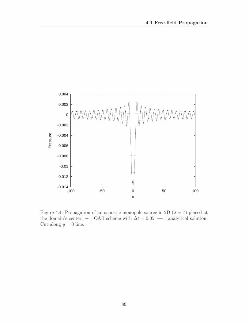
4.1 Free-field Propagation
-0.014
-0.012
-0.01
-0.008
-0.006
-0.004
-0.002
0
0.002
0.004
-100 -50 0 50 100
Pre
ssur
e
x
Figure 4.4: Propagation of an acoustic monopole source in 2D (λ = 7) placed atthe domain’s center. + : OAB scheme with ∆t = 0.05, — : analytical solution.Cut along y = 0 line.
89
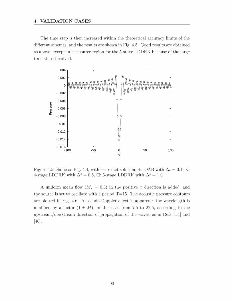
4. VALIDATION CASES
The time step is then increased within the theoretical accuracy limits of the
different schemes, and the results are shown in Fig. 4.5. Good results are obtained
as above, except in the source region for the 5-stage LDDRK because of the large
time-steps involved.
-0.016
-0.014
-0.012
-0.01
-0.008
-0.006
-0.004
-0.002
0
0.002
0.004
-100 -50 0 50 100
Pre
ssur
e
x
Figure 4.5: Same as Fig. 4.4, with —: exact solution, +: OAB with ∆t = 0.1, ×:4-stage LDDRK with ∆t = 0.5, �: 5-stage LDDRK with ∆t = 1.0.
A uniform mean flow (Mx = 0.3) in the positive x direction is added, and
the source is set to oscillate with a period T=15. The acoustic pressure contours
are plotted in Fig. 4.6. A pseudo-Doppler effect is apparent: the wavelength is
modified by a factor (1 ± M), in this case from 7.5 to 22.5, according to the
upstream/dowstream direction of propagation of the waves, as in Refs. [54] and
[46].
90
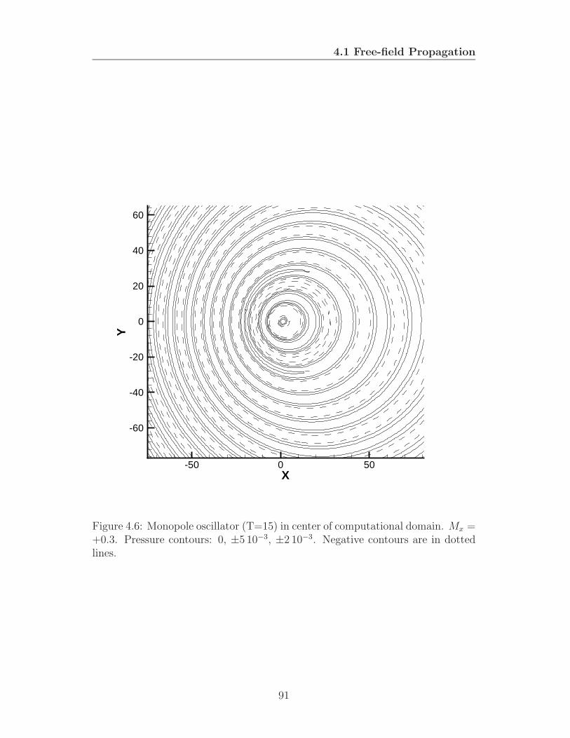
4.1 Free-field Propagation
X
Y
-50 0 50
-60
-40
-20
0
20
40
60
Figure 4.6: Monopole oscillator (T=15) in center of computational domain. Mx =+0.3. Pressure contours: 0, ±5 10−3, ±2 10−3. Negative contours are in dottedlines.
91
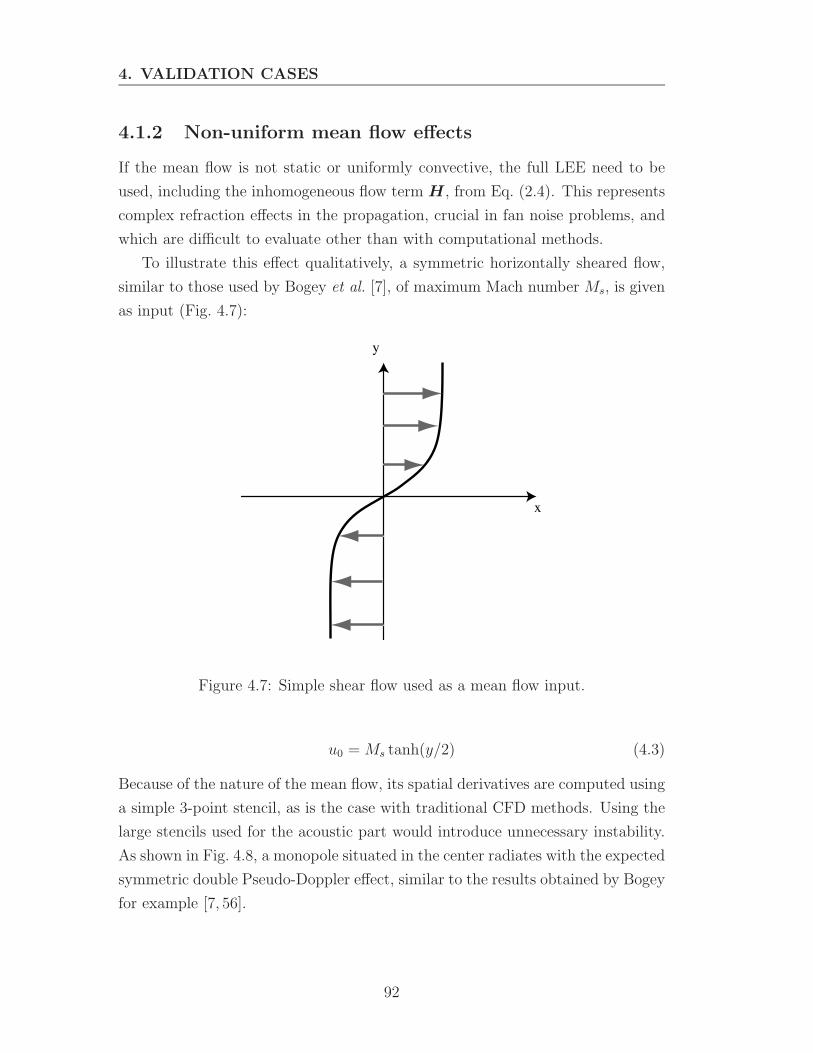
4. VALIDATION CASES
4.1.2 Non-uniform mean flow effects
If the mean flow is not static or uniformly convective, the full LEE need to be
used, including the inhomogeneous flow term H , from Eq. (2.4). This represents
complex refraction effects in the propagation, crucial in fan noise problems, and
which are difficult to evaluate other than with computational methods.
To illustrate this effect qualitatively, a symmetric horizontally sheared flow,
similar to those used by Bogey et al. [7], of maximum Mach number Ms, is given
as input (Fig. 4.7):
x
y
Figure 4.7: Simple shear flow used as a mean flow input.
u0 = Ms tanh(y/2) (4.3)
Because of the nature of the mean flow, its spatial derivatives are computed using
a simple 3-point stencil, as is the case with traditional CFD methods. Using the
large stencils used for the acoustic part would introduce unnecessary instability.
As shown in Fig. 4.8, a monopole situated in the center radiates with the expected
symmetric double Pseudo-Doppler effect, similar to the results obtained by Bogey
for example [7, 56].
92
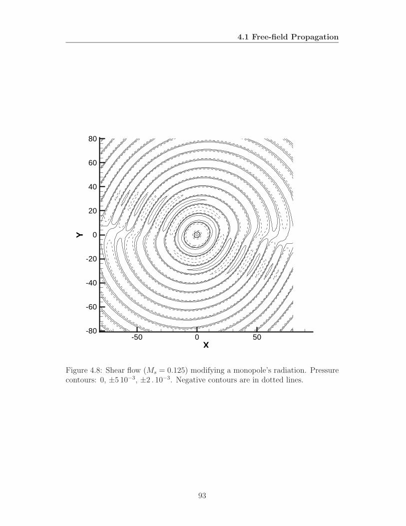
4.1 Free-field Propagation
X
Y
-50 0 50-80
-60
-40
-20
0
20
40
60
80
Figure 4.8: Shear flow (Ms = 0.125) modifying a monopole’s radiation. Pressurecontours: 0, ±5 10−3, ±2 . 10−3. Negative contours are in dotted lines.
93
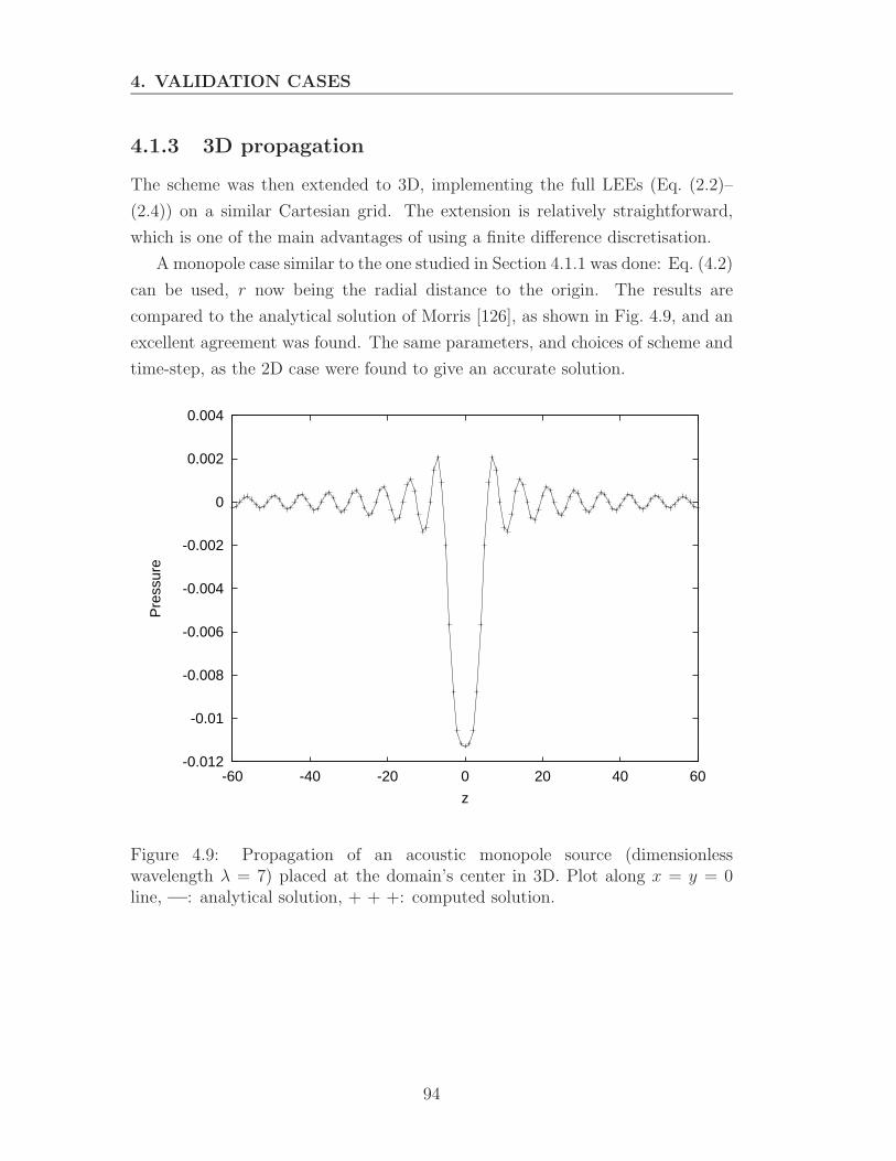
4. VALIDATION CASES
4.1.3 3D propagation
The scheme was then extended to 3D, implementing the full LEEs (Eq. (2.2)–
(2.4)) on a similar Cartesian grid. The extension is relatively straightforward,
which is one of the main advantages of using a finite difference discretisation.
A monopole case similar to the one studied in Section 4.1.1 was done: Eq. (4.2)
can be used, r now being the radial distance to the origin. The results are
compared to the analytical solution of Morris [126], as shown in Fig. 4.9, and an
excellent agreement was found. The same parameters, and choices of scheme and
time-step, as the 2D case were found to give an accurate solution.
-0.012
-0.01
-0.008
-0.006
-0.004
-0.002
0
0.002
0.004
-60 -40 -20 0 20 40 60
Pre
ssur
e
z
Figure 4.9: Propagation of an acoustic monopole source (dimensionlesswavelength λ = 7) placed at the domain’s center in 3D. Plot along x = y = 0line, —: analytical solution, + + +: computed solution.
94
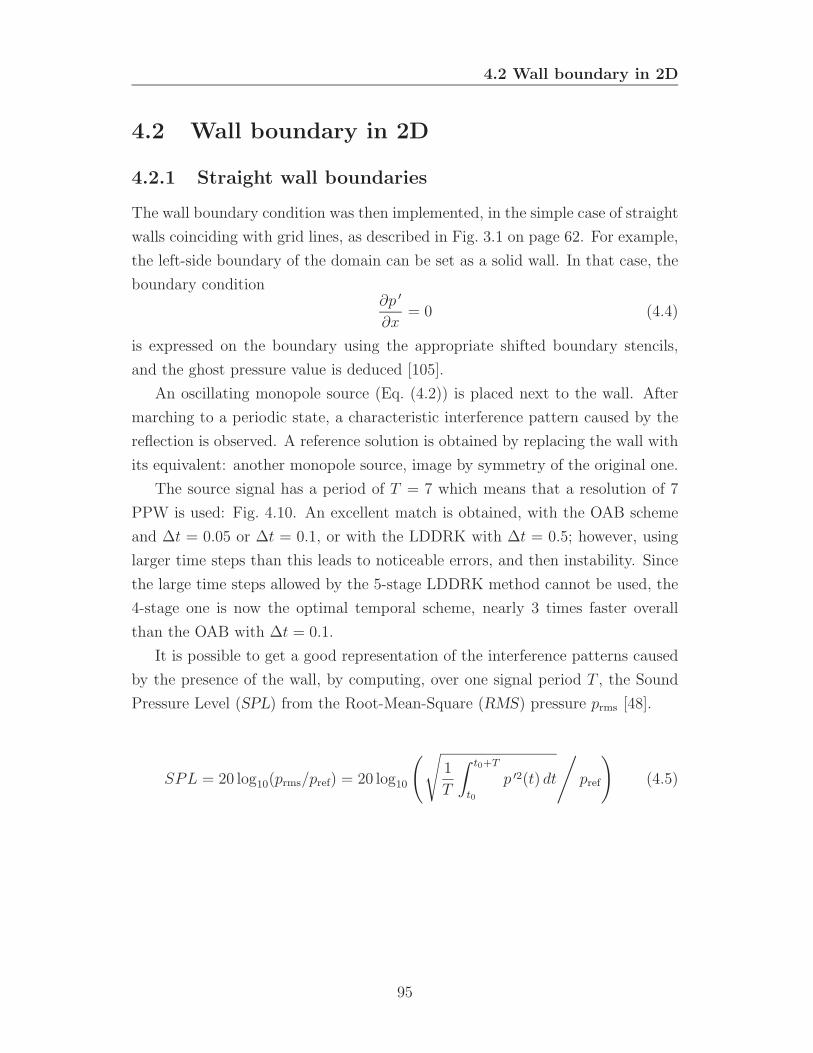
4.2 Wall boundary in 2D
4.2 Wall boundary in 2D
4.2.1 Straight wall boundaries
The wall boundary condition was then implemented, in the simple case of straight
walls coinciding with grid lines, as described in Fig. 3.1 on page 62. For example,
the left-side boundary of the domain can be set as a solid wall. In that case, the
boundary condition∂p ′
∂x= 0 (4.4)
is expressed on the boundary using the appropriate shifted boundary stencils,
and the ghost pressure value is deduced [105].
An oscillating monopole source (Eq. (4.2)) is placed next to the wall. After
marching to a periodic state, a characteristic interference pattern caused by the
reflection is observed. A reference solution is obtained by replacing the wall with
its equivalent: another monopole source, image by symmetry of the original one.
The source signal has a period of T = 7 which means that a resolution of 7
PPW is used: Fig. 4.10. An excellent match is obtained, with the OAB scheme
and ∆t = 0.05 or ∆t = 0.1, or with the LDDRK with ∆t = 0.5; however, using
larger time steps than this leads to noticeable errors, and then instability. Since
the large time steps allowed by the 5-stage LDDRK method cannot be used, the
4-stage one is now the optimal temporal scheme, nearly 3 times faster overall
than the OAB with ∆t = 0.1.
It is possible to get a good representation of the interference patterns caused
by the presence of the wall, by computing, over one signal period T , the Sound
Pressure Level (SPL) from the Root-Mean-Square (RMS) pressure prms [48].
SPL = 20 log10(prms/pref) = 20 log10
(
√
1
T
∫ t0+T
t0
p ′2(t) dt
/
pref
)
(4.5)
95
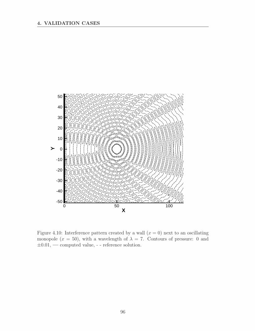
4. VALIDATION CASES
X
Y
0 50 100-50
-40
-30
-20
-10
0
10
20
30
40
50
Figure 4.10: Interference pattern created by a wall (x = 0) next to an oscillatingmonopole (x = 50), with a wavelength of λ = 7. Contours of pressure: 0 and±0.01, — computed value, - - reference solution.
96
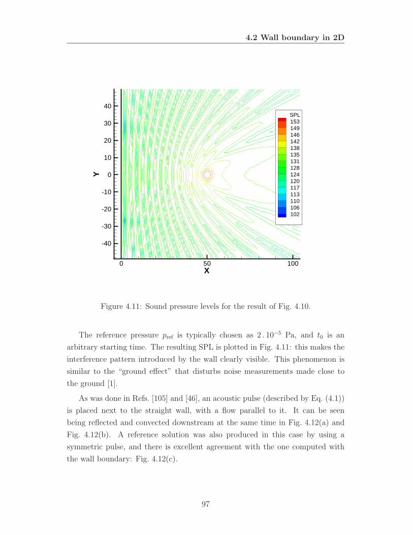
4.2 Wall boundary in 2D
X
Y
0 50 100
-40
-30
-20
-10
0
10
20
30
40SPL153149146142138135131128124120117113110106102
Figure 4.11: Sound pressure levels for the result of Fig. 4.10.
The reference pressure pref is typically chosen as 2 . 10−5 Pa, and t0 is an
arbitrary starting time. The resulting SPL is plotted in Fig. 4.11: this makes the
interference pattern introduced by the wall clearly visible. This phenomenon is
similar to the “ground effect” that disturbs noise measurements made close to
the ground [1].
As was done in Refs. [105] and [46], an acoustic pulse (described by Eq. (4.1))
is placed next to the straight wall, with a flow parallel to it. It can be seen
being reflected and convected downstream at the same time in Fig. 4.12(a) and
Fig. 4.12(b). A reference solution was also produced in this case by using a
symmetric pulse, and there is excellent agreement with the one computed with
the wall boundary: Fig. 4.12(c).
97
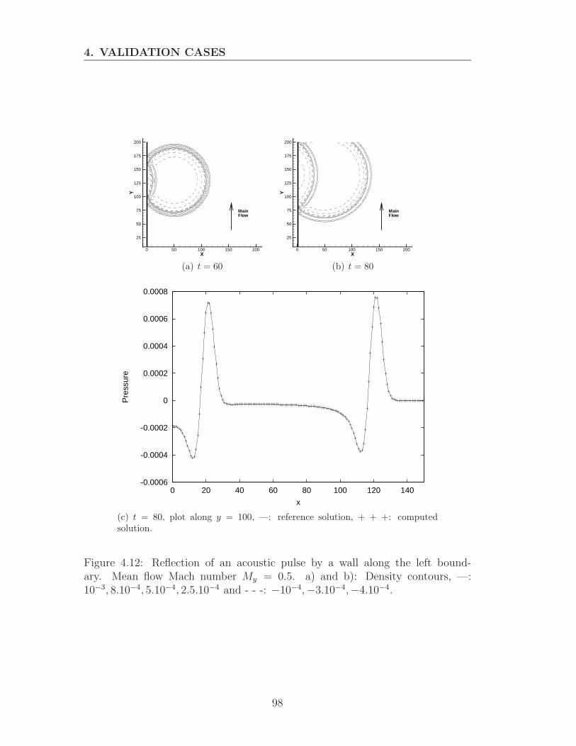
4. VALIDATION CASES
X
Y
0 50 100 150 200
25
50
75
100
125
150
175
200
MainFlow
(a) t = 60
X
Y
0 50 100 150 200
25
50
75
100
125
150
175
200
MainFlow
(b) t = 80
-0.0006
-0.0004
-0.0002
0
0.0002
0.0004
0.0006
0.0008
0 20 40 60 80 100 120 140
Pre
ssur
e
x
(c) t = 80, plot along y = 100, —: reference solution, + + +: computedsolution.
Figure 4.12: Reflection of an acoustic pulse by a wall along the left bound-ary. Mean flow Mach number My = 0.5. a) and b): Density contours, —:10−3, 8.10−4, 5.10−4, 2.5.10−4 and - - -: −10−4,−3.10−4,−4.10−4.
98
4.2 Wall boundary in 2D
4.2.2 Curved wall boundaries
The 2D curved wall method of Kurbatskii was then implemented. This method
has been validated thoroughly for a variety of different cases, even at high-order
resolutions (λ = 8∆x) [121]. To prove that the implementation was correctly
done, problem 1 from category 1 in the second CAA workshop on benchmark
problems [60] was considered; it consists of computing the scattering of the oscil-
lating acoustic source of Section 4.1.1 by a solid cylinder of radius a.
An interesting characteristic of the resolution is the dimensionless wavenum-
ber, or Helmholtz number:
α = 2πa/λ (4.6)
The computation is first done with a resolution of 7 PPW with a = 20, which
gives α ≃ 18, which represents a challenging test case. Using an insufficient
level of dissipation close to the wall boundary leads to crippling instability, as
shown in Fig. 4.13(a). If the optimal selective dissipation technique described
in Section 3.2.4 (with Rw∆ in the range 0.3–0.4) is used then a correct solution
is obtained: Fig. 4.13(b). Once the computed solution has reached a periodic
state, the interference pattern caused by the scattering is apparent, as well as the
“shadow zone”: the silent zone created by the masking of the cylinder. Further-
more, the waves appear to exit the boundaries with no noticeable reflections. A
plot of the SPL is shown in Fig. 4.14, making the features of the scattered field
more clearly apparent.
In Fig. 4.15, the computed solution, cut along the y = 0 line, is compared to
an analytical solution by Morris [125]. It is clear that an excellent agreement is
obtained, even at this relatively low grid density.
Extensive numerical testing was performed for various test cases, to further
validate the method and to confirm the parameters of the artificial selective nu-
merical dissipation, as described in Section 3.2.4. The optimal set-up was found
in agreement with Kurbatskii [121]: the dissipation terms are applied to all equa-
tions, but the smallest, 3-point dissipation stencils do not include the ghost values
of pressure. The same distribution of Rw∆ is used regardless of the Helmholtz num-
ber of the problem. If the dissipation is not applied to the pressure equation, then
a larger Rw∆ amplitude (> 0.7) needs to be used to ensure stability, which leads,
99
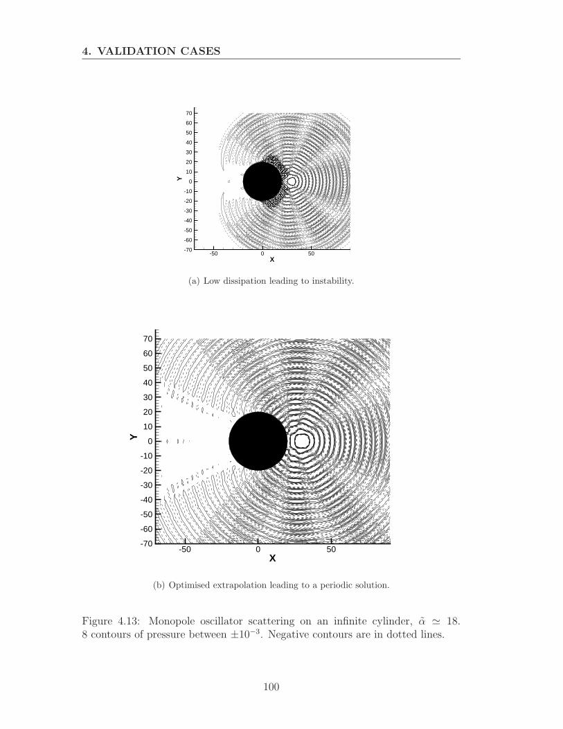
4. VALIDATION CASES
X
Y
-50 0 50-70
-60
-50
-40
-30
-20
-10
0
10
20
30
40
50
60
70
(a) Low dissipation leading to instability.
X
Y
-50 0 50-70
-60
-50
-40
-30
-20
-10
0
10
20
30
40
50
60
70
(b) Optimised extrapolation leading to a periodic solution.
Figure 4.13: Monopole oscillator scattering on an infinite cylinder, α ≃ 18.8 contours of pressure between ±10−3. Negative contours are in dotted lines.
100

4.2 Wall boundary in 2D
X
Y
-50 0 50 100
-70
-60
-50
-40
-30
-20
-10
0
10
20
30
40
50
60
70
80
SPL14013212411710910193867870
Figure 4.14: Sound pressure levels of the computed solution of Fig. 4.13.
-0.014
-0.012
-0.01
-0.008
-0.006
-0.004
-0.002
0
0.002
0.004
-40 -20 0 20 40 60
Pre
ssur
e
x
Figure 4.15: Cut along the y = 0 line of a source of λ = 7 at x = 30, scatteredby a cylinder of radius a = 20. — : analytical solution; computed solution:+ + + with optimal dissipation, ××× with large Rw
∆ coefficient.
101

4. VALIDATION CASES
noticeably in Fig. 4.15, to a dissipated and dispersed solution; more particularly
in the shadow zone, because the sound waves must travel along the whole surface
of the cylinder.
The simulation was run with the (4-stage) LDDRK scheme, with time-steps
no larger than ∆t = 0.3, with no apparent difference with the result obtained
with a OAB scheme (∆t = 0.1), but the latter scheme runs faster overall because
it only evaluates one residual per time step, and gives slightly more accuracy and
stability. The instability introduced by the curved wall surface makes the use
of large time steps impossible, and makes the OAB scheme the optimal scheme
to use. One could argue that this does in effect reduce the effective temporal
order of the scheme. In the studies of Refs. [121] and [46], very small time steps
(∆t = 0.05) were also used in all cases. In the work of Ozyoruk [9], although high
CFL numbers are used (typically 0.5) with a Runge-Kutta method, this results
in small time steps (384 per period) because of the deformed grid: it is necessary
to use the smallest time step allowed by the grid metrics over the whole domain.
With the current approach, the instability is limited to the vicinity of the wall
boundaries, and not present in most of the domain where a simple uniform grid
is used. Chapter 3 presented many of the other advantages of such an approach.
4.2.3 Flow around the wall surface
The effect of a mean flow surrounding the immersed boundary will now be in-
vestigated (this was not done in Ref. [121]). In the general case, a steady solution
of the flow in the presence of the wall boundary can be obtained simply by using
a traditional CFD program; this can then be interpolated on the Cartesian grid
obtained. In the case of a 2D inviscid potential flow around a cylinder of radius
a, the solution can be expressed simply in the 2D cylindrical coordinate system
(r, θ) centered on the cylinder [127]:
vr = U∞
(
1 −(a
r
)2)
cos θ (4.7)
vθ = −U∞
(
1 +(a
r
)2)
sin θ (4.8)
p = p∞ + 1/2ρU2∞
(1 − 4 sin2 θ) (4.9)
102
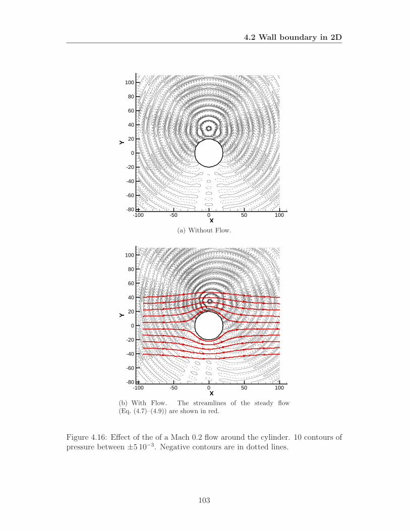
4.2 Wall boundary in 2D
X
Y
-100 -50 0 50 100-80
-60
-40
-20
0
20
40
60
80
100
(a) Without Flow.
X
Y
-100 -50 0 50 100-80
-60
-40
-20
0
20
40
60
80
100
(b) With Flow. The streamlines of the steady flow(Eq. (4.7)–(4.9)) are shown in red.
Figure 4.16: Effect of the of a Mach 0.2 flow around the cylinder. 10 contours ofpressure between ±5 10−3. Negative contours are in dotted lines.
103
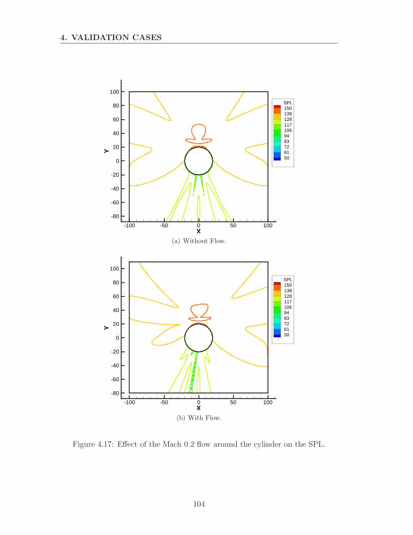
4. VALIDATION CASES
X
Y
-100 -50 0 50 100
-80
-60
-40
-20
0
20
40
60
80
100
SPL1501391281171069483726150
(a) Without Flow.
X
Y
-100 -50 0 50 100
-80
-60
-40
-20
0
20
40
60
80
100
SPL1501391281171069483726150
(b) With Flow.
Figure 4.17: Effect of the Mach 0.2 flow around the cylinder on the SPL.
104
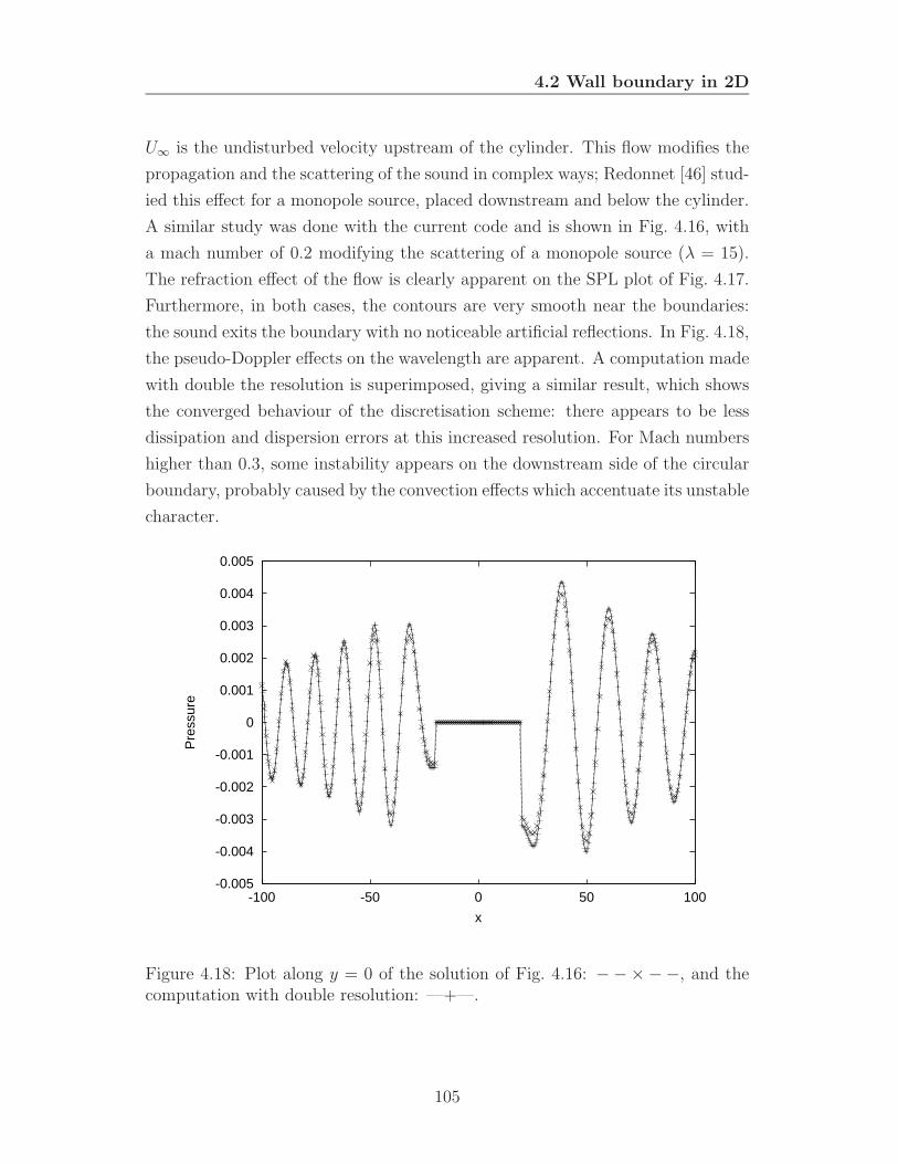
4.2 Wall boundary in 2D
U∞ is the undisturbed velocity upstream of the cylinder. This flow modifies the
propagation and the scattering of the sound in complex ways; Redonnet [46] stud-
ied this effect for a monopole source, placed downstream and below the cylinder.
A similar study was done with the current code and is shown in Fig. 4.16, with
a mach number of 0.2 modifying the scattering of a monopole source (λ = 15).
The refraction effect of the flow is clearly apparent on the SPL plot of Fig. 4.17.
Furthermore, in both cases, the contours are very smooth near the boundaries:
the sound exits the boundary with no noticeable artificial reflections. In Fig. 4.18,
the pseudo-Doppler effects on the wavelength are apparent. A computation made
with double the resolution is superimposed, giving a similar result, which shows
the converged behaviour of the discretisation scheme: there appears to be less
dissipation and dispersion errors at this increased resolution. For Mach numbers
higher than 0.3, some instability appears on the downstream side of the circular
boundary, probably caused by the convection effects which accentuate its unstable
character.
-0.005
-0.004
-0.003
-0.002
-0.001
0
0.001
0.002
0.003
0.004
0.005
-100 -50 0 50 100
Pre
ssur
e
x
Figure 4.18: Plot along y = 0 of the solution of Fig. 4.16: −−×−−, and thecomputation with double resolution: —+—.
105
4. VALIDATION CASES
4.3 Wall boundary in 3D
4.3.1 Scattering from a sphere
The 3D method described in Section 3.2 was implemented. Basic tests have
already been performed in Section 3.2.2, making sure that the normals were
correctly evaluated and that no artificial asymmetry was introduced by the surface
analysis algorithm.
A scattering problem [126], similar to problems 3 and 4 of category 1 in
the second conference on acoustic benchmark tests [60], is used to validate the
boundary condition. In this case, a sphere scatters, in 3D, a monopole acoustic
source situated on the z axis. This problem has been used to validate other 3D
methods: Zhuang and Chen [83] use an adapted spherical coordinate system,
with excellent results, but this cannot be used in more complex cases. Morris [81]
used a simple staircase boundary.
After some iterations, a periodic state is obtained. The effects of the scattering
are apparent on Fig. 4.19: the interference pattern from the reflected signal and
the shadow zone behind the sphere. Fig. 4.20 and Fig. 4.21 show the computed
solution, compared to the analytic one, for different parameters. A range of
resolutions is studied, as described by the dimensionless wavenumber α = 2πa/λ,
where a is the radius of the sphere. The case of Fig. 4.20(a) has α = 6.8; in
Fig. 4.20(b) α = 12.6; finally in Fig. 4.21, where the spatial resolution is 7 PPW,
α goes up to 17.9. This performs a convergence study of this problem.
In all cases, there is excellent agreement in the zone closest to the source.
But, examining the solution on the x axis (Fig. 4.21(b)), or, more strikingly, in
the shadow zone behind the solid, it appears that increasing dissipation errors
seem to accumulate as the waves are diffracted around the wall surface. This
is similar to what was observed in 2D, but with an increased magnitude. This
is probably because three extrapolations need to be done for most ghost points,
instead of a maximum of two for the 2D method. The unavoidable error intro-
duced by discretising the curved surface, more important in 3D as was shown in
Section 3.2.2, is also probably a factor. The wave, as it travels along the wall,
is more dissipated than it is dispersed, which is consistent with general results
106
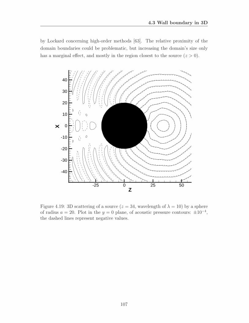
4.3 Wall boundary in 3D
by Lockard concerning high-order methods [63]. The relative proximity of the
domain boundaries could be problematic, but increasing the domain’s size only
has a marginal effect, and mostly in the region closest to the source (z > 0).
Z
X
-25 0 25 50
-40
-30
-20
-10
0
10
20
30
40
Figure 4.19: 3D scattering of a source (z = 34, wavelength of λ = 10) by a sphereof radius a = 20. Plot in the y = 0 plane, of acoustic pressure contours: ±10−4,the dashed lines represent negative values.
107
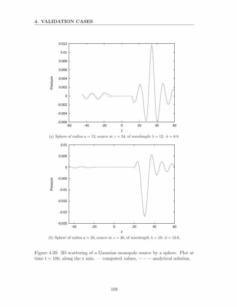
4. VALIDATION CASES
-0.006
-0.004
-0.002
0
0.002
0.004
0.006
0.008
0.01
0.012
-60 -40 -20 0 20 40 60
Pre
ssur
e
z
(a) Sphere of radius a = 13, source at z = 34, of wavelength λ = 12: α = 6.8.
-0.025
-0.02
-0.015
-0.01
-0.005
0
0.005
0.01
-40 -20 0 20 40 60
Pre
ssur
e
z
(b) Sphere of radius a = 20, source at z = 30, of wavelength λ = 10: α = 12.6.
Figure 4.20: 3D scattering of a Gaussian monopole source by a sphere. Plot attime t = 100, along the z axis. — computed values, −−− analytical solution.
108
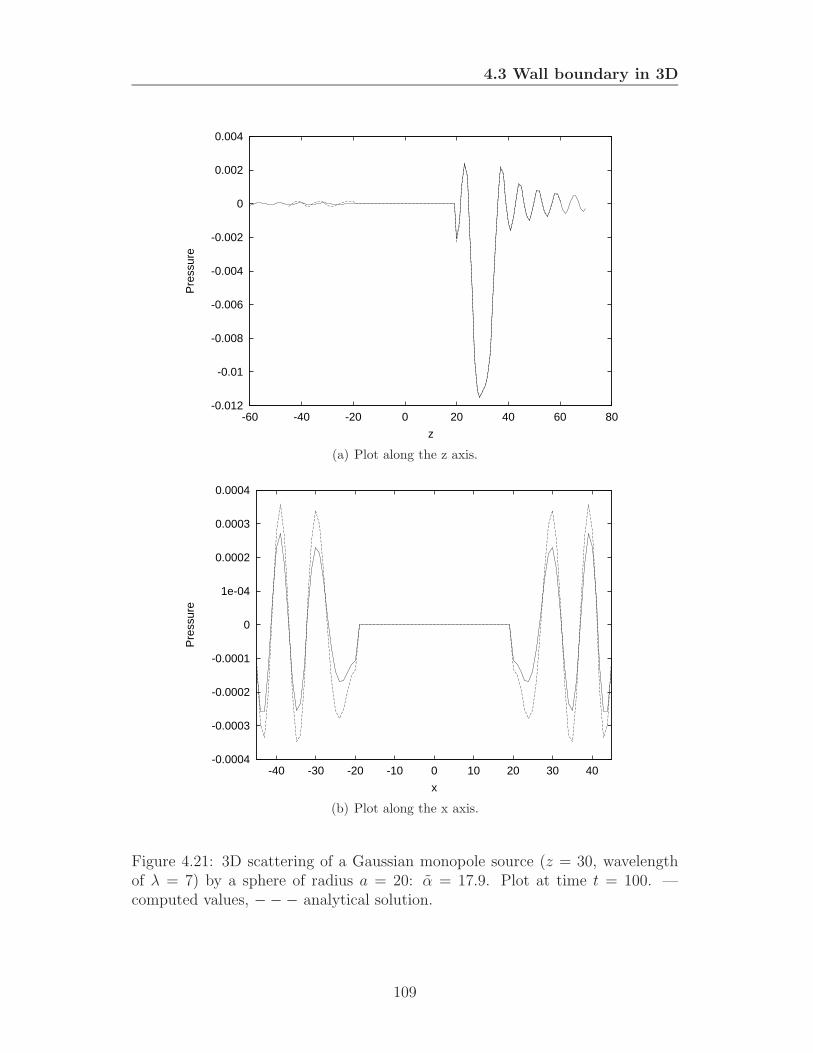
4.3 Wall boundary in 3D
-0.012
-0.01
-0.008
-0.006
-0.004
-0.002
0
0.002
0.004
-60 -40 -20 0 20 40 60 80
Pre
ssur
e
z
(a) Plot along the z axis.
-0.0004
-0.0003
-0.0002
-0.0001
0
1e-04
0.0002
0.0003
0.0004
-40 -30 -20 -10 0 10 20 30 40
Pre
ssur
e
x
(b) Plot along the x axis.
Figure 4.21: 3D scattering of a Gaussian monopole source (z = 30, wavelengthof λ = 7) by a sphere of radius a = 20: α = 17.9. Plot at time t = 100. —computed values, −−− analytical solution.
109
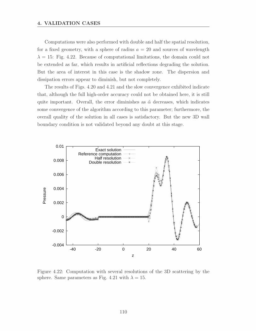
4. VALIDATION CASES
Computations were also performed with double and half the spatial resolution,
for a fixed geometry, with a sphere of radius a = 20 and sources of wavelength
λ = 15: Fig. 4.22. Because of computational limitations, the domain could not
be extended as far, which results in artificial reflections degrading the solution.
But the area of interest in this case is the shadow zone. The dispersion and
dissipation errors appear to diminish, but not completely.
The results of Figs. 4.20 and 4.21 and the slow convergence exhibited indicate
that, although the full high-order accuracy could not be obtained here, it is still
quite important. Overall, the error diminishes as α decreases, which indicates
some convergence of the algorithm according to this parameter; furthermore, the
overall quality of the solution in all cases is satisfactory. But the new 3D wall
boundary condition is not validated beyond any doubt at this stage.
-0.004
-0.002
0
0.002
0.004
0.006
0.008
0.01
-40 -20 0 20 40 60
Pre
ssur
e
z
Exact solutionReference computation
Half resolutionDouble resolution
Figure 4.22: Computation with several resolutions of the 3D scattering by thesphere. Same parameters as Fig. 4.21 with λ = 15.
110
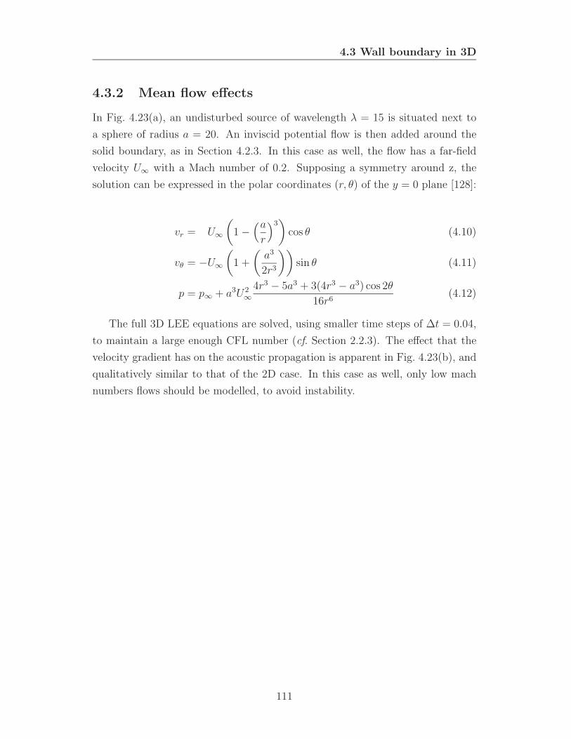
4.3 Wall boundary in 3D
4.3.2 Mean flow effects
In Fig. 4.23(a), an undisturbed source of wavelength λ = 15 is situated next to
a sphere of radius a = 20. An inviscid potential flow is then added around the
solid boundary, as in Section 4.2.3. In this case as well, the flow has a far-field
velocity U∞ with a Mach number of 0.2. Supposing a symmetry around z, the
solution can be expressed in the polar coordinates (r, θ) of the y = 0 plane [128]:
vr = U∞
(
1 −(a
r
)3)
cos θ (4.10)
vθ = −U∞
(
1 +
(
a3
2r3
))
sin θ (4.11)
p = p∞ + a3U2∞
4r3 − 5a3 + 3(4r3 − a3) cos 2θ
16r6(4.12)
The full 3D LEE equations are solved, using smaller time steps of ∆t = 0.04,
to maintain a large enough CFL number (cf. Section 2.2.3). The effect that the
velocity gradient has on the acoustic propagation is apparent in Fig. 4.23(b), and
qualitatively similar to that of the 2D case. In this case as well, only low mach
numbers flows should be modelled, to avoid instability.
111
4. VALIDATION CASES
Z
X
-50 0 50
-30
-20
-10
0
10
20
30
40
50
60
(a) Without Flow.
Z
X
-50 0 50
-30
-20
-10
0
10
20
30
40
50
60
(b) With Flow. Streamlines of the steady flow are shownin red.
Figure 4.23: Effect of the of a Mach 0.2 flow around the sphere. 10 contours ofpressure between ±4 10−3. Negative contours are in dotted lines.
112
4.3 Wall boundary in 3D
Concluding remarks
First of all, the implementation of the chosen numerical scheme was investigated
and verified using standard test cases found in the literature, as summarised in
Table 4.1. Its high accuracy was confirmed, and observations made by other
authors were replicated. A detailed analysis of two time integration schemes was
made, establishing that for simple cases, the theoretical stability and accuracy
limits are verified and that the frequency-optimised Runge-Kutta scheme was
the optimal choice. But when more complex cases including wall boundaries
were considered, smaller time steps needed to be used to prevent instability, and
the 4-level OAB scheme became the best option.
The 2D immersed boundary method of Kurbatskii was implemented, and
many results were replicated. It was also observed that the mean flow effects are
compatible with this boundary condition, for flows of low Mach numbers, which
could be a problematic limitation. The new 3D algorithm described in Chapter 3
was implemented, and tested on a standard benchmark problem. The high-order
accuracy that the immersed boundary condition possessed in 2D could not be
fully replicated in 3D, mainly because of extra inaccuracies in the extrapolation
process. The overall scheme remains high-order accurate in most of the domain.
The more representative applications in the following chapter will provide more
interesting validations, and assess the efficiency of the method compared to tra-
ditional CFD schemes.
Type 2D 3DPulse p. 86
Monopole p. 88 p. 94Straight walls p. 95Curved walls p. 99 p. 106
Table 4.1: Summary of the main validations cases used in this chapter.
113

4. VALIDATION CASES
114
Chapter 5
Study of representative industrial
cases
The CAA LEE code described in Chapter 2, together with the 3D wall boundary
method described in Chapter 3, were applied in Chapter 4. This methodology
will now be referred to as the High-Order Propagation (HOP) method. In this
chapter, the HOP method is applied to representative industrial geometries. The
plane wave propagation case from Chapter 2 is first solved, illustrating the gains
obtained when a high-order discretisation is used. Then, the problem of sound
propagation from engine inlets, of great importance as described in Chapter 1, is
studied to further evaluate the wall algorithm of Chapter 3. The propagation of
several different acoustic modes is computed for two different axisymmetric inlet
geometries: one based on the JT15D engine, and the other on an elliptic profile.
The HOP results are compared with simple analytical results, and with results
obtained by a 2D frequency-domain CAA code and by a traditional CFD code.
Finally, a fully 3D problem is studied, investigating the effects of inlet scarfing
with a simple model.
115
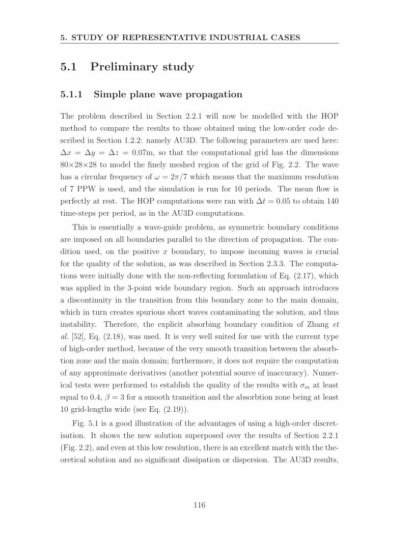
5. STUDY OF REPRESENTATIVE INDUSTRIAL CASES
5.1 Preliminary study
5.1.1 Simple plane wave propagation
The problem described in Section 2.2.1 will now be modelled with the HOP
method to compare the results to those obtained using the low-order code de-
scribed in Section 1.2.2: namely AU3D. The following parameters are used here:
∆x = ∆y = ∆z = 0.07m, so that the computational grid has the dimensions
80×28×28 to model the finely meshed region of the grid of Fig. 2.2. The wave
has a circular frequency of ω = 2π/7 which means that the maximum resolution
of 7 PPW is used, and the simulation is run for 10 periods. The mean flow is
perfectly at rest. The HOP computations were ran with ∆t = 0.05 to obtain 140
time-steps per period, as in the AU3D computations.
This is essentially a wave-guide problem, as symmetric boundary conditions
are imposed on all boundaries parallel to the direction of propagation. The con-
dition used, on the positive x boundary, to impose incoming waves is crucial
for the quality of the solution, as was described in Section 2.3.3. The computa-
tions were initially done with the non-reflecting formulation of Eq. (2.17), which
was applied in the 3-point wide boundary region. Such an approach introduces
a discontinuity in the transition from this boundary zone to the main domain,
which in turn creates spurious short waves contaminating the solution, and thus
instability. Therefore, the explicit absorbing boundary condition of Zhang et
al. [52], Eq. (2.18), was used. It is very well suited for use with the current type
of high-order method, because of the very smooth transition between the absorb-
tion zone and the main domain; furthermore, it does not require the computation
of any approximate derivatives (another potential source of inaccuracy). Numer-
ical tests were performed to establish the quality of the results with σm at least
equal to 0.4, β = 3 for a smooth transition and the absorbtion zone being at least
10 grid-lengths wide (see Eq. (2.19)).
Fig. 5.1 is a good illustration of the advantages of using a high-order discret-
isation. It shows the new solution superposed over the results of Section 2.2.1
(Fig. 2.2), and even at this low resolution, there is an excellent match with the the-
oretical solution and no significant dissipation or dispersion. The AU3D results,
116
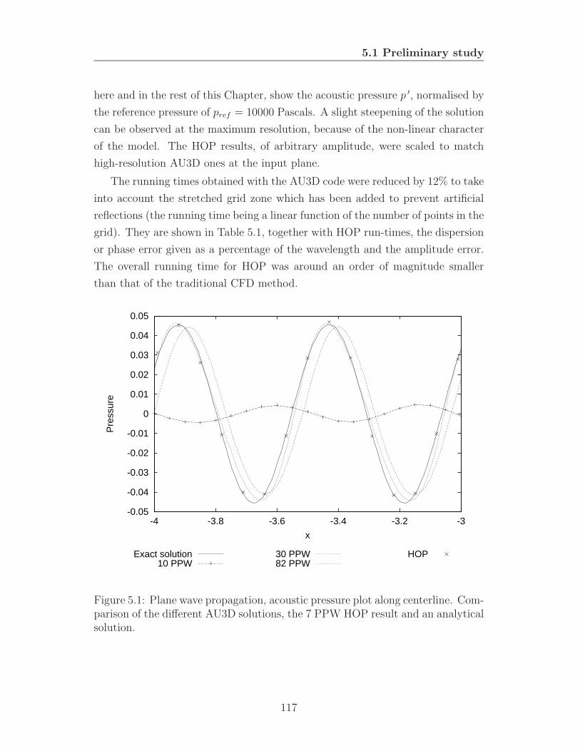
5.1 Preliminary study
here and in the rest of this Chapter, show the acoustic pressure p ′, normalised by
the reference pressure of pref = 10000 Pascals. A slight steepening of the solution
can be observed at the maximum resolution, because of the non-linear character
of the model. The HOP results, of arbitrary amplitude, were scaled to match
high-resolution AU3D ones at the input plane.
The running times obtained with the AU3D code were reduced by 12% to take
into account the stretched grid zone which has been added to prevent artificial
reflections (the running time being a linear function of the number of points in the
grid). They are shown in Table 5.1, together with HOP run-times, the dispersion
or phase error given as a percentage of the wavelength and the amplitude error.
The overall running time for HOP was around an order of magnitude smaller
than that of the traditional CFD method.
-0.05
-0.04
-0.03
-0.02
-0.01
0
0.01
0.02
0.03
0.04
0.05
-4 -3.8 -3.6 -3.4 -3.2 -3
Pre
ssur
e
x
Exact solution10 PPW
30 PPW82 PPW
HOP
Figure 5.1: Plane wave propagation, acoustic pressure plot along centerline. Com-parison of the different AU3D solutions, the 7 PPW HOP result and an analyticalsolution.
117
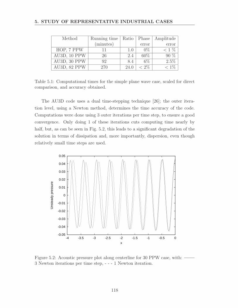
5. STUDY OF REPRESENTATIVE INDUSTRIAL CASES
Method Running time Ratio Phase Amplitude(minutes) error error
HOP, 7 PPW 11 1.0 0% < 1 %AU3D, 10 PPW 26 2.4 60% 90 %AU3D, 30 PPW 92 8.4 6% 2.5%AU3D, 82 PPW 270 24.0 < 2% < 1%
Table 5.1: Computational times for the simple plane wave case, scaled for directcomparison, and accuracy obtained.
The AU3D code uses a dual time-stepping technique [26]; the outer itera-
tion level, using a Newton method, determines the time accuracy of the code.
Computations were done using 3 outer iterations per time step, to ensure a good
convergence. Only doing 1 of these iterations cuts computing time nearly by
half, but, as can be seen in Fig. 5.2, this leads to a significant degradation of the
solution in terms of dissipation and, more importantly, dispersion, even though
relatively small time steps are used.
-0.05
-0.04
-0.03
-0.02
-0.01
0
0.01
0.02
0.03
0.04
0.05
-4 -3.5 -3 -2.5 -2 -1.5 -1 -0.5 0
Uns
tead
y pr
essu
re
x
Figure 5.2: Acoustic pressure plot along centerline for 30 PPW case, with: ——3 Newton iterations per time step, - - - 1 Newton iteration.
118
5.1 Preliminary study
The time step used in HOP can be increased from ∆t = 0.05 to 0.1 for
example, while retaining an accurate solution, thus doubling the computational
gains. However, as was explained in Chapter 4, this would be incompatible
with the curved boundary condition used in the rest of the study, and create
instability. This means that the gains obtained mainly come from the different
spatial schemes, as the time-step size used is of the same order. Nevertheless, the
superiority of the HOP method is still apparent. The observations made on this
simple case will be used for the more complex cases below.
5.1.2 Spinning modes of an infinite cylinder
Some of the essential nomenclature and conventions used in the rest of this chapter
will be now be clarified, by considering the eigensolutions of the convected wave
equation in an infinite cylindrical duct [9, 13]. These “spinning modes” are typical
of the sound field generated by the fan or rotor-stator interactions in the core of
the engine. Up to now, the source of sound Q ′
in, to be numerically propagated
through the inlet or the bypass sections, was assumed to be known or given by a
non-linear CFD computation. For the purpose of the study and validation of the
methodology, in the following sections the source will be directly imposed as one
or several modes, whose analytical formulation is described below.
Let rw be the radius of an infinite cylinder, centered on the ~x axis, in which
the mode propagates, cd the local speed of sound, Md the Mach number of an
eventual uniform convective flow. The acoustic pressure p ′ is expressed, in the
cylindrical coordinates (x, r, θ) of the duct, as a sum of modes
p ′ = ℜ(
∑
n,m,µ
pnmµ
)
(5.1)
each of the form:
pnmµ = AnmµJm(αmµr)ei[αx,mµx+mθ+φ]e−iωnt (5.2)
with Anmµ being the amplitude and φ an optional phase. A mode is usually refer-
enced by the (m,µ) pair, the azimuthal and the radial mode orders respectively,
119
5. STUDY OF REPRESENTATIVE INDUSTRIAL CASES
and n is the time harmonic index. Jm is the bessel function of the first kind,
of order m. αmµ is the radial wavenumber, determined as the µth eigenvalue
that satisfies Jm′(kr) = 0 at r = rw. In an engine inlet, the circular frequency
ω depends on the rotating frequency of the fan, generally characterised by the
Blade Passing Frequency (BPF), which depends on the operating conditions [9].
αx,mµ is the axial wavenumber. For waves propagating in the negative x-direction,
upstream in the traditional convention, it is given by:
αx,mµ =−Mdα −
√
α2 − (1 − M2d )α2
mµ
1 − M2d
(5.3)
where α = nωcd
is the wavenumber. Depending on the Mach number Md and the
ratio (αmµ/α), the axial wavenumber αx,mµ can sometimes be purely imaginary:
the mode is then cut off, i.e. it decays as it propagates; otherwise, it is cut on,
and it will effectively propagate. A cut-off ratio is then usually defined as
ξ =√
(1 − M2d )αmµ/α (5.4)
and will be less than 1 for propagating modes only. Modern aircraft engines are
designed so that most of the modes generated from the rotor/stator interactions
will be cut off under typical operating conditions.
In the case of an annular duct, described by an inner radius ri and outer
radius ro, a similar set of modes can be obtained [52]. To satisfy both boundary
conditions, the radial eigenfunction Jm is replaced by a sum of Bessel functions
of the first and second kind:
Jm(αmµr) −→ Jm(α ′
mµr) + ζYm(α ′
mµr) (5.5)
where ζ and the corresponding new radial wavenumber α ′
mµ are determined by
solving the equation:
ζ =J ′
m(α ′
mµro)
Y ′
m(αmµro)=
J ′
m(α ′
mµri)
Y ′
m(α ′mµri)
(5.6)
120
5.2 First case study: JT15D inlet
5.2 First case study: JT15D inlet
5.2.1 Description
The JT15D is a small Pratt & Whitney turbofan engine, with a bellmouth in-
let, whose acoustic behaviour has been studied extensively both experimentally
(NASA in static and flight configurations), and numerically to validate sound
propagation models [9, 41, 42, 72]. It was designed so that, for normal operations,
the acoustic modes generated by the rotor-stator interaction are cut-off and do
not propagate out of the inlet. In experimental settings, a certain number of rods
are added in the mouth to create a disturbance, whose interaction with the fan
is designed to generate a cut-on azimuthal mode. This allows a precise control of
the inlet acoustics.
As in Refs. [9] and [42], a simplified version of the axisymmetric bell-mouth
inlet, used for static testing, will be modelled here. A schematic diagram of the
approximate geometry, taken from Ref. [72], is shown in Fig. 5.3. The profile of
the centerbody can be approximated by the polynomial:
r = 1.228(L − x) − 0.0575(L − x)2 + 0.001025(L − x)3 (5.7)
where all quantities are expressed in cm.
The following problems could be solved with a 2D or 2.5D method, but the
full geometry will be considered to demonstrate the feasibility of large 3D com-
putations. Since HOP does not include a far-field integration method, it was not
possible to perform a comparison with experimental results in this study. In the
following sections, there will be a direct comparison, in the mid-field region, of
HOP with both a high-order CAA and a low-order CFD code. Qualitative com-
parison with theoretical predictions of the propagation will also be made. This
will allow further validation of the current code in realistic 3D situations, and give
an evaluation of the gain obtained when using the current high-order approach.
The current boundary treatment can deal with the centerbody; however, it
will first be omitted, as in Ref. [9], to simplify the problem and allow comparisons
with analytical results. In that case, the source plane is placed 23cm from the
inlet mouth, as indicated by the D line in Fig. 5.3. The resulting problem is
121
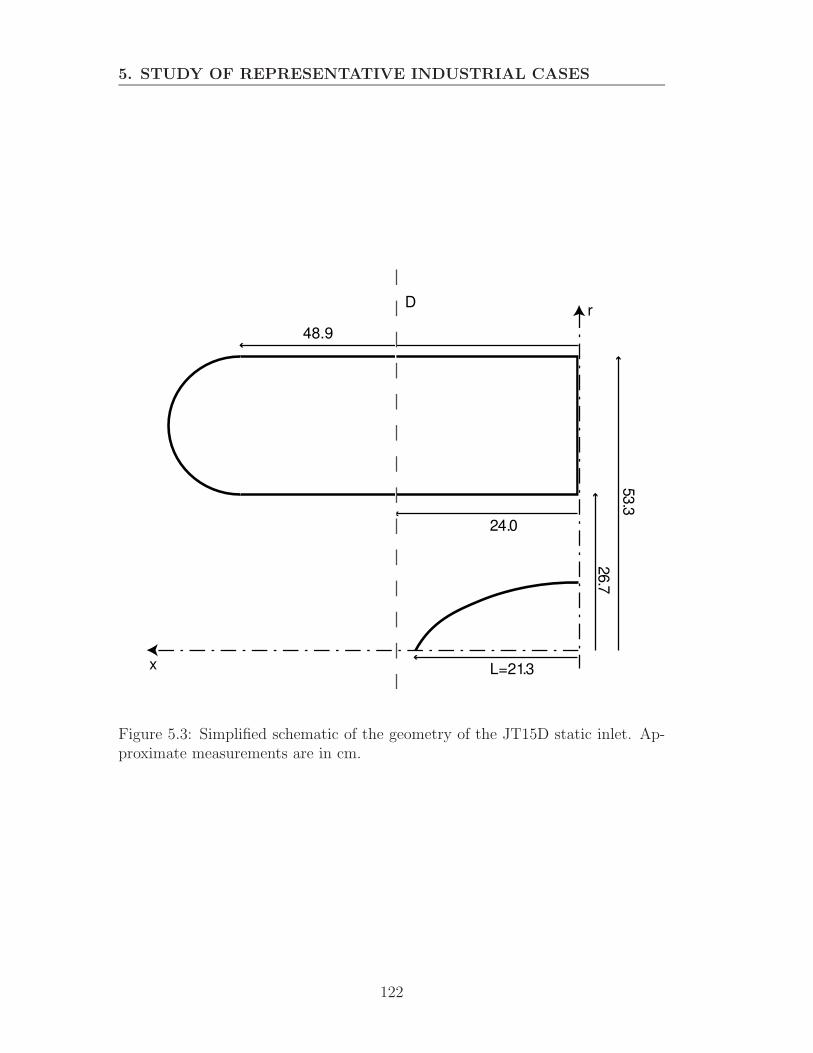
5. STUDY OF REPRESENTATIVE INDUSTRIAL CASES
48.9
L=21.3
24.0
26.7
53.3
x
rD
Figure 5.3: Simplified schematic of the geometry of the JT15D static inlet. Ap-proximate measurements are in cm.
122
5.2 First case study: JT15D inlet
discretised with HOP using a uniform, regular Cartesian grid with ∆x = ∆y =
∆z = 0.012m. It contains 111×111×116 points, including 15940 ghost points, 24
of which need to be evaluated with the 4-point normal extrapolation described
in Section 3.3: this is 0.15% of all points, so it should not noticeably affect the
accuracy. The incoming waves are imposed with an absorbing boundary condition
because, as in Section 5.1.1, using the condition of Eq. (2.17) led to the generation
of spurious waves. For similar reasons, and in all the following cases, the initial
wave amplitude is smoothly increased from zero to its final value over t = 25.
5.2.2 Azimuthal modes
The propagation out of the inlet of several azimuthal, or “spinning”, acoustic
modes, as described by Eq. (5.2), is first computed, to study a type of 3D propaga-
tion found in typical fan noise problems (see Chapter 1). The nomenclature of
Section 5.1.2 will be used throughout. The computation was made until a peri-
odic regime is obtained, as is shown in Fig. 5.4. Several modes are studied, with
different azimuthal orders, wavelengths and increasing cut-off ratios: Table 5.2.
A frequency of 3150Hz (λ = 10.6 cm) is typical of the sound produced at normal
engine operating conditions [41, 72], and the associated large Helmholtz number
(α = αa = 2πa/λ ≃ 16) would represents a challenging computational problem
for a low-order method. For atmospheric ambient conditions, it is represented by
8.84 points-per-wavelength with the HOP model.
Strongly cut-on modes
The main features of the radiation pattern can first be theoretically estimated.
Lordi and Homicz [129] obtained an approximate analytical solution for the ra-
diation to the far-field of acoustic modes from an infinitely thin cylinder of finite
length. The full result is complex, but the authors show that, for well cut-on
modes, most of the radiation is centered on a “principal lobe”, whose direction
is the same as the polar mode angle inside the duct1. If θ is the angle measured
1Non-planar modes are equivalent to a sum of several plane waves propagating at a certainangle, which depends on the wavenumber and the modal order [22, 48].
123
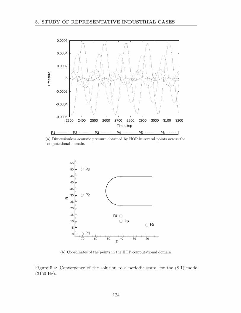
5. STUDY OF REPRESENTATIVE INDUSTRIAL CASES
-0.0006
-0.0004
-0.0002
0
0.0002
0.0004
0.0006
2300 2400 2500 2600 2700 2800 2900 3000 3100 3200
Pre
ssur
e
Time step
P1 P2 P3 P4 P5 P6
(a) Dimensionless acoustic pressure obtained by HOP in several points across thecomputational domain.
Z
R
-70 -60 -50 -40 -30 -20
0
5
10
15
20
25
30
35
40
45
50
55
P1
P2
P3
P4
P6P5
(b) Coordinates of the points in the HOP computational domain.
Figure 5.4: Convergence of the solution to a periodic state, for the (8,1) mode(3150 Hz).
124
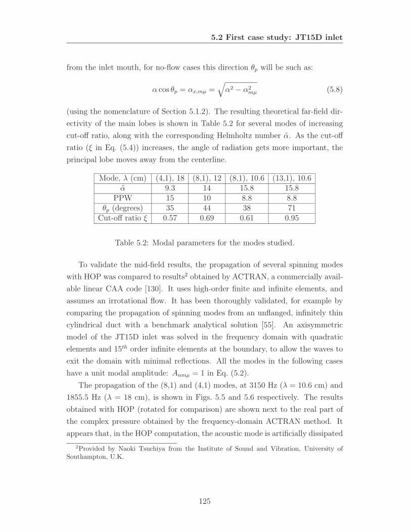
5.2 First case study: JT15D inlet
from the inlet mouth, for no-flow cases this direction θp will be such as:
α cos θp = αx,mµ =√
α2 − α2mµ (5.8)
(using the nomenclature of Section 5.1.2). The resulting theoretical far-field dir-
ectivity of the main lobes is shown in Table 5.2 for several modes of increasing
cut-off ratio, along with the corresponding Helmholtz number α. As the cut-off
ratio (ξ in Eq. (5.4)) increases, the angle of radiation gets more important, the
principal lobe moves away from the centerline.
Mode, λ (cm) (4,1), 18 (8,1), 12 (8,1), 10.6 (13,1), 10.6α 9.3 14 15.8 15.8
PPW 15 10 8.8 8.8θp (degrees) 35 44 38 71
Cut-off ratio ξ 0.57 0.69 0.61 0.95
Table 5.2: Modal parameters for the modes studied.
To validate the mid-field results, the propagation of several spinning modes
with HOP was compared to results2 obtained by ACTRAN, a commercially avail-
able linear CAA code [130]. It uses high-order finite and infinite elements, and
assumes an irrotational flow. It has been thoroughly validated, for example by
comparing the propagation of spinning modes from an unflanged, infinitely thin
cylindrical duct with a benchmark analytical solution [55]. An axisymmetric
model of the JT15D inlet was solved in the frequency domain with quadratic
elements and 15th order infinite elements at the boundary, to allow the waves to
exit the domain with minimal reflections. All the modes in the following cases
have a unit modal amplitude: Anmµ = 1 in Eq. (5.2).
The propagation of the (8,1) and (4,1) modes, at 3150 Hz (λ = 10.6 cm) and
1855.5 Hz (λ = 18 cm), is shown in Figs. 5.5 and 5.6 respectively. The results
obtained with HOP (rotated for comparison) are shown next to the real part of
the complex pressure obtained by the frequency-domain ACTRAN method. It
appears that, in the HOP computation, the acoustic mode is artificially dissipated
2Provided by Naoki Tsuchiya from the Institute of Sound and Vibration, University ofSouthampton, U.K.
125
5. STUDY OF REPRESENTATIVE INDUSTRIAL CASES
as it propagates along the wall. However, apart from the presence of a low level
of pressure along the centerline in both HOP results, in both cases the solution
behaves similarly after it is diffracted by the inlet mouth, with good agreement
in the directivity pattern.
These observations are now confirmed by examining the radiation patterns
for both methods in more detail, for the first three modes of Table 5.2. A good
measure of the directivity of the modal radiation is given by the amplitude of
the complex pressure obtained by ACTRAN, which can be compared to the
root-mean-square (RMS) of the pressure signal in HOP, computed in the last
period of oscillation (see Fig. 5.4(a)). These quantities, taken along an arc of
radius 60 cm centered on the inlet mouth at z=48.9 cm, are plotted in Fig. 5.7.
The RMS values from the HOP computation were scaled by√
2 to match the
pressure amplitudes given by ACTRAN. The modes appear highly dissipated
after propagation. This dissipation is more important as the cut-off ratio and
the modal angle increase. There is also a spurious amount of radiation along the
centerline (θ < 15 degrees), representing an artificial scattering into other radial
modes. The match in directivity, however, is very good for the main lobe, where
most of the acoustic energy is present. These results are also consistent with the
theoretical directivity trend of Table 5.2.
126
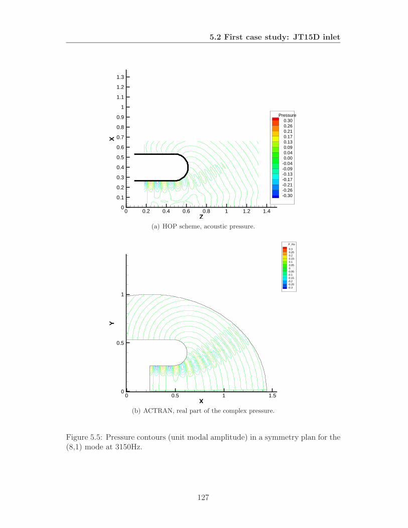
5.2 First case study: JT15D inlet
Z
X
0 0.2 0.4 0.6 0.8 1 1.2 1.40
0.1
0.2
0.3
0.4
0.5
0.6
0.7
0.8
0.9
1
1.1
1.2
1.3
Pressure0.300.260.210.170.130.090.040.00
-0.04-0.09-0.13-0.17-0.21-0.26-0.30
(a) HOP scheme, acoustic pressure.
X
Y
0 0.5 1 1.50
0.5
1
P_Re
0.30.250.20.150.10.050
-0.05-0.1-0.15-0.2-0.25-0.3
(b) ACTRAN, real part of the complex pressure.
Figure 5.5: Pressure contours (unit modal amplitude) in a symmetry plan for the(8,1) mode at 3150Hz.
127
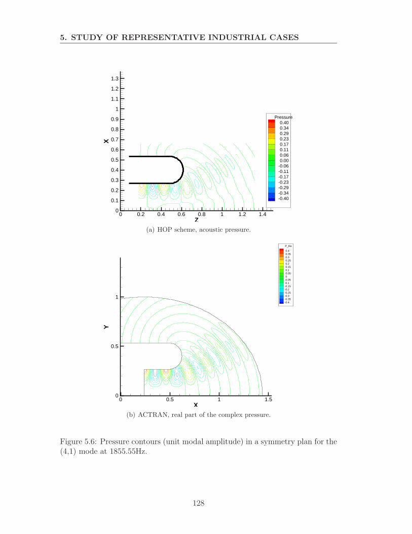
5. STUDY OF REPRESENTATIVE INDUSTRIAL CASES
Z
X
0 0.2 0.4 0.6 0.8 1 1.2 1.40
0.1
0.2
0.3
0.4
0.5
0.6
0.7
0.8
0.9
1
1.1
1.2
1.3
Pressure0.400.340.290.230.170.110.060.00
-0.06-0.11-0.17-0.23-0.29-0.34-0.40
(a) HOP scheme, acoustic pressure.
X
Y
0 0.5 1 1.50
0.5
1
P_Re
0.40.350.30.250.20.150.10.050
-0.05-0.1-0.15-0.2-0.25-0.3-0.35-0.4
(b) ACTRAN, real part of the complex pressure.
Figure 5.6: Pressure contours (unit modal amplitude) in a symmetry plan for the(4,1) mode at 1855.55Hz.
128
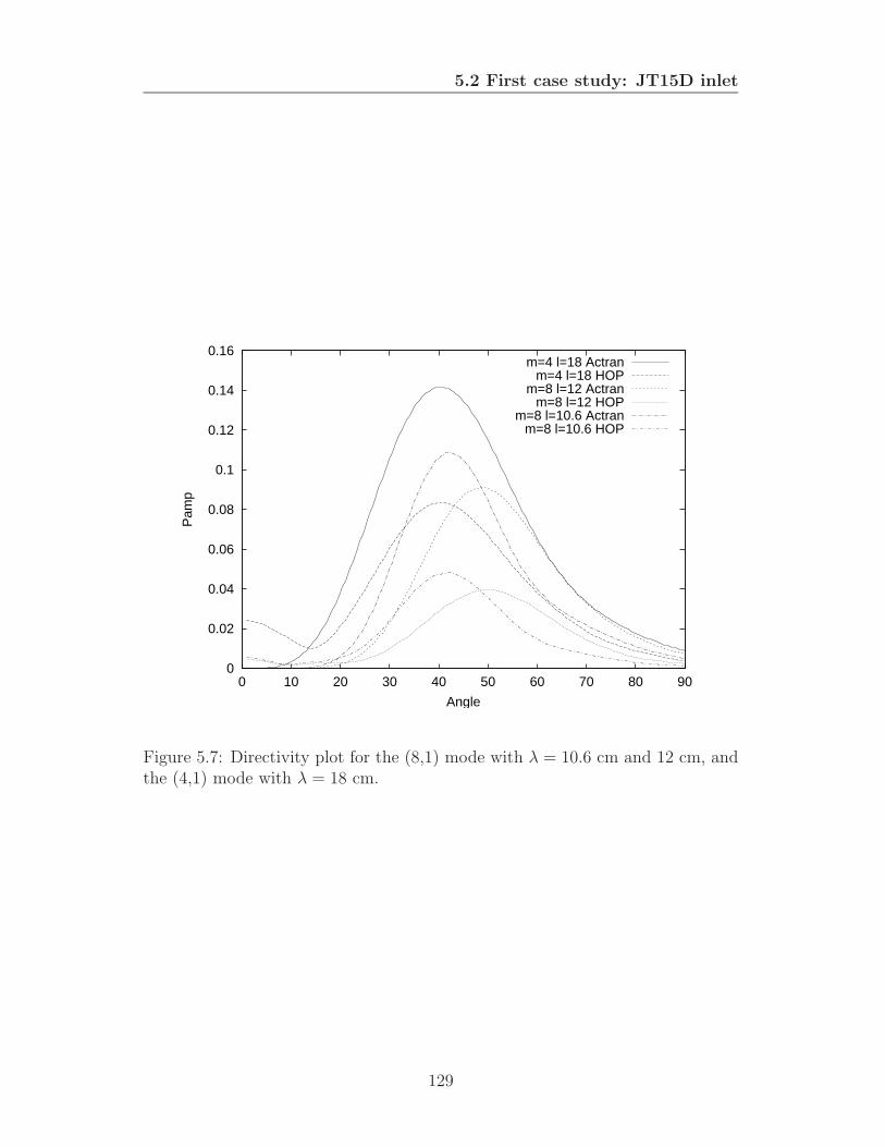
5.2 First case study: JT15D inlet
0
0.02
0.04
0.06
0.08
0.1
0.12
0.14
0.16
0 10 20 30 40 50 60 70 80 90
Pam
p
Angle
m=4 l=18 Actranm=4 l=18 HOP
m=8 l=12 Actranm=8 l=12 HOP
m=8 l=10.6 Actranm=8 l=10.6 HOP
Figure 5.7: Directivity plot for the (8,1) mode with λ = 10.6 cm and 12 cm, andthe (4,1) mode with λ = 18 cm.
129
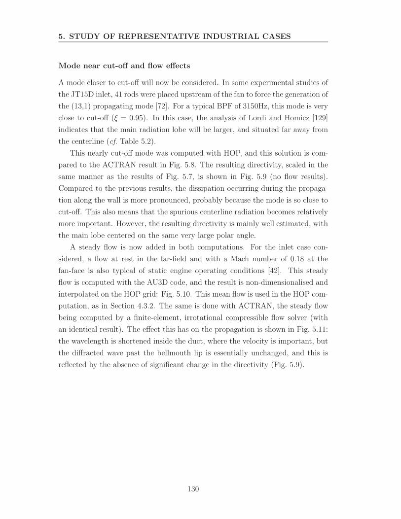
5. STUDY OF REPRESENTATIVE INDUSTRIAL CASES
Mode near cut-off and flow effects
A mode closer to cut-off will now be considered. In some experimental studies of
the JT15D inlet, 41 rods were placed upstream of the fan to force the generation of
the (13,1) propagating mode [72]. For a typical BPF of 3150Hz, this mode is very
close to cut-off (ξ = 0.95). In this case, the analysis of Lordi and Homicz [129]
indicates that the main radiation lobe will be larger, and situated far away from
the centerline (cf. Table 5.2).
This nearly cut-off mode was computed with HOP, and this solution is com-
pared to the ACTRAN result in Fig. 5.8. The resulting directivity, scaled in the
same manner as the results of Fig. 5.7, is shown in Fig. 5.9 (no flow results).
Compared to the previous results, the dissipation occurring during the propaga-
tion along the wall is more pronounced, probably because the mode is so close to
cut-off. This also means that the spurious centerline radiation becomes relatively
more important. However, the resulting directivity is mainly well estimated, with
the main lobe centered on the same very large polar angle.
A steady flow is now added in both computations. For the inlet case con-
sidered, a flow at rest in the far-field and with a Mach number of 0.18 at the
fan-face is also typical of static engine operating conditions [42]. This steady
flow is computed with the AU3D code, and the result is non-dimensionalised and
interpolated on the HOP grid: Fig. 5.10. This mean flow is used in the HOP com-
putation, as in Section 4.3.2. The same is done with ACTRAN, the steady flow
being computed by a finite-element, irrotational compressible flow solver (with
an identical result). The effect this has on the propagation is shown in Fig. 5.11:
the wavelength is shortened inside the duct, where the velocity is important, but
the diffracted wave past the bellmouth lip is essentially unchanged, and this is
reflected by the absence of significant change in the directivity (Fig. 5.9).
130
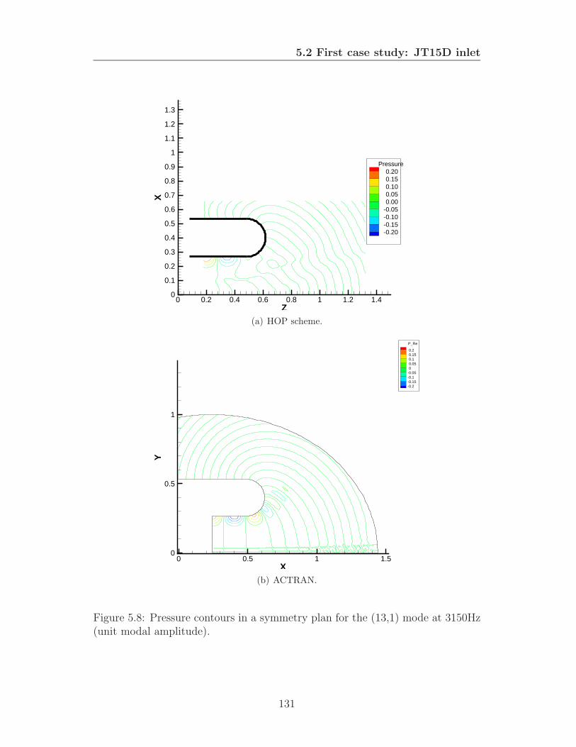
5.2 First case study: JT15D inlet
Z
X
0 0.2 0.4 0.6 0.8 1 1.2 1.40
0.1
0.2
0.3
0.4
0.5
0.6
0.7
0.8
0.9
1
1.1
1.2
1.3
Pressure0.200.150.100.050.00
-0.05-0.10-0.15-0.20
(a) HOP scheme.
X
Y
0 0.5 1 1.50
0.5
1
P_Re
0.20.150.10.050
-0.05-0.1-0.15-0.2
(b) ACTRAN.
Figure 5.8: Pressure contours in a symmetry plan for the (13,1) mode at 3150Hz(unit modal amplitude).
131
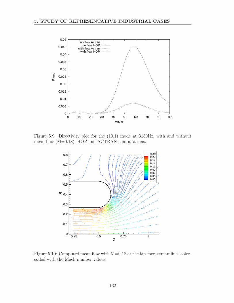
5. STUDY OF REPRESENTATIVE INDUSTRIAL CASES
0
0.005
0.01
0.015
0.02
0.025
0.03
0.035
0.04
0.045
0.05
0 10 20 30 40 50 60 70 80 90
Pam
p
Angle
no flow Actranno flow HOP
with flow Actranwith flow HOP
Figure 5.9: Directivity plot for the (13,1) mode at 3150Hz, with and withoutmean flow (M=0.18), HOP and ACTRAN computations.
Z
R
0.25 0.5 0.75 10
0.1
0.2
0.3
0.4
0.5
0.6
0.7
0.8 mach0.200.170.140.110.090.060.030.00
Figure 5.10: Computed mean flow with M=0.18 at the fan-face, streamlines color-coded with the Mach number values.
132
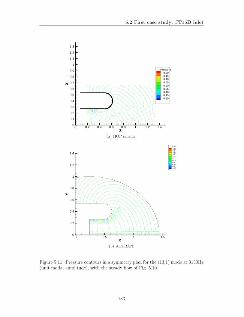
5.2 First case study: JT15D inlet
Z
X
0 0.2 0.4 0.6 0.8 1 1.2 1.40
0.1
0.2
0.3
0.4
0.5
0.6
0.7
0.8
0.9
1
1.1
1.2
1.3
Pressure0.200.150.100.050.00
-0.05-0.10-0.15-0.20
(a) HOP scheme.
X
Y
0 0.5 1 1.50
0.2
0.4
0.6
0.8
1
1.2
1.4
P_Re
0.250.20.150.10.050
-0.05-0.1-0.15-0.2-0.25
(b) ACTRAN.
Figure 5.11: Pressure contours in a symmetry plan for the (13,1) mode at 3150Hz(unit modal amplitude), with the steady flow of Fig. 5.10.
133
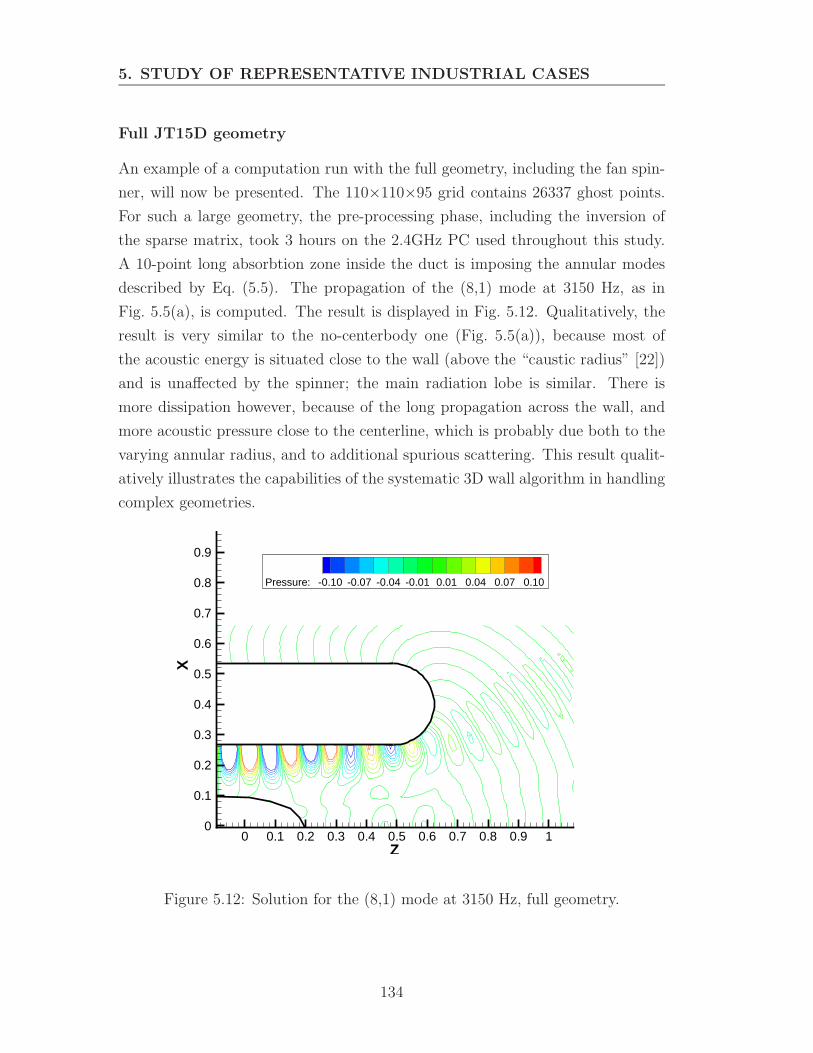
5. STUDY OF REPRESENTATIVE INDUSTRIAL CASES
Full JT15D geometry
An example of a computation run with the full geometry, including the fan spin-
ner, will now be presented. The 110×110×95 grid contains 26337 ghost points.
For such a large geometry, the pre-processing phase, including the inversion of
the sparse matrix, took 3 hours on the 2.4GHz PC used throughout this study.
A 10-point long absorbtion zone inside the duct is imposing the annular modes
described by Eq. (5.5). The propagation of the (8,1) mode at 3150 Hz, as in
Fig. 5.5(a), is computed. The result is displayed in Fig. 5.12. Qualitatively, the
result is very similar to the no-centerbody one (Fig. 5.5(a)), because most of
the acoustic energy is situated close to the wall (above the “caustic radius” [22])
and is unaffected by the spinner; the main radiation lobe is similar. There is
more dissipation however, because of the long propagation across the wall, and
more acoustic pressure close to the centerline, which is probably due both to the
varying annular radius, and to additional spurious scattering. This result qualit-
atively illustrates the capabilities of the systematic 3D wall algorithm in handling
complex geometries.
Z
X
0 0.1 0.2 0.3 0.4 0.5 0.6 0.7 0.8 0.9 10
0.1
0.2
0.3
0.4
0.5
0.6
0.7
0.8
0.9
Pressure: -0.10 -0.07 -0.04 -0.01 0.01 0.04 0.07 0.10
Figure 5.12: Solution for the (8,1) mode at 3150 Hz, full geometry.
134
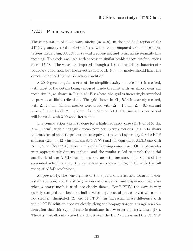
5.2 First case study: JT15D inlet
5.2.3 Plane wave cases
The computation of plane wave modes (m = 0), in the mid-field region of the
JT15D geometry used in Section 5.2.2, will now be compared to similar compu-
tations made using AU3D, for several frequencies, and using an increasingly fine
meshing. This code was used with success in similar problems for low-frequencies
cases [17, 18]. The waves are imposed through a 1D non-reflecting characteristic
boundary condition, but the investigation of 1D (m = 0) modes should limit the
errors introduced by the boundary condition.
A 30 degrees angular sector of the simplified axisymmetric inlet is meshed,
with most of the details being captured inside the inlet with an almost constant
mesh size ∆, as shown in Fig. 5.13. Elsewhere, the grid is increasingly stretched
to prevent artificial reflections. The grid shown in Fig. 5.13 is coarsely meshed,
with ∆=1.0 cm. Similar meshes were made with: ∆ = 1.5 cm, ∆ = 0.5 cm and
a very fine grid with ∆ = 0.2 cm. As in Section 5.1.1, 150 time steps per period
will be used, with 3 Newton iterations.
The computation was first done for a high-frequency case (BPF of 3150 Hz,
λ = 10.6cm), with a negligible mean flow, for 16 wave periods. Fig. 5.14 shows
the contours of acoustic pressure in an equivalent plane of symmetry for the HOP
solution (∆x=0.012 which means 8.84 PPW) and the equivalent AU3D one with
∆ = 0.2 cm (53 PPW). Here, and in the following cases, the HOP length-scales
were appropriately dimensionalised, and the results scaled to match the initial
amplitude of the AU3D non-dimensional acoustic pressure. The values of the
computed solutions along the centerline are shown in Fig. 5.15, with the full
range of AU3D resolutions.
As previously, the convergence of the spatial discretisation towards a con-
sistent solution, and the strong numerical dissipation and dispersion that arise
when a coarse mesh is used, are clearly shown. For 7 PPW, the wave is very
quickly damped and becomes half a wavelength out of phase. Even when it is
not strongly dissipated (21 and 11 PPW), an increasing phase difference with
the 53 PPW solution appears clearly along the propagation; this is again a con-
firmation that this type of error is dominant in low-order codes (Lockard [63]).
There is, overall, only a good match between the HOP solution and the 53 PPW
135
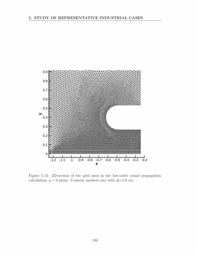
5. STUDY OF REPRESENTATIVE INDUSTRIAL CASES
x
y
-1.2 -1.1 -1 -0.9 -0.8 -0.7 -0.6 -0.5 -0.4 -0.3 -0.2
0
0.1
0.2
0.3
0.4
0.5
0.6
0.7
0.8
0.9
Figure 5.13: 2D-section of the grid used in the low-order sound propagationcalculation, y = 0 plane. Coarsely meshed case with ∆=1.0 cm.
136
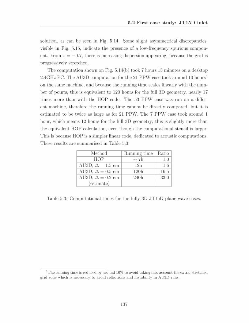
5.2 First case study: JT15D inlet
solution, as can be seen in Fig. 5.14. Some slight asymmetrical discrepancies,
visible in Fig. 5.15, indicate the presence of a low-frequency spurious compon-
ent. From x = −0.7, there is increasing dispersion appearing, because the grid is
progressively stretched.
The computation shown on Fig. 5.14(b) took 7 hours 15 minutes on a desktop
2.4GHz PC. The AU3D computation for the 21 PPW case took around 10 hours3
on the same machine, and because the running time scales linearly with the num-
ber of points, this is equivalent to 120 hours for the full 3D geometry, nearly 17
times more than with the HOP code. The 53 PPW case was run on a differ-
ent machine, therefore the running time cannot be directly compared, but it is
estimated to be twice as large as for 21 PPW. The 7 PPW case took around 1
hour, which means 12 hours for the full 3D geometry; this is slightly more than
the equivalent HOP calculation, even though the computational stencil is larger.
This is because HOP is a simpler linear code, dedicated to acoustic computations.
These results are summarised in Table 5.3.
Method Running time RatioHOP ∼ 7h 1.0
AU3D, ∆ = 1.5 cm 12h 1.6AU3D, ∆ = 0.5 cm 120h 16.5AU3D, ∆ = 0.2 cm 240h 33.0
(estimate)
Table 5.3: Computational times for the fully 3D JT15D plane wave cases.
3The running time is reduced by around 10% to avoid taking into account the extra, stretchedgrid zone which is necessary to avoid reflections and instability in AU3D runs.
137

5. STUDY OF REPRESENTATIVE INDUSTRIAL CASES
x
y
-1.2 -1.1 -1 -0.9 -0.8 -0.7 -0.6 -0.5 -0.4 -0.3 -0.20
0.1
0.2
0.3
0.4
0.5
0.6
0.7
0.8
0.9
p5.0E-023.9E-022.8E-021.7E-025.6E-03
-5.6E-03-1.7E-02-2.8E-02-3.9E-02-5.0E-02
(a) AU3D result with ∆ = 0.2cm, 53 PPW.
Z
X
-1.2 -1.1 -1 -0.9 -0.8 -0.7 -0.6 -0.5 -0.4 -0.3 -0.20
0.1
0.2
0.3
0.4
0.5
0.6
0.7
0.8
0.9 Pressure5.0E-023.9E-022.8E-021.7E-025.6E-03
-5.6E-03-1.7E-02-2.8E-02-3.9E-02-5.0E-02
(b) HOP result (scaled) with ∆x = 1.2 cm, 8.84 PPW.
Figure 5.14: Propagation of the (0,0) mode with λ = 10.6 cm. Contours ofnon-dimensional acoustic pressure in a symmetry plane.
138
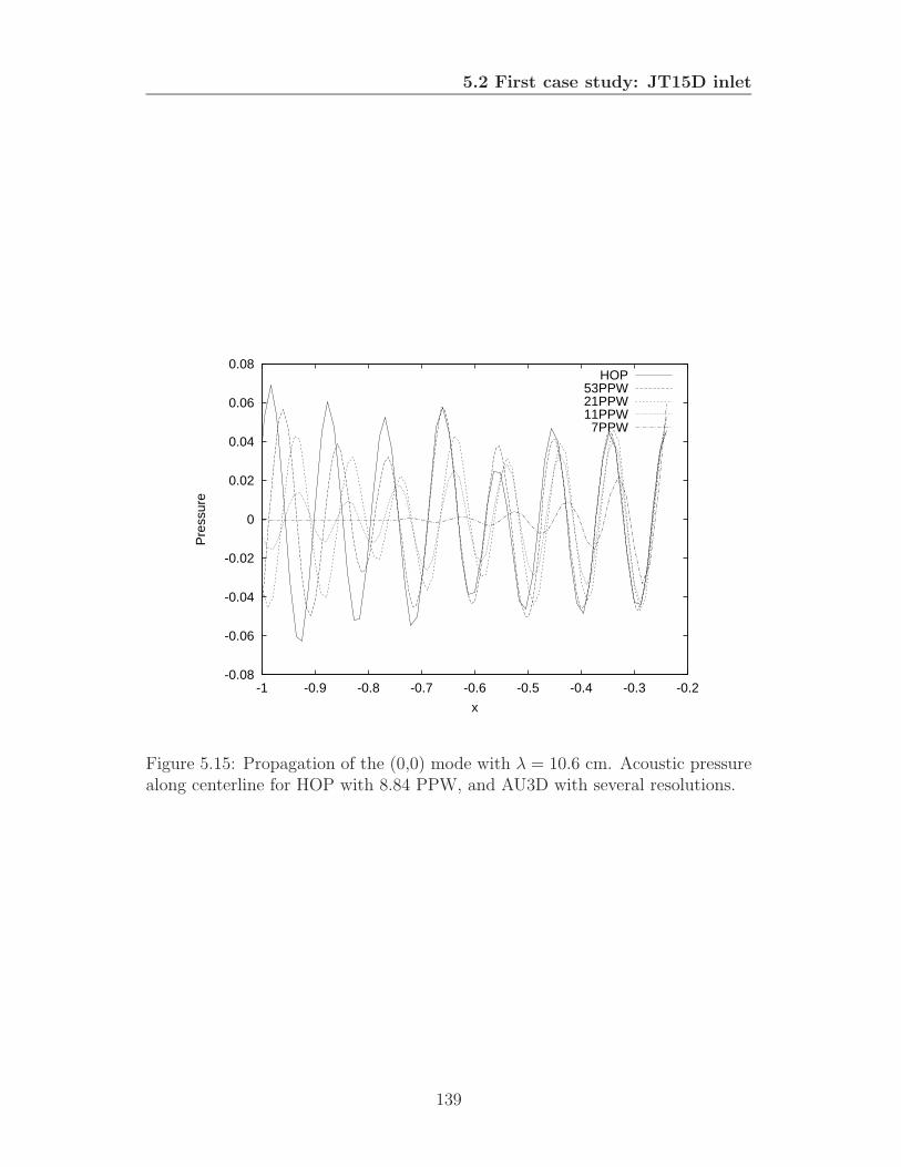
5.2 First case study: JT15D inlet
-0.08
-0.06
-0.04
-0.02
0
0.02
0.04
0.06
0.08
-1 -0.9 -0.8 -0.7 -0.6 -0.5 -0.4 -0.3 -0.2
Pre
ssur
e
x
HOP53PPW21PPW11PPW
7PPW
Figure 5.15: Propagation of the (0,0) mode with λ = 10.6 cm. Acoustic pressurealong centerline for HOP with 8.84 PPW, and AU3D with several resolutions.
139
5. STUDY OF REPRESENTATIVE INDUSTRIAL CASES
The same computations are also made for λ = 13.2cm, which represents a
frequency of approximately 2532Hz, to study the evolution of the convergence
of both solutions (now α ≃ 13). Results are displayed in Fig. 5.16: the AU3D
solution with a 66 PPW resolution, and 11 PPW for HOP. The pressure along
the centerline is shown in Fig. 5.18. Similar observations as for the λ = 10.6 cm
case can be made.
The computation was finally done for a low-frequency case, λ = 30 cm or
ν ≃ 1113.3 Hz (now α ≃ 5.6), for 8 wave periods. Fig. 5.17 shows the pressure
contours in the symmetry plane. The match between the HOP computation with
25 PPW and the first three AU3D cases, as shown in Fig. 5.19, is not as good
as above, although the low-order solution seems to converge as the resolution is
increased from 20 and 30 PPW to 60.
The ratios of the running times for the last two cases are similar to those
presented in Table 5.3. Taking all these results together, it is clear that, as the
PPW resolution of the AU3D computations is increased, there is convergence
towards a single solution, with the dissipation and the dispersion errors being
reduced, in that order. As in the previous HOP computations, some dissipation
appears close to the wall, but there is an overall good match of both solutions,
and the diffraction seems to be correctly represented. Examining the solution
along the centerline, this match seems to degrade as the wavelength is increased,
with a slowly varying amplitude discrepancy appearing. Overall, this is not a
very serious problem, as the high-order HOP method is not as advantageous for
low-frequency problems. But it was not the case in Section 5.1.1, when no wall
was present, and the validation results of Section 4.3.1 showed that the errors of
the new wall boundary condition tended to disappear as α decreased. It could
come from the AU3D boundary conditions, which are not designed for acoustic
computations, or from the limited size of the HOP domain which leads to artificial
reflections, particularly since the radiation depicted in Fig. 5.17 is very different
from a monopole source. The absorbing condition used to impose the incoming
acoustic solution could also be a source of low-wavelength error.
140
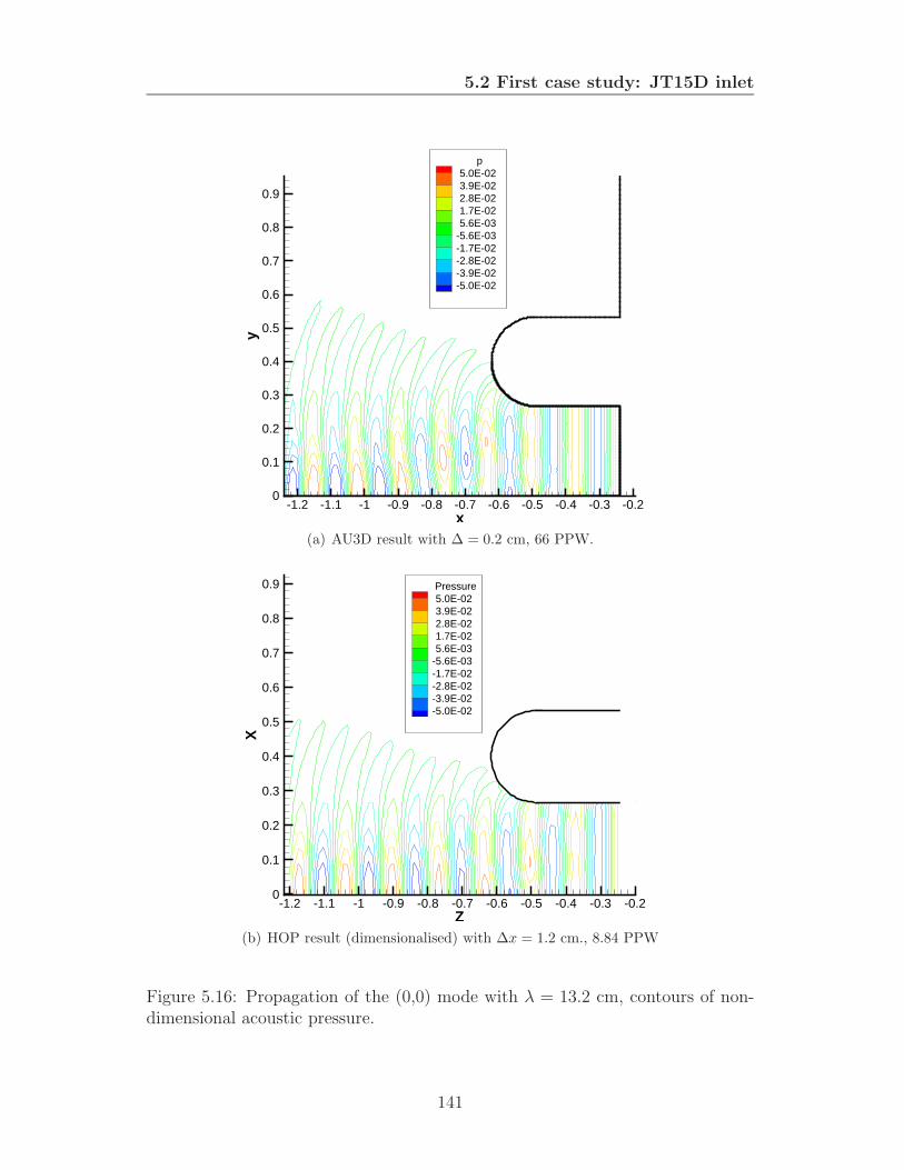
5.2 First case study: JT15D inlet
x
y
-1.2 -1.1 -1 -0.9 -0.8 -0.7 -0.6 -0.5 -0.4 -0.3 -0.20
0.1
0.2
0.3
0.4
0.5
0.6
0.7
0.8
0.9
p5.0E-023.9E-022.8E-021.7E-025.6E-03
-5.6E-03-1.7E-02-2.8E-02-3.9E-02-5.0E-02
(a) AU3D result with ∆ = 0.2 cm, 66 PPW.
Z
X
-1.2 -1.1 -1 -0.9 -0.8 -0.7 -0.6 -0.5 -0.4 -0.3 -0.20
0.1
0.2
0.3
0.4
0.5
0.6
0.7
0.8
0.9 Pressure5.0E-023.9E-022.8E-021.7E-025.6E-03
-5.6E-03-1.7E-02-2.8E-02-3.9E-02-5.0E-02
(b) HOP result (dimensionalised) with ∆x = 1.2 cm., 8.84 PPW
Figure 5.16: Propagation of the (0,0) mode with λ = 13.2 cm, contours of non-dimensional acoustic pressure.
141
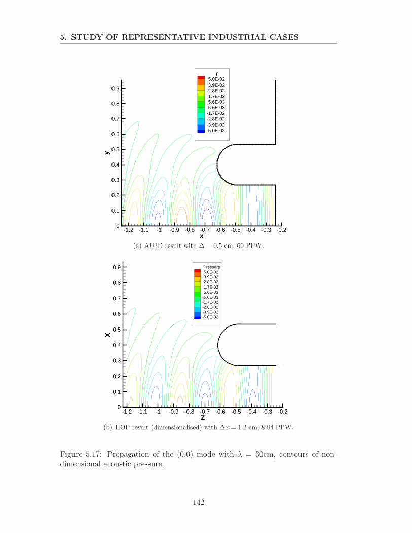
5. STUDY OF REPRESENTATIVE INDUSTRIAL CASES
x
y
-1.2 -1.1 -1 -0.9 -0.8 -0.7 -0.6 -0.5 -0.4 -0.3 -0.20
0.1
0.2
0.3
0.4
0.5
0.6
0.7
0.8
0.9
p5.0E-023.9E-022.8E-021.7E-025.6E-03
-5.6E-03-1.7E-02-2.8E-02-3.9E-02-5.0E-02
(a) AU3D result with ∆ = 0.5 cm, 60 PPW.
Z
X
-1.2 -1.1 -1 -0.9 -0.8 -0.7 -0.6 -0.5 -0.4 -0.3 -0.20
0.1
0.2
0.3
0.4
0.5
0.6
0.7
0.8
0.9 Pressure5.0E-023.9E-022.8E-021.7E-025.6E-03
-5.6E-03-1.7E-02-2.8E-02-3.9E-02-5.0E-02
(b) HOP result (dimensionalised) with ∆x = 1.2 cm, 8.84 PPW.
Figure 5.17: Propagation of the (0,0) mode with λ = 30cm, contours of non-dimensional acoustic pressure.
142
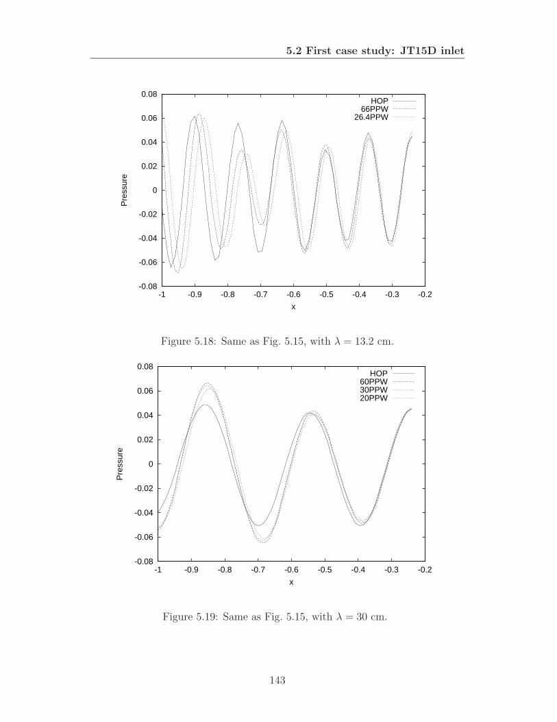
5.2 First case study: JT15D inlet
-0.08
-0.06
-0.04
-0.02
0
0.02
0.04
0.06
0.08
-1 -0.9 -0.8 -0.7 -0.6 -0.5 -0.4 -0.3 -0.2
Pre
ssur
e
x
HOP66PPW
26.4PPW
Figure 5.18: Same as Fig. 5.15, with λ = 13.2 cm.
-0.08
-0.06
-0.04
-0.02
0
0.02
0.04
0.06
0.08
-1 -0.9 -0.8 -0.7 -0.6 -0.5 -0.4 -0.3 -0.2
Pre
ssur
e
x
HOP60PPW30PPW20PPW
Figure 5.19: Same as Fig. 5.15, with λ = 30 cm.
143
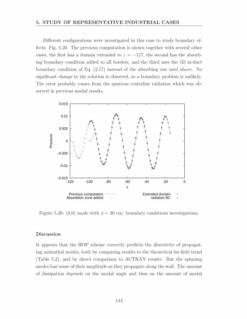
5. STUDY OF REPRESENTATIVE INDUSTRIAL CASES
Different configurations were investigated in this case to study boundary ef-
fects: Fig. 5.20. The previous computation is shown together with several other
cases, the first has a domain extended to z = −117, the second has the absorb-
ing boundary condition added to all borders, and the third uses the 1D in-duct
boundary condition of Eq. (2.17) instead of the absorbing one used above. No
significant change to the solution is observed, so a boundary problem is unlikely.
The error probably comes from the spurious centerline radiation which was ob-
served in previous modal results.
-0.015
-0.01
-0.005
0
0.005
0.01
0.015
-120 -100 -80 -60 -40 -20 0
Pre
ssur
e
z
Previous computationAbsorbtion zone added
Extended domainradiation BC
Figure 5.20: (0,0) mode with λ = 30 cm: boundary conditions investigations.
Discussion
It appears that the HOP scheme correctly predicts the directivity of propagat-
ing azimuthal modes, both by comparing results to the theoretical far-field trend
(Table 5.2), and by direct comparison to ACTRAN results. But the spinning
modes lose some of their amplitude as they propagate along the wall. The amount
of dissipation depends on the modal angle and thus on the amount of modal
144
5.2 First case study: JT15D inlet
reflections on the wall. This defect is related to the validation results of Sec-
tion 4.3.1: for important Helmholtz numbers, the wave is dissipated as it travels
along the wall boundary, more than it is dispersed (its phase is more accurate):
see Fig. 4.21(b) for example.
This probably comes from the extrapolation inaccuracies, exacerbated by the
fact that three are performed in 3D. The selective artificial dissipation, necessary
to maintain stability, could possibly also be a factor, but it is little different
to the 2D case. However, together with Section 5.1.1, these results effectively
show that, if a low-order discretisation is employed, it is necessary to use at
least 30 PPW to propagate an acoustic wave over 10 wavelengths, even for a low
target accuracy. Using such resolutions with acoustic problems of large Helmholtz
numbers (more than 10) leads to impractical situations in the mid-field region,
with large computational and memory costs. With the HOP code, gains of one
order of magnitude in the computational time are obtained (see Table 5.3), for
equivalent solutions. This ratio of around 20 to 30 times is also slightly under-
estimated because of the grid-stretching employed from x = −0.7, and could
become even larger if higher accuracy or a larger propagation distance are needed.
One of the defects appearing in the HOP solutions is the excessive radiation
appearing along the centerline, between 0 and 20 degrees, after the mode is
diffracted by the inlet mouth. It does not disappear as the wavelength is increased,
and represents, in a sense, a scattering of the incoming mode into higher radial
orders, probably caused by the dissipation occurring along the wall. The low-
order normal extrapolation, used on a few points which are situated around the
bellmouth inlet lip, could also be at the origin of this defect, but it is only used
for a limited amount of ghost points.
145
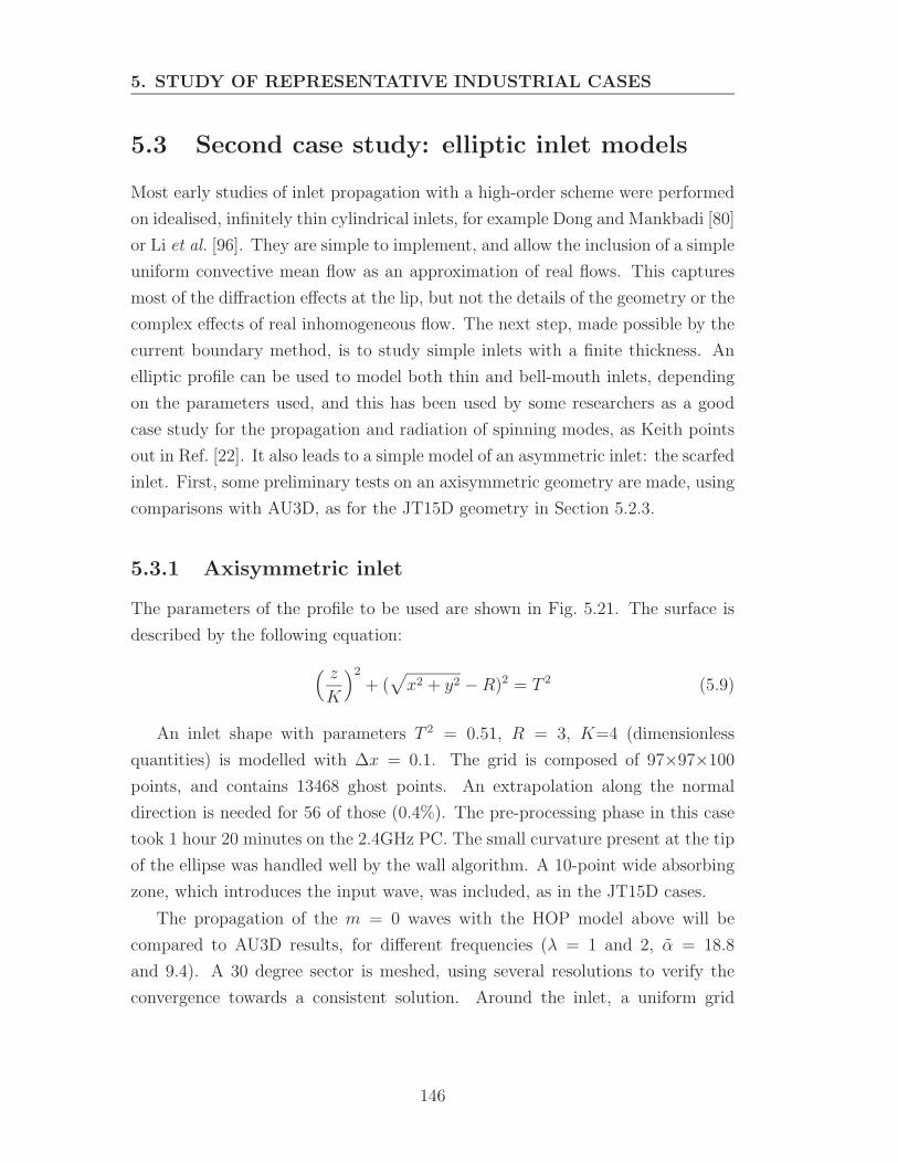
5. STUDY OF REPRESENTATIVE INDUSTRIAL CASES
5.3 Second case study: elliptic inlet models
Most early studies of inlet propagation with a high-order scheme were performed
on idealised, infinitely thin cylindrical inlets, for example Dong and Mankbadi [80]
or Li et al. [96]. They are simple to implement, and allow the inclusion of a simple
uniform convective mean flow as an approximation of real flows. This captures
most of the diffraction effects at the lip, but not the details of the geometry or the
complex effects of real inhomogeneous flow. The next step, made possible by the
current boundary method, is to study simple inlets with a finite thickness. An
elliptic profile can be used to model both thin and bell-mouth inlets, depending
on the parameters used, and this has been used by some researchers as a good
case study for the propagation and radiation of spinning modes, as Keith points
out in Ref. [22]. It also leads to a simple model of an asymmetric inlet: the scarfed
inlet. First, some preliminary tests on an axisymmetric geometry are made, using
comparisons with AU3D, as for the JT15D geometry in Section 5.2.3.
5.3.1 Axisymmetric inlet
The parameters of the profile to be used are shown in Fig. 5.21. The surface is
described by the following equation:
( z
K
)2
+ (√
x2 + y2 − R)2 = T 2 (5.9)
An inlet shape with parameters T 2 = 0.51, R = 3, K=4 (dimensionless
quantities) is modelled with ∆x = 0.1. The grid is composed of 97×97×100
points, and contains 13468 ghost points. An extrapolation along the normal
direction is needed for 56 of those (0.4%). The pre-processing phase in this case
took 1 hour 20 minutes on the 2.4GHz PC. The small curvature present at the tip
of the ellipse was handled well by the wall algorithm. A 10-point wide absorbing
zone, which introduces the input wave, was included, as in the JT15D cases.
The propagation of the m = 0 waves with the HOP model above will be
compared to AU3D results, for different frequencies (λ = 1 and 2, α = 18.8
and 9.4). A 30 degree sector is meshed, using several resolutions to verify the
convergence towards a consistent solution. Around the inlet, a uniform grid
146
5.3 Second case study: elliptic inlet models
z
y
0
K.T
T
x
R
Figure 5.21: Description of the elliptic inlet geometry.
resolution of ∆ is used, and the grid is stretched elsewhere. ∆ = 0.1, ∆ = 0.05
and ∆ = 0.033 will be used, to obtain respectively 10, 20 and 30 PPW for the first
case and 20, 40, 60 in the second. The low resolution grid is shown in Fig. 5.22.
λ = 1
The λ = 1 case is first computed, using the same time step parameters as in
Section 5.2.3, and running the computation for 16 wave periods. The results for
the HOP and the high-resolution AU3D computations are shown in Fig. 5.23,
and the pressure was scaled in the same way as for Section 5.2.3. Some amount
of artificial distortion appears in the HOP result because of aliasing from the low
resolution and contour plot artifacts near the elliptic boundary.
The match in most of the domain is good, even if an increasing phase difference
appears as the wave propagates. Examining the results along the centerline,
in Fig. 5.24, confirms this. It appears that the 10 PPW solution is strongly
numerically dissipated, and that increasing the grid resolution reduces this effect.
147
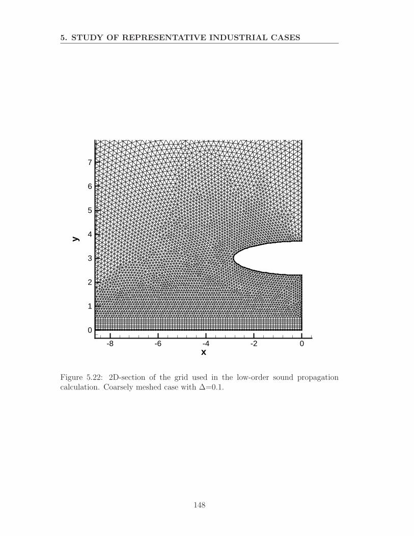
5. STUDY OF REPRESENTATIVE INDUSTRIAL CASES
x
y
-8 -6 -4 -2 0
0
1
2
3
4
5
6
7
Figure 5.22: 2D-section of the grid used in the low-order sound propagationcalculation. Coarsely meshed case with ∆=0.1.
148
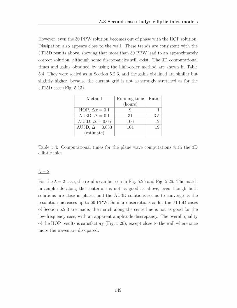
5.3 Second case study: elliptic inlet models
However, even the 30 PPW solution becomes out of phase with the HOP solution.
Dissipation also appears close to the wall. These trends are consistent with the
JT15D results above, showing that more than 30 PPW lead to an approximately
correct solution, although some discrepancies still exist. The 3D computational
times and gains obtained by using the high-order method are shown in Table
5.4. They were scaled as in Section 5.2.3, and the gains obtained are similar but
slightly higher, because the current grid is not as strongly stretched as for the
JT15D case (Fig. 5.13).
Method Running time Ratio(hours)
HOP, ∆x = 0.1 9 1AU3D, ∆ = 0.1 31 3.5AU3D, ∆ = 0.05 106 12AU3D, ∆ = 0.033 164 19
(estimate)
Table 5.4: Computational times for the plane wave computations with the 3Delliptic inlet.
λ = 2
For the λ = 2 case, the results can be seen in Fig. 5.25 and Fig. 5.26. The match
in amplitude along the centerline is not as good as above, even though both
solutions are close in phase, and the AU3D solutions seems to converge as the
resolution increases up to 60 PPW. Similar observations as for the JT15D cases
of Section 5.2.3 are made: the match along the centerline is not as good for the
low-frequency case, with an apparent amplitude discrepancy. The overall quality
of the HOP results is satisfactory (Fig. 5.26), except close to the wall where once
more the waves are dissipated.
149
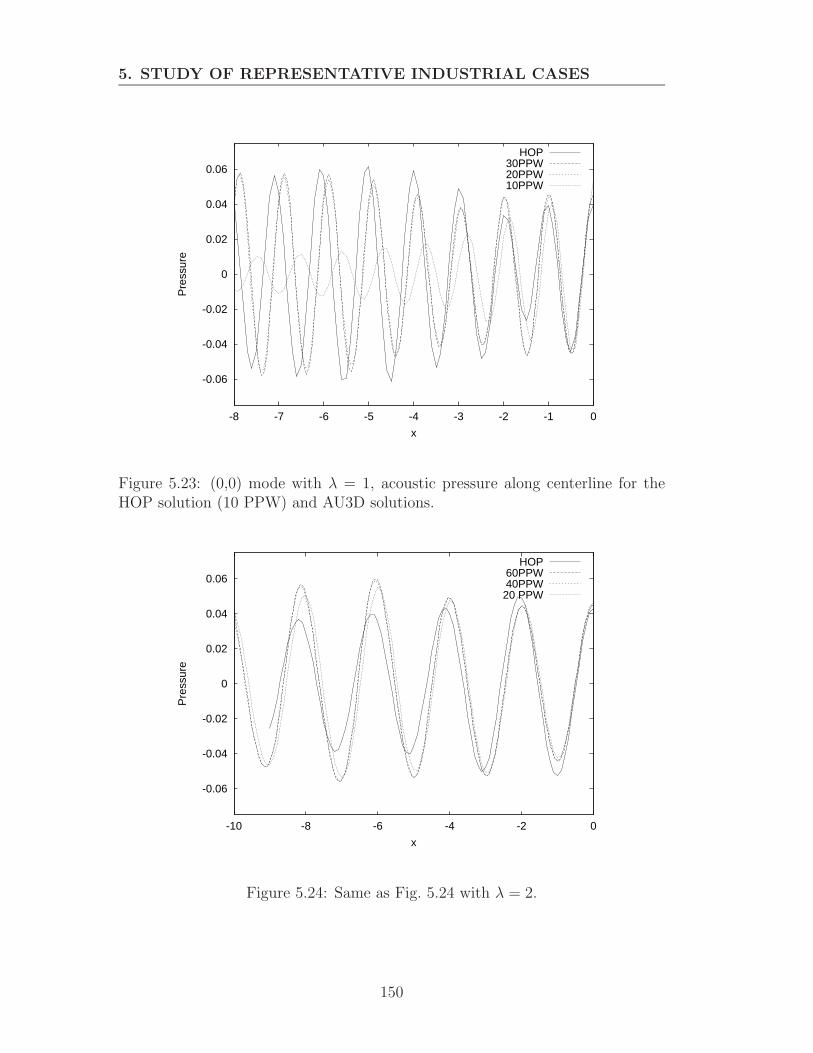
5. STUDY OF REPRESENTATIVE INDUSTRIAL CASES
-0.06
-0.04
-0.02
0
0.02
0.04
0.06
-8 -7 -6 -5 -4 -3 -2 -1 0
Pre
ssur
e
x
HOP30PPW20PPW10PPW
Figure 5.23: (0,0) mode with λ = 1, acoustic pressure along centerline for theHOP solution (10 PPW) and AU3D solutions.
-0.06
-0.04
-0.02
0
0.02
0.04
0.06
-10 -8 -6 -4 -2 0
Pre
ssur
e
x
HOP60PPW40PPW
20 PPW
Figure 5.24: Same as Fig. 5.24 with λ = 2.
150
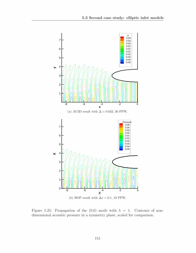
5.3 Second case study: elliptic inlet models
x
y
-8 -6 -4 -2 0
1
2
3
4
5
6
7
p0.050.040.030.020.01
-0.01-0.02-0.03-0.04-0.05
(a) AU3D result with ∆ = 0.033, 30 PPW.
Z
X
-8 -6 -4 -2 00
1
2
3
4
5
6
7
Pressure0.050.040.030.020.01
-0.01-0.02-0.03-0.04-0.05
(b) HOP result with ∆x = 0.1, 10 PPW.
Figure 5.25: Propagation of the (0,0) mode with λ = 1. Contours of non-dimensional acoustic pressure in a symmetry plane, scaled for comparison.
151
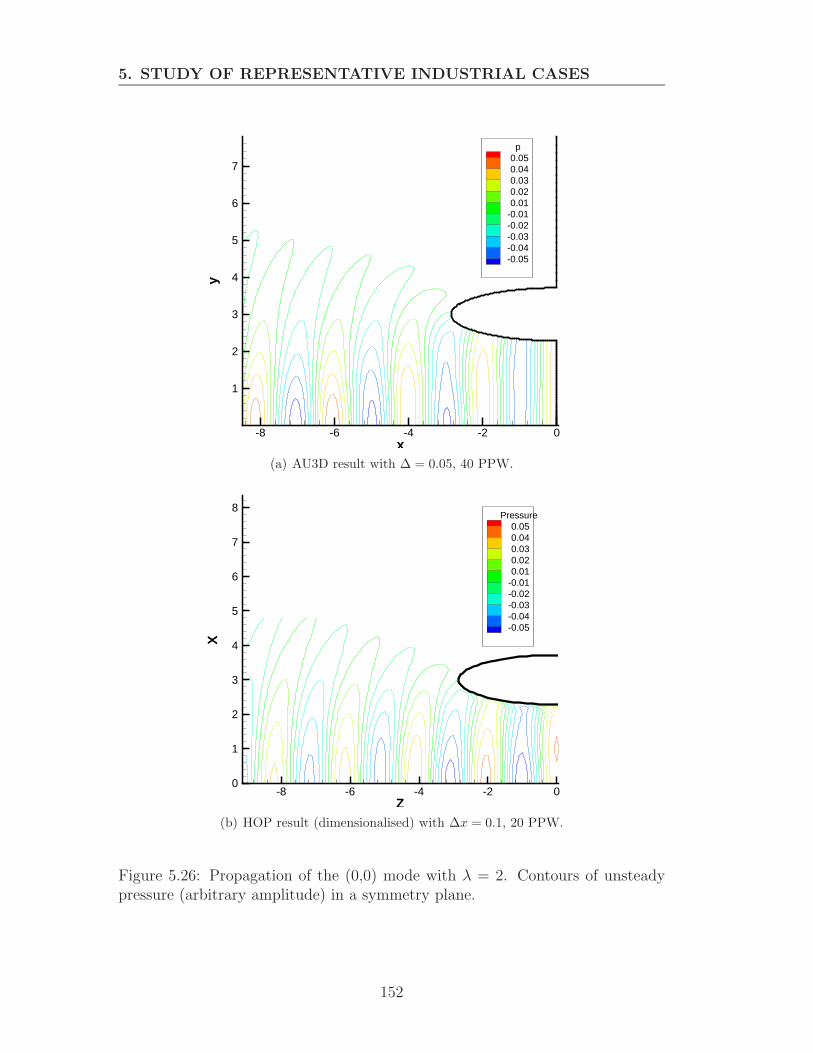
5. STUDY OF REPRESENTATIVE INDUSTRIAL CASES
x
y
-8 -6 -4 -2 0
1
2
3
4
5
6
7
p0.050.040.030.020.01
-0.01-0.02-0.03-0.04-0.05
(a) AU3D result with ∆ = 0.05, 40 PPW.
Z
X
-8 -6 -4 -2 00
1
2
3
4
5
6
7
8Pressure
0.050.040.030.020.01
-0.01-0.02-0.03-0.04-0.05
(b) HOP result (dimensionalised) with ∆x = 0.1, 20 PPW.
Figure 5.26: Propagation of the (0,0) mode with λ = 2. Contours of unsteadypressure (arbitrary amplitude) in a symmetry plane.
152
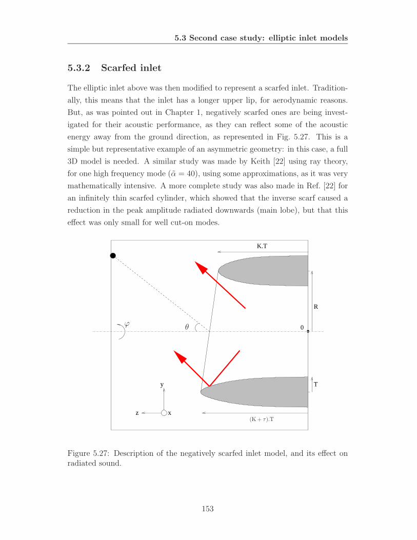
5.3 Second case study: elliptic inlet models
5.3.2 Scarfed inlet
The elliptic inlet above was then modified to represent a scarfed inlet. Tradition-
ally, this means that the inlet has a longer upper lip, for aerodynamic reasons.
But, as was pointed out in Chapter 1, negatively scarfed ones are being invest-
igated for their acoustic performance, as they can reflect some of the acoustic
energy away from the ground direction, as represented in Fig. 5.27. This is a
simple but representative example of an asymmetric geometry: in this case, a full
3D model is needed. A similar study was made by Keith [22] using ray theory,
for one high frequency mode (α = 40), using some approximations, as it was very
mathematically intensive. A more complete study was also made in Ref. [22] for
an infinitely thin scarfed cylinder, which showed that the inverse scarf caused a
reduction in the peak amplitude radiated downwards (main lobe), but that this
effect was only small for well cut-on modes.
z
y
x
0
T
K.T
R
ϕ θ
(K + τ).T
Figure 5.27: Description of the negatively scarfed inlet model, and its effect onradiated sound.
153

5. STUDY OF REPRESENTATIVE INDUSTRIAL CASES
The HOP scheme is very interesting for this problem. 30 PPW would be
required with a low-order scheme: this would represent a grid of more than 2 mil-
lion points, around 1.7Gb of memory and a run-time of several hundred hours,
because the full annulus would need to be included. As explained in Chapter
2, compact or quadrature-based methods also become very costly in 3D, as they
require solving large linear systems. Ozyoruk used a finite difference method
which could handle 3D inlets, using cylindrical coordinates, but did not invest-
igate asymmetrical geometries [9]. A good-quality body-fitted grid, structured
or unstructured, would be difficult to generate in this case, particularly for high
scarfing ratios. The Cartesian grid used here, containing the immersed boundary,
remains smooth and uniform in most of the domain.
The geometry is modelled by modifying the elliptic profile of Eq. (5.9), as
shown in Fig. 5.27. The radius is still R = 3, and T 2 = 51, but this time the
surface equation is modified by a scarfing ratio 0 < τ ≤ 1:
(
z
K + τ sin(ϕ)
)2
+ (√
x2 + y2 − R)2 = T 2 (5.10)
if ϕ is the azimuthal angle around the z axis. The particular geometry studied
uses τ = 0.4. The grid is identical to that of the axi-symmetric case above, but
contains 13470 ghost points, 44 of which need extrapolation along the normal.
The wall algorithm used in HOP has no difficulty in handling this asymmetrical
geometry, shown in Fig. 5.28.
The effect of the scarfing on several acoustic modes will be investigated. First,
a plane wave mode is used as input, with λ = 0.9 (9 PPW, α ≃ 21). The compu-
tation is run until a periodic regime is obtained. The mid-field SPL directivity
obtained along the domain’s boundary is shown in Fig. 5.29 as a function of the
polar angle θ (cf. Fig. 5.27). Most of the energy radiates in the center, so the
scarfed lip does not have a strong effect on the directivity of most of the sound,
which is in any case not radiated towards the ground. A small difference for the
secondary diffraction lobes is however noticeable.
The behaviour of spinning modes is more important, because, as was seen in
Section 5.2.2, most of the acoustic energy is directed away from the centerline
direction. The SPL obtained is shown in Fig. 5.30, for several different modes
154

5.3 Second case study: elliptic inlet models
Figure 5.28: 3D scarfed elliptic inlet surface, overlayed with the intersections withthe Cartesian grid.
155
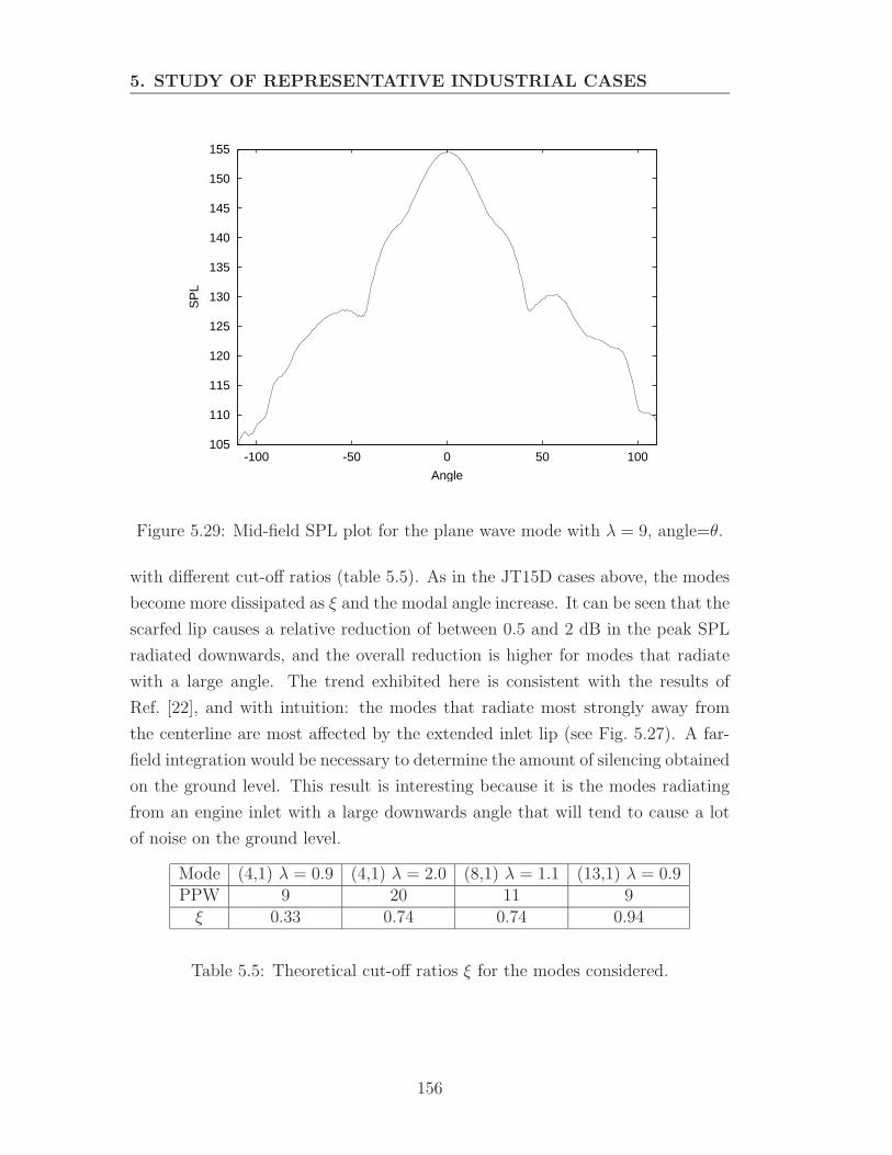
5. STUDY OF REPRESENTATIVE INDUSTRIAL CASES
105
110
115
120
125
130
135
140
145
150
155
-100 -50 0 50 100
SP
L
Angle
Figure 5.29: Mid-field SPL plot for the plane wave mode with λ = 9, angle=θ.
with different cut-off ratios (table 5.5). As in the JT15D cases above, the modes
become more dissipated as ξ and the modal angle increase. It can be seen that the
scarfed lip causes a relative reduction of between 0.5 and 2 dB in the peak SPL
radiated downwards, and the overall reduction is higher for modes that radiate
with a large angle. The trend exhibited here is consistent with the results of
Ref. [22], and with intuition: the modes that radiate most strongly away from
the centerline are most affected by the extended inlet lip (see Fig. 5.27). A far-
field integration would be necessary to determine the amount of silencing obtained
on the ground level. This result is interesting because it is the modes radiating
from an engine inlet with a large downwards angle that will tend to cause a lot
of noise on the ground level.
Mode (4,1) λ = 0.9 (4,1) λ = 2.0 (8,1) λ = 1.1 (13,1) λ = 0.9PPW 9 20 11 9
ξ 0.33 0.74 0.74 0.94
Table 5.5: Theoretical cut-off ratios ξ for the modes considered.
156

5.4 Concluding remarks
70
80
90
100
110
120
130
140
-100 -50 0 50 100
Spl
Angle
m=4 l=0.9m=4 l=2.0m=8 l=1.1
m=13 l=0.9
Figure 5.30: Mid-field SPL plot for the modes of Table 5.5.
5.4 Concluding remarks
The first case studied in this chapter, a simple wave propagation problem with
no wall surfaces, confirmed classic CAA results by demonstrating the efficiency of
the high-order DRP scheme. The new wall boundary condition was then added
to HOP, and both the JT15D and the elliptic inlet geometries were modelled.
Although no direct comparison with far-field results could be made, mid-field
HOP computations were related to equivalent ones obtained with other schemes.
Similarly to the validation results of Chapter 4, comparisons with an extensively
benchmarked 2D CAA program, ACTRAN, showed that important dissipation,
caused by the extra extrapolations used in the 3D method, occurred as the sound
propagated. Probably because of this, a small quantity of spurious waves was
also found radiating at low angles, close to the centerline. However, the directiv-
ity patterns obtained with HOP were consistent with reference and theoretical
results.
Comparisons made for plane wave cases, in both geometries, with solutions
157
5. STUDY OF REPRESENTATIVE INDUSTRIAL CASES
obtained with the low-order AU3D method, showed that the dissipation occurred
close to the wall boundary, and was more important as the modal angle increased.
Centerline discrepancies appeared for large wavelengths, because of the spurious
radiation described above. A good overall match was obtained, but low-order
computations were found to need at least 30 PPW, which leads to an increase in
computational time of more than 15 times compared to 8 PPW HOP computa-
tions. The memory cost of solving a fully 3D problem with such a fine grid would
probably be a crucial limiting factor.
Potential instability leads to the use of reduced time steps, as shown in
Chapter 4, but this is also the case for traditional methods using body-fitted
grids. Even if the full resolution of 7 PPW, found in free-field problems, cannot
be used, the permitted resolutions are effective and still largely more efficient than
with a low-order code. For comparison, the non-optimised high-order scheme of
Ozyoruk was used with resolutions of 12 PPW [36]. However, the important
dissipation associated with the immersed boundary condition in 3D preclude its
immediate use in its present state of development.
The acoustic shielding effect of a negatively scarfed inlet for certain acoustic
modes was investigated using a simple but fully 3D model. The new 3D wall
boundary condition developed in chapter 3 handled the asymmetric geometry
while keeping a high-quality, uniform Cartesian grid in most of the domain. Re-
ductions of around 2 dB in the mid-field SPL were observed for spinning modes
that radiate strongly towards the ground direction. This case illustrates how
complex, multi-dimensional effects could be investigated with the current ap-
proach. To use a low-order or implicit method would be extremely costly for
similar problems, unless a 2.5D model with substantial simplifying assumptions
is used.
Overall, the duct cases presented in this chapter suggest that the wall bound-
ary developed in this work exhibits some important dissipation which is depend-
ant on the modal angle, and thus on the number of internal modal reflections
occurring. As currently implemented, the scheme’s accuracy is insufficient for
direct application to industrial problems.
158
Chapter 6
Conclusions and further work
6.1 Conclusions
In the current work:
• A fully 3D sound propagation code (“HOP”) was developed. It uses a finite
difference discretisation to solve the time domain, non-conservative LEE
equations. Both spatial and temporal schemes are optimised for wavenum-
ber accuracy.
• This scheme was chosen after a review of existing computational aero-
acoustics schemes. These generally high-order accurate schemes were de-
veloped because of the inefficiency of traditional, low-order accurate CFD
methods when used for acoustics.
• A novel 3D wall boundary condition was developed, using a structured im-
mersed boundary approach, to enforce the slip boundary condition while
keeping a regular Cartesian grid in the whole of the computational domain.
It can model disconnected and concave surfaces, with no sharp edges. Few,
if any, existing immersed boundary method have been developed in con-
junction with a high-order scheme. The associated algorithm was described
in detail, and the discretisation errors were estimated.
• The effects of complex underlying steady flows, essential to the fan noise
problem, were studied in conjunction with the immersed boundary ap-
159
6. CONCLUSIONS AND FURTHER WORK
proach, a first in the CAA literature to the author’s knowledge. The effects
of the presence of a low Mach-number underlying steady flow were shown,
but higher-speed flows caused instability.
• The HOP scheme was validated on a variety of classic test cases, of in-
creasing complexity (first in 2D and then in 3D), including, if needed, the
appropriate wall boundary condition.
• Two different time integration scheme were implemented and compared in
detail on a variety of validation cases. Although the optimised Runge-
Kutta schemes are theoretically the most efficient, when the time step is
restricted because of stability concerns, the optimised Adams-Bashforth
scheme becomes the optimal choice.
• Several test cases representative of sound propagation in turbofan engines
were also studied, and computations made with HOP were compared with
analytical and alternative computational solutions. It was also observed
that the wall algorithm could handle complex, realistic geometries, but
some important inaccuracies appeared close to the wall boundaries, which
caused a dissipation of acoustic modes as a function of their cut-off ratio.
• Two different boundary conditions, introducing the input acoustic modes
while minimising the reflections, were implemented. The explicit absorbing
boundary was found to perform better than a 1-D radiation condition.
• It was shown that using a high-order method meant obtaining a gain of at
least one order of magnitude in the computing time, when compared to a
traditional CFD method, AU3D.
As noise constraints become fundamental for the airlines and the aeronautics
industry, engines must become quieter; the associated design choices affect other
aspects of the turbomachinery’s behaviour, so computational modelling should
ultimately include all these effects and their interactions to obtain a complete
design solution. Robust computational methods already exist to simulate fluid
dynamics (CFD), and their interaction with structures (aeroelasticity). This
160
6.1 Conclusions
includes the internal generation of sound, but not its propagation to the point of
observation.
In this study, dedicated, efficient acoustic propagation methods, to be used
in conjunction with these traditional CFD techniques, were investigated. Many
existing methods CAA employ 2D models, with simplifying assumptions (uniform
or irrotational mean flow etc.). To study more general interaction effects, a set
of 3D perturbed Euler equations was chosen here, making use of the increase
in available computing power. An hybrid linear approach splits the equations
between the steady mean flow (computed by a dedicated code) and the acoustic
perturbations (governed by the LEE equations).
The computational efficiency of the chosen discretisation method is then of
paramount importance. Traditional CFD techniques are inefficient for acoustic
computations, and many dedicated, high-order accurate methods have emerged.
Popular methods were reviewed, including implicit or explicit finite difference
and finite element schemes. In the current work, a structured, finite difference
approach that dispenses from using traditional meshing techniques was taken.
Finding correct ways of handling non-trivial wall geometries is an important
topic of research in CAA, even before 3D situations are considered. A 2D wall
boundary condition by Kurbatskii, designed for finite difference discretisations,
and allowing the use of a simple regular grid, was extended to 3D as described
in detail in Chapter 3. This represents one of the main contributions of the
current work. It is based on a complex but systematic algorithm that analyses
the geometrical situation for each relevant point behind the wall surface, and
determines the appropriate normal direction. The pressure gradient on the wall
surface is obtained using an extrapolation optimised in the wavenumber space,
performed along the coordinate axes. This is done in a pre-processing phase,
and the large resulting matrices are stored in a sparse fashion and inverted using
an appropriate iterative method. This approach allows the automatic treatment
of complex geometries without using lengthy meshing procedures, which can be
problematic, particularly with high-order discretisations. Furthermore, body-
fitted grids were developed for traditional, more dissipative CFD schemes and
can lead to instability and inaccuracy if used with high-order schemes, which are
generally less robust, particularly if the grid is highly stretched or of low quality.
161
6. CONCLUSIONS AND FURTHER WORK
In Chapter 4, the results of several classic test cases, used to verify the cor-
rect implementation of the chosen CAA methods, were presented. The 3D wall
boundary condition of Chapter 3 was tested against a standard 3D scattering
benchmark. The results were overall correct, but the accuracy was inferior than
with similar 2D results. Because the normal directions were estimated correctly,
this is due to the additional extrapolations required. It was shown that the new
3D treatment converged as the Helmholtz number increased. It appeared that
small time steps were needed to prevent instability near the wall, which, in a
sense, reduces the overall temporal order of the method.
In Chapter 5, the developed code was used for cases directly representative of
the aero-acoustic problems described in the introduction. Detailed comparisons
of spinning mode propagation from an axisymmetric inlet with results from equi-
valent low- and high-order methods confirmed that dissipation occurred close to
the wall boundary. For plane wave propagation results, the overall scheme re-
mains more efficient than low-order approaches, as a gain of at least one order of
magnitude in the computational time needed was clearly established.
Because of the inaccuracies observed, the wall boundary in its present state
cannot be directly applied to practical engineering problems such as the fan noise
cases presented in Chapter 1. For now, traditional structured approaches using
body-fitted grids, or unstructured discontinuous Galerkin techniques remain the
principal solutions to be used. For the approach investigated in the current
work to be salvaged, the accuracy of the wall boundary in 3D would need to be
enhanced, probably orienting research along the directions outlined below. The
inclusion of steady flows with the immersed wall boundary condition, exhibited in
Chapters 4 and 5, is also an important contribution of this work, but instability
problems that occurred in the presence of steady flows with important Mach
number represent an important limitation of the method in its current state.
To evaluate wether an immersed boundary approach should be retained, it
should be kept in mind that other approaches also introduce errors: “chimera”
grids are connected using extrapolations, and traditional deformed or unstruc-
tured grids introduce errors. Furthermore, a body-fitted grid of good quality
is often very difficult to obtain, particularly for the inlet mouth region. In the
comparable study of Ozyoruk [9], it was generated with difficulty, in a specific
162
6.2 Recommendations for further work
axisymmetric case. This strongly limits the application of grid-mapping methods
to the design of modern inlets, where several asymmetric geometries need to be
investigated.
6.2 Recommendations for further work
Extrapolation scheme: compared to the 2D method, the accuracy of the 3D
extrapolation procedure is problematic because of the additional extrapolations
required. This is a major difficulty, and future research in this direction could
aim at improving results, while carefully maintaining stability (following the dis-
cussion of Section 3.3 at the end of Chapter 3). A more stable method would
allow the time step to be extended, with substantial gains on the computational
efficiency relative to low-order methods, but this must not be offset by a loss of
spatial accuracy. Attempts made in this direction during the current research
were inconclusive. It is too early to say wether the limitations of high-order ac-
curate 3D extrapolation are fundamental, and the present method represents the
best accuracy/stability compromise, or wether a better method can be found.
The approach of Bin et al. [124], using only one interpolation direction, seems
promising in that respect. Some dissipation is also probably caused by the se-
lective damping used at the boundaries, therefore the use of higher-order filters
which would preserve more of the frequencies of interest could be investigated.
In order to reduce the instability appearing close to the wall boundary, par-
ticularly in the presence of large Mach number flows, up-winding techniques such
as those of Ref. [83] could be investigated, and integrated in the algorithm of
Chapter 3. The use of conservative LEE equations could also possibly lead to
more numerical stability [46].
Liners: because of its wide use in modern aero-engines, the soft-wall bound-
ary condition, used to model absorbing panels (or “liners”), is of great interest
in CAA, and should be added to the current method. Difficulties arise when
frequency-domain impedance models are used with time-domain computations,
but several successful approaches now exist, as was discussed in Section 2.3.2,
163
6. CONCLUSIONS AND FURTHER WORK
and their inclusion in the current immersed boundary would be straightforward:
Eq. (2.16) needs to be modified. But the presence of mean flow next to a porous
wall, in an inviscid model, leads to fundamental instability problems which might
be difficult to handle because of the current method’s lack of robustness.
Hybrid system: on a practical level, the connection between the propagation
scheme and the source of sound would need to be carefully designed, to obtain
the complete design system described in the introduction. Both codes would
need to run together, in the time domain, for optimal efficiency, with correct
data transmission between boundaries. The absorbing boundary condition used
in Chapter 5 makes this easier, since it can use an acoustic solution directly as
input. For certain cases, a feedback of the waves reflected at the inlet mouth into
the source domain could be necessary.
Non-linearities: although non-linear effects were not included in this study,
the current approach allows such an extension by adding the relevant correct-
ive terms. As pointed out in Chapter 2, shock-capturing techniques could also
be avoided through the careful use of pressure-sensitive selective dissipation. In
the context of noise propagation from the aircraft inlet, it is important to con-
sider where to set the limit of the middle-field domain, where the new CAA
method would be used for acoustic propagation. For example, if computing
N-wave propagation, the near field zone should include the region where the
propagation is non-linear because of the high amplitude of the waves.
Other applications: the immersed boundary approach developed here could
be applied to other problems; for example, 3D finite difference computations of
sound scattering from complex or disconnected geometries, which are difficult to
model with traditional structured grids. It would also be interesting to use this
approach for optimisation problems, where several geometries need to be assessed
automatically, by varying a parameter for example: the pre-processing could be
done automatically.
164
Bibliography
[1] M. J. T. Smith. Aircraft Noise. Cambridge University Press, 1989.
[2] K. A. Kurbatskii and C. K. W. Tam. Cartesian Boundary Treatment ofCurved Walls for High-order Computational Aeroacoustics Schemes. AIAAJournal, 35(1):133–140, 1997.
[3] J. E. Green. Civil Aviation and the Environmental Challenge. The Aero-nautical Journal, 107(1072):281–299, June 2003.
[4] P. C. Ruffles. Aero Engines of the Future. The Aeronautical Journal,107(1072):307–321, June 2003.
[5] M. D. Guynn and E. D. Olson. Evaluation of an aircraft concept with over-wing, hydrogen-fueled engines for reduced noise and emissions. TechnicalReport NASA/TM-2002-211926, NASA, Langley Research Center,http://techreports.larc.nasa.gov/ltrs/2002-cit.html, September2002.
[6] A. H. Nayfeh et al. Acoustics of Aircraft Engine-Duct Systems. AIAAJournal, 13(2):130–153, 1975.
[7] C. Bogey. Calcul Direct du Bruit Aerodynamique et Validation de Modelesacoustiques Hybrides. PhD thesis, Ecole Centrale de Lyon, Laboratoire deMecanique des Fluides et d’Acoustique, Lyon, France, April 2000.
[8] H. Shen and C. K. W. Tam. Numerical simulation of the Generation ofAxisymmetric Mode Jet Screech Tones. AIAA Journal, 36(10):1801–1807,1998.
[9] Y. Ozyoruk. Sound Radiation from Ducted Fans Using ComputationalAeroacoustics on Parallel Computers. PhD thesis, Pensylvenia State Uni-versity, 1995.
[10] E. Envia. Fan Noise Reduction: an Overview. International Journal ofAeroacoustics, 1(1):43–64, 2002.
165
BIBLIOGRAPHY
[11] J. M. Mendoza, B. Schuster, J. H. Lan, and C. Gerhold. Application ofDuct Propagation Codes to the Prediction of Far Field Turbofan GeneratedNoise. [131].
[12] E. J. Richards and D. J. Mead. Noise and Acoustic Fatigue in Aeronautics.John Wiley & Sons, 1968.
[13] J. M. Tyler and T. G. Sofrin. Axial Flow Compressor Noise Studies. SAETransactions, 70:309–332, 1962.
[14] A. McAlpine and M. J. Fisher. On the Prediction of “buzz-saw” Noise inAero-Engine Inlet Ducts. Journal of Sound and Vibration, 248(1):123–149,2001.
[15] M. J. Fisher and R. H. Self. Aeroacoustic Research in Europe: the CEAS-ASC Rerport on 2001 Highlights. Journal of Sound and Vibration, 258(1):1–30, 2002.
[16] J. G. Marshall and M. Imregun. A Review of Aeroelasticity Methods withEmphasis on Turbomachinery Applications. Journal of Fluids and Struc-tures, 10(3):237–267, 1996.
[17] M. Vahdati, A. I. Sayma, C. Breard, and M. Imregun. Computational Studyof Intake Duct Effects on Fan Flutter Stability. AIAA Journal, 40(3):408–418, 2002.
[18] X. Wu, A. I. Sayma, M. Vahdati, and M. Imregun. Computational tech-niques for aeroelasticity and aeroacoustic analyses of aero-engine fan as-semblies. In International Conference on Fans, number C631/005/2004,pages 85–98, ImechE Headquarters, London, UK, 9-10 Nov. 2004. ImechE,Professional Engineering Publishing Ltd.
[19] M. E. Goldstein. Aeroacoustics. Mc Graw-Hill, 1976.
[20] S. W. Rienstra. Sound transmission in slowly varying circular and annularlined ducts with flow. Journal of Fluid Mechanics, 380:279–296, 1999.
[21] C. J. Chapman. Sound Radiation from a Cylindrical Duct. Part1. RayStructure of the Duct Modes and of the External Field. Journal of FluidMechanics, 281:293–311, 1994.
[22] G. M. Keith. A Theoretical Investigation Into the Acoustic Radiation froman Aeroengine Intake. PhD thesis.
166
BIBLIOGRAPHY
[23] P. Gliebe, R. Mani, and H. Shin. Aeroacoustic Prediction Codes. TechnicalReport NASA/CR-2000-210244, NASA Glenn Research Center, 2000.
[24] K. A. Kurbatskii and C. K. W. Tam. Microfluid Dynamics and Acousticsof Resonant Liners. AIAA Journal, 38(8):1331–1339, 2000.
[25] T. J. Chung. Computational Fluid Dynamics. Cambridge University Press,Cambridge, U.K., 2002.
[26] A. I. Sayma, M. Vahdati, and M. Imregun. An Integrated Nonlinear Ap-proach for Turbomachinery Forced Response Prediction. Part I: Formula-tion. Journal of Fluids and Structures, 14:87–101, 2000.
[27] A. I. Sayma, M. Vahdati, and M. Imregun. An Integrated Nonlinear Ap-proach for Turbomachinery Forced Response Prediction. Part II: Case Stud-ies. Journal of Fluids and Structures, 14:103–125, 2000.
[28] A. I. Sayma, M. Vahdati, L. Sbardella, and M. Imregun. Modelling of Three-Dimensional Viscous Compressible Turbomachinery Flows Using Unstruc-tured Hybrid Grids. AIAA Journal, 38(6):945–954, 2000.
[29] C. L. Rumsey, R. T. Biedron, F. Farassat, and P. L. Spence. Ducted-FanEngine Acoustic Predictions Using a Navier-Stokes Code. Journal of Soundand Vibration, 213(4):643–664, 1998.
[30] C. K. W. Tam. Computational Acoustics: Issues and Methods. AIAAJournal, 33(10):1788–1796, 1995.
[31] D. P. Lockard. An investigation of accuracy requirements for computa-tional aeroacoustics. Master’s thesis, George Washingon University, JIAFS,Hampton, VA, USA, July 1993.
[32] C. K. W. Tam and J. C. Webb. Dispersion-Relation Preserving FiniteDifference Schemes for Computational Acoustics. Journal of ComputationalPhysics, 107:262–281, 1993.
[33] J. C. Hardin, J. R. Ristorcelli, and C. K. W. Tam, editors. ICASE/LARCWorkshop on Benchmark Problems in Computational Acoustics. 1995.NASA CP 3300.
[34] A. S. Lyrintzis. Integral Methods in Computational Aeroacoustics - Fromthe CFD (Near-Field) to the (Acoustic) Far-Field. In CEAS Workshop“From CFD to CAA”, Athens, Greece, 2002.
167
BIBLIOGRAPHY
[35] Y. Ozyoruk, L. N. Long, and V. Ahuja. Time Domain Simulation of Ra-diation from Ducted Fans with Liners. In 7th AIAA/CEAS AeroacousticsConference, 2001. AIAA paper 2001-2171.
[36] Y. Ozyoruk and V. Ahuja. Numerical Simulation of Fore and Aft SoundFields of a Turbofan. AIAA Journal, 42(10):2028–2034, 2004.
[37] D. Stanescu, D. Ait-Ali-Yahia, W. G. Habashi, and M. P. Robichaud. Mul-tidomain Spectral Computations of Sound Radiation from Ducted Fans.AIAA Journal, 37(3):296–302, 1999.
[38] D. Stanescu, D. Ait-Ali-Yahia, W. G. Habashi, and M. P. Robichaud. Spec-tral Element Method for Linear Fan Tone Noise Radiation. AIAA Journal,42(4):696–705, 2004.
[39] D. Stanescu, M. Y. Hussaini, and F. Farassat. Aircraft engine noise scat-tering by fuselage and wings: a computational approach. Journal of Soundand Vibration, 263:319–333, 2003.
[40] C. Breard. Acoustic Propagation and Radiation Modeling of Lined DuctWith Linear and Non-linear Frequency-Domain Solver. In 9th AIAA/CEASAeroacoustics Conference, number AIAA 2003-3265, Hilton Head, SouthCarolina, U.S.A., May 2003.
[41] W. Eversman and A. V. Parrett and J. S. Preisser and R. J. Silcox. Con-tributions to the finite element solution of the fan noise radiation problem.Journal of Vibration, Acoustics, Stress, and Reliability in Design, Transac-tions of the ASME, 107:216–223, April 1985.
[42] J. H. Lan, Y. Guo, and C. Breard. Validation of Acoustic PropagationCode with JT15D Static and Flight Test Data. [131].
[43] C. K. W. Tam and N. Pastouchenko. Noise from Fine-scale Turbulence ofNonaxisymmetric Jets. AIAA Journal, 40(3):456–464, 2002.
[44] C. Bailly and C. Bogey. Contributions Of Computational Aeroacoustics toJet Noise Research and Prediction. International Journal of ComputationalFluid Dynamics, 18(6):481–491, 2004.
[45] O. Marsden, C. Bogey, and C. Bailly. High-order curvilinear simulations offlows around non-Cartesian bodies. [131].
[46] S. Redonnet. Simulation de la Propagation Acoustique en Presence d’Ecou-lements Quelconques et de Structures Solides Par Resolution Numerique des
168
BIBLIOGRAPHY
Equations d’Euler. PhD thesis, Universite Bordeaux 1, Bordeaux, France,November 2001.
[47] P. Morse and K. Ingard. Theoretical Acoustics. Mc Graw-Hill, 1968.
[48] F. Fahy. Foundations of Engineering Acoustics. Academic Press, 2001.
[49] F. Farassat and M. K. Myers. Extension of Kirchhoff’s formula for Radi-ation from Moving Surfaces. Journal of Sound and Vibration, 123:451–460,1988.
[50] J. E. Ffowcs Williams and D. L. Hawking. Sound Generation by Turbulenceand Surfaces in Arbitrary Motion. Transactions of the Royal Society ofLondon, A264:321–342, 1969.
[51] F. Farassat. Linear Acoustic Formulas for Calculation of Rotating BladeNoise. AIAA Journal, 19:1122–1120, 1981.
[52] X. Zhang, X. X. Chen, C. L. Morfey, and B. J. Tester. Computation of FanNoise Radiation through A Realistic Engine Exhaust Geometry with Flow.In 9th AIAA/CEAS Aeroacoustics Conference, number AIAA 2003-3267,Hilton Head, South Carolina, U.S.A., May 2003.
[53] P. J. Morris, L. N. Long, et al. Simulations of supersonic Jet Noise. Inter-national Journal of Aeroacoustics, 1(1):17–41, 2002.
[54] C. Bailly and D. Juve. Numerical Solutions of Acoustic Propagation Prob-lems Using Linearized Euler Equations. AIAA Journal, 38(1):22–29, 2000.
[55] R. J. Astley, J. A. Hamilton, N. Baker, and E. H. Kitchen. Modellingtone propagation from turbofan inlets the effect of extended lip liners.In Proceedings of the 8th AIAA/CEAS Aeroacoustics Conference, numberAIAA 2002-2449, Breckenridge, Colorado, USA, 2002.
[56] C. Bogey, C. Bailly, and D. Juve. Computation of Flow Noise Using SourceTerms in Linearized Euler’s Equations. AIAA Journal, 40(2):235–243, 2002.
[57] C. K. W. Tam and H. Shen. Direct Computation of Nonlinear Acous-tic Pulses Using High Order Finite Difference Schemes. In 15th AIAAAeroacoustics Conference, 1993. AIAA paper 93-4325.
[58] P. J. Morris, L. N. Long, A. Bangalore, and Q. Wang. A Parallel Three-Dimensional Computational Aeroacoustics Method Using Nonlinear Dis-turbance Equations. Journal of Computational Physics, 133:56–74, 1997.
169
BIBLIOGRAPHY
[59] L. N. Long. A Nonconservative Nonlinear Flowfield Splitting Method for3-D Unsteady Fluid Dynamics. In 6th AIAA/CEAS Aeroacoustics Confer-ence, 2000. AIAA paper 2000-1998.
[60] J. C. Hardin and C. K. W. Tam, editors. Second Computational Acous-tics Workshop on Benchmark Problems. NASA Langley Research Center,Hampton VA, 1997. NASA CP 3352.
[61] J. C. Hardin, D. Huff, and C. K. W. Tam, editors. Third Computa-tional AeroAcoustics (CAA) Workshop on Benchmark Problems. NumberNASA/CP-2000-209790. Ohio Aerospace Institute, Cleveland, Ohio, USA,November 1999.
[62] W. Press, P. Flannery, S. Teulosky, and W. Vetterling. Numerical Recipes(FORTRAN). Cambridge University Press, 1989.
[63] D. P. Lockard, K. S. Brenner, and H. L. Atkins. High-Accuracy Algorithmsfor Computational Acoustics. AIAA Journal, 33(2):246–251, 1995.
[64] C. Bogey and C. Bailly. A Family of Low Dispersive and Low Dissipat-ive Explicit Schemes for Noise Computations. Journal of ComputationalPhysics, 194:194–214, 2004.
[65] J. Berland, C. Bogey, and C. Bailly. Optimized explicit schemes: matchingand boundary schemes and 4th-order Runge-Kutta algorithm. [131].
[66] R. R. Mankbadi, M. E. Hayder, and L. A. Povinelli. Structure of SupersonicJet Flow and Its Radiated Sound . AIAA Journal, 32(5):897–906, 1994.
[67] F. Owis and P. Balakumar. Jet Noise Computation Using Explicit McCor-mack Schemes and Non-Reflecting Boundary Conditions. AIAA Journal,39(10):2019, 2001.
[68] S. K. Lele. Compact Finite Difference Schemes with Spectral-Like Resolu-tion. Journal of Computational Physics, 103(16):42, 1992.
[69] A. Harten and S. Osher. Uniformly High-Order accurate Non-OscillatorySchemes, I. SIAM Journal of Numerical Analysis, 24:279–309, 1987.
[70] J. Casper and K. R. Meadows. Using High-Order Accurate EssentiallyNonoscillatory Schemes for Aeroacoustic Applications. AIAA Journal,34(2):244–250, 1996.
[71] G. S. Jiang and C. W. Shu. Efficient Implementation of Weighted ENOSchemes. Journal of Computational Physics, 126:202–212, 1996.
170
BIBLIOGRAPHY
[72] K. J. Baumeister and S. J. Horowitz. Finite Element-Integral AcousticSimulation of JT15D Turbofan Engine. Journal of Vibration, Acoustics,Stress, and Reliability in Design, Transactions of the ASME, 106:405–413,July 1984.
[73] H. L. Atkins and C.-W. Shu. Quadrature-Free Implementation of the Dis-continuous Galerkin Method for Hyperbolic Equations. In 2nd AIAA/CEASAeroacoustics Conference, 1996. AIAA paper 96-1683.
[74] C. Canuto, M. Y. Hussaini, A. Quarteroni, and T. A. Zang. Spectral Meth-ods in Fluid Dynamics. Springer-Ferlag, New-York/Berlin, 1988.
[75] M. Ganesh and I. G. Graham. A high-order algorithm for obstacle scatteringin three dimensions. Journal of Computational Physics, 198:211–242, 2004.
[76] S. J. Sherwin and G. E. Karniadakis. Tetrahedral hp Finite Elements: Al-gorithms and Flow Simulations. Journal of Computational Physics, 124:14–45, 1996.
[77] D. Casalino, M. Roger, and M. C. Jacob. Prediction of Sound Propagationin Ducted Potential Flows Using Green’s Function Discretization. AIAAJournal, 42(4):736, 2004.
[78] D. Casalino, P. D. Francescantonio, and Y. Druon. GFD Predictions of FanNoise Propagation. [131].
[79] K. Yokoi, F. Xiao, H. Liu, and K. Fukasaku. Three-Dimensional Numer-ical Simulation of Flows With Complex Geometries in a Regular CartesianGrid and its Application to Blood Flow in Cerebral Artery with MultipleAneurysms. Journal of Computational Physics, 202:1–19, 2005.
[80] T. Z. Dong and R. R. Mankbadi. Direct Numerical Simulation of EngineInternal Noise Propagation and Radiation. In First Joint CEAS/AIAAAeroacoustics Conference, Volume I. DGLR, 1995. CEAS/AIAA paper 95-064.
[81] P. J. Morris and C. Shieh. 3D Calculations of Acoustic Scatterings by aSphere: a Parallel Implementation. In Hardin and Tam [60]. NASA CP3352.
[82] E. J. Avital. Optimized Differentiation Schemes on Non-Uniformgridsfor Computational Aeroacoustics. Journal of Computational Acoustics,10(2):195–209, 2002.
171
BIBLIOGRAPHY
[83] M. Zhuang and R. F. Chen. Applications of High-Order Optimized UpwindSchemes for Computational Aeroacoustics. AIAA Journal, 40(3):443–449,2002.
[84] K. A. Kurbatskii and C. K. W. Tam. A Wavenumber Based Extrapolationand Interpolation Method for Use in Conjunction with High-Order FiniteDifference Schemes. Journal of Computational Physics, 157:588–617, 2000.
[85] C. K. W. Tam and K. A. Kurbatskii. Multi-Size-Mesh Multi-Time-Step Dispersion-Relation-Preserving Scheme for Multiple-Scales Aeroacous-tics Problems. International Journal of Computational Fluid Dynamics,17(2):119–132, 2003.
[86] C. Wall, C. D. Pierce, and P. Moin. A Semi-implicit Method for Resolutionof Acoustic Waves in Low Mach Number Flows. Journal of ComputationalPhysics, 181:545–563, 2002.
[87] F. Q. Hu, M. Y. Hussaini, and J. L. Manthey. Low-Dissipation and Low-Dispersion Runge-Kutta Schemes for Computational Acoustics. Journal ofComputational Physics, 124:177–191, 1996.
[88] D. Stanescu and W. G. Habashi. 2N-storage Low-Dissipation and Dis-persion Runge-Kutta Schemes for Computational Acoustics. Journal ofComputational Physics, 143:674–681, 1998.
[89] K. W. Thompson. Time Dependent Boundary Conditions for HyperbolicSystems, I. Journal of Computational Physics, 68:1–24, 1987.
[90] M. B. Giles. Nonreflecting Boundary Conditions for Euler Equations Cal-culations. AIAA Journal, 28(12):2050–2058, 1990.
[91] F. Q. Hu. On Absorbing Boundary Conditions for Linearized Euler Equa-tions by a Perfectly Matched Layer. Journal of Computational Physics,129:201–219, 1996.
[92] C. K. W. Tam, L. Auriault, and F. Cambuli. Perfectly Matched Layer asan Absorbing Boundary Conditions for the Linearized Euler Equations inOpen and Ducted Domains. Journal of Computational Physics, 144:213–234, 1998.
[93] F. Q. Hu. On using Perfectly Matched Layer for the Euler Equations witha Non-Uniform Mean Flow. [131].
[94] A. Bayliss and E. Turkel. Far-field Boundary Conditions for CompressibleFlows. Journal of Computational Physics, 48:182–199, 1982.
172
BIBLIOGRAPHY
[95] C. K. W. Tam, J. Fang, and K. A. Kurbatskii. Non-Homogeneous Radi-ation and Outflow Boundary Conditions Simulating Incoming Acoustic andVorticity Waves for Exterior Computational Aeroacoustics Problems. In-ternational Journal for Numerical Methods in Fluids, 26:1107–1123, 1998.
[96] X. D. Li, N. Schonwald, and F. Thiele. Numerical Computation of SoundPropagation and Radiation in a Duct. In 7th AIAA/CEAS AeroacousticsConference, 2001. AIAA paper 2001-2179.
[97] C. K. W. Tam and L. Auriault. Time-Domain Impedance Boundary Condi-tion for Computational Aeroacoustics. AIAA Journal, 34(5):917–923, 1996.
[98] L. Sbardella, M. Imregun, and B. Tester. A Time Domain Method for thePrediction of Sound Attenuation in Lined Ducts. Journal of Sound andVibration, 239(3):379–396, 2001.
[99] J. A. Lordi, G. F. Homicz, and R. G. Rehm. Effects of Finite Duct Lengthand Blade Chord on Noise Generation by a Rotating Blade Row. In AIAA7th Fluids and Plasmadynamics Conference, 1974. AIAA paper 74-555.
[100] N. C. Ovenden and S. W. Rienstra. Mode-Matching Strategies in SlowlyVarying Engine Ducts. AIAA Journal, 42(9):1832–1840, 2004.
[101] T. Z. Dong and L. A. Povinelli. On computations of Duct Acoustics withNear Cut-Off Frequency. In Hardin and Tam [60]. NASA CP 3352.
[102] S. Zheng, M. Zhuang, and F. Thiele. Noise Prediction and OptimizationSystem for Turbofan Engine Inlet Duct Design. [131].
[103] M. R. Visbal and D. V. Gaitonde. Nonreflecting Boundary Conditionsfor the Time-dependent Convective Wave Equation in a Duct. Journal ofComputational Physics, 197:737–758, 2004.
[104] D. Givoli and I. Patlashenko. Dirichlet-to-Neumann Boundary Condi-tion for Time-dependent Dispersive Waves in Three-Dimensional Guides.Journal of Computational Physics, 199:339–354, 2004.
[105] C. K. W. Tam and Z. Dong. Wall Boundary Conditions for High-OrderFinite-Difference Schemes in Computational Aeroacoustics. TheoreticalComputational Fluid Dynamics, 6:303–322, 1994.
[106] E. A. Fadlun, R. Verzicco, P. Orlandi, and J. Mohd-Yusof. Combinedimmersed-boundary finite-difference methods for three-dimensional com-plex flow simulations. Journal of Computational Physics, 161:35–60, 2000.
173
BIBLIOGRAPHY
[107] S. J. Sherwin and J. Peiro. Mesh generation in Curvilinear Domains Us-ing High-Order Elements. International Journal of Numerical Methods inEngineering, 153:207–223, 2002.
[108] E. Manoha, R. Guenanff, S. Redonnet, and M. Terracol. Acoustic ScatteringFrom Complex Geometries. [131].
[109] C. K. W. Tam and F. Q. Hu. An Optimized Multi-Dimensional Interpola-tion Scheme for Computational Aeroacoustics Applications Using OversetGrids. [131].
[110] C. Cheong and S. Lee. Grid-Optimized Dispersion-Relation-PreservingSchemes on General Geometries for Computational Aeroacoustics. Journalof Computational Physics, 174(1):248–276, 2001.
[111] Y. M. Chung and P. G. Tucker. Accuracy of Higher-Order Finite DifferenceSchemes on Nonuniform Grids. AIAA Journal, 41(8):1609–1611, 2003.
[112] M. R. Visbal and D. V. Gaitonde. On the Use of Higher-Order Finite-Difference Schemes on Curvilinear and Deforming Meshes. Journal of Com-putational Physics, 181:155–185, 2002.
[113] C. S. Peskin. The Immersed Boundary Method. Acta Numerica, pages479–518, 2002.
[114] L. B. Tran and H. S. Udaykumar. A Particle-Level Set-Based Sharp Inter-face Cartesian Grid Method for Impact, Penetration, and Void Collapse.Journal of Computational Physics, 193:469–510, 2004.
[115] A. Gilmanov, F. Sotiropoulos, and E. Balaras. A General ReconstructionAlgorithm for Stimulating Flows with Complex 3D Immersed Boundarieson Cartesian Grids. Journal of Computational Physics, 191:660–669, 2003.
[116] Y.-H. Tseng and J. H. Ferziger. A Ghost-cell Immersed Boundary Methodfor Flow in Complex Geometry. Journal of Computational Physics, 192:593–623, 2003.
[117] G. Yang, D. M. Causon, and D. M. Ingram. Calculation of Compress-ible Flows about Complex Moving Geometries Using a Three-DimensionalCartesian Cut Cell Method. International Journal for Numerical MethodsIn Fluids, 33:1121–1151, 2000.
[118] M. P. Kirkpatrick, S. W. Armfield, and J. H. Kent. A Representation ofCurved Boundaries for the Solution of the NavierStokes Equations on a
174
BIBLIOGRAPHY
Staggered Three-dimensional Cartesian Grid. Journal of ComputationalPhysics, 184:1–36, 2003.
[119] W. J. Coirier and K. G. Powell. An Accuracy Assessment of Cartesian-MeshApproaches for the Euler Equations. Journal of Computational Physics,117:121–131, 1995.
[120] B. Lombard and J. Piraux. Numerical Treatment Of Two-Dimensional In-terfaces for Acoustic And Elastic Waves. Journal of Computational Physics,195:90–116, 2004.
[121] K. A. Kurbatskii. Solid Wall Boundary Conditions for ComputationalAeroacoustics Problems. PhD thesis, The Florida State University, Col-lege of Arts and Science, Florida, USA, Fall 1997.
[122] M. J. Aftosmis, M. J. Berger, and J. E. Melton. Robust and Effi-cient Cartesian Mesh Generation for Component-Based Geometry. AIAAJournal, 36(6):946–951, 1998.
[123] A. S. Glassner, editor. Graphic Gems. AP Professional, 1995.
[124] J. Bin, C. Cheong, and S. Lee. Optimised Boundary Treatment ofCurved Walls for High-Order Computational Aeroacoustics Schemes. AIAAJournal, 42(2):414–417, 2004.
[125] P. J. Morris. The Scattering of Sound from a Spatially Distributed, axisym-metric cylindrical source by a Circular Cylinder. Journal of the AcousticalSociety of America, 97(5):2651–2656, 1995.
[126] P. J. Morris. Scattering of Sound from a Spatially Distributed, Spheric-ally Symmetric Source by a Sphere. Journal of the Acoustical Society ofAmerica, 98(6):3536–3539, 1995.
[127] F. M. White. Viscous Fluid Flow. Mechanical Engineering. Mc Graw-HillInternational, 2nd edition, 1991.
[128] M. M. Denn, editor. Process Fluid Mechanics. Prentice Hall PTR.
[129] J. A. Lordi and G. F. Homicz. A Note on The Radiative Directivity Patternsof Duct Acoustic Modes. Journal of Sound and Vibration, 41(3):283–290,1975.
[130] R. Astley and W. Eversman. Wave Enveloppe and Infinite Element Schemesfor Fan Noise Radiation from Turbofan Inlets. AIAA Journal, 22:1719–1726, 1984.
175
BIBLIOGRAPHY
[131] 10th AIAA/CEAS Aeroacoustics Conference, Manchester, U.K., May 2004.
[132] A. Chaigne. Ondes acoustiques. Les editions de l’Ecole Polytechnique,Palaiseau, France, 2001.
[133] M. Goossens, F. Mittelbach, and A. Samarin. The LATEXCompanion.Addison-Wesley, 1994.
[134] H. J. Greenberg. A simplified introduction to LATEX.http://www.cudenver.edu/∼hgreenbe/, April 2000.
[135] M. M. Cand. Computing the 3-Dimensional Propagation of Forward-ArcFan Noise from Aero-Engines. In Up and Coming in Fluid Machinery,Seminar Proceedings, London, U.K., 9 October 2003. IMechE.
[136] M. M. Cand, A. I. Sayma, and M. Imregun. 3-Dimensional Noise Propaga-tion Using a Cartesian Grid. [131].
[137] M. M. Cand, A. I. Sayma, and M. Imregun. Efficient 3-Dimensional NoisePropagation using an Immersed Boundary. Journal of Sound and Vibration.Submitted for consideration.
176