aerodynamics and aeroacoustics study of...

11th World Congress on Computational Mechanics (WCCM XI)5th European Conference on Computational Mechanics (ECCM V)

6th European Conference on Computational Fluid Dynamics (ECFD VI)E. Onate, J. Oliver and A. Huerta (Eds)

AERODYNAMICS AND AEROACOUSTICS STUDY OFTHE FLOW AROUND AN AUTOMOTIVE FAN AIRFOIL

RABEA MATOUK∗, GERARD DEGREZ† AND JULIEN CHRISTOPHE‡

∗ Universite Libre de BruxellesRue Emile Banning 124, B-1050 Brussels, Belgium

e-mail: [email protected]

† Universite Libre de BruxellesCP 165/43, 50 Av. F.D. Roosevelt, B-1050 Brussels, Belgium


‡ von Karman Institute for Fluid Dynamics72 Chausee de Waterloo, B-1640 Rhode-st-genese, Belgium


Key words: LES, CD (Controlled-Diffusion) Airfoil, Pressure spectrum, Smagorinsky,WALE, Amiet.

Abstract. This paper presents the results of aerodynamic simulations of the flow arounda CD (Controlled-Diffusion) airfoil for the turbulent regime by the in-house SFELESsolver which is a hybrid spectral/finite elements code capable of simulating 3D unsteadyincompressible viscous flows over axisymmetric and planar geometries with a directionof periodicity. The results are compared with experimental results obtained by Moreauand Roger [1] and Moreau et al. [2] as well as other numerical results performed byJ.Christophe [4] using OpenFoam. The simulations were carried out for Re=160,000 inorder to study the unsteady turbulent boundary layer and to calculate the wall pressurespectrum used for noise predictions. Several SGS models, such as the static Smagorinskymodel, the WALE model and the model proposed by G.Ghorbaniasl [5], were used andtheir results were compared to study the influence of the LES sub grid-scale on the results.Amiet’s aeroacoustic theory [6, 7] is then applied using the wall pressure spectrum fora station near the trailing edge in order to calculate the trailing-edge noise. The soundpressure level and its directivity are computed for the three SGS models and comparedwith experiments.

1 INTRODUCTION

Several experimental and numerical studies (finite volumes and finite differences sim-ulations) were performed on the CD airfoil in order to study the unsteady and turbulent

1

R.Matouk, G.Degrez and J.Christophe

boundary layer and wake in order to calculate the noise sources for sound predictions.The broadband self-noise generated by this particular airfoil is mainly due to the trailing-edge noise produced by the scattering of the boundary layer at trailing edge. The readeris referred to [4] where most of studies are reported. The first LES numerical study hasbeen performed by Wang [9], by LES hybrid finite differences/spectral code. Another re-cent study has been performed by Christophe [4], by a LES Fluent and OpenFoam finitevolumes simulations. The two studies have been achieved on a sub-domain around theairfoil using velocities, extracted from a RANS simulation performed by Wang [9] on alarger domain including the jet and the airfoil, as boundary conditions on the LES domaininlet. It has bean shown by Moreau [3] that there are significant differences between theresults obtained from a simulation performed on an isolated airfoil in a uniform streamand that performed on an airfoil in an open-jet wind tunnel facility. The same procedureis applied in our study and the velocities, extracted from the RANS simulation are usedas inlet boundary condition. In the present work SFELES is used to solve the flow.SFELES [10] is a hybrid spectral/finite elements code capable of simulating 3D unsteadyincompressible viscous flows over axisymmetric and planar geometries. It is large eddysimulation solver based on a combination of a spectral discretization in the periodic (az-imuthal or transverse) direction and a finite elements discretization in the perpendicular(meridian or longitudinal) plane. The main advantage of this code is its ability to exploitthe existence of a direction of periodicity in the geometry to increase the computationalefficiency.Three SGS models have been used in the present study. The first is the Smagorinskymodel [11] with Cs = 0.17. The second model considered is the WALE model [12] withCw = 0.55. The third model is a recent model proposed by Ghorbaniasl [5]. In this modelthe Smagorinsky constant Cs is supposed to be a function of the flow variables includingthe rotational and translational velocities. The final formulation of this model is:

Cs = min(Gx, Gy, Gz) (1)

where Gx = |Ωxux|2D

, Gy = |Ωyuy |2D

, Gz = |Ωzuz |2D

and D =√

(Ωxux)2 + (Ωyuy)2 + (Ωzuz)

2.

The constant Cs is computed dynamically but without the need of dynamic procedurewhich means a gain of time computation. This model has been validated for simplecases (channel flow and circular cylinder) and for low Reynolds numbers (180 and 3900)by Ghorbaniasl [5]. In this work, it is implemented in SFELES and tested for a morecomplicated case (the CD airfoil) for high Reynolds number (160000). SFELES uses thestabilized Galerkin FEM method where the added stabilizations terms are the SUPG(Streamline - Upwind Petrov - Galerkin) and the PSPG (Pressure Stabilised Petrov -Galerkin) [13, 14]. It is assumed that the flow in the spanwise direction is periodic andknown at discrete points in space, therefore the pressure and velocity can be developed asa sum of discrete Fourier modes [10, 16]. Considering the temporal discretization, Crank-Nicolson method is used for the pressure and diffusive terms while Adams-Bashforthmethod is used for convective terms.

2


2 CASE DEFINITION

Fig. 1 shows the automotive cooling module, its 9-blades rotor and the profile of theblade, cut at mid-span, on which all simulations were performed. It is located in the middleof the blade span. The airfoil thickness is 4%C and Its camber angle is 12. The chordlength is C = 0.1356 m. The airfoil is set at 8 angle of attack. The spanwise dimensionof the numerical domain is 10% of the chord length. Fig. 2 shows the computational

Figure 1: The automotive cooling module, its 9-blades fan and the airfoil of the blade

domain with the used mesh. The size of the computational domain is 4C in the stream-wise direction (x) and 2.5C in the transverse direction (y). The domain was divided intotriangular elements with nearly 160,000 elements and nearly 80,000 nodes. This mesh isrefined to capture small perturbations in the flow. The refinement was done such that thefirst grid points of the surface lie within 1.1 wall units of the wall (y+ < 1.1). Velocity was

Figure 2: The computational domain with the structured mesh

prescribed on the inlet (along the outer C boundary), pressure was imposed on the outlet(it is imposed equal to 0) and no-slip conditions were imposed on the airfoil. Inlet velocityprofiles on the restricted domain were extracted from RANS computations. Furthermore,a periodicity condition in the spanwise direction (z) was assumed. In order to trigger3D instabilities, some random perturbations (noise) are added to the solution during thesimulation for a period of 0.4 time units t*, where t∗ = t∗U0

C, for all mesh nodes. This is

a good way to start the turbulent motions where the intensity of the fluctuations appliedis 0.1% for all turbulent simulations.

3


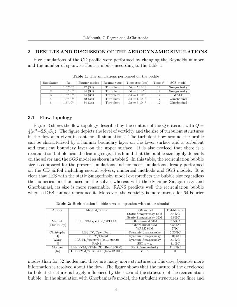
3 RESULTS AND DISCUSSION OF THE AERODYNAMIC SIMULATIONS

Five simulations of the CD-profile were performed by changing the Reynolds numberand the number of spanwise Fourier modes according to the table 1:

Table 1: The simulations performed on the profile

Simulation Re Fourier modes Regime type Time step (sec) Time t* SGS model

1 1.6*105 32 (3d) Turbulent ∆t = 5.10−6 12 Smagorinsky2 1.6*105 64 (3d) Turbulent ∆t = 5.10−6 12 Smagorinsky3 1.6*105 64 (3d) Turbulent 4t = 1.10−6 12 WALE4 1.6*105 32 (3d) Turbulent 4t = 1.10−6 12 Ghorbaniasl5 1.6*105 64 (3d) Turbulent 4t = 5.10−6 12 Ghorbaniasl

3.1 Flow topology

Figure 3 shows the flow topology described by the contour of the Q criterion with Q =14(ω2+2SijSij). The figure depicts the level of vorticity and the size of turbulent structures

in the flow at a given instant for all simulations. The turbulent flow around the profilecan be characterized by a laminar boundary layer on the lower surface and a turbulentand transient boundary layer on the upper surface. It is also noticed that there is arecirculation bubble near the leading edge. It is found that the bubble size highly dependson the solver and the SGS model as shown in table 2. In this table, the recirculation bubblesize is compared for the present simulations and for most simulations already performedon the CD airfoil including several solvers, numerical methods and SGS models. It isclear that LES with the static Smagorinsky model overpredicts the bubble size regardlessthe numerical method used in the solver whereas with the dynamic Smagorinsky andGhorbaniasl, its size is more reasonable. RANS predicts well the recirculation bubblewhereas DES can not reproduce it. Moreover, the vorticity is more intense for 64 Fourier

Table 2: Recirculation bubble size: comparsion with other simulations

Author Method/Solver SGS model Bubble sizeStatic Smagorinsky 64M 8.4%CStatic Smagorinsky 32M 9.8%C

Matouk LES FEM spectral/SFELES Ghorbaniasl 64M 3.5%C(This study) Ghorbaniasl 32M 3.55%C

WALE 64M 7%CChristophe LES FV/OpenFoam Dynamic Smagorinsky 5.26%C

[4] LES FV/Fluent Dynamic Smagorinsky 5.04%CWang LES FD/spectral (Re=150000) Dynamic Smagorinsky 3.7%C

[9] RANS SST k − ω 3.1%CMoreau LES FVM/STAR-CD (Re=120000) Static Smagorinsky 11.2%C

[15] DES FVM/STAR-CD (Re=120000) k − ε 0

modes than for 32 modes and there are many more structures in this case, because moreinformation is resolved about the flow. The figure shows that the nature of the developedturbulent structures is largely influenced by the size and the structure of the recirculationbubble. In the simulation with Ghorbaniasl’s model, the turbulent structures are finer and

4


more intense than for the simulation with the Smagorinsky model but the total energyconvected at the trailing edge is almost the same as it will be shown when the wall-pressure spectrum is computed (see Fig. 6). Furthermore, a small vortex shedding fromthe pressure side is noticed. It is more important for with Ghorbaniasl’s model, especiallyfor 64M. This shedding depends largely on the angle of attack of the profile and the freestream velocity [8]. It has important effects when the calculation of the total noise isrequested. A narrow-band or tonal contribution is added to the overall sound [8].

Figure 3: Topology of the flow for all simulations described by the criterion Q(Q.C2

U20

= 1000) and colored

by the longitudinal instantaneous velocity with the model: a) Smagorinsky 32M, b) Smagorinsky 64M,c) Ghorbaniasl 32M, d) Ghorbaniasl 64M, e) WALE 64M

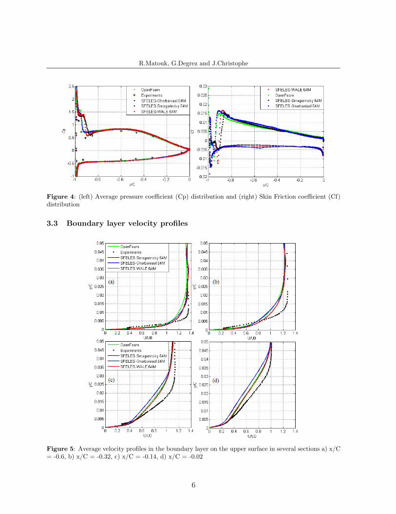
3.2 Pressure and friction coefficients distribution on the airfoil surface

Figure 4 shows the mean pressure and friction coefficients distribution on the airfoil.As far as the pressure distribution is concerned, first considering the Smagorinsky andWALE results, one observes a very good agreement with experimental results as well asOpenFoam simulations except near the leading edge where the results are influenced bythe size of the recirculation bubble which is larger than in OpenFoam results as mentionedabove. In contrast, for Ghorbaniasl’s model, we have a very good agreement with Open-Foam’s results in this region. As far as skin friction on the upper surface is concerned,there is a region toward the leading edge in which the friction coefficient is negative, thisregion corresponds to the recirculation bubble. Downstream of the reattachment, thepresent results are seen to be in good agreement with the OpenFoam results in particular,for the simulation with 64 M using Ghorbaniasl’s model. The skin friction on the lowersurface is uniform and less important because the boundary layer is laminar.

5


Figure 4: (left) Average pressure coefficient (Cp) distribution and (right) Skin Friction coefficient (Cf)distribution

3.3 Boundary layer velocity profiles

Figure 5: Average velocity profiles in the boundary layer on the upper surface in several sections a) x/C= -0.6, b) x/C = -0.32, c) x/C = -0.14, d) x/C = -0.02

6


The average longitudinal velocity profiles in the boundary layer have been extracted inseveral positions along the airfoil (x/C = −0.6, x/C = −0.32, x/C = −0.14 and x/C =−0.02) as illustrated in Fig. 5. In our mesh the trailing edge corresponds to(x/C = 0) andthe leading edge corresponds to(x/C = −1), x is aligned with the chord and pointing inthe streamwise direction, y is crosswise. It is noticed that the thickness of the boundarylayer developed on the upper surface increases from the leading edge to the trailing edge.One observes on Fig. 5 a very good agreement with the OpenFoam simulations as well aswith the experimental results when the boundary layer thickness is considered and as ageneral profiles. Average quantity were obtained by averaging in spanwise direction andin time for 7t*.

3.4 Wall pressure spectra

The pressure evolution with respect to time was acquired and averaged spanwise in twopositions near the trailing edge on the suction side: x/C=-0.08 and x/C=-0.02 during aperiod of 6t* for all simulations. Then, wall-pressure spectra are computed and comparedwith OpenFoam and the experimental results. The pressure spectra are expressed as thePower Spectral Density (PSD). In order to express the PSD in [dB], the following trans-

formation is applied: SPL = 20log10(

√Gpp(f)

P0) Where P0 = 2 ∗ 10−5[pa] is the reference

pressure. Welch method is used in order to estimate the spectra with applying the averag-ing over segments of 29 points and with a multiplication by a Hanning window and overlap50% between the segments. The results are illustrated in Fig. 6 . At the two positions, the

Figure 6: Power Spectral Density of pressure fluctuations at the positions: x/C=-0.08, x/C=-0.02(comparison with OpenFoam and the experiments)

results show a very good agreement with the experiments and OpenFoam especially for

7


the low and mid frequency ranges for the three SGS models with a difference up to 2dB.At high frequencies, SFELES results are closer to experiments than OpenFoam. Thereare little differences between the SGS models, WALE and Smagorinsky curves are closerto the experiments. In contrast, the Ghorbaniasl’s model curve is dropping quicker. It isnoticed that the recirculation bubble size does not influence the pressure spectra for thesections near the trailing edge so it will have little effects on the radiated sound.

4 AEROACOUSTIC STUDY: THE APPLICATION OF AMIET’S THE-ORY

Broadband self-noise or trailing edge noise, caused by the scattering of the blade tur-bulent boundary layer at the trailing edge into acoustic waves, is a major contributor ofthe overall radiated noise. It is the minimum noise that could be produced by the rotatingmachines [19]. In this paper, Amiet’s theory with its extensions [6, 7] is applied in order tocalculate this noise in the far field using LES input data represented by the wall pressurespectrum already calculated in a point near the trailing edge (x/C = −0.02). This proce-dure is physically justified by the fact that when the incident aerodynamic wall pressure isconvected past the trailing edge, it behaves as equivalent acoustic sources. Amiet’s modeldescribes how the hydrodynamic waves convected within the boundary layer are scatteredby the trailing edge; thereby unsteady loads are generated over the blade surface. Thenoise is generated by these forces. Schwarzschild’s procedure [17] is applied iterativelysuch that the turbulent boundary layer is considered as a series of waves traveling towardsthe trailing edge. Each scattered wave gives rise to an upstream traveling wave such thatthe total pressure vanishes downstream the flat plate. These scattered waves create theunsteady loads which generate the noise. It is assumed that the airfoil is a flat plate(the thickness of the blade isn’t considered in the model directly but within the pressurespectrum) extended to the infinity in the downstream direction so it is restricted to highfrequencies. The extension to include low frequencies was developed by Roger & Moreau[7] by taking into account the back-scattering from the leading edge, accounting for thefinite chord length, in the model. This is done using a two-step Schwarzschild’s solution[7]. The final far-field acoustic pressure power spectral density formula applied in thispaper for a given frequency ω is:

Spp(X,ω) = (sinθ

2πR)2.(kC)2d.|Γ|2Φpp(ω)ly(ω) (2)

The reader is referred to [7] for the complete derivation. In this equation d is the mock-upsemi-span, where the span is assumed to equal to 40C, C is the airfoil chord length, k isthe acoustic wavenumber. R = 2 m and θ = 90o are the listener location which is placedin the mid-span plane above the trailing edge in our case. Φpp(ω) is the wall-pressurepower spectral density and ly(ω) is the spanwise correlation length near the trailing edgewhich is computed using the Corcos’s model [18] given by the relation: ly(ω) = b.Uc

ωwith

Uc = 0.7U0 the convection speed and the coefficient b = 1.5. Γ is the aeroacoustic transfer

8


function (Γ = Γ1 + Γ2) with Γ1 is the transfer function of the trailing edge and Γ2 is theback-scattering leading edge correction.

4.1 Results and discusion

Fig. 7 shows the PSD of the sound pressure level at the considered observer. First,considering the left Figure without the leading edge back-scattering correction, we havea very good agreement with the experimental results with a discrepancies up to 2 dBat low frequencies,it is expected because the actual chord length is not yet considered.Second, on the right Figure where the leading edge correction is applied, the results areimproved for low frequencies between 100 and 300 Hz as expected. The back-scatteringcorrection has no important influences on the results for high frequencies. It is clear thatSFELES results are in very good agreement with experimental results and closer thanOpenFoam in particular for frequencies between 1500 and 2000 Hz. Comparing withOpenFoam results, the results are in good agreement in the domain 100-1500 Hz andthen our curves have higher values but closer to experimental results (1500-2000 Hz),this is linked directly to the the differences in the wall pressure spectra estimation, (seeFig. 6). As far as the comparison between the three used SGS models is concerned, onecan notice that there are no important differences because the wall-pressure spectra werevery similar, the difference does not exceed 2 dB in the domain of interest (100-2000 Hz).The directivity patterns of the acoustic pressure are shown in Fig. 8 for the three SGSmodels. The behavior is very similar in the three cases. The dipolar behavior is clearwhere there are two big dominant lobes, they multiply and orient towards the leading edgefor high frequencies. The secondary lobes are more important when the WALE model isconsidered at the frequency 1804 Hz

Figure 7: Trailing edge sound using Amiet’s theory for the three SGS models (left) without the leadingedge correction (right) with the leading edge correction, comparison with OpenFoam and Experiments.The receiver is placed in the mid-span plane above the trailing edge (R=2 m, θ = 90o)

9


Figure 8: The noise directivity patterns [dB] for all SGS model, (a): Smagorinsky, (b): WALE, (c):Ghorbaniasl

5 CONCLUSION

In the present paper, aerodynamics and aeroacoustics study of the CD Valeo profileis performed. The in-house solver SFELES is used to solve the flow. Average pressureand friction coefficients distribution, boundary layer profiles and the wall-pressure spectraare computed and compared with experimental and OpenFoam results. Three turbulencemodels are used which are the static Smagorinsky model, the WALE model and Ghorbani-asl’s model. Amiet’s aeroacoustics theory is then applied using the wall-pressure spectrumextracted near the trailing edge during the simulations as input data. The sound pressurelevel and its directivity are computed for the three SGS models and compared. The mainobservations were made are:

• First considering the aerodynamics results:

– A good agreement is obtained in general with previous experimental and nu-merical studies with differences in the region towards the leading edge due tothe high variability of the leading edge recirculation bubble size with the solverand the SGS model as shown in table 2.

10


– The new SGS model proposed by G.Ghorbaniasl is implemented and validated.It is found that the results are improved in general, especially near the leadingedge, comparing with OpenFoam and experimental results. The recirculationbubble size is found equal to 3.5%C.

– The recirculation bubble size has no important effects on the wall-pressurespectra near the trailing edge whereas it influences largely the pressure andfriction coefficients in the region near the leading edge.

– The wall-pressure spectrum computed by SFELES is in excellent agreementwith experiments and better than OpenFoam for frequencies between 1000 Hzand 5000 Hz.

• Second considering the aeroacousitcs results: The predicted noise obtained using thewall-pressure spectrum of SFELES are in very good agreement with experimentalresults and closer than OpenFoam in particular for frequencies between 1000 and2000 Hz regardless of the SGS model. The dipolar behaviour of the noise sources isfound and the lobes multiply and orient towards the leading edge for high frequencieswhen the acoustic pressure directivity is considered. The secondary lobes are moreimportant when the WALE model is considered at the frequency 1804 Hz.

References

[1] S. Moreau and M. Roger. Effect of Airfoil Aerodynamic Loading on Trailing-EdgeNoise Sources. AIAA Journal, 43(1):41–52, January 2005.

[2] S. Moreau, D. Neal, and J. Foss. Hot-Wire Measurements Around a ControlledDiffusion Airfoil in an Open-Jet Anechoic Wind Tunnel. J. Fluids Eng, 128:699-706,2006.

[3] S.Moreau , G.Iaccarino, M.Roger AND M.Wang. CFD analysis of flow in an open-jet aeroacoustic experiment. Center for Turbulence Research Annual Research Briefs,343-351, 2001.

[4] J. Christophe. Application of Hybrid Methods to High Frequency Aeroacoustics. PhDThesis, Universite Libre de Bruxelles, 2011.

[5] G. Ghorbaniasl,V. Agnihotri,C. Lacor. A self-adjusting flow dependent formulationfor the classical Smagorinsky model coefficient. Physics of Fluids, 25, 099101, 2013.

[6] R. K. Amiet. Noise due to Turbulent Flow past a Trailing Edge. Journal of Soundand Vibration, 47(3):387-393, 1976.

[7] M. Roger and S. Moreau. Back-Scattering Correction and Further Extensions ofAmiet’s Trailing-Edge Noise Model. Part 1: Theory . Journal of Sound and Vibration,286:477-506, 2005.

11


[8] S. Moreau and M. Roger. Back-Scattering Correction and Further Extensions ofAmiet’s Trailing-Edge Noise Model. Part 2: Application . Journal of Sound andVibration, 323:397-425, 2009.

[9] M. Wang, S. Moreau, G. Iaccarino, and M. Roger. LES Prediction of Pressure Fluc-tuations on a Low Speed Airfoil. In Annual Research Briefs. Centre for TurbulenceResearch, Stanford Univ./NASA Ames, 2004.

[10] D.Snyder. A parallel finite-element/spectral LES algorithm for complex two dimen-sional geometries. PhD Thesis, von Karman Institute for Fluid Dynamics, Belgium,Utah State University, USA 2002.

[11] J.Smagorinsky. General circulation experiments with the primitive equations part I:the basic experiment. Monthly Weather Review, 91:99−164, 1963.

[12] Nicoud F, Ducros F. Subgrid-Scale Stress Modelling Based on the Square of theVelocity Gradient Tensor. Flow, Turbulence and Combustion, 1999.

[13] T.E. Tezduyar, S. Mittal, S.E. Ray, and R. Shih. Incompressible flow computa-tions with stabilized bilinear and linear equal-order interpolation velocity- pressureelements. Comput. Methods Appl. Mech. Engrg, 95:221−242, 1992.

[14] T.E. Tezduyar and Y. Osawa. Finite element stabilization parameters computed fromelement matrices and vectors. Comput. Methods Appl. Mech. Engrg, 190:411−430,2000.

[15] S. Moreau, F. Mendonca, O. Qazi, R. Prosser, and D. Laurence. Influence of Tur-bulence Modeling on Airfoil Unsteady Simulations of Broadband Noise Sources. In11thAIAA/ CEAS Aeroacoustics Conference, 2005.

[16] C. Canuto, M.Y Hussaini, A.Quarteroni, and T.A Zang. Spectral Methods in FluidDynamics. Springer-Verlag, Berlin, 1988.

[17] K. Schwartzschild. Die Beugung und Polarisation des Lichts durch einenSpalt. i.Mathematische Annalen, 55:177-247, 1902.

[18] G. M. Corcos. The Structure of Turbulent Pressure Field in Boundary-Layer Flows.J. Fluid Mech., 18(3):353-378, 1964.

[19] S. E. Wright. The acoustic spectrum of axial flow machines. J. Sound Vib. 45, 165-223, 1976.

12

aerodynamics and aeroacoustics study of...

Documents