a brief introduction to calculus
TRANSCRIPT

A Brief Introduction to Calculus
1

Contents
Introduction
1. Functions and Graphs
2. Linear Functions, Lines, and Linear Equations
3. Limits
4. Continuity
5. Linear Approximation
6. Introduction to the Derivative
7. Product, Quotient, and Chain Rules
8. Derivatives and Rates
9. Increasing and Decreasing Functions
10. Concavity
11. Optimization
12. Exponential and Logarithmic Functions
13. Antiderivatives
14. Integrals
2

Introduction
These notes are intended as a brief introduction to some of the mainideas and methods of calculus. They are very brief and are notintended as a mathematical exposition of the subject. They do notcontain recipes for solving problems. Hence, you will not be able tosolve homework problems by looking back through the notes andfinding similar examples.
We feel that the only way one can really learn calculus (or any anothersubject) is to take basic ideas and apply those ideas to solve newproblems. Hence the learning process is accomplished primarily bysolving the problems.
These notes were prepared with support from a National ScienceFoundation Grant.
Copyright: Robert Molzon
Copies of these notes may be made under the terms of the GeneralPublic License.
3

1. Functions and Graphs
A function is a rule that assigns one number to a given number. Ingeneral “number” will mean real number such as 1.25 or 6.498, 2 , orπ. The rule that defines the function can be described in severaldifferent ways. Perhaps the most common way of describing thefunction is an algebraic expression. For example
ft = t2
is the function that assigns the square of number to any given number.The notation above is sometimes referred to as “functional notation”.We may compute the value the function assigns to a given number bysubstitution the given number into the algebraic expression and thenperforming the algebra. For example, with the above function ft = t2
we evaluate
f2 = 22 = 4
f3 = 32 = 9
f4.1 = 4.12 = 16.81
Functions may also be described by tables or lists. Suppose wemeasure some quantity such as weight or length at certain fixed timesand express the results in a table. For example, suppose ourmeasurements give the following results.
Time Weight
1 3.2
2 4.5
3 6.2
4 7.8
5 9.3
We can then consider the table as a rule that assigns a number(weight) to a given time. Notice that this function is only defined for thevalues of time 1,2, 3, 4, and 5. If we denote the function described bythe table using functional notation we could write Wt to denote theweight at time t. In this case Wt only makes sense for the t valuesabove.
4

In some cases it may be necessary to combine the two approachesabove in order to adequately describe a function. For example
ht = t if t ≥ 0
ht = −t if t < 0describes the function ht by two algebraic expressions and theexpression that applies depends on the value of t. You may recognizethe above function as the “absolute value” function.
Note that in the above examples, we have used the letter “t” to indicatethe number or value with which we start, and ft or ht as the numberassigned to this starting value. We could use other letters or symbolsinstead of “t” and you should get used to writing functions using avariety of symbols or letters. Basic texts in mathematics frequently use“x” to represent the starting value, but in applications (for example infinance or other business settings) more descriptive letters are usuallyused.
Algebraic Operations with Functions
We can perform algebraic operations with functions just as we do withnumbers. Performing the algebraic operation results in a new function.For example if
ft = t and gt = t2 then
ht = ft + gt = t + t2
Another operation on functions is composition. For example
ft = t2 + t + 1 and gt = t3 then
fgt = t32 + t3 + 1
Composition is also frequently written as
fgt = f ∘ gtIt is very important to realize that the function is defined by the rule andnot by the symbol used to describe the rule. For example we couldhave presented the composition example above as follows.
ft = t2 + t + 1 and gs = s3
fgx = x32 + x3 + 1
Note that if we use one symbol for a variable on the left side of anequation, we must use the same symbol on the right side. Thus theexpression
Ft = x2
5

does not make sense.
The values of the variable for which the function is defined is called the
domain of the function. If we write
Ft = 3t + 4 for t ≥ 0then the domain of the function, Ft, is t ≥ 0.When we write an algebraic expression to define a function withoutputting specific conditions on the values of the variable, then thedomain is assumed to be all values of the variable for which theexpression makes sense. For example the domain of
Gx = x
is x ≥ 0. The domain of the function
Gt = 1t
is t ≠ 0.Graphs
Graphs give us a visual way of understanding functions. The functionrule is presented in a manner that allows us to see the properties of thefunction quickly if not precisely. The graph of a function (of onevariable) is a two dimensional object, and the graph is usuallydescribed algebraically as an equation. Here is an example.
y = ft = 1t2 − 4
The symbol t is called the independent variable and the symbol y is
6

called the dependent variable. Points in the two dimensional drawingare indicated by a pair of numbers, a,b, with a as the value of theindependent variable, t, and b the value of the dependent variable, y.The horizontal axis is in this case the t axis and the vertical axis is the yaxis. Note that one may use y as a horizontal axis.
In this example the domain of the function is the set of all t ≠ ±2.Wesee immediately from the graph the behavior of the function for largepositive or negative values of t as well as the behavior for values of tnear 2 and −2. Hence for getting an overall idea of the behavior of thefunction, the graph is often more useful than the algebraic expression.Of course, for computations we need the algebraic expression.
When we graph a function that is defined by different algebraicexpressions for different values of the (independent) variable, we mustbe careful to indicate how the function is defined at the break. Forexample if
fx = −1 if x < −2 and
fx = 1 if x ≥ −2we can place a solid dot at the point −2,1 to indicate that the value ofthe function at −2 is 1.
Often an open dot or circle is used at the point −2,−1 to indicate thatthe value at −2 is not −1.If the graph of a function crosses an axis, for example the t axis, thenthe point of crossing is called a t intercept.
7

2. Linear Functions, Lines, and Linear Equations
Lines are the simplest geometric object after a point, and linearfunctions are the simplest algebraic functions. The approximation ofcomplicated functions by linear functions is one of the basic tools inmathematics and its applications. Hence, an absolutely firmunderstanding of linear functions is essential to an understanding ofmore complicated functions.
A linear function of the variable x is a function of the form
Lx = a + bx
where a and b are constants. For example,
Lx = 3 + 5x
is a linear function. Note that the function
Lx = A + Bx − cis also a linear function, although it is written in a slightly different form.For example,
Lx = 8 + 5x − 1can be rewritten as
Lx = 8 + 5x − 1
= 8 + 5x − 5
= 8 − 5 + 5x
= 3 + 5x
This particular form of a linear function, Lx = A + Bx − c, will beuseful later.
Lines and Linear Equations
The graph of a linear function is a line. If Lx is a linear function andwe introduce the dependent variable y, then
y = Lx
is a linear equation. Note the terminology we use here. Be sure youunderstand the difference between a linear function, line, and linearequation, since they represent three different mathematical objects. If
8

Lx = a + bx then the equation of the line ( the graph of the functionLx ) can be written as
y = Lx
y = a + bx
If Lx = A + Bx − c then the equation of the line representing thegraph of Lx is
y = A + Bx − cFor example if Lx = 8 + 5x − 1 we have
y = 8 + 5x − 1If we graph the linear function Lx = 8 + 5x − 1 we get
We can obtain this graph by plotting a couple of points and thendrawing the line through the two points. For example, a table of valuesfor Lx is
x Lx
1 8
2 13
If we plot the two points 1,8 and 2,13 and then draw the linethrough the two points, we obtain the graph of Lx.Notice that when xincreases by one unit (from 1 to 2 ) the value of Lx (or y ) increasesby 5 units. The number 5 appeared as the coefficient of x − 1 in theexpression for Lx.We would have seen exactly the same thing if wehad used different values for x. For example,
9

x y
5 28
6 33
The increase in Lx or y for a unit increase in x always appears as thecoefficient of x in the expression for Lx. The value is called the slopeof the line y = Lx. In applications this value is also called themarginal value of L. If, for example, Lx represents the cost ofproducing x items and Lx = 8 + 5x − 1 then the marginal cost is 5.It represents the cost of producing one additional unit. The slope of aline has a nice geometric interpretation. It measures the steepness ofthe graph of the linear function. The larger the value of the slope, thesteeper the line. If the slope is negative, then the linear functiondecreases as the value of the independent variable increases, and thegraph “ heads downhill”.
The above example gives us two ways to determine the expression fora linear function or equivalently, to find the equation of a line. Firstsuppose we are given two points on the line - perhaps by a table. Wewill use the values above as an example since we already know whatwe should get as an expression for Lx. So, for example, suppose thetwo points are 1,8 and 2,13. The value of Lx for x = 1 must be 8,so we write
Lx = 8 + mx − 1where m represents some constant that we must determine. (Think ofm as the marginal value). How do we determine m? When x = 2 ,Lx = 13 so we substitute these values into the expression for Lx.We get
L2 = 13
8 + m2 − 1 = 13
Now we can solve this last equation for m. In two steps we get
8 + m2 − 1 = 13
8 + m = 13
m = 5
Hence the expression for Lx is Lx = 8 + 5x − 1 which is asexpected.
10

From the above calculation, it should be clear that a linear function iscompletely determined by its value at two points (two x values).
Now suppose we are given a point and the slope of the linear function.How do we determine the expression for the linear function? It is eveneasier than in the above case (given two points). For example supposethe point is 6,33 and the slope is 5. Then the expression for Lx is
Lx = 33 + mx − 6since we must get 33 when x = 6. But we are given the value of theslope, m = 5. Hence the expression for Lx is
Lx = 33 + 5x − 6So we really did not need any calculation at all! You should now seethe advantage of the form
Lx = A + Bx − cfor a linear equation.
Note that we could rewrite Lx as
Lx = 33 + 5x − 6
= 33 + 5x − 1 − 5
= 33 + 5x − 1 + 5−5
= 33 + 5x − 1 − 25
= 8 + 5x − 1If we multiplied out the 5 and the x − 1 we would obtain
Lx = 8 + 5x − 5
= 3 + 5x
This is the form we had at the very beginning.
The above method of finding the expression for a linear function maybe slightly different than what you are familiar with from algebra.However it has several advantages and you should try to understandthis method. First of all, given a point and slope, the method allows youto write down immediately the expression for the linear function.Second, you are much less likely to get mixed up if symbols other thanx and y are used as the independent and dependent variablesrespectively. For example, suppose you know the relationship between
11

cost, c, and interest rate, r, is linear. You are given a cost rate table.
c r
300 7
400 8
Suppose you want to find c as a linear function of r.Write
c = Lr
= 300 + mr − 7Now find m.
400 = 300 + m8 − 7 = 300 + m
100 = m
Hence
c = Lr = 300 + 100r − 7Of course you can work this problem using the other methods forfinding the equation of a line, but it is easy to get things backwards(usually the mistake that is made is getting the reciprocal of the slope).
We should finally mention one particular line that is not the graph of afunction. Recall again that a line is a geometric object. Suppose wehave drawn a vertical line in the x,y plane. Then there is no linearfunction Lx such that the vertical line is the graph of the function Lx,since a function Lx may take on at most one value for a given x,However, it is possible to write an equation that represents the line. Forexample, consider the vertical line through the point 2,5. Since theline is vertical, the x value of any point on the line must be 5, There isno restriction on the y value of a point on the line. Hence the equationof the line is
x = 2
Finally, we summarize three different forms for the equation of a line.Each has an advantage in some setting.
y = a + mx − b, the equation of the line through a,b with slope m
y = c + mx, the equation of the line through 0,c with slope m
Ax + By + C = 0, the equation of a line that can be used to describe vertical lines
12

3. Limits
The concept of limit is one idea that allows calculus to solve problemsthat are impossible to solve with algebra alone. The combination of theideas of limit and linear approximation together provide most of theresults of calculus. We are not going to give a precise mathematicaldefinition of limit here, since we believe it is important that you firstdevelop a feel for the idea through computations and examples beforeattempting to understand a precise definition. Here are a couple ofexamples of problems that require the use of limit.
Suppose you deposit $1000 in an account that pays 10% interestcompounded one time per year. After one year the account contains$1100. Now suppose the interest is compounded two times per year.The amount in the account after one year is now $1102.50. If theinterest is compounded four times per year the amount after one yearis $1103.80. Here is a table that gives the resulting amount in theaccount after one year as a function of the number of times per yearthat the interest is compounded.
Times Compounded Amount (in dollars)
1 1100
2 1102.50
4 1103.80
12 1104.70
(You may not be familiar with compound interest, but your bank andevery bank uses this method to compute interest. Don’t worry aboutthe details of this now, but just keep in mind that it is a simple algebraiccomputation that you can do on your calculator.) We see that as thenumber of times we compound the interest increases, the amount inthe account at the end of the year increases. An obvious question isthis; does this amount get larger and larger without bound. Forexample, if we compound enough times per year might we end up with$2000 in the account at the end of the year? The answer is no. In factno matter how many times we compound per year we would never endup with more than $1,105.20 (approximately). To obtain this result wecould try increasing the number of rows in our table above, andcompute the amount in the account at the end of the year. If you do
13

this with a calculator you will quickly come to the limiting value of$1,105.20. In fact if you compounded 1000 times per year and then2000 times per year the difference in the amount in the account at theend of the year would be so small that it could not be indicated with thenumber of digits available on the calculator.
Here is a second example of a problem that requires the concept oflimit to solve. Find the area of a circle of radius two (2. You mightobject and say that every high school student knows the answer: π22
or just 4π. This is of course correct, but one might ask - what is thedecimal value of π. The answer to this question requires the concept oflimit.
Finally, here is a third example of the use of limit. In this case theresulting limit is rather obvious, but the example still might help youunderstand the concept. Suppose I start with $1000 in an account (the account does not pay interest). I spend 1/2 of the money on 1January. The next day I spend 1/2 of the remaining amount ($500).The day after that, I spend 1/2 of the amount remaining. I continue thisprocess day after day. What is the limiting amount in my account? Theanswer is clearly $0. It should also be clear that this will never happen!Even after 10 years I would have some minuscule amount remaining inthe account (assuming we can subdivide currency as small as we like).
With these three examples, we are ready to consider an example usingfunctional notation. Suppose Fx = 1/x. Since this function is notdefined (does not make sense) if x = 0, we consider only positivevalues of x. consider the following question. What is the limiting valueof Fx as x gets larger and larger. (You should see the connection withthe previous example). If we substitute larger and larger values for xinto the expression for Fx it becomes clear that the limiting value is 0.We want to introduce some notation that will summarize the questionand the answer. First we need notation for the concept of “x gets largerand larger”. You are probably already familiar with the notation that willbe used, but it can create a great deal of confusion. So be aware thatthe concept of “infinity” is a very difficult one to define and understand.The notation we use for “x gets larger and larger” is
x → ∞and we say this as ”x tends to infinity”. Since we are considering larger
14

and larger positive values of x we can be more precise and say ”xtends to positive infinity”. Now using this notation and the idea of limitthat we have intuitively introduced above we have the notation
limx→∞
Fx = limx→∞
1/x = 0
How do we compute limits? In the first example above we suggestedcomputing the limit of the amount in the account at the end of the yearby doing computations using more and more compounding periods.Frequently this may be necessary to evaluate the limit. It can obviouslybe quite time consuming, and we would like to have easier methods. Inmany cases algebraic simplification can be used to put a functionexpression in a form so the limiting value becomes obvious. Forexample, suppose
Gx = 1 + xx + x2
and we want to compute
limx→∞
Gx
If we rewrite
Gx = 1 + xx + x2
= 1 + x1 + xx
= 1x
(which we can do if the value of x is positive) then we see
limx→∞
Gx = limx→∞
1/x = 0
With the example Fx = 1/x we could also consider what happens tothe values of Fx for positive values of x that get smaller and smaller;in other words as these positive values get closer and closer to 0. Thenotation for this is
limx→0
1/x
A couple of computations should convince you that the values becomelarger and larger positive numbers. Note that if you did the samecomputations with negative values of x very close to zero, you wouldget more and more negative values of the function. To distinguishthese various possibilities we can augment our notation in the followingway. The meaning of the following should be clear from our discussion.
limx→0+
1/x = +∞
limx→0−
1/x = −∞
15

It will help to understand this notation by graphing the function 1/x.
The above notation x → 0+ can be extended in an obvious way. If wewrite x → 3+ we mean that “x tends to 3 from the right”. Similarly, x → 3−
means that “x tends to 3 from the left”. This will become importantwhen we consider continuity in the next section.
It can happen that the limit of a certain function may not exist, that is itmay not make sense to talk about the limit. For example suppose afunction oscillates back and forth between −1 and +1. An example isthe function sinx whose graph looks like
In this case we write
limx→∞sinx does not exist.
Note that
limx→0
1/x does not exit (be sure you can explain why not)
16

Limits of functions satisfy certain nice properties that makecomputations easier than one might guess. If fx,gx, and hx arefunctions, a is a number, and the limits
limx→afx, lim
x→agx, and lim
x→ahx
all exist and are not zero, then the following rules hold
limx→a
fx + gx = limx→afx + lim
x→agx
limx→a
fxgx = limx→afx lim
x→agx
limx→a
fx/hx =limx→a fxlimx→a hx
If one or more of the original limits does not exist or equals zero, thenone must be very careful in evaluating limits of sums, products , orquotients.
17

4. Continuity
The concept of continuity is closely related to limits. One canunderstand the concept by considering a couple of examples. First, letfx be defined by
fx = 0 if x < 0
fx = 1 if x ≥ 0This function is discontinuous in the sense that the value of fx jumpsas x goes from negative to positive. Here is a slightly more complicatedexample. Let
gifx = the greatest integer less than or equal to x
So, for example gif3.2 = 3. This function is sometimes denoted bybrackets, gifx = x. This function is discontinuous at the integers.Here is a plot.
On the other hand, the function
gx = |x|,
18

the absolute value function, is continuous since there are no jumps inthe value of the function. We can be more precise in talking aboutcontinuity or discontinuity by specifying the points at which we havediscontinuity. The function fx is discontinuous at x = 0 but iscontinuous everywhere else. The function, gifx is discontinuous at theintegers but continuous everywhere else. The absolute value functionis continuous for all values of x. The connection with limits can beexpressed as follows.
limt→0−
fx = 0
limt→0+−
fx = 1
Since the left and right limits are not equal, the function fx is notcontinuous at 0. In general, for any function Fx, if
limt→a−
Fx = limt→a+
Fx = Fa
then Fx is continuous at a. If Fx is continuous at all points, wesimply say F is continuous. In some cases, a function may bediscontinuous at a point because the function is not defined at thepoint. For example,
hx = 1x − 7
is not continuous at x = 7, but it is continuous for all other values of x.
Why is the concept of continuity important?
First of all, it is generally much easier to work with functions that arecontinuous. Hence, we might have a preference for continuousfunctions when we model economic or physical events. However, indoing so, we should be sure that this is reasonable. For example,suppose you wanted to model stock prices of a certain company from10:00 am to 11:00 am on a business day. It is reasonable to assume
19

the stock price varies continuously in this time period. Now supposeyou wish to model a stock price between 3:00 PM of one business dayto 10:00 am of the next business day. It would be unreasonable tomodel the stock price during this time period by a continuous functionsince rather drastic events may occur between the close of businessone day and the opening of business the next day. Since essentially allpotential stock buyers would have time to react to the events, stockprices could change dramatically overnight.
Continuity can also tell us something about existence of solutions ofequations. A very important example is the Intermediate ValueTheorem. If the function Fx is continuous on the interval a,b andFa = m, Fb = M, then f takes on all values between m and M.
20

5. Linear Approximation
The concept of limit applied to the tool of linear approximation is thefoundation of calculus and modern analysis. In the second section wediscussed linear functions. We will now apply linear functions to makeapproximations of more complicated functions. We start with someexamples.
Suppose
Fx = x3 + x − 3Here is the plot.
Now suppose we want to solve the equation
Fx = 0 or
x3 + x − 3 = 0
From the graph, it appears the solution should be a number between 1and 2. In fact, F1 = −1 and F2 = 7, so by continuity there must besome x value between 1 and 2 where the function is 0. Note that this isan application of the Intermediate Value Theorem mentioned above.Let’s use these two values to find a linear function, Lx thatapproximates Fx for x between 1 and 2.With L1 = −1 = F1 andL2 = 7 = F2, we have
Lx = −1 + mx − 1.Now using L2 = 7 , we have
L2 = 7 = −1 + m2 − 1Solving for m, we get
7 = −1 + m2 − 1
8 = m
21

Hence,
Lx = −1 + 8x − 1Now, instead of solving the equation Fx = 0, we solve Lx = 0. Thisshould give us an approximation to the solution to Fx = 0. SolvingLx = 0 gives
Lx = −1 + 8x − 1 = 0
x = 1.125
If you use a calculator to solve the original equation, Fx = 0, youshould get a value for x of approximately 1.2134. Hence, ourapproximation is off by about .1. In fact, the calculator obtains the valueit does by essentially continuing the linear approximation process.Here is a plot of the function Fx and the linear approximation.
Here is a summary of the idea of linear approximation applied to afunction using two values.
Given a function Fx
We want a linear function Lx that approximates Fx
Select two values of x, say a and b, and compute Fa and Fb
Find Lx, the linear function through the points a,Fa and b,Fb
Lx = Fa + mx − a with m =Fb − Fa
b − aThis one simple formula above is extremely powerful and useful. Itgives the linear approximation to a function using two points. Theexpression above for m is a difference quotient, and has importantgeometric and practical interpretations. First, the difference quotientrepresents the slope of the line defined by the equation
y = Lx = Fa + mx − a.
22

It has the practical interpretation as the average rate of increase of thefunction Fx between the x values a and b. The difference quotient willplay an important role in the next section when we considerderivatives, but for now we give one example of an application.
Rate of Increase Example. The annual growth rate of a business isoften used to measure investment desirability. Suppose a businesshas sales of $1,500,000 ($1.5 m) during January and $1.6 m duringFebruary. What is the annual growth rate for the business? What arethe expected sales during July (assuming linear growth rate)? Sincethe increase is $.1m per month, you should see that the expected Julysales will be $2.1 m. Let’s express expected sales as a function oftime, t.
Let’s first decide on units. Use millions of dollars for sales amountduring a month and call it S. Use years for time with the end of Januarycorresponding to t = 1/12. Now using the linear model for growth wehave
S = 1.5 + mt − 1/12We obtain this since at the end of January (1/12 year form thebeginning of January) we have sales of $1.5 m. Now find the value ofm.
1.6 = 1.5 + m2/12 − 1/12
m = 1.6 − 1.52/12 − 1/12
Note that this is a difference quotient. If we compute this value, we get
m = 1.6 − 1.52/12 − 1/12
= 1.2
What are the units? Since we used millions of dollars for sales andyears for time, we have
m = $1.2 million per year
This is the annual growth rate. An expression for S in terms of t is
S = 1.5 + 1.2t − 1/12Since the end of July corresponds to t = 7/12, we have expected salesfor July will
S = 1.5 + 1.27/12 − 1/12 = 2.1
23

or sales of $2.1 million during July. Note that in this example, S itself isa rate since S represents monthly sales or sales per month. Thus itmakes perfect sense to consider any t value greater than 0. Note that Sdoes not represent total sales from the first of January. How would youcompute total sales? We will come back to this problem later, but youshould be able to figure out how you get the total sales for the year, forexample.
Summary Linear Approximation is one of the most useful tools ofapplied mathematics. The above discussion shows how one obtains alinear approximation, and it introduces the difference quotient. Thedifference quotient represents a rate of increase.
24

6. Introduction to the Derivative
In the last section we introduced the linear approximation to a functionF, and we saw that finding a linear approximation involved a differencequotient. This difference quotient was (geometric interpretation) theslope of the line through the points
a,Fa and b,Fb
Suppose now that the value b is just a little to the right of a on the xaxis. Write b as
b = a + h
where we think of h as taking on a small positive value. The differencequotient then becomes
Fb − Fab − a =
Fa + h − Faa + h − a
=Fa + h − Fa
h
What is the limiting value of the difference quotient as h → 0 (or as bapproaches a. If F is continuous, then both the numerator anddenominator get closer and closer to zero so the limit may not exist.However, in many cases the limit does exist, and it has the geometricinterpretation as the slope of the tangent line to the graph of
y = Fx
at the point a,Fa. In case the limit does exist it is called thederivative of the function F at the point a. There are several differentnotations used for this limit; we will use the notation F′a. Hence wehave
F′a = limh→0
Fa + h − Fah
provided this limit exists.
Here is a simple example. To be sure you do not become dependenton our calling the independent variable “x”, let
fs = s2
Let’s find f ′3.We first form the difference quotient and simplify.
f3 + h − f3h
=3 + h2 − 32
h= 9 + 6h + h2 − 9
h
= 6h + h2
h= 6 + h
Now we take the limit as h tends to 0 of this difference quotient.
25

f ′3 = limh→0
f3 + h − f3h
= limh→0
6 + h = 6
Suppose we wanted to find f ′4 instead. We could obviously gothrough the same steps to get the result. However, it would make moresense to try to get an expression for the derivative in general. Computef ′s where s represents any value. Going through the same steps withs replacing 3 above we have
f ′s = limh→0
fs + h − fsh
limh→0
s + h2 − s2h
= limh→0
s2 + 2sh + h2 − s2h
= limh→0
2s + h = 2s
Hence if
fs = s2 then
f ′s = 2s
Let’s check this with s = 3.We get f ′3 = 2 × 3 = 6 as before. Similarlyf ′4 = 8. In fact the above steps, compute the difference quotient andtake the limit, can be applied in a very general setting. Although thealgebra gets a little more complicated, it is fairly easy to see that if n isany integer other than 0 and if
fs = sn then
f ′s = nsn−1
What about the case when n = 0? In fact the same formula holds - youshould figure out why it holds.
We can see what is going on by plotting the function fs = s2 and twolinear approximations. We will make the linear approximations usingthe points s = 3 and s = 4 for the first linear approximation and s = 3and s = 3.5 for the second. Here is the plot.
26

As you can see, we get lines that are very close to the tangent in bothcases.
What does the value f ′3 represent? It is the slope of the tangent lineto the graph of fs at the point s = 3. Let’s write down the expressionfor the linear function, Ls, that defines the tangent line. We alreadyhave the slope; it is f ′3 = 6 as we computed above. Thus using ournice form for linear functions we have immediately
Ls = 9 + 6s − 3This linear function is the linear approximation to f(s)=s2 at the points=3. Note that now we are using only one point (in this case s = 3 todefine the linear approximation. Of course we need either two points orone point and a slope to define a linear function. Hence, here we useone point and the slope (the derivative of the function) to get the linearapproximation. Be sure you understand the difference between the twomethods of getting a linear approximation. We can write down anexpression for the linear approximation of an arbitrary function, Fs, ata point s = a as follows. Since the derivative of F at s = a is F′a, wesee that the linear approximation to Fs at s = a is
Ls = Fa + F′as − aAgain, you should compare this with the linear approximation using twopoints. These two versions of linear approximation are probably thetwo most important things to learn in calculus. Of course “learn” does
27

not mean memorize the formula!
We used the rather simple function fs = s2 as an example and had notrouble computing the limit of the difference quotient. In fact, in manycases it is not only difficult to compute the limit of the differencequotient, but the limit may not exist. Why not? The geometric meaningof the derivative at a point is the slope of the tangent line. Supposethere is no tangent line. Then we would not expect the derivative toexist. As an example, consider the absolute value function, Fs = |s|.The graph of the function should convince you that there is no tangentline at the point s = 0. Try to compute the derivative of this function ats = 0. In the expression for the limit of the difference quotient
limh→0
f0 + h − f0h
= limh→0
|h|h
the value for h can be positive or negative (close to 0. Try h = .1 andh = −.1 to see why the limit will not exist.
You might wonder how useful this procedure for finding the derivativeis since forming the difference quotient and computing the limit wouldbe very complicated except for the simplest functions. Fortunately, thisprocess can be broken down into a sequence of separate steps, andsome general rules developed which makes the computation quitesimple in many cases. For example, one can write down the derivativeof a polynomial with essentially no computation. We shall see how todo this below.
Perhaps the most important and useful property of differentiation islinearity (don’t confuse this linearity with linear function - linearity usedhere describes a property of the differentiation process). Suppose fsand gs are two functions and A and B are two constants. Define anew function by
hs = Afs + Bgs
Then
h ′s = Af ′s + Bg ′s
provided the derivatives exist. Thus the derivative of a sum is the sum
28

of the derivatives and the derivative of a constant times a function isthe constant times the derivative of the function. These propertiestogether with the rule given above for the derivative of a power allowsus to differentiate polynomials very easily. Suppose
Ps = 5s4 + 7s2 + 3s + 8
Then
P′s = 54s3 + 72s + 3
= 20s3 + 14s + 3
As a second (non polynomial) example let
Qs = 2s2
+ 3s + s + 4
Qs = 2s−2 + 3s−1 + s + 4
Then
Q ′s = 2−2s−3 + 3−1s−2 + 1
= −4s3
+ −3s2
+ 1
Several different notations are commonly used to denote the derivativeof a function. We present some of them below. Suppose fx is afunction and the derivative exists at all values of x. Two ways ofindicating the derivative are f ′x and df/dx. If we write the equation
y = fx,
setting the dependent variable y equal to the value of the function atthe point x, we may also write y ′x or dy/dx to denote the derivative. Ifwe wish to evaluate the derivative the value x = a, then we write thisas f ′a, df
dx|x=a, y ′a, or
dy
dx|x=a
Higher Derivatives
Note that the derivative of a function is a function itself. For example, iffx = x2 then f ′x = 2x. Hence it makes sense to talk about thederivative of the derivative. Since this would make rather awkwardterminology, we refer to the derivative of the derivative as the secondderivative. We write this as f ′′x. Alternate notation is
f ′′x
d2fdx2
d2y/dx2
We also have similar notation for the second derivative evaluated at a
29

point. We can also take more than two derivatives, In fact we can takeas many as we like.
Example. Suppose fx = x3 + 7x2 + 2x + 3. Then we have
fx = x3 + 7x2 + 2x + 3
f ′x = 3x2 + 14x + 2
f ′′x = 6x + 14
f ′′′x = 6
f ′′′′x = 0
All additional (higher) derivatives of fx equal the 0 function.
30
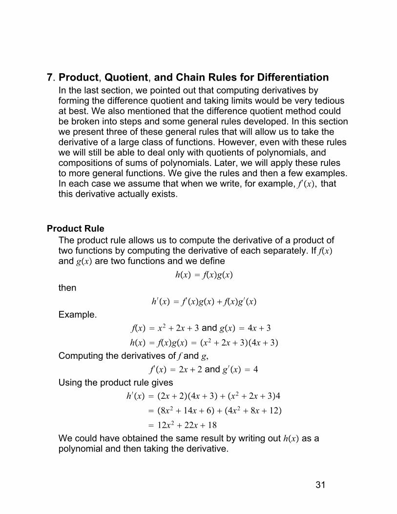
7. Product, Quotient, and Chain Rules for Differentiation
In the last section, we pointed out that computing derivatives byforming the difference quotient and taking limits would be very tediousat best. We also mentioned that the difference quotient method couldbe broken into steps and some general rules developed. In this sectionwe present three of these general rules that will allow us to take thederivative of a large class of functions. However, even with these ruleswe will still be able to deal only with quotients of polynomials, andcompositions of sums of polynomials. Later, we will apply these rulesto more general functions. We give the rules and then a few examples.In each case we assume that when we write, for example, f ′x, thatthis derivative actually exists.
Product Rule
The product rule allows us to compute the derivative of a product oftwo functions by computing the derivative of each separately. If fxand gx are two functions and we define
hx = fxgx
then
h ′x = f ′xgx + fxg ′x
Example.
fx = x2 + 2x + 3 and gx = 4x + 3
hx = fxgx = x2 + 2x + 34x + 3
Computing the derivatives of f and g,
f ′x = 2x + 2 and g ′x = 4
Using the product rule gives
h ′x = 2x + 24x + 3 + x2 + 2x + 34
= 8x2 + 14x + 6 + 4x2 + 8x + 12
= 12x2 + 22x + 18
We could have obtained the same result by writing out hx as apolynomial and then taking the derivative.
31

Quotient Rule
The quotient rule allows us to compute the derivative of a quotient oftwo functions by computing the derivative of each separately. If fxand gx are two functions and we define
hx =fxgx
then
h ′x =f ′xgx − fxg ′x
g2x
Example.
fx = x + 3 and gx = x2 + 1
hx =fxgx
= x + 3x2 + 1
Then
f ′x = 1 and g ′x = 2x
h ′x =f ′xgx − fxg ′x
g2x=
1x2 + 1 − x + 32xx2 + 12
= x2 + 1 − 2x2 − 6xx2 + 12
= −x2 − 6x + 1x2 + 12
Example. Here is another example that can be checked by a previousmethod.
fx = 1 and gx = x
hx =fxgx
= 1x
Then
h ′x =f ′xgx − fxg ′x
g2x= 0 − 1
x2= −1x2
Chain Rule
The chain rule allows us to compute the derivative of the compositionof two functions by computing the derivative of each separately. If fxand gx are two functions and we define
hx = fgx = f ∘ gx
32

then
h ′x = f ′gxg ′x
It is worth writing this out in words.
The derivative of the composition of fx with gx is the derivative offx evaluated at gx times the derivative of gx.Example. In this example we could obtain the same result by writingthe composition as a polynomial and then differentiating thepolynomial. Convince yourself that this would be a poor way tocompute the derivative!
fx = x10 and gx = x3 + x2 + x + 1
hx = fgx = x3 + x2 + x + 110
Then
f ′x = 10x9 and g ′x = 3x2 + 2x + 1
h ′x = f ′gxg ′x = 10x3 + x2 + x + 193x2 + 2x + 1
Finally, let’s use this last computation, and find the linearapproximation to
hx = x3 + x2 + x + 110
at x = 0. First we need the value of h ′0.We get this immediately fromthe above computation.
h ′0 = 10191 = 10
Hence the linear approximation to hx at x = 0 is
Lx = h0 + h ′0x − 0
= 1 + 10x
How good is this linear approximation of hx for values of x close to 0?
h.05 = 1.670078187 (approximately)
L.05 = 1.5
Note that the computation of L.05 is immediate, but the calculation ofh.05 requires a calculator or a great deal of paper!
33

8. Derivatives and Rates
One common practical application of the derivative is as ameasurement of rate of change. So for a quantity that is increasing wewant to measure how fast it is increasing. For a quantity that isdecreasing we want to measure how fast it is decreasing. Aninvestment that is growing quickly is better than one that is growingslowly (or decreasing!) and we would like a way to quantify this. Wefrequently use time as the independent variable when talking aboutrates, so in this section we will use the symbol t for our variable.
Let At denote a quantity whose value is changing with time. Perhapsthe most straightforward way to measure the rate of growth (assumeAt is increasing), at some particular time, T, is to compute AT,compute AT + 1, and take the difference, AT + 1 − AT. This givesus the average rate of growth over one time unit beginning at T. Moregenerally, we could compute
AT + ΔT − ATT + ΔT − T
=AT + ΔT − AT
ΔT
This gives us the average rate of growth over the time intervalT,T + ΔT per unit time since we have divided by the length of the timeinterval. You should recognize the above as a difference quotient verysimilar to what we used in computing the derivative. The instantaneousrate of growth at time T is the limit of the average rate of growth overthe interval [T,T+ΔT as ΔT tends to zero. Of course this is just thederivative! Thus the instantaneous rate of growth of At at t = T isA′T.
One particular quantity whose rate of change is physically important is“distance from a reference point.” The rate of change in this case iscalled velocity. For example, if xt represents the position of a pointon the x axis at time t, then x ′t represents the velocity of the point attime t.
The chain rule is often useful in computing rates. For example supposethe radius of a circle, rt, is increasing at a constant rate. This meansthat r ′t is a constant. Suppose this constant is 3, so r ′t = 3 for all
34

values of t How fast is the area of the circle changing when the radiusis 5? The relationship between area and radius is given by
At = πr2t
Applying the chain rule we have
A′t = 2πrtr ′t
Using the given values for r and r ′ we have
A′ = 2π53 = 30π
You might note that we omitted writing the t dependence of the left sideof the equation. The point here is that the rate at which the area isincreasing when r = 5 depends only on the value of r and itsderivative. It does not depend on t directly. We do not know the t valuethat corresponds to r = 5 and we don’t need to know this t value.
Higher Derivatives and Rates
There is a nice geometric or physical interpretation of the secondderivative of the distance function. It is acceleration. So if xtrepresents position (or distance from 0 then
xt distance
x ′t = vt velocity
x ′′t = v ′t = at acceleration
Note that if velocity is negative then xt is decreasing so the point ismoving to the left. If acceleration is negative then the velocity isdecreasing so the point is slowing down. The term acceleration is alsofrequently used in economics. For example, we can talk about“accelerating growth” to mean that the rate of increase of growth isincreasing. The term “inflation is increasing” or “accelerating inflation”is a statement about the second derivative of prices.
Example. Suppose sales of a small business are increasing at aconstantly increasing rate of 50 units per year per year. Current sales(t = 0 are 8,000 units, and sales are currently increasing at a rate of100 units per year. When will sales reach 10,000 units?
35

Let S(t) represent sales at time t measured in years from right now(t=0). We don’t have an expression for S(t) but we know S ′′t = 50.(Read the statement very carefully to understand where this comesfrom.) First let’s find an expression for S ′t. Since S ′′t is constant, wemust have S ′t = A + 50t.We know S ′0 = 100 so A = 100 andS ′t = 100 + 50t. Now what about St? From the expression for S ′t weconclude St = k + 100t + 50t2/2 where k is a constant. Convinceyourself this is true by taking the derivative. Now, since current salesare 800 units, we have k=8000. Hence the expression for St is
St = 8000 + 100t + 50t2/2
We want to know when sales will reach 10000 units.
St = 8000 + 100t + 50t2/2
10000 = 8000 + 100t + 50t2/2
solve for t to get
t = 7.165 (approximately)
Hence sales will reach 10000 approximately 7.165 years form now.
This example required you to realize that a function whose derivative isconstant must be linear and a function whose derivative is linear mustbe quadratic. We will come to more complicated inferences of this typewhen we consider antiderivatives and integration. For now, you shouldat least be able to verify the conclusions obtained above.
36

9. Increasing and Decreasing Functions
The derivative can be a very useful tool in graphing functions. In thissection we will use the derivative as an aid in graphing by determiningregions for which the function is increasing or decreasing. As a start,recall that the derivative of a function fx at a point corresponds to theslope of the tangent line to the graph of the function at that point. Thus,if the derivative is positive (negative), the slope of the tangent ispositive (negative). If the derivative is zero, the slope of the tangent iszero and therefore the tangent is horizontal. Here is a plot of fx = x2
showing the two tangents at x = 1 and x = −1.
For which value of x will the tangent be horizontal?
Now suppose we do not have an explicit expression for a function, butwe do know something about the derivative. For example, we mightknow where the derivative is positive and where it is negative. We canuse this information to get a rough idea of the graph of the function. Ifwe have specific values for the derivative at several points we can plottangent lines at those points and sketch in the graph.
Example. Suppose fx is a function with the following values of thederivative at five points.
37

x f ′x
−3 2
−1 −6
0 −1
1 10
2 27
From this information we see that the graph will have a horizontaltangent between x = −3 and x = −1.We also see that the tangent getsvery steep as we go from x = 1 to x = 2. Here is a sketch of a curvethat has the specified values for the derivatives.
Keep in mind that positive slope of the tangent corresponds to anincreasing function, negative slope of tangent corresponds to adecreasing function, and slope equal to zero corresponds to ahorizontal tangent.
A point (x value) at which f ′x = 0 is called a critical point of a function.The corresponding value of the function at a critical point is called acritical value. CAUTION. The term critical point is used in two different
38

ways. It may refer to the value of the argument of the function at whichthe derivative is zero or undefined (the x value) or it may refer to thevalue of the argument and the value of the function at that point (thex,y values. The context should make it clear if we are talking aboutthe x value alone or the x,y values. These points are importantbecause they indicate horizontal tangents and a possible maximum orminimum of the function. You should see that the functioncorresponding to the above graph has two critical points. In this case,these points correspond to a local maximum and a local minimum. Weuse the term local maximum (minimum) because if we look only at xvalues close to the critical points, then f will have a maximum(minimum) at the critical point. A graph concentrated around the criticalpoint should make this clear.
In this case, it is clear from the graph that these local maximum andlocal minimum values are not the maximum and minimum values thatthe function attains. Note that the function is increasing for x valuesslightly to the left of the critical point and it is decreasing slightly to theright of the critical point. Hence the derivative will go from positive tonegative (left to right) near the local maximum.
Note that a function may go from (for example) decreasing toincreasing with the derivative never equal to zero. The absolute valuefunction is an example ; the derivative (if it exists) is either −1 or +1.The derivative does not exist at zero.
39

At this point you should have a good understanding of the relationshipbetween the sign of the derivative and the increasing/decreasingbehavior of a function. In particular, you should be able to give anexample (by a graph) of a function with specified signs of thederivative.
40

10. Concavity
Concavity is an important concept in applications. Here are twoexamples from economics.
Decreasing Marginal Return. Suppose we invest resources inproduction of a product. A common phenomenon is decreasing returnon additional investment. In other words, when we first begin investinga resource, we see a large return for each unit of resource invested.But, as we invest more and more of the resource, each additional unitof resource does not result in as much additional production as theprevious unit of resource. How does this show up mathematically?Suppose Pr denotes production as a function of the amount ofresource, r. As r increases, P also increases. This means thatP′r > 0. Recall that P′r measures the marginal return. In otherwords, it measures how much production increases per unit increase inresource, r. Hence decreasing marginal return means that P′r isdecreasing. This means that the derivative of P′r is negative. But thederivative of P′r is just P′′r. Hence decreasing marginal returncorresponds to P′′r < 0. Here is the graph of a function with thisproperty.
A function with this property is said to be concave. The term concavedown is also sometimes used instead of simply concave.
Increasing Marginal Return Now we consider a situation with marginalreturn increasing. This occurs, for example, with deposits earning
41

interest. The larger the amount in the account, the faster the accountgrows. Suppose At denotes the amount in an account at time t. Theaccount earns interest so At is increasing with t. Hence, A′t > 0. Ifthe rate of increase also increases as A and t increase, then A′t is anincreasing function, Hence the derivative of A′t is positive, or in otherwords, A′′t > 0. Here is a graph of a function of this type.
A function with this property is said to be convex. The term concave upis sometimes used instead of convex.
We summarize the relationship between the second derivative of afunction, fx, and the shape of the graph.
Second Derivative Shape
f ′′x > 0 convex
f ′′x < 0 concave
One must keep in mind that the relationship between the sign of thesecond derivative and the convexity/concavity of the graph is a localproperty. In other words, the second derivative of a function may benegative in some regions of the domain and positive in other regions.An example is
42

fx = x3 − 4x
A computation gives f ′′x = 6x. Hence for x < 0, f ′′x < 0, and forx > 0, f ′′x > 0. Thus for x < 0 the graph is concave, and for x > 0 thegraph is convex.
For a continuous function it is possible to give a characterization ofconvexity and concavity that does not depend upon the secondderivative (which may not exist in many cases). Note that if we selecttwo points on the graph of a function which is convex, and connect thetwo points by a line segment, then the line segment lies on or abovethe graph of the function.
43

This property can be used to define convexity and concavity. It has theadvantage that is applies even in case the second derivative does notexist. For example, using this concept of convexity, the absolute valuefunction, |x|, is seen to be convex. The first two examples of thissection introduced convexity and concavity through the example ofmarginal return. If we have only marginal return data at a discrete setof points, and we do not have an explicit expression for the return orthe marginal return, we can still get an idea of the convexity/concavityproperties of the return by using this concept of convexity. Forexample, suppose we have the following set of data for the quantitySt as a function of t.
t St
1 1.3
2 3.8
3 9.2
Do you expect St to be concave or convex for t values from 1 to 3?
The first and second derivatives together (or equivalently theproperties of increasing/decreasing and convex/concave) give twopowerful tools that help us graph a function. We compute the first and
44

second derivatives, and determine regions for which the derivativesare positive and negative. We can then use this information, togetherwith the values of the function at a few points to get a rough idea of thegraph. Here is a summary for the function fx.
f ′ f ′′ Shape Example
+ + increasing and convex fx = x2 for x > 0
+ − increasing and concave fx = x for x > 0
− + decreasing and convex fx = 1/x for x > 0
− − decreasing and concave fx = −x2 for x > 0
We suggest you graph each of the examples to be sure youunderstand them.
45

11. Optimization
One of the fundamental and most common applications of basiccalculus is optimization. In other words, one would like to find the valueof a controllable quantity to give an optimum (maximum or minimum)result. For example, suppose we can vary the number of employees ata particular facility. We might be interested in determining the numberof employees that will maximize our profit or the number of employeesthat will minimize our cost. Note that the answer to the second problemis not necessarily zero as zero employees may result in a lostopportunity or lost profit cost.
The previous sections on increasing/decreasing functions andconvexity/concavity provide the necessary tools to solve manyoptimization problems. In many cases the most difficult part of anoptimization problem is the translation from a written description of theproblem to a mathematical description of the problem. It requires agreat deal of practice and experience to be able to perform thistranslation quickly and effectively. Hence, the only way to learn thismaterial is to work lots of examples. Here is one.
Inventory Control Problem. This example is used frequently infinding an optimal ordering policy for a product. Suppose a product issold at a steady rate. The seller has three costs associated withstocking the product. The costs are the purchase cost, a storage cost,and an order cost. Suppose the product is sold at a steady rate of 100units per month, and each unit costs $50. Each time the seller orders,a fixed cost of $20 is incurred. The storage cost is $10 per unit permonth. Suppose the seller places an order for Q units each time anorder is placed. The units are then sold at the constant rate until theyrun out. A new order for Q units is then placed. We want to find theoptimal order policy. In other words, determine the quantity Q thatshould be ordered each time an order is placed to minimize costs. Wewould also like to know the time between the placement of orders.
The first step is to write down an expression for the total cost per unittime (in this case one month). Let’s call this cost C.We have
46

C = O + S + P
O is the ordering cost
S is the storage cost
P is the purchasing cost
First we determine O , the ordering cost. Let N be the number of orderswe place per month. Since we order a quantity Q each time we order,and we need 100 units per month we must have
NQ = 100
or
N = 100Q
Now since we have an ordering cost of $20 each time we order, wehave a total ordering cost of
O = $20 × 100Q
dollars per month
Next we determine the storage cost S. Since we order a quantity Q andwe sell the product at a steady rate until we run out, we store anaverage of Q/2 units per order cycle. The same process repeats itself.At the beginning of a cycle we have Q units in stock and at the end ofthe cycle we have no units in stock. Hence on the average we haveQ/2 units in stock. Hence we finally get as the storage cost per month
S = $10 ×Q2.
Finally we compute the purchase cost. Since each unit costs $50 andwe need 100 units per month, our total purchase cost per month is
P = $50 × 100
We can now write down the total cost C per month as a function of Q.
C = 20 × 100Q
+ 10 × Q2 + 50 × 100
where we have omitted the $ signs. At this point, we might be temptedto simplify the arithmetic. However, there is an advantage in leavingthe expression for C in this form since we can easily see where each ofthe constants comes from. Here is a plot of C as a function of Q.
47

The next step is to find the value of Q that minimizes cost. Of coursewe are looking for a Q value greater than 0. The above plot gives us apretty good idea of the value we expect as a minimizer. To find theminimizing value of Q we differentiate the function CQ and set thederivative equal to 0.
C ′Q = −20 × 100Q2
+ 10 × 12
C ′Q = −20 × 100Q2
+ 10 × 12 = 0
10 × 12
= 20 × 100Q2
Q2 = 20 × 10010 × 1/2
= 2 × 20 × 10010
Q = 2 × 20 × 10010
Q = 20
So the Economic Order Quantity or EOQ (as the quantity thatminimizes cost is called) is 20 units. In other words, we should order20 units each time we order and we will order 5 times per month. You
48

should be able to provide an argument that this value actuallycorresponds to a minimum (and not a maximum). Notice from the costfunction, that for very small values of Q the cost is very large.
This example was somewhat complicated, but it illustrates what isinvolved in solving real world business problems. Note that we solvedthe problem by breaking it up into several steps. It seems pretty clearthat setting up the problem in mathematical form is the most difficultpart. It should also be clear at this point how we can use the abovecalculations to develop a general expression for the EOQ that holds forarbitrary values of the costs. Let s denote the storage cost per unittime, K the ordering cost per order, and d the demand or number soldper unit time. Write down an expression for the EOQ (call it Q∗) interms of s,K, and d. Note that the price per unit plays no role indetermining the EOQ.
49
12. Exponential and Logarithmic Functions
Exponential and logarithmic functions occur frequently in mathematicalmodels for economics, finance, other social sciences as well as in thenatural sciences. For example, the exponential function is used tomodel the growth of stock and bonds, radioactive decay, and growth ofbacteria, and the logarithmic function is used to model the utility ofwealth. A good understanding of these functions is essential for allfields that use mathematical models.
First we review some of the basic rules and notation for exponentialsand logarithms. For a positive number a and a positive integer n, wehave
an = a × a × a × ⋅ ⋅ ⋅ ×a
where the a on the right side of the equation appears n times. Similarlyfor n a positive integer
a1/n = b
means
b × b × ⋅ ⋅ ⋅ ×b = a
where the b appears n times on the left side of the equation. Puttingthese two notations together we write, for example,
a3/2 = a1/23
We also write
a−1 = 1a
Now with the notational rule for composition for exponentials,
apq = apq
and the first three notational rules, we can define exponentials forrational numbers (quotients of integers). When the exponent is not arational number, a precise definition of the exponential is much moredifficult and involves a limit in one form or another. At any rate thefollowing notational rules hold even when the exponent is not a rational
50

number.
apq = apq
apaq = ap+q
1ap
= a−p
ap
aq= ap−q
a0 = 1
The logarithm is the inverse of the exponential. Hence we must havesome way to indicate the base used in the exponential when we write alogarithm. For example
23 = 8
log28 = 3
express a relationship between the numbers 2,3 and 8 in two differentbut equivalent ways. The second equation requires a subscript on thelog to indicate the base. If the base is 10 we frequently omit thesubscript. Hence
102 = 100
log10100 = log100 = 2
There are notational rules for logarithms that correspond to the rulesfor exponents. We give examples using the base 10 logarithm.
logap = p loga
logab = loga + logb
log 1a = − loga
log ab = loga − logb
log1 = 0
There is one base for exponentials that has very nice properties ofdifferentiation that we will see later. This base is the real number ewhich is approximately 2.71828. The number e is not a rationalnumber; it can not be written as a fraction. (The number π is anotherexample of an irrational). It is so important for applications that mostcalculators have a function that enables them to compute powers of e.
51

Perhaps the easiest way to define the number e is as a limit.
e = limn→∞
1 + 1n n
The numbers n in the limit are taken to be positive integers. Forexample
1 + 110000
10000 is approximately 2.718145927
The logarithm associated with the base e is called the natural logarithmand frequently written as ln .We have for example
If a = e5 then
lna = 5
Since the exponential and logarithm are inverses of one another, wehave
e lna = a and
lneb = b
Now we are ready to discuss the exponential and logarithmic functions.We consider the function defined by exponentiating the number e.
fx = ex
This is often written as
expx = ex
Here is a plot of this function.
52

Because the function increases so rapidly, it might have been moreconvenient to have chosen different scales on the horizontal andvertical axes. However, we use the same scale to help explain the niceproperty of the exponential function when e is used as base. First notethat
e0 = 1
as one sees from the plot. Note also the slopes of tangents to thegraph are always positive and increase as we move left to right on thegraph. What about the slope of the tangent through the point 0,1?You should be able to see that the slope of the tangent through thispoint would be fairly close to 1. In fact it is 1. The important property ofthe exponential function with respect to differentiation can almost beseen from the graph. That property is
53

If fx = expx = ex then
f ′x = expx orddx
expx = expx
In other words the exponential function is its own derivative!
Because of this property of the exponential function, it is very importantthat we be able to express other exponential functions in terms of thenatural exponential. For example
2x = 2x = e ln2x = eln2x
Note how we used the in the first step to help us rewrite theexponential base 2 in terms of the natural exponential. You should beable to do this for any base. Now we can combine this with the chainrule to compute some more complicated derivatives. For example
ddx
expkx = kexpx
ddx
expx2 = 2xexpx2
By applying the natural logarithm to a variable, we get the naturallogarithm function
lnx
Here is a plot.
Note that this function is defined only for positive values of x. Also notethat the graph passes through the point 1,0 since ln1 = 0. Againnotice that the slope of the tangent to the graph through the point 1,0
54

seems to be close to the value 1. In fact it is 1. Using the definition ofthe derivative as a limit, it is possible to compute the derivative of thefunction lnx.
ddx
lnx = 1x
You should at least be able to see that this is consistent with the graph.The derivative is positive for positive values of x and the derivativebecomes a large positive number as x gets close to 0. Again, using thechain rule we can compute some more complicated derivativesinvolving the natural logarithm. for example
ddx
ln3x + 1 = 33x + 1
Now let’s turn to some applications. First we go back to the problem ofcompound interest. Recall that if we earn interest at a rate rcompounded n times per year and we deposit $1 at the beginning ofthe year, then at the end of the year we have an amount A with
A = 1 + rn
n
If we let1k
= rn
then this can be written as
A = 1 + 1kkr = 1 + 1
kkr
Now when n is very large, k is also very large (for a fixed value of theinterest rate r. But for large values of k, the expression inside thesquare brackets,
1 + 1kk
is very close to the number e. In fact,
limk→∞
1 + 1kk = e.
Hence the amount in the account is approximately
A er
For example if the interest rate is 7% or .07 then now matter how manytimes per year we compound the interest we will never have more than
e .07 1.072508181
with an initial deposit of $1.
55

Continuously Compounded Interest. From the above example we seethat the amount in an account that pays interest at rate r with an initialdeposit of $1 will contain no more than the amount er at the end of oneyear. If the amount, At, at time t in an account that pays interest at arate r, with an initial deposit of K is given by
At = Kert
then we say that interest is compounded continuously. In fact, it ismuch easier to work with this model for growth of money in a bondthan it is to work with the model of growth with interest compounded atdiscrete time intervals. Hence, for pricing and modeling many financialinstruments, it is the model of choice.
56

13. Antiderivatives
In the previous sections we have seen how the derivative of a functioncan be used to give us information about the function itself. Forexample, the first derivative tells us when a function is increasing ordecreasing, and the second derivative tells us if the function is convexor concave. It is natural to ask if the derivative tells us even moreabout the function. In other words, suppose we know the derivative ofa function. How much do we know about the function itself? Theanswer is - almost everything. This is the idea of the antiderivative. Wewould like to be able to reconstruct the function itself from thederivative. In fact, to accomplish this we need one additional bit ofinformation about the function - we need the value at a single point.
Here is the simplest example. Suppose the function fx has theproperty that its derivative is 0 for all values of x. In other words
f ′x = 0 for all x
What can we say about fx? Since the tangent to the graph of fx ishorizontal everywhere, it should be intuitively clear that fx must beconstant. We cannot determine the constant without more informationsince all constant functions have the property that their derivativesequal 0 for all x values. However, if we know the value of fx at asingle point, then we know the value of this constant. We summarizethis as follows.
If f ′x = 0 for all x and
fa = A then fx = A for all x.
Here is a second example.
Suppose fx = k for all x
Then fx = kx + c where c is a constant.
For example suppose
57

f ′x = 3 for all x and f2 = 5
Then fx = 3x + c for some constant c
Since f2 = 5 we have f2 = 3 × 2 + c = 5
or 6 + c = 5 so c = −1 and
fx = 3x − 1It should be clear at this point that finding the antiderivative of afunction (in other words finding a function whose derivative equalssome given expression) involves working backwards from thedifferentiation process. Hence the more differentiation examples youhave worked, the easier it will be to find antiderivatives. It might help torecall the rules for differentiation since these will play a role in findingthe antiderivatives. First,
ddx
fx + gx = f ′x + g ′x
Hence to find the antiderivative of a sum we simply find theantiderivative of each term in the sum and then add the antiderivatives.For example
If F′x = 3x + 7 and F1 = 2 then
Fx = 3 x2
2 + 7x + c
We get this by noting that an antiderivative of x is x2/2 and anantiderivative of 7 is 7x. If we differentiate the above expression for Fxwe do get 3x + 7. Now we determine the constant c.
Fx = 3 x2
2 + 7x + c so
F1 = 3 12
2 + 7 × 1 + c = 2
c = 2 − 3 12
2 − 7 = 1/2 − 7 = −13
2and
Fx = 3 x2
2 + 7x + −13
2
A more complicated example involves the chain rule. Recallddx
Fux = F′ux × u ′x = u ′xF′ux
Suppose we are given
H ′x = 2xx2 + 8
If we let
58

ux = x2 + 8 then u ′x = 2x
Therefore we can write
H ′x = u ′xF′ux if
F′u = u since then F′x2 + 8 = x2 + 8
Now we must find Fu. Since
F′u = u
Fu = u2
2+ c
This gives
Hx = Fux + c =ux2
2+ c
=x2 + 82
2+ c
You should check this by differentiating the expression for Hx to besure you get 2xx2 + 8.
The above method of finding the antiderivative is known as substitutionsince we substituted the symbol u for the expression x2 + 8.We didthis since the derivative of u appeared in the original expression forH ′x ; it was 2x. The method of substitution works when we are giventhe derivative of a composition.
Notation The following notation is used for the antiderivative of afunction fx,
Antiderivative of fx is written as ∫ fxdxNote that the antiderivative is determined only up to a constant. If weare given the value of the antiderivative at some point, then thisconstant can be determined. Another term used (perhaps morecommonly) for the antiderivative is the integral and the sign, ∫, is an
“integral” sign. Writing the term dx after the function fx is customaryfor historical reasons that we shall explain in the next section. Howeverthe dx does serve the useful purpose of reminding us that the functionexpression is to be considered as a function of x. This may beimportant when the function contains one or more parameters. For
59

example
∫x + Adx = ?
The symbol A is to be regarded as a constant parameter and thevariable is x. A more subtle example is
∫x + tdtIn this case x is to be regarded as a constant parameter and thevariable is t. You should evaluate both integrals above.
The dx plays a second useful notational (or heuristic) role with respectto actually evaluating integrals (or finding antiderivatives) bysubstitution. Let’s rework the example with substitution (after making itslightly more complicated).
∫2xx2 + 83dxLet
u = x2 + 8
Again we make this substitution since the derivative of u appears afterthe integral sign. Now we write
du = 2xdx
This “equation” can be given a precise mathematical meaning but youshould realize that our discussion of the derivative does not give aprecise definition. (We defined
dudx
= u ′x
as a limit, but du by itself does not mean anything. At any rate thenotational trick above, du = 2xdx makes the substitution method veryalgorithmic. Substituting u and du in the integral, integrating (or findingthe antiderivative), and substituting back, gives
∫2xx2 + 83dx = ∫x2 + 832xdx = ∫ u3du = u4
4+ c =
x2 + 84
+ c
Most people find this notational trick very helpful in makingsubstitutions for finding antiderivatives.
Finding antiderivatives is something of an art (or skill with algebra) and
60

many methods have been devised to help. Many calculators are ableto find the antiderivatives of a large number of functions, so perfectingthis skill is not terribly important. However, you should be able to dosimple examples such as those above and the problems from thehomework.
It is very important to realize that it may be impossible to write down anexplicit expression for the antiderivative of even fairly simple functions.For example,
∫ expx2dx = ∫ ex2dxcannot be written in terms of functions involving exponentials andpolynomials. This antiderivative plays an extremely important role instatistics.
61

14. Integrals
In the last section we discussed the antiderivative and introduced the“integral sign”, ∫, as notation for the antiderivative. So, in some sense
we have already discussed ”integrals”. However the integral has asecond interpretation, a geometric interpretation that was historicallydeveloped before the antiderivative. This section concerns thegeometric meaning of the integral and will explain the integral notation.
The integral was developed to solve the problem of finding the areaenclosed by a curve - a circle for example. We can algebraicallycompute areas only for very simple curves or figures such asrectangles, trapezoids, and right triangles. How might we find the areaenclosed by a circle or a more complicated curve? One approachwould be to fill up the area by many small rectangles, compute thearea of each rectangle, and then add up all of the areas. Of course,this would give only an approximation since we cannot exactly fill thearea inside the circle with small rectangles. However, we could getbetter and better approximations by making the rectangles smaller andsmaller. With some good fortune we would be able to compute thelimiting value of the total areas of the rectangles. This is exactly theidea of the integral.
The remarkable result of calculus is the equivalence of the problem offinding area enclosed by a curve and the antiderivative. This result isknown as the fundamental theorem of calculus. We first consider anexample where we can check the result by algebra. Let
fx = x
62

Suppose we want to find the area under the curve fx = x, above the xaxis, and between the vertical lines, x = 0 and x = 3. In other words,we just want to find the area of the right triangle with nonhypotenuseside lengths 3 and 3.We know the answer by algebra. The area is
A = 123 × 3 = 9
2
We could, using the idea of approximation mentioned above, get anapproximate value by filling up, as best as possible, the triangle byrectangles. The base of each rectangle will lie on the x −axis, and theheight of each rectangle will be as large as possible without goingoutside the triangle. For example, if the rectangles are placed side byside with base length 1, we get for the approximate area
A ≊ 1 × 0 + 1 × 1 + 1 × 2 = 3
If the base length is 1/2 we get for the approximate area
A ≊ .5 × 0 + .5 × .5 + .5 × 1 + .5 × 1.5 + .5 × 2 + .5 × 2.5 = 3.75
If the base length is .1, we get for the approximate area
A ≊ .1 × 0 + .1 × .1 + .1 × .2 +⋅ ⋅ ⋅ +.1 × 1.9 = 4.35
The approximations are getting closer and closer to the actual value ofthe area. In order to explain the integral sign notation and to give theprecise expression of the area as a limit we introduce one additional bitof notation that is commonly used in many applications - thesummation notation. Suppose the length of each base is some smallvalue we call Δx. Then the total number of rectangles will be N with
N = 3Δx
The first rectangle will have height 0 and the last rectangle will have
63

height 3 − Δx. The approximate area will be
A Δx × 0 + Δx × Δx + Δx × 2Δx +⋅ ⋅ ⋅ +Δx × N − 1ΔxThere are N terms in the sum (since the first term is 0). The notation forthis is
A ∑k=0
k=N−1
kΔxΔx
Note that the value kΔx is just the value of the function fx = xevaluated at the point kΔx. Therefore we could write the above sum as
A ∑k=0
k=N−1
fkΔxΔx
The value k = 0 corresponds to x = 0 and k = N − 1 corresponds tox = 3 − Δx. Now we can write the actual area as a limit.
A = limΔx→0
∑k=0
k=N−1
fkΔxΔx = ∑k=0
k=N−1
kΔxΔx
Note that as Δx → 0 N → ∞. In other words as the base length tends tozero, the number of rectangles tends to infinity.
In fact this is precisely the definition of the integral, and we write
∫0
3
fxdx = limΔx→0
∑k=0
k=N−1
fkΔxΔx
where N = 3Δx
The exact same definition is used when fx is an arbitrary function.
In general it would be extremely difficult to write down the sum andcompute the limit as above (although in the above case we could dothis quite explicitly). However, this is often unnecessary since thefundamental theorem of calculus tells us that the integral defined as alimit can be computed from the antiderivative. In the above examplewe found the area between the x-axis and the graph of the functionfx = x for x between 0 and 3. In general we can use any values welike for the variable. In this case we write
64

∫a
b
fxdx = limΔx→0
∑k=1
k=N
fxkΔx
Here, the points xk are points on the x-axis with x1 corresponding to thepoint a and xN corresponding to the point b − Δx. (We could just as welllet x1 correspond to the point a + Δx and xN corresponding to the pointb.) The number N equals the number of rectangles we use in anapproximation. N ×Δx = b − a. The above expression for the integralcan be modified in various ways. For example, it is not necessary touse rectangles with the length of the bases equal to one another, butfor simplicity we will stick to the above form when possible. Weincorporate the above expression for the integral and the integralnotation for the antiderivative to give a statement of the
Fundamental Theorem of Calculus
Fb − Fa = ∫a
b
fxdx = limΔx→0
∑k=1
k=N
fxkΔx
where
F′x = fx
In other words, to evaluate the area between the graph of fx and thex-axis for x between a and b, we compute the difference of theantiderivative of fx, namely Fx, evaluated at a and b.
The above example with fx = x, a = 0, and b = 3 follows.
∫0
3
fxdx = ∫0
3
xdx = F3 − F0
where
Fx = x2
2is an antiderivative of fx = x
Hence
∫0
3
fxdx = ∫0
3
xdx = F3 − F0 = 32
2− 0
2
2= 92
Here is a more complicated example. Find the area between the graphof fx = x2 and the x −axis for x between 1 and 4.
65

∫1
4
x2dx = F4 − F1 with Fx = x3
3
∫1
4
x2dx = F4 − F1 = 43
3− 1
3
3= 633
= 21
What about functions that take on negative values? For example,consider the function fx = −x2 for x ≥ 0. The antiderivative offx = −x2 is Fx = −x3/3. Hence if we use the above expression for theintegral we have
∫1
4
−x2dx = F4 − F1 with Fx = −x33
∫1
4
x2dx = F4 − F1 = −433
− −133
= −633
= −21
In other words we just get the negative of the previous result. Fornegative functions the integral will be negative. If a function issometimes positive and sometimes negative on a certain interval, thenintegrating over that interval will result in some of the negativecontribution canceling some of the positive contribution. For example
∫−3
3
xdx = F3 − F−3 with Fx = x2
2
∫−3
3
xdx = F3 − F−3 = 32
2− −32
2= 0
One must be very careful about signs when using the integral to
66

compute area since area must have a positive value.
We observed above that multiplying a function by −1 and integratinggives the negative of the integral of the function. This property can beextended to multiplication by any constant. The basic properties ofderivatives transfer over to corresponding properties for integrals. Thetwo most important properties are linearity.
∫a
b
kfxdx = k ∫a
b
fxdx
∫a
b
fx + gxdx = ∫a
b
fxdx + ∫a
b
gxdx
Another important additive property of the integral lets us break upintegration over an interval into the sum of integrals over subintervals.
If a < b < c then
∫a
c
fxdx = ∫a
b
fxdx + ∫b
c
fxdx
As we pointed out in the section on antiderivatives, even very simplefunctions may not have antiderivatives that can be written in terms ofelementary functions such as polynomials, exponentials, and so on. Inthis case it may be only possible to obtain approximations to theintegral using the rectangle method.
Another important application of the summation approximation to theintegral is the case of an unknown function. We first explain what wemean by the average of a continuous function. What value we woulduse for the “average” of the function fx = x2 for x between 1 and 4? Apicture will help.
67

The horizontal line is at height 7 and the area under the horizontal lineequals the area under the graph of fx = x2 for 1 ≤ x ≤ 4. So theaverage is just the value of the integral divided by the length of theinterval over which we integrate.
Avgfx = 1b − a ∫a
b
fxdx
Now suppose we have collected data that represents the values ofsome unknown continuous function of time at various points in time.Here is an example of what such data might look like.
Time 0 1 3 4 7 8 10 13
Function Value 1.2 3.4 5.1 6.7 8.2 9.3 14.6 17.0
How would we find the “average value” of this function between times0 and 13? It would not make sense to simply add all the functionvalues and divide by the total number of values (Why not? ). The totallength of the interval of x values is 13. Hence if we approximate theintegral of the unknown function using rectangles and then divide by 13we will have an approximation to the average. To approximate theintegral we have
68

Approximate Integral = 1 − 0 × 1.2 + 3 − 1 × 3.4 + 4 − 3 × 5.1 +
7 − 4 × 6.7 + 8 − 7 × 8.2 + 10 − 8 × 9.3 + 13 − 10 × 14.6
= 103.8
We can therefore compute the approximate average of the function f.
Avgf ≊ 103.813
= 7.98
69