a brief introduction to pde constrained optimization · a brief introduction to pde constrained...
TRANSCRIPT

A brief introduction to PDE constrainedoptimization
Harbir Antil
Department of Mathematical SciencesGeorge Mason University
hantilgmuedu
June 6 2016
Frontiers in PDE-constrained OptimizationInstitute for Mathematics and its Applications
Funding ExxonMobil IMA
H Antil 060616 1
Outline
Motivation and examples
Linear elliptic optimal control problems
Differentiation in Banach spaces
First-order necessary conditions
Optimal control of semilinear PDEs
An abstract problem
Discretization using finite element methods
H Antil 060616 2
Outline
Motivation and examples
Linear elliptic optimal control problems
Differentiation in Banach spaces
First-order necessary conditions
Optimal control of semilinear PDEs
An abstract problem
Discretization using finite element methods
H Antil 060616 3
Controlling pollutants in river Antil Heinkenschloss Hoppe 2010
(Loading movieavi)
H Antil 060616 4
Outline
Motivation and examples
Linear elliptic optimal control problems
Differentiation in Banach spaces
First-order necessary conditions
Optimal control of semilinear PDEs
An abstract problem
Discretization using finite element methods
H Antil 060616 3
Controlling pollutants in river Antil Heinkenschloss Hoppe 2010
(Loading movieavi)
H Antil 060616 4
Controlling pollutants in river Antil Heinkenschloss Hoppe 2010
(Loading movieavi)
H Antil 060616 4

Magnetic drug targeting Antil Nochetto Venegas 2016
The magnetic field exerts a force on magnetic materials such as magneticnanoparticles (MNPs)
Experimental setup (Shapiro et al 2013)
H Antil 060616 5
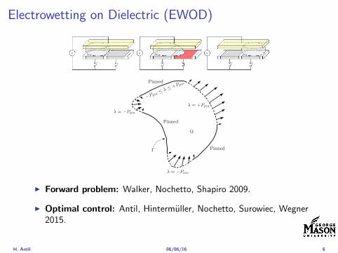
Electrowetting on Dielectric (EWOD)
maximal ldquopinning pressurerdquo Ppin=2cpin H in dimensionalform which represents the maximum opposing force perliquid-gas interface area that the contact line can applyagainst motion of the interface The factor of ldquo2rdquo accountsfor the interface contact line pinning at the floor and ceilingof the EWOD device The nondimensional pinning pressureis then given by
Ppin =1P0
2cpin
H 12
where P0 is the dimensional reference pressure scale forceper unit of area
This allows us to introduce a locally defined pinningpressure into the boundary conditions in nondimensionalform
p = + E + 13
= Ppin sgnu middot n
In other words if the normal velocity of the liquid-gas inter-face is positive then the pinning pressure will push backwith maximum positive pressure +Ppin to limit the motionLikewise if the normal velocity is negative the pinningpressure will push back in the opposite direction Ppin Andif the normal velocity is zero then takes on a value be-tween Ppin and acts as a Lagrange multiplier to enforce theconstraint that the interface does not move also see Fig 5This definition of ensures $ Ppin and so is consistentwith the experimental observation in Sec II D 1
Numerical implementation of this simple phenomeno-logical model is difficult because of the discontinuity $thesign function of Eq 13 see Fig 6 This discontinuityhowever is essential If it was replaced by a smooth functionthen no droplet could ever be pinned in a noncircular shapesomething that does occur in the experiments see Fig 12below To show this we argue by contradiction Assume no
EWOD forcing so the boundary pressure is given by p=+ $from Eq 13 Suppose the droplet has become com-pletely pinned in a noncircular shape but the function relat-ing to the normal front velocity u middotn is smooth Any sym-metric smoothed version f of the sign function ldquosgnrdquo musthave = Ppinf0=0 which implies p= by Eq 13 But ifthe droplet is pinned in a noncircular shape then will notbe constant around the droplets circumference hence thepressure field inside the droplet will not be constant72 ByEq 1 the velocity u will not be zero which contradicts thedroplet being pinned Note that a smooth but steep function fwill lead to a slowly creeping liquid but only a discontinu-ous f can truly pin the liquid Moreover our model with thesgn function is a physically motivated description538ndash4463ndash68
Our model with Eq 13 is nonlinear and introduces thevelocity into the pressure boundary conditions Moreover itis local meaning that multiple parts of the boundary canbe pinned and unpinned simultaneously Furthermore the re-gions where the droplet is pinnedunpinned are not known apriori this must be determined as part of the solution Ourpinning model is similar to the Signorini problem inelasticity73 which models the deformation of an elastic bodyagainst a rigid obstacle and utilizes a contact variable to en-force the rigid constraint similarly to our Our model canbe increased in complexity see Sec II D 3 to account formore interesting contact line dynamics54ndash57 We are able toinclude this model into our variational formulation of SecIII and we have a method of solving for the velocity pres-sure and 2574 Knowing immediately yields where theboundary is pinnedunpinned
One important issue here is the three-phase linesingularity75ndash77 which originates because of an apparentparadox between the no-slip boundary condition on the wallsof the device and the fact that the contact line moves Ourformulation is only a two dimensional description as appro-priate for planar devices We do not track the location of thethree-phase line in our model in three dimensions we onlyhave an ldquoaveragedrdquo description of the liquid-gas interfaceRecall that the velocity field in the z direction is parabolic afundamental assumption in Hele-Shaw flow Thus in our
Pinned
Pinned
Pinned
= Ppin
= Ppin
= +Ppin
Ppin +Ppin
FIG 5 A two dimensional droplet top view with parts of the boundarypinned electrode grid not shown The pinned regions are denoted by asolid line unpinned regions are shown as a dashed line with velocity arrowsindicating direction of motion An outward motion is considered positiveu middotnamp0 and an inward motion is negative u middotn0 The pinning variable is defined on the boundary of the droplet On the unpinned regions thevalue of saturates to Ppin On the pinned regions u middotn=0 variesbetween Ppin and +Ppin see Fig 6 In our simulations Ppin is used toindicate where the boundary is pinned
+Ppin
Ppin
u middot n
FIG 6 A more realistic relationship between the resistive pressure at theinterface and the normal velocity Here $+Dviscu middotn is plotted as the thickline Note how the interface pressure increases with increasing velocity Thedashed line depicts a slightly more nonlinear relationship $+Dviscu middotn+Gfricu middotn $see Eq 16 The qualitative form of the dashed line has beenshown in the work of Refs 54ndash57 Note the dashed line asymptotes towardthe thin line Dviscu middotn
102103-6 Walker Shapiro and Nochetto Phys Fluids 21 102103 2009
Downloaded 29 Jun 2010 to 168725468 Redistribution subject to AIP license or copyright see httppofaiporgpofcopyrightjsp
I Forward problem Walker Nochetto Shapiro 2009
I Optimal control Antil Hintermuller Nochetto Surowiec Wegner2015
H Antil 060616 6
Shape optimization of microfluidic biochip Antil
Heinkenschloss Hoppe Linsenmann Wixforth 2010
Microfluidic Biochip
H Antil 060616 7
PDE constrained optimization
PDE constrained optimization or optimal control of PDEs (OCP) has 4major components
I control z
I state u which associates with every control z a state u
I cost functional J which depends on z and u to be minimized
I constraints obeyed by z (control constraints) and u (stateconstraints)
Today
I Control constraints are pointwise ae
I State equation is a boundary value problem or a variationalinequality
H Antil 060616 8
Steps to analyze OCPAnalysis
I Existence of solution to PDE Is it unique
I Existence of solution to optimization problem
I First-order necessary conditionsI Adjoint equations
I If possible second order necessarysufficient conditions
Solver development (function space)
I GradientHessian based
Discrete problem solver
I FD FV FE for problem and solver
I Analysis of discrete solver mesh independence
I EfficiencyI Adaptive finite element methods (AFEM)I Model reduction Proper orthogonal decomposition reduced basis
I Software development Trilinos Rapid Optimization Library (ROL)Dolfin-Adjoint
H Antil 060616 9
Optimal heat sourceI Domain Let Ω sub Rd d ge 1 be open bounded Lipschitz domain
with boundary partΩ
I Goal Choose a distributed source z in such a way that thetemperature u = u(x) is close to a desired ud = ud(x) in Ω
Linear-quadratic elliptic OCP
min J(u z) =1
2uminus ud2L2(Ω) +
λ
2z2L2(Ω)
subject to
minusdiv (Anablau) = z in Ω
u = 0 on partΩ
and the pointwise control constraints
z isin Zad = v isin L2(Ω) za(x) le v(x) le zb(x) ae x isin Ω
λ gt 0 is a parameter za zb isin Linfin(Ω) with za lt zb are given A isbounded symmetric positive
H Antil 060616 10
Problems involving semilinear elliptic PDEsI Heating with radiation boundary condition If the heat radiation
of the heated body is taken into account then we obtain
minus∆u = 0 in Ω
partνu = α(z4 minus u4) on partΩ
where the control z is the temperature of the surrounding medium
I Simplified supercondutivity
minus∆u+ u+ u3 = z in Ω
u = 0 on partΩ
I Control of stationary flows
minusmicro∆u + (u middot nabla)u +nablap = f in Ω
div u = 0 in Ω
u = g on partΩ
H Antil 060616 11
Optimal control of variational inequalitiesProblem
min J(u z) =1
2uminus ud2L2(Ω) +
λ
2z2L2(Ω)
subject to u isin K = w isin H10 (Ω) w(x) ge 0 ae x isin Ωint
Ω
nablau middot nabla(uminus v) dx le (z + f uminus v) forallv isin K
with z isin Zad
Regularized problem
min J(u z) =1
2uminus ud2L2(Ω) +
λ
2z2L2(Ω)
subject to (semilinear PDE)
u isin H10 (Ω) minus∆u+ γρε(minusu) = z + f in Ω
and z isin Zad γ gt 0 and ε gt 0 are the penealization and regularizationparameters respectively
H Antil 060616 12
Outline
Motivation and examples
Linear elliptic optimal control problems
Differentiation in Banach spaces
First-order necessary conditions
Optimal control of semilinear PDEs
An abstract problem
Discretization using finite element methods
H Antil 060616 13
Linear elliptic problemsΩ sub Rn bounded Lipschitz domain
Sobolev spacesI Lp(Ω) 1 le p le infin are Lebesgue spaces p = 2 L2(Ω) is a Hilbert
space with inner product (u v) =int
Ωu(x)v(x) dx
I W sp for s isin R 1 le p le infin are Sobolev spaces When p = 2W s2(Ω) = Hs(Ω) is a Hilbert space
I H10 (Ω) = v isin H1(Ω) v|partΩ = 0 with norm (due to Poincare
inequality)uH1
0 (Ω) = nablauL2(Ω)
I H10 (Ω)lowast = Hminus1(Ω)
I Note L2(Ω) sub Hminus1(Ω)
Model problem
minusdiv (Anablau) = f in Ω
u = 0 on partΩ
H Antil 060616 14
Well-posed
I Weak solution Given f isin Hminus1(Ω) a function u isin H10 (Ω) is called
a weak solution iffintΩ
Anablau middot nablav = 〈f v〉minus11 forallv isin H10 (Ω)
where 〈middot middot〉minus11 denotes the Hminus1(Ω)ndashH1(Ω) duality pairing
I Existence and uniqueness For each f isin Hminus1(Ω) there exists aunique u isin H1
0 (Ω) such that
nablauL2(Ω) le CdΩfHminus1(Ω)
I A = I the result is due to the Riesz-representation theorem
I A 6= I (maybe non-symmetric) the result is due to Lax-Milgramlemma
I For general W 1p-spaces use inf-sup conditions combined withBanach-Necas theorem which is a necessary and sufficient condition
H Antil 060616 15
Linear-quadratic elliptic OCP
min J(u z) =1
2uminus ud2L2(Ω) +
λ
2z2L2(Ω)
subject to
minusdiv (Anablau) = z in Ω
u = 0 on partΩ
and the pointwise control constraints
z isin Zad = v isin L2(Ω) za(x) le v(x) le zb(x) ae x isin Ω
λ gt 0 is a parameter za zb isin Linfin(Ω) with za lt zb are given A isbounded symmetric positive
H Antil 060616 16
Reduced OCP
I Control to state map The solution operator defined as
S Hminus1(Ω)rarr H10 (Ω) z 7rarr u(z) = Sz
Note In view of the embedding
H10 (Ω) rarr L2(Ω) rarr Hminus1(Ω)
we may also consider S from L2(Ω) to L2(Ω) We will use the samenotation for this operator (for simplicity)
I Reduced cost functional The reduced cost functionalJ L2(Ω)rarr R is defined as
J (z) = J(Sz z)
I Reduced problem minzisinZadJ (z)
H Antil 060616 17
Existence of solution Direct methodThere exists a unique solution to the above problem
I Minimizing sequence J is bounded below by zero therefore thereexists a minimizing sequence znnisinN such that
limnrarrinfin
J (zn) = inf J (z)
I Weak compactness zn sub L2(Ω) is bounded Since L2(Ω) isreflexive therefore there exists a subsequence (not relabeled) suchthat
zn z and z isin Zad
where the latter is a consequence of Zad being closed and convex
I Optimality Since J is continuous and convex and therefore isweakly lower semicontinuous We obtain
lim inf J (zn) ge J (z)
which implies that z is optimal
I Uniqueness Exercise
H Antil 060616 18
Outline
Motivation and examples
Linear elliptic optimal control problems
Differentiation in Banach spaces
First-order necessary conditions
Optimal control of semilinear PDEs
An abstract problem
Discretization using finite element methods
H Antil 060616 19
Differentiation in Banach spacesLet (Z middot Z) (V middot V ) B-spaces Z sub Z open and F Z rarr V
Let z isin Z
I If exist δF (z h) = limtdarr01t (F (z + th)minus F (z)) then δF (z h) is called
the directional derivative of F at z in direction h
I If exist δF (z h) forallh isin Z then h 7rarr δF (z h) is the first variation of Fat z
I Let exist the first variation δF (z middot) F is said to be Gateauxdifferentiable at z iff existA isin L(Z V ) such that δF (z h) = Ahforallh isin Z We write A = F primeG(z)
I F is said to be Frechet differentiable at z iff existA isin L(Z V ) and amapping r(z middot) Z rarr V such that for all h isin U with z + h isin Zwe have
F (z+h) = F (z)+Ah+r(z h) withr(z h)VhZ
rarr 0 as hZ rarr 0
We write F prime(z) = A
H Antil 060616 20
ExamplesExample 1 (H (middot middot)H) Hilbert space F (z) = z2H = (z z)H
forallz h F (z + h)minus F (z) = 2(z h)H + h2HThen
F prime(z)h = (2z h)H
Reisz representation theorem (identify H with Hlowast) we can write
F prime(z)h = (nablaF (z) h)H
where nablaF (z) = 2z is the gradient
Example 2 Let (Z (middot middot)Z) (H (middot middot)H) Hilbert spaces ud isin H fixedLet S isin L(ZH) Consider E Z rarr R
E(z) = Sz minus ud2H
Then E(z) = G(F (z)) where G(v) = v2H and F (z) = Sz minus ud
Eprime(z)h = Gprime(F (z))F prime(z)h = (2v F prime(z)h)H
= 2(Sz minus ud Sh)H = 2(Slowast(Sz minus ud) h)Z
we denote the gradient as nablaE(z) = 2Slowast(Sz minus ud)
H Antil 060616 21
ExamplesExample 1 (H (middot middot)H) Hilbert space F (z) = z2H = (z z)H
forallz h F (z + h)minus F (z) = 2(z h)H + h2HThen
F prime(z)h = (2z h)H
Reisz representation theorem (identify H with Hlowast) we can write
F prime(z)h = (nablaF (z) h)H
where nablaF (z) = 2z is the gradient
Example 2 Let (Z (middot middot)Z) (H (middot middot)H) Hilbert spaces ud isin H fixedLet S isin L(ZH) Consider E Z rarr R
E(z) = Sz minus ud2H
Then E(z) = G(F (z)) where G(v) = v2H and F (z) = Sz minus ud
Eprime(z)h = Gprime(F (z))F prime(z)h = (2v F prime(z)h)H
= 2(Sz minus ud Sh)H = 2(Slowast(Sz minus ud) h)Z
we denote the gradient as nablaE(z) = 2Slowast(Sz minus ud)H Antil 060616 21
Outline
Motivation and examples
Linear elliptic optimal control problems
Differentiation in Banach spaces
First-order necessary conditions
Optimal control of semilinear PDEs
An abstract problem
Discretization using finite element methods
H Antil 060616 22
First order necessary optimality conditions
Most of the theory is based on these two simple results
Theorem Let (Z middot Z) be a normed space J Z rarr (infin+infin] amapping with J 6equiv +infin Then z isin Z minimizer of J hArr 0 isin partJ (z)
Proof 0 isin partJ (z) means by definition of partJ (z) J (z)minus J (z) le 0forallz isin Z
Theorem Let (Z middot Z) be a normed space Zad sub Z nonemptyconvex closed J Z rarr R Gateaux differentiable where Zad sub Z sub ZZ open If z isin Zad is a solution to
minzisinZad
J (z)
then z solvesJ prime(z)(z minus z) ge 0 forallz isin Zad
Proof Exercise
H Antil 060616 23
Linear quadratic OCPI Reduced funcational
J (z) =1
2Sz minus ud2L2(Ω) +
λ
2z2L2(Ω)
I Gradient computation using sensitivity
J prime(z)h = (Slowast(Sz minus ud) + λz h)L2(Ω) forallh isin L2(Ω)
we denote the gradient by
nablaJ (z) = Slowast(Sz minus ud) + λz
I First order necessary and sufficient optimality condition
(nablaJ (z) z minus z)L2(Ω) ge 0 forallz isin Zad
I Adjoint equation Let p = Slowast(Sz minus ud) which translates intop isin H1
0 (Ω) solving
minusdiv (Anablap) = uminus ud in Ω
p = 0 on partΩ
I Gradient computation using adjoint nablaJ (z) = p+ λz
H Antil 060616 24
Optimality system
I State u isin H10 (Ω)
intΩAnablau middot nablav =
intΩzv forallv isin H1
0 (Ω)
I Adjoint p isin H10 (Ω)
intΩAnablap middot nablav =
intΩ
(uminus ud)v forallv isin H10 (Ω)
I Control z isin Zad (p+ λz z minus z) ge 0 forallz isin Zad
H Antil 060616 25
Pointwise interpretation
The variational inequality
(p+ λz z minus z) ge 0 forallz isin Zad
is equivalent to for ae x isin Ω
z(x) =
za(x) if p(x) + λz(x) gt 0isin [za(x) zb(x)] if p(x) + λz(x) = 0zb(x) if p(x) + λz(x) lt 0
Consequence
I When λ gt 0 then ae in Ω
z(x) = P[za(x)zb(x)]
minus 1
λp(x)
= min
zb(x)max
za(x)minus 1
λp(x)
H Antil 060616 26
Formal Lagrange method applied to linear OCPIntroduce L H1
0 (Ω)times Zad timesH1(Ω)rarr R defined as
L(u z p) = J(u z)minusint
Ω
(minusdiv (Anablau)minus z
)p dx
Integrate by parts to arrive at
L(u z p) = J(u z)minusint
Ω
(minusdiv (Anablap)uminus zp
)dx+
intpartΩ
(Anablau)p ds
If (u z p) is a stationary point then
I State
DpL(u z p)h = 0 forallh isin H1(Ω)
I AdjointDuL(u z p)h = 0 forallh isin H1
0 (Ω)
I ControlDzL(u z p)(z minus z) ge 0 forallz isin Zad
H Antil 060616 27
Outline
Motivation and examples
Linear elliptic optimal control problems
Differentiation in Banach spaces
First-order necessary conditions
Optimal control of semilinear PDEs
An abstract problem
Discretization using finite element methods
H Antil 060616 28
Semilinear elliptic OCP
min J(u z) =1
2uminus ud2L2(Ω) +
λ
2z2L2(Ω)
subject to
minus∆u+ g(x u) = z in Ω
u = 0 on partΩ
and z isin Zad with za zb isin Linfin(Ω)
H Antil 060616 29
State space(A1) Ω sub Rd open bounded partΩ is Lipschitz
(A2) g Ωtimes Rrarr R is bounded and measurable with respect to x isin Ωfor every u isin R
(A3) g is continuous monotone increasing and Lipschitz continuous in ufor ae x isin Ω
(A4) g(x 0) = 0 for ae x isin Ω (not really necessary)
Theorem Suppose (A1)minus (A4) hold For every z isin Lr(Ω) withr gt d2 the state equation has a unique weak solutionu isin H1
0 (Ω) cap C(Ω) ie we haveintΩ
nablau middot nablav dx+
intΩ
g(x u(x))v(x) dx =
intΩ
zv dx forallv isin H10 (Ω)
Moreover there exists a constant C gt 0 such that
uH1(Ω) + uC(Ω) le CzLr(Ω)
RemarkI The proof of the theorem uses the BrowderndashMinty theorem on
monotone operators
H Antil 060616 30
Control-to-state map and reduced problem
I Control to state map
S Linfin(Ω)rarr H10 (Ω) cap C(Ω)
is well defined and is globally Lipschitz continuous
I Reduced problem
minJ (z) =1
2S(u)minus ud2L2(Ω) +
λ
2z2L2(Ω)
H Antil 060616 31
Control-to-state map and reduced problem
I Control to state map
S Linfin(Ω)rarr H10 (Ω) cap C(Ω)
is well defined and is globally Lipschitz continuous
I Reduced problem
minJ (z) =1
2S(u)minus ud2L2(Ω) +
λ
2z2L2(Ω)
H Antil 060616 31
First-order necessary conditionsI Lagrangian functional
L(u z p) = J(u z)minusint
Ω
(minus∆u+ g(x u(x))minus z
)p dx
= J(u z)minusint
Ω
(nablau middot nablap+ g(x u(x))pminus zp
)dx
I Adjoint system For all h isin H10 (Ω)
0 = DuL(u z p)h =
intΩ
(uminus ud)h dxminusint
Ω
(nablah middot nablap+ gu(x u(x))ph
)which yields
minus∆p+ gu(x u(x))p = uminus ud in Ω
p = 0 on partΩ
I Control
DzL(u z p)(z minus z) = (p+ λz z minus z) dx ge 0 forallz isin ZadI Gradient
nablaJ (z) = p+ λz
H Antil 060616 32
First-order necessary conditionsI Lagrangian functional
L(u z p) = J(u z)minusint
Ω
(minus∆u+ g(x u(x))minus z
)p dx
= J(u z)minusint
Ω
(nablau middot nablap+ g(x u(x))pminus zp
)dx
I Adjoint system For all h isin H10 (Ω)
0 = DuL(u z p)h =
intΩ
(uminus ud)h dxminusint
Ω
(nablah middot nablap+ gu(x u(x))ph
)which yields
minus∆p+ gu(x u(x))p = uminus ud in Ω
p = 0 on partΩ
I Control
DzL(u z p)(z minus z) = (p+ λz z minus z) dx ge 0 forallz isin Zad
I GradientnablaJ (z) = p+ λz
H Antil 060616 32
First-order necessary conditionsI Lagrangian functional
L(u z p) = J(u z)minusint
Ω
(minus∆u+ g(x u(x))minus z
)p dx
= J(u z)minusint
Ω
(nablau middot nablap+ g(x u(x))pminus zp
)dx
I Adjoint system For all h isin H10 (Ω)
0 = DuL(u z p)h =
intΩ
(uminus ud)h dxminusint
Ω
(nablah middot nablap+ gu(x u(x))ph
)which yields
minus∆p+ gu(x u(x))p = uminus ud in Ω
p = 0 on partΩ
I Control
DzL(u z p)(z minus z) = (p+ λz z minus z) dx ge 0 forallz isin ZadI Gradient
nablaJ (z) = p+ λz
H Antil 060616 32
Differentiability of Nemytskii operator
The rigorous proof uses
Theorem In addition to (A1)-(A4) if
(A5) g is continuously differentiable with respect to u for ae x isin Ωand we have
(i) |gu(x 0)| le K for ae x isin Ω(ii) gu is locally Lipschitz with respect to u isin R
then the Nemytskii operator G u 7rarr g(middot u(middot)) is continuously Frechetdifferentiable from Linfin(Ω) into itself and
(Gprime(u)h)(x) = gu(x u(x))h(x) ae in Ω forallh isin Linfin(Ω)
Remark (A5) holds if g(x u) = g(u) and g isin C2(R)
H Antil 060616 33
Outline
Motivation and examples
Linear elliptic optimal control problems
Differentiation in Banach spaces
First-order necessary conditions
Optimal control of semilinear PDEs
An abstract problem
Discretization using finite element methods
H Antil 060616 34
Gradient computation via adjoint general formI Abstract problem
min J(u z)
subject toc(u z) = 0
and z isin Zad
I Directional derivative Let S be the control to state map(nonlinear in general)
z 7rarr S(z) = u(z)
Under the assumptions of ldquoimplicit function theoremrdquo
J prime(z)h = (nablauJ (u(z) z) Sprime(z)h) + (nablazJ (u(z) z) h)
I Sensitivity of u with respect to z Differentiating the stateequation
cu(S(z) z)Sprime(z)h = minuscz(S(z) z)h
leads toSprime(z)h = minuscu(S(z) z)minus1
(cz(S(z) z)h
)
provided cu(S(z) z)minus1 is well-defined
H Antil 060616 35
Gradient computation via adjoint general formI Abstract problem
min J(u z)
subject toc(u z) = 0
and z isin ZadI Directional derivative Let S be the control to state map
(nonlinear in general)
z 7rarr S(z) = u(z)
Under the assumptions of ldquoimplicit function theoremrdquo
J prime(z)h = (nablauJ (u(z) z) Sprime(z)h) + (nablazJ (u(z) z) h)
I Sensitivity of u with respect to z Differentiating the stateequation
cu(S(z) z)Sprime(z)h = minuscz(S(z) z)h
leads toSprime(z)h = minuscu(S(z) z)minus1
(cz(S(z) z)h
)
provided cu(S(z) z)minus1 is well-defined
H Antil 060616 35
Adjoint equation and gradient general form
I Directional derivative
J prime(z)h = minus(nablauJ (u(z) z) cu(u(z) z)minus1cz(u(z) z)h
)+ (nablazJ (u(z) z) h)
I Gradient
nablaJ (z) = minuscz(u(z) z)lowast(cu(u(z) z)minuslowastnablauJ (u(z) z)
)+nablazJ (u(z) z)
I Introducing adjoint variable p solving
cu(u(z) z)lowastp = nablauJ (u(z) z)
we arrive at following form of gradient
nablaJ (z) = minuscz(u(z) z)lowastp+nablazJ (u(z) z)
which is tractable
H Antil 060616 36
Hessian computation general form
I Lagrangian L(u z p) = J(u z)minusint
Ωc(u z)p dx Then we have
DzJ (z)h = DzL(u z p)h
I Second order derivative
D2zJ (z)[h1 h2] = DuDzL(u z p)[h1 S
prime(z)h2] +D2zL(u z p)[h1 h2]
+DpDzL(u z p)[h1 Dzp(z)h2]
I We already know Sprime(z)h2 moreover
DpDzL(u z p)[h1 Dzp(z)h2] = minus(cu(u z)h1 Dzp(z)h2
)
It remain to identify Dzp(z)h2
H Antil 060616 37
Outline
Motivation and examples
Linear elliptic optimal control problems
Differentiation in Banach spaces
First-order necessary conditions
Optimal control of semilinear PDEs
An abstract problem
Discretization using finite element methods
H Antil 060616 38
Numerical approximation of Poisson equation MeshTo avoid technical issues we will assume that partΩ is polygonal
I Mesh Let T = K be a mesh of Ω where K sub Rd is an elementthat is isoparametrically equivalent to a unit simplex in Rd
I Conforming mesh We say that the mesh is conforming ifI Ω = cupKisinT KI If K1 cap K2 = x then x is a node of K1 and K2I If K1 cap K2 6= empty and K1 cap K2 6= x then K1 cap K2 is an edgeface
contained in partK1 cap partK2
I Shape regular Let T be the collection of all conformingrefinements of an original mesh T 0 Then T is called shape regularif exist κ gt 0 such that
hKρKle κ forallK isin cupiT i
where hK = diam K ρK = maxρ gt 0|Bρ sub KI Quasi-uniform A family of shape regular meshes is called-quasi
uniform if there exist a constant σ gt 0 such that
maxhKminhK
le σ
uniformly for all meshes in the family
Numerical approximation of Poisson equation MeshTo avoid technical issues we will assume that partΩ is polygonal
I Mesh Let T = K be a mesh of Ω where K sub Rd is an elementthat is isoparametrically equivalent to a unit simplex in Rd
I Conforming mesh We say that the mesh is conforming ifI Ω = cupKisinT KI If K1 cap K2 = x then x is a node of K1 and K2I If K1 cap K2 6= empty and K1 cap K2 6= x then K1 cap K2 is an edgeface
contained in partK1 cap partK2
I Shape regular Let T be the collection of all conformingrefinements of an original mesh T 0 Then T is called shape regularif exist κ gt 0 such that
hKρKle κ forallK isin cupiT i
where hK = diam K ρK = maxρ gt 0|Bρ sub K
I Quasi-uniform A family of shape regular meshes is called-quasiuniform if there exist a constant σ gt 0 such that
maxhKminhK
le σ
uniformly for all meshes in the family
Numerical approximation of Poisson equation MeshTo avoid technical issues we will assume that partΩ is polygonal
I Mesh Let T = K be a mesh of Ω where K sub Rd is an elementthat is isoparametrically equivalent to a unit simplex in Rd
I Conforming mesh We say that the mesh is conforming ifI Ω = cupKisinT KI If K1 cap K2 = x then x is a node of K1 and K2I If K1 cap K2 6= empty and K1 cap K2 6= x then K1 cap K2 is an edgeface
contained in partK1 cap partK2
I Shape regular Let T be the collection of all conformingrefinements of an original mesh T 0 Then T is called shape regularif exist κ gt 0 such that
hKρKle κ forallK isin cupiT i
where hK = diam K ρK = maxρ gt 0|Bρ sub KI Quasi-uniform A family of shape regular meshes is called-quasi
uniform if there exist a constant σ gt 0 such that
maxhKminhK
le σ
uniformly for all meshes in the family
FE space and Galerkin approximationI Finite element space For T isin T we define the finite element
space as
V(T ) = W isin C0(Ω) WK isin P1forallK isin T W |partΩ = 0
where P1 is the set of polynomials of degree at most 1
I Galerkin approximation of continuous problem is given by
Find UT isin V(T )
intΩ
AnablaUT middot nablaV = 〈f V 〉 forallV isin V(T )
The discrete problem is well-posedI Nodal basis Consists of functions ψi isin V(T ) with xi isin N (T )
satisfyingψxi
(xj) = δij
where N (T ) denotes the interior (plus Neumann) nodesI Galerkin orthogonality(
nabla(uminus UT )nablaW)L2(Ω)
= 0 forallW isin V(T )
H Antil 060616 40
FE space and Galerkin approximationI Finite element space For T isin T we define the finite element
space as
V(T ) = W isin C0(Ω) WK isin P1forallK isin T W |partΩ = 0
where P1 is the set of polynomials of degree at most 1I Galerkin approximation of continuous problem is given by
Find UT isin V(T )
intΩ
AnablaUT middot nablaV = 〈f V 〉 forallV isin V(T )
The discrete problem is well-posed
I Nodal basis Consists of functions ψi isin V(T ) with xi isin N (T )satisfying
ψxi(xj) = δij
where N (T ) denotes the interior (plus Neumann) nodesI Galerkin orthogonality(
nabla(uminus UT )nablaW)L2(Ω)
= 0 forallW isin V(T )
H Antil 060616 40
FE space and Galerkin approximationI Finite element space For T isin T we define the finite element
space as
V(T ) = W isin C0(Ω) WK isin P1forallK isin T W |partΩ = 0
where P1 is the set of polynomials of degree at most 1I Galerkin approximation of continuous problem is given by
Find UT isin V(T )
intΩ
AnablaUT middot nablaV = 〈f V 〉 forallV isin V(T )
The discrete problem is well-posedI Nodal basis Consists of functions ψi isin V(T ) with xi isin N (T )
satisfyingψxi
(xj) = δij
where N (T ) denotes the interior (plus Neumann) nodes
I Galerkin orthogonality(nabla(uminus UT )nablaW
)L2(Ω)
= 0 forallW isin V(T )
H Antil 060616 40
FE space and Galerkin approximationI Finite element space For T isin T we define the finite element
space as
V(T ) = W isin C0(Ω) WK isin P1forallK isin T W |partΩ = 0
where P1 is the set of polynomials of degree at most 1I Galerkin approximation of continuous problem is given by
Find UT isin V(T )
intΩ
AnablaUT middot nablaV = 〈f V 〉 forallV isin V(T )
The discrete problem is well-posedI Nodal basis Consists of functions ψi isin V(T ) with xi isin N (T )
satisfyingψxi
(xj) = δij
where N (T ) denotes the interior (plus Neumann) nodesI Galerkin orthogonality(
nabla(uminus UT )nablaW)L2(Ω)
= 0 forallW isin V(T )
H Antil 060616 40
Best approximation
I Cearsquos lemma
nabla(uminus UT )L2(Ω) le C infWisinV(T )
nabla(uminusW )L2(Ω)
I Nodal interpolation operator ΠT C(Ω)rarr V(T ) satisfies
ΠT u(xi) = u(xi) forallxi isin N (T )
and is defined as
ΠT u =sum
xiisinN (T )
u(xi)ψxi
I Error estimates In Cearsquos lemma replace W by ΠT u and thencompute the interpolation error
H Antil 060616 41
Algebraic system state equation
I Recall UT isin V(T ) solves
a(UT V ) = 〈f V 〉 forallV isin V(T )
I Now setting UT =sumN
j=1 Ujψj V = ψi we get
Nsumj=1
Uja(φj φi) = 〈f ψi〉 i = 1 N
which is the matrix-vector system
AU = F
I Stiffness matrix A is SPD
H Antil 060616 42
Algebraic system state equation
I Recall UT isin V(T ) solves
a(UT V ) = 〈f V 〉 forallV isin V(T )
I Now setting UT =sumN
j=1 Ujψj V = ψi we get
Nsumj=1
Uja(φj φi) = 〈f ψi〉 i = 1 N
which is the matrix-vector system
AU = F
I Stiffness matrix A is SPD
H Antil 060616 42
Algebraic system state equation
I Recall UT isin V(T ) solves
a(UT V ) = 〈f V 〉 forallV isin V(T )
I Now setting UT =sumN
j=1 Ujψj V = ψi we get
Nsumj=1
Uja(φj φi) = 〈f ψi〉 i = 1 N
which is the matrix-vector system
AU = F
I Stiffness matrix A is SPD
H Antil 060616 42
Discrete linear elliptic OCP
min JT (UT ZT ) =1
2UT minus ud2L2(Ω) +
λ
2ZT 2L2(Ω)
subject to
Find UT isin V(T )
intΩ
nablaUT middot nablaV = (ZT V )L2(Ω) forallV isin V(T )
and whereZT isin Zad(T ) = Zad cap Z(T )
is either one of these
Z(T ) =
V(T )L2(Ω) variational discretization (Hinze)WT isin Linfin(Ω) ZT |K isin P0(K)K isin T
H Antil 060616 43
Recent books
F TroltzschOptimal control of partial differential equations volume 112 ofGraduate Studies in MathematicsAmerican Mathematical Society Providence RI 2010Theory methods and applications Translated from the 2005 Germanoriginal by Jurgen Sprekels
K Ito and K KunischLagrange multiplier approach to variational problems andapplications volume 15 of Advances in Design and ControlSociety for Industrial and Applied Mathematics (SIAM)Philadelphia PA 2008
H Antil 060616 44
- Motivation and examples
- Linear elliptic optimal control problems
- Differentiation in Banach spaces
- First-order necessary conditions
- Optimal control of semilinear PDEs
- An abstract problem
- Discretization using finite element methods
-
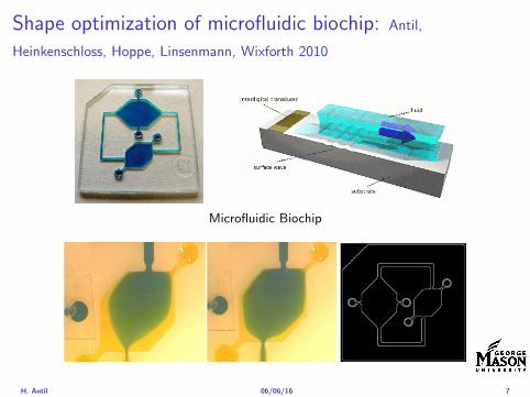

PDE constrained optimization
PDE constrained optimization or optimal control of PDEs (OCP) has 4major components
I control z
I state u which associates with every control z a state u
I cost functional J which depends on z and u to be minimized
I constraints obeyed by z (control constraints) and u (stateconstraints)
Today
I Control constraints are pointwise ae
I State equation is a boundary value problem or a variationalinequality
H Antil 060616 8
Steps to analyze OCPAnalysis
I Existence of solution to PDE Is it unique
I Existence of solution to optimization problem
I First-order necessary conditionsI Adjoint equations
I If possible second order necessarysufficient conditions
Solver development (function space)
I GradientHessian based
Discrete problem solver
I FD FV FE for problem and solver
I Analysis of discrete solver mesh independence
I EfficiencyI Adaptive finite element methods (AFEM)I Model reduction Proper orthogonal decomposition reduced basis
I Software development Trilinos Rapid Optimization Library (ROL)Dolfin-Adjoint
H Antil 060616 9
Optimal heat sourceI Domain Let Ω sub Rd d ge 1 be open bounded Lipschitz domain
with boundary partΩ
I Goal Choose a distributed source z in such a way that thetemperature u = u(x) is close to a desired ud = ud(x) in Ω
Linear-quadratic elliptic OCP
min J(u z) =1
2uminus ud2L2(Ω) +
λ
2z2L2(Ω)
subject to
minusdiv (Anablau) = z in Ω
u = 0 on partΩ
and the pointwise control constraints
z isin Zad = v isin L2(Ω) za(x) le v(x) le zb(x) ae x isin Ω
λ gt 0 is a parameter za zb isin Linfin(Ω) with za lt zb are given A isbounded symmetric positive
H Antil 060616 10
Problems involving semilinear elliptic PDEsI Heating with radiation boundary condition If the heat radiation
of the heated body is taken into account then we obtain
minus∆u = 0 in Ω
partνu = α(z4 minus u4) on partΩ
where the control z is the temperature of the surrounding medium
I Simplified supercondutivity
minus∆u+ u+ u3 = z in Ω
u = 0 on partΩ
I Control of stationary flows
minusmicro∆u + (u middot nabla)u +nablap = f in Ω
div u = 0 in Ω
u = g on partΩ
H Antil 060616 11
Optimal control of variational inequalitiesProblem
min J(u z) =1
2uminus ud2L2(Ω) +
λ
2z2L2(Ω)
subject to u isin K = w isin H10 (Ω) w(x) ge 0 ae x isin Ωint
Ω
nablau middot nabla(uminus v) dx le (z + f uminus v) forallv isin K
with z isin Zad
Regularized problem
min J(u z) =1
2uminus ud2L2(Ω) +
λ
2z2L2(Ω)
subject to (semilinear PDE)
u isin H10 (Ω) minus∆u+ γρε(minusu) = z + f in Ω
and z isin Zad γ gt 0 and ε gt 0 are the penealization and regularizationparameters respectively
H Antil 060616 12
Outline
Motivation and examples
Linear elliptic optimal control problems
Differentiation in Banach spaces
First-order necessary conditions
Optimal control of semilinear PDEs
An abstract problem
Discretization using finite element methods
H Antil 060616 13
Linear elliptic problemsΩ sub Rn bounded Lipschitz domain
Sobolev spacesI Lp(Ω) 1 le p le infin are Lebesgue spaces p = 2 L2(Ω) is a Hilbert
space with inner product (u v) =int
Ωu(x)v(x) dx
I W sp for s isin R 1 le p le infin are Sobolev spaces When p = 2W s2(Ω) = Hs(Ω) is a Hilbert space
I H10 (Ω) = v isin H1(Ω) v|partΩ = 0 with norm (due to Poincare
inequality)uH1
0 (Ω) = nablauL2(Ω)
I H10 (Ω)lowast = Hminus1(Ω)
I Note L2(Ω) sub Hminus1(Ω)
Model problem
minusdiv (Anablau) = f in Ω
u = 0 on partΩ
H Antil 060616 14
Linear elliptic problemsΩ sub Rn bounded Lipschitz domain
Sobolev spacesI Lp(Ω) 1 le p le infin are Lebesgue spaces p = 2 L2(Ω) is a Hilbert
space with inner product (u v) =int
Ωu(x)v(x) dx
I W sp for s isin R 1 le p le infin are Sobolev spaces When p = 2W s2(Ω) = Hs(Ω) is a Hilbert space
I H10 (Ω) = v isin H1(Ω) v|partΩ = 0 with norm (due to Poincare
inequality)uH1
0 (Ω) = nablauL2(Ω)
I H10 (Ω)lowast = Hminus1(Ω)
I Note L2(Ω) sub Hminus1(Ω)
Model problem
minusdiv (Anablau) = f in Ω
u = 0 on partΩ
H Antil 060616 14
Linear elliptic problemsΩ sub Rn bounded Lipschitz domain
Sobolev spacesI Lp(Ω) 1 le p le infin are Lebesgue spaces p = 2 L2(Ω) is a Hilbert
space with inner product (u v) =int
Ωu(x)v(x) dx
I W sp for s isin R 1 le p le infin are Sobolev spaces When p = 2W s2(Ω) = Hs(Ω) is a Hilbert space
I H10 (Ω) = v isin H1(Ω) v|partΩ = 0 with norm (due to Poincare
inequality)uH1
0 (Ω) = nablauL2(Ω)
I H10 (Ω)lowast = Hminus1(Ω)
I Note L2(Ω) sub Hminus1(Ω)
Model problem
minusdiv (Anablau) = f in Ω
u = 0 on partΩ
H Antil 060616 14
Linear elliptic problemsΩ sub Rn bounded Lipschitz domain
Sobolev spacesI Lp(Ω) 1 le p le infin are Lebesgue spaces p = 2 L2(Ω) is a Hilbert
space with inner product (u v) =int
Ωu(x)v(x) dx
I W sp for s isin R 1 le p le infin are Sobolev spaces When p = 2W s2(Ω) = Hs(Ω) is a Hilbert space
I H10 (Ω) = v isin H1(Ω) v|partΩ = 0 with norm (due to Poincare
inequality)uH1
0 (Ω) = nablauL2(Ω)
I H10 (Ω)lowast = Hminus1(Ω)
I Note L2(Ω) sub Hminus1(Ω)
Model problem
minusdiv (Anablau) = f in Ω
u = 0 on partΩ
H Antil 060616 14
Linear elliptic problemsΩ sub Rn bounded Lipschitz domain
Sobolev spacesI Lp(Ω) 1 le p le infin are Lebesgue spaces p = 2 L2(Ω) is a Hilbert
space with inner product (u v) =int
Ωu(x)v(x) dx
I W sp for s isin R 1 le p le infin are Sobolev spaces When p = 2W s2(Ω) = Hs(Ω) is a Hilbert space
I H10 (Ω) = v isin H1(Ω) v|partΩ = 0 with norm (due to Poincare
inequality)uH1
0 (Ω) = nablauL2(Ω)
I H10 (Ω)lowast = Hminus1(Ω)
I Note L2(Ω) sub Hminus1(Ω)
Model problem
minusdiv (Anablau) = f in Ω
u = 0 on partΩ
H Antil 060616 14
Well-posed
I Weak solution Given f isin Hminus1(Ω) a function u isin H10 (Ω) is called
a weak solution iffintΩ
Anablau middot nablav = 〈f v〉minus11 forallv isin H10 (Ω)
where 〈middot middot〉minus11 denotes the Hminus1(Ω)ndashH1(Ω) duality pairing
I Existence and uniqueness For each f isin Hminus1(Ω) there exists aunique u isin H1
0 (Ω) such that
nablauL2(Ω) le CdΩfHminus1(Ω)
I A = I the result is due to the Riesz-representation theorem
I A 6= I (maybe non-symmetric) the result is due to Lax-Milgramlemma
I For general W 1p-spaces use inf-sup conditions combined withBanach-Necas theorem which is a necessary and sufficient condition
H Antil 060616 15
Well-posed
I Weak solution Given f isin Hminus1(Ω) a function u isin H10 (Ω) is called
a weak solution iffintΩ
Anablau middot nablav = 〈f v〉minus11 forallv isin H10 (Ω)
where 〈middot middot〉minus11 denotes the Hminus1(Ω)ndashH1(Ω) duality pairing
I Existence and uniqueness For each f isin Hminus1(Ω) there exists aunique u isin H1
0 (Ω) such that
nablauL2(Ω) le CdΩfHminus1(Ω)
I A = I the result is due to the Riesz-representation theorem
I A 6= I (maybe non-symmetric) the result is due to Lax-Milgramlemma
I For general W 1p-spaces use inf-sup conditions combined withBanach-Necas theorem which is a necessary and sufficient condition
H Antil 060616 15
Linear-quadratic elliptic OCP
min J(u z) =1
2uminus ud2L2(Ω) +
λ
2z2L2(Ω)
subject to
minusdiv (Anablau) = z in Ω
u = 0 on partΩ
and the pointwise control constraints
z isin Zad = v isin L2(Ω) za(x) le v(x) le zb(x) ae x isin Ω
λ gt 0 is a parameter za zb isin Linfin(Ω) with za lt zb are given A isbounded symmetric positive
H Antil 060616 16
Reduced OCP
I Control to state map The solution operator defined as
S Hminus1(Ω)rarr H10 (Ω) z 7rarr u(z) = Sz
Note In view of the embedding
H10 (Ω) rarr L2(Ω) rarr Hminus1(Ω)
we may also consider S from L2(Ω) to L2(Ω) We will use the samenotation for this operator (for simplicity)
I Reduced cost functional The reduced cost functionalJ L2(Ω)rarr R is defined as
J (z) = J(Sz z)
I Reduced problem minzisinZadJ (z)
H Antil 060616 17
Reduced OCP
I Control to state map The solution operator defined as
S Hminus1(Ω)rarr H10 (Ω) z 7rarr u(z) = Sz
Note In view of the embedding
H10 (Ω) rarr L2(Ω) rarr Hminus1(Ω)
we may also consider S from L2(Ω) to L2(Ω) We will use the samenotation for this operator (for simplicity)
I Reduced cost functional The reduced cost functionalJ L2(Ω)rarr R is defined as
J (z) = J(Sz z)
I Reduced problem minzisinZadJ (z)
H Antil 060616 17
Reduced OCP
I Control to state map The solution operator defined as
S Hminus1(Ω)rarr H10 (Ω) z 7rarr u(z) = Sz
Note In view of the embedding
H10 (Ω) rarr L2(Ω) rarr Hminus1(Ω)
we may also consider S from L2(Ω) to L2(Ω) We will use the samenotation for this operator (for simplicity)
I Reduced cost functional The reduced cost functionalJ L2(Ω)rarr R is defined as
J (z) = J(Sz z)
I Reduced problem minzisinZadJ (z)
H Antil 060616 17
Existence of solution Direct methodThere exists a unique solution to the above problem
I Minimizing sequence J is bounded below by zero therefore thereexists a minimizing sequence znnisinN such that
limnrarrinfin
J (zn) = inf J (z)
I Weak compactness zn sub L2(Ω) is bounded Since L2(Ω) isreflexive therefore there exists a subsequence (not relabeled) suchthat
zn z and z isin Zad
where the latter is a consequence of Zad being closed and convex
I Optimality Since J is continuous and convex and therefore isweakly lower semicontinuous We obtain
lim inf J (zn) ge J (z)
which implies that z is optimal
I Uniqueness Exercise
H Antil 060616 18
Existence of solution Direct methodThere exists a unique solution to the above problem
I Minimizing sequence J is bounded below by zero therefore thereexists a minimizing sequence znnisinN such that
limnrarrinfin
J (zn) = inf J (z)
I Weak compactness zn sub L2(Ω) is bounded Since L2(Ω) isreflexive therefore there exists a subsequence (not relabeled) suchthat
zn z and z isin Zad
where the latter is a consequence of Zad being closed and convex
I Optimality Since J is continuous and convex and therefore isweakly lower semicontinuous We obtain
lim inf J (zn) ge J (z)
which implies that z is optimal
I Uniqueness Exercise
H Antil 060616 18
Existence of solution Direct methodThere exists a unique solution to the above problem
I Minimizing sequence J is bounded below by zero therefore thereexists a minimizing sequence znnisinN such that
limnrarrinfin
J (zn) = inf J (z)
I Weak compactness zn sub L2(Ω) is bounded Since L2(Ω) isreflexive therefore there exists a subsequence (not relabeled) suchthat
zn z and z isin Zad
where the latter is a consequence of Zad being closed and convex
I Optimality Since J is continuous and convex and therefore isweakly lower semicontinuous We obtain
lim inf J (zn) ge J (z)
which implies that z is optimal
I Uniqueness Exercise
H Antil 060616 18
Existence of solution Direct methodThere exists a unique solution to the above problem
I Minimizing sequence J is bounded below by zero therefore thereexists a minimizing sequence znnisinN such that
limnrarrinfin
J (zn) = inf J (z)
I Weak compactness zn sub L2(Ω) is bounded Since L2(Ω) isreflexive therefore there exists a subsequence (not relabeled) suchthat
zn z and z isin Zad
where the latter is a consequence of Zad being closed and convex
I Optimality Since J is continuous and convex and therefore isweakly lower semicontinuous We obtain
lim inf J (zn) ge J (z)
which implies that z is optimal
I Uniqueness Exercise
H Antil 060616 18
Outline
Motivation and examples
Linear elliptic optimal control problems
Differentiation in Banach spaces
First-order necessary conditions
Optimal control of semilinear PDEs
An abstract problem
Discretization using finite element methods
H Antil 060616 19
Differentiation in Banach spacesLet (Z middot Z) (V middot V ) B-spaces Z sub Z open and F Z rarr V
Let z isin Z
I If exist δF (z h) = limtdarr01t (F (z + th)minus F (z)) then δF (z h) is called
the directional derivative of F at z in direction h
I If exist δF (z h) forallh isin Z then h 7rarr δF (z h) is the first variation of Fat z
I Let exist the first variation δF (z middot) F is said to be Gateauxdifferentiable at z iff existA isin L(Z V ) such that δF (z h) = Ahforallh isin Z We write A = F primeG(z)
I F is said to be Frechet differentiable at z iff existA isin L(Z V ) and amapping r(z middot) Z rarr V such that for all h isin U with z + h isin Zwe have
F (z+h) = F (z)+Ah+r(z h) withr(z h)VhZ
rarr 0 as hZ rarr 0
We write F prime(z) = A
H Antil 060616 20
Differentiation in Banach spacesLet (Z middot Z) (V middot V ) B-spaces Z sub Z open and F Z rarr V
Let z isin Z
I If exist δF (z h) = limtdarr01t (F (z + th)minus F (z)) then δF (z h) is called
the directional derivative of F at z in direction h
I If exist δF (z h) forallh isin Z then h 7rarr δF (z h) is the first variation of Fat z
I Let exist the first variation δF (z middot) F is said to be Gateauxdifferentiable at z iff existA isin L(Z V ) such that δF (z h) = Ahforallh isin Z We write A = F primeG(z)
I F is said to be Frechet differentiable at z iff existA isin L(Z V ) and amapping r(z middot) Z rarr V such that for all h isin U with z + h isin Zwe have
F (z+h) = F (z)+Ah+r(z h) withr(z h)VhZ
rarr 0 as hZ rarr 0
We write F prime(z) = A
H Antil 060616 20
Differentiation in Banach spacesLet (Z middot Z) (V middot V ) B-spaces Z sub Z open and F Z rarr V
Let z isin Z
I If exist δF (z h) = limtdarr01t (F (z + th)minus F (z)) then δF (z h) is called
the directional derivative of F at z in direction h
I If exist δF (z h) forallh isin Z then h 7rarr δF (z h) is the first variation of Fat z
I Let exist the first variation δF (z middot) F is said to be Gateauxdifferentiable at z iff existA isin L(Z V ) such that δF (z h) = Ahforallh isin Z We write A = F primeG(z)
I F is said to be Frechet differentiable at z iff existA isin L(Z V ) and amapping r(z middot) Z rarr V such that for all h isin U with z + h isin Zwe have
F (z+h) = F (z)+Ah+r(z h) withr(z h)VhZ
rarr 0 as hZ rarr 0
We write F prime(z) = A
H Antil 060616 20
Differentiation in Banach spacesLet (Z middot Z) (V middot V ) B-spaces Z sub Z open and F Z rarr V
Let z isin Z
I If exist δF (z h) = limtdarr01t (F (z + th)minus F (z)) then δF (z h) is called
the directional derivative of F at z in direction h
I If exist δF (z h) forallh isin Z then h 7rarr δF (z h) is the first variation of Fat z
I Let exist the first variation δF (z middot) F is said to be Gateauxdifferentiable at z iff existA isin L(Z V ) such that δF (z h) = Ahforallh isin Z We write A = F primeG(z)
I F is said to be Frechet differentiable at z iff existA isin L(Z V ) and amapping r(z middot) Z rarr V such that for all h isin U with z + h isin Zwe have
F (z+h) = F (z)+Ah+r(z h) withr(z h)VhZ
rarr 0 as hZ rarr 0
We write F prime(z) = A
H Antil 060616 20
ExamplesExample 1 (H (middot middot)H) Hilbert space F (z) = z2H = (z z)H
forallz h F (z + h)minus F (z) = 2(z h)H + h2HThen
F prime(z)h = (2z h)H
Reisz representation theorem (identify H with Hlowast) we can write
F prime(z)h = (nablaF (z) h)H
where nablaF (z) = 2z is the gradient
Example 2 Let (Z (middot middot)Z) (H (middot middot)H) Hilbert spaces ud isin H fixedLet S isin L(ZH) Consider E Z rarr R
E(z) = Sz minus ud2H
Then E(z) = G(F (z)) where G(v) = v2H and F (z) = Sz minus ud
Eprime(z)h = Gprime(F (z))F prime(z)h = (2v F prime(z)h)H
= 2(Sz minus ud Sh)H = 2(Slowast(Sz minus ud) h)Z
we denote the gradient as nablaE(z) = 2Slowast(Sz minus ud)
H Antil 060616 21
ExamplesExample 1 (H (middot middot)H) Hilbert space F (z) = z2H = (z z)H
forallz h F (z + h)minus F (z) = 2(z h)H + h2HThen
F prime(z)h = (2z h)H
Reisz representation theorem (identify H with Hlowast) we can write
F prime(z)h = (nablaF (z) h)H
where nablaF (z) = 2z is the gradient
Example 2 Let (Z (middot middot)Z) (H (middot middot)H) Hilbert spaces ud isin H fixedLet S isin L(ZH) Consider E Z rarr R
E(z) = Sz minus ud2H
Then E(z) = G(F (z)) where G(v) = v2H and F (z) = Sz minus ud
Eprime(z)h = Gprime(F (z))F prime(z)h = (2v F prime(z)h)H
= 2(Sz minus ud Sh)H = 2(Slowast(Sz minus ud) h)Z
we denote the gradient as nablaE(z) = 2Slowast(Sz minus ud)H Antil 060616 21
Outline
Motivation and examples
Linear elliptic optimal control problems
Differentiation in Banach spaces
First-order necessary conditions
Optimal control of semilinear PDEs
An abstract problem
Discretization using finite element methods
H Antil 060616 22
First order necessary optimality conditions
Most of the theory is based on these two simple results
Theorem Let (Z middot Z) be a normed space J Z rarr (infin+infin] amapping with J 6equiv +infin Then z isin Z minimizer of J hArr 0 isin partJ (z)
Proof 0 isin partJ (z) means by definition of partJ (z) J (z)minus J (z) le 0forallz isin Z
Theorem Let (Z middot Z) be a normed space Zad sub Z nonemptyconvex closed J Z rarr R Gateaux differentiable where Zad sub Z sub ZZ open If z isin Zad is a solution to
minzisinZad
J (z)
then z solvesJ prime(z)(z minus z) ge 0 forallz isin Zad
Proof Exercise
H Antil 060616 23
First order necessary optimality conditions
Most of the theory is based on these two simple results
Theorem Let (Z middot Z) be a normed space J Z rarr (infin+infin] amapping with J 6equiv +infin Then z isin Z minimizer of J hArr 0 isin partJ (z)
Proof 0 isin partJ (z) means by definition of partJ (z) J (z)minus J (z) le 0forallz isin Z
Theorem Let (Z middot Z) be a normed space Zad sub Z nonemptyconvex closed J Z rarr R Gateaux differentiable where Zad sub Z sub ZZ open If z isin Zad is a solution to
minzisinZad
J (z)
then z solvesJ prime(z)(z minus z) ge 0 forallz isin Zad
Proof Exercise
H Antil 060616 23
Linear quadratic OCPI Reduced funcational
J (z) =1
2Sz minus ud2L2(Ω) +
λ
2z2L2(Ω)
I Gradient computation using sensitivity
J prime(z)h = (Slowast(Sz minus ud) + λz h)L2(Ω) forallh isin L2(Ω)
we denote the gradient by
nablaJ (z) = Slowast(Sz minus ud) + λz
I First order necessary and sufficient optimality condition
(nablaJ (z) z minus z)L2(Ω) ge 0 forallz isin Zad
I Adjoint equation Let p = Slowast(Sz minus ud) which translates intop isin H1
0 (Ω) solving
minusdiv (Anablap) = uminus ud in Ω
p = 0 on partΩ
I Gradient computation using adjoint nablaJ (z) = p+ λz
H Antil 060616 24
Linear quadratic OCPI Reduced funcational
J (z) =1
2Sz minus ud2L2(Ω) +
λ
2z2L2(Ω)
I Gradient computation using sensitivity
J prime(z)h = (Slowast(Sz minus ud) + λz h)L2(Ω) forallh isin L2(Ω)
we denote the gradient by
nablaJ (z) = Slowast(Sz minus ud) + λz
I First order necessary and sufficient optimality condition
(nablaJ (z) z minus z)L2(Ω) ge 0 forallz isin Zad
I Adjoint equation Let p = Slowast(Sz minus ud) which translates intop isin H1
0 (Ω) solving
minusdiv (Anablap) = uminus ud in Ω
p = 0 on partΩ
I Gradient computation using adjoint nablaJ (z) = p+ λz
H Antil 060616 24
Linear quadratic OCPI Reduced funcational
J (z) =1
2Sz minus ud2L2(Ω) +
λ
2z2L2(Ω)
I Gradient computation using sensitivity
J prime(z)h = (Slowast(Sz minus ud) + λz h)L2(Ω) forallh isin L2(Ω)
we denote the gradient by
nablaJ (z) = Slowast(Sz minus ud) + λz
I First order necessary and sufficient optimality condition
(nablaJ (z) z minus z)L2(Ω) ge 0 forallz isin Zad
I Adjoint equation Let p = Slowast(Sz minus ud) which translates intop isin H1
0 (Ω) solving
minusdiv (Anablap) = uminus ud in Ω
p = 0 on partΩ
I Gradient computation using adjoint nablaJ (z) = p+ λz
H Antil 060616 24
Linear quadratic OCPI Reduced funcational
J (z) =1
2Sz minus ud2L2(Ω) +
λ
2z2L2(Ω)
I Gradient computation using sensitivity
J prime(z)h = (Slowast(Sz minus ud) + λz h)L2(Ω) forallh isin L2(Ω)
we denote the gradient by
nablaJ (z) = Slowast(Sz minus ud) + λz
I First order necessary and sufficient optimality condition
(nablaJ (z) z minus z)L2(Ω) ge 0 forallz isin Zad
I Adjoint equation Let p = Slowast(Sz minus ud) which translates intop isin H1
0 (Ω) solving
minusdiv (Anablap) = uminus ud in Ω
p = 0 on partΩ
I Gradient computation using adjoint nablaJ (z) = p+ λz
H Antil 060616 24
Linear quadratic OCPI Reduced funcational
J (z) =1
2Sz minus ud2L2(Ω) +
λ
2z2L2(Ω)
I Gradient computation using sensitivity
J prime(z)h = (Slowast(Sz minus ud) + λz h)L2(Ω) forallh isin L2(Ω)
we denote the gradient by
nablaJ (z) = Slowast(Sz minus ud) + λz
I First order necessary and sufficient optimality condition
(nablaJ (z) z minus z)L2(Ω) ge 0 forallz isin Zad
I Adjoint equation Let p = Slowast(Sz minus ud) which translates intop isin H1
0 (Ω) solving
minusdiv (Anablap) = uminus ud in Ω
p = 0 on partΩ
I Gradient computation using adjoint nablaJ (z) = p+ λz
H Antil 060616 24
Optimality system
I State u isin H10 (Ω)
intΩAnablau middot nablav =
intΩzv forallv isin H1
0 (Ω)
I Adjoint p isin H10 (Ω)
intΩAnablap middot nablav =
intΩ
(uminus ud)v forallv isin H10 (Ω)
I Control z isin Zad (p+ λz z minus z) ge 0 forallz isin Zad
H Antil 060616 25
Pointwise interpretation
The variational inequality
(p+ λz z minus z) ge 0 forallz isin Zad
is equivalent to for ae x isin Ω
z(x) =
za(x) if p(x) + λz(x) gt 0isin [za(x) zb(x)] if p(x) + λz(x) = 0zb(x) if p(x) + λz(x) lt 0
Consequence
I When λ gt 0 then ae in Ω
z(x) = P[za(x)zb(x)]
minus 1
λp(x)
= min
zb(x)max
za(x)minus 1
λp(x)
H Antil 060616 26
Formal Lagrange method applied to linear OCPIntroduce L H1
0 (Ω)times Zad timesH1(Ω)rarr R defined as
L(u z p) = J(u z)minusint
Ω
(minusdiv (Anablau)minus z
)p dx
Integrate by parts to arrive at
L(u z p) = J(u z)minusint
Ω
(minusdiv (Anablap)uminus zp
)dx+
intpartΩ
(Anablau)p ds
If (u z p) is a stationary point then
I State
DpL(u z p)h = 0 forallh isin H1(Ω)
I AdjointDuL(u z p)h = 0 forallh isin H1
0 (Ω)
I ControlDzL(u z p)(z minus z) ge 0 forallz isin Zad
H Antil 060616 27
Formal Lagrange method applied to linear OCPIntroduce L H1
0 (Ω)times Zad timesH1(Ω)rarr R defined as
L(u z p) = J(u z)minusint
Ω
(minusdiv (Anablau)minus z
)p dx
Integrate by parts to arrive at
L(u z p) = J(u z)minusint
Ω
(minusdiv (Anablap)uminus zp
)dx+
intpartΩ
(Anablau)p ds
If (u z p) is a stationary point then
I State
DpL(u z p)h = 0 forallh isin H1(Ω)
I AdjointDuL(u z p)h = 0 forallh isin H1
0 (Ω)
I ControlDzL(u z p)(z minus z) ge 0 forallz isin Zad
H Antil 060616 27
Formal Lagrange method applied to linear OCPIntroduce L H1
0 (Ω)times Zad timesH1(Ω)rarr R defined as
L(u z p) = J(u z)minusint
Ω
(minusdiv (Anablau)minus z
)p dx
Integrate by parts to arrive at
L(u z p) = J(u z)minusint
Ω
(minusdiv (Anablap)uminus zp
)dx+
intpartΩ
(Anablau)p ds
If (u z p) is a stationary point then
I State
DpL(u z p)h = 0 forallh isin H1(Ω)
I AdjointDuL(u z p)h = 0 forallh isin H1
0 (Ω)
I ControlDzL(u z p)(z minus z) ge 0 forallz isin Zad
H Antil 060616 27
Formal Lagrange method applied to linear OCPIntroduce L H1
0 (Ω)times Zad timesH1(Ω)rarr R defined as
L(u z p) = J(u z)minusint
Ω
(minusdiv (Anablau)minus z
)p dx
Integrate by parts to arrive at
L(u z p) = J(u z)minusint
Ω
(minusdiv (Anablap)uminus zp
)dx+
intpartΩ
(Anablau)p ds
If (u z p) is a stationary point then
I State
DpL(u z p)h = 0 forallh isin H1(Ω)
I AdjointDuL(u z p)h = 0 forallh isin H1
0 (Ω)
I ControlDzL(u z p)(z minus z) ge 0 forallz isin Zad
H Antil 060616 27
Formal Lagrange method applied to linear OCPIntroduce L H1
0 (Ω)times Zad timesH1(Ω)rarr R defined as
L(u z p) = J(u z)minusint
Ω
(minusdiv (Anablau)minus z
)p dx
Integrate by parts to arrive at
L(u z p) = J(u z)minusint
Ω
(minusdiv (Anablap)uminus zp
)dx+
intpartΩ
(Anablau)p ds
If (u z p) is a stationary point then
I State
DpL(u z p)h = 0 forallh isin H1(Ω)
I AdjointDuL(u z p)h = 0 forallh isin H1
0 (Ω)
I ControlDzL(u z p)(z minus z) ge 0 forallz isin Zad
H Antil 060616 27
Outline
Motivation and examples
Linear elliptic optimal control problems
Differentiation in Banach spaces
First-order necessary conditions
Optimal control of semilinear PDEs
An abstract problem
Discretization using finite element methods
H Antil 060616 28
Semilinear elliptic OCP
min J(u z) =1
2uminus ud2L2(Ω) +
λ
2z2L2(Ω)
subject to
minus∆u+ g(x u) = z in Ω
u = 0 on partΩ
and z isin Zad with za zb isin Linfin(Ω)
H Antil 060616 29
State space(A1) Ω sub Rd open bounded partΩ is Lipschitz
(A2) g Ωtimes Rrarr R is bounded and measurable with respect to x isin Ωfor every u isin R
(A3) g is continuous monotone increasing and Lipschitz continuous in ufor ae x isin Ω
(A4) g(x 0) = 0 for ae x isin Ω (not really necessary)
Theorem Suppose (A1)minus (A4) hold For every z isin Lr(Ω) withr gt d2 the state equation has a unique weak solutionu isin H1
0 (Ω) cap C(Ω) ie we haveintΩ
nablau middot nablav dx+
intΩ
g(x u(x))v(x) dx =
intΩ
zv dx forallv isin H10 (Ω)
Moreover there exists a constant C gt 0 such that
uH1(Ω) + uC(Ω) le CzLr(Ω)
RemarkI The proof of the theorem uses the BrowderndashMinty theorem on
monotone operators
H Antil 060616 30
State space(A1) Ω sub Rd open bounded partΩ is Lipschitz
(A2) g Ωtimes Rrarr R is bounded and measurable with respect to x isin Ωfor every u isin R
(A3) g is continuous monotone increasing and Lipschitz continuous in ufor ae x isin Ω
(A4) g(x 0) = 0 for ae x isin Ω (not really necessary)
Theorem Suppose (A1)minus (A4) hold For every z isin Lr(Ω) withr gt d2 the state equation has a unique weak solutionu isin H1
0 (Ω) cap C(Ω) ie we haveintΩ
nablau middot nablav dx+
intΩ
g(x u(x))v(x) dx =
intΩ
zv dx forallv isin H10 (Ω)
Moreover there exists a constant C gt 0 such that
uH1(Ω) + uC(Ω) le CzLr(Ω)
RemarkI The proof of the theorem uses the BrowderndashMinty theorem on
monotone operators
H Antil 060616 30
State space(A1) Ω sub Rd open bounded partΩ is Lipschitz
(A2) g Ωtimes Rrarr R is bounded and measurable with respect to x isin Ωfor every u isin R
(A3) g is continuous monotone increasing and Lipschitz continuous in ufor ae x isin Ω
(A4) g(x 0) = 0 for ae x isin Ω (not really necessary)
Theorem Suppose (A1)minus (A4) hold For every z isin Lr(Ω) withr gt d2 the state equation has a unique weak solutionu isin H1
0 (Ω) cap C(Ω) ie we haveintΩ
nablau middot nablav dx+
intΩ
g(x u(x))v(x) dx =
intΩ
zv dx forallv isin H10 (Ω)
Moreover there exists a constant C gt 0 such that
uH1(Ω) + uC(Ω) le CzLr(Ω)
RemarkI The proof of the theorem uses the BrowderndashMinty theorem on
monotone operators
H Antil 060616 30
Control-to-state map and reduced problem
I Control to state map
S Linfin(Ω)rarr H10 (Ω) cap C(Ω)
is well defined and is globally Lipschitz continuous
I Reduced problem
minJ (z) =1
2S(u)minus ud2L2(Ω) +
λ
2z2L2(Ω)
H Antil 060616 31
Control-to-state map and reduced problem
I Control to state map
S Linfin(Ω)rarr H10 (Ω) cap C(Ω)
is well defined and is globally Lipschitz continuous
I Reduced problem
minJ (z) =1
2S(u)minus ud2L2(Ω) +
λ
2z2L2(Ω)
H Antil 060616 31
First-order necessary conditionsI Lagrangian functional
L(u z p) = J(u z)minusint
Ω
(minus∆u+ g(x u(x))minus z
)p dx
= J(u z)minusint
Ω
(nablau middot nablap+ g(x u(x))pminus zp
)dx
I Adjoint system For all h isin H10 (Ω)
0 = DuL(u z p)h =
intΩ
(uminus ud)h dxminusint
Ω
(nablah middot nablap+ gu(x u(x))ph
)which yields
minus∆p+ gu(x u(x))p = uminus ud in Ω
p = 0 on partΩ
I Control
DzL(u z p)(z minus z) = (p+ λz z minus z) dx ge 0 forallz isin ZadI Gradient
nablaJ (z) = p+ λz
H Antil 060616 32
First-order necessary conditionsI Lagrangian functional
L(u z p) = J(u z)minusint
Ω
(minus∆u+ g(x u(x))minus z
)p dx
= J(u z)minusint
Ω
(nablau middot nablap+ g(x u(x))pminus zp
)dx
I Adjoint system For all h isin H10 (Ω)
0 = DuL(u z p)h =
intΩ
(uminus ud)h dxminusint
Ω
(nablah middot nablap+ gu(x u(x))ph
)which yields
minus∆p+ gu(x u(x))p = uminus ud in Ω
p = 0 on partΩ
I Control
DzL(u z p)(z minus z) = (p+ λz z minus z) dx ge 0 forallz isin ZadI Gradient
nablaJ (z) = p+ λz
H Antil 060616 32
First-order necessary conditionsI Lagrangian functional
L(u z p) = J(u z)minusint
Ω
(minus∆u+ g(x u(x))minus z
)p dx
= J(u z)minusint
Ω
(nablau middot nablap+ g(x u(x))pminus zp
)dx
I Adjoint system For all h isin H10 (Ω)
0 = DuL(u z p)h =
intΩ
(uminus ud)h dxminusint
Ω
(nablah middot nablap+ gu(x u(x))ph
)which yields
minus∆p+ gu(x u(x))p = uminus ud in Ω
p = 0 on partΩ
I Control
DzL(u z p)(z minus z) = (p+ λz z minus z) dx ge 0 forallz isin Zad
I GradientnablaJ (z) = p+ λz
H Antil 060616 32
First-order necessary conditionsI Lagrangian functional
L(u z p) = J(u z)minusint
Ω
(minus∆u+ g(x u(x))minus z
)p dx
= J(u z)minusint
Ω
(nablau middot nablap+ g(x u(x))pminus zp
)dx
I Adjoint system For all h isin H10 (Ω)
0 = DuL(u z p)h =
intΩ
(uminus ud)h dxminusint
Ω
(nablah middot nablap+ gu(x u(x))ph
)which yields
minus∆p+ gu(x u(x))p = uminus ud in Ω
p = 0 on partΩ
I Control
DzL(u z p)(z minus z) = (p+ λz z minus z) dx ge 0 forallz isin ZadI Gradient
nablaJ (z) = p+ λz
H Antil 060616 32
Differentiability of Nemytskii operator
The rigorous proof uses
Theorem In addition to (A1)-(A4) if
(A5) g is continuously differentiable with respect to u for ae x isin Ωand we have
(i) |gu(x 0)| le K for ae x isin Ω(ii) gu is locally Lipschitz with respect to u isin R
then the Nemytskii operator G u 7rarr g(middot u(middot)) is continuously Frechetdifferentiable from Linfin(Ω) into itself and
(Gprime(u)h)(x) = gu(x u(x))h(x) ae in Ω forallh isin Linfin(Ω)
Remark (A5) holds if g(x u) = g(u) and g isin C2(R)
H Antil 060616 33
Outline
Motivation and examples
Linear elliptic optimal control problems
Differentiation in Banach spaces
First-order necessary conditions
Optimal control of semilinear PDEs
An abstract problem
Discretization using finite element methods
H Antil 060616 34
Gradient computation via adjoint general formI Abstract problem
min J(u z)
subject toc(u z) = 0
and z isin Zad
I Directional derivative Let S be the control to state map(nonlinear in general)
z 7rarr S(z) = u(z)
Under the assumptions of ldquoimplicit function theoremrdquo
J prime(z)h = (nablauJ (u(z) z) Sprime(z)h) + (nablazJ (u(z) z) h)
I Sensitivity of u with respect to z Differentiating the stateequation
cu(S(z) z)Sprime(z)h = minuscz(S(z) z)h
leads toSprime(z)h = minuscu(S(z) z)minus1
(cz(S(z) z)h
)
provided cu(S(z) z)minus1 is well-defined
H Antil 060616 35
Gradient computation via adjoint general formI Abstract problem
min J(u z)
subject toc(u z) = 0
and z isin ZadI Directional derivative Let S be the control to state map
(nonlinear in general)
z 7rarr S(z) = u(z)
Under the assumptions of ldquoimplicit function theoremrdquo
J prime(z)h = (nablauJ (u(z) z) Sprime(z)h) + (nablazJ (u(z) z) h)
I Sensitivity of u with respect to z Differentiating the stateequation
cu(S(z) z)Sprime(z)h = minuscz(S(z) z)h
leads toSprime(z)h = minuscu(S(z) z)minus1
(cz(S(z) z)h
)
provided cu(S(z) z)minus1 is well-defined
H Antil 060616 35
Gradient computation via adjoint general formI Abstract problem
min J(u z)
subject toc(u z) = 0
and z isin ZadI Directional derivative Let S be the control to state map
(nonlinear in general)
z 7rarr S(z) = u(z)
Under the assumptions of ldquoimplicit function theoremrdquo
J prime(z)h = (nablauJ (u(z) z) Sprime(z)h) + (nablazJ (u(z) z) h)
I Sensitivity of u with respect to z Differentiating the stateequation
cu(S(z) z)Sprime(z)h = minuscz(S(z) z)h
leads toSprime(z)h = minuscu(S(z) z)minus1
(cz(S(z) z)h
)
provided cu(S(z) z)minus1 is well-defined
H Antil 060616 35
Adjoint equation and gradient general form
I Directional derivative
J prime(z)h = minus(nablauJ (u(z) z) cu(u(z) z)minus1cz(u(z) z)h
)+ (nablazJ (u(z) z) h)
I Gradient
nablaJ (z) = minuscz(u(z) z)lowast(cu(u(z) z)minuslowastnablauJ (u(z) z)
)+nablazJ (u(z) z)
I Introducing adjoint variable p solving
cu(u(z) z)lowastp = nablauJ (u(z) z)
we arrive at following form of gradient
nablaJ (z) = minuscz(u(z) z)lowastp+nablazJ (u(z) z)
which is tractable
H Antil 060616 36
Adjoint equation and gradient general form
I Directional derivative
J prime(z)h = minus(nablauJ (u(z) z) cu(u(z) z)minus1cz(u(z) z)h
)+ (nablazJ (u(z) z) h)
I Gradient
nablaJ (z) = minuscz(u(z) z)lowast(cu(u(z) z)minuslowastnablauJ (u(z) z)
)+nablazJ (u(z) z)
I Introducing adjoint variable p solving
cu(u(z) z)lowastp = nablauJ (u(z) z)
we arrive at following form of gradient
nablaJ (z) = minuscz(u(z) z)lowastp+nablazJ (u(z) z)
which is tractable
H Antil 060616 36
Adjoint equation and gradient general form
I Directional derivative
J prime(z)h = minus(nablauJ (u(z) z) cu(u(z) z)minus1cz(u(z) z)h
)+ (nablazJ (u(z) z) h)
I Gradient
nablaJ (z) = minuscz(u(z) z)lowast(cu(u(z) z)minuslowastnablauJ (u(z) z)
)+nablazJ (u(z) z)
I Introducing adjoint variable p solving
cu(u(z) z)lowastp = nablauJ (u(z) z)
we arrive at following form of gradient
nablaJ (z) = minuscz(u(z) z)lowastp+nablazJ (u(z) z)
which is tractable
H Antil 060616 36
Hessian computation general form
I Lagrangian L(u z p) = J(u z)minusint
Ωc(u z)p dx Then we have
DzJ (z)h = DzL(u z p)h
I Second order derivative
D2zJ (z)[h1 h2] = DuDzL(u z p)[h1 S
prime(z)h2] +D2zL(u z p)[h1 h2]
+DpDzL(u z p)[h1 Dzp(z)h2]
I We already know Sprime(z)h2 moreover
DpDzL(u z p)[h1 Dzp(z)h2] = minus(cu(u z)h1 Dzp(z)h2
)
It remain to identify Dzp(z)h2
H Antil 060616 37
Hessian computation general form
I Lagrangian L(u z p) = J(u z)minusint
Ωc(u z)p dx Then we have
DzJ (z)h = DzL(u z p)h
I Second order derivative
D2zJ (z)[h1 h2] = DuDzL(u z p)[h1 S
prime(z)h2] +D2zL(u z p)[h1 h2]
+DpDzL(u z p)[h1 Dzp(z)h2]
I We already know Sprime(z)h2 moreover
DpDzL(u z p)[h1 Dzp(z)h2] = minus(cu(u z)h1 Dzp(z)h2
)
It remain to identify Dzp(z)h2
H Antil 060616 37
Hessian computation general form
I Lagrangian L(u z p) = J(u z)minusint
Ωc(u z)p dx Then we have
DzJ (z)h = DzL(u z p)h
I Second order derivative
D2zJ (z)[h1 h2] = DuDzL(u z p)[h1 S
prime(z)h2] +D2zL(u z p)[h1 h2]
+DpDzL(u z p)[h1 Dzp(z)h2]
I We already know Sprime(z)h2 moreover
DpDzL(u z p)[h1 Dzp(z)h2] = minus(cu(u z)h1 Dzp(z)h2
)
It remain to identify Dzp(z)h2
H Antil 060616 37
Outline
Motivation and examples
Linear elliptic optimal control problems
Differentiation in Banach spaces
First-order necessary conditions
Optimal control of semilinear PDEs
An abstract problem
Discretization using finite element methods
H Antil 060616 38
Numerical approximation of Poisson equation MeshTo avoid technical issues we will assume that partΩ is polygonal
I Mesh Let T = K be a mesh of Ω where K sub Rd is an elementthat is isoparametrically equivalent to a unit simplex in Rd
I Conforming mesh We say that the mesh is conforming ifI Ω = cupKisinT KI If K1 cap K2 = x then x is a node of K1 and K2I If K1 cap K2 6= empty and K1 cap K2 6= x then K1 cap K2 is an edgeface
contained in partK1 cap partK2
I Shape regular Let T be the collection of all conformingrefinements of an original mesh T 0 Then T is called shape regularif exist κ gt 0 such that
hKρKle κ forallK isin cupiT i
where hK = diam K ρK = maxρ gt 0|Bρ sub KI Quasi-uniform A family of shape regular meshes is called-quasi
uniform if there exist a constant σ gt 0 such that
maxhKminhK
le σ
uniformly for all meshes in the family
Numerical approximation of Poisson equation MeshTo avoid technical issues we will assume that partΩ is polygonal
I Mesh Let T = K be a mesh of Ω where K sub Rd is an elementthat is isoparametrically equivalent to a unit simplex in Rd
I Conforming mesh We say that the mesh is conforming ifI Ω = cupKisinT KI If K1 cap K2 = x then x is a node of K1 and K2I If K1 cap K2 6= empty and K1 cap K2 6= x then K1 cap K2 is an edgeface
contained in partK1 cap partK2
I Shape regular Let T be the collection of all conformingrefinements of an original mesh T 0 Then T is called shape regularif exist κ gt 0 such that
hKρKle κ forallK isin cupiT i
where hK = diam K ρK = maxρ gt 0|Bρ sub KI Quasi-uniform A family of shape regular meshes is called-quasi
uniform if there exist a constant σ gt 0 such that
maxhKminhK
le σ
uniformly for all meshes in the family
Numerical approximation of Poisson equation MeshTo avoid technical issues we will assume that partΩ is polygonal
I Mesh Let T = K be a mesh of Ω where K sub Rd is an elementthat is isoparametrically equivalent to a unit simplex in Rd
I Conforming mesh We say that the mesh is conforming ifI Ω = cupKisinT KI If K1 cap K2 = x then x is a node of K1 and K2I If K1 cap K2 6= empty and K1 cap K2 6= x then K1 cap K2 is an edgeface
contained in partK1 cap partK2
I Shape regular Let T be the collection of all conformingrefinements of an original mesh T 0 Then T is called shape regularif exist κ gt 0 such that
hKρKle κ forallK isin cupiT i
where hK = diam K ρK = maxρ gt 0|Bρ sub K
I Quasi-uniform A family of shape regular meshes is called-quasiuniform if there exist a constant σ gt 0 such that
maxhKminhK
le σ
uniformly for all meshes in the family
Numerical approximation of Poisson equation MeshTo avoid technical issues we will assume that partΩ is polygonal
I Mesh Let T = K be a mesh of Ω where K sub Rd is an elementthat is isoparametrically equivalent to a unit simplex in Rd
I Conforming mesh We say that the mesh is conforming ifI Ω = cupKisinT KI If K1 cap K2 = x then x is a node of K1 and K2I If K1 cap K2 6= empty and K1 cap K2 6= x then K1 cap K2 is an edgeface
contained in partK1 cap partK2
I Shape regular Let T be the collection of all conformingrefinements of an original mesh T 0 Then T is called shape regularif exist κ gt 0 such that
hKρKle κ forallK isin cupiT i
where hK = diam K ρK = maxρ gt 0|Bρ sub KI Quasi-uniform A family of shape regular meshes is called-quasi
uniform if there exist a constant σ gt 0 such that
maxhKminhK
le σ
uniformly for all meshes in the family
FE space and Galerkin approximationI Finite element space For T isin T we define the finite element
space as
V(T ) = W isin C0(Ω) WK isin P1forallK isin T W |partΩ = 0
where P1 is the set of polynomials of degree at most 1
I Galerkin approximation of continuous problem is given by
Find UT isin V(T )
intΩ
AnablaUT middot nablaV = 〈f V 〉 forallV isin V(T )
The discrete problem is well-posedI Nodal basis Consists of functions ψi isin V(T ) with xi isin N (T )
satisfyingψxi
(xj) = δij
where N (T ) denotes the interior (plus Neumann) nodesI Galerkin orthogonality(
nabla(uminus UT )nablaW)L2(Ω)
= 0 forallW isin V(T )
H Antil 060616 40
FE space and Galerkin approximationI Finite element space For T isin T we define the finite element
space as
V(T ) = W isin C0(Ω) WK isin P1forallK isin T W |partΩ = 0
where P1 is the set of polynomials of degree at most 1I Galerkin approximation of continuous problem is given by
Find UT isin V(T )
intΩ
AnablaUT middot nablaV = 〈f V 〉 forallV isin V(T )
The discrete problem is well-posed
I Nodal basis Consists of functions ψi isin V(T ) with xi isin N (T )satisfying
ψxi(xj) = δij
where N (T ) denotes the interior (plus Neumann) nodesI Galerkin orthogonality(
nabla(uminus UT )nablaW)L2(Ω)
= 0 forallW isin V(T )
H Antil 060616 40
FE space and Galerkin approximationI Finite element space For T isin T we define the finite element
space as
V(T ) = W isin C0(Ω) WK isin P1forallK isin T W |partΩ = 0
where P1 is the set of polynomials of degree at most 1I Galerkin approximation of continuous problem is given by
Find UT isin V(T )
intΩ
AnablaUT middot nablaV = 〈f V 〉 forallV isin V(T )
The discrete problem is well-posedI Nodal basis Consists of functions ψi isin V(T ) with xi isin N (T )
satisfyingψxi
(xj) = δij
where N (T ) denotes the interior (plus Neumann) nodes
I Galerkin orthogonality(nabla(uminus UT )nablaW
)L2(Ω)
= 0 forallW isin V(T )
H Antil 060616 40
FE space and Galerkin approximationI Finite element space For T isin T we define the finite element
space as
V(T ) = W isin C0(Ω) WK isin P1forallK isin T W |partΩ = 0
where P1 is the set of polynomials of degree at most 1I Galerkin approximation of continuous problem is given by
Find UT isin V(T )
intΩ
AnablaUT middot nablaV = 〈f V 〉 forallV isin V(T )
The discrete problem is well-posedI Nodal basis Consists of functions ψi isin V(T ) with xi isin N (T )
satisfyingψxi
(xj) = δij
where N (T ) denotes the interior (plus Neumann) nodesI Galerkin orthogonality(
nabla(uminus UT )nablaW)L2(Ω)
= 0 forallW isin V(T )
H Antil 060616 40
Best approximation
I Cearsquos lemma
nabla(uminus UT )L2(Ω) le C infWisinV(T )
nabla(uminusW )L2(Ω)
I Nodal interpolation operator ΠT C(Ω)rarr V(T ) satisfies
ΠT u(xi) = u(xi) forallxi isin N (T )
and is defined as
ΠT u =sum
xiisinN (T )
u(xi)ψxi
I Error estimates In Cearsquos lemma replace W by ΠT u and thencompute the interpolation error
H Antil 060616 41
Best approximation
I Cearsquos lemma
nabla(uminus UT )L2(Ω) le C infWisinV(T )
nabla(uminusW )L2(Ω)
I Nodal interpolation operator ΠT C(Ω)rarr V(T ) satisfies
ΠT u(xi) = u(xi) forallxi isin N (T )
and is defined as
ΠT u =sum
xiisinN (T )
u(xi)ψxi
I Error estimates In Cearsquos lemma replace W by ΠT u and thencompute the interpolation error
H Antil 060616 41
Best approximation
I Cearsquos lemma
nabla(uminus UT )L2(Ω) le C infWisinV(T )
nabla(uminusW )L2(Ω)
I Nodal interpolation operator ΠT C(Ω)rarr V(T ) satisfies
ΠT u(xi) = u(xi) forallxi isin N (T )
and is defined as
ΠT u =sum
xiisinN (T )
u(xi)ψxi
I Error estimates In Cearsquos lemma replace W by ΠT u and thencompute the interpolation error
H Antil 060616 41
Algebraic system state equation
I Recall UT isin V(T ) solves
a(UT V ) = 〈f V 〉 forallV isin V(T )
I Now setting UT =sumN
j=1 Ujψj V = ψi we get
Nsumj=1
Uja(φj φi) = 〈f ψi〉 i = 1 N
which is the matrix-vector system
AU = F
I Stiffness matrix A is SPD
H Antil 060616 42
Algebraic system state equation
I Recall UT isin V(T ) solves
a(UT V ) = 〈f V 〉 forallV isin V(T )
I Now setting UT =sumN
j=1 Ujψj V = ψi we get
Nsumj=1
Uja(φj φi) = 〈f ψi〉 i = 1 N
which is the matrix-vector system
AU = F
I Stiffness matrix A is SPD
H Antil 060616 42
Algebraic system state equation
I Recall UT isin V(T ) solves
a(UT V ) = 〈f V 〉 forallV isin V(T )
I Now setting UT =sumN
j=1 Ujψj V = ψi we get
Nsumj=1
Uja(φj φi) = 〈f ψi〉 i = 1 N
which is the matrix-vector system
AU = F
I Stiffness matrix A is SPD
H Antil 060616 42
Discrete linear elliptic OCP
min JT (UT ZT ) =1
2UT minus ud2L2(Ω) +
λ
2ZT 2L2(Ω)
subject to
Find UT isin V(T )
intΩ
nablaUT middot nablaV = (ZT V )L2(Ω) forallV isin V(T )
and whereZT isin Zad(T ) = Zad cap Z(T )
is either one of these
Z(T ) =
V(T )L2(Ω) variational discretization (Hinze)WT isin Linfin(Ω) ZT |K isin P0(K)K isin T
H Antil 060616 43
Recent books
F TroltzschOptimal control of partial differential equations volume 112 ofGraduate Studies in MathematicsAmerican Mathematical Society Providence RI 2010Theory methods and applications Translated from the 2005 Germanoriginal by Jurgen Sprekels
K Ito and K KunischLagrange multiplier approach to variational problems andapplications volume 15 of Advances in Design and ControlSociety for Industrial and Applied Mathematics (SIAM)Philadelphia PA 2008
H Antil 060616 44
- Motivation and examples
- Linear elliptic optimal control problems
- Differentiation in Banach spaces
- First-order necessary conditions
- Optimal control of semilinear PDEs
- An abstract problem
- Discretization using finite element methods
-

PDE constrained optimization
PDE constrained optimization or optimal control of PDEs (OCP) has 4major components
I control z
I state u which associates with every control z a state u
I cost functional J which depends on z and u to be minimized
I constraints obeyed by z (control constraints) and u (stateconstraints)
Today
I Control constraints are pointwise ae
I State equation is a boundary value problem or a variationalinequality
H Antil 060616 8
PDE constrained optimization
PDE constrained optimization or optimal control of PDEs (OCP) has 4major components
I control z
I state u which associates with every control z a state u
I cost functional J which depends on z and u to be minimized
I constraints obeyed by z (control constraints) and u (stateconstraints)
Today
I Control constraints are pointwise ae
I State equation is a boundary value problem or a variationalinequality
H Antil 060616 8
PDE constrained optimization
PDE constrained optimization or optimal control of PDEs (OCP) has 4major components
I control z
I state u which associates with every control z a state u
I cost functional J which depends on z and u to be minimized
I constraints obeyed by z (control constraints) and u (stateconstraints)
Today
I Control constraints are pointwise ae
I State equation is a boundary value problem or a variationalinequality
H Antil 060616 8
PDE constrained optimization
PDE constrained optimization or optimal control of PDEs (OCP) has 4major components
I control z
I state u which associates with every control z a state u
I cost functional J which depends on z and u to be minimized
I constraints obeyed by z (control constraints) and u (stateconstraints)
Today
I Control constraints are pointwise ae
I State equation is a boundary value problem or a variationalinequality
H Antil 060616 8
Steps to analyze OCPAnalysis
I Existence of solution to PDE Is it unique
I Existence of solution to optimization problem
I First-order necessary conditionsI Adjoint equations
I If possible second order necessarysufficient conditions
Solver development (function space)
I GradientHessian based
Discrete problem solver
I FD FV FE for problem and solver
I Analysis of discrete solver mesh independence
I EfficiencyI Adaptive finite element methods (AFEM)I Model reduction Proper orthogonal decomposition reduced basis
I Software development Trilinos Rapid Optimization Library (ROL)Dolfin-Adjoint
H Antil 060616 9
Optimal heat sourceI Domain Let Ω sub Rd d ge 1 be open bounded Lipschitz domain
with boundary partΩ
I Goal Choose a distributed source z in such a way that thetemperature u = u(x) is close to a desired ud = ud(x) in Ω
Linear-quadratic elliptic OCP
min J(u z) =1
2uminus ud2L2(Ω) +
λ
2z2L2(Ω)
subject to
minusdiv (Anablau) = z in Ω
u = 0 on partΩ
and the pointwise control constraints
z isin Zad = v isin L2(Ω) za(x) le v(x) le zb(x) ae x isin Ω
λ gt 0 is a parameter za zb isin Linfin(Ω) with za lt zb are given A isbounded symmetric positive
H Antil 060616 10
Problems involving semilinear elliptic PDEsI Heating with radiation boundary condition If the heat radiation
of the heated body is taken into account then we obtain
minus∆u = 0 in Ω
partνu = α(z4 minus u4) on partΩ
where the control z is the temperature of the surrounding medium
I Simplified supercondutivity
minus∆u+ u+ u3 = z in Ω
u = 0 on partΩ
I Control of stationary flows
minusmicro∆u + (u middot nabla)u +nablap = f in Ω
div u = 0 in Ω
u = g on partΩ
H Antil 060616 11
Optimal control of variational inequalitiesProblem
min J(u z) =1
2uminus ud2L2(Ω) +
λ
2z2L2(Ω)
subject to u isin K = w isin H10 (Ω) w(x) ge 0 ae x isin Ωint
Ω
nablau middot nabla(uminus v) dx le (z + f uminus v) forallv isin K
with z isin Zad
Regularized problem
min J(u z) =1
2uminus ud2L2(Ω) +
λ
2z2L2(Ω)
subject to (semilinear PDE)
u isin H10 (Ω) minus∆u+ γρε(minusu) = z + f in Ω
and z isin Zad γ gt 0 and ε gt 0 are the penealization and regularizationparameters respectively
H Antil 060616 12
Outline
Motivation and examples
Linear elliptic optimal control problems
Differentiation in Banach spaces
First-order necessary conditions
Optimal control of semilinear PDEs
An abstract problem
Discretization using finite element methods
H Antil 060616 13
Linear elliptic problemsΩ sub Rn bounded Lipschitz domain
Sobolev spacesI Lp(Ω) 1 le p le infin are Lebesgue spaces p = 2 L2(Ω) is a Hilbert
space with inner product (u v) =int
Ωu(x)v(x) dx
I W sp for s isin R 1 le p le infin are Sobolev spaces When p = 2W s2(Ω) = Hs(Ω) is a Hilbert space
I H10 (Ω) = v isin H1(Ω) v|partΩ = 0 with norm (due to Poincare
inequality)uH1
0 (Ω) = nablauL2(Ω)
I H10 (Ω)lowast = Hminus1(Ω)
I Note L2(Ω) sub Hminus1(Ω)
Model problem
minusdiv (Anablau) = f in Ω
u = 0 on partΩ
H Antil 060616 14
Linear elliptic problemsΩ sub Rn bounded Lipschitz domain
Sobolev spacesI Lp(Ω) 1 le p le infin are Lebesgue spaces p = 2 L2(Ω) is a Hilbert
space with inner product (u v) =int
Ωu(x)v(x) dx
I W sp for s isin R 1 le p le infin are Sobolev spaces When p = 2W s2(Ω) = Hs(Ω) is a Hilbert space
I H10 (Ω) = v isin H1(Ω) v|partΩ = 0 with norm (due to Poincare
inequality)uH1
0 (Ω) = nablauL2(Ω)
I H10 (Ω)lowast = Hminus1(Ω)
I Note L2(Ω) sub Hminus1(Ω)
Model problem
minusdiv (Anablau) = f in Ω
u = 0 on partΩ
H Antil 060616 14
Linear elliptic problemsΩ sub Rn bounded Lipschitz domain
Sobolev spacesI Lp(Ω) 1 le p le infin are Lebesgue spaces p = 2 L2(Ω) is a Hilbert
space with inner product (u v) =int
Ωu(x)v(x) dx
I W sp for s isin R 1 le p le infin are Sobolev spaces When p = 2W s2(Ω) = Hs(Ω) is a Hilbert space
I H10 (Ω) = v isin H1(Ω) v|partΩ = 0 with norm (due to Poincare
inequality)uH1
0 (Ω) = nablauL2(Ω)
I H10 (Ω)lowast = Hminus1(Ω)
I Note L2(Ω) sub Hminus1(Ω)
Model problem
minusdiv (Anablau) = f in Ω
u = 0 on partΩ
H Antil 060616 14
Linear elliptic problemsΩ sub Rn bounded Lipschitz domain
Sobolev spacesI Lp(Ω) 1 le p le infin are Lebesgue spaces p = 2 L2(Ω) is a Hilbert
space with inner product (u v) =int
Ωu(x)v(x) dx
I W sp for s isin R 1 le p le infin are Sobolev spaces When p = 2W s2(Ω) = Hs(Ω) is a Hilbert space
I H10 (Ω) = v isin H1(Ω) v|partΩ = 0 with norm (due to Poincare
inequality)uH1
0 (Ω) = nablauL2(Ω)
I H10 (Ω)lowast = Hminus1(Ω)
I Note L2(Ω) sub Hminus1(Ω)
Model problem
minusdiv (Anablau) = f in Ω
u = 0 on partΩ
H Antil 060616 14
Linear elliptic problemsΩ sub Rn bounded Lipschitz domain
Sobolev spacesI Lp(Ω) 1 le p le infin are Lebesgue spaces p = 2 L2(Ω) is a Hilbert
space with inner product (u v) =int
Ωu(x)v(x) dx
I W sp for s isin R 1 le p le infin are Sobolev spaces When p = 2W s2(Ω) = Hs(Ω) is a Hilbert space
I H10 (Ω) = v isin H1(Ω) v|partΩ = 0 with norm (due to Poincare
inequality)uH1
0 (Ω) = nablauL2(Ω)
I H10 (Ω)lowast = Hminus1(Ω)
I Note L2(Ω) sub Hminus1(Ω)
Model problem
minusdiv (Anablau) = f in Ω
u = 0 on partΩ
H Antil 060616 14
Well-posed
I Weak solution Given f isin Hminus1(Ω) a function u isin H10 (Ω) is called
a weak solution iffintΩ
Anablau middot nablav = 〈f v〉minus11 forallv isin H10 (Ω)
where 〈middot middot〉minus11 denotes the Hminus1(Ω)ndashH1(Ω) duality pairing
I Existence and uniqueness For each f isin Hminus1(Ω) there exists aunique u isin H1
0 (Ω) such that
nablauL2(Ω) le CdΩfHminus1(Ω)
I A = I the result is due to the Riesz-representation theorem
I A 6= I (maybe non-symmetric) the result is due to Lax-Milgramlemma
I For general W 1p-spaces use inf-sup conditions combined withBanach-Necas theorem which is a necessary and sufficient condition
H Antil 060616 15
Well-posed
I Weak solution Given f isin Hminus1(Ω) a function u isin H10 (Ω) is called
a weak solution iffintΩ
Anablau middot nablav = 〈f v〉minus11 forallv isin H10 (Ω)
where 〈middot middot〉minus11 denotes the Hminus1(Ω)ndashH1(Ω) duality pairing
I Existence and uniqueness For each f isin Hminus1(Ω) there exists aunique u isin H1
0 (Ω) such that
nablauL2(Ω) le CdΩfHminus1(Ω)
I A = I the result is due to the Riesz-representation theorem
I A 6= I (maybe non-symmetric) the result is due to Lax-Milgramlemma
I For general W 1p-spaces use inf-sup conditions combined withBanach-Necas theorem which is a necessary and sufficient condition
H Antil 060616 15
Linear-quadratic elliptic OCP
min J(u z) =1
2uminus ud2L2(Ω) +
λ
2z2L2(Ω)
subject to
minusdiv (Anablau) = z in Ω
u = 0 on partΩ
and the pointwise control constraints
z isin Zad = v isin L2(Ω) za(x) le v(x) le zb(x) ae x isin Ω
λ gt 0 is a parameter za zb isin Linfin(Ω) with za lt zb are given A isbounded symmetric positive
H Antil 060616 16
Reduced OCP
I Control to state map The solution operator defined as
S Hminus1(Ω)rarr H10 (Ω) z 7rarr u(z) = Sz
Note In view of the embedding
H10 (Ω) rarr L2(Ω) rarr Hminus1(Ω)
we may also consider S from L2(Ω) to L2(Ω) We will use the samenotation for this operator (for simplicity)
I Reduced cost functional The reduced cost functionalJ L2(Ω)rarr R is defined as
J (z) = J(Sz z)
I Reduced problem minzisinZadJ (z)
H Antil 060616 17
Reduced OCP
I Control to state map The solution operator defined as
S Hminus1(Ω)rarr H10 (Ω) z 7rarr u(z) = Sz
Note In view of the embedding
H10 (Ω) rarr L2(Ω) rarr Hminus1(Ω)
we may also consider S from L2(Ω) to L2(Ω) We will use the samenotation for this operator (for simplicity)
I Reduced cost functional The reduced cost functionalJ L2(Ω)rarr R is defined as
J (z) = J(Sz z)
I Reduced problem minzisinZadJ (z)
H Antil 060616 17
Reduced OCP
I Control to state map The solution operator defined as
S Hminus1(Ω)rarr H10 (Ω) z 7rarr u(z) = Sz
Note In view of the embedding
H10 (Ω) rarr L2(Ω) rarr Hminus1(Ω)
we may also consider S from L2(Ω) to L2(Ω) We will use the samenotation for this operator (for simplicity)
I Reduced cost functional The reduced cost functionalJ L2(Ω)rarr R is defined as
J (z) = J(Sz z)
I Reduced problem minzisinZadJ (z)
H Antil 060616 17
Existence of solution Direct methodThere exists a unique solution to the above problem
I Minimizing sequence J is bounded below by zero therefore thereexists a minimizing sequence znnisinN such that
limnrarrinfin
J (zn) = inf J (z)
I Weak compactness zn sub L2(Ω) is bounded Since L2(Ω) isreflexive therefore there exists a subsequence (not relabeled) suchthat
zn z and z isin Zad
where the latter is a consequence of Zad being closed and convex
I Optimality Since J is continuous and convex and therefore isweakly lower semicontinuous We obtain
lim inf J (zn) ge J (z)
which implies that z is optimal
I Uniqueness Exercise
H Antil 060616 18
Existence of solution Direct methodThere exists a unique solution to the above problem
I Minimizing sequence J is bounded below by zero therefore thereexists a minimizing sequence znnisinN such that
limnrarrinfin
J (zn) = inf J (z)
I Weak compactness zn sub L2(Ω) is bounded Since L2(Ω) isreflexive therefore there exists a subsequence (not relabeled) suchthat
zn z and z isin Zad
where the latter is a consequence of Zad being closed and convex
I Optimality Since J is continuous and convex and therefore isweakly lower semicontinuous We obtain
lim inf J (zn) ge J (z)
which implies that z is optimal
I Uniqueness Exercise
H Antil 060616 18
Existence of solution Direct methodThere exists a unique solution to the above problem
I Minimizing sequence J is bounded below by zero therefore thereexists a minimizing sequence znnisinN such that
limnrarrinfin
J (zn) = inf J (z)
I Weak compactness zn sub L2(Ω) is bounded Since L2(Ω) isreflexive therefore there exists a subsequence (not relabeled) suchthat
zn z and z isin Zad
where the latter is a consequence of Zad being closed and convex
I Optimality Since J is continuous and convex and therefore isweakly lower semicontinuous We obtain
lim inf J (zn) ge J (z)
which implies that z is optimal
I Uniqueness Exercise
H Antil 060616 18
Existence of solution Direct methodThere exists a unique solution to the above problem
I Minimizing sequence J is bounded below by zero therefore thereexists a minimizing sequence znnisinN such that
limnrarrinfin
J (zn) = inf J (z)
I Weak compactness zn sub L2(Ω) is bounded Since L2(Ω) isreflexive therefore there exists a subsequence (not relabeled) suchthat
zn z and z isin Zad
where the latter is a consequence of Zad being closed and convex
I Optimality Since J is continuous and convex and therefore isweakly lower semicontinuous We obtain
lim inf J (zn) ge J (z)
which implies that z is optimal
I Uniqueness Exercise
H Antil 060616 18
Outline
Motivation and examples
Linear elliptic optimal control problems
Differentiation in Banach spaces
First-order necessary conditions
Optimal control of semilinear PDEs
An abstract problem
Discretization using finite element methods
H Antil 060616 19
Differentiation in Banach spacesLet (Z middot Z) (V middot V ) B-spaces Z sub Z open and F Z rarr V
Let z isin Z
I If exist δF (z h) = limtdarr01t (F (z + th)minus F (z)) then δF (z h) is called
the directional derivative of F at z in direction h
I If exist δF (z h) forallh isin Z then h 7rarr δF (z h) is the first variation of Fat z
I Let exist the first variation δF (z middot) F is said to be Gateauxdifferentiable at z iff existA isin L(Z V ) such that δF (z h) = Ahforallh isin Z We write A = F primeG(z)
I F is said to be Frechet differentiable at z iff existA isin L(Z V ) and amapping r(z middot) Z rarr V such that for all h isin U with z + h isin Zwe have
F (z+h) = F (z)+Ah+r(z h) withr(z h)VhZ
rarr 0 as hZ rarr 0
We write F prime(z) = A
H Antil 060616 20
Differentiation in Banach spacesLet (Z middot Z) (V middot V ) B-spaces Z sub Z open and F Z rarr V
Let z isin Z
I If exist δF (z h) = limtdarr01t (F (z + th)minus F (z)) then δF (z h) is called
the directional derivative of F at z in direction h
I If exist δF (z h) forallh isin Z then h 7rarr δF (z h) is the first variation of Fat z
I Let exist the first variation δF (z middot) F is said to be Gateauxdifferentiable at z iff existA isin L(Z V ) such that δF (z h) = Ahforallh isin Z We write A = F primeG(z)
I F is said to be Frechet differentiable at z iff existA isin L(Z V ) and amapping r(z middot) Z rarr V such that for all h isin U with z + h isin Zwe have
F (z+h) = F (z)+Ah+r(z h) withr(z h)VhZ
rarr 0 as hZ rarr 0
We write F prime(z) = A
H Antil 060616 20
Differentiation in Banach spacesLet (Z middot Z) (V middot V ) B-spaces Z sub Z open and F Z rarr V
Let z isin Z
I If exist δF (z h) = limtdarr01t (F (z + th)minus F (z)) then δF (z h) is called
the directional derivative of F at z in direction h
I If exist δF (z h) forallh isin Z then h 7rarr δF (z h) is the first variation of Fat z
I Let exist the first variation δF (z middot) F is said to be Gateauxdifferentiable at z iff existA isin L(Z V ) such that δF (z h) = Ahforallh isin Z We write A = F primeG(z)
I F is said to be Frechet differentiable at z iff existA isin L(Z V ) and amapping r(z middot) Z rarr V such that for all h isin U with z + h isin Zwe have
F (z+h) = F (z)+Ah+r(z h) withr(z h)VhZ
rarr 0 as hZ rarr 0
We write F prime(z) = A
H Antil 060616 20
Differentiation in Banach spacesLet (Z middot Z) (V middot V ) B-spaces Z sub Z open and F Z rarr V
Let z isin Z
I If exist δF (z h) = limtdarr01t (F (z + th)minus F (z)) then δF (z h) is called
the directional derivative of F at z in direction h
I If exist δF (z h) forallh isin Z then h 7rarr δF (z h) is the first variation of Fat z
I Let exist the first variation δF (z middot) F is said to be Gateauxdifferentiable at z iff existA isin L(Z V ) such that δF (z h) = Ahforallh isin Z We write A = F primeG(z)
I F is said to be Frechet differentiable at z iff existA isin L(Z V ) and amapping r(z middot) Z rarr V such that for all h isin U with z + h isin Zwe have
F (z+h) = F (z)+Ah+r(z h) withr(z h)VhZ
rarr 0 as hZ rarr 0
We write F prime(z) = A
H Antil 060616 20
ExamplesExample 1 (H (middot middot)H) Hilbert space F (z) = z2H = (z z)H
forallz h F (z + h)minus F (z) = 2(z h)H + h2HThen
F prime(z)h = (2z h)H
Reisz representation theorem (identify H with Hlowast) we can write
F prime(z)h = (nablaF (z) h)H
where nablaF (z) = 2z is the gradient
Example 2 Let (Z (middot middot)Z) (H (middot middot)H) Hilbert spaces ud isin H fixedLet S isin L(ZH) Consider E Z rarr R
E(z) = Sz minus ud2H
Then E(z) = G(F (z)) where G(v) = v2H and F (z) = Sz minus ud
Eprime(z)h = Gprime(F (z))F prime(z)h = (2v F prime(z)h)H
= 2(Sz minus ud Sh)H = 2(Slowast(Sz minus ud) h)Z
we denote the gradient as nablaE(z) = 2Slowast(Sz minus ud)
H Antil 060616 21
ExamplesExample 1 (H (middot middot)H) Hilbert space F (z) = z2H = (z z)H
forallz h F (z + h)minus F (z) = 2(z h)H + h2HThen
F prime(z)h = (2z h)H
Reisz representation theorem (identify H with Hlowast) we can write
F prime(z)h = (nablaF (z) h)H
where nablaF (z) = 2z is the gradient
Example 2 Let (Z (middot middot)Z) (H (middot middot)H) Hilbert spaces ud isin H fixedLet S isin L(ZH) Consider E Z rarr R
E(z) = Sz minus ud2H
Then E(z) = G(F (z)) where G(v) = v2H and F (z) = Sz minus ud
Eprime(z)h = Gprime(F (z))F prime(z)h = (2v F prime(z)h)H
= 2(Sz minus ud Sh)H = 2(Slowast(Sz minus ud) h)Z
we denote the gradient as nablaE(z) = 2Slowast(Sz minus ud)H Antil 060616 21
Outline
Motivation and examples
Linear elliptic optimal control problems
Differentiation in Banach spaces
First-order necessary conditions
Optimal control of semilinear PDEs
An abstract problem
Discretization using finite element methods
H Antil 060616 22
First order necessary optimality conditions
Most of the theory is based on these two simple results
Theorem Let (Z middot Z) be a normed space J Z rarr (infin+infin] amapping with J 6equiv +infin Then z isin Z minimizer of J hArr 0 isin partJ (z)
Proof 0 isin partJ (z) means by definition of partJ (z) J (z)minus J (z) le 0forallz isin Z
Theorem Let (Z middot Z) be a normed space Zad sub Z nonemptyconvex closed J Z rarr R Gateaux differentiable where Zad sub Z sub ZZ open If z isin Zad is a solution to
minzisinZad
J (z)
then z solvesJ prime(z)(z minus z) ge 0 forallz isin Zad
Proof Exercise
H Antil 060616 23
First order necessary optimality conditions
Most of the theory is based on these two simple results
Theorem Let (Z middot Z) be a normed space J Z rarr (infin+infin] amapping with J 6equiv +infin Then z isin Z minimizer of J hArr 0 isin partJ (z)
Proof 0 isin partJ (z) means by definition of partJ (z) J (z)minus J (z) le 0forallz isin Z
Theorem Let (Z middot Z) be a normed space Zad sub Z nonemptyconvex closed J Z rarr R Gateaux differentiable where Zad sub Z sub ZZ open If z isin Zad is a solution to
minzisinZad
J (z)
then z solvesJ prime(z)(z minus z) ge 0 forallz isin Zad
Proof Exercise
H Antil 060616 23
Linear quadratic OCPI Reduced funcational
J (z) =1
2Sz minus ud2L2(Ω) +
λ
2z2L2(Ω)
I Gradient computation using sensitivity
J prime(z)h = (Slowast(Sz minus ud) + λz h)L2(Ω) forallh isin L2(Ω)
we denote the gradient by
nablaJ (z) = Slowast(Sz minus ud) + λz
I First order necessary and sufficient optimality condition
(nablaJ (z) z minus z)L2(Ω) ge 0 forallz isin Zad
I Adjoint equation Let p = Slowast(Sz minus ud) which translates intop isin H1
0 (Ω) solving
minusdiv (Anablap) = uminus ud in Ω
p = 0 on partΩ
I Gradient computation using adjoint nablaJ (z) = p+ λz
H Antil 060616 24
Linear quadratic OCPI Reduced funcational
J (z) =1
2Sz minus ud2L2(Ω) +
λ
2z2L2(Ω)
I Gradient computation using sensitivity
J prime(z)h = (Slowast(Sz minus ud) + λz h)L2(Ω) forallh isin L2(Ω)
we denote the gradient by
nablaJ (z) = Slowast(Sz minus ud) + λz
I First order necessary and sufficient optimality condition
(nablaJ (z) z minus z)L2(Ω) ge 0 forallz isin Zad
I Adjoint equation Let p = Slowast(Sz minus ud) which translates intop isin H1
0 (Ω) solving
minusdiv (Anablap) = uminus ud in Ω
p = 0 on partΩ
I Gradient computation using adjoint nablaJ (z) = p+ λz
H Antil 060616 24
Linear quadratic OCPI Reduced funcational
J (z) =1
2Sz minus ud2L2(Ω) +
λ
2z2L2(Ω)
I Gradient computation using sensitivity
J prime(z)h = (Slowast(Sz minus ud) + λz h)L2(Ω) forallh isin L2(Ω)
we denote the gradient by
nablaJ (z) = Slowast(Sz minus ud) + λz
I First order necessary and sufficient optimality condition
(nablaJ (z) z minus z)L2(Ω) ge 0 forallz isin Zad
I Adjoint equation Let p = Slowast(Sz minus ud) which translates intop isin H1
0 (Ω) solving
minusdiv (Anablap) = uminus ud in Ω
p = 0 on partΩ
I Gradient computation using adjoint nablaJ (z) = p+ λz
H Antil 060616 24
Linear quadratic OCPI Reduced funcational
J (z) =1
2Sz minus ud2L2(Ω) +
λ
2z2L2(Ω)
I Gradient computation using sensitivity
J prime(z)h = (Slowast(Sz minus ud) + λz h)L2(Ω) forallh isin L2(Ω)
we denote the gradient by
nablaJ (z) = Slowast(Sz minus ud) + λz
I First order necessary and sufficient optimality condition
(nablaJ (z) z minus z)L2(Ω) ge 0 forallz isin Zad
I Adjoint equation Let p = Slowast(Sz minus ud) which translates intop isin H1
0 (Ω) solving
minusdiv (Anablap) = uminus ud in Ω
p = 0 on partΩ
I Gradient computation using adjoint nablaJ (z) = p+ λz
H Antil 060616 24
Linear quadratic OCPI Reduced funcational
J (z) =1
2Sz minus ud2L2(Ω) +
λ
2z2L2(Ω)
I Gradient computation using sensitivity
J prime(z)h = (Slowast(Sz minus ud) + λz h)L2(Ω) forallh isin L2(Ω)
we denote the gradient by
nablaJ (z) = Slowast(Sz minus ud) + λz
I First order necessary and sufficient optimality condition
(nablaJ (z) z minus z)L2(Ω) ge 0 forallz isin Zad
I Adjoint equation Let p = Slowast(Sz minus ud) which translates intop isin H1
0 (Ω) solving
minusdiv (Anablap) = uminus ud in Ω
p = 0 on partΩ
I Gradient computation using adjoint nablaJ (z) = p+ λz
H Antil 060616 24
Optimality system
I State u isin H10 (Ω)
intΩAnablau middot nablav =
intΩzv forallv isin H1
0 (Ω)
I Adjoint p isin H10 (Ω)
intΩAnablap middot nablav =
intΩ
(uminus ud)v forallv isin H10 (Ω)
I Control z isin Zad (p+ λz z minus z) ge 0 forallz isin Zad
H Antil 060616 25
Pointwise interpretation
The variational inequality
(p+ λz z minus z) ge 0 forallz isin Zad
is equivalent to for ae x isin Ω
z(x) =
za(x) if p(x) + λz(x) gt 0isin [za(x) zb(x)] if p(x) + λz(x) = 0zb(x) if p(x) + λz(x) lt 0
Consequence
I When λ gt 0 then ae in Ω
z(x) = P[za(x)zb(x)]
minus 1
λp(x)
= min
zb(x)max
za(x)minus 1
λp(x)
H Antil 060616 26
Formal Lagrange method applied to linear OCPIntroduce L H1
0 (Ω)times Zad timesH1(Ω)rarr R defined as
L(u z p) = J(u z)minusint
Ω
(minusdiv (Anablau)minus z
)p dx
Integrate by parts to arrive at
L(u z p) = J(u z)minusint
Ω
(minusdiv (Anablap)uminus zp
)dx+
intpartΩ
(Anablau)p ds
If (u z p) is a stationary point then
I State
DpL(u z p)h = 0 forallh isin H1(Ω)
I AdjointDuL(u z p)h = 0 forallh isin H1
0 (Ω)
I ControlDzL(u z p)(z minus z) ge 0 forallz isin Zad
H Antil 060616 27
Formal Lagrange method applied to linear OCPIntroduce L H1
0 (Ω)times Zad timesH1(Ω)rarr R defined as
L(u z p) = J(u z)minusint
Ω
(minusdiv (Anablau)minus z
)p dx
Integrate by parts to arrive at
L(u z p) = J(u z)minusint
Ω
(minusdiv (Anablap)uminus zp
)dx+
intpartΩ
(Anablau)p ds
If (u z p) is a stationary point then
I State
DpL(u z p)h = 0 forallh isin H1(Ω)
I AdjointDuL(u z p)h = 0 forallh isin H1
0 (Ω)
I ControlDzL(u z p)(z minus z) ge 0 forallz isin Zad
H Antil 060616 27
Formal Lagrange method applied to linear OCPIntroduce L H1
0 (Ω)times Zad timesH1(Ω)rarr R defined as
L(u z p) = J(u z)minusint
Ω
(minusdiv (Anablau)minus z
)p dx
Integrate by parts to arrive at
L(u z p) = J(u z)minusint
Ω
(minusdiv (Anablap)uminus zp
)dx+
intpartΩ
(Anablau)p ds
If (u z p) is a stationary point then
I State
DpL(u z p)h = 0 forallh isin H1(Ω)
I AdjointDuL(u z p)h = 0 forallh isin H1
0 (Ω)
I ControlDzL(u z p)(z minus z) ge 0 forallz isin Zad
H Antil 060616 27
Formal Lagrange method applied to linear OCPIntroduce L H1
0 (Ω)times Zad timesH1(Ω)rarr R defined as
L(u z p) = J(u z)minusint
Ω
(minusdiv (Anablau)minus z
)p dx
Integrate by parts to arrive at
L(u z p) = J(u z)minusint
Ω
(minusdiv (Anablap)uminus zp
)dx+
intpartΩ
(Anablau)p ds
If (u z p) is a stationary point then
I State
DpL(u z p)h = 0 forallh isin H1(Ω)
I AdjointDuL(u z p)h = 0 forallh isin H1
0 (Ω)
I ControlDzL(u z p)(z minus z) ge 0 forallz isin Zad
H Antil 060616 27
Formal Lagrange method applied to linear OCPIntroduce L H1
0 (Ω)times Zad timesH1(Ω)rarr R defined as
L(u z p) = J(u z)minusint
Ω
(minusdiv (Anablau)minus z
)p dx
Integrate by parts to arrive at
L(u z p) = J(u z)minusint
Ω
(minusdiv (Anablap)uminus zp
)dx+
intpartΩ
(Anablau)p ds
If (u z p) is a stationary point then
I State
DpL(u z p)h = 0 forallh isin H1(Ω)
I AdjointDuL(u z p)h = 0 forallh isin H1
0 (Ω)
I ControlDzL(u z p)(z minus z) ge 0 forallz isin Zad
H Antil 060616 27
Outline
Motivation and examples
Linear elliptic optimal control problems
Differentiation in Banach spaces
First-order necessary conditions
Optimal control of semilinear PDEs
An abstract problem
Discretization using finite element methods
H Antil 060616 28
Semilinear elliptic OCP
min J(u z) =1
2uminus ud2L2(Ω) +
λ
2z2L2(Ω)
subject to
minus∆u+ g(x u) = z in Ω
u = 0 on partΩ
and z isin Zad with za zb isin Linfin(Ω)
H Antil 060616 29
State space(A1) Ω sub Rd open bounded partΩ is Lipschitz
(A2) g Ωtimes Rrarr R is bounded and measurable with respect to x isin Ωfor every u isin R
(A3) g is continuous monotone increasing and Lipschitz continuous in ufor ae x isin Ω
(A4) g(x 0) = 0 for ae x isin Ω (not really necessary)
Theorem Suppose (A1)minus (A4) hold For every z isin Lr(Ω) withr gt d2 the state equation has a unique weak solutionu isin H1
0 (Ω) cap C(Ω) ie we haveintΩ
nablau middot nablav dx+
intΩ
g(x u(x))v(x) dx =
intΩ
zv dx forallv isin H10 (Ω)
Moreover there exists a constant C gt 0 such that
uH1(Ω) + uC(Ω) le CzLr(Ω)
RemarkI The proof of the theorem uses the BrowderndashMinty theorem on
monotone operators
H Antil 060616 30
State space(A1) Ω sub Rd open bounded partΩ is Lipschitz
(A2) g Ωtimes Rrarr R is bounded and measurable with respect to x isin Ωfor every u isin R
(A3) g is continuous monotone increasing and Lipschitz continuous in ufor ae x isin Ω
(A4) g(x 0) = 0 for ae x isin Ω (not really necessary)
Theorem Suppose (A1)minus (A4) hold For every z isin Lr(Ω) withr gt d2 the state equation has a unique weak solutionu isin H1
0 (Ω) cap C(Ω) ie we haveintΩ
nablau middot nablav dx+
intΩ
g(x u(x))v(x) dx =
intΩ
zv dx forallv isin H10 (Ω)
Moreover there exists a constant C gt 0 such that
uH1(Ω) + uC(Ω) le CzLr(Ω)
RemarkI The proof of the theorem uses the BrowderndashMinty theorem on
monotone operators
H Antil 060616 30
State space(A1) Ω sub Rd open bounded partΩ is Lipschitz
(A2) g Ωtimes Rrarr R is bounded and measurable with respect to x isin Ωfor every u isin R
(A3) g is continuous monotone increasing and Lipschitz continuous in ufor ae x isin Ω
(A4) g(x 0) = 0 for ae x isin Ω (not really necessary)
Theorem Suppose (A1)minus (A4) hold For every z isin Lr(Ω) withr gt d2 the state equation has a unique weak solutionu isin H1
0 (Ω) cap C(Ω) ie we haveintΩ
nablau middot nablav dx+
intΩ
g(x u(x))v(x) dx =
intΩ
zv dx forallv isin H10 (Ω)
Moreover there exists a constant C gt 0 such that
uH1(Ω) + uC(Ω) le CzLr(Ω)
RemarkI The proof of the theorem uses the BrowderndashMinty theorem on
monotone operators
H Antil 060616 30
Control-to-state map and reduced problem
I Control to state map
S Linfin(Ω)rarr H10 (Ω) cap C(Ω)
is well defined and is globally Lipschitz continuous
I Reduced problem
minJ (z) =1
2S(u)minus ud2L2(Ω) +
λ
2z2L2(Ω)
H Antil 060616 31
Control-to-state map and reduced problem
I Control to state map
S Linfin(Ω)rarr H10 (Ω) cap C(Ω)
is well defined and is globally Lipschitz continuous
I Reduced problem
minJ (z) =1
2S(u)minus ud2L2(Ω) +
λ
2z2L2(Ω)
H Antil 060616 31
First-order necessary conditionsI Lagrangian functional
L(u z p) = J(u z)minusint
Ω
(minus∆u+ g(x u(x))minus z
)p dx
= J(u z)minusint
Ω
(nablau middot nablap+ g(x u(x))pminus zp
)dx
I Adjoint system For all h isin H10 (Ω)
0 = DuL(u z p)h =
intΩ
(uminus ud)h dxminusint
Ω
(nablah middot nablap+ gu(x u(x))ph
)which yields
minus∆p+ gu(x u(x))p = uminus ud in Ω
p = 0 on partΩ
I Control
DzL(u z p)(z minus z) = (p+ λz z minus z) dx ge 0 forallz isin ZadI Gradient
nablaJ (z) = p+ λz
H Antil 060616 32
First-order necessary conditionsI Lagrangian functional
L(u z p) = J(u z)minusint
Ω
(minus∆u+ g(x u(x))minus z
)p dx
= J(u z)minusint
Ω
(nablau middot nablap+ g(x u(x))pminus zp
)dx
I Adjoint system For all h isin H10 (Ω)
0 = DuL(u z p)h =
intΩ
(uminus ud)h dxminusint
Ω
(nablah middot nablap+ gu(x u(x))ph
)which yields
minus∆p+ gu(x u(x))p = uminus ud in Ω
p = 0 on partΩ
I Control
DzL(u z p)(z minus z) = (p+ λz z minus z) dx ge 0 forallz isin ZadI Gradient
nablaJ (z) = p+ λz
H Antil 060616 32
First-order necessary conditionsI Lagrangian functional
L(u z p) = J(u z)minusint
Ω
(minus∆u+ g(x u(x))minus z
)p dx
= J(u z)minusint
Ω
(nablau middot nablap+ g(x u(x))pminus zp
)dx
I Adjoint system For all h isin H10 (Ω)
0 = DuL(u z p)h =
intΩ
(uminus ud)h dxminusint
Ω
(nablah middot nablap+ gu(x u(x))ph
)which yields
minus∆p+ gu(x u(x))p = uminus ud in Ω
p = 0 on partΩ
I Control
DzL(u z p)(z minus z) = (p+ λz z minus z) dx ge 0 forallz isin Zad
I GradientnablaJ (z) = p+ λz
H Antil 060616 32
First-order necessary conditionsI Lagrangian functional
L(u z p) = J(u z)minusint
Ω
(minus∆u+ g(x u(x))minus z
)p dx
= J(u z)minusint
Ω
(nablau middot nablap+ g(x u(x))pminus zp
)dx
I Adjoint system For all h isin H10 (Ω)
0 = DuL(u z p)h =
intΩ
(uminus ud)h dxminusint
Ω
(nablah middot nablap+ gu(x u(x))ph
)which yields
minus∆p+ gu(x u(x))p = uminus ud in Ω
p = 0 on partΩ
I Control
DzL(u z p)(z minus z) = (p+ λz z minus z) dx ge 0 forallz isin ZadI Gradient
nablaJ (z) = p+ λz
H Antil 060616 32
Differentiability of Nemytskii operator
The rigorous proof uses
Theorem In addition to (A1)-(A4) if
(A5) g is continuously differentiable with respect to u for ae x isin Ωand we have
(i) |gu(x 0)| le K for ae x isin Ω(ii) gu is locally Lipschitz with respect to u isin R
then the Nemytskii operator G u 7rarr g(middot u(middot)) is continuously Frechetdifferentiable from Linfin(Ω) into itself and
(Gprime(u)h)(x) = gu(x u(x))h(x) ae in Ω forallh isin Linfin(Ω)
Remark (A5) holds if g(x u) = g(u) and g isin C2(R)
H Antil 060616 33
Outline
Motivation and examples
Linear elliptic optimal control problems
Differentiation in Banach spaces
First-order necessary conditions
Optimal control of semilinear PDEs
An abstract problem
Discretization using finite element methods
H Antil 060616 34
Gradient computation via adjoint general formI Abstract problem
min J(u z)
subject toc(u z) = 0
and z isin Zad
I Directional derivative Let S be the control to state map(nonlinear in general)
z 7rarr S(z) = u(z)
Under the assumptions of ldquoimplicit function theoremrdquo
J prime(z)h = (nablauJ (u(z) z) Sprime(z)h) + (nablazJ (u(z) z) h)
I Sensitivity of u with respect to z Differentiating the stateequation
cu(S(z) z)Sprime(z)h = minuscz(S(z) z)h
leads toSprime(z)h = minuscu(S(z) z)minus1
(cz(S(z) z)h
)
provided cu(S(z) z)minus1 is well-defined
H Antil 060616 35
Gradient computation via adjoint general formI Abstract problem
min J(u z)
subject toc(u z) = 0
and z isin ZadI Directional derivative Let S be the control to state map
(nonlinear in general)
z 7rarr S(z) = u(z)
Under the assumptions of ldquoimplicit function theoremrdquo
J prime(z)h = (nablauJ (u(z) z) Sprime(z)h) + (nablazJ (u(z) z) h)
I Sensitivity of u with respect to z Differentiating the stateequation
cu(S(z) z)Sprime(z)h = minuscz(S(z) z)h
leads toSprime(z)h = minuscu(S(z) z)minus1
(cz(S(z) z)h
)
provided cu(S(z) z)minus1 is well-defined
H Antil 060616 35
Gradient computation via adjoint general formI Abstract problem
min J(u z)
subject toc(u z) = 0
and z isin ZadI Directional derivative Let S be the control to state map
(nonlinear in general)
z 7rarr S(z) = u(z)
Under the assumptions of ldquoimplicit function theoremrdquo
J prime(z)h = (nablauJ (u(z) z) Sprime(z)h) + (nablazJ (u(z) z) h)
I Sensitivity of u with respect to z Differentiating the stateequation
cu(S(z) z)Sprime(z)h = minuscz(S(z) z)h
leads toSprime(z)h = minuscu(S(z) z)minus1
(cz(S(z) z)h
)
provided cu(S(z) z)minus1 is well-defined
H Antil 060616 35
Adjoint equation and gradient general form
I Directional derivative
J prime(z)h = minus(nablauJ (u(z) z) cu(u(z) z)minus1cz(u(z) z)h
)+ (nablazJ (u(z) z) h)
I Gradient
nablaJ (z) = minuscz(u(z) z)lowast(cu(u(z) z)minuslowastnablauJ (u(z) z)
)+nablazJ (u(z) z)
I Introducing adjoint variable p solving
cu(u(z) z)lowastp = nablauJ (u(z) z)
we arrive at following form of gradient
nablaJ (z) = minuscz(u(z) z)lowastp+nablazJ (u(z) z)
which is tractable
H Antil 060616 36
Adjoint equation and gradient general form
I Directional derivative
J prime(z)h = minus(nablauJ (u(z) z) cu(u(z) z)minus1cz(u(z) z)h
)+ (nablazJ (u(z) z) h)
I Gradient
nablaJ (z) = minuscz(u(z) z)lowast(cu(u(z) z)minuslowastnablauJ (u(z) z)
)+nablazJ (u(z) z)
I Introducing adjoint variable p solving
cu(u(z) z)lowastp = nablauJ (u(z) z)
we arrive at following form of gradient
nablaJ (z) = minuscz(u(z) z)lowastp+nablazJ (u(z) z)
which is tractable
H Antil 060616 36
Adjoint equation and gradient general form
I Directional derivative
J prime(z)h = minus(nablauJ (u(z) z) cu(u(z) z)minus1cz(u(z) z)h
)+ (nablazJ (u(z) z) h)
I Gradient
nablaJ (z) = minuscz(u(z) z)lowast(cu(u(z) z)minuslowastnablauJ (u(z) z)
)+nablazJ (u(z) z)
I Introducing adjoint variable p solving
cu(u(z) z)lowastp = nablauJ (u(z) z)
we arrive at following form of gradient
nablaJ (z) = minuscz(u(z) z)lowastp+nablazJ (u(z) z)
which is tractable
H Antil 060616 36
Hessian computation general form
I Lagrangian L(u z p) = J(u z)minusint
Ωc(u z)p dx Then we have
DzJ (z)h = DzL(u z p)h
I Second order derivative
D2zJ (z)[h1 h2] = DuDzL(u z p)[h1 S
prime(z)h2] +D2zL(u z p)[h1 h2]
+DpDzL(u z p)[h1 Dzp(z)h2]
I We already know Sprime(z)h2 moreover
DpDzL(u z p)[h1 Dzp(z)h2] = minus(cu(u z)h1 Dzp(z)h2
)
It remain to identify Dzp(z)h2
H Antil 060616 37
Hessian computation general form
I Lagrangian L(u z p) = J(u z)minusint
Ωc(u z)p dx Then we have
DzJ (z)h = DzL(u z p)h
I Second order derivative
D2zJ (z)[h1 h2] = DuDzL(u z p)[h1 S
prime(z)h2] +D2zL(u z p)[h1 h2]
+DpDzL(u z p)[h1 Dzp(z)h2]
I We already know Sprime(z)h2 moreover
DpDzL(u z p)[h1 Dzp(z)h2] = minus(cu(u z)h1 Dzp(z)h2
)
It remain to identify Dzp(z)h2
H Antil 060616 37
Hessian computation general form
I Lagrangian L(u z p) = J(u z)minusint
Ωc(u z)p dx Then we have
DzJ (z)h = DzL(u z p)h
I Second order derivative
D2zJ (z)[h1 h2] = DuDzL(u z p)[h1 S
prime(z)h2] +D2zL(u z p)[h1 h2]
+DpDzL(u z p)[h1 Dzp(z)h2]
I We already know Sprime(z)h2 moreover
DpDzL(u z p)[h1 Dzp(z)h2] = minus(cu(u z)h1 Dzp(z)h2
)
It remain to identify Dzp(z)h2
H Antil 060616 37
Outline
Motivation and examples
Linear elliptic optimal control problems
Differentiation in Banach spaces
First-order necessary conditions
Optimal control of semilinear PDEs
An abstract problem
Discretization using finite element methods
H Antil 060616 38
Numerical approximation of Poisson equation MeshTo avoid technical issues we will assume that partΩ is polygonal
I Mesh Let T = K be a mesh of Ω where K sub Rd is an elementthat is isoparametrically equivalent to a unit simplex in Rd
I Conforming mesh We say that the mesh is conforming ifI Ω = cupKisinT KI If K1 cap K2 = x then x is a node of K1 and K2I If K1 cap K2 6= empty and K1 cap K2 6= x then K1 cap K2 is an edgeface
contained in partK1 cap partK2
I Shape regular Let T be the collection of all conformingrefinements of an original mesh T 0 Then T is called shape regularif exist κ gt 0 such that
hKρKle κ forallK isin cupiT i
where hK = diam K ρK = maxρ gt 0|Bρ sub KI Quasi-uniform A family of shape regular meshes is called-quasi
uniform if there exist a constant σ gt 0 such that
maxhKminhK
le σ
uniformly for all meshes in the family
Numerical approximation of Poisson equation MeshTo avoid technical issues we will assume that partΩ is polygonal
I Mesh Let T = K be a mesh of Ω where K sub Rd is an elementthat is isoparametrically equivalent to a unit simplex in Rd
I Conforming mesh We say that the mesh is conforming ifI Ω = cupKisinT KI If K1 cap K2 = x then x is a node of K1 and K2I If K1 cap K2 6= empty and K1 cap K2 6= x then K1 cap K2 is an edgeface
contained in partK1 cap partK2
I Shape regular Let T be the collection of all conformingrefinements of an original mesh T 0 Then T is called shape regularif exist κ gt 0 such that
hKρKle κ forallK isin cupiT i
where hK = diam K ρK = maxρ gt 0|Bρ sub KI Quasi-uniform A family of shape regular meshes is called-quasi
uniform if there exist a constant σ gt 0 such that
maxhKminhK
le σ
uniformly for all meshes in the family
Numerical approximation of Poisson equation MeshTo avoid technical issues we will assume that partΩ is polygonal
I Mesh Let T = K be a mesh of Ω where K sub Rd is an elementthat is isoparametrically equivalent to a unit simplex in Rd
I Conforming mesh We say that the mesh is conforming ifI Ω = cupKisinT KI If K1 cap K2 = x then x is a node of K1 and K2I If K1 cap K2 6= empty and K1 cap K2 6= x then K1 cap K2 is an edgeface
contained in partK1 cap partK2
I Shape regular Let T be the collection of all conformingrefinements of an original mesh T 0 Then T is called shape regularif exist κ gt 0 such that
hKρKle κ forallK isin cupiT i
where hK = diam K ρK = maxρ gt 0|Bρ sub K
I Quasi-uniform A family of shape regular meshes is called-quasiuniform if there exist a constant σ gt 0 such that
maxhKminhK
le σ
uniformly for all meshes in the family
Numerical approximation of Poisson equation MeshTo avoid technical issues we will assume that partΩ is polygonal
I Mesh Let T = K be a mesh of Ω where K sub Rd is an elementthat is isoparametrically equivalent to a unit simplex in Rd
I Conforming mesh We say that the mesh is conforming ifI Ω = cupKisinT KI If K1 cap K2 = x then x is a node of K1 and K2I If K1 cap K2 6= empty and K1 cap K2 6= x then K1 cap K2 is an edgeface
contained in partK1 cap partK2
I Shape regular Let T be the collection of all conformingrefinements of an original mesh T 0 Then T is called shape regularif exist κ gt 0 such that
hKρKle κ forallK isin cupiT i
where hK = diam K ρK = maxρ gt 0|Bρ sub KI Quasi-uniform A family of shape regular meshes is called-quasi
uniform if there exist a constant σ gt 0 such that
maxhKminhK
le σ
uniformly for all meshes in the family
FE space and Galerkin approximationI Finite element space For T isin T we define the finite element
space as
V(T ) = W isin C0(Ω) WK isin P1forallK isin T W |partΩ = 0
where P1 is the set of polynomials of degree at most 1
I Galerkin approximation of continuous problem is given by
Find UT isin V(T )
intΩ
AnablaUT middot nablaV = 〈f V 〉 forallV isin V(T )
The discrete problem is well-posedI Nodal basis Consists of functions ψi isin V(T ) with xi isin N (T )
satisfyingψxi
(xj) = δij
where N (T ) denotes the interior (plus Neumann) nodesI Galerkin orthogonality(
nabla(uminus UT )nablaW)L2(Ω)
= 0 forallW isin V(T )
H Antil 060616 40
FE space and Galerkin approximationI Finite element space For T isin T we define the finite element
space as
V(T ) = W isin C0(Ω) WK isin P1forallK isin T W |partΩ = 0
where P1 is the set of polynomials of degree at most 1I Galerkin approximation of continuous problem is given by
Find UT isin V(T )
intΩ
AnablaUT middot nablaV = 〈f V 〉 forallV isin V(T )
The discrete problem is well-posed
I Nodal basis Consists of functions ψi isin V(T ) with xi isin N (T )satisfying
ψxi(xj) = δij
where N (T ) denotes the interior (plus Neumann) nodesI Galerkin orthogonality(
nabla(uminus UT )nablaW)L2(Ω)
= 0 forallW isin V(T )
H Antil 060616 40
FE space and Galerkin approximationI Finite element space For T isin T we define the finite element
space as
V(T ) = W isin C0(Ω) WK isin P1forallK isin T W |partΩ = 0
where P1 is the set of polynomials of degree at most 1I Galerkin approximation of continuous problem is given by
Find UT isin V(T )
intΩ
AnablaUT middot nablaV = 〈f V 〉 forallV isin V(T )
The discrete problem is well-posedI Nodal basis Consists of functions ψi isin V(T ) with xi isin N (T )
satisfyingψxi
(xj) = δij
where N (T ) denotes the interior (plus Neumann) nodes
I Galerkin orthogonality(nabla(uminus UT )nablaW
)L2(Ω)
= 0 forallW isin V(T )
H Antil 060616 40
FE space and Galerkin approximationI Finite element space For T isin T we define the finite element
space as
V(T ) = W isin C0(Ω) WK isin P1forallK isin T W |partΩ = 0
where P1 is the set of polynomials of degree at most 1I Galerkin approximation of continuous problem is given by
Find UT isin V(T )
intΩ
AnablaUT middot nablaV = 〈f V 〉 forallV isin V(T )
The discrete problem is well-posedI Nodal basis Consists of functions ψi isin V(T ) with xi isin N (T )
satisfyingψxi
(xj) = δij
where N (T ) denotes the interior (plus Neumann) nodesI Galerkin orthogonality(
nabla(uminus UT )nablaW)L2(Ω)
= 0 forallW isin V(T )
H Antil 060616 40
Best approximation
I Cearsquos lemma
nabla(uminus UT )L2(Ω) le C infWisinV(T )
nabla(uminusW )L2(Ω)
I Nodal interpolation operator ΠT C(Ω)rarr V(T ) satisfies
ΠT u(xi) = u(xi) forallxi isin N (T )
and is defined as
ΠT u =sum
xiisinN (T )
u(xi)ψxi
I Error estimates In Cearsquos lemma replace W by ΠT u and thencompute the interpolation error
H Antil 060616 41
Best approximation
I Cearsquos lemma
nabla(uminus UT )L2(Ω) le C infWisinV(T )
nabla(uminusW )L2(Ω)
I Nodal interpolation operator ΠT C(Ω)rarr V(T ) satisfies
ΠT u(xi) = u(xi) forallxi isin N (T )
and is defined as
ΠT u =sum
xiisinN (T )
u(xi)ψxi
I Error estimates In Cearsquos lemma replace W by ΠT u and thencompute the interpolation error
H Antil 060616 41
Best approximation
I Cearsquos lemma
nabla(uminus UT )L2(Ω) le C infWisinV(T )
nabla(uminusW )L2(Ω)
I Nodal interpolation operator ΠT C(Ω)rarr V(T ) satisfies
ΠT u(xi) = u(xi) forallxi isin N (T )
and is defined as
ΠT u =sum
xiisinN (T )
u(xi)ψxi
I Error estimates In Cearsquos lemma replace W by ΠT u and thencompute the interpolation error
H Antil 060616 41
Algebraic system state equation
I Recall UT isin V(T ) solves
a(UT V ) = 〈f V 〉 forallV isin V(T )
I Now setting UT =sumN
j=1 Ujψj V = ψi we get
Nsumj=1
Uja(φj φi) = 〈f ψi〉 i = 1 N
which is the matrix-vector system
AU = F
I Stiffness matrix A is SPD
H Antil 060616 42
Algebraic system state equation
I Recall UT isin V(T ) solves
a(UT V ) = 〈f V 〉 forallV isin V(T )
I Now setting UT =sumN
j=1 Ujψj V = ψi we get
Nsumj=1
Uja(φj φi) = 〈f ψi〉 i = 1 N
which is the matrix-vector system
AU = F
I Stiffness matrix A is SPD
H Antil 060616 42
Algebraic system state equation
I Recall UT isin V(T ) solves
a(UT V ) = 〈f V 〉 forallV isin V(T )
I Now setting UT =sumN
j=1 Ujψj V = ψi we get
Nsumj=1
Uja(φj φi) = 〈f ψi〉 i = 1 N
which is the matrix-vector system
AU = F
I Stiffness matrix A is SPD
H Antil 060616 42
Discrete linear elliptic OCP
min JT (UT ZT ) =1
2UT minus ud2L2(Ω) +
λ
2ZT 2L2(Ω)
subject to
Find UT isin V(T )
intΩ
nablaUT middot nablaV = (ZT V )L2(Ω) forallV isin V(T )
and whereZT isin Zad(T ) = Zad cap Z(T )
is either one of these
Z(T ) =
V(T )L2(Ω) variational discretization (Hinze)WT isin Linfin(Ω) ZT |K isin P0(K)K isin T
H Antil 060616 43
Recent books
F TroltzschOptimal control of partial differential equations volume 112 ofGraduate Studies in MathematicsAmerican Mathematical Society Providence RI 2010Theory methods and applications Translated from the 2005 Germanoriginal by Jurgen Sprekels
K Ito and K KunischLagrange multiplier approach to variational problems andapplications volume 15 of Advances in Design and ControlSociety for Industrial and Applied Mathematics (SIAM)Philadelphia PA 2008
H Antil 060616 44
- Motivation and examples
- Linear elliptic optimal control problems
- Differentiation in Banach spaces
- First-order necessary conditions
- Optimal control of semilinear PDEs
- An abstract problem
- Discretization using finite element methods
-

PDE constrained optimization
PDE constrained optimization or optimal control of PDEs (OCP) has 4major components
I control z
I state u which associates with every control z a state u
I cost functional J which depends on z and u to be minimized
I constraints obeyed by z (control constraints) and u (stateconstraints)
Today
I Control constraints are pointwise ae
I State equation is a boundary value problem or a variationalinequality
H Antil 060616 8
PDE constrained optimization
PDE constrained optimization or optimal control of PDEs (OCP) has 4major components
I control z
I state u which associates with every control z a state u
I cost functional J which depends on z and u to be minimized
I constraints obeyed by z (control constraints) and u (stateconstraints)
Today
I Control constraints are pointwise ae
I State equation is a boundary value problem or a variationalinequality
H Antil 060616 8
PDE constrained optimization
PDE constrained optimization or optimal control of PDEs (OCP) has 4major components
I control z
I state u which associates with every control z a state u
I cost functional J which depends on z and u to be minimized
I constraints obeyed by z (control constraints) and u (stateconstraints)
Today
I Control constraints are pointwise ae
I State equation is a boundary value problem or a variationalinequality
H Antil 060616 8
Steps to analyze OCPAnalysis
I Existence of solution to PDE Is it unique
I Existence of solution to optimization problem
I First-order necessary conditionsI Adjoint equations
I If possible second order necessarysufficient conditions
Solver development (function space)
I GradientHessian based
Discrete problem solver
I FD FV FE for problem and solver
I Analysis of discrete solver mesh independence
I EfficiencyI Adaptive finite element methods (AFEM)I Model reduction Proper orthogonal decomposition reduced basis
I Software development Trilinos Rapid Optimization Library (ROL)Dolfin-Adjoint
H Antil 060616 9
Optimal heat sourceI Domain Let Ω sub Rd d ge 1 be open bounded Lipschitz domain
with boundary partΩ
I Goal Choose a distributed source z in such a way that thetemperature u = u(x) is close to a desired ud = ud(x) in Ω
Linear-quadratic elliptic OCP
min J(u z) =1
2uminus ud2L2(Ω) +
λ
2z2L2(Ω)
subject to
minusdiv (Anablau) = z in Ω
u = 0 on partΩ
and the pointwise control constraints
z isin Zad = v isin L2(Ω) za(x) le v(x) le zb(x) ae x isin Ω
λ gt 0 is a parameter za zb isin Linfin(Ω) with za lt zb are given A isbounded symmetric positive
H Antil 060616 10
Problems involving semilinear elliptic PDEsI Heating with radiation boundary condition If the heat radiation
of the heated body is taken into account then we obtain
minus∆u = 0 in Ω
partνu = α(z4 minus u4) on partΩ
where the control z is the temperature of the surrounding medium
I Simplified supercondutivity
minus∆u+ u+ u3 = z in Ω
u = 0 on partΩ
I Control of stationary flows
minusmicro∆u + (u middot nabla)u +nablap = f in Ω
div u = 0 in Ω
u = g on partΩ
H Antil 060616 11
Optimal control of variational inequalitiesProblem
min J(u z) =1
2uminus ud2L2(Ω) +
λ
2z2L2(Ω)
subject to u isin K = w isin H10 (Ω) w(x) ge 0 ae x isin Ωint
Ω
nablau middot nabla(uminus v) dx le (z + f uminus v) forallv isin K
with z isin Zad
Regularized problem
min J(u z) =1
2uminus ud2L2(Ω) +
λ
2z2L2(Ω)
subject to (semilinear PDE)
u isin H10 (Ω) minus∆u+ γρε(minusu) = z + f in Ω
and z isin Zad γ gt 0 and ε gt 0 are the penealization and regularizationparameters respectively
H Antil 060616 12
Outline
Motivation and examples
Linear elliptic optimal control problems
Differentiation in Banach spaces
First-order necessary conditions
Optimal control of semilinear PDEs
An abstract problem
Discretization using finite element methods
H Antil 060616 13
Linear elliptic problemsΩ sub Rn bounded Lipschitz domain
Sobolev spacesI Lp(Ω) 1 le p le infin are Lebesgue spaces p = 2 L2(Ω) is a Hilbert
space with inner product (u v) =int
Ωu(x)v(x) dx
I W sp for s isin R 1 le p le infin are Sobolev spaces When p = 2W s2(Ω) = Hs(Ω) is a Hilbert space
I H10 (Ω) = v isin H1(Ω) v|partΩ = 0 with norm (due to Poincare
inequality)uH1
0 (Ω) = nablauL2(Ω)
I H10 (Ω)lowast = Hminus1(Ω)
I Note L2(Ω) sub Hminus1(Ω)
Model problem
minusdiv (Anablau) = f in Ω
u = 0 on partΩ
H Antil 060616 14
Linear elliptic problemsΩ sub Rn bounded Lipschitz domain
Sobolev spacesI Lp(Ω) 1 le p le infin are Lebesgue spaces p = 2 L2(Ω) is a Hilbert
space with inner product (u v) =int
Ωu(x)v(x) dx
I W sp for s isin R 1 le p le infin are Sobolev spaces When p = 2W s2(Ω) = Hs(Ω) is a Hilbert space
I H10 (Ω) = v isin H1(Ω) v|partΩ = 0 with norm (due to Poincare
inequality)uH1
0 (Ω) = nablauL2(Ω)
I H10 (Ω)lowast = Hminus1(Ω)
I Note L2(Ω) sub Hminus1(Ω)
Model problem
minusdiv (Anablau) = f in Ω
u = 0 on partΩ
H Antil 060616 14
Linear elliptic problemsΩ sub Rn bounded Lipschitz domain
Sobolev spacesI Lp(Ω) 1 le p le infin are Lebesgue spaces p = 2 L2(Ω) is a Hilbert
space with inner product (u v) =int
Ωu(x)v(x) dx
I W sp for s isin R 1 le p le infin are Sobolev spaces When p = 2W s2(Ω) = Hs(Ω) is a Hilbert space
I H10 (Ω) = v isin H1(Ω) v|partΩ = 0 with norm (due to Poincare
inequality)uH1
0 (Ω) = nablauL2(Ω)
I H10 (Ω)lowast = Hminus1(Ω)
I Note L2(Ω) sub Hminus1(Ω)
Model problem
minusdiv (Anablau) = f in Ω
u = 0 on partΩ
H Antil 060616 14
Linear elliptic problemsΩ sub Rn bounded Lipschitz domain
Sobolev spacesI Lp(Ω) 1 le p le infin are Lebesgue spaces p = 2 L2(Ω) is a Hilbert
space with inner product (u v) =int
Ωu(x)v(x) dx
I W sp for s isin R 1 le p le infin are Sobolev spaces When p = 2W s2(Ω) = Hs(Ω) is a Hilbert space
I H10 (Ω) = v isin H1(Ω) v|partΩ = 0 with norm (due to Poincare
inequality)uH1
0 (Ω) = nablauL2(Ω)
I H10 (Ω)lowast = Hminus1(Ω)
I Note L2(Ω) sub Hminus1(Ω)
Model problem
minusdiv (Anablau) = f in Ω
u = 0 on partΩ
H Antil 060616 14
Linear elliptic problemsΩ sub Rn bounded Lipschitz domain
Sobolev spacesI Lp(Ω) 1 le p le infin are Lebesgue spaces p = 2 L2(Ω) is a Hilbert
space with inner product (u v) =int
Ωu(x)v(x) dx
I W sp for s isin R 1 le p le infin are Sobolev spaces When p = 2W s2(Ω) = Hs(Ω) is a Hilbert space
I H10 (Ω) = v isin H1(Ω) v|partΩ = 0 with norm (due to Poincare
inequality)uH1
0 (Ω) = nablauL2(Ω)
I H10 (Ω)lowast = Hminus1(Ω)
I Note L2(Ω) sub Hminus1(Ω)
Model problem
minusdiv (Anablau) = f in Ω
u = 0 on partΩ
H Antil 060616 14
Well-posed
I Weak solution Given f isin Hminus1(Ω) a function u isin H10 (Ω) is called
a weak solution iffintΩ
Anablau middot nablav = 〈f v〉minus11 forallv isin H10 (Ω)
where 〈middot middot〉minus11 denotes the Hminus1(Ω)ndashH1(Ω) duality pairing
I Existence and uniqueness For each f isin Hminus1(Ω) there exists aunique u isin H1
0 (Ω) such that
nablauL2(Ω) le CdΩfHminus1(Ω)
I A = I the result is due to the Riesz-representation theorem
I A 6= I (maybe non-symmetric) the result is due to Lax-Milgramlemma
I For general W 1p-spaces use inf-sup conditions combined withBanach-Necas theorem which is a necessary and sufficient condition
H Antil 060616 15
Well-posed
I Weak solution Given f isin Hminus1(Ω) a function u isin H10 (Ω) is called
a weak solution iffintΩ
Anablau middot nablav = 〈f v〉minus11 forallv isin H10 (Ω)
where 〈middot middot〉minus11 denotes the Hminus1(Ω)ndashH1(Ω) duality pairing
I Existence and uniqueness For each f isin Hminus1(Ω) there exists aunique u isin H1
0 (Ω) such that
nablauL2(Ω) le CdΩfHminus1(Ω)
I A = I the result is due to the Riesz-representation theorem
I A 6= I (maybe non-symmetric) the result is due to Lax-Milgramlemma
I For general W 1p-spaces use inf-sup conditions combined withBanach-Necas theorem which is a necessary and sufficient condition
H Antil 060616 15
Linear-quadratic elliptic OCP
min J(u z) =1
2uminus ud2L2(Ω) +
λ
2z2L2(Ω)
subject to
minusdiv (Anablau) = z in Ω
u = 0 on partΩ
and the pointwise control constraints
z isin Zad = v isin L2(Ω) za(x) le v(x) le zb(x) ae x isin Ω
λ gt 0 is a parameter za zb isin Linfin(Ω) with za lt zb are given A isbounded symmetric positive
H Antil 060616 16
Reduced OCP
I Control to state map The solution operator defined as
S Hminus1(Ω)rarr H10 (Ω) z 7rarr u(z) = Sz
Note In view of the embedding
H10 (Ω) rarr L2(Ω) rarr Hminus1(Ω)
we may also consider S from L2(Ω) to L2(Ω) We will use the samenotation for this operator (for simplicity)
I Reduced cost functional The reduced cost functionalJ L2(Ω)rarr R is defined as
J (z) = J(Sz z)
I Reduced problem minzisinZadJ (z)
H Antil 060616 17
Reduced OCP
I Control to state map The solution operator defined as
S Hminus1(Ω)rarr H10 (Ω) z 7rarr u(z) = Sz
Note In view of the embedding
H10 (Ω) rarr L2(Ω) rarr Hminus1(Ω)
we may also consider S from L2(Ω) to L2(Ω) We will use the samenotation for this operator (for simplicity)
I Reduced cost functional The reduced cost functionalJ L2(Ω)rarr R is defined as
J (z) = J(Sz z)
I Reduced problem minzisinZadJ (z)
H Antil 060616 17
Reduced OCP
I Control to state map The solution operator defined as
S Hminus1(Ω)rarr H10 (Ω) z 7rarr u(z) = Sz
Note In view of the embedding
H10 (Ω) rarr L2(Ω) rarr Hminus1(Ω)
we may also consider S from L2(Ω) to L2(Ω) We will use the samenotation for this operator (for simplicity)
I Reduced cost functional The reduced cost functionalJ L2(Ω)rarr R is defined as
J (z) = J(Sz z)
I Reduced problem minzisinZadJ (z)
H Antil 060616 17
Existence of solution Direct methodThere exists a unique solution to the above problem
I Minimizing sequence J is bounded below by zero therefore thereexists a minimizing sequence znnisinN such that
limnrarrinfin
J (zn) = inf J (z)
I Weak compactness zn sub L2(Ω) is bounded Since L2(Ω) isreflexive therefore there exists a subsequence (not relabeled) suchthat
zn z and z isin Zad
where the latter is a consequence of Zad being closed and convex
I Optimality Since J is continuous and convex and therefore isweakly lower semicontinuous We obtain
lim inf J (zn) ge J (z)
which implies that z is optimal
I Uniqueness Exercise
H Antil 060616 18
Existence of solution Direct methodThere exists a unique solution to the above problem
I Minimizing sequence J is bounded below by zero therefore thereexists a minimizing sequence znnisinN such that
limnrarrinfin
J (zn) = inf J (z)
I Weak compactness zn sub L2(Ω) is bounded Since L2(Ω) isreflexive therefore there exists a subsequence (not relabeled) suchthat
zn z and z isin Zad
where the latter is a consequence of Zad being closed and convex
I Optimality Since J is continuous and convex and therefore isweakly lower semicontinuous We obtain
lim inf J (zn) ge J (z)
which implies that z is optimal
I Uniqueness Exercise
H Antil 060616 18
Existence of solution Direct methodThere exists a unique solution to the above problem
I Minimizing sequence J is bounded below by zero therefore thereexists a minimizing sequence znnisinN such that
limnrarrinfin
J (zn) = inf J (z)
I Weak compactness zn sub L2(Ω) is bounded Since L2(Ω) isreflexive therefore there exists a subsequence (not relabeled) suchthat
zn z and z isin Zad
where the latter is a consequence of Zad being closed and convex
I Optimality Since J is continuous and convex and therefore isweakly lower semicontinuous We obtain
lim inf J (zn) ge J (z)
which implies that z is optimal
I Uniqueness Exercise
H Antil 060616 18
Existence of solution Direct methodThere exists a unique solution to the above problem
I Minimizing sequence J is bounded below by zero therefore thereexists a minimizing sequence znnisinN such that
limnrarrinfin
J (zn) = inf J (z)
I Weak compactness zn sub L2(Ω) is bounded Since L2(Ω) isreflexive therefore there exists a subsequence (not relabeled) suchthat
zn z and z isin Zad
where the latter is a consequence of Zad being closed and convex
I Optimality Since J is continuous and convex and therefore isweakly lower semicontinuous We obtain
lim inf J (zn) ge J (z)
which implies that z is optimal
I Uniqueness Exercise
H Antil 060616 18
Outline
Motivation and examples
Linear elliptic optimal control problems
Differentiation in Banach spaces
First-order necessary conditions
Optimal control of semilinear PDEs
An abstract problem
Discretization using finite element methods
H Antil 060616 19
Differentiation in Banach spacesLet (Z middot Z) (V middot V ) B-spaces Z sub Z open and F Z rarr V
Let z isin Z
I If exist δF (z h) = limtdarr01t (F (z + th)minus F (z)) then δF (z h) is called
the directional derivative of F at z in direction h
I If exist δF (z h) forallh isin Z then h 7rarr δF (z h) is the first variation of Fat z
I Let exist the first variation δF (z middot) F is said to be Gateauxdifferentiable at z iff existA isin L(Z V ) such that δF (z h) = Ahforallh isin Z We write A = F primeG(z)
I F is said to be Frechet differentiable at z iff existA isin L(Z V ) and amapping r(z middot) Z rarr V such that for all h isin U with z + h isin Zwe have
F (z+h) = F (z)+Ah+r(z h) withr(z h)VhZ
rarr 0 as hZ rarr 0
We write F prime(z) = A
H Antil 060616 20
Differentiation in Banach spacesLet (Z middot Z) (V middot V ) B-spaces Z sub Z open and F Z rarr V
Let z isin Z
I If exist δF (z h) = limtdarr01t (F (z + th)minus F (z)) then δF (z h) is called
the directional derivative of F at z in direction h
I If exist δF (z h) forallh isin Z then h 7rarr δF (z h) is the first variation of Fat z
I Let exist the first variation δF (z middot) F is said to be Gateauxdifferentiable at z iff existA isin L(Z V ) such that δF (z h) = Ahforallh isin Z We write A = F primeG(z)
I F is said to be Frechet differentiable at z iff existA isin L(Z V ) and amapping r(z middot) Z rarr V such that for all h isin U with z + h isin Zwe have
F (z+h) = F (z)+Ah+r(z h) withr(z h)VhZ
rarr 0 as hZ rarr 0
We write F prime(z) = A
H Antil 060616 20
Differentiation in Banach spacesLet (Z middot Z) (V middot V ) B-spaces Z sub Z open and F Z rarr V
Let z isin Z
I If exist δF (z h) = limtdarr01t (F (z + th)minus F (z)) then δF (z h) is called
the directional derivative of F at z in direction h
I If exist δF (z h) forallh isin Z then h 7rarr δF (z h) is the first variation of Fat z
I Let exist the first variation δF (z middot) F is said to be Gateauxdifferentiable at z iff existA isin L(Z V ) such that δF (z h) = Ahforallh isin Z We write A = F primeG(z)
I F is said to be Frechet differentiable at z iff existA isin L(Z V ) and amapping r(z middot) Z rarr V such that for all h isin U with z + h isin Zwe have
F (z+h) = F (z)+Ah+r(z h) withr(z h)VhZ
rarr 0 as hZ rarr 0
We write F prime(z) = A
H Antil 060616 20
Differentiation in Banach spacesLet (Z middot Z) (V middot V ) B-spaces Z sub Z open and F Z rarr V
Let z isin Z
I If exist δF (z h) = limtdarr01t (F (z + th)minus F (z)) then δF (z h) is called
the directional derivative of F at z in direction h
I If exist δF (z h) forallh isin Z then h 7rarr δF (z h) is the first variation of Fat z
I Let exist the first variation δF (z middot) F is said to be Gateauxdifferentiable at z iff existA isin L(Z V ) such that δF (z h) = Ahforallh isin Z We write A = F primeG(z)
I F is said to be Frechet differentiable at z iff existA isin L(Z V ) and amapping r(z middot) Z rarr V such that for all h isin U with z + h isin Zwe have
F (z+h) = F (z)+Ah+r(z h) withr(z h)VhZ
rarr 0 as hZ rarr 0
We write F prime(z) = A
H Antil 060616 20
ExamplesExample 1 (H (middot middot)H) Hilbert space F (z) = z2H = (z z)H
forallz h F (z + h)minus F (z) = 2(z h)H + h2HThen
F prime(z)h = (2z h)H
Reisz representation theorem (identify H with Hlowast) we can write
F prime(z)h = (nablaF (z) h)H
where nablaF (z) = 2z is the gradient
Example 2 Let (Z (middot middot)Z) (H (middot middot)H) Hilbert spaces ud isin H fixedLet S isin L(ZH) Consider E Z rarr R
E(z) = Sz minus ud2H
Then E(z) = G(F (z)) where G(v) = v2H and F (z) = Sz minus ud
Eprime(z)h = Gprime(F (z))F prime(z)h = (2v F prime(z)h)H
= 2(Sz minus ud Sh)H = 2(Slowast(Sz minus ud) h)Z
we denote the gradient as nablaE(z) = 2Slowast(Sz minus ud)
H Antil 060616 21
ExamplesExample 1 (H (middot middot)H) Hilbert space F (z) = z2H = (z z)H
forallz h F (z + h)minus F (z) = 2(z h)H + h2HThen
F prime(z)h = (2z h)H
Reisz representation theorem (identify H with Hlowast) we can write
F prime(z)h = (nablaF (z) h)H
where nablaF (z) = 2z is the gradient
Example 2 Let (Z (middot middot)Z) (H (middot middot)H) Hilbert spaces ud isin H fixedLet S isin L(ZH) Consider E Z rarr R
E(z) = Sz minus ud2H
Then E(z) = G(F (z)) where G(v) = v2H and F (z) = Sz minus ud
Eprime(z)h = Gprime(F (z))F prime(z)h = (2v F prime(z)h)H
= 2(Sz minus ud Sh)H = 2(Slowast(Sz minus ud) h)Z
we denote the gradient as nablaE(z) = 2Slowast(Sz minus ud)H Antil 060616 21
Outline
Motivation and examples
Linear elliptic optimal control problems
Differentiation in Banach spaces
First-order necessary conditions
Optimal control of semilinear PDEs
An abstract problem
Discretization using finite element methods
H Antil 060616 22
First order necessary optimality conditions
Most of the theory is based on these two simple results
Theorem Let (Z middot Z) be a normed space J Z rarr (infin+infin] amapping with J 6equiv +infin Then z isin Z minimizer of J hArr 0 isin partJ (z)
Proof 0 isin partJ (z) means by definition of partJ (z) J (z)minus J (z) le 0forallz isin Z
Theorem Let (Z middot Z) be a normed space Zad sub Z nonemptyconvex closed J Z rarr R Gateaux differentiable where Zad sub Z sub ZZ open If z isin Zad is a solution to
minzisinZad
J (z)
then z solvesJ prime(z)(z minus z) ge 0 forallz isin Zad
Proof Exercise
H Antil 060616 23
First order necessary optimality conditions
Most of the theory is based on these two simple results
Theorem Let (Z middot Z) be a normed space J Z rarr (infin+infin] amapping with J 6equiv +infin Then z isin Z minimizer of J hArr 0 isin partJ (z)
Proof 0 isin partJ (z) means by definition of partJ (z) J (z)minus J (z) le 0forallz isin Z
Theorem Let (Z middot Z) be a normed space Zad sub Z nonemptyconvex closed J Z rarr R Gateaux differentiable where Zad sub Z sub ZZ open If z isin Zad is a solution to
minzisinZad
J (z)
then z solvesJ prime(z)(z minus z) ge 0 forallz isin Zad
Proof Exercise
H Antil 060616 23
Linear quadratic OCPI Reduced funcational
J (z) =1
2Sz minus ud2L2(Ω) +
λ
2z2L2(Ω)
I Gradient computation using sensitivity
J prime(z)h = (Slowast(Sz minus ud) + λz h)L2(Ω) forallh isin L2(Ω)
we denote the gradient by
nablaJ (z) = Slowast(Sz minus ud) + λz
I First order necessary and sufficient optimality condition
(nablaJ (z) z minus z)L2(Ω) ge 0 forallz isin Zad
I Adjoint equation Let p = Slowast(Sz minus ud) which translates intop isin H1
0 (Ω) solving
minusdiv (Anablap) = uminus ud in Ω
p = 0 on partΩ
I Gradient computation using adjoint nablaJ (z) = p+ λz
H Antil 060616 24
Linear quadratic OCPI Reduced funcational
J (z) =1
2Sz minus ud2L2(Ω) +
λ
2z2L2(Ω)
I Gradient computation using sensitivity
J prime(z)h = (Slowast(Sz minus ud) + λz h)L2(Ω) forallh isin L2(Ω)
we denote the gradient by
nablaJ (z) = Slowast(Sz minus ud) + λz
I First order necessary and sufficient optimality condition
(nablaJ (z) z minus z)L2(Ω) ge 0 forallz isin Zad
I Adjoint equation Let p = Slowast(Sz minus ud) which translates intop isin H1
0 (Ω) solving
minusdiv (Anablap) = uminus ud in Ω
p = 0 on partΩ
I Gradient computation using adjoint nablaJ (z) = p+ λz
H Antil 060616 24
Linear quadratic OCPI Reduced funcational
J (z) =1
2Sz minus ud2L2(Ω) +
λ
2z2L2(Ω)
I Gradient computation using sensitivity
J prime(z)h = (Slowast(Sz minus ud) + λz h)L2(Ω) forallh isin L2(Ω)
we denote the gradient by
nablaJ (z) = Slowast(Sz minus ud) + λz
I First order necessary and sufficient optimality condition
(nablaJ (z) z minus z)L2(Ω) ge 0 forallz isin Zad
I Adjoint equation Let p = Slowast(Sz minus ud) which translates intop isin H1
0 (Ω) solving
minusdiv (Anablap) = uminus ud in Ω
p = 0 on partΩ
I Gradient computation using adjoint nablaJ (z) = p+ λz
H Antil 060616 24
Linear quadratic OCPI Reduced funcational
J (z) =1
2Sz minus ud2L2(Ω) +
λ
2z2L2(Ω)
I Gradient computation using sensitivity
J prime(z)h = (Slowast(Sz minus ud) + λz h)L2(Ω) forallh isin L2(Ω)
we denote the gradient by
nablaJ (z) = Slowast(Sz minus ud) + λz
I First order necessary and sufficient optimality condition
(nablaJ (z) z minus z)L2(Ω) ge 0 forallz isin Zad
I Adjoint equation Let p = Slowast(Sz minus ud) which translates intop isin H1
0 (Ω) solving
minusdiv (Anablap) = uminus ud in Ω
p = 0 on partΩ
I Gradient computation using adjoint nablaJ (z) = p+ λz
H Antil 060616 24
Linear quadratic OCPI Reduced funcational
J (z) =1
2Sz minus ud2L2(Ω) +
λ
2z2L2(Ω)
I Gradient computation using sensitivity
J prime(z)h = (Slowast(Sz minus ud) + λz h)L2(Ω) forallh isin L2(Ω)
we denote the gradient by
nablaJ (z) = Slowast(Sz minus ud) + λz
I First order necessary and sufficient optimality condition
(nablaJ (z) z minus z)L2(Ω) ge 0 forallz isin Zad
I Adjoint equation Let p = Slowast(Sz minus ud) which translates intop isin H1
0 (Ω) solving
minusdiv (Anablap) = uminus ud in Ω
p = 0 on partΩ
I Gradient computation using adjoint nablaJ (z) = p+ λz
H Antil 060616 24
Optimality system
I State u isin H10 (Ω)
intΩAnablau middot nablav =
intΩzv forallv isin H1
0 (Ω)
I Adjoint p isin H10 (Ω)
intΩAnablap middot nablav =
intΩ
(uminus ud)v forallv isin H10 (Ω)
I Control z isin Zad (p+ λz z minus z) ge 0 forallz isin Zad
H Antil 060616 25
Pointwise interpretation
The variational inequality
(p+ λz z minus z) ge 0 forallz isin Zad
is equivalent to for ae x isin Ω
z(x) =
za(x) if p(x) + λz(x) gt 0isin [za(x) zb(x)] if p(x) + λz(x) = 0zb(x) if p(x) + λz(x) lt 0
Consequence
I When λ gt 0 then ae in Ω
z(x) = P[za(x)zb(x)]
minus 1
λp(x)
= min
zb(x)max
za(x)minus 1
λp(x)
H Antil 060616 26
Formal Lagrange method applied to linear OCPIntroduce L H1
0 (Ω)times Zad timesH1(Ω)rarr R defined as
L(u z p) = J(u z)minusint
Ω
(minusdiv (Anablau)minus z
)p dx
Integrate by parts to arrive at
L(u z p) = J(u z)minusint
Ω
(minusdiv (Anablap)uminus zp
)dx+
intpartΩ
(Anablau)p ds
If (u z p) is a stationary point then
I State
DpL(u z p)h = 0 forallh isin H1(Ω)
I AdjointDuL(u z p)h = 0 forallh isin H1
0 (Ω)
I ControlDzL(u z p)(z minus z) ge 0 forallz isin Zad
H Antil 060616 27
Formal Lagrange method applied to linear OCPIntroduce L H1
0 (Ω)times Zad timesH1(Ω)rarr R defined as
L(u z p) = J(u z)minusint
Ω
(minusdiv (Anablau)minus z
)p dx
Integrate by parts to arrive at
L(u z p) = J(u z)minusint
Ω
(minusdiv (Anablap)uminus zp
)dx+
intpartΩ
(Anablau)p ds
If (u z p) is a stationary point then
I State
DpL(u z p)h = 0 forallh isin H1(Ω)
I AdjointDuL(u z p)h = 0 forallh isin H1
0 (Ω)
I ControlDzL(u z p)(z minus z) ge 0 forallz isin Zad
H Antil 060616 27
Formal Lagrange method applied to linear OCPIntroduce L H1
0 (Ω)times Zad timesH1(Ω)rarr R defined as
L(u z p) = J(u z)minusint
Ω
(minusdiv (Anablau)minus z
)p dx
Integrate by parts to arrive at
L(u z p) = J(u z)minusint
Ω
(minusdiv (Anablap)uminus zp
)dx+
intpartΩ
(Anablau)p ds
If (u z p) is a stationary point then
I State
DpL(u z p)h = 0 forallh isin H1(Ω)
I AdjointDuL(u z p)h = 0 forallh isin H1
0 (Ω)
I ControlDzL(u z p)(z minus z) ge 0 forallz isin Zad
H Antil 060616 27
Formal Lagrange method applied to linear OCPIntroduce L H1
0 (Ω)times Zad timesH1(Ω)rarr R defined as
L(u z p) = J(u z)minusint
Ω
(minusdiv (Anablau)minus z
)p dx
Integrate by parts to arrive at
L(u z p) = J(u z)minusint
Ω
(minusdiv (Anablap)uminus zp
)dx+
intpartΩ
(Anablau)p ds
If (u z p) is a stationary point then
I State
DpL(u z p)h = 0 forallh isin H1(Ω)
I AdjointDuL(u z p)h = 0 forallh isin H1
0 (Ω)
I ControlDzL(u z p)(z minus z) ge 0 forallz isin Zad
H Antil 060616 27
Formal Lagrange method applied to linear OCPIntroduce L H1
0 (Ω)times Zad timesH1(Ω)rarr R defined as
L(u z p) = J(u z)minusint
Ω
(minusdiv (Anablau)minus z
)p dx
Integrate by parts to arrive at
L(u z p) = J(u z)minusint
Ω
(minusdiv (Anablap)uminus zp
)dx+
intpartΩ
(Anablau)p ds
If (u z p) is a stationary point then
I State
DpL(u z p)h = 0 forallh isin H1(Ω)
I AdjointDuL(u z p)h = 0 forallh isin H1
0 (Ω)
I ControlDzL(u z p)(z minus z) ge 0 forallz isin Zad
H Antil 060616 27
Outline
Motivation and examples
Linear elliptic optimal control problems
Differentiation in Banach spaces
First-order necessary conditions
Optimal control of semilinear PDEs
An abstract problem
Discretization using finite element methods
H Antil 060616 28
Semilinear elliptic OCP
min J(u z) =1
2uminus ud2L2(Ω) +
λ
2z2L2(Ω)
subject to
minus∆u+ g(x u) = z in Ω
u = 0 on partΩ
and z isin Zad with za zb isin Linfin(Ω)
H Antil 060616 29
State space(A1) Ω sub Rd open bounded partΩ is Lipschitz
(A2) g Ωtimes Rrarr R is bounded and measurable with respect to x isin Ωfor every u isin R
(A3) g is continuous monotone increasing and Lipschitz continuous in ufor ae x isin Ω
(A4) g(x 0) = 0 for ae x isin Ω (not really necessary)
Theorem Suppose (A1)minus (A4) hold For every z isin Lr(Ω) withr gt d2 the state equation has a unique weak solutionu isin H1
0 (Ω) cap C(Ω) ie we haveintΩ
nablau middot nablav dx+
intΩ
g(x u(x))v(x) dx =
intΩ
zv dx forallv isin H10 (Ω)
Moreover there exists a constant C gt 0 such that
uH1(Ω) + uC(Ω) le CzLr(Ω)
RemarkI The proof of the theorem uses the BrowderndashMinty theorem on
monotone operators
H Antil 060616 30
State space(A1) Ω sub Rd open bounded partΩ is Lipschitz
(A2) g Ωtimes Rrarr R is bounded and measurable with respect to x isin Ωfor every u isin R
(A3) g is continuous monotone increasing and Lipschitz continuous in ufor ae x isin Ω
(A4) g(x 0) = 0 for ae x isin Ω (not really necessary)
Theorem Suppose (A1)minus (A4) hold For every z isin Lr(Ω) withr gt d2 the state equation has a unique weak solutionu isin H1
0 (Ω) cap C(Ω) ie we haveintΩ
nablau middot nablav dx+
intΩ
g(x u(x))v(x) dx =
intΩ
zv dx forallv isin H10 (Ω)
Moreover there exists a constant C gt 0 such that
uH1(Ω) + uC(Ω) le CzLr(Ω)
RemarkI The proof of the theorem uses the BrowderndashMinty theorem on
monotone operators
H Antil 060616 30
State space(A1) Ω sub Rd open bounded partΩ is Lipschitz
(A2) g Ωtimes Rrarr R is bounded and measurable with respect to x isin Ωfor every u isin R
(A3) g is continuous monotone increasing and Lipschitz continuous in ufor ae x isin Ω
(A4) g(x 0) = 0 for ae x isin Ω (not really necessary)
Theorem Suppose (A1)minus (A4) hold For every z isin Lr(Ω) withr gt d2 the state equation has a unique weak solutionu isin H1
0 (Ω) cap C(Ω) ie we haveintΩ
nablau middot nablav dx+
intΩ
g(x u(x))v(x) dx =
intΩ
zv dx forallv isin H10 (Ω)
Moreover there exists a constant C gt 0 such that
uH1(Ω) + uC(Ω) le CzLr(Ω)
RemarkI The proof of the theorem uses the BrowderndashMinty theorem on
monotone operators
H Antil 060616 30
Control-to-state map and reduced problem
I Control to state map
S Linfin(Ω)rarr H10 (Ω) cap C(Ω)
is well defined and is globally Lipschitz continuous
I Reduced problem
minJ (z) =1
2S(u)minus ud2L2(Ω) +
λ
2z2L2(Ω)
H Antil 060616 31
Control-to-state map and reduced problem
I Control to state map
S Linfin(Ω)rarr H10 (Ω) cap C(Ω)
is well defined and is globally Lipschitz continuous
I Reduced problem
minJ (z) =1
2S(u)minus ud2L2(Ω) +
λ
2z2L2(Ω)
H Antil 060616 31
First-order necessary conditionsI Lagrangian functional
L(u z p) = J(u z)minusint
Ω
(minus∆u+ g(x u(x))minus z
)p dx
= J(u z)minusint
Ω
(nablau middot nablap+ g(x u(x))pminus zp
)dx
I Adjoint system For all h isin H10 (Ω)
0 = DuL(u z p)h =
intΩ
(uminus ud)h dxminusint
Ω
(nablah middot nablap+ gu(x u(x))ph
)which yields
minus∆p+ gu(x u(x))p = uminus ud in Ω
p = 0 on partΩ
I Control
DzL(u z p)(z minus z) = (p+ λz z minus z) dx ge 0 forallz isin ZadI Gradient
nablaJ (z) = p+ λz
H Antil 060616 32
First-order necessary conditionsI Lagrangian functional
L(u z p) = J(u z)minusint
Ω
(minus∆u+ g(x u(x))minus z
)p dx
= J(u z)minusint
Ω
(nablau middot nablap+ g(x u(x))pminus zp
)dx
I Adjoint system For all h isin H10 (Ω)
0 = DuL(u z p)h =
intΩ
(uminus ud)h dxminusint
Ω
(nablah middot nablap+ gu(x u(x))ph
)which yields
minus∆p+ gu(x u(x))p = uminus ud in Ω
p = 0 on partΩ
I Control
DzL(u z p)(z minus z) = (p+ λz z minus z) dx ge 0 forallz isin ZadI Gradient
nablaJ (z) = p+ λz
H Antil 060616 32
First-order necessary conditionsI Lagrangian functional
L(u z p) = J(u z)minusint
Ω
(minus∆u+ g(x u(x))minus z
)p dx
= J(u z)minusint
Ω
(nablau middot nablap+ g(x u(x))pminus zp
)dx
I Adjoint system For all h isin H10 (Ω)
0 = DuL(u z p)h =
intΩ
(uminus ud)h dxminusint
Ω
(nablah middot nablap+ gu(x u(x))ph
)which yields
minus∆p+ gu(x u(x))p = uminus ud in Ω
p = 0 on partΩ
I Control
DzL(u z p)(z minus z) = (p+ λz z minus z) dx ge 0 forallz isin Zad
I GradientnablaJ (z) = p+ λz
H Antil 060616 32
First-order necessary conditionsI Lagrangian functional
L(u z p) = J(u z)minusint
Ω
(minus∆u+ g(x u(x))minus z
)p dx
= J(u z)minusint
Ω
(nablau middot nablap+ g(x u(x))pminus zp
)dx
I Adjoint system For all h isin H10 (Ω)
0 = DuL(u z p)h =
intΩ
(uminus ud)h dxminusint
Ω
(nablah middot nablap+ gu(x u(x))ph
)which yields
minus∆p+ gu(x u(x))p = uminus ud in Ω
p = 0 on partΩ
I Control
DzL(u z p)(z minus z) = (p+ λz z minus z) dx ge 0 forallz isin ZadI Gradient
nablaJ (z) = p+ λz
H Antil 060616 32
Differentiability of Nemytskii operator
The rigorous proof uses
Theorem In addition to (A1)-(A4) if
(A5) g is continuously differentiable with respect to u for ae x isin Ωand we have
(i) |gu(x 0)| le K for ae x isin Ω(ii) gu is locally Lipschitz with respect to u isin R
then the Nemytskii operator G u 7rarr g(middot u(middot)) is continuously Frechetdifferentiable from Linfin(Ω) into itself and
(Gprime(u)h)(x) = gu(x u(x))h(x) ae in Ω forallh isin Linfin(Ω)
Remark (A5) holds if g(x u) = g(u) and g isin C2(R)
H Antil 060616 33
Outline
Motivation and examples
Linear elliptic optimal control problems
Differentiation in Banach spaces
First-order necessary conditions
Optimal control of semilinear PDEs
An abstract problem
Discretization using finite element methods
H Antil 060616 34
Gradient computation via adjoint general formI Abstract problem
min J(u z)
subject toc(u z) = 0
and z isin Zad
I Directional derivative Let S be the control to state map(nonlinear in general)
z 7rarr S(z) = u(z)
Under the assumptions of ldquoimplicit function theoremrdquo
J prime(z)h = (nablauJ (u(z) z) Sprime(z)h) + (nablazJ (u(z) z) h)
I Sensitivity of u with respect to z Differentiating the stateequation
cu(S(z) z)Sprime(z)h = minuscz(S(z) z)h
leads toSprime(z)h = minuscu(S(z) z)minus1
(cz(S(z) z)h
)
provided cu(S(z) z)minus1 is well-defined
H Antil 060616 35
Gradient computation via adjoint general formI Abstract problem
min J(u z)
subject toc(u z) = 0
and z isin ZadI Directional derivative Let S be the control to state map
(nonlinear in general)
z 7rarr S(z) = u(z)
Under the assumptions of ldquoimplicit function theoremrdquo
J prime(z)h = (nablauJ (u(z) z) Sprime(z)h) + (nablazJ (u(z) z) h)
I Sensitivity of u with respect to z Differentiating the stateequation
cu(S(z) z)Sprime(z)h = minuscz(S(z) z)h
leads toSprime(z)h = minuscu(S(z) z)minus1
(cz(S(z) z)h
)
provided cu(S(z) z)minus1 is well-defined
H Antil 060616 35
Gradient computation via adjoint general formI Abstract problem
min J(u z)
subject toc(u z) = 0
and z isin ZadI Directional derivative Let S be the control to state map
(nonlinear in general)
z 7rarr S(z) = u(z)
Under the assumptions of ldquoimplicit function theoremrdquo
J prime(z)h = (nablauJ (u(z) z) Sprime(z)h) + (nablazJ (u(z) z) h)
I Sensitivity of u with respect to z Differentiating the stateequation
cu(S(z) z)Sprime(z)h = minuscz(S(z) z)h
leads toSprime(z)h = minuscu(S(z) z)minus1
(cz(S(z) z)h
)
provided cu(S(z) z)minus1 is well-defined
H Antil 060616 35
Adjoint equation and gradient general form
I Directional derivative
J prime(z)h = minus(nablauJ (u(z) z) cu(u(z) z)minus1cz(u(z) z)h
)+ (nablazJ (u(z) z) h)
I Gradient
nablaJ (z) = minuscz(u(z) z)lowast(cu(u(z) z)minuslowastnablauJ (u(z) z)
)+nablazJ (u(z) z)
I Introducing adjoint variable p solving
cu(u(z) z)lowastp = nablauJ (u(z) z)
we arrive at following form of gradient
nablaJ (z) = minuscz(u(z) z)lowastp+nablazJ (u(z) z)
which is tractable
H Antil 060616 36
Adjoint equation and gradient general form
I Directional derivative
J prime(z)h = minus(nablauJ (u(z) z) cu(u(z) z)minus1cz(u(z) z)h
)+ (nablazJ (u(z) z) h)
I Gradient
nablaJ (z) = minuscz(u(z) z)lowast(cu(u(z) z)minuslowastnablauJ (u(z) z)
)+nablazJ (u(z) z)
I Introducing adjoint variable p solving
cu(u(z) z)lowastp = nablauJ (u(z) z)
we arrive at following form of gradient
nablaJ (z) = minuscz(u(z) z)lowastp+nablazJ (u(z) z)
which is tractable
H Antil 060616 36
Adjoint equation and gradient general form
I Directional derivative
J prime(z)h = minus(nablauJ (u(z) z) cu(u(z) z)minus1cz(u(z) z)h
)+ (nablazJ (u(z) z) h)
I Gradient
nablaJ (z) = minuscz(u(z) z)lowast(cu(u(z) z)minuslowastnablauJ (u(z) z)
)+nablazJ (u(z) z)
I Introducing adjoint variable p solving
cu(u(z) z)lowastp = nablauJ (u(z) z)
we arrive at following form of gradient
nablaJ (z) = minuscz(u(z) z)lowastp+nablazJ (u(z) z)
which is tractable
H Antil 060616 36
Hessian computation general form
I Lagrangian L(u z p) = J(u z)minusint
Ωc(u z)p dx Then we have
DzJ (z)h = DzL(u z p)h
I Second order derivative
D2zJ (z)[h1 h2] = DuDzL(u z p)[h1 S
prime(z)h2] +D2zL(u z p)[h1 h2]
+DpDzL(u z p)[h1 Dzp(z)h2]
I We already know Sprime(z)h2 moreover
DpDzL(u z p)[h1 Dzp(z)h2] = minus(cu(u z)h1 Dzp(z)h2
)
It remain to identify Dzp(z)h2
H Antil 060616 37
Hessian computation general form
I Lagrangian L(u z p) = J(u z)minusint
Ωc(u z)p dx Then we have
DzJ (z)h = DzL(u z p)h
I Second order derivative
D2zJ (z)[h1 h2] = DuDzL(u z p)[h1 S
prime(z)h2] +D2zL(u z p)[h1 h2]
+DpDzL(u z p)[h1 Dzp(z)h2]
I We already know Sprime(z)h2 moreover
DpDzL(u z p)[h1 Dzp(z)h2] = minus(cu(u z)h1 Dzp(z)h2
)
It remain to identify Dzp(z)h2
H Antil 060616 37
Hessian computation general form
I Lagrangian L(u z p) = J(u z)minusint
Ωc(u z)p dx Then we have
DzJ (z)h = DzL(u z p)h
I Second order derivative
D2zJ (z)[h1 h2] = DuDzL(u z p)[h1 S
prime(z)h2] +D2zL(u z p)[h1 h2]
+DpDzL(u z p)[h1 Dzp(z)h2]
I We already know Sprime(z)h2 moreover
DpDzL(u z p)[h1 Dzp(z)h2] = minus(cu(u z)h1 Dzp(z)h2
)
It remain to identify Dzp(z)h2
H Antil 060616 37
Outline
Motivation and examples
Linear elliptic optimal control problems
Differentiation in Banach spaces
First-order necessary conditions
Optimal control of semilinear PDEs
An abstract problem
Discretization using finite element methods
H Antil 060616 38
Numerical approximation of Poisson equation MeshTo avoid technical issues we will assume that partΩ is polygonal
I Mesh Let T = K be a mesh of Ω where K sub Rd is an elementthat is isoparametrically equivalent to a unit simplex in Rd
I Conforming mesh We say that the mesh is conforming ifI Ω = cupKisinT KI If K1 cap K2 = x then x is a node of K1 and K2I If K1 cap K2 6= empty and K1 cap K2 6= x then K1 cap K2 is an edgeface
contained in partK1 cap partK2
I Shape regular Let T be the collection of all conformingrefinements of an original mesh T 0 Then T is called shape regularif exist κ gt 0 such that
hKρKle κ forallK isin cupiT i
where hK = diam K ρK = maxρ gt 0|Bρ sub KI Quasi-uniform A family of shape regular meshes is called-quasi
uniform if there exist a constant σ gt 0 such that
maxhKminhK
le σ
uniformly for all meshes in the family
Numerical approximation of Poisson equation MeshTo avoid technical issues we will assume that partΩ is polygonal
I Mesh Let T = K be a mesh of Ω where K sub Rd is an elementthat is isoparametrically equivalent to a unit simplex in Rd
I Conforming mesh We say that the mesh is conforming ifI Ω = cupKisinT KI If K1 cap K2 = x then x is a node of K1 and K2I If K1 cap K2 6= empty and K1 cap K2 6= x then K1 cap K2 is an edgeface
contained in partK1 cap partK2
I Shape regular Let T be the collection of all conformingrefinements of an original mesh T 0 Then T is called shape regularif exist κ gt 0 such that
hKρKle κ forallK isin cupiT i
where hK = diam K ρK = maxρ gt 0|Bρ sub KI Quasi-uniform A family of shape regular meshes is called-quasi
uniform if there exist a constant σ gt 0 such that
maxhKminhK
le σ
uniformly for all meshes in the family
Numerical approximation of Poisson equation MeshTo avoid technical issues we will assume that partΩ is polygonal
I Mesh Let T = K be a mesh of Ω where K sub Rd is an elementthat is isoparametrically equivalent to a unit simplex in Rd
I Conforming mesh We say that the mesh is conforming ifI Ω = cupKisinT KI If K1 cap K2 = x then x is a node of K1 and K2I If K1 cap K2 6= empty and K1 cap K2 6= x then K1 cap K2 is an edgeface
contained in partK1 cap partK2
I Shape regular Let T be the collection of all conformingrefinements of an original mesh T 0 Then T is called shape regularif exist κ gt 0 such that
hKρKle κ forallK isin cupiT i
where hK = diam K ρK = maxρ gt 0|Bρ sub K
I Quasi-uniform A family of shape regular meshes is called-quasiuniform if there exist a constant σ gt 0 such that
maxhKminhK
le σ
uniformly for all meshes in the family
Numerical approximation of Poisson equation MeshTo avoid technical issues we will assume that partΩ is polygonal
I Mesh Let T = K be a mesh of Ω where K sub Rd is an elementthat is isoparametrically equivalent to a unit simplex in Rd
I Conforming mesh We say that the mesh is conforming ifI Ω = cupKisinT KI If K1 cap K2 = x then x is a node of K1 and K2I If K1 cap K2 6= empty and K1 cap K2 6= x then K1 cap K2 is an edgeface
contained in partK1 cap partK2
I Shape regular Let T be the collection of all conformingrefinements of an original mesh T 0 Then T is called shape regularif exist κ gt 0 such that
hKρKle κ forallK isin cupiT i
where hK = diam K ρK = maxρ gt 0|Bρ sub KI Quasi-uniform A family of shape regular meshes is called-quasi
uniform if there exist a constant σ gt 0 such that
maxhKminhK
le σ
uniformly for all meshes in the family
FE space and Galerkin approximationI Finite element space For T isin T we define the finite element
space as
V(T ) = W isin C0(Ω) WK isin P1forallK isin T W |partΩ = 0
where P1 is the set of polynomials of degree at most 1
I Galerkin approximation of continuous problem is given by
Find UT isin V(T )
intΩ
AnablaUT middot nablaV = 〈f V 〉 forallV isin V(T )
The discrete problem is well-posedI Nodal basis Consists of functions ψi isin V(T ) with xi isin N (T )
satisfyingψxi
(xj) = δij
where N (T ) denotes the interior (plus Neumann) nodesI Galerkin orthogonality(
nabla(uminus UT )nablaW)L2(Ω)
= 0 forallW isin V(T )
H Antil 060616 40
FE space and Galerkin approximationI Finite element space For T isin T we define the finite element
space as
V(T ) = W isin C0(Ω) WK isin P1forallK isin T W |partΩ = 0
where P1 is the set of polynomials of degree at most 1I Galerkin approximation of continuous problem is given by
Find UT isin V(T )
intΩ
AnablaUT middot nablaV = 〈f V 〉 forallV isin V(T )
The discrete problem is well-posed
I Nodal basis Consists of functions ψi isin V(T ) with xi isin N (T )satisfying
ψxi(xj) = δij
where N (T ) denotes the interior (plus Neumann) nodesI Galerkin orthogonality(
nabla(uminus UT )nablaW)L2(Ω)
= 0 forallW isin V(T )
H Antil 060616 40
FE space and Galerkin approximationI Finite element space For T isin T we define the finite element
space as
V(T ) = W isin C0(Ω) WK isin P1forallK isin T W |partΩ = 0
where P1 is the set of polynomials of degree at most 1I Galerkin approximation of continuous problem is given by
Find UT isin V(T )
intΩ
AnablaUT middot nablaV = 〈f V 〉 forallV isin V(T )
The discrete problem is well-posedI Nodal basis Consists of functions ψi isin V(T ) with xi isin N (T )
satisfyingψxi
(xj) = δij
where N (T ) denotes the interior (plus Neumann) nodes
I Galerkin orthogonality(nabla(uminus UT )nablaW
)L2(Ω)
= 0 forallW isin V(T )
H Antil 060616 40
FE space and Galerkin approximationI Finite element space For T isin T we define the finite element
space as
V(T ) = W isin C0(Ω) WK isin P1forallK isin T W |partΩ = 0
where P1 is the set of polynomials of degree at most 1I Galerkin approximation of continuous problem is given by
Find UT isin V(T )
intΩ
AnablaUT middot nablaV = 〈f V 〉 forallV isin V(T )
The discrete problem is well-posedI Nodal basis Consists of functions ψi isin V(T ) with xi isin N (T )
satisfyingψxi
(xj) = δij
where N (T ) denotes the interior (plus Neumann) nodesI Galerkin orthogonality(
nabla(uminus UT )nablaW)L2(Ω)
= 0 forallW isin V(T )
H Antil 060616 40
Best approximation
I Cearsquos lemma
nabla(uminus UT )L2(Ω) le C infWisinV(T )
nabla(uminusW )L2(Ω)
I Nodal interpolation operator ΠT C(Ω)rarr V(T ) satisfies
ΠT u(xi) = u(xi) forallxi isin N (T )
and is defined as
ΠT u =sum
xiisinN (T )
u(xi)ψxi
I Error estimates In Cearsquos lemma replace W by ΠT u and thencompute the interpolation error
H Antil 060616 41
Best approximation
I Cearsquos lemma
nabla(uminus UT )L2(Ω) le C infWisinV(T )
nabla(uminusW )L2(Ω)
I Nodal interpolation operator ΠT C(Ω)rarr V(T ) satisfies
ΠT u(xi) = u(xi) forallxi isin N (T )
and is defined as
ΠT u =sum
xiisinN (T )
u(xi)ψxi
I Error estimates In Cearsquos lemma replace W by ΠT u and thencompute the interpolation error
H Antil 060616 41
Best approximation
I Cearsquos lemma
nabla(uminus UT )L2(Ω) le C infWisinV(T )
nabla(uminusW )L2(Ω)
I Nodal interpolation operator ΠT C(Ω)rarr V(T ) satisfies
ΠT u(xi) = u(xi) forallxi isin N (T )
and is defined as
ΠT u =sum
xiisinN (T )
u(xi)ψxi
I Error estimates In Cearsquos lemma replace W by ΠT u and thencompute the interpolation error
H Antil 060616 41
Algebraic system state equation
I Recall UT isin V(T ) solves
a(UT V ) = 〈f V 〉 forallV isin V(T )
I Now setting UT =sumN
j=1 Ujψj V = ψi we get
Nsumj=1
Uja(φj φi) = 〈f ψi〉 i = 1 N
which is the matrix-vector system
AU = F
I Stiffness matrix A is SPD
H Antil 060616 42
Algebraic system state equation
I Recall UT isin V(T ) solves
a(UT V ) = 〈f V 〉 forallV isin V(T )
I Now setting UT =sumN
j=1 Ujψj V = ψi we get
Nsumj=1
Uja(φj φi) = 〈f ψi〉 i = 1 N
which is the matrix-vector system
AU = F
I Stiffness matrix A is SPD
H Antil 060616 42
Algebraic system state equation
I Recall UT isin V(T ) solves
a(UT V ) = 〈f V 〉 forallV isin V(T )
I Now setting UT =sumN
j=1 Ujψj V = ψi we get
Nsumj=1
Uja(φj φi) = 〈f ψi〉 i = 1 N
which is the matrix-vector system
AU = F
I Stiffness matrix A is SPD
H Antil 060616 42
Discrete linear elliptic OCP
min JT (UT ZT ) =1
2UT minus ud2L2(Ω) +
λ
2ZT 2L2(Ω)
subject to
Find UT isin V(T )
intΩ
nablaUT middot nablaV = (ZT V )L2(Ω) forallV isin V(T )
and whereZT isin Zad(T ) = Zad cap Z(T )
is either one of these
Z(T ) =
V(T )L2(Ω) variational discretization (Hinze)WT isin Linfin(Ω) ZT |K isin P0(K)K isin T
H Antil 060616 43
Recent books
F TroltzschOptimal control of partial differential equations volume 112 ofGraduate Studies in MathematicsAmerican Mathematical Society Providence RI 2010Theory methods and applications Translated from the 2005 Germanoriginal by Jurgen Sprekels
K Ito and K KunischLagrange multiplier approach to variational problems andapplications volume 15 of Advances in Design and ControlSociety for Industrial and Applied Mathematics (SIAM)Philadelphia PA 2008
H Antil 060616 44
- Motivation and examples
- Linear elliptic optimal control problems
- Differentiation in Banach spaces
- First-order necessary conditions
- Optimal control of semilinear PDEs
- An abstract problem
- Discretization using finite element methods
-
PDE constrained optimization
PDE constrained optimization or optimal control of PDEs (OCP) has 4major components
I control z
I state u which associates with every control z a state u
I cost functional J which depends on z and u to be minimized
I constraints obeyed by z (control constraints) and u (stateconstraints)
Today
I Control constraints are pointwise ae
I State equation is a boundary value problem or a variationalinequality
H Antil 060616 8
Steps to analyze OCPAnalysis
I Existence of solution to PDE Is it unique
I Existence of solution to optimization problem
I First-order necessary conditionsI Adjoint equations
I If possible second order necessarysufficient conditions
Solver development (function space)
I GradientHessian based
Discrete problem solver
I FD FV FE for problem and solver
I Analysis of discrete solver mesh independence
I EfficiencyI Adaptive finite element methods (AFEM)I Model reduction Proper orthogonal decomposition reduced basis
I Software development Trilinos Rapid Optimization Library (ROL)Dolfin-Adjoint
H Antil 060616 9
Optimal heat sourceI Domain Let Ω sub Rd d ge 1 be open bounded Lipschitz domain
with boundary partΩ
I Goal Choose a distributed source z in such a way that thetemperature u = u(x) is close to a desired ud = ud(x) in Ω
Linear-quadratic elliptic OCP
min J(u z) =1
2uminus ud2L2(Ω) +
λ
2z2L2(Ω)
subject to
minusdiv (Anablau) = z in Ω
u = 0 on partΩ
and the pointwise control constraints
z isin Zad = v isin L2(Ω) za(x) le v(x) le zb(x) ae x isin Ω
λ gt 0 is a parameter za zb isin Linfin(Ω) with za lt zb are given A isbounded symmetric positive
H Antil 060616 10
Problems involving semilinear elliptic PDEsI Heating with radiation boundary condition If the heat radiation
of the heated body is taken into account then we obtain
minus∆u = 0 in Ω
partνu = α(z4 minus u4) on partΩ
where the control z is the temperature of the surrounding medium
I Simplified supercondutivity
minus∆u+ u+ u3 = z in Ω
u = 0 on partΩ
I Control of stationary flows
minusmicro∆u + (u middot nabla)u +nablap = f in Ω
div u = 0 in Ω
u = g on partΩ
H Antil 060616 11
Optimal control of variational inequalitiesProblem
min J(u z) =1
2uminus ud2L2(Ω) +
λ
2z2L2(Ω)
subject to u isin K = w isin H10 (Ω) w(x) ge 0 ae x isin Ωint
Ω
nablau middot nabla(uminus v) dx le (z + f uminus v) forallv isin K
with z isin Zad
Regularized problem
min J(u z) =1
2uminus ud2L2(Ω) +
λ
2z2L2(Ω)
subject to (semilinear PDE)
u isin H10 (Ω) minus∆u+ γρε(minusu) = z + f in Ω
and z isin Zad γ gt 0 and ε gt 0 are the penealization and regularizationparameters respectively
H Antil 060616 12
Outline
Motivation and examples
Linear elliptic optimal control problems
Differentiation in Banach spaces
First-order necessary conditions
Optimal control of semilinear PDEs
An abstract problem
Discretization using finite element methods
H Antil 060616 13
Linear elliptic problemsΩ sub Rn bounded Lipschitz domain
Sobolev spacesI Lp(Ω) 1 le p le infin are Lebesgue spaces p = 2 L2(Ω) is a Hilbert
space with inner product (u v) =int
Ωu(x)v(x) dx
I W sp for s isin R 1 le p le infin are Sobolev spaces When p = 2W s2(Ω) = Hs(Ω) is a Hilbert space
I H10 (Ω) = v isin H1(Ω) v|partΩ = 0 with norm (due to Poincare
inequality)uH1
0 (Ω) = nablauL2(Ω)
I H10 (Ω)lowast = Hminus1(Ω)
I Note L2(Ω) sub Hminus1(Ω)
Model problem
minusdiv (Anablau) = f in Ω
u = 0 on partΩ
H Antil 060616 14
Linear elliptic problemsΩ sub Rn bounded Lipschitz domain
Sobolev spacesI Lp(Ω) 1 le p le infin are Lebesgue spaces p = 2 L2(Ω) is a Hilbert
space with inner product (u v) =int
Ωu(x)v(x) dx
I W sp for s isin R 1 le p le infin are Sobolev spaces When p = 2W s2(Ω) = Hs(Ω) is a Hilbert space
I H10 (Ω) = v isin H1(Ω) v|partΩ = 0 with norm (due to Poincare
inequality)uH1
0 (Ω) = nablauL2(Ω)
I H10 (Ω)lowast = Hminus1(Ω)
I Note L2(Ω) sub Hminus1(Ω)
Model problem
minusdiv (Anablau) = f in Ω
u = 0 on partΩ
H Antil 060616 14
Linear elliptic problemsΩ sub Rn bounded Lipschitz domain
Sobolev spacesI Lp(Ω) 1 le p le infin are Lebesgue spaces p = 2 L2(Ω) is a Hilbert
space with inner product (u v) =int
Ωu(x)v(x) dx
I W sp for s isin R 1 le p le infin are Sobolev spaces When p = 2W s2(Ω) = Hs(Ω) is a Hilbert space
I H10 (Ω) = v isin H1(Ω) v|partΩ = 0 with norm (due to Poincare
inequality)uH1
0 (Ω) = nablauL2(Ω)
I H10 (Ω)lowast = Hminus1(Ω)
I Note L2(Ω) sub Hminus1(Ω)
Model problem
minusdiv (Anablau) = f in Ω
u = 0 on partΩ
H Antil 060616 14
Linear elliptic problemsΩ sub Rn bounded Lipschitz domain
Sobolev spacesI Lp(Ω) 1 le p le infin are Lebesgue spaces p = 2 L2(Ω) is a Hilbert
space with inner product (u v) =int
Ωu(x)v(x) dx
I W sp for s isin R 1 le p le infin are Sobolev spaces When p = 2W s2(Ω) = Hs(Ω) is a Hilbert space
I H10 (Ω) = v isin H1(Ω) v|partΩ = 0 with norm (due to Poincare
inequality)uH1
0 (Ω) = nablauL2(Ω)
I H10 (Ω)lowast = Hminus1(Ω)
I Note L2(Ω) sub Hminus1(Ω)
Model problem
minusdiv (Anablau) = f in Ω
u = 0 on partΩ
H Antil 060616 14
Linear elliptic problemsΩ sub Rn bounded Lipschitz domain
Sobolev spacesI Lp(Ω) 1 le p le infin are Lebesgue spaces p = 2 L2(Ω) is a Hilbert
space with inner product (u v) =int
Ωu(x)v(x) dx
I W sp for s isin R 1 le p le infin are Sobolev spaces When p = 2W s2(Ω) = Hs(Ω) is a Hilbert space
I H10 (Ω) = v isin H1(Ω) v|partΩ = 0 with norm (due to Poincare
inequality)uH1
0 (Ω) = nablauL2(Ω)
I H10 (Ω)lowast = Hminus1(Ω)
I Note L2(Ω) sub Hminus1(Ω)
Model problem
minusdiv (Anablau) = f in Ω
u = 0 on partΩ
H Antil 060616 14
Well-posed
I Weak solution Given f isin Hminus1(Ω) a function u isin H10 (Ω) is called
a weak solution iffintΩ
Anablau middot nablav = 〈f v〉minus11 forallv isin H10 (Ω)
where 〈middot middot〉minus11 denotes the Hminus1(Ω)ndashH1(Ω) duality pairing
I Existence and uniqueness For each f isin Hminus1(Ω) there exists aunique u isin H1
0 (Ω) such that
nablauL2(Ω) le CdΩfHminus1(Ω)
I A = I the result is due to the Riesz-representation theorem
I A 6= I (maybe non-symmetric) the result is due to Lax-Milgramlemma
I For general W 1p-spaces use inf-sup conditions combined withBanach-Necas theorem which is a necessary and sufficient condition
H Antil 060616 15
Well-posed
I Weak solution Given f isin Hminus1(Ω) a function u isin H10 (Ω) is called
a weak solution iffintΩ
Anablau middot nablav = 〈f v〉minus11 forallv isin H10 (Ω)
where 〈middot middot〉minus11 denotes the Hminus1(Ω)ndashH1(Ω) duality pairing
I Existence and uniqueness For each f isin Hminus1(Ω) there exists aunique u isin H1
0 (Ω) such that
nablauL2(Ω) le CdΩfHminus1(Ω)
I A = I the result is due to the Riesz-representation theorem
I A 6= I (maybe non-symmetric) the result is due to Lax-Milgramlemma
I For general W 1p-spaces use inf-sup conditions combined withBanach-Necas theorem which is a necessary and sufficient condition
H Antil 060616 15
Linear-quadratic elliptic OCP
min J(u z) =1
2uminus ud2L2(Ω) +
λ
2z2L2(Ω)
subject to
minusdiv (Anablau) = z in Ω
u = 0 on partΩ
and the pointwise control constraints
z isin Zad = v isin L2(Ω) za(x) le v(x) le zb(x) ae x isin Ω
λ gt 0 is a parameter za zb isin Linfin(Ω) with za lt zb are given A isbounded symmetric positive
H Antil 060616 16
Reduced OCP
I Control to state map The solution operator defined as
S Hminus1(Ω)rarr H10 (Ω) z 7rarr u(z) = Sz
Note In view of the embedding
H10 (Ω) rarr L2(Ω) rarr Hminus1(Ω)
we may also consider S from L2(Ω) to L2(Ω) We will use the samenotation for this operator (for simplicity)
I Reduced cost functional The reduced cost functionalJ L2(Ω)rarr R is defined as
J (z) = J(Sz z)
I Reduced problem minzisinZadJ (z)
H Antil 060616 17
Reduced OCP
I Control to state map The solution operator defined as
S Hminus1(Ω)rarr H10 (Ω) z 7rarr u(z) = Sz
Note In view of the embedding
H10 (Ω) rarr L2(Ω) rarr Hminus1(Ω)
we may also consider S from L2(Ω) to L2(Ω) We will use the samenotation for this operator (for simplicity)
I Reduced cost functional The reduced cost functionalJ L2(Ω)rarr R is defined as
J (z) = J(Sz z)
I Reduced problem minzisinZadJ (z)
H Antil 060616 17
Reduced OCP
I Control to state map The solution operator defined as
S Hminus1(Ω)rarr H10 (Ω) z 7rarr u(z) = Sz
Note In view of the embedding
H10 (Ω) rarr L2(Ω) rarr Hminus1(Ω)
we may also consider S from L2(Ω) to L2(Ω) We will use the samenotation for this operator (for simplicity)
I Reduced cost functional The reduced cost functionalJ L2(Ω)rarr R is defined as
J (z) = J(Sz z)
I Reduced problem minzisinZadJ (z)
H Antil 060616 17
Existence of solution Direct methodThere exists a unique solution to the above problem
I Minimizing sequence J is bounded below by zero therefore thereexists a minimizing sequence znnisinN such that
limnrarrinfin
J (zn) = inf J (z)
I Weak compactness zn sub L2(Ω) is bounded Since L2(Ω) isreflexive therefore there exists a subsequence (not relabeled) suchthat
zn z and z isin Zad
where the latter is a consequence of Zad being closed and convex
I Optimality Since J is continuous and convex and therefore isweakly lower semicontinuous We obtain
lim inf J (zn) ge J (z)
which implies that z is optimal
I Uniqueness Exercise
H Antil 060616 18
Existence of solution Direct methodThere exists a unique solution to the above problem
I Minimizing sequence J is bounded below by zero therefore thereexists a minimizing sequence znnisinN such that
limnrarrinfin
J (zn) = inf J (z)
I Weak compactness zn sub L2(Ω) is bounded Since L2(Ω) isreflexive therefore there exists a subsequence (not relabeled) suchthat
zn z and z isin Zad
where the latter is a consequence of Zad being closed and convex
I Optimality Since J is continuous and convex and therefore isweakly lower semicontinuous We obtain
lim inf J (zn) ge J (z)
which implies that z is optimal
I Uniqueness Exercise
H Antil 060616 18
Existence of solution Direct methodThere exists a unique solution to the above problem
I Minimizing sequence J is bounded below by zero therefore thereexists a minimizing sequence znnisinN such that
limnrarrinfin
J (zn) = inf J (z)
I Weak compactness zn sub L2(Ω) is bounded Since L2(Ω) isreflexive therefore there exists a subsequence (not relabeled) suchthat
zn z and z isin Zad
where the latter is a consequence of Zad being closed and convex
I Optimality Since J is continuous and convex and therefore isweakly lower semicontinuous We obtain
lim inf J (zn) ge J (z)
which implies that z is optimal
I Uniqueness Exercise
H Antil 060616 18
Existence of solution Direct methodThere exists a unique solution to the above problem
I Minimizing sequence J is bounded below by zero therefore thereexists a minimizing sequence znnisinN such that
limnrarrinfin
J (zn) = inf J (z)
I Weak compactness zn sub L2(Ω) is bounded Since L2(Ω) isreflexive therefore there exists a subsequence (not relabeled) suchthat
zn z and z isin Zad
where the latter is a consequence of Zad being closed and convex
I Optimality Since J is continuous and convex and therefore isweakly lower semicontinuous We obtain
lim inf J (zn) ge J (z)
which implies that z is optimal
I Uniqueness Exercise
H Antil 060616 18
Outline
Motivation and examples
Linear elliptic optimal control problems
Differentiation in Banach spaces
First-order necessary conditions
Optimal control of semilinear PDEs
An abstract problem
Discretization using finite element methods
H Antil 060616 19
Differentiation in Banach spacesLet (Z middot Z) (V middot V ) B-spaces Z sub Z open and F Z rarr V
Let z isin Z
I If exist δF (z h) = limtdarr01t (F (z + th)minus F (z)) then δF (z h) is called
the directional derivative of F at z in direction h
I If exist δF (z h) forallh isin Z then h 7rarr δF (z h) is the first variation of Fat z
I Let exist the first variation δF (z middot) F is said to be Gateauxdifferentiable at z iff existA isin L(Z V ) such that δF (z h) = Ahforallh isin Z We write A = F primeG(z)
I F is said to be Frechet differentiable at z iff existA isin L(Z V ) and amapping r(z middot) Z rarr V such that for all h isin U with z + h isin Zwe have
F (z+h) = F (z)+Ah+r(z h) withr(z h)VhZ
rarr 0 as hZ rarr 0
We write F prime(z) = A
H Antil 060616 20
Differentiation in Banach spacesLet (Z middot Z) (V middot V ) B-spaces Z sub Z open and F Z rarr V
Let z isin Z
I If exist δF (z h) = limtdarr01t (F (z + th)minus F (z)) then δF (z h) is called
the directional derivative of F at z in direction h
I If exist δF (z h) forallh isin Z then h 7rarr δF (z h) is the first variation of Fat z
I Let exist the first variation δF (z middot) F is said to be Gateauxdifferentiable at z iff existA isin L(Z V ) such that δF (z h) = Ahforallh isin Z We write A = F primeG(z)
I F is said to be Frechet differentiable at z iff existA isin L(Z V ) and amapping r(z middot) Z rarr V such that for all h isin U with z + h isin Zwe have
F (z+h) = F (z)+Ah+r(z h) withr(z h)VhZ
rarr 0 as hZ rarr 0
We write F prime(z) = A
H Antil 060616 20
Differentiation in Banach spacesLet (Z middot Z) (V middot V ) B-spaces Z sub Z open and F Z rarr V
Let z isin Z
I If exist δF (z h) = limtdarr01t (F (z + th)minus F (z)) then δF (z h) is called
the directional derivative of F at z in direction h
I If exist δF (z h) forallh isin Z then h 7rarr δF (z h) is the first variation of Fat z
I Let exist the first variation δF (z middot) F is said to be Gateauxdifferentiable at z iff existA isin L(Z V ) such that δF (z h) = Ahforallh isin Z We write A = F primeG(z)
I F is said to be Frechet differentiable at z iff existA isin L(Z V ) and amapping r(z middot) Z rarr V such that for all h isin U with z + h isin Zwe have
F (z+h) = F (z)+Ah+r(z h) withr(z h)VhZ
rarr 0 as hZ rarr 0
We write F prime(z) = A
H Antil 060616 20
Differentiation in Banach spacesLet (Z middot Z) (V middot V ) B-spaces Z sub Z open and F Z rarr V
Let z isin Z
I If exist δF (z h) = limtdarr01t (F (z + th)minus F (z)) then δF (z h) is called
the directional derivative of F at z in direction h
I If exist δF (z h) forallh isin Z then h 7rarr δF (z h) is the first variation of Fat z
I Let exist the first variation δF (z middot) F is said to be Gateauxdifferentiable at z iff existA isin L(Z V ) such that δF (z h) = Ahforallh isin Z We write A = F primeG(z)
I F is said to be Frechet differentiable at z iff existA isin L(Z V ) and amapping r(z middot) Z rarr V such that for all h isin U with z + h isin Zwe have
F (z+h) = F (z)+Ah+r(z h) withr(z h)VhZ
rarr 0 as hZ rarr 0
We write F prime(z) = A
H Antil 060616 20
ExamplesExample 1 (H (middot middot)H) Hilbert space F (z) = z2H = (z z)H
forallz h F (z + h)minus F (z) = 2(z h)H + h2HThen
F prime(z)h = (2z h)H
Reisz representation theorem (identify H with Hlowast) we can write
F prime(z)h = (nablaF (z) h)H
where nablaF (z) = 2z is the gradient
Example 2 Let (Z (middot middot)Z) (H (middot middot)H) Hilbert spaces ud isin H fixedLet S isin L(ZH) Consider E Z rarr R
E(z) = Sz minus ud2H
Then E(z) = G(F (z)) where G(v) = v2H and F (z) = Sz minus ud
Eprime(z)h = Gprime(F (z))F prime(z)h = (2v F prime(z)h)H
= 2(Sz minus ud Sh)H = 2(Slowast(Sz minus ud) h)Z
we denote the gradient as nablaE(z) = 2Slowast(Sz minus ud)
H Antil 060616 21
ExamplesExample 1 (H (middot middot)H) Hilbert space F (z) = z2H = (z z)H
forallz h F (z + h)minus F (z) = 2(z h)H + h2HThen
F prime(z)h = (2z h)H
Reisz representation theorem (identify H with Hlowast) we can write
F prime(z)h = (nablaF (z) h)H
where nablaF (z) = 2z is the gradient
Example 2 Let (Z (middot middot)Z) (H (middot middot)H) Hilbert spaces ud isin H fixedLet S isin L(ZH) Consider E Z rarr R
E(z) = Sz minus ud2H
Then E(z) = G(F (z)) where G(v) = v2H and F (z) = Sz minus ud
Eprime(z)h = Gprime(F (z))F prime(z)h = (2v F prime(z)h)H
= 2(Sz minus ud Sh)H = 2(Slowast(Sz minus ud) h)Z
we denote the gradient as nablaE(z) = 2Slowast(Sz minus ud)H Antil 060616 21
Outline
Motivation and examples
Linear elliptic optimal control problems
Differentiation in Banach spaces
First-order necessary conditions
Optimal control of semilinear PDEs
An abstract problem
Discretization using finite element methods
H Antil 060616 22
First order necessary optimality conditions
Most of the theory is based on these two simple results
Theorem Let (Z middot Z) be a normed space J Z rarr (infin+infin] amapping with J 6equiv +infin Then z isin Z minimizer of J hArr 0 isin partJ (z)
Proof 0 isin partJ (z) means by definition of partJ (z) J (z)minus J (z) le 0forallz isin Z
Theorem Let (Z middot Z) be a normed space Zad sub Z nonemptyconvex closed J Z rarr R Gateaux differentiable where Zad sub Z sub ZZ open If z isin Zad is a solution to
minzisinZad
J (z)
then z solvesJ prime(z)(z minus z) ge 0 forallz isin Zad
Proof Exercise
H Antil 060616 23
First order necessary optimality conditions
Most of the theory is based on these two simple results
Theorem Let (Z middot Z) be a normed space J Z rarr (infin+infin] amapping with J 6equiv +infin Then z isin Z minimizer of J hArr 0 isin partJ (z)
Proof 0 isin partJ (z) means by definition of partJ (z) J (z)minus J (z) le 0forallz isin Z
Theorem Let (Z middot Z) be a normed space Zad sub Z nonemptyconvex closed J Z rarr R Gateaux differentiable where Zad sub Z sub ZZ open If z isin Zad is a solution to
minzisinZad
J (z)
then z solvesJ prime(z)(z minus z) ge 0 forallz isin Zad
Proof Exercise
H Antil 060616 23
Linear quadratic OCPI Reduced funcational
J (z) =1
2Sz minus ud2L2(Ω) +
λ
2z2L2(Ω)
I Gradient computation using sensitivity
J prime(z)h = (Slowast(Sz minus ud) + λz h)L2(Ω) forallh isin L2(Ω)
we denote the gradient by
nablaJ (z) = Slowast(Sz minus ud) + λz
I First order necessary and sufficient optimality condition
(nablaJ (z) z minus z)L2(Ω) ge 0 forallz isin Zad
I Adjoint equation Let p = Slowast(Sz minus ud) which translates intop isin H1
0 (Ω) solving
minusdiv (Anablap) = uminus ud in Ω
p = 0 on partΩ
I Gradient computation using adjoint nablaJ (z) = p+ λz
H Antil 060616 24
Linear quadratic OCPI Reduced funcational
J (z) =1
2Sz minus ud2L2(Ω) +
λ
2z2L2(Ω)
I Gradient computation using sensitivity
J prime(z)h = (Slowast(Sz minus ud) + λz h)L2(Ω) forallh isin L2(Ω)
we denote the gradient by
nablaJ (z) = Slowast(Sz minus ud) + λz
I First order necessary and sufficient optimality condition
(nablaJ (z) z minus z)L2(Ω) ge 0 forallz isin Zad
I Adjoint equation Let p = Slowast(Sz minus ud) which translates intop isin H1
0 (Ω) solving
minusdiv (Anablap) = uminus ud in Ω
p = 0 on partΩ
I Gradient computation using adjoint nablaJ (z) = p+ λz
H Antil 060616 24
Linear quadratic OCPI Reduced funcational
J (z) =1
2Sz minus ud2L2(Ω) +
λ
2z2L2(Ω)
I Gradient computation using sensitivity
J prime(z)h = (Slowast(Sz minus ud) + λz h)L2(Ω) forallh isin L2(Ω)
we denote the gradient by
nablaJ (z) = Slowast(Sz minus ud) + λz
I First order necessary and sufficient optimality condition
(nablaJ (z) z minus z)L2(Ω) ge 0 forallz isin Zad
I Adjoint equation Let p = Slowast(Sz minus ud) which translates intop isin H1
0 (Ω) solving
minusdiv (Anablap) = uminus ud in Ω
p = 0 on partΩ
I Gradient computation using adjoint nablaJ (z) = p+ λz
H Antil 060616 24
Linear quadratic OCPI Reduced funcational
J (z) =1
2Sz minus ud2L2(Ω) +
λ
2z2L2(Ω)
I Gradient computation using sensitivity
J prime(z)h = (Slowast(Sz minus ud) + λz h)L2(Ω) forallh isin L2(Ω)
we denote the gradient by
nablaJ (z) = Slowast(Sz minus ud) + λz
I First order necessary and sufficient optimality condition
(nablaJ (z) z minus z)L2(Ω) ge 0 forallz isin Zad
I Adjoint equation Let p = Slowast(Sz minus ud) which translates intop isin H1
0 (Ω) solving
minusdiv (Anablap) = uminus ud in Ω
p = 0 on partΩ
I Gradient computation using adjoint nablaJ (z) = p+ λz
H Antil 060616 24
Linear quadratic OCPI Reduced funcational
J (z) =1
2Sz minus ud2L2(Ω) +
λ
2z2L2(Ω)
I Gradient computation using sensitivity
J prime(z)h = (Slowast(Sz minus ud) + λz h)L2(Ω) forallh isin L2(Ω)
we denote the gradient by
nablaJ (z) = Slowast(Sz minus ud) + λz
I First order necessary and sufficient optimality condition
(nablaJ (z) z minus z)L2(Ω) ge 0 forallz isin Zad
I Adjoint equation Let p = Slowast(Sz minus ud) which translates intop isin H1
0 (Ω) solving
minusdiv (Anablap) = uminus ud in Ω
p = 0 on partΩ
I Gradient computation using adjoint nablaJ (z) = p+ λz
H Antil 060616 24
Optimality system
I State u isin H10 (Ω)
intΩAnablau middot nablav =
intΩzv forallv isin H1
0 (Ω)
I Adjoint p isin H10 (Ω)
intΩAnablap middot nablav =
intΩ
(uminus ud)v forallv isin H10 (Ω)
I Control z isin Zad (p+ λz z minus z) ge 0 forallz isin Zad
H Antil 060616 25
Pointwise interpretation
The variational inequality
(p+ λz z minus z) ge 0 forallz isin Zad
is equivalent to for ae x isin Ω
z(x) =
za(x) if p(x) + λz(x) gt 0isin [za(x) zb(x)] if p(x) + λz(x) = 0zb(x) if p(x) + λz(x) lt 0
Consequence
I When λ gt 0 then ae in Ω
z(x) = P[za(x)zb(x)]
minus 1
λp(x)
= min
zb(x)max
za(x)minus 1
λp(x)
H Antil 060616 26
Formal Lagrange method applied to linear OCPIntroduce L H1
0 (Ω)times Zad timesH1(Ω)rarr R defined as
L(u z p) = J(u z)minusint
Ω
(minusdiv (Anablau)minus z
)p dx
Integrate by parts to arrive at
L(u z p) = J(u z)minusint
Ω
(minusdiv (Anablap)uminus zp
)dx+
intpartΩ
(Anablau)p ds
If (u z p) is a stationary point then
I State
DpL(u z p)h = 0 forallh isin H1(Ω)
I AdjointDuL(u z p)h = 0 forallh isin H1
0 (Ω)
I ControlDzL(u z p)(z minus z) ge 0 forallz isin Zad
H Antil 060616 27
Formal Lagrange method applied to linear OCPIntroduce L H1
0 (Ω)times Zad timesH1(Ω)rarr R defined as
L(u z p) = J(u z)minusint
Ω
(minusdiv (Anablau)minus z
)p dx
Integrate by parts to arrive at
L(u z p) = J(u z)minusint
Ω
(minusdiv (Anablap)uminus zp
)dx+
intpartΩ
(Anablau)p ds
If (u z p) is a stationary point then
I State
DpL(u z p)h = 0 forallh isin H1(Ω)
I AdjointDuL(u z p)h = 0 forallh isin H1
0 (Ω)
I ControlDzL(u z p)(z minus z) ge 0 forallz isin Zad
H Antil 060616 27
Formal Lagrange method applied to linear OCPIntroduce L H1
0 (Ω)times Zad timesH1(Ω)rarr R defined as
L(u z p) = J(u z)minusint
Ω
(minusdiv (Anablau)minus z
)p dx
Integrate by parts to arrive at
L(u z p) = J(u z)minusint
Ω
(minusdiv (Anablap)uminus zp
)dx+
intpartΩ
(Anablau)p ds
If (u z p) is a stationary point then
I State
DpL(u z p)h = 0 forallh isin H1(Ω)
I AdjointDuL(u z p)h = 0 forallh isin H1
0 (Ω)
I ControlDzL(u z p)(z minus z) ge 0 forallz isin Zad
H Antil 060616 27
Formal Lagrange method applied to linear OCPIntroduce L H1
0 (Ω)times Zad timesH1(Ω)rarr R defined as
L(u z p) = J(u z)minusint
Ω
(minusdiv (Anablau)minus z
)p dx
Integrate by parts to arrive at
L(u z p) = J(u z)minusint
Ω
(minusdiv (Anablap)uminus zp
)dx+
intpartΩ
(Anablau)p ds
If (u z p) is a stationary point then
I State
DpL(u z p)h = 0 forallh isin H1(Ω)
I AdjointDuL(u z p)h = 0 forallh isin H1
0 (Ω)
I ControlDzL(u z p)(z minus z) ge 0 forallz isin Zad
H Antil 060616 27
Formal Lagrange method applied to linear OCPIntroduce L H1
0 (Ω)times Zad timesH1(Ω)rarr R defined as
L(u z p) = J(u z)minusint
Ω
(minusdiv (Anablau)minus z
)p dx
Integrate by parts to arrive at
L(u z p) = J(u z)minusint
Ω
(minusdiv (Anablap)uminus zp
)dx+
intpartΩ
(Anablau)p ds
If (u z p) is a stationary point then
I State
DpL(u z p)h = 0 forallh isin H1(Ω)
I AdjointDuL(u z p)h = 0 forallh isin H1
0 (Ω)
I ControlDzL(u z p)(z minus z) ge 0 forallz isin Zad
H Antil 060616 27
Outline
Motivation and examples
Linear elliptic optimal control problems
Differentiation in Banach spaces
First-order necessary conditions
Optimal control of semilinear PDEs
An abstract problem
Discretization using finite element methods
H Antil 060616 28
Semilinear elliptic OCP
min J(u z) =1
2uminus ud2L2(Ω) +
λ
2z2L2(Ω)
subject to
minus∆u+ g(x u) = z in Ω
u = 0 on partΩ
and z isin Zad with za zb isin Linfin(Ω)
H Antil 060616 29
State space(A1) Ω sub Rd open bounded partΩ is Lipschitz
(A2) g Ωtimes Rrarr R is bounded and measurable with respect to x isin Ωfor every u isin R
(A3) g is continuous monotone increasing and Lipschitz continuous in ufor ae x isin Ω
(A4) g(x 0) = 0 for ae x isin Ω (not really necessary)
Theorem Suppose (A1)minus (A4) hold For every z isin Lr(Ω) withr gt d2 the state equation has a unique weak solutionu isin H1
0 (Ω) cap C(Ω) ie we haveintΩ
nablau middot nablav dx+
intΩ
g(x u(x))v(x) dx =
intΩ
zv dx forallv isin H10 (Ω)
Moreover there exists a constant C gt 0 such that
uH1(Ω) + uC(Ω) le CzLr(Ω)
RemarkI The proof of the theorem uses the BrowderndashMinty theorem on
monotone operators
H Antil 060616 30
State space(A1) Ω sub Rd open bounded partΩ is Lipschitz
(A2) g Ωtimes Rrarr R is bounded and measurable with respect to x isin Ωfor every u isin R
(A3) g is continuous monotone increasing and Lipschitz continuous in ufor ae x isin Ω
(A4) g(x 0) = 0 for ae x isin Ω (not really necessary)
Theorem Suppose (A1)minus (A4) hold For every z isin Lr(Ω) withr gt d2 the state equation has a unique weak solutionu isin H1
0 (Ω) cap C(Ω) ie we haveintΩ
nablau middot nablav dx+
intΩ
g(x u(x))v(x) dx =
intΩ
zv dx forallv isin H10 (Ω)
Moreover there exists a constant C gt 0 such that
uH1(Ω) + uC(Ω) le CzLr(Ω)
RemarkI The proof of the theorem uses the BrowderndashMinty theorem on
monotone operators
H Antil 060616 30
State space(A1) Ω sub Rd open bounded partΩ is Lipschitz
(A2) g Ωtimes Rrarr R is bounded and measurable with respect to x isin Ωfor every u isin R
(A3) g is continuous monotone increasing and Lipschitz continuous in ufor ae x isin Ω
(A4) g(x 0) = 0 for ae x isin Ω (not really necessary)
Theorem Suppose (A1)minus (A4) hold For every z isin Lr(Ω) withr gt d2 the state equation has a unique weak solutionu isin H1
0 (Ω) cap C(Ω) ie we haveintΩ
nablau middot nablav dx+
intΩ
g(x u(x))v(x) dx =
intΩ
zv dx forallv isin H10 (Ω)
Moreover there exists a constant C gt 0 such that
uH1(Ω) + uC(Ω) le CzLr(Ω)
RemarkI The proof of the theorem uses the BrowderndashMinty theorem on
monotone operators
H Antil 060616 30
Control-to-state map and reduced problem
I Control to state map
S Linfin(Ω)rarr H10 (Ω) cap C(Ω)
is well defined and is globally Lipschitz continuous
I Reduced problem
minJ (z) =1
2S(u)minus ud2L2(Ω) +
λ
2z2L2(Ω)
H Antil 060616 31
Control-to-state map and reduced problem
I Control to state map
S Linfin(Ω)rarr H10 (Ω) cap C(Ω)
is well defined and is globally Lipschitz continuous
I Reduced problem
minJ (z) =1
2S(u)minus ud2L2(Ω) +
λ
2z2L2(Ω)
H Antil 060616 31
First-order necessary conditionsI Lagrangian functional
L(u z p) = J(u z)minusint
Ω
(minus∆u+ g(x u(x))minus z
)p dx
= J(u z)minusint
Ω
(nablau middot nablap+ g(x u(x))pminus zp
)dx
I Adjoint system For all h isin H10 (Ω)
0 = DuL(u z p)h =
intΩ
(uminus ud)h dxminusint
Ω
(nablah middot nablap+ gu(x u(x))ph
)which yields
minus∆p+ gu(x u(x))p = uminus ud in Ω
p = 0 on partΩ
I Control
DzL(u z p)(z minus z) = (p+ λz z minus z) dx ge 0 forallz isin ZadI Gradient
nablaJ (z) = p+ λz
H Antil 060616 32
First-order necessary conditionsI Lagrangian functional
L(u z p) = J(u z)minusint
Ω
(minus∆u+ g(x u(x))minus z
)p dx
= J(u z)minusint
Ω
(nablau middot nablap+ g(x u(x))pminus zp
)dx
I Adjoint system For all h isin H10 (Ω)
0 = DuL(u z p)h =
intΩ
(uminus ud)h dxminusint
Ω
(nablah middot nablap+ gu(x u(x))ph
)which yields
minus∆p+ gu(x u(x))p = uminus ud in Ω
p = 0 on partΩ
I Control
DzL(u z p)(z minus z) = (p+ λz z minus z) dx ge 0 forallz isin ZadI Gradient
nablaJ (z) = p+ λz
H Antil 060616 32
First-order necessary conditionsI Lagrangian functional
L(u z p) = J(u z)minusint
Ω
(minus∆u+ g(x u(x))minus z
)p dx
= J(u z)minusint
Ω
(nablau middot nablap+ g(x u(x))pminus zp
)dx
I Adjoint system For all h isin H10 (Ω)
0 = DuL(u z p)h =
intΩ
(uminus ud)h dxminusint
Ω
(nablah middot nablap+ gu(x u(x))ph
)which yields
minus∆p+ gu(x u(x))p = uminus ud in Ω
p = 0 on partΩ
I Control
DzL(u z p)(z minus z) = (p+ λz z minus z) dx ge 0 forallz isin Zad
I GradientnablaJ (z) = p+ λz
H Antil 060616 32
First-order necessary conditionsI Lagrangian functional
L(u z p) = J(u z)minusint
Ω
(minus∆u+ g(x u(x))minus z
)p dx
= J(u z)minusint
Ω
(nablau middot nablap+ g(x u(x))pminus zp
)dx
I Adjoint system For all h isin H10 (Ω)
0 = DuL(u z p)h =
intΩ
(uminus ud)h dxminusint
Ω
(nablah middot nablap+ gu(x u(x))ph
)which yields
minus∆p+ gu(x u(x))p = uminus ud in Ω
p = 0 on partΩ
I Control
DzL(u z p)(z minus z) = (p+ λz z minus z) dx ge 0 forallz isin ZadI Gradient
nablaJ (z) = p+ λz
H Antil 060616 32
Differentiability of Nemytskii operator
The rigorous proof uses
Theorem In addition to (A1)-(A4) if
(A5) g is continuously differentiable with respect to u for ae x isin Ωand we have
(i) |gu(x 0)| le K for ae x isin Ω(ii) gu is locally Lipschitz with respect to u isin R
then the Nemytskii operator G u 7rarr g(middot u(middot)) is continuously Frechetdifferentiable from Linfin(Ω) into itself and
(Gprime(u)h)(x) = gu(x u(x))h(x) ae in Ω forallh isin Linfin(Ω)
Remark (A5) holds if g(x u) = g(u) and g isin C2(R)
H Antil 060616 33
Outline
Motivation and examples
Linear elliptic optimal control problems
Differentiation in Banach spaces
First-order necessary conditions
Optimal control of semilinear PDEs
An abstract problem
Discretization using finite element methods
H Antil 060616 34
Gradient computation via adjoint general formI Abstract problem
min J(u z)
subject toc(u z) = 0
and z isin Zad
I Directional derivative Let S be the control to state map(nonlinear in general)
z 7rarr S(z) = u(z)
Under the assumptions of ldquoimplicit function theoremrdquo
J prime(z)h = (nablauJ (u(z) z) Sprime(z)h) + (nablazJ (u(z) z) h)
I Sensitivity of u with respect to z Differentiating the stateequation
cu(S(z) z)Sprime(z)h = minuscz(S(z) z)h
leads toSprime(z)h = minuscu(S(z) z)minus1
(cz(S(z) z)h
)
provided cu(S(z) z)minus1 is well-defined
H Antil 060616 35
Gradient computation via adjoint general formI Abstract problem
min J(u z)
subject toc(u z) = 0
and z isin ZadI Directional derivative Let S be the control to state map
(nonlinear in general)
z 7rarr S(z) = u(z)
Under the assumptions of ldquoimplicit function theoremrdquo
J prime(z)h = (nablauJ (u(z) z) Sprime(z)h) + (nablazJ (u(z) z) h)
I Sensitivity of u with respect to z Differentiating the stateequation
cu(S(z) z)Sprime(z)h = minuscz(S(z) z)h
leads toSprime(z)h = minuscu(S(z) z)minus1
(cz(S(z) z)h
)
provided cu(S(z) z)minus1 is well-defined
H Antil 060616 35
Gradient computation via adjoint general formI Abstract problem
min J(u z)
subject toc(u z) = 0
and z isin ZadI Directional derivative Let S be the control to state map
(nonlinear in general)
z 7rarr S(z) = u(z)
Under the assumptions of ldquoimplicit function theoremrdquo
J prime(z)h = (nablauJ (u(z) z) Sprime(z)h) + (nablazJ (u(z) z) h)
I Sensitivity of u with respect to z Differentiating the stateequation
cu(S(z) z)Sprime(z)h = minuscz(S(z) z)h
leads toSprime(z)h = minuscu(S(z) z)minus1
(cz(S(z) z)h
)
provided cu(S(z) z)minus1 is well-defined
H Antil 060616 35
Adjoint equation and gradient general form
I Directional derivative
J prime(z)h = minus(nablauJ (u(z) z) cu(u(z) z)minus1cz(u(z) z)h
)+ (nablazJ (u(z) z) h)
I Gradient
nablaJ (z) = minuscz(u(z) z)lowast(cu(u(z) z)minuslowastnablauJ (u(z) z)
)+nablazJ (u(z) z)
I Introducing adjoint variable p solving
cu(u(z) z)lowastp = nablauJ (u(z) z)
we arrive at following form of gradient
nablaJ (z) = minuscz(u(z) z)lowastp+nablazJ (u(z) z)
which is tractable
H Antil 060616 36
Adjoint equation and gradient general form
I Directional derivative
J prime(z)h = minus(nablauJ (u(z) z) cu(u(z) z)minus1cz(u(z) z)h
)+ (nablazJ (u(z) z) h)
I Gradient
nablaJ (z) = minuscz(u(z) z)lowast(cu(u(z) z)minuslowastnablauJ (u(z) z)
)+nablazJ (u(z) z)
I Introducing adjoint variable p solving
cu(u(z) z)lowastp = nablauJ (u(z) z)
we arrive at following form of gradient
nablaJ (z) = minuscz(u(z) z)lowastp+nablazJ (u(z) z)
which is tractable
H Antil 060616 36
Adjoint equation and gradient general form
I Directional derivative
J prime(z)h = minus(nablauJ (u(z) z) cu(u(z) z)minus1cz(u(z) z)h
)+ (nablazJ (u(z) z) h)
I Gradient
nablaJ (z) = minuscz(u(z) z)lowast(cu(u(z) z)minuslowastnablauJ (u(z) z)
)+nablazJ (u(z) z)
I Introducing adjoint variable p solving
cu(u(z) z)lowastp = nablauJ (u(z) z)
we arrive at following form of gradient
nablaJ (z) = minuscz(u(z) z)lowastp+nablazJ (u(z) z)
which is tractable
H Antil 060616 36
Hessian computation general form
I Lagrangian L(u z p) = J(u z)minusint
Ωc(u z)p dx Then we have
DzJ (z)h = DzL(u z p)h
I Second order derivative
D2zJ (z)[h1 h2] = DuDzL(u z p)[h1 S
prime(z)h2] +D2zL(u z p)[h1 h2]
+DpDzL(u z p)[h1 Dzp(z)h2]
I We already know Sprime(z)h2 moreover
DpDzL(u z p)[h1 Dzp(z)h2] = minus(cu(u z)h1 Dzp(z)h2
)
It remain to identify Dzp(z)h2
H Antil 060616 37
Hessian computation general form
I Lagrangian L(u z p) = J(u z)minusint
Ωc(u z)p dx Then we have
DzJ (z)h = DzL(u z p)h
I Second order derivative
D2zJ (z)[h1 h2] = DuDzL(u z p)[h1 S
prime(z)h2] +D2zL(u z p)[h1 h2]
+DpDzL(u z p)[h1 Dzp(z)h2]
I We already know Sprime(z)h2 moreover
DpDzL(u z p)[h1 Dzp(z)h2] = minus(cu(u z)h1 Dzp(z)h2
)
It remain to identify Dzp(z)h2
H Antil 060616 37
Hessian computation general form
I Lagrangian L(u z p) = J(u z)minusint
Ωc(u z)p dx Then we have
DzJ (z)h = DzL(u z p)h
I Second order derivative
D2zJ (z)[h1 h2] = DuDzL(u z p)[h1 S
prime(z)h2] +D2zL(u z p)[h1 h2]
+DpDzL(u z p)[h1 Dzp(z)h2]
I We already know Sprime(z)h2 moreover
DpDzL(u z p)[h1 Dzp(z)h2] = minus(cu(u z)h1 Dzp(z)h2
)
It remain to identify Dzp(z)h2
H Antil 060616 37
Outline
Motivation and examples
Linear elliptic optimal control problems
Differentiation in Banach spaces
First-order necessary conditions
Optimal control of semilinear PDEs
An abstract problem
Discretization using finite element methods
H Antil 060616 38
Numerical approximation of Poisson equation MeshTo avoid technical issues we will assume that partΩ is polygonal
I Mesh Let T = K be a mesh of Ω where K sub Rd is an elementthat is isoparametrically equivalent to a unit simplex in Rd
I Conforming mesh We say that the mesh is conforming ifI Ω = cupKisinT KI If K1 cap K2 = x then x is a node of K1 and K2I If K1 cap K2 6= empty and K1 cap K2 6= x then K1 cap K2 is an edgeface
contained in partK1 cap partK2
I Shape regular Let T be the collection of all conformingrefinements of an original mesh T 0 Then T is called shape regularif exist κ gt 0 such that
hKρKle κ forallK isin cupiT i
where hK = diam K ρK = maxρ gt 0|Bρ sub KI Quasi-uniform A family of shape regular meshes is called-quasi
uniform if there exist a constant σ gt 0 such that
maxhKminhK
le σ
uniformly for all meshes in the family
Numerical approximation of Poisson equation MeshTo avoid technical issues we will assume that partΩ is polygonal
I Mesh Let T = K be a mesh of Ω where K sub Rd is an elementthat is isoparametrically equivalent to a unit simplex in Rd
I Conforming mesh We say that the mesh is conforming ifI Ω = cupKisinT KI If K1 cap K2 = x then x is a node of K1 and K2I If K1 cap K2 6= empty and K1 cap K2 6= x then K1 cap K2 is an edgeface
contained in partK1 cap partK2
I Shape regular Let T be the collection of all conformingrefinements of an original mesh T 0 Then T is called shape regularif exist κ gt 0 such that
hKρKle κ forallK isin cupiT i
where hK = diam K ρK = maxρ gt 0|Bρ sub KI Quasi-uniform A family of shape regular meshes is called-quasi
uniform if there exist a constant σ gt 0 such that
maxhKminhK
le σ
uniformly for all meshes in the family
Numerical approximation of Poisson equation MeshTo avoid technical issues we will assume that partΩ is polygonal
I Mesh Let T = K be a mesh of Ω where K sub Rd is an elementthat is isoparametrically equivalent to a unit simplex in Rd
I Conforming mesh We say that the mesh is conforming ifI Ω = cupKisinT KI If K1 cap K2 = x then x is a node of K1 and K2I If K1 cap K2 6= empty and K1 cap K2 6= x then K1 cap K2 is an edgeface
contained in partK1 cap partK2
I Shape regular Let T be the collection of all conformingrefinements of an original mesh T 0 Then T is called shape regularif exist κ gt 0 such that
hKρKle κ forallK isin cupiT i
where hK = diam K ρK = maxρ gt 0|Bρ sub K
I Quasi-uniform A family of shape regular meshes is called-quasiuniform if there exist a constant σ gt 0 such that
maxhKminhK
le σ
uniformly for all meshes in the family
Numerical approximation of Poisson equation MeshTo avoid technical issues we will assume that partΩ is polygonal
I Mesh Let T = K be a mesh of Ω where K sub Rd is an elementthat is isoparametrically equivalent to a unit simplex in Rd
I Conforming mesh We say that the mesh is conforming ifI Ω = cupKisinT KI If K1 cap K2 = x then x is a node of K1 and K2I If K1 cap K2 6= empty and K1 cap K2 6= x then K1 cap K2 is an edgeface
contained in partK1 cap partK2
I Shape regular Let T be the collection of all conformingrefinements of an original mesh T 0 Then T is called shape regularif exist κ gt 0 such that
hKρKle κ forallK isin cupiT i
where hK = diam K ρK = maxρ gt 0|Bρ sub KI Quasi-uniform A family of shape regular meshes is called-quasi
uniform if there exist a constant σ gt 0 such that
maxhKminhK
le σ
uniformly for all meshes in the family
FE space and Galerkin approximationI Finite element space For T isin T we define the finite element
space as
V(T ) = W isin C0(Ω) WK isin P1forallK isin T W |partΩ = 0
where P1 is the set of polynomials of degree at most 1
I Galerkin approximation of continuous problem is given by
Find UT isin V(T )
intΩ
AnablaUT middot nablaV = 〈f V 〉 forallV isin V(T )
The discrete problem is well-posedI Nodal basis Consists of functions ψi isin V(T ) with xi isin N (T )
satisfyingψxi
(xj) = δij
where N (T ) denotes the interior (plus Neumann) nodesI Galerkin orthogonality(
nabla(uminus UT )nablaW)L2(Ω)
= 0 forallW isin V(T )
H Antil 060616 40
FE space and Galerkin approximationI Finite element space For T isin T we define the finite element
space as
V(T ) = W isin C0(Ω) WK isin P1forallK isin T W |partΩ = 0
where P1 is the set of polynomials of degree at most 1I Galerkin approximation of continuous problem is given by
Find UT isin V(T )
intΩ
AnablaUT middot nablaV = 〈f V 〉 forallV isin V(T )
The discrete problem is well-posed
I Nodal basis Consists of functions ψi isin V(T ) with xi isin N (T )satisfying
ψxi(xj) = δij
where N (T ) denotes the interior (plus Neumann) nodesI Galerkin orthogonality(
nabla(uminus UT )nablaW)L2(Ω)
= 0 forallW isin V(T )
H Antil 060616 40
FE space and Galerkin approximationI Finite element space For T isin T we define the finite element
space as
V(T ) = W isin C0(Ω) WK isin P1forallK isin T W |partΩ = 0
where P1 is the set of polynomials of degree at most 1I Galerkin approximation of continuous problem is given by
Find UT isin V(T )
intΩ
AnablaUT middot nablaV = 〈f V 〉 forallV isin V(T )
The discrete problem is well-posedI Nodal basis Consists of functions ψi isin V(T ) with xi isin N (T )
satisfyingψxi
(xj) = δij
where N (T ) denotes the interior (plus Neumann) nodes
I Galerkin orthogonality(nabla(uminus UT )nablaW
)L2(Ω)
= 0 forallW isin V(T )
H Antil 060616 40
FE space and Galerkin approximationI Finite element space For T isin T we define the finite element
space as
V(T ) = W isin C0(Ω) WK isin P1forallK isin T W |partΩ = 0
where P1 is the set of polynomials of degree at most 1I Galerkin approximation of continuous problem is given by
Find UT isin V(T )
intΩ
AnablaUT middot nablaV = 〈f V 〉 forallV isin V(T )
The discrete problem is well-posedI Nodal basis Consists of functions ψi isin V(T ) with xi isin N (T )
satisfyingψxi
(xj) = δij
where N (T ) denotes the interior (plus Neumann) nodesI Galerkin orthogonality(
nabla(uminus UT )nablaW)L2(Ω)
= 0 forallW isin V(T )
H Antil 060616 40
Best approximation
I Cearsquos lemma
nabla(uminus UT )L2(Ω) le C infWisinV(T )
nabla(uminusW )L2(Ω)
I Nodal interpolation operator ΠT C(Ω)rarr V(T ) satisfies
ΠT u(xi) = u(xi) forallxi isin N (T )
and is defined as
ΠT u =sum
xiisinN (T )
u(xi)ψxi
I Error estimates In Cearsquos lemma replace W by ΠT u and thencompute the interpolation error
H Antil 060616 41
Best approximation
I Cearsquos lemma
nabla(uminus UT )L2(Ω) le C infWisinV(T )
nabla(uminusW )L2(Ω)
I Nodal interpolation operator ΠT C(Ω)rarr V(T ) satisfies
ΠT u(xi) = u(xi) forallxi isin N (T )
and is defined as
ΠT u =sum
xiisinN (T )
u(xi)ψxi
I Error estimates In Cearsquos lemma replace W by ΠT u and thencompute the interpolation error
H Antil 060616 41
Best approximation
I Cearsquos lemma
nabla(uminus UT )L2(Ω) le C infWisinV(T )
nabla(uminusW )L2(Ω)
I Nodal interpolation operator ΠT C(Ω)rarr V(T ) satisfies
ΠT u(xi) = u(xi) forallxi isin N (T )
and is defined as
ΠT u =sum
xiisinN (T )
u(xi)ψxi
I Error estimates In Cearsquos lemma replace W by ΠT u and thencompute the interpolation error
H Antil 060616 41
Algebraic system state equation
I Recall UT isin V(T ) solves
a(UT V ) = 〈f V 〉 forallV isin V(T )
I Now setting UT =sumN
j=1 Ujψj V = ψi we get
Nsumj=1
Uja(φj φi) = 〈f ψi〉 i = 1 N
which is the matrix-vector system
AU = F
I Stiffness matrix A is SPD
H Antil 060616 42
Algebraic system state equation
I Recall UT isin V(T ) solves
a(UT V ) = 〈f V 〉 forallV isin V(T )
I Now setting UT =sumN
j=1 Ujψj V = ψi we get
Nsumj=1
Uja(φj φi) = 〈f ψi〉 i = 1 N
which is the matrix-vector system
AU = F
I Stiffness matrix A is SPD
H Antil 060616 42
Algebraic system state equation
I Recall UT isin V(T ) solves
a(UT V ) = 〈f V 〉 forallV isin V(T )
I Now setting UT =sumN
j=1 Ujψj V = ψi we get
Nsumj=1
Uja(φj φi) = 〈f ψi〉 i = 1 N
which is the matrix-vector system
AU = F
I Stiffness matrix A is SPD
H Antil 060616 42
Discrete linear elliptic OCP
min JT (UT ZT ) =1
2UT minus ud2L2(Ω) +
λ
2ZT 2L2(Ω)
subject to
Find UT isin V(T )
intΩ
nablaUT middot nablaV = (ZT V )L2(Ω) forallV isin V(T )
and whereZT isin Zad(T ) = Zad cap Z(T )
is either one of these
Z(T ) =
V(T )L2(Ω) variational discretization (Hinze)WT isin Linfin(Ω) ZT |K isin P0(K)K isin T
H Antil 060616 43
Recent books
F TroltzschOptimal control of partial differential equations volume 112 ofGraduate Studies in MathematicsAmerican Mathematical Society Providence RI 2010Theory methods and applications Translated from the 2005 Germanoriginal by Jurgen Sprekels
K Ito and K KunischLagrange multiplier approach to variational problems andapplications volume 15 of Advances in Design and ControlSociety for Industrial and Applied Mathematics (SIAM)Philadelphia PA 2008
H Antil 060616 44
- Motivation and examples
- Linear elliptic optimal control problems
- Differentiation in Banach spaces
- First-order necessary conditions
- Optimal control of semilinear PDEs
- An abstract problem
- Discretization using finite element methods
-
PDE constrained optimization
PDE constrained optimization or optimal control of PDEs (OCP) has 4major components
I control z
I state u which associates with every control z a state u
I cost functional J which depends on z and u to be minimized
I constraints obeyed by z (control constraints) and u (stateconstraints)
Today
I Control constraints are pointwise ae
I State equation is a boundary value problem or a variationalinequality
H Antil 060616 8
Steps to analyze OCPAnalysis
I Existence of solution to PDE Is it unique
I Existence of solution to optimization problem
I First-order necessary conditionsI Adjoint equations
I If possible second order necessarysufficient conditions
Solver development (function space)
I GradientHessian based
Discrete problem solver
I FD FV FE for problem and solver
I Analysis of discrete solver mesh independence
I EfficiencyI Adaptive finite element methods (AFEM)I Model reduction Proper orthogonal decomposition reduced basis
I Software development Trilinos Rapid Optimization Library (ROL)Dolfin-Adjoint
H Antil 060616 9
Optimal heat sourceI Domain Let Ω sub Rd d ge 1 be open bounded Lipschitz domain
with boundary partΩ
I Goal Choose a distributed source z in such a way that thetemperature u = u(x) is close to a desired ud = ud(x) in Ω
Linear-quadratic elliptic OCP
min J(u z) =1
2uminus ud2L2(Ω) +
λ
2z2L2(Ω)
subject to
minusdiv (Anablau) = z in Ω
u = 0 on partΩ
and the pointwise control constraints
z isin Zad = v isin L2(Ω) za(x) le v(x) le zb(x) ae x isin Ω
λ gt 0 is a parameter za zb isin Linfin(Ω) with za lt zb are given A isbounded symmetric positive
H Antil 060616 10
Problems involving semilinear elliptic PDEsI Heating with radiation boundary condition If the heat radiation
of the heated body is taken into account then we obtain
minus∆u = 0 in Ω
partνu = α(z4 minus u4) on partΩ
where the control z is the temperature of the surrounding medium
I Simplified supercondutivity
minus∆u+ u+ u3 = z in Ω
u = 0 on partΩ
I Control of stationary flows
minusmicro∆u + (u middot nabla)u +nablap = f in Ω
div u = 0 in Ω
u = g on partΩ
H Antil 060616 11
Optimal control of variational inequalitiesProblem
min J(u z) =1
2uminus ud2L2(Ω) +
λ
2z2L2(Ω)
subject to u isin K = w isin H10 (Ω) w(x) ge 0 ae x isin Ωint
Ω
nablau middot nabla(uminus v) dx le (z + f uminus v) forallv isin K
with z isin Zad
Regularized problem
min J(u z) =1
2uminus ud2L2(Ω) +
λ
2z2L2(Ω)
subject to (semilinear PDE)
u isin H10 (Ω) minus∆u+ γρε(minusu) = z + f in Ω
and z isin Zad γ gt 0 and ε gt 0 are the penealization and regularizationparameters respectively
H Antil 060616 12
Outline
Motivation and examples
Linear elliptic optimal control problems
Differentiation in Banach spaces
First-order necessary conditions
Optimal control of semilinear PDEs
An abstract problem
Discretization using finite element methods
H Antil 060616 13
Linear elliptic problemsΩ sub Rn bounded Lipschitz domain
Sobolev spacesI Lp(Ω) 1 le p le infin are Lebesgue spaces p = 2 L2(Ω) is a Hilbert
space with inner product (u v) =int
Ωu(x)v(x) dx
I W sp for s isin R 1 le p le infin are Sobolev spaces When p = 2W s2(Ω) = Hs(Ω) is a Hilbert space
I H10 (Ω) = v isin H1(Ω) v|partΩ = 0 with norm (due to Poincare
inequality)uH1
0 (Ω) = nablauL2(Ω)
I H10 (Ω)lowast = Hminus1(Ω)
I Note L2(Ω) sub Hminus1(Ω)
Model problem
minusdiv (Anablau) = f in Ω
u = 0 on partΩ
H Antil 060616 14
Linear elliptic problemsΩ sub Rn bounded Lipschitz domain
Sobolev spacesI Lp(Ω) 1 le p le infin are Lebesgue spaces p = 2 L2(Ω) is a Hilbert
space with inner product (u v) =int
Ωu(x)v(x) dx
I W sp for s isin R 1 le p le infin are Sobolev spaces When p = 2W s2(Ω) = Hs(Ω) is a Hilbert space
I H10 (Ω) = v isin H1(Ω) v|partΩ = 0 with norm (due to Poincare
inequality)uH1
0 (Ω) = nablauL2(Ω)
I H10 (Ω)lowast = Hminus1(Ω)
I Note L2(Ω) sub Hminus1(Ω)
Model problem
minusdiv (Anablau) = f in Ω
u = 0 on partΩ
H Antil 060616 14
Linear elliptic problemsΩ sub Rn bounded Lipschitz domain
Sobolev spacesI Lp(Ω) 1 le p le infin are Lebesgue spaces p = 2 L2(Ω) is a Hilbert
space with inner product (u v) =int
Ωu(x)v(x) dx
I W sp for s isin R 1 le p le infin are Sobolev spaces When p = 2W s2(Ω) = Hs(Ω) is a Hilbert space
I H10 (Ω) = v isin H1(Ω) v|partΩ = 0 with norm (due to Poincare
inequality)uH1
0 (Ω) = nablauL2(Ω)
I H10 (Ω)lowast = Hminus1(Ω)
I Note L2(Ω) sub Hminus1(Ω)
Model problem
minusdiv (Anablau) = f in Ω
u = 0 on partΩ
H Antil 060616 14
Linear elliptic problemsΩ sub Rn bounded Lipschitz domain
Sobolev spacesI Lp(Ω) 1 le p le infin are Lebesgue spaces p = 2 L2(Ω) is a Hilbert
space with inner product (u v) =int
Ωu(x)v(x) dx
I W sp for s isin R 1 le p le infin are Sobolev spaces When p = 2W s2(Ω) = Hs(Ω) is a Hilbert space
I H10 (Ω) = v isin H1(Ω) v|partΩ = 0 with norm (due to Poincare
inequality)uH1
0 (Ω) = nablauL2(Ω)
I H10 (Ω)lowast = Hminus1(Ω)
I Note L2(Ω) sub Hminus1(Ω)
Model problem
minusdiv (Anablau) = f in Ω
u = 0 on partΩ
H Antil 060616 14
Linear elliptic problemsΩ sub Rn bounded Lipschitz domain
Sobolev spacesI Lp(Ω) 1 le p le infin are Lebesgue spaces p = 2 L2(Ω) is a Hilbert
space with inner product (u v) =int
Ωu(x)v(x) dx
I W sp for s isin R 1 le p le infin are Sobolev spaces When p = 2W s2(Ω) = Hs(Ω) is a Hilbert space
I H10 (Ω) = v isin H1(Ω) v|partΩ = 0 with norm (due to Poincare
inequality)uH1
0 (Ω) = nablauL2(Ω)
I H10 (Ω)lowast = Hminus1(Ω)
I Note L2(Ω) sub Hminus1(Ω)
Model problem
minusdiv (Anablau) = f in Ω
u = 0 on partΩ
H Antil 060616 14
Well-posed
I Weak solution Given f isin Hminus1(Ω) a function u isin H10 (Ω) is called
a weak solution iffintΩ
Anablau middot nablav = 〈f v〉minus11 forallv isin H10 (Ω)
where 〈middot middot〉minus11 denotes the Hminus1(Ω)ndashH1(Ω) duality pairing
I Existence and uniqueness For each f isin Hminus1(Ω) there exists aunique u isin H1
0 (Ω) such that
nablauL2(Ω) le CdΩfHminus1(Ω)
I A = I the result is due to the Riesz-representation theorem
I A 6= I (maybe non-symmetric) the result is due to Lax-Milgramlemma
I For general W 1p-spaces use inf-sup conditions combined withBanach-Necas theorem which is a necessary and sufficient condition
H Antil 060616 15
Well-posed
I Weak solution Given f isin Hminus1(Ω) a function u isin H10 (Ω) is called
a weak solution iffintΩ
Anablau middot nablav = 〈f v〉minus11 forallv isin H10 (Ω)
where 〈middot middot〉minus11 denotes the Hminus1(Ω)ndashH1(Ω) duality pairing
I Existence and uniqueness For each f isin Hminus1(Ω) there exists aunique u isin H1
0 (Ω) such that
nablauL2(Ω) le CdΩfHminus1(Ω)
I A = I the result is due to the Riesz-representation theorem
I A 6= I (maybe non-symmetric) the result is due to Lax-Milgramlemma
I For general W 1p-spaces use inf-sup conditions combined withBanach-Necas theorem which is a necessary and sufficient condition
H Antil 060616 15
Linear-quadratic elliptic OCP
min J(u z) =1
2uminus ud2L2(Ω) +
λ
2z2L2(Ω)
subject to
minusdiv (Anablau) = z in Ω
u = 0 on partΩ
and the pointwise control constraints
z isin Zad = v isin L2(Ω) za(x) le v(x) le zb(x) ae x isin Ω
λ gt 0 is a parameter za zb isin Linfin(Ω) with za lt zb are given A isbounded symmetric positive
H Antil 060616 16
Reduced OCP
I Control to state map The solution operator defined as
S Hminus1(Ω)rarr H10 (Ω) z 7rarr u(z) = Sz
Note In view of the embedding
H10 (Ω) rarr L2(Ω) rarr Hminus1(Ω)
we may also consider S from L2(Ω) to L2(Ω) We will use the samenotation for this operator (for simplicity)
I Reduced cost functional The reduced cost functionalJ L2(Ω)rarr R is defined as
J (z) = J(Sz z)
I Reduced problem minzisinZadJ (z)
H Antil 060616 17
Reduced OCP
I Control to state map The solution operator defined as
S Hminus1(Ω)rarr H10 (Ω) z 7rarr u(z) = Sz
Note In view of the embedding
H10 (Ω) rarr L2(Ω) rarr Hminus1(Ω)
we may also consider S from L2(Ω) to L2(Ω) We will use the samenotation for this operator (for simplicity)
I Reduced cost functional The reduced cost functionalJ L2(Ω)rarr R is defined as
J (z) = J(Sz z)
I Reduced problem minzisinZadJ (z)
H Antil 060616 17
Reduced OCP
I Control to state map The solution operator defined as
S Hminus1(Ω)rarr H10 (Ω) z 7rarr u(z) = Sz
Note In view of the embedding
H10 (Ω) rarr L2(Ω) rarr Hminus1(Ω)
we may also consider S from L2(Ω) to L2(Ω) We will use the samenotation for this operator (for simplicity)
I Reduced cost functional The reduced cost functionalJ L2(Ω)rarr R is defined as
J (z) = J(Sz z)
I Reduced problem minzisinZadJ (z)
H Antil 060616 17
Existence of solution Direct methodThere exists a unique solution to the above problem
I Minimizing sequence J is bounded below by zero therefore thereexists a minimizing sequence znnisinN such that
limnrarrinfin
J (zn) = inf J (z)
I Weak compactness zn sub L2(Ω) is bounded Since L2(Ω) isreflexive therefore there exists a subsequence (not relabeled) suchthat
zn z and z isin Zad
where the latter is a consequence of Zad being closed and convex
I Optimality Since J is continuous and convex and therefore isweakly lower semicontinuous We obtain
lim inf J (zn) ge J (z)
which implies that z is optimal
I Uniqueness Exercise
H Antil 060616 18
Existence of solution Direct methodThere exists a unique solution to the above problem
I Minimizing sequence J is bounded below by zero therefore thereexists a minimizing sequence znnisinN such that
limnrarrinfin
J (zn) = inf J (z)
I Weak compactness zn sub L2(Ω) is bounded Since L2(Ω) isreflexive therefore there exists a subsequence (not relabeled) suchthat
zn z and z isin Zad
where the latter is a consequence of Zad being closed and convex
I Optimality Since J is continuous and convex and therefore isweakly lower semicontinuous We obtain
lim inf J (zn) ge J (z)
which implies that z is optimal
I Uniqueness Exercise
H Antil 060616 18
Existence of solution Direct methodThere exists a unique solution to the above problem
I Minimizing sequence J is bounded below by zero therefore thereexists a minimizing sequence znnisinN such that
limnrarrinfin
J (zn) = inf J (z)
I Weak compactness zn sub L2(Ω) is bounded Since L2(Ω) isreflexive therefore there exists a subsequence (not relabeled) suchthat
zn z and z isin Zad
where the latter is a consequence of Zad being closed and convex
I Optimality Since J is continuous and convex and therefore isweakly lower semicontinuous We obtain
lim inf J (zn) ge J (z)
which implies that z is optimal
I Uniqueness Exercise
H Antil 060616 18
Existence of solution Direct methodThere exists a unique solution to the above problem
I Minimizing sequence J is bounded below by zero therefore thereexists a minimizing sequence znnisinN such that
limnrarrinfin
J (zn) = inf J (z)
I Weak compactness zn sub L2(Ω) is bounded Since L2(Ω) isreflexive therefore there exists a subsequence (not relabeled) suchthat
zn z and z isin Zad
where the latter is a consequence of Zad being closed and convex
I Optimality Since J is continuous and convex and therefore isweakly lower semicontinuous We obtain
lim inf J (zn) ge J (z)
which implies that z is optimal
I Uniqueness Exercise
H Antil 060616 18
Outline
Motivation and examples
Linear elliptic optimal control problems
Differentiation in Banach spaces
First-order necessary conditions
Optimal control of semilinear PDEs
An abstract problem
Discretization using finite element methods
H Antil 060616 19
Differentiation in Banach spacesLet (Z middot Z) (V middot V ) B-spaces Z sub Z open and F Z rarr V
Let z isin Z
I If exist δF (z h) = limtdarr01t (F (z + th)minus F (z)) then δF (z h) is called
the directional derivative of F at z in direction h
I If exist δF (z h) forallh isin Z then h 7rarr δF (z h) is the first variation of Fat z
I Let exist the first variation δF (z middot) F is said to be Gateauxdifferentiable at z iff existA isin L(Z V ) such that δF (z h) = Ahforallh isin Z We write A = F primeG(z)
I F is said to be Frechet differentiable at z iff existA isin L(Z V ) and amapping r(z middot) Z rarr V such that for all h isin U with z + h isin Zwe have
F (z+h) = F (z)+Ah+r(z h) withr(z h)VhZ
rarr 0 as hZ rarr 0
We write F prime(z) = A
H Antil 060616 20
Differentiation in Banach spacesLet (Z middot Z) (V middot V ) B-spaces Z sub Z open and F Z rarr V
Let z isin Z
I If exist δF (z h) = limtdarr01t (F (z + th)minus F (z)) then δF (z h) is called
the directional derivative of F at z in direction h
I If exist δF (z h) forallh isin Z then h 7rarr δF (z h) is the first variation of Fat z
I Let exist the first variation δF (z middot) F is said to be Gateauxdifferentiable at z iff existA isin L(Z V ) such that δF (z h) = Ahforallh isin Z We write A = F primeG(z)
I F is said to be Frechet differentiable at z iff existA isin L(Z V ) and amapping r(z middot) Z rarr V such that for all h isin U with z + h isin Zwe have
F (z+h) = F (z)+Ah+r(z h) withr(z h)VhZ
rarr 0 as hZ rarr 0
We write F prime(z) = A
H Antil 060616 20
Differentiation in Banach spacesLet (Z middot Z) (V middot V ) B-spaces Z sub Z open and F Z rarr V
Let z isin Z
I If exist δF (z h) = limtdarr01t (F (z + th)minus F (z)) then δF (z h) is called
the directional derivative of F at z in direction h
I If exist δF (z h) forallh isin Z then h 7rarr δF (z h) is the first variation of Fat z
I Let exist the first variation δF (z middot) F is said to be Gateauxdifferentiable at z iff existA isin L(Z V ) such that δF (z h) = Ahforallh isin Z We write A = F primeG(z)
I F is said to be Frechet differentiable at z iff existA isin L(Z V ) and amapping r(z middot) Z rarr V such that for all h isin U with z + h isin Zwe have
F (z+h) = F (z)+Ah+r(z h) withr(z h)VhZ
rarr 0 as hZ rarr 0
We write F prime(z) = A
H Antil 060616 20
Differentiation in Banach spacesLet (Z middot Z) (V middot V ) B-spaces Z sub Z open and F Z rarr V
Let z isin Z
I If exist δF (z h) = limtdarr01t (F (z + th)minus F (z)) then δF (z h) is called
the directional derivative of F at z in direction h
I If exist δF (z h) forallh isin Z then h 7rarr δF (z h) is the first variation of Fat z
I Let exist the first variation δF (z middot) F is said to be Gateauxdifferentiable at z iff existA isin L(Z V ) such that δF (z h) = Ahforallh isin Z We write A = F primeG(z)
I F is said to be Frechet differentiable at z iff existA isin L(Z V ) and amapping r(z middot) Z rarr V such that for all h isin U with z + h isin Zwe have
F (z+h) = F (z)+Ah+r(z h) withr(z h)VhZ
rarr 0 as hZ rarr 0
We write F prime(z) = A
H Antil 060616 20
ExamplesExample 1 (H (middot middot)H) Hilbert space F (z) = z2H = (z z)H
forallz h F (z + h)minus F (z) = 2(z h)H + h2HThen
F prime(z)h = (2z h)H
Reisz representation theorem (identify H with Hlowast) we can write
F prime(z)h = (nablaF (z) h)H
where nablaF (z) = 2z is the gradient
Example 2 Let (Z (middot middot)Z) (H (middot middot)H) Hilbert spaces ud isin H fixedLet S isin L(ZH) Consider E Z rarr R
E(z) = Sz minus ud2H
Then E(z) = G(F (z)) where G(v) = v2H and F (z) = Sz minus ud
Eprime(z)h = Gprime(F (z))F prime(z)h = (2v F prime(z)h)H
= 2(Sz minus ud Sh)H = 2(Slowast(Sz minus ud) h)Z
we denote the gradient as nablaE(z) = 2Slowast(Sz minus ud)
H Antil 060616 21
ExamplesExample 1 (H (middot middot)H) Hilbert space F (z) = z2H = (z z)H
forallz h F (z + h)minus F (z) = 2(z h)H + h2HThen
F prime(z)h = (2z h)H
Reisz representation theorem (identify H with Hlowast) we can write
F prime(z)h = (nablaF (z) h)H
where nablaF (z) = 2z is the gradient
Example 2 Let (Z (middot middot)Z) (H (middot middot)H) Hilbert spaces ud isin H fixedLet S isin L(ZH) Consider E Z rarr R
E(z) = Sz minus ud2H
Then E(z) = G(F (z)) where G(v) = v2H and F (z) = Sz minus ud
Eprime(z)h = Gprime(F (z))F prime(z)h = (2v F prime(z)h)H
= 2(Sz minus ud Sh)H = 2(Slowast(Sz minus ud) h)Z
we denote the gradient as nablaE(z) = 2Slowast(Sz minus ud)H Antil 060616 21
Outline
Motivation and examples
Linear elliptic optimal control problems
Differentiation in Banach spaces
First-order necessary conditions
Optimal control of semilinear PDEs
An abstract problem
Discretization using finite element methods
H Antil 060616 22
First order necessary optimality conditions
Most of the theory is based on these two simple results
Theorem Let (Z middot Z) be a normed space J Z rarr (infin+infin] amapping with J 6equiv +infin Then z isin Z minimizer of J hArr 0 isin partJ (z)
Proof 0 isin partJ (z) means by definition of partJ (z) J (z)minus J (z) le 0forallz isin Z
Theorem Let (Z middot Z) be a normed space Zad sub Z nonemptyconvex closed J Z rarr R Gateaux differentiable where Zad sub Z sub ZZ open If z isin Zad is a solution to
minzisinZad
J (z)
then z solvesJ prime(z)(z minus z) ge 0 forallz isin Zad
Proof Exercise
H Antil 060616 23
First order necessary optimality conditions
Most of the theory is based on these two simple results
Theorem Let (Z middot Z) be a normed space J Z rarr (infin+infin] amapping with J 6equiv +infin Then z isin Z minimizer of J hArr 0 isin partJ (z)
Proof 0 isin partJ (z) means by definition of partJ (z) J (z)minus J (z) le 0forallz isin Z
Theorem Let (Z middot Z) be a normed space Zad sub Z nonemptyconvex closed J Z rarr R Gateaux differentiable where Zad sub Z sub ZZ open If z isin Zad is a solution to
minzisinZad
J (z)
then z solvesJ prime(z)(z minus z) ge 0 forallz isin Zad
Proof Exercise
H Antil 060616 23
Linear quadratic OCPI Reduced funcational
J (z) =1
2Sz minus ud2L2(Ω) +
λ
2z2L2(Ω)
I Gradient computation using sensitivity
J prime(z)h = (Slowast(Sz minus ud) + λz h)L2(Ω) forallh isin L2(Ω)
we denote the gradient by
nablaJ (z) = Slowast(Sz minus ud) + λz
I First order necessary and sufficient optimality condition
(nablaJ (z) z minus z)L2(Ω) ge 0 forallz isin Zad
I Adjoint equation Let p = Slowast(Sz minus ud) which translates intop isin H1
0 (Ω) solving
minusdiv (Anablap) = uminus ud in Ω
p = 0 on partΩ
I Gradient computation using adjoint nablaJ (z) = p+ λz
H Antil 060616 24
Linear quadratic OCPI Reduced funcational
J (z) =1
2Sz minus ud2L2(Ω) +
λ
2z2L2(Ω)
I Gradient computation using sensitivity
J prime(z)h = (Slowast(Sz minus ud) + λz h)L2(Ω) forallh isin L2(Ω)
we denote the gradient by
nablaJ (z) = Slowast(Sz minus ud) + λz
I First order necessary and sufficient optimality condition
(nablaJ (z) z minus z)L2(Ω) ge 0 forallz isin Zad
I Adjoint equation Let p = Slowast(Sz minus ud) which translates intop isin H1
0 (Ω) solving
minusdiv (Anablap) = uminus ud in Ω
p = 0 on partΩ
I Gradient computation using adjoint nablaJ (z) = p+ λz
H Antil 060616 24
Linear quadratic OCPI Reduced funcational
J (z) =1
2Sz minus ud2L2(Ω) +
λ
2z2L2(Ω)
I Gradient computation using sensitivity
J prime(z)h = (Slowast(Sz minus ud) + λz h)L2(Ω) forallh isin L2(Ω)
we denote the gradient by
nablaJ (z) = Slowast(Sz minus ud) + λz
I First order necessary and sufficient optimality condition
(nablaJ (z) z minus z)L2(Ω) ge 0 forallz isin Zad
I Adjoint equation Let p = Slowast(Sz minus ud) which translates intop isin H1
0 (Ω) solving
minusdiv (Anablap) = uminus ud in Ω
p = 0 on partΩ
I Gradient computation using adjoint nablaJ (z) = p+ λz
H Antil 060616 24
Linear quadratic OCPI Reduced funcational
J (z) =1
2Sz minus ud2L2(Ω) +
λ
2z2L2(Ω)
I Gradient computation using sensitivity
J prime(z)h = (Slowast(Sz minus ud) + λz h)L2(Ω) forallh isin L2(Ω)
we denote the gradient by
nablaJ (z) = Slowast(Sz minus ud) + λz
I First order necessary and sufficient optimality condition
(nablaJ (z) z minus z)L2(Ω) ge 0 forallz isin Zad
I Adjoint equation Let p = Slowast(Sz minus ud) which translates intop isin H1
0 (Ω) solving
minusdiv (Anablap) = uminus ud in Ω
p = 0 on partΩ
I Gradient computation using adjoint nablaJ (z) = p+ λz
H Antil 060616 24
Linear quadratic OCPI Reduced funcational
J (z) =1
2Sz minus ud2L2(Ω) +
λ
2z2L2(Ω)
I Gradient computation using sensitivity
J prime(z)h = (Slowast(Sz minus ud) + λz h)L2(Ω) forallh isin L2(Ω)
we denote the gradient by
nablaJ (z) = Slowast(Sz minus ud) + λz
I First order necessary and sufficient optimality condition
(nablaJ (z) z minus z)L2(Ω) ge 0 forallz isin Zad
I Adjoint equation Let p = Slowast(Sz minus ud) which translates intop isin H1
0 (Ω) solving
minusdiv (Anablap) = uminus ud in Ω
p = 0 on partΩ
I Gradient computation using adjoint nablaJ (z) = p+ λz
H Antil 060616 24
Optimality system
I State u isin H10 (Ω)
intΩAnablau middot nablav =
intΩzv forallv isin H1
0 (Ω)
I Adjoint p isin H10 (Ω)
intΩAnablap middot nablav =
intΩ
(uminus ud)v forallv isin H10 (Ω)
I Control z isin Zad (p+ λz z minus z) ge 0 forallz isin Zad
H Antil 060616 25
Pointwise interpretation
The variational inequality
(p+ λz z minus z) ge 0 forallz isin Zad
is equivalent to for ae x isin Ω
z(x) =
za(x) if p(x) + λz(x) gt 0isin [za(x) zb(x)] if p(x) + λz(x) = 0zb(x) if p(x) + λz(x) lt 0
Consequence
I When λ gt 0 then ae in Ω
z(x) = P[za(x)zb(x)]
minus 1
λp(x)
= min
zb(x)max
za(x)minus 1
λp(x)
H Antil 060616 26
Formal Lagrange method applied to linear OCPIntroduce L H1
0 (Ω)times Zad timesH1(Ω)rarr R defined as
L(u z p) = J(u z)minusint
Ω
(minusdiv (Anablau)minus z
)p dx
Integrate by parts to arrive at
L(u z p) = J(u z)minusint
Ω
(minusdiv (Anablap)uminus zp
)dx+
intpartΩ
(Anablau)p ds
If (u z p) is a stationary point then
I State
DpL(u z p)h = 0 forallh isin H1(Ω)
I AdjointDuL(u z p)h = 0 forallh isin H1
0 (Ω)
I ControlDzL(u z p)(z minus z) ge 0 forallz isin Zad
H Antil 060616 27
Formal Lagrange method applied to linear OCPIntroduce L H1
0 (Ω)times Zad timesH1(Ω)rarr R defined as
L(u z p) = J(u z)minusint
Ω
(minusdiv (Anablau)minus z
)p dx
Integrate by parts to arrive at
L(u z p) = J(u z)minusint
Ω
(minusdiv (Anablap)uminus zp
)dx+
intpartΩ
(Anablau)p ds
If (u z p) is a stationary point then
I State
DpL(u z p)h = 0 forallh isin H1(Ω)
I AdjointDuL(u z p)h = 0 forallh isin H1
0 (Ω)
I ControlDzL(u z p)(z minus z) ge 0 forallz isin Zad
H Antil 060616 27
Formal Lagrange method applied to linear OCPIntroduce L H1
0 (Ω)times Zad timesH1(Ω)rarr R defined as
L(u z p) = J(u z)minusint
Ω
(minusdiv (Anablau)minus z
)p dx
Integrate by parts to arrive at
L(u z p) = J(u z)minusint
Ω
(minusdiv (Anablap)uminus zp
)dx+
intpartΩ
(Anablau)p ds
If (u z p) is a stationary point then
I State
DpL(u z p)h = 0 forallh isin H1(Ω)
I AdjointDuL(u z p)h = 0 forallh isin H1
0 (Ω)
I ControlDzL(u z p)(z minus z) ge 0 forallz isin Zad
H Antil 060616 27
Formal Lagrange method applied to linear OCPIntroduce L H1
0 (Ω)times Zad timesH1(Ω)rarr R defined as
L(u z p) = J(u z)minusint
Ω
(minusdiv (Anablau)minus z
)p dx
Integrate by parts to arrive at
L(u z p) = J(u z)minusint
Ω
(minusdiv (Anablap)uminus zp
)dx+
intpartΩ
(Anablau)p ds
If (u z p) is a stationary point then
I State
DpL(u z p)h = 0 forallh isin H1(Ω)
I AdjointDuL(u z p)h = 0 forallh isin H1
0 (Ω)
I ControlDzL(u z p)(z minus z) ge 0 forallz isin Zad
H Antil 060616 27
Formal Lagrange method applied to linear OCPIntroduce L H1
0 (Ω)times Zad timesH1(Ω)rarr R defined as
L(u z p) = J(u z)minusint
Ω
(minusdiv (Anablau)minus z
)p dx
Integrate by parts to arrive at
L(u z p) = J(u z)minusint
Ω
(minusdiv (Anablap)uminus zp
)dx+
intpartΩ
(Anablau)p ds
If (u z p) is a stationary point then
I State
DpL(u z p)h = 0 forallh isin H1(Ω)
I AdjointDuL(u z p)h = 0 forallh isin H1
0 (Ω)
I ControlDzL(u z p)(z minus z) ge 0 forallz isin Zad
H Antil 060616 27
Outline
Motivation and examples
Linear elliptic optimal control problems
Differentiation in Banach spaces
First-order necessary conditions
Optimal control of semilinear PDEs
An abstract problem
Discretization using finite element methods
H Antil 060616 28
Semilinear elliptic OCP
min J(u z) =1
2uminus ud2L2(Ω) +
λ
2z2L2(Ω)
subject to
minus∆u+ g(x u) = z in Ω
u = 0 on partΩ
and z isin Zad with za zb isin Linfin(Ω)
H Antil 060616 29
State space(A1) Ω sub Rd open bounded partΩ is Lipschitz
(A2) g Ωtimes Rrarr R is bounded and measurable with respect to x isin Ωfor every u isin R
(A3) g is continuous monotone increasing and Lipschitz continuous in ufor ae x isin Ω
(A4) g(x 0) = 0 for ae x isin Ω (not really necessary)
Theorem Suppose (A1)minus (A4) hold For every z isin Lr(Ω) withr gt d2 the state equation has a unique weak solutionu isin H1
0 (Ω) cap C(Ω) ie we haveintΩ
nablau middot nablav dx+
intΩ
g(x u(x))v(x) dx =
intΩ
zv dx forallv isin H10 (Ω)
Moreover there exists a constant C gt 0 such that
uH1(Ω) + uC(Ω) le CzLr(Ω)
RemarkI The proof of the theorem uses the BrowderndashMinty theorem on
monotone operators
H Antil 060616 30
State space(A1) Ω sub Rd open bounded partΩ is Lipschitz
(A2) g Ωtimes Rrarr R is bounded and measurable with respect to x isin Ωfor every u isin R
(A3) g is continuous monotone increasing and Lipschitz continuous in ufor ae x isin Ω
(A4) g(x 0) = 0 for ae x isin Ω (not really necessary)
Theorem Suppose (A1)minus (A4) hold For every z isin Lr(Ω) withr gt d2 the state equation has a unique weak solutionu isin H1
0 (Ω) cap C(Ω) ie we haveintΩ
nablau middot nablav dx+
intΩ
g(x u(x))v(x) dx =
intΩ
zv dx forallv isin H10 (Ω)
Moreover there exists a constant C gt 0 such that
uH1(Ω) + uC(Ω) le CzLr(Ω)
RemarkI The proof of the theorem uses the BrowderndashMinty theorem on
monotone operators
H Antil 060616 30
State space(A1) Ω sub Rd open bounded partΩ is Lipschitz
(A2) g Ωtimes Rrarr R is bounded and measurable with respect to x isin Ωfor every u isin R
(A3) g is continuous monotone increasing and Lipschitz continuous in ufor ae x isin Ω
(A4) g(x 0) = 0 for ae x isin Ω (not really necessary)
Theorem Suppose (A1)minus (A4) hold For every z isin Lr(Ω) withr gt d2 the state equation has a unique weak solutionu isin H1
0 (Ω) cap C(Ω) ie we haveintΩ
nablau middot nablav dx+
intΩ
g(x u(x))v(x) dx =
intΩ
zv dx forallv isin H10 (Ω)
Moreover there exists a constant C gt 0 such that
uH1(Ω) + uC(Ω) le CzLr(Ω)
RemarkI The proof of the theorem uses the BrowderndashMinty theorem on
monotone operators
H Antil 060616 30
Control-to-state map and reduced problem
I Control to state map
S Linfin(Ω)rarr H10 (Ω) cap C(Ω)
is well defined and is globally Lipschitz continuous
I Reduced problem
minJ (z) =1
2S(u)minus ud2L2(Ω) +
λ
2z2L2(Ω)
H Antil 060616 31
Control-to-state map and reduced problem
I Control to state map
S Linfin(Ω)rarr H10 (Ω) cap C(Ω)
is well defined and is globally Lipschitz continuous
I Reduced problem
minJ (z) =1
2S(u)minus ud2L2(Ω) +
λ
2z2L2(Ω)
H Antil 060616 31
First-order necessary conditionsI Lagrangian functional
L(u z p) = J(u z)minusint
Ω
(minus∆u+ g(x u(x))minus z
)p dx
= J(u z)minusint
Ω
(nablau middot nablap+ g(x u(x))pminus zp
)dx
I Adjoint system For all h isin H10 (Ω)
0 = DuL(u z p)h =
intΩ
(uminus ud)h dxminusint
Ω
(nablah middot nablap+ gu(x u(x))ph
)which yields
minus∆p+ gu(x u(x))p = uminus ud in Ω
p = 0 on partΩ
I Control
DzL(u z p)(z minus z) = (p+ λz z minus z) dx ge 0 forallz isin ZadI Gradient
nablaJ (z) = p+ λz
H Antil 060616 32
First-order necessary conditionsI Lagrangian functional
L(u z p) = J(u z)minusint
Ω
(minus∆u+ g(x u(x))minus z
)p dx
= J(u z)minusint
Ω
(nablau middot nablap+ g(x u(x))pminus zp
)dx
I Adjoint system For all h isin H10 (Ω)
0 = DuL(u z p)h =
intΩ
(uminus ud)h dxminusint
Ω
(nablah middot nablap+ gu(x u(x))ph
)which yields
minus∆p+ gu(x u(x))p = uminus ud in Ω
p = 0 on partΩ
I Control
DzL(u z p)(z minus z) = (p+ λz z minus z) dx ge 0 forallz isin ZadI Gradient
nablaJ (z) = p+ λz
H Antil 060616 32
First-order necessary conditionsI Lagrangian functional
L(u z p) = J(u z)minusint
Ω
(minus∆u+ g(x u(x))minus z
)p dx
= J(u z)minusint
Ω
(nablau middot nablap+ g(x u(x))pminus zp
)dx
I Adjoint system For all h isin H10 (Ω)
0 = DuL(u z p)h =
intΩ
(uminus ud)h dxminusint
Ω
(nablah middot nablap+ gu(x u(x))ph
)which yields
minus∆p+ gu(x u(x))p = uminus ud in Ω
p = 0 on partΩ
I Control
DzL(u z p)(z minus z) = (p+ λz z minus z) dx ge 0 forallz isin Zad
I GradientnablaJ (z) = p+ λz
H Antil 060616 32
First-order necessary conditionsI Lagrangian functional
L(u z p) = J(u z)minusint
Ω
(minus∆u+ g(x u(x))minus z
)p dx
= J(u z)minusint
Ω
(nablau middot nablap+ g(x u(x))pminus zp
)dx
I Adjoint system For all h isin H10 (Ω)
0 = DuL(u z p)h =
intΩ
(uminus ud)h dxminusint
Ω
(nablah middot nablap+ gu(x u(x))ph
)which yields
minus∆p+ gu(x u(x))p = uminus ud in Ω
p = 0 on partΩ
I Control
DzL(u z p)(z minus z) = (p+ λz z minus z) dx ge 0 forallz isin ZadI Gradient
nablaJ (z) = p+ λz
H Antil 060616 32
Differentiability of Nemytskii operator
The rigorous proof uses
Theorem In addition to (A1)-(A4) if
(A5) g is continuously differentiable with respect to u for ae x isin Ωand we have
(i) |gu(x 0)| le K for ae x isin Ω(ii) gu is locally Lipschitz with respect to u isin R
then the Nemytskii operator G u 7rarr g(middot u(middot)) is continuously Frechetdifferentiable from Linfin(Ω) into itself and
(Gprime(u)h)(x) = gu(x u(x))h(x) ae in Ω forallh isin Linfin(Ω)
Remark (A5) holds if g(x u) = g(u) and g isin C2(R)
H Antil 060616 33
Outline
Motivation and examples
Linear elliptic optimal control problems
Differentiation in Banach spaces
First-order necessary conditions
Optimal control of semilinear PDEs
An abstract problem
Discretization using finite element methods
H Antil 060616 34
Gradient computation via adjoint general formI Abstract problem
min J(u z)
subject toc(u z) = 0
and z isin Zad
I Directional derivative Let S be the control to state map(nonlinear in general)
z 7rarr S(z) = u(z)
Under the assumptions of ldquoimplicit function theoremrdquo
J prime(z)h = (nablauJ (u(z) z) Sprime(z)h) + (nablazJ (u(z) z) h)
I Sensitivity of u with respect to z Differentiating the stateequation
cu(S(z) z)Sprime(z)h = minuscz(S(z) z)h
leads toSprime(z)h = minuscu(S(z) z)minus1
(cz(S(z) z)h
)
provided cu(S(z) z)minus1 is well-defined
H Antil 060616 35
Gradient computation via adjoint general formI Abstract problem
min J(u z)
subject toc(u z) = 0
and z isin ZadI Directional derivative Let S be the control to state map
(nonlinear in general)
z 7rarr S(z) = u(z)
Under the assumptions of ldquoimplicit function theoremrdquo
J prime(z)h = (nablauJ (u(z) z) Sprime(z)h) + (nablazJ (u(z) z) h)
I Sensitivity of u with respect to z Differentiating the stateequation
cu(S(z) z)Sprime(z)h = minuscz(S(z) z)h
leads toSprime(z)h = minuscu(S(z) z)minus1
(cz(S(z) z)h
)
provided cu(S(z) z)minus1 is well-defined
H Antil 060616 35
Gradient computation via adjoint general formI Abstract problem
min J(u z)
subject toc(u z) = 0
and z isin ZadI Directional derivative Let S be the control to state map
(nonlinear in general)
z 7rarr S(z) = u(z)
Under the assumptions of ldquoimplicit function theoremrdquo
J prime(z)h = (nablauJ (u(z) z) Sprime(z)h) + (nablazJ (u(z) z) h)
I Sensitivity of u with respect to z Differentiating the stateequation
cu(S(z) z)Sprime(z)h = minuscz(S(z) z)h
leads toSprime(z)h = minuscu(S(z) z)minus1
(cz(S(z) z)h
)
provided cu(S(z) z)minus1 is well-defined
H Antil 060616 35
Adjoint equation and gradient general form
I Directional derivative
J prime(z)h = minus(nablauJ (u(z) z) cu(u(z) z)minus1cz(u(z) z)h
)+ (nablazJ (u(z) z) h)
I Gradient
nablaJ (z) = minuscz(u(z) z)lowast(cu(u(z) z)minuslowastnablauJ (u(z) z)
)+nablazJ (u(z) z)
I Introducing adjoint variable p solving
cu(u(z) z)lowastp = nablauJ (u(z) z)
we arrive at following form of gradient
nablaJ (z) = minuscz(u(z) z)lowastp+nablazJ (u(z) z)
which is tractable
H Antil 060616 36
Adjoint equation and gradient general form
I Directional derivative
J prime(z)h = minus(nablauJ (u(z) z) cu(u(z) z)minus1cz(u(z) z)h
)+ (nablazJ (u(z) z) h)
I Gradient
nablaJ (z) = minuscz(u(z) z)lowast(cu(u(z) z)minuslowastnablauJ (u(z) z)
)+nablazJ (u(z) z)
I Introducing adjoint variable p solving
cu(u(z) z)lowastp = nablauJ (u(z) z)
we arrive at following form of gradient
nablaJ (z) = minuscz(u(z) z)lowastp+nablazJ (u(z) z)
which is tractable
H Antil 060616 36
Adjoint equation and gradient general form
I Directional derivative
J prime(z)h = minus(nablauJ (u(z) z) cu(u(z) z)minus1cz(u(z) z)h
)+ (nablazJ (u(z) z) h)
I Gradient
nablaJ (z) = minuscz(u(z) z)lowast(cu(u(z) z)minuslowastnablauJ (u(z) z)
)+nablazJ (u(z) z)
I Introducing adjoint variable p solving
cu(u(z) z)lowastp = nablauJ (u(z) z)
we arrive at following form of gradient
nablaJ (z) = minuscz(u(z) z)lowastp+nablazJ (u(z) z)
which is tractable
H Antil 060616 36
Hessian computation general form
I Lagrangian L(u z p) = J(u z)minusint
Ωc(u z)p dx Then we have
DzJ (z)h = DzL(u z p)h
I Second order derivative
D2zJ (z)[h1 h2] = DuDzL(u z p)[h1 S
prime(z)h2] +D2zL(u z p)[h1 h2]
+DpDzL(u z p)[h1 Dzp(z)h2]
I We already know Sprime(z)h2 moreover
DpDzL(u z p)[h1 Dzp(z)h2] = minus(cu(u z)h1 Dzp(z)h2
)
It remain to identify Dzp(z)h2
H Antil 060616 37
Hessian computation general form
I Lagrangian L(u z p) = J(u z)minusint
Ωc(u z)p dx Then we have
DzJ (z)h = DzL(u z p)h
I Second order derivative
D2zJ (z)[h1 h2] = DuDzL(u z p)[h1 S
prime(z)h2] +D2zL(u z p)[h1 h2]
+DpDzL(u z p)[h1 Dzp(z)h2]
I We already know Sprime(z)h2 moreover
DpDzL(u z p)[h1 Dzp(z)h2] = minus(cu(u z)h1 Dzp(z)h2
)
It remain to identify Dzp(z)h2
H Antil 060616 37
Hessian computation general form
I Lagrangian L(u z p) = J(u z)minusint
Ωc(u z)p dx Then we have
DzJ (z)h = DzL(u z p)h
I Second order derivative
D2zJ (z)[h1 h2] = DuDzL(u z p)[h1 S
prime(z)h2] +D2zL(u z p)[h1 h2]
+DpDzL(u z p)[h1 Dzp(z)h2]
I We already know Sprime(z)h2 moreover
DpDzL(u z p)[h1 Dzp(z)h2] = minus(cu(u z)h1 Dzp(z)h2
)
It remain to identify Dzp(z)h2
H Antil 060616 37
Outline
Motivation and examples
Linear elliptic optimal control problems
Differentiation in Banach spaces
First-order necessary conditions
Optimal control of semilinear PDEs
An abstract problem
Discretization using finite element methods
H Antil 060616 38
Numerical approximation of Poisson equation MeshTo avoid technical issues we will assume that partΩ is polygonal
I Mesh Let T = K be a mesh of Ω where K sub Rd is an elementthat is isoparametrically equivalent to a unit simplex in Rd
I Conforming mesh We say that the mesh is conforming ifI Ω = cupKisinT KI If K1 cap K2 = x then x is a node of K1 and K2I If K1 cap K2 6= empty and K1 cap K2 6= x then K1 cap K2 is an edgeface
contained in partK1 cap partK2
I Shape regular Let T be the collection of all conformingrefinements of an original mesh T 0 Then T is called shape regularif exist κ gt 0 such that
hKρKle κ forallK isin cupiT i
where hK = diam K ρK = maxρ gt 0|Bρ sub KI Quasi-uniform A family of shape regular meshes is called-quasi
uniform if there exist a constant σ gt 0 such that
maxhKminhK
le σ
uniformly for all meshes in the family
Numerical approximation of Poisson equation MeshTo avoid technical issues we will assume that partΩ is polygonal
I Mesh Let T = K be a mesh of Ω where K sub Rd is an elementthat is isoparametrically equivalent to a unit simplex in Rd
I Conforming mesh We say that the mesh is conforming ifI Ω = cupKisinT KI If K1 cap K2 = x then x is a node of K1 and K2I If K1 cap K2 6= empty and K1 cap K2 6= x then K1 cap K2 is an edgeface
contained in partK1 cap partK2
I Shape regular Let T be the collection of all conformingrefinements of an original mesh T 0 Then T is called shape regularif exist κ gt 0 such that
hKρKle κ forallK isin cupiT i
where hK = diam K ρK = maxρ gt 0|Bρ sub KI Quasi-uniform A family of shape regular meshes is called-quasi
uniform if there exist a constant σ gt 0 such that
maxhKminhK
le σ
uniformly for all meshes in the family
Numerical approximation of Poisson equation MeshTo avoid technical issues we will assume that partΩ is polygonal
I Mesh Let T = K be a mesh of Ω where K sub Rd is an elementthat is isoparametrically equivalent to a unit simplex in Rd
I Conforming mesh We say that the mesh is conforming ifI Ω = cupKisinT KI If K1 cap K2 = x then x is a node of K1 and K2I If K1 cap K2 6= empty and K1 cap K2 6= x then K1 cap K2 is an edgeface
contained in partK1 cap partK2
I Shape regular Let T be the collection of all conformingrefinements of an original mesh T 0 Then T is called shape regularif exist κ gt 0 such that
hKρKle κ forallK isin cupiT i
where hK = diam K ρK = maxρ gt 0|Bρ sub K
I Quasi-uniform A family of shape regular meshes is called-quasiuniform if there exist a constant σ gt 0 such that
maxhKminhK
le σ
uniformly for all meshes in the family
Numerical approximation of Poisson equation MeshTo avoid technical issues we will assume that partΩ is polygonal
I Mesh Let T = K be a mesh of Ω where K sub Rd is an elementthat is isoparametrically equivalent to a unit simplex in Rd
I Conforming mesh We say that the mesh is conforming ifI Ω = cupKisinT KI If K1 cap K2 = x then x is a node of K1 and K2I If K1 cap K2 6= empty and K1 cap K2 6= x then K1 cap K2 is an edgeface
contained in partK1 cap partK2
I Shape regular Let T be the collection of all conformingrefinements of an original mesh T 0 Then T is called shape regularif exist κ gt 0 such that
hKρKle κ forallK isin cupiT i
where hK = diam K ρK = maxρ gt 0|Bρ sub KI Quasi-uniform A family of shape regular meshes is called-quasi
uniform if there exist a constant σ gt 0 such that
maxhKminhK
le σ
uniformly for all meshes in the family
FE space and Galerkin approximationI Finite element space For T isin T we define the finite element
space as
V(T ) = W isin C0(Ω) WK isin P1forallK isin T W |partΩ = 0
where P1 is the set of polynomials of degree at most 1
I Galerkin approximation of continuous problem is given by
Find UT isin V(T )
intΩ
AnablaUT middot nablaV = 〈f V 〉 forallV isin V(T )
The discrete problem is well-posedI Nodal basis Consists of functions ψi isin V(T ) with xi isin N (T )
satisfyingψxi
(xj) = δij
where N (T ) denotes the interior (plus Neumann) nodesI Galerkin orthogonality(
nabla(uminus UT )nablaW)L2(Ω)
= 0 forallW isin V(T )
H Antil 060616 40
FE space and Galerkin approximationI Finite element space For T isin T we define the finite element
space as
V(T ) = W isin C0(Ω) WK isin P1forallK isin T W |partΩ = 0
where P1 is the set of polynomials of degree at most 1I Galerkin approximation of continuous problem is given by
Find UT isin V(T )
intΩ
AnablaUT middot nablaV = 〈f V 〉 forallV isin V(T )
The discrete problem is well-posed
I Nodal basis Consists of functions ψi isin V(T ) with xi isin N (T )satisfying
ψxi(xj) = δij
where N (T ) denotes the interior (plus Neumann) nodesI Galerkin orthogonality(
nabla(uminus UT )nablaW)L2(Ω)
= 0 forallW isin V(T )
H Antil 060616 40
FE space and Galerkin approximationI Finite element space For T isin T we define the finite element
space as
V(T ) = W isin C0(Ω) WK isin P1forallK isin T W |partΩ = 0
where P1 is the set of polynomials of degree at most 1I Galerkin approximation of continuous problem is given by
Find UT isin V(T )
intΩ
AnablaUT middot nablaV = 〈f V 〉 forallV isin V(T )
The discrete problem is well-posedI Nodal basis Consists of functions ψi isin V(T ) with xi isin N (T )
satisfyingψxi
(xj) = δij
where N (T ) denotes the interior (plus Neumann) nodes
I Galerkin orthogonality(nabla(uminus UT )nablaW
)L2(Ω)
= 0 forallW isin V(T )
H Antil 060616 40
FE space and Galerkin approximationI Finite element space For T isin T we define the finite element
space as
V(T ) = W isin C0(Ω) WK isin P1forallK isin T W |partΩ = 0
where P1 is the set of polynomials of degree at most 1I Galerkin approximation of continuous problem is given by
Find UT isin V(T )
intΩ
AnablaUT middot nablaV = 〈f V 〉 forallV isin V(T )
The discrete problem is well-posedI Nodal basis Consists of functions ψi isin V(T ) with xi isin N (T )
satisfyingψxi
(xj) = δij
where N (T ) denotes the interior (plus Neumann) nodesI Galerkin orthogonality(
nabla(uminus UT )nablaW)L2(Ω)
= 0 forallW isin V(T )
H Antil 060616 40
Best approximation
I Cearsquos lemma
nabla(uminus UT )L2(Ω) le C infWisinV(T )
nabla(uminusW )L2(Ω)
I Nodal interpolation operator ΠT C(Ω)rarr V(T ) satisfies
ΠT u(xi) = u(xi) forallxi isin N (T )
and is defined as
ΠT u =sum
xiisinN (T )
u(xi)ψxi
I Error estimates In Cearsquos lemma replace W by ΠT u and thencompute the interpolation error
H Antil 060616 41
Best approximation
I Cearsquos lemma
nabla(uminus UT )L2(Ω) le C infWisinV(T )
nabla(uminusW )L2(Ω)
I Nodal interpolation operator ΠT C(Ω)rarr V(T ) satisfies
ΠT u(xi) = u(xi) forallxi isin N (T )
and is defined as
ΠT u =sum
xiisinN (T )
u(xi)ψxi
I Error estimates In Cearsquos lemma replace W by ΠT u and thencompute the interpolation error
H Antil 060616 41
Best approximation
I Cearsquos lemma
nabla(uminus UT )L2(Ω) le C infWisinV(T )
nabla(uminusW )L2(Ω)
I Nodal interpolation operator ΠT C(Ω)rarr V(T ) satisfies
ΠT u(xi) = u(xi) forallxi isin N (T )
and is defined as
ΠT u =sum
xiisinN (T )
u(xi)ψxi
I Error estimates In Cearsquos lemma replace W by ΠT u and thencompute the interpolation error
H Antil 060616 41
Algebraic system state equation
I Recall UT isin V(T ) solves
a(UT V ) = 〈f V 〉 forallV isin V(T )
I Now setting UT =sumN
j=1 Ujψj V = ψi we get
Nsumj=1
Uja(φj φi) = 〈f ψi〉 i = 1 N
which is the matrix-vector system
AU = F
I Stiffness matrix A is SPD
H Antil 060616 42
Algebraic system state equation
I Recall UT isin V(T ) solves
a(UT V ) = 〈f V 〉 forallV isin V(T )
I Now setting UT =sumN
j=1 Ujψj V = ψi we get
Nsumj=1
Uja(φj φi) = 〈f ψi〉 i = 1 N
which is the matrix-vector system
AU = F
I Stiffness matrix A is SPD
H Antil 060616 42
Algebraic system state equation
I Recall UT isin V(T ) solves
a(UT V ) = 〈f V 〉 forallV isin V(T )
I Now setting UT =sumN
j=1 Ujψj V = ψi we get
Nsumj=1
Uja(φj φi) = 〈f ψi〉 i = 1 N
which is the matrix-vector system
AU = F
I Stiffness matrix A is SPD
H Antil 060616 42
Discrete linear elliptic OCP
min JT (UT ZT ) =1
2UT minus ud2L2(Ω) +
λ
2ZT 2L2(Ω)
subject to
Find UT isin V(T )
intΩ
nablaUT middot nablaV = (ZT V )L2(Ω) forallV isin V(T )
and whereZT isin Zad(T ) = Zad cap Z(T )
is either one of these
Z(T ) =
V(T )L2(Ω) variational discretization (Hinze)WT isin Linfin(Ω) ZT |K isin P0(K)K isin T
H Antil 060616 43
Recent books
F TroltzschOptimal control of partial differential equations volume 112 ofGraduate Studies in MathematicsAmerican Mathematical Society Providence RI 2010Theory methods and applications Translated from the 2005 Germanoriginal by Jurgen Sprekels
K Ito and K KunischLagrange multiplier approach to variational problems andapplications volume 15 of Advances in Design and ControlSociety for Industrial and Applied Mathematics (SIAM)Philadelphia PA 2008
H Antil 060616 44
- Motivation and examples
- Linear elliptic optimal control problems
- Differentiation in Banach spaces
- First-order necessary conditions
- Optimal control of semilinear PDEs
- An abstract problem
- Discretization using finite element methods
-
Steps to analyze OCPAnalysis
I Existence of solution to PDE Is it unique
I Existence of solution to optimization problem
I First-order necessary conditionsI Adjoint equations
I If possible second order necessarysufficient conditions
Solver development (function space)
I GradientHessian based
Discrete problem solver
I FD FV FE for problem and solver
I Analysis of discrete solver mesh independence
I EfficiencyI Adaptive finite element methods (AFEM)I Model reduction Proper orthogonal decomposition reduced basis
I Software development Trilinos Rapid Optimization Library (ROL)Dolfin-Adjoint
H Antil 060616 9
Optimal heat sourceI Domain Let Ω sub Rd d ge 1 be open bounded Lipschitz domain
with boundary partΩ
I Goal Choose a distributed source z in such a way that thetemperature u = u(x) is close to a desired ud = ud(x) in Ω
Linear-quadratic elliptic OCP
min J(u z) =1
2uminus ud2L2(Ω) +
λ
2z2L2(Ω)
subject to
minusdiv (Anablau) = z in Ω
u = 0 on partΩ
and the pointwise control constraints
z isin Zad = v isin L2(Ω) za(x) le v(x) le zb(x) ae x isin Ω
λ gt 0 is a parameter za zb isin Linfin(Ω) with za lt zb are given A isbounded symmetric positive
H Antil 060616 10
Problems involving semilinear elliptic PDEsI Heating with radiation boundary condition If the heat radiation
of the heated body is taken into account then we obtain
minus∆u = 0 in Ω
partνu = α(z4 minus u4) on partΩ
where the control z is the temperature of the surrounding medium
I Simplified supercondutivity
minus∆u+ u+ u3 = z in Ω
u = 0 on partΩ
I Control of stationary flows
minusmicro∆u + (u middot nabla)u +nablap = f in Ω
div u = 0 in Ω
u = g on partΩ
H Antil 060616 11
Optimal control of variational inequalitiesProblem
min J(u z) =1
2uminus ud2L2(Ω) +
λ
2z2L2(Ω)
subject to u isin K = w isin H10 (Ω) w(x) ge 0 ae x isin Ωint
Ω
nablau middot nabla(uminus v) dx le (z + f uminus v) forallv isin K
with z isin Zad
Regularized problem
min J(u z) =1
2uminus ud2L2(Ω) +
λ
2z2L2(Ω)
subject to (semilinear PDE)
u isin H10 (Ω) minus∆u+ γρε(minusu) = z + f in Ω
and z isin Zad γ gt 0 and ε gt 0 are the penealization and regularizationparameters respectively
H Antil 060616 12
Outline
Motivation and examples
Linear elliptic optimal control problems
Differentiation in Banach spaces
First-order necessary conditions
Optimal control of semilinear PDEs
An abstract problem
Discretization using finite element methods
H Antil 060616 13
Linear elliptic problemsΩ sub Rn bounded Lipschitz domain
Sobolev spacesI Lp(Ω) 1 le p le infin are Lebesgue spaces p = 2 L2(Ω) is a Hilbert
space with inner product (u v) =int
Ωu(x)v(x) dx
I W sp for s isin R 1 le p le infin are Sobolev spaces When p = 2W s2(Ω) = Hs(Ω) is a Hilbert space
I H10 (Ω) = v isin H1(Ω) v|partΩ = 0 with norm (due to Poincare
inequality)uH1
0 (Ω) = nablauL2(Ω)
I H10 (Ω)lowast = Hminus1(Ω)
I Note L2(Ω) sub Hminus1(Ω)
Model problem
minusdiv (Anablau) = f in Ω
u = 0 on partΩ
H Antil 060616 14
Linear elliptic problemsΩ sub Rn bounded Lipschitz domain
Sobolev spacesI Lp(Ω) 1 le p le infin are Lebesgue spaces p = 2 L2(Ω) is a Hilbert
space with inner product (u v) =int
Ωu(x)v(x) dx
I W sp for s isin R 1 le p le infin are Sobolev spaces When p = 2W s2(Ω) = Hs(Ω) is a Hilbert space
I H10 (Ω) = v isin H1(Ω) v|partΩ = 0 with norm (due to Poincare
inequality)uH1
0 (Ω) = nablauL2(Ω)
I H10 (Ω)lowast = Hminus1(Ω)
I Note L2(Ω) sub Hminus1(Ω)
Model problem
minusdiv (Anablau) = f in Ω
u = 0 on partΩ
H Antil 060616 14
Linear elliptic problemsΩ sub Rn bounded Lipschitz domain
Sobolev spacesI Lp(Ω) 1 le p le infin are Lebesgue spaces p = 2 L2(Ω) is a Hilbert
space with inner product (u v) =int
Ωu(x)v(x) dx
I W sp for s isin R 1 le p le infin are Sobolev spaces When p = 2W s2(Ω) = Hs(Ω) is a Hilbert space
I H10 (Ω) = v isin H1(Ω) v|partΩ = 0 with norm (due to Poincare
inequality)uH1
0 (Ω) = nablauL2(Ω)
I H10 (Ω)lowast = Hminus1(Ω)
I Note L2(Ω) sub Hminus1(Ω)
Model problem
minusdiv (Anablau) = f in Ω
u = 0 on partΩ
H Antil 060616 14
Linear elliptic problemsΩ sub Rn bounded Lipschitz domain
Sobolev spacesI Lp(Ω) 1 le p le infin are Lebesgue spaces p = 2 L2(Ω) is a Hilbert
space with inner product (u v) =int
Ωu(x)v(x) dx
I W sp for s isin R 1 le p le infin are Sobolev spaces When p = 2W s2(Ω) = Hs(Ω) is a Hilbert space
I H10 (Ω) = v isin H1(Ω) v|partΩ = 0 with norm (due to Poincare
inequality)uH1
0 (Ω) = nablauL2(Ω)
I H10 (Ω)lowast = Hminus1(Ω)
I Note L2(Ω) sub Hminus1(Ω)
Model problem
minusdiv (Anablau) = f in Ω
u = 0 on partΩ
H Antil 060616 14
Linear elliptic problemsΩ sub Rn bounded Lipschitz domain
Sobolev spacesI Lp(Ω) 1 le p le infin are Lebesgue spaces p = 2 L2(Ω) is a Hilbert
space with inner product (u v) =int
Ωu(x)v(x) dx
I W sp for s isin R 1 le p le infin are Sobolev spaces When p = 2W s2(Ω) = Hs(Ω) is a Hilbert space
I H10 (Ω) = v isin H1(Ω) v|partΩ = 0 with norm (due to Poincare
inequality)uH1
0 (Ω) = nablauL2(Ω)
I H10 (Ω)lowast = Hminus1(Ω)
I Note L2(Ω) sub Hminus1(Ω)
Model problem
minusdiv (Anablau) = f in Ω
u = 0 on partΩ
H Antil 060616 14
Well-posed
I Weak solution Given f isin Hminus1(Ω) a function u isin H10 (Ω) is called
a weak solution iffintΩ
Anablau middot nablav = 〈f v〉minus11 forallv isin H10 (Ω)
where 〈middot middot〉minus11 denotes the Hminus1(Ω)ndashH1(Ω) duality pairing
I Existence and uniqueness For each f isin Hminus1(Ω) there exists aunique u isin H1
0 (Ω) such that
nablauL2(Ω) le CdΩfHminus1(Ω)
I A = I the result is due to the Riesz-representation theorem
I A 6= I (maybe non-symmetric) the result is due to Lax-Milgramlemma
I For general W 1p-spaces use inf-sup conditions combined withBanach-Necas theorem which is a necessary and sufficient condition
H Antil 060616 15
Well-posed
I Weak solution Given f isin Hminus1(Ω) a function u isin H10 (Ω) is called
a weak solution iffintΩ
Anablau middot nablav = 〈f v〉minus11 forallv isin H10 (Ω)
where 〈middot middot〉minus11 denotes the Hminus1(Ω)ndashH1(Ω) duality pairing
I Existence and uniqueness For each f isin Hminus1(Ω) there exists aunique u isin H1
0 (Ω) such that
nablauL2(Ω) le CdΩfHminus1(Ω)
I A = I the result is due to the Riesz-representation theorem
I A 6= I (maybe non-symmetric) the result is due to Lax-Milgramlemma
I For general W 1p-spaces use inf-sup conditions combined withBanach-Necas theorem which is a necessary and sufficient condition
H Antil 060616 15
Linear-quadratic elliptic OCP
min J(u z) =1
2uminus ud2L2(Ω) +
λ
2z2L2(Ω)
subject to
minusdiv (Anablau) = z in Ω
u = 0 on partΩ
and the pointwise control constraints
z isin Zad = v isin L2(Ω) za(x) le v(x) le zb(x) ae x isin Ω
λ gt 0 is a parameter za zb isin Linfin(Ω) with za lt zb are given A isbounded symmetric positive
H Antil 060616 16
Reduced OCP
I Control to state map The solution operator defined as
S Hminus1(Ω)rarr H10 (Ω) z 7rarr u(z) = Sz
Note In view of the embedding
H10 (Ω) rarr L2(Ω) rarr Hminus1(Ω)
we may also consider S from L2(Ω) to L2(Ω) We will use the samenotation for this operator (for simplicity)
I Reduced cost functional The reduced cost functionalJ L2(Ω)rarr R is defined as
J (z) = J(Sz z)
I Reduced problem minzisinZadJ (z)
H Antil 060616 17
Reduced OCP
I Control to state map The solution operator defined as
S Hminus1(Ω)rarr H10 (Ω) z 7rarr u(z) = Sz
Note In view of the embedding
H10 (Ω) rarr L2(Ω) rarr Hminus1(Ω)
we may also consider S from L2(Ω) to L2(Ω) We will use the samenotation for this operator (for simplicity)
I Reduced cost functional The reduced cost functionalJ L2(Ω)rarr R is defined as
J (z) = J(Sz z)
I Reduced problem minzisinZadJ (z)
H Antil 060616 17
Reduced OCP
I Control to state map The solution operator defined as
S Hminus1(Ω)rarr H10 (Ω) z 7rarr u(z) = Sz
Note In view of the embedding
H10 (Ω) rarr L2(Ω) rarr Hminus1(Ω)
we may also consider S from L2(Ω) to L2(Ω) We will use the samenotation for this operator (for simplicity)
I Reduced cost functional The reduced cost functionalJ L2(Ω)rarr R is defined as
J (z) = J(Sz z)
I Reduced problem minzisinZadJ (z)
H Antil 060616 17
Existence of solution Direct methodThere exists a unique solution to the above problem
I Minimizing sequence J is bounded below by zero therefore thereexists a minimizing sequence znnisinN such that
limnrarrinfin
J (zn) = inf J (z)
I Weak compactness zn sub L2(Ω) is bounded Since L2(Ω) isreflexive therefore there exists a subsequence (not relabeled) suchthat
zn z and z isin Zad
where the latter is a consequence of Zad being closed and convex
I Optimality Since J is continuous and convex and therefore isweakly lower semicontinuous We obtain
lim inf J (zn) ge J (z)
which implies that z is optimal
I Uniqueness Exercise
H Antil 060616 18
Existence of solution Direct methodThere exists a unique solution to the above problem
I Minimizing sequence J is bounded below by zero therefore thereexists a minimizing sequence znnisinN such that
limnrarrinfin
J (zn) = inf J (z)
I Weak compactness zn sub L2(Ω) is bounded Since L2(Ω) isreflexive therefore there exists a subsequence (not relabeled) suchthat
zn z and z isin Zad
where the latter is a consequence of Zad being closed and convex
I Optimality Since J is continuous and convex and therefore isweakly lower semicontinuous We obtain
lim inf J (zn) ge J (z)
which implies that z is optimal
I Uniqueness Exercise
H Antil 060616 18
Existence of solution Direct methodThere exists a unique solution to the above problem
I Minimizing sequence J is bounded below by zero therefore thereexists a minimizing sequence znnisinN such that
limnrarrinfin
J (zn) = inf J (z)
I Weak compactness zn sub L2(Ω) is bounded Since L2(Ω) isreflexive therefore there exists a subsequence (not relabeled) suchthat
zn z and z isin Zad
where the latter is a consequence of Zad being closed and convex
I Optimality Since J is continuous and convex and therefore isweakly lower semicontinuous We obtain
lim inf J (zn) ge J (z)
which implies that z is optimal
I Uniqueness Exercise
H Antil 060616 18
Existence of solution Direct methodThere exists a unique solution to the above problem
I Minimizing sequence J is bounded below by zero therefore thereexists a minimizing sequence znnisinN such that
limnrarrinfin
J (zn) = inf J (z)
I Weak compactness zn sub L2(Ω) is bounded Since L2(Ω) isreflexive therefore there exists a subsequence (not relabeled) suchthat
zn z and z isin Zad
where the latter is a consequence of Zad being closed and convex
I Optimality Since J is continuous and convex and therefore isweakly lower semicontinuous We obtain
lim inf J (zn) ge J (z)
which implies that z is optimal
I Uniqueness Exercise
H Antil 060616 18
Outline
Motivation and examples
Linear elliptic optimal control problems
Differentiation in Banach spaces
First-order necessary conditions
Optimal control of semilinear PDEs
An abstract problem
Discretization using finite element methods
H Antil 060616 19
Differentiation in Banach spacesLet (Z middot Z) (V middot V ) B-spaces Z sub Z open and F Z rarr V
Let z isin Z
I If exist δF (z h) = limtdarr01t (F (z + th)minus F (z)) then δF (z h) is called
the directional derivative of F at z in direction h
I If exist δF (z h) forallh isin Z then h 7rarr δF (z h) is the first variation of Fat z
I Let exist the first variation δF (z middot) F is said to be Gateauxdifferentiable at z iff existA isin L(Z V ) such that δF (z h) = Ahforallh isin Z We write A = F primeG(z)
I F is said to be Frechet differentiable at z iff existA isin L(Z V ) and amapping r(z middot) Z rarr V such that for all h isin U with z + h isin Zwe have
F (z+h) = F (z)+Ah+r(z h) withr(z h)VhZ
rarr 0 as hZ rarr 0
We write F prime(z) = A
H Antil 060616 20
Differentiation in Banach spacesLet (Z middot Z) (V middot V ) B-spaces Z sub Z open and F Z rarr V
Let z isin Z
I If exist δF (z h) = limtdarr01t (F (z + th)minus F (z)) then δF (z h) is called
the directional derivative of F at z in direction h
I If exist δF (z h) forallh isin Z then h 7rarr δF (z h) is the first variation of Fat z
I Let exist the first variation δF (z middot) F is said to be Gateauxdifferentiable at z iff existA isin L(Z V ) such that δF (z h) = Ahforallh isin Z We write A = F primeG(z)
I F is said to be Frechet differentiable at z iff existA isin L(Z V ) and amapping r(z middot) Z rarr V such that for all h isin U with z + h isin Zwe have
F (z+h) = F (z)+Ah+r(z h) withr(z h)VhZ
rarr 0 as hZ rarr 0
We write F prime(z) = A
H Antil 060616 20
Differentiation in Banach spacesLet (Z middot Z) (V middot V ) B-spaces Z sub Z open and F Z rarr V
Let z isin Z
I If exist δF (z h) = limtdarr01t (F (z + th)minus F (z)) then δF (z h) is called
the directional derivative of F at z in direction h
I If exist δF (z h) forallh isin Z then h 7rarr δF (z h) is the first variation of Fat z
I Let exist the first variation δF (z middot) F is said to be Gateauxdifferentiable at z iff existA isin L(Z V ) such that δF (z h) = Ahforallh isin Z We write A = F primeG(z)
I F is said to be Frechet differentiable at z iff existA isin L(Z V ) and amapping r(z middot) Z rarr V such that for all h isin U with z + h isin Zwe have
F (z+h) = F (z)+Ah+r(z h) withr(z h)VhZ
rarr 0 as hZ rarr 0
We write F prime(z) = A
H Antil 060616 20
Differentiation in Banach spacesLet (Z middot Z) (V middot V ) B-spaces Z sub Z open and F Z rarr V
Let z isin Z
I If exist δF (z h) = limtdarr01t (F (z + th)minus F (z)) then δF (z h) is called
the directional derivative of F at z in direction h
I If exist δF (z h) forallh isin Z then h 7rarr δF (z h) is the first variation of Fat z
I Let exist the first variation δF (z middot) F is said to be Gateauxdifferentiable at z iff existA isin L(Z V ) such that δF (z h) = Ahforallh isin Z We write A = F primeG(z)
I F is said to be Frechet differentiable at z iff existA isin L(Z V ) and amapping r(z middot) Z rarr V such that for all h isin U with z + h isin Zwe have
F (z+h) = F (z)+Ah+r(z h) withr(z h)VhZ
rarr 0 as hZ rarr 0
We write F prime(z) = A
H Antil 060616 20
ExamplesExample 1 (H (middot middot)H) Hilbert space F (z) = z2H = (z z)H
forallz h F (z + h)minus F (z) = 2(z h)H + h2HThen
F prime(z)h = (2z h)H
Reisz representation theorem (identify H with Hlowast) we can write
F prime(z)h = (nablaF (z) h)H
where nablaF (z) = 2z is the gradient
Example 2 Let (Z (middot middot)Z) (H (middot middot)H) Hilbert spaces ud isin H fixedLet S isin L(ZH) Consider E Z rarr R
E(z) = Sz minus ud2H
Then E(z) = G(F (z)) where G(v) = v2H and F (z) = Sz minus ud
Eprime(z)h = Gprime(F (z))F prime(z)h = (2v F prime(z)h)H
= 2(Sz minus ud Sh)H = 2(Slowast(Sz minus ud) h)Z
we denote the gradient as nablaE(z) = 2Slowast(Sz minus ud)
H Antil 060616 21
ExamplesExample 1 (H (middot middot)H) Hilbert space F (z) = z2H = (z z)H
forallz h F (z + h)minus F (z) = 2(z h)H + h2HThen
F prime(z)h = (2z h)H
Reisz representation theorem (identify H with Hlowast) we can write
F prime(z)h = (nablaF (z) h)H
where nablaF (z) = 2z is the gradient
Example 2 Let (Z (middot middot)Z) (H (middot middot)H) Hilbert spaces ud isin H fixedLet S isin L(ZH) Consider E Z rarr R
E(z) = Sz minus ud2H
Then E(z) = G(F (z)) where G(v) = v2H and F (z) = Sz minus ud
Eprime(z)h = Gprime(F (z))F prime(z)h = (2v F prime(z)h)H
= 2(Sz minus ud Sh)H = 2(Slowast(Sz minus ud) h)Z
we denote the gradient as nablaE(z) = 2Slowast(Sz minus ud)H Antil 060616 21
Outline
Motivation and examples
Linear elliptic optimal control problems
Differentiation in Banach spaces
First-order necessary conditions
Optimal control of semilinear PDEs
An abstract problem
Discretization using finite element methods
H Antil 060616 22
First order necessary optimality conditions
Most of the theory is based on these two simple results
Theorem Let (Z middot Z) be a normed space J Z rarr (infin+infin] amapping with J 6equiv +infin Then z isin Z minimizer of J hArr 0 isin partJ (z)
Proof 0 isin partJ (z) means by definition of partJ (z) J (z)minus J (z) le 0forallz isin Z
Theorem Let (Z middot Z) be a normed space Zad sub Z nonemptyconvex closed J Z rarr R Gateaux differentiable where Zad sub Z sub ZZ open If z isin Zad is a solution to
minzisinZad
J (z)
then z solvesJ prime(z)(z minus z) ge 0 forallz isin Zad
Proof Exercise
H Antil 060616 23
First order necessary optimality conditions
Most of the theory is based on these two simple results
Theorem Let (Z middot Z) be a normed space J Z rarr (infin+infin] amapping with J 6equiv +infin Then z isin Z minimizer of J hArr 0 isin partJ (z)
Proof 0 isin partJ (z) means by definition of partJ (z) J (z)minus J (z) le 0forallz isin Z
Theorem Let (Z middot Z) be a normed space Zad sub Z nonemptyconvex closed J Z rarr R Gateaux differentiable where Zad sub Z sub ZZ open If z isin Zad is a solution to
minzisinZad
J (z)
then z solvesJ prime(z)(z minus z) ge 0 forallz isin Zad
Proof Exercise
H Antil 060616 23
Linear quadratic OCPI Reduced funcational
J (z) =1
2Sz minus ud2L2(Ω) +
λ
2z2L2(Ω)
I Gradient computation using sensitivity
J prime(z)h = (Slowast(Sz minus ud) + λz h)L2(Ω) forallh isin L2(Ω)
we denote the gradient by
nablaJ (z) = Slowast(Sz minus ud) + λz
I First order necessary and sufficient optimality condition
(nablaJ (z) z minus z)L2(Ω) ge 0 forallz isin Zad
I Adjoint equation Let p = Slowast(Sz minus ud) which translates intop isin H1
0 (Ω) solving
minusdiv (Anablap) = uminus ud in Ω
p = 0 on partΩ
I Gradient computation using adjoint nablaJ (z) = p+ λz
H Antil 060616 24
Linear quadratic OCPI Reduced funcational
J (z) =1
2Sz minus ud2L2(Ω) +
λ
2z2L2(Ω)
I Gradient computation using sensitivity
J prime(z)h = (Slowast(Sz minus ud) + λz h)L2(Ω) forallh isin L2(Ω)
we denote the gradient by
nablaJ (z) = Slowast(Sz minus ud) + λz
I First order necessary and sufficient optimality condition
(nablaJ (z) z minus z)L2(Ω) ge 0 forallz isin Zad
I Adjoint equation Let p = Slowast(Sz minus ud) which translates intop isin H1
0 (Ω) solving
minusdiv (Anablap) = uminus ud in Ω
p = 0 on partΩ
I Gradient computation using adjoint nablaJ (z) = p+ λz
H Antil 060616 24
Linear quadratic OCPI Reduced funcational
J (z) =1
2Sz minus ud2L2(Ω) +
λ
2z2L2(Ω)
I Gradient computation using sensitivity
J prime(z)h = (Slowast(Sz minus ud) + λz h)L2(Ω) forallh isin L2(Ω)
we denote the gradient by
nablaJ (z) = Slowast(Sz minus ud) + λz
I First order necessary and sufficient optimality condition
(nablaJ (z) z minus z)L2(Ω) ge 0 forallz isin Zad
I Adjoint equation Let p = Slowast(Sz minus ud) which translates intop isin H1
0 (Ω) solving
minusdiv (Anablap) = uminus ud in Ω
p = 0 on partΩ
I Gradient computation using adjoint nablaJ (z) = p+ λz
H Antil 060616 24
Linear quadratic OCPI Reduced funcational
J (z) =1
2Sz minus ud2L2(Ω) +
λ
2z2L2(Ω)
I Gradient computation using sensitivity
J prime(z)h = (Slowast(Sz minus ud) + λz h)L2(Ω) forallh isin L2(Ω)
we denote the gradient by
nablaJ (z) = Slowast(Sz minus ud) + λz
I First order necessary and sufficient optimality condition
(nablaJ (z) z minus z)L2(Ω) ge 0 forallz isin Zad
I Adjoint equation Let p = Slowast(Sz minus ud) which translates intop isin H1
0 (Ω) solving
minusdiv (Anablap) = uminus ud in Ω
p = 0 on partΩ
I Gradient computation using adjoint nablaJ (z) = p+ λz
H Antil 060616 24
Linear quadratic OCPI Reduced funcational
J (z) =1
2Sz minus ud2L2(Ω) +
λ
2z2L2(Ω)
I Gradient computation using sensitivity
J prime(z)h = (Slowast(Sz minus ud) + λz h)L2(Ω) forallh isin L2(Ω)
we denote the gradient by
nablaJ (z) = Slowast(Sz minus ud) + λz
I First order necessary and sufficient optimality condition
(nablaJ (z) z minus z)L2(Ω) ge 0 forallz isin Zad
I Adjoint equation Let p = Slowast(Sz minus ud) which translates intop isin H1
0 (Ω) solving
minusdiv (Anablap) = uminus ud in Ω
p = 0 on partΩ
I Gradient computation using adjoint nablaJ (z) = p+ λz
H Antil 060616 24
Optimality system
I State u isin H10 (Ω)
intΩAnablau middot nablav =
intΩzv forallv isin H1
0 (Ω)
I Adjoint p isin H10 (Ω)
intΩAnablap middot nablav =
intΩ
(uminus ud)v forallv isin H10 (Ω)
I Control z isin Zad (p+ λz z minus z) ge 0 forallz isin Zad
H Antil 060616 25
Pointwise interpretation
The variational inequality
(p+ λz z minus z) ge 0 forallz isin Zad
is equivalent to for ae x isin Ω
z(x) =
za(x) if p(x) + λz(x) gt 0isin [za(x) zb(x)] if p(x) + λz(x) = 0zb(x) if p(x) + λz(x) lt 0
Consequence
I When λ gt 0 then ae in Ω
z(x) = P[za(x)zb(x)]
minus 1
λp(x)
= min
zb(x)max
za(x)minus 1
λp(x)
H Antil 060616 26
Formal Lagrange method applied to linear OCPIntroduce L H1
0 (Ω)times Zad timesH1(Ω)rarr R defined as
L(u z p) = J(u z)minusint
Ω
(minusdiv (Anablau)minus z
)p dx
Integrate by parts to arrive at
L(u z p) = J(u z)minusint
Ω
(minusdiv (Anablap)uminus zp
)dx+
intpartΩ
(Anablau)p ds
If (u z p) is a stationary point then
I State
DpL(u z p)h = 0 forallh isin H1(Ω)
I AdjointDuL(u z p)h = 0 forallh isin H1
0 (Ω)
I ControlDzL(u z p)(z minus z) ge 0 forallz isin Zad
H Antil 060616 27
Formal Lagrange method applied to linear OCPIntroduce L H1
0 (Ω)times Zad timesH1(Ω)rarr R defined as
L(u z p) = J(u z)minusint
Ω
(minusdiv (Anablau)minus z
)p dx
Integrate by parts to arrive at
L(u z p) = J(u z)minusint
Ω
(minusdiv (Anablap)uminus zp
)dx+
intpartΩ
(Anablau)p ds
If (u z p) is a stationary point then
I State
DpL(u z p)h = 0 forallh isin H1(Ω)
I AdjointDuL(u z p)h = 0 forallh isin H1
0 (Ω)
I ControlDzL(u z p)(z minus z) ge 0 forallz isin Zad
H Antil 060616 27
Formal Lagrange method applied to linear OCPIntroduce L H1
0 (Ω)times Zad timesH1(Ω)rarr R defined as
L(u z p) = J(u z)minusint
Ω
(minusdiv (Anablau)minus z
)p dx
Integrate by parts to arrive at
L(u z p) = J(u z)minusint
Ω
(minusdiv (Anablap)uminus zp
)dx+
intpartΩ
(Anablau)p ds
If (u z p) is a stationary point then
I State
DpL(u z p)h = 0 forallh isin H1(Ω)
I AdjointDuL(u z p)h = 0 forallh isin H1
0 (Ω)
I ControlDzL(u z p)(z minus z) ge 0 forallz isin Zad
H Antil 060616 27
Formal Lagrange method applied to linear OCPIntroduce L H1
0 (Ω)times Zad timesH1(Ω)rarr R defined as
L(u z p) = J(u z)minusint
Ω
(minusdiv (Anablau)minus z
)p dx
Integrate by parts to arrive at
L(u z p) = J(u z)minusint
Ω
(minusdiv (Anablap)uminus zp
)dx+
intpartΩ
(Anablau)p ds
If (u z p) is a stationary point then
I State
DpL(u z p)h = 0 forallh isin H1(Ω)
I AdjointDuL(u z p)h = 0 forallh isin H1
0 (Ω)
I ControlDzL(u z p)(z minus z) ge 0 forallz isin Zad
H Antil 060616 27
Formal Lagrange method applied to linear OCPIntroduce L H1
0 (Ω)times Zad timesH1(Ω)rarr R defined as
L(u z p) = J(u z)minusint
Ω
(minusdiv (Anablau)minus z
)p dx
Integrate by parts to arrive at
L(u z p) = J(u z)minusint
Ω
(minusdiv (Anablap)uminus zp
)dx+
intpartΩ
(Anablau)p ds
If (u z p) is a stationary point then
I State
DpL(u z p)h = 0 forallh isin H1(Ω)
I AdjointDuL(u z p)h = 0 forallh isin H1
0 (Ω)
I ControlDzL(u z p)(z minus z) ge 0 forallz isin Zad
H Antil 060616 27
Outline
Motivation and examples
Linear elliptic optimal control problems
Differentiation in Banach spaces
First-order necessary conditions
Optimal control of semilinear PDEs
An abstract problem
Discretization using finite element methods
H Antil 060616 28
Semilinear elliptic OCP
min J(u z) =1
2uminus ud2L2(Ω) +
λ
2z2L2(Ω)
subject to
minus∆u+ g(x u) = z in Ω
u = 0 on partΩ
and z isin Zad with za zb isin Linfin(Ω)
H Antil 060616 29
State space(A1) Ω sub Rd open bounded partΩ is Lipschitz
(A2) g Ωtimes Rrarr R is bounded and measurable with respect to x isin Ωfor every u isin R
(A3) g is continuous monotone increasing and Lipschitz continuous in ufor ae x isin Ω
(A4) g(x 0) = 0 for ae x isin Ω (not really necessary)
Theorem Suppose (A1)minus (A4) hold For every z isin Lr(Ω) withr gt d2 the state equation has a unique weak solutionu isin H1
0 (Ω) cap C(Ω) ie we haveintΩ
nablau middot nablav dx+
intΩ
g(x u(x))v(x) dx =
intΩ
zv dx forallv isin H10 (Ω)
Moreover there exists a constant C gt 0 such that
uH1(Ω) + uC(Ω) le CzLr(Ω)
RemarkI The proof of the theorem uses the BrowderndashMinty theorem on
monotone operators
H Antil 060616 30
State space(A1) Ω sub Rd open bounded partΩ is Lipschitz
(A2) g Ωtimes Rrarr R is bounded and measurable with respect to x isin Ωfor every u isin R
(A3) g is continuous monotone increasing and Lipschitz continuous in ufor ae x isin Ω
(A4) g(x 0) = 0 for ae x isin Ω (not really necessary)
Theorem Suppose (A1)minus (A4) hold For every z isin Lr(Ω) withr gt d2 the state equation has a unique weak solutionu isin H1
0 (Ω) cap C(Ω) ie we haveintΩ
nablau middot nablav dx+
intΩ
g(x u(x))v(x) dx =
intΩ
zv dx forallv isin H10 (Ω)
Moreover there exists a constant C gt 0 such that
uH1(Ω) + uC(Ω) le CzLr(Ω)
RemarkI The proof of the theorem uses the BrowderndashMinty theorem on
monotone operators
H Antil 060616 30
State space(A1) Ω sub Rd open bounded partΩ is Lipschitz
(A2) g Ωtimes Rrarr R is bounded and measurable with respect to x isin Ωfor every u isin R
(A3) g is continuous monotone increasing and Lipschitz continuous in ufor ae x isin Ω
(A4) g(x 0) = 0 for ae x isin Ω (not really necessary)
Theorem Suppose (A1)minus (A4) hold For every z isin Lr(Ω) withr gt d2 the state equation has a unique weak solutionu isin H1
0 (Ω) cap C(Ω) ie we haveintΩ
nablau middot nablav dx+
intΩ
g(x u(x))v(x) dx =
intΩ
zv dx forallv isin H10 (Ω)
Moreover there exists a constant C gt 0 such that
uH1(Ω) + uC(Ω) le CzLr(Ω)
RemarkI The proof of the theorem uses the BrowderndashMinty theorem on
monotone operators
H Antil 060616 30
Control-to-state map and reduced problem
I Control to state map
S Linfin(Ω)rarr H10 (Ω) cap C(Ω)
is well defined and is globally Lipschitz continuous
I Reduced problem
minJ (z) =1
2S(u)minus ud2L2(Ω) +
λ
2z2L2(Ω)
H Antil 060616 31
Control-to-state map and reduced problem
I Control to state map
S Linfin(Ω)rarr H10 (Ω) cap C(Ω)
is well defined and is globally Lipschitz continuous
I Reduced problem
minJ (z) =1
2S(u)minus ud2L2(Ω) +
λ
2z2L2(Ω)
H Antil 060616 31
First-order necessary conditionsI Lagrangian functional
L(u z p) = J(u z)minusint
Ω
(minus∆u+ g(x u(x))minus z
)p dx
= J(u z)minusint
Ω
(nablau middot nablap+ g(x u(x))pminus zp
)dx
I Adjoint system For all h isin H10 (Ω)
0 = DuL(u z p)h =
intΩ
(uminus ud)h dxminusint
Ω
(nablah middot nablap+ gu(x u(x))ph
)which yields
minus∆p+ gu(x u(x))p = uminus ud in Ω
p = 0 on partΩ
I Control
DzL(u z p)(z minus z) = (p+ λz z minus z) dx ge 0 forallz isin ZadI Gradient
nablaJ (z) = p+ λz
H Antil 060616 32
First-order necessary conditionsI Lagrangian functional
L(u z p) = J(u z)minusint
Ω
(minus∆u+ g(x u(x))minus z
)p dx
= J(u z)minusint
Ω
(nablau middot nablap+ g(x u(x))pminus zp
)dx
I Adjoint system For all h isin H10 (Ω)
0 = DuL(u z p)h =
intΩ
(uminus ud)h dxminusint
Ω
(nablah middot nablap+ gu(x u(x))ph
)which yields
minus∆p+ gu(x u(x))p = uminus ud in Ω
p = 0 on partΩ
I Control
DzL(u z p)(z minus z) = (p+ λz z minus z) dx ge 0 forallz isin ZadI Gradient
nablaJ (z) = p+ λz
H Antil 060616 32
First-order necessary conditionsI Lagrangian functional
L(u z p) = J(u z)minusint
Ω
(minus∆u+ g(x u(x))minus z
)p dx
= J(u z)minusint
Ω
(nablau middot nablap+ g(x u(x))pminus zp
)dx
I Adjoint system For all h isin H10 (Ω)
0 = DuL(u z p)h =
intΩ
(uminus ud)h dxminusint
Ω
(nablah middot nablap+ gu(x u(x))ph
)which yields
minus∆p+ gu(x u(x))p = uminus ud in Ω
p = 0 on partΩ
I Control
DzL(u z p)(z minus z) = (p+ λz z minus z) dx ge 0 forallz isin Zad
I GradientnablaJ (z) = p+ λz
H Antil 060616 32
First-order necessary conditionsI Lagrangian functional
L(u z p) = J(u z)minusint
Ω
(minus∆u+ g(x u(x))minus z
)p dx
= J(u z)minusint
Ω
(nablau middot nablap+ g(x u(x))pminus zp
)dx
I Adjoint system For all h isin H10 (Ω)
0 = DuL(u z p)h =
intΩ
(uminus ud)h dxminusint
Ω
(nablah middot nablap+ gu(x u(x))ph
)which yields
minus∆p+ gu(x u(x))p = uminus ud in Ω
p = 0 on partΩ
I Control
DzL(u z p)(z minus z) = (p+ λz z minus z) dx ge 0 forallz isin ZadI Gradient
nablaJ (z) = p+ λz
H Antil 060616 32
Differentiability of Nemytskii operator
The rigorous proof uses
Theorem In addition to (A1)-(A4) if
(A5) g is continuously differentiable with respect to u for ae x isin Ωand we have
(i) |gu(x 0)| le K for ae x isin Ω(ii) gu is locally Lipschitz with respect to u isin R
then the Nemytskii operator G u 7rarr g(middot u(middot)) is continuously Frechetdifferentiable from Linfin(Ω) into itself and
(Gprime(u)h)(x) = gu(x u(x))h(x) ae in Ω forallh isin Linfin(Ω)
Remark (A5) holds if g(x u) = g(u) and g isin C2(R)
H Antil 060616 33
Outline
Motivation and examples
Linear elliptic optimal control problems
Differentiation in Banach spaces
First-order necessary conditions
Optimal control of semilinear PDEs
An abstract problem
Discretization using finite element methods
H Antil 060616 34
Gradient computation via adjoint general formI Abstract problem
min J(u z)
subject toc(u z) = 0
and z isin Zad
I Directional derivative Let S be the control to state map(nonlinear in general)
z 7rarr S(z) = u(z)
Under the assumptions of ldquoimplicit function theoremrdquo
J prime(z)h = (nablauJ (u(z) z) Sprime(z)h) + (nablazJ (u(z) z) h)
I Sensitivity of u with respect to z Differentiating the stateequation
cu(S(z) z)Sprime(z)h = minuscz(S(z) z)h
leads toSprime(z)h = minuscu(S(z) z)minus1
(cz(S(z) z)h
)
provided cu(S(z) z)minus1 is well-defined
H Antil 060616 35
Gradient computation via adjoint general formI Abstract problem
min J(u z)
subject toc(u z) = 0
and z isin ZadI Directional derivative Let S be the control to state map
(nonlinear in general)
z 7rarr S(z) = u(z)
Under the assumptions of ldquoimplicit function theoremrdquo
J prime(z)h = (nablauJ (u(z) z) Sprime(z)h) + (nablazJ (u(z) z) h)
I Sensitivity of u with respect to z Differentiating the stateequation
cu(S(z) z)Sprime(z)h = minuscz(S(z) z)h
leads toSprime(z)h = minuscu(S(z) z)minus1
(cz(S(z) z)h
)
provided cu(S(z) z)minus1 is well-defined
H Antil 060616 35
Gradient computation via adjoint general formI Abstract problem
min J(u z)
subject toc(u z) = 0
and z isin ZadI Directional derivative Let S be the control to state map
(nonlinear in general)
z 7rarr S(z) = u(z)
Under the assumptions of ldquoimplicit function theoremrdquo
J prime(z)h = (nablauJ (u(z) z) Sprime(z)h) + (nablazJ (u(z) z) h)
I Sensitivity of u with respect to z Differentiating the stateequation
cu(S(z) z)Sprime(z)h = minuscz(S(z) z)h
leads toSprime(z)h = minuscu(S(z) z)minus1
(cz(S(z) z)h
)
provided cu(S(z) z)minus1 is well-defined
H Antil 060616 35
Adjoint equation and gradient general form
I Directional derivative
J prime(z)h = minus(nablauJ (u(z) z) cu(u(z) z)minus1cz(u(z) z)h
)+ (nablazJ (u(z) z) h)
I Gradient
nablaJ (z) = minuscz(u(z) z)lowast(cu(u(z) z)minuslowastnablauJ (u(z) z)
)+nablazJ (u(z) z)
I Introducing adjoint variable p solving
cu(u(z) z)lowastp = nablauJ (u(z) z)
we arrive at following form of gradient
nablaJ (z) = minuscz(u(z) z)lowastp+nablazJ (u(z) z)
which is tractable
H Antil 060616 36
Adjoint equation and gradient general form
I Directional derivative
J prime(z)h = minus(nablauJ (u(z) z) cu(u(z) z)minus1cz(u(z) z)h
)+ (nablazJ (u(z) z) h)
I Gradient
nablaJ (z) = minuscz(u(z) z)lowast(cu(u(z) z)minuslowastnablauJ (u(z) z)
)+nablazJ (u(z) z)
I Introducing adjoint variable p solving
cu(u(z) z)lowastp = nablauJ (u(z) z)
we arrive at following form of gradient
nablaJ (z) = minuscz(u(z) z)lowastp+nablazJ (u(z) z)
which is tractable
H Antil 060616 36
Adjoint equation and gradient general form
I Directional derivative
J prime(z)h = minus(nablauJ (u(z) z) cu(u(z) z)minus1cz(u(z) z)h
)+ (nablazJ (u(z) z) h)
I Gradient
nablaJ (z) = minuscz(u(z) z)lowast(cu(u(z) z)minuslowastnablauJ (u(z) z)
)+nablazJ (u(z) z)
I Introducing adjoint variable p solving
cu(u(z) z)lowastp = nablauJ (u(z) z)
we arrive at following form of gradient
nablaJ (z) = minuscz(u(z) z)lowastp+nablazJ (u(z) z)
which is tractable
H Antil 060616 36
Hessian computation general form
I Lagrangian L(u z p) = J(u z)minusint
Ωc(u z)p dx Then we have
DzJ (z)h = DzL(u z p)h
I Second order derivative
D2zJ (z)[h1 h2] = DuDzL(u z p)[h1 S
prime(z)h2] +D2zL(u z p)[h1 h2]
+DpDzL(u z p)[h1 Dzp(z)h2]
I We already know Sprime(z)h2 moreover
DpDzL(u z p)[h1 Dzp(z)h2] = minus(cu(u z)h1 Dzp(z)h2
)
It remain to identify Dzp(z)h2
H Antil 060616 37
Hessian computation general form
I Lagrangian L(u z p) = J(u z)minusint
Ωc(u z)p dx Then we have
DzJ (z)h = DzL(u z p)h
I Second order derivative
D2zJ (z)[h1 h2] = DuDzL(u z p)[h1 S
prime(z)h2] +D2zL(u z p)[h1 h2]
+DpDzL(u z p)[h1 Dzp(z)h2]
I We already know Sprime(z)h2 moreover
DpDzL(u z p)[h1 Dzp(z)h2] = minus(cu(u z)h1 Dzp(z)h2
)
It remain to identify Dzp(z)h2
H Antil 060616 37
Hessian computation general form
I Lagrangian L(u z p) = J(u z)minusint
Ωc(u z)p dx Then we have
DzJ (z)h = DzL(u z p)h
I Second order derivative
D2zJ (z)[h1 h2] = DuDzL(u z p)[h1 S
prime(z)h2] +D2zL(u z p)[h1 h2]
+DpDzL(u z p)[h1 Dzp(z)h2]
I We already know Sprime(z)h2 moreover
DpDzL(u z p)[h1 Dzp(z)h2] = minus(cu(u z)h1 Dzp(z)h2
)
It remain to identify Dzp(z)h2
H Antil 060616 37
Outline
Motivation and examples
Linear elliptic optimal control problems
Differentiation in Banach spaces
First-order necessary conditions
Optimal control of semilinear PDEs
An abstract problem
Discretization using finite element methods
H Antil 060616 38
Numerical approximation of Poisson equation MeshTo avoid technical issues we will assume that partΩ is polygonal
I Mesh Let T = K be a mesh of Ω where K sub Rd is an elementthat is isoparametrically equivalent to a unit simplex in Rd
I Conforming mesh We say that the mesh is conforming ifI Ω = cupKisinT KI If K1 cap K2 = x then x is a node of K1 and K2I If K1 cap K2 6= empty and K1 cap K2 6= x then K1 cap K2 is an edgeface
contained in partK1 cap partK2
I Shape regular Let T be the collection of all conformingrefinements of an original mesh T 0 Then T is called shape regularif exist κ gt 0 such that
hKρKle κ forallK isin cupiT i
where hK = diam K ρK = maxρ gt 0|Bρ sub KI Quasi-uniform A family of shape regular meshes is called-quasi
uniform if there exist a constant σ gt 0 such that
maxhKminhK
le σ
uniformly for all meshes in the family
Numerical approximation of Poisson equation MeshTo avoid technical issues we will assume that partΩ is polygonal
I Mesh Let T = K be a mesh of Ω where K sub Rd is an elementthat is isoparametrically equivalent to a unit simplex in Rd
I Conforming mesh We say that the mesh is conforming ifI Ω = cupKisinT KI If K1 cap K2 = x then x is a node of K1 and K2I If K1 cap K2 6= empty and K1 cap K2 6= x then K1 cap K2 is an edgeface
contained in partK1 cap partK2
I Shape regular Let T be the collection of all conformingrefinements of an original mesh T 0 Then T is called shape regularif exist κ gt 0 such that
hKρKle κ forallK isin cupiT i
where hK = diam K ρK = maxρ gt 0|Bρ sub KI Quasi-uniform A family of shape regular meshes is called-quasi
uniform if there exist a constant σ gt 0 such that
maxhKminhK
le σ
uniformly for all meshes in the family
Numerical approximation of Poisson equation MeshTo avoid technical issues we will assume that partΩ is polygonal
I Mesh Let T = K be a mesh of Ω where K sub Rd is an elementthat is isoparametrically equivalent to a unit simplex in Rd
I Conforming mesh We say that the mesh is conforming ifI Ω = cupKisinT KI If K1 cap K2 = x then x is a node of K1 and K2I If K1 cap K2 6= empty and K1 cap K2 6= x then K1 cap K2 is an edgeface
contained in partK1 cap partK2
I Shape regular Let T be the collection of all conformingrefinements of an original mesh T 0 Then T is called shape regularif exist κ gt 0 such that
hKρKle κ forallK isin cupiT i
where hK = diam K ρK = maxρ gt 0|Bρ sub K
I Quasi-uniform A family of shape regular meshes is called-quasiuniform if there exist a constant σ gt 0 such that
maxhKminhK
le σ
uniformly for all meshes in the family
Numerical approximation of Poisson equation MeshTo avoid technical issues we will assume that partΩ is polygonal
I Mesh Let T = K be a mesh of Ω where K sub Rd is an elementthat is isoparametrically equivalent to a unit simplex in Rd
I Conforming mesh We say that the mesh is conforming ifI Ω = cupKisinT KI If K1 cap K2 = x then x is a node of K1 and K2I If K1 cap K2 6= empty and K1 cap K2 6= x then K1 cap K2 is an edgeface
contained in partK1 cap partK2
I Shape regular Let T be the collection of all conformingrefinements of an original mesh T 0 Then T is called shape regularif exist κ gt 0 such that
hKρKle κ forallK isin cupiT i
where hK = diam K ρK = maxρ gt 0|Bρ sub KI Quasi-uniform A family of shape regular meshes is called-quasi
uniform if there exist a constant σ gt 0 such that
maxhKminhK
le σ
uniformly for all meshes in the family
FE space and Galerkin approximationI Finite element space For T isin T we define the finite element
space as
V(T ) = W isin C0(Ω) WK isin P1forallK isin T W |partΩ = 0
where P1 is the set of polynomials of degree at most 1
I Galerkin approximation of continuous problem is given by
Find UT isin V(T )
intΩ
AnablaUT middot nablaV = 〈f V 〉 forallV isin V(T )
The discrete problem is well-posedI Nodal basis Consists of functions ψi isin V(T ) with xi isin N (T )
satisfyingψxi
(xj) = δij
where N (T ) denotes the interior (plus Neumann) nodesI Galerkin orthogonality(
nabla(uminus UT )nablaW)L2(Ω)
= 0 forallW isin V(T )
H Antil 060616 40
FE space and Galerkin approximationI Finite element space For T isin T we define the finite element
space as
V(T ) = W isin C0(Ω) WK isin P1forallK isin T W |partΩ = 0
where P1 is the set of polynomials of degree at most 1I Galerkin approximation of continuous problem is given by
Find UT isin V(T )
intΩ
AnablaUT middot nablaV = 〈f V 〉 forallV isin V(T )
The discrete problem is well-posed
I Nodal basis Consists of functions ψi isin V(T ) with xi isin N (T )satisfying
ψxi(xj) = δij
where N (T ) denotes the interior (plus Neumann) nodesI Galerkin orthogonality(
nabla(uminus UT )nablaW)L2(Ω)
= 0 forallW isin V(T )
H Antil 060616 40
FE space and Galerkin approximationI Finite element space For T isin T we define the finite element
space as
V(T ) = W isin C0(Ω) WK isin P1forallK isin T W |partΩ = 0
where P1 is the set of polynomials of degree at most 1I Galerkin approximation of continuous problem is given by
Find UT isin V(T )
intΩ
AnablaUT middot nablaV = 〈f V 〉 forallV isin V(T )
The discrete problem is well-posedI Nodal basis Consists of functions ψi isin V(T ) with xi isin N (T )
satisfyingψxi
(xj) = δij
where N (T ) denotes the interior (plus Neumann) nodes
I Galerkin orthogonality(nabla(uminus UT )nablaW
)L2(Ω)
= 0 forallW isin V(T )
H Antil 060616 40
FE space and Galerkin approximationI Finite element space For T isin T we define the finite element
space as
V(T ) = W isin C0(Ω) WK isin P1forallK isin T W |partΩ = 0
where P1 is the set of polynomials of degree at most 1I Galerkin approximation of continuous problem is given by
Find UT isin V(T )
intΩ
AnablaUT middot nablaV = 〈f V 〉 forallV isin V(T )
The discrete problem is well-posedI Nodal basis Consists of functions ψi isin V(T ) with xi isin N (T )
satisfyingψxi
(xj) = δij
where N (T ) denotes the interior (plus Neumann) nodesI Galerkin orthogonality(
nabla(uminus UT )nablaW)L2(Ω)
= 0 forallW isin V(T )
H Antil 060616 40
Best approximation
I Cearsquos lemma
nabla(uminus UT )L2(Ω) le C infWisinV(T )
nabla(uminusW )L2(Ω)
I Nodal interpolation operator ΠT C(Ω)rarr V(T ) satisfies
ΠT u(xi) = u(xi) forallxi isin N (T )
and is defined as
ΠT u =sum
xiisinN (T )
u(xi)ψxi
I Error estimates In Cearsquos lemma replace W by ΠT u and thencompute the interpolation error
H Antil 060616 41
Best approximation
I Cearsquos lemma
nabla(uminus UT )L2(Ω) le C infWisinV(T )
nabla(uminusW )L2(Ω)
I Nodal interpolation operator ΠT C(Ω)rarr V(T ) satisfies
ΠT u(xi) = u(xi) forallxi isin N (T )
and is defined as
ΠT u =sum
xiisinN (T )
u(xi)ψxi
I Error estimates In Cearsquos lemma replace W by ΠT u and thencompute the interpolation error
H Antil 060616 41
Best approximation
I Cearsquos lemma
nabla(uminus UT )L2(Ω) le C infWisinV(T )
nabla(uminusW )L2(Ω)
I Nodal interpolation operator ΠT C(Ω)rarr V(T ) satisfies
ΠT u(xi) = u(xi) forallxi isin N (T )
and is defined as
ΠT u =sum
xiisinN (T )
u(xi)ψxi
I Error estimates In Cearsquos lemma replace W by ΠT u and thencompute the interpolation error
H Antil 060616 41
Algebraic system state equation
I Recall UT isin V(T ) solves
a(UT V ) = 〈f V 〉 forallV isin V(T )
I Now setting UT =sumN
j=1 Ujψj V = ψi we get
Nsumj=1
Uja(φj φi) = 〈f ψi〉 i = 1 N
which is the matrix-vector system
AU = F
I Stiffness matrix A is SPD
H Antil 060616 42
Algebraic system state equation
I Recall UT isin V(T ) solves
a(UT V ) = 〈f V 〉 forallV isin V(T )
I Now setting UT =sumN
j=1 Ujψj V = ψi we get
Nsumj=1
Uja(φj φi) = 〈f ψi〉 i = 1 N
which is the matrix-vector system
AU = F
I Stiffness matrix A is SPD
H Antil 060616 42
Algebraic system state equation
I Recall UT isin V(T ) solves
a(UT V ) = 〈f V 〉 forallV isin V(T )
I Now setting UT =sumN
j=1 Ujψj V = ψi we get
Nsumj=1
Uja(φj φi) = 〈f ψi〉 i = 1 N
which is the matrix-vector system
AU = F
I Stiffness matrix A is SPD
H Antil 060616 42
Discrete linear elliptic OCP
min JT (UT ZT ) =1
2UT minus ud2L2(Ω) +
λ
2ZT 2L2(Ω)
subject to
Find UT isin V(T )
intΩ
nablaUT middot nablaV = (ZT V )L2(Ω) forallV isin V(T )
and whereZT isin Zad(T ) = Zad cap Z(T )
is either one of these
Z(T ) =
V(T )L2(Ω) variational discretization (Hinze)WT isin Linfin(Ω) ZT |K isin P0(K)K isin T
H Antil 060616 43
Recent books
F TroltzschOptimal control of partial differential equations volume 112 ofGraduate Studies in MathematicsAmerican Mathematical Society Providence RI 2010Theory methods and applications Translated from the 2005 Germanoriginal by Jurgen Sprekels
K Ito and K KunischLagrange multiplier approach to variational problems andapplications volume 15 of Advances in Design and ControlSociety for Industrial and Applied Mathematics (SIAM)Philadelphia PA 2008
H Antil 060616 44
- Motivation and examples
- Linear elliptic optimal control problems
- Differentiation in Banach spaces
- First-order necessary conditions
- Optimal control of semilinear PDEs
- An abstract problem
- Discretization using finite element methods
-
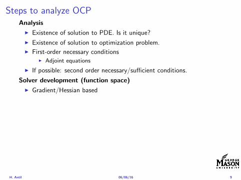
Steps to analyze OCPAnalysis
I Existence of solution to PDE Is it unique
I Existence of solution to optimization problem
I First-order necessary conditionsI Adjoint equations
I If possible second order necessarysufficient conditions
Solver development (function space)
I GradientHessian based
Discrete problem solver
I FD FV FE for problem and solver
I Analysis of discrete solver mesh independence
I EfficiencyI Adaptive finite element methods (AFEM)I Model reduction Proper orthogonal decomposition reduced basis
I Software development Trilinos Rapid Optimization Library (ROL)Dolfin-Adjoint
H Antil 060616 9
Optimal heat sourceI Domain Let Ω sub Rd d ge 1 be open bounded Lipschitz domain
with boundary partΩ
I Goal Choose a distributed source z in such a way that thetemperature u = u(x) is close to a desired ud = ud(x) in Ω
Linear-quadratic elliptic OCP
min J(u z) =1
2uminus ud2L2(Ω) +
λ
2z2L2(Ω)
subject to
minusdiv (Anablau) = z in Ω
u = 0 on partΩ
and the pointwise control constraints
z isin Zad = v isin L2(Ω) za(x) le v(x) le zb(x) ae x isin Ω
λ gt 0 is a parameter za zb isin Linfin(Ω) with za lt zb are given A isbounded symmetric positive
H Antil 060616 10
Problems involving semilinear elliptic PDEsI Heating with radiation boundary condition If the heat radiation
of the heated body is taken into account then we obtain
minus∆u = 0 in Ω
partνu = α(z4 minus u4) on partΩ
where the control z is the temperature of the surrounding medium
I Simplified supercondutivity
minus∆u+ u+ u3 = z in Ω
u = 0 on partΩ
I Control of stationary flows
minusmicro∆u + (u middot nabla)u +nablap = f in Ω
div u = 0 in Ω
u = g on partΩ
H Antil 060616 11
Optimal control of variational inequalitiesProblem
min J(u z) =1
2uminus ud2L2(Ω) +
λ
2z2L2(Ω)
subject to u isin K = w isin H10 (Ω) w(x) ge 0 ae x isin Ωint
Ω
nablau middot nabla(uminus v) dx le (z + f uminus v) forallv isin K
with z isin Zad
Regularized problem
min J(u z) =1
2uminus ud2L2(Ω) +
λ
2z2L2(Ω)
subject to (semilinear PDE)
u isin H10 (Ω) minus∆u+ γρε(minusu) = z + f in Ω
and z isin Zad γ gt 0 and ε gt 0 are the penealization and regularizationparameters respectively
H Antil 060616 12
Outline
Motivation and examples
Linear elliptic optimal control problems
Differentiation in Banach spaces
First-order necessary conditions
Optimal control of semilinear PDEs
An abstract problem
Discretization using finite element methods
H Antil 060616 13
Linear elliptic problemsΩ sub Rn bounded Lipschitz domain
Sobolev spacesI Lp(Ω) 1 le p le infin are Lebesgue spaces p = 2 L2(Ω) is a Hilbert
space with inner product (u v) =int
Ωu(x)v(x) dx
I W sp for s isin R 1 le p le infin are Sobolev spaces When p = 2W s2(Ω) = Hs(Ω) is a Hilbert space
I H10 (Ω) = v isin H1(Ω) v|partΩ = 0 with norm (due to Poincare
inequality)uH1
0 (Ω) = nablauL2(Ω)
I H10 (Ω)lowast = Hminus1(Ω)
I Note L2(Ω) sub Hminus1(Ω)
Model problem
minusdiv (Anablau) = f in Ω
u = 0 on partΩ
H Antil 060616 14
Linear elliptic problemsΩ sub Rn bounded Lipschitz domain
Sobolev spacesI Lp(Ω) 1 le p le infin are Lebesgue spaces p = 2 L2(Ω) is a Hilbert
space with inner product (u v) =int
Ωu(x)v(x) dx
I W sp for s isin R 1 le p le infin are Sobolev spaces When p = 2W s2(Ω) = Hs(Ω) is a Hilbert space
I H10 (Ω) = v isin H1(Ω) v|partΩ = 0 with norm (due to Poincare
inequality)uH1
0 (Ω) = nablauL2(Ω)
I H10 (Ω)lowast = Hminus1(Ω)
I Note L2(Ω) sub Hminus1(Ω)
Model problem
minusdiv (Anablau) = f in Ω
u = 0 on partΩ
H Antil 060616 14
Linear elliptic problemsΩ sub Rn bounded Lipschitz domain
Sobolev spacesI Lp(Ω) 1 le p le infin are Lebesgue spaces p = 2 L2(Ω) is a Hilbert
space with inner product (u v) =int
Ωu(x)v(x) dx
I W sp for s isin R 1 le p le infin are Sobolev spaces When p = 2W s2(Ω) = Hs(Ω) is a Hilbert space
I H10 (Ω) = v isin H1(Ω) v|partΩ = 0 with norm (due to Poincare
inequality)uH1
0 (Ω) = nablauL2(Ω)
I H10 (Ω)lowast = Hminus1(Ω)
I Note L2(Ω) sub Hminus1(Ω)
Model problem
minusdiv (Anablau) = f in Ω
u = 0 on partΩ
H Antil 060616 14
Linear elliptic problemsΩ sub Rn bounded Lipschitz domain
Sobolev spacesI Lp(Ω) 1 le p le infin are Lebesgue spaces p = 2 L2(Ω) is a Hilbert
space with inner product (u v) =int
Ωu(x)v(x) dx
I W sp for s isin R 1 le p le infin are Sobolev spaces When p = 2W s2(Ω) = Hs(Ω) is a Hilbert space
I H10 (Ω) = v isin H1(Ω) v|partΩ = 0 with norm (due to Poincare
inequality)uH1
0 (Ω) = nablauL2(Ω)
I H10 (Ω)lowast = Hminus1(Ω)
I Note L2(Ω) sub Hminus1(Ω)
Model problem
minusdiv (Anablau) = f in Ω
u = 0 on partΩ
H Antil 060616 14
Linear elliptic problemsΩ sub Rn bounded Lipschitz domain
Sobolev spacesI Lp(Ω) 1 le p le infin are Lebesgue spaces p = 2 L2(Ω) is a Hilbert
space with inner product (u v) =int
Ωu(x)v(x) dx
I W sp for s isin R 1 le p le infin are Sobolev spaces When p = 2W s2(Ω) = Hs(Ω) is a Hilbert space
I H10 (Ω) = v isin H1(Ω) v|partΩ = 0 with norm (due to Poincare
inequality)uH1
0 (Ω) = nablauL2(Ω)
I H10 (Ω)lowast = Hminus1(Ω)
I Note L2(Ω) sub Hminus1(Ω)
Model problem
minusdiv (Anablau) = f in Ω
u = 0 on partΩ
H Antil 060616 14
Well-posed
I Weak solution Given f isin Hminus1(Ω) a function u isin H10 (Ω) is called
a weak solution iffintΩ
Anablau middot nablav = 〈f v〉minus11 forallv isin H10 (Ω)
where 〈middot middot〉minus11 denotes the Hminus1(Ω)ndashH1(Ω) duality pairing
I Existence and uniqueness For each f isin Hminus1(Ω) there exists aunique u isin H1
0 (Ω) such that
nablauL2(Ω) le CdΩfHminus1(Ω)
I A = I the result is due to the Riesz-representation theorem
I A 6= I (maybe non-symmetric) the result is due to Lax-Milgramlemma
I For general W 1p-spaces use inf-sup conditions combined withBanach-Necas theorem which is a necessary and sufficient condition
H Antil 060616 15
Well-posed
I Weak solution Given f isin Hminus1(Ω) a function u isin H10 (Ω) is called
a weak solution iffintΩ
Anablau middot nablav = 〈f v〉minus11 forallv isin H10 (Ω)
where 〈middot middot〉minus11 denotes the Hminus1(Ω)ndashH1(Ω) duality pairing
I Existence and uniqueness For each f isin Hminus1(Ω) there exists aunique u isin H1
0 (Ω) such that
nablauL2(Ω) le CdΩfHminus1(Ω)
I A = I the result is due to the Riesz-representation theorem
I A 6= I (maybe non-symmetric) the result is due to Lax-Milgramlemma
I For general W 1p-spaces use inf-sup conditions combined withBanach-Necas theorem which is a necessary and sufficient condition
H Antil 060616 15
Linear-quadratic elliptic OCP
min J(u z) =1
2uminus ud2L2(Ω) +
λ
2z2L2(Ω)
subject to
minusdiv (Anablau) = z in Ω
u = 0 on partΩ
and the pointwise control constraints
z isin Zad = v isin L2(Ω) za(x) le v(x) le zb(x) ae x isin Ω
λ gt 0 is a parameter za zb isin Linfin(Ω) with za lt zb are given A isbounded symmetric positive
H Antil 060616 16
Reduced OCP
I Control to state map The solution operator defined as
S Hminus1(Ω)rarr H10 (Ω) z 7rarr u(z) = Sz
Note In view of the embedding
H10 (Ω) rarr L2(Ω) rarr Hminus1(Ω)
we may also consider S from L2(Ω) to L2(Ω) We will use the samenotation for this operator (for simplicity)
I Reduced cost functional The reduced cost functionalJ L2(Ω)rarr R is defined as
J (z) = J(Sz z)
I Reduced problem minzisinZadJ (z)
H Antil 060616 17
Reduced OCP
I Control to state map The solution operator defined as
S Hminus1(Ω)rarr H10 (Ω) z 7rarr u(z) = Sz
Note In view of the embedding
H10 (Ω) rarr L2(Ω) rarr Hminus1(Ω)
we may also consider S from L2(Ω) to L2(Ω) We will use the samenotation for this operator (for simplicity)
I Reduced cost functional The reduced cost functionalJ L2(Ω)rarr R is defined as
J (z) = J(Sz z)
I Reduced problem minzisinZadJ (z)
H Antil 060616 17
Reduced OCP
I Control to state map The solution operator defined as
S Hminus1(Ω)rarr H10 (Ω) z 7rarr u(z) = Sz
Note In view of the embedding
H10 (Ω) rarr L2(Ω) rarr Hminus1(Ω)
we may also consider S from L2(Ω) to L2(Ω) We will use the samenotation for this operator (for simplicity)
I Reduced cost functional The reduced cost functionalJ L2(Ω)rarr R is defined as
J (z) = J(Sz z)
I Reduced problem minzisinZadJ (z)
H Antil 060616 17
Existence of solution Direct methodThere exists a unique solution to the above problem
I Minimizing sequence J is bounded below by zero therefore thereexists a minimizing sequence znnisinN such that
limnrarrinfin
J (zn) = inf J (z)
I Weak compactness zn sub L2(Ω) is bounded Since L2(Ω) isreflexive therefore there exists a subsequence (not relabeled) suchthat
zn z and z isin Zad
where the latter is a consequence of Zad being closed and convex
I Optimality Since J is continuous and convex and therefore isweakly lower semicontinuous We obtain
lim inf J (zn) ge J (z)
which implies that z is optimal
I Uniqueness Exercise
H Antil 060616 18
Existence of solution Direct methodThere exists a unique solution to the above problem
I Minimizing sequence J is bounded below by zero therefore thereexists a minimizing sequence znnisinN such that
limnrarrinfin
J (zn) = inf J (z)
I Weak compactness zn sub L2(Ω) is bounded Since L2(Ω) isreflexive therefore there exists a subsequence (not relabeled) suchthat
zn z and z isin Zad
where the latter is a consequence of Zad being closed and convex
I Optimality Since J is continuous and convex and therefore isweakly lower semicontinuous We obtain
lim inf J (zn) ge J (z)
which implies that z is optimal
I Uniqueness Exercise
H Antil 060616 18
Existence of solution Direct methodThere exists a unique solution to the above problem
I Minimizing sequence J is bounded below by zero therefore thereexists a minimizing sequence znnisinN such that
limnrarrinfin
J (zn) = inf J (z)
I Weak compactness zn sub L2(Ω) is bounded Since L2(Ω) isreflexive therefore there exists a subsequence (not relabeled) suchthat
zn z and z isin Zad
where the latter is a consequence of Zad being closed and convex
I Optimality Since J is continuous and convex and therefore isweakly lower semicontinuous We obtain
lim inf J (zn) ge J (z)
which implies that z is optimal
I Uniqueness Exercise
H Antil 060616 18
Existence of solution Direct methodThere exists a unique solution to the above problem
I Minimizing sequence J is bounded below by zero therefore thereexists a minimizing sequence znnisinN such that
limnrarrinfin
J (zn) = inf J (z)
I Weak compactness zn sub L2(Ω) is bounded Since L2(Ω) isreflexive therefore there exists a subsequence (not relabeled) suchthat
zn z and z isin Zad
where the latter is a consequence of Zad being closed and convex
I Optimality Since J is continuous and convex and therefore isweakly lower semicontinuous We obtain
lim inf J (zn) ge J (z)
which implies that z is optimal
I Uniqueness Exercise
H Antil 060616 18
Outline
Motivation and examples
Linear elliptic optimal control problems
Differentiation in Banach spaces
First-order necessary conditions
Optimal control of semilinear PDEs
An abstract problem
Discretization using finite element methods
H Antil 060616 19
Differentiation in Banach spacesLet (Z middot Z) (V middot V ) B-spaces Z sub Z open and F Z rarr V
Let z isin Z
I If exist δF (z h) = limtdarr01t (F (z + th)minus F (z)) then δF (z h) is called
the directional derivative of F at z in direction h
I If exist δF (z h) forallh isin Z then h 7rarr δF (z h) is the first variation of Fat z
I Let exist the first variation δF (z middot) F is said to be Gateauxdifferentiable at z iff existA isin L(Z V ) such that δF (z h) = Ahforallh isin Z We write A = F primeG(z)
I F is said to be Frechet differentiable at z iff existA isin L(Z V ) and amapping r(z middot) Z rarr V such that for all h isin U with z + h isin Zwe have
F (z+h) = F (z)+Ah+r(z h) withr(z h)VhZ
rarr 0 as hZ rarr 0
We write F prime(z) = A
H Antil 060616 20
Differentiation in Banach spacesLet (Z middot Z) (V middot V ) B-spaces Z sub Z open and F Z rarr V
Let z isin Z
I If exist δF (z h) = limtdarr01t (F (z + th)minus F (z)) then δF (z h) is called
the directional derivative of F at z in direction h
I If exist δF (z h) forallh isin Z then h 7rarr δF (z h) is the first variation of Fat z
I Let exist the first variation δF (z middot) F is said to be Gateauxdifferentiable at z iff existA isin L(Z V ) such that δF (z h) = Ahforallh isin Z We write A = F primeG(z)
I F is said to be Frechet differentiable at z iff existA isin L(Z V ) and amapping r(z middot) Z rarr V such that for all h isin U with z + h isin Zwe have
F (z+h) = F (z)+Ah+r(z h) withr(z h)VhZ
rarr 0 as hZ rarr 0
We write F prime(z) = A
H Antil 060616 20
Differentiation in Banach spacesLet (Z middot Z) (V middot V ) B-spaces Z sub Z open and F Z rarr V
Let z isin Z
I If exist δF (z h) = limtdarr01t (F (z + th)minus F (z)) then δF (z h) is called
the directional derivative of F at z in direction h
I If exist δF (z h) forallh isin Z then h 7rarr δF (z h) is the first variation of Fat z
I Let exist the first variation δF (z middot) F is said to be Gateauxdifferentiable at z iff existA isin L(Z V ) such that δF (z h) = Ahforallh isin Z We write A = F primeG(z)
I F is said to be Frechet differentiable at z iff existA isin L(Z V ) and amapping r(z middot) Z rarr V such that for all h isin U with z + h isin Zwe have
F (z+h) = F (z)+Ah+r(z h) withr(z h)VhZ
rarr 0 as hZ rarr 0
We write F prime(z) = A
H Antil 060616 20
Differentiation in Banach spacesLet (Z middot Z) (V middot V ) B-spaces Z sub Z open and F Z rarr V
Let z isin Z
I If exist δF (z h) = limtdarr01t (F (z + th)minus F (z)) then δF (z h) is called
the directional derivative of F at z in direction h
I If exist δF (z h) forallh isin Z then h 7rarr δF (z h) is the first variation of Fat z
I Let exist the first variation δF (z middot) F is said to be Gateauxdifferentiable at z iff existA isin L(Z V ) such that δF (z h) = Ahforallh isin Z We write A = F primeG(z)
I F is said to be Frechet differentiable at z iff existA isin L(Z V ) and amapping r(z middot) Z rarr V such that for all h isin U with z + h isin Zwe have
F (z+h) = F (z)+Ah+r(z h) withr(z h)VhZ
rarr 0 as hZ rarr 0
We write F prime(z) = A
H Antil 060616 20
ExamplesExample 1 (H (middot middot)H) Hilbert space F (z) = z2H = (z z)H
forallz h F (z + h)minus F (z) = 2(z h)H + h2HThen
F prime(z)h = (2z h)H
Reisz representation theorem (identify H with Hlowast) we can write
F prime(z)h = (nablaF (z) h)H
where nablaF (z) = 2z is the gradient
Example 2 Let (Z (middot middot)Z) (H (middot middot)H) Hilbert spaces ud isin H fixedLet S isin L(ZH) Consider E Z rarr R
E(z) = Sz minus ud2H
Then E(z) = G(F (z)) where G(v) = v2H and F (z) = Sz minus ud
Eprime(z)h = Gprime(F (z))F prime(z)h = (2v F prime(z)h)H
= 2(Sz minus ud Sh)H = 2(Slowast(Sz minus ud) h)Z
we denote the gradient as nablaE(z) = 2Slowast(Sz minus ud)
H Antil 060616 21
ExamplesExample 1 (H (middot middot)H) Hilbert space F (z) = z2H = (z z)H
forallz h F (z + h)minus F (z) = 2(z h)H + h2HThen
F prime(z)h = (2z h)H
Reisz representation theorem (identify H with Hlowast) we can write
F prime(z)h = (nablaF (z) h)H
where nablaF (z) = 2z is the gradient
Example 2 Let (Z (middot middot)Z) (H (middot middot)H) Hilbert spaces ud isin H fixedLet S isin L(ZH) Consider E Z rarr R
E(z) = Sz minus ud2H
Then E(z) = G(F (z)) where G(v) = v2H and F (z) = Sz minus ud
Eprime(z)h = Gprime(F (z))F prime(z)h = (2v F prime(z)h)H
= 2(Sz minus ud Sh)H = 2(Slowast(Sz minus ud) h)Z
we denote the gradient as nablaE(z) = 2Slowast(Sz minus ud)H Antil 060616 21
Outline
Motivation and examples
Linear elliptic optimal control problems
Differentiation in Banach spaces
First-order necessary conditions
Optimal control of semilinear PDEs
An abstract problem
Discretization using finite element methods
H Antil 060616 22
First order necessary optimality conditions
Most of the theory is based on these two simple results
Theorem Let (Z middot Z) be a normed space J Z rarr (infin+infin] amapping with J 6equiv +infin Then z isin Z minimizer of J hArr 0 isin partJ (z)
Proof 0 isin partJ (z) means by definition of partJ (z) J (z)minus J (z) le 0forallz isin Z
Theorem Let (Z middot Z) be a normed space Zad sub Z nonemptyconvex closed J Z rarr R Gateaux differentiable where Zad sub Z sub ZZ open If z isin Zad is a solution to
minzisinZad
J (z)
then z solvesJ prime(z)(z minus z) ge 0 forallz isin Zad
Proof Exercise
H Antil 060616 23
First order necessary optimality conditions
Most of the theory is based on these two simple results
Theorem Let (Z middot Z) be a normed space J Z rarr (infin+infin] amapping with J 6equiv +infin Then z isin Z minimizer of J hArr 0 isin partJ (z)
Proof 0 isin partJ (z) means by definition of partJ (z) J (z)minus J (z) le 0forallz isin Z
Theorem Let (Z middot Z) be a normed space Zad sub Z nonemptyconvex closed J Z rarr R Gateaux differentiable where Zad sub Z sub ZZ open If z isin Zad is a solution to
minzisinZad
J (z)
then z solvesJ prime(z)(z minus z) ge 0 forallz isin Zad
Proof Exercise
H Antil 060616 23
Linear quadratic OCPI Reduced funcational
J (z) =1
2Sz minus ud2L2(Ω) +
λ
2z2L2(Ω)
I Gradient computation using sensitivity
J prime(z)h = (Slowast(Sz minus ud) + λz h)L2(Ω) forallh isin L2(Ω)
we denote the gradient by
nablaJ (z) = Slowast(Sz minus ud) + λz
I First order necessary and sufficient optimality condition
(nablaJ (z) z minus z)L2(Ω) ge 0 forallz isin Zad
I Adjoint equation Let p = Slowast(Sz minus ud) which translates intop isin H1
0 (Ω) solving
minusdiv (Anablap) = uminus ud in Ω
p = 0 on partΩ
I Gradient computation using adjoint nablaJ (z) = p+ λz
H Antil 060616 24
Linear quadratic OCPI Reduced funcational
J (z) =1
2Sz minus ud2L2(Ω) +
λ
2z2L2(Ω)
I Gradient computation using sensitivity
J prime(z)h = (Slowast(Sz minus ud) + λz h)L2(Ω) forallh isin L2(Ω)
we denote the gradient by
nablaJ (z) = Slowast(Sz minus ud) + λz
I First order necessary and sufficient optimality condition
(nablaJ (z) z minus z)L2(Ω) ge 0 forallz isin Zad
I Adjoint equation Let p = Slowast(Sz minus ud) which translates intop isin H1
0 (Ω) solving
minusdiv (Anablap) = uminus ud in Ω
p = 0 on partΩ
I Gradient computation using adjoint nablaJ (z) = p+ λz
H Antil 060616 24
Linear quadratic OCPI Reduced funcational
J (z) =1
2Sz minus ud2L2(Ω) +
λ
2z2L2(Ω)
I Gradient computation using sensitivity
J prime(z)h = (Slowast(Sz minus ud) + λz h)L2(Ω) forallh isin L2(Ω)
we denote the gradient by
nablaJ (z) = Slowast(Sz minus ud) + λz
I First order necessary and sufficient optimality condition
(nablaJ (z) z minus z)L2(Ω) ge 0 forallz isin Zad
I Adjoint equation Let p = Slowast(Sz minus ud) which translates intop isin H1
0 (Ω) solving
minusdiv (Anablap) = uminus ud in Ω
p = 0 on partΩ
I Gradient computation using adjoint nablaJ (z) = p+ λz
H Antil 060616 24
Linear quadratic OCPI Reduced funcational
J (z) =1
2Sz minus ud2L2(Ω) +
λ
2z2L2(Ω)
I Gradient computation using sensitivity
J prime(z)h = (Slowast(Sz minus ud) + λz h)L2(Ω) forallh isin L2(Ω)
we denote the gradient by
nablaJ (z) = Slowast(Sz minus ud) + λz
I First order necessary and sufficient optimality condition
(nablaJ (z) z minus z)L2(Ω) ge 0 forallz isin Zad
I Adjoint equation Let p = Slowast(Sz minus ud) which translates intop isin H1
0 (Ω) solving
minusdiv (Anablap) = uminus ud in Ω
p = 0 on partΩ
I Gradient computation using adjoint nablaJ (z) = p+ λz
H Antil 060616 24
Linear quadratic OCPI Reduced funcational
J (z) =1
2Sz minus ud2L2(Ω) +
λ
2z2L2(Ω)
I Gradient computation using sensitivity
J prime(z)h = (Slowast(Sz minus ud) + λz h)L2(Ω) forallh isin L2(Ω)
we denote the gradient by
nablaJ (z) = Slowast(Sz minus ud) + λz
I First order necessary and sufficient optimality condition
(nablaJ (z) z minus z)L2(Ω) ge 0 forallz isin Zad
I Adjoint equation Let p = Slowast(Sz minus ud) which translates intop isin H1
0 (Ω) solving
minusdiv (Anablap) = uminus ud in Ω
p = 0 on partΩ
I Gradient computation using adjoint nablaJ (z) = p+ λz
H Antil 060616 24
Optimality system
I State u isin H10 (Ω)
intΩAnablau middot nablav =
intΩzv forallv isin H1
0 (Ω)
I Adjoint p isin H10 (Ω)
intΩAnablap middot nablav =
intΩ
(uminus ud)v forallv isin H10 (Ω)
I Control z isin Zad (p+ λz z minus z) ge 0 forallz isin Zad
H Antil 060616 25
Pointwise interpretation
The variational inequality
(p+ λz z minus z) ge 0 forallz isin Zad
is equivalent to for ae x isin Ω
z(x) =
za(x) if p(x) + λz(x) gt 0isin [za(x) zb(x)] if p(x) + λz(x) = 0zb(x) if p(x) + λz(x) lt 0
Consequence
I When λ gt 0 then ae in Ω
z(x) = P[za(x)zb(x)]
minus 1
λp(x)
= min
zb(x)max
za(x)minus 1
λp(x)
H Antil 060616 26
Formal Lagrange method applied to linear OCPIntroduce L H1
0 (Ω)times Zad timesH1(Ω)rarr R defined as
L(u z p) = J(u z)minusint
Ω
(minusdiv (Anablau)minus z
)p dx
Integrate by parts to arrive at
L(u z p) = J(u z)minusint
Ω
(minusdiv (Anablap)uminus zp
)dx+
intpartΩ
(Anablau)p ds
If (u z p) is a stationary point then
I State
DpL(u z p)h = 0 forallh isin H1(Ω)
I AdjointDuL(u z p)h = 0 forallh isin H1
0 (Ω)
I ControlDzL(u z p)(z minus z) ge 0 forallz isin Zad
H Antil 060616 27
Formal Lagrange method applied to linear OCPIntroduce L H1
0 (Ω)times Zad timesH1(Ω)rarr R defined as
L(u z p) = J(u z)minusint
Ω
(minusdiv (Anablau)minus z
)p dx
Integrate by parts to arrive at
L(u z p) = J(u z)minusint
Ω
(minusdiv (Anablap)uminus zp
)dx+
intpartΩ
(Anablau)p ds
If (u z p) is a stationary point then
I State
DpL(u z p)h = 0 forallh isin H1(Ω)
I AdjointDuL(u z p)h = 0 forallh isin H1
0 (Ω)
I ControlDzL(u z p)(z minus z) ge 0 forallz isin Zad
H Antil 060616 27
Formal Lagrange method applied to linear OCPIntroduce L H1
0 (Ω)times Zad timesH1(Ω)rarr R defined as
L(u z p) = J(u z)minusint
Ω
(minusdiv (Anablau)minus z
)p dx
Integrate by parts to arrive at
L(u z p) = J(u z)minusint
Ω
(minusdiv (Anablap)uminus zp
)dx+
intpartΩ
(Anablau)p ds
If (u z p) is a stationary point then
I State
DpL(u z p)h = 0 forallh isin H1(Ω)
I AdjointDuL(u z p)h = 0 forallh isin H1
0 (Ω)
I ControlDzL(u z p)(z minus z) ge 0 forallz isin Zad
H Antil 060616 27
Formal Lagrange method applied to linear OCPIntroduce L H1
0 (Ω)times Zad timesH1(Ω)rarr R defined as
L(u z p) = J(u z)minusint
Ω
(minusdiv (Anablau)minus z
)p dx
Integrate by parts to arrive at
L(u z p) = J(u z)minusint
Ω
(minusdiv (Anablap)uminus zp
)dx+
intpartΩ
(Anablau)p ds
If (u z p) is a stationary point then
I State
DpL(u z p)h = 0 forallh isin H1(Ω)
I AdjointDuL(u z p)h = 0 forallh isin H1
0 (Ω)
I ControlDzL(u z p)(z minus z) ge 0 forallz isin Zad
H Antil 060616 27
Formal Lagrange method applied to linear OCPIntroduce L H1
0 (Ω)times Zad timesH1(Ω)rarr R defined as
L(u z p) = J(u z)minusint
Ω
(minusdiv (Anablau)minus z
)p dx
Integrate by parts to arrive at
L(u z p) = J(u z)minusint
Ω
(minusdiv (Anablap)uminus zp
)dx+
intpartΩ
(Anablau)p ds
If (u z p) is a stationary point then
I State
DpL(u z p)h = 0 forallh isin H1(Ω)
I AdjointDuL(u z p)h = 0 forallh isin H1
0 (Ω)
I ControlDzL(u z p)(z minus z) ge 0 forallz isin Zad
H Antil 060616 27
Outline
Motivation and examples
Linear elliptic optimal control problems
Differentiation in Banach spaces
First-order necessary conditions
Optimal control of semilinear PDEs
An abstract problem
Discretization using finite element methods
H Antil 060616 28
Semilinear elliptic OCP
min J(u z) =1
2uminus ud2L2(Ω) +
λ
2z2L2(Ω)
subject to
minus∆u+ g(x u) = z in Ω
u = 0 on partΩ
and z isin Zad with za zb isin Linfin(Ω)
H Antil 060616 29
State space(A1) Ω sub Rd open bounded partΩ is Lipschitz
(A2) g Ωtimes Rrarr R is bounded and measurable with respect to x isin Ωfor every u isin R
(A3) g is continuous monotone increasing and Lipschitz continuous in ufor ae x isin Ω
(A4) g(x 0) = 0 for ae x isin Ω (not really necessary)
Theorem Suppose (A1)minus (A4) hold For every z isin Lr(Ω) withr gt d2 the state equation has a unique weak solutionu isin H1
0 (Ω) cap C(Ω) ie we haveintΩ
nablau middot nablav dx+
intΩ
g(x u(x))v(x) dx =
intΩ
zv dx forallv isin H10 (Ω)
Moreover there exists a constant C gt 0 such that
uH1(Ω) + uC(Ω) le CzLr(Ω)
RemarkI The proof of the theorem uses the BrowderndashMinty theorem on
monotone operators
H Antil 060616 30
State space(A1) Ω sub Rd open bounded partΩ is Lipschitz
(A2) g Ωtimes Rrarr R is bounded and measurable with respect to x isin Ωfor every u isin R
(A3) g is continuous monotone increasing and Lipschitz continuous in ufor ae x isin Ω
(A4) g(x 0) = 0 for ae x isin Ω (not really necessary)
Theorem Suppose (A1)minus (A4) hold For every z isin Lr(Ω) withr gt d2 the state equation has a unique weak solutionu isin H1
0 (Ω) cap C(Ω) ie we haveintΩ
nablau middot nablav dx+
intΩ
g(x u(x))v(x) dx =
intΩ
zv dx forallv isin H10 (Ω)
Moreover there exists a constant C gt 0 such that
uH1(Ω) + uC(Ω) le CzLr(Ω)
RemarkI The proof of the theorem uses the BrowderndashMinty theorem on
monotone operators
H Antil 060616 30
State space(A1) Ω sub Rd open bounded partΩ is Lipschitz
(A2) g Ωtimes Rrarr R is bounded and measurable with respect to x isin Ωfor every u isin R
(A3) g is continuous monotone increasing and Lipschitz continuous in ufor ae x isin Ω
(A4) g(x 0) = 0 for ae x isin Ω (not really necessary)
Theorem Suppose (A1)minus (A4) hold For every z isin Lr(Ω) withr gt d2 the state equation has a unique weak solutionu isin H1
0 (Ω) cap C(Ω) ie we haveintΩ
nablau middot nablav dx+
intΩ
g(x u(x))v(x) dx =
intΩ
zv dx forallv isin H10 (Ω)
Moreover there exists a constant C gt 0 such that
uH1(Ω) + uC(Ω) le CzLr(Ω)
RemarkI The proof of the theorem uses the BrowderndashMinty theorem on
monotone operators
H Antil 060616 30
Control-to-state map and reduced problem
I Control to state map
S Linfin(Ω)rarr H10 (Ω) cap C(Ω)
is well defined and is globally Lipschitz continuous
I Reduced problem
minJ (z) =1
2S(u)minus ud2L2(Ω) +
λ
2z2L2(Ω)
H Antil 060616 31
Control-to-state map and reduced problem
I Control to state map
S Linfin(Ω)rarr H10 (Ω) cap C(Ω)
is well defined and is globally Lipschitz continuous
I Reduced problem
minJ (z) =1
2S(u)minus ud2L2(Ω) +
λ
2z2L2(Ω)
H Antil 060616 31
First-order necessary conditionsI Lagrangian functional
L(u z p) = J(u z)minusint
Ω
(minus∆u+ g(x u(x))minus z
)p dx
= J(u z)minusint
Ω
(nablau middot nablap+ g(x u(x))pminus zp
)dx
I Adjoint system For all h isin H10 (Ω)
0 = DuL(u z p)h =
intΩ
(uminus ud)h dxminusint
Ω
(nablah middot nablap+ gu(x u(x))ph
)which yields
minus∆p+ gu(x u(x))p = uminus ud in Ω
p = 0 on partΩ
I Control
DzL(u z p)(z minus z) = (p+ λz z minus z) dx ge 0 forallz isin ZadI Gradient
nablaJ (z) = p+ λz
H Antil 060616 32
First-order necessary conditionsI Lagrangian functional
L(u z p) = J(u z)minusint
Ω
(minus∆u+ g(x u(x))minus z
)p dx
= J(u z)minusint
Ω
(nablau middot nablap+ g(x u(x))pminus zp
)dx
I Adjoint system For all h isin H10 (Ω)
0 = DuL(u z p)h =
intΩ
(uminus ud)h dxminusint
Ω
(nablah middot nablap+ gu(x u(x))ph
)which yields
minus∆p+ gu(x u(x))p = uminus ud in Ω
p = 0 on partΩ
I Control
DzL(u z p)(z minus z) = (p+ λz z minus z) dx ge 0 forallz isin ZadI Gradient
nablaJ (z) = p+ λz
H Antil 060616 32
First-order necessary conditionsI Lagrangian functional
L(u z p) = J(u z)minusint
Ω
(minus∆u+ g(x u(x))minus z
)p dx
= J(u z)minusint
Ω
(nablau middot nablap+ g(x u(x))pminus zp
)dx
I Adjoint system For all h isin H10 (Ω)
0 = DuL(u z p)h =
intΩ
(uminus ud)h dxminusint
Ω
(nablah middot nablap+ gu(x u(x))ph
)which yields
minus∆p+ gu(x u(x))p = uminus ud in Ω
p = 0 on partΩ
I Control
DzL(u z p)(z minus z) = (p+ λz z minus z) dx ge 0 forallz isin Zad
I GradientnablaJ (z) = p+ λz
H Antil 060616 32
First-order necessary conditionsI Lagrangian functional
L(u z p) = J(u z)minusint
Ω
(minus∆u+ g(x u(x))minus z
)p dx
= J(u z)minusint
Ω
(nablau middot nablap+ g(x u(x))pminus zp
)dx
I Adjoint system For all h isin H10 (Ω)
0 = DuL(u z p)h =
intΩ
(uminus ud)h dxminusint
Ω
(nablah middot nablap+ gu(x u(x))ph
)which yields
minus∆p+ gu(x u(x))p = uminus ud in Ω
p = 0 on partΩ
I Control
DzL(u z p)(z minus z) = (p+ λz z minus z) dx ge 0 forallz isin ZadI Gradient
nablaJ (z) = p+ λz
H Antil 060616 32
Differentiability of Nemytskii operator
The rigorous proof uses
Theorem In addition to (A1)-(A4) if
(A5) g is continuously differentiable with respect to u for ae x isin Ωand we have
(i) |gu(x 0)| le K for ae x isin Ω(ii) gu is locally Lipschitz with respect to u isin R
then the Nemytskii operator G u 7rarr g(middot u(middot)) is continuously Frechetdifferentiable from Linfin(Ω) into itself and
(Gprime(u)h)(x) = gu(x u(x))h(x) ae in Ω forallh isin Linfin(Ω)
Remark (A5) holds if g(x u) = g(u) and g isin C2(R)
H Antil 060616 33
Outline
Motivation and examples
Linear elliptic optimal control problems
Differentiation in Banach spaces
First-order necessary conditions
Optimal control of semilinear PDEs
An abstract problem
Discretization using finite element methods
H Antil 060616 34
Gradient computation via adjoint general formI Abstract problem
min J(u z)
subject toc(u z) = 0
and z isin Zad
I Directional derivative Let S be the control to state map(nonlinear in general)
z 7rarr S(z) = u(z)
Under the assumptions of ldquoimplicit function theoremrdquo
J prime(z)h = (nablauJ (u(z) z) Sprime(z)h) + (nablazJ (u(z) z) h)
I Sensitivity of u with respect to z Differentiating the stateequation
cu(S(z) z)Sprime(z)h = minuscz(S(z) z)h
leads toSprime(z)h = minuscu(S(z) z)minus1
(cz(S(z) z)h
)
provided cu(S(z) z)minus1 is well-defined
H Antil 060616 35
Gradient computation via adjoint general formI Abstract problem
min J(u z)
subject toc(u z) = 0
and z isin ZadI Directional derivative Let S be the control to state map
(nonlinear in general)
z 7rarr S(z) = u(z)
Under the assumptions of ldquoimplicit function theoremrdquo
J prime(z)h = (nablauJ (u(z) z) Sprime(z)h) + (nablazJ (u(z) z) h)
I Sensitivity of u with respect to z Differentiating the stateequation
cu(S(z) z)Sprime(z)h = minuscz(S(z) z)h
leads toSprime(z)h = minuscu(S(z) z)minus1
(cz(S(z) z)h
)
provided cu(S(z) z)minus1 is well-defined
H Antil 060616 35
Gradient computation via adjoint general formI Abstract problem
min J(u z)
subject toc(u z) = 0
and z isin ZadI Directional derivative Let S be the control to state map
(nonlinear in general)
z 7rarr S(z) = u(z)
Under the assumptions of ldquoimplicit function theoremrdquo
J prime(z)h = (nablauJ (u(z) z) Sprime(z)h) + (nablazJ (u(z) z) h)
I Sensitivity of u with respect to z Differentiating the stateequation
cu(S(z) z)Sprime(z)h = minuscz(S(z) z)h
leads toSprime(z)h = minuscu(S(z) z)minus1
(cz(S(z) z)h
)
provided cu(S(z) z)minus1 is well-defined
H Antil 060616 35
Adjoint equation and gradient general form
I Directional derivative
J prime(z)h = minus(nablauJ (u(z) z) cu(u(z) z)minus1cz(u(z) z)h
)+ (nablazJ (u(z) z) h)
I Gradient
nablaJ (z) = minuscz(u(z) z)lowast(cu(u(z) z)minuslowastnablauJ (u(z) z)
)+nablazJ (u(z) z)
I Introducing adjoint variable p solving
cu(u(z) z)lowastp = nablauJ (u(z) z)
we arrive at following form of gradient
nablaJ (z) = minuscz(u(z) z)lowastp+nablazJ (u(z) z)
which is tractable
H Antil 060616 36
Adjoint equation and gradient general form
I Directional derivative
J prime(z)h = minus(nablauJ (u(z) z) cu(u(z) z)minus1cz(u(z) z)h
)+ (nablazJ (u(z) z) h)
I Gradient
nablaJ (z) = minuscz(u(z) z)lowast(cu(u(z) z)minuslowastnablauJ (u(z) z)
)+nablazJ (u(z) z)
I Introducing adjoint variable p solving
cu(u(z) z)lowastp = nablauJ (u(z) z)
we arrive at following form of gradient
nablaJ (z) = minuscz(u(z) z)lowastp+nablazJ (u(z) z)
which is tractable
H Antil 060616 36
Adjoint equation and gradient general form
I Directional derivative
J prime(z)h = minus(nablauJ (u(z) z) cu(u(z) z)minus1cz(u(z) z)h
)+ (nablazJ (u(z) z) h)
I Gradient
nablaJ (z) = minuscz(u(z) z)lowast(cu(u(z) z)minuslowastnablauJ (u(z) z)
)+nablazJ (u(z) z)
I Introducing adjoint variable p solving
cu(u(z) z)lowastp = nablauJ (u(z) z)
we arrive at following form of gradient
nablaJ (z) = minuscz(u(z) z)lowastp+nablazJ (u(z) z)
which is tractable
H Antil 060616 36
Hessian computation general form
I Lagrangian L(u z p) = J(u z)minusint
Ωc(u z)p dx Then we have
DzJ (z)h = DzL(u z p)h
I Second order derivative
D2zJ (z)[h1 h2] = DuDzL(u z p)[h1 S
prime(z)h2] +D2zL(u z p)[h1 h2]
+DpDzL(u z p)[h1 Dzp(z)h2]
I We already know Sprime(z)h2 moreover
DpDzL(u z p)[h1 Dzp(z)h2] = minus(cu(u z)h1 Dzp(z)h2
)
It remain to identify Dzp(z)h2
H Antil 060616 37
Hessian computation general form
I Lagrangian L(u z p) = J(u z)minusint
Ωc(u z)p dx Then we have
DzJ (z)h = DzL(u z p)h
I Second order derivative
D2zJ (z)[h1 h2] = DuDzL(u z p)[h1 S
prime(z)h2] +D2zL(u z p)[h1 h2]
+DpDzL(u z p)[h1 Dzp(z)h2]
I We already know Sprime(z)h2 moreover
DpDzL(u z p)[h1 Dzp(z)h2] = minus(cu(u z)h1 Dzp(z)h2
)
It remain to identify Dzp(z)h2
H Antil 060616 37
Hessian computation general form
I Lagrangian L(u z p) = J(u z)minusint
Ωc(u z)p dx Then we have
DzJ (z)h = DzL(u z p)h
I Second order derivative
D2zJ (z)[h1 h2] = DuDzL(u z p)[h1 S
prime(z)h2] +D2zL(u z p)[h1 h2]
+DpDzL(u z p)[h1 Dzp(z)h2]
I We already know Sprime(z)h2 moreover
DpDzL(u z p)[h1 Dzp(z)h2] = minus(cu(u z)h1 Dzp(z)h2
)
It remain to identify Dzp(z)h2
H Antil 060616 37
Outline
Motivation and examples
Linear elliptic optimal control problems
Differentiation in Banach spaces
First-order necessary conditions
Optimal control of semilinear PDEs
An abstract problem
Discretization using finite element methods
H Antil 060616 38
Numerical approximation of Poisson equation MeshTo avoid technical issues we will assume that partΩ is polygonal
I Mesh Let T = K be a mesh of Ω where K sub Rd is an elementthat is isoparametrically equivalent to a unit simplex in Rd
I Conforming mesh We say that the mesh is conforming ifI Ω = cupKisinT KI If K1 cap K2 = x then x is a node of K1 and K2I If K1 cap K2 6= empty and K1 cap K2 6= x then K1 cap K2 is an edgeface
contained in partK1 cap partK2
I Shape regular Let T be the collection of all conformingrefinements of an original mesh T 0 Then T is called shape regularif exist κ gt 0 such that
hKρKle κ forallK isin cupiT i
where hK = diam K ρK = maxρ gt 0|Bρ sub KI Quasi-uniform A family of shape regular meshes is called-quasi
uniform if there exist a constant σ gt 0 such that
maxhKminhK
le σ
uniformly for all meshes in the family
Numerical approximation of Poisson equation MeshTo avoid technical issues we will assume that partΩ is polygonal
I Mesh Let T = K be a mesh of Ω where K sub Rd is an elementthat is isoparametrically equivalent to a unit simplex in Rd
I Conforming mesh We say that the mesh is conforming ifI Ω = cupKisinT KI If K1 cap K2 = x then x is a node of K1 and K2I If K1 cap K2 6= empty and K1 cap K2 6= x then K1 cap K2 is an edgeface
contained in partK1 cap partK2
I Shape regular Let T be the collection of all conformingrefinements of an original mesh T 0 Then T is called shape regularif exist κ gt 0 such that
hKρKle κ forallK isin cupiT i
where hK = diam K ρK = maxρ gt 0|Bρ sub KI Quasi-uniform A family of shape regular meshes is called-quasi
uniform if there exist a constant σ gt 0 such that
maxhKminhK
le σ
uniformly for all meshes in the family
Numerical approximation of Poisson equation MeshTo avoid technical issues we will assume that partΩ is polygonal
I Mesh Let T = K be a mesh of Ω where K sub Rd is an elementthat is isoparametrically equivalent to a unit simplex in Rd
I Conforming mesh We say that the mesh is conforming ifI Ω = cupKisinT KI If K1 cap K2 = x then x is a node of K1 and K2I If K1 cap K2 6= empty and K1 cap K2 6= x then K1 cap K2 is an edgeface
contained in partK1 cap partK2
I Shape regular Let T be the collection of all conformingrefinements of an original mesh T 0 Then T is called shape regularif exist κ gt 0 such that
hKρKle κ forallK isin cupiT i
where hK = diam K ρK = maxρ gt 0|Bρ sub K
I Quasi-uniform A family of shape regular meshes is called-quasiuniform if there exist a constant σ gt 0 such that
maxhKminhK
le σ
uniformly for all meshes in the family
Numerical approximation of Poisson equation MeshTo avoid technical issues we will assume that partΩ is polygonal
I Mesh Let T = K be a mesh of Ω where K sub Rd is an elementthat is isoparametrically equivalent to a unit simplex in Rd
I Conforming mesh We say that the mesh is conforming ifI Ω = cupKisinT KI If K1 cap K2 = x then x is a node of K1 and K2I If K1 cap K2 6= empty and K1 cap K2 6= x then K1 cap K2 is an edgeface
contained in partK1 cap partK2
I Shape regular Let T be the collection of all conformingrefinements of an original mesh T 0 Then T is called shape regularif exist κ gt 0 such that
hKρKle κ forallK isin cupiT i
where hK = diam K ρK = maxρ gt 0|Bρ sub KI Quasi-uniform A family of shape regular meshes is called-quasi
uniform if there exist a constant σ gt 0 such that
maxhKminhK
le σ
uniformly for all meshes in the family
FE space and Galerkin approximationI Finite element space For T isin T we define the finite element
space as
V(T ) = W isin C0(Ω) WK isin P1forallK isin T W |partΩ = 0
where P1 is the set of polynomials of degree at most 1
I Galerkin approximation of continuous problem is given by
Find UT isin V(T )
intΩ
AnablaUT middot nablaV = 〈f V 〉 forallV isin V(T )
The discrete problem is well-posedI Nodal basis Consists of functions ψi isin V(T ) with xi isin N (T )
satisfyingψxi
(xj) = δij
where N (T ) denotes the interior (plus Neumann) nodesI Galerkin orthogonality(
nabla(uminus UT )nablaW)L2(Ω)
= 0 forallW isin V(T )
H Antil 060616 40
FE space and Galerkin approximationI Finite element space For T isin T we define the finite element
space as
V(T ) = W isin C0(Ω) WK isin P1forallK isin T W |partΩ = 0
where P1 is the set of polynomials of degree at most 1I Galerkin approximation of continuous problem is given by
Find UT isin V(T )
intΩ
AnablaUT middot nablaV = 〈f V 〉 forallV isin V(T )
The discrete problem is well-posed
I Nodal basis Consists of functions ψi isin V(T ) with xi isin N (T )satisfying
ψxi(xj) = δij
where N (T ) denotes the interior (plus Neumann) nodesI Galerkin orthogonality(
nabla(uminus UT )nablaW)L2(Ω)
= 0 forallW isin V(T )
H Antil 060616 40
FE space and Galerkin approximationI Finite element space For T isin T we define the finite element
space as
V(T ) = W isin C0(Ω) WK isin P1forallK isin T W |partΩ = 0
where P1 is the set of polynomials of degree at most 1I Galerkin approximation of continuous problem is given by
Find UT isin V(T )
intΩ
AnablaUT middot nablaV = 〈f V 〉 forallV isin V(T )
The discrete problem is well-posedI Nodal basis Consists of functions ψi isin V(T ) with xi isin N (T )
satisfyingψxi
(xj) = δij
where N (T ) denotes the interior (plus Neumann) nodes
I Galerkin orthogonality(nabla(uminus UT )nablaW
)L2(Ω)
= 0 forallW isin V(T )
H Antil 060616 40
FE space and Galerkin approximationI Finite element space For T isin T we define the finite element
space as
V(T ) = W isin C0(Ω) WK isin P1forallK isin T W |partΩ = 0
where P1 is the set of polynomials of degree at most 1I Galerkin approximation of continuous problem is given by
Find UT isin V(T )
intΩ
AnablaUT middot nablaV = 〈f V 〉 forallV isin V(T )
The discrete problem is well-posedI Nodal basis Consists of functions ψi isin V(T ) with xi isin N (T )
satisfyingψxi
(xj) = δij
where N (T ) denotes the interior (plus Neumann) nodesI Galerkin orthogonality(
nabla(uminus UT )nablaW)L2(Ω)
= 0 forallW isin V(T )
H Antil 060616 40
Best approximation
I Cearsquos lemma
nabla(uminus UT )L2(Ω) le C infWisinV(T )
nabla(uminusW )L2(Ω)
I Nodal interpolation operator ΠT C(Ω)rarr V(T ) satisfies
ΠT u(xi) = u(xi) forallxi isin N (T )
and is defined as
ΠT u =sum
xiisinN (T )
u(xi)ψxi
I Error estimates In Cearsquos lemma replace W by ΠT u and thencompute the interpolation error
H Antil 060616 41
Best approximation
I Cearsquos lemma
nabla(uminus UT )L2(Ω) le C infWisinV(T )
nabla(uminusW )L2(Ω)
I Nodal interpolation operator ΠT C(Ω)rarr V(T ) satisfies
ΠT u(xi) = u(xi) forallxi isin N (T )
and is defined as
ΠT u =sum
xiisinN (T )
u(xi)ψxi
I Error estimates In Cearsquos lemma replace W by ΠT u and thencompute the interpolation error
H Antil 060616 41
Best approximation
I Cearsquos lemma
nabla(uminus UT )L2(Ω) le C infWisinV(T )
nabla(uminusW )L2(Ω)
I Nodal interpolation operator ΠT C(Ω)rarr V(T ) satisfies
ΠT u(xi) = u(xi) forallxi isin N (T )
and is defined as
ΠT u =sum
xiisinN (T )
u(xi)ψxi
I Error estimates In Cearsquos lemma replace W by ΠT u and thencompute the interpolation error
H Antil 060616 41
Algebraic system state equation
I Recall UT isin V(T ) solves
a(UT V ) = 〈f V 〉 forallV isin V(T )
I Now setting UT =sumN
j=1 Ujψj V = ψi we get
Nsumj=1
Uja(φj φi) = 〈f ψi〉 i = 1 N
which is the matrix-vector system
AU = F
I Stiffness matrix A is SPD
H Antil 060616 42
Algebraic system state equation
I Recall UT isin V(T ) solves
a(UT V ) = 〈f V 〉 forallV isin V(T )
I Now setting UT =sumN
j=1 Ujψj V = ψi we get
Nsumj=1
Uja(φj φi) = 〈f ψi〉 i = 1 N
which is the matrix-vector system
AU = F
I Stiffness matrix A is SPD
H Antil 060616 42
Algebraic system state equation
I Recall UT isin V(T ) solves
a(UT V ) = 〈f V 〉 forallV isin V(T )
I Now setting UT =sumN
j=1 Ujψj V = ψi we get
Nsumj=1
Uja(φj φi) = 〈f ψi〉 i = 1 N
which is the matrix-vector system
AU = F
I Stiffness matrix A is SPD
H Antil 060616 42
Discrete linear elliptic OCP
min JT (UT ZT ) =1
2UT minus ud2L2(Ω) +
λ
2ZT 2L2(Ω)
subject to
Find UT isin V(T )
intΩ
nablaUT middot nablaV = (ZT V )L2(Ω) forallV isin V(T )
and whereZT isin Zad(T ) = Zad cap Z(T )
is either one of these
Z(T ) =
V(T )L2(Ω) variational discretization (Hinze)WT isin Linfin(Ω) ZT |K isin P0(K)K isin T
H Antil 060616 43
Recent books
F TroltzschOptimal control of partial differential equations volume 112 ofGraduate Studies in MathematicsAmerican Mathematical Society Providence RI 2010Theory methods and applications Translated from the 2005 Germanoriginal by Jurgen Sprekels
K Ito and K KunischLagrange multiplier approach to variational problems andapplications volume 15 of Advances in Design and ControlSociety for Industrial and Applied Mathematics (SIAM)Philadelphia PA 2008
H Antil 060616 44
- Motivation and examples
- Linear elliptic optimal control problems
- Differentiation in Banach spaces
- First-order necessary conditions
- Optimal control of semilinear PDEs
- An abstract problem
- Discretization using finite element methods
-
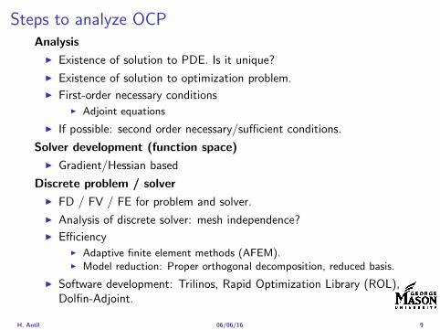
Steps to analyze OCPAnalysis
I Existence of solution to PDE Is it unique
I Existence of solution to optimization problem
I First-order necessary conditionsI Adjoint equations
I If possible second order necessarysufficient conditions
Solver development (function space)
I GradientHessian based
Discrete problem solver
I FD FV FE for problem and solver
I Analysis of discrete solver mesh independence
I EfficiencyI Adaptive finite element methods (AFEM)I Model reduction Proper orthogonal decomposition reduced basis
I Software development Trilinos Rapid Optimization Library (ROL)Dolfin-Adjoint
H Antil 060616 9
Optimal heat sourceI Domain Let Ω sub Rd d ge 1 be open bounded Lipschitz domain
with boundary partΩ
I Goal Choose a distributed source z in such a way that thetemperature u = u(x) is close to a desired ud = ud(x) in Ω
Linear-quadratic elliptic OCP
min J(u z) =1
2uminus ud2L2(Ω) +
λ
2z2L2(Ω)
subject to
minusdiv (Anablau) = z in Ω
u = 0 on partΩ
and the pointwise control constraints
z isin Zad = v isin L2(Ω) za(x) le v(x) le zb(x) ae x isin Ω
λ gt 0 is a parameter za zb isin Linfin(Ω) with za lt zb are given A isbounded symmetric positive
H Antil 060616 10
Problems involving semilinear elliptic PDEsI Heating with radiation boundary condition If the heat radiation
of the heated body is taken into account then we obtain
minus∆u = 0 in Ω
partνu = α(z4 minus u4) on partΩ
where the control z is the temperature of the surrounding medium
I Simplified supercondutivity
minus∆u+ u+ u3 = z in Ω
u = 0 on partΩ
I Control of stationary flows
minusmicro∆u + (u middot nabla)u +nablap = f in Ω
div u = 0 in Ω
u = g on partΩ
H Antil 060616 11
Optimal control of variational inequalitiesProblem
min J(u z) =1
2uminus ud2L2(Ω) +
λ
2z2L2(Ω)
subject to u isin K = w isin H10 (Ω) w(x) ge 0 ae x isin Ωint
Ω
nablau middot nabla(uminus v) dx le (z + f uminus v) forallv isin K
with z isin Zad
Regularized problem
min J(u z) =1
2uminus ud2L2(Ω) +
λ
2z2L2(Ω)
subject to (semilinear PDE)
u isin H10 (Ω) minus∆u+ γρε(minusu) = z + f in Ω
and z isin Zad γ gt 0 and ε gt 0 are the penealization and regularizationparameters respectively
H Antil 060616 12
Outline
Motivation and examples
Linear elliptic optimal control problems
Differentiation in Banach spaces
First-order necessary conditions
Optimal control of semilinear PDEs
An abstract problem
Discretization using finite element methods
H Antil 060616 13
Linear elliptic problemsΩ sub Rn bounded Lipschitz domain
Sobolev spacesI Lp(Ω) 1 le p le infin are Lebesgue spaces p = 2 L2(Ω) is a Hilbert
space with inner product (u v) =int
Ωu(x)v(x) dx
I W sp for s isin R 1 le p le infin are Sobolev spaces When p = 2W s2(Ω) = Hs(Ω) is a Hilbert space
I H10 (Ω) = v isin H1(Ω) v|partΩ = 0 with norm (due to Poincare
inequality)uH1
0 (Ω) = nablauL2(Ω)
I H10 (Ω)lowast = Hminus1(Ω)
I Note L2(Ω) sub Hminus1(Ω)
Model problem
minusdiv (Anablau) = f in Ω
u = 0 on partΩ
H Antil 060616 14
Linear elliptic problemsΩ sub Rn bounded Lipschitz domain
Sobolev spacesI Lp(Ω) 1 le p le infin are Lebesgue spaces p = 2 L2(Ω) is a Hilbert
space with inner product (u v) =int
Ωu(x)v(x) dx
I W sp for s isin R 1 le p le infin are Sobolev spaces When p = 2W s2(Ω) = Hs(Ω) is a Hilbert space
I H10 (Ω) = v isin H1(Ω) v|partΩ = 0 with norm (due to Poincare
inequality)uH1
0 (Ω) = nablauL2(Ω)
I H10 (Ω)lowast = Hminus1(Ω)
I Note L2(Ω) sub Hminus1(Ω)
Model problem
minusdiv (Anablau) = f in Ω
u = 0 on partΩ
H Antil 060616 14
Linear elliptic problemsΩ sub Rn bounded Lipschitz domain
Sobolev spacesI Lp(Ω) 1 le p le infin are Lebesgue spaces p = 2 L2(Ω) is a Hilbert
space with inner product (u v) =int
Ωu(x)v(x) dx
I W sp for s isin R 1 le p le infin are Sobolev spaces When p = 2W s2(Ω) = Hs(Ω) is a Hilbert space
I H10 (Ω) = v isin H1(Ω) v|partΩ = 0 with norm (due to Poincare
inequality)uH1
0 (Ω) = nablauL2(Ω)
I H10 (Ω)lowast = Hminus1(Ω)
I Note L2(Ω) sub Hminus1(Ω)
Model problem
minusdiv (Anablau) = f in Ω
u = 0 on partΩ
H Antil 060616 14
Linear elliptic problemsΩ sub Rn bounded Lipschitz domain
Sobolev spacesI Lp(Ω) 1 le p le infin are Lebesgue spaces p = 2 L2(Ω) is a Hilbert
space with inner product (u v) =int
Ωu(x)v(x) dx
I W sp for s isin R 1 le p le infin are Sobolev spaces When p = 2W s2(Ω) = Hs(Ω) is a Hilbert space
I H10 (Ω) = v isin H1(Ω) v|partΩ = 0 with norm (due to Poincare
inequality)uH1
0 (Ω) = nablauL2(Ω)
I H10 (Ω)lowast = Hminus1(Ω)
I Note L2(Ω) sub Hminus1(Ω)
Model problem
minusdiv (Anablau) = f in Ω
u = 0 on partΩ
H Antil 060616 14
Linear elliptic problemsΩ sub Rn bounded Lipschitz domain
Sobolev spacesI Lp(Ω) 1 le p le infin are Lebesgue spaces p = 2 L2(Ω) is a Hilbert
space with inner product (u v) =int
Ωu(x)v(x) dx
I W sp for s isin R 1 le p le infin are Sobolev spaces When p = 2W s2(Ω) = Hs(Ω) is a Hilbert space
I H10 (Ω) = v isin H1(Ω) v|partΩ = 0 with norm (due to Poincare
inequality)uH1
0 (Ω) = nablauL2(Ω)
I H10 (Ω)lowast = Hminus1(Ω)
I Note L2(Ω) sub Hminus1(Ω)
Model problem
minusdiv (Anablau) = f in Ω
u = 0 on partΩ
H Antil 060616 14
Well-posed
I Weak solution Given f isin Hminus1(Ω) a function u isin H10 (Ω) is called
a weak solution iffintΩ
Anablau middot nablav = 〈f v〉minus11 forallv isin H10 (Ω)
where 〈middot middot〉minus11 denotes the Hminus1(Ω)ndashH1(Ω) duality pairing
I Existence and uniqueness For each f isin Hminus1(Ω) there exists aunique u isin H1
0 (Ω) such that
nablauL2(Ω) le CdΩfHminus1(Ω)
I A = I the result is due to the Riesz-representation theorem
I A 6= I (maybe non-symmetric) the result is due to Lax-Milgramlemma
I For general W 1p-spaces use inf-sup conditions combined withBanach-Necas theorem which is a necessary and sufficient condition
H Antil 060616 15
Well-posed
I Weak solution Given f isin Hminus1(Ω) a function u isin H10 (Ω) is called
a weak solution iffintΩ
Anablau middot nablav = 〈f v〉minus11 forallv isin H10 (Ω)
where 〈middot middot〉minus11 denotes the Hminus1(Ω)ndashH1(Ω) duality pairing
I Existence and uniqueness For each f isin Hminus1(Ω) there exists aunique u isin H1
0 (Ω) such that
nablauL2(Ω) le CdΩfHminus1(Ω)
I A = I the result is due to the Riesz-representation theorem
I A 6= I (maybe non-symmetric) the result is due to Lax-Milgramlemma
I For general W 1p-spaces use inf-sup conditions combined withBanach-Necas theorem which is a necessary and sufficient condition
H Antil 060616 15
Linear-quadratic elliptic OCP
min J(u z) =1
2uminus ud2L2(Ω) +
λ
2z2L2(Ω)
subject to
minusdiv (Anablau) = z in Ω
u = 0 on partΩ
and the pointwise control constraints
z isin Zad = v isin L2(Ω) za(x) le v(x) le zb(x) ae x isin Ω
λ gt 0 is a parameter za zb isin Linfin(Ω) with za lt zb are given A isbounded symmetric positive
H Antil 060616 16
Reduced OCP
I Control to state map The solution operator defined as
S Hminus1(Ω)rarr H10 (Ω) z 7rarr u(z) = Sz
Note In view of the embedding
H10 (Ω) rarr L2(Ω) rarr Hminus1(Ω)
we may also consider S from L2(Ω) to L2(Ω) We will use the samenotation for this operator (for simplicity)
I Reduced cost functional The reduced cost functionalJ L2(Ω)rarr R is defined as
J (z) = J(Sz z)
I Reduced problem minzisinZadJ (z)
H Antil 060616 17
Reduced OCP
I Control to state map The solution operator defined as
S Hminus1(Ω)rarr H10 (Ω) z 7rarr u(z) = Sz
Note In view of the embedding
H10 (Ω) rarr L2(Ω) rarr Hminus1(Ω)
we may also consider S from L2(Ω) to L2(Ω) We will use the samenotation for this operator (for simplicity)
I Reduced cost functional The reduced cost functionalJ L2(Ω)rarr R is defined as
J (z) = J(Sz z)
I Reduced problem minzisinZadJ (z)
H Antil 060616 17
Reduced OCP
I Control to state map The solution operator defined as
S Hminus1(Ω)rarr H10 (Ω) z 7rarr u(z) = Sz
Note In view of the embedding
H10 (Ω) rarr L2(Ω) rarr Hminus1(Ω)
we may also consider S from L2(Ω) to L2(Ω) We will use the samenotation for this operator (for simplicity)
I Reduced cost functional The reduced cost functionalJ L2(Ω)rarr R is defined as
J (z) = J(Sz z)
I Reduced problem minzisinZadJ (z)
H Antil 060616 17
Existence of solution Direct methodThere exists a unique solution to the above problem
I Minimizing sequence J is bounded below by zero therefore thereexists a minimizing sequence znnisinN such that
limnrarrinfin
J (zn) = inf J (z)
I Weak compactness zn sub L2(Ω) is bounded Since L2(Ω) isreflexive therefore there exists a subsequence (not relabeled) suchthat
zn z and z isin Zad
where the latter is a consequence of Zad being closed and convex
I Optimality Since J is continuous and convex and therefore isweakly lower semicontinuous We obtain
lim inf J (zn) ge J (z)
which implies that z is optimal
I Uniqueness Exercise
H Antil 060616 18
Existence of solution Direct methodThere exists a unique solution to the above problem
I Minimizing sequence J is bounded below by zero therefore thereexists a minimizing sequence znnisinN such that
limnrarrinfin
J (zn) = inf J (z)
I Weak compactness zn sub L2(Ω) is bounded Since L2(Ω) isreflexive therefore there exists a subsequence (not relabeled) suchthat
zn z and z isin Zad
where the latter is a consequence of Zad being closed and convex
I Optimality Since J is continuous and convex and therefore isweakly lower semicontinuous We obtain
lim inf J (zn) ge J (z)
which implies that z is optimal
I Uniqueness Exercise
H Antil 060616 18
Existence of solution Direct methodThere exists a unique solution to the above problem
I Minimizing sequence J is bounded below by zero therefore thereexists a minimizing sequence znnisinN such that
limnrarrinfin
J (zn) = inf J (z)
I Weak compactness zn sub L2(Ω) is bounded Since L2(Ω) isreflexive therefore there exists a subsequence (not relabeled) suchthat
zn z and z isin Zad
where the latter is a consequence of Zad being closed and convex
I Optimality Since J is continuous and convex and therefore isweakly lower semicontinuous We obtain
lim inf J (zn) ge J (z)
which implies that z is optimal
I Uniqueness Exercise
H Antil 060616 18
Existence of solution Direct methodThere exists a unique solution to the above problem
I Minimizing sequence J is bounded below by zero therefore thereexists a minimizing sequence znnisinN such that
limnrarrinfin
J (zn) = inf J (z)
I Weak compactness zn sub L2(Ω) is bounded Since L2(Ω) isreflexive therefore there exists a subsequence (not relabeled) suchthat
zn z and z isin Zad
where the latter is a consequence of Zad being closed and convex
I Optimality Since J is continuous and convex and therefore isweakly lower semicontinuous We obtain
lim inf J (zn) ge J (z)
which implies that z is optimal
I Uniqueness Exercise
H Antil 060616 18
Outline
Motivation and examples
Linear elliptic optimal control problems
Differentiation in Banach spaces
First-order necessary conditions
Optimal control of semilinear PDEs
An abstract problem
Discretization using finite element methods
H Antil 060616 19
Differentiation in Banach spacesLet (Z middot Z) (V middot V ) B-spaces Z sub Z open and F Z rarr V
Let z isin Z
I If exist δF (z h) = limtdarr01t (F (z + th)minus F (z)) then δF (z h) is called
the directional derivative of F at z in direction h
I If exist δF (z h) forallh isin Z then h 7rarr δF (z h) is the first variation of Fat z
I Let exist the first variation δF (z middot) F is said to be Gateauxdifferentiable at z iff existA isin L(Z V ) such that δF (z h) = Ahforallh isin Z We write A = F primeG(z)
I F is said to be Frechet differentiable at z iff existA isin L(Z V ) and amapping r(z middot) Z rarr V such that for all h isin U with z + h isin Zwe have
F (z+h) = F (z)+Ah+r(z h) withr(z h)VhZ
rarr 0 as hZ rarr 0
We write F prime(z) = A
H Antil 060616 20
Differentiation in Banach spacesLet (Z middot Z) (V middot V ) B-spaces Z sub Z open and F Z rarr V
Let z isin Z
I If exist δF (z h) = limtdarr01t (F (z + th)minus F (z)) then δF (z h) is called
the directional derivative of F at z in direction h
I If exist δF (z h) forallh isin Z then h 7rarr δF (z h) is the first variation of Fat z
I Let exist the first variation δF (z middot) F is said to be Gateauxdifferentiable at z iff existA isin L(Z V ) such that δF (z h) = Ahforallh isin Z We write A = F primeG(z)
I F is said to be Frechet differentiable at z iff existA isin L(Z V ) and amapping r(z middot) Z rarr V such that for all h isin U with z + h isin Zwe have
F (z+h) = F (z)+Ah+r(z h) withr(z h)VhZ
rarr 0 as hZ rarr 0
We write F prime(z) = A
H Antil 060616 20
Differentiation in Banach spacesLet (Z middot Z) (V middot V ) B-spaces Z sub Z open and F Z rarr V
Let z isin Z
I If exist δF (z h) = limtdarr01t (F (z + th)minus F (z)) then δF (z h) is called
the directional derivative of F at z in direction h
I If exist δF (z h) forallh isin Z then h 7rarr δF (z h) is the first variation of Fat z
I Let exist the first variation δF (z middot) F is said to be Gateauxdifferentiable at z iff existA isin L(Z V ) such that δF (z h) = Ahforallh isin Z We write A = F primeG(z)
I F is said to be Frechet differentiable at z iff existA isin L(Z V ) and amapping r(z middot) Z rarr V such that for all h isin U with z + h isin Zwe have
F (z+h) = F (z)+Ah+r(z h) withr(z h)VhZ
rarr 0 as hZ rarr 0
We write F prime(z) = A
H Antil 060616 20
Differentiation in Banach spacesLet (Z middot Z) (V middot V ) B-spaces Z sub Z open and F Z rarr V
Let z isin Z
I If exist δF (z h) = limtdarr01t (F (z + th)minus F (z)) then δF (z h) is called
the directional derivative of F at z in direction h
I If exist δF (z h) forallh isin Z then h 7rarr δF (z h) is the first variation of Fat z
I Let exist the first variation δF (z middot) F is said to be Gateauxdifferentiable at z iff existA isin L(Z V ) such that δF (z h) = Ahforallh isin Z We write A = F primeG(z)
I F is said to be Frechet differentiable at z iff existA isin L(Z V ) and amapping r(z middot) Z rarr V such that for all h isin U with z + h isin Zwe have
F (z+h) = F (z)+Ah+r(z h) withr(z h)VhZ
rarr 0 as hZ rarr 0
We write F prime(z) = A
H Antil 060616 20
ExamplesExample 1 (H (middot middot)H) Hilbert space F (z) = z2H = (z z)H
forallz h F (z + h)minus F (z) = 2(z h)H + h2HThen
F prime(z)h = (2z h)H
Reisz representation theorem (identify H with Hlowast) we can write
F prime(z)h = (nablaF (z) h)H
where nablaF (z) = 2z is the gradient
Example 2 Let (Z (middot middot)Z) (H (middot middot)H) Hilbert spaces ud isin H fixedLet S isin L(ZH) Consider E Z rarr R
E(z) = Sz minus ud2H
Then E(z) = G(F (z)) where G(v) = v2H and F (z) = Sz minus ud
Eprime(z)h = Gprime(F (z))F prime(z)h = (2v F prime(z)h)H
= 2(Sz minus ud Sh)H = 2(Slowast(Sz minus ud) h)Z
we denote the gradient as nablaE(z) = 2Slowast(Sz minus ud)
H Antil 060616 21
ExamplesExample 1 (H (middot middot)H) Hilbert space F (z) = z2H = (z z)H
forallz h F (z + h)minus F (z) = 2(z h)H + h2HThen
F prime(z)h = (2z h)H
Reisz representation theorem (identify H with Hlowast) we can write
F prime(z)h = (nablaF (z) h)H
where nablaF (z) = 2z is the gradient
Example 2 Let (Z (middot middot)Z) (H (middot middot)H) Hilbert spaces ud isin H fixedLet S isin L(ZH) Consider E Z rarr R
E(z) = Sz minus ud2H
Then E(z) = G(F (z)) where G(v) = v2H and F (z) = Sz minus ud
Eprime(z)h = Gprime(F (z))F prime(z)h = (2v F prime(z)h)H
= 2(Sz minus ud Sh)H = 2(Slowast(Sz minus ud) h)Z
we denote the gradient as nablaE(z) = 2Slowast(Sz minus ud)H Antil 060616 21
Outline
Motivation and examples
Linear elliptic optimal control problems
Differentiation in Banach spaces
First-order necessary conditions
Optimal control of semilinear PDEs
An abstract problem
Discretization using finite element methods
H Antil 060616 22
First order necessary optimality conditions
Most of the theory is based on these two simple results
Theorem Let (Z middot Z) be a normed space J Z rarr (infin+infin] amapping with J 6equiv +infin Then z isin Z minimizer of J hArr 0 isin partJ (z)
Proof 0 isin partJ (z) means by definition of partJ (z) J (z)minus J (z) le 0forallz isin Z
Theorem Let (Z middot Z) be a normed space Zad sub Z nonemptyconvex closed J Z rarr R Gateaux differentiable where Zad sub Z sub ZZ open If z isin Zad is a solution to
minzisinZad
J (z)
then z solvesJ prime(z)(z minus z) ge 0 forallz isin Zad
Proof Exercise
H Antil 060616 23
First order necessary optimality conditions
Most of the theory is based on these two simple results
Theorem Let (Z middot Z) be a normed space J Z rarr (infin+infin] amapping with J 6equiv +infin Then z isin Z minimizer of J hArr 0 isin partJ (z)
Proof 0 isin partJ (z) means by definition of partJ (z) J (z)minus J (z) le 0forallz isin Z
Theorem Let (Z middot Z) be a normed space Zad sub Z nonemptyconvex closed J Z rarr R Gateaux differentiable where Zad sub Z sub ZZ open If z isin Zad is a solution to
minzisinZad
J (z)
then z solvesJ prime(z)(z minus z) ge 0 forallz isin Zad
Proof Exercise
H Antil 060616 23
Linear quadratic OCPI Reduced funcational
J (z) =1
2Sz minus ud2L2(Ω) +
λ
2z2L2(Ω)
I Gradient computation using sensitivity
J prime(z)h = (Slowast(Sz minus ud) + λz h)L2(Ω) forallh isin L2(Ω)
we denote the gradient by
nablaJ (z) = Slowast(Sz minus ud) + λz
I First order necessary and sufficient optimality condition
(nablaJ (z) z minus z)L2(Ω) ge 0 forallz isin Zad
I Adjoint equation Let p = Slowast(Sz minus ud) which translates intop isin H1
0 (Ω) solving
minusdiv (Anablap) = uminus ud in Ω
p = 0 on partΩ
I Gradient computation using adjoint nablaJ (z) = p+ λz
H Antil 060616 24
Linear quadratic OCPI Reduced funcational
J (z) =1
2Sz minus ud2L2(Ω) +
λ
2z2L2(Ω)
I Gradient computation using sensitivity
J prime(z)h = (Slowast(Sz minus ud) + λz h)L2(Ω) forallh isin L2(Ω)
we denote the gradient by
nablaJ (z) = Slowast(Sz minus ud) + λz
I First order necessary and sufficient optimality condition
(nablaJ (z) z minus z)L2(Ω) ge 0 forallz isin Zad
I Adjoint equation Let p = Slowast(Sz minus ud) which translates intop isin H1
0 (Ω) solving
minusdiv (Anablap) = uminus ud in Ω
p = 0 on partΩ
I Gradient computation using adjoint nablaJ (z) = p+ λz
H Antil 060616 24
Linear quadratic OCPI Reduced funcational
J (z) =1
2Sz minus ud2L2(Ω) +
λ
2z2L2(Ω)
I Gradient computation using sensitivity
J prime(z)h = (Slowast(Sz minus ud) + λz h)L2(Ω) forallh isin L2(Ω)
we denote the gradient by
nablaJ (z) = Slowast(Sz minus ud) + λz
I First order necessary and sufficient optimality condition
(nablaJ (z) z minus z)L2(Ω) ge 0 forallz isin Zad
I Adjoint equation Let p = Slowast(Sz minus ud) which translates intop isin H1
0 (Ω) solving
minusdiv (Anablap) = uminus ud in Ω
p = 0 on partΩ
I Gradient computation using adjoint nablaJ (z) = p+ λz
H Antil 060616 24
Linear quadratic OCPI Reduced funcational
J (z) =1
2Sz minus ud2L2(Ω) +
λ
2z2L2(Ω)
I Gradient computation using sensitivity
J prime(z)h = (Slowast(Sz minus ud) + λz h)L2(Ω) forallh isin L2(Ω)
we denote the gradient by
nablaJ (z) = Slowast(Sz minus ud) + λz
I First order necessary and sufficient optimality condition
(nablaJ (z) z minus z)L2(Ω) ge 0 forallz isin Zad
I Adjoint equation Let p = Slowast(Sz minus ud) which translates intop isin H1
0 (Ω) solving
minusdiv (Anablap) = uminus ud in Ω
p = 0 on partΩ
I Gradient computation using adjoint nablaJ (z) = p+ λz
H Antil 060616 24
Linear quadratic OCPI Reduced funcational
J (z) =1
2Sz minus ud2L2(Ω) +
λ
2z2L2(Ω)
I Gradient computation using sensitivity
J prime(z)h = (Slowast(Sz minus ud) + λz h)L2(Ω) forallh isin L2(Ω)
we denote the gradient by
nablaJ (z) = Slowast(Sz minus ud) + λz
I First order necessary and sufficient optimality condition
(nablaJ (z) z minus z)L2(Ω) ge 0 forallz isin Zad
I Adjoint equation Let p = Slowast(Sz minus ud) which translates intop isin H1
0 (Ω) solving
minusdiv (Anablap) = uminus ud in Ω
p = 0 on partΩ
I Gradient computation using adjoint nablaJ (z) = p+ λz
H Antil 060616 24
Optimality system
I State u isin H10 (Ω)
intΩAnablau middot nablav =
intΩzv forallv isin H1
0 (Ω)
I Adjoint p isin H10 (Ω)
intΩAnablap middot nablav =
intΩ
(uminus ud)v forallv isin H10 (Ω)
I Control z isin Zad (p+ λz z minus z) ge 0 forallz isin Zad
H Antil 060616 25
Pointwise interpretation
The variational inequality
(p+ λz z minus z) ge 0 forallz isin Zad
is equivalent to for ae x isin Ω
z(x) =
za(x) if p(x) + λz(x) gt 0isin [za(x) zb(x)] if p(x) + λz(x) = 0zb(x) if p(x) + λz(x) lt 0
Consequence
I When λ gt 0 then ae in Ω
z(x) = P[za(x)zb(x)]
minus 1
λp(x)
= min
zb(x)max
za(x)minus 1
λp(x)
H Antil 060616 26
Formal Lagrange method applied to linear OCPIntroduce L H1
0 (Ω)times Zad timesH1(Ω)rarr R defined as
L(u z p) = J(u z)minusint
Ω
(minusdiv (Anablau)minus z
)p dx
Integrate by parts to arrive at
L(u z p) = J(u z)minusint
Ω
(minusdiv (Anablap)uminus zp
)dx+
intpartΩ
(Anablau)p ds
If (u z p) is a stationary point then
I State
DpL(u z p)h = 0 forallh isin H1(Ω)
I AdjointDuL(u z p)h = 0 forallh isin H1
0 (Ω)
I ControlDzL(u z p)(z minus z) ge 0 forallz isin Zad
H Antil 060616 27
Formal Lagrange method applied to linear OCPIntroduce L H1
0 (Ω)times Zad timesH1(Ω)rarr R defined as
L(u z p) = J(u z)minusint
Ω
(minusdiv (Anablau)minus z
)p dx
Integrate by parts to arrive at
L(u z p) = J(u z)minusint
Ω
(minusdiv (Anablap)uminus zp
)dx+
intpartΩ
(Anablau)p ds
If (u z p) is a stationary point then
I State
DpL(u z p)h = 0 forallh isin H1(Ω)
I AdjointDuL(u z p)h = 0 forallh isin H1
0 (Ω)
I ControlDzL(u z p)(z minus z) ge 0 forallz isin Zad
H Antil 060616 27
Formal Lagrange method applied to linear OCPIntroduce L H1
0 (Ω)times Zad timesH1(Ω)rarr R defined as
L(u z p) = J(u z)minusint
Ω
(minusdiv (Anablau)minus z
)p dx
Integrate by parts to arrive at
L(u z p) = J(u z)minusint
Ω
(minusdiv (Anablap)uminus zp
)dx+
intpartΩ
(Anablau)p ds
If (u z p) is a stationary point then
I State
DpL(u z p)h = 0 forallh isin H1(Ω)
I AdjointDuL(u z p)h = 0 forallh isin H1
0 (Ω)
I ControlDzL(u z p)(z minus z) ge 0 forallz isin Zad
H Antil 060616 27
Formal Lagrange method applied to linear OCPIntroduce L H1
0 (Ω)times Zad timesH1(Ω)rarr R defined as
L(u z p) = J(u z)minusint
Ω
(minusdiv (Anablau)minus z
)p dx
Integrate by parts to arrive at
L(u z p) = J(u z)minusint
Ω
(minusdiv (Anablap)uminus zp
)dx+
intpartΩ
(Anablau)p ds
If (u z p) is a stationary point then
I State
DpL(u z p)h = 0 forallh isin H1(Ω)
I AdjointDuL(u z p)h = 0 forallh isin H1
0 (Ω)
I ControlDzL(u z p)(z minus z) ge 0 forallz isin Zad
H Antil 060616 27
Formal Lagrange method applied to linear OCPIntroduce L H1
0 (Ω)times Zad timesH1(Ω)rarr R defined as
L(u z p) = J(u z)minusint
Ω
(minusdiv (Anablau)minus z
)p dx
Integrate by parts to arrive at
L(u z p) = J(u z)minusint
Ω
(minusdiv (Anablap)uminus zp
)dx+
intpartΩ
(Anablau)p ds
If (u z p) is a stationary point then
I State
DpL(u z p)h = 0 forallh isin H1(Ω)
I AdjointDuL(u z p)h = 0 forallh isin H1
0 (Ω)
I ControlDzL(u z p)(z minus z) ge 0 forallz isin Zad
H Antil 060616 27
Outline
Motivation and examples
Linear elliptic optimal control problems
Differentiation in Banach spaces
First-order necessary conditions
Optimal control of semilinear PDEs
An abstract problem
Discretization using finite element methods
H Antil 060616 28
Semilinear elliptic OCP
min J(u z) =1
2uminus ud2L2(Ω) +
λ
2z2L2(Ω)
subject to
minus∆u+ g(x u) = z in Ω
u = 0 on partΩ
and z isin Zad with za zb isin Linfin(Ω)
H Antil 060616 29
State space(A1) Ω sub Rd open bounded partΩ is Lipschitz
(A2) g Ωtimes Rrarr R is bounded and measurable with respect to x isin Ωfor every u isin R
(A3) g is continuous monotone increasing and Lipschitz continuous in ufor ae x isin Ω
(A4) g(x 0) = 0 for ae x isin Ω (not really necessary)
Theorem Suppose (A1)minus (A4) hold For every z isin Lr(Ω) withr gt d2 the state equation has a unique weak solutionu isin H1
0 (Ω) cap C(Ω) ie we haveintΩ
nablau middot nablav dx+
intΩ
g(x u(x))v(x) dx =
intΩ
zv dx forallv isin H10 (Ω)
Moreover there exists a constant C gt 0 such that
uH1(Ω) + uC(Ω) le CzLr(Ω)
RemarkI The proof of the theorem uses the BrowderndashMinty theorem on
monotone operators
H Antil 060616 30
State space(A1) Ω sub Rd open bounded partΩ is Lipschitz
(A2) g Ωtimes Rrarr R is bounded and measurable with respect to x isin Ωfor every u isin R
(A3) g is continuous monotone increasing and Lipschitz continuous in ufor ae x isin Ω
(A4) g(x 0) = 0 for ae x isin Ω (not really necessary)
Theorem Suppose (A1)minus (A4) hold For every z isin Lr(Ω) withr gt d2 the state equation has a unique weak solutionu isin H1
0 (Ω) cap C(Ω) ie we haveintΩ
nablau middot nablav dx+
intΩ
g(x u(x))v(x) dx =
intΩ
zv dx forallv isin H10 (Ω)
Moreover there exists a constant C gt 0 such that
uH1(Ω) + uC(Ω) le CzLr(Ω)
RemarkI The proof of the theorem uses the BrowderndashMinty theorem on
monotone operators
H Antil 060616 30
State space(A1) Ω sub Rd open bounded partΩ is Lipschitz
(A2) g Ωtimes Rrarr R is bounded and measurable with respect to x isin Ωfor every u isin R
(A3) g is continuous monotone increasing and Lipschitz continuous in ufor ae x isin Ω
(A4) g(x 0) = 0 for ae x isin Ω (not really necessary)
Theorem Suppose (A1)minus (A4) hold For every z isin Lr(Ω) withr gt d2 the state equation has a unique weak solutionu isin H1
0 (Ω) cap C(Ω) ie we haveintΩ
nablau middot nablav dx+
intΩ
g(x u(x))v(x) dx =
intΩ
zv dx forallv isin H10 (Ω)
Moreover there exists a constant C gt 0 such that
uH1(Ω) + uC(Ω) le CzLr(Ω)
RemarkI The proof of the theorem uses the BrowderndashMinty theorem on
monotone operators
H Antil 060616 30
Control-to-state map and reduced problem
I Control to state map
S Linfin(Ω)rarr H10 (Ω) cap C(Ω)
is well defined and is globally Lipschitz continuous
I Reduced problem
minJ (z) =1
2S(u)minus ud2L2(Ω) +
λ
2z2L2(Ω)
H Antil 060616 31
Control-to-state map and reduced problem
I Control to state map
S Linfin(Ω)rarr H10 (Ω) cap C(Ω)
is well defined and is globally Lipschitz continuous
I Reduced problem
minJ (z) =1
2S(u)minus ud2L2(Ω) +
λ
2z2L2(Ω)
H Antil 060616 31
First-order necessary conditionsI Lagrangian functional
L(u z p) = J(u z)minusint
Ω
(minus∆u+ g(x u(x))minus z
)p dx
= J(u z)minusint
Ω
(nablau middot nablap+ g(x u(x))pminus zp
)dx
I Adjoint system For all h isin H10 (Ω)
0 = DuL(u z p)h =
intΩ
(uminus ud)h dxminusint
Ω
(nablah middot nablap+ gu(x u(x))ph
)which yields
minus∆p+ gu(x u(x))p = uminus ud in Ω
p = 0 on partΩ
I Control
DzL(u z p)(z minus z) = (p+ λz z minus z) dx ge 0 forallz isin ZadI Gradient
nablaJ (z) = p+ λz
H Antil 060616 32
First-order necessary conditionsI Lagrangian functional
L(u z p) = J(u z)minusint
Ω
(minus∆u+ g(x u(x))minus z
)p dx
= J(u z)minusint
Ω
(nablau middot nablap+ g(x u(x))pminus zp
)dx
I Adjoint system For all h isin H10 (Ω)
0 = DuL(u z p)h =
intΩ
(uminus ud)h dxminusint
Ω
(nablah middot nablap+ gu(x u(x))ph
)which yields
minus∆p+ gu(x u(x))p = uminus ud in Ω
p = 0 on partΩ
I Control
DzL(u z p)(z minus z) = (p+ λz z minus z) dx ge 0 forallz isin ZadI Gradient
nablaJ (z) = p+ λz
H Antil 060616 32
First-order necessary conditionsI Lagrangian functional
L(u z p) = J(u z)minusint
Ω
(minus∆u+ g(x u(x))minus z
)p dx
= J(u z)minusint
Ω
(nablau middot nablap+ g(x u(x))pminus zp
)dx
I Adjoint system For all h isin H10 (Ω)
0 = DuL(u z p)h =
intΩ
(uminus ud)h dxminusint
Ω
(nablah middot nablap+ gu(x u(x))ph
)which yields
minus∆p+ gu(x u(x))p = uminus ud in Ω
p = 0 on partΩ
I Control
DzL(u z p)(z minus z) = (p+ λz z minus z) dx ge 0 forallz isin Zad
I GradientnablaJ (z) = p+ λz
H Antil 060616 32
First-order necessary conditionsI Lagrangian functional
L(u z p) = J(u z)minusint
Ω
(minus∆u+ g(x u(x))minus z
)p dx
= J(u z)minusint
Ω
(nablau middot nablap+ g(x u(x))pminus zp
)dx
I Adjoint system For all h isin H10 (Ω)
0 = DuL(u z p)h =
intΩ
(uminus ud)h dxminusint
Ω
(nablah middot nablap+ gu(x u(x))ph
)which yields
minus∆p+ gu(x u(x))p = uminus ud in Ω
p = 0 on partΩ
I Control
DzL(u z p)(z minus z) = (p+ λz z minus z) dx ge 0 forallz isin ZadI Gradient
nablaJ (z) = p+ λz
H Antil 060616 32
Differentiability of Nemytskii operator
The rigorous proof uses
Theorem In addition to (A1)-(A4) if
(A5) g is continuously differentiable with respect to u for ae x isin Ωand we have
(i) |gu(x 0)| le K for ae x isin Ω(ii) gu is locally Lipschitz with respect to u isin R
then the Nemytskii operator G u 7rarr g(middot u(middot)) is continuously Frechetdifferentiable from Linfin(Ω) into itself and
(Gprime(u)h)(x) = gu(x u(x))h(x) ae in Ω forallh isin Linfin(Ω)
Remark (A5) holds if g(x u) = g(u) and g isin C2(R)
H Antil 060616 33
Outline
Motivation and examples
Linear elliptic optimal control problems
Differentiation in Banach spaces
First-order necessary conditions
Optimal control of semilinear PDEs
An abstract problem
Discretization using finite element methods
H Antil 060616 34
Gradient computation via adjoint general formI Abstract problem
min J(u z)
subject toc(u z) = 0
and z isin Zad
I Directional derivative Let S be the control to state map(nonlinear in general)
z 7rarr S(z) = u(z)
Under the assumptions of ldquoimplicit function theoremrdquo
J prime(z)h = (nablauJ (u(z) z) Sprime(z)h) + (nablazJ (u(z) z) h)
I Sensitivity of u with respect to z Differentiating the stateequation
cu(S(z) z)Sprime(z)h = minuscz(S(z) z)h
leads toSprime(z)h = minuscu(S(z) z)minus1
(cz(S(z) z)h
)
provided cu(S(z) z)minus1 is well-defined
H Antil 060616 35
Gradient computation via adjoint general formI Abstract problem
min J(u z)
subject toc(u z) = 0
and z isin ZadI Directional derivative Let S be the control to state map
(nonlinear in general)
z 7rarr S(z) = u(z)
Under the assumptions of ldquoimplicit function theoremrdquo
J prime(z)h = (nablauJ (u(z) z) Sprime(z)h) + (nablazJ (u(z) z) h)
I Sensitivity of u with respect to z Differentiating the stateequation
cu(S(z) z)Sprime(z)h = minuscz(S(z) z)h
leads toSprime(z)h = minuscu(S(z) z)minus1
(cz(S(z) z)h
)
provided cu(S(z) z)minus1 is well-defined
H Antil 060616 35
Gradient computation via adjoint general formI Abstract problem
min J(u z)
subject toc(u z) = 0
and z isin ZadI Directional derivative Let S be the control to state map
(nonlinear in general)
z 7rarr S(z) = u(z)
Under the assumptions of ldquoimplicit function theoremrdquo
J prime(z)h = (nablauJ (u(z) z) Sprime(z)h) + (nablazJ (u(z) z) h)
I Sensitivity of u with respect to z Differentiating the stateequation
cu(S(z) z)Sprime(z)h = minuscz(S(z) z)h
leads toSprime(z)h = minuscu(S(z) z)minus1
(cz(S(z) z)h
)
provided cu(S(z) z)minus1 is well-defined
H Antil 060616 35
Adjoint equation and gradient general form
I Directional derivative
J prime(z)h = minus(nablauJ (u(z) z) cu(u(z) z)minus1cz(u(z) z)h
)+ (nablazJ (u(z) z) h)
I Gradient
nablaJ (z) = minuscz(u(z) z)lowast(cu(u(z) z)minuslowastnablauJ (u(z) z)
)+nablazJ (u(z) z)
I Introducing adjoint variable p solving
cu(u(z) z)lowastp = nablauJ (u(z) z)
we arrive at following form of gradient
nablaJ (z) = minuscz(u(z) z)lowastp+nablazJ (u(z) z)
which is tractable
H Antil 060616 36
Adjoint equation and gradient general form
I Directional derivative
J prime(z)h = minus(nablauJ (u(z) z) cu(u(z) z)minus1cz(u(z) z)h
)+ (nablazJ (u(z) z) h)
I Gradient
nablaJ (z) = minuscz(u(z) z)lowast(cu(u(z) z)minuslowastnablauJ (u(z) z)
)+nablazJ (u(z) z)
I Introducing adjoint variable p solving
cu(u(z) z)lowastp = nablauJ (u(z) z)
we arrive at following form of gradient
nablaJ (z) = minuscz(u(z) z)lowastp+nablazJ (u(z) z)
which is tractable
H Antil 060616 36
Adjoint equation and gradient general form
I Directional derivative
J prime(z)h = minus(nablauJ (u(z) z) cu(u(z) z)minus1cz(u(z) z)h
)+ (nablazJ (u(z) z) h)
I Gradient
nablaJ (z) = minuscz(u(z) z)lowast(cu(u(z) z)minuslowastnablauJ (u(z) z)
)+nablazJ (u(z) z)
I Introducing adjoint variable p solving
cu(u(z) z)lowastp = nablauJ (u(z) z)
we arrive at following form of gradient
nablaJ (z) = minuscz(u(z) z)lowastp+nablazJ (u(z) z)
which is tractable
H Antil 060616 36
Hessian computation general form
I Lagrangian L(u z p) = J(u z)minusint
Ωc(u z)p dx Then we have
DzJ (z)h = DzL(u z p)h
I Second order derivative
D2zJ (z)[h1 h2] = DuDzL(u z p)[h1 S
prime(z)h2] +D2zL(u z p)[h1 h2]
+DpDzL(u z p)[h1 Dzp(z)h2]
I We already know Sprime(z)h2 moreover
DpDzL(u z p)[h1 Dzp(z)h2] = minus(cu(u z)h1 Dzp(z)h2
)
It remain to identify Dzp(z)h2
H Antil 060616 37
Hessian computation general form
I Lagrangian L(u z p) = J(u z)minusint
Ωc(u z)p dx Then we have
DzJ (z)h = DzL(u z p)h
I Second order derivative
D2zJ (z)[h1 h2] = DuDzL(u z p)[h1 S
prime(z)h2] +D2zL(u z p)[h1 h2]
+DpDzL(u z p)[h1 Dzp(z)h2]
I We already know Sprime(z)h2 moreover
DpDzL(u z p)[h1 Dzp(z)h2] = minus(cu(u z)h1 Dzp(z)h2
)
It remain to identify Dzp(z)h2
H Antil 060616 37
Hessian computation general form
I Lagrangian L(u z p) = J(u z)minusint
Ωc(u z)p dx Then we have
DzJ (z)h = DzL(u z p)h
I Second order derivative
D2zJ (z)[h1 h2] = DuDzL(u z p)[h1 S
prime(z)h2] +D2zL(u z p)[h1 h2]
+DpDzL(u z p)[h1 Dzp(z)h2]
I We already know Sprime(z)h2 moreover
DpDzL(u z p)[h1 Dzp(z)h2] = minus(cu(u z)h1 Dzp(z)h2
)
It remain to identify Dzp(z)h2
H Antil 060616 37
Outline
Motivation and examples
Linear elliptic optimal control problems
Differentiation in Banach spaces
First-order necessary conditions
Optimal control of semilinear PDEs
An abstract problem
Discretization using finite element methods
H Antil 060616 38
Numerical approximation of Poisson equation MeshTo avoid technical issues we will assume that partΩ is polygonal
I Mesh Let T = K be a mesh of Ω where K sub Rd is an elementthat is isoparametrically equivalent to a unit simplex in Rd
I Conforming mesh We say that the mesh is conforming ifI Ω = cupKisinT KI If K1 cap K2 = x then x is a node of K1 and K2I If K1 cap K2 6= empty and K1 cap K2 6= x then K1 cap K2 is an edgeface
contained in partK1 cap partK2
I Shape regular Let T be the collection of all conformingrefinements of an original mesh T 0 Then T is called shape regularif exist κ gt 0 such that
hKρKle κ forallK isin cupiT i
where hK = diam K ρK = maxρ gt 0|Bρ sub KI Quasi-uniform A family of shape regular meshes is called-quasi
uniform if there exist a constant σ gt 0 such that
maxhKminhK
le σ
uniformly for all meshes in the family
Numerical approximation of Poisson equation MeshTo avoid technical issues we will assume that partΩ is polygonal
I Mesh Let T = K be a mesh of Ω where K sub Rd is an elementthat is isoparametrically equivalent to a unit simplex in Rd
I Conforming mesh We say that the mesh is conforming ifI Ω = cupKisinT KI If K1 cap K2 = x then x is a node of K1 and K2I If K1 cap K2 6= empty and K1 cap K2 6= x then K1 cap K2 is an edgeface
contained in partK1 cap partK2
I Shape regular Let T be the collection of all conformingrefinements of an original mesh T 0 Then T is called shape regularif exist κ gt 0 such that
hKρKle κ forallK isin cupiT i
where hK = diam K ρK = maxρ gt 0|Bρ sub KI Quasi-uniform A family of shape regular meshes is called-quasi
uniform if there exist a constant σ gt 0 such that
maxhKminhK
le σ
uniformly for all meshes in the family
Numerical approximation of Poisson equation MeshTo avoid technical issues we will assume that partΩ is polygonal
I Mesh Let T = K be a mesh of Ω where K sub Rd is an elementthat is isoparametrically equivalent to a unit simplex in Rd
I Conforming mesh We say that the mesh is conforming ifI Ω = cupKisinT KI If K1 cap K2 = x then x is a node of K1 and K2I If K1 cap K2 6= empty and K1 cap K2 6= x then K1 cap K2 is an edgeface
contained in partK1 cap partK2
I Shape regular Let T be the collection of all conformingrefinements of an original mesh T 0 Then T is called shape regularif exist κ gt 0 such that
hKρKle κ forallK isin cupiT i
where hK = diam K ρK = maxρ gt 0|Bρ sub K
I Quasi-uniform A family of shape regular meshes is called-quasiuniform if there exist a constant σ gt 0 such that
maxhKminhK
le σ
uniformly for all meshes in the family
Numerical approximation of Poisson equation MeshTo avoid technical issues we will assume that partΩ is polygonal
I Mesh Let T = K be a mesh of Ω where K sub Rd is an elementthat is isoparametrically equivalent to a unit simplex in Rd
I Conforming mesh We say that the mesh is conforming ifI Ω = cupKisinT KI If K1 cap K2 = x then x is a node of K1 and K2I If K1 cap K2 6= empty and K1 cap K2 6= x then K1 cap K2 is an edgeface
contained in partK1 cap partK2
I Shape regular Let T be the collection of all conformingrefinements of an original mesh T 0 Then T is called shape regularif exist κ gt 0 such that
hKρKle κ forallK isin cupiT i
where hK = diam K ρK = maxρ gt 0|Bρ sub KI Quasi-uniform A family of shape regular meshes is called-quasi
uniform if there exist a constant σ gt 0 such that
maxhKminhK
le σ
uniformly for all meshes in the family
FE space and Galerkin approximationI Finite element space For T isin T we define the finite element
space as
V(T ) = W isin C0(Ω) WK isin P1forallK isin T W |partΩ = 0
where P1 is the set of polynomials of degree at most 1
I Galerkin approximation of continuous problem is given by
Find UT isin V(T )
intΩ
AnablaUT middot nablaV = 〈f V 〉 forallV isin V(T )
The discrete problem is well-posedI Nodal basis Consists of functions ψi isin V(T ) with xi isin N (T )
satisfyingψxi
(xj) = δij
where N (T ) denotes the interior (plus Neumann) nodesI Galerkin orthogonality(
nabla(uminus UT )nablaW)L2(Ω)
= 0 forallW isin V(T )
H Antil 060616 40
FE space and Galerkin approximationI Finite element space For T isin T we define the finite element
space as
V(T ) = W isin C0(Ω) WK isin P1forallK isin T W |partΩ = 0
where P1 is the set of polynomials of degree at most 1I Galerkin approximation of continuous problem is given by
Find UT isin V(T )
intΩ
AnablaUT middot nablaV = 〈f V 〉 forallV isin V(T )
The discrete problem is well-posed
I Nodal basis Consists of functions ψi isin V(T ) with xi isin N (T )satisfying
ψxi(xj) = δij
where N (T ) denotes the interior (plus Neumann) nodesI Galerkin orthogonality(
nabla(uminus UT )nablaW)L2(Ω)
= 0 forallW isin V(T )
H Antil 060616 40
FE space and Galerkin approximationI Finite element space For T isin T we define the finite element
space as
V(T ) = W isin C0(Ω) WK isin P1forallK isin T W |partΩ = 0
where P1 is the set of polynomials of degree at most 1I Galerkin approximation of continuous problem is given by
Find UT isin V(T )
intΩ
AnablaUT middot nablaV = 〈f V 〉 forallV isin V(T )
The discrete problem is well-posedI Nodal basis Consists of functions ψi isin V(T ) with xi isin N (T )
satisfyingψxi
(xj) = δij
where N (T ) denotes the interior (plus Neumann) nodes
I Galerkin orthogonality(nabla(uminus UT )nablaW
)L2(Ω)
= 0 forallW isin V(T )
H Antil 060616 40
FE space and Galerkin approximationI Finite element space For T isin T we define the finite element
space as
V(T ) = W isin C0(Ω) WK isin P1forallK isin T W |partΩ = 0
where P1 is the set of polynomials of degree at most 1I Galerkin approximation of continuous problem is given by
Find UT isin V(T )
intΩ
AnablaUT middot nablaV = 〈f V 〉 forallV isin V(T )
The discrete problem is well-posedI Nodal basis Consists of functions ψi isin V(T ) with xi isin N (T )
satisfyingψxi
(xj) = δij
where N (T ) denotes the interior (plus Neumann) nodesI Galerkin orthogonality(
nabla(uminus UT )nablaW)L2(Ω)
= 0 forallW isin V(T )
H Antil 060616 40
Best approximation
I Cearsquos lemma
nabla(uminus UT )L2(Ω) le C infWisinV(T )
nabla(uminusW )L2(Ω)
I Nodal interpolation operator ΠT C(Ω)rarr V(T ) satisfies
ΠT u(xi) = u(xi) forallxi isin N (T )
and is defined as
ΠT u =sum
xiisinN (T )
u(xi)ψxi
I Error estimates In Cearsquos lemma replace W by ΠT u and thencompute the interpolation error
H Antil 060616 41
Best approximation
I Cearsquos lemma
nabla(uminus UT )L2(Ω) le C infWisinV(T )
nabla(uminusW )L2(Ω)
I Nodal interpolation operator ΠT C(Ω)rarr V(T ) satisfies
ΠT u(xi) = u(xi) forallxi isin N (T )
and is defined as
ΠT u =sum
xiisinN (T )
u(xi)ψxi
I Error estimates In Cearsquos lemma replace W by ΠT u and thencompute the interpolation error
H Antil 060616 41
Best approximation
I Cearsquos lemma
nabla(uminus UT )L2(Ω) le C infWisinV(T )
nabla(uminusW )L2(Ω)
I Nodal interpolation operator ΠT C(Ω)rarr V(T ) satisfies
ΠT u(xi) = u(xi) forallxi isin N (T )
and is defined as
ΠT u =sum
xiisinN (T )
u(xi)ψxi
I Error estimates In Cearsquos lemma replace W by ΠT u and thencompute the interpolation error
H Antil 060616 41
Algebraic system state equation
I Recall UT isin V(T ) solves
a(UT V ) = 〈f V 〉 forallV isin V(T )
I Now setting UT =sumN
j=1 Ujψj V = ψi we get
Nsumj=1
Uja(φj φi) = 〈f ψi〉 i = 1 N
which is the matrix-vector system
AU = F
I Stiffness matrix A is SPD
H Antil 060616 42
Algebraic system state equation
I Recall UT isin V(T ) solves
a(UT V ) = 〈f V 〉 forallV isin V(T )
I Now setting UT =sumN
j=1 Ujψj V = ψi we get
Nsumj=1
Uja(φj φi) = 〈f ψi〉 i = 1 N
which is the matrix-vector system
AU = F
I Stiffness matrix A is SPD
H Antil 060616 42
Algebraic system state equation
I Recall UT isin V(T ) solves
a(UT V ) = 〈f V 〉 forallV isin V(T )
I Now setting UT =sumN
j=1 Ujψj V = ψi we get
Nsumj=1
Uja(φj φi) = 〈f ψi〉 i = 1 N
which is the matrix-vector system
AU = F
I Stiffness matrix A is SPD
H Antil 060616 42
Discrete linear elliptic OCP
min JT (UT ZT ) =1
2UT minus ud2L2(Ω) +
λ
2ZT 2L2(Ω)
subject to
Find UT isin V(T )
intΩ
nablaUT middot nablaV = (ZT V )L2(Ω) forallV isin V(T )
and whereZT isin Zad(T ) = Zad cap Z(T )
is either one of these
Z(T ) =
V(T )L2(Ω) variational discretization (Hinze)WT isin Linfin(Ω) ZT |K isin P0(K)K isin T
H Antil 060616 43
Recent books
F TroltzschOptimal control of partial differential equations volume 112 ofGraduate Studies in MathematicsAmerican Mathematical Society Providence RI 2010Theory methods and applications Translated from the 2005 Germanoriginal by Jurgen Sprekels
K Ito and K KunischLagrange multiplier approach to variational problems andapplications volume 15 of Advances in Design and ControlSociety for Industrial and Applied Mathematics (SIAM)Philadelphia PA 2008
H Antil 060616 44
- Motivation and examples
- Linear elliptic optimal control problems
- Differentiation in Banach spaces
- First-order necessary conditions
- Optimal control of semilinear PDEs
- An abstract problem
- Discretization using finite element methods
-
Optimal heat sourceI Domain Let Ω sub Rd d ge 1 be open bounded Lipschitz domain
with boundary partΩ
I Goal Choose a distributed source z in such a way that thetemperature u = u(x) is close to a desired ud = ud(x) in Ω
Linear-quadratic elliptic OCP
min J(u z) =1
2uminus ud2L2(Ω) +
λ
2z2L2(Ω)
subject to
minusdiv (Anablau) = z in Ω
u = 0 on partΩ
and the pointwise control constraints
z isin Zad = v isin L2(Ω) za(x) le v(x) le zb(x) ae x isin Ω
λ gt 0 is a parameter za zb isin Linfin(Ω) with za lt zb are given A isbounded symmetric positive
H Antil 060616 10
Problems involving semilinear elliptic PDEsI Heating with radiation boundary condition If the heat radiation
of the heated body is taken into account then we obtain
minus∆u = 0 in Ω
partνu = α(z4 minus u4) on partΩ
where the control z is the temperature of the surrounding medium
I Simplified supercondutivity
minus∆u+ u+ u3 = z in Ω
u = 0 on partΩ
I Control of stationary flows
minusmicro∆u + (u middot nabla)u +nablap = f in Ω
div u = 0 in Ω
u = g on partΩ
H Antil 060616 11
Optimal control of variational inequalitiesProblem
min J(u z) =1
2uminus ud2L2(Ω) +
λ
2z2L2(Ω)
subject to u isin K = w isin H10 (Ω) w(x) ge 0 ae x isin Ωint
Ω
nablau middot nabla(uminus v) dx le (z + f uminus v) forallv isin K
with z isin Zad
Regularized problem
min J(u z) =1
2uminus ud2L2(Ω) +
λ
2z2L2(Ω)
subject to (semilinear PDE)
u isin H10 (Ω) minus∆u+ γρε(minusu) = z + f in Ω
and z isin Zad γ gt 0 and ε gt 0 are the penealization and regularizationparameters respectively
H Antil 060616 12
Outline
Motivation and examples
Linear elliptic optimal control problems
Differentiation in Banach spaces
First-order necessary conditions
Optimal control of semilinear PDEs
An abstract problem
Discretization using finite element methods
H Antil 060616 13
Linear elliptic problemsΩ sub Rn bounded Lipschitz domain
Sobolev spacesI Lp(Ω) 1 le p le infin are Lebesgue spaces p = 2 L2(Ω) is a Hilbert
space with inner product (u v) =int
Ωu(x)v(x) dx
I W sp for s isin R 1 le p le infin are Sobolev spaces When p = 2W s2(Ω) = Hs(Ω) is a Hilbert space
I H10 (Ω) = v isin H1(Ω) v|partΩ = 0 with norm (due to Poincare
inequality)uH1
0 (Ω) = nablauL2(Ω)
I H10 (Ω)lowast = Hminus1(Ω)
I Note L2(Ω) sub Hminus1(Ω)
Model problem
minusdiv (Anablau) = f in Ω
u = 0 on partΩ
H Antil 060616 14
Linear elliptic problemsΩ sub Rn bounded Lipschitz domain
Sobolev spacesI Lp(Ω) 1 le p le infin are Lebesgue spaces p = 2 L2(Ω) is a Hilbert
space with inner product (u v) =int
Ωu(x)v(x) dx
I W sp for s isin R 1 le p le infin are Sobolev spaces When p = 2W s2(Ω) = Hs(Ω) is a Hilbert space
I H10 (Ω) = v isin H1(Ω) v|partΩ = 0 with norm (due to Poincare
inequality)uH1
0 (Ω) = nablauL2(Ω)
I H10 (Ω)lowast = Hminus1(Ω)
I Note L2(Ω) sub Hminus1(Ω)
Model problem
minusdiv (Anablau) = f in Ω
u = 0 on partΩ
H Antil 060616 14
Linear elliptic problemsΩ sub Rn bounded Lipschitz domain
Sobolev spacesI Lp(Ω) 1 le p le infin are Lebesgue spaces p = 2 L2(Ω) is a Hilbert
space with inner product (u v) =int
Ωu(x)v(x) dx
I W sp for s isin R 1 le p le infin are Sobolev spaces When p = 2W s2(Ω) = Hs(Ω) is a Hilbert space
I H10 (Ω) = v isin H1(Ω) v|partΩ = 0 with norm (due to Poincare
inequality)uH1
0 (Ω) = nablauL2(Ω)
I H10 (Ω)lowast = Hminus1(Ω)
I Note L2(Ω) sub Hminus1(Ω)
Model problem
minusdiv (Anablau) = f in Ω
u = 0 on partΩ
H Antil 060616 14
Linear elliptic problemsΩ sub Rn bounded Lipschitz domain
Sobolev spacesI Lp(Ω) 1 le p le infin are Lebesgue spaces p = 2 L2(Ω) is a Hilbert
space with inner product (u v) =int
Ωu(x)v(x) dx
I W sp for s isin R 1 le p le infin are Sobolev spaces When p = 2W s2(Ω) = Hs(Ω) is a Hilbert space
I H10 (Ω) = v isin H1(Ω) v|partΩ = 0 with norm (due to Poincare
inequality)uH1
0 (Ω) = nablauL2(Ω)
I H10 (Ω)lowast = Hminus1(Ω)
I Note L2(Ω) sub Hminus1(Ω)
Model problem
minusdiv (Anablau) = f in Ω
u = 0 on partΩ
H Antil 060616 14
Linear elliptic problemsΩ sub Rn bounded Lipschitz domain
Sobolev spacesI Lp(Ω) 1 le p le infin are Lebesgue spaces p = 2 L2(Ω) is a Hilbert
space with inner product (u v) =int
Ωu(x)v(x) dx
I W sp for s isin R 1 le p le infin are Sobolev spaces When p = 2W s2(Ω) = Hs(Ω) is a Hilbert space
I H10 (Ω) = v isin H1(Ω) v|partΩ = 0 with norm (due to Poincare
inequality)uH1
0 (Ω) = nablauL2(Ω)
I H10 (Ω)lowast = Hminus1(Ω)
I Note L2(Ω) sub Hminus1(Ω)
Model problem
minusdiv (Anablau) = f in Ω
u = 0 on partΩ
H Antil 060616 14
Well-posed
I Weak solution Given f isin Hminus1(Ω) a function u isin H10 (Ω) is called
a weak solution iffintΩ
Anablau middot nablav = 〈f v〉minus11 forallv isin H10 (Ω)
where 〈middot middot〉minus11 denotes the Hminus1(Ω)ndashH1(Ω) duality pairing
I Existence and uniqueness For each f isin Hminus1(Ω) there exists aunique u isin H1
0 (Ω) such that
nablauL2(Ω) le CdΩfHminus1(Ω)
I A = I the result is due to the Riesz-representation theorem
I A 6= I (maybe non-symmetric) the result is due to Lax-Milgramlemma
I For general W 1p-spaces use inf-sup conditions combined withBanach-Necas theorem which is a necessary and sufficient condition
H Antil 060616 15
Well-posed
I Weak solution Given f isin Hminus1(Ω) a function u isin H10 (Ω) is called
a weak solution iffintΩ
Anablau middot nablav = 〈f v〉minus11 forallv isin H10 (Ω)
where 〈middot middot〉minus11 denotes the Hminus1(Ω)ndashH1(Ω) duality pairing
I Existence and uniqueness For each f isin Hminus1(Ω) there exists aunique u isin H1
0 (Ω) such that
nablauL2(Ω) le CdΩfHminus1(Ω)
I A = I the result is due to the Riesz-representation theorem
I A 6= I (maybe non-symmetric) the result is due to Lax-Milgramlemma
I For general W 1p-spaces use inf-sup conditions combined withBanach-Necas theorem which is a necessary and sufficient condition
H Antil 060616 15
Linear-quadratic elliptic OCP
min J(u z) =1
2uminus ud2L2(Ω) +
λ
2z2L2(Ω)
subject to
minusdiv (Anablau) = z in Ω
u = 0 on partΩ
and the pointwise control constraints
z isin Zad = v isin L2(Ω) za(x) le v(x) le zb(x) ae x isin Ω
λ gt 0 is a parameter za zb isin Linfin(Ω) with za lt zb are given A isbounded symmetric positive
H Antil 060616 16
Reduced OCP
I Control to state map The solution operator defined as
S Hminus1(Ω)rarr H10 (Ω) z 7rarr u(z) = Sz
Note In view of the embedding
H10 (Ω) rarr L2(Ω) rarr Hminus1(Ω)
we may also consider S from L2(Ω) to L2(Ω) We will use the samenotation for this operator (for simplicity)
I Reduced cost functional The reduced cost functionalJ L2(Ω)rarr R is defined as
J (z) = J(Sz z)
I Reduced problem minzisinZadJ (z)
H Antil 060616 17
Reduced OCP
I Control to state map The solution operator defined as
S Hminus1(Ω)rarr H10 (Ω) z 7rarr u(z) = Sz
Note In view of the embedding
H10 (Ω) rarr L2(Ω) rarr Hminus1(Ω)
we may also consider S from L2(Ω) to L2(Ω) We will use the samenotation for this operator (for simplicity)
I Reduced cost functional The reduced cost functionalJ L2(Ω)rarr R is defined as
J (z) = J(Sz z)
I Reduced problem minzisinZadJ (z)
H Antil 060616 17
Reduced OCP
I Control to state map The solution operator defined as
S Hminus1(Ω)rarr H10 (Ω) z 7rarr u(z) = Sz
Note In view of the embedding
H10 (Ω) rarr L2(Ω) rarr Hminus1(Ω)
we may also consider S from L2(Ω) to L2(Ω) We will use the samenotation for this operator (for simplicity)
I Reduced cost functional The reduced cost functionalJ L2(Ω)rarr R is defined as
J (z) = J(Sz z)
I Reduced problem minzisinZadJ (z)
H Antil 060616 17
Existence of solution Direct methodThere exists a unique solution to the above problem
I Minimizing sequence J is bounded below by zero therefore thereexists a minimizing sequence znnisinN such that
limnrarrinfin
J (zn) = inf J (z)
I Weak compactness zn sub L2(Ω) is bounded Since L2(Ω) isreflexive therefore there exists a subsequence (not relabeled) suchthat
zn z and z isin Zad
where the latter is a consequence of Zad being closed and convex
I Optimality Since J is continuous and convex and therefore isweakly lower semicontinuous We obtain
lim inf J (zn) ge J (z)
which implies that z is optimal
I Uniqueness Exercise
H Antil 060616 18
Existence of solution Direct methodThere exists a unique solution to the above problem
I Minimizing sequence J is bounded below by zero therefore thereexists a minimizing sequence znnisinN such that
limnrarrinfin
J (zn) = inf J (z)
I Weak compactness zn sub L2(Ω) is bounded Since L2(Ω) isreflexive therefore there exists a subsequence (not relabeled) suchthat
zn z and z isin Zad
where the latter is a consequence of Zad being closed and convex
I Optimality Since J is continuous and convex and therefore isweakly lower semicontinuous We obtain
lim inf J (zn) ge J (z)
which implies that z is optimal
I Uniqueness Exercise
H Antil 060616 18
Existence of solution Direct methodThere exists a unique solution to the above problem
I Minimizing sequence J is bounded below by zero therefore thereexists a minimizing sequence znnisinN such that
limnrarrinfin
J (zn) = inf J (z)
I Weak compactness zn sub L2(Ω) is bounded Since L2(Ω) isreflexive therefore there exists a subsequence (not relabeled) suchthat
zn z and z isin Zad
where the latter is a consequence of Zad being closed and convex
I Optimality Since J is continuous and convex and therefore isweakly lower semicontinuous We obtain
lim inf J (zn) ge J (z)
which implies that z is optimal
I Uniqueness Exercise
H Antil 060616 18
Existence of solution Direct methodThere exists a unique solution to the above problem
I Minimizing sequence J is bounded below by zero therefore thereexists a minimizing sequence znnisinN such that
limnrarrinfin
J (zn) = inf J (z)
I Weak compactness zn sub L2(Ω) is bounded Since L2(Ω) isreflexive therefore there exists a subsequence (not relabeled) suchthat
zn z and z isin Zad
where the latter is a consequence of Zad being closed and convex
I Optimality Since J is continuous and convex and therefore isweakly lower semicontinuous We obtain
lim inf J (zn) ge J (z)
which implies that z is optimal
I Uniqueness Exercise
H Antil 060616 18
Outline
Motivation and examples
Linear elliptic optimal control problems
Differentiation in Banach spaces
First-order necessary conditions
Optimal control of semilinear PDEs
An abstract problem
Discretization using finite element methods
H Antil 060616 19
Differentiation in Banach spacesLet (Z middot Z) (V middot V ) B-spaces Z sub Z open and F Z rarr V
Let z isin Z
I If exist δF (z h) = limtdarr01t (F (z + th)minus F (z)) then δF (z h) is called
the directional derivative of F at z in direction h
I If exist δF (z h) forallh isin Z then h 7rarr δF (z h) is the first variation of Fat z
I Let exist the first variation δF (z middot) F is said to be Gateauxdifferentiable at z iff existA isin L(Z V ) such that δF (z h) = Ahforallh isin Z We write A = F primeG(z)
I F is said to be Frechet differentiable at z iff existA isin L(Z V ) and amapping r(z middot) Z rarr V such that for all h isin U with z + h isin Zwe have
F (z+h) = F (z)+Ah+r(z h) withr(z h)VhZ
rarr 0 as hZ rarr 0
We write F prime(z) = A
H Antil 060616 20
Differentiation in Banach spacesLet (Z middot Z) (V middot V ) B-spaces Z sub Z open and F Z rarr V
Let z isin Z
I If exist δF (z h) = limtdarr01t (F (z + th)minus F (z)) then δF (z h) is called
the directional derivative of F at z in direction h
I If exist δF (z h) forallh isin Z then h 7rarr δF (z h) is the first variation of Fat z
I Let exist the first variation δF (z middot) F is said to be Gateauxdifferentiable at z iff existA isin L(Z V ) such that δF (z h) = Ahforallh isin Z We write A = F primeG(z)
I F is said to be Frechet differentiable at z iff existA isin L(Z V ) and amapping r(z middot) Z rarr V such that for all h isin U with z + h isin Zwe have
F (z+h) = F (z)+Ah+r(z h) withr(z h)VhZ
rarr 0 as hZ rarr 0
We write F prime(z) = A
H Antil 060616 20
Differentiation in Banach spacesLet (Z middot Z) (V middot V ) B-spaces Z sub Z open and F Z rarr V
Let z isin Z
I If exist δF (z h) = limtdarr01t (F (z + th)minus F (z)) then δF (z h) is called
the directional derivative of F at z in direction h
I If exist δF (z h) forallh isin Z then h 7rarr δF (z h) is the first variation of Fat z
I Let exist the first variation δF (z middot) F is said to be Gateauxdifferentiable at z iff existA isin L(Z V ) such that δF (z h) = Ahforallh isin Z We write A = F primeG(z)
I F is said to be Frechet differentiable at z iff existA isin L(Z V ) and amapping r(z middot) Z rarr V such that for all h isin U with z + h isin Zwe have
F (z+h) = F (z)+Ah+r(z h) withr(z h)VhZ
rarr 0 as hZ rarr 0
We write F prime(z) = A
H Antil 060616 20
Differentiation in Banach spacesLet (Z middot Z) (V middot V ) B-spaces Z sub Z open and F Z rarr V
Let z isin Z
I If exist δF (z h) = limtdarr01t (F (z + th)minus F (z)) then δF (z h) is called
the directional derivative of F at z in direction h
I If exist δF (z h) forallh isin Z then h 7rarr δF (z h) is the first variation of Fat z
I Let exist the first variation δF (z middot) F is said to be Gateauxdifferentiable at z iff existA isin L(Z V ) such that δF (z h) = Ahforallh isin Z We write A = F primeG(z)
I F is said to be Frechet differentiable at z iff existA isin L(Z V ) and amapping r(z middot) Z rarr V such that for all h isin U with z + h isin Zwe have
F (z+h) = F (z)+Ah+r(z h) withr(z h)VhZ
rarr 0 as hZ rarr 0
We write F prime(z) = A
H Antil 060616 20
ExamplesExample 1 (H (middot middot)H) Hilbert space F (z) = z2H = (z z)H
forallz h F (z + h)minus F (z) = 2(z h)H + h2HThen
F prime(z)h = (2z h)H
Reisz representation theorem (identify H with Hlowast) we can write
F prime(z)h = (nablaF (z) h)H
where nablaF (z) = 2z is the gradient
Example 2 Let (Z (middot middot)Z) (H (middot middot)H) Hilbert spaces ud isin H fixedLet S isin L(ZH) Consider E Z rarr R
E(z) = Sz minus ud2H
Then E(z) = G(F (z)) where G(v) = v2H and F (z) = Sz minus ud
Eprime(z)h = Gprime(F (z))F prime(z)h = (2v F prime(z)h)H
= 2(Sz minus ud Sh)H = 2(Slowast(Sz minus ud) h)Z
we denote the gradient as nablaE(z) = 2Slowast(Sz minus ud)
H Antil 060616 21
ExamplesExample 1 (H (middot middot)H) Hilbert space F (z) = z2H = (z z)H
forallz h F (z + h)minus F (z) = 2(z h)H + h2HThen
F prime(z)h = (2z h)H
Reisz representation theorem (identify H with Hlowast) we can write
F prime(z)h = (nablaF (z) h)H
where nablaF (z) = 2z is the gradient
Example 2 Let (Z (middot middot)Z) (H (middot middot)H) Hilbert spaces ud isin H fixedLet S isin L(ZH) Consider E Z rarr R
E(z) = Sz minus ud2H
Then E(z) = G(F (z)) where G(v) = v2H and F (z) = Sz minus ud
Eprime(z)h = Gprime(F (z))F prime(z)h = (2v F prime(z)h)H
= 2(Sz minus ud Sh)H = 2(Slowast(Sz minus ud) h)Z
we denote the gradient as nablaE(z) = 2Slowast(Sz minus ud)H Antil 060616 21
Outline
Motivation and examples
Linear elliptic optimal control problems
Differentiation in Banach spaces
First-order necessary conditions
Optimal control of semilinear PDEs
An abstract problem
Discretization using finite element methods
H Antil 060616 22
First order necessary optimality conditions
Most of the theory is based on these two simple results
Theorem Let (Z middot Z) be a normed space J Z rarr (infin+infin] amapping with J 6equiv +infin Then z isin Z minimizer of J hArr 0 isin partJ (z)
Proof 0 isin partJ (z) means by definition of partJ (z) J (z)minus J (z) le 0forallz isin Z
Theorem Let (Z middot Z) be a normed space Zad sub Z nonemptyconvex closed J Z rarr R Gateaux differentiable where Zad sub Z sub ZZ open If z isin Zad is a solution to
minzisinZad
J (z)
then z solvesJ prime(z)(z minus z) ge 0 forallz isin Zad
Proof Exercise
H Antil 060616 23
First order necessary optimality conditions
Most of the theory is based on these two simple results
Theorem Let (Z middot Z) be a normed space J Z rarr (infin+infin] amapping with J 6equiv +infin Then z isin Z minimizer of J hArr 0 isin partJ (z)
Proof 0 isin partJ (z) means by definition of partJ (z) J (z)minus J (z) le 0forallz isin Z
Theorem Let (Z middot Z) be a normed space Zad sub Z nonemptyconvex closed J Z rarr R Gateaux differentiable where Zad sub Z sub ZZ open If z isin Zad is a solution to
minzisinZad
J (z)
then z solvesJ prime(z)(z minus z) ge 0 forallz isin Zad
Proof Exercise
H Antil 060616 23
Linear quadratic OCPI Reduced funcational
J (z) =1
2Sz minus ud2L2(Ω) +
λ
2z2L2(Ω)
I Gradient computation using sensitivity
J prime(z)h = (Slowast(Sz minus ud) + λz h)L2(Ω) forallh isin L2(Ω)
we denote the gradient by
nablaJ (z) = Slowast(Sz minus ud) + λz
I First order necessary and sufficient optimality condition
(nablaJ (z) z minus z)L2(Ω) ge 0 forallz isin Zad
I Adjoint equation Let p = Slowast(Sz minus ud) which translates intop isin H1
0 (Ω) solving
minusdiv (Anablap) = uminus ud in Ω
p = 0 on partΩ
I Gradient computation using adjoint nablaJ (z) = p+ λz
H Antil 060616 24
Linear quadratic OCPI Reduced funcational
J (z) =1
2Sz minus ud2L2(Ω) +
λ
2z2L2(Ω)
I Gradient computation using sensitivity
J prime(z)h = (Slowast(Sz minus ud) + λz h)L2(Ω) forallh isin L2(Ω)
we denote the gradient by
nablaJ (z) = Slowast(Sz minus ud) + λz
I First order necessary and sufficient optimality condition
(nablaJ (z) z minus z)L2(Ω) ge 0 forallz isin Zad
I Adjoint equation Let p = Slowast(Sz minus ud) which translates intop isin H1
0 (Ω) solving
minusdiv (Anablap) = uminus ud in Ω
p = 0 on partΩ
I Gradient computation using adjoint nablaJ (z) = p+ λz
H Antil 060616 24
Linear quadratic OCPI Reduced funcational
J (z) =1
2Sz minus ud2L2(Ω) +
λ
2z2L2(Ω)
I Gradient computation using sensitivity
J prime(z)h = (Slowast(Sz minus ud) + λz h)L2(Ω) forallh isin L2(Ω)
we denote the gradient by
nablaJ (z) = Slowast(Sz minus ud) + λz
I First order necessary and sufficient optimality condition
(nablaJ (z) z minus z)L2(Ω) ge 0 forallz isin Zad
I Adjoint equation Let p = Slowast(Sz minus ud) which translates intop isin H1
0 (Ω) solving
minusdiv (Anablap) = uminus ud in Ω
p = 0 on partΩ
I Gradient computation using adjoint nablaJ (z) = p+ λz
H Antil 060616 24
Linear quadratic OCPI Reduced funcational
J (z) =1
2Sz minus ud2L2(Ω) +
λ
2z2L2(Ω)
I Gradient computation using sensitivity
J prime(z)h = (Slowast(Sz minus ud) + λz h)L2(Ω) forallh isin L2(Ω)
we denote the gradient by
nablaJ (z) = Slowast(Sz minus ud) + λz
I First order necessary and sufficient optimality condition
(nablaJ (z) z minus z)L2(Ω) ge 0 forallz isin Zad
I Adjoint equation Let p = Slowast(Sz minus ud) which translates intop isin H1
0 (Ω) solving
minusdiv (Anablap) = uminus ud in Ω
p = 0 on partΩ
I Gradient computation using adjoint nablaJ (z) = p+ λz
H Antil 060616 24
Linear quadratic OCPI Reduced funcational
J (z) =1
2Sz minus ud2L2(Ω) +
λ
2z2L2(Ω)
I Gradient computation using sensitivity
J prime(z)h = (Slowast(Sz minus ud) + λz h)L2(Ω) forallh isin L2(Ω)
we denote the gradient by
nablaJ (z) = Slowast(Sz minus ud) + λz
I First order necessary and sufficient optimality condition
(nablaJ (z) z minus z)L2(Ω) ge 0 forallz isin Zad
I Adjoint equation Let p = Slowast(Sz minus ud) which translates intop isin H1
0 (Ω) solving
minusdiv (Anablap) = uminus ud in Ω
p = 0 on partΩ
I Gradient computation using adjoint nablaJ (z) = p+ λz
H Antil 060616 24
Optimality system
I State u isin H10 (Ω)
intΩAnablau middot nablav =
intΩzv forallv isin H1
0 (Ω)
I Adjoint p isin H10 (Ω)
intΩAnablap middot nablav =
intΩ
(uminus ud)v forallv isin H10 (Ω)
I Control z isin Zad (p+ λz z minus z) ge 0 forallz isin Zad
H Antil 060616 25
Pointwise interpretation
The variational inequality
(p+ λz z minus z) ge 0 forallz isin Zad
is equivalent to for ae x isin Ω
z(x) =
za(x) if p(x) + λz(x) gt 0isin [za(x) zb(x)] if p(x) + λz(x) = 0zb(x) if p(x) + λz(x) lt 0
Consequence
I When λ gt 0 then ae in Ω
z(x) = P[za(x)zb(x)]
minus 1
λp(x)
= min
zb(x)max
za(x)minus 1
λp(x)
H Antil 060616 26
Formal Lagrange method applied to linear OCPIntroduce L H1
0 (Ω)times Zad timesH1(Ω)rarr R defined as
L(u z p) = J(u z)minusint
Ω
(minusdiv (Anablau)minus z
)p dx
Integrate by parts to arrive at
L(u z p) = J(u z)minusint
Ω
(minusdiv (Anablap)uminus zp
)dx+
intpartΩ
(Anablau)p ds
If (u z p) is a stationary point then
I State
DpL(u z p)h = 0 forallh isin H1(Ω)
I AdjointDuL(u z p)h = 0 forallh isin H1
0 (Ω)
I ControlDzL(u z p)(z minus z) ge 0 forallz isin Zad
H Antil 060616 27
Formal Lagrange method applied to linear OCPIntroduce L H1
0 (Ω)times Zad timesH1(Ω)rarr R defined as
L(u z p) = J(u z)minusint
Ω
(minusdiv (Anablau)minus z
)p dx
Integrate by parts to arrive at
L(u z p) = J(u z)minusint
Ω
(minusdiv (Anablap)uminus zp
)dx+
intpartΩ
(Anablau)p ds
If (u z p) is a stationary point then
I State
DpL(u z p)h = 0 forallh isin H1(Ω)
I AdjointDuL(u z p)h = 0 forallh isin H1
0 (Ω)
I ControlDzL(u z p)(z minus z) ge 0 forallz isin Zad
H Antil 060616 27
Formal Lagrange method applied to linear OCPIntroduce L H1
0 (Ω)times Zad timesH1(Ω)rarr R defined as
L(u z p) = J(u z)minusint
Ω
(minusdiv (Anablau)minus z
)p dx
Integrate by parts to arrive at
L(u z p) = J(u z)minusint
Ω
(minusdiv (Anablap)uminus zp
)dx+
intpartΩ
(Anablau)p ds
If (u z p) is a stationary point then
I State
DpL(u z p)h = 0 forallh isin H1(Ω)
I AdjointDuL(u z p)h = 0 forallh isin H1
0 (Ω)
I ControlDzL(u z p)(z minus z) ge 0 forallz isin Zad
H Antil 060616 27
Formal Lagrange method applied to linear OCPIntroduce L H1
0 (Ω)times Zad timesH1(Ω)rarr R defined as
L(u z p) = J(u z)minusint
Ω
(minusdiv (Anablau)minus z
)p dx
Integrate by parts to arrive at
L(u z p) = J(u z)minusint
Ω
(minusdiv (Anablap)uminus zp
)dx+
intpartΩ
(Anablau)p ds
If (u z p) is a stationary point then
I State
DpL(u z p)h = 0 forallh isin H1(Ω)
I AdjointDuL(u z p)h = 0 forallh isin H1
0 (Ω)
I ControlDzL(u z p)(z minus z) ge 0 forallz isin Zad
H Antil 060616 27
Formal Lagrange method applied to linear OCPIntroduce L H1
0 (Ω)times Zad timesH1(Ω)rarr R defined as
L(u z p) = J(u z)minusint
Ω
(minusdiv (Anablau)minus z
)p dx
Integrate by parts to arrive at
L(u z p) = J(u z)minusint
Ω
(minusdiv (Anablap)uminus zp
)dx+
intpartΩ
(Anablau)p ds
If (u z p) is a stationary point then
I State
DpL(u z p)h = 0 forallh isin H1(Ω)
I AdjointDuL(u z p)h = 0 forallh isin H1
0 (Ω)
I ControlDzL(u z p)(z minus z) ge 0 forallz isin Zad
H Antil 060616 27
Outline
Motivation and examples
Linear elliptic optimal control problems
Differentiation in Banach spaces
First-order necessary conditions
Optimal control of semilinear PDEs
An abstract problem
Discretization using finite element methods
H Antil 060616 28
Semilinear elliptic OCP
min J(u z) =1
2uminus ud2L2(Ω) +
λ
2z2L2(Ω)
subject to
minus∆u+ g(x u) = z in Ω
u = 0 on partΩ
and z isin Zad with za zb isin Linfin(Ω)
H Antil 060616 29
State space(A1) Ω sub Rd open bounded partΩ is Lipschitz
(A2) g Ωtimes Rrarr R is bounded and measurable with respect to x isin Ωfor every u isin R
(A3) g is continuous monotone increasing and Lipschitz continuous in ufor ae x isin Ω
(A4) g(x 0) = 0 for ae x isin Ω (not really necessary)
Theorem Suppose (A1)minus (A4) hold For every z isin Lr(Ω) withr gt d2 the state equation has a unique weak solutionu isin H1
0 (Ω) cap C(Ω) ie we haveintΩ
nablau middot nablav dx+
intΩ
g(x u(x))v(x) dx =
intΩ
zv dx forallv isin H10 (Ω)
Moreover there exists a constant C gt 0 such that
uH1(Ω) + uC(Ω) le CzLr(Ω)
RemarkI The proof of the theorem uses the BrowderndashMinty theorem on
monotone operators
H Antil 060616 30
State space(A1) Ω sub Rd open bounded partΩ is Lipschitz
(A2) g Ωtimes Rrarr R is bounded and measurable with respect to x isin Ωfor every u isin R
(A3) g is continuous monotone increasing and Lipschitz continuous in ufor ae x isin Ω
(A4) g(x 0) = 0 for ae x isin Ω (not really necessary)
Theorem Suppose (A1)minus (A4) hold For every z isin Lr(Ω) withr gt d2 the state equation has a unique weak solutionu isin H1
0 (Ω) cap C(Ω) ie we haveintΩ
nablau middot nablav dx+
intΩ
g(x u(x))v(x) dx =
intΩ
zv dx forallv isin H10 (Ω)
Moreover there exists a constant C gt 0 such that
uH1(Ω) + uC(Ω) le CzLr(Ω)
RemarkI The proof of the theorem uses the BrowderndashMinty theorem on
monotone operators
H Antil 060616 30
State space(A1) Ω sub Rd open bounded partΩ is Lipschitz
(A2) g Ωtimes Rrarr R is bounded and measurable with respect to x isin Ωfor every u isin R
(A3) g is continuous monotone increasing and Lipschitz continuous in ufor ae x isin Ω
(A4) g(x 0) = 0 for ae x isin Ω (not really necessary)
Theorem Suppose (A1)minus (A4) hold For every z isin Lr(Ω) withr gt d2 the state equation has a unique weak solutionu isin H1
0 (Ω) cap C(Ω) ie we haveintΩ
nablau middot nablav dx+
intΩ
g(x u(x))v(x) dx =
intΩ
zv dx forallv isin H10 (Ω)
Moreover there exists a constant C gt 0 such that
uH1(Ω) + uC(Ω) le CzLr(Ω)
RemarkI The proof of the theorem uses the BrowderndashMinty theorem on
monotone operators
H Antil 060616 30
Control-to-state map and reduced problem
I Control to state map
S Linfin(Ω)rarr H10 (Ω) cap C(Ω)
is well defined and is globally Lipschitz continuous
I Reduced problem
minJ (z) =1
2S(u)minus ud2L2(Ω) +
λ
2z2L2(Ω)
H Antil 060616 31
Control-to-state map and reduced problem
I Control to state map
S Linfin(Ω)rarr H10 (Ω) cap C(Ω)
is well defined and is globally Lipschitz continuous
I Reduced problem
minJ (z) =1
2S(u)minus ud2L2(Ω) +
λ
2z2L2(Ω)
H Antil 060616 31
First-order necessary conditionsI Lagrangian functional
L(u z p) = J(u z)minusint
Ω
(minus∆u+ g(x u(x))minus z
)p dx
= J(u z)minusint
Ω
(nablau middot nablap+ g(x u(x))pminus zp
)dx
I Adjoint system For all h isin H10 (Ω)
0 = DuL(u z p)h =
intΩ
(uminus ud)h dxminusint
Ω
(nablah middot nablap+ gu(x u(x))ph
)which yields
minus∆p+ gu(x u(x))p = uminus ud in Ω
p = 0 on partΩ
I Control
DzL(u z p)(z minus z) = (p+ λz z minus z) dx ge 0 forallz isin ZadI Gradient
nablaJ (z) = p+ λz
H Antil 060616 32
First-order necessary conditionsI Lagrangian functional
L(u z p) = J(u z)minusint
Ω
(minus∆u+ g(x u(x))minus z
)p dx
= J(u z)minusint
Ω
(nablau middot nablap+ g(x u(x))pminus zp
)dx
I Adjoint system For all h isin H10 (Ω)
0 = DuL(u z p)h =
intΩ
(uminus ud)h dxminusint
Ω
(nablah middot nablap+ gu(x u(x))ph
)which yields
minus∆p+ gu(x u(x))p = uminus ud in Ω
p = 0 on partΩ
I Control
DzL(u z p)(z minus z) = (p+ λz z minus z) dx ge 0 forallz isin ZadI Gradient
nablaJ (z) = p+ λz
H Antil 060616 32
First-order necessary conditionsI Lagrangian functional
L(u z p) = J(u z)minusint
Ω
(minus∆u+ g(x u(x))minus z
)p dx
= J(u z)minusint
Ω
(nablau middot nablap+ g(x u(x))pminus zp
)dx
I Adjoint system For all h isin H10 (Ω)
0 = DuL(u z p)h =
intΩ
(uminus ud)h dxminusint
Ω
(nablah middot nablap+ gu(x u(x))ph
)which yields
minus∆p+ gu(x u(x))p = uminus ud in Ω
p = 0 on partΩ
I Control
DzL(u z p)(z minus z) = (p+ λz z minus z) dx ge 0 forallz isin Zad
I GradientnablaJ (z) = p+ λz
H Antil 060616 32
First-order necessary conditionsI Lagrangian functional
L(u z p) = J(u z)minusint
Ω
(minus∆u+ g(x u(x))minus z
)p dx
= J(u z)minusint
Ω
(nablau middot nablap+ g(x u(x))pminus zp
)dx
I Adjoint system For all h isin H10 (Ω)
0 = DuL(u z p)h =
intΩ
(uminus ud)h dxminusint
Ω
(nablah middot nablap+ gu(x u(x))ph
)which yields
minus∆p+ gu(x u(x))p = uminus ud in Ω
p = 0 on partΩ
I Control
DzL(u z p)(z minus z) = (p+ λz z minus z) dx ge 0 forallz isin ZadI Gradient
nablaJ (z) = p+ λz
H Antil 060616 32
Differentiability of Nemytskii operator
The rigorous proof uses
Theorem In addition to (A1)-(A4) if
(A5) g is continuously differentiable with respect to u for ae x isin Ωand we have
(i) |gu(x 0)| le K for ae x isin Ω(ii) gu is locally Lipschitz with respect to u isin R
then the Nemytskii operator G u 7rarr g(middot u(middot)) is continuously Frechetdifferentiable from Linfin(Ω) into itself and
(Gprime(u)h)(x) = gu(x u(x))h(x) ae in Ω forallh isin Linfin(Ω)
Remark (A5) holds if g(x u) = g(u) and g isin C2(R)
H Antil 060616 33
Outline
Motivation and examples
Linear elliptic optimal control problems
Differentiation in Banach spaces
First-order necessary conditions
Optimal control of semilinear PDEs
An abstract problem
Discretization using finite element methods
H Antil 060616 34
Gradient computation via adjoint general formI Abstract problem
min J(u z)
subject toc(u z) = 0
and z isin Zad
I Directional derivative Let S be the control to state map(nonlinear in general)
z 7rarr S(z) = u(z)
Under the assumptions of ldquoimplicit function theoremrdquo
J prime(z)h = (nablauJ (u(z) z) Sprime(z)h) + (nablazJ (u(z) z) h)
I Sensitivity of u with respect to z Differentiating the stateequation
cu(S(z) z)Sprime(z)h = minuscz(S(z) z)h
leads toSprime(z)h = minuscu(S(z) z)minus1
(cz(S(z) z)h
)
provided cu(S(z) z)minus1 is well-defined
H Antil 060616 35
Gradient computation via adjoint general formI Abstract problem
min J(u z)
subject toc(u z) = 0
and z isin ZadI Directional derivative Let S be the control to state map
(nonlinear in general)
z 7rarr S(z) = u(z)
Under the assumptions of ldquoimplicit function theoremrdquo
J prime(z)h = (nablauJ (u(z) z) Sprime(z)h) + (nablazJ (u(z) z) h)
I Sensitivity of u with respect to z Differentiating the stateequation
cu(S(z) z)Sprime(z)h = minuscz(S(z) z)h
leads toSprime(z)h = minuscu(S(z) z)minus1
(cz(S(z) z)h
)
provided cu(S(z) z)minus1 is well-defined
H Antil 060616 35
Gradient computation via adjoint general formI Abstract problem
min J(u z)
subject toc(u z) = 0
and z isin ZadI Directional derivative Let S be the control to state map
(nonlinear in general)
z 7rarr S(z) = u(z)
Under the assumptions of ldquoimplicit function theoremrdquo
J prime(z)h = (nablauJ (u(z) z) Sprime(z)h) + (nablazJ (u(z) z) h)
I Sensitivity of u with respect to z Differentiating the stateequation
cu(S(z) z)Sprime(z)h = minuscz(S(z) z)h
leads toSprime(z)h = minuscu(S(z) z)minus1
(cz(S(z) z)h
)
provided cu(S(z) z)minus1 is well-defined
H Antil 060616 35
Adjoint equation and gradient general form
I Directional derivative
J prime(z)h = minus(nablauJ (u(z) z) cu(u(z) z)minus1cz(u(z) z)h
)+ (nablazJ (u(z) z) h)
I Gradient
nablaJ (z) = minuscz(u(z) z)lowast(cu(u(z) z)minuslowastnablauJ (u(z) z)
)+nablazJ (u(z) z)
I Introducing adjoint variable p solving
cu(u(z) z)lowastp = nablauJ (u(z) z)
we arrive at following form of gradient
nablaJ (z) = minuscz(u(z) z)lowastp+nablazJ (u(z) z)
which is tractable
H Antil 060616 36
Adjoint equation and gradient general form
I Directional derivative
J prime(z)h = minus(nablauJ (u(z) z) cu(u(z) z)minus1cz(u(z) z)h
)+ (nablazJ (u(z) z) h)
I Gradient
nablaJ (z) = minuscz(u(z) z)lowast(cu(u(z) z)minuslowastnablauJ (u(z) z)
)+nablazJ (u(z) z)
I Introducing adjoint variable p solving
cu(u(z) z)lowastp = nablauJ (u(z) z)
we arrive at following form of gradient
nablaJ (z) = minuscz(u(z) z)lowastp+nablazJ (u(z) z)
which is tractable
H Antil 060616 36
Adjoint equation and gradient general form
I Directional derivative
J prime(z)h = minus(nablauJ (u(z) z) cu(u(z) z)minus1cz(u(z) z)h
)+ (nablazJ (u(z) z) h)
I Gradient
nablaJ (z) = minuscz(u(z) z)lowast(cu(u(z) z)minuslowastnablauJ (u(z) z)
)+nablazJ (u(z) z)
I Introducing adjoint variable p solving
cu(u(z) z)lowastp = nablauJ (u(z) z)
we arrive at following form of gradient
nablaJ (z) = minuscz(u(z) z)lowastp+nablazJ (u(z) z)
which is tractable
H Antil 060616 36
Hessian computation general form
I Lagrangian L(u z p) = J(u z)minusint
Ωc(u z)p dx Then we have
DzJ (z)h = DzL(u z p)h
I Second order derivative
D2zJ (z)[h1 h2] = DuDzL(u z p)[h1 S
prime(z)h2] +D2zL(u z p)[h1 h2]
+DpDzL(u z p)[h1 Dzp(z)h2]
I We already know Sprime(z)h2 moreover
DpDzL(u z p)[h1 Dzp(z)h2] = minus(cu(u z)h1 Dzp(z)h2
)
It remain to identify Dzp(z)h2
H Antil 060616 37
Hessian computation general form
I Lagrangian L(u z p) = J(u z)minusint
Ωc(u z)p dx Then we have
DzJ (z)h = DzL(u z p)h
I Second order derivative
D2zJ (z)[h1 h2] = DuDzL(u z p)[h1 S
prime(z)h2] +D2zL(u z p)[h1 h2]
+DpDzL(u z p)[h1 Dzp(z)h2]
I We already know Sprime(z)h2 moreover
DpDzL(u z p)[h1 Dzp(z)h2] = minus(cu(u z)h1 Dzp(z)h2
)
It remain to identify Dzp(z)h2
H Antil 060616 37
Hessian computation general form
I Lagrangian L(u z p) = J(u z)minusint
Ωc(u z)p dx Then we have
DzJ (z)h = DzL(u z p)h
I Second order derivative
D2zJ (z)[h1 h2] = DuDzL(u z p)[h1 S
prime(z)h2] +D2zL(u z p)[h1 h2]
+DpDzL(u z p)[h1 Dzp(z)h2]
I We already know Sprime(z)h2 moreover
DpDzL(u z p)[h1 Dzp(z)h2] = minus(cu(u z)h1 Dzp(z)h2
)
It remain to identify Dzp(z)h2
H Antil 060616 37
Outline
Motivation and examples
Linear elliptic optimal control problems
Differentiation in Banach spaces
First-order necessary conditions
Optimal control of semilinear PDEs
An abstract problem
Discretization using finite element methods
H Antil 060616 38
Numerical approximation of Poisson equation MeshTo avoid technical issues we will assume that partΩ is polygonal
I Mesh Let T = K be a mesh of Ω where K sub Rd is an elementthat is isoparametrically equivalent to a unit simplex in Rd
I Conforming mesh We say that the mesh is conforming ifI Ω = cupKisinT KI If K1 cap K2 = x then x is a node of K1 and K2I If K1 cap K2 6= empty and K1 cap K2 6= x then K1 cap K2 is an edgeface
contained in partK1 cap partK2
I Shape regular Let T be the collection of all conformingrefinements of an original mesh T 0 Then T is called shape regularif exist κ gt 0 such that
hKρKle κ forallK isin cupiT i
where hK = diam K ρK = maxρ gt 0|Bρ sub KI Quasi-uniform A family of shape regular meshes is called-quasi
uniform if there exist a constant σ gt 0 such that
maxhKminhK
le σ
uniformly for all meshes in the family
Numerical approximation of Poisson equation MeshTo avoid technical issues we will assume that partΩ is polygonal
I Mesh Let T = K be a mesh of Ω where K sub Rd is an elementthat is isoparametrically equivalent to a unit simplex in Rd
I Conforming mesh We say that the mesh is conforming ifI Ω = cupKisinT KI If K1 cap K2 = x then x is a node of K1 and K2I If K1 cap K2 6= empty and K1 cap K2 6= x then K1 cap K2 is an edgeface
contained in partK1 cap partK2
I Shape regular Let T be the collection of all conformingrefinements of an original mesh T 0 Then T is called shape regularif exist κ gt 0 such that
hKρKle κ forallK isin cupiT i
where hK = diam K ρK = maxρ gt 0|Bρ sub KI Quasi-uniform A family of shape regular meshes is called-quasi
uniform if there exist a constant σ gt 0 such that
maxhKminhK
le σ
uniformly for all meshes in the family
Numerical approximation of Poisson equation MeshTo avoid technical issues we will assume that partΩ is polygonal
I Mesh Let T = K be a mesh of Ω where K sub Rd is an elementthat is isoparametrically equivalent to a unit simplex in Rd
I Conforming mesh We say that the mesh is conforming ifI Ω = cupKisinT KI If K1 cap K2 = x then x is a node of K1 and K2I If K1 cap K2 6= empty and K1 cap K2 6= x then K1 cap K2 is an edgeface
contained in partK1 cap partK2
I Shape regular Let T be the collection of all conformingrefinements of an original mesh T 0 Then T is called shape regularif exist κ gt 0 such that
hKρKle κ forallK isin cupiT i
where hK = diam K ρK = maxρ gt 0|Bρ sub K
I Quasi-uniform A family of shape regular meshes is called-quasiuniform if there exist a constant σ gt 0 such that
maxhKminhK
le σ
uniformly for all meshes in the family
Numerical approximation of Poisson equation MeshTo avoid technical issues we will assume that partΩ is polygonal
I Mesh Let T = K be a mesh of Ω where K sub Rd is an elementthat is isoparametrically equivalent to a unit simplex in Rd
I Conforming mesh We say that the mesh is conforming ifI Ω = cupKisinT KI If K1 cap K2 = x then x is a node of K1 and K2I If K1 cap K2 6= empty and K1 cap K2 6= x then K1 cap K2 is an edgeface
contained in partK1 cap partK2
I Shape regular Let T be the collection of all conformingrefinements of an original mesh T 0 Then T is called shape regularif exist κ gt 0 such that
hKρKle κ forallK isin cupiT i
where hK = diam K ρK = maxρ gt 0|Bρ sub KI Quasi-uniform A family of shape regular meshes is called-quasi
uniform if there exist a constant σ gt 0 such that
maxhKminhK
le σ
uniformly for all meshes in the family
FE space and Galerkin approximationI Finite element space For T isin T we define the finite element
space as
V(T ) = W isin C0(Ω) WK isin P1forallK isin T W |partΩ = 0
where P1 is the set of polynomials of degree at most 1
I Galerkin approximation of continuous problem is given by
Find UT isin V(T )
intΩ
AnablaUT middot nablaV = 〈f V 〉 forallV isin V(T )
The discrete problem is well-posedI Nodal basis Consists of functions ψi isin V(T ) with xi isin N (T )
satisfyingψxi
(xj) = δij
where N (T ) denotes the interior (plus Neumann) nodesI Galerkin orthogonality(
nabla(uminus UT )nablaW)L2(Ω)
= 0 forallW isin V(T )
H Antil 060616 40
FE space and Galerkin approximationI Finite element space For T isin T we define the finite element
space as
V(T ) = W isin C0(Ω) WK isin P1forallK isin T W |partΩ = 0
where P1 is the set of polynomials of degree at most 1I Galerkin approximation of continuous problem is given by
Find UT isin V(T )
intΩ
AnablaUT middot nablaV = 〈f V 〉 forallV isin V(T )
The discrete problem is well-posed
I Nodal basis Consists of functions ψi isin V(T ) with xi isin N (T )satisfying
ψxi(xj) = δij
where N (T ) denotes the interior (plus Neumann) nodesI Galerkin orthogonality(
nabla(uminus UT )nablaW)L2(Ω)
= 0 forallW isin V(T )
H Antil 060616 40
FE space and Galerkin approximationI Finite element space For T isin T we define the finite element
space as
V(T ) = W isin C0(Ω) WK isin P1forallK isin T W |partΩ = 0
where P1 is the set of polynomials of degree at most 1I Galerkin approximation of continuous problem is given by
Find UT isin V(T )
intΩ
AnablaUT middot nablaV = 〈f V 〉 forallV isin V(T )
The discrete problem is well-posedI Nodal basis Consists of functions ψi isin V(T ) with xi isin N (T )
satisfyingψxi
(xj) = δij
where N (T ) denotes the interior (plus Neumann) nodes
I Galerkin orthogonality(nabla(uminus UT )nablaW
)L2(Ω)
= 0 forallW isin V(T )
H Antil 060616 40
FE space and Galerkin approximationI Finite element space For T isin T we define the finite element
space as
V(T ) = W isin C0(Ω) WK isin P1forallK isin T W |partΩ = 0
where P1 is the set of polynomials of degree at most 1I Galerkin approximation of continuous problem is given by
Find UT isin V(T )
intΩ
AnablaUT middot nablaV = 〈f V 〉 forallV isin V(T )
The discrete problem is well-posedI Nodal basis Consists of functions ψi isin V(T ) with xi isin N (T )
satisfyingψxi
(xj) = δij
where N (T ) denotes the interior (plus Neumann) nodesI Galerkin orthogonality(
nabla(uminus UT )nablaW)L2(Ω)
= 0 forallW isin V(T )
H Antil 060616 40
Best approximation
I Cearsquos lemma
nabla(uminus UT )L2(Ω) le C infWisinV(T )
nabla(uminusW )L2(Ω)
I Nodal interpolation operator ΠT C(Ω)rarr V(T ) satisfies
ΠT u(xi) = u(xi) forallxi isin N (T )
and is defined as
ΠT u =sum
xiisinN (T )
u(xi)ψxi
I Error estimates In Cearsquos lemma replace W by ΠT u and thencompute the interpolation error
H Antil 060616 41
Best approximation
I Cearsquos lemma
nabla(uminus UT )L2(Ω) le C infWisinV(T )
nabla(uminusW )L2(Ω)
I Nodal interpolation operator ΠT C(Ω)rarr V(T ) satisfies
ΠT u(xi) = u(xi) forallxi isin N (T )
and is defined as
ΠT u =sum
xiisinN (T )
u(xi)ψxi
I Error estimates In Cearsquos lemma replace W by ΠT u and thencompute the interpolation error
H Antil 060616 41
Best approximation
I Cearsquos lemma
nabla(uminus UT )L2(Ω) le C infWisinV(T )
nabla(uminusW )L2(Ω)
I Nodal interpolation operator ΠT C(Ω)rarr V(T ) satisfies
ΠT u(xi) = u(xi) forallxi isin N (T )
and is defined as
ΠT u =sum
xiisinN (T )
u(xi)ψxi
I Error estimates In Cearsquos lemma replace W by ΠT u and thencompute the interpolation error
H Antil 060616 41
Algebraic system state equation
I Recall UT isin V(T ) solves
a(UT V ) = 〈f V 〉 forallV isin V(T )
I Now setting UT =sumN
j=1 Ujψj V = ψi we get
Nsumj=1
Uja(φj φi) = 〈f ψi〉 i = 1 N
which is the matrix-vector system
AU = F
I Stiffness matrix A is SPD
H Antil 060616 42
Algebraic system state equation
I Recall UT isin V(T ) solves
a(UT V ) = 〈f V 〉 forallV isin V(T )
I Now setting UT =sumN
j=1 Ujψj V = ψi we get
Nsumj=1
Uja(φj φi) = 〈f ψi〉 i = 1 N
which is the matrix-vector system
AU = F
I Stiffness matrix A is SPD
H Antil 060616 42
Algebraic system state equation
I Recall UT isin V(T ) solves
a(UT V ) = 〈f V 〉 forallV isin V(T )
I Now setting UT =sumN
j=1 Ujψj V = ψi we get
Nsumj=1
Uja(φj φi) = 〈f ψi〉 i = 1 N
which is the matrix-vector system
AU = F
I Stiffness matrix A is SPD
H Antil 060616 42
Discrete linear elliptic OCP
min JT (UT ZT ) =1
2UT minus ud2L2(Ω) +
λ
2ZT 2L2(Ω)
subject to
Find UT isin V(T )
intΩ
nablaUT middot nablaV = (ZT V )L2(Ω) forallV isin V(T )
and whereZT isin Zad(T ) = Zad cap Z(T )
is either one of these
Z(T ) =
V(T )L2(Ω) variational discretization (Hinze)WT isin Linfin(Ω) ZT |K isin P0(K)K isin T
H Antil 060616 43
Recent books
F TroltzschOptimal control of partial differential equations volume 112 ofGraduate Studies in MathematicsAmerican Mathematical Society Providence RI 2010Theory methods and applications Translated from the 2005 Germanoriginal by Jurgen Sprekels
K Ito and K KunischLagrange multiplier approach to variational problems andapplications volume 15 of Advances in Design and ControlSociety for Industrial and Applied Mathematics (SIAM)Philadelphia PA 2008
H Antil 060616 44
- Motivation and examples
- Linear elliptic optimal control problems
- Differentiation in Banach spaces
- First-order necessary conditions
- Optimal control of semilinear PDEs
- An abstract problem
- Discretization using finite element methods
-

Optimal heat sourceI Domain Let Ω sub Rd d ge 1 be open bounded Lipschitz domain
with boundary partΩ
I Goal Choose a distributed source z in such a way that thetemperature u = u(x) is close to a desired ud = ud(x) in Ω
Linear-quadratic elliptic OCP
min J(u z) =1
2uminus ud2L2(Ω) +
λ
2z2L2(Ω)
subject to
minusdiv (Anablau) = z in Ω
u = 0 on partΩ
and the pointwise control constraints
z isin Zad = v isin L2(Ω) za(x) le v(x) le zb(x) ae x isin Ω
λ gt 0 is a parameter za zb isin Linfin(Ω) with za lt zb are given A isbounded symmetric positive
H Antil 060616 10
Problems involving semilinear elliptic PDEsI Heating with radiation boundary condition If the heat radiation
of the heated body is taken into account then we obtain
minus∆u = 0 in Ω
partνu = α(z4 minus u4) on partΩ
where the control z is the temperature of the surrounding medium
I Simplified supercondutivity
minus∆u+ u+ u3 = z in Ω
u = 0 on partΩ
I Control of stationary flows
minusmicro∆u + (u middot nabla)u +nablap = f in Ω
div u = 0 in Ω
u = g on partΩ
H Antil 060616 11
Optimal control of variational inequalitiesProblem
min J(u z) =1
2uminus ud2L2(Ω) +
λ
2z2L2(Ω)
subject to u isin K = w isin H10 (Ω) w(x) ge 0 ae x isin Ωint
Ω
nablau middot nabla(uminus v) dx le (z + f uminus v) forallv isin K
with z isin Zad
Regularized problem
min J(u z) =1
2uminus ud2L2(Ω) +
λ
2z2L2(Ω)
subject to (semilinear PDE)
u isin H10 (Ω) minus∆u+ γρε(minusu) = z + f in Ω
and z isin Zad γ gt 0 and ε gt 0 are the penealization and regularizationparameters respectively
H Antil 060616 12
Outline
Motivation and examples
Linear elliptic optimal control problems
Differentiation in Banach spaces
First-order necessary conditions
Optimal control of semilinear PDEs
An abstract problem
Discretization using finite element methods
H Antil 060616 13
Linear elliptic problemsΩ sub Rn bounded Lipschitz domain
Sobolev spacesI Lp(Ω) 1 le p le infin are Lebesgue spaces p = 2 L2(Ω) is a Hilbert
space with inner product (u v) =int
Ωu(x)v(x) dx
I W sp for s isin R 1 le p le infin are Sobolev spaces When p = 2W s2(Ω) = Hs(Ω) is a Hilbert space
I H10 (Ω) = v isin H1(Ω) v|partΩ = 0 with norm (due to Poincare
inequality)uH1
0 (Ω) = nablauL2(Ω)
I H10 (Ω)lowast = Hminus1(Ω)
I Note L2(Ω) sub Hminus1(Ω)
Model problem
minusdiv (Anablau) = f in Ω
u = 0 on partΩ
H Antil 060616 14
Linear elliptic problemsΩ sub Rn bounded Lipschitz domain
Sobolev spacesI Lp(Ω) 1 le p le infin are Lebesgue spaces p = 2 L2(Ω) is a Hilbert
space with inner product (u v) =int
Ωu(x)v(x) dx
I W sp for s isin R 1 le p le infin are Sobolev spaces When p = 2W s2(Ω) = Hs(Ω) is a Hilbert space
I H10 (Ω) = v isin H1(Ω) v|partΩ = 0 with norm (due to Poincare
inequality)uH1
0 (Ω) = nablauL2(Ω)
I H10 (Ω)lowast = Hminus1(Ω)
I Note L2(Ω) sub Hminus1(Ω)
Model problem
minusdiv (Anablau) = f in Ω
u = 0 on partΩ
H Antil 060616 14
Linear elliptic problemsΩ sub Rn bounded Lipschitz domain
Sobolev spacesI Lp(Ω) 1 le p le infin are Lebesgue spaces p = 2 L2(Ω) is a Hilbert
space with inner product (u v) =int
Ωu(x)v(x) dx
I W sp for s isin R 1 le p le infin are Sobolev spaces When p = 2W s2(Ω) = Hs(Ω) is a Hilbert space
I H10 (Ω) = v isin H1(Ω) v|partΩ = 0 with norm (due to Poincare
inequality)uH1
0 (Ω) = nablauL2(Ω)
I H10 (Ω)lowast = Hminus1(Ω)
I Note L2(Ω) sub Hminus1(Ω)
Model problem
minusdiv (Anablau) = f in Ω
u = 0 on partΩ
H Antil 060616 14
Linear elliptic problemsΩ sub Rn bounded Lipschitz domain
Sobolev spacesI Lp(Ω) 1 le p le infin are Lebesgue spaces p = 2 L2(Ω) is a Hilbert
space with inner product (u v) =int
Ωu(x)v(x) dx
I W sp for s isin R 1 le p le infin are Sobolev spaces When p = 2W s2(Ω) = Hs(Ω) is a Hilbert space
I H10 (Ω) = v isin H1(Ω) v|partΩ = 0 with norm (due to Poincare
inequality)uH1
0 (Ω) = nablauL2(Ω)
I H10 (Ω)lowast = Hminus1(Ω)
I Note L2(Ω) sub Hminus1(Ω)
Model problem
minusdiv (Anablau) = f in Ω
u = 0 on partΩ
H Antil 060616 14
Linear elliptic problemsΩ sub Rn bounded Lipschitz domain
Sobolev spacesI Lp(Ω) 1 le p le infin are Lebesgue spaces p = 2 L2(Ω) is a Hilbert
space with inner product (u v) =int
Ωu(x)v(x) dx
I W sp for s isin R 1 le p le infin are Sobolev spaces When p = 2W s2(Ω) = Hs(Ω) is a Hilbert space
I H10 (Ω) = v isin H1(Ω) v|partΩ = 0 with norm (due to Poincare
inequality)uH1
0 (Ω) = nablauL2(Ω)
I H10 (Ω)lowast = Hminus1(Ω)
I Note L2(Ω) sub Hminus1(Ω)
Model problem
minusdiv (Anablau) = f in Ω
u = 0 on partΩ
H Antil 060616 14
Well-posed
I Weak solution Given f isin Hminus1(Ω) a function u isin H10 (Ω) is called
a weak solution iffintΩ
Anablau middot nablav = 〈f v〉minus11 forallv isin H10 (Ω)
where 〈middot middot〉minus11 denotes the Hminus1(Ω)ndashH1(Ω) duality pairing
I Existence and uniqueness For each f isin Hminus1(Ω) there exists aunique u isin H1
0 (Ω) such that
nablauL2(Ω) le CdΩfHminus1(Ω)
I A = I the result is due to the Riesz-representation theorem
I A 6= I (maybe non-symmetric) the result is due to Lax-Milgramlemma
I For general W 1p-spaces use inf-sup conditions combined withBanach-Necas theorem which is a necessary and sufficient condition
H Antil 060616 15
Well-posed
I Weak solution Given f isin Hminus1(Ω) a function u isin H10 (Ω) is called
a weak solution iffintΩ
Anablau middot nablav = 〈f v〉minus11 forallv isin H10 (Ω)
where 〈middot middot〉minus11 denotes the Hminus1(Ω)ndashH1(Ω) duality pairing
I Existence and uniqueness For each f isin Hminus1(Ω) there exists aunique u isin H1
0 (Ω) such that
nablauL2(Ω) le CdΩfHminus1(Ω)
I A = I the result is due to the Riesz-representation theorem
I A 6= I (maybe non-symmetric) the result is due to Lax-Milgramlemma
I For general W 1p-spaces use inf-sup conditions combined withBanach-Necas theorem which is a necessary and sufficient condition
H Antil 060616 15
Linear-quadratic elliptic OCP
min J(u z) =1
2uminus ud2L2(Ω) +
λ
2z2L2(Ω)
subject to
minusdiv (Anablau) = z in Ω
u = 0 on partΩ
and the pointwise control constraints
z isin Zad = v isin L2(Ω) za(x) le v(x) le zb(x) ae x isin Ω
λ gt 0 is a parameter za zb isin Linfin(Ω) with za lt zb are given A isbounded symmetric positive
H Antil 060616 16
Reduced OCP
I Control to state map The solution operator defined as
S Hminus1(Ω)rarr H10 (Ω) z 7rarr u(z) = Sz
Note In view of the embedding
H10 (Ω) rarr L2(Ω) rarr Hminus1(Ω)
we may also consider S from L2(Ω) to L2(Ω) We will use the samenotation for this operator (for simplicity)
I Reduced cost functional The reduced cost functionalJ L2(Ω)rarr R is defined as
J (z) = J(Sz z)
I Reduced problem minzisinZadJ (z)
H Antil 060616 17
Reduced OCP
I Control to state map The solution operator defined as
S Hminus1(Ω)rarr H10 (Ω) z 7rarr u(z) = Sz
Note In view of the embedding
H10 (Ω) rarr L2(Ω) rarr Hminus1(Ω)
we may also consider S from L2(Ω) to L2(Ω) We will use the samenotation for this operator (for simplicity)
I Reduced cost functional The reduced cost functionalJ L2(Ω)rarr R is defined as
J (z) = J(Sz z)
I Reduced problem minzisinZadJ (z)
H Antil 060616 17
Reduced OCP
I Control to state map The solution operator defined as
S Hminus1(Ω)rarr H10 (Ω) z 7rarr u(z) = Sz
Note In view of the embedding
H10 (Ω) rarr L2(Ω) rarr Hminus1(Ω)
we may also consider S from L2(Ω) to L2(Ω) We will use the samenotation for this operator (for simplicity)
I Reduced cost functional The reduced cost functionalJ L2(Ω)rarr R is defined as
J (z) = J(Sz z)
I Reduced problem minzisinZadJ (z)
H Antil 060616 17
Existence of solution Direct methodThere exists a unique solution to the above problem
I Minimizing sequence J is bounded below by zero therefore thereexists a minimizing sequence znnisinN such that
limnrarrinfin
J (zn) = inf J (z)
I Weak compactness zn sub L2(Ω) is bounded Since L2(Ω) isreflexive therefore there exists a subsequence (not relabeled) suchthat
zn z and z isin Zad
where the latter is a consequence of Zad being closed and convex
I Optimality Since J is continuous and convex and therefore isweakly lower semicontinuous We obtain
lim inf J (zn) ge J (z)
which implies that z is optimal
I Uniqueness Exercise
H Antil 060616 18
Existence of solution Direct methodThere exists a unique solution to the above problem
I Minimizing sequence J is bounded below by zero therefore thereexists a minimizing sequence znnisinN such that
limnrarrinfin
J (zn) = inf J (z)
I Weak compactness zn sub L2(Ω) is bounded Since L2(Ω) isreflexive therefore there exists a subsequence (not relabeled) suchthat
zn z and z isin Zad
where the latter is a consequence of Zad being closed and convex
I Optimality Since J is continuous and convex and therefore isweakly lower semicontinuous We obtain
lim inf J (zn) ge J (z)
which implies that z is optimal
I Uniqueness Exercise
H Antil 060616 18
Existence of solution Direct methodThere exists a unique solution to the above problem
I Minimizing sequence J is bounded below by zero therefore thereexists a minimizing sequence znnisinN such that
limnrarrinfin
J (zn) = inf J (z)
I Weak compactness zn sub L2(Ω) is bounded Since L2(Ω) isreflexive therefore there exists a subsequence (not relabeled) suchthat
zn z and z isin Zad
where the latter is a consequence of Zad being closed and convex
I Optimality Since J is continuous and convex and therefore isweakly lower semicontinuous We obtain
lim inf J (zn) ge J (z)
which implies that z is optimal
I Uniqueness Exercise
H Antil 060616 18
Existence of solution Direct methodThere exists a unique solution to the above problem
I Minimizing sequence J is bounded below by zero therefore thereexists a minimizing sequence znnisinN such that
limnrarrinfin
J (zn) = inf J (z)
I Weak compactness zn sub L2(Ω) is bounded Since L2(Ω) isreflexive therefore there exists a subsequence (not relabeled) suchthat
zn z and z isin Zad
where the latter is a consequence of Zad being closed and convex
I Optimality Since J is continuous and convex and therefore isweakly lower semicontinuous We obtain
lim inf J (zn) ge J (z)
which implies that z is optimal
I Uniqueness Exercise
H Antil 060616 18
Outline
Motivation and examples
Linear elliptic optimal control problems
Differentiation in Banach spaces
First-order necessary conditions
Optimal control of semilinear PDEs
An abstract problem
Discretization using finite element methods
H Antil 060616 19
Differentiation in Banach spacesLet (Z middot Z) (V middot V ) B-spaces Z sub Z open and F Z rarr V
Let z isin Z
I If exist δF (z h) = limtdarr01t (F (z + th)minus F (z)) then δF (z h) is called
the directional derivative of F at z in direction h
I If exist δF (z h) forallh isin Z then h 7rarr δF (z h) is the first variation of Fat z
I Let exist the first variation δF (z middot) F is said to be Gateauxdifferentiable at z iff existA isin L(Z V ) such that δF (z h) = Ahforallh isin Z We write A = F primeG(z)
I F is said to be Frechet differentiable at z iff existA isin L(Z V ) and amapping r(z middot) Z rarr V such that for all h isin U with z + h isin Zwe have
F (z+h) = F (z)+Ah+r(z h) withr(z h)VhZ
rarr 0 as hZ rarr 0
We write F prime(z) = A
H Antil 060616 20
Differentiation in Banach spacesLet (Z middot Z) (V middot V ) B-spaces Z sub Z open and F Z rarr V
Let z isin Z
I If exist δF (z h) = limtdarr01t (F (z + th)minus F (z)) then δF (z h) is called
the directional derivative of F at z in direction h
I If exist δF (z h) forallh isin Z then h 7rarr δF (z h) is the first variation of Fat z
I Let exist the first variation δF (z middot) F is said to be Gateauxdifferentiable at z iff existA isin L(Z V ) such that δF (z h) = Ahforallh isin Z We write A = F primeG(z)
I F is said to be Frechet differentiable at z iff existA isin L(Z V ) and amapping r(z middot) Z rarr V such that for all h isin U with z + h isin Zwe have
F (z+h) = F (z)+Ah+r(z h) withr(z h)VhZ
rarr 0 as hZ rarr 0
We write F prime(z) = A
H Antil 060616 20
Differentiation in Banach spacesLet (Z middot Z) (V middot V ) B-spaces Z sub Z open and F Z rarr V
Let z isin Z
I If exist δF (z h) = limtdarr01t (F (z + th)minus F (z)) then δF (z h) is called
the directional derivative of F at z in direction h
I If exist δF (z h) forallh isin Z then h 7rarr δF (z h) is the first variation of Fat z
I Let exist the first variation δF (z middot) F is said to be Gateauxdifferentiable at z iff existA isin L(Z V ) such that δF (z h) = Ahforallh isin Z We write A = F primeG(z)
I F is said to be Frechet differentiable at z iff existA isin L(Z V ) and amapping r(z middot) Z rarr V such that for all h isin U with z + h isin Zwe have
F (z+h) = F (z)+Ah+r(z h) withr(z h)VhZ
rarr 0 as hZ rarr 0
We write F prime(z) = A
H Antil 060616 20
Differentiation in Banach spacesLet (Z middot Z) (V middot V ) B-spaces Z sub Z open and F Z rarr V
Let z isin Z
I If exist δF (z h) = limtdarr01t (F (z + th)minus F (z)) then δF (z h) is called
the directional derivative of F at z in direction h
I If exist δF (z h) forallh isin Z then h 7rarr δF (z h) is the first variation of Fat z
I Let exist the first variation δF (z middot) F is said to be Gateauxdifferentiable at z iff existA isin L(Z V ) such that δF (z h) = Ahforallh isin Z We write A = F primeG(z)
I F is said to be Frechet differentiable at z iff existA isin L(Z V ) and amapping r(z middot) Z rarr V such that for all h isin U with z + h isin Zwe have
F (z+h) = F (z)+Ah+r(z h) withr(z h)VhZ
rarr 0 as hZ rarr 0
We write F prime(z) = A
H Antil 060616 20
ExamplesExample 1 (H (middot middot)H) Hilbert space F (z) = z2H = (z z)H
forallz h F (z + h)minus F (z) = 2(z h)H + h2HThen
F prime(z)h = (2z h)H
Reisz representation theorem (identify H with Hlowast) we can write
F prime(z)h = (nablaF (z) h)H
where nablaF (z) = 2z is the gradient
Example 2 Let (Z (middot middot)Z) (H (middot middot)H) Hilbert spaces ud isin H fixedLet S isin L(ZH) Consider E Z rarr R
E(z) = Sz minus ud2H
Then E(z) = G(F (z)) where G(v) = v2H and F (z) = Sz minus ud
Eprime(z)h = Gprime(F (z))F prime(z)h = (2v F prime(z)h)H
= 2(Sz minus ud Sh)H = 2(Slowast(Sz minus ud) h)Z
we denote the gradient as nablaE(z) = 2Slowast(Sz minus ud)
H Antil 060616 21
ExamplesExample 1 (H (middot middot)H) Hilbert space F (z) = z2H = (z z)H
forallz h F (z + h)minus F (z) = 2(z h)H + h2HThen
F prime(z)h = (2z h)H
Reisz representation theorem (identify H with Hlowast) we can write
F prime(z)h = (nablaF (z) h)H
where nablaF (z) = 2z is the gradient
Example 2 Let (Z (middot middot)Z) (H (middot middot)H) Hilbert spaces ud isin H fixedLet S isin L(ZH) Consider E Z rarr R
E(z) = Sz minus ud2H
Then E(z) = G(F (z)) where G(v) = v2H and F (z) = Sz minus ud
Eprime(z)h = Gprime(F (z))F prime(z)h = (2v F prime(z)h)H
= 2(Sz minus ud Sh)H = 2(Slowast(Sz minus ud) h)Z
we denote the gradient as nablaE(z) = 2Slowast(Sz minus ud)H Antil 060616 21
Outline
Motivation and examples
Linear elliptic optimal control problems
Differentiation in Banach spaces
First-order necessary conditions
Optimal control of semilinear PDEs
An abstract problem
Discretization using finite element methods
H Antil 060616 22
First order necessary optimality conditions
Most of the theory is based on these two simple results
Theorem Let (Z middot Z) be a normed space J Z rarr (infin+infin] amapping with J 6equiv +infin Then z isin Z minimizer of J hArr 0 isin partJ (z)
Proof 0 isin partJ (z) means by definition of partJ (z) J (z)minus J (z) le 0forallz isin Z
Theorem Let (Z middot Z) be a normed space Zad sub Z nonemptyconvex closed J Z rarr R Gateaux differentiable where Zad sub Z sub ZZ open If z isin Zad is a solution to
minzisinZad
J (z)
then z solvesJ prime(z)(z minus z) ge 0 forallz isin Zad
Proof Exercise
H Antil 060616 23
First order necessary optimality conditions
Most of the theory is based on these two simple results
Theorem Let (Z middot Z) be a normed space J Z rarr (infin+infin] amapping with J 6equiv +infin Then z isin Z minimizer of J hArr 0 isin partJ (z)
Proof 0 isin partJ (z) means by definition of partJ (z) J (z)minus J (z) le 0forallz isin Z
Theorem Let (Z middot Z) be a normed space Zad sub Z nonemptyconvex closed J Z rarr R Gateaux differentiable where Zad sub Z sub ZZ open If z isin Zad is a solution to
minzisinZad
J (z)
then z solvesJ prime(z)(z minus z) ge 0 forallz isin Zad
Proof Exercise
H Antil 060616 23
Linear quadratic OCPI Reduced funcational
J (z) =1
2Sz minus ud2L2(Ω) +
λ
2z2L2(Ω)
I Gradient computation using sensitivity
J prime(z)h = (Slowast(Sz minus ud) + λz h)L2(Ω) forallh isin L2(Ω)
we denote the gradient by
nablaJ (z) = Slowast(Sz minus ud) + λz
I First order necessary and sufficient optimality condition
(nablaJ (z) z minus z)L2(Ω) ge 0 forallz isin Zad
I Adjoint equation Let p = Slowast(Sz minus ud) which translates intop isin H1
0 (Ω) solving
minusdiv (Anablap) = uminus ud in Ω
p = 0 on partΩ
I Gradient computation using adjoint nablaJ (z) = p+ λz
H Antil 060616 24
Linear quadratic OCPI Reduced funcational
J (z) =1
2Sz minus ud2L2(Ω) +
λ
2z2L2(Ω)
I Gradient computation using sensitivity
J prime(z)h = (Slowast(Sz minus ud) + λz h)L2(Ω) forallh isin L2(Ω)
we denote the gradient by
nablaJ (z) = Slowast(Sz minus ud) + λz
I First order necessary and sufficient optimality condition
(nablaJ (z) z minus z)L2(Ω) ge 0 forallz isin Zad
I Adjoint equation Let p = Slowast(Sz minus ud) which translates intop isin H1
0 (Ω) solving
minusdiv (Anablap) = uminus ud in Ω
p = 0 on partΩ
I Gradient computation using adjoint nablaJ (z) = p+ λz
H Antil 060616 24
Linear quadratic OCPI Reduced funcational
J (z) =1
2Sz minus ud2L2(Ω) +
λ
2z2L2(Ω)
I Gradient computation using sensitivity
J prime(z)h = (Slowast(Sz minus ud) + λz h)L2(Ω) forallh isin L2(Ω)
we denote the gradient by
nablaJ (z) = Slowast(Sz minus ud) + λz
I First order necessary and sufficient optimality condition
(nablaJ (z) z minus z)L2(Ω) ge 0 forallz isin Zad
I Adjoint equation Let p = Slowast(Sz minus ud) which translates intop isin H1
0 (Ω) solving
minusdiv (Anablap) = uminus ud in Ω
p = 0 on partΩ
I Gradient computation using adjoint nablaJ (z) = p+ λz
H Antil 060616 24
Linear quadratic OCPI Reduced funcational
J (z) =1
2Sz minus ud2L2(Ω) +
λ
2z2L2(Ω)
I Gradient computation using sensitivity
J prime(z)h = (Slowast(Sz minus ud) + λz h)L2(Ω) forallh isin L2(Ω)
we denote the gradient by
nablaJ (z) = Slowast(Sz minus ud) + λz
I First order necessary and sufficient optimality condition
(nablaJ (z) z minus z)L2(Ω) ge 0 forallz isin Zad
I Adjoint equation Let p = Slowast(Sz minus ud) which translates intop isin H1
0 (Ω) solving
minusdiv (Anablap) = uminus ud in Ω
p = 0 on partΩ
I Gradient computation using adjoint nablaJ (z) = p+ λz
H Antil 060616 24
Linear quadratic OCPI Reduced funcational
J (z) =1
2Sz minus ud2L2(Ω) +
λ
2z2L2(Ω)
I Gradient computation using sensitivity
J prime(z)h = (Slowast(Sz minus ud) + λz h)L2(Ω) forallh isin L2(Ω)
we denote the gradient by
nablaJ (z) = Slowast(Sz minus ud) + λz
I First order necessary and sufficient optimality condition
(nablaJ (z) z minus z)L2(Ω) ge 0 forallz isin Zad
I Adjoint equation Let p = Slowast(Sz minus ud) which translates intop isin H1
0 (Ω) solving
minusdiv (Anablap) = uminus ud in Ω
p = 0 on partΩ
I Gradient computation using adjoint nablaJ (z) = p+ λz
H Antil 060616 24
Optimality system
I State u isin H10 (Ω)
intΩAnablau middot nablav =
intΩzv forallv isin H1
0 (Ω)
I Adjoint p isin H10 (Ω)
intΩAnablap middot nablav =
intΩ
(uminus ud)v forallv isin H10 (Ω)
I Control z isin Zad (p+ λz z minus z) ge 0 forallz isin Zad
H Antil 060616 25
Pointwise interpretation
The variational inequality
(p+ λz z minus z) ge 0 forallz isin Zad
is equivalent to for ae x isin Ω
z(x) =
za(x) if p(x) + λz(x) gt 0isin [za(x) zb(x)] if p(x) + λz(x) = 0zb(x) if p(x) + λz(x) lt 0
Consequence
I When λ gt 0 then ae in Ω
z(x) = P[za(x)zb(x)]
minus 1
λp(x)
= min
zb(x)max
za(x)minus 1
λp(x)
H Antil 060616 26
Formal Lagrange method applied to linear OCPIntroduce L H1
0 (Ω)times Zad timesH1(Ω)rarr R defined as
L(u z p) = J(u z)minusint
Ω
(minusdiv (Anablau)minus z
)p dx
Integrate by parts to arrive at
L(u z p) = J(u z)minusint
Ω
(minusdiv (Anablap)uminus zp
)dx+
intpartΩ
(Anablau)p ds
If (u z p) is a stationary point then
I State
DpL(u z p)h = 0 forallh isin H1(Ω)
I AdjointDuL(u z p)h = 0 forallh isin H1
0 (Ω)
I ControlDzL(u z p)(z minus z) ge 0 forallz isin Zad
H Antil 060616 27
Formal Lagrange method applied to linear OCPIntroduce L H1
0 (Ω)times Zad timesH1(Ω)rarr R defined as
L(u z p) = J(u z)minusint
Ω
(minusdiv (Anablau)minus z
)p dx
Integrate by parts to arrive at
L(u z p) = J(u z)minusint
Ω
(minusdiv (Anablap)uminus zp
)dx+
intpartΩ
(Anablau)p ds
If (u z p) is a stationary point then
I State
DpL(u z p)h = 0 forallh isin H1(Ω)
I AdjointDuL(u z p)h = 0 forallh isin H1
0 (Ω)
I ControlDzL(u z p)(z minus z) ge 0 forallz isin Zad
H Antil 060616 27
Formal Lagrange method applied to linear OCPIntroduce L H1
0 (Ω)times Zad timesH1(Ω)rarr R defined as
L(u z p) = J(u z)minusint
Ω
(minusdiv (Anablau)minus z
)p dx
Integrate by parts to arrive at
L(u z p) = J(u z)minusint
Ω
(minusdiv (Anablap)uminus zp
)dx+
intpartΩ
(Anablau)p ds
If (u z p) is a stationary point then
I State
DpL(u z p)h = 0 forallh isin H1(Ω)
I AdjointDuL(u z p)h = 0 forallh isin H1
0 (Ω)
I ControlDzL(u z p)(z minus z) ge 0 forallz isin Zad
H Antil 060616 27
Formal Lagrange method applied to linear OCPIntroduce L H1
0 (Ω)times Zad timesH1(Ω)rarr R defined as
L(u z p) = J(u z)minusint
Ω
(minusdiv (Anablau)minus z
)p dx
Integrate by parts to arrive at
L(u z p) = J(u z)minusint
Ω
(minusdiv (Anablap)uminus zp
)dx+
intpartΩ
(Anablau)p ds
If (u z p) is a stationary point then
I State
DpL(u z p)h = 0 forallh isin H1(Ω)
I AdjointDuL(u z p)h = 0 forallh isin H1
0 (Ω)
I ControlDzL(u z p)(z minus z) ge 0 forallz isin Zad
H Antil 060616 27
Formal Lagrange method applied to linear OCPIntroduce L H1
0 (Ω)times Zad timesH1(Ω)rarr R defined as
L(u z p) = J(u z)minusint
Ω
(minusdiv (Anablau)minus z
)p dx
Integrate by parts to arrive at
L(u z p) = J(u z)minusint
Ω
(minusdiv (Anablap)uminus zp
)dx+
intpartΩ
(Anablau)p ds
If (u z p) is a stationary point then
I State
DpL(u z p)h = 0 forallh isin H1(Ω)
I AdjointDuL(u z p)h = 0 forallh isin H1
0 (Ω)
I ControlDzL(u z p)(z minus z) ge 0 forallz isin Zad
H Antil 060616 27
Outline
Motivation and examples
Linear elliptic optimal control problems
Differentiation in Banach spaces
First-order necessary conditions
Optimal control of semilinear PDEs
An abstract problem
Discretization using finite element methods
H Antil 060616 28
Semilinear elliptic OCP
min J(u z) =1
2uminus ud2L2(Ω) +
λ
2z2L2(Ω)
subject to
minus∆u+ g(x u) = z in Ω
u = 0 on partΩ
and z isin Zad with za zb isin Linfin(Ω)
H Antil 060616 29
State space(A1) Ω sub Rd open bounded partΩ is Lipschitz
(A2) g Ωtimes Rrarr R is bounded and measurable with respect to x isin Ωfor every u isin R
(A3) g is continuous monotone increasing and Lipschitz continuous in ufor ae x isin Ω
(A4) g(x 0) = 0 for ae x isin Ω (not really necessary)
Theorem Suppose (A1)minus (A4) hold For every z isin Lr(Ω) withr gt d2 the state equation has a unique weak solutionu isin H1
0 (Ω) cap C(Ω) ie we haveintΩ
nablau middot nablav dx+
intΩ
g(x u(x))v(x) dx =
intΩ
zv dx forallv isin H10 (Ω)
Moreover there exists a constant C gt 0 such that
uH1(Ω) + uC(Ω) le CzLr(Ω)
RemarkI The proof of the theorem uses the BrowderndashMinty theorem on
monotone operators
H Antil 060616 30
State space(A1) Ω sub Rd open bounded partΩ is Lipschitz
(A2) g Ωtimes Rrarr R is bounded and measurable with respect to x isin Ωfor every u isin R
(A3) g is continuous monotone increasing and Lipschitz continuous in ufor ae x isin Ω
(A4) g(x 0) = 0 for ae x isin Ω (not really necessary)
Theorem Suppose (A1)minus (A4) hold For every z isin Lr(Ω) withr gt d2 the state equation has a unique weak solutionu isin H1
0 (Ω) cap C(Ω) ie we haveintΩ
nablau middot nablav dx+
intΩ
g(x u(x))v(x) dx =
intΩ
zv dx forallv isin H10 (Ω)
Moreover there exists a constant C gt 0 such that
uH1(Ω) + uC(Ω) le CzLr(Ω)
RemarkI The proof of the theorem uses the BrowderndashMinty theorem on
monotone operators
H Antil 060616 30
State space(A1) Ω sub Rd open bounded partΩ is Lipschitz
(A2) g Ωtimes Rrarr R is bounded and measurable with respect to x isin Ωfor every u isin R
(A3) g is continuous monotone increasing and Lipschitz continuous in ufor ae x isin Ω
(A4) g(x 0) = 0 for ae x isin Ω (not really necessary)
Theorem Suppose (A1)minus (A4) hold For every z isin Lr(Ω) withr gt d2 the state equation has a unique weak solutionu isin H1
0 (Ω) cap C(Ω) ie we haveintΩ
nablau middot nablav dx+
intΩ
g(x u(x))v(x) dx =
intΩ
zv dx forallv isin H10 (Ω)
Moreover there exists a constant C gt 0 such that
uH1(Ω) + uC(Ω) le CzLr(Ω)
RemarkI The proof of the theorem uses the BrowderndashMinty theorem on
monotone operators
H Antil 060616 30
Control-to-state map and reduced problem
I Control to state map
S Linfin(Ω)rarr H10 (Ω) cap C(Ω)
is well defined and is globally Lipschitz continuous
I Reduced problem
minJ (z) =1
2S(u)minus ud2L2(Ω) +
λ
2z2L2(Ω)
H Antil 060616 31
Control-to-state map and reduced problem
I Control to state map
S Linfin(Ω)rarr H10 (Ω) cap C(Ω)
is well defined and is globally Lipschitz continuous
I Reduced problem
minJ (z) =1
2S(u)minus ud2L2(Ω) +
λ
2z2L2(Ω)
H Antil 060616 31
First-order necessary conditionsI Lagrangian functional
L(u z p) = J(u z)minusint
Ω
(minus∆u+ g(x u(x))minus z
)p dx
= J(u z)minusint
Ω
(nablau middot nablap+ g(x u(x))pminus zp
)dx
I Adjoint system For all h isin H10 (Ω)
0 = DuL(u z p)h =
intΩ
(uminus ud)h dxminusint
Ω
(nablah middot nablap+ gu(x u(x))ph
)which yields
minus∆p+ gu(x u(x))p = uminus ud in Ω
p = 0 on partΩ
I Control
DzL(u z p)(z minus z) = (p+ λz z minus z) dx ge 0 forallz isin ZadI Gradient
nablaJ (z) = p+ λz
H Antil 060616 32
First-order necessary conditionsI Lagrangian functional
L(u z p) = J(u z)minusint
Ω
(minus∆u+ g(x u(x))minus z
)p dx
= J(u z)minusint
Ω
(nablau middot nablap+ g(x u(x))pminus zp
)dx
I Adjoint system For all h isin H10 (Ω)
0 = DuL(u z p)h =
intΩ
(uminus ud)h dxminusint
Ω
(nablah middot nablap+ gu(x u(x))ph
)which yields
minus∆p+ gu(x u(x))p = uminus ud in Ω
p = 0 on partΩ
I Control
DzL(u z p)(z minus z) = (p+ λz z minus z) dx ge 0 forallz isin ZadI Gradient
nablaJ (z) = p+ λz
H Antil 060616 32
First-order necessary conditionsI Lagrangian functional
L(u z p) = J(u z)minusint
Ω
(minus∆u+ g(x u(x))minus z
)p dx
= J(u z)minusint
Ω
(nablau middot nablap+ g(x u(x))pminus zp
)dx
I Adjoint system For all h isin H10 (Ω)
0 = DuL(u z p)h =
intΩ
(uminus ud)h dxminusint
Ω
(nablah middot nablap+ gu(x u(x))ph
)which yields
minus∆p+ gu(x u(x))p = uminus ud in Ω
p = 0 on partΩ
I Control
DzL(u z p)(z minus z) = (p+ λz z minus z) dx ge 0 forallz isin Zad
I GradientnablaJ (z) = p+ λz
H Antil 060616 32
First-order necessary conditionsI Lagrangian functional
L(u z p) = J(u z)minusint
Ω
(minus∆u+ g(x u(x))minus z
)p dx
= J(u z)minusint
Ω
(nablau middot nablap+ g(x u(x))pminus zp
)dx
I Adjoint system For all h isin H10 (Ω)
0 = DuL(u z p)h =
intΩ
(uminus ud)h dxminusint
Ω
(nablah middot nablap+ gu(x u(x))ph
)which yields
minus∆p+ gu(x u(x))p = uminus ud in Ω
p = 0 on partΩ
I Control
DzL(u z p)(z minus z) = (p+ λz z minus z) dx ge 0 forallz isin ZadI Gradient
nablaJ (z) = p+ λz
H Antil 060616 32
Differentiability of Nemytskii operator
The rigorous proof uses
Theorem In addition to (A1)-(A4) if
(A5) g is continuously differentiable with respect to u for ae x isin Ωand we have
(i) |gu(x 0)| le K for ae x isin Ω(ii) gu is locally Lipschitz with respect to u isin R
then the Nemytskii operator G u 7rarr g(middot u(middot)) is continuously Frechetdifferentiable from Linfin(Ω) into itself and
(Gprime(u)h)(x) = gu(x u(x))h(x) ae in Ω forallh isin Linfin(Ω)
Remark (A5) holds if g(x u) = g(u) and g isin C2(R)
H Antil 060616 33
Outline
Motivation and examples
Linear elliptic optimal control problems
Differentiation in Banach spaces
First-order necessary conditions
Optimal control of semilinear PDEs
An abstract problem
Discretization using finite element methods
H Antil 060616 34
Gradient computation via adjoint general formI Abstract problem
min J(u z)
subject toc(u z) = 0
and z isin Zad
I Directional derivative Let S be the control to state map(nonlinear in general)
z 7rarr S(z) = u(z)
Under the assumptions of ldquoimplicit function theoremrdquo
J prime(z)h = (nablauJ (u(z) z) Sprime(z)h) + (nablazJ (u(z) z) h)
I Sensitivity of u with respect to z Differentiating the stateequation
cu(S(z) z)Sprime(z)h = minuscz(S(z) z)h
leads toSprime(z)h = minuscu(S(z) z)minus1
(cz(S(z) z)h
)
provided cu(S(z) z)minus1 is well-defined
H Antil 060616 35
Gradient computation via adjoint general formI Abstract problem
min J(u z)
subject toc(u z) = 0
and z isin ZadI Directional derivative Let S be the control to state map
(nonlinear in general)
z 7rarr S(z) = u(z)
Under the assumptions of ldquoimplicit function theoremrdquo
J prime(z)h = (nablauJ (u(z) z) Sprime(z)h) + (nablazJ (u(z) z) h)
I Sensitivity of u with respect to z Differentiating the stateequation
cu(S(z) z)Sprime(z)h = minuscz(S(z) z)h
leads toSprime(z)h = minuscu(S(z) z)minus1
(cz(S(z) z)h
)
provided cu(S(z) z)minus1 is well-defined
H Antil 060616 35
Gradient computation via adjoint general formI Abstract problem
min J(u z)
subject toc(u z) = 0
and z isin ZadI Directional derivative Let S be the control to state map
(nonlinear in general)
z 7rarr S(z) = u(z)
Under the assumptions of ldquoimplicit function theoremrdquo
J prime(z)h = (nablauJ (u(z) z) Sprime(z)h) + (nablazJ (u(z) z) h)
I Sensitivity of u with respect to z Differentiating the stateequation
cu(S(z) z)Sprime(z)h = minuscz(S(z) z)h
leads toSprime(z)h = minuscu(S(z) z)minus1
(cz(S(z) z)h
)
provided cu(S(z) z)minus1 is well-defined
H Antil 060616 35
Adjoint equation and gradient general form
I Directional derivative
J prime(z)h = minus(nablauJ (u(z) z) cu(u(z) z)minus1cz(u(z) z)h
)+ (nablazJ (u(z) z) h)
I Gradient
nablaJ (z) = minuscz(u(z) z)lowast(cu(u(z) z)minuslowastnablauJ (u(z) z)
)+nablazJ (u(z) z)
I Introducing adjoint variable p solving
cu(u(z) z)lowastp = nablauJ (u(z) z)
we arrive at following form of gradient
nablaJ (z) = minuscz(u(z) z)lowastp+nablazJ (u(z) z)
which is tractable
H Antil 060616 36
Adjoint equation and gradient general form
I Directional derivative
J prime(z)h = minus(nablauJ (u(z) z) cu(u(z) z)minus1cz(u(z) z)h
)+ (nablazJ (u(z) z) h)
I Gradient
nablaJ (z) = minuscz(u(z) z)lowast(cu(u(z) z)minuslowastnablauJ (u(z) z)
)+nablazJ (u(z) z)
I Introducing adjoint variable p solving
cu(u(z) z)lowastp = nablauJ (u(z) z)
we arrive at following form of gradient
nablaJ (z) = minuscz(u(z) z)lowastp+nablazJ (u(z) z)
which is tractable
H Antil 060616 36
Adjoint equation and gradient general form
I Directional derivative
J prime(z)h = minus(nablauJ (u(z) z) cu(u(z) z)minus1cz(u(z) z)h
)+ (nablazJ (u(z) z) h)
I Gradient
nablaJ (z) = minuscz(u(z) z)lowast(cu(u(z) z)minuslowastnablauJ (u(z) z)
)+nablazJ (u(z) z)
I Introducing adjoint variable p solving
cu(u(z) z)lowastp = nablauJ (u(z) z)
we arrive at following form of gradient
nablaJ (z) = minuscz(u(z) z)lowastp+nablazJ (u(z) z)
which is tractable
H Antil 060616 36
Hessian computation general form
I Lagrangian L(u z p) = J(u z)minusint
Ωc(u z)p dx Then we have
DzJ (z)h = DzL(u z p)h
I Second order derivative
D2zJ (z)[h1 h2] = DuDzL(u z p)[h1 S
prime(z)h2] +D2zL(u z p)[h1 h2]
+DpDzL(u z p)[h1 Dzp(z)h2]
I We already know Sprime(z)h2 moreover
DpDzL(u z p)[h1 Dzp(z)h2] = minus(cu(u z)h1 Dzp(z)h2
)
It remain to identify Dzp(z)h2
H Antil 060616 37
Hessian computation general form
I Lagrangian L(u z p) = J(u z)minusint
Ωc(u z)p dx Then we have
DzJ (z)h = DzL(u z p)h
I Second order derivative
D2zJ (z)[h1 h2] = DuDzL(u z p)[h1 S
prime(z)h2] +D2zL(u z p)[h1 h2]
+DpDzL(u z p)[h1 Dzp(z)h2]
I We already know Sprime(z)h2 moreover
DpDzL(u z p)[h1 Dzp(z)h2] = minus(cu(u z)h1 Dzp(z)h2
)
It remain to identify Dzp(z)h2
H Antil 060616 37
Hessian computation general form
I Lagrangian L(u z p) = J(u z)minusint
Ωc(u z)p dx Then we have
DzJ (z)h = DzL(u z p)h
I Second order derivative
D2zJ (z)[h1 h2] = DuDzL(u z p)[h1 S
prime(z)h2] +D2zL(u z p)[h1 h2]
+DpDzL(u z p)[h1 Dzp(z)h2]
I We already know Sprime(z)h2 moreover
DpDzL(u z p)[h1 Dzp(z)h2] = minus(cu(u z)h1 Dzp(z)h2
)
It remain to identify Dzp(z)h2
H Antil 060616 37
Outline
Motivation and examples
Linear elliptic optimal control problems
Differentiation in Banach spaces
First-order necessary conditions
Optimal control of semilinear PDEs
An abstract problem
Discretization using finite element methods
H Antil 060616 38
Numerical approximation of Poisson equation MeshTo avoid technical issues we will assume that partΩ is polygonal
I Mesh Let T = K be a mesh of Ω where K sub Rd is an elementthat is isoparametrically equivalent to a unit simplex in Rd
I Conforming mesh We say that the mesh is conforming ifI Ω = cupKisinT KI If K1 cap K2 = x then x is a node of K1 and K2I If K1 cap K2 6= empty and K1 cap K2 6= x then K1 cap K2 is an edgeface
contained in partK1 cap partK2
I Shape regular Let T be the collection of all conformingrefinements of an original mesh T 0 Then T is called shape regularif exist κ gt 0 such that
hKρKle κ forallK isin cupiT i
where hK = diam K ρK = maxρ gt 0|Bρ sub KI Quasi-uniform A family of shape regular meshes is called-quasi
uniform if there exist a constant σ gt 0 such that
maxhKminhK
le σ
uniformly for all meshes in the family
Numerical approximation of Poisson equation MeshTo avoid technical issues we will assume that partΩ is polygonal
I Mesh Let T = K be a mesh of Ω where K sub Rd is an elementthat is isoparametrically equivalent to a unit simplex in Rd
I Conforming mesh We say that the mesh is conforming ifI Ω = cupKisinT KI If K1 cap K2 = x then x is a node of K1 and K2I If K1 cap K2 6= empty and K1 cap K2 6= x then K1 cap K2 is an edgeface
contained in partK1 cap partK2
I Shape regular Let T be the collection of all conformingrefinements of an original mesh T 0 Then T is called shape regularif exist κ gt 0 such that
hKρKle κ forallK isin cupiT i
where hK = diam K ρK = maxρ gt 0|Bρ sub KI Quasi-uniform A family of shape regular meshes is called-quasi
uniform if there exist a constant σ gt 0 such that
maxhKminhK
le σ
uniformly for all meshes in the family
Numerical approximation of Poisson equation MeshTo avoid technical issues we will assume that partΩ is polygonal
I Mesh Let T = K be a mesh of Ω where K sub Rd is an elementthat is isoparametrically equivalent to a unit simplex in Rd
I Conforming mesh We say that the mesh is conforming ifI Ω = cupKisinT KI If K1 cap K2 = x then x is a node of K1 and K2I If K1 cap K2 6= empty and K1 cap K2 6= x then K1 cap K2 is an edgeface
contained in partK1 cap partK2
I Shape regular Let T be the collection of all conformingrefinements of an original mesh T 0 Then T is called shape regularif exist κ gt 0 such that
hKρKle κ forallK isin cupiT i
where hK = diam K ρK = maxρ gt 0|Bρ sub K
I Quasi-uniform A family of shape regular meshes is called-quasiuniform if there exist a constant σ gt 0 such that
maxhKminhK
le σ
uniformly for all meshes in the family
Numerical approximation of Poisson equation MeshTo avoid technical issues we will assume that partΩ is polygonal
I Mesh Let T = K be a mesh of Ω where K sub Rd is an elementthat is isoparametrically equivalent to a unit simplex in Rd
I Conforming mesh We say that the mesh is conforming ifI Ω = cupKisinT KI If K1 cap K2 = x then x is a node of K1 and K2I If K1 cap K2 6= empty and K1 cap K2 6= x then K1 cap K2 is an edgeface
contained in partK1 cap partK2
I Shape regular Let T be the collection of all conformingrefinements of an original mesh T 0 Then T is called shape regularif exist κ gt 0 such that
hKρKle κ forallK isin cupiT i
where hK = diam K ρK = maxρ gt 0|Bρ sub KI Quasi-uniform A family of shape regular meshes is called-quasi
uniform if there exist a constant σ gt 0 such that
maxhKminhK
le σ
uniformly for all meshes in the family
FE space and Galerkin approximationI Finite element space For T isin T we define the finite element
space as
V(T ) = W isin C0(Ω) WK isin P1forallK isin T W |partΩ = 0
where P1 is the set of polynomials of degree at most 1
I Galerkin approximation of continuous problem is given by
Find UT isin V(T )
intΩ
AnablaUT middot nablaV = 〈f V 〉 forallV isin V(T )
The discrete problem is well-posedI Nodal basis Consists of functions ψi isin V(T ) with xi isin N (T )
satisfyingψxi
(xj) = δij
where N (T ) denotes the interior (plus Neumann) nodesI Galerkin orthogonality(
nabla(uminus UT )nablaW)L2(Ω)
= 0 forallW isin V(T )
H Antil 060616 40
FE space and Galerkin approximationI Finite element space For T isin T we define the finite element
space as
V(T ) = W isin C0(Ω) WK isin P1forallK isin T W |partΩ = 0
where P1 is the set of polynomials of degree at most 1I Galerkin approximation of continuous problem is given by
Find UT isin V(T )
intΩ
AnablaUT middot nablaV = 〈f V 〉 forallV isin V(T )
The discrete problem is well-posed
I Nodal basis Consists of functions ψi isin V(T ) with xi isin N (T )satisfying
ψxi(xj) = δij
where N (T ) denotes the interior (plus Neumann) nodesI Galerkin orthogonality(
nabla(uminus UT )nablaW)L2(Ω)
= 0 forallW isin V(T )
H Antil 060616 40
FE space and Galerkin approximationI Finite element space For T isin T we define the finite element
space as
V(T ) = W isin C0(Ω) WK isin P1forallK isin T W |partΩ = 0
where P1 is the set of polynomials of degree at most 1I Galerkin approximation of continuous problem is given by
Find UT isin V(T )
intΩ
AnablaUT middot nablaV = 〈f V 〉 forallV isin V(T )
The discrete problem is well-posedI Nodal basis Consists of functions ψi isin V(T ) with xi isin N (T )
satisfyingψxi
(xj) = δij
where N (T ) denotes the interior (plus Neumann) nodes
I Galerkin orthogonality(nabla(uminus UT )nablaW
)L2(Ω)
= 0 forallW isin V(T )
H Antil 060616 40
FE space and Galerkin approximationI Finite element space For T isin T we define the finite element
space as
V(T ) = W isin C0(Ω) WK isin P1forallK isin T W |partΩ = 0
where P1 is the set of polynomials of degree at most 1I Galerkin approximation of continuous problem is given by
Find UT isin V(T )
intΩ
AnablaUT middot nablaV = 〈f V 〉 forallV isin V(T )
The discrete problem is well-posedI Nodal basis Consists of functions ψi isin V(T ) with xi isin N (T )
satisfyingψxi
(xj) = δij
where N (T ) denotes the interior (plus Neumann) nodesI Galerkin orthogonality(
nabla(uminus UT )nablaW)L2(Ω)
= 0 forallW isin V(T )
H Antil 060616 40
Best approximation
I Cearsquos lemma
nabla(uminus UT )L2(Ω) le C infWisinV(T )
nabla(uminusW )L2(Ω)
I Nodal interpolation operator ΠT C(Ω)rarr V(T ) satisfies
ΠT u(xi) = u(xi) forallxi isin N (T )
and is defined as
ΠT u =sum
xiisinN (T )
u(xi)ψxi
I Error estimates In Cearsquos lemma replace W by ΠT u and thencompute the interpolation error
H Antil 060616 41
Best approximation
I Cearsquos lemma
nabla(uminus UT )L2(Ω) le C infWisinV(T )
nabla(uminusW )L2(Ω)
I Nodal interpolation operator ΠT C(Ω)rarr V(T ) satisfies
ΠT u(xi) = u(xi) forallxi isin N (T )
and is defined as
ΠT u =sum
xiisinN (T )
u(xi)ψxi
I Error estimates In Cearsquos lemma replace W by ΠT u and thencompute the interpolation error
H Antil 060616 41
Best approximation
I Cearsquos lemma
nabla(uminus UT )L2(Ω) le C infWisinV(T )
nabla(uminusW )L2(Ω)
I Nodal interpolation operator ΠT C(Ω)rarr V(T ) satisfies
ΠT u(xi) = u(xi) forallxi isin N (T )
and is defined as
ΠT u =sum
xiisinN (T )
u(xi)ψxi
I Error estimates In Cearsquos lemma replace W by ΠT u and thencompute the interpolation error
H Antil 060616 41
Algebraic system state equation
I Recall UT isin V(T ) solves
a(UT V ) = 〈f V 〉 forallV isin V(T )
I Now setting UT =sumN
j=1 Ujψj V = ψi we get
Nsumj=1
Uja(φj φi) = 〈f ψi〉 i = 1 N
which is the matrix-vector system
AU = F
I Stiffness matrix A is SPD
H Antil 060616 42
Algebraic system state equation
I Recall UT isin V(T ) solves
a(UT V ) = 〈f V 〉 forallV isin V(T )
I Now setting UT =sumN
j=1 Ujψj V = ψi we get
Nsumj=1
Uja(φj φi) = 〈f ψi〉 i = 1 N
which is the matrix-vector system
AU = F
I Stiffness matrix A is SPD
H Antil 060616 42
Algebraic system state equation
I Recall UT isin V(T ) solves
a(UT V ) = 〈f V 〉 forallV isin V(T )
I Now setting UT =sumN
j=1 Ujψj V = ψi we get
Nsumj=1
Uja(φj φi) = 〈f ψi〉 i = 1 N
which is the matrix-vector system
AU = F
I Stiffness matrix A is SPD
H Antil 060616 42
Discrete linear elliptic OCP
min JT (UT ZT ) =1
2UT minus ud2L2(Ω) +
λ
2ZT 2L2(Ω)
subject to
Find UT isin V(T )
intΩ
nablaUT middot nablaV = (ZT V )L2(Ω) forallV isin V(T )
and whereZT isin Zad(T ) = Zad cap Z(T )
is either one of these
Z(T ) =
V(T )L2(Ω) variational discretization (Hinze)WT isin Linfin(Ω) ZT |K isin P0(K)K isin T
H Antil 060616 43
Recent books
F TroltzschOptimal control of partial differential equations volume 112 ofGraduate Studies in MathematicsAmerican Mathematical Society Providence RI 2010Theory methods and applications Translated from the 2005 Germanoriginal by Jurgen Sprekels
K Ito and K KunischLagrange multiplier approach to variational problems andapplications volume 15 of Advances in Design and ControlSociety for Industrial and Applied Mathematics (SIAM)Philadelphia PA 2008
H Antil 060616 44
- Motivation and examples
- Linear elliptic optimal control problems
- Differentiation in Banach spaces
- First-order necessary conditions
- Optimal control of semilinear PDEs
- An abstract problem
- Discretization using finite element methods
-
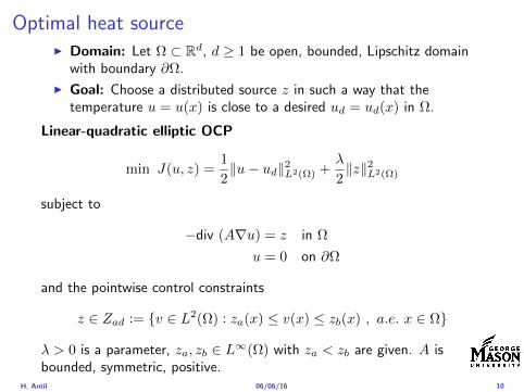
Optimal heat sourceI Domain Let Ω sub Rd d ge 1 be open bounded Lipschitz domain
with boundary partΩ
I Goal Choose a distributed source z in such a way that thetemperature u = u(x) is close to a desired ud = ud(x) in Ω
Linear-quadratic elliptic OCP
min J(u z) =1
2uminus ud2L2(Ω) +
λ
2z2L2(Ω)
subject to
minusdiv (Anablau) = z in Ω
u = 0 on partΩ
and the pointwise control constraints
z isin Zad = v isin L2(Ω) za(x) le v(x) le zb(x) ae x isin Ω
λ gt 0 is a parameter za zb isin Linfin(Ω) with za lt zb are given A isbounded symmetric positive
H Antil 060616 10
Problems involving semilinear elliptic PDEsI Heating with radiation boundary condition If the heat radiation
of the heated body is taken into account then we obtain
minus∆u = 0 in Ω
partνu = α(z4 minus u4) on partΩ
where the control z is the temperature of the surrounding medium
I Simplified supercondutivity
minus∆u+ u+ u3 = z in Ω
u = 0 on partΩ
I Control of stationary flows
minusmicro∆u + (u middot nabla)u +nablap = f in Ω
div u = 0 in Ω
u = g on partΩ
H Antil 060616 11
Optimal control of variational inequalitiesProblem
min J(u z) =1
2uminus ud2L2(Ω) +
λ
2z2L2(Ω)
subject to u isin K = w isin H10 (Ω) w(x) ge 0 ae x isin Ωint
Ω
nablau middot nabla(uminus v) dx le (z + f uminus v) forallv isin K
with z isin Zad
Regularized problem
min J(u z) =1
2uminus ud2L2(Ω) +
λ
2z2L2(Ω)
subject to (semilinear PDE)
u isin H10 (Ω) minus∆u+ γρε(minusu) = z + f in Ω
and z isin Zad γ gt 0 and ε gt 0 are the penealization and regularizationparameters respectively
H Antil 060616 12
Outline
Motivation and examples
Linear elliptic optimal control problems
Differentiation in Banach spaces
First-order necessary conditions
Optimal control of semilinear PDEs
An abstract problem
Discretization using finite element methods
H Antil 060616 13
Linear elliptic problemsΩ sub Rn bounded Lipschitz domain
Sobolev spacesI Lp(Ω) 1 le p le infin are Lebesgue spaces p = 2 L2(Ω) is a Hilbert
space with inner product (u v) =int
Ωu(x)v(x) dx
I W sp for s isin R 1 le p le infin are Sobolev spaces When p = 2W s2(Ω) = Hs(Ω) is a Hilbert space
I H10 (Ω) = v isin H1(Ω) v|partΩ = 0 with norm (due to Poincare
inequality)uH1
0 (Ω) = nablauL2(Ω)
I H10 (Ω)lowast = Hminus1(Ω)
I Note L2(Ω) sub Hminus1(Ω)
Model problem
minusdiv (Anablau) = f in Ω
u = 0 on partΩ
H Antil 060616 14
Linear elliptic problemsΩ sub Rn bounded Lipschitz domain
Sobolev spacesI Lp(Ω) 1 le p le infin are Lebesgue spaces p = 2 L2(Ω) is a Hilbert
space with inner product (u v) =int
Ωu(x)v(x) dx
I W sp for s isin R 1 le p le infin are Sobolev spaces When p = 2W s2(Ω) = Hs(Ω) is a Hilbert space
I H10 (Ω) = v isin H1(Ω) v|partΩ = 0 with norm (due to Poincare
inequality)uH1
0 (Ω) = nablauL2(Ω)
I H10 (Ω)lowast = Hminus1(Ω)
I Note L2(Ω) sub Hminus1(Ω)
Model problem
minusdiv (Anablau) = f in Ω
u = 0 on partΩ
H Antil 060616 14
Linear elliptic problemsΩ sub Rn bounded Lipschitz domain
Sobolev spacesI Lp(Ω) 1 le p le infin are Lebesgue spaces p = 2 L2(Ω) is a Hilbert
space with inner product (u v) =int
Ωu(x)v(x) dx
I W sp for s isin R 1 le p le infin are Sobolev spaces When p = 2W s2(Ω) = Hs(Ω) is a Hilbert space
I H10 (Ω) = v isin H1(Ω) v|partΩ = 0 with norm (due to Poincare
inequality)uH1
0 (Ω) = nablauL2(Ω)
I H10 (Ω)lowast = Hminus1(Ω)
I Note L2(Ω) sub Hminus1(Ω)
Model problem
minusdiv (Anablau) = f in Ω
u = 0 on partΩ
H Antil 060616 14
Linear elliptic problemsΩ sub Rn bounded Lipschitz domain
Sobolev spacesI Lp(Ω) 1 le p le infin are Lebesgue spaces p = 2 L2(Ω) is a Hilbert
space with inner product (u v) =int
Ωu(x)v(x) dx
I W sp for s isin R 1 le p le infin are Sobolev spaces When p = 2W s2(Ω) = Hs(Ω) is a Hilbert space
I H10 (Ω) = v isin H1(Ω) v|partΩ = 0 with norm (due to Poincare
inequality)uH1
0 (Ω) = nablauL2(Ω)
I H10 (Ω)lowast = Hminus1(Ω)
I Note L2(Ω) sub Hminus1(Ω)
Model problem
minusdiv (Anablau) = f in Ω
u = 0 on partΩ
H Antil 060616 14
Linear elliptic problemsΩ sub Rn bounded Lipschitz domain
Sobolev spacesI Lp(Ω) 1 le p le infin are Lebesgue spaces p = 2 L2(Ω) is a Hilbert
space with inner product (u v) =int
Ωu(x)v(x) dx
I W sp for s isin R 1 le p le infin are Sobolev spaces When p = 2W s2(Ω) = Hs(Ω) is a Hilbert space
I H10 (Ω) = v isin H1(Ω) v|partΩ = 0 with norm (due to Poincare
inequality)uH1
0 (Ω) = nablauL2(Ω)
I H10 (Ω)lowast = Hminus1(Ω)
I Note L2(Ω) sub Hminus1(Ω)
Model problem
minusdiv (Anablau) = f in Ω
u = 0 on partΩ
H Antil 060616 14
Well-posed
I Weak solution Given f isin Hminus1(Ω) a function u isin H10 (Ω) is called
a weak solution iffintΩ
Anablau middot nablav = 〈f v〉minus11 forallv isin H10 (Ω)
where 〈middot middot〉minus11 denotes the Hminus1(Ω)ndashH1(Ω) duality pairing
I Existence and uniqueness For each f isin Hminus1(Ω) there exists aunique u isin H1
0 (Ω) such that
nablauL2(Ω) le CdΩfHminus1(Ω)
I A = I the result is due to the Riesz-representation theorem
I A 6= I (maybe non-symmetric) the result is due to Lax-Milgramlemma
I For general W 1p-spaces use inf-sup conditions combined withBanach-Necas theorem which is a necessary and sufficient condition
H Antil 060616 15
Well-posed
I Weak solution Given f isin Hminus1(Ω) a function u isin H10 (Ω) is called
a weak solution iffintΩ
Anablau middot nablav = 〈f v〉minus11 forallv isin H10 (Ω)
where 〈middot middot〉minus11 denotes the Hminus1(Ω)ndashH1(Ω) duality pairing
I Existence and uniqueness For each f isin Hminus1(Ω) there exists aunique u isin H1
0 (Ω) such that
nablauL2(Ω) le CdΩfHminus1(Ω)
I A = I the result is due to the Riesz-representation theorem
I A 6= I (maybe non-symmetric) the result is due to Lax-Milgramlemma
I For general W 1p-spaces use inf-sup conditions combined withBanach-Necas theorem which is a necessary and sufficient condition
H Antil 060616 15
Linear-quadratic elliptic OCP
min J(u z) =1
2uminus ud2L2(Ω) +
λ
2z2L2(Ω)
subject to
minusdiv (Anablau) = z in Ω
u = 0 on partΩ
and the pointwise control constraints
z isin Zad = v isin L2(Ω) za(x) le v(x) le zb(x) ae x isin Ω
λ gt 0 is a parameter za zb isin Linfin(Ω) with za lt zb are given A isbounded symmetric positive
H Antil 060616 16
Reduced OCP
I Control to state map The solution operator defined as
S Hminus1(Ω)rarr H10 (Ω) z 7rarr u(z) = Sz
Note In view of the embedding
H10 (Ω) rarr L2(Ω) rarr Hminus1(Ω)
we may also consider S from L2(Ω) to L2(Ω) We will use the samenotation for this operator (for simplicity)
I Reduced cost functional The reduced cost functionalJ L2(Ω)rarr R is defined as
J (z) = J(Sz z)
I Reduced problem minzisinZadJ (z)
H Antil 060616 17
Reduced OCP
I Control to state map The solution operator defined as
S Hminus1(Ω)rarr H10 (Ω) z 7rarr u(z) = Sz
Note In view of the embedding
H10 (Ω) rarr L2(Ω) rarr Hminus1(Ω)
we may also consider S from L2(Ω) to L2(Ω) We will use the samenotation for this operator (for simplicity)
I Reduced cost functional The reduced cost functionalJ L2(Ω)rarr R is defined as
J (z) = J(Sz z)
I Reduced problem minzisinZadJ (z)
H Antil 060616 17
Reduced OCP
I Control to state map The solution operator defined as
S Hminus1(Ω)rarr H10 (Ω) z 7rarr u(z) = Sz
Note In view of the embedding
H10 (Ω) rarr L2(Ω) rarr Hminus1(Ω)
we may also consider S from L2(Ω) to L2(Ω) We will use the samenotation for this operator (for simplicity)
I Reduced cost functional The reduced cost functionalJ L2(Ω)rarr R is defined as
J (z) = J(Sz z)
I Reduced problem minzisinZadJ (z)
H Antil 060616 17
Existence of solution Direct methodThere exists a unique solution to the above problem
I Minimizing sequence J is bounded below by zero therefore thereexists a minimizing sequence znnisinN such that
limnrarrinfin
J (zn) = inf J (z)
I Weak compactness zn sub L2(Ω) is bounded Since L2(Ω) isreflexive therefore there exists a subsequence (not relabeled) suchthat
zn z and z isin Zad
where the latter is a consequence of Zad being closed and convex
I Optimality Since J is continuous and convex and therefore isweakly lower semicontinuous We obtain
lim inf J (zn) ge J (z)
which implies that z is optimal
I Uniqueness Exercise
H Antil 060616 18
Existence of solution Direct methodThere exists a unique solution to the above problem
I Minimizing sequence J is bounded below by zero therefore thereexists a minimizing sequence znnisinN such that
limnrarrinfin
J (zn) = inf J (z)
I Weak compactness zn sub L2(Ω) is bounded Since L2(Ω) isreflexive therefore there exists a subsequence (not relabeled) suchthat
zn z and z isin Zad
where the latter is a consequence of Zad being closed and convex
I Optimality Since J is continuous and convex and therefore isweakly lower semicontinuous We obtain
lim inf J (zn) ge J (z)
which implies that z is optimal
I Uniqueness Exercise
H Antil 060616 18
Existence of solution Direct methodThere exists a unique solution to the above problem
I Minimizing sequence J is bounded below by zero therefore thereexists a minimizing sequence znnisinN such that
limnrarrinfin
J (zn) = inf J (z)
I Weak compactness zn sub L2(Ω) is bounded Since L2(Ω) isreflexive therefore there exists a subsequence (not relabeled) suchthat
zn z and z isin Zad
where the latter is a consequence of Zad being closed and convex
I Optimality Since J is continuous and convex and therefore isweakly lower semicontinuous We obtain
lim inf J (zn) ge J (z)
which implies that z is optimal
I Uniqueness Exercise
H Antil 060616 18
Existence of solution Direct methodThere exists a unique solution to the above problem
I Minimizing sequence J is bounded below by zero therefore thereexists a minimizing sequence znnisinN such that
limnrarrinfin
J (zn) = inf J (z)
I Weak compactness zn sub L2(Ω) is bounded Since L2(Ω) isreflexive therefore there exists a subsequence (not relabeled) suchthat
zn z and z isin Zad
where the latter is a consequence of Zad being closed and convex
I Optimality Since J is continuous and convex and therefore isweakly lower semicontinuous We obtain
lim inf J (zn) ge J (z)
which implies that z is optimal
I Uniqueness Exercise
H Antil 060616 18
Outline
Motivation and examples
Linear elliptic optimal control problems
Differentiation in Banach spaces
First-order necessary conditions
Optimal control of semilinear PDEs
An abstract problem
Discretization using finite element methods
H Antil 060616 19
Differentiation in Banach spacesLet (Z middot Z) (V middot V ) B-spaces Z sub Z open and F Z rarr V
Let z isin Z
I If exist δF (z h) = limtdarr01t (F (z + th)minus F (z)) then δF (z h) is called
the directional derivative of F at z in direction h
I If exist δF (z h) forallh isin Z then h 7rarr δF (z h) is the first variation of Fat z
I Let exist the first variation δF (z middot) F is said to be Gateauxdifferentiable at z iff existA isin L(Z V ) such that δF (z h) = Ahforallh isin Z We write A = F primeG(z)
I F is said to be Frechet differentiable at z iff existA isin L(Z V ) and amapping r(z middot) Z rarr V such that for all h isin U with z + h isin Zwe have
F (z+h) = F (z)+Ah+r(z h) withr(z h)VhZ
rarr 0 as hZ rarr 0
We write F prime(z) = A
H Antil 060616 20
Differentiation in Banach spacesLet (Z middot Z) (V middot V ) B-spaces Z sub Z open and F Z rarr V
Let z isin Z
I If exist δF (z h) = limtdarr01t (F (z + th)minus F (z)) then δF (z h) is called
the directional derivative of F at z in direction h
I If exist δF (z h) forallh isin Z then h 7rarr δF (z h) is the first variation of Fat z
I Let exist the first variation δF (z middot) F is said to be Gateauxdifferentiable at z iff existA isin L(Z V ) such that δF (z h) = Ahforallh isin Z We write A = F primeG(z)
I F is said to be Frechet differentiable at z iff existA isin L(Z V ) and amapping r(z middot) Z rarr V such that for all h isin U with z + h isin Zwe have
F (z+h) = F (z)+Ah+r(z h) withr(z h)VhZ
rarr 0 as hZ rarr 0
We write F prime(z) = A
H Antil 060616 20
Differentiation in Banach spacesLet (Z middot Z) (V middot V ) B-spaces Z sub Z open and F Z rarr V
Let z isin Z
I If exist δF (z h) = limtdarr01t (F (z + th)minus F (z)) then δF (z h) is called
the directional derivative of F at z in direction h
I If exist δF (z h) forallh isin Z then h 7rarr δF (z h) is the first variation of Fat z
I Let exist the first variation δF (z middot) F is said to be Gateauxdifferentiable at z iff existA isin L(Z V ) such that δF (z h) = Ahforallh isin Z We write A = F primeG(z)
I F is said to be Frechet differentiable at z iff existA isin L(Z V ) and amapping r(z middot) Z rarr V such that for all h isin U with z + h isin Zwe have
F (z+h) = F (z)+Ah+r(z h) withr(z h)VhZ
rarr 0 as hZ rarr 0
We write F prime(z) = A
H Antil 060616 20
Differentiation in Banach spacesLet (Z middot Z) (V middot V ) B-spaces Z sub Z open and F Z rarr V
Let z isin Z
I If exist δF (z h) = limtdarr01t (F (z + th)minus F (z)) then δF (z h) is called
the directional derivative of F at z in direction h
I If exist δF (z h) forallh isin Z then h 7rarr δF (z h) is the first variation of Fat z
I Let exist the first variation δF (z middot) F is said to be Gateauxdifferentiable at z iff existA isin L(Z V ) such that δF (z h) = Ahforallh isin Z We write A = F primeG(z)
I F is said to be Frechet differentiable at z iff existA isin L(Z V ) and amapping r(z middot) Z rarr V such that for all h isin U with z + h isin Zwe have
F (z+h) = F (z)+Ah+r(z h) withr(z h)VhZ
rarr 0 as hZ rarr 0
We write F prime(z) = A
H Antil 060616 20
ExamplesExample 1 (H (middot middot)H) Hilbert space F (z) = z2H = (z z)H
forallz h F (z + h)minus F (z) = 2(z h)H + h2HThen
F prime(z)h = (2z h)H
Reisz representation theorem (identify H with Hlowast) we can write
F prime(z)h = (nablaF (z) h)H
where nablaF (z) = 2z is the gradient
Example 2 Let (Z (middot middot)Z) (H (middot middot)H) Hilbert spaces ud isin H fixedLet S isin L(ZH) Consider E Z rarr R
E(z) = Sz minus ud2H
Then E(z) = G(F (z)) where G(v) = v2H and F (z) = Sz minus ud
Eprime(z)h = Gprime(F (z))F prime(z)h = (2v F prime(z)h)H
= 2(Sz minus ud Sh)H = 2(Slowast(Sz minus ud) h)Z
we denote the gradient as nablaE(z) = 2Slowast(Sz minus ud)
H Antil 060616 21
ExamplesExample 1 (H (middot middot)H) Hilbert space F (z) = z2H = (z z)H
forallz h F (z + h)minus F (z) = 2(z h)H + h2HThen
F prime(z)h = (2z h)H
Reisz representation theorem (identify H with Hlowast) we can write
F prime(z)h = (nablaF (z) h)H
where nablaF (z) = 2z is the gradient
Example 2 Let (Z (middot middot)Z) (H (middot middot)H) Hilbert spaces ud isin H fixedLet S isin L(ZH) Consider E Z rarr R
E(z) = Sz minus ud2H
Then E(z) = G(F (z)) where G(v) = v2H and F (z) = Sz minus ud
Eprime(z)h = Gprime(F (z))F prime(z)h = (2v F prime(z)h)H
= 2(Sz minus ud Sh)H = 2(Slowast(Sz minus ud) h)Z
we denote the gradient as nablaE(z) = 2Slowast(Sz minus ud)H Antil 060616 21
Outline
Motivation and examples
Linear elliptic optimal control problems
Differentiation in Banach spaces
First-order necessary conditions
Optimal control of semilinear PDEs
An abstract problem
Discretization using finite element methods
H Antil 060616 22
First order necessary optimality conditions
Most of the theory is based on these two simple results
Theorem Let (Z middot Z) be a normed space J Z rarr (infin+infin] amapping with J 6equiv +infin Then z isin Z minimizer of J hArr 0 isin partJ (z)
Proof 0 isin partJ (z) means by definition of partJ (z) J (z)minus J (z) le 0forallz isin Z
Theorem Let (Z middot Z) be a normed space Zad sub Z nonemptyconvex closed J Z rarr R Gateaux differentiable where Zad sub Z sub ZZ open If z isin Zad is a solution to
minzisinZad
J (z)
then z solvesJ prime(z)(z minus z) ge 0 forallz isin Zad
Proof Exercise
H Antil 060616 23
First order necessary optimality conditions
Most of the theory is based on these two simple results
Theorem Let (Z middot Z) be a normed space J Z rarr (infin+infin] amapping with J 6equiv +infin Then z isin Z minimizer of J hArr 0 isin partJ (z)
Proof 0 isin partJ (z) means by definition of partJ (z) J (z)minus J (z) le 0forallz isin Z
Theorem Let (Z middot Z) be a normed space Zad sub Z nonemptyconvex closed J Z rarr R Gateaux differentiable where Zad sub Z sub ZZ open If z isin Zad is a solution to
minzisinZad
J (z)
then z solvesJ prime(z)(z minus z) ge 0 forallz isin Zad
Proof Exercise
H Antil 060616 23
Linear quadratic OCPI Reduced funcational
J (z) =1
2Sz minus ud2L2(Ω) +
λ
2z2L2(Ω)
I Gradient computation using sensitivity
J prime(z)h = (Slowast(Sz minus ud) + λz h)L2(Ω) forallh isin L2(Ω)
we denote the gradient by
nablaJ (z) = Slowast(Sz minus ud) + λz
I First order necessary and sufficient optimality condition
(nablaJ (z) z minus z)L2(Ω) ge 0 forallz isin Zad
I Adjoint equation Let p = Slowast(Sz minus ud) which translates intop isin H1
0 (Ω) solving
minusdiv (Anablap) = uminus ud in Ω
p = 0 on partΩ
I Gradient computation using adjoint nablaJ (z) = p+ λz
H Antil 060616 24
Linear quadratic OCPI Reduced funcational
J (z) =1
2Sz minus ud2L2(Ω) +
λ
2z2L2(Ω)
I Gradient computation using sensitivity
J prime(z)h = (Slowast(Sz minus ud) + λz h)L2(Ω) forallh isin L2(Ω)
we denote the gradient by
nablaJ (z) = Slowast(Sz minus ud) + λz
I First order necessary and sufficient optimality condition
(nablaJ (z) z minus z)L2(Ω) ge 0 forallz isin Zad
I Adjoint equation Let p = Slowast(Sz minus ud) which translates intop isin H1
0 (Ω) solving
minusdiv (Anablap) = uminus ud in Ω
p = 0 on partΩ
I Gradient computation using adjoint nablaJ (z) = p+ λz
H Antil 060616 24
Linear quadratic OCPI Reduced funcational
J (z) =1
2Sz minus ud2L2(Ω) +
λ
2z2L2(Ω)
I Gradient computation using sensitivity
J prime(z)h = (Slowast(Sz minus ud) + λz h)L2(Ω) forallh isin L2(Ω)
we denote the gradient by
nablaJ (z) = Slowast(Sz minus ud) + λz
I First order necessary and sufficient optimality condition
(nablaJ (z) z minus z)L2(Ω) ge 0 forallz isin Zad
I Adjoint equation Let p = Slowast(Sz minus ud) which translates intop isin H1
0 (Ω) solving
minusdiv (Anablap) = uminus ud in Ω
p = 0 on partΩ
I Gradient computation using adjoint nablaJ (z) = p+ λz
H Antil 060616 24
Linear quadratic OCPI Reduced funcational
J (z) =1
2Sz minus ud2L2(Ω) +
λ
2z2L2(Ω)
I Gradient computation using sensitivity
J prime(z)h = (Slowast(Sz minus ud) + λz h)L2(Ω) forallh isin L2(Ω)
we denote the gradient by
nablaJ (z) = Slowast(Sz minus ud) + λz
I First order necessary and sufficient optimality condition
(nablaJ (z) z minus z)L2(Ω) ge 0 forallz isin Zad
I Adjoint equation Let p = Slowast(Sz minus ud) which translates intop isin H1
0 (Ω) solving
minusdiv (Anablap) = uminus ud in Ω
p = 0 on partΩ
I Gradient computation using adjoint nablaJ (z) = p+ λz
H Antil 060616 24
Linear quadratic OCPI Reduced funcational
J (z) =1
2Sz minus ud2L2(Ω) +
λ
2z2L2(Ω)
I Gradient computation using sensitivity
J prime(z)h = (Slowast(Sz minus ud) + λz h)L2(Ω) forallh isin L2(Ω)
we denote the gradient by
nablaJ (z) = Slowast(Sz minus ud) + λz
I First order necessary and sufficient optimality condition
(nablaJ (z) z minus z)L2(Ω) ge 0 forallz isin Zad
I Adjoint equation Let p = Slowast(Sz minus ud) which translates intop isin H1
0 (Ω) solving
minusdiv (Anablap) = uminus ud in Ω
p = 0 on partΩ
I Gradient computation using adjoint nablaJ (z) = p+ λz
H Antil 060616 24
Optimality system
I State u isin H10 (Ω)
intΩAnablau middot nablav =
intΩzv forallv isin H1
0 (Ω)
I Adjoint p isin H10 (Ω)
intΩAnablap middot nablav =
intΩ
(uminus ud)v forallv isin H10 (Ω)
I Control z isin Zad (p+ λz z minus z) ge 0 forallz isin Zad
H Antil 060616 25
Pointwise interpretation
The variational inequality
(p+ λz z minus z) ge 0 forallz isin Zad
is equivalent to for ae x isin Ω
z(x) =
za(x) if p(x) + λz(x) gt 0isin [za(x) zb(x)] if p(x) + λz(x) = 0zb(x) if p(x) + λz(x) lt 0
Consequence
I When λ gt 0 then ae in Ω
z(x) = P[za(x)zb(x)]
minus 1
λp(x)
= min
zb(x)max
za(x)minus 1
λp(x)
H Antil 060616 26
Formal Lagrange method applied to linear OCPIntroduce L H1
0 (Ω)times Zad timesH1(Ω)rarr R defined as
L(u z p) = J(u z)minusint
Ω
(minusdiv (Anablau)minus z
)p dx
Integrate by parts to arrive at
L(u z p) = J(u z)minusint
Ω
(minusdiv (Anablap)uminus zp
)dx+
intpartΩ
(Anablau)p ds
If (u z p) is a stationary point then
I State
DpL(u z p)h = 0 forallh isin H1(Ω)
I AdjointDuL(u z p)h = 0 forallh isin H1
0 (Ω)
I ControlDzL(u z p)(z minus z) ge 0 forallz isin Zad
H Antil 060616 27
Formal Lagrange method applied to linear OCPIntroduce L H1
0 (Ω)times Zad timesH1(Ω)rarr R defined as
L(u z p) = J(u z)minusint
Ω
(minusdiv (Anablau)minus z
)p dx
Integrate by parts to arrive at
L(u z p) = J(u z)minusint
Ω
(minusdiv (Anablap)uminus zp
)dx+
intpartΩ
(Anablau)p ds
If (u z p) is a stationary point then
I State
DpL(u z p)h = 0 forallh isin H1(Ω)
I AdjointDuL(u z p)h = 0 forallh isin H1
0 (Ω)
I ControlDzL(u z p)(z minus z) ge 0 forallz isin Zad
H Antil 060616 27
Formal Lagrange method applied to linear OCPIntroduce L H1
0 (Ω)times Zad timesH1(Ω)rarr R defined as
L(u z p) = J(u z)minusint
Ω
(minusdiv (Anablau)minus z
)p dx
Integrate by parts to arrive at
L(u z p) = J(u z)minusint
Ω
(minusdiv (Anablap)uminus zp
)dx+
intpartΩ
(Anablau)p ds
If (u z p) is a stationary point then
I State
DpL(u z p)h = 0 forallh isin H1(Ω)
I AdjointDuL(u z p)h = 0 forallh isin H1
0 (Ω)
I ControlDzL(u z p)(z minus z) ge 0 forallz isin Zad
H Antil 060616 27
Formal Lagrange method applied to linear OCPIntroduce L H1
0 (Ω)times Zad timesH1(Ω)rarr R defined as
L(u z p) = J(u z)minusint
Ω
(minusdiv (Anablau)minus z
)p dx
Integrate by parts to arrive at
L(u z p) = J(u z)minusint
Ω
(minusdiv (Anablap)uminus zp
)dx+
intpartΩ
(Anablau)p ds
If (u z p) is a stationary point then
I State
DpL(u z p)h = 0 forallh isin H1(Ω)
I AdjointDuL(u z p)h = 0 forallh isin H1
0 (Ω)
I ControlDzL(u z p)(z minus z) ge 0 forallz isin Zad
H Antil 060616 27
Formal Lagrange method applied to linear OCPIntroduce L H1
0 (Ω)times Zad timesH1(Ω)rarr R defined as
L(u z p) = J(u z)minusint
Ω
(minusdiv (Anablau)minus z
)p dx
Integrate by parts to arrive at
L(u z p) = J(u z)minusint
Ω
(minusdiv (Anablap)uminus zp
)dx+
intpartΩ
(Anablau)p ds
If (u z p) is a stationary point then
I State
DpL(u z p)h = 0 forallh isin H1(Ω)
I AdjointDuL(u z p)h = 0 forallh isin H1
0 (Ω)
I ControlDzL(u z p)(z minus z) ge 0 forallz isin Zad
H Antil 060616 27
Outline
Motivation and examples
Linear elliptic optimal control problems
Differentiation in Banach spaces
First-order necessary conditions
Optimal control of semilinear PDEs
An abstract problem
Discretization using finite element methods
H Antil 060616 28
Semilinear elliptic OCP
min J(u z) =1
2uminus ud2L2(Ω) +
λ
2z2L2(Ω)
subject to
minus∆u+ g(x u) = z in Ω
u = 0 on partΩ
and z isin Zad with za zb isin Linfin(Ω)
H Antil 060616 29
State space(A1) Ω sub Rd open bounded partΩ is Lipschitz
(A2) g Ωtimes Rrarr R is bounded and measurable with respect to x isin Ωfor every u isin R
(A3) g is continuous monotone increasing and Lipschitz continuous in ufor ae x isin Ω
(A4) g(x 0) = 0 for ae x isin Ω (not really necessary)
Theorem Suppose (A1)minus (A4) hold For every z isin Lr(Ω) withr gt d2 the state equation has a unique weak solutionu isin H1
0 (Ω) cap C(Ω) ie we haveintΩ
nablau middot nablav dx+
intΩ
g(x u(x))v(x) dx =
intΩ
zv dx forallv isin H10 (Ω)
Moreover there exists a constant C gt 0 such that
uH1(Ω) + uC(Ω) le CzLr(Ω)
RemarkI The proof of the theorem uses the BrowderndashMinty theorem on
monotone operators
H Antil 060616 30
State space(A1) Ω sub Rd open bounded partΩ is Lipschitz
(A2) g Ωtimes Rrarr R is bounded and measurable with respect to x isin Ωfor every u isin R
(A3) g is continuous monotone increasing and Lipschitz continuous in ufor ae x isin Ω
(A4) g(x 0) = 0 for ae x isin Ω (not really necessary)
Theorem Suppose (A1)minus (A4) hold For every z isin Lr(Ω) withr gt d2 the state equation has a unique weak solutionu isin H1
0 (Ω) cap C(Ω) ie we haveintΩ
nablau middot nablav dx+
intΩ
g(x u(x))v(x) dx =
intΩ
zv dx forallv isin H10 (Ω)
Moreover there exists a constant C gt 0 such that
uH1(Ω) + uC(Ω) le CzLr(Ω)
RemarkI The proof of the theorem uses the BrowderndashMinty theorem on
monotone operators
H Antil 060616 30
State space(A1) Ω sub Rd open bounded partΩ is Lipschitz
(A2) g Ωtimes Rrarr R is bounded and measurable with respect to x isin Ωfor every u isin R
(A3) g is continuous monotone increasing and Lipschitz continuous in ufor ae x isin Ω
(A4) g(x 0) = 0 for ae x isin Ω (not really necessary)
Theorem Suppose (A1)minus (A4) hold For every z isin Lr(Ω) withr gt d2 the state equation has a unique weak solutionu isin H1
0 (Ω) cap C(Ω) ie we haveintΩ
nablau middot nablav dx+
intΩ
g(x u(x))v(x) dx =
intΩ
zv dx forallv isin H10 (Ω)
Moreover there exists a constant C gt 0 such that
uH1(Ω) + uC(Ω) le CzLr(Ω)
RemarkI The proof of the theorem uses the BrowderndashMinty theorem on
monotone operators
H Antil 060616 30
Control-to-state map and reduced problem
I Control to state map
S Linfin(Ω)rarr H10 (Ω) cap C(Ω)
is well defined and is globally Lipschitz continuous
I Reduced problem
minJ (z) =1
2S(u)minus ud2L2(Ω) +
λ
2z2L2(Ω)
H Antil 060616 31
Control-to-state map and reduced problem
I Control to state map
S Linfin(Ω)rarr H10 (Ω) cap C(Ω)
is well defined and is globally Lipschitz continuous
I Reduced problem
minJ (z) =1
2S(u)minus ud2L2(Ω) +
λ
2z2L2(Ω)
H Antil 060616 31
First-order necessary conditionsI Lagrangian functional
L(u z p) = J(u z)minusint
Ω
(minus∆u+ g(x u(x))minus z
)p dx
= J(u z)minusint
Ω
(nablau middot nablap+ g(x u(x))pminus zp
)dx
I Adjoint system For all h isin H10 (Ω)
0 = DuL(u z p)h =
intΩ
(uminus ud)h dxminusint
Ω
(nablah middot nablap+ gu(x u(x))ph
)which yields
minus∆p+ gu(x u(x))p = uminus ud in Ω
p = 0 on partΩ
I Control
DzL(u z p)(z minus z) = (p+ λz z minus z) dx ge 0 forallz isin ZadI Gradient
nablaJ (z) = p+ λz
H Antil 060616 32
First-order necessary conditionsI Lagrangian functional
L(u z p) = J(u z)minusint
Ω
(minus∆u+ g(x u(x))minus z
)p dx
= J(u z)minusint
Ω
(nablau middot nablap+ g(x u(x))pminus zp
)dx
I Adjoint system For all h isin H10 (Ω)
0 = DuL(u z p)h =
intΩ
(uminus ud)h dxminusint
Ω
(nablah middot nablap+ gu(x u(x))ph
)which yields
minus∆p+ gu(x u(x))p = uminus ud in Ω
p = 0 on partΩ
I Control
DzL(u z p)(z minus z) = (p+ λz z minus z) dx ge 0 forallz isin ZadI Gradient
nablaJ (z) = p+ λz
H Antil 060616 32
First-order necessary conditionsI Lagrangian functional
L(u z p) = J(u z)minusint
Ω
(minus∆u+ g(x u(x))minus z
)p dx
= J(u z)minusint
Ω
(nablau middot nablap+ g(x u(x))pminus zp
)dx
I Adjoint system For all h isin H10 (Ω)
0 = DuL(u z p)h =
intΩ
(uminus ud)h dxminusint
Ω
(nablah middot nablap+ gu(x u(x))ph
)which yields
minus∆p+ gu(x u(x))p = uminus ud in Ω
p = 0 on partΩ
I Control
DzL(u z p)(z minus z) = (p+ λz z minus z) dx ge 0 forallz isin Zad
I GradientnablaJ (z) = p+ λz
H Antil 060616 32
First-order necessary conditionsI Lagrangian functional
L(u z p) = J(u z)minusint
Ω
(minus∆u+ g(x u(x))minus z
)p dx
= J(u z)minusint
Ω
(nablau middot nablap+ g(x u(x))pminus zp
)dx
I Adjoint system For all h isin H10 (Ω)
0 = DuL(u z p)h =
intΩ
(uminus ud)h dxminusint
Ω
(nablah middot nablap+ gu(x u(x))ph
)which yields
minus∆p+ gu(x u(x))p = uminus ud in Ω
p = 0 on partΩ
I Control
DzL(u z p)(z minus z) = (p+ λz z minus z) dx ge 0 forallz isin ZadI Gradient
nablaJ (z) = p+ λz
H Antil 060616 32
Differentiability of Nemytskii operator
The rigorous proof uses
Theorem In addition to (A1)-(A4) if
(A5) g is continuously differentiable with respect to u for ae x isin Ωand we have
(i) |gu(x 0)| le K for ae x isin Ω(ii) gu is locally Lipschitz with respect to u isin R
then the Nemytskii operator G u 7rarr g(middot u(middot)) is continuously Frechetdifferentiable from Linfin(Ω) into itself and
(Gprime(u)h)(x) = gu(x u(x))h(x) ae in Ω forallh isin Linfin(Ω)
Remark (A5) holds if g(x u) = g(u) and g isin C2(R)
H Antil 060616 33
Outline
Motivation and examples
Linear elliptic optimal control problems
Differentiation in Banach spaces
First-order necessary conditions
Optimal control of semilinear PDEs
An abstract problem
Discretization using finite element methods
H Antil 060616 34
Gradient computation via adjoint general formI Abstract problem
min J(u z)
subject toc(u z) = 0
and z isin Zad
I Directional derivative Let S be the control to state map(nonlinear in general)
z 7rarr S(z) = u(z)
Under the assumptions of ldquoimplicit function theoremrdquo
J prime(z)h = (nablauJ (u(z) z) Sprime(z)h) + (nablazJ (u(z) z) h)
I Sensitivity of u with respect to z Differentiating the stateequation
cu(S(z) z)Sprime(z)h = minuscz(S(z) z)h
leads toSprime(z)h = minuscu(S(z) z)minus1
(cz(S(z) z)h
)
provided cu(S(z) z)minus1 is well-defined
H Antil 060616 35
Gradient computation via adjoint general formI Abstract problem
min J(u z)
subject toc(u z) = 0
and z isin ZadI Directional derivative Let S be the control to state map
(nonlinear in general)
z 7rarr S(z) = u(z)
Under the assumptions of ldquoimplicit function theoremrdquo
J prime(z)h = (nablauJ (u(z) z) Sprime(z)h) + (nablazJ (u(z) z) h)
I Sensitivity of u with respect to z Differentiating the stateequation
cu(S(z) z)Sprime(z)h = minuscz(S(z) z)h
leads toSprime(z)h = minuscu(S(z) z)minus1
(cz(S(z) z)h
)
provided cu(S(z) z)minus1 is well-defined
H Antil 060616 35
Gradient computation via adjoint general formI Abstract problem
min J(u z)
subject toc(u z) = 0
and z isin ZadI Directional derivative Let S be the control to state map
(nonlinear in general)
z 7rarr S(z) = u(z)
Under the assumptions of ldquoimplicit function theoremrdquo
J prime(z)h = (nablauJ (u(z) z) Sprime(z)h) + (nablazJ (u(z) z) h)
I Sensitivity of u with respect to z Differentiating the stateequation
cu(S(z) z)Sprime(z)h = minuscz(S(z) z)h
leads toSprime(z)h = minuscu(S(z) z)minus1
(cz(S(z) z)h
)
provided cu(S(z) z)minus1 is well-defined
H Antil 060616 35
Adjoint equation and gradient general form
I Directional derivative
J prime(z)h = minus(nablauJ (u(z) z) cu(u(z) z)minus1cz(u(z) z)h
)+ (nablazJ (u(z) z) h)
I Gradient
nablaJ (z) = minuscz(u(z) z)lowast(cu(u(z) z)minuslowastnablauJ (u(z) z)
)+nablazJ (u(z) z)
I Introducing adjoint variable p solving
cu(u(z) z)lowastp = nablauJ (u(z) z)
we arrive at following form of gradient
nablaJ (z) = minuscz(u(z) z)lowastp+nablazJ (u(z) z)
which is tractable
H Antil 060616 36
Adjoint equation and gradient general form
I Directional derivative
J prime(z)h = minus(nablauJ (u(z) z) cu(u(z) z)minus1cz(u(z) z)h
)+ (nablazJ (u(z) z) h)
I Gradient
nablaJ (z) = minuscz(u(z) z)lowast(cu(u(z) z)minuslowastnablauJ (u(z) z)
)+nablazJ (u(z) z)
I Introducing adjoint variable p solving
cu(u(z) z)lowastp = nablauJ (u(z) z)
we arrive at following form of gradient
nablaJ (z) = minuscz(u(z) z)lowastp+nablazJ (u(z) z)
which is tractable
H Antil 060616 36
Adjoint equation and gradient general form
I Directional derivative
J prime(z)h = minus(nablauJ (u(z) z) cu(u(z) z)minus1cz(u(z) z)h
)+ (nablazJ (u(z) z) h)
I Gradient
nablaJ (z) = minuscz(u(z) z)lowast(cu(u(z) z)minuslowastnablauJ (u(z) z)
)+nablazJ (u(z) z)
I Introducing adjoint variable p solving
cu(u(z) z)lowastp = nablauJ (u(z) z)
we arrive at following form of gradient
nablaJ (z) = minuscz(u(z) z)lowastp+nablazJ (u(z) z)
which is tractable
H Antil 060616 36
Hessian computation general form
I Lagrangian L(u z p) = J(u z)minusint
Ωc(u z)p dx Then we have
DzJ (z)h = DzL(u z p)h
I Second order derivative
D2zJ (z)[h1 h2] = DuDzL(u z p)[h1 S
prime(z)h2] +D2zL(u z p)[h1 h2]
+DpDzL(u z p)[h1 Dzp(z)h2]
I We already know Sprime(z)h2 moreover
DpDzL(u z p)[h1 Dzp(z)h2] = minus(cu(u z)h1 Dzp(z)h2
)
It remain to identify Dzp(z)h2
H Antil 060616 37
Hessian computation general form
I Lagrangian L(u z p) = J(u z)minusint
Ωc(u z)p dx Then we have
DzJ (z)h = DzL(u z p)h
I Second order derivative
D2zJ (z)[h1 h2] = DuDzL(u z p)[h1 S
prime(z)h2] +D2zL(u z p)[h1 h2]
+DpDzL(u z p)[h1 Dzp(z)h2]
I We already know Sprime(z)h2 moreover
DpDzL(u z p)[h1 Dzp(z)h2] = minus(cu(u z)h1 Dzp(z)h2
)
It remain to identify Dzp(z)h2
H Antil 060616 37
Hessian computation general form
I Lagrangian L(u z p) = J(u z)minusint
Ωc(u z)p dx Then we have
DzJ (z)h = DzL(u z p)h
I Second order derivative
D2zJ (z)[h1 h2] = DuDzL(u z p)[h1 S
prime(z)h2] +D2zL(u z p)[h1 h2]
+DpDzL(u z p)[h1 Dzp(z)h2]
I We already know Sprime(z)h2 moreover
DpDzL(u z p)[h1 Dzp(z)h2] = minus(cu(u z)h1 Dzp(z)h2
)
It remain to identify Dzp(z)h2
H Antil 060616 37
Outline
Motivation and examples
Linear elliptic optimal control problems
Differentiation in Banach spaces
First-order necessary conditions
Optimal control of semilinear PDEs
An abstract problem
Discretization using finite element methods
H Antil 060616 38
Numerical approximation of Poisson equation MeshTo avoid technical issues we will assume that partΩ is polygonal
I Mesh Let T = K be a mesh of Ω where K sub Rd is an elementthat is isoparametrically equivalent to a unit simplex in Rd
I Conforming mesh We say that the mesh is conforming ifI Ω = cupKisinT KI If K1 cap K2 = x then x is a node of K1 and K2I If K1 cap K2 6= empty and K1 cap K2 6= x then K1 cap K2 is an edgeface
contained in partK1 cap partK2
I Shape regular Let T be the collection of all conformingrefinements of an original mesh T 0 Then T is called shape regularif exist κ gt 0 such that
hKρKle κ forallK isin cupiT i
where hK = diam K ρK = maxρ gt 0|Bρ sub KI Quasi-uniform A family of shape regular meshes is called-quasi
uniform if there exist a constant σ gt 0 such that
maxhKminhK
le σ
uniformly for all meshes in the family
Numerical approximation of Poisson equation MeshTo avoid technical issues we will assume that partΩ is polygonal
I Mesh Let T = K be a mesh of Ω where K sub Rd is an elementthat is isoparametrically equivalent to a unit simplex in Rd
I Conforming mesh We say that the mesh is conforming ifI Ω = cupKisinT KI If K1 cap K2 = x then x is a node of K1 and K2I If K1 cap K2 6= empty and K1 cap K2 6= x then K1 cap K2 is an edgeface
contained in partK1 cap partK2
I Shape regular Let T be the collection of all conformingrefinements of an original mesh T 0 Then T is called shape regularif exist κ gt 0 such that
hKρKle κ forallK isin cupiT i
where hK = diam K ρK = maxρ gt 0|Bρ sub KI Quasi-uniform A family of shape regular meshes is called-quasi
uniform if there exist a constant σ gt 0 such that
maxhKminhK
le σ
uniformly for all meshes in the family
Numerical approximation of Poisson equation MeshTo avoid technical issues we will assume that partΩ is polygonal
I Mesh Let T = K be a mesh of Ω where K sub Rd is an elementthat is isoparametrically equivalent to a unit simplex in Rd
I Conforming mesh We say that the mesh is conforming ifI Ω = cupKisinT KI If K1 cap K2 = x then x is a node of K1 and K2I If K1 cap K2 6= empty and K1 cap K2 6= x then K1 cap K2 is an edgeface
contained in partK1 cap partK2
I Shape regular Let T be the collection of all conformingrefinements of an original mesh T 0 Then T is called shape regularif exist κ gt 0 such that
hKρKle κ forallK isin cupiT i
where hK = diam K ρK = maxρ gt 0|Bρ sub K
I Quasi-uniform A family of shape regular meshes is called-quasiuniform if there exist a constant σ gt 0 such that
maxhKminhK
le σ
uniformly for all meshes in the family
Numerical approximation of Poisson equation MeshTo avoid technical issues we will assume that partΩ is polygonal
I Mesh Let T = K be a mesh of Ω where K sub Rd is an elementthat is isoparametrically equivalent to a unit simplex in Rd
I Conforming mesh We say that the mesh is conforming ifI Ω = cupKisinT KI If K1 cap K2 = x then x is a node of K1 and K2I If K1 cap K2 6= empty and K1 cap K2 6= x then K1 cap K2 is an edgeface
contained in partK1 cap partK2
I Shape regular Let T be the collection of all conformingrefinements of an original mesh T 0 Then T is called shape regularif exist κ gt 0 such that
hKρKle κ forallK isin cupiT i
where hK = diam K ρK = maxρ gt 0|Bρ sub KI Quasi-uniform A family of shape regular meshes is called-quasi
uniform if there exist a constant σ gt 0 such that
maxhKminhK
le σ
uniformly for all meshes in the family
FE space and Galerkin approximationI Finite element space For T isin T we define the finite element
space as
V(T ) = W isin C0(Ω) WK isin P1forallK isin T W |partΩ = 0
where P1 is the set of polynomials of degree at most 1
I Galerkin approximation of continuous problem is given by
Find UT isin V(T )
intΩ
AnablaUT middot nablaV = 〈f V 〉 forallV isin V(T )
The discrete problem is well-posedI Nodal basis Consists of functions ψi isin V(T ) with xi isin N (T )
satisfyingψxi
(xj) = δij
where N (T ) denotes the interior (plus Neumann) nodesI Galerkin orthogonality(
nabla(uminus UT )nablaW)L2(Ω)
= 0 forallW isin V(T )
H Antil 060616 40
FE space and Galerkin approximationI Finite element space For T isin T we define the finite element
space as
V(T ) = W isin C0(Ω) WK isin P1forallK isin T W |partΩ = 0
where P1 is the set of polynomials of degree at most 1I Galerkin approximation of continuous problem is given by
Find UT isin V(T )
intΩ
AnablaUT middot nablaV = 〈f V 〉 forallV isin V(T )
The discrete problem is well-posed
I Nodal basis Consists of functions ψi isin V(T ) with xi isin N (T )satisfying
ψxi(xj) = δij
where N (T ) denotes the interior (plus Neumann) nodesI Galerkin orthogonality(
nabla(uminus UT )nablaW)L2(Ω)
= 0 forallW isin V(T )
H Antil 060616 40
FE space and Galerkin approximationI Finite element space For T isin T we define the finite element
space as
V(T ) = W isin C0(Ω) WK isin P1forallK isin T W |partΩ = 0
where P1 is the set of polynomials of degree at most 1I Galerkin approximation of continuous problem is given by
Find UT isin V(T )
intΩ
AnablaUT middot nablaV = 〈f V 〉 forallV isin V(T )
The discrete problem is well-posedI Nodal basis Consists of functions ψi isin V(T ) with xi isin N (T )
satisfyingψxi
(xj) = δij
where N (T ) denotes the interior (plus Neumann) nodes
I Galerkin orthogonality(nabla(uminus UT )nablaW
)L2(Ω)
= 0 forallW isin V(T )
H Antil 060616 40
FE space and Galerkin approximationI Finite element space For T isin T we define the finite element
space as
V(T ) = W isin C0(Ω) WK isin P1forallK isin T W |partΩ = 0
where P1 is the set of polynomials of degree at most 1I Galerkin approximation of continuous problem is given by
Find UT isin V(T )
intΩ
AnablaUT middot nablaV = 〈f V 〉 forallV isin V(T )
The discrete problem is well-posedI Nodal basis Consists of functions ψi isin V(T ) with xi isin N (T )
satisfyingψxi
(xj) = δij
where N (T ) denotes the interior (plus Neumann) nodesI Galerkin orthogonality(
nabla(uminus UT )nablaW)L2(Ω)
= 0 forallW isin V(T )
H Antil 060616 40
Best approximation
I Cearsquos lemma
nabla(uminus UT )L2(Ω) le C infWisinV(T )
nabla(uminusW )L2(Ω)
I Nodal interpolation operator ΠT C(Ω)rarr V(T ) satisfies
ΠT u(xi) = u(xi) forallxi isin N (T )
and is defined as
ΠT u =sum
xiisinN (T )
u(xi)ψxi
I Error estimates In Cearsquos lemma replace W by ΠT u and thencompute the interpolation error
H Antil 060616 41
Best approximation
I Cearsquos lemma
nabla(uminus UT )L2(Ω) le C infWisinV(T )
nabla(uminusW )L2(Ω)
I Nodal interpolation operator ΠT C(Ω)rarr V(T ) satisfies
ΠT u(xi) = u(xi) forallxi isin N (T )
and is defined as
ΠT u =sum
xiisinN (T )
u(xi)ψxi
I Error estimates In Cearsquos lemma replace W by ΠT u and thencompute the interpolation error
H Antil 060616 41
Best approximation
I Cearsquos lemma
nabla(uminus UT )L2(Ω) le C infWisinV(T )
nabla(uminusW )L2(Ω)
I Nodal interpolation operator ΠT C(Ω)rarr V(T ) satisfies
ΠT u(xi) = u(xi) forallxi isin N (T )
and is defined as
ΠT u =sum
xiisinN (T )
u(xi)ψxi
I Error estimates In Cearsquos lemma replace W by ΠT u and thencompute the interpolation error
H Antil 060616 41
Algebraic system state equation
I Recall UT isin V(T ) solves
a(UT V ) = 〈f V 〉 forallV isin V(T )
I Now setting UT =sumN
j=1 Ujψj V = ψi we get
Nsumj=1
Uja(φj φi) = 〈f ψi〉 i = 1 N
which is the matrix-vector system
AU = F
I Stiffness matrix A is SPD
H Antil 060616 42
Algebraic system state equation
I Recall UT isin V(T ) solves
a(UT V ) = 〈f V 〉 forallV isin V(T )
I Now setting UT =sumN
j=1 Ujψj V = ψi we get
Nsumj=1
Uja(φj φi) = 〈f ψi〉 i = 1 N
which is the matrix-vector system
AU = F
I Stiffness matrix A is SPD
H Antil 060616 42
Algebraic system state equation
I Recall UT isin V(T ) solves
a(UT V ) = 〈f V 〉 forallV isin V(T )
I Now setting UT =sumN
j=1 Ujψj V = ψi we get
Nsumj=1
Uja(φj φi) = 〈f ψi〉 i = 1 N
which is the matrix-vector system
AU = F
I Stiffness matrix A is SPD
H Antil 060616 42
Discrete linear elliptic OCP
min JT (UT ZT ) =1
2UT minus ud2L2(Ω) +
λ
2ZT 2L2(Ω)
subject to
Find UT isin V(T )
intΩ
nablaUT middot nablaV = (ZT V )L2(Ω) forallV isin V(T )
and whereZT isin Zad(T ) = Zad cap Z(T )
is either one of these
Z(T ) =
V(T )L2(Ω) variational discretization (Hinze)WT isin Linfin(Ω) ZT |K isin P0(K)K isin T
H Antil 060616 43
Recent books
F TroltzschOptimal control of partial differential equations volume 112 ofGraduate Studies in MathematicsAmerican Mathematical Society Providence RI 2010Theory methods and applications Translated from the 2005 Germanoriginal by Jurgen Sprekels
K Ito and K KunischLagrange multiplier approach to variational problems andapplications volume 15 of Advances in Design and ControlSociety for Industrial and Applied Mathematics (SIAM)Philadelphia PA 2008
H Antil 060616 44
- Motivation and examples
- Linear elliptic optimal control problems
- Differentiation in Banach spaces
- First-order necessary conditions
- Optimal control of semilinear PDEs
- An abstract problem
- Discretization using finite element methods
-
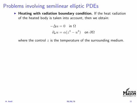
Problems involving semilinear elliptic PDEsI Heating with radiation boundary condition If the heat radiation
of the heated body is taken into account then we obtain
minus∆u = 0 in Ω
partνu = α(z4 minus u4) on partΩ
where the control z is the temperature of the surrounding medium
I Simplified supercondutivity
minus∆u+ u+ u3 = z in Ω
u = 0 on partΩ
I Control of stationary flows
minusmicro∆u + (u middot nabla)u +nablap = f in Ω
div u = 0 in Ω
u = g on partΩ
H Antil 060616 11
Optimal control of variational inequalitiesProblem
min J(u z) =1
2uminus ud2L2(Ω) +
λ
2z2L2(Ω)
subject to u isin K = w isin H10 (Ω) w(x) ge 0 ae x isin Ωint
Ω
nablau middot nabla(uminus v) dx le (z + f uminus v) forallv isin K
with z isin Zad
Regularized problem
min J(u z) =1
2uminus ud2L2(Ω) +
λ
2z2L2(Ω)
subject to (semilinear PDE)
u isin H10 (Ω) minus∆u+ γρε(minusu) = z + f in Ω
and z isin Zad γ gt 0 and ε gt 0 are the penealization and regularizationparameters respectively
H Antil 060616 12
Outline
Motivation and examples
Linear elliptic optimal control problems
Differentiation in Banach spaces
First-order necessary conditions
Optimal control of semilinear PDEs
An abstract problem
Discretization using finite element methods
H Antil 060616 13
Linear elliptic problemsΩ sub Rn bounded Lipschitz domain
Sobolev spacesI Lp(Ω) 1 le p le infin are Lebesgue spaces p = 2 L2(Ω) is a Hilbert
space with inner product (u v) =int
Ωu(x)v(x) dx
I W sp for s isin R 1 le p le infin are Sobolev spaces When p = 2W s2(Ω) = Hs(Ω) is a Hilbert space
I H10 (Ω) = v isin H1(Ω) v|partΩ = 0 with norm (due to Poincare
inequality)uH1
0 (Ω) = nablauL2(Ω)
I H10 (Ω)lowast = Hminus1(Ω)
I Note L2(Ω) sub Hminus1(Ω)
Model problem
minusdiv (Anablau) = f in Ω
u = 0 on partΩ
H Antil 060616 14
Linear elliptic problemsΩ sub Rn bounded Lipschitz domain
Sobolev spacesI Lp(Ω) 1 le p le infin are Lebesgue spaces p = 2 L2(Ω) is a Hilbert
space with inner product (u v) =int
Ωu(x)v(x) dx
I W sp for s isin R 1 le p le infin are Sobolev spaces When p = 2W s2(Ω) = Hs(Ω) is a Hilbert space
I H10 (Ω) = v isin H1(Ω) v|partΩ = 0 with norm (due to Poincare
inequality)uH1
0 (Ω) = nablauL2(Ω)
I H10 (Ω)lowast = Hminus1(Ω)
I Note L2(Ω) sub Hminus1(Ω)
Model problem
minusdiv (Anablau) = f in Ω
u = 0 on partΩ
H Antil 060616 14
Linear elliptic problemsΩ sub Rn bounded Lipschitz domain
Sobolev spacesI Lp(Ω) 1 le p le infin are Lebesgue spaces p = 2 L2(Ω) is a Hilbert
space with inner product (u v) =int
Ωu(x)v(x) dx
I W sp for s isin R 1 le p le infin are Sobolev spaces When p = 2W s2(Ω) = Hs(Ω) is a Hilbert space
I H10 (Ω) = v isin H1(Ω) v|partΩ = 0 with norm (due to Poincare
inequality)uH1
0 (Ω) = nablauL2(Ω)
I H10 (Ω)lowast = Hminus1(Ω)
I Note L2(Ω) sub Hminus1(Ω)
Model problem
minusdiv (Anablau) = f in Ω
u = 0 on partΩ
H Antil 060616 14
Linear elliptic problemsΩ sub Rn bounded Lipschitz domain
Sobolev spacesI Lp(Ω) 1 le p le infin are Lebesgue spaces p = 2 L2(Ω) is a Hilbert
space with inner product (u v) =int
Ωu(x)v(x) dx
I W sp for s isin R 1 le p le infin are Sobolev spaces When p = 2W s2(Ω) = Hs(Ω) is a Hilbert space
I H10 (Ω) = v isin H1(Ω) v|partΩ = 0 with norm (due to Poincare
inequality)uH1
0 (Ω) = nablauL2(Ω)
I H10 (Ω)lowast = Hminus1(Ω)
I Note L2(Ω) sub Hminus1(Ω)
Model problem
minusdiv (Anablau) = f in Ω
u = 0 on partΩ
H Antil 060616 14
Linear elliptic problemsΩ sub Rn bounded Lipschitz domain
Sobolev spacesI Lp(Ω) 1 le p le infin are Lebesgue spaces p = 2 L2(Ω) is a Hilbert
space with inner product (u v) =int
Ωu(x)v(x) dx
I W sp for s isin R 1 le p le infin are Sobolev spaces When p = 2W s2(Ω) = Hs(Ω) is a Hilbert space
I H10 (Ω) = v isin H1(Ω) v|partΩ = 0 with norm (due to Poincare
inequality)uH1
0 (Ω) = nablauL2(Ω)
I H10 (Ω)lowast = Hminus1(Ω)
I Note L2(Ω) sub Hminus1(Ω)
Model problem
minusdiv (Anablau) = f in Ω
u = 0 on partΩ
H Antil 060616 14
Well-posed
I Weak solution Given f isin Hminus1(Ω) a function u isin H10 (Ω) is called
a weak solution iffintΩ
Anablau middot nablav = 〈f v〉minus11 forallv isin H10 (Ω)
where 〈middot middot〉minus11 denotes the Hminus1(Ω)ndashH1(Ω) duality pairing
I Existence and uniqueness For each f isin Hminus1(Ω) there exists aunique u isin H1
0 (Ω) such that
nablauL2(Ω) le CdΩfHminus1(Ω)
I A = I the result is due to the Riesz-representation theorem
I A 6= I (maybe non-symmetric) the result is due to Lax-Milgramlemma
I For general W 1p-spaces use inf-sup conditions combined withBanach-Necas theorem which is a necessary and sufficient condition
H Antil 060616 15
Well-posed
I Weak solution Given f isin Hminus1(Ω) a function u isin H10 (Ω) is called
a weak solution iffintΩ
Anablau middot nablav = 〈f v〉minus11 forallv isin H10 (Ω)
where 〈middot middot〉minus11 denotes the Hminus1(Ω)ndashH1(Ω) duality pairing
I Existence and uniqueness For each f isin Hminus1(Ω) there exists aunique u isin H1
0 (Ω) such that
nablauL2(Ω) le CdΩfHminus1(Ω)
I A = I the result is due to the Riesz-representation theorem
I A 6= I (maybe non-symmetric) the result is due to Lax-Milgramlemma
I For general W 1p-spaces use inf-sup conditions combined withBanach-Necas theorem which is a necessary and sufficient condition
H Antil 060616 15
Linear-quadratic elliptic OCP
min J(u z) =1
2uminus ud2L2(Ω) +
λ
2z2L2(Ω)
subject to
minusdiv (Anablau) = z in Ω
u = 0 on partΩ
and the pointwise control constraints
z isin Zad = v isin L2(Ω) za(x) le v(x) le zb(x) ae x isin Ω
λ gt 0 is a parameter za zb isin Linfin(Ω) with za lt zb are given A isbounded symmetric positive
H Antil 060616 16
Reduced OCP
I Control to state map The solution operator defined as
S Hminus1(Ω)rarr H10 (Ω) z 7rarr u(z) = Sz
Note In view of the embedding
H10 (Ω) rarr L2(Ω) rarr Hminus1(Ω)
we may also consider S from L2(Ω) to L2(Ω) We will use the samenotation for this operator (for simplicity)
I Reduced cost functional The reduced cost functionalJ L2(Ω)rarr R is defined as
J (z) = J(Sz z)
I Reduced problem minzisinZadJ (z)
H Antil 060616 17
Reduced OCP
I Control to state map The solution operator defined as
S Hminus1(Ω)rarr H10 (Ω) z 7rarr u(z) = Sz
Note In view of the embedding
H10 (Ω) rarr L2(Ω) rarr Hminus1(Ω)
we may also consider S from L2(Ω) to L2(Ω) We will use the samenotation for this operator (for simplicity)
I Reduced cost functional The reduced cost functionalJ L2(Ω)rarr R is defined as
J (z) = J(Sz z)
I Reduced problem minzisinZadJ (z)
H Antil 060616 17
Reduced OCP
I Control to state map The solution operator defined as
S Hminus1(Ω)rarr H10 (Ω) z 7rarr u(z) = Sz
Note In view of the embedding
H10 (Ω) rarr L2(Ω) rarr Hminus1(Ω)
we may also consider S from L2(Ω) to L2(Ω) We will use the samenotation for this operator (for simplicity)
I Reduced cost functional The reduced cost functionalJ L2(Ω)rarr R is defined as
J (z) = J(Sz z)
I Reduced problem minzisinZadJ (z)
H Antil 060616 17
Existence of solution Direct methodThere exists a unique solution to the above problem
I Minimizing sequence J is bounded below by zero therefore thereexists a minimizing sequence znnisinN such that
limnrarrinfin
J (zn) = inf J (z)
I Weak compactness zn sub L2(Ω) is bounded Since L2(Ω) isreflexive therefore there exists a subsequence (not relabeled) suchthat
zn z and z isin Zad
where the latter is a consequence of Zad being closed and convex
I Optimality Since J is continuous and convex and therefore isweakly lower semicontinuous We obtain
lim inf J (zn) ge J (z)
which implies that z is optimal
I Uniqueness Exercise
H Antil 060616 18
Existence of solution Direct methodThere exists a unique solution to the above problem
I Minimizing sequence J is bounded below by zero therefore thereexists a minimizing sequence znnisinN such that
limnrarrinfin
J (zn) = inf J (z)
I Weak compactness zn sub L2(Ω) is bounded Since L2(Ω) isreflexive therefore there exists a subsequence (not relabeled) suchthat
zn z and z isin Zad
where the latter is a consequence of Zad being closed and convex
I Optimality Since J is continuous and convex and therefore isweakly lower semicontinuous We obtain
lim inf J (zn) ge J (z)
which implies that z is optimal
I Uniqueness Exercise
H Antil 060616 18
Existence of solution Direct methodThere exists a unique solution to the above problem
I Minimizing sequence J is bounded below by zero therefore thereexists a minimizing sequence znnisinN such that
limnrarrinfin
J (zn) = inf J (z)
I Weak compactness zn sub L2(Ω) is bounded Since L2(Ω) isreflexive therefore there exists a subsequence (not relabeled) suchthat
zn z and z isin Zad
where the latter is a consequence of Zad being closed and convex
I Optimality Since J is continuous and convex and therefore isweakly lower semicontinuous We obtain
lim inf J (zn) ge J (z)
which implies that z is optimal
I Uniqueness Exercise
H Antil 060616 18
Existence of solution Direct methodThere exists a unique solution to the above problem
I Minimizing sequence J is bounded below by zero therefore thereexists a minimizing sequence znnisinN such that
limnrarrinfin
J (zn) = inf J (z)
I Weak compactness zn sub L2(Ω) is bounded Since L2(Ω) isreflexive therefore there exists a subsequence (not relabeled) suchthat
zn z and z isin Zad
where the latter is a consequence of Zad being closed and convex
I Optimality Since J is continuous and convex and therefore isweakly lower semicontinuous We obtain
lim inf J (zn) ge J (z)
which implies that z is optimal
I Uniqueness Exercise
H Antil 060616 18
Outline
Motivation and examples
Linear elliptic optimal control problems
Differentiation in Banach spaces
First-order necessary conditions
Optimal control of semilinear PDEs
An abstract problem
Discretization using finite element methods
H Antil 060616 19
Differentiation in Banach spacesLet (Z middot Z) (V middot V ) B-spaces Z sub Z open and F Z rarr V
Let z isin Z
I If exist δF (z h) = limtdarr01t (F (z + th)minus F (z)) then δF (z h) is called
the directional derivative of F at z in direction h
I If exist δF (z h) forallh isin Z then h 7rarr δF (z h) is the first variation of Fat z
I Let exist the first variation δF (z middot) F is said to be Gateauxdifferentiable at z iff existA isin L(Z V ) such that δF (z h) = Ahforallh isin Z We write A = F primeG(z)
I F is said to be Frechet differentiable at z iff existA isin L(Z V ) and amapping r(z middot) Z rarr V such that for all h isin U with z + h isin Zwe have
F (z+h) = F (z)+Ah+r(z h) withr(z h)VhZ
rarr 0 as hZ rarr 0
We write F prime(z) = A
H Antil 060616 20
Differentiation in Banach spacesLet (Z middot Z) (V middot V ) B-spaces Z sub Z open and F Z rarr V
Let z isin Z
I If exist δF (z h) = limtdarr01t (F (z + th)minus F (z)) then δF (z h) is called
the directional derivative of F at z in direction h
I If exist δF (z h) forallh isin Z then h 7rarr δF (z h) is the first variation of Fat z
I Let exist the first variation δF (z middot) F is said to be Gateauxdifferentiable at z iff existA isin L(Z V ) such that δF (z h) = Ahforallh isin Z We write A = F primeG(z)
I F is said to be Frechet differentiable at z iff existA isin L(Z V ) and amapping r(z middot) Z rarr V such that for all h isin U with z + h isin Zwe have
F (z+h) = F (z)+Ah+r(z h) withr(z h)VhZ
rarr 0 as hZ rarr 0
We write F prime(z) = A
H Antil 060616 20
Differentiation in Banach spacesLet (Z middot Z) (V middot V ) B-spaces Z sub Z open and F Z rarr V
Let z isin Z
I If exist δF (z h) = limtdarr01t (F (z + th)minus F (z)) then δF (z h) is called
the directional derivative of F at z in direction h
I If exist δF (z h) forallh isin Z then h 7rarr δF (z h) is the first variation of Fat z
I Let exist the first variation δF (z middot) F is said to be Gateauxdifferentiable at z iff existA isin L(Z V ) such that δF (z h) = Ahforallh isin Z We write A = F primeG(z)
I F is said to be Frechet differentiable at z iff existA isin L(Z V ) and amapping r(z middot) Z rarr V such that for all h isin U with z + h isin Zwe have
F (z+h) = F (z)+Ah+r(z h) withr(z h)VhZ
rarr 0 as hZ rarr 0
We write F prime(z) = A
H Antil 060616 20
Differentiation in Banach spacesLet (Z middot Z) (V middot V ) B-spaces Z sub Z open and F Z rarr V
Let z isin Z
I If exist δF (z h) = limtdarr01t (F (z + th)minus F (z)) then δF (z h) is called
the directional derivative of F at z in direction h
I If exist δF (z h) forallh isin Z then h 7rarr δF (z h) is the first variation of Fat z
I Let exist the first variation δF (z middot) F is said to be Gateauxdifferentiable at z iff existA isin L(Z V ) such that δF (z h) = Ahforallh isin Z We write A = F primeG(z)
I F is said to be Frechet differentiable at z iff existA isin L(Z V ) and amapping r(z middot) Z rarr V such that for all h isin U with z + h isin Zwe have
F (z+h) = F (z)+Ah+r(z h) withr(z h)VhZ
rarr 0 as hZ rarr 0
We write F prime(z) = A
H Antil 060616 20
ExamplesExample 1 (H (middot middot)H) Hilbert space F (z) = z2H = (z z)H
forallz h F (z + h)minus F (z) = 2(z h)H + h2HThen
F prime(z)h = (2z h)H
Reisz representation theorem (identify H with Hlowast) we can write
F prime(z)h = (nablaF (z) h)H
where nablaF (z) = 2z is the gradient
Example 2 Let (Z (middot middot)Z) (H (middot middot)H) Hilbert spaces ud isin H fixedLet S isin L(ZH) Consider E Z rarr R
E(z) = Sz minus ud2H
Then E(z) = G(F (z)) where G(v) = v2H and F (z) = Sz minus ud
Eprime(z)h = Gprime(F (z))F prime(z)h = (2v F prime(z)h)H
= 2(Sz minus ud Sh)H = 2(Slowast(Sz minus ud) h)Z
we denote the gradient as nablaE(z) = 2Slowast(Sz minus ud)
H Antil 060616 21
ExamplesExample 1 (H (middot middot)H) Hilbert space F (z) = z2H = (z z)H
forallz h F (z + h)minus F (z) = 2(z h)H + h2HThen
F prime(z)h = (2z h)H
Reisz representation theorem (identify H with Hlowast) we can write
F prime(z)h = (nablaF (z) h)H
where nablaF (z) = 2z is the gradient
Example 2 Let (Z (middot middot)Z) (H (middot middot)H) Hilbert spaces ud isin H fixedLet S isin L(ZH) Consider E Z rarr R
E(z) = Sz minus ud2H
Then E(z) = G(F (z)) where G(v) = v2H and F (z) = Sz minus ud
Eprime(z)h = Gprime(F (z))F prime(z)h = (2v F prime(z)h)H
= 2(Sz minus ud Sh)H = 2(Slowast(Sz minus ud) h)Z
we denote the gradient as nablaE(z) = 2Slowast(Sz minus ud)H Antil 060616 21
Outline
Motivation and examples
Linear elliptic optimal control problems
Differentiation in Banach spaces
First-order necessary conditions
Optimal control of semilinear PDEs
An abstract problem
Discretization using finite element methods
H Antil 060616 22
First order necessary optimality conditions
Most of the theory is based on these two simple results
Theorem Let (Z middot Z) be a normed space J Z rarr (infin+infin] amapping with J 6equiv +infin Then z isin Z minimizer of J hArr 0 isin partJ (z)
Proof 0 isin partJ (z) means by definition of partJ (z) J (z)minus J (z) le 0forallz isin Z
Theorem Let (Z middot Z) be a normed space Zad sub Z nonemptyconvex closed J Z rarr R Gateaux differentiable where Zad sub Z sub ZZ open If z isin Zad is a solution to
minzisinZad
J (z)
then z solvesJ prime(z)(z minus z) ge 0 forallz isin Zad
Proof Exercise
H Antil 060616 23
First order necessary optimality conditions
Most of the theory is based on these two simple results
Theorem Let (Z middot Z) be a normed space J Z rarr (infin+infin] amapping with J 6equiv +infin Then z isin Z minimizer of J hArr 0 isin partJ (z)
Proof 0 isin partJ (z) means by definition of partJ (z) J (z)minus J (z) le 0forallz isin Z
Theorem Let (Z middot Z) be a normed space Zad sub Z nonemptyconvex closed J Z rarr R Gateaux differentiable where Zad sub Z sub ZZ open If z isin Zad is a solution to
minzisinZad
J (z)
then z solvesJ prime(z)(z minus z) ge 0 forallz isin Zad
Proof Exercise
H Antil 060616 23
Linear quadratic OCPI Reduced funcational
J (z) =1
2Sz minus ud2L2(Ω) +
λ
2z2L2(Ω)
I Gradient computation using sensitivity
J prime(z)h = (Slowast(Sz minus ud) + λz h)L2(Ω) forallh isin L2(Ω)
we denote the gradient by
nablaJ (z) = Slowast(Sz minus ud) + λz
I First order necessary and sufficient optimality condition
(nablaJ (z) z minus z)L2(Ω) ge 0 forallz isin Zad
I Adjoint equation Let p = Slowast(Sz minus ud) which translates intop isin H1
0 (Ω) solving
minusdiv (Anablap) = uminus ud in Ω
p = 0 on partΩ
I Gradient computation using adjoint nablaJ (z) = p+ λz
H Antil 060616 24
Linear quadratic OCPI Reduced funcational
J (z) =1
2Sz minus ud2L2(Ω) +
λ
2z2L2(Ω)
I Gradient computation using sensitivity
J prime(z)h = (Slowast(Sz minus ud) + λz h)L2(Ω) forallh isin L2(Ω)
we denote the gradient by
nablaJ (z) = Slowast(Sz minus ud) + λz
I First order necessary and sufficient optimality condition
(nablaJ (z) z minus z)L2(Ω) ge 0 forallz isin Zad
I Adjoint equation Let p = Slowast(Sz minus ud) which translates intop isin H1
0 (Ω) solving
minusdiv (Anablap) = uminus ud in Ω
p = 0 on partΩ
I Gradient computation using adjoint nablaJ (z) = p+ λz
H Antil 060616 24
Linear quadratic OCPI Reduced funcational
J (z) =1
2Sz minus ud2L2(Ω) +
λ
2z2L2(Ω)
I Gradient computation using sensitivity
J prime(z)h = (Slowast(Sz minus ud) + λz h)L2(Ω) forallh isin L2(Ω)
we denote the gradient by
nablaJ (z) = Slowast(Sz minus ud) + λz
I First order necessary and sufficient optimality condition
(nablaJ (z) z minus z)L2(Ω) ge 0 forallz isin Zad
I Adjoint equation Let p = Slowast(Sz minus ud) which translates intop isin H1
0 (Ω) solving
minusdiv (Anablap) = uminus ud in Ω
p = 0 on partΩ
I Gradient computation using adjoint nablaJ (z) = p+ λz
H Antil 060616 24
Linear quadratic OCPI Reduced funcational
J (z) =1
2Sz minus ud2L2(Ω) +
λ
2z2L2(Ω)
I Gradient computation using sensitivity
J prime(z)h = (Slowast(Sz minus ud) + λz h)L2(Ω) forallh isin L2(Ω)
we denote the gradient by
nablaJ (z) = Slowast(Sz minus ud) + λz
I First order necessary and sufficient optimality condition
(nablaJ (z) z minus z)L2(Ω) ge 0 forallz isin Zad
I Adjoint equation Let p = Slowast(Sz minus ud) which translates intop isin H1
0 (Ω) solving
minusdiv (Anablap) = uminus ud in Ω
p = 0 on partΩ
I Gradient computation using adjoint nablaJ (z) = p+ λz
H Antil 060616 24
Linear quadratic OCPI Reduced funcational
J (z) =1
2Sz minus ud2L2(Ω) +
λ
2z2L2(Ω)
I Gradient computation using sensitivity
J prime(z)h = (Slowast(Sz minus ud) + λz h)L2(Ω) forallh isin L2(Ω)
we denote the gradient by
nablaJ (z) = Slowast(Sz minus ud) + λz
I First order necessary and sufficient optimality condition
(nablaJ (z) z minus z)L2(Ω) ge 0 forallz isin Zad
I Adjoint equation Let p = Slowast(Sz minus ud) which translates intop isin H1
0 (Ω) solving
minusdiv (Anablap) = uminus ud in Ω
p = 0 on partΩ
I Gradient computation using adjoint nablaJ (z) = p+ λz
H Antil 060616 24
Optimality system
I State u isin H10 (Ω)
intΩAnablau middot nablav =
intΩzv forallv isin H1
0 (Ω)
I Adjoint p isin H10 (Ω)
intΩAnablap middot nablav =
intΩ
(uminus ud)v forallv isin H10 (Ω)
I Control z isin Zad (p+ λz z minus z) ge 0 forallz isin Zad
H Antil 060616 25
Pointwise interpretation
The variational inequality
(p+ λz z minus z) ge 0 forallz isin Zad
is equivalent to for ae x isin Ω
z(x) =
za(x) if p(x) + λz(x) gt 0isin [za(x) zb(x)] if p(x) + λz(x) = 0zb(x) if p(x) + λz(x) lt 0
Consequence
I When λ gt 0 then ae in Ω
z(x) = P[za(x)zb(x)]
minus 1
λp(x)
= min
zb(x)max
za(x)minus 1
λp(x)
H Antil 060616 26
Formal Lagrange method applied to linear OCPIntroduce L H1
0 (Ω)times Zad timesH1(Ω)rarr R defined as
L(u z p) = J(u z)minusint
Ω
(minusdiv (Anablau)minus z
)p dx
Integrate by parts to arrive at
L(u z p) = J(u z)minusint
Ω
(minusdiv (Anablap)uminus zp
)dx+
intpartΩ
(Anablau)p ds
If (u z p) is a stationary point then
I State
DpL(u z p)h = 0 forallh isin H1(Ω)
I AdjointDuL(u z p)h = 0 forallh isin H1
0 (Ω)
I ControlDzL(u z p)(z minus z) ge 0 forallz isin Zad
H Antil 060616 27
Formal Lagrange method applied to linear OCPIntroduce L H1
0 (Ω)times Zad timesH1(Ω)rarr R defined as
L(u z p) = J(u z)minusint
Ω
(minusdiv (Anablau)minus z
)p dx
Integrate by parts to arrive at
L(u z p) = J(u z)minusint
Ω
(minusdiv (Anablap)uminus zp
)dx+
intpartΩ
(Anablau)p ds
If (u z p) is a stationary point then
I State
DpL(u z p)h = 0 forallh isin H1(Ω)
I AdjointDuL(u z p)h = 0 forallh isin H1
0 (Ω)
I ControlDzL(u z p)(z minus z) ge 0 forallz isin Zad
H Antil 060616 27
Formal Lagrange method applied to linear OCPIntroduce L H1
0 (Ω)times Zad timesH1(Ω)rarr R defined as
L(u z p) = J(u z)minusint
Ω
(minusdiv (Anablau)minus z
)p dx
Integrate by parts to arrive at
L(u z p) = J(u z)minusint
Ω
(minusdiv (Anablap)uminus zp
)dx+
intpartΩ
(Anablau)p ds
If (u z p) is a stationary point then
I State
DpL(u z p)h = 0 forallh isin H1(Ω)
I AdjointDuL(u z p)h = 0 forallh isin H1
0 (Ω)
I ControlDzL(u z p)(z minus z) ge 0 forallz isin Zad
H Antil 060616 27
Formal Lagrange method applied to linear OCPIntroduce L H1
0 (Ω)times Zad timesH1(Ω)rarr R defined as
L(u z p) = J(u z)minusint
Ω
(minusdiv (Anablau)minus z
)p dx
Integrate by parts to arrive at
L(u z p) = J(u z)minusint
Ω
(minusdiv (Anablap)uminus zp
)dx+
intpartΩ
(Anablau)p ds
If (u z p) is a stationary point then
I State
DpL(u z p)h = 0 forallh isin H1(Ω)
I AdjointDuL(u z p)h = 0 forallh isin H1
0 (Ω)
I ControlDzL(u z p)(z minus z) ge 0 forallz isin Zad
H Antil 060616 27
Formal Lagrange method applied to linear OCPIntroduce L H1
0 (Ω)times Zad timesH1(Ω)rarr R defined as
L(u z p) = J(u z)minusint
Ω
(minusdiv (Anablau)minus z
)p dx
Integrate by parts to arrive at
L(u z p) = J(u z)minusint
Ω
(minusdiv (Anablap)uminus zp
)dx+
intpartΩ
(Anablau)p ds
If (u z p) is a stationary point then
I State
DpL(u z p)h = 0 forallh isin H1(Ω)
I AdjointDuL(u z p)h = 0 forallh isin H1
0 (Ω)
I ControlDzL(u z p)(z minus z) ge 0 forallz isin Zad
H Antil 060616 27
Outline
Motivation and examples
Linear elliptic optimal control problems
Differentiation in Banach spaces
First-order necessary conditions
Optimal control of semilinear PDEs
An abstract problem
Discretization using finite element methods
H Antil 060616 28
Semilinear elliptic OCP
min J(u z) =1
2uminus ud2L2(Ω) +
λ
2z2L2(Ω)
subject to
minus∆u+ g(x u) = z in Ω
u = 0 on partΩ
and z isin Zad with za zb isin Linfin(Ω)
H Antil 060616 29
State space(A1) Ω sub Rd open bounded partΩ is Lipschitz
(A2) g Ωtimes Rrarr R is bounded and measurable with respect to x isin Ωfor every u isin R
(A3) g is continuous monotone increasing and Lipschitz continuous in ufor ae x isin Ω
(A4) g(x 0) = 0 for ae x isin Ω (not really necessary)
Theorem Suppose (A1)minus (A4) hold For every z isin Lr(Ω) withr gt d2 the state equation has a unique weak solutionu isin H1
0 (Ω) cap C(Ω) ie we haveintΩ
nablau middot nablav dx+
intΩ
g(x u(x))v(x) dx =
intΩ
zv dx forallv isin H10 (Ω)
Moreover there exists a constant C gt 0 such that
uH1(Ω) + uC(Ω) le CzLr(Ω)
RemarkI The proof of the theorem uses the BrowderndashMinty theorem on
monotone operators
H Antil 060616 30
State space(A1) Ω sub Rd open bounded partΩ is Lipschitz
(A2) g Ωtimes Rrarr R is bounded and measurable with respect to x isin Ωfor every u isin R
(A3) g is continuous monotone increasing and Lipschitz continuous in ufor ae x isin Ω
(A4) g(x 0) = 0 for ae x isin Ω (not really necessary)
Theorem Suppose (A1)minus (A4) hold For every z isin Lr(Ω) withr gt d2 the state equation has a unique weak solutionu isin H1
0 (Ω) cap C(Ω) ie we haveintΩ
nablau middot nablav dx+
intΩ
g(x u(x))v(x) dx =
intΩ
zv dx forallv isin H10 (Ω)
Moreover there exists a constant C gt 0 such that
uH1(Ω) + uC(Ω) le CzLr(Ω)
RemarkI The proof of the theorem uses the BrowderndashMinty theorem on
monotone operators
H Antil 060616 30
State space(A1) Ω sub Rd open bounded partΩ is Lipschitz
(A2) g Ωtimes Rrarr R is bounded and measurable with respect to x isin Ωfor every u isin R
(A3) g is continuous monotone increasing and Lipschitz continuous in ufor ae x isin Ω
(A4) g(x 0) = 0 for ae x isin Ω (not really necessary)
Theorem Suppose (A1)minus (A4) hold For every z isin Lr(Ω) withr gt d2 the state equation has a unique weak solutionu isin H1
0 (Ω) cap C(Ω) ie we haveintΩ
nablau middot nablav dx+
intΩ
g(x u(x))v(x) dx =
intΩ
zv dx forallv isin H10 (Ω)
Moreover there exists a constant C gt 0 such that
uH1(Ω) + uC(Ω) le CzLr(Ω)
RemarkI The proof of the theorem uses the BrowderndashMinty theorem on
monotone operators
H Antil 060616 30
Control-to-state map and reduced problem
I Control to state map
S Linfin(Ω)rarr H10 (Ω) cap C(Ω)
is well defined and is globally Lipschitz continuous
I Reduced problem
minJ (z) =1
2S(u)minus ud2L2(Ω) +
λ
2z2L2(Ω)
H Antil 060616 31
Control-to-state map and reduced problem
I Control to state map
S Linfin(Ω)rarr H10 (Ω) cap C(Ω)
is well defined and is globally Lipschitz continuous
I Reduced problem
minJ (z) =1
2S(u)minus ud2L2(Ω) +
λ
2z2L2(Ω)
H Antil 060616 31
First-order necessary conditionsI Lagrangian functional
L(u z p) = J(u z)minusint
Ω
(minus∆u+ g(x u(x))minus z
)p dx
= J(u z)minusint
Ω
(nablau middot nablap+ g(x u(x))pminus zp
)dx
I Adjoint system For all h isin H10 (Ω)
0 = DuL(u z p)h =
intΩ
(uminus ud)h dxminusint
Ω
(nablah middot nablap+ gu(x u(x))ph
)which yields
minus∆p+ gu(x u(x))p = uminus ud in Ω
p = 0 on partΩ
I Control
DzL(u z p)(z minus z) = (p+ λz z minus z) dx ge 0 forallz isin ZadI Gradient
nablaJ (z) = p+ λz
H Antil 060616 32
First-order necessary conditionsI Lagrangian functional
L(u z p) = J(u z)minusint
Ω
(minus∆u+ g(x u(x))minus z
)p dx
= J(u z)minusint
Ω
(nablau middot nablap+ g(x u(x))pminus zp
)dx
I Adjoint system For all h isin H10 (Ω)
0 = DuL(u z p)h =
intΩ
(uminus ud)h dxminusint
Ω
(nablah middot nablap+ gu(x u(x))ph
)which yields
minus∆p+ gu(x u(x))p = uminus ud in Ω
p = 0 on partΩ
I Control
DzL(u z p)(z minus z) = (p+ λz z minus z) dx ge 0 forallz isin ZadI Gradient
nablaJ (z) = p+ λz
H Antil 060616 32
First-order necessary conditionsI Lagrangian functional
L(u z p) = J(u z)minusint
Ω
(minus∆u+ g(x u(x))minus z
)p dx
= J(u z)minusint
Ω
(nablau middot nablap+ g(x u(x))pminus zp
)dx
I Adjoint system For all h isin H10 (Ω)
0 = DuL(u z p)h =
intΩ
(uminus ud)h dxminusint
Ω
(nablah middot nablap+ gu(x u(x))ph
)which yields
minus∆p+ gu(x u(x))p = uminus ud in Ω
p = 0 on partΩ
I Control
DzL(u z p)(z minus z) = (p+ λz z minus z) dx ge 0 forallz isin Zad
I GradientnablaJ (z) = p+ λz
H Antil 060616 32
First-order necessary conditionsI Lagrangian functional
L(u z p) = J(u z)minusint
Ω
(minus∆u+ g(x u(x))minus z
)p dx
= J(u z)minusint
Ω
(nablau middot nablap+ g(x u(x))pminus zp
)dx
I Adjoint system For all h isin H10 (Ω)
0 = DuL(u z p)h =
intΩ
(uminus ud)h dxminusint
Ω
(nablah middot nablap+ gu(x u(x))ph
)which yields
minus∆p+ gu(x u(x))p = uminus ud in Ω
p = 0 on partΩ
I Control
DzL(u z p)(z minus z) = (p+ λz z minus z) dx ge 0 forallz isin ZadI Gradient
nablaJ (z) = p+ λz
H Antil 060616 32
Differentiability of Nemytskii operator
The rigorous proof uses
Theorem In addition to (A1)-(A4) if
(A5) g is continuously differentiable with respect to u for ae x isin Ωand we have
(i) |gu(x 0)| le K for ae x isin Ω(ii) gu is locally Lipschitz with respect to u isin R
then the Nemytskii operator G u 7rarr g(middot u(middot)) is continuously Frechetdifferentiable from Linfin(Ω) into itself and
(Gprime(u)h)(x) = gu(x u(x))h(x) ae in Ω forallh isin Linfin(Ω)
Remark (A5) holds if g(x u) = g(u) and g isin C2(R)
H Antil 060616 33
Outline
Motivation and examples
Linear elliptic optimal control problems
Differentiation in Banach spaces
First-order necessary conditions
Optimal control of semilinear PDEs
An abstract problem
Discretization using finite element methods
H Antil 060616 34
Gradient computation via adjoint general formI Abstract problem
min J(u z)
subject toc(u z) = 0
and z isin Zad
I Directional derivative Let S be the control to state map(nonlinear in general)
z 7rarr S(z) = u(z)
Under the assumptions of ldquoimplicit function theoremrdquo
J prime(z)h = (nablauJ (u(z) z) Sprime(z)h) + (nablazJ (u(z) z) h)
I Sensitivity of u with respect to z Differentiating the stateequation
cu(S(z) z)Sprime(z)h = minuscz(S(z) z)h
leads toSprime(z)h = minuscu(S(z) z)minus1
(cz(S(z) z)h
)
provided cu(S(z) z)minus1 is well-defined
H Antil 060616 35
Gradient computation via adjoint general formI Abstract problem
min J(u z)
subject toc(u z) = 0
and z isin ZadI Directional derivative Let S be the control to state map
(nonlinear in general)
z 7rarr S(z) = u(z)
Under the assumptions of ldquoimplicit function theoremrdquo
J prime(z)h = (nablauJ (u(z) z) Sprime(z)h) + (nablazJ (u(z) z) h)
I Sensitivity of u with respect to z Differentiating the stateequation
cu(S(z) z)Sprime(z)h = minuscz(S(z) z)h
leads toSprime(z)h = minuscu(S(z) z)minus1
(cz(S(z) z)h
)
provided cu(S(z) z)minus1 is well-defined
H Antil 060616 35
Gradient computation via adjoint general formI Abstract problem
min J(u z)
subject toc(u z) = 0
and z isin ZadI Directional derivative Let S be the control to state map
(nonlinear in general)
z 7rarr S(z) = u(z)
Under the assumptions of ldquoimplicit function theoremrdquo
J prime(z)h = (nablauJ (u(z) z) Sprime(z)h) + (nablazJ (u(z) z) h)
I Sensitivity of u with respect to z Differentiating the stateequation
cu(S(z) z)Sprime(z)h = minuscz(S(z) z)h
leads toSprime(z)h = minuscu(S(z) z)minus1
(cz(S(z) z)h
)
provided cu(S(z) z)minus1 is well-defined
H Antil 060616 35
Adjoint equation and gradient general form
I Directional derivative
J prime(z)h = minus(nablauJ (u(z) z) cu(u(z) z)minus1cz(u(z) z)h
)+ (nablazJ (u(z) z) h)
I Gradient
nablaJ (z) = minuscz(u(z) z)lowast(cu(u(z) z)minuslowastnablauJ (u(z) z)
)+nablazJ (u(z) z)
I Introducing adjoint variable p solving
cu(u(z) z)lowastp = nablauJ (u(z) z)
we arrive at following form of gradient
nablaJ (z) = minuscz(u(z) z)lowastp+nablazJ (u(z) z)
which is tractable
H Antil 060616 36
Adjoint equation and gradient general form
I Directional derivative
J prime(z)h = minus(nablauJ (u(z) z) cu(u(z) z)minus1cz(u(z) z)h
)+ (nablazJ (u(z) z) h)
I Gradient
nablaJ (z) = minuscz(u(z) z)lowast(cu(u(z) z)minuslowastnablauJ (u(z) z)
)+nablazJ (u(z) z)
I Introducing adjoint variable p solving
cu(u(z) z)lowastp = nablauJ (u(z) z)
we arrive at following form of gradient
nablaJ (z) = minuscz(u(z) z)lowastp+nablazJ (u(z) z)
which is tractable
H Antil 060616 36
Adjoint equation and gradient general form
I Directional derivative
J prime(z)h = minus(nablauJ (u(z) z) cu(u(z) z)minus1cz(u(z) z)h
)+ (nablazJ (u(z) z) h)
I Gradient
nablaJ (z) = minuscz(u(z) z)lowast(cu(u(z) z)minuslowastnablauJ (u(z) z)
)+nablazJ (u(z) z)
I Introducing adjoint variable p solving
cu(u(z) z)lowastp = nablauJ (u(z) z)
we arrive at following form of gradient
nablaJ (z) = minuscz(u(z) z)lowastp+nablazJ (u(z) z)
which is tractable
H Antil 060616 36
Hessian computation general form
I Lagrangian L(u z p) = J(u z)minusint
Ωc(u z)p dx Then we have
DzJ (z)h = DzL(u z p)h
I Second order derivative
D2zJ (z)[h1 h2] = DuDzL(u z p)[h1 S
prime(z)h2] +D2zL(u z p)[h1 h2]
+DpDzL(u z p)[h1 Dzp(z)h2]
I We already know Sprime(z)h2 moreover
DpDzL(u z p)[h1 Dzp(z)h2] = minus(cu(u z)h1 Dzp(z)h2
)
It remain to identify Dzp(z)h2
H Antil 060616 37
Hessian computation general form
I Lagrangian L(u z p) = J(u z)minusint
Ωc(u z)p dx Then we have
DzJ (z)h = DzL(u z p)h
I Second order derivative
D2zJ (z)[h1 h2] = DuDzL(u z p)[h1 S
prime(z)h2] +D2zL(u z p)[h1 h2]
+DpDzL(u z p)[h1 Dzp(z)h2]
I We already know Sprime(z)h2 moreover
DpDzL(u z p)[h1 Dzp(z)h2] = minus(cu(u z)h1 Dzp(z)h2
)
It remain to identify Dzp(z)h2
H Antil 060616 37
Hessian computation general form
I Lagrangian L(u z p) = J(u z)minusint
Ωc(u z)p dx Then we have
DzJ (z)h = DzL(u z p)h
I Second order derivative
D2zJ (z)[h1 h2] = DuDzL(u z p)[h1 S
prime(z)h2] +D2zL(u z p)[h1 h2]
+DpDzL(u z p)[h1 Dzp(z)h2]
I We already know Sprime(z)h2 moreover
DpDzL(u z p)[h1 Dzp(z)h2] = minus(cu(u z)h1 Dzp(z)h2
)
It remain to identify Dzp(z)h2
H Antil 060616 37
Outline
Motivation and examples
Linear elliptic optimal control problems
Differentiation in Banach spaces
First-order necessary conditions
Optimal control of semilinear PDEs
An abstract problem
Discretization using finite element methods
H Antil 060616 38
Numerical approximation of Poisson equation MeshTo avoid technical issues we will assume that partΩ is polygonal
I Mesh Let T = K be a mesh of Ω where K sub Rd is an elementthat is isoparametrically equivalent to a unit simplex in Rd
I Conforming mesh We say that the mesh is conforming ifI Ω = cupKisinT KI If K1 cap K2 = x then x is a node of K1 and K2I If K1 cap K2 6= empty and K1 cap K2 6= x then K1 cap K2 is an edgeface
contained in partK1 cap partK2
I Shape regular Let T be the collection of all conformingrefinements of an original mesh T 0 Then T is called shape regularif exist κ gt 0 such that
hKρKle κ forallK isin cupiT i
where hK = diam K ρK = maxρ gt 0|Bρ sub KI Quasi-uniform A family of shape regular meshes is called-quasi
uniform if there exist a constant σ gt 0 such that
maxhKminhK
le σ
uniformly for all meshes in the family
Numerical approximation of Poisson equation MeshTo avoid technical issues we will assume that partΩ is polygonal
I Mesh Let T = K be a mesh of Ω where K sub Rd is an elementthat is isoparametrically equivalent to a unit simplex in Rd
I Conforming mesh We say that the mesh is conforming ifI Ω = cupKisinT KI If K1 cap K2 = x then x is a node of K1 and K2I If K1 cap K2 6= empty and K1 cap K2 6= x then K1 cap K2 is an edgeface
contained in partK1 cap partK2
I Shape regular Let T be the collection of all conformingrefinements of an original mesh T 0 Then T is called shape regularif exist κ gt 0 such that
hKρKle κ forallK isin cupiT i
where hK = diam K ρK = maxρ gt 0|Bρ sub KI Quasi-uniform A family of shape regular meshes is called-quasi
uniform if there exist a constant σ gt 0 such that
maxhKminhK
le σ
uniformly for all meshes in the family
Numerical approximation of Poisson equation MeshTo avoid technical issues we will assume that partΩ is polygonal
I Mesh Let T = K be a mesh of Ω where K sub Rd is an elementthat is isoparametrically equivalent to a unit simplex in Rd
I Conforming mesh We say that the mesh is conforming ifI Ω = cupKisinT KI If K1 cap K2 = x then x is a node of K1 and K2I If K1 cap K2 6= empty and K1 cap K2 6= x then K1 cap K2 is an edgeface
contained in partK1 cap partK2
I Shape regular Let T be the collection of all conformingrefinements of an original mesh T 0 Then T is called shape regularif exist κ gt 0 such that
hKρKle κ forallK isin cupiT i
where hK = diam K ρK = maxρ gt 0|Bρ sub K
I Quasi-uniform A family of shape regular meshes is called-quasiuniform if there exist a constant σ gt 0 such that
maxhKminhK
le σ
uniformly for all meshes in the family
Numerical approximation of Poisson equation MeshTo avoid technical issues we will assume that partΩ is polygonal
I Mesh Let T = K be a mesh of Ω where K sub Rd is an elementthat is isoparametrically equivalent to a unit simplex in Rd
I Conforming mesh We say that the mesh is conforming ifI Ω = cupKisinT KI If K1 cap K2 = x then x is a node of K1 and K2I If K1 cap K2 6= empty and K1 cap K2 6= x then K1 cap K2 is an edgeface
contained in partK1 cap partK2
I Shape regular Let T be the collection of all conformingrefinements of an original mesh T 0 Then T is called shape regularif exist κ gt 0 such that
hKρKle κ forallK isin cupiT i
where hK = diam K ρK = maxρ gt 0|Bρ sub KI Quasi-uniform A family of shape regular meshes is called-quasi
uniform if there exist a constant σ gt 0 such that
maxhKminhK
le σ
uniformly for all meshes in the family
FE space and Galerkin approximationI Finite element space For T isin T we define the finite element
space as
V(T ) = W isin C0(Ω) WK isin P1forallK isin T W |partΩ = 0
where P1 is the set of polynomials of degree at most 1
I Galerkin approximation of continuous problem is given by
Find UT isin V(T )
intΩ
AnablaUT middot nablaV = 〈f V 〉 forallV isin V(T )
The discrete problem is well-posedI Nodal basis Consists of functions ψi isin V(T ) with xi isin N (T )
satisfyingψxi
(xj) = δij
where N (T ) denotes the interior (plus Neumann) nodesI Galerkin orthogonality(
nabla(uminus UT )nablaW)L2(Ω)
= 0 forallW isin V(T )
H Antil 060616 40
FE space and Galerkin approximationI Finite element space For T isin T we define the finite element
space as
V(T ) = W isin C0(Ω) WK isin P1forallK isin T W |partΩ = 0
where P1 is the set of polynomials of degree at most 1I Galerkin approximation of continuous problem is given by
Find UT isin V(T )
intΩ
AnablaUT middot nablaV = 〈f V 〉 forallV isin V(T )
The discrete problem is well-posed
I Nodal basis Consists of functions ψi isin V(T ) with xi isin N (T )satisfying
ψxi(xj) = δij
where N (T ) denotes the interior (plus Neumann) nodesI Galerkin orthogonality(
nabla(uminus UT )nablaW)L2(Ω)
= 0 forallW isin V(T )
H Antil 060616 40
FE space and Galerkin approximationI Finite element space For T isin T we define the finite element
space as
V(T ) = W isin C0(Ω) WK isin P1forallK isin T W |partΩ = 0
where P1 is the set of polynomials of degree at most 1I Galerkin approximation of continuous problem is given by
Find UT isin V(T )
intΩ
AnablaUT middot nablaV = 〈f V 〉 forallV isin V(T )
The discrete problem is well-posedI Nodal basis Consists of functions ψi isin V(T ) with xi isin N (T )
satisfyingψxi
(xj) = δij
where N (T ) denotes the interior (plus Neumann) nodes
I Galerkin orthogonality(nabla(uminus UT )nablaW
)L2(Ω)
= 0 forallW isin V(T )
H Antil 060616 40
FE space and Galerkin approximationI Finite element space For T isin T we define the finite element
space as
V(T ) = W isin C0(Ω) WK isin P1forallK isin T W |partΩ = 0
where P1 is the set of polynomials of degree at most 1I Galerkin approximation of continuous problem is given by
Find UT isin V(T )
intΩ
AnablaUT middot nablaV = 〈f V 〉 forallV isin V(T )
The discrete problem is well-posedI Nodal basis Consists of functions ψi isin V(T ) with xi isin N (T )
satisfyingψxi
(xj) = δij
where N (T ) denotes the interior (plus Neumann) nodesI Galerkin orthogonality(
nabla(uminus UT )nablaW)L2(Ω)
= 0 forallW isin V(T )
H Antil 060616 40
Best approximation
I Cearsquos lemma
nabla(uminus UT )L2(Ω) le C infWisinV(T )
nabla(uminusW )L2(Ω)
I Nodal interpolation operator ΠT C(Ω)rarr V(T ) satisfies
ΠT u(xi) = u(xi) forallxi isin N (T )
and is defined as
ΠT u =sum
xiisinN (T )
u(xi)ψxi
I Error estimates In Cearsquos lemma replace W by ΠT u and thencompute the interpolation error
H Antil 060616 41
Best approximation
I Cearsquos lemma
nabla(uminus UT )L2(Ω) le C infWisinV(T )
nabla(uminusW )L2(Ω)
I Nodal interpolation operator ΠT C(Ω)rarr V(T ) satisfies
ΠT u(xi) = u(xi) forallxi isin N (T )
and is defined as
ΠT u =sum
xiisinN (T )
u(xi)ψxi
I Error estimates In Cearsquos lemma replace W by ΠT u and thencompute the interpolation error
H Antil 060616 41
Best approximation
I Cearsquos lemma
nabla(uminus UT )L2(Ω) le C infWisinV(T )
nabla(uminusW )L2(Ω)
I Nodal interpolation operator ΠT C(Ω)rarr V(T ) satisfies
ΠT u(xi) = u(xi) forallxi isin N (T )
and is defined as
ΠT u =sum
xiisinN (T )
u(xi)ψxi
I Error estimates In Cearsquos lemma replace W by ΠT u and thencompute the interpolation error
H Antil 060616 41
Algebraic system state equation
I Recall UT isin V(T ) solves
a(UT V ) = 〈f V 〉 forallV isin V(T )
I Now setting UT =sumN
j=1 Ujψj V = ψi we get
Nsumj=1
Uja(φj φi) = 〈f ψi〉 i = 1 N
which is the matrix-vector system
AU = F
I Stiffness matrix A is SPD
H Antil 060616 42
Algebraic system state equation
I Recall UT isin V(T ) solves
a(UT V ) = 〈f V 〉 forallV isin V(T )
I Now setting UT =sumN
j=1 Ujψj V = ψi we get
Nsumj=1
Uja(φj φi) = 〈f ψi〉 i = 1 N
which is the matrix-vector system
AU = F
I Stiffness matrix A is SPD
H Antil 060616 42
Algebraic system state equation
I Recall UT isin V(T ) solves
a(UT V ) = 〈f V 〉 forallV isin V(T )
I Now setting UT =sumN
j=1 Ujψj V = ψi we get
Nsumj=1
Uja(φj φi) = 〈f ψi〉 i = 1 N
which is the matrix-vector system
AU = F
I Stiffness matrix A is SPD
H Antil 060616 42
Discrete linear elliptic OCP
min JT (UT ZT ) =1
2UT minus ud2L2(Ω) +
λ
2ZT 2L2(Ω)
subject to
Find UT isin V(T )
intΩ
nablaUT middot nablaV = (ZT V )L2(Ω) forallV isin V(T )
and whereZT isin Zad(T ) = Zad cap Z(T )
is either one of these
Z(T ) =
V(T )L2(Ω) variational discretization (Hinze)WT isin Linfin(Ω) ZT |K isin P0(K)K isin T
H Antil 060616 43
Recent books
F TroltzschOptimal control of partial differential equations volume 112 ofGraduate Studies in MathematicsAmerican Mathematical Society Providence RI 2010Theory methods and applications Translated from the 2005 Germanoriginal by Jurgen Sprekels
K Ito and K KunischLagrange multiplier approach to variational problems andapplications volume 15 of Advances in Design and ControlSociety for Industrial and Applied Mathematics (SIAM)Philadelphia PA 2008
H Antil 060616 44
- Motivation and examples
- Linear elliptic optimal control problems
- Differentiation in Banach spaces
- First-order necessary conditions
- Optimal control of semilinear PDEs
- An abstract problem
- Discretization using finite element methods
-
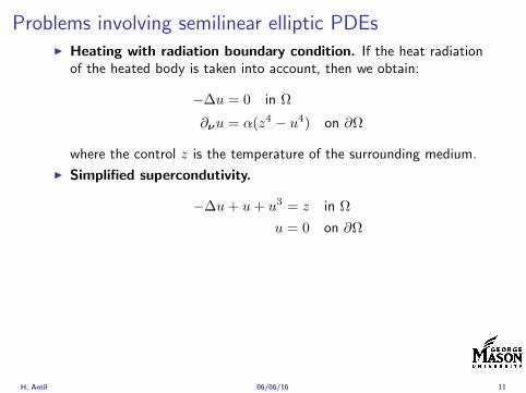
Problems involving semilinear elliptic PDEsI Heating with radiation boundary condition If the heat radiation
of the heated body is taken into account then we obtain
minus∆u = 0 in Ω
partνu = α(z4 minus u4) on partΩ
where the control z is the temperature of the surrounding medium
I Simplified supercondutivity
minus∆u+ u+ u3 = z in Ω
u = 0 on partΩ
I Control of stationary flows
minusmicro∆u + (u middot nabla)u +nablap = f in Ω
div u = 0 in Ω
u = g on partΩ
H Antil 060616 11
Problems involving semilinear elliptic PDEsI Heating with radiation boundary condition If the heat radiation
of the heated body is taken into account then we obtain
minus∆u = 0 in Ω
partνu = α(z4 minus u4) on partΩ
where the control z is the temperature of the surrounding medium
I Simplified supercondutivity
minus∆u+ u+ u3 = z in Ω
u = 0 on partΩ
I Control of stationary flows
minusmicro∆u + (u middot nabla)u +nablap = f in Ω
div u = 0 in Ω
u = g on partΩ
H Antil 060616 11
Optimal control of variational inequalitiesProblem
min J(u z) =1
2uminus ud2L2(Ω) +
λ
2z2L2(Ω)
subject to u isin K = w isin H10 (Ω) w(x) ge 0 ae x isin Ωint
Ω
nablau middot nabla(uminus v) dx le (z + f uminus v) forallv isin K
with z isin Zad
Regularized problem
min J(u z) =1
2uminus ud2L2(Ω) +
λ
2z2L2(Ω)
subject to (semilinear PDE)
u isin H10 (Ω) minus∆u+ γρε(minusu) = z + f in Ω
and z isin Zad γ gt 0 and ε gt 0 are the penealization and regularizationparameters respectively
H Antil 060616 12
Outline
Motivation and examples
Linear elliptic optimal control problems
Differentiation in Banach spaces
First-order necessary conditions
Optimal control of semilinear PDEs
An abstract problem
Discretization using finite element methods
H Antil 060616 13
Linear elliptic problemsΩ sub Rn bounded Lipschitz domain
Sobolev spacesI Lp(Ω) 1 le p le infin are Lebesgue spaces p = 2 L2(Ω) is a Hilbert
space with inner product (u v) =int
Ωu(x)v(x) dx
I W sp for s isin R 1 le p le infin are Sobolev spaces When p = 2W s2(Ω) = Hs(Ω) is a Hilbert space
I H10 (Ω) = v isin H1(Ω) v|partΩ = 0 with norm (due to Poincare
inequality)uH1
0 (Ω) = nablauL2(Ω)
I H10 (Ω)lowast = Hminus1(Ω)
I Note L2(Ω) sub Hminus1(Ω)
Model problem
minusdiv (Anablau) = f in Ω
u = 0 on partΩ
H Antil 060616 14
Linear elliptic problemsΩ sub Rn bounded Lipschitz domain
Sobolev spacesI Lp(Ω) 1 le p le infin are Lebesgue spaces p = 2 L2(Ω) is a Hilbert
space with inner product (u v) =int
Ωu(x)v(x) dx
I W sp for s isin R 1 le p le infin are Sobolev spaces When p = 2W s2(Ω) = Hs(Ω) is a Hilbert space
I H10 (Ω) = v isin H1(Ω) v|partΩ = 0 with norm (due to Poincare
inequality)uH1
0 (Ω) = nablauL2(Ω)
I H10 (Ω)lowast = Hminus1(Ω)
I Note L2(Ω) sub Hminus1(Ω)
Model problem
minusdiv (Anablau) = f in Ω
u = 0 on partΩ
H Antil 060616 14
Linear elliptic problemsΩ sub Rn bounded Lipschitz domain
Sobolev spacesI Lp(Ω) 1 le p le infin are Lebesgue spaces p = 2 L2(Ω) is a Hilbert
space with inner product (u v) =int
Ωu(x)v(x) dx
I W sp for s isin R 1 le p le infin are Sobolev spaces When p = 2W s2(Ω) = Hs(Ω) is a Hilbert space
I H10 (Ω) = v isin H1(Ω) v|partΩ = 0 with norm (due to Poincare
inequality)uH1
0 (Ω) = nablauL2(Ω)
I H10 (Ω)lowast = Hminus1(Ω)
I Note L2(Ω) sub Hminus1(Ω)
Model problem
minusdiv (Anablau) = f in Ω
u = 0 on partΩ
H Antil 060616 14
Linear elliptic problemsΩ sub Rn bounded Lipschitz domain
Sobolev spacesI Lp(Ω) 1 le p le infin are Lebesgue spaces p = 2 L2(Ω) is a Hilbert
space with inner product (u v) =int
Ωu(x)v(x) dx
I W sp for s isin R 1 le p le infin are Sobolev spaces When p = 2W s2(Ω) = Hs(Ω) is a Hilbert space
I H10 (Ω) = v isin H1(Ω) v|partΩ = 0 with norm (due to Poincare
inequality)uH1
0 (Ω) = nablauL2(Ω)
I H10 (Ω)lowast = Hminus1(Ω)
I Note L2(Ω) sub Hminus1(Ω)
Model problem
minusdiv (Anablau) = f in Ω
u = 0 on partΩ
H Antil 060616 14
Linear elliptic problemsΩ sub Rn bounded Lipschitz domain
Sobolev spacesI Lp(Ω) 1 le p le infin are Lebesgue spaces p = 2 L2(Ω) is a Hilbert
space with inner product (u v) =int
Ωu(x)v(x) dx
I W sp for s isin R 1 le p le infin are Sobolev spaces When p = 2W s2(Ω) = Hs(Ω) is a Hilbert space
I H10 (Ω) = v isin H1(Ω) v|partΩ = 0 with norm (due to Poincare
inequality)uH1
0 (Ω) = nablauL2(Ω)
I H10 (Ω)lowast = Hminus1(Ω)
I Note L2(Ω) sub Hminus1(Ω)
Model problem
minusdiv (Anablau) = f in Ω
u = 0 on partΩ
H Antil 060616 14
Well-posed
I Weak solution Given f isin Hminus1(Ω) a function u isin H10 (Ω) is called
a weak solution iffintΩ
Anablau middot nablav = 〈f v〉minus11 forallv isin H10 (Ω)
where 〈middot middot〉minus11 denotes the Hminus1(Ω)ndashH1(Ω) duality pairing
I Existence and uniqueness For each f isin Hminus1(Ω) there exists aunique u isin H1
0 (Ω) such that
nablauL2(Ω) le CdΩfHminus1(Ω)
I A = I the result is due to the Riesz-representation theorem
I A 6= I (maybe non-symmetric) the result is due to Lax-Milgramlemma
I For general W 1p-spaces use inf-sup conditions combined withBanach-Necas theorem which is a necessary and sufficient condition
H Antil 060616 15
Well-posed
I Weak solution Given f isin Hminus1(Ω) a function u isin H10 (Ω) is called
a weak solution iffintΩ
Anablau middot nablav = 〈f v〉minus11 forallv isin H10 (Ω)
where 〈middot middot〉minus11 denotes the Hminus1(Ω)ndashH1(Ω) duality pairing
I Existence and uniqueness For each f isin Hminus1(Ω) there exists aunique u isin H1
0 (Ω) such that
nablauL2(Ω) le CdΩfHminus1(Ω)
I A = I the result is due to the Riesz-representation theorem
I A 6= I (maybe non-symmetric) the result is due to Lax-Milgramlemma
I For general W 1p-spaces use inf-sup conditions combined withBanach-Necas theorem which is a necessary and sufficient condition
H Antil 060616 15
Linear-quadratic elliptic OCP
min J(u z) =1
2uminus ud2L2(Ω) +
λ
2z2L2(Ω)
subject to
minusdiv (Anablau) = z in Ω
u = 0 on partΩ
and the pointwise control constraints
z isin Zad = v isin L2(Ω) za(x) le v(x) le zb(x) ae x isin Ω
λ gt 0 is a parameter za zb isin Linfin(Ω) with za lt zb are given A isbounded symmetric positive
H Antil 060616 16
Reduced OCP
I Control to state map The solution operator defined as
S Hminus1(Ω)rarr H10 (Ω) z 7rarr u(z) = Sz
Note In view of the embedding
H10 (Ω) rarr L2(Ω) rarr Hminus1(Ω)
we may also consider S from L2(Ω) to L2(Ω) We will use the samenotation for this operator (for simplicity)
I Reduced cost functional The reduced cost functionalJ L2(Ω)rarr R is defined as
J (z) = J(Sz z)
I Reduced problem minzisinZadJ (z)
H Antil 060616 17
Reduced OCP
I Control to state map The solution operator defined as
S Hminus1(Ω)rarr H10 (Ω) z 7rarr u(z) = Sz
Note In view of the embedding
H10 (Ω) rarr L2(Ω) rarr Hminus1(Ω)
we may also consider S from L2(Ω) to L2(Ω) We will use the samenotation for this operator (for simplicity)
I Reduced cost functional The reduced cost functionalJ L2(Ω)rarr R is defined as
J (z) = J(Sz z)
I Reduced problem minzisinZadJ (z)
H Antil 060616 17
Reduced OCP
I Control to state map The solution operator defined as
S Hminus1(Ω)rarr H10 (Ω) z 7rarr u(z) = Sz
Note In view of the embedding
H10 (Ω) rarr L2(Ω) rarr Hminus1(Ω)
we may also consider S from L2(Ω) to L2(Ω) We will use the samenotation for this operator (for simplicity)
I Reduced cost functional The reduced cost functionalJ L2(Ω)rarr R is defined as
J (z) = J(Sz z)
I Reduced problem minzisinZadJ (z)
H Antil 060616 17
Existence of solution Direct methodThere exists a unique solution to the above problem
I Minimizing sequence J is bounded below by zero therefore thereexists a minimizing sequence znnisinN such that
limnrarrinfin
J (zn) = inf J (z)
I Weak compactness zn sub L2(Ω) is bounded Since L2(Ω) isreflexive therefore there exists a subsequence (not relabeled) suchthat
zn z and z isin Zad
where the latter is a consequence of Zad being closed and convex
I Optimality Since J is continuous and convex and therefore isweakly lower semicontinuous We obtain
lim inf J (zn) ge J (z)
which implies that z is optimal
I Uniqueness Exercise
H Antil 060616 18
Existence of solution Direct methodThere exists a unique solution to the above problem
I Minimizing sequence J is bounded below by zero therefore thereexists a minimizing sequence znnisinN such that
limnrarrinfin
J (zn) = inf J (z)
I Weak compactness zn sub L2(Ω) is bounded Since L2(Ω) isreflexive therefore there exists a subsequence (not relabeled) suchthat
zn z and z isin Zad
where the latter is a consequence of Zad being closed and convex
I Optimality Since J is continuous and convex and therefore isweakly lower semicontinuous We obtain
lim inf J (zn) ge J (z)
which implies that z is optimal
I Uniqueness Exercise
H Antil 060616 18
Existence of solution Direct methodThere exists a unique solution to the above problem
I Minimizing sequence J is bounded below by zero therefore thereexists a minimizing sequence znnisinN such that
limnrarrinfin
J (zn) = inf J (z)
I Weak compactness zn sub L2(Ω) is bounded Since L2(Ω) isreflexive therefore there exists a subsequence (not relabeled) suchthat
zn z and z isin Zad
where the latter is a consequence of Zad being closed and convex
I Optimality Since J is continuous and convex and therefore isweakly lower semicontinuous We obtain
lim inf J (zn) ge J (z)
which implies that z is optimal
I Uniqueness Exercise
H Antil 060616 18
Existence of solution Direct methodThere exists a unique solution to the above problem
I Minimizing sequence J is bounded below by zero therefore thereexists a minimizing sequence znnisinN such that
limnrarrinfin
J (zn) = inf J (z)
I Weak compactness zn sub L2(Ω) is bounded Since L2(Ω) isreflexive therefore there exists a subsequence (not relabeled) suchthat
zn z and z isin Zad
where the latter is a consequence of Zad being closed and convex
I Optimality Since J is continuous and convex and therefore isweakly lower semicontinuous We obtain
lim inf J (zn) ge J (z)
which implies that z is optimal
I Uniqueness Exercise
H Antil 060616 18
Outline
Motivation and examples
Linear elliptic optimal control problems
Differentiation in Banach spaces
First-order necessary conditions
Optimal control of semilinear PDEs
An abstract problem
Discretization using finite element methods
H Antil 060616 19
Differentiation in Banach spacesLet (Z middot Z) (V middot V ) B-spaces Z sub Z open and F Z rarr V
Let z isin Z
I If exist δF (z h) = limtdarr01t (F (z + th)minus F (z)) then δF (z h) is called
the directional derivative of F at z in direction h
I If exist δF (z h) forallh isin Z then h 7rarr δF (z h) is the first variation of Fat z
I Let exist the first variation δF (z middot) F is said to be Gateauxdifferentiable at z iff existA isin L(Z V ) such that δF (z h) = Ahforallh isin Z We write A = F primeG(z)
I F is said to be Frechet differentiable at z iff existA isin L(Z V ) and amapping r(z middot) Z rarr V such that for all h isin U with z + h isin Zwe have
F (z+h) = F (z)+Ah+r(z h) withr(z h)VhZ
rarr 0 as hZ rarr 0
We write F prime(z) = A
H Antil 060616 20
Differentiation in Banach spacesLet (Z middot Z) (V middot V ) B-spaces Z sub Z open and F Z rarr V
Let z isin Z
I If exist δF (z h) = limtdarr01t (F (z + th)minus F (z)) then δF (z h) is called
the directional derivative of F at z in direction h
I If exist δF (z h) forallh isin Z then h 7rarr δF (z h) is the first variation of Fat z
I Let exist the first variation δF (z middot) F is said to be Gateauxdifferentiable at z iff existA isin L(Z V ) such that δF (z h) = Ahforallh isin Z We write A = F primeG(z)
I F is said to be Frechet differentiable at z iff existA isin L(Z V ) and amapping r(z middot) Z rarr V such that for all h isin U with z + h isin Zwe have
F (z+h) = F (z)+Ah+r(z h) withr(z h)VhZ
rarr 0 as hZ rarr 0
We write F prime(z) = A
H Antil 060616 20
Differentiation in Banach spacesLet (Z middot Z) (V middot V ) B-spaces Z sub Z open and F Z rarr V
Let z isin Z
I If exist δF (z h) = limtdarr01t (F (z + th)minus F (z)) then δF (z h) is called
the directional derivative of F at z in direction h
I If exist δF (z h) forallh isin Z then h 7rarr δF (z h) is the first variation of Fat z
I Let exist the first variation δF (z middot) F is said to be Gateauxdifferentiable at z iff existA isin L(Z V ) such that δF (z h) = Ahforallh isin Z We write A = F primeG(z)
I F is said to be Frechet differentiable at z iff existA isin L(Z V ) and amapping r(z middot) Z rarr V such that for all h isin U with z + h isin Zwe have
F (z+h) = F (z)+Ah+r(z h) withr(z h)VhZ
rarr 0 as hZ rarr 0
We write F prime(z) = A
H Antil 060616 20
Differentiation in Banach spacesLet (Z middot Z) (V middot V ) B-spaces Z sub Z open and F Z rarr V
Let z isin Z
I If exist δF (z h) = limtdarr01t (F (z + th)minus F (z)) then δF (z h) is called
the directional derivative of F at z in direction h
I If exist δF (z h) forallh isin Z then h 7rarr δF (z h) is the first variation of Fat z
I Let exist the first variation δF (z middot) F is said to be Gateauxdifferentiable at z iff existA isin L(Z V ) such that δF (z h) = Ahforallh isin Z We write A = F primeG(z)
I F is said to be Frechet differentiable at z iff existA isin L(Z V ) and amapping r(z middot) Z rarr V such that for all h isin U with z + h isin Zwe have
F (z+h) = F (z)+Ah+r(z h) withr(z h)VhZ
rarr 0 as hZ rarr 0
We write F prime(z) = A
H Antil 060616 20
ExamplesExample 1 (H (middot middot)H) Hilbert space F (z) = z2H = (z z)H
forallz h F (z + h)minus F (z) = 2(z h)H + h2HThen
F prime(z)h = (2z h)H
Reisz representation theorem (identify H with Hlowast) we can write
F prime(z)h = (nablaF (z) h)H
where nablaF (z) = 2z is the gradient
Example 2 Let (Z (middot middot)Z) (H (middot middot)H) Hilbert spaces ud isin H fixedLet S isin L(ZH) Consider E Z rarr R
E(z) = Sz minus ud2H
Then E(z) = G(F (z)) where G(v) = v2H and F (z) = Sz minus ud
Eprime(z)h = Gprime(F (z))F prime(z)h = (2v F prime(z)h)H
= 2(Sz minus ud Sh)H = 2(Slowast(Sz minus ud) h)Z
we denote the gradient as nablaE(z) = 2Slowast(Sz minus ud)
H Antil 060616 21
ExamplesExample 1 (H (middot middot)H) Hilbert space F (z) = z2H = (z z)H
forallz h F (z + h)minus F (z) = 2(z h)H + h2HThen
F prime(z)h = (2z h)H
Reisz representation theorem (identify H with Hlowast) we can write
F prime(z)h = (nablaF (z) h)H
where nablaF (z) = 2z is the gradient
Example 2 Let (Z (middot middot)Z) (H (middot middot)H) Hilbert spaces ud isin H fixedLet S isin L(ZH) Consider E Z rarr R
E(z) = Sz minus ud2H
Then E(z) = G(F (z)) where G(v) = v2H and F (z) = Sz minus ud
Eprime(z)h = Gprime(F (z))F prime(z)h = (2v F prime(z)h)H
= 2(Sz minus ud Sh)H = 2(Slowast(Sz minus ud) h)Z
we denote the gradient as nablaE(z) = 2Slowast(Sz minus ud)H Antil 060616 21
Outline
Motivation and examples
Linear elliptic optimal control problems
Differentiation in Banach spaces
First-order necessary conditions
Optimal control of semilinear PDEs
An abstract problem
Discretization using finite element methods
H Antil 060616 22
First order necessary optimality conditions
Most of the theory is based on these two simple results
Theorem Let (Z middot Z) be a normed space J Z rarr (infin+infin] amapping with J 6equiv +infin Then z isin Z minimizer of J hArr 0 isin partJ (z)
Proof 0 isin partJ (z) means by definition of partJ (z) J (z)minus J (z) le 0forallz isin Z
Theorem Let (Z middot Z) be a normed space Zad sub Z nonemptyconvex closed J Z rarr R Gateaux differentiable where Zad sub Z sub ZZ open If z isin Zad is a solution to
minzisinZad
J (z)
then z solvesJ prime(z)(z minus z) ge 0 forallz isin Zad
Proof Exercise
H Antil 060616 23
First order necessary optimality conditions
Most of the theory is based on these two simple results
Theorem Let (Z middot Z) be a normed space J Z rarr (infin+infin] amapping with J 6equiv +infin Then z isin Z minimizer of J hArr 0 isin partJ (z)
Proof 0 isin partJ (z) means by definition of partJ (z) J (z)minus J (z) le 0forallz isin Z
Theorem Let (Z middot Z) be a normed space Zad sub Z nonemptyconvex closed J Z rarr R Gateaux differentiable where Zad sub Z sub ZZ open If z isin Zad is a solution to
minzisinZad
J (z)
then z solvesJ prime(z)(z minus z) ge 0 forallz isin Zad
Proof Exercise
H Antil 060616 23
Linear quadratic OCPI Reduced funcational
J (z) =1
2Sz minus ud2L2(Ω) +
λ
2z2L2(Ω)
I Gradient computation using sensitivity
J prime(z)h = (Slowast(Sz minus ud) + λz h)L2(Ω) forallh isin L2(Ω)
we denote the gradient by
nablaJ (z) = Slowast(Sz minus ud) + λz
I First order necessary and sufficient optimality condition
(nablaJ (z) z minus z)L2(Ω) ge 0 forallz isin Zad
I Adjoint equation Let p = Slowast(Sz minus ud) which translates intop isin H1
0 (Ω) solving
minusdiv (Anablap) = uminus ud in Ω
p = 0 on partΩ
I Gradient computation using adjoint nablaJ (z) = p+ λz
H Antil 060616 24
Linear quadratic OCPI Reduced funcational
J (z) =1
2Sz minus ud2L2(Ω) +
λ
2z2L2(Ω)
I Gradient computation using sensitivity
J prime(z)h = (Slowast(Sz minus ud) + λz h)L2(Ω) forallh isin L2(Ω)
we denote the gradient by
nablaJ (z) = Slowast(Sz minus ud) + λz
I First order necessary and sufficient optimality condition
(nablaJ (z) z minus z)L2(Ω) ge 0 forallz isin Zad
I Adjoint equation Let p = Slowast(Sz minus ud) which translates intop isin H1
0 (Ω) solving
minusdiv (Anablap) = uminus ud in Ω
p = 0 on partΩ
I Gradient computation using adjoint nablaJ (z) = p+ λz
H Antil 060616 24
Linear quadratic OCPI Reduced funcational
J (z) =1
2Sz minus ud2L2(Ω) +
λ
2z2L2(Ω)
I Gradient computation using sensitivity
J prime(z)h = (Slowast(Sz minus ud) + λz h)L2(Ω) forallh isin L2(Ω)
we denote the gradient by
nablaJ (z) = Slowast(Sz minus ud) + λz
I First order necessary and sufficient optimality condition
(nablaJ (z) z minus z)L2(Ω) ge 0 forallz isin Zad
I Adjoint equation Let p = Slowast(Sz minus ud) which translates intop isin H1
0 (Ω) solving
minusdiv (Anablap) = uminus ud in Ω
p = 0 on partΩ
I Gradient computation using adjoint nablaJ (z) = p+ λz
H Antil 060616 24
Linear quadratic OCPI Reduced funcational
J (z) =1
2Sz minus ud2L2(Ω) +
λ
2z2L2(Ω)
I Gradient computation using sensitivity
J prime(z)h = (Slowast(Sz minus ud) + λz h)L2(Ω) forallh isin L2(Ω)
we denote the gradient by
nablaJ (z) = Slowast(Sz minus ud) + λz
I First order necessary and sufficient optimality condition
(nablaJ (z) z minus z)L2(Ω) ge 0 forallz isin Zad
I Adjoint equation Let p = Slowast(Sz minus ud) which translates intop isin H1
0 (Ω) solving
minusdiv (Anablap) = uminus ud in Ω
p = 0 on partΩ
I Gradient computation using adjoint nablaJ (z) = p+ λz
H Antil 060616 24
Linear quadratic OCPI Reduced funcational
J (z) =1
2Sz minus ud2L2(Ω) +
λ
2z2L2(Ω)
I Gradient computation using sensitivity
J prime(z)h = (Slowast(Sz minus ud) + λz h)L2(Ω) forallh isin L2(Ω)
we denote the gradient by
nablaJ (z) = Slowast(Sz minus ud) + λz
I First order necessary and sufficient optimality condition
(nablaJ (z) z minus z)L2(Ω) ge 0 forallz isin Zad
I Adjoint equation Let p = Slowast(Sz minus ud) which translates intop isin H1
0 (Ω) solving
minusdiv (Anablap) = uminus ud in Ω
p = 0 on partΩ
I Gradient computation using adjoint nablaJ (z) = p+ λz
H Antil 060616 24
Optimality system
I State u isin H10 (Ω)
intΩAnablau middot nablav =
intΩzv forallv isin H1
0 (Ω)
I Adjoint p isin H10 (Ω)
intΩAnablap middot nablav =
intΩ
(uminus ud)v forallv isin H10 (Ω)
I Control z isin Zad (p+ λz z minus z) ge 0 forallz isin Zad
H Antil 060616 25
Pointwise interpretation
The variational inequality
(p+ λz z minus z) ge 0 forallz isin Zad
is equivalent to for ae x isin Ω
z(x) =
za(x) if p(x) + λz(x) gt 0isin [za(x) zb(x)] if p(x) + λz(x) = 0zb(x) if p(x) + λz(x) lt 0
Consequence
I When λ gt 0 then ae in Ω
z(x) = P[za(x)zb(x)]
minus 1
λp(x)
= min
zb(x)max
za(x)minus 1
λp(x)
H Antil 060616 26
Formal Lagrange method applied to linear OCPIntroduce L H1
0 (Ω)times Zad timesH1(Ω)rarr R defined as
L(u z p) = J(u z)minusint
Ω
(minusdiv (Anablau)minus z
)p dx
Integrate by parts to arrive at
L(u z p) = J(u z)minusint
Ω
(minusdiv (Anablap)uminus zp
)dx+
intpartΩ
(Anablau)p ds
If (u z p) is a stationary point then
I State
DpL(u z p)h = 0 forallh isin H1(Ω)
I AdjointDuL(u z p)h = 0 forallh isin H1
0 (Ω)
I ControlDzL(u z p)(z minus z) ge 0 forallz isin Zad
H Antil 060616 27
Formal Lagrange method applied to linear OCPIntroduce L H1
0 (Ω)times Zad timesH1(Ω)rarr R defined as
L(u z p) = J(u z)minusint
Ω
(minusdiv (Anablau)minus z
)p dx
Integrate by parts to arrive at
L(u z p) = J(u z)minusint
Ω
(minusdiv (Anablap)uminus zp
)dx+
intpartΩ
(Anablau)p ds
If (u z p) is a stationary point then
I State
DpL(u z p)h = 0 forallh isin H1(Ω)
I AdjointDuL(u z p)h = 0 forallh isin H1
0 (Ω)
I ControlDzL(u z p)(z minus z) ge 0 forallz isin Zad
H Antil 060616 27
Formal Lagrange method applied to linear OCPIntroduce L H1
0 (Ω)times Zad timesH1(Ω)rarr R defined as
L(u z p) = J(u z)minusint
Ω
(minusdiv (Anablau)minus z
)p dx
Integrate by parts to arrive at
L(u z p) = J(u z)minusint
Ω
(minusdiv (Anablap)uminus zp
)dx+
intpartΩ
(Anablau)p ds
If (u z p) is a stationary point then
I State
DpL(u z p)h = 0 forallh isin H1(Ω)
I AdjointDuL(u z p)h = 0 forallh isin H1
0 (Ω)
I ControlDzL(u z p)(z minus z) ge 0 forallz isin Zad
H Antil 060616 27
Formal Lagrange method applied to linear OCPIntroduce L H1
0 (Ω)times Zad timesH1(Ω)rarr R defined as
L(u z p) = J(u z)minusint
Ω
(minusdiv (Anablau)minus z
)p dx
Integrate by parts to arrive at
L(u z p) = J(u z)minusint
Ω
(minusdiv (Anablap)uminus zp
)dx+
intpartΩ
(Anablau)p ds
If (u z p) is a stationary point then
I State
DpL(u z p)h = 0 forallh isin H1(Ω)
I AdjointDuL(u z p)h = 0 forallh isin H1
0 (Ω)
I ControlDzL(u z p)(z minus z) ge 0 forallz isin Zad
H Antil 060616 27
Formal Lagrange method applied to linear OCPIntroduce L H1
0 (Ω)times Zad timesH1(Ω)rarr R defined as
L(u z p) = J(u z)minusint
Ω
(minusdiv (Anablau)minus z
)p dx
Integrate by parts to arrive at
L(u z p) = J(u z)minusint
Ω
(minusdiv (Anablap)uminus zp
)dx+
intpartΩ
(Anablau)p ds
If (u z p) is a stationary point then
I State
DpL(u z p)h = 0 forallh isin H1(Ω)
I AdjointDuL(u z p)h = 0 forallh isin H1
0 (Ω)
I ControlDzL(u z p)(z minus z) ge 0 forallz isin Zad
H Antil 060616 27
Outline
Motivation and examples
Linear elliptic optimal control problems
Differentiation in Banach spaces
First-order necessary conditions
Optimal control of semilinear PDEs
An abstract problem
Discretization using finite element methods
H Antil 060616 28
Semilinear elliptic OCP
min J(u z) =1
2uminus ud2L2(Ω) +
λ
2z2L2(Ω)
subject to
minus∆u+ g(x u) = z in Ω
u = 0 on partΩ
and z isin Zad with za zb isin Linfin(Ω)
H Antil 060616 29
State space(A1) Ω sub Rd open bounded partΩ is Lipschitz
(A2) g Ωtimes Rrarr R is bounded and measurable with respect to x isin Ωfor every u isin R
(A3) g is continuous monotone increasing and Lipschitz continuous in ufor ae x isin Ω
(A4) g(x 0) = 0 for ae x isin Ω (not really necessary)
Theorem Suppose (A1)minus (A4) hold For every z isin Lr(Ω) withr gt d2 the state equation has a unique weak solutionu isin H1
0 (Ω) cap C(Ω) ie we haveintΩ
nablau middot nablav dx+
intΩ
g(x u(x))v(x) dx =
intΩ
zv dx forallv isin H10 (Ω)
Moreover there exists a constant C gt 0 such that
uH1(Ω) + uC(Ω) le CzLr(Ω)
RemarkI The proof of the theorem uses the BrowderndashMinty theorem on
monotone operators
H Antil 060616 30
State space(A1) Ω sub Rd open bounded partΩ is Lipschitz
(A2) g Ωtimes Rrarr R is bounded and measurable with respect to x isin Ωfor every u isin R
(A3) g is continuous monotone increasing and Lipschitz continuous in ufor ae x isin Ω
(A4) g(x 0) = 0 for ae x isin Ω (not really necessary)
Theorem Suppose (A1)minus (A4) hold For every z isin Lr(Ω) withr gt d2 the state equation has a unique weak solutionu isin H1
0 (Ω) cap C(Ω) ie we haveintΩ
nablau middot nablav dx+
intΩ
g(x u(x))v(x) dx =
intΩ
zv dx forallv isin H10 (Ω)
Moreover there exists a constant C gt 0 such that
uH1(Ω) + uC(Ω) le CzLr(Ω)
RemarkI The proof of the theorem uses the BrowderndashMinty theorem on
monotone operators
H Antil 060616 30
State space(A1) Ω sub Rd open bounded partΩ is Lipschitz
(A2) g Ωtimes Rrarr R is bounded and measurable with respect to x isin Ωfor every u isin R
(A3) g is continuous monotone increasing and Lipschitz continuous in ufor ae x isin Ω
(A4) g(x 0) = 0 for ae x isin Ω (not really necessary)
Theorem Suppose (A1)minus (A4) hold For every z isin Lr(Ω) withr gt d2 the state equation has a unique weak solutionu isin H1
0 (Ω) cap C(Ω) ie we haveintΩ
nablau middot nablav dx+
intΩ
g(x u(x))v(x) dx =
intΩ
zv dx forallv isin H10 (Ω)
Moreover there exists a constant C gt 0 such that
uH1(Ω) + uC(Ω) le CzLr(Ω)
RemarkI The proof of the theorem uses the BrowderndashMinty theorem on
monotone operators
H Antil 060616 30
Control-to-state map and reduced problem
I Control to state map
S Linfin(Ω)rarr H10 (Ω) cap C(Ω)
is well defined and is globally Lipschitz continuous
I Reduced problem
minJ (z) =1
2S(u)minus ud2L2(Ω) +
λ
2z2L2(Ω)
H Antil 060616 31
Control-to-state map and reduced problem
I Control to state map
S Linfin(Ω)rarr H10 (Ω) cap C(Ω)
is well defined and is globally Lipschitz continuous
I Reduced problem
minJ (z) =1
2S(u)minus ud2L2(Ω) +
λ
2z2L2(Ω)
H Antil 060616 31
First-order necessary conditionsI Lagrangian functional
L(u z p) = J(u z)minusint
Ω
(minus∆u+ g(x u(x))minus z
)p dx
= J(u z)minusint
Ω
(nablau middot nablap+ g(x u(x))pminus zp
)dx
I Adjoint system For all h isin H10 (Ω)
0 = DuL(u z p)h =
intΩ
(uminus ud)h dxminusint
Ω
(nablah middot nablap+ gu(x u(x))ph
)which yields
minus∆p+ gu(x u(x))p = uminus ud in Ω
p = 0 on partΩ
I Control
DzL(u z p)(z minus z) = (p+ λz z minus z) dx ge 0 forallz isin ZadI Gradient
nablaJ (z) = p+ λz
H Antil 060616 32
First-order necessary conditionsI Lagrangian functional
L(u z p) = J(u z)minusint
Ω
(minus∆u+ g(x u(x))minus z
)p dx
= J(u z)minusint
Ω
(nablau middot nablap+ g(x u(x))pminus zp
)dx
I Adjoint system For all h isin H10 (Ω)
0 = DuL(u z p)h =
intΩ
(uminus ud)h dxminusint
Ω
(nablah middot nablap+ gu(x u(x))ph
)which yields
minus∆p+ gu(x u(x))p = uminus ud in Ω
p = 0 on partΩ
I Control
DzL(u z p)(z minus z) = (p+ λz z minus z) dx ge 0 forallz isin ZadI Gradient
nablaJ (z) = p+ λz
H Antil 060616 32
First-order necessary conditionsI Lagrangian functional
L(u z p) = J(u z)minusint
Ω
(minus∆u+ g(x u(x))minus z
)p dx
= J(u z)minusint
Ω
(nablau middot nablap+ g(x u(x))pminus zp
)dx
I Adjoint system For all h isin H10 (Ω)
0 = DuL(u z p)h =
intΩ
(uminus ud)h dxminusint
Ω
(nablah middot nablap+ gu(x u(x))ph
)which yields
minus∆p+ gu(x u(x))p = uminus ud in Ω
p = 0 on partΩ
I Control
DzL(u z p)(z minus z) = (p+ λz z minus z) dx ge 0 forallz isin Zad
I GradientnablaJ (z) = p+ λz
H Antil 060616 32
First-order necessary conditionsI Lagrangian functional
L(u z p) = J(u z)minusint
Ω
(minus∆u+ g(x u(x))minus z
)p dx
= J(u z)minusint
Ω
(nablau middot nablap+ g(x u(x))pminus zp
)dx
I Adjoint system For all h isin H10 (Ω)
0 = DuL(u z p)h =
intΩ
(uminus ud)h dxminusint
Ω
(nablah middot nablap+ gu(x u(x))ph
)which yields
minus∆p+ gu(x u(x))p = uminus ud in Ω
p = 0 on partΩ
I Control
DzL(u z p)(z minus z) = (p+ λz z minus z) dx ge 0 forallz isin ZadI Gradient
nablaJ (z) = p+ λz
H Antil 060616 32
Differentiability of Nemytskii operator
The rigorous proof uses
Theorem In addition to (A1)-(A4) if
(A5) g is continuously differentiable with respect to u for ae x isin Ωand we have
(i) |gu(x 0)| le K for ae x isin Ω(ii) gu is locally Lipschitz with respect to u isin R
then the Nemytskii operator G u 7rarr g(middot u(middot)) is continuously Frechetdifferentiable from Linfin(Ω) into itself and
(Gprime(u)h)(x) = gu(x u(x))h(x) ae in Ω forallh isin Linfin(Ω)
Remark (A5) holds if g(x u) = g(u) and g isin C2(R)
H Antil 060616 33
Outline
Motivation and examples
Linear elliptic optimal control problems
Differentiation in Banach spaces
First-order necessary conditions
Optimal control of semilinear PDEs
An abstract problem
Discretization using finite element methods
H Antil 060616 34
Gradient computation via adjoint general formI Abstract problem
min J(u z)
subject toc(u z) = 0
and z isin Zad
I Directional derivative Let S be the control to state map(nonlinear in general)
z 7rarr S(z) = u(z)
Under the assumptions of ldquoimplicit function theoremrdquo
J prime(z)h = (nablauJ (u(z) z) Sprime(z)h) + (nablazJ (u(z) z) h)
I Sensitivity of u with respect to z Differentiating the stateequation
cu(S(z) z)Sprime(z)h = minuscz(S(z) z)h
leads toSprime(z)h = minuscu(S(z) z)minus1
(cz(S(z) z)h
)
provided cu(S(z) z)minus1 is well-defined
H Antil 060616 35
Gradient computation via adjoint general formI Abstract problem
min J(u z)
subject toc(u z) = 0
and z isin ZadI Directional derivative Let S be the control to state map
(nonlinear in general)
z 7rarr S(z) = u(z)
Under the assumptions of ldquoimplicit function theoremrdquo
J prime(z)h = (nablauJ (u(z) z) Sprime(z)h) + (nablazJ (u(z) z) h)
I Sensitivity of u with respect to z Differentiating the stateequation
cu(S(z) z)Sprime(z)h = minuscz(S(z) z)h
leads toSprime(z)h = minuscu(S(z) z)minus1
(cz(S(z) z)h
)
provided cu(S(z) z)minus1 is well-defined
H Antil 060616 35
Gradient computation via adjoint general formI Abstract problem
min J(u z)
subject toc(u z) = 0
and z isin ZadI Directional derivative Let S be the control to state map
(nonlinear in general)
z 7rarr S(z) = u(z)
Under the assumptions of ldquoimplicit function theoremrdquo
J prime(z)h = (nablauJ (u(z) z) Sprime(z)h) + (nablazJ (u(z) z) h)
I Sensitivity of u with respect to z Differentiating the stateequation
cu(S(z) z)Sprime(z)h = minuscz(S(z) z)h
leads toSprime(z)h = minuscu(S(z) z)minus1
(cz(S(z) z)h
)
provided cu(S(z) z)minus1 is well-defined
H Antil 060616 35
Adjoint equation and gradient general form
I Directional derivative
J prime(z)h = minus(nablauJ (u(z) z) cu(u(z) z)minus1cz(u(z) z)h
)+ (nablazJ (u(z) z) h)
I Gradient
nablaJ (z) = minuscz(u(z) z)lowast(cu(u(z) z)minuslowastnablauJ (u(z) z)
)+nablazJ (u(z) z)
I Introducing adjoint variable p solving
cu(u(z) z)lowastp = nablauJ (u(z) z)
we arrive at following form of gradient
nablaJ (z) = minuscz(u(z) z)lowastp+nablazJ (u(z) z)
which is tractable
H Antil 060616 36
Adjoint equation and gradient general form
I Directional derivative
J prime(z)h = minus(nablauJ (u(z) z) cu(u(z) z)minus1cz(u(z) z)h
)+ (nablazJ (u(z) z) h)
I Gradient
nablaJ (z) = minuscz(u(z) z)lowast(cu(u(z) z)minuslowastnablauJ (u(z) z)
)+nablazJ (u(z) z)
I Introducing adjoint variable p solving
cu(u(z) z)lowastp = nablauJ (u(z) z)
we arrive at following form of gradient
nablaJ (z) = minuscz(u(z) z)lowastp+nablazJ (u(z) z)
which is tractable
H Antil 060616 36
Adjoint equation and gradient general form
I Directional derivative
J prime(z)h = minus(nablauJ (u(z) z) cu(u(z) z)minus1cz(u(z) z)h
)+ (nablazJ (u(z) z) h)
I Gradient
nablaJ (z) = minuscz(u(z) z)lowast(cu(u(z) z)minuslowastnablauJ (u(z) z)
)+nablazJ (u(z) z)
I Introducing adjoint variable p solving
cu(u(z) z)lowastp = nablauJ (u(z) z)
we arrive at following form of gradient
nablaJ (z) = minuscz(u(z) z)lowastp+nablazJ (u(z) z)
which is tractable
H Antil 060616 36
Hessian computation general form
I Lagrangian L(u z p) = J(u z)minusint
Ωc(u z)p dx Then we have
DzJ (z)h = DzL(u z p)h
I Second order derivative
D2zJ (z)[h1 h2] = DuDzL(u z p)[h1 S
prime(z)h2] +D2zL(u z p)[h1 h2]
+DpDzL(u z p)[h1 Dzp(z)h2]
I We already know Sprime(z)h2 moreover
DpDzL(u z p)[h1 Dzp(z)h2] = minus(cu(u z)h1 Dzp(z)h2
)
It remain to identify Dzp(z)h2
H Antil 060616 37
Hessian computation general form
I Lagrangian L(u z p) = J(u z)minusint
Ωc(u z)p dx Then we have
DzJ (z)h = DzL(u z p)h
I Second order derivative
D2zJ (z)[h1 h2] = DuDzL(u z p)[h1 S
prime(z)h2] +D2zL(u z p)[h1 h2]
+DpDzL(u z p)[h1 Dzp(z)h2]
I We already know Sprime(z)h2 moreover
DpDzL(u z p)[h1 Dzp(z)h2] = minus(cu(u z)h1 Dzp(z)h2
)
It remain to identify Dzp(z)h2
H Antil 060616 37
Hessian computation general form
I Lagrangian L(u z p) = J(u z)minusint
Ωc(u z)p dx Then we have
DzJ (z)h = DzL(u z p)h
I Second order derivative
D2zJ (z)[h1 h2] = DuDzL(u z p)[h1 S
prime(z)h2] +D2zL(u z p)[h1 h2]
+DpDzL(u z p)[h1 Dzp(z)h2]
I We already know Sprime(z)h2 moreover
DpDzL(u z p)[h1 Dzp(z)h2] = minus(cu(u z)h1 Dzp(z)h2
)
It remain to identify Dzp(z)h2
H Antil 060616 37
Outline
Motivation and examples
Linear elliptic optimal control problems
Differentiation in Banach spaces
First-order necessary conditions
Optimal control of semilinear PDEs
An abstract problem
Discretization using finite element methods
H Antil 060616 38
Numerical approximation of Poisson equation MeshTo avoid technical issues we will assume that partΩ is polygonal
I Mesh Let T = K be a mesh of Ω where K sub Rd is an elementthat is isoparametrically equivalent to a unit simplex in Rd
I Conforming mesh We say that the mesh is conforming ifI Ω = cupKisinT KI If K1 cap K2 = x then x is a node of K1 and K2I If K1 cap K2 6= empty and K1 cap K2 6= x then K1 cap K2 is an edgeface
contained in partK1 cap partK2
I Shape regular Let T be the collection of all conformingrefinements of an original mesh T 0 Then T is called shape regularif exist κ gt 0 such that
hKρKle κ forallK isin cupiT i
where hK = diam K ρK = maxρ gt 0|Bρ sub KI Quasi-uniform A family of shape regular meshes is called-quasi
uniform if there exist a constant σ gt 0 such that
maxhKminhK
le σ
uniformly for all meshes in the family
Numerical approximation of Poisson equation MeshTo avoid technical issues we will assume that partΩ is polygonal
I Mesh Let T = K be a mesh of Ω where K sub Rd is an elementthat is isoparametrically equivalent to a unit simplex in Rd
I Conforming mesh We say that the mesh is conforming ifI Ω = cupKisinT KI If K1 cap K2 = x then x is a node of K1 and K2I If K1 cap K2 6= empty and K1 cap K2 6= x then K1 cap K2 is an edgeface
contained in partK1 cap partK2
I Shape regular Let T be the collection of all conformingrefinements of an original mesh T 0 Then T is called shape regularif exist κ gt 0 such that
hKρKle κ forallK isin cupiT i
where hK = diam K ρK = maxρ gt 0|Bρ sub KI Quasi-uniform A family of shape regular meshes is called-quasi
uniform if there exist a constant σ gt 0 such that
maxhKminhK
le σ
uniformly for all meshes in the family
Numerical approximation of Poisson equation MeshTo avoid technical issues we will assume that partΩ is polygonal
I Mesh Let T = K be a mesh of Ω where K sub Rd is an elementthat is isoparametrically equivalent to a unit simplex in Rd
I Conforming mesh We say that the mesh is conforming ifI Ω = cupKisinT KI If K1 cap K2 = x then x is a node of K1 and K2I If K1 cap K2 6= empty and K1 cap K2 6= x then K1 cap K2 is an edgeface
contained in partK1 cap partK2
I Shape regular Let T be the collection of all conformingrefinements of an original mesh T 0 Then T is called shape regularif exist κ gt 0 such that
hKρKle κ forallK isin cupiT i
where hK = diam K ρK = maxρ gt 0|Bρ sub K
I Quasi-uniform A family of shape regular meshes is called-quasiuniform if there exist a constant σ gt 0 such that
maxhKminhK
le σ
uniformly for all meshes in the family
Numerical approximation of Poisson equation MeshTo avoid technical issues we will assume that partΩ is polygonal
I Mesh Let T = K be a mesh of Ω where K sub Rd is an elementthat is isoparametrically equivalent to a unit simplex in Rd
I Conforming mesh We say that the mesh is conforming ifI Ω = cupKisinT KI If K1 cap K2 = x then x is a node of K1 and K2I If K1 cap K2 6= empty and K1 cap K2 6= x then K1 cap K2 is an edgeface
contained in partK1 cap partK2
I Shape regular Let T be the collection of all conformingrefinements of an original mesh T 0 Then T is called shape regularif exist κ gt 0 such that
hKρKle κ forallK isin cupiT i
where hK = diam K ρK = maxρ gt 0|Bρ sub KI Quasi-uniform A family of shape regular meshes is called-quasi
uniform if there exist a constant σ gt 0 such that
maxhKminhK
le σ
uniformly for all meshes in the family
FE space and Galerkin approximationI Finite element space For T isin T we define the finite element
space as
V(T ) = W isin C0(Ω) WK isin P1forallK isin T W |partΩ = 0
where P1 is the set of polynomials of degree at most 1
I Galerkin approximation of continuous problem is given by
Find UT isin V(T )
intΩ
AnablaUT middot nablaV = 〈f V 〉 forallV isin V(T )
The discrete problem is well-posedI Nodal basis Consists of functions ψi isin V(T ) with xi isin N (T )
satisfyingψxi
(xj) = δij
where N (T ) denotes the interior (plus Neumann) nodesI Galerkin orthogonality(
nabla(uminus UT )nablaW)L2(Ω)
= 0 forallW isin V(T )
H Antil 060616 40
FE space and Galerkin approximationI Finite element space For T isin T we define the finite element
space as
V(T ) = W isin C0(Ω) WK isin P1forallK isin T W |partΩ = 0
where P1 is the set of polynomials of degree at most 1I Galerkin approximation of continuous problem is given by
Find UT isin V(T )
intΩ
AnablaUT middot nablaV = 〈f V 〉 forallV isin V(T )
The discrete problem is well-posed
I Nodal basis Consists of functions ψi isin V(T ) with xi isin N (T )satisfying
ψxi(xj) = δij
where N (T ) denotes the interior (plus Neumann) nodesI Galerkin orthogonality(
nabla(uminus UT )nablaW)L2(Ω)
= 0 forallW isin V(T )
H Antil 060616 40
FE space and Galerkin approximationI Finite element space For T isin T we define the finite element
space as
V(T ) = W isin C0(Ω) WK isin P1forallK isin T W |partΩ = 0
where P1 is the set of polynomials of degree at most 1I Galerkin approximation of continuous problem is given by
Find UT isin V(T )
intΩ
AnablaUT middot nablaV = 〈f V 〉 forallV isin V(T )
The discrete problem is well-posedI Nodal basis Consists of functions ψi isin V(T ) with xi isin N (T )
satisfyingψxi
(xj) = δij
where N (T ) denotes the interior (plus Neumann) nodes
I Galerkin orthogonality(nabla(uminus UT )nablaW
)L2(Ω)
= 0 forallW isin V(T )
H Antil 060616 40
FE space and Galerkin approximationI Finite element space For T isin T we define the finite element
space as
V(T ) = W isin C0(Ω) WK isin P1forallK isin T W |partΩ = 0
where P1 is the set of polynomials of degree at most 1I Galerkin approximation of continuous problem is given by
Find UT isin V(T )
intΩ
AnablaUT middot nablaV = 〈f V 〉 forallV isin V(T )
The discrete problem is well-posedI Nodal basis Consists of functions ψi isin V(T ) with xi isin N (T )
satisfyingψxi
(xj) = δij
where N (T ) denotes the interior (plus Neumann) nodesI Galerkin orthogonality(
nabla(uminus UT )nablaW)L2(Ω)
= 0 forallW isin V(T )
H Antil 060616 40
Best approximation
I Cearsquos lemma
nabla(uminus UT )L2(Ω) le C infWisinV(T )
nabla(uminusW )L2(Ω)
I Nodal interpolation operator ΠT C(Ω)rarr V(T ) satisfies
ΠT u(xi) = u(xi) forallxi isin N (T )
and is defined as
ΠT u =sum
xiisinN (T )
u(xi)ψxi
I Error estimates In Cearsquos lemma replace W by ΠT u and thencompute the interpolation error
H Antil 060616 41
Best approximation
I Cearsquos lemma
nabla(uminus UT )L2(Ω) le C infWisinV(T )
nabla(uminusW )L2(Ω)
I Nodal interpolation operator ΠT C(Ω)rarr V(T ) satisfies
ΠT u(xi) = u(xi) forallxi isin N (T )
and is defined as
ΠT u =sum
xiisinN (T )
u(xi)ψxi
I Error estimates In Cearsquos lemma replace W by ΠT u and thencompute the interpolation error
H Antil 060616 41
Best approximation
I Cearsquos lemma
nabla(uminus UT )L2(Ω) le C infWisinV(T )
nabla(uminusW )L2(Ω)
I Nodal interpolation operator ΠT C(Ω)rarr V(T ) satisfies
ΠT u(xi) = u(xi) forallxi isin N (T )
and is defined as
ΠT u =sum
xiisinN (T )
u(xi)ψxi
I Error estimates In Cearsquos lemma replace W by ΠT u and thencompute the interpolation error
H Antil 060616 41
Algebraic system state equation
I Recall UT isin V(T ) solves
a(UT V ) = 〈f V 〉 forallV isin V(T )
I Now setting UT =sumN
j=1 Ujψj V = ψi we get
Nsumj=1
Uja(φj φi) = 〈f ψi〉 i = 1 N
which is the matrix-vector system
AU = F
I Stiffness matrix A is SPD
H Antil 060616 42
Algebraic system state equation
I Recall UT isin V(T ) solves
a(UT V ) = 〈f V 〉 forallV isin V(T )
I Now setting UT =sumN
j=1 Ujψj V = ψi we get
Nsumj=1
Uja(φj φi) = 〈f ψi〉 i = 1 N
which is the matrix-vector system
AU = F
I Stiffness matrix A is SPD
H Antil 060616 42
Algebraic system state equation
I Recall UT isin V(T ) solves
a(UT V ) = 〈f V 〉 forallV isin V(T )
I Now setting UT =sumN
j=1 Ujψj V = ψi we get
Nsumj=1
Uja(φj φi) = 〈f ψi〉 i = 1 N
which is the matrix-vector system
AU = F
I Stiffness matrix A is SPD
H Antil 060616 42
Discrete linear elliptic OCP
min JT (UT ZT ) =1
2UT minus ud2L2(Ω) +
λ
2ZT 2L2(Ω)
subject to
Find UT isin V(T )
intΩ
nablaUT middot nablaV = (ZT V )L2(Ω) forallV isin V(T )
and whereZT isin Zad(T ) = Zad cap Z(T )
is either one of these
Z(T ) =
V(T )L2(Ω) variational discretization (Hinze)WT isin Linfin(Ω) ZT |K isin P0(K)K isin T
H Antil 060616 43
Recent books
F TroltzschOptimal control of partial differential equations volume 112 ofGraduate Studies in MathematicsAmerican Mathematical Society Providence RI 2010Theory methods and applications Translated from the 2005 Germanoriginal by Jurgen Sprekels
K Ito and K KunischLagrange multiplier approach to variational problems andapplications volume 15 of Advances in Design and ControlSociety for Industrial and Applied Mathematics (SIAM)Philadelphia PA 2008
H Antil 060616 44
- Motivation and examples
- Linear elliptic optimal control problems
- Differentiation in Banach spaces
- First-order necessary conditions
- Optimal control of semilinear PDEs
- An abstract problem
- Discretization using finite element methods
-
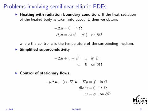
Problems involving semilinear elliptic PDEsI Heating with radiation boundary condition If the heat radiation
of the heated body is taken into account then we obtain
minus∆u = 0 in Ω
partνu = α(z4 minus u4) on partΩ
where the control z is the temperature of the surrounding medium
I Simplified supercondutivity
minus∆u+ u+ u3 = z in Ω
u = 0 on partΩ
I Control of stationary flows
minusmicro∆u + (u middot nabla)u +nablap = f in Ω
div u = 0 in Ω
u = g on partΩ
H Antil 060616 11
Optimal control of variational inequalitiesProblem
min J(u z) =1
2uminus ud2L2(Ω) +
λ
2z2L2(Ω)
subject to u isin K = w isin H10 (Ω) w(x) ge 0 ae x isin Ωint
Ω
nablau middot nabla(uminus v) dx le (z + f uminus v) forallv isin K
with z isin Zad
Regularized problem
min J(u z) =1
2uminus ud2L2(Ω) +
λ
2z2L2(Ω)
subject to (semilinear PDE)
u isin H10 (Ω) minus∆u+ γρε(minusu) = z + f in Ω
and z isin Zad γ gt 0 and ε gt 0 are the penealization and regularizationparameters respectively
H Antil 060616 12
Outline
Motivation and examples
Linear elliptic optimal control problems
Differentiation in Banach spaces
First-order necessary conditions
Optimal control of semilinear PDEs
An abstract problem
Discretization using finite element methods
H Antil 060616 13
Linear elliptic problemsΩ sub Rn bounded Lipschitz domain
Sobolev spacesI Lp(Ω) 1 le p le infin are Lebesgue spaces p = 2 L2(Ω) is a Hilbert
space with inner product (u v) =int
Ωu(x)v(x) dx
I W sp for s isin R 1 le p le infin are Sobolev spaces When p = 2W s2(Ω) = Hs(Ω) is a Hilbert space
I H10 (Ω) = v isin H1(Ω) v|partΩ = 0 with norm (due to Poincare
inequality)uH1
0 (Ω) = nablauL2(Ω)
I H10 (Ω)lowast = Hminus1(Ω)
I Note L2(Ω) sub Hminus1(Ω)
Model problem
minusdiv (Anablau) = f in Ω
u = 0 on partΩ
H Antil 060616 14
Linear elliptic problemsΩ sub Rn bounded Lipschitz domain
Sobolev spacesI Lp(Ω) 1 le p le infin are Lebesgue spaces p = 2 L2(Ω) is a Hilbert
space with inner product (u v) =int
Ωu(x)v(x) dx
I W sp for s isin R 1 le p le infin are Sobolev spaces When p = 2W s2(Ω) = Hs(Ω) is a Hilbert space
I H10 (Ω) = v isin H1(Ω) v|partΩ = 0 with norm (due to Poincare
inequality)uH1
0 (Ω) = nablauL2(Ω)
I H10 (Ω)lowast = Hminus1(Ω)
I Note L2(Ω) sub Hminus1(Ω)
Model problem
minusdiv (Anablau) = f in Ω
u = 0 on partΩ
H Antil 060616 14
Linear elliptic problemsΩ sub Rn bounded Lipschitz domain
Sobolev spacesI Lp(Ω) 1 le p le infin are Lebesgue spaces p = 2 L2(Ω) is a Hilbert
space with inner product (u v) =int
Ωu(x)v(x) dx
I W sp for s isin R 1 le p le infin are Sobolev spaces When p = 2W s2(Ω) = Hs(Ω) is a Hilbert space
I H10 (Ω) = v isin H1(Ω) v|partΩ = 0 with norm (due to Poincare
inequality)uH1
0 (Ω) = nablauL2(Ω)
I H10 (Ω)lowast = Hminus1(Ω)
I Note L2(Ω) sub Hminus1(Ω)
Model problem
minusdiv (Anablau) = f in Ω
u = 0 on partΩ
H Antil 060616 14
Linear elliptic problemsΩ sub Rn bounded Lipschitz domain
Sobolev spacesI Lp(Ω) 1 le p le infin are Lebesgue spaces p = 2 L2(Ω) is a Hilbert
space with inner product (u v) =int
Ωu(x)v(x) dx
I W sp for s isin R 1 le p le infin are Sobolev spaces When p = 2W s2(Ω) = Hs(Ω) is a Hilbert space
I H10 (Ω) = v isin H1(Ω) v|partΩ = 0 with norm (due to Poincare
inequality)uH1
0 (Ω) = nablauL2(Ω)
I H10 (Ω)lowast = Hminus1(Ω)
I Note L2(Ω) sub Hminus1(Ω)
Model problem
minusdiv (Anablau) = f in Ω
u = 0 on partΩ
H Antil 060616 14
Linear elliptic problemsΩ sub Rn bounded Lipschitz domain
Sobolev spacesI Lp(Ω) 1 le p le infin are Lebesgue spaces p = 2 L2(Ω) is a Hilbert
space with inner product (u v) =int
Ωu(x)v(x) dx
I W sp for s isin R 1 le p le infin are Sobolev spaces When p = 2W s2(Ω) = Hs(Ω) is a Hilbert space
I H10 (Ω) = v isin H1(Ω) v|partΩ = 0 with norm (due to Poincare
inequality)uH1
0 (Ω) = nablauL2(Ω)
I H10 (Ω)lowast = Hminus1(Ω)
I Note L2(Ω) sub Hminus1(Ω)
Model problem
minusdiv (Anablau) = f in Ω
u = 0 on partΩ
H Antil 060616 14
Well-posed
I Weak solution Given f isin Hminus1(Ω) a function u isin H10 (Ω) is called
a weak solution iffintΩ
Anablau middot nablav = 〈f v〉minus11 forallv isin H10 (Ω)
where 〈middot middot〉minus11 denotes the Hminus1(Ω)ndashH1(Ω) duality pairing
I Existence and uniqueness For each f isin Hminus1(Ω) there exists aunique u isin H1
0 (Ω) such that
nablauL2(Ω) le CdΩfHminus1(Ω)
I A = I the result is due to the Riesz-representation theorem
I A 6= I (maybe non-symmetric) the result is due to Lax-Milgramlemma
I For general W 1p-spaces use inf-sup conditions combined withBanach-Necas theorem which is a necessary and sufficient condition
H Antil 060616 15
Well-posed
I Weak solution Given f isin Hminus1(Ω) a function u isin H10 (Ω) is called
a weak solution iffintΩ
Anablau middot nablav = 〈f v〉minus11 forallv isin H10 (Ω)
where 〈middot middot〉minus11 denotes the Hminus1(Ω)ndashH1(Ω) duality pairing
I Existence and uniqueness For each f isin Hminus1(Ω) there exists aunique u isin H1
0 (Ω) such that
nablauL2(Ω) le CdΩfHminus1(Ω)
I A = I the result is due to the Riesz-representation theorem
I A 6= I (maybe non-symmetric) the result is due to Lax-Milgramlemma
I For general W 1p-spaces use inf-sup conditions combined withBanach-Necas theorem which is a necessary and sufficient condition
H Antil 060616 15
Linear-quadratic elliptic OCP
min J(u z) =1
2uminus ud2L2(Ω) +
λ
2z2L2(Ω)
subject to
minusdiv (Anablau) = z in Ω
u = 0 on partΩ
and the pointwise control constraints
z isin Zad = v isin L2(Ω) za(x) le v(x) le zb(x) ae x isin Ω
λ gt 0 is a parameter za zb isin Linfin(Ω) with za lt zb are given A isbounded symmetric positive
H Antil 060616 16
Reduced OCP
I Control to state map The solution operator defined as
S Hminus1(Ω)rarr H10 (Ω) z 7rarr u(z) = Sz
Note In view of the embedding
H10 (Ω) rarr L2(Ω) rarr Hminus1(Ω)
we may also consider S from L2(Ω) to L2(Ω) We will use the samenotation for this operator (for simplicity)
I Reduced cost functional The reduced cost functionalJ L2(Ω)rarr R is defined as
J (z) = J(Sz z)
I Reduced problem minzisinZadJ (z)
H Antil 060616 17
Reduced OCP
I Control to state map The solution operator defined as
S Hminus1(Ω)rarr H10 (Ω) z 7rarr u(z) = Sz
Note In view of the embedding
H10 (Ω) rarr L2(Ω) rarr Hminus1(Ω)
we may also consider S from L2(Ω) to L2(Ω) We will use the samenotation for this operator (for simplicity)
I Reduced cost functional The reduced cost functionalJ L2(Ω)rarr R is defined as
J (z) = J(Sz z)
I Reduced problem minzisinZadJ (z)
H Antil 060616 17
Reduced OCP
I Control to state map The solution operator defined as
S Hminus1(Ω)rarr H10 (Ω) z 7rarr u(z) = Sz
Note In view of the embedding
H10 (Ω) rarr L2(Ω) rarr Hminus1(Ω)
we may also consider S from L2(Ω) to L2(Ω) We will use the samenotation for this operator (for simplicity)
I Reduced cost functional The reduced cost functionalJ L2(Ω)rarr R is defined as
J (z) = J(Sz z)
I Reduced problem minzisinZadJ (z)
H Antil 060616 17
Existence of solution Direct methodThere exists a unique solution to the above problem
I Minimizing sequence J is bounded below by zero therefore thereexists a minimizing sequence znnisinN such that
limnrarrinfin
J (zn) = inf J (z)
I Weak compactness zn sub L2(Ω) is bounded Since L2(Ω) isreflexive therefore there exists a subsequence (not relabeled) suchthat
zn z and z isin Zad
where the latter is a consequence of Zad being closed and convex
I Optimality Since J is continuous and convex and therefore isweakly lower semicontinuous We obtain
lim inf J (zn) ge J (z)
which implies that z is optimal
I Uniqueness Exercise
H Antil 060616 18
Existence of solution Direct methodThere exists a unique solution to the above problem
I Minimizing sequence J is bounded below by zero therefore thereexists a minimizing sequence znnisinN such that
limnrarrinfin
J (zn) = inf J (z)
I Weak compactness zn sub L2(Ω) is bounded Since L2(Ω) isreflexive therefore there exists a subsequence (not relabeled) suchthat
zn z and z isin Zad
where the latter is a consequence of Zad being closed and convex
I Optimality Since J is continuous and convex and therefore isweakly lower semicontinuous We obtain
lim inf J (zn) ge J (z)
which implies that z is optimal
I Uniqueness Exercise
H Antil 060616 18
Existence of solution Direct methodThere exists a unique solution to the above problem
I Minimizing sequence J is bounded below by zero therefore thereexists a minimizing sequence znnisinN such that
limnrarrinfin
J (zn) = inf J (z)
I Weak compactness zn sub L2(Ω) is bounded Since L2(Ω) isreflexive therefore there exists a subsequence (not relabeled) suchthat
zn z and z isin Zad
where the latter is a consequence of Zad being closed and convex
I Optimality Since J is continuous and convex and therefore isweakly lower semicontinuous We obtain
lim inf J (zn) ge J (z)
which implies that z is optimal
I Uniqueness Exercise
H Antil 060616 18
Existence of solution Direct methodThere exists a unique solution to the above problem
I Minimizing sequence J is bounded below by zero therefore thereexists a minimizing sequence znnisinN such that
limnrarrinfin
J (zn) = inf J (z)
I Weak compactness zn sub L2(Ω) is bounded Since L2(Ω) isreflexive therefore there exists a subsequence (not relabeled) suchthat
zn z and z isin Zad
where the latter is a consequence of Zad being closed and convex
I Optimality Since J is continuous and convex and therefore isweakly lower semicontinuous We obtain
lim inf J (zn) ge J (z)
which implies that z is optimal
I Uniqueness Exercise
H Antil 060616 18
Outline
Motivation and examples
Linear elliptic optimal control problems
Differentiation in Banach spaces
First-order necessary conditions
Optimal control of semilinear PDEs
An abstract problem
Discretization using finite element methods
H Antil 060616 19
Differentiation in Banach spacesLet (Z middot Z) (V middot V ) B-spaces Z sub Z open and F Z rarr V
Let z isin Z
I If exist δF (z h) = limtdarr01t (F (z + th)minus F (z)) then δF (z h) is called
the directional derivative of F at z in direction h
I If exist δF (z h) forallh isin Z then h 7rarr δF (z h) is the first variation of Fat z
I Let exist the first variation δF (z middot) F is said to be Gateauxdifferentiable at z iff existA isin L(Z V ) such that δF (z h) = Ahforallh isin Z We write A = F primeG(z)
I F is said to be Frechet differentiable at z iff existA isin L(Z V ) and amapping r(z middot) Z rarr V such that for all h isin U with z + h isin Zwe have
F (z+h) = F (z)+Ah+r(z h) withr(z h)VhZ
rarr 0 as hZ rarr 0
We write F prime(z) = A
H Antil 060616 20
Differentiation in Banach spacesLet (Z middot Z) (V middot V ) B-spaces Z sub Z open and F Z rarr V
Let z isin Z
I If exist δF (z h) = limtdarr01t (F (z + th)minus F (z)) then δF (z h) is called
the directional derivative of F at z in direction h
I If exist δF (z h) forallh isin Z then h 7rarr δF (z h) is the first variation of Fat z
I Let exist the first variation δF (z middot) F is said to be Gateauxdifferentiable at z iff existA isin L(Z V ) such that δF (z h) = Ahforallh isin Z We write A = F primeG(z)
I F is said to be Frechet differentiable at z iff existA isin L(Z V ) and amapping r(z middot) Z rarr V such that for all h isin U with z + h isin Zwe have
F (z+h) = F (z)+Ah+r(z h) withr(z h)VhZ
rarr 0 as hZ rarr 0
We write F prime(z) = A
H Antil 060616 20
Differentiation in Banach spacesLet (Z middot Z) (V middot V ) B-spaces Z sub Z open and F Z rarr V
Let z isin Z
I If exist δF (z h) = limtdarr01t (F (z + th)minus F (z)) then δF (z h) is called
the directional derivative of F at z in direction h
I If exist δF (z h) forallh isin Z then h 7rarr δF (z h) is the first variation of Fat z
I Let exist the first variation δF (z middot) F is said to be Gateauxdifferentiable at z iff existA isin L(Z V ) such that δF (z h) = Ahforallh isin Z We write A = F primeG(z)
I F is said to be Frechet differentiable at z iff existA isin L(Z V ) and amapping r(z middot) Z rarr V such that for all h isin U with z + h isin Zwe have
F (z+h) = F (z)+Ah+r(z h) withr(z h)VhZ
rarr 0 as hZ rarr 0
We write F prime(z) = A
H Antil 060616 20
Differentiation in Banach spacesLet (Z middot Z) (V middot V ) B-spaces Z sub Z open and F Z rarr V
Let z isin Z
I If exist δF (z h) = limtdarr01t (F (z + th)minus F (z)) then δF (z h) is called
the directional derivative of F at z in direction h
I If exist δF (z h) forallh isin Z then h 7rarr δF (z h) is the first variation of Fat z
I Let exist the first variation δF (z middot) F is said to be Gateauxdifferentiable at z iff existA isin L(Z V ) such that δF (z h) = Ahforallh isin Z We write A = F primeG(z)
I F is said to be Frechet differentiable at z iff existA isin L(Z V ) and amapping r(z middot) Z rarr V such that for all h isin U with z + h isin Zwe have
F (z+h) = F (z)+Ah+r(z h) withr(z h)VhZ
rarr 0 as hZ rarr 0
We write F prime(z) = A
H Antil 060616 20
ExamplesExample 1 (H (middot middot)H) Hilbert space F (z) = z2H = (z z)H
forallz h F (z + h)minus F (z) = 2(z h)H + h2HThen
F prime(z)h = (2z h)H
Reisz representation theorem (identify H with Hlowast) we can write
F prime(z)h = (nablaF (z) h)H
where nablaF (z) = 2z is the gradient
Example 2 Let (Z (middot middot)Z) (H (middot middot)H) Hilbert spaces ud isin H fixedLet S isin L(ZH) Consider E Z rarr R
E(z) = Sz minus ud2H
Then E(z) = G(F (z)) where G(v) = v2H and F (z) = Sz minus ud
Eprime(z)h = Gprime(F (z))F prime(z)h = (2v F prime(z)h)H
= 2(Sz minus ud Sh)H = 2(Slowast(Sz minus ud) h)Z
we denote the gradient as nablaE(z) = 2Slowast(Sz minus ud)
H Antil 060616 21
ExamplesExample 1 (H (middot middot)H) Hilbert space F (z) = z2H = (z z)H
forallz h F (z + h)minus F (z) = 2(z h)H + h2HThen
F prime(z)h = (2z h)H
Reisz representation theorem (identify H with Hlowast) we can write
F prime(z)h = (nablaF (z) h)H
where nablaF (z) = 2z is the gradient
Example 2 Let (Z (middot middot)Z) (H (middot middot)H) Hilbert spaces ud isin H fixedLet S isin L(ZH) Consider E Z rarr R
E(z) = Sz minus ud2H
Then E(z) = G(F (z)) where G(v) = v2H and F (z) = Sz minus ud
Eprime(z)h = Gprime(F (z))F prime(z)h = (2v F prime(z)h)H
= 2(Sz minus ud Sh)H = 2(Slowast(Sz minus ud) h)Z
we denote the gradient as nablaE(z) = 2Slowast(Sz minus ud)H Antil 060616 21
Outline
Motivation and examples
Linear elliptic optimal control problems
Differentiation in Banach spaces
First-order necessary conditions
Optimal control of semilinear PDEs
An abstract problem
Discretization using finite element methods
H Antil 060616 22
First order necessary optimality conditions
Most of the theory is based on these two simple results
Theorem Let (Z middot Z) be a normed space J Z rarr (infin+infin] amapping with J 6equiv +infin Then z isin Z minimizer of J hArr 0 isin partJ (z)
Proof 0 isin partJ (z) means by definition of partJ (z) J (z)minus J (z) le 0forallz isin Z
Theorem Let (Z middot Z) be a normed space Zad sub Z nonemptyconvex closed J Z rarr R Gateaux differentiable where Zad sub Z sub ZZ open If z isin Zad is a solution to
minzisinZad
J (z)
then z solvesJ prime(z)(z minus z) ge 0 forallz isin Zad
Proof Exercise
H Antil 060616 23
First order necessary optimality conditions
Most of the theory is based on these two simple results
Theorem Let (Z middot Z) be a normed space J Z rarr (infin+infin] amapping with J 6equiv +infin Then z isin Z minimizer of J hArr 0 isin partJ (z)
Proof 0 isin partJ (z) means by definition of partJ (z) J (z)minus J (z) le 0forallz isin Z
Theorem Let (Z middot Z) be a normed space Zad sub Z nonemptyconvex closed J Z rarr R Gateaux differentiable where Zad sub Z sub ZZ open If z isin Zad is a solution to
minzisinZad
J (z)
then z solvesJ prime(z)(z minus z) ge 0 forallz isin Zad
Proof Exercise
H Antil 060616 23
Linear quadratic OCPI Reduced funcational
J (z) =1
2Sz minus ud2L2(Ω) +
λ
2z2L2(Ω)
I Gradient computation using sensitivity
J prime(z)h = (Slowast(Sz minus ud) + λz h)L2(Ω) forallh isin L2(Ω)
we denote the gradient by
nablaJ (z) = Slowast(Sz minus ud) + λz
I First order necessary and sufficient optimality condition
(nablaJ (z) z minus z)L2(Ω) ge 0 forallz isin Zad
I Adjoint equation Let p = Slowast(Sz minus ud) which translates intop isin H1
0 (Ω) solving
minusdiv (Anablap) = uminus ud in Ω
p = 0 on partΩ
I Gradient computation using adjoint nablaJ (z) = p+ λz
H Antil 060616 24
Linear quadratic OCPI Reduced funcational
J (z) =1
2Sz minus ud2L2(Ω) +
λ
2z2L2(Ω)
I Gradient computation using sensitivity
J prime(z)h = (Slowast(Sz minus ud) + λz h)L2(Ω) forallh isin L2(Ω)
we denote the gradient by
nablaJ (z) = Slowast(Sz minus ud) + λz
I First order necessary and sufficient optimality condition
(nablaJ (z) z minus z)L2(Ω) ge 0 forallz isin Zad
I Adjoint equation Let p = Slowast(Sz minus ud) which translates intop isin H1
0 (Ω) solving
minusdiv (Anablap) = uminus ud in Ω
p = 0 on partΩ
I Gradient computation using adjoint nablaJ (z) = p+ λz
H Antil 060616 24
Linear quadratic OCPI Reduced funcational
J (z) =1
2Sz minus ud2L2(Ω) +
λ
2z2L2(Ω)
I Gradient computation using sensitivity
J prime(z)h = (Slowast(Sz minus ud) + λz h)L2(Ω) forallh isin L2(Ω)
we denote the gradient by
nablaJ (z) = Slowast(Sz minus ud) + λz
I First order necessary and sufficient optimality condition
(nablaJ (z) z minus z)L2(Ω) ge 0 forallz isin Zad
I Adjoint equation Let p = Slowast(Sz minus ud) which translates intop isin H1
0 (Ω) solving
minusdiv (Anablap) = uminus ud in Ω
p = 0 on partΩ
I Gradient computation using adjoint nablaJ (z) = p+ λz
H Antil 060616 24
Linear quadratic OCPI Reduced funcational
J (z) =1
2Sz minus ud2L2(Ω) +
λ
2z2L2(Ω)
I Gradient computation using sensitivity
J prime(z)h = (Slowast(Sz minus ud) + λz h)L2(Ω) forallh isin L2(Ω)
we denote the gradient by
nablaJ (z) = Slowast(Sz minus ud) + λz
I First order necessary and sufficient optimality condition
(nablaJ (z) z minus z)L2(Ω) ge 0 forallz isin Zad
I Adjoint equation Let p = Slowast(Sz minus ud) which translates intop isin H1
0 (Ω) solving
minusdiv (Anablap) = uminus ud in Ω
p = 0 on partΩ
I Gradient computation using adjoint nablaJ (z) = p+ λz
H Antil 060616 24
Linear quadratic OCPI Reduced funcational
J (z) =1
2Sz minus ud2L2(Ω) +
λ
2z2L2(Ω)
I Gradient computation using sensitivity
J prime(z)h = (Slowast(Sz minus ud) + λz h)L2(Ω) forallh isin L2(Ω)
we denote the gradient by
nablaJ (z) = Slowast(Sz minus ud) + λz
I First order necessary and sufficient optimality condition
(nablaJ (z) z minus z)L2(Ω) ge 0 forallz isin Zad
I Adjoint equation Let p = Slowast(Sz minus ud) which translates intop isin H1
0 (Ω) solving
minusdiv (Anablap) = uminus ud in Ω
p = 0 on partΩ
I Gradient computation using adjoint nablaJ (z) = p+ λz
H Antil 060616 24
Optimality system
I State u isin H10 (Ω)
intΩAnablau middot nablav =
intΩzv forallv isin H1
0 (Ω)
I Adjoint p isin H10 (Ω)
intΩAnablap middot nablav =
intΩ
(uminus ud)v forallv isin H10 (Ω)
I Control z isin Zad (p+ λz z minus z) ge 0 forallz isin Zad
H Antil 060616 25
Pointwise interpretation
The variational inequality
(p+ λz z minus z) ge 0 forallz isin Zad
is equivalent to for ae x isin Ω
z(x) =
za(x) if p(x) + λz(x) gt 0isin [za(x) zb(x)] if p(x) + λz(x) = 0zb(x) if p(x) + λz(x) lt 0
Consequence
I When λ gt 0 then ae in Ω
z(x) = P[za(x)zb(x)]
minus 1
λp(x)
= min
zb(x)max
za(x)minus 1
λp(x)
H Antil 060616 26
Formal Lagrange method applied to linear OCPIntroduce L H1
0 (Ω)times Zad timesH1(Ω)rarr R defined as
L(u z p) = J(u z)minusint
Ω
(minusdiv (Anablau)minus z
)p dx
Integrate by parts to arrive at
L(u z p) = J(u z)minusint
Ω
(minusdiv (Anablap)uminus zp
)dx+
intpartΩ
(Anablau)p ds
If (u z p) is a stationary point then
I State
DpL(u z p)h = 0 forallh isin H1(Ω)
I AdjointDuL(u z p)h = 0 forallh isin H1
0 (Ω)
I ControlDzL(u z p)(z minus z) ge 0 forallz isin Zad
H Antil 060616 27
Formal Lagrange method applied to linear OCPIntroduce L H1
0 (Ω)times Zad timesH1(Ω)rarr R defined as
L(u z p) = J(u z)minusint
Ω
(minusdiv (Anablau)minus z
)p dx
Integrate by parts to arrive at
L(u z p) = J(u z)minusint
Ω
(minusdiv (Anablap)uminus zp
)dx+
intpartΩ
(Anablau)p ds
If (u z p) is a stationary point then
I State
DpL(u z p)h = 0 forallh isin H1(Ω)
I AdjointDuL(u z p)h = 0 forallh isin H1
0 (Ω)
I ControlDzL(u z p)(z minus z) ge 0 forallz isin Zad
H Antil 060616 27
Formal Lagrange method applied to linear OCPIntroduce L H1
0 (Ω)times Zad timesH1(Ω)rarr R defined as
L(u z p) = J(u z)minusint
Ω
(minusdiv (Anablau)minus z
)p dx
Integrate by parts to arrive at
L(u z p) = J(u z)minusint
Ω
(minusdiv (Anablap)uminus zp
)dx+
intpartΩ
(Anablau)p ds
If (u z p) is a stationary point then
I State
DpL(u z p)h = 0 forallh isin H1(Ω)
I AdjointDuL(u z p)h = 0 forallh isin H1
0 (Ω)
I ControlDzL(u z p)(z minus z) ge 0 forallz isin Zad
H Antil 060616 27
Formal Lagrange method applied to linear OCPIntroduce L H1
0 (Ω)times Zad timesH1(Ω)rarr R defined as
L(u z p) = J(u z)minusint
Ω
(minusdiv (Anablau)minus z
)p dx
Integrate by parts to arrive at
L(u z p) = J(u z)minusint
Ω
(minusdiv (Anablap)uminus zp
)dx+
intpartΩ
(Anablau)p ds
If (u z p) is a stationary point then
I State
DpL(u z p)h = 0 forallh isin H1(Ω)
I AdjointDuL(u z p)h = 0 forallh isin H1
0 (Ω)
I ControlDzL(u z p)(z minus z) ge 0 forallz isin Zad
H Antil 060616 27
Formal Lagrange method applied to linear OCPIntroduce L H1
0 (Ω)times Zad timesH1(Ω)rarr R defined as
L(u z p) = J(u z)minusint
Ω
(minusdiv (Anablau)minus z
)p dx
Integrate by parts to arrive at
L(u z p) = J(u z)minusint
Ω
(minusdiv (Anablap)uminus zp
)dx+
intpartΩ
(Anablau)p ds
If (u z p) is a stationary point then
I State
DpL(u z p)h = 0 forallh isin H1(Ω)
I AdjointDuL(u z p)h = 0 forallh isin H1
0 (Ω)
I ControlDzL(u z p)(z minus z) ge 0 forallz isin Zad
H Antil 060616 27
Outline
Motivation and examples
Linear elliptic optimal control problems
Differentiation in Banach spaces
First-order necessary conditions
Optimal control of semilinear PDEs
An abstract problem
Discretization using finite element methods
H Antil 060616 28
Semilinear elliptic OCP
min J(u z) =1
2uminus ud2L2(Ω) +
λ
2z2L2(Ω)
subject to
minus∆u+ g(x u) = z in Ω
u = 0 on partΩ
and z isin Zad with za zb isin Linfin(Ω)
H Antil 060616 29
State space(A1) Ω sub Rd open bounded partΩ is Lipschitz
(A2) g Ωtimes Rrarr R is bounded and measurable with respect to x isin Ωfor every u isin R
(A3) g is continuous monotone increasing and Lipschitz continuous in ufor ae x isin Ω
(A4) g(x 0) = 0 for ae x isin Ω (not really necessary)
Theorem Suppose (A1)minus (A4) hold For every z isin Lr(Ω) withr gt d2 the state equation has a unique weak solutionu isin H1
0 (Ω) cap C(Ω) ie we haveintΩ
nablau middot nablav dx+
intΩ
g(x u(x))v(x) dx =
intΩ
zv dx forallv isin H10 (Ω)
Moreover there exists a constant C gt 0 such that
uH1(Ω) + uC(Ω) le CzLr(Ω)
RemarkI The proof of the theorem uses the BrowderndashMinty theorem on
monotone operators
H Antil 060616 30
State space(A1) Ω sub Rd open bounded partΩ is Lipschitz
(A2) g Ωtimes Rrarr R is bounded and measurable with respect to x isin Ωfor every u isin R
(A3) g is continuous monotone increasing and Lipschitz continuous in ufor ae x isin Ω
(A4) g(x 0) = 0 for ae x isin Ω (not really necessary)
Theorem Suppose (A1)minus (A4) hold For every z isin Lr(Ω) withr gt d2 the state equation has a unique weak solutionu isin H1
0 (Ω) cap C(Ω) ie we haveintΩ
nablau middot nablav dx+
intΩ
g(x u(x))v(x) dx =
intΩ
zv dx forallv isin H10 (Ω)
Moreover there exists a constant C gt 0 such that
uH1(Ω) + uC(Ω) le CzLr(Ω)
RemarkI The proof of the theorem uses the BrowderndashMinty theorem on
monotone operators
H Antil 060616 30
State space(A1) Ω sub Rd open bounded partΩ is Lipschitz
(A2) g Ωtimes Rrarr R is bounded and measurable with respect to x isin Ωfor every u isin R
(A3) g is continuous monotone increasing and Lipschitz continuous in ufor ae x isin Ω
(A4) g(x 0) = 0 for ae x isin Ω (not really necessary)
Theorem Suppose (A1)minus (A4) hold For every z isin Lr(Ω) withr gt d2 the state equation has a unique weak solutionu isin H1
0 (Ω) cap C(Ω) ie we haveintΩ
nablau middot nablav dx+
intΩ
g(x u(x))v(x) dx =
intΩ
zv dx forallv isin H10 (Ω)
Moreover there exists a constant C gt 0 such that
uH1(Ω) + uC(Ω) le CzLr(Ω)
RemarkI The proof of the theorem uses the BrowderndashMinty theorem on
monotone operators
H Antil 060616 30
Control-to-state map and reduced problem
I Control to state map
S Linfin(Ω)rarr H10 (Ω) cap C(Ω)
is well defined and is globally Lipschitz continuous
I Reduced problem
minJ (z) =1
2S(u)minus ud2L2(Ω) +
λ
2z2L2(Ω)
H Antil 060616 31
Control-to-state map and reduced problem
I Control to state map
S Linfin(Ω)rarr H10 (Ω) cap C(Ω)
is well defined and is globally Lipschitz continuous
I Reduced problem
minJ (z) =1
2S(u)minus ud2L2(Ω) +
λ
2z2L2(Ω)
H Antil 060616 31
First-order necessary conditionsI Lagrangian functional
L(u z p) = J(u z)minusint
Ω
(minus∆u+ g(x u(x))minus z
)p dx
= J(u z)minusint
Ω
(nablau middot nablap+ g(x u(x))pminus zp
)dx
I Adjoint system For all h isin H10 (Ω)
0 = DuL(u z p)h =
intΩ
(uminus ud)h dxminusint
Ω
(nablah middot nablap+ gu(x u(x))ph
)which yields
minus∆p+ gu(x u(x))p = uminus ud in Ω
p = 0 on partΩ
I Control
DzL(u z p)(z minus z) = (p+ λz z minus z) dx ge 0 forallz isin ZadI Gradient
nablaJ (z) = p+ λz
H Antil 060616 32
First-order necessary conditionsI Lagrangian functional
L(u z p) = J(u z)minusint
Ω
(minus∆u+ g(x u(x))minus z
)p dx
= J(u z)minusint
Ω
(nablau middot nablap+ g(x u(x))pminus zp
)dx
I Adjoint system For all h isin H10 (Ω)
0 = DuL(u z p)h =
intΩ
(uminus ud)h dxminusint
Ω
(nablah middot nablap+ gu(x u(x))ph
)which yields
minus∆p+ gu(x u(x))p = uminus ud in Ω
p = 0 on partΩ
I Control
DzL(u z p)(z minus z) = (p+ λz z minus z) dx ge 0 forallz isin ZadI Gradient
nablaJ (z) = p+ λz
H Antil 060616 32
First-order necessary conditionsI Lagrangian functional
L(u z p) = J(u z)minusint
Ω
(minus∆u+ g(x u(x))minus z
)p dx
= J(u z)minusint
Ω
(nablau middot nablap+ g(x u(x))pminus zp
)dx
I Adjoint system For all h isin H10 (Ω)
0 = DuL(u z p)h =
intΩ
(uminus ud)h dxminusint
Ω
(nablah middot nablap+ gu(x u(x))ph
)which yields
minus∆p+ gu(x u(x))p = uminus ud in Ω
p = 0 on partΩ
I Control
DzL(u z p)(z minus z) = (p+ λz z minus z) dx ge 0 forallz isin Zad
I GradientnablaJ (z) = p+ λz
H Antil 060616 32
First-order necessary conditionsI Lagrangian functional
L(u z p) = J(u z)minusint
Ω
(minus∆u+ g(x u(x))minus z
)p dx
= J(u z)minusint
Ω
(nablau middot nablap+ g(x u(x))pminus zp
)dx
I Adjoint system For all h isin H10 (Ω)
0 = DuL(u z p)h =
intΩ
(uminus ud)h dxminusint
Ω
(nablah middot nablap+ gu(x u(x))ph
)which yields
minus∆p+ gu(x u(x))p = uminus ud in Ω
p = 0 on partΩ
I Control
DzL(u z p)(z minus z) = (p+ λz z minus z) dx ge 0 forallz isin ZadI Gradient
nablaJ (z) = p+ λz
H Antil 060616 32
Differentiability of Nemytskii operator
The rigorous proof uses
Theorem In addition to (A1)-(A4) if
(A5) g is continuously differentiable with respect to u for ae x isin Ωand we have
(i) |gu(x 0)| le K for ae x isin Ω(ii) gu is locally Lipschitz with respect to u isin R
then the Nemytskii operator G u 7rarr g(middot u(middot)) is continuously Frechetdifferentiable from Linfin(Ω) into itself and
(Gprime(u)h)(x) = gu(x u(x))h(x) ae in Ω forallh isin Linfin(Ω)
Remark (A5) holds if g(x u) = g(u) and g isin C2(R)
H Antil 060616 33
Outline
Motivation and examples
Linear elliptic optimal control problems
Differentiation in Banach spaces
First-order necessary conditions
Optimal control of semilinear PDEs
An abstract problem
Discretization using finite element methods
H Antil 060616 34
Gradient computation via adjoint general formI Abstract problem
min J(u z)
subject toc(u z) = 0
and z isin Zad
I Directional derivative Let S be the control to state map(nonlinear in general)
z 7rarr S(z) = u(z)
Under the assumptions of ldquoimplicit function theoremrdquo
J prime(z)h = (nablauJ (u(z) z) Sprime(z)h) + (nablazJ (u(z) z) h)
I Sensitivity of u with respect to z Differentiating the stateequation
cu(S(z) z)Sprime(z)h = minuscz(S(z) z)h
leads toSprime(z)h = minuscu(S(z) z)minus1
(cz(S(z) z)h
)
provided cu(S(z) z)minus1 is well-defined
H Antil 060616 35
Gradient computation via adjoint general formI Abstract problem
min J(u z)
subject toc(u z) = 0
and z isin ZadI Directional derivative Let S be the control to state map
(nonlinear in general)
z 7rarr S(z) = u(z)
Under the assumptions of ldquoimplicit function theoremrdquo
J prime(z)h = (nablauJ (u(z) z) Sprime(z)h) + (nablazJ (u(z) z) h)
I Sensitivity of u with respect to z Differentiating the stateequation
cu(S(z) z)Sprime(z)h = minuscz(S(z) z)h
leads toSprime(z)h = minuscu(S(z) z)minus1
(cz(S(z) z)h
)
provided cu(S(z) z)minus1 is well-defined
H Antil 060616 35
Gradient computation via adjoint general formI Abstract problem
min J(u z)
subject toc(u z) = 0
and z isin ZadI Directional derivative Let S be the control to state map
(nonlinear in general)
z 7rarr S(z) = u(z)
Under the assumptions of ldquoimplicit function theoremrdquo
J prime(z)h = (nablauJ (u(z) z) Sprime(z)h) + (nablazJ (u(z) z) h)
I Sensitivity of u with respect to z Differentiating the stateequation
cu(S(z) z)Sprime(z)h = minuscz(S(z) z)h
leads toSprime(z)h = minuscu(S(z) z)minus1
(cz(S(z) z)h
)
provided cu(S(z) z)minus1 is well-defined
H Antil 060616 35
Adjoint equation and gradient general form
I Directional derivative
J prime(z)h = minus(nablauJ (u(z) z) cu(u(z) z)minus1cz(u(z) z)h
)+ (nablazJ (u(z) z) h)
I Gradient
nablaJ (z) = minuscz(u(z) z)lowast(cu(u(z) z)minuslowastnablauJ (u(z) z)
)+nablazJ (u(z) z)
I Introducing adjoint variable p solving
cu(u(z) z)lowastp = nablauJ (u(z) z)
we arrive at following form of gradient
nablaJ (z) = minuscz(u(z) z)lowastp+nablazJ (u(z) z)
which is tractable
H Antil 060616 36
Adjoint equation and gradient general form
I Directional derivative
J prime(z)h = minus(nablauJ (u(z) z) cu(u(z) z)minus1cz(u(z) z)h
)+ (nablazJ (u(z) z) h)
I Gradient
nablaJ (z) = minuscz(u(z) z)lowast(cu(u(z) z)minuslowastnablauJ (u(z) z)
)+nablazJ (u(z) z)
I Introducing adjoint variable p solving
cu(u(z) z)lowastp = nablauJ (u(z) z)
we arrive at following form of gradient
nablaJ (z) = minuscz(u(z) z)lowastp+nablazJ (u(z) z)
which is tractable
H Antil 060616 36
Adjoint equation and gradient general form
I Directional derivative
J prime(z)h = minus(nablauJ (u(z) z) cu(u(z) z)minus1cz(u(z) z)h
)+ (nablazJ (u(z) z) h)
I Gradient
nablaJ (z) = minuscz(u(z) z)lowast(cu(u(z) z)minuslowastnablauJ (u(z) z)
)+nablazJ (u(z) z)
I Introducing adjoint variable p solving
cu(u(z) z)lowastp = nablauJ (u(z) z)
we arrive at following form of gradient
nablaJ (z) = minuscz(u(z) z)lowastp+nablazJ (u(z) z)
which is tractable
H Antil 060616 36
Hessian computation general form
I Lagrangian L(u z p) = J(u z)minusint
Ωc(u z)p dx Then we have
DzJ (z)h = DzL(u z p)h
I Second order derivative
D2zJ (z)[h1 h2] = DuDzL(u z p)[h1 S
prime(z)h2] +D2zL(u z p)[h1 h2]
+DpDzL(u z p)[h1 Dzp(z)h2]
I We already know Sprime(z)h2 moreover
DpDzL(u z p)[h1 Dzp(z)h2] = minus(cu(u z)h1 Dzp(z)h2
)
It remain to identify Dzp(z)h2
H Antil 060616 37
Hessian computation general form
I Lagrangian L(u z p) = J(u z)minusint
Ωc(u z)p dx Then we have
DzJ (z)h = DzL(u z p)h
I Second order derivative
D2zJ (z)[h1 h2] = DuDzL(u z p)[h1 S
prime(z)h2] +D2zL(u z p)[h1 h2]
+DpDzL(u z p)[h1 Dzp(z)h2]
I We already know Sprime(z)h2 moreover
DpDzL(u z p)[h1 Dzp(z)h2] = minus(cu(u z)h1 Dzp(z)h2
)
It remain to identify Dzp(z)h2
H Antil 060616 37
Hessian computation general form
I Lagrangian L(u z p) = J(u z)minusint
Ωc(u z)p dx Then we have
DzJ (z)h = DzL(u z p)h
I Second order derivative
D2zJ (z)[h1 h2] = DuDzL(u z p)[h1 S
prime(z)h2] +D2zL(u z p)[h1 h2]
+DpDzL(u z p)[h1 Dzp(z)h2]
I We already know Sprime(z)h2 moreover
DpDzL(u z p)[h1 Dzp(z)h2] = minus(cu(u z)h1 Dzp(z)h2
)
It remain to identify Dzp(z)h2
H Antil 060616 37
Outline
Motivation and examples
Linear elliptic optimal control problems
Differentiation in Banach spaces
First-order necessary conditions
Optimal control of semilinear PDEs
An abstract problem
Discretization using finite element methods
H Antil 060616 38
Numerical approximation of Poisson equation MeshTo avoid technical issues we will assume that partΩ is polygonal
I Mesh Let T = K be a mesh of Ω where K sub Rd is an elementthat is isoparametrically equivalent to a unit simplex in Rd
I Conforming mesh We say that the mesh is conforming ifI Ω = cupKisinT KI If K1 cap K2 = x then x is a node of K1 and K2I If K1 cap K2 6= empty and K1 cap K2 6= x then K1 cap K2 is an edgeface
contained in partK1 cap partK2
I Shape regular Let T be the collection of all conformingrefinements of an original mesh T 0 Then T is called shape regularif exist κ gt 0 such that
hKρKle κ forallK isin cupiT i
where hK = diam K ρK = maxρ gt 0|Bρ sub KI Quasi-uniform A family of shape regular meshes is called-quasi
uniform if there exist a constant σ gt 0 such that
maxhKminhK
le σ
uniformly for all meshes in the family
Numerical approximation of Poisson equation MeshTo avoid technical issues we will assume that partΩ is polygonal
I Mesh Let T = K be a mesh of Ω where K sub Rd is an elementthat is isoparametrically equivalent to a unit simplex in Rd
I Conforming mesh We say that the mesh is conforming ifI Ω = cupKisinT KI If K1 cap K2 = x then x is a node of K1 and K2I If K1 cap K2 6= empty and K1 cap K2 6= x then K1 cap K2 is an edgeface
contained in partK1 cap partK2
I Shape regular Let T be the collection of all conformingrefinements of an original mesh T 0 Then T is called shape regularif exist κ gt 0 such that
hKρKle κ forallK isin cupiT i
where hK = diam K ρK = maxρ gt 0|Bρ sub KI Quasi-uniform A family of shape regular meshes is called-quasi
uniform if there exist a constant σ gt 0 such that
maxhKminhK
le σ
uniformly for all meshes in the family
Numerical approximation of Poisson equation MeshTo avoid technical issues we will assume that partΩ is polygonal
I Mesh Let T = K be a mesh of Ω where K sub Rd is an elementthat is isoparametrically equivalent to a unit simplex in Rd
I Conforming mesh We say that the mesh is conforming ifI Ω = cupKisinT KI If K1 cap K2 = x then x is a node of K1 and K2I If K1 cap K2 6= empty and K1 cap K2 6= x then K1 cap K2 is an edgeface
contained in partK1 cap partK2
I Shape regular Let T be the collection of all conformingrefinements of an original mesh T 0 Then T is called shape regularif exist κ gt 0 such that
hKρKle κ forallK isin cupiT i
where hK = diam K ρK = maxρ gt 0|Bρ sub K
I Quasi-uniform A family of shape regular meshes is called-quasiuniform if there exist a constant σ gt 0 such that
maxhKminhK
le σ
uniformly for all meshes in the family
Numerical approximation of Poisson equation MeshTo avoid technical issues we will assume that partΩ is polygonal
I Mesh Let T = K be a mesh of Ω where K sub Rd is an elementthat is isoparametrically equivalent to a unit simplex in Rd
I Conforming mesh We say that the mesh is conforming ifI Ω = cupKisinT KI If K1 cap K2 = x then x is a node of K1 and K2I If K1 cap K2 6= empty and K1 cap K2 6= x then K1 cap K2 is an edgeface
contained in partK1 cap partK2
I Shape regular Let T be the collection of all conformingrefinements of an original mesh T 0 Then T is called shape regularif exist κ gt 0 such that
hKρKle κ forallK isin cupiT i
where hK = diam K ρK = maxρ gt 0|Bρ sub KI Quasi-uniform A family of shape regular meshes is called-quasi
uniform if there exist a constant σ gt 0 such that
maxhKminhK
le σ
uniformly for all meshes in the family
FE space and Galerkin approximationI Finite element space For T isin T we define the finite element
space as
V(T ) = W isin C0(Ω) WK isin P1forallK isin T W |partΩ = 0
where P1 is the set of polynomials of degree at most 1
I Galerkin approximation of continuous problem is given by
Find UT isin V(T )
intΩ
AnablaUT middot nablaV = 〈f V 〉 forallV isin V(T )
The discrete problem is well-posedI Nodal basis Consists of functions ψi isin V(T ) with xi isin N (T )
satisfyingψxi
(xj) = δij
where N (T ) denotes the interior (plus Neumann) nodesI Galerkin orthogonality(
nabla(uminus UT )nablaW)L2(Ω)
= 0 forallW isin V(T )
H Antil 060616 40
FE space and Galerkin approximationI Finite element space For T isin T we define the finite element
space as
V(T ) = W isin C0(Ω) WK isin P1forallK isin T W |partΩ = 0
where P1 is the set of polynomials of degree at most 1I Galerkin approximation of continuous problem is given by
Find UT isin V(T )
intΩ
AnablaUT middot nablaV = 〈f V 〉 forallV isin V(T )
The discrete problem is well-posed
I Nodal basis Consists of functions ψi isin V(T ) with xi isin N (T )satisfying
ψxi(xj) = δij
where N (T ) denotes the interior (plus Neumann) nodesI Galerkin orthogonality(
nabla(uminus UT )nablaW)L2(Ω)
= 0 forallW isin V(T )
H Antil 060616 40
FE space and Galerkin approximationI Finite element space For T isin T we define the finite element
space as
V(T ) = W isin C0(Ω) WK isin P1forallK isin T W |partΩ = 0
where P1 is the set of polynomials of degree at most 1I Galerkin approximation of continuous problem is given by
Find UT isin V(T )
intΩ
AnablaUT middot nablaV = 〈f V 〉 forallV isin V(T )
The discrete problem is well-posedI Nodal basis Consists of functions ψi isin V(T ) with xi isin N (T )
satisfyingψxi
(xj) = δij
where N (T ) denotes the interior (plus Neumann) nodes
I Galerkin orthogonality(nabla(uminus UT )nablaW
)L2(Ω)
= 0 forallW isin V(T )
H Antil 060616 40
FE space and Galerkin approximationI Finite element space For T isin T we define the finite element
space as
V(T ) = W isin C0(Ω) WK isin P1forallK isin T W |partΩ = 0
where P1 is the set of polynomials of degree at most 1I Galerkin approximation of continuous problem is given by
Find UT isin V(T )
intΩ
AnablaUT middot nablaV = 〈f V 〉 forallV isin V(T )
The discrete problem is well-posedI Nodal basis Consists of functions ψi isin V(T ) with xi isin N (T )
satisfyingψxi
(xj) = δij
where N (T ) denotes the interior (plus Neumann) nodesI Galerkin orthogonality(
nabla(uminus UT )nablaW)L2(Ω)
= 0 forallW isin V(T )
H Antil 060616 40
Best approximation
I Cearsquos lemma
nabla(uminus UT )L2(Ω) le C infWisinV(T )
nabla(uminusW )L2(Ω)
I Nodal interpolation operator ΠT C(Ω)rarr V(T ) satisfies
ΠT u(xi) = u(xi) forallxi isin N (T )
and is defined as
ΠT u =sum
xiisinN (T )
u(xi)ψxi
I Error estimates In Cearsquos lemma replace W by ΠT u and thencompute the interpolation error
H Antil 060616 41
Best approximation
I Cearsquos lemma
nabla(uminus UT )L2(Ω) le C infWisinV(T )
nabla(uminusW )L2(Ω)
I Nodal interpolation operator ΠT C(Ω)rarr V(T ) satisfies
ΠT u(xi) = u(xi) forallxi isin N (T )
and is defined as
ΠT u =sum
xiisinN (T )
u(xi)ψxi
I Error estimates In Cearsquos lemma replace W by ΠT u and thencompute the interpolation error
H Antil 060616 41
Best approximation
I Cearsquos lemma
nabla(uminus UT )L2(Ω) le C infWisinV(T )
nabla(uminusW )L2(Ω)
I Nodal interpolation operator ΠT C(Ω)rarr V(T ) satisfies
ΠT u(xi) = u(xi) forallxi isin N (T )
and is defined as
ΠT u =sum
xiisinN (T )
u(xi)ψxi
I Error estimates In Cearsquos lemma replace W by ΠT u and thencompute the interpolation error
H Antil 060616 41
Algebraic system state equation
I Recall UT isin V(T ) solves
a(UT V ) = 〈f V 〉 forallV isin V(T )
I Now setting UT =sumN
j=1 Ujψj V = ψi we get
Nsumj=1
Uja(φj φi) = 〈f ψi〉 i = 1 N
which is the matrix-vector system
AU = F
I Stiffness matrix A is SPD
H Antil 060616 42
Algebraic system state equation
I Recall UT isin V(T ) solves
a(UT V ) = 〈f V 〉 forallV isin V(T )
I Now setting UT =sumN
j=1 Ujψj V = ψi we get
Nsumj=1
Uja(φj φi) = 〈f ψi〉 i = 1 N
which is the matrix-vector system
AU = F
I Stiffness matrix A is SPD
H Antil 060616 42
Algebraic system state equation
I Recall UT isin V(T ) solves
a(UT V ) = 〈f V 〉 forallV isin V(T )
I Now setting UT =sumN
j=1 Ujψj V = ψi we get
Nsumj=1
Uja(φj φi) = 〈f ψi〉 i = 1 N
which is the matrix-vector system
AU = F
I Stiffness matrix A is SPD
H Antil 060616 42
Discrete linear elliptic OCP
min JT (UT ZT ) =1
2UT minus ud2L2(Ω) +
λ
2ZT 2L2(Ω)
subject to
Find UT isin V(T )
intΩ
nablaUT middot nablaV = (ZT V )L2(Ω) forallV isin V(T )
and whereZT isin Zad(T ) = Zad cap Z(T )
is either one of these
Z(T ) =
V(T )L2(Ω) variational discretization (Hinze)WT isin Linfin(Ω) ZT |K isin P0(K)K isin T
H Antil 060616 43
Recent books
F TroltzschOptimal control of partial differential equations volume 112 ofGraduate Studies in MathematicsAmerican Mathematical Society Providence RI 2010Theory methods and applications Translated from the 2005 Germanoriginal by Jurgen Sprekels
K Ito and K KunischLagrange multiplier approach to variational problems andapplications volume 15 of Advances in Design and ControlSociety for Industrial and Applied Mathematics (SIAM)Philadelphia PA 2008
H Antil 060616 44
- Motivation and examples
- Linear elliptic optimal control problems
- Differentiation in Banach spaces
- First-order necessary conditions
- Optimal control of semilinear PDEs
- An abstract problem
- Discretization using finite element methods
-
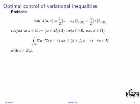
Optimal control of variational inequalitiesProblem
min J(u z) =1
2uminus ud2L2(Ω) +
λ
2z2L2(Ω)
subject to u isin K = w isin H10 (Ω) w(x) ge 0 ae x isin Ωint
Ω
nablau middot nabla(uminus v) dx le (z + f uminus v) forallv isin K
with z isin Zad
Regularized problem
min J(u z) =1
2uminus ud2L2(Ω) +
λ
2z2L2(Ω)
subject to (semilinear PDE)
u isin H10 (Ω) minus∆u+ γρε(minusu) = z + f in Ω
and z isin Zad γ gt 0 and ε gt 0 are the penealization and regularizationparameters respectively
H Antil 060616 12
Outline
Motivation and examples
Linear elliptic optimal control problems
Differentiation in Banach spaces
First-order necessary conditions
Optimal control of semilinear PDEs
An abstract problem
Discretization using finite element methods
H Antil 060616 13
Linear elliptic problemsΩ sub Rn bounded Lipschitz domain
Sobolev spacesI Lp(Ω) 1 le p le infin are Lebesgue spaces p = 2 L2(Ω) is a Hilbert
space with inner product (u v) =int
Ωu(x)v(x) dx
I W sp for s isin R 1 le p le infin are Sobolev spaces When p = 2W s2(Ω) = Hs(Ω) is a Hilbert space
I H10 (Ω) = v isin H1(Ω) v|partΩ = 0 with norm (due to Poincare
inequality)uH1
0 (Ω) = nablauL2(Ω)
I H10 (Ω)lowast = Hminus1(Ω)
I Note L2(Ω) sub Hminus1(Ω)
Model problem
minusdiv (Anablau) = f in Ω
u = 0 on partΩ
H Antil 060616 14
Linear elliptic problemsΩ sub Rn bounded Lipschitz domain
Sobolev spacesI Lp(Ω) 1 le p le infin are Lebesgue spaces p = 2 L2(Ω) is a Hilbert
space with inner product (u v) =int
Ωu(x)v(x) dx
I W sp for s isin R 1 le p le infin are Sobolev spaces When p = 2W s2(Ω) = Hs(Ω) is a Hilbert space
I H10 (Ω) = v isin H1(Ω) v|partΩ = 0 with norm (due to Poincare
inequality)uH1
0 (Ω) = nablauL2(Ω)
I H10 (Ω)lowast = Hminus1(Ω)
I Note L2(Ω) sub Hminus1(Ω)
Model problem
minusdiv (Anablau) = f in Ω
u = 0 on partΩ
H Antil 060616 14
Linear elliptic problemsΩ sub Rn bounded Lipschitz domain
Sobolev spacesI Lp(Ω) 1 le p le infin are Lebesgue spaces p = 2 L2(Ω) is a Hilbert
space with inner product (u v) =int
Ωu(x)v(x) dx
I W sp for s isin R 1 le p le infin are Sobolev spaces When p = 2W s2(Ω) = Hs(Ω) is a Hilbert space
I H10 (Ω) = v isin H1(Ω) v|partΩ = 0 with norm (due to Poincare
inequality)uH1
0 (Ω) = nablauL2(Ω)
I H10 (Ω)lowast = Hminus1(Ω)
I Note L2(Ω) sub Hminus1(Ω)
Model problem
minusdiv (Anablau) = f in Ω
u = 0 on partΩ
H Antil 060616 14
Linear elliptic problemsΩ sub Rn bounded Lipschitz domain
Sobolev spacesI Lp(Ω) 1 le p le infin are Lebesgue spaces p = 2 L2(Ω) is a Hilbert
space with inner product (u v) =int
Ωu(x)v(x) dx
I W sp for s isin R 1 le p le infin are Sobolev spaces When p = 2W s2(Ω) = Hs(Ω) is a Hilbert space
I H10 (Ω) = v isin H1(Ω) v|partΩ = 0 with norm (due to Poincare
inequality)uH1
0 (Ω) = nablauL2(Ω)
I H10 (Ω)lowast = Hminus1(Ω)
I Note L2(Ω) sub Hminus1(Ω)
Model problem
minusdiv (Anablau) = f in Ω
u = 0 on partΩ
H Antil 060616 14
Linear elliptic problemsΩ sub Rn bounded Lipschitz domain
Sobolev spacesI Lp(Ω) 1 le p le infin are Lebesgue spaces p = 2 L2(Ω) is a Hilbert
space with inner product (u v) =int
Ωu(x)v(x) dx
I W sp for s isin R 1 le p le infin are Sobolev spaces When p = 2W s2(Ω) = Hs(Ω) is a Hilbert space
I H10 (Ω) = v isin H1(Ω) v|partΩ = 0 with norm (due to Poincare
inequality)uH1
0 (Ω) = nablauL2(Ω)
I H10 (Ω)lowast = Hminus1(Ω)
I Note L2(Ω) sub Hminus1(Ω)
Model problem
minusdiv (Anablau) = f in Ω
u = 0 on partΩ
H Antil 060616 14
Well-posed
I Weak solution Given f isin Hminus1(Ω) a function u isin H10 (Ω) is called
a weak solution iffintΩ
Anablau middot nablav = 〈f v〉minus11 forallv isin H10 (Ω)
where 〈middot middot〉minus11 denotes the Hminus1(Ω)ndashH1(Ω) duality pairing
I Existence and uniqueness For each f isin Hminus1(Ω) there exists aunique u isin H1
0 (Ω) such that
nablauL2(Ω) le CdΩfHminus1(Ω)
I A = I the result is due to the Riesz-representation theorem
I A 6= I (maybe non-symmetric) the result is due to Lax-Milgramlemma
I For general W 1p-spaces use inf-sup conditions combined withBanach-Necas theorem which is a necessary and sufficient condition
H Antil 060616 15
Well-posed
I Weak solution Given f isin Hminus1(Ω) a function u isin H10 (Ω) is called
a weak solution iffintΩ
Anablau middot nablav = 〈f v〉minus11 forallv isin H10 (Ω)
where 〈middot middot〉minus11 denotes the Hminus1(Ω)ndashH1(Ω) duality pairing
I Existence and uniqueness For each f isin Hminus1(Ω) there exists aunique u isin H1
0 (Ω) such that
nablauL2(Ω) le CdΩfHminus1(Ω)
I A = I the result is due to the Riesz-representation theorem
I A 6= I (maybe non-symmetric) the result is due to Lax-Milgramlemma
I For general W 1p-spaces use inf-sup conditions combined withBanach-Necas theorem which is a necessary and sufficient condition
H Antil 060616 15
Linear-quadratic elliptic OCP
min J(u z) =1
2uminus ud2L2(Ω) +
λ
2z2L2(Ω)
subject to
minusdiv (Anablau) = z in Ω
u = 0 on partΩ
and the pointwise control constraints
z isin Zad = v isin L2(Ω) za(x) le v(x) le zb(x) ae x isin Ω
λ gt 0 is a parameter za zb isin Linfin(Ω) with za lt zb are given A isbounded symmetric positive
H Antil 060616 16
Reduced OCP
I Control to state map The solution operator defined as
S Hminus1(Ω)rarr H10 (Ω) z 7rarr u(z) = Sz
Note In view of the embedding
H10 (Ω) rarr L2(Ω) rarr Hminus1(Ω)
we may also consider S from L2(Ω) to L2(Ω) We will use the samenotation for this operator (for simplicity)
I Reduced cost functional The reduced cost functionalJ L2(Ω)rarr R is defined as
J (z) = J(Sz z)
I Reduced problem minzisinZadJ (z)
H Antil 060616 17
Reduced OCP
I Control to state map The solution operator defined as
S Hminus1(Ω)rarr H10 (Ω) z 7rarr u(z) = Sz
Note In view of the embedding
H10 (Ω) rarr L2(Ω) rarr Hminus1(Ω)
we may also consider S from L2(Ω) to L2(Ω) We will use the samenotation for this operator (for simplicity)
I Reduced cost functional The reduced cost functionalJ L2(Ω)rarr R is defined as
J (z) = J(Sz z)
I Reduced problem minzisinZadJ (z)
H Antil 060616 17
Reduced OCP
I Control to state map The solution operator defined as
S Hminus1(Ω)rarr H10 (Ω) z 7rarr u(z) = Sz
Note In view of the embedding
H10 (Ω) rarr L2(Ω) rarr Hminus1(Ω)
we may also consider S from L2(Ω) to L2(Ω) We will use the samenotation for this operator (for simplicity)
I Reduced cost functional The reduced cost functionalJ L2(Ω)rarr R is defined as
J (z) = J(Sz z)
I Reduced problem minzisinZadJ (z)
H Antil 060616 17
Existence of solution Direct methodThere exists a unique solution to the above problem
I Minimizing sequence J is bounded below by zero therefore thereexists a minimizing sequence znnisinN such that
limnrarrinfin
J (zn) = inf J (z)
I Weak compactness zn sub L2(Ω) is bounded Since L2(Ω) isreflexive therefore there exists a subsequence (not relabeled) suchthat
zn z and z isin Zad
where the latter is a consequence of Zad being closed and convex
I Optimality Since J is continuous and convex and therefore isweakly lower semicontinuous We obtain
lim inf J (zn) ge J (z)
which implies that z is optimal
I Uniqueness Exercise
H Antil 060616 18
Existence of solution Direct methodThere exists a unique solution to the above problem
I Minimizing sequence J is bounded below by zero therefore thereexists a minimizing sequence znnisinN such that
limnrarrinfin
J (zn) = inf J (z)
I Weak compactness zn sub L2(Ω) is bounded Since L2(Ω) isreflexive therefore there exists a subsequence (not relabeled) suchthat
zn z and z isin Zad
where the latter is a consequence of Zad being closed and convex
I Optimality Since J is continuous and convex and therefore isweakly lower semicontinuous We obtain
lim inf J (zn) ge J (z)
which implies that z is optimal
I Uniqueness Exercise
H Antil 060616 18
Existence of solution Direct methodThere exists a unique solution to the above problem
I Minimizing sequence J is bounded below by zero therefore thereexists a minimizing sequence znnisinN such that
limnrarrinfin
J (zn) = inf J (z)
I Weak compactness zn sub L2(Ω) is bounded Since L2(Ω) isreflexive therefore there exists a subsequence (not relabeled) suchthat
zn z and z isin Zad
where the latter is a consequence of Zad being closed and convex
I Optimality Since J is continuous and convex and therefore isweakly lower semicontinuous We obtain
lim inf J (zn) ge J (z)
which implies that z is optimal
I Uniqueness Exercise
H Antil 060616 18
Existence of solution Direct methodThere exists a unique solution to the above problem
I Minimizing sequence J is bounded below by zero therefore thereexists a minimizing sequence znnisinN such that
limnrarrinfin
J (zn) = inf J (z)
I Weak compactness zn sub L2(Ω) is bounded Since L2(Ω) isreflexive therefore there exists a subsequence (not relabeled) suchthat
zn z and z isin Zad
where the latter is a consequence of Zad being closed and convex
I Optimality Since J is continuous and convex and therefore isweakly lower semicontinuous We obtain
lim inf J (zn) ge J (z)
which implies that z is optimal
I Uniqueness Exercise
H Antil 060616 18
Outline
Motivation and examples
Linear elliptic optimal control problems
Differentiation in Banach spaces
First-order necessary conditions
Optimal control of semilinear PDEs
An abstract problem
Discretization using finite element methods
H Antil 060616 19
Differentiation in Banach spacesLet (Z middot Z) (V middot V ) B-spaces Z sub Z open and F Z rarr V
Let z isin Z
I If exist δF (z h) = limtdarr01t (F (z + th)minus F (z)) then δF (z h) is called
the directional derivative of F at z in direction h
I If exist δF (z h) forallh isin Z then h 7rarr δF (z h) is the first variation of Fat z
I Let exist the first variation δF (z middot) F is said to be Gateauxdifferentiable at z iff existA isin L(Z V ) such that δF (z h) = Ahforallh isin Z We write A = F primeG(z)
I F is said to be Frechet differentiable at z iff existA isin L(Z V ) and amapping r(z middot) Z rarr V such that for all h isin U with z + h isin Zwe have
F (z+h) = F (z)+Ah+r(z h) withr(z h)VhZ
rarr 0 as hZ rarr 0
We write F prime(z) = A
H Antil 060616 20
Differentiation in Banach spacesLet (Z middot Z) (V middot V ) B-spaces Z sub Z open and F Z rarr V
Let z isin Z
I If exist δF (z h) = limtdarr01t (F (z + th)minus F (z)) then δF (z h) is called
the directional derivative of F at z in direction h
I If exist δF (z h) forallh isin Z then h 7rarr δF (z h) is the first variation of Fat z
I Let exist the first variation δF (z middot) F is said to be Gateauxdifferentiable at z iff existA isin L(Z V ) such that δF (z h) = Ahforallh isin Z We write A = F primeG(z)
I F is said to be Frechet differentiable at z iff existA isin L(Z V ) and amapping r(z middot) Z rarr V such that for all h isin U with z + h isin Zwe have
F (z+h) = F (z)+Ah+r(z h) withr(z h)VhZ
rarr 0 as hZ rarr 0
We write F prime(z) = A
H Antil 060616 20
Differentiation in Banach spacesLet (Z middot Z) (V middot V ) B-spaces Z sub Z open and F Z rarr V
Let z isin Z
I If exist δF (z h) = limtdarr01t (F (z + th)minus F (z)) then δF (z h) is called
the directional derivative of F at z in direction h
I If exist δF (z h) forallh isin Z then h 7rarr δF (z h) is the first variation of Fat z
I Let exist the first variation δF (z middot) F is said to be Gateauxdifferentiable at z iff existA isin L(Z V ) such that δF (z h) = Ahforallh isin Z We write A = F primeG(z)
I F is said to be Frechet differentiable at z iff existA isin L(Z V ) and amapping r(z middot) Z rarr V such that for all h isin U with z + h isin Zwe have
F (z+h) = F (z)+Ah+r(z h) withr(z h)VhZ
rarr 0 as hZ rarr 0
We write F prime(z) = A
H Antil 060616 20
Differentiation in Banach spacesLet (Z middot Z) (V middot V ) B-spaces Z sub Z open and F Z rarr V
Let z isin Z
I If exist δF (z h) = limtdarr01t (F (z + th)minus F (z)) then δF (z h) is called
the directional derivative of F at z in direction h
I If exist δF (z h) forallh isin Z then h 7rarr δF (z h) is the first variation of Fat z
I Let exist the first variation δF (z middot) F is said to be Gateauxdifferentiable at z iff existA isin L(Z V ) such that δF (z h) = Ahforallh isin Z We write A = F primeG(z)
I F is said to be Frechet differentiable at z iff existA isin L(Z V ) and amapping r(z middot) Z rarr V such that for all h isin U with z + h isin Zwe have
F (z+h) = F (z)+Ah+r(z h) withr(z h)VhZ
rarr 0 as hZ rarr 0
We write F prime(z) = A
H Antil 060616 20
ExamplesExample 1 (H (middot middot)H) Hilbert space F (z) = z2H = (z z)H
forallz h F (z + h)minus F (z) = 2(z h)H + h2HThen
F prime(z)h = (2z h)H
Reisz representation theorem (identify H with Hlowast) we can write
F prime(z)h = (nablaF (z) h)H
where nablaF (z) = 2z is the gradient
Example 2 Let (Z (middot middot)Z) (H (middot middot)H) Hilbert spaces ud isin H fixedLet S isin L(ZH) Consider E Z rarr R
E(z) = Sz minus ud2H
Then E(z) = G(F (z)) where G(v) = v2H and F (z) = Sz minus ud
Eprime(z)h = Gprime(F (z))F prime(z)h = (2v F prime(z)h)H
= 2(Sz minus ud Sh)H = 2(Slowast(Sz minus ud) h)Z
we denote the gradient as nablaE(z) = 2Slowast(Sz minus ud)
H Antil 060616 21
ExamplesExample 1 (H (middot middot)H) Hilbert space F (z) = z2H = (z z)H
forallz h F (z + h)minus F (z) = 2(z h)H + h2HThen
F prime(z)h = (2z h)H
Reisz representation theorem (identify H with Hlowast) we can write
F prime(z)h = (nablaF (z) h)H
where nablaF (z) = 2z is the gradient
Example 2 Let (Z (middot middot)Z) (H (middot middot)H) Hilbert spaces ud isin H fixedLet S isin L(ZH) Consider E Z rarr R
E(z) = Sz minus ud2H
Then E(z) = G(F (z)) where G(v) = v2H and F (z) = Sz minus ud
Eprime(z)h = Gprime(F (z))F prime(z)h = (2v F prime(z)h)H
= 2(Sz minus ud Sh)H = 2(Slowast(Sz minus ud) h)Z
we denote the gradient as nablaE(z) = 2Slowast(Sz minus ud)H Antil 060616 21
Outline
Motivation and examples
Linear elliptic optimal control problems
Differentiation in Banach spaces
First-order necessary conditions
Optimal control of semilinear PDEs
An abstract problem
Discretization using finite element methods
H Antil 060616 22
First order necessary optimality conditions
Most of the theory is based on these two simple results
Theorem Let (Z middot Z) be a normed space J Z rarr (infin+infin] amapping with J 6equiv +infin Then z isin Z minimizer of J hArr 0 isin partJ (z)
Proof 0 isin partJ (z) means by definition of partJ (z) J (z)minus J (z) le 0forallz isin Z
Theorem Let (Z middot Z) be a normed space Zad sub Z nonemptyconvex closed J Z rarr R Gateaux differentiable where Zad sub Z sub ZZ open If z isin Zad is a solution to
minzisinZad
J (z)
then z solvesJ prime(z)(z minus z) ge 0 forallz isin Zad
Proof Exercise
H Antil 060616 23
First order necessary optimality conditions
Most of the theory is based on these two simple results
Theorem Let (Z middot Z) be a normed space J Z rarr (infin+infin] amapping with J 6equiv +infin Then z isin Z minimizer of J hArr 0 isin partJ (z)
Proof 0 isin partJ (z) means by definition of partJ (z) J (z)minus J (z) le 0forallz isin Z
Theorem Let (Z middot Z) be a normed space Zad sub Z nonemptyconvex closed J Z rarr R Gateaux differentiable where Zad sub Z sub ZZ open If z isin Zad is a solution to
minzisinZad
J (z)
then z solvesJ prime(z)(z minus z) ge 0 forallz isin Zad
Proof Exercise
H Antil 060616 23
Linear quadratic OCPI Reduced funcational
J (z) =1
2Sz minus ud2L2(Ω) +
λ
2z2L2(Ω)
I Gradient computation using sensitivity
J prime(z)h = (Slowast(Sz minus ud) + λz h)L2(Ω) forallh isin L2(Ω)
we denote the gradient by
nablaJ (z) = Slowast(Sz minus ud) + λz
I First order necessary and sufficient optimality condition
(nablaJ (z) z minus z)L2(Ω) ge 0 forallz isin Zad
I Adjoint equation Let p = Slowast(Sz minus ud) which translates intop isin H1
0 (Ω) solving
minusdiv (Anablap) = uminus ud in Ω
p = 0 on partΩ
I Gradient computation using adjoint nablaJ (z) = p+ λz
H Antil 060616 24
Linear quadratic OCPI Reduced funcational
J (z) =1
2Sz minus ud2L2(Ω) +
λ
2z2L2(Ω)
I Gradient computation using sensitivity
J prime(z)h = (Slowast(Sz minus ud) + λz h)L2(Ω) forallh isin L2(Ω)
we denote the gradient by
nablaJ (z) = Slowast(Sz minus ud) + λz
I First order necessary and sufficient optimality condition
(nablaJ (z) z minus z)L2(Ω) ge 0 forallz isin Zad
I Adjoint equation Let p = Slowast(Sz minus ud) which translates intop isin H1
0 (Ω) solving
minusdiv (Anablap) = uminus ud in Ω
p = 0 on partΩ
I Gradient computation using adjoint nablaJ (z) = p+ λz
H Antil 060616 24
Linear quadratic OCPI Reduced funcational
J (z) =1
2Sz minus ud2L2(Ω) +
λ
2z2L2(Ω)
I Gradient computation using sensitivity
J prime(z)h = (Slowast(Sz minus ud) + λz h)L2(Ω) forallh isin L2(Ω)
we denote the gradient by
nablaJ (z) = Slowast(Sz minus ud) + λz
I First order necessary and sufficient optimality condition
(nablaJ (z) z minus z)L2(Ω) ge 0 forallz isin Zad
I Adjoint equation Let p = Slowast(Sz minus ud) which translates intop isin H1
0 (Ω) solving
minusdiv (Anablap) = uminus ud in Ω
p = 0 on partΩ
I Gradient computation using adjoint nablaJ (z) = p+ λz
H Antil 060616 24
Linear quadratic OCPI Reduced funcational
J (z) =1
2Sz minus ud2L2(Ω) +
λ
2z2L2(Ω)
I Gradient computation using sensitivity
J prime(z)h = (Slowast(Sz minus ud) + λz h)L2(Ω) forallh isin L2(Ω)
we denote the gradient by
nablaJ (z) = Slowast(Sz minus ud) + λz
I First order necessary and sufficient optimality condition
(nablaJ (z) z minus z)L2(Ω) ge 0 forallz isin Zad
I Adjoint equation Let p = Slowast(Sz minus ud) which translates intop isin H1
0 (Ω) solving
minusdiv (Anablap) = uminus ud in Ω
p = 0 on partΩ
I Gradient computation using adjoint nablaJ (z) = p+ λz
H Antil 060616 24
Linear quadratic OCPI Reduced funcational
J (z) =1
2Sz minus ud2L2(Ω) +
λ
2z2L2(Ω)
I Gradient computation using sensitivity
J prime(z)h = (Slowast(Sz minus ud) + λz h)L2(Ω) forallh isin L2(Ω)
we denote the gradient by
nablaJ (z) = Slowast(Sz minus ud) + λz
I First order necessary and sufficient optimality condition
(nablaJ (z) z minus z)L2(Ω) ge 0 forallz isin Zad
I Adjoint equation Let p = Slowast(Sz minus ud) which translates intop isin H1
0 (Ω) solving
minusdiv (Anablap) = uminus ud in Ω
p = 0 on partΩ
I Gradient computation using adjoint nablaJ (z) = p+ λz
H Antil 060616 24
Optimality system
I State u isin H10 (Ω)
intΩAnablau middot nablav =
intΩzv forallv isin H1
0 (Ω)
I Adjoint p isin H10 (Ω)
intΩAnablap middot nablav =
intΩ
(uminus ud)v forallv isin H10 (Ω)
I Control z isin Zad (p+ λz z minus z) ge 0 forallz isin Zad
H Antil 060616 25
Pointwise interpretation
The variational inequality
(p+ λz z minus z) ge 0 forallz isin Zad
is equivalent to for ae x isin Ω
z(x) =
za(x) if p(x) + λz(x) gt 0isin [za(x) zb(x)] if p(x) + λz(x) = 0zb(x) if p(x) + λz(x) lt 0
Consequence
I When λ gt 0 then ae in Ω
z(x) = P[za(x)zb(x)]
minus 1
λp(x)
= min
zb(x)max
za(x)minus 1
λp(x)
H Antil 060616 26
Formal Lagrange method applied to linear OCPIntroduce L H1
0 (Ω)times Zad timesH1(Ω)rarr R defined as
L(u z p) = J(u z)minusint
Ω
(minusdiv (Anablau)minus z
)p dx
Integrate by parts to arrive at
L(u z p) = J(u z)minusint
Ω
(minusdiv (Anablap)uminus zp
)dx+
intpartΩ
(Anablau)p ds
If (u z p) is a stationary point then
I State
DpL(u z p)h = 0 forallh isin H1(Ω)
I AdjointDuL(u z p)h = 0 forallh isin H1
0 (Ω)
I ControlDzL(u z p)(z minus z) ge 0 forallz isin Zad
H Antil 060616 27
Formal Lagrange method applied to linear OCPIntroduce L H1
0 (Ω)times Zad timesH1(Ω)rarr R defined as
L(u z p) = J(u z)minusint
Ω
(minusdiv (Anablau)minus z
)p dx
Integrate by parts to arrive at
L(u z p) = J(u z)minusint
Ω
(minusdiv (Anablap)uminus zp
)dx+
intpartΩ
(Anablau)p ds
If (u z p) is a stationary point then
I State
DpL(u z p)h = 0 forallh isin H1(Ω)
I AdjointDuL(u z p)h = 0 forallh isin H1
0 (Ω)
I ControlDzL(u z p)(z minus z) ge 0 forallz isin Zad
H Antil 060616 27
Formal Lagrange method applied to linear OCPIntroduce L H1
0 (Ω)times Zad timesH1(Ω)rarr R defined as
L(u z p) = J(u z)minusint
Ω
(minusdiv (Anablau)minus z
)p dx
Integrate by parts to arrive at
L(u z p) = J(u z)minusint
Ω
(minusdiv (Anablap)uminus zp
)dx+
intpartΩ
(Anablau)p ds
If (u z p) is a stationary point then
I State
DpL(u z p)h = 0 forallh isin H1(Ω)
I AdjointDuL(u z p)h = 0 forallh isin H1
0 (Ω)
I ControlDzL(u z p)(z minus z) ge 0 forallz isin Zad
H Antil 060616 27
Formal Lagrange method applied to linear OCPIntroduce L H1
0 (Ω)times Zad timesH1(Ω)rarr R defined as
L(u z p) = J(u z)minusint
Ω
(minusdiv (Anablau)minus z
)p dx
Integrate by parts to arrive at
L(u z p) = J(u z)minusint
Ω
(minusdiv (Anablap)uminus zp
)dx+
intpartΩ
(Anablau)p ds
If (u z p) is a stationary point then
I State
DpL(u z p)h = 0 forallh isin H1(Ω)
I AdjointDuL(u z p)h = 0 forallh isin H1
0 (Ω)
I ControlDzL(u z p)(z minus z) ge 0 forallz isin Zad
H Antil 060616 27
Formal Lagrange method applied to linear OCPIntroduce L H1
0 (Ω)times Zad timesH1(Ω)rarr R defined as
L(u z p) = J(u z)minusint
Ω
(minusdiv (Anablau)minus z
)p dx
Integrate by parts to arrive at
L(u z p) = J(u z)minusint
Ω
(minusdiv (Anablap)uminus zp
)dx+
intpartΩ
(Anablau)p ds
If (u z p) is a stationary point then
I State
DpL(u z p)h = 0 forallh isin H1(Ω)
I AdjointDuL(u z p)h = 0 forallh isin H1
0 (Ω)
I ControlDzL(u z p)(z minus z) ge 0 forallz isin Zad
H Antil 060616 27
Outline
Motivation and examples
Linear elliptic optimal control problems
Differentiation in Banach spaces
First-order necessary conditions
Optimal control of semilinear PDEs
An abstract problem
Discretization using finite element methods
H Antil 060616 28
Semilinear elliptic OCP
min J(u z) =1
2uminus ud2L2(Ω) +
λ
2z2L2(Ω)
subject to
minus∆u+ g(x u) = z in Ω
u = 0 on partΩ
and z isin Zad with za zb isin Linfin(Ω)
H Antil 060616 29
State space(A1) Ω sub Rd open bounded partΩ is Lipschitz
(A2) g Ωtimes Rrarr R is bounded and measurable with respect to x isin Ωfor every u isin R
(A3) g is continuous monotone increasing and Lipschitz continuous in ufor ae x isin Ω
(A4) g(x 0) = 0 for ae x isin Ω (not really necessary)
Theorem Suppose (A1)minus (A4) hold For every z isin Lr(Ω) withr gt d2 the state equation has a unique weak solutionu isin H1
0 (Ω) cap C(Ω) ie we haveintΩ
nablau middot nablav dx+
intΩ
g(x u(x))v(x) dx =
intΩ
zv dx forallv isin H10 (Ω)
Moreover there exists a constant C gt 0 such that
uH1(Ω) + uC(Ω) le CzLr(Ω)
RemarkI The proof of the theorem uses the BrowderndashMinty theorem on
monotone operators
H Antil 060616 30
State space(A1) Ω sub Rd open bounded partΩ is Lipschitz
(A2) g Ωtimes Rrarr R is bounded and measurable with respect to x isin Ωfor every u isin R
(A3) g is continuous monotone increasing and Lipschitz continuous in ufor ae x isin Ω
(A4) g(x 0) = 0 for ae x isin Ω (not really necessary)
Theorem Suppose (A1)minus (A4) hold For every z isin Lr(Ω) withr gt d2 the state equation has a unique weak solutionu isin H1
0 (Ω) cap C(Ω) ie we haveintΩ
nablau middot nablav dx+
intΩ
g(x u(x))v(x) dx =
intΩ
zv dx forallv isin H10 (Ω)
Moreover there exists a constant C gt 0 such that
uH1(Ω) + uC(Ω) le CzLr(Ω)
RemarkI The proof of the theorem uses the BrowderndashMinty theorem on
monotone operators
H Antil 060616 30
State space(A1) Ω sub Rd open bounded partΩ is Lipschitz
(A2) g Ωtimes Rrarr R is bounded and measurable with respect to x isin Ωfor every u isin R
(A3) g is continuous monotone increasing and Lipschitz continuous in ufor ae x isin Ω
(A4) g(x 0) = 0 for ae x isin Ω (not really necessary)
Theorem Suppose (A1)minus (A4) hold For every z isin Lr(Ω) withr gt d2 the state equation has a unique weak solutionu isin H1
0 (Ω) cap C(Ω) ie we haveintΩ
nablau middot nablav dx+
intΩ
g(x u(x))v(x) dx =
intΩ
zv dx forallv isin H10 (Ω)
Moreover there exists a constant C gt 0 such that
uH1(Ω) + uC(Ω) le CzLr(Ω)
RemarkI The proof of the theorem uses the BrowderndashMinty theorem on
monotone operators
H Antil 060616 30
Control-to-state map and reduced problem
I Control to state map
S Linfin(Ω)rarr H10 (Ω) cap C(Ω)
is well defined and is globally Lipschitz continuous
I Reduced problem
minJ (z) =1
2S(u)minus ud2L2(Ω) +
λ
2z2L2(Ω)
H Antil 060616 31
Control-to-state map and reduced problem
I Control to state map
S Linfin(Ω)rarr H10 (Ω) cap C(Ω)
is well defined and is globally Lipschitz continuous
I Reduced problem
minJ (z) =1
2S(u)minus ud2L2(Ω) +
λ
2z2L2(Ω)
H Antil 060616 31
First-order necessary conditionsI Lagrangian functional
L(u z p) = J(u z)minusint
Ω
(minus∆u+ g(x u(x))minus z
)p dx
= J(u z)minusint
Ω
(nablau middot nablap+ g(x u(x))pminus zp
)dx
I Adjoint system For all h isin H10 (Ω)
0 = DuL(u z p)h =
intΩ
(uminus ud)h dxminusint
Ω
(nablah middot nablap+ gu(x u(x))ph
)which yields
minus∆p+ gu(x u(x))p = uminus ud in Ω
p = 0 on partΩ
I Control
DzL(u z p)(z minus z) = (p+ λz z minus z) dx ge 0 forallz isin ZadI Gradient
nablaJ (z) = p+ λz
H Antil 060616 32
First-order necessary conditionsI Lagrangian functional
L(u z p) = J(u z)minusint
Ω
(minus∆u+ g(x u(x))minus z
)p dx
= J(u z)minusint
Ω
(nablau middot nablap+ g(x u(x))pminus zp
)dx
I Adjoint system For all h isin H10 (Ω)
0 = DuL(u z p)h =
intΩ
(uminus ud)h dxminusint
Ω
(nablah middot nablap+ gu(x u(x))ph
)which yields
minus∆p+ gu(x u(x))p = uminus ud in Ω
p = 0 on partΩ
I Control
DzL(u z p)(z minus z) = (p+ λz z minus z) dx ge 0 forallz isin ZadI Gradient
nablaJ (z) = p+ λz
H Antil 060616 32
First-order necessary conditionsI Lagrangian functional
L(u z p) = J(u z)minusint
Ω
(minus∆u+ g(x u(x))minus z
)p dx
= J(u z)minusint
Ω
(nablau middot nablap+ g(x u(x))pminus zp
)dx
I Adjoint system For all h isin H10 (Ω)
0 = DuL(u z p)h =
intΩ
(uminus ud)h dxminusint
Ω
(nablah middot nablap+ gu(x u(x))ph
)which yields
minus∆p+ gu(x u(x))p = uminus ud in Ω
p = 0 on partΩ
I Control
DzL(u z p)(z minus z) = (p+ λz z minus z) dx ge 0 forallz isin Zad
I GradientnablaJ (z) = p+ λz
H Antil 060616 32
First-order necessary conditionsI Lagrangian functional
L(u z p) = J(u z)minusint
Ω
(minus∆u+ g(x u(x))minus z
)p dx
= J(u z)minusint
Ω
(nablau middot nablap+ g(x u(x))pminus zp
)dx
I Adjoint system For all h isin H10 (Ω)
0 = DuL(u z p)h =
intΩ
(uminus ud)h dxminusint
Ω
(nablah middot nablap+ gu(x u(x))ph
)which yields
minus∆p+ gu(x u(x))p = uminus ud in Ω
p = 0 on partΩ
I Control
DzL(u z p)(z minus z) = (p+ λz z minus z) dx ge 0 forallz isin ZadI Gradient
nablaJ (z) = p+ λz
H Antil 060616 32
Differentiability of Nemytskii operator
The rigorous proof uses
Theorem In addition to (A1)-(A4) if
(A5) g is continuously differentiable with respect to u for ae x isin Ωand we have
(i) |gu(x 0)| le K for ae x isin Ω(ii) gu is locally Lipschitz with respect to u isin R
then the Nemytskii operator G u 7rarr g(middot u(middot)) is continuously Frechetdifferentiable from Linfin(Ω) into itself and
(Gprime(u)h)(x) = gu(x u(x))h(x) ae in Ω forallh isin Linfin(Ω)
Remark (A5) holds if g(x u) = g(u) and g isin C2(R)
H Antil 060616 33
Outline
Motivation and examples
Linear elliptic optimal control problems
Differentiation in Banach spaces
First-order necessary conditions
Optimal control of semilinear PDEs
An abstract problem
Discretization using finite element methods
H Antil 060616 34
Gradient computation via adjoint general formI Abstract problem
min J(u z)
subject toc(u z) = 0
and z isin Zad
I Directional derivative Let S be the control to state map(nonlinear in general)
z 7rarr S(z) = u(z)
Under the assumptions of ldquoimplicit function theoremrdquo
J prime(z)h = (nablauJ (u(z) z) Sprime(z)h) + (nablazJ (u(z) z) h)
I Sensitivity of u with respect to z Differentiating the stateequation
cu(S(z) z)Sprime(z)h = minuscz(S(z) z)h
leads toSprime(z)h = minuscu(S(z) z)minus1
(cz(S(z) z)h
)
provided cu(S(z) z)minus1 is well-defined
H Antil 060616 35
Gradient computation via adjoint general formI Abstract problem
min J(u z)
subject toc(u z) = 0
and z isin ZadI Directional derivative Let S be the control to state map
(nonlinear in general)
z 7rarr S(z) = u(z)
Under the assumptions of ldquoimplicit function theoremrdquo
J prime(z)h = (nablauJ (u(z) z) Sprime(z)h) + (nablazJ (u(z) z) h)
I Sensitivity of u with respect to z Differentiating the stateequation
cu(S(z) z)Sprime(z)h = minuscz(S(z) z)h
leads toSprime(z)h = minuscu(S(z) z)minus1
(cz(S(z) z)h
)
provided cu(S(z) z)minus1 is well-defined
H Antil 060616 35
Gradient computation via adjoint general formI Abstract problem
min J(u z)
subject toc(u z) = 0
and z isin ZadI Directional derivative Let S be the control to state map
(nonlinear in general)
z 7rarr S(z) = u(z)
Under the assumptions of ldquoimplicit function theoremrdquo
J prime(z)h = (nablauJ (u(z) z) Sprime(z)h) + (nablazJ (u(z) z) h)
I Sensitivity of u with respect to z Differentiating the stateequation
cu(S(z) z)Sprime(z)h = minuscz(S(z) z)h
leads toSprime(z)h = minuscu(S(z) z)minus1
(cz(S(z) z)h
)
provided cu(S(z) z)minus1 is well-defined
H Antil 060616 35
Adjoint equation and gradient general form
I Directional derivative
J prime(z)h = minus(nablauJ (u(z) z) cu(u(z) z)minus1cz(u(z) z)h
)+ (nablazJ (u(z) z) h)
I Gradient
nablaJ (z) = minuscz(u(z) z)lowast(cu(u(z) z)minuslowastnablauJ (u(z) z)
)+nablazJ (u(z) z)
I Introducing adjoint variable p solving
cu(u(z) z)lowastp = nablauJ (u(z) z)
we arrive at following form of gradient
nablaJ (z) = minuscz(u(z) z)lowastp+nablazJ (u(z) z)
which is tractable
H Antil 060616 36
Adjoint equation and gradient general form
I Directional derivative
J prime(z)h = minus(nablauJ (u(z) z) cu(u(z) z)minus1cz(u(z) z)h
)+ (nablazJ (u(z) z) h)
I Gradient
nablaJ (z) = minuscz(u(z) z)lowast(cu(u(z) z)minuslowastnablauJ (u(z) z)
)+nablazJ (u(z) z)
I Introducing adjoint variable p solving
cu(u(z) z)lowastp = nablauJ (u(z) z)
we arrive at following form of gradient
nablaJ (z) = minuscz(u(z) z)lowastp+nablazJ (u(z) z)
which is tractable
H Antil 060616 36
Adjoint equation and gradient general form
I Directional derivative
J prime(z)h = minus(nablauJ (u(z) z) cu(u(z) z)minus1cz(u(z) z)h
)+ (nablazJ (u(z) z) h)
I Gradient
nablaJ (z) = minuscz(u(z) z)lowast(cu(u(z) z)minuslowastnablauJ (u(z) z)
)+nablazJ (u(z) z)
I Introducing adjoint variable p solving
cu(u(z) z)lowastp = nablauJ (u(z) z)
we arrive at following form of gradient
nablaJ (z) = minuscz(u(z) z)lowastp+nablazJ (u(z) z)
which is tractable
H Antil 060616 36
Hessian computation general form
I Lagrangian L(u z p) = J(u z)minusint
Ωc(u z)p dx Then we have
DzJ (z)h = DzL(u z p)h
I Second order derivative
D2zJ (z)[h1 h2] = DuDzL(u z p)[h1 S
prime(z)h2] +D2zL(u z p)[h1 h2]
+DpDzL(u z p)[h1 Dzp(z)h2]
I We already know Sprime(z)h2 moreover
DpDzL(u z p)[h1 Dzp(z)h2] = minus(cu(u z)h1 Dzp(z)h2
)
It remain to identify Dzp(z)h2
H Antil 060616 37
Hessian computation general form
I Lagrangian L(u z p) = J(u z)minusint
Ωc(u z)p dx Then we have
DzJ (z)h = DzL(u z p)h
I Second order derivative
D2zJ (z)[h1 h2] = DuDzL(u z p)[h1 S
prime(z)h2] +D2zL(u z p)[h1 h2]
+DpDzL(u z p)[h1 Dzp(z)h2]
I We already know Sprime(z)h2 moreover
DpDzL(u z p)[h1 Dzp(z)h2] = minus(cu(u z)h1 Dzp(z)h2
)
It remain to identify Dzp(z)h2
H Antil 060616 37
Hessian computation general form
I Lagrangian L(u z p) = J(u z)minusint
Ωc(u z)p dx Then we have
DzJ (z)h = DzL(u z p)h
I Second order derivative
D2zJ (z)[h1 h2] = DuDzL(u z p)[h1 S
prime(z)h2] +D2zL(u z p)[h1 h2]
+DpDzL(u z p)[h1 Dzp(z)h2]
I We already know Sprime(z)h2 moreover
DpDzL(u z p)[h1 Dzp(z)h2] = minus(cu(u z)h1 Dzp(z)h2
)
It remain to identify Dzp(z)h2
H Antil 060616 37
Outline
Motivation and examples
Linear elliptic optimal control problems
Differentiation in Banach spaces
First-order necessary conditions
Optimal control of semilinear PDEs
An abstract problem
Discretization using finite element methods
H Antil 060616 38
Numerical approximation of Poisson equation MeshTo avoid technical issues we will assume that partΩ is polygonal
I Mesh Let T = K be a mesh of Ω where K sub Rd is an elementthat is isoparametrically equivalent to a unit simplex in Rd
I Conforming mesh We say that the mesh is conforming ifI Ω = cupKisinT KI If K1 cap K2 = x then x is a node of K1 and K2I If K1 cap K2 6= empty and K1 cap K2 6= x then K1 cap K2 is an edgeface
contained in partK1 cap partK2
I Shape regular Let T be the collection of all conformingrefinements of an original mesh T 0 Then T is called shape regularif exist κ gt 0 such that
hKρKle κ forallK isin cupiT i
where hK = diam K ρK = maxρ gt 0|Bρ sub KI Quasi-uniform A family of shape regular meshes is called-quasi
uniform if there exist a constant σ gt 0 such that
maxhKminhK
le σ
uniformly for all meshes in the family
Numerical approximation of Poisson equation MeshTo avoid technical issues we will assume that partΩ is polygonal
I Mesh Let T = K be a mesh of Ω where K sub Rd is an elementthat is isoparametrically equivalent to a unit simplex in Rd
I Conforming mesh We say that the mesh is conforming ifI Ω = cupKisinT KI If K1 cap K2 = x then x is a node of K1 and K2I If K1 cap K2 6= empty and K1 cap K2 6= x then K1 cap K2 is an edgeface
contained in partK1 cap partK2
I Shape regular Let T be the collection of all conformingrefinements of an original mesh T 0 Then T is called shape regularif exist κ gt 0 such that
hKρKle κ forallK isin cupiT i
where hK = diam K ρK = maxρ gt 0|Bρ sub KI Quasi-uniform A family of shape regular meshes is called-quasi
uniform if there exist a constant σ gt 0 such that
maxhKminhK
le σ
uniformly for all meshes in the family
Numerical approximation of Poisson equation MeshTo avoid technical issues we will assume that partΩ is polygonal
I Mesh Let T = K be a mesh of Ω where K sub Rd is an elementthat is isoparametrically equivalent to a unit simplex in Rd
I Conforming mesh We say that the mesh is conforming ifI Ω = cupKisinT KI If K1 cap K2 = x then x is a node of K1 and K2I If K1 cap K2 6= empty and K1 cap K2 6= x then K1 cap K2 is an edgeface
contained in partK1 cap partK2
I Shape regular Let T be the collection of all conformingrefinements of an original mesh T 0 Then T is called shape regularif exist κ gt 0 such that
hKρKle κ forallK isin cupiT i
where hK = diam K ρK = maxρ gt 0|Bρ sub K
I Quasi-uniform A family of shape regular meshes is called-quasiuniform if there exist a constant σ gt 0 such that
maxhKminhK
le σ
uniformly for all meshes in the family
Numerical approximation of Poisson equation MeshTo avoid technical issues we will assume that partΩ is polygonal
I Mesh Let T = K be a mesh of Ω where K sub Rd is an elementthat is isoparametrically equivalent to a unit simplex in Rd
I Conforming mesh We say that the mesh is conforming ifI Ω = cupKisinT KI If K1 cap K2 = x then x is a node of K1 and K2I If K1 cap K2 6= empty and K1 cap K2 6= x then K1 cap K2 is an edgeface
contained in partK1 cap partK2
I Shape regular Let T be the collection of all conformingrefinements of an original mesh T 0 Then T is called shape regularif exist κ gt 0 such that
hKρKle κ forallK isin cupiT i
where hK = diam K ρK = maxρ gt 0|Bρ sub KI Quasi-uniform A family of shape regular meshes is called-quasi
uniform if there exist a constant σ gt 0 such that
maxhKminhK
le σ
uniformly for all meshes in the family
FE space and Galerkin approximationI Finite element space For T isin T we define the finite element
space as
V(T ) = W isin C0(Ω) WK isin P1forallK isin T W |partΩ = 0
where P1 is the set of polynomials of degree at most 1
I Galerkin approximation of continuous problem is given by
Find UT isin V(T )
intΩ
AnablaUT middot nablaV = 〈f V 〉 forallV isin V(T )
The discrete problem is well-posedI Nodal basis Consists of functions ψi isin V(T ) with xi isin N (T )
satisfyingψxi
(xj) = δij
where N (T ) denotes the interior (plus Neumann) nodesI Galerkin orthogonality(
nabla(uminus UT )nablaW)L2(Ω)
= 0 forallW isin V(T )
H Antil 060616 40
FE space and Galerkin approximationI Finite element space For T isin T we define the finite element
space as
V(T ) = W isin C0(Ω) WK isin P1forallK isin T W |partΩ = 0
where P1 is the set of polynomials of degree at most 1I Galerkin approximation of continuous problem is given by
Find UT isin V(T )
intΩ
AnablaUT middot nablaV = 〈f V 〉 forallV isin V(T )
The discrete problem is well-posed
I Nodal basis Consists of functions ψi isin V(T ) with xi isin N (T )satisfying
ψxi(xj) = δij
where N (T ) denotes the interior (plus Neumann) nodesI Galerkin orthogonality(
nabla(uminus UT )nablaW)L2(Ω)
= 0 forallW isin V(T )
H Antil 060616 40
FE space and Galerkin approximationI Finite element space For T isin T we define the finite element
space as
V(T ) = W isin C0(Ω) WK isin P1forallK isin T W |partΩ = 0
where P1 is the set of polynomials of degree at most 1I Galerkin approximation of continuous problem is given by
Find UT isin V(T )
intΩ
AnablaUT middot nablaV = 〈f V 〉 forallV isin V(T )
The discrete problem is well-posedI Nodal basis Consists of functions ψi isin V(T ) with xi isin N (T )
satisfyingψxi
(xj) = δij
where N (T ) denotes the interior (plus Neumann) nodes
I Galerkin orthogonality(nabla(uminus UT )nablaW
)L2(Ω)
= 0 forallW isin V(T )
H Antil 060616 40
FE space and Galerkin approximationI Finite element space For T isin T we define the finite element
space as
V(T ) = W isin C0(Ω) WK isin P1forallK isin T W |partΩ = 0
where P1 is the set of polynomials of degree at most 1I Galerkin approximation of continuous problem is given by
Find UT isin V(T )
intΩ
AnablaUT middot nablaV = 〈f V 〉 forallV isin V(T )
The discrete problem is well-posedI Nodal basis Consists of functions ψi isin V(T ) with xi isin N (T )
satisfyingψxi
(xj) = δij
where N (T ) denotes the interior (plus Neumann) nodesI Galerkin orthogonality(
nabla(uminus UT )nablaW)L2(Ω)
= 0 forallW isin V(T )
H Antil 060616 40
Best approximation
I Cearsquos lemma
nabla(uminus UT )L2(Ω) le C infWisinV(T )
nabla(uminusW )L2(Ω)
I Nodal interpolation operator ΠT C(Ω)rarr V(T ) satisfies
ΠT u(xi) = u(xi) forallxi isin N (T )
and is defined as
ΠT u =sum
xiisinN (T )
u(xi)ψxi
I Error estimates In Cearsquos lemma replace W by ΠT u and thencompute the interpolation error
H Antil 060616 41
Best approximation
I Cearsquos lemma
nabla(uminus UT )L2(Ω) le C infWisinV(T )
nabla(uminusW )L2(Ω)
I Nodal interpolation operator ΠT C(Ω)rarr V(T ) satisfies
ΠT u(xi) = u(xi) forallxi isin N (T )
and is defined as
ΠT u =sum
xiisinN (T )
u(xi)ψxi
I Error estimates In Cearsquos lemma replace W by ΠT u and thencompute the interpolation error
H Antil 060616 41
Best approximation
I Cearsquos lemma
nabla(uminus UT )L2(Ω) le C infWisinV(T )
nabla(uminusW )L2(Ω)
I Nodal interpolation operator ΠT C(Ω)rarr V(T ) satisfies
ΠT u(xi) = u(xi) forallxi isin N (T )
and is defined as
ΠT u =sum
xiisinN (T )
u(xi)ψxi
I Error estimates In Cearsquos lemma replace W by ΠT u and thencompute the interpolation error
H Antil 060616 41
Algebraic system state equation
I Recall UT isin V(T ) solves
a(UT V ) = 〈f V 〉 forallV isin V(T )
I Now setting UT =sumN
j=1 Ujψj V = ψi we get
Nsumj=1
Uja(φj φi) = 〈f ψi〉 i = 1 N
which is the matrix-vector system
AU = F
I Stiffness matrix A is SPD
H Antil 060616 42
Algebraic system state equation
I Recall UT isin V(T ) solves
a(UT V ) = 〈f V 〉 forallV isin V(T )
I Now setting UT =sumN
j=1 Ujψj V = ψi we get
Nsumj=1
Uja(φj φi) = 〈f ψi〉 i = 1 N
which is the matrix-vector system
AU = F
I Stiffness matrix A is SPD
H Antil 060616 42
Algebraic system state equation
I Recall UT isin V(T ) solves
a(UT V ) = 〈f V 〉 forallV isin V(T )
I Now setting UT =sumN
j=1 Ujψj V = ψi we get
Nsumj=1
Uja(φj φi) = 〈f ψi〉 i = 1 N
which is the matrix-vector system
AU = F
I Stiffness matrix A is SPD
H Antil 060616 42
Discrete linear elliptic OCP
min JT (UT ZT ) =1
2UT minus ud2L2(Ω) +
λ
2ZT 2L2(Ω)
subject to
Find UT isin V(T )
intΩ
nablaUT middot nablaV = (ZT V )L2(Ω) forallV isin V(T )
and whereZT isin Zad(T ) = Zad cap Z(T )
is either one of these
Z(T ) =
V(T )L2(Ω) variational discretization (Hinze)WT isin Linfin(Ω) ZT |K isin P0(K)K isin T
H Antil 060616 43
Recent books
F TroltzschOptimal control of partial differential equations volume 112 ofGraduate Studies in MathematicsAmerican Mathematical Society Providence RI 2010Theory methods and applications Translated from the 2005 Germanoriginal by Jurgen Sprekels
K Ito and K KunischLagrange multiplier approach to variational problems andapplications volume 15 of Advances in Design and ControlSociety for Industrial and Applied Mathematics (SIAM)Philadelphia PA 2008
H Antil 060616 44
- Motivation and examples
- Linear elliptic optimal control problems
- Differentiation in Banach spaces
- First-order necessary conditions
- Optimal control of semilinear PDEs
- An abstract problem
- Discretization using finite element methods
-
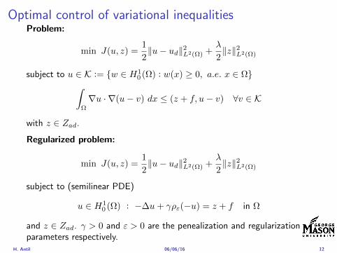
Optimal control of variational inequalitiesProblem
min J(u z) =1
2uminus ud2L2(Ω) +
λ
2z2L2(Ω)
subject to u isin K = w isin H10 (Ω) w(x) ge 0 ae x isin Ωint
Ω
nablau middot nabla(uminus v) dx le (z + f uminus v) forallv isin K
with z isin Zad
Regularized problem
min J(u z) =1
2uminus ud2L2(Ω) +
λ
2z2L2(Ω)
subject to (semilinear PDE)
u isin H10 (Ω) minus∆u+ γρε(minusu) = z + f in Ω
and z isin Zad γ gt 0 and ε gt 0 are the penealization and regularizationparameters respectively
H Antil 060616 12
Outline
Motivation and examples
Linear elliptic optimal control problems
Differentiation in Banach spaces
First-order necessary conditions
Optimal control of semilinear PDEs
An abstract problem
Discretization using finite element methods
H Antil 060616 13
Linear elliptic problemsΩ sub Rn bounded Lipschitz domain
Sobolev spacesI Lp(Ω) 1 le p le infin are Lebesgue spaces p = 2 L2(Ω) is a Hilbert
space with inner product (u v) =int
Ωu(x)v(x) dx
I W sp for s isin R 1 le p le infin are Sobolev spaces When p = 2W s2(Ω) = Hs(Ω) is a Hilbert space
I H10 (Ω) = v isin H1(Ω) v|partΩ = 0 with norm (due to Poincare
inequality)uH1
0 (Ω) = nablauL2(Ω)
I H10 (Ω)lowast = Hminus1(Ω)
I Note L2(Ω) sub Hminus1(Ω)
Model problem
minusdiv (Anablau) = f in Ω
u = 0 on partΩ
H Antil 060616 14
Linear elliptic problemsΩ sub Rn bounded Lipschitz domain
Sobolev spacesI Lp(Ω) 1 le p le infin are Lebesgue spaces p = 2 L2(Ω) is a Hilbert
space with inner product (u v) =int
Ωu(x)v(x) dx
I W sp for s isin R 1 le p le infin are Sobolev spaces When p = 2W s2(Ω) = Hs(Ω) is a Hilbert space
I H10 (Ω) = v isin H1(Ω) v|partΩ = 0 with norm (due to Poincare
inequality)uH1
0 (Ω) = nablauL2(Ω)
I H10 (Ω)lowast = Hminus1(Ω)
I Note L2(Ω) sub Hminus1(Ω)
Model problem
minusdiv (Anablau) = f in Ω
u = 0 on partΩ
H Antil 060616 14
Linear elliptic problemsΩ sub Rn bounded Lipschitz domain
Sobolev spacesI Lp(Ω) 1 le p le infin are Lebesgue spaces p = 2 L2(Ω) is a Hilbert
space with inner product (u v) =int
Ωu(x)v(x) dx
I W sp for s isin R 1 le p le infin are Sobolev spaces When p = 2W s2(Ω) = Hs(Ω) is a Hilbert space
I H10 (Ω) = v isin H1(Ω) v|partΩ = 0 with norm (due to Poincare
inequality)uH1
0 (Ω) = nablauL2(Ω)
I H10 (Ω)lowast = Hminus1(Ω)
I Note L2(Ω) sub Hminus1(Ω)
Model problem
minusdiv (Anablau) = f in Ω
u = 0 on partΩ
H Antil 060616 14
Linear elliptic problemsΩ sub Rn bounded Lipschitz domain
Sobolev spacesI Lp(Ω) 1 le p le infin are Lebesgue spaces p = 2 L2(Ω) is a Hilbert
space with inner product (u v) =int
Ωu(x)v(x) dx
I W sp for s isin R 1 le p le infin are Sobolev spaces When p = 2W s2(Ω) = Hs(Ω) is a Hilbert space
I H10 (Ω) = v isin H1(Ω) v|partΩ = 0 with norm (due to Poincare
inequality)uH1
0 (Ω) = nablauL2(Ω)
I H10 (Ω)lowast = Hminus1(Ω)
I Note L2(Ω) sub Hminus1(Ω)
Model problem
minusdiv (Anablau) = f in Ω
u = 0 on partΩ
H Antil 060616 14
Linear elliptic problemsΩ sub Rn bounded Lipschitz domain
Sobolev spacesI Lp(Ω) 1 le p le infin are Lebesgue spaces p = 2 L2(Ω) is a Hilbert
space with inner product (u v) =int
Ωu(x)v(x) dx
I W sp for s isin R 1 le p le infin are Sobolev spaces When p = 2W s2(Ω) = Hs(Ω) is a Hilbert space
I H10 (Ω) = v isin H1(Ω) v|partΩ = 0 with norm (due to Poincare
inequality)uH1
0 (Ω) = nablauL2(Ω)
I H10 (Ω)lowast = Hminus1(Ω)
I Note L2(Ω) sub Hminus1(Ω)
Model problem
minusdiv (Anablau) = f in Ω
u = 0 on partΩ
H Antil 060616 14
Well-posed
I Weak solution Given f isin Hminus1(Ω) a function u isin H10 (Ω) is called
a weak solution iffintΩ
Anablau middot nablav = 〈f v〉minus11 forallv isin H10 (Ω)
where 〈middot middot〉minus11 denotes the Hminus1(Ω)ndashH1(Ω) duality pairing
I Existence and uniqueness For each f isin Hminus1(Ω) there exists aunique u isin H1
0 (Ω) such that
nablauL2(Ω) le CdΩfHminus1(Ω)
I A = I the result is due to the Riesz-representation theorem
I A 6= I (maybe non-symmetric) the result is due to Lax-Milgramlemma
I For general W 1p-spaces use inf-sup conditions combined withBanach-Necas theorem which is a necessary and sufficient condition
H Antil 060616 15
Well-posed
I Weak solution Given f isin Hminus1(Ω) a function u isin H10 (Ω) is called
a weak solution iffintΩ
Anablau middot nablav = 〈f v〉minus11 forallv isin H10 (Ω)
where 〈middot middot〉minus11 denotes the Hminus1(Ω)ndashH1(Ω) duality pairing
I Existence and uniqueness For each f isin Hminus1(Ω) there exists aunique u isin H1
0 (Ω) such that
nablauL2(Ω) le CdΩfHminus1(Ω)
I A = I the result is due to the Riesz-representation theorem
I A 6= I (maybe non-symmetric) the result is due to Lax-Milgramlemma
I For general W 1p-spaces use inf-sup conditions combined withBanach-Necas theorem which is a necessary and sufficient condition
H Antil 060616 15
Linear-quadratic elliptic OCP
min J(u z) =1
2uminus ud2L2(Ω) +
λ
2z2L2(Ω)
subject to
minusdiv (Anablau) = z in Ω
u = 0 on partΩ
and the pointwise control constraints
z isin Zad = v isin L2(Ω) za(x) le v(x) le zb(x) ae x isin Ω
λ gt 0 is a parameter za zb isin Linfin(Ω) with za lt zb are given A isbounded symmetric positive
H Antil 060616 16
Reduced OCP
I Control to state map The solution operator defined as
S Hminus1(Ω)rarr H10 (Ω) z 7rarr u(z) = Sz
Note In view of the embedding
H10 (Ω) rarr L2(Ω) rarr Hminus1(Ω)
we may also consider S from L2(Ω) to L2(Ω) We will use the samenotation for this operator (for simplicity)
I Reduced cost functional The reduced cost functionalJ L2(Ω)rarr R is defined as
J (z) = J(Sz z)
I Reduced problem minzisinZadJ (z)
H Antil 060616 17
Reduced OCP
I Control to state map The solution operator defined as
S Hminus1(Ω)rarr H10 (Ω) z 7rarr u(z) = Sz
Note In view of the embedding
H10 (Ω) rarr L2(Ω) rarr Hminus1(Ω)
we may also consider S from L2(Ω) to L2(Ω) We will use the samenotation for this operator (for simplicity)
I Reduced cost functional The reduced cost functionalJ L2(Ω)rarr R is defined as
J (z) = J(Sz z)
I Reduced problem minzisinZadJ (z)
H Antil 060616 17
Reduced OCP
I Control to state map The solution operator defined as
S Hminus1(Ω)rarr H10 (Ω) z 7rarr u(z) = Sz
Note In view of the embedding
H10 (Ω) rarr L2(Ω) rarr Hminus1(Ω)
we may also consider S from L2(Ω) to L2(Ω) We will use the samenotation for this operator (for simplicity)
I Reduced cost functional The reduced cost functionalJ L2(Ω)rarr R is defined as
J (z) = J(Sz z)
I Reduced problem minzisinZadJ (z)
H Antil 060616 17
Existence of solution Direct methodThere exists a unique solution to the above problem
I Minimizing sequence J is bounded below by zero therefore thereexists a minimizing sequence znnisinN such that
limnrarrinfin
J (zn) = inf J (z)
I Weak compactness zn sub L2(Ω) is bounded Since L2(Ω) isreflexive therefore there exists a subsequence (not relabeled) suchthat
zn z and z isin Zad
where the latter is a consequence of Zad being closed and convex
I Optimality Since J is continuous and convex and therefore isweakly lower semicontinuous We obtain
lim inf J (zn) ge J (z)
which implies that z is optimal
I Uniqueness Exercise
H Antil 060616 18
Existence of solution Direct methodThere exists a unique solution to the above problem
I Minimizing sequence J is bounded below by zero therefore thereexists a minimizing sequence znnisinN such that
limnrarrinfin
J (zn) = inf J (z)
I Weak compactness zn sub L2(Ω) is bounded Since L2(Ω) isreflexive therefore there exists a subsequence (not relabeled) suchthat
zn z and z isin Zad
where the latter is a consequence of Zad being closed and convex
I Optimality Since J is continuous and convex and therefore isweakly lower semicontinuous We obtain
lim inf J (zn) ge J (z)
which implies that z is optimal
I Uniqueness Exercise
H Antil 060616 18
Existence of solution Direct methodThere exists a unique solution to the above problem
I Minimizing sequence J is bounded below by zero therefore thereexists a minimizing sequence znnisinN such that
limnrarrinfin
J (zn) = inf J (z)
I Weak compactness zn sub L2(Ω) is bounded Since L2(Ω) isreflexive therefore there exists a subsequence (not relabeled) suchthat
zn z and z isin Zad
where the latter is a consequence of Zad being closed and convex
I Optimality Since J is continuous and convex and therefore isweakly lower semicontinuous We obtain
lim inf J (zn) ge J (z)
which implies that z is optimal
I Uniqueness Exercise
H Antil 060616 18
Existence of solution Direct methodThere exists a unique solution to the above problem
I Minimizing sequence J is bounded below by zero therefore thereexists a minimizing sequence znnisinN such that
limnrarrinfin
J (zn) = inf J (z)
I Weak compactness zn sub L2(Ω) is bounded Since L2(Ω) isreflexive therefore there exists a subsequence (not relabeled) suchthat
zn z and z isin Zad
where the latter is a consequence of Zad being closed and convex
I Optimality Since J is continuous and convex and therefore isweakly lower semicontinuous We obtain
lim inf J (zn) ge J (z)
which implies that z is optimal
I Uniqueness Exercise
H Antil 060616 18
Outline
Motivation and examples
Linear elliptic optimal control problems
Differentiation in Banach spaces
First-order necessary conditions
Optimal control of semilinear PDEs
An abstract problem
Discretization using finite element methods
H Antil 060616 19
Differentiation in Banach spacesLet (Z middot Z) (V middot V ) B-spaces Z sub Z open and F Z rarr V
Let z isin Z
I If exist δF (z h) = limtdarr01t (F (z + th)minus F (z)) then δF (z h) is called
the directional derivative of F at z in direction h
I If exist δF (z h) forallh isin Z then h 7rarr δF (z h) is the first variation of Fat z
I Let exist the first variation δF (z middot) F is said to be Gateauxdifferentiable at z iff existA isin L(Z V ) such that δF (z h) = Ahforallh isin Z We write A = F primeG(z)
I F is said to be Frechet differentiable at z iff existA isin L(Z V ) and amapping r(z middot) Z rarr V such that for all h isin U with z + h isin Zwe have
F (z+h) = F (z)+Ah+r(z h) withr(z h)VhZ
rarr 0 as hZ rarr 0
We write F prime(z) = A
H Antil 060616 20
Differentiation in Banach spacesLet (Z middot Z) (V middot V ) B-spaces Z sub Z open and F Z rarr V
Let z isin Z
I If exist δF (z h) = limtdarr01t (F (z + th)minus F (z)) then δF (z h) is called
the directional derivative of F at z in direction h
I If exist δF (z h) forallh isin Z then h 7rarr δF (z h) is the first variation of Fat z
I Let exist the first variation δF (z middot) F is said to be Gateauxdifferentiable at z iff existA isin L(Z V ) such that δF (z h) = Ahforallh isin Z We write A = F primeG(z)
I F is said to be Frechet differentiable at z iff existA isin L(Z V ) and amapping r(z middot) Z rarr V such that for all h isin U with z + h isin Zwe have
F (z+h) = F (z)+Ah+r(z h) withr(z h)VhZ
rarr 0 as hZ rarr 0
We write F prime(z) = A
H Antil 060616 20
Differentiation in Banach spacesLet (Z middot Z) (V middot V ) B-spaces Z sub Z open and F Z rarr V
Let z isin Z
I If exist δF (z h) = limtdarr01t (F (z + th)minus F (z)) then δF (z h) is called
the directional derivative of F at z in direction h
I If exist δF (z h) forallh isin Z then h 7rarr δF (z h) is the first variation of Fat z
I Let exist the first variation δF (z middot) F is said to be Gateauxdifferentiable at z iff existA isin L(Z V ) such that δF (z h) = Ahforallh isin Z We write A = F primeG(z)
I F is said to be Frechet differentiable at z iff existA isin L(Z V ) and amapping r(z middot) Z rarr V such that for all h isin U with z + h isin Zwe have
F (z+h) = F (z)+Ah+r(z h) withr(z h)VhZ
rarr 0 as hZ rarr 0
We write F prime(z) = A
H Antil 060616 20
Differentiation in Banach spacesLet (Z middot Z) (V middot V ) B-spaces Z sub Z open and F Z rarr V
Let z isin Z
I If exist δF (z h) = limtdarr01t (F (z + th)minus F (z)) then δF (z h) is called
the directional derivative of F at z in direction h
I If exist δF (z h) forallh isin Z then h 7rarr δF (z h) is the first variation of Fat z
I Let exist the first variation δF (z middot) F is said to be Gateauxdifferentiable at z iff existA isin L(Z V ) such that δF (z h) = Ahforallh isin Z We write A = F primeG(z)
I F is said to be Frechet differentiable at z iff existA isin L(Z V ) and amapping r(z middot) Z rarr V such that for all h isin U with z + h isin Zwe have
F (z+h) = F (z)+Ah+r(z h) withr(z h)VhZ
rarr 0 as hZ rarr 0
We write F prime(z) = A
H Antil 060616 20
ExamplesExample 1 (H (middot middot)H) Hilbert space F (z) = z2H = (z z)H
forallz h F (z + h)minus F (z) = 2(z h)H + h2HThen
F prime(z)h = (2z h)H
Reisz representation theorem (identify H with Hlowast) we can write
F prime(z)h = (nablaF (z) h)H
where nablaF (z) = 2z is the gradient
Example 2 Let (Z (middot middot)Z) (H (middot middot)H) Hilbert spaces ud isin H fixedLet S isin L(ZH) Consider E Z rarr R
E(z) = Sz minus ud2H
Then E(z) = G(F (z)) where G(v) = v2H and F (z) = Sz minus ud
Eprime(z)h = Gprime(F (z))F prime(z)h = (2v F prime(z)h)H
= 2(Sz minus ud Sh)H = 2(Slowast(Sz minus ud) h)Z
we denote the gradient as nablaE(z) = 2Slowast(Sz minus ud)
H Antil 060616 21
ExamplesExample 1 (H (middot middot)H) Hilbert space F (z) = z2H = (z z)H
forallz h F (z + h)minus F (z) = 2(z h)H + h2HThen
F prime(z)h = (2z h)H
Reisz representation theorem (identify H with Hlowast) we can write
F prime(z)h = (nablaF (z) h)H
where nablaF (z) = 2z is the gradient
Example 2 Let (Z (middot middot)Z) (H (middot middot)H) Hilbert spaces ud isin H fixedLet S isin L(ZH) Consider E Z rarr R
E(z) = Sz minus ud2H
Then E(z) = G(F (z)) where G(v) = v2H and F (z) = Sz minus ud
Eprime(z)h = Gprime(F (z))F prime(z)h = (2v F prime(z)h)H
= 2(Sz minus ud Sh)H = 2(Slowast(Sz minus ud) h)Z
we denote the gradient as nablaE(z) = 2Slowast(Sz minus ud)H Antil 060616 21
Outline
Motivation and examples
Linear elliptic optimal control problems
Differentiation in Banach spaces
First-order necessary conditions
Optimal control of semilinear PDEs
An abstract problem
Discretization using finite element methods
H Antil 060616 22
First order necessary optimality conditions
Most of the theory is based on these two simple results
Theorem Let (Z middot Z) be a normed space J Z rarr (infin+infin] amapping with J 6equiv +infin Then z isin Z minimizer of J hArr 0 isin partJ (z)
Proof 0 isin partJ (z) means by definition of partJ (z) J (z)minus J (z) le 0forallz isin Z
Theorem Let (Z middot Z) be a normed space Zad sub Z nonemptyconvex closed J Z rarr R Gateaux differentiable where Zad sub Z sub ZZ open If z isin Zad is a solution to
minzisinZad
J (z)
then z solvesJ prime(z)(z minus z) ge 0 forallz isin Zad
Proof Exercise
H Antil 060616 23
First order necessary optimality conditions
Most of the theory is based on these two simple results
Theorem Let (Z middot Z) be a normed space J Z rarr (infin+infin] amapping with J 6equiv +infin Then z isin Z minimizer of J hArr 0 isin partJ (z)
Proof 0 isin partJ (z) means by definition of partJ (z) J (z)minus J (z) le 0forallz isin Z
Theorem Let (Z middot Z) be a normed space Zad sub Z nonemptyconvex closed J Z rarr R Gateaux differentiable where Zad sub Z sub ZZ open If z isin Zad is a solution to
minzisinZad
J (z)
then z solvesJ prime(z)(z minus z) ge 0 forallz isin Zad
Proof Exercise
H Antil 060616 23
Linear quadratic OCPI Reduced funcational
J (z) =1
2Sz minus ud2L2(Ω) +
λ
2z2L2(Ω)
I Gradient computation using sensitivity
J prime(z)h = (Slowast(Sz minus ud) + λz h)L2(Ω) forallh isin L2(Ω)
we denote the gradient by
nablaJ (z) = Slowast(Sz minus ud) + λz
I First order necessary and sufficient optimality condition
(nablaJ (z) z minus z)L2(Ω) ge 0 forallz isin Zad
I Adjoint equation Let p = Slowast(Sz minus ud) which translates intop isin H1
0 (Ω) solving
minusdiv (Anablap) = uminus ud in Ω
p = 0 on partΩ
I Gradient computation using adjoint nablaJ (z) = p+ λz
H Antil 060616 24
Linear quadratic OCPI Reduced funcational
J (z) =1
2Sz minus ud2L2(Ω) +
λ
2z2L2(Ω)
I Gradient computation using sensitivity
J prime(z)h = (Slowast(Sz minus ud) + λz h)L2(Ω) forallh isin L2(Ω)
we denote the gradient by
nablaJ (z) = Slowast(Sz minus ud) + λz
I First order necessary and sufficient optimality condition
(nablaJ (z) z minus z)L2(Ω) ge 0 forallz isin Zad
I Adjoint equation Let p = Slowast(Sz minus ud) which translates intop isin H1
0 (Ω) solving
minusdiv (Anablap) = uminus ud in Ω
p = 0 on partΩ
I Gradient computation using adjoint nablaJ (z) = p+ λz
H Antil 060616 24
Linear quadratic OCPI Reduced funcational
J (z) =1
2Sz minus ud2L2(Ω) +
λ
2z2L2(Ω)
I Gradient computation using sensitivity
J prime(z)h = (Slowast(Sz minus ud) + λz h)L2(Ω) forallh isin L2(Ω)
we denote the gradient by
nablaJ (z) = Slowast(Sz minus ud) + λz
I First order necessary and sufficient optimality condition
(nablaJ (z) z minus z)L2(Ω) ge 0 forallz isin Zad
I Adjoint equation Let p = Slowast(Sz minus ud) which translates intop isin H1
0 (Ω) solving
minusdiv (Anablap) = uminus ud in Ω
p = 0 on partΩ
I Gradient computation using adjoint nablaJ (z) = p+ λz
H Antil 060616 24
Linear quadratic OCPI Reduced funcational
J (z) =1
2Sz minus ud2L2(Ω) +
λ
2z2L2(Ω)
I Gradient computation using sensitivity
J prime(z)h = (Slowast(Sz minus ud) + λz h)L2(Ω) forallh isin L2(Ω)
we denote the gradient by
nablaJ (z) = Slowast(Sz minus ud) + λz
I First order necessary and sufficient optimality condition
(nablaJ (z) z minus z)L2(Ω) ge 0 forallz isin Zad
I Adjoint equation Let p = Slowast(Sz minus ud) which translates intop isin H1
0 (Ω) solving
minusdiv (Anablap) = uminus ud in Ω
p = 0 on partΩ
I Gradient computation using adjoint nablaJ (z) = p+ λz
H Antil 060616 24
Linear quadratic OCPI Reduced funcational
J (z) =1
2Sz minus ud2L2(Ω) +
λ
2z2L2(Ω)
I Gradient computation using sensitivity
J prime(z)h = (Slowast(Sz minus ud) + λz h)L2(Ω) forallh isin L2(Ω)
we denote the gradient by
nablaJ (z) = Slowast(Sz minus ud) + λz
I First order necessary and sufficient optimality condition
(nablaJ (z) z minus z)L2(Ω) ge 0 forallz isin Zad
I Adjoint equation Let p = Slowast(Sz minus ud) which translates intop isin H1
0 (Ω) solving
minusdiv (Anablap) = uminus ud in Ω
p = 0 on partΩ
I Gradient computation using adjoint nablaJ (z) = p+ λz
H Antil 060616 24
Optimality system
I State u isin H10 (Ω)
intΩAnablau middot nablav =
intΩzv forallv isin H1
0 (Ω)
I Adjoint p isin H10 (Ω)
intΩAnablap middot nablav =
intΩ
(uminus ud)v forallv isin H10 (Ω)
I Control z isin Zad (p+ λz z minus z) ge 0 forallz isin Zad
H Antil 060616 25
Pointwise interpretation
The variational inequality
(p+ λz z minus z) ge 0 forallz isin Zad
is equivalent to for ae x isin Ω
z(x) =
za(x) if p(x) + λz(x) gt 0isin [za(x) zb(x)] if p(x) + λz(x) = 0zb(x) if p(x) + λz(x) lt 0
Consequence
I When λ gt 0 then ae in Ω
z(x) = P[za(x)zb(x)]
minus 1
λp(x)
= min
zb(x)max
za(x)minus 1
λp(x)
H Antil 060616 26
Formal Lagrange method applied to linear OCPIntroduce L H1
0 (Ω)times Zad timesH1(Ω)rarr R defined as
L(u z p) = J(u z)minusint
Ω
(minusdiv (Anablau)minus z
)p dx
Integrate by parts to arrive at
L(u z p) = J(u z)minusint
Ω
(minusdiv (Anablap)uminus zp
)dx+
intpartΩ
(Anablau)p ds
If (u z p) is a stationary point then
I State
DpL(u z p)h = 0 forallh isin H1(Ω)
I AdjointDuL(u z p)h = 0 forallh isin H1
0 (Ω)
I ControlDzL(u z p)(z minus z) ge 0 forallz isin Zad
H Antil 060616 27
Formal Lagrange method applied to linear OCPIntroduce L H1
0 (Ω)times Zad timesH1(Ω)rarr R defined as
L(u z p) = J(u z)minusint
Ω
(minusdiv (Anablau)minus z
)p dx
Integrate by parts to arrive at
L(u z p) = J(u z)minusint
Ω
(minusdiv (Anablap)uminus zp
)dx+
intpartΩ
(Anablau)p ds
If (u z p) is a stationary point then
I State
DpL(u z p)h = 0 forallh isin H1(Ω)
I AdjointDuL(u z p)h = 0 forallh isin H1
0 (Ω)
I ControlDzL(u z p)(z minus z) ge 0 forallz isin Zad
H Antil 060616 27
Formal Lagrange method applied to linear OCPIntroduce L H1
0 (Ω)times Zad timesH1(Ω)rarr R defined as
L(u z p) = J(u z)minusint
Ω
(minusdiv (Anablau)minus z
)p dx
Integrate by parts to arrive at
L(u z p) = J(u z)minusint
Ω
(minusdiv (Anablap)uminus zp
)dx+
intpartΩ
(Anablau)p ds
If (u z p) is a stationary point then
I State
DpL(u z p)h = 0 forallh isin H1(Ω)
I AdjointDuL(u z p)h = 0 forallh isin H1
0 (Ω)
I ControlDzL(u z p)(z minus z) ge 0 forallz isin Zad
H Antil 060616 27
Formal Lagrange method applied to linear OCPIntroduce L H1
0 (Ω)times Zad timesH1(Ω)rarr R defined as
L(u z p) = J(u z)minusint
Ω
(minusdiv (Anablau)minus z
)p dx
Integrate by parts to arrive at
L(u z p) = J(u z)minusint
Ω
(minusdiv (Anablap)uminus zp
)dx+
intpartΩ
(Anablau)p ds
If (u z p) is a stationary point then
I State
DpL(u z p)h = 0 forallh isin H1(Ω)
I AdjointDuL(u z p)h = 0 forallh isin H1
0 (Ω)
I ControlDzL(u z p)(z minus z) ge 0 forallz isin Zad
H Antil 060616 27
Formal Lagrange method applied to linear OCPIntroduce L H1
0 (Ω)times Zad timesH1(Ω)rarr R defined as
L(u z p) = J(u z)minusint
Ω
(minusdiv (Anablau)minus z
)p dx
Integrate by parts to arrive at
L(u z p) = J(u z)minusint
Ω
(minusdiv (Anablap)uminus zp
)dx+
intpartΩ
(Anablau)p ds
If (u z p) is a stationary point then
I State
DpL(u z p)h = 0 forallh isin H1(Ω)
I AdjointDuL(u z p)h = 0 forallh isin H1
0 (Ω)
I ControlDzL(u z p)(z minus z) ge 0 forallz isin Zad
H Antil 060616 27
Outline
Motivation and examples
Linear elliptic optimal control problems
Differentiation in Banach spaces
First-order necessary conditions
Optimal control of semilinear PDEs
An abstract problem
Discretization using finite element methods
H Antil 060616 28
Semilinear elliptic OCP
min J(u z) =1
2uminus ud2L2(Ω) +
λ
2z2L2(Ω)
subject to
minus∆u+ g(x u) = z in Ω
u = 0 on partΩ
and z isin Zad with za zb isin Linfin(Ω)
H Antil 060616 29
State space(A1) Ω sub Rd open bounded partΩ is Lipschitz
(A2) g Ωtimes Rrarr R is bounded and measurable with respect to x isin Ωfor every u isin R
(A3) g is continuous monotone increasing and Lipschitz continuous in ufor ae x isin Ω
(A4) g(x 0) = 0 for ae x isin Ω (not really necessary)
Theorem Suppose (A1)minus (A4) hold For every z isin Lr(Ω) withr gt d2 the state equation has a unique weak solutionu isin H1
0 (Ω) cap C(Ω) ie we haveintΩ
nablau middot nablav dx+
intΩ
g(x u(x))v(x) dx =
intΩ
zv dx forallv isin H10 (Ω)
Moreover there exists a constant C gt 0 such that
uH1(Ω) + uC(Ω) le CzLr(Ω)
RemarkI The proof of the theorem uses the BrowderndashMinty theorem on
monotone operators
H Antil 060616 30
State space(A1) Ω sub Rd open bounded partΩ is Lipschitz
(A2) g Ωtimes Rrarr R is bounded and measurable with respect to x isin Ωfor every u isin R
(A3) g is continuous monotone increasing and Lipschitz continuous in ufor ae x isin Ω
(A4) g(x 0) = 0 for ae x isin Ω (not really necessary)
Theorem Suppose (A1)minus (A4) hold For every z isin Lr(Ω) withr gt d2 the state equation has a unique weak solutionu isin H1
0 (Ω) cap C(Ω) ie we haveintΩ
nablau middot nablav dx+
intΩ
g(x u(x))v(x) dx =
intΩ
zv dx forallv isin H10 (Ω)
Moreover there exists a constant C gt 0 such that
uH1(Ω) + uC(Ω) le CzLr(Ω)
RemarkI The proof of the theorem uses the BrowderndashMinty theorem on
monotone operators
H Antil 060616 30
State space(A1) Ω sub Rd open bounded partΩ is Lipschitz
(A2) g Ωtimes Rrarr R is bounded and measurable with respect to x isin Ωfor every u isin R
(A3) g is continuous monotone increasing and Lipschitz continuous in ufor ae x isin Ω
(A4) g(x 0) = 0 for ae x isin Ω (not really necessary)
Theorem Suppose (A1)minus (A4) hold For every z isin Lr(Ω) withr gt d2 the state equation has a unique weak solutionu isin H1
0 (Ω) cap C(Ω) ie we haveintΩ
nablau middot nablav dx+
intΩ
g(x u(x))v(x) dx =
intΩ
zv dx forallv isin H10 (Ω)
Moreover there exists a constant C gt 0 such that
uH1(Ω) + uC(Ω) le CzLr(Ω)
RemarkI The proof of the theorem uses the BrowderndashMinty theorem on
monotone operators
H Antil 060616 30
Control-to-state map and reduced problem
I Control to state map
S Linfin(Ω)rarr H10 (Ω) cap C(Ω)
is well defined and is globally Lipschitz continuous
I Reduced problem
minJ (z) =1
2S(u)minus ud2L2(Ω) +
λ
2z2L2(Ω)
H Antil 060616 31
Control-to-state map and reduced problem
I Control to state map
S Linfin(Ω)rarr H10 (Ω) cap C(Ω)
is well defined and is globally Lipschitz continuous
I Reduced problem
minJ (z) =1
2S(u)minus ud2L2(Ω) +
λ
2z2L2(Ω)
H Antil 060616 31
First-order necessary conditionsI Lagrangian functional
L(u z p) = J(u z)minusint
Ω
(minus∆u+ g(x u(x))minus z
)p dx
= J(u z)minusint
Ω
(nablau middot nablap+ g(x u(x))pminus zp
)dx
I Adjoint system For all h isin H10 (Ω)
0 = DuL(u z p)h =
intΩ
(uminus ud)h dxminusint
Ω
(nablah middot nablap+ gu(x u(x))ph
)which yields
minus∆p+ gu(x u(x))p = uminus ud in Ω
p = 0 on partΩ
I Control
DzL(u z p)(z minus z) = (p+ λz z minus z) dx ge 0 forallz isin ZadI Gradient
nablaJ (z) = p+ λz
H Antil 060616 32
First-order necessary conditionsI Lagrangian functional
L(u z p) = J(u z)minusint
Ω
(minus∆u+ g(x u(x))minus z
)p dx
= J(u z)minusint
Ω
(nablau middot nablap+ g(x u(x))pminus zp
)dx
I Adjoint system For all h isin H10 (Ω)
0 = DuL(u z p)h =
intΩ
(uminus ud)h dxminusint
Ω
(nablah middot nablap+ gu(x u(x))ph
)which yields
minus∆p+ gu(x u(x))p = uminus ud in Ω
p = 0 on partΩ
I Control
DzL(u z p)(z minus z) = (p+ λz z minus z) dx ge 0 forallz isin ZadI Gradient
nablaJ (z) = p+ λz
H Antil 060616 32
First-order necessary conditionsI Lagrangian functional
L(u z p) = J(u z)minusint
Ω
(minus∆u+ g(x u(x))minus z
)p dx
= J(u z)minusint
Ω
(nablau middot nablap+ g(x u(x))pminus zp
)dx
I Adjoint system For all h isin H10 (Ω)
0 = DuL(u z p)h =
intΩ
(uminus ud)h dxminusint
Ω
(nablah middot nablap+ gu(x u(x))ph
)which yields
minus∆p+ gu(x u(x))p = uminus ud in Ω
p = 0 on partΩ
I Control
DzL(u z p)(z minus z) = (p+ λz z minus z) dx ge 0 forallz isin Zad
I GradientnablaJ (z) = p+ λz
H Antil 060616 32
First-order necessary conditionsI Lagrangian functional
L(u z p) = J(u z)minusint
Ω
(minus∆u+ g(x u(x))minus z
)p dx
= J(u z)minusint
Ω
(nablau middot nablap+ g(x u(x))pminus zp
)dx
I Adjoint system For all h isin H10 (Ω)
0 = DuL(u z p)h =
intΩ
(uminus ud)h dxminusint
Ω
(nablah middot nablap+ gu(x u(x))ph
)which yields
minus∆p+ gu(x u(x))p = uminus ud in Ω
p = 0 on partΩ
I Control
DzL(u z p)(z minus z) = (p+ λz z minus z) dx ge 0 forallz isin ZadI Gradient
nablaJ (z) = p+ λz
H Antil 060616 32
Differentiability of Nemytskii operator
The rigorous proof uses
Theorem In addition to (A1)-(A4) if
(A5) g is continuously differentiable with respect to u for ae x isin Ωand we have
(i) |gu(x 0)| le K for ae x isin Ω(ii) gu is locally Lipschitz with respect to u isin R
then the Nemytskii operator G u 7rarr g(middot u(middot)) is continuously Frechetdifferentiable from Linfin(Ω) into itself and
(Gprime(u)h)(x) = gu(x u(x))h(x) ae in Ω forallh isin Linfin(Ω)
Remark (A5) holds if g(x u) = g(u) and g isin C2(R)
H Antil 060616 33
Outline
Motivation and examples
Linear elliptic optimal control problems
Differentiation in Banach spaces
First-order necessary conditions
Optimal control of semilinear PDEs
An abstract problem
Discretization using finite element methods
H Antil 060616 34
Gradient computation via adjoint general formI Abstract problem
min J(u z)
subject toc(u z) = 0
and z isin Zad
I Directional derivative Let S be the control to state map(nonlinear in general)
z 7rarr S(z) = u(z)
Under the assumptions of ldquoimplicit function theoremrdquo
J prime(z)h = (nablauJ (u(z) z) Sprime(z)h) + (nablazJ (u(z) z) h)
I Sensitivity of u with respect to z Differentiating the stateequation
cu(S(z) z)Sprime(z)h = minuscz(S(z) z)h
leads toSprime(z)h = minuscu(S(z) z)minus1
(cz(S(z) z)h
)
provided cu(S(z) z)minus1 is well-defined
H Antil 060616 35
Gradient computation via adjoint general formI Abstract problem
min J(u z)
subject toc(u z) = 0
and z isin ZadI Directional derivative Let S be the control to state map
(nonlinear in general)
z 7rarr S(z) = u(z)
Under the assumptions of ldquoimplicit function theoremrdquo
J prime(z)h = (nablauJ (u(z) z) Sprime(z)h) + (nablazJ (u(z) z) h)
I Sensitivity of u with respect to z Differentiating the stateequation
cu(S(z) z)Sprime(z)h = minuscz(S(z) z)h
leads toSprime(z)h = minuscu(S(z) z)minus1
(cz(S(z) z)h
)
provided cu(S(z) z)minus1 is well-defined
H Antil 060616 35
Gradient computation via adjoint general formI Abstract problem
min J(u z)
subject toc(u z) = 0
and z isin ZadI Directional derivative Let S be the control to state map
(nonlinear in general)
z 7rarr S(z) = u(z)
Under the assumptions of ldquoimplicit function theoremrdquo
J prime(z)h = (nablauJ (u(z) z) Sprime(z)h) + (nablazJ (u(z) z) h)
I Sensitivity of u with respect to z Differentiating the stateequation
cu(S(z) z)Sprime(z)h = minuscz(S(z) z)h
leads toSprime(z)h = minuscu(S(z) z)minus1
(cz(S(z) z)h
)
provided cu(S(z) z)minus1 is well-defined
H Antil 060616 35
Adjoint equation and gradient general form
I Directional derivative
J prime(z)h = minus(nablauJ (u(z) z) cu(u(z) z)minus1cz(u(z) z)h
)+ (nablazJ (u(z) z) h)
I Gradient
nablaJ (z) = minuscz(u(z) z)lowast(cu(u(z) z)minuslowastnablauJ (u(z) z)
)+nablazJ (u(z) z)
I Introducing adjoint variable p solving
cu(u(z) z)lowastp = nablauJ (u(z) z)
we arrive at following form of gradient
nablaJ (z) = minuscz(u(z) z)lowastp+nablazJ (u(z) z)
which is tractable
H Antil 060616 36
Adjoint equation and gradient general form
I Directional derivative
J prime(z)h = minus(nablauJ (u(z) z) cu(u(z) z)minus1cz(u(z) z)h
)+ (nablazJ (u(z) z) h)
I Gradient
nablaJ (z) = minuscz(u(z) z)lowast(cu(u(z) z)minuslowastnablauJ (u(z) z)
)+nablazJ (u(z) z)
I Introducing adjoint variable p solving
cu(u(z) z)lowastp = nablauJ (u(z) z)
we arrive at following form of gradient
nablaJ (z) = minuscz(u(z) z)lowastp+nablazJ (u(z) z)
which is tractable
H Antil 060616 36
Adjoint equation and gradient general form
I Directional derivative
J prime(z)h = minus(nablauJ (u(z) z) cu(u(z) z)minus1cz(u(z) z)h
)+ (nablazJ (u(z) z) h)
I Gradient
nablaJ (z) = minuscz(u(z) z)lowast(cu(u(z) z)minuslowastnablauJ (u(z) z)
)+nablazJ (u(z) z)
I Introducing adjoint variable p solving
cu(u(z) z)lowastp = nablauJ (u(z) z)
we arrive at following form of gradient
nablaJ (z) = minuscz(u(z) z)lowastp+nablazJ (u(z) z)
which is tractable
H Antil 060616 36
Hessian computation general form
I Lagrangian L(u z p) = J(u z)minusint
Ωc(u z)p dx Then we have
DzJ (z)h = DzL(u z p)h
I Second order derivative
D2zJ (z)[h1 h2] = DuDzL(u z p)[h1 S
prime(z)h2] +D2zL(u z p)[h1 h2]
+DpDzL(u z p)[h1 Dzp(z)h2]
I We already know Sprime(z)h2 moreover
DpDzL(u z p)[h1 Dzp(z)h2] = minus(cu(u z)h1 Dzp(z)h2
)
It remain to identify Dzp(z)h2
H Antil 060616 37
Hessian computation general form
I Lagrangian L(u z p) = J(u z)minusint
Ωc(u z)p dx Then we have
DzJ (z)h = DzL(u z p)h
I Second order derivative
D2zJ (z)[h1 h2] = DuDzL(u z p)[h1 S
prime(z)h2] +D2zL(u z p)[h1 h2]
+DpDzL(u z p)[h1 Dzp(z)h2]
I We already know Sprime(z)h2 moreover
DpDzL(u z p)[h1 Dzp(z)h2] = minus(cu(u z)h1 Dzp(z)h2
)
It remain to identify Dzp(z)h2
H Antil 060616 37
Hessian computation general form
I Lagrangian L(u z p) = J(u z)minusint
Ωc(u z)p dx Then we have
DzJ (z)h = DzL(u z p)h
I Second order derivative
D2zJ (z)[h1 h2] = DuDzL(u z p)[h1 S
prime(z)h2] +D2zL(u z p)[h1 h2]
+DpDzL(u z p)[h1 Dzp(z)h2]
I We already know Sprime(z)h2 moreover
DpDzL(u z p)[h1 Dzp(z)h2] = minus(cu(u z)h1 Dzp(z)h2
)
It remain to identify Dzp(z)h2
H Antil 060616 37
Outline
Motivation and examples
Linear elliptic optimal control problems
Differentiation in Banach spaces
First-order necessary conditions
Optimal control of semilinear PDEs
An abstract problem
Discretization using finite element methods
H Antil 060616 38
Numerical approximation of Poisson equation MeshTo avoid technical issues we will assume that partΩ is polygonal
I Mesh Let T = K be a mesh of Ω where K sub Rd is an elementthat is isoparametrically equivalent to a unit simplex in Rd
I Conforming mesh We say that the mesh is conforming ifI Ω = cupKisinT KI If K1 cap K2 = x then x is a node of K1 and K2I If K1 cap K2 6= empty and K1 cap K2 6= x then K1 cap K2 is an edgeface
contained in partK1 cap partK2
I Shape regular Let T be the collection of all conformingrefinements of an original mesh T 0 Then T is called shape regularif exist κ gt 0 such that
hKρKle κ forallK isin cupiT i
where hK = diam K ρK = maxρ gt 0|Bρ sub KI Quasi-uniform A family of shape regular meshes is called-quasi
uniform if there exist a constant σ gt 0 such that
maxhKminhK
le σ
uniformly for all meshes in the family
Numerical approximation of Poisson equation MeshTo avoid technical issues we will assume that partΩ is polygonal
I Mesh Let T = K be a mesh of Ω where K sub Rd is an elementthat is isoparametrically equivalent to a unit simplex in Rd
I Conforming mesh We say that the mesh is conforming ifI Ω = cupKisinT KI If K1 cap K2 = x then x is a node of K1 and K2I If K1 cap K2 6= empty and K1 cap K2 6= x then K1 cap K2 is an edgeface
contained in partK1 cap partK2
I Shape regular Let T be the collection of all conformingrefinements of an original mesh T 0 Then T is called shape regularif exist κ gt 0 such that
hKρKle κ forallK isin cupiT i
where hK = diam K ρK = maxρ gt 0|Bρ sub KI Quasi-uniform A family of shape regular meshes is called-quasi
uniform if there exist a constant σ gt 0 such that
maxhKminhK
le σ
uniformly for all meshes in the family
Numerical approximation of Poisson equation MeshTo avoid technical issues we will assume that partΩ is polygonal
I Mesh Let T = K be a mesh of Ω where K sub Rd is an elementthat is isoparametrically equivalent to a unit simplex in Rd
I Conforming mesh We say that the mesh is conforming ifI Ω = cupKisinT KI If K1 cap K2 = x then x is a node of K1 and K2I If K1 cap K2 6= empty and K1 cap K2 6= x then K1 cap K2 is an edgeface
contained in partK1 cap partK2
I Shape regular Let T be the collection of all conformingrefinements of an original mesh T 0 Then T is called shape regularif exist κ gt 0 such that
hKρKle κ forallK isin cupiT i
where hK = diam K ρK = maxρ gt 0|Bρ sub K
I Quasi-uniform A family of shape regular meshes is called-quasiuniform if there exist a constant σ gt 0 such that
maxhKminhK
le σ
uniformly for all meshes in the family
Numerical approximation of Poisson equation MeshTo avoid technical issues we will assume that partΩ is polygonal
I Mesh Let T = K be a mesh of Ω where K sub Rd is an elementthat is isoparametrically equivalent to a unit simplex in Rd
I Conforming mesh We say that the mesh is conforming ifI Ω = cupKisinT KI If K1 cap K2 = x then x is a node of K1 and K2I If K1 cap K2 6= empty and K1 cap K2 6= x then K1 cap K2 is an edgeface
contained in partK1 cap partK2
I Shape regular Let T be the collection of all conformingrefinements of an original mesh T 0 Then T is called shape regularif exist κ gt 0 such that
hKρKle κ forallK isin cupiT i
where hK = diam K ρK = maxρ gt 0|Bρ sub KI Quasi-uniform A family of shape regular meshes is called-quasi
uniform if there exist a constant σ gt 0 such that
maxhKminhK
le σ
uniformly for all meshes in the family
FE space and Galerkin approximationI Finite element space For T isin T we define the finite element
space as
V(T ) = W isin C0(Ω) WK isin P1forallK isin T W |partΩ = 0
where P1 is the set of polynomials of degree at most 1
I Galerkin approximation of continuous problem is given by
Find UT isin V(T )
intΩ
AnablaUT middot nablaV = 〈f V 〉 forallV isin V(T )
The discrete problem is well-posedI Nodal basis Consists of functions ψi isin V(T ) with xi isin N (T )
satisfyingψxi
(xj) = δij
where N (T ) denotes the interior (plus Neumann) nodesI Galerkin orthogonality(
nabla(uminus UT )nablaW)L2(Ω)
= 0 forallW isin V(T )
H Antil 060616 40
FE space and Galerkin approximationI Finite element space For T isin T we define the finite element
space as
V(T ) = W isin C0(Ω) WK isin P1forallK isin T W |partΩ = 0
where P1 is the set of polynomials of degree at most 1I Galerkin approximation of continuous problem is given by
Find UT isin V(T )
intΩ
AnablaUT middot nablaV = 〈f V 〉 forallV isin V(T )
The discrete problem is well-posed
I Nodal basis Consists of functions ψi isin V(T ) with xi isin N (T )satisfying
ψxi(xj) = δij
where N (T ) denotes the interior (plus Neumann) nodesI Galerkin orthogonality(
nabla(uminus UT )nablaW)L2(Ω)
= 0 forallW isin V(T )
H Antil 060616 40
FE space and Galerkin approximationI Finite element space For T isin T we define the finite element
space as
V(T ) = W isin C0(Ω) WK isin P1forallK isin T W |partΩ = 0
where P1 is the set of polynomials of degree at most 1I Galerkin approximation of continuous problem is given by
Find UT isin V(T )
intΩ
AnablaUT middot nablaV = 〈f V 〉 forallV isin V(T )
The discrete problem is well-posedI Nodal basis Consists of functions ψi isin V(T ) with xi isin N (T )
satisfyingψxi
(xj) = δij
where N (T ) denotes the interior (plus Neumann) nodes
I Galerkin orthogonality(nabla(uminus UT )nablaW
)L2(Ω)
= 0 forallW isin V(T )
H Antil 060616 40
FE space and Galerkin approximationI Finite element space For T isin T we define the finite element
space as
V(T ) = W isin C0(Ω) WK isin P1forallK isin T W |partΩ = 0
where P1 is the set of polynomials of degree at most 1I Galerkin approximation of continuous problem is given by
Find UT isin V(T )
intΩ
AnablaUT middot nablaV = 〈f V 〉 forallV isin V(T )
The discrete problem is well-posedI Nodal basis Consists of functions ψi isin V(T ) with xi isin N (T )
satisfyingψxi
(xj) = δij
where N (T ) denotes the interior (plus Neumann) nodesI Galerkin orthogonality(
nabla(uminus UT )nablaW)L2(Ω)
= 0 forallW isin V(T )
H Antil 060616 40
Best approximation
I Cearsquos lemma
nabla(uminus UT )L2(Ω) le C infWisinV(T )
nabla(uminusW )L2(Ω)
I Nodal interpolation operator ΠT C(Ω)rarr V(T ) satisfies
ΠT u(xi) = u(xi) forallxi isin N (T )
and is defined as
ΠT u =sum
xiisinN (T )
u(xi)ψxi
I Error estimates In Cearsquos lemma replace W by ΠT u and thencompute the interpolation error
H Antil 060616 41
Best approximation
I Cearsquos lemma
nabla(uminus UT )L2(Ω) le C infWisinV(T )
nabla(uminusW )L2(Ω)
I Nodal interpolation operator ΠT C(Ω)rarr V(T ) satisfies
ΠT u(xi) = u(xi) forallxi isin N (T )
and is defined as
ΠT u =sum
xiisinN (T )
u(xi)ψxi
I Error estimates In Cearsquos lemma replace W by ΠT u and thencompute the interpolation error
H Antil 060616 41
Best approximation
I Cearsquos lemma
nabla(uminus UT )L2(Ω) le C infWisinV(T )
nabla(uminusW )L2(Ω)
I Nodal interpolation operator ΠT C(Ω)rarr V(T ) satisfies
ΠT u(xi) = u(xi) forallxi isin N (T )
and is defined as
ΠT u =sum
xiisinN (T )
u(xi)ψxi
I Error estimates In Cearsquos lemma replace W by ΠT u and thencompute the interpolation error
H Antil 060616 41
Algebraic system state equation
I Recall UT isin V(T ) solves
a(UT V ) = 〈f V 〉 forallV isin V(T )
I Now setting UT =sumN
j=1 Ujψj V = ψi we get
Nsumj=1
Uja(φj φi) = 〈f ψi〉 i = 1 N
which is the matrix-vector system
AU = F
I Stiffness matrix A is SPD
H Antil 060616 42
Algebraic system state equation
I Recall UT isin V(T ) solves
a(UT V ) = 〈f V 〉 forallV isin V(T )
I Now setting UT =sumN
j=1 Ujψj V = ψi we get
Nsumj=1
Uja(φj φi) = 〈f ψi〉 i = 1 N
which is the matrix-vector system
AU = F
I Stiffness matrix A is SPD
H Antil 060616 42
Algebraic system state equation
I Recall UT isin V(T ) solves
a(UT V ) = 〈f V 〉 forallV isin V(T )
I Now setting UT =sumN
j=1 Ujψj V = ψi we get
Nsumj=1
Uja(φj φi) = 〈f ψi〉 i = 1 N
which is the matrix-vector system
AU = F
I Stiffness matrix A is SPD
H Antil 060616 42
Discrete linear elliptic OCP
min JT (UT ZT ) =1
2UT minus ud2L2(Ω) +
λ
2ZT 2L2(Ω)
subject to
Find UT isin V(T )
intΩ
nablaUT middot nablaV = (ZT V )L2(Ω) forallV isin V(T )
and whereZT isin Zad(T ) = Zad cap Z(T )
is either one of these
Z(T ) =
V(T )L2(Ω) variational discretization (Hinze)WT isin Linfin(Ω) ZT |K isin P0(K)K isin T
H Antil 060616 43
Recent books
F TroltzschOptimal control of partial differential equations volume 112 ofGraduate Studies in MathematicsAmerican Mathematical Society Providence RI 2010Theory methods and applications Translated from the 2005 Germanoriginal by Jurgen Sprekels
K Ito and K KunischLagrange multiplier approach to variational problems andapplications volume 15 of Advances in Design and ControlSociety for Industrial and Applied Mathematics (SIAM)Philadelphia PA 2008
H Antil 060616 44
- Motivation and examples
- Linear elliptic optimal control problems
- Differentiation in Banach spaces
- First-order necessary conditions
- Optimal control of semilinear PDEs
- An abstract problem
- Discretization using finite element methods
-
Outline
Motivation and examples
Linear elliptic optimal control problems
Differentiation in Banach spaces
First-order necessary conditions
Optimal control of semilinear PDEs
An abstract problem
Discretization using finite element methods
H Antil 060616 13
Linear elliptic problemsΩ sub Rn bounded Lipschitz domain
Sobolev spacesI Lp(Ω) 1 le p le infin are Lebesgue spaces p = 2 L2(Ω) is a Hilbert
space with inner product (u v) =int
Ωu(x)v(x) dx
I W sp for s isin R 1 le p le infin are Sobolev spaces When p = 2W s2(Ω) = Hs(Ω) is a Hilbert space
I H10 (Ω) = v isin H1(Ω) v|partΩ = 0 with norm (due to Poincare
inequality)uH1
0 (Ω) = nablauL2(Ω)
I H10 (Ω)lowast = Hminus1(Ω)
I Note L2(Ω) sub Hminus1(Ω)
Model problem
minusdiv (Anablau) = f in Ω
u = 0 on partΩ
H Antil 060616 14
Linear elliptic problemsΩ sub Rn bounded Lipschitz domain
Sobolev spacesI Lp(Ω) 1 le p le infin are Lebesgue spaces p = 2 L2(Ω) is a Hilbert
space with inner product (u v) =int
Ωu(x)v(x) dx
I W sp for s isin R 1 le p le infin are Sobolev spaces When p = 2W s2(Ω) = Hs(Ω) is a Hilbert space
I H10 (Ω) = v isin H1(Ω) v|partΩ = 0 with norm (due to Poincare
inequality)uH1
0 (Ω) = nablauL2(Ω)
I H10 (Ω)lowast = Hminus1(Ω)
I Note L2(Ω) sub Hminus1(Ω)
Model problem
minusdiv (Anablau) = f in Ω
u = 0 on partΩ
H Antil 060616 14
Linear elliptic problemsΩ sub Rn bounded Lipschitz domain
Sobolev spacesI Lp(Ω) 1 le p le infin are Lebesgue spaces p = 2 L2(Ω) is a Hilbert
space with inner product (u v) =int
Ωu(x)v(x) dx
I W sp for s isin R 1 le p le infin are Sobolev spaces When p = 2W s2(Ω) = Hs(Ω) is a Hilbert space
I H10 (Ω) = v isin H1(Ω) v|partΩ = 0 with norm (due to Poincare
inequality)uH1
0 (Ω) = nablauL2(Ω)
I H10 (Ω)lowast = Hminus1(Ω)
I Note L2(Ω) sub Hminus1(Ω)
Model problem
minusdiv (Anablau) = f in Ω
u = 0 on partΩ
H Antil 060616 14
Linear elliptic problemsΩ sub Rn bounded Lipschitz domain
Sobolev spacesI Lp(Ω) 1 le p le infin are Lebesgue spaces p = 2 L2(Ω) is a Hilbert
space with inner product (u v) =int
Ωu(x)v(x) dx
I W sp for s isin R 1 le p le infin are Sobolev spaces When p = 2W s2(Ω) = Hs(Ω) is a Hilbert space
I H10 (Ω) = v isin H1(Ω) v|partΩ = 0 with norm (due to Poincare
inequality)uH1
0 (Ω) = nablauL2(Ω)
I H10 (Ω)lowast = Hminus1(Ω)
I Note L2(Ω) sub Hminus1(Ω)
Model problem
minusdiv (Anablau) = f in Ω
u = 0 on partΩ
H Antil 060616 14
Linear elliptic problemsΩ sub Rn bounded Lipschitz domain
Sobolev spacesI Lp(Ω) 1 le p le infin are Lebesgue spaces p = 2 L2(Ω) is a Hilbert
space with inner product (u v) =int
Ωu(x)v(x) dx
I W sp for s isin R 1 le p le infin are Sobolev spaces When p = 2W s2(Ω) = Hs(Ω) is a Hilbert space
I H10 (Ω) = v isin H1(Ω) v|partΩ = 0 with norm (due to Poincare
inequality)uH1
0 (Ω) = nablauL2(Ω)
I H10 (Ω)lowast = Hminus1(Ω)
I Note L2(Ω) sub Hminus1(Ω)
Model problem
minusdiv (Anablau) = f in Ω
u = 0 on partΩ
H Antil 060616 14
Well-posed
I Weak solution Given f isin Hminus1(Ω) a function u isin H10 (Ω) is called
a weak solution iffintΩ
Anablau middot nablav = 〈f v〉minus11 forallv isin H10 (Ω)
where 〈middot middot〉minus11 denotes the Hminus1(Ω)ndashH1(Ω) duality pairing
I Existence and uniqueness For each f isin Hminus1(Ω) there exists aunique u isin H1
0 (Ω) such that
nablauL2(Ω) le CdΩfHminus1(Ω)
I A = I the result is due to the Riesz-representation theorem
I A 6= I (maybe non-symmetric) the result is due to Lax-Milgramlemma
I For general W 1p-spaces use inf-sup conditions combined withBanach-Necas theorem which is a necessary and sufficient condition
H Antil 060616 15
Well-posed
I Weak solution Given f isin Hminus1(Ω) a function u isin H10 (Ω) is called
a weak solution iffintΩ
Anablau middot nablav = 〈f v〉minus11 forallv isin H10 (Ω)
where 〈middot middot〉minus11 denotes the Hminus1(Ω)ndashH1(Ω) duality pairing
I Existence and uniqueness For each f isin Hminus1(Ω) there exists aunique u isin H1
0 (Ω) such that
nablauL2(Ω) le CdΩfHminus1(Ω)
I A = I the result is due to the Riesz-representation theorem
I A 6= I (maybe non-symmetric) the result is due to Lax-Milgramlemma
I For general W 1p-spaces use inf-sup conditions combined withBanach-Necas theorem which is a necessary and sufficient condition
H Antil 060616 15
Linear-quadratic elliptic OCP
min J(u z) =1
2uminus ud2L2(Ω) +
λ
2z2L2(Ω)
subject to
minusdiv (Anablau) = z in Ω
u = 0 on partΩ
and the pointwise control constraints
z isin Zad = v isin L2(Ω) za(x) le v(x) le zb(x) ae x isin Ω
λ gt 0 is a parameter za zb isin Linfin(Ω) with za lt zb are given A isbounded symmetric positive
H Antil 060616 16
Reduced OCP
I Control to state map The solution operator defined as
S Hminus1(Ω)rarr H10 (Ω) z 7rarr u(z) = Sz
Note In view of the embedding
H10 (Ω) rarr L2(Ω) rarr Hminus1(Ω)
we may also consider S from L2(Ω) to L2(Ω) We will use the samenotation for this operator (for simplicity)
I Reduced cost functional The reduced cost functionalJ L2(Ω)rarr R is defined as
J (z) = J(Sz z)
I Reduced problem minzisinZadJ (z)
H Antil 060616 17
Reduced OCP
I Control to state map The solution operator defined as
S Hminus1(Ω)rarr H10 (Ω) z 7rarr u(z) = Sz
Note In view of the embedding
H10 (Ω) rarr L2(Ω) rarr Hminus1(Ω)
we may also consider S from L2(Ω) to L2(Ω) We will use the samenotation for this operator (for simplicity)
I Reduced cost functional The reduced cost functionalJ L2(Ω)rarr R is defined as
J (z) = J(Sz z)
I Reduced problem minzisinZadJ (z)
H Antil 060616 17
Reduced OCP
I Control to state map The solution operator defined as
S Hminus1(Ω)rarr H10 (Ω) z 7rarr u(z) = Sz
Note In view of the embedding
H10 (Ω) rarr L2(Ω) rarr Hminus1(Ω)
we may also consider S from L2(Ω) to L2(Ω) We will use the samenotation for this operator (for simplicity)
I Reduced cost functional The reduced cost functionalJ L2(Ω)rarr R is defined as
J (z) = J(Sz z)
I Reduced problem minzisinZadJ (z)
H Antil 060616 17
Existence of solution Direct methodThere exists a unique solution to the above problem
I Minimizing sequence J is bounded below by zero therefore thereexists a minimizing sequence znnisinN such that
limnrarrinfin
J (zn) = inf J (z)
I Weak compactness zn sub L2(Ω) is bounded Since L2(Ω) isreflexive therefore there exists a subsequence (not relabeled) suchthat
zn z and z isin Zad
where the latter is a consequence of Zad being closed and convex
I Optimality Since J is continuous and convex and therefore isweakly lower semicontinuous We obtain
lim inf J (zn) ge J (z)
which implies that z is optimal
I Uniqueness Exercise
H Antil 060616 18
Existence of solution Direct methodThere exists a unique solution to the above problem
I Minimizing sequence J is bounded below by zero therefore thereexists a minimizing sequence znnisinN such that
limnrarrinfin
J (zn) = inf J (z)
I Weak compactness zn sub L2(Ω) is bounded Since L2(Ω) isreflexive therefore there exists a subsequence (not relabeled) suchthat
zn z and z isin Zad
where the latter is a consequence of Zad being closed and convex
I Optimality Since J is continuous and convex and therefore isweakly lower semicontinuous We obtain
lim inf J (zn) ge J (z)
which implies that z is optimal
I Uniqueness Exercise
H Antil 060616 18
Existence of solution Direct methodThere exists a unique solution to the above problem
I Minimizing sequence J is bounded below by zero therefore thereexists a minimizing sequence znnisinN such that
limnrarrinfin
J (zn) = inf J (z)
I Weak compactness zn sub L2(Ω) is bounded Since L2(Ω) isreflexive therefore there exists a subsequence (not relabeled) suchthat
zn z and z isin Zad
where the latter is a consequence of Zad being closed and convex
I Optimality Since J is continuous and convex and therefore isweakly lower semicontinuous We obtain
lim inf J (zn) ge J (z)
which implies that z is optimal
I Uniqueness Exercise
H Antil 060616 18
Existence of solution Direct methodThere exists a unique solution to the above problem
I Minimizing sequence J is bounded below by zero therefore thereexists a minimizing sequence znnisinN such that
limnrarrinfin
J (zn) = inf J (z)
I Weak compactness zn sub L2(Ω) is bounded Since L2(Ω) isreflexive therefore there exists a subsequence (not relabeled) suchthat
zn z and z isin Zad
where the latter is a consequence of Zad being closed and convex
I Optimality Since J is continuous and convex and therefore isweakly lower semicontinuous We obtain
lim inf J (zn) ge J (z)
which implies that z is optimal
I Uniqueness Exercise
H Antil 060616 18
Outline
Motivation and examples
Linear elliptic optimal control problems
Differentiation in Banach spaces
First-order necessary conditions
Optimal control of semilinear PDEs
An abstract problem
Discretization using finite element methods
H Antil 060616 19
Differentiation in Banach spacesLet (Z middot Z) (V middot V ) B-spaces Z sub Z open and F Z rarr V
Let z isin Z
I If exist δF (z h) = limtdarr01t (F (z + th)minus F (z)) then δF (z h) is called
the directional derivative of F at z in direction h
I If exist δF (z h) forallh isin Z then h 7rarr δF (z h) is the first variation of Fat z
I Let exist the first variation δF (z middot) F is said to be Gateauxdifferentiable at z iff existA isin L(Z V ) such that δF (z h) = Ahforallh isin Z We write A = F primeG(z)
I F is said to be Frechet differentiable at z iff existA isin L(Z V ) and amapping r(z middot) Z rarr V such that for all h isin U with z + h isin Zwe have
F (z+h) = F (z)+Ah+r(z h) withr(z h)VhZ
rarr 0 as hZ rarr 0
We write F prime(z) = A
H Antil 060616 20
Differentiation in Banach spacesLet (Z middot Z) (V middot V ) B-spaces Z sub Z open and F Z rarr V
Let z isin Z
I If exist δF (z h) = limtdarr01t (F (z + th)minus F (z)) then δF (z h) is called
the directional derivative of F at z in direction h
I If exist δF (z h) forallh isin Z then h 7rarr δF (z h) is the first variation of Fat z
I Let exist the first variation δF (z middot) F is said to be Gateauxdifferentiable at z iff existA isin L(Z V ) such that δF (z h) = Ahforallh isin Z We write A = F primeG(z)
I F is said to be Frechet differentiable at z iff existA isin L(Z V ) and amapping r(z middot) Z rarr V such that for all h isin U with z + h isin Zwe have
F (z+h) = F (z)+Ah+r(z h) withr(z h)VhZ
rarr 0 as hZ rarr 0
We write F prime(z) = A
H Antil 060616 20
Differentiation in Banach spacesLet (Z middot Z) (V middot V ) B-spaces Z sub Z open and F Z rarr V
Let z isin Z
I If exist δF (z h) = limtdarr01t (F (z + th)minus F (z)) then δF (z h) is called
the directional derivative of F at z in direction h
I If exist δF (z h) forallh isin Z then h 7rarr δF (z h) is the first variation of Fat z
I Let exist the first variation δF (z middot) F is said to be Gateauxdifferentiable at z iff existA isin L(Z V ) such that δF (z h) = Ahforallh isin Z We write A = F primeG(z)
I F is said to be Frechet differentiable at z iff existA isin L(Z V ) and amapping r(z middot) Z rarr V such that for all h isin U with z + h isin Zwe have
F (z+h) = F (z)+Ah+r(z h) withr(z h)VhZ
rarr 0 as hZ rarr 0
We write F prime(z) = A
H Antil 060616 20
Differentiation in Banach spacesLet (Z middot Z) (V middot V ) B-spaces Z sub Z open and F Z rarr V
Let z isin Z
I If exist δF (z h) = limtdarr01t (F (z + th)minus F (z)) then δF (z h) is called
the directional derivative of F at z in direction h
I If exist δF (z h) forallh isin Z then h 7rarr δF (z h) is the first variation of Fat z
I Let exist the first variation δF (z middot) F is said to be Gateauxdifferentiable at z iff existA isin L(Z V ) such that δF (z h) = Ahforallh isin Z We write A = F primeG(z)
I F is said to be Frechet differentiable at z iff existA isin L(Z V ) and amapping r(z middot) Z rarr V such that for all h isin U with z + h isin Zwe have
F (z+h) = F (z)+Ah+r(z h) withr(z h)VhZ
rarr 0 as hZ rarr 0
We write F prime(z) = A
H Antil 060616 20
ExamplesExample 1 (H (middot middot)H) Hilbert space F (z) = z2H = (z z)H
forallz h F (z + h)minus F (z) = 2(z h)H + h2HThen
F prime(z)h = (2z h)H
Reisz representation theorem (identify H with Hlowast) we can write
F prime(z)h = (nablaF (z) h)H
where nablaF (z) = 2z is the gradient
Example 2 Let (Z (middot middot)Z) (H (middot middot)H) Hilbert spaces ud isin H fixedLet S isin L(ZH) Consider E Z rarr R
E(z) = Sz minus ud2H
Then E(z) = G(F (z)) where G(v) = v2H and F (z) = Sz minus ud
Eprime(z)h = Gprime(F (z))F prime(z)h = (2v F prime(z)h)H
= 2(Sz minus ud Sh)H = 2(Slowast(Sz minus ud) h)Z
we denote the gradient as nablaE(z) = 2Slowast(Sz minus ud)
H Antil 060616 21
ExamplesExample 1 (H (middot middot)H) Hilbert space F (z) = z2H = (z z)H
forallz h F (z + h)minus F (z) = 2(z h)H + h2HThen
F prime(z)h = (2z h)H
Reisz representation theorem (identify H with Hlowast) we can write
F prime(z)h = (nablaF (z) h)H
where nablaF (z) = 2z is the gradient
Example 2 Let (Z (middot middot)Z) (H (middot middot)H) Hilbert spaces ud isin H fixedLet S isin L(ZH) Consider E Z rarr R
E(z) = Sz minus ud2H
Then E(z) = G(F (z)) where G(v) = v2H and F (z) = Sz minus ud
Eprime(z)h = Gprime(F (z))F prime(z)h = (2v F prime(z)h)H
= 2(Sz minus ud Sh)H = 2(Slowast(Sz minus ud) h)Z
we denote the gradient as nablaE(z) = 2Slowast(Sz minus ud)H Antil 060616 21
Outline
Motivation and examples
Linear elliptic optimal control problems
Differentiation in Banach spaces
First-order necessary conditions
Optimal control of semilinear PDEs
An abstract problem
Discretization using finite element methods
H Antil 060616 22
First order necessary optimality conditions
Most of the theory is based on these two simple results
Theorem Let (Z middot Z) be a normed space J Z rarr (infin+infin] amapping with J 6equiv +infin Then z isin Z minimizer of J hArr 0 isin partJ (z)
Proof 0 isin partJ (z) means by definition of partJ (z) J (z)minus J (z) le 0forallz isin Z
Theorem Let (Z middot Z) be a normed space Zad sub Z nonemptyconvex closed J Z rarr R Gateaux differentiable where Zad sub Z sub ZZ open If z isin Zad is a solution to
minzisinZad
J (z)
then z solvesJ prime(z)(z minus z) ge 0 forallz isin Zad
Proof Exercise
H Antil 060616 23
First order necessary optimality conditions
Most of the theory is based on these two simple results
Theorem Let (Z middot Z) be a normed space J Z rarr (infin+infin] amapping with J 6equiv +infin Then z isin Z minimizer of J hArr 0 isin partJ (z)
Proof 0 isin partJ (z) means by definition of partJ (z) J (z)minus J (z) le 0forallz isin Z
Theorem Let (Z middot Z) be a normed space Zad sub Z nonemptyconvex closed J Z rarr R Gateaux differentiable where Zad sub Z sub ZZ open If z isin Zad is a solution to
minzisinZad
J (z)
then z solvesJ prime(z)(z minus z) ge 0 forallz isin Zad
Proof Exercise
H Antil 060616 23
Linear quadratic OCPI Reduced funcational
J (z) =1
2Sz minus ud2L2(Ω) +
λ
2z2L2(Ω)
I Gradient computation using sensitivity
J prime(z)h = (Slowast(Sz minus ud) + λz h)L2(Ω) forallh isin L2(Ω)
we denote the gradient by
nablaJ (z) = Slowast(Sz minus ud) + λz
I First order necessary and sufficient optimality condition
(nablaJ (z) z minus z)L2(Ω) ge 0 forallz isin Zad
I Adjoint equation Let p = Slowast(Sz minus ud) which translates intop isin H1
0 (Ω) solving
minusdiv (Anablap) = uminus ud in Ω
p = 0 on partΩ
I Gradient computation using adjoint nablaJ (z) = p+ λz
H Antil 060616 24
Linear quadratic OCPI Reduced funcational
J (z) =1
2Sz minus ud2L2(Ω) +
λ
2z2L2(Ω)
I Gradient computation using sensitivity
J prime(z)h = (Slowast(Sz minus ud) + λz h)L2(Ω) forallh isin L2(Ω)
we denote the gradient by
nablaJ (z) = Slowast(Sz minus ud) + λz
I First order necessary and sufficient optimality condition
(nablaJ (z) z minus z)L2(Ω) ge 0 forallz isin Zad
I Adjoint equation Let p = Slowast(Sz minus ud) which translates intop isin H1
0 (Ω) solving
minusdiv (Anablap) = uminus ud in Ω
p = 0 on partΩ
I Gradient computation using adjoint nablaJ (z) = p+ λz
H Antil 060616 24
Linear quadratic OCPI Reduced funcational
J (z) =1
2Sz minus ud2L2(Ω) +
λ
2z2L2(Ω)
I Gradient computation using sensitivity
J prime(z)h = (Slowast(Sz minus ud) + λz h)L2(Ω) forallh isin L2(Ω)
we denote the gradient by
nablaJ (z) = Slowast(Sz minus ud) + λz
I First order necessary and sufficient optimality condition
(nablaJ (z) z minus z)L2(Ω) ge 0 forallz isin Zad
I Adjoint equation Let p = Slowast(Sz minus ud) which translates intop isin H1
0 (Ω) solving
minusdiv (Anablap) = uminus ud in Ω
p = 0 on partΩ
I Gradient computation using adjoint nablaJ (z) = p+ λz
H Antil 060616 24
Linear quadratic OCPI Reduced funcational
J (z) =1
2Sz minus ud2L2(Ω) +
λ
2z2L2(Ω)
I Gradient computation using sensitivity
J prime(z)h = (Slowast(Sz minus ud) + λz h)L2(Ω) forallh isin L2(Ω)
we denote the gradient by
nablaJ (z) = Slowast(Sz minus ud) + λz
I First order necessary and sufficient optimality condition
(nablaJ (z) z minus z)L2(Ω) ge 0 forallz isin Zad
I Adjoint equation Let p = Slowast(Sz minus ud) which translates intop isin H1
0 (Ω) solving
minusdiv (Anablap) = uminus ud in Ω
p = 0 on partΩ
I Gradient computation using adjoint nablaJ (z) = p+ λz
H Antil 060616 24
Linear quadratic OCPI Reduced funcational
J (z) =1
2Sz minus ud2L2(Ω) +
λ
2z2L2(Ω)
I Gradient computation using sensitivity
J prime(z)h = (Slowast(Sz minus ud) + λz h)L2(Ω) forallh isin L2(Ω)
we denote the gradient by
nablaJ (z) = Slowast(Sz minus ud) + λz
I First order necessary and sufficient optimality condition
(nablaJ (z) z minus z)L2(Ω) ge 0 forallz isin Zad
I Adjoint equation Let p = Slowast(Sz minus ud) which translates intop isin H1
0 (Ω) solving
minusdiv (Anablap) = uminus ud in Ω
p = 0 on partΩ
I Gradient computation using adjoint nablaJ (z) = p+ λz
H Antil 060616 24
Optimality system
I State u isin H10 (Ω)
intΩAnablau middot nablav =
intΩzv forallv isin H1
0 (Ω)
I Adjoint p isin H10 (Ω)
intΩAnablap middot nablav =
intΩ
(uminus ud)v forallv isin H10 (Ω)
I Control z isin Zad (p+ λz z minus z) ge 0 forallz isin Zad
H Antil 060616 25
Pointwise interpretation
The variational inequality
(p+ λz z minus z) ge 0 forallz isin Zad
is equivalent to for ae x isin Ω
z(x) =
za(x) if p(x) + λz(x) gt 0isin [za(x) zb(x)] if p(x) + λz(x) = 0zb(x) if p(x) + λz(x) lt 0
Consequence
I When λ gt 0 then ae in Ω
z(x) = P[za(x)zb(x)]
minus 1
λp(x)
= min
zb(x)max
za(x)minus 1
λp(x)
H Antil 060616 26
Formal Lagrange method applied to linear OCPIntroduce L H1
0 (Ω)times Zad timesH1(Ω)rarr R defined as
L(u z p) = J(u z)minusint
Ω
(minusdiv (Anablau)minus z
)p dx
Integrate by parts to arrive at
L(u z p) = J(u z)minusint
Ω
(minusdiv (Anablap)uminus zp
)dx+
intpartΩ
(Anablau)p ds
If (u z p) is a stationary point then
I State
DpL(u z p)h = 0 forallh isin H1(Ω)
I AdjointDuL(u z p)h = 0 forallh isin H1
0 (Ω)
I ControlDzL(u z p)(z minus z) ge 0 forallz isin Zad
H Antil 060616 27
Formal Lagrange method applied to linear OCPIntroduce L H1
0 (Ω)times Zad timesH1(Ω)rarr R defined as
L(u z p) = J(u z)minusint
Ω
(minusdiv (Anablau)minus z
)p dx
Integrate by parts to arrive at
L(u z p) = J(u z)minusint
Ω
(minusdiv (Anablap)uminus zp
)dx+
intpartΩ
(Anablau)p ds
If (u z p) is a stationary point then
I State
DpL(u z p)h = 0 forallh isin H1(Ω)
I AdjointDuL(u z p)h = 0 forallh isin H1
0 (Ω)
I ControlDzL(u z p)(z minus z) ge 0 forallz isin Zad
H Antil 060616 27
Formal Lagrange method applied to linear OCPIntroduce L H1
0 (Ω)times Zad timesH1(Ω)rarr R defined as
L(u z p) = J(u z)minusint
Ω
(minusdiv (Anablau)minus z
)p dx
Integrate by parts to arrive at
L(u z p) = J(u z)minusint
Ω
(minusdiv (Anablap)uminus zp
)dx+
intpartΩ
(Anablau)p ds
If (u z p) is a stationary point then
I State
DpL(u z p)h = 0 forallh isin H1(Ω)
I AdjointDuL(u z p)h = 0 forallh isin H1
0 (Ω)
I ControlDzL(u z p)(z minus z) ge 0 forallz isin Zad
H Antil 060616 27
Formal Lagrange method applied to linear OCPIntroduce L H1
0 (Ω)times Zad timesH1(Ω)rarr R defined as
L(u z p) = J(u z)minusint
Ω
(minusdiv (Anablau)minus z
)p dx
Integrate by parts to arrive at
L(u z p) = J(u z)minusint
Ω
(minusdiv (Anablap)uminus zp
)dx+
intpartΩ
(Anablau)p ds
If (u z p) is a stationary point then
I State
DpL(u z p)h = 0 forallh isin H1(Ω)
I AdjointDuL(u z p)h = 0 forallh isin H1
0 (Ω)
I ControlDzL(u z p)(z minus z) ge 0 forallz isin Zad
H Antil 060616 27
Formal Lagrange method applied to linear OCPIntroduce L H1
0 (Ω)times Zad timesH1(Ω)rarr R defined as
L(u z p) = J(u z)minusint
Ω
(minusdiv (Anablau)minus z
)p dx
Integrate by parts to arrive at
L(u z p) = J(u z)minusint
Ω
(minusdiv (Anablap)uminus zp
)dx+
intpartΩ
(Anablau)p ds
If (u z p) is a stationary point then
I State
DpL(u z p)h = 0 forallh isin H1(Ω)
I AdjointDuL(u z p)h = 0 forallh isin H1
0 (Ω)
I ControlDzL(u z p)(z minus z) ge 0 forallz isin Zad
H Antil 060616 27
Outline
Motivation and examples
Linear elliptic optimal control problems
Differentiation in Banach spaces
First-order necessary conditions
Optimal control of semilinear PDEs
An abstract problem
Discretization using finite element methods
H Antil 060616 28
Semilinear elliptic OCP
min J(u z) =1
2uminus ud2L2(Ω) +
λ
2z2L2(Ω)
subject to
minus∆u+ g(x u) = z in Ω
u = 0 on partΩ
and z isin Zad with za zb isin Linfin(Ω)
H Antil 060616 29
State space(A1) Ω sub Rd open bounded partΩ is Lipschitz
(A2) g Ωtimes Rrarr R is bounded and measurable with respect to x isin Ωfor every u isin R
(A3) g is continuous monotone increasing and Lipschitz continuous in ufor ae x isin Ω
(A4) g(x 0) = 0 for ae x isin Ω (not really necessary)
Theorem Suppose (A1)minus (A4) hold For every z isin Lr(Ω) withr gt d2 the state equation has a unique weak solutionu isin H1
0 (Ω) cap C(Ω) ie we haveintΩ
nablau middot nablav dx+
intΩ
g(x u(x))v(x) dx =
intΩ
zv dx forallv isin H10 (Ω)
Moreover there exists a constant C gt 0 such that
uH1(Ω) + uC(Ω) le CzLr(Ω)
RemarkI The proof of the theorem uses the BrowderndashMinty theorem on
monotone operators
H Antil 060616 30
State space(A1) Ω sub Rd open bounded partΩ is Lipschitz
(A2) g Ωtimes Rrarr R is bounded and measurable with respect to x isin Ωfor every u isin R
(A3) g is continuous monotone increasing and Lipschitz continuous in ufor ae x isin Ω
(A4) g(x 0) = 0 for ae x isin Ω (not really necessary)
Theorem Suppose (A1)minus (A4) hold For every z isin Lr(Ω) withr gt d2 the state equation has a unique weak solutionu isin H1
0 (Ω) cap C(Ω) ie we haveintΩ
nablau middot nablav dx+
intΩ
g(x u(x))v(x) dx =
intΩ
zv dx forallv isin H10 (Ω)
Moreover there exists a constant C gt 0 such that
uH1(Ω) + uC(Ω) le CzLr(Ω)
RemarkI The proof of the theorem uses the BrowderndashMinty theorem on
monotone operators
H Antil 060616 30
State space(A1) Ω sub Rd open bounded partΩ is Lipschitz
(A2) g Ωtimes Rrarr R is bounded and measurable with respect to x isin Ωfor every u isin R
(A3) g is continuous monotone increasing and Lipschitz continuous in ufor ae x isin Ω
(A4) g(x 0) = 0 for ae x isin Ω (not really necessary)
Theorem Suppose (A1)minus (A4) hold For every z isin Lr(Ω) withr gt d2 the state equation has a unique weak solutionu isin H1
0 (Ω) cap C(Ω) ie we haveintΩ
nablau middot nablav dx+
intΩ
g(x u(x))v(x) dx =
intΩ
zv dx forallv isin H10 (Ω)
Moreover there exists a constant C gt 0 such that
uH1(Ω) + uC(Ω) le CzLr(Ω)
RemarkI The proof of the theorem uses the BrowderndashMinty theorem on
monotone operators
H Antil 060616 30
Control-to-state map and reduced problem
I Control to state map
S Linfin(Ω)rarr H10 (Ω) cap C(Ω)
is well defined and is globally Lipschitz continuous
I Reduced problem
minJ (z) =1
2S(u)minus ud2L2(Ω) +
λ
2z2L2(Ω)
H Antil 060616 31
Control-to-state map and reduced problem
I Control to state map
S Linfin(Ω)rarr H10 (Ω) cap C(Ω)
is well defined and is globally Lipschitz continuous
I Reduced problem
minJ (z) =1
2S(u)minus ud2L2(Ω) +
λ
2z2L2(Ω)
H Antil 060616 31
First-order necessary conditionsI Lagrangian functional
L(u z p) = J(u z)minusint
Ω
(minus∆u+ g(x u(x))minus z
)p dx
= J(u z)minusint
Ω
(nablau middot nablap+ g(x u(x))pminus zp
)dx
I Adjoint system For all h isin H10 (Ω)
0 = DuL(u z p)h =
intΩ
(uminus ud)h dxminusint
Ω
(nablah middot nablap+ gu(x u(x))ph
)which yields
minus∆p+ gu(x u(x))p = uminus ud in Ω
p = 0 on partΩ
I Control
DzL(u z p)(z minus z) = (p+ λz z minus z) dx ge 0 forallz isin ZadI Gradient
nablaJ (z) = p+ λz
H Antil 060616 32
First-order necessary conditionsI Lagrangian functional
L(u z p) = J(u z)minusint
Ω
(minus∆u+ g(x u(x))minus z
)p dx
= J(u z)minusint
Ω
(nablau middot nablap+ g(x u(x))pminus zp
)dx
I Adjoint system For all h isin H10 (Ω)
0 = DuL(u z p)h =
intΩ
(uminus ud)h dxminusint
Ω
(nablah middot nablap+ gu(x u(x))ph
)which yields
minus∆p+ gu(x u(x))p = uminus ud in Ω
p = 0 on partΩ
I Control
DzL(u z p)(z minus z) = (p+ λz z minus z) dx ge 0 forallz isin ZadI Gradient
nablaJ (z) = p+ λz
H Antil 060616 32
First-order necessary conditionsI Lagrangian functional
L(u z p) = J(u z)minusint
Ω
(minus∆u+ g(x u(x))minus z
)p dx
= J(u z)minusint
Ω
(nablau middot nablap+ g(x u(x))pminus zp
)dx
I Adjoint system For all h isin H10 (Ω)
0 = DuL(u z p)h =
intΩ
(uminus ud)h dxminusint
Ω
(nablah middot nablap+ gu(x u(x))ph
)which yields
minus∆p+ gu(x u(x))p = uminus ud in Ω
p = 0 on partΩ
I Control
DzL(u z p)(z minus z) = (p+ λz z minus z) dx ge 0 forallz isin Zad
I GradientnablaJ (z) = p+ λz
H Antil 060616 32
First-order necessary conditionsI Lagrangian functional
L(u z p) = J(u z)minusint
Ω
(minus∆u+ g(x u(x))minus z
)p dx
= J(u z)minusint
Ω
(nablau middot nablap+ g(x u(x))pminus zp
)dx
I Adjoint system For all h isin H10 (Ω)
0 = DuL(u z p)h =
intΩ
(uminus ud)h dxminusint
Ω
(nablah middot nablap+ gu(x u(x))ph
)which yields
minus∆p+ gu(x u(x))p = uminus ud in Ω
p = 0 on partΩ
I Control
DzL(u z p)(z minus z) = (p+ λz z minus z) dx ge 0 forallz isin ZadI Gradient
nablaJ (z) = p+ λz
H Antil 060616 32
Differentiability of Nemytskii operator
The rigorous proof uses
Theorem In addition to (A1)-(A4) if
(A5) g is continuously differentiable with respect to u for ae x isin Ωand we have
(i) |gu(x 0)| le K for ae x isin Ω(ii) gu is locally Lipschitz with respect to u isin R
then the Nemytskii operator G u 7rarr g(middot u(middot)) is continuously Frechetdifferentiable from Linfin(Ω) into itself and
(Gprime(u)h)(x) = gu(x u(x))h(x) ae in Ω forallh isin Linfin(Ω)
Remark (A5) holds if g(x u) = g(u) and g isin C2(R)
H Antil 060616 33
Outline
Motivation and examples
Linear elliptic optimal control problems
Differentiation in Banach spaces
First-order necessary conditions
Optimal control of semilinear PDEs
An abstract problem
Discretization using finite element methods
H Antil 060616 34
Gradient computation via adjoint general formI Abstract problem
min J(u z)
subject toc(u z) = 0
and z isin Zad
I Directional derivative Let S be the control to state map(nonlinear in general)
z 7rarr S(z) = u(z)
Under the assumptions of ldquoimplicit function theoremrdquo
J prime(z)h = (nablauJ (u(z) z) Sprime(z)h) + (nablazJ (u(z) z) h)
I Sensitivity of u with respect to z Differentiating the stateequation
cu(S(z) z)Sprime(z)h = minuscz(S(z) z)h
leads toSprime(z)h = minuscu(S(z) z)minus1
(cz(S(z) z)h
)
provided cu(S(z) z)minus1 is well-defined
H Antil 060616 35
Gradient computation via adjoint general formI Abstract problem
min J(u z)
subject toc(u z) = 0
and z isin ZadI Directional derivative Let S be the control to state map
(nonlinear in general)
z 7rarr S(z) = u(z)
Under the assumptions of ldquoimplicit function theoremrdquo
J prime(z)h = (nablauJ (u(z) z) Sprime(z)h) + (nablazJ (u(z) z) h)
I Sensitivity of u with respect to z Differentiating the stateequation
cu(S(z) z)Sprime(z)h = minuscz(S(z) z)h
leads toSprime(z)h = minuscu(S(z) z)minus1
(cz(S(z) z)h
)
provided cu(S(z) z)minus1 is well-defined
H Antil 060616 35
Gradient computation via adjoint general formI Abstract problem
min J(u z)
subject toc(u z) = 0
and z isin ZadI Directional derivative Let S be the control to state map
(nonlinear in general)
z 7rarr S(z) = u(z)
Under the assumptions of ldquoimplicit function theoremrdquo
J prime(z)h = (nablauJ (u(z) z) Sprime(z)h) + (nablazJ (u(z) z) h)
I Sensitivity of u with respect to z Differentiating the stateequation
cu(S(z) z)Sprime(z)h = minuscz(S(z) z)h
leads toSprime(z)h = minuscu(S(z) z)minus1
(cz(S(z) z)h
)
provided cu(S(z) z)minus1 is well-defined
H Antil 060616 35
Adjoint equation and gradient general form
I Directional derivative
J prime(z)h = minus(nablauJ (u(z) z) cu(u(z) z)minus1cz(u(z) z)h
)+ (nablazJ (u(z) z) h)
I Gradient
nablaJ (z) = minuscz(u(z) z)lowast(cu(u(z) z)minuslowastnablauJ (u(z) z)
)+nablazJ (u(z) z)
I Introducing adjoint variable p solving
cu(u(z) z)lowastp = nablauJ (u(z) z)
we arrive at following form of gradient
nablaJ (z) = minuscz(u(z) z)lowastp+nablazJ (u(z) z)
which is tractable
H Antil 060616 36
Adjoint equation and gradient general form
I Directional derivative
J prime(z)h = minus(nablauJ (u(z) z) cu(u(z) z)minus1cz(u(z) z)h
)+ (nablazJ (u(z) z) h)
I Gradient
nablaJ (z) = minuscz(u(z) z)lowast(cu(u(z) z)minuslowastnablauJ (u(z) z)
)+nablazJ (u(z) z)
I Introducing adjoint variable p solving
cu(u(z) z)lowastp = nablauJ (u(z) z)
we arrive at following form of gradient
nablaJ (z) = minuscz(u(z) z)lowastp+nablazJ (u(z) z)
which is tractable
H Antil 060616 36
Adjoint equation and gradient general form
I Directional derivative
J prime(z)h = minus(nablauJ (u(z) z) cu(u(z) z)minus1cz(u(z) z)h
)+ (nablazJ (u(z) z) h)
I Gradient
nablaJ (z) = minuscz(u(z) z)lowast(cu(u(z) z)minuslowastnablauJ (u(z) z)
)+nablazJ (u(z) z)
I Introducing adjoint variable p solving
cu(u(z) z)lowastp = nablauJ (u(z) z)
we arrive at following form of gradient
nablaJ (z) = minuscz(u(z) z)lowastp+nablazJ (u(z) z)
which is tractable
H Antil 060616 36
Hessian computation general form
I Lagrangian L(u z p) = J(u z)minusint
Ωc(u z)p dx Then we have
DzJ (z)h = DzL(u z p)h
I Second order derivative
D2zJ (z)[h1 h2] = DuDzL(u z p)[h1 S
prime(z)h2] +D2zL(u z p)[h1 h2]
+DpDzL(u z p)[h1 Dzp(z)h2]
I We already know Sprime(z)h2 moreover
DpDzL(u z p)[h1 Dzp(z)h2] = minus(cu(u z)h1 Dzp(z)h2
)
It remain to identify Dzp(z)h2
H Antil 060616 37
Hessian computation general form
I Lagrangian L(u z p) = J(u z)minusint
Ωc(u z)p dx Then we have
DzJ (z)h = DzL(u z p)h
I Second order derivative
D2zJ (z)[h1 h2] = DuDzL(u z p)[h1 S
prime(z)h2] +D2zL(u z p)[h1 h2]
+DpDzL(u z p)[h1 Dzp(z)h2]
I We already know Sprime(z)h2 moreover
DpDzL(u z p)[h1 Dzp(z)h2] = minus(cu(u z)h1 Dzp(z)h2
)
It remain to identify Dzp(z)h2
H Antil 060616 37
Hessian computation general form
I Lagrangian L(u z p) = J(u z)minusint
Ωc(u z)p dx Then we have
DzJ (z)h = DzL(u z p)h
I Second order derivative
D2zJ (z)[h1 h2] = DuDzL(u z p)[h1 S
prime(z)h2] +D2zL(u z p)[h1 h2]
+DpDzL(u z p)[h1 Dzp(z)h2]
I We already know Sprime(z)h2 moreover
DpDzL(u z p)[h1 Dzp(z)h2] = minus(cu(u z)h1 Dzp(z)h2
)
It remain to identify Dzp(z)h2
H Antil 060616 37
Outline
Motivation and examples
Linear elliptic optimal control problems
Differentiation in Banach spaces
First-order necessary conditions
Optimal control of semilinear PDEs
An abstract problem
Discretization using finite element methods
H Antil 060616 38
Numerical approximation of Poisson equation MeshTo avoid technical issues we will assume that partΩ is polygonal
I Mesh Let T = K be a mesh of Ω where K sub Rd is an elementthat is isoparametrically equivalent to a unit simplex in Rd
I Conforming mesh We say that the mesh is conforming ifI Ω = cupKisinT KI If K1 cap K2 = x then x is a node of K1 and K2I If K1 cap K2 6= empty and K1 cap K2 6= x then K1 cap K2 is an edgeface
contained in partK1 cap partK2
I Shape regular Let T be the collection of all conformingrefinements of an original mesh T 0 Then T is called shape regularif exist κ gt 0 such that
hKρKle κ forallK isin cupiT i
where hK = diam K ρK = maxρ gt 0|Bρ sub KI Quasi-uniform A family of shape regular meshes is called-quasi
uniform if there exist a constant σ gt 0 such that
maxhKminhK
le σ
uniformly for all meshes in the family
Numerical approximation of Poisson equation MeshTo avoid technical issues we will assume that partΩ is polygonal
I Mesh Let T = K be a mesh of Ω where K sub Rd is an elementthat is isoparametrically equivalent to a unit simplex in Rd
I Conforming mesh We say that the mesh is conforming ifI Ω = cupKisinT KI If K1 cap K2 = x then x is a node of K1 and K2I If K1 cap K2 6= empty and K1 cap K2 6= x then K1 cap K2 is an edgeface
contained in partK1 cap partK2
I Shape regular Let T be the collection of all conformingrefinements of an original mesh T 0 Then T is called shape regularif exist κ gt 0 such that
hKρKle κ forallK isin cupiT i
where hK = diam K ρK = maxρ gt 0|Bρ sub KI Quasi-uniform A family of shape regular meshes is called-quasi
uniform if there exist a constant σ gt 0 such that
maxhKminhK
le σ
uniformly for all meshes in the family
Numerical approximation of Poisson equation MeshTo avoid technical issues we will assume that partΩ is polygonal
I Mesh Let T = K be a mesh of Ω where K sub Rd is an elementthat is isoparametrically equivalent to a unit simplex in Rd
I Conforming mesh We say that the mesh is conforming ifI Ω = cupKisinT KI If K1 cap K2 = x then x is a node of K1 and K2I If K1 cap K2 6= empty and K1 cap K2 6= x then K1 cap K2 is an edgeface
contained in partK1 cap partK2
I Shape regular Let T be the collection of all conformingrefinements of an original mesh T 0 Then T is called shape regularif exist κ gt 0 such that
hKρKle κ forallK isin cupiT i
where hK = diam K ρK = maxρ gt 0|Bρ sub K
I Quasi-uniform A family of shape regular meshes is called-quasiuniform if there exist a constant σ gt 0 such that
maxhKminhK
le σ
uniformly for all meshes in the family
Numerical approximation of Poisson equation MeshTo avoid technical issues we will assume that partΩ is polygonal
I Mesh Let T = K be a mesh of Ω where K sub Rd is an elementthat is isoparametrically equivalent to a unit simplex in Rd
I Conforming mesh We say that the mesh is conforming ifI Ω = cupKisinT KI If K1 cap K2 = x then x is a node of K1 and K2I If K1 cap K2 6= empty and K1 cap K2 6= x then K1 cap K2 is an edgeface
contained in partK1 cap partK2
I Shape regular Let T be the collection of all conformingrefinements of an original mesh T 0 Then T is called shape regularif exist κ gt 0 such that
hKρKle κ forallK isin cupiT i
where hK = diam K ρK = maxρ gt 0|Bρ sub KI Quasi-uniform A family of shape regular meshes is called-quasi
uniform if there exist a constant σ gt 0 such that
maxhKminhK
le σ
uniformly for all meshes in the family
FE space and Galerkin approximationI Finite element space For T isin T we define the finite element
space as
V(T ) = W isin C0(Ω) WK isin P1forallK isin T W |partΩ = 0
where P1 is the set of polynomials of degree at most 1
I Galerkin approximation of continuous problem is given by
Find UT isin V(T )
intΩ
AnablaUT middot nablaV = 〈f V 〉 forallV isin V(T )
The discrete problem is well-posedI Nodal basis Consists of functions ψi isin V(T ) with xi isin N (T )
satisfyingψxi
(xj) = δij
where N (T ) denotes the interior (plus Neumann) nodesI Galerkin orthogonality(
nabla(uminus UT )nablaW)L2(Ω)
= 0 forallW isin V(T )
H Antil 060616 40
FE space and Galerkin approximationI Finite element space For T isin T we define the finite element
space as
V(T ) = W isin C0(Ω) WK isin P1forallK isin T W |partΩ = 0
where P1 is the set of polynomials of degree at most 1I Galerkin approximation of continuous problem is given by
Find UT isin V(T )
intΩ
AnablaUT middot nablaV = 〈f V 〉 forallV isin V(T )
The discrete problem is well-posed
I Nodal basis Consists of functions ψi isin V(T ) with xi isin N (T )satisfying
ψxi(xj) = δij
where N (T ) denotes the interior (plus Neumann) nodesI Galerkin orthogonality(
nabla(uminus UT )nablaW)L2(Ω)
= 0 forallW isin V(T )
H Antil 060616 40
FE space and Galerkin approximationI Finite element space For T isin T we define the finite element
space as
V(T ) = W isin C0(Ω) WK isin P1forallK isin T W |partΩ = 0
where P1 is the set of polynomials of degree at most 1I Galerkin approximation of continuous problem is given by
Find UT isin V(T )
intΩ
AnablaUT middot nablaV = 〈f V 〉 forallV isin V(T )
The discrete problem is well-posedI Nodal basis Consists of functions ψi isin V(T ) with xi isin N (T )
satisfyingψxi
(xj) = δij
where N (T ) denotes the interior (plus Neumann) nodes
I Galerkin orthogonality(nabla(uminus UT )nablaW
)L2(Ω)
= 0 forallW isin V(T )
H Antil 060616 40
FE space and Galerkin approximationI Finite element space For T isin T we define the finite element
space as
V(T ) = W isin C0(Ω) WK isin P1forallK isin T W |partΩ = 0
where P1 is the set of polynomials of degree at most 1I Galerkin approximation of continuous problem is given by
Find UT isin V(T )
intΩ
AnablaUT middot nablaV = 〈f V 〉 forallV isin V(T )
The discrete problem is well-posedI Nodal basis Consists of functions ψi isin V(T ) with xi isin N (T )
satisfyingψxi
(xj) = δij
where N (T ) denotes the interior (plus Neumann) nodesI Galerkin orthogonality(
nabla(uminus UT )nablaW)L2(Ω)
= 0 forallW isin V(T )
H Antil 060616 40
Best approximation
I Cearsquos lemma
nabla(uminus UT )L2(Ω) le C infWisinV(T )
nabla(uminusW )L2(Ω)
I Nodal interpolation operator ΠT C(Ω)rarr V(T ) satisfies
ΠT u(xi) = u(xi) forallxi isin N (T )
and is defined as
ΠT u =sum
xiisinN (T )
u(xi)ψxi
I Error estimates In Cearsquos lemma replace W by ΠT u and thencompute the interpolation error
H Antil 060616 41
Best approximation
I Cearsquos lemma
nabla(uminus UT )L2(Ω) le C infWisinV(T )
nabla(uminusW )L2(Ω)
I Nodal interpolation operator ΠT C(Ω)rarr V(T ) satisfies
ΠT u(xi) = u(xi) forallxi isin N (T )
and is defined as
ΠT u =sum
xiisinN (T )
u(xi)ψxi
I Error estimates In Cearsquos lemma replace W by ΠT u and thencompute the interpolation error
H Antil 060616 41
Best approximation
I Cearsquos lemma
nabla(uminus UT )L2(Ω) le C infWisinV(T )
nabla(uminusW )L2(Ω)
I Nodal interpolation operator ΠT C(Ω)rarr V(T ) satisfies
ΠT u(xi) = u(xi) forallxi isin N (T )
and is defined as
ΠT u =sum
xiisinN (T )
u(xi)ψxi
I Error estimates In Cearsquos lemma replace W by ΠT u and thencompute the interpolation error
H Antil 060616 41
Algebraic system state equation
I Recall UT isin V(T ) solves
a(UT V ) = 〈f V 〉 forallV isin V(T )
I Now setting UT =sumN
j=1 Ujψj V = ψi we get
Nsumj=1
Uja(φj φi) = 〈f ψi〉 i = 1 N
which is the matrix-vector system
AU = F
I Stiffness matrix A is SPD
H Antil 060616 42
Algebraic system state equation
I Recall UT isin V(T ) solves
a(UT V ) = 〈f V 〉 forallV isin V(T )
I Now setting UT =sumN
j=1 Ujψj V = ψi we get
Nsumj=1
Uja(φj φi) = 〈f ψi〉 i = 1 N
which is the matrix-vector system
AU = F
I Stiffness matrix A is SPD
H Antil 060616 42
Algebraic system state equation
I Recall UT isin V(T ) solves
a(UT V ) = 〈f V 〉 forallV isin V(T )
I Now setting UT =sumN
j=1 Ujψj V = ψi we get
Nsumj=1
Uja(φj φi) = 〈f ψi〉 i = 1 N
which is the matrix-vector system
AU = F
I Stiffness matrix A is SPD
H Antil 060616 42
Discrete linear elliptic OCP
min JT (UT ZT ) =1
2UT minus ud2L2(Ω) +
λ
2ZT 2L2(Ω)
subject to
Find UT isin V(T )
intΩ
nablaUT middot nablaV = (ZT V )L2(Ω) forallV isin V(T )
and whereZT isin Zad(T ) = Zad cap Z(T )
is either one of these
Z(T ) =
V(T )L2(Ω) variational discretization (Hinze)WT isin Linfin(Ω) ZT |K isin P0(K)K isin T
H Antil 060616 43
Recent books
F TroltzschOptimal control of partial differential equations volume 112 ofGraduate Studies in MathematicsAmerican Mathematical Society Providence RI 2010Theory methods and applications Translated from the 2005 Germanoriginal by Jurgen Sprekels
K Ito and K KunischLagrange multiplier approach to variational problems andapplications volume 15 of Advances in Design and ControlSociety for Industrial and Applied Mathematics (SIAM)Philadelphia PA 2008
H Antil 060616 44
- Motivation and examples
- Linear elliptic optimal control problems
- Differentiation in Banach spaces
- First-order necessary conditions
- Optimal control of semilinear PDEs
- An abstract problem
- Discretization using finite element methods
-
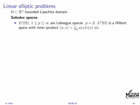
Linear elliptic problemsΩ sub Rn bounded Lipschitz domain
Sobolev spacesI Lp(Ω) 1 le p le infin are Lebesgue spaces p = 2 L2(Ω) is a Hilbert
space with inner product (u v) =int
Ωu(x)v(x) dx
I W sp for s isin R 1 le p le infin are Sobolev spaces When p = 2W s2(Ω) = Hs(Ω) is a Hilbert space
I H10 (Ω) = v isin H1(Ω) v|partΩ = 0 with norm (due to Poincare
inequality)uH1
0 (Ω) = nablauL2(Ω)
I H10 (Ω)lowast = Hminus1(Ω)
I Note L2(Ω) sub Hminus1(Ω)
Model problem
minusdiv (Anablau) = f in Ω
u = 0 on partΩ
H Antil 060616 14
Well-posed
I Weak solution Given f isin Hminus1(Ω) a function u isin H10 (Ω) is called
a weak solution iffintΩ
Anablau middot nablav = 〈f v〉minus11 forallv isin H10 (Ω)
where 〈middot middot〉minus11 denotes the Hminus1(Ω)ndashH1(Ω) duality pairing
I Existence and uniqueness For each f isin Hminus1(Ω) there exists aunique u isin H1
0 (Ω) such that
nablauL2(Ω) le CdΩfHminus1(Ω)
I A = I the result is due to the Riesz-representation theorem
I A 6= I (maybe non-symmetric) the result is due to Lax-Milgramlemma
I For general W 1p-spaces use inf-sup conditions combined withBanach-Necas theorem which is a necessary and sufficient condition
H Antil 060616 15
Linear-quadratic elliptic OCP
min J(u z) =1
2uminus ud2L2(Ω) +
λ
2z2L2(Ω)
subject to
minusdiv (Anablau) = z in Ω
u = 0 on partΩ
and the pointwise control constraints
z isin Zad = v isin L2(Ω) za(x) le v(x) le zb(x) ae x isin Ω
λ gt 0 is a parameter za zb isin Linfin(Ω) with za lt zb are given A isbounded symmetric positive
H Antil 060616 16
Reduced OCP
I Control to state map The solution operator defined as
S Hminus1(Ω)rarr H10 (Ω) z 7rarr u(z) = Sz
Note In view of the embedding
H10 (Ω) rarr L2(Ω) rarr Hminus1(Ω)
we may also consider S from L2(Ω) to L2(Ω) We will use the samenotation for this operator (for simplicity)
I Reduced cost functional The reduced cost functionalJ L2(Ω)rarr R is defined as
J (z) = J(Sz z)
I Reduced problem minzisinZadJ (z)
H Antil 060616 17
Reduced OCP
I Control to state map The solution operator defined as
S Hminus1(Ω)rarr H10 (Ω) z 7rarr u(z) = Sz
Note In view of the embedding
H10 (Ω) rarr L2(Ω) rarr Hminus1(Ω)
we may also consider S from L2(Ω) to L2(Ω) We will use the samenotation for this operator (for simplicity)
I Reduced cost functional The reduced cost functionalJ L2(Ω)rarr R is defined as
J (z) = J(Sz z)
I Reduced problem minzisinZadJ (z)
H Antil 060616 17
Reduced OCP
I Control to state map The solution operator defined as
S Hminus1(Ω)rarr H10 (Ω) z 7rarr u(z) = Sz
Note In view of the embedding
H10 (Ω) rarr L2(Ω) rarr Hminus1(Ω)
we may also consider S from L2(Ω) to L2(Ω) We will use the samenotation for this operator (for simplicity)
I Reduced cost functional The reduced cost functionalJ L2(Ω)rarr R is defined as
J (z) = J(Sz z)
I Reduced problem minzisinZadJ (z)
H Antil 060616 17
Existence of solution Direct methodThere exists a unique solution to the above problem
I Minimizing sequence J is bounded below by zero therefore thereexists a minimizing sequence znnisinN such that
limnrarrinfin
J (zn) = inf J (z)
I Weak compactness zn sub L2(Ω) is bounded Since L2(Ω) isreflexive therefore there exists a subsequence (not relabeled) suchthat
zn z and z isin Zad
where the latter is a consequence of Zad being closed and convex
I Optimality Since J is continuous and convex and therefore isweakly lower semicontinuous We obtain
lim inf J (zn) ge J (z)
which implies that z is optimal
I Uniqueness Exercise
H Antil 060616 18
Existence of solution Direct methodThere exists a unique solution to the above problem
I Minimizing sequence J is bounded below by zero therefore thereexists a minimizing sequence znnisinN such that
limnrarrinfin
J (zn) = inf J (z)
I Weak compactness zn sub L2(Ω) is bounded Since L2(Ω) isreflexive therefore there exists a subsequence (not relabeled) suchthat
zn z and z isin Zad
where the latter is a consequence of Zad being closed and convex
I Optimality Since J is continuous and convex and therefore isweakly lower semicontinuous We obtain
lim inf J (zn) ge J (z)
which implies that z is optimal
I Uniqueness Exercise
H Antil 060616 18
Existence of solution Direct methodThere exists a unique solution to the above problem
I Minimizing sequence J is bounded below by zero therefore thereexists a minimizing sequence znnisinN such that
limnrarrinfin
J (zn) = inf J (z)
I Weak compactness zn sub L2(Ω) is bounded Since L2(Ω) isreflexive therefore there exists a subsequence (not relabeled) suchthat
zn z and z isin Zad
where the latter is a consequence of Zad being closed and convex
I Optimality Since J is continuous and convex and therefore isweakly lower semicontinuous We obtain
lim inf J (zn) ge J (z)
which implies that z is optimal
I Uniqueness Exercise
H Antil 060616 18
Existence of solution Direct methodThere exists a unique solution to the above problem
I Minimizing sequence J is bounded below by zero therefore thereexists a minimizing sequence znnisinN such that
limnrarrinfin
J (zn) = inf J (z)
I Weak compactness zn sub L2(Ω) is bounded Since L2(Ω) isreflexive therefore there exists a subsequence (not relabeled) suchthat
zn z and z isin Zad
where the latter is a consequence of Zad being closed and convex
I Optimality Since J is continuous and convex and therefore isweakly lower semicontinuous We obtain
lim inf J (zn) ge J (z)
which implies that z is optimal
I Uniqueness Exercise
H Antil 060616 18
Outline
Motivation and examples
Linear elliptic optimal control problems
Differentiation in Banach spaces
First-order necessary conditions
Optimal control of semilinear PDEs
An abstract problem
Discretization using finite element methods
H Antil 060616 19
Differentiation in Banach spacesLet (Z middot Z) (V middot V ) B-spaces Z sub Z open and F Z rarr V
Let z isin Z
I If exist δF (z h) = limtdarr01t (F (z + th)minus F (z)) then δF (z h) is called
the directional derivative of F at z in direction h
I If exist δF (z h) forallh isin Z then h 7rarr δF (z h) is the first variation of Fat z
I Let exist the first variation δF (z middot) F is said to be Gateauxdifferentiable at z iff existA isin L(Z V ) such that δF (z h) = Ahforallh isin Z We write A = F primeG(z)
I F is said to be Frechet differentiable at z iff existA isin L(Z V ) and amapping r(z middot) Z rarr V such that for all h isin U with z + h isin Zwe have
F (z+h) = F (z)+Ah+r(z h) withr(z h)VhZ
rarr 0 as hZ rarr 0
We write F prime(z) = A
H Antil 060616 20
Differentiation in Banach spacesLet (Z middot Z) (V middot V ) B-spaces Z sub Z open and F Z rarr V
Let z isin Z
I If exist δF (z h) = limtdarr01t (F (z + th)minus F (z)) then δF (z h) is called
the directional derivative of F at z in direction h
I If exist δF (z h) forallh isin Z then h 7rarr δF (z h) is the first variation of Fat z
I Let exist the first variation δF (z middot) F is said to be Gateauxdifferentiable at z iff existA isin L(Z V ) such that δF (z h) = Ahforallh isin Z We write A = F primeG(z)
I F is said to be Frechet differentiable at z iff existA isin L(Z V ) and amapping r(z middot) Z rarr V such that for all h isin U with z + h isin Zwe have
F (z+h) = F (z)+Ah+r(z h) withr(z h)VhZ
rarr 0 as hZ rarr 0
We write F prime(z) = A
H Antil 060616 20
Differentiation in Banach spacesLet (Z middot Z) (V middot V ) B-spaces Z sub Z open and F Z rarr V
Let z isin Z
I If exist δF (z h) = limtdarr01t (F (z + th)minus F (z)) then δF (z h) is called
the directional derivative of F at z in direction h
I If exist δF (z h) forallh isin Z then h 7rarr δF (z h) is the first variation of Fat z
I Let exist the first variation δF (z middot) F is said to be Gateauxdifferentiable at z iff existA isin L(Z V ) such that δF (z h) = Ahforallh isin Z We write A = F primeG(z)
I F is said to be Frechet differentiable at z iff existA isin L(Z V ) and amapping r(z middot) Z rarr V such that for all h isin U with z + h isin Zwe have
F (z+h) = F (z)+Ah+r(z h) withr(z h)VhZ
rarr 0 as hZ rarr 0
We write F prime(z) = A
H Antil 060616 20
Differentiation in Banach spacesLet (Z middot Z) (V middot V ) B-spaces Z sub Z open and F Z rarr V
Let z isin Z
I If exist δF (z h) = limtdarr01t (F (z + th)minus F (z)) then δF (z h) is called
the directional derivative of F at z in direction h
I If exist δF (z h) forallh isin Z then h 7rarr δF (z h) is the first variation of Fat z
I Let exist the first variation δF (z middot) F is said to be Gateauxdifferentiable at z iff existA isin L(Z V ) such that δF (z h) = Ahforallh isin Z We write A = F primeG(z)
I F is said to be Frechet differentiable at z iff existA isin L(Z V ) and amapping r(z middot) Z rarr V such that for all h isin U with z + h isin Zwe have
F (z+h) = F (z)+Ah+r(z h) withr(z h)VhZ
rarr 0 as hZ rarr 0
We write F prime(z) = A
H Antil 060616 20
ExamplesExample 1 (H (middot middot)H) Hilbert space F (z) = z2H = (z z)H
forallz h F (z + h)minus F (z) = 2(z h)H + h2HThen
F prime(z)h = (2z h)H
Reisz representation theorem (identify H with Hlowast) we can write
F prime(z)h = (nablaF (z) h)H
where nablaF (z) = 2z is the gradient
Example 2 Let (Z (middot middot)Z) (H (middot middot)H) Hilbert spaces ud isin H fixedLet S isin L(ZH) Consider E Z rarr R
E(z) = Sz minus ud2H
Then E(z) = G(F (z)) where G(v) = v2H and F (z) = Sz minus ud
Eprime(z)h = Gprime(F (z))F prime(z)h = (2v F prime(z)h)H
= 2(Sz minus ud Sh)H = 2(Slowast(Sz minus ud) h)Z
we denote the gradient as nablaE(z) = 2Slowast(Sz minus ud)
H Antil 060616 21
ExamplesExample 1 (H (middot middot)H) Hilbert space F (z) = z2H = (z z)H
forallz h F (z + h)minus F (z) = 2(z h)H + h2HThen
F prime(z)h = (2z h)H
Reisz representation theorem (identify H with Hlowast) we can write
F prime(z)h = (nablaF (z) h)H
where nablaF (z) = 2z is the gradient
Example 2 Let (Z (middot middot)Z) (H (middot middot)H) Hilbert spaces ud isin H fixedLet S isin L(ZH) Consider E Z rarr R
E(z) = Sz minus ud2H
Then E(z) = G(F (z)) where G(v) = v2H and F (z) = Sz minus ud
Eprime(z)h = Gprime(F (z))F prime(z)h = (2v F prime(z)h)H
= 2(Sz minus ud Sh)H = 2(Slowast(Sz minus ud) h)Z
we denote the gradient as nablaE(z) = 2Slowast(Sz minus ud)H Antil 060616 21
Outline
Motivation and examples
Linear elliptic optimal control problems
Differentiation in Banach spaces
First-order necessary conditions
Optimal control of semilinear PDEs
An abstract problem
Discretization using finite element methods
H Antil 060616 22
First order necessary optimality conditions
Most of the theory is based on these two simple results
Theorem Let (Z middot Z) be a normed space J Z rarr (infin+infin] amapping with J 6equiv +infin Then z isin Z minimizer of J hArr 0 isin partJ (z)
Proof 0 isin partJ (z) means by definition of partJ (z) J (z)minus J (z) le 0forallz isin Z
Theorem Let (Z middot Z) be a normed space Zad sub Z nonemptyconvex closed J Z rarr R Gateaux differentiable where Zad sub Z sub ZZ open If z isin Zad is a solution to
minzisinZad
J (z)
then z solvesJ prime(z)(z minus z) ge 0 forallz isin Zad
Proof Exercise
H Antil 060616 23
First order necessary optimality conditions
Most of the theory is based on these two simple results
Theorem Let (Z middot Z) be a normed space J Z rarr (infin+infin] amapping with J 6equiv +infin Then z isin Z minimizer of J hArr 0 isin partJ (z)
Proof 0 isin partJ (z) means by definition of partJ (z) J (z)minus J (z) le 0forallz isin Z
Theorem Let (Z middot Z) be a normed space Zad sub Z nonemptyconvex closed J Z rarr R Gateaux differentiable where Zad sub Z sub ZZ open If z isin Zad is a solution to
minzisinZad
J (z)
then z solvesJ prime(z)(z minus z) ge 0 forallz isin Zad
Proof Exercise
H Antil 060616 23
Linear quadratic OCPI Reduced funcational
J (z) =1
2Sz minus ud2L2(Ω) +
λ
2z2L2(Ω)
I Gradient computation using sensitivity
J prime(z)h = (Slowast(Sz minus ud) + λz h)L2(Ω) forallh isin L2(Ω)
we denote the gradient by
nablaJ (z) = Slowast(Sz minus ud) + λz
I First order necessary and sufficient optimality condition
(nablaJ (z) z minus z)L2(Ω) ge 0 forallz isin Zad
I Adjoint equation Let p = Slowast(Sz minus ud) which translates intop isin H1
0 (Ω) solving
minusdiv (Anablap) = uminus ud in Ω
p = 0 on partΩ
I Gradient computation using adjoint nablaJ (z) = p+ λz
H Antil 060616 24
Linear quadratic OCPI Reduced funcational
J (z) =1
2Sz minus ud2L2(Ω) +
λ
2z2L2(Ω)
I Gradient computation using sensitivity
J prime(z)h = (Slowast(Sz minus ud) + λz h)L2(Ω) forallh isin L2(Ω)
we denote the gradient by
nablaJ (z) = Slowast(Sz minus ud) + λz
I First order necessary and sufficient optimality condition
(nablaJ (z) z minus z)L2(Ω) ge 0 forallz isin Zad
I Adjoint equation Let p = Slowast(Sz minus ud) which translates intop isin H1
0 (Ω) solving
minusdiv (Anablap) = uminus ud in Ω
p = 0 on partΩ
I Gradient computation using adjoint nablaJ (z) = p+ λz
H Antil 060616 24
Linear quadratic OCPI Reduced funcational
J (z) =1
2Sz minus ud2L2(Ω) +
λ
2z2L2(Ω)
I Gradient computation using sensitivity
J prime(z)h = (Slowast(Sz minus ud) + λz h)L2(Ω) forallh isin L2(Ω)
we denote the gradient by
nablaJ (z) = Slowast(Sz minus ud) + λz
I First order necessary and sufficient optimality condition
(nablaJ (z) z minus z)L2(Ω) ge 0 forallz isin Zad
I Adjoint equation Let p = Slowast(Sz minus ud) which translates intop isin H1
0 (Ω) solving
minusdiv (Anablap) = uminus ud in Ω
p = 0 on partΩ
I Gradient computation using adjoint nablaJ (z) = p+ λz
H Antil 060616 24
Linear quadratic OCPI Reduced funcational
J (z) =1
2Sz minus ud2L2(Ω) +
λ
2z2L2(Ω)
I Gradient computation using sensitivity
J prime(z)h = (Slowast(Sz minus ud) + λz h)L2(Ω) forallh isin L2(Ω)
we denote the gradient by
nablaJ (z) = Slowast(Sz minus ud) + λz
I First order necessary and sufficient optimality condition
(nablaJ (z) z minus z)L2(Ω) ge 0 forallz isin Zad
I Adjoint equation Let p = Slowast(Sz minus ud) which translates intop isin H1
0 (Ω) solving
minusdiv (Anablap) = uminus ud in Ω
p = 0 on partΩ
I Gradient computation using adjoint nablaJ (z) = p+ λz
H Antil 060616 24
Linear quadratic OCPI Reduced funcational
J (z) =1
2Sz minus ud2L2(Ω) +
λ
2z2L2(Ω)
I Gradient computation using sensitivity
J prime(z)h = (Slowast(Sz minus ud) + λz h)L2(Ω) forallh isin L2(Ω)
we denote the gradient by
nablaJ (z) = Slowast(Sz minus ud) + λz
I First order necessary and sufficient optimality condition
(nablaJ (z) z minus z)L2(Ω) ge 0 forallz isin Zad
I Adjoint equation Let p = Slowast(Sz minus ud) which translates intop isin H1
0 (Ω) solving
minusdiv (Anablap) = uminus ud in Ω
p = 0 on partΩ
I Gradient computation using adjoint nablaJ (z) = p+ λz
H Antil 060616 24
Optimality system
I State u isin H10 (Ω)
intΩAnablau middot nablav =
intΩzv forallv isin H1
0 (Ω)
I Adjoint p isin H10 (Ω)
intΩAnablap middot nablav =
intΩ
(uminus ud)v forallv isin H10 (Ω)
I Control z isin Zad (p+ λz z minus z) ge 0 forallz isin Zad
H Antil 060616 25
Pointwise interpretation
The variational inequality
(p+ λz z minus z) ge 0 forallz isin Zad
is equivalent to for ae x isin Ω
z(x) =
za(x) if p(x) + λz(x) gt 0isin [za(x) zb(x)] if p(x) + λz(x) = 0zb(x) if p(x) + λz(x) lt 0
Consequence
I When λ gt 0 then ae in Ω
z(x) = P[za(x)zb(x)]
minus 1
λp(x)
= min
zb(x)max
za(x)minus 1
λp(x)
H Antil 060616 26
Formal Lagrange method applied to linear OCPIntroduce L H1
0 (Ω)times Zad timesH1(Ω)rarr R defined as
L(u z p) = J(u z)minusint
Ω
(minusdiv (Anablau)minus z
)p dx
Integrate by parts to arrive at
L(u z p) = J(u z)minusint
Ω
(minusdiv (Anablap)uminus zp
)dx+
intpartΩ
(Anablau)p ds
If (u z p) is a stationary point then
I State
DpL(u z p)h = 0 forallh isin H1(Ω)
I AdjointDuL(u z p)h = 0 forallh isin H1
0 (Ω)
I ControlDzL(u z p)(z minus z) ge 0 forallz isin Zad
H Antil 060616 27
Formal Lagrange method applied to linear OCPIntroduce L H1
0 (Ω)times Zad timesH1(Ω)rarr R defined as
L(u z p) = J(u z)minusint
Ω
(minusdiv (Anablau)minus z
)p dx
Integrate by parts to arrive at
L(u z p) = J(u z)minusint
Ω
(minusdiv (Anablap)uminus zp
)dx+
intpartΩ
(Anablau)p ds
If (u z p) is a stationary point then
I State
DpL(u z p)h = 0 forallh isin H1(Ω)
I AdjointDuL(u z p)h = 0 forallh isin H1
0 (Ω)
I ControlDzL(u z p)(z minus z) ge 0 forallz isin Zad
H Antil 060616 27
Formal Lagrange method applied to linear OCPIntroduce L H1
0 (Ω)times Zad timesH1(Ω)rarr R defined as
L(u z p) = J(u z)minusint
Ω
(minusdiv (Anablau)minus z
)p dx
Integrate by parts to arrive at
L(u z p) = J(u z)minusint
Ω
(minusdiv (Anablap)uminus zp
)dx+
intpartΩ
(Anablau)p ds
If (u z p) is a stationary point then
I State
DpL(u z p)h = 0 forallh isin H1(Ω)
I AdjointDuL(u z p)h = 0 forallh isin H1
0 (Ω)
I ControlDzL(u z p)(z minus z) ge 0 forallz isin Zad
H Antil 060616 27
Formal Lagrange method applied to linear OCPIntroduce L H1
0 (Ω)times Zad timesH1(Ω)rarr R defined as
L(u z p) = J(u z)minusint
Ω
(minusdiv (Anablau)minus z
)p dx
Integrate by parts to arrive at
L(u z p) = J(u z)minusint
Ω
(minusdiv (Anablap)uminus zp
)dx+
intpartΩ
(Anablau)p ds
If (u z p) is a stationary point then
I State
DpL(u z p)h = 0 forallh isin H1(Ω)
I AdjointDuL(u z p)h = 0 forallh isin H1
0 (Ω)
I ControlDzL(u z p)(z minus z) ge 0 forallz isin Zad
H Antil 060616 27
Formal Lagrange method applied to linear OCPIntroduce L H1
0 (Ω)times Zad timesH1(Ω)rarr R defined as
L(u z p) = J(u z)minusint
Ω
(minusdiv (Anablau)minus z
)p dx
Integrate by parts to arrive at
L(u z p) = J(u z)minusint
Ω
(minusdiv (Anablap)uminus zp
)dx+
intpartΩ
(Anablau)p ds
If (u z p) is a stationary point then
I State
DpL(u z p)h = 0 forallh isin H1(Ω)
I AdjointDuL(u z p)h = 0 forallh isin H1
0 (Ω)
I ControlDzL(u z p)(z minus z) ge 0 forallz isin Zad
H Antil 060616 27
Outline
Motivation and examples
Linear elliptic optimal control problems
Differentiation in Banach spaces
First-order necessary conditions
Optimal control of semilinear PDEs
An abstract problem
Discretization using finite element methods
H Antil 060616 28
Semilinear elliptic OCP
min J(u z) =1
2uminus ud2L2(Ω) +
λ
2z2L2(Ω)
subject to
minus∆u+ g(x u) = z in Ω
u = 0 on partΩ
and z isin Zad with za zb isin Linfin(Ω)
H Antil 060616 29
State space(A1) Ω sub Rd open bounded partΩ is Lipschitz
(A2) g Ωtimes Rrarr R is bounded and measurable with respect to x isin Ωfor every u isin R
(A3) g is continuous monotone increasing and Lipschitz continuous in ufor ae x isin Ω
(A4) g(x 0) = 0 for ae x isin Ω (not really necessary)
Theorem Suppose (A1)minus (A4) hold For every z isin Lr(Ω) withr gt d2 the state equation has a unique weak solutionu isin H1
0 (Ω) cap C(Ω) ie we haveintΩ
nablau middot nablav dx+
intΩ
g(x u(x))v(x) dx =
intΩ
zv dx forallv isin H10 (Ω)
Moreover there exists a constant C gt 0 such that
uH1(Ω) + uC(Ω) le CzLr(Ω)
RemarkI The proof of the theorem uses the BrowderndashMinty theorem on
monotone operators
H Antil 060616 30
State space(A1) Ω sub Rd open bounded partΩ is Lipschitz
(A2) g Ωtimes Rrarr R is bounded and measurable with respect to x isin Ωfor every u isin R
(A3) g is continuous monotone increasing and Lipschitz continuous in ufor ae x isin Ω
(A4) g(x 0) = 0 for ae x isin Ω (not really necessary)
Theorem Suppose (A1)minus (A4) hold For every z isin Lr(Ω) withr gt d2 the state equation has a unique weak solutionu isin H1
0 (Ω) cap C(Ω) ie we haveintΩ
nablau middot nablav dx+
intΩ
g(x u(x))v(x) dx =
intΩ
zv dx forallv isin H10 (Ω)
Moreover there exists a constant C gt 0 such that
uH1(Ω) + uC(Ω) le CzLr(Ω)
RemarkI The proof of the theorem uses the BrowderndashMinty theorem on
monotone operators
H Antil 060616 30
State space(A1) Ω sub Rd open bounded partΩ is Lipschitz
(A2) g Ωtimes Rrarr R is bounded and measurable with respect to x isin Ωfor every u isin R
(A3) g is continuous monotone increasing and Lipschitz continuous in ufor ae x isin Ω
(A4) g(x 0) = 0 for ae x isin Ω (not really necessary)
Theorem Suppose (A1)minus (A4) hold For every z isin Lr(Ω) withr gt d2 the state equation has a unique weak solutionu isin H1
0 (Ω) cap C(Ω) ie we haveintΩ
nablau middot nablav dx+
intΩ
g(x u(x))v(x) dx =
intΩ
zv dx forallv isin H10 (Ω)
Moreover there exists a constant C gt 0 such that
uH1(Ω) + uC(Ω) le CzLr(Ω)
RemarkI The proof of the theorem uses the BrowderndashMinty theorem on
monotone operators
H Antil 060616 30
Control-to-state map and reduced problem
I Control to state map
S Linfin(Ω)rarr H10 (Ω) cap C(Ω)
is well defined and is globally Lipschitz continuous
I Reduced problem
minJ (z) =1
2S(u)minus ud2L2(Ω) +
λ
2z2L2(Ω)
H Antil 060616 31
Control-to-state map and reduced problem
I Control to state map
S Linfin(Ω)rarr H10 (Ω) cap C(Ω)
is well defined and is globally Lipschitz continuous
I Reduced problem
minJ (z) =1
2S(u)minus ud2L2(Ω) +
λ
2z2L2(Ω)
H Antil 060616 31
First-order necessary conditionsI Lagrangian functional
L(u z p) = J(u z)minusint
Ω
(minus∆u+ g(x u(x))minus z
)p dx
= J(u z)minusint
Ω
(nablau middot nablap+ g(x u(x))pminus zp
)dx
I Adjoint system For all h isin H10 (Ω)
0 = DuL(u z p)h =
intΩ
(uminus ud)h dxminusint
Ω
(nablah middot nablap+ gu(x u(x))ph
)which yields
minus∆p+ gu(x u(x))p = uminus ud in Ω
p = 0 on partΩ
I Control
DzL(u z p)(z minus z) = (p+ λz z minus z) dx ge 0 forallz isin ZadI Gradient
nablaJ (z) = p+ λz
H Antil 060616 32
First-order necessary conditionsI Lagrangian functional
L(u z p) = J(u z)minusint
Ω
(minus∆u+ g(x u(x))minus z
)p dx
= J(u z)minusint
Ω
(nablau middot nablap+ g(x u(x))pminus zp
)dx
I Adjoint system For all h isin H10 (Ω)
0 = DuL(u z p)h =
intΩ
(uminus ud)h dxminusint
Ω
(nablah middot nablap+ gu(x u(x))ph
)which yields
minus∆p+ gu(x u(x))p = uminus ud in Ω
p = 0 on partΩ
I Control
DzL(u z p)(z minus z) = (p+ λz z minus z) dx ge 0 forallz isin ZadI Gradient
nablaJ (z) = p+ λz
H Antil 060616 32
First-order necessary conditionsI Lagrangian functional
L(u z p) = J(u z)minusint
Ω
(minus∆u+ g(x u(x))minus z
)p dx
= J(u z)minusint
Ω
(nablau middot nablap+ g(x u(x))pminus zp
)dx
I Adjoint system For all h isin H10 (Ω)
0 = DuL(u z p)h =
intΩ
(uminus ud)h dxminusint
Ω
(nablah middot nablap+ gu(x u(x))ph
)which yields
minus∆p+ gu(x u(x))p = uminus ud in Ω
p = 0 on partΩ
I Control
DzL(u z p)(z minus z) = (p+ λz z minus z) dx ge 0 forallz isin Zad
I GradientnablaJ (z) = p+ λz
H Antil 060616 32
First-order necessary conditionsI Lagrangian functional
L(u z p) = J(u z)minusint
Ω
(minus∆u+ g(x u(x))minus z
)p dx
= J(u z)minusint
Ω
(nablau middot nablap+ g(x u(x))pminus zp
)dx
I Adjoint system For all h isin H10 (Ω)
0 = DuL(u z p)h =
intΩ
(uminus ud)h dxminusint
Ω
(nablah middot nablap+ gu(x u(x))ph
)which yields
minus∆p+ gu(x u(x))p = uminus ud in Ω
p = 0 on partΩ
I Control
DzL(u z p)(z minus z) = (p+ λz z minus z) dx ge 0 forallz isin ZadI Gradient
nablaJ (z) = p+ λz
H Antil 060616 32
Differentiability of Nemytskii operator
The rigorous proof uses
Theorem In addition to (A1)-(A4) if
(A5) g is continuously differentiable with respect to u for ae x isin Ωand we have
(i) |gu(x 0)| le K for ae x isin Ω(ii) gu is locally Lipschitz with respect to u isin R
then the Nemytskii operator G u 7rarr g(middot u(middot)) is continuously Frechetdifferentiable from Linfin(Ω) into itself and
(Gprime(u)h)(x) = gu(x u(x))h(x) ae in Ω forallh isin Linfin(Ω)
Remark (A5) holds if g(x u) = g(u) and g isin C2(R)
H Antil 060616 33
Outline
Motivation and examples
Linear elliptic optimal control problems
Differentiation in Banach spaces
First-order necessary conditions
Optimal control of semilinear PDEs
An abstract problem
Discretization using finite element methods
H Antil 060616 34
Gradient computation via adjoint general formI Abstract problem
min J(u z)
subject toc(u z) = 0
and z isin Zad
I Directional derivative Let S be the control to state map(nonlinear in general)
z 7rarr S(z) = u(z)
Under the assumptions of ldquoimplicit function theoremrdquo
J prime(z)h = (nablauJ (u(z) z) Sprime(z)h) + (nablazJ (u(z) z) h)
I Sensitivity of u with respect to z Differentiating the stateequation
cu(S(z) z)Sprime(z)h = minuscz(S(z) z)h
leads toSprime(z)h = minuscu(S(z) z)minus1
(cz(S(z) z)h
)
provided cu(S(z) z)minus1 is well-defined
H Antil 060616 35
Gradient computation via adjoint general formI Abstract problem
min J(u z)
subject toc(u z) = 0
and z isin ZadI Directional derivative Let S be the control to state map
(nonlinear in general)
z 7rarr S(z) = u(z)
Under the assumptions of ldquoimplicit function theoremrdquo
J prime(z)h = (nablauJ (u(z) z) Sprime(z)h) + (nablazJ (u(z) z) h)
I Sensitivity of u with respect to z Differentiating the stateequation
cu(S(z) z)Sprime(z)h = minuscz(S(z) z)h
leads toSprime(z)h = minuscu(S(z) z)minus1
(cz(S(z) z)h
)
provided cu(S(z) z)minus1 is well-defined
H Antil 060616 35
Gradient computation via adjoint general formI Abstract problem
min J(u z)
subject toc(u z) = 0
and z isin ZadI Directional derivative Let S be the control to state map
(nonlinear in general)
z 7rarr S(z) = u(z)
Under the assumptions of ldquoimplicit function theoremrdquo
J prime(z)h = (nablauJ (u(z) z) Sprime(z)h) + (nablazJ (u(z) z) h)
I Sensitivity of u with respect to z Differentiating the stateequation
cu(S(z) z)Sprime(z)h = minuscz(S(z) z)h
leads toSprime(z)h = minuscu(S(z) z)minus1
(cz(S(z) z)h
)
provided cu(S(z) z)minus1 is well-defined
H Antil 060616 35
Adjoint equation and gradient general form
I Directional derivative
J prime(z)h = minus(nablauJ (u(z) z) cu(u(z) z)minus1cz(u(z) z)h
)+ (nablazJ (u(z) z) h)
I Gradient
nablaJ (z) = minuscz(u(z) z)lowast(cu(u(z) z)minuslowastnablauJ (u(z) z)
)+nablazJ (u(z) z)
I Introducing adjoint variable p solving
cu(u(z) z)lowastp = nablauJ (u(z) z)
we arrive at following form of gradient
nablaJ (z) = minuscz(u(z) z)lowastp+nablazJ (u(z) z)
which is tractable
H Antil 060616 36
Adjoint equation and gradient general form
I Directional derivative
J prime(z)h = minus(nablauJ (u(z) z) cu(u(z) z)minus1cz(u(z) z)h
)+ (nablazJ (u(z) z) h)
I Gradient
nablaJ (z) = minuscz(u(z) z)lowast(cu(u(z) z)minuslowastnablauJ (u(z) z)
)+nablazJ (u(z) z)
I Introducing adjoint variable p solving
cu(u(z) z)lowastp = nablauJ (u(z) z)
we arrive at following form of gradient
nablaJ (z) = minuscz(u(z) z)lowastp+nablazJ (u(z) z)
which is tractable
H Antil 060616 36
Adjoint equation and gradient general form
I Directional derivative
J prime(z)h = minus(nablauJ (u(z) z) cu(u(z) z)minus1cz(u(z) z)h
)+ (nablazJ (u(z) z) h)
I Gradient
nablaJ (z) = minuscz(u(z) z)lowast(cu(u(z) z)minuslowastnablauJ (u(z) z)
)+nablazJ (u(z) z)
I Introducing adjoint variable p solving
cu(u(z) z)lowastp = nablauJ (u(z) z)
we arrive at following form of gradient
nablaJ (z) = minuscz(u(z) z)lowastp+nablazJ (u(z) z)
which is tractable
H Antil 060616 36
Hessian computation general form
I Lagrangian L(u z p) = J(u z)minusint
Ωc(u z)p dx Then we have
DzJ (z)h = DzL(u z p)h
I Second order derivative
D2zJ (z)[h1 h2] = DuDzL(u z p)[h1 S
prime(z)h2] +D2zL(u z p)[h1 h2]
+DpDzL(u z p)[h1 Dzp(z)h2]
I We already know Sprime(z)h2 moreover
DpDzL(u z p)[h1 Dzp(z)h2] = minus(cu(u z)h1 Dzp(z)h2
)
It remain to identify Dzp(z)h2
H Antil 060616 37
Hessian computation general form
I Lagrangian L(u z p) = J(u z)minusint
Ωc(u z)p dx Then we have
DzJ (z)h = DzL(u z p)h
I Second order derivative
D2zJ (z)[h1 h2] = DuDzL(u z p)[h1 S
prime(z)h2] +D2zL(u z p)[h1 h2]
+DpDzL(u z p)[h1 Dzp(z)h2]
I We already know Sprime(z)h2 moreover
DpDzL(u z p)[h1 Dzp(z)h2] = minus(cu(u z)h1 Dzp(z)h2
)
It remain to identify Dzp(z)h2
H Antil 060616 37
Hessian computation general form
I Lagrangian L(u z p) = J(u z)minusint
Ωc(u z)p dx Then we have
DzJ (z)h = DzL(u z p)h
I Second order derivative
D2zJ (z)[h1 h2] = DuDzL(u z p)[h1 S
prime(z)h2] +D2zL(u z p)[h1 h2]
+DpDzL(u z p)[h1 Dzp(z)h2]
I We already know Sprime(z)h2 moreover
DpDzL(u z p)[h1 Dzp(z)h2] = minus(cu(u z)h1 Dzp(z)h2
)
It remain to identify Dzp(z)h2
H Antil 060616 37
Outline
Motivation and examples
Linear elliptic optimal control problems
Differentiation in Banach spaces
First-order necessary conditions
Optimal control of semilinear PDEs
An abstract problem
Discretization using finite element methods
H Antil 060616 38
Numerical approximation of Poisson equation MeshTo avoid technical issues we will assume that partΩ is polygonal
I Mesh Let T = K be a mesh of Ω where K sub Rd is an elementthat is isoparametrically equivalent to a unit simplex in Rd
I Conforming mesh We say that the mesh is conforming ifI Ω = cupKisinT KI If K1 cap K2 = x then x is a node of K1 and K2I If K1 cap K2 6= empty and K1 cap K2 6= x then K1 cap K2 is an edgeface
contained in partK1 cap partK2
I Shape regular Let T be the collection of all conformingrefinements of an original mesh T 0 Then T is called shape regularif exist κ gt 0 such that
hKρKle κ forallK isin cupiT i
where hK = diam K ρK = maxρ gt 0|Bρ sub KI Quasi-uniform A family of shape regular meshes is called-quasi
uniform if there exist a constant σ gt 0 such that
maxhKminhK
le σ
uniformly for all meshes in the family
Numerical approximation of Poisson equation MeshTo avoid technical issues we will assume that partΩ is polygonal
I Mesh Let T = K be a mesh of Ω where K sub Rd is an elementthat is isoparametrically equivalent to a unit simplex in Rd
I Conforming mesh We say that the mesh is conforming ifI Ω = cupKisinT KI If K1 cap K2 = x then x is a node of K1 and K2I If K1 cap K2 6= empty and K1 cap K2 6= x then K1 cap K2 is an edgeface
contained in partK1 cap partK2
I Shape regular Let T be the collection of all conformingrefinements of an original mesh T 0 Then T is called shape regularif exist κ gt 0 such that
hKρKle κ forallK isin cupiT i
where hK = diam K ρK = maxρ gt 0|Bρ sub KI Quasi-uniform A family of shape regular meshes is called-quasi
uniform if there exist a constant σ gt 0 such that
maxhKminhK
le σ
uniformly for all meshes in the family
Numerical approximation of Poisson equation MeshTo avoid technical issues we will assume that partΩ is polygonal
I Mesh Let T = K be a mesh of Ω where K sub Rd is an elementthat is isoparametrically equivalent to a unit simplex in Rd
I Conforming mesh We say that the mesh is conforming ifI Ω = cupKisinT KI If K1 cap K2 = x then x is a node of K1 and K2I If K1 cap K2 6= empty and K1 cap K2 6= x then K1 cap K2 is an edgeface
contained in partK1 cap partK2
I Shape regular Let T be the collection of all conformingrefinements of an original mesh T 0 Then T is called shape regularif exist κ gt 0 such that
hKρKle κ forallK isin cupiT i
where hK = diam K ρK = maxρ gt 0|Bρ sub K
I Quasi-uniform A family of shape regular meshes is called-quasiuniform if there exist a constant σ gt 0 such that
maxhKminhK
le σ
uniformly for all meshes in the family
Numerical approximation of Poisson equation MeshTo avoid technical issues we will assume that partΩ is polygonal
I Mesh Let T = K be a mesh of Ω where K sub Rd is an elementthat is isoparametrically equivalent to a unit simplex in Rd
I Conforming mesh We say that the mesh is conforming ifI Ω = cupKisinT KI If K1 cap K2 = x then x is a node of K1 and K2I If K1 cap K2 6= empty and K1 cap K2 6= x then K1 cap K2 is an edgeface
contained in partK1 cap partK2
I Shape regular Let T be the collection of all conformingrefinements of an original mesh T 0 Then T is called shape regularif exist κ gt 0 such that
hKρKle κ forallK isin cupiT i
where hK = diam K ρK = maxρ gt 0|Bρ sub KI Quasi-uniform A family of shape regular meshes is called-quasi
uniform if there exist a constant σ gt 0 such that
maxhKminhK
le σ
uniformly for all meshes in the family
FE space and Galerkin approximationI Finite element space For T isin T we define the finite element
space as
V(T ) = W isin C0(Ω) WK isin P1forallK isin T W |partΩ = 0
where P1 is the set of polynomials of degree at most 1
I Galerkin approximation of continuous problem is given by
Find UT isin V(T )
intΩ
AnablaUT middot nablaV = 〈f V 〉 forallV isin V(T )
The discrete problem is well-posedI Nodal basis Consists of functions ψi isin V(T ) with xi isin N (T )
satisfyingψxi
(xj) = δij
where N (T ) denotes the interior (plus Neumann) nodesI Galerkin orthogonality(
nabla(uminus UT )nablaW)L2(Ω)
= 0 forallW isin V(T )
H Antil 060616 40
FE space and Galerkin approximationI Finite element space For T isin T we define the finite element
space as
V(T ) = W isin C0(Ω) WK isin P1forallK isin T W |partΩ = 0
where P1 is the set of polynomials of degree at most 1I Galerkin approximation of continuous problem is given by
Find UT isin V(T )
intΩ
AnablaUT middot nablaV = 〈f V 〉 forallV isin V(T )
The discrete problem is well-posed
I Nodal basis Consists of functions ψi isin V(T ) with xi isin N (T )satisfying
ψxi(xj) = δij
where N (T ) denotes the interior (plus Neumann) nodesI Galerkin orthogonality(
nabla(uminus UT )nablaW)L2(Ω)
= 0 forallW isin V(T )
H Antil 060616 40
FE space and Galerkin approximationI Finite element space For T isin T we define the finite element
space as
V(T ) = W isin C0(Ω) WK isin P1forallK isin T W |partΩ = 0
where P1 is the set of polynomials of degree at most 1I Galerkin approximation of continuous problem is given by
Find UT isin V(T )
intΩ
AnablaUT middot nablaV = 〈f V 〉 forallV isin V(T )
The discrete problem is well-posedI Nodal basis Consists of functions ψi isin V(T ) with xi isin N (T )
satisfyingψxi
(xj) = δij
where N (T ) denotes the interior (plus Neumann) nodes
I Galerkin orthogonality(nabla(uminus UT )nablaW
)L2(Ω)
= 0 forallW isin V(T )
H Antil 060616 40
FE space and Galerkin approximationI Finite element space For T isin T we define the finite element
space as
V(T ) = W isin C0(Ω) WK isin P1forallK isin T W |partΩ = 0
where P1 is the set of polynomials of degree at most 1I Galerkin approximation of continuous problem is given by
Find UT isin V(T )
intΩ
AnablaUT middot nablaV = 〈f V 〉 forallV isin V(T )
The discrete problem is well-posedI Nodal basis Consists of functions ψi isin V(T ) with xi isin N (T )
satisfyingψxi
(xj) = δij
where N (T ) denotes the interior (plus Neumann) nodesI Galerkin orthogonality(
nabla(uminus UT )nablaW)L2(Ω)
= 0 forallW isin V(T )
H Antil 060616 40
Best approximation
I Cearsquos lemma
nabla(uminus UT )L2(Ω) le C infWisinV(T )
nabla(uminusW )L2(Ω)
I Nodal interpolation operator ΠT C(Ω)rarr V(T ) satisfies
ΠT u(xi) = u(xi) forallxi isin N (T )
and is defined as
ΠT u =sum
xiisinN (T )
u(xi)ψxi
I Error estimates In Cearsquos lemma replace W by ΠT u and thencompute the interpolation error
H Antil 060616 41
Best approximation
I Cearsquos lemma
nabla(uminus UT )L2(Ω) le C infWisinV(T )
nabla(uminusW )L2(Ω)
I Nodal interpolation operator ΠT C(Ω)rarr V(T ) satisfies
ΠT u(xi) = u(xi) forallxi isin N (T )
and is defined as
ΠT u =sum
xiisinN (T )
u(xi)ψxi
I Error estimates In Cearsquos lemma replace W by ΠT u and thencompute the interpolation error
H Antil 060616 41
Best approximation
I Cearsquos lemma
nabla(uminus UT )L2(Ω) le C infWisinV(T )
nabla(uminusW )L2(Ω)
I Nodal interpolation operator ΠT C(Ω)rarr V(T ) satisfies
ΠT u(xi) = u(xi) forallxi isin N (T )
and is defined as
ΠT u =sum
xiisinN (T )
u(xi)ψxi
I Error estimates In Cearsquos lemma replace W by ΠT u and thencompute the interpolation error
H Antil 060616 41
Algebraic system state equation
I Recall UT isin V(T ) solves
a(UT V ) = 〈f V 〉 forallV isin V(T )
I Now setting UT =sumN
j=1 Ujψj V = ψi we get
Nsumj=1
Uja(φj φi) = 〈f ψi〉 i = 1 N
which is the matrix-vector system
AU = F
I Stiffness matrix A is SPD
H Antil 060616 42
Algebraic system state equation
I Recall UT isin V(T ) solves
a(UT V ) = 〈f V 〉 forallV isin V(T )
I Now setting UT =sumN
j=1 Ujψj V = ψi we get
Nsumj=1
Uja(φj φi) = 〈f ψi〉 i = 1 N
which is the matrix-vector system
AU = F
I Stiffness matrix A is SPD
H Antil 060616 42
Algebraic system state equation
I Recall UT isin V(T ) solves
a(UT V ) = 〈f V 〉 forallV isin V(T )
I Now setting UT =sumN
j=1 Ujψj V = ψi we get
Nsumj=1
Uja(φj φi) = 〈f ψi〉 i = 1 N
which is the matrix-vector system
AU = F
I Stiffness matrix A is SPD
H Antil 060616 42
Discrete linear elliptic OCP
min JT (UT ZT ) =1
2UT minus ud2L2(Ω) +
λ
2ZT 2L2(Ω)
subject to
Find UT isin V(T )
intΩ
nablaUT middot nablaV = (ZT V )L2(Ω) forallV isin V(T )
and whereZT isin Zad(T ) = Zad cap Z(T )
is either one of these
Z(T ) =
V(T )L2(Ω) variational discretization (Hinze)WT isin Linfin(Ω) ZT |K isin P0(K)K isin T
H Antil 060616 43
Recent books
F TroltzschOptimal control of partial differential equations volume 112 ofGraduate Studies in MathematicsAmerican Mathematical Society Providence RI 2010Theory methods and applications Translated from the 2005 Germanoriginal by Jurgen Sprekels
K Ito and K KunischLagrange multiplier approach to variational problems andapplications volume 15 of Advances in Design and ControlSociety for Industrial and Applied Mathematics (SIAM)Philadelphia PA 2008
H Antil 060616 44
- Motivation and examples
- Linear elliptic optimal control problems
- Differentiation in Banach spaces
- First-order necessary conditions
- Optimal control of semilinear PDEs
- An abstract problem
- Discretization using finite element methods
-
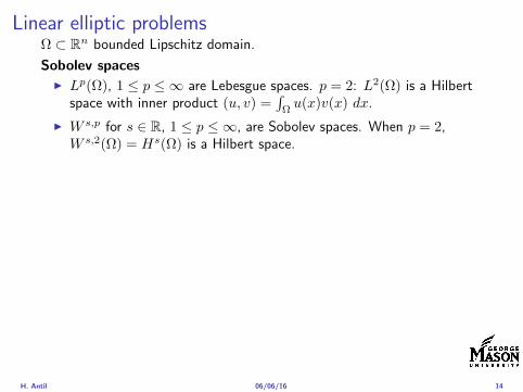
Linear elliptic problemsΩ sub Rn bounded Lipschitz domain
Sobolev spacesI Lp(Ω) 1 le p le infin are Lebesgue spaces p = 2 L2(Ω) is a Hilbert
space with inner product (u v) =int
Ωu(x)v(x) dx
I W sp for s isin R 1 le p le infin are Sobolev spaces When p = 2W s2(Ω) = Hs(Ω) is a Hilbert space
I H10 (Ω) = v isin H1(Ω) v|partΩ = 0 with norm (due to Poincare
inequality)uH1
0 (Ω) = nablauL2(Ω)
I H10 (Ω)lowast = Hminus1(Ω)
I Note L2(Ω) sub Hminus1(Ω)
Model problem
minusdiv (Anablau) = f in Ω
u = 0 on partΩ
H Antil 060616 14
Linear elliptic problemsΩ sub Rn bounded Lipschitz domain
Sobolev spacesI Lp(Ω) 1 le p le infin are Lebesgue spaces p = 2 L2(Ω) is a Hilbert
space with inner product (u v) =int
Ωu(x)v(x) dx
I W sp for s isin R 1 le p le infin are Sobolev spaces When p = 2W s2(Ω) = Hs(Ω) is a Hilbert space
I H10 (Ω) = v isin H1(Ω) v|partΩ = 0 with norm (due to Poincare
inequality)uH1
0 (Ω) = nablauL2(Ω)
I H10 (Ω)lowast = Hminus1(Ω)
I Note L2(Ω) sub Hminus1(Ω)
Model problem
minusdiv (Anablau) = f in Ω
u = 0 on partΩ
H Antil 060616 14
Linear elliptic problemsΩ sub Rn bounded Lipschitz domain
Sobolev spacesI Lp(Ω) 1 le p le infin are Lebesgue spaces p = 2 L2(Ω) is a Hilbert
space with inner product (u v) =int
Ωu(x)v(x) dx
I W sp for s isin R 1 le p le infin are Sobolev spaces When p = 2W s2(Ω) = Hs(Ω) is a Hilbert space
I H10 (Ω) = v isin H1(Ω) v|partΩ = 0 with norm (due to Poincare
inequality)uH1
0 (Ω) = nablauL2(Ω)
I H10 (Ω)lowast = Hminus1(Ω)
I Note L2(Ω) sub Hminus1(Ω)
Model problem
minusdiv (Anablau) = f in Ω
u = 0 on partΩ
H Antil 060616 14
Linear elliptic problemsΩ sub Rn bounded Lipschitz domain
Sobolev spacesI Lp(Ω) 1 le p le infin are Lebesgue spaces p = 2 L2(Ω) is a Hilbert
space with inner product (u v) =int
Ωu(x)v(x) dx
I W sp for s isin R 1 le p le infin are Sobolev spaces When p = 2W s2(Ω) = Hs(Ω) is a Hilbert space
I H10 (Ω) = v isin H1(Ω) v|partΩ = 0 with norm (due to Poincare
inequality)uH1
0 (Ω) = nablauL2(Ω)
I H10 (Ω)lowast = Hminus1(Ω)
I Note L2(Ω) sub Hminus1(Ω)
Model problem
minusdiv (Anablau) = f in Ω
u = 0 on partΩ
H Antil 060616 14
Well-posed
I Weak solution Given f isin Hminus1(Ω) a function u isin H10 (Ω) is called
a weak solution iffintΩ
Anablau middot nablav = 〈f v〉minus11 forallv isin H10 (Ω)
where 〈middot middot〉minus11 denotes the Hminus1(Ω)ndashH1(Ω) duality pairing
I Existence and uniqueness For each f isin Hminus1(Ω) there exists aunique u isin H1
0 (Ω) such that
nablauL2(Ω) le CdΩfHminus1(Ω)
I A = I the result is due to the Riesz-representation theorem
I A 6= I (maybe non-symmetric) the result is due to Lax-Milgramlemma
I For general W 1p-spaces use inf-sup conditions combined withBanach-Necas theorem which is a necessary and sufficient condition
H Antil 060616 15
Linear-quadratic elliptic OCP
min J(u z) =1
2uminus ud2L2(Ω) +
λ
2z2L2(Ω)
subject to
minusdiv (Anablau) = z in Ω
u = 0 on partΩ
and the pointwise control constraints
z isin Zad = v isin L2(Ω) za(x) le v(x) le zb(x) ae x isin Ω
λ gt 0 is a parameter za zb isin Linfin(Ω) with za lt zb are given A isbounded symmetric positive
H Antil 060616 16
Reduced OCP
I Control to state map The solution operator defined as
S Hminus1(Ω)rarr H10 (Ω) z 7rarr u(z) = Sz
Note In view of the embedding
H10 (Ω) rarr L2(Ω) rarr Hminus1(Ω)
we may also consider S from L2(Ω) to L2(Ω) We will use the samenotation for this operator (for simplicity)
I Reduced cost functional The reduced cost functionalJ L2(Ω)rarr R is defined as
J (z) = J(Sz z)
I Reduced problem minzisinZadJ (z)
H Antil 060616 17
Reduced OCP
I Control to state map The solution operator defined as
S Hminus1(Ω)rarr H10 (Ω) z 7rarr u(z) = Sz
Note In view of the embedding
H10 (Ω) rarr L2(Ω) rarr Hminus1(Ω)
we may also consider S from L2(Ω) to L2(Ω) We will use the samenotation for this operator (for simplicity)
I Reduced cost functional The reduced cost functionalJ L2(Ω)rarr R is defined as
J (z) = J(Sz z)
I Reduced problem minzisinZadJ (z)
H Antil 060616 17
Reduced OCP
I Control to state map The solution operator defined as
S Hminus1(Ω)rarr H10 (Ω) z 7rarr u(z) = Sz
Note In view of the embedding
H10 (Ω) rarr L2(Ω) rarr Hminus1(Ω)
we may also consider S from L2(Ω) to L2(Ω) We will use the samenotation for this operator (for simplicity)
I Reduced cost functional The reduced cost functionalJ L2(Ω)rarr R is defined as
J (z) = J(Sz z)
I Reduced problem minzisinZadJ (z)
H Antil 060616 17
Existence of solution Direct methodThere exists a unique solution to the above problem
I Minimizing sequence J is bounded below by zero therefore thereexists a minimizing sequence znnisinN such that
limnrarrinfin
J (zn) = inf J (z)
I Weak compactness zn sub L2(Ω) is bounded Since L2(Ω) isreflexive therefore there exists a subsequence (not relabeled) suchthat
zn z and z isin Zad
where the latter is a consequence of Zad being closed and convex
I Optimality Since J is continuous and convex and therefore isweakly lower semicontinuous We obtain
lim inf J (zn) ge J (z)
which implies that z is optimal
I Uniqueness Exercise
H Antil 060616 18
Existence of solution Direct methodThere exists a unique solution to the above problem
I Minimizing sequence J is bounded below by zero therefore thereexists a minimizing sequence znnisinN such that
limnrarrinfin
J (zn) = inf J (z)
I Weak compactness zn sub L2(Ω) is bounded Since L2(Ω) isreflexive therefore there exists a subsequence (not relabeled) suchthat
zn z and z isin Zad
where the latter is a consequence of Zad being closed and convex
I Optimality Since J is continuous and convex and therefore isweakly lower semicontinuous We obtain
lim inf J (zn) ge J (z)
which implies that z is optimal
I Uniqueness Exercise
H Antil 060616 18
Existence of solution Direct methodThere exists a unique solution to the above problem
I Minimizing sequence J is bounded below by zero therefore thereexists a minimizing sequence znnisinN such that
limnrarrinfin
J (zn) = inf J (z)
I Weak compactness zn sub L2(Ω) is bounded Since L2(Ω) isreflexive therefore there exists a subsequence (not relabeled) suchthat
zn z and z isin Zad
where the latter is a consequence of Zad being closed and convex
I Optimality Since J is continuous and convex and therefore isweakly lower semicontinuous We obtain
lim inf J (zn) ge J (z)
which implies that z is optimal
I Uniqueness Exercise
H Antil 060616 18
Existence of solution Direct methodThere exists a unique solution to the above problem
I Minimizing sequence J is bounded below by zero therefore thereexists a minimizing sequence znnisinN such that
limnrarrinfin
J (zn) = inf J (z)
I Weak compactness zn sub L2(Ω) is bounded Since L2(Ω) isreflexive therefore there exists a subsequence (not relabeled) suchthat
zn z and z isin Zad
where the latter is a consequence of Zad being closed and convex
I Optimality Since J is continuous and convex and therefore isweakly lower semicontinuous We obtain
lim inf J (zn) ge J (z)
which implies that z is optimal
I Uniqueness Exercise
H Antil 060616 18
Outline
Motivation and examples
Linear elliptic optimal control problems
Differentiation in Banach spaces
First-order necessary conditions
Optimal control of semilinear PDEs
An abstract problem
Discretization using finite element methods
H Antil 060616 19
Differentiation in Banach spacesLet (Z middot Z) (V middot V ) B-spaces Z sub Z open and F Z rarr V
Let z isin Z
I If exist δF (z h) = limtdarr01t (F (z + th)minus F (z)) then δF (z h) is called
the directional derivative of F at z in direction h
I If exist δF (z h) forallh isin Z then h 7rarr δF (z h) is the first variation of Fat z
I Let exist the first variation δF (z middot) F is said to be Gateauxdifferentiable at z iff existA isin L(Z V ) such that δF (z h) = Ahforallh isin Z We write A = F primeG(z)
I F is said to be Frechet differentiable at z iff existA isin L(Z V ) and amapping r(z middot) Z rarr V such that for all h isin U with z + h isin Zwe have
F (z+h) = F (z)+Ah+r(z h) withr(z h)VhZ
rarr 0 as hZ rarr 0
We write F prime(z) = A
H Antil 060616 20
Differentiation in Banach spacesLet (Z middot Z) (V middot V ) B-spaces Z sub Z open and F Z rarr V
Let z isin Z
I If exist δF (z h) = limtdarr01t (F (z + th)minus F (z)) then δF (z h) is called
the directional derivative of F at z in direction h
I If exist δF (z h) forallh isin Z then h 7rarr δF (z h) is the first variation of Fat z
I Let exist the first variation δF (z middot) F is said to be Gateauxdifferentiable at z iff existA isin L(Z V ) such that δF (z h) = Ahforallh isin Z We write A = F primeG(z)
I F is said to be Frechet differentiable at z iff existA isin L(Z V ) and amapping r(z middot) Z rarr V such that for all h isin U with z + h isin Zwe have
F (z+h) = F (z)+Ah+r(z h) withr(z h)VhZ
rarr 0 as hZ rarr 0
We write F prime(z) = A
H Antil 060616 20
Differentiation in Banach spacesLet (Z middot Z) (V middot V ) B-spaces Z sub Z open and F Z rarr V
Let z isin Z
I If exist δF (z h) = limtdarr01t (F (z + th)minus F (z)) then δF (z h) is called
the directional derivative of F at z in direction h
I If exist δF (z h) forallh isin Z then h 7rarr δF (z h) is the first variation of Fat z
I Let exist the first variation δF (z middot) F is said to be Gateauxdifferentiable at z iff existA isin L(Z V ) such that δF (z h) = Ahforallh isin Z We write A = F primeG(z)
I F is said to be Frechet differentiable at z iff existA isin L(Z V ) and amapping r(z middot) Z rarr V such that for all h isin U with z + h isin Zwe have
F (z+h) = F (z)+Ah+r(z h) withr(z h)VhZ
rarr 0 as hZ rarr 0
We write F prime(z) = A
H Antil 060616 20
Differentiation in Banach spacesLet (Z middot Z) (V middot V ) B-spaces Z sub Z open and F Z rarr V
Let z isin Z
I If exist δF (z h) = limtdarr01t (F (z + th)minus F (z)) then δF (z h) is called
the directional derivative of F at z in direction h
I If exist δF (z h) forallh isin Z then h 7rarr δF (z h) is the first variation of Fat z
I Let exist the first variation δF (z middot) F is said to be Gateauxdifferentiable at z iff existA isin L(Z V ) such that δF (z h) = Ahforallh isin Z We write A = F primeG(z)
I F is said to be Frechet differentiable at z iff existA isin L(Z V ) and amapping r(z middot) Z rarr V such that for all h isin U with z + h isin Zwe have
F (z+h) = F (z)+Ah+r(z h) withr(z h)VhZ
rarr 0 as hZ rarr 0
We write F prime(z) = A
H Antil 060616 20
ExamplesExample 1 (H (middot middot)H) Hilbert space F (z) = z2H = (z z)H
forallz h F (z + h)minus F (z) = 2(z h)H + h2HThen
F prime(z)h = (2z h)H
Reisz representation theorem (identify H with Hlowast) we can write
F prime(z)h = (nablaF (z) h)H
where nablaF (z) = 2z is the gradient
Example 2 Let (Z (middot middot)Z) (H (middot middot)H) Hilbert spaces ud isin H fixedLet S isin L(ZH) Consider E Z rarr R
E(z) = Sz minus ud2H
Then E(z) = G(F (z)) where G(v) = v2H and F (z) = Sz minus ud
Eprime(z)h = Gprime(F (z))F prime(z)h = (2v F prime(z)h)H
= 2(Sz minus ud Sh)H = 2(Slowast(Sz minus ud) h)Z
we denote the gradient as nablaE(z) = 2Slowast(Sz minus ud)
H Antil 060616 21
ExamplesExample 1 (H (middot middot)H) Hilbert space F (z) = z2H = (z z)H
forallz h F (z + h)minus F (z) = 2(z h)H + h2HThen
F prime(z)h = (2z h)H
Reisz representation theorem (identify H with Hlowast) we can write
F prime(z)h = (nablaF (z) h)H
where nablaF (z) = 2z is the gradient
Example 2 Let (Z (middot middot)Z) (H (middot middot)H) Hilbert spaces ud isin H fixedLet S isin L(ZH) Consider E Z rarr R
E(z) = Sz minus ud2H
Then E(z) = G(F (z)) where G(v) = v2H and F (z) = Sz minus ud
Eprime(z)h = Gprime(F (z))F prime(z)h = (2v F prime(z)h)H
= 2(Sz minus ud Sh)H = 2(Slowast(Sz minus ud) h)Z
we denote the gradient as nablaE(z) = 2Slowast(Sz minus ud)H Antil 060616 21
Outline
Motivation and examples
Linear elliptic optimal control problems
Differentiation in Banach spaces
First-order necessary conditions
Optimal control of semilinear PDEs
An abstract problem
Discretization using finite element methods
H Antil 060616 22
First order necessary optimality conditions
Most of the theory is based on these two simple results
Theorem Let (Z middot Z) be a normed space J Z rarr (infin+infin] amapping with J 6equiv +infin Then z isin Z minimizer of J hArr 0 isin partJ (z)
Proof 0 isin partJ (z) means by definition of partJ (z) J (z)minus J (z) le 0forallz isin Z
Theorem Let (Z middot Z) be a normed space Zad sub Z nonemptyconvex closed J Z rarr R Gateaux differentiable where Zad sub Z sub ZZ open If z isin Zad is a solution to
minzisinZad
J (z)
then z solvesJ prime(z)(z minus z) ge 0 forallz isin Zad
Proof Exercise
H Antil 060616 23
First order necessary optimality conditions
Most of the theory is based on these two simple results
Theorem Let (Z middot Z) be a normed space J Z rarr (infin+infin] amapping with J 6equiv +infin Then z isin Z minimizer of J hArr 0 isin partJ (z)
Proof 0 isin partJ (z) means by definition of partJ (z) J (z)minus J (z) le 0forallz isin Z
Theorem Let (Z middot Z) be a normed space Zad sub Z nonemptyconvex closed J Z rarr R Gateaux differentiable where Zad sub Z sub ZZ open If z isin Zad is a solution to
minzisinZad
J (z)
then z solvesJ prime(z)(z minus z) ge 0 forallz isin Zad
Proof Exercise
H Antil 060616 23
Linear quadratic OCPI Reduced funcational
J (z) =1
2Sz minus ud2L2(Ω) +
λ
2z2L2(Ω)
I Gradient computation using sensitivity
J prime(z)h = (Slowast(Sz minus ud) + λz h)L2(Ω) forallh isin L2(Ω)
we denote the gradient by
nablaJ (z) = Slowast(Sz minus ud) + λz
I First order necessary and sufficient optimality condition
(nablaJ (z) z minus z)L2(Ω) ge 0 forallz isin Zad
I Adjoint equation Let p = Slowast(Sz minus ud) which translates intop isin H1
0 (Ω) solving
minusdiv (Anablap) = uminus ud in Ω
p = 0 on partΩ
I Gradient computation using adjoint nablaJ (z) = p+ λz
H Antil 060616 24
Linear quadratic OCPI Reduced funcational
J (z) =1
2Sz minus ud2L2(Ω) +
λ
2z2L2(Ω)
I Gradient computation using sensitivity
J prime(z)h = (Slowast(Sz minus ud) + λz h)L2(Ω) forallh isin L2(Ω)
we denote the gradient by
nablaJ (z) = Slowast(Sz minus ud) + λz
I First order necessary and sufficient optimality condition
(nablaJ (z) z minus z)L2(Ω) ge 0 forallz isin Zad
I Adjoint equation Let p = Slowast(Sz minus ud) which translates intop isin H1
0 (Ω) solving
minusdiv (Anablap) = uminus ud in Ω
p = 0 on partΩ
I Gradient computation using adjoint nablaJ (z) = p+ λz
H Antil 060616 24
Linear quadratic OCPI Reduced funcational
J (z) =1
2Sz minus ud2L2(Ω) +
λ
2z2L2(Ω)
I Gradient computation using sensitivity
J prime(z)h = (Slowast(Sz minus ud) + λz h)L2(Ω) forallh isin L2(Ω)
we denote the gradient by
nablaJ (z) = Slowast(Sz minus ud) + λz
I First order necessary and sufficient optimality condition
(nablaJ (z) z minus z)L2(Ω) ge 0 forallz isin Zad
I Adjoint equation Let p = Slowast(Sz minus ud) which translates intop isin H1
0 (Ω) solving
minusdiv (Anablap) = uminus ud in Ω
p = 0 on partΩ
I Gradient computation using adjoint nablaJ (z) = p+ λz
H Antil 060616 24
Linear quadratic OCPI Reduced funcational
J (z) =1
2Sz minus ud2L2(Ω) +
λ
2z2L2(Ω)
I Gradient computation using sensitivity
J prime(z)h = (Slowast(Sz minus ud) + λz h)L2(Ω) forallh isin L2(Ω)
we denote the gradient by
nablaJ (z) = Slowast(Sz minus ud) + λz
I First order necessary and sufficient optimality condition
(nablaJ (z) z minus z)L2(Ω) ge 0 forallz isin Zad
I Adjoint equation Let p = Slowast(Sz minus ud) which translates intop isin H1
0 (Ω) solving
minusdiv (Anablap) = uminus ud in Ω
p = 0 on partΩ
I Gradient computation using adjoint nablaJ (z) = p+ λz
H Antil 060616 24
Linear quadratic OCPI Reduced funcational
J (z) =1
2Sz minus ud2L2(Ω) +
λ
2z2L2(Ω)
I Gradient computation using sensitivity
J prime(z)h = (Slowast(Sz minus ud) + λz h)L2(Ω) forallh isin L2(Ω)
we denote the gradient by
nablaJ (z) = Slowast(Sz minus ud) + λz
I First order necessary and sufficient optimality condition
(nablaJ (z) z minus z)L2(Ω) ge 0 forallz isin Zad
I Adjoint equation Let p = Slowast(Sz minus ud) which translates intop isin H1
0 (Ω) solving
minusdiv (Anablap) = uminus ud in Ω
p = 0 on partΩ
I Gradient computation using adjoint nablaJ (z) = p+ λz
H Antil 060616 24
Optimality system
I State u isin H10 (Ω)
intΩAnablau middot nablav =
intΩzv forallv isin H1
0 (Ω)
I Adjoint p isin H10 (Ω)
intΩAnablap middot nablav =
intΩ
(uminus ud)v forallv isin H10 (Ω)
I Control z isin Zad (p+ λz z minus z) ge 0 forallz isin Zad
H Antil 060616 25
Pointwise interpretation
The variational inequality
(p+ λz z minus z) ge 0 forallz isin Zad
is equivalent to for ae x isin Ω
z(x) =
za(x) if p(x) + λz(x) gt 0isin [za(x) zb(x)] if p(x) + λz(x) = 0zb(x) if p(x) + λz(x) lt 0
Consequence
I When λ gt 0 then ae in Ω
z(x) = P[za(x)zb(x)]
minus 1
λp(x)
= min
zb(x)max
za(x)minus 1
λp(x)
H Antil 060616 26
Formal Lagrange method applied to linear OCPIntroduce L H1
0 (Ω)times Zad timesH1(Ω)rarr R defined as
L(u z p) = J(u z)minusint
Ω
(minusdiv (Anablau)minus z
)p dx
Integrate by parts to arrive at
L(u z p) = J(u z)minusint
Ω
(minusdiv (Anablap)uminus zp
)dx+
intpartΩ
(Anablau)p ds
If (u z p) is a stationary point then
I State
DpL(u z p)h = 0 forallh isin H1(Ω)
I AdjointDuL(u z p)h = 0 forallh isin H1
0 (Ω)
I ControlDzL(u z p)(z minus z) ge 0 forallz isin Zad
H Antil 060616 27
Formal Lagrange method applied to linear OCPIntroduce L H1
0 (Ω)times Zad timesH1(Ω)rarr R defined as
L(u z p) = J(u z)minusint
Ω
(minusdiv (Anablau)minus z
)p dx
Integrate by parts to arrive at
L(u z p) = J(u z)minusint
Ω
(minusdiv (Anablap)uminus zp
)dx+
intpartΩ
(Anablau)p ds
If (u z p) is a stationary point then
I State
DpL(u z p)h = 0 forallh isin H1(Ω)
I AdjointDuL(u z p)h = 0 forallh isin H1
0 (Ω)
I ControlDzL(u z p)(z minus z) ge 0 forallz isin Zad
H Antil 060616 27
Formal Lagrange method applied to linear OCPIntroduce L H1
0 (Ω)times Zad timesH1(Ω)rarr R defined as
L(u z p) = J(u z)minusint
Ω
(minusdiv (Anablau)minus z
)p dx
Integrate by parts to arrive at
L(u z p) = J(u z)minusint
Ω
(minusdiv (Anablap)uminus zp
)dx+
intpartΩ
(Anablau)p ds
If (u z p) is a stationary point then
I State
DpL(u z p)h = 0 forallh isin H1(Ω)
I AdjointDuL(u z p)h = 0 forallh isin H1
0 (Ω)
I ControlDzL(u z p)(z minus z) ge 0 forallz isin Zad
H Antil 060616 27
Formal Lagrange method applied to linear OCPIntroduce L H1
0 (Ω)times Zad timesH1(Ω)rarr R defined as
L(u z p) = J(u z)minusint
Ω
(minusdiv (Anablau)minus z
)p dx
Integrate by parts to arrive at
L(u z p) = J(u z)minusint
Ω
(minusdiv (Anablap)uminus zp
)dx+
intpartΩ
(Anablau)p ds
If (u z p) is a stationary point then
I State
DpL(u z p)h = 0 forallh isin H1(Ω)
I AdjointDuL(u z p)h = 0 forallh isin H1
0 (Ω)
I ControlDzL(u z p)(z minus z) ge 0 forallz isin Zad
H Antil 060616 27
Formal Lagrange method applied to linear OCPIntroduce L H1
0 (Ω)times Zad timesH1(Ω)rarr R defined as
L(u z p) = J(u z)minusint
Ω
(minusdiv (Anablau)minus z
)p dx
Integrate by parts to arrive at
L(u z p) = J(u z)minusint
Ω
(minusdiv (Anablap)uminus zp
)dx+
intpartΩ
(Anablau)p ds
If (u z p) is a stationary point then
I State
DpL(u z p)h = 0 forallh isin H1(Ω)
I AdjointDuL(u z p)h = 0 forallh isin H1
0 (Ω)
I ControlDzL(u z p)(z minus z) ge 0 forallz isin Zad
H Antil 060616 27
Outline
Motivation and examples
Linear elliptic optimal control problems
Differentiation in Banach spaces
First-order necessary conditions
Optimal control of semilinear PDEs
An abstract problem
Discretization using finite element methods
H Antil 060616 28
Semilinear elliptic OCP
min J(u z) =1
2uminus ud2L2(Ω) +
λ
2z2L2(Ω)
subject to
minus∆u+ g(x u) = z in Ω
u = 0 on partΩ
and z isin Zad with za zb isin Linfin(Ω)
H Antil 060616 29
State space(A1) Ω sub Rd open bounded partΩ is Lipschitz
(A2) g Ωtimes Rrarr R is bounded and measurable with respect to x isin Ωfor every u isin R
(A3) g is continuous monotone increasing and Lipschitz continuous in ufor ae x isin Ω
(A4) g(x 0) = 0 for ae x isin Ω (not really necessary)
Theorem Suppose (A1)minus (A4) hold For every z isin Lr(Ω) withr gt d2 the state equation has a unique weak solutionu isin H1
0 (Ω) cap C(Ω) ie we haveintΩ
nablau middot nablav dx+
intΩ
g(x u(x))v(x) dx =
intΩ
zv dx forallv isin H10 (Ω)
Moreover there exists a constant C gt 0 such that
uH1(Ω) + uC(Ω) le CzLr(Ω)
RemarkI The proof of the theorem uses the BrowderndashMinty theorem on
monotone operators
H Antil 060616 30
State space(A1) Ω sub Rd open bounded partΩ is Lipschitz
(A2) g Ωtimes Rrarr R is bounded and measurable with respect to x isin Ωfor every u isin R
(A3) g is continuous monotone increasing and Lipschitz continuous in ufor ae x isin Ω
(A4) g(x 0) = 0 for ae x isin Ω (not really necessary)
Theorem Suppose (A1)minus (A4) hold For every z isin Lr(Ω) withr gt d2 the state equation has a unique weak solutionu isin H1
0 (Ω) cap C(Ω) ie we haveintΩ
nablau middot nablav dx+
intΩ
g(x u(x))v(x) dx =
intΩ
zv dx forallv isin H10 (Ω)
Moreover there exists a constant C gt 0 such that
uH1(Ω) + uC(Ω) le CzLr(Ω)
RemarkI The proof of the theorem uses the BrowderndashMinty theorem on
monotone operators
H Antil 060616 30
State space(A1) Ω sub Rd open bounded partΩ is Lipschitz
(A2) g Ωtimes Rrarr R is bounded and measurable with respect to x isin Ωfor every u isin R
(A3) g is continuous monotone increasing and Lipschitz continuous in ufor ae x isin Ω
(A4) g(x 0) = 0 for ae x isin Ω (not really necessary)
Theorem Suppose (A1)minus (A4) hold For every z isin Lr(Ω) withr gt d2 the state equation has a unique weak solutionu isin H1
0 (Ω) cap C(Ω) ie we haveintΩ
nablau middot nablav dx+
intΩ
g(x u(x))v(x) dx =
intΩ
zv dx forallv isin H10 (Ω)
Moreover there exists a constant C gt 0 such that
uH1(Ω) + uC(Ω) le CzLr(Ω)
RemarkI The proof of the theorem uses the BrowderndashMinty theorem on
monotone operators
H Antil 060616 30
Control-to-state map and reduced problem
I Control to state map
S Linfin(Ω)rarr H10 (Ω) cap C(Ω)
is well defined and is globally Lipschitz continuous
I Reduced problem
minJ (z) =1
2S(u)minus ud2L2(Ω) +
λ
2z2L2(Ω)
H Antil 060616 31
Control-to-state map and reduced problem
I Control to state map
S Linfin(Ω)rarr H10 (Ω) cap C(Ω)
is well defined and is globally Lipschitz continuous
I Reduced problem
minJ (z) =1
2S(u)minus ud2L2(Ω) +
λ
2z2L2(Ω)
H Antil 060616 31
First-order necessary conditionsI Lagrangian functional
L(u z p) = J(u z)minusint
Ω
(minus∆u+ g(x u(x))minus z
)p dx
= J(u z)minusint
Ω
(nablau middot nablap+ g(x u(x))pminus zp
)dx
I Adjoint system For all h isin H10 (Ω)
0 = DuL(u z p)h =
intΩ
(uminus ud)h dxminusint
Ω
(nablah middot nablap+ gu(x u(x))ph
)which yields
minus∆p+ gu(x u(x))p = uminus ud in Ω
p = 0 on partΩ
I Control
DzL(u z p)(z minus z) = (p+ λz z minus z) dx ge 0 forallz isin ZadI Gradient
nablaJ (z) = p+ λz
H Antil 060616 32
First-order necessary conditionsI Lagrangian functional
L(u z p) = J(u z)minusint
Ω
(minus∆u+ g(x u(x))minus z
)p dx
= J(u z)minusint
Ω
(nablau middot nablap+ g(x u(x))pminus zp
)dx
I Adjoint system For all h isin H10 (Ω)
0 = DuL(u z p)h =
intΩ
(uminus ud)h dxminusint
Ω
(nablah middot nablap+ gu(x u(x))ph
)which yields
minus∆p+ gu(x u(x))p = uminus ud in Ω
p = 0 on partΩ
I Control
DzL(u z p)(z minus z) = (p+ λz z minus z) dx ge 0 forallz isin ZadI Gradient
nablaJ (z) = p+ λz
H Antil 060616 32
First-order necessary conditionsI Lagrangian functional
L(u z p) = J(u z)minusint
Ω
(minus∆u+ g(x u(x))minus z
)p dx
= J(u z)minusint
Ω
(nablau middot nablap+ g(x u(x))pminus zp
)dx
I Adjoint system For all h isin H10 (Ω)
0 = DuL(u z p)h =
intΩ
(uminus ud)h dxminusint
Ω
(nablah middot nablap+ gu(x u(x))ph
)which yields
minus∆p+ gu(x u(x))p = uminus ud in Ω
p = 0 on partΩ
I Control
DzL(u z p)(z minus z) = (p+ λz z minus z) dx ge 0 forallz isin Zad
I GradientnablaJ (z) = p+ λz
H Antil 060616 32
First-order necessary conditionsI Lagrangian functional
L(u z p) = J(u z)minusint
Ω
(minus∆u+ g(x u(x))minus z
)p dx
= J(u z)minusint
Ω
(nablau middot nablap+ g(x u(x))pminus zp
)dx
I Adjoint system For all h isin H10 (Ω)
0 = DuL(u z p)h =
intΩ
(uminus ud)h dxminusint
Ω
(nablah middot nablap+ gu(x u(x))ph
)which yields
minus∆p+ gu(x u(x))p = uminus ud in Ω
p = 0 on partΩ
I Control
DzL(u z p)(z minus z) = (p+ λz z minus z) dx ge 0 forallz isin ZadI Gradient
nablaJ (z) = p+ λz
H Antil 060616 32
Differentiability of Nemytskii operator
The rigorous proof uses
Theorem In addition to (A1)-(A4) if
(A5) g is continuously differentiable with respect to u for ae x isin Ωand we have
(i) |gu(x 0)| le K for ae x isin Ω(ii) gu is locally Lipschitz with respect to u isin R
then the Nemytskii operator G u 7rarr g(middot u(middot)) is continuously Frechetdifferentiable from Linfin(Ω) into itself and
(Gprime(u)h)(x) = gu(x u(x))h(x) ae in Ω forallh isin Linfin(Ω)
Remark (A5) holds if g(x u) = g(u) and g isin C2(R)
H Antil 060616 33
Outline
Motivation and examples
Linear elliptic optimal control problems
Differentiation in Banach spaces
First-order necessary conditions
Optimal control of semilinear PDEs
An abstract problem
Discretization using finite element methods
H Antil 060616 34
Gradient computation via adjoint general formI Abstract problem
min J(u z)
subject toc(u z) = 0
and z isin Zad
I Directional derivative Let S be the control to state map(nonlinear in general)
z 7rarr S(z) = u(z)
Under the assumptions of ldquoimplicit function theoremrdquo
J prime(z)h = (nablauJ (u(z) z) Sprime(z)h) + (nablazJ (u(z) z) h)
I Sensitivity of u with respect to z Differentiating the stateequation
cu(S(z) z)Sprime(z)h = minuscz(S(z) z)h
leads toSprime(z)h = minuscu(S(z) z)minus1
(cz(S(z) z)h
)
provided cu(S(z) z)minus1 is well-defined
H Antil 060616 35
Gradient computation via adjoint general formI Abstract problem
min J(u z)
subject toc(u z) = 0
and z isin ZadI Directional derivative Let S be the control to state map
(nonlinear in general)
z 7rarr S(z) = u(z)
Under the assumptions of ldquoimplicit function theoremrdquo
J prime(z)h = (nablauJ (u(z) z) Sprime(z)h) + (nablazJ (u(z) z) h)
I Sensitivity of u with respect to z Differentiating the stateequation
cu(S(z) z)Sprime(z)h = minuscz(S(z) z)h
leads toSprime(z)h = minuscu(S(z) z)minus1
(cz(S(z) z)h
)
provided cu(S(z) z)minus1 is well-defined
H Antil 060616 35
Gradient computation via adjoint general formI Abstract problem
min J(u z)
subject toc(u z) = 0
and z isin ZadI Directional derivative Let S be the control to state map
(nonlinear in general)
z 7rarr S(z) = u(z)
Under the assumptions of ldquoimplicit function theoremrdquo
J prime(z)h = (nablauJ (u(z) z) Sprime(z)h) + (nablazJ (u(z) z) h)
I Sensitivity of u with respect to z Differentiating the stateequation
cu(S(z) z)Sprime(z)h = minuscz(S(z) z)h
leads toSprime(z)h = minuscu(S(z) z)minus1
(cz(S(z) z)h
)
provided cu(S(z) z)minus1 is well-defined
H Antil 060616 35
Adjoint equation and gradient general form
I Directional derivative
J prime(z)h = minus(nablauJ (u(z) z) cu(u(z) z)minus1cz(u(z) z)h
)+ (nablazJ (u(z) z) h)
I Gradient
nablaJ (z) = minuscz(u(z) z)lowast(cu(u(z) z)minuslowastnablauJ (u(z) z)
)+nablazJ (u(z) z)
I Introducing adjoint variable p solving
cu(u(z) z)lowastp = nablauJ (u(z) z)
we arrive at following form of gradient
nablaJ (z) = minuscz(u(z) z)lowastp+nablazJ (u(z) z)
which is tractable
H Antil 060616 36
Adjoint equation and gradient general form
I Directional derivative
J prime(z)h = minus(nablauJ (u(z) z) cu(u(z) z)minus1cz(u(z) z)h
)+ (nablazJ (u(z) z) h)
I Gradient
nablaJ (z) = minuscz(u(z) z)lowast(cu(u(z) z)minuslowastnablauJ (u(z) z)
)+nablazJ (u(z) z)
I Introducing adjoint variable p solving
cu(u(z) z)lowastp = nablauJ (u(z) z)
we arrive at following form of gradient
nablaJ (z) = minuscz(u(z) z)lowastp+nablazJ (u(z) z)
which is tractable
H Antil 060616 36
Adjoint equation and gradient general form
I Directional derivative
J prime(z)h = minus(nablauJ (u(z) z) cu(u(z) z)minus1cz(u(z) z)h
)+ (nablazJ (u(z) z) h)
I Gradient
nablaJ (z) = minuscz(u(z) z)lowast(cu(u(z) z)minuslowastnablauJ (u(z) z)
)+nablazJ (u(z) z)
I Introducing adjoint variable p solving
cu(u(z) z)lowastp = nablauJ (u(z) z)
we arrive at following form of gradient
nablaJ (z) = minuscz(u(z) z)lowastp+nablazJ (u(z) z)
which is tractable
H Antil 060616 36
Hessian computation general form
I Lagrangian L(u z p) = J(u z)minusint
Ωc(u z)p dx Then we have
DzJ (z)h = DzL(u z p)h
I Second order derivative
D2zJ (z)[h1 h2] = DuDzL(u z p)[h1 S
prime(z)h2] +D2zL(u z p)[h1 h2]
+DpDzL(u z p)[h1 Dzp(z)h2]
I We already know Sprime(z)h2 moreover
DpDzL(u z p)[h1 Dzp(z)h2] = minus(cu(u z)h1 Dzp(z)h2
)
It remain to identify Dzp(z)h2
H Antil 060616 37
Hessian computation general form
I Lagrangian L(u z p) = J(u z)minusint
Ωc(u z)p dx Then we have
DzJ (z)h = DzL(u z p)h
I Second order derivative
D2zJ (z)[h1 h2] = DuDzL(u z p)[h1 S
prime(z)h2] +D2zL(u z p)[h1 h2]
+DpDzL(u z p)[h1 Dzp(z)h2]
I We already know Sprime(z)h2 moreover
DpDzL(u z p)[h1 Dzp(z)h2] = minus(cu(u z)h1 Dzp(z)h2
)
It remain to identify Dzp(z)h2
H Antil 060616 37
Hessian computation general form
I Lagrangian L(u z p) = J(u z)minusint
Ωc(u z)p dx Then we have
DzJ (z)h = DzL(u z p)h
I Second order derivative
D2zJ (z)[h1 h2] = DuDzL(u z p)[h1 S
prime(z)h2] +D2zL(u z p)[h1 h2]
+DpDzL(u z p)[h1 Dzp(z)h2]
I We already know Sprime(z)h2 moreover
DpDzL(u z p)[h1 Dzp(z)h2] = minus(cu(u z)h1 Dzp(z)h2
)
It remain to identify Dzp(z)h2
H Antil 060616 37
Outline
Motivation and examples
Linear elliptic optimal control problems
Differentiation in Banach spaces
First-order necessary conditions
Optimal control of semilinear PDEs
An abstract problem
Discretization using finite element methods
H Antil 060616 38
Numerical approximation of Poisson equation MeshTo avoid technical issues we will assume that partΩ is polygonal
I Mesh Let T = K be a mesh of Ω where K sub Rd is an elementthat is isoparametrically equivalent to a unit simplex in Rd
I Conforming mesh We say that the mesh is conforming ifI Ω = cupKisinT KI If K1 cap K2 = x then x is a node of K1 and K2I If K1 cap K2 6= empty and K1 cap K2 6= x then K1 cap K2 is an edgeface
contained in partK1 cap partK2
I Shape regular Let T be the collection of all conformingrefinements of an original mesh T 0 Then T is called shape regularif exist κ gt 0 such that
hKρKle κ forallK isin cupiT i
where hK = diam K ρK = maxρ gt 0|Bρ sub KI Quasi-uniform A family of shape regular meshes is called-quasi
uniform if there exist a constant σ gt 0 such that
maxhKminhK
le σ
uniformly for all meshes in the family
Numerical approximation of Poisson equation MeshTo avoid technical issues we will assume that partΩ is polygonal
I Mesh Let T = K be a mesh of Ω where K sub Rd is an elementthat is isoparametrically equivalent to a unit simplex in Rd
I Conforming mesh We say that the mesh is conforming ifI Ω = cupKisinT KI If K1 cap K2 = x then x is a node of K1 and K2I If K1 cap K2 6= empty and K1 cap K2 6= x then K1 cap K2 is an edgeface
contained in partK1 cap partK2
I Shape regular Let T be the collection of all conformingrefinements of an original mesh T 0 Then T is called shape regularif exist κ gt 0 such that
hKρKle κ forallK isin cupiT i
where hK = diam K ρK = maxρ gt 0|Bρ sub KI Quasi-uniform A family of shape regular meshes is called-quasi
uniform if there exist a constant σ gt 0 such that
maxhKminhK
le σ
uniformly for all meshes in the family
Numerical approximation of Poisson equation MeshTo avoid technical issues we will assume that partΩ is polygonal
I Mesh Let T = K be a mesh of Ω where K sub Rd is an elementthat is isoparametrically equivalent to a unit simplex in Rd
I Conforming mesh We say that the mesh is conforming ifI Ω = cupKisinT KI If K1 cap K2 = x then x is a node of K1 and K2I If K1 cap K2 6= empty and K1 cap K2 6= x then K1 cap K2 is an edgeface
contained in partK1 cap partK2
I Shape regular Let T be the collection of all conformingrefinements of an original mesh T 0 Then T is called shape regularif exist κ gt 0 such that
hKρKle κ forallK isin cupiT i
where hK = diam K ρK = maxρ gt 0|Bρ sub K
I Quasi-uniform A family of shape regular meshes is called-quasiuniform if there exist a constant σ gt 0 such that
maxhKminhK
le σ
uniformly for all meshes in the family
Numerical approximation of Poisson equation MeshTo avoid technical issues we will assume that partΩ is polygonal
I Mesh Let T = K be a mesh of Ω where K sub Rd is an elementthat is isoparametrically equivalent to a unit simplex in Rd
I Conforming mesh We say that the mesh is conforming ifI Ω = cupKisinT KI If K1 cap K2 = x then x is a node of K1 and K2I If K1 cap K2 6= empty and K1 cap K2 6= x then K1 cap K2 is an edgeface
contained in partK1 cap partK2
I Shape regular Let T be the collection of all conformingrefinements of an original mesh T 0 Then T is called shape regularif exist κ gt 0 such that
hKρKle κ forallK isin cupiT i
where hK = diam K ρK = maxρ gt 0|Bρ sub KI Quasi-uniform A family of shape regular meshes is called-quasi
uniform if there exist a constant σ gt 0 such that
maxhKminhK
le σ
uniformly for all meshes in the family
FE space and Galerkin approximationI Finite element space For T isin T we define the finite element
space as
V(T ) = W isin C0(Ω) WK isin P1forallK isin T W |partΩ = 0
where P1 is the set of polynomials of degree at most 1
I Galerkin approximation of continuous problem is given by
Find UT isin V(T )
intΩ
AnablaUT middot nablaV = 〈f V 〉 forallV isin V(T )
The discrete problem is well-posedI Nodal basis Consists of functions ψi isin V(T ) with xi isin N (T )
satisfyingψxi
(xj) = δij
where N (T ) denotes the interior (plus Neumann) nodesI Galerkin orthogonality(
nabla(uminus UT )nablaW)L2(Ω)
= 0 forallW isin V(T )
H Antil 060616 40
FE space and Galerkin approximationI Finite element space For T isin T we define the finite element
space as
V(T ) = W isin C0(Ω) WK isin P1forallK isin T W |partΩ = 0
where P1 is the set of polynomials of degree at most 1I Galerkin approximation of continuous problem is given by
Find UT isin V(T )
intΩ
AnablaUT middot nablaV = 〈f V 〉 forallV isin V(T )
The discrete problem is well-posed
I Nodal basis Consists of functions ψi isin V(T ) with xi isin N (T )satisfying
ψxi(xj) = δij
where N (T ) denotes the interior (plus Neumann) nodesI Galerkin orthogonality(
nabla(uminus UT )nablaW)L2(Ω)
= 0 forallW isin V(T )
H Antil 060616 40
FE space and Galerkin approximationI Finite element space For T isin T we define the finite element
space as
V(T ) = W isin C0(Ω) WK isin P1forallK isin T W |partΩ = 0
where P1 is the set of polynomials of degree at most 1I Galerkin approximation of continuous problem is given by
Find UT isin V(T )
intΩ
AnablaUT middot nablaV = 〈f V 〉 forallV isin V(T )
The discrete problem is well-posedI Nodal basis Consists of functions ψi isin V(T ) with xi isin N (T )
satisfyingψxi
(xj) = δij
where N (T ) denotes the interior (plus Neumann) nodes
I Galerkin orthogonality(nabla(uminus UT )nablaW
)L2(Ω)
= 0 forallW isin V(T )
H Antil 060616 40
FE space and Galerkin approximationI Finite element space For T isin T we define the finite element
space as
V(T ) = W isin C0(Ω) WK isin P1forallK isin T W |partΩ = 0
where P1 is the set of polynomials of degree at most 1I Galerkin approximation of continuous problem is given by
Find UT isin V(T )
intΩ
AnablaUT middot nablaV = 〈f V 〉 forallV isin V(T )
The discrete problem is well-posedI Nodal basis Consists of functions ψi isin V(T ) with xi isin N (T )
satisfyingψxi
(xj) = δij
where N (T ) denotes the interior (plus Neumann) nodesI Galerkin orthogonality(
nabla(uminus UT )nablaW)L2(Ω)
= 0 forallW isin V(T )
H Antil 060616 40
Best approximation
I Cearsquos lemma
nabla(uminus UT )L2(Ω) le C infWisinV(T )
nabla(uminusW )L2(Ω)
I Nodal interpolation operator ΠT C(Ω)rarr V(T ) satisfies
ΠT u(xi) = u(xi) forallxi isin N (T )
and is defined as
ΠT u =sum
xiisinN (T )
u(xi)ψxi
I Error estimates In Cearsquos lemma replace W by ΠT u and thencompute the interpolation error
H Antil 060616 41
Best approximation
I Cearsquos lemma
nabla(uminus UT )L2(Ω) le C infWisinV(T )
nabla(uminusW )L2(Ω)
I Nodal interpolation operator ΠT C(Ω)rarr V(T ) satisfies
ΠT u(xi) = u(xi) forallxi isin N (T )
and is defined as
ΠT u =sum
xiisinN (T )
u(xi)ψxi
I Error estimates In Cearsquos lemma replace W by ΠT u and thencompute the interpolation error
H Antil 060616 41
Best approximation
I Cearsquos lemma
nabla(uminus UT )L2(Ω) le C infWisinV(T )
nabla(uminusW )L2(Ω)
I Nodal interpolation operator ΠT C(Ω)rarr V(T ) satisfies
ΠT u(xi) = u(xi) forallxi isin N (T )
and is defined as
ΠT u =sum
xiisinN (T )
u(xi)ψxi
I Error estimates In Cearsquos lemma replace W by ΠT u and thencompute the interpolation error
H Antil 060616 41
Algebraic system state equation
I Recall UT isin V(T ) solves
a(UT V ) = 〈f V 〉 forallV isin V(T )
I Now setting UT =sumN
j=1 Ujψj V = ψi we get
Nsumj=1
Uja(φj φi) = 〈f ψi〉 i = 1 N
which is the matrix-vector system
AU = F
I Stiffness matrix A is SPD
H Antil 060616 42
Algebraic system state equation
I Recall UT isin V(T ) solves
a(UT V ) = 〈f V 〉 forallV isin V(T )
I Now setting UT =sumN
j=1 Ujψj V = ψi we get
Nsumj=1
Uja(φj φi) = 〈f ψi〉 i = 1 N
which is the matrix-vector system
AU = F
I Stiffness matrix A is SPD
H Antil 060616 42
Algebraic system state equation
I Recall UT isin V(T ) solves
a(UT V ) = 〈f V 〉 forallV isin V(T )
I Now setting UT =sumN
j=1 Ujψj V = ψi we get
Nsumj=1
Uja(φj φi) = 〈f ψi〉 i = 1 N
which is the matrix-vector system
AU = F
I Stiffness matrix A is SPD
H Antil 060616 42
Discrete linear elliptic OCP
min JT (UT ZT ) =1
2UT minus ud2L2(Ω) +
λ
2ZT 2L2(Ω)
subject to
Find UT isin V(T )
intΩ
nablaUT middot nablaV = (ZT V )L2(Ω) forallV isin V(T )
and whereZT isin Zad(T ) = Zad cap Z(T )
is either one of these
Z(T ) =
V(T )L2(Ω) variational discretization (Hinze)WT isin Linfin(Ω) ZT |K isin P0(K)K isin T
H Antil 060616 43
Recent books
F TroltzschOptimal control of partial differential equations volume 112 ofGraduate Studies in MathematicsAmerican Mathematical Society Providence RI 2010Theory methods and applications Translated from the 2005 Germanoriginal by Jurgen Sprekels
K Ito and K KunischLagrange multiplier approach to variational problems andapplications volume 15 of Advances in Design and ControlSociety for Industrial and Applied Mathematics (SIAM)Philadelphia PA 2008
H Antil 060616 44
- Motivation and examples
- Linear elliptic optimal control problems
- Differentiation in Banach spaces
- First-order necessary conditions
- Optimal control of semilinear PDEs
- An abstract problem
- Discretization using finite element methods
-
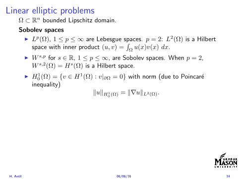
Linear elliptic problemsΩ sub Rn bounded Lipschitz domain
Sobolev spacesI Lp(Ω) 1 le p le infin are Lebesgue spaces p = 2 L2(Ω) is a Hilbert
space with inner product (u v) =int
Ωu(x)v(x) dx
I W sp for s isin R 1 le p le infin are Sobolev spaces When p = 2W s2(Ω) = Hs(Ω) is a Hilbert space
I H10 (Ω) = v isin H1(Ω) v|partΩ = 0 with norm (due to Poincare
inequality)uH1
0 (Ω) = nablauL2(Ω)
I H10 (Ω)lowast = Hminus1(Ω)
I Note L2(Ω) sub Hminus1(Ω)
Model problem
minusdiv (Anablau) = f in Ω
u = 0 on partΩ
H Antil 060616 14
Linear elliptic problemsΩ sub Rn bounded Lipschitz domain
Sobolev spacesI Lp(Ω) 1 le p le infin are Lebesgue spaces p = 2 L2(Ω) is a Hilbert
space with inner product (u v) =int
Ωu(x)v(x) dx
I W sp for s isin R 1 le p le infin are Sobolev spaces When p = 2W s2(Ω) = Hs(Ω) is a Hilbert space
I H10 (Ω) = v isin H1(Ω) v|partΩ = 0 with norm (due to Poincare
inequality)uH1
0 (Ω) = nablauL2(Ω)
I H10 (Ω)lowast = Hminus1(Ω)
I Note L2(Ω) sub Hminus1(Ω)
Model problem
minusdiv (Anablau) = f in Ω
u = 0 on partΩ
H Antil 060616 14
Linear elliptic problemsΩ sub Rn bounded Lipschitz domain
Sobolev spacesI Lp(Ω) 1 le p le infin are Lebesgue spaces p = 2 L2(Ω) is a Hilbert
space with inner product (u v) =int
Ωu(x)v(x) dx
I W sp for s isin R 1 le p le infin are Sobolev spaces When p = 2W s2(Ω) = Hs(Ω) is a Hilbert space
I H10 (Ω) = v isin H1(Ω) v|partΩ = 0 with norm (due to Poincare
inequality)uH1
0 (Ω) = nablauL2(Ω)
I H10 (Ω)lowast = Hminus1(Ω)
I Note L2(Ω) sub Hminus1(Ω)
Model problem
minusdiv (Anablau) = f in Ω
u = 0 on partΩ
H Antil 060616 14
Well-posed
I Weak solution Given f isin Hminus1(Ω) a function u isin H10 (Ω) is called
a weak solution iffintΩ
Anablau middot nablav = 〈f v〉minus11 forallv isin H10 (Ω)
where 〈middot middot〉minus11 denotes the Hminus1(Ω)ndashH1(Ω) duality pairing
I Existence and uniqueness For each f isin Hminus1(Ω) there exists aunique u isin H1
0 (Ω) such that
nablauL2(Ω) le CdΩfHminus1(Ω)
I A = I the result is due to the Riesz-representation theorem
I A 6= I (maybe non-symmetric) the result is due to Lax-Milgramlemma
I For general W 1p-spaces use inf-sup conditions combined withBanach-Necas theorem which is a necessary and sufficient condition
H Antil 060616 15
Linear-quadratic elliptic OCP
min J(u z) =1
2uminus ud2L2(Ω) +
λ
2z2L2(Ω)
subject to
minusdiv (Anablau) = z in Ω
u = 0 on partΩ
and the pointwise control constraints
z isin Zad = v isin L2(Ω) za(x) le v(x) le zb(x) ae x isin Ω
λ gt 0 is a parameter za zb isin Linfin(Ω) with za lt zb are given A isbounded symmetric positive
H Antil 060616 16
Reduced OCP
I Control to state map The solution operator defined as
S Hminus1(Ω)rarr H10 (Ω) z 7rarr u(z) = Sz
Note In view of the embedding
H10 (Ω) rarr L2(Ω) rarr Hminus1(Ω)
we may also consider S from L2(Ω) to L2(Ω) We will use the samenotation for this operator (for simplicity)
I Reduced cost functional The reduced cost functionalJ L2(Ω)rarr R is defined as
J (z) = J(Sz z)
I Reduced problem minzisinZadJ (z)
H Antil 060616 17
Reduced OCP
I Control to state map The solution operator defined as
S Hminus1(Ω)rarr H10 (Ω) z 7rarr u(z) = Sz
Note In view of the embedding
H10 (Ω) rarr L2(Ω) rarr Hminus1(Ω)
we may also consider S from L2(Ω) to L2(Ω) We will use the samenotation for this operator (for simplicity)
I Reduced cost functional The reduced cost functionalJ L2(Ω)rarr R is defined as
J (z) = J(Sz z)
I Reduced problem minzisinZadJ (z)
H Antil 060616 17
Reduced OCP
I Control to state map The solution operator defined as
S Hminus1(Ω)rarr H10 (Ω) z 7rarr u(z) = Sz
Note In view of the embedding
H10 (Ω) rarr L2(Ω) rarr Hminus1(Ω)
we may also consider S from L2(Ω) to L2(Ω) We will use the samenotation for this operator (for simplicity)
I Reduced cost functional The reduced cost functionalJ L2(Ω)rarr R is defined as
J (z) = J(Sz z)
I Reduced problem minzisinZadJ (z)
H Antil 060616 17
Existence of solution Direct methodThere exists a unique solution to the above problem
I Minimizing sequence J is bounded below by zero therefore thereexists a minimizing sequence znnisinN such that
limnrarrinfin
J (zn) = inf J (z)
I Weak compactness zn sub L2(Ω) is bounded Since L2(Ω) isreflexive therefore there exists a subsequence (not relabeled) suchthat
zn z and z isin Zad
where the latter is a consequence of Zad being closed and convex
I Optimality Since J is continuous and convex and therefore isweakly lower semicontinuous We obtain
lim inf J (zn) ge J (z)
which implies that z is optimal
I Uniqueness Exercise
H Antil 060616 18
Existence of solution Direct methodThere exists a unique solution to the above problem
I Minimizing sequence J is bounded below by zero therefore thereexists a minimizing sequence znnisinN such that
limnrarrinfin
J (zn) = inf J (z)
I Weak compactness zn sub L2(Ω) is bounded Since L2(Ω) isreflexive therefore there exists a subsequence (not relabeled) suchthat
zn z and z isin Zad
where the latter is a consequence of Zad being closed and convex
I Optimality Since J is continuous and convex and therefore isweakly lower semicontinuous We obtain
lim inf J (zn) ge J (z)
which implies that z is optimal
I Uniqueness Exercise
H Antil 060616 18
Existence of solution Direct methodThere exists a unique solution to the above problem
I Minimizing sequence J is bounded below by zero therefore thereexists a minimizing sequence znnisinN such that
limnrarrinfin
J (zn) = inf J (z)
I Weak compactness zn sub L2(Ω) is bounded Since L2(Ω) isreflexive therefore there exists a subsequence (not relabeled) suchthat
zn z and z isin Zad
where the latter is a consequence of Zad being closed and convex
I Optimality Since J is continuous and convex and therefore isweakly lower semicontinuous We obtain
lim inf J (zn) ge J (z)
which implies that z is optimal
I Uniqueness Exercise
H Antil 060616 18
Existence of solution Direct methodThere exists a unique solution to the above problem
I Minimizing sequence J is bounded below by zero therefore thereexists a minimizing sequence znnisinN such that
limnrarrinfin
J (zn) = inf J (z)
I Weak compactness zn sub L2(Ω) is bounded Since L2(Ω) isreflexive therefore there exists a subsequence (not relabeled) suchthat
zn z and z isin Zad
where the latter is a consequence of Zad being closed and convex
I Optimality Since J is continuous and convex and therefore isweakly lower semicontinuous We obtain
lim inf J (zn) ge J (z)
which implies that z is optimal
I Uniqueness Exercise
H Antil 060616 18
Outline
Motivation and examples
Linear elliptic optimal control problems
Differentiation in Banach spaces
First-order necessary conditions
Optimal control of semilinear PDEs
An abstract problem
Discretization using finite element methods
H Antil 060616 19
Differentiation in Banach spacesLet (Z middot Z) (V middot V ) B-spaces Z sub Z open and F Z rarr V
Let z isin Z
I If exist δF (z h) = limtdarr01t (F (z + th)minus F (z)) then δF (z h) is called
the directional derivative of F at z in direction h
I If exist δF (z h) forallh isin Z then h 7rarr δF (z h) is the first variation of Fat z
I Let exist the first variation δF (z middot) F is said to be Gateauxdifferentiable at z iff existA isin L(Z V ) such that δF (z h) = Ahforallh isin Z We write A = F primeG(z)
I F is said to be Frechet differentiable at z iff existA isin L(Z V ) and amapping r(z middot) Z rarr V such that for all h isin U with z + h isin Zwe have
F (z+h) = F (z)+Ah+r(z h) withr(z h)VhZ
rarr 0 as hZ rarr 0
We write F prime(z) = A
H Antil 060616 20
Differentiation in Banach spacesLet (Z middot Z) (V middot V ) B-spaces Z sub Z open and F Z rarr V
Let z isin Z
I If exist δF (z h) = limtdarr01t (F (z + th)minus F (z)) then δF (z h) is called
the directional derivative of F at z in direction h
I If exist δF (z h) forallh isin Z then h 7rarr δF (z h) is the first variation of Fat z
I Let exist the first variation δF (z middot) F is said to be Gateauxdifferentiable at z iff existA isin L(Z V ) such that δF (z h) = Ahforallh isin Z We write A = F primeG(z)
I F is said to be Frechet differentiable at z iff existA isin L(Z V ) and amapping r(z middot) Z rarr V such that for all h isin U with z + h isin Zwe have
F (z+h) = F (z)+Ah+r(z h) withr(z h)VhZ
rarr 0 as hZ rarr 0
We write F prime(z) = A
H Antil 060616 20
Differentiation in Banach spacesLet (Z middot Z) (V middot V ) B-spaces Z sub Z open and F Z rarr V
Let z isin Z
I If exist δF (z h) = limtdarr01t (F (z + th)minus F (z)) then δF (z h) is called
the directional derivative of F at z in direction h
I If exist δF (z h) forallh isin Z then h 7rarr δF (z h) is the first variation of Fat z
I Let exist the first variation δF (z middot) F is said to be Gateauxdifferentiable at z iff existA isin L(Z V ) such that δF (z h) = Ahforallh isin Z We write A = F primeG(z)
I F is said to be Frechet differentiable at z iff existA isin L(Z V ) and amapping r(z middot) Z rarr V such that for all h isin U with z + h isin Zwe have
F (z+h) = F (z)+Ah+r(z h) withr(z h)VhZ
rarr 0 as hZ rarr 0
We write F prime(z) = A
H Antil 060616 20
Differentiation in Banach spacesLet (Z middot Z) (V middot V ) B-spaces Z sub Z open and F Z rarr V
Let z isin Z
I If exist δF (z h) = limtdarr01t (F (z + th)minus F (z)) then δF (z h) is called
the directional derivative of F at z in direction h
I If exist δF (z h) forallh isin Z then h 7rarr δF (z h) is the first variation of Fat z
I Let exist the first variation δF (z middot) F is said to be Gateauxdifferentiable at z iff existA isin L(Z V ) such that δF (z h) = Ahforallh isin Z We write A = F primeG(z)
I F is said to be Frechet differentiable at z iff existA isin L(Z V ) and amapping r(z middot) Z rarr V such that for all h isin U with z + h isin Zwe have
F (z+h) = F (z)+Ah+r(z h) withr(z h)VhZ
rarr 0 as hZ rarr 0
We write F prime(z) = A
H Antil 060616 20
ExamplesExample 1 (H (middot middot)H) Hilbert space F (z) = z2H = (z z)H
forallz h F (z + h)minus F (z) = 2(z h)H + h2HThen
F prime(z)h = (2z h)H
Reisz representation theorem (identify H with Hlowast) we can write
F prime(z)h = (nablaF (z) h)H
where nablaF (z) = 2z is the gradient
Example 2 Let (Z (middot middot)Z) (H (middot middot)H) Hilbert spaces ud isin H fixedLet S isin L(ZH) Consider E Z rarr R
E(z) = Sz minus ud2H
Then E(z) = G(F (z)) where G(v) = v2H and F (z) = Sz minus ud
Eprime(z)h = Gprime(F (z))F prime(z)h = (2v F prime(z)h)H
= 2(Sz minus ud Sh)H = 2(Slowast(Sz minus ud) h)Z
we denote the gradient as nablaE(z) = 2Slowast(Sz minus ud)
H Antil 060616 21
ExamplesExample 1 (H (middot middot)H) Hilbert space F (z) = z2H = (z z)H
forallz h F (z + h)minus F (z) = 2(z h)H + h2HThen
F prime(z)h = (2z h)H
Reisz representation theorem (identify H with Hlowast) we can write
F prime(z)h = (nablaF (z) h)H
where nablaF (z) = 2z is the gradient
Example 2 Let (Z (middot middot)Z) (H (middot middot)H) Hilbert spaces ud isin H fixedLet S isin L(ZH) Consider E Z rarr R
E(z) = Sz minus ud2H
Then E(z) = G(F (z)) where G(v) = v2H and F (z) = Sz minus ud
Eprime(z)h = Gprime(F (z))F prime(z)h = (2v F prime(z)h)H
= 2(Sz minus ud Sh)H = 2(Slowast(Sz minus ud) h)Z
we denote the gradient as nablaE(z) = 2Slowast(Sz minus ud)H Antil 060616 21
Outline
Motivation and examples
Linear elliptic optimal control problems
Differentiation in Banach spaces
First-order necessary conditions
Optimal control of semilinear PDEs
An abstract problem
Discretization using finite element methods
H Antil 060616 22
First order necessary optimality conditions
Most of the theory is based on these two simple results
Theorem Let (Z middot Z) be a normed space J Z rarr (infin+infin] amapping with J 6equiv +infin Then z isin Z minimizer of J hArr 0 isin partJ (z)
Proof 0 isin partJ (z) means by definition of partJ (z) J (z)minus J (z) le 0forallz isin Z
Theorem Let (Z middot Z) be a normed space Zad sub Z nonemptyconvex closed J Z rarr R Gateaux differentiable where Zad sub Z sub ZZ open If z isin Zad is a solution to
minzisinZad
J (z)
then z solvesJ prime(z)(z minus z) ge 0 forallz isin Zad
Proof Exercise
H Antil 060616 23
First order necessary optimality conditions
Most of the theory is based on these two simple results
Theorem Let (Z middot Z) be a normed space J Z rarr (infin+infin] amapping with J 6equiv +infin Then z isin Z minimizer of J hArr 0 isin partJ (z)
Proof 0 isin partJ (z) means by definition of partJ (z) J (z)minus J (z) le 0forallz isin Z
Theorem Let (Z middot Z) be a normed space Zad sub Z nonemptyconvex closed J Z rarr R Gateaux differentiable where Zad sub Z sub ZZ open If z isin Zad is a solution to
minzisinZad
J (z)
then z solvesJ prime(z)(z minus z) ge 0 forallz isin Zad
Proof Exercise
H Antil 060616 23
Linear quadratic OCPI Reduced funcational
J (z) =1
2Sz minus ud2L2(Ω) +
λ
2z2L2(Ω)
I Gradient computation using sensitivity
J prime(z)h = (Slowast(Sz minus ud) + λz h)L2(Ω) forallh isin L2(Ω)
we denote the gradient by
nablaJ (z) = Slowast(Sz minus ud) + λz
I First order necessary and sufficient optimality condition
(nablaJ (z) z minus z)L2(Ω) ge 0 forallz isin Zad
I Adjoint equation Let p = Slowast(Sz minus ud) which translates intop isin H1
0 (Ω) solving
minusdiv (Anablap) = uminus ud in Ω
p = 0 on partΩ
I Gradient computation using adjoint nablaJ (z) = p+ λz
H Antil 060616 24
Linear quadratic OCPI Reduced funcational
J (z) =1
2Sz minus ud2L2(Ω) +
λ
2z2L2(Ω)
I Gradient computation using sensitivity
J prime(z)h = (Slowast(Sz minus ud) + λz h)L2(Ω) forallh isin L2(Ω)
we denote the gradient by
nablaJ (z) = Slowast(Sz minus ud) + λz
I First order necessary and sufficient optimality condition
(nablaJ (z) z minus z)L2(Ω) ge 0 forallz isin Zad
I Adjoint equation Let p = Slowast(Sz minus ud) which translates intop isin H1
0 (Ω) solving
minusdiv (Anablap) = uminus ud in Ω
p = 0 on partΩ
I Gradient computation using adjoint nablaJ (z) = p+ λz
H Antil 060616 24
Linear quadratic OCPI Reduced funcational
J (z) =1
2Sz minus ud2L2(Ω) +
λ
2z2L2(Ω)
I Gradient computation using sensitivity
J prime(z)h = (Slowast(Sz minus ud) + λz h)L2(Ω) forallh isin L2(Ω)
we denote the gradient by
nablaJ (z) = Slowast(Sz minus ud) + λz
I First order necessary and sufficient optimality condition
(nablaJ (z) z minus z)L2(Ω) ge 0 forallz isin Zad
I Adjoint equation Let p = Slowast(Sz minus ud) which translates intop isin H1
0 (Ω) solving
minusdiv (Anablap) = uminus ud in Ω
p = 0 on partΩ
I Gradient computation using adjoint nablaJ (z) = p+ λz
H Antil 060616 24
Linear quadratic OCPI Reduced funcational
J (z) =1
2Sz minus ud2L2(Ω) +
λ
2z2L2(Ω)
I Gradient computation using sensitivity
J prime(z)h = (Slowast(Sz minus ud) + λz h)L2(Ω) forallh isin L2(Ω)
we denote the gradient by
nablaJ (z) = Slowast(Sz minus ud) + λz
I First order necessary and sufficient optimality condition
(nablaJ (z) z minus z)L2(Ω) ge 0 forallz isin Zad
I Adjoint equation Let p = Slowast(Sz minus ud) which translates intop isin H1
0 (Ω) solving
minusdiv (Anablap) = uminus ud in Ω
p = 0 on partΩ
I Gradient computation using adjoint nablaJ (z) = p+ λz
H Antil 060616 24
Linear quadratic OCPI Reduced funcational
J (z) =1
2Sz minus ud2L2(Ω) +
λ
2z2L2(Ω)
I Gradient computation using sensitivity
J prime(z)h = (Slowast(Sz minus ud) + λz h)L2(Ω) forallh isin L2(Ω)
we denote the gradient by
nablaJ (z) = Slowast(Sz minus ud) + λz
I First order necessary and sufficient optimality condition
(nablaJ (z) z minus z)L2(Ω) ge 0 forallz isin Zad
I Adjoint equation Let p = Slowast(Sz minus ud) which translates intop isin H1
0 (Ω) solving
minusdiv (Anablap) = uminus ud in Ω
p = 0 on partΩ
I Gradient computation using adjoint nablaJ (z) = p+ λz
H Antil 060616 24
Optimality system
I State u isin H10 (Ω)
intΩAnablau middot nablav =
intΩzv forallv isin H1
0 (Ω)
I Adjoint p isin H10 (Ω)
intΩAnablap middot nablav =
intΩ
(uminus ud)v forallv isin H10 (Ω)
I Control z isin Zad (p+ λz z minus z) ge 0 forallz isin Zad
H Antil 060616 25
Pointwise interpretation
The variational inequality
(p+ λz z minus z) ge 0 forallz isin Zad
is equivalent to for ae x isin Ω
z(x) =
za(x) if p(x) + λz(x) gt 0isin [za(x) zb(x)] if p(x) + λz(x) = 0zb(x) if p(x) + λz(x) lt 0
Consequence
I When λ gt 0 then ae in Ω
z(x) = P[za(x)zb(x)]
minus 1
λp(x)
= min
zb(x)max
za(x)minus 1
λp(x)
H Antil 060616 26
Formal Lagrange method applied to linear OCPIntroduce L H1
0 (Ω)times Zad timesH1(Ω)rarr R defined as
L(u z p) = J(u z)minusint
Ω
(minusdiv (Anablau)minus z
)p dx
Integrate by parts to arrive at
L(u z p) = J(u z)minusint
Ω
(minusdiv (Anablap)uminus zp
)dx+
intpartΩ
(Anablau)p ds
If (u z p) is a stationary point then
I State
DpL(u z p)h = 0 forallh isin H1(Ω)
I AdjointDuL(u z p)h = 0 forallh isin H1
0 (Ω)
I ControlDzL(u z p)(z minus z) ge 0 forallz isin Zad
H Antil 060616 27
Formal Lagrange method applied to linear OCPIntroduce L H1
0 (Ω)times Zad timesH1(Ω)rarr R defined as
L(u z p) = J(u z)minusint
Ω
(minusdiv (Anablau)minus z
)p dx
Integrate by parts to arrive at
L(u z p) = J(u z)minusint
Ω
(minusdiv (Anablap)uminus zp
)dx+
intpartΩ
(Anablau)p ds
If (u z p) is a stationary point then
I State
DpL(u z p)h = 0 forallh isin H1(Ω)
I AdjointDuL(u z p)h = 0 forallh isin H1
0 (Ω)
I ControlDzL(u z p)(z minus z) ge 0 forallz isin Zad
H Antil 060616 27
Formal Lagrange method applied to linear OCPIntroduce L H1
0 (Ω)times Zad timesH1(Ω)rarr R defined as
L(u z p) = J(u z)minusint
Ω
(minusdiv (Anablau)minus z
)p dx
Integrate by parts to arrive at
L(u z p) = J(u z)minusint
Ω
(minusdiv (Anablap)uminus zp
)dx+
intpartΩ
(Anablau)p ds
If (u z p) is a stationary point then
I State
DpL(u z p)h = 0 forallh isin H1(Ω)
I AdjointDuL(u z p)h = 0 forallh isin H1
0 (Ω)
I ControlDzL(u z p)(z minus z) ge 0 forallz isin Zad
H Antil 060616 27
Formal Lagrange method applied to linear OCPIntroduce L H1
0 (Ω)times Zad timesH1(Ω)rarr R defined as
L(u z p) = J(u z)minusint
Ω
(minusdiv (Anablau)minus z
)p dx
Integrate by parts to arrive at
L(u z p) = J(u z)minusint
Ω
(minusdiv (Anablap)uminus zp
)dx+
intpartΩ
(Anablau)p ds
If (u z p) is a stationary point then
I State
DpL(u z p)h = 0 forallh isin H1(Ω)
I AdjointDuL(u z p)h = 0 forallh isin H1
0 (Ω)
I ControlDzL(u z p)(z minus z) ge 0 forallz isin Zad
H Antil 060616 27
Formal Lagrange method applied to linear OCPIntroduce L H1
0 (Ω)times Zad timesH1(Ω)rarr R defined as
L(u z p) = J(u z)minusint
Ω
(minusdiv (Anablau)minus z
)p dx
Integrate by parts to arrive at
L(u z p) = J(u z)minusint
Ω
(minusdiv (Anablap)uminus zp
)dx+
intpartΩ
(Anablau)p ds
If (u z p) is a stationary point then
I State
DpL(u z p)h = 0 forallh isin H1(Ω)
I AdjointDuL(u z p)h = 0 forallh isin H1
0 (Ω)
I ControlDzL(u z p)(z minus z) ge 0 forallz isin Zad
H Antil 060616 27
Outline
Motivation and examples
Linear elliptic optimal control problems
Differentiation in Banach spaces
First-order necessary conditions
Optimal control of semilinear PDEs
An abstract problem
Discretization using finite element methods
H Antil 060616 28
Semilinear elliptic OCP
min J(u z) =1
2uminus ud2L2(Ω) +
λ
2z2L2(Ω)
subject to
minus∆u+ g(x u) = z in Ω
u = 0 on partΩ
and z isin Zad with za zb isin Linfin(Ω)
H Antil 060616 29
State space(A1) Ω sub Rd open bounded partΩ is Lipschitz
(A2) g Ωtimes Rrarr R is bounded and measurable with respect to x isin Ωfor every u isin R
(A3) g is continuous monotone increasing and Lipschitz continuous in ufor ae x isin Ω
(A4) g(x 0) = 0 for ae x isin Ω (not really necessary)
Theorem Suppose (A1)minus (A4) hold For every z isin Lr(Ω) withr gt d2 the state equation has a unique weak solutionu isin H1
0 (Ω) cap C(Ω) ie we haveintΩ
nablau middot nablav dx+
intΩ
g(x u(x))v(x) dx =
intΩ
zv dx forallv isin H10 (Ω)
Moreover there exists a constant C gt 0 such that
uH1(Ω) + uC(Ω) le CzLr(Ω)
RemarkI The proof of the theorem uses the BrowderndashMinty theorem on
monotone operators
H Antil 060616 30
State space(A1) Ω sub Rd open bounded partΩ is Lipschitz
(A2) g Ωtimes Rrarr R is bounded and measurable with respect to x isin Ωfor every u isin R
(A3) g is continuous monotone increasing and Lipschitz continuous in ufor ae x isin Ω
(A4) g(x 0) = 0 for ae x isin Ω (not really necessary)
Theorem Suppose (A1)minus (A4) hold For every z isin Lr(Ω) withr gt d2 the state equation has a unique weak solutionu isin H1
0 (Ω) cap C(Ω) ie we haveintΩ
nablau middot nablav dx+
intΩ
g(x u(x))v(x) dx =
intΩ
zv dx forallv isin H10 (Ω)
Moreover there exists a constant C gt 0 such that
uH1(Ω) + uC(Ω) le CzLr(Ω)
RemarkI The proof of the theorem uses the BrowderndashMinty theorem on
monotone operators
H Antil 060616 30
State space(A1) Ω sub Rd open bounded partΩ is Lipschitz
(A2) g Ωtimes Rrarr R is bounded and measurable with respect to x isin Ωfor every u isin R
(A3) g is continuous monotone increasing and Lipschitz continuous in ufor ae x isin Ω
(A4) g(x 0) = 0 for ae x isin Ω (not really necessary)
Theorem Suppose (A1)minus (A4) hold For every z isin Lr(Ω) withr gt d2 the state equation has a unique weak solutionu isin H1
0 (Ω) cap C(Ω) ie we haveintΩ
nablau middot nablav dx+
intΩ
g(x u(x))v(x) dx =
intΩ
zv dx forallv isin H10 (Ω)
Moreover there exists a constant C gt 0 such that
uH1(Ω) + uC(Ω) le CzLr(Ω)
RemarkI The proof of the theorem uses the BrowderndashMinty theorem on
monotone operators
H Antil 060616 30
Control-to-state map and reduced problem
I Control to state map
S Linfin(Ω)rarr H10 (Ω) cap C(Ω)
is well defined and is globally Lipschitz continuous
I Reduced problem
minJ (z) =1
2S(u)minus ud2L2(Ω) +
λ
2z2L2(Ω)
H Antil 060616 31
Control-to-state map and reduced problem
I Control to state map
S Linfin(Ω)rarr H10 (Ω) cap C(Ω)
is well defined and is globally Lipschitz continuous
I Reduced problem
minJ (z) =1
2S(u)minus ud2L2(Ω) +
λ
2z2L2(Ω)
H Antil 060616 31
First-order necessary conditionsI Lagrangian functional
L(u z p) = J(u z)minusint
Ω
(minus∆u+ g(x u(x))minus z
)p dx
= J(u z)minusint
Ω
(nablau middot nablap+ g(x u(x))pminus zp
)dx
I Adjoint system For all h isin H10 (Ω)
0 = DuL(u z p)h =
intΩ
(uminus ud)h dxminusint
Ω
(nablah middot nablap+ gu(x u(x))ph
)which yields
minus∆p+ gu(x u(x))p = uminus ud in Ω
p = 0 on partΩ
I Control
DzL(u z p)(z minus z) = (p+ λz z minus z) dx ge 0 forallz isin ZadI Gradient
nablaJ (z) = p+ λz
H Antil 060616 32
First-order necessary conditionsI Lagrangian functional
L(u z p) = J(u z)minusint
Ω
(minus∆u+ g(x u(x))minus z
)p dx
= J(u z)minusint
Ω
(nablau middot nablap+ g(x u(x))pminus zp
)dx
I Adjoint system For all h isin H10 (Ω)
0 = DuL(u z p)h =
intΩ
(uminus ud)h dxminusint
Ω
(nablah middot nablap+ gu(x u(x))ph
)which yields
minus∆p+ gu(x u(x))p = uminus ud in Ω
p = 0 on partΩ
I Control
DzL(u z p)(z minus z) = (p+ λz z minus z) dx ge 0 forallz isin ZadI Gradient
nablaJ (z) = p+ λz
H Antil 060616 32
First-order necessary conditionsI Lagrangian functional
L(u z p) = J(u z)minusint
Ω
(minus∆u+ g(x u(x))minus z
)p dx
= J(u z)minusint
Ω
(nablau middot nablap+ g(x u(x))pminus zp
)dx
I Adjoint system For all h isin H10 (Ω)
0 = DuL(u z p)h =
intΩ
(uminus ud)h dxminusint
Ω
(nablah middot nablap+ gu(x u(x))ph
)which yields
minus∆p+ gu(x u(x))p = uminus ud in Ω
p = 0 on partΩ
I Control
DzL(u z p)(z minus z) = (p+ λz z minus z) dx ge 0 forallz isin Zad
I GradientnablaJ (z) = p+ λz
H Antil 060616 32
First-order necessary conditionsI Lagrangian functional
L(u z p) = J(u z)minusint
Ω
(minus∆u+ g(x u(x))minus z
)p dx
= J(u z)minusint
Ω
(nablau middot nablap+ g(x u(x))pminus zp
)dx
I Adjoint system For all h isin H10 (Ω)
0 = DuL(u z p)h =
intΩ
(uminus ud)h dxminusint
Ω
(nablah middot nablap+ gu(x u(x))ph
)which yields
minus∆p+ gu(x u(x))p = uminus ud in Ω
p = 0 on partΩ
I Control
DzL(u z p)(z minus z) = (p+ λz z minus z) dx ge 0 forallz isin ZadI Gradient
nablaJ (z) = p+ λz
H Antil 060616 32
Differentiability of Nemytskii operator
The rigorous proof uses
Theorem In addition to (A1)-(A4) if
(A5) g is continuously differentiable with respect to u for ae x isin Ωand we have
(i) |gu(x 0)| le K for ae x isin Ω(ii) gu is locally Lipschitz with respect to u isin R
then the Nemytskii operator G u 7rarr g(middot u(middot)) is continuously Frechetdifferentiable from Linfin(Ω) into itself and
(Gprime(u)h)(x) = gu(x u(x))h(x) ae in Ω forallh isin Linfin(Ω)
Remark (A5) holds if g(x u) = g(u) and g isin C2(R)
H Antil 060616 33
Outline
Motivation and examples
Linear elliptic optimal control problems
Differentiation in Banach spaces
First-order necessary conditions
Optimal control of semilinear PDEs
An abstract problem
Discretization using finite element methods
H Antil 060616 34
Gradient computation via adjoint general formI Abstract problem
min J(u z)
subject toc(u z) = 0
and z isin Zad
I Directional derivative Let S be the control to state map(nonlinear in general)
z 7rarr S(z) = u(z)
Under the assumptions of ldquoimplicit function theoremrdquo
J prime(z)h = (nablauJ (u(z) z) Sprime(z)h) + (nablazJ (u(z) z) h)
I Sensitivity of u with respect to z Differentiating the stateequation
cu(S(z) z)Sprime(z)h = minuscz(S(z) z)h
leads toSprime(z)h = minuscu(S(z) z)minus1
(cz(S(z) z)h
)
provided cu(S(z) z)minus1 is well-defined
H Antil 060616 35
Gradient computation via adjoint general formI Abstract problem
min J(u z)
subject toc(u z) = 0
and z isin ZadI Directional derivative Let S be the control to state map
(nonlinear in general)
z 7rarr S(z) = u(z)
Under the assumptions of ldquoimplicit function theoremrdquo
J prime(z)h = (nablauJ (u(z) z) Sprime(z)h) + (nablazJ (u(z) z) h)
I Sensitivity of u with respect to z Differentiating the stateequation
cu(S(z) z)Sprime(z)h = minuscz(S(z) z)h
leads toSprime(z)h = minuscu(S(z) z)minus1
(cz(S(z) z)h
)
provided cu(S(z) z)minus1 is well-defined
H Antil 060616 35
Gradient computation via adjoint general formI Abstract problem
min J(u z)
subject toc(u z) = 0
and z isin ZadI Directional derivative Let S be the control to state map
(nonlinear in general)
z 7rarr S(z) = u(z)
Under the assumptions of ldquoimplicit function theoremrdquo
J prime(z)h = (nablauJ (u(z) z) Sprime(z)h) + (nablazJ (u(z) z) h)
I Sensitivity of u with respect to z Differentiating the stateequation
cu(S(z) z)Sprime(z)h = minuscz(S(z) z)h
leads toSprime(z)h = minuscu(S(z) z)minus1
(cz(S(z) z)h
)
provided cu(S(z) z)minus1 is well-defined
H Antil 060616 35
Adjoint equation and gradient general form
I Directional derivative
J prime(z)h = minus(nablauJ (u(z) z) cu(u(z) z)minus1cz(u(z) z)h
)+ (nablazJ (u(z) z) h)
I Gradient
nablaJ (z) = minuscz(u(z) z)lowast(cu(u(z) z)minuslowastnablauJ (u(z) z)
)+nablazJ (u(z) z)
I Introducing adjoint variable p solving
cu(u(z) z)lowastp = nablauJ (u(z) z)
we arrive at following form of gradient
nablaJ (z) = minuscz(u(z) z)lowastp+nablazJ (u(z) z)
which is tractable
H Antil 060616 36
Adjoint equation and gradient general form
I Directional derivative
J prime(z)h = minus(nablauJ (u(z) z) cu(u(z) z)minus1cz(u(z) z)h
)+ (nablazJ (u(z) z) h)
I Gradient
nablaJ (z) = minuscz(u(z) z)lowast(cu(u(z) z)minuslowastnablauJ (u(z) z)
)+nablazJ (u(z) z)
I Introducing adjoint variable p solving
cu(u(z) z)lowastp = nablauJ (u(z) z)
we arrive at following form of gradient
nablaJ (z) = minuscz(u(z) z)lowastp+nablazJ (u(z) z)
which is tractable
H Antil 060616 36
Adjoint equation and gradient general form
I Directional derivative
J prime(z)h = minus(nablauJ (u(z) z) cu(u(z) z)minus1cz(u(z) z)h
)+ (nablazJ (u(z) z) h)
I Gradient
nablaJ (z) = minuscz(u(z) z)lowast(cu(u(z) z)minuslowastnablauJ (u(z) z)
)+nablazJ (u(z) z)
I Introducing adjoint variable p solving
cu(u(z) z)lowastp = nablauJ (u(z) z)
we arrive at following form of gradient
nablaJ (z) = minuscz(u(z) z)lowastp+nablazJ (u(z) z)
which is tractable
H Antil 060616 36
Hessian computation general form
I Lagrangian L(u z p) = J(u z)minusint
Ωc(u z)p dx Then we have
DzJ (z)h = DzL(u z p)h
I Second order derivative
D2zJ (z)[h1 h2] = DuDzL(u z p)[h1 S
prime(z)h2] +D2zL(u z p)[h1 h2]
+DpDzL(u z p)[h1 Dzp(z)h2]
I We already know Sprime(z)h2 moreover
DpDzL(u z p)[h1 Dzp(z)h2] = minus(cu(u z)h1 Dzp(z)h2
)
It remain to identify Dzp(z)h2
H Antil 060616 37
Hessian computation general form
I Lagrangian L(u z p) = J(u z)minusint
Ωc(u z)p dx Then we have
DzJ (z)h = DzL(u z p)h
I Second order derivative
D2zJ (z)[h1 h2] = DuDzL(u z p)[h1 S
prime(z)h2] +D2zL(u z p)[h1 h2]
+DpDzL(u z p)[h1 Dzp(z)h2]
I We already know Sprime(z)h2 moreover
DpDzL(u z p)[h1 Dzp(z)h2] = minus(cu(u z)h1 Dzp(z)h2
)
It remain to identify Dzp(z)h2
H Antil 060616 37
Hessian computation general form
I Lagrangian L(u z p) = J(u z)minusint
Ωc(u z)p dx Then we have
DzJ (z)h = DzL(u z p)h
I Second order derivative
D2zJ (z)[h1 h2] = DuDzL(u z p)[h1 S
prime(z)h2] +D2zL(u z p)[h1 h2]
+DpDzL(u z p)[h1 Dzp(z)h2]
I We already know Sprime(z)h2 moreover
DpDzL(u z p)[h1 Dzp(z)h2] = minus(cu(u z)h1 Dzp(z)h2
)
It remain to identify Dzp(z)h2
H Antil 060616 37
Outline
Motivation and examples
Linear elliptic optimal control problems
Differentiation in Banach spaces
First-order necessary conditions
Optimal control of semilinear PDEs
An abstract problem
Discretization using finite element methods
H Antil 060616 38
Numerical approximation of Poisson equation MeshTo avoid technical issues we will assume that partΩ is polygonal
I Mesh Let T = K be a mesh of Ω where K sub Rd is an elementthat is isoparametrically equivalent to a unit simplex in Rd
I Conforming mesh We say that the mesh is conforming ifI Ω = cupKisinT KI If K1 cap K2 = x then x is a node of K1 and K2I If K1 cap K2 6= empty and K1 cap K2 6= x then K1 cap K2 is an edgeface
contained in partK1 cap partK2
I Shape regular Let T be the collection of all conformingrefinements of an original mesh T 0 Then T is called shape regularif exist κ gt 0 such that
hKρKle κ forallK isin cupiT i
where hK = diam K ρK = maxρ gt 0|Bρ sub KI Quasi-uniform A family of shape regular meshes is called-quasi
uniform if there exist a constant σ gt 0 such that
maxhKminhK
le σ
uniformly for all meshes in the family
Numerical approximation of Poisson equation MeshTo avoid technical issues we will assume that partΩ is polygonal
I Mesh Let T = K be a mesh of Ω where K sub Rd is an elementthat is isoparametrically equivalent to a unit simplex in Rd
I Conforming mesh We say that the mesh is conforming ifI Ω = cupKisinT KI If K1 cap K2 = x then x is a node of K1 and K2I If K1 cap K2 6= empty and K1 cap K2 6= x then K1 cap K2 is an edgeface
contained in partK1 cap partK2
I Shape regular Let T be the collection of all conformingrefinements of an original mesh T 0 Then T is called shape regularif exist κ gt 0 such that
hKρKle κ forallK isin cupiT i
where hK = diam K ρK = maxρ gt 0|Bρ sub KI Quasi-uniform A family of shape regular meshes is called-quasi
uniform if there exist a constant σ gt 0 such that
maxhKminhK
le σ
uniformly for all meshes in the family
Numerical approximation of Poisson equation MeshTo avoid technical issues we will assume that partΩ is polygonal
I Mesh Let T = K be a mesh of Ω where K sub Rd is an elementthat is isoparametrically equivalent to a unit simplex in Rd
I Conforming mesh We say that the mesh is conforming ifI Ω = cupKisinT KI If K1 cap K2 = x then x is a node of K1 and K2I If K1 cap K2 6= empty and K1 cap K2 6= x then K1 cap K2 is an edgeface
contained in partK1 cap partK2
I Shape regular Let T be the collection of all conformingrefinements of an original mesh T 0 Then T is called shape regularif exist κ gt 0 such that
hKρKle κ forallK isin cupiT i
where hK = diam K ρK = maxρ gt 0|Bρ sub K
I Quasi-uniform A family of shape regular meshes is called-quasiuniform if there exist a constant σ gt 0 such that
maxhKminhK
le σ
uniformly for all meshes in the family
Numerical approximation of Poisson equation MeshTo avoid technical issues we will assume that partΩ is polygonal
I Mesh Let T = K be a mesh of Ω where K sub Rd is an elementthat is isoparametrically equivalent to a unit simplex in Rd
I Conforming mesh We say that the mesh is conforming ifI Ω = cupKisinT KI If K1 cap K2 = x then x is a node of K1 and K2I If K1 cap K2 6= empty and K1 cap K2 6= x then K1 cap K2 is an edgeface
contained in partK1 cap partK2
I Shape regular Let T be the collection of all conformingrefinements of an original mesh T 0 Then T is called shape regularif exist κ gt 0 such that
hKρKle κ forallK isin cupiT i
where hK = diam K ρK = maxρ gt 0|Bρ sub KI Quasi-uniform A family of shape regular meshes is called-quasi
uniform if there exist a constant σ gt 0 such that
maxhKminhK
le σ
uniformly for all meshes in the family
FE space and Galerkin approximationI Finite element space For T isin T we define the finite element
space as
V(T ) = W isin C0(Ω) WK isin P1forallK isin T W |partΩ = 0
where P1 is the set of polynomials of degree at most 1
I Galerkin approximation of continuous problem is given by
Find UT isin V(T )
intΩ
AnablaUT middot nablaV = 〈f V 〉 forallV isin V(T )
The discrete problem is well-posedI Nodal basis Consists of functions ψi isin V(T ) with xi isin N (T )
satisfyingψxi
(xj) = δij
where N (T ) denotes the interior (plus Neumann) nodesI Galerkin orthogonality(
nabla(uminus UT )nablaW)L2(Ω)
= 0 forallW isin V(T )
H Antil 060616 40
FE space and Galerkin approximationI Finite element space For T isin T we define the finite element
space as
V(T ) = W isin C0(Ω) WK isin P1forallK isin T W |partΩ = 0
where P1 is the set of polynomials of degree at most 1I Galerkin approximation of continuous problem is given by
Find UT isin V(T )
intΩ
AnablaUT middot nablaV = 〈f V 〉 forallV isin V(T )
The discrete problem is well-posed
I Nodal basis Consists of functions ψi isin V(T ) with xi isin N (T )satisfying
ψxi(xj) = δij
where N (T ) denotes the interior (plus Neumann) nodesI Galerkin orthogonality(
nabla(uminus UT )nablaW)L2(Ω)
= 0 forallW isin V(T )
H Antil 060616 40
FE space and Galerkin approximationI Finite element space For T isin T we define the finite element
space as
V(T ) = W isin C0(Ω) WK isin P1forallK isin T W |partΩ = 0
where P1 is the set of polynomials of degree at most 1I Galerkin approximation of continuous problem is given by
Find UT isin V(T )
intΩ
AnablaUT middot nablaV = 〈f V 〉 forallV isin V(T )
The discrete problem is well-posedI Nodal basis Consists of functions ψi isin V(T ) with xi isin N (T )
satisfyingψxi
(xj) = δij
where N (T ) denotes the interior (plus Neumann) nodes
I Galerkin orthogonality(nabla(uminus UT )nablaW
)L2(Ω)
= 0 forallW isin V(T )
H Antil 060616 40
FE space and Galerkin approximationI Finite element space For T isin T we define the finite element
space as
V(T ) = W isin C0(Ω) WK isin P1forallK isin T W |partΩ = 0
where P1 is the set of polynomials of degree at most 1I Galerkin approximation of continuous problem is given by
Find UT isin V(T )
intΩ
AnablaUT middot nablaV = 〈f V 〉 forallV isin V(T )
The discrete problem is well-posedI Nodal basis Consists of functions ψi isin V(T ) with xi isin N (T )
satisfyingψxi
(xj) = δij
where N (T ) denotes the interior (plus Neumann) nodesI Galerkin orthogonality(
nabla(uminus UT )nablaW)L2(Ω)
= 0 forallW isin V(T )
H Antil 060616 40
Best approximation
I Cearsquos lemma
nabla(uminus UT )L2(Ω) le C infWisinV(T )
nabla(uminusW )L2(Ω)
I Nodal interpolation operator ΠT C(Ω)rarr V(T ) satisfies
ΠT u(xi) = u(xi) forallxi isin N (T )
and is defined as
ΠT u =sum
xiisinN (T )
u(xi)ψxi
I Error estimates In Cearsquos lemma replace W by ΠT u and thencompute the interpolation error
H Antil 060616 41
Best approximation
I Cearsquos lemma
nabla(uminus UT )L2(Ω) le C infWisinV(T )
nabla(uminusW )L2(Ω)
I Nodal interpolation operator ΠT C(Ω)rarr V(T ) satisfies
ΠT u(xi) = u(xi) forallxi isin N (T )
and is defined as
ΠT u =sum
xiisinN (T )
u(xi)ψxi
I Error estimates In Cearsquos lemma replace W by ΠT u and thencompute the interpolation error
H Antil 060616 41
Best approximation
I Cearsquos lemma
nabla(uminus UT )L2(Ω) le C infWisinV(T )
nabla(uminusW )L2(Ω)
I Nodal interpolation operator ΠT C(Ω)rarr V(T ) satisfies
ΠT u(xi) = u(xi) forallxi isin N (T )
and is defined as
ΠT u =sum
xiisinN (T )
u(xi)ψxi
I Error estimates In Cearsquos lemma replace W by ΠT u and thencompute the interpolation error
H Antil 060616 41
Algebraic system state equation
I Recall UT isin V(T ) solves
a(UT V ) = 〈f V 〉 forallV isin V(T )
I Now setting UT =sumN
j=1 Ujψj V = ψi we get
Nsumj=1
Uja(φj φi) = 〈f ψi〉 i = 1 N
which is the matrix-vector system
AU = F
I Stiffness matrix A is SPD
H Antil 060616 42
Algebraic system state equation
I Recall UT isin V(T ) solves
a(UT V ) = 〈f V 〉 forallV isin V(T )
I Now setting UT =sumN
j=1 Ujψj V = ψi we get
Nsumj=1
Uja(φj φi) = 〈f ψi〉 i = 1 N
which is the matrix-vector system
AU = F
I Stiffness matrix A is SPD
H Antil 060616 42
Algebraic system state equation
I Recall UT isin V(T ) solves
a(UT V ) = 〈f V 〉 forallV isin V(T )
I Now setting UT =sumN
j=1 Ujψj V = ψi we get
Nsumj=1
Uja(φj φi) = 〈f ψi〉 i = 1 N
which is the matrix-vector system
AU = F
I Stiffness matrix A is SPD
H Antil 060616 42
Discrete linear elliptic OCP
min JT (UT ZT ) =1
2UT minus ud2L2(Ω) +
λ
2ZT 2L2(Ω)
subject to
Find UT isin V(T )
intΩ
nablaUT middot nablaV = (ZT V )L2(Ω) forallV isin V(T )
and whereZT isin Zad(T ) = Zad cap Z(T )
is either one of these
Z(T ) =
V(T )L2(Ω) variational discretization (Hinze)WT isin Linfin(Ω) ZT |K isin P0(K)K isin T
H Antil 060616 43
Recent books
F TroltzschOptimal control of partial differential equations volume 112 ofGraduate Studies in MathematicsAmerican Mathematical Society Providence RI 2010Theory methods and applications Translated from the 2005 Germanoriginal by Jurgen Sprekels
K Ito and K KunischLagrange multiplier approach to variational problems andapplications volume 15 of Advances in Design and ControlSociety for Industrial and Applied Mathematics (SIAM)Philadelphia PA 2008
H Antil 060616 44
- Motivation and examples
- Linear elliptic optimal control problems
- Differentiation in Banach spaces
- First-order necessary conditions
- Optimal control of semilinear PDEs
- An abstract problem
- Discretization using finite element methods
-
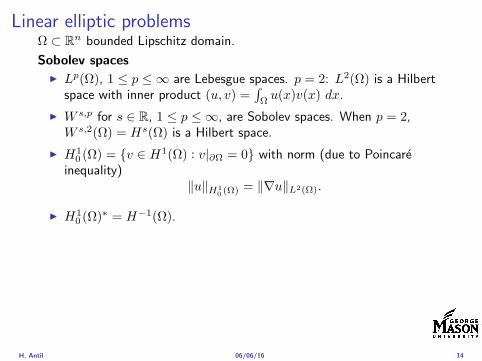
Linear elliptic problemsΩ sub Rn bounded Lipschitz domain
Sobolev spacesI Lp(Ω) 1 le p le infin are Lebesgue spaces p = 2 L2(Ω) is a Hilbert
space with inner product (u v) =int
Ωu(x)v(x) dx
I W sp for s isin R 1 le p le infin are Sobolev spaces When p = 2W s2(Ω) = Hs(Ω) is a Hilbert space
I H10 (Ω) = v isin H1(Ω) v|partΩ = 0 with norm (due to Poincare
inequality)uH1
0 (Ω) = nablauL2(Ω)
I H10 (Ω)lowast = Hminus1(Ω)
I Note L2(Ω) sub Hminus1(Ω)
Model problem
minusdiv (Anablau) = f in Ω
u = 0 on partΩ
H Antil 060616 14
Linear elliptic problemsΩ sub Rn bounded Lipschitz domain
Sobolev spacesI Lp(Ω) 1 le p le infin are Lebesgue spaces p = 2 L2(Ω) is a Hilbert
space with inner product (u v) =int
Ωu(x)v(x) dx
I W sp for s isin R 1 le p le infin are Sobolev spaces When p = 2W s2(Ω) = Hs(Ω) is a Hilbert space
I H10 (Ω) = v isin H1(Ω) v|partΩ = 0 with norm (due to Poincare
inequality)uH1
0 (Ω) = nablauL2(Ω)
I H10 (Ω)lowast = Hminus1(Ω)
I Note L2(Ω) sub Hminus1(Ω)
Model problem
minusdiv (Anablau) = f in Ω
u = 0 on partΩ
H Antil 060616 14
Well-posed
I Weak solution Given f isin Hminus1(Ω) a function u isin H10 (Ω) is called
a weak solution iffintΩ
Anablau middot nablav = 〈f v〉minus11 forallv isin H10 (Ω)
where 〈middot middot〉minus11 denotes the Hminus1(Ω)ndashH1(Ω) duality pairing
I Existence and uniqueness For each f isin Hminus1(Ω) there exists aunique u isin H1
0 (Ω) such that
nablauL2(Ω) le CdΩfHminus1(Ω)
I A = I the result is due to the Riesz-representation theorem
I A 6= I (maybe non-symmetric) the result is due to Lax-Milgramlemma
I For general W 1p-spaces use inf-sup conditions combined withBanach-Necas theorem which is a necessary and sufficient condition
H Antil 060616 15
Linear-quadratic elliptic OCP
min J(u z) =1
2uminus ud2L2(Ω) +
λ
2z2L2(Ω)
subject to
minusdiv (Anablau) = z in Ω
u = 0 on partΩ
and the pointwise control constraints
z isin Zad = v isin L2(Ω) za(x) le v(x) le zb(x) ae x isin Ω
λ gt 0 is a parameter za zb isin Linfin(Ω) with za lt zb are given A isbounded symmetric positive
H Antil 060616 16
Reduced OCP
I Control to state map The solution operator defined as
S Hminus1(Ω)rarr H10 (Ω) z 7rarr u(z) = Sz
Note In view of the embedding
H10 (Ω) rarr L2(Ω) rarr Hminus1(Ω)
we may also consider S from L2(Ω) to L2(Ω) We will use the samenotation for this operator (for simplicity)
I Reduced cost functional The reduced cost functionalJ L2(Ω)rarr R is defined as
J (z) = J(Sz z)
I Reduced problem minzisinZadJ (z)
H Antil 060616 17
Reduced OCP
I Control to state map The solution operator defined as
S Hminus1(Ω)rarr H10 (Ω) z 7rarr u(z) = Sz
Note In view of the embedding
H10 (Ω) rarr L2(Ω) rarr Hminus1(Ω)
we may also consider S from L2(Ω) to L2(Ω) We will use the samenotation for this operator (for simplicity)
I Reduced cost functional The reduced cost functionalJ L2(Ω)rarr R is defined as
J (z) = J(Sz z)
I Reduced problem minzisinZadJ (z)
H Antil 060616 17
Reduced OCP
I Control to state map The solution operator defined as
S Hminus1(Ω)rarr H10 (Ω) z 7rarr u(z) = Sz
Note In view of the embedding
H10 (Ω) rarr L2(Ω) rarr Hminus1(Ω)
we may also consider S from L2(Ω) to L2(Ω) We will use the samenotation for this operator (for simplicity)
I Reduced cost functional The reduced cost functionalJ L2(Ω)rarr R is defined as
J (z) = J(Sz z)
I Reduced problem minzisinZadJ (z)
H Antil 060616 17
Existence of solution Direct methodThere exists a unique solution to the above problem
I Minimizing sequence J is bounded below by zero therefore thereexists a minimizing sequence znnisinN such that
limnrarrinfin
J (zn) = inf J (z)
I Weak compactness zn sub L2(Ω) is bounded Since L2(Ω) isreflexive therefore there exists a subsequence (not relabeled) suchthat
zn z and z isin Zad
where the latter is a consequence of Zad being closed and convex
I Optimality Since J is continuous and convex and therefore isweakly lower semicontinuous We obtain
lim inf J (zn) ge J (z)
which implies that z is optimal
I Uniqueness Exercise
H Antil 060616 18
Existence of solution Direct methodThere exists a unique solution to the above problem
I Minimizing sequence J is bounded below by zero therefore thereexists a minimizing sequence znnisinN such that
limnrarrinfin
J (zn) = inf J (z)
I Weak compactness zn sub L2(Ω) is bounded Since L2(Ω) isreflexive therefore there exists a subsequence (not relabeled) suchthat
zn z and z isin Zad
where the latter is a consequence of Zad being closed and convex
I Optimality Since J is continuous and convex and therefore isweakly lower semicontinuous We obtain
lim inf J (zn) ge J (z)
which implies that z is optimal
I Uniqueness Exercise
H Antil 060616 18
Existence of solution Direct methodThere exists a unique solution to the above problem
I Minimizing sequence J is bounded below by zero therefore thereexists a minimizing sequence znnisinN such that
limnrarrinfin
J (zn) = inf J (z)
I Weak compactness zn sub L2(Ω) is bounded Since L2(Ω) isreflexive therefore there exists a subsequence (not relabeled) suchthat
zn z and z isin Zad
where the latter is a consequence of Zad being closed and convex
I Optimality Since J is continuous and convex and therefore isweakly lower semicontinuous We obtain
lim inf J (zn) ge J (z)
which implies that z is optimal
I Uniqueness Exercise
H Antil 060616 18
Existence of solution Direct methodThere exists a unique solution to the above problem
I Minimizing sequence J is bounded below by zero therefore thereexists a minimizing sequence znnisinN such that
limnrarrinfin
J (zn) = inf J (z)
I Weak compactness zn sub L2(Ω) is bounded Since L2(Ω) isreflexive therefore there exists a subsequence (not relabeled) suchthat
zn z and z isin Zad
where the latter is a consequence of Zad being closed and convex
I Optimality Since J is continuous and convex and therefore isweakly lower semicontinuous We obtain
lim inf J (zn) ge J (z)
which implies that z is optimal
I Uniqueness Exercise
H Antil 060616 18
Outline
Motivation and examples
Linear elliptic optimal control problems
Differentiation in Banach spaces
First-order necessary conditions
Optimal control of semilinear PDEs
An abstract problem
Discretization using finite element methods
H Antil 060616 19
Differentiation in Banach spacesLet (Z middot Z) (V middot V ) B-spaces Z sub Z open and F Z rarr V
Let z isin Z
I If exist δF (z h) = limtdarr01t (F (z + th)minus F (z)) then δF (z h) is called
the directional derivative of F at z in direction h
I If exist δF (z h) forallh isin Z then h 7rarr δF (z h) is the first variation of Fat z
I Let exist the first variation δF (z middot) F is said to be Gateauxdifferentiable at z iff existA isin L(Z V ) such that δF (z h) = Ahforallh isin Z We write A = F primeG(z)
I F is said to be Frechet differentiable at z iff existA isin L(Z V ) and amapping r(z middot) Z rarr V such that for all h isin U with z + h isin Zwe have
F (z+h) = F (z)+Ah+r(z h) withr(z h)VhZ
rarr 0 as hZ rarr 0
We write F prime(z) = A
H Antil 060616 20
Differentiation in Banach spacesLet (Z middot Z) (V middot V ) B-spaces Z sub Z open and F Z rarr V
Let z isin Z
I If exist δF (z h) = limtdarr01t (F (z + th)minus F (z)) then δF (z h) is called
the directional derivative of F at z in direction h
I If exist δF (z h) forallh isin Z then h 7rarr δF (z h) is the first variation of Fat z
I Let exist the first variation δF (z middot) F is said to be Gateauxdifferentiable at z iff existA isin L(Z V ) such that δF (z h) = Ahforallh isin Z We write A = F primeG(z)
I F is said to be Frechet differentiable at z iff existA isin L(Z V ) and amapping r(z middot) Z rarr V such that for all h isin U with z + h isin Zwe have
F (z+h) = F (z)+Ah+r(z h) withr(z h)VhZ
rarr 0 as hZ rarr 0
We write F prime(z) = A
H Antil 060616 20
Differentiation in Banach spacesLet (Z middot Z) (V middot V ) B-spaces Z sub Z open and F Z rarr V
Let z isin Z
I If exist δF (z h) = limtdarr01t (F (z + th)minus F (z)) then δF (z h) is called
the directional derivative of F at z in direction h
I If exist δF (z h) forallh isin Z then h 7rarr δF (z h) is the first variation of Fat z
I Let exist the first variation δF (z middot) F is said to be Gateauxdifferentiable at z iff existA isin L(Z V ) such that δF (z h) = Ahforallh isin Z We write A = F primeG(z)
I F is said to be Frechet differentiable at z iff existA isin L(Z V ) and amapping r(z middot) Z rarr V such that for all h isin U with z + h isin Zwe have
F (z+h) = F (z)+Ah+r(z h) withr(z h)VhZ
rarr 0 as hZ rarr 0
We write F prime(z) = A
H Antil 060616 20
Differentiation in Banach spacesLet (Z middot Z) (V middot V ) B-spaces Z sub Z open and F Z rarr V
Let z isin Z
I If exist δF (z h) = limtdarr01t (F (z + th)minus F (z)) then δF (z h) is called
the directional derivative of F at z in direction h
I If exist δF (z h) forallh isin Z then h 7rarr δF (z h) is the first variation of Fat z
I Let exist the first variation δF (z middot) F is said to be Gateauxdifferentiable at z iff existA isin L(Z V ) such that δF (z h) = Ahforallh isin Z We write A = F primeG(z)
I F is said to be Frechet differentiable at z iff existA isin L(Z V ) and amapping r(z middot) Z rarr V such that for all h isin U with z + h isin Zwe have
F (z+h) = F (z)+Ah+r(z h) withr(z h)VhZ
rarr 0 as hZ rarr 0
We write F prime(z) = A
H Antil 060616 20
ExamplesExample 1 (H (middot middot)H) Hilbert space F (z) = z2H = (z z)H
forallz h F (z + h)minus F (z) = 2(z h)H + h2HThen
F prime(z)h = (2z h)H
Reisz representation theorem (identify H with Hlowast) we can write
F prime(z)h = (nablaF (z) h)H
where nablaF (z) = 2z is the gradient
Example 2 Let (Z (middot middot)Z) (H (middot middot)H) Hilbert spaces ud isin H fixedLet S isin L(ZH) Consider E Z rarr R
E(z) = Sz minus ud2H
Then E(z) = G(F (z)) where G(v) = v2H and F (z) = Sz minus ud
Eprime(z)h = Gprime(F (z))F prime(z)h = (2v F prime(z)h)H
= 2(Sz minus ud Sh)H = 2(Slowast(Sz minus ud) h)Z
we denote the gradient as nablaE(z) = 2Slowast(Sz minus ud)
H Antil 060616 21
ExamplesExample 1 (H (middot middot)H) Hilbert space F (z) = z2H = (z z)H
forallz h F (z + h)minus F (z) = 2(z h)H + h2HThen
F prime(z)h = (2z h)H
Reisz representation theorem (identify H with Hlowast) we can write
F prime(z)h = (nablaF (z) h)H
where nablaF (z) = 2z is the gradient
Example 2 Let (Z (middot middot)Z) (H (middot middot)H) Hilbert spaces ud isin H fixedLet S isin L(ZH) Consider E Z rarr R
E(z) = Sz minus ud2H
Then E(z) = G(F (z)) where G(v) = v2H and F (z) = Sz minus ud
Eprime(z)h = Gprime(F (z))F prime(z)h = (2v F prime(z)h)H
= 2(Sz minus ud Sh)H = 2(Slowast(Sz minus ud) h)Z
we denote the gradient as nablaE(z) = 2Slowast(Sz minus ud)H Antil 060616 21
Outline
Motivation and examples
Linear elliptic optimal control problems
Differentiation in Banach spaces
First-order necessary conditions
Optimal control of semilinear PDEs
An abstract problem
Discretization using finite element methods
H Antil 060616 22
First order necessary optimality conditions
Most of the theory is based on these two simple results
Theorem Let (Z middot Z) be a normed space J Z rarr (infin+infin] amapping with J 6equiv +infin Then z isin Z minimizer of J hArr 0 isin partJ (z)
Proof 0 isin partJ (z) means by definition of partJ (z) J (z)minus J (z) le 0forallz isin Z
Theorem Let (Z middot Z) be a normed space Zad sub Z nonemptyconvex closed J Z rarr R Gateaux differentiable where Zad sub Z sub ZZ open If z isin Zad is a solution to
minzisinZad
J (z)
then z solvesJ prime(z)(z minus z) ge 0 forallz isin Zad
Proof Exercise
H Antil 060616 23
First order necessary optimality conditions
Most of the theory is based on these two simple results
Theorem Let (Z middot Z) be a normed space J Z rarr (infin+infin] amapping with J 6equiv +infin Then z isin Z minimizer of J hArr 0 isin partJ (z)
Proof 0 isin partJ (z) means by definition of partJ (z) J (z)minus J (z) le 0forallz isin Z
Theorem Let (Z middot Z) be a normed space Zad sub Z nonemptyconvex closed J Z rarr R Gateaux differentiable where Zad sub Z sub ZZ open If z isin Zad is a solution to
minzisinZad
J (z)
then z solvesJ prime(z)(z minus z) ge 0 forallz isin Zad
Proof Exercise
H Antil 060616 23
Linear quadratic OCPI Reduced funcational
J (z) =1
2Sz minus ud2L2(Ω) +
λ
2z2L2(Ω)
I Gradient computation using sensitivity
J prime(z)h = (Slowast(Sz minus ud) + λz h)L2(Ω) forallh isin L2(Ω)
we denote the gradient by
nablaJ (z) = Slowast(Sz minus ud) + λz
I First order necessary and sufficient optimality condition
(nablaJ (z) z minus z)L2(Ω) ge 0 forallz isin Zad
I Adjoint equation Let p = Slowast(Sz minus ud) which translates intop isin H1
0 (Ω) solving
minusdiv (Anablap) = uminus ud in Ω
p = 0 on partΩ
I Gradient computation using adjoint nablaJ (z) = p+ λz
H Antil 060616 24
Linear quadratic OCPI Reduced funcational
J (z) =1
2Sz minus ud2L2(Ω) +
λ
2z2L2(Ω)
I Gradient computation using sensitivity
J prime(z)h = (Slowast(Sz minus ud) + λz h)L2(Ω) forallh isin L2(Ω)
we denote the gradient by
nablaJ (z) = Slowast(Sz minus ud) + λz
I First order necessary and sufficient optimality condition
(nablaJ (z) z minus z)L2(Ω) ge 0 forallz isin Zad
I Adjoint equation Let p = Slowast(Sz minus ud) which translates intop isin H1
0 (Ω) solving
minusdiv (Anablap) = uminus ud in Ω
p = 0 on partΩ
I Gradient computation using adjoint nablaJ (z) = p+ λz
H Antil 060616 24
Linear quadratic OCPI Reduced funcational
J (z) =1
2Sz minus ud2L2(Ω) +
λ
2z2L2(Ω)
I Gradient computation using sensitivity
J prime(z)h = (Slowast(Sz minus ud) + λz h)L2(Ω) forallh isin L2(Ω)
we denote the gradient by
nablaJ (z) = Slowast(Sz minus ud) + λz
I First order necessary and sufficient optimality condition
(nablaJ (z) z minus z)L2(Ω) ge 0 forallz isin Zad
I Adjoint equation Let p = Slowast(Sz minus ud) which translates intop isin H1
0 (Ω) solving
minusdiv (Anablap) = uminus ud in Ω
p = 0 on partΩ
I Gradient computation using adjoint nablaJ (z) = p+ λz
H Antil 060616 24
Linear quadratic OCPI Reduced funcational
J (z) =1
2Sz minus ud2L2(Ω) +
λ
2z2L2(Ω)
I Gradient computation using sensitivity
J prime(z)h = (Slowast(Sz minus ud) + λz h)L2(Ω) forallh isin L2(Ω)
we denote the gradient by
nablaJ (z) = Slowast(Sz minus ud) + λz
I First order necessary and sufficient optimality condition
(nablaJ (z) z minus z)L2(Ω) ge 0 forallz isin Zad
I Adjoint equation Let p = Slowast(Sz minus ud) which translates intop isin H1
0 (Ω) solving
minusdiv (Anablap) = uminus ud in Ω
p = 0 on partΩ
I Gradient computation using adjoint nablaJ (z) = p+ λz
H Antil 060616 24
Linear quadratic OCPI Reduced funcational
J (z) =1
2Sz minus ud2L2(Ω) +
λ
2z2L2(Ω)
I Gradient computation using sensitivity
J prime(z)h = (Slowast(Sz minus ud) + λz h)L2(Ω) forallh isin L2(Ω)
we denote the gradient by
nablaJ (z) = Slowast(Sz minus ud) + λz
I First order necessary and sufficient optimality condition
(nablaJ (z) z minus z)L2(Ω) ge 0 forallz isin Zad
I Adjoint equation Let p = Slowast(Sz minus ud) which translates intop isin H1
0 (Ω) solving
minusdiv (Anablap) = uminus ud in Ω
p = 0 on partΩ
I Gradient computation using adjoint nablaJ (z) = p+ λz
H Antil 060616 24
Optimality system
I State u isin H10 (Ω)
intΩAnablau middot nablav =
intΩzv forallv isin H1
0 (Ω)
I Adjoint p isin H10 (Ω)
intΩAnablap middot nablav =
intΩ
(uminus ud)v forallv isin H10 (Ω)
I Control z isin Zad (p+ λz z minus z) ge 0 forallz isin Zad
H Antil 060616 25
Pointwise interpretation
The variational inequality
(p+ λz z minus z) ge 0 forallz isin Zad
is equivalent to for ae x isin Ω
z(x) =
za(x) if p(x) + λz(x) gt 0isin [za(x) zb(x)] if p(x) + λz(x) = 0zb(x) if p(x) + λz(x) lt 0
Consequence
I When λ gt 0 then ae in Ω
z(x) = P[za(x)zb(x)]
minus 1
λp(x)
= min
zb(x)max
za(x)minus 1
λp(x)
H Antil 060616 26
Formal Lagrange method applied to linear OCPIntroduce L H1
0 (Ω)times Zad timesH1(Ω)rarr R defined as
L(u z p) = J(u z)minusint
Ω
(minusdiv (Anablau)minus z
)p dx
Integrate by parts to arrive at
L(u z p) = J(u z)minusint
Ω
(minusdiv (Anablap)uminus zp
)dx+
intpartΩ
(Anablau)p ds
If (u z p) is a stationary point then
I State
DpL(u z p)h = 0 forallh isin H1(Ω)
I AdjointDuL(u z p)h = 0 forallh isin H1
0 (Ω)
I ControlDzL(u z p)(z minus z) ge 0 forallz isin Zad
H Antil 060616 27
Formal Lagrange method applied to linear OCPIntroduce L H1
0 (Ω)times Zad timesH1(Ω)rarr R defined as
L(u z p) = J(u z)minusint
Ω
(minusdiv (Anablau)minus z
)p dx
Integrate by parts to arrive at
L(u z p) = J(u z)minusint
Ω
(minusdiv (Anablap)uminus zp
)dx+
intpartΩ
(Anablau)p ds
If (u z p) is a stationary point then
I State
DpL(u z p)h = 0 forallh isin H1(Ω)
I AdjointDuL(u z p)h = 0 forallh isin H1
0 (Ω)
I ControlDzL(u z p)(z minus z) ge 0 forallz isin Zad
H Antil 060616 27
Formal Lagrange method applied to linear OCPIntroduce L H1
0 (Ω)times Zad timesH1(Ω)rarr R defined as
L(u z p) = J(u z)minusint
Ω
(minusdiv (Anablau)minus z
)p dx
Integrate by parts to arrive at
L(u z p) = J(u z)minusint
Ω
(minusdiv (Anablap)uminus zp
)dx+
intpartΩ
(Anablau)p ds
If (u z p) is a stationary point then
I State
DpL(u z p)h = 0 forallh isin H1(Ω)
I AdjointDuL(u z p)h = 0 forallh isin H1
0 (Ω)
I ControlDzL(u z p)(z minus z) ge 0 forallz isin Zad
H Antil 060616 27
Formal Lagrange method applied to linear OCPIntroduce L H1
0 (Ω)times Zad timesH1(Ω)rarr R defined as
L(u z p) = J(u z)minusint
Ω
(minusdiv (Anablau)minus z
)p dx
Integrate by parts to arrive at
L(u z p) = J(u z)minusint
Ω
(minusdiv (Anablap)uminus zp
)dx+
intpartΩ
(Anablau)p ds
If (u z p) is a stationary point then
I State
DpL(u z p)h = 0 forallh isin H1(Ω)
I AdjointDuL(u z p)h = 0 forallh isin H1
0 (Ω)
I ControlDzL(u z p)(z minus z) ge 0 forallz isin Zad
H Antil 060616 27
Formal Lagrange method applied to linear OCPIntroduce L H1
0 (Ω)times Zad timesH1(Ω)rarr R defined as
L(u z p) = J(u z)minusint
Ω
(minusdiv (Anablau)minus z
)p dx
Integrate by parts to arrive at
L(u z p) = J(u z)minusint
Ω
(minusdiv (Anablap)uminus zp
)dx+
intpartΩ
(Anablau)p ds
If (u z p) is a stationary point then
I State
DpL(u z p)h = 0 forallh isin H1(Ω)
I AdjointDuL(u z p)h = 0 forallh isin H1
0 (Ω)
I ControlDzL(u z p)(z minus z) ge 0 forallz isin Zad
H Antil 060616 27
Outline
Motivation and examples
Linear elliptic optimal control problems
Differentiation in Banach spaces
First-order necessary conditions
Optimal control of semilinear PDEs
An abstract problem
Discretization using finite element methods
H Antil 060616 28
Semilinear elliptic OCP
min J(u z) =1
2uminus ud2L2(Ω) +
λ
2z2L2(Ω)
subject to
minus∆u+ g(x u) = z in Ω
u = 0 on partΩ
and z isin Zad with za zb isin Linfin(Ω)
H Antil 060616 29
State space(A1) Ω sub Rd open bounded partΩ is Lipschitz
(A2) g Ωtimes Rrarr R is bounded and measurable with respect to x isin Ωfor every u isin R
(A3) g is continuous monotone increasing and Lipschitz continuous in ufor ae x isin Ω
(A4) g(x 0) = 0 for ae x isin Ω (not really necessary)
Theorem Suppose (A1)minus (A4) hold For every z isin Lr(Ω) withr gt d2 the state equation has a unique weak solutionu isin H1
0 (Ω) cap C(Ω) ie we haveintΩ
nablau middot nablav dx+
intΩ
g(x u(x))v(x) dx =
intΩ
zv dx forallv isin H10 (Ω)
Moreover there exists a constant C gt 0 such that
uH1(Ω) + uC(Ω) le CzLr(Ω)
RemarkI The proof of the theorem uses the BrowderndashMinty theorem on
monotone operators
H Antil 060616 30
State space(A1) Ω sub Rd open bounded partΩ is Lipschitz
(A2) g Ωtimes Rrarr R is bounded and measurable with respect to x isin Ωfor every u isin R
(A3) g is continuous monotone increasing and Lipschitz continuous in ufor ae x isin Ω
(A4) g(x 0) = 0 for ae x isin Ω (not really necessary)
Theorem Suppose (A1)minus (A4) hold For every z isin Lr(Ω) withr gt d2 the state equation has a unique weak solutionu isin H1
0 (Ω) cap C(Ω) ie we haveintΩ
nablau middot nablav dx+
intΩ
g(x u(x))v(x) dx =
intΩ
zv dx forallv isin H10 (Ω)
Moreover there exists a constant C gt 0 such that
uH1(Ω) + uC(Ω) le CzLr(Ω)
RemarkI The proof of the theorem uses the BrowderndashMinty theorem on
monotone operators
H Antil 060616 30
State space(A1) Ω sub Rd open bounded partΩ is Lipschitz
(A2) g Ωtimes Rrarr R is bounded and measurable with respect to x isin Ωfor every u isin R
(A3) g is continuous monotone increasing and Lipschitz continuous in ufor ae x isin Ω
(A4) g(x 0) = 0 for ae x isin Ω (not really necessary)
Theorem Suppose (A1)minus (A4) hold For every z isin Lr(Ω) withr gt d2 the state equation has a unique weak solutionu isin H1
0 (Ω) cap C(Ω) ie we haveintΩ
nablau middot nablav dx+
intΩ
g(x u(x))v(x) dx =
intΩ
zv dx forallv isin H10 (Ω)
Moreover there exists a constant C gt 0 such that
uH1(Ω) + uC(Ω) le CzLr(Ω)
RemarkI The proof of the theorem uses the BrowderndashMinty theorem on
monotone operators
H Antil 060616 30
Control-to-state map and reduced problem
I Control to state map
S Linfin(Ω)rarr H10 (Ω) cap C(Ω)
is well defined and is globally Lipschitz continuous
I Reduced problem
minJ (z) =1
2S(u)minus ud2L2(Ω) +
λ
2z2L2(Ω)
H Antil 060616 31
Control-to-state map and reduced problem
I Control to state map
S Linfin(Ω)rarr H10 (Ω) cap C(Ω)
is well defined and is globally Lipschitz continuous
I Reduced problem
minJ (z) =1
2S(u)minus ud2L2(Ω) +
λ
2z2L2(Ω)
H Antil 060616 31
First-order necessary conditionsI Lagrangian functional
L(u z p) = J(u z)minusint
Ω
(minus∆u+ g(x u(x))minus z
)p dx
= J(u z)minusint
Ω
(nablau middot nablap+ g(x u(x))pminus zp
)dx
I Adjoint system For all h isin H10 (Ω)
0 = DuL(u z p)h =
intΩ
(uminus ud)h dxminusint
Ω
(nablah middot nablap+ gu(x u(x))ph
)which yields
minus∆p+ gu(x u(x))p = uminus ud in Ω
p = 0 on partΩ
I Control
DzL(u z p)(z minus z) = (p+ λz z minus z) dx ge 0 forallz isin ZadI Gradient
nablaJ (z) = p+ λz
H Antil 060616 32
First-order necessary conditionsI Lagrangian functional
L(u z p) = J(u z)minusint
Ω
(minus∆u+ g(x u(x))minus z
)p dx
= J(u z)minusint
Ω
(nablau middot nablap+ g(x u(x))pminus zp
)dx
I Adjoint system For all h isin H10 (Ω)
0 = DuL(u z p)h =
intΩ
(uminus ud)h dxminusint
Ω
(nablah middot nablap+ gu(x u(x))ph
)which yields
minus∆p+ gu(x u(x))p = uminus ud in Ω
p = 0 on partΩ
I Control
DzL(u z p)(z minus z) = (p+ λz z minus z) dx ge 0 forallz isin ZadI Gradient
nablaJ (z) = p+ λz
H Antil 060616 32
First-order necessary conditionsI Lagrangian functional
L(u z p) = J(u z)minusint
Ω
(minus∆u+ g(x u(x))minus z
)p dx
= J(u z)minusint
Ω
(nablau middot nablap+ g(x u(x))pminus zp
)dx
I Adjoint system For all h isin H10 (Ω)
0 = DuL(u z p)h =
intΩ
(uminus ud)h dxminusint
Ω
(nablah middot nablap+ gu(x u(x))ph
)which yields
minus∆p+ gu(x u(x))p = uminus ud in Ω
p = 0 on partΩ
I Control
DzL(u z p)(z minus z) = (p+ λz z minus z) dx ge 0 forallz isin Zad
I GradientnablaJ (z) = p+ λz
H Antil 060616 32
First-order necessary conditionsI Lagrangian functional
L(u z p) = J(u z)minusint
Ω
(minus∆u+ g(x u(x))minus z
)p dx
= J(u z)minusint
Ω
(nablau middot nablap+ g(x u(x))pminus zp
)dx
I Adjoint system For all h isin H10 (Ω)
0 = DuL(u z p)h =
intΩ
(uminus ud)h dxminusint
Ω
(nablah middot nablap+ gu(x u(x))ph
)which yields
minus∆p+ gu(x u(x))p = uminus ud in Ω
p = 0 on partΩ
I Control
DzL(u z p)(z minus z) = (p+ λz z minus z) dx ge 0 forallz isin ZadI Gradient
nablaJ (z) = p+ λz
H Antil 060616 32
Differentiability of Nemytskii operator
The rigorous proof uses
Theorem In addition to (A1)-(A4) if
(A5) g is continuously differentiable with respect to u for ae x isin Ωand we have
(i) |gu(x 0)| le K for ae x isin Ω(ii) gu is locally Lipschitz with respect to u isin R
then the Nemytskii operator G u 7rarr g(middot u(middot)) is continuously Frechetdifferentiable from Linfin(Ω) into itself and
(Gprime(u)h)(x) = gu(x u(x))h(x) ae in Ω forallh isin Linfin(Ω)
Remark (A5) holds if g(x u) = g(u) and g isin C2(R)
H Antil 060616 33
Outline
Motivation and examples
Linear elliptic optimal control problems
Differentiation in Banach spaces
First-order necessary conditions
Optimal control of semilinear PDEs
An abstract problem
Discretization using finite element methods
H Antil 060616 34
Gradient computation via adjoint general formI Abstract problem
min J(u z)
subject toc(u z) = 0
and z isin Zad
I Directional derivative Let S be the control to state map(nonlinear in general)
z 7rarr S(z) = u(z)
Under the assumptions of ldquoimplicit function theoremrdquo
J prime(z)h = (nablauJ (u(z) z) Sprime(z)h) + (nablazJ (u(z) z) h)
I Sensitivity of u with respect to z Differentiating the stateequation
cu(S(z) z)Sprime(z)h = minuscz(S(z) z)h
leads toSprime(z)h = minuscu(S(z) z)minus1
(cz(S(z) z)h
)
provided cu(S(z) z)minus1 is well-defined
H Antil 060616 35
Gradient computation via adjoint general formI Abstract problem
min J(u z)
subject toc(u z) = 0
and z isin ZadI Directional derivative Let S be the control to state map
(nonlinear in general)
z 7rarr S(z) = u(z)
Under the assumptions of ldquoimplicit function theoremrdquo
J prime(z)h = (nablauJ (u(z) z) Sprime(z)h) + (nablazJ (u(z) z) h)
I Sensitivity of u with respect to z Differentiating the stateequation
cu(S(z) z)Sprime(z)h = minuscz(S(z) z)h
leads toSprime(z)h = minuscu(S(z) z)minus1
(cz(S(z) z)h
)
provided cu(S(z) z)minus1 is well-defined
H Antil 060616 35
Gradient computation via adjoint general formI Abstract problem
min J(u z)
subject toc(u z) = 0
and z isin ZadI Directional derivative Let S be the control to state map
(nonlinear in general)
z 7rarr S(z) = u(z)
Under the assumptions of ldquoimplicit function theoremrdquo
J prime(z)h = (nablauJ (u(z) z) Sprime(z)h) + (nablazJ (u(z) z) h)
I Sensitivity of u with respect to z Differentiating the stateequation
cu(S(z) z)Sprime(z)h = minuscz(S(z) z)h
leads toSprime(z)h = minuscu(S(z) z)minus1
(cz(S(z) z)h
)
provided cu(S(z) z)minus1 is well-defined
H Antil 060616 35
Adjoint equation and gradient general form
I Directional derivative
J prime(z)h = minus(nablauJ (u(z) z) cu(u(z) z)minus1cz(u(z) z)h
)+ (nablazJ (u(z) z) h)
I Gradient
nablaJ (z) = minuscz(u(z) z)lowast(cu(u(z) z)minuslowastnablauJ (u(z) z)
)+nablazJ (u(z) z)
I Introducing adjoint variable p solving
cu(u(z) z)lowastp = nablauJ (u(z) z)
we arrive at following form of gradient
nablaJ (z) = minuscz(u(z) z)lowastp+nablazJ (u(z) z)
which is tractable
H Antil 060616 36
Adjoint equation and gradient general form
I Directional derivative
J prime(z)h = minus(nablauJ (u(z) z) cu(u(z) z)minus1cz(u(z) z)h
)+ (nablazJ (u(z) z) h)
I Gradient
nablaJ (z) = minuscz(u(z) z)lowast(cu(u(z) z)minuslowastnablauJ (u(z) z)
)+nablazJ (u(z) z)
I Introducing adjoint variable p solving
cu(u(z) z)lowastp = nablauJ (u(z) z)
we arrive at following form of gradient
nablaJ (z) = minuscz(u(z) z)lowastp+nablazJ (u(z) z)
which is tractable
H Antil 060616 36
Adjoint equation and gradient general form
I Directional derivative
J prime(z)h = minus(nablauJ (u(z) z) cu(u(z) z)minus1cz(u(z) z)h
)+ (nablazJ (u(z) z) h)
I Gradient
nablaJ (z) = minuscz(u(z) z)lowast(cu(u(z) z)minuslowastnablauJ (u(z) z)
)+nablazJ (u(z) z)
I Introducing adjoint variable p solving
cu(u(z) z)lowastp = nablauJ (u(z) z)
we arrive at following form of gradient
nablaJ (z) = minuscz(u(z) z)lowastp+nablazJ (u(z) z)
which is tractable
H Antil 060616 36
Hessian computation general form
I Lagrangian L(u z p) = J(u z)minusint
Ωc(u z)p dx Then we have
DzJ (z)h = DzL(u z p)h
I Second order derivative
D2zJ (z)[h1 h2] = DuDzL(u z p)[h1 S
prime(z)h2] +D2zL(u z p)[h1 h2]
+DpDzL(u z p)[h1 Dzp(z)h2]
I We already know Sprime(z)h2 moreover
DpDzL(u z p)[h1 Dzp(z)h2] = minus(cu(u z)h1 Dzp(z)h2
)
It remain to identify Dzp(z)h2
H Antil 060616 37
Hessian computation general form
I Lagrangian L(u z p) = J(u z)minusint
Ωc(u z)p dx Then we have
DzJ (z)h = DzL(u z p)h
I Second order derivative
D2zJ (z)[h1 h2] = DuDzL(u z p)[h1 S
prime(z)h2] +D2zL(u z p)[h1 h2]
+DpDzL(u z p)[h1 Dzp(z)h2]
I We already know Sprime(z)h2 moreover
DpDzL(u z p)[h1 Dzp(z)h2] = minus(cu(u z)h1 Dzp(z)h2
)
It remain to identify Dzp(z)h2
H Antil 060616 37
Hessian computation general form
I Lagrangian L(u z p) = J(u z)minusint
Ωc(u z)p dx Then we have
DzJ (z)h = DzL(u z p)h
I Second order derivative
D2zJ (z)[h1 h2] = DuDzL(u z p)[h1 S
prime(z)h2] +D2zL(u z p)[h1 h2]
+DpDzL(u z p)[h1 Dzp(z)h2]
I We already know Sprime(z)h2 moreover
DpDzL(u z p)[h1 Dzp(z)h2] = minus(cu(u z)h1 Dzp(z)h2
)
It remain to identify Dzp(z)h2
H Antil 060616 37
Outline
Motivation and examples
Linear elliptic optimal control problems
Differentiation in Banach spaces
First-order necessary conditions
Optimal control of semilinear PDEs
An abstract problem
Discretization using finite element methods
H Antil 060616 38
Numerical approximation of Poisson equation MeshTo avoid technical issues we will assume that partΩ is polygonal
I Mesh Let T = K be a mesh of Ω where K sub Rd is an elementthat is isoparametrically equivalent to a unit simplex in Rd
I Conforming mesh We say that the mesh is conforming ifI Ω = cupKisinT KI If K1 cap K2 = x then x is a node of K1 and K2I If K1 cap K2 6= empty and K1 cap K2 6= x then K1 cap K2 is an edgeface
contained in partK1 cap partK2
I Shape regular Let T be the collection of all conformingrefinements of an original mesh T 0 Then T is called shape regularif exist κ gt 0 such that
hKρKle κ forallK isin cupiT i
where hK = diam K ρK = maxρ gt 0|Bρ sub KI Quasi-uniform A family of shape regular meshes is called-quasi
uniform if there exist a constant σ gt 0 such that
maxhKminhK
le σ
uniformly for all meshes in the family
Numerical approximation of Poisson equation MeshTo avoid technical issues we will assume that partΩ is polygonal
I Mesh Let T = K be a mesh of Ω where K sub Rd is an elementthat is isoparametrically equivalent to a unit simplex in Rd
I Conforming mesh We say that the mesh is conforming ifI Ω = cupKisinT KI If K1 cap K2 = x then x is a node of K1 and K2I If K1 cap K2 6= empty and K1 cap K2 6= x then K1 cap K2 is an edgeface
contained in partK1 cap partK2
I Shape regular Let T be the collection of all conformingrefinements of an original mesh T 0 Then T is called shape regularif exist κ gt 0 such that
hKρKle κ forallK isin cupiT i
where hK = diam K ρK = maxρ gt 0|Bρ sub KI Quasi-uniform A family of shape regular meshes is called-quasi
uniform if there exist a constant σ gt 0 such that
maxhKminhK
le σ
uniformly for all meshes in the family
Numerical approximation of Poisson equation MeshTo avoid technical issues we will assume that partΩ is polygonal
I Mesh Let T = K be a mesh of Ω where K sub Rd is an elementthat is isoparametrically equivalent to a unit simplex in Rd
I Conforming mesh We say that the mesh is conforming ifI Ω = cupKisinT KI If K1 cap K2 = x then x is a node of K1 and K2I If K1 cap K2 6= empty and K1 cap K2 6= x then K1 cap K2 is an edgeface
contained in partK1 cap partK2
I Shape regular Let T be the collection of all conformingrefinements of an original mesh T 0 Then T is called shape regularif exist κ gt 0 such that
hKρKle κ forallK isin cupiT i
where hK = diam K ρK = maxρ gt 0|Bρ sub K
I Quasi-uniform A family of shape regular meshes is called-quasiuniform if there exist a constant σ gt 0 such that
maxhKminhK
le σ
uniformly for all meshes in the family
Numerical approximation of Poisson equation MeshTo avoid technical issues we will assume that partΩ is polygonal
I Mesh Let T = K be a mesh of Ω where K sub Rd is an elementthat is isoparametrically equivalent to a unit simplex in Rd
I Conforming mesh We say that the mesh is conforming ifI Ω = cupKisinT KI If K1 cap K2 = x then x is a node of K1 and K2I If K1 cap K2 6= empty and K1 cap K2 6= x then K1 cap K2 is an edgeface
contained in partK1 cap partK2
I Shape regular Let T be the collection of all conformingrefinements of an original mesh T 0 Then T is called shape regularif exist κ gt 0 such that
hKρKle κ forallK isin cupiT i
where hK = diam K ρK = maxρ gt 0|Bρ sub KI Quasi-uniform A family of shape regular meshes is called-quasi
uniform if there exist a constant σ gt 0 such that
maxhKminhK
le σ
uniformly for all meshes in the family
FE space and Galerkin approximationI Finite element space For T isin T we define the finite element
space as
V(T ) = W isin C0(Ω) WK isin P1forallK isin T W |partΩ = 0
where P1 is the set of polynomials of degree at most 1
I Galerkin approximation of continuous problem is given by
Find UT isin V(T )
intΩ
AnablaUT middot nablaV = 〈f V 〉 forallV isin V(T )
The discrete problem is well-posedI Nodal basis Consists of functions ψi isin V(T ) with xi isin N (T )
satisfyingψxi
(xj) = δij
where N (T ) denotes the interior (plus Neumann) nodesI Galerkin orthogonality(
nabla(uminus UT )nablaW)L2(Ω)
= 0 forallW isin V(T )
H Antil 060616 40
FE space and Galerkin approximationI Finite element space For T isin T we define the finite element
space as
V(T ) = W isin C0(Ω) WK isin P1forallK isin T W |partΩ = 0
where P1 is the set of polynomials of degree at most 1I Galerkin approximation of continuous problem is given by
Find UT isin V(T )
intΩ
AnablaUT middot nablaV = 〈f V 〉 forallV isin V(T )
The discrete problem is well-posed
I Nodal basis Consists of functions ψi isin V(T ) with xi isin N (T )satisfying
ψxi(xj) = δij
where N (T ) denotes the interior (plus Neumann) nodesI Galerkin orthogonality(
nabla(uminus UT )nablaW)L2(Ω)
= 0 forallW isin V(T )
H Antil 060616 40
FE space and Galerkin approximationI Finite element space For T isin T we define the finite element
space as
V(T ) = W isin C0(Ω) WK isin P1forallK isin T W |partΩ = 0
where P1 is the set of polynomials of degree at most 1I Galerkin approximation of continuous problem is given by
Find UT isin V(T )
intΩ
AnablaUT middot nablaV = 〈f V 〉 forallV isin V(T )
The discrete problem is well-posedI Nodal basis Consists of functions ψi isin V(T ) with xi isin N (T )
satisfyingψxi
(xj) = δij
where N (T ) denotes the interior (plus Neumann) nodes
I Galerkin orthogonality(nabla(uminus UT )nablaW
)L2(Ω)
= 0 forallW isin V(T )
H Antil 060616 40
FE space and Galerkin approximationI Finite element space For T isin T we define the finite element
space as
V(T ) = W isin C0(Ω) WK isin P1forallK isin T W |partΩ = 0
where P1 is the set of polynomials of degree at most 1I Galerkin approximation of continuous problem is given by
Find UT isin V(T )
intΩ
AnablaUT middot nablaV = 〈f V 〉 forallV isin V(T )
The discrete problem is well-posedI Nodal basis Consists of functions ψi isin V(T ) with xi isin N (T )
satisfyingψxi
(xj) = δij
where N (T ) denotes the interior (plus Neumann) nodesI Galerkin orthogonality(
nabla(uminus UT )nablaW)L2(Ω)
= 0 forallW isin V(T )
H Antil 060616 40
Best approximation
I Cearsquos lemma
nabla(uminus UT )L2(Ω) le C infWisinV(T )
nabla(uminusW )L2(Ω)
I Nodal interpolation operator ΠT C(Ω)rarr V(T ) satisfies
ΠT u(xi) = u(xi) forallxi isin N (T )
and is defined as
ΠT u =sum
xiisinN (T )
u(xi)ψxi
I Error estimates In Cearsquos lemma replace W by ΠT u and thencompute the interpolation error
H Antil 060616 41
Best approximation
I Cearsquos lemma
nabla(uminus UT )L2(Ω) le C infWisinV(T )
nabla(uminusW )L2(Ω)
I Nodal interpolation operator ΠT C(Ω)rarr V(T ) satisfies
ΠT u(xi) = u(xi) forallxi isin N (T )
and is defined as
ΠT u =sum
xiisinN (T )
u(xi)ψxi
I Error estimates In Cearsquos lemma replace W by ΠT u and thencompute the interpolation error
H Antil 060616 41
Best approximation
I Cearsquos lemma
nabla(uminus UT )L2(Ω) le C infWisinV(T )
nabla(uminusW )L2(Ω)
I Nodal interpolation operator ΠT C(Ω)rarr V(T ) satisfies
ΠT u(xi) = u(xi) forallxi isin N (T )
and is defined as
ΠT u =sum
xiisinN (T )
u(xi)ψxi
I Error estimates In Cearsquos lemma replace W by ΠT u and thencompute the interpolation error
H Antil 060616 41
Algebraic system state equation
I Recall UT isin V(T ) solves
a(UT V ) = 〈f V 〉 forallV isin V(T )
I Now setting UT =sumN
j=1 Ujψj V = ψi we get
Nsumj=1
Uja(φj φi) = 〈f ψi〉 i = 1 N
which is the matrix-vector system
AU = F
I Stiffness matrix A is SPD
H Antil 060616 42
Algebraic system state equation
I Recall UT isin V(T ) solves
a(UT V ) = 〈f V 〉 forallV isin V(T )
I Now setting UT =sumN
j=1 Ujψj V = ψi we get
Nsumj=1
Uja(φj φi) = 〈f ψi〉 i = 1 N
which is the matrix-vector system
AU = F
I Stiffness matrix A is SPD
H Antil 060616 42
Algebraic system state equation
I Recall UT isin V(T ) solves
a(UT V ) = 〈f V 〉 forallV isin V(T )
I Now setting UT =sumN
j=1 Ujψj V = ψi we get
Nsumj=1
Uja(φj φi) = 〈f ψi〉 i = 1 N
which is the matrix-vector system
AU = F
I Stiffness matrix A is SPD
H Antil 060616 42
Discrete linear elliptic OCP
min JT (UT ZT ) =1
2UT minus ud2L2(Ω) +
λ
2ZT 2L2(Ω)
subject to
Find UT isin V(T )
intΩ
nablaUT middot nablaV = (ZT V )L2(Ω) forallV isin V(T )
and whereZT isin Zad(T ) = Zad cap Z(T )
is either one of these
Z(T ) =
V(T )L2(Ω) variational discretization (Hinze)WT isin Linfin(Ω) ZT |K isin P0(K)K isin T
H Antil 060616 43
Recent books
F TroltzschOptimal control of partial differential equations volume 112 ofGraduate Studies in MathematicsAmerican Mathematical Society Providence RI 2010Theory methods and applications Translated from the 2005 Germanoriginal by Jurgen Sprekels
K Ito and K KunischLagrange multiplier approach to variational problems andapplications volume 15 of Advances in Design and ControlSociety for Industrial and Applied Mathematics (SIAM)Philadelphia PA 2008
H Antil 060616 44
- Motivation and examples
- Linear elliptic optimal control problems
- Differentiation in Banach spaces
- First-order necessary conditions
- Optimal control of semilinear PDEs
- An abstract problem
- Discretization using finite element methods
-
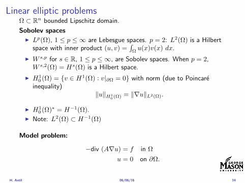
Linear elliptic problemsΩ sub Rn bounded Lipschitz domain
Sobolev spacesI Lp(Ω) 1 le p le infin are Lebesgue spaces p = 2 L2(Ω) is a Hilbert
space with inner product (u v) =int
Ωu(x)v(x) dx
I W sp for s isin R 1 le p le infin are Sobolev spaces When p = 2W s2(Ω) = Hs(Ω) is a Hilbert space
I H10 (Ω) = v isin H1(Ω) v|partΩ = 0 with norm (due to Poincare
inequality)uH1
0 (Ω) = nablauL2(Ω)
I H10 (Ω)lowast = Hminus1(Ω)
I Note L2(Ω) sub Hminus1(Ω)
Model problem
minusdiv (Anablau) = f in Ω
u = 0 on partΩ
H Antil 060616 14
Well-posed
I Weak solution Given f isin Hminus1(Ω) a function u isin H10 (Ω) is called
a weak solution iffintΩ
Anablau middot nablav = 〈f v〉minus11 forallv isin H10 (Ω)
where 〈middot middot〉minus11 denotes the Hminus1(Ω)ndashH1(Ω) duality pairing
I Existence and uniqueness For each f isin Hminus1(Ω) there exists aunique u isin H1
0 (Ω) such that
nablauL2(Ω) le CdΩfHminus1(Ω)
I A = I the result is due to the Riesz-representation theorem
I A 6= I (maybe non-symmetric) the result is due to Lax-Milgramlemma
I For general W 1p-spaces use inf-sup conditions combined withBanach-Necas theorem which is a necessary and sufficient condition
H Antil 060616 15
Linear-quadratic elliptic OCP
min J(u z) =1
2uminus ud2L2(Ω) +
λ
2z2L2(Ω)
subject to
minusdiv (Anablau) = z in Ω
u = 0 on partΩ
and the pointwise control constraints
z isin Zad = v isin L2(Ω) za(x) le v(x) le zb(x) ae x isin Ω
λ gt 0 is a parameter za zb isin Linfin(Ω) with za lt zb are given A isbounded symmetric positive
H Antil 060616 16
Reduced OCP
I Control to state map The solution operator defined as
S Hminus1(Ω)rarr H10 (Ω) z 7rarr u(z) = Sz
Note In view of the embedding
H10 (Ω) rarr L2(Ω) rarr Hminus1(Ω)
we may also consider S from L2(Ω) to L2(Ω) We will use the samenotation for this operator (for simplicity)
I Reduced cost functional The reduced cost functionalJ L2(Ω)rarr R is defined as
J (z) = J(Sz z)
I Reduced problem minzisinZadJ (z)
H Antil 060616 17
Reduced OCP
I Control to state map The solution operator defined as
S Hminus1(Ω)rarr H10 (Ω) z 7rarr u(z) = Sz
Note In view of the embedding
H10 (Ω) rarr L2(Ω) rarr Hminus1(Ω)
we may also consider S from L2(Ω) to L2(Ω) We will use the samenotation for this operator (for simplicity)
I Reduced cost functional The reduced cost functionalJ L2(Ω)rarr R is defined as
J (z) = J(Sz z)
I Reduced problem minzisinZadJ (z)
H Antil 060616 17
Reduced OCP
I Control to state map The solution operator defined as
S Hminus1(Ω)rarr H10 (Ω) z 7rarr u(z) = Sz
Note In view of the embedding
H10 (Ω) rarr L2(Ω) rarr Hminus1(Ω)
we may also consider S from L2(Ω) to L2(Ω) We will use the samenotation for this operator (for simplicity)
I Reduced cost functional The reduced cost functionalJ L2(Ω)rarr R is defined as
J (z) = J(Sz z)
I Reduced problem minzisinZadJ (z)
H Antil 060616 17
Existence of solution Direct methodThere exists a unique solution to the above problem
I Minimizing sequence J is bounded below by zero therefore thereexists a minimizing sequence znnisinN such that
limnrarrinfin
J (zn) = inf J (z)
I Weak compactness zn sub L2(Ω) is bounded Since L2(Ω) isreflexive therefore there exists a subsequence (not relabeled) suchthat
zn z and z isin Zad
where the latter is a consequence of Zad being closed and convex
I Optimality Since J is continuous and convex and therefore isweakly lower semicontinuous We obtain
lim inf J (zn) ge J (z)
which implies that z is optimal
I Uniqueness Exercise
H Antil 060616 18
Existence of solution Direct methodThere exists a unique solution to the above problem
I Minimizing sequence J is bounded below by zero therefore thereexists a minimizing sequence znnisinN such that
limnrarrinfin
J (zn) = inf J (z)
I Weak compactness zn sub L2(Ω) is bounded Since L2(Ω) isreflexive therefore there exists a subsequence (not relabeled) suchthat
zn z and z isin Zad
where the latter is a consequence of Zad being closed and convex
I Optimality Since J is continuous and convex and therefore isweakly lower semicontinuous We obtain
lim inf J (zn) ge J (z)
which implies that z is optimal
I Uniqueness Exercise
H Antil 060616 18
Existence of solution Direct methodThere exists a unique solution to the above problem
I Minimizing sequence J is bounded below by zero therefore thereexists a minimizing sequence znnisinN such that
limnrarrinfin
J (zn) = inf J (z)
I Weak compactness zn sub L2(Ω) is bounded Since L2(Ω) isreflexive therefore there exists a subsequence (not relabeled) suchthat
zn z and z isin Zad
where the latter is a consequence of Zad being closed and convex
I Optimality Since J is continuous and convex and therefore isweakly lower semicontinuous We obtain
lim inf J (zn) ge J (z)
which implies that z is optimal
I Uniqueness Exercise
H Antil 060616 18
Existence of solution Direct methodThere exists a unique solution to the above problem
I Minimizing sequence J is bounded below by zero therefore thereexists a minimizing sequence znnisinN such that
limnrarrinfin
J (zn) = inf J (z)
I Weak compactness zn sub L2(Ω) is bounded Since L2(Ω) isreflexive therefore there exists a subsequence (not relabeled) suchthat
zn z and z isin Zad
where the latter is a consequence of Zad being closed and convex
I Optimality Since J is continuous and convex and therefore isweakly lower semicontinuous We obtain
lim inf J (zn) ge J (z)
which implies that z is optimal
I Uniqueness Exercise
H Antil 060616 18
Outline
Motivation and examples
Linear elliptic optimal control problems
Differentiation in Banach spaces
First-order necessary conditions
Optimal control of semilinear PDEs
An abstract problem
Discretization using finite element methods
H Antil 060616 19
Differentiation in Banach spacesLet (Z middot Z) (V middot V ) B-spaces Z sub Z open and F Z rarr V
Let z isin Z
I If exist δF (z h) = limtdarr01t (F (z + th)minus F (z)) then δF (z h) is called
the directional derivative of F at z in direction h
I If exist δF (z h) forallh isin Z then h 7rarr δF (z h) is the first variation of Fat z
I Let exist the first variation δF (z middot) F is said to be Gateauxdifferentiable at z iff existA isin L(Z V ) such that δF (z h) = Ahforallh isin Z We write A = F primeG(z)
I F is said to be Frechet differentiable at z iff existA isin L(Z V ) and amapping r(z middot) Z rarr V such that for all h isin U with z + h isin Zwe have
F (z+h) = F (z)+Ah+r(z h) withr(z h)VhZ
rarr 0 as hZ rarr 0
We write F prime(z) = A
H Antil 060616 20
Differentiation in Banach spacesLet (Z middot Z) (V middot V ) B-spaces Z sub Z open and F Z rarr V
Let z isin Z
I If exist δF (z h) = limtdarr01t (F (z + th)minus F (z)) then δF (z h) is called
the directional derivative of F at z in direction h
I If exist δF (z h) forallh isin Z then h 7rarr δF (z h) is the first variation of Fat z
I Let exist the first variation δF (z middot) F is said to be Gateauxdifferentiable at z iff existA isin L(Z V ) such that δF (z h) = Ahforallh isin Z We write A = F primeG(z)
I F is said to be Frechet differentiable at z iff existA isin L(Z V ) and amapping r(z middot) Z rarr V such that for all h isin U with z + h isin Zwe have
F (z+h) = F (z)+Ah+r(z h) withr(z h)VhZ
rarr 0 as hZ rarr 0
We write F prime(z) = A
H Antil 060616 20
Differentiation in Banach spacesLet (Z middot Z) (V middot V ) B-spaces Z sub Z open and F Z rarr V
Let z isin Z
I If exist δF (z h) = limtdarr01t (F (z + th)minus F (z)) then δF (z h) is called
the directional derivative of F at z in direction h
I If exist δF (z h) forallh isin Z then h 7rarr δF (z h) is the first variation of Fat z
I Let exist the first variation δF (z middot) F is said to be Gateauxdifferentiable at z iff existA isin L(Z V ) such that δF (z h) = Ahforallh isin Z We write A = F primeG(z)
I F is said to be Frechet differentiable at z iff existA isin L(Z V ) and amapping r(z middot) Z rarr V such that for all h isin U with z + h isin Zwe have
F (z+h) = F (z)+Ah+r(z h) withr(z h)VhZ
rarr 0 as hZ rarr 0
We write F prime(z) = A
H Antil 060616 20
Differentiation in Banach spacesLet (Z middot Z) (V middot V ) B-spaces Z sub Z open and F Z rarr V
Let z isin Z
I If exist δF (z h) = limtdarr01t (F (z + th)minus F (z)) then δF (z h) is called
the directional derivative of F at z in direction h
I If exist δF (z h) forallh isin Z then h 7rarr δF (z h) is the first variation of Fat z
I Let exist the first variation δF (z middot) F is said to be Gateauxdifferentiable at z iff existA isin L(Z V ) such that δF (z h) = Ahforallh isin Z We write A = F primeG(z)
I F is said to be Frechet differentiable at z iff existA isin L(Z V ) and amapping r(z middot) Z rarr V such that for all h isin U with z + h isin Zwe have
F (z+h) = F (z)+Ah+r(z h) withr(z h)VhZ
rarr 0 as hZ rarr 0
We write F prime(z) = A
H Antil 060616 20
ExamplesExample 1 (H (middot middot)H) Hilbert space F (z) = z2H = (z z)H
forallz h F (z + h)minus F (z) = 2(z h)H + h2HThen
F prime(z)h = (2z h)H
Reisz representation theorem (identify H with Hlowast) we can write
F prime(z)h = (nablaF (z) h)H
where nablaF (z) = 2z is the gradient
Example 2 Let (Z (middot middot)Z) (H (middot middot)H) Hilbert spaces ud isin H fixedLet S isin L(ZH) Consider E Z rarr R
E(z) = Sz minus ud2H
Then E(z) = G(F (z)) where G(v) = v2H and F (z) = Sz minus ud
Eprime(z)h = Gprime(F (z))F prime(z)h = (2v F prime(z)h)H
= 2(Sz minus ud Sh)H = 2(Slowast(Sz minus ud) h)Z
we denote the gradient as nablaE(z) = 2Slowast(Sz minus ud)
H Antil 060616 21
ExamplesExample 1 (H (middot middot)H) Hilbert space F (z) = z2H = (z z)H
forallz h F (z + h)minus F (z) = 2(z h)H + h2HThen
F prime(z)h = (2z h)H
Reisz representation theorem (identify H with Hlowast) we can write
F prime(z)h = (nablaF (z) h)H
where nablaF (z) = 2z is the gradient
Example 2 Let (Z (middot middot)Z) (H (middot middot)H) Hilbert spaces ud isin H fixedLet S isin L(ZH) Consider E Z rarr R
E(z) = Sz minus ud2H
Then E(z) = G(F (z)) where G(v) = v2H and F (z) = Sz minus ud
Eprime(z)h = Gprime(F (z))F prime(z)h = (2v F prime(z)h)H
= 2(Sz minus ud Sh)H = 2(Slowast(Sz minus ud) h)Z
we denote the gradient as nablaE(z) = 2Slowast(Sz minus ud)H Antil 060616 21
Outline
Motivation and examples
Linear elliptic optimal control problems
Differentiation in Banach spaces
First-order necessary conditions
Optimal control of semilinear PDEs
An abstract problem
Discretization using finite element methods
H Antil 060616 22
First order necessary optimality conditions
Most of the theory is based on these two simple results
Theorem Let (Z middot Z) be a normed space J Z rarr (infin+infin] amapping with J 6equiv +infin Then z isin Z minimizer of J hArr 0 isin partJ (z)
Proof 0 isin partJ (z) means by definition of partJ (z) J (z)minus J (z) le 0forallz isin Z
Theorem Let (Z middot Z) be a normed space Zad sub Z nonemptyconvex closed J Z rarr R Gateaux differentiable where Zad sub Z sub ZZ open If z isin Zad is a solution to
minzisinZad
J (z)
then z solvesJ prime(z)(z minus z) ge 0 forallz isin Zad
Proof Exercise
H Antil 060616 23
First order necessary optimality conditions
Most of the theory is based on these two simple results
Theorem Let (Z middot Z) be a normed space J Z rarr (infin+infin] amapping with J 6equiv +infin Then z isin Z minimizer of J hArr 0 isin partJ (z)
Proof 0 isin partJ (z) means by definition of partJ (z) J (z)minus J (z) le 0forallz isin Z
Theorem Let (Z middot Z) be a normed space Zad sub Z nonemptyconvex closed J Z rarr R Gateaux differentiable where Zad sub Z sub ZZ open If z isin Zad is a solution to
minzisinZad
J (z)
then z solvesJ prime(z)(z minus z) ge 0 forallz isin Zad
Proof Exercise
H Antil 060616 23
Linear quadratic OCPI Reduced funcational
J (z) =1
2Sz minus ud2L2(Ω) +
λ
2z2L2(Ω)
I Gradient computation using sensitivity
J prime(z)h = (Slowast(Sz minus ud) + λz h)L2(Ω) forallh isin L2(Ω)
we denote the gradient by
nablaJ (z) = Slowast(Sz minus ud) + λz
I First order necessary and sufficient optimality condition
(nablaJ (z) z minus z)L2(Ω) ge 0 forallz isin Zad
I Adjoint equation Let p = Slowast(Sz minus ud) which translates intop isin H1
0 (Ω) solving
minusdiv (Anablap) = uminus ud in Ω
p = 0 on partΩ
I Gradient computation using adjoint nablaJ (z) = p+ λz
H Antil 060616 24
Linear quadratic OCPI Reduced funcational
J (z) =1
2Sz minus ud2L2(Ω) +
λ
2z2L2(Ω)
I Gradient computation using sensitivity
J prime(z)h = (Slowast(Sz minus ud) + λz h)L2(Ω) forallh isin L2(Ω)
we denote the gradient by
nablaJ (z) = Slowast(Sz minus ud) + λz
I First order necessary and sufficient optimality condition
(nablaJ (z) z minus z)L2(Ω) ge 0 forallz isin Zad
I Adjoint equation Let p = Slowast(Sz minus ud) which translates intop isin H1
0 (Ω) solving
minusdiv (Anablap) = uminus ud in Ω
p = 0 on partΩ
I Gradient computation using adjoint nablaJ (z) = p+ λz
H Antil 060616 24
Linear quadratic OCPI Reduced funcational
J (z) =1
2Sz minus ud2L2(Ω) +
λ
2z2L2(Ω)
I Gradient computation using sensitivity
J prime(z)h = (Slowast(Sz minus ud) + λz h)L2(Ω) forallh isin L2(Ω)
we denote the gradient by
nablaJ (z) = Slowast(Sz minus ud) + λz
I First order necessary and sufficient optimality condition
(nablaJ (z) z minus z)L2(Ω) ge 0 forallz isin Zad
I Adjoint equation Let p = Slowast(Sz minus ud) which translates intop isin H1
0 (Ω) solving
minusdiv (Anablap) = uminus ud in Ω
p = 0 on partΩ
I Gradient computation using adjoint nablaJ (z) = p+ λz
H Antil 060616 24
Linear quadratic OCPI Reduced funcational
J (z) =1
2Sz minus ud2L2(Ω) +
λ
2z2L2(Ω)
I Gradient computation using sensitivity
J prime(z)h = (Slowast(Sz minus ud) + λz h)L2(Ω) forallh isin L2(Ω)
we denote the gradient by
nablaJ (z) = Slowast(Sz minus ud) + λz
I First order necessary and sufficient optimality condition
(nablaJ (z) z minus z)L2(Ω) ge 0 forallz isin Zad
I Adjoint equation Let p = Slowast(Sz minus ud) which translates intop isin H1
0 (Ω) solving
minusdiv (Anablap) = uminus ud in Ω
p = 0 on partΩ
I Gradient computation using adjoint nablaJ (z) = p+ λz
H Antil 060616 24
Linear quadratic OCPI Reduced funcational
J (z) =1
2Sz minus ud2L2(Ω) +
λ
2z2L2(Ω)
I Gradient computation using sensitivity
J prime(z)h = (Slowast(Sz minus ud) + λz h)L2(Ω) forallh isin L2(Ω)
we denote the gradient by
nablaJ (z) = Slowast(Sz minus ud) + λz
I First order necessary and sufficient optimality condition
(nablaJ (z) z minus z)L2(Ω) ge 0 forallz isin Zad
I Adjoint equation Let p = Slowast(Sz minus ud) which translates intop isin H1
0 (Ω) solving
minusdiv (Anablap) = uminus ud in Ω
p = 0 on partΩ
I Gradient computation using adjoint nablaJ (z) = p+ λz
H Antil 060616 24
Optimality system
I State u isin H10 (Ω)
intΩAnablau middot nablav =
intΩzv forallv isin H1
0 (Ω)
I Adjoint p isin H10 (Ω)
intΩAnablap middot nablav =
intΩ
(uminus ud)v forallv isin H10 (Ω)
I Control z isin Zad (p+ λz z minus z) ge 0 forallz isin Zad
H Antil 060616 25
Pointwise interpretation
The variational inequality
(p+ λz z minus z) ge 0 forallz isin Zad
is equivalent to for ae x isin Ω
z(x) =
za(x) if p(x) + λz(x) gt 0isin [za(x) zb(x)] if p(x) + λz(x) = 0zb(x) if p(x) + λz(x) lt 0
Consequence
I When λ gt 0 then ae in Ω
z(x) = P[za(x)zb(x)]
minus 1
λp(x)
= min
zb(x)max
za(x)minus 1
λp(x)
H Antil 060616 26
Formal Lagrange method applied to linear OCPIntroduce L H1
0 (Ω)times Zad timesH1(Ω)rarr R defined as
L(u z p) = J(u z)minusint
Ω
(minusdiv (Anablau)minus z
)p dx
Integrate by parts to arrive at
L(u z p) = J(u z)minusint
Ω
(minusdiv (Anablap)uminus zp
)dx+
intpartΩ
(Anablau)p ds
If (u z p) is a stationary point then
I State
DpL(u z p)h = 0 forallh isin H1(Ω)
I AdjointDuL(u z p)h = 0 forallh isin H1
0 (Ω)
I ControlDzL(u z p)(z minus z) ge 0 forallz isin Zad
H Antil 060616 27
Formal Lagrange method applied to linear OCPIntroduce L H1
0 (Ω)times Zad timesH1(Ω)rarr R defined as
L(u z p) = J(u z)minusint
Ω
(minusdiv (Anablau)minus z
)p dx
Integrate by parts to arrive at
L(u z p) = J(u z)minusint
Ω
(minusdiv (Anablap)uminus zp
)dx+
intpartΩ
(Anablau)p ds
If (u z p) is a stationary point then
I State
DpL(u z p)h = 0 forallh isin H1(Ω)
I AdjointDuL(u z p)h = 0 forallh isin H1
0 (Ω)
I ControlDzL(u z p)(z minus z) ge 0 forallz isin Zad
H Antil 060616 27
Formal Lagrange method applied to linear OCPIntroduce L H1
0 (Ω)times Zad timesH1(Ω)rarr R defined as
L(u z p) = J(u z)minusint
Ω
(minusdiv (Anablau)minus z
)p dx
Integrate by parts to arrive at
L(u z p) = J(u z)minusint
Ω
(minusdiv (Anablap)uminus zp
)dx+
intpartΩ
(Anablau)p ds
If (u z p) is a stationary point then
I State
DpL(u z p)h = 0 forallh isin H1(Ω)
I AdjointDuL(u z p)h = 0 forallh isin H1
0 (Ω)
I ControlDzL(u z p)(z minus z) ge 0 forallz isin Zad
H Antil 060616 27
Formal Lagrange method applied to linear OCPIntroduce L H1
0 (Ω)times Zad timesH1(Ω)rarr R defined as
L(u z p) = J(u z)minusint
Ω
(minusdiv (Anablau)minus z
)p dx
Integrate by parts to arrive at
L(u z p) = J(u z)minusint
Ω
(minusdiv (Anablap)uminus zp
)dx+
intpartΩ
(Anablau)p ds
If (u z p) is a stationary point then
I State
DpL(u z p)h = 0 forallh isin H1(Ω)
I AdjointDuL(u z p)h = 0 forallh isin H1
0 (Ω)
I ControlDzL(u z p)(z minus z) ge 0 forallz isin Zad
H Antil 060616 27
Formal Lagrange method applied to linear OCPIntroduce L H1
0 (Ω)times Zad timesH1(Ω)rarr R defined as
L(u z p) = J(u z)minusint
Ω
(minusdiv (Anablau)minus z
)p dx
Integrate by parts to arrive at
L(u z p) = J(u z)minusint
Ω
(minusdiv (Anablap)uminus zp
)dx+
intpartΩ
(Anablau)p ds
If (u z p) is a stationary point then
I State
DpL(u z p)h = 0 forallh isin H1(Ω)
I AdjointDuL(u z p)h = 0 forallh isin H1
0 (Ω)
I ControlDzL(u z p)(z minus z) ge 0 forallz isin Zad
H Antil 060616 27
Outline
Motivation and examples
Linear elliptic optimal control problems
Differentiation in Banach spaces
First-order necessary conditions
Optimal control of semilinear PDEs
An abstract problem
Discretization using finite element methods
H Antil 060616 28
Semilinear elliptic OCP
min J(u z) =1
2uminus ud2L2(Ω) +
λ
2z2L2(Ω)
subject to
minus∆u+ g(x u) = z in Ω
u = 0 on partΩ
and z isin Zad with za zb isin Linfin(Ω)
H Antil 060616 29
State space(A1) Ω sub Rd open bounded partΩ is Lipschitz
(A2) g Ωtimes Rrarr R is bounded and measurable with respect to x isin Ωfor every u isin R
(A3) g is continuous monotone increasing and Lipschitz continuous in ufor ae x isin Ω
(A4) g(x 0) = 0 for ae x isin Ω (not really necessary)
Theorem Suppose (A1)minus (A4) hold For every z isin Lr(Ω) withr gt d2 the state equation has a unique weak solutionu isin H1
0 (Ω) cap C(Ω) ie we haveintΩ
nablau middot nablav dx+
intΩ
g(x u(x))v(x) dx =
intΩ
zv dx forallv isin H10 (Ω)
Moreover there exists a constant C gt 0 such that
uH1(Ω) + uC(Ω) le CzLr(Ω)
RemarkI The proof of the theorem uses the BrowderndashMinty theorem on
monotone operators
H Antil 060616 30
State space(A1) Ω sub Rd open bounded partΩ is Lipschitz
(A2) g Ωtimes Rrarr R is bounded and measurable with respect to x isin Ωfor every u isin R
(A3) g is continuous monotone increasing and Lipschitz continuous in ufor ae x isin Ω
(A4) g(x 0) = 0 for ae x isin Ω (not really necessary)
Theorem Suppose (A1)minus (A4) hold For every z isin Lr(Ω) withr gt d2 the state equation has a unique weak solutionu isin H1
0 (Ω) cap C(Ω) ie we haveintΩ
nablau middot nablav dx+
intΩ
g(x u(x))v(x) dx =
intΩ
zv dx forallv isin H10 (Ω)
Moreover there exists a constant C gt 0 such that
uH1(Ω) + uC(Ω) le CzLr(Ω)
RemarkI The proof of the theorem uses the BrowderndashMinty theorem on
monotone operators
H Antil 060616 30
State space(A1) Ω sub Rd open bounded partΩ is Lipschitz
(A2) g Ωtimes Rrarr R is bounded and measurable with respect to x isin Ωfor every u isin R
(A3) g is continuous monotone increasing and Lipschitz continuous in ufor ae x isin Ω
(A4) g(x 0) = 0 for ae x isin Ω (not really necessary)
Theorem Suppose (A1)minus (A4) hold For every z isin Lr(Ω) withr gt d2 the state equation has a unique weak solutionu isin H1
0 (Ω) cap C(Ω) ie we haveintΩ
nablau middot nablav dx+
intΩ
g(x u(x))v(x) dx =
intΩ
zv dx forallv isin H10 (Ω)
Moreover there exists a constant C gt 0 such that
uH1(Ω) + uC(Ω) le CzLr(Ω)
RemarkI The proof of the theorem uses the BrowderndashMinty theorem on
monotone operators
H Antil 060616 30
Control-to-state map and reduced problem
I Control to state map
S Linfin(Ω)rarr H10 (Ω) cap C(Ω)
is well defined and is globally Lipschitz continuous
I Reduced problem
minJ (z) =1
2S(u)minus ud2L2(Ω) +
λ
2z2L2(Ω)
H Antil 060616 31
Control-to-state map and reduced problem
I Control to state map
S Linfin(Ω)rarr H10 (Ω) cap C(Ω)
is well defined and is globally Lipschitz continuous
I Reduced problem
minJ (z) =1
2S(u)minus ud2L2(Ω) +
λ
2z2L2(Ω)
H Antil 060616 31
First-order necessary conditionsI Lagrangian functional
L(u z p) = J(u z)minusint
Ω
(minus∆u+ g(x u(x))minus z
)p dx
= J(u z)minusint
Ω
(nablau middot nablap+ g(x u(x))pminus zp
)dx
I Adjoint system For all h isin H10 (Ω)
0 = DuL(u z p)h =
intΩ
(uminus ud)h dxminusint
Ω
(nablah middot nablap+ gu(x u(x))ph
)which yields
minus∆p+ gu(x u(x))p = uminus ud in Ω
p = 0 on partΩ
I Control
DzL(u z p)(z minus z) = (p+ λz z minus z) dx ge 0 forallz isin ZadI Gradient
nablaJ (z) = p+ λz
H Antil 060616 32
First-order necessary conditionsI Lagrangian functional
L(u z p) = J(u z)minusint
Ω
(minus∆u+ g(x u(x))minus z
)p dx
= J(u z)minusint
Ω
(nablau middot nablap+ g(x u(x))pminus zp
)dx
I Adjoint system For all h isin H10 (Ω)
0 = DuL(u z p)h =
intΩ
(uminus ud)h dxminusint
Ω
(nablah middot nablap+ gu(x u(x))ph
)which yields
minus∆p+ gu(x u(x))p = uminus ud in Ω
p = 0 on partΩ
I Control
DzL(u z p)(z minus z) = (p+ λz z minus z) dx ge 0 forallz isin ZadI Gradient
nablaJ (z) = p+ λz
H Antil 060616 32
First-order necessary conditionsI Lagrangian functional
L(u z p) = J(u z)minusint
Ω
(minus∆u+ g(x u(x))minus z
)p dx
= J(u z)minusint
Ω
(nablau middot nablap+ g(x u(x))pminus zp
)dx
I Adjoint system For all h isin H10 (Ω)
0 = DuL(u z p)h =
intΩ
(uminus ud)h dxminusint
Ω
(nablah middot nablap+ gu(x u(x))ph
)which yields
minus∆p+ gu(x u(x))p = uminus ud in Ω
p = 0 on partΩ
I Control
DzL(u z p)(z minus z) = (p+ λz z minus z) dx ge 0 forallz isin Zad
I GradientnablaJ (z) = p+ λz
H Antil 060616 32
First-order necessary conditionsI Lagrangian functional
L(u z p) = J(u z)minusint
Ω
(minus∆u+ g(x u(x))minus z
)p dx
= J(u z)minusint
Ω
(nablau middot nablap+ g(x u(x))pminus zp
)dx
I Adjoint system For all h isin H10 (Ω)
0 = DuL(u z p)h =
intΩ
(uminus ud)h dxminusint
Ω
(nablah middot nablap+ gu(x u(x))ph
)which yields
minus∆p+ gu(x u(x))p = uminus ud in Ω
p = 0 on partΩ
I Control
DzL(u z p)(z minus z) = (p+ λz z minus z) dx ge 0 forallz isin ZadI Gradient
nablaJ (z) = p+ λz
H Antil 060616 32
Differentiability of Nemytskii operator
The rigorous proof uses
Theorem In addition to (A1)-(A4) if
(A5) g is continuously differentiable with respect to u for ae x isin Ωand we have
(i) |gu(x 0)| le K for ae x isin Ω(ii) gu is locally Lipschitz with respect to u isin R
then the Nemytskii operator G u 7rarr g(middot u(middot)) is continuously Frechetdifferentiable from Linfin(Ω) into itself and
(Gprime(u)h)(x) = gu(x u(x))h(x) ae in Ω forallh isin Linfin(Ω)
Remark (A5) holds if g(x u) = g(u) and g isin C2(R)
H Antil 060616 33
Outline
Motivation and examples
Linear elliptic optimal control problems
Differentiation in Banach spaces
First-order necessary conditions
Optimal control of semilinear PDEs
An abstract problem
Discretization using finite element methods
H Antil 060616 34
Gradient computation via adjoint general formI Abstract problem
min J(u z)
subject toc(u z) = 0
and z isin Zad
I Directional derivative Let S be the control to state map(nonlinear in general)
z 7rarr S(z) = u(z)
Under the assumptions of ldquoimplicit function theoremrdquo
J prime(z)h = (nablauJ (u(z) z) Sprime(z)h) + (nablazJ (u(z) z) h)
I Sensitivity of u with respect to z Differentiating the stateequation
cu(S(z) z)Sprime(z)h = minuscz(S(z) z)h
leads toSprime(z)h = minuscu(S(z) z)minus1
(cz(S(z) z)h
)
provided cu(S(z) z)minus1 is well-defined
H Antil 060616 35
Gradient computation via adjoint general formI Abstract problem
min J(u z)
subject toc(u z) = 0
and z isin ZadI Directional derivative Let S be the control to state map
(nonlinear in general)
z 7rarr S(z) = u(z)
Under the assumptions of ldquoimplicit function theoremrdquo
J prime(z)h = (nablauJ (u(z) z) Sprime(z)h) + (nablazJ (u(z) z) h)
I Sensitivity of u with respect to z Differentiating the stateequation
cu(S(z) z)Sprime(z)h = minuscz(S(z) z)h
leads toSprime(z)h = minuscu(S(z) z)minus1
(cz(S(z) z)h
)
provided cu(S(z) z)minus1 is well-defined
H Antil 060616 35
Gradient computation via adjoint general formI Abstract problem
min J(u z)
subject toc(u z) = 0
and z isin ZadI Directional derivative Let S be the control to state map
(nonlinear in general)
z 7rarr S(z) = u(z)
Under the assumptions of ldquoimplicit function theoremrdquo
J prime(z)h = (nablauJ (u(z) z) Sprime(z)h) + (nablazJ (u(z) z) h)
I Sensitivity of u with respect to z Differentiating the stateequation
cu(S(z) z)Sprime(z)h = minuscz(S(z) z)h
leads toSprime(z)h = minuscu(S(z) z)minus1
(cz(S(z) z)h
)
provided cu(S(z) z)minus1 is well-defined
H Antil 060616 35
Adjoint equation and gradient general form
I Directional derivative
J prime(z)h = minus(nablauJ (u(z) z) cu(u(z) z)minus1cz(u(z) z)h
)+ (nablazJ (u(z) z) h)
I Gradient
nablaJ (z) = minuscz(u(z) z)lowast(cu(u(z) z)minuslowastnablauJ (u(z) z)
)+nablazJ (u(z) z)
I Introducing adjoint variable p solving
cu(u(z) z)lowastp = nablauJ (u(z) z)
we arrive at following form of gradient
nablaJ (z) = minuscz(u(z) z)lowastp+nablazJ (u(z) z)
which is tractable
H Antil 060616 36
Adjoint equation and gradient general form
I Directional derivative
J prime(z)h = minus(nablauJ (u(z) z) cu(u(z) z)minus1cz(u(z) z)h
)+ (nablazJ (u(z) z) h)
I Gradient
nablaJ (z) = minuscz(u(z) z)lowast(cu(u(z) z)minuslowastnablauJ (u(z) z)
)+nablazJ (u(z) z)
I Introducing adjoint variable p solving
cu(u(z) z)lowastp = nablauJ (u(z) z)
we arrive at following form of gradient
nablaJ (z) = minuscz(u(z) z)lowastp+nablazJ (u(z) z)
which is tractable
H Antil 060616 36
Adjoint equation and gradient general form
I Directional derivative
J prime(z)h = minus(nablauJ (u(z) z) cu(u(z) z)minus1cz(u(z) z)h
)+ (nablazJ (u(z) z) h)
I Gradient
nablaJ (z) = minuscz(u(z) z)lowast(cu(u(z) z)minuslowastnablauJ (u(z) z)
)+nablazJ (u(z) z)
I Introducing adjoint variable p solving
cu(u(z) z)lowastp = nablauJ (u(z) z)
we arrive at following form of gradient
nablaJ (z) = minuscz(u(z) z)lowastp+nablazJ (u(z) z)
which is tractable
H Antil 060616 36
Hessian computation general form
I Lagrangian L(u z p) = J(u z)minusint
Ωc(u z)p dx Then we have
DzJ (z)h = DzL(u z p)h
I Second order derivative
D2zJ (z)[h1 h2] = DuDzL(u z p)[h1 S
prime(z)h2] +D2zL(u z p)[h1 h2]
+DpDzL(u z p)[h1 Dzp(z)h2]
I We already know Sprime(z)h2 moreover
DpDzL(u z p)[h1 Dzp(z)h2] = minus(cu(u z)h1 Dzp(z)h2
)
It remain to identify Dzp(z)h2
H Antil 060616 37
Hessian computation general form
I Lagrangian L(u z p) = J(u z)minusint
Ωc(u z)p dx Then we have
DzJ (z)h = DzL(u z p)h
I Second order derivative
D2zJ (z)[h1 h2] = DuDzL(u z p)[h1 S
prime(z)h2] +D2zL(u z p)[h1 h2]
+DpDzL(u z p)[h1 Dzp(z)h2]
I We already know Sprime(z)h2 moreover
DpDzL(u z p)[h1 Dzp(z)h2] = minus(cu(u z)h1 Dzp(z)h2
)
It remain to identify Dzp(z)h2
H Antil 060616 37
Hessian computation general form
I Lagrangian L(u z p) = J(u z)minusint
Ωc(u z)p dx Then we have
DzJ (z)h = DzL(u z p)h
I Second order derivative
D2zJ (z)[h1 h2] = DuDzL(u z p)[h1 S
prime(z)h2] +D2zL(u z p)[h1 h2]
+DpDzL(u z p)[h1 Dzp(z)h2]
I We already know Sprime(z)h2 moreover
DpDzL(u z p)[h1 Dzp(z)h2] = minus(cu(u z)h1 Dzp(z)h2
)
It remain to identify Dzp(z)h2
H Antil 060616 37
Outline
Motivation and examples
Linear elliptic optimal control problems
Differentiation in Banach spaces
First-order necessary conditions
Optimal control of semilinear PDEs
An abstract problem
Discretization using finite element methods
H Antil 060616 38
Numerical approximation of Poisson equation MeshTo avoid technical issues we will assume that partΩ is polygonal
I Mesh Let T = K be a mesh of Ω where K sub Rd is an elementthat is isoparametrically equivalent to a unit simplex in Rd
I Conforming mesh We say that the mesh is conforming ifI Ω = cupKisinT KI If K1 cap K2 = x then x is a node of K1 and K2I If K1 cap K2 6= empty and K1 cap K2 6= x then K1 cap K2 is an edgeface
contained in partK1 cap partK2
I Shape regular Let T be the collection of all conformingrefinements of an original mesh T 0 Then T is called shape regularif exist κ gt 0 such that
hKρKle κ forallK isin cupiT i
where hK = diam K ρK = maxρ gt 0|Bρ sub KI Quasi-uniform A family of shape regular meshes is called-quasi
uniform if there exist a constant σ gt 0 such that
maxhKminhK
le σ
uniformly for all meshes in the family
Numerical approximation of Poisson equation MeshTo avoid technical issues we will assume that partΩ is polygonal
I Mesh Let T = K be a mesh of Ω where K sub Rd is an elementthat is isoparametrically equivalent to a unit simplex in Rd
I Conforming mesh We say that the mesh is conforming ifI Ω = cupKisinT KI If K1 cap K2 = x then x is a node of K1 and K2I If K1 cap K2 6= empty and K1 cap K2 6= x then K1 cap K2 is an edgeface
contained in partK1 cap partK2
I Shape regular Let T be the collection of all conformingrefinements of an original mesh T 0 Then T is called shape regularif exist κ gt 0 such that
hKρKle κ forallK isin cupiT i
where hK = diam K ρK = maxρ gt 0|Bρ sub KI Quasi-uniform A family of shape regular meshes is called-quasi
uniform if there exist a constant σ gt 0 such that
maxhKminhK
le σ
uniformly for all meshes in the family
Numerical approximation of Poisson equation MeshTo avoid technical issues we will assume that partΩ is polygonal
I Mesh Let T = K be a mesh of Ω where K sub Rd is an elementthat is isoparametrically equivalent to a unit simplex in Rd
I Conforming mesh We say that the mesh is conforming ifI Ω = cupKisinT KI If K1 cap K2 = x then x is a node of K1 and K2I If K1 cap K2 6= empty and K1 cap K2 6= x then K1 cap K2 is an edgeface
contained in partK1 cap partK2
I Shape regular Let T be the collection of all conformingrefinements of an original mesh T 0 Then T is called shape regularif exist κ gt 0 such that
hKρKle κ forallK isin cupiT i
where hK = diam K ρK = maxρ gt 0|Bρ sub K
I Quasi-uniform A family of shape regular meshes is called-quasiuniform if there exist a constant σ gt 0 such that
maxhKminhK
le σ
uniformly for all meshes in the family
Numerical approximation of Poisson equation MeshTo avoid technical issues we will assume that partΩ is polygonal
I Mesh Let T = K be a mesh of Ω where K sub Rd is an elementthat is isoparametrically equivalent to a unit simplex in Rd
I Conforming mesh We say that the mesh is conforming ifI Ω = cupKisinT KI If K1 cap K2 = x then x is a node of K1 and K2I If K1 cap K2 6= empty and K1 cap K2 6= x then K1 cap K2 is an edgeface
contained in partK1 cap partK2
I Shape regular Let T be the collection of all conformingrefinements of an original mesh T 0 Then T is called shape regularif exist κ gt 0 such that
hKρKle κ forallK isin cupiT i
where hK = diam K ρK = maxρ gt 0|Bρ sub KI Quasi-uniform A family of shape regular meshes is called-quasi
uniform if there exist a constant σ gt 0 such that
maxhKminhK
le σ
uniformly for all meshes in the family
FE space and Galerkin approximationI Finite element space For T isin T we define the finite element
space as
V(T ) = W isin C0(Ω) WK isin P1forallK isin T W |partΩ = 0
where P1 is the set of polynomials of degree at most 1
I Galerkin approximation of continuous problem is given by
Find UT isin V(T )
intΩ
AnablaUT middot nablaV = 〈f V 〉 forallV isin V(T )
The discrete problem is well-posedI Nodal basis Consists of functions ψi isin V(T ) with xi isin N (T )
satisfyingψxi
(xj) = δij
where N (T ) denotes the interior (plus Neumann) nodesI Galerkin orthogonality(
nabla(uminus UT )nablaW)L2(Ω)
= 0 forallW isin V(T )
H Antil 060616 40
FE space and Galerkin approximationI Finite element space For T isin T we define the finite element
space as
V(T ) = W isin C0(Ω) WK isin P1forallK isin T W |partΩ = 0
where P1 is the set of polynomials of degree at most 1I Galerkin approximation of continuous problem is given by
Find UT isin V(T )
intΩ
AnablaUT middot nablaV = 〈f V 〉 forallV isin V(T )
The discrete problem is well-posed
I Nodal basis Consists of functions ψi isin V(T ) with xi isin N (T )satisfying
ψxi(xj) = δij
where N (T ) denotes the interior (plus Neumann) nodesI Galerkin orthogonality(
nabla(uminus UT )nablaW)L2(Ω)
= 0 forallW isin V(T )
H Antil 060616 40
FE space and Galerkin approximationI Finite element space For T isin T we define the finite element
space as
V(T ) = W isin C0(Ω) WK isin P1forallK isin T W |partΩ = 0
where P1 is the set of polynomials of degree at most 1I Galerkin approximation of continuous problem is given by
Find UT isin V(T )
intΩ
AnablaUT middot nablaV = 〈f V 〉 forallV isin V(T )
The discrete problem is well-posedI Nodal basis Consists of functions ψi isin V(T ) with xi isin N (T )
satisfyingψxi
(xj) = δij
where N (T ) denotes the interior (plus Neumann) nodes
I Galerkin orthogonality(nabla(uminus UT )nablaW
)L2(Ω)
= 0 forallW isin V(T )
H Antil 060616 40
FE space and Galerkin approximationI Finite element space For T isin T we define the finite element
space as
V(T ) = W isin C0(Ω) WK isin P1forallK isin T W |partΩ = 0
where P1 is the set of polynomials of degree at most 1I Galerkin approximation of continuous problem is given by
Find UT isin V(T )
intΩ
AnablaUT middot nablaV = 〈f V 〉 forallV isin V(T )
The discrete problem is well-posedI Nodal basis Consists of functions ψi isin V(T ) with xi isin N (T )
satisfyingψxi
(xj) = δij
where N (T ) denotes the interior (plus Neumann) nodesI Galerkin orthogonality(
nabla(uminus UT )nablaW)L2(Ω)
= 0 forallW isin V(T )
H Antil 060616 40
Best approximation
I Cearsquos lemma
nabla(uminus UT )L2(Ω) le C infWisinV(T )
nabla(uminusW )L2(Ω)
I Nodal interpolation operator ΠT C(Ω)rarr V(T ) satisfies
ΠT u(xi) = u(xi) forallxi isin N (T )
and is defined as
ΠT u =sum
xiisinN (T )
u(xi)ψxi
I Error estimates In Cearsquos lemma replace W by ΠT u and thencompute the interpolation error
H Antil 060616 41
Best approximation
I Cearsquos lemma
nabla(uminus UT )L2(Ω) le C infWisinV(T )
nabla(uminusW )L2(Ω)
I Nodal interpolation operator ΠT C(Ω)rarr V(T ) satisfies
ΠT u(xi) = u(xi) forallxi isin N (T )
and is defined as
ΠT u =sum
xiisinN (T )
u(xi)ψxi
I Error estimates In Cearsquos lemma replace W by ΠT u and thencompute the interpolation error
H Antil 060616 41
Best approximation
I Cearsquos lemma
nabla(uminus UT )L2(Ω) le C infWisinV(T )
nabla(uminusW )L2(Ω)
I Nodal interpolation operator ΠT C(Ω)rarr V(T ) satisfies
ΠT u(xi) = u(xi) forallxi isin N (T )
and is defined as
ΠT u =sum
xiisinN (T )
u(xi)ψxi
I Error estimates In Cearsquos lemma replace W by ΠT u and thencompute the interpolation error
H Antil 060616 41
Algebraic system state equation
I Recall UT isin V(T ) solves
a(UT V ) = 〈f V 〉 forallV isin V(T )
I Now setting UT =sumN
j=1 Ujψj V = ψi we get
Nsumj=1
Uja(φj φi) = 〈f ψi〉 i = 1 N
which is the matrix-vector system
AU = F
I Stiffness matrix A is SPD
H Antil 060616 42
Algebraic system state equation
I Recall UT isin V(T ) solves
a(UT V ) = 〈f V 〉 forallV isin V(T )
I Now setting UT =sumN
j=1 Ujψj V = ψi we get
Nsumj=1
Uja(φj φi) = 〈f ψi〉 i = 1 N
which is the matrix-vector system
AU = F
I Stiffness matrix A is SPD
H Antil 060616 42
Algebraic system state equation
I Recall UT isin V(T ) solves
a(UT V ) = 〈f V 〉 forallV isin V(T )
I Now setting UT =sumN
j=1 Ujψj V = ψi we get
Nsumj=1
Uja(φj φi) = 〈f ψi〉 i = 1 N
which is the matrix-vector system
AU = F
I Stiffness matrix A is SPD
H Antil 060616 42
Discrete linear elliptic OCP
min JT (UT ZT ) =1
2UT minus ud2L2(Ω) +
λ
2ZT 2L2(Ω)
subject to
Find UT isin V(T )
intΩ
nablaUT middot nablaV = (ZT V )L2(Ω) forallV isin V(T )
and whereZT isin Zad(T ) = Zad cap Z(T )
is either one of these
Z(T ) =
V(T )L2(Ω) variational discretization (Hinze)WT isin Linfin(Ω) ZT |K isin P0(K)K isin T
H Antil 060616 43
Recent books
F TroltzschOptimal control of partial differential equations volume 112 ofGraduate Studies in MathematicsAmerican Mathematical Society Providence RI 2010Theory methods and applications Translated from the 2005 Germanoriginal by Jurgen Sprekels
K Ito and K KunischLagrange multiplier approach to variational problems andapplications volume 15 of Advances in Design and ControlSociety for Industrial and Applied Mathematics (SIAM)Philadelphia PA 2008
H Antil 060616 44
- Motivation and examples
- Linear elliptic optimal control problems
- Differentiation in Banach spaces
- First-order necessary conditions
- Optimal control of semilinear PDEs
- An abstract problem
- Discretization using finite element methods
-
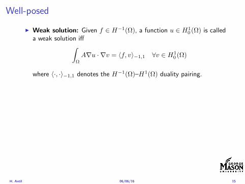
Well-posed
I Weak solution Given f isin Hminus1(Ω) a function u isin H10 (Ω) is called
a weak solution iffintΩ
Anablau middot nablav = 〈f v〉minus11 forallv isin H10 (Ω)
where 〈middot middot〉minus11 denotes the Hminus1(Ω)ndashH1(Ω) duality pairing
I Existence and uniqueness For each f isin Hminus1(Ω) there exists aunique u isin H1
0 (Ω) such that
nablauL2(Ω) le CdΩfHminus1(Ω)
I A = I the result is due to the Riesz-representation theorem
I A 6= I (maybe non-symmetric) the result is due to Lax-Milgramlemma
I For general W 1p-spaces use inf-sup conditions combined withBanach-Necas theorem which is a necessary and sufficient condition
H Antil 060616 15
Linear-quadratic elliptic OCP
min J(u z) =1
2uminus ud2L2(Ω) +
λ
2z2L2(Ω)
subject to
minusdiv (Anablau) = z in Ω
u = 0 on partΩ
and the pointwise control constraints
z isin Zad = v isin L2(Ω) za(x) le v(x) le zb(x) ae x isin Ω
λ gt 0 is a parameter za zb isin Linfin(Ω) with za lt zb are given A isbounded symmetric positive
H Antil 060616 16
Reduced OCP
I Control to state map The solution operator defined as
S Hminus1(Ω)rarr H10 (Ω) z 7rarr u(z) = Sz
Note In view of the embedding
H10 (Ω) rarr L2(Ω) rarr Hminus1(Ω)
we may also consider S from L2(Ω) to L2(Ω) We will use the samenotation for this operator (for simplicity)
I Reduced cost functional The reduced cost functionalJ L2(Ω)rarr R is defined as
J (z) = J(Sz z)
I Reduced problem minzisinZadJ (z)
H Antil 060616 17
Reduced OCP
I Control to state map The solution operator defined as
S Hminus1(Ω)rarr H10 (Ω) z 7rarr u(z) = Sz
Note In view of the embedding
H10 (Ω) rarr L2(Ω) rarr Hminus1(Ω)
we may also consider S from L2(Ω) to L2(Ω) We will use the samenotation for this operator (for simplicity)
I Reduced cost functional The reduced cost functionalJ L2(Ω)rarr R is defined as
J (z) = J(Sz z)
I Reduced problem minzisinZadJ (z)
H Antil 060616 17
Reduced OCP
I Control to state map The solution operator defined as
S Hminus1(Ω)rarr H10 (Ω) z 7rarr u(z) = Sz
Note In view of the embedding
H10 (Ω) rarr L2(Ω) rarr Hminus1(Ω)
we may also consider S from L2(Ω) to L2(Ω) We will use the samenotation for this operator (for simplicity)
I Reduced cost functional The reduced cost functionalJ L2(Ω)rarr R is defined as
J (z) = J(Sz z)
I Reduced problem minzisinZadJ (z)
H Antil 060616 17
Existence of solution Direct methodThere exists a unique solution to the above problem
I Minimizing sequence J is bounded below by zero therefore thereexists a minimizing sequence znnisinN such that
limnrarrinfin
J (zn) = inf J (z)
I Weak compactness zn sub L2(Ω) is bounded Since L2(Ω) isreflexive therefore there exists a subsequence (not relabeled) suchthat
zn z and z isin Zad
where the latter is a consequence of Zad being closed and convex
I Optimality Since J is continuous and convex and therefore isweakly lower semicontinuous We obtain
lim inf J (zn) ge J (z)
which implies that z is optimal
I Uniqueness Exercise
H Antil 060616 18
Existence of solution Direct methodThere exists a unique solution to the above problem
I Minimizing sequence J is bounded below by zero therefore thereexists a minimizing sequence znnisinN such that
limnrarrinfin
J (zn) = inf J (z)
I Weak compactness zn sub L2(Ω) is bounded Since L2(Ω) isreflexive therefore there exists a subsequence (not relabeled) suchthat
zn z and z isin Zad
where the latter is a consequence of Zad being closed and convex
I Optimality Since J is continuous and convex and therefore isweakly lower semicontinuous We obtain
lim inf J (zn) ge J (z)
which implies that z is optimal
I Uniqueness Exercise
H Antil 060616 18
Existence of solution Direct methodThere exists a unique solution to the above problem
I Minimizing sequence J is bounded below by zero therefore thereexists a minimizing sequence znnisinN such that
limnrarrinfin
J (zn) = inf J (z)
I Weak compactness zn sub L2(Ω) is bounded Since L2(Ω) isreflexive therefore there exists a subsequence (not relabeled) suchthat
zn z and z isin Zad
where the latter is a consequence of Zad being closed and convex
I Optimality Since J is continuous and convex and therefore isweakly lower semicontinuous We obtain
lim inf J (zn) ge J (z)
which implies that z is optimal
I Uniqueness Exercise
H Antil 060616 18
Existence of solution Direct methodThere exists a unique solution to the above problem
I Minimizing sequence J is bounded below by zero therefore thereexists a minimizing sequence znnisinN such that
limnrarrinfin
J (zn) = inf J (z)
I Weak compactness zn sub L2(Ω) is bounded Since L2(Ω) isreflexive therefore there exists a subsequence (not relabeled) suchthat
zn z and z isin Zad
where the latter is a consequence of Zad being closed and convex
I Optimality Since J is continuous and convex and therefore isweakly lower semicontinuous We obtain
lim inf J (zn) ge J (z)
which implies that z is optimal
I Uniqueness Exercise
H Antil 060616 18
Outline
Motivation and examples
Linear elliptic optimal control problems
Differentiation in Banach spaces
First-order necessary conditions
Optimal control of semilinear PDEs
An abstract problem
Discretization using finite element methods
H Antil 060616 19
Differentiation in Banach spacesLet (Z middot Z) (V middot V ) B-spaces Z sub Z open and F Z rarr V
Let z isin Z
I If exist δF (z h) = limtdarr01t (F (z + th)minus F (z)) then δF (z h) is called
the directional derivative of F at z in direction h
I If exist δF (z h) forallh isin Z then h 7rarr δF (z h) is the first variation of Fat z
I Let exist the first variation δF (z middot) F is said to be Gateauxdifferentiable at z iff existA isin L(Z V ) such that δF (z h) = Ahforallh isin Z We write A = F primeG(z)
I F is said to be Frechet differentiable at z iff existA isin L(Z V ) and amapping r(z middot) Z rarr V such that for all h isin U with z + h isin Zwe have
F (z+h) = F (z)+Ah+r(z h) withr(z h)VhZ
rarr 0 as hZ rarr 0
We write F prime(z) = A
H Antil 060616 20
Differentiation in Banach spacesLet (Z middot Z) (V middot V ) B-spaces Z sub Z open and F Z rarr V
Let z isin Z
I If exist δF (z h) = limtdarr01t (F (z + th)minus F (z)) then δF (z h) is called
the directional derivative of F at z in direction h
I If exist δF (z h) forallh isin Z then h 7rarr δF (z h) is the first variation of Fat z
I Let exist the first variation δF (z middot) F is said to be Gateauxdifferentiable at z iff existA isin L(Z V ) such that δF (z h) = Ahforallh isin Z We write A = F primeG(z)
I F is said to be Frechet differentiable at z iff existA isin L(Z V ) and amapping r(z middot) Z rarr V such that for all h isin U with z + h isin Zwe have
F (z+h) = F (z)+Ah+r(z h) withr(z h)VhZ
rarr 0 as hZ rarr 0
We write F prime(z) = A
H Antil 060616 20
Differentiation in Banach spacesLet (Z middot Z) (V middot V ) B-spaces Z sub Z open and F Z rarr V
Let z isin Z
I If exist δF (z h) = limtdarr01t (F (z + th)minus F (z)) then δF (z h) is called
the directional derivative of F at z in direction h
I If exist δF (z h) forallh isin Z then h 7rarr δF (z h) is the first variation of Fat z
I Let exist the first variation δF (z middot) F is said to be Gateauxdifferentiable at z iff existA isin L(Z V ) such that δF (z h) = Ahforallh isin Z We write A = F primeG(z)
I F is said to be Frechet differentiable at z iff existA isin L(Z V ) and amapping r(z middot) Z rarr V such that for all h isin U with z + h isin Zwe have
F (z+h) = F (z)+Ah+r(z h) withr(z h)VhZ
rarr 0 as hZ rarr 0
We write F prime(z) = A
H Antil 060616 20
Differentiation in Banach spacesLet (Z middot Z) (V middot V ) B-spaces Z sub Z open and F Z rarr V
Let z isin Z
I If exist δF (z h) = limtdarr01t (F (z + th)minus F (z)) then δF (z h) is called
the directional derivative of F at z in direction h
I If exist δF (z h) forallh isin Z then h 7rarr δF (z h) is the first variation of Fat z
I Let exist the first variation δF (z middot) F is said to be Gateauxdifferentiable at z iff existA isin L(Z V ) such that δF (z h) = Ahforallh isin Z We write A = F primeG(z)
I F is said to be Frechet differentiable at z iff existA isin L(Z V ) and amapping r(z middot) Z rarr V such that for all h isin U with z + h isin Zwe have
F (z+h) = F (z)+Ah+r(z h) withr(z h)VhZ
rarr 0 as hZ rarr 0
We write F prime(z) = A
H Antil 060616 20
ExamplesExample 1 (H (middot middot)H) Hilbert space F (z) = z2H = (z z)H
forallz h F (z + h)minus F (z) = 2(z h)H + h2HThen
F prime(z)h = (2z h)H
Reisz representation theorem (identify H with Hlowast) we can write
F prime(z)h = (nablaF (z) h)H
where nablaF (z) = 2z is the gradient
Example 2 Let (Z (middot middot)Z) (H (middot middot)H) Hilbert spaces ud isin H fixedLet S isin L(ZH) Consider E Z rarr R
E(z) = Sz minus ud2H
Then E(z) = G(F (z)) where G(v) = v2H and F (z) = Sz minus ud
Eprime(z)h = Gprime(F (z))F prime(z)h = (2v F prime(z)h)H
= 2(Sz minus ud Sh)H = 2(Slowast(Sz minus ud) h)Z
we denote the gradient as nablaE(z) = 2Slowast(Sz minus ud)
H Antil 060616 21
ExamplesExample 1 (H (middot middot)H) Hilbert space F (z) = z2H = (z z)H
forallz h F (z + h)minus F (z) = 2(z h)H + h2HThen
F prime(z)h = (2z h)H
Reisz representation theorem (identify H with Hlowast) we can write
F prime(z)h = (nablaF (z) h)H
where nablaF (z) = 2z is the gradient
Example 2 Let (Z (middot middot)Z) (H (middot middot)H) Hilbert spaces ud isin H fixedLet S isin L(ZH) Consider E Z rarr R
E(z) = Sz minus ud2H
Then E(z) = G(F (z)) where G(v) = v2H and F (z) = Sz minus ud
Eprime(z)h = Gprime(F (z))F prime(z)h = (2v F prime(z)h)H
= 2(Sz minus ud Sh)H = 2(Slowast(Sz minus ud) h)Z
we denote the gradient as nablaE(z) = 2Slowast(Sz minus ud)H Antil 060616 21
Outline
Motivation and examples
Linear elliptic optimal control problems
Differentiation in Banach spaces
First-order necessary conditions
Optimal control of semilinear PDEs
An abstract problem
Discretization using finite element methods
H Antil 060616 22
First order necessary optimality conditions
Most of the theory is based on these two simple results
Theorem Let (Z middot Z) be a normed space J Z rarr (infin+infin] amapping with J 6equiv +infin Then z isin Z minimizer of J hArr 0 isin partJ (z)
Proof 0 isin partJ (z) means by definition of partJ (z) J (z)minus J (z) le 0forallz isin Z
Theorem Let (Z middot Z) be a normed space Zad sub Z nonemptyconvex closed J Z rarr R Gateaux differentiable where Zad sub Z sub ZZ open If z isin Zad is a solution to
minzisinZad
J (z)
then z solvesJ prime(z)(z minus z) ge 0 forallz isin Zad
Proof Exercise
H Antil 060616 23
First order necessary optimality conditions
Most of the theory is based on these two simple results
Theorem Let (Z middot Z) be a normed space J Z rarr (infin+infin] amapping with J 6equiv +infin Then z isin Z minimizer of J hArr 0 isin partJ (z)
Proof 0 isin partJ (z) means by definition of partJ (z) J (z)minus J (z) le 0forallz isin Z
Theorem Let (Z middot Z) be a normed space Zad sub Z nonemptyconvex closed J Z rarr R Gateaux differentiable where Zad sub Z sub ZZ open If z isin Zad is a solution to
minzisinZad
J (z)
then z solvesJ prime(z)(z minus z) ge 0 forallz isin Zad
Proof Exercise
H Antil 060616 23
Linear quadratic OCPI Reduced funcational
J (z) =1
2Sz minus ud2L2(Ω) +
λ
2z2L2(Ω)
I Gradient computation using sensitivity
J prime(z)h = (Slowast(Sz minus ud) + λz h)L2(Ω) forallh isin L2(Ω)
we denote the gradient by
nablaJ (z) = Slowast(Sz minus ud) + λz
I First order necessary and sufficient optimality condition
(nablaJ (z) z minus z)L2(Ω) ge 0 forallz isin Zad
I Adjoint equation Let p = Slowast(Sz minus ud) which translates intop isin H1
0 (Ω) solving
minusdiv (Anablap) = uminus ud in Ω
p = 0 on partΩ
I Gradient computation using adjoint nablaJ (z) = p+ λz
H Antil 060616 24
Linear quadratic OCPI Reduced funcational
J (z) =1
2Sz minus ud2L2(Ω) +
λ
2z2L2(Ω)
I Gradient computation using sensitivity
J prime(z)h = (Slowast(Sz minus ud) + λz h)L2(Ω) forallh isin L2(Ω)
we denote the gradient by
nablaJ (z) = Slowast(Sz minus ud) + λz
I First order necessary and sufficient optimality condition
(nablaJ (z) z minus z)L2(Ω) ge 0 forallz isin Zad
I Adjoint equation Let p = Slowast(Sz minus ud) which translates intop isin H1
0 (Ω) solving
minusdiv (Anablap) = uminus ud in Ω
p = 0 on partΩ
I Gradient computation using adjoint nablaJ (z) = p+ λz
H Antil 060616 24
Linear quadratic OCPI Reduced funcational
J (z) =1
2Sz minus ud2L2(Ω) +
λ
2z2L2(Ω)
I Gradient computation using sensitivity
J prime(z)h = (Slowast(Sz minus ud) + λz h)L2(Ω) forallh isin L2(Ω)
we denote the gradient by
nablaJ (z) = Slowast(Sz minus ud) + λz
I First order necessary and sufficient optimality condition
(nablaJ (z) z minus z)L2(Ω) ge 0 forallz isin Zad
I Adjoint equation Let p = Slowast(Sz minus ud) which translates intop isin H1
0 (Ω) solving
minusdiv (Anablap) = uminus ud in Ω
p = 0 on partΩ
I Gradient computation using adjoint nablaJ (z) = p+ λz
H Antil 060616 24
Linear quadratic OCPI Reduced funcational
J (z) =1
2Sz minus ud2L2(Ω) +
λ
2z2L2(Ω)
I Gradient computation using sensitivity
J prime(z)h = (Slowast(Sz minus ud) + λz h)L2(Ω) forallh isin L2(Ω)
we denote the gradient by
nablaJ (z) = Slowast(Sz minus ud) + λz
I First order necessary and sufficient optimality condition
(nablaJ (z) z minus z)L2(Ω) ge 0 forallz isin Zad
I Adjoint equation Let p = Slowast(Sz minus ud) which translates intop isin H1
0 (Ω) solving
minusdiv (Anablap) = uminus ud in Ω
p = 0 on partΩ
I Gradient computation using adjoint nablaJ (z) = p+ λz
H Antil 060616 24
Linear quadratic OCPI Reduced funcational
J (z) =1
2Sz minus ud2L2(Ω) +
λ
2z2L2(Ω)
I Gradient computation using sensitivity
J prime(z)h = (Slowast(Sz minus ud) + λz h)L2(Ω) forallh isin L2(Ω)
we denote the gradient by
nablaJ (z) = Slowast(Sz minus ud) + λz
I First order necessary and sufficient optimality condition
(nablaJ (z) z minus z)L2(Ω) ge 0 forallz isin Zad
I Adjoint equation Let p = Slowast(Sz minus ud) which translates intop isin H1
0 (Ω) solving
minusdiv (Anablap) = uminus ud in Ω
p = 0 on partΩ
I Gradient computation using adjoint nablaJ (z) = p+ λz
H Antil 060616 24
Optimality system
I State u isin H10 (Ω)
intΩAnablau middot nablav =
intΩzv forallv isin H1
0 (Ω)
I Adjoint p isin H10 (Ω)
intΩAnablap middot nablav =
intΩ
(uminus ud)v forallv isin H10 (Ω)
I Control z isin Zad (p+ λz z minus z) ge 0 forallz isin Zad
H Antil 060616 25
Pointwise interpretation
The variational inequality
(p+ λz z minus z) ge 0 forallz isin Zad
is equivalent to for ae x isin Ω
z(x) =
za(x) if p(x) + λz(x) gt 0isin [za(x) zb(x)] if p(x) + λz(x) = 0zb(x) if p(x) + λz(x) lt 0
Consequence
I When λ gt 0 then ae in Ω
z(x) = P[za(x)zb(x)]
minus 1
λp(x)
= min
zb(x)max
za(x)minus 1
λp(x)
H Antil 060616 26
Formal Lagrange method applied to linear OCPIntroduce L H1
0 (Ω)times Zad timesH1(Ω)rarr R defined as
L(u z p) = J(u z)minusint
Ω
(minusdiv (Anablau)minus z
)p dx
Integrate by parts to arrive at
L(u z p) = J(u z)minusint
Ω
(minusdiv (Anablap)uminus zp
)dx+
intpartΩ
(Anablau)p ds
If (u z p) is a stationary point then
I State
DpL(u z p)h = 0 forallh isin H1(Ω)
I AdjointDuL(u z p)h = 0 forallh isin H1
0 (Ω)
I ControlDzL(u z p)(z minus z) ge 0 forallz isin Zad
H Antil 060616 27
Formal Lagrange method applied to linear OCPIntroduce L H1
0 (Ω)times Zad timesH1(Ω)rarr R defined as
L(u z p) = J(u z)minusint
Ω
(minusdiv (Anablau)minus z
)p dx
Integrate by parts to arrive at
L(u z p) = J(u z)minusint
Ω
(minusdiv (Anablap)uminus zp
)dx+
intpartΩ
(Anablau)p ds
If (u z p) is a stationary point then
I State
DpL(u z p)h = 0 forallh isin H1(Ω)
I AdjointDuL(u z p)h = 0 forallh isin H1
0 (Ω)
I ControlDzL(u z p)(z minus z) ge 0 forallz isin Zad
H Antil 060616 27
Formal Lagrange method applied to linear OCPIntroduce L H1
0 (Ω)times Zad timesH1(Ω)rarr R defined as
L(u z p) = J(u z)minusint
Ω
(minusdiv (Anablau)minus z
)p dx
Integrate by parts to arrive at
L(u z p) = J(u z)minusint
Ω
(minusdiv (Anablap)uminus zp
)dx+
intpartΩ
(Anablau)p ds
If (u z p) is a stationary point then
I State
DpL(u z p)h = 0 forallh isin H1(Ω)
I AdjointDuL(u z p)h = 0 forallh isin H1
0 (Ω)
I ControlDzL(u z p)(z minus z) ge 0 forallz isin Zad
H Antil 060616 27
Formal Lagrange method applied to linear OCPIntroduce L H1
0 (Ω)times Zad timesH1(Ω)rarr R defined as
L(u z p) = J(u z)minusint
Ω
(minusdiv (Anablau)minus z
)p dx
Integrate by parts to arrive at
L(u z p) = J(u z)minusint
Ω
(minusdiv (Anablap)uminus zp
)dx+
intpartΩ
(Anablau)p ds
If (u z p) is a stationary point then
I State
DpL(u z p)h = 0 forallh isin H1(Ω)
I AdjointDuL(u z p)h = 0 forallh isin H1
0 (Ω)
I ControlDzL(u z p)(z minus z) ge 0 forallz isin Zad
H Antil 060616 27
Formal Lagrange method applied to linear OCPIntroduce L H1
0 (Ω)times Zad timesH1(Ω)rarr R defined as
L(u z p) = J(u z)minusint
Ω
(minusdiv (Anablau)minus z
)p dx
Integrate by parts to arrive at
L(u z p) = J(u z)minusint
Ω
(minusdiv (Anablap)uminus zp
)dx+
intpartΩ
(Anablau)p ds
If (u z p) is a stationary point then
I State
DpL(u z p)h = 0 forallh isin H1(Ω)
I AdjointDuL(u z p)h = 0 forallh isin H1
0 (Ω)
I ControlDzL(u z p)(z minus z) ge 0 forallz isin Zad
H Antil 060616 27
Outline
Motivation and examples
Linear elliptic optimal control problems
Differentiation in Banach spaces
First-order necessary conditions
Optimal control of semilinear PDEs
An abstract problem
Discretization using finite element methods
H Antil 060616 28
Semilinear elliptic OCP
min J(u z) =1
2uminus ud2L2(Ω) +
λ
2z2L2(Ω)
subject to
minus∆u+ g(x u) = z in Ω
u = 0 on partΩ
and z isin Zad with za zb isin Linfin(Ω)
H Antil 060616 29
State space(A1) Ω sub Rd open bounded partΩ is Lipschitz
(A2) g Ωtimes Rrarr R is bounded and measurable with respect to x isin Ωfor every u isin R
(A3) g is continuous monotone increasing and Lipschitz continuous in ufor ae x isin Ω
(A4) g(x 0) = 0 for ae x isin Ω (not really necessary)
Theorem Suppose (A1)minus (A4) hold For every z isin Lr(Ω) withr gt d2 the state equation has a unique weak solutionu isin H1
0 (Ω) cap C(Ω) ie we haveintΩ
nablau middot nablav dx+
intΩ
g(x u(x))v(x) dx =
intΩ
zv dx forallv isin H10 (Ω)
Moreover there exists a constant C gt 0 such that
uH1(Ω) + uC(Ω) le CzLr(Ω)
RemarkI The proof of the theorem uses the BrowderndashMinty theorem on
monotone operators
H Antil 060616 30
State space(A1) Ω sub Rd open bounded partΩ is Lipschitz
(A2) g Ωtimes Rrarr R is bounded and measurable with respect to x isin Ωfor every u isin R
(A3) g is continuous monotone increasing and Lipschitz continuous in ufor ae x isin Ω
(A4) g(x 0) = 0 for ae x isin Ω (not really necessary)
Theorem Suppose (A1)minus (A4) hold For every z isin Lr(Ω) withr gt d2 the state equation has a unique weak solutionu isin H1
0 (Ω) cap C(Ω) ie we haveintΩ
nablau middot nablav dx+
intΩ
g(x u(x))v(x) dx =
intΩ
zv dx forallv isin H10 (Ω)
Moreover there exists a constant C gt 0 such that
uH1(Ω) + uC(Ω) le CzLr(Ω)
RemarkI The proof of the theorem uses the BrowderndashMinty theorem on
monotone operators
H Antil 060616 30
State space(A1) Ω sub Rd open bounded partΩ is Lipschitz
(A2) g Ωtimes Rrarr R is bounded and measurable with respect to x isin Ωfor every u isin R
(A3) g is continuous monotone increasing and Lipschitz continuous in ufor ae x isin Ω
(A4) g(x 0) = 0 for ae x isin Ω (not really necessary)
Theorem Suppose (A1)minus (A4) hold For every z isin Lr(Ω) withr gt d2 the state equation has a unique weak solutionu isin H1
0 (Ω) cap C(Ω) ie we haveintΩ
nablau middot nablav dx+
intΩ
g(x u(x))v(x) dx =
intΩ
zv dx forallv isin H10 (Ω)
Moreover there exists a constant C gt 0 such that
uH1(Ω) + uC(Ω) le CzLr(Ω)
RemarkI The proof of the theorem uses the BrowderndashMinty theorem on
monotone operators
H Antil 060616 30
Control-to-state map and reduced problem
I Control to state map
S Linfin(Ω)rarr H10 (Ω) cap C(Ω)
is well defined and is globally Lipschitz continuous
I Reduced problem
minJ (z) =1
2S(u)minus ud2L2(Ω) +
λ
2z2L2(Ω)
H Antil 060616 31
Control-to-state map and reduced problem
I Control to state map
S Linfin(Ω)rarr H10 (Ω) cap C(Ω)
is well defined and is globally Lipschitz continuous
I Reduced problem
minJ (z) =1
2S(u)minus ud2L2(Ω) +
λ
2z2L2(Ω)
H Antil 060616 31
First-order necessary conditionsI Lagrangian functional
L(u z p) = J(u z)minusint
Ω
(minus∆u+ g(x u(x))minus z
)p dx
= J(u z)minusint
Ω
(nablau middot nablap+ g(x u(x))pminus zp
)dx
I Adjoint system For all h isin H10 (Ω)
0 = DuL(u z p)h =
intΩ
(uminus ud)h dxminusint
Ω
(nablah middot nablap+ gu(x u(x))ph
)which yields
minus∆p+ gu(x u(x))p = uminus ud in Ω
p = 0 on partΩ
I Control
DzL(u z p)(z minus z) = (p+ λz z minus z) dx ge 0 forallz isin ZadI Gradient
nablaJ (z) = p+ λz
H Antil 060616 32
First-order necessary conditionsI Lagrangian functional
L(u z p) = J(u z)minusint
Ω
(minus∆u+ g(x u(x))minus z
)p dx
= J(u z)minusint
Ω
(nablau middot nablap+ g(x u(x))pminus zp
)dx
I Adjoint system For all h isin H10 (Ω)
0 = DuL(u z p)h =
intΩ
(uminus ud)h dxminusint
Ω
(nablah middot nablap+ gu(x u(x))ph
)which yields
minus∆p+ gu(x u(x))p = uminus ud in Ω
p = 0 on partΩ
I Control
DzL(u z p)(z minus z) = (p+ λz z minus z) dx ge 0 forallz isin ZadI Gradient
nablaJ (z) = p+ λz
H Antil 060616 32
First-order necessary conditionsI Lagrangian functional
L(u z p) = J(u z)minusint
Ω
(minus∆u+ g(x u(x))minus z
)p dx
= J(u z)minusint
Ω
(nablau middot nablap+ g(x u(x))pminus zp
)dx
I Adjoint system For all h isin H10 (Ω)
0 = DuL(u z p)h =
intΩ
(uminus ud)h dxminusint
Ω
(nablah middot nablap+ gu(x u(x))ph
)which yields
minus∆p+ gu(x u(x))p = uminus ud in Ω
p = 0 on partΩ
I Control
DzL(u z p)(z minus z) = (p+ λz z minus z) dx ge 0 forallz isin Zad
I GradientnablaJ (z) = p+ λz
H Antil 060616 32
First-order necessary conditionsI Lagrangian functional
L(u z p) = J(u z)minusint
Ω
(minus∆u+ g(x u(x))minus z
)p dx
= J(u z)minusint
Ω
(nablau middot nablap+ g(x u(x))pminus zp
)dx
I Adjoint system For all h isin H10 (Ω)
0 = DuL(u z p)h =
intΩ
(uminus ud)h dxminusint
Ω
(nablah middot nablap+ gu(x u(x))ph
)which yields
minus∆p+ gu(x u(x))p = uminus ud in Ω
p = 0 on partΩ
I Control
DzL(u z p)(z minus z) = (p+ λz z minus z) dx ge 0 forallz isin ZadI Gradient
nablaJ (z) = p+ λz
H Antil 060616 32
Differentiability of Nemytskii operator
The rigorous proof uses
Theorem In addition to (A1)-(A4) if
(A5) g is continuously differentiable with respect to u for ae x isin Ωand we have
(i) |gu(x 0)| le K for ae x isin Ω(ii) gu is locally Lipschitz with respect to u isin R
then the Nemytskii operator G u 7rarr g(middot u(middot)) is continuously Frechetdifferentiable from Linfin(Ω) into itself and
(Gprime(u)h)(x) = gu(x u(x))h(x) ae in Ω forallh isin Linfin(Ω)
Remark (A5) holds if g(x u) = g(u) and g isin C2(R)
H Antil 060616 33
Outline
Motivation and examples
Linear elliptic optimal control problems
Differentiation in Banach spaces
First-order necessary conditions
Optimal control of semilinear PDEs
An abstract problem
Discretization using finite element methods
H Antil 060616 34
Gradient computation via adjoint general formI Abstract problem
min J(u z)
subject toc(u z) = 0
and z isin Zad
I Directional derivative Let S be the control to state map(nonlinear in general)
z 7rarr S(z) = u(z)
Under the assumptions of ldquoimplicit function theoremrdquo
J prime(z)h = (nablauJ (u(z) z) Sprime(z)h) + (nablazJ (u(z) z) h)
I Sensitivity of u with respect to z Differentiating the stateequation
cu(S(z) z)Sprime(z)h = minuscz(S(z) z)h
leads toSprime(z)h = minuscu(S(z) z)minus1
(cz(S(z) z)h
)
provided cu(S(z) z)minus1 is well-defined
H Antil 060616 35
Gradient computation via adjoint general formI Abstract problem
min J(u z)
subject toc(u z) = 0
and z isin ZadI Directional derivative Let S be the control to state map
(nonlinear in general)
z 7rarr S(z) = u(z)
Under the assumptions of ldquoimplicit function theoremrdquo
J prime(z)h = (nablauJ (u(z) z) Sprime(z)h) + (nablazJ (u(z) z) h)
I Sensitivity of u with respect to z Differentiating the stateequation
cu(S(z) z)Sprime(z)h = minuscz(S(z) z)h
leads toSprime(z)h = minuscu(S(z) z)minus1
(cz(S(z) z)h
)
provided cu(S(z) z)minus1 is well-defined
H Antil 060616 35
Gradient computation via adjoint general formI Abstract problem
min J(u z)
subject toc(u z) = 0
and z isin ZadI Directional derivative Let S be the control to state map
(nonlinear in general)
z 7rarr S(z) = u(z)
Under the assumptions of ldquoimplicit function theoremrdquo
J prime(z)h = (nablauJ (u(z) z) Sprime(z)h) + (nablazJ (u(z) z) h)
I Sensitivity of u with respect to z Differentiating the stateequation
cu(S(z) z)Sprime(z)h = minuscz(S(z) z)h
leads toSprime(z)h = minuscu(S(z) z)minus1
(cz(S(z) z)h
)
provided cu(S(z) z)minus1 is well-defined
H Antil 060616 35
Adjoint equation and gradient general form
I Directional derivative
J prime(z)h = minus(nablauJ (u(z) z) cu(u(z) z)minus1cz(u(z) z)h
)+ (nablazJ (u(z) z) h)
I Gradient
nablaJ (z) = minuscz(u(z) z)lowast(cu(u(z) z)minuslowastnablauJ (u(z) z)
)+nablazJ (u(z) z)
I Introducing adjoint variable p solving
cu(u(z) z)lowastp = nablauJ (u(z) z)
we arrive at following form of gradient
nablaJ (z) = minuscz(u(z) z)lowastp+nablazJ (u(z) z)
which is tractable
H Antil 060616 36
Adjoint equation and gradient general form
I Directional derivative
J prime(z)h = minus(nablauJ (u(z) z) cu(u(z) z)minus1cz(u(z) z)h
)+ (nablazJ (u(z) z) h)
I Gradient
nablaJ (z) = minuscz(u(z) z)lowast(cu(u(z) z)minuslowastnablauJ (u(z) z)
)+nablazJ (u(z) z)
I Introducing adjoint variable p solving
cu(u(z) z)lowastp = nablauJ (u(z) z)
we arrive at following form of gradient
nablaJ (z) = minuscz(u(z) z)lowastp+nablazJ (u(z) z)
which is tractable
H Antil 060616 36
Adjoint equation and gradient general form
I Directional derivative
J prime(z)h = minus(nablauJ (u(z) z) cu(u(z) z)minus1cz(u(z) z)h
)+ (nablazJ (u(z) z) h)
I Gradient
nablaJ (z) = minuscz(u(z) z)lowast(cu(u(z) z)minuslowastnablauJ (u(z) z)
)+nablazJ (u(z) z)
I Introducing adjoint variable p solving
cu(u(z) z)lowastp = nablauJ (u(z) z)
we arrive at following form of gradient
nablaJ (z) = minuscz(u(z) z)lowastp+nablazJ (u(z) z)
which is tractable
H Antil 060616 36
Hessian computation general form
I Lagrangian L(u z p) = J(u z)minusint
Ωc(u z)p dx Then we have
DzJ (z)h = DzL(u z p)h
I Second order derivative
D2zJ (z)[h1 h2] = DuDzL(u z p)[h1 S
prime(z)h2] +D2zL(u z p)[h1 h2]
+DpDzL(u z p)[h1 Dzp(z)h2]
I We already know Sprime(z)h2 moreover
DpDzL(u z p)[h1 Dzp(z)h2] = minus(cu(u z)h1 Dzp(z)h2
)
It remain to identify Dzp(z)h2
H Antil 060616 37
Hessian computation general form
I Lagrangian L(u z p) = J(u z)minusint
Ωc(u z)p dx Then we have
DzJ (z)h = DzL(u z p)h
I Second order derivative
D2zJ (z)[h1 h2] = DuDzL(u z p)[h1 S
prime(z)h2] +D2zL(u z p)[h1 h2]
+DpDzL(u z p)[h1 Dzp(z)h2]
I We already know Sprime(z)h2 moreover
DpDzL(u z p)[h1 Dzp(z)h2] = minus(cu(u z)h1 Dzp(z)h2
)
It remain to identify Dzp(z)h2
H Antil 060616 37
Hessian computation general form
I Lagrangian L(u z p) = J(u z)minusint
Ωc(u z)p dx Then we have
DzJ (z)h = DzL(u z p)h
I Second order derivative
D2zJ (z)[h1 h2] = DuDzL(u z p)[h1 S
prime(z)h2] +D2zL(u z p)[h1 h2]
+DpDzL(u z p)[h1 Dzp(z)h2]
I We already know Sprime(z)h2 moreover
DpDzL(u z p)[h1 Dzp(z)h2] = minus(cu(u z)h1 Dzp(z)h2
)
It remain to identify Dzp(z)h2
H Antil 060616 37
Outline
Motivation and examples
Linear elliptic optimal control problems
Differentiation in Banach spaces
First-order necessary conditions
Optimal control of semilinear PDEs
An abstract problem
Discretization using finite element methods
H Antil 060616 38
Numerical approximation of Poisson equation MeshTo avoid technical issues we will assume that partΩ is polygonal
I Mesh Let T = K be a mesh of Ω where K sub Rd is an elementthat is isoparametrically equivalent to a unit simplex in Rd
I Conforming mesh We say that the mesh is conforming ifI Ω = cupKisinT KI If K1 cap K2 = x then x is a node of K1 and K2I If K1 cap K2 6= empty and K1 cap K2 6= x then K1 cap K2 is an edgeface
contained in partK1 cap partK2
I Shape regular Let T be the collection of all conformingrefinements of an original mesh T 0 Then T is called shape regularif exist κ gt 0 such that
hKρKle κ forallK isin cupiT i
where hK = diam K ρK = maxρ gt 0|Bρ sub KI Quasi-uniform A family of shape regular meshes is called-quasi
uniform if there exist a constant σ gt 0 such that
maxhKminhK
le σ
uniformly for all meshes in the family
Numerical approximation of Poisson equation MeshTo avoid technical issues we will assume that partΩ is polygonal
I Mesh Let T = K be a mesh of Ω where K sub Rd is an elementthat is isoparametrically equivalent to a unit simplex in Rd
I Conforming mesh We say that the mesh is conforming ifI Ω = cupKisinT KI If K1 cap K2 = x then x is a node of K1 and K2I If K1 cap K2 6= empty and K1 cap K2 6= x then K1 cap K2 is an edgeface
contained in partK1 cap partK2
I Shape regular Let T be the collection of all conformingrefinements of an original mesh T 0 Then T is called shape regularif exist κ gt 0 such that
hKρKle κ forallK isin cupiT i
where hK = diam K ρK = maxρ gt 0|Bρ sub KI Quasi-uniform A family of shape regular meshes is called-quasi
uniform if there exist a constant σ gt 0 such that
maxhKminhK
le σ
uniformly for all meshes in the family
Numerical approximation of Poisson equation MeshTo avoid technical issues we will assume that partΩ is polygonal
I Mesh Let T = K be a mesh of Ω where K sub Rd is an elementthat is isoparametrically equivalent to a unit simplex in Rd
I Conforming mesh We say that the mesh is conforming ifI Ω = cupKisinT KI If K1 cap K2 = x then x is a node of K1 and K2I If K1 cap K2 6= empty and K1 cap K2 6= x then K1 cap K2 is an edgeface
contained in partK1 cap partK2
I Shape regular Let T be the collection of all conformingrefinements of an original mesh T 0 Then T is called shape regularif exist κ gt 0 such that
hKρKle κ forallK isin cupiT i
where hK = diam K ρK = maxρ gt 0|Bρ sub K
I Quasi-uniform A family of shape regular meshes is called-quasiuniform if there exist a constant σ gt 0 such that
maxhKminhK
le σ
uniformly for all meshes in the family
Numerical approximation of Poisson equation MeshTo avoid technical issues we will assume that partΩ is polygonal
I Mesh Let T = K be a mesh of Ω where K sub Rd is an elementthat is isoparametrically equivalent to a unit simplex in Rd
I Conforming mesh We say that the mesh is conforming ifI Ω = cupKisinT KI If K1 cap K2 = x then x is a node of K1 and K2I If K1 cap K2 6= empty and K1 cap K2 6= x then K1 cap K2 is an edgeface
contained in partK1 cap partK2
I Shape regular Let T be the collection of all conformingrefinements of an original mesh T 0 Then T is called shape regularif exist κ gt 0 such that
hKρKle κ forallK isin cupiT i
where hK = diam K ρK = maxρ gt 0|Bρ sub KI Quasi-uniform A family of shape regular meshes is called-quasi
uniform if there exist a constant σ gt 0 such that
maxhKminhK
le σ
uniformly for all meshes in the family
FE space and Galerkin approximationI Finite element space For T isin T we define the finite element
space as
V(T ) = W isin C0(Ω) WK isin P1forallK isin T W |partΩ = 0
where P1 is the set of polynomials of degree at most 1
I Galerkin approximation of continuous problem is given by
Find UT isin V(T )
intΩ
AnablaUT middot nablaV = 〈f V 〉 forallV isin V(T )
The discrete problem is well-posedI Nodal basis Consists of functions ψi isin V(T ) with xi isin N (T )
satisfyingψxi
(xj) = δij
where N (T ) denotes the interior (plus Neumann) nodesI Galerkin orthogonality(
nabla(uminus UT )nablaW)L2(Ω)
= 0 forallW isin V(T )
H Antil 060616 40
FE space and Galerkin approximationI Finite element space For T isin T we define the finite element
space as
V(T ) = W isin C0(Ω) WK isin P1forallK isin T W |partΩ = 0
where P1 is the set of polynomials of degree at most 1I Galerkin approximation of continuous problem is given by
Find UT isin V(T )
intΩ
AnablaUT middot nablaV = 〈f V 〉 forallV isin V(T )
The discrete problem is well-posed
I Nodal basis Consists of functions ψi isin V(T ) with xi isin N (T )satisfying
ψxi(xj) = δij
where N (T ) denotes the interior (plus Neumann) nodesI Galerkin orthogonality(
nabla(uminus UT )nablaW)L2(Ω)
= 0 forallW isin V(T )
H Antil 060616 40
FE space and Galerkin approximationI Finite element space For T isin T we define the finite element
space as
V(T ) = W isin C0(Ω) WK isin P1forallK isin T W |partΩ = 0
where P1 is the set of polynomials of degree at most 1I Galerkin approximation of continuous problem is given by
Find UT isin V(T )
intΩ
AnablaUT middot nablaV = 〈f V 〉 forallV isin V(T )
The discrete problem is well-posedI Nodal basis Consists of functions ψi isin V(T ) with xi isin N (T )
satisfyingψxi
(xj) = δij
where N (T ) denotes the interior (plus Neumann) nodes
I Galerkin orthogonality(nabla(uminus UT )nablaW
)L2(Ω)
= 0 forallW isin V(T )
H Antil 060616 40
FE space and Galerkin approximationI Finite element space For T isin T we define the finite element
space as
V(T ) = W isin C0(Ω) WK isin P1forallK isin T W |partΩ = 0
where P1 is the set of polynomials of degree at most 1I Galerkin approximation of continuous problem is given by
Find UT isin V(T )
intΩ
AnablaUT middot nablaV = 〈f V 〉 forallV isin V(T )
The discrete problem is well-posedI Nodal basis Consists of functions ψi isin V(T ) with xi isin N (T )
satisfyingψxi
(xj) = δij
where N (T ) denotes the interior (plus Neumann) nodesI Galerkin orthogonality(
nabla(uminus UT )nablaW)L2(Ω)
= 0 forallW isin V(T )
H Antil 060616 40
Best approximation
I Cearsquos lemma
nabla(uminus UT )L2(Ω) le C infWisinV(T )
nabla(uminusW )L2(Ω)
I Nodal interpolation operator ΠT C(Ω)rarr V(T ) satisfies
ΠT u(xi) = u(xi) forallxi isin N (T )
and is defined as
ΠT u =sum
xiisinN (T )
u(xi)ψxi
I Error estimates In Cearsquos lemma replace W by ΠT u and thencompute the interpolation error
H Antil 060616 41
Best approximation
I Cearsquos lemma
nabla(uminus UT )L2(Ω) le C infWisinV(T )
nabla(uminusW )L2(Ω)
I Nodal interpolation operator ΠT C(Ω)rarr V(T ) satisfies
ΠT u(xi) = u(xi) forallxi isin N (T )
and is defined as
ΠT u =sum
xiisinN (T )
u(xi)ψxi
I Error estimates In Cearsquos lemma replace W by ΠT u and thencompute the interpolation error
H Antil 060616 41
Best approximation
I Cearsquos lemma
nabla(uminus UT )L2(Ω) le C infWisinV(T )
nabla(uminusW )L2(Ω)
I Nodal interpolation operator ΠT C(Ω)rarr V(T ) satisfies
ΠT u(xi) = u(xi) forallxi isin N (T )
and is defined as
ΠT u =sum
xiisinN (T )
u(xi)ψxi
I Error estimates In Cearsquos lemma replace W by ΠT u and thencompute the interpolation error
H Antil 060616 41
Algebraic system state equation
I Recall UT isin V(T ) solves
a(UT V ) = 〈f V 〉 forallV isin V(T )
I Now setting UT =sumN
j=1 Ujψj V = ψi we get
Nsumj=1
Uja(φj φi) = 〈f ψi〉 i = 1 N
which is the matrix-vector system
AU = F
I Stiffness matrix A is SPD
H Antil 060616 42
Algebraic system state equation
I Recall UT isin V(T ) solves
a(UT V ) = 〈f V 〉 forallV isin V(T )
I Now setting UT =sumN
j=1 Ujψj V = ψi we get
Nsumj=1
Uja(φj φi) = 〈f ψi〉 i = 1 N
which is the matrix-vector system
AU = F
I Stiffness matrix A is SPD
H Antil 060616 42
Algebraic system state equation
I Recall UT isin V(T ) solves
a(UT V ) = 〈f V 〉 forallV isin V(T )
I Now setting UT =sumN
j=1 Ujψj V = ψi we get
Nsumj=1
Uja(φj φi) = 〈f ψi〉 i = 1 N
which is the matrix-vector system
AU = F
I Stiffness matrix A is SPD
H Antil 060616 42
Discrete linear elliptic OCP
min JT (UT ZT ) =1
2UT minus ud2L2(Ω) +
λ
2ZT 2L2(Ω)
subject to
Find UT isin V(T )
intΩ
nablaUT middot nablaV = (ZT V )L2(Ω) forallV isin V(T )
and whereZT isin Zad(T ) = Zad cap Z(T )
is either one of these
Z(T ) =
V(T )L2(Ω) variational discretization (Hinze)WT isin Linfin(Ω) ZT |K isin P0(K)K isin T
H Antil 060616 43
Recent books
F TroltzschOptimal control of partial differential equations volume 112 ofGraduate Studies in MathematicsAmerican Mathematical Society Providence RI 2010Theory methods and applications Translated from the 2005 Germanoriginal by Jurgen Sprekels
K Ito and K KunischLagrange multiplier approach to variational problems andapplications volume 15 of Advances in Design and ControlSociety for Industrial and Applied Mathematics (SIAM)Philadelphia PA 2008
H Antil 060616 44
- Motivation and examples
- Linear elliptic optimal control problems
- Differentiation in Banach spaces
- First-order necessary conditions
- Optimal control of semilinear PDEs
- An abstract problem
- Discretization using finite element methods
-

Well-posed
I Weak solution Given f isin Hminus1(Ω) a function u isin H10 (Ω) is called
a weak solution iffintΩ
Anablau middot nablav = 〈f v〉minus11 forallv isin H10 (Ω)
where 〈middot middot〉minus11 denotes the Hminus1(Ω)ndashH1(Ω) duality pairing
I Existence and uniqueness For each f isin Hminus1(Ω) there exists aunique u isin H1
0 (Ω) such that
nablauL2(Ω) le CdΩfHminus1(Ω)
I A = I the result is due to the Riesz-representation theorem
I A 6= I (maybe non-symmetric) the result is due to Lax-Milgramlemma
I For general W 1p-spaces use inf-sup conditions combined withBanach-Necas theorem which is a necessary and sufficient condition
H Antil 060616 15
Linear-quadratic elliptic OCP
min J(u z) =1
2uminus ud2L2(Ω) +
λ
2z2L2(Ω)
subject to
minusdiv (Anablau) = z in Ω
u = 0 on partΩ
and the pointwise control constraints
z isin Zad = v isin L2(Ω) za(x) le v(x) le zb(x) ae x isin Ω
λ gt 0 is a parameter za zb isin Linfin(Ω) with za lt zb are given A isbounded symmetric positive
H Antil 060616 16
Reduced OCP
I Control to state map The solution operator defined as
S Hminus1(Ω)rarr H10 (Ω) z 7rarr u(z) = Sz
Note In view of the embedding
H10 (Ω) rarr L2(Ω) rarr Hminus1(Ω)
we may also consider S from L2(Ω) to L2(Ω) We will use the samenotation for this operator (for simplicity)
I Reduced cost functional The reduced cost functionalJ L2(Ω)rarr R is defined as
J (z) = J(Sz z)
I Reduced problem minzisinZadJ (z)
H Antil 060616 17
Reduced OCP
I Control to state map The solution operator defined as
S Hminus1(Ω)rarr H10 (Ω) z 7rarr u(z) = Sz
Note In view of the embedding
H10 (Ω) rarr L2(Ω) rarr Hminus1(Ω)
we may also consider S from L2(Ω) to L2(Ω) We will use the samenotation for this operator (for simplicity)
I Reduced cost functional The reduced cost functionalJ L2(Ω)rarr R is defined as
J (z) = J(Sz z)
I Reduced problem minzisinZadJ (z)
H Antil 060616 17
Reduced OCP
I Control to state map The solution operator defined as
S Hminus1(Ω)rarr H10 (Ω) z 7rarr u(z) = Sz
Note In view of the embedding
H10 (Ω) rarr L2(Ω) rarr Hminus1(Ω)
we may also consider S from L2(Ω) to L2(Ω) We will use the samenotation for this operator (for simplicity)
I Reduced cost functional The reduced cost functionalJ L2(Ω)rarr R is defined as
J (z) = J(Sz z)
I Reduced problem minzisinZadJ (z)
H Antil 060616 17
Existence of solution Direct methodThere exists a unique solution to the above problem
I Minimizing sequence J is bounded below by zero therefore thereexists a minimizing sequence znnisinN such that
limnrarrinfin
J (zn) = inf J (z)
I Weak compactness zn sub L2(Ω) is bounded Since L2(Ω) isreflexive therefore there exists a subsequence (not relabeled) suchthat
zn z and z isin Zad
where the latter is a consequence of Zad being closed and convex
I Optimality Since J is continuous and convex and therefore isweakly lower semicontinuous We obtain
lim inf J (zn) ge J (z)
which implies that z is optimal
I Uniqueness Exercise
H Antil 060616 18
Existence of solution Direct methodThere exists a unique solution to the above problem
I Minimizing sequence J is bounded below by zero therefore thereexists a minimizing sequence znnisinN such that
limnrarrinfin
J (zn) = inf J (z)
I Weak compactness zn sub L2(Ω) is bounded Since L2(Ω) isreflexive therefore there exists a subsequence (not relabeled) suchthat
zn z and z isin Zad
where the latter is a consequence of Zad being closed and convex
I Optimality Since J is continuous and convex and therefore isweakly lower semicontinuous We obtain
lim inf J (zn) ge J (z)
which implies that z is optimal
I Uniqueness Exercise
H Antil 060616 18
Existence of solution Direct methodThere exists a unique solution to the above problem
I Minimizing sequence J is bounded below by zero therefore thereexists a minimizing sequence znnisinN such that
limnrarrinfin
J (zn) = inf J (z)
I Weak compactness zn sub L2(Ω) is bounded Since L2(Ω) isreflexive therefore there exists a subsequence (not relabeled) suchthat
zn z and z isin Zad
where the latter is a consequence of Zad being closed and convex
I Optimality Since J is continuous and convex and therefore isweakly lower semicontinuous We obtain
lim inf J (zn) ge J (z)
which implies that z is optimal
I Uniqueness Exercise
H Antil 060616 18
Existence of solution Direct methodThere exists a unique solution to the above problem
I Minimizing sequence J is bounded below by zero therefore thereexists a minimizing sequence znnisinN such that
limnrarrinfin
J (zn) = inf J (z)
I Weak compactness zn sub L2(Ω) is bounded Since L2(Ω) isreflexive therefore there exists a subsequence (not relabeled) suchthat
zn z and z isin Zad
where the latter is a consequence of Zad being closed and convex
I Optimality Since J is continuous and convex and therefore isweakly lower semicontinuous We obtain
lim inf J (zn) ge J (z)
which implies that z is optimal
I Uniqueness Exercise
H Antil 060616 18
Outline
Motivation and examples
Linear elliptic optimal control problems
Differentiation in Banach spaces
First-order necessary conditions
Optimal control of semilinear PDEs
An abstract problem
Discretization using finite element methods
H Antil 060616 19
Differentiation in Banach spacesLet (Z middot Z) (V middot V ) B-spaces Z sub Z open and F Z rarr V
Let z isin Z
I If exist δF (z h) = limtdarr01t (F (z + th)minus F (z)) then δF (z h) is called
the directional derivative of F at z in direction h
I If exist δF (z h) forallh isin Z then h 7rarr δF (z h) is the first variation of Fat z
I Let exist the first variation δF (z middot) F is said to be Gateauxdifferentiable at z iff existA isin L(Z V ) such that δF (z h) = Ahforallh isin Z We write A = F primeG(z)
I F is said to be Frechet differentiable at z iff existA isin L(Z V ) and amapping r(z middot) Z rarr V such that for all h isin U with z + h isin Zwe have
F (z+h) = F (z)+Ah+r(z h) withr(z h)VhZ
rarr 0 as hZ rarr 0
We write F prime(z) = A
H Antil 060616 20
Differentiation in Banach spacesLet (Z middot Z) (V middot V ) B-spaces Z sub Z open and F Z rarr V
Let z isin Z
I If exist δF (z h) = limtdarr01t (F (z + th)minus F (z)) then δF (z h) is called
the directional derivative of F at z in direction h
I If exist δF (z h) forallh isin Z then h 7rarr δF (z h) is the first variation of Fat z
I Let exist the first variation δF (z middot) F is said to be Gateauxdifferentiable at z iff existA isin L(Z V ) such that δF (z h) = Ahforallh isin Z We write A = F primeG(z)
I F is said to be Frechet differentiable at z iff existA isin L(Z V ) and amapping r(z middot) Z rarr V such that for all h isin U with z + h isin Zwe have
F (z+h) = F (z)+Ah+r(z h) withr(z h)VhZ
rarr 0 as hZ rarr 0
We write F prime(z) = A
H Antil 060616 20
Differentiation in Banach spacesLet (Z middot Z) (V middot V ) B-spaces Z sub Z open and F Z rarr V
Let z isin Z
I If exist δF (z h) = limtdarr01t (F (z + th)minus F (z)) then δF (z h) is called
the directional derivative of F at z in direction h
I If exist δF (z h) forallh isin Z then h 7rarr δF (z h) is the first variation of Fat z
I Let exist the first variation δF (z middot) F is said to be Gateauxdifferentiable at z iff existA isin L(Z V ) such that δF (z h) = Ahforallh isin Z We write A = F primeG(z)
I F is said to be Frechet differentiable at z iff existA isin L(Z V ) and amapping r(z middot) Z rarr V such that for all h isin U with z + h isin Zwe have
F (z+h) = F (z)+Ah+r(z h) withr(z h)VhZ
rarr 0 as hZ rarr 0
We write F prime(z) = A
H Antil 060616 20
Differentiation in Banach spacesLet (Z middot Z) (V middot V ) B-spaces Z sub Z open and F Z rarr V
Let z isin Z
I If exist δF (z h) = limtdarr01t (F (z + th)minus F (z)) then δF (z h) is called
the directional derivative of F at z in direction h
I If exist δF (z h) forallh isin Z then h 7rarr δF (z h) is the first variation of Fat z
I Let exist the first variation δF (z middot) F is said to be Gateauxdifferentiable at z iff existA isin L(Z V ) such that δF (z h) = Ahforallh isin Z We write A = F primeG(z)
I F is said to be Frechet differentiable at z iff existA isin L(Z V ) and amapping r(z middot) Z rarr V such that for all h isin U with z + h isin Zwe have
F (z+h) = F (z)+Ah+r(z h) withr(z h)VhZ
rarr 0 as hZ rarr 0
We write F prime(z) = A
H Antil 060616 20
ExamplesExample 1 (H (middot middot)H) Hilbert space F (z) = z2H = (z z)H
forallz h F (z + h)minus F (z) = 2(z h)H + h2HThen
F prime(z)h = (2z h)H
Reisz representation theorem (identify H with Hlowast) we can write
F prime(z)h = (nablaF (z) h)H
where nablaF (z) = 2z is the gradient
Example 2 Let (Z (middot middot)Z) (H (middot middot)H) Hilbert spaces ud isin H fixedLet S isin L(ZH) Consider E Z rarr R
E(z) = Sz minus ud2H
Then E(z) = G(F (z)) where G(v) = v2H and F (z) = Sz minus ud
Eprime(z)h = Gprime(F (z))F prime(z)h = (2v F prime(z)h)H
= 2(Sz minus ud Sh)H = 2(Slowast(Sz minus ud) h)Z
we denote the gradient as nablaE(z) = 2Slowast(Sz minus ud)
H Antil 060616 21
ExamplesExample 1 (H (middot middot)H) Hilbert space F (z) = z2H = (z z)H
forallz h F (z + h)minus F (z) = 2(z h)H + h2HThen
F prime(z)h = (2z h)H
Reisz representation theorem (identify H with Hlowast) we can write
F prime(z)h = (nablaF (z) h)H
where nablaF (z) = 2z is the gradient
Example 2 Let (Z (middot middot)Z) (H (middot middot)H) Hilbert spaces ud isin H fixedLet S isin L(ZH) Consider E Z rarr R
E(z) = Sz minus ud2H
Then E(z) = G(F (z)) where G(v) = v2H and F (z) = Sz minus ud
Eprime(z)h = Gprime(F (z))F prime(z)h = (2v F prime(z)h)H
= 2(Sz minus ud Sh)H = 2(Slowast(Sz minus ud) h)Z
we denote the gradient as nablaE(z) = 2Slowast(Sz minus ud)H Antil 060616 21
Outline
Motivation and examples
Linear elliptic optimal control problems
Differentiation in Banach spaces
First-order necessary conditions
Optimal control of semilinear PDEs
An abstract problem
Discretization using finite element methods
H Antil 060616 22
First order necessary optimality conditions
Most of the theory is based on these two simple results
Theorem Let (Z middot Z) be a normed space J Z rarr (infin+infin] amapping with J 6equiv +infin Then z isin Z minimizer of J hArr 0 isin partJ (z)
Proof 0 isin partJ (z) means by definition of partJ (z) J (z)minus J (z) le 0forallz isin Z
Theorem Let (Z middot Z) be a normed space Zad sub Z nonemptyconvex closed J Z rarr R Gateaux differentiable where Zad sub Z sub ZZ open If z isin Zad is a solution to
minzisinZad
J (z)
then z solvesJ prime(z)(z minus z) ge 0 forallz isin Zad
Proof Exercise
H Antil 060616 23
First order necessary optimality conditions
Most of the theory is based on these two simple results
Theorem Let (Z middot Z) be a normed space J Z rarr (infin+infin] amapping with J 6equiv +infin Then z isin Z minimizer of J hArr 0 isin partJ (z)
Proof 0 isin partJ (z) means by definition of partJ (z) J (z)minus J (z) le 0forallz isin Z
Theorem Let (Z middot Z) be a normed space Zad sub Z nonemptyconvex closed J Z rarr R Gateaux differentiable where Zad sub Z sub ZZ open If z isin Zad is a solution to
minzisinZad
J (z)
then z solvesJ prime(z)(z minus z) ge 0 forallz isin Zad
Proof Exercise
H Antil 060616 23
Linear quadratic OCPI Reduced funcational
J (z) =1
2Sz minus ud2L2(Ω) +
λ
2z2L2(Ω)
I Gradient computation using sensitivity
J prime(z)h = (Slowast(Sz minus ud) + λz h)L2(Ω) forallh isin L2(Ω)
we denote the gradient by
nablaJ (z) = Slowast(Sz minus ud) + λz
I First order necessary and sufficient optimality condition
(nablaJ (z) z minus z)L2(Ω) ge 0 forallz isin Zad
I Adjoint equation Let p = Slowast(Sz minus ud) which translates intop isin H1
0 (Ω) solving
minusdiv (Anablap) = uminus ud in Ω
p = 0 on partΩ
I Gradient computation using adjoint nablaJ (z) = p+ λz
H Antil 060616 24
Linear quadratic OCPI Reduced funcational
J (z) =1
2Sz minus ud2L2(Ω) +
λ
2z2L2(Ω)
I Gradient computation using sensitivity
J prime(z)h = (Slowast(Sz minus ud) + λz h)L2(Ω) forallh isin L2(Ω)
we denote the gradient by
nablaJ (z) = Slowast(Sz minus ud) + λz
I First order necessary and sufficient optimality condition
(nablaJ (z) z minus z)L2(Ω) ge 0 forallz isin Zad
I Adjoint equation Let p = Slowast(Sz minus ud) which translates intop isin H1
0 (Ω) solving
minusdiv (Anablap) = uminus ud in Ω
p = 0 on partΩ
I Gradient computation using adjoint nablaJ (z) = p+ λz
H Antil 060616 24
Linear quadratic OCPI Reduced funcational
J (z) =1
2Sz minus ud2L2(Ω) +
λ
2z2L2(Ω)
I Gradient computation using sensitivity
J prime(z)h = (Slowast(Sz minus ud) + λz h)L2(Ω) forallh isin L2(Ω)
we denote the gradient by
nablaJ (z) = Slowast(Sz minus ud) + λz
I First order necessary and sufficient optimality condition
(nablaJ (z) z minus z)L2(Ω) ge 0 forallz isin Zad
I Adjoint equation Let p = Slowast(Sz minus ud) which translates intop isin H1
0 (Ω) solving
minusdiv (Anablap) = uminus ud in Ω
p = 0 on partΩ
I Gradient computation using adjoint nablaJ (z) = p+ λz
H Antil 060616 24
Linear quadratic OCPI Reduced funcational
J (z) =1
2Sz minus ud2L2(Ω) +
λ
2z2L2(Ω)
I Gradient computation using sensitivity
J prime(z)h = (Slowast(Sz minus ud) + λz h)L2(Ω) forallh isin L2(Ω)
we denote the gradient by
nablaJ (z) = Slowast(Sz minus ud) + λz
I First order necessary and sufficient optimality condition
(nablaJ (z) z minus z)L2(Ω) ge 0 forallz isin Zad
I Adjoint equation Let p = Slowast(Sz minus ud) which translates intop isin H1
0 (Ω) solving
minusdiv (Anablap) = uminus ud in Ω
p = 0 on partΩ
I Gradient computation using adjoint nablaJ (z) = p+ λz
H Antil 060616 24
Linear quadratic OCPI Reduced funcational
J (z) =1
2Sz minus ud2L2(Ω) +
λ
2z2L2(Ω)
I Gradient computation using sensitivity
J prime(z)h = (Slowast(Sz minus ud) + λz h)L2(Ω) forallh isin L2(Ω)
we denote the gradient by
nablaJ (z) = Slowast(Sz minus ud) + λz
I First order necessary and sufficient optimality condition
(nablaJ (z) z minus z)L2(Ω) ge 0 forallz isin Zad
I Adjoint equation Let p = Slowast(Sz minus ud) which translates intop isin H1
0 (Ω) solving
minusdiv (Anablap) = uminus ud in Ω
p = 0 on partΩ
I Gradient computation using adjoint nablaJ (z) = p+ λz
H Antil 060616 24
Optimality system
I State u isin H10 (Ω)
intΩAnablau middot nablav =
intΩzv forallv isin H1
0 (Ω)
I Adjoint p isin H10 (Ω)
intΩAnablap middot nablav =
intΩ
(uminus ud)v forallv isin H10 (Ω)
I Control z isin Zad (p+ λz z minus z) ge 0 forallz isin Zad
H Antil 060616 25
Pointwise interpretation
The variational inequality
(p+ λz z minus z) ge 0 forallz isin Zad
is equivalent to for ae x isin Ω
z(x) =
za(x) if p(x) + λz(x) gt 0isin [za(x) zb(x)] if p(x) + λz(x) = 0zb(x) if p(x) + λz(x) lt 0
Consequence
I When λ gt 0 then ae in Ω
z(x) = P[za(x)zb(x)]
minus 1
λp(x)
= min
zb(x)max
za(x)minus 1
λp(x)
H Antil 060616 26
Formal Lagrange method applied to linear OCPIntroduce L H1
0 (Ω)times Zad timesH1(Ω)rarr R defined as
L(u z p) = J(u z)minusint
Ω
(minusdiv (Anablau)minus z
)p dx
Integrate by parts to arrive at
L(u z p) = J(u z)minusint
Ω
(minusdiv (Anablap)uminus zp
)dx+
intpartΩ
(Anablau)p ds
If (u z p) is a stationary point then
I State
DpL(u z p)h = 0 forallh isin H1(Ω)
I AdjointDuL(u z p)h = 0 forallh isin H1
0 (Ω)
I ControlDzL(u z p)(z minus z) ge 0 forallz isin Zad
H Antil 060616 27
Formal Lagrange method applied to linear OCPIntroduce L H1
0 (Ω)times Zad timesH1(Ω)rarr R defined as
L(u z p) = J(u z)minusint
Ω
(minusdiv (Anablau)minus z
)p dx
Integrate by parts to arrive at
L(u z p) = J(u z)minusint
Ω
(minusdiv (Anablap)uminus zp
)dx+
intpartΩ
(Anablau)p ds
If (u z p) is a stationary point then
I State
DpL(u z p)h = 0 forallh isin H1(Ω)
I AdjointDuL(u z p)h = 0 forallh isin H1
0 (Ω)
I ControlDzL(u z p)(z minus z) ge 0 forallz isin Zad
H Antil 060616 27
Formal Lagrange method applied to linear OCPIntroduce L H1
0 (Ω)times Zad timesH1(Ω)rarr R defined as
L(u z p) = J(u z)minusint
Ω
(minusdiv (Anablau)minus z
)p dx
Integrate by parts to arrive at
L(u z p) = J(u z)minusint
Ω
(minusdiv (Anablap)uminus zp
)dx+
intpartΩ
(Anablau)p ds
If (u z p) is a stationary point then
I State
DpL(u z p)h = 0 forallh isin H1(Ω)
I AdjointDuL(u z p)h = 0 forallh isin H1
0 (Ω)
I ControlDzL(u z p)(z minus z) ge 0 forallz isin Zad
H Antil 060616 27
Formal Lagrange method applied to linear OCPIntroduce L H1
0 (Ω)times Zad timesH1(Ω)rarr R defined as
L(u z p) = J(u z)minusint
Ω
(minusdiv (Anablau)minus z
)p dx
Integrate by parts to arrive at
L(u z p) = J(u z)minusint
Ω
(minusdiv (Anablap)uminus zp
)dx+
intpartΩ
(Anablau)p ds
If (u z p) is a stationary point then
I State
DpL(u z p)h = 0 forallh isin H1(Ω)
I AdjointDuL(u z p)h = 0 forallh isin H1
0 (Ω)
I ControlDzL(u z p)(z minus z) ge 0 forallz isin Zad
H Antil 060616 27
Formal Lagrange method applied to linear OCPIntroduce L H1
0 (Ω)times Zad timesH1(Ω)rarr R defined as
L(u z p) = J(u z)minusint
Ω
(minusdiv (Anablau)minus z
)p dx
Integrate by parts to arrive at
L(u z p) = J(u z)minusint
Ω
(minusdiv (Anablap)uminus zp
)dx+
intpartΩ
(Anablau)p ds
If (u z p) is a stationary point then
I State
DpL(u z p)h = 0 forallh isin H1(Ω)
I AdjointDuL(u z p)h = 0 forallh isin H1
0 (Ω)
I ControlDzL(u z p)(z minus z) ge 0 forallz isin Zad
H Antil 060616 27
Outline
Motivation and examples
Linear elliptic optimal control problems
Differentiation in Banach spaces
First-order necessary conditions
Optimal control of semilinear PDEs
An abstract problem
Discretization using finite element methods
H Antil 060616 28
Semilinear elliptic OCP
min J(u z) =1
2uminus ud2L2(Ω) +
λ
2z2L2(Ω)
subject to
minus∆u+ g(x u) = z in Ω
u = 0 on partΩ
and z isin Zad with za zb isin Linfin(Ω)
H Antil 060616 29
State space(A1) Ω sub Rd open bounded partΩ is Lipschitz
(A2) g Ωtimes Rrarr R is bounded and measurable with respect to x isin Ωfor every u isin R
(A3) g is continuous monotone increasing and Lipschitz continuous in ufor ae x isin Ω
(A4) g(x 0) = 0 for ae x isin Ω (not really necessary)
Theorem Suppose (A1)minus (A4) hold For every z isin Lr(Ω) withr gt d2 the state equation has a unique weak solutionu isin H1
0 (Ω) cap C(Ω) ie we haveintΩ
nablau middot nablav dx+
intΩ
g(x u(x))v(x) dx =
intΩ
zv dx forallv isin H10 (Ω)
Moreover there exists a constant C gt 0 such that
uH1(Ω) + uC(Ω) le CzLr(Ω)
RemarkI The proof of the theorem uses the BrowderndashMinty theorem on
monotone operators
H Antil 060616 30
State space(A1) Ω sub Rd open bounded partΩ is Lipschitz
(A2) g Ωtimes Rrarr R is bounded and measurable with respect to x isin Ωfor every u isin R
(A3) g is continuous monotone increasing and Lipschitz continuous in ufor ae x isin Ω
(A4) g(x 0) = 0 for ae x isin Ω (not really necessary)
Theorem Suppose (A1)minus (A4) hold For every z isin Lr(Ω) withr gt d2 the state equation has a unique weak solutionu isin H1
0 (Ω) cap C(Ω) ie we haveintΩ
nablau middot nablav dx+
intΩ
g(x u(x))v(x) dx =
intΩ
zv dx forallv isin H10 (Ω)
Moreover there exists a constant C gt 0 such that
uH1(Ω) + uC(Ω) le CzLr(Ω)
RemarkI The proof of the theorem uses the BrowderndashMinty theorem on
monotone operators
H Antil 060616 30
State space(A1) Ω sub Rd open bounded partΩ is Lipschitz
(A2) g Ωtimes Rrarr R is bounded and measurable with respect to x isin Ωfor every u isin R
(A3) g is continuous monotone increasing and Lipschitz continuous in ufor ae x isin Ω
(A4) g(x 0) = 0 for ae x isin Ω (not really necessary)
Theorem Suppose (A1)minus (A4) hold For every z isin Lr(Ω) withr gt d2 the state equation has a unique weak solutionu isin H1
0 (Ω) cap C(Ω) ie we haveintΩ
nablau middot nablav dx+
intΩ
g(x u(x))v(x) dx =
intΩ
zv dx forallv isin H10 (Ω)
Moreover there exists a constant C gt 0 such that
uH1(Ω) + uC(Ω) le CzLr(Ω)
RemarkI The proof of the theorem uses the BrowderndashMinty theorem on
monotone operators
H Antil 060616 30
Control-to-state map and reduced problem
I Control to state map
S Linfin(Ω)rarr H10 (Ω) cap C(Ω)
is well defined and is globally Lipschitz continuous
I Reduced problem
minJ (z) =1
2S(u)minus ud2L2(Ω) +
λ
2z2L2(Ω)
H Antil 060616 31
Control-to-state map and reduced problem
I Control to state map
S Linfin(Ω)rarr H10 (Ω) cap C(Ω)
is well defined and is globally Lipschitz continuous
I Reduced problem
minJ (z) =1
2S(u)minus ud2L2(Ω) +
λ
2z2L2(Ω)
H Antil 060616 31
First-order necessary conditionsI Lagrangian functional
L(u z p) = J(u z)minusint
Ω
(minus∆u+ g(x u(x))minus z
)p dx
= J(u z)minusint
Ω
(nablau middot nablap+ g(x u(x))pminus zp
)dx
I Adjoint system For all h isin H10 (Ω)
0 = DuL(u z p)h =
intΩ
(uminus ud)h dxminusint
Ω
(nablah middot nablap+ gu(x u(x))ph
)which yields
minus∆p+ gu(x u(x))p = uminus ud in Ω
p = 0 on partΩ
I Control
DzL(u z p)(z minus z) = (p+ λz z minus z) dx ge 0 forallz isin ZadI Gradient
nablaJ (z) = p+ λz
H Antil 060616 32
First-order necessary conditionsI Lagrangian functional
L(u z p) = J(u z)minusint
Ω
(minus∆u+ g(x u(x))minus z
)p dx
= J(u z)minusint
Ω
(nablau middot nablap+ g(x u(x))pminus zp
)dx
I Adjoint system For all h isin H10 (Ω)
0 = DuL(u z p)h =
intΩ
(uminus ud)h dxminusint
Ω
(nablah middot nablap+ gu(x u(x))ph
)which yields
minus∆p+ gu(x u(x))p = uminus ud in Ω
p = 0 on partΩ
I Control
DzL(u z p)(z minus z) = (p+ λz z minus z) dx ge 0 forallz isin ZadI Gradient
nablaJ (z) = p+ λz
H Antil 060616 32
First-order necessary conditionsI Lagrangian functional
L(u z p) = J(u z)minusint
Ω
(minus∆u+ g(x u(x))minus z
)p dx
= J(u z)minusint
Ω
(nablau middot nablap+ g(x u(x))pminus zp
)dx
I Adjoint system For all h isin H10 (Ω)
0 = DuL(u z p)h =
intΩ
(uminus ud)h dxminusint
Ω
(nablah middot nablap+ gu(x u(x))ph
)which yields
minus∆p+ gu(x u(x))p = uminus ud in Ω
p = 0 on partΩ
I Control
DzL(u z p)(z minus z) = (p+ λz z minus z) dx ge 0 forallz isin Zad
I GradientnablaJ (z) = p+ λz
H Antil 060616 32
First-order necessary conditionsI Lagrangian functional
L(u z p) = J(u z)minusint
Ω
(minus∆u+ g(x u(x))minus z
)p dx
= J(u z)minusint
Ω
(nablau middot nablap+ g(x u(x))pminus zp
)dx
I Adjoint system For all h isin H10 (Ω)
0 = DuL(u z p)h =
intΩ
(uminus ud)h dxminusint
Ω
(nablah middot nablap+ gu(x u(x))ph
)which yields
minus∆p+ gu(x u(x))p = uminus ud in Ω
p = 0 on partΩ
I Control
DzL(u z p)(z minus z) = (p+ λz z minus z) dx ge 0 forallz isin ZadI Gradient
nablaJ (z) = p+ λz
H Antil 060616 32
Differentiability of Nemytskii operator
The rigorous proof uses
Theorem In addition to (A1)-(A4) if
(A5) g is continuously differentiable with respect to u for ae x isin Ωand we have
(i) |gu(x 0)| le K for ae x isin Ω(ii) gu is locally Lipschitz with respect to u isin R
then the Nemytskii operator G u 7rarr g(middot u(middot)) is continuously Frechetdifferentiable from Linfin(Ω) into itself and
(Gprime(u)h)(x) = gu(x u(x))h(x) ae in Ω forallh isin Linfin(Ω)
Remark (A5) holds if g(x u) = g(u) and g isin C2(R)
H Antil 060616 33
Outline
Motivation and examples
Linear elliptic optimal control problems
Differentiation in Banach spaces
First-order necessary conditions
Optimal control of semilinear PDEs
An abstract problem
Discretization using finite element methods
H Antil 060616 34
Gradient computation via adjoint general formI Abstract problem
min J(u z)
subject toc(u z) = 0
and z isin Zad
I Directional derivative Let S be the control to state map(nonlinear in general)
z 7rarr S(z) = u(z)
Under the assumptions of ldquoimplicit function theoremrdquo
J prime(z)h = (nablauJ (u(z) z) Sprime(z)h) + (nablazJ (u(z) z) h)
I Sensitivity of u with respect to z Differentiating the stateequation
cu(S(z) z)Sprime(z)h = minuscz(S(z) z)h
leads toSprime(z)h = minuscu(S(z) z)minus1
(cz(S(z) z)h
)
provided cu(S(z) z)minus1 is well-defined
H Antil 060616 35
Gradient computation via adjoint general formI Abstract problem
min J(u z)
subject toc(u z) = 0
and z isin ZadI Directional derivative Let S be the control to state map
(nonlinear in general)
z 7rarr S(z) = u(z)
Under the assumptions of ldquoimplicit function theoremrdquo
J prime(z)h = (nablauJ (u(z) z) Sprime(z)h) + (nablazJ (u(z) z) h)
I Sensitivity of u with respect to z Differentiating the stateequation
cu(S(z) z)Sprime(z)h = minuscz(S(z) z)h
leads toSprime(z)h = minuscu(S(z) z)minus1
(cz(S(z) z)h
)
provided cu(S(z) z)minus1 is well-defined
H Antil 060616 35
Gradient computation via adjoint general formI Abstract problem
min J(u z)
subject toc(u z) = 0
and z isin ZadI Directional derivative Let S be the control to state map
(nonlinear in general)
z 7rarr S(z) = u(z)
Under the assumptions of ldquoimplicit function theoremrdquo
J prime(z)h = (nablauJ (u(z) z) Sprime(z)h) + (nablazJ (u(z) z) h)
I Sensitivity of u with respect to z Differentiating the stateequation
cu(S(z) z)Sprime(z)h = minuscz(S(z) z)h
leads toSprime(z)h = minuscu(S(z) z)minus1
(cz(S(z) z)h
)
provided cu(S(z) z)minus1 is well-defined
H Antil 060616 35
Adjoint equation and gradient general form
I Directional derivative
J prime(z)h = minus(nablauJ (u(z) z) cu(u(z) z)minus1cz(u(z) z)h
)+ (nablazJ (u(z) z) h)
I Gradient
nablaJ (z) = minuscz(u(z) z)lowast(cu(u(z) z)minuslowastnablauJ (u(z) z)
)+nablazJ (u(z) z)
I Introducing adjoint variable p solving
cu(u(z) z)lowastp = nablauJ (u(z) z)
we arrive at following form of gradient
nablaJ (z) = minuscz(u(z) z)lowastp+nablazJ (u(z) z)
which is tractable
H Antil 060616 36
Adjoint equation and gradient general form
I Directional derivative
J prime(z)h = minus(nablauJ (u(z) z) cu(u(z) z)minus1cz(u(z) z)h
)+ (nablazJ (u(z) z) h)
I Gradient
nablaJ (z) = minuscz(u(z) z)lowast(cu(u(z) z)minuslowastnablauJ (u(z) z)
)+nablazJ (u(z) z)
I Introducing adjoint variable p solving
cu(u(z) z)lowastp = nablauJ (u(z) z)
we arrive at following form of gradient
nablaJ (z) = minuscz(u(z) z)lowastp+nablazJ (u(z) z)
which is tractable
H Antil 060616 36
Adjoint equation and gradient general form
I Directional derivative
J prime(z)h = minus(nablauJ (u(z) z) cu(u(z) z)minus1cz(u(z) z)h
)+ (nablazJ (u(z) z) h)
I Gradient
nablaJ (z) = minuscz(u(z) z)lowast(cu(u(z) z)minuslowastnablauJ (u(z) z)
)+nablazJ (u(z) z)
I Introducing adjoint variable p solving
cu(u(z) z)lowastp = nablauJ (u(z) z)
we arrive at following form of gradient
nablaJ (z) = minuscz(u(z) z)lowastp+nablazJ (u(z) z)
which is tractable
H Antil 060616 36
Hessian computation general form
I Lagrangian L(u z p) = J(u z)minusint
Ωc(u z)p dx Then we have
DzJ (z)h = DzL(u z p)h
I Second order derivative
D2zJ (z)[h1 h2] = DuDzL(u z p)[h1 S
prime(z)h2] +D2zL(u z p)[h1 h2]
+DpDzL(u z p)[h1 Dzp(z)h2]
I We already know Sprime(z)h2 moreover
DpDzL(u z p)[h1 Dzp(z)h2] = minus(cu(u z)h1 Dzp(z)h2
)
It remain to identify Dzp(z)h2
H Antil 060616 37
Hessian computation general form
I Lagrangian L(u z p) = J(u z)minusint
Ωc(u z)p dx Then we have
DzJ (z)h = DzL(u z p)h
I Second order derivative
D2zJ (z)[h1 h2] = DuDzL(u z p)[h1 S
prime(z)h2] +D2zL(u z p)[h1 h2]
+DpDzL(u z p)[h1 Dzp(z)h2]
I We already know Sprime(z)h2 moreover
DpDzL(u z p)[h1 Dzp(z)h2] = minus(cu(u z)h1 Dzp(z)h2
)
It remain to identify Dzp(z)h2
H Antil 060616 37
Hessian computation general form
I Lagrangian L(u z p) = J(u z)minusint
Ωc(u z)p dx Then we have
DzJ (z)h = DzL(u z p)h
I Second order derivative
D2zJ (z)[h1 h2] = DuDzL(u z p)[h1 S
prime(z)h2] +D2zL(u z p)[h1 h2]
+DpDzL(u z p)[h1 Dzp(z)h2]
I We already know Sprime(z)h2 moreover
DpDzL(u z p)[h1 Dzp(z)h2] = minus(cu(u z)h1 Dzp(z)h2
)
It remain to identify Dzp(z)h2
H Antil 060616 37
Outline
Motivation and examples
Linear elliptic optimal control problems
Differentiation in Banach spaces
First-order necessary conditions
Optimal control of semilinear PDEs
An abstract problem
Discretization using finite element methods
H Antil 060616 38
Numerical approximation of Poisson equation MeshTo avoid technical issues we will assume that partΩ is polygonal
I Mesh Let T = K be a mesh of Ω where K sub Rd is an elementthat is isoparametrically equivalent to a unit simplex in Rd
I Conforming mesh We say that the mesh is conforming ifI Ω = cupKisinT KI If K1 cap K2 = x then x is a node of K1 and K2I If K1 cap K2 6= empty and K1 cap K2 6= x then K1 cap K2 is an edgeface
contained in partK1 cap partK2
I Shape regular Let T be the collection of all conformingrefinements of an original mesh T 0 Then T is called shape regularif exist κ gt 0 such that
hKρKle κ forallK isin cupiT i
where hK = diam K ρK = maxρ gt 0|Bρ sub KI Quasi-uniform A family of shape regular meshes is called-quasi
uniform if there exist a constant σ gt 0 such that
maxhKminhK
le σ
uniformly for all meshes in the family
Numerical approximation of Poisson equation MeshTo avoid technical issues we will assume that partΩ is polygonal
I Mesh Let T = K be a mesh of Ω where K sub Rd is an elementthat is isoparametrically equivalent to a unit simplex in Rd
I Conforming mesh We say that the mesh is conforming ifI Ω = cupKisinT KI If K1 cap K2 = x then x is a node of K1 and K2I If K1 cap K2 6= empty and K1 cap K2 6= x then K1 cap K2 is an edgeface
contained in partK1 cap partK2
I Shape regular Let T be the collection of all conformingrefinements of an original mesh T 0 Then T is called shape regularif exist κ gt 0 such that
hKρKle κ forallK isin cupiT i
where hK = diam K ρK = maxρ gt 0|Bρ sub KI Quasi-uniform A family of shape regular meshes is called-quasi
uniform if there exist a constant σ gt 0 such that
maxhKminhK
le σ
uniformly for all meshes in the family
Numerical approximation of Poisson equation MeshTo avoid technical issues we will assume that partΩ is polygonal
I Mesh Let T = K be a mesh of Ω where K sub Rd is an elementthat is isoparametrically equivalent to a unit simplex in Rd
I Conforming mesh We say that the mesh is conforming ifI Ω = cupKisinT KI If K1 cap K2 = x then x is a node of K1 and K2I If K1 cap K2 6= empty and K1 cap K2 6= x then K1 cap K2 is an edgeface
contained in partK1 cap partK2
I Shape regular Let T be the collection of all conformingrefinements of an original mesh T 0 Then T is called shape regularif exist κ gt 0 such that
hKρKle κ forallK isin cupiT i
where hK = diam K ρK = maxρ gt 0|Bρ sub K
I Quasi-uniform A family of shape regular meshes is called-quasiuniform if there exist a constant σ gt 0 such that
maxhKminhK
le σ
uniformly for all meshes in the family
Numerical approximation of Poisson equation MeshTo avoid technical issues we will assume that partΩ is polygonal
I Mesh Let T = K be a mesh of Ω where K sub Rd is an elementthat is isoparametrically equivalent to a unit simplex in Rd
I Conforming mesh We say that the mesh is conforming ifI Ω = cupKisinT KI If K1 cap K2 = x then x is a node of K1 and K2I If K1 cap K2 6= empty and K1 cap K2 6= x then K1 cap K2 is an edgeface
contained in partK1 cap partK2
I Shape regular Let T be the collection of all conformingrefinements of an original mesh T 0 Then T is called shape regularif exist κ gt 0 such that
hKρKle κ forallK isin cupiT i
where hK = diam K ρK = maxρ gt 0|Bρ sub KI Quasi-uniform A family of shape regular meshes is called-quasi
uniform if there exist a constant σ gt 0 such that
maxhKminhK
le σ
uniformly for all meshes in the family
FE space and Galerkin approximationI Finite element space For T isin T we define the finite element
space as
V(T ) = W isin C0(Ω) WK isin P1forallK isin T W |partΩ = 0
where P1 is the set of polynomials of degree at most 1
I Galerkin approximation of continuous problem is given by
Find UT isin V(T )
intΩ
AnablaUT middot nablaV = 〈f V 〉 forallV isin V(T )
The discrete problem is well-posedI Nodal basis Consists of functions ψi isin V(T ) with xi isin N (T )
satisfyingψxi
(xj) = δij
where N (T ) denotes the interior (plus Neumann) nodesI Galerkin orthogonality(
nabla(uminus UT )nablaW)L2(Ω)
= 0 forallW isin V(T )
H Antil 060616 40
FE space and Galerkin approximationI Finite element space For T isin T we define the finite element
space as
V(T ) = W isin C0(Ω) WK isin P1forallK isin T W |partΩ = 0
where P1 is the set of polynomials of degree at most 1I Galerkin approximation of continuous problem is given by
Find UT isin V(T )
intΩ
AnablaUT middot nablaV = 〈f V 〉 forallV isin V(T )
The discrete problem is well-posed
I Nodal basis Consists of functions ψi isin V(T ) with xi isin N (T )satisfying
ψxi(xj) = δij
where N (T ) denotes the interior (plus Neumann) nodesI Galerkin orthogonality(
nabla(uminus UT )nablaW)L2(Ω)
= 0 forallW isin V(T )
H Antil 060616 40
FE space and Galerkin approximationI Finite element space For T isin T we define the finite element
space as
V(T ) = W isin C0(Ω) WK isin P1forallK isin T W |partΩ = 0
where P1 is the set of polynomials of degree at most 1I Galerkin approximation of continuous problem is given by
Find UT isin V(T )
intΩ
AnablaUT middot nablaV = 〈f V 〉 forallV isin V(T )
The discrete problem is well-posedI Nodal basis Consists of functions ψi isin V(T ) with xi isin N (T )
satisfyingψxi
(xj) = δij
where N (T ) denotes the interior (plus Neumann) nodes
I Galerkin orthogonality(nabla(uminus UT )nablaW
)L2(Ω)
= 0 forallW isin V(T )
H Antil 060616 40
FE space and Galerkin approximationI Finite element space For T isin T we define the finite element
space as
V(T ) = W isin C0(Ω) WK isin P1forallK isin T W |partΩ = 0
where P1 is the set of polynomials of degree at most 1I Galerkin approximation of continuous problem is given by
Find UT isin V(T )
intΩ
AnablaUT middot nablaV = 〈f V 〉 forallV isin V(T )
The discrete problem is well-posedI Nodal basis Consists of functions ψi isin V(T ) with xi isin N (T )
satisfyingψxi
(xj) = δij
where N (T ) denotes the interior (plus Neumann) nodesI Galerkin orthogonality(
nabla(uminus UT )nablaW)L2(Ω)
= 0 forallW isin V(T )
H Antil 060616 40
Best approximation
I Cearsquos lemma
nabla(uminus UT )L2(Ω) le C infWisinV(T )
nabla(uminusW )L2(Ω)
I Nodal interpolation operator ΠT C(Ω)rarr V(T ) satisfies
ΠT u(xi) = u(xi) forallxi isin N (T )
and is defined as
ΠT u =sum
xiisinN (T )
u(xi)ψxi
I Error estimates In Cearsquos lemma replace W by ΠT u and thencompute the interpolation error
H Antil 060616 41
Best approximation
I Cearsquos lemma
nabla(uminus UT )L2(Ω) le C infWisinV(T )
nabla(uminusW )L2(Ω)
I Nodal interpolation operator ΠT C(Ω)rarr V(T ) satisfies
ΠT u(xi) = u(xi) forallxi isin N (T )
and is defined as
ΠT u =sum
xiisinN (T )
u(xi)ψxi
I Error estimates In Cearsquos lemma replace W by ΠT u and thencompute the interpolation error
H Antil 060616 41
Best approximation
I Cearsquos lemma
nabla(uminus UT )L2(Ω) le C infWisinV(T )
nabla(uminusW )L2(Ω)
I Nodal interpolation operator ΠT C(Ω)rarr V(T ) satisfies
ΠT u(xi) = u(xi) forallxi isin N (T )
and is defined as
ΠT u =sum
xiisinN (T )
u(xi)ψxi
I Error estimates In Cearsquos lemma replace W by ΠT u and thencompute the interpolation error
H Antil 060616 41
Algebraic system state equation
I Recall UT isin V(T ) solves
a(UT V ) = 〈f V 〉 forallV isin V(T )
I Now setting UT =sumN
j=1 Ujψj V = ψi we get
Nsumj=1
Uja(φj φi) = 〈f ψi〉 i = 1 N
which is the matrix-vector system
AU = F
I Stiffness matrix A is SPD
H Antil 060616 42
Algebraic system state equation
I Recall UT isin V(T ) solves
a(UT V ) = 〈f V 〉 forallV isin V(T )
I Now setting UT =sumN
j=1 Ujψj V = ψi we get
Nsumj=1
Uja(φj φi) = 〈f ψi〉 i = 1 N
which is the matrix-vector system
AU = F
I Stiffness matrix A is SPD
H Antil 060616 42
Algebraic system state equation
I Recall UT isin V(T ) solves
a(UT V ) = 〈f V 〉 forallV isin V(T )
I Now setting UT =sumN
j=1 Ujψj V = ψi we get
Nsumj=1
Uja(φj φi) = 〈f ψi〉 i = 1 N
which is the matrix-vector system
AU = F
I Stiffness matrix A is SPD
H Antil 060616 42
Discrete linear elliptic OCP
min JT (UT ZT ) =1
2UT minus ud2L2(Ω) +
λ
2ZT 2L2(Ω)
subject to
Find UT isin V(T )
intΩ
nablaUT middot nablaV = (ZT V )L2(Ω) forallV isin V(T )
and whereZT isin Zad(T ) = Zad cap Z(T )
is either one of these
Z(T ) =
V(T )L2(Ω) variational discretization (Hinze)WT isin Linfin(Ω) ZT |K isin P0(K)K isin T
H Antil 060616 43
Recent books
F TroltzschOptimal control of partial differential equations volume 112 ofGraduate Studies in MathematicsAmerican Mathematical Society Providence RI 2010Theory methods and applications Translated from the 2005 Germanoriginal by Jurgen Sprekels
K Ito and K KunischLagrange multiplier approach to variational problems andapplications volume 15 of Advances in Design and ControlSociety for Industrial and Applied Mathematics (SIAM)Philadelphia PA 2008
H Antil 060616 44
- Motivation and examples
- Linear elliptic optimal control problems
- Differentiation in Banach spaces
- First-order necessary conditions
- Optimal control of semilinear PDEs
- An abstract problem
- Discretization using finite element methods
-
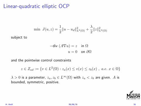
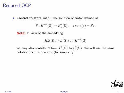
Reduced OCP
I Control to state map The solution operator defined as
S Hminus1(Ω)rarr H10 (Ω) z 7rarr u(z) = Sz
Note In view of the embedding
H10 (Ω) rarr L2(Ω) rarr Hminus1(Ω)
we may also consider S from L2(Ω) to L2(Ω) We will use the samenotation for this operator (for simplicity)
I Reduced cost functional The reduced cost functionalJ L2(Ω)rarr R is defined as
J (z) = J(Sz z)
I Reduced problem minzisinZadJ (z)
H Antil 060616 17
Existence of solution Direct methodThere exists a unique solution to the above problem
I Minimizing sequence J is bounded below by zero therefore thereexists a minimizing sequence znnisinN such that
limnrarrinfin
J (zn) = inf J (z)
I Weak compactness zn sub L2(Ω) is bounded Since L2(Ω) isreflexive therefore there exists a subsequence (not relabeled) suchthat
zn z and z isin Zad
where the latter is a consequence of Zad being closed and convex
I Optimality Since J is continuous and convex and therefore isweakly lower semicontinuous We obtain
lim inf J (zn) ge J (z)
which implies that z is optimal
I Uniqueness Exercise
H Antil 060616 18
Outline
Motivation and examples
Linear elliptic optimal control problems
Differentiation in Banach spaces
First-order necessary conditions
Optimal control of semilinear PDEs
An abstract problem
Discretization using finite element methods
H Antil 060616 19
Differentiation in Banach spacesLet (Z middot Z) (V middot V ) B-spaces Z sub Z open and F Z rarr V
Let z isin Z
I If exist δF (z h) = limtdarr01t (F (z + th)minus F (z)) then δF (z h) is called
the directional derivative of F at z in direction h
I If exist δF (z h) forallh isin Z then h 7rarr δF (z h) is the first variation of Fat z
I Let exist the first variation δF (z middot) F is said to be Gateauxdifferentiable at z iff existA isin L(Z V ) such that δF (z h) = Ahforallh isin Z We write A = F primeG(z)
I F is said to be Frechet differentiable at z iff existA isin L(Z V ) and amapping r(z middot) Z rarr V such that for all h isin U with z + h isin Zwe have
F (z+h) = F (z)+Ah+r(z h) withr(z h)VhZ
rarr 0 as hZ rarr 0
We write F prime(z) = A
H Antil 060616 20
Differentiation in Banach spacesLet (Z middot Z) (V middot V ) B-spaces Z sub Z open and F Z rarr V
Let z isin Z
I If exist δF (z h) = limtdarr01t (F (z + th)minus F (z)) then δF (z h) is called
the directional derivative of F at z in direction h
I If exist δF (z h) forallh isin Z then h 7rarr δF (z h) is the first variation of Fat z
I Let exist the first variation δF (z middot) F is said to be Gateauxdifferentiable at z iff existA isin L(Z V ) such that δF (z h) = Ahforallh isin Z We write A = F primeG(z)
I F is said to be Frechet differentiable at z iff existA isin L(Z V ) and amapping r(z middot) Z rarr V such that for all h isin U with z + h isin Zwe have
F (z+h) = F (z)+Ah+r(z h) withr(z h)VhZ
rarr 0 as hZ rarr 0
We write F prime(z) = A
H Antil 060616 20
Differentiation in Banach spacesLet (Z middot Z) (V middot V ) B-spaces Z sub Z open and F Z rarr V
Let z isin Z
I If exist δF (z h) = limtdarr01t (F (z + th)minus F (z)) then δF (z h) is called
the directional derivative of F at z in direction h
I If exist δF (z h) forallh isin Z then h 7rarr δF (z h) is the first variation of Fat z
I Let exist the first variation δF (z middot) F is said to be Gateauxdifferentiable at z iff existA isin L(Z V ) such that δF (z h) = Ahforallh isin Z We write A = F primeG(z)
I F is said to be Frechet differentiable at z iff existA isin L(Z V ) and amapping r(z middot) Z rarr V such that for all h isin U with z + h isin Zwe have
F (z+h) = F (z)+Ah+r(z h) withr(z h)VhZ
rarr 0 as hZ rarr 0
We write F prime(z) = A
H Antil 060616 20
Differentiation in Banach spacesLet (Z middot Z) (V middot V ) B-spaces Z sub Z open and F Z rarr V
Let z isin Z
I If exist δF (z h) = limtdarr01t (F (z + th)minus F (z)) then δF (z h) is called
the directional derivative of F at z in direction h
I If exist δF (z h) forallh isin Z then h 7rarr δF (z h) is the first variation of Fat z
I Let exist the first variation δF (z middot) F is said to be Gateauxdifferentiable at z iff existA isin L(Z V ) such that δF (z h) = Ahforallh isin Z We write A = F primeG(z)
I F is said to be Frechet differentiable at z iff existA isin L(Z V ) and amapping r(z middot) Z rarr V such that for all h isin U with z + h isin Zwe have
F (z+h) = F (z)+Ah+r(z h) withr(z h)VhZ
rarr 0 as hZ rarr 0
We write F prime(z) = A
H Antil 060616 20
ExamplesExample 1 (H (middot middot)H) Hilbert space F (z) = z2H = (z z)H
forallz h F (z + h)minus F (z) = 2(z h)H + h2HThen
F prime(z)h = (2z h)H
Reisz representation theorem (identify H with Hlowast) we can write
F prime(z)h = (nablaF (z) h)H
where nablaF (z) = 2z is the gradient
Example 2 Let (Z (middot middot)Z) (H (middot middot)H) Hilbert spaces ud isin H fixedLet S isin L(ZH) Consider E Z rarr R
E(z) = Sz minus ud2H
Then E(z) = G(F (z)) where G(v) = v2H and F (z) = Sz minus ud
Eprime(z)h = Gprime(F (z))F prime(z)h = (2v F prime(z)h)H
= 2(Sz minus ud Sh)H = 2(Slowast(Sz minus ud) h)Z
we denote the gradient as nablaE(z) = 2Slowast(Sz minus ud)
H Antil 060616 21
ExamplesExample 1 (H (middot middot)H) Hilbert space F (z) = z2H = (z z)H
forallz h F (z + h)minus F (z) = 2(z h)H + h2HThen
F prime(z)h = (2z h)H
Reisz representation theorem (identify H with Hlowast) we can write
F prime(z)h = (nablaF (z) h)H
where nablaF (z) = 2z is the gradient
Example 2 Let (Z (middot middot)Z) (H (middot middot)H) Hilbert spaces ud isin H fixedLet S isin L(ZH) Consider E Z rarr R
E(z) = Sz minus ud2H
Then E(z) = G(F (z)) where G(v) = v2H and F (z) = Sz minus ud
Eprime(z)h = Gprime(F (z))F prime(z)h = (2v F prime(z)h)H
= 2(Sz minus ud Sh)H = 2(Slowast(Sz minus ud) h)Z
we denote the gradient as nablaE(z) = 2Slowast(Sz minus ud)H Antil 060616 21
Outline
Motivation and examples
Linear elliptic optimal control problems
Differentiation in Banach spaces
First-order necessary conditions
Optimal control of semilinear PDEs
An abstract problem
Discretization using finite element methods
H Antil 060616 22
First order necessary optimality conditions
Most of the theory is based on these two simple results
Theorem Let (Z middot Z) be a normed space J Z rarr (infin+infin] amapping with J 6equiv +infin Then z isin Z minimizer of J hArr 0 isin partJ (z)
Proof 0 isin partJ (z) means by definition of partJ (z) J (z)minus J (z) le 0forallz isin Z
Theorem Let (Z middot Z) be a normed space Zad sub Z nonemptyconvex closed J Z rarr R Gateaux differentiable where Zad sub Z sub ZZ open If z isin Zad is a solution to
minzisinZad
J (z)
then z solvesJ prime(z)(z minus z) ge 0 forallz isin Zad
Proof Exercise
H Antil 060616 23
First order necessary optimality conditions
Most of the theory is based on these two simple results
Theorem Let (Z middot Z) be a normed space J Z rarr (infin+infin] amapping with J 6equiv +infin Then z isin Z minimizer of J hArr 0 isin partJ (z)
Proof 0 isin partJ (z) means by definition of partJ (z) J (z)minus J (z) le 0forallz isin Z
Theorem Let (Z middot Z) be a normed space Zad sub Z nonemptyconvex closed J Z rarr R Gateaux differentiable where Zad sub Z sub ZZ open If z isin Zad is a solution to
minzisinZad
J (z)
then z solvesJ prime(z)(z minus z) ge 0 forallz isin Zad
Proof Exercise
H Antil 060616 23
Linear quadratic OCPI Reduced funcational
J (z) =1
2Sz minus ud2L2(Ω) +
λ
2z2L2(Ω)
I Gradient computation using sensitivity
J prime(z)h = (Slowast(Sz minus ud) + λz h)L2(Ω) forallh isin L2(Ω)
we denote the gradient by
nablaJ (z) = Slowast(Sz minus ud) + λz
I First order necessary and sufficient optimality condition
(nablaJ (z) z minus z)L2(Ω) ge 0 forallz isin Zad
I Adjoint equation Let p = Slowast(Sz minus ud) which translates intop isin H1
0 (Ω) solving
minusdiv (Anablap) = uminus ud in Ω
p = 0 on partΩ
I Gradient computation using adjoint nablaJ (z) = p+ λz
H Antil 060616 24
Linear quadratic OCPI Reduced funcational
J (z) =1
2Sz minus ud2L2(Ω) +
λ
2z2L2(Ω)
I Gradient computation using sensitivity
J prime(z)h = (Slowast(Sz minus ud) + λz h)L2(Ω) forallh isin L2(Ω)
we denote the gradient by
nablaJ (z) = Slowast(Sz minus ud) + λz
I First order necessary and sufficient optimality condition
(nablaJ (z) z minus z)L2(Ω) ge 0 forallz isin Zad
I Adjoint equation Let p = Slowast(Sz minus ud) which translates intop isin H1
0 (Ω) solving
minusdiv (Anablap) = uminus ud in Ω
p = 0 on partΩ
I Gradient computation using adjoint nablaJ (z) = p+ λz
H Antil 060616 24
Linear quadratic OCPI Reduced funcational
J (z) =1
2Sz minus ud2L2(Ω) +
λ
2z2L2(Ω)
I Gradient computation using sensitivity
J prime(z)h = (Slowast(Sz minus ud) + λz h)L2(Ω) forallh isin L2(Ω)
we denote the gradient by
nablaJ (z) = Slowast(Sz minus ud) + λz
I First order necessary and sufficient optimality condition
(nablaJ (z) z minus z)L2(Ω) ge 0 forallz isin Zad
I Adjoint equation Let p = Slowast(Sz minus ud) which translates intop isin H1
0 (Ω) solving
minusdiv (Anablap) = uminus ud in Ω
p = 0 on partΩ
I Gradient computation using adjoint nablaJ (z) = p+ λz
H Antil 060616 24
Linear quadratic OCPI Reduced funcational
J (z) =1
2Sz minus ud2L2(Ω) +
λ
2z2L2(Ω)
I Gradient computation using sensitivity
J prime(z)h = (Slowast(Sz minus ud) + λz h)L2(Ω) forallh isin L2(Ω)
we denote the gradient by
nablaJ (z) = Slowast(Sz minus ud) + λz
I First order necessary and sufficient optimality condition
(nablaJ (z) z minus z)L2(Ω) ge 0 forallz isin Zad
I Adjoint equation Let p = Slowast(Sz minus ud) which translates intop isin H1
0 (Ω) solving
minusdiv (Anablap) = uminus ud in Ω
p = 0 on partΩ
I Gradient computation using adjoint nablaJ (z) = p+ λz
H Antil 060616 24
Linear quadratic OCPI Reduced funcational
J (z) =1
2Sz minus ud2L2(Ω) +
λ
2z2L2(Ω)
I Gradient computation using sensitivity
J prime(z)h = (Slowast(Sz minus ud) + λz h)L2(Ω) forallh isin L2(Ω)
we denote the gradient by
nablaJ (z) = Slowast(Sz minus ud) + λz
I First order necessary and sufficient optimality condition
(nablaJ (z) z minus z)L2(Ω) ge 0 forallz isin Zad
I Adjoint equation Let p = Slowast(Sz minus ud) which translates intop isin H1
0 (Ω) solving
minusdiv (Anablap) = uminus ud in Ω
p = 0 on partΩ
I Gradient computation using adjoint nablaJ (z) = p+ λz
H Antil 060616 24
Optimality system
I State u isin H10 (Ω)
intΩAnablau middot nablav =
intΩzv forallv isin H1
0 (Ω)
I Adjoint p isin H10 (Ω)
intΩAnablap middot nablav =
intΩ
(uminus ud)v forallv isin H10 (Ω)
I Control z isin Zad (p+ λz z minus z) ge 0 forallz isin Zad
H Antil 060616 25
Pointwise interpretation
The variational inequality
(p+ λz z minus z) ge 0 forallz isin Zad
is equivalent to for ae x isin Ω
z(x) =
za(x) if p(x) + λz(x) gt 0isin [za(x) zb(x)] if p(x) + λz(x) = 0zb(x) if p(x) + λz(x) lt 0
Consequence
I When λ gt 0 then ae in Ω
z(x) = P[za(x)zb(x)]
minus 1
λp(x)
= min
zb(x)max
za(x)minus 1
λp(x)
H Antil 060616 26
Formal Lagrange method applied to linear OCPIntroduce L H1
0 (Ω)times Zad timesH1(Ω)rarr R defined as
L(u z p) = J(u z)minusint
Ω
(minusdiv (Anablau)minus z
)p dx
Integrate by parts to arrive at
L(u z p) = J(u z)minusint
Ω
(minusdiv (Anablap)uminus zp
)dx+
intpartΩ
(Anablau)p ds
If (u z p) is a stationary point then
I State
DpL(u z p)h = 0 forallh isin H1(Ω)
I AdjointDuL(u z p)h = 0 forallh isin H1
0 (Ω)
I ControlDzL(u z p)(z minus z) ge 0 forallz isin Zad
H Antil 060616 27
Formal Lagrange method applied to linear OCPIntroduce L H1
0 (Ω)times Zad timesH1(Ω)rarr R defined as
L(u z p) = J(u z)minusint
Ω
(minusdiv (Anablau)minus z
)p dx
Integrate by parts to arrive at
L(u z p) = J(u z)minusint
Ω
(minusdiv (Anablap)uminus zp
)dx+
intpartΩ
(Anablau)p ds
If (u z p) is a stationary point then
I State
DpL(u z p)h = 0 forallh isin H1(Ω)
I AdjointDuL(u z p)h = 0 forallh isin H1
0 (Ω)
I ControlDzL(u z p)(z minus z) ge 0 forallz isin Zad
H Antil 060616 27
Formal Lagrange method applied to linear OCPIntroduce L H1
0 (Ω)times Zad timesH1(Ω)rarr R defined as
L(u z p) = J(u z)minusint
Ω
(minusdiv (Anablau)minus z
)p dx
Integrate by parts to arrive at
L(u z p) = J(u z)minusint
Ω
(minusdiv (Anablap)uminus zp
)dx+
intpartΩ
(Anablau)p ds
If (u z p) is a stationary point then
I State
DpL(u z p)h = 0 forallh isin H1(Ω)
I AdjointDuL(u z p)h = 0 forallh isin H1
0 (Ω)
I ControlDzL(u z p)(z minus z) ge 0 forallz isin Zad
H Antil 060616 27
Formal Lagrange method applied to linear OCPIntroduce L H1
0 (Ω)times Zad timesH1(Ω)rarr R defined as
L(u z p) = J(u z)minusint
Ω
(minusdiv (Anablau)minus z
)p dx
Integrate by parts to arrive at
L(u z p) = J(u z)minusint
Ω
(minusdiv (Anablap)uminus zp
)dx+
intpartΩ
(Anablau)p ds
If (u z p) is a stationary point then
I State
DpL(u z p)h = 0 forallh isin H1(Ω)
I AdjointDuL(u z p)h = 0 forallh isin H1
0 (Ω)
I ControlDzL(u z p)(z minus z) ge 0 forallz isin Zad
H Antil 060616 27
Formal Lagrange method applied to linear OCPIntroduce L H1
0 (Ω)times Zad timesH1(Ω)rarr R defined as
L(u z p) = J(u z)minusint
Ω
(minusdiv (Anablau)minus z
)p dx
Integrate by parts to arrive at
L(u z p) = J(u z)minusint
Ω
(minusdiv (Anablap)uminus zp
)dx+
intpartΩ
(Anablau)p ds
If (u z p) is a stationary point then
I State
DpL(u z p)h = 0 forallh isin H1(Ω)
I AdjointDuL(u z p)h = 0 forallh isin H1
0 (Ω)
I ControlDzL(u z p)(z minus z) ge 0 forallz isin Zad
H Antil 060616 27
Outline
Motivation and examples
Linear elliptic optimal control problems
Differentiation in Banach spaces
First-order necessary conditions
Optimal control of semilinear PDEs
An abstract problem
Discretization using finite element methods
H Antil 060616 28
Semilinear elliptic OCP
min J(u z) =1
2uminus ud2L2(Ω) +
λ
2z2L2(Ω)
subject to
minus∆u+ g(x u) = z in Ω
u = 0 on partΩ
and z isin Zad with za zb isin Linfin(Ω)
H Antil 060616 29
State space(A1) Ω sub Rd open bounded partΩ is Lipschitz
(A2) g Ωtimes Rrarr R is bounded and measurable with respect to x isin Ωfor every u isin R
(A3) g is continuous monotone increasing and Lipschitz continuous in ufor ae x isin Ω
(A4) g(x 0) = 0 for ae x isin Ω (not really necessary)
Theorem Suppose (A1)minus (A4) hold For every z isin Lr(Ω) withr gt d2 the state equation has a unique weak solutionu isin H1
0 (Ω) cap C(Ω) ie we haveintΩ
nablau middot nablav dx+
intΩ
g(x u(x))v(x) dx =
intΩ
zv dx forallv isin H10 (Ω)
Moreover there exists a constant C gt 0 such that
uH1(Ω) + uC(Ω) le CzLr(Ω)
RemarkI The proof of the theorem uses the BrowderndashMinty theorem on
monotone operators
H Antil 060616 30
State space(A1) Ω sub Rd open bounded partΩ is Lipschitz
(A2) g Ωtimes Rrarr R is bounded and measurable with respect to x isin Ωfor every u isin R
(A3) g is continuous monotone increasing and Lipschitz continuous in ufor ae x isin Ω
(A4) g(x 0) = 0 for ae x isin Ω (not really necessary)
Theorem Suppose (A1)minus (A4) hold For every z isin Lr(Ω) withr gt d2 the state equation has a unique weak solutionu isin H1
0 (Ω) cap C(Ω) ie we haveintΩ
nablau middot nablav dx+
intΩ
g(x u(x))v(x) dx =
intΩ
zv dx forallv isin H10 (Ω)
Moreover there exists a constant C gt 0 such that
uH1(Ω) + uC(Ω) le CzLr(Ω)
RemarkI The proof of the theorem uses the BrowderndashMinty theorem on
monotone operators
H Antil 060616 30
State space(A1) Ω sub Rd open bounded partΩ is Lipschitz
(A2) g Ωtimes Rrarr R is bounded and measurable with respect to x isin Ωfor every u isin R
(A3) g is continuous monotone increasing and Lipschitz continuous in ufor ae x isin Ω
(A4) g(x 0) = 0 for ae x isin Ω (not really necessary)
Theorem Suppose (A1)minus (A4) hold For every z isin Lr(Ω) withr gt d2 the state equation has a unique weak solutionu isin H1
0 (Ω) cap C(Ω) ie we haveintΩ
nablau middot nablav dx+
intΩ
g(x u(x))v(x) dx =
intΩ
zv dx forallv isin H10 (Ω)
Moreover there exists a constant C gt 0 such that
uH1(Ω) + uC(Ω) le CzLr(Ω)
RemarkI The proof of the theorem uses the BrowderndashMinty theorem on
monotone operators
H Antil 060616 30
Control-to-state map and reduced problem
I Control to state map
S Linfin(Ω)rarr H10 (Ω) cap C(Ω)
is well defined and is globally Lipschitz continuous
I Reduced problem
minJ (z) =1
2S(u)minus ud2L2(Ω) +
λ
2z2L2(Ω)
H Antil 060616 31
Control-to-state map and reduced problem
I Control to state map
S Linfin(Ω)rarr H10 (Ω) cap C(Ω)
is well defined and is globally Lipschitz continuous
I Reduced problem
minJ (z) =1
2S(u)minus ud2L2(Ω) +
λ
2z2L2(Ω)
H Antil 060616 31
First-order necessary conditionsI Lagrangian functional
L(u z p) = J(u z)minusint
Ω
(minus∆u+ g(x u(x))minus z
)p dx
= J(u z)minusint
Ω
(nablau middot nablap+ g(x u(x))pminus zp
)dx
I Adjoint system For all h isin H10 (Ω)
0 = DuL(u z p)h =
intΩ
(uminus ud)h dxminusint
Ω
(nablah middot nablap+ gu(x u(x))ph
)which yields
minus∆p+ gu(x u(x))p = uminus ud in Ω
p = 0 on partΩ
I Control
DzL(u z p)(z minus z) = (p+ λz z minus z) dx ge 0 forallz isin ZadI Gradient
nablaJ (z) = p+ λz
H Antil 060616 32
First-order necessary conditionsI Lagrangian functional
L(u z p) = J(u z)minusint
Ω
(minus∆u+ g(x u(x))minus z
)p dx
= J(u z)minusint
Ω
(nablau middot nablap+ g(x u(x))pminus zp
)dx
I Adjoint system For all h isin H10 (Ω)
0 = DuL(u z p)h =
intΩ
(uminus ud)h dxminusint
Ω
(nablah middot nablap+ gu(x u(x))ph
)which yields
minus∆p+ gu(x u(x))p = uminus ud in Ω
p = 0 on partΩ
I Control
DzL(u z p)(z minus z) = (p+ λz z minus z) dx ge 0 forallz isin ZadI Gradient
nablaJ (z) = p+ λz
H Antil 060616 32
First-order necessary conditionsI Lagrangian functional
L(u z p) = J(u z)minusint
Ω
(minus∆u+ g(x u(x))minus z
)p dx
= J(u z)minusint
Ω
(nablau middot nablap+ g(x u(x))pminus zp
)dx
I Adjoint system For all h isin H10 (Ω)
0 = DuL(u z p)h =
intΩ
(uminus ud)h dxminusint
Ω
(nablah middot nablap+ gu(x u(x))ph
)which yields
minus∆p+ gu(x u(x))p = uminus ud in Ω
p = 0 on partΩ
I Control
DzL(u z p)(z minus z) = (p+ λz z minus z) dx ge 0 forallz isin Zad
I GradientnablaJ (z) = p+ λz
H Antil 060616 32
First-order necessary conditionsI Lagrangian functional
L(u z p) = J(u z)minusint
Ω
(minus∆u+ g(x u(x))minus z
)p dx
= J(u z)minusint
Ω
(nablau middot nablap+ g(x u(x))pminus zp
)dx
I Adjoint system For all h isin H10 (Ω)
0 = DuL(u z p)h =
intΩ
(uminus ud)h dxminusint
Ω
(nablah middot nablap+ gu(x u(x))ph
)which yields
minus∆p+ gu(x u(x))p = uminus ud in Ω
p = 0 on partΩ
I Control
DzL(u z p)(z minus z) = (p+ λz z minus z) dx ge 0 forallz isin ZadI Gradient
nablaJ (z) = p+ λz
H Antil 060616 32
Differentiability of Nemytskii operator
The rigorous proof uses
Theorem In addition to (A1)-(A4) if
(A5) g is continuously differentiable with respect to u for ae x isin Ωand we have
(i) |gu(x 0)| le K for ae x isin Ω(ii) gu is locally Lipschitz with respect to u isin R
then the Nemytskii operator G u 7rarr g(middot u(middot)) is continuously Frechetdifferentiable from Linfin(Ω) into itself and
(Gprime(u)h)(x) = gu(x u(x))h(x) ae in Ω forallh isin Linfin(Ω)
Remark (A5) holds if g(x u) = g(u) and g isin C2(R)
H Antil 060616 33
Outline
Motivation and examples
Linear elliptic optimal control problems
Differentiation in Banach spaces
First-order necessary conditions
Optimal control of semilinear PDEs
An abstract problem
Discretization using finite element methods
H Antil 060616 34
Gradient computation via adjoint general formI Abstract problem
min J(u z)
subject toc(u z) = 0
and z isin Zad
I Directional derivative Let S be the control to state map(nonlinear in general)
z 7rarr S(z) = u(z)
Under the assumptions of ldquoimplicit function theoremrdquo
J prime(z)h = (nablauJ (u(z) z) Sprime(z)h) + (nablazJ (u(z) z) h)
I Sensitivity of u with respect to z Differentiating the stateequation
cu(S(z) z)Sprime(z)h = minuscz(S(z) z)h
leads toSprime(z)h = minuscu(S(z) z)minus1
(cz(S(z) z)h
)
provided cu(S(z) z)minus1 is well-defined
H Antil 060616 35
Gradient computation via adjoint general formI Abstract problem
min J(u z)
subject toc(u z) = 0
and z isin ZadI Directional derivative Let S be the control to state map
(nonlinear in general)
z 7rarr S(z) = u(z)
Under the assumptions of ldquoimplicit function theoremrdquo
J prime(z)h = (nablauJ (u(z) z) Sprime(z)h) + (nablazJ (u(z) z) h)
I Sensitivity of u with respect to z Differentiating the stateequation
cu(S(z) z)Sprime(z)h = minuscz(S(z) z)h
leads toSprime(z)h = minuscu(S(z) z)minus1
(cz(S(z) z)h
)
provided cu(S(z) z)minus1 is well-defined
H Antil 060616 35
Gradient computation via adjoint general formI Abstract problem
min J(u z)
subject toc(u z) = 0
and z isin ZadI Directional derivative Let S be the control to state map
(nonlinear in general)
z 7rarr S(z) = u(z)
Under the assumptions of ldquoimplicit function theoremrdquo
J prime(z)h = (nablauJ (u(z) z) Sprime(z)h) + (nablazJ (u(z) z) h)
I Sensitivity of u with respect to z Differentiating the stateequation
cu(S(z) z)Sprime(z)h = minuscz(S(z) z)h
leads toSprime(z)h = minuscu(S(z) z)minus1
(cz(S(z) z)h
)
provided cu(S(z) z)minus1 is well-defined
H Antil 060616 35
Adjoint equation and gradient general form
I Directional derivative
J prime(z)h = minus(nablauJ (u(z) z) cu(u(z) z)minus1cz(u(z) z)h
)+ (nablazJ (u(z) z) h)
I Gradient
nablaJ (z) = minuscz(u(z) z)lowast(cu(u(z) z)minuslowastnablauJ (u(z) z)
)+nablazJ (u(z) z)
I Introducing adjoint variable p solving
cu(u(z) z)lowastp = nablauJ (u(z) z)
we arrive at following form of gradient
nablaJ (z) = minuscz(u(z) z)lowastp+nablazJ (u(z) z)
which is tractable
H Antil 060616 36
Adjoint equation and gradient general form
I Directional derivative
J prime(z)h = minus(nablauJ (u(z) z) cu(u(z) z)minus1cz(u(z) z)h
)+ (nablazJ (u(z) z) h)
I Gradient
nablaJ (z) = minuscz(u(z) z)lowast(cu(u(z) z)minuslowastnablauJ (u(z) z)
)+nablazJ (u(z) z)
I Introducing adjoint variable p solving
cu(u(z) z)lowastp = nablauJ (u(z) z)
we arrive at following form of gradient
nablaJ (z) = minuscz(u(z) z)lowastp+nablazJ (u(z) z)
which is tractable
H Antil 060616 36
Adjoint equation and gradient general form
I Directional derivative
J prime(z)h = minus(nablauJ (u(z) z) cu(u(z) z)minus1cz(u(z) z)h
)+ (nablazJ (u(z) z) h)
I Gradient
nablaJ (z) = minuscz(u(z) z)lowast(cu(u(z) z)minuslowastnablauJ (u(z) z)
)+nablazJ (u(z) z)
I Introducing adjoint variable p solving
cu(u(z) z)lowastp = nablauJ (u(z) z)
we arrive at following form of gradient
nablaJ (z) = minuscz(u(z) z)lowastp+nablazJ (u(z) z)
which is tractable
H Antil 060616 36
Hessian computation general form
I Lagrangian L(u z p) = J(u z)minusint
Ωc(u z)p dx Then we have
DzJ (z)h = DzL(u z p)h
I Second order derivative
D2zJ (z)[h1 h2] = DuDzL(u z p)[h1 S
prime(z)h2] +D2zL(u z p)[h1 h2]
+DpDzL(u z p)[h1 Dzp(z)h2]
I We already know Sprime(z)h2 moreover
DpDzL(u z p)[h1 Dzp(z)h2] = minus(cu(u z)h1 Dzp(z)h2
)
It remain to identify Dzp(z)h2
H Antil 060616 37
Hessian computation general form
I Lagrangian L(u z p) = J(u z)minusint
Ωc(u z)p dx Then we have
DzJ (z)h = DzL(u z p)h
I Second order derivative
D2zJ (z)[h1 h2] = DuDzL(u z p)[h1 S
prime(z)h2] +D2zL(u z p)[h1 h2]
+DpDzL(u z p)[h1 Dzp(z)h2]
I We already know Sprime(z)h2 moreover
DpDzL(u z p)[h1 Dzp(z)h2] = minus(cu(u z)h1 Dzp(z)h2
)
It remain to identify Dzp(z)h2
H Antil 060616 37
Hessian computation general form
I Lagrangian L(u z p) = J(u z)minusint
Ωc(u z)p dx Then we have
DzJ (z)h = DzL(u z p)h
I Second order derivative
D2zJ (z)[h1 h2] = DuDzL(u z p)[h1 S
prime(z)h2] +D2zL(u z p)[h1 h2]
+DpDzL(u z p)[h1 Dzp(z)h2]
I We already know Sprime(z)h2 moreover
DpDzL(u z p)[h1 Dzp(z)h2] = minus(cu(u z)h1 Dzp(z)h2
)
It remain to identify Dzp(z)h2
H Antil 060616 37
Outline
Motivation and examples
Linear elliptic optimal control problems
Differentiation in Banach spaces
First-order necessary conditions
Optimal control of semilinear PDEs
An abstract problem
Discretization using finite element methods
H Antil 060616 38
Numerical approximation of Poisson equation MeshTo avoid technical issues we will assume that partΩ is polygonal
I Mesh Let T = K be a mesh of Ω where K sub Rd is an elementthat is isoparametrically equivalent to a unit simplex in Rd
I Conforming mesh We say that the mesh is conforming ifI Ω = cupKisinT KI If K1 cap K2 = x then x is a node of K1 and K2I If K1 cap K2 6= empty and K1 cap K2 6= x then K1 cap K2 is an edgeface
contained in partK1 cap partK2
I Shape regular Let T be the collection of all conformingrefinements of an original mesh T 0 Then T is called shape regularif exist κ gt 0 such that
hKρKle κ forallK isin cupiT i
where hK = diam K ρK = maxρ gt 0|Bρ sub KI Quasi-uniform A family of shape regular meshes is called-quasi
uniform if there exist a constant σ gt 0 such that
maxhKminhK
le σ
uniformly for all meshes in the family
Numerical approximation of Poisson equation MeshTo avoid technical issues we will assume that partΩ is polygonal
I Mesh Let T = K be a mesh of Ω where K sub Rd is an elementthat is isoparametrically equivalent to a unit simplex in Rd
I Conforming mesh We say that the mesh is conforming ifI Ω = cupKisinT KI If K1 cap K2 = x then x is a node of K1 and K2I If K1 cap K2 6= empty and K1 cap K2 6= x then K1 cap K2 is an edgeface
contained in partK1 cap partK2
I Shape regular Let T be the collection of all conformingrefinements of an original mesh T 0 Then T is called shape regularif exist κ gt 0 such that
hKρKle κ forallK isin cupiT i
where hK = diam K ρK = maxρ gt 0|Bρ sub KI Quasi-uniform A family of shape regular meshes is called-quasi
uniform if there exist a constant σ gt 0 such that
maxhKminhK
le σ
uniformly for all meshes in the family
Numerical approximation of Poisson equation MeshTo avoid technical issues we will assume that partΩ is polygonal
I Mesh Let T = K be a mesh of Ω where K sub Rd is an elementthat is isoparametrically equivalent to a unit simplex in Rd
I Conforming mesh We say that the mesh is conforming ifI Ω = cupKisinT KI If K1 cap K2 = x then x is a node of K1 and K2I If K1 cap K2 6= empty and K1 cap K2 6= x then K1 cap K2 is an edgeface
contained in partK1 cap partK2
I Shape regular Let T be the collection of all conformingrefinements of an original mesh T 0 Then T is called shape regularif exist κ gt 0 such that
hKρKle κ forallK isin cupiT i
where hK = diam K ρK = maxρ gt 0|Bρ sub K
I Quasi-uniform A family of shape regular meshes is called-quasiuniform if there exist a constant σ gt 0 such that
maxhKminhK
le σ
uniformly for all meshes in the family
Numerical approximation of Poisson equation MeshTo avoid technical issues we will assume that partΩ is polygonal
I Mesh Let T = K be a mesh of Ω where K sub Rd is an elementthat is isoparametrically equivalent to a unit simplex in Rd
I Conforming mesh We say that the mesh is conforming ifI Ω = cupKisinT KI If K1 cap K2 = x then x is a node of K1 and K2I If K1 cap K2 6= empty and K1 cap K2 6= x then K1 cap K2 is an edgeface
contained in partK1 cap partK2
I Shape regular Let T be the collection of all conformingrefinements of an original mesh T 0 Then T is called shape regularif exist κ gt 0 such that
hKρKle κ forallK isin cupiT i
where hK = diam K ρK = maxρ gt 0|Bρ sub KI Quasi-uniform A family of shape regular meshes is called-quasi
uniform if there exist a constant σ gt 0 such that
maxhKminhK
le σ
uniformly for all meshes in the family
FE space and Galerkin approximationI Finite element space For T isin T we define the finite element
space as
V(T ) = W isin C0(Ω) WK isin P1forallK isin T W |partΩ = 0
where P1 is the set of polynomials of degree at most 1
I Galerkin approximation of continuous problem is given by
Find UT isin V(T )
intΩ
AnablaUT middot nablaV = 〈f V 〉 forallV isin V(T )
The discrete problem is well-posedI Nodal basis Consists of functions ψi isin V(T ) with xi isin N (T )
satisfyingψxi
(xj) = δij
where N (T ) denotes the interior (plus Neumann) nodesI Galerkin orthogonality(
nabla(uminus UT )nablaW)L2(Ω)
= 0 forallW isin V(T )
H Antil 060616 40
FE space and Galerkin approximationI Finite element space For T isin T we define the finite element
space as
V(T ) = W isin C0(Ω) WK isin P1forallK isin T W |partΩ = 0
where P1 is the set of polynomials of degree at most 1I Galerkin approximation of continuous problem is given by
Find UT isin V(T )
intΩ
AnablaUT middot nablaV = 〈f V 〉 forallV isin V(T )
The discrete problem is well-posed
I Nodal basis Consists of functions ψi isin V(T ) with xi isin N (T )satisfying
ψxi(xj) = δij
where N (T ) denotes the interior (plus Neumann) nodesI Galerkin orthogonality(
nabla(uminus UT )nablaW)L2(Ω)
= 0 forallW isin V(T )
H Antil 060616 40
FE space and Galerkin approximationI Finite element space For T isin T we define the finite element
space as
V(T ) = W isin C0(Ω) WK isin P1forallK isin T W |partΩ = 0
where P1 is the set of polynomials of degree at most 1I Galerkin approximation of continuous problem is given by
Find UT isin V(T )
intΩ
AnablaUT middot nablaV = 〈f V 〉 forallV isin V(T )
The discrete problem is well-posedI Nodal basis Consists of functions ψi isin V(T ) with xi isin N (T )
satisfyingψxi
(xj) = δij
where N (T ) denotes the interior (plus Neumann) nodes
I Galerkin orthogonality(nabla(uminus UT )nablaW
)L2(Ω)
= 0 forallW isin V(T )
H Antil 060616 40
FE space and Galerkin approximationI Finite element space For T isin T we define the finite element
space as
V(T ) = W isin C0(Ω) WK isin P1forallK isin T W |partΩ = 0
where P1 is the set of polynomials of degree at most 1I Galerkin approximation of continuous problem is given by
Find UT isin V(T )
intΩ
AnablaUT middot nablaV = 〈f V 〉 forallV isin V(T )
The discrete problem is well-posedI Nodal basis Consists of functions ψi isin V(T ) with xi isin N (T )
satisfyingψxi
(xj) = δij
where N (T ) denotes the interior (plus Neumann) nodesI Galerkin orthogonality(
nabla(uminus UT )nablaW)L2(Ω)
= 0 forallW isin V(T )
H Antil 060616 40
Best approximation
I Cearsquos lemma
nabla(uminus UT )L2(Ω) le C infWisinV(T )
nabla(uminusW )L2(Ω)
I Nodal interpolation operator ΠT C(Ω)rarr V(T ) satisfies
ΠT u(xi) = u(xi) forallxi isin N (T )
and is defined as
ΠT u =sum
xiisinN (T )
u(xi)ψxi
I Error estimates In Cearsquos lemma replace W by ΠT u and thencompute the interpolation error
H Antil 060616 41
Best approximation
I Cearsquos lemma
nabla(uminus UT )L2(Ω) le C infWisinV(T )
nabla(uminusW )L2(Ω)
I Nodal interpolation operator ΠT C(Ω)rarr V(T ) satisfies
ΠT u(xi) = u(xi) forallxi isin N (T )
and is defined as
ΠT u =sum
xiisinN (T )
u(xi)ψxi
I Error estimates In Cearsquos lemma replace W by ΠT u and thencompute the interpolation error
H Antil 060616 41
Best approximation
I Cearsquos lemma
nabla(uminus UT )L2(Ω) le C infWisinV(T )
nabla(uminusW )L2(Ω)
I Nodal interpolation operator ΠT C(Ω)rarr V(T ) satisfies
ΠT u(xi) = u(xi) forallxi isin N (T )
and is defined as
ΠT u =sum
xiisinN (T )
u(xi)ψxi
I Error estimates In Cearsquos lemma replace W by ΠT u and thencompute the interpolation error
H Antil 060616 41
Algebraic system state equation
I Recall UT isin V(T ) solves
a(UT V ) = 〈f V 〉 forallV isin V(T )
I Now setting UT =sumN
j=1 Ujψj V = ψi we get
Nsumj=1
Uja(φj φi) = 〈f ψi〉 i = 1 N
which is the matrix-vector system
AU = F
I Stiffness matrix A is SPD
H Antil 060616 42
Algebraic system state equation
I Recall UT isin V(T ) solves
a(UT V ) = 〈f V 〉 forallV isin V(T )
I Now setting UT =sumN
j=1 Ujψj V = ψi we get
Nsumj=1
Uja(φj φi) = 〈f ψi〉 i = 1 N
which is the matrix-vector system
AU = F
I Stiffness matrix A is SPD
H Antil 060616 42
Algebraic system state equation
I Recall UT isin V(T ) solves
a(UT V ) = 〈f V 〉 forallV isin V(T )
I Now setting UT =sumN
j=1 Ujψj V = ψi we get
Nsumj=1
Uja(φj φi) = 〈f ψi〉 i = 1 N
which is the matrix-vector system
AU = F
I Stiffness matrix A is SPD
H Antil 060616 42
Discrete linear elliptic OCP
min JT (UT ZT ) =1
2UT minus ud2L2(Ω) +
λ
2ZT 2L2(Ω)
subject to
Find UT isin V(T )
intΩ
nablaUT middot nablaV = (ZT V )L2(Ω) forallV isin V(T )
and whereZT isin Zad(T ) = Zad cap Z(T )
is either one of these
Z(T ) =
V(T )L2(Ω) variational discretization (Hinze)WT isin Linfin(Ω) ZT |K isin P0(K)K isin T
H Antil 060616 43
Recent books
F TroltzschOptimal control of partial differential equations volume 112 ofGraduate Studies in MathematicsAmerican Mathematical Society Providence RI 2010Theory methods and applications Translated from the 2005 Germanoriginal by Jurgen Sprekels
K Ito and K KunischLagrange multiplier approach to variational problems andapplications volume 15 of Advances in Design and ControlSociety for Industrial and Applied Mathematics (SIAM)Philadelphia PA 2008
H Antil 060616 44
- Motivation and examples
- Linear elliptic optimal control problems
- Differentiation in Banach spaces
- First-order necessary conditions
- Optimal control of semilinear PDEs
- An abstract problem
- Discretization using finite element methods
-
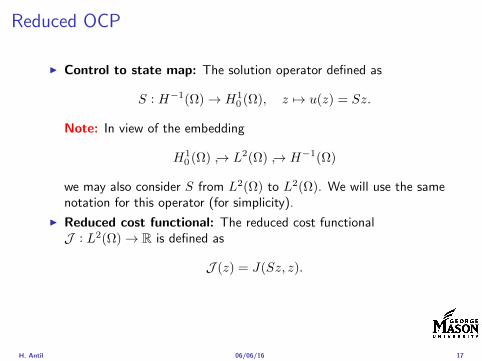
Reduced OCP
I Control to state map The solution operator defined as
S Hminus1(Ω)rarr H10 (Ω) z 7rarr u(z) = Sz
Note In view of the embedding
H10 (Ω) rarr L2(Ω) rarr Hminus1(Ω)
we may also consider S from L2(Ω) to L2(Ω) We will use the samenotation for this operator (for simplicity)
I Reduced cost functional The reduced cost functionalJ L2(Ω)rarr R is defined as
J (z) = J(Sz z)
I Reduced problem minzisinZadJ (z)
H Antil 060616 17
Reduced OCP
I Control to state map The solution operator defined as
S Hminus1(Ω)rarr H10 (Ω) z 7rarr u(z) = Sz
Note In view of the embedding
H10 (Ω) rarr L2(Ω) rarr Hminus1(Ω)
we may also consider S from L2(Ω) to L2(Ω) We will use the samenotation for this operator (for simplicity)
I Reduced cost functional The reduced cost functionalJ L2(Ω)rarr R is defined as
J (z) = J(Sz z)
I Reduced problem minzisinZadJ (z)
H Antil 060616 17
Existence of solution Direct methodThere exists a unique solution to the above problem
I Minimizing sequence J is bounded below by zero therefore thereexists a minimizing sequence znnisinN such that
limnrarrinfin
J (zn) = inf J (z)
I Weak compactness zn sub L2(Ω) is bounded Since L2(Ω) isreflexive therefore there exists a subsequence (not relabeled) suchthat
zn z and z isin Zad
where the latter is a consequence of Zad being closed and convex
I Optimality Since J is continuous and convex and therefore isweakly lower semicontinuous We obtain
lim inf J (zn) ge J (z)
which implies that z is optimal
I Uniqueness Exercise
H Antil 060616 18
Outline
Motivation and examples
Linear elliptic optimal control problems
Differentiation in Banach spaces
First-order necessary conditions
Optimal control of semilinear PDEs
An abstract problem
Discretization using finite element methods
H Antil 060616 19
Differentiation in Banach spacesLet (Z middot Z) (V middot V ) B-spaces Z sub Z open and F Z rarr V
Let z isin Z
I If exist δF (z h) = limtdarr01t (F (z + th)minus F (z)) then δF (z h) is called
the directional derivative of F at z in direction h
I If exist δF (z h) forallh isin Z then h 7rarr δF (z h) is the first variation of Fat z
I Let exist the first variation δF (z middot) F is said to be Gateauxdifferentiable at z iff existA isin L(Z V ) such that δF (z h) = Ahforallh isin Z We write A = F primeG(z)
I F is said to be Frechet differentiable at z iff existA isin L(Z V ) and amapping r(z middot) Z rarr V such that for all h isin U with z + h isin Zwe have
F (z+h) = F (z)+Ah+r(z h) withr(z h)VhZ
rarr 0 as hZ rarr 0
We write F prime(z) = A
H Antil 060616 20
Differentiation in Banach spacesLet (Z middot Z) (V middot V ) B-spaces Z sub Z open and F Z rarr V
Let z isin Z
I If exist δF (z h) = limtdarr01t (F (z + th)minus F (z)) then δF (z h) is called
the directional derivative of F at z in direction h
I If exist δF (z h) forallh isin Z then h 7rarr δF (z h) is the first variation of Fat z
I Let exist the first variation δF (z middot) F is said to be Gateauxdifferentiable at z iff existA isin L(Z V ) such that δF (z h) = Ahforallh isin Z We write A = F primeG(z)
I F is said to be Frechet differentiable at z iff existA isin L(Z V ) and amapping r(z middot) Z rarr V such that for all h isin U with z + h isin Zwe have
F (z+h) = F (z)+Ah+r(z h) withr(z h)VhZ
rarr 0 as hZ rarr 0
We write F prime(z) = A
H Antil 060616 20
Differentiation in Banach spacesLet (Z middot Z) (V middot V ) B-spaces Z sub Z open and F Z rarr V
Let z isin Z
I If exist δF (z h) = limtdarr01t (F (z + th)minus F (z)) then δF (z h) is called
the directional derivative of F at z in direction h
I If exist δF (z h) forallh isin Z then h 7rarr δF (z h) is the first variation of Fat z
I Let exist the first variation δF (z middot) F is said to be Gateauxdifferentiable at z iff existA isin L(Z V ) such that δF (z h) = Ahforallh isin Z We write A = F primeG(z)
I F is said to be Frechet differentiable at z iff existA isin L(Z V ) and amapping r(z middot) Z rarr V such that for all h isin U with z + h isin Zwe have
F (z+h) = F (z)+Ah+r(z h) withr(z h)VhZ
rarr 0 as hZ rarr 0
We write F prime(z) = A
H Antil 060616 20
Differentiation in Banach spacesLet (Z middot Z) (V middot V ) B-spaces Z sub Z open and F Z rarr V
Let z isin Z
I If exist δF (z h) = limtdarr01t (F (z + th)minus F (z)) then δF (z h) is called
the directional derivative of F at z in direction h
I If exist δF (z h) forallh isin Z then h 7rarr δF (z h) is the first variation of Fat z
I Let exist the first variation δF (z middot) F is said to be Gateauxdifferentiable at z iff existA isin L(Z V ) such that δF (z h) = Ahforallh isin Z We write A = F primeG(z)
I F is said to be Frechet differentiable at z iff existA isin L(Z V ) and amapping r(z middot) Z rarr V such that for all h isin U with z + h isin Zwe have
F (z+h) = F (z)+Ah+r(z h) withr(z h)VhZ
rarr 0 as hZ rarr 0
We write F prime(z) = A
H Antil 060616 20
ExamplesExample 1 (H (middot middot)H) Hilbert space F (z) = z2H = (z z)H
forallz h F (z + h)minus F (z) = 2(z h)H + h2HThen
F prime(z)h = (2z h)H
Reisz representation theorem (identify H with Hlowast) we can write
F prime(z)h = (nablaF (z) h)H
where nablaF (z) = 2z is the gradient
Example 2 Let (Z (middot middot)Z) (H (middot middot)H) Hilbert spaces ud isin H fixedLet S isin L(ZH) Consider E Z rarr R
E(z) = Sz minus ud2H
Then E(z) = G(F (z)) where G(v) = v2H and F (z) = Sz minus ud
Eprime(z)h = Gprime(F (z))F prime(z)h = (2v F prime(z)h)H
= 2(Sz minus ud Sh)H = 2(Slowast(Sz minus ud) h)Z
we denote the gradient as nablaE(z) = 2Slowast(Sz minus ud)
H Antil 060616 21
ExamplesExample 1 (H (middot middot)H) Hilbert space F (z) = z2H = (z z)H
forallz h F (z + h)minus F (z) = 2(z h)H + h2HThen
F prime(z)h = (2z h)H
Reisz representation theorem (identify H with Hlowast) we can write
F prime(z)h = (nablaF (z) h)H
where nablaF (z) = 2z is the gradient
Example 2 Let (Z (middot middot)Z) (H (middot middot)H) Hilbert spaces ud isin H fixedLet S isin L(ZH) Consider E Z rarr R
E(z) = Sz minus ud2H
Then E(z) = G(F (z)) where G(v) = v2H and F (z) = Sz minus ud
Eprime(z)h = Gprime(F (z))F prime(z)h = (2v F prime(z)h)H
= 2(Sz minus ud Sh)H = 2(Slowast(Sz minus ud) h)Z
we denote the gradient as nablaE(z) = 2Slowast(Sz minus ud)H Antil 060616 21
Outline
Motivation and examples
Linear elliptic optimal control problems
Differentiation in Banach spaces
First-order necessary conditions
Optimal control of semilinear PDEs
An abstract problem
Discretization using finite element methods
H Antil 060616 22
First order necessary optimality conditions
Most of the theory is based on these two simple results
Theorem Let (Z middot Z) be a normed space J Z rarr (infin+infin] amapping with J 6equiv +infin Then z isin Z minimizer of J hArr 0 isin partJ (z)
Proof 0 isin partJ (z) means by definition of partJ (z) J (z)minus J (z) le 0forallz isin Z
Theorem Let (Z middot Z) be a normed space Zad sub Z nonemptyconvex closed J Z rarr R Gateaux differentiable where Zad sub Z sub ZZ open If z isin Zad is a solution to
minzisinZad
J (z)
then z solvesJ prime(z)(z minus z) ge 0 forallz isin Zad
Proof Exercise
H Antil 060616 23
First order necessary optimality conditions
Most of the theory is based on these two simple results
Theorem Let (Z middot Z) be a normed space J Z rarr (infin+infin] amapping with J 6equiv +infin Then z isin Z minimizer of J hArr 0 isin partJ (z)
Proof 0 isin partJ (z) means by definition of partJ (z) J (z)minus J (z) le 0forallz isin Z
Theorem Let (Z middot Z) be a normed space Zad sub Z nonemptyconvex closed J Z rarr R Gateaux differentiable where Zad sub Z sub ZZ open If z isin Zad is a solution to
minzisinZad
J (z)
then z solvesJ prime(z)(z minus z) ge 0 forallz isin Zad
Proof Exercise
H Antil 060616 23
Linear quadratic OCPI Reduced funcational
J (z) =1
2Sz minus ud2L2(Ω) +
λ
2z2L2(Ω)
I Gradient computation using sensitivity
J prime(z)h = (Slowast(Sz minus ud) + λz h)L2(Ω) forallh isin L2(Ω)
we denote the gradient by
nablaJ (z) = Slowast(Sz minus ud) + λz
I First order necessary and sufficient optimality condition
(nablaJ (z) z minus z)L2(Ω) ge 0 forallz isin Zad
I Adjoint equation Let p = Slowast(Sz minus ud) which translates intop isin H1
0 (Ω) solving
minusdiv (Anablap) = uminus ud in Ω
p = 0 on partΩ
I Gradient computation using adjoint nablaJ (z) = p+ λz
H Antil 060616 24
Linear quadratic OCPI Reduced funcational
J (z) =1
2Sz minus ud2L2(Ω) +
λ
2z2L2(Ω)
I Gradient computation using sensitivity
J prime(z)h = (Slowast(Sz minus ud) + λz h)L2(Ω) forallh isin L2(Ω)
we denote the gradient by
nablaJ (z) = Slowast(Sz minus ud) + λz
I First order necessary and sufficient optimality condition
(nablaJ (z) z minus z)L2(Ω) ge 0 forallz isin Zad
I Adjoint equation Let p = Slowast(Sz minus ud) which translates intop isin H1
0 (Ω) solving
minusdiv (Anablap) = uminus ud in Ω
p = 0 on partΩ
I Gradient computation using adjoint nablaJ (z) = p+ λz
H Antil 060616 24
Linear quadratic OCPI Reduced funcational
J (z) =1
2Sz minus ud2L2(Ω) +
λ
2z2L2(Ω)
I Gradient computation using sensitivity
J prime(z)h = (Slowast(Sz minus ud) + λz h)L2(Ω) forallh isin L2(Ω)
we denote the gradient by
nablaJ (z) = Slowast(Sz minus ud) + λz
I First order necessary and sufficient optimality condition
(nablaJ (z) z minus z)L2(Ω) ge 0 forallz isin Zad
I Adjoint equation Let p = Slowast(Sz minus ud) which translates intop isin H1
0 (Ω) solving
minusdiv (Anablap) = uminus ud in Ω
p = 0 on partΩ
I Gradient computation using adjoint nablaJ (z) = p+ λz
H Antil 060616 24
Linear quadratic OCPI Reduced funcational
J (z) =1
2Sz minus ud2L2(Ω) +
λ
2z2L2(Ω)
I Gradient computation using sensitivity
J prime(z)h = (Slowast(Sz minus ud) + λz h)L2(Ω) forallh isin L2(Ω)
we denote the gradient by
nablaJ (z) = Slowast(Sz minus ud) + λz
I First order necessary and sufficient optimality condition
(nablaJ (z) z minus z)L2(Ω) ge 0 forallz isin Zad
I Adjoint equation Let p = Slowast(Sz minus ud) which translates intop isin H1
0 (Ω) solving
minusdiv (Anablap) = uminus ud in Ω
p = 0 on partΩ
I Gradient computation using adjoint nablaJ (z) = p+ λz
H Antil 060616 24
Linear quadratic OCPI Reduced funcational
J (z) =1
2Sz minus ud2L2(Ω) +
λ
2z2L2(Ω)
I Gradient computation using sensitivity
J prime(z)h = (Slowast(Sz minus ud) + λz h)L2(Ω) forallh isin L2(Ω)
we denote the gradient by
nablaJ (z) = Slowast(Sz minus ud) + λz
I First order necessary and sufficient optimality condition
(nablaJ (z) z minus z)L2(Ω) ge 0 forallz isin Zad
I Adjoint equation Let p = Slowast(Sz minus ud) which translates intop isin H1
0 (Ω) solving
minusdiv (Anablap) = uminus ud in Ω
p = 0 on partΩ
I Gradient computation using adjoint nablaJ (z) = p+ λz
H Antil 060616 24
Optimality system
I State u isin H10 (Ω)
intΩAnablau middot nablav =
intΩzv forallv isin H1
0 (Ω)
I Adjoint p isin H10 (Ω)
intΩAnablap middot nablav =
intΩ
(uminus ud)v forallv isin H10 (Ω)
I Control z isin Zad (p+ λz z minus z) ge 0 forallz isin Zad
H Antil 060616 25
Pointwise interpretation
The variational inequality
(p+ λz z minus z) ge 0 forallz isin Zad
is equivalent to for ae x isin Ω
z(x) =
za(x) if p(x) + λz(x) gt 0isin [za(x) zb(x)] if p(x) + λz(x) = 0zb(x) if p(x) + λz(x) lt 0
Consequence
I When λ gt 0 then ae in Ω
z(x) = P[za(x)zb(x)]
minus 1
λp(x)
= min
zb(x)max
za(x)minus 1
λp(x)
H Antil 060616 26
Formal Lagrange method applied to linear OCPIntroduce L H1
0 (Ω)times Zad timesH1(Ω)rarr R defined as
L(u z p) = J(u z)minusint
Ω
(minusdiv (Anablau)minus z
)p dx
Integrate by parts to arrive at
L(u z p) = J(u z)minusint
Ω
(minusdiv (Anablap)uminus zp
)dx+
intpartΩ
(Anablau)p ds
If (u z p) is a stationary point then
I State
DpL(u z p)h = 0 forallh isin H1(Ω)
I AdjointDuL(u z p)h = 0 forallh isin H1
0 (Ω)
I ControlDzL(u z p)(z minus z) ge 0 forallz isin Zad
H Antil 060616 27
Formal Lagrange method applied to linear OCPIntroduce L H1
0 (Ω)times Zad timesH1(Ω)rarr R defined as
L(u z p) = J(u z)minusint
Ω
(minusdiv (Anablau)minus z
)p dx
Integrate by parts to arrive at
L(u z p) = J(u z)minusint
Ω
(minusdiv (Anablap)uminus zp
)dx+
intpartΩ
(Anablau)p ds
If (u z p) is a stationary point then
I State
DpL(u z p)h = 0 forallh isin H1(Ω)
I AdjointDuL(u z p)h = 0 forallh isin H1
0 (Ω)
I ControlDzL(u z p)(z minus z) ge 0 forallz isin Zad
H Antil 060616 27
Formal Lagrange method applied to linear OCPIntroduce L H1
0 (Ω)times Zad timesH1(Ω)rarr R defined as
L(u z p) = J(u z)minusint
Ω
(minusdiv (Anablau)minus z
)p dx
Integrate by parts to arrive at
L(u z p) = J(u z)minusint
Ω
(minusdiv (Anablap)uminus zp
)dx+
intpartΩ
(Anablau)p ds
If (u z p) is a stationary point then
I State
DpL(u z p)h = 0 forallh isin H1(Ω)
I AdjointDuL(u z p)h = 0 forallh isin H1
0 (Ω)
I ControlDzL(u z p)(z minus z) ge 0 forallz isin Zad
H Antil 060616 27
Formal Lagrange method applied to linear OCPIntroduce L H1
0 (Ω)times Zad timesH1(Ω)rarr R defined as
L(u z p) = J(u z)minusint
Ω
(minusdiv (Anablau)minus z
)p dx
Integrate by parts to arrive at
L(u z p) = J(u z)minusint
Ω
(minusdiv (Anablap)uminus zp
)dx+
intpartΩ
(Anablau)p ds
If (u z p) is a stationary point then
I State
DpL(u z p)h = 0 forallh isin H1(Ω)
I AdjointDuL(u z p)h = 0 forallh isin H1
0 (Ω)
I ControlDzL(u z p)(z minus z) ge 0 forallz isin Zad
H Antil 060616 27
Formal Lagrange method applied to linear OCPIntroduce L H1
0 (Ω)times Zad timesH1(Ω)rarr R defined as
L(u z p) = J(u z)minusint
Ω
(minusdiv (Anablau)minus z
)p dx
Integrate by parts to arrive at
L(u z p) = J(u z)minusint
Ω
(minusdiv (Anablap)uminus zp
)dx+
intpartΩ
(Anablau)p ds
If (u z p) is a stationary point then
I State
DpL(u z p)h = 0 forallh isin H1(Ω)
I AdjointDuL(u z p)h = 0 forallh isin H1
0 (Ω)
I ControlDzL(u z p)(z minus z) ge 0 forallz isin Zad
H Antil 060616 27
Outline
Motivation and examples
Linear elliptic optimal control problems
Differentiation in Banach spaces
First-order necessary conditions
Optimal control of semilinear PDEs
An abstract problem
Discretization using finite element methods
H Antil 060616 28
Semilinear elliptic OCP
min J(u z) =1
2uminus ud2L2(Ω) +
λ
2z2L2(Ω)
subject to
minus∆u+ g(x u) = z in Ω
u = 0 on partΩ
and z isin Zad with za zb isin Linfin(Ω)
H Antil 060616 29
State space(A1) Ω sub Rd open bounded partΩ is Lipschitz
(A2) g Ωtimes Rrarr R is bounded and measurable with respect to x isin Ωfor every u isin R
(A3) g is continuous monotone increasing and Lipschitz continuous in ufor ae x isin Ω
(A4) g(x 0) = 0 for ae x isin Ω (not really necessary)
Theorem Suppose (A1)minus (A4) hold For every z isin Lr(Ω) withr gt d2 the state equation has a unique weak solutionu isin H1
0 (Ω) cap C(Ω) ie we haveintΩ
nablau middot nablav dx+
intΩ
g(x u(x))v(x) dx =
intΩ
zv dx forallv isin H10 (Ω)
Moreover there exists a constant C gt 0 such that
uH1(Ω) + uC(Ω) le CzLr(Ω)
RemarkI The proof of the theorem uses the BrowderndashMinty theorem on
monotone operators
H Antil 060616 30
State space(A1) Ω sub Rd open bounded partΩ is Lipschitz
(A2) g Ωtimes Rrarr R is bounded and measurable with respect to x isin Ωfor every u isin R
(A3) g is continuous monotone increasing and Lipschitz continuous in ufor ae x isin Ω
(A4) g(x 0) = 0 for ae x isin Ω (not really necessary)
Theorem Suppose (A1)minus (A4) hold For every z isin Lr(Ω) withr gt d2 the state equation has a unique weak solutionu isin H1
0 (Ω) cap C(Ω) ie we haveintΩ
nablau middot nablav dx+
intΩ
g(x u(x))v(x) dx =
intΩ
zv dx forallv isin H10 (Ω)
Moreover there exists a constant C gt 0 such that
uH1(Ω) + uC(Ω) le CzLr(Ω)
RemarkI The proof of the theorem uses the BrowderndashMinty theorem on
monotone operators
H Antil 060616 30
State space(A1) Ω sub Rd open bounded partΩ is Lipschitz
(A2) g Ωtimes Rrarr R is bounded and measurable with respect to x isin Ωfor every u isin R
(A3) g is continuous monotone increasing and Lipschitz continuous in ufor ae x isin Ω
(A4) g(x 0) = 0 for ae x isin Ω (not really necessary)
Theorem Suppose (A1)minus (A4) hold For every z isin Lr(Ω) withr gt d2 the state equation has a unique weak solutionu isin H1
0 (Ω) cap C(Ω) ie we haveintΩ
nablau middot nablav dx+
intΩ
g(x u(x))v(x) dx =
intΩ
zv dx forallv isin H10 (Ω)
Moreover there exists a constant C gt 0 such that
uH1(Ω) + uC(Ω) le CzLr(Ω)
RemarkI The proof of the theorem uses the BrowderndashMinty theorem on
monotone operators
H Antil 060616 30
Control-to-state map and reduced problem
I Control to state map
S Linfin(Ω)rarr H10 (Ω) cap C(Ω)
is well defined and is globally Lipschitz continuous
I Reduced problem
minJ (z) =1
2S(u)minus ud2L2(Ω) +
λ
2z2L2(Ω)
H Antil 060616 31
Control-to-state map and reduced problem
I Control to state map
S Linfin(Ω)rarr H10 (Ω) cap C(Ω)
is well defined and is globally Lipschitz continuous
I Reduced problem
minJ (z) =1
2S(u)minus ud2L2(Ω) +
λ
2z2L2(Ω)
H Antil 060616 31
First-order necessary conditionsI Lagrangian functional
L(u z p) = J(u z)minusint
Ω
(minus∆u+ g(x u(x))minus z
)p dx
= J(u z)minusint
Ω
(nablau middot nablap+ g(x u(x))pminus zp
)dx
I Adjoint system For all h isin H10 (Ω)
0 = DuL(u z p)h =
intΩ
(uminus ud)h dxminusint
Ω
(nablah middot nablap+ gu(x u(x))ph
)which yields
minus∆p+ gu(x u(x))p = uminus ud in Ω
p = 0 on partΩ
I Control
DzL(u z p)(z minus z) = (p+ λz z minus z) dx ge 0 forallz isin ZadI Gradient
nablaJ (z) = p+ λz
H Antil 060616 32
First-order necessary conditionsI Lagrangian functional
L(u z p) = J(u z)minusint
Ω
(minus∆u+ g(x u(x))minus z
)p dx
= J(u z)minusint
Ω
(nablau middot nablap+ g(x u(x))pminus zp
)dx
I Adjoint system For all h isin H10 (Ω)
0 = DuL(u z p)h =
intΩ
(uminus ud)h dxminusint
Ω
(nablah middot nablap+ gu(x u(x))ph
)which yields
minus∆p+ gu(x u(x))p = uminus ud in Ω
p = 0 on partΩ
I Control
DzL(u z p)(z minus z) = (p+ λz z minus z) dx ge 0 forallz isin ZadI Gradient
nablaJ (z) = p+ λz
H Antil 060616 32
First-order necessary conditionsI Lagrangian functional
L(u z p) = J(u z)minusint
Ω
(minus∆u+ g(x u(x))minus z
)p dx
= J(u z)minusint
Ω
(nablau middot nablap+ g(x u(x))pminus zp
)dx
I Adjoint system For all h isin H10 (Ω)
0 = DuL(u z p)h =
intΩ
(uminus ud)h dxminusint
Ω
(nablah middot nablap+ gu(x u(x))ph
)which yields
minus∆p+ gu(x u(x))p = uminus ud in Ω
p = 0 on partΩ
I Control
DzL(u z p)(z minus z) = (p+ λz z minus z) dx ge 0 forallz isin Zad
I GradientnablaJ (z) = p+ λz
H Antil 060616 32
First-order necessary conditionsI Lagrangian functional
L(u z p) = J(u z)minusint
Ω
(minus∆u+ g(x u(x))minus z
)p dx
= J(u z)minusint
Ω
(nablau middot nablap+ g(x u(x))pminus zp
)dx
I Adjoint system For all h isin H10 (Ω)
0 = DuL(u z p)h =
intΩ
(uminus ud)h dxminusint
Ω
(nablah middot nablap+ gu(x u(x))ph
)which yields
minus∆p+ gu(x u(x))p = uminus ud in Ω
p = 0 on partΩ
I Control
DzL(u z p)(z minus z) = (p+ λz z minus z) dx ge 0 forallz isin ZadI Gradient
nablaJ (z) = p+ λz
H Antil 060616 32
Differentiability of Nemytskii operator
The rigorous proof uses
Theorem In addition to (A1)-(A4) if
(A5) g is continuously differentiable with respect to u for ae x isin Ωand we have
(i) |gu(x 0)| le K for ae x isin Ω(ii) gu is locally Lipschitz with respect to u isin R
then the Nemytskii operator G u 7rarr g(middot u(middot)) is continuously Frechetdifferentiable from Linfin(Ω) into itself and
(Gprime(u)h)(x) = gu(x u(x))h(x) ae in Ω forallh isin Linfin(Ω)
Remark (A5) holds if g(x u) = g(u) and g isin C2(R)
H Antil 060616 33
Outline
Motivation and examples
Linear elliptic optimal control problems
Differentiation in Banach spaces
First-order necessary conditions
Optimal control of semilinear PDEs
An abstract problem
Discretization using finite element methods
H Antil 060616 34
Gradient computation via adjoint general formI Abstract problem
min J(u z)
subject toc(u z) = 0
and z isin Zad
I Directional derivative Let S be the control to state map(nonlinear in general)
z 7rarr S(z) = u(z)
Under the assumptions of ldquoimplicit function theoremrdquo
J prime(z)h = (nablauJ (u(z) z) Sprime(z)h) + (nablazJ (u(z) z) h)
I Sensitivity of u with respect to z Differentiating the stateequation
cu(S(z) z)Sprime(z)h = minuscz(S(z) z)h
leads toSprime(z)h = minuscu(S(z) z)minus1
(cz(S(z) z)h
)
provided cu(S(z) z)minus1 is well-defined
H Antil 060616 35
Gradient computation via adjoint general formI Abstract problem
min J(u z)
subject toc(u z) = 0
and z isin ZadI Directional derivative Let S be the control to state map
(nonlinear in general)
z 7rarr S(z) = u(z)
Under the assumptions of ldquoimplicit function theoremrdquo
J prime(z)h = (nablauJ (u(z) z) Sprime(z)h) + (nablazJ (u(z) z) h)
I Sensitivity of u with respect to z Differentiating the stateequation
cu(S(z) z)Sprime(z)h = minuscz(S(z) z)h
leads toSprime(z)h = minuscu(S(z) z)minus1
(cz(S(z) z)h
)
provided cu(S(z) z)minus1 is well-defined
H Antil 060616 35
Gradient computation via adjoint general formI Abstract problem
min J(u z)
subject toc(u z) = 0
and z isin ZadI Directional derivative Let S be the control to state map
(nonlinear in general)
z 7rarr S(z) = u(z)
Under the assumptions of ldquoimplicit function theoremrdquo
J prime(z)h = (nablauJ (u(z) z) Sprime(z)h) + (nablazJ (u(z) z) h)
I Sensitivity of u with respect to z Differentiating the stateequation
cu(S(z) z)Sprime(z)h = minuscz(S(z) z)h
leads toSprime(z)h = minuscu(S(z) z)minus1
(cz(S(z) z)h
)
provided cu(S(z) z)minus1 is well-defined
H Antil 060616 35
Adjoint equation and gradient general form
I Directional derivative
J prime(z)h = minus(nablauJ (u(z) z) cu(u(z) z)minus1cz(u(z) z)h
)+ (nablazJ (u(z) z) h)
I Gradient
nablaJ (z) = minuscz(u(z) z)lowast(cu(u(z) z)minuslowastnablauJ (u(z) z)
)+nablazJ (u(z) z)
I Introducing adjoint variable p solving
cu(u(z) z)lowastp = nablauJ (u(z) z)
we arrive at following form of gradient
nablaJ (z) = minuscz(u(z) z)lowastp+nablazJ (u(z) z)
which is tractable
H Antil 060616 36
Adjoint equation and gradient general form
I Directional derivative
J prime(z)h = minus(nablauJ (u(z) z) cu(u(z) z)minus1cz(u(z) z)h
)+ (nablazJ (u(z) z) h)
I Gradient
nablaJ (z) = minuscz(u(z) z)lowast(cu(u(z) z)minuslowastnablauJ (u(z) z)
)+nablazJ (u(z) z)
I Introducing adjoint variable p solving
cu(u(z) z)lowastp = nablauJ (u(z) z)
we arrive at following form of gradient
nablaJ (z) = minuscz(u(z) z)lowastp+nablazJ (u(z) z)
which is tractable
H Antil 060616 36
Adjoint equation and gradient general form
I Directional derivative
J prime(z)h = minus(nablauJ (u(z) z) cu(u(z) z)minus1cz(u(z) z)h
)+ (nablazJ (u(z) z) h)
I Gradient
nablaJ (z) = minuscz(u(z) z)lowast(cu(u(z) z)minuslowastnablauJ (u(z) z)
)+nablazJ (u(z) z)
I Introducing adjoint variable p solving
cu(u(z) z)lowastp = nablauJ (u(z) z)
we arrive at following form of gradient
nablaJ (z) = minuscz(u(z) z)lowastp+nablazJ (u(z) z)
which is tractable
H Antil 060616 36
Hessian computation general form
I Lagrangian L(u z p) = J(u z)minusint
Ωc(u z)p dx Then we have
DzJ (z)h = DzL(u z p)h
I Second order derivative
D2zJ (z)[h1 h2] = DuDzL(u z p)[h1 S
prime(z)h2] +D2zL(u z p)[h1 h2]
+DpDzL(u z p)[h1 Dzp(z)h2]
I We already know Sprime(z)h2 moreover
DpDzL(u z p)[h1 Dzp(z)h2] = minus(cu(u z)h1 Dzp(z)h2
)
It remain to identify Dzp(z)h2
H Antil 060616 37
Hessian computation general form
I Lagrangian L(u z p) = J(u z)minusint
Ωc(u z)p dx Then we have
DzJ (z)h = DzL(u z p)h
I Second order derivative
D2zJ (z)[h1 h2] = DuDzL(u z p)[h1 S
prime(z)h2] +D2zL(u z p)[h1 h2]
+DpDzL(u z p)[h1 Dzp(z)h2]
I We already know Sprime(z)h2 moreover
DpDzL(u z p)[h1 Dzp(z)h2] = minus(cu(u z)h1 Dzp(z)h2
)
It remain to identify Dzp(z)h2
H Antil 060616 37
Hessian computation general form
I Lagrangian L(u z p) = J(u z)minusint
Ωc(u z)p dx Then we have
DzJ (z)h = DzL(u z p)h
I Second order derivative
D2zJ (z)[h1 h2] = DuDzL(u z p)[h1 S
prime(z)h2] +D2zL(u z p)[h1 h2]
+DpDzL(u z p)[h1 Dzp(z)h2]
I We already know Sprime(z)h2 moreover
DpDzL(u z p)[h1 Dzp(z)h2] = minus(cu(u z)h1 Dzp(z)h2
)
It remain to identify Dzp(z)h2
H Antil 060616 37
Outline
Motivation and examples
Linear elliptic optimal control problems
Differentiation in Banach spaces
First-order necessary conditions
Optimal control of semilinear PDEs
An abstract problem
Discretization using finite element methods
H Antil 060616 38
Numerical approximation of Poisson equation MeshTo avoid technical issues we will assume that partΩ is polygonal
I Mesh Let T = K be a mesh of Ω where K sub Rd is an elementthat is isoparametrically equivalent to a unit simplex in Rd
I Conforming mesh We say that the mesh is conforming ifI Ω = cupKisinT KI If K1 cap K2 = x then x is a node of K1 and K2I If K1 cap K2 6= empty and K1 cap K2 6= x then K1 cap K2 is an edgeface
contained in partK1 cap partK2
I Shape regular Let T be the collection of all conformingrefinements of an original mesh T 0 Then T is called shape regularif exist κ gt 0 such that
hKρKle κ forallK isin cupiT i
where hK = diam K ρK = maxρ gt 0|Bρ sub KI Quasi-uniform A family of shape regular meshes is called-quasi
uniform if there exist a constant σ gt 0 such that
maxhKminhK
le σ
uniformly for all meshes in the family
Numerical approximation of Poisson equation MeshTo avoid technical issues we will assume that partΩ is polygonal
I Mesh Let T = K be a mesh of Ω where K sub Rd is an elementthat is isoparametrically equivalent to a unit simplex in Rd
I Conforming mesh We say that the mesh is conforming ifI Ω = cupKisinT KI If K1 cap K2 = x then x is a node of K1 and K2I If K1 cap K2 6= empty and K1 cap K2 6= x then K1 cap K2 is an edgeface
contained in partK1 cap partK2
I Shape regular Let T be the collection of all conformingrefinements of an original mesh T 0 Then T is called shape regularif exist κ gt 0 such that
hKρKle κ forallK isin cupiT i
where hK = diam K ρK = maxρ gt 0|Bρ sub KI Quasi-uniform A family of shape regular meshes is called-quasi
uniform if there exist a constant σ gt 0 such that
maxhKminhK
le σ
uniformly for all meshes in the family
Numerical approximation of Poisson equation MeshTo avoid technical issues we will assume that partΩ is polygonal
I Mesh Let T = K be a mesh of Ω where K sub Rd is an elementthat is isoparametrically equivalent to a unit simplex in Rd
I Conforming mesh We say that the mesh is conforming ifI Ω = cupKisinT KI If K1 cap K2 = x then x is a node of K1 and K2I If K1 cap K2 6= empty and K1 cap K2 6= x then K1 cap K2 is an edgeface
contained in partK1 cap partK2
I Shape regular Let T be the collection of all conformingrefinements of an original mesh T 0 Then T is called shape regularif exist κ gt 0 such that
hKρKle κ forallK isin cupiT i
where hK = diam K ρK = maxρ gt 0|Bρ sub K
I Quasi-uniform A family of shape regular meshes is called-quasiuniform if there exist a constant σ gt 0 such that
maxhKminhK
le σ
uniformly for all meshes in the family
Numerical approximation of Poisson equation MeshTo avoid technical issues we will assume that partΩ is polygonal
I Mesh Let T = K be a mesh of Ω where K sub Rd is an elementthat is isoparametrically equivalent to a unit simplex in Rd
I Conforming mesh We say that the mesh is conforming ifI Ω = cupKisinT KI If K1 cap K2 = x then x is a node of K1 and K2I If K1 cap K2 6= empty and K1 cap K2 6= x then K1 cap K2 is an edgeface
contained in partK1 cap partK2
I Shape regular Let T be the collection of all conformingrefinements of an original mesh T 0 Then T is called shape regularif exist κ gt 0 such that
hKρKle κ forallK isin cupiT i
where hK = diam K ρK = maxρ gt 0|Bρ sub KI Quasi-uniform A family of shape regular meshes is called-quasi
uniform if there exist a constant σ gt 0 such that
maxhKminhK
le σ
uniformly for all meshes in the family
FE space and Galerkin approximationI Finite element space For T isin T we define the finite element
space as
V(T ) = W isin C0(Ω) WK isin P1forallK isin T W |partΩ = 0
where P1 is the set of polynomials of degree at most 1
I Galerkin approximation of continuous problem is given by
Find UT isin V(T )
intΩ
AnablaUT middot nablaV = 〈f V 〉 forallV isin V(T )
The discrete problem is well-posedI Nodal basis Consists of functions ψi isin V(T ) with xi isin N (T )
satisfyingψxi
(xj) = δij
where N (T ) denotes the interior (plus Neumann) nodesI Galerkin orthogonality(
nabla(uminus UT )nablaW)L2(Ω)
= 0 forallW isin V(T )
H Antil 060616 40
FE space and Galerkin approximationI Finite element space For T isin T we define the finite element
space as
V(T ) = W isin C0(Ω) WK isin P1forallK isin T W |partΩ = 0
where P1 is the set of polynomials of degree at most 1I Galerkin approximation of continuous problem is given by
Find UT isin V(T )
intΩ
AnablaUT middot nablaV = 〈f V 〉 forallV isin V(T )
The discrete problem is well-posed
I Nodal basis Consists of functions ψi isin V(T ) with xi isin N (T )satisfying
ψxi(xj) = δij
where N (T ) denotes the interior (plus Neumann) nodesI Galerkin orthogonality(
nabla(uminus UT )nablaW)L2(Ω)
= 0 forallW isin V(T )
H Antil 060616 40
FE space and Galerkin approximationI Finite element space For T isin T we define the finite element
space as
V(T ) = W isin C0(Ω) WK isin P1forallK isin T W |partΩ = 0
where P1 is the set of polynomials of degree at most 1I Galerkin approximation of continuous problem is given by
Find UT isin V(T )
intΩ
AnablaUT middot nablaV = 〈f V 〉 forallV isin V(T )
The discrete problem is well-posedI Nodal basis Consists of functions ψi isin V(T ) with xi isin N (T )
satisfyingψxi
(xj) = δij
where N (T ) denotes the interior (plus Neumann) nodes
I Galerkin orthogonality(nabla(uminus UT )nablaW
)L2(Ω)
= 0 forallW isin V(T )
H Antil 060616 40
FE space and Galerkin approximationI Finite element space For T isin T we define the finite element
space as
V(T ) = W isin C0(Ω) WK isin P1forallK isin T W |partΩ = 0
where P1 is the set of polynomials of degree at most 1I Galerkin approximation of continuous problem is given by
Find UT isin V(T )
intΩ
AnablaUT middot nablaV = 〈f V 〉 forallV isin V(T )
The discrete problem is well-posedI Nodal basis Consists of functions ψi isin V(T ) with xi isin N (T )
satisfyingψxi
(xj) = δij
where N (T ) denotes the interior (plus Neumann) nodesI Galerkin orthogonality(
nabla(uminus UT )nablaW)L2(Ω)
= 0 forallW isin V(T )
H Antil 060616 40
Best approximation
I Cearsquos lemma
nabla(uminus UT )L2(Ω) le C infWisinV(T )
nabla(uminusW )L2(Ω)
I Nodal interpolation operator ΠT C(Ω)rarr V(T ) satisfies
ΠT u(xi) = u(xi) forallxi isin N (T )
and is defined as
ΠT u =sum
xiisinN (T )
u(xi)ψxi
I Error estimates In Cearsquos lemma replace W by ΠT u and thencompute the interpolation error
H Antil 060616 41
Best approximation
I Cearsquos lemma
nabla(uminus UT )L2(Ω) le C infWisinV(T )
nabla(uminusW )L2(Ω)
I Nodal interpolation operator ΠT C(Ω)rarr V(T ) satisfies
ΠT u(xi) = u(xi) forallxi isin N (T )
and is defined as
ΠT u =sum
xiisinN (T )
u(xi)ψxi
I Error estimates In Cearsquos lemma replace W by ΠT u and thencompute the interpolation error
H Antil 060616 41
Best approximation
I Cearsquos lemma
nabla(uminus UT )L2(Ω) le C infWisinV(T )
nabla(uminusW )L2(Ω)
I Nodal interpolation operator ΠT C(Ω)rarr V(T ) satisfies
ΠT u(xi) = u(xi) forallxi isin N (T )
and is defined as
ΠT u =sum
xiisinN (T )
u(xi)ψxi
I Error estimates In Cearsquos lemma replace W by ΠT u and thencompute the interpolation error
H Antil 060616 41
Algebraic system state equation
I Recall UT isin V(T ) solves
a(UT V ) = 〈f V 〉 forallV isin V(T )
I Now setting UT =sumN
j=1 Ujψj V = ψi we get
Nsumj=1
Uja(φj φi) = 〈f ψi〉 i = 1 N
which is the matrix-vector system
AU = F
I Stiffness matrix A is SPD
H Antil 060616 42
Algebraic system state equation
I Recall UT isin V(T ) solves
a(UT V ) = 〈f V 〉 forallV isin V(T )
I Now setting UT =sumN
j=1 Ujψj V = ψi we get
Nsumj=1
Uja(φj φi) = 〈f ψi〉 i = 1 N
which is the matrix-vector system
AU = F
I Stiffness matrix A is SPD
H Antil 060616 42
Algebraic system state equation
I Recall UT isin V(T ) solves
a(UT V ) = 〈f V 〉 forallV isin V(T )
I Now setting UT =sumN
j=1 Ujψj V = ψi we get
Nsumj=1
Uja(φj φi) = 〈f ψi〉 i = 1 N
which is the matrix-vector system
AU = F
I Stiffness matrix A is SPD
H Antil 060616 42
Discrete linear elliptic OCP
min JT (UT ZT ) =1
2UT minus ud2L2(Ω) +
λ
2ZT 2L2(Ω)
subject to
Find UT isin V(T )
intΩ
nablaUT middot nablaV = (ZT V )L2(Ω) forallV isin V(T )
and whereZT isin Zad(T ) = Zad cap Z(T )
is either one of these
Z(T ) =
V(T )L2(Ω) variational discretization (Hinze)WT isin Linfin(Ω) ZT |K isin P0(K)K isin T
H Antil 060616 43
Recent books
F TroltzschOptimal control of partial differential equations volume 112 ofGraduate Studies in MathematicsAmerican Mathematical Society Providence RI 2010Theory methods and applications Translated from the 2005 Germanoriginal by Jurgen Sprekels
K Ito and K KunischLagrange multiplier approach to variational problems andapplications volume 15 of Advances in Design and ControlSociety for Industrial and Applied Mathematics (SIAM)Philadelphia PA 2008
H Antil 060616 44
- Motivation and examples
- Linear elliptic optimal control problems
- Differentiation in Banach spaces
- First-order necessary conditions
- Optimal control of semilinear PDEs
- An abstract problem
- Discretization using finite element methods
-
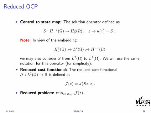
Reduced OCP
I Control to state map The solution operator defined as
S Hminus1(Ω)rarr H10 (Ω) z 7rarr u(z) = Sz
Note In view of the embedding
H10 (Ω) rarr L2(Ω) rarr Hminus1(Ω)
we may also consider S from L2(Ω) to L2(Ω) We will use the samenotation for this operator (for simplicity)
I Reduced cost functional The reduced cost functionalJ L2(Ω)rarr R is defined as
J (z) = J(Sz z)
I Reduced problem minzisinZadJ (z)
H Antil 060616 17
Existence of solution Direct methodThere exists a unique solution to the above problem
I Minimizing sequence J is bounded below by zero therefore thereexists a minimizing sequence znnisinN such that
limnrarrinfin
J (zn) = inf J (z)
I Weak compactness zn sub L2(Ω) is bounded Since L2(Ω) isreflexive therefore there exists a subsequence (not relabeled) suchthat
zn z and z isin Zad
where the latter is a consequence of Zad being closed and convex
I Optimality Since J is continuous and convex and therefore isweakly lower semicontinuous We obtain
lim inf J (zn) ge J (z)
which implies that z is optimal
I Uniqueness Exercise
H Antil 060616 18
Outline
Motivation and examples
Linear elliptic optimal control problems
Differentiation in Banach spaces
First-order necessary conditions
Optimal control of semilinear PDEs
An abstract problem
Discretization using finite element methods
H Antil 060616 19
Differentiation in Banach spacesLet (Z middot Z) (V middot V ) B-spaces Z sub Z open and F Z rarr V
Let z isin Z
I If exist δF (z h) = limtdarr01t (F (z + th)minus F (z)) then δF (z h) is called
the directional derivative of F at z in direction h
I If exist δF (z h) forallh isin Z then h 7rarr δF (z h) is the first variation of Fat z
I Let exist the first variation δF (z middot) F is said to be Gateauxdifferentiable at z iff existA isin L(Z V ) such that δF (z h) = Ahforallh isin Z We write A = F primeG(z)
I F is said to be Frechet differentiable at z iff existA isin L(Z V ) and amapping r(z middot) Z rarr V such that for all h isin U with z + h isin Zwe have
F (z+h) = F (z)+Ah+r(z h) withr(z h)VhZ
rarr 0 as hZ rarr 0
We write F prime(z) = A
H Antil 060616 20
Differentiation in Banach spacesLet (Z middot Z) (V middot V ) B-spaces Z sub Z open and F Z rarr V
Let z isin Z
I If exist δF (z h) = limtdarr01t (F (z + th)minus F (z)) then δF (z h) is called
the directional derivative of F at z in direction h
I If exist δF (z h) forallh isin Z then h 7rarr δF (z h) is the first variation of Fat z
I Let exist the first variation δF (z middot) F is said to be Gateauxdifferentiable at z iff existA isin L(Z V ) such that δF (z h) = Ahforallh isin Z We write A = F primeG(z)
I F is said to be Frechet differentiable at z iff existA isin L(Z V ) and amapping r(z middot) Z rarr V such that for all h isin U with z + h isin Zwe have
F (z+h) = F (z)+Ah+r(z h) withr(z h)VhZ
rarr 0 as hZ rarr 0
We write F prime(z) = A
H Antil 060616 20
Differentiation in Banach spacesLet (Z middot Z) (V middot V ) B-spaces Z sub Z open and F Z rarr V
Let z isin Z
I If exist δF (z h) = limtdarr01t (F (z + th)minus F (z)) then δF (z h) is called
the directional derivative of F at z in direction h
I If exist δF (z h) forallh isin Z then h 7rarr δF (z h) is the first variation of Fat z
I Let exist the first variation δF (z middot) F is said to be Gateauxdifferentiable at z iff existA isin L(Z V ) such that δF (z h) = Ahforallh isin Z We write A = F primeG(z)
I F is said to be Frechet differentiable at z iff existA isin L(Z V ) and amapping r(z middot) Z rarr V such that for all h isin U with z + h isin Zwe have
F (z+h) = F (z)+Ah+r(z h) withr(z h)VhZ
rarr 0 as hZ rarr 0
We write F prime(z) = A
H Antil 060616 20
Differentiation in Banach spacesLet (Z middot Z) (V middot V ) B-spaces Z sub Z open and F Z rarr V
Let z isin Z
I If exist δF (z h) = limtdarr01t (F (z + th)minus F (z)) then δF (z h) is called
the directional derivative of F at z in direction h
I If exist δF (z h) forallh isin Z then h 7rarr δF (z h) is the first variation of Fat z
I Let exist the first variation δF (z middot) F is said to be Gateauxdifferentiable at z iff existA isin L(Z V ) such that δF (z h) = Ahforallh isin Z We write A = F primeG(z)
I F is said to be Frechet differentiable at z iff existA isin L(Z V ) and amapping r(z middot) Z rarr V such that for all h isin U with z + h isin Zwe have
F (z+h) = F (z)+Ah+r(z h) withr(z h)VhZ
rarr 0 as hZ rarr 0
We write F prime(z) = A
H Antil 060616 20
ExamplesExample 1 (H (middot middot)H) Hilbert space F (z) = z2H = (z z)H
forallz h F (z + h)minus F (z) = 2(z h)H + h2HThen
F prime(z)h = (2z h)H
Reisz representation theorem (identify H with Hlowast) we can write
F prime(z)h = (nablaF (z) h)H
where nablaF (z) = 2z is the gradient
Example 2 Let (Z (middot middot)Z) (H (middot middot)H) Hilbert spaces ud isin H fixedLet S isin L(ZH) Consider E Z rarr R
E(z) = Sz minus ud2H
Then E(z) = G(F (z)) where G(v) = v2H and F (z) = Sz minus ud
Eprime(z)h = Gprime(F (z))F prime(z)h = (2v F prime(z)h)H
= 2(Sz minus ud Sh)H = 2(Slowast(Sz minus ud) h)Z
we denote the gradient as nablaE(z) = 2Slowast(Sz minus ud)
H Antil 060616 21
ExamplesExample 1 (H (middot middot)H) Hilbert space F (z) = z2H = (z z)H
forallz h F (z + h)minus F (z) = 2(z h)H + h2HThen
F prime(z)h = (2z h)H
Reisz representation theorem (identify H with Hlowast) we can write
F prime(z)h = (nablaF (z) h)H
where nablaF (z) = 2z is the gradient
Example 2 Let (Z (middot middot)Z) (H (middot middot)H) Hilbert spaces ud isin H fixedLet S isin L(ZH) Consider E Z rarr R
E(z) = Sz minus ud2H
Then E(z) = G(F (z)) where G(v) = v2H and F (z) = Sz minus ud
Eprime(z)h = Gprime(F (z))F prime(z)h = (2v F prime(z)h)H
= 2(Sz minus ud Sh)H = 2(Slowast(Sz minus ud) h)Z
we denote the gradient as nablaE(z) = 2Slowast(Sz minus ud)H Antil 060616 21
Outline
Motivation and examples
Linear elliptic optimal control problems
Differentiation in Banach spaces
First-order necessary conditions
Optimal control of semilinear PDEs
An abstract problem
Discretization using finite element methods
H Antil 060616 22
First order necessary optimality conditions
Most of the theory is based on these two simple results
Theorem Let (Z middot Z) be a normed space J Z rarr (infin+infin] amapping with J 6equiv +infin Then z isin Z minimizer of J hArr 0 isin partJ (z)
Proof 0 isin partJ (z) means by definition of partJ (z) J (z)minus J (z) le 0forallz isin Z
Theorem Let (Z middot Z) be a normed space Zad sub Z nonemptyconvex closed J Z rarr R Gateaux differentiable where Zad sub Z sub ZZ open If z isin Zad is a solution to
minzisinZad
J (z)
then z solvesJ prime(z)(z minus z) ge 0 forallz isin Zad
Proof Exercise
H Antil 060616 23
First order necessary optimality conditions
Most of the theory is based on these two simple results
Theorem Let (Z middot Z) be a normed space J Z rarr (infin+infin] amapping with J 6equiv +infin Then z isin Z minimizer of J hArr 0 isin partJ (z)
Proof 0 isin partJ (z) means by definition of partJ (z) J (z)minus J (z) le 0forallz isin Z
Theorem Let (Z middot Z) be a normed space Zad sub Z nonemptyconvex closed J Z rarr R Gateaux differentiable where Zad sub Z sub ZZ open If z isin Zad is a solution to
minzisinZad
J (z)
then z solvesJ prime(z)(z minus z) ge 0 forallz isin Zad
Proof Exercise
H Antil 060616 23
Linear quadratic OCPI Reduced funcational
J (z) =1
2Sz minus ud2L2(Ω) +
λ
2z2L2(Ω)
I Gradient computation using sensitivity
J prime(z)h = (Slowast(Sz minus ud) + λz h)L2(Ω) forallh isin L2(Ω)
we denote the gradient by
nablaJ (z) = Slowast(Sz minus ud) + λz
I First order necessary and sufficient optimality condition
(nablaJ (z) z minus z)L2(Ω) ge 0 forallz isin Zad
I Adjoint equation Let p = Slowast(Sz minus ud) which translates intop isin H1
0 (Ω) solving
minusdiv (Anablap) = uminus ud in Ω
p = 0 on partΩ
I Gradient computation using adjoint nablaJ (z) = p+ λz
H Antil 060616 24
Linear quadratic OCPI Reduced funcational
J (z) =1
2Sz minus ud2L2(Ω) +
λ
2z2L2(Ω)
I Gradient computation using sensitivity
J prime(z)h = (Slowast(Sz minus ud) + λz h)L2(Ω) forallh isin L2(Ω)
we denote the gradient by
nablaJ (z) = Slowast(Sz minus ud) + λz
I First order necessary and sufficient optimality condition
(nablaJ (z) z minus z)L2(Ω) ge 0 forallz isin Zad
I Adjoint equation Let p = Slowast(Sz minus ud) which translates intop isin H1
0 (Ω) solving
minusdiv (Anablap) = uminus ud in Ω
p = 0 on partΩ
I Gradient computation using adjoint nablaJ (z) = p+ λz
H Antil 060616 24
Linear quadratic OCPI Reduced funcational
J (z) =1
2Sz minus ud2L2(Ω) +
λ
2z2L2(Ω)
I Gradient computation using sensitivity
J prime(z)h = (Slowast(Sz minus ud) + λz h)L2(Ω) forallh isin L2(Ω)
we denote the gradient by
nablaJ (z) = Slowast(Sz minus ud) + λz
I First order necessary and sufficient optimality condition
(nablaJ (z) z minus z)L2(Ω) ge 0 forallz isin Zad
I Adjoint equation Let p = Slowast(Sz minus ud) which translates intop isin H1
0 (Ω) solving
minusdiv (Anablap) = uminus ud in Ω
p = 0 on partΩ
I Gradient computation using adjoint nablaJ (z) = p+ λz
H Antil 060616 24
Linear quadratic OCPI Reduced funcational
J (z) =1
2Sz minus ud2L2(Ω) +
λ
2z2L2(Ω)
I Gradient computation using sensitivity
J prime(z)h = (Slowast(Sz minus ud) + λz h)L2(Ω) forallh isin L2(Ω)
we denote the gradient by
nablaJ (z) = Slowast(Sz minus ud) + λz
I First order necessary and sufficient optimality condition
(nablaJ (z) z minus z)L2(Ω) ge 0 forallz isin Zad
I Adjoint equation Let p = Slowast(Sz minus ud) which translates intop isin H1
0 (Ω) solving
minusdiv (Anablap) = uminus ud in Ω
p = 0 on partΩ
I Gradient computation using adjoint nablaJ (z) = p+ λz
H Antil 060616 24
Linear quadratic OCPI Reduced funcational
J (z) =1
2Sz minus ud2L2(Ω) +
λ
2z2L2(Ω)
I Gradient computation using sensitivity
J prime(z)h = (Slowast(Sz minus ud) + λz h)L2(Ω) forallh isin L2(Ω)
we denote the gradient by
nablaJ (z) = Slowast(Sz minus ud) + λz
I First order necessary and sufficient optimality condition
(nablaJ (z) z minus z)L2(Ω) ge 0 forallz isin Zad
I Adjoint equation Let p = Slowast(Sz minus ud) which translates intop isin H1
0 (Ω) solving
minusdiv (Anablap) = uminus ud in Ω
p = 0 on partΩ
I Gradient computation using adjoint nablaJ (z) = p+ λz
H Antil 060616 24
Optimality system
I State u isin H10 (Ω)
intΩAnablau middot nablav =
intΩzv forallv isin H1
0 (Ω)
I Adjoint p isin H10 (Ω)
intΩAnablap middot nablav =
intΩ
(uminus ud)v forallv isin H10 (Ω)
I Control z isin Zad (p+ λz z minus z) ge 0 forallz isin Zad
H Antil 060616 25
Pointwise interpretation
The variational inequality
(p+ λz z minus z) ge 0 forallz isin Zad
is equivalent to for ae x isin Ω
z(x) =
za(x) if p(x) + λz(x) gt 0isin [za(x) zb(x)] if p(x) + λz(x) = 0zb(x) if p(x) + λz(x) lt 0
Consequence
I When λ gt 0 then ae in Ω
z(x) = P[za(x)zb(x)]
minus 1
λp(x)
= min
zb(x)max
za(x)minus 1
λp(x)
H Antil 060616 26
Formal Lagrange method applied to linear OCPIntroduce L H1
0 (Ω)times Zad timesH1(Ω)rarr R defined as
L(u z p) = J(u z)minusint
Ω
(minusdiv (Anablau)minus z
)p dx
Integrate by parts to arrive at
L(u z p) = J(u z)minusint
Ω
(minusdiv (Anablap)uminus zp
)dx+
intpartΩ
(Anablau)p ds
If (u z p) is a stationary point then
I State
DpL(u z p)h = 0 forallh isin H1(Ω)
I AdjointDuL(u z p)h = 0 forallh isin H1
0 (Ω)
I ControlDzL(u z p)(z minus z) ge 0 forallz isin Zad
H Antil 060616 27
Formal Lagrange method applied to linear OCPIntroduce L H1
0 (Ω)times Zad timesH1(Ω)rarr R defined as
L(u z p) = J(u z)minusint
Ω
(minusdiv (Anablau)minus z
)p dx
Integrate by parts to arrive at
L(u z p) = J(u z)minusint
Ω
(minusdiv (Anablap)uminus zp
)dx+
intpartΩ
(Anablau)p ds
If (u z p) is a stationary point then
I State
DpL(u z p)h = 0 forallh isin H1(Ω)
I AdjointDuL(u z p)h = 0 forallh isin H1
0 (Ω)
I ControlDzL(u z p)(z minus z) ge 0 forallz isin Zad
H Antil 060616 27
Formal Lagrange method applied to linear OCPIntroduce L H1
0 (Ω)times Zad timesH1(Ω)rarr R defined as
L(u z p) = J(u z)minusint
Ω
(minusdiv (Anablau)minus z
)p dx
Integrate by parts to arrive at
L(u z p) = J(u z)minusint
Ω
(minusdiv (Anablap)uminus zp
)dx+
intpartΩ
(Anablau)p ds
If (u z p) is a stationary point then
I State
DpL(u z p)h = 0 forallh isin H1(Ω)
I AdjointDuL(u z p)h = 0 forallh isin H1
0 (Ω)
I ControlDzL(u z p)(z minus z) ge 0 forallz isin Zad
H Antil 060616 27
Formal Lagrange method applied to linear OCPIntroduce L H1
0 (Ω)times Zad timesH1(Ω)rarr R defined as
L(u z p) = J(u z)minusint
Ω
(minusdiv (Anablau)minus z
)p dx
Integrate by parts to arrive at
L(u z p) = J(u z)minusint
Ω
(minusdiv (Anablap)uminus zp
)dx+
intpartΩ
(Anablau)p ds
If (u z p) is a stationary point then
I State
DpL(u z p)h = 0 forallh isin H1(Ω)
I AdjointDuL(u z p)h = 0 forallh isin H1
0 (Ω)
I ControlDzL(u z p)(z minus z) ge 0 forallz isin Zad
H Antil 060616 27
Formal Lagrange method applied to linear OCPIntroduce L H1
0 (Ω)times Zad timesH1(Ω)rarr R defined as
L(u z p) = J(u z)minusint
Ω
(minusdiv (Anablau)minus z
)p dx
Integrate by parts to arrive at
L(u z p) = J(u z)minusint
Ω
(minusdiv (Anablap)uminus zp
)dx+
intpartΩ
(Anablau)p ds
If (u z p) is a stationary point then
I State
DpL(u z p)h = 0 forallh isin H1(Ω)
I AdjointDuL(u z p)h = 0 forallh isin H1
0 (Ω)
I ControlDzL(u z p)(z minus z) ge 0 forallz isin Zad
H Antil 060616 27
Outline
Motivation and examples
Linear elliptic optimal control problems
Differentiation in Banach spaces
First-order necessary conditions
Optimal control of semilinear PDEs
An abstract problem
Discretization using finite element methods
H Antil 060616 28
Semilinear elliptic OCP
min J(u z) =1
2uminus ud2L2(Ω) +
λ
2z2L2(Ω)
subject to
minus∆u+ g(x u) = z in Ω
u = 0 on partΩ
and z isin Zad with za zb isin Linfin(Ω)
H Antil 060616 29
State space(A1) Ω sub Rd open bounded partΩ is Lipschitz
(A2) g Ωtimes Rrarr R is bounded and measurable with respect to x isin Ωfor every u isin R
(A3) g is continuous monotone increasing and Lipschitz continuous in ufor ae x isin Ω
(A4) g(x 0) = 0 for ae x isin Ω (not really necessary)
Theorem Suppose (A1)minus (A4) hold For every z isin Lr(Ω) withr gt d2 the state equation has a unique weak solutionu isin H1
0 (Ω) cap C(Ω) ie we haveintΩ
nablau middot nablav dx+
intΩ
g(x u(x))v(x) dx =
intΩ
zv dx forallv isin H10 (Ω)
Moreover there exists a constant C gt 0 such that
uH1(Ω) + uC(Ω) le CzLr(Ω)
RemarkI The proof of the theorem uses the BrowderndashMinty theorem on
monotone operators
H Antil 060616 30
State space(A1) Ω sub Rd open bounded partΩ is Lipschitz
(A2) g Ωtimes Rrarr R is bounded and measurable with respect to x isin Ωfor every u isin R
(A3) g is continuous monotone increasing and Lipschitz continuous in ufor ae x isin Ω
(A4) g(x 0) = 0 for ae x isin Ω (not really necessary)
Theorem Suppose (A1)minus (A4) hold For every z isin Lr(Ω) withr gt d2 the state equation has a unique weak solutionu isin H1
0 (Ω) cap C(Ω) ie we haveintΩ
nablau middot nablav dx+
intΩ
g(x u(x))v(x) dx =
intΩ
zv dx forallv isin H10 (Ω)
Moreover there exists a constant C gt 0 such that
uH1(Ω) + uC(Ω) le CzLr(Ω)
RemarkI The proof of the theorem uses the BrowderndashMinty theorem on
monotone operators
H Antil 060616 30
State space(A1) Ω sub Rd open bounded partΩ is Lipschitz
(A2) g Ωtimes Rrarr R is bounded and measurable with respect to x isin Ωfor every u isin R
(A3) g is continuous monotone increasing and Lipschitz continuous in ufor ae x isin Ω
(A4) g(x 0) = 0 for ae x isin Ω (not really necessary)
Theorem Suppose (A1)minus (A4) hold For every z isin Lr(Ω) withr gt d2 the state equation has a unique weak solutionu isin H1
0 (Ω) cap C(Ω) ie we haveintΩ
nablau middot nablav dx+
intΩ
g(x u(x))v(x) dx =
intΩ
zv dx forallv isin H10 (Ω)
Moreover there exists a constant C gt 0 such that
uH1(Ω) + uC(Ω) le CzLr(Ω)
RemarkI The proof of the theorem uses the BrowderndashMinty theorem on
monotone operators
H Antil 060616 30
Control-to-state map and reduced problem
I Control to state map
S Linfin(Ω)rarr H10 (Ω) cap C(Ω)
is well defined and is globally Lipschitz continuous
I Reduced problem
minJ (z) =1
2S(u)minus ud2L2(Ω) +
λ
2z2L2(Ω)
H Antil 060616 31
Control-to-state map and reduced problem
I Control to state map
S Linfin(Ω)rarr H10 (Ω) cap C(Ω)
is well defined and is globally Lipschitz continuous
I Reduced problem
minJ (z) =1
2S(u)minus ud2L2(Ω) +
λ
2z2L2(Ω)
H Antil 060616 31
First-order necessary conditionsI Lagrangian functional
L(u z p) = J(u z)minusint
Ω
(minus∆u+ g(x u(x))minus z
)p dx
= J(u z)minusint
Ω
(nablau middot nablap+ g(x u(x))pminus zp
)dx
I Adjoint system For all h isin H10 (Ω)
0 = DuL(u z p)h =
intΩ
(uminus ud)h dxminusint
Ω
(nablah middot nablap+ gu(x u(x))ph
)which yields
minus∆p+ gu(x u(x))p = uminus ud in Ω
p = 0 on partΩ
I Control
DzL(u z p)(z minus z) = (p+ λz z minus z) dx ge 0 forallz isin ZadI Gradient
nablaJ (z) = p+ λz
H Antil 060616 32
First-order necessary conditionsI Lagrangian functional
L(u z p) = J(u z)minusint
Ω
(minus∆u+ g(x u(x))minus z
)p dx
= J(u z)minusint
Ω
(nablau middot nablap+ g(x u(x))pminus zp
)dx
I Adjoint system For all h isin H10 (Ω)
0 = DuL(u z p)h =
intΩ
(uminus ud)h dxminusint
Ω
(nablah middot nablap+ gu(x u(x))ph
)which yields
minus∆p+ gu(x u(x))p = uminus ud in Ω
p = 0 on partΩ
I Control
DzL(u z p)(z minus z) = (p+ λz z minus z) dx ge 0 forallz isin ZadI Gradient
nablaJ (z) = p+ λz
H Antil 060616 32
First-order necessary conditionsI Lagrangian functional
L(u z p) = J(u z)minusint
Ω
(minus∆u+ g(x u(x))minus z
)p dx
= J(u z)minusint
Ω
(nablau middot nablap+ g(x u(x))pminus zp
)dx
I Adjoint system For all h isin H10 (Ω)
0 = DuL(u z p)h =
intΩ
(uminus ud)h dxminusint
Ω
(nablah middot nablap+ gu(x u(x))ph
)which yields
minus∆p+ gu(x u(x))p = uminus ud in Ω
p = 0 on partΩ
I Control
DzL(u z p)(z minus z) = (p+ λz z minus z) dx ge 0 forallz isin Zad
I GradientnablaJ (z) = p+ λz
H Antil 060616 32
First-order necessary conditionsI Lagrangian functional
L(u z p) = J(u z)minusint
Ω
(minus∆u+ g(x u(x))minus z
)p dx
= J(u z)minusint
Ω
(nablau middot nablap+ g(x u(x))pminus zp
)dx
I Adjoint system For all h isin H10 (Ω)
0 = DuL(u z p)h =
intΩ
(uminus ud)h dxminusint
Ω
(nablah middot nablap+ gu(x u(x))ph
)which yields
minus∆p+ gu(x u(x))p = uminus ud in Ω
p = 0 on partΩ
I Control
DzL(u z p)(z minus z) = (p+ λz z minus z) dx ge 0 forallz isin ZadI Gradient
nablaJ (z) = p+ λz
H Antil 060616 32
Differentiability of Nemytskii operator
The rigorous proof uses
Theorem In addition to (A1)-(A4) if
(A5) g is continuously differentiable with respect to u for ae x isin Ωand we have
(i) |gu(x 0)| le K for ae x isin Ω(ii) gu is locally Lipschitz with respect to u isin R
then the Nemytskii operator G u 7rarr g(middot u(middot)) is continuously Frechetdifferentiable from Linfin(Ω) into itself and
(Gprime(u)h)(x) = gu(x u(x))h(x) ae in Ω forallh isin Linfin(Ω)
Remark (A5) holds if g(x u) = g(u) and g isin C2(R)
H Antil 060616 33
Outline
Motivation and examples
Linear elliptic optimal control problems
Differentiation in Banach spaces
First-order necessary conditions
Optimal control of semilinear PDEs
An abstract problem
Discretization using finite element methods
H Antil 060616 34
Gradient computation via adjoint general formI Abstract problem
min J(u z)
subject toc(u z) = 0
and z isin Zad
I Directional derivative Let S be the control to state map(nonlinear in general)
z 7rarr S(z) = u(z)
Under the assumptions of ldquoimplicit function theoremrdquo
J prime(z)h = (nablauJ (u(z) z) Sprime(z)h) + (nablazJ (u(z) z) h)
I Sensitivity of u with respect to z Differentiating the stateequation
cu(S(z) z)Sprime(z)h = minuscz(S(z) z)h
leads toSprime(z)h = minuscu(S(z) z)minus1
(cz(S(z) z)h
)
provided cu(S(z) z)minus1 is well-defined
H Antil 060616 35
Gradient computation via adjoint general formI Abstract problem
min J(u z)
subject toc(u z) = 0
and z isin ZadI Directional derivative Let S be the control to state map
(nonlinear in general)
z 7rarr S(z) = u(z)
Under the assumptions of ldquoimplicit function theoremrdquo
J prime(z)h = (nablauJ (u(z) z) Sprime(z)h) + (nablazJ (u(z) z) h)
I Sensitivity of u with respect to z Differentiating the stateequation
cu(S(z) z)Sprime(z)h = minuscz(S(z) z)h
leads toSprime(z)h = minuscu(S(z) z)minus1
(cz(S(z) z)h
)
provided cu(S(z) z)minus1 is well-defined
H Antil 060616 35
Gradient computation via adjoint general formI Abstract problem
min J(u z)
subject toc(u z) = 0
and z isin ZadI Directional derivative Let S be the control to state map
(nonlinear in general)
z 7rarr S(z) = u(z)
Under the assumptions of ldquoimplicit function theoremrdquo
J prime(z)h = (nablauJ (u(z) z) Sprime(z)h) + (nablazJ (u(z) z) h)
I Sensitivity of u with respect to z Differentiating the stateequation
cu(S(z) z)Sprime(z)h = minuscz(S(z) z)h
leads toSprime(z)h = minuscu(S(z) z)minus1
(cz(S(z) z)h
)
provided cu(S(z) z)minus1 is well-defined
H Antil 060616 35
Adjoint equation and gradient general form
I Directional derivative
J prime(z)h = minus(nablauJ (u(z) z) cu(u(z) z)minus1cz(u(z) z)h
)+ (nablazJ (u(z) z) h)
I Gradient
nablaJ (z) = minuscz(u(z) z)lowast(cu(u(z) z)minuslowastnablauJ (u(z) z)
)+nablazJ (u(z) z)
I Introducing adjoint variable p solving
cu(u(z) z)lowastp = nablauJ (u(z) z)
we arrive at following form of gradient
nablaJ (z) = minuscz(u(z) z)lowastp+nablazJ (u(z) z)
which is tractable
H Antil 060616 36
Adjoint equation and gradient general form
I Directional derivative
J prime(z)h = minus(nablauJ (u(z) z) cu(u(z) z)minus1cz(u(z) z)h
)+ (nablazJ (u(z) z) h)
I Gradient
nablaJ (z) = minuscz(u(z) z)lowast(cu(u(z) z)minuslowastnablauJ (u(z) z)
)+nablazJ (u(z) z)
I Introducing adjoint variable p solving
cu(u(z) z)lowastp = nablauJ (u(z) z)
we arrive at following form of gradient
nablaJ (z) = minuscz(u(z) z)lowastp+nablazJ (u(z) z)
which is tractable
H Antil 060616 36
Adjoint equation and gradient general form
I Directional derivative
J prime(z)h = minus(nablauJ (u(z) z) cu(u(z) z)minus1cz(u(z) z)h
)+ (nablazJ (u(z) z) h)
I Gradient
nablaJ (z) = minuscz(u(z) z)lowast(cu(u(z) z)minuslowastnablauJ (u(z) z)
)+nablazJ (u(z) z)
I Introducing adjoint variable p solving
cu(u(z) z)lowastp = nablauJ (u(z) z)
we arrive at following form of gradient
nablaJ (z) = minuscz(u(z) z)lowastp+nablazJ (u(z) z)
which is tractable
H Antil 060616 36
Hessian computation general form
I Lagrangian L(u z p) = J(u z)minusint
Ωc(u z)p dx Then we have
DzJ (z)h = DzL(u z p)h
I Second order derivative
D2zJ (z)[h1 h2] = DuDzL(u z p)[h1 S
prime(z)h2] +D2zL(u z p)[h1 h2]
+DpDzL(u z p)[h1 Dzp(z)h2]
I We already know Sprime(z)h2 moreover
DpDzL(u z p)[h1 Dzp(z)h2] = minus(cu(u z)h1 Dzp(z)h2
)
It remain to identify Dzp(z)h2
H Antil 060616 37
Hessian computation general form
I Lagrangian L(u z p) = J(u z)minusint
Ωc(u z)p dx Then we have
DzJ (z)h = DzL(u z p)h
I Second order derivative
D2zJ (z)[h1 h2] = DuDzL(u z p)[h1 S
prime(z)h2] +D2zL(u z p)[h1 h2]
+DpDzL(u z p)[h1 Dzp(z)h2]
I We already know Sprime(z)h2 moreover
DpDzL(u z p)[h1 Dzp(z)h2] = minus(cu(u z)h1 Dzp(z)h2
)
It remain to identify Dzp(z)h2
H Antil 060616 37
Hessian computation general form
I Lagrangian L(u z p) = J(u z)minusint
Ωc(u z)p dx Then we have
DzJ (z)h = DzL(u z p)h
I Second order derivative
D2zJ (z)[h1 h2] = DuDzL(u z p)[h1 S
prime(z)h2] +D2zL(u z p)[h1 h2]
+DpDzL(u z p)[h1 Dzp(z)h2]
I We already know Sprime(z)h2 moreover
DpDzL(u z p)[h1 Dzp(z)h2] = minus(cu(u z)h1 Dzp(z)h2
)
It remain to identify Dzp(z)h2
H Antil 060616 37
Outline
Motivation and examples
Linear elliptic optimal control problems
Differentiation in Banach spaces
First-order necessary conditions
Optimal control of semilinear PDEs
An abstract problem
Discretization using finite element methods
H Antil 060616 38
Numerical approximation of Poisson equation MeshTo avoid technical issues we will assume that partΩ is polygonal
I Mesh Let T = K be a mesh of Ω where K sub Rd is an elementthat is isoparametrically equivalent to a unit simplex in Rd
I Conforming mesh We say that the mesh is conforming ifI Ω = cupKisinT KI If K1 cap K2 = x then x is a node of K1 and K2I If K1 cap K2 6= empty and K1 cap K2 6= x then K1 cap K2 is an edgeface
contained in partK1 cap partK2
I Shape regular Let T be the collection of all conformingrefinements of an original mesh T 0 Then T is called shape regularif exist κ gt 0 such that
hKρKle κ forallK isin cupiT i
where hK = diam K ρK = maxρ gt 0|Bρ sub KI Quasi-uniform A family of shape regular meshes is called-quasi
uniform if there exist a constant σ gt 0 such that
maxhKminhK
le σ
uniformly for all meshes in the family
Numerical approximation of Poisson equation MeshTo avoid technical issues we will assume that partΩ is polygonal
I Mesh Let T = K be a mesh of Ω where K sub Rd is an elementthat is isoparametrically equivalent to a unit simplex in Rd
I Conforming mesh We say that the mesh is conforming ifI Ω = cupKisinT KI If K1 cap K2 = x then x is a node of K1 and K2I If K1 cap K2 6= empty and K1 cap K2 6= x then K1 cap K2 is an edgeface
contained in partK1 cap partK2
I Shape regular Let T be the collection of all conformingrefinements of an original mesh T 0 Then T is called shape regularif exist κ gt 0 such that
hKρKle κ forallK isin cupiT i
where hK = diam K ρK = maxρ gt 0|Bρ sub KI Quasi-uniform A family of shape regular meshes is called-quasi
uniform if there exist a constant σ gt 0 such that
maxhKminhK
le σ
uniformly for all meshes in the family
Numerical approximation of Poisson equation MeshTo avoid technical issues we will assume that partΩ is polygonal
I Mesh Let T = K be a mesh of Ω where K sub Rd is an elementthat is isoparametrically equivalent to a unit simplex in Rd
I Conforming mesh We say that the mesh is conforming ifI Ω = cupKisinT KI If K1 cap K2 = x then x is a node of K1 and K2I If K1 cap K2 6= empty and K1 cap K2 6= x then K1 cap K2 is an edgeface
contained in partK1 cap partK2
I Shape regular Let T be the collection of all conformingrefinements of an original mesh T 0 Then T is called shape regularif exist κ gt 0 such that
hKρKle κ forallK isin cupiT i
where hK = diam K ρK = maxρ gt 0|Bρ sub K
I Quasi-uniform A family of shape regular meshes is called-quasiuniform if there exist a constant σ gt 0 such that
maxhKminhK
le σ
uniformly for all meshes in the family
Numerical approximation of Poisson equation MeshTo avoid technical issues we will assume that partΩ is polygonal
I Mesh Let T = K be a mesh of Ω where K sub Rd is an elementthat is isoparametrically equivalent to a unit simplex in Rd
I Conforming mesh We say that the mesh is conforming ifI Ω = cupKisinT KI If K1 cap K2 = x then x is a node of K1 and K2I If K1 cap K2 6= empty and K1 cap K2 6= x then K1 cap K2 is an edgeface
contained in partK1 cap partK2
I Shape regular Let T be the collection of all conformingrefinements of an original mesh T 0 Then T is called shape regularif exist κ gt 0 such that
hKρKle κ forallK isin cupiT i
where hK = diam K ρK = maxρ gt 0|Bρ sub KI Quasi-uniform A family of shape regular meshes is called-quasi
uniform if there exist a constant σ gt 0 such that
maxhKminhK
le σ
uniformly for all meshes in the family
FE space and Galerkin approximationI Finite element space For T isin T we define the finite element
space as
V(T ) = W isin C0(Ω) WK isin P1forallK isin T W |partΩ = 0
where P1 is the set of polynomials of degree at most 1
I Galerkin approximation of continuous problem is given by
Find UT isin V(T )
intΩ
AnablaUT middot nablaV = 〈f V 〉 forallV isin V(T )
The discrete problem is well-posedI Nodal basis Consists of functions ψi isin V(T ) with xi isin N (T )
satisfyingψxi
(xj) = δij
where N (T ) denotes the interior (plus Neumann) nodesI Galerkin orthogonality(
nabla(uminus UT )nablaW)L2(Ω)
= 0 forallW isin V(T )
H Antil 060616 40
FE space and Galerkin approximationI Finite element space For T isin T we define the finite element
space as
V(T ) = W isin C0(Ω) WK isin P1forallK isin T W |partΩ = 0
where P1 is the set of polynomials of degree at most 1I Galerkin approximation of continuous problem is given by
Find UT isin V(T )
intΩ
AnablaUT middot nablaV = 〈f V 〉 forallV isin V(T )
The discrete problem is well-posed
I Nodal basis Consists of functions ψi isin V(T ) with xi isin N (T )satisfying
ψxi(xj) = δij
where N (T ) denotes the interior (plus Neumann) nodesI Galerkin orthogonality(
nabla(uminus UT )nablaW)L2(Ω)
= 0 forallW isin V(T )
H Antil 060616 40
FE space and Galerkin approximationI Finite element space For T isin T we define the finite element
space as
V(T ) = W isin C0(Ω) WK isin P1forallK isin T W |partΩ = 0
where P1 is the set of polynomials of degree at most 1I Galerkin approximation of continuous problem is given by
Find UT isin V(T )
intΩ
AnablaUT middot nablaV = 〈f V 〉 forallV isin V(T )
The discrete problem is well-posedI Nodal basis Consists of functions ψi isin V(T ) with xi isin N (T )
satisfyingψxi
(xj) = δij
where N (T ) denotes the interior (plus Neumann) nodes
I Galerkin orthogonality(nabla(uminus UT )nablaW
)L2(Ω)
= 0 forallW isin V(T )
H Antil 060616 40
FE space and Galerkin approximationI Finite element space For T isin T we define the finite element
space as
V(T ) = W isin C0(Ω) WK isin P1forallK isin T W |partΩ = 0
where P1 is the set of polynomials of degree at most 1I Galerkin approximation of continuous problem is given by
Find UT isin V(T )
intΩ
AnablaUT middot nablaV = 〈f V 〉 forallV isin V(T )
The discrete problem is well-posedI Nodal basis Consists of functions ψi isin V(T ) with xi isin N (T )
satisfyingψxi
(xj) = δij
where N (T ) denotes the interior (plus Neumann) nodesI Galerkin orthogonality(
nabla(uminus UT )nablaW)L2(Ω)
= 0 forallW isin V(T )
H Antil 060616 40
Best approximation
I Cearsquos lemma
nabla(uminus UT )L2(Ω) le C infWisinV(T )
nabla(uminusW )L2(Ω)
I Nodal interpolation operator ΠT C(Ω)rarr V(T ) satisfies
ΠT u(xi) = u(xi) forallxi isin N (T )
and is defined as
ΠT u =sum
xiisinN (T )
u(xi)ψxi
I Error estimates In Cearsquos lemma replace W by ΠT u and thencompute the interpolation error
H Antil 060616 41
Best approximation
I Cearsquos lemma
nabla(uminus UT )L2(Ω) le C infWisinV(T )
nabla(uminusW )L2(Ω)
I Nodal interpolation operator ΠT C(Ω)rarr V(T ) satisfies
ΠT u(xi) = u(xi) forallxi isin N (T )
and is defined as
ΠT u =sum
xiisinN (T )
u(xi)ψxi
I Error estimates In Cearsquos lemma replace W by ΠT u and thencompute the interpolation error
H Antil 060616 41
Best approximation
I Cearsquos lemma
nabla(uminus UT )L2(Ω) le C infWisinV(T )
nabla(uminusW )L2(Ω)
I Nodal interpolation operator ΠT C(Ω)rarr V(T ) satisfies
ΠT u(xi) = u(xi) forallxi isin N (T )
and is defined as
ΠT u =sum
xiisinN (T )
u(xi)ψxi
I Error estimates In Cearsquos lemma replace W by ΠT u and thencompute the interpolation error
H Antil 060616 41
Algebraic system state equation
I Recall UT isin V(T ) solves
a(UT V ) = 〈f V 〉 forallV isin V(T )
I Now setting UT =sumN
j=1 Ujψj V = ψi we get
Nsumj=1
Uja(φj φi) = 〈f ψi〉 i = 1 N
which is the matrix-vector system
AU = F
I Stiffness matrix A is SPD
H Antil 060616 42
Algebraic system state equation
I Recall UT isin V(T ) solves
a(UT V ) = 〈f V 〉 forallV isin V(T )
I Now setting UT =sumN
j=1 Ujψj V = ψi we get
Nsumj=1
Uja(φj φi) = 〈f ψi〉 i = 1 N
which is the matrix-vector system
AU = F
I Stiffness matrix A is SPD
H Antil 060616 42
Algebraic system state equation
I Recall UT isin V(T ) solves
a(UT V ) = 〈f V 〉 forallV isin V(T )
I Now setting UT =sumN
j=1 Ujψj V = ψi we get
Nsumj=1
Uja(φj φi) = 〈f ψi〉 i = 1 N
which is the matrix-vector system
AU = F
I Stiffness matrix A is SPD
H Antil 060616 42
Discrete linear elliptic OCP
min JT (UT ZT ) =1
2UT minus ud2L2(Ω) +
λ
2ZT 2L2(Ω)
subject to
Find UT isin V(T )
intΩ
nablaUT middot nablaV = (ZT V )L2(Ω) forallV isin V(T )
and whereZT isin Zad(T ) = Zad cap Z(T )
is either one of these
Z(T ) =
V(T )L2(Ω) variational discretization (Hinze)WT isin Linfin(Ω) ZT |K isin P0(K)K isin T
H Antil 060616 43
Recent books
F TroltzschOptimal control of partial differential equations volume 112 ofGraduate Studies in MathematicsAmerican Mathematical Society Providence RI 2010Theory methods and applications Translated from the 2005 Germanoriginal by Jurgen Sprekels
K Ito and K KunischLagrange multiplier approach to variational problems andapplications volume 15 of Advances in Design and ControlSociety for Industrial and Applied Mathematics (SIAM)Philadelphia PA 2008
H Antil 060616 44
- Motivation and examples
- Linear elliptic optimal control problems
- Differentiation in Banach spaces
- First-order necessary conditions
- Optimal control of semilinear PDEs
- An abstract problem
- Discretization using finite element methods
-
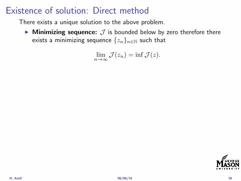
Existence of solution Direct methodThere exists a unique solution to the above problem
I Minimizing sequence J is bounded below by zero therefore thereexists a minimizing sequence znnisinN such that
limnrarrinfin
J (zn) = inf J (z)
I Weak compactness zn sub L2(Ω) is bounded Since L2(Ω) isreflexive therefore there exists a subsequence (not relabeled) suchthat
zn z and z isin Zad
where the latter is a consequence of Zad being closed and convex
I Optimality Since J is continuous and convex and therefore isweakly lower semicontinuous We obtain
lim inf J (zn) ge J (z)
which implies that z is optimal
I Uniqueness Exercise
H Antil 060616 18
Outline
Motivation and examples
Linear elliptic optimal control problems
Differentiation in Banach spaces
First-order necessary conditions
Optimal control of semilinear PDEs
An abstract problem
Discretization using finite element methods
H Antil 060616 19
Differentiation in Banach spacesLet (Z middot Z) (V middot V ) B-spaces Z sub Z open and F Z rarr V
Let z isin Z
I If exist δF (z h) = limtdarr01t (F (z + th)minus F (z)) then δF (z h) is called
the directional derivative of F at z in direction h
I If exist δF (z h) forallh isin Z then h 7rarr δF (z h) is the first variation of Fat z
I Let exist the first variation δF (z middot) F is said to be Gateauxdifferentiable at z iff existA isin L(Z V ) such that δF (z h) = Ahforallh isin Z We write A = F primeG(z)
I F is said to be Frechet differentiable at z iff existA isin L(Z V ) and amapping r(z middot) Z rarr V such that for all h isin U with z + h isin Zwe have
F (z+h) = F (z)+Ah+r(z h) withr(z h)VhZ
rarr 0 as hZ rarr 0
We write F prime(z) = A
H Antil 060616 20
Differentiation in Banach spacesLet (Z middot Z) (V middot V ) B-spaces Z sub Z open and F Z rarr V
Let z isin Z
I If exist δF (z h) = limtdarr01t (F (z + th)minus F (z)) then δF (z h) is called
the directional derivative of F at z in direction h
I If exist δF (z h) forallh isin Z then h 7rarr δF (z h) is the first variation of Fat z
I Let exist the first variation δF (z middot) F is said to be Gateauxdifferentiable at z iff existA isin L(Z V ) such that δF (z h) = Ahforallh isin Z We write A = F primeG(z)
I F is said to be Frechet differentiable at z iff existA isin L(Z V ) and amapping r(z middot) Z rarr V such that for all h isin U with z + h isin Zwe have
F (z+h) = F (z)+Ah+r(z h) withr(z h)VhZ
rarr 0 as hZ rarr 0
We write F prime(z) = A
H Antil 060616 20
Differentiation in Banach spacesLet (Z middot Z) (V middot V ) B-spaces Z sub Z open and F Z rarr V
Let z isin Z
I If exist δF (z h) = limtdarr01t (F (z + th)minus F (z)) then δF (z h) is called
the directional derivative of F at z in direction h
I If exist δF (z h) forallh isin Z then h 7rarr δF (z h) is the first variation of Fat z
I Let exist the first variation δF (z middot) F is said to be Gateauxdifferentiable at z iff existA isin L(Z V ) such that δF (z h) = Ahforallh isin Z We write A = F primeG(z)
I F is said to be Frechet differentiable at z iff existA isin L(Z V ) and amapping r(z middot) Z rarr V such that for all h isin U with z + h isin Zwe have
F (z+h) = F (z)+Ah+r(z h) withr(z h)VhZ
rarr 0 as hZ rarr 0
We write F prime(z) = A
H Antil 060616 20
Differentiation in Banach spacesLet (Z middot Z) (V middot V ) B-spaces Z sub Z open and F Z rarr V
Let z isin Z
I If exist δF (z h) = limtdarr01t (F (z + th)minus F (z)) then δF (z h) is called
the directional derivative of F at z in direction h
I If exist δF (z h) forallh isin Z then h 7rarr δF (z h) is the first variation of Fat z
I Let exist the first variation δF (z middot) F is said to be Gateauxdifferentiable at z iff existA isin L(Z V ) such that δF (z h) = Ahforallh isin Z We write A = F primeG(z)
I F is said to be Frechet differentiable at z iff existA isin L(Z V ) and amapping r(z middot) Z rarr V such that for all h isin U with z + h isin Zwe have
F (z+h) = F (z)+Ah+r(z h) withr(z h)VhZ
rarr 0 as hZ rarr 0
We write F prime(z) = A
H Antil 060616 20
ExamplesExample 1 (H (middot middot)H) Hilbert space F (z) = z2H = (z z)H
forallz h F (z + h)minus F (z) = 2(z h)H + h2HThen
F prime(z)h = (2z h)H
Reisz representation theorem (identify H with Hlowast) we can write
F prime(z)h = (nablaF (z) h)H
where nablaF (z) = 2z is the gradient
Example 2 Let (Z (middot middot)Z) (H (middot middot)H) Hilbert spaces ud isin H fixedLet S isin L(ZH) Consider E Z rarr R
E(z) = Sz minus ud2H
Then E(z) = G(F (z)) where G(v) = v2H and F (z) = Sz minus ud
Eprime(z)h = Gprime(F (z))F prime(z)h = (2v F prime(z)h)H
= 2(Sz minus ud Sh)H = 2(Slowast(Sz minus ud) h)Z
we denote the gradient as nablaE(z) = 2Slowast(Sz minus ud)
H Antil 060616 21
ExamplesExample 1 (H (middot middot)H) Hilbert space F (z) = z2H = (z z)H
forallz h F (z + h)minus F (z) = 2(z h)H + h2HThen
F prime(z)h = (2z h)H
Reisz representation theorem (identify H with Hlowast) we can write
F prime(z)h = (nablaF (z) h)H
where nablaF (z) = 2z is the gradient
Example 2 Let (Z (middot middot)Z) (H (middot middot)H) Hilbert spaces ud isin H fixedLet S isin L(ZH) Consider E Z rarr R
E(z) = Sz minus ud2H
Then E(z) = G(F (z)) where G(v) = v2H and F (z) = Sz minus ud
Eprime(z)h = Gprime(F (z))F prime(z)h = (2v F prime(z)h)H
= 2(Sz minus ud Sh)H = 2(Slowast(Sz minus ud) h)Z
we denote the gradient as nablaE(z) = 2Slowast(Sz minus ud)H Antil 060616 21
Outline
Motivation and examples
Linear elliptic optimal control problems
Differentiation in Banach spaces
First-order necessary conditions
Optimal control of semilinear PDEs
An abstract problem
Discretization using finite element methods
H Antil 060616 22
First order necessary optimality conditions
Most of the theory is based on these two simple results
Theorem Let (Z middot Z) be a normed space J Z rarr (infin+infin] amapping with J 6equiv +infin Then z isin Z minimizer of J hArr 0 isin partJ (z)
Proof 0 isin partJ (z) means by definition of partJ (z) J (z)minus J (z) le 0forallz isin Z
Theorem Let (Z middot Z) be a normed space Zad sub Z nonemptyconvex closed J Z rarr R Gateaux differentiable where Zad sub Z sub ZZ open If z isin Zad is a solution to
minzisinZad
J (z)
then z solvesJ prime(z)(z minus z) ge 0 forallz isin Zad
Proof Exercise
H Antil 060616 23
First order necessary optimality conditions
Most of the theory is based on these two simple results
Theorem Let (Z middot Z) be a normed space J Z rarr (infin+infin] amapping with J 6equiv +infin Then z isin Z minimizer of J hArr 0 isin partJ (z)
Proof 0 isin partJ (z) means by definition of partJ (z) J (z)minus J (z) le 0forallz isin Z
Theorem Let (Z middot Z) be a normed space Zad sub Z nonemptyconvex closed J Z rarr R Gateaux differentiable where Zad sub Z sub ZZ open If z isin Zad is a solution to
minzisinZad
J (z)
then z solvesJ prime(z)(z minus z) ge 0 forallz isin Zad
Proof Exercise
H Antil 060616 23
Linear quadratic OCPI Reduced funcational
J (z) =1
2Sz minus ud2L2(Ω) +
λ
2z2L2(Ω)
I Gradient computation using sensitivity
J prime(z)h = (Slowast(Sz minus ud) + λz h)L2(Ω) forallh isin L2(Ω)
we denote the gradient by
nablaJ (z) = Slowast(Sz minus ud) + λz
I First order necessary and sufficient optimality condition
(nablaJ (z) z minus z)L2(Ω) ge 0 forallz isin Zad
I Adjoint equation Let p = Slowast(Sz minus ud) which translates intop isin H1
0 (Ω) solving
minusdiv (Anablap) = uminus ud in Ω
p = 0 on partΩ
I Gradient computation using adjoint nablaJ (z) = p+ λz
H Antil 060616 24
Linear quadratic OCPI Reduced funcational
J (z) =1
2Sz minus ud2L2(Ω) +
λ
2z2L2(Ω)
I Gradient computation using sensitivity
J prime(z)h = (Slowast(Sz minus ud) + λz h)L2(Ω) forallh isin L2(Ω)
we denote the gradient by
nablaJ (z) = Slowast(Sz minus ud) + λz
I First order necessary and sufficient optimality condition
(nablaJ (z) z minus z)L2(Ω) ge 0 forallz isin Zad
I Adjoint equation Let p = Slowast(Sz minus ud) which translates intop isin H1
0 (Ω) solving
minusdiv (Anablap) = uminus ud in Ω
p = 0 on partΩ
I Gradient computation using adjoint nablaJ (z) = p+ λz
H Antil 060616 24
Linear quadratic OCPI Reduced funcational
J (z) =1
2Sz minus ud2L2(Ω) +
λ
2z2L2(Ω)
I Gradient computation using sensitivity
J prime(z)h = (Slowast(Sz minus ud) + λz h)L2(Ω) forallh isin L2(Ω)
we denote the gradient by
nablaJ (z) = Slowast(Sz minus ud) + λz
I First order necessary and sufficient optimality condition
(nablaJ (z) z minus z)L2(Ω) ge 0 forallz isin Zad
I Adjoint equation Let p = Slowast(Sz minus ud) which translates intop isin H1
0 (Ω) solving
minusdiv (Anablap) = uminus ud in Ω
p = 0 on partΩ
I Gradient computation using adjoint nablaJ (z) = p+ λz
H Antil 060616 24
Linear quadratic OCPI Reduced funcational
J (z) =1
2Sz minus ud2L2(Ω) +
λ
2z2L2(Ω)
I Gradient computation using sensitivity
J prime(z)h = (Slowast(Sz minus ud) + λz h)L2(Ω) forallh isin L2(Ω)
we denote the gradient by
nablaJ (z) = Slowast(Sz minus ud) + λz
I First order necessary and sufficient optimality condition
(nablaJ (z) z minus z)L2(Ω) ge 0 forallz isin Zad
I Adjoint equation Let p = Slowast(Sz minus ud) which translates intop isin H1
0 (Ω) solving
minusdiv (Anablap) = uminus ud in Ω
p = 0 on partΩ
I Gradient computation using adjoint nablaJ (z) = p+ λz
H Antil 060616 24
Linear quadratic OCPI Reduced funcational
J (z) =1
2Sz minus ud2L2(Ω) +
λ
2z2L2(Ω)
I Gradient computation using sensitivity
J prime(z)h = (Slowast(Sz minus ud) + λz h)L2(Ω) forallh isin L2(Ω)
we denote the gradient by
nablaJ (z) = Slowast(Sz minus ud) + λz
I First order necessary and sufficient optimality condition
(nablaJ (z) z minus z)L2(Ω) ge 0 forallz isin Zad
I Adjoint equation Let p = Slowast(Sz minus ud) which translates intop isin H1
0 (Ω) solving
minusdiv (Anablap) = uminus ud in Ω
p = 0 on partΩ
I Gradient computation using adjoint nablaJ (z) = p+ λz
H Antil 060616 24
Optimality system
I State u isin H10 (Ω)
intΩAnablau middot nablav =
intΩzv forallv isin H1
0 (Ω)
I Adjoint p isin H10 (Ω)
intΩAnablap middot nablav =
intΩ
(uminus ud)v forallv isin H10 (Ω)
I Control z isin Zad (p+ λz z minus z) ge 0 forallz isin Zad
H Antil 060616 25
Pointwise interpretation
The variational inequality
(p+ λz z minus z) ge 0 forallz isin Zad
is equivalent to for ae x isin Ω
z(x) =
za(x) if p(x) + λz(x) gt 0isin [za(x) zb(x)] if p(x) + λz(x) = 0zb(x) if p(x) + λz(x) lt 0
Consequence
I When λ gt 0 then ae in Ω
z(x) = P[za(x)zb(x)]
minus 1
λp(x)
= min
zb(x)max
za(x)minus 1
λp(x)
H Antil 060616 26
Formal Lagrange method applied to linear OCPIntroduce L H1
0 (Ω)times Zad timesH1(Ω)rarr R defined as
L(u z p) = J(u z)minusint
Ω
(minusdiv (Anablau)minus z
)p dx
Integrate by parts to arrive at
L(u z p) = J(u z)minusint
Ω
(minusdiv (Anablap)uminus zp
)dx+
intpartΩ
(Anablau)p ds
If (u z p) is a stationary point then
I State
DpL(u z p)h = 0 forallh isin H1(Ω)
I AdjointDuL(u z p)h = 0 forallh isin H1
0 (Ω)
I ControlDzL(u z p)(z minus z) ge 0 forallz isin Zad
H Antil 060616 27
Formal Lagrange method applied to linear OCPIntroduce L H1
0 (Ω)times Zad timesH1(Ω)rarr R defined as
L(u z p) = J(u z)minusint
Ω
(minusdiv (Anablau)minus z
)p dx
Integrate by parts to arrive at
L(u z p) = J(u z)minusint
Ω
(minusdiv (Anablap)uminus zp
)dx+
intpartΩ
(Anablau)p ds
If (u z p) is a stationary point then
I State
DpL(u z p)h = 0 forallh isin H1(Ω)
I AdjointDuL(u z p)h = 0 forallh isin H1
0 (Ω)
I ControlDzL(u z p)(z minus z) ge 0 forallz isin Zad
H Antil 060616 27
Formal Lagrange method applied to linear OCPIntroduce L H1
0 (Ω)times Zad timesH1(Ω)rarr R defined as
L(u z p) = J(u z)minusint
Ω
(minusdiv (Anablau)minus z
)p dx
Integrate by parts to arrive at
L(u z p) = J(u z)minusint
Ω
(minusdiv (Anablap)uminus zp
)dx+
intpartΩ
(Anablau)p ds
If (u z p) is a stationary point then
I State
DpL(u z p)h = 0 forallh isin H1(Ω)
I AdjointDuL(u z p)h = 0 forallh isin H1
0 (Ω)
I ControlDzL(u z p)(z minus z) ge 0 forallz isin Zad
H Antil 060616 27
Formal Lagrange method applied to linear OCPIntroduce L H1
0 (Ω)times Zad timesH1(Ω)rarr R defined as
L(u z p) = J(u z)minusint
Ω
(minusdiv (Anablau)minus z
)p dx
Integrate by parts to arrive at
L(u z p) = J(u z)minusint
Ω
(minusdiv (Anablap)uminus zp
)dx+
intpartΩ
(Anablau)p ds
If (u z p) is a stationary point then
I State
DpL(u z p)h = 0 forallh isin H1(Ω)
I AdjointDuL(u z p)h = 0 forallh isin H1
0 (Ω)
I ControlDzL(u z p)(z minus z) ge 0 forallz isin Zad
H Antil 060616 27
Formal Lagrange method applied to linear OCPIntroduce L H1
0 (Ω)times Zad timesH1(Ω)rarr R defined as
L(u z p) = J(u z)minusint
Ω
(minusdiv (Anablau)minus z
)p dx
Integrate by parts to arrive at
L(u z p) = J(u z)minusint
Ω
(minusdiv (Anablap)uminus zp
)dx+
intpartΩ
(Anablau)p ds
If (u z p) is a stationary point then
I State
DpL(u z p)h = 0 forallh isin H1(Ω)
I AdjointDuL(u z p)h = 0 forallh isin H1
0 (Ω)
I ControlDzL(u z p)(z minus z) ge 0 forallz isin Zad
H Antil 060616 27
Outline
Motivation and examples
Linear elliptic optimal control problems
Differentiation in Banach spaces
First-order necessary conditions
Optimal control of semilinear PDEs
An abstract problem
Discretization using finite element methods
H Antil 060616 28
Semilinear elliptic OCP
min J(u z) =1
2uminus ud2L2(Ω) +
λ
2z2L2(Ω)
subject to
minus∆u+ g(x u) = z in Ω
u = 0 on partΩ
and z isin Zad with za zb isin Linfin(Ω)
H Antil 060616 29
State space(A1) Ω sub Rd open bounded partΩ is Lipschitz
(A2) g Ωtimes Rrarr R is bounded and measurable with respect to x isin Ωfor every u isin R
(A3) g is continuous monotone increasing and Lipschitz continuous in ufor ae x isin Ω
(A4) g(x 0) = 0 for ae x isin Ω (not really necessary)
Theorem Suppose (A1)minus (A4) hold For every z isin Lr(Ω) withr gt d2 the state equation has a unique weak solutionu isin H1
0 (Ω) cap C(Ω) ie we haveintΩ
nablau middot nablav dx+
intΩ
g(x u(x))v(x) dx =
intΩ
zv dx forallv isin H10 (Ω)
Moreover there exists a constant C gt 0 such that
uH1(Ω) + uC(Ω) le CzLr(Ω)
RemarkI The proof of the theorem uses the BrowderndashMinty theorem on
monotone operators
H Antil 060616 30
State space(A1) Ω sub Rd open bounded partΩ is Lipschitz
(A2) g Ωtimes Rrarr R is bounded and measurable with respect to x isin Ωfor every u isin R
(A3) g is continuous monotone increasing and Lipschitz continuous in ufor ae x isin Ω
(A4) g(x 0) = 0 for ae x isin Ω (not really necessary)
Theorem Suppose (A1)minus (A4) hold For every z isin Lr(Ω) withr gt d2 the state equation has a unique weak solutionu isin H1
0 (Ω) cap C(Ω) ie we haveintΩ
nablau middot nablav dx+
intΩ
g(x u(x))v(x) dx =
intΩ
zv dx forallv isin H10 (Ω)
Moreover there exists a constant C gt 0 such that
uH1(Ω) + uC(Ω) le CzLr(Ω)
RemarkI The proof of the theorem uses the BrowderndashMinty theorem on
monotone operators
H Antil 060616 30
State space(A1) Ω sub Rd open bounded partΩ is Lipschitz
(A2) g Ωtimes Rrarr R is bounded and measurable with respect to x isin Ωfor every u isin R
(A3) g is continuous monotone increasing and Lipschitz continuous in ufor ae x isin Ω
(A4) g(x 0) = 0 for ae x isin Ω (not really necessary)
Theorem Suppose (A1)minus (A4) hold For every z isin Lr(Ω) withr gt d2 the state equation has a unique weak solutionu isin H1
0 (Ω) cap C(Ω) ie we haveintΩ
nablau middot nablav dx+
intΩ
g(x u(x))v(x) dx =
intΩ
zv dx forallv isin H10 (Ω)
Moreover there exists a constant C gt 0 such that
uH1(Ω) + uC(Ω) le CzLr(Ω)
RemarkI The proof of the theorem uses the BrowderndashMinty theorem on
monotone operators
H Antil 060616 30
Control-to-state map and reduced problem
I Control to state map
S Linfin(Ω)rarr H10 (Ω) cap C(Ω)
is well defined and is globally Lipschitz continuous
I Reduced problem
minJ (z) =1
2S(u)minus ud2L2(Ω) +
λ
2z2L2(Ω)
H Antil 060616 31
Control-to-state map and reduced problem
I Control to state map
S Linfin(Ω)rarr H10 (Ω) cap C(Ω)
is well defined and is globally Lipschitz continuous
I Reduced problem
minJ (z) =1
2S(u)minus ud2L2(Ω) +
λ
2z2L2(Ω)
H Antil 060616 31
First-order necessary conditionsI Lagrangian functional
L(u z p) = J(u z)minusint
Ω
(minus∆u+ g(x u(x))minus z
)p dx
= J(u z)minusint
Ω
(nablau middot nablap+ g(x u(x))pminus zp
)dx
I Adjoint system For all h isin H10 (Ω)
0 = DuL(u z p)h =
intΩ
(uminus ud)h dxminusint
Ω
(nablah middot nablap+ gu(x u(x))ph
)which yields
minus∆p+ gu(x u(x))p = uminus ud in Ω
p = 0 on partΩ
I Control
DzL(u z p)(z minus z) = (p+ λz z minus z) dx ge 0 forallz isin ZadI Gradient
nablaJ (z) = p+ λz
H Antil 060616 32
First-order necessary conditionsI Lagrangian functional
L(u z p) = J(u z)minusint
Ω
(minus∆u+ g(x u(x))minus z
)p dx
= J(u z)minusint
Ω
(nablau middot nablap+ g(x u(x))pminus zp
)dx
I Adjoint system For all h isin H10 (Ω)
0 = DuL(u z p)h =
intΩ
(uminus ud)h dxminusint
Ω
(nablah middot nablap+ gu(x u(x))ph
)which yields
minus∆p+ gu(x u(x))p = uminus ud in Ω
p = 0 on partΩ
I Control
DzL(u z p)(z minus z) = (p+ λz z minus z) dx ge 0 forallz isin ZadI Gradient
nablaJ (z) = p+ λz
H Antil 060616 32
First-order necessary conditionsI Lagrangian functional
L(u z p) = J(u z)minusint
Ω
(minus∆u+ g(x u(x))minus z
)p dx
= J(u z)minusint
Ω
(nablau middot nablap+ g(x u(x))pminus zp
)dx
I Adjoint system For all h isin H10 (Ω)
0 = DuL(u z p)h =
intΩ
(uminus ud)h dxminusint
Ω
(nablah middot nablap+ gu(x u(x))ph
)which yields
minus∆p+ gu(x u(x))p = uminus ud in Ω
p = 0 on partΩ
I Control
DzL(u z p)(z minus z) = (p+ λz z minus z) dx ge 0 forallz isin Zad
I GradientnablaJ (z) = p+ λz
H Antil 060616 32
First-order necessary conditionsI Lagrangian functional
L(u z p) = J(u z)minusint
Ω
(minus∆u+ g(x u(x))minus z
)p dx
= J(u z)minusint
Ω
(nablau middot nablap+ g(x u(x))pminus zp
)dx
I Adjoint system For all h isin H10 (Ω)
0 = DuL(u z p)h =
intΩ
(uminus ud)h dxminusint
Ω
(nablah middot nablap+ gu(x u(x))ph
)which yields
minus∆p+ gu(x u(x))p = uminus ud in Ω
p = 0 on partΩ
I Control
DzL(u z p)(z minus z) = (p+ λz z minus z) dx ge 0 forallz isin ZadI Gradient
nablaJ (z) = p+ λz
H Antil 060616 32
Differentiability of Nemytskii operator
The rigorous proof uses
Theorem In addition to (A1)-(A4) if
(A5) g is continuously differentiable with respect to u for ae x isin Ωand we have
(i) |gu(x 0)| le K for ae x isin Ω(ii) gu is locally Lipschitz with respect to u isin R
then the Nemytskii operator G u 7rarr g(middot u(middot)) is continuously Frechetdifferentiable from Linfin(Ω) into itself and
(Gprime(u)h)(x) = gu(x u(x))h(x) ae in Ω forallh isin Linfin(Ω)
Remark (A5) holds if g(x u) = g(u) and g isin C2(R)
H Antil 060616 33
Outline
Motivation and examples
Linear elliptic optimal control problems
Differentiation in Banach spaces
First-order necessary conditions
Optimal control of semilinear PDEs
An abstract problem
Discretization using finite element methods
H Antil 060616 34
Gradient computation via adjoint general formI Abstract problem
min J(u z)
subject toc(u z) = 0
and z isin Zad
I Directional derivative Let S be the control to state map(nonlinear in general)
z 7rarr S(z) = u(z)
Under the assumptions of ldquoimplicit function theoremrdquo
J prime(z)h = (nablauJ (u(z) z) Sprime(z)h) + (nablazJ (u(z) z) h)
I Sensitivity of u with respect to z Differentiating the stateequation
cu(S(z) z)Sprime(z)h = minuscz(S(z) z)h
leads toSprime(z)h = minuscu(S(z) z)minus1
(cz(S(z) z)h
)
provided cu(S(z) z)minus1 is well-defined
H Antil 060616 35
Gradient computation via adjoint general formI Abstract problem
min J(u z)
subject toc(u z) = 0
and z isin ZadI Directional derivative Let S be the control to state map
(nonlinear in general)
z 7rarr S(z) = u(z)
Under the assumptions of ldquoimplicit function theoremrdquo
J prime(z)h = (nablauJ (u(z) z) Sprime(z)h) + (nablazJ (u(z) z) h)
I Sensitivity of u with respect to z Differentiating the stateequation
cu(S(z) z)Sprime(z)h = minuscz(S(z) z)h
leads toSprime(z)h = minuscu(S(z) z)minus1
(cz(S(z) z)h
)
provided cu(S(z) z)minus1 is well-defined
H Antil 060616 35
Gradient computation via adjoint general formI Abstract problem
min J(u z)
subject toc(u z) = 0
and z isin ZadI Directional derivative Let S be the control to state map
(nonlinear in general)
z 7rarr S(z) = u(z)
Under the assumptions of ldquoimplicit function theoremrdquo
J prime(z)h = (nablauJ (u(z) z) Sprime(z)h) + (nablazJ (u(z) z) h)
I Sensitivity of u with respect to z Differentiating the stateequation
cu(S(z) z)Sprime(z)h = minuscz(S(z) z)h
leads toSprime(z)h = minuscu(S(z) z)minus1
(cz(S(z) z)h
)
provided cu(S(z) z)minus1 is well-defined
H Antil 060616 35
Adjoint equation and gradient general form
I Directional derivative
J prime(z)h = minus(nablauJ (u(z) z) cu(u(z) z)minus1cz(u(z) z)h
)+ (nablazJ (u(z) z) h)
I Gradient
nablaJ (z) = minuscz(u(z) z)lowast(cu(u(z) z)minuslowastnablauJ (u(z) z)
)+nablazJ (u(z) z)
I Introducing adjoint variable p solving
cu(u(z) z)lowastp = nablauJ (u(z) z)
we arrive at following form of gradient
nablaJ (z) = minuscz(u(z) z)lowastp+nablazJ (u(z) z)
which is tractable
H Antil 060616 36
Adjoint equation and gradient general form
I Directional derivative
J prime(z)h = minus(nablauJ (u(z) z) cu(u(z) z)minus1cz(u(z) z)h
)+ (nablazJ (u(z) z) h)
I Gradient
nablaJ (z) = minuscz(u(z) z)lowast(cu(u(z) z)minuslowastnablauJ (u(z) z)
)+nablazJ (u(z) z)
I Introducing adjoint variable p solving
cu(u(z) z)lowastp = nablauJ (u(z) z)
we arrive at following form of gradient
nablaJ (z) = minuscz(u(z) z)lowastp+nablazJ (u(z) z)
which is tractable
H Antil 060616 36
Adjoint equation and gradient general form
I Directional derivative
J prime(z)h = minus(nablauJ (u(z) z) cu(u(z) z)minus1cz(u(z) z)h
)+ (nablazJ (u(z) z) h)
I Gradient
nablaJ (z) = minuscz(u(z) z)lowast(cu(u(z) z)minuslowastnablauJ (u(z) z)
)+nablazJ (u(z) z)
I Introducing adjoint variable p solving
cu(u(z) z)lowastp = nablauJ (u(z) z)
we arrive at following form of gradient
nablaJ (z) = minuscz(u(z) z)lowastp+nablazJ (u(z) z)
which is tractable
H Antil 060616 36
Hessian computation general form
I Lagrangian L(u z p) = J(u z)minusint
Ωc(u z)p dx Then we have
DzJ (z)h = DzL(u z p)h
I Second order derivative
D2zJ (z)[h1 h2] = DuDzL(u z p)[h1 S
prime(z)h2] +D2zL(u z p)[h1 h2]
+DpDzL(u z p)[h1 Dzp(z)h2]
I We already know Sprime(z)h2 moreover
DpDzL(u z p)[h1 Dzp(z)h2] = minus(cu(u z)h1 Dzp(z)h2
)
It remain to identify Dzp(z)h2
H Antil 060616 37
Hessian computation general form
I Lagrangian L(u z p) = J(u z)minusint
Ωc(u z)p dx Then we have
DzJ (z)h = DzL(u z p)h
I Second order derivative
D2zJ (z)[h1 h2] = DuDzL(u z p)[h1 S
prime(z)h2] +D2zL(u z p)[h1 h2]
+DpDzL(u z p)[h1 Dzp(z)h2]
I We already know Sprime(z)h2 moreover
DpDzL(u z p)[h1 Dzp(z)h2] = minus(cu(u z)h1 Dzp(z)h2
)
It remain to identify Dzp(z)h2
H Antil 060616 37
Hessian computation general form
I Lagrangian L(u z p) = J(u z)minusint
Ωc(u z)p dx Then we have
DzJ (z)h = DzL(u z p)h
I Second order derivative
D2zJ (z)[h1 h2] = DuDzL(u z p)[h1 S
prime(z)h2] +D2zL(u z p)[h1 h2]
+DpDzL(u z p)[h1 Dzp(z)h2]
I We already know Sprime(z)h2 moreover
DpDzL(u z p)[h1 Dzp(z)h2] = minus(cu(u z)h1 Dzp(z)h2
)
It remain to identify Dzp(z)h2
H Antil 060616 37
Outline
Motivation and examples
Linear elliptic optimal control problems
Differentiation in Banach spaces
First-order necessary conditions
Optimal control of semilinear PDEs
An abstract problem
Discretization using finite element methods
H Antil 060616 38
Numerical approximation of Poisson equation MeshTo avoid technical issues we will assume that partΩ is polygonal
I Mesh Let T = K be a mesh of Ω where K sub Rd is an elementthat is isoparametrically equivalent to a unit simplex in Rd
I Conforming mesh We say that the mesh is conforming ifI Ω = cupKisinT KI If K1 cap K2 = x then x is a node of K1 and K2I If K1 cap K2 6= empty and K1 cap K2 6= x then K1 cap K2 is an edgeface
contained in partK1 cap partK2
I Shape regular Let T be the collection of all conformingrefinements of an original mesh T 0 Then T is called shape regularif exist κ gt 0 such that
hKρKle κ forallK isin cupiT i
where hK = diam K ρK = maxρ gt 0|Bρ sub KI Quasi-uniform A family of shape regular meshes is called-quasi
uniform if there exist a constant σ gt 0 such that
maxhKminhK
le σ
uniformly for all meshes in the family
Numerical approximation of Poisson equation MeshTo avoid technical issues we will assume that partΩ is polygonal
I Mesh Let T = K be a mesh of Ω where K sub Rd is an elementthat is isoparametrically equivalent to a unit simplex in Rd
I Conforming mesh We say that the mesh is conforming ifI Ω = cupKisinT KI If K1 cap K2 = x then x is a node of K1 and K2I If K1 cap K2 6= empty and K1 cap K2 6= x then K1 cap K2 is an edgeface
contained in partK1 cap partK2
I Shape regular Let T be the collection of all conformingrefinements of an original mesh T 0 Then T is called shape regularif exist κ gt 0 such that
hKρKle κ forallK isin cupiT i
where hK = diam K ρK = maxρ gt 0|Bρ sub KI Quasi-uniform A family of shape regular meshes is called-quasi
uniform if there exist a constant σ gt 0 such that
maxhKminhK
le σ
uniformly for all meshes in the family
Numerical approximation of Poisson equation MeshTo avoid technical issues we will assume that partΩ is polygonal
I Mesh Let T = K be a mesh of Ω where K sub Rd is an elementthat is isoparametrically equivalent to a unit simplex in Rd
I Conforming mesh We say that the mesh is conforming ifI Ω = cupKisinT KI If K1 cap K2 = x then x is a node of K1 and K2I If K1 cap K2 6= empty and K1 cap K2 6= x then K1 cap K2 is an edgeface
contained in partK1 cap partK2
I Shape regular Let T be the collection of all conformingrefinements of an original mesh T 0 Then T is called shape regularif exist κ gt 0 such that
hKρKle κ forallK isin cupiT i
where hK = diam K ρK = maxρ gt 0|Bρ sub K
I Quasi-uniform A family of shape regular meshes is called-quasiuniform if there exist a constant σ gt 0 such that
maxhKminhK
le σ
uniformly for all meshes in the family
Numerical approximation of Poisson equation MeshTo avoid technical issues we will assume that partΩ is polygonal
I Mesh Let T = K be a mesh of Ω where K sub Rd is an elementthat is isoparametrically equivalent to a unit simplex in Rd
I Conforming mesh We say that the mesh is conforming ifI Ω = cupKisinT KI If K1 cap K2 = x then x is a node of K1 and K2I If K1 cap K2 6= empty and K1 cap K2 6= x then K1 cap K2 is an edgeface
contained in partK1 cap partK2
I Shape regular Let T be the collection of all conformingrefinements of an original mesh T 0 Then T is called shape regularif exist κ gt 0 such that
hKρKle κ forallK isin cupiT i
where hK = diam K ρK = maxρ gt 0|Bρ sub KI Quasi-uniform A family of shape regular meshes is called-quasi
uniform if there exist a constant σ gt 0 such that
maxhKminhK
le σ
uniformly for all meshes in the family
FE space and Galerkin approximationI Finite element space For T isin T we define the finite element
space as
V(T ) = W isin C0(Ω) WK isin P1forallK isin T W |partΩ = 0
where P1 is the set of polynomials of degree at most 1
I Galerkin approximation of continuous problem is given by
Find UT isin V(T )
intΩ
AnablaUT middot nablaV = 〈f V 〉 forallV isin V(T )
The discrete problem is well-posedI Nodal basis Consists of functions ψi isin V(T ) with xi isin N (T )
satisfyingψxi
(xj) = δij
where N (T ) denotes the interior (plus Neumann) nodesI Galerkin orthogonality(
nabla(uminus UT )nablaW)L2(Ω)
= 0 forallW isin V(T )
H Antil 060616 40
FE space and Galerkin approximationI Finite element space For T isin T we define the finite element
space as
V(T ) = W isin C0(Ω) WK isin P1forallK isin T W |partΩ = 0
where P1 is the set of polynomials of degree at most 1I Galerkin approximation of continuous problem is given by
Find UT isin V(T )
intΩ
AnablaUT middot nablaV = 〈f V 〉 forallV isin V(T )
The discrete problem is well-posed
I Nodal basis Consists of functions ψi isin V(T ) with xi isin N (T )satisfying
ψxi(xj) = δij
where N (T ) denotes the interior (plus Neumann) nodesI Galerkin orthogonality(
nabla(uminus UT )nablaW)L2(Ω)
= 0 forallW isin V(T )
H Antil 060616 40
FE space and Galerkin approximationI Finite element space For T isin T we define the finite element
space as
V(T ) = W isin C0(Ω) WK isin P1forallK isin T W |partΩ = 0
where P1 is the set of polynomials of degree at most 1I Galerkin approximation of continuous problem is given by
Find UT isin V(T )
intΩ
AnablaUT middot nablaV = 〈f V 〉 forallV isin V(T )
The discrete problem is well-posedI Nodal basis Consists of functions ψi isin V(T ) with xi isin N (T )
satisfyingψxi
(xj) = δij
where N (T ) denotes the interior (plus Neumann) nodes
I Galerkin orthogonality(nabla(uminus UT )nablaW
)L2(Ω)
= 0 forallW isin V(T )
H Antil 060616 40
FE space and Galerkin approximationI Finite element space For T isin T we define the finite element
space as
V(T ) = W isin C0(Ω) WK isin P1forallK isin T W |partΩ = 0
where P1 is the set of polynomials of degree at most 1I Galerkin approximation of continuous problem is given by
Find UT isin V(T )
intΩ
AnablaUT middot nablaV = 〈f V 〉 forallV isin V(T )
The discrete problem is well-posedI Nodal basis Consists of functions ψi isin V(T ) with xi isin N (T )
satisfyingψxi
(xj) = δij
where N (T ) denotes the interior (plus Neumann) nodesI Galerkin orthogonality(
nabla(uminus UT )nablaW)L2(Ω)
= 0 forallW isin V(T )
H Antil 060616 40
Best approximation
I Cearsquos lemma
nabla(uminus UT )L2(Ω) le C infWisinV(T )
nabla(uminusW )L2(Ω)
I Nodal interpolation operator ΠT C(Ω)rarr V(T ) satisfies
ΠT u(xi) = u(xi) forallxi isin N (T )
and is defined as
ΠT u =sum
xiisinN (T )
u(xi)ψxi
I Error estimates In Cearsquos lemma replace W by ΠT u and thencompute the interpolation error
H Antil 060616 41
Best approximation
I Cearsquos lemma
nabla(uminus UT )L2(Ω) le C infWisinV(T )
nabla(uminusW )L2(Ω)
I Nodal interpolation operator ΠT C(Ω)rarr V(T ) satisfies
ΠT u(xi) = u(xi) forallxi isin N (T )
and is defined as
ΠT u =sum
xiisinN (T )
u(xi)ψxi
I Error estimates In Cearsquos lemma replace W by ΠT u and thencompute the interpolation error
H Antil 060616 41
Best approximation
I Cearsquos lemma
nabla(uminus UT )L2(Ω) le C infWisinV(T )
nabla(uminusW )L2(Ω)
I Nodal interpolation operator ΠT C(Ω)rarr V(T ) satisfies
ΠT u(xi) = u(xi) forallxi isin N (T )
and is defined as
ΠT u =sum
xiisinN (T )
u(xi)ψxi
I Error estimates In Cearsquos lemma replace W by ΠT u and thencompute the interpolation error
H Antil 060616 41
Algebraic system state equation
I Recall UT isin V(T ) solves
a(UT V ) = 〈f V 〉 forallV isin V(T )
I Now setting UT =sumN
j=1 Ujψj V = ψi we get
Nsumj=1
Uja(φj φi) = 〈f ψi〉 i = 1 N
which is the matrix-vector system
AU = F
I Stiffness matrix A is SPD
H Antil 060616 42
Algebraic system state equation
I Recall UT isin V(T ) solves
a(UT V ) = 〈f V 〉 forallV isin V(T )
I Now setting UT =sumN
j=1 Ujψj V = ψi we get
Nsumj=1
Uja(φj φi) = 〈f ψi〉 i = 1 N
which is the matrix-vector system
AU = F
I Stiffness matrix A is SPD
H Antil 060616 42
Algebraic system state equation
I Recall UT isin V(T ) solves
a(UT V ) = 〈f V 〉 forallV isin V(T )
I Now setting UT =sumN
j=1 Ujψj V = ψi we get
Nsumj=1
Uja(φj φi) = 〈f ψi〉 i = 1 N
which is the matrix-vector system
AU = F
I Stiffness matrix A is SPD
H Antil 060616 42
Discrete linear elliptic OCP
min JT (UT ZT ) =1
2UT minus ud2L2(Ω) +
λ
2ZT 2L2(Ω)
subject to
Find UT isin V(T )
intΩ
nablaUT middot nablaV = (ZT V )L2(Ω) forallV isin V(T )
and whereZT isin Zad(T ) = Zad cap Z(T )
is either one of these
Z(T ) =
V(T )L2(Ω) variational discretization (Hinze)WT isin Linfin(Ω) ZT |K isin P0(K)K isin T
H Antil 060616 43
Recent books
F TroltzschOptimal control of partial differential equations volume 112 ofGraduate Studies in MathematicsAmerican Mathematical Society Providence RI 2010Theory methods and applications Translated from the 2005 Germanoriginal by Jurgen Sprekels
K Ito and K KunischLagrange multiplier approach to variational problems andapplications volume 15 of Advances in Design and ControlSociety for Industrial and Applied Mathematics (SIAM)Philadelphia PA 2008
H Antil 060616 44
- Motivation and examples
- Linear elliptic optimal control problems
- Differentiation in Banach spaces
- First-order necessary conditions
- Optimal control of semilinear PDEs
- An abstract problem
- Discretization using finite element methods
-

Existence of solution Direct methodThere exists a unique solution to the above problem
I Minimizing sequence J is bounded below by zero therefore thereexists a minimizing sequence znnisinN such that
limnrarrinfin
J (zn) = inf J (z)
I Weak compactness zn sub L2(Ω) is bounded Since L2(Ω) isreflexive therefore there exists a subsequence (not relabeled) suchthat
zn z and z isin Zad
where the latter is a consequence of Zad being closed and convex
I Optimality Since J is continuous and convex and therefore isweakly lower semicontinuous We obtain
lim inf J (zn) ge J (z)
which implies that z is optimal
I Uniqueness Exercise
H Antil 060616 18
Existence of solution Direct methodThere exists a unique solution to the above problem
I Minimizing sequence J is bounded below by zero therefore thereexists a minimizing sequence znnisinN such that
limnrarrinfin
J (zn) = inf J (z)
I Weak compactness zn sub L2(Ω) is bounded Since L2(Ω) isreflexive therefore there exists a subsequence (not relabeled) suchthat
zn z and z isin Zad
where the latter is a consequence of Zad being closed and convex
I Optimality Since J is continuous and convex and therefore isweakly lower semicontinuous We obtain
lim inf J (zn) ge J (z)
which implies that z is optimal
I Uniqueness Exercise
H Antil 060616 18
Existence of solution Direct methodThere exists a unique solution to the above problem
I Minimizing sequence J is bounded below by zero therefore thereexists a minimizing sequence znnisinN such that
limnrarrinfin
J (zn) = inf J (z)
I Weak compactness zn sub L2(Ω) is bounded Since L2(Ω) isreflexive therefore there exists a subsequence (not relabeled) suchthat
zn z and z isin Zad
where the latter is a consequence of Zad being closed and convex
I Optimality Since J is continuous and convex and therefore isweakly lower semicontinuous We obtain
lim inf J (zn) ge J (z)
which implies that z is optimal
I Uniqueness Exercise
H Antil 060616 18
Outline
Motivation and examples
Linear elliptic optimal control problems
Differentiation in Banach spaces
First-order necessary conditions
Optimal control of semilinear PDEs
An abstract problem
Discretization using finite element methods
H Antil 060616 19
Differentiation in Banach spacesLet (Z middot Z) (V middot V ) B-spaces Z sub Z open and F Z rarr V
Let z isin Z
I If exist δF (z h) = limtdarr01t (F (z + th)minus F (z)) then δF (z h) is called
the directional derivative of F at z in direction h
I If exist δF (z h) forallh isin Z then h 7rarr δF (z h) is the first variation of Fat z
I Let exist the first variation δF (z middot) F is said to be Gateauxdifferentiable at z iff existA isin L(Z V ) such that δF (z h) = Ahforallh isin Z We write A = F primeG(z)
I F is said to be Frechet differentiable at z iff existA isin L(Z V ) and amapping r(z middot) Z rarr V such that for all h isin U with z + h isin Zwe have
F (z+h) = F (z)+Ah+r(z h) withr(z h)VhZ
rarr 0 as hZ rarr 0
We write F prime(z) = A
H Antil 060616 20
Differentiation in Banach spacesLet (Z middot Z) (V middot V ) B-spaces Z sub Z open and F Z rarr V
Let z isin Z
I If exist δF (z h) = limtdarr01t (F (z + th)minus F (z)) then δF (z h) is called
the directional derivative of F at z in direction h
I If exist δF (z h) forallh isin Z then h 7rarr δF (z h) is the first variation of Fat z
I Let exist the first variation δF (z middot) F is said to be Gateauxdifferentiable at z iff existA isin L(Z V ) such that δF (z h) = Ahforallh isin Z We write A = F primeG(z)
I F is said to be Frechet differentiable at z iff existA isin L(Z V ) and amapping r(z middot) Z rarr V such that for all h isin U with z + h isin Zwe have
F (z+h) = F (z)+Ah+r(z h) withr(z h)VhZ
rarr 0 as hZ rarr 0
We write F prime(z) = A
H Antil 060616 20
Differentiation in Banach spacesLet (Z middot Z) (V middot V ) B-spaces Z sub Z open and F Z rarr V
Let z isin Z
I If exist δF (z h) = limtdarr01t (F (z + th)minus F (z)) then δF (z h) is called
the directional derivative of F at z in direction h
I If exist δF (z h) forallh isin Z then h 7rarr δF (z h) is the first variation of Fat z
I Let exist the first variation δF (z middot) F is said to be Gateauxdifferentiable at z iff existA isin L(Z V ) such that δF (z h) = Ahforallh isin Z We write A = F primeG(z)
I F is said to be Frechet differentiable at z iff existA isin L(Z V ) and amapping r(z middot) Z rarr V such that for all h isin U with z + h isin Zwe have
F (z+h) = F (z)+Ah+r(z h) withr(z h)VhZ
rarr 0 as hZ rarr 0
We write F prime(z) = A
H Antil 060616 20
Differentiation in Banach spacesLet (Z middot Z) (V middot V ) B-spaces Z sub Z open and F Z rarr V
Let z isin Z
I If exist δF (z h) = limtdarr01t (F (z + th)minus F (z)) then δF (z h) is called
the directional derivative of F at z in direction h
I If exist δF (z h) forallh isin Z then h 7rarr δF (z h) is the first variation of Fat z
I Let exist the first variation δF (z middot) F is said to be Gateauxdifferentiable at z iff existA isin L(Z V ) such that δF (z h) = Ahforallh isin Z We write A = F primeG(z)
I F is said to be Frechet differentiable at z iff existA isin L(Z V ) and amapping r(z middot) Z rarr V such that for all h isin U with z + h isin Zwe have
F (z+h) = F (z)+Ah+r(z h) withr(z h)VhZ
rarr 0 as hZ rarr 0
We write F prime(z) = A
H Antil 060616 20
ExamplesExample 1 (H (middot middot)H) Hilbert space F (z) = z2H = (z z)H
forallz h F (z + h)minus F (z) = 2(z h)H + h2HThen
F prime(z)h = (2z h)H
Reisz representation theorem (identify H with Hlowast) we can write
F prime(z)h = (nablaF (z) h)H
where nablaF (z) = 2z is the gradient
Example 2 Let (Z (middot middot)Z) (H (middot middot)H) Hilbert spaces ud isin H fixedLet S isin L(ZH) Consider E Z rarr R
E(z) = Sz minus ud2H
Then E(z) = G(F (z)) where G(v) = v2H and F (z) = Sz minus ud
Eprime(z)h = Gprime(F (z))F prime(z)h = (2v F prime(z)h)H
= 2(Sz minus ud Sh)H = 2(Slowast(Sz minus ud) h)Z
we denote the gradient as nablaE(z) = 2Slowast(Sz minus ud)
H Antil 060616 21
ExamplesExample 1 (H (middot middot)H) Hilbert space F (z) = z2H = (z z)H
forallz h F (z + h)minus F (z) = 2(z h)H + h2HThen
F prime(z)h = (2z h)H
Reisz representation theorem (identify H with Hlowast) we can write
F prime(z)h = (nablaF (z) h)H
where nablaF (z) = 2z is the gradient
Example 2 Let (Z (middot middot)Z) (H (middot middot)H) Hilbert spaces ud isin H fixedLet S isin L(ZH) Consider E Z rarr R
E(z) = Sz minus ud2H
Then E(z) = G(F (z)) where G(v) = v2H and F (z) = Sz minus ud
Eprime(z)h = Gprime(F (z))F prime(z)h = (2v F prime(z)h)H
= 2(Sz minus ud Sh)H = 2(Slowast(Sz minus ud) h)Z
we denote the gradient as nablaE(z) = 2Slowast(Sz minus ud)H Antil 060616 21
Outline
Motivation and examples
Linear elliptic optimal control problems
Differentiation in Banach spaces
First-order necessary conditions
Optimal control of semilinear PDEs
An abstract problem
Discretization using finite element methods
H Antil 060616 22
First order necessary optimality conditions
Most of the theory is based on these two simple results
Theorem Let (Z middot Z) be a normed space J Z rarr (infin+infin] amapping with J 6equiv +infin Then z isin Z minimizer of J hArr 0 isin partJ (z)
Proof 0 isin partJ (z) means by definition of partJ (z) J (z)minus J (z) le 0forallz isin Z
Theorem Let (Z middot Z) be a normed space Zad sub Z nonemptyconvex closed J Z rarr R Gateaux differentiable where Zad sub Z sub ZZ open If z isin Zad is a solution to
minzisinZad
J (z)
then z solvesJ prime(z)(z minus z) ge 0 forallz isin Zad
Proof Exercise
H Antil 060616 23
First order necessary optimality conditions
Most of the theory is based on these two simple results
Theorem Let (Z middot Z) be a normed space J Z rarr (infin+infin] amapping with J 6equiv +infin Then z isin Z minimizer of J hArr 0 isin partJ (z)
Proof 0 isin partJ (z) means by definition of partJ (z) J (z)minus J (z) le 0forallz isin Z
Theorem Let (Z middot Z) be a normed space Zad sub Z nonemptyconvex closed J Z rarr R Gateaux differentiable where Zad sub Z sub ZZ open If z isin Zad is a solution to
minzisinZad
J (z)
then z solvesJ prime(z)(z minus z) ge 0 forallz isin Zad
Proof Exercise
H Antil 060616 23
Linear quadratic OCPI Reduced funcational
J (z) =1
2Sz minus ud2L2(Ω) +
λ
2z2L2(Ω)
I Gradient computation using sensitivity
J prime(z)h = (Slowast(Sz minus ud) + λz h)L2(Ω) forallh isin L2(Ω)
we denote the gradient by
nablaJ (z) = Slowast(Sz minus ud) + λz
I First order necessary and sufficient optimality condition
(nablaJ (z) z minus z)L2(Ω) ge 0 forallz isin Zad
I Adjoint equation Let p = Slowast(Sz minus ud) which translates intop isin H1
0 (Ω) solving
minusdiv (Anablap) = uminus ud in Ω
p = 0 on partΩ
I Gradient computation using adjoint nablaJ (z) = p+ λz
H Antil 060616 24
Linear quadratic OCPI Reduced funcational
J (z) =1
2Sz minus ud2L2(Ω) +
λ
2z2L2(Ω)
I Gradient computation using sensitivity
J prime(z)h = (Slowast(Sz minus ud) + λz h)L2(Ω) forallh isin L2(Ω)
we denote the gradient by
nablaJ (z) = Slowast(Sz minus ud) + λz
I First order necessary and sufficient optimality condition
(nablaJ (z) z minus z)L2(Ω) ge 0 forallz isin Zad
I Adjoint equation Let p = Slowast(Sz minus ud) which translates intop isin H1
0 (Ω) solving
minusdiv (Anablap) = uminus ud in Ω
p = 0 on partΩ
I Gradient computation using adjoint nablaJ (z) = p+ λz
H Antil 060616 24
Linear quadratic OCPI Reduced funcational
J (z) =1
2Sz minus ud2L2(Ω) +
λ
2z2L2(Ω)
I Gradient computation using sensitivity
J prime(z)h = (Slowast(Sz minus ud) + λz h)L2(Ω) forallh isin L2(Ω)
we denote the gradient by
nablaJ (z) = Slowast(Sz minus ud) + λz
I First order necessary and sufficient optimality condition
(nablaJ (z) z minus z)L2(Ω) ge 0 forallz isin Zad
I Adjoint equation Let p = Slowast(Sz minus ud) which translates intop isin H1
0 (Ω) solving
minusdiv (Anablap) = uminus ud in Ω
p = 0 on partΩ
I Gradient computation using adjoint nablaJ (z) = p+ λz
H Antil 060616 24
Linear quadratic OCPI Reduced funcational
J (z) =1
2Sz minus ud2L2(Ω) +
λ
2z2L2(Ω)
I Gradient computation using sensitivity
J prime(z)h = (Slowast(Sz minus ud) + λz h)L2(Ω) forallh isin L2(Ω)
we denote the gradient by
nablaJ (z) = Slowast(Sz minus ud) + λz
I First order necessary and sufficient optimality condition
(nablaJ (z) z minus z)L2(Ω) ge 0 forallz isin Zad
I Adjoint equation Let p = Slowast(Sz minus ud) which translates intop isin H1
0 (Ω) solving
minusdiv (Anablap) = uminus ud in Ω
p = 0 on partΩ
I Gradient computation using adjoint nablaJ (z) = p+ λz
H Antil 060616 24
Linear quadratic OCPI Reduced funcational
J (z) =1
2Sz minus ud2L2(Ω) +
λ
2z2L2(Ω)
I Gradient computation using sensitivity
J prime(z)h = (Slowast(Sz minus ud) + λz h)L2(Ω) forallh isin L2(Ω)
we denote the gradient by
nablaJ (z) = Slowast(Sz minus ud) + λz
I First order necessary and sufficient optimality condition
(nablaJ (z) z minus z)L2(Ω) ge 0 forallz isin Zad
I Adjoint equation Let p = Slowast(Sz minus ud) which translates intop isin H1
0 (Ω) solving
minusdiv (Anablap) = uminus ud in Ω
p = 0 on partΩ
I Gradient computation using adjoint nablaJ (z) = p+ λz
H Antil 060616 24
Optimality system
I State u isin H10 (Ω)
intΩAnablau middot nablav =
intΩzv forallv isin H1
0 (Ω)
I Adjoint p isin H10 (Ω)
intΩAnablap middot nablav =
intΩ
(uminus ud)v forallv isin H10 (Ω)
I Control z isin Zad (p+ λz z minus z) ge 0 forallz isin Zad
H Antil 060616 25
Pointwise interpretation
The variational inequality
(p+ λz z minus z) ge 0 forallz isin Zad
is equivalent to for ae x isin Ω
z(x) =
za(x) if p(x) + λz(x) gt 0isin [za(x) zb(x)] if p(x) + λz(x) = 0zb(x) if p(x) + λz(x) lt 0
Consequence
I When λ gt 0 then ae in Ω
z(x) = P[za(x)zb(x)]
minus 1
λp(x)
= min
zb(x)max
za(x)minus 1
λp(x)
H Antil 060616 26
Formal Lagrange method applied to linear OCPIntroduce L H1
0 (Ω)times Zad timesH1(Ω)rarr R defined as
L(u z p) = J(u z)minusint
Ω
(minusdiv (Anablau)minus z
)p dx
Integrate by parts to arrive at
L(u z p) = J(u z)minusint
Ω
(minusdiv (Anablap)uminus zp
)dx+
intpartΩ
(Anablau)p ds
If (u z p) is a stationary point then
I State
DpL(u z p)h = 0 forallh isin H1(Ω)
I AdjointDuL(u z p)h = 0 forallh isin H1
0 (Ω)
I ControlDzL(u z p)(z minus z) ge 0 forallz isin Zad
H Antil 060616 27
Formal Lagrange method applied to linear OCPIntroduce L H1
0 (Ω)times Zad timesH1(Ω)rarr R defined as
L(u z p) = J(u z)minusint
Ω
(minusdiv (Anablau)minus z
)p dx
Integrate by parts to arrive at
L(u z p) = J(u z)minusint
Ω
(minusdiv (Anablap)uminus zp
)dx+
intpartΩ
(Anablau)p ds
If (u z p) is a stationary point then
I State
DpL(u z p)h = 0 forallh isin H1(Ω)
I AdjointDuL(u z p)h = 0 forallh isin H1
0 (Ω)
I ControlDzL(u z p)(z minus z) ge 0 forallz isin Zad
H Antil 060616 27
Formal Lagrange method applied to linear OCPIntroduce L H1
0 (Ω)times Zad timesH1(Ω)rarr R defined as
L(u z p) = J(u z)minusint
Ω
(minusdiv (Anablau)minus z
)p dx
Integrate by parts to arrive at
L(u z p) = J(u z)minusint
Ω
(minusdiv (Anablap)uminus zp
)dx+
intpartΩ
(Anablau)p ds
If (u z p) is a stationary point then
I State
DpL(u z p)h = 0 forallh isin H1(Ω)
I AdjointDuL(u z p)h = 0 forallh isin H1
0 (Ω)
I ControlDzL(u z p)(z minus z) ge 0 forallz isin Zad
H Antil 060616 27
Formal Lagrange method applied to linear OCPIntroduce L H1
0 (Ω)times Zad timesH1(Ω)rarr R defined as
L(u z p) = J(u z)minusint
Ω
(minusdiv (Anablau)minus z
)p dx
Integrate by parts to arrive at
L(u z p) = J(u z)minusint
Ω
(minusdiv (Anablap)uminus zp
)dx+
intpartΩ
(Anablau)p ds
If (u z p) is a stationary point then
I State
DpL(u z p)h = 0 forallh isin H1(Ω)
I AdjointDuL(u z p)h = 0 forallh isin H1
0 (Ω)
I ControlDzL(u z p)(z minus z) ge 0 forallz isin Zad
H Antil 060616 27
Formal Lagrange method applied to linear OCPIntroduce L H1
0 (Ω)times Zad timesH1(Ω)rarr R defined as
L(u z p) = J(u z)minusint
Ω
(minusdiv (Anablau)minus z
)p dx
Integrate by parts to arrive at
L(u z p) = J(u z)minusint
Ω
(minusdiv (Anablap)uminus zp
)dx+
intpartΩ
(Anablau)p ds
If (u z p) is a stationary point then
I State
DpL(u z p)h = 0 forallh isin H1(Ω)
I AdjointDuL(u z p)h = 0 forallh isin H1
0 (Ω)
I ControlDzL(u z p)(z minus z) ge 0 forallz isin Zad
H Antil 060616 27
Outline
Motivation and examples
Linear elliptic optimal control problems
Differentiation in Banach spaces
First-order necessary conditions
Optimal control of semilinear PDEs
An abstract problem
Discretization using finite element methods
H Antil 060616 28
Semilinear elliptic OCP
min J(u z) =1
2uminus ud2L2(Ω) +
λ
2z2L2(Ω)
subject to
minus∆u+ g(x u) = z in Ω
u = 0 on partΩ
and z isin Zad with za zb isin Linfin(Ω)
H Antil 060616 29
State space(A1) Ω sub Rd open bounded partΩ is Lipschitz
(A2) g Ωtimes Rrarr R is bounded and measurable with respect to x isin Ωfor every u isin R
(A3) g is continuous monotone increasing and Lipschitz continuous in ufor ae x isin Ω
(A4) g(x 0) = 0 for ae x isin Ω (not really necessary)
Theorem Suppose (A1)minus (A4) hold For every z isin Lr(Ω) withr gt d2 the state equation has a unique weak solutionu isin H1
0 (Ω) cap C(Ω) ie we haveintΩ
nablau middot nablav dx+
intΩ
g(x u(x))v(x) dx =
intΩ
zv dx forallv isin H10 (Ω)
Moreover there exists a constant C gt 0 such that
uH1(Ω) + uC(Ω) le CzLr(Ω)
RemarkI The proof of the theorem uses the BrowderndashMinty theorem on
monotone operators
H Antil 060616 30
State space(A1) Ω sub Rd open bounded partΩ is Lipschitz
(A2) g Ωtimes Rrarr R is bounded and measurable with respect to x isin Ωfor every u isin R
(A3) g is continuous monotone increasing and Lipschitz continuous in ufor ae x isin Ω
(A4) g(x 0) = 0 for ae x isin Ω (not really necessary)
Theorem Suppose (A1)minus (A4) hold For every z isin Lr(Ω) withr gt d2 the state equation has a unique weak solutionu isin H1
0 (Ω) cap C(Ω) ie we haveintΩ
nablau middot nablav dx+
intΩ
g(x u(x))v(x) dx =
intΩ
zv dx forallv isin H10 (Ω)
Moreover there exists a constant C gt 0 such that
uH1(Ω) + uC(Ω) le CzLr(Ω)
RemarkI The proof of the theorem uses the BrowderndashMinty theorem on
monotone operators
H Antil 060616 30
State space(A1) Ω sub Rd open bounded partΩ is Lipschitz
(A2) g Ωtimes Rrarr R is bounded and measurable with respect to x isin Ωfor every u isin R
(A3) g is continuous monotone increasing and Lipschitz continuous in ufor ae x isin Ω
(A4) g(x 0) = 0 for ae x isin Ω (not really necessary)
Theorem Suppose (A1)minus (A4) hold For every z isin Lr(Ω) withr gt d2 the state equation has a unique weak solutionu isin H1
0 (Ω) cap C(Ω) ie we haveintΩ
nablau middot nablav dx+
intΩ
g(x u(x))v(x) dx =
intΩ
zv dx forallv isin H10 (Ω)
Moreover there exists a constant C gt 0 such that
uH1(Ω) + uC(Ω) le CzLr(Ω)
RemarkI The proof of the theorem uses the BrowderndashMinty theorem on
monotone operators
H Antil 060616 30
Control-to-state map and reduced problem
I Control to state map
S Linfin(Ω)rarr H10 (Ω) cap C(Ω)
is well defined and is globally Lipschitz continuous
I Reduced problem
minJ (z) =1
2S(u)minus ud2L2(Ω) +
λ
2z2L2(Ω)
H Antil 060616 31
Control-to-state map and reduced problem
I Control to state map
S Linfin(Ω)rarr H10 (Ω) cap C(Ω)
is well defined and is globally Lipschitz continuous
I Reduced problem
minJ (z) =1
2S(u)minus ud2L2(Ω) +
λ
2z2L2(Ω)
H Antil 060616 31
First-order necessary conditionsI Lagrangian functional
L(u z p) = J(u z)minusint
Ω
(minus∆u+ g(x u(x))minus z
)p dx
= J(u z)minusint
Ω
(nablau middot nablap+ g(x u(x))pminus zp
)dx
I Adjoint system For all h isin H10 (Ω)
0 = DuL(u z p)h =
intΩ
(uminus ud)h dxminusint
Ω
(nablah middot nablap+ gu(x u(x))ph
)which yields
minus∆p+ gu(x u(x))p = uminus ud in Ω
p = 0 on partΩ
I Control
DzL(u z p)(z minus z) = (p+ λz z minus z) dx ge 0 forallz isin ZadI Gradient
nablaJ (z) = p+ λz
H Antil 060616 32
First-order necessary conditionsI Lagrangian functional
L(u z p) = J(u z)minusint
Ω
(minus∆u+ g(x u(x))minus z
)p dx
= J(u z)minusint
Ω
(nablau middot nablap+ g(x u(x))pminus zp
)dx
I Adjoint system For all h isin H10 (Ω)
0 = DuL(u z p)h =
intΩ
(uminus ud)h dxminusint
Ω
(nablah middot nablap+ gu(x u(x))ph
)which yields
minus∆p+ gu(x u(x))p = uminus ud in Ω
p = 0 on partΩ
I Control
DzL(u z p)(z minus z) = (p+ λz z minus z) dx ge 0 forallz isin ZadI Gradient
nablaJ (z) = p+ λz
H Antil 060616 32
First-order necessary conditionsI Lagrangian functional
L(u z p) = J(u z)minusint
Ω
(minus∆u+ g(x u(x))minus z
)p dx
= J(u z)minusint
Ω
(nablau middot nablap+ g(x u(x))pminus zp
)dx
I Adjoint system For all h isin H10 (Ω)
0 = DuL(u z p)h =
intΩ
(uminus ud)h dxminusint
Ω
(nablah middot nablap+ gu(x u(x))ph
)which yields
minus∆p+ gu(x u(x))p = uminus ud in Ω
p = 0 on partΩ
I Control
DzL(u z p)(z minus z) = (p+ λz z minus z) dx ge 0 forallz isin Zad
I GradientnablaJ (z) = p+ λz
H Antil 060616 32
First-order necessary conditionsI Lagrangian functional
L(u z p) = J(u z)minusint
Ω
(minus∆u+ g(x u(x))minus z
)p dx
= J(u z)minusint
Ω
(nablau middot nablap+ g(x u(x))pminus zp
)dx
I Adjoint system For all h isin H10 (Ω)
0 = DuL(u z p)h =
intΩ
(uminus ud)h dxminusint
Ω
(nablah middot nablap+ gu(x u(x))ph
)which yields
minus∆p+ gu(x u(x))p = uminus ud in Ω
p = 0 on partΩ
I Control
DzL(u z p)(z minus z) = (p+ λz z minus z) dx ge 0 forallz isin ZadI Gradient
nablaJ (z) = p+ λz
H Antil 060616 32
Differentiability of Nemytskii operator
The rigorous proof uses
Theorem In addition to (A1)-(A4) if
(A5) g is continuously differentiable with respect to u for ae x isin Ωand we have
(i) |gu(x 0)| le K for ae x isin Ω(ii) gu is locally Lipschitz with respect to u isin R
then the Nemytskii operator G u 7rarr g(middot u(middot)) is continuously Frechetdifferentiable from Linfin(Ω) into itself and
(Gprime(u)h)(x) = gu(x u(x))h(x) ae in Ω forallh isin Linfin(Ω)
Remark (A5) holds if g(x u) = g(u) and g isin C2(R)
H Antil 060616 33
Outline
Motivation and examples
Linear elliptic optimal control problems
Differentiation in Banach spaces
First-order necessary conditions
Optimal control of semilinear PDEs
An abstract problem
Discretization using finite element methods
H Antil 060616 34
Gradient computation via adjoint general formI Abstract problem
min J(u z)
subject toc(u z) = 0
and z isin Zad
I Directional derivative Let S be the control to state map(nonlinear in general)
z 7rarr S(z) = u(z)
Under the assumptions of ldquoimplicit function theoremrdquo
J prime(z)h = (nablauJ (u(z) z) Sprime(z)h) + (nablazJ (u(z) z) h)
I Sensitivity of u with respect to z Differentiating the stateequation
cu(S(z) z)Sprime(z)h = minuscz(S(z) z)h
leads toSprime(z)h = minuscu(S(z) z)minus1
(cz(S(z) z)h
)
provided cu(S(z) z)minus1 is well-defined
H Antil 060616 35
Gradient computation via adjoint general formI Abstract problem
min J(u z)
subject toc(u z) = 0
and z isin ZadI Directional derivative Let S be the control to state map
(nonlinear in general)
z 7rarr S(z) = u(z)
Under the assumptions of ldquoimplicit function theoremrdquo
J prime(z)h = (nablauJ (u(z) z) Sprime(z)h) + (nablazJ (u(z) z) h)
I Sensitivity of u with respect to z Differentiating the stateequation
cu(S(z) z)Sprime(z)h = minuscz(S(z) z)h
leads toSprime(z)h = minuscu(S(z) z)minus1
(cz(S(z) z)h
)
provided cu(S(z) z)minus1 is well-defined
H Antil 060616 35
Gradient computation via adjoint general formI Abstract problem
min J(u z)
subject toc(u z) = 0
and z isin ZadI Directional derivative Let S be the control to state map
(nonlinear in general)
z 7rarr S(z) = u(z)
Under the assumptions of ldquoimplicit function theoremrdquo
J prime(z)h = (nablauJ (u(z) z) Sprime(z)h) + (nablazJ (u(z) z) h)
I Sensitivity of u with respect to z Differentiating the stateequation
cu(S(z) z)Sprime(z)h = minuscz(S(z) z)h
leads toSprime(z)h = minuscu(S(z) z)minus1
(cz(S(z) z)h
)
provided cu(S(z) z)minus1 is well-defined
H Antil 060616 35
Adjoint equation and gradient general form
I Directional derivative
J prime(z)h = minus(nablauJ (u(z) z) cu(u(z) z)minus1cz(u(z) z)h
)+ (nablazJ (u(z) z) h)
I Gradient
nablaJ (z) = minuscz(u(z) z)lowast(cu(u(z) z)minuslowastnablauJ (u(z) z)
)+nablazJ (u(z) z)
I Introducing adjoint variable p solving
cu(u(z) z)lowastp = nablauJ (u(z) z)
we arrive at following form of gradient
nablaJ (z) = minuscz(u(z) z)lowastp+nablazJ (u(z) z)
which is tractable
H Antil 060616 36
Adjoint equation and gradient general form
I Directional derivative
J prime(z)h = minus(nablauJ (u(z) z) cu(u(z) z)minus1cz(u(z) z)h
)+ (nablazJ (u(z) z) h)
I Gradient
nablaJ (z) = minuscz(u(z) z)lowast(cu(u(z) z)minuslowastnablauJ (u(z) z)
)+nablazJ (u(z) z)
I Introducing adjoint variable p solving
cu(u(z) z)lowastp = nablauJ (u(z) z)
we arrive at following form of gradient
nablaJ (z) = minuscz(u(z) z)lowastp+nablazJ (u(z) z)
which is tractable
H Antil 060616 36
Adjoint equation and gradient general form
I Directional derivative
J prime(z)h = minus(nablauJ (u(z) z) cu(u(z) z)minus1cz(u(z) z)h
)+ (nablazJ (u(z) z) h)
I Gradient
nablaJ (z) = minuscz(u(z) z)lowast(cu(u(z) z)minuslowastnablauJ (u(z) z)
)+nablazJ (u(z) z)
I Introducing adjoint variable p solving
cu(u(z) z)lowastp = nablauJ (u(z) z)
we arrive at following form of gradient
nablaJ (z) = minuscz(u(z) z)lowastp+nablazJ (u(z) z)
which is tractable
H Antil 060616 36
Hessian computation general form
I Lagrangian L(u z p) = J(u z)minusint
Ωc(u z)p dx Then we have
DzJ (z)h = DzL(u z p)h
I Second order derivative
D2zJ (z)[h1 h2] = DuDzL(u z p)[h1 S
prime(z)h2] +D2zL(u z p)[h1 h2]
+DpDzL(u z p)[h1 Dzp(z)h2]
I We already know Sprime(z)h2 moreover
DpDzL(u z p)[h1 Dzp(z)h2] = minus(cu(u z)h1 Dzp(z)h2
)
It remain to identify Dzp(z)h2
H Antil 060616 37
Hessian computation general form
I Lagrangian L(u z p) = J(u z)minusint
Ωc(u z)p dx Then we have
DzJ (z)h = DzL(u z p)h
I Second order derivative
D2zJ (z)[h1 h2] = DuDzL(u z p)[h1 S
prime(z)h2] +D2zL(u z p)[h1 h2]
+DpDzL(u z p)[h1 Dzp(z)h2]
I We already know Sprime(z)h2 moreover
DpDzL(u z p)[h1 Dzp(z)h2] = minus(cu(u z)h1 Dzp(z)h2
)
It remain to identify Dzp(z)h2
H Antil 060616 37
Hessian computation general form
I Lagrangian L(u z p) = J(u z)minusint
Ωc(u z)p dx Then we have
DzJ (z)h = DzL(u z p)h
I Second order derivative
D2zJ (z)[h1 h2] = DuDzL(u z p)[h1 S
prime(z)h2] +D2zL(u z p)[h1 h2]
+DpDzL(u z p)[h1 Dzp(z)h2]
I We already know Sprime(z)h2 moreover
DpDzL(u z p)[h1 Dzp(z)h2] = minus(cu(u z)h1 Dzp(z)h2
)
It remain to identify Dzp(z)h2
H Antil 060616 37
Outline
Motivation and examples
Linear elliptic optimal control problems
Differentiation in Banach spaces
First-order necessary conditions
Optimal control of semilinear PDEs
An abstract problem
Discretization using finite element methods
H Antil 060616 38
Numerical approximation of Poisson equation MeshTo avoid technical issues we will assume that partΩ is polygonal
I Mesh Let T = K be a mesh of Ω where K sub Rd is an elementthat is isoparametrically equivalent to a unit simplex in Rd
I Conforming mesh We say that the mesh is conforming ifI Ω = cupKisinT KI If K1 cap K2 = x then x is a node of K1 and K2I If K1 cap K2 6= empty and K1 cap K2 6= x then K1 cap K2 is an edgeface
contained in partK1 cap partK2
I Shape regular Let T be the collection of all conformingrefinements of an original mesh T 0 Then T is called shape regularif exist κ gt 0 such that
hKρKle κ forallK isin cupiT i
where hK = diam K ρK = maxρ gt 0|Bρ sub KI Quasi-uniform A family of shape regular meshes is called-quasi
uniform if there exist a constant σ gt 0 such that
maxhKminhK
le σ
uniformly for all meshes in the family
Numerical approximation of Poisson equation MeshTo avoid technical issues we will assume that partΩ is polygonal
I Mesh Let T = K be a mesh of Ω where K sub Rd is an elementthat is isoparametrically equivalent to a unit simplex in Rd
I Conforming mesh We say that the mesh is conforming ifI Ω = cupKisinT KI If K1 cap K2 = x then x is a node of K1 and K2I If K1 cap K2 6= empty and K1 cap K2 6= x then K1 cap K2 is an edgeface
contained in partK1 cap partK2
I Shape regular Let T be the collection of all conformingrefinements of an original mesh T 0 Then T is called shape regularif exist κ gt 0 such that
hKρKle κ forallK isin cupiT i
where hK = diam K ρK = maxρ gt 0|Bρ sub KI Quasi-uniform A family of shape regular meshes is called-quasi
uniform if there exist a constant σ gt 0 such that
maxhKminhK
le σ
uniformly for all meshes in the family
Numerical approximation of Poisson equation MeshTo avoid technical issues we will assume that partΩ is polygonal
I Mesh Let T = K be a mesh of Ω where K sub Rd is an elementthat is isoparametrically equivalent to a unit simplex in Rd
I Conforming mesh We say that the mesh is conforming ifI Ω = cupKisinT KI If K1 cap K2 = x then x is a node of K1 and K2I If K1 cap K2 6= empty and K1 cap K2 6= x then K1 cap K2 is an edgeface
contained in partK1 cap partK2
I Shape regular Let T be the collection of all conformingrefinements of an original mesh T 0 Then T is called shape regularif exist κ gt 0 such that
hKρKle κ forallK isin cupiT i
where hK = diam K ρK = maxρ gt 0|Bρ sub K
I Quasi-uniform A family of shape regular meshes is called-quasiuniform if there exist a constant σ gt 0 such that
maxhKminhK
le σ
uniformly for all meshes in the family
Numerical approximation of Poisson equation MeshTo avoid technical issues we will assume that partΩ is polygonal
I Mesh Let T = K be a mesh of Ω where K sub Rd is an elementthat is isoparametrically equivalent to a unit simplex in Rd
I Conforming mesh We say that the mesh is conforming ifI Ω = cupKisinT KI If K1 cap K2 = x then x is a node of K1 and K2I If K1 cap K2 6= empty and K1 cap K2 6= x then K1 cap K2 is an edgeface
contained in partK1 cap partK2
I Shape regular Let T be the collection of all conformingrefinements of an original mesh T 0 Then T is called shape regularif exist κ gt 0 such that
hKρKle κ forallK isin cupiT i
where hK = diam K ρK = maxρ gt 0|Bρ sub KI Quasi-uniform A family of shape regular meshes is called-quasi
uniform if there exist a constant σ gt 0 such that
maxhKminhK
le σ
uniformly for all meshes in the family
FE space and Galerkin approximationI Finite element space For T isin T we define the finite element
space as
V(T ) = W isin C0(Ω) WK isin P1forallK isin T W |partΩ = 0
where P1 is the set of polynomials of degree at most 1
I Galerkin approximation of continuous problem is given by
Find UT isin V(T )
intΩ
AnablaUT middot nablaV = 〈f V 〉 forallV isin V(T )
The discrete problem is well-posedI Nodal basis Consists of functions ψi isin V(T ) with xi isin N (T )
satisfyingψxi
(xj) = δij
where N (T ) denotes the interior (plus Neumann) nodesI Galerkin orthogonality(
nabla(uminus UT )nablaW)L2(Ω)
= 0 forallW isin V(T )
H Antil 060616 40
FE space and Galerkin approximationI Finite element space For T isin T we define the finite element
space as
V(T ) = W isin C0(Ω) WK isin P1forallK isin T W |partΩ = 0
where P1 is the set of polynomials of degree at most 1I Galerkin approximation of continuous problem is given by
Find UT isin V(T )
intΩ
AnablaUT middot nablaV = 〈f V 〉 forallV isin V(T )
The discrete problem is well-posed
I Nodal basis Consists of functions ψi isin V(T ) with xi isin N (T )satisfying
ψxi(xj) = δij
where N (T ) denotes the interior (plus Neumann) nodesI Galerkin orthogonality(
nabla(uminus UT )nablaW)L2(Ω)
= 0 forallW isin V(T )
H Antil 060616 40
FE space and Galerkin approximationI Finite element space For T isin T we define the finite element
space as
V(T ) = W isin C0(Ω) WK isin P1forallK isin T W |partΩ = 0
where P1 is the set of polynomials of degree at most 1I Galerkin approximation of continuous problem is given by
Find UT isin V(T )
intΩ
AnablaUT middot nablaV = 〈f V 〉 forallV isin V(T )
The discrete problem is well-posedI Nodal basis Consists of functions ψi isin V(T ) with xi isin N (T )
satisfyingψxi
(xj) = δij
where N (T ) denotes the interior (plus Neumann) nodes
I Galerkin orthogonality(nabla(uminus UT )nablaW
)L2(Ω)
= 0 forallW isin V(T )
H Antil 060616 40
FE space and Galerkin approximationI Finite element space For T isin T we define the finite element
space as
V(T ) = W isin C0(Ω) WK isin P1forallK isin T W |partΩ = 0
where P1 is the set of polynomials of degree at most 1I Galerkin approximation of continuous problem is given by
Find UT isin V(T )
intΩ
AnablaUT middot nablaV = 〈f V 〉 forallV isin V(T )
The discrete problem is well-posedI Nodal basis Consists of functions ψi isin V(T ) with xi isin N (T )
satisfyingψxi
(xj) = δij
where N (T ) denotes the interior (plus Neumann) nodesI Galerkin orthogonality(
nabla(uminus UT )nablaW)L2(Ω)
= 0 forallW isin V(T )
H Antil 060616 40
Best approximation
I Cearsquos lemma
nabla(uminus UT )L2(Ω) le C infWisinV(T )
nabla(uminusW )L2(Ω)
I Nodal interpolation operator ΠT C(Ω)rarr V(T ) satisfies
ΠT u(xi) = u(xi) forallxi isin N (T )
and is defined as
ΠT u =sum
xiisinN (T )
u(xi)ψxi
I Error estimates In Cearsquos lemma replace W by ΠT u and thencompute the interpolation error
H Antil 060616 41
Best approximation
I Cearsquos lemma
nabla(uminus UT )L2(Ω) le C infWisinV(T )
nabla(uminusW )L2(Ω)
I Nodal interpolation operator ΠT C(Ω)rarr V(T ) satisfies
ΠT u(xi) = u(xi) forallxi isin N (T )
and is defined as
ΠT u =sum
xiisinN (T )
u(xi)ψxi
I Error estimates In Cearsquos lemma replace W by ΠT u and thencompute the interpolation error
H Antil 060616 41
Best approximation
I Cearsquos lemma
nabla(uminus UT )L2(Ω) le C infWisinV(T )
nabla(uminusW )L2(Ω)
I Nodal interpolation operator ΠT C(Ω)rarr V(T ) satisfies
ΠT u(xi) = u(xi) forallxi isin N (T )
and is defined as
ΠT u =sum
xiisinN (T )
u(xi)ψxi
I Error estimates In Cearsquos lemma replace W by ΠT u and thencompute the interpolation error
H Antil 060616 41
Algebraic system state equation
I Recall UT isin V(T ) solves
a(UT V ) = 〈f V 〉 forallV isin V(T )
I Now setting UT =sumN
j=1 Ujψj V = ψi we get
Nsumj=1
Uja(φj φi) = 〈f ψi〉 i = 1 N
which is the matrix-vector system
AU = F
I Stiffness matrix A is SPD
H Antil 060616 42
Algebraic system state equation
I Recall UT isin V(T ) solves
a(UT V ) = 〈f V 〉 forallV isin V(T )
I Now setting UT =sumN
j=1 Ujψj V = ψi we get
Nsumj=1
Uja(φj φi) = 〈f ψi〉 i = 1 N
which is the matrix-vector system
AU = F
I Stiffness matrix A is SPD
H Antil 060616 42
Algebraic system state equation
I Recall UT isin V(T ) solves
a(UT V ) = 〈f V 〉 forallV isin V(T )
I Now setting UT =sumN
j=1 Ujψj V = ψi we get
Nsumj=1
Uja(φj φi) = 〈f ψi〉 i = 1 N
which is the matrix-vector system
AU = F
I Stiffness matrix A is SPD
H Antil 060616 42
Discrete linear elliptic OCP
min JT (UT ZT ) =1
2UT minus ud2L2(Ω) +
λ
2ZT 2L2(Ω)
subject to
Find UT isin V(T )
intΩ
nablaUT middot nablaV = (ZT V )L2(Ω) forallV isin V(T )
and whereZT isin Zad(T ) = Zad cap Z(T )
is either one of these
Z(T ) =
V(T )L2(Ω) variational discretization (Hinze)WT isin Linfin(Ω) ZT |K isin P0(K)K isin T
H Antil 060616 43
Recent books
F TroltzschOptimal control of partial differential equations volume 112 ofGraduate Studies in MathematicsAmerican Mathematical Society Providence RI 2010Theory methods and applications Translated from the 2005 Germanoriginal by Jurgen Sprekels
K Ito and K KunischLagrange multiplier approach to variational problems andapplications volume 15 of Advances in Design and ControlSociety for Industrial and Applied Mathematics (SIAM)Philadelphia PA 2008
H Antil 060616 44
- Motivation and examples
- Linear elliptic optimal control problems
- Differentiation in Banach spaces
- First-order necessary conditions
- Optimal control of semilinear PDEs
- An abstract problem
- Discretization using finite element methods
-
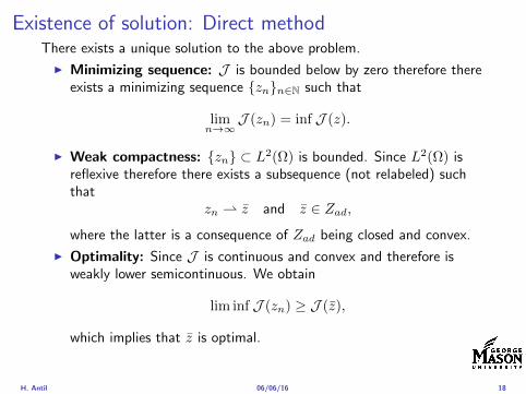
Existence of solution Direct methodThere exists a unique solution to the above problem
I Minimizing sequence J is bounded below by zero therefore thereexists a minimizing sequence znnisinN such that
limnrarrinfin
J (zn) = inf J (z)
I Weak compactness zn sub L2(Ω) is bounded Since L2(Ω) isreflexive therefore there exists a subsequence (not relabeled) suchthat
zn z and z isin Zad
where the latter is a consequence of Zad being closed and convex
I Optimality Since J is continuous and convex and therefore isweakly lower semicontinuous We obtain
lim inf J (zn) ge J (z)
which implies that z is optimal
I Uniqueness Exercise
H Antil 060616 18
Existence of solution Direct methodThere exists a unique solution to the above problem
I Minimizing sequence J is bounded below by zero therefore thereexists a minimizing sequence znnisinN such that
limnrarrinfin
J (zn) = inf J (z)
I Weak compactness zn sub L2(Ω) is bounded Since L2(Ω) isreflexive therefore there exists a subsequence (not relabeled) suchthat
zn z and z isin Zad
where the latter is a consequence of Zad being closed and convex
I Optimality Since J is continuous and convex and therefore isweakly lower semicontinuous We obtain
lim inf J (zn) ge J (z)
which implies that z is optimal
I Uniqueness Exercise
H Antil 060616 18
Outline
Motivation and examples
Linear elliptic optimal control problems
Differentiation in Banach spaces
First-order necessary conditions
Optimal control of semilinear PDEs
An abstract problem
Discretization using finite element methods
H Antil 060616 19
Differentiation in Banach spacesLet (Z middot Z) (V middot V ) B-spaces Z sub Z open and F Z rarr V
Let z isin Z
I If exist δF (z h) = limtdarr01t (F (z + th)minus F (z)) then δF (z h) is called
the directional derivative of F at z in direction h
I If exist δF (z h) forallh isin Z then h 7rarr δF (z h) is the first variation of Fat z
I Let exist the first variation δF (z middot) F is said to be Gateauxdifferentiable at z iff existA isin L(Z V ) such that δF (z h) = Ahforallh isin Z We write A = F primeG(z)
I F is said to be Frechet differentiable at z iff existA isin L(Z V ) and amapping r(z middot) Z rarr V such that for all h isin U with z + h isin Zwe have
F (z+h) = F (z)+Ah+r(z h) withr(z h)VhZ
rarr 0 as hZ rarr 0
We write F prime(z) = A
H Antil 060616 20
Differentiation in Banach spacesLet (Z middot Z) (V middot V ) B-spaces Z sub Z open and F Z rarr V
Let z isin Z
I If exist δF (z h) = limtdarr01t (F (z + th)minus F (z)) then δF (z h) is called
the directional derivative of F at z in direction h
I If exist δF (z h) forallh isin Z then h 7rarr δF (z h) is the first variation of Fat z
I Let exist the first variation δF (z middot) F is said to be Gateauxdifferentiable at z iff existA isin L(Z V ) such that δF (z h) = Ahforallh isin Z We write A = F primeG(z)
I F is said to be Frechet differentiable at z iff existA isin L(Z V ) and amapping r(z middot) Z rarr V such that for all h isin U with z + h isin Zwe have
F (z+h) = F (z)+Ah+r(z h) withr(z h)VhZ
rarr 0 as hZ rarr 0
We write F prime(z) = A
H Antil 060616 20
Differentiation in Banach spacesLet (Z middot Z) (V middot V ) B-spaces Z sub Z open and F Z rarr V
Let z isin Z
I If exist δF (z h) = limtdarr01t (F (z + th)minus F (z)) then δF (z h) is called
the directional derivative of F at z in direction h
I If exist δF (z h) forallh isin Z then h 7rarr δF (z h) is the first variation of Fat z
I Let exist the first variation δF (z middot) F is said to be Gateauxdifferentiable at z iff existA isin L(Z V ) such that δF (z h) = Ahforallh isin Z We write A = F primeG(z)
I F is said to be Frechet differentiable at z iff existA isin L(Z V ) and amapping r(z middot) Z rarr V such that for all h isin U with z + h isin Zwe have
F (z+h) = F (z)+Ah+r(z h) withr(z h)VhZ
rarr 0 as hZ rarr 0
We write F prime(z) = A
H Antil 060616 20
Differentiation in Banach spacesLet (Z middot Z) (V middot V ) B-spaces Z sub Z open and F Z rarr V
Let z isin Z
I If exist δF (z h) = limtdarr01t (F (z + th)minus F (z)) then δF (z h) is called
the directional derivative of F at z in direction h
I If exist δF (z h) forallh isin Z then h 7rarr δF (z h) is the first variation of Fat z
I Let exist the first variation δF (z middot) F is said to be Gateauxdifferentiable at z iff existA isin L(Z V ) such that δF (z h) = Ahforallh isin Z We write A = F primeG(z)
I F is said to be Frechet differentiable at z iff existA isin L(Z V ) and amapping r(z middot) Z rarr V such that for all h isin U with z + h isin Zwe have
F (z+h) = F (z)+Ah+r(z h) withr(z h)VhZ
rarr 0 as hZ rarr 0
We write F prime(z) = A
H Antil 060616 20
ExamplesExample 1 (H (middot middot)H) Hilbert space F (z) = z2H = (z z)H
forallz h F (z + h)minus F (z) = 2(z h)H + h2HThen
F prime(z)h = (2z h)H
Reisz representation theorem (identify H with Hlowast) we can write
F prime(z)h = (nablaF (z) h)H
where nablaF (z) = 2z is the gradient
Example 2 Let (Z (middot middot)Z) (H (middot middot)H) Hilbert spaces ud isin H fixedLet S isin L(ZH) Consider E Z rarr R
E(z) = Sz minus ud2H
Then E(z) = G(F (z)) where G(v) = v2H and F (z) = Sz minus ud
Eprime(z)h = Gprime(F (z))F prime(z)h = (2v F prime(z)h)H
= 2(Sz minus ud Sh)H = 2(Slowast(Sz minus ud) h)Z
we denote the gradient as nablaE(z) = 2Slowast(Sz minus ud)
H Antil 060616 21
ExamplesExample 1 (H (middot middot)H) Hilbert space F (z) = z2H = (z z)H
forallz h F (z + h)minus F (z) = 2(z h)H + h2HThen
F prime(z)h = (2z h)H
Reisz representation theorem (identify H with Hlowast) we can write
F prime(z)h = (nablaF (z) h)H
where nablaF (z) = 2z is the gradient
Example 2 Let (Z (middot middot)Z) (H (middot middot)H) Hilbert spaces ud isin H fixedLet S isin L(ZH) Consider E Z rarr R
E(z) = Sz minus ud2H
Then E(z) = G(F (z)) where G(v) = v2H and F (z) = Sz minus ud
Eprime(z)h = Gprime(F (z))F prime(z)h = (2v F prime(z)h)H
= 2(Sz minus ud Sh)H = 2(Slowast(Sz minus ud) h)Z
we denote the gradient as nablaE(z) = 2Slowast(Sz minus ud)H Antil 060616 21
Outline
Motivation and examples
Linear elliptic optimal control problems
Differentiation in Banach spaces
First-order necessary conditions
Optimal control of semilinear PDEs
An abstract problem
Discretization using finite element methods
H Antil 060616 22
First order necessary optimality conditions
Most of the theory is based on these two simple results
Theorem Let (Z middot Z) be a normed space J Z rarr (infin+infin] amapping with J 6equiv +infin Then z isin Z minimizer of J hArr 0 isin partJ (z)
Proof 0 isin partJ (z) means by definition of partJ (z) J (z)minus J (z) le 0forallz isin Z
Theorem Let (Z middot Z) be a normed space Zad sub Z nonemptyconvex closed J Z rarr R Gateaux differentiable where Zad sub Z sub ZZ open If z isin Zad is a solution to
minzisinZad
J (z)
then z solvesJ prime(z)(z minus z) ge 0 forallz isin Zad
Proof Exercise
H Antil 060616 23
First order necessary optimality conditions
Most of the theory is based on these two simple results
Theorem Let (Z middot Z) be a normed space J Z rarr (infin+infin] amapping with J 6equiv +infin Then z isin Z minimizer of J hArr 0 isin partJ (z)
Proof 0 isin partJ (z) means by definition of partJ (z) J (z)minus J (z) le 0forallz isin Z
Theorem Let (Z middot Z) be a normed space Zad sub Z nonemptyconvex closed J Z rarr R Gateaux differentiable where Zad sub Z sub ZZ open If z isin Zad is a solution to
minzisinZad
J (z)
then z solvesJ prime(z)(z minus z) ge 0 forallz isin Zad
Proof Exercise
H Antil 060616 23
Linear quadratic OCPI Reduced funcational
J (z) =1
2Sz minus ud2L2(Ω) +
λ
2z2L2(Ω)
I Gradient computation using sensitivity
J prime(z)h = (Slowast(Sz minus ud) + λz h)L2(Ω) forallh isin L2(Ω)
we denote the gradient by
nablaJ (z) = Slowast(Sz minus ud) + λz
I First order necessary and sufficient optimality condition
(nablaJ (z) z minus z)L2(Ω) ge 0 forallz isin Zad
I Adjoint equation Let p = Slowast(Sz minus ud) which translates intop isin H1
0 (Ω) solving
minusdiv (Anablap) = uminus ud in Ω
p = 0 on partΩ
I Gradient computation using adjoint nablaJ (z) = p+ λz
H Antil 060616 24
Linear quadratic OCPI Reduced funcational
J (z) =1
2Sz minus ud2L2(Ω) +
λ
2z2L2(Ω)
I Gradient computation using sensitivity
J prime(z)h = (Slowast(Sz minus ud) + λz h)L2(Ω) forallh isin L2(Ω)
we denote the gradient by
nablaJ (z) = Slowast(Sz minus ud) + λz
I First order necessary and sufficient optimality condition
(nablaJ (z) z minus z)L2(Ω) ge 0 forallz isin Zad
I Adjoint equation Let p = Slowast(Sz minus ud) which translates intop isin H1
0 (Ω) solving
minusdiv (Anablap) = uminus ud in Ω
p = 0 on partΩ
I Gradient computation using adjoint nablaJ (z) = p+ λz
H Antil 060616 24
Linear quadratic OCPI Reduced funcational
J (z) =1
2Sz minus ud2L2(Ω) +
λ
2z2L2(Ω)
I Gradient computation using sensitivity
J prime(z)h = (Slowast(Sz minus ud) + λz h)L2(Ω) forallh isin L2(Ω)
we denote the gradient by
nablaJ (z) = Slowast(Sz minus ud) + λz
I First order necessary and sufficient optimality condition
(nablaJ (z) z minus z)L2(Ω) ge 0 forallz isin Zad
I Adjoint equation Let p = Slowast(Sz minus ud) which translates intop isin H1
0 (Ω) solving
minusdiv (Anablap) = uminus ud in Ω
p = 0 on partΩ
I Gradient computation using adjoint nablaJ (z) = p+ λz
H Antil 060616 24
Linear quadratic OCPI Reduced funcational
J (z) =1
2Sz minus ud2L2(Ω) +
λ
2z2L2(Ω)
I Gradient computation using sensitivity
J prime(z)h = (Slowast(Sz minus ud) + λz h)L2(Ω) forallh isin L2(Ω)
we denote the gradient by
nablaJ (z) = Slowast(Sz minus ud) + λz
I First order necessary and sufficient optimality condition
(nablaJ (z) z minus z)L2(Ω) ge 0 forallz isin Zad
I Adjoint equation Let p = Slowast(Sz minus ud) which translates intop isin H1
0 (Ω) solving
minusdiv (Anablap) = uminus ud in Ω
p = 0 on partΩ
I Gradient computation using adjoint nablaJ (z) = p+ λz
H Antil 060616 24
Linear quadratic OCPI Reduced funcational
J (z) =1
2Sz minus ud2L2(Ω) +
λ
2z2L2(Ω)
I Gradient computation using sensitivity
J prime(z)h = (Slowast(Sz minus ud) + λz h)L2(Ω) forallh isin L2(Ω)
we denote the gradient by
nablaJ (z) = Slowast(Sz minus ud) + λz
I First order necessary and sufficient optimality condition
(nablaJ (z) z minus z)L2(Ω) ge 0 forallz isin Zad
I Adjoint equation Let p = Slowast(Sz minus ud) which translates intop isin H1
0 (Ω) solving
minusdiv (Anablap) = uminus ud in Ω
p = 0 on partΩ
I Gradient computation using adjoint nablaJ (z) = p+ λz
H Antil 060616 24
Optimality system
I State u isin H10 (Ω)
intΩAnablau middot nablav =
intΩzv forallv isin H1
0 (Ω)
I Adjoint p isin H10 (Ω)
intΩAnablap middot nablav =
intΩ
(uminus ud)v forallv isin H10 (Ω)
I Control z isin Zad (p+ λz z minus z) ge 0 forallz isin Zad
H Antil 060616 25
Pointwise interpretation
The variational inequality
(p+ λz z minus z) ge 0 forallz isin Zad
is equivalent to for ae x isin Ω
z(x) =
za(x) if p(x) + λz(x) gt 0isin [za(x) zb(x)] if p(x) + λz(x) = 0zb(x) if p(x) + λz(x) lt 0
Consequence
I When λ gt 0 then ae in Ω
z(x) = P[za(x)zb(x)]
minus 1
λp(x)
= min
zb(x)max
za(x)minus 1
λp(x)
H Antil 060616 26
Formal Lagrange method applied to linear OCPIntroduce L H1
0 (Ω)times Zad timesH1(Ω)rarr R defined as
L(u z p) = J(u z)minusint
Ω
(minusdiv (Anablau)minus z
)p dx
Integrate by parts to arrive at
L(u z p) = J(u z)minusint
Ω
(minusdiv (Anablap)uminus zp
)dx+
intpartΩ
(Anablau)p ds
If (u z p) is a stationary point then
I State
DpL(u z p)h = 0 forallh isin H1(Ω)
I AdjointDuL(u z p)h = 0 forallh isin H1
0 (Ω)
I ControlDzL(u z p)(z minus z) ge 0 forallz isin Zad
H Antil 060616 27
Formal Lagrange method applied to linear OCPIntroduce L H1
0 (Ω)times Zad timesH1(Ω)rarr R defined as
L(u z p) = J(u z)minusint
Ω
(minusdiv (Anablau)minus z
)p dx
Integrate by parts to arrive at
L(u z p) = J(u z)minusint
Ω
(minusdiv (Anablap)uminus zp
)dx+
intpartΩ
(Anablau)p ds
If (u z p) is a stationary point then
I State
DpL(u z p)h = 0 forallh isin H1(Ω)
I AdjointDuL(u z p)h = 0 forallh isin H1
0 (Ω)
I ControlDzL(u z p)(z minus z) ge 0 forallz isin Zad
H Antil 060616 27
Formal Lagrange method applied to linear OCPIntroduce L H1
0 (Ω)times Zad timesH1(Ω)rarr R defined as
L(u z p) = J(u z)minusint
Ω
(minusdiv (Anablau)minus z
)p dx
Integrate by parts to arrive at
L(u z p) = J(u z)minusint
Ω
(minusdiv (Anablap)uminus zp
)dx+
intpartΩ
(Anablau)p ds
If (u z p) is a stationary point then
I State
DpL(u z p)h = 0 forallh isin H1(Ω)
I AdjointDuL(u z p)h = 0 forallh isin H1
0 (Ω)
I ControlDzL(u z p)(z minus z) ge 0 forallz isin Zad
H Antil 060616 27
Formal Lagrange method applied to linear OCPIntroduce L H1
0 (Ω)times Zad timesH1(Ω)rarr R defined as
L(u z p) = J(u z)minusint
Ω
(minusdiv (Anablau)minus z
)p dx
Integrate by parts to arrive at
L(u z p) = J(u z)minusint
Ω
(minusdiv (Anablap)uminus zp
)dx+
intpartΩ
(Anablau)p ds
If (u z p) is a stationary point then
I State
DpL(u z p)h = 0 forallh isin H1(Ω)
I AdjointDuL(u z p)h = 0 forallh isin H1
0 (Ω)
I ControlDzL(u z p)(z minus z) ge 0 forallz isin Zad
H Antil 060616 27
Formal Lagrange method applied to linear OCPIntroduce L H1
0 (Ω)times Zad timesH1(Ω)rarr R defined as
L(u z p) = J(u z)minusint
Ω
(minusdiv (Anablau)minus z
)p dx
Integrate by parts to arrive at
L(u z p) = J(u z)minusint
Ω
(minusdiv (Anablap)uminus zp
)dx+
intpartΩ
(Anablau)p ds
If (u z p) is a stationary point then
I State
DpL(u z p)h = 0 forallh isin H1(Ω)
I AdjointDuL(u z p)h = 0 forallh isin H1
0 (Ω)
I ControlDzL(u z p)(z minus z) ge 0 forallz isin Zad
H Antil 060616 27
Outline
Motivation and examples
Linear elliptic optimal control problems
Differentiation in Banach spaces
First-order necessary conditions
Optimal control of semilinear PDEs
An abstract problem
Discretization using finite element methods
H Antil 060616 28
Semilinear elliptic OCP
min J(u z) =1
2uminus ud2L2(Ω) +
λ
2z2L2(Ω)
subject to
minus∆u+ g(x u) = z in Ω
u = 0 on partΩ
and z isin Zad with za zb isin Linfin(Ω)
H Antil 060616 29
State space(A1) Ω sub Rd open bounded partΩ is Lipschitz
(A2) g Ωtimes Rrarr R is bounded and measurable with respect to x isin Ωfor every u isin R
(A3) g is continuous monotone increasing and Lipschitz continuous in ufor ae x isin Ω
(A4) g(x 0) = 0 for ae x isin Ω (not really necessary)
Theorem Suppose (A1)minus (A4) hold For every z isin Lr(Ω) withr gt d2 the state equation has a unique weak solutionu isin H1
0 (Ω) cap C(Ω) ie we haveintΩ
nablau middot nablav dx+
intΩ
g(x u(x))v(x) dx =
intΩ
zv dx forallv isin H10 (Ω)
Moreover there exists a constant C gt 0 such that
uH1(Ω) + uC(Ω) le CzLr(Ω)
RemarkI The proof of the theorem uses the BrowderndashMinty theorem on
monotone operators
H Antil 060616 30
State space(A1) Ω sub Rd open bounded partΩ is Lipschitz
(A2) g Ωtimes Rrarr R is bounded and measurable with respect to x isin Ωfor every u isin R
(A3) g is continuous monotone increasing and Lipschitz continuous in ufor ae x isin Ω
(A4) g(x 0) = 0 for ae x isin Ω (not really necessary)
Theorem Suppose (A1)minus (A4) hold For every z isin Lr(Ω) withr gt d2 the state equation has a unique weak solutionu isin H1
0 (Ω) cap C(Ω) ie we haveintΩ
nablau middot nablav dx+
intΩ
g(x u(x))v(x) dx =
intΩ
zv dx forallv isin H10 (Ω)
Moreover there exists a constant C gt 0 such that
uH1(Ω) + uC(Ω) le CzLr(Ω)
RemarkI The proof of the theorem uses the BrowderndashMinty theorem on
monotone operators
H Antil 060616 30
State space(A1) Ω sub Rd open bounded partΩ is Lipschitz
(A2) g Ωtimes Rrarr R is bounded and measurable with respect to x isin Ωfor every u isin R
(A3) g is continuous monotone increasing and Lipschitz continuous in ufor ae x isin Ω
(A4) g(x 0) = 0 for ae x isin Ω (not really necessary)
Theorem Suppose (A1)minus (A4) hold For every z isin Lr(Ω) withr gt d2 the state equation has a unique weak solutionu isin H1
0 (Ω) cap C(Ω) ie we haveintΩ
nablau middot nablav dx+
intΩ
g(x u(x))v(x) dx =
intΩ
zv dx forallv isin H10 (Ω)
Moreover there exists a constant C gt 0 such that
uH1(Ω) + uC(Ω) le CzLr(Ω)
RemarkI The proof of the theorem uses the BrowderndashMinty theorem on
monotone operators
H Antil 060616 30
Control-to-state map and reduced problem
I Control to state map
S Linfin(Ω)rarr H10 (Ω) cap C(Ω)
is well defined and is globally Lipschitz continuous
I Reduced problem
minJ (z) =1
2S(u)minus ud2L2(Ω) +
λ
2z2L2(Ω)
H Antil 060616 31
Control-to-state map and reduced problem
I Control to state map
S Linfin(Ω)rarr H10 (Ω) cap C(Ω)
is well defined and is globally Lipschitz continuous
I Reduced problem
minJ (z) =1
2S(u)minus ud2L2(Ω) +
λ
2z2L2(Ω)
H Antil 060616 31
First-order necessary conditionsI Lagrangian functional
L(u z p) = J(u z)minusint
Ω
(minus∆u+ g(x u(x))minus z
)p dx
= J(u z)minusint
Ω
(nablau middot nablap+ g(x u(x))pminus zp
)dx
I Adjoint system For all h isin H10 (Ω)
0 = DuL(u z p)h =
intΩ
(uminus ud)h dxminusint
Ω
(nablah middot nablap+ gu(x u(x))ph
)which yields
minus∆p+ gu(x u(x))p = uminus ud in Ω
p = 0 on partΩ
I Control
DzL(u z p)(z minus z) = (p+ λz z minus z) dx ge 0 forallz isin ZadI Gradient
nablaJ (z) = p+ λz
H Antil 060616 32
First-order necessary conditionsI Lagrangian functional
L(u z p) = J(u z)minusint
Ω
(minus∆u+ g(x u(x))minus z
)p dx
= J(u z)minusint
Ω
(nablau middot nablap+ g(x u(x))pminus zp
)dx
I Adjoint system For all h isin H10 (Ω)
0 = DuL(u z p)h =
intΩ
(uminus ud)h dxminusint
Ω
(nablah middot nablap+ gu(x u(x))ph
)which yields
minus∆p+ gu(x u(x))p = uminus ud in Ω
p = 0 on partΩ
I Control
DzL(u z p)(z minus z) = (p+ λz z minus z) dx ge 0 forallz isin ZadI Gradient
nablaJ (z) = p+ λz
H Antil 060616 32
First-order necessary conditionsI Lagrangian functional
L(u z p) = J(u z)minusint
Ω
(minus∆u+ g(x u(x))minus z
)p dx
= J(u z)minusint
Ω
(nablau middot nablap+ g(x u(x))pminus zp
)dx
I Adjoint system For all h isin H10 (Ω)
0 = DuL(u z p)h =
intΩ
(uminus ud)h dxminusint
Ω
(nablah middot nablap+ gu(x u(x))ph
)which yields
minus∆p+ gu(x u(x))p = uminus ud in Ω
p = 0 on partΩ
I Control
DzL(u z p)(z minus z) = (p+ λz z minus z) dx ge 0 forallz isin Zad
I GradientnablaJ (z) = p+ λz
H Antil 060616 32
First-order necessary conditionsI Lagrangian functional
L(u z p) = J(u z)minusint
Ω
(minus∆u+ g(x u(x))minus z
)p dx
= J(u z)minusint
Ω
(nablau middot nablap+ g(x u(x))pminus zp
)dx
I Adjoint system For all h isin H10 (Ω)
0 = DuL(u z p)h =
intΩ
(uminus ud)h dxminusint
Ω
(nablah middot nablap+ gu(x u(x))ph
)which yields
minus∆p+ gu(x u(x))p = uminus ud in Ω
p = 0 on partΩ
I Control
DzL(u z p)(z minus z) = (p+ λz z minus z) dx ge 0 forallz isin ZadI Gradient
nablaJ (z) = p+ λz
H Antil 060616 32
Differentiability of Nemytskii operator
The rigorous proof uses
Theorem In addition to (A1)-(A4) if
(A5) g is continuously differentiable with respect to u for ae x isin Ωand we have
(i) |gu(x 0)| le K for ae x isin Ω(ii) gu is locally Lipschitz with respect to u isin R
then the Nemytskii operator G u 7rarr g(middot u(middot)) is continuously Frechetdifferentiable from Linfin(Ω) into itself and
(Gprime(u)h)(x) = gu(x u(x))h(x) ae in Ω forallh isin Linfin(Ω)
Remark (A5) holds if g(x u) = g(u) and g isin C2(R)
H Antil 060616 33
Outline
Motivation and examples
Linear elliptic optimal control problems
Differentiation in Banach spaces
First-order necessary conditions
Optimal control of semilinear PDEs
An abstract problem
Discretization using finite element methods
H Antil 060616 34
Gradient computation via adjoint general formI Abstract problem
min J(u z)
subject toc(u z) = 0
and z isin Zad
I Directional derivative Let S be the control to state map(nonlinear in general)
z 7rarr S(z) = u(z)
Under the assumptions of ldquoimplicit function theoremrdquo
J prime(z)h = (nablauJ (u(z) z) Sprime(z)h) + (nablazJ (u(z) z) h)
I Sensitivity of u with respect to z Differentiating the stateequation
cu(S(z) z)Sprime(z)h = minuscz(S(z) z)h
leads toSprime(z)h = minuscu(S(z) z)minus1
(cz(S(z) z)h
)
provided cu(S(z) z)minus1 is well-defined
H Antil 060616 35
Gradient computation via adjoint general formI Abstract problem
min J(u z)
subject toc(u z) = 0
and z isin ZadI Directional derivative Let S be the control to state map
(nonlinear in general)
z 7rarr S(z) = u(z)
Under the assumptions of ldquoimplicit function theoremrdquo
J prime(z)h = (nablauJ (u(z) z) Sprime(z)h) + (nablazJ (u(z) z) h)
I Sensitivity of u with respect to z Differentiating the stateequation
cu(S(z) z)Sprime(z)h = minuscz(S(z) z)h
leads toSprime(z)h = minuscu(S(z) z)minus1
(cz(S(z) z)h
)
provided cu(S(z) z)minus1 is well-defined
H Antil 060616 35
Gradient computation via adjoint general formI Abstract problem
min J(u z)
subject toc(u z) = 0
and z isin ZadI Directional derivative Let S be the control to state map
(nonlinear in general)
z 7rarr S(z) = u(z)
Under the assumptions of ldquoimplicit function theoremrdquo
J prime(z)h = (nablauJ (u(z) z) Sprime(z)h) + (nablazJ (u(z) z) h)
I Sensitivity of u with respect to z Differentiating the stateequation
cu(S(z) z)Sprime(z)h = minuscz(S(z) z)h
leads toSprime(z)h = minuscu(S(z) z)minus1
(cz(S(z) z)h
)
provided cu(S(z) z)minus1 is well-defined
H Antil 060616 35
Adjoint equation and gradient general form
I Directional derivative
J prime(z)h = minus(nablauJ (u(z) z) cu(u(z) z)minus1cz(u(z) z)h
)+ (nablazJ (u(z) z) h)
I Gradient
nablaJ (z) = minuscz(u(z) z)lowast(cu(u(z) z)minuslowastnablauJ (u(z) z)
)+nablazJ (u(z) z)
I Introducing adjoint variable p solving
cu(u(z) z)lowastp = nablauJ (u(z) z)
we arrive at following form of gradient
nablaJ (z) = minuscz(u(z) z)lowastp+nablazJ (u(z) z)
which is tractable
H Antil 060616 36
Adjoint equation and gradient general form
I Directional derivative
J prime(z)h = minus(nablauJ (u(z) z) cu(u(z) z)minus1cz(u(z) z)h
)+ (nablazJ (u(z) z) h)
I Gradient
nablaJ (z) = minuscz(u(z) z)lowast(cu(u(z) z)minuslowastnablauJ (u(z) z)
)+nablazJ (u(z) z)
I Introducing adjoint variable p solving
cu(u(z) z)lowastp = nablauJ (u(z) z)
we arrive at following form of gradient
nablaJ (z) = minuscz(u(z) z)lowastp+nablazJ (u(z) z)
which is tractable
H Antil 060616 36
Adjoint equation and gradient general form
I Directional derivative
J prime(z)h = minus(nablauJ (u(z) z) cu(u(z) z)minus1cz(u(z) z)h
)+ (nablazJ (u(z) z) h)
I Gradient
nablaJ (z) = minuscz(u(z) z)lowast(cu(u(z) z)minuslowastnablauJ (u(z) z)
)+nablazJ (u(z) z)
I Introducing adjoint variable p solving
cu(u(z) z)lowastp = nablauJ (u(z) z)
we arrive at following form of gradient
nablaJ (z) = minuscz(u(z) z)lowastp+nablazJ (u(z) z)
which is tractable
H Antil 060616 36
Hessian computation general form
I Lagrangian L(u z p) = J(u z)minusint
Ωc(u z)p dx Then we have
DzJ (z)h = DzL(u z p)h
I Second order derivative
D2zJ (z)[h1 h2] = DuDzL(u z p)[h1 S
prime(z)h2] +D2zL(u z p)[h1 h2]
+DpDzL(u z p)[h1 Dzp(z)h2]
I We already know Sprime(z)h2 moreover
DpDzL(u z p)[h1 Dzp(z)h2] = minus(cu(u z)h1 Dzp(z)h2
)
It remain to identify Dzp(z)h2
H Antil 060616 37
Hessian computation general form
I Lagrangian L(u z p) = J(u z)minusint
Ωc(u z)p dx Then we have
DzJ (z)h = DzL(u z p)h
I Second order derivative
D2zJ (z)[h1 h2] = DuDzL(u z p)[h1 S
prime(z)h2] +D2zL(u z p)[h1 h2]
+DpDzL(u z p)[h1 Dzp(z)h2]
I We already know Sprime(z)h2 moreover
DpDzL(u z p)[h1 Dzp(z)h2] = minus(cu(u z)h1 Dzp(z)h2
)
It remain to identify Dzp(z)h2
H Antil 060616 37
Hessian computation general form
I Lagrangian L(u z p) = J(u z)minusint
Ωc(u z)p dx Then we have
DzJ (z)h = DzL(u z p)h
I Second order derivative
D2zJ (z)[h1 h2] = DuDzL(u z p)[h1 S
prime(z)h2] +D2zL(u z p)[h1 h2]
+DpDzL(u z p)[h1 Dzp(z)h2]
I We already know Sprime(z)h2 moreover
DpDzL(u z p)[h1 Dzp(z)h2] = minus(cu(u z)h1 Dzp(z)h2
)
It remain to identify Dzp(z)h2
H Antil 060616 37
Outline
Motivation and examples
Linear elliptic optimal control problems
Differentiation in Banach spaces
First-order necessary conditions
Optimal control of semilinear PDEs
An abstract problem
Discretization using finite element methods
H Antil 060616 38
Numerical approximation of Poisson equation MeshTo avoid technical issues we will assume that partΩ is polygonal
I Mesh Let T = K be a mesh of Ω where K sub Rd is an elementthat is isoparametrically equivalent to a unit simplex in Rd
I Conforming mesh We say that the mesh is conforming ifI Ω = cupKisinT KI If K1 cap K2 = x then x is a node of K1 and K2I If K1 cap K2 6= empty and K1 cap K2 6= x then K1 cap K2 is an edgeface
contained in partK1 cap partK2
I Shape regular Let T be the collection of all conformingrefinements of an original mesh T 0 Then T is called shape regularif exist κ gt 0 such that
hKρKle κ forallK isin cupiT i
where hK = diam K ρK = maxρ gt 0|Bρ sub KI Quasi-uniform A family of shape regular meshes is called-quasi
uniform if there exist a constant σ gt 0 such that
maxhKminhK
le σ
uniformly for all meshes in the family
Numerical approximation of Poisson equation MeshTo avoid technical issues we will assume that partΩ is polygonal
I Mesh Let T = K be a mesh of Ω where K sub Rd is an elementthat is isoparametrically equivalent to a unit simplex in Rd
I Conforming mesh We say that the mesh is conforming ifI Ω = cupKisinT KI If K1 cap K2 = x then x is a node of K1 and K2I If K1 cap K2 6= empty and K1 cap K2 6= x then K1 cap K2 is an edgeface
contained in partK1 cap partK2
I Shape regular Let T be the collection of all conformingrefinements of an original mesh T 0 Then T is called shape regularif exist κ gt 0 such that
hKρKle κ forallK isin cupiT i
where hK = diam K ρK = maxρ gt 0|Bρ sub KI Quasi-uniform A family of shape regular meshes is called-quasi
uniform if there exist a constant σ gt 0 such that
maxhKminhK
le σ
uniformly for all meshes in the family
Numerical approximation of Poisson equation MeshTo avoid technical issues we will assume that partΩ is polygonal
I Mesh Let T = K be a mesh of Ω where K sub Rd is an elementthat is isoparametrically equivalent to a unit simplex in Rd
I Conforming mesh We say that the mesh is conforming ifI Ω = cupKisinT KI If K1 cap K2 = x then x is a node of K1 and K2I If K1 cap K2 6= empty and K1 cap K2 6= x then K1 cap K2 is an edgeface
contained in partK1 cap partK2
I Shape regular Let T be the collection of all conformingrefinements of an original mesh T 0 Then T is called shape regularif exist κ gt 0 such that
hKρKle κ forallK isin cupiT i
where hK = diam K ρK = maxρ gt 0|Bρ sub K
I Quasi-uniform A family of shape regular meshes is called-quasiuniform if there exist a constant σ gt 0 such that
maxhKminhK
le σ
uniformly for all meshes in the family
Numerical approximation of Poisson equation MeshTo avoid technical issues we will assume that partΩ is polygonal
I Mesh Let T = K be a mesh of Ω where K sub Rd is an elementthat is isoparametrically equivalent to a unit simplex in Rd
I Conforming mesh We say that the mesh is conforming ifI Ω = cupKisinT KI If K1 cap K2 = x then x is a node of K1 and K2I If K1 cap K2 6= empty and K1 cap K2 6= x then K1 cap K2 is an edgeface
contained in partK1 cap partK2
I Shape regular Let T be the collection of all conformingrefinements of an original mesh T 0 Then T is called shape regularif exist κ gt 0 such that
hKρKle κ forallK isin cupiT i
where hK = diam K ρK = maxρ gt 0|Bρ sub KI Quasi-uniform A family of shape regular meshes is called-quasi
uniform if there exist a constant σ gt 0 such that
maxhKminhK
le σ
uniformly for all meshes in the family
FE space and Galerkin approximationI Finite element space For T isin T we define the finite element
space as
V(T ) = W isin C0(Ω) WK isin P1forallK isin T W |partΩ = 0
where P1 is the set of polynomials of degree at most 1
I Galerkin approximation of continuous problem is given by
Find UT isin V(T )
intΩ
AnablaUT middot nablaV = 〈f V 〉 forallV isin V(T )
The discrete problem is well-posedI Nodal basis Consists of functions ψi isin V(T ) with xi isin N (T )
satisfyingψxi
(xj) = δij
where N (T ) denotes the interior (plus Neumann) nodesI Galerkin orthogonality(
nabla(uminus UT )nablaW)L2(Ω)
= 0 forallW isin V(T )
H Antil 060616 40
FE space and Galerkin approximationI Finite element space For T isin T we define the finite element
space as
V(T ) = W isin C0(Ω) WK isin P1forallK isin T W |partΩ = 0
where P1 is the set of polynomials of degree at most 1I Galerkin approximation of continuous problem is given by
Find UT isin V(T )
intΩ
AnablaUT middot nablaV = 〈f V 〉 forallV isin V(T )
The discrete problem is well-posed
I Nodal basis Consists of functions ψi isin V(T ) with xi isin N (T )satisfying
ψxi(xj) = δij
where N (T ) denotes the interior (plus Neumann) nodesI Galerkin orthogonality(
nabla(uminus UT )nablaW)L2(Ω)
= 0 forallW isin V(T )
H Antil 060616 40
FE space and Galerkin approximationI Finite element space For T isin T we define the finite element
space as
V(T ) = W isin C0(Ω) WK isin P1forallK isin T W |partΩ = 0
where P1 is the set of polynomials of degree at most 1I Galerkin approximation of continuous problem is given by
Find UT isin V(T )
intΩ
AnablaUT middot nablaV = 〈f V 〉 forallV isin V(T )
The discrete problem is well-posedI Nodal basis Consists of functions ψi isin V(T ) with xi isin N (T )
satisfyingψxi
(xj) = δij
where N (T ) denotes the interior (plus Neumann) nodes
I Galerkin orthogonality(nabla(uminus UT )nablaW
)L2(Ω)
= 0 forallW isin V(T )
H Antil 060616 40
FE space and Galerkin approximationI Finite element space For T isin T we define the finite element
space as
V(T ) = W isin C0(Ω) WK isin P1forallK isin T W |partΩ = 0
where P1 is the set of polynomials of degree at most 1I Galerkin approximation of continuous problem is given by
Find UT isin V(T )
intΩ
AnablaUT middot nablaV = 〈f V 〉 forallV isin V(T )
The discrete problem is well-posedI Nodal basis Consists of functions ψi isin V(T ) with xi isin N (T )
satisfyingψxi
(xj) = δij
where N (T ) denotes the interior (plus Neumann) nodesI Galerkin orthogonality(
nabla(uminus UT )nablaW)L2(Ω)
= 0 forallW isin V(T )
H Antil 060616 40
Best approximation
I Cearsquos lemma
nabla(uminus UT )L2(Ω) le C infWisinV(T )
nabla(uminusW )L2(Ω)
I Nodal interpolation operator ΠT C(Ω)rarr V(T ) satisfies
ΠT u(xi) = u(xi) forallxi isin N (T )
and is defined as
ΠT u =sum
xiisinN (T )
u(xi)ψxi
I Error estimates In Cearsquos lemma replace W by ΠT u and thencompute the interpolation error
H Antil 060616 41
Best approximation
I Cearsquos lemma
nabla(uminus UT )L2(Ω) le C infWisinV(T )
nabla(uminusW )L2(Ω)
I Nodal interpolation operator ΠT C(Ω)rarr V(T ) satisfies
ΠT u(xi) = u(xi) forallxi isin N (T )
and is defined as
ΠT u =sum
xiisinN (T )
u(xi)ψxi
I Error estimates In Cearsquos lemma replace W by ΠT u and thencompute the interpolation error
H Antil 060616 41
Best approximation
I Cearsquos lemma
nabla(uminus UT )L2(Ω) le C infWisinV(T )
nabla(uminusW )L2(Ω)
I Nodal interpolation operator ΠT C(Ω)rarr V(T ) satisfies
ΠT u(xi) = u(xi) forallxi isin N (T )
and is defined as
ΠT u =sum
xiisinN (T )
u(xi)ψxi
I Error estimates In Cearsquos lemma replace W by ΠT u and thencompute the interpolation error
H Antil 060616 41
Algebraic system state equation
I Recall UT isin V(T ) solves
a(UT V ) = 〈f V 〉 forallV isin V(T )
I Now setting UT =sumN
j=1 Ujψj V = ψi we get
Nsumj=1
Uja(φj φi) = 〈f ψi〉 i = 1 N
which is the matrix-vector system
AU = F
I Stiffness matrix A is SPD
H Antil 060616 42
Algebraic system state equation
I Recall UT isin V(T ) solves
a(UT V ) = 〈f V 〉 forallV isin V(T )
I Now setting UT =sumN
j=1 Ujψj V = ψi we get
Nsumj=1
Uja(φj φi) = 〈f ψi〉 i = 1 N
which is the matrix-vector system
AU = F
I Stiffness matrix A is SPD
H Antil 060616 42
Algebraic system state equation
I Recall UT isin V(T ) solves
a(UT V ) = 〈f V 〉 forallV isin V(T )
I Now setting UT =sumN
j=1 Ujψj V = ψi we get
Nsumj=1
Uja(φj φi) = 〈f ψi〉 i = 1 N
which is the matrix-vector system
AU = F
I Stiffness matrix A is SPD
H Antil 060616 42
Discrete linear elliptic OCP
min JT (UT ZT ) =1
2UT minus ud2L2(Ω) +
λ
2ZT 2L2(Ω)
subject to
Find UT isin V(T )
intΩ
nablaUT middot nablaV = (ZT V )L2(Ω) forallV isin V(T )
and whereZT isin Zad(T ) = Zad cap Z(T )
is either one of these
Z(T ) =
V(T )L2(Ω) variational discretization (Hinze)WT isin Linfin(Ω) ZT |K isin P0(K)K isin T
H Antil 060616 43
Recent books
F TroltzschOptimal control of partial differential equations volume 112 ofGraduate Studies in MathematicsAmerican Mathematical Society Providence RI 2010Theory methods and applications Translated from the 2005 Germanoriginal by Jurgen Sprekels
K Ito and K KunischLagrange multiplier approach to variational problems andapplications volume 15 of Advances in Design and ControlSociety for Industrial and Applied Mathematics (SIAM)Philadelphia PA 2008
H Antil 060616 44
- Motivation and examples
- Linear elliptic optimal control problems
- Differentiation in Banach spaces
- First-order necessary conditions
- Optimal control of semilinear PDEs
- An abstract problem
- Discretization using finite element methods
-
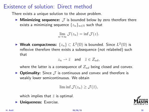
Existence of solution Direct methodThere exists a unique solution to the above problem
I Minimizing sequence J is bounded below by zero therefore thereexists a minimizing sequence znnisinN such that
limnrarrinfin
J (zn) = inf J (z)
I Weak compactness zn sub L2(Ω) is bounded Since L2(Ω) isreflexive therefore there exists a subsequence (not relabeled) suchthat
zn z and z isin Zad
where the latter is a consequence of Zad being closed and convex
I Optimality Since J is continuous and convex and therefore isweakly lower semicontinuous We obtain
lim inf J (zn) ge J (z)
which implies that z is optimal
I Uniqueness Exercise
H Antil 060616 18
Outline
Motivation and examples
Linear elliptic optimal control problems
Differentiation in Banach spaces
First-order necessary conditions
Optimal control of semilinear PDEs
An abstract problem
Discretization using finite element methods
H Antil 060616 19
Differentiation in Banach spacesLet (Z middot Z) (V middot V ) B-spaces Z sub Z open and F Z rarr V
Let z isin Z
I If exist δF (z h) = limtdarr01t (F (z + th)minus F (z)) then δF (z h) is called
the directional derivative of F at z in direction h
I If exist δF (z h) forallh isin Z then h 7rarr δF (z h) is the first variation of Fat z
I Let exist the first variation δF (z middot) F is said to be Gateauxdifferentiable at z iff existA isin L(Z V ) such that δF (z h) = Ahforallh isin Z We write A = F primeG(z)
I F is said to be Frechet differentiable at z iff existA isin L(Z V ) and amapping r(z middot) Z rarr V such that for all h isin U with z + h isin Zwe have
F (z+h) = F (z)+Ah+r(z h) withr(z h)VhZ
rarr 0 as hZ rarr 0
We write F prime(z) = A
H Antil 060616 20
Differentiation in Banach spacesLet (Z middot Z) (V middot V ) B-spaces Z sub Z open and F Z rarr V
Let z isin Z
I If exist δF (z h) = limtdarr01t (F (z + th)minus F (z)) then δF (z h) is called
the directional derivative of F at z in direction h
I If exist δF (z h) forallh isin Z then h 7rarr δF (z h) is the first variation of Fat z
I Let exist the first variation δF (z middot) F is said to be Gateauxdifferentiable at z iff existA isin L(Z V ) such that δF (z h) = Ahforallh isin Z We write A = F primeG(z)
I F is said to be Frechet differentiable at z iff existA isin L(Z V ) and amapping r(z middot) Z rarr V such that for all h isin U with z + h isin Zwe have
F (z+h) = F (z)+Ah+r(z h) withr(z h)VhZ
rarr 0 as hZ rarr 0
We write F prime(z) = A
H Antil 060616 20
Differentiation in Banach spacesLet (Z middot Z) (V middot V ) B-spaces Z sub Z open and F Z rarr V
Let z isin Z
I If exist δF (z h) = limtdarr01t (F (z + th)minus F (z)) then δF (z h) is called
the directional derivative of F at z in direction h
I If exist δF (z h) forallh isin Z then h 7rarr δF (z h) is the first variation of Fat z
I Let exist the first variation δF (z middot) F is said to be Gateauxdifferentiable at z iff existA isin L(Z V ) such that δF (z h) = Ahforallh isin Z We write A = F primeG(z)
I F is said to be Frechet differentiable at z iff existA isin L(Z V ) and amapping r(z middot) Z rarr V such that for all h isin U with z + h isin Zwe have
F (z+h) = F (z)+Ah+r(z h) withr(z h)VhZ
rarr 0 as hZ rarr 0
We write F prime(z) = A
H Antil 060616 20
Differentiation in Banach spacesLet (Z middot Z) (V middot V ) B-spaces Z sub Z open and F Z rarr V
Let z isin Z
I If exist δF (z h) = limtdarr01t (F (z + th)minus F (z)) then δF (z h) is called
the directional derivative of F at z in direction h
I If exist δF (z h) forallh isin Z then h 7rarr δF (z h) is the first variation of Fat z
I Let exist the first variation δF (z middot) F is said to be Gateauxdifferentiable at z iff existA isin L(Z V ) such that δF (z h) = Ahforallh isin Z We write A = F primeG(z)
I F is said to be Frechet differentiable at z iff existA isin L(Z V ) and amapping r(z middot) Z rarr V such that for all h isin U with z + h isin Zwe have
F (z+h) = F (z)+Ah+r(z h) withr(z h)VhZ
rarr 0 as hZ rarr 0
We write F prime(z) = A
H Antil 060616 20
ExamplesExample 1 (H (middot middot)H) Hilbert space F (z) = z2H = (z z)H
forallz h F (z + h)minus F (z) = 2(z h)H + h2HThen
F prime(z)h = (2z h)H
Reisz representation theorem (identify H with Hlowast) we can write
F prime(z)h = (nablaF (z) h)H
where nablaF (z) = 2z is the gradient
Example 2 Let (Z (middot middot)Z) (H (middot middot)H) Hilbert spaces ud isin H fixedLet S isin L(ZH) Consider E Z rarr R
E(z) = Sz minus ud2H
Then E(z) = G(F (z)) where G(v) = v2H and F (z) = Sz minus ud
Eprime(z)h = Gprime(F (z))F prime(z)h = (2v F prime(z)h)H
= 2(Sz minus ud Sh)H = 2(Slowast(Sz minus ud) h)Z
we denote the gradient as nablaE(z) = 2Slowast(Sz minus ud)
H Antil 060616 21
ExamplesExample 1 (H (middot middot)H) Hilbert space F (z) = z2H = (z z)H
forallz h F (z + h)minus F (z) = 2(z h)H + h2HThen
F prime(z)h = (2z h)H
Reisz representation theorem (identify H with Hlowast) we can write
F prime(z)h = (nablaF (z) h)H
where nablaF (z) = 2z is the gradient
Example 2 Let (Z (middot middot)Z) (H (middot middot)H) Hilbert spaces ud isin H fixedLet S isin L(ZH) Consider E Z rarr R
E(z) = Sz minus ud2H
Then E(z) = G(F (z)) where G(v) = v2H and F (z) = Sz minus ud
Eprime(z)h = Gprime(F (z))F prime(z)h = (2v F prime(z)h)H
= 2(Sz minus ud Sh)H = 2(Slowast(Sz minus ud) h)Z
we denote the gradient as nablaE(z) = 2Slowast(Sz minus ud)H Antil 060616 21
Outline
Motivation and examples
Linear elliptic optimal control problems
Differentiation in Banach spaces
First-order necessary conditions
Optimal control of semilinear PDEs
An abstract problem
Discretization using finite element methods
H Antil 060616 22
First order necessary optimality conditions
Most of the theory is based on these two simple results
Theorem Let (Z middot Z) be a normed space J Z rarr (infin+infin] amapping with J 6equiv +infin Then z isin Z minimizer of J hArr 0 isin partJ (z)
Proof 0 isin partJ (z) means by definition of partJ (z) J (z)minus J (z) le 0forallz isin Z
Theorem Let (Z middot Z) be a normed space Zad sub Z nonemptyconvex closed J Z rarr R Gateaux differentiable where Zad sub Z sub ZZ open If z isin Zad is a solution to
minzisinZad
J (z)
then z solvesJ prime(z)(z minus z) ge 0 forallz isin Zad
Proof Exercise
H Antil 060616 23
First order necessary optimality conditions
Most of the theory is based on these two simple results
Theorem Let (Z middot Z) be a normed space J Z rarr (infin+infin] amapping with J 6equiv +infin Then z isin Z minimizer of J hArr 0 isin partJ (z)
Proof 0 isin partJ (z) means by definition of partJ (z) J (z)minus J (z) le 0forallz isin Z
Theorem Let (Z middot Z) be a normed space Zad sub Z nonemptyconvex closed J Z rarr R Gateaux differentiable where Zad sub Z sub ZZ open If z isin Zad is a solution to
minzisinZad
J (z)
then z solvesJ prime(z)(z minus z) ge 0 forallz isin Zad
Proof Exercise
H Antil 060616 23
Linear quadratic OCPI Reduced funcational
J (z) =1
2Sz minus ud2L2(Ω) +
λ
2z2L2(Ω)
I Gradient computation using sensitivity
J prime(z)h = (Slowast(Sz minus ud) + λz h)L2(Ω) forallh isin L2(Ω)
we denote the gradient by
nablaJ (z) = Slowast(Sz minus ud) + λz
I First order necessary and sufficient optimality condition
(nablaJ (z) z minus z)L2(Ω) ge 0 forallz isin Zad
I Adjoint equation Let p = Slowast(Sz minus ud) which translates intop isin H1
0 (Ω) solving
minusdiv (Anablap) = uminus ud in Ω
p = 0 on partΩ
I Gradient computation using adjoint nablaJ (z) = p+ λz
H Antil 060616 24
Linear quadratic OCPI Reduced funcational
J (z) =1
2Sz minus ud2L2(Ω) +
λ
2z2L2(Ω)
I Gradient computation using sensitivity
J prime(z)h = (Slowast(Sz minus ud) + λz h)L2(Ω) forallh isin L2(Ω)
we denote the gradient by
nablaJ (z) = Slowast(Sz minus ud) + λz
I First order necessary and sufficient optimality condition
(nablaJ (z) z minus z)L2(Ω) ge 0 forallz isin Zad
I Adjoint equation Let p = Slowast(Sz minus ud) which translates intop isin H1
0 (Ω) solving
minusdiv (Anablap) = uminus ud in Ω
p = 0 on partΩ
I Gradient computation using adjoint nablaJ (z) = p+ λz
H Antil 060616 24
Linear quadratic OCPI Reduced funcational
J (z) =1
2Sz minus ud2L2(Ω) +
λ
2z2L2(Ω)
I Gradient computation using sensitivity
J prime(z)h = (Slowast(Sz minus ud) + λz h)L2(Ω) forallh isin L2(Ω)
we denote the gradient by
nablaJ (z) = Slowast(Sz minus ud) + λz
I First order necessary and sufficient optimality condition
(nablaJ (z) z minus z)L2(Ω) ge 0 forallz isin Zad
I Adjoint equation Let p = Slowast(Sz minus ud) which translates intop isin H1
0 (Ω) solving
minusdiv (Anablap) = uminus ud in Ω
p = 0 on partΩ
I Gradient computation using adjoint nablaJ (z) = p+ λz
H Antil 060616 24
Linear quadratic OCPI Reduced funcational
J (z) =1
2Sz minus ud2L2(Ω) +
λ
2z2L2(Ω)
I Gradient computation using sensitivity
J prime(z)h = (Slowast(Sz minus ud) + λz h)L2(Ω) forallh isin L2(Ω)
we denote the gradient by
nablaJ (z) = Slowast(Sz minus ud) + λz
I First order necessary and sufficient optimality condition
(nablaJ (z) z minus z)L2(Ω) ge 0 forallz isin Zad
I Adjoint equation Let p = Slowast(Sz minus ud) which translates intop isin H1
0 (Ω) solving
minusdiv (Anablap) = uminus ud in Ω
p = 0 on partΩ
I Gradient computation using adjoint nablaJ (z) = p+ λz
H Antil 060616 24
Linear quadratic OCPI Reduced funcational
J (z) =1
2Sz minus ud2L2(Ω) +
λ
2z2L2(Ω)
I Gradient computation using sensitivity
J prime(z)h = (Slowast(Sz minus ud) + λz h)L2(Ω) forallh isin L2(Ω)
we denote the gradient by
nablaJ (z) = Slowast(Sz minus ud) + λz
I First order necessary and sufficient optimality condition
(nablaJ (z) z minus z)L2(Ω) ge 0 forallz isin Zad
I Adjoint equation Let p = Slowast(Sz minus ud) which translates intop isin H1
0 (Ω) solving
minusdiv (Anablap) = uminus ud in Ω
p = 0 on partΩ
I Gradient computation using adjoint nablaJ (z) = p+ λz
H Antil 060616 24
Optimality system
I State u isin H10 (Ω)
intΩAnablau middot nablav =
intΩzv forallv isin H1
0 (Ω)
I Adjoint p isin H10 (Ω)
intΩAnablap middot nablav =
intΩ
(uminus ud)v forallv isin H10 (Ω)
I Control z isin Zad (p+ λz z minus z) ge 0 forallz isin Zad
H Antil 060616 25
Pointwise interpretation
The variational inequality
(p+ λz z minus z) ge 0 forallz isin Zad
is equivalent to for ae x isin Ω
z(x) =
za(x) if p(x) + λz(x) gt 0isin [za(x) zb(x)] if p(x) + λz(x) = 0zb(x) if p(x) + λz(x) lt 0
Consequence
I When λ gt 0 then ae in Ω
z(x) = P[za(x)zb(x)]
minus 1
λp(x)
= min
zb(x)max
za(x)minus 1
λp(x)
H Antil 060616 26
Formal Lagrange method applied to linear OCPIntroduce L H1
0 (Ω)times Zad timesH1(Ω)rarr R defined as
L(u z p) = J(u z)minusint
Ω
(minusdiv (Anablau)minus z
)p dx
Integrate by parts to arrive at
L(u z p) = J(u z)minusint
Ω
(minusdiv (Anablap)uminus zp
)dx+
intpartΩ
(Anablau)p ds
If (u z p) is a stationary point then
I State
DpL(u z p)h = 0 forallh isin H1(Ω)
I AdjointDuL(u z p)h = 0 forallh isin H1
0 (Ω)
I ControlDzL(u z p)(z minus z) ge 0 forallz isin Zad
H Antil 060616 27
Formal Lagrange method applied to linear OCPIntroduce L H1
0 (Ω)times Zad timesH1(Ω)rarr R defined as
L(u z p) = J(u z)minusint
Ω
(minusdiv (Anablau)minus z
)p dx
Integrate by parts to arrive at
L(u z p) = J(u z)minusint
Ω
(minusdiv (Anablap)uminus zp
)dx+
intpartΩ
(Anablau)p ds
If (u z p) is a stationary point then
I State
DpL(u z p)h = 0 forallh isin H1(Ω)
I AdjointDuL(u z p)h = 0 forallh isin H1
0 (Ω)
I ControlDzL(u z p)(z minus z) ge 0 forallz isin Zad
H Antil 060616 27
Formal Lagrange method applied to linear OCPIntroduce L H1
0 (Ω)times Zad timesH1(Ω)rarr R defined as
L(u z p) = J(u z)minusint
Ω
(minusdiv (Anablau)minus z
)p dx
Integrate by parts to arrive at
L(u z p) = J(u z)minusint
Ω
(minusdiv (Anablap)uminus zp
)dx+
intpartΩ
(Anablau)p ds
If (u z p) is a stationary point then
I State
DpL(u z p)h = 0 forallh isin H1(Ω)
I AdjointDuL(u z p)h = 0 forallh isin H1
0 (Ω)
I ControlDzL(u z p)(z minus z) ge 0 forallz isin Zad
H Antil 060616 27
Formal Lagrange method applied to linear OCPIntroduce L H1
0 (Ω)times Zad timesH1(Ω)rarr R defined as
L(u z p) = J(u z)minusint
Ω
(minusdiv (Anablau)minus z
)p dx
Integrate by parts to arrive at
L(u z p) = J(u z)minusint
Ω
(minusdiv (Anablap)uminus zp
)dx+
intpartΩ
(Anablau)p ds
If (u z p) is a stationary point then
I State
DpL(u z p)h = 0 forallh isin H1(Ω)
I AdjointDuL(u z p)h = 0 forallh isin H1
0 (Ω)
I ControlDzL(u z p)(z minus z) ge 0 forallz isin Zad
H Antil 060616 27
Formal Lagrange method applied to linear OCPIntroduce L H1
0 (Ω)times Zad timesH1(Ω)rarr R defined as
L(u z p) = J(u z)minusint
Ω
(minusdiv (Anablau)minus z
)p dx
Integrate by parts to arrive at
L(u z p) = J(u z)minusint
Ω
(minusdiv (Anablap)uminus zp
)dx+
intpartΩ
(Anablau)p ds
If (u z p) is a stationary point then
I State
DpL(u z p)h = 0 forallh isin H1(Ω)
I AdjointDuL(u z p)h = 0 forallh isin H1
0 (Ω)
I ControlDzL(u z p)(z minus z) ge 0 forallz isin Zad
H Antil 060616 27
Outline
Motivation and examples
Linear elliptic optimal control problems
Differentiation in Banach spaces
First-order necessary conditions
Optimal control of semilinear PDEs
An abstract problem
Discretization using finite element methods
H Antil 060616 28
Semilinear elliptic OCP
min J(u z) =1
2uminus ud2L2(Ω) +
λ
2z2L2(Ω)
subject to
minus∆u+ g(x u) = z in Ω
u = 0 on partΩ
and z isin Zad with za zb isin Linfin(Ω)
H Antil 060616 29
State space(A1) Ω sub Rd open bounded partΩ is Lipschitz
(A2) g Ωtimes Rrarr R is bounded and measurable with respect to x isin Ωfor every u isin R
(A3) g is continuous monotone increasing and Lipschitz continuous in ufor ae x isin Ω
(A4) g(x 0) = 0 for ae x isin Ω (not really necessary)
Theorem Suppose (A1)minus (A4) hold For every z isin Lr(Ω) withr gt d2 the state equation has a unique weak solutionu isin H1
0 (Ω) cap C(Ω) ie we haveintΩ
nablau middot nablav dx+
intΩ
g(x u(x))v(x) dx =
intΩ
zv dx forallv isin H10 (Ω)
Moreover there exists a constant C gt 0 such that
uH1(Ω) + uC(Ω) le CzLr(Ω)
RemarkI The proof of the theorem uses the BrowderndashMinty theorem on
monotone operators
H Antil 060616 30
State space(A1) Ω sub Rd open bounded partΩ is Lipschitz
(A2) g Ωtimes Rrarr R is bounded and measurable with respect to x isin Ωfor every u isin R
(A3) g is continuous monotone increasing and Lipschitz continuous in ufor ae x isin Ω
(A4) g(x 0) = 0 for ae x isin Ω (not really necessary)
Theorem Suppose (A1)minus (A4) hold For every z isin Lr(Ω) withr gt d2 the state equation has a unique weak solutionu isin H1
0 (Ω) cap C(Ω) ie we haveintΩ
nablau middot nablav dx+
intΩ
g(x u(x))v(x) dx =
intΩ
zv dx forallv isin H10 (Ω)
Moreover there exists a constant C gt 0 such that
uH1(Ω) + uC(Ω) le CzLr(Ω)
RemarkI The proof of the theorem uses the BrowderndashMinty theorem on
monotone operators
H Antil 060616 30
State space(A1) Ω sub Rd open bounded partΩ is Lipschitz
(A2) g Ωtimes Rrarr R is bounded and measurable with respect to x isin Ωfor every u isin R
(A3) g is continuous monotone increasing and Lipschitz continuous in ufor ae x isin Ω
(A4) g(x 0) = 0 for ae x isin Ω (not really necessary)
Theorem Suppose (A1)minus (A4) hold For every z isin Lr(Ω) withr gt d2 the state equation has a unique weak solutionu isin H1
0 (Ω) cap C(Ω) ie we haveintΩ
nablau middot nablav dx+
intΩ
g(x u(x))v(x) dx =
intΩ
zv dx forallv isin H10 (Ω)
Moreover there exists a constant C gt 0 such that
uH1(Ω) + uC(Ω) le CzLr(Ω)
RemarkI The proof of the theorem uses the BrowderndashMinty theorem on
monotone operators
H Antil 060616 30
Control-to-state map and reduced problem
I Control to state map
S Linfin(Ω)rarr H10 (Ω) cap C(Ω)
is well defined and is globally Lipschitz continuous
I Reduced problem
minJ (z) =1
2S(u)minus ud2L2(Ω) +
λ
2z2L2(Ω)
H Antil 060616 31
Control-to-state map and reduced problem
I Control to state map
S Linfin(Ω)rarr H10 (Ω) cap C(Ω)
is well defined and is globally Lipschitz continuous
I Reduced problem
minJ (z) =1
2S(u)minus ud2L2(Ω) +
λ
2z2L2(Ω)
H Antil 060616 31
First-order necessary conditionsI Lagrangian functional
L(u z p) = J(u z)minusint
Ω
(minus∆u+ g(x u(x))minus z
)p dx
= J(u z)minusint
Ω
(nablau middot nablap+ g(x u(x))pminus zp
)dx
I Adjoint system For all h isin H10 (Ω)
0 = DuL(u z p)h =
intΩ
(uminus ud)h dxminusint
Ω
(nablah middot nablap+ gu(x u(x))ph
)which yields
minus∆p+ gu(x u(x))p = uminus ud in Ω
p = 0 on partΩ
I Control
DzL(u z p)(z minus z) = (p+ λz z minus z) dx ge 0 forallz isin ZadI Gradient
nablaJ (z) = p+ λz
H Antil 060616 32
First-order necessary conditionsI Lagrangian functional
L(u z p) = J(u z)minusint
Ω
(minus∆u+ g(x u(x))minus z
)p dx
= J(u z)minusint
Ω
(nablau middot nablap+ g(x u(x))pminus zp
)dx
I Adjoint system For all h isin H10 (Ω)
0 = DuL(u z p)h =
intΩ
(uminus ud)h dxminusint
Ω
(nablah middot nablap+ gu(x u(x))ph
)which yields
minus∆p+ gu(x u(x))p = uminus ud in Ω
p = 0 on partΩ
I Control
DzL(u z p)(z minus z) = (p+ λz z minus z) dx ge 0 forallz isin ZadI Gradient
nablaJ (z) = p+ λz
H Antil 060616 32
First-order necessary conditionsI Lagrangian functional
L(u z p) = J(u z)minusint
Ω
(minus∆u+ g(x u(x))minus z
)p dx
= J(u z)minusint
Ω
(nablau middot nablap+ g(x u(x))pminus zp
)dx
I Adjoint system For all h isin H10 (Ω)
0 = DuL(u z p)h =
intΩ
(uminus ud)h dxminusint
Ω
(nablah middot nablap+ gu(x u(x))ph
)which yields
minus∆p+ gu(x u(x))p = uminus ud in Ω
p = 0 on partΩ
I Control
DzL(u z p)(z minus z) = (p+ λz z minus z) dx ge 0 forallz isin Zad
I GradientnablaJ (z) = p+ λz
H Antil 060616 32
First-order necessary conditionsI Lagrangian functional
L(u z p) = J(u z)minusint
Ω
(minus∆u+ g(x u(x))minus z
)p dx
= J(u z)minusint
Ω
(nablau middot nablap+ g(x u(x))pminus zp
)dx
I Adjoint system For all h isin H10 (Ω)
0 = DuL(u z p)h =
intΩ
(uminus ud)h dxminusint
Ω
(nablah middot nablap+ gu(x u(x))ph
)which yields
minus∆p+ gu(x u(x))p = uminus ud in Ω
p = 0 on partΩ
I Control
DzL(u z p)(z minus z) = (p+ λz z minus z) dx ge 0 forallz isin ZadI Gradient
nablaJ (z) = p+ λz
H Antil 060616 32
Differentiability of Nemytskii operator
The rigorous proof uses
Theorem In addition to (A1)-(A4) if
(A5) g is continuously differentiable with respect to u for ae x isin Ωand we have
(i) |gu(x 0)| le K for ae x isin Ω(ii) gu is locally Lipschitz with respect to u isin R
then the Nemytskii operator G u 7rarr g(middot u(middot)) is continuously Frechetdifferentiable from Linfin(Ω) into itself and
(Gprime(u)h)(x) = gu(x u(x))h(x) ae in Ω forallh isin Linfin(Ω)
Remark (A5) holds if g(x u) = g(u) and g isin C2(R)
H Antil 060616 33
Outline
Motivation and examples
Linear elliptic optimal control problems
Differentiation in Banach spaces
First-order necessary conditions
Optimal control of semilinear PDEs
An abstract problem
Discretization using finite element methods
H Antil 060616 34
Gradient computation via adjoint general formI Abstract problem
min J(u z)
subject toc(u z) = 0
and z isin Zad
I Directional derivative Let S be the control to state map(nonlinear in general)
z 7rarr S(z) = u(z)
Under the assumptions of ldquoimplicit function theoremrdquo
J prime(z)h = (nablauJ (u(z) z) Sprime(z)h) + (nablazJ (u(z) z) h)
I Sensitivity of u with respect to z Differentiating the stateequation
cu(S(z) z)Sprime(z)h = minuscz(S(z) z)h
leads toSprime(z)h = minuscu(S(z) z)minus1
(cz(S(z) z)h
)
provided cu(S(z) z)minus1 is well-defined
H Antil 060616 35
Gradient computation via adjoint general formI Abstract problem
min J(u z)
subject toc(u z) = 0
and z isin ZadI Directional derivative Let S be the control to state map
(nonlinear in general)
z 7rarr S(z) = u(z)
Under the assumptions of ldquoimplicit function theoremrdquo
J prime(z)h = (nablauJ (u(z) z) Sprime(z)h) + (nablazJ (u(z) z) h)
I Sensitivity of u with respect to z Differentiating the stateequation
cu(S(z) z)Sprime(z)h = minuscz(S(z) z)h
leads toSprime(z)h = minuscu(S(z) z)minus1
(cz(S(z) z)h
)
provided cu(S(z) z)minus1 is well-defined
H Antil 060616 35
Gradient computation via adjoint general formI Abstract problem
min J(u z)
subject toc(u z) = 0
and z isin ZadI Directional derivative Let S be the control to state map
(nonlinear in general)
z 7rarr S(z) = u(z)
Under the assumptions of ldquoimplicit function theoremrdquo
J prime(z)h = (nablauJ (u(z) z) Sprime(z)h) + (nablazJ (u(z) z) h)
I Sensitivity of u with respect to z Differentiating the stateequation
cu(S(z) z)Sprime(z)h = minuscz(S(z) z)h
leads toSprime(z)h = minuscu(S(z) z)minus1
(cz(S(z) z)h
)
provided cu(S(z) z)minus1 is well-defined
H Antil 060616 35
Adjoint equation and gradient general form
I Directional derivative
J prime(z)h = minus(nablauJ (u(z) z) cu(u(z) z)minus1cz(u(z) z)h
)+ (nablazJ (u(z) z) h)
I Gradient
nablaJ (z) = minuscz(u(z) z)lowast(cu(u(z) z)minuslowastnablauJ (u(z) z)
)+nablazJ (u(z) z)
I Introducing adjoint variable p solving
cu(u(z) z)lowastp = nablauJ (u(z) z)
we arrive at following form of gradient
nablaJ (z) = minuscz(u(z) z)lowastp+nablazJ (u(z) z)
which is tractable
H Antil 060616 36
Adjoint equation and gradient general form
I Directional derivative
J prime(z)h = minus(nablauJ (u(z) z) cu(u(z) z)minus1cz(u(z) z)h
)+ (nablazJ (u(z) z) h)
I Gradient
nablaJ (z) = minuscz(u(z) z)lowast(cu(u(z) z)minuslowastnablauJ (u(z) z)
)+nablazJ (u(z) z)
I Introducing adjoint variable p solving
cu(u(z) z)lowastp = nablauJ (u(z) z)
we arrive at following form of gradient
nablaJ (z) = minuscz(u(z) z)lowastp+nablazJ (u(z) z)
which is tractable
H Antil 060616 36
Adjoint equation and gradient general form
I Directional derivative
J prime(z)h = minus(nablauJ (u(z) z) cu(u(z) z)minus1cz(u(z) z)h
)+ (nablazJ (u(z) z) h)
I Gradient
nablaJ (z) = minuscz(u(z) z)lowast(cu(u(z) z)minuslowastnablauJ (u(z) z)
)+nablazJ (u(z) z)
I Introducing adjoint variable p solving
cu(u(z) z)lowastp = nablauJ (u(z) z)
we arrive at following form of gradient
nablaJ (z) = minuscz(u(z) z)lowastp+nablazJ (u(z) z)
which is tractable
H Antil 060616 36
Hessian computation general form
I Lagrangian L(u z p) = J(u z)minusint
Ωc(u z)p dx Then we have
DzJ (z)h = DzL(u z p)h
I Second order derivative
D2zJ (z)[h1 h2] = DuDzL(u z p)[h1 S
prime(z)h2] +D2zL(u z p)[h1 h2]
+DpDzL(u z p)[h1 Dzp(z)h2]
I We already know Sprime(z)h2 moreover
DpDzL(u z p)[h1 Dzp(z)h2] = minus(cu(u z)h1 Dzp(z)h2
)
It remain to identify Dzp(z)h2
H Antil 060616 37
Hessian computation general form
I Lagrangian L(u z p) = J(u z)minusint
Ωc(u z)p dx Then we have
DzJ (z)h = DzL(u z p)h
I Second order derivative
D2zJ (z)[h1 h2] = DuDzL(u z p)[h1 S
prime(z)h2] +D2zL(u z p)[h1 h2]
+DpDzL(u z p)[h1 Dzp(z)h2]
I We already know Sprime(z)h2 moreover
DpDzL(u z p)[h1 Dzp(z)h2] = minus(cu(u z)h1 Dzp(z)h2
)
It remain to identify Dzp(z)h2
H Antil 060616 37
Hessian computation general form
I Lagrangian L(u z p) = J(u z)minusint
Ωc(u z)p dx Then we have
DzJ (z)h = DzL(u z p)h
I Second order derivative
D2zJ (z)[h1 h2] = DuDzL(u z p)[h1 S
prime(z)h2] +D2zL(u z p)[h1 h2]
+DpDzL(u z p)[h1 Dzp(z)h2]
I We already know Sprime(z)h2 moreover
DpDzL(u z p)[h1 Dzp(z)h2] = minus(cu(u z)h1 Dzp(z)h2
)
It remain to identify Dzp(z)h2
H Antil 060616 37
Outline
Motivation and examples
Linear elliptic optimal control problems
Differentiation in Banach spaces
First-order necessary conditions
Optimal control of semilinear PDEs
An abstract problem
Discretization using finite element methods
H Antil 060616 38
Numerical approximation of Poisson equation MeshTo avoid technical issues we will assume that partΩ is polygonal
I Mesh Let T = K be a mesh of Ω where K sub Rd is an elementthat is isoparametrically equivalent to a unit simplex in Rd
I Conforming mesh We say that the mesh is conforming ifI Ω = cupKisinT KI If K1 cap K2 = x then x is a node of K1 and K2I If K1 cap K2 6= empty and K1 cap K2 6= x then K1 cap K2 is an edgeface
contained in partK1 cap partK2
I Shape regular Let T be the collection of all conformingrefinements of an original mesh T 0 Then T is called shape regularif exist κ gt 0 such that
hKρKle κ forallK isin cupiT i
where hK = diam K ρK = maxρ gt 0|Bρ sub KI Quasi-uniform A family of shape regular meshes is called-quasi
uniform if there exist a constant σ gt 0 such that
maxhKminhK
le σ
uniformly for all meshes in the family
Numerical approximation of Poisson equation MeshTo avoid technical issues we will assume that partΩ is polygonal
I Mesh Let T = K be a mesh of Ω where K sub Rd is an elementthat is isoparametrically equivalent to a unit simplex in Rd
I Conforming mesh We say that the mesh is conforming ifI Ω = cupKisinT KI If K1 cap K2 = x then x is a node of K1 and K2I If K1 cap K2 6= empty and K1 cap K2 6= x then K1 cap K2 is an edgeface
contained in partK1 cap partK2
I Shape regular Let T be the collection of all conformingrefinements of an original mesh T 0 Then T is called shape regularif exist κ gt 0 such that
hKρKle κ forallK isin cupiT i
where hK = diam K ρK = maxρ gt 0|Bρ sub KI Quasi-uniform A family of shape regular meshes is called-quasi
uniform if there exist a constant σ gt 0 such that
maxhKminhK
le σ
uniformly for all meshes in the family
Numerical approximation of Poisson equation MeshTo avoid technical issues we will assume that partΩ is polygonal
I Mesh Let T = K be a mesh of Ω where K sub Rd is an elementthat is isoparametrically equivalent to a unit simplex in Rd
I Conforming mesh We say that the mesh is conforming ifI Ω = cupKisinT KI If K1 cap K2 = x then x is a node of K1 and K2I If K1 cap K2 6= empty and K1 cap K2 6= x then K1 cap K2 is an edgeface
contained in partK1 cap partK2
I Shape regular Let T be the collection of all conformingrefinements of an original mesh T 0 Then T is called shape regularif exist κ gt 0 such that
hKρKle κ forallK isin cupiT i
where hK = diam K ρK = maxρ gt 0|Bρ sub K
I Quasi-uniform A family of shape regular meshes is called-quasiuniform if there exist a constant σ gt 0 such that
maxhKminhK
le σ
uniformly for all meshes in the family
Numerical approximation of Poisson equation MeshTo avoid technical issues we will assume that partΩ is polygonal
I Mesh Let T = K be a mesh of Ω where K sub Rd is an elementthat is isoparametrically equivalent to a unit simplex in Rd
I Conforming mesh We say that the mesh is conforming ifI Ω = cupKisinT KI If K1 cap K2 = x then x is a node of K1 and K2I If K1 cap K2 6= empty and K1 cap K2 6= x then K1 cap K2 is an edgeface
contained in partK1 cap partK2
I Shape regular Let T be the collection of all conformingrefinements of an original mesh T 0 Then T is called shape regularif exist κ gt 0 such that
hKρKle κ forallK isin cupiT i
where hK = diam K ρK = maxρ gt 0|Bρ sub KI Quasi-uniform A family of shape regular meshes is called-quasi
uniform if there exist a constant σ gt 0 such that
maxhKminhK
le σ
uniformly for all meshes in the family
FE space and Galerkin approximationI Finite element space For T isin T we define the finite element
space as
V(T ) = W isin C0(Ω) WK isin P1forallK isin T W |partΩ = 0
where P1 is the set of polynomials of degree at most 1
I Galerkin approximation of continuous problem is given by
Find UT isin V(T )
intΩ
AnablaUT middot nablaV = 〈f V 〉 forallV isin V(T )
The discrete problem is well-posedI Nodal basis Consists of functions ψi isin V(T ) with xi isin N (T )
satisfyingψxi
(xj) = δij
where N (T ) denotes the interior (plus Neumann) nodesI Galerkin orthogonality(
nabla(uminus UT )nablaW)L2(Ω)
= 0 forallW isin V(T )
H Antil 060616 40
FE space and Galerkin approximationI Finite element space For T isin T we define the finite element
space as
V(T ) = W isin C0(Ω) WK isin P1forallK isin T W |partΩ = 0
where P1 is the set of polynomials of degree at most 1I Galerkin approximation of continuous problem is given by
Find UT isin V(T )
intΩ
AnablaUT middot nablaV = 〈f V 〉 forallV isin V(T )
The discrete problem is well-posed
I Nodal basis Consists of functions ψi isin V(T ) with xi isin N (T )satisfying
ψxi(xj) = δij
where N (T ) denotes the interior (plus Neumann) nodesI Galerkin orthogonality(
nabla(uminus UT )nablaW)L2(Ω)
= 0 forallW isin V(T )
H Antil 060616 40
FE space and Galerkin approximationI Finite element space For T isin T we define the finite element
space as
V(T ) = W isin C0(Ω) WK isin P1forallK isin T W |partΩ = 0
where P1 is the set of polynomials of degree at most 1I Galerkin approximation of continuous problem is given by
Find UT isin V(T )
intΩ
AnablaUT middot nablaV = 〈f V 〉 forallV isin V(T )
The discrete problem is well-posedI Nodal basis Consists of functions ψi isin V(T ) with xi isin N (T )
satisfyingψxi
(xj) = δij
where N (T ) denotes the interior (plus Neumann) nodes
I Galerkin orthogonality(nabla(uminus UT )nablaW
)L2(Ω)
= 0 forallW isin V(T )
H Antil 060616 40
FE space and Galerkin approximationI Finite element space For T isin T we define the finite element
space as
V(T ) = W isin C0(Ω) WK isin P1forallK isin T W |partΩ = 0
where P1 is the set of polynomials of degree at most 1I Galerkin approximation of continuous problem is given by
Find UT isin V(T )
intΩ
AnablaUT middot nablaV = 〈f V 〉 forallV isin V(T )
The discrete problem is well-posedI Nodal basis Consists of functions ψi isin V(T ) with xi isin N (T )
satisfyingψxi
(xj) = δij
where N (T ) denotes the interior (plus Neumann) nodesI Galerkin orthogonality(
nabla(uminus UT )nablaW)L2(Ω)
= 0 forallW isin V(T )
H Antil 060616 40
Best approximation
I Cearsquos lemma
nabla(uminus UT )L2(Ω) le C infWisinV(T )
nabla(uminusW )L2(Ω)
I Nodal interpolation operator ΠT C(Ω)rarr V(T ) satisfies
ΠT u(xi) = u(xi) forallxi isin N (T )
and is defined as
ΠT u =sum
xiisinN (T )
u(xi)ψxi
I Error estimates In Cearsquos lemma replace W by ΠT u and thencompute the interpolation error
H Antil 060616 41
Best approximation
I Cearsquos lemma
nabla(uminus UT )L2(Ω) le C infWisinV(T )
nabla(uminusW )L2(Ω)
I Nodal interpolation operator ΠT C(Ω)rarr V(T ) satisfies
ΠT u(xi) = u(xi) forallxi isin N (T )
and is defined as
ΠT u =sum
xiisinN (T )
u(xi)ψxi
I Error estimates In Cearsquos lemma replace W by ΠT u and thencompute the interpolation error
H Antil 060616 41
Best approximation
I Cearsquos lemma
nabla(uminus UT )L2(Ω) le C infWisinV(T )
nabla(uminusW )L2(Ω)
I Nodal interpolation operator ΠT C(Ω)rarr V(T ) satisfies
ΠT u(xi) = u(xi) forallxi isin N (T )
and is defined as
ΠT u =sum
xiisinN (T )
u(xi)ψxi
I Error estimates In Cearsquos lemma replace W by ΠT u and thencompute the interpolation error
H Antil 060616 41
Algebraic system state equation
I Recall UT isin V(T ) solves
a(UT V ) = 〈f V 〉 forallV isin V(T )
I Now setting UT =sumN
j=1 Ujψj V = ψi we get
Nsumj=1
Uja(φj φi) = 〈f ψi〉 i = 1 N
which is the matrix-vector system
AU = F
I Stiffness matrix A is SPD
H Antil 060616 42
Algebraic system state equation
I Recall UT isin V(T ) solves
a(UT V ) = 〈f V 〉 forallV isin V(T )
I Now setting UT =sumN
j=1 Ujψj V = ψi we get
Nsumj=1
Uja(φj φi) = 〈f ψi〉 i = 1 N
which is the matrix-vector system
AU = F
I Stiffness matrix A is SPD
H Antil 060616 42
Algebraic system state equation
I Recall UT isin V(T ) solves
a(UT V ) = 〈f V 〉 forallV isin V(T )
I Now setting UT =sumN
j=1 Ujψj V = ψi we get
Nsumj=1
Uja(φj φi) = 〈f ψi〉 i = 1 N
which is the matrix-vector system
AU = F
I Stiffness matrix A is SPD
H Antil 060616 42
Discrete linear elliptic OCP
min JT (UT ZT ) =1
2UT minus ud2L2(Ω) +
λ
2ZT 2L2(Ω)
subject to
Find UT isin V(T )
intΩ
nablaUT middot nablaV = (ZT V )L2(Ω) forallV isin V(T )
and whereZT isin Zad(T ) = Zad cap Z(T )
is either one of these
Z(T ) =
V(T )L2(Ω) variational discretization (Hinze)WT isin Linfin(Ω) ZT |K isin P0(K)K isin T
H Antil 060616 43
Recent books
F TroltzschOptimal control of partial differential equations volume 112 ofGraduate Studies in MathematicsAmerican Mathematical Society Providence RI 2010Theory methods and applications Translated from the 2005 Germanoriginal by Jurgen Sprekels
K Ito and K KunischLagrange multiplier approach to variational problems andapplications volume 15 of Advances in Design and ControlSociety for Industrial and Applied Mathematics (SIAM)Philadelphia PA 2008
H Antil 060616 44
- Motivation and examples
- Linear elliptic optimal control problems
- Differentiation in Banach spaces
- First-order necessary conditions
- Optimal control of semilinear PDEs
- An abstract problem
- Discretization using finite element methods
-
Outline
Motivation and examples
Linear elliptic optimal control problems
Differentiation in Banach spaces
First-order necessary conditions
Optimal control of semilinear PDEs
An abstract problem
Discretization using finite element methods
H Antil 060616 19
Differentiation in Banach spacesLet (Z middot Z) (V middot V ) B-spaces Z sub Z open and F Z rarr V
Let z isin Z
I If exist δF (z h) = limtdarr01t (F (z + th)minus F (z)) then δF (z h) is called
the directional derivative of F at z in direction h
I If exist δF (z h) forallh isin Z then h 7rarr δF (z h) is the first variation of Fat z
I Let exist the first variation δF (z middot) F is said to be Gateauxdifferentiable at z iff existA isin L(Z V ) such that δF (z h) = Ahforallh isin Z We write A = F primeG(z)
I F is said to be Frechet differentiable at z iff existA isin L(Z V ) and amapping r(z middot) Z rarr V such that for all h isin U with z + h isin Zwe have
F (z+h) = F (z)+Ah+r(z h) withr(z h)VhZ
rarr 0 as hZ rarr 0
We write F prime(z) = A
H Antil 060616 20
Differentiation in Banach spacesLet (Z middot Z) (V middot V ) B-spaces Z sub Z open and F Z rarr V
Let z isin Z
I If exist δF (z h) = limtdarr01t (F (z + th)minus F (z)) then δF (z h) is called
the directional derivative of F at z in direction h
I If exist δF (z h) forallh isin Z then h 7rarr δF (z h) is the first variation of Fat z
I Let exist the first variation δF (z middot) F is said to be Gateauxdifferentiable at z iff existA isin L(Z V ) such that δF (z h) = Ahforallh isin Z We write A = F primeG(z)
I F is said to be Frechet differentiable at z iff existA isin L(Z V ) and amapping r(z middot) Z rarr V such that for all h isin U with z + h isin Zwe have
F (z+h) = F (z)+Ah+r(z h) withr(z h)VhZ
rarr 0 as hZ rarr 0
We write F prime(z) = A
H Antil 060616 20
Differentiation in Banach spacesLet (Z middot Z) (V middot V ) B-spaces Z sub Z open and F Z rarr V
Let z isin Z
I If exist δF (z h) = limtdarr01t (F (z + th)minus F (z)) then δF (z h) is called
the directional derivative of F at z in direction h
I If exist δF (z h) forallh isin Z then h 7rarr δF (z h) is the first variation of Fat z
I Let exist the first variation δF (z middot) F is said to be Gateauxdifferentiable at z iff existA isin L(Z V ) such that δF (z h) = Ahforallh isin Z We write A = F primeG(z)
I F is said to be Frechet differentiable at z iff existA isin L(Z V ) and amapping r(z middot) Z rarr V such that for all h isin U with z + h isin Zwe have
F (z+h) = F (z)+Ah+r(z h) withr(z h)VhZ
rarr 0 as hZ rarr 0
We write F prime(z) = A
H Antil 060616 20
Differentiation in Banach spacesLet (Z middot Z) (V middot V ) B-spaces Z sub Z open and F Z rarr V
Let z isin Z
I If exist δF (z h) = limtdarr01t (F (z + th)minus F (z)) then δF (z h) is called
the directional derivative of F at z in direction h
I If exist δF (z h) forallh isin Z then h 7rarr δF (z h) is the first variation of Fat z
I Let exist the first variation δF (z middot) F is said to be Gateauxdifferentiable at z iff existA isin L(Z V ) such that δF (z h) = Ahforallh isin Z We write A = F primeG(z)
I F is said to be Frechet differentiable at z iff existA isin L(Z V ) and amapping r(z middot) Z rarr V such that for all h isin U with z + h isin Zwe have
F (z+h) = F (z)+Ah+r(z h) withr(z h)VhZ
rarr 0 as hZ rarr 0
We write F prime(z) = A
H Antil 060616 20
ExamplesExample 1 (H (middot middot)H) Hilbert space F (z) = z2H = (z z)H
forallz h F (z + h)minus F (z) = 2(z h)H + h2HThen
F prime(z)h = (2z h)H
Reisz representation theorem (identify H with Hlowast) we can write
F prime(z)h = (nablaF (z) h)H
where nablaF (z) = 2z is the gradient
Example 2 Let (Z (middot middot)Z) (H (middot middot)H) Hilbert spaces ud isin H fixedLet S isin L(ZH) Consider E Z rarr R
E(z) = Sz minus ud2H
Then E(z) = G(F (z)) where G(v) = v2H and F (z) = Sz minus ud
Eprime(z)h = Gprime(F (z))F prime(z)h = (2v F prime(z)h)H
= 2(Sz minus ud Sh)H = 2(Slowast(Sz minus ud) h)Z
we denote the gradient as nablaE(z) = 2Slowast(Sz minus ud)
H Antil 060616 21
ExamplesExample 1 (H (middot middot)H) Hilbert space F (z) = z2H = (z z)H
forallz h F (z + h)minus F (z) = 2(z h)H + h2HThen
F prime(z)h = (2z h)H
Reisz representation theorem (identify H with Hlowast) we can write
F prime(z)h = (nablaF (z) h)H
where nablaF (z) = 2z is the gradient
Example 2 Let (Z (middot middot)Z) (H (middot middot)H) Hilbert spaces ud isin H fixedLet S isin L(ZH) Consider E Z rarr R
E(z) = Sz minus ud2H
Then E(z) = G(F (z)) where G(v) = v2H and F (z) = Sz minus ud
Eprime(z)h = Gprime(F (z))F prime(z)h = (2v F prime(z)h)H
= 2(Sz minus ud Sh)H = 2(Slowast(Sz minus ud) h)Z
we denote the gradient as nablaE(z) = 2Slowast(Sz minus ud)H Antil 060616 21
Outline
Motivation and examples
Linear elliptic optimal control problems
Differentiation in Banach spaces
First-order necessary conditions
Optimal control of semilinear PDEs
An abstract problem
Discretization using finite element methods
H Antil 060616 22
First order necessary optimality conditions
Most of the theory is based on these two simple results
Theorem Let (Z middot Z) be a normed space J Z rarr (infin+infin] amapping with J 6equiv +infin Then z isin Z minimizer of J hArr 0 isin partJ (z)
Proof 0 isin partJ (z) means by definition of partJ (z) J (z)minus J (z) le 0forallz isin Z
Theorem Let (Z middot Z) be a normed space Zad sub Z nonemptyconvex closed J Z rarr R Gateaux differentiable where Zad sub Z sub ZZ open If z isin Zad is a solution to
minzisinZad
J (z)
then z solvesJ prime(z)(z minus z) ge 0 forallz isin Zad
Proof Exercise
H Antil 060616 23
First order necessary optimality conditions
Most of the theory is based on these two simple results
Theorem Let (Z middot Z) be a normed space J Z rarr (infin+infin] amapping with J 6equiv +infin Then z isin Z minimizer of J hArr 0 isin partJ (z)
Proof 0 isin partJ (z) means by definition of partJ (z) J (z)minus J (z) le 0forallz isin Z
Theorem Let (Z middot Z) be a normed space Zad sub Z nonemptyconvex closed J Z rarr R Gateaux differentiable where Zad sub Z sub ZZ open If z isin Zad is a solution to
minzisinZad
J (z)
then z solvesJ prime(z)(z minus z) ge 0 forallz isin Zad
Proof Exercise
H Antil 060616 23
Linear quadratic OCPI Reduced funcational
J (z) =1
2Sz minus ud2L2(Ω) +
λ
2z2L2(Ω)
I Gradient computation using sensitivity
J prime(z)h = (Slowast(Sz minus ud) + λz h)L2(Ω) forallh isin L2(Ω)
we denote the gradient by
nablaJ (z) = Slowast(Sz minus ud) + λz
I First order necessary and sufficient optimality condition
(nablaJ (z) z minus z)L2(Ω) ge 0 forallz isin Zad
I Adjoint equation Let p = Slowast(Sz minus ud) which translates intop isin H1
0 (Ω) solving
minusdiv (Anablap) = uminus ud in Ω
p = 0 on partΩ
I Gradient computation using adjoint nablaJ (z) = p+ λz
H Antil 060616 24
Linear quadratic OCPI Reduced funcational
J (z) =1
2Sz minus ud2L2(Ω) +
λ
2z2L2(Ω)
I Gradient computation using sensitivity
J prime(z)h = (Slowast(Sz minus ud) + λz h)L2(Ω) forallh isin L2(Ω)
we denote the gradient by
nablaJ (z) = Slowast(Sz minus ud) + λz
I First order necessary and sufficient optimality condition
(nablaJ (z) z minus z)L2(Ω) ge 0 forallz isin Zad
I Adjoint equation Let p = Slowast(Sz minus ud) which translates intop isin H1
0 (Ω) solving
minusdiv (Anablap) = uminus ud in Ω
p = 0 on partΩ
I Gradient computation using adjoint nablaJ (z) = p+ λz
H Antil 060616 24
Linear quadratic OCPI Reduced funcational
J (z) =1
2Sz minus ud2L2(Ω) +
λ
2z2L2(Ω)
I Gradient computation using sensitivity
J prime(z)h = (Slowast(Sz minus ud) + λz h)L2(Ω) forallh isin L2(Ω)
we denote the gradient by
nablaJ (z) = Slowast(Sz minus ud) + λz
I First order necessary and sufficient optimality condition
(nablaJ (z) z minus z)L2(Ω) ge 0 forallz isin Zad
I Adjoint equation Let p = Slowast(Sz minus ud) which translates intop isin H1
0 (Ω) solving
minusdiv (Anablap) = uminus ud in Ω
p = 0 on partΩ
I Gradient computation using adjoint nablaJ (z) = p+ λz
H Antil 060616 24
Linear quadratic OCPI Reduced funcational
J (z) =1
2Sz minus ud2L2(Ω) +
λ
2z2L2(Ω)
I Gradient computation using sensitivity
J prime(z)h = (Slowast(Sz minus ud) + λz h)L2(Ω) forallh isin L2(Ω)
we denote the gradient by
nablaJ (z) = Slowast(Sz minus ud) + λz
I First order necessary and sufficient optimality condition
(nablaJ (z) z minus z)L2(Ω) ge 0 forallz isin Zad
I Adjoint equation Let p = Slowast(Sz minus ud) which translates intop isin H1
0 (Ω) solving
minusdiv (Anablap) = uminus ud in Ω
p = 0 on partΩ
I Gradient computation using adjoint nablaJ (z) = p+ λz
H Antil 060616 24
Linear quadratic OCPI Reduced funcational
J (z) =1
2Sz minus ud2L2(Ω) +
λ
2z2L2(Ω)
I Gradient computation using sensitivity
J prime(z)h = (Slowast(Sz minus ud) + λz h)L2(Ω) forallh isin L2(Ω)
we denote the gradient by
nablaJ (z) = Slowast(Sz minus ud) + λz
I First order necessary and sufficient optimality condition
(nablaJ (z) z minus z)L2(Ω) ge 0 forallz isin Zad
I Adjoint equation Let p = Slowast(Sz minus ud) which translates intop isin H1
0 (Ω) solving
minusdiv (Anablap) = uminus ud in Ω
p = 0 on partΩ
I Gradient computation using adjoint nablaJ (z) = p+ λz
H Antil 060616 24
Optimality system
I State u isin H10 (Ω)
intΩAnablau middot nablav =
intΩzv forallv isin H1
0 (Ω)
I Adjoint p isin H10 (Ω)
intΩAnablap middot nablav =
intΩ
(uminus ud)v forallv isin H10 (Ω)
I Control z isin Zad (p+ λz z minus z) ge 0 forallz isin Zad
H Antil 060616 25
Pointwise interpretation
The variational inequality
(p+ λz z minus z) ge 0 forallz isin Zad
is equivalent to for ae x isin Ω
z(x) =
za(x) if p(x) + λz(x) gt 0isin [za(x) zb(x)] if p(x) + λz(x) = 0zb(x) if p(x) + λz(x) lt 0
Consequence
I When λ gt 0 then ae in Ω
z(x) = P[za(x)zb(x)]
minus 1
λp(x)
= min
zb(x)max
za(x)minus 1
λp(x)
H Antil 060616 26
Formal Lagrange method applied to linear OCPIntroduce L H1
0 (Ω)times Zad timesH1(Ω)rarr R defined as
L(u z p) = J(u z)minusint
Ω
(minusdiv (Anablau)minus z
)p dx
Integrate by parts to arrive at
L(u z p) = J(u z)minusint
Ω
(minusdiv (Anablap)uminus zp
)dx+
intpartΩ
(Anablau)p ds
If (u z p) is a stationary point then
I State
DpL(u z p)h = 0 forallh isin H1(Ω)
I AdjointDuL(u z p)h = 0 forallh isin H1
0 (Ω)
I ControlDzL(u z p)(z minus z) ge 0 forallz isin Zad
H Antil 060616 27
Formal Lagrange method applied to linear OCPIntroduce L H1
0 (Ω)times Zad timesH1(Ω)rarr R defined as
L(u z p) = J(u z)minusint
Ω
(minusdiv (Anablau)minus z
)p dx
Integrate by parts to arrive at
L(u z p) = J(u z)minusint
Ω
(minusdiv (Anablap)uminus zp
)dx+
intpartΩ
(Anablau)p ds
If (u z p) is a stationary point then
I State
DpL(u z p)h = 0 forallh isin H1(Ω)
I AdjointDuL(u z p)h = 0 forallh isin H1
0 (Ω)
I ControlDzL(u z p)(z minus z) ge 0 forallz isin Zad
H Antil 060616 27
Formal Lagrange method applied to linear OCPIntroduce L H1
0 (Ω)times Zad timesH1(Ω)rarr R defined as
L(u z p) = J(u z)minusint
Ω
(minusdiv (Anablau)minus z
)p dx
Integrate by parts to arrive at
L(u z p) = J(u z)minusint
Ω
(minusdiv (Anablap)uminus zp
)dx+
intpartΩ
(Anablau)p ds
If (u z p) is a stationary point then
I State
DpL(u z p)h = 0 forallh isin H1(Ω)
I AdjointDuL(u z p)h = 0 forallh isin H1
0 (Ω)
I ControlDzL(u z p)(z minus z) ge 0 forallz isin Zad
H Antil 060616 27
Formal Lagrange method applied to linear OCPIntroduce L H1
0 (Ω)times Zad timesH1(Ω)rarr R defined as
L(u z p) = J(u z)minusint
Ω
(minusdiv (Anablau)minus z
)p dx
Integrate by parts to arrive at
L(u z p) = J(u z)minusint
Ω
(minusdiv (Anablap)uminus zp
)dx+
intpartΩ
(Anablau)p ds
If (u z p) is a stationary point then
I State
DpL(u z p)h = 0 forallh isin H1(Ω)
I AdjointDuL(u z p)h = 0 forallh isin H1
0 (Ω)
I ControlDzL(u z p)(z minus z) ge 0 forallz isin Zad
H Antil 060616 27
Formal Lagrange method applied to linear OCPIntroduce L H1
0 (Ω)times Zad timesH1(Ω)rarr R defined as
L(u z p) = J(u z)minusint
Ω
(minusdiv (Anablau)minus z
)p dx
Integrate by parts to arrive at
L(u z p) = J(u z)minusint
Ω
(minusdiv (Anablap)uminus zp
)dx+
intpartΩ
(Anablau)p ds
If (u z p) is a stationary point then
I State
DpL(u z p)h = 0 forallh isin H1(Ω)
I AdjointDuL(u z p)h = 0 forallh isin H1
0 (Ω)
I ControlDzL(u z p)(z minus z) ge 0 forallz isin Zad
H Antil 060616 27
Outline
Motivation and examples
Linear elliptic optimal control problems
Differentiation in Banach spaces
First-order necessary conditions
Optimal control of semilinear PDEs
An abstract problem
Discretization using finite element methods
H Antil 060616 28
Semilinear elliptic OCP
min J(u z) =1
2uminus ud2L2(Ω) +
λ
2z2L2(Ω)
subject to
minus∆u+ g(x u) = z in Ω
u = 0 on partΩ
and z isin Zad with za zb isin Linfin(Ω)
H Antil 060616 29
State space(A1) Ω sub Rd open bounded partΩ is Lipschitz
(A2) g Ωtimes Rrarr R is bounded and measurable with respect to x isin Ωfor every u isin R
(A3) g is continuous monotone increasing and Lipschitz continuous in ufor ae x isin Ω
(A4) g(x 0) = 0 for ae x isin Ω (not really necessary)
Theorem Suppose (A1)minus (A4) hold For every z isin Lr(Ω) withr gt d2 the state equation has a unique weak solutionu isin H1
0 (Ω) cap C(Ω) ie we haveintΩ
nablau middot nablav dx+
intΩ
g(x u(x))v(x) dx =
intΩ
zv dx forallv isin H10 (Ω)
Moreover there exists a constant C gt 0 such that
uH1(Ω) + uC(Ω) le CzLr(Ω)
RemarkI The proof of the theorem uses the BrowderndashMinty theorem on
monotone operators
H Antil 060616 30
State space(A1) Ω sub Rd open bounded partΩ is Lipschitz
(A2) g Ωtimes Rrarr R is bounded and measurable with respect to x isin Ωfor every u isin R
(A3) g is continuous monotone increasing and Lipschitz continuous in ufor ae x isin Ω
(A4) g(x 0) = 0 for ae x isin Ω (not really necessary)
Theorem Suppose (A1)minus (A4) hold For every z isin Lr(Ω) withr gt d2 the state equation has a unique weak solutionu isin H1
0 (Ω) cap C(Ω) ie we haveintΩ
nablau middot nablav dx+
intΩ
g(x u(x))v(x) dx =
intΩ
zv dx forallv isin H10 (Ω)
Moreover there exists a constant C gt 0 such that
uH1(Ω) + uC(Ω) le CzLr(Ω)
RemarkI The proof of the theorem uses the BrowderndashMinty theorem on
monotone operators
H Antil 060616 30
State space(A1) Ω sub Rd open bounded partΩ is Lipschitz
(A2) g Ωtimes Rrarr R is bounded and measurable with respect to x isin Ωfor every u isin R
(A3) g is continuous monotone increasing and Lipschitz continuous in ufor ae x isin Ω
(A4) g(x 0) = 0 for ae x isin Ω (not really necessary)
Theorem Suppose (A1)minus (A4) hold For every z isin Lr(Ω) withr gt d2 the state equation has a unique weak solutionu isin H1
0 (Ω) cap C(Ω) ie we haveintΩ
nablau middot nablav dx+
intΩ
g(x u(x))v(x) dx =
intΩ
zv dx forallv isin H10 (Ω)
Moreover there exists a constant C gt 0 such that
uH1(Ω) + uC(Ω) le CzLr(Ω)
RemarkI The proof of the theorem uses the BrowderndashMinty theorem on
monotone operators
H Antil 060616 30
Control-to-state map and reduced problem
I Control to state map
S Linfin(Ω)rarr H10 (Ω) cap C(Ω)
is well defined and is globally Lipschitz continuous
I Reduced problem
minJ (z) =1
2S(u)minus ud2L2(Ω) +
λ
2z2L2(Ω)
H Antil 060616 31
Control-to-state map and reduced problem
I Control to state map
S Linfin(Ω)rarr H10 (Ω) cap C(Ω)
is well defined and is globally Lipschitz continuous
I Reduced problem
minJ (z) =1
2S(u)minus ud2L2(Ω) +
λ
2z2L2(Ω)
H Antil 060616 31
First-order necessary conditionsI Lagrangian functional
L(u z p) = J(u z)minusint
Ω
(minus∆u+ g(x u(x))minus z
)p dx
= J(u z)minusint
Ω
(nablau middot nablap+ g(x u(x))pminus zp
)dx
I Adjoint system For all h isin H10 (Ω)
0 = DuL(u z p)h =
intΩ
(uminus ud)h dxminusint
Ω
(nablah middot nablap+ gu(x u(x))ph
)which yields
minus∆p+ gu(x u(x))p = uminus ud in Ω
p = 0 on partΩ
I Control
DzL(u z p)(z minus z) = (p+ λz z minus z) dx ge 0 forallz isin ZadI Gradient
nablaJ (z) = p+ λz
H Antil 060616 32
First-order necessary conditionsI Lagrangian functional
L(u z p) = J(u z)minusint
Ω
(minus∆u+ g(x u(x))minus z
)p dx
= J(u z)minusint
Ω
(nablau middot nablap+ g(x u(x))pminus zp
)dx
I Adjoint system For all h isin H10 (Ω)
0 = DuL(u z p)h =
intΩ
(uminus ud)h dxminusint
Ω
(nablah middot nablap+ gu(x u(x))ph
)which yields
minus∆p+ gu(x u(x))p = uminus ud in Ω
p = 0 on partΩ
I Control
DzL(u z p)(z minus z) = (p+ λz z minus z) dx ge 0 forallz isin ZadI Gradient
nablaJ (z) = p+ λz
H Antil 060616 32
First-order necessary conditionsI Lagrangian functional
L(u z p) = J(u z)minusint
Ω
(minus∆u+ g(x u(x))minus z
)p dx
= J(u z)minusint
Ω
(nablau middot nablap+ g(x u(x))pminus zp
)dx
I Adjoint system For all h isin H10 (Ω)
0 = DuL(u z p)h =
intΩ
(uminus ud)h dxminusint
Ω
(nablah middot nablap+ gu(x u(x))ph
)which yields
minus∆p+ gu(x u(x))p = uminus ud in Ω
p = 0 on partΩ
I Control
DzL(u z p)(z minus z) = (p+ λz z minus z) dx ge 0 forallz isin Zad
I GradientnablaJ (z) = p+ λz
H Antil 060616 32
First-order necessary conditionsI Lagrangian functional
L(u z p) = J(u z)minusint
Ω
(minus∆u+ g(x u(x))minus z
)p dx
= J(u z)minusint
Ω
(nablau middot nablap+ g(x u(x))pminus zp
)dx
I Adjoint system For all h isin H10 (Ω)
0 = DuL(u z p)h =
intΩ
(uminus ud)h dxminusint
Ω
(nablah middot nablap+ gu(x u(x))ph
)which yields
minus∆p+ gu(x u(x))p = uminus ud in Ω
p = 0 on partΩ
I Control
DzL(u z p)(z minus z) = (p+ λz z minus z) dx ge 0 forallz isin ZadI Gradient
nablaJ (z) = p+ λz
H Antil 060616 32
Differentiability of Nemytskii operator
The rigorous proof uses
Theorem In addition to (A1)-(A4) if
(A5) g is continuously differentiable with respect to u for ae x isin Ωand we have
(i) |gu(x 0)| le K for ae x isin Ω(ii) gu is locally Lipschitz with respect to u isin R
then the Nemytskii operator G u 7rarr g(middot u(middot)) is continuously Frechetdifferentiable from Linfin(Ω) into itself and
(Gprime(u)h)(x) = gu(x u(x))h(x) ae in Ω forallh isin Linfin(Ω)
Remark (A5) holds if g(x u) = g(u) and g isin C2(R)
H Antil 060616 33
Outline
Motivation and examples
Linear elliptic optimal control problems
Differentiation in Banach spaces
First-order necessary conditions
Optimal control of semilinear PDEs
An abstract problem
Discretization using finite element methods
H Antil 060616 34
Gradient computation via adjoint general formI Abstract problem
min J(u z)
subject toc(u z) = 0
and z isin Zad
I Directional derivative Let S be the control to state map(nonlinear in general)
z 7rarr S(z) = u(z)
Under the assumptions of ldquoimplicit function theoremrdquo
J prime(z)h = (nablauJ (u(z) z) Sprime(z)h) + (nablazJ (u(z) z) h)
I Sensitivity of u with respect to z Differentiating the stateequation
cu(S(z) z)Sprime(z)h = minuscz(S(z) z)h
leads toSprime(z)h = minuscu(S(z) z)minus1
(cz(S(z) z)h
)
provided cu(S(z) z)minus1 is well-defined
H Antil 060616 35
Gradient computation via adjoint general formI Abstract problem
min J(u z)
subject toc(u z) = 0
and z isin ZadI Directional derivative Let S be the control to state map
(nonlinear in general)
z 7rarr S(z) = u(z)
Under the assumptions of ldquoimplicit function theoremrdquo
J prime(z)h = (nablauJ (u(z) z) Sprime(z)h) + (nablazJ (u(z) z) h)
I Sensitivity of u with respect to z Differentiating the stateequation
cu(S(z) z)Sprime(z)h = minuscz(S(z) z)h
leads toSprime(z)h = minuscu(S(z) z)minus1
(cz(S(z) z)h
)
provided cu(S(z) z)minus1 is well-defined
H Antil 060616 35
Gradient computation via adjoint general formI Abstract problem
min J(u z)
subject toc(u z) = 0
and z isin ZadI Directional derivative Let S be the control to state map
(nonlinear in general)
z 7rarr S(z) = u(z)
Under the assumptions of ldquoimplicit function theoremrdquo
J prime(z)h = (nablauJ (u(z) z) Sprime(z)h) + (nablazJ (u(z) z) h)
I Sensitivity of u with respect to z Differentiating the stateequation
cu(S(z) z)Sprime(z)h = minuscz(S(z) z)h
leads toSprime(z)h = minuscu(S(z) z)minus1
(cz(S(z) z)h
)
provided cu(S(z) z)minus1 is well-defined
H Antil 060616 35
Adjoint equation and gradient general form
I Directional derivative
J prime(z)h = minus(nablauJ (u(z) z) cu(u(z) z)minus1cz(u(z) z)h
)+ (nablazJ (u(z) z) h)
I Gradient
nablaJ (z) = minuscz(u(z) z)lowast(cu(u(z) z)minuslowastnablauJ (u(z) z)
)+nablazJ (u(z) z)
I Introducing adjoint variable p solving
cu(u(z) z)lowastp = nablauJ (u(z) z)
we arrive at following form of gradient
nablaJ (z) = minuscz(u(z) z)lowastp+nablazJ (u(z) z)
which is tractable
H Antil 060616 36
Adjoint equation and gradient general form
I Directional derivative
J prime(z)h = minus(nablauJ (u(z) z) cu(u(z) z)minus1cz(u(z) z)h
)+ (nablazJ (u(z) z) h)
I Gradient
nablaJ (z) = minuscz(u(z) z)lowast(cu(u(z) z)minuslowastnablauJ (u(z) z)
)+nablazJ (u(z) z)
I Introducing adjoint variable p solving
cu(u(z) z)lowastp = nablauJ (u(z) z)
we arrive at following form of gradient
nablaJ (z) = minuscz(u(z) z)lowastp+nablazJ (u(z) z)
which is tractable
H Antil 060616 36
Adjoint equation and gradient general form
I Directional derivative
J prime(z)h = minus(nablauJ (u(z) z) cu(u(z) z)minus1cz(u(z) z)h
)+ (nablazJ (u(z) z) h)
I Gradient
nablaJ (z) = minuscz(u(z) z)lowast(cu(u(z) z)minuslowastnablauJ (u(z) z)
)+nablazJ (u(z) z)
I Introducing adjoint variable p solving
cu(u(z) z)lowastp = nablauJ (u(z) z)
we arrive at following form of gradient
nablaJ (z) = minuscz(u(z) z)lowastp+nablazJ (u(z) z)
which is tractable
H Antil 060616 36
Hessian computation general form
I Lagrangian L(u z p) = J(u z)minusint
Ωc(u z)p dx Then we have
DzJ (z)h = DzL(u z p)h
I Second order derivative
D2zJ (z)[h1 h2] = DuDzL(u z p)[h1 S
prime(z)h2] +D2zL(u z p)[h1 h2]
+DpDzL(u z p)[h1 Dzp(z)h2]
I We already know Sprime(z)h2 moreover
DpDzL(u z p)[h1 Dzp(z)h2] = minus(cu(u z)h1 Dzp(z)h2
)
It remain to identify Dzp(z)h2
H Antil 060616 37
Hessian computation general form
I Lagrangian L(u z p) = J(u z)minusint
Ωc(u z)p dx Then we have
DzJ (z)h = DzL(u z p)h
I Second order derivative
D2zJ (z)[h1 h2] = DuDzL(u z p)[h1 S
prime(z)h2] +D2zL(u z p)[h1 h2]
+DpDzL(u z p)[h1 Dzp(z)h2]
I We already know Sprime(z)h2 moreover
DpDzL(u z p)[h1 Dzp(z)h2] = minus(cu(u z)h1 Dzp(z)h2
)
It remain to identify Dzp(z)h2
H Antil 060616 37
Hessian computation general form
I Lagrangian L(u z p) = J(u z)minusint
Ωc(u z)p dx Then we have
DzJ (z)h = DzL(u z p)h
I Second order derivative
D2zJ (z)[h1 h2] = DuDzL(u z p)[h1 S
prime(z)h2] +D2zL(u z p)[h1 h2]
+DpDzL(u z p)[h1 Dzp(z)h2]
I We already know Sprime(z)h2 moreover
DpDzL(u z p)[h1 Dzp(z)h2] = minus(cu(u z)h1 Dzp(z)h2
)
It remain to identify Dzp(z)h2
H Antil 060616 37
Outline
Motivation and examples
Linear elliptic optimal control problems
Differentiation in Banach spaces
First-order necessary conditions
Optimal control of semilinear PDEs
An abstract problem
Discretization using finite element methods
H Antil 060616 38
Numerical approximation of Poisson equation MeshTo avoid technical issues we will assume that partΩ is polygonal
I Mesh Let T = K be a mesh of Ω where K sub Rd is an elementthat is isoparametrically equivalent to a unit simplex in Rd
I Conforming mesh We say that the mesh is conforming ifI Ω = cupKisinT KI If K1 cap K2 = x then x is a node of K1 and K2I If K1 cap K2 6= empty and K1 cap K2 6= x then K1 cap K2 is an edgeface
contained in partK1 cap partK2
I Shape regular Let T be the collection of all conformingrefinements of an original mesh T 0 Then T is called shape regularif exist κ gt 0 such that
hKρKle κ forallK isin cupiT i
where hK = diam K ρK = maxρ gt 0|Bρ sub KI Quasi-uniform A family of shape regular meshes is called-quasi
uniform if there exist a constant σ gt 0 such that
maxhKminhK
le σ
uniformly for all meshes in the family
Numerical approximation of Poisson equation MeshTo avoid technical issues we will assume that partΩ is polygonal
I Mesh Let T = K be a mesh of Ω where K sub Rd is an elementthat is isoparametrically equivalent to a unit simplex in Rd
I Conforming mesh We say that the mesh is conforming ifI Ω = cupKisinT KI If K1 cap K2 = x then x is a node of K1 and K2I If K1 cap K2 6= empty and K1 cap K2 6= x then K1 cap K2 is an edgeface
contained in partK1 cap partK2
I Shape regular Let T be the collection of all conformingrefinements of an original mesh T 0 Then T is called shape regularif exist κ gt 0 such that
hKρKle κ forallK isin cupiT i
where hK = diam K ρK = maxρ gt 0|Bρ sub KI Quasi-uniform A family of shape regular meshes is called-quasi
uniform if there exist a constant σ gt 0 such that
maxhKminhK
le σ
uniformly for all meshes in the family
Numerical approximation of Poisson equation MeshTo avoid technical issues we will assume that partΩ is polygonal
I Mesh Let T = K be a mesh of Ω where K sub Rd is an elementthat is isoparametrically equivalent to a unit simplex in Rd
I Conforming mesh We say that the mesh is conforming ifI Ω = cupKisinT KI If K1 cap K2 = x then x is a node of K1 and K2I If K1 cap K2 6= empty and K1 cap K2 6= x then K1 cap K2 is an edgeface
contained in partK1 cap partK2
I Shape regular Let T be the collection of all conformingrefinements of an original mesh T 0 Then T is called shape regularif exist κ gt 0 such that
hKρKle κ forallK isin cupiT i
where hK = diam K ρK = maxρ gt 0|Bρ sub K
I Quasi-uniform A family of shape regular meshes is called-quasiuniform if there exist a constant σ gt 0 such that
maxhKminhK
le σ
uniformly for all meshes in the family
Numerical approximation of Poisson equation MeshTo avoid technical issues we will assume that partΩ is polygonal
I Mesh Let T = K be a mesh of Ω where K sub Rd is an elementthat is isoparametrically equivalent to a unit simplex in Rd
I Conforming mesh We say that the mesh is conforming ifI Ω = cupKisinT KI If K1 cap K2 = x then x is a node of K1 and K2I If K1 cap K2 6= empty and K1 cap K2 6= x then K1 cap K2 is an edgeface
contained in partK1 cap partK2
I Shape regular Let T be the collection of all conformingrefinements of an original mesh T 0 Then T is called shape regularif exist κ gt 0 such that
hKρKle κ forallK isin cupiT i
where hK = diam K ρK = maxρ gt 0|Bρ sub KI Quasi-uniform A family of shape regular meshes is called-quasi
uniform if there exist a constant σ gt 0 such that
maxhKminhK
le σ
uniformly for all meshes in the family
FE space and Galerkin approximationI Finite element space For T isin T we define the finite element
space as
V(T ) = W isin C0(Ω) WK isin P1forallK isin T W |partΩ = 0
where P1 is the set of polynomials of degree at most 1
I Galerkin approximation of continuous problem is given by
Find UT isin V(T )
intΩ
AnablaUT middot nablaV = 〈f V 〉 forallV isin V(T )
The discrete problem is well-posedI Nodal basis Consists of functions ψi isin V(T ) with xi isin N (T )
satisfyingψxi
(xj) = δij
where N (T ) denotes the interior (plus Neumann) nodesI Galerkin orthogonality(
nabla(uminus UT )nablaW)L2(Ω)
= 0 forallW isin V(T )
H Antil 060616 40
FE space and Galerkin approximationI Finite element space For T isin T we define the finite element
space as
V(T ) = W isin C0(Ω) WK isin P1forallK isin T W |partΩ = 0
where P1 is the set of polynomials of degree at most 1I Galerkin approximation of continuous problem is given by
Find UT isin V(T )
intΩ
AnablaUT middot nablaV = 〈f V 〉 forallV isin V(T )
The discrete problem is well-posed
I Nodal basis Consists of functions ψi isin V(T ) with xi isin N (T )satisfying
ψxi(xj) = δij
where N (T ) denotes the interior (plus Neumann) nodesI Galerkin orthogonality(
nabla(uminus UT )nablaW)L2(Ω)
= 0 forallW isin V(T )
H Antil 060616 40
FE space and Galerkin approximationI Finite element space For T isin T we define the finite element
space as
V(T ) = W isin C0(Ω) WK isin P1forallK isin T W |partΩ = 0
where P1 is the set of polynomials of degree at most 1I Galerkin approximation of continuous problem is given by
Find UT isin V(T )
intΩ
AnablaUT middot nablaV = 〈f V 〉 forallV isin V(T )
The discrete problem is well-posedI Nodal basis Consists of functions ψi isin V(T ) with xi isin N (T )
satisfyingψxi
(xj) = δij
where N (T ) denotes the interior (plus Neumann) nodes
I Galerkin orthogonality(nabla(uminus UT )nablaW
)L2(Ω)
= 0 forallW isin V(T )
H Antil 060616 40
FE space and Galerkin approximationI Finite element space For T isin T we define the finite element
space as
V(T ) = W isin C0(Ω) WK isin P1forallK isin T W |partΩ = 0
where P1 is the set of polynomials of degree at most 1I Galerkin approximation of continuous problem is given by
Find UT isin V(T )
intΩ
AnablaUT middot nablaV = 〈f V 〉 forallV isin V(T )
The discrete problem is well-posedI Nodal basis Consists of functions ψi isin V(T ) with xi isin N (T )
satisfyingψxi
(xj) = δij
where N (T ) denotes the interior (plus Neumann) nodesI Galerkin orthogonality(
nabla(uminus UT )nablaW)L2(Ω)
= 0 forallW isin V(T )
H Antil 060616 40
Best approximation
I Cearsquos lemma
nabla(uminus UT )L2(Ω) le C infWisinV(T )
nabla(uminusW )L2(Ω)
I Nodal interpolation operator ΠT C(Ω)rarr V(T ) satisfies
ΠT u(xi) = u(xi) forallxi isin N (T )
and is defined as
ΠT u =sum
xiisinN (T )
u(xi)ψxi
I Error estimates In Cearsquos lemma replace W by ΠT u and thencompute the interpolation error
H Antil 060616 41
Best approximation
I Cearsquos lemma
nabla(uminus UT )L2(Ω) le C infWisinV(T )
nabla(uminusW )L2(Ω)
I Nodal interpolation operator ΠT C(Ω)rarr V(T ) satisfies
ΠT u(xi) = u(xi) forallxi isin N (T )
and is defined as
ΠT u =sum
xiisinN (T )
u(xi)ψxi
I Error estimates In Cearsquos lemma replace W by ΠT u and thencompute the interpolation error
H Antil 060616 41
Best approximation
I Cearsquos lemma
nabla(uminus UT )L2(Ω) le C infWisinV(T )
nabla(uminusW )L2(Ω)
I Nodal interpolation operator ΠT C(Ω)rarr V(T ) satisfies
ΠT u(xi) = u(xi) forallxi isin N (T )
and is defined as
ΠT u =sum
xiisinN (T )
u(xi)ψxi
I Error estimates In Cearsquos lemma replace W by ΠT u and thencompute the interpolation error
H Antil 060616 41
Algebraic system state equation
I Recall UT isin V(T ) solves
a(UT V ) = 〈f V 〉 forallV isin V(T )
I Now setting UT =sumN
j=1 Ujψj V = ψi we get
Nsumj=1
Uja(φj φi) = 〈f ψi〉 i = 1 N
which is the matrix-vector system
AU = F
I Stiffness matrix A is SPD
H Antil 060616 42
Algebraic system state equation
I Recall UT isin V(T ) solves
a(UT V ) = 〈f V 〉 forallV isin V(T )
I Now setting UT =sumN
j=1 Ujψj V = ψi we get
Nsumj=1
Uja(φj φi) = 〈f ψi〉 i = 1 N
which is the matrix-vector system
AU = F
I Stiffness matrix A is SPD
H Antil 060616 42
Algebraic system state equation
I Recall UT isin V(T ) solves
a(UT V ) = 〈f V 〉 forallV isin V(T )
I Now setting UT =sumN
j=1 Ujψj V = ψi we get
Nsumj=1
Uja(φj φi) = 〈f ψi〉 i = 1 N
which is the matrix-vector system
AU = F
I Stiffness matrix A is SPD
H Antil 060616 42
Discrete linear elliptic OCP
min JT (UT ZT ) =1
2UT minus ud2L2(Ω) +
λ
2ZT 2L2(Ω)
subject to
Find UT isin V(T )
intΩ
nablaUT middot nablaV = (ZT V )L2(Ω) forallV isin V(T )
and whereZT isin Zad(T ) = Zad cap Z(T )
is either one of these
Z(T ) =
V(T )L2(Ω) variational discretization (Hinze)WT isin Linfin(Ω) ZT |K isin P0(K)K isin T
H Antil 060616 43
Recent books
F TroltzschOptimal control of partial differential equations volume 112 ofGraduate Studies in MathematicsAmerican Mathematical Society Providence RI 2010Theory methods and applications Translated from the 2005 Germanoriginal by Jurgen Sprekels
K Ito and K KunischLagrange multiplier approach to variational problems andapplications volume 15 of Advances in Design and ControlSociety for Industrial and Applied Mathematics (SIAM)Philadelphia PA 2008
H Antil 060616 44
- Motivation and examples
- Linear elliptic optimal control problems
- Differentiation in Banach spaces
- First-order necessary conditions
- Optimal control of semilinear PDEs
- An abstract problem
- Discretization using finite element methods
-
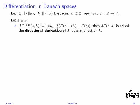
Differentiation in Banach spacesLet (Z middot Z) (V middot V ) B-spaces Z sub Z open and F Z rarr V
Let z isin Z
I If exist δF (z h) = limtdarr01t (F (z + th)minus F (z)) then δF (z h) is called
the directional derivative of F at z in direction h
I If exist δF (z h) forallh isin Z then h 7rarr δF (z h) is the first variation of Fat z
I Let exist the first variation δF (z middot) F is said to be Gateauxdifferentiable at z iff existA isin L(Z V ) such that δF (z h) = Ahforallh isin Z We write A = F primeG(z)
I F is said to be Frechet differentiable at z iff existA isin L(Z V ) and amapping r(z middot) Z rarr V such that for all h isin U with z + h isin Zwe have
F (z+h) = F (z)+Ah+r(z h) withr(z h)VhZ
rarr 0 as hZ rarr 0
We write F prime(z) = A
H Antil 060616 20
ExamplesExample 1 (H (middot middot)H) Hilbert space F (z) = z2H = (z z)H
forallz h F (z + h)minus F (z) = 2(z h)H + h2HThen
F prime(z)h = (2z h)H
Reisz representation theorem (identify H with Hlowast) we can write
F prime(z)h = (nablaF (z) h)H
where nablaF (z) = 2z is the gradient
Example 2 Let (Z (middot middot)Z) (H (middot middot)H) Hilbert spaces ud isin H fixedLet S isin L(ZH) Consider E Z rarr R
E(z) = Sz minus ud2H
Then E(z) = G(F (z)) where G(v) = v2H and F (z) = Sz minus ud
Eprime(z)h = Gprime(F (z))F prime(z)h = (2v F prime(z)h)H
= 2(Sz minus ud Sh)H = 2(Slowast(Sz minus ud) h)Z
we denote the gradient as nablaE(z) = 2Slowast(Sz minus ud)
H Antil 060616 21
ExamplesExample 1 (H (middot middot)H) Hilbert space F (z) = z2H = (z z)H
forallz h F (z + h)minus F (z) = 2(z h)H + h2HThen
F prime(z)h = (2z h)H
Reisz representation theorem (identify H with Hlowast) we can write
F prime(z)h = (nablaF (z) h)H
where nablaF (z) = 2z is the gradient
Example 2 Let (Z (middot middot)Z) (H (middot middot)H) Hilbert spaces ud isin H fixedLet S isin L(ZH) Consider E Z rarr R
E(z) = Sz minus ud2H
Then E(z) = G(F (z)) where G(v) = v2H and F (z) = Sz minus ud
Eprime(z)h = Gprime(F (z))F prime(z)h = (2v F prime(z)h)H
= 2(Sz minus ud Sh)H = 2(Slowast(Sz minus ud) h)Z
we denote the gradient as nablaE(z) = 2Slowast(Sz minus ud)H Antil 060616 21
Outline
Motivation and examples
Linear elliptic optimal control problems
Differentiation in Banach spaces
First-order necessary conditions
Optimal control of semilinear PDEs
An abstract problem
Discretization using finite element methods
H Antil 060616 22
First order necessary optimality conditions
Most of the theory is based on these two simple results
Theorem Let (Z middot Z) be a normed space J Z rarr (infin+infin] amapping with J 6equiv +infin Then z isin Z minimizer of J hArr 0 isin partJ (z)
Proof 0 isin partJ (z) means by definition of partJ (z) J (z)minus J (z) le 0forallz isin Z
Theorem Let (Z middot Z) be a normed space Zad sub Z nonemptyconvex closed J Z rarr R Gateaux differentiable where Zad sub Z sub ZZ open If z isin Zad is a solution to
minzisinZad
J (z)
then z solvesJ prime(z)(z minus z) ge 0 forallz isin Zad
Proof Exercise
H Antil 060616 23
First order necessary optimality conditions
Most of the theory is based on these two simple results
Theorem Let (Z middot Z) be a normed space J Z rarr (infin+infin] amapping with J 6equiv +infin Then z isin Z minimizer of J hArr 0 isin partJ (z)
Proof 0 isin partJ (z) means by definition of partJ (z) J (z)minus J (z) le 0forallz isin Z
Theorem Let (Z middot Z) be a normed space Zad sub Z nonemptyconvex closed J Z rarr R Gateaux differentiable where Zad sub Z sub ZZ open If z isin Zad is a solution to
minzisinZad
J (z)
then z solvesJ prime(z)(z minus z) ge 0 forallz isin Zad
Proof Exercise
H Antil 060616 23
Linear quadratic OCPI Reduced funcational
J (z) =1
2Sz minus ud2L2(Ω) +
λ
2z2L2(Ω)
I Gradient computation using sensitivity
J prime(z)h = (Slowast(Sz minus ud) + λz h)L2(Ω) forallh isin L2(Ω)
we denote the gradient by
nablaJ (z) = Slowast(Sz minus ud) + λz
I First order necessary and sufficient optimality condition
(nablaJ (z) z minus z)L2(Ω) ge 0 forallz isin Zad
I Adjoint equation Let p = Slowast(Sz minus ud) which translates intop isin H1
0 (Ω) solving
minusdiv (Anablap) = uminus ud in Ω
p = 0 on partΩ
I Gradient computation using adjoint nablaJ (z) = p+ λz
H Antil 060616 24
Linear quadratic OCPI Reduced funcational
J (z) =1
2Sz minus ud2L2(Ω) +
λ
2z2L2(Ω)
I Gradient computation using sensitivity
J prime(z)h = (Slowast(Sz minus ud) + λz h)L2(Ω) forallh isin L2(Ω)
we denote the gradient by
nablaJ (z) = Slowast(Sz minus ud) + λz
I First order necessary and sufficient optimality condition
(nablaJ (z) z minus z)L2(Ω) ge 0 forallz isin Zad
I Adjoint equation Let p = Slowast(Sz minus ud) which translates intop isin H1
0 (Ω) solving
minusdiv (Anablap) = uminus ud in Ω
p = 0 on partΩ
I Gradient computation using adjoint nablaJ (z) = p+ λz
H Antil 060616 24
Linear quadratic OCPI Reduced funcational
J (z) =1
2Sz minus ud2L2(Ω) +
λ
2z2L2(Ω)
I Gradient computation using sensitivity
J prime(z)h = (Slowast(Sz minus ud) + λz h)L2(Ω) forallh isin L2(Ω)
we denote the gradient by
nablaJ (z) = Slowast(Sz minus ud) + λz
I First order necessary and sufficient optimality condition
(nablaJ (z) z minus z)L2(Ω) ge 0 forallz isin Zad
I Adjoint equation Let p = Slowast(Sz minus ud) which translates intop isin H1
0 (Ω) solving
minusdiv (Anablap) = uminus ud in Ω
p = 0 on partΩ
I Gradient computation using adjoint nablaJ (z) = p+ λz
H Antil 060616 24
Linear quadratic OCPI Reduced funcational
J (z) =1
2Sz minus ud2L2(Ω) +
λ
2z2L2(Ω)
I Gradient computation using sensitivity
J prime(z)h = (Slowast(Sz minus ud) + λz h)L2(Ω) forallh isin L2(Ω)
we denote the gradient by
nablaJ (z) = Slowast(Sz minus ud) + λz
I First order necessary and sufficient optimality condition
(nablaJ (z) z minus z)L2(Ω) ge 0 forallz isin Zad
I Adjoint equation Let p = Slowast(Sz minus ud) which translates intop isin H1
0 (Ω) solving
minusdiv (Anablap) = uminus ud in Ω
p = 0 on partΩ
I Gradient computation using adjoint nablaJ (z) = p+ λz
H Antil 060616 24
Linear quadratic OCPI Reduced funcational
J (z) =1
2Sz minus ud2L2(Ω) +
λ
2z2L2(Ω)
I Gradient computation using sensitivity
J prime(z)h = (Slowast(Sz minus ud) + λz h)L2(Ω) forallh isin L2(Ω)
we denote the gradient by
nablaJ (z) = Slowast(Sz minus ud) + λz
I First order necessary and sufficient optimality condition
(nablaJ (z) z minus z)L2(Ω) ge 0 forallz isin Zad
I Adjoint equation Let p = Slowast(Sz minus ud) which translates intop isin H1
0 (Ω) solving
minusdiv (Anablap) = uminus ud in Ω
p = 0 on partΩ
I Gradient computation using adjoint nablaJ (z) = p+ λz
H Antil 060616 24
Optimality system
I State u isin H10 (Ω)
intΩAnablau middot nablav =
intΩzv forallv isin H1
0 (Ω)
I Adjoint p isin H10 (Ω)
intΩAnablap middot nablav =
intΩ
(uminus ud)v forallv isin H10 (Ω)
I Control z isin Zad (p+ λz z minus z) ge 0 forallz isin Zad
H Antil 060616 25
Pointwise interpretation
The variational inequality
(p+ λz z minus z) ge 0 forallz isin Zad
is equivalent to for ae x isin Ω
z(x) =
za(x) if p(x) + λz(x) gt 0isin [za(x) zb(x)] if p(x) + λz(x) = 0zb(x) if p(x) + λz(x) lt 0
Consequence
I When λ gt 0 then ae in Ω
z(x) = P[za(x)zb(x)]
minus 1
λp(x)
= min
zb(x)max
za(x)minus 1
λp(x)
H Antil 060616 26
Formal Lagrange method applied to linear OCPIntroduce L H1
0 (Ω)times Zad timesH1(Ω)rarr R defined as
L(u z p) = J(u z)minusint
Ω
(minusdiv (Anablau)minus z
)p dx
Integrate by parts to arrive at
L(u z p) = J(u z)minusint
Ω
(minusdiv (Anablap)uminus zp
)dx+
intpartΩ
(Anablau)p ds
If (u z p) is a stationary point then
I State
DpL(u z p)h = 0 forallh isin H1(Ω)
I AdjointDuL(u z p)h = 0 forallh isin H1
0 (Ω)
I ControlDzL(u z p)(z minus z) ge 0 forallz isin Zad
H Antil 060616 27
Formal Lagrange method applied to linear OCPIntroduce L H1
0 (Ω)times Zad timesH1(Ω)rarr R defined as
L(u z p) = J(u z)minusint
Ω
(minusdiv (Anablau)minus z
)p dx
Integrate by parts to arrive at
L(u z p) = J(u z)minusint
Ω
(minusdiv (Anablap)uminus zp
)dx+
intpartΩ
(Anablau)p ds
If (u z p) is a stationary point then
I State
DpL(u z p)h = 0 forallh isin H1(Ω)
I AdjointDuL(u z p)h = 0 forallh isin H1
0 (Ω)
I ControlDzL(u z p)(z minus z) ge 0 forallz isin Zad
H Antil 060616 27
Formal Lagrange method applied to linear OCPIntroduce L H1
0 (Ω)times Zad timesH1(Ω)rarr R defined as
L(u z p) = J(u z)minusint
Ω
(minusdiv (Anablau)minus z
)p dx
Integrate by parts to arrive at
L(u z p) = J(u z)minusint
Ω
(minusdiv (Anablap)uminus zp
)dx+
intpartΩ
(Anablau)p ds
If (u z p) is a stationary point then
I State
DpL(u z p)h = 0 forallh isin H1(Ω)
I AdjointDuL(u z p)h = 0 forallh isin H1
0 (Ω)
I ControlDzL(u z p)(z minus z) ge 0 forallz isin Zad
H Antil 060616 27
Formal Lagrange method applied to linear OCPIntroduce L H1
0 (Ω)times Zad timesH1(Ω)rarr R defined as
L(u z p) = J(u z)minusint
Ω
(minusdiv (Anablau)minus z
)p dx
Integrate by parts to arrive at
L(u z p) = J(u z)minusint
Ω
(minusdiv (Anablap)uminus zp
)dx+
intpartΩ
(Anablau)p ds
If (u z p) is a stationary point then
I State
DpL(u z p)h = 0 forallh isin H1(Ω)
I AdjointDuL(u z p)h = 0 forallh isin H1
0 (Ω)
I ControlDzL(u z p)(z minus z) ge 0 forallz isin Zad
H Antil 060616 27
Formal Lagrange method applied to linear OCPIntroduce L H1
0 (Ω)times Zad timesH1(Ω)rarr R defined as
L(u z p) = J(u z)minusint
Ω
(minusdiv (Anablau)minus z
)p dx
Integrate by parts to arrive at
L(u z p) = J(u z)minusint
Ω
(minusdiv (Anablap)uminus zp
)dx+
intpartΩ
(Anablau)p ds
If (u z p) is a stationary point then
I State
DpL(u z p)h = 0 forallh isin H1(Ω)
I AdjointDuL(u z p)h = 0 forallh isin H1
0 (Ω)
I ControlDzL(u z p)(z minus z) ge 0 forallz isin Zad
H Antil 060616 27
Outline
Motivation and examples
Linear elliptic optimal control problems
Differentiation in Banach spaces
First-order necessary conditions
Optimal control of semilinear PDEs
An abstract problem
Discretization using finite element methods
H Antil 060616 28
Semilinear elliptic OCP
min J(u z) =1
2uminus ud2L2(Ω) +
λ
2z2L2(Ω)
subject to
minus∆u+ g(x u) = z in Ω
u = 0 on partΩ
and z isin Zad with za zb isin Linfin(Ω)
H Antil 060616 29
State space(A1) Ω sub Rd open bounded partΩ is Lipschitz
(A2) g Ωtimes Rrarr R is bounded and measurable with respect to x isin Ωfor every u isin R
(A3) g is continuous monotone increasing and Lipschitz continuous in ufor ae x isin Ω
(A4) g(x 0) = 0 for ae x isin Ω (not really necessary)
Theorem Suppose (A1)minus (A4) hold For every z isin Lr(Ω) withr gt d2 the state equation has a unique weak solutionu isin H1
0 (Ω) cap C(Ω) ie we haveintΩ
nablau middot nablav dx+
intΩ
g(x u(x))v(x) dx =
intΩ
zv dx forallv isin H10 (Ω)
Moreover there exists a constant C gt 0 such that
uH1(Ω) + uC(Ω) le CzLr(Ω)
RemarkI The proof of the theorem uses the BrowderndashMinty theorem on
monotone operators
H Antil 060616 30
State space(A1) Ω sub Rd open bounded partΩ is Lipschitz
(A2) g Ωtimes Rrarr R is bounded and measurable with respect to x isin Ωfor every u isin R
(A3) g is continuous monotone increasing and Lipschitz continuous in ufor ae x isin Ω
(A4) g(x 0) = 0 for ae x isin Ω (not really necessary)
Theorem Suppose (A1)minus (A4) hold For every z isin Lr(Ω) withr gt d2 the state equation has a unique weak solutionu isin H1
0 (Ω) cap C(Ω) ie we haveintΩ
nablau middot nablav dx+
intΩ
g(x u(x))v(x) dx =
intΩ
zv dx forallv isin H10 (Ω)
Moreover there exists a constant C gt 0 such that
uH1(Ω) + uC(Ω) le CzLr(Ω)
RemarkI The proof of the theorem uses the BrowderndashMinty theorem on
monotone operators
H Antil 060616 30
State space(A1) Ω sub Rd open bounded partΩ is Lipschitz
(A2) g Ωtimes Rrarr R is bounded and measurable with respect to x isin Ωfor every u isin R
(A3) g is continuous monotone increasing and Lipschitz continuous in ufor ae x isin Ω
(A4) g(x 0) = 0 for ae x isin Ω (not really necessary)
Theorem Suppose (A1)minus (A4) hold For every z isin Lr(Ω) withr gt d2 the state equation has a unique weak solutionu isin H1
0 (Ω) cap C(Ω) ie we haveintΩ
nablau middot nablav dx+
intΩ
g(x u(x))v(x) dx =
intΩ
zv dx forallv isin H10 (Ω)
Moreover there exists a constant C gt 0 such that
uH1(Ω) + uC(Ω) le CzLr(Ω)
RemarkI The proof of the theorem uses the BrowderndashMinty theorem on
monotone operators
H Antil 060616 30
Control-to-state map and reduced problem
I Control to state map
S Linfin(Ω)rarr H10 (Ω) cap C(Ω)
is well defined and is globally Lipschitz continuous
I Reduced problem
minJ (z) =1
2S(u)minus ud2L2(Ω) +
λ
2z2L2(Ω)
H Antil 060616 31
Control-to-state map and reduced problem
I Control to state map
S Linfin(Ω)rarr H10 (Ω) cap C(Ω)
is well defined and is globally Lipschitz continuous
I Reduced problem
minJ (z) =1
2S(u)minus ud2L2(Ω) +
λ
2z2L2(Ω)
H Antil 060616 31
First-order necessary conditionsI Lagrangian functional
L(u z p) = J(u z)minusint
Ω
(minus∆u+ g(x u(x))minus z
)p dx
= J(u z)minusint
Ω
(nablau middot nablap+ g(x u(x))pminus zp
)dx
I Adjoint system For all h isin H10 (Ω)
0 = DuL(u z p)h =
intΩ
(uminus ud)h dxminusint
Ω
(nablah middot nablap+ gu(x u(x))ph
)which yields
minus∆p+ gu(x u(x))p = uminus ud in Ω
p = 0 on partΩ
I Control
DzL(u z p)(z minus z) = (p+ λz z minus z) dx ge 0 forallz isin ZadI Gradient
nablaJ (z) = p+ λz
H Antil 060616 32
First-order necessary conditionsI Lagrangian functional
L(u z p) = J(u z)minusint
Ω
(minus∆u+ g(x u(x))minus z
)p dx
= J(u z)minusint
Ω
(nablau middot nablap+ g(x u(x))pminus zp
)dx
I Adjoint system For all h isin H10 (Ω)
0 = DuL(u z p)h =
intΩ
(uminus ud)h dxminusint
Ω
(nablah middot nablap+ gu(x u(x))ph
)which yields
minus∆p+ gu(x u(x))p = uminus ud in Ω
p = 0 on partΩ
I Control
DzL(u z p)(z minus z) = (p+ λz z minus z) dx ge 0 forallz isin ZadI Gradient
nablaJ (z) = p+ λz
H Antil 060616 32
First-order necessary conditionsI Lagrangian functional
L(u z p) = J(u z)minusint
Ω
(minus∆u+ g(x u(x))minus z
)p dx
= J(u z)minusint
Ω
(nablau middot nablap+ g(x u(x))pminus zp
)dx
I Adjoint system For all h isin H10 (Ω)
0 = DuL(u z p)h =
intΩ
(uminus ud)h dxminusint
Ω
(nablah middot nablap+ gu(x u(x))ph
)which yields
minus∆p+ gu(x u(x))p = uminus ud in Ω
p = 0 on partΩ
I Control
DzL(u z p)(z minus z) = (p+ λz z minus z) dx ge 0 forallz isin Zad
I GradientnablaJ (z) = p+ λz
H Antil 060616 32
First-order necessary conditionsI Lagrangian functional
L(u z p) = J(u z)minusint
Ω
(minus∆u+ g(x u(x))minus z
)p dx
= J(u z)minusint
Ω
(nablau middot nablap+ g(x u(x))pminus zp
)dx
I Adjoint system For all h isin H10 (Ω)
0 = DuL(u z p)h =
intΩ
(uminus ud)h dxminusint
Ω
(nablah middot nablap+ gu(x u(x))ph
)which yields
minus∆p+ gu(x u(x))p = uminus ud in Ω
p = 0 on partΩ
I Control
DzL(u z p)(z minus z) = (p+ λz z minus z) dx ge 0 forallz isin ZadI Gradient
nablaJ (z) = p+ λz
H Antil 060616 32
Differentiability of Nemytskii operator
The rigorous proof uses
Theorem In addition to (A1)-(A4) if
(A5) g is continuously differentiable with respect to u for ae x isin Ωand we have
(i) |gu(x 0)| le K for ae x isin Ω(ii) gu is locally Lipschitz with respect to u isin R
then the Nemytskii operator G u 7rarr g(middot u(middot)) is continuously Frechetdifferentiable from Linfin(Ω) into itself and
(Gprime(u)h)(x) = gu(x u(x))h(x) ae in Ω forallh isin Linfin(Ω)
Remark (A5) holds if g(x u) = g(u) and g isin C2(R)
H Antil 060616 33
Outline
Motivation and examples
Linear elliptic optimal control problems
Differentiation in Banach spaces
First-order necessary conditions
Optimal control of semilinear PDEs
An abstract problem
Discretization using finite element methods
H Antil 060616 34
Gradient computation via adjoint general formI Abstract problem
min J(u z)
subject toc(u z) = 0
and z isin Zad
I Directional derivative Let S be the control to state map(nonlinear in general)
z 7rarr S(z) = u(z)
Under the assumptions of ldquoimplicit function theoremrdquo
J prime(z)h = (nablauJ (u(z) z) Sprime(z)h) + (nablazJ (u(z) z) h)
I Sensitivity of u with respect to z Differentiating the stateequation
cu(S(z) z)Sprime(z)h = minuscz(S(z) z)h
leads toSprime(z)h = minuscu(S(z) z)minus1
(cz(S(z) z)h
)
provided cu(S(z) z)minus1 is well-defined
H Antil 060616 35
Gradient computation via adjoint general formI Abstract problem
min J(u z)
subject toc(u z) = 0
and z isin ZadI Directional derivative Let S be the control to state map
(nonlinear in general)
z 7rarr S(z) = u(z)
Under the assumptions of ldquoimplicit function theoremrdquo
J prime(z)h = (nablauJ (u(z) z) Sprime(z)h) + (nablazJ (u(z) z) h)
I Sensitivity of u with respect to z Differentiating the stateequation
cu(S(z) z)Sprime(z)h = minuscz(S(z) z)h
leads toSprime(z)h = minuscu(S(z) z)minus1
(cz(S(z) z)h
)
provided cu(S(z) z)minus1 is well-defined
H Antil 060616 35
Gradient computation via adjoint general formI Abstract problem
min J(u z)
subject toc(u z) = 0
and z isin ZadI Directional derivative Let S be the control to state map
(nonlinear in general)
z 7rarr S(z) = u(z)
Under the assumptions of ldquoimplicit function theoremrdquo
J prime(z)h = (nablauJ (u(z) z) Sprime(z)h) + (nablazJ (u(z) z) h)
I Sensitivity of u with respect to z Differentiating the stateequation
cu(S(z) z)Sprime(z)h = minuscz(S(z) z)h
leads toSprime(z)h = minuscu(S(z) z)minus1
(cz(S(z) z)h
)
provided cu(S(z) z)minus1 is well-defined
H Antil 060616 35
Adjoint equation and gradient general form
I Directional derivative
J prime(z)h = minus(nablauJ (u(z) z) cu(u(z) z)minus1cz(u(z) z)h
)+ (nablazJ (u(z) z) h)
I Gradient
nablaJ (z) = minuscz(u(z) z)lowast(cu(u(z) z)minuslowastnablauJ (u(z) z)
)+nablazJ (u(z) z)
I Introducing adjoint variable p solving
cu(u(z) z)lowastp = nablauJ (u(z) z)
we arrive at following form of gradient
nablaJ (z) = minuscz(u(z) z)lowastp+nablazJ (u(z) z)
which is tractable
H Antil 060616 36
Adjoint equation and gradient general form
I Directional derivative
J prime(z)h = minus(nablauJ (u(z) z) cu(u(z) z)minus1cz(u(z) z)h
)+ (nablazJ (u(z) z) h)
I Gradient
nablaJ (z) = minuscz(u(z) z)lowast(cu(u(z) z)minuslowastnablauJ (u(z) z)
)+nablazJ (u(z) z)
I Introducing adjoint variable p solving
cu(u(z) z)lowastp = nablauJ (u(z) z)
we arrive at following form of gradient
nablaJ (z) = minuscz(u(z) z)lowastp+nablazJ (u(z) z)
which is tractable
H Antil 060616 36
Adjoint equation and gradient general form
I Directional derivative
J prime(z)h = minus(nablauJ (u(z) z) cu(u(z) z)minus1cz(u(z) z)h
)+ (nablazJ (u(z) z) h)
I Gradient
nablaJ (z) = minuscz(u(z) z)lowast(cu(u(z) z)minuslowastnablauJ (u(z) z)
)+nablazJ (u(z) z)
I Introducing adjoint variable p solving
cu(u(z) z)lowastp = nablauJ (u(z) z)
we arrive at following form of gradient
nablaJ (z) = minuscz(u(z) z)lowastp+nablazJ (u(z) z)
which is tractable
H Antil 060616 36
Hessian computation general form
I Lagrangian L(u z p) = J(u z)minusint
Ωc(u z)p dx Then we have
DzJ (z)h = DzL(u z p)h
I Second order derivative
D2zJ (z)[h1 h2] = DuDzL(u z p)[h1 S
prime(z)h2] +D2zL(u z p)[h1 h2]
+DpDzL(u z p)[h1 Dzp(z)h2]
I We already know Sprime(z)h2 moreover
DpDzL(u z p)[h1 Dzp(z)h2] = minus(cu(u z)h1 Dzp(z)h2
)
It remain to identify Dzp(z)h2
H Antil 060616 37
Hessian computation general form
I Lagrangian L(u z p) = J(u z)minusint
Ωc(u z)p dx Then we have
DzJ (z)h = DzL(u z p)h
I Second order derivative
D2zJ (z)[h1 h2] = DuDzL(u z p)[h1 S
prime(z)h2] +D2zL(u z p)[h1 h2]
+DpDzL(u z p)[h1 Dzp(z)h2]
I We already know Sprime(z)h2 moreover
DpDzL(u z p)[h1 Dzp(z)h2] = minus(cu(u z)h1 Dzp(z)h2
)
It remain to identify Dzp(z)h2
H Antil 060616 37
Hessian computation general form
I Lagrangian L(u z p) = J(u z)minusint
Ωc(u z)p dx Then we have
DzJ (z)h = DzL(u z p)h
I Second order derivative
D2zJ (z)[h1 h2] = DuDzL(u z p)[h1 S
prime(z)h2] +D2zL(u z p)[h1 h2]
+DpDzL(u z p)[h1 Dzp(z)h2]
I We already know Sprime(z)h2 moreover
DpDzL(u z p)[h1 Dzp(z)h2] = minus(cu(u z)h1 Dzp(z)h2
)
It remain to identify Dzp(z)h2
H Antil 060616 37
Outline
Motivation and examples
Linear elliptic optimal control problems
Differentiation in Banach spaces
First-order necessary conditions
Optimal control of semilinear PDEs
An abstract problem
Discretization using finite element methods
H Antil 060616 38
Numerical approximation of Poisson equation MeshTo avoid technical issues we will assume that partΩ is polygonal
I Mesh Let T = K be a mesh of Ω where K sub Rd is an elementthat is isoparametrically equivalent to a unit simplex in Rd
I Conforming mesh We say that the mesh is conforming ifI Ω = cupKisinT KI If K1 cap K2 = x then x is a node of K1 and K2I If K1 cap K2 6= empty and K1 cap K2 6= x then K1 cap K2 is an edgeface
contained in partK1 cap partK2
I Shape regular Let T be the collection of all conformingrefinements of an original mesh T 0 Then T is called shape regularif exist κ gt 0 such that
hKρKle κ forallK isin cupiT i
where hK = diam K ρK = maxρ gt 0|Bρ sub KI Quasi-uniform A family of shape regular meshes is called-quasi
uniform if there exist a constant σ gt 0 such that
maxhKminhK
le σ
uniformly for all meshes in the family
Numerical approximation of Poisson equation MeshTo avoid technical issues we will assume that partΩ is polygonal
I Mesh Let T = K be a mesh of Ω where K sub Rd is an elementthat is isoparametrically equivalent to a unit simplex in Rd
I Conforming mesh We say that the mesh is conforming ifI Ω = cupKisinT KI If K1 cap K2 = x then x is a node of K1 and K2I If K1 cap K2 6= empty and K1 cap K2 6= x then K1 cap K2 is an edgeface
contained in partK1 cap partK2
I Shape regular Let T be the collection of all conformingrefinements of an original mesh T 0 Then T is called shape regularif exist κ gt 0 such that
hKρKle κ forallK isin cupiT i
where hK = diam K ρK = maxρ gt 0|Bρ sub KI Quasi-uniform A family of shape regular meshes is called-quasi
uniform if there exist a constant σ gt 0 such that
maxhKminhK
le σ
uniformly for all meshes in the family
Numerical approximation of Poisson equation MeshTo avoid technical issues we will assume that partΩ is polygonal
I Mesh Let T = K be a mesh of Ω where K sub Rd is an elementthat is isoparametrically equivalent to a unit simplex in Rd
I Conforming mesh We say that the mesh is conforming ifI Ω = cupKisinT KI If K1 cap K2 = x then x is a node of K1 and K2I If K1 cap K2 6= empty and K1 cap K2 6= x then K1 cap K2 is an edgeface
contained in partK1 cap partK2
I Shape regular Let T be the collection of all conformingrefinements of an original mesh T 0 Then T is called shape regularif exist κ gt 0 such that
hKρKle κ forallK isin cupiT i
where hK = diam K ρK = maxρ gt 0|Bρ sub K
I Quasi-uniform A family of shape regular meshes is called-quasiuniform if there exist a constant σ gt 0 such that
maxhKminhK
le σ
uniformly for all meshes in the family
Numerical approximation of Poisson equation MeshTo avoid technical issues we will assume that partΩ is polygonal
I Mesh Let T = K be a mesh of Ω where K sub Rd is an elementthat is isoparametrically equivalent to a unit simplex in Rd
I Conforming mesh We say that the mesh is conforming ifI Ω = cupKisinT KI If K1 cap K2 = x then x is a node of K1 and K2I If K1 cap K2 6= empty and K1 cap K2 6= x then K1 cap K2 is an edgeface
contained in partK1 cap partK2
I Shape regular Let T be the collection of all conformingrefinements of an original mesh T 0 Then T is called shape regularif exist κ gt 0 such that
hKρKle κ forallK isin cupiT i
where hK = diam K ρK = maxρ gt 0|Bρ sub KI Quasi-uniform A family of shape regular meshes is called-quasi
uniform if there exist a constant σ gt 0 such that
maxhKminhK
le σ
uniformly for all meshes in the family
FE space and Galerkin approximationI Finite element space For T isin T we define the finite element
space as
V(T ) = W isin C0(Ω) WK isin P1forallK isin T W |partΩ = 0
where P1 is the set of polynomials of degree at most 1
I Galerkin approximation of continuous problem is given by
Find UT isin V(T )
intΩ
AnablaUT middot nablaV = 〈f V 〉 forallV isin V(T )
The discrete problem is well-posedI Nodal basis Consists of functions ψi isin V(T ) with xi isin N (T )
satisfyingψxi
(xj) = δij
where N (T ) denotes the interior (plus Neumann) nodesI Galerkin orthogonality(
nabla(uminus UT )nablaW)L2(Ω)
= 0 forallW isin V(T )
H Antil 060616 40
FE space and Galerkin approximationI Finite element space For T isin T we define the finite element
space as
V(T ) = W isin C0(Ω) WK isin P1forallK isin T W |partΩ = 0
where P1 is the set of polynomials of degree at most 1I Galerkin approximation of continuous problem is given by
Find UT isin V(T )
intΩ
AnablaUT middot nablaV = 〈f V 〉 forallV isin V(T )
The discrete problem is well-posed
I Nodal basis Consists of functions ψi isin V(T ) with xi isin N (T )satisfying
ψxi(xj) = δij
where N (T ) denotes the interior (plus Neumann) nodesI Galerkin orthogonality(
nabla(uminus UT )nablaW)L2(Ω)
= 0 forallW isin V(T )
H Antil 060616 40
FE space and Galerkin approximationI Finite element space For T isin T we define the finite element
space as
V(T ) = W isin C0(Ω) WK isin P1forallK isin T W |partΩ = 0
where P1 is the set of polynomials of degree at most 1I Galerkin approximation of continuous problem is given by
Find UT isin V(T )
intΩ
AnablaUT middot nablaV = 〈f V 〉 forallV isin V(T )
The discrete problem is well-posedI Nodal basis Consists of functions ψi isin V(T ) with xi isin N (T )
satisfyingψxi
(xj) = δij
where N (T ) denotes the interior (plus Neumann) nodes
I Galerkin orthogonality(nabla(uminus UT )nablaW
)L2(Ω)
= 0 forallW isin V(T )
H Antil 060616 40
FE space and Galerkin approximationI Finite element space For T isin T we define the finite element
space as
V(T ) = W isin C0(Ω) WK isin P1forallK isin T W |partΩ = 0
where P1 is the set of polynomials of degree at most 1I Galerkin approximation of continuous problem is given by
Find UT isin V(T )
intΩ
AnablaUT middot nablaV = 〈f V 〉 forallV isin V(T )
The discrete problem is well-posedI Nodal basis Consists of functions ψi isin V(T ) with xi isin N (T )
satisfyingψxi
(xj) = δij
where N (T ) denotes the interior (plus Neumann) nodesI Galerkin orthogonality(
nabla(uminus UT )nablaW)L2(Ω)
= 0 forallW isin V(T )
H Antil 060616 40
Best approximation
I Cearsquos lemma
nabla(uminus UT )L2(Ω) le C infWisinV(T )
nabla(uminusW )L2(Ω)
I Nodal interpolation operator ΠT C(Ω)rarr V(T ) satisfies
ΠT u(xi) = u(xi) forallxi isin N (T )
and is defined as
ΠT u =sum
xiisinN (T )
u(xi)ψxi
I Error estimates In Cearsquos lemma replace W by ΠT u and thencompute the interpolation error
H Antil 060616 41
Best approximation
I Cearsquos lemma
nabla(uminus UT )L2(Ω) le C infWisinV(T )
nabla(uminusW )L2(Ω)
I Nodal interpolation operator ΠT C(Ω)rarr V(T ) satisfies
ΠT u(xi) = u(xi) forallxi isin N (T )
and is defined as
ΠT u =sum
xiisinN (T )
u(xi)ψxi
I Error estimates In Cearsquos lemma replace W by ΠT u and thencompute the interpolation error
H Antil 060616 41
Best approximation
I Cearsquos lemma
nabla(uminus UT )L2(Ω) le C infWisinV(T )
nabla(uminusW )L2(Ω)
I Nodal interpolation operator ΠT C(Ω)rarr V(T ) satisfies
ΠT u(xi) = u(xi) forallxi isin N (T )
and is defined as
ΠT u =sum
xiisinN (T )
u(xi)ψxi
I Error estimates In Cearsquos lemma replace W by ΠT u and thencompute the interpolation error
H Antil 060616 41
Algebraic system state equation
I Recall UT isin V(T ) solves
a(UT V ) = 〈f V 〉 forallV isin V(T )
I Now setting UT =sumN
j=1 Ujψj V = ψi we get
Nsumj=1
Uja(φj φi) = 〈f ψi〉 i = 1 N
which is the matrix-vector system
AU = F
I Stiffness matrix A is SPD
H Antil 060616 42
Algebraic system state equation
I Recall UT isin V(T ) solves
a(UT V ) = 〈f V 〉 forallV isin V(T )
I Now setting UT =sumN
j=1 Ujψj V = ψi we get
Nsumj=1
Uja(φj φi) = 〈f ψi〉 i = 1 N
which is the matrix-vector system
AU = F
I Stiffness matrix A is SPD
H Antil 060616 42
Algebraic system state equation
I Recall UT isin V(T ) solves
a(UT V ) = 〈f V 〉 forallV isin V(T )
I Now setting UT =sumN
j=1 Ujψj V = ψi we get
Nsumj=1
Uja(φj φi) = 〈f ψi〉 i = 1 N
which is the matrix-vector system
AU = F
I Stiffness matrix A is SPD
H Antil 060616 42
Discrete linear elliptic OCP
min JT (UT ZT ) =1
2UT minus ud2L2(Ω) +
λ
2ZT 2L2(Ω)
subject to
Find UT isin V(T )
intΩ
nablaUT middot nablaV = (ZT V )L2(Ω) forallV isin V(T )
and whereZT isin Zad(T ) = Zad cap Z(T )
is either one of these
Z(T ) =
V(T )L2(Ω) variational discretization (Hinze)WT isin Linfin(Ω) ZT |K isin P0(K)K isin T
H Antil 060616 43
Recent books
F TroltzschOptimal control of partial differential equations volume 112 ofGraduate Studies in MathematicsAmerican Mathematical Society Providence RI 2010Theory methods and applications Translated from the 2005 Germanoriginal by Jurgen Sprekels
K Ito and K KunischLagrange multiplier approach to variational problems andapplications volume 15 of Advances in Design and ControlSociety for Industrial and Applied Mathematics (SIAM)Philadelphia PA 2008
H Antil 060616 44
- Motivation and examples
- Linear elliptic optimal control problems
- Differentiation in Banach spaces
- First-order necessary conditions
- Optimal control of semilinear PDEs
- An abstract problem
- Discretization using finite element methods
-
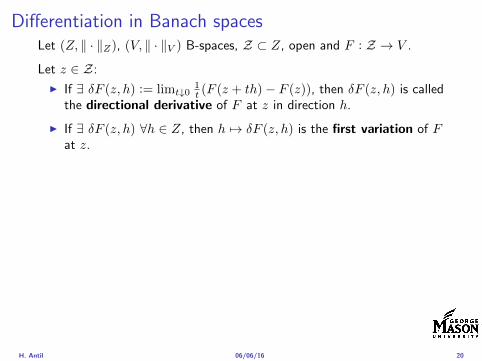
Differentiation in Banach spacesLet (Z middot Z) (V middot V ) B-spaces Z sub Z open and F Z rarr V
Let z isin Z
I If exist δF (z h) = limtdarr01t (F (z + th)minus F (z)) then δF (z h) is called
the directional derivative of F at z in direction h
I If exist δF (z h) forallh isin Z then h 7rarr δF (z h) is the first variation of Fat z
I Let exist the first variation δF (z middot) F is said to be Gateauxdifferentiable at z iff existA isin L(Z V ) such that δF (z h) = Ahforallh isin Z We write A = F primeG(z)
I F is said to be Frechet differentiable at z iff existA isin L(Z V ) and amapping r(z middot) Z rarr V such that for all h isin U with z + h isin Zwe have
F (z+h) = F (z)+Ah+r(z h) withr(z h)VhZ
rarr 0 as hZ rarr 0
We write F prime(z) = A
H Antil 060616 20
Differentiation in Banach spacesLet (Z middot Z) (V middot V ) B-spaces Z sub Z open and F Z rarr V
Let z isin Z
I If exist δF (z h) = limtdarr01t (F (z + th)minus F (z)) then δF (z h) is called
the directional derivative of F at z in direction h
I If exist δF (z h) forallh isin Z then h 7rarr δF (z h) is the first variation of Fat z
I Let exist the first variation δF (z middot) F is said to be Gateauxdifferentiable at z iff existA isin L(Z V ) such that δF (z h) = Ahforallh isin Z We write A = F primeG(z)
I F is said to be Frechet differentiable at z iff existA isin L(Z V ) and amapping r(z middot) Z rarr V such that for all h isin U with z + h isin Zwe have
F (z+h) = F (z)+Ah+r(z h) withr(z h)VhZ
rarr 0 as hZ rarr 0
We write F prime(z) = A
H Antil 060616 20
Differentiation in Banach spacesLet (Z middot Z) (V middot V ) B-spaces Z sub Z open and F Z rarr V
Let z isin Z
I If exist δF (z h) = limtdarr01t (F (z + th)minus F (z)) then δF (z h) is called
the directional derivative of F at z in direction h
I If exist δF (z h) forallh isin Z then h 7rarr δF (z h) is the first variation of Fat z
I Let exist the first variation δF (z middot) F is said to be Gateauxdifferentiable at z iff existA isin L(Z V ) such that δF (z h) = Ahforallh isin Z We write A = F primeG(z)
I F is said to be Frechet differentiable at z iff existA isin L(Z V ) and amapping r(z middot) Z rarr V such that for all h isin U with z + h isin Zwe have
F (z+h) = F (z)+Ah+r(z h) withr(z h)VhZ
rarr 0 as hZ rarr 0
We write F prime(z) = A
H Antil 060616 20
ExamplesExample 1 (H (middot middot)H) Hilbert space F (z) = z2H = (z z)H
forallz h F (z + h)minus F (z) = 2(z h)H + h2HThen
F prime(z)h = (2z h)H
Reisz representation theorem (identify H with Hlowast) we can write
F prime(z)h = (nablaF (z) h)H
where nablaF (z) = 2z is the gradient
Example 2 Let (Z (middot middot)Z) (H (middot middot)H) Hilbert spaces ud isin H fixedLet S isin L(ZH) Consider E Z rarr R
E(z) = Sz minus ud2H
Then E(z) = G(F (z)) where G(v) = v2H and F (z) = Sz minus ud
Eprime(z)h = Gprime(F (z))F prime(z)h = (2v F prime(z)h)H
= 2(Sz minus ud Sh)H = 2(Slowast(Sz minus ud) h)Z
we denote the gradient as nablaE(z) = 2Slowast(Sz minus ud)
H Antil 060616 21
ExamplesExample 1 (H (middot middot)H) Hilbert space F (z) = z2H = (z z)H
forallz h F (z + h)minus F (z) = 2(z h)H + h2HThen
F prime(z)h = (2z h)H
Reisz representation theorem (identify H with Hlowast) we can write
F prime(z)h = (nablaF (z) h)H
where nablaF (z) = 2z is the gradient
Example 2 Let (Z (middot middot)Z) (H (middot middot)H) Hilbert spaces ud isin H fixedLet S isin L(ZH) Consider E Z rarr R
E(z) = Sz minus ud2H
Then E(z) = G(F (z)) where G(v) = v2H and F (z) = Sz minus ud
Eprime(z)h = Gprime(F (z))F prime(z)h = (2v F prime(z)h)H
= 2(Sz minus ud Sh)H = 2(Slowast(Sz minus ud) h)Z
we denote the gradient as nablaE(z) = 2Slowast(Sz minus ud)H Antil 060616 21
Outline
Motivation and examples
Linear elliptic optimal control problems
Differentiation in Banach spaces
First-order necessary conditions
Optimal control of semilinear PDEs
An abstract problem
Discretization using finite element methods
H Antil 060616 22
First order necessary optimality conditions
Most of the theory is based on these two simple results
Theorem Let (Z middot Z) be a normed space J Z rarr (infin+infin] amapping with J 6equiv +infin Then z isin Z minimizer of J hArr 0 isin partJ (z)
Proof 0 isin partJ (z) means by definition of partJ (z) J (z)minus J (z) le 0forallz isin Z
Theorem Let (Z middot Z) be a normed space Zad sub Z nonemptyconvex closed J Z rarr R Gateaux differentiable where Zad sub Z sub ZZ open If z isin Zad is a solution to
minzisinZad
J (z)
then z solvesJ prime(z)(z minus z) ge 0 forallz isin Zad
Proof Exercise
H Antil 060616 23
First order necessary optimality conditions
Most of the theory is based on these two simple results
Theorem Let (Z middot Z) be a normed space J Z rarr (infin+infin] amapping with J 6equiv +infin Then z isin Z minimizer of J hArr 0 isin partJ (z)
Proof 0 isin partJ (z) means by definition of partJ (z) J (z)minus J (z) le 0forallz isin Z
Theorem Let (Z middot Z) be a normed space Zad sub Z nonemptyconvex closed J Z rarr R Gateaux differentiable where Zad sub Z sub ZZ open If z isin Zad is a solution to
minzisinZad
J (z)
then z solvesJ prime(z)(z minus z) ge 0 forallz isin Zad
Proof Exercise
H Antil 060616 23
Linear quadratic OCPI Reduced funcational
J (z) =1
2Sz minus ud2L2(Ω) +
λ
2z2L2(Ω)
I Gradient computation using sensitivity
J prime(z)h = (Slowast(Sz minus ud) + λz h)L2(Ω) forallh isin L2(Ω)
we denote the gradient by
nablaJ (z) = Slowast(Sz minus ud) + λz
I First order necessary and sufficient optimality condition
(nablaJ (z) z minus z)L2(Ω) ge 0 forallz isin Zad
I Adjoint equation Let p = Slowast(Sz minus ud) which translates intop isin H1
0 (Ω) solving
minusdiv (Anablap) = uminus ud in Ω
p = 0 on partΩ
I Gradient computation using adjoint nablaJ (z) = p+ λz
H Antil 060616 24
Linear quadratic OCPI Reduced funcational
J (z) =1
2Sz minus ud2L2(Ω) +
λ
2z2L2(Ω)
I Gradient computation using sensitivity
J prime(z)h = (Slowast(Sz minus ud) + λz h)L2(Ω) forallh isin L2(Ω)
we denote the gradient by
nablaJ (z) = Slowast(Sz minus ud) + λz
I First order necessary and sufficient optimality condition
(nablaJ (z) z minus z)L2(Ω) ge 0 forallz isin Zad
I Adjoint equation Let p = Slowast(Sz minus ud) which translates intop isin H1
0 (Ω) solving
minusdiv (Anablap) = uminus ud in Ω
p = 0 on partΩ
I Gradient computation using adjoint nablaJ (z) = p+ λz
H Antil 060616 24
Linear quadratic OCPI Reduced funcational
J (z) =1
2Sz minus ud2L2(Ω) +
λ
2z2L2(Ω)
I Gradient computation using sensitivity
J prime(z)h = (Slowast(Sz minus ud) + λz h)L2(Ω) forallh isin L2(Ω)
we denote the gradient by
nablaJ (z) = Slowast(Sz minus ud) + λz
I First order necessary and sufficient optimality condition
(nablaJ (z) z minus z)L2(Ω) ge 0 forallz isin Zad
I Adjoint equation Let p = Slowast(Sz minus ud) which translates intop isin H1
0 (Ω) solving
minusdiv (Anablap) = uminus ud in Ω
p = 0 on partΩ
I Gradient computation using adjoint nablaJ (z) = p+ λz
H Antil 060616 24
Linear quadratic OCPI Reduced funcational
J (z) =1
2Sz minus ud2L2(Ω) +
λ
2z2L2(Ω)
I Gradient computation using sensitivity
J prime(z)h = (Slowast(Sz minus ud) + λz h)L2(Ω) forallh isin L2(Ω)
we denote the gradient by
nablaJ (z) = Slowast(Sz minus ud) + λz
I First order necessary and sufficient optimality condition
(nablaJ (z) z minus z)L2(Ω) ge 0 forallz isin Zad
I Adjoint equation Let p = Slowast(Sz minus ud) which translates intop isin H1
0 (Ω) solving
minusdiv (Anablap) = uminus ud in Ω
p = 0 on partΩ
I Gradient computation using adjoint nablaJ (z) = p+ λz
H Antil 060616 24
Linear quadratic OCPI Reduced funcational
J (z) =1
2Sz minus ud2L2(Ω) +
λ
2z2L2(Ω)
I Gradient computation using sensitivity
J prime(z)h = (Slowast(Sz minus ud) + λz h)L2(Ω) forallh isin L2(Ω)
we denote the gradient by
nablaJ (z) = Slowast(Sz minus ud) + λz
I First order necessary and sufficient optimality condition
(nablaJ (z) z minus z)L2(Ω) ge 0 forallz isin Zad
I Adjoint equation Let p = Slowast(Sz minus ud) which translates intop isin H1
0 (Ω) solving
minusdiv (Anablap) = uminus ud in Ω
p = 0 on partΩ
I Gradient computation using adjoint nablaJ (z) = p+ λz
H Antil 060616 24
Optimality system
I State u isin H10 (Ω)
intΩAnablau middot nablav =
intΩzv forallv isin H1
0 (Ω)
I Adjoint p isin H10 (Ω)
intΩAnablap middot nablav =
intΩ
(uminus ud)v forallv isin H10 (Ω)
I Control z isin Zad (p+ λz z minus z) ge 0 forallz isin Zad
H Antil 060616 25
Pointwise interpretation
The variational inequality
(p+ λz z minus z) ge 0 forallz isin Zad
is equivalent to for ae x isin Ω
z(x) =
za(x) if p(x) + λz(x) gt 0isin [za(x) zb(x)] if p(x) + λz(x) = 0zb(x) if p(x) + λz(x) lt 0
Consequence
I When λ gt 0 then ae in Ω
z(x) = P[za(x)zb(x)]
minus 1
λp(x)
= min
zb(x)max
za(x)minus 1
λp(x)
H Antil 060616 26
Formal Lagrange method applied to linear OCPIntroduce L H1
0 (Ω)times Zad timesH1(Ω)rarr R defined as
L(u z p) = J(u z)minusint
Ω
(minusdiv (Anablau)minus z
)p dx
Integrate by parts to arrive at
L(u z p) = J(u z)minusint
Ω
(minusdiv (Anablap)uminus zp
)dx+
intpartΩ
(Anablau)p ds
If (u z p) is a stationary point then
I State
DpL(u z p)h = 0 forallh isin H1(Ω)
I AdjointDuL(u z p)h = 0 forallh isin H1
0 (Ω)
I ControlDzL(u z p)(z minus z) ge 0 forallz isin Zad
H Antil 060616 27
Formal Lagrange method applied to linear OCPIntroduce L H1
0 (Ω)times Zad timesH1(Ω)rarr R defined as
L(u z p) = J(u z)minusint
Ω
(minusdiv (Anablau)minus z
)p dx
Integrate by parts to arrive at
L(u z p) = J(u z)minusint
Ω
(minusdiv (Anablap)uminus zp
)dx+
intpartΩ
(Anablau)p ds
If (u z p) is a stationary point then
I State
DpL(u z p)h = 0 forallh isin H1(Ω)
I AdjointDuL(u z p)h = 0 forallh isin H1
0 (Ω)
I ControlDzL(u z p)(z minus z) ge 0 forallz isin Zad
H Antil 060616 27
Formal Lagrange method applied to linear OCPIntroduce L H1
0 (Ω)times Zad timesH1(Ω)rarr R defined as
L(u z p) = J(u z)minusint
Ω
(minusdiv (Anablau)minus z
)p dx
Integrate by parts to arrive at
L(u z p) = J(u z)minusint
Ω
(minusdiv (Anablap)uminus zp
)dx+
intpartΩ
(Anablau)p ds
If (u z p) is a stationary point then
I State
DpL(u z p)h = 0 forallh isin H1(Ω)
I AdjointDuL(u z p)h = 0 forallh isin H1
0 (Ω)
I ControlDzL(u z p)(z minus z) ge 0 forallz isin Zad
H Antil 060616 27
Formal Lagrange method applied to linear OCPIntroduce L H1
0 (Ω)times Zad timesH1(Ω)rarr R defined as
L(u z p) = J(u z)minusint
Ω
(minusdiv (Anablau)minus z
)p dx
Integrate by parts to arrive at
L(u z p) = J(u z)minusint
Ω
(minusdiv (Anablap)uminus zp
)dx+
intpartΩ
(Anablau)p ds
If (u z p) is a stationary point then
I State
DpL(u z p)h = 0 forallh isin H1(Ω)
I AdjointDuL(u z p)h = 0 forallh isin H1
0 (Ω)
I ControlDzL(u z p)(z minus z) ge 0 forallz isin Zad
H Antil 060616 27
Formal Lagrange method applied to linear OCPIntroduce L H1
0 (Ω)times Zad timesH1(Ω)rarr R defined as
L(u z p) = J(u z)minusint
Ω
(minusdiv (Anablau)minus z
)p dx
Integrate by parts to arrive at
L(u z p) = J(u z)minusint
Ω
(minusdiv (Anablap)uminus zp
)dx+
intpartΩ
(Anablau)p ds
If (u z p) is a stationary point then
I State
DpL(u z p)h = 0 forallh isin H1(Ω)
I AdjointDuL(u z p)h = 0 forallh isin H1
0 (Ω)
I ControlDzL(u z p)(z minus z) ge 0 forallz isin Zad
H Antil 060616 27
Outline
Motivation and examples
Linear elliptic optimal control problems
Differentiation in Banach spaces
First-order necessary conditions
Optimal control of semilinear PDEs
An abstract problem
Discretization using finite element methods
H Antil 060616 28
Semilinear elliptic OCP
min J(u z) =1
2uminus ud2L2(Ω) +
λ
2z2L2(Ω)
subject to
minus∆u+ g(x u) = z in Ω
u = 0 on partΩ
and z isin Zad with za zb isin Linfin(Ω)
H Antil 060616 29
State space(A1) Ω sub Rd open bounded partΩ is Lipschitz
(A2) g Ωtimes Rrarr R is bounded and measurable with respect to x isin Ωfor every u isin R
(A3) g is continuous monotone increasing and Lipschitz continuous in ufor ae x isin Ω
(A4) g(x 0) = 0 for ae x isin Ω (not really necessary)
Theorem Suppose (A1)minus (A4) hold For every z isin Lr(Ω) withr gt d2 the state equation has a unique weak solutionu isin H1
0 (Ω) cap C(Ω) ie we haveintΩ
nablau middot nablav dx+
intΩ
g(x u(x))v(x) dx =
intΩ
zv dx forallv isin H10 (Ω)
Moreover there exists a constant C gt 0 such that
uH1(Ω) + uC(Ω) le CzLr(Ω)
RemarkI The proof of the theorem uses the BrowderndashMinty theorem on
monotone operators
H Antil 060616 30
State space(A1) Ω sub Rd open bounded partΩ is Lipschitz
(A2) g Ωtimes Rrarr R is bounded and measurable with respect to x isin Ωfor every u isin R
(A3) g is continuous monotone increasing and Lipschitz continuous in ufor ae x isin Ω
(A4) g(x 0) = 0 for ae x isin Ω (not really necessary)
Theorem Suppose (A1)minus (A4) hold For every z isin Lr(Ω) withr gt d2 the state equation has a unique weak solutionu isin H1
0 (Ω) cap C(Ω) ie we haveintΩ
nablau middot nablav dx+
intΩ
g(x u(x))v(x) dx =
intΩ
zv dx forallv isin H10 (Ω)
Moreover there exists a constant C gt 0 such that
uH1(Ω) + uC(Ω) le CzLr(Ω)
RemarkI The proof of the theorem uses the BrowderndashMinty theorem on
monotone operators
H Antil 060616 30
State space(A1) Ω sub Rd open bounded partΩ is Lipschitz
(A2) g Ωtimes Rrarr R is bounded and measurable with respect to x isin Ωfor every u isin R
(A3) g is continuous monotone increasing and Lipschitz continuous in ufor ae x isin Ω
(A4) g(x 0) = 0 for ae x isin Ω (not really necessary)
Theorem Suppose (A1)minus (A4) hold For every z isin Lr(Ω) withr gt d2 the state equation has a unique weak solutionu isin H1
0 (Ω) cap C(Ω) ie we haveintΩ
nablau middot nablav dx+
intΩ
g(x u(x))v(x) dx =
intΩ
zv dx forallv isin H10 (Ω)
Moreover there exists a constant C gt 0 such that
uH1(Ω) + uC(Ω) le CzLr(Ω)
RemarkI The proof of the theorem uses the BrowderndashMinty theorem on
monotone operators
H Antil 060616 30
Control-to-state map and reduced problem
I Control to state map
S Linfin(Ω)rarr H10 (Ω) cap C(Ω)
is well defined and is globally Lipschitz continuous
I Reduced problem
minJ (z) =1
2S(u)minus ud2L2(Ω) +
λ
2z2L2(Ω)
H Antil 060616 31
Control-to-state map and reduced problem
I Control to state map
S Linfin(Ω)rarr H10 (Ω) cap C(Ω)
is well defined and is globally Lipschitz continuous
I Reduced problem
minJ (z) =1
2S(u)minus ud2L2(Ω) +
λ
2z2L2(Ω)
H Antil 060616 31
First-order necessary conditionsI Lagrangian functional
L(u z p) = J(u z)minusint
Ω
(minus∆u+ g(x u(x))minus z
)p dx
= J(u z)minusint
Ω
(nablau middot nablap+ g(x u(x))pminus zp
)dx
I Adjoint system For all h isin H10 (Ω)
0 = DuL(u z p)h =
intΩ
(uminus ud)h dxminusint
Ω
(nablah middot nablap+ gu(x u(x))ph
)which yields
minus∆p+ gu(x u(x))p = uminus ud in Ω
p = 0 on partΩ
I Control
DzL(u z p)(z minus z) = (p+ λz z minus z) dx ge 0 forallz isin ZadI Gradient
nablaJ (z) = p+ λz
H Antil 060616 32
First-order necessary conditionsI Lagrangian functional
L(u z p) = J(u z)minusint
Ω
(minus∆u+ g(x u(x))minus z
)p dx
= J(u z)minusint
Ω
(nablau middot nablap+ g(x u(x))pminus zp
)dx
I Adjoint system For all h isin H10 (Ω)
0 = DuL(u z p)h =
intΩ
(uminus ud)h dxminusint
Ω
(nablah middot nablap+ gu(x u(x))ph
)which yields
minus∆p+ gu(x u(x))p = uminus ud in Ω
p = 0 on partΩ
I Control
DzL(u z p)(z minus z) = (p+ λz z minus z) dx ge 0 forallz isin ZadI Gradient
nablaJ (z) = p+ λz
H Antil 060616 32
First-order necessary conditionsI Lagrangian functional
L(u z p) = J(u z)minusint
Ω
(minus∆u+ g(x u(x))minus z
)p dx
= J(u z)minusint
Ω
(nablau middot nablap+ g(x u(x))pminus zp
)dx
I Adjoint system For all h isin H10 (Ω)
0 = DuL(u z p)h =
intΩ
(uminus ud)h dxminusint
Ω
(nablah middot nablap+ gu(x u(x))ph
)which yields
minus∆p+ gu(x u(x))p = uminus ud in Ω
p = 0 on partΩ
I Control
DzL(u z p)(z minus z) = (p+ λz z minus z) dx ge 0 forallz isin Zad
I GradientnablaJ (z) = p+ λz
H Antil 060616 32
First-order necessary conditionsI Lagrangian functional
L(u z p) = J(u z)minusint
Ω
(minus∆u+ g(x u(x))minus z
)p dx
= J(u z)minusint
Ω
(nablau middot nablap+ g(x u(x))pminus zp
)dx
I Adjoint system For all h isin H10 (Ω)
0 = DuL(u z p)h =
intΩ
(uminus ud)h dxminusint
Ω
(nablah middot nablap+ gu(x u(x))ph
)which yields
minus∆p+ gu(x u(x))p = uminus ud in Ω
p = 0 on partΩ
I Control
DzL(u z p)(z minus z) = (p+ λz z minus z) dx ge 0 forallz isin ZadI Gradient
nablaJ (z) = p+ λz
H Antil 060616 32
Differentiability of Nemytskii operator
The rigorous proof uses
Theorem In addition to (A1)-(A4) if
(A5) g is continuously differentiable with respect to u for ae x isin Ωand we have
(i) |gu(x 0)| le K for ae x isin Ω(ii) gu is locally Lipschitz with respect to u isin R
then the Nemytskii operator G u 7rarr g(middot u(middot)) is continuously Frechetdifferentiable from Linfin(Ω) into itself and
(Gprime(u)h)(x) = gu(x u(x))h(x) ae in Ω forallh isin Linfin(Ω)
Remark (A5) holds if g(x u) = g(u) and g isin C2(R)
H Antil 060616 33
Outline
Motivation and examples
Linear elliptic optimal control problems
Differentiation in Banach spaces
First-order necessary conditions
Optimal control of semilinear PDEs
An abstract problem
Discretization using finite element methods
H Antil 060616 34
Gradient computation via adjoint general formI Abstract problem
min J(u z)
subject toc(u z) = 0
and z isin Zad
I Directional derivative Let S be the control to state map(nonlinear in general)
z 7rarr S(z) = u(z)
Under the assumptions of ldquoimplicit function theoremrdquo
J prime(z)h = (nablauJ (u(z) z) Sprime(z)h) + (nablazJ (u(z) z) h)
I Sensitivity of u with respect to z Differentiating the stateequation
cu(S(z) z)Sprime(z)h = minuscz(S(z) z)h
leads toSprime(z)h = minuscu(S(z) z)minus1
(cz(S(z) z)h
)
provided cu(S(z) z)minus1 is well-defined
H Antil 060616 35
Gradient computation via adjoint general formI Abstract problem
min J(u z)
subject toc(u z) = 0
and z isin ZadI Directional derivative Let S be the control to state map
(nonlinear in general)
z 7rarr S(z) = u(z)
Under the assumptions of ldquoimplicit function theoremrdquo
J prime(z)h = (nablauJ (u(z) z) Sprime(z)h) + (nablazJ (u(z) z) h)
I Sensitivity of u with respect to z Differentiating the stateequation
cu(S(z) z)Sprime(z)h = minuscz(S(z) z)h
leads toSprime(z)h = minuscu(S(z) z)minus1
(cz(S(z) z)h
)
provided cu(S(z) z)minus1 is well-defined
H Antil 060616 35
Gradient computation via adjoint general formI Abstract problem
min J(u z)
subject toc(u z) = 0
and z isin ZadI Directional derivative Let S be the control to state map
(nonlinear in general)
z 7rarr S(z) = u(z)
Under the assumptions of ldquoimplicit function theoremrdquo
J prime(z)h = (nablauJ (u(z) z) Sprime(z)h) + (nablazJ (u(z) z) h)
I Sensitivity of u with respect to z Differentiating the stateequation
cu(S(z) z)Sprime(z)h = minuscz(S(z) z)h
leads toSprime(z)h = minuscu(S(z) z)minus1
(cz(S(z) z)h
)
provided cu(S(z) z)minus1 is well-defined
H Antil 060616 35
Adjoint equation and gradient general form
I Directional derivative
J prime(z)h = minus(nablauJ (u(z) z) cu(u(z) z)minus1cz(u(z) z)h
)+ (nablazJ (u(z) z) h)
I Gradient
nablaJ (z) = minuscz(u(z) z)lowast(cu(u(z) z)minuslowastnablauJ (u(z) z)
)+nablazJ (u(z) z)
I Introducing adjoint variable p solving
cu(u(z) z)lowastp = nablauJ (u(z) z)
we arrive at following form of gradient
nablaJ (z) = minuscz(u(z) z)lowastp+nablazJ (u(z) z)
which is tractable
H Antil 060616 36
Adjoint equation and gradient general form
I Directional derivative
J prime(z)h = minus(nablauJ (u(z) z) cu(u(z) z)minus1cz(u(z) z)h
)+ (nablazJ (u(z) z) h)
I Gradient
nablaJ (z) = minuscz(u(z) z)lowast(cu(u(z) z)minuslowastnablauJ (u(z) z)
)+nablazJ (u(z) z)
I Introducing adjoint variable p solving
cu(u(z) z)lowastp = nablauJ (u(z) z)
we arrive at following form of gradient
nablaJ (z) = minuscz(u(z) z)lowastp+nablazJ (u(z) z)
which is tractable
H Antil 060616 36
Adjoint equation and gradient general form
I Directional derivative
J prime(z)h = minus(nablauJ (u(z) z) cu(u(z) z)minus1cz(u(z) z)h
)+ (nablazJ (u(z) z) h)
I Gradient
nablaJ (z) = minuscz(u(z) z)lowast(cu(u(z) z)minuslowastnablauJ (u(z) z)
)+nablazJ (u(z) z)
I Introducing adjoint variable p solving
cu(u(z) z)lowastp = nablauJ (u(z) z)
we arrive at following form of gradient
nablaJ (z) = minuscz(u(z) z)lowastp+nablazJ (u(z) z)
which is tractable
H Antil 060616 36
Hessian computation general form
I Lagrangian L(u z p) = J(u z)minusint
Ωc(u z)p dx Then we have
DzJ (z)h = DzL(u z p)h
I Second order derivative
D2zJ (z)[h1 h2] = DuDzL(u z p)[h1 S
prime(z)h2] +D2zL(u z p)[h1 h2]
+DpDzL(u z p)[h1 Dzp(z)h2]
I We already know Sprime(z)h2 moreover
DpDzL(u z p)[h1 Dzp(z)h2] = minus(cu(u z)h1 Dzp(z)h2
)
It remain to identify Dzp(z)h2
H Antil 060616 37
Hessian computation general form
I Lagrangian L(u z p) = J(u z)minusint
Ωc(u z)p dx Then we have
DzJ (z)h = DzL(u z p)h
I Second order derivative
D2zJ (z)[h1 h2] = DuDzL(u z p)[h1 S
prime(z)h2] +D2zL(u z p)[h1 h2]
+DpDzL(u z p)[h1 Dzp(z)h2]
I We already know Sprime(z)h2 moreover
DpDzL(u z p)[h1 Dzp(z)h2] = minus(cu(u z)h1 Dzp(z)h2
)
It remain to identify Dzp(z)h2
H Antil 060616 37
Hessian computation general form
I Lagrangian L(u z p) = J(u z)minusint
Ωc(u z)p dx Then we have
DzJ (z)h = DzL(u z p)h
I Second order derivative
D2zJ (z)[h1 h2] = DuDzL(u z p)[h1 S
prime(z)h2] +D2zL(u z p)[h1 h2]
+DpDzL(u z p)[h1 Dzp(z)h2]
I We already know Sprime(z)h2 moreover
DpDzL(u z p)[h1 Dzp(z)h2] = minus(cu(u z)h1 Dzp(z)h2
)
It remain to identify Dzp(z)h2
H Antil 060616 37
Outline
Motivation and examples
Linear elliptic optimal control problems
Differentiation in Banach spaces
First-order necessary conditions
Optimal control of semilinear PDEs
An abstract problem
Discretization using finite element methods
H Antil 060616 38
Numerical approximation of Poisson equation MeshTo avoid technical issues we will assume that partΩ is polygonal
I Mesh Let T = K be a mesh of Ω where K sub Rd is an elementthat is isoparametrically equivalent to a unit simplex in Rd
I Conforming mesh We say that the mesh is conforming ifI Ω = cupKisinT KI If K1 cap K2 = x then x is a node of K1 and K2I If K1 cap K2 6= empty and K1 cap K2 6= x then K1 cap K2 is an edgeface
contained in partK1 cap partK2
I Shape regular Let T be the collection of all conformingrefinements of an original mesh T 0 Then T is called shape regularif exist κ gt 0 such that
hKρKle κ forallK isin cupiT i
where hK = diam K ρK = maxρ gt 0|Bρ sub KI Quasi-uniform A family of shape regular meshes is called-quasi
uniform if there exist a constant σ gt 0 such that
maxhKminhK
le σ
uniformly for all meshes in the family
Numerical approximation of Poisson equation MeshTo avoid technical issues we will assume that partΩ is polygonal
I Mesh Let T = K be a mesh of Ω where K sub Rd is an elementthat is isoparametrically equivalent to a unit simplex in Rd
I Conforming mesh We say that the mesh is conforming ifI Ω = cupKisinT KI If K1 cap K2 = x then x is a node of K1 and K2I If K1 cap K2 6= empty and K1 cap K2 6= x then K1 cap K2 is an edgeface
contained in partK1 cap partK2
I Shape regular Let T be the collection of all conformingrefinements of an original mesh T 0 Then T is called shape regularif exist κ gt 0 such that
hKρKle κ forallK isin cupiT i
where hK = diam K ρK = maxρ gt 0|Bρ sub KI Quasi-uniform A family of shape regular meshes is called-quasi
uniform if there exist a constant σ gt 0 such that
maxhKminhK
le σ
uniformly for all meshes in the family
Numerical approximation of Poisson equation MeshTo avoid technical issues we will assume that partΩ is polygonal
I Mesh Let T = K be a mesh of Ω where K sub Rd is an elementthat is isoparametrically equivalent to a unit simplex in Rd
I Conforming mesh We say that the mesh is conforming ifI Ω = cupKisinT KI If K1 cap K2 = x then x is a node of K1 and K2I If K1 cap K2 6= empty and K1 cap K2 6= x then K1 cap K2 is an edgeface
contained in partK1 cap partK2
I Shape regular Let T be the collection of all conformingrefinements of an original mesh T 0 Then T is called shape regularif exist κ gt 0 such that
hKρKle κ forallK isin cupiT i
where hK = diam K ρK = maxρ gt 0|Bρ sub K
I Quasi-uniform A family of shape regular meshes is called-quasiuniform if there exist a constant σ gt 0 such that
maxhKminhK
le σ
uniformly for all meshes in the family
Numerical approximation of Poisson equation MeshTo avoid technical issues we will assume that partΩ is polygonal
I Mesh Let T = K be a mesh of Ω where K sub Rd is an elementthat is isoparametrically equivalent to a unit simplex in Rd
I Conforming mesh We say that the mesh is conforming ifI Ω = cupKisinT KI If K1 cap K2 = x then x is a node of K1 and K2I If K1 cap K2 6= empty and K1 cap K2 6= x then K1 cap K2 is an edgeface
contained in partK1 cap partK2
I Shape regular Let T be the collection of all conformingrefinements of an original mesh T 0 Then T is called shape regularif exist κ gt 0 such that
hKρKle κ forallK isin cupiT i
where hK = diam K ρK = maxρ gt 0|Bρ sub KI Quasi-uniform A family of shape regular meshes is called-quasi
uniform if there exist a constant σ gt 0 such that
maxhKminhK
le σ
uniformly for all meshes in the family
FE space and Galerkin approximationI Finite element space For T isin T we define the finite element
space as
V(T ) = W isin C0(Ω) WK isin P1forallK isin T W |partΩ = 0
where P1 is the set of polynomials of degree at most 1
I Galerkin approximation of continuous problem is given by
Find UT isin V(T )
intΩ
AnablaUT middot nablaV = 〈f V 〉 forallV isin V(T )
The discrete problem is well-posedI Nodal basis Consists of functions ψi isin V(T ) with xi isin N (T )
satisfyingψxi
(xj) = δij
where N (T ) denotes the interior (plus Neumann) nodesI Galerkin orthogonality(
nabla(uminus UT )nablaW)L2(Ω)
= 0 forallW isin V(T )
H Antil 060616 40
FE space and Galerkin approximationI Finite element space For T isin T we define the finite element
space as
V(T ) = W isin C0(Ω) WK isin P1forallK isin T W |partΩ = 0
where P1 is the set of polynomials of degree at most 1I Galerkin approximation of continuous problem is given by
Find UT isin V(T )
intΩ
AnablaUT middot nablaV = 〈f V 〉 forallV isin V(T )
The discrete problem is well-posed
I Nodal basis Consists of functions ψi isin V(T ) with xi isin N (T )satisfying
ψxi(xj) = δij
where N (T ) denotes the interior (plus Neumann) nodesI Galerkin orthogonality(
nabla(uminus UT )nablaW)L2(Ω)
= 0 forallW isin V(T )
H Antil 060616 40
FE space and Galerkin approximationI Finite element space For T isin T we define the finite element
space as
V(T ) = W isin C0(Ω) WK isin P1forallK isin T W |partΩ = 0
where P1 is the set of polynomials of degree at most 1I Galerkin approximation of continuous problem is given by
Find UT isin V(T )
intΩ
AnablaUT middot nablaV = 〈f V 〉 forallV isin V(T )
The discrete problem is well-posedI Nodal basis Consists of functions ψi isin V(T ) with xi isin N (T )
satisfyingψxi
(xj) = δij
where N (T ) denotes the interior (plus Neumann) nodes
I Galerkin orthogonality(nabla(uminus UT )nablaW
)L2(Ω)
= 0 forallW isin V(T )
H Antil 060616 40
FE space and Galerkin approximationI Finite element space For T isin T we define the finite element
space as
V(T ) = W isin C0(Ω) WK isin P1forallK isin T W |partΩ = 0
where P1 is the set of polynomials of degree at most 1I Galerkin approximation of continuous problem is given by
Find UT isin V(T )
intΩ
AnablaUT middot nablaV = 〈f V 〉 forallV isin V(T )
The discrete problem is well-posedI Nodal basis Consists of functions ψi isin V(T ) with xi isin N (T )
satisfyingψxi
(xj) = δij
where N (T ) denotes the interior (plus Neumann) nodesI Galerkin orthogonality(
nabla(uminus UT )nablaW)L2(Ω)
= 0 forallW isin V(T )
H Antil 060616 40
Best approximation
I Cearsquos lemma
nabla(uminus UT )L2(Ω) le C infWisinV(T )
nabla(uminusW )L2(Ω)
I Nodal interpolation operator ΠT C(Ω)rarr V(T ) satisfies
ΠT u(xi) = u(xi) forallxi isin N (T )
and is defined as
ΠT u =sum
xiisinN (T )
u(xi)ψxi
I Error estimates In Cearsquos lemma replace W by ΠT u and thencompute the interpolation error
H Antil 060616 41
Best approximation
I Cearsquos lemma
nabla(uminus UT )L2(Ω) le C infWisinV(T )
nabla(uminusW )L2(Ω)
I Nodal interpolation operator ΠT C(Ω)rarr V(T ) satisfies
ΠT u(xi) = u(xi) forallxi isin N (T )
and is defined as
ΠT u =sum
xiisinN (T )
u(xi)ψxi
I Error estimates In Cearsquos lemma replace W by ΠT u and thencompute the interpolation error
H Antil 060616 41
Best approximation
I Cearsquos lemma
nabla(uminus UT )L2(Ω) le C infWisinV(T )
nabla(uminusW )L2(Ω)
I Nodal interpolation operator ΠT C(Ω)rarr V(T ) satisfies
ΠT u(xi) = u(xi) forallxi isin N (T )
and is defined as
ΠT u =sum
xiisinN (T )
u(xi)ψxi
I Error estimates In Cearsquos lemma replace W by ΠT u and thencompute the interpolation error
H Antil 060616 41
Algebraic system state equation
I Recall UT isin V(T ) solves
a(UT V ) = 〈f V 〉 forallV isin V(T )
I Now setting UT =sumN
j=1 Ujψj V = ψi we get
Nsumj=1
Uja(φj φi) = 〈f ψi〉 i = 1 N
which is the matrix-vector system
AU = F
I Stiffness matrix A is SPD
H Antil 060616 42
Algebraic system state equation
I Recall UT isin V(T ) solves
a(UT V ) = 〈f V 〉 forallV isin V(T )
I Now setting UT =sumN
j=1 Ujψj V = ψi we get
Nsumj=1
Uja(φj φi) = 〈f ψi〉 i = 1 N
which is the matrix-vector system
AU = F
I Stiffness matrix A is SPD
H Antil 060616 42
Algebraic system state equation
I Recall UT isin V(T ) solves
a(UT V ) = 〈f V 〉 forallV isin V(T )
I Now setting UT =sumN
j=1 Ujψj V = ψi we get
Nsumj=1
Uja(φj φi) = 〈f ψi〉 i = 1 N
which is the matrix-vector system
AU = F
I Stiffness matrix A is SPD
H Antil 060616 42
Discrete linear elliptic OCP
min JT (UT ZT ) =1
2UT minus ud2L2(Ω) +
λ
2ZT 2L2(Ω)
subject to
Find UT isin V(T )
intΩ
nablaUT middot nablaV = (ZT V )L2(Ω) forallV isin V(T )
and whereZT isin Zad(T ) = Zad cap Z(T )
is either one of these
Z(T ) =
V(T )L2(Ω) variational discretization (Hinze)WT isin Linfin(Ω) ZT |K isin P0(K)K isin T
H Antil 060616 43
Recent books
F TroltzschOptimal control of partial differential equations volume 112 ofGraduate Studies in MathematicsAmerican Mathematical Society Providence RI 2010Theory methods and applications Translated from the 2005 Germanoriginal by Jurgen Sprekels
K Ito and K KunischLagrange multiplier approach to variational problems andapplications volume 15 of Advances in Design and ControlSociety for Industrial and Applied Mathematics (SIAM)Philadelphia PA 2008
H Antil 060616 44
- Motivation and examples
- Linear elliptic optimal control problems
- Differentiation in Banach spaces
- First-order necessary conditions
- Optimal control of semilinear PDEs
- An abstract problem
- Discretization using finite element methods
-
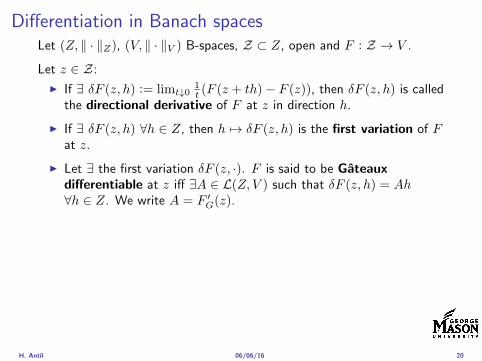
Differentiation in Banach spacesLet (Z middot Z) (V middot V ) B-spaces Z sub Z open and F Z rarr V
Let z isin Z
I If exist δF (z h) = limtdarr01t (F (z + th)minus F (z)) then δF (z h) is called
the directional derivative of F at z in direction h
I If exist δF (z h) forallh isin Z then h 7rarr δF (z h) is the first variation of Fat z
I Let exist the first variation δF (z middot) F is said to be Gateauxdifferentiable at z iff existA isin L(Z V ) such that δF (z h) = Ahforallh isin Z We write A = F primeG(z)
I F is said to be Frechet differentiable at z iff existA isin L(Z V ) and amapping r(z middot) Z rarr V such that for all h isin U with z + h isin Zwe have
F (z+h) = F (z)+Ah+r(z h) withr(z h)VhZ
rarr 0 as hZ rarr 0
We write F prime(z) = A
H Antil 060616 20
Differentiation in Banach spacesLet (Z middot Z) (V middot V ) B-spaces Z sub Z open and F Z rarr V
Let z isin Z
I If exist δF (z h) = limtdarr01t (F (z + th)minus F (z)) then δF (z h) is called
the directional derivative of F at z in direction h
I If exist δF (z h) forallh isin Z then h 7rarr δF (z h) is the first variation of Fat z
I Let exist the first variation δF (z middot) F is said to be Gateauxdifferentiable at z iff existA isin L(Z V ) such that δF (z h) = Ahforallh isin Z We write A = F primeG(z)
I F is said to be Frechet differentiable at z iff existA isin L(Z V ) and amapping r(z middot) Z rarr V such that for all h isin U with z + h isin Zwe have
F (z+h) = F (z)+Ah+r(z h) withr(z h)VhZ
rarr 0 as hZ rarr 0
We write F prime(z) = A
H Antil 060616 20
ExamplesExample 1 (H (middot middot)H) Hilbert space F (z) = z2H = (z z)H
forallz h F (z + h)minus F (z) = 2(z h)H + h2HThen
F prime(z)h = (2z h)H
Reisz representation theorem (identify H with Hlowast) we can write
F prime(z)h = (nablaF (z) h)H
where nablaF (z) = 2z is the gradient
Example 2 Let (Z (middot middot)Z) (H (middot middot)H) Hilbert spaces ud isin H fixedLet S isin L(ZH) Consider E Z rarr R
E(z) = Sz minus ud2H
Then E(z) = G(F (z)) where G(v) = v2H and F (z) = Sz minus ud
Eprime(z)h = Gprime(F (z))F prime(z)h = (2v F prime(z)h)H
= 2(Sz minus ud Sh)H = 2(Slowast(Sz minus ud) h)Z
we denote the gradient as nablaE(z) = 2Slowast(Sz minus ud)
H Antil 060616 21
ExamplesExample 1 (H (middot middot)H) Hilbert space F (z) = z2H = (z z)H
forallz h F (z + h)minus F (z) = 2(z h)H + h2HThen
F prime(z)h = (2z h)H
Reisz representation theorem (identify H with Hlowast) we can write
F prime(z)h = (nablaF (z) h)H
where nablaF (z) = 2z is the gradient
Example 2 Let (Z (middot middot)Z) (H (middot middot)H) Hilbert spaces ud isin H fixedLet S isin L(ZH) Consider E Z rarr R
E(z) = Sz minus ud2H
Then E(z) = G(F (z)) where G(v) = v2H and F (z) = Sz minus ud
Eprime(z)h = Gprime(F (z))F prime(z)h = (2v F prime(z)h)H
= 2(Sz minus ud Sh)H = 2(Slowast(Sz minus ud) h)Z
we denote the gradient as nablaE(z) = 2Slowast(Sz minus ud)H Antil 060616 21
Outline
Motivation and examples
Linear elliptic optimal control problems
Differentiation in Banach spaces
First-order necessary conditions
Optimal control of semilinear PDEs
An abstract problem
Discretization using finite element methods
H Antil 060616 22
First order necessary optimality conditions
Most of the theory is based on these two simple results
Theorem Let (Z middot Z) be a normed space J Z rarr (infin+infin] amapping with J 6equiv +infin Then z isin Z minimizer of J hArr 0 isin partJ (z)
Proof 0 isin partJ (z) means by definition of partJ (z) J (z)minus J (z) le 0forallz isin Z
Theorem Let (Z middot Z) be a normed space Zad sub Z nonemptyconvex closed J Z rarr R Gateaux differentiable where Zad sub Z sub ZZ open If z isin Zad is a solution to
minzisinZad
J (z)
then z solvesJ prime(z)(z minus z) ge 0 forallz isin Zad
Proof Exercise
H Antil 060616 23
First order necessary optimality conditions
Most of the theory is based on these two simple results
Theorem Let (Z middot Z) be a normed space J Z rarr (infin+infin] amapping with J 6equiv +infin Then z isin Z minimizer of J hArr 0 isin partJ (z)
Proof 0 isin partJ (z) means by definition of partJ (z) J (z)minus J (z) le 0forallz isin Z
Theorem Let (Z middot Z) be a normed space Zad sub Z nonemptyconvex closed J Z rarr R Gateaux differentiable where Zad sub Z sub ZZ open If z isin Zad is a solution to
minzisinZad
J (z)
then z solvesJ prime(z)(z minus z) ge 0 forallz isin Zad
Proof Exercise
H Antil 060616 23
Linear quadratic OCPI Reduced funcational
J (z) =1
2Sz minus ud2L2(Ω) +
λ
2z2L2(Ω)
I Gradient computation using sensitivity
J prime(z)h = (Slowast(Sz minus ud) + λz h)L2(Ω) forallh isin L2(Ω)
we denote the gradient by
nablaJ (z) = Slowast(Sz minus ud) + λz
I First order necessary and sufficient optimality condition
(nablaJ (z) z minus z)L2(Ω) ge 0 forallz isin Zad
I Adjoint equation Let p = Slowast(Sz minus ud) which translates intop isin H1
0 (Ω) solving
minusdiv (Anablap) = uminus ud in Ω
p = 0 on partΩ
I Gradient computation using adjoint nablaJ (z) = p+ λz
H Antil 060616 24
Linear quadratic OCPI Reduced funcational
J (z) =1
2Sz minus ud2L2(Ω) +
λ
2z2L2(Ω)
I Gradient computation using sensitivity
J prime(z)h = (Slowast(Sz minus ud) + λz h)L2(Ω) forallh isin L2(Ω)
we denote the gradient by
nablaJ (z) = Slowast(Sz minus ud) + λz
I First order necessary and sufficient optimality condition
(nablaJ (z) z minus z)L2(Ω) ge 0 forallz isin Zad
I Adjoint equation Let p = Slowast(Sz minus ud) which translates intop isin H1
0 (Ω) solving
minusdiv (Anablap) = uminus ud in Ω
p = 0 on partΩ
I Gradient computation using adjoint nablaJ (z) = p+ λz
H Antil 060616 24
Linear quadratic OCPI Reduced funcational
J (z) =1
2Sz minus ud2L2(Ω) +
λ
2z2L2(Ω)
I Gradient computation using sensitivity
J prime(z)h = (Slowast(Sz minus ud) + λz h)L2(Ω) forallh isin L2(Ω)
we denote the gradient by
nablaJ (z) = Slowast(Sz minus ud) + λz
I First order necessary and sufficient optimality condition
(nablaJ (z) z minus z)L2(Ω) ge 0 forallz isin Zad
I Adjoint equation Let p = Slowast(Sz minus ud) which translates intop isin H1
0 (Ω) solving
minusdiv (Anablap) = uminus ud in Ω
p = 0 on partΩ
I Gradient computation using adjoint nablaJ (z) = p+ λz
H Antil 060616 24
Linear quadratic OCPI Reduced funcational
J (z) =1
2Sz minus ud2L2(Ω) +
λ
2z2L2(Ω)
I Gradient computation using sensitivity
J prime(z)h = (Slowast(Sz minus ud) + λz h)L2(Ω) forallh isin L2(Ω)
we denote the gradient by
nablaJ (z) = Slowast(Sz minus ud) + λz
I First order necessary and sufficient optimality condition
(nablaJ (z) z minus z)L2(Ω) ge 0 forallz isin Zad
I Adjoint equation Let p = Slowast(Sz minus ud) which translates intop isin H1
0 (Ω) solving
minusdiv (Anablap) = uminus ud in Ω
p = 0 on partΩ
I Gradient computation using adjoint nablaJ (z) = p+ λz
H Antil 060616 24
Linear quadratic OCPI Reduced funcational
J (z) =1
2Sz minus ud2L2(Ω) +
λ
2z2L2(Ω)
I Gradient computation using sensitivity
J prime(z)h = (Slowast(Sz minus ud) + λz h)L2(Ω) forallh isin L2(Ω)
we denote the gradient by
nablaJ (z) = Slowast(Sz minus ud) + λz
I First order necessary and sufficient optimality condition
(nablaJ (z) z minus z)L2(Ω) ge 0 forallz isin Zad
I Adjoint equation Let p = Slowast(Sz minus ud) which translates intop isin H1
0 (Ω) solving
minusdiv (Anablap) = uminus ud in Ω
p = 0 on partΩ
I Gradient computation using adjoint nablaJ (z) = p+ λz
H Antil 060616 24
Optimality system
I State u isin H10 (Ω)
intΩAnablau middot nablav =
intΩzv forallv isin H1
0 (Ω)
I Adjoint p isin H10 (Ω)
intΩAnablap middot nablav =
intΩ
(uminus ud)v forallv isin H10 (Ω)
I Control z isin Zad (p+ λz z minus z) ge 0 forallz isin Zad
H Antil 060616 25
Pointwise interpretation
The variational inequality
(p+ λz z minus z) ge 0 forallz isin Zad
is equivalent to for ae x isin Ω
z(x) =
za(x) if p(x) + λz(x) gt 0isin [za(x) zb(x)] if p(x) + λz(x) = 0zb(x) if p(x) + λz(x) lt 0
Consequence
I When λ gt 0 then ae in Ω
z(x) = P[za(x)zb(x)]
minus 1
λp(x)
= min
zb(x)max
za(x)minus 1
λp(x)
H Antil 060616 26
Formal Lagrange method applied to linear OCPIntroduce L H1
0 (Ω)times Zad timesH1(Ω)rarr R defined as
L(u z p) = J(u z)minusint
Ω
(minusdiv (Anablau)minus z
)p dx
Integrate by parts to arrive at
L(u z p) = J(u z)minusint
Ω
(minusdiv (Anablap)uminus zp
)dx+
intpartΩ
(Anablau)p ds
If (u z p) is a stationary point then
I State
DpL(u z p)h = 0 forallh isin H1(Ω)
I AdjointDuL(u z p)h = 0 forallh isin H1
0 (Ω)
I ControlDzL(u z p)(z minus z) ge 0 forallz isin Zad
H Antil 060616 27
Formal Lagrange method applied to linear OCPIntroduce L H1
0 (Ω)times Zad timesH1(Ω)rarr R defined as
L(u z p) = J(u z)minusint
Ω
(minusdiv (Anablau)minus z
)p dx
Integrate by parts to arrive at
L(u z p) = J(u z)minusint
Ω
(minusdiv (Anablap)uminus zp
)dx+
intpartΩ
(Anablau)p ds
If (u z p) is a stationary point then
I State
DpL(u z p)h = 0 forallh isin H1(Ω)
I AdjointDuL(u z p)h = 0 forallh isin H1
0 (Ω)
I ControlDzL(u z p)(z minus z) ge 0 forallz isin Zad
H Antil 060616 27
Formal Lagrange method applied to linear OCPIntroduce L H1
0 (Ω)times Zad timesH1(Ω)rarr R defined as
L(u z p) = J(u z)minusint
Ω
(minusdiv (Anablau)minus z
)p dx
Integrate by parts to arrive at
L(u z p) = J(u z)minusint
Ω
(minusdiv (Anablap)uminus zp
)dx+
intpartΩ
(Anablau)p ds
If (u z p) is a stationary point then
I State
DpL(u z p)h = 0 forallh isin H1(Ω)
I AdjointDuL(u z p)h = 0 forallh isin H1
0 (Ω)
I ControlDzL(u z p)(z minus z) ge 0 forallz isin Zad
H Antil 060616 27
Formal Lagrange method applied to linear OCPIntroduce L H1
0 (Ω)times Zad timesH1(Ω)rarr R defined as
L(u z p) = J(u z)minusint
Ω
(minusdiv (Anablau)minus z
)p dx
Integrate by parts to arrive at
L(u z p) = J(u z)minusint
Ω
(minusdiv (Anablap)uminus zp
)dx+
intpartΩ
(Anablau)p ds
If (u z p) is a stationary point then
I State
DpL(u z p)h = 0 forallh isin H1(Ω)
I AdjointDuL(u z p)h = 0 forallh isin H1
0 (Ω)
I ControlDzL(u z p)(z minus z) ge 0 forallz isin Zad
H Antil 060616 27
Formal Lagrange method applied to linear OCPIntroduce L H1
0 (Ω)times Zad timesH1(Ω)rarr R defined as
L(u z p) = J(u z)minusint
Ω
(minusdiv (Anablau)minus z
)p dx
Integrate by parts to arrive at
L(u z p) = J(u z)minusint
Ω
(minusdiv (Anablap)uminus zp
)dx+
intpartΩ
(Anablau)p ds
If (u z p) is a stationary point then
I State
DpL(u z p)h = 0 forallh isin H1(Ω)
I AdjointDuL(u z p)h = 0 forallh isin H1
0 (Ω)
I ControlDzL(u z p)(z minus z) ge 0 forallz isin Zad
H Antil 060616 27
Outline
Motivation and examples
Linear elliptic optimal control problems
Differentiation in Banach spaces
First-order necessary conditions
Optimal control of semilinear PDEs
An abstract problem
Discretization using finite element methods
H Antil 060616 28
Semilinear elliptic OCP
min J(u z) =1
2uminus ud2L2(Ω) +
λ
2z2L2(Ω)
subject to
minus∆u+ g(x u) = z in Ω
u = 0 on partΩ
and z isin Zad with za zb isin Linfin(Ω)
H Antil 060616 29
State space(A1) Ω sub Rd open bounded partΩ is Lipschitz
(A2) g Ωtimes Rrarr R is bounded and measurable with respect to x isin Ωfor every u isin R
(A3) g is continuous monotone increasing and Lipschitz continuous in ufor ae x isin Ω
(A4) g(x 0) = 0 for ae x isin Ω (not really necessary)
Theorem Suppose (A1)minus (A4) hold For every z isin Lr(Ω) withr gt d2 the state equation has a unique weak solutionu isin H1
0 (Ω) cap C(Ω) ie we haveintΩ
nablau middot nablav dx+
intΩ
g(x u(x))v(x) dx =
intΩ
zv dx forallv isin H10 (Ω)
Moreover there exists a constant C gt 0 such that
uH1(Ω) + uC(Ω) le CzLr(Ω)
RemarkI The proof of the theorem uses the BrowderndashMinty theorem on
monotone operators
H Antil 060616 30
State space(A1) Ω sub Rd open bounded partΩ is Lipschitz
(A2) g Ωtimes Rrarr R is bounded and measurable with respect to x isin Ωfor every u isin R
(A3) g is continuous monotone increasing and Lipschitz continuous in ufor ae x isin Ω
(A4) g(x 0) = 0 for ae x isin Ω (not really necessary)
Theorem Suppose (A1)minus (A4) hold For every z isin Lr(Ω) withr gt d2 the state equation has a unique weak solutionu isin H1
0 (Ω) cap C(Ω) ie we haveintΩ
nablau middot nablav dx+
intΩ
g(x u(x))v(x) dx =
intΩ
zv dx forallv isin H10 (Ω)
Moreover there exists a constant C gt 0 such that
uH1(Ω) + uC(Ω) le CzLr(Ω)
RemarkI The proof of the theorem uses the BrowderndashMinty theorem on
monotone operators
H Antil 060616 30
State space(A1) Ω sub Rd open bounded partΩ is Lipschitz
(A2) g Ωtimes Rrarr R is bounded and measurable with respect to x isin Ωfor every u isin R
(A3) g is continuous monotone increasing and Lipschitz continuous in ufor ae x isin Ω
(A4) g(x 0) = 0 for ae x isin Ω (not really necessary)
Theorem Suppose (A1)minus (A4) hold For every z isin Lr(Ω) withr gt d2 the state equation has a unique weak solutionu isin H1
0 (Ω) cap C(Ω) ie we haveintΩ
nablau middot nablav dx+
intΩ
g(x u(x))v(x) dx =
intΩ
zv dx forallv isin H10 (Ω)
Moreover there exists a constant C gt 0 such that
uH1(Ω) + uC(Ω) le CzLr(Ω)
RemarkI The proof of the theorem uses the BrowderndashMinty theorem on
monotone operators
H Antil 060616 30
Control-to-state map and reduced problem
I Control to state map
S Linfin(Ω)rarr H10 (Ω) cap C(Ω)
is well defined and is globally Lipschitz continuous
I Reduced problem
minJ (z) =1
2S(u)minus ud2L2(Ω) +
λ
2z2L2(Ω)
H Antil 060616 31
Control-to-state map and reduced problem
I Control to state map
S Linfin(Ω)rarr H10 (Ω) cap C(Ω)
is well defined and is globally Lipschitz continuous
I Reduced problem
minJ (z) =1
2S(u)minus ud2L2(Ω) +
λ
2z2L2(Ω)
H Antil 060616 31
First-order necessary conditionsI Lagrangian functional
L(u z p) = J(u z)minusint
Ω
(minus∆u+ g(x u(x))minus z
)p dx
= J(u z)minusint
Ω
(nablau middot nablap+ g(x u(x))pminus zp
)dx
I Adjoint system For all h isin H10 (Ω)
0 = DuL(u z p)h =
intΩ
(uminus ud)h dxminusint
Ω
(nablah middot nablap+ gu(x u(x))ph
)which yields
minus∆p+ gu(x u(x))p = uminus ud in Ω
p = 0 on partΩ
I Control
DzL(u z p)(z minus z) = (p+ λz z minus z) dx ge 0 forallz isin ZadI Gradient
nablaJ (z) = p+ λz
H Antil 060616 32
First-order necessary conditionsI Lagrangian functional
L(u z p) = J(u z)minusint
Ω
(minus∆u+ g(x u(x))minus z
)p dx
= J(u z)minusint
Ω
(nablau middot nablap+ g(x u(x))pminus zp
)dx
I Adjoint system For all h isin H10 (Ω)
0 = DuL(u z p)h =
intΩ
(uminus ud)h dxminusint
Ω
(nablah middot nablap+ gu(x u(x))ph
)which yields
minus∆p+ gu(x u(x))p = uminus ud in Ω
p = 0 on partΩ
I Control
DzL(u z p)(z minus z) = (p+ λz z minus z) dx ge 0 forallz isin ZadI Gradient
nablaJ (z) = p+ λz
H Antil 060616 32
First-order necessary conditionsI Lagrangian functional
L(u z p) = J(u z)minusint
Ω
(minus∆u+ g(x u(x))minus z
)p dx
= J(u z)minusint
Ω
(nablau middot nablap+ g(x u(x))pminus zp
)dx
I Adjoint system For all h isin H10 (Ω)
0 = DuL(u z p)h =
intΩ
(uminus ud)h dxminusint
Ω
(nablah middot nablap+ gu(x u(x))ph
)which yields
minus∆p+ gu(x u(x))p = uminus ud in Ω
p = 0 on partΩ
I Control
DzL(u z p)(z minus z) = (p+ λz z minus z) dx ge 0 forallz isin Zad
I GradientnablaJ (z) = p+ λz
H Antil 060616 32
First-order necessary conditionsI Lagrangian functional
L(u z p) = J(u z)minusint
Ω
(minus∆u+ g(x u(x))minus z
)p dx
= J(u z)minusint
Ω
(nablau middot nablap+ g(x u(x))pminus zp
)dx
I Adjoint system For all h isin H10 (Ω)
0 = DuL(u z p)h =
intΩ
(uminus ud)h dxminusint
Ω
(nablah middot nablap+ gu(x u(x))ph
)which yields
minus∆p+ gu(x u(x))p = uminus ud in Ω
p = 0 on partΩ
I Control
DzL(u z p)(z minus z) = (p+ λz z minus z) dx ge 0 forallz isin ZadI Gradient
nablaJ (z) = p+ λz
H Antil 060616 32
Differentiability of Nemytskii operator
The rigorous proof uses
Theorem In addition to (A1)-(A4) if
(A5) g is continuously differentiable with respect to u for ae x isin Ωand we have
(i) |gu(x 0)| le K for ae x isin Ω(ii) gu is locally Lipschitz with respect to u isin R
then the Nemytskii operator G u 7rarr g(middot u(middot)) is continuously Frechetdifferentiable from Linfin(Ω) into itself and
(Gprime(u)h)(x) = gu(x u(x))h(x) ae in Ω forallh isin Linfin(Ω)
Remark (A5) holds if g(x u) = g(u) and g isin C2(R)
H Antil 060616 33
Outline
Motivation and examples
Linear elliptic optimal control problems
Differentiation in Banach spaces
First-order necessary conditions
Optimal control of semilinear PDEs
An abstract problem
Discretization using finite element methods
H Antil 060616 34
Gradient computation via adjoint general formI Abstract problem
min J(u z)
subject toc(u z) = 0
and z isin Zad
I Directional derivative Let S be the control to state map(nonlinear in general)
z 7rarr S(z) = u(z)
Under the assumptions of ldquoimplicit function theoremrdquo
J prime(z)h = (nablauJ (u(z) z) Sprime(z)h) + (nablazJ (u(z) z) h)
I Sensitivity of u with respect to z Differentiating the stateequation
cu(S(z) z)Sprime(z)h = minuscz(S(z) z)h
leads toSprime(z)h = minuscu(S(z) z)minus1
(cz(S(z) z)h
)
provided cu(S(z) z)minus1 is well-defined
H Antil 060616 35
Gradient computation via adjoint general formI Abstract problem
min J(u z)
subject toc(u z) = 0
and z isin ZadI Directional derivative Let S be the control to state map
(nonlinear in general)
z 7rarr S(z) = u(z)
Under the assumptions of ldquoimplicit function theoremrdquo
J prime(z)h = (nablauJ (u(z) z) Sprime(z)h) + (nablazJ (u(z) z) h)
I Sensitivity of u with respect to z Differentiating the stateequation
cu(S(z) z)Sprime(z)h = minuscz(S(z) z)h
leads toSprime(z)h = minuscu(S(z) z)minus1
(cz(S(z) z)h
)
provided cu(S(z) z)minus1 is well-defined
H Antil 060616 35
Gradient computation via adjoint general formI Abstract problem
min J(u z)
subject toc(u z) = 0
and z isin ZadI Directional derivative Let S be the control to state map
(nonlinear in general)
z 7rarr S(z) = u(z)
Under the assumptions of ldquoimplicit function theoremrdquo
J prime(z)h = (nablauJ (u(z) z) Sprime(z)h) + (nablazJ (u(z) z) h)
I Sensitivity of u with respect to z Differentiating the stateequation
cu(S(z) z)Sprime(z)h = minuscz(S(z) z)h
leads toSprime(z)h = minuscu(S(z) z)minus1
(cz(S(z) z)h
)
provided cu(S(z) z)minus1 is well-defined
H Antil 060616 35
Adjoint equation and gradient general form
I Directional derivative
J prime(z)h = minus(nablauJ (u(z) z) cu(u(z) z)minus1cz(u(z) z)h
)+ (nablazJ (u(z) z) h)
I Gradient
nablaJ (z) = minuscz(u(z) z)lowast(cu(u(z) z)minuslowastnablauJ (u(z) z)
)+nablazJ (u(z) z)
I Introducing adjoint variable p solving
cu(u(z) z)lowastp = nablauJ (u(z) z)
we arrive at following form of gradient
nablaJ (z) = minuscz(u(z) z)lowastp+nablazJ (u(z) z)
which is tractable
H Antil 060616 36
Adjoint equation and gradient general form
I Directional derivative
J prime(z)h = minus(nablauJ (u(z) z) cu(u(z) z)minus1cz(u(z) z)h
)+ (nablazJ (u(z) z) h)
I Gradient
nablaJ (z) = minuscz(u(z) z)lowast(cu(u(z) z)minuslowastnablauJ (u(z) z)
)+nablazJ (u(z) z)
I Introducing adjoint variable p solving
cu(u(z) z)lowastp = nablauJ (u(z) z)
we arrive at following form of gradient
nablaJ (z) = minuscz(u(z) z)lowastp+nablazJ (u(z) z)
which is tractable
H Antil 060616 36
Adjoint equation and gradient general form
I Directional derivative
J prime(z)h = minus(nablauJ (u(z) z) cu(u(z) z)minus1cz(u(z) z)h
)+ (nablazJ (u(z) z) h)
I Gradient
nablaJ (z) = minuscz(u(z) z)lowast(cu(u(z) z)minuslowastnablauJ (u(z) z)
)+nablazJ (u(z) z)
I Introducing adjoint variable p solving
cu(u(z) z)lowastp = nablauJ (u(z) z)
we arrive at following form of gradient
nablaJ (z) = minuscz(u(z) z)lowastp+nablazJ (u(z) z)
which is tractable
H Antil 060616 36
Hessian computation general form
I Lagrangian L(u z p) = J(u z)minusint
Ωc(u z)p dx Then we have
DzJ (z)h = DzL(u z p)h
I Second order derivative
D2zJ (z)[h1 h2] = DuDzL(u z p)[h1 S
prime(z)h2] +D2zL(u z p)[h1 h2]
+DpDzL(u z p)[h1 Dzp(z)h2]
I We already know Sprime(z)h2 moreover
DpDzL(u z p)[h1 Dzp(z)h2] = minus(cu(u z)h1 Dzp(z)h2
)
It remain to identify Dzp(z)h2
H Antil 060616 37
Hessian computation general form
I Lagrangian L(u z p) = J(u z)minusint
Ωc(u z)p dx Then we have
DzJ (z)h = DzL(u z p)h
I Second order derivative
D2zJ (z)[h1 h2] = DuDzL(u z p)[h1 S
prime(z)h2] +D2zL(u z p)[h1 h2]
+DpDzL(u z p)[h1 Dzp(z)h2]
I We already know Sprime(z)h2 moreover
DpDzL(u z p)[h1 Dzp(z)h2] = minus(cu(u z)h1 Dzp(z)h2
)
It remain to identify Dzp(z)h2
H Antil 060616 37
Hessian computation general form
I Lagrangian L(u z p) = J(u z)minusint
Ωc(u z)p dx Then we have
DzJ (z)h = DzL(u z p)h
I Second order derivative
D2zJ (z)[h1 h2] = DuDzL(u z p)[h1 S
prime(z)h2] +D2zL(u z p)[h1 h2]
+DpDzL(u z p)[h1 Dzp(z)h2]
I We already know Sprime(z)h2 moreover
DpDzL(u z p)[h1 Dzp(z)h2] = minus(cu(u z)h1 Dzp(z)h2
)
It remain to identify Dzp(z)h2
H Antil 060616 37
Outline
Motivation and examples
Linear elliptic optimal control problems
Differentiation in Banach spaces
First-order necessary conditions
Optimal control of semilinear PDEs
An abstract problem
Discretization using finite element methods
H Antil 060616 38
Numerical approximation of Poisson equation MeshTo avoid technical issues we will assume that partΩ is polygonal
I Mesh Let T = K be a mesh of Ω where K sub Rd is an elementthat is isoparametrically equivalent to a unit simplex in Rd
I Conforming mesh We say that the mesh is conforming ifI Ω = cupKisinT KI If K1 cap K2 = x then x is a node of K1 and K2I If K1 cap K2 6= empty and K1 cap K2 6= x then K1 cap K2 is an edgeface
contained in partK1 cap partK2
I Shape regular Let T be the collection of all conformingrefinements of an original mesh T 0 Then T is called shape regularif exist κ gt 0 such that
hKρKle κ forallK isin cupiT i
where hK = diam K ρK = maxρ gt 0|Bρ sub KI Quasi-uniform A family of shape regular meshes is called-quasi
uniform if there exist a constant σ gt 0 such that
maxhKminhK
le σ
uniformly for all meshes in the family
Numerical approximation of Poisson equation MeshTo avoid technical issues we will assume that partΩ is polygonal
I Mesh Let T = K be a mesh of Ω where K sub Rd is an elementthat is isoparametrically equivalent to a unit simplex in Rd
I Conforming mesh We say that the mesh is conforming ifI Ω = cupKisinT KI If K1 cap K2 = x then x is a node of K1 and K2I If K1 cap K2 6= empty and K1 cap K2 6= x then K1 cap K2 is an edgeface
contained in partK1 cap partK2
I Shape regular Let T be the collection of all conformingrefinements of an original mesh T 0 Then T is called shape regularif exist κ gt 0 such that
hKρKle κ forallK isin cupiT i
where hK = diam K ρK = maxρ gt 0|Bρ sub KI Quasi-uniform A family of shape regular meshes is called-quasi
uniform if there exist a constant σ gt 0 such that
maxhKminhK
le σ
uniformly for all meshes in the family
Numerical approximation of Poisson equation MeshTo avoid technical issues we will assume that partΩ is polygonal
I Mesh Let T = K be a mesh of Ω where K sub Rd is an elementthat is isoparametrically equivalent to a unit simplex in Rd
I Conforming mesh We say that the mesh is conforming ifI Ω = cupKisinT KI If K1 cap K2 = x then x is a node of K1 and K2I If K1 cap K2 6= empty and K1 cap K2 6= x then K1 cap K2 is an edgeface
contained in partK1 cap partK2
I Shape regular Let T be the collection of all conformingrefinements of an original mesh T 0 Then T is called shape regularif exist κ gt 0 such that
hKρKle κ forallK isin cupiT i
where hK = diam K ρK = maxρ gt 0|Bρ sub K
I Quasi-uniform A family of shape regular meshes is called-quasiuniform if there exist a constant σ gt 0 such that
maxhKminhK
le σ
uniformly for all meshes in the family
Numerical approximation of Poisson equation MeshTo avoid technical issues we will assume that partΩ is polygonal
I Mesh Let T = K be a mesh of Ω where K sub Rd is an elementthat is isoparametrically equivalent to a unit simplex in Rd
I Conforming mesh We say that the mesh is conforming ifI Ω = cupKisinT KI If K1 cap K2 = x then x is a node of K1 and K2I If K1 cap K2 6= empty and K1 cap K2 6= x then K1 cap K2 is an edgeface
contained in partK1 cap partK2
I Shape regular Let T be the collection of all conformingrefinements of an original mesh T 0 Then T is called shape regularif exist κ gt 0 such that
hKρKle κ forallK isin cupiT i
where hK = diam K ρK = maxρ gt 0|Bρ sub KI Quasi-uniform A family of shape regular meshes is called-quasi
uniform if there exist a constant σ gt 0 such that
maxhKminhK
le σ
uniformly for all meshes in the family
FE space and Galerkin approximationI Finite element space For T isin T we define the finite element
space as
V(T ) = W isin C0(Ω) WK isin P1forallK isin T W |partΩ = 0
where P1 is the set of polynomials of degree at most 1
I Galerkin approximation of continuous problem is given by
Find UT isin V(T )
intΩ
AnablaUT middot nablaV = 〈f V 〉 forallV isin V(T )
The discrete problem is well-posedI Nodal basis Consists of functions ψi isin V(T ) with xi isin N (T )
satisfyingψxi
(xj) = δij
where N (T ) denotes the interior (plus Neumann) nodesI Galerkin orthogonality(
nabla(uminus UT )nablaW)L2(Ω)
= 0 forallW isin V(T )
H Antil 060616 40
FE space and Galerkin approximationI Finite element space For T isin T we define the finite element
space as
V(T ) = W isin C0(Ω) WK isin P1forallK isin T W |partΩ = 0
where P1 is the set of polynomials of degree at most 1I Galerkin approximation of continuous problem is given by
Find UT isin V(T )
intΩ
AnablaUT middot nablaV = 〈f V 〉 forallV isin V(T )
The discrete problem is well-posed
I Nodal basis Consists of functions ψi isin V(T ) with xi isin N (T )satisfying
ψxi(xj) = δij
where N (T ) denotes the interior (plus Neumann) nodesI Galerkin orthogonality(
nabla(uminus UT )nablaW)L2(Ω)
= 0 forallW isin V(T )
H Antil 060616 40
FE space and Galerkin approximationI Finite element space For T isin T we define the finite element
space as
V(T ) = W isin C0(Ω) WK isin P1forallK isin T W |partΩ = 0
where P1 is the set of polynomials of degree at most 1I Galerkin approximation of continuous problem is given by
Find UT isin V(T )
intΩ
AnablaUT middot nablaV = 〈f V 〉 forallV isin V(T )
The discrete problem is well-posedI Nodal basis Consists of functions ψi isin V(T ) with xi isin N (T )
satisfyingψxi
(xj) = δij
where N (T ) denotes the interior (plus Neumann) nodes
I Galerkin orthogonality(nabla(uminus UT )nablaW
)L2(Ω)
= 0 forallW isin V(T )
H Antil 060616 40
FE space and Galerkin approximationI Finite element space For T isin T we define the finite element
space as
V(T ) = W isin C0(Ω) WK isin P1forallK isin T W |partΩ = 0
where P1 is the set of polynomials of degree at most 1I Galerkin approximation of continuous problem is given by
Find UT isin V(T )
intΩ
AnablaUT middot nablaV = 〈f V 〉 forallV isin V(T )
The discrete problem is well-posedI Nodal basis Consists of functions ψi isin V(T ) with xi isin N (T )
satisfyingψxi
(xj) = δij
where N (T ) denotes the interior (plus Neumann) nodesI Galerkin orthogonality(
nabla(uminus UT )nablaW)L2(Ω)
= 0 forallW isin V(T )
H Antil 060616 40
Best approximation
I Cearsquos lemma
nabla(uminus UT )L2(Ω) le C infWisinV(T )
nabla(uminusW )L2(Ω)
I Nodal interpolation operator ΠT C(Ω)rarr V(T ) satisfies
ΠT u(xi) = u(xi) forallxi isin N (T )
and is defined as
ΠT u =sum
xiisinN (T )
u(xi)ψxi
I Error estimates In Cearsquos lemma replace W by ΠT u and thencompute the interpolation error
H Antil 060616 41
Best approximation
I Cearsquos lemma
nabla(uminus UT )L2(Ω) le C infWisinV(T )
nabla(uminusW )L2(Ω)
I Nodal interpolation operator ΠT C(Ω)rarr V(T ) satisfies
ΠT u(xi) = u(xi) forallxi isin N (T )
and is defined as
ΠT u =sum
xiisinN (T )
u(xi)ψxi
I Error estimates In Cearsquos lemma replace W by ΠT u and thencompute the interpolation error
H Antil 060616 41
Best approximation
I Cearsquos lemma
nabla(uminus UT )L2(Ω) le C infWisinV(T )
nabla(uminusW )L2(Ω)
I Nodal interpolation operator ΠT C(Ω)rarr V(T ) satisfies
ΠT u(xi) = u(xi) forallxi isin N (T )
and is defined as
ΠT u =sum
xiisinN (T )
u(xi)ψxi
I Error estimates In Cearsquos lemma replace W by ΠT u and thencompute the interpolation error
H Antil 060616 41
Algebraic system state equation
I Recall UT isin V(T ) solves
a(UT V ) = 〈f V 〉 forallV isin V(T )
I Now setting UT =sumN
j=1 Ujψj V = ψi we get
Nsumj=1
Uja(φj φi) = 〈f ψi〉 i = 1 N
which is the matrix-vector system
AU = F
I Stiffness matrix A is SPD
H Antil 060616 42
Algebraic system state equation
I Recall UT isin V(T ) solves
a(UT V ) = 〈f V 〉 forallV isin V(T )
I Now setting UT =sumN
j=1 Ujψj V = ψi we get
Nsumj=1
Uja(φj φi) = 〈f ψi〉 i = 1 N
which is the matrix-vector system
AU = F
I Stiffness matrix A is SPD
H Antil 060616 42
Algebraic system state equation
I Recall UT isin V(T ) solves
a(UT V ) = 〈f V 〉 forallV isin V(T )
I Now setting UT =sumN
j=1 Ujψj V = ψi we get
Nsumj=1
Uja(φj φi) = 〈f ψi〉 i = 1 N
which is the matrix-vector system
AU = F
I Stiffness matrix A is SPD
H Antil 060616 42
Discrete linear elliptic OCP
min JT (UT ZT ) =1
2UT minus ud2L2(Ω) +
λ
2ZT 2L2(Ω)
subject to
Find UT isin V(T )
intΩ
nablaUT middot nablaV = (ZT V )L2(Ω) forallV isin V(T )
and whereZT isin Zad(T ) = Zad cap Z(T )
is either one of these
Z(T ) =
V(T )L2(Ω) variational discretization (Hinze)WT isin Linfin(Ω) ZT |K isin P0(K)K isin T
H Antil 060616 43
Recent books
F TroltzschOptimal control of partial differential equations volume 112 ofGraduate Studies in MathematicsAmerican Mathematical Society Providence RI 2010Theory methods and applications Translated from the 2005 Germanoriginal by Jurgen Sprekels
K Ito and K KunischLagrange multiplier approach to variational problems andapplications volume 15 of Advances in Design and ControlSociety for Industrial and Applied Mathematics (SIAM)Philadelphia PA 2008
H Antil 060616 44
- Motivation and examples
- Linear elliptic optimal control problems
- Differentiation in Banach spaces
- First-order necessary conditions
- Optimal control of semilinear PDEs
- An abstract problem
- Discretization using finite element methods
-

Differentiation in Banach spacesLet (Z middot Z) (V middot V ) B-spaces Z sub Z open and F Z rarr V
Let z isin Z
I If exist δF (z h) = limtdarr01t (F (z + th)minus F (z)) then δF (z h) is called
the directional derivative of F at z in direction h
I If exist δF (z h) forallh isin Z then h 7rarr δF (z h) is the first variation of Fat z
I Let exist the first variation δF (z middot) F is said to be Gateauxdifferentiable at z iff existA isin L(Z V ) such that δF (z h) = Ahforallh isin Z We write A = F primeG(z)
I F is said to be Frechet differentiable at z iff existA isin L(Z V ) and amapping r(z middot) Z rarr V such that for all h isin U with z + h isin Zwe have
F (z+h) = F (z)+Ah+r(z h) withr(z h)VhZ
rarr 0 as hZ rarr 0
We write F prime(z) = A
H Antil 060616 20
ExamplesExample 1 (H (middot middot)H) Hilbert space F (z) = z2H = (z z)H
forallz h F (z + h)minus F (z) = 2(z h)H + h2HThen
F prime(z)h = (2z h)H
Reisz representation theorem (identify H with Hlowast) we can write
F prime(z)h = (nablaF (z) h)H
where nablaF (z) = 2z is the gradient
Example 2 Let (Z (middot middot)Z) (H (middot middot)H) Hilbert spaces ud isin H fixedLet S isin L(ZH) Consider E Z rarr R
E(z) = Sz minus ud2H
Then E(z) = G(F (z)) where G(v) = v2H and F (z) = Sz minus ud
Eprime(z)h = Gprime(F (z))F prime(z)h = (2v F prime(z)h)H
= 2(Sz minus ud Sh)H = 2(Slowast(Sz minus ud) h)Z
we denote the gradient as nablaE(z) = 2Slowast(Sz minus ud)
H Antil 060616 21
ExamplesExample 1 (H (middot middot)H) Hilbert space F (z) = z2H = (z z)H
forallz h F (z + h)minus F (z) = 2(z h)H + h2HThen
F prime(z)h = (2z h)H
Reisz representation theorem (identify H with Hlowast) we can write
F prime(z)h = (nablaF (z) h)H
where nablaF (z) = 2z is the gradient
Example 2 Let (Z (middot middot)Z) (H (middot middot)H) Hilbert spaces ud isin H fixedLet S isin L(ZH) Consider E Z rarr R
E(z) = Sz minus ud2H
Then E(z) = G(F (z)) where G(v) = v2H and F (z) = Sz minus ud
Eprime(z)h = Gprime(F (z))F prime(z)h = (2v F prime(z)h)H
= 2(Sz minus ud Sh)H = 2(Slowast(Sz minus ud) h)Z
we denote the gradient as nablaE(z) = 2Slowast(Sz minus ud)H Antil 060616 21
Outline
Motivation and examples
Linear elliptic optimal control problems
Differentiation in Banach spaces
First-order necessary conditions
Optimal control of semilinear PDEs
An abstract problem
Discretization using finite element methods
H Antil 060616 22
First order necessary optimality conditions
Most of the theory is based on these two simple results
Theorem Let (Z middot Z) be a normed space J Z rarr (infin+infin] amapping with J 6equiv +infin Then z isin Z minimizer of J hArr 0 isin partJ (z)
Proof 0 isin partJ (z) means by definition of partJ (z) J (z)minus J (z) le 0forallz isin Z
Theorem Let (Z middot Z) be a normed space Zad sub Z nonemptyconvex closed J Z rarr R Gateaux differentiable where Zad sub Z sub ZZ open If z isin Zad is a solution to
minzisinZad
J (z)
then z solvesJ prime(z)(z minus z) ge 0 forallz isin Zad
Proof Exercise
H Antil 060616 23
First order necessary optimality conditions
Most of the theory is based on these two simple results
Theorem Let (Z middot Z) be a normed space J Z rarr (infin+infin] amapping with J 6equiv +infin Then z isin Z minimizer of J hArr 0 isin partJ (z)
Proof 0 isin partJ (z) means by definition of partJ (z) J (z)minus J (z) le 0forallz isin Z
Theorem Let (Z middot Z) be a normed space Zad sub Z nonemptyconvex closed J Z rarr R Gateaux differentiable where Zad sub Z sub ZZ open If z isin Zad is a solution to
minzisinZad
J (z)
then z solvesJ prime(z)(z minus z) ge 0 forallz isin Zad
Proof Exercise
H Antil 060616 23
Linear quadratic OCPI Reduced funcational
J (z) =1
2Sz minus ud2L2(Ω) +
λ
2z2L2(Ω)
I Gradient computation using sensitivity
J prime(z)h = (Slowast(Sz minus ud) + λz h)L2(Ω) forallh isin L2(Ω)
we denote the gradient by
nablaJ (z) = Slowast(Sz minus ud) + λz
I First order necessary and sufficient optimality condition
(nablaJ (z) z minus z)L2(Ω) ge 0 forallz isin Zad
I Adjoint equation Let p = Slowast(Sz minus ud) which translates intop isin H1
0 (Ω) solving
minusdiv (Anablap) = uminus ud in Ω
p = 0 on partΩ
I Gradient computation using adjoint nablaJ (z) = p+ λz
H Antil 060616 24
Linear quadratic OCPI Reduced funcational
J (z) =1
2Sz minus ud2L2(Ω) +
λ
2z2L2(Ω)
I Gradient computation using sensitivity
J prime(z)h = (Slowast(Sz minus ud) + λz h)L2(Ω) forallh isin L2(Ω)
we denote the gradient by
nablaJ (z) = Slowast(Sz minus ud) + λz
I First order necessary and sufficient optimality condition
(nablaJ (z) z minus z)L2(Ω) ge 0 forallz isin Zad
I Adjoint equation Let p = Slowast(Sz minus ud) which translates intop isin H1
0 (Ω) solving
minusdiv (Anablap) = uminus ud in Ω
p = 0 on partΩ
I Gradient computation using adjoint nablaJ (z) = p+ λz
H Antil 060616 24
Linear quadratic OCPI Reduced funcational
J (z) =1
2Sz minus ud2L2(Ω) +
λ
2z2L2(Ω)
I Gradient computation using sensitivity
J prime(z)h = (Slowast(Sz minus ud) + λz h)L2(Ω) forallh isin L2(Ω)
we denote the gradient by
nablaJ (z) = Slowast(Sz minus ud) + λz
I First order necessary and sufficient optimality condition
(nablaJ (z) z minus z)L2(Ω) ge 0 forallz isin Zad
I Adjoint equation Let p = Slowast(Sz minus ud) which translates intop isin H1
0 (Ω) solving
minusdiv (Anablap) = uminus ud in Ω
p = 0 on partΩ
I Gradient computation using adjoint nablaJ (z) = p+ λz
H Antil 060616 24
Linear quadratic OCPI Reduced funcational
J (z) =1
2Sz minus ud2L2(Ω) +
λ
2z2L2(Ω)
I Gradient computation using sensitivity
J prime(z)h = (Slowast(Sz minus ud) + λz h)L2(Ω) forallh isin L2(Ω)
we denote the gradient by
nablaJ (z) = Slowast(Sz minus ud) + λz
I First order necessary and sufficient optimality condition
(nablaJ (z) z minus z)L2(Ω) ge 0 forallz isin Zad
I Adjoint equation Let p = Slowast(Sz minus ud) which translates intop isin H1
0 (Ω) solving
minusdiv (Anablap) = uminus ud in Ω
p = 0 on partΩ
I Gradient computation using adjoint nablaJ (z) = p+ λz
H Antil 060616 24
Linear quadratic OCPI Reduced funcational
J (z) =1
2Sz minus ud2L2(Ω) +
λ
2z2L2(Ω)
I Gradient computation using sensitivity
J prime(z)h = (Slowast(Sz minus ud) + λz h)L2(Ω) forallh isin L2(Ω)
we denote the gradient by
nablaJ (z) = Slowast(Sz minus ud) + λz
I First order necessary and sufficient optimality condition
(nablaJ (z) z minus z)L2(Ω) ge 0 forallz isin Zad
I Adjoint equation Let p = Slowast(Sz minus ud) which translates intop isin H1
0 (Ω) solving
minusdiv (Anablap) = uminus ud in Ω
p = 0 on partΩ
I Gradient computation using adjoint nablaJ (z) = p+ λz
H Antil 060616 24
Optimality system
I State u isin H10 (Ω)
intΩAnablau middot nablav =
intΩzv forallv isin H1
0 (Ω)
I Adjoint p isin H10 (Ω)
intΩAnablap middot nablav =
intΩ
(uminus ud)v forallv isin H10 (Ω)
I Control z isin Zad (p+ λz z minus z) ge 0 forallz isin Zad
H Antil 060616 25
Pointwise interpretation
The variational inequality
(p+ λz z minus z) ge 0 forallz isin Zad
is equivalent to for ae x isin Ω
z(x) =
za(x) if p(x) + λz(x) gt 0isin [za(x) zb(x)] if p(x) + λz(x) = 0zb(x) if p(x) + λz(x) lt 0
Consequence
I When λ gt 0 then ae in Ω
z(x) = P[za(x)zb(x)]
minus 1
λp(x)
= min
zb(x)max
za(x)minus 1
λp(x)
H Antil 060616 26
Formal Lagrange method applied to linear OCPIntroduce L H1
0 (Ω)times Zad timesH1(Ω)rarr R defined as
L(u z p) = J(u z)minusint
Ω
(minusdiv (Anablau)minus z
)p dx
Integrate by parts to arrive at
L(u z p) = J(u z)minusint
Ω
(minusdiv (Anablap)uminus zp
)dx+
intpartΩ
(Anablau)p ds
If (u z p) is a stationary point then
I State
DpL(u z p)h = 0 forallh isin H1(Ω)
I AdjointDuL(u z p)h = 0 forallh isin H1
0 (Ω)
I ControlDzL(u z p)(z minus z) ge 0 forallz isin Zad
H Antil 060616 27
Formal Lagrange method applied to linear OCPIntroduce L H1
0 (Ω)times Zad timesH1(Ω)rarr R defined as
L(u z p) = J(u z)minusint
Ω
(minusdiv (Anablau)minus z
)p dx
Integrate by parts to arrive at
L(u z p) = J(u z)minusint
Ω
(minusdiv (Anablap)uminus zp
)dx+
intpartΩ
(Anablau)p ds
If (u z p) is a stationary point then
I State
DpL(u z p)h = 0 forallh isin H1(Ω)
I AdjointDuL(u z p)h = 0 forallh isin H1
0 (Ω)
I ControlDzL(u z p)(z minus z) ge 0 forallz isin Zad
H Antil 060616 27
Formal Lagrange method applied to linear OCPIntroduce L H1
0 (Ω)times Zad timesH1(Ω)rarr R defined as
L(u z p) = J(u z)minusint
Ω
(minusdiv (Anablau)minus z
)p dx
Integrate by parts to arrive at
L(u z p) = J(u z)minusint
Ω
(minusdiv (Anablap)uminus zp
)dx+
intpartΩ
(Anablau)p ds
If (u z p) is a stationary point then
I State
DpL(u z p)h = 0 forallh isin H1(Ω)
I AdjointDuL(u z p)h = 0 forallh isin H1
0 (Ω)
I ControlDzL(u z p)(z minus z) ge 0 forallz isin Zad
H Antil 060616 27
Formal Lagrange method applied to linear OCPIntroduce L H1
0 (Ω)times Zad timesH1(Ω)rarr R defined as
L(u z p) = J(u z)minusint
Ω
(minusdiv (Anablau)minus z
)p dx
Integrate by parts to arrive at
L(u z p) = J(u z)minusint
Ω
(minusdiv (Anablap)uminus zp
)dx+
intpartΩ
(Anablau)p ds
If (u z p) is a stationary point then
I State
DpL(u z p)h = 0 forallh isin H1(Ω)
I AdjointDuL(u z p)h = 0 forallh isin H1
0 (Ω)
I ControlDzL(u z p)(z minus z) ge 0 forallz isin Zad
H Antil 060616 27
Formal Lagrange method applied to linear OCPIntroduce L H1
0 (Ω)times Zad timesH1(Ω)rarr R defined as
L(u z p) = J(u z)minusint
Ω
(minusdiv (Anablau)minus z
)p dx
Integrate by parts to arrive at
L(u z p) = J(u z)minusint
Ω
(minusdiv (Anablap)uminus zp
)dx+
intpartΩ
(Anablau)p ds
If (u z p) is a stationary point then
I State
DpL(u z p)h = 0 forallh isin H1(Ω)
I AdjointDuL(u z p)h = 0 forallh isin H1
0 (Ω)
I ControlDzL(u z p)(z minus z) ge 0 forallz isin Zad
H Antil 060616 27
Outline
Motivation and examples
Linear elliptic optimal control problems
Differentiation in Banach spaces
First-order necessary conditions
Optimal control of semilinear PDEs
An abstract problem
Discretization using finite element methods
H Antil 060616 28
Semilinear elliptic OCP
min J(u z) =1
2uminus ud2L2(Ω) +
λ
2z2L2(Ω)
subject to
minus∆u+ g(x u) = z in Ω
u = 0 on partΩ
and z isin Zad with za zb isin Linfin(Ω)
H Antil 060616 29
State space(A1) Ω sub Rd open bounded partΩ is Lipschitz
(A2) g Ωtimes Rrarr R is bounded and measurable with respect to x isin Ωfor every u isin R
(A3) g is continuous monotone increasing and Lipschitz continuous in ufor ae x isin Ω
(A4) g(x 0) = 0 for ae x isin Ω (not really necessary)
Theorem Suppose (A1)minus (A4) hold For every z isin Lr(Ω) withr gt d2 the state equation has a unique weak solutionu isin H1
0 (Ω) cap C(Ω) ie we haveintΩ
nablau middot nablav dx+
intΩ
g(x u(x))v(x) dx =
intΩ
zv dx forallv isin H10 (Ω)
Moreover there exists a constant C gt 0 such that
uH1(Ω) + uC(Ω) le CzLr(Ω)
RemarkI The proof of the theorem uses the BrowderndashMinty theorem on
monotone operators
H Antil 060616 30
State space(A1) Ω sub Rd open bounded partΩ is Lipschitz
(A2) g Ωtimes Rrarr R is bounded and measurable with respect to x isin Ωfor every u isin R
(A3) g is continuous monotone increasing and Lipschitz continuous in ufor ae x isin Ω
(A4) g(x 0) = 0 for ae x isin Ω (not really necessary)
Theorem Suppose (A1)minus (A4) hold For every z isin Lr(Ω) withr gt d2 the state equation has a unique weak solutionu isin H1
0 (Ω) cap C(Ω) ie we haveintΩ
nablau middot nablav dx+
intΩ
g(x u(x))v(x) dx =
intΩ
zv dx forallv isin H10 (Ω)
Moreover there exists a constant C gt 0 such that
uH1(Ω) + uC(Ω) le CzLr(Ω)
RemarkI The proof of the theorem uses the BrowderndashMinty theorem on
monotone operators
H Antil 060616 30
State space(A1) Ω sub Rd open bounded partΩ is Lipschitz
(A2) g Ωtimes Rrarr R is bounded and measurable with respect to x isin Ωfor every u isin R
(A3) g is continuous monotone increasing and Lipschitz continuous in ufor ae x isin Ω
(A4) g(x 0) = 0 for ae x isin Ω (not really necessary)
Theorem Suppose (A1)minus (A4) hold For every z isin Lr(Ω) withr gt d2 the state equation has a unique weak solutionu isin H1
0 (Ω) cap C(Ω) ie we haveintΩ
nablau middot nablav dx+
intΩ
g(x u(x))v(x) dx =
intΩ
zv dx forallv isin H10 (Ω)
Moreover there exists a constant C gt 0 such that
uH1(Ω) + uC(Ω) le CzLr(Ω)
RemarkI The proof of the theorem uses the BrowderndashMinty theorem on
monotone operators
H Antil 060616 30
Control-to-state map and reduced problem
I Control to state map
S Linfin(Ω)rarr H10 (Ω) cap C(Ω)
is well defined and is globally Lipschitz continuous
I Reduced problem
minJ (z) =1
2S(u)minus ud2L2(Ω) +
λ
2z2L2(Ω)
H Antil 060616 31
Control-to-state map and reduced problem
I Control to state map
S Linfin(Ω)rarr H10 (Ω) cap C(Ω)
is well defined and is globally Lipschitz continuous
I Reduced problem
minJ (z) =1
2S(u)minus ud2L2(Ω) +
λ
2z2L2(Ω)
H Antil 060616 31
First-order necessary conditionsI Lagrangian functional
L(u z p) = J(u z)minusint
Ω
(minus∆u+ g(x u(x))minus z
)p dx
= J(u z)minusint
Ω
(nablau middot nablap+ g(x u(x))pminus zp
)dx
I Adjoint system For all h isin H10 (Ω)
0 = DuL(u z p)h =
intΩ
(uminus ud)h dxminusint
Ω
(nablah middot nablap+ gu(x u(x))ph
)which yields
minus∆p+ gu(x u(x))p = uminus ud in Ω
p = 0 on partΩ
I Control
DzL(u z p)(z minus z) = (p+ λz z minus z) dx ge 0 forallz isin ZadI Gradient
nablaJ (z) = p+ λz
H Antil 060616 32
First-order necessary conditionsI Lagrangian functional
L(u z p) = J(u z)minusint
Ω
(minus∆u+ g(x u(x))minus z
)p dx
= J(u z)minusint
Ω
(nablau middot nablap+ g(x u(x))pminus zp
)dx
I Adjoint system For all h isin H10 (Ω)
0 = DuL(u z p)h =
intΩ
(uminus ud)h dxminusint
Ω
(nablah middot nablap+ gu(x u(x))ph
)which yields
minus∆p+ gu(x u(x))p = uminus ud in Ω
p = 0 on partΩ
I Control
DzL(u z p)(z minus z) = (p+ λz z minus z) dx ge 0 forallz isin ZadI Gradient
nablaJ (z) = p+ λz
H Antil 060616 32
First-order necessary conditionsI Lagrangian functional
L(u z p) = J(u z)minusint
Ω
(minus∆u+ g(x u(x))minus z
)p dx
= J(u z)minusint
Ω
(nablau middot nablap+ g(x u(x))pminus zp
)dx
I Adjoint system For all h isin H10 (Ω)
0 = DuL(u z p)h =
intΩ
(uminus ud)h dxminusint
Ω
(nablah middot nablap+ gu(x u(x))ph
)which yields
minus∆p+ gu(x u(x))p = uminus ud in Ω
p = 0 on partΩ
I Control
DzL(u z p)(z minus z) = (p+ λz z minus z) dx ge 0 forallz isin Zad
I GradientnablaJ (z) = p+ λz
H Antil 060616 32
First-order necessary conditionsI Lagrangian functional
L(u z p) = J(u z)minusint
Ω
(minus∆u+ g(x u(x))minus z
)p dx
= J(u z)minusint
Ω
(nablau middot nablap+ g(x u(x))pminus zp
)dx
I Adjoint system For all h isin H10 (Ω)
0 = DuL(u z p)h =
intΩ
(uminus ud)h dxminusint
Ω
(nablah middot nablap+ gu(x u(x))ph
)which yields
minus∆p+ gu(x u(x))p = uminus ud in Ω
p = 0 on partΩ
I Control
DzL(u z p)(z minus z) = (p+ λz z minus z) dx ge 0 forallz isin ZadI Gradient
nablaJ (z) = p+ λz
H Antil 060616 32
Differentiability of Nemytskii operator
The rigorous proof uses
Theorem In addition to (A1)-(A4) if
(A5) g is continuously differentiable with respect to u for ae x isin Ωand we have
(i) |gu(x 0)| le K for ae x isin Ω(ii) gu is locally Lipschitz with respect to u isin R
then the Nemytskii operator G u 7rarr g(middot u(middot)) is continuously Frechetdifferentiable from Linfin(Ω) into itself and
(Gprime(u)h)(x) = gu(x u(x))h(x) ae in Ω forallh isin Linfin(Ω)
Remark (A5) holds if g(x u) = g(u) and g isin C2(R)
H Antil 060616 33
Outline
Motivation and examples
Linear elliptic optimal control problems
Differentiation in Banach spaces
First-order necessary conditions
Optimal control of semilinear PDEs
An abstract problem
Discretization using finite element methods
H Antil 060616 34
Gradient computation via adjoint general formI Abstract problem
min J(u z)
subject toc(u z) = 0
and z isin Zad
I Directional derivative Let S be the control to state map(nonlinear in general)
z 7rarr S(z) = u(z)
Under the assumptions of ldquoimplicit function theoremrdquo
J prime(z)h = (nablauJ (u(z) z) Sprime(z)h) + (nablazJ (u(z) z) h)
I Sensitivity of u with respect to z Differentiating the stateequation
cu(S(z) z)Sprime(z)h = minuscz(S(z) z)h
leads toSprime(z)h = minuscu(S(z) z)minus1
(cz(S(z) z)h
)
provided cu(S(z) z)minus1 is well-defined
H Antil 060616 35
Gradient computation via adjoint general formI Abstract problem
min J(u z)
subject toc(u z) = 0
and z isin ZadI Directional derivative Let S be the control to state map
(nonlinear in general)
z 7rarr S(z) = u(z)
Under the assumptions of ldquoimplicit function theoremrdquo
J prime(z)h = (nablauJ (u(z) z) Sprime(z)h) + (nablazJ (u(z) z) h)
I Sensitivity of u with respect to z Differentiating the stateequation
cu(S(z) z)Sprime(z)h = minuscz(S(z) z)h
leads toSprime(z)h = minuscu(S(z) z)minus1
(cz(S(z) z)h
)
provided cu(S(z) z)minus1 is well-defined
H Antil 060616 35
Gradient computation via adjoint general formI Abstract problem
min J(u z)
subject toc(u z) = 0
and z isin ZadI Directional derivative Let S be the control to state map
(nonlinear in general)
z 7rarr S(z) = u(z)
Under the assumptions of ldquoimplicit function theoremrdquo
J prime(z)h = (nablauJ (u(z) z) Sprime(z)h) + (nablazJ (u(z) z) h)
I Sensitivity of u with respect to z Differentiating the stateequation
cu(S(z) z)Sprime(z)h = minuscz(S(z) z)h
leads toSprime(z)h = minuscu(S(z) z)minus1
(cz(S(z) z)h
)
provided cu(S(z) z)minus1 is well-defined
H Antil 060616 35
Adjoint equation and gradient general form
I Directional derivative
J prime(z)h = minus(nablauJ (u(z) z) cu(u(z) z)minus1cz(u(z) z)h
)+ (nablazJ (u(z) z) h)
I Gradient
nablaJ (z) = minuscz(u(z) z)lowast(cu(u(z) z)minuslowastnablauJ (u(z) z)
)+nablazJ (u(z) z)
I Introducing adjoint variable p solving
cu(u(z) z)lowastp = nablauJ (u(z) z)
we arrive at following form of gradient
nablaJ (z) = minuscz(u(z) z)lowastp+nablazJ (u(z) z)
which is tractable
H Antil 060616 36
Adjoint equation and gradient general form
I Directional derivative
J prime(z)h = minus(nablauJ (u(z) z) cu(u(z) z)minus1cz(u(z) z)h
)+ (nablazJ (u(z) z) h)
I Gradient
nablaJ (z) = minuscz(u(z) z)lowast(cu(u(z) z)minuslowastnablauJ (u(z) z)
)+nablazJ (u(z) z)
I Introducing adjoint variable p solving
cu(u(z) z)lowastp = nablauJ (u(z) z)
we arrive at following form of gradient
nablaJ (z) = minuscz(u(z) z)lowastp+nablazJ (u(z) z)
which is tractable
H Antil 060616 36
Adjoint equation and gradient general form
I Directional derivative
J prime(z)h = minus(nablauJ (u(z) z) cu(u(z) z)minus1cz(u(z) z)h
)+ (nablazJ (u(z) z) h)
I Gradient
nablaJ (z) = minuscz(u(z) z)lowast(cu(u(z) z)minuslowastnablauJ (u(z) z)
)+nablazJ (u(z) z)
I Introducing adjoint variable p solving
cu(u(z) z)lowastp = nablauJ (u(z) z)
we arrive at following form of gradient
nablaJ (z) = minuscz(u(z) z)lowastp+nablazJ (u(z) z)
which is tractable
H Antil 060616 36
Hessian computation general form
I Lagrangian L(u z p) = J(u z)minusint
Ωc(u z)p dx Then we have
DzJ (z)h = DzL(u z p)h
I Second order derivative
D2zJ (z)[h1 h2] = DuDzL(u z p)[h1 S
prime(z)h2] +D2zL(u z p)[h1 h2]
+DpDzL(u z p)[h1 Dzp(z)h2]
I We already know Sprime(z)h2 moreover
DpDzL(u z p)[h1 Dzp(z)h2] = minus(cu(u z)h1 Dzp(z)h2
)
It remain to identify Dzp(z)h2
H Antil 060616 37
Hessian computation general form
I Lagrangian L(u z p) = J(u z)minusint
Ωc(u z)p dx Then we have
DzJ (z)h = DzL(u z p)h
I Second order derivative
D2zJ (z)[h1 h2] = DuDzL(u z p)[h1 S
prime(z)h2] +D2zL(u z p)[h1 h2]
+DpDzL(u z p)[h1 Dzp(z)h2]
I We already know Sprime(z)h2 moreover
DpDzL(u z p)[h1 Dzp(z)h2] = minus(cu(u z)h1 Dzp(z)h2
)
It remain to identify Dzp(z)h2
H Antil 060616 37
Hessian computation general form
I Lagrangian L(u z p) = J(u z)minusint
Ωc(u z)p dx Then we have
DzJ (z)h = DzL(u z p)h
I Second order derivative
D2zJ (z)[h1 h2] = DuDzL(u z p)[h1 S
prime(z)h2] +D2zL(u z p)[h1 h2]
+DpDzL(u z p)[h1 Dzp(z)h2]
I We already know Sprime(z)h2 moreover
DpDzL(u z p)[h1 Dzp(z)h2] = minus(cu(u z)h1 Dzp(z)h2
)
It remain to identify Dzp(z)h2
H Antil 060616 37
Outline
Motivation and examples
Linear elliptic optimal control problems
Differentiation in Banach spaces
First-order necessary conditions
Optimal control of semilinear PDEs
An abstract problem
Discretization using finite element methods
H Antil 060616 38
Numerical approximation of Poisson equation MeshTo avoid technical issues we will assume that partΩ is polygonal
I Mesh Let T = K be a mesh of Ω where K sub Rd is an elementthat is isoparametrically equivalent to a unit simplex in Rd
I Conforming mesh We say that the mesh is conforming ifI Ω = cupKisinT KI If K1 cap K2 = x then x is a node of K1 and K2I If K1 cap K2 6= empty and K1 cap K2 6= x then K1 cap K2 is an edgeface
contained in partK1 cap partK2
I Shape regular Let T be the collection of all conformingrefinements of an original mesh T 0 Then T is called shape regularif exist κ gt 0 such that
hKρKle κ forallK isin cupiT i
where hK = diam K ρK = maxρ gt 0|Bρ sub KI Quasi-uniform A family of shape regular meshes is called-quasi
uniform if there exist a constant σ gt 0 such that
maxhKminhK
le σ
uniformly for all meshes in the family
Numerical approximation of Poisson equation MeshTo avoid technical issues we will assume that partΩ is polygonal
I Mesh Let T = K be a mesh of Ω where K sub Rd is an elementthat is isoparametrically equivalent to a unit simplex in Rd
I Conforming mesh We say that the mesh is conforming ifI Ω = cupKisinT KI If K1 cap K2 = x then x is a node of K1 and K2I If K1 cap K2 6= empty and K1 cap K2 6= x then K1 cap K2 is an edgeface
contained in partK1 cap partK2
I Shape regular Let T be the collection of all conformingrefinements of an original mesh T 0 Then T is called shape regularif exist κ gt 0 such that
hKρKle κ forallK isin cupiT i
where hK = diam K ρK = maxρ gt 0|Bρ sub KI Quasi-uniform A family of shape regular meshes is called-quasi
uniform if there exist a constant σ gt 0 such that
maxhKminhK
le σ
uniformly for all meshes in the family
Numerical approximation of Poisson equation MeshTo avoid technical issues we will assume that partΩ is polygonal
I Mesh Let T = K be a mesh of Ω where K sub Rd is an elementthat is isoparametrically equivalent to a unit simplex in Rd
I Conforming mesh We say that the mesh is conforming ifI Ω = cupKisinT KI If K1 cap K2 = x then x is a node of K1 and K2I If K1 cap K2 6= empty and K1 cap K2 6= x then K1 cap K2 is an edgeface
contained in partK1 cap partK2
I Shape regular Let T be the collection of all conformingrefinements of an original mesh T 0 Then T is called shape regularif exist κ gt 0 such that
hKρKle κ forallK isin cupiT i
where hK = diam K ρK = maxρ gt 0|Bρ sub K
I Quasi-uniform A family of shape regular meshes is called-quasiuniform if there exist a constant σ gt 0 such that
maxhKminhK
le σ
uniformly for all meshes in the family
Numerical approximation of Poisson equation MeshTo avoid technical issues we will assume that partΩ is polygonal
I Mesh Let T = K be a mesh of Ω where K sub Rd is an elementthat is isoparametrically equivalent to a unit simplex in Rd
I Conforming mesh We say that the mesh is conforming ifI Ω = cupKisinT KI If K1 cap K2 = x then x is a node of K1 and K2I If K1 cap K2 6= empty and K1 cap K2 6= x then K1 cap K2 is an edgeface
contained in partK1 cap partK2
I Shape regular Let T be the collection of all conformingrefinements of an original mesh T 0 Then T is called shape regularif exist κ gt 0 such that
hKρKle κ forallK isin cupiT i
where hK = diam K ρK = maxρ gt 0|Bρ sub KI Quasi-uniform A family of shape regular meshes is called-quasi
uniform if there exist a constant σ gt 0 such that
maxhKminhK
le σ
uniformly for all meshes in the family
FE space and Galerkin approximationI Finite element space For T isin T we define the finite element
space as
V(T ) = W isin C0(Ω) WK isin P1forallK isin T W |partΩ = 0
where P1 is the set of polynomials of degree at most 1
I Galerkin approximation of continuous problem is given by
Find UT isin V(T )
intΩ
AnablaUT middot nablaV = 〈f V 〉 forallV isin V(T )
The discrete problem is well-posedI Nodal basis Consists of functions ψi isin V(T ) with xi isin N (T )
satisfyingψxi
(xj) = δij
where N (T ) denotes the interior (plus Neumann) nodesI Galerkin orthogonality(
nabla(uminus UT )nablaW)L2(Ω)
= 0 forallW isin V(T )
H Antil 060616 40
FE space and Galerkin approximationI Finite element space For T isin T we define the finite element
space as
V(T ) = W isin C0(Ω) WK isin P1forallK isin T W |partΩ = 0
where P1 is the set of polynomials of degree at most 1I Galerkin approximation of continuous problem is given by
Find UT isin V(T )
intΩ
AnablaUT middot nablaV = 〈f V 〉 forallV isin V(T )
The discrete problem is well-posed
I Nodal basis Consists of functions ψi isin V(T ) with xi isin N (T )satisfying
ψxi(xj) = δij
where N (T ) denotes the interior (plus Neumann) nodesI Galerkin orthogonality(
nabla(uminus UT )nablaW)L2(Ω)
= 0 forallW isin V(T )
H Antil 060616 40
FE space and Galerkin approximationI Finite element space For T isin T we define the finite element
space as
V(T ) = W isin C0(Ω) WK isin P1forallK isin T W |partΩ = 0
where P1 is the set of polynomials of degree at most 1I Galerkin approximation of continuous problem is given by
Find UT isin V(T )
intΩ
AnablaUT middot nablaV = 〈f V 〉 forallV isin V(T )
The discrete problem is well-posedI Nodal basis Consists of functions ψi isin V(T ) with xi isin N (T )
satisfyingψxi
(xj) = δij
where N (T ) denotes the interior (plus Neumann) nodes
I Galerkin orthogonality(nabla(uminus UT )nablaW
)L2(Ω)
= 0 forallW isin V(T )
H Antil 060616 40
FE space and Galerkin approximationI Finite element space For T isin T we define the finite element
space as
V(T ) = W isin C0(Ω) WK isin P1forallK isin T W |partΩ = 0
where P1 is the set of polynomials of degree at most 1I Galerkin approximation of continuous problem is given by
Find UT isin V(T )
intΩ
AnablaUT middot nablaV = 〈f V 〉 forallV isin V(T )
The discrete problem is well-posedI Nodal basis Consists of functions ψi isin V(T ) with xi isin N (T )
satisfyingψxi
(xj) = δij
where N (T ) denotes the interior (plus Neumann) nodesI Galerkin orthogonality(
nabla(uminus UT )nablaW)L2(Ω)
= 0 forallW isin V(T )
H Antil 060616 40
Best approximation
I Cearsquos lemma
nabla(uminus UT )L2(Ω) le C infWisinV(T )
nabla(uminusW )L2(Ω)
I Nodal interpolation operator ΠT C(Ω)rarr V(T ) satisfies
ΠT u(xi) = u(xi) forallxi isin N (T )
and is defined as
ΠT u =sum
xiisinN (T )
u(xi)ψxi
I Error estimates In Cearsquos lemma replace W by ΠT u and thencompute the interpolation error
H Antil 060616 41
Best approximation
I Cearsquos lemma
nabla(uminus UT )L2(Ω) le C infWisinV(T )
nabla(uminusW )L2(Ω)
I Nodal interpolation operator ΠT C(Ω)rarr V(T ) satisfies
ΠT u(xi) = u(xi) forallxi isin N (T )
and is defined as
ΠT u =sum
xiisinN (T )
u(xi)ψxi
I Error estimates In Cearsquos lemma replace W by ΠT u and thencompute the interpolation error
H Antil 060616 41
Best approximation
I Cearsquos lemma
nabla(uminus UT )L2(Ω) le C infWisinV(T )
nabla(uminusW )L2(Ω)
I Nodal interpolation operator ΠT C(Ω)rarr V(T ) satisfies
ΠT u(xi) = u(xi) forallxi isin N (T )
and is defined as
ΠT u =sum
xiisinN (T )
u(xi)ψxi
I Error estimates In Cearsquos lemma replace W by ΠT u and thencompute the interpolation error
H Antil 060616 41
Algebraic system state equation
I Recall UT isin V(T ) solves
a(UT V ) = 〈f V 〉 forallV isin V(T )
I Now setting UT =sumN
j=1 Ujψj V = ψi we get
Nsumj=1
Uja(φj φi) = 〈f ψi〉 i = 1 N
which is the matrix-vector system
AU = F
I Stiffness matrix A is SPD
H Antil 060616 42
Algebraic system state equation
I Recall UT isin V(T ) solves
a(UT V ) = 〈f V 〉 forallV isin V(T )
I Now setting UT =sumN
j=1 Ujψj V = ψi we get
Nsumj=1
Uja(φj φi) = 〈f ψi〉 i = 1 N
which is the matrix-vector system
AU = F
I Stiffness matrix A is SPD
H Antil 060616 42
Algebraic system state equation
I Recall UT isin V(T ) solves
a(UT V ) = 〈f V 〉 forallV isin V(T )
I Now setting UT =sumN
j=1 Ujψj V = ψi we get
Nsumj=1
Uja(φj φi) = 〈f ψi〉 i = 1 N
which is the matrix-vector system
AU = F
I Stiffness matrix A is SPD
H Antil 060616 42
Discrete linear elliptic OCP
min JT (UT ZT ) =1
2UT minus ud2L2(Ω) +
λ
2ZT 2L2(Ω)
subject to
Find UT isin V(T )
intΩ
nablaUT middot nablaV = (ZT V )L2(Ω) forallV isin V(T )
and whereZT isin Zad(T ) = Zad cap Z(T )
is either one of these
Z(T ) =
V(T )L2(Ω) variational discretization (Hinze)WT isin Linfin(Ω) ZT |K isin P0(K)K isin T
H Antil 060616 43
Recent books
F TroltzschOptimal control of partial differential equations volume 112 ofGraduate Studies in MathematicsAmerican Mathematical Society Providence RI 2010Theory methods and applications Translated from the 2005 Germanoriginal by Jurgen Sprekels
K Ito and K KunischLagrange multiplier approach to variational problems andapplications volume 15 of Advances in Design and ControlSociety for Industrial and Applied Mathematics (SIAM)Philadelphia PA 2008
H Antil 060616 44
- Motivation and examples
- Linear elliptic optimal control problems
- Differentiation in Banach spaces
- First-order necessary conditions
- Optimal control of semilinear PDEs
- An abstract problem
- Discretization using finite element methods
-
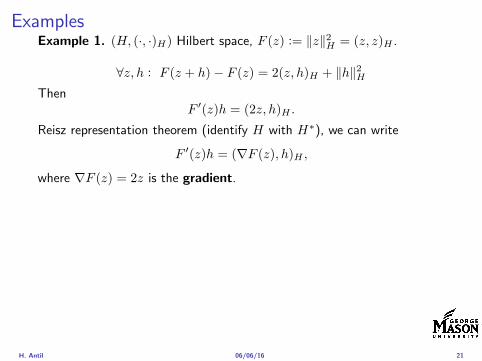
ExamplesExample 1 (H (middot middot)H) Hilbert space F (z) = z2H = (z z)H
forallz h F (z + h)minus F (z) = 2(z h)H + h2HThen
F prime(z)h = (2z h)H
Reisz representation theorem (identify H with Hlowast) we can write
F prime(z)h = (nablaF (z) h)H
where nablaF (z) = 2z is the gradient
Example 2 Let (Z (middot middot)Z) (H (middot middot)H) Hilbert spaces ud isin H fixedLet S isin L(ZH) Consider E Z rarr R
E(z) = Sz minus ud2H
Then E(z) = G(F (z)) where G(v) = v2H and F (z) = Sz minus ud
Eprime(z)h = Gprime(F (z))F prime(z)h = (2v F prime(z)h)H
= 2(Sz minus ud Sh)H = 2(Slowast(Sz minus ud) h)Z
we denote the gradient as nablaE(z) = 2Slowast(Sz minus ud)
H Antil 060616 21
ExamplesExample 1 (H (middot middot)H) Hilbert space F (z) = z2H = (z z)H
forallz h F (z + h)minus F (z) = 2(z h)H + h2HThen
F prime(z)h = (2z h)H
Reisz representation theorem (identify H with Hlowast) we can write
F prime(z)h = (nablaF (z) h)H
where nablaF (z) = 2z is the gradient
Example 2 Let (Z (middot middot)Z) (H (middot middot)H) Hilbert spaces ud isin H fixedLet S isin L(ZH) Consider E Z rarr R
E(z) = Sz minus ud2H
Then E(z) = G(F (z)) where G(v) = v2H and F (z) = Sz minus ud
Eprime(z)h = Gprime(F (z))F prime(z)h = (2v F prime(z)h)H
= 2(Sz minus ud Sh)H = 2(Slowast(Sz minus ud) h)Z
we denote the gradient as nablaE(z) = 2Slowast(Sz minus ud)H Antil 060616 21
Outline
Motivation and examples
Linear elliptic optimal control problems
Differentiation in Banach spaces
First-order necessary conditions
Optimal control of semilinear PDEs
An abstract problem
Discretization using finite element methods
H Antil 060616 22
First order necessary optimality conditions
Most of the theory is based on these two simple results
Theorem Let (Z middot Z) be a normed space J Z rarr (infin+infin] amapping with J 6equiv +infin Then z isin Z minimizer of J hArr 0 isin partJ (z)
Proof 0 isin partJ (z) means by definition of partJ (z) J (z)minus J (z) le 0forallz isin Z
Theorem Let (Z middot Z) be a normed space Zad sub Z nonemptyconvex closed J Z rarr R Gateaux differentiable where Zad sub Z sub ZZ open If z isin Zad is a solution to
minzisinZad
J (z)
then z solvesJ prime(z)(z minus z) ge 0 forallz isin Zad
Proof Exercise
H Antil 060616 23
First order necessary optimality conditions
Most of the theory is based on these two simple results
Theorem Let (Z middot Z) be a normed space J Z rarr (infin+infin] amapping with J 6equiv +infin Then z isin Z minimizer of J hArr 0 isin partJ (z)
Proof 0 isin partJ (z) means by definition of partJ (z) J (z)minus J (z) le 0forallz isin Z
Theorem Let (Z middot Z) be a normed space Zad sub Z nonemptyconvex closed J Z rarr R Gateaux differentiable where Zad sub Z sub ZZ open If z isin Zad is a solution to
minzisinZad
J (z)
then z solvesJ prime(z)(z minus z) ge 0 forallz isin Zad
Proof Exercise
H Antil 060616 23
Linear quadratic OCPI Reduced funcational
J (z) =1
2Sz minus ud2L2(Ω) +
λ
2z2L2(Ω)
I Gradient computation using sensitivity
J prime(z)h = (Slowast(Sz minus ud) + λz h)L2(Ω) forallh isin L2(Ω)
we denote the gradient by
nablaJ (z) = Slowast(Sz minus ud) + λz
I First order necessary and sufficient optimality condition
(nablaJ (z) z minus z)L2(Ω) ge 0 forallz isin Zad
I Adjoint equation Let p = Slowast(Sz minus ud) which translates intop isin H1
0 (Ω) solving
minusdiv (Anablap) = uminus ud in Ω
p = 0 on partΩ
I Gradient computation using adjoint nablaJ (z) = p+ λz
H Antil 060616 24
Linear quadratic OCPI Reduced funcational
J (z) =1
2Sz minus ud2L2(Ω) +
λ
2z2L2(Ω)
I Gradient computation using sensitivity
J prime(z)h = (Slowast(Sz minus ud) + λz h)L2(Ω) forallh isin L2(Ω)
we denote the gradient by
nablaJ (z) = Slowast(Sz minus ud) + λz
I First order necessary and sufficient optimality condition
(nablaJ (z) z minus z)L2(Ω) ge 0 forallz isin Zad
I Adjoint equation Let p = Slowast(Sz minus ud) which translates intop isin H1
0 (Ω) solving
minusdiv (Anablap) = uminus ud in Ω
p = 0 on partΩ
I Gradient computation using adjoint nablaJ (z) = p+ λz
H Antil 060616 24
Linear quadratic OCPI Reduced funcational
J (z) =1
2Sz minus ud2L2(Ω) +
λ
2z2L2(Ω)
I Gradient computation using sensitivity
J prime(z)h = (Slowast(Sz minus ud) + λz h)L2(Ω) forallh isin L2(Ω)
we denote the gradient by
nablaJ (z) = Slowast(Sz minus ud) + λz
I First order necessary and sufficient optimality condition
(nablaJ (z) z minus z)L2(Ω) ge 0 forallz isin Zad
I Adjoint equation Let p = Slowast(Sz minus ud) which translates intop isin H1
0 (Ω) solving
minusdiv (Anablap) = uminus ud in Ω
p = 0 on partΩ
I Gradient computation using adjoint nablaJ (z) = p+ λz
H Antil 060616 24
Linear quadratic OCPI Reduced funcational
J (z) =1
2Sz minus ud2L2(Ω) +
λ
2z2L2(Ω)
I Gradient computation using sensitivity
J prime(z)h = (Slowast(Sz minus ud) + λz h)L2(Ω) forallh isin L2(Ω)
we denote the gradient by
nablaJ (z) = Slowast(Sz minus ud) + λz
I First order necessary and sufficient optimality condition
(nablaJ (z) z minus z)L2(Ω) ge 0 forallz isin Zad
I Adjoint equation Let p = Slowast(Sz minus ud) which translates intop isin H1
0 (Ω) solving
minusdiv (Anablap) = uminus ud in Ω
p = 0 on partΩ
I Gradient computation using adjoint nablaJ (z) = p+ λz
H Antil 060616 24
Linear quadratic OCPI Reduced funcational
J (z) =1
2Sz minus ud2L2(Ω) +
λ
2z2L2(Ω)
I Gradient computation using sensitivity
J prime(z)h = (Slowast(Sz minus ud) + λz h)L2(Ω) forallh isin L2(Ω)
we denote the gradient by
nablaJ (z) = Slowast(Sz minus ud) + λz
I First order necessary and sufficient optimality condition
(nablaJ (z) z minus z)L2(Ω) ge 0 forallz isin Zad
I Adjoint equation Let p = Slowast(Sz minus ud) which translates intop isin H1
0 (Ω) solving
minusdiv (Anablap) = uminus ud in Ω
p = 0 on partΩ
I Gradient computation using adjoint nablaJ (z) = p+ λz
H Antil 060616 24
Optimality system
I State u isin H10 (Ω)
intΩAnablau middot nablav =
intΩzv forallv isin H1
0 (Ω)
I Adjoint p isin H10 (Ω)
intΩAnablap middot nablav =
intΩ
(uminus ud)v forallv isin H10 (Ω)
I Control z isin Zad (p+ λz z minus z) ge 0 forallz isin Zad
H Antil 060616 25
Pointwise interpretation
The variational inequality
(p+ λz z minus z) ge 0 forallz isin Zad
is equivalent to for ae x isin Ω
z(x) =
za(x) if p(x) + λz(x) gt 0isin [za(x) zb(x)] if p(x) + λz(x) = 0zb(x) if p(x) + λz(x) lt 0
Consequence
I When λ gt 0 then ae in Ω
z(x) = P[za(x)zb(x)]
minus 1
λp(x)
= min
zb(x)max
za(x)minus 1
λp(x)
H Antil 060616 26
Formal Lagrange method applied to linear OCPIntroduce L H1
0 (Ω)times Zad timesH1(Ω)rarr R defined as
L(u z p) = J(u z)minusint
Ω
(minusdiv (Anablau)minus z
)p dx
Integrate by parts to arrive at
L(u z p) = J(u z)minusint
Ω
(minusdiv (Anablap)uminus zp
)dx+
intpartΩ
(Anablau)p ds
If (u z p) is a stationary point then
I State
DpL(u z p)h = 0 forallh isin H1(Ω)
I AdjointDuL(u z p)h = 0 forallh isin H1
0 (Ω)
I ControlDzL(u z p)(z minus z) ge 0 forallz isin Zad
H Antil 060616 27
Formal Lagrange method applied to linear OCPIntroduce L H1
0 (Ω)times Zad timesH1(Ω)rarr R defined as
L(u z p) = J(u z)minusint
Ω
(minusdiv (Anablau)minus z
)p dx
Integrate by parts to arrive at
L(u z p) = J(u z)minusint
Ω
(minusdiv (Anablap)uminus zp
)dx+
intpartΩ
(Anablau)p ds
If (u z p) is a stationary point then
I State
DpL(u z p)h = 0 forallh isin H1(Ω)
I AdjointDuL(u z p)h = 0 forallh isin H1
0 (Ω)
I ControlDzL(u z p)(z minus z) ge 0 forallz isin Zad
H Antil 060616 27
Formal Lagrange method applied to linear OCPIntroduce L H1
0 (Ω)times Zad timesH1(Ω)rarr R defined as
L(u z p) = J(u z)minusint
Ω
(minusdiv (Anablau)minus z
)p dx
Integrate by parts to arrive at
L(u z p) = J(u z)minusint
Ω
(minusdiv (Anablap)uminus zp
)dx+
intpartΩ
(Anablau)p ds
If (u z p) is a stationary point then
I State
DpL(u z p)h = 0 forallh isin H1(Ω)
I AdjointDuL(u z p)h = 0 forallh isin H1
0 (Ω)
I ControlDzL(u z p)(z minus z) ge 0 forallz isin Zad
H Antil 060616 27
Formal Lagrange method applied to linear OCPIntroduce L H1
0 (Ω)times Zad timesH1(Ω)rarr R defined as
L(u z p) = J(u z)minusint
Ω
(minusdiv (Anablau)minus z
)p dx
Integrate by parts to arrive at
L(u z p) = J(u z)minusint
Ω
(minusdiv (Anablap)uminus zp
)dx+
intpartΩ
(Anablau)p ds
If (u z p) is a stationary point then
I State
DpL(u z p)h = 0 forallh isin H1(Ω)
I AdjointDuL(u z p)h = 0 forallh isin H1
0 (Ω)
I ControlDzL(u z p)(z minus z) ge 0 forallz isin Zad
H Antil 060616 27
Formal Lagrange method applied to linear OCPIntroduce L H1
0 (Ω)times Zad timesH1(Ω)rarr R defined as
L(u z p) = J(u z)minusint
Ω
(minusdiv (Anablau)minus z
)p dx
Integrate by parts to arrive at
L(u z p) = J(u z)minusint
Ω
(minusdiv (Anablap)uminus zp
)dx+
intpartΩ
(Anablau)p ds
If (u z p) is a stationary point then
I State
DpL(u z p)h = 0 forallh isin H1(Ω)
I AdjointDuL(u z p)h = 0 forallh isin H1
0 (Ω)
I ControlDzL(u z p)(z minus z) ge 0 forallz isin Zad
H Antil 060616 27
Outline
Motivation and examples
Linear elliptic optimal control problems
Differentiation in Banach spaces
First-order necessary conditions
Optimal control of semilinear PDEs
An abstract problem
Discretization using finite element methods
H Antil 060616 28
Semilinear elliptic OCP
min J(u z) =1
2uminus ud2L2(Ω) +
λ
2z2L2(Ω)
subject to
minus∆u+ g(x u) = z in Ω
u = 0 on partΩ
and z isin Zad with za zb isin Linfin(Ω)
H Antil 060616 29
State space(A1) Ω sub Rd open bounded partΩ is Lipschitz
(A2) g Ωtimes Rrarr R is bounded and measurable with respect to x isin Ωfor every u isin R
(A3) g is continuous monotone increasing and Lipschitz continuous in ufor ae x isin Ω
(A4) g(x 0) = 0 for ae x isin Ω (not really necessary)
Theorem Suppose (A1)minus (A4) hold For every z isin Lr(Ω) withr gt d2 the state equation has a unique weak solutionu isin H1
0 (Ω) cap C(Ω) ie we haveintΩ
nablau middot nablav dx+
intΩ
g(x u(x))v(x) dx =
intΩ
zv dx forallv isin H10 (Ω)
Moreover there exists a constant C gt 0 such that
uH1(Ω) + uC(Ω) le CzLr(Ω)
RemarkI The proof of the theorem uses the BrowderndashMinty theorem on
monotone operators
H Antil 060616 30
State space(A1) Ω sub Rd open bounded partΩ is Lipschitz
(A2) g Ωtimes Rrarr R is bounded and measurable with respect to x isin Ωfor every u isin R
(A3) g is continuous monotone increasing and Lipschitz continuous in ufor ae x isin Ω
(A4) g(x 0) = 0 for ae x isin Ω (not really necessary)
Theorem Suppose (A1)minus (A4) hold For every z isin Lr(Ω) withr gt d2 the state equation has a unique weak solutionu isin H1
0 (Ω) cap C(Ω) ie we haveintΩ
nablau middot nablav dx+
intΩ
g(x u(x))v(x) dx =
intΩ
zv dx forallv isin H10 (Ω)
Moreover there exists a constant C gt 0 such that
uH1(Ω) + uC(Ω) le CzLr(Ω)
RemarkI The proof of the theorem uses the BrowderndashMinty theorem on
monotone operators
H Antil 060616 30
State space(A1) Ω sub Rd open bounded partΩ is Lipschitz
(A2) g Ωtimes Rrarr R is bounded and measurable with respect to x isin Ωfor every u isin R
(A3) g is continuous monotone increasing and Lipschitz continuous in ufor ae x isin Ω
(A4) g(x 0) = 0 for ae x isin Ω (not really necessary)
Theorem Suppose (A1)minus (A4) hold For every z isin Lr(Ω) withr gt d2 the state equation has a unique weak solutionu isin H1
0 (Ω) cap C(Ω) ie we haveintΩ
nablau middot nablav dx+
intΩ
g(x u(x))v(x) dx =
intΩ
zv dx forallv isin H10 (Ω)
Moreover there exists a constant C gt 0 such that
uH1(Ω) + uC(Ω) le CzLr(Ω)
RemarkI The proof of the theorem uses the BrowderndashMinty theorem on
monotone operators
H Antil 060616 30
Control-to-state map and reduced problem
I Control to state map
S Linfin(Ω)rarr H10 (Ω) cap C(Ω)
is well defined and is globally Lipschitz continuous
I Reduced problem
minJ (z) =1
2S(u)minus ud2L2(Ω) +
λ
2z2L2(Ω)
H Antil 060616 31
Control-to-state map and reduced problem
I Control to state map
S Linfin(Ω)rarr H10 (Ω) cap C(Ω)
is well defined and is globally Lipschitz continuous
I Reduced problem
minJ (z) =1
2S(u)minus ud2L2(Ω) +
λ
2z2L2(Ω)
H Antil 060616 31
First-order necessary conditionsI Lagrangian functional
L(u z p) = J(u z)minusint
Ω
(minus∆u+ g(x u(x))minus z
)p dx
= J(u z)minusint
Ω
(nablau middot nablap+ g(x u(x))pminus zp
)dx
I Adjoint system For all h isin H10 (Ω)
0 = DuL(u z p)h =
intΩ
(uminus ud)h dxminusint
Ω
(nablah middot nablap+ gu(x u(x))ph
)which yields
minus∆p+ gu(x u(x))p = uminus ud in Ω
p = 0 on partΩ
I Control
DzL(u z p)(z minus z) = (p+ λz z minus z) dx ge 0 forallz isin ZadI Gradient
nablaJ (z) = p+ λz
H Antil 060616 32
First-order necessary conditionsI Lagrangian functional
L(u z p) = J(u z)minusint
Ω
(minus∆u+ g(x u(x))minus z
)p dx
= J(u z)minusint
Ω
(nablau middot nablap+ g(x u(x))pminus zp
)dx
I Adjoint system For all h isin H10 (Ω)
0 = DuL(u z p)h =
intΩ
(uminus ud)h dxminusint
Ω
(nablah middot nablap+ gu(x u(x))ph
)which yields
minus∆p+ gu(x u(x))p = uminus ud in Ω
p = 0 on partΩ
I Control
DzL(u z p)(z minus z) = (p+ λz z minus z) dx ge 0 forallz isin ZadI Gradient
nablaJ (z) = p+ λz
H Antil 060616 32
First-order necessary conditionsI Lagrangian functional
L(u z p) = J(u z)minusint
Ω
(minus∆u+ g(x u(x))minus z
)p dx
= J(u z)minusint
Ω
(nablau middot nablap+ g(x u(x))pminus zp
)dx
I Adjoint system For all h isin H10 (Ω)
0 = DuL(u z p)h =
intΩ
(uminus ud)h dxminusint
Ω
(nablah middot nablap+ gu(x u(x))ph
)which yields
minus∆p+ gu(x u(x))p = uminus ud in Ω
p = 0 on partΩ
I Control
DzL(u z p)(z minus z) = (p+ λz z minus z) dx ge 0 forallz isin Zad
I GradientnablaJ (z) = p+ λz
H Antil 060616 32
First-order necessary conditionsI Lagrangian functional
L(u z p) = J(u z)minusint
Ω
(minus∆u+ g(x u(x))minus z
)p dx
= J(u z)minusint
Ω
(nablau middot nablap+ g(x u(x))pminus zp
)dx
I Adjoint system For all h isin H10 (Ω)
0 = DuL(u z p)h =
intΩ
(uminus ud)h dxminusint
Ω
(nablah middot nablap+ gu(x u(x))ph
)which yields
minus∆p+ gu(x u(x))p = uminus ud in Ω
p = 0 on partΩ
I Control
DzL(u z p)(z minus z) = (p+ λz z minus z) dx ge 0 forallz isin ZadI Gradient
nablaJ (z) = p+ λz
H Antil 060616 32
Differentiability of Nemytskii operator
The rigorous proof uses
Theorem In addition to (A1)-(A4) if
(A5) g is continuously differentiable with respect to u for ae x isin Ωand we have
(i) |gu(x 0)| le K for ae x isin Ω(ii) gu is locally Lipschitz with respect to u isin R
then the Nemytskii operator G u 7rarr g(middot u(middot)) is continuously Frechetdifferentiable from Linfin(Ω) into itself and
(Gprime(u)h)(x) = gu(x u(x))h(x) ae in Ω forallh isin Linfin(Ω)
Remark (A5) holds if g(x u) = g(u) and g isin C2(R)
H Antil 060616 33
Outline
Motivation and examples
Linear elliptic optimal control problems
Differentiation in Banach spaces
First-order necessary conditions
Optimal control of semilinear PDEs
An abstract problem
Discretization using finite element methods
H Antil 060616 34
Gradient computation via adjoint general formI Abstract problem
min J(u z)
subject toc(u z) = 0
and z isin Zad
I Directional derivative Let S be the control to state map(nonlinear in general)
z 7rarr S(z) = u(z)
Under the assumptions of ldquoimplicit function theoremrdquo
J prime(z)h = (nablauJ (u(z) z) Sprime(z)h) + (nablazJ (u(z) z) h)
I Sensitivity of u with respect to z Differentiating the stateequation
cu(S(z) z)Sprime(z)h = minuscz(S(z) z)h
leads toSprime(z)h = minuscu(S(z) z)minus1
(cz(S(z) z)h
)
provided cu(S(z) z)minus1 is well-defined
H Antil 060616 35
Gradient computation via adjoint general formI Abstract problem
min J(u z)
subject toc(u z) = 0
and z isin ZadI Directional derivative Let S be the control to state map
(nonlinear in general)
z 7rarr S(z) = u(z)
Under the assumptions of ldquoimplicit function theoremrdquo
J prime(z)h = (nablauJ (u(z) z) Sprime(z)h) + (nablazJ (u(z) z) h)
I Sensitivity of u with respect to z Differentiating the stateequation
cu(S(z) z)Sprime(z)h = minuscz(S(z) z)h
leads toSprime(z)h = minuscu(S(z) z)minus1
(cz(S(z) z)h
)
provided cu(S(z) z)minus1 is well-defined
H Antil 060616 35
Gradient computation via adjoint general formI Abstract problem
min J(u z)
subject toc(u z) = 0
and z isin ZadI Directional derivative Let S be the control to state map
(nonlinear in general)
z 7rarr S(z) = u(z)
Under the assumptions of ldquoimplicit function theoremrdquo
J prime(z)h = (nablauJ (u(z) z) Sprime(z)h) + (nablazJ (u(z) z) h)
I Sensitivity of u with respect to z Differentiating the stateequation
cu(S(z) z)Sprime(z)h = minuscz(S(z) z)h
leads toSprime(z)h = minuscu(S(z) z)minus1
(cz(S(z) z)h
)
provided cu(S(z) z)minus1 is well-defined
H Antil 060616 35
Adjoint equation and gradient general form
I Directional derivative
J prime(z)h = minus(nablauJ (u(z) z) cu(u(z) z)minus1cz(u(z) z)h
)+ (nablazJ (u(z) z) h)
I Gradient
nablaJ (z) = minuscz(u(z) z)lowast(cu(u(z) z)minuslowastnablauJ (u(z) z)
)+nablazJ (u(z) z)
I Introducing adjoint variable p solving
cu(u(z) z)lowastp = nablauJ (u(z) z)
we arrive at following form of gradient
nablaJ (z) = minuscz(u(z) z)lowastp+nablazJ (u(z) z)
which is tractable
H Antil 060616 36
Adjoint equation and gradient general form
I Directional derivative
J prime(z)h = minus(nablauJ (u(z) z) cu(u(z) z)minus1cz(u(z) z)h
)+ (nablazJ (u(z) z) h)
I Gradient
nablaJ (z) = minuscz(u(z) z)lowast(cu(u(z) z)minuslowastnablauJ (u(z) z)
)+nablazJ (u(z) z)
I Introducing adjoint variable p solving
cu(u(z) z)lowastp = nablauJ (u(z) z)
we arrive at following form of gradient
nablaJ (z) = minuscz(u(z) z)lowastp+nablazJ (u(z) z)
which is tractable
H Antil 060616 36
Adjoint equation and gradient general form
I Directional derivative
J prime(z)h = minus(nablauJ (u(z) z) cu(u(z) z)minus1cz(u(z) z)h
)+ (nablazJ (u(z) z) h)
I Gradient
nablaJ (z) = minuscz(u(z) z)lowast(cu(u(z) z)minuslowastnablauJ (u(z) z)
)+nablazJ (u(z) z)
I Introducing adjoint variable p solving
cu(u(z) z)lowastp = nablauJ (u(z) z)
we arrive at following form of gradient
nablaJ (z) = minuscz(u(z) z)lowastp+nablazJ (u(z) z)
which is tractable
H Antil 060616 36
Hessian computation general form
I Lagrangian L(u z p) = J(u z)minusint
Ωc(u z)p dx Then we have
DzJ (z)h = DzL(u z p)h
I Second order derivative
D2zJ (z)[h1 h2] = DuDzL(u z p)[h1 S
prime(z)h2] +D2zL(u z p)[h1 h2]
+DpDzL(u z p)[h1 Dzp(z)h2]
I We already know Sprime(z)h2 moreover
DpDzL(u z p)[h1 Dzp(z)h2] = minus(cu(u z)h1 Dzp(z)h2
)
It remain to identify Dzp(z)h2
H Antil 060616 37
Hessian computation general form
I Lagrangian L(u z p) = J(u z)minusint
Ωc(u z)p dx Then we have
DzJ (z)h = DzL(u z p)h
I Second order derivative
D2zJ (z)[h1 h2] = DuDzL(u z p)[h1 S
prime(z)h2] +D2zL(u z p)[h1 h2]
+DpDzL(u z p)[h1 Dzp(z)h2]
I We already know Sprime(z)h2 moreover
DpDzL(u z p)[h1 Dzp(z)h2] = minus(cu(u z)h1 Dzp(z)h2
)
It remain to identify Dzp(z)h2
H Antil 060616 37
Hessian computation general form
I Lagrangian L(u z p) = J(u z)minusint
Ωc(u z)p dx Then we have
DzJ (z)h = DzL(u z p)h
I Second order derivative
D2zJ (z)[h1 h2] = DuDzL(u z p)[h1 S
prime(z)h2] +D2zL(u z p)[h1 h2]
+DpDzL(u z p)[h1 Dzp(z)h2]
I We already know Sprime(z)h2 moreover
DpDzL(u z p)[h1 Dzp(z)h2] = minus(cu(u z)h1 Dzp(z)h2
)
It remain to identify Dzp(z)h2
H Antil 060616 37
Outline
Motivation and examples
Linear elliptic optimal control problems
Differentiation in Banach spaces
First-order necessary conditions
Optimal control of semilinear PDEs
An abstract problem
Discretization using finite element methods
H Antil 060616 38
Numerical approximation of Poisson equation MeshTo avoid technical issues we will assume that partΩ is polygonal
I Mesh Let T = K be a mesh of Ω where K sub Rd is an elementthat is isoparametrically equivalent to a unit simplex in Rd
I Conforming mesh We say that the mesh is conforming ifI Ω = cupKisinT KI If K1 cap K2 = x then x is a node of K1 and K2I If K1 cap K2 6= empty and K1 cap K2 6= x then K1 cap K2 is an edgeface
contained in partK1 cap partK2
I Shape regular Let T be the collection of all conformingrefinements of an original mesh T 0 Then T is called shape regularif exist κ gt 0 such that
hKρKle κ forallK isin cupiT i
where hK = diam K ρK = maxρ gt 0|Bρ sub KI Quasi-uniform A family of shape regular meshes is called-quasi
uniform if there exist a constant σ gt 0 such that
maxhKminhK
le σ
uniformly for all meshes in the family
Numerical approximation of Poisson equation MeshTo avoid technical issues we will assume that partΩ is polygonal
I Mesh Let T = K be a mesh of Ω where K sub Rd is an elementthat is isoparametrically equivalent to a unit simplex in Rd
I Conforming mesh We say that the mesh is conforming ifI Ω = cupKisinT KI If K1 cap K2 = x then x is a node of K1 and K2I If K1 cap K2 6= empty and K1 cap K2 6= x then K1 cap K2 is an edgeface
contained in partK1 cap partK2
I Shape regular Let T be the collection of all conformingrefinements of an original mesh T 0 Then T is called shape regularif exist κ gt 0 such that
hKρKle κ forallK isin cupiT i
where hK = diam K ρK = maxρ gt 0|Bρ sub KI Quasi-uniform A family of shape regular meshes is called-quasi
uniform if there exist a constant σ gt 0 such that
maxhKminhK
le σ
uniformly for all meshes in the family
Numerical approximation of Poisson equation MeshTo avoid technical issues we will assume that partΩ is polygonal
I Mesh Let T = K be a mesh of Ω where K sub Rd is an elementthat is isoparametrically equivalent to a unit simplex in Rd
I Conforming mesh We say that the mesh is conforming ifI Ω = cupKisinT KI If K1 cap K2 = x then x is a node of K1 and K2I If K1 cap K2 6= empty and K1 cap K2 6= x then K1 cap K2 is an edgeface
contained in partK1 cap partK2
I Shape regular Let T be the collection of all conformingrefinements of an original mesh T 0 Then T is called shape regularif exist κ gt 0 such that
hKρKle κ forallK isin cupiT i
where hK = diam K ρK = maxρ gt 0|Bρ sub K
I Quasi-uniform A family of shape regular meshes is called-quasiuniform if there exist a constant σ gt 0 such that
maxhKminhK
le σ
uniformly for all meshes in the family
Numerical approximation of Poisson equation MeshTo avoid technical issues we will assume that partΩ is polygonal
I Mesh Let T = K be a mesh of Ω where K sub Rd is an elementthat is isoparametrically equivalent to a unit simplex in Rd
I Conforming mesh We say that the mesh is conforming ifI Ω = cupKisinT KI If K1 cap K2 = x then x is a node of K1 and K2I If K1 cap K2 6= empty and K1 cap K2 6= x then K1 cap K2 is an edgeface
contained in partK1 cap partK2
I Shape regular Let T be the collection of all conformingrefinements of an original mesh T 0 Then T is called shape regularif exist κ gt 0 such that
hKρKle κ forallK isin cupiT i
where hK = diam K ρK = maxρ gt 0|Bρ sub KI Quasi-uniform A family of shape regular meshes is called-quasi
uniform if there exist a constant σ gt 0 such that
maxhKminhK
le σ
uniformly for all meshes in the family
FE space and Galerkin approximationI Finite element space For T isin T we define the finite element
space as
V(T ) = W isin C0(Ω) WK isin P1forallK isin T W |partΩ = 0
where P1 is the set of polynomials of degree at most 1
I Galerkin approximation of continuous problem is given by
Find UT isin V(T )
intΩ
AnablaUT middot nablaV = 〈f V 〉 forallV isin V(T )
The discrete problem is well-posedI Nodal basis Consists of functions ψi isin V(T ) with xi isin N (T )
satisfyingψxi
(xj) = δij
where N (T ) denotes the interior (plus Neumann) nodesI Galerkin orthogonality(
nabla(uminus UT )nablaW)L2(Ω)
= 0 forallW isin V(T )
H Antil 060616 40
FE space and Galerkin approximationI Finite element space For T isin T we define the finite element
space as
V(T ) = W isin C0(Ω) WK isin P1forallK isin T W |partΩ = 0
where P1 is the set of polynomials of degree at most 1I Galerkin approximation of continuous problem is given by
Find UT isin V(T )
intΩ
AnablaUT middot nablaV = 〈f V 〉 forallV isin V(T )
The discrete problem is well-posed
I Nodal basis Consists of functions ψi isin V(T ) with xi isin N (T )satisfying
ψxi(xj) = δij
where N (T ) denotes the interior (plus Neumann) nodesI Galerkin orthogonality(
nabla(uminus UT )nablaW)L2(Ω)
= 0 forallW isin V(T )
H Antil 060616 40
FE space and Galerkin approximationI Finite element space For T isin T we define the finite element
space as
V(T ) = W isin C0(Ω) WK isin P1forallK isin T W |partΩ = 0
where P1 is the set of polynomials of degree at most 1I Galerkin approximation of continuous problem is given by
Find UT isin V(T )
intΩ
AnablaUT middot nablaV = 〈f V 〉 forallV isin V(T )
The discrete problem is well-posedI Nodal basis Consists of functions ψi isin V(T ) with xi isin N (T )
satisfyingψxi
(xj) = δij
where N (T ) denotes the interior (plus Neumann) nodes
I Galerkin orthogonality(nabla(uminus UT )nablaW
)L2(Ω)
= 0 forallW isin V(T )
H Antil 060616 40
FE space and Galerkin approximationI Finite element space For T isin T we define the finite element
space as
V(T ) = W isin C0(Ω) WK isin P1forallK isin T W |partΩ = 0
where P1 is the set of polynomials of degree at most 1I Galerkin approximation of continuous problem is given by
Find UT isin V(T )
intΩ
AnablaUT middot nablaV = 〈f V 〉 forallV isin V(T )
The discrete problem is well-posedI Nodal basis Consists of functions ψi isin V(T ) with xi isin N (T )
satisfyingψxi
(xj) = δij
where N (T ) denotes the interior (plus Neumann) nodesI Galerkin orthogonality(
nabla(uminus UT )nablaW)L2(Ω)
= 0 forallW isin V(T )
H Antil 060616 40
Best approximation
I Cearsquos lemma
nabla(uminus UT )L2(Ω) le C infWisinV(T )
nabla(uminusW )L2(Ω)
I Nodal interpolation operator ΠT C(Ω)rarr V(T ) satisfies
ΠT u(xi) = u(xi) forallxi isin N (T )
and is defined as
ΠT u =sum
xiisinN (T )
u(xi)ψxi
I Error estimates In Cearsquos lemma replace W by ΠT u and thencompute the interpolation error
H Antil 060616 41
Best approximation
I Cearsquos lemma
nabla(uminus UT )L2(Ω) le C infWisinV(T )
nabla(uminusW )L2(Ω)
I Nodal interpolation operator ΠT C(Ω)rarr V(T ) satisfies
ΠT u(xi) = u(xi) forallxi isin N (T )
and is defined as
ΠT u =sum
xiisinN (T )
u(xi)ψxi
I Error estimates In Cearsquos lemma replace W by ΠT u and thencompute the interpolation error
H Antil 060616 41
Best approximation
I Cearsquos lemma
nabla(uminus UT )L2(Ω) le C infWisinV(T )
nabla(uminusW )L2(Ω)
I Nodal interpolation operator ΠT C(Ω)rarr V(T ) satisfies
ΠT u(xi) = u(xi) forallxi isin N (T )
and is defined as
ΠT u =sum
xiisinN (T )
u(xi)ψxi
I Error estimates In Cearsquos lemma replace W by ΠT u and thencompute the interpolation error
H Antil 060616 41
Algebraic system state equation
I Recall UT isin V(T ) solves
a(UT V ) = 〈f V 〉 forallV isin V(T )
I Now setting UT =sumN
j=1 Ujψj V = ψi we get
Nsumj=1
Uja(φj φi) = 〈f ψi〉 i = 1 N
which is the matrix-vector system
AU = F
I Stiffness matrix A is SPD
H Antil 060616 42
Algebraic system state equation
I Recall UT isin V(T ) solves
a(UT V ) = 〈f V 〉 forallV isin V(T )
I Now setting UT =sumN
j=1 Ujψj V = ψi we get
Nsumj=1
Uja(φj φi) = 〈f ψi〉 i = 1 N
which is the matrix-vector system
AU = F
I Stiffness matrix A is SPD
H Antil 060616 42
Algebraic system state equation
I Recall UT isin V(T ) solves
a(UT V ) = 〈f V 〉 forallV isin V(T )
I Now setting UT =sumN
j=1 Ujψj V = ψi we get
Nsumj=1
Uja(φj φi) = 〈f ψi〉 i = 1 N
which is the matrix-vector system
AU = F
I Stiffness matrix A is SPD
H Antil 060616 42
Discrete linear elliptic OCP
min JT (UT ZT ) =1
2UT minus ud2L2(Ω) +
λ
2ZT 2L2(Ω)
subject to
Find UT isin V(T )
intΩ
nablaUT middot nablaV = (ZT V )L2(Ω) forallV isin V(T )
and whereZT isin Zad(T ) = Zad cap Z(T )
is either one of these
Z(T ) =
V(T )L2(Ω) variational discretization (Hinze)WT isin Linfin(Ω) ZT |K isin P0(K)K isin T
H Antil 060616 43
Recent books
F TroltzschOptimal control of partial differential equations volume 112 ofGraduate Studies in MathematicsAmerican Mathematical Society Providence RI 2010Theory methods and applications Translated from the 2005 Germanoriginal by Jurgen Sprekels
K Ito and K KunischLagrange multiplier approach to variational problems andapplications volume 15 of Advances in Design and ControlSociety for Industrial and Applied Mathematics (SIAM)Philadelphia PA 2008
H Antil 060616 44
- Motivation and examples
- Linear elliptic optimal control problems
- Differentiation in Banach spaces
- First-order necessary conditions
- Optimal control of semilinear PDEs
- An abstract problem
- Discretization using finite element methods
-
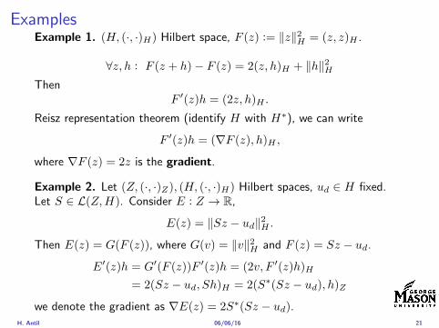
ExamplesExample 1 (H (middot middot)H) Hilbert space F (z) = z2H = (z z)H
forallz h F (z + h)minus F (z) = 2(z h)H + h2HThen
F prime(z)h = (2z h)H
Reisz representation theorem (identify H with Hlowast) we can write
F prime(z)h = (nablaF (z) h)H
where nablaF (z) = 2z is the gradient
Example 2 Let (Z (middot middot)Z) (H (middot middot)H) Hilbert spaces ud isin H fixedLet S isin L(ZH) Consider E Z rarr R
E(z) = Sz minus ud2H
Then E(z) = G(F (z)) where G(v) = v2H and F (z) = Sz minus ud
Eprime(z)h = Gprime(F (z))F prime(z)h = (2v F prime(z)h)H
= 2(Sz minus ud Sh)H = 2(Slowast(Sz minus ud) h)Z
we denote the gradient as nablaE(z) = 2Slowast(Sz minus ud)H Antil 060616 21
Outline
Motivation and examples
Linear elliptic optimal control problems
Differentiation in Banach spaces
First-order necessary conditions
Optimal control of semilinear PDEs
An abstract problem
Discretization using finite element methods
H Antil 060616 22
First order necessary optimality conditions
Most of the theory is based on these two simple results
Theorem Let (Z middot Z) be a normed space J Z rarr (infin+infin] amapping with J 6equiv +infin Then z isin Z minimizer of J hArr 0 isin partJ (z)
Proof 0 isin partJ (z) means by definition of partJ (z) J (z)minus J (z) le 0forallz isin Z
Theorem Let (Z middot Z) be a normed space Zad sub Z nonemptyconvex closed J Z rarr R Gateaux differentiable where Zad sub Z sub ZZ open If z isin Zad is a solution to
minzisinZad
J (z)
then z solvesJ prime(z)(z minus z) ge 0 forallz isin Zad
Proof Exercise
H Antil 060616 23
First order necessary optimality conditions
Most of the theory is based on these two simple results
Theorem Let (Z middot Z) be a normed space J Z rarr (infin+infin] amapping with J 6equiv +infin Then z isin Z minimizer of J hArr 0 isin partJ (z)
Proof 0 isin partJ (z) means by definition of partJ (z) J (z)minus J (z) le 0forallz isin Z
Theorem Let (Z middot Z) be a normed space Zad sub Z nonemptyconvex closed J Z rarr R Gateaux differentiable where Zad sub Z sub ZZ open If z isin Zad is a solution to
minzisinZad
J (z)
then z solvesJ prime(z)(z minus z) ge 0 forallz isin Zad
Proof Exercise
H Antil 060616 23
Linear quadratic OCPI Reduced funcational
J (z) =1
2Sz minus ud2L2(Ω) +
λ
2z2L2(Ω)
I Gradient computation using sensitivity
J prime(z)h = (Slowast(Sz minus ud) + λz h)L2(Ω) forallh isin L2(Ω)
we denote the gradient by
nablaJ (z) = Slowast(Sz minus ud) + λz
I First order necessary and sufficient optimality condition
(nablaJ (z) z minus z)L2(Ω) ge 0 forallz isin Zad
I Adjoint equation Let p = Slowast(Sz minus ud) which translates intop isin H1
0 (Ω) solving
minusdiv (Anablap) = uminus ud in Ω
p = 0 on partΩ
I Gradient computation using adjoint nablaJ (z) = p+ λz
H Antil 060616 24
Linear quadratic OCPI Reduced funcational
J (z) =1
2Sz minus ud2L2(Ω) +
λ
2z2L2(Ω)
I Gradient computation using sensitivity
J prime(z)h = (Slowast(Sz minus ud) + λz h)L2(Ω) forallh isin L2(Ω)
we denote the gradient by
nablaJ (z) = Slowast(Sz minus ud) + λz
I First order necessary and sufficient optimality condition
(nablaJ (z) z minus z)L2(Ω) ge 0 forallz isin Zad
I Adjoint equation Let p = Slowast(Sz minus ud) which translates intop isin H1
0 (Ω) solving
minusdiv (Anablap) = uminus ud in Ω
p = 0 on partΩ
I Gradient computation using adjoint nablaJ (z) = p+ λz
H Antil 060616 24
Linear quadratic OCPI Reduced funcational
J (z) =1
2Sz minus ud2L2(Ω) +
λ
2z2L2(Ω)
I Gradient computation using sensitivity
J prime(z)h = (Slowast(Sz minus ud) + λz h)L2(Ω) forallh isin L2(Ω)
we denote the gradient by
nablaJ (z) = Slowast(Sz minus ud) + λz
I First order necessary and sufficient optimality condition
(nablaJ (z) z minus z)L2(Ω) ge 0 forallz isin Zad
I Adjoint equation Let p = Slowast(Sz minus ud) which translates intop isin H1
0 (Ω) solving
minusdiv (Anablap) = uminus ud in Ω
p = 0 on partΩ
I Gradient computation using adjoint nablaJ (z) = p+ λz
H Antil 060616 24
Linear quadratic OCPI Reduced funcational
J (z) =1
2Sz minus ud2L2(Ω) +
λ
2z2L2(Ω)
I Gradient computation using sensitivity
J prime(z)h = (Slowast(Sz minus ud) + λz h)L2(Ω) forallh isin L2(Ω)
we denote the gradient by
nablaJ (z) = Slowast(Sz minus ud) + λz
I First order necessary and sufficient optimality condition
(nablaJ (z) z minus z)L2(Ω) ge 0 forallz isin Zad
I Adjoint equation Let p = Slowast(Sz minus ud) which translates intop isin H1
0 (Ω) solving
minusdiv (Anablap) = uminus ud in Ω
p = 0 on partΩ
I Gradient computation using adjoint nablaJ (z) = p+ λz
H Antil 060616 24
Linear quadratic OCPI Reduced funcational
J (z) =1
2Sz minus ud2L2(Ω) +
λ
2z2L2(Ω)
I Gradient computation using sensitivity
J prime(z)h = (Slowast(Sz minus ud) + λz h)L2(Ω) forallh isin L2(Ω)
we denote the gradient by
nablaJ (z) = Slowast(Sz minus ud) + λz
I First order necessary and sufficient optimality condition
(nablaJ (z) z minus z)L2(Ω) ge 0 forallz isin Zad
I Adjoint equation Let p = Slowast(Sz minus ud) which translates intop isin H1
0 (Ω) solving
minusdiv (Anablap) = uminus ud in Ω
p = 0 on partΩ
I Gradient computation using adjoint nablaJ (z) = p+ λz
H Antil 060616 24
Optimality system
I State u isin H10 (Ω)
intΩAnablau middot nablav =
intΩzv forallv isin H1
0 (Ω)
I Adjoint p isin H10 (Ω)
intΩAnablap middot nablav =
intΩ
(uminus ud)v forallv isin H10 (Ω)
I Control z isin Zad (p+ λz z minus z) ge 0 forallz isin Zad
H Antil 060616 25
Pointwise interpretation
The variational inequality
(p+ λz z minus z) ge 0 forallz isin Zad
is equivalent to for ae x isin Ω
z(x) =
za(x) if p(x) + λz(x) gt 0isin [za(x) zb(x)] if p(x) + λz(x) = 0zb(x) if p(x) + λz(x) lt 0
Consequence
I When λ gt 0 then ae in Ω
z(x) = P[za(x)zb(x)]
minus 1
λp(x)
= min
zb(x)max
za(x)minus 1
λp(x)
H Antil 060616 26
Formal Lagrange method applied to linear OCPIntroduce L H1
0 (Ω)times Zad timesH1(Ω)rarr R defined as
L(u z p) = J(u z)minusint
Ω
(minusdiv (Anablau)minus z
)p dx
Integrate by parts to arrive at
L(u z p) = J(u z)minusint
Ω
(minusdiv (Anablap)uminus zp
)dx+
intpartΩ
(Anablau)p ds
If (u z p) is a stationary point then
I State
DpL(u z p)h = 0 forallh isin H1(Ω)
I AdjointDuL(u z p)h = 0 forallh isin H1
0 (Ω)
I ControlDzL(u z p)(z minus z) ge 0 forallz isin Zad
H Antil 060616 27
Formal Lagrange method applied to linear OCPIntroduce L H1
0 (Ω)times Zad timesH1(Ω)rarr R defined as
L(u z p) = J(u z)minusint
Ω
(minusdiv (Anablau)minus z
)p dx
Integrate by parts to arrive at
L(u z p) = J(u z)minusint
Ω
(minusdiv (Anablap)uminus zp
)dx+
intpartΩ
(Anablau)p ds
If (u z p) is a stationary point then
I State
DpL(u z p)h = 0 forallh isin H1(Ω)
I AdjointDuL(u z p)h = 0 forallh isin H1
0 (Ω)
I ControlDzL(u z p)(z minus z) ge 0 forallz isin Zad
H Antil 060616 27
Formal Lagrange method applied to linear OCPIntroduce L H1
0 (Ω)times Zad timesH1(Ω)rarr R defined as
L(u z p) = J(u z)minusint
Ω
(minusdiv (Anablau)minus z
)p dx
Integrate by parts to arrive at
L(u z p) = J(u z)minusint
Ω
(minusdiv (Anablap)uminus zp
)dx+
intpartΩ
(Anablau)p ds
If (u z p) is a stationary point then
I State
DpL(u z p)h = 0 forallh isin H1(Ω)
I AdjointDuL(u z p)h = 0 forallh isin H1
0 (Ω)
I ControlDzL(u z p)(z minus z) ge 0 forallz isin Zad
H Antil 060616 27
Formal Lagrange method applied to linear OCPIntroduce L H1
0 (Ω)times Zad timesH1(Ω)rarr R defined as
L(u z p) = J(u z)minusint
Ω
(minusdiv (Anablau)minus z
)p dx
Integrate by parts to arrive at
L(u z p) = J(u z)minusint
Ω
(minusdiv (Anablap)uminus zp
)dx+
intpartΩ
(Anablau)p ds
If (u z p) is a stationary point then
I State
DpL(u z p)h = 0 forallh isin H1(Ω)
I AdjointDuL(u z p)h = 0 forallh isin H1
0 (Ω)
I ControlDzL(u z p)(z minus z) ge 0 forallz isin Zad
H Antil 060616 27
Formal Lagrange method applied to linear OCPIntroduce L H1
0 (Ω)times Zad timesH1(Ω)rarr R defined as
L(u z p) = J(u z)minusint
Ω
(minusdiv (Anablau)minus z
)p dx
Integrate by parts to arrive at
L(u z p) = J(u z)minusint
Ω
(minusdiv (Anablap)uminus zp
)dx+
intpartΩ
(Anablau)p ds
If (u z p) is a stationary point then
I State
DpL(u z p)h = 0 forallh isin H1(Ω)
I AdjointDuL(u z p)h = 0 forallh isin H1
0 (Ω)
I ControlDzL(u z p)(z minus z) ge 0 forallz isin Zad
H Antil 060616 27
Outline
Motivation and examples
Linear elliptic optimal control problems
Differentiation in Banach spaces
First-order necessary conditions
Optimal control of semilinear PDEs
An abstract problem
Discretization using finite element methods
H Antil 060616 28
Semilinear elliptic OCP
min J(u z) =1
2uminus ud2L2(Ω) +
λ
2z2L2(Ω)
subject to
minus∆u+ g(x u) = z in Ω
u = 0 on partΩ
and z isin Zad with za zb isin Linfin(Ω)
H Antil 060616 29
State space(A1) Ω sub Rd open bounded partΩ is Lipschitz
(A2) g Ωtimes Rrarr R is bounded and measurable with respect to x isin Ωfor every u isin R
(A3) g is continuous monotone increasing and Lipschitz continuous in ufor ae x isin Ω
(A4) g(x 0) = 0 for ae x isin Ω (not really necessary)
Theorem Suppose (A1)minus (A4) hold For every z isin Lr(Ω) withr gt d2 the state equation has a unique weak solutionu isin H1
0 (Ω) cap C(Ω) ie we haveintΩ
nablau middot nablav dx+
intΩ
g(x u(x))v(x) dx =
intΩ
zv dx forallv isin H10 (Ω)
Moreover there exists a constant C gt 0 such that
uH1(Ω) + uC(Ω) le CzLr(Ω)
RemarkI The proof of the theorem uses the BrowderndashMinty theorem on
monotone operators
H Antil 060616 30
State space(A1) Ω sub Rd open bounded partΩ is Lipschitz
(A2) g Ωtimes Rrarr R is bounded and measurable with respect to x isin Ωfor every u isin R
(A3) g is continuous monotone increasing and Lipschitz continuous in ufor ae x isin Ω
(A4) g(x 0) = 0 for ae x isin Ω (not really necessary)
Theorem Suppose (A1)minus (A4) hold For every z isin Lr(Ω) withr gt d2 the state equation has a unique weak solutionu isin H1
0 (Ω) cap C(Ω) ie we haveintΩ
nablau middot nablav dx+
intΩ
g(x u(x))v(x) dx =
intΩ
zv dx forallv isin H10 (Ω)
Moreover there exists a constant C gt 0 such that
uH1(Ω) + uC(Ω) le CzLr(Ω)
RemarkI The proof of the theorem uses the BrowderndashMinty theorem on
monotone operators
H Antil 060616 30
State space(A1) Ω sub Rd open bounded partΩ is Lipschitz
(A2) g Ωtimes Rrarr R is bounded and measurable with respect to x isin Ωfor every u isin R
(A3) g is continuous monotone increasing and Lipschitz continuous in ufor ae x isin Ω
(A4) g(x 0) = 0 for ae x isin Ω (not really necessary)
Theorem Suppose (A1)minus (A4) hold For every z isin Lr(Ω) withr gt d2 the state equation has a unique weak solutionu isin H1
0 (Ω) cap C(Ω) ie we haveintΩ
nablau middot nablav dx+
intΩ
g(x u(x))v(x) dx =
intΩ
zv dx forallv isin H10 (Ω)
Moreover there exists a constant C gt 0 such that
uH1(Ω) + uC(Ω) le CzLr(Ω)
RemarkI The proof of the theorem uses the BrowderndashMinty theorem on
monotone operators
H Antil 060616 30
Control-to-state map and reduced problem
I Control to state map
S Linfin(Ω)rarr H10 (Ω) cap C(Ω)
is well defined and is globally Lipschitz continuous
I Reduced problem
minJ (z) =1
2S(u)minus ud2L2(Ω) +
λ
2z2L2(Ω)
H Antil 060616 31
Control-to-state map and reduced problem
I Control to state map
S Linfin(Ω)rarr H10 (Ω) cap C(Ω)
is well defined and is globally Lipschitz continuous
I Reduced problem
minJ (z) =1
2S(u)minus ud2L2(Ω) +
λ
2z2L2(Ω)
H Antil 060616 31
First-order necessary conditionsI Lagrangian functional
L(u z p) = J(u z)minusint
Ω
(minus∆u+ g(x u(x))minus z
)p dx
= J(u z)minusint
Ω
(nablau middot nablap+ g(x u(x))pminus zp
)dx
I Adjoint system For all h isin H10 (Ω)
0 = DuL(u z p)h =
intΩ
(uminus ud)h dxminusint
Ω
(nablah middot nablap+ gu(x u(x))ph
)which yields
minus∆p+ gu(x u(x))p = uminus ud in Ω
p = 0 on partΩ
I Control
DzL(u z p)(z minus z) = (p+ λz z minus z) dx ge 0 forallz isin ZadI Gradient
nablaJ (z) = p+ λz
H Antil 060616 32
First-order necessary conditionsI Lagrangian functional
L(u z p) = J(u z)minusint
Ω
(minus∆u+ g(x u(x))minus z
)p dx
= J(u z)minusint
Ω
(nablau middot nablap+ g(x u(x))pminus zp
)dx
I Adjoint system For all h isin H10 (Ω)
0 = DuL(u z p)h =
intΩ
(uminus ud)h dxminusint
Ω
(nablah middot nablap+ gu(x u(x))ph
)which yields
minus∆p+ gu(x u(x))p = uminus ud in Ω
p = 0 on partΩ
I Control
DzL(u z p)(z minus z) = (p+ λz z minus z) dx ge 0 forallz isin ZadI Gradient
nablaJ (z) = p+ λz
H Antil 060616 32
First-order necessary conditionsI Lagrangian functional
L(u z p) = J(u z)minusint
Ω
(minus∆u+ g(x u(x))minus z
)p dx
= J(u z)minusint
Ω
(nablau middot nablap+ g(x u(x))pminus zp
)dx
I Adjoint system For all h isin H10 (Ω)
0 = DuL(u z p)h =
intΩ
(uminus ud)h dxminusint
Ω
(nablah middot nablap+ gu(x u(x))ph
)which yields
minus∆p+ gu(x u(x))p = uminus ud in Ω
p = 0 on partΩ
I Control
DzL(u z p)(z minus z) = (p+ λz z minus z) dx ge 0 forallz isin Zad
I GradientnablaJ (z) = p+ λz
H Antil 060616 32
First-order necessary conditionsI Lagrangian functional
L(u z p) = J(u z)minusint
Ω
(minus∆u+ g(x u(x))minus z
)p dx
= J(u z)minusint
Ω
(nablau middot nablap+ g(x u(x))pminus zp
)dx
I Adjoint system For all h isin H10 (Ω)
0 = DuL(u z p)h =
intΩ
(uminus ud)h dxminusint
Ω
(nablah middot nablap+ gu(x u(x))ph
)which yields
minus∆p+ gu(x u(x))p = uminus ud in Ω
p = 0 on partΩ
I Control
DzL(u z p)(z minus z) = (p+ λz z minus z) dx ge 0 forallz isin ZadI Gradient
nablaJ (z) = p+ λz
H Antil 060616 32
Differentiability of Nemytskii operator
The rigorous proof uses
Theorem In addition to (A1)-(A4) if
(A5) g is continuously differentiable with respect to u for ae x isin Ωand we have
(i) |gu(x 0)| le K for ae x isin Ω(ii) gu is locally Lipschitz with respect to u isin R
then the Nemytskii operator G u 7rarr g(middot u(middot)) is continuously Frechetdifferentiable from Linfin(Ω) into itself and
(Gprime(u)h)(x) = gu(x u(x))h(x) ae in Ω forallh isin Linfin(Ω)
Remark (A5) holds if g(x u) = g(u) and g isin C2(R)
H Antil 060616 33
Outline
Motivation and examples
Linear elliptic optimal control problems
Differentiation in Banach spaces
First-order necessary conditions
Optimal control of semilinear PDEs
An abstract problem
Discretization using finite element methods
H Antil 060616 34
Gradient computation via adjoint general formI Abstract problem
min J(u z)
subject toc(u z) = 0
and z isin Zad
I Directional derivative Let S be the control to state map(nonlinear in general)
z 7rarr S(z) = u(z)
Under the assumptions of ldquoimplicit function theoremrdquo
J prime(z)h = (nablauJ (u(z) z) Sprime(z)h) + (nablazJ (u(z) z) h)
I Sensitivity of u with respect to z Differentiating the stateequation
cu(S(z) z)Sprime(z)h = minuscz(S(z) z)h
leads toSprime(z)h = minuscu(S(z) z)minus1
(cz(S(z) z)h
)
provided cu(S(z) z)minus1 is well-defined
H Antil 060616 35
Gradient computation via adjoint general formI Abstract problem
min J(u z)
subject toc(u z) = 0
and z isin ZadI Directional derivative Let S be the control to state map
(nonlinear in general)
z 7rarr S(z) = u(z)
Under the assumptions of ldquoimplicit function theoremrdquo
J prime(z)h = (nablauJ (u(z) z) Sprime(z)h) + (nablazJ (u(z) z) h)
I Sensitivity of u with respect to z Differentiating the stateequation
cu(S(z) z)Sprime(z)h = minuscz(S(z) z)h
leads toSprime(z)h = minuscu(S(z) z)minus1
(cz(S(z) z)h
)
provided cu(S(z) z)minus1 is well-defined
H Antil 060616 35
Gradient computation via adjoint general formI Abstract problem
min J(u z)
subject toc(u z) = 0
and z isin ZadI Directional derivative Let S be the control to state map
(nonlinear in general)
z 7rarr S(z) = u(z)
Under the assumptions of ldquoimplicit function theoremrdquo
J prime(z)h = (nablauJ (u(z) z) Sprime(z)h) + (nablazJ (u(z) z) h)
I Sensitivity of u with respect to z Differentiating the stateequation
cu(S(z) z)Sprime(z)h = minuscz(S(z) z)h
leads toSprime(z)h = minuscu(S(z) z)minus1
(cz(S(z) z)h
)
provided cu(S(z) z)minus1 is well-defined
H Antil 060616 35
Adjoint equation and gradient general form
I Directional derivative
J prime(z)h = minus(nablauJ (u(z) z) cu(u(z) z)minus1cz(u(z) z)h
)+ (nablazJ (u(z) z) h)
I Gradient
nablaJ (z) = minuscz(u(z) z)lowast(cu(u(z) z)minuslowastnablauJ (u(z) z)
)+nablazJ (u(z) z)
I Introducing adjoint variable p solving
cu(u(z) z)lowastp = nablauJ (u(z) z)
we arrive at following form of gradient
nablaJ (z) = minuscz(u(z) z)lowastp+nablazJ (u(z) z)
which is tractable
H Antil 060616 36
Adjoint equation and gradient general form
I Directional derivative
J prime(z)h = minus(nablauJ (u(z) z) cu(u(z) z)minus1cz(u(z) z)h
)+ (nablazJ (u(z) z) h)
I Gradient
nablaJ (z) = minuscz(u(z) z)lowast(cu(u(z) z)minuslowastnablauJ (u(z) z)
)+nablazJ (u(z) z)
I Introducing adjoint variable p solving
cu(u(z) z)lowastp = nablauJ (u(z) z)
we arrive at following form of gradient
nablaJ (z) = minuscz(u(z) z)lowastp+nablazJ (u(z) z)
which is tractable
H Antil 060616 36
Adjoint equation and gradient general form
I Directional derivative
J prime(z)h = minus(nablauJ (u(z) z) cu(u(z) z)minus1cz(u(z) z)h
)+ (nablazJ (u(z) z) h)
I Gradient
nablaJ (z) = minuscz(u(z) z)lowast(cu(u(z) z)minuslowastnablauJ (u(z) z)
)+nablazJ (u(z) z)
I Introducing adjoint variable p solving
cu(u(z) z)lowastp = nablauJ (u(z) z)
we arrive at following form of gradient
nablaJ (z) = minuscz(u(z) z)lowastp+nablazJ (u(z) z)
which is tractable
H Antil 060616 36
Hessian computation general form
I Lagrangian L(u z p) = J(u z)minusint
Ωc(u z)p dx Then we have
DzJ (z)h = DzL(u z p)h
I Second order derivative
D2zJ (z)[h1 h2] = DuDzL(u z p)[h1 S
prime(z)h2] +D2zL(u z p)[h1 h2]
+DpDzL(u z p)[h1 Dzp(z)h2]
I We already know Sprime(z)h2 moreover
DpDzL(u z p)[h1 Dzp(z)h2] = minus(cu(u z)h1 Dzp(z)h2
)
It remain to identify Dzp(z)h2
H Antil 060616 37
Hessian computation general form
I Lagrangian L(u z p) = J(u z)minusint
Ωc(u z)p dx Then we have
DzJ (z)h = DzL(u z p)h
I Second order derivative
D2zJ (z)[h1 h2] = DuDzL(u z p)[h1 S
prime(z)h2] +D2zL(u z p)[h1 h2]
+DpDzL(u z p)[h1 Dzp(z)h2]
I We already know Sprime(z)h2 moreover
DpDzL(u z p)[h1 Dzp(z)h2] = minus(cu(u z)h1 Dzp(z)h2
)
It remain to identify Dzp(z)h2
H Antil 060616 37
Hessian computation general form
I Lagrangian L(u z p) = J(u z)minusint
Ωc(u z)p dx Then we have
DzJ (z)h = DzL(u z p)h
I Second order derivative
D2zJ (z)[h1 h2] = DuDzL(u z p)[h1 S
prime(z)h2] +D2zL(u z p)[h1 h2]
+DpDzL(u z p)[h1 Dzp(z)h2]
I We already know Sprime(z)h2 moreover
DpDzL(u z p)[h1 Dzp(z)h2] = minus(cu(u z)h1 Dzp(z)h2
)
It remain to identify Dzp(z)h2
H Antil 060616 37
Outline
Motivation and examples
Linear elliptic optimal control problems
Differentiation in Banach spaces
First-order necessary conditions
Optimal control of semilinear PDEs
An abstract problem
Discretization using finite element methods
H Antil 060616 38
Numerical approximation of Poisson equation MeshTo avoid technical issues we will assume that partΩ is polygonal
I Mesh Let T = K be a mesh of Ω where K sub Rd is an elementthat is isoparametrically equivalent to a unit simplex in Rd
I Conforming mesh We say that the mesh is conforming ifI Ω = cupKisinT KI If K1 cap K2 = x then x is a node of K1 and K2I If K1 cap K2 6= empty and K1 cap K2 6= x then K1 cap K2 is an edgeface
contained in partK1 cap partK2
I Shape regular Let T be the collection of all conformingrefinements of an original mesh T 0 Then T is called shape regularif exist κ gt 0 such that
hKρKle κ forallK isin cupiT i
where hK = diam K ρK = maxρ gt 0|Bρ sub KI Quasi-uniform A family of shape regular meshes is called-quasi
uniform if there exist a constant σ gt 0 such that
maxhKminhK
le σ
uniformly for all meshes in the family
Numerical approximation of Poisson equation MeshTo avoid technical issues we will assume that partΩ is polygonal
I Mesh Let T = K be a mesh of Ω where K sub Rd is an elementthat is isoparametrically equivalent to a unit simplex in Rd
I Conforming mesh We say that the mesh is conforming ifI Ω = cupKisinT KI If K1 cap K2 = x then x is a node of K1 and K2I If K1 cap K2 6= empty and K1 cap K2 6= x then K1 cap K2 is an edgeface
contained in partK1 cap partK2
I Shape regular Let T be the collection of all conformingrefinements of an original mesh T 0 Then T is called shape regularif exist κ gt 0 such that
hKρKle κ forallK isin cupiT i
where hK = diam K ρK = maxρ gt 0|Bρ sub KI Quasi-uniform A family of shape regular meshes is called-quasi
uniform if there exist a constant σ gt 0 such that
maxhKminhK
le σ
uniformly for all meshes in the family
Numerical approximation of Poisson equation MeshTo avoid technical issues we will assume that partΩ is polygonal
I Mesh Let T = K be a mesh of Ω where K sub Rd is an elementthat is isoparametrically equivalent to a unit simplex in Rd
I Conforming mesh We say that the mesh is conforming ifI Ω = cupKisinT KI If K1 cap K2 = x then x is a node of K1 and K2I If K1 cap K2 6= empty and K1 cap K2 6= x then K1 cap K2 is an edgeface
contained in partK1 cap partK2
I Shape regular Let T be the collection of all conformingrefinements of an original mesh T 0 Then T is called shape regularif exist κ gt 0 such that
hKρKle κ forallK isin cupiT i
where hK = diam K ρK = maxρ gt 0|Bρ sub K
I Quasi-uniform A family of shape regular meshes is called-quasiuniform if there exist a constant σ gt 0 such that
maxhKminhK
le σ
uniformly for all meshes in the family
Numerical approximation of Poisson equation MeshTo avoid technical issues we will assume that partΩ is polygonal
I Mesh Let T = K be a mesh of Ω where K sub Rd is an elementthat is isoparametrically equivalent to a unit simplex in Rd
I Conforming mesh We say that the mesh is conforming ifI Ω = cupKisinT KI If K1 cap K2 = x then x is a node of K1 and K2I If K1 cap K2 6= empty and K1 cap K2 6= x then K1 cap K2 is an edgeface
contained in partK1 cap partK2
I Shape regular Let T be the collection of all conformingrefinements of an original mesh T 0 Then T is called shape regularif exist κ gt 0 such that
hKρKle κ forallK isin cupiT i
where hK = diam K ρK = maxρ gt 0|Bρ sub KI Quasi-uniform A family of shape regular meshes is called-quasi
uniform if there exist a constant σ gt 0 such that
maxhKminhK
le σ
uniformly for all meshes in the family
FE space and Galerkin approximationI Finite element space For T isin T we define the finite element
space as
V(T ) = W isin C0(Ω) WK isin P1forallK isin T W |partΩ = 0
where P1 is the set of polynomials of degree at most 1
I Galerkin approximation of continuous problem is given by
Find UT isin V(T )
intΩ
AnablaUT middot nablaV = 〈f V 〉 forallV isin V(T )
The discrete problem is well-posedI Nodal basis Consists of functions ψi isin V(T ) with xi isin N (T )
satisfyingψxi
(xj) = δij
where N (T ) denotes the interior (plus Neumann) nodesI Galerkin orthogonality(
nabla(uminus UT )nablaW)L2(Ω)
= 0 forallW isin V(T )
H Antil 060616 40
FE space and Galerkin approximationI Finite element space For T isin T we define the finite element
space as
V(T ) = W isin C0(Ω) WK isin P1forallK isin T W |partΩ = 0
where P1 is the set of polynomials of degree at most 1I Galerkin approximation of continuous problem is given by
Find UT isin V(T )
intΩ
AnablaUT middot nablaV = 〈f V 〉 forallV isin V(T )
The discrete problem is well-posed
I Nodal basis Consists of functions ψi isin V(T ) with xi isin N (T )satisfying
ψxi(xj) = δij
where N (T ) denotes the interior (plus Neumann) nodesI Galerkin orthogonality(
nabla(uminus UT )nablaW)L2(Ω)
= 0 forallW isin V(T )
H Antil 060616 40
FE space and Galerkin approximationI Finite element space For T isin T we define the finite element
space as
V(T ) = W isin C0(Ω) WK isin P1forallK isin T W |partΩ = 0
where P1 is the set of polynomials of degree at most 1I Galerkin approximation of continuous problem is given by
Find UT isin V(T )
intΩ
AnablaUT middot nablaV = 〈f V 〉 forallV isin V(T )
The discrete problem is well-posedI Nodal basis Consists of functions ψi isin V(T ) with xi isin N (T )
satisfyingψxi
(xj) = δij
where N (T ) denotes the interior (plus Neumann) nodes
I Galerkin orthogonality(nabla(uminus UT )nablaW
)L2(Ω)
= 0 forallW isin V(T )
H Antil 060616 40
FE space and Galerkin approximationI Finite element space For T isin T we define the finite element
space as
V(T ) = W isin C0(Ω) WK isin P1forallK isin T W |partΩ = 0
where P1 is the set of polynomials of degree at most 1I Galerkin approximation of continuous problem is given by
Find UT isin V(T )
intΩ
AnablaUT middot nablaV = 〈f V 〉 forallV isin V(T )
The discrete problem is well-posedI Nodal basis Consists of functions ψi isin V(T ) with xi isin N (T )
satisfyingψxi
(xj) = δij
where N (T ) denotes the interior (plus Neumann) nodesI Galerkin orthogonality(
nabla(uminus UT )nablaW)L2(Ω)
= 0 forallW isin V(T )
H Antil 060616 40
Best approximation
I Cearsquos lemma
nabla(uminus UT )L2(Ω) le C infWisinV(T )
nabla(uminusW )L2(Ω)
I Nodal interpolation operator ΠT C(Ω)rarr V(T ) satisfies
ΠT u(xi) = u(xi) forallxi isin N (T )
and is defined as
ΠT u =sum
xiisinN (T )
u(xi)ψxi
I Error estimates In Cearsquos lemma replace W by ΠT u and thencompute the interpolation error
H Antil 060616 41
Best approximation
I Cearsquos lemma
nabla(uminus UT )L2(Ω) le C infWisinV(T )
nabla(uminusW )L2(Ω)
I Nodal interpolation operator ΠT C(Ω)rarr V(T ) satisfies
ΠT u(xi) = u(xi) forallxi isin N (T )
and is defined as
ΠT u =sum
xiisinN (T )
u(xi)ψxi
I Error estimates In Cearsquos lemma replace W by ΠT u and thencompute the interpolation error
H Antil 060616 41
Best approximation
I Cearsquos lemma
nabla(uminus UT )L2(Ω) le C infWisinV(T )
nabla(uminusW )L2(Ω)
I Nodal interpolation operator ΠT C(Ω)rarr V(T ) satisfies
ΠT u(xi) = u(xi) forallxi isin N (T )
and is defined as
ΠT u =sum
xiisinN (T )
u(xi)ψxi
I Error estimates In Cearsquos lemma replace W by ΠT u and thencompute the interpolation error
H Antil 060616 41
Algebraic system state equation
I Recall UT isin V(T ) solves
a(UT V ) = 〈f V 〉 forallV isin V(T )
I Now setting UT =sumN
j=1 Ujψj V = ψi we get
Nsumj=1
Uja(φj φi) = 〈f ψi〉 i = 1 N
which is the matrix-vector system
AU = F
I Stiffness matrix A is SPD
H Antil 060616 42
Algebraic system state equation
I Recall UT isin V(T ) solves
a(UT V ) = 〈f V 〉 forallV isin V(T )
I Now setting UT =sumN
j=1 Ujψj V = ψi we get
Nsumj=1
Uja(φj φi) = 〈f ψi〉 i = 1 N
which is the matrix-vector system
AU = F
I Stiffness matrix A is SPD
H Antil 060616 42
Algebraic system state equation
I Recall UT isin V(T ) solves
a(UT V ) = 〈f V 〉 forallV isin V(T )
I Now setting UT =sumN
j=1 Ujψj V = ψi we get
Nsumj=1
Uja(φj φi) = 〈f ψi〉 i = 1 N
which is the matrix-vector system
AU = F
I Stiffness matrix A is SPD
H Antil 060616 42
Discrete linear elliptic OCP
min JT (UT ZT ) =1
2UT minus ud2L2(Ω) +
λ
2ZT 2L2(Ω)
subject to
Find UT isin V(T )
intΩ
nablaUT middot nablaV = (ZT V )L2(Ω) forallV isin V(T )
and whereZT isin Zad(T ) = Zad cap Z(T )
is either one of these
Z(T ) =
V(T )L2(Ω) variational discretization (Hinze)WT isin Linfin(Ω) ZT |K isin P0(K)K isin T
H Antil 060616 43
Recent books
F TroltzschOptimal control of partial differential equations volume 112 ofGraduate Studies in MathematicsAmerican Mathematical Society Providence RI 2010Theory methods and applications Translated from the 2005 Germanoriginal by Jurgen Sprekels
K Ito and K KunischLagrange multiplier approach to variational problems andapplications volume 15 of Advances in Design and ControlSociety for Industrial and Applied Mathematics (SIAM)Philadelphia PA 2008
H Antil 060616 44
- Motivation and examples
- Linear elliptic optimal control problems
- Differentiation in Banach spaces
- First-order necessary conditions
- Optimal control of semilinear PDEs
- An abstract problem
- Discretization using finite element methods
-
Outline
Motivation and examples
Linear elliptic optimal control problems
Differentiation in Banach spaces
First-order necessary conditions
Optimal control of semilinear PDEs
An abstract problem
Discretization using finite element methods
H Antil 060616 22
First order necessary optimality conditions
Most of the theory is based on these two simple results
Theorem Let (Z middot Z) be a normed space J Z rarr (infin+infin] amapping with J 6equiv +infin Then z isin Z minimizer of J hArr 0 isin partJ (z)
Proof 0 isin partJ (z) means by definition of partJ (z) J (z)minus J (z) le 0forallz isin Z
Theorem Let (Z middot Z) be a normed space Zad sub Z nonemptyconvex closed J Z rarr R Gateaux differentiable where Zad sub Z sub ZZ open If z isin Zad is a solution to
minzisinZad
J (z)
then z solvesJ prime(z)(z minus z) ge 0 forallz isin Zad
Proof Exercise
H Antil 060616 23
First order necessary optimality conditions
Most of the theory is based on these two simple results
Theorem Let (Z middot Z) be a normed space J Z rarr (infin+infin] amapping with J 6equiv +infin Then z isin Z minimizer of J hArr 0 isin partJ (z)
Proof 0 isin partJ (z) means by definition of partJ (z) J (z)minus J (z) le 0forallz isin Z
Theorem Let (Z middot Z) be a normed space Zad sub Z nonemptyconvex closed J Z rarr R Gateaux differentiable where Zad sub Z sub ZZ open If z isin Zad is a solution to
minzisinZad
J (z)
then z solvesJ prime(z)(z minus z) ge 0 forallz isin Zad
Proof Exercise
H Antil 060616 23
Linear quadratic OCPI Reduced funcational
J (z) =1
2Sz minus ud2L2(Ω) +
λ
2z2L2(Ω)
I Gradient computation using sensitivity
J prime(z)h = (Slowast(Sz minus ud) + λz h)L2(Ω) forallh isin L2(Ω)
we denote the gradient by
nablaJ (z) = Slowast(Sz minus ud) + λz
I First order necessary and sufficient optimality condition
(nablaJ (z) z minus z)L2(Ω) ge 0 forallz isin Zad
I Adjoint equation Let p = Slowast(Sz minus ud) which translates intop isin H1
0 (Ω) solving
minusdiv (Anablap) = uminus ud in Ω
p = 0 on partΩ
I Gradient computation using adjoint nablaJ (z) = p+ λz
H Antil 060616 24
Linear quadratic OCPI Reduced funcational
J (z) =1
2Sz minus ud2L2(Ω) +
λ
2z2L2(Ω)
I Gradient computation using sensitivity
J prime(z)h = (Slowast(Sz minus ud) + λz h)L2(Ω) forallh isin L2(Ω)
we denote the gradient by
nablaJ (z) = Slowast(Sz minus ud) + λz
I First order necessary and sufficient optimality condition
(nablaJ (z) z minus z)L2(Ω) ge 0 forallz isin Zad
I Adjoint equation Let p = Slowast(Sz minus ud) which translates intop isin H1
0 (Ω) solving
minusdiv (Anablap) = uminus ud in Ω
p = 0 on partΩ
I Gradient computation using adjoint nablaJ (z) = p+ λz
H Antil 060616 24
Linear quadratic OCPI Reduced funcational
J (z) =1
2Sz minus ud2L2(Ω) +
λ
2z2L2(Ω)
I Gradient computation using sensitivity
J prime(z)h = (Slowast(Sz minus ud) + λz h)L2(Ω) forallh isin L2(Ω)
we denote the gradient by
nablaJ (z) = Slowast(Sz minus ud) + λz
I First order necessary and sufficient optimality condition
(nablaJ (z) z minus z)L2(Ω) ge 0 forallz isin Zad
I Adjoint equation Let p = Slowast(Sz minus ud) which translates intop isin H1
0 (Ω) solving
minusdiv (Anablap) = uminus ud in Ω
p = 0 on partΩ
I Gradient computation using adjoint nablaJ (z) = p+ λz
H Antil 060616 24
Linear quadratic OCPI Reduced funcational
J (z) =1
2Sz minus ud2L2(Ω) +
λ
2z2L2(Ω)
I Gradient computation using sensitivity
J prime(z)h = (Slowast(Sz minus ud) + λz h)L2(Ω) forallh isin L2(Ω)
we denote the gradient by
nablaJ (z) = Slowast(Sz minus ud) + λz
I First order necessary and sufficient optimality condition
(nablaJ (z) z minus z)L2(Ω) ge 0 forallz isin Zad
I Adjoint equation Let p = Slowast(Sz minus ud) which translates intop isin H1
0 (Ω) solving
minusdiv (Anablap) = uminus ud in Ω
p = 0 on partΩ
I Gradient computation using adjoint nablaJ (z) = p+ λz
H Antil 060616 24
Linear quadratic OCPI Reduced funcational
J (z) =1
2Sz minus ud2L2(Ω) +
λ
2z2L2(Ω)
I Gradient computation using sensitivity
J prime(z)h = (Slowast(Sz minus ud) + λz h)L2(Ω) forallh isin L2(Ω)
we denote the gradient by
nablaJ (z) = Slowast(Sz minus ud) + λz
I First order necessary and sufficient optimality condition
(nablaJ (z) z minus z)L2(Ω) ge 0 forallz isin Zad
I Adjoint equation Let p = Slowast(Sz minus ud) which translates intop isin H1
0 (Ω) solving
minusdiv (Anablap) = uminus ud in Ω
p = 0 on partΩ
I Gradient computation using adjoint nablaJ (z) = p+ λz
H Antil 060616 24
Optimality system
I State u isin H10 (Ω)
intΩAnablau middot nablav =
intΩzv forallv isin H1
0 (Ω)
I Adjoint p isin H10 (Ω)
intΩAnablap middot nablav =
intΩ
(uminus ud)v forallv isin H10 (Ω)
I Control z isin Zad (p+ λz z minus z) ge 0 forallz isin Zad
H Antil 060616 25
Pointwise interpretation
The variational inequality
(p+ λz z minus z) ge 0 forallz isin Zad
is equivalent to for ae x isin Ω
z(x) =
za(x) if p(x) + λz(x) gt 0isin [za(x) zb(x)] if p(x) + λz(x) = 0zb(x) if p(x) + λz(x) lt 0
Consequence
I When λ gt 0 then ae in Ω
z(x) = P[za(x)zb(x)]
minus 1
λp(x)
= min
zb(x)max
za(x)minus 1
λp(x)
H Antil 060616 26
Formal Lagrange method applied to linear OCPIntroduce L H1
0 (Ω)times Zad timesH1(Ω)rarr R defined as
L(u z p) = J(u z)minusint
Ω
(minusdiv (Anablau)minus z
)p dx
Integrate by parts to arrive at
L(u z p) = J(u z)minusint
Ω
(minusdiv (Anablap)uminus zp
)dx+
intpartΩ
(Anablau)p ds
If (u z p) is a stationary point then
I State
DpL(u z p)h = 0 forallh isin H1(Ω)
I AdjointDuL(u z p)h = 0 forallh isin H1
0 (Ω)
I ControlDzL(u z p)(z minus z) ge 0 forallz isin Zad
H Antil 060616 27
Formal Lagrange method applied to linear OCPIntroduce L H1
0 (Ω)times Zad timesH1(Ω)rarr R defined as
L(u z p) = J(u z)minusint
Ω
(minusdiv (Anablau)minus z
)p dx
Integrate by parts to arrive at
L(u z p) = J(u z)minusint
Ω
(minusdiv (Anablap)uminus zp
)dx+
intpartΩ
(Anablau)p ds
If (u z p) is a stationary point then
I State
DpL(u z p)h = 0 forallh isin H1(Ω)
I AdjointDuL(u z p)h = 0 forallh isin H1
0 (Ω)
I ControlDzL(u z p)(z minus z) ge 0 forallz isin Zad
H Antil 060616 27
Formal Lagrange method applied to linear OCPIntroduce L H1
0 (Ω)times Zad timesH1(Ω)rarr R defined as
L(u z p) = J(u z)minusint
Ω
(minusdiv (Anablau)minus z
)p dx
Integrate by parts to arrive at
L(u z p) = J(u z)minusint
Ω
(minusdiv (Anablap)uminus zp
)dx+
intpartΩ
(Anablau)p ds
If (u z p) is a stationary point then
I State
DpL(u z p)h = 0 forallh isin H1(Ω)
I AdjointDuL(u z p)h = 0 forallh isin H1
0 (Ω)
I ControlDzL(u z p)(z minus z) ge 0 forallz isin Zad
H Antil 060616 27
Formal Lagrange method applied to linear OCPIntroduce L H1
0 (Ω)times Zad timesH1(Ω)rarr R defined as
L(u z p) = J(u z)minusint
Ω
(minusdiv (Anablau)minus z
)p dx
Integrate by parts to arrive at
L(u z p) = J(u z)minusint
Ω
(minusdiv (Anablap)uminus zp
)dx+
intpartΩ
(Anablau)p ds
If (u z p) is a stationary point then
I State
DpL(u z p)h = 0 forallh isin H1(Ω)
I AdjointDuL(u z p)h = 0 forallh isin H1
0 (Ω)
I ControlDzL(u z p)(z minus z) ge 0 forallz isin Zad
H Antil 060616 27
Formal Lagrange method applied to linear OCPIntroduce L H1
0 (Ω)times Zad timesH1(Ω)rarr R defined as
L(u z p) = J(u z)minusint
Ω
(minusdiv (Anablau)minus z
)p dx
Integrate by parts to arrive at
L(u z p) = J(u z)minusint
Ω
(minusdiv (Anablap)uminus zp
)dx+
intpartΩ
(Anablau)p ds
If (u z p) is a stationary point then
I State
DpL(u z p)h = 0 forallh isin H1(Ω)
I AdjointDuL(u z p)h = 0 forallh isin H1
0 (Ω)
I ControlDzL(u z p)(z minus z) ge 0 forallz isin Zad
H Antil 060616 27
Outline
Motivation and examples
Linear elliptic optimal control problems
Differentiation in Banach spaces
First-order necessary conditions
Optimal control of semilinear PDEs
An abstract problem
Discretization using finite element methods
H Antil 060616 28
Semilinear elliptic OCP
min J(u z) =1
2uminus ud2L2(Ω) +
λ
2z2L2(Ω)
subject to
minus∆u+ g(x u) = z in Ω
u = 0 on partΩ
and z isin Zad with za zb isin Linfin(Ω)
H Antil 060616 29
State space(A1) Ω sub Rd open bounded partΩ is Lipschitz
(A2) g Ωtimes Rrarr R is bounded and measurable with respect to x isin Ωfor every u isin R
(A3) g is continuous monotone increasing and Lipschitz continuous in ufor ae x isin Ω
(A4) g(x 0) = 0 for ae x isin Ω (not really necessary)
Theorem Suppose (A1)minus (A4) hold For every z isin Lr(Ω) withr gt d2 the state equation has a unique weak solutionu isin H1
0 (Ω) cap C(Ω) ie we haveintΩ
nablau middot nablav dx+
intΩ
g(x u(x))v(x) dx =
intΩ
zv dx forallv isin H10 (Ω)
Moreover there exists a constant C gt 0 such that
uH1(Ω) + uC(Ω) le CzLr(Ω)
RemarkI The proof of the theorem uses the BrowderndashMinty theorem on
monotone operators
H Antil 060616 30
State space(A1) Ω sub Rd open bounded partΩ is Lipschitz
(A2) g Ωtimes Rrarr R is bounded and measurable with respect to x isin Ωfor every u isin R
(A3) g is continuous monotone increasing and Lipschitz continuous in ufor ae x isin Ω
(A4) g(x 0) = 0 for ae x isin Ω (not really necessary)
Theorem Suppose (A1)minus (A4) hold For every z isin Lr(Ω) withr gt d2 the state equation has a unique weak solutionu isin H1
0 (Ω) cap C(Ω) ie we haveintΩ
nablau middot nablav dx+
intΩ
g(x u(x))v(x) dx =
intΩ
zv dx forallv isin H10 (Ω)
Moreover there exists a constant C gt 0 such that
uH1(Ω) + uC(Ω) le CzLr(Ω)
RemarkI The proof of the theorem uses the BrowderndashMinty theorem on
monotone operators
H Antil 060616 30
State space(A1) Ω sub Rd open bounded partΩ is Lipschitz
(A2) g Ωtimes Rrarr R is bounded and measurable with respect to x isin Ωfor every u isin R
(A3) g is continuous monotone increasing and Lipschitz continuous in ufor ae x isin Ω
(A4) g(x 0) = 0 for ae x isin Ω (not really necessary)
Theorem Suppose (A1)minus (A4) hold For every z isin Lr(Ω) withr gt d2 the state equation has a unique weak solutionu isin H1
0 (Ω) cap C(Ω) ie we haveintΩ
nablau middot nablav dx+
intΩ
g(x u(x))v(x) dx =
intΩ
zv dx forallv isin H10 (Ω)
Moreover there exists a constant C gt 0 such that
uH1(Ω) + uC(Ω) le CzLr(Ω)
RemarkI The proof of the theorem uses the BrowderndashMinty theorem on
monotone operators
H Antil 060616 30
Control-to-state map and reduced problem
I Control to state map
S Linfin(Ω)rarr H10 (Ω) cap C(Ω)
is well defined and is globally Lipschitz continuous
I Reduced problem
minJ (z) =1
2S(u)minus ud2L2(Ω) +
λ
2z2L2(Ω)
H Antil 060616 31
Control-to-state map and reduced problem
I Control to state map
S Linfin(Ω)rarr H10 (Ω) cap C(Ω)
is well defined and is globally Lipschitz continuous
I Reduced problem
minJ (z) =1
2S(u)minus ud2L2(Ω) +
λ
2z2L2(Ω)
H Antil 060616 31
First-order necessary conditionsI Lagrangian functional
L(u z p) = J(u z)minusint
Ω
(minus∆u+ g(x u(x))minus z
)p dx
= J(u z)minusint
Ω
(nablau middot nablap+ g(x u(x))pminus zp
)dx
I Adjoint system For all h isin H10 (Ω)
0 = DuL(u z p)h =
intΩ
(uminus ud)h dxminusint
Ω
(nablah middot nablap+ gu(x u(x))ph
)which yields
minus∆p+ gu(x u(x))p = uminus ud in Ω
p = 0 on partΩ
I Control
DzL(u z p)(z minus z) = (p+ λz z minus z) dx ge 0 forallz isin ZadI Gradient
nablaJ (z) = p+ λz
H Antil 060616 32
First-order necessary conditionsI Lagrangian functional
L(u z p) = J(u z)minusint
Ω
(minus∆u+ g(x u(x))minus z
)p dx
= J(u z)minusint
Ω
(nablau middot nablap+ g(x u(x))pminus zp
)dx
I Adjoint system For all h isin H10 (Ω)
0 = DuL(u z p)h =
intΩ
(uminus ud)h dxminusint
Ω
(nablah middot nablap+ gu(x u(x))ph
)which yields
minus∆p+ gu(x u(x))p = uminus ud in Ω
p = 0 on partΩ
I Control
DzL(u z p)(z minus z) = (p+ λz z minus z) dx ge 0 forallz isin ZadI Gradient
nablaJ (z) = p+ λz
H Antil 060616 32
First-order necessary conditionsI Lagrangian functional
L(u z p) = J(u z)minusint
Ω
(minus∆u+ g(x u(x))minus z
)p dx
= J(u z)minusint
Ω
(nablau middot nablap+ g(x u(x))pminus zp
)dx
I Adjoint system For all h isin H10 (Ω)
0 = DuL(u z p)h =
intΩ
(uminus ud)h dxminusint
Ω
(nablah middot nablap+ gu(x u(x))ph
)which yields
minus∆p+ gu(x u(x))p = uminus ud in Ω
p = 0 on partΩ
I Control
DzL(u z p)(z minus z) = (p+ λz z minus z) dx ge 0 forallz isin Zad
I GradientnablaJ (z) = p+ λz
H Antil 060616 32
First-order necessary conditionsI Lagrangian functional
L(u z p) = J(u z)minusint
Ω
(minus∆u+ g(x u(x))minus z
)p dx
= J(u z)minusint
Ω
(nablau middot nablap+ g(x u(x))pminus zp
)dx
I Adjoint system For all h isin H10 (Ω)
0 = DuL(u z p)h =
intΩ
(uminus ud)h dxminusint
Ω
(nablah middot nablap+ gu(x u(x))ph
)which yields
minus∆p+ gu(x u(x))p = uminus ud in Ω
p = 0 on partΩ
I Control
DzL(u z p)(z minus z) = (p+ λz z minus z) dx ge 0 forallz isin ZadI Gradient
nablaJ (z) = p+ λz
H Antil 060616 32
Differentiability of Nemytskii operator
The rigorous proof uses
Theorem In addition to (A1)-(A4) if
(A5) g is continuously differentiable with respect to u for ae x isin Ωand we have
(i) |gu(x 0)| le K for ae x isin Ω(ii) gu is locally Lipschitz with respect to u isin R
then the Nemytskii operator G u 7rarr g(middot u(middot)) is continuously Frechetdifferentiable from Linfin(Ω) into itself and
(Gprime(u)h)(x) = gu(x u(x))h(x) ae in Ω forallh isin Linfin(Ω)
Remark (A5) holds if g(x u) = g(u) and g isin C2(R)
H Antil 060616 33
Outline
Motivation and examples
Linear elliptic optimal control problems
Differentiation in Banach spaces
First-order necessary conditions
Optimal control of semilinear PDEs
An abstract problem
Discretization using finite element methods
H Antil 060616 34
Gradient computation via adjoint general formI Abstract problem
min J(u z)
subject toc(u z) = 0
and z isin Zad
I Directional derivative Let S be the control to state map(nonlinear in general)
z 7rarr S(z) = u(z)
Under the assumptions of ldquoimplicit function theoremrdquo
J prime(z)h = (nablauJ (u(z) z) Sprime(z)h) + (nablazJ (u(z) z) h)
I Sensitivity of u with respect to z Differentiating the stateequation
cu(S(z) z)Sprime(z)h = minuscz(S(z) z)h
leads toSprime(z)h = minuscu(S(z) z)minus1
(cz(S(z) z)h
)
provided cu(S(z) z)minus1 is well-defined
H Antil 060616 35
Gradient computation via adjoint general formI Abstract problem
min J(u z)
subject toc(u z) = 0
and z isin ZadI Directional derivative Let S be the control to state map
(nonlinear in general)
z 7rarr S(z) = u(z)
Under the assumptions of ldquoimplicit function theoremrdquo
J prime(z)h = (nablauJ (u(z) z) Sprime(z)h) + (nablazJ (u(z) z) h)
I Sensitivity of u with respect to z Differentiating the stateequation
cu(S(z) z)Sprime(z)h = minuscz(S(z) z)h
leads toSprime(z)h = minuscu(S(z) z)minus1
(cz(S(z) z)h
)
provided cu(S(z) z)minus1 is well-defined
H Antil 060616 35
Gradient computation via adjoint general formI Abstract problem
min J(u z)
subject toc(u z) = 0
and z isin ZadI Directional derivative Let S be the control to state map
(nonlinear in general)
z 7rarr S(z) = u(z)
Under the assumptions of ldquoimplicit function theoremrdquo
J prime(z)h = (nablauJ (u(z) z) Sprime(z)h) + (nablazJ (u(z) z) h)
I Sensitivity of u with respect to z Differentiating the stateequation
cu(S(z) z)Sprime(z)h = minuscz(S(z) z)h
leads toSprime(z)h = minuscu(S(z) z)minus1
(cz(S(z) z)h
)
provided cu(S(z) z)minus1 is well-defined
H Antil 060616 35
Adjoint equation and gradient general form
I Directional derivative
J prime(z)h = minus(nablauJ (u(z) z) cu(u(z) z)minus1cz(u(z) z)h
)+ (nablazJ (u(z) z) h)
I Gradient
nablaJ (z) = minuscz(u(z) z)lowast(cu(u(z) z)minuslowastnablauJ (u(z) z)
)+nablazJ (u(z) z)
I Introducing adjoint variable p solving
cu(u(z) z)lowastp = nablauJ (u(z) z)
we arrive at following form of gradient
nablaJ (z) = minuscz(u(z) z)lowastp+nablazJ (u(z) z)
which is tractable
H Antil 060616 36
Adjoint equation and gradient general form
I Directional derivative
J prime(z)h = minus(nablauJ (u(z) z) cu(u(z) z)minus1cz(u(z) z)h
)+ (nablazJ (u(z) z) h)
I Gradient
nablaJ (z) = minuscz(u(z) z)lowast(cu(u(z) z)minuslowastnablauJ (u(z) z)
)+nablazJ (u(z) z)
I Introducing adjoint variable p solving
cu(u(z) z)lowastp = nablauJ (u(z) z)
we arrive at following form of gradient
nablaJ (z) = minuscz(u(z) z)lowastp+nablazJ (u(z) z)
which is tractable
H Antil 060616 36
Adjoint equation and gradient general form
I Directional derivative
J prime(z)h = minus(nablauJ (u(z) z) cu(u(z) z)minus1cz(u(z) z)h
)+ (nablazJ (u(z) z) h)
I Gradient
nablaJ (z) = minuscz(u(z) z)lowast(cu(u(z) z)minuslowastnablauJ (u(z) z)
)+nablazJ (u(z) z)
I Introducing adjoint variable p solving
cu(u(z) z)lowastp = nablauJ (u(z) z)
we arrive at following form of gradient
nablaJ (z) = minuscz(u(z) z)lowastp+nablazJ (u(z) z)
which is tractable
H Antil 060616 36
Hessian computation general form
I Lagrangian L(u z p) = J(u z)minusint
Ωc(u z)p dx Then we have
DzJ (z)h = DzL(u z p)h
I Second order derivative
D2zJ (z)[h1 h2] = DuDzL(u z p)[h1 S
prime(z)h2] +D2zL(u z p)[h1 h2]
+DpDzL(u z p)[h1 Dzp(z)h2]
I We already know Sprime(z)h2 moreover
DpDzL(u z p)[h1 Dzp(z)h2] = minus(cu(u z)h1 Dzp(z)h2
)
It remain to identify Dzp(z)h2
H Antil 060616 37
Hessian computation general form
I Lagrangian L(u z p) = J(u z)minusint
Ωc(u z)p dx Then we have
DzJ (z)h = DzL(u z p)h
I Second order derivative
D2zJ (z)[h1 h2] = DuDzL(u z p)[h1 S
prime(z)h2] +D2zL(u z p)[h1 h2]
+DpDzL(u z p)[h1 Dzp(z)h2]
I We already know Sprime(z)h2 moreover
DpDzL(u z p)[h1 Dzp(z)h2] = minus(cu(u z)h1 Dzp(z)h2
)
It remain to identify Dzp(z)h2
H Antil 060616 37
Hessian computation general form
I Lagrangian L(u z p) = J(u z)minusint
Ωc(u z)p dx Then we have
DzJ (z)h = DzL(u z p)h
I Second order derivative
D2zJ (z)[h1 h2] = DuDzL(u z p)[h1 S
prime(z)h2] +D2zL(u z p)[h1 h2]
+DpDzL(u z p)[h1 Dzp(z)h2]
I We already know Sprime(z)h2 moreover
DpDzL(u z p)[h1 Dzp(z)h2] = minus(cu(u z)h1 Dzp(z)h2
)
It remain to identify Dzp(z)h2
H Antil 060616 37
Outline
Motivation and examples
Linear elliptic optimal control problems
Differentiation in Banach spaces
First-order necessary conditions
Optimal control of semilinear PDEs
An abstract problem
Discretization using finite element methods
H Antil 060616 38
Numerical approximation of Poisson equation MeshTo avoid technical issues we will assume that partΩ is polygonal
I Mesh Let T = K be a mesh of Ω where K sub Rd is an elementthat is isoparametrically equivalent to a unit simplex in Rd
I Conforming mesh We say that the mesh is conforming ifI Ω = cupKisinT KI If K1 cap K2 = x then x is a node of K1 and K2I If K1 cap K2 6= empty and K1 cap K2 6= x then K1 cap K2 is an edgeface
contained in partK1 cap partK2
I Shape regular Let T be the collection of all conformingrefinements of an original mesh T 0 Then T is called shape regularif exist κ gt 0 such that
hKρKle κ forallK isin cupiT i
where hK = diam K ρK = maxρ gt 0|Bρ sub KI Quasi-uniform A family of shape regular meshes is called-quasi
uniform if there exist a constant σ gt 0 such that
maxhKminhK
le σ
uniformly for all meshes in the family
Numerical approximation of Poisson equation MeshTo avoid technical issues we will assume that partΩ is polygonal
I Mesh Let T = K be a mesh of Ω where K sub Rd is an elementthat is isoparametrically equivalent to a unit simplex in Rd
I Conforming mesh We say that the mesh is conforming ifI Ω = cupKisinT KI If K1 cap K2 = x then x is a node of K1 and K2I If K1 cap K2 6= empty and K1 cap K2 6= x then K1 cap K2 is an edgeface
contained in partK1 cap partK2
I Shape regular Let T be the collection of all conformingrefinements of an original mesh T 0 Then T is called shape regularif exist κ gt 0 such that
hKρKle κ forallK isin cupiT i
where hK = diam K ρK = maxρ gt 0|Bρ sub KI Quasi-uniform A family of shape regular meshes is called-quasi
uniform if there exist a constant σ gt 0 such that
maxhKminhK
le σ
uniformly for all meshes in the family
Numerical approximation of Poisson equation MeshTo avoid technical issues we will assume that partΩ is polygonal
I Mesh Let T = K be a mesh of Ω where K sub Rd is an elementthat is isoparametrically equivalent to a unit simplex in Rd
I Conforming mesh We say that the mesh is conforming ifI Ω = cupKisinT KI If K1 cap K2 = x then x is a node of K1 and K2I If K1 cap K2 6= empty and K1 cap K2 6= x then K1 cap K2 is an edgeface
contained in partK1 cap partK2
I Shape regular Let T be the collection of all conformingrefinements of an original mesh T 0 Then T is called shape regularif exist κ gt 0 such that
hKρKle κ forallK isin cupiT i
where hK = diam K ρK = maxρ gt 0|Bρ sub K
I Quasi-uniform A family of shape regular meshes is called-quasiuniform if there exist a constant σ gt 0 such that
maxhKminhK
le σ
uniformly for all meshes in the family
Numerical approximation of Poisson equation MeshTo avoid technical issues we will assume that partΩ is polygonal
I Mesh Let T = K be a mesh of Ω where K sub Rd is an elementthat is isoparametrically equivalent to a unit simplex in Rd
I Conforming mesh We say that the mesh is conforming ifI Ω = cupKisinT KI If K1 cap K2 = x then x is a node of K1 and K2I If K1 cap K2 6= empty and K1 cap K2 6= x then K1 cap K2 is an edgeface
contained in partK1 cap partK2
I Shape regular Let T be the collection of all conformingrefinements of an original mesh T 0 Then T is called shape regularif exist κ gt 0 such that
hKρKle κ forallK isin cupiT i
where hK = diam K ρK = maxρ gt 0|Bρ sub KI Quasi-uniform A family of shape regular meshes is called-quasi
uniform if there exist a constant σ gt 0 such that
maxhKminhK
le σ
uniformly for all meshes in the family
FE space and Galerkin approximationI Finite element space For T isin T we define the finite element
space as
V(T ) = W isin C0(Ω) WK isin P1forallK isin T W |partΩ = 0
where P1 is the set of polynomials of degree at most 1
I Galerkin approximation of continuous problem is given by
Find UT isin V(T )
intΩ
AnablaUT middot nablaV = 〈f V 〉 forallV isin V(T )
The discrete problem is well-posedI Nodal basis Consists of functions ψi isin V(T ) with xi isin N (T )
satisfyingψxi
(xj) = δij
where N (T ) denotes the interior (plus Neumann) nodesI Galerkin orthogonality(
nabla(uminus UT )nablaW)L2(Ω)
= 0 forallW isin V(T )
H Antil 060616 40
FE space and Galerkin approximationI Finite element space For T isin T we define the finite element
space as
V(T ) = W isin C0(Ω) WK isin P1forallK isin T W |partΩ = 0
where P1 is the set of polynomials of degree at most 1I Galerkin approximation of continuous problem is given by
Find UT isin V(T )
intΩ
AnablaUT middot nablaV = 〈f V 〉 forallV isin V(T )
The discrete problem is well-posed
I Nodal basis Consists of functions ψi isin V(T ) with xi isin N (T )satisfying
ψxi(xj) = δij
where N (T ) denotes the interior (plus Neumann) nodesI Galerkin orthogonality(
nabla(uminus UT )nablaW)L2(Ω)
= 0 forallW isin V(T )
H Antil 060616 40
FE space and Galerkin approximationI Finite element space For T isin T we define the finite element
space as
V(T ) = W isin C0(Ω) WK isin P1forallK isin T W |partΩ = 0
where P1 is the set of polynomials of degree at most 1I Galerkin approximation of continuous problem is given by
Find UT isin V(T )
intΩ
AnablaUT middot nablaV = 〈f V 〉 forallV isin V(T )
The discrete problem is well-posedI Nodal basis Consists of functions ψi isin V(T ) with xi isin N (T )
satisfyingψxi
(xj) = δij
where N (T ) denotes the interior (plus Neumann) nodes
I Galerkin orthogonality(nabla(uminus UT )nablaW
)L2(Ω)
= 0 forallW isin V(T )
H Antil 060616 40
FE space and Galerkin approximationI Finite element space For T isin T we define the finite element
space as
V(T ) = W isin C0(Ω) WK isin P1forallK isin T W |partΩ = 0
where P1 is the set of polynomials of degree at most 1I Galerkin approximation of continuous problem is given by
Find UT isin V(T )
intΩ
AnablaUT middot nablaV = 〈f V 〉 forallV isin V(T )
The discrete problem is well-posedI Nodal basis Consists of functions ψi isin V(T ) with xi isin N (T )
satisfyingψxi
(xj) = δij
where N (T ) denotes the interior (plus Neumann) nodesI Galerkin orthogonality(
nabla(uminus UT )nablaW)L2(Ω)
= 0 forallW isin V(T )
H Antil 060616 40
Best approximation
I Cearsquos lemma
nabla(uminus UT )L2(Ω) le C infWisinV(T )
nabla(uminusW )L2(Ω)
I Nodal interpolation operator ΠT C(Ω)rarr V(T ) satisfies
ΠT u(xi) = u(xi) forallxi isin N (T )
and is defined as
ΠT u =sum
xiisinN (T )
u(xi)ψxi
I Error estimates In Cearsquos lemma replace W by ΠT u and thencompute the interpolation error
H Antil 060616 41
Best approximation
I Cearsquos lemma
nabla(uminus UT )L2(Ω) le C infWisinV(T )
nabla(uminusW )L2(Ω)
I Nodal interpolation operator ΠT C(Ω)rarr V(T ) satisfies
ΠT u(xi) = u(xi) forallxi isin N (T )
and is defined as
ΠT u =sum
xiisinN (T )
u(xi)ψxi
I Error estimates In Cearsquos lemma replace W by ΠT u and thencompute the interpolation error
H Antil 060616 41
Best approximation
I Cearsquos lemma
nabla(uminus UT )L2(Ω) le C infWisinV(T )
nabla(uminusW )L2(Ω)
I Nodal interpolation operator ΠT C(Ω)rarr V(T ) satisfies
ΠT u(xi) = u(xi) forallxi isin N (T )
and is defined as
ΠT u =sum
xiisinN (T )
u(xi)ψxi
I Error estimates In Cearsquos lemma replace W by ΠT u and thencompute the interpolation error
H Antil 060616 41
Algebraic system state equation
I Recall UT isin V(T ) solves
a(UT V ) = 〈f V 〉 forallV isin V(T )
I Now setting UT =sumN
j=1 Ujψj V = ψi we get
Nsumj=1
Uja(φj φi) = 〈f ψi〉 i = 1 N
which is the matrix-vector system
AU = F
I Stiffness matrix A is SPD
H Antil 060616 42
Algebraic system state equation
I Recall UT isin V(T ) solves
a(UT V ) = 〈f V 〉 forallV isin V(T )
I Now setting UT =sumN
j=1 Ujψj V = ψi we get
Nsumj=1
Uja(φj φi) = 〈f ψi〉 i = 1 N
which is the matrix-vector system
AU = F
I Stiffness matrix A is SPD
H Antil 060616 42
Algebraic system state equation
I Recall UT isin V(T ) solves
a(UT V ) = 〈f V 〉 forallV isin V(T )
I Now setting UT =sumN
j=1 Ujψj V = ψi we get
Nsumj=1
Uja(φj φi) = 〈f ψi〉 i = 1 N
which is the matrix-vector system
AU = F
I Stiffness matrix A is SPD
H Antil 060616 42
Discrete linear elliptic OCP
min JT (UT ZT ) =1
2UT minus ud2L2(Ω) +
λ
2ZT 2L2(Ω)
subject to
Find UT isin V(T )
intΩ
nablaUT middot nablaV = (ZT V )L2(Ω) forallV isin V(T )
and whereZT isin Zad(T ) = Zad cap Z(T )
is either one of these
Z(T ) =
V(T )L2(Ω) variational discretization (Hinze)WT isin Linfin(Ω) ZT |K isin P0(K)K isin T
H Antil 060616 43
Recent books
F TroltzschOptimal control of partial differential equations volume 112 ofGraduate Studies in MathematicsAmerican Mathematical Society Providence RI 2010Theory methods and applications Translated from the 2005 Germanoriginal by Jurgen Sprekels
K Ito and K KunischLagrange multiplier approach to variational problems andapplications volume 15 of Advances in Design and ControlSociety for Industrial and Applied Mathematics (SIAM)Philadelphia PA 2008
H Antil 060616 44
- Motivation and examples
- Linear elliptic optimal control problems
- Differentiation in Banach spaces
- First-order necessary conditions
- Optimal control of semilinear PDEs
- An abstract problem
- Discretization using finite element methods
-
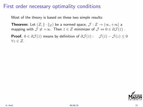
First order necessary optimality conditions
Most of the theory is based on these two simple results
Theorem Let (Z middot Z) be a normed space J Z rarr (infin+infin] amapping with J 6equiv +infin Then z isin Z minimizer of J hArr 0 isin partJ (z)
Proof 0 isin partJ (z) means by definition of partJ (z) J (z)minus J (z) le 0forallz isin Z
Theorem Let (Z middot Z) be a normed space Zad sub Z nonemptyconvex closed J Z rarr R Gateaux differentiable where Zad sub Z sub ZZ open If z isin Zad is a solution to
minzisinZad
J (z)
then z solvesJ prime(z)(z minus z) ge 0 forallz isin Zad
Proof Exercise
H Antil 060616 23
Linear quadratic OCPI Reduced funcational
J (z) =1
2Sz minus ud2L2(Ω) +
λ
2z2L2(Ω)
I Gradient computation using sensitivity
J prime(z)h = (Slowast(Sz minus ud) + λz h)L2(Ω) forallh isin L2(Ω)
we denote the gradient by
nablaJ (z) = Slowast(Sz minus ud) + λz
I First order necessary and sufficient optimality condition
(nablaJ (z) z minus z)L2(Ω) ge 0 forallz isin Zad
I Adjoint equation Let p = Slowast(Sz minus ud) which translates intop isin H1
0 (Ω) solving
minusdiv (Anablap) = uminus ud in Ω
p = 0 on partΩ
I Gradient computation using adjoint nablaJ (z) = p+ λz
H Antil 060616 24
Optimality system
I State u isin H10 (Ω)
intΩAnablau middot nablav =
intΩzv forallv isin H1
0 (Ω)
I Adjoint p isin H10 (Ω)
intΩAnablap middot nablav =
intΩ
(uminus ud)v forallv isin H10 (Ω)
I Control z isin Zad (p+ λz z minus z) ge 0 forallz isin Zad
H Antil 060616 25
Pointwise interpretation
The variational inequality
(p+ λz z minus z) ge 0 forallz isin Zad
is equivalent to for ae x isin Ω
z(x) =
za(x) if p(x) + λz(x) gt 0isin [za(x) zb(x)] if p(x) + λz(x) = 0zb(x) if p(x) + λz(x) lt 0
Consequence
I When λ gt 0 then ae in Ω
z(x) = P[za(x)zb(x)]
minus 1
λp(x)
= min
zb(x)max
za(x)minus 1
λp(x)
H Antil 060616 26
Formal Lagrange method applied to linear OCPIntroduce L H1
0 (Ω)times Zad timesH1(Ω)rarr R defined as
L(u z p) = J(u z)minusint
Ω
(minusdiv (Anablau)minus z
)p dx
Integrate by parts to arrive at
L(u z p) = J(u z)minusint
Ω
(minusdiv (Anablap)uminus zp
)dx+
intpartΩ
(Anablau)p ds
If (u z p) is a stationary point then
I State
DpL(u z p)h = 0 forallh isin H1(Ω)
I AdjointDuL(u z p)h = 0 forallh isin H1
0 (Ω)
I ControlDzL(u z p)(z minus z) ge 0 forallz isin Zad
H Antil 060616 27
Formal Lagrange method applied to linear OCPIntroduce L H1
0 (Ω)times Zad timesH1(Ω)rarr R defined as
L(u z p) = J(u z)minusint
Ω
(minusdiv (Anablau)minus z
)p dx
Integrate by parts to arrive at
L(u z p) = J(u z)minusint
Ω
(minusdiv (Anablap)uminus zp
)dx+
intpartΩ
(Anablau)p ds
If (u z p) is a stationary point then
I State
DpL(u z p)h = 0 forallh isin H1(Ω)
I AdjointDuL(u z p)h = 0 forallh isin H1
0 (Ω)
I ControlDzL(u z p)(z minus z) ge 0 forallz isin Zad
H Antil 060616 27
Formal Lagrange method applied to linear OCPIntroduce L H1
0 (Ω)times Zad timesH1(Ω)rarr R defined as
L(u z p) = J(u z)minusint
Ω
(minusdiv (Anablau)minus z
)p dx
Integrate by parts to arrive at
L(u z p) = J(u z)minusint
Ω
(minusdiv (Anablap)uminus zp
)dx+
intpartΩ
(Anablau)p ds
If (u z p) is a stationary point then
I State
DpL(u z p)h = 0 forallh isin H1(Ω)
I AdjointDuL(u z p)h = 0 forallh isin H1
0 (Ω)
I ControlDzL(u z p)(z minus z) ge 0 forallz isin Zad
H Antil 060616 27
Formal Lagrange method applied to linear OCPIntroduce L H1
0 (Ω)times Zad timesH1(Ω)rarr R defined as
L(u z p) = J(u z)minusint
Ω
(minusdiv (Anablau)minus z
)p dx
Integrate by parts to arrive at
L(u z p) = J(u z)minusint
Ω
(minusdiv (Anablap)uminus zp
)dx+
intpartΩ
(Anablau)p ds
If (u z p) is a stationary point then
I State
DpL(u z p)h = 0 forallh isin H1(Ω)
I AdjointDuL(u z p)h = 0 forallh isin H1
0 (Ω)
I ControlDzL(u z p)(z minus z) ge 0 forallz isin Zad
H Antil 060616 27
Formal Lagrange method applied to linear OCPIntroduce L H1
0 (Ω)times Zad timesH1(Ω)rarr R defined as
L(u z p) = J(u z)minusint
Ω
(minusdiv (Anablau)minus z
)p dx
Integrate by parts to arrive at
L(u z p) = J(u z)minusint
Ω
(minusdiv (Anablap)uminus zp
)dx+
intpartΩ
(Anablau)p ds
If (u z p) is a stationary point then
I State
DpL(u z p)h = 0 forallh isin H1(Ω)
I AdjointDuL(u z p)h = 0 forallh isin H1
0 (Ω)
I ControlDzL(u z p)(z minus z) ge 0 forallz isin Zad
H Antil 060616 27
Outline
Motivation and examples
Linear elliptic optimal control problems
Differentiation in Banach spaces
First-order necessary conditions
Optimal control of semilinear PDEs
An abstract problem
Discretization using finite element methods
H Antil 060616 28
Semilinear elliptic OCP
min J(u z) =1
2uminus ud2L2(Ω) +
λ
2z2L2(Ω)
subject to
minus∆u+ g(x u) = z in Ω
u = 0 on partΩ
and z isin Zad with za zb isin Linfin(Ω)
H Antil 060616 29
State space(A1) Ω sub Rd open bounded partΩ is Lipschitz
(A2) g Ωtimes Rrarr R is bounded and measurable with respect to x isin Ωfor every u isin R
(A3) g is continuous monotone increasing and Lipschitz continuous in ufor ae x isin Ω
(A4) g(x 0) = 0 for ae x isin Ω (not really necessary)
Theorem Suppose (A1)minus (A4) hold For every z isin Lr(Ω) withr gt d2 the state equation has a unique weak solutionu isin H1
0 (Ω) cap C(Ω) ie we haveintΩ
nablau middot nablav dx+
intΩ
g(x u(x))v(x) dx =
intΩ
zv dx forallv isin H10 (Ω)
Moreover there exists a constant C gt 0 such that
uH1(Ω) + uC(Ω) le CzLr(Ω)
RemarkI The proof of the theorem uses the BrowderndashMinty theorem on
monotone operators
H Antil 060616 30
State space(A1) Ω sub Rd open bounded partΩ is Lipschitz
(A2) g Ωtimes Rrarr R is bounded and measurable with respect to x isin Ωfor every u isin R
(A3) g is continuous monotone increasing and Lipschitz continuous in ufor ae x isin Ω
(A4) g(x 0) = 0 for ae x isin Ω (not really necessary)
Theorem Suppose (A1)minus (A4) hold For every z isin Lr(Ω) withr gt d2 the state equation has a unique weak solutionu isin H1
0 (Ω) cap C(Ω) ie we haveintΩ
nablau middot nablav dx+
intΩ
g(x u(x))v(x) dx =
intΩ
zv dx forallv isin H10 (Ω)
Moreover there exists a constant C gt 0 such that
uH1(Ω) + uC(Ω) le CzLr(Ω)
RemarkI The proof of the theorem uses the BrowderndashMinty theorem on
monotone operators
H Antil 060616 30
State space(A1) Ω sub Rd open bounded partΩ is Lipschitz
(A2) g Ωtimes Rrarr R is bounded and measurable with respect to x isin Ωfor every u isin R
(A3) g is continuous monotone increasing and Lipschitz continuous in ufor ae x isin Ω
(A4) g(x 0) = 0 for ae x isin Ω (not really necessary)
Theorem Suppose (A1)minus (A4) hold For every z isin Lr(Ω) withr gt d2 the state equation has a unique weak solutionu isin H1
0 (Ω) cap C(Ω) ie we haveintΩ
nablau middot nablav dx+
intΩ
g(x u(x))v(x) dx =
intΩ
zv dx forallv isin H10 (Ω)
Moreover there exists a constant C gt 0 such that
uH1(Ω) + uC(Ω) le CzLr(Ω)
RemarkI The proof of the theorem uses the BrowderndashMinty theorem on
monotone operators
H Antil 060616 30
Control-to-state map and reduced problem
I Control to state map
S Linfin(Ω)rarr H10 (Ω) cap C(Ω)
is well defined and is globally Lipschitz continuous
I Reduced problem
minJ (z) =1
2S(u)minus ud2L2(Ω) +
λ
2z2L2(Ω)
H Antil 060616 31
Control-to-state map and reduced problem
I Control to state map
S Linfin(Ω)rarr H10 (Ω) cap C(Ω)
is well defined and is globally Lipschitz continuous
I Reduced problem
minJ (z) =1
2S(u)minus ud2L2(Ω) +
λ
2z2L2(Ω)
H Antil 060616 31
First-order necessary conditionsI Lagrangian functional
L(u z p) = J(u z)minusint
Ω
(minus∆u+ g(x u(x))minus z
)p dx
= J(u z)minusint
Ω
(nablau middot nablap+ g(x u(x))pminus zp
)dx
I Adjoint system For all h isin H10 (Ω)
0 = DuL(u z p)h =
intΩ
(uminus ud)h dxminusint
Ω
(nablah middot nablap+ gu(x u(x))ph
)which yields
minus∆p+ gu(x u(x))p = uminus ud in Ω
p = 0 on partΩ
I Control
DzL(u z p)(z minus z) = (p+ λz z minus z) dx ge 0 forallz isin ZadI Gradient
nablaJ (z) = p+ λz
H Antil 060616 32
First-order necessary conditionsI Lagrangian functional
L(u z p) = J(u z)minusint
Ω
(minus∆u+ g(x u(x))minus z
)p dx
= J(u z)minusint
Ω
(nablau middot nablap+ g(x u(x))pminus zp
)dx
I Adjoint system For all h isin H10 (Ω)
0 = DuL(u z p)h =
intΩ
(uminus ud)h dxminusint
Ω
(nablah middot nablap+ gu(x u(x))ph
)which yields
minus∆p+ gu(x u(x))p = uminus ud in Ω
p = 0 on partΩ
I Control
DzL(u z p)(z minus z) = (p+ λz z minus z) dx ge 0 forallz isin ZadI Gradient
nablaJ (z) = p+ λz
H Antil 060616 32
First-order necessary conditionsI Lagrangian functional
L(u z p) = J(u z)minusint
Ω
(minus∆u+ g(x u(x))minus z
)p dx
= J(u z)minusint
Ω
(nablau middot nablap+ g(x u(x))pminus zp
)dx
I Adjoint system For all h isin H10 (Ω)
0 = DuL(u z p)h =
intΩ
(uminus ud)h dxminusint
Ω
(nablah middot nablap+ gu(x u(x))ph
)which yields
minus∆p+ gu(x u(x))p = uminus ud in Ω
p = 0 on partΩ
I Control
DzL(u z p)(z minus z) = (p+ λz z minus z) dx ge 0 forallz isin Zad
I GradientnablaJ (z) = p+ λz
H Antil 060616 32
First-order necessary conditionsI Lagrangian functional
L(u z p) = J(u z)minusint
Ω
(minus∆u+ g(x u(x))minus z
)p dx
= J(u z)minusint
Ω
(nablau middot nablap+ g(x u(x))pminus zp
)dx
I Adjoint system For all h isin H10 (Ω)
0 = DuL(u z p)h =
intΩ
(uminus ud)h dxminusint
Ω
(nablah middot nablap+ gu(x u(x))ph
)which yields
minus∆p+ gu(x u(x))p = uminus ud in Ω
p = 0 on partΩ
I Control
DzL(u z p)(z minus z) = (p+ λz z minus z) dx ge 0 forallz isin ZadI Gradient
nablaJ (z) = p+ λz
H Antil 060616 32
Differentiability of Nemytskii operator
The rigorous proof uses
Theorem In addition to (A1)-(A4) if
(A5) g is continuously differentiable with respect to u for ae x isin Ωand we have
(i) |gu(x 0)| le K for ae x isin Ω(ii) gu is locally Lipschitz with respect to u isin R
then the Nemytskii operator G u 7rarr g(middot u(middot)) is continuously Frechetdifferentiable from Linfin(Ω) into itself and
(Gprime(u)h)(x) = gu(x u(x))h(x) ae in Ω forallh isin Linfin(Ω)
Remark (A5) holds if g(x u) = g(u) and g isin C2(R)
H Antil 060616 33
Outline
Motivation and examples
Linear elliptic optimal control problems
Differentiation in Banach spaces
First-order necessary conditions
Optimal control of semilinear PDEs
An abstract problem
Discretization using finite element methods
H Antil 060616 34
Gradient computation via adjoint general formI Abstract problem
min J(u z)
subject toc(u z) = 0
and z isin Zad
I Directional derivative Let S be the control to state map(nonlinear in general)
z 7rarr S(z) = u(z)
Under the assumptions of ldquoimplicit function theoremrdquo
J prime(z)h = (nablauJ (u(z) z) Sprime(z)h) + (nablazJ (u(z) z) h)
I Sensitivity of u with respect to z Differentiating the stateequation
cu(S(z) z)Sprime(z)h = minuscz(S(z) z)h
leads toSprime(z)h = minuscu(S(z) z)minus1
(cz(S(z) z)h
)
provided cu(S(z) z)minus1 is well-defined
H Antil 060616 35
Gradient computation via adjoint general formI Abstract problem
min J(u z)
subject toc(u z) = 0
and z isin ZadI Directional derivative Let S be the control to state map
(nonlinear in general)
z 7rarr S(z) = u(z)
Under the assumptions of ldquoimplicit function theoremrdquo
J prime(z)h = (nablauJ (u(z) z) Sprime(z)h) + (nablazJ (u(z) z) h)
I Sensitivity of u with respect to z Differentiating the stateequation
cu(S(z) z)Sprime(z)h = minuscz(S(z) z)h
leads toSprime(z)h = minuscu(S(z) z)minus1
(cz(S(z) z)h
)
provided cu(S(z) z)minus1 is well-defined
H Antil 060616 35
Gradient computation via adjoint general formI Abstract problem
min J(u z)
subject toc(u z) = 0
and z isin ZadI Directional derivative Let S be the control to state map
(nonlinear in general)
z 7rarr S(z) = u(z)
Under the assumptions of ldquoimplicit function theoremrdquo
J prime(z)h = (nablauJ (u(z) z) Sprime(z)h) + (nablazJ (u(z) z) h)
I Sensitivity of u with respect to z Differentiating the stateequation
cu(S(z) z)Sprime(z)h = minuscz(S(z) z)h
leads toSprime(z)h = minuscu(S(z) z)minus1
(cz(S(z) z)h
)
provided cu(S(z) z)minus1 is well-defined
H Antil 060616 35
Adjoint equation and gradient general form
I Directional derivative
J prime(z)h = minus(nablauJ (u(z) z) cu(u(z) z)minus1cz(u(z) z)h
)+ (nablazJ (u(z) z) h)
I Gradient
nablaJ (z) = minuscz(u(z) z)lowast(cu(u(z) z)minuslowastnablauJ (u(z) z)
)+nablazJ (u(z) z)
I Introducing adjoint variable p solving
cu(u(z) z)lowastp = nablauJ (u(z) z)
we arrive at following form of gradient
nablaJ (z) = minuscz(u(z) z)lowastp+nablazJ (u(z) z)
which is tractable
H Antil 060616 36
Adjoint equation and gradient general form
I Directional derivative
J prime(z)h = minus(nablauJ (u(z) z) cu(u(z) z)minus1cz(u(z) z)h
)+ (nablazJ (u(z) z) h)
I Gradient
nablaJ (z) = minuscz(u(z) z)lowast(cu(u(z) z)minuslowastnablauJ (u(z) z)
)+nablazJ (u(z) z)
I Introducing adjoint variable p solving
cu(u(z) z)lowastp = nablauJ (u(z) z)
we arrive at following form of gradient
nablaJ (z) = minuscz(u(z) z)lowastp+nablazJ (u(z) z)
which is tractable
H Antil 060616 36
Adjoint equation and gradient general form
I Directional derivative
J prime(z)h = minus(nablauJ (u(z) z) cu(u(z) z)minus1cz(u(z) z)h
)+ (nablazJ (u(z) z) h)
I Gradient
nablaJ (z) = minuscz(u(z) z)lowast(cu(u(z) z)minuslowastnablauJ (u(z) z)
)+nablazJ (u(z) z)
I Introducing adjoint variable p solving
cu(u(z) z)lowastp = nablauJ (u(z) z)
we arrive at following form of gradient
nablaJ (z) = minuscz(u(z) z)lowastp+nablazJ (u(z) z)
which is tractable
H Antil 060616 36
Hessian computation general form
I Lagrangian L(u z p) = J(u z)minusint
Ωc(u z)p dx Then we have
DzJ (z)h = DzL(u z p)h
I Second order derivative
D2zJ (z)[h1 h2] = DuDzL(u z p)[h1 S
prime(z)h2] +D2zL(u z p)[h1 h2]
+DpDzL(u z p)[h1 Dzp(z)h2]
I We already know Sprime(z)h2 moreover
DpDzL(u z p)[h1 Dzp(z)h2] = minus(cu(u z)h1 Dzp(z)h2
)
It remain to identify Dzp(z)h2
H Antil 060616 37
Hessian computation general form
I Lagrangian L(u z p) = J(u z)minusint
Ωc(u z)p dx Then we have
DzJ (z)h = DzL(u z p)h
I Second order derivative
D2zJ (z)[h1 h2] = DuDzL(u z p)[h1 S
prime(z)h2] +D2zL(u z p)[h1 h2]
+DpDzL(u z p)[h1 Dzp(z)h2]
I We already know Sprime(z)h2 moreover
DpDzL(u z p)[h1 Dzp(z)h2] = minus(cu(u z)h1 Dzp(z)h2
)
It remain to identify Dzp(z)h2
H Antil 060616 37
Hessian computation general form
I Lagrangian L(u z p) = J(u z)minusint
Ωc(u z)p dx Then we have
DzJ (z)h = DzL(u z p)h
I Second order derivative
D2zJ (z)[h1 h2] = DuDzL(u z p)[h1 S
prime(z)h2] +D2zL(u z p)[h1 h2]
+DpDzL(u z p)[h1 Dzp(z)h2]
I We already know Sprime(z)h2 moreover
DpDzL(u z p)[h1 Dzp(z)h2] = minus(cu(u z)h1 Dzp(z)h2
)
It remain to identify Dzp(z)h2
H Antil 060616 37
Outline
Motivation and examples
Linear elliptic optimal control problems
Differentiation in Banach spaces
First-order necessary conditions
Optimal control of semilinear PDEs
An abstract problem
Discretization using finite element methods
H Antil 060616 38
Numerical approximation of Poisson equation MeshTo avoid technical issues we will assume that partΩ is polygonal
I Mesh Let T = K be a mesh of Ω where K sub Rd is an elementthat is isoparametrically equivalent to a unit simplex in Rd
I Conforming mesh We say that the mesh is conforming ifI Ω = cupKisinT KI If K1 cap K2 = x then x is a node of K1 and K2I If K1 cap K2 6= empty and K1 cap K2 6= x then K1 cap K2 is an edgeface
contained in partK1 cap partK2
I Shape regular Let T be the collection of all conformingrefinements of an original mesh T 0 Then T is called shape regularif exist κ gt 0 such that
hKρKle κ forallK isin cupiT i
where hK = diam K ρK = maxρ gt 0|Bρ sub KI Quasi-uniform A family of shape regular meshes is called-quasi
uniform if there exist a constant σ gt 0 such that
maxhKminhK
le σ
uniformly for all meshes in the family
Numerical approximation of Poisson equation MeshTo avoid technical issues we will assume that partΩ is polygonal
I Mesh Let T = K be a mesh of Ω where K sub Rd is an elementthat is isoparametrically equivalent to a unit simplex in Rd
I Conforming mesh We say that the mesh is conforming ifI Ω = cupKisinT KI If K1 cap K2 = x then x is a node of K1 and K2I If K1 cap K2 6= empty and K1 cap K2 6= x then K1 cap K2 is an edgeface
contained in partK1 cap partK2
I Shape regular Let T be the collection of all conformingrefinements of an original mesh T 0 Then T is called shape regularif exist κ gt 0 such that
hKρKle κ forallK isin cupiT i
where hK = diam K ρK = maxρ gt 0|Bρ sub KI Quasi-uniform A family of shape regular meshes is called-quasi
uniform if there exist a constant σ gt 0 such that
maxhKminhK
le σ
uniformly for all meshes in the family
Numerical approximation of Poisson equation MeshTo avoid technical issues we will assume that partΩ is polygonal
I Mesh Let T = K be a mesh of Ω where K sub Rd is an elementthat is isoparametrically equivalent to a unit simplex in Rd
I Conforming mesh We say that the mesh is conforming ifI Ω = cupKisinT KI If K1 cap K2 = x then x is a node of K1 and K2I If K1 cap K2 6= empty and K1 cap K2 6= x then K1 cap K2 is an edgeface
contained in partK1 cap partK2
I Shape regular Let T be the collection of all conformingrefinements of an original mesh T 0 Then T is called shape regularif exist κ gt 0 such that
hKρKle κ forallK isin cupiT i
where hK = diam K ρK = maxρ gt 0|Bρ sub K
I Quasi-uniform A family of shape regular meshes is called-quasiuniform if there exist a constant σ gt 0 such that
maxhKminhK
le σ
uniformly for all meshes in the family
Numerical approximation of Poisson equation MeshTo avoid technical issues we will assume that partΩ is polygonal
I Mesh Let T = K be a mesh of Ω where K sub Rd is an elementthat is isoparametrically equivalent to a unit simplex in Rd
I Conforming mesh We say that the mesh is conforming ifI Ω = cupKisinT KI If K1 cap K2 = x then x is a node of K1 and K2I If K1 cap K2 6= empty and K1 cap K2 6= x then K1 cap K2 is an edgeface
contained in partK1 cap partK2
I Shape regular Let T be the collection of all conformingrefinements of an original mesh T 0 Then T is called shape regularif exist κ gt 0 such that
hKρKle κ forallK isin cupiT i
where hK = diam K ρK = maxρ gt 0|Bρ sub KI Quasi-uniform A family of shape regular meshes is called-quasi
uniform if there exist a constant σ gt 0 such that
maxhKminhK
le σ
uniformly for all meshes in the family
FE space and Galerkin approximationI Finite element space For T isin T we define the finite element
space as
V(T ) = W isin C0(Ω) WK isin P1forallK isin T W |partΩ = 0
where P1 is the set of polynomials of degree at most 1
I Galerkin approximation of continuous problem is given by
Find UT isin V(T )
intΩ
AnablaUT middot nablaV = 〈f V 〉 forallV isin V(T )
The discrete problem is well-posedI Nodal basis Consists of functions ψi isin V(T ) with xi isin N (T )
satisfyingψxi
(xj) = δij
where N (T ) denotes the interior (plus Neumann) nodesI Galerkin orthogonality(
nabla(uminus UT )nablaW)L2(Ω)
= 0 forallW isin V(T )
H Antil 060616 40
FE space and Galerkin approximationI Finite element space For T isin T we define the finite element
space as
V(T ) = W isin C0(Ω) WK isin P1forallK isin T W |partΩ = 0
where P1 is the set of polynomials of degree at most 1I Galerkin approximation of continuous problem is given by
Find UT isin V(T )
intΩ
AnablaUT middot nablaV = 〈f V 〉 forallV isin V(T )
The discrete problem is well-posed
I Nodal basis Consists of functions ψi isin V(T ) with xi isin N (T )satisfying
ψxi(xj) = δij
where N (T ) denotes the interior (plus Neumann) nodesI Galerkin orthogonality(
nabla(uminus UT )nablaW)L2(Ω)
= 0 forallW isin V(T )
H Antil 060616 40
FE space and Galerkin approximationI Finite element space For T isin T we define the finite element
space as
V(T ) = W isin C0(Ω) WK isin P1forallK isin T W |partΩ = 0
where P1 is the set of polynomials of degree at most 1I Galerkin approximation of continuous problem is given by
Find UT isin V(T )
intΩ
AnablaUT middot nablaV = 〈f V 〉 forallV isin V(T )
The discrete problem is well-posedI Nodal basis Consists of functions ψi isin V(T ) with xi isin N (T )
satisfyingψxi
(xj) = δij
where N (T ) denotes the interior (plus Neumann) nodes
I Galerkin orthogonality(nabla(uminus UT )nablaW
)L2(Ω)
= 0 forallW isin V(T )
H Antil 060616 40
FE space and Galerkin approximationI Finite element space For T isin T we define the finite element
space as
V(T ) = W isin C0(Ω) WK isin P1forallK isin T W |partΩ = 0
where P1 is the set of polynomials of degree at most 1I Galerkin approximation of continuous problem is given by
Find UT isin V(T )
intΩ
AnablaUT middot nablaV = 〈f V 〉 forallV isin V(T )
The discrete problem is well-posedI Nodal basis Consists of functions ψi isin V(T ) with xi isin N (T )
satisfyingψxi
(xj) = δij
where N (T ) denotes the interior (plus Neumann) nodesI Galerkin orthogonality(
nabla(uminus UT )nablaW)L2(Ω)
= 0 forallW isin V(T )
H Antil 060616 40
Best approximation
I Cearsquos lemma
nabla(uminus UT )L2(Ω) le C infWisinV(T )
nabla(uminusW )L2(Ω)
I Nodal interpolation operator ΠT C(Ω)rarr V(T ) satisfies
ΠT u(xi) = u(xi) forallxi isin N (T )
and is defined as
ΠT u =sum
xiisinN (T )
u(xi)ψxi
I Error estimates In Cearsquos lemma replace W by ΠT u and thencompute the interpolation error
H Antil 060616 41
Best approximation
I Cearsquos lemma
nabla(uminus UT )L2(Ω) le C infWisinV(T )
nabla(uminusW )L2(Ω)
I Nodal interpolation operator ΠT C(Ω)rarr V(T ) satisfies
ΠT u(xi) = u(xi) forallxi isin N (T )
and is defined as
ΠT u =sum
xiisinN (T )
u(xi)ψxi
I Error estimates In Cearsquos lemma replace W by ΠT u and thencompute the interpolation error
H Antil 060616 41
Best approximation
I Cearsquos lemma
nabla(uminus UT )L2(Ω) le C infWisinV(T )
nabla(uminusW )L2(Ω)
I Nodal interpolation operator ΠT C(Ω)rarr V(T ) satisfies
ΠT u(xi) = u(xi) forallxi isin N (T )
and is defined as
ΠT u =sum
xiisinN (T )
u(xi)ψxi
I Error estimates In Cearsquos lemma replace W by ΠT u and thencompute the interpolation error
H Antil 060616 41
Algebraic system state equation
I Recall UT isin V(T ) solves
a(UT V ) = 〈f V 〉 forallV isin V(T )
I Now setting UT =sumN
j=1 Ujψj V = ψi we get
Nsumj=1
Uja(φj φi) = 〈f ψi〉 i = 1 N
which is the matrix-vector system
AU = F
I Stiffness matrix A is SPD
H Antil 060616 42
Algebraic system state equation
I Recall UT isin V(T ) solves
a(UT V ) = 〈f V 〉 forallV isin V(T )
I Now setting UT =sumN
j=1 Ujψj V = ψi we get
Nsumj=1
Uja(φj φi) = 〈f ψi〉 i = 1 N
which is the matrix-vector system
AU = F
I Stiffness matrix A is SPD
H Antil 060616 42
Algebraic system state equation
I Recall UT isin V(T ) solves
a(UT V ) = 〈f V 〉 forallV isin V(T )
I Now setting UT =sumN
j=1 Ujψj V = ψi we get
Nsumj=1
Uja(φj φi) = 〈f ψi〉 i = 1 N
which is the matrix-vector system
AU = F
I Stiffness matrix A is SPD
H Antil 060616 42
Discrete linear elliptic OCP
min JT (UT ZT ) =1
2UT minus ud2L2(Ω) +
λ
2ZT 2L2(Ω)
subject to
Find UT isin V(T )
intΩ
nablaUT middot nablaV = (ZT V )L2(Ω) forallV isin V(T )
and whereZT isin Zad(T ) = Zad cap Z(T )
is either one of these
Z(T ) =
V(T )L2(Ω) variational discretization (Hinze)WT isin Linfin(Ω) ZT |K isin P0(K)K isin T
H Antil 060616 43
Recent books
F TroltzschOptimal control of partial differential equations volume 112 ofGraduate Studies in MathematicsAmerican Mathematical Society Providence RI 2010Theory methods and applications Translated from the 2005 Germanoriginal by Jurgen Sprekels
K Ito and K KunischLagrange multiplier approach to variational problems andapplications volume 15 of Advances in Design and ControlSociety for Industrial and Applied Mathematics (SIAM)Philadelphia PA 2008
H Antil 060616 44
- Motivation and examples
- Linear elliptic optimal control problems
- Differentiation in Banach spaces
- First-order necessary conditions
- Optimal control of semilinear PDEs
- An abstract problem
- Discretization using finite element methods
-
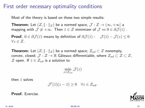
First order necessary optimality conditions
Most of the theory is based on these two simple results
Theorem Let (Z middot Z) be a normed space J Z rarr (infin+infin] amapping with J 6equiv +infin Then z isin Z minimizer of J hArr 0 isin partJ (z)
Proof 0 isin partJ (z) means by definition of partJ (z) J (z)minus J (z) le 0forallz isin Z
Theorem Let (Z middot Z) be a normed space Zad sub Z nonemptyconvex closed J Z rarr R Gateaux differentiable where Zad sub Z sub ZZ open If z isin Zad is a solution to
minzisinZad
J (z)
then z solvesJ prime(z)(z minus z) ge 0 forallz isin Zad
Proof Exercise
H Antil 060616 23
Linear quadratic OCPI Reduced funcational
J (z) =1
2Sz minus ud2L2(Ω) +
λ
2z2L2(Ω)
I Gradient computation using sensitivity
J prime(z)h = (Slowast(Sz minus ud) + λz h)L2(Ω) forallh isin L2(Ω)
we denote the gradient by
nablaJ (z) = Slowast(Sz minus ud) + λz
I First order necessary and sufficient optimality condition
(nablaJ (z) z minus z)L2(Ω) ge 0 forallz isin Zad
I Adjoint equation Let p = Slowast(Sz minus ud) which translates intop isin H1
0 (Ω) solving
minusdiv (Anablap) = uminus ud in Ω
p = 0 on partΩ
I Gradient computation using adjoint nablaJ (z) = p+ λz
H Antil 060616 24
Optimality system
I State u isin H10 (Ω)
intΩAnablau middot nablav =
intΩzv forallv isin H1
0 (Ω)
I Adjoint p isin H10 (Ω)
intΩAnablap middot nablav =
intΩ
(uminus ud)v forallv isin H10 (Ω)
I Control z isin Zad (p+ λz z minus z) ge 0 forallz isin Zad
H Antil 060616 25
Pointwise interpretation
The variational inequality
(p+ λz z minus z) ge 0 forallz isin Zad
is equivalent to for ae x isin Ω
z(x) =
za(x) if p(x) + λz(x) gt 0isin [za(x) zb(x)] if p(x) + λz(x) = 0zb(x) if p(x) + λz(x) lt 0
Consequence
I When λ gt 0 then ae in Ω
z(x) = P[za(x)zb(x)]
minus 1
λp(x)
= min
zb(x)max
za(x)minus 1
λp(x)
H Antil 060616 26
Formal Lagrange method applied to linear OCPIntroduce L H1
0 (Ω)times Zad timesH1(Ω)rarr R defined as
L(u z p) = J(u z)minusint
Ω
(minusdiv (Anablau)minus z
)p dx
Integrate by parts to arrive at
L(u z p) = J(u z)minusint
Ω
(minusdiv (Anablap)uminus zp
)dx+
intpartΩ
(Anablau)p ds
If (u z p) is a stationary point then
I State
DpL(u z p)h = 0 forallh isin H1(Ω)
I AdjointDuL(u z p)h = 0 forallh isin H1
0 (Ω)
I ControlDzL(u z p)(z minus z) ge 0 forallz isin Zad
H Antil 060616 27
Formal Lagrange method applied to linear OCPIntroduce L H1
0 (Ω)times Zad timesH1(Ω)rarr R defined as
L(u z p) = J(u z)minusint
Ω
(minusdiv (Anablau)minus z
)p dx
Integrate by parts to arrive at
L(u z p) = J(u z)minusint
Ω
(minusdiv (Anablap)uminus zp
)dx+
intpartΩ
(Anablau)p ds
If (u z p) is a stationary point then
I State
DpL(u z p)h = 0 forallh isin H1(Ω)
I AdjointDuL(u z p)h = 0 forallh isin H1
0 (Ω)
I ControlDzL(u z p)(z minus z) ge 0 forallz isin Zad
H Antil 060616 27
Formal Lagrange method applied to linear OCPIntroduce L H1
0 (Ω)times Zad timesH1(Ω)rarr R defined as
L(u z p) = J(u z)minusint
Ω
(minusdiv (Anablau)minus z
)p dx
Integrate by parts to arrive at
L(u z p) = J(u z)minusint
Ω
(minusdiv (Anablap)uminus zp
)dx+
intpartΩ
(Anablau)p ds
If (u z p) is a stationary point then
I State
DpL(u z p)h = 0 forallh isin H1(Ω)
I AdjointDuL(u z p)h = 0 forallh isin H1
0 (Ω)
I ControlDzL(u z p)(z minus z) ge 0 forallz isin Zad
H Antil 060616 27
Formal Lagrange method applied to linear OCPIntroduce L H1
0 (Ω)times Zad timesH1(Ω)rarr R defined as
L(u z p) = J(u z)minusint
Ω
(minusdiv (Anablau)minus z
)p dx
Integrate by parts to arrive at
L(u z p) = J(u z)minusint
Ω
(minusdiv (Anablap)uminus zp
)dx+
intpartΩ
(Anablau)p ds
If (u z p) is a stationary point then
I State
DpL(u z p)h = 0 forallh isin H1(Ω)
I AdjointDuL(u z p)h = 0 forallh isin H1
0 (Ω)
I ControlDzL(u z p)(z minus z) ge 0 forallz isin Zad
H Antil 060616 27
Formal Lagrange method applied to linear OCPIntroduce L H1
0 (Ω)times Zad timesH1(Ω)rarr R defined as
L(u z p) = J(u z)minusint
Ω
(minusdiv (Anablau)minus z
)p dx
Integrate by parts to arrive at
L(u z p) = J(u z)minusint
Ω
(minusdiv (Anablap)uminus zp
)dx+
intpartΩ
(Anablau)p ds
If (u z p) is a stationary point then
I State
DpL(u z p)h = 0 forallh isin H1(Ω)
I AdjointDuL(u z p)h = 0 forallh isin H1
0 (Ω)
I ControlDzL(u z p)(z minus z) ge 0 forallz isin Zad
H Antil 060616 27
Outline
Motivation and examples
Linear elliptic optimal control problems
Differentiation in Banach spaces
First-order necessary conditions
Optimal control of semilinear PDEs
An abstract problem
Discretization using finite element methods
H Antil 060616 28
Semilinear elliptic OCP
min J(u z) =1
2uminus ud2L2(Ω) +
λ
2z2L2(Ω)
subject to
minus∆u+ g(x u) = z in Ω
u = 0 on partΩ
and z isin Zad with za zb isin Linfin(Ω)
H Antil 060616 29
State space(A1) Ω sub Rd open bounded partΩ is Lipschitz
(A2) g Ωtimes Rrarr R is bounded and measurable with respect to x isin Ωfor every u isin R
(A3) g is continuous monotone increasing and Lipschitz continuous in ufor ae x isin Ω
(A4) g(x 0) = 0 for ae x isin Ω (not really necessary)
Theorem Suppose (A1)minus (A4) hold For every z isin Lr(Ω) withr gt d2 the state equation has a unique weak solutionu isin H1
0 (Ω) cap C(Ω) ie we haveintΩ
nablau middot nablav dx+
intΩ
g(x u(x))v(x) dx =
intΩ
zv dx forallv isin H10 (Ω)
Moreover there exists a constant C gt 0 such that
uH1(Ω) + uC(Ω) le CzLr(Ω)
RemarkI The proof of the theorem uses the BrowderndashMinty theorem on
monotone operators
H Antil 060616 30
State space(A1) Ω sub Rd open bounded partΩ is Lipschitz
(A2) g Ωtimes Rrarr R is bounded and measurable with respect to x isin Ωfor every u isin R
(A3) g is continuous monotone increasing and Lipschitz continuous in ufor ae x isin Ω
(A4) g(x 0) = 0 for ae x isin Ω (not really necessary)
Theorem Suppose (A1)minus (A4) hold For every z isin Lr(Ω) withr gt d2 the state equation has a unique weak solutionu isin H1
0 (Ω) cap C(Ω) ie we haveintΩ
nablau middot nablav dx+
intΩ
g(x u(x))v(x) dx =
intΩ
zv dx forallv isin H10 (Ω)
Moreover there exists a constant C gt 0 such that
uH1(Ω) + uC(Ω) le CzLr(Ω)
RemarkI The proof of the theorem uses the BrowderndashMinty theorem on
monotone operators
H Antil 060616 30
State space(A1) Ω sub Rd open bounded partΩ is Lipschitz
(A2) g Ωtimes Rrarr R is bounded and measurable with respect to x isin Ωfor every u isin R
(A3) g is continuous monotone increasing and Lipschitz continuous in ufor ae x isin Ω
(A4) g(x 0) = 0 for ae x isin Ω (not really necessary)
Theorem Suppose (A1)minus (A4) hold For every z isin Lr(Ω) withr gt d2 the state equation has a unique weak solutionu isin H1
0 (Ω) cap C(Ω) ie we haveintΩ
nablau middot nablav dx+
intΩ
g(x u(x))v(x) dx =
intΩ
zv dx forallv isin H10 (Ω)
Moreover there exists a constant C gt 0 such that
uH1(Ω) + uC(Ω) le CzLr(Ω)
RemarkI The proof of the theorem uses the BrowderndashMinty theorem on
monotone operators
H Antil 060616 30
Control-to-state map and reduced problem
I Control to state map
S Linfin(Ω)rarr H10 (Ω) cap C(Ω)
is well defined and is globally Lipschitz continuous
I Reduced problem
minJ (z) =1
2S(u)minus ud2L2(Ω) +
λ
2z2L2(Ω)
H Antil 060616 31
Control-to-state map and reduced problem
I Control to state map
S Linfin(Ω)rarr H10 (Ω) cap C(Ω)
is well defined and is globally Lipschitz continuous
I Reduced problem
minJ (z) =1
2S(u)minus ud2L2(Ω) +
λ
2z2L2(Ω)
H Antil 060616 31
First-order necessary conditionsI Lagrangian functional
L(u z p) = J(u z)minusint
Ω
(minus∆u+ g(x u(x))minus z
)p dx
= J(u z)minusint
Ω
(nablau middot nablap+ g(x u(x))pminus zp
)dx
I Adjoint system For all h isin H10 (Ω)
0 = DuL(u z p)h =
intΩ
(uminus ud)h dxminusint
Ω
(nablah middot nablap+ gu(x u(x))ph
)which yields
minus∆p+ gu(x u(x))p = uminus ud in Ω
p = 0 on partΩ
I Control
DzL(u z p)(z minus z) = (p+ λz z minus z) dx ge 0 forallz isin ZadI Gradient
nablaJ (z) = p+ λz
H Antil 060616 32
First-order necessary conditionsI Lagrangian functional
L(u z p) = J(u z)minusint
Ω
(minus∆u+ g(x u(x))minus z
)p dx
= J(u z)minusint
Ω
(nablau middot nablap+ g(x u(x))pminus zp
)dx
I Adjoint system For all h isin H10 (Ω)
0 = DuL(u z p)h =
intΩ
(uminus ud)h dxminusint
Ω
(nablah middot nablap+ gu(x u(x))ph
)which yields
minus∆p+ gu(x u(x))p = uminus ud in Ω
p = 0 on partΩ
I Control
DzL(u z p)(z minus z) = (p+ λz z minus z) dx ge 0 forallz isin ZadI Gradient
nablaJ (z) = p+ λz
H Antil 060616 32
First-order necessary conditionsI Lagrangian functional
L(u z p) = J(u z)minusint
Ω
(minus∆u+ g(x u(x))minus z
)p dx
= J(u z)minusint
Ω
(nablau middot nablap+ g(x u(x))pminus zp
)dx
I Adjoint system For all h isin H10 (Ω)
0 = DuL(u z p)h =
intΩ
(uminus ud)h dxminusint
Ω
(nablah middot nablap+ gu(x u(x))ph
)which yields
minus∆p+ gu(x u(x))p = uminus ud in Ω
p = 0 on partΩ
I Control
DzL(u z p)(z minus z) = (p+ λz z minus z) dx ge 0 forallz isin Zad
I GradientnablaJ (z) = p+ λz
H Antil 060616 32
First-order necessary conditionsI Lagrangian functional
L(u z p) = J(u z)minusint
Ω
(minus∆u+ g(x u(x))minus z
)p dx
= J(u z)minusint
Ω
(nablau middot nablap+ g(x u(x))pminus zp
)dx
I Adjoint system For all h isin H10 (Ω)
0 = DuL(u z p)h =
intΩ
(uminus ud)h dxminusint
Ω
(nablah middot nablap+ gu(x u(x))ph
)which yields
minus∆p+ gu(x u(x))p = uminus ud in Ω
p = 0 on partΩ
I Control
DzL(u z p)(z minus z) = (p+ λz z minus z) dx ge 0 forallz isin ZadI Gradient
nablaJ (z) = p+ λz
H Antil 060616 32
Differentiability of Nemytskii operator
The rigorous proof uses
Theorem In addition to (A1)-(A4) if
(A5) g is continuously differentiable with respect to u for ae x isin Ωand we have
(i) |gu(x 0)| le K for ae x isin Ω(ii) gu is locally Lipschitz with respect to u isin R
then the Nemytskii operator G u 7rarr g(middot u(middot)) is continuously Frechetdifferentiable from Linfin(Ω) into itself and
(Gprime(u)h)(x) = gu(x u(x))h(x) ae in Ω forallh isin Linfin(Ω)
Remark (A5) holds if g(x u) = g(u) and g isin C2(R)
H Antil 060616 33
Outline
Motivation and examples
Linear elliptic optimal control problems
Differentiation in Banach spaces
First-order necessary conditions
Optimal control of semilinear PDEs
An abstract problem
Discretization using finite element methods
H Antil 060616 34
Gradient computation via adjoint general formI Abstract problem
min J(u z)
subject toc(u z) = 0
and z isin Zad
I Directional derivative Let S be the control to state map(nonlinear in general)
z 7rarr S(z) = u(z)
Under the assumptions of ldquoimplicit function theoremrdquo
J prime(z)h = (nablauJ (u(z) z) Sprime(z)h) + (nablazJ (u(z) z) h)
I Sensitivity of u with respect to z Differentiating the stateequation
cu(S(z) z)Sprime(z)h = minuscz(S(z) z)h
leads toSprime(z)h = minuscu(S(z) z)minus1
(cz(S(z) z)h
)
provided cu(S(z) z)minus1 is well-defined
H Antil 060616 35
Gradient computation via adjoint general formI Abstract problem
min J(u z)
subject toc(u z) = 0
and z isin ZadI Directional derivative Let S be the control to state map
(nonlinear in general)
z 7rarr S(z) = u(z)
Under the assumptions of ldquoimplicit function theoremrdquo
J prime(z)h = (nablauJ (u(z) z) Sprime(z)h) + (nablazJ (u(z) z) h)
I Sensitivity of u with respect to z Differentiating the stateequation
cu(S(z) z)Sprime(z)h = minuscz(S(z) z)h
leads toSprime(z)h = minuscu(S(z) z)minus1
(cz(S(z) z)h
)
provided cu(S(z) z)minus1 is well-defined
H Antil 060616 35
Gradient computation via adjoint general formI Abstract problem
min J(u z)
subject toc(u z) = 0
and z isin ZadI Directional derivative Let S be the control to state map
(nonlinear in general)
z 7rarr S(z) = u(z)
Under the assumptions of ldquoimplicit function theoremrdquo
J prime(z)h = (nablauJ (u(z) z) Sprime(z)h) + (nablazJ (u(z) z) h)
I Sensitivity of u with respect to z Differentiating the stateequation
cu(S(z) z)Sprime(z)h = minuscz(S(z) z)h
leads toSprime(z)h = minuscu(S(z) z)minus1
(cz(S(z) z)h
)
provided cu(S(z) z)minus1 is well-defined
H Antil 060616 35
Adjoint equation and gradient general form
I Directional derivative
J prime(z)h = minus(nablauJ (u(z) z) cu(u(z) z)minus1cz(u(z) z)h
)+ (nablazJ (u(z) z) h)
I Gradient
nablaJ (z) = minuscz(u(z) z)lowast(cu(u(z) z)minuslowastnablauJ (u(z) z)
)+nablazJ (u(z) z)
I Introducing adjoint variable p solving
cu(u(z) z)lowastp = nablauJ (u(z) z)
we arrive at following form of gradient
nablaJ (z) = minuscz(u(z) z)lowastp+nablazJ (u(z) z)
which is tractable
H Antil 060616 36
Adjoint equation and gradient general form
I Directional derivative
J prime(z)h = minus(nablauJ (u(z) z) cu(u(z) z)minus1cz(u(z) z)h
)+ (nablazJ (u(z) z) h)
I Gradient
nablaJ (z) = minuscz(u(z) z)lowast(cu(u(z) z)minuslowastnablauJ (u(z) z)
)+nablazJ (u(z) z)
I Introducing adjoint variable p solving
cu(u(z) z)lowastp = nablauJ (u(z) z)
we arrive at following form of gradient
nablaJ (z) = minuscz(u(z) z)lowastp+nablazJ (u(z) z)
which is tractable
H Antil 060616 36
Adjoint equation and gradient general form
I Directional derivative
J prime(z)h = minus(nablauJ (u(z) z) cu(u(z) z)minus1cz(u(z) z)h
)+ (nablazJ (u(z) z) h)
I Gradient
nablaJ (z) = minuscz(u(z) z)lowast(cu(u(z) z)minuslowastnablauJ (u(z) z)
)+nablazJ (u(z) z)
I Introducing adjoint variable p solving
cu(u(z) z)lowastp = nablauJ (u(z) z)
we arrive at following form of gradient
nablaJ (z) = minuscz(u(z) z)lowastp+nablazJ (u(z) z)
which is tractable
H Antil 060616 36
Hessian computation general form
I Lagrangian L(u z p) = J(u z)minusint
Ωc(u z)p dx Then we have
DzJ (z)h = DzL(u z p)h
I Second order derivative
D2zJ (z)[h1 h2] = DuDzL(u z p)[h1 S
prime(z)h2] +D2zL(u z p)[h1 h2]
+DpDzL(u z p)[h1 Dzp(z)h2]
I We already know Sprime(z)h2 moreover
DpDzL(u z p)[h1 Dzp(z)h2] = minus(cu(u z)h1 Dzp(z)h2
)
It remain to identify Dzp(z)h2
H Antil 060616 37
Hessian computation general form
I Lagrangian L(u z p) = J(u z)minusint
Ωc(u z)p dx Then we have
DzJ (z)h = DzL(u z p)h
I Second order derivative
D2zJ (z)[h1 h2] = DuDzL(u z p)[h1 S
prime(z)h2] +D2zL(u z p)[h1 h2]
+DpDzL(u z p)[h1 Dzp(z)h2]
I We already know Sprime(z)h2 moreover
DpDzL(u z p)[h1 Dzp(z)h2] = minus(cu(u z)h1 Dzp(z)h2
)
It remain to identify Dzp(z)h2
H Antil 060616 37
Hessian computation general form
I Lagrangian L(u z p) = J(u z)minusint
Ωc(u z)p dx Then we have
DzJ (z)h = DzL(u z p)h
I Second order derivative
D2zJ (z)[h1 h2] = DuDzL(u z p)[h1 S
prime(z)h2] +D2zL(u z p)[h1 h2]
+DpDzL(u z p)[h1 Dzp(z)h2]
I We already know Sprime(z)h2 moreover
DpDzL(u z p)[h1 Dzp(z)h2] = minus(cu(u z)h1 Dzp(z)h2
)
It remain to identify Dzp(z)h2
H Antil 060616 37
Outline
Motivation and examples
Linear elliptic optimal control problems
Differentiation in Banach spaces
First-order necessary conditions
Optimal control of semilinear PDEs
An abstract problem
Discretization using finite element methods
H Antil 060616 38
Numerical approximation of Poisson equation MeshTo avoid technical issues we will assume that partΩ is polygonal
I Mesh Let T = K be a mesh of Ω where K sub Rd is an elementthat is isoparametrically equivalent to a unit simplex in Rd
I Conforming mesh We say that the mesh is conforming ifI Ω = cupKisinT KI If K1 cap K2 = x then x is a node of K1 and K2I If K1 cap K2 6= empty and K1 cap K2 6= x then K1 cap K2 is an edgeface
contained in partK1 cap partK2
I Shape regular Let T be the collection of all conformingrefinements of an original mesh T 0 Then T is called shape regularif exist κ gt 0 such that
hKρKle κ forallK isin cupiT i
where hK = diam K ρK = maxρ gt 0|Bρ sub KI Quasi-uniform A family of shape regular meshes is called-quasi
uniform if there exist a constant σ gt 0 such that
maxhKminhK
le σ
uniformly for all meshes in the family
Numerical approximation of Poisson equation MeshTo avoid technical issues we will assume that partΩ is polygonal
I Mesh Let T = K be a mesh of Ω where K sub Rd is an elementthat is isoparametrically equivalent to a unit simplex in Rd
I Conforming mesh We say that the mesh is conforming ifI Ω = cupKisinT KI If K1 cap K2 = x then x is a node of K1 and K2I If K1 cap K2 6= empty and K1 cap K2 6= x then K1 cap K2 is an edgeface
contained in partK1 cap partK2
I Shape regular Let T be the collection of all conformingrefinements of an original mesh T 0 Then T is called shape regularif exist κ gt 0 such that
hKρKle κ forallK isin cupiT i
where hK = diam K ρK = maxρ gt 0|Bρ sub KI Quasi-uniform A family of shape regular meshes is called-quasi
uniform if there exist a constant σ gt 0 such that
maxhKminhK
le σ
uniformly for all meshes in the family
Numerical approximation of Poisson equation MeshTo avoid technical issues we will assume that partΩ is polygonal
I Mesh Let T = K be a mesh of Ω where K sub Rd is an elementthat is isoparametrically equivalent to a unit simplex in Rd
I Conforming mesh We say that the mesh is conforming ifI Ω = cupKisinT KI If K1 cap K2 = x then x is a node of K1 and K2I If K1 cap K2 6= empty and K1 cap K2 6= x then K1 cap K2 is an edgeface
contained in partK1 cap partK2
I Shape regular Let T be the collection of all conformingrefinements of an original mesh T 0 Then T is called shape regularif exist κ gt 0 such that
hKρKle κ forallK isin cupiT i
where hK = diam K ρK = maxρ gt 0|Bρ sub K
I Quasi-uniform A family of shape regular meshes is called-quasiuniform if there exist a constant σ gt 0 such that
maxhKminhK
le σ
uniformly for all meshes in the family
Numerical approximation of Poisson equation MeshTo avoid technical issues we will assume that partΩ is polygonal
I Mesh Let T = K be a mesh of Ω where K sub Rd is an elementthat is isoparametrically equivalent to a unit simplex in Rd
I Conforming mesh We say that the mesh is conforming ifI Ω = cupKisinT KI If K1 cap K2 = x then x is a node of K1 and K2I If K1 cap K2 6= empty and K1 cap K2 6= x then K1 cap K2 is an edgeface
contained in partK1 cap partK2
I Shape regular Let T be the collection of all conformingrefinements of an original mesh T 0 Then T is called shape regularif exist κ gt 0 such that
hKρKle κ forallK isin cupiT i
where hK = diam K ρK = maxρ gt 0|Bρ sub KI Quasi-uniform A family of shape regular meshes is called-quasi
uniform if there exist a constant σ gt 0 such that
maxhKminhK
le σ
uniformly for all meshes in the family
FE space and Galerkin approximationI Finite element space For T isin T we define the finite element
space as
V(T ) = W isin C0(Ω) WK isin P1forallK isin T W |partΩ = 0
where P1 is the set of polynomials of degree at most 1
I Galerkin approximation of continuous problem is given by
Find UT isin V(T )
intΩ
AnablaUT middot nablaV = 〈f V 〉 forallV isin V(T )
The discrete problem is well-posedI Nodal basis Consists of functions ψi isin V(T ) with xi isin N (T )
satisfyingψxi
(xj) = δij
where N (T ) denotes the interior (plus Neumann) nodesI Galerkin orthogonality(
nabla(uminus UT )nablaW)L2(Ω)
= 0 forallW isin V(T )
H Antil 060616 40
FE space and Galerkin approximationI Finite element space For T isin T we define the finite element
space as
V(T ) = W isin C0(Ω) WK isin P1forallK isin T W |partΩ = 0
where P1 is the set of polynomials of degree at most 1I Galerkin approximation of continuous problem is given by
Find UT isin V(T )
intΩ
AnablaUT middot nablaV = 〈f V 〉 forallV isin V(T )
The discrete problem is well-posed
I Nodal basis Consists of functions ψi isin V(T ) with xi isin N (T )satisfying
ψxi(xj) = δij
where N (T ) denotes the interior (plus Neumann) nodesI Galerkin orthogonality(
nabla(uminus UT )nablaW)L2(Ω)
= 0 forallW isin V(T )
H Antil 060616 40
FE space and Galerkin approximationI Finite element space For T isin T we define the finite element
space as
V(T ) = W isin C0(Ω) WK isin P1forallK isin T W |partΩ = 0
where P1 is the set of polynomials of degree at most 1I Galerkin approximation of continuous problem is given by
Find UT isin V(T )
intΩ
AnablaUT middot nablaV = 〈f V 〉 forallV isin V(T )
The discrete problem is well-posedI Nodal basis Consists of functions ψi isin V(T ) with xi isin N (T )
satisfyingψxi
(xj) = δij
where N (T ) denotes the interior (plus Neumann) nodes
I Galerkin orthogonality(nabla(uminus UT )nablaW
)L2(Ω)
= 0 forallW isin V(T )
H Antil 060616 40
FE space and Galerkin approximationI Finite element space For T isin T we define the finite element
space as
V(T ) = W isin C0(Ω) WK isin P1forallK isin T W |partΩ = 0
where P1 is the set of polynomials of degree at most 1I Galerkin approximation of continuous problem is given by
Find UT isin V(T )
intΩ
AnablaUT middot nablaV = 〈f V 〉 forallV isin V(T )
The discrete problem is well-posedI Nodal basis Consists of functions ψi isin V(T ) with xi isin N (T )
satisfyingψxi
(xj) = δij
where N (T ) denotes the interior (plus Neumann) nodesI Galerkin orthogonality(
nabla(uminus UT )nablaW)L2(Ω)
= 0 forallW isin V(T )
H Antil 060616 40
Best approximation
I Cearsquos lemma
nabla(uminus UT )L2(Ω) le C infWisinV(T )
nabla(uminusW )L2(Ω)
I Nodal interpolation operator ΠT C(Ω)rarr V(T ) satisfies
ΠT u(xi) = u(xi) forallxi isin N (T )
and is defined as
ΠT u =sum
xiisinN (T )
u(xi)ψxi
I Error estimates In Cearsquos lemma replace W by ΠT u and thencompute the interpolation error
H Antil 060616 41
Best approximation
I Cearsquos lemma
nabla(uminus UT )L2(Ω) le C infWisinV(T )
nabla(uminusW )L2(Ω)
I Nodal interpolation operator ΠT C(Ω)rarr V(T ) satisfies
ΠT u(xi) = u(xi) forallxi isin N (T )
and is defined as
ΠT u =sum
xiisinN (T )
u(xi)ψxi
I Error estimates In Cearsquos lemma replace W by ΠT u and thencompute the interpolation error
H Antil 060616 41
Best approximation
I Cearsquos lemma
nabla(uminus UT )L2(Ω) le C infWisinV(T )
nabla(uminusW )L2(Ω)
I Nodal interpolation operator ΠT C(Ω)rarr V(T ) satisfies
ΠT u(xi) = u(xi) forallxi isin N (T )
and is defined as
ΠT u =sum
xiisinN (T )
u(xi)ψxi
I Error estimates In Cearsquos lemma replace W by ΠT u and thencompute the interpolation error
H Antil 060616 41
Algebraic system state equation
I Recall UT isin V(T ) solves
a(UT V ) = 〈f V 〉 forallV isin V(T )
I Now setting UT =sumN
j=1 Ujψj V = ψi we get
Nsumj=1
Uja(φj φi) = 〈f ψi〉 i = 1 N
which is the matrix-vector system
AU = F
I Stiffness matrix A is SPD
H Antil 060616 42
Algebraic system state equation
I Recall UT isin V(T ) solves
a(UT V ) = 〈f V 〉 forallV isin V(T )
I Now setting UT =sumN
j=1 Ujψj V = ψi we get
Nsumj=1
Uja(φj φi) = 〈f ψi〉 i = 1 N
which is the matrix-vector system
AU = F
I Stiffness matrix A is SPD
H Antil 060616 42
Algebraic system state equation
I Recall UT isin V(T ) solves
a(UT V ) = 〈f V 〉 forallV isin V(T )
I Now setting UT =sumN
j=1 Ujψj V = ψi we get
Nsumj=1
Uja(φj φi) = 〈f ψi〉 i = 1 N
which is the matrix-vector system
AU = F
I Stiffness matrix A is SPD
H Antil 060616 42
Discrete linear elliptic OCP
min JT (UT ZT ) =1
2UT minus ud2L2(Ω) +
λ
2ZT 2L2(Ω)
subject to
Find UT isin V(T )
intΩ
nablaUT middot nablaV = (ZT V )L2(Ω) forallV isin V(T )
and whereZT isin Zad(T ) = Zad cap Z(T )
is either one of these
Z(T ) =
V(T )L2(Ω) variational discretization (Hinze)WT isin Linfin(Ω) ZT |K isin P0(K)K isin T
H Antil 060616 43
Recent books
F TroltzschOptimal control of partial differential equations volume 112 ofGraduate Studies in MathematicsAmerican Mathematical Society Providence RI 2010Theory methods and applications Translated from the 2005 Germanoriginal by Jurgen Sprekels
K Ito and K KunischLagrange multiplier approach to variational problems andapplications volume 15 of Advances in Design and ControlSociety for Industrial and Applied Mathematics (SIAM)Philadelphia PA 2008
H Antil 060616 44
- Motivation and examples
- Linear elliptic optimal control problems
- Differentiation in Banach spaces
- First-order necessary conditions
- Optimal control of semilinear PDEs
- An abstract problem
- Discretization using finite element methods
-
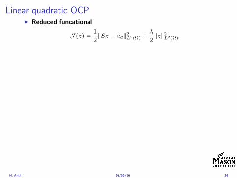
Linear quadratic OCPI Reduced funcational
J (z) =1
2Sz minus ud2L2(Ω) +
λ
2z2L2(Ω)
I Gradient computation using sensitivity
J prime(z)h = (Slowast(Sz minus ud) + λz h)L2(Ω) forallh isin L2(Ω)
we denote the gradient by
nablaJ (z) = Slowast(Sz minus ud) + λz
I First order necessary and sufficient optimality condition
(nablaJ (z) z minus z)L2(Ω) ge 0 forallz isin Zad
I Adjoint equation Let p = Slowast(Sz minus ud) which translates intop isin H1
0 (Ω) solving
minusdiv (Anablap) = uminus ud in Ω
p = 0 on partΩ
I Gradient computation using adjoint nablaJ (z) = p+ λz
H Antil 060616 24
Optimality system
I State u isin H10 (Ω)
intΩAnablau middot nablav =
intΩzv forallv isin H1
0 (Ω)
I Adjoint p isin H10 (Ω)
intΩAnablap middot nablav =
intΩ
(uminus ud)v forallv isin H10 (Ω)
I Control z isin Zad (p+ λz z minus z) ge 0 forallz isin Zad
H Antil 060616 25
Pointwise interpretation
The variational inequality
(p+ λz z minus z) ge 0 forallz isin Zad
is equivalent to for ae x isin Ω
z(x) =
za(x) if p(x) + λz(x) gt 0isin [za(x) zb(x)] if p(x) + λz(x) = 0zb(x) if p(x) + λz(x) lt 0
Consequence
I When λ gt 0 then ae in Ω
z(x) = P[za(x)zb(x)]
minus 1
λp(x)
= min
zb(x)max
za(x)minus 1
λp(x)
H Antil 060616 26
Formal Lagrange method applied to linear OCPIntroduce L H1
0 (Ω)times Zad timesH1(Ω)rarr R defined as
L(u z p) = J(u z)minusint
Ω
(minusdiv (Anablau)minus z
)p dx
Integrate by parts to arrive at
L(u z p) = J(u z)minusint
Ω
(minusdiv (Anablap)uminus zp
)dx+
intpartΩ
(Anablau)p ds
If (u z p) is a stationary point then
I State
DpL(u z p)h = 0 forallh isin H1(Ω)
I AdjointDuL(u z p)h = 0 forallh isin H1
0 (Ω)
I ControlDzL(u z p)(z minus z) ge 0 forallz isin Zad
H Antil 060616 27
Formal Lagrange method applied to linear OCPIntroduce L H1
0 (Ω)times Zad timesH1(Ω)rarr R defined as
L(u z p) = J(u z)minusint
Ω
(minusdiv (Anablau)minus z
)p dx
Integrate by parts to arrive at
L(u z p) = J(u z)minusint
Ω
(minusdiv (Anablap)uminus zp
)dx+
intpartΩ
(Anablau)p ds
If (u z p) is a stationary point then
I State
DpL(u z p)h = 0 forallh isin H1(Ω)
I AdjointDuL(u z p)h = 0 forallh isin H1
0 (Ω)
I ControlDzL(u z p)(z minus z) ge 0 forallz isin Zad
H Antil 060616 27
Formal Lagrange method applied to linear OCPIntroduce L H1
0 (Ω)times Zad timesH1(Ω)rarr R defined as
L(u z p) = J(u z)minusint
Ω
(minusdiv (Anablau)minus z
)p dx
Integrate by parts to arrive at
L(u z p) = J(u z)minusint
Ω
(minusdiv (Anablap)uminus zp
)dx+
intpartΩ
(Anablau)p ds
If (u z p) is a stationary point then
I State
DpL(u z p)h = 0 forallh isin H1(Ω)
I AdjointDuL(u z p)h = 0 forallh isin H1
0 (Ω)
I ControlDzL(u z p)(z minus z) ge 0 forallz isin Zad
H Antil 060616 27
Formal Lagrange method applied to linear OCPIntroduce L H1
0 (Ω)times Zad timesH1(Ω)rarr R defined as
L(u z p) = J(u z)minusint
Ω
(minusdiv (Anablau)minus z
)p dx
Integrate by parts to arrive at
L(u z p) = J(u z)minusint
Ω
(minusdiv (Anablap)uminus zp
)dx+
intpartΩ
(Anablau)p ds
If (u z p) is a stationary point then
I State
DpL(u z p)h = 0 forallh isin H1(Ω)
I AdjointDuL(u z p)h = 0 forallh isin H1
0 (Ω)
I ControlDzL(u z p)(z minus z) ge 0 forallz isin Zad
H Antil 060616 27
Formal Lagrange method applied to linear OCPIntroduce L H1
0 (Ω)times Zad timesH1(Ω)rarr R defined as
L(u z p) = J(u z)minusint
Ω
(minusdiv (Anablau)minus z
)p dx
Integrate by parts to arrive at
L(u z p) = J(u z)minusint
Ω
(minusdiv (Anablap)uminus zp
)dx+
intpartΩ
(Anablau)p ds
If (u z p) is a stationary point then
I State
DpL(u z p)h = 0 forallh isin H1(Ω)
I AdjointDuL(u z p)h = 0 forallh isin H1
0 (Ω)
I ControlDzL(u z p)(z minus z) ge 0 forallz isin Zad
H Antil 060616 27
Outline
Motivation and examples
Linear elliptic optimal control problems
Differentiation in Banach spaces
First-order necessary conditions
Optimal control of semilinear PDEs
An abstract problem
Discretization using finite element methods
H Antil 060616 28
Semilinear elliptic OCP
min J(u z) =1
2uminus ud2L2(Ω) +
λ
2z2L2(Ω)
subject to
minus∆u+ g(x u) = z in Ω
u = 0 on partΩ
and z isin Zad with za zb isin Linfin(Ω)
H Antil 060616 29
State space(A1) Ω sub Rd open bounded partΩ is Lipschitz
(A2) g Ωtimes Rrarr R is bounded and measurable with respect to x isin Ωfor every u isin R
(A3) g is continuous monotone increasing and Lipschitz continuous in ufor ae x isin Ω
(A4) g(x 0) = 0 for ae x isin Ω (not really necessary)
Theorem Suppose (A1)minus (A4) hold For every z isin Lr(Ω) withr gt d2 the state equation has a unique weak solutionu isin H1
0 (Ω) cap C(Ω) ie we haveintΩ
nablau middot nablav dx+
intΩ
g(x u(x))v(x) dx =
intΩ
zv dx forallv isin H10 (Ω)
Moreover there exists a constant C gt 0 such that
uH1(Ω) + uC(Ω) le CzLr(Ω)
RemarkI The proof of the theorem uses the BrowderndashMinty theorem on
monotone operators
H Antil 060616 30
State space(A1) Ω sub Rd open bounded partΩ is Lipschitz
(A2) g Ωtimes Rrarr R is bounded and measurable with respect to x isin Ωfor every u isin R
(A3) g is continuous monotone increasing and Lipschitz continuous in ufor ae x isin Ω
(A4) g(x 0) = 0 for ae x isin Ω (not really necessary)
Theorem Suppose (A1)minus (A4) hold For every z isin Lr(Ω) withr gt d2 the state equation has a unique weak solutionu isin H1
0 (Ω) cap C(Ω) ie we haveintΩ
nablau middot nablav dx+
intΩ
g(x u(x))v(x) dx =
intΩ
zv dx forallv isin H10 (Ω)
Moreover there exists a constant C gt 0 such that
uH1(Ω) + uC(Ω) le CzLr(Ω)
RemarkI The proof of the theorem uses the BrowderndashMinty theorem on
monotone operators
H Antil 060616 30
State space(A1) Ω sub Rd open bounded partΩ is Lipschitz
(A2) g Ωtimes Rrarr R is bounded and measurable with respect to x isin Ωfor every u isin R
(A3) g is continuous monotone increasing and Lipschitz continuous in ufor ae x isin Ω
(A4) g(x 0) = 0 for ae x isin Ω (not really necessary)
Theorem Suppose (A1)minus (A4) hold For every z isin Lr(Ω) withr gt d2 the state equation has a unique weak solutionu isin H1
0 (Ω) cap C(Ω) ie we haveintΩ
nablau middot nablav dx+
intΩ
g(x u(x))v(x) dx =
intΩ
zv dx forallv isin H10 (Ω)
Moreover there exists a constant C gt 0 such that
uH1(Ω) + uC(Ω) le CzLr(Ω)
RemarkI The proof of the theorem uses the BrowderndashMinty theorem on
monotone operators
H Antil 060616 30
Control-to-state map and reduced problem
I Control to state map
S Linfin(Ω)rarr H10 (Ω) cap C(Ω)
is well defined and is globally Lipschitz continuous
I Reduced problem
minJ (z) =1
2S(u)minus ud2L2(Ω) +
λ
2z2L2(Ω)
H Antil 060616 31
Control-to-state map and reduced problem
I Control to state map
S Linfin(Ω)rarr H10 (Ω) cap C(Ω)
is well defined and is globally Lipschitz continuous
I Reduced problem
minJ (z) =1
2S(u)minus ud2L2(Ω) +
λ
2z2L2(Ω)
H Antil 060616 31
First-order necessary conditionsI Lagrangian functional
L(u z p) = J(u z)minusint
Ω
(minus∆u+ g(x u(x))minus z
)p dx
= J(u z)minusint
Ω
(nablau middot nablap+ g(x u(x))pminus zp
)dx
I Adjoint system For all h isin H10 (Ω)
0 = DuL(u z p)h =
intΩ
(uminus ud)h dxminusint
Ω
(nablah middot nablap+ gu(x u(x))ph
)which yields
minus∆p+ gu(x u(x))p = uminus ud in Ω
p = 0 on partΩ
I Control
DzL(u z p)(z minus z) = (p+ λz z minus z) dx ge 0 forallz isin ZadI Gradient
nablaJ (z) = p+ λz
H Antil 060616 32
First-order necessary conditionsI Lagrangian functional
L(u z p) = J(u z)minusint
Ω
(minus∆u+ g(x u(x))minus z
)p dx
= J(u z)minusint
Ω
(nablau middot nablap+ g(x u(x))pminus zp
)dx
I Adjoint system For all h isin H10 (Ω)
0 = DuL(u z p)h =
intΩ
(uminus ud)h dxminusint
Ω
(nablah middot nablap+ gu(x u(x))ph
)which yields
minus∆p+ gu(x u(x))p = uminus ud in Ω
p = 0 on partΩ
I Control
DzL(u z p)(z minus z) = (p+ λz z minus z) dx ge 0 forallz isin ZadI Gradient
nablaJ (z) = p+ λz
H Antil 060616 32
First-order necessary conditionsI Lagrangian functional
L(u z p) = J(u z)minusint
Ω
(minus∆u+ g(x u(x))minus z
)p dx
= J(u z)minusint
Ω
(nablau middot nablap+ g(x u(x))pminus zp
)dx
I Adjoint system For all h isin H10 (Ω)
0 = DuL(u z p)h =
intΩ
(uminus ud)h dxminusint
Ω
(nablah middot nablap+ gu(x u(x))ph
)which yields
minus∆p+ gu(x u(x))p = uminus ud in Ω
p = 0 on partΩ
I Control
DzL(u z p)(z minus z) = (p+ λz z minus z) dx ge 0 forallz isin Zad
I GradientnablaJ (z) = p+ λz
H Antil 060616 32
First-order necessary conditionsI Lagrangian functional
L(u z p) = J(u z)minusint
Ω
(minus∆u+ g(x u(x))minus z
)p dx
= J(u z)minusint
Ω
(nablau middot nablap+ g(x u(x))pminus zp
)dx
I Adjoint system For all h isin H10 (Ω)
0 = DuL(u z p)h =
intΩ
(uminus ud)h dxminusint
Ω
(nablah middot nablap+ gu(x u(x))ph
)which yields
minus∆p+ gu(x u(x))p = uminus ud in Ω
p = 0 on partΩ
I Control
DzL(u z p)(z minus z) = (p+ λz z minus z) dx ge 0 forallz isin ZadI Gradient
nablaJ (z) = p+ λz
H Antil 060616 32
Differentiability of Nemytskii operator
The rigorous proof uses
Theorem In addition to (A1)-(A4) if
(A5) g is continuously differentiable with respect to u for ae x isin Ωand we have
(i) |gu(x 0)| le K for ae x isin Ω(ii) gu is locally Lipschitz with respect to u isin R
then the Nemytskii operator G u 7rarr g(middot u(middot)) is continuously Frechetdifferentiable from Linfin(Ω) into itself and
(Gprime(u)h)(x) = gu(x u(x))h(x) ae in Ω forallh isin Linfin(Ω)
Remark (A5) holds if g(x u) = g(u) and g isin C2(R)
H Antil 060616 33
Outline
Motivation and examples
Linear elliptic optimal control problems
Differentiation in Banach spaces
First-order necessary conditions
Optimal control of semilinear PDEs
An abstract problem
Discretization using finite element methods
H Antil 060616 34
Gradient computation via adjoint general formI Abstract problem
min J(u z)
subject toc(u z) = 0
and z isin Zad
I Directional derivative Let S be the control to state map(nonlinear in general)
z 7rarr S(z) = u(z)
Under the assumptions of ldquoimplicit function theoremrdquo
J prime(z)h = (nablauJ (u(z) z) Sprime(z)h) + (nablazJ (u(z) z) h)
I Sensitivity of u with respect to z Differentiating the stateequation
cu(S(z) z)Sprime(z)h = minuscz(S(z) z)h
leads toSprime(z)h = minuscu(S(z) z)minus1
(cz(S(z) z)h
)
provided cu(S(z) z)minus1 is well-defined
H Antil 060616 35
Gradient computation via adjoint general formI Abstract problem
min J(u z)
subject toc(u z) = 0
and z isin ZadI Directional derivative Let S be the control to state map
(nonlinear in general)
z 7rarr S(z) = u(z)
Under the assumptions of ldquoimplicit function theoremrdquo
J prime(z)h = (nablauJ (u(z) z) Sprime(z)h) + (nablazJ (u(z) z) h)
I Sensitivity of u with respect to z Differentiating the stateequation
cu(S(z) z)Sprime(z)h = minuscz(S(z) z)h
leads toSprime(z)h = minuscu(S(z) z)minus1
(cz(S(z) z)h
)
provided cu(S(z) z)minus1 is well-defined
H Antil 060616 35
Gradient computation via adjoint general formI Abstract problem
min J(u z)
subject toc(u z) = 0
and z isin ZadI Directional derivative Let S be the control to state map
(nonlinear in general)
z 7rarr S(z) = u(z)
Under the assumptions of ldquoimplicit function theoremrdquo
J prime(z)h = (nablauJ (u(z) z) Sprime(z)h) + (nablazJ (u(z) z) h)
I Sensitivity of u with respect to z Differentiating the stateequation
cu(S(z) z)Sprime(z)h = minuscz(S(z) z)h
leads toSprime(z)h = minuscu(S(z) z)minus1
(cz(S(z) z)h
)
provided cu(S(z) z)minus1 is well-defined
H Antil 060616 35
Adjoint equation and gradient general form
I Directional derivative
J prime(z)h = minus(nablauJ (u(z) z) cu(u(z) z)minus1cz(u(z) z)h
)+ (nablazJ (u(z) z) h)
I Gradient
nablaJ (z) = minuscz(u(z) z)lowast(cu(u(z) z)minuslowastnablauJ (u(z) z)
)+nablazJ (u(z) z)
I Introducing adjoint variable p solving
cu(u(z) z)lowastp = nablauJ (u(z) z)
we arrive at following form of gradient
nablaJ (z) = minuscz(u(z) z)lowastp+nablazJ (u(z) z)
which is tractable
H Antil 060616 36
Adjoint equation and gradient general form
I Directional derivative
J prime(z)h = minus(nablauJ (u(z) z) cu(u(z) z)minus1cz(u(z) z)h
)+ (nablazJ (u(z) z) h)
I Gradient
nablaJ (z) = minuscz(u(z) z)lowast(cu(u(z) z)minuslowastnablauJ (u(z) z)
)+nablazJ (u(z) z)
I Introducing adjoint variable p solving
cu(u(z) z)lowastp = nablauJ (u(z) z)
we arrive at following form of gradient
nablaJ (z) = minuscz(u(z) z)lowastp+nablazJ (u(z) z)
which is tractable
H Antil 060616 36
Adjoint equation and gradient general form
I Directional derivative
J prime(z)h = minus(nablauJ (u(z) z) cu(u(z) z)minus1cz(u(z) z)h
)+ (nablazJ (u(z) z) h)
I Gradient
nablaJ (z) = minuscz(u(z) z)lowast(cu(u(z) z)minuslowastnablauJ (u(z) z)
)+nablazJ (u(z) z)
I Introducing adjoint variable p solving
cu(u(z) z)lowastp = nablauJ (u(z) z)
we arrive at following form of gradient
nablaJ (z) = minuscz(u(z) z)lowastp+nablazJ (u(z) z)
which is tractable
H Antil 060616 36
Hessian computation general form
I Lagrangian L(u z p) = J(u z)minusint
Ωc(u z)p dx Then we have
DzJ (z)h = DzL(u z p)h
I Second order derivative
D2zJ (z)[h1 h2] = DuDzL(u z p)[h1 S
prime(z)h2] +D2zL(u z p)[h1 h2]
+DpDzL(u z p)[h1 Dzp(z)h2]
I We already know Sprime(z)h2 moreover
DpDzL(u z p)[h1 Dzp(z)h2] = minus(cu(u z)h1 Dzp(z)h2
)
It remain to identify Dzp(z)h2
H Antil 060616 37
Hessian computation general form
I Lagrangian L(u z p) = J(u z)minusint
Ωc(u z)p dx Then we have
DzJ (z)h = DzL(u z p)h
I Second order derivative
D2zJ (z)[h1 h2] = DuDzL(u z p)[h1 S
prime(z)h2] +D2zL(u z p)[h1 h2]
+DpDzL(u z p)[h1 Dzp(z)h2]
I We already know Sprime(z)h2 moreover
DpDzL(u z p)[h1 Dzp(z)h2] = minus(cu(u z)h1 Dzp(z)h2
)
It remain to identify Dzp(z)h2
H Antil 060616 37
Hessian computation general form
I Lagrangian L(u z p) = J(u z)minusint
Ωc(u z)p dx Then we have
DzJ (z)h = DzL(u z p)h
I Second order derivative
D2zJ (z)[h1 h2] = DuDzL(u z p)[h1 S
prime(z)h2] +D2zL(u z p)[h1 h2]
+DpDzL(u z p)[h1 Dzp(z)h2]
I We already know Sprime(z)h2 moreover
DpDzL(u z p)[h1 Dzp(z)h2] = minus(cu(u z)h1 Dzp(z)h2
)
It remain to identify Dzp(z)h2
H Antil 060616 37
Outline
Motivation and examples
Linear elliptic optimal control problems
Differentiation in Banach spaces
First-order necessary conditions
Optimal control of semilinear PDEs
An abstract problem
Discretization using finite element methods
H Antil 060616 38
Numerical approximation of Poisson equation MeshTo avoid technical issues we will assume that partΩ is polygonal
I Mesh Let T = K be a mesh of Ω where K sub Rd is an elementthat is isoparametrically equivalent to a unit simplex in Rd
I Conforming mesh We say that the mesh is conforming ifI Ω = cupKisinT KI If K1 cap K2 = x then x is a node of K1 and K2I If K1 cap K2 6= empty and K1 cap K2 6= x then K1 cap K2 is an edgeface
contained in partK1 cap partK2
I Shape regular Let T be the collection of all conformingrefinements of an original mesh T 0 Then T is called shape regularif exist κ gt 0 such that
hKρKle κ forallK isin cupiT i
where hK = diam K ρK = maxρ gt 0|Bρ sub KI Quasi-uniform A family of shape regular meshes is called-quasi
uniform if there exist a constant σ gt 0 such that
maxhKminhK
le σ
uniformly for all meshes in the family
Numerical approximation of Poisson equation MeshTo avoid technical issues we will assume that partΩ is polygonal
I Mesh Let T = K be a mesh of Ω where K sub Rd is an elementthat is isoparametrically equivalent to a unit simplex in Rd
I Conforming mesh We say that the mesh is conforming ifI Ω = cupKisinT KI If K1 cap K2 = x then x is a node of K1 and K2I If K1 cap K2 6= empty and K1 cap K2 6= x then K1 cap K2 is an edgeface
contained in partK1 cap partK2
I Shape regular Let T be the collection of all conformingrefinements of an original mesh T 0 Then T is called shape regularif exist κ gt 0 such that
hKρKle κ forallK isin cupiT i
where hK = diam K ρK = maxρ gt 0|Bρ sub KI Quasi-uniform A family of shape regular meshes is called-quasi
uniform if there exist a constant σ gt 0 such that
maxhKminhK
le σ
uniformly for all meshes in the family
Numerical approximation of Poisson equation MeshTo avoid technical issues we will assume that partΩ is polygonal
I Mesh Let T = K be a mesh of Ω where K sub Rd is an elementthat is isoparametrically equivalent to a unit simplex in Rd
I Conforming mesh We say that the mesh is conforming ifI Ω = cupKisinT KI If K1 cap K2 = x then x is a node of K1 and K2I If K1 cap K2 6= empty and K1 cap K2 6= x then K1 cap K2 is an edgeface
contained in partK1 cap partK2
I Shape regular Let T be the collection of all conformingrefinements of an original mesh T 0 Then T is called shape regularif exist κ gt 0 such that
hKρKle κ forallK isin cupiT i
where hK = diam K ρK = maxρ gt 0|Bρ sub K
I Quasi-uniform A family of shape regular meshes is called-quasiuniform if there exist a constant σ gt 0 such that
maxhKminhK
le σ
uniformly for all meshes in the family
Numerical approximation of Poisson equation MeshTo avoid technical issues we will assume that partΩ is polygonal
I Mesh Let T = K be a mesh of Ω where K sub Rd is an elementthat is isoparametrically equivalent to a unit simplex in Rd
I Conforming mesh We say that the mesh is conforming ifI Ω = cupKisinT KI If K1 cap K2 = x then x is a node of K1 and K2I If K1 cap K2 6= empty and K1 cap K2 6= x then K1 cap K2 is an edgeface
contained in partK1 cap partK2
I Shape regular Let T be the collection of all conformingrefinements of an original mesh T 0 Then T is called shape regularif exist κ gt 0 such that
hKρKle κ forallK isin cupiT i
where hK = diam K ρK = maxρ gt 0|Bρ sub KI Quasi-uniform A family of shape regular meshes is called-quasi
uniform if there exist a constant σ gt 0 such that
maxhKminhK
le σ
uniformly for all meshes in the family
FE space and Galerkin approximationI Finite element space For T isin T we define the finite element
space as
V(T ) = W isin C0(Ω) WK isin P1forallK isin T W |partΩ = 0
where P1 is the set of polynomials of degree at most 1
I Galerkin approximation of continuous problem is given by
Find UT isin V(T )
intΩ
AnablaUT middot nablaV = 〈f V 〉 forallV isin V(T )
The discrete problem is well-posedI Nodal basis Consists of functions ψi isin V(T ) with xi isin N (T )
satisfyingψxi
(xj) = δij
where N (T ) denotes the interior (plus Neumann) nodesI Galerkin orthogonality(
nabla(uminus UT )nablaW)L2(Ω)
= 0 forallW isin V(T )
H Antil 060616 40
FE space and Galerkin approximationI Finite element space For T isin T we define the finite element
space as
V(T ) = W isin C0(Ω) WK isin P1forallK isin T W |partΩ = 0
where P1 is the set of polynomials of degree at most 1I Galerkin approximation of continuous problem is given by
Find UT isin V(T )
intΩ
AnablaUT middot nablaV = 〈f V 〉 forallV isin V(T )
The discrete problem is well-posed
I Nodal basis Consists of functions ψi isin V(T ) with xi isin N (T )satisfying
ψxi(xj) = δij
where N (T ) denotes the interior (plus Neumann) nodesI Galerkin orthogonality(
nabla(uminus UT )nablaW)L2(Ω)
= 0 forallW isin V(T )
H Antil 060616 40
FE space and Galerkin approximationI Finite element space For T isin T we define the finite element
space as
V(T ) = W isin C0(Ω) WK isin P1forallK isin T W |partΩ = 0
where P1 is the set of polynomials of degree at most 1I Galerkin approximation of continuous problem is given by
Find UT isin V(T )
intΩ
AnablaUT middot nablaV = 〈f V 〉 forallV isin V(T )
The discrete problem is well-posedI Nodal basis Consists of functions ψi isin V(T ) with xi isin N (T )
satisfyingψxi
(xj) = δij
where N (T ) denotes the interior (plus Neumann) nodes
I Galerkin orthogonality(nabla(uminus UT )nablaW
)L2(Ω)
= 0 forallW isin V(T )
H Antil 060616 40
FE space and Galerkin approximationI Finite element space For T isin T we define the finite element
space as
V(T ) = W isin C0(Ω) WK isin P1forallK isin T W |partΩ = 0
where P1 is the set of polynomials of degree at most 1I Galerkin approximation of continuous problem is given by
Find UT isin V(T )
intΩ
AnablaUT middot nablaV = 〈f V 〉 forallV isin V(T )
The discrete problem is well-posedI Nodal basis Consists of functions ψi isin V(T ) with xi isin N (T )
satisfyingψxi
(xj) = δij
where N (T ) denotes the interior (plus Neumann) nodesI Galerkin orthogonality(
nabla(uminus UT )nablaW)L2(Ω)
= 0 forallW isin V(T )
H Antil 060616 40
Best approximation
I Cearsquos lemma
nabla(uminus UT )L2(Ω) le C infWisinV(T )
nabla(uminusW )L2(Ω)
I Nodal interpolation operator ΠT C(Ω)rarr V(T ) satisfies
ΠT u(xi) = u(xi) forallxi isin N (T )
and is defined as
ΠT u =sum
xiisinN (T )
u(xi)ψxi
I Error estimates In Cearsquos lemma replace W by ΠT u and thencompute the interpolation error
H Antil 060616 41
Best approximation
I Cearsquos lemma
nabla(uminus UT )L2(Ω) le C infWisinV(T )
nabla(uminusW )L2(Ω)
I Nodal interpolation operator ΠT C(Ω)rarr V(T ) satisfies
ΠT u(xi) = u(xi) forallxi isin N (T )
and is defined as
ΠT u =sum
xiisinN (T )
u(xi)ψxi
I Error estimates In Cearsquos lemma replace W by ΠT u and thencompute the interpolation error
H Antil 060616 41
Best approximation
I Cearsquos lemma
nabla(uminus UT )L2(Ω) le C infWisinV(T )
nabla(uminusW )L2(Ω)
I Nodal interpolation operator ΠT C(Ω)rarr V(T ) satisfies
ΠT u(xi) = u(xi) forallxi isin N (T )
and is defined as
ΠT u =sum
xiisinN (T )
u(xi)ψxi
I Error estimates In Cearsquos lemma replace W by ΠT u and thencompute the interpolation error
H Antil 060616 41
Algebraic system state equation
I Recall UT isin V(T ) solves
a(UT V ) = 〈f V 〉 forallV isin V(T )
I Now setting UT =sumN
j=1 Ujψj V = ψi we get
Nsumj=1
Uja(φj φi) = 〈f ψi〉 i = 1 N
which is the matrix-vector system
AU = F
I Stiffness matrix A is SPD
H Antil 060616 42
Algebraic system state equation
I Recall UT isin V(T ) solves
a(UT V ) = 〈f V 〉 forallV isin V(T )
I Now setting UT =sumN
j=1 Ujψj V = ψi we get
Nsumj=1
Uja(φj φi) = 〈f ψi〉 i = 1 N
which is the matrix-vector system
AU = F
I Stiffness matrix A is SPD
H Antil 060616 42
Algebraic system state equation
I Recall UT isin V(T ) solves
a(UT V ) = 〈f V 〉 forallV isin V(T )
I Now setting UT =sumN
j=1 Ujψj V = ψi we get
Nsumj=1
Uja(φj φi) = 〈f ψi〉 i = 1 N
which is the matrix-vector system
AU = F
I Stiffness matrix A is SPD
H Antil 060616 42
Discrete linear elliptic OCP
min JT (UT ZT ) =1
2UT minus ud2L2(Ω) +
λ
2ZT 2L2(Ω)
subject to
Find UT isin V(T )
intΩ
nablaUT middot nablaV = (ZT V )L2(Ω) forallV isin V(T )
and whereZT isin Zad(T ) = Zad cap Z(T )
is either one of these
Z(T ) =
V(T )L2(Ω) variational discretization (Hinze)WT isin Linfin(Ω) ZT |K isin P0(K)K isin T
H Antil 060616 43
Recent books
F TroltzschOptimal control of partial differential equations volume 112 ofGraduate Studies in MathematicsAmerican Mathematical Society Providence RI 2010Theory methods and applications Translated from the 2005 Germanoriginal by Jurgen Sprekels
K Ito and K KunischLagrange multiplier approach to variational problems andapplications volume 15 of Advances in Design and ControlSociety for Industrial and Applied Mathematics (SIAM)Philadelphia PA 2008
H Antil 060616 44
- Motivation and examples
- Linear elliptic optimal control problems
- Differentiation in Banach spaces
- First-order necessary conditions
- Optimal control of semilinear PDEs
- An abstract problem
- Discretization using finite element methods
-
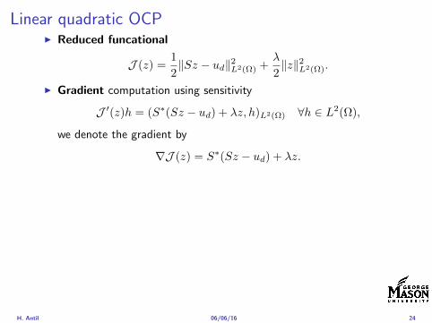
Linear quadratic OCPI Reduced funcational
J (z) =1
2Sz minus ud2L2(Ω) +
λ
2z2L2(Ω)
I Gradient computation using sensitivity
J prime(z)h = (Slowast(Sz minus ud) + λz h)L2(Ω) forallh isin L2(Ω)
we denote the gradient by
nablaJ (z) = Slowast(Sz minus ud) + λz
I First order necessary and sufficient optimality condition
(nablaJ (z) z minus z)L2(Ω) ge 0 forallz isin Zad
I Adjoint equation Let p = Slowast(Sz minus ud) which translates intop isin H1
0 (Ω) solving
minusdiv (Anablap) = uminus ud in Ω
p = 0 on partΩ
I Gradient computation using adjoint nablaJ (z) = p+ λz
H Antil 060616 24
Linear quadratic OCPI Reduced funcational
J (z) =1
2Sz minus ud2L2(Ω) +
λ
2z2L2(Ω)
I Gradient computation using sensitivity
J prime(z)h = (Slowast(Sz minus ud) + λz h)L2(Ω) forallh isin L2(Ω)
we denote the gradient by
nablaJ (z) = Slowast(Sz minus ud) + λz
I First order necessary and sufficient optimality condition
(nablaJ (z) z minus z)L2(Ω) ge 0 forallz isin Zad
I Adjoint equation Let p = Slowast(Sz minus ud) which translates intop isin H1
0 (Ω) solving
minusdiv (Anablap) = uminus ud in Ω
p = 0 on partΩ
I Gradient computation using adjoint nablaJ (z) = p+ λz
H Antil 060616 24
Linear quadratic OCPI Reduced funcational
J (z) =1
2Sz minus ud2L2(Ω) +
λ
2z2L2(Ω)
I Gradient computation using sensitivity
J prime(z)h = (Slowast(Sz minus ud) + λz h)L2(Ω) forallh isin L2(Ω)
we denote the gradient by
nablaJ (z) = Slowast(Sz minus ud) + λz
I First order necessary and sufficient optimality condition
(nablaJ (z) z minus z)L2(Ω) ge 0 forallz isin Zad
I Adjoint equation Let p = Slowast(Sz minus ud) which translates intop isin H1
0 (Ω) solving
minusdiv (Anablap) = uminus ud in Ω
p = 0 on partΩ
I Gradient computation using adjoint nablaJ (z) = p+ λz
H Antil 060616 24
Linear quadratic OCPI Reduced funcational
J (z) =1
2Sz minus ud2L2(Ω) +
λ
2z2L2(Ω)
I Gradient computation using sensitivity
J prime(z)h = (Slowast(Sz minus ud) + λz h)L2(Ω) forallh isin L2(Ω)
we denote the gradient by
nablaJ (z) = Slowast(Sz minus ud) + λz
I First order necessary and sufficient optimality condition
(nablaJ (z) z minus z)L2(Ω) ge 0 forallz isin Zad
I Adjoint equation Let p = Slowast(Sz minus ud) which translates intop isin H1
0 (Ω) solving
minusdiv (Anablap) = uminus ud in Ω
p = 0 on partΩ
I Gradient computation using adjoint nablaJ (z) = p+ λz
H Antil 060616 24
Optimality system
I State u isin H10 (Ω)
intΩAnablau middot nablav =
intΩzv forallv isin H1
0 (Ω)
I Adjoint p isin H10 (Ω)
intΩAnablap middot nablav =
intΩ
(uminus ud)v forallv isin H10 (Ω)
I Control z isin Zad (p+ λz z minus z) ge 0 forallz isin Zad
H Antil 060616 25
Pointwise interpretation
The variational inequality
(p+ λz z minus z) ge 0 forallz isin Zad
is equivalent to for ae x isin Ω
z(x) =
za(x) if p(x) + λz(x) gt 0isin [za(x) zb(x)] if p(x) + λz(x) = 0zb(x) if p(x) + λz(x) lt 0
Consequence
I When λ gt 0 then ae in Ω
z(x) = P[za(x)zb(x)]
minus 1
λp(x)
= min
zb(x)max
za(x)minus 1
λp(x)
H Antil 060616 26
Formal Lagrange method applied to linear OCPIntroduce L H1
0 (Ω)times Zad timesH1(Ω)rarr R defined as
L(u z p) = J(u z)minusint
Ω
(minusdiv (Anablau)minus z
)p dx
Integrate by parts to arrive at
L(u z p) = J(u z)minusint
Ω
(minusdiv (Anablap)uminus zp
)dx+
intpartΩ
(Anablau)p ds
If (u z p) is a stationary point then
I State
DpL(u z p)h = 0 forallh isin H1(Ω)
I AdjointDuL(u z p)h = 0 forallh isin H1
0 (Ω)
I ControlDzL(u z p)(z minus z) ge 0 forallz isin Zad
H Antil 060616 27
Formal Lagrange method applied to linear OCPIntroduce L H1
0 (Ω)times Zad timesH1(Ω)rarr R defined as
L(u z p) = J(u z)minusint
Ω
(minusdiv (Anablau)minus z
)p dx
Integrate by parts to arrive at
L(u z p) = J(u z)minusint
Ω
(minusdiv (Anablap)uminus zp
)dx+
intpartΩ
(Anablau)p ds
If (u z p) is a stationary point then
I State
DpL(u z p)h = 0 forallh isin H1(Ω)
I AdjointDuL(u z p)h = 0 forallh isin H1
0 (Ω)
I ControlDzL(u z p)(z minus z) ge 0 forallz isin Zad
H Antil 060616 27
Formal Lagrange method applied to linear OCPIntroduce L H1
0 (Ω)times Zad timesH1(Ω)rarr R defined as
L(u z p) = J(u z)minusint
Ω
(minusdiv (Anablau)minus z
)p dx
Integrate by parts to arrive at
L(u z p) = J(u z)minusint
Ω
(minusdiv (Anablap)uminus zp
)dx+
intpartΩ
(Anablau)p ds
If (u z p) is a stationary point then
I State
DpL(u z p)h = 0 forallh isin H1(Ω)
I AdjointDuL(u z p)h = 0 forallh isin H1
0 (Ω)
I ControlDzL(u z p)(z minus z) ge 0 forallz isin Zad
H Antil 060616 27
Formal Lagrange method applied to linear OCPIntroduce L H1
0 (Ω)times Zad timesH1(Ω)rarr R defined as
L(u z p) = J(u z)minusint
Ω
(minusdiv (Anablau)minus z
)p dx
Integrate by parts to arrive at
L(u z p) = J(u z)minusint
Ω
(minusdiv (Anablap)uminus zp
)dx+
intpartΩ
(Anablau)p ds
If (u z p) is a stationary point then
I State
DpL(u z p)h = 0 forallh isin H1(Ω)
I AdjointDuL(u z p)h = 0 forallh isin H1
0 (Ω)
I ControlDzL(u z p)(z minus z) ge 0 forallz isin Zad
H Antil 060616 27
Formal Lagrange method applied to linear OCPIntroduce L H1
0 (Ω)times Zad timesH1(Ω)rarr R defined as
L(u z p) = J(u z)minusint
Ω
(minusdiv (Anablau)minus z
)p dx
Integrate by parts to arrive at
L(u z p) = J(u z)minusint
Ω
(minusdiv (Anablap)uminus zp
)dx+
intpartΩ
(Anablau)p ds
If (u z p) is a stationary point then
I State
DpL(u z p)h = 0 forallh isin H1(Ω)
I AdjointDuL(u z p)h = 0 forallh isin H1
0 (Ω)
I ControlDzL(u z p)(z minus z) ge 0 forallz isin Zad
H Antil 060616 27
Outline
Motivation and examples
Linear elliptic optimal control problems
Differentiation in Banach spaces
First-order necessary conditions
Optimal control of semilinear PDEs
An abstract problem
Discretization using finite element methods
H Antil 060616 28
Semilinear elliptic OCP
min J(u z) =1
2uminus ud2L2(Ω) +
λ
2z2L2(Ω)
subject to
minus∆u+ g(x u) = z in Ω
u = 0 on partΩ
and z isin Zad with za zb isin Linfin(Ω)
H Antil 060616 29
State space(A1) Ω sub Rd open bounded partΩ is Lipschitz
(A2) g Ωtimes Rrarr R is bounded and measurable with respect to x isin Ωfor every u isin R
(A3) g is continuous monotone increasing and Lipschitz continuous in ufor ae x isin Ω
(A4) g(x 0) = 0 for ae x isin Ω (not really necessary)
Theorem Suppose (A1)minus (A4) hold For every z isin Lr(Ω) withr gt d2 the state equation has a unique weak solutionu isin H1
0 (Ω) cap C(Ω) ie we haveintΩ
nablau middot nablav dx+
intΩ
g(x u(x))v(x) dx =
intΩ
zv dx forallv isin H10 (Ω)
Moreover there exists a constant C gt 0 such that
uH1(Ω) + uC(Ω) le CzLr(Ω)
RemarkI The proof of the theorem uses the BrowderndashMinty theorem on
monotone operators
H Antil 060616 30
State space(A1) Ω sub Rd open bounded partΩ is Lipschitz
(A2) g Ωtimes Rrarr R is bounded and measurable with respect to x isin Ωfor every u isin R
(A3) g is continuous monotone increasing and Lipschitz continuous in ufor ae x isin Ω
(A4) g(x 0) = 0 for ae x isin Ω (not really necessary)
Theorem Suppose (A1)minus (A4) hold For every z isin Lr(Ω) withr gt d2 the state equation has a unique weak solutionu isin H1
0 (Ω) cap C(Ω) ie we haveintΩ
nablau middot nablav dx+
intΩ
g(x u(x))v(x) dx =
intΩ
zv dx forallv isin H10 (Ω)
Moreover there exists a constant C gt 0 such that
uH1(Ω) + uC(Ω) le CzLr(Ω)
RemarkI The proof of the theorem uses the BrowderndashMinty theorem on
monotone operators
H Antil 060616 30
State space(A1) Ω sub Rd open bounded partΩ is Lipschitz
(A2) g Ωtimes Rrarr R is bounded and measurable with respect to x isin Ωfor every u isin R
(A3) g is continuous monotone increasing and Lipschitz continuous in ufor ae x isin Ω
(A4) g(x 0) = 0 for ae x isin Ω (not really necessary)
Theorem Suppose (A1)minus (A4) hold For every z isin Lr(Ω) withr gt d2 the state equation has a unique weak solutionu isin H1
0 (Ω) cap C(Ω) ie we haveintΩ
nablau middot nablav dx+
intΩ
g(x u(x))v(x) dx =
intΩ
zv dx forallv isin H10 (Ω)
Moreover there exists a constant C gt 0 such that
uH1(Ω) + uC(Ω) le CzLr(Ω)
RemarkI The proof of the theorem uses the BrowderndashMinty theorem on
monotone operators
H Antil 060616 30
Control-to-state map and reduced problem
I Control to state map
S Linfin(Ω)rarr H10 (Ω) cap C(Ω)
is well defined and is globally Lipschitz continuous
I Reduced problem
minJ (z) =1
2S(u)minus ud2L2(Ω) +
λ
2z2L2(Ω)
H Antil 060616 31
Control-to-state map and reduced problem
I Control to state map
S Linfin(Ω)rarr H10 (Ω) cap C(Ω)
is well defined and is globally Lipschitz continuous
I Reduced problem
minJ (z) =1
2S(u)minus ud2L2(Ω) +
λ
2z2L2(Ω)
H Antil 060616 31
First-order necessary conditionsI Lagrangian functional
L(u z p) = J(u z)minusint
Ω
(minus∆u+ g(x u(x))minus z
)p dx
= J(u z)minusint
Ω
(nablau middot nablap+ g(x u(x))pminus zp
)dx
I Adjoint system For all h isin H10 (Ω)
0 = DuL(u z p)h =
intΩ
(uminus ud)h dxminusint
Ω
(nablah middot nablap+ gu(x u(x))ph
)which yields
minus∆p+ gu(x u(x))p = uminus ud in Ω
p = 0 on partΩ
I Control
DzL(u z p)(z minus z) = (p+ λz z minus z) dx ge 0 forallz isin ZadI Gradient
nablaJ (z) = p+ λz
H Antil 060616 32
First-order necessary conditionsI Lagrangian functional
L(u z p) = J(u z)minusint
Ω
(minus∆u+ g(x u(x))minus z
)p dx
= J(u z)minusint
Ω
(nablau middot nablap+ g(x u(x))pminus zp
)dx
I Adjoint system For all h isin H10 (Ω)
0 = DuL(u z p)h =
intΩ
(uminus ud)h dxminusint
Ω
(nablah middot nablap+ gu(x u(x))ph
)which yields
minus∆p+ gu(x u(x))p = uminus ud in Ω
p = 0 on partΩ
I Control
DzL(u z p)(z minus z) = (p+ λz z minus z) dx ge 0 forallz isin ZadI Gradient
nablaJ (z) = p+ λz
H Antil 060616 32
First-order necessary conditionsI Lagrangian functional
L(u z p) = J(u z)minusint
Ω
(minus∆u+ g(x u(x))minus z
)p dx
= J(u z)minusint
Ω
(nablau middot nablap+ g(x u(x))pminus zp
)dx
I Adjoint system For all h isin H10 (Ω)
0 = DuL(u z p)h =
intΩ
(uminus ud)h dxminusint
Ω
(nablah middot nablap+ gu(x u(x))ph
)which yields
minus∆p+ gu(x u(x))p = uminus ud in Ω
p = 0 on partΩ
I Control
DzL(u z p)(z minus z) = (p+ λz z minus z) dx ge 0 forallz isin Zad
I GradientnablaJ (z) = p+ λz
H Antil 060616 32
First-order necessary conditionsI Lagrangian functional
L(u z p) = J(u z)minusint
Ω
(minus∆u+ g(x u(x))minus z
)p dx
= J(u z)minusint
Ω
(nablau middot nablap+ g(x u(x))pminus zp
)dx
I Adjoint system For all h isin H10 (Ω)
0 = DuL(u z p)h =
intΩ
(uminus ud)h dxminusint
Ω
(nablah middot nablap+ gu(x u(x))ph
)which yields
minus∆p+ gu(x u(x))p = uminus ud in Ω
p = 0 on partΩ
I Control
DzL(u z p)(z minus z) = (p+ λz z minus z) dx ge 0 forallz isin ZadI Gradient
nablaJ (z) = p+ λz
H Antil 060616 32
Differentiability of Nemytskii operator
The rigorous proof uses
Theorem In addition to (A1)-(A4) if
(A5) g is continuously differentiable with respect to u for ae x isin Ωand we have
(i) |gu(x 0)| le K for ae x isin Ω(ii) gu is locally Lipschitz with respect to u isin R
then the Nemytskii operator G u 7rarr g(middot u(middot)) is continuously Frechetdifferentiable from Linfin(Ω) into itself and
(Gprime(u)h)(x) = gu(x u(x))h(x) ae in Ω forallh isin Linfin(Ω)
Remark (A5) holds if g(x u) = g(u) and g isin C2(R)
H Antil 060616 33
Outline
Motivation and examples
Linear elliptic optimal control problems
Differentiation in Banach spaces
First-order necessary conditions
Optimal control of semilinear PDEs
An abstract problem
Discretization using finite element methods
H Antil 060616 34
Gradient computation via adjoint general formI Abstract problem
min J(u z)
subject toc(u z) = 0
and z isin Zad
I Directional derivative Let S be the control to state map(nonlinear in general)
z 7rarr S(z) = u(z)
Under the assumptions of ldquoimplicit function theoremrdquo
J prime(z)h = (nablauJ (u(z) z) Sprime(z)h) + (nablazJ (u(z) z) h)
I Sensitivity of u with respect to z Differentiating the stateequation
cu(S(z) z)Sprime(z)h = minuscz(S(z) z)h
leads toSprime(z)h = minuscu(S(z) z)minus1
(cz(S(z) z)h
)
provided cu(S(z) z)minus1 is well-defined
H Antil 060616 35
Gradient computation via adjoint general formI Abstract problem
min J(u z)
subject toc(u z) = 0
and z isin ZadI Directional derivative Let S be the control to state map
(nonlinear in general)
z 7rarr S(z) = u(z)
Under the assumptions of ldquoimplicit function theoremrdquo
J prime(z)h = (nablauJ (u(z) z) Sprime(z)h) + (nablazJ (u(z) z) h)
I Sensitivity of u with respect to z Differentiating the stateequation
cu(S(z) z)Sprime(z)h = minuscz(S(z) z)h
leads toSprime(z)h = minuscu(S(z) z)minus1
(cz(S(z) z)h
)
provided cu(S(z) z)minus1 is well-defined
H Antil 060616 35
Gradient computation via adjoint general formI Abstract problem
min J(u z)
subject toc(u z) = 0
and z isin ZadI Directional derivative Let S be the control to state map
(nonlinear in general)
z 7rarr S(z) = u(z)
Under the assumptions of ldquoimplicit function theoremrdquo
J prime(z)h = (nablauJ (u(z) z) Sprime(z)h) + (nablazJ (u(z) z) h)
I Sensitivity of u with respect to z Differentiating the stateequation
cu(S(z) z)Sprime(z)h = minuscz(S(z) z)h
leads toSprime(z)h = minuscu(S(z) z)minus1
(cz(S(z) z)h
)
provided cu(S(z) z)minus1 is well-defined
H Antil 060616 35
Adjoint equation and gradient general form
I Directional derivative
J prime(z)h = minus(nablauJ (u(z) z) cu(u(z) z)minus1cz(u(z) z)h
)+ (nablazJ (u(z) z) h)
I Gradient
nablaJ (z) = minuscz(u(z) z)lowast(cu(u(z) z)minuslowastnablauJ (u(z) z)
)+nablazJ (u(z) z)
I Introducing adjoint variable p solving
cu(u(z) z)lowastp = nablauJ (u(z) z)
we arrive at following form of gradient
nablaJ (z) = minuscz(u(z) z)lowastp+nablazJ (u(z) z)
which is tractable
H Antil 060616 36
Adjoint equation and gradient general form
I Directional derivative
J prime(z)h = minus(nablauJ (u(z) z) cu(u(z) z)minus1cz(u(z) z)h
)+ (nablazJ (u(z) z) h)
I Gradient
nablaJ (z) = minuscz(u(z) z)lowast(cu(u(z) z)minuslowastnablauJ (u(z) z)
)+nablazJ (u(z) z)
I Introducing adjoint variable p solving
cu(u(z) z)lowastp = nablauJ (u(z) z)
we arrive at following form of gradient
nablaJ (z) = minuscz(u(z) z)lowastp+nablazJ (u(z) z)
which is tractable
H Antil 060616 36
Adjoint equation and gradient general form
I Directional derivative
J prime(z)h = minus(nablauJ (u(z) z) cu(u(z) z)minus1cz(u(z) z)h
)+ (nablazJ (u(z) z) h)
I Gradient
nablaJ (z) = minuscz(u(z) z)lowast(cu(u(z) z)minuslowastnablauJ (u(z) z)
)+nablazJ (u(z) z)
I Introducing adjoint variable p solving
cu(u(z) z)lowastp = nablauJ (u(z) z)
we arrive at following form of gradient
nablaJ (z) = minuscz(u(z) z)lowastp+nablazJ (u(z) z)
which is tractable
H Antil 060616 36
Hessian computation general form
I Lagrangian L(u z p) = J(u z)minusint
Ωc(u z)p dx Then we have
DzJ (z)h = DzL(u z p)h
I Second order derivative
D2zJ (z)[h1 h2] = DuDzL(u z p)[h1 S
prime(z)h2] +D2zL(u z p)[h1 h2]
+DpDzL(u z p)[h1 Dzp(z)h2]
I We already know Sprime(z)h2 moreover
DpDzL(u z p)[h1 Dzp(z)h2] = minus(cu(u z)h1 Dzp(z)h2
)
It remain to identify Dzp(z)h2
H Antil 060616 37
Hessian computation general form
I Lagrangian L(u z p) = J(u z)minusint
Ωc(u z)p dx Then we have
DzJ (z)h = DzL(u z p)h
I Second order derivative
D2zJ (z)[h1 h2] = DuDzL(u z p)[h1 S
prime(z)h2] +D2zL(u z p)[h1 h2]
+DpDzL(u z p)[h1 Dzp(z)h2]
I We already know Sprime(z)h2 moreover
DpDzL(u z p)[h1 Dzp(z)h2] = minus(cu(u z)h1 Dzp(z)h2
)
It remain to identify Dzp(z)h2
H Antil 060616 37
Hessian computation general form
I Lagrangian L(u z p) = J(u z)minusint
Ωc(u z)p dx Then we have
DzJ (z)h = DzL(u z p)h
I Second order derivative
D2zJ (z)[h1 h2] = DuDzL(u z p)[h1 S
prime(z)h2] +D2zL(u z p)[h1 h2]
+DpDzL(u z p)[h1 Dzp(z)h2]
I We already know Sprime(z)h2 moreover
DpDzL(u z p)[h1 Dzp(z)h2] = minus(cu(u z)h1 Dzp(z)h2
)
It remain to identify Dzp(z)h2
H Antil 060616 37
Outline
Motivation and examples
Linear elliptic optimal control problems
Differentiation in Banach spaces
First-order necessary conditions
Optimal control of semilinear PDEs
An abstract problem
Discretization using finite element methods
H Antil 060616 38
Numerical approximation of Poisson equation MeshTo avoid technical issues we will assume that partΩ is polygonal
I Mesh Let T = K be a mesh of Ω where K sub Rd is an elementthat is isoparametrically equivalent to a unit simplex in Rd
I Conforming mesh We say that the mesh is conforming ifI Ω = cupKisinT KI If K1 cap K2 = x then x is a node of K1 and K2I If K1 cap K2 6= empty and K1 cap K2 6= x then K1 cap K2 is an edgeface
contained in partK1 cap partK2
I Shape regular Let T be the collection of all conformingrefinements of an original mesh T 0 Then T is called shape regularif exist κ gt 0 such that
hKρKle κ forallK isin cupiT i
where hK = diam K ρK = maxρ gt 0|Bρ sub KI Quasi-uniform A family of shape regular meshes is called-quasi
uniform if there exist a constant σ gt 0 such that
maxhKminhK
le σ
uniformly for all meshes in the family
Numerical approximation of Poisson equation MeshTo avoid technical issues we will assume that partΩ is polygonal
I Mesh Let T = K be a mesh of Ω where K sub Rd is an elementthat is isoparametrically equivalent to a unit simplex in Rd
I Conforming mesh We say that the mesh is conforming ifI Ω = cupKisinT KI If K1 cap K2 = x then x is a node of K1 and K2I If K1 cap K2 6= empty and K1 cap K2 6= x then K1 cap K2 is an edgeface
contained in partK1 cap partK2
I Shape regular Let T be the collection of all conformingrefinements of an original mesh T 0 Then T is called shape regularif exist κ gt 0 such that
hKρKle κ forallK isin cupiT i
where hK = diam K ρK = maxρ gt 0|Bρ sub KI Quasi-uniform A family of shape regular meshes is called-quasi
uniform if there exist a constant σ gt 0 such that
maxhKminhK
le σ
uniformly for all meshes in the family
Numerical approximation of Poisson equation MeshTo avoid technical issues we will assume that partΩ is polygonal
I Mesh Let T = K be a mesh of Ω where K sub Rd is an elementthat is isoparametrically equivalent to a unit simplex in Rd
I Conforming mesh We say that the mesh is conforming ifI Ω = cupKisinT KI If K1 cap K2 = x then x is a node of K1 and K2I If K1 cap K2 6= empty and K1 cap K2 6= x then K1 cap K2 is an edgeface
contained in partK1 cap partK2
I Shape regular Let T be the collection of all conformingrefinements of an original mesh T 0 Then T is called shape regularif exist κ gt 0 such that
hKρKle κ forallK isin cupiT i
where hK = diam K ρK = maxρ gt 0|Bρ sub K
I Quasi-uniform A family of shape regular meshes is called-quasiuniform if there exist a constant σ gt 0 such that
maxhKminhK
le σ
uniformly for all meshes in the family
Numerical approximation of Poisson equation MeshTo avoid technical issues we will assume that partΩ is polygonal
I Mesh Let T = K be a mesh of Ω where K sub Rd is an elementthat is isoparametrically equivalent to a unit simplex in Rd
I Conforming mesh We say that the mesh is conforming ifI Ω = cupKisinT KI If K1 cap K2 = x then x is a node of K1 and K2I If K1 cap K2 6= empty and K1 cap K2 6= x then K1 cap K2 is an edgeface
contained in partK1 cap partK2
I Shape regular Let T be the collection of all conformingrefinements of an original mesh T 0 Then T is called shape regularif exist κ gt 0 such that
hKρKle κ forallK isin cupiT i
where hK = diam K ρK = maxρ gt 0|Bρ sub KI Quasi-uniform A family of shape regular meshes is called-quasi
uniform if there exist a constant σ gt 0 such that
maxhKminhK
le σ
uniformly for all meshes in the family
FE space and Galerkin approximationI Finite element space For T isin T we define the finite element
space as
V(T ) = W isin C0(Ω) WK isin P1forallK isin T W |partΩ = 0
where P1 is the set of polynomials of degree at most 1
I Galerkin approximation of continuous problem is given by
Find UT isin V(T )
intΩ
AnablaUT middot nablaV = 〈f V 〉 forallV isin V(T )
The discrete problem is well-posedI Nodal basis Consists of functions ψi isin V(T ) with xi isin N (T )
satisfyingψxi
(xj) = δij
where N (T ) denotes the interior (plus Neumann) nodesI Galerkin orthogonality(
nabla(uminus UT )nablaW)L2(Ω)
= 0 forallW isin V(T )
H Antil 060616 40
FE space and Galerkin approximationI Finite element space For T isin T we define the finite element
space as
V(T ) = W isin C0(Ω) WK isin P1forallK isin T W |partΩ = 0
where P1 is the set of polynomials of degree at most 1I Galerkin approximation of continuous problem is given by
Find UT isin V(T )
intΩ
AnablaUT middot nablaV = 〈f V 〉 forallV isin V(T )
The discrete problem is well-posed
I Nodal basis Consists of functions ψi isin V(T ) with xi isin N (T )satisfying
ψxi(xj) = δij
where N (T ) denotes the interior (plus Neumann) nodesI Galerkin orthogonality(
nabla(uminus UT )nablaW)L2(Ω)
= 0 forallW isin V(T )
H Antil 060616 40
FE space and Galerkin approximationI Finite element space For T isin T we define the finite element
space as
V(T ) = W isin C0(Ω) WK isin P1forallK isin T W |partΩ = 0
where P1 is the set of polynomials of degree at most 1I Galerkin approximation of continuous problem is given by
Find UT isin V(T )
intΩ
AnablaUT middot nablaV = 〈f V 〉 forallV isin V(T )
The discrete problem is well-posedI Nodal basis Consists of functions ψi isin V(T ) with xi isin N (T )
satisfyingψxi
(xj) = δij
where N (T ) denotes the interior (plus Neumann) nodes
I Galerkin orthogonality(nabla(uminus UT )nablaW
)L2(Ω)
= 0 forallW isin V(T )
H Antil 060616 40
FE space and Galerkin approximationI Finite element space For T isin T we define the finite element
space as
V(T ) = W isin C0(Ω) WK isin P1forallK isin T W |partΩ = 0
where P1 is the set of polynomials of degree at most 1I Galerkin approximation of continuous problem is given by
Find UT isin V(T )
intΩ
AnablaUT middot nablaV = 〈f V 〉 forallV isin V(T )
The discrete problem is well-posedI Nodal basis Consists of functions ψi isin V(T ) with xi isin N (T )
satisfyingψxi
(xj) = δij
where N (T ) denotes the interior (plus Neumann) nodesI Galerkin orthogonality(
nabla(uminus UT )nablaW)L2(Ω)
= 0 forallW isin V(T )
H Antil 060616 40
Best approximation
I Cearsquos lemma
nabla(uminus UT )L2(Ω) le C infWisinV(T )
nabla(uminusW )L2(Ω)
I Nodal interpolation operator ΠT C(Ω)rarr V(T ) satisfies
ΠT u(xi) = u(xi) forallxi isin N (T )
and is defined as
ΠT u =sum
xiisinN (T )
u(xi)ψxi
I Error estimates In Cearsquos lemma replace W by ΠT u and thencompute the interpolation error
H Antil 060616 41
Best approximation
I Cearsquos lemma
nabla(uminus UT )L2(Ω) le C infWisinV(T )
nabla(uminusW )L2(Ω)
I Nodal interpolation operator ΠT C(Ω)rarr V(T ) satisfies
ΠT u(xi) = u(xi) forallxi isin N (T )
and is defined as
ΠT u =sum
xiisinN (T )
u(xi)ψxi
I Error estimates In Cearsquos lemma replace W by ΠT u and thencompute the interpolation error
H Antil 060616 41
Best approximation
I Cearsquos lemma
nabla(uminus UT )L2(Ω) le C infWisinV(T )
nabla(uminusW )L2(Ω)
I Nodal interpolation operator ΠT C(Ω)rarr V(T ) satisfies
ΠT u(xi) = u(xi) forallxi isin N (T )
and is defined as
ΠT u =sum
xiisinN (T )
u(xi)ψxi
I Error estimates In Cearsquos lemma replace W by ΠT u and thencompute the interpolation error
H Antil 060616 41
Algebraic system state equation
I Recall UT isin V(T ) solves
a(UT V ) = 〈f V 〉 forallV isin V(T )
I Now setting UT =sumN
j=1 Ujψj V = ψi we get
Nsumj=1
Uja(φj φi) = 〈f ψi〉 i = 1 N
which is the matrix-vector system
AU = F
I Stiffness matrix A is SPD
H Antil 060616 42
Algebraic system state equation
I Recall UT isin V(T ) solves
a(UT V ) = 〈f V 〉 forallV isin V(T )
I Now setting UT =sumN
j=1 Ujψj V = ψi we get
Nsumj=1
Uja(φj φi) = 〈f ψi〉 i = 1 N
which is the matrix-vector system
AU = F
I Stiffness matrix A is SPD
H Antil 060616 42
Algebraic system state equation
I Recall UT isin V(T ) solves
a(UT V ) = 〈f V 〉 forallV isin V(T )
I Now setting UT =sumN
j=1 Ujψj V = ψi we get
Nsumj=1
Uja(φj φi) = 〈f ψi〉 i = 1 N
which is the matrix-vector system
AU = F
I Stiffness matrix A is SPD
H Antil 060616 42
Discrete linear elliptic OCP
min JT (UT ZT ) =1
2UT minus ud2L2(Ω) +
λ
2ZT 2L2(Ω)
subject to
Find UT isin V(T )
intΩ
nablaUT middot nablaV = (ZT V )L2(Ω) forallV isin V(T )
and whereZT isin Zad(T ) = Zad cap Z(T )
is either one of these
Z(T ) =
V(T )L2(Ω) variational discretization (Hinze)WT isin Linfin(Ω) ZT |K isin P0(K)K isin T
H Antil 060616 43
Recent books
F TroltzschOptimal control of partial differential equations volume 112 ofGraduate Studies in MathematicsAmerican Mathematical Society Providence RI 2010Theory methods and applications Translated from the 2005 Germanoriginal by Jurgen Sprekels
K Ito and K KunischLagrange multiplier approach to variational problems andapplications volume 15 of Advances in Design and ControlSociety for Industrial and Applied Mathematics (SIAM)Philadelphia PA 2008
H Antil 060616 44
- Motivation and examples
- Linear elliptic optimal control problems
- Differentiation in Banach spaces
- First-order necessary conditions
- Optimal control of semilinear PDEs
- An abstract problem
- Discretization using finite element methods
-

Linear quadratic OCPI Reduced funcational
J (z) =1
2Sz minus ud2L2(Ω) +
λ
2z2L2(Ω)
I Gradient computation using sensitivity
J prime(z)h = (Slowast(Sz minus ud) + λz h)L2(Ω) forallh isin L2(Ω)
we denote the gradient by
nablaJ (z) = Slowast(Sz minus ud) + λz
I First order necessary and sufficient optimality condition
(nablaJ (z) z minus z)L2(Ω) ge 0 forallz isin Zad
I Adjoint equation Let p = Slowast(Sz minus ud) which translates intop isin H1
0 (Ω) solving
minusdiv (Anablap) = uminus ud in Ω
p = 0 on partΩ
I Gradient computation using adjoint nablaJ (z) = p+ λz
H Antil 060616 24
Linear quadratic OCPI Reduced funcational
J (z) =1
2Sz minus ud2L2(Ω) +
λ
2z2L2(Ω)
I Gradient computation using sensitivity
J prime(z)h = (Slowast(Sz minus ud) + λz h)L2(Ω) forallh isin L2(Ω)
we denote the gradient by
nablaJ (z) = Slowast(Sz minus ud) + λz
I First order necessary and sufficient optimality condition
(nablaJ (z) z minus z)L2(Ω) ge 0 forallz isin Zad
I Adjoint equation Let p = Slowast(Sz minus ud) which translates intop isin H1
0 (Ω) solving
minusdiv (Anablap) = uminus ud in Ω
p = 0 on partΩ
I Gradient computation using adjoint nablaJ (z) = p+ λz
H Antil 060616 24
Linear quadratic OCPI Reduced funcational
J (z) =1
2Sz minus ud2L2(Ω) +
λ
2z2L2(Ω)
I Gradient computation using sensitivity
J prime(z)h = (Slowast(Sz minus ud) + λz h)L2(Ω) forallh isin L2(Ω)
we denote the gradient by
nablaJ (z) = Slowast(Sz minus ud) + λz
I First order necessary and sufficient optimality condition
(nablaJ (z) z minus z)L2(Ω) ge 0 forallz isin Zad
I Adjoint equation Let p = Slowast(Sz minus ud) which translates intop isin H1
0 (Ω) solving
minusdiv (Anablap) = uminus ud in Ω
p = 0 on partΩ
I Gradient computation using adjoint nablaJ (z) = p+ λz
H Antil 060616 24
Optimality system
I State u isin H10 (Ω)
intΩAnablau middot nablav =
intΩzv forallv isin H1
0 (Ω)
I Adjoint p isin H10 (Ω)
intΩAnablap middot nablav =
intΩ
(uminus ud)v forallv isin H10 (Ω)
I Control z isin Zad (p+ λz z minus z) ge 0 forallz isin Zad
H Antil 060616 25
Pointwise interpretation
The variational inequality
(p+ λz z minus z) ge 0 forallz isin Zad
is equivalent to for ae x isin Ω
z(x) =
za(x) if p(x) + λz(x) gt 0isin [za(x) zb(x)] if p(x) + λz(x) = 0zb(x) if p(x) + λz(x) lt 0
Consequence
I When λ gt 0 then ae in Ω
z(x) = P[za(x)zb(x)]
minus 1
λp(x)
= min
zb(x)max
za(x)minus 1
λp(x)
H Antil 060616 26
Formal Lagrange method applied to linear OCPIntroduce L H1
0 (Ω)times Zad timesH1(Ω)rarr R defined as
L(u z p) = J(u z)minusint
Ω
(minusdiv (Anablau)minus z
)p dx
Integrate by parts to arrive at
L(u z p) = J(u z)minusint
Ω
(minusdiv (Anablap)uminus zp
)dx+
intpartΩ
(Anablau)p ds
If (u z p) is a stationary point then
I State
DpL(u z p)h = 0 forallh isin H1(Ω)
I AdjointDuL(u z p)h = 0 forallh isin H1
0 (Ω)
I ControlDzL(u z p)(z minus z) ge 0 forallz isin Zad
H Antil 060616 27
Formal Lagrange method applied to linear OCPIntroduce L H1
0 (Ω)times Zad timesH1(Ω)rarr R defined as
L(u z p) = J(u z)minusint
Ω
(minusdiv (Anablau)minus z
)p dx
Integrate by parts to arrive at
L(u z p) = J(u z)minusint
Ω
(minusdiv (Anablap)uminus zp
)dx+
intpartΩ
(Anablau)p ds
If (u z p) is a stationary point then
I State
DpL(u z p)h = 0 forallh isin H1(Ω)
I AdjointDuL(u z p)h = 0 forallh isin H1
0 (Ω)
I ControlDzL(u z p)(z minus z) ge 0 forallz isin Zad
H Antil 060616 27
Formal Lagrange method applied to linear OCPIntroduce L H1
0 (Ω)times Zad timesH1(Ω)rarr R defined as
L(u z p) = J(u z)minusint
Ω
(minusdiv (Anablau)minus z
)p dx
Integrate by parts to arrive at
L(u z p) = J(u z)minusint
Ω
(minusdiv (Anablap)uminus zp
)dx+
intpartΩ
(Anablau)p ds
If (u z p) is a stationary point then
I State
DpL(u z p)h = 0 forallh isin H1(Ω)
I AdjointDuL(u z p)h = 0 forallh isin H1
0 (Ω)
I ControlDzL(u z p)(z minus z) ge 0 forallz isin Zad
H Antil 060616 27
Formal Lagrange method applied to linear OCPIntroduce L H1
0 (Ω)times Zad timesH1(Ω)rarr R defined as
L(u z p) = J(u z)minusint
Ω
(minusdiv (Anablau)minus z
)p dx
Integrate by parts to arrive at
L(u z p) = J(u z)minusint
Ω
(minusdiv (Anablap)uminus zp
)dx+
intpartΩ
(Anablau)p ds
If (u z p) is a stationary point then
I State
DpL(u z p)h = 0 forallh isin H1(Ω)
I AdjointDuL(u z p)h = 0 forallh isin H1
0 (Ω)
I ControlDzL(u z p)(z minus z) ge 0 forallz isin Zad
H Antil 060616 27
Formal Lagrange method applied to linear OCPIntroduce L H1
0 (Ω)times Zad timesH1(Ω)rarr R defined as
L(u z p) = J(u z)minusint
Ω
(minusdiv (Anablau)minus z
)p dx
Integrate by parts to arrive at
L(u z p) = J(u z)minusint
Ω
(minusdiv (Anablap)uminus zp
)dx+
intpartΩ
(Anablau)p ds
If (u z p) is a stationary point then
I State
DpL(u z p)h = 0 forallh isin H1(Ω)
I AdjointDuL(u z p)h = 0 forallh isin H1
0 (Ω)
I ControlDzL(u z p)(z minus z) ge 0 forallz isin Zad
H Antil 060616 27
Outline
Motivation and examples
Linear elliptic optimal control problems
Differentiation in Banach spaces
First-order necessary conditions
Optimal control of semilinear PDEs
An abstract problem
Discretization using finite element methods
H Antil 060616 28
Semilinear elliptic OCP
min J(u z) =1
2uminus ud2L2(Ω) +
λ
2z2L2(Ω)
subject to
minus∆u+ g(x u) = z in Ω
u = 0 on partΩ
and z isin Zad with za zb isin Linfin(Ω)
H Antil 060616 29
State space(A1) Ω sub Rd open bounded partΩ is Lipschitz
(A2) g Ωtimes Rrarr R is bounded and measurable with respect to x isin Ωfor every u isin R
(A3) g is continuous monotone increasing and Lipschitz continuous in ufor ae x isin Ω
(A4) g(x 0) = 0 for ae x isin Ω (not really necessary)
Theorem Suppose (A1)minus (A4) hold For every z isin Lr(Ω) withr gt d2 the state equation has a unique weak solutionu isin H1
0 (Ω) cap C(Ω) ie we haveintΩ
nablau middot nablav dx+
intΩ
g(x u(x))v(x) dx =
intΩ
zv dx forallv isin H10 (Ω)
Moreover there exists a constant C gt 0 such that
uH1(Ω) + uC(Ω) le CzLr(Ω)
RemarkI The proof of the theorem uses the BrowderndashMinty theorem on
monotone operators
H Antil 060616 30
State space(A1) Ω sub Rd open bounded partΩ is Lipschitz
(A2) g Ωtimes Rrarr R is bounded and measurable with respect to x isin Ωfor every u isin R
(A3) g is continuous monotone increasing and Lipschitz continuous in ufor ae x isin Ω
(A4) g(x 0) = 0 for ae x isin Ω (not really necessary)
Theorem Suppose (A1)minus (A4) hold For every z isin Lr(Ω) withr gt d2 the state equation has a unique weak solutionu isin H1
0 (Ω) cap C(Ω) ie we haveintΩ
nablau middot nablav dx+
intΩ
g(x u(x))v(x) dx =
intΩ
zv dx forallv isin H10 (Ω)
Moreover there exists a constant C gt 0 such that
uH1(Ω) + uC(Ω) le CzLr(Ω)
RemarkI The proof of the theorem uses the BrowderndashMinty theorem on
monotone operators
H Antil 060616 30
State space(A1) Ω sub Rd open bounded partΩ is Lipschitz
(A2) g Ωtimes Rrarr R is bounded and measurable with respect to x isin Ωfor every u isin R
(A3) g is continuous monotone increasing and Lipschitz continuous in ufor ae x isin Ω
(A4) g(x 0) = 0 for ae x isin Ω (not really necessary)
Theorem Suppose (A1)minus (A4) hold For every z isin Lr(Ω) withr gt d2 the state equation has a unique weak solutionu isin H1
0 (Ω) cap C(Ω) ie we haveintΩ
nablau middot nablav dx+
intΩ
g(x u(x))v(x) dx =
intΩ
zv dx forallv isin H10 (Ω)
Moreover there exists a constant C gt 0 such that
uH1(Ω) + uC(Ω) le CzLr(Ω)
RemarkI The proof of the theorem uses the BrowderndashMinty theorem on
monotone operators
H Antil 060616 30
Control-to-state map and reduced problem
I Control to state map
S Linfin(Ω)rarr H10 (Ω) cap C(Ω)
is well defined and is globally Lipschitz continuous
I Reduced problem
minJ (z) =1
2S(u)minus ud2L2(Ω) +
λ
2z2L2(Ω)
H Antil 060616 31
Control-to-state map and reduced problem
I Control to state map
S Linfin(Ω)rarr H10 (Ω) cap C(Ω)
is well defined and is globally Lipschitz continuous
I Reduced problem
minJ (z) =1
2S(u)minus ud2L2(Ω) +
λ
2z2L2(Ω)
H Antil 060616 31
First-order necessary conditionsI Lagrangian functional
L(u z p) = J(u z)minusint
Ω
(minus∆u+ g(x u(x))minus z
)p dx
= J(u z)minusint
Ω
(nablau middot nablap+ g(x u(x))pminus zp
)dx
I Adjoint system For all h isin H10 (Ω)
0 = DuL(u z p)h =
intΩ
(uminus ud)h dxminusint
Ω
(nablah middot nablap+ gu(x u(x))ph
)which yields
minus∆p+ gu(x u(x))p = uminus ud in Ω
p = 0 on partΩ
I Control
DzL(u z p)(z minus z) = (p+ λz z minus z) dx ge 0 forallz isin ZadI Gradient
nablaJ (z) = p+ λz
H Antil 060616 32
First-order necessary conditionsI Lagrangian functional
L(u z p) = J(u z)minusint
Ω
(minus∆u+ g(x u(x))minus z
)p dx
= J(u z)minusint
Ω
(nablau middot nablap+ g(x u(x))pminus zp
)dx
I Adjoint system For all h isin H10 (Ω)
0 = DuL(u z p)h =
intΩ
(uminus ud)h dxminusint
Ω
(nablah middot nablap+ gu(x u(x))ph
)which yields
minus∆p+ gu(x u(x))p = uminus ud in Ω
p = 0 on partΩ
I Control
DzL(u z p)(z minus z) = (p+ λz z minus z) dx ge 0 forallz isin ZadI Gradient
nablaJ (z) = p+ λz
H Antil 060616 32
First-order necessary conditionsI Lagrangian functional
L(u z p) = J(u z)minusint
Ω
(minus∆u+ g(x u(x))minus z
)p dx
= J(u z)minusint
Ω
(nablau middot nablap+ g(x u(x))pminus zp
)dx
I Adjoint system For all h isin H10 (Ω)
0 = DuL(u z p)h =
intΩ
(uminus ud)h dxminusint
Ω
(nablah middot nablap+ gu(x u(x))ph
)which yields
minus∆p+ gu(x u(x))p = uminus ud in Ω
p = 0 on partΩ
I Control
DzL(u z p)(z minus z) = (p+ λz z minus z) dx ge 0 forallz isin Zad
I GradientnablaJ (z) = p+ λz
H Antil 060616 32
First-order necessary conditionsI Lagrangian functional
L(u z p) = J(u z)minusint
Ω
(minus∆u+ g(x u(x))minus z
)p dx
= J(u z)minusint
Ω
(nablau middot nablap+ g(x u(x))pminus zp
)dx
I Adjoint system For all h isin H10 (Ω)
0 = DuL(u z p)h =
intΩ
(uminus ud)h dxminusint
Ω
(nablah middot nablap+ gu(x u(x))ph
)which yields
minus∆p+ gu(x u(x))p = uminus ud in Ω
p = 0 on partΩ
I Control
DzL(u z p)(z minus z) = (p+ λz z minus z) dx ge 0 forallz isin ZadI Gradient
nablaJ (z) = p+ λz
H Antil 060616 32
Differentiability of Nemytskii operator
The rigorous proof uses
Theorem In addition to (A1)-(A4) if
(A5) g is continuously differentiable with respect to u for ae x isin Ωand we have
(i) |gu(x 0)| le K for ae x isin Ω(ii) gu is locally Lipschitz with respect to u isin R
then the Nemytskii operator G u 7rarr g(middot u(middot)) is continuously Frechetdifferentiable from Linfin(Ω) into itself and
(Gprime(u)h)(x) = gu(x u(x))h(x) ae in Ω forallh isin Linfin(Ω)
Remark (A5) holds if g(x u) = g(u) and g isin C2(R)
H Antil 060616 33
Outline
Motivation and examples
Linear elliptic optimal control problems
Differentiation in Banach spaces
First-order necessary conditions
Optimal control of semilinear PDEs
An abstract problem
Discretization using finite element methods
H Antil 060616 34
Gradient computation via adjoint general formI Abstract problem
min J(u z)
subject toc(u z) = 0
and z isin Zad
I Directional derivative Let S be the control to state map(nonlinear in general)
z 7rarr S(z) = u(z)
Under the assumptions of ldquoimplicit function theoremrdquo
J prime(z)h = (nablauJ (u(z) z) Sprime(z)h) + (nablazJ (u(z) z) h)
I Sensitivity of u with respect to z Differentiating the stateequation
cu(S(z) z)Sprime(z)h = minuscz(S(z) z)h
leads toSprime(z)h = minuscu(S(z) z)minus1
(cz(S(z) z)h
)
provided cu(S(z) z)minus1 is well-defined
H Antil 060616 35
Gradient computation via adjoint general formI Abstract problem
min J(u z)
subject toc(u z) = 0
and z isin ZadI Directional derivative Let S be the control to state map
(nonlinear in general)
z 7rarr S(z) = u(z)
Under the assumptions of ldquoimplicit function theoremrdquo
J prime(z)h = (nablauJ (u(z) z) Sprime(z)h) + (nablazJ (u(z) z) h)
I Sensitivity of u with respect to z Differentiating the stateequation
cu(S(z) z)Sprime(z)h = minuscz(S(z) z)h
leads toSprime(z)h = minuscu(S(z) z)minus1
(cz(S(z) z)h
)
provided cu(S(z) z)minus1 is well-defined
H Antil 060616 35
Gradient computation via adjoint general formI Abstract problem
min J(u z)
subject toc(u z) = 0
and z isin ZadI Directional derivative Let S be the control to state map
(nonlinear in general)
z 7rarr S(z) = u(z)
Under the assumptions of ldquoimplicit function theoremrdquo
J prime(z)h = (nablauJ (u(z) z) Sprime(z)h) + (nablazJ (u(z) z) h)
I Sensitivity of u with respect to z Differentiating the stateequation
cu(S(z) z)Sprime(z)h = minuscz(S(z) z)h
leads toSprime(z)h = minuscu(S(z) z)minus1
(cz(S(z) z)h
)
provided cu(S(z) z)minus1 is well-defined
H Antil 060616 35
Adjoint equation and gradient general form
I Directional derivative
J prime(z)h = minus(nablauJ (u(z) z) cu(u(z) z)minus1cz(u(z) z)h
)+ (nablazJ (u(z) z) h)
I Gradient
nablaJ (z) = minuscz(u(z) z)lowast(cu(u(z) z)minuslowastnablauJ (u(z) z)
)+nablazJ (u(z) z)
I Introducing adjoint variable p solving
cu(u(z) z)lowastp = nablauJ (u(z) z)
we arrive at following form of gradient
nablaJ (z) = minuscz(u(z) z)lowastp+nablazJ (u(z) z)
which is tractable
H Antil 060616 36
Adjoint equation and gradient general form
I Directional derivative
J prime(z)h = minus(nablauJ (u(z) z) cu(u(z) z)minus1cz(u(z) z)h
)+ (nablazJ (u(z) z) h)
I Gradient
nablaJ (z) = minuscz(u(z) z)lowast(cu(u(z) z)minuslowastnablauJ (u(z) z)
)+nablazJ (u(z) z)
I Introducing adjoint variable p solving
cu(u(z) z)lowastp = nablauJ (u(z) z)
we arrive at following form of gradient
nablaJ (z) = minuscz(u(z) z)lowastp+nablazJ (u(z) z)
which is tractable
H Antil 060616 36
Adjoint equation and gradient general form
I Directional derivative
J prime(z)h = minus(nablauJ (u(z) z) cu(u(z) z)minus1cz(u(z) z)h
)+ (nablazJ (u(z) z) h)
I Gradient
nablaJ (z) = minuscz(u(z) z)lowast(cu(u(z) z)minuslowastnablauJ (u(z) z)
)+nablazJ (u(z) z)
I Introducing adjoint variable p solving
cu(u(z) z)lowastp = nablauJ (u(z) z)
we arrive at following form of gradient
nablaJ (z) = minuscz(u(z) z)lowastp+nablazJ (u(z) z)
which is tractable
H Antil 060616 36
Hessian computation general form
I Lagrangian L(u z p) = J(u z)minusint
Ωc(u z)p dx Then we have
DzJ (z)h = DzL(u z p)h
I Second order derivative
D2zJ (z)[h1 h2] = DuDzL(u z p)[h1 S
prime(z)h2] +D2zL(u z p)[h1 h2]
+DpDzL(u z p)[h1 Dzp(z)h2]
I We already know Sprime(z)h2 moreover
DpDzL(u z p)[h1 Dzp(z)h2] = minus(cu(u z)h1 Dzp(z)h2
)
It remain to identify Dzp(z)h2
H Antil 060616 37
Hessian computation general form
I Lagrangian L(u z p) = J(u z)minusint
Ωc(u z)p dx Then we have
DzJ (z)h = DzL(u z p)h
I Second order derivative
D2zJ (z)[h1 h2] = DuDzL(u z p)[h1 S
prime(z)h2] +D2zL(u z p)[h1 h2]
+DpDzL(u z p)[h1 Dzp(z)h2]
I We already know Sprime(z)h2 moreover
DpDzL(u z p)[h1 Dzp(z)h2] = minus(cu(u z)h1 Dzp(z)h2
)
It remain to identify Dzp(z)h2
H Antil 060616 37
Hessian computation general form
I Lagrangian L(u z p) = J(u z)minusint
Ωc(u z)p dx Then we have
DzJ (z)h = DzL(u z p)h
I Second order derivative
D2zJ (z)[h1 h2] = DuDzL(u z p)[h1 S
prime(z)h2] +D2zL(u z p)[h1 h2]
+DpDzL(u z p)[h1 Dzp(z)h2]
I We already know Sprime(z)h2 moreover
DpDzL(u z p)[h1 Dzp(z)h2] = minus(cu(u z)h1 Dzp(z)h2
)
It remain to identify Dzp(z)h2
H Antil 060616 37
Outline
Motivation and examples
Linear elliptic optimal control problems
Differentiation in Banach spaces
First-order necessary conditions
Optimal control of semilinear PDEs
An abstract problem
Discretization using finite element methods
H Antil 060616 38
Numerical approximation of Poisson equation MeshTo avoid technical issues we will assume that partΩ is polygonal
I Mesh Let T = K be a mesh of Ω where K sub Rd is an elementthat is isoparametrically equivalent to a unit simplex in Rd
I Conforming mesh We say that the mesh is conforming ifI Ω = cupKisinT KI If K1 cap K2 = x then x is a node of K1 and K2I If K1 cap K2 6= empty and K1 cap K2 6= x then K1 cap K2 is an edgeface
contained in partK1 cap partK2
I Shape regular Let T be the collection of all conformingrefinements of an original mesh T 0 Then T is called shape regularif exist κ gt 0 such that
hKρKle κ forallK isin cupiT i
where hK = diam K ρK = maxρ gt 0|Bρ sub KI Quasi-uniform A family of shape regular meshes is called-quasi
uniform if there exist a constant σ gt 0 such that
maxhKminhK
le σ
uniformly for all meshes in the family
Numerical approximation of Poisson equation MeshTo avoid technical issues we will assume that partΩ is polygonal
I Mesh Let T = K be a mesh of Ω where K sub Rd is an elementthat is isoparametrically equivalent to a unit simplex in Rd
I Conforming mesh We say that the mesh is conforming ifI Ω = cupKisinT KI If K1 cap K2 = x then x is a node of K1 and K2I If K1 cap K2 6= empty and K1 cap K2 6= x then K1 cap K2 is an edgeface
contained in partK1 cap partK2
I Shape regular Let T be the collection of all conformingrefinements of an original mesh T 0 Then T is called shape regularif exist κ gt 0 such that
hKρKle κ forallK isin cupiT i
where hK = diam K ρK = maxρ gt 0|Bρ sub KI Quasi-uniform A family of shape regular meshes is called-quasi
uniform if there exist a constant σ gt 0 such that
maxhKminhK
le σ
uniformly for all meshes in the family
Numerical approximation of Poisson equation MeshTo avoid technical issues we will assume that partΩ is polygonal
I Mesh Let T = K be a mesh of Ω where K sub Rd is an elementthat is isoparametrically equivalent to a unit simplex in Rd
I Conforming mesh We say that the mesh is conforming ifI Ω = cupKisinT KI If K1 cap K2 = x then x is a node of K1 and K2I If K1 cap K2 6= empty and K1 cap K2 6= x then K1 cap K2 is an edgeface
contained in partK1 cap partK2
I Shape regular Let T be the collection of all conformingrefinements of an original mesh T 0 Then T is called shape regularif exist κ gt 0 such that
hKρKle κ forallK isin cupiT i
where hK = diam K ρK = maxρ gt 0|Bρ sub K
I Quasi-uniform A family of shape regular meshes is called-quasiuniform if there exist a constant σ gt 0 such that
maxhKminhK
le σ
uniformly for all meshes in the family
Numerical approximation of Poisson equation MeshTo avoid technical issues we will assume that partΩ is polygonal
I Mesh Let T = K be a mesh of Ω where K sub Rd is an elementthat is isoparametrically equivalent to a unit simplex in Rd
I Conforming mesh We say that the mesh is conforming ifI Ω = cupKisinT KI If K1 cap K2 = x then x is a node of K1 and K2I If K1 cap K2 6= empty and K1 cap K2 6= x then K1 cap K2 is an edgeface
contained in partK1 cap partK2
I Shape regular Let T be the collection of all conformingrefinements of an original mesh T 0 Then T is called shape regularif exist κ gt 0 such that
hKρKle κ forallK isin cupiT i
where hK = diam K ρK = maxρ gt 0|Bρ sub KI Quasi-uniform A family of shape regular meshes is called-quasi
uniform if there exist a constant σ gt 0 such that
maxhKminhK
le σ
uniformly for all meshes in the family
FE space and Galerkin approximationI Finite element space For T isin T we define the finite element
space as
V(T ) = W isin C0(Ω) WK isin P1forallK isin T W |partΩ = 0
where P1 is the set of polynomials of degree at most 1
I Galerkin approximation of continuous problem is given by
Find UT isin V(T )
intΩ
AnablaUT middot nablaV = 〈f V 〉 forallV isin V(T )
The discrete problem is well-posedI Nodal basis Consists of functions ψi isin V(T ) with xi isin N (T )
satisfyingψxi
(xj) = δij
where N (T ) denotes the interior (plus Neumann) nodesI Galerkin orthogonality(
nabla(uminus UT )nablaW)L2(Ω)
= 0 forallW isin V(T )
H Antil 060616 40
FE space and Galerkin approximationI Finite element space For T isin T we define the finite element
space as
V(T ) = W isin C0(Ω) WK isin P1forallK isin T W |partΩ = 0
where P1 is the set of polynomials of degree at most 1I Galerkin approximation of continuous problem is given by
Find UT isin V(T )
intΩ
AnablaUT middot nablaV = 〈f V 〉 forallV isin V(T )
The discrete problem is well-posed
I Nodal basis Consists of functions ψi isin V(T ) with xi isin N (T )satisfying
ψxi(xj) = δij
where N (T ) denotes the interior (plus Neumann) nodesI Galerkin orthogonality(
nabla(uminus UT )nablaW)L2(Ω)
= 0 forallW isin V(T )
H Antil 060616 40
FE space and Galerkin approximationI Finite element space For T isin T we define the finite element
space as
V(T ) = W isin C0(Ω) WK isin P1forallK isin T W |partΩ = 0
where P1 is the set of polynomials of degree at most 1I Galerkin approximation of continuous problem is given by
Find UT isin V(T )
intΩ
AnablaUT middot nablaV = 〈f V 〉 forallV isin V(T )
The discrete problem is well-posedI Nodal basis Consists of functions ψi isin V(T ) with xi isin N (T )
satisfyingψxi
(xj) = δij
where N (T ) denotes the interior (plus Neumann) nodes
I Galerkin orthogonality(nabla(uminus UT )nablaW
)L2(Ω)
= 0 forallW isin V(T )
H Antil 060616 40
FE space and Galerkin approximationI Finite element space For T isin T we define the finite element
space as
V(T ) = W isin C0(Ω) WK isin P1forallK isin T W |partΩ = 0
where P1 is the set of polynomials of degree at most 1I Galerkin approximation of continuous problem is given by
Find UT isin V(T )
intΩ
AnablaUT middot nablaV = 〈f V 〉 forallV isin V(T )
The discrete problem is well-posedI Nodal basis Consists of functions ψi isin V(T ) with xi isin N (T )
satisfyingψxi
(xj) = δij
where N (T ) denotes the interior (plus Neumann) nodesI Galerkin orthogonality(
nabla(uminus UT )nablaW)L2(Ω)
= 0 forallW isin V(T )
H Antil 060616 40
Best approximation
I Cearsquos lemma
nabla(uminus UT )L2(Ω) le C infWisinV(T )
nabla(uminusW )L2(Ω)
I Nodal interpolation operator ΠT C(Ω)rarr V(T ) satisfies
ΠT u(xi) = u(xi) forallxi isin N (T )
and is defined as
ΠT u =sum
xiisinN (T )
u(xi)ψxi
I Error estimates In Cearsquos lemma replace W by ΠT u and thencompute the interpolation error
H Antil 060616 41
Best approximation
I Cearsquos lemma
nabla(uminus UT )L2(Ω) le C infWisinV(T )
nabla(uminusW )L2(Ω)
I Nodal interpolation operator ΠT C(Ω)rarr V(T ) satisfies
ΠT u(xi) = u(xi) forallxi isin N (T )
and is defined as
ΠT u =sum
xiisinN (T )
u(xi)ψxi
I Error estimates In Cearsquos lemma replace W by ΠT u and thencompute the interpolation error
H Antil 060616 41
Best approximation
I Cearsquos lemma
nabla(uminus UT )L2(Ω) le C infWisinV(T )
nabla(uminusW )L2(Ω)
I Nodal interpolation operator ΠT C(Ω)rarr V(T ) satisfies
ΠT u(xi) = u(xi) forallxi isin N (T )
and is defined as
ΠT u =sum
xiisinN (T )
u(xi)ψxi
I Error estimates In Cearsquos lemma replace W by ΠT u and thencompute the interpolation error
H Antil 060616 41
Algebraic system state equation
I Recall UT isin V(T ) solves
a(UT V ) = 〈f V 〉 forallV isin V(T )
I Now setting UT =sumN
j=1 Ujψj V = ψi we get
Nsumj=1
Uja(φj φi) = 〈f ψi〉 i = 1 N
which is the matrix-vector system
AU = F
I Stiffness matrix A is SPD
H Antil 060616 42
Algebraic system state equation
I Recall UT isin V(T ) solves
a(UT V ) = 〈f V 〉 forallV isin V(T )
I Now setting UT =sumN
j=1 Ujψj V = ψi we get
Nsumj=1
Uja(φj φi) = 〈f ψi〉 i = 1 N
which is the matrix-vector system
AU = F
I Stiffness matrix A is SPD
H Antil 060616 42
Algebraic system state equation
I Recall UT isin V(T ) solves
a(UT V ) = 〈f V 〉 forallV isin V(T )
I Now setting UT =sumN
j=1 Ujψj V = ψi we get
Nsumj=1
Uja(φj φi) = 〈f ψi〉 i = 1 N
which is the matrix-vector system
AU = F
I Stiffness matrix A is SPD
H Antil 060616 42
Discrete linear elliptic OCP
min JT (UT ZT ) =1
2UT minus ud2L2(Ω) +
λ
2ZT 2L2(Ω)
subject to
Find UT isin V(T )
intΩ
nablaUT middot nablaV = (ZT V )L2(Ω) forallV isin V(T )
and whereZT isin Zad(T ) = Zad cap Z(T )
is either one of these
Z(T ) =
V(T )L2(Ω) variational discretization (Hinze)WT isin Linfin(Ω) ZT |K isin P0(K)K isin T
H Antil 060616 43
Recent books
F TroltzschOptimal control of partial differential equations volume 112 ofGraduate Studies in MathematicsAmerican Mathematical Society Providence RI 2010Theory methods and applications Translated from the 2005 Germanoriginal by Jurgen Sprekels
K Ito and K KunischLagrange multiplier approach to variational problems andapplications volume 15 of Advances in Design and ControlSociety for Industrial and Applied Mathematics (SIAM)Philadelphia PA 2008
H Antil 060616 44
- Motivation and examples
- Linear elliptic optimal control problems
- Differentiation in Banach spaces
- First-order necessary conditions
- Optimal control of semilinear PDEs
- An abstract problem
- Discretization using finite element methods
-
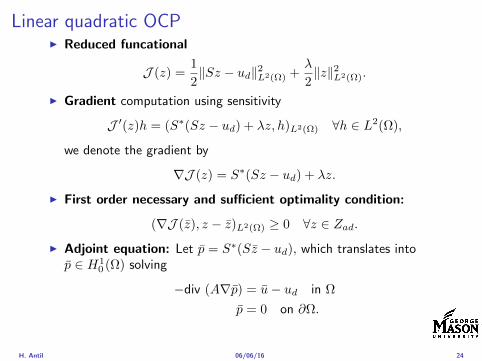
Linear quadratic OCPI Reduced funcational
J (z) =1
2Sz minus ud2L2(Ω) +
λ
2z2L2(Ω)
I Gradient computation using sensitivity
J prime(z)h = (Slowast(Sz minus ud) + λz h)L2(Ω) forallh isin L2(Ω)
we denote the gradient by
nablaJ (z) = Slowast(Sz minus ud) + λz
I First order necessary and sufficient optimality condition
(nablaJ (z) z minus z)L2(Ω) ge 0 forallz isin Zad
I Adjoint equation Let p = Slowast(Sz minus ud) which translates intop isin H1
0 (Ω) solving
minusdiv (Anablap) = uminus ud in Ω
p = 0 on partΩ
I Gradient computation using adjoint nablaJ (z) = p+ λz
H Antil 060616 24
Linear quadratic OCPI Reduced funcational
J (z) =1
2Sz minus ud2L2(Ω) +
λ
2z2L2(Ω)
I Gradient computation using sensitivity
J prime(z)h = (Slowast(Sz minus ud) + λz h)L2(Ω) forallh isin L2(Ω)
we denote the gradient by
nablaJ (z) = Slowast(Sz minus ud) + λz
I First order necessary and sufficient optimality condition
(nablaJ (z) z minus z)L2(Ω) ge 0 forallz isin Zad
I Adjoint equation Let p = Slowast(Sz minus ud) which translates intop isin H1
0 (Ω) solving
minusdiv (Anablap) = uminus ud in Ω
p = 0 on partΩ
I Gradient computation using adjoint nablaJ (z) = p+ λz
H Antil 060616 24
Optimality system
I State u isin H10 (Ω)
intΩAnablau middot nablav =
intΩzv forallv isin H1
0 (Ω)
I Adjoint p isin H10 (Ω)
intΩAnablap middot nablav =
intΩ
(uminus ud)v forallv isin H10 (Ω)
I Control z isin Zad (p+ λz z minus z) ge 0 forallz isin Zad
H Antil 060616 25
Pointwise interpretation
The variational inequality
(p+ λz z minus z) ge 0 forallz isin Zad
is equivalent to for ae x isin Ω
z(x) =
za(x) if p(x) + λz(x) gt 0isin [za(x) zb(x)] if p(x) + λz(x) = 0zb(x) if p(x) + λz(x) lt 0
Consequence
I When λ gt 0 then ae in Ω
z(x) = P[za(x)zb(x)]
minus 1
λp(x)
= min
zb(x)max
za(x)minus 1
λp(x)
H Antil 060616 26
Formal Lagrange method applied to linear OCPIntroduce L H1
0 (Ω)times Zad timesH1(Ω)rarr R defined as
L(u z p) = J(u z)minusint
Ω
(minusdiv (Anablau)minus z
)p dx
Integrate by parts to arrive at
L(u z p) = J(u z)minusint
Ω
(minusdiv (Anablap)uminus zp
)dx+
intpartΩ
(Anablau)p ds
If (u z p) is a stationary point then
I State
DpL(u z p)h = 0 forallh isin H1(Ω)
I AdjointDuL(u z p)h = 0 forallh isin H1
0 (Ω)
I ControlDzL(u z p)(z minus z) ge 0 forallz isin Zad
H Antil 060616 27
Formal Lagrange method applied to linear OCPIntroduce L H1
0 (Ω)times Zad timesH1(Ω)rarr R defined as
L(u z p) = J(u z)minusint
Ω
(minusdiv (Anablau)minus z
)p dx
Integrate by parts to arrive at
L(u z p) = J(u z)minusint
Ω
(minusdiv (Anablap)uminus zp
)dx+
intpartΩ
(Anablau)p ds
If (u z p) is a stationary point then
I State
DpL(u z p)h = 0 forallh isin H1(Ω)
I AdjointDuL(u z p)h = 0 forallh isin H1
0 (Ω)
I ControlDzL(u z p)(z minus z) ge 0 forallz isin Zad
H Antil 060616 27
Formal Lagrange method applied to linear OCPIntroduce L H1
0 (Ω)times Zad timesH1(Ω)rarr R defined as
L(u z p) = J(u z)minusint
Ω
(minusdiv (Anablau)minus z
)p dx
Integrate by parts to arrive at
L(u z p) = J(u z)minusint
Ω
(minusdiv (Anablap)uminus zp
)dx+
intpartΩ
(Anablau)p ds
If (u z p) is a stationary point then
I State
DpL(u z p)h = 0 forallh isin H1(Ω)
I AdjointDuL(u z p)h = 0 forallh isin H1
0 (Ω)
I ControlDzL(u z p)(z minus z) ge 0 forallz isin Zad
H Antil 060616 27
Formal Lagrange method applied to linear OCPIntroduce L H1
0 (Ω)times Zad timesH1(Ω)rarr R defined as
L(u z p) = J(u z)minusint
Ω
(minusdiv (Anablau)minus z
)p dx
Integrate by parts to arrive at
L(u z p) = J(u z)minusint
Ω
(minusdiv (Anablap)uminus zp
)dx+
intpartΩ
(Anablau)p ds
If (u z p) is a stationary point then
I State
DpL(u z p)h = 0 forallh isin H1(Ω)
I AdjointDuL(u z p)h = 0 forallh isin H1
0 (Ω)
I ControlDzL(u z p)(z minus z) ge 0 forallz isin Zad
H Antil 060616 27
Formal Lagrange method applied to linear OCPIntroduce L H1
0 (Ω)times Zad timesH1(Ω)rarr R defined as
L(u z p) = J(u z)minusint
Ω
(minusdiv (Anablau)minus z
)p dx
Integrate by parts to arrive at
L(u z p) = J(u z)minusint
Ω
(minusdiv (Anablap)uminus zp
)dx+
intpartΩ
(Anablau)p ds
If (u z p) is a stationary point then
I State
DpL(u z p)h = 0 forallh isin H1(Ω)
I AdjointDuL(u z p)h = 0 forallh isin H1
0 (Ω)
I ControlDzL(u z p)(z minus z) ge 0 forallz isin Zad
H Antil 060616 27
Outline
Motivation and examples
Linear elliptic optimal control problems
Differentiation in Banach spaces
First-order necessary conditions
Optimal control of semilinear PDEs
An abstract problem
Discretization using finite element methods
H Antil 060616 28
Semilinear elliptic OCP
min J(u z) =1
2uminus ud2L2(Ω) +
λ
2z2L2(Ω)
subject to
minus∆u+ g(x u) = z in Ω
u = 0 on partΩ
and z isin Zad with za zb isin Linfin(Ω)
H Antil 060616 29
State space(A1) Ω sub Rd open bounded partΩ is Lipschitz
(A2) g Ωtimes Rrarr R is bounded and measurable with respect to x isin Ωfor every u isin R
(A3) g is continuous monotone increasing and Lipschitz continuous in ufor ae x isin Ω
(A4) g(x 0) = 0 for ae x isin Ω (not really necessary)
Theorem Suppose (A1)minus (A4) hold For every z isin Lr(Ω) withr gt d2 the state equation has a unique weak solutionu isin H1
0 (Ω) cap C(Ω) ie we haveintΩ
nablau middot nablav dx+
intΩ
g(x u(x))v(x) dx =
intΩ
zv dx forallv isin H10 (Ω)
Moreover there exists a constant C gt 0 such that
uH1(Ω) + uC(Ω) le CzLr(Ω)
RemarkI The proof of the theorem uses the BrowderndashMinty theorem on
monotone operators
H Antil 060616 30
State space(A1) Ω sub Rd open bounded partΩ is Lipschitz
(A2) g Ωtimes Rrarr R is bounded and measurable with respect to x isin Ωfor every u isin R
(A3) g is continuous monotone increasing and Lipschitz continuous in ufor ae x isin Ω
(A4) g(x 0) = 0 for ae x isin Ω (not really necessary)
Theorem Suppose (A1)minus (A4) hold For every z isin Lr(Ω) withr gt d2 the state equation has a unique weak solutionu isin H1
0 (Ω) cap C(Ω) ie we haveintΩ
nablau middot nablav dx+
intΩ
g(x u(x))v(x) dx =
intΩ
zv dx forallv isin H10 (Ω)
Moreover there exists a constant C gt 0 such that
uH1(Ω) + uC(Ω) le CzLr(Ω)
RemarkI The proof of the theorem uses the BrowderndashMinty theorem on
monotone operators
H Antil 060616 30
State space(A1) Ω sub Rd open bounded partΩ is Lipschitz
(A2) g Ωtimes Rrarr R is bounded and measurable with respect to x isin Ωfor every u isin R
(A3) g is continuous monotone increasing and Lipschitz continuous in ufor ae x isin Ω
(A4) g(x 0) = 0 for ae x isin Ω (not really necessary)
Theorem Suppose (A1)minus (A4) hold For every z isin Lr(Ω) withr gt d2 the state equation has a unique weak solutionu isin H1
0 (Ω) cap C(Ω) ie we haveintΩ
nablau middot nablav dx+
intΩ
g(x u(x))v(x) dx =
intΩ
zv dx forallv isin H10 (Ω)
Moreover there exists a constant C gt 0 such that
uH1(Ω) + uC(Ω) le CzLr(Ω)
RemarkI The proof of the theorem uses the BrowderndashMinty theorem on
monotone operators
H Antil 060616 30
Control-to-state map and reduced problem
I Control to state map
S Linfin(Ω)rarr H10 (Ω) cap C(Ω)
is well defined and is globally Lipschitz continuous
I Reduced problem
minJ (z) =1
2S(u)minus ud2L2(Ω) +
λ
2z2L2(Ω)
H Antil 060616 31
Control-to-state map and reduced problem
I Control to state map
S Linfin(Ω)rarr H10 (Ω) cap C(Ω)
is well defined and is globally Lipschitz continuous
I Reduced problem
minJ (z) =1
2S(u)minus ud2L2(Ω) +
λ
2z2L2(Ω)
H Antil 060616 31
First-order necessary conditionsI Lagrangian functional
L(u z p) = J(u z)minusint
Ω
(minus∆u+ g(x u(x))minus z
)p dx
= J(u z)minusint
Ω
(nablau middot nablap+ g(x u(x))pminus zp
)dx
I Adjoint system For all h isin H10 (Ω)
0 = DuL(u z p)h =
intΩ
(uminus ud)h dxminusint
Ω
(nablah middot nablap+ gu(x u(x))ph
)which yields
minus∆p+ gu(x u(x))p = uminus ud in Ω
p = 0 on partΩ
I Control
DzL(u z p)(z minus z) = (p+ λz z minus z) dx ge 0 forallz isin ZadI Gradient
nablaJ (z) = p+ λz
H Antil 060616 32
First-order necessary conditionsI Lagrangian functional
L(u z p) = J(u z)minusint
Ω
(minus∆u+ g(x u(x))minus z
)p dx
= J(u z)minusint
Ω
(nablau middot nablap+ g(x u(x))pminus zp
)dx
I Adjoint system For all h isin H10 (Ω)
0 = DuL(u z p)h =
intΩ
(uminus ud)h dxminusint
Ω
(nablah middot nablap+ gu(x u(x))ph
)which yields
minus∆p+ gu(x u(x))p = uminus ud in Ω
p = 0 on partΩ
I Control
DzL(u z p)(z minus z) = (p+ λz z minus z) dx ge 0 forallz isin ZadI Gradient
nablaJ (z) = p+ λz
H Antil 060616 32
First-order necessary conditionsI Lagrangian functional
L(u z p) = J(u z)minusint
Ω
(minus∆u+ g(x u(x))minus z
)p dx
= J(u z)minusint
Ω
(nablau middot nablap+ g(x u(x))pminus zp
)dx
I Adjoint system For all h isin H10 (Ω)
0 = DuL(u z p)h =
intΩ
(uminus ud)h dxminusint
Ω
(nablah middot nablap+ gu(x u(x))ph
)which yields
minus∆p+ gu(x u(x))p = uminus ud in Ω
p = 0 on partΩ
I Control
DzL(u z p)(z minus z) = (p+ λz z minus z) dx ge 0 forallz isin Zad
I GradientnablaJ (z) = p+ λz
H Antil 060616 32
First-order necessary conditionsI Lagrangian functional
L(u z p) = J(u z)minusint
Ω
(minus∆u+ g(x u(x))minus z
)p dx
= J(u z)minusint
Ω
(nablau middot nablap+ g(x u(x))pminus zp
)dx
I Adjoint system For all h isin H10 (Ω)
0 = DuL(u z p)h =
intΩ
(uminus ud)h dxminusint
Ω
(nablah middot nablap+ gu(x u(x))ph
)which yields
minus∆p+ gu(x u(x))p = uminus ud in Ω
p = 0 on partΩ
I Control
DzL(u z p)(z minus z) = (p+ λz z minus z) dx ge 0 forallz isin ZadI Gradient
nablaJ (z) = p+ λz
H Antil 060616 32
Differentiability of Nemytskii operator
The rigorous proof uses
Theorem In addition to (A1)-(A4) if
(A5) g is continuously differentiable with respect to u for ae x isin Ωand we have
(i) |gu(x 0)| le K for ae x isin Ω(ii) gu is locally Lipschitz with respect to u isin R
then the Nemytskii operator G u 7rarr g(middot u(middot)) is continuously Frechetdifferentiable from Linfin(Ω) into itself and
(Gprime(u)h)(x) = gu(x u(x))h(x) ae in Ω forallh isin Linfin(Ω)
Remark (A5) holds if g(x u) = g(u) and g isin C2(R)
H Antil 060616 33
Outline
Motivation and examples
Linear elliptic optimal control problems
Differentiation in Banach spaces
First-order necessary conditions
Optimal control of semilinear PDEs
An abstract problem
Discretization using finite element methods
H Antil 060616 34
Gradient computation via adjoint general formI Abstract problem
min J(u z)
subject toc(u z) = 0
and z isin Zad
I Directional derivative Let S be the control to state map(nonlinear in general)
z 7rarr S(z) = u(z)
Under the assumptions of ldquoimplicit function theoremrdquo
J prime(z)h = (nablauJ (u(z) z) Sprime(z)h) + (nablazJ (u(z) z) h)
I Sensitivity of u with respect to z Differentiating the stateequation
cu(S(z) z)Sprime(z)h = minuscz(S(z) z)h
leads toSprime(z)h = minuscu(S(z) z)minus1
(cz(S(z) z)h
)
provided cu(S(z) z)minus1 is well-defined
H Antil 060616 35
Gradient computation via adjoint general formI Abstract problem
min J(u z)
subject toc(u z) = 0
and z isin ZadI Directional derivative Let S be the control to state map
(nonlinear in general)
z 7rarr S(z) = u(z)
Under the assumptions of ldquoimplicit function theoremrdquo
J prime(z)h = (nablauJ (u(z) z) Sprime(z)h) + (nablazJ (u(z) z) h)
I Sensitivity of u with respect to z Differentiating the stateequation
cu(S(z) z)Sprime(z)h = minuscz(S(z) z)h
leads toSprime(z)h = minuscu(S(z) z)minus1
(cz(S(z) z)h
)
provided cu(S(z) z)minus1 is well-defined
H Antil 060616 35
Gradient computation via adjoint general formI Abstract problem
min J(u z)
subject toc(u z) = 0
and z isin ZadI Directional derivative Let S be the control to state map
(nonlinear in general)
z 7rarr S(z) = u(z)
Under the assumptions of ldquoimplicit function theoremrdquo
J prime(z)h = (nablauJ (u(z) z) Sprime(z)h) + (nablazJ (u(z) z) h)
I Sensitivity of u with respect to z Differentiating the stateequation
cu(S(z) z)Sprime(z)h = minuscz(S(z) z)h
leads toSprime(z)h = minuscu(S(z) z)minus1
(cz(S(z) z)h
)
provided cu(S(z) z)minus1 is well-defined
H Antil 060616 35
Adjoint equation and gradient general form
I Directional derivative
J prime(z)h = minus(nablauJ (u(z) z) cu(u(z) z)minus1cz(u(z) z)h
)+ (nablazJ (u(z) z) h)
I Gradient
nablaJ (z) = minuscz(u(z) z)lowast(cu(u(z) z)minuslowastnablauJ (u(z) z)
)+nablazJ (u(z) z)
I Introducing adjoint variable p solving
cu(u(z) z)lowastp = nablauJ (u(z) z)
we arrive at following form of gradient
nablaJ (z) = minuscz(u(z) z)lowastp+nablazJ (u(z) z)
which is tractable
H Antil 060616 36
Adjoint equation and gradient general form
I Directional derivative
J prime(z)h = minus(nablauJ (u(z) z) cu(u(z) z)minus1cz(u(z) z)h
)+ (nablazJ (u(z) z) h)
I Gradient
nablaJ (z) = minuscz(u(z) z)lowast(cu(u(z) z)minuslowastnablauJ (u(z) z)
)+nablazJ (u(z) z)
I Introducing adjoint variable p solving
cu(u(z) z)lowastp = nablauJ (u(z) z)
we arrive at following form of gradient
nablaJ (z) = minuscz(u(z) z)lowastp+nablazJ (u(z) z)
which is tractable
H Antil 060616 36
Adjoint equation and gradient general form
I Directional derivative
J prime(z)h = minus(nablauJ (u(z) z) cu(u(z) z)minus1cz(u(z) z)h
)+ (nablazJ (u(z) z) h)
I Gradient
nablaJ (z) = minuscz(u(z) z)lowast(cu(u(z) z)minuslowastnablauJ (u(z) z)
)+nablazJ (u(z) z)
I Introducing adjoint variable p solving
cu(u(z) z)lowastp = nablauJ (u(z) z)
we arrive at following form of gradient
nablaJ (z) = minuscz(u(z) z)lowastp+nablazJ (u(z) z)
which is tractable
H Antil 060616 36
Hessian computation general form
I Lagrangian L(u z p) = J(u z)minusint
Ωc(u z)p dx Then we have
DzJ (z)h = DzL(u z p)h
I Second order derivative
D2zJ (z)[h1 h2] = DuDzL(u z p)[h1 S
prime(z)h2] +D2zL(u z p)[h1 h2]
+DpDzL(u z p)[h1 Dzp(z)h2]
I We already know Sprime(z)h2 moreover
DpDzL(u z p)[h1 Dzp(z)h2] = minus(cu(u z)h1 Dzp(z)h2
)
It remain to identify Dzp(z)h2
H Antil 060616 37
Hessian computation general form
I Lagrangian L(u z p) = J(u z)minusint
Ωc(u z)p dx Then we have
DzJ (z)h = DzL(u z p)h
I Second order derivative
D2zJ (z)[h1 h2] = DuDzL(u z p)[h1 S
prime(z)h2] +D2zL(u z p)[h1 h2]
+DpDzL(u z p)[h1 Dzp(z)h2]
I We already know Sprime(z)h2 moreover
DpDzL(u z p)[h1 Dzp(z)h2] = minus(cu(u z)h1 Dzp(z)h2
)
It remain to identify Dzp(z)h2
H Antil 060616 37
Hessian computation general form
I Lagrangian L(u z p) = J(u z)minusint
Ωc(u z)p dx Then we have
DzJ (z)h = DzL(u z p)h
I Second order derivative
D2zJ (z)[h1 h2] = DuDzL(u z p)[h1 S
prime(z)h2] +D2zL(u z p)[h1 h2]
+DpDzL(u z p)[h1 Dzp(z)h2]
I We already know Sprime(z)h2 moreover
DpDzL(u z p)[h1 Dzp(z)h2] = minus(cu(u z)h1 Dzp(z)h2
)
It remain to identify Dzp(z)h2
H Antil 060616 37
Outline
Motivation and examples
Linear elliptic optimal control problems
Differentiation in Banach spaces
First-order necessary conditions
Optimal control of semilinear PDEs
An abstract problem
Discretization using finite element methods
H Antil 060616 38
Numerical approximation of Poisson equation MeshTo avoid technical issues we will assume that partΩ is polygonal
I Mesh Let T = K be a mesh of Ω where K sub Rd is an elementthat is isoparametrically equivalent to a unit simplex in Rd
I Conforming mesh We say that the mesh is conforming ifI Ω = cupKisinT KI If K1 cap K2 = x then x is a node of K1 and K2I If K1 cap K2 6= empty and K1 cap K2 6= x then K1 cap K2 is an edgeface
contained in partK1 cap partK2
I Shape regular Let T be the collection of all conformingrefinements of an original mesh T 0 Then T is called shape regularif exist κ gt 0 such that
hKρKle κ forallK isin cupiT i
where hK = diam K ρK = maxρ gt 0|Bρ sub KI Quasi-uniform A family of shape regular meshes is called-quasi
uniform if there exist a constant σ gt 0 such that
maxhKminhK
le σ
uniformly for all meshes in the family
Numerical approximation of Poisson equation MeshTo avoid technical issues we will assume that partΩ is polygonal
I Mesh Let T = K be a mesh of Ω where K sub Rd is an elementthat is isoparametrically equivalent to a unit simplex in Rd
I Conforming mesh We say that the mesh is conforming ifI Ω = cupKisinT KI If K1 cap K2 = x then x is a node of K1 and K2I If K1 cap K2 6= empty and K1 cap K2 6= x then K1 cap K2 is an edgeface
contained in partK1 cap partK2
I Shape regular Let T be the collection of all conformingrefinements of an original mesh T 0 Then T is called shape regularif exist κ gt 0 such that
hKρKle κ forallK isin cupiT i
where hK = diam K ρK = maxρ gt 0|Bρ sub KI Quasi-uniform A family of shape regular meshes is called-quasi
uniform if there exist a constant σ gt 0 such that
maxhKminhK
le σ
uniformly for all meshes in the family
Numerical approximation of Poisson equation MeshTo avoid technical issues we will assume that partΩ is polygonal
I Mesh Let T = K be a mesh of Ω where K sub Rd is an elementthat is isoparametrically equivalent to a unit simplex in Rd
I Conforming mesh We say that the mesh is conforming ifI Ω = cupKisinT KI If K1 cap K2 = x then x is a node of K1 and K2I If K1 cap K2 6= empty and K1 cap K2 6= x then K1 cap K2 is an edgeface
contained in partK1 cap partK2
I Shape regular Let T be the collection of all conformingrefinements of an original mesh T 0 Then T is called shape regularif exist κ gt 0 such that
hKρKle κ forallK isin cupiT i
where hK = diam K ρK = maxρ gt 0|Bρ sub K
I Quasi-uniform A family of shape regular meshes is called-quasiuniform if there exist a constant σ gt 0 such that
maxhKminhK
le σ
uniformly for all meshes in the family
Numerical approximation of Poisson equation MeshTo avoid technical issues we will assume that partΩ is polygonal
I Mesh Let T = K be a mesh of Ω where K sub Rd is an elementthat is isoparametrically equivalent to a unit simplex in Rd
I Conforming mesh We say that the mesh is conforming ifI Ω = cupKisinT KI If K1 cap K2 = x then x is a node of K1 and K2I If K1 cap K2 6= empty and K1 cap K2 6= x then K1 cap K2 is an edgeface
contained in partK1 cap partK2
I Shape regular Let T be the collection of all conformingrefinements of an original mesh T 0 Then T is called shape regularif exist κ gt 0 such that
hKρKle κ forallK isin cupiT i
where hK = diam K ρK = maxρ gt 0|Bρ sub KI Quasi-uniform A family of shape regular meshes is called-quasi
uniform if there exist a constant σ gt 0 such that
maxhKminhK
le σ
uniformly for all meshes in the family
FE space and Galerkin approximationI Finite element space For T isin T we define the finite element
space as
V(T ) = W isin C0(Ω) WK isin P1forallK isin T W |partΩ = 0
where P1 is the set of polynomials of degree at most 1
I Galerkin approximation of continuous problem is given by
Find UT isin V(T )
intΩ
AnablaUT middot nablaV = 〈f V 〉 forallV isin V(T )
The discrete problem is well-posedI Nodal basis Consists of functions ψi isin V(T ) with xi isin N (T )
satisfyingψxi
(xj) = δij
where N (T ) denotes the interior (plus Neumann) nodesI Galerkin orthogonality(
nabla(uminus UT )nablaW)L2(Ω)
= 0 forallW isin V(T )
H Antil 060616 40
FE space and Galerkin approximationI Finite element space For T isin T we define the finite element
space as
V(T ) = W isin C0(Ω) WK isin P1forallK isin T W |partΩ = 0
where P1 is the set of polynomials of degree at most 1I Galerkin approximation of continuous problem is given by
Find UT isin V(T )
intΩ
AnablaUT middot nablaV = 〈f V 〉 forallV isin V(T )
The discrete problem is well-posed
I Nodal basis Consists of functions ψi isin V(T ) with xi isin N (T )satisfying
ψxi(xj) = δij
where N (T ) denotes the interior (plus Neumann) nodesI Galerkin orthogonality(
nabla(uminus UT )nablaW)L2(Ω)
= 0 forallW isin V(T )
H Antil 060616 40
FE space and Galerkin approximationI Finite element space For T isin T we define the finite element
space as
V(T ) = W isin C0(Ω) WK isin P1forallK isin T W |partΩ = 0
where P1 is the set of polynomials of degree at most 1I Galerkin approximation of continuous problem is given by
Find UT isin V(T )
intΩ
AnablaUT middot nablaV = 〈f V 〉 forallV isin V(T )
The discrete problem is well-posedI Nodal basis Consists of functions ψi isin V(T ) with xi isin N (T )
satisfyingψxi
(xj) = δij
where N (T ) denotes the interior (plus Neumann) nodes
I Galerkin orthogonality(nabla(uminus UT )nablaW
)L2(Ω)
= 0 forallW isin V(T )
H Antil 060616 40
FE space and Galerkin approximationI Finite element space For T isin T we define the finite element
space as
V(T ) = W isin C0(Ω) WK isin P1forallK isin T W |partΩ = 0
where P1 is the set of polynomials of degree at most 1I Galerkin approximation of continuous problem is given by
Find UT isin V(T )
intΩ
AnablaUT middot nablaV = 〈f V 〉 forallV isin V(T )
The discrete problem is well-posedI Nodal basis Consists of functions ψi isin V(T ) with xi isin N (T )
satisfyingψxi
(xj) = δij
where N (T ) denotes the interior (plus Neumann) nodesI Galerkin orthogonality(
nabla(uminus UT )nablaW)L2(Ω)
= 0 forallW isin V(T )
H Antil 060616 40
Best approximation
I Cearsquos lemma
nabla(uminus UT )L2(Ω) le C infWisinV(T )
nabla(uminusW )L2(Ω)
I Nodal interpolation operator ΠT C(Ω)rarr V(T ) satisfies
ΠT u(xi) = u(xi) forallxi isin N (T )
and is defined as
ΠT u =sum
xiisinN (T )
u(xi)ψxi
I Error estimates In Cearsquos lemma replace W by ΠT u and thencompute the interpolation error
H Antil 060616 41
Best approximation
I Cearsquos lemma
nabla(uminus UT )L2(Ω) le C infWisinV(T )
nabla(uminusW )L2(Ω)
I Nodal interpolation operator ΠT C(Ω)rarr V(T ) satisfies
ΠT u(xi) = u(xi) forallxi isin N (T )
and is defined as
ΠT u =sum
xiisinN (T )
u(xi)ψxi
I Error estimates In Cearsquos lemma replace W by ΠT u and thencompute the interpolation error
H Antil 060616 41
Best approximation
I Cearsquos lemma
nabla(uminus UT )L2(Ω) le C infWisinV(T )
nabla(uminusW )L2(Ω)
I Nodal interpolation operator ΠT C(Ω)rarr V(T ) satisfies
ΠT u(xi) = u(xi) forallxi isin N (T )
and is defined as
ΠT u =sum
xiisinN (T )
u(xi)ψxi
I Error estimates In Cearsquos lemma replace W by ΠT u and thencompute the interpolation error
H Antil 060616 41
Algebraic system state equation
I Recall UT isin V(T ) solves
a(UT V ) = 〈f V 〉 forallV isin V(T )
I Now setting UT =sumN
j=1 Ujψj V = ψi we get
Nsumj=1
Uja(φj φi) = 〈f ψi〉 i = 1 N
which is the matrix-vector system
AU = F
I Stiffness matrix A is SPD
H Antil 060616 42
Algebraic system state equation
I Recall UT isin V(T ) solves
a(UT V ) = 〈f V 〉 forallV isin V(T )
I Now setting UT =sumN
j=1 Ujψj V = ψi we get
Nsumj=1
Uja(φj φi) = 〈f ψi〉 i = 1 N
which is the matrix-vector system
AU = F
I Stiffness matrix A is SPD
H Antil 060616 42
Algebraic system state equation
I Recall UT isin V(T ) solves
a(UT V ) = 〈f V 〉 forallV isin V(T )
I Now setting UT =sumN
j=1 Ujψj V = ψi we get
Nsumj=1
Uja(φj φi) = 〈f ψi〉 i = 1 N
which is the matrix-vector system
AU = F
I Stiffness matrix A is SPD
H Antil 060616 42
Discrete linear elliptic OCP
min JT (UT ZT ) =1
2UT minus ud2L2(Ω) +
λ
2ZT 2L2(Ω)
subject to
Find UT isin V(T )
intΩ
nablaUT middot nablaV = (ZT V )L2(Ω) forallV isin V(T )
and whereZT isin Zad(T ) = Zad cap Z(T )
is either one of these
Z(T ) =
V(T )L2(Ω) variational discretization (Hinze)WT isin Linfin(Ω) ZT |K isin P0(K)K isin T
H Antil 060616 43
Recent books
F TroltzschOptimal control of partial differential equations volume 112 ofGraduate Studies in MathematicsAmerican Mathematical Society Providence RI 2010Theory methods and applications Translated from the 2005 Germanoriginal by Jurgen Sprekels
K Ito and K KunischLagrange multiplier approach to variational problems andapplications volume 15 of Advances in Design and ControlSociety for Industrial and Applied Mathematics (SIAM)Philadelphia PA 2008
H Antil 060616 44
- Motivation and examples
- Linear elliptic optimal control problems
- Differentiation in Banach spaces
- First-order necessary conditions
- Optimal control of semilinear PDEs
- An abstract problem
- Discretization using finite element methods
-
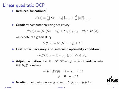
Linear quadratic OCPI Reduced funcational
J (z) =1
2Sz minus ud2L2(Ω) +
λ
2z2L2(Ω)
I Gradient computation using sensitivity
J prime(z)h = (Slowast(Sz minus ud) + λz h)L2(Ω) forallh isin L2(Ω)
we denote the gradient by
nablaJ (z) = Slowast(Sz minus ud) + λz
I First order necessary and sufficient optimality condition
(nablaJ (z) z minus z)L2(Ω) ge 0 forallz isin Zad
I Adjoint equation Let p = Slowast(Sz minus ud) which translates intop isin H1
0 (Ω) solving
minusdiv (Anablap) = uminus ud in Ω
p = 0 on partΩ
I Gradient computation using adjoint nablaJ (z) = p+ λz
H Antil 060616 24
Optimality system
I State u isin H10 (Ω)
intΩAnablau middot nablav =
intΩzv forallv isin H1
0 (Ω)
I Adjoint p isin H10 (Ω)
intΩAnablap middot nablav =
intΩ
(uminus ud)v forallv isin H10 (Ω)
I Control z isin Zad (p+ λz z minus z) ge 0 forallz isin Zad
H Antil 060616 25
Pointwise interpretation
The variational inequality
(p+ λz z minus z) ge 0 forallz isin Zad
is equivalent to for ae x isin Ω
z(x) =
za(x) if p(x) + λz(x) gt 0isin [za(x) zb(x)] if p(x) + λz(x) = 0zb(x) if p(x) + λz(x) lt 0
Consequence
I When λ gt 0 then ae in Ω
z(x) = P[za(x)zb(x)]
minus 1
λp(x)
= min
zb(x)max
za(x)minus 1
λp(x)
H Antil 060616 26
Formal Lagrange method applied to linear OCPIntroduce L H1
0 (Ω)times Zad timesH1(Ω)rarr R defined as
L(u z p) = J(u z)minusint
Ω
(minusdiv (Anablau)minus z
)p dx
Integrate by parts to arrive at
L(u z p) = J(u z)minusint
Ω
(minusdiv (Anablap)uminus zp
)dx+
intpartΩ
(Anablau)p ds
If (u z p) is a stationary point then
I State
DpL(u z p)h = 0 forallh isin H1(Ω)
I AdjointDuL(u z p)h = 0 forallh isin H1
0 (Ω)
I ControlDzL(u z p)(z minus z) ge 0 forallz isin Zad
H Antil 060616 27
Formal Lagrange method applied to linear OCPIntroduce L H1
0 (Ω)times Zad timesH1(Ω)rarr R defined as
L(u z p) = J(u z)minusint
Ω
(minusdiv (Anablau)minus z
)p dx
Integrate by parts to arrive at
L(u z p) = J(u z)minusint
Ω
(minusdiv (Anablap)uminus zp
)dx+
intpartΩ
(Anablau)p ds
If (u z p) is a stationary point then
I State
DpL(u z p)h = 0 forallh isin H1(Ω)
I AdjointDuL(u z p)h = 0 forallh isin H1
0 (Ω)
I ControlDzL(u z p)(z minus z) ge 0 forallz isin Zad
H Antil 060616 27
Formal Lagrange method applied to linear OCPIntroduce L H1
0 (Ω)times Zad timesH1(Ω)rarr R defined as
L(u z p) = J(u z)minusint
Ω
(minusdiv (Anablau)minus z
)p dx
Integrate by parts to arrive at
L(u z p) = J(u z)minusint
Ω
(minusdiv (Anablap)uminus zp
)dx+
intpartΩ
(Anablau)p ds
If (u z p) is a stationary point then
I State
DpL(u z p)h = 0 forallh isin H1(Ω)
I AdjointDuL(u z p)h = 0 forallh isin H1
0 (Ω)
I ControlDzL(u z p)(z minus z) ge 0 forallz isin Zad
H Antil 060616 27
Formal Lagrange method applied to linear OCPIntroduce L H1
0 (Ω)times Zad timesH1(Ω)rarr R defined as
L(u z p) = J(u z)minusint
Ω
(minusdiv (Anablau)minus z
)p dx
Integrate by parts to arrive at
L(u z p) = J(u z)minusint
Ω
(minusdiv (Anablap)uminus zp
)dx+
intpartΩ
(Anablau)p ds
If (u z p) is a stationary point then
I State
DpL(u z p)h = 0 forallh isin H1(Ω)
I AdjointDuL(u z p)h = 0 forallh isin H1
0 (Ω)
I ControlDzL(u z p)(z minus z) ge 0 forallz isin Zad
H Antil 060616 27
Formal Lagrange method applied to linear OCPIntroduce L H1
0 (Ω)times Zad timesH1(Ω)rarr R defined as
L(u z p) = J(u z)minusint
Ω
(minusdiv (Anablau)minus z
)p dx
Integrate by parts to arrive at
L(u z p) = J(u z)minusint
Ω
(minusdiv (Anablap)uminus zp
)dx+
intpartΩ
(Anablau)p ds
If (u z p) is a stationary point then
I State
DpL(u z p)h = 0 forallh isin H1(Ω)
I AdjointDuL(u z p)h = 0 forallh isin H1
0 (Ω)
I ControlDzL(u z p)(z minus z) ge 0 forallz isin Zad
H Antil 060616 27
Outline
Motivation and examples
Linear elliptic optimal control problems
Differentiation in Banach spaces
First-order necessary conditions
Optimal control of semilinear PDEs
An abstract problem
Discretization using finite element methods
H Antil 060616 28
Semilinear elliptic OCP
min J(u z) =1
2uminus ud2L2(Ω) +
λ
2z2L2(Ω)
subject to
minus∆u+ g(x u) = z in Ω
u = 0 on partΩ
and z isin Zad with za zb isin Linfin(Ω)
H Antil 060616 29
State space(A1) Ω sub Rd open bounded partΩ is Lipschitz
(A2) g Ωtimes Rrarr R is bounded and measurable with respect to x isin Ωfor every u isin R
(A3) g is continuous monotone increasing and Lipschitz continuous in ufor ae x isin Ω
(A4) g(x 0) = 0 for ae x isin Ω (not really necessary)
Theorem Suppose (A1)minus (A4) hold For every z isin Lr(Ω) withr gt d2 the state equation has a unique weak solutionu isin H1
0 (Ω) cap C(Ω) ie we haveintΩ
nablau middot nablav dx+
intΩ
g(x u(x))v(x) dx =
intΩ
zv dx forallv isin H10 (Ω)
Moreover there exists a constant C gt 0 such that
uH1(Ω) + uC(Ω) le CzLr(Ω)
RemarkI The proof of the theorem uses the BrowderndashMinty theorem on
monotone operators
H Antil 060616 30
State space(A1) Ω sub Rd open bounded partΩ is Lipschitz
(A2) g Ωtimes Rrarr R is bounded and measurable with respect to x isin Ωfor every u isin R
(A3) g is continuous monotone increasing and Lipschitz continuous in ufor ae x isin Ω
(A4) g(x 0) = 0 for ae x isin Ω (not really necessary)
Theorem Suppose (A1)minus (A4) hold For every z isin Lr(Ω) withr gt d2 the state equation has a unique weak solutionu isin H1
0 (Ω) cap C(Ω) ie we haveintΩ
nablau middot nablav dx+
intΩ
g(x u(x))v(x) dx =
intΩ
zv dx forallv isin H10 (Ω)
Moreover there exists a constant C gt 0 such that
uH1(Ω) + uC(Ω) le CzLr(Ω)
RemarkI The proof of the theorem uses the BrowderndashMinty theorem on
monotone operators
H Antil 060616 30
State space(A1) Ω sub Rd open bounded partΩ is Lipschitz
(A2) g Ωtimes Rrarr R is bounded and measurable with respect to x isin Ωfor every u isin R
(A3) g is continuous monotone increasing and Lipschitz continuous in ufor ae x isin Ω
(A4) g(x 0) = 0 for ae x isin Ω (not really necessary)
Theorem Suppose (A1)minus (A4) hold For every z isin Lr(Ω) withr gt d2 the state equation has a unique weak solutionu isin H1
0 (Ω) cap C(Ω) ie we haveintΩ
nablau middot nablav dx+
intΩ
g(x u(x))v(x) dx =
intΩ
zv dx forallv isin H10 (Ω)
Moreover there exists a constant C gt 0 such that
uH1(Ω) + uC(Ω) le CzLr(Ω)
RemarkI The proof of the theorem uses the BrowderndashMinty theorem on
monotone operators
H Antil 060616 30
Control-to-state map and reduced problem
I Control to state map
S Linfin(Ω)rarr H10 (Ω) cap C(Ω)
is well defined and is globally Lipschitz continuous
I Reduced problem
minJ (z) =1
2S(u)minus ud2L2(Ω) +
λ
2z2L2(Ω)
H Antil 060616 31
Control-to-state map and reduced problem
I Control to state map
S Linfin(Ω)rarr H10 (Ω) cap C(Ω)
is well defined and is globally Lipschitz continuous
I Reduced problem
minJ (z) =1
2S(u)minus ud2L2(Ω) +
λ
2z2L2(Ω)
H Antil 060616 31
First-order necessary conditionsI Lagrangian functional
L(u z p) = J(u z)minusint
Ω
(minus∆u+ g(x u(x))minus z
)p dx
= J(u z)minusint
Ω
(nablau middot nablap+ g(x u(x))pminus zp
)dx
I Adjoint system For all h isin H10 (Ω)
0 = DuL(u z p)h =
intΩ
(uminus ud)h dxminusint
Ω
(nablah middot nablap+ gu(x u(x))ph
)which yields
minus∆p+ gu(x u(x))p = uminus ud in Ω
p = 0 on partΩ
I Control
DzL(u z p)(z minus z) = (p+ λz z minus z) dx ge 0 forallz isin ZadI Gradient
nablaJ (z) = p+ λz
H Antil 060616 32
First-order necessary conditionsI Lagrangian functional
L(u z p) = J(u z)minusint
Ω
(minus∆u+ g(x u(x))minus z
)p dx
= J(u z)minusint
Ω
(nablau middot nablap+ g(x u(x))pminus zp
)dx
I Adjoint system For all h isin H10 (Ω)
0 = DuL(u z p)h =
intΩ
(uminus ud)h dxminusint
Ω
(nablah middot nablap+ gu(x u(x))ph
)which yields
minus∆p+ gu(x u(x))p = uminus ud in Ω
p = 0 on partΩ
I Control
DzL(u z p)(z minus z) = (p+ λz z minus z) dx ge 0 forallz isin ZadI Gradient
nablaJ (z) = p+ λz
H Antil 060616 32
First-order necessary conditionsI Lagrangian functional
L(u z p) = J(u z)minusint
Ω
(minus∆u+ g(x u(x))minus z
)p dx
= J(u z)minusint
Ω
(nablau middot nablap+ g(x u(x))pminus zp
)dx
I Adjoint system For all h isin H10 (Ω)
0 = DuL(u z p)h =
intΩ
(uminus ud)h dxminusint
Ω
(nablah middot nablap+ gu(x u(x))ph
)which yields
minus∆p+ gu(x u(x))p = uminus ud in Ω
p = 0 on partΩ
I Control
DzL(u z p)(z minus z) = (p+ λz z minus z) dx ge 0 forallz isin Zad
I GradientnablaJ (z) = p+ λz
H Antil 060616 32
First-order necessary conditionsI Lagrangian functional
L(u z p) = J(u z)minusint
Ω
(minus∆u+ g(x u(x))minus z
)p dx
= J(u z)minusint
Ω
(nablau middot nablap+ g(x u(x))pminus zp
)dx
I Adjoint system For all h isin H10 (Ω)
0 = DuL(u z p)h =
intΩ
(uminus ud)h dxminusint
Ω
(nablah middot nablap+ gu(x u(x))ph
)which yields
minus∆p+ gu(x u(x))p = uminus ud in Ω
p = 0 on partΩ
I Control
DzL(u z p)(z minus z) = (p+ λz z minus z) dx ge 0 forallz isin ZadI Gradient
nablaJ (z) = p+ λz
H Antil 060616 32
Differentiability of Nemytskii operator
The rigorous proof uses
Theorem In addition to (A1)-(A4) if
(A5) g is continuously differentiable with respect to u for ae x isin Ωand we have
(i) |gu(x 0)| le K for ae x isin Ω(ii) gu is locally Lipschitz with respect to u isin R
then the Nemytskii operator G u 7rarr g(middot u(middot)) is continuously Frechetdifferentiable from Linfin(Ω) into itself and
(Gprime(u)h)(x) = gu(x u(x))h(x) ae in Ω forallh isin Linfin(Ω)
Remark (A5) holds if g(x u) = g(u) and g isin C2(R)
H Antil 060616 33
Outline
Motivation and examples
Linear elliptic optimal control problems
Differentiation in Banach spaces
First-order necessary conditions
Optimal control of semilinear PDEs
An abstract problem
Discretization using finite element methods
H Antil 060616 34
Gradient computation via adjoint general formI Abstract problem
min J(u z)
subject toc(u z) = 0
and z isin Zad
I Directional derivative Let S be the control to state map(nonlinear in general)
z 7rarr S(z) = u(z)
Under the assumptions of ldquoimplicit function theoremrdquo
J prime(z)h = (nablauJ (u(z) z) Sprime(z)h) + (nablazJ (u(z) z) h)
I Sensitivity of u with respect to z Differentiating the stateequation
cu(S(z) z)Sprime(z)h = minuscz(S(z) z)h
leads toSprime(z)h = minuscu(S(z) z)minus1
(cz(S(z) z)h
)
provided cu(S(z) z)minus1 is well-defined
H Antil 060616 35
Gradient computation via adjoint general formI Abstract problem
min J(u z)
subject toc(u z) = 0
and z isin ZadI Directional derivative Let S be the control to state map
(nonlinear in general)
z 7rarr S(z) = u(z)
Under the assumptions of ldquoimplicit function theoremrdquo
J prime(z)h = (nablauJ (u(z) z) Sprime(z)h) + (nablazJ (u(z) z) h)
I Sensitivity of u with respect to z Differentiating the stateequation
cu(S(z) z)Sprime(z)h = minuscz(S(z) z)h
leads toSprime(z)h = minuscu(S(z) z)minus1
(cz(S(z) z)h
)
provided cu(S(z) z)minus1 is well-defined
H Antil 060616 35
Gradient computation via adjoint general formI Abstract problem
min J(u z)
subject toc(u z) = 0
and z isin ZadI Directional derivative Let S be the control to state map
(nonlinear in general)
z 7rarr S(z) = u(z)
Under the assumptions of ldquoimplicit function theoremrdquo
J prime(z)h = (nablauJ (u(z) z) Sprime(z)h) + (nablazJ (u(z) z) h)
I Sensitivity of u with respect to z Differentiating the stateequation
cu(S(z) z)Sprime(z)h = minuscz(S(z) z)h
leads toSprime(z)h = minuscu(S(z) z)minus1
(cz(S(z) z)h
)
provided cu(S(z) z)minus1 is well-defined
H Antil 060616 35
Adjoint equation and gradient general form
I Directional derivative
J prime(z)h = minus(nablauJ (u(z) z) cu(u(z) z)minus1cz(u(z) z)h
)+ (nablazJ (u(z) z) h)
I Gradient
nablaJ (z) = minuscz(u(z) z)lowast(cu(u(z) z)minuslowastnablauJ (u(z) z)
)+nablazJ (u(z) z)
I Introducing adjoint variable p solving
cu(u(z) z)lowastp = nablauJ (u(z) z)
we arrive at following form of gradient
nablaJ (z) = minuscz(u(z) z)lowastp+nablazJ (u(z) z)
which is tractable
H Antil 060616 36
Adjoint equation and gradient general form
I Directional derivative
J prime(z)h = minus(nablauJ (u(z) z) cu(u(z) z)minus1cz(u(z) z)h
)+ (nablazJ (u(z) z) h)
I Gradient
nablaJ (z) = minuscz(u(z) z)lowast(cu(u(z) z)minuslowastnablauJ (u(z) z)
)+nablazJ (u(z) z)
I Introducing adjoint variable p solving
cu(u(z) z)lowastp = nablauJ (u(z) z)
we arrive at following form of gradient
nablaJ (z) = minuscz(u(z) z)lowastp+nablazJ (u(z) z)
which is tractable
H Antil 060616 36
Adjoint equation and gradient general form
I Directional derivative
J prime(z)h = minus(nablauJ (u(z) z) cu(u(z) z)minus1cz(u(z) z)h
)+ (nablazJ (u(z) z) h)
I Gradient
nablaJ (z) = minuscz(u(z) z)lowast(cu(u(z) z)minuslowastnablauJ (u(z) z)
)+nablazJ (u(z) z)
I Introducing adjoint variable p solving
cu(u(z) z)lowastp = nablauJ (u(z) z)
we arrive at following form of gradient
nablaJ (z) = minuscz(u(z) z)lowastp+nablazJ (u(z) z)
which is tractable
H Antil 060616 36
Hessian computation general form
I Lagrangian L(u z p) = J(u z)minusint
Ωc(u z)p dx Then we have
DzJ (z)h = DzL(u z p)h
I Second order derivative
D2zJ (z)[h1 h2] = DuDzL(u z p)[h1 S
prime(z)h2] +D2zL(u z p)[h1 h2]
+DpDzL(u z p)[h1 Dzp(z)h2]
I We already know Sprime(z)h2 moreover
DpDzL(u z p)[h1 Dzp(z)h2] = minus(cu(u z)h1 Dzp(z)h2
)
It remain to identify Dzp(z)h2
H Antil 060616 37
Hessian computation general form
I Lagrangian L(u z p) = J(u z)minusint
Ωc(u z)p dx Then we have
DzJ (z)h = DzL(u z p)h
I Second order derivative
D2zJ (z)[h1 h2] = DuDzL(u z p)[h1 S
prime(z)h2] +D2zL(u z p)[h1 h2]
+DpDzL(u z p)[h1 Dzp(z)h2]
I We already know Sprime(z)h2 moreover
DpDzL(u z p)[h1 Dzp(z)h2] = minus(cu(u z)h1 Dzp(z)h2
)
It remain to identify Dzp(z)h2
H Antil 060616 37
Hessian computation general form
I Lagrangian L(u z p) = J(u z)minusint
Ωc(u z)p dx Then we have
DzJ (z)h = DzL(u z p)h
I Second order derivative
D2zJ (z)[h1 h2] = DuDzL(u z p)[h1 S
prime(z)h2] +D2zL(u z p)[h1 h2]
+DpDzL(u z p)[h1 Dzp(z)h2]
I We already know Sprime(z)h2 moreover
DpDzL(u z p)[h1 Dzp(z)h2] = minus(cu(u z)h1 Dzp(z)h2
)
It remain to identify Dzp(z)h2
H Antil 060616 37
Outline
Motivation and examples
Linear elliptic optimal control problems
Differentiation in Banach spaces
First-order necessary conditions
Optimal control of semilinear PDEs
An abstract problem
Discretization using finite element methods
H Antil 060616 38
Numerical approximation of Poisson equation MeshTo avoid technical issues we will assume that partΩ is polygonal
I Mesh Let T = K be a mesh of Ω where K sub Rd is an elementthat is isoparametrically equivalent to a unit simplex in Rd
I Conforming mesh We say that the mesh is conforming ifI Ω = cupKisinT KI If K1 cap K2 = x then x is a node of K1 and K2I If K1 cap K2 6= empty and K1 cap K2 6= x then K1 cap K2 is an edgeface
contained in partK1 cap partK2
I Shape regular Let T be the collection of all conformingrefinements of an original mesh T 0 Then T is called shape regularif exist κ gt 0 such that
hKρKle κ forallK isin cupiT i
where hK = diam K ρK = maxρ gt 0|Bρ sub KI Quasi-uniform A family of shape regular meshes is called-quasi
uniform if there exist a constant σ gt 0 such that
maxhKminhK
le σ
uniformly for all meshes in the family
Numerical approximation of Poisson equation MeshTo avoid technical issues we will assume that partΩ is polygonal
I Mesh Let T = K be a mesh of Ω where K sub Rd is an elementthat is isoparametrically equivalent to a unit simplex in Rd
I Conforming mesh We say that the mesh is conforming ifI Ω = cupKisinT KI If K1 cap K2 = x then x is a node of K1 and K2I If K1 cap K2 6= empty and K1 cap K2 6= x then K1 cap K2 is an edgeface
contained in partK1 cap partK2
I Shape regular Let T be the collection of all conformingrefinements of an original mesh T 0 Then T is called shape regularif exist κ gt 0 such that
hKρKle κ forallK isin cupiT i
where hK = diam K ρK = maxρ gt 0|Bρ sub KI Quasi-uniform A family of shape regular meshes is called-quasi
uniform if there exist a constant σ gt 0 such that
maxhKminhK
le σ
uniformly for all meshes in the family
Numerical approximation of Poisson equation MeshTo avoid technical issues we will assume that partΩ is polygonal
I Mesh Let T = K be a mesh of Ω where K sub Rd is an elementthat is isoparametrically equivalent to a unit simplex in Rd
I Conforming mesh We say that the mesh is conforming ifI Ω = cupKisinT KI If K1 cap K2 = x then x is a node of K1 and K2I If K1 cap K2 6= empty and K1 cap K2 6= x then K1 cap K2 is an edgeface
contained in partK1 cap partK2
I Shape regular Let T be the collection of all conformingrefinements of an original mesh T 0 Then T is called shape regularif exist κ gt 0 such that
hKρKle κ forallK isin cupiT i
where hK = diam K ρK = maxρ gt 0|Bρ sub K
I Quasi-uniform A family of shape regular meshes is called-quasiuniform if there exist a constant σ gt 0 such that
maxhKminhK
le σ
uniformly for all meshes in the family
Numerical approximation of Poisson equation MeshTo avoid technical issues we will assume that partΩ is polygonal
I Mesh Let T = K be a mesh of Ω where K sub Rd is an elementthat is isoparametrically equivalent to a unit simplex in Rd
I Conforming mesh We say that the mesh is conforming ifI Ω = cupKisinT KI If K1 cap K2 = x then x is a node of K1 and K2I If K1 cap K2 6= empty and K1 cap K2 6= x then K1 cap K2 is an edgeface
contained in partK1 cap partK2
I Shape regular Let T be the collection of all conformingrefinements of an original mesh T 0 Then T is called shape regularif exist κ gt 0 such that
hKρKle κ forallK isin cupiT i
where hK = diam K ρK = maxρ gt 0|Bρ sub KI Quasi-uniform A family of shape regular meshes is called-quasi
uniform if there exist a constant σ gt 0 such that
maxhKminhK
le σ
uniformly for all meshes in the family
FE space and Galerkin approximationI Finite element space For T isin T we define the finite element
space as
V(T ) = W isin C0(Ω) WK isin P1forallK isin T W |partΩ = 0
where P1 is the set of polynomials of degree at most 1
I Galerkin approximation of continuous problem is given by
Find UT isin V(T )
intΩ
AnablaUT middot nablaV = 〈f V 〉 forallV isin V(T )
The discrete problem is well-posedI Nodal basis Consists of functions ψi isin V(T ) with xi isin N (T )
satisfyingψxi
(xj) = δij
where N (T ) denotes the interior (plus Neumann) nodesI Galerkin orthogonality(
nabla(uminus UT )nablaW)L2(Ω)
= 0 forallW isin V(T )
H Antil 060616 40
FE space and Galerkin approximationI Finite element space For T isin T we define the finite element
space as
V(T ) = W isin C0(Ω) WK isin P1forallK isin T W |partΩ = 0
where P1 is the set of polynomials of degree at most 1I Galerkin approximation of continuous problem is given by
Find UT isin V(T )
intΩ
AnablaUT middot nablaV = 〈f V 〉 forallV isin V(T )
The discrete problem is well-posed
I Nodal basis Consists of functions ψi isin V(T ) with xi isin N (T )satisfying
ψxi(xj) = δij
where N (T ) denotes the interior (plus Neumann) nodesI Galerkin orthogonality(
nabla(uminus UT )nablaW)L2(Ω)
= 0 forallW isin V(T )
H Antil 060616 40
FE space and Galerkin approximationI Finite element space For T isin T we define the finite element
space as
V(T ) = W isin C0(Ω) WK isin P1forallK isin T W |partΩ = 0
where P1 is the set of polynomials of degree at most 1I Galerkin approximation of continuous problem is given by
Find UT isin V(T )
intΩ
AnablaUT middot nablaV = 〈f V 〉 forallV isin V(T )
The discrete problem is well-posedI Nodal basis Consists of functions ψi isin V(T ) with xi isin N (T )
satisfyingψxi
(xj) = δij
where N (T ) denotes the interior (plus Neumann) nodes
I Galerkin orthogonality(nabla(uminus UT )nablaW
)L2(Ω)
= 0 forallW isin V(T )
H Antil 060616 40
FE space and Galerkin approximationI Finite element space For T isin T we define the finite element
space as
V(T ) = W isin C0(Ω) WK isin P1forallK isin T W |partΩ = 0
where P1 is the set of polynomials of degree at most 1I Galerkin approximation of continuous problem is given by
Find UT isin V(T )
intΩ
AnablaUT middot nablaV = 〈f V 〉 forallV isin V(T )
The discrete problem is well-posedI Nodal basis Consists of functions ψi isin V(T ) with xi isin N (T )
satisfyingψxi
(xj) = δij
where N (T ) denotes the interior (plus Neumann) nodesI Galerkin orthogonality(
nabla(uminus UT )nablaW)L2(Ω)
= 0 forallW isin V(T )
H Antil 060616 40
Best approximation
I Cearsquos lemma
nabla(uminus UT )L2(Ω) le C infWisinV(T )
nabla(uminusW )L2(Ω)
I Nodal interpolation operator ΠT C(Ω)rarr V(T ) satisfies
ΠT u(xi) = u(xi) forallxi isin N (T )
and is defined as
ΠT u =sum
xiisinN (T )
u(xi)ψxi
I Error estimates In Cearsquos lemma replace W by ΠT u and thencompute the interpolation error
H Antil 060616 41
Best approximation
I Cearsquos lemma
nabla(uminus UT )L2(Ω) le C infWisinV(T )
nabla(uminusW )L2(Ω)
I Nodal interpolation operator ΠT C(Ω)rarr V(T ) satisfies
ΠT u(xi) = u(xi) forallxi isin N (T )
and is defined as
ΠT u =sum
xiisinN (T )
u(xi)ψxi
I Error estimates In Cearsquos lemma replace W by ΠT u and thencompute the interpolation error
H Antil 060616 41
Best approximation
I Cearsquos lemma
nabla(uminus UT )L2(Ω) le C infWisinV(T )
nabla(uminusW )L2(Ω)
I Nodal interpolation operator ΠT C(Ω)rarr V(T ) satisfies
ΠT u(xi) = u(xi) forallxi isin N (T )
and is defined as
ΠT u =sum
xiisinN (T )
u(xi)ψxi
I Error estimates In Cearsquos lemma replace W by ΠT u and thencompute the interpolation error
H Antil 060616 41
Algebraic system state equation
I Recall UT isin V(T ) solves
a(UT V ) = 〈f V 〉 forallV isin V(T )
I Now setting UT =sumN
j=1 Ujψj V = ψi we get
Nsumj=1
Uja(φj φi) = 〈f ψi〉 i = 1 N
which is the matrix-vector system
AU = F
I Stiffness matrix A is SPD
H Antil 060616 42
Algebraic system state equation
I Recall UT isin V(T ) solves
a(UT V ) = 〈f V 〉 forallV isin V(T )
I Now setting UT =sumN
j=1 Ujψj V = ψi we get
Nsumj=1
Uja(φj φi) = 〈f ψi〉 i = 1 N
which is the matrix-vector system
AU = F
I Stiffness matrix A is SPD
H Antil 060616 42
Algebraic system state equation
I Recall UT isin V(T ) solves
a(UT V ) = 〈f V 〉 forallV isin V(T )
I Now setting UT =sumN
j=1 Ujψj V = ψi we get
Nsumj=1
Uja(φj φi) = 〈f ψi〉 i = 1 N
which is the matrix-vector system
AU = F
I Stiffness matrix A is SPD
H Antil 060616 42
Discrete linear elliptic OCP
min JT (UT ZT ) =1
2UT minus ud2L2(Ω) +
λ
2ZT 2L2(Ω)
subject to
Find UT isin V(T )
intΩ
nablaUT middot nablaV = (ZT V )L2(Ω) forallV isin V(T )
and whereZT isin Zad(T ) = Zad cap Z(T )
is either one of these
Z(T ) =
V(T )L2(Ω) variational discretization (Hinze)WT isin Linfin(Ω) ZT |K isin P0(K)K isin T
H Antil 060616 43
Recent books
F TroltzschOptimal control of partial differential equations volume 112 ofGraduate Studies in MathematicsAmerican Mathematical Society Providence RI 2010Theory methods and applications Translated from the 2005 Germanoriginal by Jurgen Sprekels
K Ito and K KunischLagrange multiplier approach to variational problems andapplications volume 15 of Advances in Design and ControlSociety for Industrial and Applied Mathematics (SIAM)Philadelphia PA 2008
H Antil 060616 44
- Motivation and examples
- Linear elliptic optimal control problems
- Differentiation in Banach spaces
- First-order necessary conditions
- Optimal control of semilinear PDEs
- An abstract problem
- Discretization using finite element methods
-
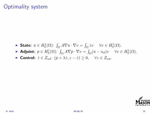
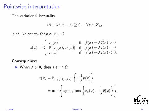
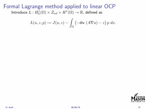
Formal Lagrange method applied to linear OCPIntroduce L H1
0 (Ω)times Zad timesH1(Ω)rarr R defined as
L(u z p) = J(u z)minusint
Ω
(minusdiv (Anablau)minus z
)p dx
Integrate by parts to arrive at
L(u z p) = J(u z)minusint
Ω
(minusdiv (Anablap)uminus zp
)dx+
intpartΩ
(Anablau)p ds
If (u z p) is a stationary point then
I State
DpL(u z p)h = 0 forallh isin H1(Ω)
I AdjointDuL(u z p)h = 0 forallh isin H1
0 (Ω)
I ControlDzL(u z p)(z minus z) ge 0 forallz isin Zad
H Antil 060616 27
Outline
Motivation and examples
Linear elliptic optimal control problems
Differentiation in Banach spaces
First-order necessary conditions
Optimal control of semilinear PDEs
An abstract problem
Discretization using finite element methods
H Antil 060616 28
Semilinear elliptic OCP
min J(u z) =1
2uminus ud2L2(Ω) +
λ
2z2L2(Ω)
subject to
minus∆u+ g(x u) = z in Ω
u = 0 on partΩ
and z isin Zad with za zb isin Linfin(Ω)
H Antil 060616 29
State space(A1) Ω sub Rd open bounded partΩ is Lipschitz
(A2) g Ωtimes Rrarr R is bounded and measurable with respect to x isin Ωfor every u isin R
(A3) g is continuous monotone increasing and Lipschitz continuous in ufor ae x isin Ω
(A4) g(x 0) = 0 for ae x isin Ω (not really necessary)
Theorem Suppose (A1)minus (A4) hold For every z isin Lr(Ω) withr gt d2 the state equation has a unique weak solutionu isin H1
0 (Ω) cap C(Ω) ie we haveintΩ
nablau middot nablav dx+
intΩ
g(x u(x))v(x) dx =
intΩ
zv dx forallv isin H10 (Ω)
Moreover there exists a constant C gt 0 such that
uH1(Ω) + uC(Ω) le CzLr(Ω)
RemarkI The proof of the theorem uses the BrowderndashMinty theorem on
monotone operators
H Antil 060616 30
State space(A1) Ω sub Rd open bounded partΩ is Lipschitz
(A2) g Ωtimes Rrarr R is bounded and measurable with respect to x isin Ωfor every u isin R
(A3) g is continuous monotone increasing and Lipschitz continuous in ufor ae x isin Ω
(A4) g(x 0) = 0 for ae x isin Ω (not really necessary)
Theorem Suppose (A1)minus (A4) hold For every z isin Lr(Ω) withr gt d2 the state equation has a unique weak solutionu isin H1
0 (Ω) cap C(Ω) ie we haveintΩ
nablau middot nablav dx+
intΩ
g(x u(x))v(x) dx =
intΩ
zv dx forallv isin H10 (Ω)
Moreover there exists a constant C gt 0 such that
uH1(Ω) + uC(Ω) le CzLr(Ω)
RemarkI The proof of the theorem uses the BrowderndashMinty theorem on
monotone operators
H Antil 060616 30
State space(A1) Ω sub Rd open bounded partΩ is Lipschitz
(A2) g Ωtimes Rrarr R is bounded and measurable with respect to x isin Ωfor every u isin R
(A3) g is continuous monotone increasing and Lipschitz continuous in ufor ae x isin Ω
(A4) g(x 0) = 0 for ae x isin Ω (not really necessary)
Theorem Suppose (A1)minus (A4) hold For every z isin Lr(Ω) withr gt d2 the state equation has a unique weak solutionu isin H1
0 (Ω) cap C(Ω) ie we haveintΩ
nablau middot nablav dx+
intΩ
g(x u(x))v(x) dx =
intΩ
zv dx forallv isin H10 (Ω)
Moreover there exists a constant C gt 0 such that
uH1(Ω) + uC(Ω) le CzLr(Ω)
RemarkI The proof of the theorem uses the BrowderndashMinty theorem on
monotone operators
H Antil 060616 30
Control-to-state map and reduced problem
I Control to state map
S Linfin(Ω)rarr H10 (Ω) cap C(Ω)
is well defined and is globally Lipschitz continuous
I Reduced problem
minJ (z) =1
2S(u)minus ud2L2(Ω) +
λ
2z2L2(Ω)
H Antil 060616 31
Control-to-state map and reduced problem
I Control to state map
S Linfin(Ω)rarr H10 (Ω) cap C(Ω)
is well defined and is globally Lipschitz continuous
I Reduced problem
minJ (z) =1
2S(u)minus ud2L2(Ω) +
λ
2z2L2(Ω)
H Antil 060616 31
First-order necessary conditionsI Lagrangian functional
L(u z p) = J(u z)minusint
Ω
(minus∆u+ g(x u(x))minus z
)p dx
= J(u z)minusint
Ω
(nablau middot nablap+ g(x u(x))pminus zp
)dx
I Adjoint system For all h isin H10 (Ω)
0 = DuL(u z p)h =
intΩ
(uminus ud)h dxminusint
Ω
(nablah middot nablap+ gu(x u(x))ph
)which yields
minus∆p+ gu(x u(x))p = uminus ud in Ω
p = 0 on partΩ
I Control
DzL(u z p)(z minus z) = (p+ λz z minus z) dx ge 0 forallz isin ZadI Gradient
nablaJ (z) = p+ λz
H Antil 060616 32
First-order necessary conditionsI Lagrangian functional
L(u z p) = J(u z)minusint
Ω
(minus∆u+ g(x u(x))minus z
)p dx
= J(u z)minusint
Ω
(nablau middot nablap+ g(x u(x))pminus zp
)dx
I Adjoint system For all h isin H10 (Ω)
0 = DuL(u z p)h =
intΩ
(uminus ud)h dxminusint
Ω
(nablah middot nablap+ gu(x u(x))ph
)which yields
minus∆p+ gu(x u(x))p = uminus ud in Ω
p = 0 on partΩ
I Control
DzL(u z p)(z minus z) = (p+ λz z minus z) dx ge 0 forallz isin ZadI Gradient
nablaJ (z) = p+ λz
H Antil 060616 32
First-order necessary conditionsI Lagrangian functional
L(u z p) = J(u z)minusint
Ω
(minus∆u+ g(x u(x))minus z
)p dx
= J(u z)minusint
Ω
(nablau middot nablap+ g(x u(x))pminus zp
)dx
I Adjoint system For all h isin H10 (Ω)
0 = DuL(u z p)h =
intΩ
(uminus ud)h dxminusint
Ω
(nablah middot nablap+ gu(x u(x))ph
)which yields
minus∆p+ gu(x u(x))p = uminus ud in Ω
p = 0 on partΩ
I Control
DzL(u z p)(z minus z) = (p+ λz z minus z) dx ge 0 forallz isin Zad
I GradientnablaJ (z) = p+ λz
H Antil 060616 32
First-order necessary conditionsI Lagrangian functional
L(u z p) = J(u z)minusint
Ω
(minus∆u+ g(x u(x))minus z
)p dx
= J(u z)minusint
Ω
(nablau middot nablap+ g(x u(x))pminus zp
)dx
I Adjoint system For all h isin H10 (Ω)
0 = DuL(u z p)h =
intΩ
(uminus ud)h dxminusint
Ω
(nablah middot nablap+ gu(x u(x))ph
)which yields
minus∆p+ gu(x u(x))p = uminus ud in Ω
p = 0 on partΩ
I Control
DzL(u z p)(z minus z) = (p+ λz z minus z) dx ge 0 forallz isin ZadI Gradient
nablaJ (z) = p+ λz
H Antil 060616 32
Differentiability of Nemytskii operator
The rigorous proof uses
Theorem In addition to (A1)-(A4) if
(A5) g is continuously differentiable with respect to u for ae x isin Ωand we have
(i) |gu(x 0)| le K for ae x isin Ω(ii) gu is locally Lipschitz with respect to u isin R
then the Nemytskii operator G u 7rarr g(middot u(middot)) is continuously Frechetdifferentiable from Linfin(Ω) into itself and
(Gprime(u)h)(x) = gu(x u(x))h(x) ae in Ω forallh isin Linfin(Ω)
Remark (A5) holds if g(x u) = g(u) and g isin C2(R)
H Antil 060616 33
Outline
Motivation and examples
Linear elliptic optimal control problems
Differentiation in Banach spaces
First-order necessary conditions
Optimal control of semilinear PDEs
An abstract problem
Discretization using finite element methods
H Antil 060616 34
Gradient computation via adjoint general formI Abstract problem
min J(u z)
subject toc(u z) = 0
and z isin Zad
I Directional derivative Let S be the control to state map(nonlinear in general)
z 7rarr S(z) = u(z)
Under the assumptions of ldquoimplicit function theoremrdquo
J prime(z)h = (nablauJ (u(z) z) Sprime(z)h) + (nablazJ (u(z) z) h)
I Sensitivity of u with respect to z Differentiating the stateequation
cu(S(z) z)Sprime(z)h = minuscz(S(z) z)h
leads toSprime(z)h = minuscu(S(z) z)minus1
(cz(S(z) z)h
)
provided cu(S(z) z)minus1 is well-defined
H Antil 060616 35
Gradient computation via adjoint general formI Abstract problem
min J(u z)
subject toc(u z) = 0
and z isin ZadI Directional derivative Let S be the control to state map
(nonlinear in general)
z 7rarr S(z) = u(z)
Under the assumptions of ldquoimplicit function theoremrdquo
J prime(z)h = (nablauJ (u(z) z) Sprime(z)h) + (nablazJ (u(z) z) h)
I Sensitivity of u with respect to z Differentiating the stateequation
cu(S(z) z)Sprime(z)h = minuscz(S(z) z)h
leads toSprime(z)h = minuscu(S(z) z)minus1
(cz(S(z) z)h
)
provided cu(S(z) z)minus1 is well-defined
H Antil 060616 35
Gradient computation via adjoint general formI Abstract problem
min J(u z)
subject toc(u z) = 0
and z isin ZadI Directional derivative Let S be the control to state map
(nonlinear in general)
z 7rarr S(z) = u(z)
Under the assumptions of ldquoimplicit function theoremrdquo
J prime(z)h = (nablauJ (u(z) z) Sprime(z)h) + (nablazJ (u(z) z) h)
I Sensitivity of u with respect to z Differentiating the stateequation
cu(S(z) z)Sprime(z)h = minuscz(S(z) z)h
leads toSprime(z)h = minuscu(S(z) z)minus1
(cz(S(z) z)h
)
provided cu(S(z) z)minus1 is well-defined
H Antil 060616 35
Adjoint equation and gradient general form
I Directional derivative
J prime(z)h = minus(nablauJ (u(z) z) cu(u(z) z)minus1cz(u(z) z)h
)+ (nablazJ (u(z) z) h)
I Gradient
nablaJ (z) = minuscz(u(z) z)lowast(cu(u(z) z)minuslowastnablauJ (u(z) z)
)+nablazJ (u(z) z)
I Introducing adjoint variable p solving
cu(u(z) z)lowastp = nablauJ (u(z) z)
we arrive at following form of gradient
nablaJ (z) = minuscz(u(z) z)lowastp+nablazJ (u(z) z)
which is tractable
H Antil 060616 36
Adjoint equation and gradient general form
I Directional derivative
J prime(z)h = minus(nablauJ (u(z) z) cu(u(z) z)minus1cz(u(z) z)h
)+ (nablazJ (u(z) z) h)
I Gradient
nablaJ (z) = minuscz(u(z) z)lowast(cu(u(z) z)minuslowastnablauJ (u(z) z)
)+nablazJ (u(z) z)
I Introducing adjoint variable p solving
cu(u(z) z)lowastp = nablauJ (u(z) z)
we arrive at following form of gradient
nablaJ (z) = minuscz(u(z) z)lowastp+nablazJ (u(z) z)
which is tractable
H Antil 060616 36
Adjoint equation and gradient general form
I Directional derivative
J prime(z)h = minus(nablauJ (u(z) z) cu(u(z) z)minus1cz(u(z) z)h
)+ (nablazJ (u(z) z) h)
I Gradient
nablaJ (z) = minuscz(u(z) z)lowast(cu(u(z) z)minuslowastnablauJ (u(z) z)
)+nablazJ (u(z) z)
I Introducing adjoint variable p solving
cu(u(z) z)lowastp = nablauJ (u(z) z)
we arrive at following form of gradient
nablaJ (z) = minuscz(u(z) z)lowastp+nablazJ (u(z) z)
which is tractable
H Antil 060616 36
Hessian computation general form
I Lagrangian L(u z p) = J(u z)minusint
Ωc(u z)p dx Then we have
DzJ (z)h = DzL(u z p)h
I Second order derivative
D2zJ (z)[h1 h2] = DuDzL(u z p)[h1 S
prime(z)h2] +D2zL(u z p)[h1 h2]
+DpDzL(u z p)[h1 Dzp(z)h2]
I We already know Sprime(z)h2 moreover
DpDzL(u z p)[h1 Dzp(z)h2] = minus(cu(u z)h1 Dzp(z)h2
)
It remain to identify Dzp(z)h2
H Antil 060616 37
Hessian computation general form
I Lagrangian L(u z p) = J(u z)minusint
Ωc(u z)p dx Then we have
DzJ (z)h = DzL(u z p)h
I Second order derivative
D2zJ (z)[h1 h2] = DuDzL(u z p)[h1 S
prime(z)h2] +D2zL(u z p)[h1 h2]
+DpDzL(u z p)[h1 Dzp(z)h2]
I We already know Sprime(z)h2 moreover
DpDzL(u z p)[h1 Dzp(z)h2] = minus(cu(u z)h1 Dzp(z)h2
)
It remain to identify Dzp(z)h2
H Antil 060616 37
Hessian computation general form
I Lagrangian L(u z p) = J(u z)minusint
Ωc(u z)p dx Then we have
DzJ (z)h = DzL(u z p)h
I Second order derivative
D2zJ (z)[h1 h2] = DuDzL(u z p)[h1 S
prime(z)h2] +D2zL(u z p)[h1 h2]
+DpDzL(u z p)[h1 Dzp(z)h2]
I We already know Sprime(z)h2 moreover
DpDzL(u z p)[h1 Dzp(z)h2] = minus(cu(u z)h1 Dzp(z)h2
)
It remain to identify Dzp(z)h2
H Antil 060616 37
Outline
Motivation and examples
Linear elliptic optimal control problems
Differentiation in Banach spaces
First-order necessary conditions
Optimal control of semilinear PDEs
An abstract problem
Discretization using finite element methods
H Antil 060616 38
Numerical approximation of Poisson equation MeshTo avoid technical issues we will assume that partΩ is polygonal
I Mesh Let T = K be a mesh of Ω where K sub Rd is an elementthat is isoparametrically equivalent to a unit simplex in Rd
I Conforming mesh We say that the mesh is conforming ifI Ω = cupKisinT KI If K1 cap K2 = x then x is a node of K1 and K2I If K1 cap K2 6= empty and K1 cap K2 6= x then K1 cap K2 is an edgeface
contained in partK1 cap partK2
I Shape regular Let T be the collection of all conformingrefinements of an original mesh T 0 Then T is called shape regularif exist κ gt 0 such that
hKρKle κ forallK isin cupiT i
where hK = diam K ρK = maxρ gt 0|Bρ sub KI Quasi-uniform A family of shape regular meshes is called-quasi
uniform if there exist a constant σ gt 0 such that
maxhKminhK
le σ
uniformly for all meshes in the family
Numerical approximation of Poisson equation MeshTo avoid technical issues we will assume that partΩ is polygonal
I Mesh Let T = K be a mesh of Ω where K sub Rd is an elementthat is isoparametrically equivalent to a unit simplex in Rd
I Conforming mesh We say that the mesh is conforming ifI Ω = cupKisinT KI If K1 cap K2 = x then x is a node of K1 and K2I If K1 cap K2 6= empty and K1 cap K2 6= x then K1 cap K2 is an edgeface
contained in partK1 cap partK2
I Shape regular Let T be the collection of all conformingrefinements of an original mesh T 0 Then T is called shape regularif exist κ gt 0 such that
hKρKle κ forallK isin cupiT i
where hK = diam K ρK = maxρ gt 0|Bρ sub KI Quasi-uniform A family of shape regular meshes is called-quasi
uniform if there exist a constant σ gt 0 such that
maxhKminhK
le σ
uniformly for all meshes in the family
Numerical approximation of Poisson equation MeshTo avoid technical issues we will assume that partΩ is polygonal
I Mesh Let T = K be a mesh of Ω where K sub Rd is an elementthat is isoparametrically equivalent to a unit simplex in Rd
I Conforming mesh We say that the mesh is conforming ifI Ω = cupKisinT KI If K1 cap K2 = x then x is a node of K1 and K2I If K1 cap K2 6= empty and K1 cap K2 6= x then K1 cap K2 is an edgeface
contained in partK1 cap partK2
I Shape regular Let T be the collection of all conformingrefinements of an original mesh T 0 Then T is called shape regularif exist κ gt 0 such that
hKρKle κ forallK isin cupiT i
where hK = diam K ρK = maxρ gt 0|Bρ sub K
I Quasi-uniform A family of shape regular meshes is called-quasiuniform if there exist a constant σ gt 0 such that
maxhKminhK
le σ
uniformly for all meshes in the family
Numerical approximation of Poisson equation MeshTo avoid technical issues we will assume that partΩ is polygonal
I Mesh Let T = K be a mesh of Ω where K sub Rd is an elementthat is isoparametrically equivalent to a unit simplex in Rd
I Conforming mesh We say that the mesh is conforming ifI Ω = cupKisinT KI If K1 cap K2 = x then x is a node of K1 and K2I If K1 cap K2 6= empty and K1 cap K2 6= x then K1 cap K2 is an edgeface
contained in partK1 cap partK2
I Shape regular Let T be the collection of all conformingrefinements of an original mesh T 0 Then T is called shape regularif exist κ gt 0 such that
hKρKle κ forallK isin cupiT i
where hK = diam K ρK = maxρ gt 0|Bρ sub KI Quasi-uniform A family of shape regular meshes is called-quasi
uniform if there exist a constant σ gt 0 such that
maxhKminhK
le σ
uniformly for all meshes in the family
FE space and Galerkin approximationI Finite element space For T isin T we define the finite element
space as
V(T ) = W isin C0(Ω) WK isin P1forallK isin T W |partΩ = 0
where P1 is the set of polynomials of degree at most 1
I Galerkin approximation of continuous problem is given by
Find UT isin V(T )
intΩ
AnablaUT middot nablaV = 〈f V 〉 forallV isin V(T )
The discrete problem is well-posedI Nodal basis Consists of functions ψi isin V(T ) with xi isin N (T )
satisfyingψxi
(xj) = δij
where N (T ) denotes the interior (plus Neumann) nodesI Galerkin orthogonality(
nabla(uminus UT )nablaW)L2(Ω)
= 0 forallW isin V(T )
H Antil 060616 40
FE space and Galerkin approximationI Finite element space For T isin T we define the finite element
space as
V(T ) = W isin C0(Ω) WK isin P1forallK isin T W |partΩ = 0
where P1 is the set of polynomials of degree at most 1I Galerkin approximation of continuous problem is given by
Find UT isin V(T )
intΩ
AnablaUT middot nablaV = 〈f V 〉 forallV isin V(T )
The discrete problem is well-posed
I Nodal basis Consists of functions ψi isin V(T ) with xi isin N (T )satisfying
ψxi(xj) = δij
where N (T ) denotes the interior (plus Neumann) nodesI Galerkin orthogonality(
nabla(uminus UT )nablaW)L2(Ω)
= 0 forallW isin V(T )
H Antil 060616 40
FE space and Galerkin approximationI Finite element space For T isin T we define the finite element
space as
V(T ) = W isin C0(Ω) WK isin P1forallK isin T W |partΩ = 0
where P1 is the set of polynomials of degree at most 1I Galerkin approximation of continuous problem is given by
Find UT isin V(T )
intΩ
AnablaUT middot nablaV = 〈f V 〉 forallV isin V(T )
The discrete problem is well-posedI Nodal basis Consists of functions ψi isin V(T ) with xi isin N (T )
satisfyingψxi
(xj) = δij
where N (T ) denotes the interior (plus Neumann) nodes
I Galerkin orthogonality(nabla(uminus UT )nablaW
)L2(Ω)
= 0 forallW isin V(T )
H Antil 060616 40
FE space and Galerkin approximationI Finite element space For T isin T we define the finite element
space as
V(T ) = W isin C0(Ω) WK isin P1forallK isin T W |partΩ = 0
where P1 is the set of polynomials of degree at most 1I Galerkin approximation of continuous problem is given by
Find UT isin V(T )
intΩ
AnablaUT middot nablaV = 〈f V 〉 forallV isin V(T )
The discrete problem is well-posedI Nodal basis Consists of functions ψi isin V(T ) with xi isin N (T )
satisfyingψxi
(xj) = δij
where N (T ) denotes the interior (plus Neumann) nodesI Galerkin orthogonality(
nabla(uminus UT )nablaW)L2(Ω)
= 0 forallW isin V(T )
H Antil 060616 40
Best approximation
I Cearsquos lemma
nabla(uminus UT )L2(Ω) le C infWisinV(T )
nabla(uminusW )L2(Ω)
I Nodal interpolation operator ΠT C(Ω)rarr V(T ) satisfies
ΠT u(xi) = u(xi) forallxi isin N (T )
and is defined as
ΠT u =sum
xiisinN (T )
u(xi)ψxi
I Error estimates In Cearsquos lemma replace W by ΠT u and thencompute the interpolation error
H Antil 060616 41
Best approximation
I Cearsquos lemma
nabla(uminus UT )L2(Ω) le C infWisinV(T )
nabla(uminusW )L2(Ω)
I Nodal interpolation operator ΠT C(Ω)rarr V(T ) satisfies
ΠT u(xi) = u(xi) forallxi isin N (T )
and is defined as
ΠT u =sum
xiisinN (T )
u(xi)ψxi
I Error estimates In Cearsquos lemma replace W by ΠT u and thencompute the interpolation error
H Antil 060616 41
Best approximation
I Cearsquos lemma
nabla(uminus UT )L2(Ω) le C infWisinV(T )
nabla(uminusW )L2(Ω)
I Nodal interpolation operator ΠT C(Ω)rarr V(T ) satisfies
ΠT u(xi) = u(xi) forallxi isin N (T )
and is defined as
ΠT u =sum
xiisinN (T )
u(xi)ψxi
I Error estimates In Cearsquos lemma replace W by ΠT u and thencompute the interpolation error
H Antil 060616 41
Algebraic system state equation
I Recall UT isin V(T ) solves
a(UT V ) = 〈f V 〉 forallV isin V(T )
I Now setting UT =sumN
j=1 Ujψj V = ψi we get
Nsumj=1
Uja(φj φi) = 〈f ψi〉 i = 1 N
which is the matrix-vector system
AU = F
I Stiffness matrix A is SPD
H Antil 060616 42
Algebraic system state equation
I Recall UT isin V(T ) solves
a(UT V ) = 〈f V 〉 forallV isin V(T )
I Now setting UT =sumN
j=1 Ujψj V = ψi we get
Nsumj=1
Uja(φj φi) = 〈f ψi〉 i = 1 N
which is the matrix-vector system
AU = F
I Stiffness matrix A is SPD
H Antil 060616 42
Algebraic system state equation
I Recall UT isin V(T ) solves
a(UT V ) = 〈f V 〉 forallV isin V(T )
I Now setting UT =sumN
j=1 Ujψj V = ψi we get
Nsumj=1
Uja(φj φi) = 〈f ψi〉 i = 1 N
which is the matrix-vector system
AU = F
I Stiffness matrix A is SPD
H Antil 060616 42
Discrete linear elliptic OCP
min JT (UT ZT ) =1
2UT minus ud2L2(Ω) +
λ
2ZT 2L2(Ω)
subject to
Find UT isin V(T )
intΩ
nablaUT middot nablaV = (ZT V )L2(Ω) forallV isin V(T )
and whereZT isin Zad(T ) = Zad cap Z(T )
is either one of these
Z(T ) =
V(T )L2(Ω) variational discretization (Hinze)WT isin Linfin(Ω) ZT |K isin P0(K)K isin T
H Antil 060616 43
Recent books
F TroltzschOptimal control of partial differential equations volume 112 ofGraduate Studies in MathematicsAmerican Mathematical Society Providence RI 2010Theory methods and applications Translated from the 2005 Germanoriginal by Jurgen Sprekels
K Ito and K KunischLagrange multiplier approach to variational problems andapplications volume 15 of Advances in Design and ControlSociety for Industrial and Applied Mathematics (SIAM)Philadelphia PA 2008
H Antil 060616 44
- Motivation and examples
- Linear elliptic optimal control problems
- Differentiation in Banach spaces
- First-order necessary conditions
- Optimal control of semilinear PDEs
- An abstract problem
- Discretization using finite element methods
-
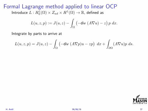
Formal Lagrange method applied to linear OCPIntroduce L H1
0 (Ω)times Zad timesH1(Ω)rarr R defined as
L(u z p) = J(u z)minusint
Ω
(minusdiv (Anablau)minus z
)p dx
Integrate by parts to arrive at
L(u z p) = J(u z)minusint
Ω
(minusdiv (Anablap)uminus zp
)dx+
intpartΩ
(Anablau)p ds
If (u z p) is a stationary point then
I State
DpL(u z p)h = 0 forallh isin H1(Ω)
I AdjointDuL(u z p)h = 0 forallh isin H1
0 (Ω)
I ControlDzL(u z p)(z minus z) ge 0 forallz isin Zad
H Antil 060616 27
Formal Lagrange method applied to linear OCPIntroduce L H1
0 (Ω)times Zad timesH1(Ω)rarr R defined as
L(u z p) = J(u z)minusint
Ω
(minusdiv (Anablau)minus z
)p dx
Integrate by parts to arrive at
L(u z p) = J(u z)minusint
Ω
(minusdiv (Anablap)uminus zp
)dx+
intpartΩ
(Anablau)p ds
If (u z p) is a stationary point then
I State
DpL(u z p)h = 0 forallh isin H1(Ω)
I AdjointDuL(u z p)h = 0 forallh isin H1
0 (Ω)
I ControlDzL(u z p)(z minus z) ge 0 forallz isin Zad
H Antil 060616 27
Formal Lagrange method applied to linear OCPIntroduce L H1
0 (Ω)times Zad timesH1(Ω)rarr R defined as
L(u z p) = J(u z)minusint
Ω
(minusdiv (Anablau)minus z
)p dx
Integrate by parts to arrive at
L(u z p) = J(u z)minusint
Ω
(minusdiv (Anablap)uminus zp
)dx+
intpartΩ
(Anablau)p ds
If (u z p) is a stationary point then
I State
DpL(u z p)h = 0 forallh isin H1(Ω)
I AdjointDuL(u z p)h = 0 forallh isin H1
0 (Ω)
I ControlDzL(u z p)(z minus z) ge 0 forallz isin Zad
H Antil 060616 27
Formal Lagrange method applied to linear OCPIntroduce L H1
0 (Ω)times Zad timesH1(Ω)rarr R defined as
L(u z p) = J(u z)minusint
Ω
(minusdiv (Anablau)minus z
)p dx
Integrate by parts to arrive at
L(u z p) = J(u z)minusint
Ω
(minusdiv (Anablap)uminus zp
)dx+
intpartΩ
(Anablau)p ds
If (u z p) is a stationary point then
I State
DpL(u z p)h = 0 forallh isin H1(Ω)
I AdjointDuL(u z p)h = 0 forallh isin H1
0 (Ω)
I ControlDzL(u z p)(z minus z) ge 0 forallz isin Zad
H Antil 060616 27
Outline
Motivation and examples
Linear elliptic optimal control problems
Differentiation in Banach spaces
First-order necessary conditions
Optimal control of semilinear PDEs
An abstract problem
Discretization using finite element methods
H Antil 060616 28
Semilinear elliptic OCP
min J(u z) =1
2uminus ud2L2(Ω) +
λ
2z2L2(Ω)
subject to
minus∆u+ g(x u) = z in Ω
u = 0 on partΩ
and z isin Zad with za zb isin Linfin(Ω)
H Antil 060616 29
State space(A1) Ω sub Rd open bounded partΩ is Lipschitz
(A2) g Ωtimes Rrarr R is bounded and measurable with respect to x isin Ωfor every u isin R
(A3) g is continuous monotone increasing and Lipschitz continuous in ufor ae x isin Ω
(A4) g(x 0) = 0 for ae x isin Ω (not really necessary)
Theorem Suppose (A1)minus (A4) hold For every z isin Lr(Ω) withr gt d2 the state equation has a unique weak solutionu isin H1
0 (Ω) cap C(Ω) ie we haveintΩ
nablau middot nablav dx+
intΩ
g(x u(x))v(x) dx =
intΩ
zv dx forallv isin H10 (Ω)
Moreover there exists a constant C gt 0 such that
uH1(Ω) + uC(Ω) le CzLr(Ω)
RemarkI The proof of the theorem uses the BrowderndashMinty theorem on
monotone operators
H Antil 060616 30
State space(A1) Ω sub Rd open bounded partΩ is Lipschitz
(A2) g Ωtimes Rrarr R is bounded and measurable with respect to x isin Ωfor every u isin R
(A3) g is continuous monotone increasing and Lipschitz continuous in ufor ae x isin Ω
(A4) g(x 0) = 0 for ae x isin Ω (not really necessary)
Theorem Suppose (A1)minus (A4) hold For every z isin Lr(Ω) withr gt d2 the state equation has a unique weak solutionu isin H1
0 (Ω) cap C(Ω) ie we haveintΩ
nablau middot nablav dx+
intΩ
g(x u(x))v(x) dx =
intΩ
zv dx forallv isin H10 (Ω)
Moreover there exists a constant C gt 0 such that
uH1(Ω) + uC(Ω) le CzLr(Ω)
RemarkI The proof of the theorem uses the BrowderndashMinty theorem on
monotone operators
H Antil 060616 30
State space(A1) Ω sub Rd open bounded partΩ is Lipschitz
(A2) g Ωtimes Rrarr R is bounded and measurable with respect to x isin Ωfor every u isin R
(A3) g is continuous monotone increasing and Lipschitz continuous in ufor ae x isin Ω
(A4) g(x 0) = 0 for ae x isin Ω (not really necessary)
Theorem Suppose (A1)minus (A4) hold For every z isin Lr(Ω) withr gt d2 the state equation has a unique weak solutionu isin H1
0 (Ω) cap C(Ω) ie we haveintΩ
nablau middot nablav dx+
intΩ
g(x u(x))v(x) dx =
intΩ
zv dx forallv isin H10 (Ω)
Moreover there exists a constant C gt 0 such that
uH1(Ω) + uC(Ω) le CzLr(Ω)
RemarkI The proof of the theorem uses the BrowderndashMinty theorem on
monotone operators
H Antil 060616 30
Control-to-state map and reduced problem
I Control to state map
S Linfin(Ω)rarr H10 (Ω) cap C(Ω)
is well defined and is globally Lipschitz continuous
I Reduced problem
minJ (z) =1
2S(u)minus ud2L2(Ω) +
λ
2z2L2(Ω)
H Antil 060616 31
Control-to-state map and reduced problem
I Control to state map
S Linfin(Ω)rarr H10 (Ω) cap C(Ω)
is well defined and is globally Lipschitz continuous
I Reduced problem
minJ (z) =1
2S(u)minus ud2L2(Ω) +
λ
2z2L2(Ω)
H Antil 060616 31
First-order necessary conditionsI Lagrangian functional
L(u z p) = J(u z)minusint
Ω
(minus∆u+ g(x u(x))minus z
)p dx
= J(u z)minusint
Ω
(nablau middot nablap+ g(x u(x))pminus zp
)dx
I Adjoint system For all h isin H10 (Ω)
0 = DuL(u z p)h =
intΩ
(uminus ud)h dxminusint
Ω
(nablah middot nablap+ gu(x u(x))ph
)which yields
minus∆p+ gu(x u(x))p = uminus ud in Ω
p = 0 on partΩ
I Control
DzL(u z p)(z minus z) = (p+ λz z minus z) dx ge 0 forallz isin ZadI Gradient
nablaJ (z) = p+ λz
H Antil 060616 32
First-order necessary conditionsI Lagrangian functional
L(u z p) = J(u z)minusint
Ω
(minus∆u+ g(x u(x))minus z
)p dx
= J(u z)minusint
Ω
(nablau middot nablap+ g(x u(x))pminus zp
)dx
I Adjoint system For all h isin H10 (Ω)
0 = DuL(u z p)h =
intΩ
(uminus ud)h dxminusint
Ω
(nablah middot nablap+ gu(x u(x))ph
)which yields
minus∆p+ gu(x u(x))p = uminus ud in Ω
p = 0 on partΩ
I Control
DzL(u z p)(z minus z) = (p+ λz z minus z) dx ge 0 forallz isin ZadI Gradient
nablaJ (z) = p+ λz
H Antil 060616 32
First-order necessary conditionsI Lagrangian functional
L(u z p) = J(u z)minusint
Ω
(minus∆u+ g(x u(x))minus z
)p dx
= J(u z)minusint
Ω
(nablau middot nablap+ g(x u(x))pminus zp
)dx
I Adjoint system For all h isin H10 (Ω)
0 = DuL(u z p)h =
intΩ
(uminus ud)h dxminusint
Ω
(nablah middot nablap+ gu(x u(x))ph
)which yields
minus∆p+ gu(x u(x))p = uminus ud in Ω
p = 0 on partΩ
I Control
DzL(u z p)(z minus z) = (p+ λz z minus z) dx ge 0 forallz isin Zad
I GradientnablaJ (z) = p+ λz
H Antil 060616 32
First-order necessary conditionsI Lagrangian functional
L(u z p) = J(u z)minusint
Ω
(minus∆u+ g(x u(x))minus z
)p dx
= J(u z)minusint
Ω
(nablau middot nablap+ g(x u(x))pminus zp
)dx
I Adjoint system For all h isin H10 (Ω)
0 = DuL(u z p)h =
intΩ
(uminus ud)h dxminusint
Ω
(nablah middot nablap+ gu(x u(x))ph
)which yields
minus∆p+ gu(x u(x))p = uminus ud in Ω
p = 0 on partΩ
I Control
DzL(u z p)(z minus z) = (p+ λz z minus z) dx ge 0 forallz isin ZadI Gradient
nablaJ (z) = p+ λz
H Antil 060616 32
Differentiability of Nemytskii operator
The rigorous proof uses
Theorem In addition to (A1)-(A4) if
(A5) g is continuously differentiable with respect to u for ae x isin Ωand we have
(i) |gu(x 0)| le K for ae x isin Ω(ii) gu is locally Lipschitz with respect to u isin R
then the Nemytskii operator G u 7rarr g(middot u(middot)) is continuously Frechetdifferentiable from Linfin(Ω) into itself and
(Gprime(u)h)(x) = gu(x u(x))h(x) ae in Ω forallh isin Linfin(Ω)
Remark (A5) holds if g(x u) = g(u) and g isin C2(R)
H Antil 060616 33
Outline
Motivation and examples
Linear elliptic optimal control problems
Differentiation in Banach spaces
First-order necessary conditions
Optimal control of semilinear PDEs
An abstract problem
Discretization using finite element methods
H Antil 060616 34
Gradient computation via adjoint general formI Abstract problem
min J(u z)
subject toc(u z) = 0
and z isin Zad
I Directional derivative Let S be the control to state map(nonlinear in general)
z 7rarr S(z) = u(z)
Under the assumptions of ldquoimplicit function theoremrdquo
J prime(z)h = (nablauJ (u(z) z) Sprime(z)h) + (nablazJ (u(z) z) h)
I Sensitivity of u with respect to z Differentiating the stateequation
cu(S(z) z)Sprime(z)h = minuscz(S(z) z)h
leads toSprime(z)h = minuscu(S(z) z)minus1
(cz(S(z) z)h
)
provided cu(S(z) z)minus1 is well-defined
H Antil 060616 35
Gradient computation via adjoint general formI Abstract problem
min J(u z)
subject toc(u z) = 0
and z isin ZadI Directional derivative Let S be the control to state map
(nonlinear in general)
z 7rarr S(z) = u(z)
Under the assumptions of ldquoimplicit function theoremrdquo
J prime(z)h = (nablauJ (u(z) z) Sprime(z)h) + (nablazJ (u(z) z) h)
I Sensitivity of u with respect to z Differentiating the stateequation
cu(S(z) z)Sprime(z)h = minuscz(S(z) z)h
leads toSprime(z)h = minuscu(S(z) z)minus1
(cz(S(z) z)h
)
provided cu(S(z) z)minus1 is well-defined
H Antil 060616 35
Gradient computation via adjoint general formI Abstract problem
min J(u z)
subject toc(u z) = 0
and z isin ZadI Directional derivative Let S be the control to state map
(nonlinear in general)
z 7rarr S(z) = u(z)
Under the assumptions of ldquoimplicit function theoremrdquo
J prime(z)h = (nablauJ (u(z) z) Sprime(z)h) + (nablazJ (u(z) z) h)
I Sensitivity of u with respect to z Differentiating the stateequation
cu(S(z) z)Sprime(z)h = minuscz(S(z) z)h
leads toSprime(z)h = minuscu(S(z) z)minus1
(cz(S(z) z)h
)
provided cu(S(z) z)minus1 is well-defined
H Antil 060616 35
Adjoint equation and gradient general form
I Directional derivative
J prime(z)h = minus(nablauJ (u(z) z) cu(u(z) z)minus1cz(u(z) z)h
)+ (nablazJ (u(z) z) h)
I Gradient
nablaJ (z) = minuscz(u(z) z)lowast(cu(u(z) z)minuslowastnablauJ (u(z) z)
)+nablazJ (u(z) z)
I Introducing adjoint variable p solving
cu(u(z) z)lowastp = nablauJ (u(z) z)
we arrive at following form of gradient
nablaJ (z) = minuscz(u(z) z)lowastp+nablazJ (u(z) z)
which is tractable
H Antil 060616 36
Adjoint equation and gradient general form
I Directional derivative
J prime(z)h = minus(nablauJ (u(z) z) cu(u(z) z)minus1cz(u(z) z)h
)+ (nablazJ (u(z) z) h)
I Gradient
nablaJ (z) = minuscz(u(z) z)lowast(cu(u(z) z)minuslowastnablauJ (u(z) z)
)+nablazJ (u(z) z)
I Introducing adjoint variable p solving
cu(u(z) z)lowastp = nablauJ (u(z) z)
we arrive at following form of gradient
nablaJ (z) = minuscz(u(z) z)lowastp+nablazJ (u(z) z)
which is tractable
H Antil 060616 36
Adjoint equation and gradient general form
I Directional derivative
J prime(z)h = minus(nablauJ (u(z) z) cu(u(z) z)minus1cz(u(z) z)h
)+ (nablazJ (u(z) z) h)
I Gradient
nablaJ (z) = minuscz(u(z) z)lowast(cu(u(z) z)minuslowastnablauJ (u(z) z)
)+nablazJ (u(z) z)
I Introducing adjoint variable p solving
cu(u(z) z)lowastp = nablauJ (u(z) z)
we arrive at following form of gradient
nablaJ (z) = minuscz(u(z) z)lowastp+nablazJ (u(z) z)
which is tractable
H Antil 060616 36
Hessian computation general form
I Lagrangian L(u z p) = J(u z)minusint
Ωc(u z)p dx Then we have
DzJ (z)h = DzL(u z p)h
I Second order derivative
D2zJ (z)[h1 h2] = DuDzL(u z p)[h1 S
prime(z)h2] +D2zL(u z p)[h1 h2]
+DpDzL(u z p)[h1 Dzp(z)h2]
I We already know Sprime(z)h2 moreover
DpDzL(u z p)[h1 Dzp(z)h2] = minus(cu(u z)h1 Dzp(z)h2
)
It remain to identify Dzp(z)h2
H Antil 060616 37
Hessian computation general form
I Lagrangian L(u z p) = J(u z)minusint
Ωc(u z)p dx Then we have
DzJ (z)h = DzL(u z p)h
I Second order derivative
D2zJ (z)[h1 h2] = DuDzL(u z p)[h1 S
prime(z)h2] +D2zL(u z p)[h1 h2]
+DpDzL(u z p)[h1 Dzp(z)h2]
I We already know Sprime(z)h2 moreover
DpDzL(u z p)[h1 Dzp(z)h2] = minus(cu(u z)h1 Dzp(z)h2
)
It remain to identify Dzp(z)h2
H Antil 060616 37
Hessian computation general form
I Lagrangian L(u z p) = J(u z)minusint
Ωc(u z)p dx Then we have
DzJ (z)h = DzL(u z p)h
I Second order derivative
D2zJ (z)[h1 h2] = DuDzL(u z p)[h1 S
prime(z)h2] +D2zL(u z p)[h1 h2]
+DpDzL(u z p)[h1 Dzp(z)h2]
I We already know Sprime(z)h2 moreover
DpDzL(u z p)[h1 Dzp(z)h2] = minus(cu(u z)h1 Dzp(z)h2
)
It remain to identify Dzp(z)h2
H Antil 060616 37
Outline
Motivation and examples
Linear elliptic optimal control problems
Differentiation in Banach spaces
First-order necessary conditions
Optimal control of semilinear PDEs
An abstract problem
Discretization using finite element methods
H Antil 060616 38
Numerical approximation of Poisson equation MeshTo avoid technical issues we will assume that partΩ is polygonal
I Mesh Let T = K be a mesh of Ω where K sub Rd is an elementthat is isoparametrically equivalent to a unit simplex in Rd
I Conforming mesh We say that the mesh is conforming ifI Ω = cupKisinT KI If K1 cap K2 = x then x is a node of K1 and K2I If K1 cap K2 6= empty and K1 cap K2 6= x then K1 cap K2 is an edgeface
contained in partK1 cap partK2
I Shape regular Let T be the collection of all conformingrefinements of an original mesh T 0 Then T is called shape regularif exist κ gt 0 such that
hKρKle κ forallK isin cupiT i
where hK = diam K ρK = maxρ gt 0|Bρ sub KI Quasi-uniform A family of shape regular meshes is called-quasi
uniform if there exist a constant σ gt 0 such that
maxhKminhK
le σ
uniformly for all meshes in the family
Numerical approximation of Poisson equation MeshTo avoid technical issues we will assume that partΩ is polygonal
I Mesh Let T = K be a mesh of Ω where K sub Rd is an elementthat is isoparametrically equivalent to a unit simplex in Rd
I Conforming mesh We say that the mesh is conforming ifI Ω = cupKisinT KI If K1 cap K2 = x then x is a node of K1 and K2I If K1 cap K2 6= empty and K1 cap K2 6= x then K1 cap K2 is an edgeface
contained in partK1 cap partK2
I Shape regular Let T be the collection of all conformingrefinements of an original mesh T 0 Then T is called shape regularif exist κ gt 0 such that
hKρKle κ forallK isin cupiT i
where hK = diam K ρK = maxρ gt 0|Bρ sub KI Quasi-uniform A family of shape regular meshes is called-quasi
uniform if there exist a constant σ gt 0 such that
maxhKminhK
le σ
uniformly for all meshes in the family
Numerical approximation of Poisson equation MeshTo avoid technical issues we will assume that partΩ is polygonal
I Mesh Let T = K be a mesh of Ω where K sub Rd is an elementthat is isoparametrically equivalent to a unit simplex in Rd
I Conforming mesh We say that the mesh is conforming ifI Ω = cupKisinT KI If K1 cap K2 = x then x is a node of K1 and K2I If K1 cap K2 6= empty and K1 cap K2 6= x then K1 cap K2 is an edgeface
contained in partK1 cap partK2
I Shape regular Let T be the collection of all conformingrefinements of an original mesh T 0 Then T is called shape regularif exist κ gt 0 such that
hKρKle κ forallK isin cupiT i
where hK = diam K ρK = maxρ gt 0|Bρ sub K
I Quasi-uniform A family of shape regular meshes is called-quasiuniform if there exist a constant σ gt 0 such that
maxhKminhK
le σ
uniformly for all meshes in the family
Numerical approximation of Poisson equation MeshTo avoid technical issues we will assume that partΩ is polygonal
I Mesh Let T = K be a mesh of Ω where K sub Rd is an elementthat is isoparametrically equivalent to a unit simplex in Rd
I Conforming mesh We say that the mesh is conforming ifI Ω = cupKisinT KI If K1 cap K2 = x then x is a node of K1 and K2I If K1 cap K2 6= empty and K1 cap K2 6= x then K1 cap K2 is an edgeface
contained in partK1 cap partK2
I Shape regular Let T be the collection of all conformingrefinements of an original mesh T 0 Then T is called shape regularif exist κ gt 0 such that
hKρKle κ forallK isin cupiT i
where hK = diam K ρK = maxρ gt 0|Bρ sub KI Quasi-uniform A family of shape regular meshes is called-quasi
uniform if there exist a constant σ gt 0 such that
maxhKminhK
le σ
uniformly for all meshes in the family
FE space and Galerkin approximationI Finite element space For T isin T we define the finite element
space as
V(T ) = W isin C0(Ω) WK isin P1forallK isin T W |partΩ = 0
where P1 is the set of polynomials of degree at most 1
I Galerkin approximation of continuous problem is given by
Find UT isin V(T )
intΩ
AnablaUT middot nablaV = 〈f V 〉 forallV isin V(T )
The discrete problem is well-posedI Nodal basis Consists of functions ψi isin V(T ) with xi isin N (T )
satisfyingψxi
(xj) = δij
where N (T ) denotes the interior (plus Neumann) nodesI Galerkin orthogonality(
nabla(uminus UT )nablaW)L2(Ω)
= 0 forallW isin V(T )
H Antil 060616 40
FE space and Galerkin approximationI Finite element space For T isin T we define the finite element
space as
V(T ) = W isin C0(Ω) WK isin P1forallK isin T W |partΩ = 0
where P1 is the set of polynomials of degree at most 1I Galerkin approximation of continuous problem is given by
Find UT isin V(T )
intΩ
AnablaUT middot nablaV = 〈f V 〉 forallV isin V(T )
The discrete problem is well-posed
I Nodal basis Consists of functions ψi isin V(T ) with xi isin N (T )satisfying
ψxi(xj) = δij
where N (T ) denotes the interior (plus Neumann) nodesI Galerkin orthogonality(
nabla(uminus UT )nablaW)L2(Ω)
= 0 forallW isin V(T )
H Antil 060616 40
FE space and Galerkin approximationI Finite element space For T isin T we define the finite element
space as
V(T ) = W isin C0(Ω) WK isin P1forallK isin T W |partΩ = 0
where P1 is the set of polynomials of degree at most 1I Galerkin approximation of continuous problem is given by
Find UT isin V(T )
intΩ
AnablaUT middot nablaV = 〈f V 〉 forallV isin V(T )
The discrete problem is well-posedI Nodal basis Consists of functions ψi isin V(T ) with xi isin N (T )
satisfyingψxi
(xj) = δij
where N (T ) denotes the interior (plus Neumann) nodes
I Galerkin orthogonality(nabla(uminus UT )nablaW
)L2(Ω)
= 0 forallW isin V(T )
H Antil 060616 40
FE space and Galerkin approximationI Finite element space For T isin T we define the finite element
space as
V(T ) = W isin C0(Ω) WK isin P1forallK isin T W |partΩ = 0
where P1 is the set of polynomials of degree at most 1I Galerkin approximation of continuous problem is given by
Find UT isin V(T )
intΩ
AnablaUT middot nablaV = 〈f V 〉 forallV isin V(T )
The discrete problem is well-posedI Nodal basis Consists of functions ψi isin V(T ) with xi isin N (T )
satisfyingψxi
(xj) = δij
where N (T ) denotes the interior (plus Neumann) nodesI Galerkin orthogonality(
nabla(uminus UT )nablaW)L2(Ω)
= 0 forallW isin V(T )
H Antil 060616 40
Best approximation
I Cearsquos lemma
nabla(uminus UT )L2(Ω) le C infWisinV(T )
nabla(uminusW )L2(Ω)
I Nodal interpolation operator ΠT C(Ω)rarr V(T ) satisfies
ΠT u(xi) = u(xi) forallxi isin N (T )
and is defined as
ΠT u =sum
xiisinN (T )
u(xi)ψxi
I Error estimates In Cearsquos lemma replace W by ΠT u and thencompute the interpolation error
H Antil 060616 41
Best approximation
I Cearsquos lemma
nabla(uminus UT )L2(Ω) le C infWisinV(T )
nabla(uminusW )L2(Ω)
I Nodal interpolation operator ΠT C(Ω)rarr V(T ) satisfies
ΠT u(xi) = u(xi) forallxi isin N (T )
and is defined as
ΠT u =sum
xiisinN (T )
u(xi)ψxi
I Error estimates In Cearsquos lemma replace W by ΠT u and thencompute the interpolation error
H Antil 060616 41
Best approximation
I Cearsquos lemma
nabla(uminus UT )L2(Ω) le C infWisinV(T )
nabla(uminusW )L2(Ω)
I Nodal interpolation operator ΠT C(Ω)rarr V(T ) satisfies
ΠT u(xi) = u(xi) forallxi isin N (T )
and is defined as
ΠT u =sum
xiisinN (T )
u(xi)ψxi
I Error estimates In Cearsquos lemma replace W by ΠT u and thencompute the interpolation error
H Antil 060616 41
Algebraic system state equation
I Recall UT isin V(T ) solves
a(UT V ) = 〈f V 〉 forallV isin V(T )
I Now setting UT =sumN
j=1 Ujψj V = ψi we get
Nsumj=1
Uja(φj φi) = 〈f ψi〉 i = 1 N
which is the matrix-vector system
AU = F
I Stiffness matrix A is SPD
H Antil 060616 42
Algebraic system state equation
I Recall UT isin V(T ) solves
a(UT V ) = 〈f V 〉 forallV isin V(T )
I Now setting UT =sumN
j=1 Ujψj V = ψi we get
Nsumj=1
Uja(φj φi) = 〈f ψi〉 i = 1 N
which is the matrix-vector system
AU = F
I Stiffness matrix A is SPD
H Antil 060616 42
Algebraic system state equation
I Recall UT isin V(T ) solves
a(UT V ) = 〈f V 〉 forallV isin V(T )
I Now setting UT =sumN
j=1 Ujψj V = ψi we get
Nsumj=1
Uja(φj φi) = 〈f ψi〉 i = 1 N
which is the matrix-vector system
AU = F
I Stiffness matrix A is SPD
H Antil 060616 42
Discrete linear elliptic OCP
min JT (UT ZT ) =1
2UT minus ud2L2(Ω) +
λ
2ZT 2L2(Ω)
subject to
Find UT isin V(T )
intΩ
nablaUT middot nablaV = (ZT V )L2(Ω) forallV isin V(T )
and whereZT isin Zad(T ) = Zad cap Z(T )
is either one of these
Z(T ) =
V(T )L2(Ω) variational discretization (Hinze)WT isin Linfin(Ω) ZT |K isin P0(K)K isin T
H Antil 060616 43
Recent books
F TroltzschOptimal control of partial differential equations volume 112 ofGraduate Studies in MathematicsAmerican Mathematical Society Providence RI 2010Theory methods and applications Translated from the 2005 Germanoriginal by Jurgen Sprekels
K Ito and K KunischLagrange multiplier approach to variational problems andapplications volume 15 of Advances in Design and ControlSociety for Industrial and Applied Mathematics (SIAM)Philadelphia PA 2008
H Antil 060616 44
- Motivation and examples
- Linear elliptic optimal control problems
- Differentiation in Banach spaces
- First-order necessary conditions
- Optimal control of semilinear PDEs
- An abstract problem
- Discretization using finite element methods
-
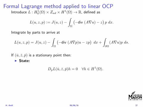
Formal Lagrange method applied to linear OCPIntroduce L H1
0 (Ω)times Zad timesH1(Ω)rarr R defined as
L(u z p) = J(u z)minusint
Ω
(minusdiv (Anablau)minus z
)p dx
Integrate by parts to arrive at
L(u z p) = J(u z)minusint
Ω
(minusdiv (Anablap)uminus zp
)dx+
intpartΩ
(Anablau)p ds
If (u z p) is a stationary point then
I State
DpL(u z p)h = 0 forallh isin H1(Ω)
I AdjointDuL(u z p)h = 0 forallh isin H1
0 (Ω)
I ControlDzL(u z p)(z minus z) ge 0 forallz isin Zad
H Antil 060616 27
Formal Lagrange method applied to linear OCPIntroduce L H1
0 (Ω)times Zad timesH1(Ω)rarr R defined as
L(u z p) = J(u z)minusint
Ω
(minusdiv (Anablau)minus z
)p dx
Integrate by parts to arrive at
L(u z p) = J(u z)minusint
Ω
(minusdiv (Anablap)uminus zp
)dx+
intpartΩ
(Anablau)p ds
If (u z p) is a stationary point then
I State
DpL(u z p)h = 0 forallh isin H1(Ω)
I AdjointDuL(u z p)h = 0 forallh isin H1
0 (Ω)
I ControlDzL(u z p)(z minus z) ge 0 forallz isin Zad
H Antil 060616 27
Formal Lagrange method applied to linear OCPIntroduce L H1
0 (Ω)times Zad timesH1(Ω)rarr R defined as
L(u z p) = J(u z)minusint
Ω
(minusdiv (Anablau)minus z
)p dx
Integrate by parts to arrive at
L(u z p) = J(u z)minusint
Ω
(minusdiv (Anablap)uminus zp
)dx+
intpartΩ
(Anablau)p ds
If (u z p) is a stationary point then
I State
DpL(u z p)h = 0 forallh isin H1(Ω)
I AdjointDuL(u z p)h = 0 forallh isin H1
0 (Ω)
I ControlDzL(u z p)(z minus z) ge 0 forallz isin Zad
H Antil 060616 27
Outline
Motivation and examples
Linear elliptic optimal control problems
Differentiation in Banach spaces
First-order necessary conditions
Optimal control of semilinear PDEs
An abstract problem
Discretization using finite element methods
H Antil 060616 28
Semilinear elliptic OCP
min J(u z) =1
2uminus ud2L2(Ω) +
λ
2z2L2(Ω)
subject to
minus∆u+ g(x u) = z in Ω
u = 0 on partΩ
and z isin Zad with za zb isin Linfin(Ω)
H Antil 060616 29
State space(A1) Ω sub Rd open bounded partΩ is Lipschitz
(A2) g Ωtimes Rrarr R is bounded and measurable with respect to x isin Ωfor every u isin R
(A3) g is continuous monotone increasing and Lipschitz continuous in ufor ae x isin Ω
(A4) g(x 0) = 0 for ae x isin Ω (not really necessary)
Theorem Suppose (A1)minus (A4) hold For every z isin Lr(Ω) withr gt d2 the state equation has a unique weak solutionu isin H1
0 (Ω) cap C(Ω) ie we haveintΩ
nablau middot nablav dx+
intΩ
g(x u(x))v(x) dx =
intΩ
zv dx forallv isin H10 (Ω)
Moreover there exists a constant C gt 0 such that
uH1(Ω) + uC(Ω) le CzLr(Ω)
RemarkI The proof of the theorem uses the BrowderndashMinty theorem on
monotone operators
H Antil 060616 30
State space(A1) Ω sub Rd open bounded partΩ is Lipschitz
(A2) g Ωtimes Rrarr R is bounded and measurable with respect to x isin Ωfor every u isin R
(A3) g is continuous monotone increasing and Lipschitz continuous in ufor ae x isin Ω
(A4) g(x 0) = 0 for ae x isin Ω (not really necessary)
Theorem Suppose (A1)minus (A4) hold For every z isin Lr(Ω) withr gt d2 the state equation has a unique weak solutionu isin H1
0 (Ω) cap C(Ω) ie we haveintΩ
nablau middot nablav dx+
intΩ
g(x u(x))v(x) dx =
intΩ
zv dx forallv isin H10 (Ω)
Moreover there exists a constant C gt 0 such that
uH1(Ω) + uC(Ω) le CzLr(Ω)
RemarkI The proof of the theorem uses the BrowderndashMinty theorem on
monotone operators
H Antil 060616 30
State space(A1) Ω sub Rd open bounded partΩ is Lipschitz
(A2) g Ωtimes Rrarr R is bounded and measurable with respect to x isin Ωfor every u isin R
(A3) g is continuous monotone increasing and Lipschitz continuous in ufor ae x isin Ω
(A4) g(x 0) = 0 for ae x isin Ω (not really necessary)
Theorem Suppose (A1)minus (A4) hold For every z isin Lr(Ω) withr gt d2 the state equation has a unique weak solutionu isin H1
0 (Ω) cap C(Ω) ie we haveintΩ
nablau middot nablav dx+
intΩ
g(x u(x))v(x) dx =
intΩ
zv dx forallv isin H10 (Ω)
Moreover there exists a constant C gt 0 such that
uH1(Ω) + uC(Ω) le CzLr(Ω)
RemarkI The proof of the theorem uses the BrowderndashMinty theorem on
monotone operators
H Antil 060616 30
Control-to-state map and reduced problem
I Control to state map
S Linfin(Ω)rarr H10 (Ω) cap C(Ω)
is well defined and is globally Lipschitz continuous
I Reduced problem
minJ (z) =1
2S(u)minus ud2L2(Ω) +
λ
2z2L2(Ω)
H Antil 060616 31
Control-to-state map and reduced problem
I Control to state map
S Linfin(Ω)rarr H10 (Ω) cap C(Ω)
is well defined and is globally Lipschitz continuous
I Reduced problem
minJ (z) =1
2S(u)minus ud2L2(Ω) +
λ
2z2L2(Ω)
H Antil 060616 31
First-order necessary conditionsI Lagrangian functional
L(u z p) = J(u z)minusint
Ω
(minus∆u+ g(x u(x))minus z
)p dx
= J(u z)minusint
Ω
(nablau middot nablap+ g(x u(x))pminus zp
)dx
I Adjoint system For all h isin H10 (Ω)
0 = DuL(u z p)h =
intΩ
(uminus ud)h dxminusint
Ω
(nablah middot nablap+ gu(x u(x))ph
)which yields
minus∆p+ gu(x u(x))p = uminus ud in Ω
p = 0 on partΩ
I Control
DzL(u z p)(z minus z) = (p+ λz z minus z) dx ge 0 forallz isin ZadI Gradient
nablaJ (z) = p+ λz
H Antil 060616 32
First-order necessary conditionsI Lagrangian functional
L(u z p) = J(u z)minusint
Ω
(minus∆u+ g(x u(x))minus z
)p dx
= J(u z)minusint
Ω
(nablau middot nablap+ g(x u(x))pminus zp
)dx
I Adjoint system For all h isin H10 (Ω)
0 = DuL(u z p)h =
intΩ
(uminus ud)h dxminusint
Ω
(nablah middot nablap+ gu(x u(x))ph
)which yields
minus∆p+ gu(x u(x))p = uminus ud in Ω
p = 0 on partΩ
I Control
DzL(u z p)(z minus z) = (p+ λz z minus z) dx ge 0 forallz isin ZadI Gradient
nablaJ (z) = p+ λz
H Antil 060616 32
First-order necessary conditionsI Lagrangian functional
L(u z p) = J(u z)minusint
Ω
(minus∆u+ g(x u(x))minus z
)p dx
= J(u z)minusint
Ω
(nablau middot nablap+ g(x u(x))pminus zp
)dx
I Adjoint system For all h isin H10 (Ω)
0 = DuL(u z p)h =
intΩ
(uminus ud)h dxminusint
Ω
(nablah middot nablap+ gu(x u(x))ph
)which yields
minus∆p+ gu(x u(x))p = uminus ud in Ω
p = 0 on partΩ
I Control
DzL(u z p)(z minus z) = (p+ λz z minus z) dx ge 0 forallz isin Zad
I GradientnablaJ (z) = p+ λz
H Antil 060616 32
First-order necessary conditionsI Lagrangian functional
L(u z p) = J(u z)minusint
Ω
(minus∆u+ g(x u(x))minus z
)p dx
= J(u z)minusint
Ω
(nablau middot nablap+ g(x u(x))pminus zp
)dx
I Adjoint system For all h isin H10 (Ω)
0 = DuL(u z p)h =
intΩ
(uminus ud)h dxminusint
Ω
(nablah middot nablap+ gu(x u(x))ph
)which yields
minus∆p+ gu(x u(x))p = uminus ud in Ω
p = 0 on partΩ
I Control
DzL(u z p)(z minus z) = (p+ λz z minus z) dx ge 0 forallz isin ZadI Gradient
nablaJ (z) = p+ λz
H Antil 060616 32
Differentiability of Nemytskii operator
The rigorous proof uses
Theorem In addition to (A1)-(A4) if
(A5) g is continuously differentiable with respect to u for ae x isin Ωand we have
(i) |gu(x 0)| le K for ae x isin Ω(ii) gu is locally Lipschitz with respect to u isin R
then the Nemytskii operator G u 7rarr g(middot u(middot)) is continuously Frechetdifferentiable from Linfin(Ω) into itself and
(Gprime(u)h)(x) = gu(x u(x))h(x) ae in Ω forallh isin Linfin(Ω)
Remark (A5) holds if g(x u) = g(u) and g isin C2(R)
H Antil 060616 33
Outline
Motivation and examples
Linear elliptic optimal control problems
Differentiation in Banach spaces
First-order necessary conditions
Optimal control of semilinear PDEs
An abstract problem
Discretization using finite element methods
H Antil 060616 34
Gradient computation via adjoint general formI Abstract problem
min J(u z)
subject toc(u z) = 0
and z isin Zad
I Directional derivative Let S be the control to state map(nonlinear in general)
z 7rarr S(z) = u(z)
Under the assumptions of ldquoimplicit function theoremrdquo
J prime(z)h = (nablauJ (u(z) z) Sprime(z)h) + (nablazJ (u(z) z) h)
I Sensitivity of u with respect to z Differentiating the stateequation
cu(S(z) z)Sprime(z)h = minuscz(S(z) z)h
leads toSprime(z)h = minuscu(S(z) z)minus1
(cz(S(z) z)h
)
provided cu(S(z) z)minus1 is well-defined
H Antil 060616 35
Gradient computation via adjoint general formI Abstract problem
min J(u z)
subject toc(u z) = 0
and z isin ZadI Directional derivative Let S be the control to state map
(nonlinear in general)
z 7rarr S(z) = u(z)
Under the assumptions of ldquoimplicit function theoremrdquo
J prime(z)h = (nablauJ (u(z) z) Sprime(z)h) + (nablazJ (u(z) z) h)
I Sensitivity of u with respect to z Differentiating the stateequation
cu(S(z) z)Sprime(z)h = minuscz(S(z) z)h
leads toSprime(z)h = minuscu(S(z) z)minus1
(cz(S(z) z)h
)
provided cu(S(z) z)minus1 is well-defined
H Antil 060616 35
Gradient computation via adjoint general formI Abstract problem
min J(u z)
subject toc(u z) = 0
and z isin ZadI Directional derivative Let S be the control to state map
(nonlinear in general)
z 7rarr S(z) = u(z)
Under the assumptions of ldquoimplicit function theoremrdquo
J prime(z)h = (nablauJ (u(z) z) Sprime(z)h) + (nablazJ (u(z) z) h)
I Sensitivity of u with respect to z Differentiating the stateequation
cu(S(z) z)Sprime(z)h = minuscz(S(z) z)h
leads toSprime(z)h = minuscu(S(z) z)minus1
(cz(S(z) z)h
)
provided cu(S(z) z)minus1 is well-defined
H Antil 060616 35
Adjoint equation and gradient general form
I Directional derivative
J prime(z)h = minus(nablauJ (u(z) z) cu(u(z) z)minus1cz(u(z) z)h
)+ (nablazJ (u(z) z) h)
I Gradient
nablaJ (z) = minuscz(u(z) z)lowast(cu(u(z) z)minuslowastnablauJ (u(z) z)
)+nablazJ (u(z) z)
I Introducing adjoint variable p solving
cu(u(z) z)lowastp = nablauJ (u(z) z)
we arrive at following form of gradient
nablaJ (z) = minuscz(u(z) z)lowastp+nablazJ (u(z) z)
which is tractable
H Antil 060616 36
Adjoint equation and gradient general form
I Directional derivative
J prime(z)h = minus(nablauJ (u(z) z) cu(u(z) z)minus1cz(u(z) z)h
)+ (nablazJ (u(z) z) h)
I Gradient
nablaJ (z) = minuscz(u(z) z)lowast(cu(u(z) z)minuslowastnablauJ (u(z) z)
)+nablazJ (u(z) z)
I Introducing adjoint variable p solving
cu(u(z) z)lowastp = nablauJ (u(z) z)
we arrive at following form of gradient
nablaJ (z) = minuscz(u(z) z)lowastp+nablazJ (u(z) z)
which is tractable
H Antil 060616 36
Adjoint equation and gradient general form
I Directional derivative
J prime(z)h = minus(nablauJ (u(z) z) cu(u(z) z)minus1cz(u(z) z)h
)+ (nablazJ (u(z) z) h)
I Gradient
nablaJ (z) = minuscz(u(z) z)lowast(cu(u(z) z)minuslowastnablauJ (u(z) z)
)+nablazJ (u(z) z)
I Introducing adjoint variable p solving
cu(u(z) z)lowastp = nablauJ (u(z) z)
we arrive at following form of gradient
nablaJ (z) = minuscz(u(z) z)lowastp+nablazJ (u(z) z)
which is tractable
H Antil 060616 36
Hessian computation general form
I Lagrangian L(u z p) = J(u z)minusint
Ωc(u z)p dx Then we have
DzJ (z)h = DzL(u z p)h
I Second order derivative
D2zJ (z)[h1 h2] = DuDzL(u z p)[h1 S
prime(z)h2] +D2zL(u z p)[h1 h2]
+DpDzL(u z p)[h1 Dzp(z)h2]
I We already know Sprime(z)h2 moreover
DpDzL(u z p)[h1 Dzp(z)h2] = minus(cu(u z)h1 Dzp(z)h2
)
It remain to identify Dzp(z)h2
H Antil 060616 37
Hessian computation general form
I Lagrangian L(u z p) = J(u z)minusint
Ωc(u z)p dx Then we have
DzJ (z)h = DzL(u z p)h
I Second order derivative
D2zJ (z)[h1 h2] = DuDzL(u z p)[h1 S
prime(z)h2] +D2zL(u z p)[h1 h2]
+DpDzL(u z p)[h1 Dzp(z)h2]
I We already know Sprime(z)h2 moreover
DpDzL(u z p)[h1 Dzp(z)h2] = minus(cu(u z)h1 Dzp(z)h2
)
It remain to identify Dzp(z)h2
H Antil 060616 37
Hessian computation general form
I Lagrangian L(u z p) = J(u z)minusint
Ωc(u z)p dx Then we have
DzJ (z)h = DzL(u z p)h
I Second order derivative
D2zJ (z)[h1 h2] = DuDzL(u z p)[h1 S
prime(z)h2] +D2zL(u z p)[h1 h2]
+DpDzL(u z p)[h1 Dzp(z)h2]
I We already know Sprime(z)h2 moreover
DpDzL(u z p)[h1 Dzp(z)h2] = minus(cu(u z)h1 Dzp(z)h2
)
It remain to identify Dzp(z)h2
H Antil 060616 37
Outline
Motivation and examples
Linear elliptic optimal control problems
Differentiation in Banach spaces
First-order necessary conditions
Optimal control of semilinear PDEs
An abstract problem
Discretization using finite element methods
H Antil 060616 38
Numerical approximation of Poisson equation MeshTo avoid technical issues we will assume that partΩ is polygonal
I Mesh Let T = K be a mesh of Ω where K sub Rd is an elementthat is isoparametrically equivalent to a unit simplex in Rd
I Conforming mesh We say that the mesh is conforming ifI Ω = cupKisinT KI If K1 cap K2 = x then x is a node of K1 and K2I If K1 cap K2 6= empty and K1 cap K2 6= x then K1 cap K2 is an edgeface
contained in partK1 cap partK2
I Shape regular Let T be the collection of all conformingrefinements of an original mesh T 0 Then T is called shape regularif exist κ gt 0 such that
hKρKle κ forallK isin cupiT i
where hK = diam K ρK = maxρ gt 0|Bρ sub KI Quasi-uniform A family of shape regular meshes is called-quasi
uniform if there exist a constant σ gt 0 such that
maxhKminhK
le σ
uniformly for all meshes in the family
Numerical approximation of Poisson equation MeshTo avoid technical issues we will assume that partΩ is polygonal
I Mesh Let T = K be a mesh of Ω where K sub Rd is an elementthat is isoparametrically equivalent to a unit simplex in Rd
I Conforming mesh We say that the mesh is conforming ifI Ω = cupKisinT KI If K1 cap K2 = x then x is a node of K1 and K2I If K1 cap K2 6= empty and K1 cap K2 6= x then K1 cap K2 is an edgeface
contained in partK1 cap partK2
I Shape regular Let T be the collection of all conformingrefinements of an original mesh T 0 Then T is called shape regularif exist κ gt 0 such that
hKρKle κ forallK isin cupiT i
where hK = diam K ρK = maxρ gt 0|Bρ sub KI Quasi-uniform A family of shape regular meshes is called-quasi
uniform if there exist a constant σ gt 0 such that
maxhKminhK
le σ
uniformly for all meshes in the family
Numerical approximation of Poisson equation MeshTo avoid technical issues we will assume that partΩ is polygonal
I Mesh Let T = K be a mesh of Ω where K sub Rd is an elementthat is isoparametrically equivalent to a unit simplex in Rd
I Conforming mesh We say that the mesh is conforming ifI Ω = cupKisinT KI If K1 cap K2 = x then x is a node of K1 and K2I If K1 cap K2 6= empty and K1 cap K2 6= x then K1 cap K2 is an edgeface
contained in partK1 cap partK2
I Shape regular Let T be the collection of all conformingrefinements of an original mesh T 0 Then T is called shape regularif exist κ gt 0 such that
hKρKle κ forallK isin cupiT i
where hK = diam K ρK = maxρ gt 0|Bρ sub K
I Quasi-uniform A family of shape regular meshes is called-quasiuniform if there exist a constant σ gt 0 such that
maxhKminhK
le σ
uniformly for all meshes in the family
Numerical approximation of Poisson equation MeshTo avoid technical issues we will assume that partΩ is polygonal
I Mesh Let T = K be a mesh of Ω where K sub Rd is an elementthat is isoparametrically equivalent to a unit simplex in Rd
I Conforming mesh We say that the mesh is conforming ifI Ω = cupKisinT KI If K1 cap K2 = x then x is a node of K1 and K2I If K1 cap K2 6= empty and K1 cap K2 6= x then K1 cap K2 is an edgeface
contained in partK1 cap partK2
I Shape regular Let T be the collection of all conformingrefinements of an original mesh T 0 Then T is called shape regularif exist κ gt 0 such that
hKρKle κ forallK isin cupiT i
where hK = diam K ρK = maxρ gt 0|Bρ sub KI Quasi-uniform A family of shape regular meshes is called-quasi
uniform if there exist a constant σ gt 0 such that
maxhKminhK
le σ
uniformly for all meshes in the family
FE space and Galerkin approximationI Finite element space For T isin T we define the finite element
space as
V(T ) = W isin C0(Ω) WK isin P1forallK isin T W |partΩ = 0
where P1 is the set of polynomials of degree at most 1
I Galerkin approximation of continuous problem is given by
Find UT isin V(T )
intΩ
AnablaUT middot nablaV = 〈f V 〉 forallV isin V(T )
The discrete problem is well-posedI Nodal basis Consists of functions ψi isin V(T ) with xi isin N (T )
satisfyingψxi
(xj) = δij
where N (T ) denotes the interior (plus Neumann) nodesI Galerkin orthogonality(
nabla(uminus UT )nablaW)L2(Ω)
= 0 forallW isin V(T )
H Antil 060616 40
FE space and Galerkin approximationI Finite element space For T isin T we define the finite element
space as
V(T ) = W isin C0(Ω) WK isin P1forallK isin T W |partΩ = 0
where P1 is the set of polynomials of degree at most 1I Galerkin approximation of continuous problem is given by
Find UT isin V(T )
intΩ
AnablaUT middot nablaV = 〈f V 〉 forallV isin V(T )
The discrete problem is well-posed
I Nodal basis Consists of functions ψi isin V(T ) with xi isin N (T )satisfying
ψxi(xj) = δij
where N (T ) denotes the interior (plus Neumann) nodesI Galerkin orthogonality(
nabla(uminus UT )nablaW)L2(Ω)
= 0 forallW isin V(T )
H Antil 060616 40
FE space and Galerkin approximationI Finite element space For T isin T we define the finite element
space as
V(T ) = W isin C0(Ω) WK isin P1forallK isin T W |partΩ = 0
where P1 is the set of polynomials of degree at most 1I Galerkin approximation of continuous problem is given by
Find UT isin V(T )
intΩ
AnablaUT middot nablaV = 〈f V 〉 forallV isin V(T )
The discrete problem is well-posedI Nodal basis Consists of functions ψi isin V(T ) with xi isin N (T )
satisfyingψxi
(xj) = δij
where N (T ) denotes the interior (plus Neumann) nodes
I Galerkin orthogonality(nabla(uminus UT )nablaW
)L2(Ω)
= 0 forallW isin V(T )
H Antil 060616 40
FE space and Galerkin approximationI Finite element space For T isin T we define the finite element
space as
V(T ) = W isin C0(Ω) WK isin P1forallK isin T W |partΩ = 0
where P1 is the set of polynomials of degree at most 1I Galerkin approximation of continuous problem is given by
Find UT isin V(T )
intΩ
AnablaUT middot nablaV = 〈f V 〉 forallV isin V(T )
The discrete problem is well-posedI Nodal basis Consists of functions ψi isin V(T ) with xi isin N (T )
satisfyingψxi
(xj) = δij
where N (T ) denotes the interior (plus Neumann) nodesI Galerkin orthogonality(
nabla(uminus UT )nablaW)L2(Ω)
= 0 forallW isin V(T )
H Antil 060616 40
Best approximation
I Cearsquos lemma
nabla(uminus UT )L2(Ω) le C infWisinV(T )
nabla(uminusW )L2(Ω)
I Nodal interpolation operator ΠT C(Ω)rarr V(T ) satisfies
ΠT u(xi) = u(xi) forallxi isin N (T )
and is defined as
ΠT u =sum
xiisinN (T )
u(xi)ψxi
I Error estimates In Cearsquos lemma replace W by ΠT u and thencompute the interpolation error
H Antil 060616 41
Best approximation
I Cearsquos lemma
nabla(uminus UT )L2(Ω) le C infWisinV(T )
nabla(uminusW )L2(Ω)
I Nodal interpolation operator ΠT C(Ω)rarr V(T ) satisfies
ΠT u(xi) = u(xi) forallxi isin N (T )
and is defined as
ΠT u =sum
xiisinN (T )
u(xi)ψxi
I Error estimates In Cearsquos lemma replace W by ΠT u and thencompute the interpolation error
H Antil 060616 41
Best approximation
I Cearsquos lemma
nabla(uminus UT )L2(Ω) le C infWisinV(T )
nabla(uminusW )L2(Ω)
I Nodal interpolation operator ΠT C(Ω)rarr V(T ) satisfies
ΠT u(xi) = u(xi) forallxi isin N (T )
and is defined as
ΠT u =sum
xiisinN (T )
u(xi)ψxi
I Error estimates In Cearsquos lemma replace W by ΠT u and thencompute the interpolation error
H Antil 060616 41
Algebraic system state equation
I Recall UT isin V(T ) solves
a(UT V ) = 〈f V 〉 forallV isin V(T )
I Now setting UT =sumN
j=1 Ujψj V = ψi we get
Nsumj=1
Uja(φj φi) = 〈f ψi〉 i = 1 N
which is the matrix-vector system
AU = F
I Stiffness matrix A is SPD
H Antil 060616 42
Algebraic system state equation
I Recall UT isin V(T ) solves
a(UT V ) = 〈f V 〉 forallV isin V(T )
I Now setting UT =sumN
j=1 Ujψj V = ψi we get
Nsumj=1
Uja(φj φi) = 〈f ψi〉 i = 1 N
which is the matrix-vector system
AU = F
I Stiffness matrix A is SPD
H Antil 060616 42
Algebraic system state equation
I Recall UT isin V(T ) solves
a(UT V ) = 〈f V 〉 forallV isin V(T )
I Now setting UT =sumN
j=1 Ujψj V = ψi we get
Nsumj=1
Uja(φj φi) = 〈f ψi〉 i = 1 N
which is the matrix-vector system
AU = F
I Stiffness matrix A is SPD
H Antil 060616 42
Discrete linear elliptic OCP
min JT (UT ZT ) =1
2UT minus ud2L2(Ω) +
λ
2ZT 2L2(Ω)
subject to
Find UT isin V(T )
intΩ
nablaUT middot nablaV = (ZT V )L2(Ω) forallV isin V(T )
and whereZT isin Zad(T ) = Zad cap Z(T )
is either one of these
Z(T ) =
V(T )L2(Ω) variational discretization (Hinze)WT isin Linfin(Ω) ZT |K isin P0(K)K isin T
H Antil 060616 43
Recent books
F TroltzschOptimal control of partial differential equations volume 112 ofGraduate Studies in MathematicsAmerican Mathematical Society Providence RI 2010Theory methods and applications Translated from the 2005 Germanoriginal by Jurgen Sprekels
K Ito and K KunischLagrange multiplier approach to variational problems andapplications volume 15 of Advances in Design and ControlSociety for Industrial and Applied Mathematics (SIAM)Philadelphia PA 2008
H Antil 060616 44
- Motivation and examples
- Linear elliptic optimal control problems
- Differentiation in Banach spaces
- First-order necessary conditions
- Optimal control of semilinear PDEs
- An abstract problem
- Discretization using finite element methods
-
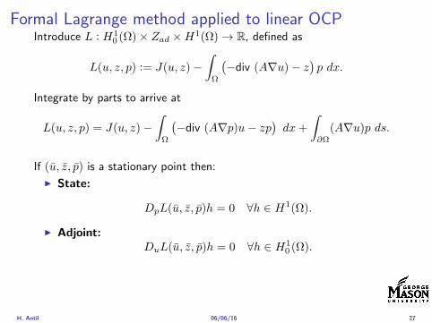
Formal Lagrange method applied to linear OCPIntroduce L H1
0 (Ω)times Zad timesH1(Ω)rarr R defined as
L(u z p) = J(u z)minusint
Ω
(minusdiv (Anablau)minus z
)p dx
Integrate by parts to arrive at
L(u z p) = J(u z)minusint
Ω
(minusdiv (Anablap)uminus zp
)dx+
intpartΩ
(Anablau)p ds
If (u z p) is a stationary point then
I State
DpL(u z p)h = 0 forallh isin H1(Ω)
I AdjointDuL(u z p)h = 0 forallh isin H1
0 (Ω)
I ControlDzL(u z p)(z minus z) ge 0 forallz isin Zad
H Antil 060616 27
Formal Lagrange method applied to linear OCPIntroduce L H1
0 (Ω)times Zad timesH1(Ω)rarr R defined as
L(u z p) = J(u z)minusint
Ω
(minusdiv (Anablau)minus z
)p dx
Integrate by parts to arrive at
L(u z p) = J(u z)minusint
Ω
(minusdiv (Anablap)uminus zp
)dx+
intpartΩ
(Anablau)p ds
If (u z p) is a stationary point then
I State
DpL(u z p)h = 0 forallh isin H1(Ω)
I AdjointDuL(u z p)h = 0 forallh isin H1
0 (Ω)
I ControlDzL(u z p)(z minus z) ge 0 forallz isin Zad
H Antil 060616 27
Outline
Motivation and examples
Linear elliptic optimal control problems
Differentiation in Banach spaces
First-order necessary conditions
Optimal control of semilinear PDEs
An abstract problem
Discretization using finite element methods
H Antil 060616 28
Semilinear elliptic OCP
min J(u z) =1
2uminus ud2L2(Ω) +
λ
2z2L2(Ω)
subject to
minus∆u+ g(x u) = z in Ω
u = 0 on partΩ
and z isin Zad with za zb isin Linfin(Ω)
H Antil 060616 29
State space(A1) Ω sub Rd open bounded partΩ is Lipschitz
(A2) g Ωtimes Rrarr R is bounded and measurable with respect to x isin Ωfor every u isin R
(A3) g is continuous monotone increasing and Lipschitz continuous in ufor ae x isin Ω
(A4) g(x 0) = 0 for ae x isin Ω (not really necessary)
Theorem Suppose (A1)minus (A4) hold For every z isin Lr(Ω) withr gt d2 the state equation has a unique weak solutionu isin H1
0 (Ω) cap C(Ω) ie we haveintΩ
nablau middot nablav dx+
intΩ
g(x u(x))v(x) dx =
intΩ
zv dx forallv isin H10 (Ω)
Moreover there exists a constant C gt 0 such that
uH1(Ω) + uC(Ω) le CzLr(Ω)
RemarkI The proof of the theorem uses the BrowderndashMinty theorem on
monotone operators
H Antil 060616 30
State space(A1) Ω sub Rd open bounded partΩ is Lipschitz
(A2) g Ωtimes Rrarr R is bounded and measurable with respect to x isin Ωfor every u isin R
(A3) g is continuous monotone increasing and Lipschitz continuous in ufor ae x isin Ω
(A4) g(x 0) = 0 for ae x isin Ω (not really necessary)
Theorem Suppose (A1)minus (A4) hold For every z isin Lr(Ω) withr gt d2 the state equation has a unique weak solutionu isin H1
0 (Ω) cap C(Ω) ie we haveintΩ
nablau middot nablav dx+
intΩ
g(x u(x))v(x) dx =
intΩ
zv dx forallv isin H10 (Ω)
Moreover there exists a constant C gt 0 such that
uH1(Ω) + uC(Ω) le CzLr(Ω)
RemarkI The proof of the theorem uses the BrowderndashMinty theorem on
monotone operators
H Antil 060616 30
State space(A1) Ω sub Rd open bounded partΩ is Lipschitz
(A2) g Ωtimes Rrarr R is bounded and measurable with respect to x isin Ωfor every u isin R
(A3) g is continuous monotone increasing and Lipschitz continuous in ufor ae x isin Ω
(A4) g(x 0) = 0 for ae x isin Ω (not really necessary)
Theorem Suppose (A1)minus (A4) hold For every z isin Lr(Ω) withr gt d2 the state equation has a unique weak solutionu isin H1
0 (Ω) cap C(Ω) ie we haveintΩ
nablau middot nablav dx+
intΩ
g(x u(x))v(x) dx =
intΩ
zv dx forallv isin H10 (Ω)
Moreover there exists a constant C gt 0 such that
uH1(Ω) + uC(Ω) le CzLr(Ω)
RemarkI The proof of the theorem uses the BrowderndashMinty theorem on
monotone operators
H Antil 060616 30
Control-to-state map and reduced problem
I Control to state map
S Linfin(Ω)rarr H10 (Ω) cap C(Ω)
is well defined and is globally Lipschitz continuous
I Reduced problem
minJ (z) =1
2S(u)minus ud2L2(Ω) +
λ
2z2L2(Ω)
H Antil 060616 31
Control-to-state map and reduced problem
I Control to state map
S Linfin(Ω)rarr H10 (Ω) cap C(Ω)
is well defined and is globally Lipschitz continuous
I Reduced problem
minJ (z) =1
2S(u)minus ud2L2(Ω) +
λ
2z2L2(Ω)
H Antil 060616 31
First-order necessary conditionsI Lagrangian functional
L(u z p) = J(u z)minusint
Ω
(minus∆u+ g(x u(x))minus z
)p dx
= J(u z)minusint
Ω
(nablau middot nablap+ g(x u(x))pminus zp
)dx
I Adjoint system For all h isin H10 (Ω)
0 = DuL(u z p)h =
intΩ
(uminus ud)h dxminusint
Ω
(nablah middot nablap+ gu(x u(x))ph
)which yields
minus∆p+ gu(x u(x))p = uminus ud in Ω
p = 0 on partΩ
I Control
DzL(u z p)(z minus z) = (p+ λz z minus z) dx ge 0 forallz isin ZadI Gradient
nablaJ (z) = p+ λz
H Antil 060616 32
First-order necessary conditionsI Lagrangian functional
L(u z p) = J(u z)minusint
Ω
(minus∆u+ g(x u(x))minus z
)p dx
= J(u z)minusint
Ω
(nablau middot nablap+ g(x u(x))pminus zp
)dx
I Adjoint system For all h isin H10 (Ω)
0 = DuL(u z p)h =
intΩ
(uminus ud)h dxminusint
Ω
(nablah middot nablap+ gu(x u(x))ph
)which yields
minus∆p+ gu(x u(x))p = uminus ud in Ω
p = 0 on partΩ
I Control
DzL(u z p)(z minus z) = (p+ λz z minus z) dx ge 0 forallz isin ZadI Gradient
nablaJ (z) = p+ λz
H Antil 060616 32
First-order necessary conditionsI Lagrangian functional
L(u z p) = J(u z)minusint
Ω
(minus∆u+ g(x u(x))minus z
)p dx
= J(u z)minusint
Ω
(nablau middot nablap+ g(x u(x))pminus zp
)dx
I Adjoint system For all h isin H10 (Ω)
0 = DuL(u z p)h =
intΩ
(uminus ud)h dxminusint
Ω
(nablah middot nablap+ gu(x u(x))ph
)which yields
minus∆p+ gu(x u(x))p = uminus ud in Ω
p = 0 on partΩ
I Control
DzL(u z p)(z minus z) = (p+ λz z minus z) dx ge 0 forallz isin Zad
I GradientnablaJ (z) = p+ λz
H Antil 060616 32
First-order necessary conditionsI Lagrangian functional
L(u z p) = J(u z)minusint
Ω
(minus∆u+ g(x u(x))minus z
)p dx
= J(u z)minusint
Ω
(nablau middot nablap+ g(x u(x))pminus zp
)dx
I Adjoint system For all h isin H10 (Ω)
0 = DuL(u z p)h =
intΩ
(uminus ud)h dxminusint
Ω
(nablah middot nablap+ gu(x u(x))ph
)which yields
minus∆p+ gu(x u(x))p = uminus ud in Ω
p = 0 on partΩ
I Control
DzL(u z p)(z minus z) = (p+ λz z minus z) dx ge 0 forallz isin ZadI Gradient
nablaJ (z) = p+ λz
H Antil 060616 32
Differentiability of Nemytskii operator
The rigorous proof uses
Theorem In addition to (A1)-(A4) if
(A5) g is continuously differentiable with respect to u for ae x isin Ωand we have
(i) |gu(x 0)| le K for ae x isin Ω(ii) gu is locally Lipschitz with respect to u isin R
then the Nemytskii operator G u 7rarr g(middot u(middot)) is continuously Frechetdifferentiable from Linfin(Ω) into itself and
(Gprime(u)h)(x) = gu(x u(x))h(x) ae in Ω forallh isin Linfin(Ω)
Remark (A5) holds if g(x u) = g(u) and g isin C2(R)
H Antil 060616 33
Outline
Motivation and examples
Linear elliptic optimal control problems
Differentiation in Banach spaces
First-order necessary conditions
Optimal control of semilinear PDEs
An abstract problem
Discretization using finite element methods
H Antil 060616 34
Gradient computation via adjoint general formI Abstract problem
min J(u z)
subject toc(u z) = 0
and z isin Zad
I Directional derivative Let S be the control to state map(nonlinear in general)
z 7rarr S(z) = u(z)
Under the assumptions of ldquoimplicit function theoremrdquo
J prime(z)h = (nablauJ (u(z) z) Sprime(z)h) + (nablazJ (u(z) z) h)
I Sensitivity of u with respect to z Differentiating the stateequation
cu(S(z) z)Sprime(z)h = minuscz(S(z) z)h
leads toSprime(z)h = minuscu(S(z) z)minus1
(cz(S(z) z)h
)
provided cu(S(z) z)minus1 is well-defined
H Antil 060616 35
Gradient computation via adjoint general formI Abstract problem
min J(u z)
subject toc(u z) = 0
and z isin ZadI Directional derivative Let S be the control to state map
(nonlinear in general)
z 7rarr S(z) = u(z)
Under the assumptions of ldquoimplicit function theoremrdquo
J prime(z)h = (nablauJ (u(z) z) Sprime(z)h) + (nablazJ (u(z) z) h)
I Sensitivity of u with respect to z Differentiating the stateequation
cu(S(z) z)Sprime(z)h = minuscz(S(z) z)h
leads toSprime(z)h = minuscu(S(z) z)minus1
(cz(S(z) z)h
)
provided cu(S(z) z)minus1 is well-defined
H Antil 060616 35
Gradient computation via adjoint general formI Abstract problem
min J(u z)
subject toc(u z) = 0
and z isin ZadI Directional derivative Let S be the control to state map
(nonlinear in general)
z 7rarr S(z) = u(z)
Under the assumptions of ldquoimplicit function theoremrdquo
J prime(z)h = (nablauJ (u(z) z) Sprime(z)h) + (nablazJ (u(z) z) h)
I Sensitivity of u with respect to z Differentiating the stateequation
cu(S(z) z)Sprime(z)h = minuscz(S(z) z)h
leads toSprime(z)h = minuscu(S(z) z)minus1
(cz(S(z) z)h
)
provided cu(S(z) z)minus1 is well-defined
H Antil 060616 35
Adjoint equation and gradient general form
I Directional derivative
J prime(z)h = minus(nablauJ (u(z) z) cu(u(z) z)minus1cz(u(z) z)h
)+ (nablazJ (u(z) z) h)
I Gradient
nablaJ (z) = minuscz(u(z) z)lowast(cu(u(z) z)minuslowastnablauJ (u(z) z)
)+nablazJ (u(z) z)
I Introducing adjoint variable p solving
cu(u(z) z)lowastp = nablauJ (u(z) z)
we arrive at following form of gradient
nablaJ (z) = minuscz(u(z) z)lowastp+nablazJ (u(z) z)
which is tractable
H Antil 060616 36
Adjoint equation and gradient general form
I Directional derivative
J prime(z)h = minus(nablauJ (u(z) z) cu(u(z) z)minus1cz(u(z) z)h
)+ (nablazJ (u(z) z) h)
I Gradient
nablaJ (z) = minuscz(u(z) z)lowast(cu(u(z) z)minuslowastnablauJ (u(z) z)
)+nablazJ (u(z) z)
I Introducing adjoint variable p solving
cu(u(z) z)lowastp = nablauJ (u(z) z)
we arrive at following form of gradient
nablaJ (z) = minuscz(u(z) z)lowastp+nablazJ (u(z) z)
which is tractable
H Antil 060616 36
Adjoint equation and gradient general form
I Directional derivative
J prime(z)h = minus(nablauJ (u(z) z) cu(u(z) z)minus1cz(u(z) z)h
)+ (nablazJ (u(z) z) h)
I Gradient
nablaJ (z) = minuscz(u(z) z)lowast(cu(u(z) z)minuslowastnablauJ (u(z) z)
)+nablazJ (u(z) z)
I Introducing adjoint variable p solving
cu(u(z) z)lowastp = nablauJ (u(z) z)
we arrive at following form of gradient
nablaJ (z) = minuscz(u(z) z)lowastp+nablazJ (u(z) z)
which is tractable
H Antil 060616 36
Hessian computation general form
I Lagrangian L(u z p) = J(u z)minusint
Ωc(u z)p dx Then we have
DzJ (z)h = DzL(u z p)h
I Second order derivative
D2zJ (z)[h1 h2] = DuDzL(u z p)[h1 S
prime(z)h2] +D2zL(u z p)[h1 h2]
+DpDzL(u z p)[h1 Dzp(z)h2]
I We already know Sprime(z)h2 moreover
DpDzL(u z p)[h1 Dzp(z)h2] = minus(cu(u z)h1 Dzp(z)h2
)
It remain to identify Dzp(z)h2
H Antil 060616 37
Hessian computation general form
I Lagrangian L(u z p) = J(u z)minusint
Ωc(u z)p dx Then we have
DzJ (z)h = DzL(u z p)h
I Second order derivative
D2zJ (z)[h1 h2] = DuDzL(u z p)[h1 S
prime(z)h2] +D2zL(u z p)[h1 h2]
+DpDzL(u z p)[h1 Dzp(z)h2]
I We already know Sprime(z)h2 moreover
DpDzL(u z p)[h1 Dzp(z)h2] = minus(cu(u z)h1 Dzp(z)h2
)
It remain to identify Dzp(z)h2
H Antil 060616 37
Hessian computation general form
I Lagrangian L(u z p) = J(u z)minusint
Ωc(u z)p dx Then we have
DzJ (z)h = DzL(u z p)h
I Second order derivative
D2zJ (z)[h1 h2] = DuDzL(u z p)[h1 S
prime(z)h2] +D2zL(u z p)[h1 h2]
+DpDzL(u z p)[h1 Dzp(z)h2]
I We already know Sprime(z)h2 moreover
DpDzL(u z p)[h1 Dzp(z)h2] = minus(cu(u z)h1 Dzp(z)h2
)
It remain to identify Dzp(z)h2
H Antil 060616 37
Outline
Motivation and examples
Linear elliptic optimal control problems
Differentiation in Banach spaces
First-order necessary conditions
Optimal control of semilinear PDEs
An abstract problem
Discretization using finite element methods
H Antil 060616 38
Numerical approximation of Poisson equation MeshTo avoid technical issues we will assume that partΩ is polygonal
I Mesh Let T = K be a mesh of Ω where K sub Rd is an elementthat is isoparametrically equivalent to a unit simplex in Rd
I Conforming mesh We say that the mesh is conforming ifI Ω = cupKisinT KI If K1 cap K2 = x then x is a node of K1 and K2I If K1 cap K2 6= empty and K1 cap K2 6= x then K1 cap K2 is an edgeface
contained in partK1 cap partK2
I Shape regular Let T be the collection of all conformingrefinements of an original mesh T 0 Then T is called shape regularif exist κ gt 0 such that
hKρKle κ forallK isin cupiT i
where hK = diam K ρK = maxρ gt 0|Bρ sub KI Quasi-uniform A family of shape regular meshes is called-quasi
uniform if there exist a constant σ gt 0 such that
maxhKminhK
le σ
uniformly for all meshes in the family
Numerical approximation of Poisson equation MeshTo avoid technical issues we will assume that partΩ is polygonal
I Mesh Let T = K be a mesh of Ω where K sub Rd is an elementthat is isoparametrically equivalent to a unit simplex in Rd
I Conforming mesh We say that the mesh is conforming ifI Ω = cupKisinT KI If K1 cap K2 = x then x is a node of K1 and K2I If K1 cap K2 6= empty and K1 cap K2 6= x then K1 cap K2 is an edgeface
contained in partK1 cap partK2
I Shape regular Let T be the collection of all conformingrefinements of an original mesh T 0 Then T is called shape regularif exist κ gt 0 such that
hKρKle κ forallK isin cupiT i
where hK = diam K ρK = maxρ gt 0|Bρ sub KI Quasi-uniform A family of shape regular meshes is called-quasi
uniform if there exist a constant σ gt 0 such that
maxhKminhK
le σ
uniformly for all meshes in the family
Numerical approximation of Poisson equation MeshTo avoid technical issues we will assume that partΩ is polygonal
I Mesh Let T = K be a mesh of Ω where K sub Rd is an elementthat is isoparametrically equivalent to a unit simplex in Rd
I Conforming mesh We say that the mesh is conforming ifI Ω = cupKisinT KI If K1 cap K2 = x then x is a node of K1 and K2I If K1 cap K2 6= empty and K1 cap K2 6= x then K1 cap K2 is an edgeface
contained in partK1 cap partK2
I Shape regular Let T be the collection of all conformingrefinements of an original mesh T 0 Then T is called shape regularif exist κ gt 0 such that
hKρKle κ forallK isin cupiT i
where hK = diam K ρK = maxρ gt 0|Bρ sub K
I Quasi-uniform A family of shape regular meshes is called-quasiuniform if there exist a constant σ gt 0 such that
maxhKminhK
le σ
uniformly for all meshes in the family
Numerical approximation of Poisson equation MeshTo avoid technical issues we will assume that partΩ is polygonal
I Mesh Let T = K be a mesh of Ω where K sub Rd is an elementthat is isoparametrically equivalent to a unit simplex in Rd
I Conforming mesh We say that the mesh is conforming ifI Ω = cupKisinT KI If K1 cap K2 = x then x is a node of K1 and K2I If K1 cap K2 6= empty and K1 cap K2 6= x then K1 cap K2 is an edgeface
contained in partK1 cap partK2
I Shape regular Let T be the collection of all conformingrefinements of an original mesh T 0 Then T is called shape regularif exist κ gt 0 such that
hKρKle κ forallK isin cupiT i
where hK = diam K ρK = maxρ gt 0|Bρ sub KI Quasi-uniform A family of shape regular meshes is called-quasi
uniform if there exist a constant σ gt 0 such that
maxhKminhK
le σ
uniformly for all meshes in the family
FE space and Galerkin approximationI Finite element space For T isin T we define the finite element
space as
V(T ) = W isin C0(Ω) WK isin P1forallK isin T W |partΩ = 0
where P1 is the set of polynomials of degree at most 1
I Galerkin approximation of continuous problem is given by
Find UT isin V(T )
intΩ
AnablaUT middot nablaV = 〈f V 〉 forallV isin V(T )
The discrete problem is well-posedI Nodal basis Consists of functions ψi isin V(T ) with xi isin N (T )
satisfyingψxi
(xj) = δij
where N (T ) denotes the interior (plus Neumann) nodesI Galerkin orthogonality(
nabla(uminus UT )nablaW)L2(Ω)
= 0 forallW isin V(T )
H Antil 060616 40
FE space and Galerkin approximationI Finite element space For T isin T we define the finite element
space as
V(T ) = W isin C0(Ω) WK isin P1forallK isin T W |partΩ = 0
where P1 is the set of polynomials of degree at most 1I Galerkin approximation of continuous problem is given by
Find UT isin V(T )
intΩ
AnablaUT middot nablaV = 〈f V 〉 forallV isin V(T )
The discrete problem is well-posed
I Nodal basis Consists of functions ψi isin V(T ) with xi isin N (T )satisfying
ψxi(xj) = δij
where N (T ) denotes the interior (plus Neumann) nodesI Galerkin orthogonality(
nabla(uminus UT )nablaW)L2(Ω)
= 0 forallW isin V(T )
H Antil 060616 40
FE space and Galerkin approximationI Finite element space For T isin T we define the finite element
space as
V(T ) = W isin C0(Ω) WK isin P1forallK isin T W |partΩ = 0
where P1 is the set of polynomials of degree at most 1I Galerkin approximation of continuous problem is given by
Find UT isin V(T )
intΩ
AnablaUT middot nablaV = 〈f V 〉 forallV isin V(T )
The discrete problem is well-posedI Nodal basis Consists of functions ψi isin V(T ) with xi isin N (T )
satisfyingψxi
(xj) = δij
where N (T ) denotes the interior (plus Neumann) nodes
I Galerkin orthogonality(nabla(uminus UT )nablaW
)L2(Ω)
= 0 forallW isin V(T )
H Antil 060616 40
FE space and Galerkin approximationI Finite element space For T isin T we define the finite element
space as
V(T ) = W isin C0(Ω) WK isin P1forallK isin T W |partΩ = 0
where P1 is the set of polynomials of degree at most 1I Galerkin approximation of continuous problem is given by
Find UT isin V(T )
intΩ
AnablaUT middot nablaV = 〈f V 〉 forallV isin V(T )
The discrete problem is well-posedI Nodal basis Consists of functions ψi isin V(T ) with xi isin N (T )
satisfyingψxi
(xj) = δij
where N (T ) denotes the interior (plus Neumann) nodesI Galerkin orthogonality(
nabla(uminus UT )nablaW)L2(Ω)
= 0 forallW isin V(T )
H Antil 060616 40
Best approximation
I Cearsquos lemma
nabla(uminus UT )L2(Ω) le C infWisinV(T )
nabla(uminusW )L2(Ω)
I Nodal interpolation operator ΠT C(Ω)rarr V(T ) satisfies
ΠT u(xi) = u(xi) forallxi isin N (T )
and is defined as
ΠT u =sum
xiisinN (T )
u(xi)ψxi
I Error estimates In Cearsquos lemma replace W by ΠT u and thencompute the interpolation error
H Antil 060616 41
Best approximation
I Cearsquos lemma
nabla(uminus UT )L2(Ω) le C infWisinV(T )
nabla(uminusW )L2(Ω)
I Nodal interpolation operator ΠT C(Ω)rarr V(T ) satisfies
ΠT u(xi) = u(xi) forallxi isin N (T )
and is defined as
ΠT u =sum
xiisinN (T )
u(xi)ψxi
I Error estimates In Cearsquos lemma replace W by ΠT u and thencompute the interpolation error
H Antil 060616 41
Best approximation
I Cearsquos lemma
nabla(uminus UT )L2(Ω) le C infWisinV(T )
nabla(uminusW )L2(Ω)
I Nodal interpolation operator ΠT C(Ω)rarr V(T ) satisfies
ΠT u(xi) = u(xi) forallxi isin N (T )
and is defined as
ΠT u =sum
xiisinN (T )
u(xi)ψxi
I Error estimates In Cearsquos lemma replace W by ΠT u and thencompute the interpolation error
H Antil 060616 41
Algebraic system state equation
I Recall UT isin V(T ) solves
a(UT V ) = 〈f V 〉 forallV isin V(T )
I Now setting UT =sumN
j=1 Ujψj V = ψi we get
Nsumj=1
Uja(φj φi) = 〈f ψi〉 i = 1 N
which is the matrix-vector system
AU = F
I Stiffness matrix A is SPD
H Antil 060616 42
Algebraic system state equation
I Recall UT isin V(T ) solves
a(UT V ) = 〈f V 〉 forallV isin V(T )
I Now setting UT =sumN
j=1 Ujψj V = ψi we get
Nsumj=1
Uja(φj φi) = 〈f ψi〉 i = 1 N
which is the matrix-vector system
AU = F
I Stiffness matrix A is SPD
H Antil 060616 42
Algebraic system state equation
I Recall UT isin V(T ) solves
a(UT V ) = 〈f V 〉 forallV isin V(T )
I Now setting UT =sumN
j=1 Ujψj V = ψi we get
Nsumj=1
Uja(φj φi) = 〈f ψi〉 i = 1 N
which is the matrix-vector system
AU = F
I Stiffness matrix A is SPD
H Antil 060616 42
Discrete linear elliptic OCP
min JT (UT ZT ) =1
2UT minus ud2L2(Ω) +
λ
2ZT 2L2(Ω)
subject to
Find UT isin V(T )
intΩ
nablaUT middot nablaV = (ZT V )L2(Ω) forallV isin V(T )
and whereZT isin Zad(T ) = Zad cap Z(T )
is either one of these
Z(T ) =
V(T )L2(Ω) variational discretization (Hinze)WT isin Linfin(Ω) ZT |K isin P0(K)K isin T
H Antil 060616 43
Recent books
F TroltzschOptimal control of partial differential equations volume 112 ofGraduate Studies in MathematicsAmerican Mathematical Society Providence RI 2010Theory methods and applications Translated from the 2005 Germanoriginal by Jurgen Sprekels
K Ito and K KunischLagrange multiplier approach to variational problems andapplications volume 15 of Advances in Design and ControlSociety for Industrial and Applied Mathematics (SIAM)Philadelphia PA 2008
H Antil 060616 44
- Motivation and examples
- Linear elliptic optimal control problems
- Differentiation in Banach spaces
- First-order necessary conditions
- Optimal control of semilinear PDEs
- An abstract problem
- Discretization using finite element methods
-
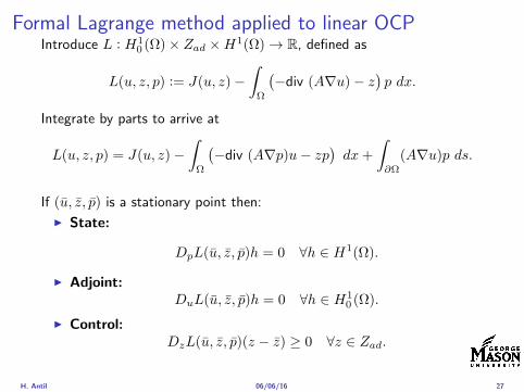
Formal Lagrange method applied to linear OCPIntroduce L H1
0 (Ω)times Zad timesH1(Ω)rarr R defined as
L(u z p) = J(u z)minusint
Ω
(minusdiv (Anablau)minus z
)p dx
Integrate by parts to arrive at
L(u z p) = J(u z)minusint
Ω
(minusdiv (Anablap)uminus zp
)dx+
intpartΩ
(Anablau)p ds
If (u z p) is a stationary point then
I State
DpL(u z p)h = 0 forallh isin H1(Ω)
I AdjointDuL(u z p)h = 0 forallh isin H1
0 (Ω)
I ControlDzL(u z p)(z minus z) ge 0 forallz isin Zad
H Antil 060616 27
Outline
Motivation and examples
Linear elliptic optimal control problems
Differentiation in Banach spaces
First-order necessary conditions
Optimal control of semilinear PDEs
An abstract problem
Discretization using finite element methods
H Antil 060616 28
Semilinear elliptic OCP
min J(u z) =1
2uminus ud2L2(Ω) +
λ
2z2L2(Ω)
subject to
minus∆u+ g(x u) = z in Ω
u = 0 on partΩ
and z isin Zad with za zb isin Linfin(Ω)
H Antil 060616 29
State space(A1) Ω sub Rd open bounded partΩ is Lipschitz
(A2) g Ωtimes Rrarr R is bounded and measurable with respect to x isin Ωfor every u isin R
(A3) g is continuous monotone increasing and Lipschitz continuous in ufor ae x isin Ω
(A4) g(x 0) = 0 for ae x isin Ω (not really necessary)
Theorem Suppose (A1)minus (A4) hold For every z isin Lr(Ω) withr gt d2 the state equation has a unique weak solutionu isin H1
0 (Ω) cap C(Ω) ie we haveintΩ
nablau middot nablav dx+
intΩ
g(x u(x))v(x) dx =
intΩ
zv dx forallv isin H10 (Ω)
Moreover there exists a constant C gt 0 such that
uH1(Ω) + uC(Ω) le CzLr(Ω)
RemarkI The proof of the theorem uses the BrowderndashMinty theorem on
monotone operators
H Antil 060616 30
State space(A1) Ω sub Rd open bounded partΩ is Lipschitz
(A2) g Ωtimes Rrarr R is bounded and measurable with respect to x isin Ωfor every u isin R
(A3) g is continuous monotone increasing and Lipschitz continuous in ufor ae x isin Ω
(A4) g(x 0) = 0 for ae x isin Ω (not really necessary)
Theorem Suppose (A1)minus (A4) hold For every z isin Lr(Ω) withr gt d2 the state equation has a unique weak solutionu isin H1
0 (Ω) cap C(Ω) ie we haveintΩ
nablau middot nablav dx+
intΩ
g(x u(x))v(x) dx =
intΩ
zv dx forallv isin H10 (Ω)
Moreover there exists a constant C gt 0 such that
uH1(Ω) + uC(Ω) le CzLr(Ω)
RemarkI The proof of the theorem uses the BrowderndashMinty theorem on
monotone operators
H Antil 060616 30
State space(A1) Ω sub Rd open bounded partΩ is Lipschitz
(A2) g Ωtimes Rrarr R is bounded and measurable with respect to x isin Ωfor every u isin R
(A3) g is continuous monotone increasing and Lipschitz continuous in ufor ae x isin Ω
(A4) g(x 0) = 0 for ae x isin Ω (not really necessary)
Theorem Suppose (A1)minus (A4) hold For every z isin Lr(Ω) withr gt d2 the state equation has a unique weak solutionu isin H1
0 (Ω) cap C(Ω) ie we haveintΩ
nablau middot nablav dx+
intΩ
g(x u(x))v(x) dx =
intΩ
zv dx forallv isin H10 (Ω)
Moreover there exists a constant C gt 0 such that
uH1(Ω) + uC(Ω) le CzLr(Ω)
RemarkI The proof of the theorem uses the BrowderndashMinty theorem on
monotone operators
H Antil 060616 30
Control-to-state map and reduced problem
I Control to state map
S Linfin(Ω)rarr H10 (Ω) cap C(Ω)
is well defined and is globally Lipschitz continuous
I Reduced problem
minJ (z) =1
2S(u)minus ud2L2(Ω) +
λ
2z2L2(Ω)
H Antil 060616 31
Control-to-state map and reduced problem
I Control to state map
S Linfin(Ω)rarr H10 (Ω) cap C(Ω)
is well defined and is globally Lipschitz continuous
I Reduced problem
minJ (z) =1
2S(u)minus ud2L2(Ω) +
λ
2z2L2(Ω)
H Antil 060616 31
First-order necessary conditionsI Lagrangian functional
L(u z p) = J(u z)minusint
Ω
(minus∆u+ g(x u(x))minus z
)p dx
= J(u z)minusint
Ω
(nablau middot nablap+ g(x u(x))pminus zp
)dx
I Adjoint system For all h isin H10 (Ω)
0 = DuL(u z p)h =
intΩ
(uminus ud)h dxminusint
Ω
(nablah middot nablap+ gu(x u(x))ph
)which yields
minus∆p+ gu(x u(x))p = uminus ud in Ω
p = 0 on partΩ
I Control
DzL(u z p)(z minus z) = (p+ λz z minus z) dx ge 0 forallz isin ZadI Gradient
nablaJ (z) = p+ λz
H Antil 060616 32
First-order necessary conditionsI Lagrangian functional
L(u z p) = J(u z)minusint
Ω
(minus∆u+ g(x u(x))minus z
)p dx
= J(u z)minusint
Ω
(nablau middot nablap+ g(x u(x))pminus zp
)dx
I Adjoint system For all h isin H10 (Ω)
0 = DuL(u z p)h =
intΩ
(uminus ud)h dxminusint
Ω
(nablah middot nablap+ gu(x u(x))ph
)which yields
minus∆p+ gu(x u(x))p = uminus ud in Ω
p = 0 on partΩ
I Control
DzL(u z p)(z minus z) = (p+ λz z minus z) dx ge 0 forallz isin ZadI Gradient
nablaJ (z) = p+ λz
H Antil 060616 32
First-order necessary conditionsI Lagrangian functional
L(u z p) = J(u z)minusint
Ω
(minus∆u+ g(x u(x))minus z
)p dx
= J(u z)minusint
Ω
(nablau middot nablap+ g(x u(x))pminus zp
)dx
I Adjoint system For all h isin H10 (Ω)
0 = DuL(u z p)h =
intΩ
(uminus ud)h dxminusint
Ω
(nablah middot nablap+ gu(x u(x))ph
)which yields
minus∆p+ gu(x u(x))p = uminus ud in Ω
p = 0 on partΩ
I Control
DzL(u z p)(z minus z) = (p+ λz z minus z) dx ge 0 forallz isin Zad
I GradientnablaJ (z) = p+ λz
H Antil 060616 32
First-order necessary conditionsI Lagrangian functional
L(u z p) = J(u z)minusint
Ω
(minus∆u+ g(x u(x))minus z
)p dx
= J(u z)minusint
Ω
(nablau middot nablap+ g(x u(x))pminus zp
)dx
I Adjoint system For all h isin H10 (Ω)
0 = DuL(u z p)h =
intΩ
(uminus ud)h dxminusint
Ω
(nablah middot nablap+ gu(x u(x))ph
)which yields
minus∆p+ gu(x u(x))p = uminus ud in Ω
p = 0 on partΩ
I Control
DzL(u z p)(z minus z) = (p+ λz z minus z) dx ge 0 forallz isin ZadI Gradient
nablaJ (z) = p+ λz
H Antil 060616 32
Differentiability of Nemytskii operator
The rigorous proof uses
Theorem In addition to (A1)-(A4) if
(A5) g is continuously differentiable with respect to u for ae x isin Ωand we have
(i) |gu(x 0)| le K for ae x isin Ω(ii) gu is locally Lipschitz with respect to u isin R
then the Nemytskii operator G u 7rarr g(middot u(middot)) is continuously Frechetdifferentiable from Linfin(Ω) into itself and
(Gprime(u)h)(x) = gu(x u(x))h(x) ae in Ω forallh isin Linfin(Ω)
Remark (A5) holds if g(x u) = g(u) and g isin C2(R)
H Antil 060616 33
Outline
Motivation and examples
Linear elliptic optimal control problems
Differentiation in Banach spaces
First-order necessary conditions
Optimal control of semilinear PDEs
An abstract problem
Discretization using finite element methods
H Antil 060616 34
Gradient computation via adjoint general formI Abstract problem
min J(u z)
subject toc(u z) = 0
and z isin Zad
I Directional derivative Let S be the control to state map(nonlinear in general)
z 7rarr S(z) = u(z)
Under the assumptions of ldquoimplicit function theoremrdquo
J prime(z)h = (nablauJ (u(z) z) Sprime(z)h) + (nablazJ (u(z) z) h)
I Sensitivity of u with respect to z Differentiating the stateequation
cu(S(z) z)Sprime(z)h = minuscz(S(z) z)h
leads toSprime(z)h = minuscu(S(z) z)minus1
(cz(S(z) z)h
)
provided cu(S(z) z)minus1 is well-defined
H Antil 060616 35
Gradient computation via adjoint general formI Abstract problem
min J(u z)
subject toc(u z) = 0
and z isin ZadI Directional derivative Let S be the control to state map
(nonlinear in general)
z 7rarr S(z) = u(z)
Under the assumptions of ldquoimplicit function theoremrdquo
J prime(z)h = (nablauJ (u(z) z) Sprime(z)h) + (nablazJ (u(z) z) h)
I Sensitivity of u with respect to z Differentiating the stateequation
cu(S(z) z)Sprime(z)h = minuscz(S(z) z)h
leads toSprime(z)h = minuscu(S(z) z)minus1
(cz(S(z) z)h
)
provided cu(S(z) z)minus1 is well-defined
H Antil 060616 35
Gradient computation via adjoint general formI Abstract problem
min J(u z)
subject toc(u z) = 0
and z isin ZadI Directional derivative Let S be the control to state map
(nonlinear in general)
z 7rarr S(z) = u(z)
Under the assumptions of ldquoimplicit function theoremrdquo
J prime(z)h = (nablauJ (u(z) z) Sprime(z)h) + (nablazJ (u(z) z) h)
I Sensitivity of u with respect to z Differentiating the stateequation
cu(S(z) z)Sprime(z)h = minuscz(S(z) z)h
leads toSprime(z)h = minuscu(S(z) z)minus1
(cz(S(z) z)h
)
provided cu(S(z) z)minus1 is well-defined
H Antil 060616 35
Adjoint equation and gradient general form
I Directional derivative
J prime(z)h = minus(nablauJ (u(z) z) cu(u(z) z)minus1cz(u(z) z)h
)+ (nablazJ (u(z) z) h)
I Gradient
nablaJ (z) = minuscz(u(z) z)lowast(cu(u(z) z)minuslowastnablauJ (u(z) z)
)+nablazJ (u(z) z)
I Introducing adjoint variable p solving
cu(u(z) z)lowastp = nablauJ (u(z) z)
we arrive at following form of gradient
nablaJ (z) = minuscz(u(z) z)lowastp+nablazJ (u(z) z)
which is tractable
H Antil 060616 36
Adjoint equation and gradient general form
I Directional derivative
J prime(z)h = minus(nablauJ (u(z) z) cu(u(z) z)minus1cz(u(z) z)h
)+ (nablazJ (u(z) z) h)
I Gradient
nablaJ (z) = minuscz(u(z) z)lowast(cu(u(z) z)minuslowastnablauJ (u(z) z)
)+nablazJ (u(z) z)
I Introducing adjoint variable p solving
cu(u(z) z)lowastp = nablauJ (u(z) z)
we arrive at following form of gradient
nablaJ (z) = minuscz(u(z) z)lowastp+nablazJ (u(z) z)
which is tractable
H Antil 060616 36
Adjoint equation and gradient general form
I Directional derivative
J prime(z)h = minus(nablauJ (u(z) z) cu(u(z) z)minus1cz(u(z) z)h
)+ (nablazJ (u(z) z) h)
I Gradient
nablaJ (z) = minuscz(u(z) z)lowast(cu(u(z) z)minuslowastnablauJ (u(z) z)
)+nablazJ (u(z) z)
I Introducing adjoint variable p solving
cu(u(z) z)lowastp = nablauJ (u(z) z)
we arrive at following form of gradient
nablaJ (z) = minuscz(u(z) z)lowastp+nablazJ (u(z) z)
which is tractable
H Antil 060616 36
Hessian computation general form
I Lagrangian L(u z p) = J(u z)minusint
Ωc(u z)p dx Then we have
DzJ (z)h = DzL(u z p)h
I Second order derivative
D2zJ (z)[h1 h2] = DuDzL(u z p)[h1 S
prime(z)h2] +D2zL(u z p)[h1 h2]
+DpDzL(u z p)[h1 Dzp(z)h2]
I We already know Sprime(z)h2 moreover
DpDzL(u z p)[h1 Dzp(z)h2] = minus(cu(u z)h1 Dzp(z)h2
)
It remain to identify Dzp(z)h2
H Antil 060616 37
Hessian computation general form
I Lagrangian L(u z p) = J(u z)minusint
Ωc(u z)p dx Then we have
DzJ (z)h = DzL(u z p)h
I Second order derivative
D2zJ (z)[h1 h2] = DuDzL(u z p)[h1 S
prime(z)h2] +D2zL(u z p)[h1 h2]
+DpDzL(u z p)[h1 Dzp(z)h2]
I We already know Sprime(z)h2 moreover
DpDzL(u z p)[h1 Dzp(z)h2] = minus(cu(u z)h1 Dzp(z)h2
)
It remain to identify Dzp(z)h2
H Antil 060616 37
Hessian computation general form
I Lagrangian L(u z p) = J(u z)minusint
Ωc(u z)p dx Then we have
DzJ (z)h = DzL(u z p)h
I Second order derivative
D2zJ (z)[h1 h2] = DuDzL(u z p)[h1 S
prime(z)h2] +D2zL(u z p)[h1 h2]
+DpDzL(u z p)[h1 Dzp(z)h2]
I We already know Sprime(z)h2 moreover
DpDzL(u z p)[h1 Dzp(z)h2] = minus(cu(u z)h1 Dzp(z)h2
)
It remain to identify Dzp(z)h2
H Antil 060616 37
Outline
Motivation and examples
Linear elliptic optimal control problems
Differentiation in Banach spaces
First-order necessary conditions
Optimal control of semilinear PDEs
An abstract problem
Discretization using finite element methods
H Antil 060616 38
Numerical approximation of Poisson equation MeshTo avoid technical issues we will assume that partΩ is polygonal
I Mesh Let T = K be a mesh of Ω where K sub Rd is an elementthat is isoparametrically equivalent to a unit simplex in Rd
I Conforming mesh We say that the mesh is conforming ifI Ω = cupKisinT KI If K1 cap K2 = x then x is a node of K1 and K2I If K1 cap K2 6= empty and K1 cap K2 6= x then K1 cap K2 is an edgeface
contained in partK1 cap partK2
I Shape regular Let T be the collection of all conformingrefinements of an original mesh T 0 Then T is called shape regularif exist κ gt 0 such that
hKρKle κ forallK isin cupiT i
where hK = diam K ρK = maxρ gt 0|Bρ sub KI Quasi-uniform A family of shape regular meshes is called-quasi
uniform if there exist a constant σ gt 0 such that
maxhKminhK
le σ
uniformly for all meshes in the family
Numerical approximation of Poisson equation MeshTo avoid technical issues we will assume that partΩ is polygonal
I Mesh Let T = K be a mesh of Ω where K sub Rd is an elementthat is isoparametrically equivalent to a unit simplex in Rd
I Conforming mesh We say that the mesh is conforming ifI Ω = cupKisinT KI If K1 cap K2 = x then x is a node of K1 and K2I If K1 cap K2 6= empty and K1 cap K2 6= x then K1 cap K2 is an edgeface
contained in partK1 cap partK2
I Shape regular Let T be the collection of all conformingrefinements of an original mesh T 0 Then T is called shape regularif exist κ gt 0 such that
hKρKle κ forallK isin cupiT i
where hK = diam K ρK = maxρ gt 0|Bρ sub KI Quasi-uniform A family of shape regular meshes is called-quasi
uniform if there exist a constant σ gt 0 such that
maxhKminhK
le σ
uniformly for all meshes in the family
Numerical approximation of Poisson equation MeshTo avoid technical issues we will assume that partΩ is polygonal
I Mesh Let T = K be a mesh of Ω where K sub Rd is an elementthat is isoparametrically equivalent to a unit simplex in Rd
I Conforming mesh We say that the mesh is conforming ifI Ω = cupKisinT KI If K1 cap K2 = x then x is a node of K1 and K2I If K1 cap K2 6= empty and K1 cap K2 6= x then K1 cap K2 is an edgeface
contained in partK1 cap partK2
I Shape regular Let T be the collection of all conformingrefinements of an original mesh T 0 Then T is called shape regularif exist κ gt 0 such that
hKρKle κ forallK isin cupiT i
where hK = diam K ρK = maxρ gt 0|Bρ sub K
I Quasi-uniform A family of shape regular meshes is called-quasiuniform if there exist a constant σ gt 0 such that
maxhKminhK
le σ
uniformly for all meshes in the family
Numerical approximation of Poisson equation MeshTo avoid technical issues we will assume that partΩ is polygonal
I Mesh Let T = K be a mesh of Ω where K sub Rd is an elementthat is isoparametrically equivalent to a unit simplex in Rd
I Conforming mesh We say that the mesh is conforming ifI Ω = cupKisinT KI If K1 cap K2 = x then x is a node of K1 and K2I If K1 cap K2 6= empty and K1 cap K2 6= x then K1 cap K2 is an edgeface
contained in partK1 cap partK2
I Shape regular Let T be the collection of all conformingrefinements of an original mesh T 0 Then T is called shape regularif exist κ gt 0 such that
hKρKle κ forallK isin cupiT i
where hK = diam K ρK = maxρ gt 0|Bρ sub KI Quasi-uniform A family of shape regular meshes is called-quasi
uniform if there exist a constant σ gt 0 such that
maxhKminhK
le σ
uniformly for all meshes in the family
FE space and Galerkin approximationI Finite element space For T isin T we define the finite element
space as
V(T ) = W isin C0(Ω) WK isin P1forallK isin T W |partΩ = 0
where P1 is the set of polynomials of degree at most 1
I Galerkin approximation of continuous problem is given by
Find UT isin V(T )
intΩ
AnablaUT middot nablaV = 〈f V 〉 forallV isin V(T )
The discrete problem is well-posedI Nodal basis Consists of functions ψi isin V(T ) with xi isin N (T )
satisfyingψxi
(xj) = δij
where N (T ) denotes the interior (plus Neumann) nodesI Galerkin orthogonality(
nabla(uminus UT )nablaW)L2(Ω)
= 0 forallW isin V(T )
H Antil 060616 40
FE space and Galerkin approximationI Finite element space For T isin T we define the finite element
space as
V(T ) = W isin C0(Ω) WK isin P1forallK isin T W |partΩ = 0
where P1 is the set of polynomials of degree at most 1I Galerkin approximation of continuous problem is given by
Find UT isin V(T )
intΩ
AnablaUT middot nablaV = 〈f V 〉 forallV isin V(T )
The discrete problem is well-posed
I Nodal basis Consists of functions ψi isin V(T ) with xi isin N (T )satisfying
ψxi(xj) = δij
where N (T ) denotes the interior (plus Neumann) nodesI Galerkin orthogonality(
nabla(uminus UT )nablaW)L2(Ω)
= 0 forallW isin V(T )
H Antil 060616 40
FE space and Galerkin approximationI Finite element space For T isin T we define the finite element
space as
V(T ) = W isin C0(Ω) WK isin P1forallK isin T W |partΩ = 0
where P1 is the set of polynomials of degree at most 1I Galerkin approximation of continuous problem is given by
Find UT isin V(T )
intΩ
AnablaUT middot nablaV = 〈f V 〉 forallV isin V(T )
The discrete problem is well-posedI Nodal basis Consists of functions ψi isin V(T ) with xi isin N (T )
satisfyingψxi
(xj) = δij
where N (T ) denotes the interior (plus Neumann) nodes
I Galerkin orthogonality(nabla(uminus UT )nablaW
)L2(Ω)
= 0 forallW isin V(T )
H Antil 060616 40
FE space and Galerkin approximationI Finite element space For T isin T we define the finite element
space as
V(T ) = W isin C0(Ω) WK isin P1forallK isin T W |partΩ = 0
where P1 is the set of polynomials of degree at most 1I Galerkin approximation of continuous problem is given by
Find UT isin V(T )
intΩ
AnablaUT middot nablaV = 〈f V 〉 forallV isin V(T )
The discrete problem is well-posedI Nodal basis Consists of functions ψi isin V(T ) with xi isin N (T )
satisfyingψxi
(xj) = δij
where N (T ) denotes the interior (plus Neumann) nodesI Galerkin orthogonality(
nabla(uminus UT )nablaW)L2(Ω)
= 0 forallW isin V(T )
H Antil 060616 40
Best approximation
I Cearsquos lemma
nabla(uminus UT )L2(Ω) le C infWisinV(T )
nabla(uminusW )L2(Ω)
I Nodal interpolation operator ΠT C(Ω)rarr V(T ) satisfies
ΠT u(xi) = u(xi) forallxi isin N (T )
and is defined as
ΠT u =sum
xiisinN (T )
u(xi)ψxi
I Error estimates In Cearsquos lemma replace W by ΠT u and thencompute the interpolation error
H Antil 060616 41
Best approximation
I Cearsquos lemma
nabla(uminus UT )L2(Ω) le C infWisinV(T )
nabla(uminusW )L2(Ω)
I Nodal interpolation operator ΠT C(Ω)rarr V(T ) satisfies
ΠT u(xi) = u(xi) forallxi isin N (T )
and is defined as
ΠT u =sum
xiisinN (T )
u(xi)ψxi
I Error estimates In Cearsquos lemma replace W by ΠT u and thencompute the interpolation error
H Antil 060616 41
Best approximation
I Cearsquos lemma
nabla(uminus UT )L2(Ω) le C infWisinV(T )
nabla(uminusW )L2(Ω)
I Nodal interpolation operator ΠT C(Ω)rarr V(T ) satisfies
ΠT u(xi) = u(xi) forallxi isin N (T )
and is defined as
ΠT u =sum
xiisinN (T )
u(xi)ψxi
I Error estimates In Cearsquos lemma replace W by ΠT u and thencompute the interpolation error
H Antil 060616 41
Algebraic system state equation
I Recall UT isin V(T ) solves
a(UT V ) = 〈f V 〉 forallV isin V(T )
I Now setting UT =sumN
j=1 Ujψj V = ψi we get
Nsumj=1
Uja(φj φi) = 〈f ψi〉 i = 1 N
which is the matrix-vector system
AU = F
I Stiffness matrix A is SPD
H Antil 060616 42
Algebraic system state equation
I Recall UT isin V(T ) solves
a(UT V ) = 〈f V 〉 forallV isin V(T )
I Now setting UT =sumN
j=1 Ujψj V = ψi we get
Nsumj=1
Uja(φj φi) = 〈f ψi〉 i = 1 N
which is the matrix-vector system
AU = F
I Stiffness matrix A is SPD
H Antil 060616 42
Algebraic system state equation
I Recall UT isin V(T ) solves
a(UT V ) = 〈f V 〉 forallV isin V(T )
I Now setting UT =sumN
j=1 Ujψj V = ψi we get
Nsumj=1
Uja(φj φi) = 〈f ψi〉 i = 1 N
which is the matrix-vector system
AU = F
I Stiffness matrix A is SPD
H Antil 060616 42
Discrete linear elliptic OCP
min JT (UT ZT ) =1
2UT minus ud2L2(Ω) +
λ
2ZT 2L2(Ω)
subject to
Find UT isin V(T )
intΩ
nablaUT middot nablaV = (ZT V )L2(Ω) forallV isin V(T )
and whereZT isin Zad(T ) = Zad cap Z(T )
is either one of these
Z(T ) =
V(T )L2(Ω) variational discretization (Hinze)WT isin Linfin(Ω) ZT |K isin P0(K)K isin T
H Antil 060616 43
Recent books
F TroltzschOptimal control of partial differential equations volume 112 ofGraduate Studies in MathematicsAmerican Mathematical Society Providence RI 2010Theory methods and applications Translated from the 2005 Germanoriginal by Jurgen Sprekels
K Ito and K KunischLagrange multiplier approach to variational problems andapplications volume 15 of Advances in Design and ControlSociety for Industrial and Applied Mathematics (SIAM)Philadelphia PA 2008
H Antil 060616 44
- Motivation and examples
- Linear elliptic optimal control problems
- Differentiation in Banach spaces
- First-order necessary conditions
- Optimal control of semilinear PDEs
- An abstract problem
- Discretization using finite element methods
-
Outline
Motivation and examples
Linear elliptic optimal control problems
Differentiation in Banach spaces
First-order necessary conditions
Optimal control of semilinear PDEs
An abstract problem
Discretization using finite element methods
H Antil 060616 28
Semilinear elliptic OCP
min J(u z) =1
2uminus ud2L2(Ω) +
λ
2z2L2(Ω)
subject to
minus∆u+ g(x u) = z in Ω
u = 0 on partΩ
and z isin Zad with za zb isin Linfin(Ω)
H Antil 060616 29
State space(A1) Ω sub Rd open bounded partΩ is Lipschitz
(A2) g Ωtimes Rrarr R is bounded and measurable with respect to x isin Ωfor every u isin R
(A3) g is continuous monotone increasing and Lipschitz continuous in ufor ae x isin Ω
(A4) g(x 0) = 0 for ae x isin Ω (not really necessary)
Theorem Suppose (A1)minus (A4) hold For every z isin Lr(Ω) withr gt d2 the state equation has a unique weak solutionu isin H1
0 (Ω) cap C(Ω) ie we haveintΩ
nablau middot nablav dx+
intΩ
g(x u(x))v(x) dx =
intΩ
zv dx forallv isin H10 (Ω)
Moreover there exists a constant C gt 0 such that
uH1(Ω) + uC(Ω) le CzLr(Ω)
RemarkI The proof of the theorem uses the BrowderndashMinty theorem on
monotone operators
H Antil 060616 30
State space(A1) Ω sub Rd open bounded partΩ is Lipschitz
(A2) g Ωtimes Rrarr R is bounded and measurable with respect to x isin Ωfor every u isin R
(A3) g is continuous monotone increasing and Lipschitz continuous in ufor ae x isin Ω
(A4) g(x 0) = 0 for ae x isin Ω (not really necessary)
Theorem Suppose (A1)minus (A4) hold For every z isin Lr(Ω) withr gt d2 the state equation has a unique weak solutionu isin H1
0 (Ω) cap C(Ω) ie we haveintΩ
nablau middot nablav dx+
intΩ
g(x u(x))v(x) dx =
intΩ
zv dx forallv isin H10 (Ω)
Moreover there exists a constant C gt 0 such that
uH1(Ω) + uC(Ω) le CzLr(Ω)
RemarkI The proof of the theorem uses the BrowderndashMinty theorem on
monotone operators
H Antil 060616 30
State space(A1) Ω sub Rd open bounded partΩ is Lipschitz
(A2) g Ωtimes Rrarr R is bounded and measurable with respect to x isin Ωfor every u isin R
(A3) g is continuous monotone increasing and Lipschitz continuous in ufor ae x isin Ω
(A4) g(x 0) = 0 for ae x isin Ω (not really necessary)
Theorem Suppose (A1)minus (A4) hold For every z isin Lr(Ω) withr gt d2 the state equation has a unique weak solutionu isin H1
0 (Ω) cap C(Ω) ie we haveintΩ
nablau middot nablav dx+
intΩ
g(x u(x))v(x) dx =
intΩ
zv dx forallv isin H10 (Ω)
Moreover there exists a constant C gt 0 such that
uH1(Ω) + uC(Ω) le CzLr(Ω)
RemarkI The proof of the theorem uses the BrowderndashMinty theorem on
monotone operators
H Antil 060616 30
Control-to-state map and reduced problem
I Control to state map
S Linfin(Ω)rarr H10 (Ω) cap C(Ω)
is well defined and is globally Lipschitz continuous
I Reduced problem
minJ (z) =1
2S(u)minus ud2L2(Ω) +
λ
2z2L2(Ω)
H Antil 060616 31
Control-to-state map and reduced problem
I Control to state map
S Linfin(Ω)rarr H10 (Ω) cap C(Ω)
is well defined and is globally Lipschitz continuous
I Reduced problem
minJ (z) =1
2S(u)minus ud2L2(Ω) +
λ
2z2L2(Ω)
H Antil 060616 31
First-order necessary conditionsI Lagrangian functional
L(u z p) = J(u z)minusint
Ω
(minus∆u+ g(x u(x))minus z
)p dx
= J(u z)minusint
Ω
(nablau middot nablap+ g(x u(x))pminus zp
)dx
I Adjoint system For all h isin H10 (Ω)
0 = DuL(u z p)h =
intΩ
(uminus ud)h dxminusint
Ω
(nablah middot nablap+ gu(x u(x))ph
)which yields
minus∆p+ gu(x u(x))p = uminus ud in Ω
p = 0 on partΩ
I Control
DzL(u z p)(z minus z) = (p+ λz z minus z) dx ge 0 forallz isin ZadI Gradient
nablaJ (z) = p+ λz
H Antil 060616 32
First-order necessary conditionsI Lagrangian functional
L(u z p) = J(u z)minusint
Ω
(minus∆u+ g(x u(x))minus z
)p dx
= J(u z)minusint
Ω
(nablau middot nablap+ g(x u(x))pminus zp
)dx
I Adjoint system For all h isin H10 (Ω)
0 = DuL(u z p)h =
intΩ
(uminus ud)h dxminusint
Ω
(nablah middot nablap+ gu(x u(x))ph
)which yields
minus∆p+ gu(x u(x))p = uminus ud in Ω
p = 0 on partΩ
I Control
DzL(u z p)(z minus z) = (p+ λz z minus z) dx ge 0 forallz isin ZadI Gradient
nablaJ (z) = p+ λz
H Antil 060616 32
First-order necessary conditionsI Lagrangian functional
L(u z p) = J(u z)minusint
Ω
(minus∆u+ g(x u(x))minus z
)p dx
= J(u z)minusint
Ω
(nablau middot nablap+ g(x u(x))pminus zp
)dx
I Adjoint system For all h isin H10 (Ω)
0 = DuL(u z p)h =
intΩ
(uminus ud)h dxminusint
Ω
(nablah middot nablap+ gu(x u(x))ph
)which yields
minus∆p+ gu(x u(x))p = uminus ud in Ω
p = 0 on partΩ
I Control
DzL(u z p)(z minus z) = (p+ λz z minus z) dx ge 0 forallz isin Zad
I GradientnablaJ (z) = p+ λz
H Antil 060616 32
First-order necessary conditionsI Lagrangian functional
L(u z p) = J(u z)minusint
Ω
(minus∆u+ g(x u(x))minus z
)p dx
= J(u z)minusint
Ω
(nablau middot nablap+ g(x u(x))pminus zp
)dx
I Adjoint system For all h isin H10 (Ω)
0 = DuL(u z p)h =
intΩ
(uminus ud)h dxminusint
Ω
(nablah middot nablap+ gu(x u(x))ph
)which yields
minus∆p+ gu(x u(x))p = uminus ud in Ω
p = 0 on partΩ
I Control
DzL(u z p)(z minus z) = (p+ λz z minus z) dx ge 0 forallz isin ZadI Gradient
nablaJ (z) = p+ λz
H Antil 060616 32
Differentiability of Nemytskii operator
The rigorous proof uses
Theorem In addition to (A1)-(A4) if
(A5) g is continuously differentiable with respect to u for ae x isin Ωand we have
(i) |gu(x 0)| le K for ae x isin Ω(ii) gu is locally Lipschitz with respect to u isin R
then the Nemytskii operator G u 7rarr g(middot u(middot)) is continuously Frechetdifferentiable from Linfin(Ω) into itself and
(Gprime(u)h)(x) = gu(x u(x))h(x) ae in Ω forallh isin Linfin(Ω)
Remark (A5) holds if g(x u) = g(u) and g isin C2(R)
H Antil 060616 33
Outline
Motivation and examples
Linear elliptic optimal control problems
Differentiation in Banach spaces
First-order necessary conditions
Optimal control of semilinear PDEs
An abstract problem
Discretization using finite element methods
H Antil 060616 34
Gradient computation via adjoint general formI Abstract problem
min J(u z)
subject toc(u z) = 0
and z isin Zad
I Directional derivative Let S be the control to state map(nonlinear in general)
z 7rarr S(z) = u(z)
Under the assumptions of ldquoimplicit function theoremrdquo
J prime(z)h = (nablauJ (u(z) z) Sprime(z)h) + (nablazJ (u(z) z) h)
I Sensitivity of u with respect to z Differentiating the stateequation
cu(S(z) z)Sprime(z)h = minuscz(S(z) z)h
leads toSprime(z)h = minuscu(S(z) z)minus1
(cz(S(z) z)h
)
provided cu(S(z) z)minus1 is well-defined
H Antil 060616 35
Gradient computation via adjoint general formI Abstract problem
min J(u z)
subject toc(u z) = 0
and z isin ZadI Directional derivative Let S be the control to state map
(nonlinear in general)
z 7rarr S(z) = u(z)
Under the assumptions of ldquoimplicit function theoremrdquo
J prime(z)h = (nablauJ (u(z) z) Sprime(z)h) + (nablazJ (u(z) z) h)
I Sensitivity of u with respect to z Differentiating the stateequation
cu(S(z) z)Sprime(z)h = minuscz(S(z) z)h
leads toSprime(z)h = minuscu(S(z) z)minus1
(cz(S(z) z)h
)
provided cu(S(z) z)minus1 is well-defined
H Antil 060616 35
Gradient computation via adjoint general formI Abstract problem
min J(u z)
subject toc(u z) = 0
and z isin ZadI Directional derivative Let S be the control to state map
(nonlinear in general)
z 7rarr S(z) = u(z)
Under the assumptions of ldquoimplicit function theoremrdquo
J prime(z)h = (nablauJ (u(z) z) Sprime(z)h) + (nablazJ (u(z) z) h)
I Sensitivity of u with respect to z Differentiating the stateequation
cu(S(z) z)Sprime(z)h = minuscz(S(z) z)h
leads toSprime(z)h = minuscu(S(z) z)minus1
(cz(S(z) z)h
)
provided cu(S(z) z)minus1 is well-defined
H Antil 060616 35
Adjoint equation and gradient general form
I Directional derivative
J prime(z)h = minus(nablauJ (u(z) z) cu(u(z) z)minus1cz(u(z) z)h
)+ (nablazJ (u(z) z) h)
I Gradient
nablaJ (z) = minuscz(u(z) z)lowast(cu(u(z) z)minuslowastnablauJ (u(z) z)
)+nablazJ (u(z) z)
I Introducing adjoint variable p solving
cu(u(z) z)lowastp = nablauJ (u(z) z)
we arrive at following form of gradient
nablaJ (z) = minuscz(u(z) z)lowastp+nablazJ (u(z) z)
which is tractable
H Antil 060616 36
Adjoint equation and gradient general form
I Directional derivative
J prime(z)h = minus(nablauJ (u(z) z) cu(u(z) z)minus1cz(u(z) z)h
)+ (nablazJ (u(z) z) h)
I Gradient
nablaJ (z) = minuscz(u(z) z)lowast(cu(u(z) z)minuslowastnablauJ (u(z) z)
)+nablazJ (u(z) z)
I Introducing adjoint variable p solving
cu(u(z) z)lowastp = nablauJ (u(z) z)
we arrive at following form of gradient
nablaJ (z) = minuscz(u(z) z)lowastp+nablazJ (u(z) z)
which is tractable
H Antil 060616 36
Adjoint equation and gradient general form
I Directional derivative
J prime(z)h = minus(nablauJ (u(z) z) cu(u(z) z)minus1cz(u(z) z)h
)+ (nablazJ (u(z) z) h)
I Gradient
nablaJ (z) = minuscz(u(z) z)lowast(cu(u(z) z)minuslowastnablauJ (u(z) z)
)+nablazJ (u(z) z)
I Introducing adjoint variable p solving
cu(u(z) z)lowastp = nablauJ (u(z) z)
we arrive at following form of gradient
nablaJ (z) = minuscz(u(z) z)lowastp+nablazJ (u(z) z)
which is tractable
H Antil 060616 36
Hessian computation general form
I Lagrangian L(u z p) = J(u z)minusint
Ωc(u z)p dx Then we have
DzJ (z)h = DzL(u z p)h
I Second order derivative
D2zJ (z)[h1 h2] = DuDzL(u z p)[h1 S
prime(z)h2] +D2zL(u z p)[h1 h2]
+DpDzL(u z p)[h1 Dzp(z)h2]
I We already know Sprime(z)h2 moreover
DpDzL(u z p)[h1 Dzp(z)h2] = minus(cu(u z)h1 Dzp(z)h2
)
It remain to identify Dzp(z)h2
H Antil 060616 37
Hessian computation general form
I Lagrangian L(u z p) = J(u z)minusint
Ωc(u z)p dx Then we have
DzJ (z)h = DzL(u z p)h
I Second order derivative
D2zJ (z)[h1 h2] = DuDzL(u z p)[h1 S
prime(z)h2] +D2zL(u z p)[h1 h2]
+DpDzL(u z p)[h1 Dzp(z)h2]
I We already know Sprime(z)h2 moreover
DpDzL(u z p)[h1 Dzp(z)h2] = minus(cu(u z)h1 Dzp(z)h2
)
It remain to identify Dzp(z)h2
H Antil 060616 37
Hessian computation general form
I Lagrangian L(u z p) = J(u z)minusint
Ωc(u z)p dx Then we have
DzJ (z)h = DzL(u z p)h
I Second order derivative
D2zJ (z)[h1 h2] = DuDzL(u z p)[h1 S
prime(z)h2] +D2zL(u z p)[h1 h2]
+DpDzL(u z p)[h1 Dzp(z)h2]
I We already know Sprime(z)h2 moreover
DpDzL(u z p)[h1 Dzp(z)h2] = minus(cu(u z)h1 Dzp(z)h2
)
It remain to identify Dzp(z)h2
H Antil 060616 37
Outline
Motivation and examples
Linear elliptic optimal control problems
Differentiation in Banach spaces
First-order necessary conditions
Optimal control of semilinear PDEs
An abstract problem
Discretization using finite element methods
H Antil 060616 38
Numerical approximation of Poisson equation MeshTo avoid technical issues we will assume that partΩ is polygonal
I Mesh Let T = K be a mesh of Ω where K sub Rd is an elementthat is isoparametrically equivalent to a unit simplex in Rd
I Conforming mesh We say that the mesh is conforming ifI Ω = cupKisinT KI If K1 cap K2 = x then x is a node of K1 and K2I If K1 cap K2 6= empty and K1 cap K2 6= x then K1 cap K2 is an edgeface
contained in partK1 cap partK2
I Shape regular Let T be the collection of all conformingrefinements of an original mesh T 0 Then T is called shape regularif exist κ gt 0 such that
hKρKle κ forallK isin cupiT i
where hK = diam K ρK = maxρ gt 0|Bρ sub KI Quasi-uniform A family of shape regular meshes is called-quasi
uniform if there exist a constant σ gt 0 such that
maxhKminhK
le σ
uniformly for all meshes in the family
Numerical approximation of Poisson equation MeshTo avoid technical issues we will assume that partΩ is polygonal
I Mesh Let T = K be a mesh of Ω where K sub Rd is an elementthat is isoparametrically equivalent to a unit simplex in Rd
I Conforming mesh We say that the mesh is conforming ifI Ω = cupKisinT KI If K1 cap K2 = x then x is a node of K1 and K2I If K1 cap K2 6= empty and K1 cap K2 6= x then K1 cap K2 is an edgeface
contained in partK1 cap partK2
I Shape regular Let T be the collection of all conformingrefinements of an original mesh T 0 Then T is called shape regularif exist κ gt 0 such that
hKρKle κ forallK isin cupiT i
where hK = diam K ρK = maxρ gt 0|Bρ sub KI Quasi-uniform A family of shape regular meshes is called-quasi
uniform if there exist a constant σ gt 0 such that
maxhKminhK
le σ
uniformly for all meshes in the family
Numerical approximation of Poisson equation MeshTo avoid technical issues we will assume that partΩ is polygonal
I Mesh Let T = K be a mesh of Ω where K sub Rd is an elementthat is isoparametrically equivalent to a unit simplex in Rd
I Conforming mesh We say that the mesh is conforming ifI Ω = cupKisinT KI If K1 cap K2 = x then x is a node of K1 and K2I If K1 cap K2 6= empty and K1 cap K2 6= x then K1 cap K2 is an edgeface
contained in partK1 cap partK2
I Shape regular Let T be the collection of all conformingrefinements of an original mesh T 0 Then T is called shape regularif exist κ gt 0 such that
hKρKle κ forallK isin cupiT i
where hK = diam K ρK = maxρ gt 0|Bρ sub K
I Quasi-uniform A family of shape regular meshes is called-quasiuniform if there exist a constant σ gt 0 such that
maxhKminhK
le σ
uniformly for all meshes in the family
Numerical approximation of Poisson equation MeshTo avoid technical issues we will assume that partΩ is polygonal
I Mesh Let T = K be a mesh of Ω where K sub Rd is an elementthat is isoparametrically equivalent to a unit simplex in Rd
I Conforming mesh We say that the mesh is conforming ifI Ω = cupKisinT KI If K1 cap K2 = x then x is a node of K1 and K2I If K1 cap K2 6= empty and K1 cap K2 6= x then K1 cap K2 is an edgeface
contained in partK1 cap partK2
I Shape regular Let T be the collection of all conformingrefinements of an original mesh T 0 Then T is called shape regularif exist κ gt 0 such that
hKρKle κ forallK isin cupiT i
where hK = diam K ρK = maxρ gt 0|Bρ sub KI Quasi-uniform A family of shape regular meshes is called-quasi
uniform if there exist a constant σ gt 0 such that
maxhKminhK
le σ
uniformly for all meshes in the family
FE space and Galerkin approximationI Finite element space For T isin T we define the finite element
space as
V(T ) = W isin C0(Ω) WK isin P1forallK isin T W |partΩ = 0
where P1 is the set of polynomials of degree at most 1
I Galerkin approximation of continuous problem is given by
Find UT isin V(T )
intΩ
AnablaUT middot nablaV = 〈f V 〉 forallV isin V(T )
The discrete problem is well-posedI Nodal basis Consists of functions ψi isin V(T ) with xi isin N (T )
satisfyingψxi
(xj) = δij
where N (T ) denotes the interior (plus Neumann) nodesI Galerkin orthogonality(
nabla(uminus UT )nablaW)L2(Ω)
= 0 forallW isin V(T )
H Antil 060616 40
FE space and Galerkin approximationI Finite element space For T isin T we define the finite element
space as
V(T ) = W isin C0(Ω) WK isin P1forallK isin T W |partΩ = 0
where P1 is the set of polynomials of degree at most 1I Galerkin approximation of continuous problem is given by
Find UT isin V(T )
intΩ
AnablaUT middot nablaV = 〈f V 〉 forallV isin V(T )
The discrete problem is well-posed
I Nodal basis Consists of functions ψi isin V(T ) with xi isin N (T )satisfying
ψxi(xj) = δij
where N (T ) denotes the interior (plus Neumann) nodesI Galerkin orthogonality(
nabla(uminus UT )nablaW)L2(Ω)
= 0 forallW isin V(T )
H Antil 060616 40
FE space and Galerkin approximationI Finite element space For T isin T we define the finite element
space as
V(T ) = W isin C0(Ω) WK isin P1forallK isin T W |partΩ = 0
where P1 is the set of polynomials of degree at most 1I Galerkin approximation of continuous problem is given by
Find UT isin V(T )
intΩ
AnablaUT middot nablaV = 〈f V 〉 forallV isin V(T )
The discrete problem is well-posedI Nodal basis Consists of functions ψi isin V(T ) with xi isin N (T )
satisfyingψxi
(xj) = δij
where N (T ) denotes the interior (plus Neumann) nodes
I Galerkin orthogonality(nabla(uminus UT )nablaW
)L2(Ω)
= 0 forallW isin V(T )
H Antil 060616 40
FE space and Galerkin approximationI Finite element space For T isin T we define the finite element
space as
V(T ) = W isin C0(Ω) WK isin P1forallK isin T W |partΩ = 0
where P1 is the set of polynomials of degree at most 1I Galerkin approximation of continuous problem is given by
Find UT isin V(T )
intΩ
AnablaUT middot nablaV = 〈f V 〉 forallV isin V(T )
The discrete problem is well-posedI Nodal basis Consists of functions ψi isin V(T ) with xi isin N (T )
satisfyingψxi
(xj) = δij
where N (T ) denotes the interior (plus Neumann) nodesI Galerkin orthogonality(
nabla(uminus UT )nablaW)L2(Ω)
= 0 forallW isin V(T )
H Antil 060616 40
Best approximation
I Cearsquos lemma
nabla(uminus UT )L2(Ω) le C infWisinV(T )
nabla(uminusW )L2(Ω)
I Nodal interpolation operator ΠT C(Ω)rarr V(T ) satisfies
ΠT u(xi) = u(xi) forallxi isin N (T )
and is defined as
ΠT u =sum
xiisinN (T )
u(xi)ψxi
I Error estimates In Cearsquos lemma replace W by ΠT u and thencompute the interpolation error
H Antil 060616 41
Best approximation
I Cearsquos lemma
nabla(uminus UT )L2(Ω) le C infWisinV(T )
nabla(uminusW )L2(Ω)
I Nodal interpolation operator ΠT C(Ω)rarr V(T ) satisfies
ΠT u(xi) = u(xi) forallxi isin N (T )
and is defined as
ΠT u =sum
xiisinN (T )
u(xi)ψxi
I Error estimates In Cearsquos lemma replace W by ΠT u and thencompute the interpolation error
H Antil 060616 41
Best approximation
I Cearsquos lemma
nabla(uminus UT )L2(Ω) le C infWisinV(T )
nabla(uminusW )L2(Ω)
I Nodal interpolation operator ΠT C(Ω)rarr V(T ) satisfies
ΠT u(xi) = u(xi) forallxi isin N (T )
and is defined as
ΠT u =sum
xiisinN (T )
u(xi)ψxi
I Error estimates In Cearsquos lemma replace W by ΠT u and thencompute the interpolation error
H Antil 060616 41
Algebraic system state equation
I Recall UT isin V(T ) solves
a(UT V ) = 〈f V 〉 forallV isin V(T )
I Now setting UT =sumN
j=1 Ujψj V = ψi we get
Nsumj=1
Uja(φj φi) = 〈f ψi〉 i = 1 N
which is the matrix-vector system
AU = F
I Stiffness matrix A is SPD
H Antil 060616 42
Algebraic system state equation
I Recall UT isin V(T ) solves
a(UT V ) = 〈f V 〉 forallV isin V(T )
I Now setting UT =sumN
j=1 Ujψj V = ψi we get
Nsumj=1
Uja(φj φi) = 〈f ψi〉 i = 1 N
which is the matrix-vector system
AU = F
I Stiffness matrix A is SPD
H Antil 060616 42
Algebraic system state equation
I Recall UT isin V(T ) solves
a(UT V ) = 〈f V 〉 forallV isin V(T )
I Now setting UT =sumN
j=1 Ujψj V = ψi we get
Nsumj=1
Uja(φj φi) = 〈f ψi〉 i = 1 N
which is the matrix-vector system
AU = F
I Stiffness matrix A is SPD
H Antil 060616 42
Discrete linear elliptic OCP
min JT (UT ZT ) =1
2UT minus ud2L2(Ω) +
λ
2ZT 2L2(Ω)
subject to
Find UT isin V(T )
intΩ
nablaUT middot nablaV = (ZT V )L2(Ω) forallV isin V(T )
and whereZT isin Zad(T ) = Zad cap Z(T )
is either one of these
Z(T ) =
V(T )L2(Ω) variational discretization (Hinze)WT isin Linfin(Ω) ZT |K isin P0(K)K isin T
H Antil 060616 43
Recent books
F TroltzschOptimal control of partial differential equations volume 112 ofGraduate Studies in MathematicsAmerican Mathematical Society Providence RI 2010Theory methods and applications Translated from the 2005 Germanoriginal by Jurgen Sprekels
K Ito and K KunischLagrange multiplier approach to variational problems andapplications volume 15 of Advances in Design and ControlSociety for Industrial and Applied Mathematics (SIAM)Philadelphia PA 2008
H Antil 060616 44
- Motivation and examples
- Linear elliptic optimal control problems
- Differentiation in Banach spaces
- First-order necessary conditions
- Optimal control of semilinear PDEs
- An abstract problem
- Discretization using finite element methods
-
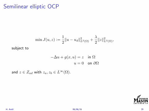
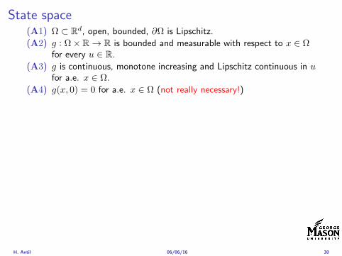
State space(A1) Ω sub Rd open bounded partΩ is Lipschitz
(A2) g Ωtimes Rrarr R is bounded and measurable with respect to x isin Ωfor every u isin R
(A3) g is continuous monotone increasing and Lipschitz continuous in ufor ae x isin Ω
(A4) g(x 0) = 0 for ae x isin Ω (not really necessary)
Theorem Suppose (A1)minus (A4) hold For every z isin Lr(Ω) withr gt d2 the state equation has a unique weak solutionu isin H1
0 (Ω) cap C(Ω) ie we haveintΩ
nablau middot nablav dx+
intΩ
g(x u(x))v(x) dx =
intΩ
zv dx forallv isin H10 (Ω)
Moreover there exists a constant C gt 0 such that
uH1(Ω) + uC(Ω) le CzLr(Ω)
RemarkI The proof of the theorem uses the BrowderndashMinty theorem on
monotone operators
H Antil 060616 30
Control-to-state map and reduced problem
I Control to state map
S Linfin(Ω)rarr H10 (Ω) cap C(Ω)
is well defined and is globally Lipschitz continuous
I Reduced problem
minJ (z) =1
2S(u)minus ud2L2(Ω) +
λ
2z2L2(Ω)
H Antil 060616 31
Control-to-state map and reduced problem
I Control to state map
S Linfin(Ω)rarr H10 (Ω) cap C(Ω)
is well defined and is globally Lipschitz continuous
I Reduced problem
minJ (z) =1
2S(u)minus ud2L2(Ω) +
λ
2z2L2(Ω)
H Antil 060616 31
First-order necessary conditionsI Lagrangian functional
L(u z p) = J(u z)minusint
Ω
(minus∆u+ g(x u(x))minus z
)p dx
= J(u z)minusint
Ω
(nablau middot nablap+ g(x u(x))pminus zp
)dx
I Adjoint system For all h isin H10 (Ω)
0 = DuL(u z p)h =
intΩ
(uminus ud)h dxminusint
Ω
(nablah middot nablap+ gu(x u(x))ph
)which yields
minus∆p+ gu(x u(x))p = uminus ud in Ω
p = 0 on partΩ
I Control
DzL(u z p)(z minus z) = (p+ λz z minus z) dx ge 0 forallz isin ZadI Gradient
nablaJ (z) = p+ λz
H Antil 060616 32
First-order necessary conditionsI Lagrangian functional
L(u z p) = J(u z)minusint
Ω
(minus∆u+ g(x u(x))minus z
)p dx
= J(u z)minusint
Ω
(nablau middot nablap+ g(x u(x))pminus zp
)dx
I Adjoint system For all h isin H10 (Ω)
0 = DuL(u z p)h =
intΩ
(uminus ud)h dxminusint
Ω
(nablah middot nablap+ gu(x u(x))ph
)which yields
minus∆p+ gu(x u(x))p = uminus ud in Ω
p = 0 on partΩ
I Control
DzL(u z p)(z minus z) = (p+ λz z minus z) dx ge 0 forallz isin Zad
I GradientnablaJ (z) = p+ λz
H Antil 060616 32
First-order necessary conditionsI Lagrangian functional
L(u z p) = J(u z)minusint
Ω
(minus∆u+ g(x u(x))minus z
)p dx
= J(u z)minusint
Ω
(nablau middot nablap+ g(x u(x))pminus zp
)dx
I Adjoint system For all h isin H10 (Ω)
0 = DuL(u z p)h =
intΩ
(uminus ud)h dxminusint
Ω
(nablah middot nablap+ gu(x u(x))ph
)which yields
minus∆p+ gu(x u(x))p = uminus ud in Ω
p = 0 on partΩ
I Control
DzL(u z p)(z minus z) = (p+ λz z minus z) dx ge 0 forallz isin ZadI Gradient
nablaJ (z) = p+ λz
H Antil 060616 32
Differentiability of Nemytskii operator
The rigorous proof uses
Theorem In addition to (A1)-(A4) if
(A5) g is continuously differentiable with respect to u for ae x isin Ωand we have
(i) |gu(x 0)| le K for ae x isin Ω(ii) gu is locally Lipschitz with respect to u isin R
then the Nemytskii operator G u 7rarr g(middot u(middot)) is continuously Frechetdifferentiable from Linfin(Ω) into itself and
(Gprime(u)h)(x) = gu(x u(x))h(x) ae in Ω forallh isin Linfin(Ω)
Remark (A5) holds if g(x u) = g(u) and g isin C2(R)
H Antil 060616 33
Outline
Motivation and examples
Linear elliptic optimal control problems
Differentiation in Banach spaces
First-order necessary conditions
Optimal control of semilinear PDEs
An abstract problem
Discretization using finite element methods
H Antil 060616 34
Gradient computation via adjoint general formI Abstract problem
min J(u z)
subject toc(u z) = 0
and z isin Zad
I Directional derivative Let S be the control to state map(nonlinear in general)
z 7rarr S(z) = u(z)
Under the assumptions of ldquoimplicit function theoremrdquo
J prime(z)h = (nablauJ (u(z) z) Sprime(z)h) + (nablazJ (u(z) z) h)
I Sensitivity of u with respect to z Differentiating the stateequation
cu(S(z) z)Sprime(z)h = minuscz(S(z) z)h
leads toSprime(z)h = minuscu(S(z) z)minus1
(cz(S(z) z)h
)
provided cu(S(z) z)minus1 is well-defined
H Antil 060616 35
Gradient computation via adjoint general formI Abstract problem
min J(u z)
subject toc(u z) = 0
and z isin ZadI Directional derivative Let S be the control to state map
(nonlinear in general)
z 7rarr S(z) = u(z)
Under the assumptions of ldquoimplicit function theoremrdquo
J prime(z)h = (nablauJ (u(z) z) Sprime(z)h) + (nablazJ (u(z) z) h)
I Sensitivity of u with respect to z Differentiating the stateequation
cu(S(z) z)Sprime(z)h = minuscz(S(z) z)h
leads toSprime(z)h = minuscu(S(z) z)minus1
(cz(S(z) z)h
)
provided cu(S(z) z)minus1 is well-defined
H Antil 060616 35
Gradient computation via adjoint general formI Abstract problem
min J(u z)
subject toc(u z) = 0
and z isin ZadI Directional derivative Let S be the control to state map
(nonlinear in general)
z 7rarr S(z) = u(z)
Under the assumptions of ldquoimplicit function theoremrdquo
J prime(z)h = (nablauJ (u(z) z) Sprime(z)h) + (nablazJ (u(z) z) h)
I Sensitivity of u with respect to z Differentiating the stateequation
cu(S(z) z)Sprime(z)h = minuscz(S(z) z)h
leads toSprime(z)h = minuscu(S(z) z)minus1
(cz(S(z) z)h
)
provided cu(S(z) z)minus1 is well-defined
H Antil 060616 35
Adjoint equation and gradient general form
I Directional derivative
J prime(z)h = minus(nablauJ (u(z) z) cu(u(z) z)minus1cz(u(z) z)h
)+ (nablazJ (u(z) z) h)
I Gradient
nablaJ (z) = minuscz(u(z) z)lowast(cu(u(z) z)minuslowastnablauJ (u(z) z)
)+nablazJ (u(z) z)
I Introducing adjoint variable p solving
cu(u(z) z)lowastp = nablauJ (u(z) z)
we arrive at following form of gradient
nablaJ (z) = minuscz(u(z) z)lowastp+nablazJ (u(z) z)
which is tractable
H Antil 060616 36
Adjoint equation and gradient general form
I Directional derivative
J prime(z)h = minus(nablauJ (u(z) z) cu(u(z) z)minus1cz(u(z) z)h
)+ (nablazJ (u(z) z) h)
I Gradient
nablaJ (z) = minuscz(u(z) z)lowast(cu(u(z) z)minuslowastnablauJ (u(z) z)
)+nablazJ (u(z) z)
I Introducing adjoint variable p solving
cu(u(z) z)lowastp = nablauJ (u(z) z)
we arrive at following form of gradient
nablaJ (z) = minuscz(u(z) z)lowastp+nablazJ (u(z) z)
which is tractable
H Antil 060616 36
Adjoint equation and gradient general form
I Directional derivative
J prime(z)h = minus(nablauJ (u(z) z) cu(u(z) z)minus1cz(u(z) z)h
)+ (nablazJ (u(z) z) h)
I Gradient
nablaJ (z) = minuscz(u(z) z)lowast(cu(u(z) z)minuslowastnablauJ (u(z) z)
)+nablazJ (u(z) z)
I Introducing adjoint variable p solving
cu(u(z) z)lowastp = nablauJ (u(z) z)
we arrive at following form of gradient
nablaJ (z) = minuscz(u(z) z)lowastp+nablazJ (u(z) z)
which is tractable
H Antil 060616 36
Hessian computation general form
I Lagrangian L(u z p) = J(u z)minusint
Ωc(u z)p dx Then we have
DzJ (z)h = DzL(u z p)h
I Second order derivative
D2zJ (z)[h1 h2] = DuDzL(u z p)[h1 S
prime(z)h2] +D2zL(u z p)[h1 h2]
+DpDzL(u z p)[h1 Dzp(z)h2]
I We already know Sprime(z)h2 moreover
DpDzL(u z p)[h1 Dzp(z)h2] = minus(cu(u z)h1 Dzp(z)h2
)
It remain to identify Dzp(z)h2
H Antil 060616 37
Hessian computation general form
I Lagrangian L(u z p) = J(u z)minusint
Ωc(u z)p dx Then we have
DzJ (z)h = DzL(u z p)h
I Second order derivative
D2zJ (z)[h1 h2] = DuDzL(u z p)[h1 S
prime(z)h2] +D2zL(u z p)[h1 h2]
+DpDzL(u z p)[h1 Dzp(z)h2]
I We already know Sprime(z)h2 moreover
DpDzL(u z p)[h1 Dzp(z)h2] = minus(cu(u z)h1 Dzp(z)h2
)
It remain to identify Dzp(z)h2
H Antil 060616 37
Hessian computation general form
I Lagrangian L(u z p) = J(u z)minusint
Ωc(u z)p dx Then we have
DzJ (z)h = DzL(u z p)h
I Second order derivative
D2zJ (z)[h1 h2] = DuDzL(u z p)[h1 S
prime(z)h2] +D2zL(u z p)[h1 h2]
+DpDzL(u z p)[h1 Dzp(z)h2]
I We already know Sprime(z)h2 moreover
DpDzL(u z p)[h1 Dzp(z)h2] = minus(cu(u z)h1 Dzp(z)h2
)
It remain to identify Dzp(z)h2
H Antil 060616 37
Outline
Motivation and examples
Linear elliptic optimal control problems
Differentiation in Banach spaces
First-order necessary conditions
Optimal control of semilinear PDEs
An abstract problem
Discretization using finite element methods
H Antil 060616 38
Numerical approximation of Poisson equation MeshTo avoid technical issues we will assume that partΩ is polygonal
I Mesh Let T = K be a mesh of Ω where K sub Rd is an elementthat is isoparametrically equivalent to a unit simplex in Rd
I Conforming mesh We say that the mesh is conforming ifI Ω = cupKisinT KI If K1 cap K2 = x then x is a node of K1 and K2I If K1 cap K2 6= empty and K1 cap K2 6= x then K1 cap K2 is an edgeface
contained in partK1 cap partK2
I Shape regular Let T be the collection of all conformingrefinements of an original mesh T 0 Then T is called shape regularif exist κ gt 0 such that
hKρKle κ forallK isin cupiT i
where hK = diam K ρK = maxρ gt 0|Bρ sub KI Quasi-uniform A family of shape regular meshes is called-quasi
uniform if there exist a constant σ gt 0 such that
maxhKminhK
le σ
uniformly for all meshes in the family
Numerical approximation of Poisson equation MeshTo avoid technical issues we will assume that partΩ is polygonal
I Mesh Let T = K be a mesh of Ω where K sub Rd is an elementthat is isoparametrically equivalent to a unit simplex in Rd
I Conforming mesh We say that the mesh is conforming ifI Ω = cupKisinT KI If K1 cap K2 = x then x is a node of K1 and K2I If K1 cap K2 6= empty and K1 cap K2 6= x then K1 cap K2 is an edgeface
contained in partK1 cap partK2
I Shape regular Let T be the collection of all conformingrefinements of an original mesh T 0 Then T is called shape regularif exist κ gt 0 such that
hKρKle κ forallK isin cupiT i
where hK = diam K ρK = maxρ gt 0|Bρ sub KI Quasi-uniform A family of shape regular meshes is called-quasi
uniform if there exist a constant σ gt 0 such that
maxhKminhK
le σ
uniformly for all meshes in the family
Numerical approximation of Poisson equation MeshTo avoid technical issues we will assume that partΩ is polygonal
I Mesh Let T = K be a mesh of Ω where K sub Rd is an elementthat is isoparametrically equivalent to a unit simplex in Rd
I Conforming mesh We say that the mesh is conforming ifI Ω = cupKisinT KI If K1 cap K2 = x then x is a node of K1 and K2I If K1 cap K2 6= empty and K1 cap K2 6= x then K1 cap K2 is an edgeface
contained in partK1 cap partK2
I Shape regular Let T be the collection of all conformingrefinements of an original mesh T 0 Then T is called shape regularif exist κ gt 0 such that
hKρKle κ forallK isin cupiT i
where hK = diam K ρK = maxρ gt 0|Bρ sub K
I Quasi-uniform A family of shape regular meshes is called-quasiuniform if there exist a constant σ gt 0 such that
maxhKminhK
le σ
uniformly for all meshes in the family
Numerical approximation of Poisson equation MeshTo avoid technical issues we will assume that partΩ is polygonal
I Mesh Let T = K be a mesh of Ω where K sub Rd is an elementthat is isoparametrically equivalent to a unit simplex in Rd
I Conforming mesh We say that the mesh is conforming ifI Ω = cupKisinT KI If K1 cap K2 = x then x is a node of K1 and K2I If K1 cap K2 6= empty and K1 cap K2 6= x then K1 cap K2 is an edgeface
contained in partK1 cap partK2
I Shape regular Let T be the collection of all conformingrefinements of an original mesh T 0 Then T is called shape regularif exist κ gt 0 such that
hKρKle κ forallK isin cupiT i
where hK = diam K ρK = maxρ gt 0|Bρ sub KI Quasi-uniform A family of shape regular meshes is called-quasi
uniform if there exist a constant σ gt 0 such that
maxhKminhK
le σ
uniformly for all meshes in the family
FE space and Galerkin approximationI Finite element space For T isin T we define the finite element
space as
V(T ) = W isin C0(Ω) WK isin P1forallK isin T W |partΩ = 0
where P1 is the set of polynomials of degree at most 1
I Galerkin approximation of continuous problem is given by
Find UT isin V(T )
intΩ
AnablaUT middot nablaV = 〈f V 〉 forallV isin V(T )
The discrete problem is well-posedI Nodal basis Consists of functions ψi isin V(T ) with xi isin N (T )
satisfyingψxi
(xj) = δij
where N (T ) denotes the interior (plus Neumann) nodesI Galerkin orthogonality(
nabla(uminus UT )nablaW)L2(Ω)
= 0 forallW isin V(T )
H Antil 060616 40
FE space and Galerkin approximationI Finite element space For T isin T we define the finite element
space as
V(T ) = W isin C0(Ω) WK isin P1forallK isin T W |partΩ = 0
where P1 is the set of polynomials of degree at most 1I Galerkin approximation of continuous problem is given by
Find UT isin V(T )
intΩ
AnablaUT middot nablaV = 〈f V 〉 forallV isin V(T )
The discrete problem is well-posed
I Nodal basis Consists of functions ψi isin V(T ) with xi isin N (T )satisfying
ψxi(xj) = δij
where N (T ) denotes the interior (plus Neumann) nodesI Galerkin orthogonality(
nabla(uminus UT )nablaW)L2(Ω)
= 0 forallW isin V(T )
H Antil 060616 40
FE space and Galerkin approximationI Finite element space For T isin T we define the finite element
space as
V(T ) = W isin C0(Ω) WK isin P1forallK isin T W |partΩ = 0
where P1 is the set of polynomials of degree at most 1I Galerkin approximation of continuous problem is given by
Find UT isin V(T )
intΩ
AnablaUT middot nablaV = 〈f V 〉 forallV isin V(T )
The discrete problem is well-posedI Nodal basis Consists of functions ψi isin V(T ) with xi isin N (T )
satisfyingψxi
(xj) = δij
where N (T ) denotes the interior (plus Neumann) nodes
I Galerkin orthogonality(nabla(uminus UT )nablaW
)L2(Ω)
= 0 forallW isin V(T )
H Antil 060616 40
FE space and Galerkin approximationI Finite element space For T isin T we define the finite element
space as
V(T ) = W isin C0(Ω) WK isin P1forallK isin T W |partΩ = 0
where P1 is the set of polynomials of degree at most 1I Galerkin approximation of continuous problem is given by
Find UT isin V(T )
intΩ
AnablaUT middot nablaV = 〈f V 〉 forallV isin V(T )
The discrete problem is well-posedI Nodal basis Consists of functions ψi isin V(T ) with xi isin N (T )
satisfyingψxi
(xj) = δij
where N (T ) denotes the interior (plus Neumann) nodesI Galerkin orthogonality(
nabla(uminus UT )nablaW)L2(Ω)
= 0 forallW isin V(T )
H Antil 060616 40
Best approximation
I Cearsquos lemma
nabla(uminus UT )L2(Ω) le C infWisinV(T )
nabla(uminusW )L2(Ω)
I Nodal interpolation operator ΠT C(Ω)rarr V(T ) satisfies
ΠT u(xi) = u(xi) forallxi isin N (T )
and is defined as
ΠT u =sum
xiisinN (T )
u(xi)ψxi
I Error estimates In Cearsquos lemma replace W by ΠT u and thencompute the interpolation error
H Antil 060616 41
Best approximation
I Cearsquos lemma
nabla(uminus UT )L2(Ω) le C infWisinV(T )
nabla(uminusW )L2(Ω)
I Nodal interpolation operator ΠT C(Ω)rarr V(T ) satisfies
ΠT u(xi) = u(xi) forallxi isin N (T )
and is defined as
ΠT u =sum
xiisinN (T )
u(xi)ψxi
I Error estimates In Cearsquos lemma replace W by ΠT u and thencompute the interpolation error
H Antil 060616 41
Best approximation
I Cearsquos lemma
nabla(uminus UT )L2(Ω) le C infWisinV(T )
nabla(uminusW )L2(Ω)
I Nodal interpolation operator ΠT C(Ω)rarr V(T ) satisfies
ΠT u(xi) = u(xi) forallxi isin N (T )
and is defined as
ΠT u =sum
xiisinN (T )
u(xi)ψxi
I Error estimates In Cearsquos lemma replace W by ΠT u and thencompute the interpolation error
H Antil 060616 41
Algebraic system state equation
I Recall UT isin V(T ) solves
a(UT V ) = 〈f V 〉 forallV isin V(T )
I Now setting UT =sumN
j=1 Ujψj V = ψi we get
Nsumj=1
Uja(φj φi) = 〈f ψi〉 i = 1 N
which is the matrix-vector system
AU = F
I Stiffness matrix A is SPD
H Antil 060616 42
Algebraic system state equation
I Recall UT isin V(T ) solves
a(UT V ) = 〈f V 〉 forallV isin V(T )
I Now setting UT =sumN
j=1 Ujψj V = ψi we get
Nsumj=1
Uja(φj φi) = 〈f ψi〉 i = 1 N
which is the matrix-vector system
AU = F
I Stiffness matrix A is SPD
H Antil 060616 42
Algebraic system state equation
I Recall UT isin V(T ) solves
a(UT V ) = 〈f V 〉 forallV isin V(T )
I Now setting UT =sumN
j=1 Ujψj V = ψi we get
Nsumj=1
Uja(φj φi) = 〈f ψi〉 i = 1 N
which is the matrix-vector system
AU = F
I Stiffness matrix A is SPD
H Antil 060616 42
Discrete linear elliptic OCP
min JT (UT ZT ) =1
2UT minus ud2L2(Ω) +
λ
2ZT 2L2(Ω)
subject to
Find UT isin V(T )
intΩ
nablaUT middot nablaV = (ZT V )L2(Ω) forallV isin V(T )
and whereZT isin Zad(T ) = Zad cap Z(T )
is either one of these
Z(T ) =
V(T )L2(Ω) variational discretization (Hinze)WT isin Linfin(Ω) ZT |K isin P0(K)K isin T
H Antil 060616 43
Recent books
F TroltzschOptimal control of partial differential equations volume 112 ofGraduate Studies in MathematicsAmerican Mathematical Society Providence RI 2010Theory methods and applications Translated from the 2005 Germanoriginal by Jurgen Sprekels
K Ito and K KunischLagrange multiplier approach to variational problems andapplications volume 15 of Advances in Design and ControlSociety for Industrial and Applied Mathematics (SIAM)Philadelphia PA 2008
H Antil 060616 44
- Motivation and examples
- Linear elliptic optimal control problems
- Differentiation in Banach spaces
- First-order necessary conditions
- Optimal control of semilinear PDEs
- An abstract problem
- Discretization using finite element methods
-
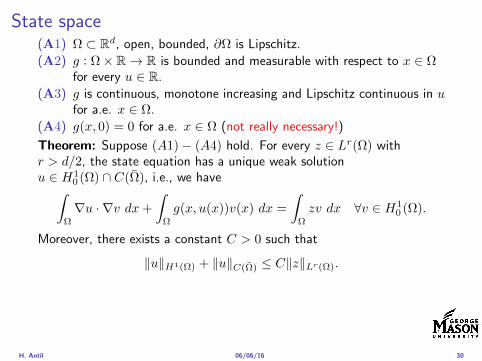
State space(A1) Ω sub Rd open bounded partΩ is Lipschitz
(A2) g Ωtimes Rrarr R is bounded and measurable with respect to x isin Ωfor every u isin R
(A3) g is continuous monotone increasing and Lipschitz continuous in ufor ae x isin Ω
(A4) g(x 0) = 0 for ae x isin Ω (not really necessary)
Theorem Suppose (A1)minus (A4) hold For every z isin Lr(Ω) withr gt d2 the state equation has a unique weak solutionu isin H1
0 (Ω) cap C(Ω) ie we haveintΩ
nablau middot nablav dx+
intΩ
g(x u(x))v(x) dx =
intΩ
zv dx forallv isin H10 (Ω)
Moreover there exists a constant C gt 0 such that
uH1(Ω) + uC(Ω) le CzLr(Ω)
RemarkI The proof of the theorem uses the BrowderndashMinty theorem on
monotone operators
H Antil 060616 30
State space(A1) Ω sub Rd open bounded partΩ is Lipschitz
(A2) g Ωtimes Rrarr R is bounded and measurable with respect to x isin Ωfor every u isin R
(A3) g is continuous monotone increasing and Lipschitz continuous in ufor ae x isin Ω
(A4) g(x 0) = 0 for ae x isin Ω (not really necessary)
Theorem Suppose (A1)minus (A4) hold For every z isin Lr(Ω) withr gt d2 the state equation has a unique weak solutionu isin H1
0 (Ω) cap C(Ω) ie we haveintΩ
nablau middot nablav dx+
intΩ
g(x u(x))v(x) dx =
intΩ
zv dx forallv isin H10 (Ω)
Moreover there exists a constant C gt 0 such that
uH1(Ω) + uC(Ω) le CzLr(Ω)
RemarkI The proof of the theorem uses the BrowderndashMinty theorem on
monotone operators
H Antil 060616 30
Control-to-state map and reduced problem
I Control to state map
S Linfin(Ω)rarr H10 (Ω) cap C(Ω)
is well defined and is globally Lipschitz continuous
I Reduced problem
minJ (z) =1
2S(u)minus ud2L2(Ω) +
λ
2z2L2(Ω)
H Antil 060616 31
Control-to-state map and reduced problem
I Control to state map
S Linfin(Ω)rarr H10 (Ω) cap C(Ω)
is well defined and is globally Lipschitz continuous
I Reduced problem
minJ (z) =1
2S(u)minus ud2L2(Ω) +
λ
2z2L2(Ω)
H Antil 060616 31
First-order necessary conditionsI Lagrangian functional
L(u z p) = J(u z)minusint
Ω
(minus∆u+ g(x u(x))minus z
)p dx
= J(u z)minusint
Ω
(nablau middot nablap+ g(x u(x))pminus zp
)dx
I Adjoint system For all h isin H10 (Ω)
0 = DuL(u z p)h =
intΩ
(uminus ud)h dxminusint
Ω
(nablah middot nablap+ gu(x u(x))ph
)which yields
minus∆p+ gu(x u(x))p = uminus ud in Ω
p = 0 on partΩ
I Control
DzL(u z p)(z minus z) = (p+ λz z minus z) dx ge 0 forallz isin ZadI Gradient
nablaJ (z) = p+ λz
H Antil 060616 32
First-order necessary conditionsI Lagrangian functional
L(u z p) = J(u z)minusint
Ω
(minus∆u+ g(x u(x))minus z
)p dx
= J(u z)minusint
Ω
(nablau middot nablap+ g(x u(x))pminus zp
)dx
I Adjoint system For all h isin H10 (Ω)
0 = DuL(u z p)h =
intΩ
(uminus ud)h dxminusint
Ω
(nablah middot nablap+ gu(x u(x))ph
)which yields
minus∆p+ gu(x u(x))p = uminus ud in Ω
p = 0 on partΩ
I Control
DzL(u z p)(z minus z) = (p+ λz z minus z) dx ge 0 forallz isin Zad
I GradientnablaJ (z) = p+ λz
H Antil 060616 32
First-order necessary conditionsI Lagrangian functional
L(u z p) = J(u z)minusint
Ω
(minus∆u+ g(x u(x))minus z
)p dx
= J(u z)minusint
Ω
(nablau middot nablap+ g(x u(x))pminus zp
)dx
I Adjoint system For all h isin H10 (Ω)
0 = DuL(u z p)h =
intΩ
(uminus ud)h dxminusint
Ω
(nablah middot nablap+ gu(x u(x))ph
)which yields
minus∆p+ gu(x u(x))p = uminus ud in Ω
p = 0 on partΩ
I Control
DzL(u z p)(z minus z) = (p+ λz z minus z) dx ge 0 forallz isin ZadI Gradient
nablaJ (z) = p+ λz
H Antil 060616 32
Differentiability of Nemytskii operator
The rigorous proof uses
Theorem In addition to (A1)-(A4) if
(A5) g is continuously differentiable with respect to u for ae x isin Ωand we have
(i) |gu(x 0)| le K for ae x isin Ω(ii) gu is locally Lipschitz with respect to u isin R
then the Nemytskii operator G u 7rarr g(middot u(middot)) is continuously Frechetdifferentiable from Linfin(Ω) into itself and
(Gprime(u)h)(x) = gu(x u(x))h(x) ae in Ω forallh isin Linfin(Ω)
Remark (A5) holds if g(x u) = g(u) and g isin C2(R)
H Antil 060616 33
Outline
Motivation and examples
Linear elliptic optimal control problems
Differentiation in Banach spaces
First-order necessary conditions
Optimal control of semilinear PDEs
An abstract problem
Discretization using finite element methods
H Antil 060616 34
Gradient computation via adjoint general formI Abstract problem
min J(u z)
subject toc(u z) = 0
and z isin Zad
I Directional derivative Let S be the control to state map(nonlinear in general)
z 7rarr S(z) = u(z)
Under the assumptions of ldquoimplicit function theoremrdquo
J prime(z)h = (nablauJ (u(z) z) Sprime(z)h) + (nablazJ (u(z) z) h)
I Sensitivity of u with respect to z Differentiating the stateequation
cu(S(z) z)Sprime(z)h = minuscz(S(z) z)h
leads toSprime(z)h = minuscu(S(z) z)minus1
(cz(S(z) z)h
)
provided cu(S(z) z)minus1 is well-defined
H Antil 060616 35
Gradient computation via adjoint general formI Abstract problem
min J(u z)
subject toc(u z) = 0
and z isin ZadI Directional derivative Let S be the control to state map
(nonlinear in general)
z 7rarr S(z) = u(z)
Under the assumptions of ldquoimplicit function theoremrdquo
J prime(z)h = (nablauJ (u(z) z) Sprime(z)h) + (nablazJ (u(z) z) h)
I Sensitivity of u with respect to z Differentiating the stateequation
cu(S(z) z)Sprime(z)h = minuscz(S(z) z)h
leads toSprime(z)h = minuscu(S(z) z)minus1
(cz(S(z) z)h
)
provided cu(S(z) z)minus1 is well-defined
H Antil 060616 35
Gradient computation via adjoint general formI Abstract problem
min J(u z)
subject toc(u z) = 0
and z isin ZadI Directional derivative Let S be the control to state map
(nonlinear in general)
z 7rarr S(z) = u(z)
Under the assumptions of ldquoimplicit function theoremrdquo
J prime(z)h = (nablauJ (u(z) z) Sprime(z)h) + (nablazJ (u(z) z) h)
I Sensitivity of u with respect to z Differentiating the stateequation
cu(S(z) z)Sprime(z)h = minuscz(S(z) z)h
leads toSprime(z)h = minuscu(S(z) z)minus1
(cz(S(z) z)h
)
provided cu(S(z) z)minus1 is well-defined
H Antil 060616 35
Adjoint equation and gradient general form
I Directional derivative
J prime(z)h = minus(nablauJ (u(z) z) cu(u(z) z)minus1cz(u(z) z)h
)+ (nablazJ (u(z) z) h)
I Gradient
nablaJ (z) = minuscz(u(z) z)lowast(cu(u(z) z)minuslowastnablauJ (u(z) z)
)+nablazJ (u(z) z)
I Introducing adjoint variable p solving
cu(u(z) z)lowastp = nablauJ (u(z) z)
we arrive at following form of gradient
nablaJ (z) = minuscz(u(z) z)lowastp+nablazJ (u(z) z)
which is tractable
H Antil 060616 36
Adjoint equation and gradient general form
I Directional derivative
J prime(z)h = minus(nablauJ (u(z) z) cu(u(z) z)minus1cz(u(z) z)h
)+ (nablazJ (u(z) z) h)
I Gradient
nablaJ (z) = minuscz(u(z) z)lowast(cu(u(z) z)minuslowastnablauJ (u(z) z)
)+nablazJ (u(z) z)
I Introducing adjoint variable p solving
cu(u(z) z)lowastp = nablauJ (u(z) z)
we arrive at following form of gradient
nablaJ (z) = minuscz(u(z) z)lowastp+nablazJ (u(z) z)
which is tractable
H Antil 060616 36
Adjoint equation and gradient general form
I Directional derivative
J prime(z)h = minus(nablauJ (u(z) z) cu(u(z) z)minus1cz(u(z) z)h
)+ (nablazJ (u(z) z) h)
I Gradient
nablaJ (z) = minuscz(u(z) z)lowast(cu(u(z) z)minuslowastnablauJ (u(z) z)
)+nablazJ (u(z) z)
I Introducing adjoint variable p solving
cu(u(z) z)lowastp = nablauJ (u(z) z)
we arrive at following form of gradient
nablaJ (z) = minuscz(u(z) z)lowastp+nablazJ (u(z) z)
which is tractable
H Antil 060616 36
Hessian computation general form
I Lagrangian L(u z p) = J(u z)minusint
Ωc(u z)p dx Then we have
DzJ (z)h = DzL(u z p)h
I Second order derivative
D2zJ (z)[h1 h2] = DuDzL(u z p)[h1 S
prime(z)h2] +D2zL(u z p)[h1 h2]
+DpDzL(u z p)[h1 Dzp(z)h2]
I We already know Sprime(z)h2 moreover
DpDzL(u z p)[h1 Dzp(z)h2] = minus(cu(u z)h1 Dzp(z)h2
)
It remain to identify Dzp(z)h2
H Antil 060616 37
Hessian computation general form
I Lagrangian L(u z p) = J(u z)minusint
Ωc(u z)p dx Then we have
DzJ (z)h = DzL(u z p)h
I Second order derivative
D2zJ (z)[h1 h2] = DuDzL(u z p)[h1 S
prime(z)h2] +D2zL(u z p)[h1 h2]
+DpDzL(u z p)[h1 Dzp(z)h2]
I We already know Sprime(z)h2 moreover
DpDzL(u z p)[h1 Dzp(z)h2] = minus(cu(u z)h1 Dzp(z)h2
)
It remain to identify Dzp(z)h2
H Antil 060616 37
Hessian computation general form
I Lagrangian L(u z p) = J(u z)minusint
Ωc(u z)p dx Then we have
DzJ (z)h = DzL(u z p)h
I Second order derivative
D2zJ (z)[h1 h2] = DuDzL(u z p)[h1 S
prime(z)h2] +D2zL(u z p)[h1 h2]
+DpDzL(u z p)[h1 Dzp(z)h2]
I We already know Sprime(z)h2 moreover
DpDzL(u z p)[h1 Dzp(z)h2] = minus(cu(u z)h1 Dzp(z)h2
)
It remain to identify Dzp(z)h2
H Antil 060616 37
Outline
Motivation and examples
Linear elliptic optimal control problems
Differentiation in Banach spaces
First-order necessary conditions
Optimal control of semilinear PDEs
An abstract problem
Discretization using finite element methods
H Antil 060616 38
Numerical approximation of Poisson equation MeshTo avoid technical issues we will assume that partΩ is polygonal
I Mesh Let T = K be a mesh of Ω where K sub Rd is an elementthat is isoparametrically equivalent to a unit simplex in Rd
I Conforming mesh We say that the mesh is conforming ifI Ω = cupKisinT KI If K1 cap K2 = x then x is a node of K1 and K2I If K1 cap K2 6= empty and K1 cap K2 6= x then K1 cap K2 is an edgeface
contained in partK1 cap partK2
I Shape regular Let T be the collection of all conformingrefinements of an original mesh T 0 Then T is called shape regularif exist κ gt 0 such that
hKρKle κ forallK isin cupiT i
where hK = diam K ρK = maxρ gt 0|Bρ sub KI Quasi-uniform A family of shape regular meshes is called-quasi
uniform if there exist a constant σ gt 0 such that
maxhKminhK
le σ
uniformly for all meshes in the family
Numerical approximation of Poisson equation MeshTo avoid technical issues we will assume that partΩ is polygonal
I Mesh Let T = K be a mesh of Ω where K sub Rd is an elementthat is isoparametrically equivalent to a unit simplex in Rd
I Conforming mesh We say that the mesh is conforming ifI Ω = cupKisinT KI If K1 cap K2 = x then x is a node of K1 and K2I If K1 cap K2 6= empty and K1 cap K2 6= x then K1 cap K2 is an edgeface
contained in partK1 cap partK2
I Shape regular Let T be the collection of all conformingrefinements of an original mesh T 0 Then T is called shape regularif exist κ gt 0 such that
hKρKle κ forallK isin cupiT i
where hK = diam K ρK = maxρ gt 0|Bρ sub KI Quasi-uniform A family of shape regular meshes is called-quasi
uniform if there exist a constant σ gt 0 such that
maxhKminhK
le σ
uniformly for all meshes in the family
Numerical approximation of Poisson equation MeshTo avoid technical issues we will assume that partΩ is polygonal
I Mesh Let T = K be a mesh of Ω where K sub Rd is an elementthat is isoparametrically equivalent to a unit simplex in Rd
I Conforming mesh We say that the mesh is conforming ifI Ω = cupKisinT KI If K1 cap K2 = x then x is a node of K1 and K2I If K1 cap K2 6= empty and K1 cap K2 6= x then K1 cap K2 is an edgeface
contained in partK1 cap partK2
I Shape regular Let T be the collection of all conformingrefinements of an original mesh T 0 Then T is called shape regularif exist κ gt 0 such that
hKρKle κ forallK isin cupiT i
where hK = diam K ρK = maxρ gt 0|Bρ sub K
I Quasi-uniform A family of shape regular meshes is called-quasiuniform if there exist a constant σ gt 0 such that
maxhKminhK
le σ
uniformly for all meshes in the family
Numerical approximation of Poisson equation MeshTo avoid technical issues we will assume that partΩ is polygonal
I Mesh Let T = K be a mesh of Ω where K sub Rd is an elementthat is isoparametrically equivalent to a unit simplex in Rd
I Conforming mesh We say that the mesh is conforming ifI Ω = cupKisinT KI If K1 cap K2 = x then x is a node of K1 and K2I If K1 cap K2 6= empty and K1 cap K2 6= x then K1 cap K2 is an edgeface
contained in partK1 cap partK2
I Shape regular Let T be the collection of all conformingrefinements of an original mesh T 0 Then T is called shape regularif exist κ gt 0 such that
hKρKle κ forallK isin cupiT i
where hK = diam K ρK = maxρ gt 0|Bρ sub KI Quasi-uniform A family of shape regular meshes is called-quasi
uniform if there exist a constant σ gt 0 such that
maxhKminhK
le σ
uniformly for all meshes in the family
FE space and Galerkin approximationI Finite element space For T isin T we define the finite element
space as
V(T ) = W isin C0(Ω) WK isin P1forallK isin T W |partΩ = 0
where P1 is the set of polynomials of degree at most 1
I Galerkin approximation of continuous problem is given by
Find UT isin V(T )
intΩ
AnablaUT middot nablaV = 〈f V 〉 forallV isin V(T )
The discrete problem is well-posedI Nodal basis Consists of functions ψi isin V(T ) with xi isin N (T )
satisfyingψxi
(xj) = δij
where N (T ) denotes the interior (plus Neumann) nodesI Galerkin orthogonality(
nabla(uminus UT )nablaW)L2(Ω)
= 0 forallW isin V(T )
H Antil 060616 40
FE space and Galerkin approximationI Finite element space For T isin T we define the finite element
space as
V(T ) = W isin C0(Ω) WK isin P1forallK isin T W |partΩ = 0
where P1 is the set of polynomials of degree at most 1I Galerkin approximation of continuous problem is given by
Find UT isin V(T )
intΩ
AnablaUT middot nablaV = 〈f V 〉 forallV isin V(T )
The discrete problem is well-posed
I Nodal basis Consists of functions ψi isin V(T ) with xi isin N (T )satisfying
ψxi(xj) = δij
where N (T ) denotes the interior (plus Neumann) nodesI Galerkin orthogonality(
nabla(uminus UT )nablaW)L2(Ω)
= 0 forallW isin V(T )
H Antil 060616 40
FE space and Galerkin approximationI Finite element space For T isin T we define the finite element
space as
V(T ) = W isin C0(Ω) WK isin P1forallK isin T W |partΩ = 0
where P1 is the set of polynomials of degree at most 1I Galerkin approximation of continuous problem is given by
Find UT isin V(T )
intΩ
AnablaUT middot nablaV = 〈f V 〉 forallV isin V(T )
The discrete problem is well-posedI Nodal basis Consists of functions ψi isin V(T ) with xi isin N (T )
satisfyingψxi
(xj) = δij
where N (T ) denotes the interior (plus Neumann) nodes
I Galerkin orthogonality(nabla(uminus UT )nablaW
)L2(Ω)
= 0 forallW isin V(T )
H Antil 060616 40
FE space and Galerkin approximationI Finite element space For T isin T we define the finite element
space as
V(T ) = W isin C0(Ω) WK isin P1forallK isin T W |partΩ = 0
where P1 is the set of polynomials of degree at most 1I Galerkin approximation of continuous problem is given by
Find UT isin V(T )
intΩ
AnablaUT middot nablaV = 〈f V 〉 forallV isin V(T )
The discrete problem is well-posedI Nodal basis Consists of functions ψi isin V(T ) with xi isin N (T )
satisfyingψxi
(xj) = δij
where N (T ) denotes the interior (plus Neumann) nodesI Galerkin orthogonality(
nabla(uminus UT )nablaW)L2(Ω)
= 0 forallW isin V(T )
H Antil 060616 40
Best approximation
I Cearsquos lemma
nabla(uminus UT )L2(Ω) le C infWisinV(T )
nabla(uminusW )L2(Ω)
I Nodal interpolation operator ΠT C(Ω)rarr V(T ) satisfies
ΠT u(xi) = u(xi) forallxi isin N (T )
and is defined as
ΠT u =sum
xiisinN (T )
u(xi)ψxi
I Error estimates In Cearsquos lemma replace W by ΠT u and thencompute the interpolation error
H Antil 060616 41
Best approximation
I Cearsquos lemma
nabla(uminus UT )L2(Ω) le C infWisinV(T )
nabla(uminusW )L2(Ω)
I Nodal interpolation operator ΠT C(Ω)rarr V(T ) satisfies
ΠT u(xi) = u(xi) forallxi isin N (T )
and is defined as
ΠT u =sum
xiisinN (T )
u(xi)ψxi
I Error estimates In Cearsquos lemma replace W by ΠT u and thencompute the interpolation error
H Antil 060616 41
Best approximation
I Cearsquos lemma
nabla(uminus UT )L2(Ω) le C infWisinV(T )
nabla(uminusW )L2(Ω)
I Nodal interpolation operator ΠT C(Ω)rarr V(T ) satisfies
ΠT u(xi) = u(xi) forallxi isin N (T )
and is defined as
ΠT u =sum
xiisinN (T )
u(xi)ψxi
I Error estimates In Cearsquos lemma replace W by ΠT u and thencompute the interpolation error
H Antil 060616 41
Algebraic system state equation
I Recall UT isin V(T ) solves
a(UT V ) = 〈f V 〉 forallV isin V(T )
I Now setting UT =sumN
j=1 Ujψj V = ψi we get
Nsumj=1
Uja(φj φi) = 〈f ψi〉 i = 1 N
which is the matrix-vector system
AU = F
I Stiffness matrix A is SPD
H Antil 060616 42
Algebraic system state equation
I Recall UT isin V(T ) solves
a(UT V ) = 〈f V 〉 forallV isin V(T )
I Now setting UT =sumN
j=1 Ujψj V = ψi we get
Nsumj=1
Uja(φj φi) = 〈f ψi〉 i = 1 N
which is the matrix-vector system
AU = F
I Stiffness matrix A is SPD
H Antil 060616 42
Algebraic system state equation
I Recall UT isin V(T ) solves
a(UT V ) = 〈f V 〉 forallV isin V(T )
I Now setting UT =sumN
j=1 Ujψj V = ψi we get
Nsumj=1
Uja(φj φi) = 〈f ψi〉 i = 1 N
which is the matrix-vector system
AU = F
I Stiffness matrix A is SPD
H Antil 060616 42
Discrete linear elliptic OCP
min JT (UT ZT ) =1
2UT minus ud2L2(Ω) +
λ
2ZT 2L2(Ω)
subject to
Find UT isin V(T )
intΩ
nablaUT middot nablaV = (ZT V )L2(Ω) forallV isin V(T )
and whereZT isin Zad(T ) = Zad cap Z(T )
is either one of these
Z(T ) =
V(T )L2(Ω) variational discretization (Hinze)WT isin Linfin(Ω) ZT |K isin P0(K)K isin T
H Antil 060616 43
Recent books
F TroltzschOptimal control of partial differential equations volume 112 ofGraduate Studies in MathematicsAmerican Mathematical Society Providence RI 2010Theory methods and applications Translated from the 2005 Germanoriginal by Jurgen Sprekels
K Ito and K KunischLagrange multiplier approach to variational problems andapplications volume 15 of Advances in Design and ControlSociety for Industrial and Applied Mathematics (SIAM)Philadelphia PA 2008
H Antil 060616 44
- Motivation and examples
- Linear elliptic optimal control problems
- Differentiation in Banach spaces
- First-order necessary conditions
- Optimal control of semilinear PDEs
- An abstract problem
- Discretization using finite element methods
-

State space(A1) Ω sub Rd open bounded partΩ is Lipschitz
(A2) g Ωtimes Rrarr R is bounded and measurable with respect to x isin Ωfor every u isin R
(A3) g is continuous monotone increasing and Lipschitz continuous in ufor ae x isin Ω
(A4) g(x 0) = 0 for ae x isin Ω (not really necessary)
Theorem Suppose (A1)minus (A4) hold For every z isin Lr(Ω) withr gt d2 the state equation has a unique weak solutionu isin H1
0 (Ω) cap C(Ω) ie we haveintΩ
nablau middot nablav dx+
intΩ
g(x u(x))v(x) dx =
intΩ
zv dx forallv isin H10 (Ω)
Moreover there exists a constant C gt 0 such that
uH1(Ω) + uC(Ω) le CzLr(Ω)
RemarkI The proof of the theorem uses the BrowderndashMinty theorem on
monotone operators
H Antil 060616 30
Control-to-state map and reduced problem
I Control to state map
S Linfin(Ω)rarr H10 (Ω) cap C(Ω)
is well defined and is globally Lipschitz continuous
I Reduced problem
minJ (z) =1
2S(u)minus ud2L2(Ω) +
λ
2z2L2(Ω)
H Antil 060616 31
Control-to-state map and reduced problem
I Control to state map
S Linfin(Ω)rarr H10 (Ω) cap C(Ω)
is well defined and is globally Lipschitz continuous
I Reduced problem
minJ (z) =1
2S(u)minus ud2L2(Ω) +
λ
2z2L2(Ω)
H Antil 060616 31
First-order necessary conditionsI Lagrangian functional
L(u z p) = J(u z)minusint
Ω
(minus∆u+ g(x u(x))minus z
)p dx
= J(u z)minusint
Ω
(nablau middot nablap+ g(x u(x))pminus zp
)dx
I Adjoint system For all h isin H10 (Ω)
0 = DuL(u z p)h =
intΩ
(uminus ud)h dxminusint
Ω
(nablah middot nablap+ gu(x u(x))ph
)which yields
minus∆p+ gu(x u(x))p = uminus ud in Ω
p = 0 on partΩ
I Control
DzL(u z p)(z minus z) = (p+ λz z minus z) dx ge 0 forallz isin ZadI Gradient
nablaJ (z) = p+ λz
H Antil 060616 32
First-order necessary conditionsI Lagrangian functional
L(u z p) = J(u z)minusint
Ω
(minus∆u+ g(x u(x))minus z
)p dx
= J(u z)minusint
Ω
(nablau middot nablap+ g(x u(x))pminus zp
)dx
I Adjoint system For all h isin H10 (Ω)
0 = DuL(u z p)h =
intΩ
(uminus ud)h dxminusint
Ω
(nablah middot nablap+ gu(x u(x))ph
)which yields
minus∆p+ gu(x u(x))p = uminus ud in Ω
p = 0 on partΩ
I Control
DzL(u z p)(z minus z) = (p+ λz z minus z) dx ge 0 forallz isin Zad
I GradientnablaJ (z) = p+ λz
H Antil 060616 32
First-order necessary conditionsI Lagrangian functional
L(u z p) = J(u z)minusint
Ω
(minus∆u+ g(x u(x))minus z
)p dx
= J(u z)minusint
Ω
(nablau middot nablap+ g(x u(x))pminus zp
)dx
I Adjoint system For all h isin H10 (Ω)
0 = DuL(u z p)h =
intΩ
(uminus ud)h dxminusint
Ω
(nablah middot nablap+ gu(x u(x))ph
)which yields
minus∆p+ gu(x u(x))p = uminus ud in Ω
p = 0 on partΩ
I Control
DzL(u z p)(z minus z) = (p+ λz z minus z) dx ge 0 forallz isin ZadI Gradient
nablaJ (z) = p+ λz
H Antil 060616 32
Differentiability of Nemytskii operator
The rigorous proof uses
Theorem In addition to (A1)-(A4) if
(A5) g is continuously differentiable with respect to u for ae x isin Ωand we have
(i) |gu(x 0)| le K for ae x isin Ω(ii) gu is locally Lipschitz with respect to u isin R
then the Nemytskii operator G u 7rarr g(middot u(middot)) is continuously Frechetdifferentiable from Linfin(Ω) into itself and
(Gprime(u)h)(x) = gu(x u(x))h(x) ae in Ω forallh isin Linfin(Ω)
Remark (A5) holds if g(x u) = g(u) and g isin C2(R)
H Antil 060616 33
Outline
Motivation and examples
Linear elliptic optimal control problems
Differentiation in Banach spaces
First-order necessary conditions
Optimal control of semilinear PDEs
An abstract problem
Discretization using finite element methods
H Antil 060616 34
Gradient computation via adjoint general formI Abstract problem
min J(u z)
subject toc(u z) = 0
and z isin Zad
I Directional derivative Let S be the control to state map(nonlinear in general)
z 7rarr S(z) = u(z)
Under the assumptions of ldquoimplicit function theoremrdquo
J prime(z)h = (nablauJ (u(z) z) Sprime(z)h) + (nablazJ (u(z) z) h)
I Sensitivity of u with respect to z Differentiating the stateequation
cu(S(z) z)Sprime(z)h = minuscz(S(z) z)h
leads toSprime(z)h = minuscu(S(z) z)minus1
(cz(S(z) z)h
)
provided cu(S(z) z)minus1 is well-defined
H Antil 060616 35
Gradient computation via adjoint general formI Abstract problem
min J(u z)
subject toc(u z) = 0
and z isin ZadI Directional derivative Let S be the control to state map
(nonlinear in general)
z 7rarr S(z) = u(z)
Under the assumptions of ldquoimplicit function theoremrdquo
J prime(z)h = (nablauJ (u(z) z) Sprime(z)h) + (nablazJ (u(z) z) h)
I Sensitivity of u with respect to z Differentiating the stateequation
cu(S(z) z)Sprime(z)h = minuscz(S(z) z)h
leads toSprime(z)h = minuscu(S(z) z)minus1
(cz(S(z) z)h
)
provided cu(S(z) z)minus1 is well-defined
H Antil 060616 35
Gradient computation via adjoint general formI Abstract problem
min J(u z)
subject toc(u z) = 0
and z isin ZadI Directional derivative Let S be the control to state map
(nonlinear in general)
z 7rarr S(z) = u(z)
Under the assumptions of ldquoimplicit function theoremrdquo
J prime(z)h = (nablauJ (u(z) z) Sprime(z)h) + (nablazJ (u(z) z) h)
I Sensitivity of u with respect to z Differentiating the stateequation
cu(S(z) z)Sprime(z)h = minuscz(S(z) z)h
leads toSprime(z)h = minuscu(S(z) z)minus1
(cz(S(z) z)h
)
provided cu(S(z) z)minus1 is well-defined
H Antil 060616 35
Adjoint equation and gradient general form
I Directional derivative
J prime(z)h = minus(nablauJ (u(z) z) cu(u(z) z)minus1cz(u(z) z)h
)+ (nablazJ (u(z) z) h)
I Gradient
nablaJ (z) = minuscz(u(z) z)lowast(cu(u(z) z)minuslowastnablauJ (u(z) z)
)+nablazJ (u(z) z)
I Introducing adjoint variable p solving
cu(u(z) z)lowastp = nablauJ (u(z) z)
we arrive at following form of gradient
nablaJ (z) = minuscz(u(z) z)lowastp+nablazJ (u(z) z)
which is tractable
H Antil 060616 36
Adjoint equation and gradient general form
I Directional derivative
J prime(z)h = minus(nablauJ (u(z) z) cu(u(z) z)minus1cz(u(z) z)h
)+ (nablazJ (u(z) z) h)
I Gradient
nablaJ (z) = minuscz(u(z) z)lowast(cu(u(z) z)minuslowastnablauJ (u(z) z)
)+nablazJ (u(z) z)
I Introducing adjoint variable p solving
cu(u(z) z)lowastp = nablauJ (u(z) z)
we arrive at following form of gradient
nablaJ (z) = minuscz(u(z) z)lowastp+nablazJ (u(z) z)
which is tractable
H Antil 060616 36
Adjoint equation and gradient general form
I Directional derivative
J prime(z)h = minus(nablauJ (u(z) z) cu(u(z) z)minus1cz(u(z) z)h
)+ (nablazJ (u(z) z) h)
I Gradient
nablaJ (z) = minuscz(u(z) z)lowast(cu(u(z) z)minuslowastnablauJ (u(z) z)
)+nablazJ (u(z) z)
I Introducing adjoint variable p solving
cu(u(z) z)lowastp = nablauJ (u(z) z)
we arrive at following form of gradient
nablaJ (z) = minuscz(u(z) z)lowastp+nablazJ (u(z) z)
which is tractable
H Antil 060616 36
Hessian computation general form
I Lagrangian L(u z p) = J(u z)minusint
Ωc(u z)p dx Then we have
DzJ (z)h = DzL(u z p)h
I Second order derivative
D2zJ (z)[h1 h2] = DuDzL(u z p)[h1 S
prime(z)h2] +D2zL(u z p)[h1 h2]
+DpDzL(u z p)[h1 Dzp(z)h2]
I We already know Sprime(z)h2 moreover
DpDzL(u z p)[h1 Dzp(z)h2] = minus(cu(u z)h1 Dzp(z)h2
)
It remain to identify Dzp(z)h2
H Antil 060616 37
Hessian computation general form
I Lagrangian L(u z p) = J(u z)minusint
Ωc(u z)p dx Then we have
DzJ (z)h = DzL(u z p)h
I Second order derivative
D2zJ (z)[h1 h2] = DuDzL(u z p)[h1 S
prime(z)h2] +D2zL(u z p)[h1 h2]
+DpDzL(u z p)[h1 Dzp(z)h2]
I We already know Sprime(z)h2 moreover
DpDzL(u z p)[h1 Dzp(z)h2] = minus(cu(u z)h1 Dzp(z)h2
)
It remain to identify Dzp(z)h2
H Antil 060616 37
Hessian computation general form
I Lagrangian L(u z p) = J(u z)minusint
Ωc(u z)p dx Then we have
DzJ (z)h = DzL(u z p)h
I Second order derivative
D2zJ (z)[h1 h2] = DuDzL(u z p)[h1 S
prime(z)h2] +D2zL(u z p)[h1 h2]
+DpDzL(u z p)[h1 Dzp(z)h2]
I We already know Sprime(z)h2 moreover
DpDzL(u z p)[h1 Dzp(z)h2] = minus(cu(u z)h1 Dzp(z)h2
)
It remain to identify Dzp(z)h2
H Antil 060616 37
Outline
Motivation and examples
Linear elliptic optimal control problems
Differentiation in Banach spaces
First-order necessary conditions
Optimal control of semilinear PDEs
An abstract problem
Discretization using finite element methods
H Antil 060616 38
Numerical approximation of Poisson equation MeshTo avoid technical issues we will assume that partΩ is polygonal
I Mesh Let T = K be a mesh of Ω where K sub Rd is an elementthat is isoparametrically equivalent to a unit simplex in Rd
I Conforming mesh We say that the mesh is conforming ifI Ω = cupKisinT KI If K1 cap K2 = x then x is a node of K1 and K2I If K1 cap K2 6= empty and K1 cap K2 6= x then K1 cap K2 is an edgeface
contained in partK1 cap partK2
I Shape regular Let T be the collection of all conformingrefinements of an original mesh T 0 Then T is called shape regularif exist κ gt 0 such that
hKρKle κ forallK isin cupiT i
where hK = diam K ρK = maxρ gt 0|Bρ sub KI Quasi-uniform A family of shape regular meshes is called-quasi
uniform if there exist a constant σ gt 0 such that
maxhKminhK
le σ
uniformly for all meshes in the family
Numerical approximation of Poisson equation MeshTo avoid technical issues we will assume that partΩ is polygonal
I Mesh Let T = K be a mesh of Ω where K sub Rd is an elementthat is isoparametrically equivalent to a unit simplex in Rd
I Conforming mesh We say that the mesh is conforming ifI Ω = cupKisinT KI If K1 cap K2 = x then x is a node of K1 and K2I If K1 cap K2 6= empty and K1 cap K2 6= x then K1 cap K2 is an edgeface
contained in partK1 cap partK2
I Shape regular Let T be the collection of all conformingrefinements of an original mesh T 0 Then T is called shape regularif exist κ gt 0 such that
hKρKle κ forallK isin cupiT i
where hK = diam K ρK = maxρ gt 0|Bρ sub KI Quasi-uniform A family of shape regular meshes is called-quasi
uniform if there exist a constant σ gt 0 such that
maxhKminhK
le σ
uniformly for all meshes in the family
Numerical approximation of Poisson equation MeshTo avoid technical issues we will assume that partΩ is polygonal
I Mesh Let T = K be a mesh of Ω where K sub Rd is an elementthat is isoparametrically equivalent to a unit simplex in Rd
I Conforming mesh We say that the mesh is conforming ifI Ω = cupKisinT KI If K1 cap K2 = x then x is a node of K1 and K2I If K1 cap K2 6= empty and K1 cap K2 6= x then K1 cap K2 is an edgeface
contained in partK1 cap partK2
I Shape regular Let T be the collection of all conformingrefinements of an original mesh T 0 Then T is called shape regularif exist κ gt 0 such that
hKρKle κ forallK isin cupiT i
where hK = diam K ρK = maxρ gt 0|Bρ sub K
I Quasi-uniform A family of shape regular meshes is called-quasiuniform if there exist a constant σ gt 0 such that
maxhKminhK
le σ
uniformly for all meshes in the family
Numerical approximation of Poisson equation MeshTo avoid technical issues we will assume that partΩ is polygonal
I Mesh Let T = K be a mesh of Ω where K sub Rd is an elementthat is isoparametrically equivalent to a unit simplex in Rd
I Conforming mesh We say that the mesh is conforming ifI Ω = cupKisinT KI If K1 cap K2 = x then x is a node of K1 and K2I If K1 cap K2 6= empty and K1 cap K2 6= x then K1 cap K2 is an edgeface
contained in partK1 cap partK2
I Shape regular Let T be the collection of all conformingrefinements of an original mesh T 0 Then T is called shape regularif exist κ gt 0 such that
hKρKle κ forallK isin cupiT i
where hK = diam K ρK = maxρ gt 0|Bρ sub KI Quasi-uniform A family of shape regular meshes is called-quasi
uniform if there exist a constant σ gt 0 such that
maxhKminhK
le σ
uniformly for all meshes in the family
FE space and Galerkin approximationI Finite element space For T isin T we define the finite element
space as
V(T ) = W isin C0(Ω) WK isin P1forallK isin T W |partΩ = 0
where P1 is the set of polynomials of degree at most 1
I Galerkin approximation of continuous problem is given by
Find UT isin V(T )
intΩ
AnablaUT middot nablaV = 〈f V 〉 forallV isin V(T )
The discrete problem is well-posedI Nodal basis Consists of functions ψi isin V(T ) with xi isin N (T )
satisfyingψxi
(xj) = δij
where N (T ) denotes the interior (plus Neumann) nodesI Galerkin orthogonality(
nabla(uminus UT )nablaW)L2(Ω)
= 0 forallW isin V(T )
H Antil 060616 40
FE space and Galerkin approximationI Finite element space For T isin T we define the finite element
space as
V(T ) = W isin C0(Ω) WK isin P1forallK isin T W |partΩ = 0
where P1 is the set of polynomials of degree at most 1I Galerkin approximation of continuous problem is given by
Find UT isin V(T )
intΩ
AnablaUT middot nablaV = 〈f V 〉 forallV isin V(T )
The discrete problem is well-posed
I Nodal basis Consists of functions ψi isin V(T ) with xi isin N (T )satisfying
ψxi(xj) = δij
where N (T ) denotes the interior (plus Neumann) nodesI Galerkin orthogonality(
nabla(uminus UT )nablaW)L2(Ω)
= 0 forallW isin V(T )
H Antil 060616 40
FE space and Galerkin approximationI Finite element space For T isin T we define the finite element
space as
V(T ) = W isin C0(Ω) WK isin P1forallK isin T W |partΩ = 0
where P1 is the set of polynomials of degree at most 1I Galerkin approximation of continuous problem is given by
Find UT isin V(T )
intΩ
AnablaUT middot nablaV = 〈f V 〉 forallV isin V(T )
The discrete problem is well-posedI Nodal basis Consists of functions ψi isin V(T ) with xi isin N (T )
satisfyingψxi
(xj) = δij
where N (T ) denotes the interior (plus Neumann) nodes
I Galerkin orthogonality(nabla(uminus UT )nablaW
)L2(Ω)
= 0 forallW isin V(T )
H Antil 060616 40
FE space and Galerkin approximationI Finite element space For T isin T we define the finite element
space as
V(T ) = W isin C0(Ω) WK isin P1forallK isin T W |partΩ = 0
where P1 is the set of polynomials of degree at most 1I Galerkin approximation of continuous problem is given by
Find UT isin V(T )
intΩ
AnablaUT middot nablaV = 〈f V 〉 forallV isin V(T )
The discrete problem is well-posedI Nodal basis Consists of functions ψi isin V(T ) with xi isin N (T )
satisfyingψxi
(xj) = δij
where N (T ) denotes the interior (plus Neumann) nodesI Galerkin orthogonality(
nabla(uminus UT )nablaW)L2(Ω)
= 0 forallW isin V(T )
H Antil 060616 40
Best approximation
I Cearsquos lemma
nabla(uminus UT )L2(Ω) le C infWisinV(T )
nabla(uminusW )L2(Ω)
I Nodal interpolation operator ΠT C(Ω)rarr V(T ) satisfies
ΠT u(xi) = u(xi) forallxi isin N (T )
and is defined as
ΠT u =sum
xiisinN (T )
u(xi)ψxi
I Error estimates In Cearsquos lemma replace W by ΠT u and thencompute the interpolation error
H Antil 060616 41
Best approximation
I Cearsquos lemma
nabla(uminus UT )L2(Ω) le C infWisinV(T )
nabla(uminusW )L2(Ω)
I Nodal interpolation operator ΠT C(Ω)rarr V(T ) satisfies
ΠT u(xi) = u(xi) forallxi isin N (T )
and is defined as
ΠT u =sum
xiisinN (T )
u(xi)ψxi
I Error estimates In Cearsquos lemma replace W by ΠT u and thencompute the interpolation error
H Antil 060616 41
Best approximation
I Cearsquos lemma
nabla(uminus UT )L2(Ω) le C infWisinV(T )
nabla(uminusW )L2(Ω)
I Nodal interpolation operator ΠT C(Ω)rarr V(T ) satisfies
ΠT u(xi) = u(xi) forallxi isin N (T )
and is defined as
ΠT u =sum
xiisinN (T )
u(xi)ψxi
I Error estimates In Cearsquos lemma replace W by ΠT u and thencompute the interpolation error
H Antil 060616 41
Algebraic system state equation
I Recall UT isin V(T ) solves
a(UT V ) = 〈f V 〉 forallV isin V(T )
I Now setting UT =sumN
j=1 Ujψj V = ψi we get
Nsumj=1
Uja(φj φi) = 〈f ψi〉 i = 1 N
which is the matrix-vector system
AU = F
I Stiffness matrix A is SPD
H Antil 060616 42
Algebraic system state equation
I Recall UT isin V(T ) solves
a(UT V ) = 〈f V 〉 forallV isin V(T )
I Now setting UT =sumN
j=1 Ujψj V = ψi we get
Nsumj=1
Uja(φj φi) = 〈f ψi〉 i = 1 N
which is the matrix-vector system
AU = F
I Stiffness matrix A is SPD
H Antil 060616 42
Algebraic system state equation
I Recall UT isin V(T ) solves
a(UT V ) = 〈f V 〉 forallV isin V(T )
I Now setting UT =sumN
j=1 Ujψj V = ψi we get
Nsumj=1
Uja(φj φi) = 〈f ψi〉 i = 1 N
which is the matrix-vector system
AU = F
I Stiffness matrix A is SPD
H Antil 060616 42
Discrete linear elliptic OCP
min JT (UT ZT ) =1
2UT minus ud2L2(Ω) +
λ
2ZT 2L2(Ω)
subject to
Find UT isin V(T )
intΩ
nablaUT middot nablaV = (ZT V )L2(Ω) forallV isin V(T )
and whereZT isin Zad(T ) = Zad cap Z(T )
is either one of these
Z(T ) =
V(T )L2(Ω) variational discretization (Hinze)WT isin Linfin(Ω) ZT |K isin P0(K)K isin T
H Antil 060616 43
Recent books
F TroltzschOptimal control of partial differential equations volume 112 ofGraduate Studies in MathematicsAmerican Mathematical Society Providence RI 2010Theory methods and applications Translated from the 2005 Germanoriginal by Jurgen Sprekels
K Ito and K KunischLagrange multiplier approach to variational problems andapplications volume 15 of Advances in Design and ControlSociety for Industrial and Applied Mathematics (SIAM)Philadelphia PA 2008
H Antil 060616 44
- Motivation and examples
- Linear elliptic optimal control problems
- Differentiation in Banach spaces
- First-order necessary conditions
- Optimal control of semilinear PDEs
- An abstract problem
- Discretization using finite element methods
-
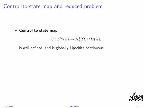
Control-to-state map and reduced problem
I Control to state map
S Linfin(Ω)rarr H10 (Ω) cap C(Ω)
is well defined and is globally Lipschitz continuous
I Reduced problem
minJ (z) =1
2S(u)minus ud2L2(Ω) +
λ
2z2L2(Ω)
H Antil 060616 31
Control-to-state map and reduced problem
I Control to state map
S Linfin(Ω)rarr H10 (Ω) cap C(Ω)
is well defined and is globally Lipschitz continuous
I Reduced problem
minJ (z) =1
2S(u)minus ud2L2(Ω) +
λ
2z2L2(Ω)
H Antil 060616 31
First-order necessary conditionsI Lagrangian functional
L(u z p) = J(u z)minusint
Ω
(minus∆u+ g(x u(x))minus z
)p dx
= J(u z)minusint
Ω
(nablau middot nablap+ g(x u(x))pminus zp
)dx
I Adjoint system For all h isin H10 (Ω)
0 = DuL(u z p)h =
intΩ
(uminus ud)h dxminusint
Ω
(nablah middot nablap+ gu(x u(x))ph
)which yields
minus∆p+ gu(x u(x))p = uminus ud in Ω
p = 0 on partΩ
I Control
DzL(u z p)(z minus z) = (p+ λz z minus z) dx ge 0 forallz isin ZadI Gradient
nablaJ (z) = p+ λz
H Antil 060616 32
First-order necessary conditionsI Lagrangian functional
L(u z p) = J(u z)minusint
Ω
(minus∆u+ g(x u(x))minus z
)p dx
= J(u z)minusint
Ω
(nablau middot nablap+ g(x u(x))pminus zp
)dx
I Adjoint system For all h isin H10 (Ω)
0 = DuL(u z p)h =
intΩ
(uminus ud)h dxminusint
Ω
(nablah middot nablap+ gu(x u(x))ph
)which yields
minus∆p+ gu(x u(x))p = uminus ud in Ω
p = 0 on partΩ
I Control
DzL(u z p)(z minus z) = (p+ λz z minus z) dx ge 0 forallz isin Zad
I GradientnablaJ (z) = p+ λz
H Antil 060616 32
First-order necessary conditionsI Lagrangian functional
L(u z p) = J(u z)minusint
Ω
(minus∆u+ g(x u(x))minus z
)p dx
= J(u z)minusint
Ω
(nablau middot nablap+ g(x u(x))pminus zp
)dx
I Adjoint system For all h isin H10 (Ω)
0 = DuL(u z p)h =
intΩ
(uminus ud)h dxminusint
Ω
(nablah middot nablap+ gu(x u(x))ph
)which yields
minus∆p+ gu(x u(x))p = uminus ud in Ω
p = 0 on partΩ
I Control
DzL(u z p)(z minus z) = (p+ λz z minus z) dx ge 0 forallz isin ZadI Gradient
nablaJ (z) = p+ λz
H Antil 060616 32
Differentiability of Nemytskii operator
The rigorous proof uses
Theorem In addition to (A1)-(A4) if
(A5) g is continuously differentiable with respect to u for ae x isin Ωand we have
(i) |gu(x 0)| le K for ae x isin Ω(ii) gu is locally Lipschitz with respect to u isin R
then the Nemytskii operator G u 7rarr g(middot u(middot)) is continuously Frechetdifferentiable from Linfin(Ω) into itself and
(Gprime(u)h)(x) = gu(x u(x))h(x) ae in Ω forallh isin Linfin(Ω)
Remark (A5) holds if g(x u) = g(u) and g isin C2(R)
H Antil 060616 33
Outline
Motivation and examples
Linear elliptic optimal control problems
Differentiation in Banach spaces
First-order necessary conditions
Optimal control of semilinear PDEs
An abstract problem
Discretization using finite element methods
H Antil 060616 34
Gradient computation via adjoint general formI Abstract problem
min J(u z)
subject toc(u z) = 0
and z isin Zad
I Directional derivative Let S be the control to state map(nonlinear in general)
z 7rarr S(z) = u(z)
Under the assumptions of ldquoimplicit function theoremrdquo
J prime(z)h = (nablauJ (u(z) z) Sprime(z)h) + (nablazJ (u(z) z) h)
I Sensitivity of u with respect to z Differentiating the stateequation
cu(S(z) z)Sprime(z)h = minuscz(S(z) z)h
leads toSprime(z)h = minuscu(S(z) z)minus1
(cz(S(z) z)h
)
provided cu(S(z) z)minus1 is well-defined
H Antil 060616 35
Gradient computation via adjoint general formI Abstract problem
min J(u z)
subject toc(u z) = 0
and z isin ZadI Directional derivative Let S be the control to state map
(nonlinear in general)
z 7rarr S(z) = u(z)
Under the assumptions of ldquoimplicit function theoremrdquo
J prime(z)h = (nablauJ (u(z) z) Sprime(z)h) + (nablazJ (u(z) z) h)
I Sensitivity of u with respect to z Differentiating the stateequation
cu(S(z) z)Sprime(z)h = minuscz(S(z) z)h
leads toSprime(z)h = minuscu(S(z) z)minus1
(cz(S(z) z)h
)
provided cu(S(z) z)minus1 is well-defined
H Antil 060616 35
Gradient computation via adjoint general formI Abstract problem
min J(u z)
subject toc(u z) = 0
and z isin ZadI Directional derivative Let S be the control to state map
(nonlinear in general)
z 7rarr S(z) = u(z)
Under the assumptions of ldquoimplicit function theoremrdquo
J prime(z)h = (nablauJ (u(z) z) Sprime(z)h) + (nablazJ (u(z) z) h)
I Sensitivity of u with respect to z Differentiating the stateequation
cu(S(z) z)Sprime(z)h = minuscz(S(z) z)h
leads toSprime(z)h = minuscu(S(z) z)minus1
(cz(S(z) z)h
)
provided cu(S(z) z)minus1 is well-defined
H Antil 060616 35
Adjoint equation and gradient general form
I Directional derivative
J prime(z)h = minus(nablauJ (u(z) z) cu(u(z) z)minus1cz(u(z) z)h
)+ (nablazJ (u(z) z) h)
I Gradient
nablaJ (z) = minuscz(u(z) z)lowast(cu(u(z) z)minuslowastnablauJ (u(z) z)
)+nablazJ (u(z) z)
I Introducing adjoint variable p solving
cu(u(z) z)lowastp = nablauJ (u(z) z)
we arrive at following form of gradient
nablaJ (z) = minuscz(u(z) z)lowastp+nablazJ (u(z) z)
which is tractable
H Antil 060616 36
Adjoint equation and gradient general form
I Directional derivative
J prime(z)h = minus(nablauJ (u(z) z) cu(u(z) z)minus1cz(u(z) z)h
)+ (nablazJ (u(z) z) h)
I Gradient
nablaJ (z) = minuscz(u(z) z)lowast(cu(u(z) z)minuslowastnablauJ (u(z) z)
)+nablazJ (u(z) z)
I Introducing adjoint variable p solving
cu(u(z) z)lowastp = nablauJ (u(z) z)
we arrive at following form of gradient
nablaJ (z) = minuscz(u(z) z)lowastp+nablazJ (u(z) z)
which is tractable
H Antil 060616 36
Adjoint equation and gradient general form
I Directional derivative
J prime(z)h = minus(nablauJ (u(z) z) cu(u(z) z)minus1cz(u(z) z)h
)+ (nablazJ (u(z) z) h)
I Gradient
nablaJ (z) = minuscz(u(z) z)lowast(cu(u(z) z)minuslowastnablauJ (u(z) z)
)+nablazJ (u(z) z)
I Introducing adjoint variable p solving
cu(u(z) z)lowastp = nablauJ (u(z) z)
we arrive at following form of gradient
nablaJ (z) = minuscz(u(z) z)lowastp+nablazJ (u(z) z)
which is tractable
H Antil 060616 36
Hessian computation general form
I Lagrangian L(u z p) = J(u z)minusint
Ωc(u z)p dx Then we have
DzJ (z)h = DzL(u z p)h
I Second order derivative
D2zJ (z)[h1 h2] = DuDzL(u z p)[h1 S
prime(z)h2] +D2zL(u z p)[h1 h2]
+DpDzL(u z p)[h1 Dzp(z)h2]
I We already know Sprime(z)h2 moreover
DpDzL(u z p)[h1 Dzp(z)h2] = minus(cu(u z)h1 Dzp(z)h2
)
It remain to identify Dzp(z)h2
H Antil 060616 37
Hessian computation general form
I Lagrangian L(u z p) = J(u z)minusint
Ωc(u z)p dx Then we have
DzJ (z)h = DzL(u z p)h
I Second order derivative
D2zJ (z)[h1 h2] = DuDzL(u z p)[h1 S
prime(z)h2] +D2zL(u z p)[h1 h2]
+DpDzL(u z p)[h1 Dzp(z)h2]
I We already know Sprime(z)h2 moreover
DpDzL(u z p)[h1 Dzp(z)h2] = minus(cu(u z)h1 Dzp(z)h2
)
It remain to identify Dzp(z)h2
H Antil 060616 37
Hessian computation general form
I Lagrangian L(u z p) = J(u z)minusint
Ωc(u z)p dx Then we have
DzJ (z)h = DzL(u z p)h
I Second order derivative
D2zJ (z)[h1 h2] = DuDzL(u z p)[h1 S
prime(z)h2] +D2zL(u z p)[h1 h2]
+DpDzL(u z p)[h1 Dzp(z)h2]
I We already know Sprime(z)h2 moreover
DpDzL(u z p)[h1 Dzp(z)h2] = minus(cu(u z)h1 Dzp(z)h2
)
It remain to identify Dzp(z)h2
H Antil 060616 37
Outline
Motivation and examples
Linear elliptic optimal control problems
Differentiation in Banach spaces
First-order necessary conditions
Optimal control of semilinear PDEs
An abstract problem
Discretization using finite element methods
H Antil 060616 38
Numerical approximation of Poisson equation MeshTo avoid technical issues we will assume that partΩ is polygonal
I Mesh Let T = K be a mesh of Ω where K sub Rd is an elementthat is isoparametrically equivalent to a unit simplex in Rd
I Conforming mesh We say that the mesh is conforming ifI Ω = cupKisinT KI If K1 cap K2 = x then x is a node of K1 and K2I If K1 cap K2 6= empty and K1 cap K2 6= x then K1 cap K2 is an edgeface
contained in partK1 cap partK2
I Shape regular Let T be the collection of all conformingrefinements of an original mesh T 0 Then T is called shape regularif exist κ gt 0 such that
hKρKle κ forallK isin cupiT i
where hK = diam K ρK = maxρ gt 0|Bρ sub KI Quasi-uniform A family of shape regular meshes is called-quasi
uniform if there exist a constant σ gt 0 such that
maxhKminhK
le σ
uniformly for all meshes in the family
Numerical approximation of Poisson equation MeshTo avoid technical issues we will assume that partΩ is polygonal
I Mesh Let T = K be a mesh of Ω where K sub Rd is an elementthat is isoparametrically equivalent to a unit simplex in Rd
I Conforming mesh We say that the mesh is conforming ifI Ω = cupKisinT KI If K1 cap K2 = x then x is a node of K1 and K2I If K1 cap K2 6= empty and K1 cap K2 6= x then K1 cap K2 is an edgeface
contained in partK1 cap partK2
I Shape regular Let T be the collection of all conformingrefinements of an original mesh T 0 Then T is called shape regularif exist κ gt 0 such that
hKρKle κ forallK isin cupiT i
where hK = diam K ρK = maxρ gt 0|Bρ sub KI Quasi-uniform A family of shape regular meshes is called-quasi
uniform if there exist a constant σ gt 0 such that
maxhKminhK
le σ
uniformly for all meshes in the family
Numerical approximation of Poisson equation MeshTo avoid technical issues we will assume that partΩ is polygonal
I Mesh Let T = K be a mesh of Ω where K sub Rd is an elementthat is isoparametrically equivalent to a unit simplex in Rd
I Conforming mesh We say that the mesh is conforming ifI Ω = cupKisinT KI If K1 cap K2 = x then x is a node of K1 and K2I If K1 cap K2 6= empty and K1 cap K2 6= x then K1 cap K2 is an edgeface
contained in partK1 cap partK2
I Shape regular Let T be the collection of all conformingrefinements of an original mesh T 0 Then T is called shape regularif exist κ gt 0 such that
hKρKle κ forallK isin cupiT i
where hK = diam K ρK = maxρ gt 0|Bρ sub K
I Quasi-uniform A family of shape regular meshes is called-quasiuniform if there exist a constant σ gt 0 such that
maxhKminhK
le σ
uniformly for all meshes in the family
Numerical approximation of Poisson equation MeshTo avoid technical issues we will assume that partΩ is polygonal
I Mesh Let T = K be a mesh of Ω where K sub Rd is an elementthat is isoparametrically equivalent to a unit simplex in Rd
I Conforming mesh We say that the mesh is conforming ifI Ω = cupKisinT KI If K1 cap K2 = x then x is a node of K1 and K2I If K1 cap K2 6= empty and K1 cap K2 6= x then K1 cap K2 is an edgeface
contained in partK1 cap partK2
I Shape regular Let T be the collection of all conformingrefinements of an original mesh T 0 Then T is called shape regularif exist κ gt 0 such that
hKρKle κ forallK isin cupiT i
where hK = diam K ρK = maxρ gt 0|Bρ sub KI Quasi-uniform A family of shape regular meshes is called-quasi
uniform if there exist a constant σ gt 0 such that
maxhKminhK
le σ
uniformly for all meshes in the family
FE space and Galerkin approximationI Finite element space For T isin T we define the finite element
space as
V(T ) = W isin C0(Ω) WK isin P1forallK isin T W |partΩ = 0
where P1 is the set of polynomials of degree at most 1
I Galerkin approximation of continuous problem is given by
Find UT isin V(T )
intΩ
AnablaUT middot nablaV = 〈f V 〉 forallV isin V(T )
The discrete problem is well-posedI Nodal basis Consists of functions ψi isin V(T ) with xi isin N (T )
satisfyingψxi
(xj) = δij
where N (T ) denotes the interior (plus Neumann) nodesI Galerkin orthogonality(
nabla(uminus UT )nablaW)L2(Ω)
= 0 forallW isin V(T )
H Antil 060616 40
FE space and Galerkin approximationI Finite element space For T isin T we define the finite element
space as
V(T ) = W isin C0(Ω) WK isin P1forallK isin T W |partΩ = 0
where P1 is the set of polynomials of degree at most 1I Galerkin approximation of continuous problem is given by
Find UT isin V(T )
intΩ
AnablaUT middot nablaV = 〈f V 〉 forallV isin V(T )
The discrete problem is well-posed
I Nodal basis Consists of functions ψi isin V(T ) with xi isin N (T )satisfying
ψxi(xj) = δij
where N (T ) denotes the interior (plus Neumann) nodesI Galerkin orthogonality(
nabla(uminus UT )nablaW)L2(Ω)
= 0 forallW isin V(T )
H Antil 060616 40
FE space and Galerkin approximationI Finite element space For T isin T we define the finite element
space as
V(T ) = W isin C0(Ω) WK isin P1forallK isin T W |partΩ = 0
where P1 is the set of polynomials of degree at most 1I Galerkin approximation of continuous problem is given by
Find UT isin V(T )
intΩ
AnablaUT middot nablaV = 〈f V 〉 forallV isin V(T )
The discrete problem is well-posedI Nodal basis Consists of functions ψi isin V(T ) with xi isin N (T )
satisfyingψxi
(xj) = δij
where N (T ) denotes the interior (plus Neumann) nodes
I Galerkin orthogonality(nabla(uminus UT )nablaW
)L2(Ω)
= 0 forallW isin V(T )
H Antil 060616 40
FE space and Galerkin approximationI Finite element space For T isin T we define the finite element
space as
V(T ) = W isin C0(Ω) WK isin P1forallK isin T W |partΩ = 0
where P1 is the set of polynomials of degree at most 1I Galerkin approximation of continuous problem is given by
Find UT isin V(T )
intΩ
AnablaUT middot nablaV = 〈f V 〉 forallV isin V(T )
The discrete problem is well-posedI Nodal basis Consists of functions ψi isin V(T ) with xi isin N (T )
satisfyingψxi
(xj) = δij
where N (T ) denotes the interior (plus Neumann) nodesI Galerkin orthogonality(
nabla(uminus UT )nablaW)L2(Ω)
= 0 forallW isin V(T )
H Antil 060616 40
Best approximation
I Cearsquos lemma
nabla(uminus UT )L2(Ω) le C infWisinV(T )
nabla(uminusW )L2(Ω)
I Nodal interpolation operator ΠT C(Ω)rarr V(T ) satisfies
ΠT u(xi) = u(xi) forallxi isin N (T )
and is defined as
ΠT u =sum
xiisinN (T )
u(xi)ψxi
I Error estimates In Cearsquos lemma replace W by ΠT u and thencompute the interpolation error
H Antil 060616 41
Best approximation
I Cearsquos lemma
nabla(uminus UT )L2(Ω) le C infWisinV(T )
nabla(uminusW )L2(Ω)
I Nodal interpolation operator ΠT C(Ω)rarr V(T ) satisfies
ΠT u(xi) = u(xi) forallxi isin N (T )
and is defined as
ΠT u =sum
xiisinN (T )
u(xi)ψxi
I Error estimates In Cearsquos lemma replace W by ΠT u and thencompute the interpolation error
H Antil 060616 41
Best approximation
I Cearsquos lemma
nabla(uminus UT )L2(Ω) le C infWisinV(T )
nabla(uminusW )L2(Ω)
I Nodal interpolation operator ΠT C(Ω)rarr V(T ) satisfies
ΠT u(xi) = u(xi) forallxi isin N (T )
and is defined as
ΠT u =sum
xiisinN (T )
u(xi)ψxi
I Error estimates In Cearsquos lemma replace W by ΠT u and thencompute the interpolation error
H Antil 060616 41
Algebraic system state equation
I Recall UT isin V(T ) solves
a(UT V ) = 〈f V 〉 forallV isin V(T )
I Now setting UT =sumN
j=1 Ujψj V = ψi we get
Nsumj=1
Uja(φj φi) = 〈f ψi〉 i = 1 N
which is the matrix-vector system
AU = F
I Stiffness matrix A is SPD
H Antil 060616 42
Algebraic system state equation
I Recall UT isin V(T ) solves
a(UT V ) = 〈f V 〉 forallV isin V(T )
I Now setting UT =sumN
j=1 Ujψj V = ψi we get
Nsumj=1
Uja(φj φi) = 〈f ψi〉 i = 1 N
which is the matrix-vector system
AU = F
I Stiffness matrix A is SPD
H Antil 060616 42
Algebraic system state equation
I Recall UT isin V(T ) solves
a(UT V ) = 〈f V 〉 forallV isin V(T )
I Now setting UT =sumN
j=1 Ujψj V = ψi we get
Nsumj=1
Uja(φj φi) = 〈f ψi〉 i = 1 N
which is the matrix-vector system
AU = F
I Stiffness matrix A is SPD
H Antil 060616 42
Discrete linear elliptic OCP
min JT (UT ZT ) =1
2UT minus ud2L2(Ω) +
λ
2ZT 2L2(Ω)
subject to
Find UT isin V(T )
intΩ
nablaUT middot nablaV = (ZT V )L2(Ω) forallV isin V(T )
and whereZT isin Zad(T ) = Zad cap Z(T )
is either one of these
Z(T ) =
V(T )L2(Ω) variational discretization (Hinze)WT isin Linfin(Ω) ZT |K isin P0(K)K isin T
H Antil 060616 43
Recent books
F TroltzschOptimal control of partial differential equations volume 112 ofGraduate Studies in MathematicsAmerican Mathematical Society Providence RI 2010Theory methods and applications Translated from the 2005 Germanoriginal by Jurgen Sprekels
K Ito and K KunischLagrange multiplier approach to variational problems andapplications volume 15 of Advances in Design and ControlSociety for Industrial and Applied Mathematics (SIAM)Philadelphia PA 2008
H Antil 060616 44
- Motivation and examples
- Linear elliptic optimal control problems
- Differentiation in Banach spaces
- First-order necessary conditions
- Optimal control of semilinear PDEs
- An abstract problem
- Discretization using finite element methods
-
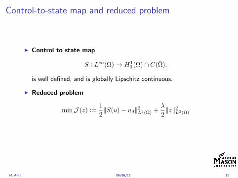
Control-to-state map and reduced problem
I Control to state map
S Linfin(Ω)rarr H10 (Ω) cap C(Ω)
is well defined and is globally Lipschitz continuous
I Reduced problem
minJ (z) =1
2S(u)minus ud2L2(Ω) +
λ
2z2L2(Ω)
H Antil 060616 31
First-order necessary conditionsI Lagrangian functional
L(u z p) = J(u z)minusint
Ω
(minus∆u+ g(x u(x))minus z
)p dx
= J(u z)minusint
Ω
(nablau middot nablap+ g(x u(x))pminus zp
)dx
I Adjoint system For all h isin H10 (Ω)
0 = DuL(u z p)h =
intΩ
(uminus ud)h dxminusint
Ω
(nablah middot nablap+ gu(x u(x))ph
)which yields
minus∆p+ gu(x u(x))p = uminus ud in Ω
p = 0 on partΩ
I Control
DzL(u z p)(z minus z) = (p+ λz z minus z) dx ge 0 forallz isin ZadI Gradient
nablaJ (z) = p+ λz
H Antil 060616 32
First-order necessary conditionsI Lagrangian functional
L(u z p) = J(u z)minusint
Ω
(minus∆u+ g(x u(x))minus z
)p dx
= J(u z)minusint
Ω
(nablau middot nablap+ g(x u(x))pminus zp
)dx
I Adjoint system For all h isin H10 (Ω)
0 = DuL(u z p)h =
intΩ
(uminus ud)h dxminusint
Ω
(nablah middot nablap+ gu(x u(x))ph
)which yields
minus∆p+ gu(x u(x))p = uminus ud in Ω
p = 0 on partΩ
I Control
DzL(u z p)(z minus z) = (p+ λz z minus z) dx ge 0 forallz isin Zad
I GradientnablaJ (z) = p+ λz
H Antil 060616 32
First-order necessary conditionsI Lagrangian functional
L(u z p) = J(u z)minusint
Ω
(minus∆u+ g(x u(x))minus z
)p dx
= J(u z)minusint
Ω
(nablau middot nablap+ g(x u(x))pminus zp
)dx
I Adjoint system For all h isin H10 (Ω)
0 = DuL(u z p)h =
intΩ
(uminus ud)h dxminusint
Ω
(nablah middot nablap+ gu(x u(x))ph
)which yields
minus∆p+ gu(x u(x))p = uminus ud in Ω
p = 0 on partΩ
I Control
DzL(u z p)(z minus z) = (p+ λz z minus z) dx ge 0 forallz isin ZadI Gradient
nablaJ (z) = p+ λz
H Antil 060616 32
Differentiability of Nemytskii operator
The rigorous proof uses
Theorem In addition to (A1)-(A4) if
(A5) g is continuously differentiable with respect to u for ae x isin Ωand we have
(i) |gu(x 0)| le K for ae x isin Ω(ii) gu is locally Lipschitz with respect to u isin R
then the Nemytskii operator G u 7rarr g(middot u(middot)) is continuously Frechetdifferentiable from Linfin(Ω) into itself and
(Gprime(u)h)(x) = gu(x u(x))h(x) ae in Ω forallh isin Linfin(Ω)
Remark (A5) holds if g(x u) = g(u) and g isin C2(R)
H Antil 060616 33
Outline
Motivation and examples
Linear elliptic optimal control problems
Differentiation in Banach spaces
First-order necessary conditions
Optimal control of semilinear PDEs
An abstract problem
Discretization using finite element methods
H Antil 060616 34
Gradient computation via adjoint general formI Abstract problem
min J(u z)
subject toc(u z) = 0
and z isin Zad
I Directional derivative Let S be the control to state map(nonlinear in general)
z 7rarr S(z) = u(z)
Under the assumptions of ldquoimplicit function theoremrdquo
J prime(z)h = (nablauJ (u(z) z) Sprime(z)h) + (nablazJ (u(z) z) h)
I Sensitivity of u with respect to z Differentiating the stateequation
cu(S(z) z)Sprime(z)h = minuscz(S(z) z)h
leads toSprime(z)h = minuscu(S(z) z)minus1
(cz(S(z) z)h
)
provided cu(S(z) z)minus1 is well-defined
H Antil 060616 35
Gradient computation via adjoint general formI Abstract problem
min J(u z)
subject toc(u z) = 0
and z isin ZadI Directional derivative Let S be the control to state map
(nonlinear in general)
z 7rarr S(z) = u(z)
Under the assumptions of ldquoimplicit function theoremrdquo
J prime(z)h = (nablauJ (u(z) z) Sprime(z)h) + (nablazJ (u(z) z) h)
I Sensitivity of u with respect to z Differentiating the stateequation
cu(S(z) z)Sprime(z)h = minuscz(S(z) z)h
leads toSprime(z)h = minuscu(S(z) z)minus1
(cz(S(z) z)h
)
provided cu(S(z) z)minus1 is well-defined
H Antil 060616 35
Gradient computation via adjoint general formI Abstract problem
min J(u z)
subject toc(u z) = 0
and z isin ZadI Directional derivative Let S be the control to state map
(nonlinear in general)
z 7rarr S(z) = u(z)
Under the assumptions of ldquoimplicit function theoremrdquo
J prime(z)h = (nablauJ (u(z) z) Sprime(z)h) + (nablazJ (u(z) z) h)
I Sensitivity of u with respect to z Differentiating the stateequation
cu(S(z) z)Sprime(z)h = minuscz(S(z) z)h
leads toSprime(z)h = minuscu(S(z) z)minus1
(cz(S(z) z)h
)
provided cu(S(z) z)minus1 is well-defined
H Antil 060616 35
Adjoint equation and gradient general form
I Directional derivative
J prime(z)h = minus(nablauJ (u(z) z) cu(u(z) z)minus1cz(u(z) z)h
)+ (nablazJ (u(z) z) h)
I Gradient
nablaJ (z) = minuscz(u(z) z)lowast(cu(u(z) z)minuslowastnablauJ (u(z) z)
)+nablazJ (u(z) z)
I Introducing adjoint variable p solving
cu(u(z) z)lowastp = nablauJ (u(z) z)
we arrive at following form of gradient
nablaJ (z) = minuscz(u(z) z)lowastp+nablazJ (u(z) z)
which is tractable
H Antil 060616 36
Adjoint equation and gradient general form
I Directional derivative
J prime(z)h = minus(nablauJ (u(z) z) cu(u(z) z)minus1cz(u(z) z)h
)+ (nablazJ (u(z) z) h)
I Gradient
nablaJ (z) = minuscz(u(z) z)lowast(cu(u(z) z)minuslowastnablauJ (u(z) z)
)+nablazJ (u(z) z)
I Introducing adjoint variable p solving
cu(u(z) z)lowastp = nablauJ (u(z) z)
we arrive at following form of gradient
nablaJ (z) = minuscz(u(z) z)lowastp+nablazJ (u(z) z)
which is tractable
H Antil 060616 36
Adjoint equation and gradient general form
I Directional derivative
J prime(z)h = minus(nablauJ (u(z) z) cu(u(z) z)minus1cz(u(z) z)h
)+ (nablazJ (u(z) z) h)
I Gradient
nablaJ (z) = minuscz(u(z) z)lowast(cu(u(z) z)minuslowastnablauJ (u(z) z)
)+nablazJ (u(z) z)
I Introducing adjoint variable p solving
cu(u(z) z)lowastp = nablauJ (u(z) z)
we arrive at following form of gradient
nablaJ (z) = minuscz(u(z) z)lowastp+nablazJ (u(z) z)
which is tractable
H Antil 060616 36
Hessian computation general form
I Lagrangian L(u z p) = J(u z)minusint
Ωc(u z)p dx Then we have
DzJ (z)h = DzL(u z p)h
I Second order derivative
D2zJ (z)[h1 h2] = DuDzL(u z p)[h1 S
prime(z)h2] +D2zL(u z p)[h1 h2]
+DpDzL(u z p)[h1 Dzp(z)h2]
I We already know Sprime(z)h2 moreover
DpDzL(u z p)[h1 Dzp(z)h2] = minus(cu(u z)h1 Dzp(z)h2
)
It remain to identify Dzp(z)h2
H Antil 060616 37
Hessian computation general form
I Lagrangian L(u z p) = J(u z)minusint
Ωc(u z)p dx Then we have
DzJ (z)h = DzL(u z p)h
I Second order derivative
D2zJ (z)[h1 h2] = DuDzL(u z p)[h1 S
prime(z)h2] +D2zL(u z p)[h1 h2]
+DpDzL(u z p)[h1 Dzp(z)h2]
I We already know Sprime(z)h2 moreover
DpDzL(u z p)[h1 Dzp(z)h2] = minus(cu(u z)h1 Dzp(z)h2
)
It remain to identify Dzp(z)h2
H Antil 060616 37
Hessian computation general form
I Lagrangian L(u z p) = J(u z)minusint
Ωc(u z)p dx Then we have
DzJ (z)h = DzL(u z p)h
I Second order derivative
D2zJ (z)[h1 h2] = DuDzL(u z p)[h1 S
prime(z)h2] +D2zL(u z p)[h1 h2]
+DpDzL(u z p)[h1 Dzp(z)h2]
I We already know Sprime(z)h2 moreover
DpDzL(u z p)[h1 Dzp(z)h2] = minus(cu(u z)h1 Dzp(z)h2
)
It remain to identify Dzp(z)h2
H Antil 060616 37
Outline
Motivation and examples
Linear elliptic optimal control problems
Differentiation in Banach spaces
First-order necessary conditions
Optimal control of semilinear PDEs
An abstract problem
Discretization using finite element methods
H Antil 060616 38
Numerical approximation of Poisson equation MeshTo avoid technical issues we will assume that partΩ is polygonal
I Mesh Let T = K be a mesh of Ω where K sub Rd is an elementthat is isoparametrically equivalent to a unit simplex in Rd
I Conforming mesh We say that the mesh is conforming ifI Ω = cupKisinT KI If K1 cap K2 = x then x is a node of K1 and K2I If K1 cap K2 6= empty and K1 cap K2 6= x then K1 cap K2 is an edgeface
contained in partK1 cap partK2
I Shape regular Let T be the collection of all conformingrefinements of an original mesh T 0 Then T is called shape regularif exist κ gt 0 such that
hKρKle κ forallK isin cupiT i
where hK = diam K ρK = maxρ gt 0|Bρ sub KI Quasi-uniform A family of shape regular meshes is called-quasi
uniform if there exist a constant σ gt 0 such that
maxhKminhK
le σ
uniformly for all meshes in the family
Numerical approximation of Poisson equation MeshTo avoid technical issues we will assume that partΩ is polygonal
I Mesh Let T = K be a mesh of Ω where K sub Rd is an elementthat is isoparametrically equivalent to a unit simplex in Rd
I Conforming mesh We say that the mesh is conforming ifI Ω = cupKisinT KI If K1 cap K2 = x then x is a node of K1 and K2I If K1 cap K2 6= empty and K1 cap K2 6= x then K1 cap K2 is an edgeface
contained in partK1 cap partK2
I Shape regular Let T be the collection of all conformingrefinements of an original mesh T 0 Then T is called shape regularif exist κ gt 0 such that
hKρKle κ forallK isin cupiT i
where hK = diam K ρK = maxρ gt 0|Bρ sub KI Quasi-uniform A family of shape regular meshes is called-quasi
uniform if there exist a constant σ gt 0 such that
maxhKminhK
le σ
uniformly for all meshes in the family
Numerical approximation of Poisson equation MeshTo avoid technical issues we will assume that partΩ is polygonal
I Mesh Let T = K be a mesh of Ω where K sub Rd is an elementthat is isoparametrically equivalent to a unit simplex in Rd
I Conforming mesh We say that the mesh is conforming ifI Ω = cupKisinT KI If K1 cap K2 = x then x is a node of K1 and K2I If K1 cap K2 6= empty and K1 cap K2 6= x then K1 cap K2 is an edgeface
contained in partK1 cap partK2
I Shape regular Let T be the collection of all conformingrefinements of an original mesh T 0 Then T is called shape regularif exist κ gt 0 such that
hKρKle κ forallK isin cupiT i
where hK = diam K ρK = maxρ gt 0|Bρ sub K
I Quasi-uniform A family of shape regular meshes is called-quasiuniform if there exist a constant σ gt 0 such that
maxhKminhK
le σ
uniformly for all meshes in the family
Numerical approximation of Poisson equation MeshTo avoid technical issues we will assume that partΩ is polygonal
I Mesh Let T = K be a mesh of Ω where K sub Rd is an elementthat is isoparametrically equivalent to a unit simplex in Rd
I Conforming mesh We say that the mesh is conforming ifI Ω = cupKisinT KI If K1 cap K2 = x then x is a node of K1 and K2I If K1 cap K2 6= empty and K1 cap K2 6= x then K1 cap K2 is an edgeface
contained in partK1 cap partK2
I Shape regular Let T be the collection of all conformingrefinements of an original mesh T 0 Then T is called shape regularif exist κ gt 0 such that
hKρKle κ forallK isin cupiT i
where hK = diam K ρK = maxρ gt 0|Bρ sub KI Quasi-uniform A family of shape regular meshes is called-quasi
uniform if there exist a constant σ gt 0 such that
maxhKminhK
le σ
uniformly for all meshes in the family
FE space and Galerkin approximationI Finite element space For T isin T we define the finite element
space as
V(T ) = W isin C0(Ω) WK isin P1forallK isin T W |partΩ = 0
where P1 is the set of polynomials of degree at most 1
I Galerkin approximation of continuous problem is given by
Find UT isin V(T )
intΩ
AnablaUT middot nablaV = 〈f V 〉 forallV isin V(T )
The discrete problem is well-posedI Nodal basis Consists of functions ψi isin V(T ) with xi isin N (T )
satisfyingψxi
(xj) = δij
where N (T ) denotes the interior (plus Neumann) nodesI Galerkin orthogonality(
nabla(uminus UT )nablaW)L2(Ω)
= 0 forallW isin V(T )
H Antil 060616 40
FE space and Galerkin approximationI Finite element space For T isin T we define the finite element
space as
V(T ) = W isin C0(Ω) WK isin P1forallK isin T W |partΩ = 0
where P1 is the set of polynomials of degree at most 1I Galerkin approximation of continuous problem is given by
Find UT isin V(T )
intΩ
AnablaUT middot nablaV = 〈f V 〉 forallV isin V(T )
The discrete problem is well-posed
I Nodal basis Consists of functions ψi isin V(T ) with xi isin N (T )satisfying
ψxi(xj) = δij
where N (T ) denotes the interior (plus Neumann) nodesI Galerkin orthogonality(
nabla(uminus UT )nablaW)L2(Ω)
= 0 forallW isin V(T )
H Antil 060616 40
FE space and Galerkin approximationI Finite element space For T isin T we define the finite element
space as
V(T ) = W isin C0(Ω) WK isin P1forallK isin T W |partΩ = 0
where P1 is the set of polynomials of degree at most 1I Galerkin approximation of continuous problem is given by
Find UT isin V(T )
intΩ
AnablaUT middot nablaV = 〈f V 〉 forallV isin V(T )
The discrete problem is well-posedI Nodal basis Consists of functions ψi isin V(T ) with xi isin N (T )
satisfyingψxi
(xj) = δij
where N (T ) denotes the interior (plus Neumann) nodes
I Galerkin orthogonality(nabla(uminus UT )nablaW
)L2(Ω)
= 0 forallW isin V(T )
H Antil 060616 40
FE space and Galerkin approximationI Finite element space For T isin T we define the finite element
space as
V(T ) = W isin C0(Ω) WK isin P1forallK isin T W |partΩ = 0
where P1 is the set of polynomials of degree at most 1I Galerkin approximation of continuous problem is given by
Find UT isin V(T )
intΩ
AnablaUT middot nablaV = 〈f V 〉 forallV isin V(T )
The discrete problem is well-posedI Nodal basis Consists of functions ψi isin V(T ) with xi isin N (T )
satisfyingψxi
(xj) = δij
where N (T ) denotes the interior (plus Neumann) nodesI Galerkin orthogonality(
nabla(uminus UT )nablaW)L2(Ω)
= 0 forallW isin V(T )
H Antil 060616 40
Best approximation
I Cearsquos lemma
nabla(uminus UT )L2(Ω) le C infWisinV(T )
nabla(uminusW )L2(Ω)
I Nodal interpolation operator ΠT C(Ω)rarr V(T ) satisfies
ΠT u(xi) = u(xi) forallxi isin N (T )
and is defined as
ΠT u =sum
xiisinN (T )
u(xi)ψxi
I Error estimates In Cearsquos lemma replace W by ΠT u and thencompute the interpolation error
H Antil 060616 41
Best approximation
I Cearsquos lemma
nabla(uminus UT )L2(Ω) le C infWisinV(T )
nabla(uminusW )L2(Ω)
I Nodal interpolation operator ΠT C(Ω)rarr V(T ) satisfies
ΠT u(xi) = u(xi) forallxi isin N (T )
and is defined as
ΠT u =sum
xiisinN (T )
u(xi)ψxi
I Error estimates In Cearsquos lemma replace W by ΠT u and thencompute the interpolation error
H Antil 060616 41
Best approximation
I Cearsquos lemma
nabla(uminus UT )L2(Ω) le C infWisinV(T )
nabla(uminusW )L2(Ω)
I Nodal interpolation operator ΠT C(Ω)rarr V(T ) satisfies
ΠT u(xi) = u(xi) forallxi isin N (T )
and is defined as
ΠT u =sum
xiisinN (T )
u(xi)ψxi
I Error estimates In Cearsquos lemma replace W by ΠT u and thencompute the interpolation error
H Antil 060616 41
Algebraic system state equation
I Recall UT isin V(T ) solves
a(UT V ) = 〈f V 〉 forallV isin V(T )
I Now setting UT =sumN
j=1 Ujψj V = ψi we get
Nsumj=1
Uja(φj φi) = 〈f ψi〉 i = 1 N
which is the matrix-vector system
AU = F
I Stiffness matrix A is SPD
H Antil 060616 42
Algebraic system state equation
I Recall UT isin V(T ) solves
a(UT V ) = 〈f V 〉 forallV isin V(T )
I Now setting UT =sumN
j=1 Ujψj V = ψi we get
Nsumj=1
Uja(φj φi) = 〈f ψi〉 i = 1 N
which is the matrix-vector system
AU = F
I Stiffness matrix A is SPD
H Antil 060616 42
Algebraic system state equation
I Recall UT isin V(T ) solves
a(UT V ) = 〈f V 〉 forallV isin V(T )
I Now setting UT =sumN
j=1 Ujψj V = ψi we get
Nsumj=1
Uja(φj φi) = 〈f ψi〉 i = 1 N
which is the matrix-vector system
AU = F
I Stiffness matrix A is SPD
H Antil 060616 42
Discrete linear elliptic OCP
min JT (UT ZT ) =1
2UT minus ud2L2(Ω) +
λ
2ZT 2L2(Ω)
subject to
Find UT isin V(T )
intΩ
nablaUT middot nablaV = (ZT V )L2(Ω) forallV isin V(T )
and whereZT isin Zad(T ) = Zad cap Z(T )
is either one of these
Z(T ) =
V(T )L2(Ω) variational discretization (Hinze)WT isin Linfin(Ω) ZT |K isin P0(K)K isin T
H Antil 060616 43
Recent books
F TroltzschOptimal control of partial differential equations volume 112 ofGraduate Studies in MathematicsAmerican Mathematical Society Providence RI 2010Theory methods and applications Translated from the 2005 Germanoriginal by Jurgen Sprekels
K Ito and K KunischLagrange multiplier approach to variational problems andapplications volume 15 of Advances in Design and ControlSociety for Industrial and Applied Mathematics (SIAM)Philadelphia PA 2008
H Antil 060616 44
- Motivation and examples
- Linear elliptic optimal control problems
- Differentiation in Banach spaces
- First-order necessary conditions
- Optimal control of semilinear PDEs
- An abstract problem
- Discretization using finite element methods
-
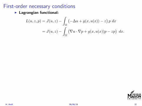
First-order necessary conditionsI Lagrangian functional
L(u z p) = J(u z)minusint
Ω
(minus∆u+ g(x u(x))minus z
)p dx
= J(u z)minusint
Ω
(nablau middot nablap+ g(x u(x))pminus zp
)dx
I Adjoint system For all h isin H10 (Ω)
0 = DuL(u z p)h =
intΩ
(uminus ud)h dxminusint
Ω
(nablah middot nablap+ gu(x u(x))ph
)which yields
minus∆p+ gu(x u(x))p = uminus ud in Ω
p = 0 on partΩ
I Control
DzL(u z p)(z minus z) = (p+ λz z minus z) dx ge 0 forallz isin ZadI Gradient
nablaJ (z) = p+ λz
H Antil 060616 32
First-order necessary conditionsI Lagrangian functional
L(u z p) = J(u z)minusint
Ω
(minus∆u+ g(x u(x))minus z
)p dx
= J(u z)minusint
Ω
(nablau middot nablap+ g(x u(x))pminus zp
)dx
I Adjoint system For all h isin H10 (Ω)
0 = DuL(u z p)h =
intΩ
(uminus ud)h dxminusint
Ω
(nablah middot nablap+ gu(x u(x))ph
)which yields
minus∆p+ gu(x u(x))p = uminus ud in Ω
p = 0 on partΩ
I Control
DzL(u z p)(z minus z) = (p+ λz z minus z) dx ge 0 forallz isin Zad
I GradientnablaJ (z) = p+ λz
H Antil 060616 32
First-order necessary conditionsI Lagrangian functional
L(u z p) = J(u z)minusint
Ω
(minus∆u+ g(x u(x))minus z
)p dx
= J(u z)minusint
Ω
(nablau middot nablap+ g(x u(x))pminus zp
)dx
I Adjoint system For all h isin H10 (Ω)
0 = DuL(u z p)h =
intΩ
(uminus ud)h dxminusint
Ω
(nablah middot nablap+ gu(x u(x))ph
)which yields
minus∆p+ gu(x u(x))p = uminus ud in Ω
p = 0 on partΩ
I Control
DzL(u z p)(z minus z) = (p+ λz z minus z) dx ge 0 forallz isin ZadI Gradient
nablaJ (z) = p+ λz
H Antil 060616 32
Differentiability of Nemytskii operator
The rigorous proof uses
Theorem In addition to (A1)-(A4) if
(A5) g is continuously differentiable with respect to u for ae x isin Ωand we have
(i) |gu(x 0)| le K for ae x isin Ω(ii) gu is locally Lipschitz with respect to u isin R
then the Nemytskii operator G u 7rarr g(middot u(middot)) is continuously Frechetdifferentiable from Linfin(Ω) into itself and
(Gprime(u)h)(x) = gu(x u(x))h(x) ae in Ω forallh isin Linfin(Ω)
Remark (A5) holds if g(x u) = g(u) and g isin C2(R)
H Antil 060616 33
Outline
Motivation and examples
Linear elliptic optimal control problems
Differentiation in Banach spaces
First-order necessary conditions
Optimal control of semilinear PDEs
An abstract problem
Discretization using finite element methods
H Antil 060616 34
Gradient computation via adjoint general formI Abstract problem
min J(u z)
subject toc(u z) = 0
and z isin Zad
I Directional derivative Let S be the control to state map(nonlinear in general)
z 7rarr S(z) = u(z)
Under the assumptions of ldquoimplicit function theoremrdquo
J prime(z)h = (nablauJ (u(z) z) Sprime(z)h) + (nablazJ (u(z) z) h)
I Sensitivity of u with respect to z Differentiating the stateequation
cu(S(z) z)Sprime(z)h = minuscz(S(z) z)h
leads toSprime(z)h = minuscu(S(z) z)minus1
(cz(S(z) z)h
)
provided cu(S(z) z)minus1 is well-defined
H Antil 060616 35
Gradient computation via adjoint general formI Abstract problem
min J(u z)
subject toc(u z) = 0
and z isin ZadI Directional derivative Let S be the control to state map
(nonlinear in general)
z 7rarr S(z) = u(z)
Under the assumptions of ldquoimplicit function theoremrdquo
J prime(z)h = (nablauJ (u(z) z) Sprime(z)h) + (nablazJ (u(z) z) h)
I Sensitivity of u with respect to z Differentiating the stateequation
cu(S(z) z)Sprime(z)h = minuscz(S(z) z)h
leads toSprime(z)h = minuscu(S(z) z)minus1
(cz(S(z) z)h
)
provided cu(S(z) z)minus1 is well-defined
H Antil 060616 35
Gradient computation via adjoint general formI Abstract problem
min J(u z)
subject toc(u z) = 0
and z isin ZadI Directional derivative Let S be the control to state map
(nonlinear in general)
z 7rarr S(z) = u(z)
Under the assumptions of ldquoimplicit function theoremrdquo
J prime(z)h = (nablauJ (u(z) z) Sprime(z)h) + (nablazJ (u(z) z) h)
I Sensitivity of u with respect to z Differentiating the stateequation
cu(S(z) z)Sprime(z)h = minuscz(S(z) z)h
leads toSprime(z)h = minuscu(S(z) z)minus1
(cz(S(z) z)h
)
provided cu(S(z) z)minus1 is well-defined
H Antil 060616 35
Adjoint equation and gradient general form
I Directional derivative
J prime(z)h = minus(nablauJ (u(z) z) cu(u(z) z)minus1cz(u(z) z)h
)+ (nablazJ (u(z) z) h)
I Gradient
nablaJ (z) = minuscz(u(z) z)lowast(cu(u(z) z)minuslowastnablauJ (u(z) z)
)+nablazJ (u(z) z)
I Introducing adjoint variable p solving
cu(u(z) z)lowastp = nablauJ (u(z) z)
we arrive at following form of gradient
nablaJ (z) = minuscz(u(z) z)lowastp+nablazJ (u(z) z)
which is tractable
H Antil 060616 36
Adjoint equation and gradient general form
I Directional derivative
J prime(z)h = minus(nablauJ (u(z) z) cu(u(z) z)minus1cz(u(z) z)h
)+ (nablazJ (u(z) z) h)
I Gradient
nablaJ (z) = minuscz(u(z) z)lowast(cu(u(z) z)minuslowastnablauJ (u(z) z)
)+nablazJ (u(z) z)
I Introducing adjoint variable p solving
cu(u(z) z)lowastp = nablauJ (u(z) z)
we arrive at following form of gradient
nablaJ (z) = minuscz(u(z) z)lowastp+nablazJ (u(z) z)
which is tractable
H Antil 060616 36
Adjoint equation and gradient general form
I Directional derivative
J prime(z)h = minus(nablauJ (u(z) z) cu(u(z) z)minus1cz(u(z) z)h
)+ (nablazJ (u(z) z) h)
I Gradient
nablaJ (z) = minuscz(u(z) z)lowast(cu(u(z) z)minuslowastnablauJ (u(z) z)
)+nablazJ (u(z) z)
I Introducing adjoint variable p solving
cu(u(z) z)lowastp = nablauJ (u(z) z)
we arrive at following form of gradient
nablaJ (z) = minuscz(u(z) z)lowastp+nablazJ (u(z) z)
which is tractable
H Antil 060616 36
Hessian computation general form
I Lagrangian L(u z p) = J(u z)minusint
Ωc(u z)p dx Then we have
DzJ (z)h = DzL(u z p)h
I Second order derivative
D2zJ (z)[h1 h2] = DuDzL(u z p)[h1 S
prime(z)h2] +D2zL(u z p)[h1 h2]
+DpDzL(u z p)[h1 Dzp(z)h2]
I We already know Sprime(z)h2 moreover
DpDzL(u z p)[h1 Dzp(z)h2] = minus(cu(u z)h1 Dzp(z)h2
)
It remain to identify Dzp(z)h2
H Antil 060616 37
Hessian computation general form
I Lagrangian L(u z p) = J(u z)minusint
Ωc(u z)p dx Then we have
DzJ (z)h = DzL(u z p)h
I Second order derivative
D2zJ (z)[h1 h2] = DuDzL(u z p)[h1 S
prime(z)h2] +D2zL(u z p)[h1 h2]
+DpDzL(u z p)[h1 Dzp(z)h2]
I We already know Sprime(z)h2 moreover
DpDzL(u z p)[h1 Dzp(z)h2] = minus(cu(u z)h1 Dzp(z)h2
)
It remain to identify Dzp(z)h2
H Antil 060616 37
Hessian computation general form
I Lagrangian L(u z p) = J(u z)minusint
Ωc(u z)p dx Then we have
DzJ (z)h = DzL(u z p)h
I Second order derivative
D2zJ (z)[h1 h2] = DuDzL(u z p)[h1 S
prime(z)h2] +D2zL(u z p)[h1 h2]
+DpDzL(u z p)[h1 Dzp(z)h2]
I We already know Sprime(z)h2 moreover
DpDzL(u z p)[h1 Dzp(z)h2] = minus(cu(u z)h1 Dzp(z)h2
)
It remain to identify Dzp(z)h2
H Antil 060616 37
Outline
Motivation and examples
Linear elliptic optimal control problems
Differentiation in Banach spaces
First-order necessary conditions
Optimal control of semilinear PDEs
An abstract problem
Discretization using finite element methods
H Antil 060616 38
Numerical approximation of Poisson equation MeshTo avoid technical issues we will assume that partΩ is polygonal
I Mesh Let T = K be a mesh of Ω where K sub Rd is an elementthat is isoparametrically equivalent to a unit simplex in Rd
I Conforming mesh We say that the mesh is conforming ifI Ω = cupKisinT KI If K1 cap K2 = x then x is a node of K1 and K2I If K1 cap K2 6= empty and K1 cap K2 6= x then K1 cap K2 is an edgeface
contained in partK1 cap partK2
I Shape regular Let T be the collection of all conformingrefinements of an original mesh T 0 Then T is called shape regularif exist κ gt 0 such that
hKρKle κ forallK isin cupiT i
where hK = diam K ρK = maxρ gt 0|Bρ sub KI Quasi-uniform A family of shape regular meshes is called-quasi
uniform if there exist a constant σ gt 0 such that
maxhKminhK
le σ
uniformly for all meshes in the family
Numerical approximation of Poisson equation MeshTo avoid technical issues we will assume that partΩ is polygonal
I Mesh Let T = K be a mesh of Ω where K sub Rd is an elementthat is isoparametrically equivalent to a unit simplex in Rd
I Conforming mesh We say that the mesh is conforming ifI Ω = cupKisinT KI If K1 cap K2 = x then x is a node of K1 and K2I If K1 cap K2 6= empty and K1 cap K2 6= x then K1 cap K2 is an edgeface
contained in partK1 cap partK2
I Shape regular Let T be the collection of all conformingrefinements of an original mesh T 0 Then T is called shape regularif exist κ gt 0 such that
hKρKle κ forallK isin cupiT i
where hK = diam K ρK = maxρ gt 0|Bρ sub KI Quasi-uniform A family of shape regular meshes is called-quasi
uniform if there exist a constant σ gt 0 such that
maxhKminhK
le σ
uniformly for all meshes in the family
Numerical approximation of Poisson equation MeshTo avoid technical issues we will assume that partΩ is polygonal
I Mesh Let T = K be a mesh of Ω where K sub Rd is an elementthat is isoparametrically equivalent to a unit simplex in Rd
I Conforming mesh We say that the mesh is conforming ifI Ω = cupKisinT KI If K1 cap K2 = x then x is a node of K1 and K2I If K1 cap K2 6= empty and K1 cap K2 6= x then K1 cap K2 is an edgeface
contained in partK1 cap partK2
I Shape regular Let T be the collection of all conformingrefinements of an original mesh T 0 Then T is called shape regularif exist κ gt 0 such that
hKρKle κ forallK isin cupiT i
where hK = diam K ρK = maxρ gt 0|Bρ sub K
I Quasi-uniform A family of shape regular meshes is called-quasiuniform if there exist a constant σ gt 0 such that
maxhKminhK
le σ
uniformly for all meshes in the family
Numerical approximation of Poisson equation MeshTo avoid technical issues we will assume that partΩ is polygonal
I Mesh Let T = K be a mesh of Ω where K sub Rd is an elementthat is isoparametrically equivalent to a unit simplex in Rd
I Conforming mesh We say that the mesh is conforming ifI Ω = cupKisinT KI If K1 cap K2 = x then x is a node of K1 and K2I If K1 cap K2 6= empty and K1 cap K2 6= x then K1 cap K2 is an edgeface
contained in partK1 cap partK2
I Shape regular Let T be the collection of all conformingrefinements of an original mesh T 0 Then T is called shape regularif exist κ gt 0 such that
hKρKle κ forallK isin cupiT i
where hK = diam K ρK = maxρ gt 0|Bρ sub KI Quasi-uniform A family of shape regular meshes is called-quasi
uniform if there exist a constant σ gt 0 such that
maxhKminhK
le σ
uniformly for all meshes in the family
FE space and Galerkin approximationI Finite element space For T isin T we define the finite element
space as
V(T ) = W isin C0(Ω) WK isin P1forallK isin T W |partΩ = 0
where P1 is the set of polynomials of degree at most 1
I Galerkin approximation of continuous problem is given by
Find UT isin V(T )
intΩ
AnablaUT middot nablaV = 〈f V 〉 forallV isin V(T )
The discrete problem is well-posedI Nodal basis Consists of functions ψi isin V(T ) with xi isin N (T )
satisfyingψxi
(xj) = δij
where N (T ) denotes the interior (plus Neumann) nodesI Galerkin orthogonality(
nabla(uminus UT )nablaW)L2(Ω)
= 0 forallW isin V(T )
H Antil 060616 40
FE space and Galerkin approximationI Finite element space For T isin T we define the finite element
space as
V(T ) = W isin C0(Ω) WK isin P1forallK isin T W |partΩ = 0
where P1 is the set of polynomials of degree at most 1I Galerkin approximation of continuous problem is given by
Find UT isin V(T )
intΩ
AnablaUT middot nablaV = 〈f V 〉 forallV isin V(T )
The discrete problem is well-posed
I Nodal basis Consists of functions ψi isin V(T ) with xi isin N (T )satisfying
ψxi(xj) = δij
where N (T ) denotes the interior (plus Neumann) nodesI Galerkin orthogonality(
nabla(uminus UT )nablaW)L2(Ω)
= 0 forallW isin V(T )
H Antil 060616 40
FE space and Galerkin approximationI Finite element space For T isin T we define the finite element
space as
V(T ) = W isin C0(Ω) WK isin P1forallK isin T W |partΩ = 0
where P1 is the set of polynomials of degree at most 1I Galerkin approximation of continuous problem is given by
Find UT isin V(T )
intΩ
AnablaUT middot nablaV = 〈f V 〉 forallV isin V(T )
The discrete problem is well-posedI Nodal basis Consists of functions ψi isin V(T ) with xi isin N (T )
satisfyingψxi
(xj) = δij
where N (T ) denotes the interior (plus Neumann) nodes
I Galerkin orthogonality(nabla(uminus UT )nablaW
)L2(Ω)
= 0 forallW isin V(T )
H Antil 060616 40
FE space and Galerkin approximationI Finite element space For T isin T we define the finite element
space as
V(T ) = W isin C0(Ω) WK isin P1forallK isin T W |partΩ = 0
where P1 is the set of polynomials of degree at most 1I Galerkin approximation of continuous problem is given by
Find UT isin V(T )
intΩ
AnablaUT middot nablaV = 〈f V 〉 forallV isin V(T )
The discrete problem is well-posedI Nodal basis Consists of functions ψi isin V(T ) with xi isin N (T )
satisfyingψxi
(xj) = δij
where N (T ) denotes the interior (plus Neumann) nodesI Galerkin orthogonality(
nabla(uminus UT )nablaW)L2(Ω)
= 0 forallW isin V(T )
H Antil 060616 40
Best approximation
I Cearsquos lemma
nabla(uminus UT )L2(Ω) le C infWisinV(T )
nabla(uminusW )L2(Ω)
I Nodal interpolation operator ΠT C(Ω)rarr V(T ) satisfies
ΠT u(xi) = u(xi) forallxi isin N (T )
and is defined as
ΠT u =sum
xiisinN (T )
u(xi)ψxi
I Error estimates In Cearsquos lemma replace W by ΠT u and thencompute the interpolation error
H Antil 060616 41
Best approximation
I Cearsquos lemma
nabla(uminus UT )L2(Ω) le C infWisinV(T )
nabla(uminusW )L2(Ω)
I Nodal interpolation operator ΠT C(Ω)rarr V(T ) satisfies
ΠT u(xi) = u(xi) forallxi isin N (T )
and is defined as
ΠT u =sum
xiisinN (T )
u(xi)ψxi
I Error estimates In Cearsquos lemma replace W by ΠT u and thencompute the interpolation error
H Antil 060616 41
Best approximation
I Cearsquos lemma
nabla(uminus UT )L2(Ω) le C infWisinV(T )
nabla(uminusW )L2(Ω)
I Nodal interpolation operator ΠT C(Ω)rarr V(T ) satisfies
ΠT u(xi) = u(xi) forallxi isin N (T )
and is defined as
ΠT u =sum
xiisinN (T )
u(xi)ψxi
I Error estimates In Cearsquos lemma replace W by ΠT u and thencompute the interpolation error
H Antil 060616 41
Algebraic system state equation
I Recall UT isin V(T ) solves
a(UT V ) = 〈f V 〉 forallV isin V(T )
I Now setting UT =sumN
j=1 Ujψj V = ψi we get
Nsumj=1
Uja(φj φi) = 〈f ψi〉 i = 1 N
which is the matrix-vector system
AU = F
I Stiffness matrix A is SPD
H Antil 060616 42
Algebraic system state equation
I Recall UT isin V(T ) solves
a(UT V ) = 〈f V 〉 forallV isin V(T )
I Now setting UT =sumN
j=1 Ujψj V = ψi we get
Nsumj=1
Uja(φj φi) = 〈f ψi〉 i = 1 N
which is the matrix-vector system
AU = F
I Stiffness matrix A is SPD
H Antil 060616 42
Algebraic system state equation
I Recall UT isin V(T ) solves
a(UT V ) = 〈f V 〉 forallV isin V(T )
I Now setting UT =sumN
j=1 Ujψj V = ψi we get
Nsumj=1
Uja(φj φi) = 〈f ψi〉 i = 1 N
which is the matrix-vector system
AU = F
I Stiffness matrix A is SPD
H Antil 060616 42
Discrete linear elliptic OCP
min JT (UT ZT ) =1
2UT minus ud2L2(Ω) +
λ
2ZT 2L2(Ω)
subject to
Find UT isin V(T )
intΩ
nablaUT middot nablaV = (ZT V )L2(Ω) forallV isin V(T )
and whereZT isin Zad(T ) = Zad cap Z(T )
is either one of these
Z(T ) =
V(T )L2(Ω) variational discretization (Hinze)WT isin Linfin(Ω) ZT |K isin P0(K)K isin T
H Antil 060616 43
Recent books
F TroltzschOptimal control of partial differential equations volume 112 ofGraduate Studies in MathematicsAmerican Mathematical Society Providence RI 2010Theory methods and applications Translated from the 2005 Germanoriginal by Jurgen Sprekels
K Ito and K KunischLagrange multiplier approach to variational problems andapplications volume 15 of Advances in Design and ControlSociety for Industrial and Applied Mathematics (SIAM)Philadelphia PA 2008
H Antil 060616 44
- Motivation and examples
- Linear elliptic optimal control problems
- Differentiation in Banach spaces
- First-order necessary conditions
- Optimal control of semilinear PDEs
- An abstract problem
- Discretization using finite element methods
-
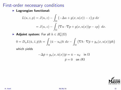
First-order necessary conditionsI Lagrangian functional
L(u z p) = J(u z)minusint
Ω
(minus∆u+ g(x u(x))minus z
)p dx
= J(u z)minusint
Ω
(nablau middot nablap+ g(x u(x))pminus zp
)dx
I Adjoint system For all h isin H10 (Ω)
0 = DuL(u z p)h =
intΩ
(uminus ud)h dxminusint
Ω
(nablah middot nablap+ gu(x u(x))ph
)which yields
minus∆p+ gu(x u(x))p = uminus ud in Ω
p = 0 on partΩ
I Control
DzL(u z p)(z minus z) = (p+ λz z minus z) dx ge 0 forallz isin ZadI Gradient
nablaJ (z) = p+ λz
H Antil 060616 32
First-order necessary conditionsI Lagrangian functional
L(u z p) = J(u z)minusint
Ω
(minus∆u+ g(x u(x))minus z
)p dx
= J(u z)minusint
Ω
(nablau middot nablap+ g(x u(x))pminus zp
)dx
I Adjoint system For all h isin H10 (Ω)
0 = DuL(u z p)h =
intΩ
(uminus ud)h dxminusint
Ω
(nablah middot nablap+ gu(x u(x))ph
)which yields
minus∆p+ gu(x u(x))p = uminus ud in Ω
p = 0 on partΩ
I Control
DzL(u z p)(z minus z) = (p+ λz z minus z) dx ge 0 forallz isin Zad
I GradientnablaJ (z) = p+ λz
H Antil 060616 32
First-order necessary conditionsI Lagrangian functional
L(u z p) = J(u z)minusint
Ω
(minus∆u+ g(x u(x))minus z
)p dx
= J(u z)minusint
Ω
(nablau middot nablap+ g(x u(x))pminus zp
)dx
I Adjoint system For all h isin H10 (Ω)
0 = DuL(u z p)h =
intΩ
(uminus ud)h dxminusint
Ω
(nablah middot nablap+ gu(x u(x))ph
)which yields
minus∆p+ gu(x u(x))p = uminus ud in Ω
p = 0 on partΩ
I Control
DzL(u z p)(z minus z) = (p+ λz z minus z) dx ge 0 forallz isin ZadI Gradient
nablaJ (z) = p+ λz
H Antil 060616 32
Differentiability of Nemytskii operator
The rigorous proof uses
Theorem In addition to (A1)-(A4) if
(A5) g is continuously differentiable with respect to u for ae x isin Ωand we have
(i) |gu(x 0)| le K for ae x isin Ω(ii) gu is locally Lipschitz with respect to u isin R
then the Nemytskii operator G u 7rarr g(middot u(middot)) is continuously Frechetdifferentiable from Linfin(Ω) into itself and
(Gprime(u)h)(x) = gu(x u(x))h(x) ae in Ω forallh isin Linfin(Ω)
Remark (A5) holds if g(x u) = g(u) and g isin C2(R)
H Antil 060616 33
Outline
Motivation and examples
Linear elliptic optimal control problems
Differentiation in Banach spaces
First-order necessary conditions
Optimal control of semilinear PDEs
An abstract problem
Discretization using finite element methods
H Antil 060616 34
Gradient computation via adjoint general formI Abstract problem
min J(u z)
subject toc(u z) = 0
and z isin Zad
I Directional derivative Let S be the control to state map(nonlinear in general)
z 7rarr S(z) = u(z)
Under the assumptions of ldquoimplicit function theoremrdquo
J prime(z)h = (nablauJ (u(z) z) Sprime(z)h) + (nablazJ (u(z) z) h)
I Sensitivity of u with respect to z Differentiating the stateequation
cu(S(z) z)Sprime(z)h = minuscz(S(z) z)h
leads toSprime(z)h = minuscu(S(z) z)minus1
(cz(S(z) z)h
)
provided cu(S(z) z)minus1 is well-defined
H Antil 060616 35
Gradient computation via adjoint general formI Abstract problem
min J(u z)
subject toc(u z) = 0
and z isin ZadI Directional derivative Let S be the control to state map
(nonlinear in general)
z 7rarr S(z) = u(z)
Under the assumptions of ldquoimplicit function theoremrdquo
J prime(z)h = (nablauJ (u(z) z) Sprime(z)h) + (nablazJ (u(z) z) h)
I Sensitivity of u with respect to z Differentiating the stateequation
cu(S(z) z)Sprime(z)h = minuscz(S(z) z)h
leads toSprime(z)h = minuscu(S(z) z)minus1
(cz(S(z) z)h
)
provided cu(S(z) z)minus1 is well-defined
H Antil 060616 35
Gradient computation via adjoint general formI Abstract problem
min J(u z)
subject toc(u z) = 0
and z isin ZadI Directional derivative Let S be the control to state map
(nonlinear in general)
z 7rarr S(z) = u(z)
Under the assumptions of ldquoimplicit function theoremrdquo
J prime(z)h = (nablauJ (u(z) z) Sprime(z)h) + (nablazJ (u(z) z) h)
I Sensitivity of u with respect to z Differentiating the stateequation
cu(S(z) z)Sprime(z)h = minuscz(S(z) z)h
leads toSprime(z)h = minuscu(S(z) z)minus1
(cz(S(z) z)h
)
provided cu(S(z) z)minus1 is well-defined
H Antil 060616 35
Adjoint equation and gradient general form
I Directional derivative
J prime(z)h = minus(nablauJ (u(z) z) cu(u(z) z)minus1cz(u(z) z)h
)+ (nablazJ (u(z) z) h)
I Gradient
nablaJ (z) = minuscz(u(z) z)lowast(cu(u(z) z)minuslowastnablauJ (u(z) z)
)+nablazJ (u(z) z)
I Introducing adjoint variable p solving
cu(u(z) z)lowastp = nablauJ (u(z) z)
we arrive at following form of gradient
nablaJ (z) = minuscz(u(z) z)lowastp+nablazJ (u(z) z)
which is tractable
H Antil 060616 36
Adjoint equation and gradient general form
I Directional derivative
J prime(z)h = minus(nablauJ (u(z) z) cu(u(z) z)minus1cz(u(z) z)h
)+ (nablazJ (u(z) z) h)
I Gradient
nablaJ (z) = minuscz(u(z) z)lowast(cu(u(z) z)minuslowastnablauJ (u(z) z)
)+nablazJ (u(z) z)
I Introducing adjoint variable p solving
cu(u(z) z)lowastp = nablauJ (u(z) z)
we arrive at following form of gradient
nablaJ (z) = minuscz(u(z) z)lowastp+nablazJ (u(z) z)
which is tractable
H Antil 060616 36
Adjoint equation and gradient general form
I Directional derivative
J prime(z)h = minus(nablauJ (u(z) z) cu(u(z) z)minus1cz(u(z) z)h
)+ (nablazJ (u(z) z) h)
I Gradient
nablaJ (z) = minuscz(u(z) z)lowast(cu(u(z) z)minuslowastnablauJ (u(z) z)
)+nablazJ (u(z) z)
I Introducing adjoint variable p solving
cu(u(z) z)lowastp = nablauJ (u(z) z)
we arrive at following form of gradient
nablaJ (z) = minuscz(u(z) z)lowastp+nablazJ (u(z) z)
which is tractable
H Antil 060616 36
Hessian computation general form
I Lagrangian L(u z p) = J(u z)minusint
Ωc(u z)p dx Then we have
DzJ (z)h = DzL(u z p)h
I Second order derivative
D2zJ (z)[h1 h2] = DuDzL(u z p)[h1 S
prime(z)h2] +D2zL(u z p)[h1 h2]
+DpDzL(u z p)[h1 Dzp(z)h2]
I We already know Sprime(z)h2 moreover
DpDzL(u z p)[h1 Dzp(z)h2] = minus(cu(u z)h1 Dzp(z)h2
)
It remain to identify Dzp(z)h2
H Antil 060616 37
Hessian computation general form
I Lagrangian L(u z p) = J(u z)minusint
Ωc(u z)p dx Then we have
DzJ (z)h = DzL(u z p)h
I Second order derivative
D2zJ (z)[h1 h2] = DuDzL(u z p)[h1 S
prime(z)h2] +D2zL(u z p)[h1 h2]
+DpDzL(u z p)[h1 Dzp(z)h2]
I We already know Sprime(z)h2 moreover
DpDzL(u z p)[h1 Dzp(z)h2] = minus(cu(u z)h1 Dzp(z)h2
)
It remain to identify Dzp(z)h2
H Antil 060616 37
Hessian computation general form
I Lagrangian L(u z p) = J(u z)minusint
Ωc(u z)p dx Then we have
DzJ (z)h = DzL(u z p)h
I Second order derivative
D2zJ (z)[h1 h2] = DuDzL(u z p)[h1 S
prime(z)h2] +D2zL(u z p)[h1 h2]
+DpDzL(u z p)[h1 Dzp(z)h2]
I We already know Sprime(z)h2 moreover
DpDzL(u z p)[h1 Dzp(z)h2] = minus(cu(u z)h1 Dzp(z)h2
)
It remain to identify Dzp(z)h2
H Antil 060616 37
Outline
Motivation and examples
Linear elliptic optimal control problems
Differentiation in Banach spaces
First-order necessary conditions
Optimal control of semilinear PDEs
An abstract problem
Discretization using finite element methods
H Antil 060616 38
Numerical approximation of Poisson equation MeshTo avoid technical issues we will assume that partΩ is polygonal
I Mesh Let T = K be a mesh of Ω where K sub Rd is an elementthat is isoparametrically equivalent to a unit simplex in Rd
I Conforming mesh We say that the mesh is conforming ifI Ω = cupKisinT KI If K1 cap K2 = x then x is a node of K1 and K2I If K1 cap K2 6= empty and K1 cap K2 6= x then K1 cap K2 is an edgeface
contained in partK1 cap partK2
I Shape regular Let T be the collection of all conformingrefinements of an original mesh T 0 Then T is called shape regularif exist κ gt 0 such that
hKρKle κ forallK isin cupiT i
where hK = diam K ρK = maxρ gt 0|Bρ sub KI Quasi-uniform A family of shape regular meshes is called-quasi
uniform if there exist a constant σ gt 0 such that
maxhKminhK
le σ
uniformly for all meshes in the family
Numerical approximation of Poisson equation MeshTo avoid technical issues we will assume that partΩ is polygonal
I Mesh Let T = K be a mesh of Ω where K sub Rd is an elementthat is isoparametrically equivalent to a unit simplex in Rd
I Conforming mesh We say that the mesh is conforming ifI Ω = cupKisinT KI If K1 cap K2 = x then x is a node of K1 and K2I If K1 cap K2 6= empty and K1 cap K2 6= x then K1 cap K2 is an edgeface
contained in partK1 cap partK2
I Shape regular Let T be the collection of all conformingrefinements of an original mesh T 0 Then T is called shape regularif exist κ gt 0 such that
hKρKle κ forallK isin cupiT i
where hK = diam K ρK = maxρ gt 0|Bρ sub KI Quasi-uniform A family of shape regular meshes is called-quasi
uniform if there exist a constant σ gt 0 such that
maxhKminhK
le σ
uniformly for all meshes in the family
Numerical approximation of Poisson equation MeshTo avoid technical issues we will assume that partΩ is polygonal
I Mesh Let T = K be a mesh of Ω where K sub Rd is an elementthat is isoparametrically equivalent to a unit simplex in Rd
I Conforming mesh We say that the mesh is conforming ifI Ω = cupKisinT KI If K1 cap K2 = x then x is a node of K1 and K2I If K1 cap K2 6= empty and K1 cap K2 6= x then K1 cap K2 is an edgeface
contained in partK1 cap partK2
I Shape regular Let T be the collection of all conformingrefinements of an original mesh T 0 Then T is called shape regularif exist κ gt 0 such that
hKρKle κ forallK isin cupiT i
where hK = diam K ρK = maxρ gt 0|Bρ sub K
I Quasi-uniform A family of shape regular meshes is called-quasiuniform if there exist a constant σ gt 0 such that
maxhKminhK
le σ
uniformly for all meshes in the family
Numerical approximation of Poisson equation MeshTo avoid technical issues we will assume that partΩ is polygonal
I Mesh Let T = K be a mesh of Ω where K sub Rd is an elementthat is isoparametrically equivalent to a unit simplex in Rd
I Conforming mesh We say that the mesh is conforming ifI Ω = cupKisinT KI If K1 cap K2 = x then x is a node of K1 and K2I If K1 cap K2 6= empty and K1 cap K2 6= x then K1 cap K2 is an edgeface
contained in partK1 cap partK2
I Shape regular Let T be the collection of all conformingrefinements of an original mesh T 0 Then T is called shape regularif exist κ gt 0 such that
hKρKle κ forallK isin cupiT i
where hK = diam K ρK = maxρ gt 0|Bρ sub KI Quasi-uniform A family of shape regular meshes is called-quasi
uniform if there exist a constant σ gt 0 such that
maxhKminhK
le σ
uniformly for all meshes in the family
FE space and Galerkin approximationI Finite element space For T isin T we define the finite element
space as
V(T ) = W isin C0(Ω) WK isin P1forallK isin T W |partΩ = 0
where P1 is the set of polynomials of degree at most 1
I Galerkin approximation of continuous problem is given by
Find UT isin V(T )
intΩ
AnablaUT middot nablaV = 〈f V 〉 forallV isin V(T )
The discrete problem is well-posedI Nodal basis Consists of functions ψi isin V(T ) with xi isin N (T )
satisfyingψxi
(xj) = δij
where N (T ) denotes the interior (plus Neumann) nodesI Galerkin orthogonality(
nabla(uminus UT )nablaW)L2(Ω)
= 0 forallW isin V(T )
H Antil 060616 40
FE space and Galerkin approximationI Finite element space For T isin T we define the finite element
space as
V(T ) = W isin C0(Ω) WK isin P1forallK isin T W |partΩ = 0
where P1 is the set of polynomials of degree at most 1I Galerkin approximation of continuous problem is given by
Find UT isin V(T )
intΩ
AnablaUT middot nablaV = 〈f V 〉 forallV isin V(T )
The discrete problem is well-posed
I Nodal basis Consists of functions ψi isin V(T ) with xi isin N (T )satisfying
ψxi(xj) = δij
where N (T ) denotes the interior (plus Neumann) nodesI Galerkin orthogonality(
nabla(uminus UT )nablaW)L2(Ω)
= 0 forallW isin V(T )
H Antil 060616 40
FE space and Galerkin approximationI Finite element space For T isin T we define the finite element
space as
V(T ) = W isin C0(Ω) WK isin P1forallK isin T W |partΩ = 0
where P1 is the set of polynomials of degree at most 1I Galerkin approximation of continuous problem is given by
Find UT isin V(T )
intΩ
AnablaUT middot nablaV = 〈f V 〉 forallV isin V(T )
The discrete problem is well-posedI Nodal basis Consists of functions ψi isin V(T ) with xi isin N (T )
satisfyingψxi
(xj) = δij
where N (T ) denotes the interior (plus Neumann) nodes
I Galerkin orthogonality(nabla(uminus UT )nablaW
)L2(Ω)
= 0 forallW isin V(T )
H Antil 060616 40
FE space and Galerkin approximationI Finite element space For T isin T we define the finite element
space as
V(T ) = W isin C0(Ω) WK isin P1forallK isin T W |partΩ = 0
where P1 is the set of polynomials of degree at most 1I Galerkin approximation of continuous problem is given by
Find UT isin V(T )
intΩ
AnablaUT middot nablaV = 〈f V 〉 forallV isin V(T )
The discrete problem is well-posedI Nodal basis Consists of functions ψi isin V(T ) with xi isin N (T )
satisfyingψxi
(xj) = δij
where N (T ) denotes the interior (plus Neumann) nodesI Galerkin orthogonality(
nabla(uminus UT )nablaW)L2(Ω)
= 0 forallW isin V(T )
H Antil 060616 40
Best approximation
I Cearsquos lemma
nabla(uminus UT )L2(Ω) le C infWisinV(T )
nabla(uminusW )L2(Ω)
I Nodal interpolation operator ΠT C(Ω)rarr V(T ) satisfies
ΠT u(xi) = u(xi) forallxi isin N (T )
and is defined as
ΠT u =sum
xiisinN (T )
u(xi)ψxi
I Error estimates In Cearsquos lemma replace W by ΠT u and thencompute the interpolation error
H Antil 060616 41
Best approximation
I Cearsquos lemma
nabla(uminus UT )L2(Ω) le C infWisinV(T )
nabla(uminusW )L2(Ω)
I Nodal interpolation operator ΠT C(Ω)rarr V(T ) satisfies
ΠT u(xi) = u(xi) forallxi isin N (T )
and is defined as
ΠT u =sum
xiisinN (T )
u(xi)ψxi
I Error estimates In Cearsquos lemma replace W by ΠT u and thencompute the interpolation error
H Antil 060616 41
Best approximation
I Cearsquos lemma
nabla(uminus UT )L2(Ω) le C infWisinV(T )
nabla(uminusW )L2(Ω)
I Nodal interpolation operator ΠT C(Ω)rarr V(T ) satisfies
ΠT u(xi) = u(xi) forallxi isin N (T )
and is defined as
ΠT u =sum
xiisinN (T )
u(xi)ψxi
I Error estimates In Cearsquos lemma replace W by ΠT u and thencompute the interpolation error
H Antil 060616 41
Algebraic system state equation
I Recall UT isin V(T ) solves
a(UT V ) = 〈f V 〉 forallV isin V(T )
I Now setting UT =sumN
j=1 Ujψj V = ψi we get
Nsumj=1
Uja(φj φi) = 〈f ψi〉 i = 1 N
which is the matrix-vector system
AU = F
I Stiffness matrix A is SPD
H Antil 060616 42
Algebraic system state equation
I Recall UT isin V(T ) solves
a(UT V ) = 〈f V 〉 forallV isin V(T )
I Now setting UT =sumN
j=1 Ujψj V = ψi we get
Nsumj=1
Uja(φj φi) = 〈f ψi〉 i = 1 N
which is the matrix-vector system
AU = F
I Stiffness matrix A is SPD
H Antil 060616 42
Algebraic system state equation
I Recall UT isin V(T ) solves
a(UT V ) = 〈f V 〉 forallV isin V(T )
I Now setting UT =sumN
j=1 Ujψj V = ψi we get
Nsumj=1
Uja(φj φi) = 〈f ψi〉 i = 1 N
which is the matrix-vector system
AU = F
I Stiffness matrix A is SPD
H Antil 060616 42
Discrete linear elliptic OCP
min JT (UT ZT ) =1
2UT minus ud2L2(Ω) +
λ
2ZT 2L2(Ω)
subject to
Find UT isin V(T )
intΩ
nablaUT middot nablaV = (ZT V )L2(Ω) forallV isin V(T )
and whereZT isin Zad(T ) = Zad cap Z(T )
is either one of these
Z(T ) =
V(T )L2(Ω) variational discretization (Hinze)WT isin Linfin(Ω) ZT |K isin P0(K)K isin T
H Antil 060616 43
Recent books
F TroltzschOptimal control of partial differential equations volume 112 ofGraduate Studies in MathematicsAmerican Mathematical Society Providence RI 2010Theory methods and applications Translated from the 2005 Germanoriginal by Jurgen Sprekels
K Ito and K KunischLagrange multiplier approach to variational problems andapplications volume 15 of Advances in Design and ControlSociety for Industrial and Applied Mathematics (SIAM)Philadelphia PA 2008
H Antil 060616 44
- Motivation and examples
- Linear elliptic optimal control problems
- Differentiation in Banach spaces
- First-order necessary conditions
- Optimal control of semilinear PDEs
- An abstract problem
- Discretization using finite element methods
-

First-order necessary conditionsI Lagrangian functional
L(u z p) = J(u z)minusint
Ω
(minus∆u+ g(x u(x))minus z
)p dx
= J(u z)minusint
Ω
(nablau middot nablap+ g(x u(x))pminus zp
)dx
I Adjoint system For all h isin H10 (Ω)
0 = DuL(u z p)h =
intΩ
(uminus ud)h dxminusint
Ω
(nablah middot nablap+ gu(x u(x))ph
)which yields
minus∆p+ gu(x u(x))p = uminus ud in Ω
p = 0 on partΩ
I Control
DzL(u z p)(z minus z) = (p+ λz z minus z) dx ge 0 forallz isin Zad
I GradientnablaJ (z) = p+ λz
H Antil 060616 32
First-order necessary conditionsI Lagrangian functional
L(u z p) = J(u z)minusint
Ω
(minus∆u+ g(x u(x))minus z
)p dx
= J(u z)minusint
Ω
(nablau middot nablap+ g(x u(x))pminus zp
)dx
I Adjoint system For all h isin H10 (Ω)
0 = DuL(u z p)h =
intΩ
(uminus ud)h dxminusint
Ω
(nablah middot nablap+ gu(x u(x))ph
)which yields
minus∆p+ gu(x u(x))p = uminus ud in Ω
p = 0 on partΩ
I Control
DzL(u z p)(z minus z) = (p+ λz z minus z) dx ge 0 forallz isin ZadI Gradient
nablaJ (z) = p+ λz
H Antil 060616 32
Differentiability of Nemytskii operator
The rigorous proof uses
Theorem In addition to (A1)-(A4) if
(A5) g is continuously differentiable with respect to u for ae x isin Ωand we have
(i) |gu(x 0)| le K for ae x isin Ω(ii) gu is locally Lipschitz with respect to u isin R
then the Nemytskii operator G u 7rarr g(middot u(middot)) is continuously Frechetdifferentiable from Linfin(Ω) into itself and
(Gprime(u)h)(x) = gu(x u(x))h(x) ae in Ω forallh isin Linfin(Ω)
Remark (A5) holds if g(x u) = g(u) and g isin C2(R)
H Antil 060616 33
Outline
Motivation and examples
Linear elliptic optimal control problems
Differentiation in Banach spaces
First-order necessary conditions
Optimal control of semilinear PDEs
An abstract problem
Discretization using finite element methods
H Antil 060616 34
Gradient computation via adjoint general formI Abstract problem
min J(u z)
subject toc(u z) = 0
and z isin Zad
I Directional derivative Let S be the control to state map(nonlinear in general)
z 7rarr S(z) = u(z)
Under the assumptions of ldquoimplicit function theoremrdquo
J prime(z)h = (nablauJ (u(z) z) Sprime(z)h) + (nablazJ (u(z) z) h)
I Sensitivity of u with respect to z Differentiating the stateequation
cu(S(z) z)Sprime(z)h = minuscz(S(z) z)h
leads toSprime(z)h = minuscu(S(z) z)minus1
(cz(S(z) z)h
)
provided cu(S(z) z)minus1 is well-defined
H Antil 060616 35
Gradient computation via adjoint general formI Abstract problem
min J(u z)
subject toc(u z) = 0
and z isin ZadI Directional derivative Let S be the control to state map
(nonlinear in general)
z 7rarr S(z) = u(z)
Under the assumptions of ldquoimplicit function theoremrdquo
J prime(z)h = (nablauJ (u(z) z) Sprime(z)h) + (nablazJ (u(z) z) h)
I Sensitivity of u with respect to z Differentiating the stateequation
cu(S(z) z)Sprime(z)h = minuscz(S(z) z)h
leads toSprime(z)h = minuscu(S(z) z)minus1
(cz(S(z) z)h
)
provided cu(S(z) z)minus1 is well-defined
H Antil 060616 35
Gradient computation via adjoint general formI Abstract problem
min J(u z)
subject toc(u z) = 0
and z isin ZadI Directional derivative Let S be the control to state map
(nonlinear in general)
z 7rarr S(z) = u(z)
Under the assumptions of ldquoimplicit function theoremrdquo
J prime(z)h = (nablauJ (u(z) z) Sprime(z)h) + (nablazJ (u(z) z) h)
I Sensitivity of u with respect to z Differentiating the stateequation
cu(S(z) z)Sprime(z)h = minuscz(S(z) z)h
leads toSprime(z)h = minuscu(S(z) z)minus1
(cz(S(z) z)h
)
provided cu(S(z) z)minus1 is well-defined
H Antil 060616 35
Adjoint equation and gradient general form
I Directional derivative
J prime(z)h = minus(nablauJ (u(z) z) cu(u(z) z)minus1cz(u(z) z)h
)+ (nablazJ (u(z) z) h)
I Gradient
nablaJ (z) = minuscz(u(z) z)lowast(cu(u(z) z)minuslowastnablauJ (u(z) z)
)+nablazJ (u(z) z)
I Introducing adjoint variable p solving
cu(u(z) z)lowastp = nablauJ (u(z) z)
we arrive at following form of gradient
nablaJ (z) = minuscz(u(z) z)lowastp+nablazJ (u(z) z)
which is tractable
H Antil 060616 36
Adjoint equation and gradient general form
I Directional derivative
J prime(z)h = minus(nablauJ (u(z) z) cu(u(z) z)minus1cz(u(z) z)h
)+ (nablazJ (u(z) z) h)
I Gradient
nablaJ (z) = minuscz(u(z) z)lowast(cu(u(z) z)minuslowastnablauJ (u(z) z)
)+nablazJ (u(z) z)
I Introducing adjoint variable p solving
cu(u(z) z)lowastp = nablauJ (u(z) z)
we arrive at following form of gradient
nablaJ (z) = minuscz(u(z) z)lowastp+nablazJ (u(z) z)
which is tractable
H Antil 060616 36
Adjoint equation and gradient general form
I Directional derivative
J prime(z)h = minus(nablauJ (u(z) z) cu(u(z) z)minus1cz(u(z) z)h
)+ (nablazJ (u(z) z) h)
I Gradient
nablaJ (z) = minuscz(u(z) z)lowast(cu(u(z) z)minuslowastnablauJ (u(z) z)
)+nablazJ (u(z) z)
I Introducing adjoint variable p solving
cu(u(z) z)lowastp = nablauJ (u(z) z)
we arrive at following form of gradient
nablaJ (z) = minuscz(u(z) z)lowastp+nablazJ (u(z) z)
which is tractable
H Antil 060616 36
Hessian computation general form
I Lagrangian L(u z p) = J(u z)minusint
Ωc(u z)p dx Then we have
DzJ (z)h = DzL(u z p)h
I Second order derivative
D2zJ (z)[h1 h2] = DuDzL(u z p)[h1 S
prime(z)h2] +D2zL(u z p)[h1 h2]
+DpDzL(u z p)[h1 Dzp(z)h2]
I We already know Sprime(z)h2 moreover
DpDzL(u z p)[h1 Dzp(z)h2] = minus(cu(u z)h1 Dzp(z)h2
)
It remain to identify Dzp(z)h2
H Antil 060616 37
Hessian computation general form
I Lagrangian L(u z p) = J(u z)minusint
Ωc(u z)p dx Then we have
DzJ (z)h = DzL(u z p)h
I Second order derivative
D2zJ (z)[h1 h2] = DuDzL(u z p)[h1 S
prime(z)h2] +D2zL(u z p)[h1 h2]
+DpDzL(u z p)[h1 Dzp(z)h2]
I We already know Sprime(z)h2 moreover
DpDzL(u z p)[h1 Dzp(z)h2] = minus(cu(u z)h1 Dzp(z)h2
)
It remain to identify Dzp(z)h2
H Antil 060616 37
Hessian computation general form
I Lagrangian L(u z p) = J(u z)minusint
Ωc(u z)p dx Then we have
DzJ (z)h = DzL(u z p)h
I Second order derivative
D2zJ (z)[h1 h2] = DuDzL(u z p)[h1 S
prime(z)h2] +D2zL(u z p)[h1 h2]
+DpDzL(u z p)[h1 Dzp(z)h2]
I We already know Sprime(z)h2 moreover
DpDzL(u z p)[h1 Dzp(z)h2] = minus(cu(u z)h1 Dzp(z)h2
)
It remain to identify Dzp(z)h2
H Antil 060616 37
Outline
Motivation and examples
Linear elliptic optimal control problems
Differentiation in Banach spaces
First-order necessary conditions
Optimal control of semilinear PDEs
An abstract problem
Discretization using finite element methods
H Antil 060616 38
Numerical approximation of Poisson equation MeshTo avoid technical issues we will assume that partΩ is polygonal
I Mesh Let T = K be a mesh of Ω where K sub Rd is an elementthat is isoparametrically equivalent to a unit simplex in Rd
I Conforming mesh We say that the mesh is conforming ifI Ω = cupKisinT KI If K1 cap K2 = x then x is a node of K1 and K2I If K1 cap K2 6= empty and K1 cap K2 6= x then K1 cap K2 is an edgeface
contained in partK1 cap partK2
I Shape regular Let T be the collection of all conformingrefinements of an original mesh T 0 Then T is called shape regularif exist κ gt 0 such that
hKρKle κ forallK isin cupiT i
where hK = diam K ρK = maxρ gt 0|Bρ sub KI Quasi-uniform A family of shape regular meshes is called-quasi
uniform if there exist a constant σ gt 0 such that
maxhKminhK
le σ
uniformly for all meshes in the family
Numerical approximation of Poisson equation MeshTo avoid technical issues we will assume that partΩ is polygonal
I Mesh Let T = K be a mesh of Ω where K sub Rd is an elementthat is isoparametrically equivalent to a unit simplex in Rd
I Conforming mesh We say that the mesh is conforming ifI Ω = cupKisinT KI If K1 cap K2 = x then x is a node of K1 and K2I If K1 cap K2 6= empty and K1 cap K2 6= x then K1 cap K2 is an edgeface
contained in partK1 cap partK2
I Shape regular Let T be the collection of all conformingrefinements of an original mesh T 0 Then T is called shape regularif exist κ gt 0 such that
hKρKle κ forallK isin cupiT i
where hK = diam K ρK = maxρ gt 0|Bρ sub KI Quasi-uniform A family of shape regular meshes is called-quasi
uniform if there exist a constant σ gt 0 such that
maxhKminhK
le σ
uniformly for all meshes in the family
Numerical approximation of Poisson equation MeshTo avoid technical issues we will assume that partΩ is polygonal
I Mesh Let T = K be a mesh of Ω where K sub Rd is an elementthat is isoparametrically equivalent to a unit simplex in Rd
I Conforming mesh We say that the mesh is conforming ifI Ω = cupKisinT KI If K1 cap K2 = x then x is a node of K1 and K2I If K1 cap K2 6= empty and K1 cap K2 6= x then K1 cap K2 is an edgeface
contained in partK1 cap partK2
I Shape regular Let T be the collection of all conformingrefinements of an original mesh T 0 Then T is called shape regularif exist κ gt 0 such that
hKρKle κ forallK isin cupiT i
where hK = diam K ρK = maxρ gt 0|Bρ sub K
I Quasi-uniform A family of shape regular meshes is called-quasiuniform if there exist a constant σ gt 0 such that
maxhKminhK
le σ
uniformly for all meshes in the family
Numerical approximation of Poisson equation MeshTo avoid technical issues we will assume that partΩ is polygonal
I Mesh Let T = K be a mesh of Ω where K sub Rd is an elementthat is isoparametrically equivalent to a unit simplex in Rd
I Conforming mesh We say that the mesh is conforming ifI Ω = cupKisinT KI If K1 cap K2 = x then x is a node of K1 and K2I If K1 cap K2 6= empty and K1 cap K2 6= x then K1 cap K2 is an edgeface
contained in partK1 cap partK2
I Shape regular Let T be the collection of all conformingrefinements of an original mesh T 0 Then T is called shape regularif exist κ gt 0 such that
hKρKle κ forallK isin cupiT i
where hK = diam K ρK = maxρ gt 0|Bρ sub KI Quasi-uniform A family of shape regular meshes is called-quasi
uniform if there exist a constant σ gt 0 such that
maxhKminhK
le σ
uniformly for all meshes in the family
FE space and Galerkin approximationI Finite element space For T isin T we define the finite element
space as
V(T ) = W isin C0(Ω) WK isin P1forallK isin T W |partΩ = 0
where P1 is the set of polynomials of degree at most 1
I Galerkin approximation of continuous problem is given by
Find UT isin V(T )
intΩ
AnablaUT middot nablaV = 〈f V 〉 forallV isin V(T )
The discrete problem is well-posedI Nodal basis Consists of functions ψi isin V(T ) with xi isin N (T )
satisfyingψxi
(xj) = δij
where N (T ) denotes the interior (plus Neumann) nodesI Galerkin orthogonality(
nabla(uminus UT )nablaW)L2(Ω)
= 0 forallW isin V(T )
H Antil 060616 40
FE space and Galerkin approximationI Finite element space For T isin T we define the finite element
space as
V(T ) = W isin C0(Ω) WK isin P1forallK isin T W |partΩ = 0
where P1 is the set of polynomials of degree at most 1I Galerkin approximation of continuous problem is given by
Find UT isin V(T )
intΩ
AnablaUT middot nablaV = 〈f V 〉 forallV isin V(T )
The discrete problem is well-posed
I Nodal basis Consists of functions ψi isin V(T ) with xi isin N (T )satisfying
ψxi(xj) = δij
where N (T ) denotes the interior (plus Neumann) nodesI Galerkin orthogonality(
nabla(uminus UT )nablaW)L2(Ω)
= 0 forallW isin V(T )
H Antil 060616 40
FE space and Galerkin approximationI Finite element space For T isin T we define the finite element
space as
V(T ) = W isin C0(Ω) WK isin P1forallK isin T W |partΩ = 0
where P1 is the set of polynomials of degree at most 1I Galerkin approximation of continuous problem is given by
Find UT isin V(T )
intΩ
AnablaUT middot nablaV = 〈f V 〉 forallV isin V(T )
The discrete problem is well-posedI Nodal basis Consists of functions ψi isin V(T ) with xi isin N (T )
satisfyingψxi
(xj) = δij
where N (T ) denotes the interior (plus Neumann) nodes
I Galerkin orthogonality(nabla(uminus UT )nablaW
)L2(Ω)
= 0 forallW isin V(T )
H Antil 060616 40
FE space and Galerkin approximationI Finite element space For T isin T we define the finite element
space as
V(T ) = W isin C0(Ω) WK isin P1forallK isin T W |partΩ = 0
where P1 is the set of polynomials of degree at most 1I Galerkin approximation of continuous problem is given by
Find UT isin V(T )
intΩ
AnablaUT middot nablaV = 〈f V 〉 forallV isin V(T )
The discrete problem is well-posedI Nodal basis Consists of functions ψi isin V(T ) with xi isin N (T )
satisfyingψxi
(xj) = δij
where N (T ) denotes the interior (plus Neumann) nodesI Galerkin orthogonality(
nabla(uminus UT )nablaW)L2(Ω)
= 0 forallW isin V(T )
H Antil 060616 40
Best approximation
I Cearsquos lemma
nabla(uminus UT )L2(Ω) le C infWisinV(T )
nabla(uminusW )L2(Ω)
I Nodal interpolation operator ΠT C(Ω)rarr V(T ) satisfies
ΠT u(xi) = u(xi) forallxi isin N (T )
and is defined as
ΠT u =sum
xiisinN (T )
u(xi)ψxi
I Error estimates In Cearsquos lemma replace W by ΠT u and thencompute the interpolation error
H Antil 060616 41
Best approximation
I Cearsquos lemma
nabla(uminus UT )L2(Ω) le C infWisinV(T )
nabla(uminusW )L2(Ω)
I Nodal interpolation operator ΠT C(Ω)rarr V(T ) satisfies
ΠT u(xi) = u(xi) forallxi isin N (T )
and is defined as
ΠT u =sum
xiisinN (T )
u(xi)ψxi
I Error estimates In Cearsquos lemma replace W by ΠT u and thencompute the interpolation error
H Antil 060616 41
Best approximation
I Cearsquos lemma
nabla(uminus UT )L2(Ω) le C infWisinV(T )
nabla(uminusW )L2(Ω)
I Nodal interpolation operator ΠT C(Ω)rarr V(T ) satisfies
ΠT u(xi) = u(xi) forallxi isin N (T )
and is defined as
ΠT u =sum
xiisinN (T )
u(xi)ψxi
I Error estimates In Cearsquos lemma replace W by ΠT u and thencompute the interpolation error
H Antil 060616 41
Algebraic system state equation
I Recall UT isin V(T ) solves
a(UT V ) = 〈f V 〉 forallV isin V(T )
I Now setting UT =sumN
j=1 Ujψj V = ψi we get
Nsumj=1
Uja(φj φi) = 〈f ψi〉 i = 1 N
which is the matrix-vector system
AU = F
I Stiffness matrix A is SPD
H Antil 060616 42
Algebraic system state equation
I Recall UT isin V(T ) solves
a(UT V ) = 〈f V 〉 forallV isin V(T )
I Now setting UT =sumN
j=1 Ujψj V = ψi we get
Nsumj=1
Uja(φj φi) = 〈f ψi〉 i = 1 N
which is the matrix-vector system
AU = F
I Stiffness matrix A is SPD
H Antil 060616 42
Algebraic system state equation
I Recall UT isin V(T ) solves
a(UT V ) = 〈f V 〉 forallV isin V(T )
I Now setting UT =sumN
j=1 Ujψj V = ψi we get
Nsumj=1
Uja(φj φi) = 〈f ψi〉 i = 1 N
which is the matrix-vector system
AU = F
I Stiffness matrix A is SPD
H Antil 060616 42
Discrete linear elliptic OCP
min JT (UT ZT ) =1
2UT minus ud2L2(Ω) +
λ
2ZT 2L2(Ω)
subject to
Find UT isin V(T )
intΩ
nablaUT middot nablaV = (ZT V )L2(Ω) forallV isin V(T )
and whereZT isin Zad(T ) = Zad cap Z(T )
is either one of these
Z(T ) =
V(T )L2(Ω) variational discretization (Hinze)WT isin Linfin(Ω) ZT |K isin P0(K)K isin T
H Antil 060616 43
Recent books
F TroltzschOptimal control of partial differential equations volume 112 ofGraduate Studies in MathematicsAmerican Mathematical Society Providence RI 2010Theory methods and applications Translated from the 2005 Germanoriginal by Jurgen Sprekels
K Ito and K KunischLagrange multiplier approach to variational problems andapplications volume 15 of Advances in Design and ControlSociety for Industrial and Applied Mathematics (SIAM)Philadelphia PA 2008
H Antil 060616 44
- Motivation and examples
- Linear elliptic optimal control problems
- Differentiation in Banach spaces
- First-order necessary conditions
- Optimal control of semilinear PDEs
- An abstract problem
- Discretization using finite element methods
-
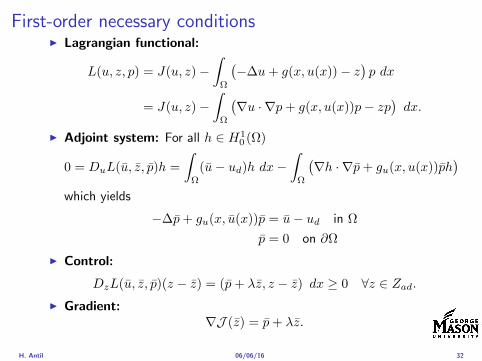
First-order necessary conditionsI Lagrangian functional
L(u z p) = J(u z)minusint
Ω
(minus∆u+ g(x u(x))minus z
)p dx
= J(u z)minusint
Ω
(nablau middot nablap+ g(x u(x))pminus zp
)dx
I Adjoint system For all h isin H10 (Ω)
0 = DuL(u z p)h =
intΩ
(uminus ud)h dxminusint
Ω
(nablah middot nablap+ gu(x u(x))ph
)which yields
minus∆p+ gu(x u(x))p = uminus ud in Ω
p = 0 on partΩ
I Control
DzL(u z p)(z minus z) = (p+ λz z minus z) dx ge 0 forallz isin ZadI Gradient
nablaJ (z) = p+ λz
H Antil 060616 32
Differentiability of Nemytskii operator
The rigorous proof uses
Theorem In addition to (A1)-(A4) if
(A5) g is continuously differentiable with respect to u for ae x isin Ωand we have
(i) |gu(x 0)| le K for ae x isin Ω(ii) gu is locally Lipschitz with respect to u isin R
then the Nemytskii operator G u 7rarr g(middot u(middot)) is continuously Frechetdifferentiable from Linfin(Ω) into itself and
(Gprime(u)h)(x) = gu(x u(x))h(x) ae in Ω forallh isin Linfin(Ω)
Remark (A5) holds if g(x u) = g(u) and g isin C2(R)
H Antil 060616 33
Outline
Motivation and examples
Linear elliptic optimal control problems
Differentiation in Banach spaces
First-order necessary conditions
Optimal control of semilinear PDEs
An abstract problem
Discretization using finite element methods
H Antil 060616 34
Gradient computation via adjoint general formI Abstract problem
min J(u z)
subject toc(u z) = 0
and z isin Zad
I Directional derivative Let S be the control to state map(nonlinear in general)
z 7rarr S(z) = u(z)
Under the assumptions of ldquoimplicit function theoremrdquo
J prime(z)h = (nablauJ (u(z) z) Sprime(z)h) + (nablazJ (u(z) z) h)
I Sensitivity of u with respect to z Differentiating the stateequation
cu(S(z) z)Sprime(z)h = minuscz(S(z) z)h
leads toSprime(z)h = minuscu(S(z) z)minus1
(cz(S(z) z)h
)
provided cu(S(z) z)minus1 is well-defined
H Antil 060616 35
Gradient computation via adjoint general formI Abstract problem
min J(u z)
subject toc(u z) = 0
and z isin ZadI Directional derivative Let S be the control to state map
(nonlinear in general)
z 7rarr S(z) = u(z)
Under the assumptions of ldquoimplicit function theoremrdquo
J prime(z)h = (nablauJ (u(z) z) Sprime(z)h) + (nablazJ (u(z) z) h)
I Sensitivity of u with respect to z Differentiating the stateequation
cu(S(z) z)Sprime(z)h = minuscz(S(z) z)h
leads toSprime(z)h = minuscu(S(z) z)minus1
(cz(S(z) z)h
)
provided cu(S(z) z)minus1 is well-defined
H Antil 060616 35
Gradient computation via adjoint general formI Abstract problem
min J(u z)
subject toc(u z) = 0
and z isin ZadI Directional derivative Let S be the control to state map
(nonlinear in general)
z 7rarr S(z) = u(z)
Under the assumptions of ldquoimplicit function theoremrdquo
J prime(z)h = (nablauJ (u(z) z) Sprime(z)h) + (nablazJ (u(z) z) h)
I Sensitivity of u with respect to z Differentiating the stateequation
cu(S(z) z)Sprime(z)h = minuscz(S(z) z)h
leads toSprime(z)h = minuscu(S(z) z)minus1
(cz(S(z) z)h
)
provided cu(S(z) z)minus1 is well-defined
H Antil 060616 35
Adjoint equation and gradient general form
I Directional derivative
J prime(z)h = minus(nablauJ (u(z) z) cu(u(z) z)minus1cz(u(z) z)h
)+ (nablazJ (u(z) z) h)
I Gradient
nablaJ (z) = minuscz(u(z) z)lowast(cu(u(z) z)minuslowastnablauJ (u(z) z)
)+nablazJ (u(z) z)
I Introducing adjoint variable p solving
cu(u(z) z)lowastp = nablauJ (u(z) z)
we arrive at following form of gradient
nablaJ (z) = minuscz(u(z) z)lowastp+nablazJ (u(z) z)
which is tractable
H Antil 060616 36
Adjoint equation and gradient general form
I Directional derivative
J prime(z)h = minus(nablauJ (u(z) z) cu(u(z) z)minus1cz(u(z) z)h
)+ (nablazJ (u(z) z) h)
I Gradient
nablaJ (z) = minuscz(u(z) z)lowast(cu(u(z) z)minuslowastnablauJ (u(z) z)
)+nablazJ (u(z) z)
I Introducing adjoint variable p solving
cu(u(z) z)lowastp = nablauJ (u(z) z)
we arrive at following form of gradient
nablaJ (z) = minuscz(u(z) z)lowastp+nablazJ (u(z) z)
which is tractable
H Antil 060616 36
Adjoint equation and gradient general form
I Directional derivative
J prime(z)h = minus(nablauJ (u(z) z) cu(u(z) z)minus1cz(u(z) z)h
)+ (nablazJ (u(z) z) h)
I Gradient
nablaJ (z) = minuscz(u(z) z)lowast(cu(u(z) z)minuslowastnablauJ (u(z) z)
)+nablazJ (u(z) z)
I Introducing adjoint variable p solving
cu(u(z) z)lowastp = nablauJ (u(z) z)
we arrive at following form of gradient
nablaJ (z) = minuscz(u(z) z)lowastp+nablazJ (u(z) z)
which is tractable
H Antil 060616 36
Hessian computation general form
I Lagrangian L(u z p) = J(u z)minusint
Ωc(u z)p dx Then we have
DzJ (z)h = DzL(u z p)h
I Second order derivative
D2zJ (z)[h1 h2] = DuDzL(u z p)[h1 S
prime(z)h2] +D2zL(u z p)[h1 h2]
+DpDzL(u z p)[h1 Dzp(z)h2]
I We already know Sprime(z)h2 moreover
DpDzL(u z p)[h1 Dzp(z)h2] = minus(cu(u z)h1 Dzp(z)h2
)
It remain to identify Dzp(z)h2
H Antil 060616 37
Hessian computation general form
I Lagrangian L(u z p) = J(u z)minusint
Ωc(u z)p dx Then we have
DzJ (z)h = DzL(u z p)h
I Second order derivative
D2zJ (z)[h1 h2] = DuDzL(u z p)[h1 S
prime(z)h2] +D2zL(u z p)[h1 h2]
+DpDzL(u z p)[h1 Dzp(z)h2]
I We already know Sprime(z)h2 moreover
DpDzL(u z p)[h1 Dzp(z)h2] = minus(cu(u z)h1 Dzp(z)h2
)
It remain to identify Dzp(z)h2
H Antil 060616 37
Hessian computation general form
I Lagrangian L(u z p) = J(u z)minusint
Ωc(u z)p dx Then we have
DzJ (z)h = DzL(u z p)h
I Second order derivative
D2zJ (z)[h1 h2] = DuDzL(u z p)[h1 S
prime(z)h2] +D2zL(u z p)[h1 h2]
+DpDzL(u z p)[h1 Dzp(z)h2]
I We already know Sprime(z)h2 moreover
DpDzL(u z p)[h1 Dzp(z)h2] = minus(cu(u z)h1 Dzp(z)h2
)
It remain to identify Dzp(z)h2
H Antil 060616 37
Outline
Motivation and examples
Linear elliptic optimal control problems
Differentiation in Banach spaces
First-order necessary conditions
Optimal control of semilinear PDEs
An abstract problem
Discretization using finite element methods
H Antil 060616 38
Numerical approximation of Poisson equation MeshTo avoid technical issues we will assume that partΩ is polygonal
I Mesh Let T = K be a mesh of Ω where K sub Rd is an elementthat is isoparametrically equivalent to a unit simplex in Rd
I Conforming mesh We say that the mesh is conforming ifI Ω = cupKisinT KI If K1 cap K2 = x then x is a node of K1 and K2I If K1 cap K2 6= empty and K1 cap K2 6= x then K1 cap K2 is an edgeface
contained in partK1 cap partK2
I Shape regular Let T be the collection of all conformingrefinements of an original mesh T 0 Then T is called shape regularif exist κ gt 0 such that
hKρKle κ forallK isin cupiT i
where hK = diam K ρK = maxρ gt 0|Bρ sub KI Quasi-uniform A family of shape regular meshes is called-quasi
uniform if there exist a constant σ gt 0 such that
maxhKminhK
le σ
uniformly for all meshes in the family
Numerical approximation of Poisson equation MeshTo avoid technical issues we will assume that partΩ is polygonal
I Mesh Let T = K be a mesh of Ω where K sub Rd is an elementthat is isoparametrically equivalent to a unit simplex in Rd
I Conforming mesh We say that the mesh is conforming ifI Ω = cupKisinT KI If K1 cap K2 = x then x is a node of K1 and K2I If K1 cap K2 6= empty and K1 cap K2 6= x then K1 cap K2 is an edgeface
contained in partK1 cap partK2
I Shape regular Let T be the collection of all conformingrefinements of an original mesh T 0 Then T is called shape regularif exist κ gt 0 such that
hKρKle κ forallK isin cupiT i
where hK = diam K ρK = maxρ gt 0|Bρ sub KI Quasi-uniform A family of shape regular meshes is called-quasi
uniform if there exist a constant σ gt 0 such that
maxhKminhK
le σ
uniformly for all meshes in the family
Numerical approximation of Poisson equation MeshTo avoid technical issues we will assume that partΩ is polygonal
I Mesh Let T = K be a mesh of Ω where K sub Rd is an elementthat is isoparametrically equivalent to a unit simplex in Rd
I Conforming mesh We say that the mesh is conforming ifI Ω = cupKisinT KI If K1 cap K2 = x then x is a node of K1 and K2I If K1 cap K2 6= empty and K1 cap K2 6= x then K1 cap K2 is an edgeface
contained in partK1 cap partK2
I Shape regular Let T be the collection of all conformingrefinements of an original mesh T 0 Then T is called shape regularif exist κ gt 0 such that
hKρKle κ forallK isin cupiT i
where hK = diam K ρK = maxρ gt 0|Bρ sub K
I Quasi-uniform A family of shape regular meshes is called-quasiuniform if there exist a constant σ gt 0 such that
maxhKminhK
le σ
uniformly for all meshes in the family
Numerical approximation of Poisson equation MeshTo avoid technical issues we will assume that partΩ is polygonal
I Mesh Let T = K be a mesh of Ω where K sub Rd is an elementthat is isoparametrically equivalent to a unit simplex in Rd
I Conforming mesh We say that the mesh is conforming ifI Ω = cupKisinT KI If K1 cap K2 = x then x is a node of K1 and K2I If K1 cap K2 6= empty and K1 cap K2 6= x then K1 cap K2 is an edgeface
contained in partK1 cap partK2
I Shape regular Let T be the collection of all conformingrefinements of an original mesh T 0 Then T is called shape regularif exist κ gt 0 such that
hKρKle κ forallK isin cupiT i
where hK = diam K ρK = maxρ gt 0|Bρ sub KI Quasi-uniform A family of shape regular meshes is called-quasi
uniform if there exist a constant σ gt 0 such that
maxhKminhK
le σ
uniformly for all meshes in the family
FE space and Galerkin approximationI Finite element space For T isin T we define the finite element
space as
V(T ) = W isin C0(Ω) WK isin P1forallK isin T W |partΩ = 0
where P1 is the set of polynomials of degree at most 1
I Galerkin approximation of continuous problem is given by
Find UT isin V(T )
intΩ
AnablaUT middot nablaV = 〈f V 〉 forallV isin V(T )
The discrete problem is well-posedI Nodal basis Consists of functions ψi isin V(T ) with xi isin N (T )
satisfyingψxi
(xj) = δij
where N (T ) denotes the interior (plus Neumann) nodesI Galerkin orthogonality(
nabla(uminus UT )nablaW)L2(Ω)
= 0 forallW isin V(T )
H Antil 060616 40
FE space and Galerkin approximationI Finite element space For T isin T we define the finite element
space as
V(T ) = W isin C0(Ω) WK isin P1forallK isin T W |partΩ = 0
where P1 is the set of polynomials of degree at most 1I Galerkin approximation of continuous problem is given by
Find UT isin V(T )
intΩ
AnablaUT middot nablaV = 〈f V 〉 forallV isin V(T )
The discrete problem is well-posed
I Nodal basis Consists of functions ψi isin V(T ) with xi isin N (T )satisfying
ψxi(xj) = δij
where N (T ) denotes the interior (plus Neumann) nodesI Galerkin orthogonality(
nabla(uminus UT )nablaW)L2(Ω)
= 0 forallW isin V(T )
H Antil 060616 40
FE space and Galerkin approximationI Finite element space For T isin T we define the finite element
space as
V(T ) = W isin C0(Ω) WK isin P1forallK isin T W |partΩ = 0
where P1 is the set of polynomials of degree at most 1I Galerkin approximation of continuous problem is given by
Find UT isin V(T )
intΩ
AnablaUT middot nablaV = 〈f V 〉 forallV isin V(T )
The discrete problem is well-posedI Nodal basis Consists of functions ψi isin V(T ) with xi isin N (T )
satisfyingψxi
(xj) = δij
where N (T ) denotes the interior (plus Neumann) nodes
I Galerkin orthogonality(nabla(uminus UT )nablaW
)L2(Ω)
= 0 forallW isin V(T )
H Antil 060616 40
FE space and Galerkin approximationI Finite element space For T isin T we define the finite element
space as
V(T ) = W isin C0(Ω) WK isin P1forallK isin T W |partΩ = 0
where P1 is the set of polynomials of degree at most 1I Galerkin approximation of continuous problem is given by
Find UT isin V(T )
intΩ
AnablaUT middot nablaV = 〈f V 〉 forallV isin V(T )
The discrete problem is well-posedI Nodal basis Consists of functions ψi isin V(T ) with xi isin N (T )
satisfyingψxi
(xj) = δij
where N (T ) denotes the interior (plus Neumann) nodesI Galerkin orthogonality(
nabla(uminus UT )nablaW)L2(Ω)
= 0 forallW isin V(T )
H Antil 060616 40
Best approximation
I Cearsquos lemma
nabla(uminus UT )L2(Ω) le C infWisinV(T )
nabla(uminusW )L2(Ω)
I Nodal interpolation operator ΠT C(Ω)rarr V(T ) satisfies
ΠT u(xi) = u(xi) forallxi isin N (T )
and is defined as
ΠT u =sum
xiisinN (T )
u(xi)ψxi
I Error estimates In Cearsquos lemma replace W by ΠT u and thencompute the interpolation error
H Antil 060616 41
Best approximation
I Cearsquos lemma
nabla(uminus UT )L2(Ω) le C infWisinV(T )
nabla(uminusW )L2(Ω)
I Nodal interpolation operator ΠT C(Ω)rarr V(T ) satisfies
ΠT u(xi) = u(xi) forallxi isin N (T )
and is defined as
ΠT u =sum
xiisinN (T )
u(xi)ψxi
I Error estimates In Cearsquos lemma replace W by ΠT u and thencompute the interpolation error
H Antil 060616 41
Best approximation
I Cearsquos lemma
nabla(uminus UT )L2(Ω) le C infWisinV(T )
nabla(uminusW )L2(Ω)
I Nodal interpolation operator ΠT C(Ω)rarr V(T ) satisfies
ΠT u(xi) = u(xi) forallxi isin N (T )
and is defined as
ΠT u =sum
xiisinN (T )
u(xi)ψxi
I Error estimates In Cearsquos lemma replace W by ΠT u and thencompute the interpolation error
H Antil 060616 41
Algebraic system state equation
I Recall UT isin V(T ) solves
a(UT V ) = 〈f V 〉 forallV isin V(T )
I Now setting UT =sumN
j=1 Ujψj V = ψi we get
Nsumj=1
Uja(φj φi) = 〈f ψi〉 i = 1 N
which is the matrix-vector system
AU = F
I Stiffness matrix A is SPD
H Antil 060616 42
Algebraic system state equation
I Recall UT isin V(T ) solves
a(UT V ) = 〈f V 〉 forallV isin V(T )
I Now setting UT =sumN
j=1 Ujψj V = ψi we get
Nsumj=1
Uja(φj φi) = 〈f ψi〉 i = 1 N
which is the matrix-vector system
AU = F
I Stiffness matrix A is SPD
H Antil 060616 42
Algebraic system state equation
I Recall UT isin V(T ) solves
a(UT V ) = 〈f V 〉 forallV isin V(T )
I Now setting UT =sumN
j=1 Ujψj V = ψi we get
Nsumj=1
Uja(φj φi) = 〈f ψi〉 i = 1 N
which is the matrix-vector system
AU = F
I Stiffness matrix A is SPD
H Antil 060616 42
Discrete linear elliptic OCP
min JT (UT ZT ) =1
2UT minus ud2L2(Ω) +
λ
2ZT 2L2(Ω)
subject to
Find UT isin V(T )
intΩ
nablaUT middot nablaV = (ZT V )L2(Ω) forallV isin V(T )
and whereZT isin Zad(T ) = Zad cap Z(T )
is either one of these
Z(T ) =
V(T )L2(Ω) variational discretization (Hinze)WT isin Linfin(Ω) ZT |K isin P0(K)K isin T
H Antil 060616 43
Recent books
F TroltzschOptimal control of partial differential equations volume 112 ofGraduate Studies in MathematicsAmerican Mathematical Society Providence RI 2010Theory methods and applications Translated from the 2005 Germanoriginal by Jurgen Sprekels
K Ito and K KunischLagrange multiplier approach to variational problems andapplications volume 15 of Advances in Design and ControlSociety for Industrial and Applied Mathematics (SIAM)Philadelphia PA 2008
H Antil 060616 44
- Motivation and examples
- Linear elliptic optimal control problems
- Differentiation in Banach spaces
- First-order necessary conditions
- Optimal control of semilinear PDEs
- An abstract problem
- Discretization using finite element methods
-
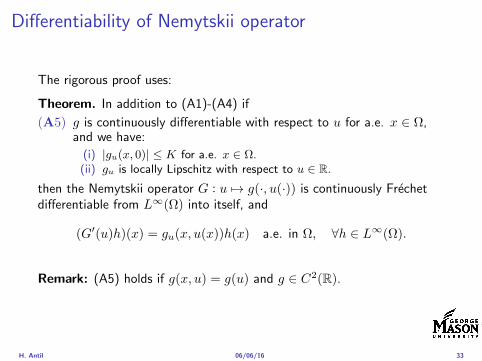
Outline
Motivation and examples
Linear elliptic optimal control problems
Differentiation in Banach spaces
First-order necessary conditions
Optimal control of semilinear PDEs
An abstract problem
Discretization using finite element methods
H Antil 060616 34
Gradient computation via adjoint general formI Abstract problem
min J(u z)
subject toc(u z) = 0
and z isin Zad
I Directional derivative Let S be the control to state map(nonlinear in general)
z 7rarr S(z) = u(z)
Under the assumptions of ldquoimplicit function theoremrdquo
J prime(z)h = (nablauJ (u(z) z) Sprime(z)h) + (nablazJ (u(z) z) h)
I Sensitivity of u with respect to z Differentiating the stateequation
cu(S(z) z)Sprime(z)h = minuscz(S(z) z)h
leads toSprime(z)h = minuscu(S(z) z)minus1
(cz(S(z) z)h
)
provided cu(S(z) z)minus1 is well-defined
H Antil 060616 35
Gradient computation via adjoint general formI Abstract problem
min J(u z)
subject toc(u z) = 0
and z isin ZadI Directional derivative Let S be the control to state map
(nonlinear in general)
z 7rarr S(z) = u(z)
Under the assumptions of ldquoimplicit function theoremrdquo
J prime(z)h = (nablauJ (u(z) z) Sprime(z)h) + (nablazJ (u(z) z) h)
I Sensitivity of u with respect to z Differentiating the stateequation
cu(S(z) z)Sprime(z)h = minuscz(S(z) z)h
leads toSprime(z)h = minuscu(S(z) z)minus1
(cz(S(z) z)h
)
provided cu(S(z) z)minus1 is well-defined
H Antil 060616 35
Gradient computation via adjoint general formI Abstract problem
min J(u z)
subject toc(u z) = 0
and z isin ZadI Directional derivative Let S be the control to state map
(nonlinear in general)
z 7rarr S(z) = u(z)
Under the assumptions of ldquoimplicit function theoremrdquo
J prime(z)h = (nablauJ (u(z) z) Sprime(z)h) + (nablazJ (u(z) z) h)
I Sensitivity of u with respect to z Differentiating the stateequation
cu(S(z) z)Sprime(z)h = minuscz(S(z) z)h
leads toSprime(z)h = minuscu(S(z) z)minus1
(cz(S(z) z)h
)
provided cu(S(z) z)minus1 is well-defined
H Antil 060616 35
Adjoint equation and gradient general form
I Directional derivative
J prime(z)h = minus(nablauJ (u(z) z) cu(u(z) z)minus1cz(u(z) z)h
)+ (nablazJ (u(z) z) h)
I Gradient
nablaJ (z) = minuscz(u(z) z)lowast(cu(u(z) z)minuslowastnablauJ (u(z) z)
)+nablazJ (u(z) z)
I Introducing adjoint variable p solving
cu(u(z) z)lowastp = nablauJ (u(z) z)
we arrive at following form of gradient
nablaJ (z) = minuscz(u(z) z)lowastp+nablazJ (u(z) z)
which is tractable
H Antil 060616 36
Adjoint equation and gradient general form
I Directional derivative
J prime(z)h = minus(nablauJ (u(z) z) cu(u(z) z)minus1cz(u(z) z)h
)+ (nablazJ (u(z) z) h)
I Gradient
nablaJ (z) = minuscz(u(z) z)lowast(cu(u(z) z)minuslowastnablauJ (u(z) z)
)+nablazJ (u(z) z)
I Introducing adjoint variable p solving
cu(u(z) z)lowastp = nablauJ (u(z) z)
we arrive at following form of gradient
nablaJ (z) = minuscz(u(z) z)lowastp+nablazJ (u(z) z)
which is tractable
H Antil 060616 36
Adjoint equation and gradient general form
I Directional derivative
J prime(z)h = minus(nablauJ (u(z) z) cu(u(z) z)minus1cz(u(z) z)h
)+ (nablazJ (u(z) z) h)
I Gradient
nablaJ (z) = minuscz(u(z) z)lowast(cu(u(z) z)minuslowastnablauJ (u(z) z)
)+nablazJ (u(z) z)
I Introducing adjoint variable p solving
cu(u(z) z)lowastp = nablauJ (u(z) z)
we arrive at following form of gradient
nablaJ (z) = minuscz(u(z) z)lowastp+nablazJ (u(z) z)
which is tractable
H Antil 060616 36
Hessian computation general form
I Lagrangian L(u z p) = J(u z)minusint
Ωc(u z)p dx Then we have
DzJ (z)h = DzL(u z p)h
I Second order derivative
D2zJ (z)[h1 h2] = DuDzL(u z p)[h1 S
prime(z)h2] +D2zL(u z p)[h1 h2]
+DpDzL(u z p)[h1 Dzp(z)h2]
I We already know Sprime(z)h2 moreover
DpDzL(u z p)[h1 Dzp(z)h2] = minus(cu(u z)h1 Dzp(z)h2
)
It remain to identify Dzp(z)h2
H Antil 060616 37
Hessian computation general form
I Lagrangian L(u z p) = J(u z)minusint
Ωc(u z)p dx Then we have
DzJ (z)h = DzL(u z p)h
I Second order derivative
D2zJ (z)[h1 h2] = DuDzL(u z p)[h1 S
prime(z)h2] +D2zL(u z p)[h1 h2]
+DpDzL(u z p)[h1 Dzp(z)h2]
I We already know Sprime(z)h2 moreover
DpDzL(u z p)[h1 Dzp(z)h2] = minus(cu(u z)h1 Dzp(z)h2
)
It remain to identify Dzp(z)h2
H Antil 060616 37
Hessian computation general form
I Lagrangian L(u z p) = J(u z)minusint
Ωc(u z)p dx Then we have
DzJ (z)h = DzL(u z p)h
I Second order derivative
D2zJ (z)[h1 h2] = DuDzL(u z p)[h1 S
prime(z)h2] +D2zL(u z p)[h1 h2]
+DpDzL(u z p)[h1 Dzp(z)h2]
I We already know Sprime(z)h2 moreover
DpDzL(u z p)[h1 Dzp(z)h2] = minus(cu(u z)h1 Dzp(z)h2
)
It remain to identify Dzp(z)h2
H Antil 060616 37
Outline
Motivation and examples
Linear elliptic optimal control problems
Differentiation in Banach spaces
First-order necessary conditions
Optimal control of semilinear PDEs
An abstract problem
Discretization using finite element methods
H Antil 060616 38
Numerical approximation of Poisson equation MeshTo avoid technical issues we will assume that partΩ is polygonal
I Mesh Let T = K be a mesh of Ω where K sub Rd is an elementthat is isoparametrically equivalent to a unit simplex in Rd
I Conforming mesh We say that the mesh is conforming ifI Ω = cupKisinT KI If K1 cap K2 = x then x is a node of K1 and K2I If K1 cap K2 6= empty and K1 cap K2 6= x then K1 cap K2 is an edgeface
contained in partK1 cap partK2
I Shape regular Let T be the collection of all conformingrefinements of an original mesh T 0 Then T is called shape regularif exist κ gt 0 such that
hKρKle κ forallK isin cupiT i
where hK = diam K ρK = maxρ gt 0|Bρ sub KI Quasi-uniform A family of shape regular meshes is called-quasi
uniform if there exist a constant σ gt 0 such that
maxhKminhK
le σ
uniformly for all meshes in the family
Numerical approximation of Poisson equation MeshTo avoid technical issues we will assume that partΩ is polygonal
I Mesh Let T = K be a mesh of Ω where K sub Rd is an elementthat is isoparametrically equivalent to a unit simplex in Rd
I Conforming mesh We say that the mesh is conforming ifI Ω = cupKisinT KI If K1 cap K2 = x then x is a node of K1 and K2I If K1 cap K2 6= empty and K1 cap K2 6= x then K1 cap K2 is an edgeface
contained in partK1 cap partK2
I Shape regular Let T be the collection of all conformingrefinements of an original mesh T 0 Then T is called shape regularif exist κ gt 0 such that
hKρKle κ forallK isin cupiT i
where hK = diam K ρK = maxρ gt 0|Bρ sub KI Quasi-uniform A family of shape regular meshes is called-quasi
uniform if there exist a constant σ gt 0 such that
maxhKminhK
le σ
uniformly for all meshes in the family
Numerical approximation of Poisson equation MeshTo avoid technical issues we will assume that partΩ is polygonal
I Mesh Let T = K be a mesh of Ω where K sub Rd is an elementthat is isoparametrically equivalent to a unit simplex in Rd
I Conforming mesh We say that the mesh is conforming ifI Ω = cupKisinT KI If K1 cap K2 = x then x is a node of K1 and K2I If K1 cap K2 6= empty and K1 cap K2 6= x then K1 cap K2 is an edgeface
contained in partK1 cap partK2
I Shape regular Let T be the collection of all conformingrefinements of an original mesh T 0 Then T is called shape regularif exist κ gt 0 such that
hKρKle κ forallK isin cupiT i
where hK = diam K ρK = maxρ gt 0|Bρ sub K
I Quasi-uniform A family of shape regular meshes is called-quasiuniform if there exist a constant σ gt 0 such that
maxhKminhK
le σ
uniformly for all meshes in the family
Numerical approximation of Poisson equation MeshTo avoid technical issues we will assume that partΩ is polygonal
I Mesh Let T = K be a mesh of Ω where K sub Rd is an elementthat is isoparametrically equivalent to a unit simplex in Rd
I Conforming mesh We say that the mesh is conforming ifI Ω = cupKisinT KI If K1 cap K2 = x then x is a node of K1 and K2I If K1 cap K2 6= empty and K1 cap K2 6= x then K1 cap K2 is an edgeface
contained in partK1 cap partK2
I Shape regular Let T be the collection of all conformingrefinements of an original mesh T 0 Then T is called shape regularif exist κ gt 0 such that
hKρKle κ forallK isin cupiT i
where hK = diam K ρK = maxρ gt 0|Bρ sub KI Quasi-uniform A family of shape regular meshes is called-quasi
uniform if there exist a constant σ gt 0 such that
maxhKminhK
le σ
uniformly for all meshes in the family
FE space and Galerkin approximationI Finite element space For T isin T we define the finite element
space as
V(T ) = W isin C0(Ω) WK isin P1forallK isin T W |partΩ = 0
where P1 is the set of polynomials of degree at most 1
I Galerkin approximation of continuous problem is given by
Find UT isin V(T )
intΩ
AnablaUT middot nablaV = 〈f V 〉 forallV isin V(T )
The discrete problem is well-posedI Nodal basis Consists of functions ψi isin V(T ) with xi isin N (T )
satisfyingψxi
(xj) = δij
where N (T ) denotes the interior (plus Neumann) nodesI Galerkin orthogonality(
nabla(uminus UT )nablaW)L2(Ω)
= 0 forallW isin V(T )
H Antil 060616 40
FE space and Galerkin approximationI Finite element space For T isin T we define the finite element
space as
V(T ) = W isin C0(Ω) WK isin P1forallK isin T W |partΩ = 0
where P1 is the set of polynomials of degree at most 1I Galerkin approximation of continuous problem is given by
Find UT isin V(T )
intΩ
AnablaUT middot nablaV = 〈f V 〉 forallV isin V(T )
The discrete problem is well-posed
I Nodal basis Consists of functions ψi isin V(T ) with xi isin N (T )satisfying
ψxi(xj) = δij
where N (T ) denotes the interior (plus Neumann) nodesI Galerkin orthogonality(
nabla(uminus UT )nablaW)L2(Ω)
= 0 forallW isin V(T )
H Antil 060616 40
FE space and Galerkin approximationI Finite element space For T isin T we define the finite element
space as
V(T ) = W isin C0(Ω) WK isin P1forallK isin T W |partΩ = 0
where P1 is the set of polynomials of degree at most 1I Galerkin approximation of continuous problem is given by
Find UT isin V(T )
intΩ
AnablaUT middot nablaV = 〈f V 〉 forallV isin V(T )
The discrete problem is well-posedI Nodal basis Consists of functions ψi isin V(T ) with xi isin N (T )
satisfyingψxi
(xj) = δij
where N (T ) denotes the interior (plus Neumann) nodes
I Galerkin orthogonality(nabla(uminus UT )nablaW
)L2(Ω)
= 0 forallW isin V(T )
H Antil 060616 40
FE space and Galerkin approximationI Finite element space For T isin T we define the finite element
space as
V(T ) = W isin C0(Ω) WK isin P1forallK isin T W |partΩ = 0
where P1 is the set of polynomials of degree at most 1I Galerkin approximation of continuous problem is given by
Find UT isin V(T )
intΩ
AnablaUT middot nablaV = 〈f V 〉 forallV isin V(T )
The discrete problem is well-posedI Nodal basis Consists of functions ψi isin V(T ) with xi isin N (T )
satisfyingψxi
(xj) = δij
where N (T ) denotes the interior (plus Neumann) nodesI Galerkin orthogonality(
nabla(uminus UT )nablaW)L2(Ω)
= 0 forallW isin V(T )
H Antil 060616 40
Best approximation
I Cearsquos lemma
nabla(uminus UT )L2(Ω) le C infWisinV(T )
nabla(uminusW )L2(Ω)
I Nodal interpolation operator ΠT C(Ω)rarr V(T ) satisfies
ΠT u(xi) = u(xi) forallxi isin N (T )
and is defined as
ΠT u =sum
xiisinN (T )
u(xi)ψxi
I Error estimates In Cearsquos lemma replace W by ΠT u and thencompute the interpolation error
H Antil 060616 41
Best approximation
I Cearsquos lemma
nabla(uminus UT )L2(Ω) le C infWisinV(T )
nabla(uminusW )L2(Ω)
I Nodal interpolation operator ΠT C(Ω)rarr V(T ) satisfies
ΠT u(xi) = u(xi) forallxi isin N (T )
and is defined as
ΠT u =sum
xiisinN (T )
u(xi)ψxi
I Error estimates In Cearsquos lemma replace W by ΠT u and thencompute the interpolation error
H Antil 060616 41
Best approximation
I Cearsquos lemma
nabla(uminus UT )L2(Ω) le C infWisinV(T )
nabla(uminusW )L2(Ω)
I Nodal interpolation operator ΠT C(Ω)rarr V(T ) satisfies
ΠT u(xi) = u(xi) forallxi isin N (T )
and is defined as
ΠT u =sum
xiisinN (T )
u(xi)ψxi
I Error estimates In Cearsquos lemma replace W by ΠT u and thencompute the interpolation error
H Antil 060616 41
Algebraic system state equation
I Recall UT isin V(T ) solves
a(UT V ) = 〈f V 〉 forallV isin V(T )
I Now setting UT =sumN
j=1 Ujψj V = ψi we get
Nsumj=1
Uja(φj φi) = 〈f ψi〉 i = 1 N
which is the matrix-vector system
AU = F
I Stiffness matrix A is SPD
H Antil 060616 42
Algebraic system state equation
I Recall UT isin V(T ) solves
a(UT V ) = 〈f V 〉 forallV isin V(T )
I Now setting UT =sumN
j=1 Ujψj V = ψi we get
Nsumj=1
Uja(φj φi) = 〈f ψi〉 i = 1 N
which is the matrix-vector system
AU = F
I Stiffness matrix A is SPD
H Antil 060616 42
Algebraic system state equation
I Recall UT isin V(T ) solves
a(UT V ) = 〈f V 〉 forallV isin V(T )
I Now setting UT =sumN
j=1 Ujψj V = ψi we get
Nsumj=1
Uja(φj φi) = 〈f ψi〉 i = 1 N
which is the matrix-vector system
AU = F
I Stiffness matrix A is SPD
H Antil 060616 42
Discrete linear elliptic OCP
min JT (UT ZT ) =1
2UT minus ud2L2(Ω) +
λ
2ZT 2L2(Ω)
subject to
Find UT isin V(T )
intΩ
nablaUT middot nablaV = (ZT V )L2(Ω) forallV isin V(T )
and whereZT isin Zad(T ) = Zad cap Z(T )
is either one of these
Z(T ) =
V(T )L2(Ω) variational discretization (Hinze)WT isin Linfin(Ω) ZT |K isin P0(K)K isin T
H Antil 060616 43
Recent books
F TroltzschOptimal control of partial differential equations volume 112 ofGraduate Studies in MathematicsAmerican Mathematical Society Providence RI 2010Theory methods and applications Translated from the 2005 Germanoriginal by Jurgen Sprekels
K Ito and K KunischLagrange multiplier approach to variational problems andapplications volume 15 of Advances in Design and ControlSociety for Industrial and Applied Mathematics (SIAM)Philadelphia PA 2008
H Antil 060616 44
- Motivation and examples
- Linear elliptic optimal control problems
- Differentiation in Banach spaces
- First-order necessary conditions
- Optimal control of semilinear PDEs
- An abstract problem
- Discretization using finite element methods
-
Gradient computation via adjoint general formI Abstract problem
min J(u z)
subject toc(u z) = 0
and z isin Zad
I Directional derivative Let S be the control to state map(nonlinear in general)
z 7rarr S(z) = u(z)
Under the assumptions of ldquoimplicit function theoremrdquo
J prime(z)h = (nablauJ (u(z) z) Sprime(z)h) + (nablazJ (u(z) z) h)
I Sensitivity of u with respect to z Differentiating the stateequation
cu(S(z) z)Sprime(z)h = minuscz(S(z) z)h
leads toSprime(z)h = minuscu(S(z) z)minus1
(cz(S(z) z)h
)
provided cu(S(z) z)minus1 is well-defined
H Antil 060616 35
Gradient computation via adjoint general formI Abstract problem
min J(u z)
subject toc(u z) = 0
and z isin ZadI Directional derivative Let S be the control to state map
(nonlinear in general)
z 7rarr S(z) = u(z)
Under the assumptions of ldquoimplicit function theoremrdquo
J prime(z)h = (nablauJ (u(z) z) Sprime(z)h) + (nablazJ (u(z) z) h)
I Sensitivity of u with respect to z Differentiating the stateequation
cu(S(z) z)Sprime(z)h = minuscz(S(z) z)h
leads toSprime(z)h = minuscu(S(z) z)minus1
(cz(S(z) z)h
)
provided cu(S(z) z)minus1 is well-defined
H Antil 060616 35
Gradient computation via adjoint general formI Abstract problem
min J(u z)
subject toc(u z) = 0
and z isin ZadI Directional derivative Let S be the control to state map
(nonlinear in general)
z 7rarr S(z) = u(z)
Under the assumptions of ldquoimplicit function theoremrdquo
J prime(z)h = (nablauJ (u(z) z) Sprime(z)h) + (nablazJ (u(z) z) h)
I Sensitivity of u with respect to z Differentiating the stateequation
cu(S(z) z)Sprime(z)h = minuscz(S(z) z)h
leads toSprime(z)h = minuscu(S(z) z)minus1
(cz(S(z) z)h
)
provided cu(S(z) z)minus1 is well-defined
H Antil 060616 35
Adjoint equation and gradient general form
I Directional derivative
J prime(z)h = minus(nablauJ (u(z) z) cu(u(z) z)minus1cz(u(z) z)h
)+ (nablazJ (u(z) z) h)
I Gradient
nablaJ (z) = minuscz(u(z) z)lowast(cu(u(z) z)minuslowastnablauJ (u(z) z)
)+nablazJ (u(z) z)
I Introducing adjoint variable p solving
cu(u(z) z)lowastp = nablauJ (u(z) z)
we arrive at following form of gradient
nablaJ (z) = minuscz(u(z) z)lowastp+nablazJ (u(z) z)
which is tractable
H Antil 060616 36
Adjoint equation and gradient general form
I Directional derivative
J prime(z)h = minus(nablauJ (u(z) z) cu(u(z) z)minus1cz(u(z) z)h
)+ (nablazJ (u(z) z) h)
I Gradient
nablaJ (z) = minuscz(u(z) z)lowast(cu(u(z) z)minuslowastnablauJ (u(z) z)
)+nablazJ (u(z) z)
I Introducing adjoint variable p solving
cu(u(z) z)lowastp = nablauJ (u(z) z)
we arrive at following form of gradient
nablaJ (z) = minuscz(u(z) z)lowastp+nablazJ (u(z) z)
which is tractable
H Antil 060616 36
Adjoint equation and gradient general form
I Directional derivative
J prime(z)h = minus(nablauJ (u(z) z) cu(u(z) z)minus1cz(u(z) z)h
)+ (nablazJ (u(z) z) h)
I Gradient
nablaJ (z) = minuscz(u(z) z)lowast(cu(u(z) z)minuslowastnablauJ (u(z) z)
)+nablazJ (u(z) z)
I Introducing adjoint variable p solving
cu(u(z) z)lowastp = nablauJ (u(z) z)
we arrive at following form of gradient
nablaJ (z) = minuscz(u(z) z)lowastp+nablazJ (u(z) z)
which is tractable
H Antil 060616 36
Hessian computation general form
I Lagrangian L(u z p) = J(u z)minusint
Ωc(u z)p dx Then we have
DzJ (z)h = DzL(u z p)h
I Second order derivative
D2zJ (z)[h1 h2] = DuDzL(u z p)[h1 S
prime(z)h2] +D2zL(u z p)[h1 h2]
+DpDzL(u z p)[h1 Dzp(z)h2]
I We already know Sprime(z)h2 moreover
DpDzL(u z p)[h1 Dzp(z)h2] = minus(cu(u z)h1 Dzp(z)h2
)
It remain to identify Dzp(z)h2
H Antil 060616 37
Hessian computation general form
I Lagrangian L(u z p) = J(u z)minusint
Ωc(u z)p dx Then we have
DzJ (z)h = DzL(u z p)h
I Second order derivative
D2zJ (z)[h1 h2] = DuDzL(u z p)[h1 S
prime(z)h2] +D2zL(u z p)[h1 h2]
+DpDzL(u z p)[h1 Dzp(z)h2]
I We already know Sprime(z)h2 moreover
DpDzL(u z p)[h1 Dzp(z)h2] = minus(cu(u z)h1 Dzp(z)h2
)
It remain to identify Dzp(z)h2
H Antil 060616 37
Hessian computation general form
I Lagrangian L(u z p) = J(u z)minusint
Ωc(u z)p dx Then we have
DzJ (z)h = DzL(u z p)h
I Second order derivative
D2zJ (z)[h1 h2] = DuDzL(u z p)[h1 S
prime(z)h2] +D2zL(u z p)[h1 h2]
+DpDzL(u z p)[h1 Dzp(z)h2]
I We already know Sprime(z)h2 moreover
DpDzL(u z p)[h1 Dzp(z)h2] = minus(cu(u z)h1 Dzp(z)h2
)
It remain to identify Dzp(z)h2
H Antil 060616 37
Outline
Motivation and examples
Linear elliptic optimal control problems
Differentiation in Banach spaces
First-order necessary conditions
Optimal control of semilinear PDEs
An abstract problem
Discretization using finite element methods
H Antil 060616 38
Numerical approximation of Poisson equation MeshTo avoid technical issues we will assume that partΩ is polygonal
I Mesh Let T = K be a mesh of Ω where K sub Rd is an elementthat is isoparametrically equivalent to a unit simplex in Rd
I Conforming mesh We say that the mesh is conforming ifI Ω = cupKisinT KI If K1 cap K2 = x then x is a node of K1 and K2I If K1 cap K2 6= empty and K1 cap K2 6= x then K1 cap K2 is an edgeface
contained in partK1 cap partK2
I Shape regular Let T be the collection of all conformingrefinements of an original mesh T 0 Then T is called shape regularif exist κ gt 0 such that
hKρKle κ forallK isin cupiT i
where hK = diam K ρK = maxρ gt 0|Bρ sub KI Quasi-uniform A family of shape regular meshes is called-quasi
uniform if there exist a constant σ gt 0 such that
maxhKminhK
le σ
uniformly for all meshes in the family
Numerical approximation of Poisson equation MeshTo avoid technical issues we will assume that partΩ is polygonal
I Mesh Let T = K be a mesh of Ω where K sub Rd is an elementthat is isoparametrically equivalent to a unit simplex in Rd
I Conforming mesh We say that the mesh is conforming ifI Ω = cupKisinT KI If K1 cap K2 = x then x is a node of K1 and K2I If K1 cap K2 6= empty and K1 cap K2 6= x then K1 cap K2 is an edgeface
contained in partK1 cap partK2
I Shape regular Let T be the collection of all conformingrefinements of an original mesh T 0 Then T is called shape regularif exist κ gt 0 such that
hKρKle κ forallK isin cupiT i
where hK = diam K ρK = maxρ gt 0|Bρ sub KI Quasi-uniform A family of shape regular meshes is called-quasi
uniform if there exist a constant σ gt 0 such that
maxhKminhK
le σ
uniformly for all meshes in the family
Numerical approximation of Poisson equation MeshTo avoid technical issues we will assume that partΩ is polygonal
I Mesh Let T = K be a mesh of Ω where K sub Rd is an elementthat is isoparametrically equivalent to a unit simplex in Rd
I Conforming mesh We say that the mesh is conforming ifI Ω = cupKisinT KI If K1 cap K2 = x then x is a node of K1 and K2I If K1 cap K2 6= empty and K1 cap K2 6= x then K1 cap K2 is an edgeface
contained in partK1 cap partK2
I Shape regular Let T be the collection of all conformingrefinements of an original mesh T 0 Then T is called shape regularif exist κ gt 0 such that
hKρKle κ forallK isin cupiT i
where hK = diam K ρK = maxρ gt 0|Bρ sub K
I Quasi-uniform A family of shape regular meshes is called-quasiuniform if there exist a constant σ gt 0 such that
maxhKminhK
le σ
uniformly for all meshes in the family
Numerical approximation of Poisson equation MeshTo avoid technical issues we will assume that partΩ is polygonal
I Mesh Let T = K be a mesh of Ω where K sub Rd is an elementthat is isoparametrically equivalent to a unit simplex in Rd
I Conforming mesh We say that the mesh is conforming ifI Ω = cupKisinT KI If K1 cap K2 = x then x is a node of K1 and K2I If K1 cap K2 6= empty and K1 cap K2 6= x then K1 cap K2 is an edgeface
contained in partK1 cap partK2
I Shape regular Let T be the collection of all conformingrefinements of an original mesh T 0 Then T is called shape regularif exist κ gt 0 such that
hKρKle κ forallK isin cupiT i
where hK = diam K ρK = maxρ gt 0|Bρ sub KI Quasi-uniform A family of shape regular meshes is called-quasi
uniform if there exist a constant σ gt 0 such that
maxhKminhK
le σ
uniformly for all meshes in the family
FE space and Galerkin approximationI Finite element space For T isin T we define the finite element
space as
V(T ) = W isin C0(Ω) WK isin P1forallK isin T W |partΩ = 0
where P1 is the set of polynomials of degree at most 1
I Galerkin approximation of continuous problem is given by
Find UT isin V(T )
intΩ
AnablaUT middot nablaV = 〈f V 〉 forallV isin V(T )
The discrete problem is well-posedI Nodal basis Consists of functions ψi isin V(T ) with xi isin N (T )
satisfyingψxi
(xj) = δij
where N (T ) denotes the interior (plus Neumann) nodesI Galerkin orthogonality(
nabla(uminus UT )nablaW)L2(Ω)
= 0 forallW isin V(T )
H Antil 060616 40
FE space and Galerkin approximationI Finite element space For T isin T we define the finite element
space as
V(T ) = W isin C0(Ω) WK isin P1forallK isin T W |partΩ = 0
where P1 is the set of polynomials of degree at most 1I Galerkin approximation of continuous problem is given by
Find UT isin V(T )
intΩ
AnablaUT middot nablaV = 〈f V 〉 forallV isin V(T )
The discrete problem is well-posed
I Nodal basis Consists of functions ψi isin V(T ) with xi isin N (T )satisfying
ψxi(xj) = δij
where N (T ) denotes the interior (plus Neumann) nodesI Galerkin orthogonality(
nabla(uminus UT )nablaW)L2(Ω)
= 0 forallW isin V(T )
H Antil 060616 40
FE space and Galerkin approximationI Finite element space For T isin T we define the finite element
space as
V(T ) = W isin C0(Ω) WK isin P1forallK isin T W |partΩ = 0
where P1 is the set of polynomials of degree at most 1I Galerkin approximation of continuous problem is given by
Find UT isin V(T )
intΩ
AnablaUT middot nablaV = 〈f V 〉 forallV isin V(T )
The discrete problem is well-posedI Nodal basis Consists of functions ψi isin V(T ) with xi isin N (T )
satisfyingψxi
(xj) = δij
where N (T ) denotes the interior (plus Neumann) nodes
I Galerkin orthogonality(nabla(uminus UT )nablaW
)L2(Ω)
= 0 forallW isin V(T )
H Antil 060616 40
FE space and Galerkin approximationI Finite element space For T isin T we define the finite element
space as
V(T ) = W isin C0(Ω) WK isin P1forallK isin T W |partΩ = 0
where P1 is the set of polynomials of degree at most 1I Galerkin approximation of continuous problem is given by
Find UT isin V(T )
intΩ
AnablaUT middot nablaV = 〈f V 〉 forallV isin V(T )
The discrete problem is well-posedI Nodal basis Consists of functions ψi isin V(T ) with xi isin N (T )
satisfyingψxi
(xj) = δij
where N (T ) denotes the interior (plus Neumann) nodesI Galerkin orthogonality(
nabla(uminus UT )nablaW)L2(Ω)
= 0 forallW isin V(T )
H Antil 060616 40
Best approximation
I Cearsquos lemma
nabla(uminus UT )L2(Ω) le C infWisinV(T )
nabla(uminusW )L2(Ω)
I Nodal interpolation operator ΠT C(Ω)rarr V(T ) satisfies
ΠT u(xi) = u(xi) forallxi isin N (T )
and is defined as
ΠT u =sum
xiisinN (T )
u(xi)ψxi
I Error estimates In Cearsquos lemma replace W by ΠT u and thencompute the interpolation error
H Antil 060616 41
Best approximation
I Cearsquos lemma
nabla(uminus UT )L2(Ω) le C infWisinV(T )
nabla(uminusW )L2(Ω)
I Nodal interpolation operator ΠT C(Ω)rarr V(T ) satisfies
ΠT u(xi) = u(xi) forallxi isin N (T )
and is defined as
ΠT u =sum
xiisinN (T )
u(xi)ψxi
I Error estimates In Cearsquos lemma replace W by ΠT u and thencompute the interpolation error
H Antil 060616 41
Best approximation
I Cearsquos lemma
nabla(uminus UT )L2(Ω) le C infWisinV(T )
nabla(uminusW )L2(Ω)
I Nodal interpolation operator ΠT C(Ω)rarr V(T ) satisfies
ΠT u(xi) = u(xi) forallxi isin N (T )
and is defined as
ΠT u =sum
xiisinN (T )
u(xi)ψxi
I Error estimates In Cearsquos lemma replace W by ΠT u and thencompute the interpolation error
H Antil 060616 41
Algebraic system state equation
I Recall UT isin V(T ) solves
a(UT V ) = 〈f V 〉 forallV isin V(T )
I Now setting UT =sumN
j=1 Ujψj V = ψi we get
Nsumj=1
Uja(φj φi) = 〈f ψi〉 i = 1 N
which is the matrix-vector system
AU = F
I Stiffness matrix A is SPD
H Antil 060616 42
Algebraic system state equation
I Recall UT isin V(T ) solves
a(UT V ) = 〈f V 〉 forallV isin V(T )
I Now setting UT =sumN
j=1 Ujψj V = ψi we get
Nsumj=1
Uja(φj φi) = 〈f ψi〉 i = 1 N
which is the matrix-vector system
AU = F
I Stiffness matrix A is SPD
H Antil 060616 42
Algebraic system state equation
I Recall UT isin V(T ) solves
a(UT V ) = 〈f V 〉 forallV isin V(T )
I Now setting UT =sumN
j=1 Ujψj V = ψi we get
Nsumj=1
Uja(φj φi) = 〈f ψi〉 i = 1 N
which is the matrix-vector system
AU = F
I Stiffness matrix A is SPD
H Antil 060616 42
Discrete linear elliptic OCP
min JT (UT ZT ) =1
2UT minus ud2L2(Ω) +
λ
2ZT 2L2(Ω)
subject to
Find UT isin V(T )
intΩ
nablaUT middot nablaV = (ZT V )L2(Ω) forallV isin V(T )
and whereZT isin Zad(T ) = Zad cap Z(T )
is either one of these
Z(T ) =
V(T )L2(Ω) variational discretization (Hinze)WT isin Linfin(Ω) ZT |K isin P0(K)K isin T
H Antil 060616 43
Recent books
F TroltzschOptimal control of partial differential equations volume 112 ofGraduate Studies in MathematicsAmerican Mathematical Society Providence RI 2010Theory methods and applications Translated from the 2005 Germanoriginal by Jurgen Sprekels
K Ito and K KunischLagrange multiplier approach to variational problems andapplications volume 15 of Advances in Design and ControlSociety for Industrial and Applied Mathematics (SIAM)Philadelphia PA 2008
H Antil 060616 44
- Motivation and examples
- Linear elliptic optimal control problems
- Differentiation in Banach spaces
- First-order necessary conditions
- Optimal control of semilinear PDEs
- An abstract problem
- Discretization using finite element methods
-
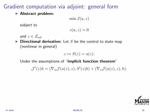
Gradient computation via adjoint general formI Abstract problem
min J(u z)
subject toc(u z) = 0
and z isin ZadI Directional derivative Let S be the control to state map
(nonlinear in general)
z 7rarr S(z) = u(z)
Under the assumptions of ldquoimplicit function theoremrdquo
J prime(z)h = (nablauJ (u(z) z) Sprime(z)h) + (nablazJ (u(z) z) h)
I Sensitivity of u with respect to z Differentiating the stateequation
cu(S(z) z)Sprime(z)h = minuscz(S(z) z)h
leads toSprime(z)h = minuscu(S(z) z)minus1
(cz(S(z) z)h
)
provided cu(S(z) z)minus1 is well-defined
H Antil 060616 35
Adjoint equation and gradient general form
I Directional derivative
J prime(z)h = minus(nablauJ (u(z) z) cu(u(z) z)minus1cz(u(z) z)h
)+ (nablazJ (u(z) z) h)
I Gradient
nablaJ (z) = minuscz(u(z) z)lowast(cu(u(z) z)minuslowastnablauJ (u(z) z)
)+nablazJ (u(z) z)
I Introducing adjoint variable p solving
cu(u(z) z)lowastp = nablauJ (u(z) z)
we arrive at following form of gradient
nablaJ (z) = minuscz(u(z) z)lowastp+nablazJ (u(z) z)
which is tractable
H Antil 060616 36
Hessian computation general form
I Lagrangian L(u z p) = J(u z)minusint
Ωc(u z)p dx Then we have
DzJ (z)h = DzL(u z p)h
I Second order derivative
D2zJ (z)[h1 h2] = DuDzL(u z p)[h1 S
prime(z)h2] +D2zL(u z p)[h1 h2]
+DpDzL(u z p)[h1 Dzp(z)h2]
I We already know Sprime(z)h2 moreover
DpDzL(u z p)[h1 Dzp(z)h2] = minus(cu(u z)h1 Dzp(z)h2
)
It remain to identify Dzp(z)h2
H Antil 060616 37
Outline
Motivation and examples
Linear elliptic optimal control problems
Differentiation in Banach spaces
First-order necessary conditions
Optimal control of semilinear PDEs
An abstract problem
Discretization using finite element methods
H Antil 060616 38
Numerical approximation of Poisson equation MeshTo avoid technical issues we will assume that partΩ is polygonal
I Mesh Let T = K be a mesh of Ω where K sub Rd is an elementthat is isoparametrically equivalent to a unit simplex in Rd
I Conforming mesh We say that the mesh is conforming ifI Ω = cupKisinT KI If K1 cap K2 = x then x is a node of K1 and K2I If K1 cap K2 6= empty and K1 cap K2 6= x then K1 cap K2 is an edgeface
contained in partK1 cap partK2
I Shape regular Let T be the collection of all conformingrefinements of an original mesh T 0 Then T is called shape regularif exist κ gt 0 such that
hKρKle κ forallK isin cupiT i
where hK = diam K ρK = maxρ gt 0|Bρ sub KI Quasi-uniform A family of shape regular meshes is called-quasi
uniform if there exist a constant σ gt 0 such that
maxhKminhK
le σ
uniformly for all meshes in the family
Numerical approximation of Poisson equation MeshTo avoid technical issues we will assume that partΩ is polygonal
I Mesh Let T = K be a mesh of Ω where K sub Rd is an elementthat is isoparametrically equivalent to a unit simplex in Rd
I Conforming mesh We say that the mesh is conforming ifI Ω = cupKisinT KI If K1 cap K2 = x then x is a node of K1 and K2I If K1 cap K2 6= empty and K1 cap K2 6= x then K1 cap K2 is an edgeface
contained in partK1 cap partK2
I Shape regular Let T be the collection of all conformingrefinements of an original mesh T 0 Then T is called shape regularif exist κ gt 0 such that
hKρKle κ forallK isin cupiT i
where hK = diam K ρK = maxρ gt 0|Bρ sub KI Quasi-uniform A family of shape regular meshes is called-quasi
uniform if there exist a constant σ gt 0 such that
maxhKminhK
le σ
uniformly for all meshes in the family
Numerical approximation of Poisson equation MeshTo avoid technical issues we will assume that partΩ is polygonal
I Mesh Let T = K be a mesh of Ω where K sub Rd is an elementthat is isoparametrically equivalent to a unit simplex in Rd
I Conforming mesh We say that the mesh is conforming ifI Ω = cupKisinT KI If K1 cap K2 = x then x is a node of K1 and K2I If K1 cap K2 6= empty and K1 cap K2 6= x then K1 cap K2 is an edgeface
contained in partK1 cap partK2
I Shape regular Let T be the collection of all conformingrefinements of an original mesh T 0 Then T is called shape regularif exist κ gt 0 such that
hKρKle κ forallK isin cupiT i
where hK = diam K ρK = maxρ gt 0|Bρ sub K
I Quasi-uniform A family of shape regular meshes is called-quasiuniform if there exist a constant σ gt 0 such that
maxhKminhK
le σ
uniformly for all meshes in the family
Numerical approximation of Poisson equation MeshTo avoid technical issues we will assume that partΩ is polygonal
I Mesh Let T = K be a mesh of Ω where K sub Rd is an elementthat is isoparametrically equivalent to a unit simplex in Rd
I Conforming mesh We say that the mesh is conforming ifI Ω = cupKisinT KI If K1 cap K2 = x then x is a node of K1 and K2I If K1 cap K2 6= empty and K1 cap K2 6= x then K1 cap K2 is an edgeface
contained in partK1 cap partK2
I Shape regular Let T be the collection of all conformingrefinements of an original mesh T 0 Then T is called shape regularif exist κ gt 0 such that
hKρKle κ forallK isin cupiT i
where hK = diam K ρK = maxρ gt 0|Bρ sub KI Quasi-uniform A family of shape regular meshes is called-quasi
uniform if there exist a constant σ gt 0 such that
maxhKminhK
le σ
uniformly for all meshes in the family
FE space and Galerkin approximationI Finite element space For T isin T we define the finite element
space as
V(T ) = W isin C0(Ω) WK isin P1forallK isin T W |partΩ = 0
where P1 is the set of polynomials of degree at most 1
I Galerkin approximation of continuous problem is given by
Find UT isin V(T )
intΩ
AnablaUT middot nablaV = 〈f V 〉 forallV isin V(T )
The discrete problem is well-posedI Nodal basis Consists of functions ψi isin V(T ) with xi isin N (T )
satisfyingψxi
(xj) = δij
where N (T ) denotes the interior (plus Neumann) nodesI Galerkin orthogonality(
nabla(uminus UT )nablaW)L2(Ω)
= 0 forallW isin V(T )
H Antil 060616 40
FE space and Galerkin approximationI Finite element space For T isin T we define the finite element
space as
V(T ) = W isin C0(Ω) WK isin P1forallK isin T W |partΩ = 0
where P1 is the set of polynomials of degree at most 1I Galerkin approximation of continuous problem is given by
Find UT isin V(T )
intΩ
AnablaUT middot nablaV = 〈f V 〉 forallV isin V(T )
The discrete problem is well-posed
I Nodal basis Consists of functions ψi isin V(T ) with xi isin N (T )satisfying
ψxi(xj) = δij
where N (T ) denotes the interior (plus Neumann) nodesI Galerkin orthogonality(
nabla(uminus UT )nablaW)L2(Ω)
= 0 forallW isin V(T )
H Antil 060616 40
FE space and Galerkin approximationI Finite element space For T isin T we define the finite element
space as
V(T ) = W isin C0(Ω) WK isin P1forallK isin T W |partΩ = 0
where P1 is the set of polynomials of degree at most 1I Galerkin approximation of continuous problem is given by
Find UT isin V(T )
intΩ
AnablaUT middot nablaV = 〈f V 〉 forallV isin V(T )
The discrete problem is well-posedI Nodal basis Consists of functions ψi isin V(T ) with xi isin N (T )
satisfyingψxi
(xj) = δij
where N (T ) denotes the interior (plus Neumann) nodes
I Galerkin orthogonality(nabla(uminus UT )nablaW
)L2(Ω)
= 0 forallW isin V(T )
H Antil 060616 40
FE space and Galerkin approximationI Finite element space For T isin T we define the finite element
space as
V(T ) = W isin C0(Ω) WK isin P1forallK isin T W |partΩ = 0
where P1 is the set of polynomials of degree at most 1I Galerkin approximation of continuous problem is given by
Find UT isin V(T )
intΩ
AnablaUT middot nablaV = 〈f V 〉 forallV isin V(T )
The discrete problem is well-posedI Nodal basis Consists of functions ψi isin V(T ) with xi isin N (T )
satisfyingψxi
(xj) = δij
where N (T ) denotes the interior (plus Neumann) nodesI Galerkin orthogonality(
nabla(uminus UT )nablaW)L2(Ω)
= 0 forallW isin V(T )
H Antil 060616 40
Best approximation
I Cearsquos lemma
nabla(uminus UT )L2(Ω) le C infWisinV(T )
nabla(uminusW )L2(Ω)
I Nodal interpolation operator ΠT C(Ω)rarr V(T ) satisfies
ΠT u(xi) = u(xi) forallxi isin N (T )
and is defined as
ΠT u =sum
xiisinN (T )
u(xi)ψxi
I Error estimates In Cearsquos lemma replace W by ΠT u and thencompute the interpolation error
H Antil 060616 41
Best approximation
I Cearsquos lemma
nabla(uminus UT )L2(Ω) le C infWisinV(T )
nabla(uminusW )L2(Ω)
I Nodal interpolation operator ΠT C(Ω)rarr V(T ) satisfies
ΠT u(xi) = u(xi) forallxi isin N (T )
and is defined as
ΠT u =sum
xiisinN (T )
u(xi)ψxi
I Error estimates In Cearsquos lemma replace W by ΠT u and thencompute the interpolation error
H Antil 060616 41
Best approximation
I Cearsquos lemma
nabla(uminus UT )L2(Ω) le C infWisinV(T )
nabla(uminusW )L2(Ω)
I Nodal interpolation operator ΠT C(Ω)rarr V(T ) satisfies
ΠT u(xi) = u(xi) forallxi isin N (T )
and is defined as
ΠT u =sum
xiisinN (T )
u(xi)ψxi
I Error estimates In Cearsquos lemma replace W by ΠT u and thencompute the interpolation error
H Antil 060616 41
Algebraic system state equation
I Recall UT isin V(T ) solves
a(UT V ) = 〈f V 〉 forallV isin V(T )
I Now setting UT =sumN
j=1 Ujψj V = ψi we get
Nsumj=1
Uja(φj φi) = 〈f ψi〉 i = 1 N
which is the matrix-vector system
AU = F
I Stiffness matrix A is SPD
H Antil 060616 42
Algebraic system state equation
I Recall UT isin V(T ) solves
a(UT V ) = 〈f V 〉 forallV isin V(T )
I Now setting UT =sumN
j=1 Ujψj V = ψi we get
Nsumj=1
Uja(φj φi) = 〈f ψi〉 i = 1 N
which is the matrix-vector system
AU = F
I Stiffness matrix A is SPD
H Antil 060616 42
Algebraic system state equation
I Recall UT isin V(T ) solves
a(UT V ) = 〈f V 〉 forallV isin V(T )
I Now setting UT =sumN
j=1 Ujψj V = ψi we get
Nsumj=1
Uja(φj φi) = 〈f ψi〉 i = 1 N
which is the matrix-vector system
AU = F
I Stiffness matrix A is SPD
H Antil 060616 42
Discrete linear elliptic OCP
min JT (UT ZT ) =1
2UT minus ud2L2(Ω) +
λ
2ZT 2L2(Ω)
subject to
Find UT isin V(T )
intΩ
nablaUT middot nablaV = (ZT V )L2(Ω) forallV isin V(T )
and whereZT isin Zad(T ) = Zad cap Z(T )
is either one of these
Z(T ) =
V(T )L2(Ω) variational discretization (Hinze)WT isin Linfin(Ω) ZT |K isin P0(K)K isin T
H Antil 060616 43
Recent books
F TroltzschOptimal control of partial differential equations volume 112 ofGraduate Studies in MathematicsAmerican Mathematical Society Providence RI 2010Theory methods and applications Translated from the 2005 Germanoriginal by Jurgen Sprekels
K Ito and K KunischLagrange multiplier approach to variational problems andapplications volume 15 of Advances in Design and ControlSociety for Industrial and Applied Mathematics (SIAM)Philadelphia PA 2008
H Antil 060616 44
- Motivation and examples
- Linear elliptic optimal control problems
- Differentiation in Banach spaces
- First-order necessary conditions
- Optimal control of semilinear PDEs
- An abstract problem
- Discretization using finite element methods
-
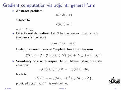
Gradient computation via adjoint general formI Abstract problem
min J(u z)
subject toc(u z) = 0
and z isin ZadI Directional derivative Let S be the control to state map
(nonlinear in general)
z 7rarr S(z) = u(z)
Under the assumptions of ldquoimplicit function theoremrdquo
J prime(z)h = (nablauJ (u(z) z) Sprime(z)h) + (nablazJ (u(z) z) h)
I Sensitivity of u with respect to z Differentiating the stateequation
cu(S(z) z)Sprime(z)h = minuscz(S(z) z)h
leads toSprime(z)h = minuscu(S(z) z)minus1
(cz(S(z) z)h
)
provided cu(S(z) z)minus1 is well-defined
H Antil 060616 35
Adjoint equation and gradient general form
I Directional derivative
J prime(z)h = minus(nablauJ (u(z) z) cu(u(z) z)minus1cz(u(z) z)h
)+ (nablazJ (u(z) z) h)
I Gradient
nablaJ (z) = minuscz(u(z) z)lowast(cu(u(z) z)minuslowastnablauJ (u(z) z)
)+nablazJ (u(z) z)
I Introducing adjoint variable p solving
cu(u(z) z)lowastp = nablauJ (u(z) z)
we arrive at following form of gradient
nablaJ (z) = minuscz(u(z) z)lowastp+nablazJ (u(z) z)
which is tractable
H Antil 060616 36
Hessian computation general form
I Lagrangian L(u z p) = J(u z)minusint
Ωc(u z)p dx Then we have
DzJ (z)h = DzL(u z p)h
I Second order derivative
D2zJ (z)[h1 h2] = DuDzL(u z p)[h1 S
prime(z)h2] +D2zL(u z p)[h1 h2]
+DpDzL(u z p)[h1 Dzp(z)h2]
I We already know Sprime(z)h2 moreover
DpDzL(u z p)[h1 Dzp(z)h2] = minus(cu(u z)h1 Dzp(z)h2
)
It remain to identify Dzp(z)h2
H Antil 060616 37
Outline
Motivation and examples
Linear elliptic optimal control problems
Differentiation in Banach spaces
First-order necessary conditions
Optimal control of semilinear PDEs
An abstract problem
Discretization using finite element methods
H Antil 060616 38
Numerical approximation of Poisson equation MeshTo avoid technical issues we will assume that partΩ is polygonal
I Mesh Let T = K be a mesh of Ω where K sub Rd is an elementthat is isoparametrically equivalent to a unit simplex in Rd
I Conforming mesh We say that the mesh is conforming ifI Ω = cupKisinT KI If K1 cap K2 = x then x is a node of K1 and K2I If K1 cap K2 6= empty and K1 cap K2 6= x then K1 cap K2 is an edgeface
contained in partK1 cap partK2
I Shape regular Let T be the collection of all conformingrefinements of an original mesh T 0 Then T is called shape regularif exist κ gt 0 such that
hKρKle κ forallK isin cupiT i
where hK = diam K ρK = maxρ gt 0|Bρ sub KI Quasi-uniform A family of shape regular meshes is called-quasi
uniform if there exist a constant σ gt 0 such that
maxhKminhK
le σ
uniformly for all meshes in the family
Numerical approximation of Poisson equation MeshTo avoid technical issues we will assume that partΩ is polygonal
I Mesh Let T = K be a mesh of Ω where K sub Rd is an elementthat is isoparametrically equivalent to a unit simplex in Rd
I Conforming mesh We say that the mesh is conforming ifI Ω = cupKisinT KI If K1 cap K2 = x then x is a node of K1 and K2I If K1 cap K2 6= empty and K1 cap K2 6= x then K1 cap K2 is an edgeface
contained in partK1 cap partK2
I Shape regular Let T be the collection of all conformingrefinements of an original mesh T 0 Then T is called shape regularif exist κ gt 0 such that
hKρKle κ forallK isin cupiT i
where hK = diam K ρK = maxρ gt 0|Bρ sub KI Quasi-uniform A family of shape regular meshes is called-quasi
uniform if there exist a constant σ gt 0 such that
maxhKminhK
le σ
uniformly for all meshes in the family
Numerical approximation of Poisson equation MeshTo avoid technical issues we will assume that partΩ is polygonal
I Mesh Let T = K be a mesh of Ω where K sub Rd is an elementthat is isoparametrically equivalent to a unit simplex in Rd
I Conforming mesh We say that the mesh is conforming ifI Ω = cupKisinT KI If K1 cap K2 = x then x is a node of K1 and K2I If K1 cap K2 6= empty and K1 cap K2 6= x then K1 cap K2 is an edgeface
contained in partK1 cap partK2
I Shape regular Let T be the collection of all conformingrefinements of an original mesh T 0 Then T is called shape regularif exist κ gt 0 such that
hKρKle κ forallK isin cupiT i
where hK = diam K ρK = maxρ gt 0|Bρ sub K
I Quasi-uniform A family of shape regular meshes is called-quasiuniform if there exist a constant σ gt 0 such that
maxhKminhK
le σ
uniformly for all meshes in the family
Numerical approximation of Poisson equation MeshTo avoid technical issues we will assume that partΩ is polygonal
I Mesh Let T = K be a mesh of Ω where K sub Rd is an elementthat is isoparametrically equivalent to a unit simplex in Rd
I Conforming mesh We say that the mesh is conforming ifI Ω = cupKisinT KI If K1 cap K2 = x then x is a node of K1 and K2I If K1 cap K2 6= empty and K1 cap K2 6= x then K1 cap K2 is an edgeface
contained in partK1 cap partK2
I Shape regular Let T be the collection of all conformingrefinements of an original mesh T 0 Then T is called shape regularif exist κ gt 0 such that
hKρKle κ forallK isin cupiT i
where hK = diam K ρK = maxρ gt 0|Bρ sub KI Quasi-uniform A family of shape regular meshes is called-quasi
uniform if there exist a constant σ gt 0 such that
maxhKminhK
le σ
uniformly for all meshes in the family
FE space and Galerkin approximationI Finite element space For T isin T we define the finite element
space as
V(T ) = W isin C0(Ω) WK isin P1forallK isin T W |partΩ = 0
where P1 is the set of polynomials of degree at most 1
I Galerkin approximation of continuous problem is given by
Find UT isin V(T )
intΩ
AnablaUT middot nablaV = 〈f V 〉 forallV isin V(T )
The discrete problem is well-posedI Nodal basis Consists of functions ψi isin V(T ) with xi isin N (T )
satisfyingψxi
(xj) = δij
where N (T ) denotes the interior (plus Neumann) nodesI Galerkin orthogonality(
nabla(uminus UT )nablaW)L2(Ω)
= 0 forallW isin V(T )
H Antil 060616 40
FE space and Galerkin approximationI Finite element space For T isin T we define the finite element
space as
V(T ) = W isin C0(Ω) WK isin P1forallK isin T W |partΩ = 0
where P1 is the set of polynomials of degree at most 1I Galerkin approximation of continuous problem is given by
Find UT isin V(T )
intΩ
AnablaUT middot nablaV = 〈f V 〉 forallV isin V(T )
The discrete problem is well-posed
I Nodal basis Consists of functions ψi isin V(T ) with xi isin N (T )satisfying
ψxi(xj) = δij
where N (T ) denotes the interior (plus Neumann) nodesI Galerkin orthogonality(
nabla(uminus UT )nablaW)L2(Ω)
= 0 forallW isin V(T )
H Antil 060616 40
FE space and Galerkin approximationI Finite element space For T isin T we define the finite element
space as
V(T ) = W isin C0(Ω) WK isin P1forallK isin T W |partΩ = 0
where P1 is the set of polynomials of degree at most 1I Galerkin approximation of continuous problem is given by
Find UT isin V(T )
intΩ
AnablaUT middot nablaV = 〈f V 〉 forallV isin V(T )
The discrete problem is well-posedI Nodal basis Consists of functions ψi isin V(T ) with xi isin N (T )
satisfyingψxi
(xj) = δij
where N (T ) denotes the interior (plus Neumann) nodes
I Galerkin orthogonality(nabla(uminus UT )nablaW
)L2(Ω)
= 0 forallW isin V(T )
H Antil 060616 40
FE space and Galerkin approximationI Finite element space For T isin T we define the finite element
space as
V(T ) = W isin C0(Ω) WK isin P1forallK isin T W |partΩ = 0
where P1 is the set of polynomials of degree at most 1I Galerkin approximation of continuous problem is given by
Find UT isin V(T )
intΩ
AnablaUT middot nablaV = 〈f V 〉 forallV isin V(T )
The discrete problem is well-posedI Nodal basis Consists of functions ψi isin V(T ) with xi isin N (T )
satisfyingψxi
(xj) = δij
where N (T ) denotes the interior (plus Neumann) nodesI Galerkin orthogonality(
nabla(uminus UT )nablaW)L2(Ω)
= 0 forallW isin V(T )
H Antil 060616 40
Best approximation
I Cearsquos lemma
nabla(uminus UT )L2(Ω) le C infWisinV(T )
nabla(uminusW )L2(Ω)
I Nodal interpolation operator ΠT C(Ω)rarr V(T ) satisfies
ΠT u(xi) = u(xi) forallxi isin N (T )
and is defined as
ΠT u =sum
xiisinN (T )
u(xi)ψxi
I Error estimates In Cearsquos lemma replace W by ΠT u and thencompute the interpolation error
H Antil 060616 41
Best approximation
I Cearsquos lemma
nabla(uminus UT )L2(Ω) le C infWisinV(T )
nabla(uminusW )L2(Ω)
I Nodal interpolation operator ΠT C(Ω)rarr V(T ) satisfies
ΠT u(xi) = u(xi) forallxi isin N (T )
and is defined as
ΠT u =sum
xiisinN (T )
u(xi)ψxi
I Error estimates In Cearsquos lemma replace W by ΠT u and thencompute the interpolation error
H Antil 060616 41
Best approximation
I Cearsquos lemma
nabla(uminus UT )L2(Ω) le C infWisinV(T )
nabla(uminusW )L2(Ω)
I Nodal interpolation operator ΠT C(Ω)rarr V(T ) satisfies
ΠT u(xi) = u(xi) forallxi isin N (T )
and is defined as
ΠT u =sum
xiisinN (T )
u(xi)ψxi
I Error estimates In Cearsquos lemma replace W by ΠT u and thencompute the interpolation error
H Antil 060616 41
Algebraic system state equation
I Recall UT isin V(T ) solves
a(UT V ) = 〈f V 〉 forallV isin V(T )
I Now setting UT =sumN
j=1 Ujψj V = ψi we get
Nsumj=1
Uja(φj φi) = 〈f ψi〉 i = 1 N
which is the matrix-vector system
AU = F
I Stiffness matrix A is SPD
H Antil 060616 42
Algebraic system state equation
I Recall UT isin V(T ) solves
a(UT V ) = 〈f V 〉 forallV isin V(T )
I Now setting UT =sumN
j=1 Ujψj V = ψi we get
Nsumj=1
Uja(φj φi) = 〈f ψi〉 i = 1 N
which is the matrix-vector system
AU = F
I Stiffness matrix A is SPD
H Antil 060616 42
Algebraic system state equation
I Recall UT isin V(T ) solves
a(UT V ) = 〈f V 〉 forallV isin V(T )
I Now setting UT =sumN
j=1 Ujψj V = ψi we get
Nsumj=1
Uja(φj φi) = 〈f ψi〉 i = 1 N
which is the matrix-vector system
AU = F
I Stiffness matrix A is SPD
H Antil 060616 42
Discrete linear elliptic OCP
min JT (UT ZT ) =1
2UT minus ud2L2(Ω) +
λ
2ZT 2L2(Ω)
subject to
Find UT isin V(T )
intΩ
nablaUT middot nablaV = (ZT V )L2(Ω) forallV isin V(T )
and whereZT isin Zad(T ) = Zad cap Z(T )
is either one of these
Z(T ) =
V(T )L2(Ω) variational discretization (Hinze)WT isin Linfin(Ω) ZT |K isin P0(K)K isin T
H Antil 060616 43
Recent books
F TroltzschOptimal control of partial differential equations volume 112 ofGraduate Studies in MathematicsAmerican Mathematical Society Providence RI 2010Theory methods and applications Translated from the 2005 Germanoriginal by Jurgen Sprekels
K Ito and K KunischLagrange multiplier approach to variational problems andapplications volume 15 of Advances in Design and ControlSociety for Industrial and Applied Mathematics (SIAM)Philadelphia PA 2008
H Antil 060616 44
- Motivation and examples
- Linear elliptic optimal control problems
- Differentiation in Banach spaces
- First-order necessary conditions
- Optimal control of semilinear PDEs
- An abstract problem
- Discretization using finite element methods
-
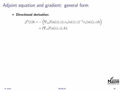
Adjoint equation and gradient general form
I Directional derivative
J prime(z)h = minus(nablauJ (u(z) z) cu(u(z) z)minus1cz(u(z) z)h
)+ (nablazJ (u(z) z) h)
I Gradient
nablaJ (z) = minuscz(u(z) z)lowast(cu(u(z) z)minuslowastnablauJ (u(z) z)
)+nablazJ (u(z) z)
I Introducing adjoint variable p solving
cu(u(z) z)lowastp = nablauJ (u(z) z)
we arrive at following form of gradient
nablaJ (z) = minuscz(u(z) z)lowastp+nablazJ (u(z) z)
which is tractable
H Antil 060616 36
Hessian computation general form
I Lagrangian L(u z p) = J(u z)minusint
Ωc(u z)p dx Then we have
DzJ (z)h = DzL(u z p)h
I Second order derivative
D2zJ (z)[h1 h2] = DuDzL(u z p)[h1 S
prime(z)h2] +D2zL(u z p)[h1 h2]
+DpDzL(u z p)[h1 Dzp(z)h2]
I We already know Sprime(z)h2 moreover
DpDzL(u z p)[h1 Dzp(z)h2] = minus(cu(u z)h1 Dzp(z)h2
)
It remain to identify Dzp(z)h2
H Antil 060616 37
Outline
Motivation and examples
Linear elliptic optimal control problems
Differentiation in Banach spaces
First-order necessary conditions
Optimal control of semilinear PDEs
An abstract problem
Discretization using finite element methods
H Antil 060616 38
Numerical approximation of Poisson equation MeshTo avoid technical issues we will assume that partΩ is polygonal
I Mesh Let T = K be a mesh of Ω where K sub Rd is an elementthat is isoparametrically equivalent to a unit simplex in Rd
I Conforming mesh We say that the mesh is conforming ifI Ω = cupKisinT KI If K1 cap K2 = x then x is a node of K1 and K2I If K1 cap K2 6= empty and K1 cap K2 6= x then K1 cap K2 is an edgeface
contained in partK1 cap partK2
I Shape regular Let T be the collection of all conformingrefinements of an original mesh T 0 Then T is called shape regularif exist κ gt 0 such that
hKρKle κ forallK isin cupiT i
where hK = diam K ρK = maxρ gt 0|Bρ sub KI Quasi-uniform A family of shape regular meshes is called-quasi
uniform if there exist a constant σ gt 0 such that
maxhKminhK
le σ
uniformly for all meshes in the family
Numerical approximation of Poisson equation MeshTo avoid technical issues we will assume that partΩ is polygonal
I Mesh Let T = K be a mesh of Ω where K sub Rd is an elementthat is isoparametrically equivalent to a unit simplex in Rd
I Conforming mesh We say that the mesh is conforming ifI Ω = cupKisinT KI If K1 cap K2 = x then x is a node of K1 and K2I If K1 cap K2 6= empty and K1 cap K2 6= x then K1 cap K2 is an edgeface
contained in partK1 cap partK2
I Shape regular Let T be the collection of all conformingrefinements of an original mesh T 0 Then T is called shape regularif exist κ gt 0 such that
hKρKle κ forallK isin cupiT i
where hK = diam K ρK = maxρ gt 0|Bρ sub KI Quasi-uniform A family of shape regular meshes is called-quasi
uniform if there exist a constant σ gt 0 such that
maxhKminhK
le σ
uniformly for all meshes in the family
Numerical approximation of Poisson equation MeshTo avoid technical issues we will assume that partΩ is polygonal
I Mesh Let T = K be a mesh of Ω where K sub Rd is an elementthat is isoparametrically equivalent to a unit simplex in Rd
I Conforming mesh We say that the mesh is conforming ifI Ω = cupKisinT KI If K1 cap K2 = x then x is a node of K1 and K2I If K1 cap K2 6= empty and K1 cap K2 6= x then K1 cap K2 is an edgeface
contained in partK1 cap partK2
I Shape regular Let T be the collection of all conformingrefinements of an original mesh T 0 Then T is called shape regularif exist κ gt 0 such that
hKρKle κ forallK isin cupiT i
where hK = diam K ρK = maxρ gt 0|Bρ sub K
I Quasi-uniform A family of shape regular meshes is called-quasiuniform if there exist a constant σ gt 0 such that
maxhKminhK
le σ
uniformly for all meshes in the family
Numerical approximation of Poisson equation MeshTo avoid technical issues we will assume that partΩ is polygonal
I Mesh Let T = K be a mesh of Ω where K sub Rd is an elementthat is isoparametrically equivalent to a unit simplex in Rd
I Conforming mesh We say that the mesh is conforming ifI Ω = cupKisinT KI If K1 cap K2 = x then x is a node of K1 and K2I If K1 cap K2 6= empty and K1 cap K2 6= x then K1 cap K2 is an edgeface
contained in partK1 cap partK2
I Shape regular Let T be the collection of all conformingrefinements of an original mesh T 0 Then T is called shape regularif exist κ gt 0 such that
hKρKle κ forallK isin cupiT i
where hK = diam K ρK = maxρ gt 0|Bρ sub KI Quasi-uniform A family of shape regular meshes is called-quasi
uniform if there exist a constant σ gt 0 such that
maxhKminhK
le σ
uniformly for all meshes in the family
FE space and Galerkin approximationI Finite element space For T isin T we define the finite element
space as
V(T ) = W isin C0(Ω) WK isin P1forallK isin T W |partΩ = 0
where P1 is the set of polynomials of degree at most 1
I Galerkin approximation of continuous problem is given by
Find UT isin V(T )
intΩ
AnablaUT middot nablaV = 〈f V 〉 forallV isin V(T )
The discrete problem is well-posedI Nodal basis Consists of functions ψi isin V(T ) with xi isin N (T )
satisfyingψxi
(xj) = δij
where N (T ) denotes the interior (plus Neumann) nodesI Galerkin orthogonality(
nabla(uminus UT )nablaW)L2(Ω)
= 0 forallW isin V(T )
H Antil 060616 40
FE space and Galerkin approximationI Finite element space For T isin T we define the finite element
space as
V(T ) = W isin C0(Ω) WK isin P1forallK isin T W |partΩ = 0
where P1 is the set of polynomials of degree at most 1I Galerkin approximation of continuous problem is given by
Find UT isin V(T )
intΩ
AnablaUT middot nablaV = 〈f V 〉 forallV isin V(T )
The discrete problem is well-posed
I Nodal basis Consists of functions ψi isin V(T ) with xi isin N (T )satisfying
ψxi(xj) = δij
where N (T ) denotes the interior (plus Neumann) nodesI Galerkin orthogonality(
nabla(uminus UT )nablaW)L2(Ω)
= 0 forallW isin V(T )
H Antil 060616 40
FE space and Galerkin approximationI Finite element space For T isin T we define the finite element
space as
V(T ) = W isin C0(Ω) WK isin P1forallK isin T W |partΩ = 0
where P1 is the set of polynomials of degree at most 1I Galerkin approximation of continuous problem is given by
Find UT isin V(T )
intΩ
AnablaUT middot nablaV = 〈f V 〉 forallV isin V(T )
The discrete problem is well-posedI Nodal basis Consists of functions ψi isin V(T ) with xi isin N (T )
satisfyingψxi
(xj) = δij
where N (T ) denotes the interior (plus Neumann) nodes
I Galerkin orthogonality(nabla(uminus UT )nablaW
)L2(Ω)
= 0 forallW isin V(T )
H Antil 060616 40
FE space and Galerkin approximationI Finite element space For T isin T we define the finite element
space as
V(T ) = W isin C0(Ω) WK isin P1forallK isin T W |partΩ = 0
where P1 is the set of polynomials of degree at most 1I Galerkin approximation of continuous problem is given by
Find UT isin V(T )
intΩ
AnablaUT middot nablaV = 〈f V 〉 forallV isin V(T )
The discrete problem is well-posedI Nodal basis Consists of functions ψi isin V(T ) with xi isin N (T )
satisfyingψxi
(xj) = δij
where N (T ) denotes the interior (plus Neumann) nodesI Galerkin orthogonality(
nabla(uminus UT )nablaW)L2(Ω)
= 0 forallW isin V(T )
H Antil 060616 40
Best approximation
I Cearsquos lemma
nabla(uminus UT )L2(Ω) le C infWisinV(T )
nabla(uminusW )L2(Ω)
I Nodal interpolation operator ΠT C(Ω)rarr V(T ) satisfies
ΠT u(xi) = u(xi) forallxi isin N (T )
and is defined as
ΠT u =sum
xiisinN (T )
u(xi)ψxi
I Error estimates In Cearsquos lemma replace W by ΠT u and thencompute the interpolation error
H Antil 060616 41
Best approximation
I Cearsquos lemma
nabla(uminus UT )L2(Ω) le C infWisinV(T )
nabla(uminusW )L2(Ω)
I Nodal interpolation operator ΠT C(Ω)rarr V(T ) satisfies
ΠT u(xi) = u(xi) forallxi isin N (T )
and is defined as
ΠT u =sum
xiisinN (T )
u(xi)ψxi
I Error estimates In Cearsquos lemma replace W by ΠT u and thencompute the interpolation error
H Antil 060616 41
Best approximation
I Cearsquos lemma
nabla(uminus UT )L2(Ω) le C infWisinV(T )
nabla(uminusW )L2(Ω)
I Nodal interpolation operator ΠT C(Ω)rarr V(T ) satisfies
ΠT u(xi) = u(xi) forallxi isin N (T )
and is defined as
ΠT u =sum
xiisinN (T )
u(xi)ψxi
I Error estimates In Cearsquos lemma replace W by ΠT u and thencompute the interpolation error
H Antil 060616 41
Algebraic system state equation
I Recall UT isin V(T ) solves
a(UT V ) = 〈f V 〉 forallV isin V(T )
I Now setting UT =sumN
j=1 Ujψj V = ψi we get
Nsumj=1
Uja(φj φi) = 〈f ψi〉 i = 1 N
which is the matrix-vector system
AU = F
I Stiffness matrix A is SPD
H Antil 060616 42
Algebraic system state equation
I Recall UT isin V(T ) solves
a(UT V ) = 〈f V 〉 forallV isin V(T )
I Now setting UT =sumN
j=1 Ujψj V = ψi we get
Nsumj=1
Uja(φj φi) = 〈f ψi〉 i = 1 N
which is the matrix-vector system
AU = F
I Stiffness matrix A is SPD
H Antil 060616 42
Algebraic system state equation
I Recall UT isin V(T ) solves
a(UT V ) = 〈f V 〉 forallV isin V(T )
I Now setting UT =sumN
j=1 Ujψj V = ψi we get
Nsumj=1
Uja(φj φi) = 〈f ψi〉 i = 1 N
which is the matrix-vector system
AU = F
I Stiffness matrix A is SPD
H Antil 060616 42
Discrete linear elliptic OCP
min JT (UT ZT ) =1
2UT minus ud2L2(Ω) +
λ
2ZT 2L2(Ω)
subject to
Find UT isin V(T )
intΩ
nablaUT middot nablaV = (ZT V )L2(Ω) forallV isin V(T )
and whereZT isin Zad(T ) = Zad cap Z(T )
is either one of these
Z(T ) =
V(T )L2(Ω) variational discretization (Hinze)WT isin Linfin(Ω) ZT |K isin P0(K)K isin T
H Antil 060616 43
Recent books
F TroltzschOptimal control of partial differential equations volume 112 ofGraduate Studies in MathematicsAmerican Mathematical Society Providence RI 2010Theory methods and applications Translated from the 2005 Germanoriginal by Jurgen Sprekels
K Ito and K KunischLagrange multiplier approach to variational problems andapplications volume 15 of Advances in Design and ControlSociety for Industrial and Applied Mathematics (SIAM)Philadelphia PA 2008
H Antil 060616 44
- Motivation and examples
- Linear elliptic optimal control problems
- Differentiation in Banach spaces
- First-order necessary conditions
- Optimal control of semilinear PDEs
- An abstract problem
- Discretization using finite element methods
-
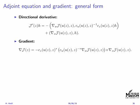
Adjoint equation and gradient general form
I Directional derivative
J prime(z)h = minus(nablauJ (u(z) z) cu(u(z) z)minus1cz(u(z) z)h
)+ (nablazJ (u(z) z) h)
I Gradient
nablaJ (z) = minuscz(u(z) z)lowast(cu(u(z) z)minuslowastnablauJ (u(z) z)
)+nablazJ (u(z) z)
I Introducing adjoint variable p solving
cu(u(z) z)lowastp = nablauJ (u(z) z)
we arrive at following form of gradient
nablaJ (z) = minuscz(u(z) z)lowastp+nablazJ (u(z) z)
which is tractable
H Antil 060616 36
Adjoint equation and gradient general form
I Directional derivative
J prime(z)h = minus(nablauJ (u(z) z) cu(u(z) z)minus1cz(u(z) z)h
)+ (nablazJ (u(z) z) h)
I Gradient
nablaJ (z) = minuscz(u(z) z)lowast(cu(u(z) z)minuslowastnablauJ (u(z) z)
)+nablazJ (u(z) z)
I Introducing adjoint variable p solving
cu(u(z) z)lowastp = nablauJ (u(z) z)
we arrive at following form of gradient
nablaJ (z) = minuscz(u(z) z)lowastp+nablazJ (u(z) z)
which is tractable
H Antil 060616 36
Hessian computation general form
I Lagrangian L(u z p) = J(u z)minusint
Ωc(u z)p dx Then we have
DzJ (z)h = DzL(u z p)h
I Second order derivative
D2zJ (z)[h1 h2] = DuDzL(u z p)[h1 S
prime(z)h2] +D2zL(u z p)[h1 h2]
+DpDzL(u z p)[h1 Dzp(z)h2]
I We already know Sprime(z)h2 moreover
DpDzL(u z p)[h1 Dzp(z)h2] = minus(cu(u z)h1 Dzp(z)h2
)
It remain to identify Dzp(z)h2
H Antil 060616 37
Outline
Motivation and examples
Linear elliptic optimal control problems
Differentiation in Banach spaces
First-order necessary conditions
Optimal control of semilinear PDEs
An abstract problem
Discretization using finite element methods
H Antil 060616 38
Numerical approximation of Poisson equation MeshTo avoid technical issues we will assume that partΩ is polygonal
I Mesh Let T = K be a mesh of Ω where K sub Rd is an elementthat is isoparametrically equivalent to a unit simplex in Rd
I Conforming mesh We say that the mesh is conforming ifI Ω = cupKisinT KI If K1 cap K2 = x then x is a node of K1 and K2I If K1 cap K2 6= empty and K1 cap K2 6= x then K1 cap K2 is an edgeface
contained in partK1 cap partK2
I Shape regular Let T be the collection of all conformingrefinements of an original mesh T 0 Then T is called shape regularif exist κ gt 0 such that
hKρKle κ forallK isin cupiT i
where hK = diam K ρK = maxρ gt 0|Bρ sub KI Quasi-uniform A family of shape regular meshes is called-quasi
uniform if there exist a constant σ gt 0 such that
maxhKminhK
le σ
uniformly for all meshes in the family
Numerical approximation of Poisson equation MeshTo avoid technical issues we will assume that partΩ is polygonal
I Mesh Let T = K be a mesh of Ω where K sub Rd is an elementthat is isoparametrically equivalent to a unit simplex in Rd
I Conforming mesh We say that the mesh is conforming ifI Ω = cupKisinT KI If K1 cap K2 = x then x is a node of K1 and K2I If K1 cap K2 6= empty and K1 cap K2 6= x then K1 cap K2 is an edgeface
contained in partK1 cap partK2
I Shape regular Let T be the collection of all conformingrefinements of an original mesh T 0 Then T is called shape regularif exist κ gt 0 such that
hKρKle κ forallK isin cupiT i
where hK = diam K ρK = maxρ gt 0|Bρ sub KI Quasi-uniform A family of shape regular meshes is called-quasi
uniform if there exist a constant σ gt 0 such that
maxhKminhK
le σ
uniformly for all meshes in the family
Numerical approximation of Poisson equation MeshTo avoid technical issues we will assume that partΩ is polygonal
I Mesh Let T = K be a mesh of Ω where K sub Rd is an elementthat is isoparametrically equivalent to a unit simplex in Rd
I Conforming mesh We say that the mesh is conforming ifI Ω = cupKisinT KI If K1 cap K2 = x then x is a node of K1 and K2I If K1 cap K2 6= empty and K1 cap K2 6= x then K1 cap K2 is an edgeface
contained in partK1 cap partK2
I Shape regular Let T be the collection of all conformingrefinements of an original mesh T 0 Then T is called shape regularif exist κ gt 0 such that
hKρKle κ forallK isin cupiT i
where hK = diam K ρK = maxρ gt 0|Bρ sub K
I Quasi-uniform A family of shape regular meshes is called-quasiuniform if there exist a constant σ gt 0 such that
maxhKminhK
le σ
uniformly for all meshes in the family
Numerical approximation of Poisson equation MeshTo avoid technical issues we will assume that partΩ is polygonal
I Mesh Let T = K be a mesh of Ω where K sub Rd is an elementthat is isoparametrically equivalent to a unit simplex in Rd
I Conforming mesh We say that the mesh is conforming ifI Ω = cupKisinT KI If K1 cap K2 = x then x is a node of K1 and K2I If K1 cap K2 6= empty and K1 cap K2 6= x then K1 cap K2 is an edgeface
contained in partK1 cap partK2
I Shape regular Let T be the collection of all conformingrefinements of an original mesh T 0 Then T is called shape regularif exist κ gt 0 such that
hKρKle κ forallK isin cupiT i
where hK = diam K ρK = maxρ gt 0|Bρ sub KI Quasi-uniform A family of shape regular meshes is called-quasi
uniform if there exist a constant σ gt 0 such that
maxhKminhK
le σ
uniformly for all meshes in the family
FE space and Galerkin approximationI Finite element space For T isin T we define the finite element
space as
V(T ) = W isin C0(Ω) WK isin P1forallK isin T W |partΩ = 0
where P1 is the set of polynomials of degree at most 1
I Galerkin approximation of continuous problem is given by
Find UT isin V(T )
intΩ
AnablaUT middot nablaV = 〈f V 〉 forallV isin V(T )
The discrete problem is well-posedI Nodal basis Consists of functions ψi isin V(T ) with xi isin N (T )
satisfyingψxi
(xj) = δij
where N (T ) denotes the interior (plus Neumann) nodesI Galerkin orthogonality(
nabla(uminus UT )nablaW)L2(Ω)
= 0 forallW isin V(T )
H Antil 060616 40
FE space and Galerkin approximationI Finite element space For T isin T we define the finite element
space as
V(T ) = W isin C0(Ω) WK isin P1forallK isin T W |partΩ = 0
where P1 is the set of polynomials of degree at most 1I Galerkin approximation of continuous problem is given by
Find UT isin V(T )
intΩ
AnablaUT middot nablaV = 〈f V 〉 forallV isin V(T )
The discrete problem is well-posed
I Nodal basis Consists of functions ψi isin V(T ) with xi isin N (T )satisfying
ψxi(xj) = δij
where N (T ) denotes the interior (plus Neumann) nodesI Galerkin orthogonality(
nabla(uminus UT )nablaW)L2(Ω)
= 0 forallW isin V(T )
H Antil 060616 40
FE space and Galerkin approximationI Finite element space For T isin T we define the finite element
space as
V(T ) = W isin C0(Ω) WK isin P1forallK isin T W |partΩ = 0
where P1 is the set of polynomials of degree at most 1I Galerkin approximation of continuous problem is given by
Find UT isin V(T )
intΩ
AnablaUT middot nablaV = 〈f V 〉 forallV isin V(T )
The discrete problem is well-posedI Nodal basis Consists of functions ψi isin V(T ) with xi isin N (T )
satisfyingψxi
(xj) = δij
where N (T ) denotes the interior (plus Neumann) nodes
I Galerkin orthogonality(nabla(uminus UT )nablaW
)L2(Ω)
= 0 forallW isin V(T )
H Antil 060616 40
FE space and Galerkin approximationI Finite element space For T isin T we define the finite element
space as
V(T ) = W isin C0(Ω) WK isin P1forallK isin T W |partΩ = 0
where P1 is the set of polynomials of degree at most 1I Galerkin approximation of continuous problem is given by
Find UT isin V(T )
intΩ
AnablaUT middot nablaV = 〈f V 〉 forallV isin V(T )
The discrete problem is well-posedI Nodal basis Consists of functions ψi isin V(T ) with xi isin N (T )
satisfyingψxi
(xj) = δij
where N (T ) denotes the interior (plus Neumann) nodesI Galerkin orthogonality(
nabla(uminus UT )nablaW)L2(Ω)
= 0 forallW isin V(T )
H Antil 060616 40
Best approximation
I Cearsquos lemma
nabla(uminus UT )L2(Ω) le C infWisinV(T )
nabla(uminusW )L2(Ω)
I Nodal interpolation operator ΠT C(Ω)rarr V(T ) satisfies
ΠT u(xi) = u(xi) forallxi isin N (T )
and is defined as
ΠT u =sum
xiisinN (T )
u(xi)ψxi
I Error estimates In Cearsquos lemma replace W by ΠT u and thencompute the interpolation error
H Antil 060616 41
Best approximation
I Cearsquos lemma
nabla(uminus UT )L2(Ω) le C infWisinV(T )
nabla(uminusW )L2(Ω)
I Nodal interpolation operator ΠT C(Ω)rarr V(T ) satisfies
ΠT u(xi) = u(xi) forallxi isin N (T )
and is defined as
ΠT u =sum
xiisinN (T )
u(xi)ψxi
I Error estimates In Cearsquos lemma replace W by ΠT u and thencompute the interpolation error
H Antil 060616 41
Best approximation
I Cearsquos lemma
nabla(uminus UT )L2(Ω) le C infWisinV(T )
nabla(uminusW )L2(Ω)
I Nodal interpolation operator ΠT C(Ω)rarr V(T ) satisfies
ΠT u(xi) = u(xi) forallxi isin N (T )
and is defined as
ΠT u =sum
xiisinN (T )
u(xi)ψxi
I Error estimates In Cearsquos lemma replace W by ΠT u and thencompute the interpolation error
H Antil 060616 41
Algebraic system state equation
I Recall UT isin V(T ) solves
a(UT V ) = 〈f V 〉 forallV isin V(T )
I Now setting UT =sumN
j=1 Ujψj V = ψi we get
Nsumj=1
Uja(φj φi) = 〈f ψi〉 i = 1 N
which is the matrix-vector system
AU = F
I Stiffness matrix A is SPD
H Antil 060616 42
Algebraic system state equation
I Recall UT isin V(T ) solves
a(UT V ) = 〈f V 〉 forallV isin V(T )
I Now setting UT =sumN
j=1 Ujψj V = ψi we get
Nsumj=1
Uja(φj φi) = 〈f ψi〉 i = 1 N
which is the matrix-vector system
AU = F
I Stiffness matrix A is SPD
H Antil 060616 42
Algebraic system state equation
I Recall UT isin V(T ) solves
a(UT V ) = 〈f V 〉 forallV isin V(T )
I Now setting UT =sumN
j=1 Ujψj V = ψi we get
Nsumj=1
Uja(φj φi) = 〈f ψi〉 i = 1 N
which is the matrix-vector system
AU = F
I Stiffness matrix A is SPD
H Antil 060616 42
Discrete linear elliptic OCP
min JT (UT ZT ) =1
2UT minus ud2L2(Ω) +
λ
2ZT 2L2(Ω)
subject to
Find UT isin V(T )
intΩ
nablaUT middot nablaV = (ZT V )L2(Ω) forallV isin V(T )
and whereZT isin Zad(T ) = Zad cap Z(T )
is either one of these
Z(T ) =
V(T )L2(Ω) variational discretization (Hinze)WT isin Linfin(Ω) ZT |K isin P0(K)K isin T
H Antil 060616 43
Recent books
F TroltzschOptimal control of partial differential equations volume 112 ofGraduate Studies in MathematicsAmerican Mathematical Society Providence RI 2010Theory methods and applications Translated from the 2005 Germanoriginal by Jurgen Sprekels
K Ito and K KunischLagrange multiplier approach to variational problems andapplications volume 15 of Advances in Design and ControlSociety for Industrial and Applied Mathematics (SIAM)Philadelphia PA 2008
H Antil 060616 44
- Motivation and examples
- Linear elliptic optimal control problems
- Differentiation in Banach spaces
- First-order necessary conditions
- Optimal control of semilinear PDEs
- An abstract problem
- Discretization using finite element methods
-
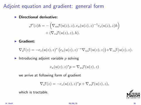
Adjoint equation and gradient general form
I Directional derivative
J prime(z)h = minus(nablauJ (u(z) z) cu(u(z) z)minus1cz(u(z) z)h
)+ (nablazJ (u(z) z) h)
I Gradient
nablaJ (z) = minuscz(u(z) z)lowast(cu(u(z) z)minuslowastnablauJ (u(z) z)
)+nablazJ (u(z) z)
I Introducing adjoint variable p solving
cu(u(z) z)lowastp = nablauJ (u(z) z)
we arrive at following form of gradient
nablaJ (z) = minuscz(u(z) z)lowastp+nablazJ (u(z) z)
which is tractable
H Antil 060616 36
Hessian computation general form
I Lagrangian L(u z p) = J(u z)minusint
Ωc(u z)p dx Then we have
DzJ (z)h = DzL(u z p)h
I Second order derivative
D2zJ (z)[h1 h2] = DuDzL(u z p)[h1 S
prime(z)h2] +D2zL(u z p)[h1 h2]
+DpDzL(u z p)[h1 Dzp(z)h2]
I We already know Sprime(z)h2 moreover
DpDzL(u z p)[h1 Dzp(z)h2] = minus(cu(u z)h1 Dzp(z)h2
)
It remain to identify Dzp(z)h2
H Antil 060616 37
Outline
Motivation and examples
Linear elliptic optimal control problems
Differentiation in Banach spaces
First-order necessary conditions
Optimal control of semilinear PDEs
An abstract problem
Discretization using finite element methods
H Antil 060616 38
Numerical approximation of Poisson equation MeshTo avoid technical issues we will assume that partΩ is polygonal
I Mesh Let T = K be a mesh of Ω where K sub Rd is an elementthat is isoparametrically equivalent to a unit simplex in Rd
I Conforming mesh We say that the mesh is conforming ifI Ω = cupKisinT KI If K1 cap K2 = x then x is a node of K1 and K2I If K1 cap K2 6= empty and K1 cap K2 6= x then K1 cap K2 is an edgeface
contained in partK1 cap partK2
I Shape regular Let T be the collection of all conformingrefinements of an original mesh T 0 Then T is called shape regularif exist κ gt 0 such that
hKρKle κ forallK isin cupiT i
where hK = diam K ρK = maxρ gt 0|Bρ sub KI Quasi-uniform A family of shape regular meshes is called-quasi
uniform if there exist a constant σ gt 0 such that
maxhKminhK
le σ
uniformly for all meshes in the family
Numerical approximation of Poisson equation MeshTo avoid technical issues we will assume that partΩ is polygonal
I Mesh Let T = K be a mesh of Ω where K sub Rd is an elementthat is isoparametrically equivalent to a unit simplex in Rd
I Conforming mesh We say that the mesh is conforming ifI Ω = cupKisinT KI If K1 cap K2 = x then x is a node of K1 and K2I If K1 cap K2 6= empty and K1 cap K2 6= x then K1 cap K2 is an edgeface
contained in partK1 cap partK2
I Shape regular Let T be the collection of all conformingrefinements of an original mesh T 0 Then T is called shape regularif exist κ gt 0 such that
hKρKle κ forallK isin cupiT i
where hK = diam K ρK = maxρ gt 0|Bρ sub KI Quasi-uniform A family of shape regular meshes is called-quasi
uniform if there exist a constant σ gt 0 such that
maxhKminhK
le σ
uniformly for all meshes in the family
Numerical approximation of Poisson equation MeshTo avoid technical issues we will assume that partΩ is polygonal
I Mesh Let T = K be a mesh of Ω where K sub Rd is an elementthat is isoparametrically equivalent to a unit simplex in Rd
I Conforming mesh We say that the mesh is conforming ifI Ω = cupKisinT KI If K1 cap K2 = x then x is a node of K1 and K2I If K1 cap K2 6= empty and K1 cap K2 6= x then K1 cap K2 is an edgeface
contained in partK1 cap partK2
I Shape regular Let T be the collection of all conformingrefinements of an original mesh T 0 Then T is called shape regularif exist κ gt 0 such that
hKρKle κ forallK isin cupiT i
where hK = diam K ρK = maxρ gt 0|Bρ sub K
I Quasi-uniform A family of shape regular meshes is called-quasiuniform if there exist a constant σ gt 0 such that
maxhKminhK
le σ
uniformly for all meshes in the family
Numerical approximation of Poisson equation MeshTo avoid technical issues we will assume that partΩ is polygonal
I Mesh Let T = K be a mesh of Ω where K sub Rd is an elementthat is isoparametrically equivalent to a unit simplex in Rd
I Conforming mesh We say that the mesh is conforming ifI Ω = cupKisinT KI If K1 cap K2 = x then x is a node of K1 and K2I If K1 cap K2 6= empty and K1 cap K2 6= x then K1 cap K2 is an edgeface
contained in partK1 cap partK2
I Shape regular Let T be the collection of all conformingrefinements of an original mesh T 0 Then T is called shape regularif exist κ gt 0 such that
hKρKle κ forallK isin cupiT i
where hK = diam K ρK = maxρ gt 0|Bρ sub KI Quasi-uniform A family of shape regular meshes is called-quasi
uniform if there exist a constant σ gt 0 such that
maxhKminhK
le σ
uniformly for all meshes in the family
FE space and Galerkin approximationI Finite element space For T isin T we define the finite element
space as
V(T ) = W isin C0(Ω) WK isin P1forallK isin T W |partΩ = 0
where P1 is the set of polynomials of degree at most 1
I Galerkin approximation of continuous problem is given by
Find UT isin V(T )
intΩ
AnablaUT middot nablaV = 〈f V 〉 forallV isin V(T )
The discrete problem is well-posedI Nodal basis Consists of functions ψi isin V(T ) with xi isin N (T )
satisfyingψxi
(xj) = δij
where N (T ) denotes the interior (plus Neumann) nodesI Galerkin orthogonality(
nabla(uminus UT )nablaW)L2(Ω)
= 0 forallW isin V(T )
H Antil 060616 40
FE space and Galerkin approximationI Finite element space For T isin T we define the finite element
space as
V(T ) = W isin C0(Ω) WK isin P1forallK isin T W |partΩ = 0
where P1 is the set of polynomials of degree at most 1I Galerkin approximation of continuous problem is given by
Find UT isin V(T )
intΩ
AnablaUT middot nablaV = 〈f V 〉 forallV isin V(T )
The discrete problem is well-posed
I Nodal basis Consists of functions ψi isin V(T ) with xi isin N (T )satisfying
ψxi(xj) = δij
where N (T ) denotes the interior (plus Neumann) nodesI Galerkin orthogonality(
nabla(uminus UT )nablaW)L2(Ω)
= 0 forallW isin V(T )
H Antil 060616 40
FE space and Galerkin approximationI Finite element space For T isin T we define the finite element
space as
V(T ) = W isin C0(Ω) WK isin P1forallK isin T W |partΩ = 0
where P1 is the set of polynomials of degree at most 1I Galerkin approximation of continuous problem is given by
Find UT isin V(T )
intΩ
AnablaUT middot nablaV = 〈f V 〉 forallV isin V(T )
The discrete problem is well-posedI Nodal basis Consists of functions ψi isin V(T ) with xi isin N (T )
satisfyingψxi
(xj) = δij
where N (T ) denotes the interior (plus Neumann) nodes
I Galerkin orthogonality(nabla(uminus UT )nablaW
)L2(Ω)
= 0 forallW isin V(T )
H Antil 060616 40
FE space and Galerkin approximationI Finite element space For T isin T we define the finite element
space as
V(T ) = W isin C0(Ω) WK isin P1forallK isin T W |partΩ = 0
where P1 is the set of polynomials of degree at most 1I Galerkin approximation of continuous problem is given by
Find UT isin V(T )
intΩ
AnablaUT middot nablaV = 〈f V 〉 forallV isin V(T )
The discrete problem is well-posedI Nodal basis Consists of functions ψi isin V(T ) with xi isin N (T )
satisfyingψxi
(xj) = δij
where N (T ) denotes the interior (plus Neumann) nodesI Galerkin orthogonality(
nabla(uminus UT )nablaW)L2(Ω)
= 0 forallW isin V(T )
H Antil 060616 40
Best approximation
I Cearsquos lemma
nabla(uminus UT )L2(Ω) le C infWisinV(T )
nabla(uminusW )L2(Ω)
I Nodal interpolation operator ΠT C(Ω)rarr V(T ) satisfies
ΠT u(xi) = u(xi) forallxi isin N (T )
and is defined as
ΠT u =sum
xiisinN (T )
u(xi)ψxi
I Error estimates In Cearsquos lemma replace W by ΠT u and thencompute the interpolation error
H Antil 060616 41
Best approximation
I Cearsquos lemma
nabla(uminus UT )L2(Ω) le C infWisinV(T )
nabla(uminusW )L2(Ω)
I Nodal interpolation operator ΠT C(Ω)rarr V(T ) satisfies
ΠT u(xi) = u(xi) forallxi isin N (T )
and is defined as
ΠT u =sum
xiisinN (T )
u(xi)ψxi
I Error estimates In Cearsquos lemma replace W by ΠT u and thencompute the interpolation error
H Antil 060616 41
Best approximation
I Cearsquos lemma
nabla(uminus UT )L2(Ω) le C infWisinV(T )
nabla(uminusW )L2(Ω)
I Nodal interpolation operator ΠT C(Ω)rarr V(T ) satisfies
ΠT u(xi) = u(xi) forallxi isin N (T )
and is defined as
ΠT u =sum
xiisinN (T )
u(xi)ψxi
I Error estimates In Cearsquos lemma replace W by ΠT u and thencompute the interpolation error
H Antil 060616 41
Algebraic system state equation
I Recall UT isin V(T ) solves
a(UT V ) = 〈f V 〉 forallV isin V(T )
I Now setting UT =sumN
j=1 Ujψj V = ψi we get
Nsumj=1
Uja(φj φi) = 〈f ψi〉 i = 1 N
which is the matrix-vector system
AU = F
I Stiffness matrix A is SPD
H Antil 060616 42
Algebraic system state equation
I Recall UT isin V(T ) solves
a(UT V ) = 〈f V 〉 forallV isin V(T )
I Now setting UT =sumN
j=1 Ujψj V = ψi we get
Nsumj=1
Uja(φj φi) = 〈f ψi〉 i = 1 N
which is the matrix-vector system
AU = F
I Stiffness matrix A is SPD
H Antil 060616 42
Algebraic system state equation
I Recall UT isin V(T ) solves
a(UT V ) = 〈f V 〉 forallV isin V(T )
I Now setting UT =sumN
j=1 Ujψj V = ψi we get
Nsumj=1
Uja(φj φi) = 〈f ψi〉 i = 1 N
which is the matrix-vector system
AU = F
I Stiffness matrix A is SPD
H Antil 060616 42
Discrete linear elliptic OCP
min JT (UT ZT ) =1
2UT minus ud2L2(Ω) +
λ
2ZT 2L2(Ω)
subject to
Find UT isin V(T )
intΩ
nablaUT middot nablaV = (ZT V )L2(Ω) forallV isin V(T )
and whereZT isin Zad(T ) = Zad cap Z(T )
is either one of these
Z(T ) =
V(T )L2(Ω) variational discretization (Hinze)WT isin Linfin(Ω) ZT |K isin P0(K)K isin T
H Antil 060616 43
Recent books
F TroltzschOptimal control of partial differential equations volume 112 ofGraduate Studies in MathematicsAmerican Mathematical Society Providence RI 2010Theory methods and applications Translated from the 2005 Germanoriginal by Jurgen Sprekels
K Ito and K KunischLagrange multiplier approach to variational problems andapplications volume 15 of Advances in Design and ControlSociety for Industrial and Applied Mathematics (SIAM)Philadelphia PA 2008
H Antil 060616 44
- Motivation and examples
- Linear elliptic optimal control problems
- Differentiation in Banach spaces
- First-order necessary conditions
- Optimal control of semilinear PDEs
- An abstract problem
- Discretization using finite element methods
-
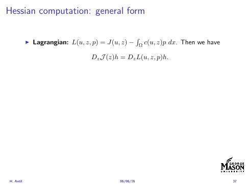
Hessian computation general form
I Lagrangian L(u z p) = J(u z)minusint
Ωc(u z)p dx Then we have
DzJ (z)h = DzL(u z p)h
I Second order derivative
D2zJ (z)[h1 h2] = DuDzL(u z p)[h1 S
prime(z)h2] +D2zL(u z p)[h1 h2]
+DpDzL(u z p)[h1 Dzp(z)h2]
I We already know Sprime(z)h2 moreover
DpDzL(u z p)[h1 Dzp(z)h2] = minus(cu(u z)h1 Dzp(z)h2
)
It remain to identify Dzp(z)h2
H Antil 060616 37
Outline
Motivation and examples
Linear elliptic optimal control problems
Differentiation in Banach spaces
First-order necessary conditions
Optimal control of semilinear PDEs
An abstract problem
Discretization using finite element methods
H Antil 060616 38
Numerical approximation of Poisson equation MeshTo avoid technical issues we will assume that partΩ is polygonal
I Mesh Let T = K be a mesh of Ω where K sub Rd is an elementthat is isoparametrically equivalent to a unit simplex in Rd
I Conforming mesh We say that the mesh is conforming ifI Ω = cupKisinT KI If K1 cap K2 = x then x is a node of K1 and K2I If K1 cap K2 6= empty and K1 cap K2 6= x then K1 cap K2 is an edgeface
contained in partK1 cap partK2
I Shape regular Let T be the collection of all conformingrefinements of an original mesh T 0 Then T is called shape regularif exist κ gt 0 such that
hKρKle κ forallK isin cupiT i
where hK = diam K ρK = maxρ gt 0|Bρ sub KI Quasi-uniform A family of shape regular meshes is called-quasi
uniform if there exist a constant σ gt 0 such that
maxhKminhK
le σ
uniformly for all meshes in the family
Numerical approximation of Poisson equation MeshTo avoid technical issues we will assume that partΩ is polygonal
I Mesh Let T = K be a mesh of Ω where K sub Rd is an elementthat is isoparametrically equivalent to a unit simplex in Rd
I Conforming mesh We say that the mesh is conforming ifI Ω = cupKisinT KI If K1 cap K2 = x then x is a node of K1 and K2I If K1 cap K2 6= empty and K1 cap K2 6= x then K1 cap K2 is an edgeface
contained in partK1 cap partK2
I Shape regular Let T be the collection of all conformingrefinements of an original mesh T 0 Then T is called shape regularif exist κ gt 0 such that
hKρKle κ forallK isin cupiT i
where hK = diam K ρK = maxρ gt 0|Bρ sub KI Quasi-uniform A family of shape regular meshes is called-quasi
uniform if there exist a constant σ gt 0 such that
maxhKminhK
le σ
uniformly for all meshes in the family
Numerical approximation of Poisson equation MeshTo avoid technical issues we will assume that partΩ is polygonal
I Mesh Let T = K be a mesh of Ω where K sub Rd is an elementthat is isoparametrically equivalent to a unit simplex in Rd
I Conforming mesh We say that the mesh is conforming ifI Ω = cupKisinT KI If K1 cap K2 = x then x is a node of K1 and K2I If K1 cap K2 6= empty and K1 cap K2 6= x then K1 cap K2 is an edgeface
contained in partK1 cap partK2
I Shape regular Let T be the collection of all conformingrefinements of an original mesh T 0 Then T is called shape regularif exist κ gt 0 such that
hKρKle κ forallK isin cupiT i
where hK = diam K ρK = maxρ gt 0|Bρ sub K
I Quasi-uniform A family of shape regular meshes is called-quasiuniform if there exist a constant σ gt 0 such that
maxhKminhK
le σ
uniformly for all meshes in the family
Numerical approximation of Poisson equation MeshTo avoid technical issues we will assume that partΩ is polygonal
I Mesh Let T = K be a mesh of Ω where K sub Rd is an elementthat is isoparametrically equivalent to a unit simplex in Rd
I Conforming mesh We say that the mesh is conforming ifI Ω = cupKisinT KI If K1 cap K2 = x then x is a node of K1 and K2I If K1 cap K2 6= empty and K1 cap K2 6= x then K1 cap K2 is an edgeface
contained in partK1 cap partK2
I Shape regular Let T be the collection of all conformingrefinements of an original mesh T 0 Then T is called shape regularif exist κ gt 0 such that
hKρKle κ forallK isin cupiT i
where hK = diam K ρK = maxρ gt 0|Bρ sub KI Quasi-uniform A family of shape regular meshes is called-quasi
uniform if there exist a constant σ gt 0 such that
maxhKminhK
le σ
uniformly for all meshes in the family
FE space and Galerkin approximationI Finite element space For T isin T we define the finite element
space as
V(T ) = W isin C0(Ω) WK isin P1forallK isin T W |partΩ = 0
where P1 is the set of polynomials of degree at most 1
I Galerkin approximation of continuous problem is given by
Find UT isin V(T )
intΩ
AnablaUT middot nablaV = 〈f V 〉 forallV isin V(T )
The discrete problem is well-posedI Nodal basis Consists of functions ψi isin V(T ) with xi isin N (T )
satisfyingψxi
(xj) = δij
where N (T ) denotes the interior (plus Neumann) nodesI Galerkin orthogonality(
nabla(uminus UT )nablaW)L2(Ω)
= 0 forallW isin V(T )
H Antil 060616 40
FE space and Galerkin approximationI Finite element space For T isin T we define the finite element
space as
V(T ) = W isin C0(Ω) WK isin P1forallK isin T W |partΩ = 0
where P1 is the set of polynomials of degree at most 1I Galerkin approximation of continuous problem is given by
Find UT isin V(T )
intΩ
AnablaUT middot nablaV = 〈f V 〉 forallV isin V(T )
The discrete problem is well-posed
I Nodal basis Consists of functions ψi isin V(T ) with xi isin N (T )satisfying
ψxi(xj) = δij
where N (T ) denotes the interior (plus Neumann) nodesI Galerkin orthogonality(
nabla(uminus UT )nablaW)L2(Ω)
= 0 forallW isin V(T )
H Antil 060616 40
FE space and Galerkin approximationI Finite element space For T isin T we define the finite element
space as
V(T ) = W isin C0(Ω) WK isin P1forallK isin T W |partΩ = 0
where P1 is the set of polynomials of degree at most 1I Galerkin approximation of continuous problem is given by
Find UT isin V(T )
intΩ
AnablaUT middot nablaV = 〈f V 〉 forallV isin V(T )
The discrete problem is well-posedI Nodal basis Consists of functions ψi isin V(T ) with xi isin N (T )
satisfyingψxi
(xj) = δij
where N (T ) denotes the interior (plus Neumann) nodes
I Galerkin orthogonality(nabla(uminus UT )nablaW
)L2(Ω)
= 0 forallW isin V(T )
H Antil 060616 40
FE space and Galerkin approximationI Finite element space For T isin T we define the finite element
space as
V(T ) = W isin C0(Ω) WK isin P1forallK isin T W |partΩ = 0
where P1 is the set of polynomials of degree at most 1I Galerkin approximation of continuous problem is given by
Find UT isin V(T )
intΩ
AnablaUT middot nablaV = 〈f V 〉 forallV isin V(T )
The discrete problem is well-posedI Nodal basis Consists of functions ψi isin V(T ) with xi isin N (T )
satisfyingψxi
(xj) = δij
where N (T ) denotes the interior (plus Neumann) nodesI Galerkin orthogonality(
nabla(uminus UT )nablaW)L2(Ω)
= 0 forallW isin V(T )
H Antil 060616 40
Best approximation
I Cearsquos lemma
nabla(uminus UT )L2(Ω) le C infWisinV(T )
nabla(uminusW )L2(Ω)
I Nodal interpolation operator ΠT C(Ω)rarr V(T ) satisfies
ΠT u(xi) = u(xi) forallxi isin N (T )
and is defined as
ΠT u =sum
xiisinN (T )
u(xi)ψxi
I Error estimates In Cearsquos lemma replace W by ΠT u and thencompute the interpolation error
H Antil 060616 41
Best approximation
I Cearsquos lemma
nabla(uminus UT )L2(Ω) le C infWisinV(T )
nabla(uminusW )L2(Ω)
I Nodal interpolation operator ΠT C(Ω)rarr V(T ) satisfies
ΠT u(xi) = u(xi) forallxi isin N (T )
and is defined as
ΠT u =sum
xiisinN (T )
u(xi)ψxi
I Error estimates In Cearsquos lemma replace W by ΠT u and thencompute the interpolation error
H Antil 060616 41
Best approximation
I Cearsquos lemma
nabla(uminus UT )L2(Ω) le C infWisinV(T )
nabla(uminusW )L2(Ω)
I Nodal interpolation operator ΠT C(Ω)rarr V(T ) satisfies
ΠT u(xi) = u(xi) forallxi isin N (T )
and is defined as
ΠT u =sum
xiisinN (T )
u(xi)ψxi
I Error estimates In Cearsquos lemma replace W by ΠT u and thencompute the interpolation error
H Antil 060616 41
Algebraic system state equation
I Recall UT isin V(T ) solves
a(UT V ) = 〈f V 〉 forallV isin V(T )
I Now setting UT =sumN
j=1 Ujψj V = ψi we get
Nsumj=1
Uja(φj φi) = 〈f ψi〉 i = 1 N
which is the matrix-vector system
AU = F
I Stiffness matrix A is SPD
H Antil 060616 42
Algebraic system state equation
I Recall UT isin V(T ) solves
a(UT V ) = 〈f V 〉 forallV isin V(T )
I Now setting UT =sumN
j=1 Ujψj V = ψi we get
Nsumj=1
Uja(φj φi) = 〈f ψi〉 i = 1 N
which is the matrix-vector system
AU = F
I Stiffness matrix A is SPD
H Antil 060616 42
Algebraic system state equation
I Recall UT isin V(T ) solves
a(UT V ) = 〈f V 〉 forallV isin V(T )
I Now setting UT =sumN
j=1 Ujψj V = ψi we get
Nsumj=1
Uja(φj φi) = 〈f ψi〉 i = 1 N
which is the matrix-vector system
AU = F
I Stiffness matrix A is SPD
H Antil 060616 42
Discrete linear elliptic OCP
min JT (UT ZT ) =1
2UT minus ud2L2(Ω) +
λ
2ZT 2L2(Ω)
subject to
Find UT isin V(T )
intΩ
nablaUT middot nablaV = (ZT V )L2(Ω) forallV isin V(T )
and whereZT isin Zad(T ) = Zad cap Z(T )
is either one of these
Z(T ) =
V(T )L2(Ω) variational discretization (Hinze)WT isin Linfin(Ω) ZT |K isin P0(K)K isin T
H Antil 060616 43
Recent books
F TroltzschOptimal control of partial differential equations volume 112 ofGraduate Studies in MathematicsAmerican Mathematical Society Providence RI 2010Theory methods and applications Translated from the 2005 Germanoriginal by Jurgen Sprekels
K Ito and K KunischLagrange multiplier approach to variational problems andapplications volume 15 of Advances in Design and ControlSociety for Industrial and Applied Mathematics (SIAM)Philadelphia PA 2008
H Antil 060616 44
- Motivation and examples
- Linear elliptic optimal control problems
- Differentiation in Banach spaces
- First-order necessary conditions
- Optimal control of semilinear PDEs
- An abstract problem
- Discretization using finite element methods
-
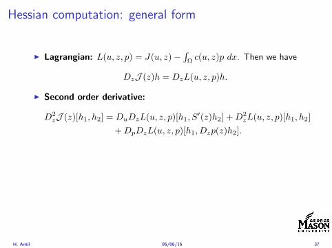
Hessian computation general form
I Lagrangian L(u z p) = J(u z)minusint
Ωc(u z)p dx Then we have
DzJ (z)h = DzL(u z p)h
I Second order derivative
D2zJ (z)[h1 h2] = DuDzL(u z p)[h1 S
prime(z)h2] +D2zL(u z p)[h1 h2]
+DpDzL(u z p)[h1 Dzp(z)h2]
I We already know Sprime(z)h2 moreover
DpDzL(u z p)[h1 Dzp(z)h2] = minus(cu(u z)h1 Dzp(z)h2
)
It remain to identify Dzp(z)h2
H Antil 060616 37
Hessian computation general form
I Lagrangian L(u z p) = J(u z)minusint
Ωc(u z)p dx Then we have
DzJ (z)h = DzL(u z p)h
I Second order derivative
D2zJ (z)[h1 h2] = DuDzL(u z p)[h1 S
prime(z)h2] +D2zL(u z p)[h1 h2]
+DpDzL(u z p)[h1 Dzp(z)h2]
I We already know Sprime(z)h2 moreover
DpDzL(u z p)[h1 Dzp(z)h2] = minus(cu(u z)h1 Dzp(z)h2
)
It remain to identify Dzp(z)h2
H Antil 060616 37
Outline
Motivation and examples
Linear elliptic optimal control problems
Differentiation in Banach spaces
First-order necessary conditions
Optimal control of semilinear PDEs
An abstract problem
Discretization using finite element methods
H Antil 060616 38
Numerical approximation of Poisson equation MeshTo avoid technical issues we will assume that partΩ is polygonal
I Mesh Let T = K be a mesh of Ω where K sub Rd is an elementthat is isoparametrically equivalent to a unit simplex in Rd
I Conforming mesh We say that the mesh is conforming ifI Ω = cupKisinT KI If K1 cap K2 = x then x is a node of K1 and K2I If K1 cap K2 6= empty and K1 cap K2 6= x then K1 cap K2 is an edgeface
contained in partK1 cap partK2
I Shape regular Let T be the collection of all conformingrefinements of an original mesh T 0 Then T is called shape regularif exist κ gt 0 such that
hKρKle κ forallK isin cupiT i
where hK = diam K ρK = maxρ gt 0|Bρ sub KI Quasi-uniform A family of shape regular meshes is called-quasi
uniform if there exist a constant σ gt 0 such that
maxhKminhK
le σ
uniformly for all meshes in the family
Numerical approximation of Poisson equation MeshTo avoid technical issues we will assume that partΩ is polygonal
I Mesh Let T = K be a mesh of Ω where K sub Rd is an elementthat is isoparametrically equivalent to a unit simplex in Rd
I Conforming mesh We say that the mesh is conforming ifI Ω = cupKisinT KI If K1 cap K2 = x then x is a node of K1 and K2I If K1 cap K2 6= empty and K1 cap K2 6= x then K1 cap K2 is an edgeface
contained in partK1 cap partK2
I Shape regular Let T be the collection of all conformingrefinements of an original mesh T 0 Then T is called shape regularif exist κ gt 0 such that
hKρKle κ forallK isin cupiT i
where hK = diam K ρK = maxρ gt 0|Bρ sub KI Quasi-uniform A family of shape regular meshes is called-quasi
uniform if there exist a constant σ gt 0 such that
maxhKminhK
le σ
uniformly for all meshes in the family
Numerical approximation of Poisson equation MeshTo avoid technical issues we will assume that partΩ is polygonal
I Mesh Let T = K be a mesh of Ω where K sub Rd is an elementthat is isoparametrically equivalent to a unit simplex in Rd
I Conforming mesh We say that the mesh is conforming ifI Ω = cupKisinT KI If K1 cap K2 = x then x is a node of K1 and K2I If K1 cap K2 6= empty and K1 cap K2 6= x then K1 cap K2 is an edgeface
contained in partK1 cap partK2
I Shape regular Let T be the collection of all conformingrefinements of an original mesh T 0 Then T is called shape regularif exist κ gt 0 such that
hKρKle κ forallK isin cupiT i
where hK = diam K ρK = maxρ gt 0|Bρ sub K
I Quasi-uniform A family of shape regular meshes is called-quasiuniform if there exist a constant σ gt 0 such that
maxhKminhK
le σ
uniformly for all meshes in the family
Numerical approximation of Poisson equation MeshTo avoid technical issues we will assume that partΩ is polygonal
I Mesh Let T = K be a mesh of Ω where K sub Rd is an elementthat is isoparametrically equivalent to a unit simplex in Rd
I Conforming mesh We say that the mesh is conforming ifI Ω = cupKisinT KI If K1 cap K2 = x then x is a node of K1 and K2I If K1 cap K2 6= empty and K1 cap K2 6= x then K1 cap K2 is an edgeface
contained in partK1 cap partK2
I Shape regular Let T be the collection of all conformingrefinements of an original mesh T 0 Then T is called shape regularif exist κ gt 0 such that
hKρKle κ forallK isin cupiT i
where hK = diam K ρK = maxρ gt 0|Bρ sub KI Quasi-uniform A family of shape regular meshes is called-quasi
uniform if there exist a constant σ gt 0 such that
maxhKminhK
le σ
uniformly for all meshes in the family
FE space and Galerkin approximationI Finite element space For T isin T we define the finite element
space as
V(T ) = W isin C0(Ω) WK isin P1forallK isin T W |partΩ = 0
where P1 is the set of polynomials of degree at most 1
I Galerkin approximation of continuous problem is given by
Find UT isin V(T )
intΩ
AnablaUT middot nablaV = 〈f V 〉 forallV isin V(T )
The discrete problem is well-posedI Nodal basis Consists of functions ψi isin V(T ) with xi isin N (T )
satisfyingψxi
(xj) = δij
where N (T ) denotes the interior (plus Neumann) nodesI Galerkin orthogonality(
nabla(uminus UT )nablaW)L2(Ω)
= 0 forallW isin V(T )
H Antil 060616 40
FE space and Galerkin approximationI Finite element space For T isin T we define the finite element
space as
V(T ) = W isin C0(Ω) WK isin P1forallK isin T W |partΩ = 0
where P1 is the set of polynomials of degree at most 1I Galerkin approximation of continuous problem is given by
Find UT isin V(T )
intΩ
AnablaUT middot nablaV = 〈f V 〉 forallV isin V(T )
The discrete problem is well-posed
I Nodal basis Consists of functions ψi isin V(T ) with xi isin N (T )satisfying
ψxi(xj) = δij
where N (T ) denotes the interior (plus Neumann) nodesI Galerkin orthogonality(
nabla(uminus UT )nablaW)L2(Ω)
= 0 forallW isin V(T )
H Antil 060616 40
FE space and Galerkin approximationI Finite element space For T isin T we define the finite element
space as
V(T ) = W isin C0(Ω) WK isin P1forallK isin T W |partΩ = 0
where P1 is the set of polynomials of degree at most 1I Galerkin approximation of continuous problem is given by
Find UT isin V(T )
intΩ
AnablaUT middot nablaV = 〈f V 〉 forallV isin V(T )
The discrete problem is well-posedI Nodal basis Consists of functions ψi isin V(T ) with xi isin N (T )
satisfyingψxi
(xj) = δij
where N (T ) denotes the interior (plus Neumann) nodes
I Galerkin orthogonality(nabla(uminus UT )nablaW
)L2(Ω)
= 0 forallW isin V(T )
H Antil 060616 40
FE space and Galerkin approximationI Finite element space For T isin T we define the finite element
space as
V(T ) = W isin C0(Ω) WK isin P1forallK isin T W |partΩ = 0
where P1 is the set of polynomials of degree at most 1I Galerkin approximation of continuous problem is given by
Find UT isin V(T )
intΩ
AnablaUT middot nablaV = 〈f V 〉 forallV isin V(T )
The discrete problem is well-posedI Nodal basis Consists of functions ψi isin V(T ) with xi isin N (T )
satisfyingψxi
(xj) = δij
where N (T ) denotes the interior (plus Neumann) nodesI Galerkin orthogonality(
nabla(uminus UT )nablaW)L2(Ω)
= 0 forallW isin V(T )
H Antil 060616 40
Best approximation
I Cearsquos lemma
nabla(uminus UT )L2(Ω) le C infWisinV(T )
nabla(uminusW )L2(Ω)
I Nodal interpolation operator ΠT C(Ω)rarr V(T ) satisfies
ΠT u(xi) = u(xi) forallxi isin N (T )
and is defined as
ΠT u =sum
xiisinN (T )
u(xi)ψxi
I Error estimates In Cearsquos lemma replace W by ΠT u and thencompute the interpolation error
H Antil 060616 41
Best approximation
I Cearsquos lemma
nabla(uminus UT )L2(Ω) le C infWisinV(T )
nabla(uminusW )L2(Ω)
I Nodal interpolation operator ΠT C(Ω)rarr V(T ) satisfies
ΠT u(xi) = u(xi) forallxi isin N (T )
and is defined as
ΠT u =sum
xiisinN (T )
u(xi)ψxi
I Error estimates In Cearsquos lemma replace W by ΠT u and thencompute the interpolation error
H Antil 060616 41
Best approximation
I Cearsquos lemma
nabla(uminus UT )L2(Ω) le C infWisinV(T )
nabla(uminusW )L2(Ω)
I Nodal interpolation operator ΠT C(Ω)rarr V(T ) satisfies
ΠT u(xi) = u(xi) forallxi isin N (T )
and is defined as
ΠT u =sum
xiisinN (T )
u(xi)ψxi
I Error estimates In Cearsquos lemma replace W by ΠT u and thencompute the interpolation error
H Antil 060616 41
Algebraic system state equation
I Recall UT isin V(T ) solves
a(UT V ) = 〈f V 〉 forallV isin V(T )
I Now setting UT =sumN
j=1 Ujψj V = ψi we get
Nsumj=1
Uja(φj φi) = 〈f ψi〉 i = 1 N
which is the matrix-vector system
AU = F
I Stiffness matrix A is SPD
H Antil 060616 42
Algebraic system state equation
I Recall UT isin V(T ) solves
a(UT V ) = 〈f V 〉 forallV isin V(T )
I Now setting UT =sumN
j=1 Ujψj V = ψi we get
Nsumj=1
Uja(φj φi) = 〈f ψi〉 i = 1 N
which is the matrix-vector system
AU = F
I Stiffness matrix A is SPD
H Antil 060616 42
Algebraic system state equation
I Recall UT isin V(T ) solves
a(UT V ) = 〈f V 〉 forallV isin V(T )
I Now setting UT =sumN
j=1 Ujψj V = ψi we get
Nsumj=1
Uja(φj φi) = 〈f ψi〉 i = 1 N
which is the matrix-vector system
AU = F
I Stiffness matrix A is SPD
H Antil 060616 42
Discrete linear elliptic OCP
min JT (UT ZT ) =1
2UT minus ud2L2(Ω) +
λ
2ZT 2L2(Ω)
subject to
Find UT isin V(T )
intΩ
nablaUT middot nablaV = (ZT V )L2(Ω) forallV isin V(T )
and whereZT isin Zad(T ) = Zad cap Z(T )
is either one of these
Z(T ) =
V(T )L2(Ω) variational discretization (Hinze)WT isin Linfin(Ω) ZT |K isin P0(K)K isin T
H Antil 060616 43
Recent books
F TroltzschOptimal control of partial differential equations volume 112 ofGraduate Studies in MathematicsAmerican Mathematical Society Providence RI 2010Theory methods and applications Translated from the 2005 Germanoriginal by Jurgen Sprekels
K Ito and K KunischLagrange multiplier approach to variational problems andapplications volume 15 of Advances in Design and ControlSociety for Industrial and Applied Mathematics (SIAM)Philadelphia PA 2008
H Antil 060616 44
- Motivation and examples
- Linear elliptic optimal control problems
- Differentiation in Banach spaces
- First-order necessary conditions
- Optimal control of semilinear PDEs
- An abstract problem
- Discretization using finite element methods
-
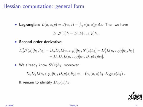
Hessian computation general form
I Lagrangian L(u z p) = J(u z)minusint
Ωc(u z)p dx Then we have
DzJ (z)h = DzL(u z p)h
I Second order derivative
D2zJ (z)[h1 h2] = DuDzL(u z p)[h1 S
prime(z)h2] +D2zL(u z p)[h1 h2]
+DpDzL(u z p)[h1 Dzp(z)h2]
I We already know Sprime(z)h2 moreover
DpDzL(u z p)[h1 Dzp(z)h2] = minus(cu(u z)h1 Dzp(z)h2
)
It remain to identify Dzp(z)h2
H Antil 060616 37
Outline
Motivation and examples
Linear elliptic optimal control problems
Differentiation in Banach spaces
First-order necessary conditions
Optimal control of semilinear PDEs
An abstract problem
Discretization using finite element methods
H Antil 060616 38
Numerical approximation of Poisson equation MeshTo avoid technical issues we will assume that partΩ is polygonal
I Mesh Let T = K be a mesh of Ω where K sub Rd is an elementthat is isoparametrically equivalent to a unit simplex in Rd
I Conforming mesh We say that the mesh is conforming ifI Ω = cupKisinT KI If K1 cap K2 = x then x is a node of K1 and K2I If K1 cap K2 6= empty and K1 cap K2 6= x then K1 cap K2 is an edgeface
contained in partK1 cap partK2
I Shape regular Let T be the collection of all conformingrefinements of an original mesh T 0 Then T is called shape regularif exist κ gt 0 such that
hKρKle κ forallK isin cupiT i
where hK = diam K ρK = maxρ gt 0|Bρ sub KI Quasi-uniform A family of shape regular meshes is called-quasi
uniform if there exist a constant σ gt 0 such that
maxhKminhK
le σ
uniformly for all meshes in the family
Numerical approximation of Poisson equation MeshTo avoid technical issues we will assume that partΩ is polygonal
I Mesh Let T = K be a mesh of Ω where K sub Rd is an elementthat is isoparametrically equivalent to a unit simplex in Rd
I Conforming mesh We say that the mesh is conforming ifI Ω = cupKisinT KI If K1 cap K2 = x then x is a node of K1 and K2I If K1 cap K2 6= empty and K1 cap K2 6= x then K1 cap K2 is an edgeface
contained in partK1 cap partK2
I Shape regular Let T be the collection of all conformingrefinements of an original mesh T 0 Then T is called shape regularif exist κ gt 0 such that
hKρKle κ forallK isin cupiT i
where hK = diam K ρK = maxρ gt 0|Bρ sub KI Quasi-uniform A family of shape regular meshes is called-quasi
uniform if there exist a constant σ gt 0 such that
maxhKminhK
le σ
uniformly for all meshes in the family
Numerical approximation of Poisson equation MeshTo avoid technical issues we will assume that partΩ is polygonal
I Mesh Let T = K be a mesh of Ω where K sub Rd is an elementthat is isoparametrically equivalent to a unit simplex in Rd
I Conforming mesh We say that the mesh is conforming ifI Ω = cupKisinT KI If K1 cap K2 = x then x is a node of K1 and K2I If K1 cap K2 6= empty and K1 cap K2 6= x then K1 cap K2 is an edgeface
contained in partK1 cap partK2
I Shape regular Let T be the collection of all conformingrefinements of an original mesh T 0 Then T is called shape regularif exist κ gt 0 such that
hKρKle κ forallK isin cupiT i
where hK = diam K ρK = maxρ gt 0|Bρ sub K
I Quasi-uniform A family of shape regular meshes is called-quasiuniform if there exist a constant σ gt 0 such that
maxhKminhK
le σ
uniformly for all meshes in the family
Numerical approximation of Poisson equation MeshTo avoid technical issues we will assume that partΩ is polygonal
I Mesh Let T = K be a mesh of Ω where K sub Rd is an elementthat is isoparametrically equivalent to a unit simplex in Rd
I Conforming mesh We say that the mesh is conforming ifI Ω = cupKisinT KI If K1 cap K2 = x then x is a node of K1 and K2I If K1 cap K2 6= empty and K1 cap K2 6= x then K1 cap K2 is an edgeface
contained in partK1 cap partK2
I Shape regular Let T be the collection of all conformingrefinements of an original mesh T 0 Then T is called shape regularif exist κ gt 0 such that
hKρKle κ forallK isin cupiT i
where hK = diam K ρK = maxρ gt 0|Bρ sub KI Quasi-uniform A family of shape regular meshes is called-quasi
uniform if there exist a constant σ gt 0 such that
maxhKminhK
le σ
uniformly for all meshes in the family
FE space and Galerkin approximationI Finite element space For T isin T we define the finite element
space as
V(T ) = W isin C0(Ω) WK isin P1forallK isin T W |partΩ = 0
where P1 is the set of polynomials of degree at most 1
I Galerkin approximation of continuous problem is given by
Find UT isin V(T )
intΩ
AnablaUT middot nablaV = 〈f V 〉 forallV isin V(T )
The discrete problem is well-posedI Nodal basis Consists of functions ψi isin V(T ) with xi isin N (T )
satisfyingψxi
(xj) = δij
where N (T ) denotes the interior (plus Neumann) nodesI Galerkin orthogonality(
nabla(uminus UT )nablaW)L2(Ω)
= 0 forallW isin V(T )
H Antil 060616 40
FE space and Galerkin approximationI Finite element space For T isin T we define the finite element
space as
V(T ) = W isin C0(Ω) WK isin P1forallK isin T W |partΩ = 0
where P1 is the set of polynomials of degree at most 1I Galerkin approximation of continuous problem is given by
Find UT isin V(T )
intΩ
AnablaUT middot nablaV = 〈f V 〉 forallV isin V(T )
The discrete problem is well-posed
I Nodal basis Consists of functions ψi isin V(T ) with xi isin N (T )satisfying
ψxi(xj) = δij
where N (T ) denotes the interior (plus Neumann) nodesI Galerkin orthogonality(
nabla(uminus UT )nablaW)L2(Ω)
= 0 forallW isin V(T )
H Antil 060616 40
FE space and Galerkin approximationI Finite element space For T isin T we define the finite element
space as
V(T ) = W isin C0(Ω) WK isin P1forallK isin T W |partΩ = 0
where P1 is the set of polynomials of degree at most 1I Galerkin approximation of continuous problem is given by
Find UT isin V(T )
intΩ
AnablaUT middot nablaV = 〈f V 〉 forallV isin V(T )
The discrete problem is well-posedI Nodal basis Consists of functions ψi isin V(T ) with xi isin N (T )
satisfyingψxi
(xj) = δij
where N (T ) denotes the interior (plus Neumann) nodes
I Galerkin orthogonality(nabla(uminus UT )nablaW
)L2(Ω)
= 0 forallW isin V(T )
H Antil 060616 40
FE space and Galerkin approximationI Finite element space For T isin T we define the finite element
space as
V(T ) = W isin C0(Ω) WK isin P1forallK isin T W |partΩ = 0
where P1 is the set of polynomials of degree at most 1I Galerkin approximation of continuous problem is given by
Find UT isin V(T )
intΩ
AnablaUT middot nablaV = 〈f V 〉 forallV isin V(T )
The discrete problem is well-posedI Nodal basis Consists of functions ψi isin V(T ) with xi isin N (T )
satisfyingψxi
(xj) = δij
where N (T ) denotes the interior (plus Neumann) nodesI Galerkin orthogonality(
nabla(uminus UT )nablaW)L2(Ω)
= 0 forallW isin V(T )
H Antil 060616 40
Best approximation
I Cearsquos lemma
nabla(uminus UT )L2(Ω) le C infWisinV(T )
nabla(uminusW )L2(Ω)
I Nodal interpolation operator ΠT C(Ω)rarr V(T ) satisfies
ΠT u(xi) = u(xi) forallxi isin N (T )
and is defined as
ΠT u =sum
xiisinN (T )
u(xi)ψxi
I Error estimates In Cearsquos lemma replace W by ΠT u and thencompute the interpolation error
H Antil 060616 41
Best approximation
I Cearsquos lemma
nabla(uminus UT )L2(Ω) le C infWisinV(T )
nabla(uminusW )L2(Ω)
I Nodal interpolation operator ΠT C(Ω)rarr V(T ) satisfies
ΠT u(xi) = u(xi) forallxi isin N (T )
and is defined as
ΠT u =sum
xiisinN (T )
u(xi)ψxi
I Error estimates In Cearsquos lemma replace W by ΠT u and thencompute the interpolation error
H Antil 060616 41
Best approximation
I Cearsquos lemma
nabla(uminus UT )L2(Ω) le C infWisinV(T )
nabla(uminusW )L2(Ω)
I Nodal interpolation operator ΠT C(Ω)rarr V(T ) satisfies
ΠT u(xi) = u(xi) forallxi isin N (T )
and is defined as
ΠT u =sum
xiisinN (T )
u(xi)ψxi
I Error estimates In Cearsquos lemma replace W by ΠT u and thencompute the interpolation error
H Antil 060616 41
Algebraic system state equation
I Recall UT isin V(T ) solves
a(UT V ) = 〈f V 〉 forallV isin V(T )
I Now setting UT =sumN
j=1 Ujψj V = ψi we get
Nsumj=1
Uja(φj φi) = 〈f ψi〉 i = 1 N
which is the matrix-vector system
AU = F
I Stiffness matrix A is SPD
H Antil 060616 42
Algebraic system state equation
I Recall UT isin V(T ) solves
a(UT V ) = 〈f V 〉 forallV isin V(T )
I Now setting UT =sumN
j=1 Ujψj V = ψi we get
Nsumj=1
Uja(φj φi) = 〈f ψi〉 i = 1 N
which is the matrix-vector system
AU = F
I Stiffness matrix A is SPD
H Antil 060616 42
Algebraic system state equation
I Recall UT isin V(T ) solves
a(UT V ) = 〈f V 〉 forallV isin V(T )
I Now setting UT =sumN
j=1 Ujψj V = ψi we get
Nsumj=1
Uja(φj φi) = 〈f ψi〉 i = 1 N
which is the matrix-vector system
AU = F
I Stiffness matrix A is SPD
H Antil 060616 42
Discrete linear elliptic OCP
min JT (UT ZT ) =1
2UT minus ud2L2(Ω) +
λ
2ZT 2L2(Ω)
subject to
Find UT isin V(T )
intΩ
nablaUT middot nablaV = (ZT V )L2(Ω) forallV isin V(T )
and whereZT isin Zad(T ) = Zad cap Z(T )
is either one of these
Z(T ) =
V(T )L2(Ω) variational discretization (Hinze)WT isin Linfin(Ω) ZT |K isin P0(K)K isin T
H Antil 060616 43
Recent books
F TroltzschOptimal control of partial differential equations volume 112 ofGraduate Studies in MathematicsAmerican Mathematical Society Providence RI 2010Theory methods and applications Translated from the 2005 Germanoriginal by Jurgen Sprekels
K Ito and K KunischLagrange multiplier approach to variational problems andapplications volume 15 of Advances in Design and ControlSociety for Industrial and Applied Mathematics (SIAM)Philadelphia PA 2008
H Antil 060616 44
- Motivation and examples
- Linear elliptic optimal control problems
- Differentiation in Banach spaces
- First-order necessary conditions
- Optimal control of semilinear PDEs
- An abstract problem
- Discretization using finite element methods
-
Numerical approximation of Poisson equation MeshTo avoid technical issues we will assume that partΩ is polygonal
I Mesh Let T = K be a mesh of Ω where K sub Rd is an elementthat is isoparametrically equivalent to a unit simplex in Rd
I Conforming mesh We say that the mesh is conforming ifI Ω = cupKisinT KI If K1 cap K2 = x then x is a node of K1 and K2I If K1 cap K2 6= empty and K1 cap K2 6= x then K1 cap K2 is an edgeface
contained in partK1 cap partK2
I Shape regular Let T be the collection of all conformingrefinements of an original mesh T 0 Then T is called shape regularif exist κ gt 0 such that
hKρKle κ forallK isin cupiT i
where hK = diam K ρK = maxρ gt 0|Bρ sub KI Quasi-uniform A family of shape regular meshes is called-quasi
uniform if there exist a constant σ gt 0 such that
maxhKminhK
le σ
uniformly for all meshes in the family
Numerical approximation of Poisson equation MeshTo avoid technical issues we will assume that partΩ is polygonal
I Mesh Let T = K be a mesh of Ω where K sub Rd is an elementthat is isoparametrically equivalent to a unit simplex in Rd
I Conforming mesh We say that the mesh is conforming ifI Ω = cupKisinT KI If K1 cap K2 = x then x is a node of K1 and K2I If K1 cap K2 6= empty and K1 cap K2 6= x then K1 cap K2 is an edgeface
contained in partK1 cap partK2
I Shape regular Let T be the collection of all conformingrefinements of an original mesh T 0 Then T is called shape regularif exist κ gt 0 such that
hKρKle κ forallK isin cupiT i
where hK = diam K ρK = maxρ gt 0|Bρ sub K
I Quasi-uniform A family of shape regular meshes is called-quasiuniform if there exist a constant σ gt 0 such that
maxhKminhK
le σ
uniformly for all meshes in the family
Numerical approximation of Poisson equation MeshTo avoid technical issues we will assume that partΩ is polygonal
I Mesh Let T = K be a mesh of Ω where K sub Rd is an elementthat is isoparametrically equivalent to a unit simplex in Rd
I Conforming mesh We say that the mesh is conforming ifI Ω = cupKisinT KI If K1 cap K2 = x then x is a node of K1 and K2I If K1 cap K2 6= empty and K1 cap K2 6= x then K1 cap K2 is an edgeface
contained in partK1 cap partK2
I Shape regular Let T be the collection of all conformingrefinements of an original mesh T 0 Then T is called shape regularif exist κ gt 0 such that
hKρKle κ forallK isin cupiT i
where hK = diam K ρK = maxρ gt 0|Bρ sub KI Quasi-uniform A family of shape regular meshes is called-quasi
uniform if there exist a constant σ gt 0 such that
maxhKminhK
le σ
uniformly for all meshes in the family
FE space and Galerkin approximationI Finite element space For T isin T we define the finite element
space as
V(T ) = W isin C0(Ω) WK isin P1forallK isin T W |partΩ = 0
where P1 is the set of polynomials of degree at most 1
I Galerkin approximation of continuous problem is given by
Find UT isin V(T )
intΩ
AnablaUT middot nablaV = 〈f V 〉 forallV isin V(T )
The discrete problem is well-posedI Nodal basis Consists of functions ψi isin V(T ) with xi isin N (T )
satisfyingψxi
(xj) = δij
where N (T ) denotes the interior (plus Neumann) nodesI Galerkin orthogonality(
nabla(uminus UT )nablaW)L2(Ω)
= 0 forallW isin V(T )
H Antil 060616 40
FE space and Galerkin approximationI Finite element space For T isin T we define the finite element
space as
V(T ) = W isin C0(Ω) WK isin P1forallK isin T W |partΩ = 0
where P1 is the set of polynomials of degree at most 1I Galerkin approximation of continuous problem is given by
Find UT isin V(T )
intΩ
AnablaUT middot nablaV = 〈f V 〉 forallV isin V(T )
The discrete problem is well-posed
I Nodal basis Consists of functions ψi isin V(T ) with xi isin N (T )satisfying
ψxi(xj) = δij
where N (T ) denotes the interior (plus Neumann) nodesI Galerkin orthogonality(
nabla(uminus UT )nablaW)L2(Ω)
= 0 forallW isin V(T )
H Antil 060616 40
FE space and Galerkin approximationI Finite element space For T isin T we define the finite element
space as
V(T ) = W isin C0(Ω) WK isin P1forallK isin T W |partΩ = 0
where P1 is the set of polynomials of degree at most 1I Galerkin approximation of continuous problem is given by
Find UT isin V(T )
intΩ
AnablaUT middot nablaV = 〈f V 〉 forallV isin V(T )
The discrete problem is well-posedI Nodal basis Consists of functions ψi isin V(T ) with xi isin N (T )
satisfyingψxi
(xj) = δij
where N (T ) denotes the interior (plus Neumann) nodes
I Galerkin orthogonality(nabla(uminus UT )nablaW
)L2(Ω)
= 0 forallW isin V(T )
H Antil 060616 40
FE space and Galerkin approximationI Finite element space For T isin T we define the finite element
space as
V(T ) = W isin C0(Ω) WK isin P1forallK isin T W |partΩ = 0
where P1 is the set of polynomials of degree at most 1I Galerkin approximation of continuous problem is given by
Find UT isin V(T )
intΩ
AnablaUT middot nablaV = 〈f V 〉 forallV isin V(T )
The discrete problem is well-posedI Nodal basis Consists of functions ψi isin V(T ) with xi isin N (T )
satisfyingψxi
(xj) = δij
where N (T ) denotes the interior (plus Neumann) nodesI Galerkin orthogonality(
nabla(uminus UT )nablaW)L2(Ω)
= 0 forallW isin V(T )
H Antil 060616 40
Best approximation
I Cearsquos lemma
nabla(uminus UT )L2(Ω) le C infWisinV(T )
nabla(uminusW )L2(Ω)
I Nodal interpolation operator ΠT C(Ω)rarr V(T ) satisfies
ΠT u(xi) = u(xi) forallxi isin N (T )
and is defined as
ΠT u =sum
xiisinN (T )
u(xi)ψxi
I Error estimates In Cearsquos lemma replace W by ΠT u and thencompute the interpolation error
H Antil 060616 41
Best approximation
I Cearsquos lemma
nabla(uminus UT )L2(Ω) le C infWisinV(T )
nabla(uminusW )L2(Ω)
I Nodal interpolation operator ΠT C(Ω)rarr V(T ) satisfies
ΠT u(xi) = u(xi) forallxi isin N (T )
and is defined as
ΠT u =sum
xiisinN (T )
u(xi)ψxi
I Error estimates In Cearsquos lemma replace W by ΠT u and thencompute the interpolation error
H Antil 060616 41
Best approximation
I Cearsquos lemma
nabla(uminus UT )L2(Ω) le C infWisinV(T )
nabla(uminusW )L2(Ω)
I Nodal interpolation operator ΠT C(Ω)rarr V(T ) satisfies
ΠT u(xi) = u(xi) forallxi isin N (T )
and is defined as
ΠT u =sum
xiisinN (T )
u(xi)ψxi
I Error estimates In Cearsquos lemma replace W by ΠT u and thencompute the interpolation error
H Antil 060616 41
Algebraic system state equation
I Recall UT isin V(T ) solves
a(UT V ) = 〈f V 〉 forallV isin V(T )
I Now setting UT =sumN
j=1 Ujψj V = ψi we get
Nsumj=1
Uja(φj φi) = 〈f ψi〉 i = 1 N
which is the matrix-vector system
AU = F
I Stiffness matrix A is SPD
H Antil 060616 42
Algebraic system state equation
I Recall UT isin V(T ) solves
a(UT V ) = 〈f V 〉 forallV isin V(T )
I Now setting UT =sumN
j=1 Ujψj V = ψi we get
Nsumj=1
Uja(φj φi) = 〈f ψi〉 i = 1 N
which is the matrix-vector system
AU = F
I Stiffness matrix A is SPD
H Antil 060616 42
Algebraic system state equation
I Recall UT isin V(T ) solves
a(UT V ) = 〈f V 〉 forallV isin V(T )
I Now setting UT =sumN
j=1 Ujψj V = ψi we get
Nsumj=1
Uja(φj φi) = 〈f ψi〉 i = 1 N
which is the matrix-vector system
AU = F
I Stiffness matrix A is SPD
H Antil 060616 42
Discrete linear elliptic OCP
min JT (UT ZT ) =1
2UT minus ud2L2(Ω) +
λ
2ZT 2L2(Ω)
subject to
Find UT isin V(T )
intΩ
nablaUT middot nablaV = (ZT V )L2(Ω) forallV isin V(T )
and whereZT isin Zad(T ) = Zad cap Z(T )
is either one of these
Z(T ) =
V(T )L2(Ω) variational discretization (Hinze)WT isin Linfin(Ω) ZT |K isin P0(K)K isin T
H Antil 060616 43
Recent books
F TroltzschOptimal control of partial differential equations volume 112 ofGraduate Studies in MathematicsAmerican Mathematical Society Providence RI 2010Theory methods and applications Translated from the 2005 Germanoriginal by Jurgen Sprekels
K Ito and K KunischLagrange multiplier approach to variational problems andapplications volume 15 of Advances in Design and ControlSociety for Industrial and Applied Mathematics (SIAM)Philadelphia PA 2008
H Antil 060616 44
- Motivation and examples
- Linear elliptic optimal control problems
- Differentiation in Banach spaces
- First-order necessary conditions
- Optimal control of semilinear PDEs
- An abstract problem
- Discretization using finite element methods
-
Numerical approximation of Poisson equation MeshTo avoid technical issues we will assume that partΩ is polygonal
I Mesh Let T = K be a mesh of Ω where K sub Rd is an elementthat is isoparametrically equivalent to a unit simplex in Rd
I Conforming mesh We say that the mesh is conforming ifI Ω = cupKisinT KI If K1 cap K2 = x then x is a node of K1 and K2I If K1 cap K2 6= empty and K1 cap K2 6= x then K1 cap K2 is an edgeface
contained in partK1 cap partK2
I Shape regular Let T be the collection of all conformingrefinements of an original mesh T 0 Then T is called shape regularif exist κ gt 0 such that
hKρKle κ forallK isin cupiT i
where hK = diam K ρK = maxρ gt 0|Bρ sub KI Quasi-uniform A family of shape regular meshes is called-quasi
uniform if there exist a constant σ gt 0 such that
maxhKminhK
le σ
uniformly for all meshes in the family
Numerical approximation of Poisson equation MeshTo avoid technical issues we will assume that partΩ is polygonal
I Mesh Let T = K be a mesh of Ω where K sub Rd is an elementthat is isoparametrically equivalent to a unit simplex in Rd
I Conforming mesh We say that the mesh is conforming ifI Ω = cupKisinT KI If K1 cap K2 = x then x is a node of K1 and K2I If K1 cap K2 6= empty and K1 cap K2 6= x then K1 cap K2 is an edgeface
contained in partK1 cap partK2
I Shape regular Let T be the collection of all conformingrefinements of an original mesh T 0 Then T is called shape regularif exist κ gt 0 such that
hKρKle κ forallK isin cupiT i
where hK = diam K ρK = maxρ gt 0|Bρ sub K
I Quasi-uniform A family of shape regular meshes is called-quasiuniform if there exist a constant σ gt 0 such that
maxhKminhK
le σ
uniformly for all meshes in the family
Numerical approximation of Poisson equation MeshTo avoid technical issues we will assume that partΩ is polygonal
I Mesh Let T = K be a mesh of Ω where K sub Rd is an elementthat is isoparametrically equivalent to a unit simplex in Rd
I Conforming mesh We say that the mesh is conforming ifI Ω = cupKisinT KI If K1 cap K2 = x then x is a node of K1 and K2I If K1 cap K2 6= empty and K1 cap K2 6= x then K1 cap K2 is an edgeface
contained in partK1 cap partK2
I Shape regular Let T be the collection of all conformingrefinements of an original mesh T 0 Then T is called shape regularif exist κ gt 0 such that
hKρKle κ forallK isin cupiT i
where hK = diam K ρK = maxρ gt 0|Bρ sub KI Quasi-uniform A family of shape regular meshes is called-quasi
uniform if there exist a constant σ gt 0 such that
maxhKminhK
le σ
uniformly for all meshes in the family
FE space and Galerkin approximationI Finite element space For T isin T we define the finite element
space as
V(T ) = W isin C0(Ω) WK isin P1forallK isin T W |partΩ = 0
where P1 is the set of polynomials of degree at most 1
I Galerkin approximation of continuous problem is given by
Find UT isin V(T )
intΩ
AnablaUT middot nablaV = 〈f V 〉 forallV isin V(T )
The discrete problem is well-posedI Nodal basis Consists of functions ψi isin V(T ) with xi isin N (T )
satisfyingψxi
(xj) = δij
where N (T ) denotes the interior (plus Neumann) nodesI Galerkin orthogonality(
nabla(uminus UT )nablaW)L2(Ω)
= 0 forallW isin V(T )
H Antil 060616 40
FE space and Galerkin approximationI Finite element space For T isin T we define the finite element
space as
V(T ) = W isin C0(Ω) WK isin P1forallK isin T W |partΩ = 0
where P1 is the set of polynomials of degree at most 1I Galerkin approximation of continuous problem is given by
Find UT isin V(T )
intΩ
AnablaUT middot nablaV = 〈f V 〉 forallV isin V(T )
The discrete problem is well-posed
I Nodal basis Consists of functions ψi isin V(T ) with xi isin N (T )satisfying
ψxi(xj) = δij
where N (T ) denotes the interior (plus Neumann) nodesI Galerkin orthogonality(
nabla(uminus UT )nablaW)L2(Ω)
= 0 forallW isin V(T )
H Antil 060616 40
FE space and Galerkin approximationI Finite element space For T isin T we define the finite element
space as
V(T ) = W isin C0(Ω) WK isin P1forallK isin T W |partΩ = 0
where P1 is the set of polynomials of degree at most 1I Galerkin approximation of continuous problem is given by
Find UT isin V(T )
intΩ
AnablaUT middot nablaV = 〈f V 〉 forallV isin V(T )
The discrete problem is well-posedI Nodal basis Consists of functions ψi isin V(T ) with xi isin N (T )
satisfyingψxi
(xj) = δij
where N (T ) denotes the interior (plus Neumann) nodes
I Galerkin orthogonality(nabla(uminus UT )nablaW
)L2(Ω)
= 0 forallW isin V(T )
H Antil 060616 40
FE space and Galerkin approximationI Finite element space For T isin T we define the finite element
space as
V(T ) = W isin C0(Ω) WK isin P1forallK isin T W |partΩ = 0
where P1 is the set of polynomials of degree at most 1I Galerkin approximation of continuous problem is given by
Find UT isin V(T )
intΩ
AnablaUT middot nablaV = 〈f V 〉 forallV isin V(T )
The discrete problem is well-posedI Nodal basis Consists of functions ψi isin V(T ) with xi isin N (T )
satisfyingψxi
(xj) = δij
where N (T ) denotes the interior (plus Neumann) nodesI Galerkin orthogonality(
nabla(uminus UT )nablaW)L2(Ω)
= 0 forallW isin V(T )
H Antil 060616 40
Best approximation
I Cearsquos lemma
nabla(uminus UT )L2(Ω) le C infWisinV(T )
nabla(uminusW )L2(Ω)
I Nodal interpolation operator ΠT C(Ω)rarr V(T ) satisfies
ΠT u(xi) = u(xi) forallxi isin N (T )
and is defined as
ΠT u =sum
xiisinN (T )
u(xi)ψxi
I Error estimates In Cearsquos lemma replace W by ΠT u and thencompute the interpolation error
H Antil 060616 41
Best approximation
I Cearsquos lemma
nabla(uminus UT )L2(Ω) le C infWisinV(T )
nabla(uminusW )L2(Ω)
I Nodal interpolation operator ΠT C(Ω)rarr V(T ) satisfies
ΠT u(xi) = u(xi) forallxi isin N (T )
and is defined as
ΠT u =sum
xiisinN (T )
u(xi)ψxi
I Error estimates In Cearsquos lemma replace W by ΠT u and thencompute the interpolation error
H Antil 060616 41
Best approximation
I Cearsquos lemma
nabla(uminus UT )L2(Ω) le C infWisinV(T )
nabla(uminusW )L2(Ω)
I Nodal interpolation operator ΠT C(Ω)rarr V(T ) satisfies
ΠT u(xi) = u(xi) forallxi isin N (T )
and is defined as
ΠT u =sum
xiisinN (T )
u(xi)ψxi
I Error estimates In Cearsquos lemma replace W by ΠT u and thencompute the interpolation error
H Antil 060616 41
Algebraic system state equation
I Recall UT isin V(T ) solves
a(UT V ) = 〈f V 〉 forallV isin V(T )
I Now setting UT =sumN
j=1 Ujψj V = ψi we get
Nsumj=1
Uja(φj φi) = 〈f ψi〉 i = 1 N
which is the matrix-vector system
AU = F
I Stiffness matrix A is SPD
H Antil 060616 42
Algebraic system state equation
I Recall UT isin V(T ) solves
a(UT V ) = 〈f V 〉 forallV isin V(T )
I Now setting UT =sumN
j=1 Ujψj V = ψi we get
Nsumj=1
Uja(φj φi) = 〈f ψi〉 i = 1 N
which is the matrix-vector system
AU = F
I Stiffness matrix A is SPD
H Antil 060616 42
Algebraic system state equation
I Recall UT isin V(T ) solves
a(UT V ) = 〈f V 〉 forallV isin V(T )
I Now setting UT =sumN
j=1 Ujψj V = ψi we get
Nsumj=1
Uja(φj φi) = 〈f ψi〉 i = 1 N
which is the matrix-vector system
AU = F
I Stiffness matrix A is SPD
H Antil 060616 42
Discrete linear elliptic OCP
min JT (UT ZT ) =1
2UT minus ud2L2(Ω) +
λ
2ZT 2L2(Ω)
subject to
Find UT isin V(T )
intΩ
nablaUT middot nablaV = (ZT V )L2(Ω) forallV isin V(T )
and whereZT isin Zad(T ) = Zad cap Z(T )
is either one of these
Z(T ) =
V(T )L2(Ω) variational discretization (Hinze)WT isin Linfin(Ω) ZT |K isin P0(K)K isin T
H Antil 060616 43
Recent books
F TroltzschOptimal control of partial differential equations volume 112 ofGraduate Studies in MathematicsAmerican Mathematical Society Providence RI 2010Theory methods and applications Translated from the 2005 Germanoriginal by Jurgen Sprekels
K Ito and K KunischLagrange multiplier approach to variational problems andapplications volume 15 of Advances in Design and ControlSociety for Industrial and Applied Mathematics (SIAM)Philadelphia PA 2008
H Antil 060616 44
- Motivation and examples
- Linear elliptic optimal control problems
- Differentiation in Banach spaces
- First-order necessary conditions
- Optimal control of semilinear PDEs
- An abstract problem
- Discretization using finite element methods
-
Numerical approximation of Poisson equation MeshTo avoid technical issues we will assume that partΩ is polygonal
I Mesh Let T = K be a mesh of Ω where K sub Rd is an elementthat is isoparametrically equivalent to a unit simplex in Rd
I Conforming mesh We say that the mesh is conforming ifI Ω = cupKisinT KI If K1 cap K2 = x then x is a node of K1 and K2I If K1 cap K2 6= empty and K1 cap K2 6= x then K1 cap K2 is an edgeface
contained in partK1 cap partK2
I Shape regular Let T be the collection of all conformingrefinements of an original mesh T 0 Then T is called shape regularif exist κ gt 0 such that
hKρKle κ forallK isin cupiT i
where hK = diam K ρK = maxρ gt 0|Bρ sub KI Quasi-uniform A family of shape regular meshes is called-quasi
uniform if there exist a constant σ gt 0 such that
maxhKminhK
le σ
uniformly for all meshes in the family
FE space and Galerkin approximationI Finite element space For T isin T we define the finite element
space as
V(T ) = W isin C0(Ω) WK isin P1forallK isin T W |partΩ = 0
where P1 is the set of polynomials of degree at most 1
I Galerkin approximation of continuous problem is given by
Find UT isin V(T )
intΩ
AnablaUT middot nablaV = 〈f V 〉 forallV isin V(T )
The discrete problem is well-posedI Nodal basis Consists of functions ψi isin V(T ) with xi isin N (T )
satisfyingψxi
(xj) = δij
where N (T ) denotes the interior (plus Neumann) nodesI Galerkin orthogonality(
nabla(uminus UT )nablaW)L2(Ω)
= 0 forallW isin V(T )
H Antil 060616 40
FE space and Galerkin approximationI Finite element space For T isin T we define the finite element
space as
V(T ) = W isin C0(Ω) WK isin P1forallK isin T W |partΩ = 0
where P1 is the set of polynomials of degree at most 1I Galerkin approximation of continuous problem is given by
Find UT isin V(T )
intΩ
AnablaUT middot nablaV = 〈f V 〉 forallV isin V(T )
The discrete problem is well-posed
I Nodal basis Consists of functions ψi isin V(T ) with xi isin N (T )satisfying
ψxi(xj) = δij
where N (T ) denotes the interior (plus Neumann) nodesI Galerkin orthogonality(
nabla(uminus UT )nablaW)L2(Ω)
= 0 forallW isin V(T )
H Antil 060616 40
FE space and Galerkin approximationI Finite element space For T isin T we define the finite element
space as
V(T ) = W isin C0(Ω) WK isin P1forallK isin T W |partΩ = 0
where P1 is the set of polynomials of degree at most 1I Galerkin approximation of continuous problem is given by
Find UT isin V(T )
intΩ
AnablaUT middot nablaV = 〈f V 〉 forallV isin V(T )
The discrete problem is well-posedI Nodal basis Consists of functions ψi isin V(T ) with xi isin N (T )
satisfyingψxi
(xj) = δij
where N (T ) denotes the interior (plus Neumann) nodes
I Galerkin orthogonality(nabla(uminus UT )nablaW
)L2(Ω)
= 0 forallW isin V(T )
H Antil 060616 40
FE space and Galerkin approximationI Finite element space For T isin T we define the finite element
space as
V(T ) = W isin C0(Ω) WK isin P1forallK isin T W |partΩ = 0
where P1 is the set of polynomials of degree at most 1I Galerkin approximation of continuous problem is given by
Find UT isin V(T )
intΩ
AnablaUT middot nablaV = 〈f V 〉 forallV isin V(T )
The discrete problem is well-posedI Nodal basis Consists of functions ψi isin V(T ) with xi isin N (T )
satisfyingψxi
(xj) = δij
where N (T ) denotes the interior (plus Neumann) nodesI Galerkin orthogonality(
nabla(uminus UT )nablaW)L2(Ω)
= 0 forallW isin V(T )
H Antil 060616 40
Best approximation
I Cearsquos lemma
nabla(uminus UT )L2(Ω) le C infWisinV(T )
nabla(uminusW )L2(Ω)
I Nodal interpolation operator ΠT C(Ω)rarr V(T ) satisfies
ΠT u(xi) = u(xi) forallxi isin N (T )
and is defined as
ΠT u =sum
xiisinN (T )
u(xi)ψxi
I Error estimates In Cearsquos lemma replace W by ΠT u and thencompute the interpolation error
H Antil 060616 41
Best approximation
I Cearsquos lemma
nabla(uminus UT )L2(Ω) le C infWisinV(T )
nabla(uminusW )L2(Ω)
I Nodal interpolation operator ΠT C(Ω)rarr V(T ) satisfies
ΠT u(xi) = u(xi) forallxi isin N (T )
and is defined as
ΠT u =sum
xiisinN (T )
u(xi)ψxi
I Error estimates In Cearsquos lemma replace W by ΠT u and thencompute the interpolation error
H Antil 060616 41
Best approximation
I Cearsquos lemma
nabla(uminus UT )L2(Ω) le C infWisinV(T )
nabla(uminusW )L2(Ω)
I Nodal interpolation operator ΠT C(Ω)rarr V(T ) satisfies
ΠT u(xi) = u(xi) forallxi isin N (T )
and is defined as
ΠT u =sum
xiisinN (T )
u(xi)ψxi
I Error estimates In Cearsquos lemma replace W by ΠT u and thencompute the interpolation error
H Antil 060616 41
Algebraic system state equation
I Recall UT isin V(T ) solves
a(UT V ) = 〈f V 〉 forallV isin V(T )
I Now setting UT =sumN
j=1 Ujψj V = ψi we get
Nsumj=1
Uja(φj φi) = 〈f ψi〉 i = 1 N
which is the matrix-vector system
AU = F
I Stiffness matrix A is SPD
H Antil 060616 42
Algebraic system state equation
I Recall UT isin V(T ) solves
a(UT V ) = 〈f V 〉 forallV isin V(T )
I Now setting UT =sumN
j=1 Ujψj V = ψi we get
Nsumj=1
Uja(φj φi) = 〈f ψi〉 i = 1 N
which is the matrix-vector system
AU = F
I Stiffness matrix A is SPD
H Antil 060616 42
Algebraic system state equation
I Recall UT isin V(T ) solves
a(UT V ) = 〈f V 〉 forallV isin V(T )
I Now setting UT =sumN
j=1 Ujψj V = ψi we get
Nsumj=1
Uja(φj φi) = 〈f ψi〉 i = 1 N
which is the matrix-vector system
AU = F
I Stiffness matrix A is SPD
H Antil 060616 42
Discrete linear elliptic OCP
min JT (UT ZT ) =1
2UT minus ud2L2(Ω) +
λ
2ZT 2L2(Ω)
subject to
Find UT isin V(T )
intΩ
nablaUT middot nablaV = (ZT V )L2(Ω) forallV isin V(T )
and whereZT isin Zad(T ) = Zad cap Z(T )
is either one of these
Z(T ) =
V(T )L2(Ω) variational discretization (Hinze)WT isin Linfin(Ω) ZT |K isin P0(K)K isin T
H Antil 060616 43
Recent books
F TroltzschOptimal control of partial differential equations volume 112 ofGraduate Studies in MathematicsAmerican Mathematical Society Providence RI 2010Theory methods and applications Translated from the 2005 Germanoriginal by Jurgen Sprekels
K Ito and K KunischLagrange multiplier approach to variational problems andapplications volume 15 of Advances in Design and ControlSociety for Industrial and Applied Mathematics (SIAM)Philadelphia PA 2008
H Antil 060616 44
- Motivation and examples
- Linear elliptic optimal control problems
- Differentiation in Banach spaces
- First-order necessary conditions
- Optimal control of semilinear PDEs
- An abstract problem
- Discretization using finite element methods
-
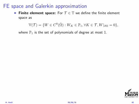
FE space and Galerkin approximationI Finite element space For T isin T we define the finite element
space as
V(T ) = W isin C0(Ω) WK isin P1forallK isin T W |partΩ = 0
where P1 is the set of polynomials of degree at most 1
I Galerkin approximation of continuous problem is given by
Find UT isin V(T )
intΩ
AnablaUT middot nablaV = 〈f V 〉 forallV isin V(T )
The discrete problem is well-posedI Nodal basis Consists of functions ψi isin V(T ) with xi isin N (T )
satisfyingψxi
(xj) = δij
where N (T ) denotes the interior (plus Neumann) nodesI Galerkin orthogonality(
nabla(uminus UT )nablaW)L2(Ω)
= 0 forallW isin V(T )
H Antil 060616 40
FE space and Galerkin approximationI Finite element space For T isin T we define the finite element
space as
V(T ) = W isin C0(Ω) WK isin P1forallK isin T W |partΩ = 0
where P1 is the set of polynomials of degree at most 1I Galerkin approximation of continuous problem is given by
Find UT isin V(T )
intΩ
AnablaUT middot nablaV = 〈f V 〉 forallV isin V(T )
The discrete problem is well-posed
I Nodal basis Consists of functions ψi isin V(T ) with xi isin N (T )satisfying
ψxi(xj) = δij
where N (T ) denotes the interior (plus Neumann) nodesI Galerkin orthogonality(
nabla(uminus UT )nablaW)L2(Ω)
= 0 forallW isin V(T )
H Antil 060616 40
FE space and Galerkin approximationI Finite element space For T isin T we define the finite element
space as
V(T ) = W isin C0(Ω) WK isin P1forallK isin T W |partΩ = 0
where P1 is the set of polynomials of degree at most 1I Galerkin approximation of continuous problem is given by
Find UT isin V(T )
intΩ
AnablaUT middot nablaV = 〈f V 〉 forallV isin V(T )
The discrete problem is well-posedI Nodal basis Consists of functions ψi isin V(T ) with xi isin N (T )
satisfyingψxi
(xj) = δij
where N (T ) denotes the interior (plus Neumann) nodes
I Galerkin orthogonality(nabla(uminus UT )nablaW
)L2(Ω)
= 0 forallW isin V(T )
H Antil 060616 40
FE space and Galerkin approximationI Finite element space For T isin T we define the finite element
space as
V(T ) = W isin C0(Ω) WK isin P1forallK isin T W |partΩ = 0
where P1 is the set of polynomials of degree at most 1I Galerkin approximation of continuous problem is given by
Find UT isin V(T )
intΩ
AnablaUT middot nablaV = 〈f V 〉 forallV isin V(T )
The discrete problem is well-posedI Nodal basis Consists of functions ψi isin V(T ) with xi isin N (T )
satisfyingψxi
(xj) = δij
where N (T ) denotes the interior (plus Neumann) nodesI Galerkin orthogonality(
nabla(uminus UT )nablaW)L2(Ω)
= 0 forallW isin V(T )
H Antil 060616 40
Best approximation
I Cearsquos lemma
nabla(uminus UT )L2(Ω) le C infWisinV(T )
nabla(uminusW )L2(Ω)
I Nodal interpolation operator ΠT C(Ω)rarr V(T ) satisfies
ΠT u(xi) = u(xi) forallxi isin N (T )
and is defined as
ΠT u =sum
xiisinN (T )
u(xi)ψxi
I Error estimates In Cearsquos lemma replace W by ΠT u and thencompute the interpolation error
H Antil 060616 41
Best approximation
I Cearsquos lemma
nabla(uminus UT )L2(Ω) le C infWisinV(T )
nabla(uminusW )L2(Ω)
I Nodal interpolation operator ΠT C(Ω)rarr V(T ) satisfies
ΠT u(xi) = u(xi) forallxi isin N (T )
and is defined as
ΠT u =sum
xiisinN (T )
u(xi)ψxi
I Error estimates In Cearsquos lemma replace W by ΠT u and thencompute the interpolation error
H Antil 060616 41
Best approximation
I Cearsquos lemma
nabla(uminus UT )L2(Ω) le C infWisinV(T )
nabla(uminusW )L2(Ω)
I Nodal interpolation operator ΠT C(Ω)rarr V(T ) satisfies
ΠT u(xi) = u(xi) forallxi isin N (T )
and is defined as
ΠT u =sum
xiisinN (T )
u(xi)ψxi
I Error estimates In Cearsquos lemma replace W by ΠT u and thencompute the interpolation error
H Antil 060616 41
Algebraic system state equation
I Recall UT isin V(T ) solves
a(UT V ) = 〈f V 〉 forallV isin V(T )
I Now setting UT =sumN
j=1 Ujψj V = ψi we get
Nsumj=1
Uja(φj φi) = 〈f ψi〉 i = 1 N
which is the matrix-vector system
AU = F
I Stiffness matrix A is SPD
H Antil 060616 42
Algebraic system state equation
I Recall UT isin V(T ) solves
a(UT V ) = 〈f V 〉 forallV isin V(T )
I Now setting UT =sumN
j=1 Ujψj V = ψi we get
Nsumj=1
Uja(φj φi) = 〈f ψi〉 i = 1 N
which is the matrix-vector system
AU = F
I Stiffness matrix A is SPD
H Antil 060616 42
Algebraic system state equation
I Recall UT isin V(T ) solves
a(UT V ) = 〈f V 〉 forallV isin V(T )
I Now setting UT =sumN
j=1 Ujψj V = ψi we get
Nsumj=1
Uja(φj φi) = 〈f ψi〉 i = 1 N
which is the matrix-vector system
AU = F
I Stiffness matrix A is SPD
H Antil 060616 42
Discrete linear elliptic OCP
min JT (UT ZT ) =1
2UT minus ud2L2(Ω) +
λ
2ZT 2L2(Ω)
subject to
Find UT isin V(T )
intΩ
nablaUT middot nablaV = (ZT V )L2(Ω) forallV isin V(T )
and whereZT isin Zad(T ) = Zad cap Z(T )
is either one of these
Z(T ) =
V(T )L2(Ω) variational discretization (Hinze)WT isin Linfin(Ω) ZT |K isin P0(K)K isin T
H Antil 060616 43
Recent books
F TroltzschOptimal control of partial differential equations volume 112 ofGraduate Studies in MathematicsAmerican Mathematical Society Providence RI 2010Theory methods and applications Translated from the 2005 Germanoriginal by Jurgen Sprekels
K Ito and K KunischLagrange multiplier approach to variational problems andapplications volume 15 of Advances in Design and ControlSociety for Industrial and Applied Mathematics (SIAM)Philadelphia PA 2008
H Antil 060616 44
- Motivation and examples
- Linear elliptic optimal control problems
- Differentiation in Banach spaces
- First-order necessary conditions
- Optimal control of semilinear PDEs
- An abstract problem
- Discretization using finite element methods
-
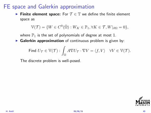
FE space and Galerkin approximationI Finite element space For T isin T we define the finite element
space as
V(T ) = W isin C0(Ω) WK isin P1forallK isin T W |partΩ = 0
where P1 is the set of polynomials of degree at most 1I Galerkin approximation of continuous problem is given by
Find UT isin V(T )
intΩ
AnablaUT middot nablaV = 〈f V 〉 forallV isin V(T )
The discrete problem is well-posed
I Nodal basis Consists of functions ψi isin V(T ) with xi isin N (T )satisfying
ψxi(xj) = δij
where N (T ) denotes the interior (plus Neumann) nodesI Galerkin orthogonality(
nabla(uminus UT )nablaW)L2(Ω)
= 0 forallW isin V(T )
H Antil 060616 40
FE space and Galerkin approximationI Finite element space For T isin T we define the finite element
space as
V(T ) = W isin C0(Ω) WK isin P1forallK isin T W |partΩ = 0
where P1 is the set of polynomials of degree at most 1I Galerkin approximation of continuous problem is given by
Find UT isin V(T )
intΩ
AnablaUT middot nablaV = 〈f V 〉 forallV isin V(T )
The discrete problem is well-posedI Nodal basis Consists of functions ψi isin V(T ) with xi isin N (T )
satisfyingψxi
(xj) = δij
where N (T ) denotes the interior (plus Neumann) nodes
I Galerkin orthogonality(nabla(uminus UT )nablaW
)L2(Ω)
= 0 forallW isin V(T )
H Antil 060616 40
FE space and Galerkin approximationI Finite element space For T isin T we define the finite element
space as
V(T ) = W isin C0(Ω) WK isin P1forallK isin T W |partΩ = 0
where P1 is the set of polynomials of degree at most 1I Galerkin approximation of continuous problem is given by
Find UT isin V(T )
intΩ
AnablaUT middot nablaV = 〈f V 〉 forallV isin V(T )
The discrete problem is well-posedI Nodal basis Consists of functions ψi isin V(T ) with xi isin N (T )
satisfyingψxi
(xj) = δij
where N (T ) denotes the interior (plus Neumann) nodesI Galerkin orthogonality(
nabla(uminus UT )nablaW)L2(Ω)
= 0 forallW isin V(T )
H Antil 060616 40
Best approximation
I Cearsquos lemma
nabla(uminus UT )L2(Ω) le C infWisinV(T )
nabla(uminusW )L2(Ω)
I Nodal interpolation operator ΠT C(Ω)rarr V(T ) satisfies
ΠT u(xi) = u(xi) forallxi isin N (T )
and is defined as
ΠT u =sum
xiisinN (T )
u(xi)ψxi
I Error estimates In Cearsquos lemma replace W by ΠT u and thencompute the interpolation error
H Antil 060616 41
Best approximation
I Cearsquos lemma
nabla(uminus UT )L2(Ω) le C infWisinV(T )
nabla(uminusW )L2(Ω)
I Nodal interpolation operator ΠT C(Ω)rarr V(T ) satisfies
ΠT u(xi) = u(xi) forallxi isin N (T )
and is defined as
ΠT u =sum
xiisinN (T )
u(xi)ψxi
I Error estimates In Cearsquos lemma replace W by ΠT u and thencompute the interpolation error
H Antil 060616 41
Best approximation
I Cearsquos lemma
nabla(uminus UT )L2(Ω) le C infWisinV(T )
nabla(uminusW )L2(Ω)
I Nodal interpolation operator ΠT C(Ω)rarr V(T ) satisfies
ΠT u(xi) = u(xi) forallxi isin N (T )
and is defined as
ΠT u =sum
xiisinN (T )
u(xi)ψxi
I Error estimates In Cearsquos lemma replace W by ΠT u and thencompute the interpolation error
H Antil 060616 41
Algebraic system state equation
I Recall UT isin V(T ) solves
a(UT V ) = 〈f V 〉 forallV isin V(T )
I Now setting UT =sumN
j=1 Ujψj V = ψi we get
Nsumj=1
Uja(φj φi) = 〈f ψi〉 i = 1 N
which is the matrix-vector system
AU = F
I Stiffness matrix A is SPD
H Antil 060616 42
Algebraic system state equation
I Recall UT isin V(T ) solves
a(UT V ) = 〈f V 〉 forallV isin V(T )
I Now setting UT =sumN
j=1 Ujψj V = ψi we get
Nsumj=1
Uja(φj φi) = 〈f ψi〉 i = 1 N
which is the matrix-vector system
AU = F
I Stiffness matrix A is SPD
H Antil 060616 42
Algebraic system state equation
I Recall UT isin V(T ) solves
a(UT V ) = 〈f V 〉 forallV isin V(T )
I Now setting UT =sumN
j=1 Ujψj V = ψi we get
Nsumj=1
Uja(φj φi) = 〈f ψi〉 i = 1 N
which is the matrix-vector system
AU = F
I Stiffness matrix A is SPD
H Antil 060616 42
Discrete linear elliptic OCP
min JT (UT ZT ) =1
2UT minus ud2L2(Ω) +
λ
2ZT 2L2(Ω)
subject to
Find UT isin V(T )
intΩ
nablaUT middot nablaV = (ZT V )L2(Ω) forallV isin V(T )
and whereZT isin Zad(T ) = Zad cap Z(T )
is either one of these
Z(T ) =
V(T )L2(Ω) variational discretization (Hinze)WT isin Linfin(Ω) ZT |K isin P0(K)K isin T
H Antil 060616 43
Recent books
F TroltzschOptimal control of partial differential equations volume 112 ofGraduate Studies in MathematicsAmerican Mathematical Society Providence RI 2010Theory methods and applications Translated from the 2005 Germanoriginal by Jurgen Sprekels
K Ito and K KunischLagrange multiplier approach to variational problems andapplications volume 15 of Advances in Design and ControlSociety for Industrial and Applied Mathematics (SIAM)Philadelphia PA 2008
H Antil 060616 44
- Motivation and examples
- Linear elliptic optimal control problems
- Differentiation in Banach spaces
- First-order necessary conditions
- Optimal control of semilinear PDEs
- An abstract problem
- Discretization using finite element methods
-
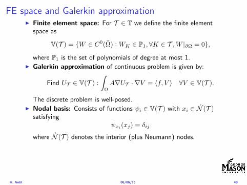
FE space and Galerkin approximationI Finite element space For T isin T we define the finite element
space as
V(T ) = W isin C0(Ω) WK isin P1forallK isin T W |partΩ = 0
where P1 is the set of polynomials of degree at most 1I Galerkin approximation of continuous problem is given by
Find UT isin V(T )
intΩ
AnablaUT middot nablaV = 〈f V 〉 forallV isin V(T )
The discrete problem is well-posedI Nodal basis Consists of functions ψi isin V(T ) with xi isin N (T )
satisfyingψxi
(xj) = δij
where N (T ) denotes the interior (plus Neumann) nodes
I Galerkin orthogonality(nabla(uminus UT )nablaW
)L2(Ω)
= 0 forallW isin V(T )
H Antil 060616 40
FE space and Galerkin approximationI Finite element space For T isin T we define the finite element
space as
V(T ) = W isin C0(Ω) WK isin P1forallK isin T W |partΩ = 0
where P1 is the set of polynomials of degree at most 1I Galerkin approximation of continuous problem is given by
Find UT isin V(T )
intΩ
AnablaUT middot nablaV = 〈f V 〉 forallV isin V(T )
The discrete problem is well-posedI Nodal basis Consists of functions ψi isin V(T ) with xi isin N (T )
satisfyingψxi
(xj) = δij
where N (T ) denotes the interior (plus Neumann) nodesI Galerkin orthogonality(
nabla(uminus UT )nablaW)L2(Ω)
= 0 forallW isin V(T )
H Antil 060616 40
Best approximation
I Cearsquos lemma
nabla(uminus UT )L2(Ω) le C infWisinV(T )
nabla(uminusW )L2(Ω)
I Nodal interpolation operator ΠT C(Ω)rarr V(T ) satisfies
ΠT u(xi) = u(xi) forallxi isin N (T )
and is defined as
ΠT u =sum
xiisinN (T )
u(xi)ψxi
I Error estimates In Cearsquos lemma replace W by ΠT u and thencompute the interpolation error
H Antil 060616 41
Best approximation
I Cearsquos lemma
nabla(uminus UT )L2(Ω) le C infWisinV(T )
nabla(uminusW )L2(Ω)
I Nodal interpolation operator ΠT C(Ω)rarr V(T ) satisfies
ΠT u(xi) = u(xi) forallxi isin N (T )
and is defined as
ΠT u =sum
xiisinN (T )
u(xi)ψxi
I Error estimates In Cearsquos lemma replace W by ΠT u and thencompute the interpolation error
H Antil 060616 41
Best approximation
I Cearsquos lemma
nabla(uminus UT )L2(Ω) le C infWisinV(T )
nabla(uminusW )L2(Ω)
I Nodal interpolation operator ΠT C(Ω)rarr V(T ) satisfies
ΠT u(xi) = u(xi) forallxi isin N (T )
and is defined as
ΠT u =sum
xiisinN (T )
u(xi)ψxi
I Error estimates In Cearsquos lemma replace W by ΠT u and thencompute the interpolation error
H Antil 060616 41
Algebraic system state equation
I Recall UT isin V(T ) solves
a(UT V ) = 〈f V 〉 forallV isin V(T )
I Now setting UT =sumN
j=1 Ujψj V = ψi we get
Nsumj=1
Uja(φj φi) = 〈f ψi〉 i = 1 N
which is the matrix-vector system
AU = F
I Stiffness matrix A is SPD
H Antil 060616 42
Algebraic system state equation
I Recall UT isin V(T ) solves
a(UT V ) = 〈f V 〉 forallV isin V(T )
I Now setting UT =sumN
j=1 Ujψj V = ψi we get
Nsumj=1
Uja(φj φi) = 〈f ψi〉 i = 1 N
which is the matrix-vector system
AU = F
I Stiffness matrix A is SPD
H Antil 060616 42
Algebraic system state equation
I Recall UT isin V(T ) solves
a(UT V ) = 〈f V 〉 forallV isin V(T )
I Now setting UT =sumN
j=1 Ujψj V = ψi we get
Nsumj=1
Uja(φj φi) = 〈f ψi〉 i = 1 N
which is the matrix-vector system
AU = F
I Stiffness matrix A is SPD
H Antil 060616 42
Discrete linear elliptic OCP
min JT (UT ZT ) =1
2UT minus ud2L2(Ω) +
λ
2ZT 2L2(Ω)
subject to
Find UT isin V(T )
intΩ
nablaUT middot nablaV = (ZT V )L2(Ω) forallV isin V(T )
and whereZT isin Zad(T ) = Zad cap Z(T )
is either one of these
Z(T ) =
V(T )L2(Ω) variational discretization (Hinze)WT isin Linfin(Ω) ZT |K isin P0(K)K isin T
H Antil 060616 43
Recent books
F TroltzschOptimal control of partial differential equations volume 112 ofGraduate Studies in MathematicsAmerican Mathematical Society Providence RI 2010Theory methods and applications Translated from the 2005 Germanoriginal by Jurgen Sprekels
K Ito and K KunischLagrange multiplier approach to variational problems andapplications volume 15 of Advances in Design and ControlSociety for Industrial and Applied Mathematics (SIAM)Philadelphia PA 2008
H Antil 060616 44
- Motivation and examples
- Linear elliptic optimal control problems
- Differentiation in Banach spaces
- First-order necessary conditions
- Optimal control of semilinear PDEs
- An abstract problem
- Discretization using finite element methods
-
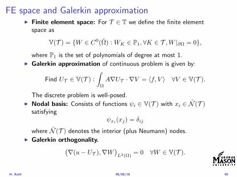
FE space and Galerkin approximationI Finite element space For T isin T we define the finite element
space as
V(T ) = W isin C0(Ω) WK isin P1forallK isin T W |partΩ = 0
where P1 is the set of polynomials of degree at most 1I Galerkin approximation of continuous problem is given by
Find UT isin V(T )
intΩ
AnablaUT middot nablaV = 〈f V 〉 forallV isin V(T )
The discrete problem is well-posedI Nodal basis Consists of functions ψi isin V(T ) with xi isin N (T )
satisfyingψxi
(xj) = δij
where N (T ) denotes the interior (plus Neumann) nodesI Galerkin orthogonality(
nabla(uminus UT )nablaW)L2(Ω)
= 0 forallW isin V(T )
H Antil 060616 40
Best approximation
I Cearsquos lemma
nabla(uminus UT )L2(Ω) le C infWisinV(T )
nabla(uminusW )L2(Ω)
I Nodal interpolation operator ΠT C(Ω)rarr V(T ) satisfies
ΠT u(xi) = u(xi) forallxi isin N (T )
and is defined as
ΠT u =sum
xiisinN (T )
u(xi)ψxi
I Error estimates In Cearsquos lemma replace W by ΠT u and thencompute the interpolation error
H Antil 060616 41
Best approximation
I Cearsquos lemma
nabla(uminus UT )L2(Ω) le C infWisinV(T )
nabla(uminusW )L2(Ω)
I Nodal interpolation operator ΠT C(Ω)rarr V(T ) satisfies
ΠT u(xi) = u(xi) forallxi isin N (T )
and is defined as
ΠT u =sum
xiisinN (T )
u(xi)ψxi
I Error estimates In Cearsquos lemma replace W by ΠT u and thencompute the interpolation error
H Antil 060616 41
Best approximation
I Cearsquos lemma
nabla(uminus UT )L2(Ω) le C infWisinV(T )
nabla(uminusW )L2(Ω)
I Nodal interpolation operator ΠT C(Ω)rarr V(T ) satisfies
ΠT u(xi) = u(xi) forallxi isin N (T )
and is defined as
ΠT u =sum
xiisinN (T )
u(xi)ψxi
I Error estimates In Cearsquos lemma replace W by ΠT u and thencompute the interpolation error
H Antil 060616 41
Algebraic system state equation
I Recall UT isin V(T ) solves
a(UT V ) = 〈f V 〉 forallV isin V(T )
I Now setting UT =sumN
j=1 Ujψj V = ψi we get
Nsumj=1
Uja(φj φi) = 〈f ψi〉 i = 1 N
which is the matrix-vector system
AU = F
I Stiffness matrix A is SPD
H Antil 060616 42
Algebraic system state equation
I Recall UT isin V(T ) solves
a(UT V ) = 〈f V 〉 forallV isin V(T )
I Now setting UT =sumN
j=1 Ujψj V = ψi we get
Nsumj=1
Uja(φj φi) = 〈f ψi〉 i = 1 N
which is the matrix-vector system
AU = F
I Stiffness matrix A is SPD
H Antil 060616 42
Algebraic system state equation
I Recall UT isin V(T ) solves
a(UT V ) = 〈f V 〉 forallV isin V(T )
I Now setting UT =sumN
j=1 Ujψj V = ψi we get
Nsumj=1
Uja(φj φi) = 〈f ψi〉 i = 1 N
which is the matrix-vector system
AU = F
I Stiffness matrix A is SPD
H Antil 060616 42
Discrete linear elliptic OCP
min JT (UT ZT ) =1
2UT minus ud2L2(Ω) +
λ
2ZT 2L2(Ω)
subject to
Find UT isin V(T )
intΩ
nablaUT middot nablaV = (ZT V )L2(Ω) forallV isin V(T )
and whereZT isin Zad(T ) = Zad cap Z(T )
is either one of these
Z(T ) =
V(T )L2(Ω) variational discretization (Hinze)WT isin Linfin(Ω) ZT |K isin P0(K)K isin T
H Antil 060616 43
Recent books
F TroltzschOptimal control of partial differential equations volume 112 ofGraduate Studies in MathematicsAmerican Mathematical Society Providence RI 2010Theory methods and applications Translated from the 2005 Germanoriginal by Jurgen Sprekels
K Ito and K KunischLagrange multiplier approach to variational problems andapplications volume 15 of Advances in Design and ControlSociety for Industrial and Applied Mathematics (SIAM)Philadelphia PA 2008
H Antil 060616 44
- Motivation and examples
- Linear elliptic optimal control problems
- Differentiation in Banach spaces
- First-order necessary conditions
- Optimal control of semilinear PDEs
- An abstract problem
- Discretization using finite element methods
-
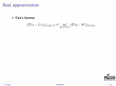
Best approximation
I Cearsquos lemma
nabla(uminus UT )L2(Ω) le C infWisinV(T )
nabla(uminusW )L2(Ω)
I Nodal interpolation operator ΠT C(Ω)rarr V(T ) satisfies
ΠT u(xi) = u(xi) forallxi isin N (T )
and is defined as
ΠT u =sum
xiisinN (T )
u(xi)ψxi
I Error estimates In Cearsquos lemma replace W by ΠT u and thencompute the interpolation error
H Antil 060616 41
Algebraic system state equation
I Recall UT isin V(T ) solves
a(UT V ) = 〈f V 〉 forallV isin V(T )
I Now setting UT =sumN
j=1 Ujψj V = ψi we get
Nsumj=1
Uja(φj φi) = 〈f ψi〉 i = 1 N
which is the matrix-vector system
AU = F
I Stiffness matrix A is SPD
H Antil 060616 42
Algebraic system state equation
I Recall UT isin V(T ) solves
a(UT V ) = 〈f V 〉 forallV isin V(T )
I Now setting UT =sumN
j=1 Ujψj V = ψi we get
Nsumj=1
Uja(φj φi) = 〈f ψi〉 i = 1 N
which is the matrix-vector system
AU = F
I Stiffness matrix A is SPD
H Antil 060616 42
Algebraic system state equation
I Recall UT isin V(T ) solves
a(UT V ) = 〈f V 〉 forallV isin V(T )
I Now setting UT =sumN
j=1 Ujψj V = ψi we get
Nsumj=1
Uja(φj φi) = 〈f ψi〉 i = 1 N
which is the matrix-vector system
AU = F
I Stiffness matrix A is SPD
H Antil 060616 42
Discrete linear elliptic OCP
min JT (UT ZT ) =1
2UT minus ud2L2(Ω) +
λ
2ZT 2L2(Ω)
subject to
Find UT isin V(T )
intΩ
nablaUT middot nablaV = (ZT V )L2(Ω) forallV isin V(T )
and whereZT isin Zad(T ) = Zad cap Z(T )
is either one of these
Z(T ) =
V(T )L2(Ω) variational discretization (Hinze)WT isin Linfin(Ω) ZT |K isin P0(K)K isin T
H Antil 060616 43
Recent books
F TroltzschOptimal control of partial differential equations volume 112 ofGraduate Studies in MathematicsAmerican Mathematical Society Providence RI 2010Theory methods and applications Translated from the 2005 Germanoriginal by Jurgen Sprekels
K Ito and K KunischLagrange multiplier approach to variational problems andapplications volume 15 of Advances in Design and ControlSociety for Industrial and Applied Mathematics (SIAM)Philadelphia PA 2008
H Antil 060616 44
- Motivation and examples
- Linear elliptic optimal control problems
- Differentiation in Banach spaces
- First-order necessary conditions
- Optimal control of semilinear PDEs
- An abstract problem
- Discretization using finite element methods
-
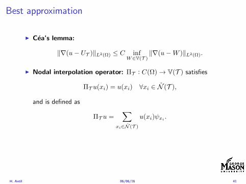
Best approximation
I Cearsquos lemma
nabla(uminus UT )L2(Ω) le C infWisinV(T )
nabla(uminusW )L2(Ω)
I Nodal interpolation operator ΠT C(Ω)rarr V(T ) satisfies
ΠT u(xi) = u(xi) forallxi isin N (T )
and is defined as
ΠT u =sum
xiisinN (T )
u(xi)ψxi
I Error estimates In Cearsquos lemma replace W by ΠT u and thencompute the interpolation error
H Antil 060616 41
Best approximation
I Cearsquos lemma
nabla(uminus UT )L2(Ω) le C infWisinV(T )
nabla(uminusW )L2(Ω)
I Nodal interpolation operator ΠT C(Ω)rarr V(T ) satisfies
ΠT u(xi) = u(xi) forallxi isin N (T )
and is defined as
ΠT u =sum
xiisinN (T )
u(xi)ψxi
I Error estimates In Cearsquos lemma replace W by ΠT u and thencompute the interpolation error
H Antil 060616 41
Algebraic system state equation
I Recall UT isin V(T ) solves
a(UT V ) = 〈f V 〉 forallV isin V(T )
I Now setting UT =sumN
j=1 Ujψj V = ψi we get
Nsumj=1
Uja(φj φi) = 〈f ψi〉 i = 1 N
which is the matrix-vector system
AU = F
I Stiffness matrix A is SPD
H Antil 060616 42
Algebraic system state equation
I Recall UT isin V(T ) solves
a(UT V ) = 〈f V 〉 forallV isin V(T )
I Now setting UT =sumN
j=1 Ujψj V = ψi we get
Nsumj=1
Uja(φj φi) = 〈f ψi〉 i = 1 N
which is the matrix-vector system
AU = F
I Stiffness matrix A is SPD
H Antil 060616 42
Algebraic system state equation
I Recall UT isin V(T ) solves
a(UT V ) = 〈f V 〉 forallV isin V(T )
I Now setting UT =sumN
j=1 Ujψj V = ψi we get
Nsumj=1
Uja(φj φi) = 〈f ψi〉 i = 1 N
which is the matrix-vector system
AU = F
I Stiffness matrix A is SPD
H Antil 060616 42
Discrete linear elliptic OCP
min JT (UT ZT ) =1
2UT minus ud2L2(Ω) +
λ
2ZT 2L2(Ω)
subject to
Find UT isin V(T )
intΩ
nablaUT middot nablaV = (ZT V )L2(Ω) forallV isin V(T )
and whereZT isin Zad(T ) = Zad cap Z(T )
is either one of these
Z(T ) =
V(T )L2(Ω) variational discretization (Hinze)WT isin Linfin(Ω) ZT |K isin P0(K)K isin T
H Antil 060616 43
Recent books
F TroltzschOptimal control of partial differential equations volume 112 ofGraduate Studies in MathematicsAmerican Mathematical Society Providence RI 2010Theory methods and applications Translated from the 2005 Germanoriginal by Jurgen Sprekels
K Ito and K KunischLagrange multiplier approach to variational problems andapplications volume 15 of Advances in Design and ControlSociety for Industrial and Applied Mathematics (SIAM)Philadelphia PA 2008
H Antil 060616 44
- Motivation and examples
- Linear elliptic optimal control problems
- Differentiation in Banach spaces
- First-order necessary conditions
- Optimal control of semilinear PDEs
- An abstract problem
- Discretization using finite element methods
-
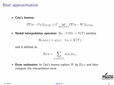
Best approximation
I Cearsquos lemma
nabla(uminus UT )L2(Ω) le C infWisinV(T )
nabla(uminusW )L2(Ω)
I Nodal interpolation operator ΠT C(Ω)rarr V(T ) satisfies
ΠT u(xi) = u(xi) forallxi isin N (T )
and is defined as
ΠT u =sum
xiisinN (T )
u(xi)ψxi
I Error estimates In Cearsquos lemma replace W by ΠT u and thencompute the interpolation error
H Antil 060616 41
Algebraic system state equation
I Recall UT isin V(T ) solves
a(UT V ) = 〈f V 〉 forallV isin V(T )
I Now setting UT =sumN
j=1 Ujψj V = ψi we get
Nsumj=1
Uja(φj φi) = 〈f ψi〉 i = 1 N
which is the matrix-vector system
AU = F
I Stiffness matrix A is SPD
H Antil 060616 42
Algebraic system state equation
I Recall UT isin V(T ) solves
a(UT V ) = 〈f V 〉 forallV isin V(T )
I Now setting UT =sumN
j=1 Ujψj V = ψi we get
Nsumj=1
Uja(φj φi) = 〈f ψi〉 i = 1 N
which is the matrix-vector system
AU = F
I Stiffness matrix A is SPD
H Antil 060616 42
Algebraic system state equation
I Recall UT isin V(T ) solves
a(UT V ) = 〈f V 〉 forallV isin V(T )
I Now setting UT =sumN
j=1 Ujψj V = ψi we get
Nsumj=1
Uja(φj φi) = 〈f ψi〉 i = 1 N
which is the matrix-vector system
AU = F
I Stiffness matrix A is SPD
H Antil 060616 42
Discrete linear elliptic OCP
min JT (UT ZT ) =1
2UT minus ud2L2(Ω) +
λ
2ZT 2L2(Ω)
subject to
Find UT isin V(T )
intΩ
nablaUT middot nablaV = (ZT V )L2(Ω) forallV isin V(T )
and whereZT isin Zad(T ) = Zad cap Z(T )
is either one of these
Z(T ) =
V(T )L2(Ω) variational discretization (Hinze)WT isin Linfin(Ω) ZT |K isin P0(K)K isin T
H Antil 060616 43
Recent books
F TroltzschOptimal control of partial differential equations volume 112 ofGraduate Studies in MathematicsAmerican Mathematical Society Providence RI 2010Theory methods and applications Translated from the 2005 Germanoriginal by Jurgen Sprekels
K Ito and K KunischLagrange multiplier approach to variational problems andapplications volume 15 of Advances in Design and ControlSociety for Industrial and Applied Mathematics (SIAM)Philadelphia PA 2008
H Antil 060616 44
- Motivation and examples
- Linear elliptic optimal control problems
- Differentiation in Banach spaces
- First-order necessary conditions
- Optimal control of semilinear PDEs
- An abstract problem
- Discretization using finite element methods
-
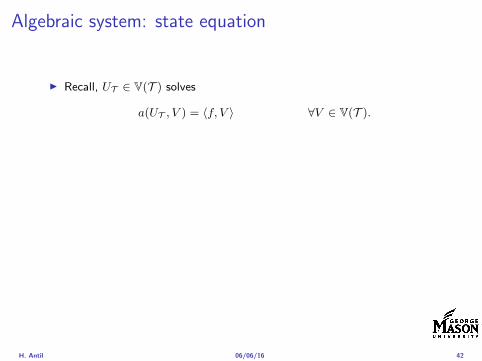
Algebraic system state equation
I Recall UT isin V(T ) solves
a(UT V ) = 〈f V 〉 forallV isin V(T )
I Now setting UT =sumN
j=1 Ujψj V = ψi we get
Nsumj=1
Uja(φj φi) = 〈f ψi〉 i = 1 N
which is the matrix-vector system
AU = F
I Stiffness matrix A is SPD
H Antil 060616 42
Algebraic system state equation
I Recall UT isin V(T ) solves
a(UT V ) = 〈f V 〉 forallV isin V(T )
I Now setting UT =sumN
j=1 Ujψj V = ψi we get
Nsumj=1
Uja(φj φi) = 〈f ψi〉 i = 1 N
which is the matrix-vector system
AU = F
I Stiffness matrix A is SPD
H Antil 060616 42
Algebraic system state equation
I Recall UT isin V(T ) solves
a(UT V ) = 〈f V 〉 forallV isin V(T )
I Now setting UT =sumN
j=1 Ujψj V = ψi we get
Nsumj=1
Uja(φj φi) = 〈f ψi〉 i = 1 N
which is the matrix-vector system
AU = F
I Stiffness matrix A is SPD
H Antil 060616 42
Discrete linear elliptic OCP
min JT (UT ZT ) =1
2UT minus ud2L2(Ω) +
λ
2ZT 2L2(Ω)
subject to
Find UT isin V(T )
intΩ
nablaUT middot nablaV = (ZT V )L2(Ω) forallV isin V(T )
and whereZT isin Zad(T ) = Zad cap Z(T )
is either one of these
Z(T ) =
V(T )L2(Ω) variational discretization (Hinze)WT isin Linfin(Ω) ZT |K isin P0(K)K isin T
H Antil 060616 43
Recent books
F TroltzschOptimal control of partial differential equations volume 112 ofGraduate Studies in MathematicsAmerican Mathematical Society Providence RI 2010Theory methods and applications Translated from the 2005 Germanoriginal by Jurgen Sprekels
K Ito and K KunischLagrange multiplier approach to variational problems andapplications volume 15 of Advances in Design and ControlSociety for Industrial and Applied Mathematics (SIAM)Philadelphia PA 2008
H Antil 060616 44
- Motivation and examples
- Linear elliptic optimal control problems
- Differentiation in Banach spaces
- First-order necessary conditions
- Optimal control of semilinear PDEs
- An abstract problem
- Discretization using finite element methods
-
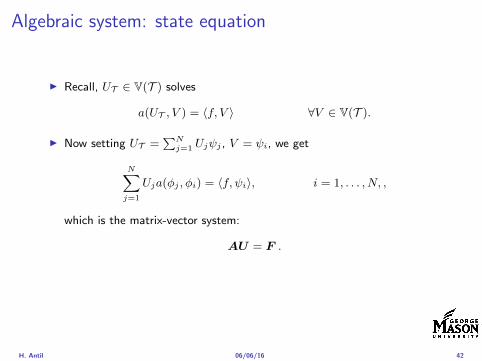
Algebraic system state equation
I Recall UT isin V(T ) solves
a(UT V ) = 〈f V 〉 forallV isin V(T )
I Now setting UT =sumN
j=1 Ujψj V = ψi we get
Nsumj=1
Uja(φj φi) = 〈f ψi〉 i = 1 N
which is the matrix-vector system
AU = F
I Stiffness matrix A is SPD
H Antil 060616 42
Algebraic system state equation
I Recall UT isin V(T ) solves
a(UT V ) = 〈f V 〉 forallV isin V(T )
I Now setting UT =sumN
j=1 Ujψj V = ψi we get
Nsumj=1
Uja(φj φi) = 〈f ψi〉 i = 1 N
which is the matrix-vector system
AU = F
I Stiffness matrix A is SPD
H Antil 060616 42
Discrete linear elliptic OCP
min JT (UT ZT ) =1
2UT minus ud2L2(Ω) +
λ
2ZT 2L2(Ω)
subject to
Find UT isin V(T )
intΩ
nablaUT middot nablaV = (ZT V )L2(Ω) forallV isin V(T )
and whereZT isin Zad(T ) = Zad cap Z(T )
is either one of these
Z(T ) =
V(T )L2(Ω) variational discretization (Hinze)WT isin Linfin(Ω) ZT |K isin P0(K)K isin T
H Antil 060616 43
Recent books
F TroltzschOptimal control of partial differential equations volume 112 ofGraduate Studies in MathematicsAmerican Mathematical Society Providence RI 2010Theory methods and applications Translated from the 2005 Germanoriginal by Jurgen Sprekels
K Ito and K KunischLagrange multiplier approach to variational problems andapplications volume 15 of Advances in Design and ControlSociety for Industrial and Applied Mathematics (SIAM)Philadelphia PA 2008
H Antil 060616 44
- Motivation and examples
- Linear elliptic optimal control problems
- Differentiation in Banach spaces
- First-order necessary conditions
- Optimal control of semilinear PDEs
- An abstract problem
- Discretization using finite element methods
-
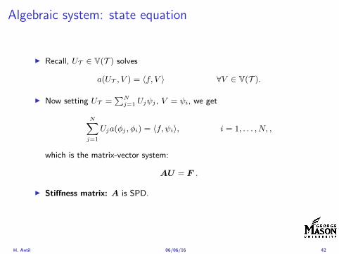
Algebraic system state equation
I Recall UT isin V(T ) solves
a(UT V ) = 〈f V 〉 forallV isin V(T )
I Now setting UT =sumN
j=1 Ujψj V = ψi we get
Nsumj=1
Uja(φj φi) = 〈f ψi〉 i = 1 N
which is the matrix-vector system
AU = F
I Stiffness matrix A is SPD
H Antil 060616 42
Discrete linear elliptic OCP
min JT (UT ZT ) =1
2UT minus ud2L2(Ω) +
λ
2ZT 2L2(Ω)
subject to
Find UT isin V(T )
intΩ
nablaUT middot nablaV = (ZT V )L2(Ω) forallV isin V(T )
and whereZT isin Zad(T ) = Zad cap Z(T )
is either one of these
Z(T ) =
V(T )L2(Ω) variational discretization (Hinze)WT isin Linfin(Ω) ZT |K isin P0(K)K isin T
H Antil 060616 43
Recent books
F TroltzschOptimal control of partial differential equations volume 112 ofGraduate Studies in MathematicsAmerican Mathematical Society Providence RI 2010Theory methods and applications Translated from the 2005 Germanoriginal by Jurgen Sprekels
K Ito and K KunischLagrange multiplier approach to variational problems andapplications volume 15 of Advances in Design and ControlSociety for Industrial and Applied Mathematics (SIAM)Philadelphia PA 2008
H Antil 060616 44
- Motivation and examples
- Linear elliptic optimal control problems
- Differentiation in Banach spaces
- First-order necessary conditions
- Optimal control of semilinear PDEs
- An abstract problem
- Discretization using finite element methods
-
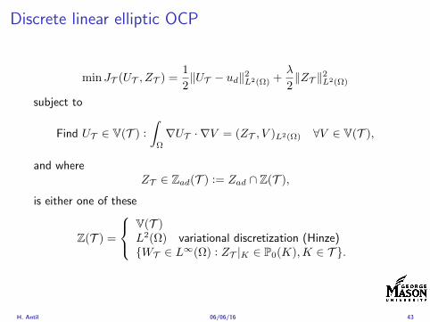