Parallel Algorithms forPDE-ConstrainedOptimization

Volkan Akcelik∗, George Biros†, Omar Ghattas‡, Judith Hill§,David Keyes¶, Bart van Bloemen Waanders‖

1 IntroductionPDE-constrained optimization refers to the optimization of systems governed by partialdifferential equations (PDEs). The simulation problem is to solve the PDEs for the statevariables (e.g. displacement, velocity, temperature, electric field, magnetic field, speciesconcentration), given appropriate data (e.g. geometry, coefficients, boundary conditions,initial conditions, source functions). The optimization problem seeks to determine someof these data—the decision variables—given performance goals in the form of an objec-tive function and possibly inequality or equality constraints on the behavior of the system.Since the behavior of the system is modeled by the PDEs, they appear as (usually equality)constraints in the optimization problem. We will refer to these PDE constraints as the stateequations.

Let u represent the state variables, d the decision variables, J the objective function,c the residual of the state equations, and h the residual of the inequality constraints. We

∗Ultrascale Simulation Laboratory, Department of Civil & Environmental Engineering, Carnegie Mellon Uni-versity, Pittsburgh, PA, USA (volkan@cs.cmu.edu)

†Departments of Mechanical Engineering & Applied Mechanics and Computer & Information Science, Uni-versity of Pennsylvania, Philadelphia, PA, USA (biros@seas.upenn.edu)

‡Institute for Computational Engineering & Sciences, Departments of Geological Sciences, Mechanical En-gineering, Computer Sciences, and Biomedical Engineering, and Institute for Geophysics, University of Texas atAustin, Austin, TX, USA (omar@ices.texas.edu)

§Optimization & Uncertainty Estimation Department, Sandia National Laboratories, Albuquerque, NM, USA(jhill@sandia.gov)

¶Department of Applied Physics & Applied Mathematics, Columbia University, New York, NY, USA(kd2112@columbia.edu)

‖Optimization & Uncertainty Estimation Department, Sandia National Laboratories, Albuquerque, NM, USA(bartv@cs.sandia.gov)

can then state the general form of a PDE-constrained optimization problem as:

minu,d

J (u,d)

subject to c(u,d) = 0 (1)

h(u,d) ≥ 0

The PDE-constrained optimization problem (1) can represent an optimal design, optimalcontrol, or inverse problem, depending on the nature of the objective function and decisionvariables. The decision variables correspondingly represent design, control, or inversionvariables.

Many engineering and science problems—in such diverse areas as aerodynamics,atmospheric sciences, chemical process industry, environment, geosciences, homeland se-curity, infrastructure, manufacturing, medicine, and physics—can be expressed in the formof a PDE-constrained optimization problem. The common difficulty is that PDE solutionis just a subproblem associated with optimization. Moreover, while the simulation prob-lem (given d, find u from c(u,d) = 0) is usually well-posed, the optimization problem(1) can be ill-posed. Finally, when the state equations are evolutionary in nature, the opti-mality conditions for (1) are a boundary value problem in space–time. For these reasons,the optimization problem is often significantly more difficult to solve than the simulationproblem.

The size, complexity, and infinite-dimensional nature of PDE-constrained optimiza-tion problems present significant challenges for general-purpose optimization algorithms.These features often require regularization, iterative solvers, preconditioning, globaliza-tion, inexactness, and parallel implementation that are tailored to the structure of the under-lying operators. Continued advances in PDE solvers, and the rapid ascendance of parallelcomputing, have in recent years motivated the development of special-purpose optimiza-tion algorithms that exploit the structure of the PDE constraints and scale to large numbersof processors. These algorithms are the focus of this chapter.

To illustrate the main issues, let us consider a distributed optimal flow control prob-lem for the steady-state Burgers equation:

minu,d

J (u, d) def=12

∫Ω

∇u · ∇u dx +ρ

2

∫Ω

d · d dx

subject to − ν∆u + (∇u)u = d in Ω (2)

u = g on ∂Ω

Here, u(x) is the velocity field, d(x) is a domain source, g(s) is a boundary source, ν isthe viscosity, Ω represents the domain and ∂Ω its boundary, and ρ is a parameter reflectingthe cost of the controls. In the simulation problem we are given the data ν, d, Ω, g and weseek the state u. In the optimization problem the situation is reversed: we wish to determinea portion of the data, for example g (boundary control), d (distributed control), Ω (shapeor topology optimization), or ν (parameter estimation), so that the decision variable andresulting state u minimize some functional of these variables. In the particular example(2), the decision variable is just the distributed source d, and ν, Ω, g are taken as knowns.The objectiveJ represents a balance between the rate of energy dissipation and the L 2 costof the controls.

A classical way to approach this problem is to introduce a Lagrange multiplier field,λ(x), known as the adjoint state or costate variable, and form a Lagrangian functional Lthat incorporates the PDE constraints via an “inner product” with λ,

L(u, λ, d) def= J (u, d) +∫

Ω

[ν∇u · ∇λ + λ · (∇u)u − d · λ] dx (3)

One then requires stationarity of L with respect to the state (u), decision (d), and adjoint(λ) variables. Taking variations and invoking the appropriate Green identities, we arriveat the following system of equations representing first-order necessary conditions for opti-mality:

−ν∆u + (∇u)u = d in Ω state equation (4)

u = g on ∂Ω

−ν∆λ + (∇u)T λ − (∇λ)u − λ div u = ∆u in Ω adjoint equation (5)

λ = 0 on ∂Ωρ d + λ = 0 in Ω decision equation (6)

The state equation (4) is just the original Burgers boundary value problem that appears asa constraint in the optimization problem (2). The adjoint equation (5), which results fromstationarity with respect to the state, is a boundary value problem that is linear in the ad-joint variable λ, and involves the adjoint of the linearized state operator. With appropriatediscretization, this adjoint operator is just the transpose of the Jacobian of the discretizedstate equation. Finally the decision equation (6) is in this case algebraic (it would havebeen differential had the cost of the controls been H 1 instead of L2). The first-order opti-mality conditions (4)–(6) are a system of coupled, nonlinear PDEs, and are often known asthe Karush-Kuhn-Tucker (KKT) conditions. For theory and analysis of PDE-constrainedoptimization problems such as (2), see for example [12], [32], [39], [66], [69]. For recentalgorithmic trends and large-scale applications, see [19].

In this chapter we review efficient parallel algorithms for solution of PDE optimal-ity systems such (4)–(6). Since the coupled optimality system can be formidable to solvesimultaneously, a popular alternative is to eliminate state and adjoint variables, and, corre-spondingly, state and adjoint equations, thereby reducing the system to a manageable onein just the decision variable. Methods of this type are known as reduced space methods.For example, a nonlinear elimination variant of a reduced space method would proceed asfollows for the KKT system (4)–(6). Given d at some iteration, solve the state equation(4) for the state variable u. Knowing the state then permits solution of the adjoint equa-tion (5) for the adjoint variable λ. Finally, with the state and adjoint known, the decisionvariable d is updated via an appropriate linearization of the decision equation. This loopis then repeated until convergence. As an alternative to such nonlinear elimination, oneoften prefers to follow the Newton strategy of first linearizing the optimality system, andthen eliminating the state and adjoint updates via block elimination on the linearized stateand adjoint equations. The resulting Schur complement operator is known as the reducedHessian, and the equation to which it corresponds can be solved to yield the decision vari-able update. Since the main components of reduced space method are (linearized) stateand adjoint PDE solves, as well as dense decision space solves, parallelism for this reduced

Newton solution of the optimization problem is typically as straightforward to achieve asit is for the simulation problem. Algorithms of this class will be reviewed in Section 2.1.

Reduced space methods are attractive for several reasons. Solving the subsets ofequations in sequence exploits the state/adjoint/decision structure of the optimality sys-tem, capitalizing on well-established methods and software for solving the state equation.Adjoint PDE solvers are becoming more popular, due to their role in goal-oriented errorestimation and efficient sensitivity computation, so they can be exploited as well. Even intheir absence, the strong similarities between the state and adjoint operators suggest that anexisting PDE solver for the state equation can be modified with reasonable effort to handlethe adjoint equation. Finally, exploiting the structure of the reduced Hessian is straight-forward (at least for problems of moderate size), since it is a Schur complement of thelinearized KKT conditions with respect to the decision variables and is therefore dense.

Another advantage of reduction is that the linearized KKT system is often very ill-conditioned (beyond, say, the usual h−2 ill-conditioning of second-order differential oper-ators); the state and adjoint blocks on the other hand inherit the conditioning properties ofthe simulation problem. Moreover, the reduced Hessian often has favorable spectral struc-ture (e.g. for many inverse problems its spectrum is similar to that of second kind integraloperators) and Krylov solvers can converge in a mesh-independent number of iterations.However, as is the case for most exact Schur-type approaches, the major disadvantage ofreduced methods is the need to solve the (linearized) state and adjoint equations exactlyat each reduced space iteration, which is a direct consequence of the reduction onto thedecision variable space.

In contrast to reduced space methods, full space methods solve for the state, decision,and adjoint variables simultaneously. For large-scale problems, this is typically effected viaNewton-Krylov iteration. That is, the linear system arising at each Newton iteration on theKKT system is solved using a Krylov iterative method. The difficulty of this approach isthe complex structure, indefiniteness, and ill-conditioning of the KKT system, which inturn requires effective preconditioning. Since the KKT optimality conditions are usuallyPDEs, it is natural to seek domain decomposition or multigrid preconditioners for this task.However, stationarity of the Lagrangian is a saddle-point problem, and existing domaindecomposition and multilevel preconditioners for the resulting indefinite systems are notas robust as those for definite systems. Furthermore, constructing the correct smoothing,prolongation, restriction, and interface operators can be quite challenging. Despite thesedifficulties, there have been several successful algorithms based on overlapping and non-overlapping domain decomposition and multigrid preconditioners; these are reviewed inSection 2.3. Since these methods regard the entire optimality system as a system of coupledPDEs, parallelism follows naturally, as it does for PDE problems, i.e. in a domain-basedway.

An alternative full-space approach to domain decomposition or multigrid is to retainthe structure-exploiting, condition-improving advantages of a reduced space method, butuse it as a preconditioner rather than a solver. That is, we solve in the full space using aNewton-Krylov method, but precondition with a reduced space method. Since the reducedspace method is just a preconditioner, it can be applied approximately, requiring just inexactstate and adjoint solves at each iteration. These inexact solves can simply be applicationsof appropriate domain decomposition or multigrid preconditioners for the state and adjointoperators. Depending on its spectral structure, one may also require preconditioners for

the reduced Hessian operator. Substantial speedups can be achieved over reduced spacemethods due to the avoidance of exact solution of the state and adjoint equations at eachdecision iteration, as the three sets of variables are simultaneously converged. Since themain work per iteration is in the application of preconditioners for the state, adjoint, anddecision equations, as well as carrying out PDE-like full space matrix-vector products,these reduced-space-preconditioned full-space methods can be made to parallelize as wellas reduced space methods, i.e. as well as the simulation problem. Such methods will bediscussed in Section 2.2.

Numerical evidence suggests that for steady-state PDE-constrained optimization prob-lems, full-space methods can outperform reduced space methods by a wide margin. Typicalmultigrid efficiency has been obtained for some classes of problems. For optimization ofsystems governed by time-dependent PDEs, the answer is not as clear. The nonlinearitieswithin each time step of a time-dependent PDE solve are usually much milder than forthe corresponding stationary PDEs, so amortizing the nonlinear PDE solve over the opti-mization iterations is less advantageous. Moreover, time dependence results in large stor-age requirements for full-space methods, since the full space optimality system becomesa boundary value problem in the space–time cylinder. For such problems, reduced spacemethods are often preferable. Section 3 provides illustrative examples of optimizationproblems governed by both steady-state and time-dependent PDEs. The governing equa-tions include convective-diffusive transport, Navier-Stokes flow, and acoustic wave propa-gation; the decision variables include those for control (for boundary sources), design-like(for PDE coefficients), and inversion (for initial conditions). Both reduced space and fullspace parallel KKT solvers are demonstrated and compared. Parallel implementation issuesare discussed in the context of the acoustic inversion problem.

Notation in this chapter respects the following conventions. Scalars are in lowercaseitalics type, vectors are in lowercase boldface Roman type, and matrices and tensors are inuppercase boldface Roman type. Infinite dimensional quantities are in italics type, whereasfinite dimensional quantities (usually discretizations) are upright. We will use d or d or dfor decision variables, u or u or u for the states, and λ or λ for adjoint variables.

2 AlgorithmsIn this section we discuss algorithmic issues related to efficient parallel solution of firstorder optimality systems by Newton-like methods. Due to space limitations, we omit dis-cussion of adaptivity and error estimation, regularization of ill-posed problems, inequalityconstraints on state and decision variables, globalization methods to ensure convergencefrom distant iterates, and checkpointing strategies for balancing work and memory in time-dependent adjoint computations. These issues must be carefully considered in order toobtain optimally scalable algorithms. The following are some representative references inthe infinite-dimensional setting; no attempt is made to be comprehensive. Globalizationin the context of PDE solvers is discussed in [63] and in the context of PDE optimizationin [51], [77]. For a discussion of active set and interior point methods for inequality con-straints in an optimal control setting, see [18], [76] and for primal-dual active set methodssee [52]. For adaptive methods and error estimation in inverse problems see [11], [16],[17], [73]; for details on regularization see [36], [45], [79]. See [37], [54] for discussions

of checkpointing strategies.Our discussion of parallel algorithms in this section will be in the context of the dis-

crete form of a typical PDE-constrained optimization problem; that is, we first discretizethe objective and constraints, and then form the Lagrangian function and derive optimal-ity conditions. Note that this is the reverse of the procedure that was employed in theoptimal flow control example in the previous section, in which the infinite-dimensional La-grangian functional was first formed and then infinite-dimensional optimality conditionswere written. When these infinite-dimensional conditions are discretized, they may resultin different discrete optimality conditions than those obtained by first discretizing and thendifferentiating to form optimality conditions. That is, differentiation and discretization donot necessarily commute. We refer the reader to [1], [31], [39], [53], [70] for details.

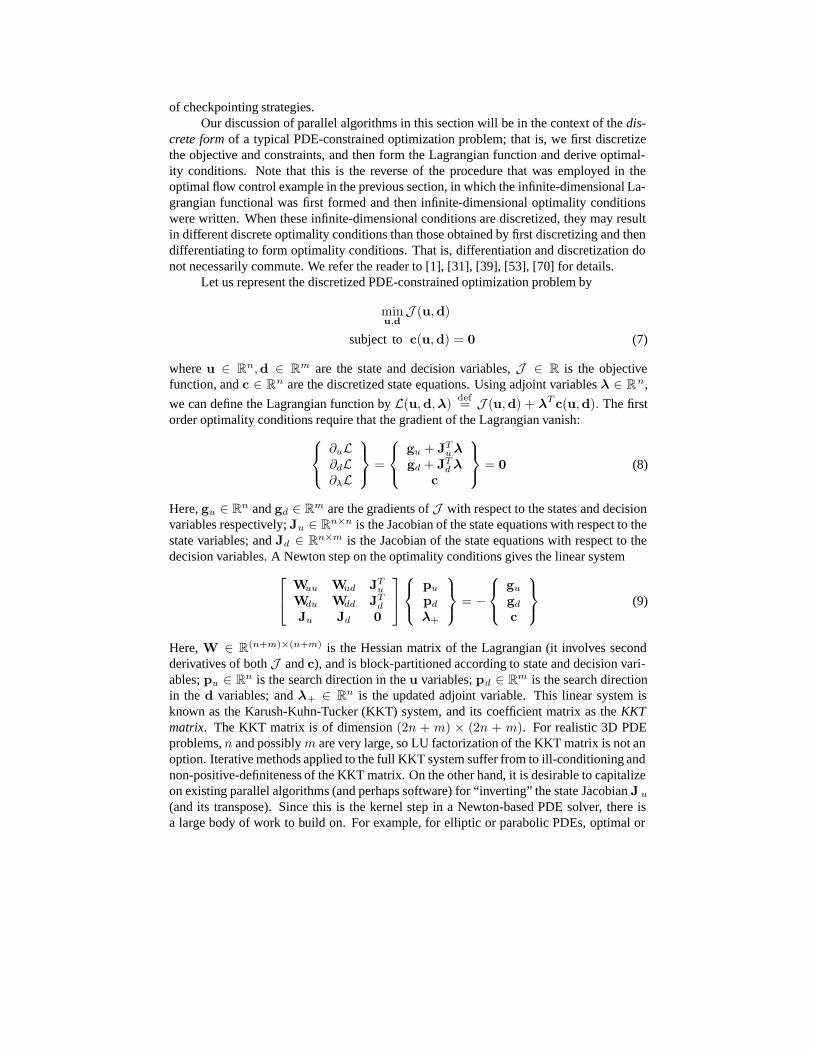
Let us represent the discretized PDE-constrained optimization problem by

minu,d

J (u,d)

subject to c(u,d) = 0 (7)

where u ∈ Rn,d ∈ R

m are the state and decision variables, J ∈ R is the objectivefunction, and c ∈ R

n are the discretized state equations. Using adjoint variables λ ∈ Rn,

we can define the Lagrangian function by L(u,d, λ) def= J (u,d) + λT c(u,d). The firstorder optimality conditions require that the gradient of the Lagrangian vanish:

⎧⎨⎩

∂uL∂dL∂λL

⎫⎬⎭ =

⎧⎨⎩

gu + JTu λ

gd + JTd λ

c

⎫⎬⎭ = 0 (8)

Here, gu ∈ Rn and gd ∈ R

m are the gradients of J with respect to the states and decisionvariables respectively; Ju ∈ R

n×n is the Jacobian of the state equations with respect to thestate variables; and Jd ∈ R

n×m is the Jacobian of the state equations with respect to thedecision variables. A Newton step on the optimality conditions gives the linear system

⎡⎣ Wuu Wud JT

u

Wdu Wdd JTd

Ju Jd 0

⎤⎦

⎧⎨⎩

pu

pd

λ+

⎫⎬⎭ = −

⎧⎨⎩

gu

gd

c

⎫⎬⎭ (9)

Here, W ∈ R(n+m)×(n+m) is the Hessian matrix of the Lagrangian (it involves second

derivatives of both J and c), and is block-partitioned according to state and decision vari-ables; pu ∈ R

n is the search direction in the u variables; pd ∈ Rm is the search direction

in the d variables; and λ+ ∈ Rn is the updated adjoint variable. This linear system is

known as the Karush-Kuhn-Tucker (KKT) system, and its coefficient matrix as the KKTmatrix. The KKT matrix is of dimension (2n + m) × (2n + m). For realistic 3D PDEproblems, n and possibly m are very large, so LU factorization of the KKT matrix is not anoption. Iterative methods applied to the full KKT system suffer from to ill-conditioning andnon-positive-definiteness of the KKT matrix. On the other hand, it is desirable to capitalizeon existing parallel algorithms (and perhaps software) for “inverting” the state Jacobian J u

(and its transpose). Since this is the kernel step in a Newton-based PDE solver, there isa large body of work to build on. For example, for elliptic or parabolic PDEs, optimal or

nearly-optimal parallel algorithms are available that require algorithmic work that is linearor weakly superlinear in n, and scale to thousands of processors and billions of variables.The ill-conditioning and complex structure of the KKT matrix, and the desire to exploit(parallel) PDE solvers for the state equations, motivate the use of reduced space methods,as discussed below.

2.1 Reduced space methods

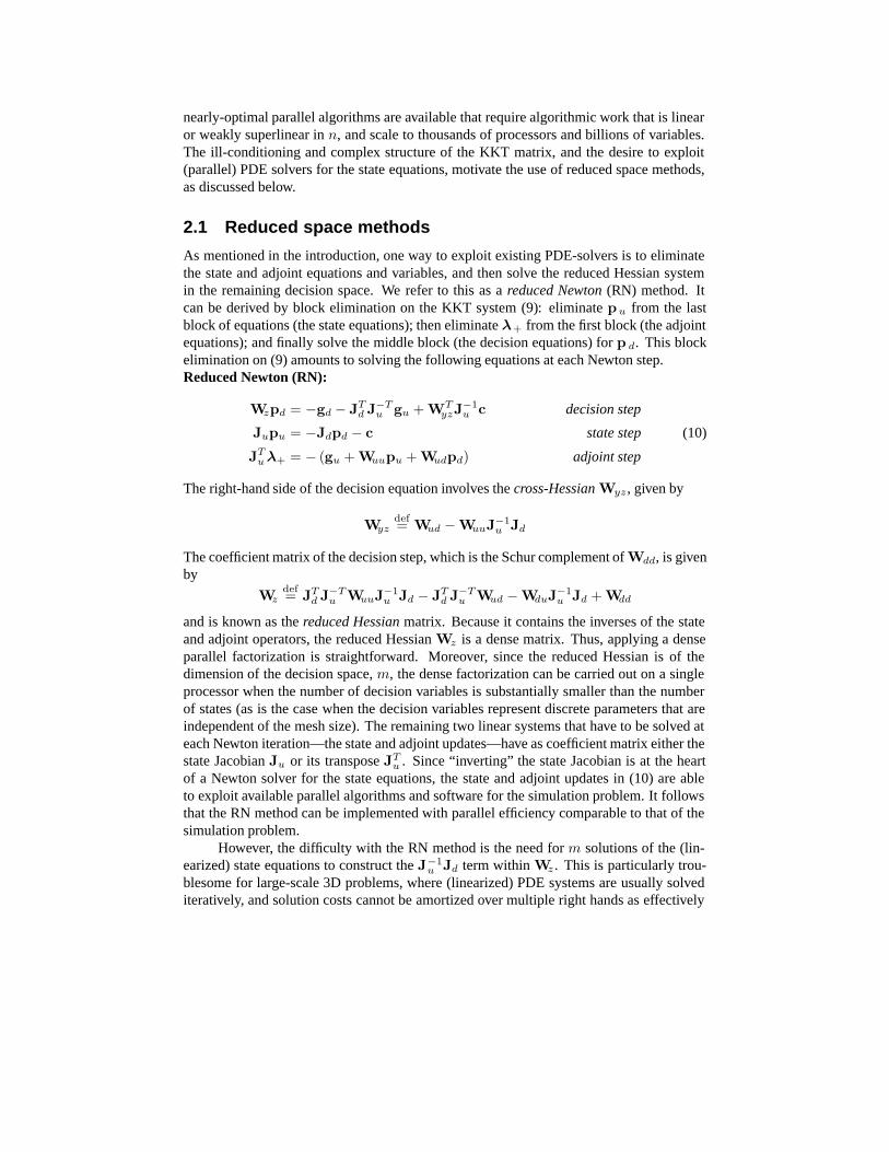
As mentioned in the introduction, one way to exploit existing PDE-solvers is to eliminatethe state and adjoint equations and variables, and then solve the reduced Hessian systemin the remaining decision space. We refer to this as a reduced Newton (RN) method. Itcan be derived by block elimination on the KKT system (9): eliminate p u from the lastblock of equations (the state equations); then eliminate λ+ from the first block (the adjointequations); and finally solve the middle block (the decision equations) for p d. This blockelimination on (9) amounts to solving the following equations at each Newton step.Reduced Newton (RN):

Wzpd = −gd − JTd J−T

u gu + WTyzJ

−1u c decision step

Jupu = −Jdpd − c state step (10)

JTu λ+ = − (gu + Wuupu + Wudpd) adjoint step

The right-hand side of the decision equation involves the cross-Hessian Wyz , given by

Wyzdef= Wud − WuuJ−1

u Jd

The coefficient matrix of the decision step, which is the Schur complement of Wdd, is givenby

Wzdef= JT

d J−Tu WuuJ−1

u Jd − JTd J−T

u Wud − WduJ−1u Jd + Wdd

and is known as the reduced Hessian matrix. Because it contains the inverses of the stateand adjoint operators, the reduced Hessian Wz is a dense matrix. Thus, applying a denseparallel factorization is straightforward. Moreover, since the reduced Hessian is of thedimension of the decision space, m, the dense factorization can be carried out on a singleprocessor when the number of decision variables is substantially smaller than the numberof states (as is the case when the decision variables represent discrete parameters that areindependent of the mesh size). The remaining two linear systems that have to be solved ateach Newton iteration—the state and adjoint updates—have as coefficient matrix either thestate Jacobian Ju or its transpose JT

u . Since “inverting” the state Jacobian is at the heartof a Newton solver for the state equations, the state and adjoint updates in (10) are ableto exploit available parallel algorithms and software for the simulation problem. It followsthat the RN method can be implemented with parallel efficiency comparable to that of thesimulation problem.

However, the difficulty with the RN method is the need for m solutions of the (lin-earized) state equations to construct the J−1

u Jd term within Wz . This is particularly trou-blesome for large-scale 3D problems, where (linearized) PDE systems are usually solvediteratively, and solution costs cannot be amortized over multiple right hands as effectively

as with direct solvers. When m is moderate or large (as will be the case when the deci-sion space is mesh-dependent), RN with exact formation of the reduced Hessian becomesintractable. So while its parallel efficiency may be high, its algorithmic efficiency can bepoor.

An alternative to forming the reduced Hessian is to solve the decision step in (10)by a Krylov method. Since the reduced Hessian is symmetric, and positive definite near aminimum, the Krylov method of choice is conjugate gradients (CG). The required actionof the reduced Hessian Wz on a decision-space vector within the CG iteration is formedin a matrix-free manner. This can be achieved with the dominant cost of a single pairof linearized PDE solves (one state and one adjoint). Moreover, the CG iteration can beterminated early to prevent oversolving in early iterations and to maintain a direction ofdescent [33]. Finally, in many cases the spectrum of the reduced Hessian is favorable forCG and convergence can be obtained in a mesh-independent number of iterations. Werefer to this method as a reduced Newton-CG (RNCG) method, and demonstrate it for alarge-scale inverse wave propagation problem in Section 3.1.

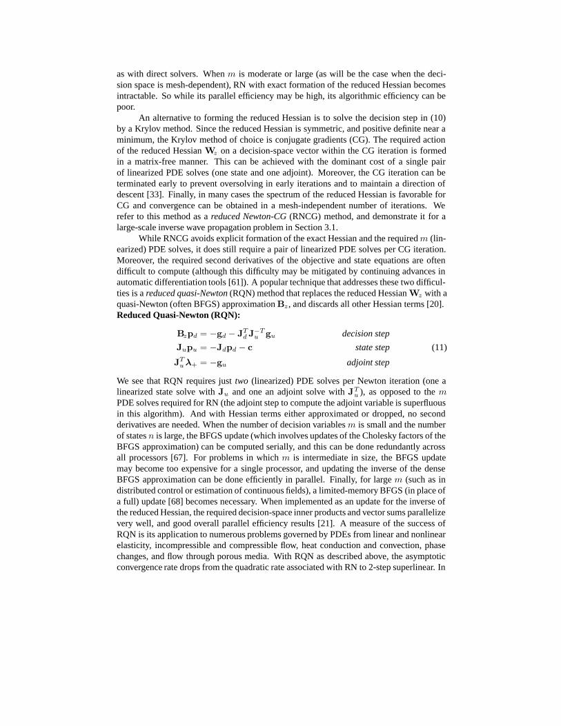
While RNCG avoids explicit formation of the exact Hessian and the required m (lin-earized) PDE solves, it does still require a pair of linearized PDE solves per CG iteration.Moreover, the required second derivatives of the objective and state equations are oftendifficult to compute (although this difficulty may be mitigated by continuing advances inautomatic differentiation tools [61]). A popular technique that addresses these two difficul-ties is a reduced quasi-Newton (RQN) method that replaces the reduced Hessian Wz with aquasi-Newton (often BFGS) approximation Bz , and discards all other Hessian terms [20].Reduced Quasi-Newton (RQN):

Bzpd = −gd − JTd J−T

u gu decision step

Jupu = −Jdpd − c state step (11)

JTu λ+ = −gu adjoint step

We see that RQN requires just two (linearized) PDE solves per Newton iteration (one alinearized state solve with Ju and one an adjoint solve with JT

u ), as opposed to the mPDE solves required for RN (the adjoint step to compute the adjoint variable is superfluousin this algorithm). And with Hessian terms either approximated or dropped, no secondderivatives are needed. When the number of decision variables m is small and the numberof states n is large, the BFGS update (which involves updates of the Cholesky factors of theBFGS approximation) can be computed serially, and this can be done redundantly acrossall processors [67]. For problems in which m is intermediate in size, the BFGS updatemay become too expensive for a single processor, and updating the inverse of the denseBFGS approximation can be done efficiently in parallel. Finally, for large m (such as indistributed control or estimation of continuous fields), a limited-memory BFGS (in place ofa full) update [68] becomes necessary. When implemented as an update for the inverse ofthe reduced Hessian, the required decision-space inner products and vector sums parallelizevery well, and good overall parallel efficiency results [21]. A measure of the success ofRQN is its application to numerous problems governed by PDEs from linear and nonlinearelasticity, incompressible and compressible flow, heat conduction and convection, phasechanges, and flow through porous media. With RQN as described above, the asymptoticconvergence rate drops from the quadratic rate associated with RN to 2-step superlinear. In

addition, unlike the usual case for RN, the number of iterations taken by RQN will typicallyincrease as the decision space is enlarged (i.e. as the mesh is refined), although this alsodepends on the spectrum of the reduced Hessian and on the difference between it and theinitial BFGS approximation. See for example [59] for discussion of quasi-Newton methodsfor infinite-dimensional problems. Specialized quasi-Newton updates that take advantageof the “compact + differential” structure of reduced Hessians for many inverse problemshave been developed [40].

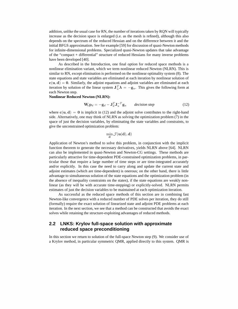
As described in the Introduction, one final option for reduced space methods is anonlinear elimination variant, which we term nonlinear reduced Newton (NLRN). This issimilar to RN, except elimination is performed on the nonlinear optimality system (8). Thestate equations and state variables are eliminated at each iteration by nonlinear solution ofc(u,d) = 0. Similarly, the adjoint equations and adjoint variables are eliminated at eachiteration by solution of the linear system JT

u λ = −gu. This gives the following form ateach Newton step.Nonlinear Reduced Newton (NLRN):

Wzpd = −gd − JTd J−T

u gu decision step (12)

where c(u,d) = 0 is implicit in (12) and the adjoint solve contributes to the right-handside. Alternatively, one may think of NLRN as solving the optimization problem (7) in thespace of just the decision variables, by eliminating the state variables and constraints, togive the unconstrained optimization problem:

mind

J (u(d),d)

Application of Newton’s method to solve this problem, in conjunction with the implicitfunction theorem to generate the necessary derivatives, yields NLRN above [64]. NLRNcan also be implemented in quasi-Newton and Newton-CG settings. These methods areparticularly attractive for time-dependent PDE-constrained optimization problems, in par-ticular those that require a large number of time steps or are time-integrated accuratelyand/or explicitly. In this case the need to carry along and update the current state andadjoint estimates (which are time-dependent) is onerous; on the other hand, there is littleadvantage to simultaneous solution of the state equations and the optimization problem (inthe absence of inequality constraints on the states), if the state equations are weakly non-linear (as they will be with accurate time-stepping) or explicitly-solved. NLRN permitsestimates of just the decision variables to be maintained at each optimization iteration.

As successful as the reduced space methods of this section are in combining fastNewton-like convergence with a reduced number of PDE solves per iteration, they do still(formally) require the exact solution of linearized state and adjoint PDE problems at eachiteration. In the next section, we see that a method can be constructed that avoids the exactsolves while retaining the structure-exploiting advantages of reduced methods.

2.2 LNKS: Krylov full-space solution with approximatereduced space preconditioning

In this section we return to solution of the full-space Newton step (9). We consider use ofa Krylov method, in particular symmetric QMR, applied directly to this system. QMR is

attractive because it does not require a positive definite preconditioner. The indefinitenessand potential ill-conditioning of the KKT matrix demand a good preconditioner. It shouldbe capable of exploiting the structure of the state constraints (specifically that good precon-ditioners for Ju are available), should be cheap to apply, should be effective in reducingthe number of Krylov iterations, and should parallelize readily. The reduced space methodsdescribed in the previous section—in particular an approximate form of RQN—fulfill theserequirements.

We begin by noting that the block elimination of (10) is equivalent to the followingblock factorization of the KKT matrix:⎡

⎣ WuuJ−1u 0 I

WduJ−1u I JT

d J−Tu

I 0 0

⎤⎦

⎡⎣ Ju Jd 0

0 Wz 00 Wyz JT

u

⎤⎦ (13)

Note that these factors can be permuted to block triangular form, so we can think of (13)as a block LU factorization of the KKT matrix. To derive the preconditioner, we replacethe reduced Hessian Wz in (13) by a (usually but not necessarily) limited memory BFGSapproximation Bz (as in RQN), drop other second derivative terms (also as in RQN), andreplace the exact (linearized) state and adjoint operators Ju and JT

u with approximationsJu and JT

u . The resulting preconditioner then takes the form of the following approximateblock-factorization of the KKT matrix:⎡

⎣ 0 0 I0 I JT

d J−Tu

I 0 0

⎤⎦

⎡⎣ Ju Jd 0

0 Bz 00 0 JT

u

⎤⎦ (14)

Applying the preconditioner by solving with the block factors (14) amounts to performingthe RQN step in (11), but with approximate state and adjoint solves. A good choice forJu is one of the available parallel preconditioners for Ju—for many PDE operators, thereexist near-spectrally-equivalent preconditioners that are both cheap to apply (their cost istypically linear or weakly superlinear in problem size) and effective (resulting in iterationcounts that are independent of, or increase very slowly in, problem size). For examplesof state-of-the-art parallel PDE preconditioners, see [2] for multigrid and [6] for domaindecomposition.

With (14) used as a preconditioner, the preconditioned KKT matrix becomes:⎡⎣ Iu O(Eu) 0

WTyz J

−1u O(Eu) + WzB−1

z O(Eu)WuuJ−1

u WyzB−1z Iu

⎤⎦

where Eudef= J−1

u − J−1u , Iu

def= JuJ−1u , Wyz

def= Wud − WuuJ−1u Jd. For exact state

equation solution, Eu = 0 and Iu = I, and we see that the reduced space preconditionerclusters the spectrum of the KKT matrix, with all eigenvalues either unit or belonging toWzB−1

z . Therefore, when Ju is a good preconditioner for the state Jacobian, and when Bz

is a good approximation of the reduced Hessian, we can expect the preconditioner (14) tobe effective in reducing the number of Krylov iterations.

We refer to this method as Lagrange-Newton-Krylov-Schur(LNKS), since it amountsto a Newton-Krylov method applied to the Lagrangian stationarity conditions, precondi-tioned by a Schur complement (i.e. reduced Hessian) approximation. See [22], [23], [24],

[25] for further details, and [14], [15], [42], [43], [46], [61] for related methods that usereduced space preconditioning ideas for full-space KKT systems.

Since LNKS applies an approximate version of a reduced space method as a precon-ditioner (by replacing the PDE solve with a PDE preconditioner application), it inheritsthe parallel efficiency of RQN in the preconditioning step. The other major cost is theKKT matrix-vector product in the Krylov iteration. For many PDE-constrained optimiza-tion problems, the Hessian of the Lagrangian and the Jacobian of the constraints are sparsewith structure dictated by the mesh (particularly when the decision variables are mesh-related). Thus, formation of the matrix-vector product at each Krylov iteration is linear inboth state and decision variables, and it parallelizes well in the usual fine-grained, domain-decomposed manner characteristic of PDE problems. To achieve overall scalability, werequire not just parallel efficiency of the components, but also algorithmic scalability inthe sense of mesh-independence (or near-independence) of both Newton and Krylov itera-tions. Mesh-independence of Newton iterations is characteristic of a wide class of smoothnonlinear operator problems, and we have observed it for a variety of PDE-constrained op-timization problems (see also [81]). Mesh-independence of LNKS’s Krylov iterations de-pends on the efficacy of the state and adjoint PDE preconditioners and the limited memoryBFGS (or other) approximation of the reduced Hessian. While the former are well-studied,the performance of the latter depends on the nature of the governing PDEs as well as theobjective functional. In Section 3.2 we demonstrate parallel scalability and superiority ofLNKS over limited memory RQN for a large-scale optimal flow control problem.

2.3 Domain decomposition and multigrid methods

As an alternative to the Schur-based method described in Section 2.2 for solution of thefull-space Newton step (9), one may pursue domain decomposition or multigrid precondi-tioners for the KKT matrix. These methods are more recent than those of Section 2.1 andare undergoing rapid development. Here we give just a brief overview and cite relevantreferences.

In [71] an overlapping Krylov-Schwarz domain decomposition method was used tosolve (9) related to the boundary control of an incompressible driven-cavity problem. Thisapproach resulted in excellent algorithmic and parallel scalability on up to 64 processorsfor a velocity-vorticity formulation of the 2D steady-state Navier-Stokes equations. Onekey insight of the method is that the necessary overlap for a control problem is larger thanthat for the simulation problem. More recently a multi-level variant has been derived [72].

Domain-decomposition preconditioners for linear-quadratic elliptic optimal controlproblems are presented in [49] for the overlapping case and [50] for the non-overlappingcase. Mesh-independent convergence for two-level variants is shown. These domain de-composition methods have been extended to advection-diffusion [13] and time-dependentparabolic [48] problems. Parallelism in the domain-decomposition methods describedabove can be achieved for the optimization problem in the same manner as it is for thesimulation problem, i.e. based on spatial decomposition. Several new ideas in parallel timedomain decomposition have emerged recently [41], [47], [78] and have been applied in theparabolic and electromagnetic settings. Although parallel efficiency is less than optimal,parallel speedups are still observed over non-time-decomposed algorithms, which may becrucial for real-time applications.

Multigrid methods are another class of preconditioners for the full-space Newtonsystem (9). An overview can be found in [35]. There are three basic approaches: multigridapplied directly to the optimization problem; multigrid as a preconditioner for the reducedHessian Wz in RNCG; and multigrid on the full space Newton system (9). In [65] multi-grid is applied directly to the optimization problem to generate a sequence of optimizationsubproblems with increasingly coarser grids. It is demonstrated that multigrid may acceler-ate solution of the optimization problem even when it may not be an appropriate solver forthe PDE problem. Multigrid for the reduced system (in the context of shape optimizationof potential and steady-state incompressible Euler flows) has been studied in [7], [8] basedon an analysis of the symbol of the reduced Hessian. For a large class of problems, es-pecially with the presence of a regularization term in the objective functional, the reducedHessian operator is spectrally equivalent to a second-kind Fredholm integral equation. Al-though this operator has a favorable spectrum leading to mesh-independent convergence,in practice preconditioning is still useful to reduce the number of iterations. It is essentialthat the smoother be tailored to the “compact + identity” structure of such operators [44],[57], [60], [62]. The use of appropriate smoothers of this type has resulted in successfulmultigrid methods for inverse problems for elliptic and parabolic PDEs [4], [34], [58].

Multigrid methods have also been developed for application to the full KKT optimal-ity system for nonlinear inverse electromagnetic problems [9] and for distributed controlof linear elliptic and parabolic problems [26], [27]. In such approaches, the state, adjoint,and decision equations are typically relaxed together in pointwise manner (or in the caseof L2 regularization, the decision variable can be eliminated and pointwise relaxation isapplied to the coupled state–adjoint system). These multigrid methods have been extendedto optimal control of nonlinear reaction-diffusion systems as well [28],[29]. Nonlinearitiesare addressed through either Newton-multigrid or the full approximation scheme (FAS).Just as with reduced space multigrid methods, careful design of the smoother is critical tothe success of full space multigrid.

3 Numerical examplesIn this section we present numerical results for parallel solution of three large-scale 3DPDE-constrained optimization problems. Section 3.1 presents an inverse acoustic scat-tering problem that can be formulated as a PDE-constrained optimization problem withhyperbolic constraints. The decision variables represent the PDE coefficient, in this casethe squared velocity of the medium (and thus the structure is similar to a design prob-lem). Because of the large number of time steps and the linearity of the forward problem,a full-space method is not warranted, and instead the reduced space methods of Section2.1 are employed. In Section 3.2 we present an optimization problem for boundary controlof steady Navier-Stokes flows. This problem is an example of an optimization problemconstrained by a nonlinear PDE with dominant elliptic term. The decision variables arevelocity sources on the boundary. The LNKS method of Section 2.2 delivers excellent per-formance for this problem. Finally, Section 3.3 presents results from an inverse problemwith a parabolic PDE, the convection-diffusion equation. The problem is to estimate theinitial condition of an atmospheric contaminant from sparse measurements of its transport.In these three examples, we encounter: elliptic, parabolic, and hyperbolic PDE constraints;

forward solvers that are explicit, linearly implicit, and nonlinearly implicit; optimizationproblems that are linear, nonlinear in the state, and nonlinear in the decision variable; de-cision variables that represent boundary condition, initial condition, and PDE coefficientfields; inverse, control, and design-like problems; reduced space and full space solvers;and domain decomposition and multigrid preconditioners. Thus, the examples provide aglimpse into a wide spectrum of problems and methods of current interest.

All of the examples presented in this section have been implemented on top of theparallel numerical PDE solver library PETSc [10]. The infinite-dimensional optimalityconditions presented in the following sections are discretized in space with finite elementsand (where applicable) in time with finite differences. For each example, we study thealgorithmic scalability of the parallel method, i.e. the growth in iterations as the problemsize and number of processors increase. In addition, for the acoustic scattering example,we provide a detailed discussion of parallel scalability and implementation issues. Dueto space limitations, we restrict the discussion of parallel scalability to this first example;however, the other examples will have similar structure and similar behavior is expected.The key idea is that the algorithms of Section 2 can be implemented for PDE-constrainedoptimization problems in such a way that the core computations are those that are found ina parallel forward PDE solver, e.g. sparse (with grid structure) operator evaluations, sparsematvecs, vector sums and inner products, and parallel PDE preconditioning. (In fact, thisis why we are able to use PETSc for our implementation.) Thus, the optimization solverslargely inherit the parallel efficiency of the forward PDE solver. Overall scalability thendepends on the algorithmic efficiency of the particular method, which is studied in thefollowing sections.

3.1 Inverse acoustic wave propagation

Here we study the performance of the reduced space methods of Section 2.1 on an inverseacoustic wave propagation problem [5], [75]. Consider an acoustic medium with domainΩ and boundary Γ. The medium is excited with a known acoustic energy source f(x, t)(for simplicity we assume a single source event), and the pressure u ∗(x, t) is observed atNr receivers, corresponding to points xj on the boundary. Our objective is to infer fromthese measurements the squared acoustic velocity distribution d(x), which is a propertyof the medium. Here d represents the decision variable and u(x, t) the state variable. Weseek to minimize, over the period t = 0 to T , an L2 norm difference between the observedstate and that predicted by the PDE model of acoustic wave propagation, at the N r receiverlocations. The PDE-constrained optimization problem can be written as:

minu,d

J (u, d) def=12

Nr∑j=1

∫ T

0

∫Ω

(u∗ − u)2 δ(x − xj) dx dt + ρ

∫Ω

(∇d · ∇d + ε)12 dx dt

subject to u −∇ · d∇u = f in Ω × (0, T )d∇u · n = 0 on Γ × (0, T ) (15)

u = u = 0 in Ω × t = 0The first term in the objective function is the misfit between observed and predicted states,the second term is a total variation (TV) regularization functional with regularization pa-

rameter ρ, and the constraints are the initial–boundary value problem for acoustic wavepropagation (assuming constant bulk modulus and variable density).

TV regularization preserves jump discontinuities in material interfaces, while smooth-ing along them. For a discussion of numerical issues and comparison with standard Tikhonovregularization, see [5], [80]. While regularization eliminates the null space of the inversionoperator (i.e. the reduced Hessian), there remains the difficulty that the objective functioncan be highly oscillatory in the space of material model d, meaning that straightforwardsolution of the optimization problem (15) can fail by becoming trapped in a local minimum[74]. To overcome this problem, we use multilevel grid and frequency continuation to gen-erate a sequence of solutions that remain in the basin of attraction of the global minimum;that is, we solve the optimization problem (15) for increasingly higher frequency compo-nents of the material model, on a sequence of increasingly finer grids with increasinglyhigher frequency sources [30]. For details see [5].

Figure 1 illustrates this multiscale approach and the effectiveness of the TV regu-larizer. The inverse problem is to reconstruct a piecewise-homogeneous velocity model(pictured at top left) that describes the geometry of a hemipelvic bone and surroundingvolume from sparse synthetic pressure measurements on four faces of a cube that enclosesthe acoustic medium. The source consists of the simultaneous introduction of a Rickerwavelet at each measurement point. Two intermediate-grid models are shown (upper right,lower left). The fine-grid reconstructed model (lower right) is able to capture fine-scalefeatures of the “ground truth” model with uncanny accuracy. The anisotropic behavior ofthe TV regularizer in revealed by its smoothing of ripple artifacts along the interface of theoriginal model. The fine-scale problem has 2.1 million material parameters and 3.4 billiontotal space-time variables, and was solved in 3 hours on 256 AlphaServer processors at thePittsburgh Supercomputing Center (PSC).

We next discuss how the optimization problem (15) is solved for a particular gridlevel in the multiscale continuation scheme. The first order optimality conditions for thisproblem take the following form:

u −∇ · d∇u = f in Ω × (0, T )d∇u · n = 0 on Γ × (0, T ) state equation (16)

u = u = 0 for Ω × t = 0

λ −∇ · d∇λ +Nr∑i=1

(u∗ − u) δ(x − xj) = 0 in Ω × (0, T )

d∇λ · n = 0 on Γ × (0, T ) adjoint equation (17)

λ = λ = 0 for Ω × t = T ∫ T

0

∇u · ∇λ dt − β∇ · (|∇d|−1ε ∇d) = 0 in Ω decision equation (18)

∇d · n = 0 on dΓ

The state equation (16) is just the acoustic wave propagation initial-boundary value prob-lem. Since the wave operator is self-adjoint in time and space, the adjoint equation (17)

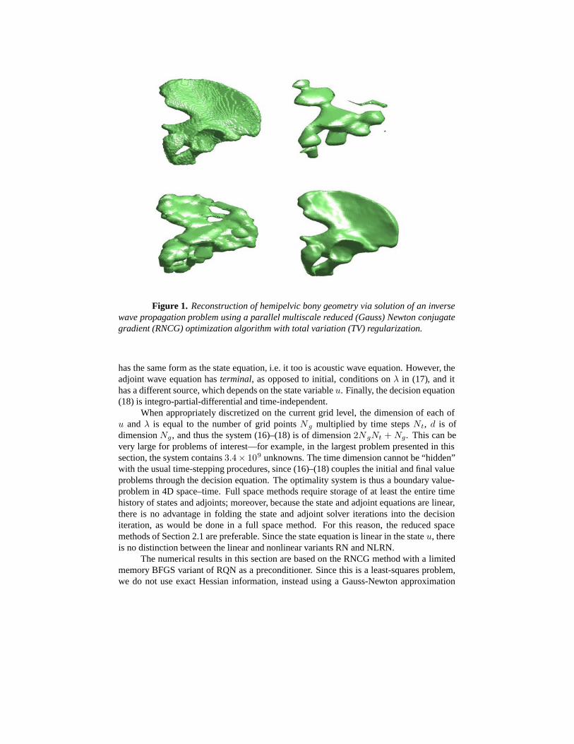
Figure 1. Reconstruction of hemipelvic bony geometry via solution of an inversewave propagation problem using a parallel multiscale reduced (Gauss) Newton conjugategradient (RNCG) optimization algorithm with total variation (TV) regularization.

has the same form as the state equation, i.e. it too is acoustic wave equation. However, theadjoint wave equation has terminal, as opposed to initial, conditions on λ in (17), and ithas a different source, which depends on the state variable u. Finally, the decision equation(18) is integro-partial-differential and time-independent.

When appropriately discretized on the current grid level, the dimension of each ofu and λ is equal to the number of grid points Ng multiplied by time steps Nt, d is ofdimension Ng , and thus the system (16)–(18) is of dimension 2NgNt + Ng. This can bevery large for problems of interest—for example, in the largest problem presented in thissection, the system contains 3.4× 109 unknowns. The time dimension cannot be “hidden”with the usual time-stepping procedures, since (16)–(18) couples the initial and final valueproblems through the decision equation. The optimality system is thus a boundary value-problem in 4D space–time. Full space methods require storage of at least the entire timehistory of states and adjoints; moreover, because the state and adjoint equations are linear,there is no advantage in folding the state and adjoint solver iterations into the decisioniteration, as would be done in a full space method. For this reason, the reduced spacemethods of Section 2.1 are preferable. Since the state equation is linear in the state u, thereis no distinction between the linear and nonlinear variants RN and NLRN.

The numerical results in this section are based on the RNCG method with a limitedmemory BFGS variant of RQN as a preconditioner. Since this is a least-squares problem,we do not use exact Hessian information, instead using a Gauss-Newton approximation

that neglects second derivative terms that involve λ. Spatial approximation is by Galerkinfinite elements, in particular piecewise trilinear basis functions for the state u, adjoint λ,and decision d fields. For the class of wave propagation problems we are interested in, theCourant-limited time step size is on the order of that dictated by accuracy considerations,and therefore we choose to discretize in time via explicit central differences. Thus, thenumber of time steps is of the order of cube root of the number of grid points. Sincewe require time accurate resolution of wave propagation phenomena, the 4D “problemdimension” scales with the 4

3 power of the number of grid points.The overall work is dominated by the cost of the CG iteration, which, because the

preconditioner is time-independent, is dominated by the Hessian-vector product. With theGauss-Newton approximation, the CG matvec requires the same work as the reduced gra-dient computation: a forward wave propagation, an adjoint wave propagation, possiblecheckpointing recomputations based on available memory, and the reduction of the stateand adjoint spatio-temporal fields onto the material model space via terms of the form∫∇u · ∇λ dt. These components are all “PDE-solver-like,” and can be parallelized ef-fectively in a fine-grained domain-based way, using many of the building blocks of sparsePDE-based parallel computation: sparse grid-based matrix-vector products, vector sums,scalings, and inner products.

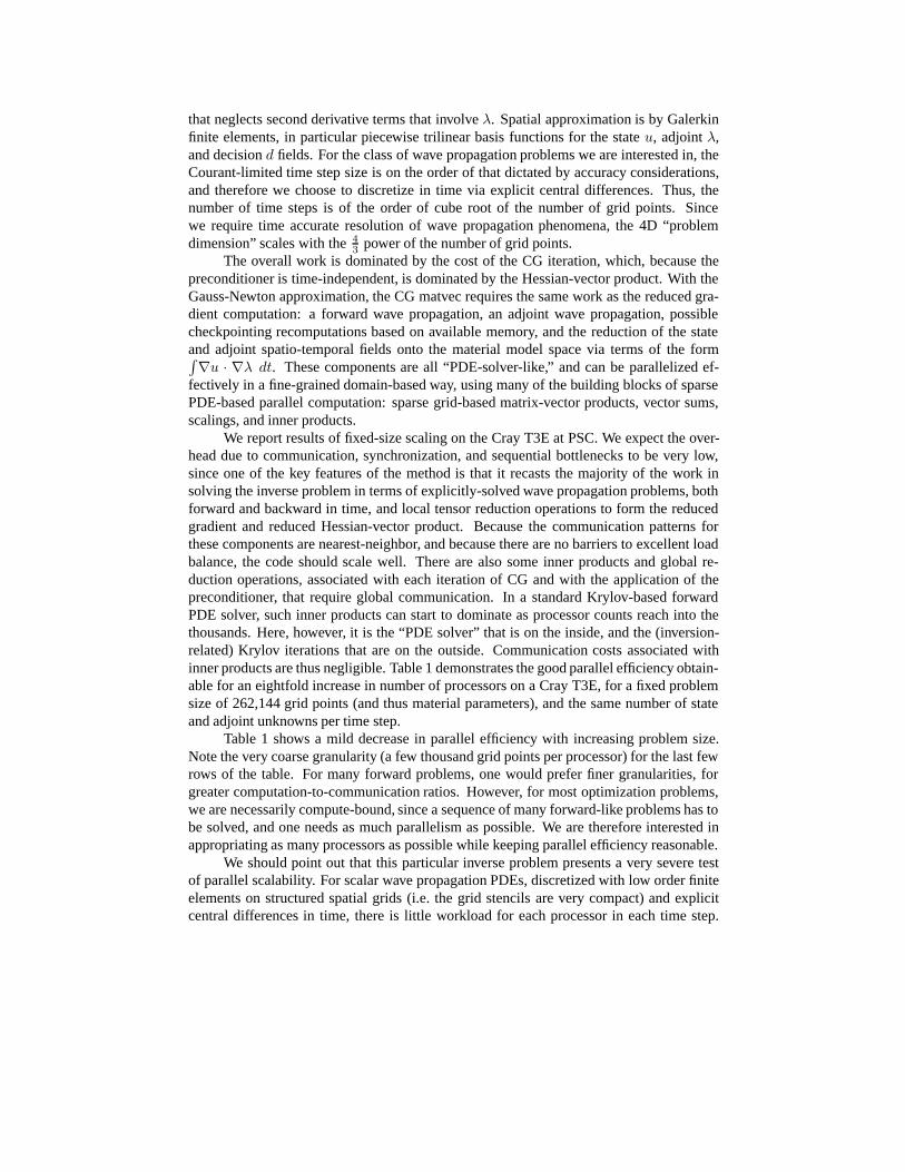
We report results of fixed-size scaling on the Cray T3E at PSC. We expect the over-head due to communication, synchronization, and sequential bottlenecks to be very low,since one of the key features of the method is that it recasts the majority of the work insolving the inverse problem in terms of explicitly-solved wave propagation problems, bothforward and backward in time, and local tensor reduction operations to form the reducedgradient and reduced Hessian-vector product. Because the communication patterns forthese components are nearest-neighbor, and because there are no barriers to excellent loadbalance, the code should scale well. There are also some inner products and global re-duction operations, associated with each iteration of CG and with the application of thepreconditioner, that require global communication. In a standard Krylov-based forwardPDE solver, such inner products can start to dominate as processor counts reach into thethousands. Here, however, it is the “PDE solver” that is on the inside, and the (inversion-related) Krylov iterations that are on the outside. Communication costs associated withinner products are thus negligible. Table 1 demonstrates the good parallel efficiency obtain-able for an eightfold increase in number of processors on a Cray T3E, for a fixed problemsize of 262,144 grid points (and thus material parameters), and the same number of stateand adjoint unknowns per time step.

Table 1 shows a mild decrease in parallel efficiency with increasing problem size.Note the very coarse granularity (a few thousand grid points per processor) for the last fewrows of the table. For many forward problems, one would prefer finer granularities, forgreater computation-to-communication ratios. However, for most optimization problems,we are necessarily compute-bound, since a sequence of many forward-like problems has tobe solved, and one needs as much parallelism as possible. We are therefore interested inappropriating as many processors as possible while keeping parallel efficiency reasonable.

We should point out that this particular inverse problem presents a very severe testof parallel scalability. For scalar wave propagation PDEs, discretized with low order finiteelements on structured spatial grids (i.e. the grid stencils are very compact) and explicitcentral differences in time, there is little workload for each processor in each time step.

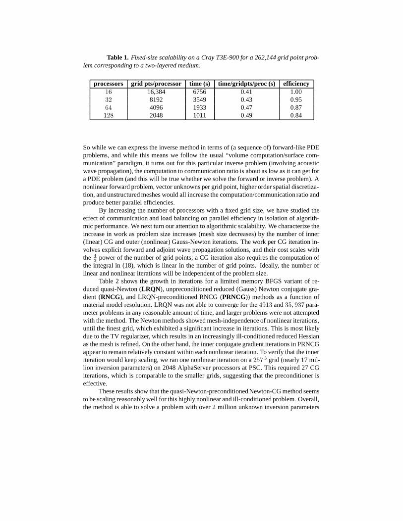
Table 1. Fixed-size scalability on a Cray T3E-900 for a 262,144 grid point prob-lem corresponding to a two-layered medium.

processors grid pts/processor time (s) time/gridpts/proc (s) efficiency16 16,384 6756 0.41 1.0032 8192 3549 0.43 0.9564 4096 1933 0.47 0.87128 2048 1011 0.49 0.84

So while we can express the inverse method in terms of (a sequence of) forward-like PDEproblems, and while this means we follow the usual “volume computation/surface com-munication” paradigm, it turns out for this particular inverse problem (involving acousticwave propagation), the computation to communication ratio is about as low as it can get fora PDE problem (and this will be true whether we solve the forward or inverse problem). Anonlinear forward problem, vector unknowns per grid point, higher order spatial discretiza-tion, and unstructured meshes would all increase the computation/communication ratio andproduce better parallel efficiencies.

By increasing the number of processors with a fixed grid size, we have studied theeffect of communication and load balancing on parallel efficiency in isolation of algorith-mic performance. We next turn our attention to algorithmic scalability. We characterize theincrease in work as problem size increases (mesh size decreases) by the number of inner(linear) CG and outer (nonlinear) Gauss-Newton iterations. The work per CG iteration in-volves explicit forward and adjoint wave propagation solutions, and their cost scales withthe 4

3 power of the number of grid points; a CG iteration also requires the computation ofthe integral in (18), which is linear in the number of grid points. Ideally, the number oflinear and nonlinear iterations will be independent of the problem size.

Table 2 shows the growth in iterations for a limited memory BFGS variant of re-duced quasi-Newton (LRQN), unpreconditioned reduced (Gauss) Newton conjugate gra-dient (RNCG), and LRQN-preconditioned RNCG (PRNCG)) methods as a function ofmaterial model resolution. LRQN was not able to converge for the 4913 and 35, 937 para-meter problems in any reasonable amount of time, and larger problems were not attemptedwith the method. The Newton methods showed mesh-independence of nonlinear iterations,until the finest grid, which exhibited a significant increase in iterations. This is most likelydue to the TV regularizer, which results in an increasingly ill-conditioned reduced Hessianas the mesh is refined. On the other hand, the inner conjugate gradient iterations in PRNCGappear to remain relatively constant within each nonlinear iteration. To verify that the inneriteration would keep scaling, we ran one nonlinear iteration on a 257 3 grid (nearly 17 mil-lion inversion parameters) on 2048 AlphaServer processors at PSC. This required 27 CGiterations, which is comparable to the smaller grids, suggesting that the preconditioner iseffective.

These results show that the quasi-Newton-preconditionedNewton-CG method seemsto be scaling reasonably well for this highly nonlinear and ill-conditioned problem. Overall,the method is able to solve a problem with over 2 million unknown inversion parameters

Table 2. Algorithmic scaling by limited memory BFGS reduced quasi-Newton(LRQN), unpreconditioned reduced (Gauss) Newton Conjugate Gradient (RNCG), andLRQN-preconditioned RNCG (PRNCG) methods as a function of material model reso-lution. For LRQN, the number of iterations is reported, and for both LRQN solver andpreconditioner, 200 L-BFGS vectors are stored. For RNCG and PRNCG, the total numberof CG iterations is reported, along with the number of Newton iterations in parentheses.On all material grids up to 653, the forward and adjoint wave propagation problems areposed on 653 grid × 400 time steps, and inversion is done on 64 PSC AlphaServer proces-sors; for the 1293 material grid, the wave equations are on 1293 grids × 800 time steps,on 256 processors. In all cases, work per iteration reported is dominated by a reducedgradient (LRQN) or reduced-gradient-like (RNCG, PRNCG) calculation, so the reportediterations can be compared across the different methods. Convergence criterion is 10−5

relative norm of the reduced gradient. “*” indicates lack of convergence; † indicates num-ber of iterations extrapolated from converging value after 6 hours of runtime.

grid size material parameters LRQN its RNCG its PRNCG its653 8 16 17 (5) 10 (5)653 27 36 57 (6) 20 (6)653 125 144 131 (7) 33 (6)653 729 156 128 (5) 85 (4)653 4913 * 144 (4) 161 (4)653 35, 937 * 177 (4) 159 (6)653 274, 625 — 350 (7) 197 (6)1293 2, 146, 689 — 1470† (22) 409 (16)

in just three hours on 256 AlphaServer processors. However, each CG iteration involvesa forward/adjoint pair of wave propagation solutions, so that the cost of inversion is over800 times the cost of the forward problem. Thus, the excellent reconstruction in Figure 1has come at significant cost. This approach has also been applied to elastic wave equationinverse problems in the context of inverse earthquake modeling with success [3].

3.2 Optimal boundary control of Navier-Stokes flow

In this second example, we give sample results for an optimal boundary control problem for3D steady Navier-Stokes flow. A survey and articles on this topic can be found in [38], [55],[56]. We use the velocity-pressure (u(x), p(x)) form of the incompressible Navier-Stokesequations. The boundary control problem seeks to find an appropriate source d(s) on thecontrol boundary ∂Ωd so that the H1 seminorm of the velocity (i.e. the rate of dissipation

of viscous energy) is minimized:

minu,p,d

J (u, p, d) def=ν

2

∫Ω

∇u · ∇u dx +ρ

2

∫∂Ωd

|d|2 ds

subject to − ν∆u + (∇u)u + ∇p = 0 in Ω∇ · u = 0 in Ω (19)

u = ug on ∂Ωu

u = d on ∂Ωd

−pn + ν(∇u)n = 0 on ∂ΩN

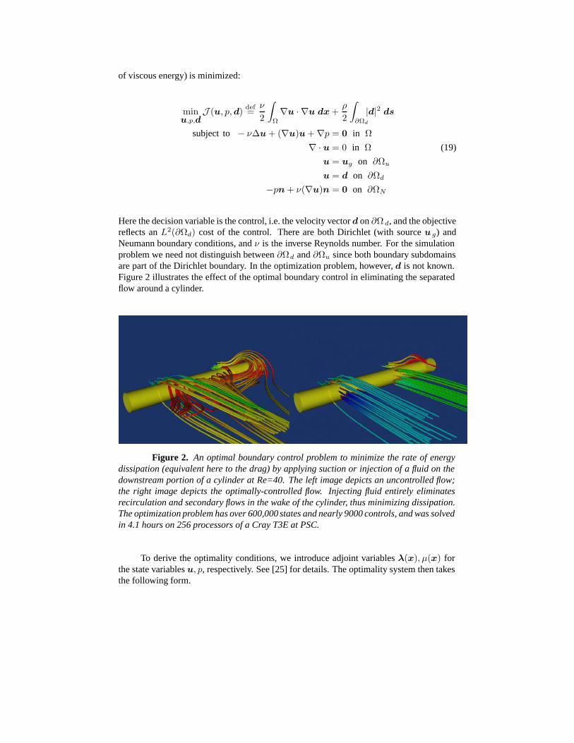
Here the decision variable is the control, i.e. the velocity vector d on ∂Ω d, and the objectivereflects an L2(∂Ωd) cost of the control. There are both Dirichlet (with source u g) andNeumann boundary conditions, and ν is the inverse Reynolds number. For the simulationproblem we need not distinguish between ∂Ωd and ∂Ωu since both boundary subdomainsare part of the Dirichlet boundary. In the optimization problem, however, d is not known.Figure 2 illustrates the effect of the optimal boundary control in eliminating the separatedflow around a cylinder.

Figure 2. An optimal boundary control problem to minimize the rate of energydissipation (equivalent here to the drag) by applying suction or injection of a fluid on thedownstream portion of a cylinder at Re=40. The left image depicts an uncontrolled flow;the right image depicts the optimally-controlled flow. Injecting fluid entirely eliminatesrecirculation and secondary flows in the wake of the cylinder, thus minimizing dissipation.The optimization problem has over 600,000 states and nearly 9000 controls, and was solvedin 4.1 hours on 256 processors of a Cray T3E at PSC.

To derive the optimality conditions, we introduce adjoint variables λ(x), µ(x) forthe state variables u, p, respectively. See [25] for details. The optimality system then takesthe following form.

State equations:

−ν∆u + (∇u)u + ∇p = 0 in Ω∇ · u = 0 in Ω

u = ug on ∂Ωu (20)

u = d on ∂Ωd

−pn + ν(∇u)n = 0 on ∂ΩN

Adjoint equations:

−ν∆λ + (∇u)T λ − (∇λ)u + ∇µ = ν∆u in Ω∇ · λ = 0 in Ω

λ = 0 on ∂Ωu (21)

λ = 0 on ∂Ωd

−µn + ν∇(λ)n + (u · n)λ = −ν(∇u)n on ∂ΩN

Decision equations:

ν(∇λ + ∇u)n − ρd = 0 on ∂Ωd (22)

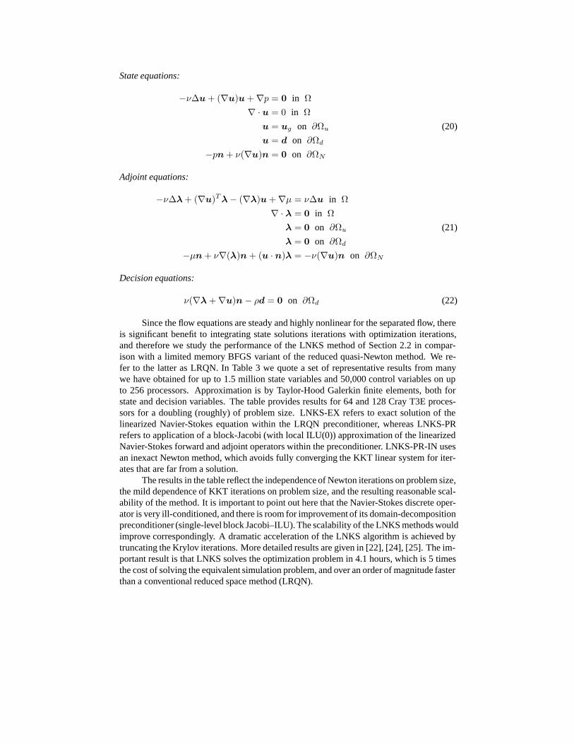
Since the flow equations are steady and highly nonlinear for the separated flow, thereis significant benefit to integrating state solutions iterations with optimization iterations,and therefore we study the performance of the LNKS method of Section 2.2 in compar-ison with a limited memory BFGS variant of the reduced quasi-Newton method. We re-fer to the latter as LRQN. In Table 3 we quote a set of representative results from manywe have obtained for up to 1.5 million state variables and 50,000 control variables on upto 256 processors. Approximation is by Taylor-Hood Galerkin finite elements, both forstate and decision variables. The table provides results for 64 and 128 Cray T3E proces-sors for a doubling (roughly) of problem size. LNKS-EX refers to exact solution of thelinearized Navier-Stokes equation within the LRQN preconditioner, whereas LNKS-PRrefers to application of a block-Jacobi (with local ILU(0)) approximation of the linearizedNavier-Stokes forward and adjoint operators within the preconditioner. LNKS-PR-IN usesan inexact Newton method, which avoids fully converging the KKT linear system for iter-ates that are far from a solution.

The results in the table reflect the independence of Newton iterations on problem size,the mild dependence of KKT iterations on problem size, and the resulting reasonable scal-ability of the method. It is important to point out here that the Navier-Stokes discrete oper-ator is very ill-conditioned, and there is room for improvement of its domain-decompositionpreconditioner (single-level block Jacobi–ILU). The scalability of the LNKS methods wouldimprove correspondingly. A dramatic acceleration of the LNKS algorithm is achieved bytruncating the Krylov iterations. More detailed results are given in [22], [24], [25]. The im-portant result is that LNKS solves the optimization problem in 4.1 hours, which is 5 timesthe cost of solving the equivalent simulation problem, and over an order of magnitude fasterthan a conventional reduced space method (LRQN).

Table 3. Algorithmic scalability for Navier-Stokes optimal flow control problemon 64 and 128 processors of a Cray T3E for a doubling (roughly) of problem size.

statescontrols

method Newton iter average KKT iter time (hours)

389,440 LRQN 189 — 46.36,549 LNKS-EX 6 19 27.4

(64 procs) LNKS-PR 6 2,153 15.7LNKS-PR-TR 13 238 3.8

615,981 LRQN 204 — 53.18,901 LNKS-EX 7 20 33.8

(128 procs) LNKS-PR 6 3,583 16.8LNKS-PR-TR 12 379 4.1

3.3 Initial condition inversion of atmospheric contaminanttransport

In this section we consider an inverse problem governed by a parabolic PDE. Given obser-vations of the concentration of an airborne contaminant u ∗

jNs

j=1 at Ns locations xjNs

j=1

inside a domain Ω, we wish to estimate the initial concentration d(x) using a convection-diffusion transport PDE model. The inverse problem is formulated as a constrained, leastsquares optimization problem:

minu,d

J (u, d) def=12

Ns∑j=1

∫Ω

(u − u∗)2 δ(x − xj) dx dt +β

2

∫Ω

d2 dx

subject to u − ν∆u + v · ∇u = 0 in Ω × (0, T ) (23)

ν∇u · n = 0 on Γ × (0, T )u = d in Ω × t = 0

The first term in the objective functional J represents the least-squares misfit of predictedconcentrations u(xj) with observed concentrations u∗(xj) at sensor locations, over a timehorizon (0, T ), and the second term provides L2 regularization of the initial condition d, re-sulting in a well-posed problem. The constraint is the convection-diffusion initial-boundaryvalue problem, where u is the contaminant concentration field, d is the initial concentra-tion, v is the wind velocity field (assumed known), and ν is the diffusion coefficient. Forsimplicity, a steady laminar incompressible Navier-Stokes solver is used to generate windvelocity fields over a terrain of interest.

Optimality conditions for (23) can be stated as as follows.State equation:

u − ν∆u + v · ∇u = 0 in Ω × (0, T )ν∇u · n = 0 on Γ × (0, T ) (24)

u = d in Ω × t = 0

Adjoint equation:

−λ − ν∆λ −∇ · (λv) = −Ns∑j=1

(u − u∗)δ(x − xj) in Ω × (0, T )

(ν ∇λ + vλ) · n = 0 on Γ × (0, T ) (25)

λ = 0 in Ω × t = T Decision equation:

β u0 − λ|t=0 = 0 in Ω (26)

Equations (24) are just the original forward convection-diffusion transport problem for thecontaminant field. The adjoint convection-diffusion problem (25) resembles the forwardproblem, but with some essential differences. First, it is a terminal value problem; that is,the adjoint λ is specified at the final time t = T . Second, convection is directed backwardalong the streamlines. Third, it is driven by a source term given by the negative of the misfitbetween predicted and measured concentrations at sensor locations. Finally, the initialconcentration equation (26) is in the present case of L 2 regularization an algebraic equation.Together, (24), (25), and (26) furnish a coupled system of linear PDEs for (u, λ, d).

The principal difficulty in solving this system is that—while the forward and ad-joint transport problems are evolution equations—the KKT optimality system is a coupledboundary value problem in 4D space-time. As in the acoustic inversion example, the 4Dspace-time nature of (24)–(26) presents prohibitive memory requirements for large scaleproblems, and thus we consider reduced space methods. In fact, the optimality system isa linear system, since the state equation is linear in the state, and the decision variable ap-pears linearly. Block elimination produces a reduced Hessian that has condition numberindependent of the mesh size (it is spectrally equivalent to a compact perturbation of theidentity). However, a preconditioner capable of reducing the number of iterations is stillcritical, since each CG iteration requires one state and one adjoint convection-diffusionsolve. We are unable to employ the limited memory BFGS preconditioner that was usedfor the acoustic inverse problem, since for this linear problem there is no opportunity forthe preconditioner to reuse built-up curvature information. Instead, we appeal to multigridmethods for second kind integral equations and compact operators [34], [44], [57], [58],[62] to precondition the reduced Hessian system. Standard multigrid smoothers (e.g. forelliptic PDEs) are inappropriate for inverse operators and instead a smoother that is tailoredto the spectral structure of the reduced Hessian must be used; for details see [4].

The optimality system (24)–(26) is discretized by SUPG-stabilized finite elements inspace and Crank-Nicolson in time. We use a logically-rectangular topography-conformingisoparametric hexahedral finite element mesh on which piecewise-trilinear basis functionsare defined. Since the Crank-Nicolson method is implicit, we “invert” the time-steppingoperator using a restarted GMRES method, accelerated by an additive Schwarz domaindecomposition preconditioner, both from the PETSc library. Figure 3 illustrates solution ofthe inverse problem for a contaminant release scenario in the Greater Los Angeles Basin.As can be seen in the figure, the reconstruction of the initial condition is very accurate.

We next study the parallel and algorithmic scalability of the multigrid precondi-tioner. We take synthetic measurements on a 7 × 7 × 7 sensor array. CG is termi-

Figure 3. Solution of a airborne contaminant inverse problem in the Greater LosAngeles Basin with onshore winds; Peclet number = 10. The target initial concentrationis shown at left, and reconstructed initial condition on right. The measurements for theinverse problem were synthesized by solving the convection-diffusion equation using thetarget initial condition, and recording measurements on a 21 × 21 × 21 uniform array ofsensors. The mesh has 917,301 grid points; the problem has the same number of initialcondition unknowns and 74 million total space-time unknowns. Inversion takes 2.5 hourson 64 AlphaServer processors at PSC. CG iterations are terminated when the norm of theresidual of the reduced space equations is reduced by five orders of magnitude.

nated when the residual of the reduced system has been reduced by six orders of mag-nitude. Table 4 presents fixed-size scalability results. The inverse problem is solved on a

Table 4. Fixed size scalability of unpreconditioned and multigrid preconditionedinversion. Here the problem size is 257×257×257×257 for all cases. We use a three-levelversion of the multigrid preconditioner. The variables are distributed across the processorsin space, whereas they are stored sequentially in time (as in a multicomponent PDE). Herehours is the wall-clock time, and η is the parallel efficiency inferred from the runtime. Theunpreconditioned code scales extremely well since there is little overhead associated withits single-grid simulations. The multigrid preconditioner also scales reasonably well, butits performance deteriorates since the problem granularity at the coarser levels is signifi-cantly reduced. Nevertheless, wall-clock time is significantly reduced over the unprecondi-tioned case.

CPUs no preconditioner multigridhours η hours η

128 5.65 1.00 2.22 1.00512 1.41 1.00 0.76 0.731024 0.74 0.95 0.48 0.58

257×257×257×257 grid, i.e. there are 17×106 inversion parameters, and 4.3×109 total

space-time unknowns in the optimality system (9). Note that while the CG iterations are in-sensitive to the number of processors, the forward and adjoint transport simulations at eachiteration rely on a single-level Schwarz domain decomposition preconditioner, whose effec-tiveness deteriorates with increasing number of processors. Thus, the efficiencies reportedin the table reflect parallel as well as (forward) algorithmic scalability. The multigrid pre-conditioner incurs non-negligible overhead as the number of processors increases for fixedproblem size, since the coarse subproblems are solved on ever larger numbers of proces-sors. For example, on 1024 processors, the 65×65×65 coarse grid solve has just 270 gridpoints per processor, which is far too few for a favorable computation-to-communicationratio.

On the other hand, the unpreconditioned CG iterations exhibit excellent parallel scal-ability since the forward and adjoint problems are solved on just the fine grids. Neverthe-less, the multigrid preconditioner achieves a net speedup in wall-clock time, varying froma factor of 2.5 for 128 processors to 1.5 for 1024 processors. Most important, the inverseproblem is solved in less than 29 minutes on 1024 processors. This is about 18 times thewall-clock time for solving a single forward transport problem.

Table 5 presents isogranular scalability results. Here the problem size ranges from

Table 5. Isogranular scalability of unpreconditioned and multigrid precondi-tioned inversion. The spatial problem size per processor is fixed (stride of 8). Ideal speedupshould result in doubling of wall-clock time. The multigrid preconditioner scales very welldue to improving algorithmic efficiency (decreasing CG iterations) with increasing problemsize. Unpreconditioned CG is not able to solve the largest problem in reasonable time.

grid size problem size CPUs no preconditioner multigridd (u, λ, d) hours iterations hours iterations

1294 2.15E+6 5.56E+8 16 2.13 23 1.05 82574 1.70E+7 8.75E+9 128 5.65 23 2.22 65134 1.35E+8 1.39E+11 1024 — — 4.89 5

5.56 × 108 to 1.39 × 1011 total space-time unknowns, while the number of processorsranges from 16 to 1024. Because we refine in time as well as in space, and because thenumber of processors increases by a factor of 8 with each refinement of the grid, the totalnumber of space-time unknowns is not constant from row to row of the table; in fact itdoubles. However, the number of grid points per processor does remain constant, and thisis the number that dictates the computation to communication ratio. For ideal overall (i.e.algorithmic + parallel) scalability, we would thus expect wall-clock time to double witheach refinement of the grid. Unpreconditioned CG becomes too expensive for the largerproblems, and is unable to solve the largest problem in reasonable time. The multigrid pre-conditioned solver, on the other hand, exhibits very good overall scalability, with overallefficiency dropping to 95% on 128 processors and 86% on 1024 processors, compared tothe 16 processor base case. From the fixed-size scalability studies in Table 4, we know thatthe parallel efficiency of the multigrid preconditioner drops on large numbers of processorsdue to the need to solve coarse problems. However, the isogranular scalability results of Ta-ble 5 indicate substantially better multigrid performance. What accounts for this? First, the

constant number of grid points per processor keeps the processors relatively well-populatedfor the coarse problems. Second, the algorithmic efficacy of the multigrid preconditionerimproves with decreasing mesh size; the number of iterations drops from 8 to 5 over twosuccessive doublings of mesh resolution. The largest problem exhibits a factor of 4.6 re-duction in CG iterations relative to the unpreconditioned case (5 vs. 23). This improvementin algorithmic efficiency helps keep the overall efficiency high.

4 ConclusionsThis chapter has given an overview of parallel algorithms for PDE-constrained optimizationproblems, focusing on reduced-space and full-space Newton-like methods. Examples illus-trate application of the methods to elliptic, parabolic, and hyperbolic problems representinginverse, control, and design problems. A key conclusion is that an appropriate choice ofoptimization method can result in an algorithm that largely inherits the parallelism prop-erties of the simulation problem. Moreover, under certain conditions, the combination oflinear work per Krylov iteration, weak dependence of Krylov iterations on problem size,and independence of Newton iterations on problem size can result in a method that scaleswell with increasing problem size and number of processors. Thus, overall (parallel +algorithmic) efficiency follows.

There is no recipe for a general-purpose parallel PDE-constrained optimization meth-od, just as there is no recipe for a general-purpose parallel PDE solver. The optimizer mustbe built around the best available numerical techniques for the state PDEs. The situation isactually more pronounced for optimization than it is for simulation, since new operators—the adjoint, the reduced Hessian, the KKT—appear that are not present in the simulationproblem. PDE-constrained optimization requires special attention to preconditioning orapproximation of these operators, a consideration that is usually not present in the designof general purpose optimization software.

However, some general themes do recur. For steady PDEs or whenever the stateequations are highly nonlinear, a full-space method that simultaneously iterates on the state,adjoint, and decision equations can be significantly more effective than a reduced spacemethod that entails satisfaction of (a linear approximation of) the state and adjoint equationsat each optimization iteration. For example, in the optimal flow control example in Section3.2, the LNKS method was able to compute the optimal control at high parallel efficiencyand at a cost of just 5 simulations. LNKS preconditions the full space KKT matrix byan approximate factorization involving subpreconditioners for state, adjoint, and reducedHessian operators, thereby capitalizing on available parallel preconditioners for the stateequation. Alternatively, methods that seek to extend domain decomposition and multigridpreconditioners for direct application to the KKT matrix are being developed and showconsiderable promise in also solving the optimization problem in a small multiple of thecost of the simulation. Careful consideration of smoothing, intergrid transfer, and interfaceconditions is required for these methods. Like their counterparts for the PDE forwardproblem, parallelism comes naturally for these methods.

At the opposite end of the spectrum, for time-dependent PDEs that are explicit, linear,or weakly nonlinear at each time step, the benefit of full-space solution is less apparent, andreduced space methods may be required, if only for memory reasons. For small numbers

of decision variables, quasi-Newton methods are likely sufficient, while for large (typicallymesh-dependent) decision spaces, Newton methods with inexactly-terminated CG solutionof the quadratic step are preferred. Preconditioning the reduced Hessian becomes essential,even when it is well-conditioned, since each CG iteration involves a pair of PDE solves(one state, one adjoint). For many large-scale inverse problems, the reduced Hessian hasa “compact + identity” or “compact + differential” structure, which can be exploited todesign effective preconditioners. Nevertheless, when the optimization problem is highlynonlinear in the decision space but weakly nonlinear or linear in the state space, such as forthe inverse wave propagation problem described in Section 3.1, we can expect that the costof solving the optimization problem will be many times that of the simulation problem.

A number of important and challenging issues were not mentioned. We assumed thatthe appropriate Jacobian, adjoint, and Hessian operators were available, which is rarelythe case for legacy code. A key difficulty not discussed here is globalization, which mustoften take on a problem-specific nature (as in the grid/frequency continuation employedfor the inverse wave propagation problem). Design of scalable parallel algorithms formesh-dependent inequality constraints on decision and state variables remains a signifi-cant challenge. Parallel adaptivity for the full KKT system complicates matters consider-ably. Nonsmoothness and singularities in the governing PDEs, such as shocks, localizationphenomena, contact, and bifurcation, can alter the convergence properties of the methodsdescribed here. Choosing the correct regularization is a crucial matter.

Nevertheless, parallel algorithms for certain classes of PDE-constrained optimiza-tion problems are sufficiently mature to warrant application to problems of exceedinglylarge scale and complexity, characteristic of the largest forward simulations performedtoday. For example, the inverse atmospheric transport problem described in Section 3.3has been solved for 135 million initial condition parameters and 139 billion total space-time unknowns in less than 5 hours on 1024 AlphaServer processors at 86% overall ef-ficiency. Such computations point to a future in which optimization for design, control,and inversion—and the decision-making enabled by it—become routine for the largest oftoday’s terascale PDE simulations.

AcknowledgmentsThis work was supported in part by the U.S. Department of Energy through the SciDACTerascale Optimal PDE Simulations (TOPS) Center and grants DE-FC02-01ER25477 andDE-FG02-04ER25646; the Computer Science Research Institute at Sandia National Lab-oratories; and the National Science Foundation under ITR grants ACI-0121667, EAR-0326449, and CCF-0427985 and DDDAS grant CNS-0540372. Computing resources at thePittsburgh Supercomputing Center were provided under NSF PACI/TeraGrid awards ASC-990003P, ASC-010025P, ASC-010036P, MCA01S002P, BCS020001P, MCA04N026P. Wethank the PETSc group at Argonne National Laboratory for their work in making PETScavailable to the research community.

Bibliography

[1] F. ABRAHAM, M. BEHR, AND M. HEINKENSCHLOSS, The effect of stabilizationin finite element methods for the optimal boundary control of the Oseen equations,Finite Elements in Analysis and Design, 41 (2004), pp. 229–251.

[2] M. F. ADAMS, H. BAYRAKTAR, T. KEAVENY, AND P. PAPADOPOULOS, Ultra-scalable implicit finite element analyses in solid mechanics with over a half a billiondegrees of freedom, in Proceedings of ACM/IEEE SC2004, Pittsburgh, 2004.

[3] V. AKCELIK, J. BIELAK, G. BIROS, I. EPANOMERITAKIS, A. FERNANDEZ,O. GHATTAS, E. KIM, D. O’HALLARON, AND T. TU, High-resolution forward andinverse earthquake modeling on terascale computers, in Proceedings of ACM/IEEESC2003, Phoenix, November 2003.

[4] V. AKCELIK, G. BIROS, A. DRAGANESCU, O. GHATTAS, J. HILL, AND B. VAN

BLOEMAN WAANDERS, Dynamic data-driven inversion for terascale simulations:Real-time identification of airborne contaminants, in Proceedings of ACM/IEEESC2005, Seattle, November 2005.

[5] V. AKCELIK, G. BIROS, AND O. GHATTAS, Parallel multiscale Gauss-Newton-Krylov methods for inverse wave propagation, in Proceedings of ACM/IEEE SC2002,Baltimore, Maryland, November 2002.

[6] W. K. ANDERSON, W. D. GROPP, D. KAUSHIK, D. E. KEYES, AND B. F. SMITH,Achieving high sustained performance in an unstructured mesh CFD application, inProceedings of ACM/IEEE SC99, Portland, November 1999.

[7] E. ARIAN AND S. TA’ASAN, Multigrid one shot methods for optimal control prob-lems: Infinite dimensional control, Tech. Report ICASE 94-52, ICASE, NASA Lan-gley Research Center, July 1994.

[8] , Analysis of the Hessian for aerodynamic optimization, Tech. Report 96-28,Institute for Computer Applications in Science and Engineering, 1996.

[9] U. ASCHER AND E. HABER, A multigrid method for distributed parameter estima-tion problems, ETNA, 15 (2003), pp. 1–12.

[10] S. BALAY, K. BUSCHELMAN, W. D. GROPP, D. KAUSHIK, M. G. KNEP-LEY, L. C. MCINNES, B. F. SMITH, AND H. ZHANG, PETSc Web page, 2001.http://www.mcs.anl.gov/petsc.

[11] W. BANGERTH, Adaptive Finite Element Methods for the Identification of DistributedParameters in Partial Differential Equations, PhD thesis, University of Heidelberg,2002.

[12] H. T. BANKS AND K. KUNISCH, Estimation Techniques for Distributed ParameterSystems, Birkhauser, 1989.

[13] R. BARTLETT, M. HEINKENSCHLOSS, D. RIDZAL, AND B. VAN BLOE-MEN WAANDERS, Domain decomposition methods for advection dominated linear-quadratic elliptic optimal control problems, Tech. Report SAND 2005-2895, SandiaNational Laboratories, April 2005.

[14] A. BATTERMANN AND M. HEINKENSCHLOSS, Preconditioners for Karush-Kuhn-Tucker matrices arising in the optimal control of distributed systems, in Optimalcontrol of partial differential equations, W. Desch, F. Kappel, and K. Kunisch, eds.,vol. 126 of International Series of Numerical Mathematics, Birkhauser Verlag, 1998,pp. 15–32.

[15] A. BATTERMANN AND E. W. SACHS, Block preconditioner for KKT systems inPDE-governed optimal control problems, in Workshop on Fast Solutions of Dis-cretized Optimization Problems, R. H. W. Hoppe, K.-H. Hoffmann, and V. Schulz,eds., Birkhauser, 2001, pp. 1–18.

[16] R. BECKER AND B. VEXLER, A posteriori error estimation for finite element dis-cretization of parameter identification problems, Numerische Mathematik, 96 (2004),pp. 435–459.

[17] L. BEILINA, Adaptive hybrid FEM/FDM methods for inverse scattering problems,Applied and Computational Mathematics, 2 (2003), pp. 119–134.

[18] M. BERGOUNIOUX, M. HADDOU, M. HINTERMULLER, AND K. KUNISCH, A com-parison of a Moreau-Yosida based active strategy and interior point methods forconstrained optimal control problems, SIAM Journal on Optimization, 11 (2000),pp. 495–521.

[19] L. BIEGLER, O. GHATTAS, M. HEINKENSCHLOSS, AND B. VAN BLOE-MEN WAANDERS, eds., Large-Scale PDE-Constrained Optimization, vol. 30 of Lec-ture Notes in Computational Science and Engineering, Springer-Verlag, 2003.

[20] L. T. BIEGLER, J. NOCEDAL, AND C. SCHMID, A reduced Hessian method forlarge-scale constrained optimization, SIAM Journal on Optimization, 5 (1995),pp. 314–347.

[21] G. BIROS, Parallel Algorithms for PDE-Constrained Optimization and Applicationto Optimal Control of Viscous Flows, PhD thesis, Carnegie Mellon University, Pitts-burgh, PA, August 2000.

[22] G. BIROS AND O. GHATTAS, Parallel Newton-Krylov algorithms for PDE-constrained optimization, in Proceedings of ACM/IEEE SC99, Portland, November1999.

[23] , Parallel preconditioners for KKT systems arising in optimal control of viscousincompressible flows, in Parallel Computational Fluid Dynamics 1999, D. E. Keyes,A. Ecer, J. Periaux, and N. Satofuka, eds., North-Holland, 1999.

[24] , Parallel Lagrange-Newton-Krylov-Schur methods for PDE-constrained opti-mization. Part I: The Krylov-Schur solver, SIAM Journal on Scientific Computing,27 (2005), pp. 687–713.

[25] , Parallel Lagrange-Newton-Krylov-Schur methods for PDE-constrained opti-mization. Part II: The Lagrange Newton solver, and its application to optimal controlof steady viscous flows, SIAM Journal on Scientific Computing, 27 (2005), pp. 714–739.

[26] A. E. BORZI, Multigrid methods for optimality systems, tech. report, University ofGraz, Austria, 2003. Habilitation Thesis.

[27] , Multigrid methods for parabolic distributed optimal control problems, Journalof Computational and Applied Mathematics, 157 (2003), pp. 365–382.

[28] A. E. BORZI AND K. KUNISCH, The numerical solution of the steady-state solidignition model and its optimal control, SIAM Journal on Scientific Computing, 22(2000), pp. 263–284.

[29] A. E. BORZI, K. KUNISCH, AND M. VANMAELE, A multigrid approach to the opti-mal control of solid fuel ignition problems, Lecture Notes in Computational Scienceand Engineering, (2000), pp. 59–65.

[30] C. BUNKS, F. M. SALECK, S. ZALESKI, AND G. CHAVENT, Multiscale seismicwaveform inversion, Geophysics, 50 (1995), pp. 1457–1473.

[31] S. S. COLLIS AND M. HEINKENSCHLOSS, Analysis of the streamline upwind/PetrovGalerkin method applied to the solution of optimal control problems, Tech. ReportCAAM TR02-01, Rice University, March 2002.

[32] M. DELFOUR AND J.-P. ZOLESIO, Shapes and Geometries: Analysis, DifferentialCalculus, and Optimization, SIAM, 2001.

[33] R. DEMBO, S. EISENSTAT, AND T. STEIHAUG, Inexact Newton methods, SIAMJournal on Numerical Analysis, 19 (1982), pp. 400–408.

[34] A. DRAGANESCU, Two investigations in numerical analysis: Monotonicity preserving finite element methods, and multigrid methods for inverse parabolic problems,PhD thesis, University of Chicago, August 2004.

[35] T. DREYER, B. MAAR, AND V. SCHULZ, Multigrid optimization in applications,Journal of Computational and Applied Mathematics, 120 (2000), pp. 67–84.

[36] H. ENGL, M. HANKE, AND A. NEUBAUER, Regularization of Inverse Problems,Kluwer, 1996.

[37] A. GRIEWANK, Achieving logarithmic growth of temporal and spatial complexity inreverse automatic differentiation, Optimization Methods and Software, 1 (1992).

[38] M. D. GUNZBURGER, ed., Flow Control, vol. 68 of IMA Math. Appl., Springer-Verlag, New York, 1995.

[39] M. D. GUNZBURGER, Perspectives in Flow Control and Optimization, SIAM, 2003.

[40] E. HABER, Quasi-Newton methods for large scale electromagnetic inverse problems,Inverse Problems, 21 (2004), pp. 305–317.

[41] , A parallel method for large scale time domain electromagnetic inverse prob-lems. To appear, IMACS Journal, 2005.

[42] E. HABER, U. ASCHER, AND D. OLDENBURG, Inversion of 3D electromagneticdata in frequency and time domain using an inexact all-at-once approach, Geo-physics, 69 (2004), pp. 1216–1228.

[43] E. HABER AND U. C. ASCHER, Preconditioned all-at-once methods for large, sparseparameter estimation problems, Inverse Problems, 17 (2001).

[44] W. HACKBUSCH, Multigrid methods and applications, vol. 4 of Springer Series inComputational Mathematics, Springer-Verlag, Berlin, 1985.

[45] P. C. HANSEN, Rank-Deficient and Discrete Ill-Posed Problems: Numerical Aspectsof Linear Inversion, SIAM, 1997.

[46] S. B. HAZRA AND V. SCHULZ, Simultaneous pseudo-timestepping for PDE-modelbased optimization problems, BIT, 44 (2004), pp. 457–472.

[47] M. HEINKENSCHLOSS, Time-domain decomposition iterative methods for the solu-tion of distributed linear quadratic optimal control problems, Journal of Computa-tional and Applied Mathematics, 173 (2005), pp. 169–198.

[48] M. HEINKENSCHLOSS AND M. HERTY, A spatial domain decomposition method forparabolic optimal control problems, Tech. Report CAAM TR05-03, Rice University,May 2005.

[49] M. HEINKENSCHLOSS AND H. NGUYEN, Domain decomposition preconditionersfor linear-quadratic elliptic optimal control problems, Tech. Report CAAM TR04-20, Rice University, November 2004.

[50] , Neumann-Neumann domain decomposition preconditioners for linear-quadratic elliptic optimal control problems, Tech. Report CAAM TR04-01, Rice Uni-versity, August 2004.

[51] M. HINTERMULLER AND M. HINZE, Globalization of SQP-methods in control ofthe instationary Navier-Stokes equations, Mathematical Modelling and NumericalAnalysis, 36 (2002), pp. 725–746.

[52] M. HINTERMULLER, K. ITO, AND K. KUNISCH, The primal-dual active set methodas a semi-smooth Newton method, SIAM Journal on Optimization, 13 (2003),pp. 865–888.

[53] M. HINZE AND T. SLAWIG, Adjoint gradients compared to gradients from algorith-mic differentiation in instantaneous control of the Navier-Stokes equations, Optimiza-tion Methods and Software, 18 (2003).

[54] M. HINZE, J. STERNBERG, AND A. WALTHER, An optimal memory-reduced pro-cedure for calculating adjoints of the instationary Navier-Stokes equations, OptimalControl Applications and Methods, (2006). To appear.

[55] L. S. HOU, Analysis and Finite Element Approximation of Some Optimal ControlProblems Associated with the Navier-Stokes Equations, PhD thesis, Carnegie MellonUniversity, Department of Mathematical Sciences, Pittsburgh, August 1989.

[56] L. S. HOU AND S. S. RAVINDRAN, Numerical approximation of optimal flow controlproblems by a penalty method: Error estimates and numerical results, SIAM Journalon Scientific Computing, 20 (1999), pp. 1753–1777.

[57] B. KALTENBACHER, V-cycle convergence of some multigrid methods for ill-posedproblems, Mathematics of Computation, 72 (2003), pp. 1711–1730.

[58] B. KALTENBACHER, M. KALTENBACHER, AND S. REITZINGER, Identification ofnonlinear B−H curves based on magnetic field computations and multigrid methodsfor ill-posed problems, European Journal of Applied Mathematics, 14 (2003), pp. 15–38.

[59] C. KELLEY AND E. SACHS, Quasi-Newton methods and unconstrained optimal con-trol problems, SIAM Journal on Control and Optimization, 25 (1987), pp. 1503–1517.

[60] C. T. KELLEY AND E. W. SACHS, Multilevel algorithms for constrained com-pact fixed point problems, SIAM Journal on Scientific and Statistical Computing, 15(1994), pp. 645–667.

[61] D. E. KEYES, P. D. HOVLAND, L. C. MCINNES, AND W. SAMYONO, Using auto-matic differentiation for second-order matrix-free methods in PDE-constrained opti-mization, in Automatic Differentiation of Algorithms: From Simulation to Optimiza-tion, Springer, 2002, pp. 35–50.

[62] J. T. KING, Multilevel algorithms for ill-posed problems, Numerische Mathematik,61 (1992), pp. 311–334.

[63] D. A. KNOLL AND D. E. KEYES, Jacobian-free Newton-Krylov methods: A survey ofapproaches and applications, Journal of Computational Physics, 193 (2004), pp. 357–397.

[64] R. M. LEWIS, Practical aspects of variable reduction formulations and reduced basisalgorithms in multidisciplinary optimization, Tech. Report 95-76, Institute for Com-puter Applications in Science and Engineering, 1995.

[65] R. M. LEWIS AND S. G. NASH, Model problems for the multigrid optimization ofsystems governed by differential equations, SIAM Journal on Scientific Computing,26 (2005), pp. 1811–1837.

[66] J.-L. LIONS, Some Aspects of the Optimal Control of Distributed Parameter Systems,SIAM, 1972.

[67] I. MALCEVIC, Large-scale unstructured mesh shape optimization on parallel com-puters, master’s thesis, Carnegie Mellon University, 1997.

[68] J. NOCEDAL AND S. J. WRIGHT, Numerical Optimization, Springer, 1999.

[69] O. PIRONNEAU, Optimal Shape Design for Elliptic Systems, Springer-Verlag, 1983.

[70] E. POLAK, Optimization: Algorithms and Consistent Approximations, Springer,1997.

[71] E. PRUDENCIO, R. BYRD, AND X.-C. CAI, Parallel full space SQP Lagrange-Newton-Krylov-Schwarz algorithms for PDE-constrained optimization problems,SIAM Journal on Scientific Computing, 27 (2006), pp. 1305–1328.

[72] E. PRUDENCIO AND X.-C. CAI, Parallel multi-level Lagrange-Newton-Krylov-Schwarz algorithms with pollution removing for PDE-constrained optimization, 2006.Submitted.

[73] R. RANNACHER AND B. VEXLER, A priori error estimates for the finite element dis-cretization of elliptic parameter identification problems with pointwise measurements,SIAM Journal on Control and Optimization, 44 (2005), pp. 1844–1863.

[74] W. W. SYMES AND J. J. CARAZZONE, Velocity inversion by differential semblanceoptimization, Geophysics, 56 (1991), pp. 654–663.

[75] A. TARANTOLA, Inversion of seismic reflection data in the acoustic approximation,Geophysics, 49 (1984), pp. 1259–1266.

[76] M. ULBRICH AND S. ULBRICH, Superlinear convergence of affine-scaling interior-point Newton methods for infinite-dimensional nonlinear problems with pointwisebounds, SIAM Journal on Control and Optimization, 6 (2000).

[77] M. ULBRICH, S. ULBRICH, AND M. HEINKENSCHLOSS, Global convergence oftrust-region interior-point algorithms for infinite-dimensional nonconvex minimiza-tion subject to pointwise bounds, SIAM Journal on Control and Optimization, 37(1999), pp. 731–764.

[78] S. ULBRICH, Generalized SQP-methods with “parareal” time-domain decomposi-tion for time-dependent PDE-constrained optimization. Submitted, 2004.

[79] C. VOGEL, Computational Methods for Inverse Problems, SIAM, 2002.

[80] C. R. VOGEL AND M. E. OMAN, Iterative methods for total variation denoising,SIAM Journal on Scientific Computing, 17 (1996), pp. 227–238.

[81] S. VOLKWEIN, Mesh-independence for an augmented Lagrangian-SQP method inHilbert spaces, SIAM Journal on Optimization, 38 (2000), pp. 767–785.