A brief introduction to the work of Haruzo Hida

Barry Mazur

August 11, 2012

Abstract

I want to thank the organizers for scheduling this hour as an introduction to the work ofHaruzo Hida. What a pleasure it is to reflect on the span of Haruzo’s mathematics! Theextraordinary range of his great accomplishments include

• his seminal analytic formulas related to adjoint representations of automorphic forms, andhis profound discoveries on both the analytic and arithmetic sides of this picture—

• his invention and development of Hida families of ordinary and nearly ordinary automor-phic forms of reductive groups, which is so crucial to much current progress in our field—

• his work on the anti-cyclotomic main conjecture (joint with J. Tilouine)—

• his study of L-invariants and exceptional zeroes—

• his contributions to the theory of Iwasawa µ-invariants.

What follows is a very brief introduction to two of these themes and their interconnection.

1

Contents

1 Plan 3

2 Congruences and the ‘continuous spectrum’ 4

2.1 Elementary congruences . . . . . . . . . . . . . . . . . . . . . . . . . . . . . . . . . . . . . . . 4

2.2 p-Adic interpolation . . . . . . . . . . . . . . . . . . . . . . . . . . . . . . . . . . . . . . . . . 5

2.3 The continuous p-adic family of Eisenstein series . . . . . . . . . . . . . . . . . . . . . . . . . 7

2.4 Noncompactness and continuous spectra . . . . . . . . . . . . . . . . . . . . . . . . . . . . . 8

3 Hida’s early work on the L-function of the adjoint representation 9

3.1 f -Intrinsic versus f -extrinsic concepts . . . . . . . . . . . . . . . . . . . . . . . . . . . . . . . 9

3.2 The large prime divisors of D(f) . . . . . . . . . . . . . . . . . . . . . . . . . . . . . . . . . . 10

3.3 The large prime divisors of L(f) . . . . . . . . . . . . . . . . . . . . . . . . . . . . . . . . . . 11

3.4 Predictions . . . . . . . . . . . . . . . . . . . . . . . . . . . . . . . . . . . . . . . . . . . . . . 12

3.5 Two randomly chosen examples . . . . . . . . . . . . . . . . . . . . . . . . . . . . . . . . . . . 13

3.6 The theme of deformations . . . . . . . . . . . . . . . . . . . . . . . . . . . . . . . . . . . . . 13

4 Hida’s p-ordinary cuspidal families 14

4.1 Revisiting the noncupidal families . . . . . . . . . . . . . . . . . . . . . . . . . . . . . . . . . 14

4.2 The basic vocabulary of Hida’s theory . . . . . . . . . . . . . . . . . . . . . . . . . . . . . . . 15

4.3 A ‘first example’ of a Hida family . . . . . . . . . . . . . . . . . . . . . . . . . . . . . . . . . . 17

4.4 Hida Families for GL2 over Q . . . . . . . . . . . . . . . . . . . . . . . . . . . . . . . . . . . . 19

4.5 The corresponding Galois representations . . . . . . . . . . . . . . . . . . . . . . . . . . . . . 20

4.6 Universality . . . . . . . . . . . . . . . . . . . . . . . . . . . . . . . . . . . . . . . . . . . . . 21

4.7 Hida’s theory over more general reductive groups . . . . . . . . . . . . . . . . . . . . . . . . . 21

5 Returning to adjoint representations and the geometry of Hida families 22

2

5.1 The branch locus . . . . . . . . . . . . . . . . . . . . . . . . . . . . . . . . . . . . . . . . . . . 22

5.2 The collisions between the Eisenstein locus and Hida families . . . . . . . . . . . . . . . . . . 23

5.3 The Archimedean question . . . . . . . . . . . . . . . . . . . . . . . . . . . . . . . . . . . . . 23

6 Appendix: a ‘near-symmetry’ of p-defect 24

6.1 The case where the mod p GQp-representation is irreducible . . . . . . . . . . . . . . . . . . . 24

6.2 The case where the mod p GQp-representation is indecomposable but not irreducible . . . . . 25

6.3 The case where the mod p GQp-representation is semisimple, and not irreducible . . . . . . . 25

1 Plan

Since we only have an hour for this introduction and Hida’s contributions are vast, we must focus things abit, and we’ll do that by beaming onto an important breakthrough of Hida’s dating back to 1979—in anunpublished paper written jointly with Doi—a result which one can view as a seed idea whose significanceforeshadows Hida’s later approach to some of his great contributions, and which encompasses much currentdeep work in the subject as well.

The nature of this idea is neatly conveyed in a quote from the article [3] written by Hida two years later.

We are going to establish a coincidence of the following two rational numbers; namely thediscriminant of the skew-symmetric or symmetric Q-bilinear form associated to the primitivecusp form f of weight k ≥ 2, and the rational part of the special value at the integer k of the‘zeta function’ associated with the same cusp form. As an application of this fact, one can provecongruences between this cusp form and another (non-Galois-conjugate) cusp form.

Here I should clarify that in those days the term ‘zeta function of f ’ was sometimes used to signify the adjointL-function, i.e., the L-function of the symmetric square of the automorphic form f ; so—for example—if

f(q) = q1 + a2q2 + a3q

3 + · · ·

is the Fourier expansion of the cuspidal Hecke eigenform f of weight k on Γ0(N), then the ‘zeta function,’Z(f, s), referred to in the quotation above would be the meromorphic (often entire) function now calledL(symm2(f), s) that is the meromorphic continuation of the (appropriate) Dirichlet series whose Euler factorat a ‘good’ prime p has the form

L{p}(symm2(f), s) := 1− α2pp−s)−1(1− pk−1−s)−1(1− β2

pp−s)−1

where αp, βp are the roots of the quadratic polynomial X2 − apX + pk−1.

Now any significant text—and especially in mathematics—is never in isolation; it can’t be, for otherwise itwould be unintelligible; it is in conversation with things that have been written or said in the past, and itis anticipating conversation with what is to be said or written in the future. My plan, then, is to discuss

3

what is behind the mathematics referred to in the above quotation, touching on some of its forerunners, andexplaining how the seed ideas in it have expanded subsequently in Hida’s work.

Here again is the sentence in it that I italicized:

As an application of this fact, one can prove congruences between this cusp form and another(non-Galois-conjugate) cusp form.

The essential theme here then is to give computable conditions that predict the existence of cuspforms thatare congruent to a given one. With this in mind, we might begin our excursion talking about the mostclassical aspects of congruences of cuspforms.

2 Congruences and the ‘continuous spectrum’

2.1 Elementary congruences

1. Congruences are everywhere, and even the most elementary of them, such as

(a+ b)` ≡ a` + b` mod `

for ` a prime number, have had a profound effect on our field. To cite an utterly randomly chosenminor example of this, consider the infinite product expansion of the Fourier series for the classicalcuspform of weight 12 of level 1:

∆(q) = q∏m

(1− qm)24

whose Fourier coefficients n 7→ τ(n) are given by Ramanujan’s tau-function (which is related to a greatnumber of important arithmetic questions) and compare it to that of the cuspform of weight 2 of level11,

ω(q) = q∏m

(1− qm)2(1− q11m)2 =∑n

anqn

whose prime Fourier coefficients {p 7→ ap} give us NE(p) := the number of rational points mod p onthe elliptic curve

E : y2 + y = x3 − x2

by the formula NE(p) = 1 + p− ap. Since

1− q11m ≡ (1− qm)11 mod 11

and since this switch from 1−q11m to (1−qm)11 converts one of these infinite products into the other,we get that

τ(n) ≡ an mod 11

4

telling us that—among all the other things it gives us— τ(p) also gives us the number, at least mod11, of solutions mod p of the equation y2 +y = x3−x2. Also—using our standard convention of sayingthat two modular forms are congruent modulo m if their corresponding Fourier coefficients are—wecan say:

∆ ≡ ω mod 11.

2. One of the most prolific generators of congruences among modular forms is the elementary Fermat’sLittle Theorem which says that

ak ≡ ap−1+k mod p

where p is any prime number, and k any integer, and a 6≡ 0 mod p and, more generally, Euler’sextension of it:

ak ≡ aφ(N)+k mod N

for (a,N) = 1 and where φ(N) is Euler’s Phi-function.

The power of Fermat’s Little Theorem to generate congruences is illustrated by comparing the classicalEisenstein series of weight k (here k ≥ 2, k is even; and keep k 6≡ 0 mod (p− 1) in this discussion).

Gk = − bk2k

+

∞∑n=1

{ ∑d | n

dk−1}qn

taken modulo p (i.e., its Fourier coefficients being taken modulo p) with the Eisenstein series of weightk + p− 1

Gk+p−1 = − bk+p−12(k + p− 1)

+

∞∑n=1

{ ∑d | n

dk−1dp−1}qn

or, more generally, comparing it modulo pr with the Eisenstein series of weight k + φ(pr):

Gk+φ(pr) = −bk+φ(pr)

2(k + φ(pr))+

∞∑n=1

{ ∑d | n

dk−1+φ(pr)}qn.

Here it is Euler’s Theorem that guarantees that the nonconstant coefficients of Gk+φ(pr) are congruentto the corresponding nonconstant coefficients of Gk modulo pr. And it is the classical Kummercongruence that guarantees the analogous result for the constant coefficients, giving us that

Gk+φ(pr) ≡ Gk mod pr.

In fact, an argument of Serre (see [16]; also [15]) and by Katz ([13]) allows you to use modularity ofthese Fourier series together with the congruences we’ve just discussed between nonconstant coefficientsto prove the analogous congruence for the constant coefficients; i.e., to prove the classical Kummercongruences as a derivative of, in effect, Euler’s Theorem.

2.2 p-Adic interpolation

We’ll exclude the case p = 2 from now on. Working with these congruences modulo pr between modularforms of weights k and k + φ(pr) = k + (p − 1)pr−1, it is natural to pass to the (projective) limit of thesequence:

· · · → Z/(p− 1)pr−1Z→ · · · → Z/(p− 1)pZ→ Z/(p− 1)Z.

5

When the dust settles—i.e., as r →∞—we get a continuous one-parameter p-adic space (a commutative Liegroup, in fact)

W := limr→∞

Z/φ(pr)Z = limr→∞

Z/(pr−1(p− 1)Z) = limr→∞

Z/pr−1Z × Z/(p− 1)Z

which we will refer to as p-adic weight space. This isomorphism provides W with a canonical productdecomposition

W = Zp × Z/(p− 1)Z

and we’ll write κ = (s, i) following this product decomposition, with s ∈ Zp, and i ∈ Z/(p − 1)Z being theimage of κ under the projections to the factors. W can be viewed as a union of p − 1 disjoint closed unitdiscs:

W = ti∈Z/(p−1)Z Wi

where Wi is the inverse image of i under the natural map W → Z/(p − 1)Z. W contains the monoid ofnatural numbers

N ⊂W

the elements of which are called “classical weights.” Since p is assumed odd, there is a natural furtherprojection:

W → Z/(p− 1)Z→ Z/2Z,

allowing us to decompose W into even weights and odd weights; this will be useful below.

W = Weven t Wodd.

For each point κ ∈W and any integer d, we can define

d{κ} := limr→∞

dwr ∈ limr→∞

Z/prZ ' Zp.

where the sequence {wr}r are positive integers tending to infinity1 such that wr ≡ κ mod φ(pr)Z for all r.Note that if d is divisible by p then d{κ} = 0.

We have, thus, “p-adically interpolated” versions of the exponential function k 7→ dk to give what are p-adicanalytic functions of W . As a result we’ve also interpolated all the nonconstant Fourier coefficients of ourfamily of Eisenstein series:

κ 7→∑d | n

d{κ}−1.

For κ ∈ Weven, the important construction of Kubota and Leopoldt—i.e., their “p-adic L-function”— per-forms, in effect, the analogous interpolation of the constant term of our family of classical Eisenstein series;

1Note that even if κ = w is an ordinary integer, we will want the approximating wr’s to be positive numberstending to infinity.

6

i.e., of interpolating the function k 7→ − bk2k for k ranging through positive integers, to obtain a p-adic

meromorphic function ranging through κ ∈Weven.

More specifically, first consider κ ∈Weven −W0 so that (by the first part of Kummer’s Congruence)

− bk2k∈ Zp.

Moreover, fixing a sequence of even positive integers {kj}j which go to infinity (when viewed in R) andwhich have the limit

limj→∞

kj = κ ∈ Weven −W0

(when viewed in W ) we define−bκ/2κ := lim

j−bkj/2kj ∈ Zp.

Writing κ = (s, i) as discussed above, one has

bκ/2κ = Lp(1− s, ωi)

Here ω is the Teichmuller character, and “Lp” denotes the Kubota-Leopoldt p-adic L-function.

2.3 The continuous p-adic family of Eisenstein series

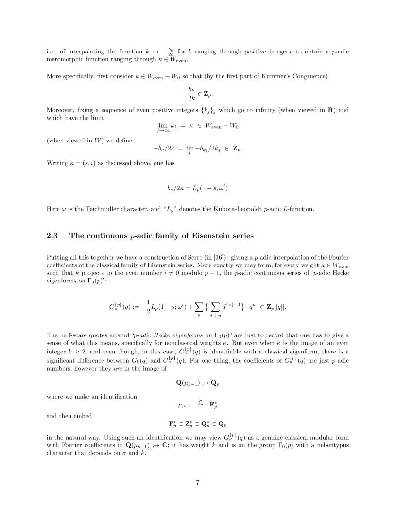
Putting all this together we have a construction of Serre (in [16]): giving a p-adic interpolation of the Fouriercoefficients of the classical family of Eisenstein series. More exactly we may form, for every weight κ ∈Weven

such that κ projects to the even number i 6= 0 modulo p − 1, the p-adic continuous series of ‘p-adic Heckeeigenforms on Γ0(p)’:

G{p}κ (q) := −1

2Lp(1− s;ωi) +

∑n

{ ∑d | n

d{κ}−1}· qn ⊂ Zp[[q]].

The half-scare quotes around ‘p-adic Hecke eigenforms on Γ0(p)’ are just to record that one has to give asense of what this means, specifically for nonclassical weights κ. But even when κ is the image of an even

integer k ≥ 2, and even though, in this case, G{p}κ (q) is identifiable with a classical eigenform, there is a

significant difference between Gk(q) and G{p}κ (q). For one thing, the coefficients of G

{p}κ (q) are just p-adic

numbers; however they are in the image of

Q(µp−1) ↪→ Qp

where we make an identificationµp−1

σ' F∗p

and then embedF∗p ⊂ Z∗p ⊂ Q∗p ⊂ Qp

in the natural way. Using such an identification we may view G{p}κ (q) as a genuine classical modular form

with Fourier coefficients in Q(µp−1) ↪→ C; it has weight k and is on the group Γ0(p) with a nebentypuscharacter that depends on σ and k.

7

Also, we don’t just throw away the Eisenstein series with weights 2 ≤ k ≡ 0 mod p − 1, these having—bythe von Staudt-Clausen Theorem—a constant term − bk

2k with negative ordp. We have other plans for theseEisenstein series: We just divide by their constant terms to get a sequence

Ek(q) = 1− 2k

bk

∞∑n=1

{ ∑d | n

dk−1}qn

which has the very useful property of being ≡ 1 mod p, and which interpolates to give another family

E{p}κ (q)

for κ ∈ W0 ⊂ Weven. The Fourier expansion of any member of this family is congruent to 1 mod p, and ifκ = 0 ∈W0 then

E{p}κ (q) = E{p}0 (q) = 1,

a fact that plays an important role in this story.

These families of eigenfunctions, varying p-adic analytically in their weights were first put forward by Serre,and can be viewed as the starting point of a significant amount of modern (p-adic) number theory.

It is natural to try to compare these families, for example, with the so-called “non-analytic” family ofcomplex Eisenstein series—eigenfunctions of the Laplacian on the upper half-plane—that, at least, haveFourier coefficients varying as functions of a complex parameter s:

Eis{∞}s (z) :=1

2

∑gcd(m,n)=1

ys

|mz + n|2s

for z = x + iy in the upper half plane y > 0 that had beginnings in work of Hecke and Reidemeister, andwas developed by Maass (and, of course, later much more substantially developed by Langlands). Thesetwo families—the p-adic Eisenstein family and the nonanalytic complex Eisenstein family2—are parallel ina certain sense and can be thought of as being (part of) the ‘continuous spectrum’ of the eigenfunctiondecomposition of Banach and Hilbert spaces of modular functions. In the complex case the existence of sucha continuous L2-spectrum is related to the noncompactness of the fundamental domain due to the allowedbehavior of these Eisenstein series at the cusps. In the p-adic case, one has the analogous relationship to thecusps; but as Hida has taught us, there are p-adic surprises coming from the so-called “discrete spectrum”here.

2.4 Noncompactness and continuous spectra

These p-adic modular eigenfunctions, and all the others we will be dealing with today all have the technicalproperty of being overconvergent in the sense that

2One can also consider in the roster of Eisenstein-families, the more naive analytic family parametrized by thecomplex variable s with Fourier series:

1

2ζ(1− s) +

∞∑n=1

{∑d | n

ds−1}qn.

8

• they can be viewed ‘geometrically’ as sections of the appropriate line bundle on the appropriate p-adicmodular curve,

• they are allowed to have essential singularities–but only of a specific controlled type—in small p-adicdiscs centered above the supersingular points in characteristic p. (To a p-adic modular form, everymodular curve is noncompact!)

The Hecke operators and the Up operator act as correspondences on the modular curves and induce op-erators on the corresponding spaces of overconvergent sections. By “eigenform” we will always mean anoverconvergent p-adic modular form that is an eigenvector for the appropriate Hecke operators. Since thesesections may have (allowed) singularities at the supersingular points, one is dealing with noncompactness—when working with any of these families—whether or not one requires regularity at the cusps. This is theunderlying reason why there can be continuous families of p-adic cuspforms, i.e., despite the fact that theclassical members of the family correspond to the discrete series in the (classical) harmonic analysis of thesemodular curves.

3 Hida’s early work on the L-function of the adjoint representa-tion

3.1 f-Intrinsic versus f-extrinsic concepts

Let us return to the quotation from Hida’s 1981 article [3] that we started with this hour:

“ We are going to establish a coincidence of the following two rational numbers; namely:

D(f) := { the discriminant of the Q-bilinear form associated to the primitive cusp form f }

9

and

L(f) := { the rational part of the special value at the integer k of the ‘zeta function’ associated with f }

As an application of this fact, one can prove congruences between this cusp form and another(non-congruent) cusp form.”

To connect this with the title of this section, the “D(f)” will be the f -extrinsic concept in that its definitioninvolves consideration of the placement of f among all the eigenforms of its own weight and level; the “L(f)”is f -intrinsic insofar as its direct calculation involves only constructions related to f alone.

For this lecture, let’s just concern ourselves with the rational prime divisors p of these numbers D(f) andL(f) and also only those p that are large compared to the weight k ≥ 2, where—to be very specific—largemeans that p > max{k − 2, 3}.

3.2 The large prime divisors of D(f)

These are the (large) primes dividing the order of the fundamental module that describes—essentiallytautologically—all possible congruences that f or its Q-conjugates can have with other eigenforms of itsweight and level. They are also what might be called primes of fusion. To be specific, for example, let f bea newform of weight k ≥ 2 on Γ0(N) and let S := Sk(N)new denote the complex vector space generated byall cuspidal newforms of weight k on Γ0(N). Let Sf = C · f ⊂ S be the complex line generated by f , andSf ⊂ S the orthogonal complement to Sf under the Peterson inner product. So,

S = Sf ⊕ Sf .

Now let T := Tk(N)new be the Z-algebra acting faithfully on S = Sk(N)new generated over Z by the Heckeoperators T` for ` not dividing N and by the Atkin-Lehner automorphisms and U` operators for ` | N . LetTf and Tf denote the quotient (Z-)algebras of T that operate faithfully on Sf and Sf respectively. So Tf

can be seen to be a sub-ring in the ring of integers of a number field3 and more specifically, Tf is the subringgenerated by the Fourier coefficients of all Q-conjugates of f . Denoting by πf : T → Tf and πf : T → Tf

the natural surjections, we get an injection of T-modules,

Tπ−→ Tf

⊕Tf ,

where π := πf ⊕ πf . Viewing this geometrically on spectra, we have the picture

3that happens to be totally real, since we are dealing with Γ0

10

and the primes of fusion associated to f measure the intersection of Spec(Tf ) and Spec(Tf ) viewed asclosed subschemes of Spec(T). To phrase things more algebraically: since πf and πf are surjections, thecokernel of π is seen to be a finite cyclic T-module, projecting isomorphically to (finite cyclic, of course)Tf - and Tf -modules under the homomorphisms πf and πf , respectively. The annihilator ideal of this cyclicTf -module is an ideal, If ⊂ Tf , that might be called the congruence ideal of f . Any prime p dividingthe order of its index could be called a prime of fusion for f .

3.3 The large prime divisors of L(f)

Here, to be notationally as simple as possible but still retaining the essence of the idea, suppose that oureigenform f has rational integral coefficients; equivalently Tf = Z. So our congruence module If ⊂ Tf isgenerated by an integer cf > 0. The formula for L(f) is then given by:

L(f) = {elementary term} · ω(f)

πk+1· Z(f, k)

where

• the “elementary term” is a truly elementary rational number: a power of 2 times a power of 3 times(k − 1)!Nφ(N),

• ω(f) is a certain period, and

• Z(f, k) is the value at s = k of the ‘zeta function’ we mentioned at the beginning of the hour4.

4i.e., Z(f, s) = L(symm2(f), s) is the entire function extending the Dirichlet series L(symm2(f), s) =∏p L{p}(symm2(f), s) where L{p}(symm2(f), s) is the appropriate Euler factor at p, which at good primes p is

given by the formulaL{p}(symm2(f), s) = (1− α2

pp−s)−1(1− pk−1−s)−1(1− β2

pp−s)−1

where αp, βp are the roots of the quadratic polynomial X2 − apX + pk−1 and ap is the p-th coefficient of the Fourier

11

By theorems of Sturm [18] and Shimura [17] this L(f) is a rational number.

Now the reason for the label f -intrinsic for this type of information about f is that—as you can see—no dataregarding modular eigenforms other than f itself has been invoked. And, yet(!) given Hida’s theorem relatingthe large prime divisors of L(f) to those of D(f), any such prime divisor p of this f -intrinsic quantity predictsthe existence of some other eigenform of the same weight and level as f , admitting a mod p congruence tof .

We’ll discuss why this is so, in a while, but first, a comment about “predictions,” and then a few randomlychosen examples.

3.4 Predictions

Hida’s result, that the large prime divisors of D(f) are equal to the large prime divisors of L(f) gives us,then, two ways of obtaining those prime divisors: either by computing D(f)—which is perhaps best donevia modular symbols technology—or L(f), where the natural computations to make (of period and L-value)are of quite a different sort. It would be interesting to get good asymptotic bounds for the running timesrelative to weight and conductor of each of these kinds of algorithms to see which side “wins,” and when.My guess is that, in general, the modular symbols methods are significantly faster, but that when restrictingattention to certain types of eigenforms—for example, CM-forms—the L(f)-computation may very well winasymptotically5. I.e., so that one does get a serious pre-diction of new eigenforms congruent to the given f .See, for example, the illuminating computations of Hida on page 259 of [3], one of which we will make useof in subsection 3.5 below.

Given the current interest in algorithms, and given our capability of making large computational experiments,one can be motivated to view certain equations as saying—among whatever else they are saying— that thealgorithm implied by the RHS has the same outcome as the algorithm implied by the LHS, and therefore asraising the subsidiary problem of determining the comparative asymptotic time-estimates for each of those

expansionf(q) = q1 + a2q

2 + a3q3 + · · ·

5Commenting on an early draft of these notes, William Stein wrote:

I agree that the L-functions method to compute this number will win – dramatically – if you’re in*any* situation where you somehow know a lot of coefficients of the modular form. One example is CMforms, but there are others, e.g., anything that can be expressed in terms of CM forms and forms withknown q-expansions like Eisenstein series (I have a recent paper http://wstein.org/papers/nimft/

with Coates, Dokchitser, etc., where we compute certain special values for non-CM f using that weknow lots of coefficients). Another situation is computing modular degrees, where Mark Watkins’sapproach via Flach/Shimura’s formula is dramatically faster than using modular symbols, since oneknows the ap for an elliptic curve efficiently; until about 15 years ago, everybody computed thesemodular degrees using modular symbols, which was massively slower. Using Watkins’s approach, onecan predict congruences (by computing modular degrees) that are infeasible to ever actually see, e.g.,the first (known) curve of rank 5 has modular degree 27∗258659. Thus there is a mod 258659 congruencebetween the newform f attached to the elliptic curve y2 + y = x3 − 79x+ 342 and some newform g inS2(Γ0(19047851)); note that 19047851 is a prime. That newform f is *probably* defined over a numberfield of degree around 793660 = [(dimS2)/2], and it’s not likely anybody could ever write down g. Inshort, we know—because of L(f)—that there is a congruence f ≡ g mod 258659, but, beyond this, weknow absolutely nothing explicit about g, not even the degree of the field it is really defined over (withcertainty), and it isn’t currently feasible as far as I can tell to compute anything about g either. Thisis a very concrete example of how L(f) can, at times, be more approachable than D(f).

12

algorithms; briefly, asking the question: under varying conditions of the computation, which side of theequation can be used more efficiently?

3.5 Two randomly chosen examples

1. Let K = Q(ζ3) where ζ3 is a primitive third root of unity, and denote by A := Z(ζ3) ⊂ K the ring ofintegers in K. Form the CM eigenform on Γ1(3) of weight 13:

f(q) :=1

6

∑a∈A

a12qNa

where Na ≥ 1 is the norm of a. One can compute—by either the D(f) or L(f) route—that 13 is theunique ‘large’ prime dividing these common numbers—predicting the existence of some cusp form gin S13(Γ1(3)) (different from f) with its Fourier coefficients congruent ‘modulo 13’ to f . I’m thankfulto Ben Lundell for communicating to me that

f(q) = q + 729q3 + 4096q4 − 153502q7 + 531441q9 + 2985984q12 − 9397582q13+

+16777216q16 + 17886962q19 +O(q20),

and that in the three dimensional space S13(Γ1(3)) the other two newforms in S13(Γ1(3)) are Galoisconjugates (pick one and call it g), and have Fourier coefficients in the field Q(

√−26). So there is a

unique prime P above p = 13 in the ring generated by the Fourier coefficients of g, and (as followsfrom Hida’s Theorem) one indeed has that modulo P the Fourier coefficients of g are equal to thoseof f mod 13.

2. The smallest prime number N for which there are two non-Galois-conjugate newforms of weight 2with ”even parity,” i.e., Atkin-Lehner eigenvalue −1 is N = 67. Letting f be the eigenform associatedto the unique isogeny class of elliptic curves of conductor 67 with even parity, one computes that thereis a prime of fusion (namely p = 5) and that p = 5 is the unique ‘large prime’ dividing D(f) is 5, andindeed there is an eigenform g such that the field generated by its Fourier coefficients is Q(

√5) and

modulo the unique prime above 5 in the ring generated by its Fourier coefficients it is congruent to f .

Regarding this example, I should also say that I know of no Hecke algebra T = Tnewk (Γ0(N); ε)

associated to newforms of weight k on Γ0(N) for N squarefree and with prescribed signs ε for allAtkin-Lehner operators6 with the property that Spec(T) is disconnected; i.e., such that Spec(T) hasmultiple components and yet there is no prime of fusion “connecting them.”

Question 1. Is there an example of such a Spec(T) that is disconnected?

For computations inspired by Maeda’s Conjecture, that raise the very interesting question of irre-ducibility of such Hecke algebras Tnew

k (Γ0(N); ε) for N squarefree and k >> 0, see [19].

3.6 The theme of deformations

weight constant Rather than attempting to outline a proof of Hida’s theorem relating D(f) to L(f)—whichwould take up this entire introductory hour—it makes sense to restrict the discussion to a few words aboutHida’s insight as seen from the vantage point of lots that have gone on in our subject since 1981; thisviewpoint includes later results of Hida himself, of Flach, Wiles, Taylor, Kisin, and others. The aim here

6I.e., ε : ` 7→ ε(`) ∈ {±1} is the function on newforms f ∈ Tnewk (Γ0(N); ε) that give the eigenvalues of the

Atkin-Lehner operators; i.e., we have w`f = ε(`) · f for all `| N .

13

is to hint about why it is not unnatural for the f -intrinsic number L(f) to predict the existence of ‘other’eigenforms.

Briefly, L(f) can be understood as related to deformations. If V is the (`-adic) Galois representation attachedto the eigenform f and to its ‘standard’ L-function, which is the analytic continuation of a Dirichlet serieswhose Euler factor at any ‘good’ prime p is

(1− αpp−s)−1(1− βpp−s)−1

then End0(V ), the trace zero endomorphism ring of V endowed with the adjoint Galois representation, isattached (after appropriate Tate twist) to the symmetric square automorphic form symm2(f) and to the‘zeta function’

L(symm2(f), s) = Z(f, s)

which is the analytic continuation of a Dirichlet series whose Euler factor at any ‘good’ prime p is

(1− α2pp−s)−1(1− pk−1−s)−1(1− β2

pp−s)−1,

i.e., Z(f, s) is the ‘zeta function’ we have been discussing, whose special value Z(f, k) (times the appropriateperiod) gives us L(f).

The gateway to Galois deformations of V (deformations that keep the weight constant and are requiredto satisfy various further features) is given by the appropriate cohomology of the adjoint representationEnd0(V )—indeed the cohomology subject to local conditions (i.e., Selmer group conditions) connected tothe features desired for those deformations. An analogue of the Birch- Swinnerton-Dyer conjecture associatedto the automorphic form symm2(f) would then make it “not unnatural” to imagine the connection betweenL(f) and D(f). This connection was what Hida established directly, way back then.

Having introduced the theme, deformations, it is time to pass to one of Hida’s grand theories having to dowith p-adic deformations of cuspforms (‘ordinary’ at p) of varying weight.

4 Hida’s p-ordinary cuspidal families

4.1 Revisiting the noncupidal families

We have already discusses p-adically varying families of objects parametrized by p-adic weight space; namelythe p-adic Eisenstein families of Serre for κ ∈Weven:

G{p}κ (q), E{p}κ (q).

Each G{p}κ (q) is an eigenvector for the Hecke operators T` for ` - p:

T`G{p}κ = (1 + `{κ})G{p}κ

and is fixed by the operator Up:

UpG{p}κ = G{p}κ ,

14

and similarly with E{p}κ (q).

We can consider these noncuspidal families as setting up the prototype for Hida’s vastly interesting class ofp-adically varying continuous families (not merely of Eisenstein series, but) of p-ordinary p-adic cuspformsconstructed by Hida.

4.2 The basic vocabulary of Hida’s theory

Definition 1. 1. (The Up-operator): If

f(q) =∑n

a(n)qn

is a power series let

Upf(q) :=∑n

a(pn)qn.

(The classical Hecke operator Up acting on modular forms on Γ0(N)—if p | N—acts on Fourier seriesat the cusp ∞ via this formula.)

2. (The p-ordinary condition): If f(q) ∈ Zp[[q]] (or, more generally, in A[[q]] where A is a discretevaluation ring which is a finite extension of Zp) say that f(q) is a p-ordinary eigenvector for Up if itis an eigenvector,

Upf = up · f,and its eigenvalue up is a unit in Zp (or in the DVR A).

3. (The p-ordinary projection operator): If f(q) ∈ Zp[[q]] consider the following limit :

ford := limt→∞

Uφ(pt)

p f.

which (if it exists) will be called the ordinary projection7 of f .

The ordinary projection operator is key to this theory; it is somewhat analogous to ‘harmonic projection’ inclassical analysis. Note, for example, if f is a finite sum of Up-eigenfunctions then ford will be the sum ofall the p-ordinary eigenfunctions among them.

The key theorem that controls the rest of this extraordinary theory is the following. Let Sk(Γ1(N); Zp) bethe Zp-module of “classical” cuspidal modular forms of weight k on Γ1(N) with Fourier coefficients in thering8 Zp.

Theorem 1. (Hida’s theorem of constancy of p-ordinary rank) Let N = p ·N0 with N0 not divisibleby p. Then the rank of the p-ordinary subspace

Sordk (Γ1(N); Zp) ⊂ Sk(Γ1(N); Zp)

is independent of k if k > 2.

7More general, if the coefficients of f lie in a finite DVR extension A of Zp with uniformizer π define:

ford := limt→∞

U |(A/πtA)∗|

p f.

8You might wonder how you can get “classical” modular forms with coefficients in rings other than in C, but thereis a straightforward natural way of doing this by passing from Z ⊂ C to Z ⊂ Zp.

15

PutSordk (Γ1(N); Qp) := Sord

k (Γ1(N); Zp)⊗Qp.

Colloquially, one can say that the number of ‘distinct’ p-ordinary (cuspidal) eigenforms in Sk(Γ1(N); Qp) isconstant (k > 2).

If you are interested in the number of distinct p-ordinary (cuspidal) eigenforms of weight k on Γ0(N) withfixed character ψ, this is periodic in the weight (> 2) with period p − 1. More precisely, the dimension ofthe Qp-vector space

Sordk (Γ0(N), ψω−k; Qp).

is constant. For a discussion of this, with more related information specifically about weight k = 2 andp-ordinary forms on Γ1(Np), see sections 1 and 2 of [11].

A large-scale numerical investigation of the statistics of ordinary rank9 might be an interesting project; e.g.,what can one say about the distribution of the arithmetic function

rord(p, i) := dimSordk (Γ0(p); Qp)

for k ≡ i mod p?

This boils down to a computation of the characteristic polygon (mod p) of Tp acting on weight k cuspformsof level 1.

I asked William Stein about this, and he very quickly produced some data, and on reviewing it we soonrealized that the essential data is best displayed if one has the following definition: For a given prime p andfor an even integer 2 ≤ k ≤ (p+ 3) by the p-ordinary defect of k let us mean the difference of dimensions:

δ(p, k) := dimSk(Γ0(p); Qp)− dimSordk (Γ0(p); Qp).

If the p-ordinary defect of k is zero, then every eigenform of low weight is p-ordinary. The followingsymmetry relationship holds for all data that he has computed so far (i.e. p < 389) :

δ(p, k) = δ(p, p+ 3− k).

Therefore the table below lists only pairs (p, k) for even integers 2 ≤ k ≤ (p+ 3)/2 with the understandingthat the full range k ≤ (p+ 3) can then be found, using the above symmetry 10.

9Kevin Buzzard had done such an investigation some years ago, and it might be good to extend the range of it.

10We see no reason for this symmetry to persist for all higher primes; see the appendix for the reason why —inany event—one might expect a close relationship between (p, k) and (p, p+ 3− k).

16

(p, k) defect(59,16) 1(79,38) 1(107,28) 1(131,40) 1(139,36) 1(151,60) 1(173,24) 1(193,72) 1(223,72) 1(229,116) 2(257,50) 1(257,100) 1(257,130) 2(263,98) 1(269,78) 1(277,92) 1(283,72) 2(307,78) 1(313,114) 1(331,84) 2(353,76) 2(379,56) 1

We have plans for a much larger project here.

4.3 A ‘first example’ of a Hida family

Let p be any prime in the range11 ≤ p ≤ 7 billion

except for p = 2411. (Visit the section “Conjecture on tau(n)” at wikipedia11 which lists p = 7758337633 asthe next prime number that should be avoided.)

For these primes p we have that the p-th Fourier coefficient, τ(p), of the classical newform ∆ (of weight 12and level 1) is a p-adic unit, and so we can factor

X2 − τ(p)X + p11 = (X − αp)(X − βp) ∈ Zp[X]

where one of these roots, say αp is a p-adic unit while ordp(βp) = 11.

Form∆{p}(z) := ∆(z)− βp∆(pz) ∈ S12(Γ0(p); Zp).

The newform ∆ is “p-ordinary” in the sense that ∆{p}, its ‘lifting’ to Γ0(p), is a p-ordinary eigenform for(the Hecke operator T` for all primes ` 6= p and also for) Up, where the eigenvalue of Up is a p-adic unit:

Up∆{p} = αp ·∆{p}.

Definition 2. A modular form that is an eigenvector for Up is said to be p-ordinary if its Up-eigenvalueis a p-adic unit.

11http://en.wikipedia.org/wiki/Tau-function#Conjectures_on

17

So ∆{p}(z) is indeed p-ordinary. Since ∆ is a generator of Sord12 (Γ0(1)) and since any newform in Sord

12 (Γ0(p))has slope12 5 = (12− 2)/2 it follows that ∆{p}(z) alone generates Sord

12 (Γ0(p); Qp).

Hida’s constant rank theorem then gives us that:

Corollary 2. The dimension ofSordk (Γ0(p), ω12−i; Qp)

is equal to 1 for all k ≥ 2.

Now multiply ∆{p} by the Eisenstein family E{p}κ —for

κ ∈W0 := {κ ∈W | κ ≡ 0 mod (p− 1)}.

Note two things: Since the Fourier expansion of E{p}κ is congruent to 1 = 1 + 0 · q + 0 · q2 + · · · modulo p,

it follows that for any κ ∈ W0, the Fourier expansion of the product, ∆{p} · E{p}κ , is congruent modulo p to

the Fourier expansion of ∆{p}. Moreover, since E{p}0 = 1 the product, ∆{p} · E{p}κ in weight κ = 12, is just

∆{p}.

Now apply the p-ordinary projection operator (which we can show converges). We get a family

F{p}12+κ := {∆{p} · E{p}κ }ord

with extraordinary properties:

1. F{p}12 := ∆{p}.

2. For any κ ∈ W0, the Fourier expansion of F{p}κ , is congruent modulo p to the Fourier expansion of∆{p}.

3. If κ ∈ W0 is the image of the integer k ≥ 2, then F{p}κ+12 is the unique generator of Sordk+12(Γ0(p); Qp).

In particular13 it is an eigenvector for the Hecke operator T` for all primes ` 6= p and also for Up.

4. This familyκ 7→ F{p}κ

defined for κ ∈ W0 extends14 to a family κ 7→ F{p}κ defined for all κ ∈ W with essentially the

same properties, except that at any classical weight 2 ≤ k = κ ∈ Wi the p-adic modular form F{p}κ

corresponds to a classical modular (cuspidal p-ordinary) eigenform15 on Γ0(p) with nebentypus ω−i.

5. The extended family κ 7→ F{p}κ has a p-adic integral structure. To prepare to explain this, form

Λ := Zp[[Z∗p]],

12The slope of a Up-eigenform is the p-adic ord of its Up-eigenvalue.

13since it is the unique generator, and the Hecke operators preserve Sordk+12(Γ0(p);Qp),

14To get the extension of this family to Wi for any i ∈ Z/(p− 1)Z perform the same construction starting not with∆ but rather with a generator of Sord

k (Γ0(p), ω12−i;Qp).

15It follows by continuity that for every κ ∈ W , F{p}κ is an eigenvector for the Hecke operator T` for all primes` 6= p and also for Up.

18

the Iwasawa ring. There is a natural homomomorphism W → End(Z∗p) and any endomorphism ofZ∗p extends to a ring homomorphism

Λ := Zp[[Z∗p]]→ Zp.

In this manner, every κ ∈ W gives us, in a natural way, a ring homomorphism which we’ll denote bythe same letter:

κ : Λ→ Zp.

For the family κ 7→ F{p}κ (with κ ∈W ) that we have been discussing we have the following theorem:

Theorem 3. For any prime ` 6= p there is an element t` ∈ Λ such that for any κ ∈W the eigenvalue

of T` acting on F{p}κ is equal to κ(t`) ∈ Zp. Also, there is an element up ∈ Λ such that for any κ ∈Wthe eigenvalue of Up acting on F{p}κ is equal to κ(up) ∈ Zp.

4.4 Hida Families for GL2 over Q

We have given an example, in the previous subsection, where Hida’s theorem gave us constant p-ordinaryrank 1. We constructed a family of p-ordinary p-adic cuspidal eigenforms—a p-adic analytic curve—thatprojected isomorphically onto weight space (a union of p− 1 discs. The construction, though is vastly moregeneral. For any N = p ·No with (p,No) = 1, if

dimQp Sordk (Γ0(N), ψ; Qp) = r

one obtains a p-adic analytic family of p-ordinary p-adic cuspidal eigenforms f forming a p-adic analyticspace H →W projecting by a finite flat mapping of degree r to the corresponding weight space:

19

These are the Hida Families. Slightly more technically, we may view Hida families as p-adic rigid analyticspaces w : H →W and consequently we talk of their points rational over Qp which is, in effect, all that wehave done so far; or we can also go further and consider their rational points over extension fields of Qp suchas Tate’s “p-adic complex numbers,” Cp := the p-adic completion of the algebraic closure of Qp. The Heckeoperators T` for primes ` not dividing the level N , or the U` for ` | N act in a rigid p-adic analytic manner onthe points f of H and their eigenvalues as functions of f then give us rigid p-adic analytic functions T` 7→ T`and U` 7→ U` on the p-adic analytic space H.

Even more striking is that Hida families all have analogous very tight p-adic integral structures as in Theorem3 above16. That is, any Hida family is a component or union of components of the rigid analytic spaceattached to some “Hida-Hecke algebra” T.

These Hida-Hecke algebras T contain elements identified with Hecke operators and have the property thatfor any continuous homomorphism h : T→ Cp there is an overconvergent p-ordinary cuspidal eigenform fhsuch that for all primes ` the image of T` ∈ T (resp., U` ∈ T) under h gives the eigenvalue of the actionof T` (resp., U`) on fh. Moreover, every classical17 p-ordinary cuspidal eigenform is a member of some Hidafamily.

4.5 The corresponding Galois representations

Over every Hida family of level N viewed as p-adic rigid analytic space w : H → W , there is a canonicaltwo-dimensional vector bundle18 V with continuous action of the absolute Galois group GQ := Gal(Q) on(the p-adic rigid analytic vector bundle) V over H,

ρ : GQ → AutH(V ),

with the property that

• ρ is unramified outside the level N = Nop and

• the trace of the action of the Frobenius element(s) attached to any prime ` - N on points f of H—whenviewed as function on H—is equal to the function T` defined in the previous subsection19.

(It is also true that the determinant, det(ρ) : H → Gm, is essentially–after mild renormalization, equal tothe projection to weight space, w : H →W .)

This associates to any Hida family H → W of level H = Nop a corresponding rigid p-analytic family ofG{Q,N}- representations parametrized by H. Here G{Q,N} is the Galois group of a maximal subextension,Galois over Q, of an algebraic closure of Q that is unramified for all primes not dividing N . So, if we let

16This p-adic integrality feature of Hida families—plus the fact that the mapping to weight space is of finite degree—is where, at least at present–Hida families, which correspond to the “slope zero” part of the eigencurve, distinguishthemselves from the other components of the eigencurve that parametrize p-adic overconvergent eigenforms of finitepositive slope.

17or more generally overconvergent

18This vector bundle with Galois action is elegantly constructed by applying the p-ordinary projection operator toan appropriate limit of p-adic cohomology of a sequence of modular curves where p-power of the level of these curvestends to infinity.

19i.e., is equal to the eigenvalue of T` on f for f varying through the points of H.

20

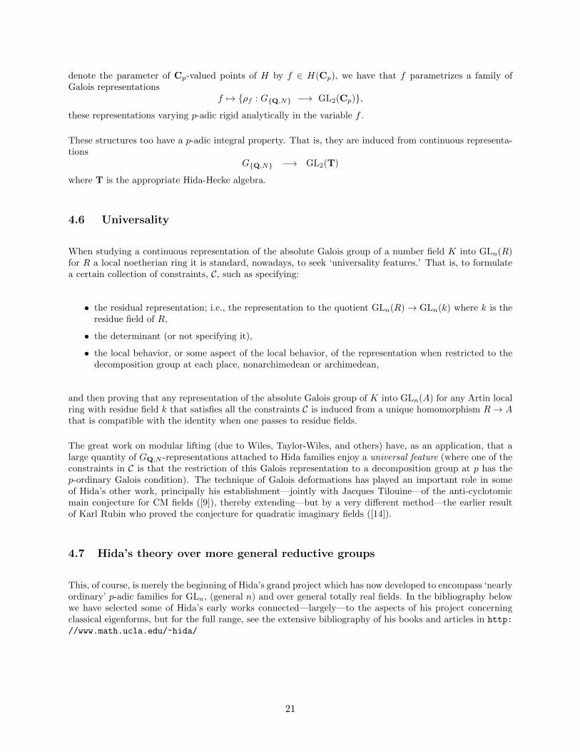
denote the parameter of Cp-valued points of H by f ∈ H(Cp), we have that f parametrizes a family ofGalois representations

f 7→ {ρf : G{Q,N} −→ GL2(Cp)},

these representations varying p-adic rigid analytically in the variable f .

These structures too have a p-adic integral property. That is, they are induced from continuous representa-tions

G{Q,N} −→ GL2(T)

where T is the appropriate Hida-Hecke algebra.

4.6 Universality

When studying a continuous representation of the absolute Galois group of a number field K into GLn(R)for R a local noetherian ring it is standard, nowadays, to seek ‘universality features.’ That is, to formulatea certain collection of constraints, C, such as specifying:

• the residual representation; i.e., the representation to the quotient GLn(R)→ GLn(k) where k is theresidue field of R,

• the determinant (or not specifying it),

• the local behavior, or some aspect of the local behavior, of the representation when restricted to thedecomposition group at each place, nonarchimedean or archimedean,

and then proving that any representation of the absolute Galois group of K into GLn(A) for any Artin localring with residue field k that satisfies all the constraints C is induced from a unique homomorphism R→ Athat is compatible with the identity when one passes to residue fields.

The great work on modular lifting (due to Wiles, Taylor-Wiles, and others) have, as an application, that alarge quantity of GQ,N -representations attached to Hida families enjoy a universal feature (where one of theconstraints in C is that the restriction of this Galois representation to a decomposition group at p has thep-ordinary Galois condition). The technique of Galois deformations has played an important role in someof Hida’s other work, principally his establishment—jointly with Jacques Tilouine—of the anti-cyclotomicmain conjecture for CM fields ([9]), thereby extending—but by a very different method—the earlier resultof Karl Rubin who proved the conjecture for quadratic imaginary fields ([14]).

4.7 Hida’s theory over more general reductive groups

This, of course, is merely the beginning of Hida’s grand project which has now developed to encompass ‘nearlyordinary’ p-adic families for GLn, (general n) and over general totally real fields. In the bibliography belowwe have selected some of Hida’s early works connected—largely—to the aspects of his project concerningclassical eigenforms, but for the full range, see the extensive bibliography of his books and articles in http:

//www.math.ucla.edu/~hida/

21

5 Returning to adjoint representations and the geometry of Hidafamilies

5.1 The branch locus

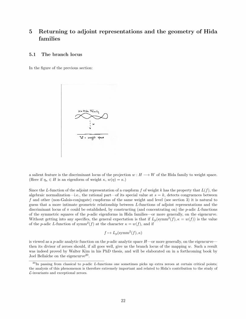
In the figure of the previous section:

a salient feature is the discriminant locus of the projection w : H −→W of the Hida family to weight space.(Here if ηκ ∈ H is an eigenform of weight κ, w(η) = κ.)

Since the L-function of the adjoint representation of a cuspform f of weight k has the property that L(f), thealgebraic normalization—i.e., the rational part—of its special value at s = k, detects congruences betweenf and other (non-Galois-conjugate) cuspforms of the same weight and level (see section 3) it is natural toguess that a more intimate geometric relationship between L-functions of adjoint representations and thediscriminant locus of π could be established, by constructing (and concentrating on) the p-adic L-functionsof the symmetric squares of the p-adic eigenforms in Hida families—or more generally, on the eigencurve.Without getting into any specifics, the general expectation is that if Lp(symm2(f), κ = w(f)) is the valueof the p-adic L-function of symm2(f) at the character κ = w(f), and if

f 7→ Lp(symm2(f), κ)

is viewed as a p-adic analytic function on the p-adic analytic space H—or more generally, on the eigencurve—then its divisor of zeroes should, if all goes well, give us the branch locus of the mapping w. Such a resultwas indeed proved by Walter Kim in his PhD thesis, and will be elaborated on in a forthcoming book byJoel Bellaıche on the eigencurve20.

20In passing from classical to p-adic L-functions one sometimes picks up extra zeroes at certain critical points;the analysis of this phenomenon is therefore extremely important and related to Hida’s contribution to the study ofL-invariants and exceptional zeroes.

22

5.2 The collisions between the Eisenstein locus and Hida families

Returning to the family of p-adic overconvergent eigenforms given by Eisenstein series

κ 7→ G{p}κ (q) = −1

2Lp(1− s;ωi) +

∑n

{ ∑d | n

d{κ}−1}· qn ⊂ Zp[[q]]

for κ ∈Weven one immediately notices that for every zero of the Kubota-Leopoldt L-function (i.e., for the κ’s

such that Lp(1−s;ωi) = 0) the corresponding p-adic eigenform G{p}κ (q) is, in effect, cuspidal. Consequently—

by the claim at the end of subsection 4.4—is a member of some Hida family of cuspidal eigenforms. Thereare, of course, mysteries here.

5.3 The Archimedean question

Since, for any prime number p, any p-adic overconvergent p-ordinary eigenform (Eisenstein or cuspidal) ‘fitsinto’ a natural one-parameter family of such eigenforms varying p-adic analytically over weight space, it isnatural to wonder whether there is some archimedean version of this theory that somehow embraces classicalcuspforms, despite the fact that they correspond to the discrete part of the spectrum. And if not, why not?

Are there such families21 other than the continuous families of complex Eisenstein series described in sub-

21together with a well-working “U∞-operator”

23

section 2.2 above; either the non-analytic version

Eis{∞}s (z) :=1

2

∑gcd(m,n)=1

ys

|mz + n|2s

or the analytic one alluded to in the footnote in that subsection22?

6 Appendix: a ‘near-symmetry’ of p-defect

Definition 3. If p > 2 is a prime number and k an even number in the range:

1 < k < p+ 3

say that (p, k) is admissible.

Definition 4. Say that an odd representation

ρ : GQ,{p,∞} → GL(Fp)

contributes to an admissible pair (p, k) if there is a newform f of level 1 and weight k whose associatedGQ-representation mod π is equivalent to ρ. Here π is some prime ideal in Of (the ring of Fourier coefficientsof f) with residue field F := Of/π of characteristic p.

6.1 The case where the mod p GQp-representation is irreducible

Definition 5. Say that an admissible (p, k) is exceptional if there is a newform f of level 1 and weight kwhose associated GQp

-representation mod π is irreducible.

One can extract the following theorem from the literature.

Theorem 4. The pair (p, k) is exceptional if and only if (p, p+ 3− k) is exceptional.

Proof: We use the discussion directly after the statement of the Theorem on section 4.5 in [2]; compareLemma 3.17 of [1]. The general set-up and notation follows Serre’s classical article [15].

As mentioned in section 4.5 of [2], the content of Theorem 4 is essentially a consequence of Prop. 3.3 (ofloc.cit.). Namely, consider an odd representation

ρ : GQ,{p,∞} → GL(Fp).

22That is,

Es(q) :=1

2ζ(1− s) +

∞∑n=1

{∑d | n

ds−1}qn,

whose Fourier coefficients lie in a ring, Λ∞, of complex analytic functions expressible as Dirichlet series in appropriatehalf-planes, and that extend to meromorphic functions on the entire plane, with certain growth conditions.

24

If the GQp-representation induced from ρ is irreducible, and if the two (diagonal) characters of niveau 2

associated to this representation are ψa, ψ′b where ψ,ψ′ = ψp are the two fundamental characters of niveau2, and 0 ≤ a < b ≤ p − 1, then we have the following facts regarding modularity of ρ. To be sure, ρ ismodular, thanks to Khare and Wintenberger. Moreover ρ arises from some–in fact many—newforms of levelone (i.e., arises as the mod π-representation associated to a modular newform f of level 1 where π ⊂ Of isa prime ideal of residual characteristic p in Of , the ring generated by the Fourier coefficients of the newformf). The question, then, is to find the list of weights k ≤ p+ 3 that correspond to such newforms f . Readingthe list given in section 4.5 of loc. cit., we see that the realizable k’s (for k ≤ p+ 3) are: k1 = 1 + b− a andk2 = p+ 2 + a− b = p+ 3− k1. So, this gives a stronger result than Theorem 4:

Theorem 5. If an odd representation

ρ : GQ,{p,∞} → GL(Fp)

whose associated GQp-representation is irreducible contributes to (p, k) then a twist of it contributes to (p, k);moreover no other twist contributes to an admissible pair.

6.2 The case where the mod p GQp-representation is indecomposable but notirreducible

Now suppose have an odd representation

ρ : GQ,{p,∞} → GL(Fp)

whose restriction to GQp is reducible. Let the two (diagonal) characters of niveau 1 be ωb, ωa where ω is theTeichmuller character, a, b are in the range [0, p− 1], and if the splitting field of ρ is wildly ramified, i.e., ifthe representation restricted to GQp

is given as

[ωb ∗0 ωa

]and “∗ 6= 0,” then the two diagonal characters occur in the indicated order, and we’ve normalized

as in Serre’s original article; i.e., 0 ≤ a < p− 1 and 0 < b ≤ p− 1.

Suppose first that “∗ 6= 0.” Reading section 4.5 of loc. cit., we see that there is only one twist of ρ by apower of the Teichmuller character that comes from a newform f of weight k in the range 2 ≤ k < p + 3,namely ρ⊗ω−a. In this case, f is p-ordinary. (So, we’re happy.) What is left is the reducible split case, i.e.,where ρ is the direct sum of two characters.

6.3 The case where the mod p GQp-representation is semisimple, and not irre-ducible

Here is where it gets interesting. The pertinent invariants for such a representation is the pair (a, b) as inthe previous subsection.

Definition 6. Say that an admissible (p, k) contains an (a, b) (we may as well normalize so that a ≤ b

and both lie in the range [0, p − 2]) if there is a ρ whose restriction to GQp is

[ωb 00 ωa

]and such that ρ

is associated to a newform of level 1 and weight k.

Using the discussion of section 4.5 in Eidixhoven, and the general literature (including results of Gross,Coleman & Voloch, and Faltings & Jordan) as reviewed in [1], it seems that the “’symmetry’” enjoyed by

25

the exceptional (p, k) in the range currently calculated may not quite be enjoyed by the admissible (p, k)’sthat contain (a, b)’s. Some of these (a, b)’s contained in admissible (p, k)’s are ordinary, but as mentionedalready, William Stein and I have a project to examine the data regarding these issues more extensively.

References

[1] K. Buzzard, F. Diamond, F. Jarvis On Serre’s Conjecture for mod ` Galois representations over totallyreal fields, Duke Math J. 155 (2010) 105-161

[2] B. Edixhoven, The weight in Serres conjectures on modular forms Invent. Math. 109 (1992), no. 3,563-594.

[3] H. Hida, Congruences of Cusp Forms and Special values of Their Zeta Functions, Inventiones Mathe-maticae Volume 63, Number 2 (1981), 225-261

[4] H. Hida, Galois representations into GL2(Zp[[X]]) attached to ordinary cusp forms, Invent. Math. 85(1986), no. 3, 545–613

[5] H. Hida, On p-adic Hecke algebras for GL2 over totally real fields, Ann. of Math. 128 295-384 (1988)

[6] H. Hida, On nearly ordinary Hecke algebras for GL(2) over totally real fields, Advanced Studies in PureMath. 17, 139-169 (1989)

[7] H. Hida. p-ordinary cohomology groups for SL(2) over number fields. Duke Math. J. 69 (1993), no. 2,259–314.

[8] H. Hida, p-Adic ordinary Hecke algebras for GL(2), Ann. de l’Institut Fourier 44 1289-1322 (1994)

[9] H. Hida, J. Tilouine, On the anti-cyclotomic main conjecture for CM fields, Invent. Math. 117 (1994),89-147

[10] H. Hida, J. Tilouine and E. Urban, Adjoint modular Galois representations and their Selmer groups,Proc. Natl. Acad. Sci. USA 94, 11121-11124 (1997)

[11] H. Hida, Control Theorems and Applications, Lectures at Tata institute of fundamental research (Ver-sion of 2/15/00) [See http://www.math.ucla.edu/~hida/]

[12] H. Hida, Hilbert Modular Forms and Iwasawa Theory, Oxford University Press (2006)

[13] N. M. Katz, p-adic properties of modular schemes and modular forms, pp. 69-190 in Modular functions ofone variable, III (Proc. Internat. Summer School, Univ. Antwerp, 1972), Lecture Notes in Mathematics350 Springer (1973)

[14] K. Rubin, Karl, The “main conjectures” of Iwasawa theory for imaginary quadratic fields, InventionesMathematicae 103 (1): 25-68 (1991)

[15] J.-P. Serre, Sur les representations modulaires de degre 2 de Gal(Q/Q), Duke Math. J. 54 (1987)179-230.

[16] J.-P. Serre, Formes modulaires et fonctions zeta p-adiques, pp. 191-268 in Modular Functions of OneVariable III Lecture Notes in Mathematics, 350 (1973)

[17] G. Shimura, The special values of the zeta functions associated with cusp forms, Comm. Pure Appl.Math. 29 (1976), no. 6, 783804.

[18] J. Sturm, Special values of zeta functions, and Eisenstein series of half integral weight, Amer. J. Math.102, No. 2 (1980), 219-240

[19] P. Tsaknias, A possible generalization of Maeda’s conjecture, arXiv:1205.3420v1 [math.NT] 15 May2012

26