a cash flow based multi-period credit risk modelliao/paper0820a.pdf3 flow model”. with the cash...
TRANSCRIPT

A Cash Flow Based Multi-period Credit Risk Model
Tsung-kang Chen * Hsien-hsing Liao **
First Version: May 15, 2004 Current Version: August 20, 2004
ABSTRACT
Many credit risk models have been proposed in the literature. According to their
assumptions and emphases, they can be roughly grouped into two categories, “structural-form" models and “reduced-form” models. The former focuses on constructing the distribution of asset values and then estimating one-period probability of default and recovery rate; the latter relies on exogenous information such as credit rating and recovery rate which are not related to asset values. Within the frameworks of the above two categories, few studies use stochastic cash flow model to assess firm’s credit risk. Based upon the two significant cash flow characteristics- “mean-reversion” and “allowing positive or negative values” and the concept of varying coefficient model, the study develops a “Time-dependent stochastic cash flow model”. To consider future industrial economic state changes’ impacts on a firm’s cash flow, we also construct a stochastic model of industrial economic state. The information forecasted from the state model is used as the base for adjusting the parameters of the time-dependent cash flow model. To perform a multi-period firm valuation, this cash flow model needs only publicly available information of corporate finance and the industrial economic state (i.e. the industrial cyclicality information). With the information of a firm’s value and debt, a “Cash Flow Based Multi-period Credit Risk Model” can be built. We can then price the corporate debt by combining the expected recovery rate generated from our model and the concept of defaultable bond pricing of Jarrow-Turnbull Model (1995).
* Ph.D Student, Department of finance, National Taiwan University, Taiwan, [email protected] **Associate Professor, Department of finance, National Taiwan University, Taiwan, [email protected]

1
I. Introduction
Many credit risk models have been proposed in the literature. According to their
assumptions and emphases, they can be roughly categorized into “structural-form" models1
and “reduced-form” models2. The “structural-form" credit models focus on constructing
the distribution of a firm’s asset value and estimating probability of default (later denoted
as PD) and recovery rate (later denoted as RR). The “reduced-form" credit models on the
other hand stress the “non-asset-value related information”, such as credit rating (Litterman
and Iben, 1991; Jarrow, Lando and Turnbull, 1997) and recovery rate. They estimate and
price a firm’s credit risk by observable market credit spreads. This makes their models
closely linked to market’s current situation. Recently, some studies take into
consideration systematic risk and develop the so-called “single systematic factor models”3.
These models investigate the relationship between macroeconomic factors and credit risk
variables, such as PD and RR. They use historical data to establish a regression model to
do a concurrent credit risk analysis 4 . Although PD and RR are both externally
determined in “Single Systematic Factor Model”, we can still find a negative relationship
between PD and RR because they both linked to a same common systematic risk factor.
Therefore the models’ characteristics are different from the above two traditionally
models5.
1Structural-form models include the first-generation and the second-generation models. The main difference is that the second-generation models relax the limitation of fixed debt. But both these two models are under Merton’s framework. The first-generation structural-form models covers Merton (1974), Black and Cox (1976), Geske (1977), Vasicek (1984), Crouhy and Galai (1994), Mason and Rosenfeld (1984). The second-generation models contain Kim, Ramaswamy and Sundaresan (1993), Nielsen, Saa-Requejo, Santa Calara (1993), Hull-White (1995), Longstaff and Schwartz (1995). 2 “Reduced-form” models include intensity models and portfolio models. The former focuses on the default intensity (the frequency of default occurs in a short time) and the latter cares about the expected portfolio loss. The former includes Litterman and Iben (1991), Madan and Unal (1995), Jarrow and Turnbull (1995), Jarrow, Lando and Turnbull (1997), Lando (1998), Duffie and Singleton (1999), Duffie (1998) and Duffee (1999). The latter covers Wilson (1997a and 1997b), Guption, Finger and Bhatia (1997), McQuown (1997) and Crosbie (1999). However, these two models require some exogenous information, such as credit rating, the market value at default (recovery rate). However, intensity models especially develop prosperously. Intensity models base on the concept of survival rate (or hazard rate on the opposite) and further estimate default rate in a short time (default intensity); that therefore focus on the exploration of default rate instead of recovery rate exogenously estimated. 3 “Single systematic factor models” include Frye (2000a and 2000b), Jarrow (2001), Carey and Gordy (2001), Altman and Brady (2002). 4 According to the credit rating records of a firm, we can employ the tables of historical default rate for different credit ratings and of historical LGD (loss given default, that is equal to one minus RR) for different credit ratings provided by Moody’s or Standard and Poor to obtain the past PD and RR of the firm. 5 The role of PD and RR in different credit risk models is discussed as follows:

2
Despite the fact that “reduced-form" credit risk models better match market current
reality, they rely on exogenous information such as credit rating and RR rather than on a
firm’s financial information. Regarding the “structural-form" models, though they use
historical financial data to do credit risk analysis, few of them can generate reasonable
multi-period value distribution of the firm6. Within the frameworks of the above two
traditional credit risk models and the recently developed “single systematic factor models”,
few studies use stochastic cash flow model to evaluate firm’s credit risk.7 It’s because
people generally think it difficult to estimate a firm’s future cash flows, and hence no one
had ever developed an applicable model to describe the stochastic characteristics of cash
flow. Through our observations of cash flow, however, we discover that the behavior of
cash flow exhibits some stochastic characteristics, such as mean-reversion and allowing
positive or negative values. In addition, these time-varying cash flows behaviors are
influenced by changes of industrial economic states.
It is widely accepted that a firm’s cash flows can, in most cases, honestly reflect its
operating value. In order to obtain a firm’s value distributions, this study starts in
building a stochastic cash flow model that is reasonably good in describing aforementioned
cash flow characteristics. To allow the cash flow model reflecting the changes of
industrial economic states, the cash flow model is designed to be time dependent. That is
the parameters of the stochastic cash flow model are time varying and alter according to
the changes of industrial economic states. Adopting the concept of varying coefficient
model, we construct a stochastic model of industrial economic state, using industrial
cyclical factors as proxies for the industrial economic states. The information forecasted
by the industrial economic state model is used as the base for adjusting the parameters of
the time-dependent cash flow model, which we call a “Time-dependent stochastic cash
In structural-form models, they are both endogenous and inversely related in the first-generation structural-form models. However, RR is exogenous and independent from PD in the second-generation structural-form models. In reduced-form models, RR is exogenous and independent from PD. However in “Single Systematic Factor Model”, they are both stochastic variables which depend on a common systematic risk factor and are negatively-correlated. 6 Black-Scholes(1973) assume stock price is lognormally-distributed. However, this assumption is not supported by empirical results. So it causes default probability will be undervalued and recovery rate will be overvalued in Merton model (1974). So based on Merton model, firm’s value distribution can not be -reasonably estimated. In fact, if you can find out the real proxy of firm value, the evaluation efficiency of structural-form models will be obviously improved. 7 To our best knowledge, there is no publicly distributed cash flow based credit risk model.
3
flow model”. With the cash flow model, we can generate a firm’s future cash flows and
subsequently can obtain the firm’s value distributions in future periods. Knowing a firm’s
multi-period value distributions and the firm’s debt information, we are able to build a
multi-period credit risk model, which we call a “Cash flow-based multi-period credit risk
model”.
PD and RR are two major indicators in measuring credit risk. Structural-form credit
risk models are mainly developed within the framework of Merton’s option theory (Merton,
1974) and other mathematical methods to derive a “single-period” firm’s asset value
distribution8. With the value distribution and the firm’s targeting debt, PD and RR can be
obtained endogenously. However, due to model constraints9, they usually can’t get
correct value distribution of the firm’s assets. To resolve the problem, models such as
KMV (KMV, 1999) were developed by heavily relying upon empirical data as base for
model calibration. On the other hand, reduced-form credit risk models simplify their
credit risk measuring process under the framework of exogenous RR 10 and
non-asset-value related information11. Therefore RR is exogenous and independent from
PD.
However, most credit models are basically established in a “single-period” framework.
Few models can be reasonably extended to multi-period. For traditional structural-form
models, they cannot be extended to multi-period structure because they are all constrained
by Merton’s framework. For the single systematic factor models, currently they can be
only used to analyze the current credit risks. For reduced-form models, although some of
them can be extended to multi-period such as Jarrow and Turnbull12 (1995), Jarrow, Lando 8 After simulation, these models can only generate a single-period result. To produce a multi-period outcome, several times of simulation then are needed. But this extension is economic-meaningless because the parameters used in the simulations are perhaps estimated from different periods or fixed in the future periods. For the former cause, it will lead to inconsistence for the future estimates; and for the latter cause, it will react on the past information.
9 The stock returns are assumed to follow the normal distribution in this kind of model;but actually” return distribution is skewed to the left, and has a higher peak and two heavier tails than those of normal distribution” (S. G. Kou, 2002) 10 In reduced-form models, they assume an exogenous RR that is either a constant or a stochastic variable independent from PD. And RR is usually assumed to follow a beta distribution. And the recovery rates are usually estimated from historical data or past experience of similar companies 11 Most of reduced-form credit risk models also employ credit rating information such as prices of different credit ratings(JT,1995), historical credit ratings’ changes data(JLT, 1997; KK, 1998), and diversity score calculation from credit rating data (portfolio models). However, credit ratings are backward information because the credit ratings can’t immediately react on the changes of a firm’s value in the future. 12 J-T model based on the no-arbitrage assumption thinks that the rising probability of interest rate in the default risk-free bond market, the default probability of defaultable bond market will be solved the unique solution when future RR and bond prices are known.

4
and Turnbull (1997) 13, and Duffie and Wang (2004), they are subjected to unrealistic
assumptions or theoretical basis. J-T model can be extended to multi-period by using the
concept of B.D.T. model (Black-Derman-Toy) but it will be limited by the assumptions of
no-arbitrage or risk-neutral14 condition and by an exogenous RR. Regarding JLT model,
its extension to multi-period will be not only limited by the risk-neutral condition but also
by the memoryless assumption of Markov’s chain. Duffie and Wang (2004) think that PD
can be decided by distance-to-default and personal income growth. They use the
time-series model to predict the future estimates of distance-to-default15 and personal
income growth. So they primarily focus on the distance-to-default and view it as a basis
of bankruptcy prediction. But, does distance-to-default actually have the stochastic
characteristic of mean-reversion 16 as they assert? Further debates are unavoidable.
Moreover, distance-to-default is calculated by the relationship between past asset and
liability data. It may not be able to reflect a firm’s future values17. In addition, recovery
rate is also exogenous in this model.
While doing a multi-period extension, past and newly developed credit risk models
have some theoretical limitations as follows: recovery rate being exogenous, the disputable
rationality of models’ assumptions, firms’ real value not being appropriately reflected18.
In this study, we start from the basic concept of structural-form models and find an
13 They utilize “Markov chains” to explore the dynamic process of credit rating in single period. Due to the memoryless assumption of Markov chain, the future credit rating changes don’t be influenced by the past credit rating when applying in multi-period researches. This doesn’t conform to the real world. According to the empirical results of Carty and Lieberman(1997), they discover that the future movement of credit rating will be influenced by the past credit rating. It demolishes Markov chain’s assumption. So we will relax the memoryless assumption when applying in multi-period researches. 14 Since the purpose of most intensity models is valuation of bonds or derivatives, it makes the model developers assume risk-neutrality to simplify valuation process. 15 They collect 28,612 historical quarter data of firms’ distance-to-default (calculated by using KMV model). The calculation method is the same as Crosbie and Bohn (2002), Vassalou and Xing (2004). Therefore, distance-to-default will have the shortcoming of non-reasonable assumption of stock price. 16 When a firm’s distance-to-default (DD) suddenly enlarges, PD will be lower and its credit rating will be higher. If a firm’s DD really has the stochastic characteristic of mean-reversion, it will be decreased to the long-run average DD and then PD will increase and credit rating will downgrade in the next period. But in real world, a higher rated company will try to maintain at least the same grade in the next period; however, a lower rated company will try to improve its current poor grade in the next period. Therefore, the dynamic process of DD or credit rating exist a phenomenon of “asymmetry”. 17 When a firm experience different business life cycle, the relationship between asset and liability will differ on different life stage. In seed stage or growth stage, debt ratio will be higher to support substantial capital expenditures; in mature stage, debt ratio will be lower. But each stage has different time period, DD can’t fully reflect the stage changes in the future because it is an absolute distance without specific economic meanings. The stage changes will exactly react on a firm’s value. 18 The mainly purpose of intensity models is to evaluate the default risk of bonds and derivatives and further to price. Intensity models usually use known price data or credit rating data of default risk bonds and default risk-free bonds instead of asset-value related information. So they don’t consider a firm’s real value so that they cannot provide a complete and systematic evaluation process based on a firm’s real value.

5
instrument variable, free cash flow, to calculate the firm’s value. Because a normally
managed firm has strong motivation to maintain its cash flows stable or stable with a
upward trend and a firm’s cash flows are severely influenced by the state of industrial state,
we have the idea to develop a time-dependent stochastic cash flow model upon which we
are able to construct a “Cash Flow Based Multi-periods Credit Risk Model”. With the
models, we can reasonably get endogenous multi-period PD and RR and then price the
corporate bond by combining the expected RR generated from our models and the concept
of defaultable bond pricing of Jarrow-Turnbull Model (1995). The edifice makes our
model successfully go beyond the constraints of Merton’s framework that dominates the
developments of most traditional structural-form models. We can also reasonably extend
the structural-form models from single-period models to multi-period models by a
stochastic cash flow model that is able to incorporate information of possible changes of
future economic states in the future cash flows it simulates.
The rest of the paper is divided into four sections: First, we construct a
time-dependent stochastic cash flow model, including a discussion on the stochastic
characteristics of cash flows, the time-dependent stochastic cash flow model, and a
stochastic industrial economic state model; Second, we present a “cash flow based
multi-period credit risk model”; Third, we empirically examine effectiveness of our
model. In the last section we conclude this study.
II. The Time-Dependent Cash Flow Model In this section, firstly, we explore the characteristics of firm’s cash flow; and second
we discuss stochastic models that can appropriately describe cash flow characteristics.
Third, we construct our cash flow models based upon previous discussion. Finally, to
consider future industrial economic state changes’ impacts on a firm’s cash flow, we
introduce a stochastic model of industrial economic state. The information forecasted
from the state model is used as the base for adjusting the parameters of the cash flow
model. 1. The characteristics of firm’s cash flow
Through our observations of cash flow, we discover that the behaviors of cash flows
exhibit some stochastic characteristics, including mean-reversion and allowing positive or
negative values. Figure 1-4 display these characteristics. It is understandable that a

6
normally managed firm tends to maintain its cash flows stable or stable with an upward
trend. Since we can only acquire the quarterly data of a firm’s free cash flows, we also
examine the moving-average cash flow per operating cycle (usually one year) in order to
correctly demonstrate the relationship between cash flows and sales revenues (eliminating
the influence management manipulation in credit policy). We discover that the trend of
moving-average cash flows appears more apparent and much better matches the sales’
nature19. In sum, based on the cash flow natures we found above, a “mean-reversion
stochastic process” seems appropriate to depict cash flow’s characteristics20.
Figure1. CSC’s original per FCF Figure 2. CSC’s MA per FCF
Figure 3. Foxconn’s original per FCF Figure 4. Foxconn’s MA per FCF
19 The relationship between sales’ natures and cash flow’s qualities will be discussed in appendix I. 20 In financial literatures, mean-reversion stochastic models are often applied to model interest rate. We therefore observe interest rate illustrated as figure A2-1 and A2-2 (refers appendix II). Comparing figures 1,2,3,4 with figures A1,A2, we discover that the mean-reversion of cash flow appear more obviously than interest rate. This is mainly because that cash flow is necessary for firm’s operation so that it is very important to maintain the level in a stable trend. On the other side, interest rate may be disturbed by many macroeconomic noises, such as the liquidity trap. When liquidity trap occurs, it will make mean-reversion disappear. So cash flow is more suitable to state by mean-reversion stochastic models.
Actual
Fits
Actual Fits
403020100
0.15
0.10
0.05
0.00
2317
Time
Yt = 9.93E-02 - 7.32E-04*t
MSD:MAD:MAPE:
0.0013 0.030063.3997
Trend Analysis for 2317Linear Trend Model
Actual
Fits
Actual Fits
403020100
0.3
0.2
0.1
0.0
-0.1
2317
Time
Yt = 8.51E-02 - 3.35E-05*t
MSD:MAD:MAPE:
0.006 0.056
122.028
Trend Analysis for 2317Linear Trend Model
Actual
Fits
Actual Fits
403020100
0.10
0.05
0.00
2002
Time
Yt = 4.03E-02 + 4.97E-04*t
MSD:MAD:MAPE:
0.001 0.028
180.367
Trend Analysis for 2002Linear Trend Model
Actual
Fits
Actual Fits
35302520151050
0.07
0.06
0.05
0.04
0.03
0.02
2002
Time
Yt = 3.93E-02 + 5.41E-04*t
MSD:MAD:MAPE:
0.0002 0.010724.9243
Trend Analysis for 2002Linear Trend Model

7
2. Mean-reversion stochastic model
A generalized time independent mean-reversion stochastic model is stated as follows:
dzXdtXbadX ⋅⋅+⋅−= βσ)( , dtdz ε= ε~N(0,1) (1) where, dX:stochastic variable X’s changes in a short time
a:stochastic variable X’s mean-reversion speed
b:the long-term average of stochastic variable X βσ X⋅ :the standard deviation of stochastic variable X’s changes in a short time (dt).
β:positive constant. So, dtXdXVar βσ 22)( ⋅=
While a generalized time-dependent mean-reversion stochastic model can be
displayed as follows:
dzXtdtXbtatdX ⋅⋅+⋅−⋅+= βσθ )()]()()([ (2)
In the equation (2), )(tθ is extra-added in drift term and it is a function of time.
In fact, equation (2) is also a kind of mean-reversion stochastic models. It can be
restated as follows:
dzXtdtXtbtadX ⋅⋅+⋅−⋅= βσ )(])('[)( (3)
In equation (3), b’(t)=?(t)/a(t) + b
b’(t) stands for the long-term average of stochastic variable X varying with time;
a(t) represents for stochastic variable X’s mean-reversion speed varying with time.
Equation (3) can better describe the stochastic variable X’s fluctuating behavior
because of the increase on parameters’ degrees of freedom.
We adopt the time-dependent version of mean-reverting stochastic model since a
firm’s cash flows are severely influenced by changes of industrial economic states.
Applying the concept of varying coefficient model21, the parameters in the cash flow
model are time-varying to reflect the changes of future economic states. While the
21 It is usually applied in time-series sample data. Its characteristic is that it takes the changes of the model’s coefficients as one or one more explainable variables in another regression model. And it makes the expected value of the coefficient be decided by a series of explaining variables.
8
expected future economic state changes are obtained from a stochastic industrial economic
state model. According to our analysis (showed in appendix III), it is appropriate to apply
a time-independent mean-reverting stochastic model22 for modeling industrial state of
economy.
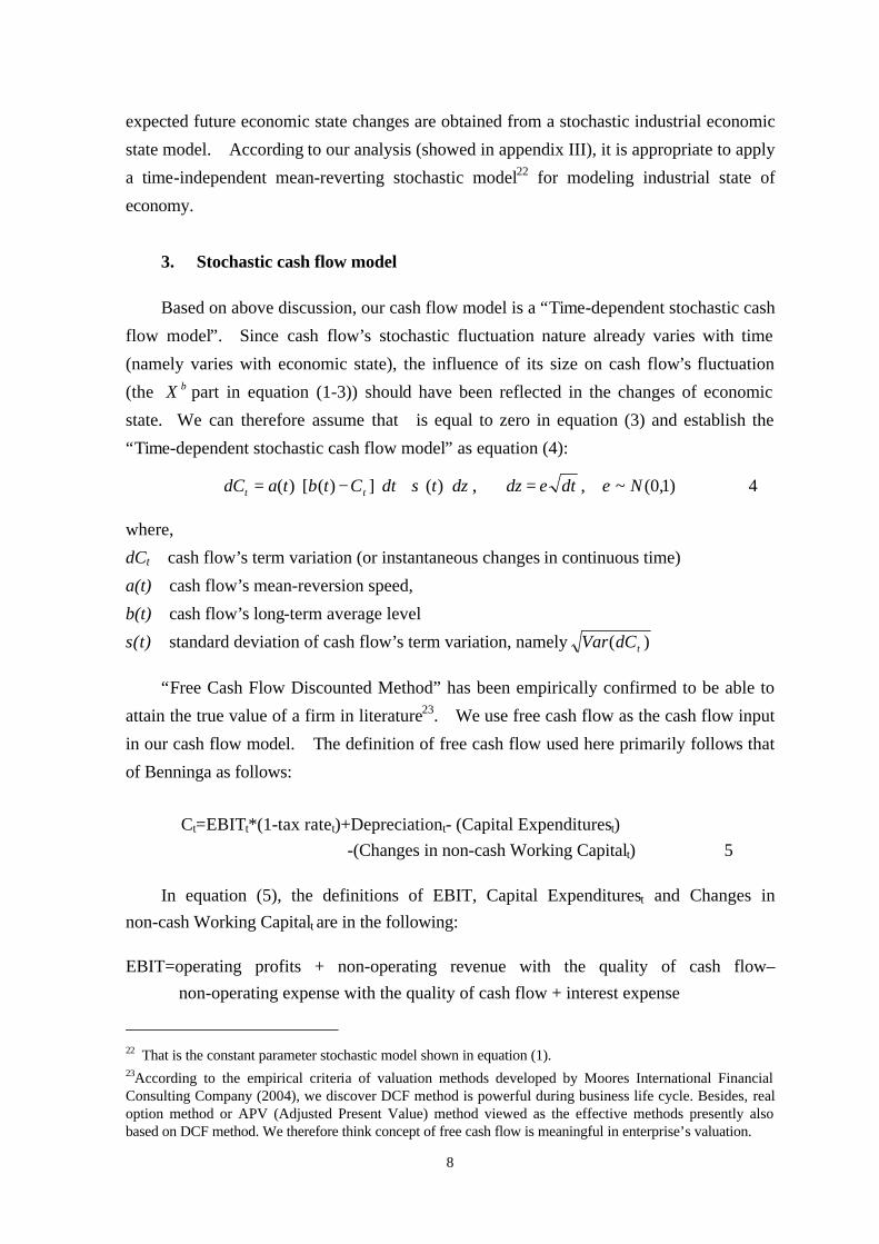
3. Stochastic cash flow model Based on above discussion, our cash flow model is a “Time-dependent stochastic cash
flow model”. Since cash flow’s stochastic fluctuation nature already varies with time
(namely varies with economic state), the influence of its size on cash flow’s fluctuation
(the βX part in equation (1-3)) should have been reflected in the changes of economic
state. We can therefore assume thatβis equal to zero in equation (3) and establish the
“Time-dependent stochastic cash flow model” as equation (4):
dztdtCtbtadC tt ⋅+⋅−⋅= )(])([)( σ , )1,0(~, Ndtdz εε= (4)
where,
dCt:cash flow’s term variation (or instantaneous changes in continuous time)
a(t):cash flow’s mean-reversion speed,
b(t):cash flow’s long-term average level
s(t):standard deviation of cash flow’s term variation, namely )( tdCVar “Free Cash Flow Discounted Method” has been empirically confirmed to be able to
attain the true value of a firm in literature23. We use free cash flow as the cash flow input
in our cash flow model. The definition of free cash flow used here primarily follows that
of Benninga as follows:
Ct=EBITt*(1-tax ratet)+Depreciationt- (Capital Expenditurest)
-(Changes in non-cash Working Capitalt) (5)
In equation (5), the definitions of EBIT, Capital Expenditurest and Changes in non-cash Working Capitalt are in the following: EBIT=operating profits + non-operating revenue with the quality of cash flow–
non-operating expense with the quality of cash flow + interest expense
22 That is the constant parameter stochastic model shown in equation (1). 23According to the empirical criteria of valuation methods developed by Moores International Financial Consulting Company (2004), we discover DCF method is powerful during business life cycle. Besides, real option method or APV (Adjusted Present Value) method viewed as the effective methods presently also based on DCF method. We therefore think concept of free cash flow is meaningful in enterprise’s valuation.

9
Capital Expenditurest = (Fixed Assetsend - FixedAssetsbeg) – Dep + R&D Exp. – Amortization + Acquisition Changes in non-cash Working Capitalt =non-cash current assetst-non-debt current liabilityt
From equation (5), we know that free cash flow is mainly influenced by EBIT, capital
expenditures necessary in maintaining a stable growth, and changes of working capitals.
EBIT and necessary capital expenditure are all related to sales. Because sales are
primarily influenced by industrial economic state (namely business cyclical factor), there
must exist a close relationship between free cash flows and economic state. Next, we will
introduce the stochastic economic state model and its relationship with parameters’
adjustments of the stochastic cash flow model.
4. Stochastic economic state model and parameters’ adjustments of the
stochastic cash flow model In order to simplify our model and without loss of generalization, we assume that a(t)
in equation (4) is equal to a constant24. The a(t) stand for long-run mean-reversion speed
of a firm’s cash flow. While, b(t) and )(tσ represent for long-term average free cash
flow and standard deviation of free cash flow’s term changes25 respectively. These three
parameters can be estimated by Chen(1996), Miao(2003) or just simple statistics of
long-term historical data.
In this study, we use a firm’s industry leading indictor26 to proxy economic state and
build a stochastic industrial economic state model as equation (6) below27. With this state
model, the economic states in the future periods can be estimated.
dzdtbad tt ⋅+⋅−⋅= − ηηη σηη ][)( 1 (6)
24 Actually a(t) will be influenced by the growth trend of individual enterprise. In this paper, we assume that a(t) is a fixed constant in order to simplify model. We therefore only consider the business life cycle of individual firm when applying so that the general form of our model will be maintained. 25 In this paper, we will consider macroeconomic cycle and industrial maturity and regard them as the adjustment basis of parameters’ term-changes in stochastic cash flow model. The basic concept of this idea is that industrial maturity will influence a firm’s growth power and then a firm’s growth power will also influence the future firm’s value and its variance. However, these two considerable factors will reflect on the industrial “the growth rate of coincident indictors” or “the growth rate of leading indictors”. We therefore lead the estimates of the future coincident or leading indictors’ growth rate into stochastic cash flow model and then it can be reflected on the changes of economic state (time). 26 It can be also applied in coincident indictors. 27 The characteristics of economic state (business cyclical factor) can be referred in appendix III. We discover that its fluctuation obviously has the nature of mean-reversion.

10
where,
tη : the growth rate of industrial leading indictor in time t.
ηb : the long-term average of industrial leading indictor’s growth rate
ησ : the standard deviation of the changes of industrial leading factor’s growth rate Consequently we can fine-tune the parameters of the stochastic cash flow model
according to the estimates of future industrial economic states which derived from the
stochastic economic state model. The parameters b(t) and s(t) in equation (4) are shown
as bellow28:
)1()( btbtb ψ+⋅= (7)
)1()( σψσσ tt +⋅= (8) In equations (7) and (8),
b : the long-term average of cash flow calculated from historical data.
σ :the standard deviation of cash flow’s term changes calculated from historical data.
When industrial economic state’s proxy is a leading indictor29:
11ˆ
αω
ωωψ ⋅
−= −tb
t (9)
121 ˆˆ
αω
ωωψ σ ⋅−= −− ttt (10)
In equation (9) and (10),
tω̂ :the estimates of industrial economic state in future periods from stochastic industrial
economic state model.
28 In our models, we assume that a firm’s cash flows reflect the state of industrial economy and then we let cash flow’s mean-reversion speed be equal to one because the cash flow model’s parameters (b,σ)have been adjusted by the future industrial economic states. The details of parameters’ adjustments in stochastic cash flow model are thoroughly discussed in appendix IV (It discusses the relationship between stochastic cash flow model’s estimation of parameters and economic states and introduces the adjustment method.). 29 When economic state’s proxy is a coincident indictor:
1
ˆα
ωωω
ψ ⋅−
= tbt 1
1ˆˆα
ωωω
ψ σ ⋅−
= −ttt

11
ω : the long-term average of industrial economic state calculated from historical data
1α : the sensitivity of cash flow per unit asset relative to industrial economic state (namely the regressive coefficient of εωαα +⋅+= ttc 10 , and tc stands for the cash flow per unit
asset in time t). In the above adjustment methods, 1α reflects the sensitivity of cash flow per unit
asset to the fluctuation of industrial economic state. In this study, we assume that both
industrial economic state and cash flow have the same fluctuating magnitude in order to
simplify model; that is to let 1α be equal to one.
On the other side, the long-term average growth rate of industrial economic state’s
( ηb ) and the standard deviation of changes of industrial economic state’s growth rate ( ησ )
are both constants and are estimated by AR(1) method(Chen, 1996) 30.
III. The Cash Flow Based Multi-Period Credit Risk Model
A multi-period credit risk model focuses on the relationship between multi-period
firm’s asset value and its liability. We first have to know the firm’s value distributions in
the future periods. With our “time-dependent stochastic cash flow model”, we can
simulate any probable free cash flow paths. We can then generate as many firm value
paths with respect to each free cash flow path as discount rate and growth rate are
reasonably estimated. As a result, we can evaluate a firm’s multi-period credit risk through
the relationship between asset value distributions and debt31.
1. Deriving a firm’s multi-period value distributions
We assume that a firm has a two-stage growth pattern. In first stage, future cash
flows are simulated from our cash flow model before time T (a future time point). In
second stage, cash flows grow with the constant rate g after time T. Consequently we can
get one future cash flow path of a firm when simulating once. With this cash flow path,
we can calculate the firm’s present value at any time t following equation (11). Therefore,
for each specific cash flow path, we can obtain a corresponding firm value path, too.
Repeating above process for N times, we can have a firm’s N cash flow paths and also N
corresponding value paths. Through a cross-sectional analysis in each period, we obtain
the firm’s multi-period value distributions.
30 A detailed presentation of Chen’s estimation method can be seen in appendix V. 31 We assume that firm’s debt is fixed here to simplify our model. It can be generalized in further study by relaxing this assumption.

12
)()1()1(.......
)1(,
11,1,
gWACCWACCFCF
WACCFCF
WACCFCF
PV tTtTi
tTtTiti
it −⋅++
+++
+= −
−−−
−−+ (11)
itPV : the firm’s present value for the i th cash flow’s path at time t (the end of period t).
itFCF : the firm’s free cash flow for the i th cash flow’s path at time t.
T: the beginning time of constant growth. WACC: firm’s weighted average costs of capital g: the estimate of constant growth.
In equation (11), g and WACC significantly influence a firm’s present value
distribution.
Regarding the WACC, we calculate it by using equation (12).
)(
)1(
fmfe
ed
rrrr
rAE
trAD
WACC
−⋅+=
⋅+−⋅⋅=
β (12)
In equation (12), the parameters er and dr play important roles. In this study, we
assume that they are fixed constants to simplify model32.
Regarding the firm cash flow’s constant growth rate after time, we employ two
common used methods in this study. First, we use the g usually appearing in corporate
finance textbook, calculating as RIROICg *= ; Where ROIC stands for the long-term
average return rate of investment capital, and RI represents for the long-term average of
re-investment rate. Second, we calculate the average growth rate of industrial leading
indictors as the estimate of the g. To choose between the two estimates of g, we introduce
time series analysis of the sales per unit asset. We pick the one that better fit the trend of
the firm’s sales per unit asset through its PACF (Partial Autocorrelation Function).
Having the WACC and growth rate, we can implement discount method and obtain
multi-period assets value distributions.
32 In this study, to determine er , the estimation of Taiwan’s market risk premium(
fm rr − ) are based on the
American’s market risk premium. We calculate the returns volatility relationship between these two markets and use the concept of CML (Capital Market Line) to derive Taiwan’s reasonable market risk premium. Through CAPM theory, we can calculate er when other variables (namely risk-free rate and beta) can be also reasonably estimated.
13
2. Deriving a firm’s multi-period value distributions
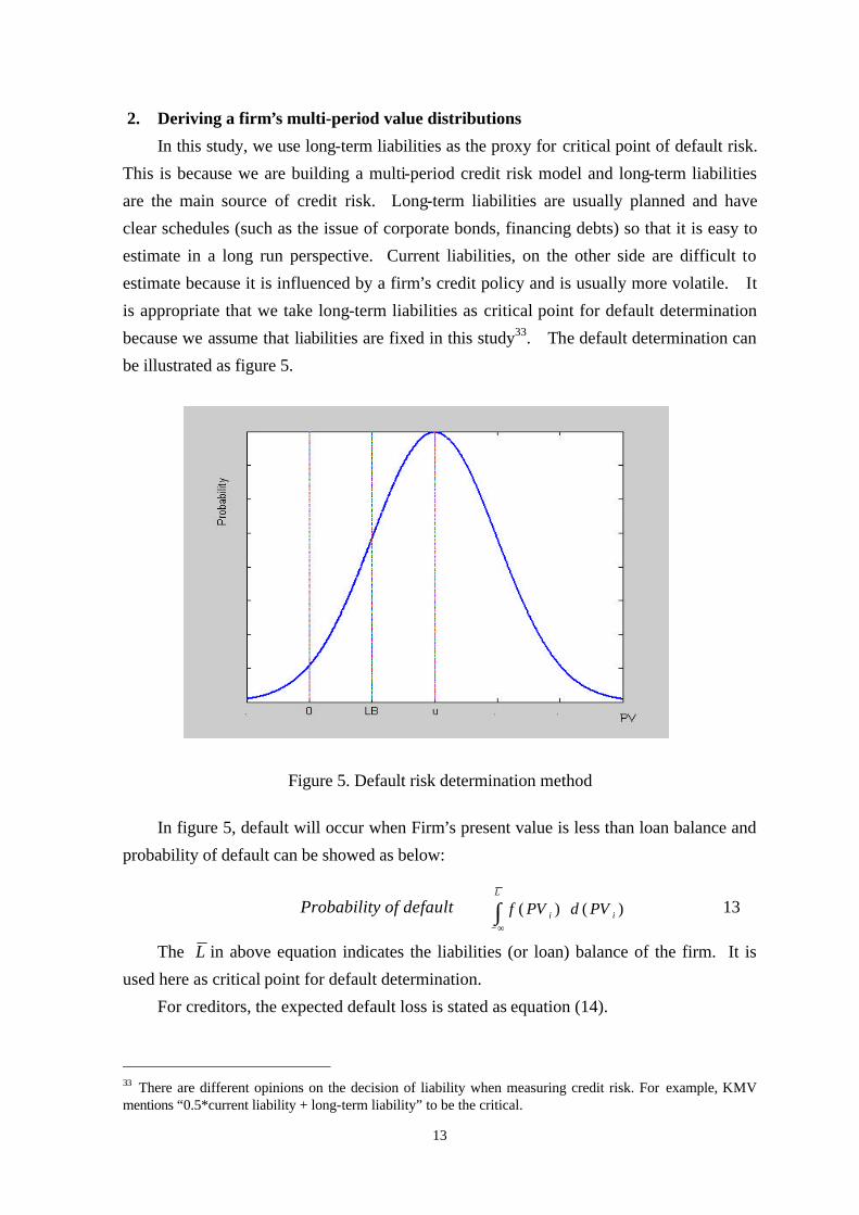
In this study, we use long-term liabilities as the proxy for critical point of default risk.
This is because we are building a multi-period credit risk model and long-term liabilities
are the main source of credit risk. Long-term liabilities are usually planned and have
clear schedules (such as the issue of corporate bonds, financing debts) so that it is easy to
estimate in a long run perspective. Current liabilities, on the other side are difficult to
estimate because it is influenced by a firm’s credit policy and is usually more volatile. It
is appropriate that we take long-term liabilities as critical point for default determination
because we assume that liabilities are fixed in this study33. The default determination can
be illustrated as figure 5.
Figure 5. Default risk determination method In figure 5, default will occur when Firm’s present value is less than loan balance and
probability of default can be showed as below:
Probability of default = ∫∞−
⋅L
ii PVdPVf )()( (13)
The L in above equation indicates the liabilities (or loan) balance of the firm. It is
used here as critical point for default determination.
For creditors, the expected default loss is stated as equation (14).
33 There are different opinions on the decision of liability when measuring credit risk. For example, KMV mentions “0.5*current liability + long-term liability” to be the critical.

14
∫ ∫∞−
⋅⋅−⋅⋅=L L
iiiii PVdPVfPVPVdPVfLLossExpected0
)()()()( (14)
For creditors, the loss given default (later denoted as LGD) can be showed as equation
(15).
∫
∫∫
⋅⋅⋅−=
⋅⋅−⋅⋅⋅=∞−
L
iii
L
iiii
L
i
PVdPVfPVPD
L
PVdPVfPVPVdPVfLPD
LGD
0
0
)()(1
)]()()()([1
(15)
Therefore, creditor’s recovery rate (RR) when default occurs can be written as equation (16):
)()(1
)]()(1
[1
00ii
L
iii
L
i PVdPVfPVPDL
PVdPVfPVPD
LLL
RR ⋅⋅⋅⋅
=⋅⋅⋅+−= ∫∫ (16)
In current study, we define a new variable, expected recovery rate (later denoted as
ERR), which is equal to one minus the ratio of expected loss to loan balances. It means
how much that creditors can expect to recover their loans. ERR can be written as
equation (17):
PDRRPDL
PDLRRPD
L
PVdPVfPVPD
L
PVdPVfPVPVdPVfLERR
L
iii
L L
iiiii
⋅+−⋅=⋅⋅
+−=
⋅⋅+−=
⋅⋅−⋅⋅−=
∫
∫ ∫∞−
)1(11
)()(1
)()()()(1
0
0
(17)
Therefore, we can make the two main credit risk factors, PD and RR, be endogenous
in our model based on the above discussion. Besides, we also discover that PD and RR
are inversely related34 and PD and ERR are negatively related.
Regarding credit risk of specific firm obligations (e.g. corporate bonds), the seniority
of the obligations becomes crucial. If there are other debts senior to the debt we are
assessing, we have to deduct those senior debt balances from the firm’s asset value before
doing above credit analysis. When there are other liabilities with the same seniority as
the debt we are considering, all those debts have to be added into L . The default
34 The inverse relationship between PD and RR will be discussed in appendix VI.

15
determination can be illustrated as equation (18).
LSPVi <− (18)
A firm’s debt composition might change in the future. Whether these changes affect
the credit of the specific debt we are interested in depends on whether they affect the PD of
the specific debt. For example, the credit of specific debt will improve if the firm
borrows subordinate debt because the firm’s asset value increases. Another example is
that the specific debt’s credit becomes worsen if there is an unexpected tax charges by
government because tax liabilities increases but asset value doesn’t.
In summary, the design process of our “Cash flow based multi-period credit risk
model and its pricing method” can be illustrated as figure 6.
Figure 6. Flow Chart of the CF-Based Multi-period Credit Risk Model and Application
Constructing “Multi-period firm value distributions”
Free Cash Flow
FCF’s stochastic characteristics
Constructing “Time-dependent stochastic FCF model”
Establishing “FCF Based Multi-period Credit Risk
Estimation of multi-period endogenous PD and RR
Combine the concept of J-T model and further calculate the multi-period expected payoff ratio (ERR)
Pricing corporate specified debts and its derivatives
Considering the future information of industrial economic states from our state model

16
IV. Empirical Analysis
In order to examine the effectiveness of our “Cash Flow Based Multi-period Credit
Risk Model”, we select 24 companies from Taiwan’s stock market to analyze their credit
risks. Moreover, we also use UMC’s unsecured corporate bonds as an example to show
the application of our model in pricing corporate specific debts.
1. Data
Because this study develops three models, “Stochastic industrial economic state
model”, “Cash flow based multi-period credit risk model”, and “Bond Pricing model with
the concept of J-T model”, we have to get all related data to do the empirical analysis.
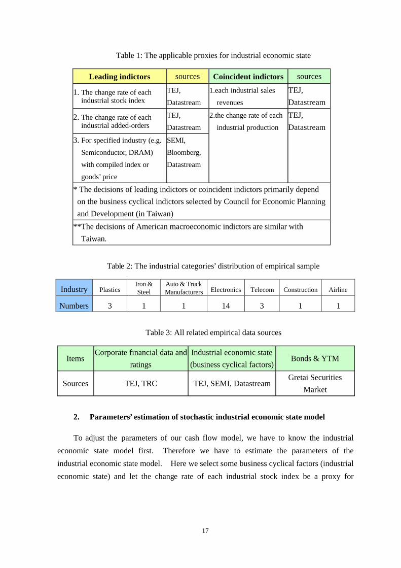
First, we establish the applicable proxies for industrial economic states according to the
criteria of NBER (in America) or Council for Economic Planning and Development (in
Taiwan) and they are illustrated in table 1.
Second, we select 24 rated firms that are rated by either Standard and Poor’s or
Taiwan Ratings Corporation (later denoted as TRC) as our samples. Names of these
sample companies are shown in table 5. These sample companies’ industrial categories are
illustrated in table 2.
Third, we get individual company’s financial data to calculate free cash flow and loan
balance from TEJ database so that we can complete the work of evaluating individual
company’s multi-period credit risk35. Forth, we get data of YTM for 2-year, 5-year, and
10-year on-the-run issues from Gretai Securities Market (an organization of Taiwan’s OTC
Market) for simulating an affine term structure of Taiwan’s YTM. Fifth, we proceed our
“Bond Pricing Model with the concept of J-T model” by using the UMC’s unsecured
corporate bond data and an affine term-structure of Taiwan’s YTM. To sum up, all the
data sources are completely illustrated in table 3.
The estimation period of business cyclical factor (industrial economic state) and free
cash flow per unit asset is from 1995 to 2003Q236.
35 In order to simulate the future PV distributions, we have to estimate the individual company’s WACC and its growth rate. On the part of WACC, we estimate Taiwan’s risk premium based on the CML theory. According to the return indexes (RI) both of American and Taiwan’s markets from datastream, we can separately calculate the RI’s annualized volatility of America (0.1815) and Taiwan (0.3393). Moreover, we can get American annualized risk premium data (7.5%) from “Ibbostson Associated, annual”. After transforming by exchange rate, we can finally estimate Taiwan’s annualized risk premium (14.03%). On the other part of growth rate, we utilize the method of financial theory (g=ROIC*RI) or industrial growth rate. 36 BB ratio is the exception. Because of its difficulty to acquiring the more past data, we can estimate the parameters from 1998Q2 to 2003Q2; But the data of telecom industry can be acquired in a shorter period, that is from 2000 to 2003Q2
17
Table 1: The applicable proxies for industrial economic state
Leading indictors sources Coincident indictors sources
1. The change rate of each industrial stock index
TEJ,
Datastream
1.each industrial sales
revenues
TEJ, Datastream
2. The change rate of each industrial added-orders
TEJ,
Datastream
3. For specified industry (e.g.
Semiconductor, DRAM)
with compiled index or
goods’ price
SEMI,
Bloomberg,
Datastream
2.the change rate of each
industrial production
TEJ, Datastream
* The decisions of leading indictors or coincident indictors primarily depend on the business cyclical indictors selected by Council for Economic Planning and Development (in Taiwan)
**The decisions of American macroeconomic indictors are similar with Taiwan.
Table 2: The industrial categories’ distribution of empirical sample
Industry Plastics Iron & Steel
Auto & Truck Manufacturers Electronics Telecom Construction Airline
Numbers 3 1 1 14 3 1 1
Table 3: All related empirical data sources
Items Corporate financial data and
ratings Industrial economic state (business cyclical factors)
Bonds & YTM
Sources TEJ, TRC TEJ, SEMI, Datastream Gretai Securities
Market
2. Parameters’ estimation of stochastic industrial economic state model To adjust the parameters of our cash flow model, we have to know the industrial
economic state model first. Therefore we have to estimate the parameters of the
industrial economic state model. Here we select some business cyclical factors (industrial
economic state) and let the change rate of each industrial stock index be a proxy for

18
industrial economic state37except semiconductor industry. We use B-B ratio as the proxy
for semiconductor industry because it can more correctly reflect the changes of industrial
economic state (business cycle). We employ AR(1) method(Chen, 1996) to estimate its
parameters and the results can be illustrated in table 4.
Table 4. Parameters’ estimation of stochastic industrial economic state model
Parameters’ estimation of stochastic industrial economic state model
industry Plastics Iron & Steel Auto & Truck
Manufacturers Electronics Semiconductor Construction Airline
Simulation
target
Change rate
of Plastics
stock index
Change rate
of Iron &
Steel stock
index
Change rate of
Auto & Truck
Manufacturers
stock index
Change rate of
Electronics
stock index
Change rate of
Book-to-Bill
ratio
Change rate of
construction
stock index
Change rate
of Airline
stock index
a 1.7779 2.1349 1.4396 1.3823 1.3053 2.1085 1.5929
b 0.0166 -0.0101 0.0587 -0.0135 0.0077 -0.0076 -0.0085
s 0.1141 0.1589 0.2052 0.0712 0.1432 0.0420 0.0469
3. Empirical results of firms’ credit ratings The empirical credit analyses results are illustrated in table 5. The sixth column of
table 5 stands for probability of default of each sample firm calculated by our credit risk
model (denoted as “model’s PD”) during the future ten years. The fifth column of table 5
represents for each firm’s theoretical rating (denoted as “model’s rating”) . The model’s
ratings are assigned to each firm by comparing model’s PD to the ten-year cumulative
default rates curve in American market38. Hence, the model’s ratings are equivalent to
American (or global) rating. Since Taiwan market is essentially not the same as American
market in terms of having different risk factors, such as political risk, country risk and so
on, our model’s rating should be lower than the firm’s local rating given by TRC39 (shown
in the fourth column of table 5).
According to empirical results illustrated in table 5, we discover that 19 firms are
downgraded for 1/3~1 rating grade from TRC rating, 3 firms are rated the same as TRC,
37 Due to the limitation of acquiring data, we can only select “the change rate of each industrial stock index” easier to be acquired to stands for industrial economic state. 38 The cumulative default rate curve is provided by Standard and Poor’s(1981~2002). 39 In practice, a rule of thumb for the rating difference is that Taiwan local ratings are about one rating grade lower than those of Global rating. For example, in practice a twA- rating is equivalent to a global rating BBB-. From model’s perspective, Taiwan’s cumulative default rates curve should add a country rating spread to be equivalent to that of global (or American) market.

19
and 2 firms are upgraded 1/3-1 rating grade from TRC rating. From these results, 19 out
of 24 firms (about 80%) are rated reasonably. Our model’s effectiveness seems
preliminarily supported by the empirical evidences. Among the 24 firms, two firms are
upgraded by our model, the Foxconn and TSMC. From our observation, these two firms
have very stable and abundant free cash flow so that their default probabilities are much
lower than other firms. TRC may consider other factors rather than just their operating
performance, such as lawsuits, significant strategic investment activities with high
uncertainty. It is our current model’s constraint that we cannot consider all the
uncertainty in our model. It could be improved by adding extra stochastic terms into our
model, such as “jump diffusion model” to take care of more uncertainties.
4. Example of corporate bond pricing Regarding our model’s application in corporate bond pricing, we take UMC’s
unsecured corporate bond issued in 2003 as our example40. We adopt Chen’s AR(1)
estimation method to estimate parameters in the stochastic industrial economic state model
and the results are illustrated in table 641. The simulated multi-period distributions of
both UMC’s free cash flows and present values are illustrated in figure 7 and 8. After
deciding UMC’s future ERR (expected recovery rate, the expect value of recovery per unit
debt), we can proceed pricing on UMC’s unsecured corporate bond with the concept of J-T
model42. The pricing results43 of UMC’s unsecured corporate bond are illustrated in
table 7.
According to table 7, we find that there existed premium for UMC’s corporate bond.
This is mainly because UMC’s rating was high and the coupon rate was higher than market
rate when issued. This example shows our model can help not only calculate theoretical
price of corporate bond but also provide a trading basis for secondary corporate bond
market.
40 This UMC’s unsecured bond has the characteristics as follows: five-year bond and annualized coupon rate is 2.0%. 41 Actually we employ three different estimation methods and found that Chen’s method provides the best estimates. The results of the other two methods are shown below:
Parameter a b σ Historical long-term average 1 0.0009 0.3085 Miao(2003) 0.7290 0.0262 0.2932
42 J-T model is based on zero-coupon government (default-free) bond. We can let N-year coupon bond(pay once per year) be divided into N’s zero coupon bond without default risk and can further calculate the prices of the N’s defaultable zero coupon bonds through ERR. And then we can get the probable price of the defaultable coupon bond by summarizing the prices of N’s defaultable zero coupon bond. 43 Because there is no complete YTM term structure in Taiwan, we utilize the on-the-run issued government bonds to construct a simulated yield curve.

20
Table 5. Empirical results of cash flow based multi-period credit risk model
Table 6. The parameters’ estimation of stochastic industrial economic state model under
different methods
Parameter a b σ
Estimate 1.3053 0.0077 0.1432
Empirical results of cash flow based multi-period credit risk model
Item Company Time Actual rating Model’s rating Model’s PD
1 CHT*** 2003/12/15 twAAA AAA 0.26% 2 Fareastone* 2003/1/27 twA+ BBB+ 6.88% 3 TCC* 2003/3/18 twA+ A- 3.67% 4 CSC* 2003/6/30 twAA+ AA- 1.43% 5 UMC* 2002/3/15 twAA- A 2.24% 6 TSMC** 2003/3/13 twAA+ AAA 0.04% 7 FPC* 2003/12/22 twAA- A+ 1.75% 8 NPC* 2003/12/4 twAA- A 1.93% 9 Foxconn** 2004/3/22 twAA- AAA- 0.72% 10 Compal* 2003/6/11 twA+ BBB 8.26% 11 Quanta* 2003/6/13 twA+ A 2.52% 12 SPIL* 2004/2/23 twBBB+ BBB 7.55% 13 NTC* 2004/2/27 twBBB+ BBB- 16.37% 14 Cmcent* 2003/12/18 twBBB BBB- 12.34% 15 RITEK*** 2003/9/16 twBB+ BB+ 18.14% 16 Yageo* 2003/12/16 twBB+ BB 26.79% 17 QDI* 2004/2/17 twBB+ BB 23.32% 18 MXIC*** 2003/5/28 twBB BB 26.39% 19 BENQ* 2003/5/29 twA- BBB 9.66% 20 WWEI* 2003/5/29 twBBB BB+ 20.61% 21 Cathay-red* 2003/11/3 twBBB BBB- 15.54% 22 China-airline* 2003/11/13 twBBB BB+ 18.20% 23 FCFC* 2003/12/4 twAA- A- 3.93% 24 Yulon-motor* 2004/2/25 twA BBB 9.67%
*:with downgrade during1~3 ranges; **:with upgrade during 1~3 ranges; ***:the same rating
Model’s PD: Under the assumption of homogenous markets, we can let model’s PD correspond to American ten-year cumulative default rates curve.

21
Table 7. The Pricing of UMC’s unsecured corporate bond
Corporate Bond Pricing
Year Zero Yield d(0,t) ERR V(0,t) C P(0,t)
1 0.91% 0.9910 1.0000 0.9910 2.0 1.9819 2 0.95% 0.9813 1.0000 0.9813 2.0 1.9627 3 1.04% 0.9694 1.0000 0.9694 2.0 1.9388 4 1.14% 0.9558 1.0000 0.9558 2.0 1.9115 5 1.23% 0.9406 0.9998 0.9404 102.0 95.9262 ΣP(0,t)= 103.7211
d(0,t):discounted factor of zero-coupon bond without default risk V(0,t):the value of zero-coupon bond with default risk/ per face value C: coupon per one hundred P(0,t):the value of zero-coupon bond with default risk / per face value in hundred ΣP(0,t):the value of coupon bond with default risk / per face value in hundred
Figure 7. UMC’s Multi-period Free Cash Flow distributions

22
Figure 8. UMC’s Multi-period Present Value distributions
V. Conclusions The development of credit risk models grows rapidly recently but mainly on the
reduced-form models. However, reduced-form credit models depend on specific
exogenous information such as credit rating and recovery rate. They cannot generate
credit risk variables such as PD, RR and LGD internally from a firm’s operation value.
Besides, the developments of multi-period credit risk models are few in literatures. This
study tries to fill up this literature gap.
“Cash Flow Based Multi-period Credit Risk Model” constructed in this study
provides a systematic measuring process of credit risk. It starts from determining a
firm’s future value distributions by our “Time-dependent stochastic cash flow model” and
then combining value distributions with liability information to perform a multi-period
credit risk assessment. It can also combine those endogenously generated PD and RR
with J-T Model to price multi-period debts. One of major merits of our models is that
they can directly price the credit risk of debts without knowing the firms’ credit rating and
they straightly consider the firm’s future operating values to do multi-period credit risk
analyses instead of a backward solution from firm’s credit rating. For outside investors
and people inside a firm, our study provides a multi-period credit risk model that needs
only publicly available information of both corporate finance and the industrial economic
state (i.e. the industrial cyclical information). We believe this “Cash Flow Based
Multi-period Credit Risk Model” has provided a new way for analyzing corporate debts.
23
Reference
1. Altman, Edward I., Brooks Brady, Andrea Resti, and Andrea Sironi, 2001, Analyzing
and Explaining Default Recovery Rates, ISDA Research Report, London, December.
2. Altman, Edward I. and Brooks Brady, 2002, “Explaining Aggregate Recovery Rates
on Corporate Bond Defaults”, NYU Salomon Center.
3. Black, Fischer and John C. Cox, 1976, “Valuing Corporate Securities: Some Effects of
Bond Indenture Provisions”, Journal of Finance, 31, 351-367.
4. Black, Fischer and Myron Scholes, 1973, “The Pricing of Options and Corporate
Liabilities”, Journal of Political Economics, May, 637-659.
5. Carey, Mark and Michael Gordy, 2003, “Systematic Risk in Recoveries on Defaulted
Debt”, mimeo, Federal Reserve Board, Washington.
6. Carty, L. and D. Lieberman, 1996, “Defaulted bank Loan Recoveries”, Moody’s
Investors Service.
7. Chen, Ren-raw (1996), Understanding and Managing Interest Rate Risks, World
Scientific, chapter 5.
8. Crouhy, Michel, Dan Galai and Robert Mark, 2000, “A Comparative Analysis of
Current Credit Risk Models”, Journal of Banking & Finance, 24, 59-117.
9. Crosbie, Peter J., 1999, “Modeling Default Risk”, mimeo, KMV Corporation, San
Francisco, CA.
10. Crosbie, P. J. and J. R. Bohn (2002). Modeling Default Risk. Technical Report, KMV,
LLC.
11. Duffee, Gregory R., 1999, “Estimating the Price of Default Risk”, Review of
Financial Studies, Spring, 12, No. 1, 197-225.
12. Duffie, Darrell, 1998, “Defaultable Term Structure Models with Fractional Recovery of
Par”, Graduate School of Business, Stanford University.
13. Duffie, Darrell and Kenneth J. Singleton, 1999, “Modeling the Term Structures of
Defaultable Bonds”, Review of Financial Studies, 12, 687-720.
14. Duffie, Darrell and David Lando, 2000, “Term Structure of Credit Spreads With
Incomplete Accounting Information”, Econometrica.
15. Duffie, Darrell and Garleanu, Nicolae, 2001, “Risk and Valuation of Collateralized
Debt Obligations”, Working Paper
16. Duffie, Darrell and Wang, Ke, 2004, “Multi-Period Corporate Failure Prediction With
Stochastic Covariates”, Working Paper
17. Frye, John, 2000a, “Collateral Damage”, Risk, April, 91-94.

24
18. Frye, John, 2000b, “Collateral Damage Detected”, Federal Reserve Bank of Chicago,
Working Paper, Emerging Issues Series, October, 1-14.
19. Frye, John, 2000c, “Depressing Recoveries”, Risk, November.
20. Geske, Robert, 1977, “The Valuation of Corporate Liabilities as Compound
Options”,Journal of Financial and Quantitative Analysis, 12, 541-552.
21. Gordy, Michael, 2000, “A Comparative Anatomy of Credit Risk Models”, Journal of
Banking and Finance, January, 119-149.
22. Gupton, Greg M., Christopher C. Finger and Mickey Bhatia, 1997, “CreditMetrics –
Technical Document, (New York, J.P.Morgan).
23. Hull, J. and A. White, 1990, "Pricing Interest Rate Derivative Securities," Review of
Financial Studies, 3, 573-592.
24. Hull, J. and A. White, 1995, “The Impact of Default Risk on the Prices of Options and
Other Derivative Securities”, Journal of Banking and Finance, 19, 299-322.
25. Kijima, Masaaki and Katsuya Komoribayashi, 1998, "A Markov chain model for
valuing credit risk derivatives", Journal of Derivatives, Vol. 6, pp. 97-108.
26. Kim I.J., K. Ramaswamy, S. Sundaresan, 1993, “Does Default Risk in Coupons
Affect the Valuation of Corporate Bonds?: A Contingent Claims Model”, Financial
Management, 22, No. 3, 117-131.
27. KOU, STEVEN G., 2002, ”A Jump Diffusion Model For Option Pricing”, Working
paper
28. Jarrow, Robert A., 2001, “Default Parameter Estimation Using Market Prices”,
Financial Analysts Journal, Vol. 57, No. 5, pp. 75-92.
29. Jarrow, Robert A., David Lando and Stuart M. Turnbull,1997, "A Markov Model for
the Term Structure of Credit Risk Spreads," The Review of Financial Studies, 10 (1),
pp481-523.
30. Jarrow, Robert A. and Stuart M. Turnbull, 1995, “Pricing Derivatives on Financial
Securities Subject to Credit Risk”, Journal of Finance 50, 53-86.
31. Judge, G. G., W. E. Griffiths, R. C. Hill, T. -C. Lee, and H. Lutkepol, 1988, Introduction
to the Theory and Practice of Econometrics, 2nd ed., John Wiley & Sons.
32. Lando, David, 1998, “On Cox Processes and Credit Risky Securities”, Review of
Derivatives Research, 2, 99-120.
33. Lea. V, Carty and Lieberman, 1997, ”Historical Default Rates of Corporate Bond
Issuers, 1920-1996”, Moody’s.
34. Litterman, Robert and T. Iben, 1991, “Corporate Bond Valuation and the Term
Structure of Credit Spreads”, Financial Analysts Journal, Spring, 52-64.
35. Longstaff, Francis A., and Eduardo S. Schwartz, 1995, “A Simple Approach to

25
Valuing Risky Fixed and Floating Rate Debt”, Journal of Finance, 50, 789-819.
36. Madan, Dileep and H. Unal, “Pricing the Risk of Recovery in Default with APR
Valuation,”Journal of Banking and Finance, forthcoming.
37. McQuown J.A., 1997, “Market versus Accounting-Based Measures of Default Risk”,
in I. Nelken, edited by, Option Embedded Bonds, Irwin Professional Publishing,
Chicago.
38. Merton, Robert C., 1974, “On the Pricing of Corporate Debt: The Risk Structure of
Interest Rates”, Journal of Finance, 2, 449-471.
39. Miao, Wei-Cheng, 2003, “Quadratic Variation Estimators for Diffusion Models in
Finance, Working paper
40. Nielsen, Lars T., Jesus Saà-Requejo, and Pedro Santa-Clara , 1993, “Default Risk and
Interest Rate Risk: The Term Structure of Default Spreads”, Working Paper,
INSEAD.
41. Vasicek, Oldrich A., 1984, Credit Valuation, KMV Corporation, March.
42. Vassalou, M. and Y. Xing (2004). Default Risk in Equity Returns. Journal of Finance
59, 831–868.
43. Wilson, Thomas C., 1997a, “Portfolio Credit Risk (I)”, Risk , Vol. 10, No. 9, 111-117.
44. Wilson, Thomas C., 1997b, “Portfolio Credit Risk (II)”, Risk, Vol. 10, No. 10, 56-61.

26
Appendix I. The explorations of the relationship between sales’ and cash flow’s
natures
In this paper, we use the quarterly financial data when estimating the parameters of
stochastic cash flow model. So the calculated quarterly free cash flow will fluctuate
greatly caused by companies’ credit policy so that it can’t completely fit in with the natures
of real sales. In order to smooth the cash flow’s huge fluctuation, we will let historical
cash flows be moving average by its operating cycle (assume one year). This rolling
method will still maintain the cycle factor of industrial economic state and exclude the
influence of credit policy on free cash flow. In this way, the moving average free cash
flow will exactly fit in with the changes of industrial economic states so that we can
reasonably utilize the “stochastic industrial economic state model” to adjust the future
estimates of the “time-dependent stochastic cash flow model”.
In the following, we will introduce the natures (namely its trend and cycle) of sales
per assets, original free cash flow per assets and moving average free cash flow per assets
by using time-series analysis and then we take TSMC as example. Figure A1-1, A1-2
individually stands for the cycle and the trend of TSMC’s quarterly sales per assets through
ACF (Autocorrelation Function) and PACF (Partial Autocorrelation Function). Figure
A1-3, A1-4 separately stands for the cycle and the trend of TSMC’s quarterly original free
cash flow per assets. Figure A1-5, A1-6 individually represents for the cycle and the
trend of TSMC’s quarterly moving average free cash flow per assets. Through the
observations of figures A1-1, A1-2, A1-3, A1-4, A1-5 and A1-6, we discover that the
natures of original free cash flow per assets don’t fit in with the natures of sales per assets
(sales’ nature is ARMA(1,2); original free cash flow’s nature is ARMA(0,0)); on the
opposite, the moving average free cash flow per assets matches up with sales’
natures( moving average free cash flow’s nature is ARMA(1,2)).
Moreover, we will also discuss what causes original free cash flow’s nature is
ARMA(0, 0). In original free cash flow per assets, its cycle can be divided into two
influencing factors. One is industrial economic state, and the other is credit policy during
the operating cycle. However, these two factors are negatively related44 so that the
characteristics of original free cash flow per assets will disappear.
44 When industrial economic state is boom, companies’ credit policy will be relaxed.

27
1 2 3 4 5 6 7 8 9 10
-1.0-0.8-0.6-0.4-0.20.00.20.40.60.81.0
Aut
ocor
rela
tion
1 2 3 4 5 6 7
8 910
0.84 0.64 0.45 0.32 0.26 0.20 0.11
0.00-0.10-0.15
5.31 2.61 1.59 1.07 0.83 0.62 0.33
0.00-0.30-0.48
30.3448.5157.7862.6665.8067.6968.25
68.2568.7770.09
Lag Corr T LBQ Lag Corr T LBQ
Autocorrelation Function for 2330
Figure A1-1. ACF of TSMC’s quarterly sales (is used to judge “cycle”)
10987654321
1.00.80.60.40.20.0
-0.2-0.4-0.6-0.8-1.0
Par
tial A
utoc
orre
latio
n
TPACLagTPACLag
0.07-0.27-0.44
-0.94-0.51 0.47 0.49-0.49-1.35 5.31
0.01-0.04-0.07
-0.15-0.08 0.07 0.08-0.08-0.21 0.84
10 9 8
7 6 5 4 3 2 1
Partial Autocorrelation Function for 2330
Figure A1-2. PACF of TSMC’s quarterly sales (is used to judge “trend”)

28
987654321
1.00.80.60.40.20.0
-0.2-0.4-0.6-0.8-1.0A
utoc
orre
latio
n
LBQTCorrLagLBQTCorrLag
5.845.83
5.714.453.273.133.112.861.64
-0.08-0.27
-0.90-0.91 0.32 0.12-0.44 1.01 1.23
-0.01-0.05
-0.16-0.16 0.05 0.02-0.07 0.17 0.20
98
7654321
Autocorrelation Function for 2330
Figure A1-3. ACF of TSMC’s original quarterly FCF (is used to judge “cycle”)
987654321
1.00.80.60.40.20.0
-0.2-0.4-0.6-0.8-1.0
Par
tial A
utoc
orre
latio
n
TPACLagTPACLag
-0.15 0.62
-0.75-1.37 0.53 0.23-0.86 0.84 1.23
-0.02 0.10
-0.12-0.22 0.09 0.04-0.14 0.13 0.20
98
7654321
Partial Autocorrelation Function for 2330
Figure A1-4. PACF of TSMC’s original quarterly FCF (is used to judge “trend”)

29
1 2 3 4 5 6 7 8 9
-1.0-0.8-0.6-0.4-0.20.00.20.40.60.81.0
Aut
ocor
rela
tion
1234567
89
0.77 0.50 0.20-0.07-0.19-0.32-0.31
-0.21-0.11
4.59 2.05 0.74-0.25-0.68-1.14-1.06
-0.72-0.35
22.9233.1134.8235.0236.5741.2345.74
48.0048.56
Lag Corr T LBQ Lag Corr T LBQ
Autocorrelation Function for 2330
Figure A1-5. ACF of TSMC’s moving-average quarterly FCF
(is used to judge “cycle”)
1 2 3 4 5 6 7 8 9
-1.0-0.8-0.6-0.4-0.20.00.20.40.60.81.0
Par
tial A
utoc
orre
latio
n
1234567
89
0.77-0.20-0.27-0.17 0.14-0.27 0.11
0.11-0.00
4.59-1.21-1.59-1.02 0.81-1.59 0.66
0.64-0.00
Lag PAC T Lag PAC T
Partial Autocorrelation Function for 2330
Figure A1-6. PACF of TSMC’s moving-average quarterly FCF
(is used to judge “trend”)

30
Appendix II. The historical trend of interest rates
CP2 historical trend in Taiwan
0.00
0.02
0.04
0.06
0.08
0.10
0.12
0.14
0.16
J-85
J-87
J-89
J-91
J-93
J-95
J-97
J-99
J-01
J-03 Time
CP2
Figure A2-1. CP2 historical trend in Taiwan45
Figure A2-2. 6-month LIBOR historical trend46
45 Sources: TEJ database 46 Sources: http://www.economagic.com/libor.htm#US
6-month LIBOR hisrorical trend
0
0.01
0.02
0.03
0.04
0.05
0.06
0.07
0.08
0.09
0.1
S-89
S-90
S-91
S-92
S-93
S-94
S-95
S-96
S-97
S-98
S-99
S-00
S-01
S-02 Time

31
Appendix III. The stochastic characteristics of industrial economic state
In this paper, we use the change rate of each industrial stock index to be the proxies
for industrial economic state factors and then observe the trends (the sample period is from
1995 to 2003). These industrial categories include plastics, iron & steels, auto
manufactures, and electronics. Moreover, we also consider the trend of book-to-bill ratio
(B/B) for semiconductors. The historical trend of each industrial economic state factor is
illustrated as the following figures and we discover that there exists the phenomenon of
mean-reversion in all industrial categories. We therefore think industrial economic state
applicable to mean-reversion stochastic model.
Figure A3-1. Plastics stock index’s %M Figure A3-2. Iron & Steel stock index’s %M
Figure A3-3. Auto Manu. stock index’s %M Figure A3-4. Electronics stock index’s %M
Actual
Fits
Actual Fits
100500
0.3
0.2
0.1
0.0
-0.1
-0.2
-0.3
Pla
stic
s
Time
Yt = -3.4E-03 + 2.34E-04*t
MSD:MAD:MAPE:
0.011 0.083
113.097
Trend Analysis for PlasticsLinear Trend Model
Actual
Fits
Actual Fits
0 50 100
-0.2
-0.1
0.0
0.1
0.2
Iron
& S
teel
Time
Yt = -3.1E-03 + 1.54E-04*t
MAPE:MAD:MSD:
130.788 0.083 0.011
Trend Analysis for Iron & SteelLinear Trend Model
Actual
Fits
Actual Fits
100500
0.3
0.2
0.1
0.0
-0.1
-0.2
-0.3
Aut
o m
anu
f.
Time
Yt = 3.93E-02 - 4.08E-04*t
MSD:MAD:MAPE:
0.015 0.095
553.708
Trend Analysis for Auto manuf.Linear Trend Model
Actual
Fits Actual Fits
100500
0.4
0.3
0.2
0.1
0.0
-0.1
-0.2
-0.3
Ele
ctro
nics
Time
Yt = -1.7E-02 + 2.57E-04*t
MSD:MAD:MAPE:
0.015 0.094
110.268
Trend Analysis for ElectronicsLinear Trend Model

32
Figure A3-5.BB %M Figure A3-6. BB%M
Actual
Fits
Actual
Fits
0 10 20 30 40 50 60 70
0.5
1.0
1.5B
/B
Time
Yt = 1.03506 - 1.35E-03*t
MAPE:MAD:MSD:
24.7847 0.2074 0.0623
Trend Analysis for B/BLinear Trend Model
Actual
Fits
Actual
Fits
0 10 20 30 40 50 60 70
-0.3
-0.2
-0.1
0.0
0.1
0.2
0.3
%B
/B
Time
Yt = 2.48E-02 - 3.25E-04*t
MAPE:MAD:MSD:
111.541 0.078 0.011
Trend Analysis for %B/BLinear Trend Model

33
Appendix IV. The method to estimate parameters of time-dependent stochastic cash
flow model In this paper, our stochastic cash flow model can be showed as equation (A4-1):
dztdtCtbtadC tt ⋅+⋅−⋅= )(])([)( σ , dtdz ε= ε ~N(0,1) (A4-1)
In equation (A4-1):
dCt:the term changes of free cash flow
a(t):the mean-reversion speed of free cash flow
b(t):the long-term average of free cash flow
s(t):the standard deviation of the term changes of free cash flow, namely )( tdCVar
In the estimation of stochastic cash flow model’s parameters(a, b, σ), we can
calculate the fixed constant by using non-parameter method (Miao, 2003), AR(1)
method(Chen, 1996), or generalized method of historical data.
Now we want to let b and σ be time-varying so that we utilize stochastic industrial
economic state model to make adjustments. In the following, we let c stand for cash flow
per unit asset and ω stand for the industrial economic state factor. Further we explore
the relationship between cash flow (c) and industrial economic state factor (ω ) by
constructing the regression showed as equation (A4-2):
)(10 ttc ωαα ⋅+= (A4-2) So we can make time-varying adjustments on the long-term average of cash flow
( b(t) ) based on the future cash flow’s growth rate relative to b. According to equation
(A4-2), we can further transfer the future cash flow’s growth rate to the future industrial
economic state factor’s growth rate:
))1(1(
))(1(
)))(
(1()(
1
1
−⋅+⋅=
⋅−
+⋅=
−+⋅=
−
−
ωω
α
αω
ωω
t
t
termlong
termlong
b
b
cctc
btb
(A4-3)
In equation (A4-3), ω
ωω −t stands for the future industrial economic state factor’s
growth rate relative to the long-term average of industrial economic state factor )(ω .

34
Moreover, we have to consider the regressive coefficient 1α when making adjustments
on the long-term average of cash flow (b(t)) according to equation (A4-3). In addition, we will discuss the method to make the variances of cash flow(σ) be
time-varying. First, we will difference on the both sides of equation (A4-2) and then take variances on the difference results. Second, we will explore the relationship between “the
effect on the changes of )( tc∆ caused by the changes of )( tω∆ ” and “the effect on the
)( tc∆σ caused by the changes of )( tω
σ∆
”. At last, we can infer the adjustment methods
for the variances of cash flow(σ). In the following, we will display our inference:
Difference on both sides of equation (A4-2) as follows:
)()( 1 ttc ωα ∆⋅=∆ (A4-4)
Take variances on both sides of equation (A4-4) as follows:
)(1)(21 ))(())((
ttctt VarcVarω
σασωα∆∆ ⋅=⇒∆⋅=∆ (A4-5)
So we can summarize as equation (A4-6) when 1α is a positive constant according to
equation (A4-4) and (A4-5):
)(
)(1 )(
)(
t
tc
t
tc
ωσ
σ
ωα
∆
∆=∆∆
= (A4-6)
And we can also get equation (A4-7) when 1α is a negative constant
)(
)(1 )(
)(
t
tc
t
tc
ωσ
σ
ωα
∆
∆=∆∆
−=− (A4-7)
We can therefore conclude that the size of “effect on the changes of )( tc∆ caused by
the changes of )( tω∆ ”(called A event ) will be the same with the size of “effect on the
)( tc∆σ caused by the changes of )( tω
σ∆
”(called B event) when industrial economic state
changes in the future. But it is necessary to notice that the relationship of these two events will vary with 1α ; that is to say, the direction of A event will be opposite to the direction of B event when 1α is negative.
35
In equations (A4-6) and (A4-7), we can know that )( tc∆σ is a function of )( tω
σ∆
and
)( tc∆ is a function of )( tω∆ . And both two functions are estimated the same base,
namely 1α which is the regressive coefficient in )()( 1 ttc ωα ∆⋅=∆ . Therefore
according to the concept of varying coefficient model, the effects on A event and B event will be the same by 1α when the industrial economic state changes in the future
( )( tω∆ ,)( tω
σ∆
). As a result, we can make adjustments on the variances of cash flow(σ)
by using A event instead of B event. In addition, we can assume that 1α is equal to one.
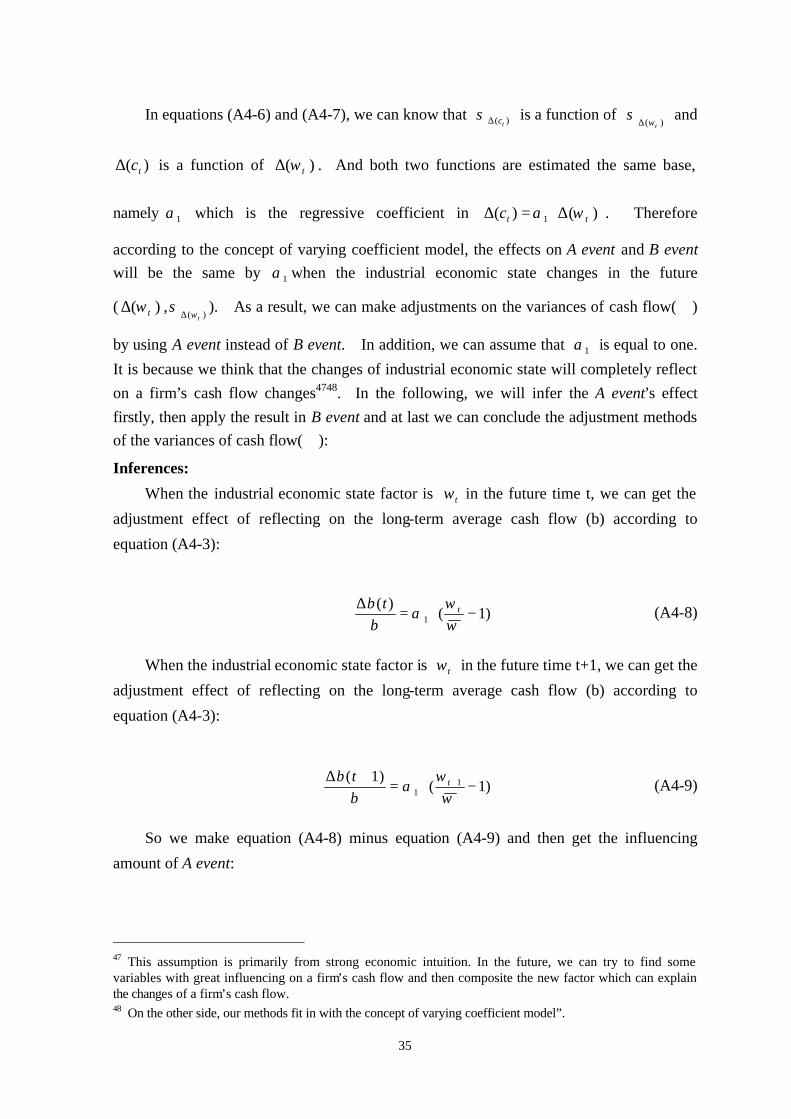
It is because we think that the changes of industrial economic state will completely reflect on a firm’s cash flow changes4748. In the following, we will infer the A event’s effect firstly, then apply the result in B event and at last we can conclude the adjustment methods of the variances of cash flow(σ):
Inferences:
When the industrial economic state factor is tω in the future time t, we can get the
adjustment effect of reflecting on the long-term average cash flow (b) according to
equation (A4-3):
)1()(
1 −⋅=∆
ωω
α t
btb (A4-8)
When the industrial economic state factor is tω in the future time t+1, we can get the
adjustment effect of reflecting on the long-term average cash flow (b) according to
equation (A4-3):
)1()1( 1
1 −⋅=+∆ +
ωω
α t
btb (A4-9)
So we make equation (A4-8) minus equation (A4-9) and then get the influencing
amount of A event:
47 This assumption is primarily from strong economic intuition. In the future, we can try to find some variables with great influencing on a firm’s cash flow and then composite the new factor which can explain the changes of a firm’s cash flow. 48 On the other side, our methods fit in with the concept of varying coefficient model”.

36
)( 11 ω
ωωα ttb
−⋅⋅ + (A4-10)
Therefore the influencing size of A event will be showed as the equation (A4-11)
when the base of cash flow is b:
)( 11 ω
ωωα tt −
⋅ + (A4-11)
According to equation (A4-11), we can know that cash flow will change by the rate of
)( 11 ω
ωωα tt −
⋅ + with the varying of industrial economic state. Moreover, we can know
that A event has the effect with B event from equation (A4-6) and (A4-7). But it is necessary to notice that 1α have to be taken as its absolute value.
In this paper, we assume that the changes of industrial economic state will fully be
reflected on the changes of firms’ firm on normal operation excluding discretionary
expenditures. So we can assume that 1α is equal to one. However, cash flow may
probably be explained by other variables so we will try to create a new factor with high
exploratory power for cash flow by using factor analysis methods. Further we can get the
better result.

37
Appendix V. Chen’s(1996) AR(1) method: apply in stochastic industrial economic
state model In this paper, we construct the stochastic industrial economic state ( tη ) model showed
as (A5-1):
dzdtbad tt ⋅+⋅−⋅= − ηηη σηη ][)( 1 (A5-1)
In equation (A5-1), both the parameters, ηb and ησ , are estimated by using the
AR(1) method (Chen, 1996). ηb stands for the long-term average change rate of industrial
economic state and ησ stands for the standard deviation of the changes of industrial
economic state’s fluctuating rate.
Chen’s estimate method is under the O-U process, and the conditional density of any
future industrial economic state is a normal distribution with the mean and variance as
follows:
)1()()]([ )()( tsatsat ebetsE −−−− −⋅+⋅= ηηη (A5-2)
ae
sVartsa
t 2]1[
)]([)(22 −−−
= ηση (A5-3)
In equation (A5-2) and (A5-3), s stands for the observed time point in the future.
With this result, we can write the equation as a discrete autoregressive process for
order 1, i.e., AR(1) process:
)()1()()( )()( sebets tsatsa ξηη η +−⋅+⋅= −−−− (A5-4)
tttata
ttt ebe ∆+∆−∆−
∆+ +−⋅+⋅= ξηη η )1( (A5-5)
Where the error term ε is normal distributed with mean 0 and variance as described
in equation (A5-3). And t∆ is a length of time interval. The AR(1) process allows tη
to satisfy all three properties of the OU process, i.e., mean, variance, and white noise with
normal density. Obtaining this exact form from discretization is essential for simplifying
the estimation process of the parameters. Equation (A5-5) can be written as the following
regression model:

38
tttt e+⋅+= ∆−ηβαη (A5-6)
where taeb ∆−=−= ββα η ),1( , so all the three parameters can be solved from
equation (A5-6).
taeMSEa
bt
Lna ∆−−
⋅=
−=
∆−
= 22
1 12
1 ηη σβ
αβ (A5-7)
According to equation (A5-7), we therefore estimate the three parameters; that are ηa , ηb
and ησ , of the stochastic industrial economic state model.

39
Appendix VI. Sensitivity analysis of credit risks’ factors
There exists a firm’s asset value distribution with mean 307 billions and the standard
deviation 123 billions. Now we assume that the speed of mean-reversion is equal to one
and implement sensitivity analysis for PD and RR in the three situations: the mean of
assets value, the standard deviation of assets value, and the debt value.
Sensitivity Analysis— PVavg
0
0.05
0.1
0.15
0.2
0.25
0.3
0.35
0.4
0.45
30%-20%-10%0% 10%20%30%PVavg
RR
PD
FigureA6-1. Sensitivity analysis—mean of asset value
Sensitivity Analysis— PVstdev
0
0.1
0.2
0.3
0.4
0.5
0.6
30%-20%-10%0% 10%20%30%PVstdev
RR
PD
FigureA6-2. Sensitivity analysis—standard deviation of asset value

40
Sensitivity Analysis—Debt
0
0.05
0.1
0.15
0.2
0.25
0.3
0.35
0.4
0.45
30%-20%-10%0% 10%20%30%Debt
RRPD
FigureA6-3. Sensitivity analysis—Debt
Figure A6-1 shows that PD will decrease and RR will increase when the firm’s value
is higher. Figure A6-2 shows that PD will increase and RR will decrease when the firm’s
volatility is higher. Figure A6-3 shows that RR is more influenced by debts’ fluctuation
than PD. This is because RR is the recovery per unit debt when defaults occur. In
summary, the above three figures appear that PD and RR are inverse-related.
Therefore both the mean and the volatility of firm’s value are more sensitive to PD
when defaults occur and disposable asset values don’t decrease greatly at the same time.
Moreover, the volatility of RR will be larger when the asset values’ fluctuation is high.

41
Appendix VII. Discussion—seniority and collateralization of corporate debt
FigureA7-1. Flow Chart-CF Based Multi-period Credit Risk Model Decision Rule
Corporate long-term debt
Loan-type Bond-type
Payoff in maturity Redeem, Putable Payment in maturity
Prepayment
Can be adjusted for its plans
2.Default Decision Rule:PV-S < L
Prepayment
Plan known
PV-A(t)-S < L Although insurance premium will reduce the firm’s value, but its protection effect make RR easier be estimated.
1.Assumption:Corporate’ total debt unchanged. Moreover, it equals to provide
quite protection on senior debt if raise subordinated debt. In the future, we will construct stochastic interest rate model to adjust the future debts’ changes.
Prepayment
Plan unknown
PV-S < L Once default occurs, internal collaterals’ value will vary greatly so that RR is hard to be estimated.
External collaterals
3. Multi-period Default Possibility, Recovery rate
Internal collaterals