t

A CFD Investigation of a Generic Bump and its Application to a Diverterless Supersonic Inlet

Master Thesis by Marlene Svensson

Aerodynamics

Examensarbete

Institutionen för ekonomisk och industriell utveckling LIU-IEI-TEK-A--08/00427--SE

_________________________________________________________________________________________

________________________________________________________________________________

3

SUMMARY

This is a Master Thesis done at the Swedish Defence Research Agency with the purpose to design and investigate how different geometries of a compression surface integrated with an intake affects the performance such as distortion, boundary layer diversion, pressure recovery and deceleration of speed.

A successful design, such as that on the Lockheed Martins F-35 Lightning II, shows that a Diverterless Supersonic Inlet (DSI) compared to a conventional intake can reduce the weigh,t and weight is the primary driver to reduce cost and increase performance of a fighter aircraft.

The work was divided in two parts. In the first part, CFD calculations using the FOI developed Edge 4.1 code were made for the compression surfaces alone. In the second part the most promising design was integrated with an intake. Two more bumps with the intake were modelled and the three geometries were compared to the intake without bump.

Surface flow, deceleration of Mach number, pressure recovery, mass flow, boundary layer diversion, lift and drag were the factors chosen to be examined, boundary layer diversion and pressure recovery being the two most vital.

The results show that an intake with a bump has higher pressure recovery than an intake without a bump. For subsonic speed the difference is negligible and for high supersonic speed the difference is about 2%. The big difference is for transonic and low supersonic speed, where the difference is 6%.

________________________________________________________________________________

4

________________________________________________________________________________

5

TABLE OF CONTENTS

SUMMARY ................................................................................................................................................ 3 TABLE OF CONTENTS........................................................................................................................... 5 NOMENCLATURE................................................................................................................................... 7 1 INTRODUCTION .......................................................................................................................... 9 2 BACKGROUND ........................................................................................................................... 11 3 THEORY ....................................................................................................................................... 15 3.1 WEDGE FLOW VS CONE FLOW.......................................................................................................... 15 3.2 REYNOLD-AVERAGED NAVIER-STOKES (RANS) EQUATIONS ......................................................... 16 3.3 RANS EQUATIONS IN EDGE............................................................................................................. 18 3.4 BOUNDARY LAYER THEORY............................................................................................................ 20 3.5 BUMP THEORY ................................................................................................................................. 22 4 GEOMETRY................................................................................................................................. 25 5 MESH GENERATION ................................................................................................................ 29 5.1 ICEM .............................................................................................................................................. 29 5.2 TRITET........................................................................................................................................... 33 5.3 FLOW SOLVER.................................................................................................................................. 36 6 RESULTS ...................................................................................................................................... 39 6.1 BUMP............................................................................................................................................... 39

6.1.1 Surface Flow ...................................................................................................................... 39 6.1.2 Mach Contour .................................................................................................................... 43 6.1.3 Pressure Recovery.............................................................................................................. 49 6.1.4 Lift & Drag Coefficients..................................................................................................... 55 6.1.5 The Boundary Layer........................................................................................................... 56

6.2 AIR INTAKE ..................................................................................................................................... 60 6.2.1 Surface Flow ...................................................................................................................... 62 6.2.2 Mach Contours................................................................................................................... 67 6.2.3 Pressure Recovery.............................................................................................................. 72 6.2.4 Mass flow ........................................................................................................................... 73 6.2.5 Boundary Layer.................................................................................................................. 78

7 DISCUSSION & CONCLUSIONS.............................................................................................. 79 8 REFERENCES.............................................................................................................................. 81 9 APPENDIX A................................................................................................................................ 83

________________________________________________________________________________

6

________________________________________________________________________________

7

NOMENCLATURE

a Speed of sound AIP Aerodynamic Interface Plane β Shock angle BLD Boundary Layer Diverter CA Capture ratio

cp Pressure coefficient qppC p )( ∞−=

c Constant ∂ Body angle DC60 Distortion DSI Diverterless Supersonic Inlet

H Total enthalpy )2( 2Vh +

h Enthalpy ρpe +

JSF Joint Strike Fighter K Constant

M Mach number avM =

p Static pressure PT Total pressure PR Pressure recovery q Dynamic pressure RANS Reynolds Average-Navier Stokes ρ Density T Temperature v Velocity (u, v, w) x-, y-, z-component of the velocity vector (X, Y, Z) Lengthwise, spanwise and amplitude axes Subscript 0, ∞ Freestream position 1 At section 1, Throat position or before shock 2 At section 2, Position at AIP, or after shock c Cone s Surface w Wedge

________________________________________________________________________________

8

________________________________________________________________________________

9

1 INTRODUCTION

This work is a Master Thesis done at the Swedish Defence Research Agency (FOI) at the institution of Computational Physics in Stockholm from October 2007 to March 2008. The aim was to investigate the effects of a bump and its application as a boundary layer diverter (BLD) and compression surface for a Diverterless Supersonic Inlet (DSI).

First, some background in the subject is described, after follows a description of the bump theory, flow equations, geometries, mesh generation and finally the results.

The remainder of the work was divided in two parts. The first part was focused on the bumps alone and in the second part the most optimal bump was integrated with an intake.

Properties such as pressure recovery, boundary layer diversion, surface flow, change in Mach number and mass flow are presented.

Special thanks to my supervisor at FOI, Magnus Tormalm.

Also thanks to Lars Johansson, my supervisor at LiTH

Stockholm, March 2008

Marlene Svensson

________________________________________________________________________________

10

________________________________________________________________________________

11

External Flow

Freestream 0

Duct Entry

Engine Face, AIP Exit

Internal Flow

Diffuser Compressor Burner Turbine

2 BACKGROUND

The purpose of the intake of an aircraft is to supply the engine with a proper airflow during various flight conditions which it can be subjected to. A good intake design is characterized by providing high pressure recovery and low distortion. Therefore it is essential to divert as much of the boundary layer as possible since it is a factor which affect the quality of the airflow. Pressure recovery is defined as the average total pressure at the engine face, Aerodynamic Interface Plane (AIP) divided by the freestream total pressure ( 02 PTPT ). Distortion is a measure of how uniform the total pressure is at the AIP. Factors which reduces the recovery is flow separation, boundary layer ingestion and shock interactions. At high speeds, the intake needs to slow down the flow before it reaches the engine face, favourable around Mach 0.5.

On aircrafts with engines installed on wing pylons, which is the most common configuration on transport- and passenger aircraft, the inlet is short and leads directly to the engine (figure 2) and the pressure recovery is nearly 100%.

Diffuser

Cowl lip

Smallest section, ”throat”

Figure 1. Principal layout of an intake and duct.

Figure 2. Duct entry of a passenger flight intake

________________________________________________________________________________

12

For engines that are integrated with the body, for example on fighter aircrafts, the airflow is travelling along the body of the aircraft before it reaches the air intake. A boundary layer builds up along the body, something which is not desirable, especially in the part of the flow that supplies the engines. The pressure recovery is lower because of this, something that has a negative effect upon engine thrust.

There are, however, ways to prevent the boundary layer from entering the inlet, or at least to minimize the amount that does. It is common to use a boundary layer diverter like the one on JAS 39 Gripen showed below in figure 4.

The diverter separates the inlet from the fuselage and the boundary layer, but it is a design feature causing the inlet weight and drag to increase and with higher maintenance requirements. It is also a negative factor when it comes to radar issues. Boundary layer bleed is a frequently used technique where the boundary layer is diverted by suction through small holes in the structure. Bleed

systems can be fixed or movable. Although these techniques are fully functional in an aerodynamic sense, they are complex and add weight and cost into the system.

Figure 4. JAS 39 Gripen, Intake with BLD

Boundary layer build up

Freestream, station 0

Throat, station 1

Cowl lip

Separation problems

Duct, diffusor

Engine

AIP, station 2

Figure 3. Fighter aircraft intake

Boundary Layer Diverter

________________________________________________________________________________

13

Another way of solving this problem is to use a compression surface, also known as a bump, that redirects the boundary layer around the intake. This design is called Diverterless Supersonic Inlet (DSI). The DSI is a new design principle, although it already exists, most famously on the Lockheed Martin F-35 Lightning II as seen in figure 5.

This design has several advantages compared to the diverter. It decreases the inlet weight, since the structure becomes less complex and it has no movable parts therefore requiring less maintenance. This further reduces the cost of the aircraft and is better concerning radar issues. It is also possible that the bump can be used to improve the negative effects caused by the bends of the duct, for example to decrease the flow separation thus creating a more uniform pressure.

Bump

Cowl lips

Figure 5. F-35 Lightning II

________________________________________________________________________________

14

________________________________________________________________________________

15

3 THEORY

3.1 Wedge flow vs Cone flow

Supersonic flow over a wedge surface has an attached, straight oblique shock wave from the nose. The flow downstream of the shock is uniform and parallel to the surface with a surface pressure equal to the static pressure behind the shock, p2w. Note that the wedge flow is two-dimensional. The shock is a function of the free stream Mach number.

A supersonic flow over a cone will also have an attached, straight oblique shock wave from the nose but since the cone is a three-dimensional body, the flow has a relieving effect. A consequence of this is that for the same body angle δ, and the same Mach number, the shock on the cone is weaker than the shock for the wedge, it will have a smaller shock angle β. For the wedge, the streamlines deflect the same angle as the wedge surface but because of the weaker shock over the cone, the streamlines over the cone is deflected a smaller angle which is gradually increasing. Because of the extra dimension of the cone, the surface pressure on the cone is lower than the surface pressure on the wedge (p2c<p2w).

The design principle for the bump is to design a compression surface similar to the cone flow described above and use the known flow fields behind conical shocks to achieve desirable results. The cone flow produces an isentropic compression which is a multi-shock compression (figure 7). The bump has pressure gradients which are spanwise and these help to redirect the boundary layer.

M∞ >1 M < 1

Figure 7. Isentropic Compression over bump

M1=2 M1=2

Wedge Cone

δ=20º δ=20º

β=53.3º β=37º

p1 p1 M2c, p2c

psc

M2w,p2w

Figure 6. Flow over a wedge and a cone.

________________________________________________________________________________

16

The surface is also used to slow down the airspeed but in reality it will not slow down all the way to subsonic speed even if this could be done in theory. It will, however, slow down to low supersonic speed. The diffuser is then used to slow down the airflow to subsonic speed.

3.2 Reynold-Averaged Navier-Stokes (RANS) equations

The Reynolds-Averaged Navier-Stokes (RANS) equations are time-averaged equations of motion for fluid flow and are primarily used while dealing with turbulent flows. They can be used with approximations based on knowledge of the properties of flow turbulence to give approximate averaged solutions to the Navier-Stokes equation.

Navier-Stokes equations (Continuity-, Momentum- & Energy Equation respectively):

(1) ( ) 0=⋅∇+∂∂ V

trr

ρρ

(2) ( ) ( ) fpVV

tV rrrrrrrrr

ρτρρ+⋅∇+∇−=⊗⋅∇+

∂∂

(3) ( ) ( )( ) ( ) cvQVfVVpe

te ϕρρτρρ rrrrrrrrrr

⋅∇−+⋅+⋅⋅∇=+⋅∇+∂

∂

The RANS equations are obtained by time averaging the Navier-Stokes system. The randomly changing flow variables are replaced by mass averages plus fluctuations about the average. After the entire equation is time-averaged. Fluctuations for viscosity, thermal conductivity and specific heat are small and therefore neglected. The definition of a time-averaged quantity and the time-averaged variables are as follows:

(4) ∫∆+

∆=

tt

tfdt

tf 0

0

1

(5) ''''

''''

HHHTTThhhppp

wwwvvvuuu

+=+=+=+=

+=+=+=+= ρρρ

For treatment of compressible flows mass-weighted averaging is required. The definition of a mass-averaged quantity and the mass-averaged variables are as follows:

(6) ρρ ff =

~

________________________________________________________________________________

17

(7) ρρ

ρρ

ρρ

ρρ

ρρ

ρρ HHTThhwwvvuu ======

~~~~~~

The fundamental equations of fluid dynamics are based on three universal laws. They are Conservation of Mass, Conservation of Momentum and Conservation of Energy. The equation that results when applying the Conservation of Mass law to a fluid flow is called the Continuity Equation. The Conservation of Momentum is Newton’s Second Law and the Conservation of Energy is the First Law of Thermodynamics.

The variables u, v and w represent the x, y and z components of the velocity vector in the Mass conservation.

For the three conservation equations new fluctuating quantities are defined as:

(8) ''''''''''''~~~~~~

HHHTTThhhwwwvvvuuu +=+=+=+=+=+=

Reynolds form of the equations are obtained by substituting the variables to mass-weighted averaged variables with fluctuations and after time-average the entire equations.

Reynolds form of the Continuity Equation is as follow:

(9) 0~

=

∂∂

+∂∂

jj

uxt

ρρ

Reynolds form of the mass-averaged Momentum Equations are as follow:

(10) ( )''''~~~

jiijji

jij

i uuxw

puux

ut

ρτρρ −∂∂

+∂∂

−=

∂∂

+

∂∂

(11)

∂∂

−

∂

∂+

∂∂

+

∂∂

−

∂∂

+∂∂

=k

kij

i

j

j

i

k

kij

i

j

j

iij

xu

xu

xu

xu

xu

xu ''

32''''

32

~~~

δµδµτ

Reynolds form of the mass-averaged Energy Equation is as follow:

(12)

+

∂∂

+∂∂

=

∂∂

−+∂∂

+

∂∂

ijiiji

jjjj

j

uuxtx

TkHuHux

Ht

ττρρρρ ''''''~~~~~

________________________________________________________________________________

18

For most problems in gas dynamics, it is possible to assume perfect gas. A perfect gas is defined as a gas whose intermolecular forces are negligible. A perfect gas obeys the perfect gas equation of state according to

(13) rTq ρ=

where r is the gas constant for the perfect gas defined as

(14) MRr =

where R is the universal gas constant and M is the molecular weight of the perfect gas.

3.3 RANS equations in Edge

In Edge 4.1, which is the flow solver used, the RANS equations are defined as:

(15) QFFt

UVI =∇+∇+

∂∂

where FI and FV are the inviscid and the viscid flux matrices and Q is the vector of source terms.

The RANS equations obtained by time averaging the Navier-Stokes equations and with first order closure based on Boussinesq’s assumption, which states that the Reynolds stress tensor is proportional to the mean strain rate tensor, and with ωi as the relative velocity component in the xi-direction the equation is:

(16) ijiji

j

j

itji k

xw

xw

ww δρδωµρ32

32 ~

~~

'''' −

∇−

∂

∂+

∂∂

=−

where

(17)

+++

=

+

+

+

+

=

=

ik

tijji

i

i

i

V

i

ii

ii

ii

i

I

kwq

f

wpE

wwp

wwp

wwp

w

f

E

w

w

wU

ii

σµ

µτ

τττ

ρ

ρδ

ρδ

ρδ

ρ

ρ

ρ

ρ

ρ

ρ

~3

2

1

~*

~

~

3

~

3*

~

2

~

2*

~

1

~

1*

~

~3

~2

~1

~

0

,,

where k is the turbulent kinetic energy and is defined as

(18) ( ) ii wwk 21=

The density and pressure are time averaged values to the instantaneous value through:

________________________________________________________________________________

19

(19) 0',' =+= qqqq

where q is the time averaged value and 'q the fluctuating part.

The energy, temperature and velocity components are density weighted averages defined as:

(20) ρρqq =~

In the following description the subscripts that denote an average are removed for clarity but note that all variables are suppose to be averaged. The static pressure and total energy contain contribution from the turbulent kinetic energy and are defined as:

(21) ( ) kpp ρ32* +=

and

(22) ( ) kwweE iii++= 32 .

The stresses and heat flux are defined as:

(23) ( ) ( ) ( )i

tiiji

j

i

itij x

Tqwxw

xw

∂∂

+=

∇−

∂

∂+

∂∂

+= κκδµµτ ,32

where κ and κt are the laminar and turbulent conductivity defined as

(24) t

ptt

p CCPr

,Pr

µκ

µκ == .

The turbulent viscosity follows from the turbulence model.

In the turbulence model, two additional transport equations for the turbulent kinetic energy k are added. The turbulence model used was the EARSM by Wallin & Johansson [16] together with the k-ω model by Hellsten [17]. The model solves for the k and ω equations and is described in detail in the incompressible form by Hellsten. The extension to compressible flows according to Wallin & Johansson [16] is used.

________________________________________________________________________________

20

Height of boundary layer. = 99% of vfree Rotational

Flow

Velocity

3.4 Boundary Layer Theory

The boundary layer is the area of the airflow closest to a wall where the friction affects the particles so that it is no longer free from rotation. In inviscid flow there is no friction and no rotation. Inviscid flow is typically is considered to be to coarse an approximation close to an aerodynamic surface. Therefore, the concept of a viscous boundary layer is introduced. For viscid flow there is friction and therefore also rotation. K.Karling [10] visualizes inviscid and viscid flow as in figure 8.

The thickness of the boundary layer was estimated using the vorticity, which is a measure of rotation in the fluid and the boundary layer is a form of rotation caused by the friction from the wall. The BL is approximated with vorticity times the wall distance. For a subsonic case this function reaches a maximum peak around half of the actual BL thickness. This estimation of the BL was taken from the Baldwin-Lomax model [3]. It should be noted that the definition of the boundary layer thickness varies between sources, but the differences are not very

large in practice, and anyway the goal here is to make a comparison between the bumps, not to compare the results with

published data.

Vorticity is defined as:

(25) ( )

∂∂

−∂

∂

∂∂

−∂∂

∂

∂−

∂∂

=×

∂∂

∂∂

∂∂

=×∇=

=

yv

xv

xv

zv

zv

yvvvv

zyxvvrot

vvvv

xyzxyzzyx

zyx

,,,,;;

,,

Figure 9. Boundary Layer

Rotation = 0 Rotation ≠ 0

Figure 8. Potential flow vs rotational flow.

________________________________________________________________________________

21

(a) Walldistance

(b) Vorticity

(c) Vorticity*Walldistance

Figure 10. Estimation of Boundary Layer height

Max ≈ ζ /2

End of BL from the Baldwin-Lomax turbulence model.

________________________________________________________________________________

22

3.5 Bump theory

The bump geometry is defined by curves at different longitudinal stations. The shapes of the bump curves were created with the help of a hyperbolic approximation for the cone-flow streamlines. If streamlines are released at a height K over a cone, they will form the shape as seen in figure 11. Streamlines are then released at different K to get the longitudinal cuts which are later connected to a three-dimensional surface in ProEngineer®. Equations taken from Seddon & Goldsmith [1] were implemented in MATLAB® to design the bumps. The intercepting plane represents the side of the fuselage.

T

The equations were as follows:

The equation of the plane, with β as the cone-shock angle:

(26) .constKz ==

(27) x

zw θβ

sectan =

The equations for the intersection of the plane and shock surface were:

(28) θβ seccotKx =

(29) θtanKy =

(30) 2222 tan Kyx =−β

Compression surface cross section Cone flow

streamline

Cone shock

Compression surface planform

β∂

Z

X Y

X

Y

ys rc

rw

K

Z

Ө

zs

Figure 11. Bump intake compression surface derived from conical flow field intercepted by plane surface.

________________________________________________________________________________

23

The equation for the streamline was:

(31) cxzr +== δθ 22222 tansec .

The streamline equation was solved for the z-coordinate before implementing it in MATLAB® to create the bump-geometry. With δ as the cone angle and c as a constant the equation were:

(32)

( )BA

Ka

cxcxz **

)1tancos(1

tansectan

2

22

2

22

+=

+=

δθδ

The initial geometry had two imperfections that were corrected as follows; first the discontinuous boundaries along the side edges were corrected by multiplying the function z with a trigonometric function A. Second, the boundary at the end downstream was not converging. To correct this problem, the function z was also multiplied with the function B. The total MATLAB®-program can be found in the appendix A.

Original Smaller Softer Blunter Mod δ π/28 π/48 π/47 π/13.5 π/15 c 0 0 0.03 0 0 K 1.3 1.3 1.3 1.3 1.0 A sin(x) sin(x) sin(x) sin(x) sin(x)

B sin((y+π)/2) sin((y+π)/2) sin((y+π)/2 sin((y+π )/2) *sin(x)/2

sin((y+π)/2) *(sin(x)/25)

Table 1. Settings in the MATLAB-program.

________________________________________________________________________________

24

________________________________________________________________________________

25

4 GEOMETRY

To investigate how different shapes and amplitudes affected the flow, four different designs were created. Based on the results which will be presented later from these four bumps, a fifth bump called Mod was created. The overall dimensions of the first four bumps are the same, but their shapes are different to investigate the difference of the flow over a variety of shapes. Bump Original has a smooth start and a blunt end. Bump Smaller has the same shape as the first bump but lower amplitude to see what significance the height of the bump has to the flow. Bump Softer has both a smooth start and a smooth end. Bump Blunter has a blunt start and blunt end. A comparison between bump Softer and bump Blunter will show, for example, how the shock changes or if the boundary layer is diverted best over a smooth or blunt surface. Their measurements can be seen in table 2 and 3 and their shapes in figure 12.

Original Smaller Softer Blunter Mod Length 1 1 1 1 1.4 Width 1 1 1 1 0.65 Height 0.2 0.1 0.2 0.2 0.18

Table 2. Bump measurements [m]

Original Smaller Softer Blunter Mod

0.65 0.65 0.6 0.55 0.84

Table 3. x-position for maximal amplitude [m]

________________________________________________________________________________

26

(a) Original Bump

(b) Original Bump (Side view)

(c) Smaller Bump

(d) Smaller Bump (Side view)

(e) Softer Bump

(f) Softer Bump (Side view)

(g) Blunter Bump

(h) Blunter Bump (Side view)

(i) Mod Bump

(j) Mod Bump (Side view)

Figure 12 Bump Geometries

________________________________________________________________________________

27

The curve geometries created in MATLAB® were imported into the commercial CAD-program ProEngineer® to create corresponding three-dimensional surfaces using the boundary blend function.

Three bumps were integrated with the intake. For the first geometry, Intake & Mod 1, the bump is the same as can be seen in figure 12 (i) and 12 (j). The three-dimensional geometry of bump Mod was scaled and directly incorporated with the three-dimensional geometry of the intake.

For the two other geometries, Intake & Mod 2 and Intake & Mod 3, the bumps were created in the ProEngineer® geometry model of the intake with the help of the sketch function. Two-dimensional curves were created with the sketch function which were blended together to a three dimensional surface with the boundary blend function.

Figure 13. Intake & Mod 2 in ProEngineer®

________________________________________________________________________________

28

________________________________________________________________________________

29

5 MESH GENERATION

5.1 ICEM

The geometries from ProEngineer® were imported into ANSYS ICEMCFD™ which is a mesh generation program. It is, in this work, used to create a surface mesh and a rough volume grid of tetrahedrals which looks like half pyramid. The boundary layer mesh and the final volume mesh are completed in the FOI developed program TRITET which is described later. It is necessary to discretizise the volume to be able to use a finite volume CFD code. A wall was created around the bump to represent the fuselage to enable the build up of a BL in front of the bump.

To have the correct conditions, the freestream boundaries were located 100 meters upstream of, downstream of and above the bump. The size of the mesh parameters in ANSYS ICEMCFD™ can be seen in table 4 and 5 on page 32 and the choice of the boundary conditions can be seen in table 9, page 36.

Duct out

Duct in

Lip out

Lip in

Inlet Bump

Figure 14. Intake & Mod 1

________________________________________________________________________________

30

Figure 15. Original bump, side view.

1 m

Figure 16. Boundary Conditions

________________________________________________________________________________

31

(a) Clean Intake

(b) Intake & Mod 1

(c) Intake & Mod 2

(d) Intake & Mod 3

Figure 17. Mesh, Side view

The three meshes with intake and a bump have about the same sizes of 2 million nodes. The meshes are refined at the top of the bump and on the surfaces of the intake for a more exact solution. A mesh that is too refined will require a lot of computer recourses and longer time to solve the CFD calculations but a mesh that is not refined enough will have a solution that is mesh dependent instead of a physical correct solution. At a distance far away from the surfaces, the volume mesh can be coarser since there will not be disturbances in the flow. The mesh for the clean intake was remade with a more refined mesh with a size twice as big as the other three. The difference in the global scale factor, see table 4 and 5, is due to the difference in the measurements in the ANSYS ICEMCFD™ models with the bump geometries being in meters and the intakes in millimetres.

________________________________________________________________________________

32

Global Mesh Parameters Original Smaller Softer Blunter Mod

Scale factor 0.05 0.05 0.05 0.07 0.2 Max element 200 200 200 200 200 Curvature refinement, min size 0.03 0.03 0.03 0.03 0.03

Mesh Size For Parts

(Max/deviation)

Bump 0.5/0.01 0.5/0.01 0.5/0.01 0.5/0.01 0.5/0.01 Bottom 100/0 100/0 100/0 80/0 100/0 Fuselage 1/0 1/0 1/0 0.8/0 1/0 Flow In 100/0 100/0 100/0 80/0 100/0 Flow Out 100/0 100/0 100/0 80/0 100/0 Left 100/0 100/0 100/0 80/0 100/0 Right 100/0 100/0 100/0 80/0 100/0 Top 100/0 100/0 100/0 80/0 100/0

Table 4. ICEM mesh parameters for the bumps

Global Mesh Parameters Clean Intake Intake &

Mod 1 Intake & Mod 2

Intake & Mod 3

Scale factor 20 20 20 15 Max element 200 200 200 200 Curvature refinement, min size 0.01 0.01 0.01 0.01

Mesh Size For Parts

(Max/deviation)

Bump - 1/0.01 1/0.01 1/0.01 Bottom 50/0 150/0 200/0 150/0 Wall 5/0 3/0.01 20/0 10/0.2 Flow In 200/0 200/0 200/0 200/0 Flow Out 200/0 200/0 200/0 200/0 Left 200/0 200/0 200/0 200/0 Right 200/0 200/0 200/0 200/0 Top 200/0 200/0 200/0 200/0 Duct In 1/0.01 1/0.01 2/0.01 1/0.2 Duct Out 1/0.01 1/0.01 2/0.01 1/0.2 Lip In 1/0.01 1/0.01 2/0.01 1/0.2 Lip Out 1/0.01 1/0.01 2/0.01 1/0.2 Inlet 1/0 1/0 2/0.01 10/0.2

Table 5. ICEM mesh parameters for the intakes

________________________________________________________________________________

33

Max deviation is used to refine the mesh close to the surface. The distance between two nodes, multiplied with the max deviation results in R. If the distance from the line between the two nodes and a point on the surface are greater than R then the mesh will cut and resized to smaller elements.

The mesh is constructed with the help of nodes, tetrahedrals, prismas and triangles. Nodes are connection points in the volume. The volume mesh consists of tetrahedrals (tetra) which look like half of a pyramid. The BL mesh consists of prismas (prism) which look like a triangle in the base which has amplitude. Therefore, on the surfaces there will be triangles (tria).

5.2 TRITET

The geometry with the tetrahedral mesh that was generated in ANSYS ICEMCFD™ was transferred to the FOI developed mesh generation program TRITET used first to add prismatic layers from the surface mesh. Prismatic layers are a refined mesh normal to the surface and must be used where boundary layers exist to have a more precise result, so in this work a prismatic layer is added along the surface of the bump and wall. Subsequently, TRITET creates the final volume mesh.

The mesh was refined in the top of the bump to give a more exact solution. The BL mesh was chosen to have a maximum of 50 layers. For each layer, the mesh elements are increased in size and when the prismatic mesh has the same size as the tetrahedrical mesh, the process is terminated.

The prismatic grid parameters in TRITET can be seen in table 7 and 8, page 35.

Figure 19. Prismatic Mesh, Bump Smaller

R

Figure 18. Deviation

________________________________________________________________________________

34

Figure 20. Surface grid, Smaller bump

Figure 21. Prismatic grid, Blunter bump

Figure 23. Prismatic grid, Mod bump

Figure 22. Prismatic grid, Clean Intake

________________________________________________________________________________

35

Figure 24. Prismatic grid blunter bump

Original Smaller Softer Blunter Mod

Nodes (e6) 1.2 1.0 0.8 0.7 0.2 Tetra (e6) 1.5 1.6 0.7 0.4 0.05 Prism (e6) 1.8 1.3 1.3 13.3 0.3

Bump (tria) (e3) 9.2 6.3 13.0 8.2 42.3 Fuselage (tria) (e3) 17.1 11.0 5.3 12.4 0.9

Table 7. Number of nodes, tetrahedrals, prismas and triangles for the bumps

Bumps Clean Intake Intake & Mod 1, Intake & Mod 2 Intake & Mod3

No of grid layers 50 50 50 50 Total extent of all

layers 0.3 0.07 0.3 0.05

Extent of 1st grid layer 1e-6 1e-6 1e-6 1e-6

Expansion break point index 0-1 0.5 0.5 0.5 0.5

Expansion modification factor

>0 1.0 1.0 1.0 1.0

Check for intersection -1/0/1 1 1 1 1

Concave corner influence 0-2 0.7 0.4 0.7 0.7

No of smoothing iterations >=0 20 20 20 20

No of optimization iterations >=0 1000 1000 1000 1000

Table 6. TRITET Parameters

Clean Intake

Intake & Mod 1

Intake & Mod 2

Intake & Mod 3

Nodes (e6) 4.8 3.4 1.4 2.2 Tetra (e6) 2.6 1.0 0.7 1.3 Prism (e6) 8.5 6.4 2.6 3.9

Bump(tria) (e3) - 34.9 2.8 49.2 Fuselage(tria) (e3) 49.7 59.5 4.6 8.5 Duct in (tria) (e3) 16.1 16.2 14.7 9.4

Duct out (tria) (e3) 13.8 13.7 12.2 10.0 Lip in (tria) (e3) 6.9 6.9 6.8 16.7

Lip out (tria) (e3) 5.2 5.2 5.1 1.8 Inlet (tria) (e3) 0.9 1.2 0.9 1.0

Table 8. Number of nodes, tetrahedrals, prismas and triangles for the Intakes

________________________________________________________________________________

36

5.3 Flow solver

After TRITET, the grid was complete and ready to be implemented in the FOI developed CFD code Edge 4.1 [2] which is a CFD flow solver for compressible flow with unstructured grids.

The solver has an edge-based formulation and uses node-centered finite volume techniques. Edge solves, in this case, the three-dimensional RANS equations (Reynolds-Averaged Navier-Stokes) for turbulent and viscous steady state flow. The equations were integrated with a third order Runge-Kutta time integration until steady state conditions were reached. The convergence was accelerated using agglomeration multigrid and implicit residual smoothing. The turbulence model used was Wallin and Johansson EARSM model with Hellsten standard k-ω.

The boundary conditions for the different models can be seen in table 9. The condition “Eulerwall” means that the part is inviscid. Standard Atmosphere values at sea level were used which correspond to 101325 Pa for static pressure, 288.15 K for temperature and mass flow of 75 kg/s.

The final results were studied in ENSIGHT which is a postprocessing program.

For each case, the computation was continued until the residuals had converged or almost converged. The cases with oscillations were computed until the oscillations were stable. The number of iterations required depends on the complexity of the geometry. Cases with large oscillations are likely to have large separations and cannot be solved by using RANS equations. These would demand timeaccurate calculations, which are a factor 60 more time consuming.

As an example, it can be seen in figure 25 (d) that the residuals are converged while they are about to converge for 25 (c). Figure 25 (a) and (b) on the other hand show ocillations.

Original Bump Smaller Bump Soft, Blunt, Mod Bump Intakes

Flow in Weak static pressure

Weak free stream pressure

Weak characteristic

pressure

Weak characteristic pressure

Flow out Weak free

stream pressure

Weak characteristic pressure

Weak characteristic

pressure

Weak static pressure

Left side Symmetry Symmetry Symmetry Weak characteristic pressure

Right side Symmetry Symmetry Symmetry Weak characteristic pressure

Top side Symmetry Symmetry Symmetry Weak characteristic pressure

Bottom Side Eulerwall Eulerwall Eulerwall Eulerwall

Surfaces (Bump, fuselage, duct) Adiabatic wall Adiabatic wall Adiabatic wall Adiabatic wall

Inlet - - - Mass flow outlet

Table 9. Boundary conditions in EDGE.

________________________________________________________________________________

37

(a) Intake & Mod 3, Mach 0.6

(b) Mod bump, Mach 1.6

(c) Clean Intake, Mach 1.3 (d) Intake & Mod 1, Mach 1.2

Figure 25. Residuals

________________________________________________________________________________

38

Residuals Forces Rho Density ρ Cl Non-dimensional lift

U Velocity in x-direction Cd Non-dimensional drag

V Velocity in y-direction Cm Non-dimensional moment

W Velocity in z-direction

E Energy (turbulent viscosity)

K Turbulent Kinetic Energy

Z Turbulent ω

Table 10. Residuals and forces

________________________________________________________________________________

39

6 RESULTS

In the following chapters, the results are presented. First the results for the bump alone are described. Surface flow, Mach contour, pressure recovery, lift, drag and boundary layer are analyzed.

In the second part the intakes are described. Both intake with and without a bump are presented. Surface flow, Mach contour, pressure recovery, boundary layer and mass flow are the chosen characteristics.

6.1 Bump

In this section, the simulations made in Edge 4.1 are described. The paths of the airflow along the surface of the bumps, changes in Mach along the bump and pressure recovery were visualized in ENSIGHT whilst boundary layer, lift and drag were plotted in MATLAB®.

Each bump was simulated for six different Mach numbers ranging from 0.6 up to 1.6 to cover subsonic-, transonic- and supersonic speed.

It should be mentioned that the bump with the best results at this stage might not be the best result in the secondary step when the intake is to be included in the geometry since there will be forces from the intake affecting the results. Thus, it is possible that the intake will counteract, for example, separation.

6.1.1 Surface Flow Streamlines are released just above the surface in front of the bump and they can show for example how well the bumps redirect the flow or if they give rise to swirls.

The colour on the surfaces indicate different values of Cp which inform us of the pressure acting on it, red areas being higher pressure and blue being lower pressure. In areas where the pressure is low, there is a risk of flow separation and turbulence. Bump Smaller and Mod have no or little high pressure area and they have less low pressure area than the other bumps.

Bump Original show tendency of separation for Mach numbers up to Mach 0.95. Bump Softer has large regions of low pressure and severe swirls for subsonic speeds and the bump Blunter has the same tendency but not as severe. Bump Smaller and Mod show the least low pressure areas and almost no swirls. The capacity to divert the streamlines smoothly is connected to how big swirls that arise. Therefore, bump Smaller and Mod has the smoothest and most effective diversion of the streamlines.

________________________________________________________________________________

40

(a) Mach 0.6 (b) Mach 0.6

(c) Mach 0.8

(d) Mach 0.8

(e) Mach 0.95

(f) Mach 0.95

Figure 26. Surface Flow, Original Bump (M0.6 to M0.95)

________________________________________________________________________________

41

(g) Mach 1.1

(h) Mach 1.1

(i) Mach 1.3

(j) Mach 1.3

(k) Mach 1.6

(l) Mach 1.6

Figure 27. Surface Flow, Original Bump (M1.1 to M1.6)

________________________________________________________________________________

42

(a) Mach 1.1

(b) Mach 1.1

Figure 28. Surface Flow, Smaller Bump

(a) Mach 1.1

(b) Mach 1.1

Figure 29. Surface Flow, Softer Bump

(a) Mach 1.1

(b) Mach 1.1

Figure 30. Surface Flow, Blunter Bump

________________________________________________________________________________

43

(a) Mach 1.1

(b) Mach 1.1

Figure 31. Surface Flow, Mod Bump

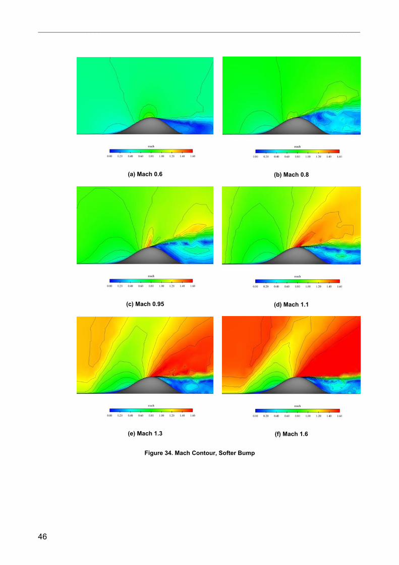
6.1.2 Mach Contour The changes in Mach number can be seen in figure 32-36. They are visualized on an X-Z cut plane along the middle of the bumps, low Mach numbers being blue areas and higher Mach numbers being red areas. Contour lines are added with ∆M=0.05 for clarity, i.e. the Mach number changes with 0.05 between the areas.

It is desirable to have a deceleration of the Mach number after the bump, giving a smaller workload on the diffuser which has to decelerate the speed of the air before it reaches the face of the engine. Naturally, there was an increase of Mach at the top of the bumps. For supersonic speeds there is a non attached oblique shock. After the shock the velocity decreases but after maximum amplitude the speed is increasing again. This gives the impression that it would be optimal to place the bump relative to the intake so that maximum amplitude of the bump are directly underneath the cowl lips of the intake.

All the first four bumps have a lot of separation caused by the abrupt end of the bumps although bump Blunter has a reduction of the wake. This could be solved by extending the bumps and give them a smoother end and is therefore not the primary issue. More important is the shock induced separation that occurs for some bumps. This causes a drop in pressure recovery which cannot be regained. A comparison between bump Original and Smaller for Mach 1.3 show that higher amplitude has more tendencies for shock induced separation.

A comparison between bump Original with Softer and Blunter for Mach 1.6 show that a smooth start has a more detached shock. An attached shock is more favourable.

Bump Original, Softer and Blunt decelerate the airflow to subsonic speed for supersonic speeds, whereas this is difficult to achieve with Bump Smaller and Mod..

The bump Mod has less separation than the other bumps and it also has less deceleration of the airflow.

________________________________________________________________________________

44

(a) Mach 0.6

(b) Mach 0.8

(c) Mach 0.95

(d) Mach 1.1

(e) Mach 1.3

(f) Mach 1.6

Figure 32. Mach Contour, Original Bump

________________________________________________________________________________

45

(a) Mach 0.6

(b) Mach 0.8

(c) Mach 0.95

(d) Mach 1.1

(e) Mach 1.3

(f) Mach 1.6

Figure 33. Mach Contour, Smaller Bump

________________________________________________________________________________

46

(a) Mach 0.6

(b) Mach 0.8

(c) Mach 0.95

(d) Mach 1.1

(e) Mach 1.3

(f) Mach 1.6

Figure 34. Mach Contour, Softer Bump

________________________________________________________________________________

47

(a) Mach 0.6

(b) Mach 0.8

(c) Mach 0.95

(d) Mach 1.1

(e) Mach 1.3

(f) Mach 1.6

Figure 35. Mach Contour, Blunter Bump

________________________________________________________________________________

48

(a) Mach 0.6

(b) Mach 0.8

(c) Mach 0.95

(d) Mach 1.1

(e) Mach 1.3

(f) Mach 1.6

Figure 36. Mach Contour, Mod Bump

________________________________________________________________________________

49

6.1.3 Pressure Recovery As mentioned above, the pressure recovery is important and it should be as close to 100 % as possible.

Figure 38-42 show the pressure recovery on a plane which represent an intake. It is placed at maximum amplitude for each bump and is at that position a fair indication of how much of the boundary layer that is diverted. The plane is modified for each case so that is has the same area.

The pressure recovery is summarized in table 11 and it shows that bump Mod has a pressure recovery greater than 99% for all Mach numbers and is superior to the other bumps. The big drop in the curves of figure 37 might be because they were not entirely converged in Edge 4.1 or the mesh was not refined enough. They might also be caused by the shock induced separation.

The irregularities in figure 40 b and c is most likely caused by non convergence.

The BL is visible on the figures and is unacceptably large at Mach numbers larger than 1.3 for bump Smaller, Softer and Blunter. As can be seen in figure 37, the size of the boundary layer has a connection with the pressure recovery. For bump Smaller at the other Mach numbers, the BL has about the same height spanwise and is therefore not redirecting the BL.

In figure 42 the diversion of the BL is clearly visible with smaller amplitude at the top of the bump which gradually increases spanwise.

Mach Original Small Soft Blunt Mod 0.6 0.99977 0.99884 0.99849 0.99799 0.99630 0.8 0.99366 0.99825 0.99377 0.99709 0.99634

0.95 0.99513 0.99702 0.98503 0.99721 0.99552 1.1 0.99348 0.98906 0.99487 0.98667 0.99410 1.3 0.98926 0.91291 0.94165 0.96099 0.99320 1.6 0.97363 0.93863 0.90657 0.93653 0.99064

Table 11. Pressure Recovery, Bumps

Figure 37. Pressure Recovery

________________________________________________________________________________

50

(a) Mach 0.6 (b) Mach 0.8

(c) Mach 0.95 (d) Mach 1.1

(e) Mach 1.3 (f) Mach 1.6

Figure 38. Pressure Recovery at max amplitude, Original Bump

________________________________________________________________________________

51

(a) Mach 0.6

(b) Mach 0.8

(c) Mach 0.95

(d) Mach 1.1

(e) Mach 1.3

(f) Mach 1.6

Figure 39. Pressure Recovery at max amplitude, Smaller Bump

________________________________________________________________________________

52

(a) Mach 0.6

(b) Mach 0.8

(c) Mach 0.95

(d) Mach 1.1

(e) Mach 1.3

(f) Mach 1.6

Figure 40. Pressure Recovery at max amplitude, Softer Bump

________________________________________________________________________________

53

(a) Mach 0.6

(b) Mach 0.8

(c) Mach 0.95

(d) Mach 1.1

(e) Mach 1.3

(f) Mach 1.6

Figure 41. Pressure Recovery at max amplitude, Blunter Bump

________________________________________________________________________________

54

(a) Mach 0.6 (b) Mach 0.8

(c) Mach 0.95 (d) Mach 1.1

(e) Mach 1.3 (f) Mach 1.6

Figure 42. Pressure Recovery at max amplitude, Mod Bump

________________________________________________________________________________

55

6.1.4 Lift & Drag Coefficients Lift and drag were plotted for a comparison between the five bumps over a range from Mach 0.6 to 1.6. Here, the most important goal is to have a bump with a low CD. In figure 43, it can be seen that the bump Blunter is superior to the others in CL but bump Mod has the lowest drag for Mach numbers up to 1.2 and bump Smaller has the lowest drag for Mach numbers above 1.2. The difference between Mod and Smaller for supersonic speed is very small.

(a) CL-Mach Number

(b) CD-Mach Number

Figure 43. Lift and Drag vs. Mach Number, Bumps

________________________________________________________________________________

56

6.1.5 The Boundary Layer A good bump will divert a large part of the boundary layer, it will have a wide range where the thickness of the boundary layer does not increase and it will divert the boundary layer smoothly. By plotting the height of the boundary layer along the bump, it can be seen which bump diverts the boundary layer most efficient.

A computation was done for a flat plate for comparison with the bumps. The height of the boundary layer for the five bumps and the flat plate can be seen in figure 44 a-f. It shows that all five bumps have a reduction in the height of the boundary layer from the x-position of 0.3 to 0.6 which is around their maximum amplitude, the boundary layer start to grow again after x-position 0.7 to 0.8. The curve from the plate continues to grow as expected. The figures show that bump Mod has the smoothest diversion of boundary layer.

________________________________________________________________________________

57

(a) Mach 0.6

(b) Mach 0.8

________________________________________________________________________________

58

(c) Mach 0.95

(d) Mach 1.1

________________________________________________________________________________

59

(e) Mach 1.3

(f) Mach 1.6

Figure 44. Boundary Layer, Bumps

________________________________________________________________________________

60

6.2 Air Intake

The next step was to integrate a bump with the intake. The latest, modified bump Mod was chosen because of its superior results of higher pressure recovery, its ability to divert boundary layer and less separation.

Before the bump was integrated with the intake, a mesh was done for the intake alone. This was done so that a comparison could be made between the intake with and without a bump.

The intake was taken from FS2020, a FoT25 study made by FOI and SAAB. It had sharp lips with zero thickness for a low signature which is suitable for high speeds but it will have problems for low speeds, for example, take-off and landing. The lips were given a more curvature and thickness for more friendly flow into the intake. A disadvantage that was chosen not to be changed is the upper and lower lips which are swept forward. It would be better if they were swept backwards so that they form an inner corner seen from above.

The ambition was to place the bump so that the cowl lips would intersect the shock caused by the bump. The design point for the airplane, from which the intake comes, is at Mach 1.2.

Two more modifications were made to see if it was possible to find geometries with less separation and possibly with higher pressure recovery and mass flow. First, a change was made to make the bump more suitable for a square intake. The second modification was made similar to bump Mod that was first used with the intake. The changes were a longer and wider bump but the principal shape and height remained the same. The geometries can be seen in figures 47-48.

Figure 45. Intake of FS2020

________________________________________________________________________________

61

(a) Top View

(b) Side View

(c) Front View (d) Iso View

Figure 46. FS 2020

(a) Iso view

(b) Front View

(c) Side View

Figure 47. Clean Intake

________________________________________________________________________________

62

(a) Intake & Mod 1, Front View

(b) Intake & Mod 1, Side View

(c) Intake & Mod 2, Front View

(d) Intake & Mod 2, Side View

(e) Intake & Mod 3, Front View

(f) Intake & Mod 3, Side View

Figure 48. Intakes

6.2.1 Surface Flow It can be seen in figure 49-52 that the bumps are redirecting more of the airflow around the intake in the lower part than in the upper part. On the upper part, the airflow is also redirected but since the cowl is swept forward, the airflow is still entering the intake. Since the geometry of the intake was chosen not to be changed, the position of the bump should be changed instead so that the airflow on the upper part also can be redirected outside of the intake. It is realized that if the bump is only repositioned further out from the intake, the airflow on the lower side might still be sucked into the intake. A possible solution would be to reshape the bump so that it has amplitude before the cowls both on the upper and lower side of the intake, i.e. to make it more square shape. This was the attempt for Intake & Mod 2.

In figure 49 b it can be seen that there are low pressure on the outside of the lower cowl lip. This will cause the flow to separate. It can also be seen that it looks uneven on the lips, this is because of the mesh which is not refined enough. Therefore it is possible that the flow over the lips are mesh dependent instead of physical dependent.

For supersonic flow, there is a shock caused by the lips of the intake. This can be seen in figure 49 f. The shock helps to push the streamlines away from the intake.

Some of the bumps have separation and swirls for supersonic speeds. This happens for example for Intake & Mod 1 at Mach 1.3. Intake & Mod 3 seem to be most eager for separation and swirls. This bump seems to be oriented too far upstream and a lot of the streamlines are not redirected outside the intake.

________________________________________________________________________________

63

(a) Mach 0.6

(b) Mach 0.8

(c) Mach 0.95

(d) Mach 1.1

(e) Mach 1.3

(f) Mach 1.6

Figure 49. Surface Flow, Clean Intake

________________________________________________________________________________

64

(a) Mach 0.6

(b) Mach 0.8

(c) Mach 0.95

(d) Mach 1.2

(e) Mach 1.3

(f) Mach 1.6

Figure 50. Surface Flow, Intake & Mod 1

________________________________________________________________________________

65

(a) Mach 0.6

(b) Mach 0.8

(c) Mach 0.95

(d) Mach 1.2

(e) Mach 1.3

(f) Mach 1.6

Figure 51. Intake & Mod 2

________________________________________________________________________________

66

(a) Mach 0.6

(b) Mach 0.8

(c) Mach 0.95

(d) Mach 1.2

(e) Mach 1.3

(f) Mach 1.6

Figure 52. Intake & Mod 3

________________________________________________________________________________

67

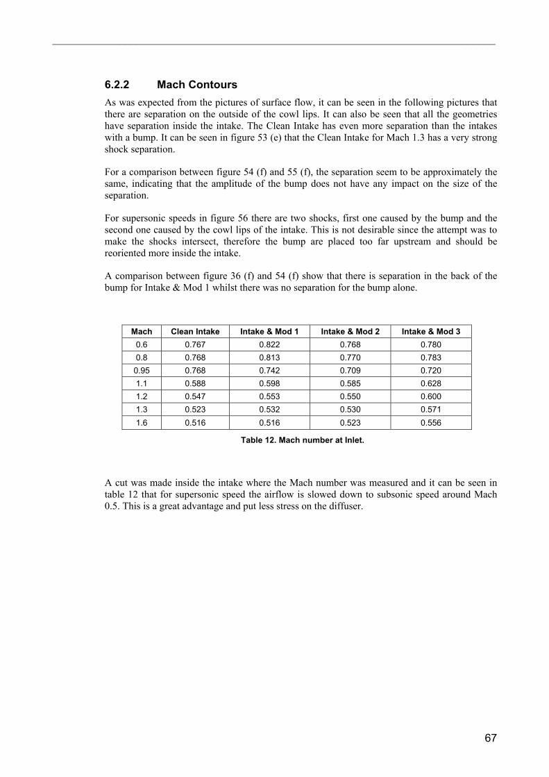
6.2.2 Mach Contours As was expected from the pictures of surface flow, it can be seen in the following pictures that there are separation on the outside of the cowl lips. It can also be seen that all the geometries have separation inside the intake. The Clean Intake has even more separation than the intakes with a bump. It can be seen in figure 53 (e) that the Clean Intake for Mach 1.3 has a very strong shock separation.

For a comparison between figure 54 (f) and 55 (f), the separation seem to be approximately the same, indicating that the amplitude of the bump does not have any impact on the size of the separation.

For supersonic speeds in figure 56 there are two shocks, first one caused by the bump and the second one caused by the cowl lips of the intake. This is not desirable since the attempt was to make the shocks intersect, therefore the bump are placed too far upstream and should be reoriented more inside the intake.

A comparison between figure 36 (f) and 54 (f) show that there is separation in the back of the bump for Intake & Mod 1 whilst there was no separation for the bump alone.

Mach Clean Intake Intake & Mod 1 Intake & Mod 2 Intake & Mod 3 0.6 0.767 0.822 0.768 0.780 0.8 0.768 0.813 0.770 0.783 0.95 0.768 0.742 0.709 0.720 1.1 0.588 0.598 0.585 0.628 1.2 0.547 0.553 0.550 0.600 1.3 0.523 0.532 0.530 0.571 1.6 0.516 0.516 0.523 0.556

Table 12. Mach number at Inlet.

A cut was made inside the intake where the Mach number was measured and it can be seen in table 12 that for supersonic speed the airflow is slowed down to subsonic speed around Mach 0.5. This is a great advantage and put less stress on the diffuser.

________________________________________________________________________________

68

(a) Mach 0.6

(b) Mach 0.8

(c) Mach 0.95

(d) Mach 1.2

(e) Mach 1.3

(f) Mach 1.6

Figure 53. Mach Contour, Clean Intake

________________________________________________________________________________

69

(a) Mach 0.6

(b) Mach 0.8

(c) Mach 0.95

(d) Mach 1.2

(e) Mach 1.3 (f) Mach 1.6

Figure 54. Mach Contour, Intake & Mod 1

________________________________________________________________________________

70

(a) Mach 0.6

(b) Mach 0.8

(c) Mach 0.95

(d) Mach 1.2

(e) Mach 1.3

(f) Mach 1.6

Figure 55. Mach Contour, Intake & Mod 2

________________________________________________________________________________

71

(a) Mach 0.6

(b) Mach 0.8

(c) Mach 0.95

(d) Mach 1.2

(e) Mach 1.3

(f) Mach 1.6

Figure 56. Mach Contour, Intake & Mod 3

________________________________________________________________________________

72

6.2.3 Pressure Recovery

Mach Clean Intake Intake & Mod 1 Intake & Mod 2 Intake & Mod 3 0.6 0.9655 0.9642 0.9728 0.9664 0.8 0.9497 0.9420 0.9593 0.9660 0.95 0.8956 0.9660 0.9632 0.9637 1.1 0.8800 0.9338 0.9294 0.9036 1.2 0.8788 0.8974 0.8847 0.8478 1.3 0.8225 0.8425 0.8306 0.7951 1.6 0.6676 0.6685 0.6803 0.6559

Table 13. Pressure recovery at Inlet

A comparison between Mod 1, Mod 2 and Mod 3 show that Mod 1 has in general the highest pressure recovery. The exception is for subsonic and high supersonic speed.

A comparison between Clean Intake with the other geometries show that an intake with a bump has higher pressure recovery for all Mach numbers.

Figure 57 and table 13 show the pressure recovery for all the intakes from Mach 0.6 to 1.6. The differences between the intakes with a bump are not very large. Compared to the Clean Intake, the gain in pressure recovery for subsonic speed is less than 0.5%. For supersonic speeds the gain is in average 2 % but the biggest gain is for transonic speed, then the difference is about 7 %.

Figure 57. Pressure Recovery, Intakes

________________________________________________________________________________

73

6.2.4 Mass flow The required mass flow for Mach 1.2 was 75 kg/s. Table 14 show that this requirement is not entirely fulfilled but it can also be seen that this requirement isn’t even fulfilled for a clean intake. Even if the difference between the four geometries are not great, figure 58 show that the mass flow are higher for intake with bump for Mach numbers lower than Mach 1.1 and the mass flow are lower for Mach numbers higher than Mach 1.3. This could be an effect caused by the computer code used, Edge 4.1, which does not allow Mach numbers higher than 1.

Mach Clean intake Intake & Mod 1 Intake & Mod 2 Intake & Mod 3 0.6 57.83 57.62 58.17 57.85 0.8 65.61 66.98 66.96 66.93 0.95 71.94 74.21 74.36 74.44 1.1 74.17 73.97 74.14 74.12 1.2 74.10 73.80 73.98 74.13 1.3 74.07 73.46 73.93 74.10 1.6 74.01 72.42 72.18 70.85

Table 14. Mass flow [kg/s]

Figure 58. Mass Flow

________________________________________________________________________________

74

(a) Mach 0.6

(b) Mach 0.8

(c) Mach 0.95

(d) Mach 1.2

(e) Mach 1.3

(f) Mach 1.6

Figure 59. Pressure Recovery, Mass flow & Mach at inlet, Clean Intake

________________________________________________________________________________

75

(a) Mach 0.6

(b) Mach 0.8

(c) Mach 0.95

(d) Mach 1.2

(e) Mach 1.3

(f) Mach 1.6

Figure 60. Pressure Recovery, Mass flow & Mach at inlet, Intake & Mod 1

________________________________________________________________________________

76

(a) Mach 0.6

(b) Mach 0.8

(c) Mach 0.95

(d) Mach 1.2

(e) Mach 1.3

(f) Mach 1.6

Figure 61. Pressure Recovery, Mass flow & Mach at inlet, Intake & Mod 2

________________________________________________________________________________

77

(a) Mach 0.6

(b) Mach 0.8

(c) Mach 0.95

(d) Mach 1.2

(e) Mach 1.3

(f) Mach 1.6

Figure 62. Pressure Recovery, Mass flow & Mach at inlet, Intake & Mod 3

________________________________________________________________________________

78

6.2.5 Boundary Layer The boundary layer curves for the intakes were unstable because of the separation that occurred for the geometries but it can still be seen that the intakes with bump are diverting the boundary layer. Intake & Mod 3 are diverting the boundary layer too early and after it has time to rebuild again before it reaches the intake. Intake & Mod 1 and Intake & Mod 2 are quite similar but the later seem to have an increase of boundary layer in the end. The Clean Intake is unstable and the flow is greatly affected by the separation and shock.

(a) Mach 0.6 (b) Mach 0.8

(c) Mach 0.95 (d) Mach 1.1

(e) Mach 1.2 (f) Mach 1.6

Figure 63. Vorticity Intakes

________________________________________________________________________________

79

7 DISCUSSION & CONCLUSIONS

A long bump with a smooth beginning and end has better results than a blunt bump. There is less separation and more importantly, less shock induced separation. The pressure recovery is higher and the boundary layer diversion is more effective. The longer, smooth bump Mod was also better than the shorter, smooth bump Original. A comparison between bump Original and Smaller show that the amplitude does not have as much influence on the results as the shape of the bump.

The results clearly show that an intake with a bump has better properties than a clean intake. It has higher pressure recovery, it diverts the boundary layer, it has about the same mass flow and the deceleration of the airflow is also about the same.

The pictures and tables show that Intake & Mod 3 has the worst results. This bump is similar to Intake & Mod 1. It is the position of the bump relative to the intake that is the major difference and this shows how important the positioning is. It indicates that it is advantageous to place the maximum amplitude of the bump close to the cowl lips of the intake, so that they coincide with the shock from the bump surface.

A comparison between Intake & Mod 1 and Intake & Mod 2 show that high a amplitude of the bump is preferable to a low amplitude. This gives both higher pressure recovery as well as better boundary layer diversion. However the results might be improved for the lower bump if the bump was repositioned further into the intake. This also shows that it is not necessary for the bump to be flattened for a square intake as was originally presumed. The low amplitude of Intake & Mod 2 does on the other hand give higher mass flow than Intake & Mod 1 with the higher amplitude.

For further investigation it would be desirable to reshape the cowl lips of the intake to attain the best possible result. It could also be examined how large mass flow is possible, instead of having a fixed value. It would also be desirable to perform simulations with the entire aircraft to investigate which impact the bumps have on the overall flying performance.

________________________________________________________________________________

80

________________________________________________________________________________

81

8 REFERENCES

[1] Seddon and Goldsmith, Intake Aerodynamics, Second edition. Virginia: AIAA Education Series, 1999. ISBN 0-632-04963-4.

[2] http://www.foi.se/edge - march 2008

[3] Baldwin, B.S., Lomax, H., Thin Layer Approximation and Algebraic Model for separated Turbulent Flows, AIAA-78-257, January, 1978.

[4] Goldsmith E.L. and Seddon J., Practical Intake Aerodynamics Design. Washington: AIAA Education Series, 1993. ISBN: 1-56347-064-0.

[5] http://www.desktopaero.com/appliedaero/preface/welcome.html - november 2007

[6] http://www.grc.nasa.gov/WWW/K-12/airplane/index.html - november 2007

[7] J.W. Hamstra, B.N. McCallum, J.D. McFarlan & J.A. Moorehouse, Development, Verification, & Transition of an Advanced Engine Inlet Concept for Combat Aircraft Application. Usa, Texas: Lockheed Martin Aeronautics Company, 2003.

[8] John D. Andersson, Jr., Modern Compressible Flow with a Historical Perspective, Second edition, USA, McGraw-Hill, Inc, 1990. ISBN 0-07-100665-6

[9] John C. Tannehill, Dale A. Andersson, Richard H.Pletcher, Computational Fluid Mechanics and Heat Transfer, Second edition, USA, Hemisphere Publishing Corporation, 1997. ISBN 1-56032-046-X

[10] Krister Karling, Aerodynamiska Grundbegrepp – Kompendium och Handbok, Utgåva 12, Linköping, 1999

[11] Oebius Kristoffer, Kempe Jonas, Luleå University, Sweden, A CFD analysis of boundary layer flow past 3-D bumps: an investigation of bump inlets, SAAB AB, 2002.

[12] W. Wong, N. Qin, A Numerical Study of Transonic Flow in a Wind Tunnel over 3D Bumps, University of Sheffield, Sheffield, Great Britain; N. Sellars, BAE Systems, Brought, Great Britain. AIAA-2005-1057, 2005

[13] G. Barakos, University of Liverpool, Great Britain; J. Huang, Queen’s University Belfast, Belfast, Northern Ireland; E. Bernard, University of Glasgow, Glasgow, Great Britain; R. Yapalparvi, University of Liverpool, Great Britain; S. Raghunathan, Queen’s University Belfast, Belfast, Northern Ireland, Investigation of Transonic Flow over a Bump; Base Flow and Control, AIAA-2008-357, 2008

[14] H. Bhanderiand, H. Babinsky, University of Cambridge, Cambridge, Great Britain, Improved Boundary Layer Quantities in the Shock Wave Boundary Layer Interaction Region on Bumps, AIAA-2005-4896, 2005

[15] S. Prioris, H. Babinsky, University of Cambridge, Cambridge, United Kingdom, Experimental Investigation of Turbulence in Transonic Shock/Boundary Layer Interactions over Bumps, AIAA-2003-448, 2003

________________________________________________________________________________

82

[16] Stefan Wallin, Arne V. Johansson, An explicit algebraic Reynolds stress model for incompressible and compressible turbulent flows, Journal of Fluid Mechanics, Vol. 403, pp. 89-132, 2000.

[17] Antti Hellsten, New Advanced k–ω Turbulence Model for High-Lift Aerodynamics, AIAA Journal, Vol. 43, N0. 9, September 2005.

________________________________________________________________________________

83

9 APPENDIX A

MATLAB PROGRAM for Original Bump.

% eqn for cross-section of stream surface x1 = [0:0.05:1]*pi; y1 = [-1:0.05:1]*pi; [m1,n1] = size(x1); [m2,n2] = size(y1); K = 1.3; c = 0.0; delta = pi/28; z1=0; x=ones(n2,n1); y=ones(n2,n1); for i = 1:n1 for j = 1:n2 z1(j,i) = sqrt(((x1(i)^2*(tan(delta))^2)+c)/(1/cos((atan(y1(j)/K))))^2)*sin(x1(i))*sin((y1(j)+pi)/2); end x(:,i)=x1(i)/pi; y(:,i)=y1/pi*0.5; end figure(1) surf(x(1,:),y(:,1),z1) title('ORGINAL BUMP') xlabel('x (length)') ylabel('y (width)') zlabel('z (height)') axis equal