a comparison of two schemes for the convective transport

Q. J. R. Meteorol. Soc. (2002), 128, pp. 991–1009

A comparison of two schemes for the convective transport of chemical speciesin a Lagrangian global chemistry model

By W. J. COLLINS1¤, R. G. DERWENT1, C. E. JOHNSON1 and D. S. STEVENSON2

1Met Of� ce, UK2Edinburgh University, UK

(Received 9 March 2001; revised 19 September 2001)

SUMMARY

We have developed a detailed parametrization scheme to represent the effects of subgrid-scale convectivetransport in a three-dimensional chemistry-transport model (CTM). The CTM utilizes the meteorological � eldsgenerated by a general-circulation model (GCM) to redistribute over 70 chemical species. The convective transportis implemented using the convective mass � uxes, entrainment rates and detrainment rates from the GCM.

We compare the modelled distributions of 222Rn with observations. This shows that the vertical pro� le ofthis species is affected by the choice of convective-transpo rt parametrization. The new parametrization is foundto improve signi� cantly the simulation of 222Rn over the summertime continents.

KEYWORDS: Chemistry-transport model Convection Radon

1. INTRODUCTION

In recent years many three-dimensional global tropospheric chemistry models havebeen developed that have started to show success in simulating the chemical evolution ofthe troposphere (Kanakidou et al. 1999a,b). These models describe the emission of tracegases, their transport and their chemical reactions with varying degrees of sophisticationand elaboration. Although there are some emission sources in the free troposphere, suchas aircraft and lightning, the majority of emissions come from surface sources whetherman-made, such as fossil-fuel burning, or from natural sources, such as vegetation orsoils. The accuracy with which chemistry models can simulate the distribution of thetrace gases and their reaction products depends on their ability to represent the transportof the chemical species out of the boundary layer, where they are emitted, and into thefree troposphere. In the free troposphere, species are more susceptible to long-rangetransport due to stronger winds and fewer removal processes. The chemical regimes arevery different in the polluted boundary layer compared with the cleaner free troposphere.Lin et al. (1988) showed that the ef� ciency of ozone production from NOX, was muchhigher in less polluted regions of the atmosphere, and Pickering et al. (1992) showedthat lifting polluted air into the free troposphere greatly increased the ozone producedfrom biomass-burning emissions.

Many studies have shown that convection is an extremely important transportprocess for tropospheric chemistry, providing an ef� cient mechanism for removingpollutants from the boundary layer and lifting them to higher altitudes (e.g. Gidel 1983).Vertical velocities in large convective clouds can reach 10 m s¡1, and so can easily liftmaterial from the boundary layer to the upper troposphere in a few tens of minutes.This should be contrasted with timescales of the order of weeks or months for adiabaticprocesses and turbulent diffusion to achieve the same effect. Thompson et al. (1994)showed that a large fraction of the CO emitted into the boundary layer of the USAwas vented to the free troposphere by deep convective processes over the centre of thecontinent. The vertical transport of CO and other ozone precursors can lead to enhanced

¤ Corresponding author: Climate Research Division, Met Of� ce, London Road, Bracknell, Berkshire RG12 2SZ,UK. e-mail: bill.collins@metof� ce.comc° Crown copyright, 2002.

991

992 W. J. COLLINS et al.

ozone production in the upper troposphere, a region where ozone is most effective as aradiatively active gas (Lacis et al. 1990). Convective clouds can also bring down lower-stratospheric ozone into the upper-tropospheric region. Recent studies show that theupper troposphere is more photochemically active than previously thought, due to theconvective transport of radical precursors, such as hydroperoxidesand carbonyls (Jaegleet al. 1997; Prather and Jacob 1997; Collins et al. 1999).

Convective clouds have a horizontal extent of the order of 1 km, and the extentof the updraught can be signi� cantly less than this. The horizontal grid spacing of thelatest global chemistry-transport models varies from 1.9± (Lawrence et al. 1999) to 10±

(Berntsen and Isaksen 1997). These equate to »200–1000 km, and so global chemistrymodels are unable to resolve convective process. Instead, models have to parametrizethese subgrid-scale effects. Two methods for parametrizing the effects of subgrid-scaleconvection in a global chemistry-transport model (STOCHEM) are described in thispaper.

As well as transporting material, convective clouds have other important effects ontropospheric chemistry. Soluble chemical species in the cloud, such as nitric acid andhydrogen peroxide, are scavenged by precipitation and so are not transported upwardsas ef� ciently as insoluble species (Mari et al. 2000). Deep convection can generatelightning � ashes which produce large quantities of NO in the free troposphere (Priceet al. 1997). The cirrus anvils of cumulonimbus will re� ect solar radiation upwards,hence decreasing the chemical photolytic reaction rates below the anvil and increasingthem above (e.g. Madronich 1987). These processes are not discussed in this paper.Details of their implementation in the STOCHEM model can be found in papers byCollins et al. (1997, 1999).

2. MODEL DESCRIPTION

The transport model used for this study (STOCHEM) has been developed tosimulate tropospheric chemistry with 70 chemical species and around two hundredchemical and photochemical reactions (Collins et al. 1997, 1999; Stevenson et al.1998a).

Most global transport models are Eulerian. In that approach, a regular rectangulargrid is built throughout the model domain and a � nite-differencing scheme is used todescribe the processes involved in this � xed framework. The accurate representation ofthe advection of trace gases is not straightforward if negative concentrations, numericaldispersion and short time steps are to be avoided (Chock and Winkler 1994; Dabduband Seinfeld 1994). Pseudo-spectral techniques offer a formally accurate alternativeto the conventional � nite-difference approach in models of atmospheric dynamics.However, when applied to atmospheric trace-gas transport, they may generate negativeconcentrations and spurious oscillations (Thuburn and McIntyre 1997). In this study,a Lagrangian approach has been adopted using 50 000 constant-mass parcels of aircarrying the mixing ratios of chemical species. The centroids of these parcels areadvected by interpolated winds from the Met Of� ce global general-circulation model(GCM) (Cullen 1993), called the Uni� ed Model (UM). One advantage of Lagrangianadvection is that all trace-gas species are advected together, so the chemistry andtransport processes can be uncoupled and chemistry time steps determined locally. Therealso are disadvantages with the Lagrangian approach; species concentrations are de� nedon parcel centroids but output is generally required on an Eulerian grid. This may beover- or underdetermined in a practical implementation where the number of parcelsmay be limited. Distortions due to wind shears can render the notion of a distinct air

COMPARISON OF CONVECTION SCHEMES 993

parcel meaningless, but mixing can be considered equivalent to rede� ning the air parcels(Walton et al. 1988).

(a) Advection schemeThe vertical coordinate in the UM is a hybrid ´ coordinate. Near the surface ´ is

terrain-following and is equal to P =Ps (where P is the pressure and Ps is the surfacepressure); at heights where pressures are lower than 30 hPa, ´ follows the pressuresurfaces and is equal to P =.1000 hPa).

The Lagrangian parcels are advected according to six-hourly winds taken from aclimate version of the UM (Johns et al. 1997), which are based on a grid of 3.75±

longitude £ 2.5± latitude and 19 unevenly spaced ´ levels between 0.997 and 0.0046for the horizontal winds (vU and vV ) and between 0.994 and 0.01 for the vertical wind(vW ). There are three levels below ´ D 0:9 (»900 hPa).

The chemistry-transport model can be run in two modes, on-line in which thechemistry code is called as a subroutine of the driving GCM, or off-line in whichthe GCM is run � rst, all the meteorological variables needed are archived and thechemistry model is then run off the archive. In either case the GCM is run speci� cally toprovide data for the chemistry model so that all the necessary diagnostic variables canbe provided.

In this transport model, a Runge–Kutta fourth-order advection scheme is used. Thevelocities are obtained at the parcel positions and times by linear interpolation in thehorizontal and in time. In the vertical dimension, the resolution is not suf� cient toresolve the tropopause and a cubic interpolation is found to represent the curvature in themeteorological � elds more accurately. Rigid boundaries are imposed at ´ D 1 (surface)and ´ D 0:1 (»100 hPa). Parcels that would be advected through these boundaries areforced to remain on them, although still in� uenced by horizontal winds, until advectedinto the model domain by a change in vertical wind.

By design, a Lagrangian scheme is always stable and any time step can be usedwithin reason. Increasing the time step just increases the error in the trajectory. Thiscontrasts with an Eulerian advection scheme which becomes unstable if the time stepexceeds the Courant–Friedrichs–Levy criterion that 1t < 1L=v where 1L is the gridspacing and v is the wind speed, i.e. the condition that air must travel less thanone grid length in one time step. Methven (1997) showed that errors in Lagrangiantrajectories did not increase signi� cantly until the advection time step approached thetime resolution of the wind data. The wind data available have a six-hourly resolutionso an advection time step (1t) of three hours was used.

Doty and Perky (1993) found that, for a mesoscale simulation of an Atlantic storm,one-hourly data resolution was necessary, but they suggested that this was largely toresolve the rapidly varying vertical motions in the storm. Lee et al. (1997) suggestedthat degrading the resolution in the horizontal reduced the sensitivity of the trajectoriesto the temporal resolution, and vice versa.

(b) Subgrid-scale mixingAs the meteorological data available necessarily have � nite resolution, some ac-

count has to be taken of important processes that occur on scales too small to be resolvedby the data. Those in� uencing transport the most are diffusion (the parametrization ofsubgrid-scale eddy transport) and convection (vertical motions often associated withclouds, occurring on a subgrid-scale in the horizontal, but possibly extending acrossseveral model layers in the vertical).


A Lagrangian transport scheme differs from an Eulerian one in that it does notsuffer from excessive numerical diffusion. In fact, instead of having to avoid diffusion,diffusion needs to be added. Without diffusive mixing between air parcels, the speciesconcentrations on the parcels can become more and more extreme, as some pick upemissions and others do not. This can lead to excessively noisy concentration � elds,which are obviously unrealistic since diffusive processes prohibit the creation of sharpconcentration gradients and air parcels do not maintain their integrity inde� nitely. Toparametrize the mixing of air parcels, the species concentrations Â on each parcel arerelaxed towards an Eulerian background concentration Â by adding a term d.Â ¡ Â/every time step, where d is a coef� cient varying between 0 and 1 determining the extentof the mixing. The background is calculated from the average concentration of all theparcels within an Eulerian grid volume, where the grid used is a regular 72 £ 36 £ 9in longitude, latitude and the vertical, giving an average parcel occupancy of two pergrid volume (more near the equator, less near the poles). The nine vertical levels areevenly spaced in ´ (1´ D 0:1). Constant ´ spacing is approximately equivalent toconstant pressure spacing, which means the layers are approximately of equal massand, hence, contain roughly equal numbers of parcels. The coef� cient d can be relatedto the horizontal eddy diffusion KH (Walton et al. 1988) by

d D

³1 ¡

¾ 20

¾ 20 C 2KH1t

´

where ¾0 is the characteristic horizontal extent of an air parcel (»300 km in this case).With a KH of 1300 m2s¡1 this would give d D 0:3 £ 10¡3. We therefore set d to 10¡3

below ´ D 0:3 (»300 hPa) and to 10¡6 above to re� ect the reduction in mixing inthe upper troposphere and lower stratosphere. We found that, in the troposphere, theresults are relatively insensitive to the value of d in that varying the lower-tropospherevalue from 10¡4 to 10¡2 produced negligible change in monthly-mean distributions ofchemical species. However, high values of d caused too much vertical mixing acrossthe tropopause. The interparcel exchange process can be regarded as partial mixingbetween parcels caused by deformation and shear, or as a partial re-initialization ofthe parcel concentrations with background values each time step. The mixing has beenparametrized so that it still conserves species mass. The interparcel mixing smoothsout differences between individual parcels and the background, but does not diffuse thebackground (Eulerian average) concentrations.

Following Walton et al. (1998), we split the diffusion term into two parts

@Â

@tD r .K rÂ/ D r .K rÂ/ C r .K r.Â ¡ Â//

where Â is the Eulerian average concentration. The last term on the right-hand sideis parametrized by the interparcel mixing. The � rst term on the right-hand side isaccounted for by adding random displacements to the parcel each time step:

X D X C np

2K1t

where X is the parcel position, n is a vector of normally distributed random numberswith zero mean and unit width. The horizontal diffusivity KH is as above and the verticaldiffusivity K´ is set to be 7£10¡11 s¡1. The vertical diffusivity corresponds to a Kz ofaround 10¡2 m2s¡1.


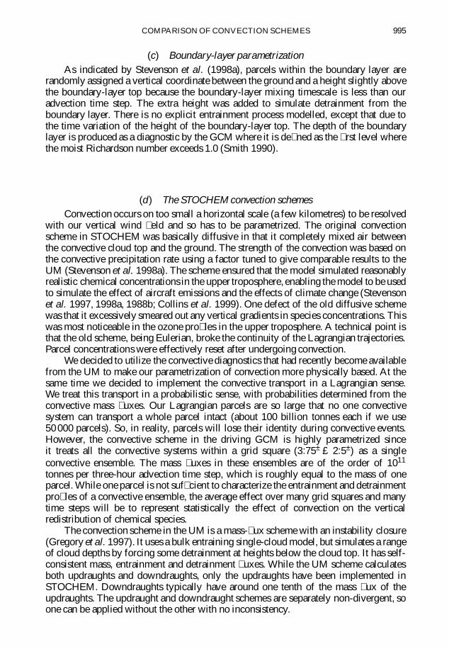
(c) Boundary-layer parametrizationAs indicated by Stevenson et al. (1998a), parcels within the boundary layer are

randomly assigned a vertical coordinate between the ground and a height slightly abovethe boundary-layer top because the boundary-layer mixing timescale is less than ouradvection time step. The extra height was added to simulate detrainment from theboundary layer. There is no explicit entrainment process modelled, except that due tothe time variation of the height of the boundary-layer top. The depth of the boundarylayer is produced as a diagnostic by the GCM where it is de� ned as the � rst level wherethe moist Richardson number exceeds 1.0 (Smith 1990).

(d ) The STOCHEM convection schemesConvection occurs on too small a horizontal scale (a few kilometres) to be resolved

with our vertical wind � eld and so has to be parametrized. The original convectionscheme in STOCHEM was basically diffusive in that it completely mixed air betweenthe convective cloud top and the ground. The strength of the convection was based onthe convective precipitation rate using a factor tuned to give comparable results to theUM (Stevenson et al. 1998a). The scheme ensured that the model simulated reasonablyrealistic chemical concentrations in the upper troposphere, enabling the model to be usedto simulate the effect of aircraft emissions and the effects of climate change (Stevensonet al. 1997, 1998a, 1988b; Collins et al. 1999). One defect of the old diffusive schemewas that it excessively smeared out any vertical gradients in species concentrations. Thiswas most noticeable in the ozone pro� les in the upper troposphere. A technical point isthat the old scheme, being Eulerian, broke the continuity of the Lagrangian trajectories.Parcel concentrations were effectively reset after undergoing convection.

We decided to utilize the convective diagnostics that had recently become availablefrom the UM to make our parametrization of convection more physically based. At thesame time we decided to implement the convective transport in a Lagrangian sense.We treat this transport in a probabilistic sense, with probabilities determined from theconvective mass � uxes. Our Lagrangian parcels are so large that no one convectivesystem can transport a whole parcel intact (about 100 billion tonnes each if we use50 000 parcels). So, in reality, parcels will lose their identity during convective events.However, the convective scheme in the driving GCM is highly parametrized sinceit treats all the convective systems within a grid square (3:75± £ 2:5±) as a singleconvective ensemble. The mass � uxes in these ensembles are of the order of 1011

tonnes per three-hour advection time step, which is roughly equal to the mass of oneparcel. While one parcel is not suf� cient to characterize the entrainment and detrainmentpro� les of a convective ensemble, the average effect over many grid squares and manytime steps will be to represent statistically the effect of convection on the verticalredistribution of chemical species.

The convection scheme in the UM is a mass-� ux scheme with an instability closure(Gregory et al. 1997). It uses a bulk entraining single-cloud model, but simulates a rangeof cloud depths by forcing some detrainment at heights below the cloud top. It has self-consistent mass, entrainment and detrainment � uxes. While the UM scheme calculatesboth updraughts and downdraughts, only the updraughts have been implemented inSTOCHEM. Downdraughts typically have around one tenth of the mass � ux of theupdraughts. The updraught and downdraught schemes are separately non-divergent, soone can be applied without the other with no inconsistency.


k+2

k-1

k+1

k

M

M

M

M

k+1

k

k-1

k+2

D

D

D

k

k-1

k+1

E

E

E

k-1

k

k+1

M

M

M

M

k+2

k

k+1

k-1

Entrainment

Detrainment

subsidence

D

D

D

P

P

P k

k+1

k-1

Updraught Environment

Figure 1. Schematic showing the � uxes used in the Uni� ed Model’s convection scheme. Symbols are de� ned inthe text.

The mass � uxes at each level are related to the entrainment and detrainment � uxesby:

MkC1 D Mk C Ek C Dk

where Mk and MkC1 are the updraughtmass � uxes at levels k and k C 1, and Ek and Dk

are the entrainment and detrainment � uxes at level k. All � uxes are in units of Pa s¡1.The � uxes are shown schematically in Fig. 1. Detrainment accounts both for detrainmentof cloud air through turbulent mixing at the edge of the cloud and forced detrainment.Detrainment � uxes are de� ned as into the plume and hence are negative numbers. If theupdraughts extend above the STOCHEM model top (currently 100 hPa) then they areforced to detrain completely in the level below the model top.


The UM convection scheme generates mass � uxes. We treat the mass � uxes as therates of exchanging masses of air between the updraught and the environment. For thesubsiding air, we convert from mass � uxes to velocities by making the assumption thatthe air over the whole grid square is descending.

For a parcel in level k, the probability (²k) of it being entrained into the updraughtplume in a time step (1t) is given by:

²k D 1tEk

1Pk

where 1Pk is the depth of the level in Pa. This probability is just derived from theresidence time of a parcel in the environment at a particular level and is independent ofthe fraction of the grid square covered by the cloud. Once the parcel is in the plume, theprobability of it detraining in level l (±lk ) is given by the fraction of the plume detrainingat that level multiplied by the probability of the parcel not having been detrained at anearlier level

±lk D¡Dl

Ml

³1 ¡

l¡1X

l0DkC1

±l0k

´:

This has the property that the sum of the detrainment probabilities from level k up to thecloud top is equal to one, i.e. all the parcels are forced to detrain from the plume in onetime step. This is equivalent to assuming that the updraught velocities are suf� cient fora parcel to ascend to the cloud top in less than a model time step.

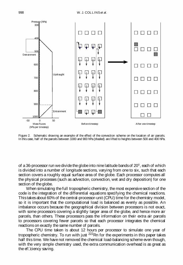
To balance the updraught, parcels in the environmental air have to subside. The rateat which they need to do this is given by balancing the � ux out of the environment atlevel k and the � ux into the environment. This implies that the subsidence � ux is equal tothe updraught � ux. To implement this, every parcel, whether it has undergone transportin the updraught or not, is moved downwards by an amount M1t (in Pa), where M isthe mass � ux interpolated to the parcel height. Figure 2 shows a simple example of theconvection scheme. The mass � uxes are shown on the left-hand side. The entrainmentand detrainment � uxes are combinations of step functions, whereas the updraught � uxis continuous. In this example the entrainment � ux is 50 hPa per time step between 1000and 900 hPa, giving an entrainment probability of 0.5 per time step, hence, on average,half the parcels within this interval are transported upwards. Since the detrainment � uxis constant between 500 and 400 hPa, the parcels are detrained evenly over this interval.All parcels then subside a distance given by the updraught � ux.

The time step used in the GCM is 15 min for both the dynamics and the physics,with diagnostics output every six hours. As a compromise between these values, wehave an advection time step in STOCHEM of three hours. If this were applied to ourconvection scheme, we would get mass � uxes at each level that were greater than themass of air in the level. We, therefore, use the 15 min time step used in the GCM to runthe convection scheme 12 times between each advection step.

The same GCM convection scheme is used to drive the old diffusive convec-tive transport parametrization and the new Lagrangian-type one described here. Theimprovements are due to the extra diagnostic information that has become available.

(e) ComputationThe chemistry-transport model has been optimized to run on a massively parallel

computer, a Cray T3E. As a compromise between minimizing the run time and mini-mizing the inter-processor communication, we usually run on 36 processors. In the case


Updraught

800

700

600

500

400

300

900

0 50-50

Pressure (hPa)

Mass fluxes(hPa per timestep)

1000

Before timestep After one timestep

Detrainment

Entrainment

Figure 2. Schematic showing an example of the effect of the convection scheme on the location of air parcels.In this case, half of the parcels between 1000 and 900 hPa (shaded) are lifted to heights between 500 and 400 hPa.

of a 36-processor run we divide the globe into nine latitude bands of 20±, each of whichis divided into a number of longitude sections, varying from one to six, such that eachsection covers a roughly equal surface area of the globe. Each processor computes allthe physical processes (such as advection, convection, wet and dry deposition) for onesection of the globe.

When simulating the full tropospheric chemistry, the most expensive section of thecode is the integration of the differential equations specifying the chemical reactions.This takes about 60% of the central-processor-unit (CPU) time for the chemistry model,so it is important that the computational load is balanced as evenly as possible. Animbalance occurs because the geographical division between processors is not exact,with some processors covering a slightly larger area of the globe, and hence more airparcels, than others. These processors pass the information on their extra air parcelsto processors covering fewer parcels so that each processor integrates the chemicalreactions on exactly the same number of parcels.

The CPU time taken is about 12 hours per processor to simulate one year oftropospheric chemistry. To run with just 222Rn for the experiments in this paper takeshalf this time. We have not removed the chemical load-balancing scheme even though,with the very simple chemistry used, the extra communication overhead is as great asthe ef� ciency saving.


3. EXPERIMENTS

As discussed previously, our model has been designed to simulate many of thecomplex series of reactions involved in tropospheric chemistry, with a focus on thedegradation of hydrocarbonsand the production of ozone. However, to try to understandthe effect of transport processes in the model it is often easier to study species with muchsimpler chemistry. Following Jacob and Prather (1990) amongst others, we focus in thispaper mainly on the distribution of 222Rn whose sole loss process is radioactive decaywith an e-folding lifetime of 5.5 days. This is of the same order as the timescale forconvective ventilation of the planetary boundary layer, although Penner et al. (1998)have shown that a better test of a model convection scheme would be to use a tracerwith a lifetime of around one day.

Our emissions are the same as those stipulated for the World Climate ResearchProgramme workshop on scavenging and deposition processes (Rasch et al. 2000). Wespecify the 222Rn source strength to be 1.0 atom cm¡2s¡1 over land areas between60±N and 60±S. To account for partially frozen land, the source strength is reduced to0.5 atom cm¡2s¡1 over land areas between 60±N and 70±N, with no seasonal variation.Land areas north of 70±N, south of 60±S and the whole of Greenland are assumed tobe permanently frozen and to be a zero source of 222Rn. This gives a global sourcestrength of around 15 kg per year. Jacob and Prather (1990) suggested that sourcestrengths can vary locally by up to a factor of three, depending on soil type and season.However, there are insuf� cient data to incorporate this variability into global models.Uncertainty in emissions may cause problems when comparing model results withsurface measurements in cases where local emissions provide the dominant contributionto the radon concentrations.

The radon emissions are added on a 5± £ 5± grid-square basis. The emissions foreach grid square are distributed equally over all the parcels that are within the boundarylayer in that grid square. If there are no cells within the boundary layer for a particulargrid square then the emissions are stored until a parcel does pass through.

For this paper, the model is run off-line, taking the driving meteorology from aclimate integration of the GCM. It uses a 1990s radiative forcing, but the meteorologydoes not correspond to any particular calendar year.

4. RESULTS

The main features of the radon distributions can be seen in Figs. 3 and 4. Theseshow results for the model with no convection, the old diffusive convection scheme andthe new Lagrangian convection scheme. The results are averaged over the month ofJune.

Figures 3(a)–(c) show a slice from the North Pole to the South Pole along a lineof longitude at 22.5±E for each scheme. The peaks at around 35±N–65±N and 30±S–25±N are located over Europe and Africa, respectively. Figures 3(d)–(f) show a slicearound the globe along a line of latitude at 2.5±N for each scheme. The peaks at around80±W–60±W, 10±E–40±E and 100±E–120±E are located over South America, Africa andsouth-east Asia, respectively. These � gures show clearly that the effect of convectionis to smear out vertically the concentrations in the plumes, so reducing the verticalgradients. It is noticeable that the two convection schemes have similar effects on theradon distribution, even though they use very different approaches. One difference is thatthe Lagrangian scheme has a greater tendency than the diffusive one to leave isolatedpockets of high radon concentrations in the upper troposphere.


h

90 60 30 0 30 60 90

0.1

0.1

0.1

1.0

1.0

3.0

0.3

0.3

0.3

no convection

90 60 30 0 30 60 90Latitude

1.0

0.9

0.8

0.7

0.6

0.5

0.4

0.3

0.2

0.1

0.0 0.1 0.3 1.0 3.0 10.0 0

1

0.0 0.1 0.3 1.0 3.0 10.0 Bq/SCM

0

1

h

90 60 30 0 30 60 90

0.1

0.3

1.0

1.0

1 .0

3.0

3.0

0.3

0.3

0.1

diffusive convection

90 60 30 0 30 60 90Latitude

1.0

0.9

0.8

0.7

0.6

0.5

0.4

0.3

0.2

0.1

0.0 0.1 0.3 1.0 3.0 10.0 0

1

0.0 0.1 0.3 1.0 3.0 10.0 Bq/SCM

0

1

h

90 60 30 0 30 60 90

0.1

0.3

1.0

1.0

1.00 .30.3

0.1

3.0

3.0

Lagrangian convection

90 60 30 0 30 60 90Latitude

1.0

0.9

0.8

0.7

0.6

0.5

0.4

0.3

0.2

0.1

0.0 0.1 0.3 1.0 3.0 10.0 0

1

0.0 0.1 0.3 1.0 3.0 10.0 Bq/SCM

0

1

180 120 60 0 60 120 180

h

Longitude

0.1

0.1

0.1

0.3

0.3

0.3

0.1

0.1

0.3

0 .3

1.0

0.1

no convection

1.0

0.9

0.8

0.7

0.6

0.5

0.4

0.3

0.2

0.1

0.0 0.1 0.3 1.0 3.0 10.0 0

1

0.0 0.1 0.3 1.0 3.0 10.0 Bq/SCM

0

1

180 120 60 0 60 120 180

h

Longitude

0.1

1.0

0.3

1.0

0.3


1.0

0.9

0.8

0.7

0.6

0.5

0.4

0.3

0.2

0.1

0.0 0.1 0.3 1.0 3.0 10.0 0

1

0.0 0.1 0.3 1.0 3.0 10.0 Bq/SCM

0

1

180 120 60 0 60 120 180

h

Longitude

0. 1

1.0

0.1

0.3

3.0

0.1


1.0

0.9

0.8

0.7

0.6

0.5

0.4

0.3

0.2

0.1

0.0 0.1 0.3 1.0 3.0 10.0 0

1

0.0 0.1 0.3 1.0 3.0 10.0 Bq/SCM

0

1

(a) (b) (c)

(d) (e) (f)

Figure 3. Slices through the June 222Rn concentrations (in Bq per standard cubic metre (SCM)) for the threedifferent convection schemes (see text). Panels (a), (b) and (c) show slices around a line of longitude (22.5±E), andpanels (d), (e) and (f) show slices around a line of latitude (2.5±N). The vertical coordinate (´) is approximately

pressure/1000 hPa.

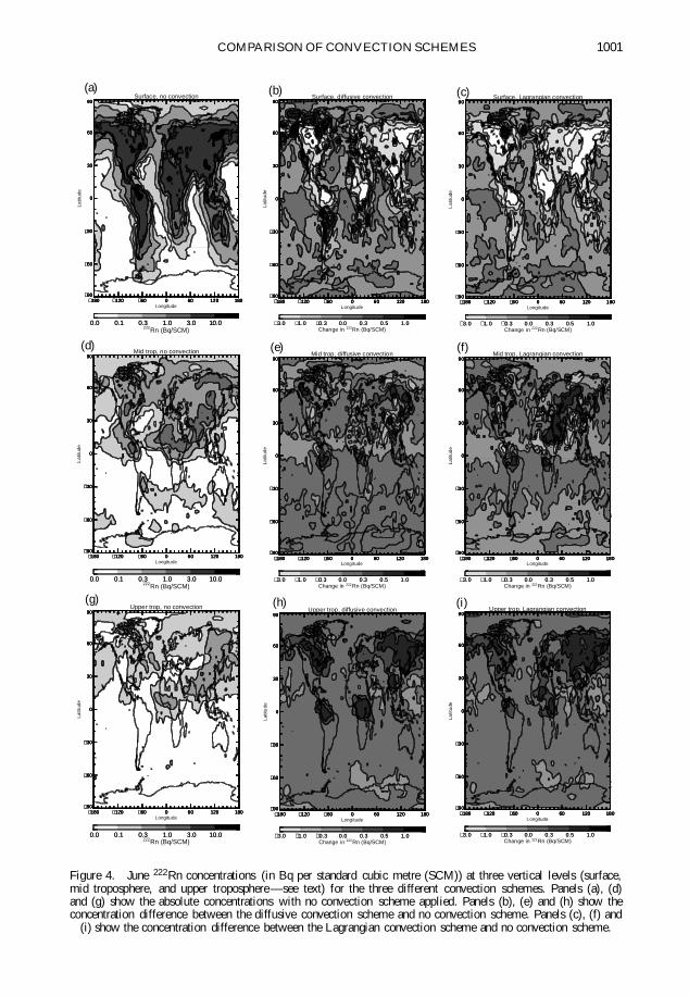
In the latitude–longitude plots (Fig. 4) the surface radon is highest over the con-tinents and lowest over the oceans. Since the 222Rn lifetime is so short, there is littleadvection out from the continents. The two transport schemes with convection are sim-ilar, both showing lower concentrations than the case with no convection, especially inthe tropics. This re� ects the lifting of radon-rich air out of the boundary layer. In the midtroposphere (»650 hPa) the concentrations are nearly an order of magnitude less than atthe surface. They again generally follow the continents, however with more advectionout over the oceans than was found at the surface. The two convection schemes showbroadly similar results with decreased radon concentrations over the ITCZ and generallyincreased concentrations over the continents. The concentrations are slightly higher inthe Lagrangian scheme. In the upper troposphere (»350 hPa) concentrations are lowerstill. The contours no longer follow the outline of the continents but appear as localizedmaxima. In the two schemes with convective transport there are higher radon concen-trations almost everywhere, with particularly large increases over convective centres in


180 120 60 0 60 120 180 90

60

30

0

30

60

90

180 120 60 0 60 120 180 90

60

30

0

30

60

90Surface, no convection

180 120 60 0 60 120 180Longitude

90

60

30

0

30

60

90

Latit

ude

0.0 0.1 0.3 1.0 3.0 10.0 0

1

0.0 0.1 0.3 1.0 3.0 10.0 222Rn (Bq/SCM)

0

1

180 120 60 0 60 120 180 90

60

30

0

30

60

90

180 120 60 0 60 120 180 90

60

30

0

30

60

90

180 120 60 0 60 120 180 90

60

30

0

30

60

90Surface, diffusive convection

180 120 60 0 60 120 180Longitude

90

60

30

0

30

60

90

Latit

ude

3.0 1.0 0.3 0.0 0.3 0.5 1.0 0

1

3.0 1.0 0.3 0.0 0.3 0.5 1.0 Change in 222Rn (Bq/SCM)

0

1

180 120 60 0 60 120 180 90

60

30

0

30

60

90

180 120 60 0 60 120 180 90

60

30

0

30

60

90

180 120 60 0 60 120 180 90

60

30

0

30

60

90Surface, Lagrangian convection

180 120 60 0 60 120 180Longitude

90

60

30

0

30

60

90

Lat

itude

3.0 1.0 0.3 0.0 0.3 0.5 1.0 0

1


0

1

180 120 60 0 60 120 180 90

60

30

0

30

60

90

180 120 60 0 60 120 180 90

60

30

0

30

60

90

180 120 60 0 60 120 180 90

60

30

0

30

60

90Mid trop, no convection

180 120 60 0 60 120 180Longitude

90

60

30

0

30

60

90

Lat

itude

0.0 0.1 0.3 1.0 3.0 10.0 0

1

0.0 0.1 0.3 1.0 3.0 10.0 222Rn (Bq/SCM)

0

1

180 120 60 0 60 120 180 90

60

30

0

30

60

90

180 120 60 0 60 120 180 90

60

30

0

30

60

90

180 120 60 0 60 120 180 90

60

30

0

30

60

90Mid trop, diffusive convection

180 120 60 0 60 120 180Longitude

90

60

30

0

30

60

90

Latit

ude

3.0 1.0 0.3 0.0 0.3 0.5 1.0 0

1


0

1

180 120 60 0 60 120 180 90

60

30

0

30

60

90

180 120 60 0 60 120 180 90

60

30

0

30

60

90

180 120 60 0 60 120 180 90

60

30

0

30

60

90Mid trop, Lagrangian convection

180 120 60 0 60 120 180Longitude

90

60

30

0

30

60

90

Latit

ude

3.0 1.0 0.3 0.0 0.3 0.5 1.0 0

1


0

1

180 120 60 0 60 120 180 90

60

30

0

30

60

90

180 120 60 0 60 120 180 90

60

30

0

30

60

90

180 120 60 0 60 120 180 90

60

30

0

30

60

90Upper trop, no convection

180 120 60 0 60 120 180Longitude

90

60

30

0

30

60

90

Latit

ude

0.0 0.1 0.3 1.0 3.0 10.0 0

1

0.0 0.1 0.3 1.0 3.0 10.0 222Rn (Bq/SCM)

0

1

180 120 60 0 60 120 180 90

60

30

0

30

60

90

180 120 60 0 60 120 180 90

60

30

0

30

60

90

180 120 60 0 60 120 180 90

60

30

0

30

60

90Upper trop, diffusive convection

180 120 60 0 60 120 180Longitude

90

60

30

0

30

60

90

Latit

ude

3.0 1.0 0.3 0.0 0.3 0.5 1.0 0

1


0

1

180 120 60 0 60 120 180 90

60

30

0

30

60

90

180 120 60 0 60 120 180 90

60

30

0

30

60

90

180 120 60 0 60 120 180 90

60

30

0

30

60

90Upper trop, Lagrangian convection

180 120 60 0 60 120 180Longitude

90

60

30

0

30

60

90

Latit

ude

3.0 1.0 0.3 0.0 0.3 0.5 1.0 0

1


0

1

180 120 60 0 60 120 180 90

60

30

0

30

60

90

(a) (b) (c)

(d) (e) (f)

(g) (h) (i)

Figure 4. June 222Rn concentrations (in Bq per standard cubic metre (SCM)) at three vertical levels (surface,mid troposphere, and upper troposphere —see text) for the three different convection schemes. Panels (a), (d)and (g) show the absolute concentrations with no convection scheme applied. Panels (b), (e) and (h) show theconcentration difference between the diffusive convection scheme and no convection scheme. Panels (c), (f) and

(i) show the concentration difference between the Lagrangian convection scheme and no convection scheme.


northern South America and central Africa, as well the continental regions of NorthAmerica and Eurasia.

5. COMPARISON WITH OBSERVATIONS

To assess the performance of the vertical redistribution by the convection schemewe have compared our models against measurements of vertical pro� les and surfaceconcentrations of 222Rn. Figure 5 shows comparisons of modelled 222Rn against sum-mertime continental pro� les compiled by Liu et al. (1984). The three model convectionschemes are the same as described in section 4. This � gure suggests that the new schemegives the best agreement with the observations, particularly when comparing against‘C’-shaped radon pro� les. The Lagrangian scheme is the only one that is able to simulatehigh radon concentrations around 8–12 km. This height range is typical of the out� owregions of summertime continental convective clouds. It must be remembered that themodel values are averages over one month, whereas the measurements over America aresingle aircraft � ights and those over the Ukraine are an average of � ve aircraft � ights.While the model values are averages over all times of day, the � ights generally occurredin the daytime when convective activity is stronger.

Measurements over coastal regions show less clear-cut results. Figure 6 comparesthe model against an average of 11 aircraft pro� les over San Francisco (Kritz et al.1998) and eight pro� les over Nova Scotia (Zaucker et al. 1996). These regions aredif� cult to model as there are large gradients in 222Rn concentration from the lowvalues over the oceans to the high values over the land. The observed concentrations willdepend strongly on the actual wind directions and strengths at the time of measurement,whereas the modelled values will more re� ect the prevailing wind conditions. Withpredominantly westerly winds at these latitudes the west-coast site might be expectedto be in� uenced by more maritime air and the east-coast site by more continental air.This is con� rmed both in the observations and model calculations which show higher222Rn concentrations over Nova Scotia than over San Francisco, even though the regioncovered by the Nova Scotia measurements is mostly sea and the San Francisco regionmostly land. At both sites the scheme without any convective transport fails to predictrealistic concentrations above 4 km. The Lagrangian scheme shows smoother transitionsthan the diffusive one from the high boundary-layer concentrations to the lower free-troposphere concentrations. However, the gradients in the measured concentrations aremuch less, with boundary-layer values half those of the models and a more gradualtransition towards the free-tropospheric values. If the aircraft pro� les can be consideredrepresentative of the monthly and regional averages, then this could suggest that themodel has insuf� cient venting of the boundary layer in these coastal regions. Oneobvious problem with simulating coastal measurements is the resolution of the model.For example the grid square holding the emissions for the San Francisco area extends outto 125±W. Measurements taken in the boundary layer will tend to be of marine air withslight contamination from local radon sources. In the model, boundary-layer air arrivingat San Francisco will have started to pick up emissions from 125±W, about 250 kmout to sea. Even though the emissions from the coastal grid square will only be abouta half of those from a continental grid square, the air will still appear more polluted.Around Nova Scotia, most of the boundary-layermeasurements were made over the sea.Although these will be strongly in� uenced by out� ow from the continent, they receiveno direct radon emission, unlike the model where radon is emitted over the entire area.

Only the Nova Scotia measurements show a ‘C’-shaped pro� le characteristic ofcontinental convection. None of the model pro� les match this. The diffusive scheme hastoo sharp a transition at 2 km, although it agrees with the observations at 5–6 km. The


Nebraska August

0.1 1.0 10.0222Rn (Bq/SCM)

0

5

10

15

heig

ht (

km)

Observations

no convection



Salt Lake City August

0.1 1.0 10.0222Rn (Bq/SCM)

0

5

10

15

heig

ht (

km)

Observations

no convection



Eastern Ukraine July

0.1 1.0 10.0222Rn (Bq/SCM)

0

5

10

15

heig

ht (

km)

Observations

no convection



(a)

(b)

(c)

Figure 5. Comparison of modelled 222Rn against observed continental summertime pro� les over (a) Nebraska,(b) Salt Lake City, and (c) eastern Ukraine. The observations over the Ukraine are the means and standard

deviations of measurements taken over � ve � ights.


San Fransisco, June and August

0.0 0.5 1.0 1.5 2.0Rn (Bq/SCM)

0

5

10

15

heig

ht (

km)

Observations

no convection

diffusive convectionLagrangian convection

Nova Scotia, August

0.0 0.5 1.0 1.5 2.0Rn (Bq/SCM)

0

5

10

15

heig

ht (

km)

Observations

No convection

diffusive convectionLagrangian convection

(a) (b)

Figure 6. Comparison of modelled pro� les of 222Rn for the three convection schemes (see text) against observedcoastal pro� les: (a) the average of 11 pro� les over San Francisco, and (b) the average of eight pro� les over Nova

Scotia.

Lagrangian scheme does have a ‘C’ shape, but the radon minimum occurs at too highan altitude, at 5 km. Neither the observations over San Francisco nor those over NovaScotia are able to discriminate between the two different parametrizations of convection,although they do suggest the scheme with no convective transport is less realistic.

Surface 222Rn data from two stations have been described by Hutter et al. (1995)¤.Data for Mauna Loa and Bermuda are shown in Fig. 7. The concentrations are presentedas monthly averages for the years 1991–1996 inclusive. Following Dentener et al.(1999), Mauna Loa data have been � ltered to select only measurements taken betweenmidnight and 0700 local time. This is to reduce the effect of local contamination dueto upslope air� ow. Interestingly, at the height of the Mauna Loa observatory (3400 m)there is little variation in the 222Rn concentrations predicted by the different convectionschemes, suggesting that the transport to Hawaii is dominated by large-scale advectionrather than subgrid-scale convection. However, the modelled vertical pro� les overMauna Loa (not shown) do indicate some differences. In particular, compared withthe other two schemes, the scheme with no convective transport generally has highersurface concentrations and lower free-tropospheric concentrations. All the modelledconcentrations underestimate the Mauna Loa observations in the spring, a problem thatis common to many other chemistry-transport models (Dentener et al. 1999; Brasseuret al. 1996; Jacob et al. 1997). Dentener et al. (1999) suggested that the high observed¤ These data are available on-line at http://www.eml.doe.gov


Mauna Loa

Jan Feb Mar Apr May Jun Jul Aug Sep Oct Nov Dec0.00

0.10

0.20

0.30

0.40

0.50R

n (B

q/S

CM

)

Observations

no convection



Bermuda

Jan Feb Mar Apr May Jun Jul Aug Sep Oct Nov Dec0.0

0.5

1.0

1.5

2.0

Rn

(mB

q/S

CM

)

Observations

no convection



(a)

(b)

Figure 7. Comparison of the time-series of monthly averaged modelled 222Rn values at the surface for the threeconvection schemes (see text) against observed marine data: (a) Mauna Loa (concentrations are for 3.4 km above

sea level) and (b) Bermuda (concentrations are for approximately sea level).

concentrations may be due to vigorous convection over east Asia transporting radon upto the level of the strong westerly winds. Our results seem to imply that convection isless important, since there is little difference in the modelled concentrations whether ornot any convective transport is simulated. The transport from east Asia to Mauna Loais critically dependent on the location of the Paci� c anticyclone (Brasseur et al. 1996).If the anticyclone simulated by the climate GCM is further to the east or north thanthe actual meteorology at the time the measurements were taken, then the modelled222Rn will be more characteristic of the central Paci� c than east Asia, relative to themeasurements. This will result in the model underestimating the Mauna Loa 222Rnconcentrations and being less sensitive to continental convection.

In contrast to the Mauna Loa site, the modelled 222Rn concentrations at Bermudavary strongly according to the convection scheme used. This is particularly true in thewinter half of the year when Bermuda is predominantly in� uenced by westerly windsbringing radon from eastern North America. Bermuda is only around 1000 km from thecontinental USA, and so receives radon directly from the continental boundary layer.The effect of this can be seen when comparing the different model convection schemes.With no convective transport the continental boundary layer is less ventilated than withthe other schemes and, hence, higher concentrations of 222Rn build up and, in winter(September to April), are advected over to Bermuda. The Lagrangian scheme in thiscase ventilates the boundary layer more ef� ciently than the diffusive scheme because the


entrainment into the convective column in the Lagrangian scheme peaks below the cloudbase rather than being constant with height as in the diffusive scheme. To compare themodel with the observations, measurements taken during the night are excluded as 222Rnconcentrations are elevated in the nocturnal boundary layer due to local emissions. Thisis particularly noticeable during anticyclonic conditions in the summer months whenBermuda is in� uenced by the Azores high. The chemistry-transport model is not able toresolve emissions from an area as small as Bermuda. In the spring, the model’s schemesall overestimate the radon concentrations, with the Lagrangian scheme giving the closestresults to the observations. This overestimate has been noticed with other chemistry-transport models (Dentener et al. 1999; Mahowald et al. 1997). In the summer, both theno-convection and Lagrangian convection schemes underestimate the radon concentra-tions. During this season Bermuda receives air masses that have circulated around theAzores high and hence are depleted in 222Rn. The diffusive convection scheme predictsgreater concentrations and so agrees better with the observations. The greater concen-trations are due to bringing down air from higher altitudes where there is more transportfrom North America than at the surface. This effect is larger using the diffusive con-vection scheme since, in this scheme, the boundary-layer air is uniformly redistributedwith height over the continent by a convective event. Over Bermuda, convection canmix air from upper levels down to the surface in one time step. This contrasts with theLagrangian scheme where boundary-layer air is transported preferentially to the altitudeof convective out� ow (10–15 km) over the continent. Over Bermuda, any subsidence inthe Lagrangian scheme due to convective events will bring down air from the uppertroposphere too slowly for the elevated 222Rn to be observed at the surface. We have not� ltered Bermuda data according to wind direction or speed and, therefore, some of thehigher summertime observations may be in� uenced by local emissions.

6. CONCLUSIONS

We have shown that the parametrization of convective-transport processes has asigni� cant effect on the three-dimensional distribution of 222Rn predicted by a globalchemical-transport model. In particular, the addition of convective-transport parametr-izations reduces the predicted surface concentrations of 222Rn over the continents andincreases the predicted concentrations in the free troposphere.

The comparison between model simulations and observations shows that havingno convective transport is unrealistic, as the model predicts a decrease in 222Rn con-centration between the continental boundary layer and the free troposphere that is toolarge. The Lagrangian parametrization gives a greater venting of the boundary layerthan the diffusive scheme and preferentially detrains this in the mid to upper tropo-sphere. However, surface 222Rn concentrations are often still too high, even with the La-grangian scheme. Over the continents in summertime, the Lagrangian scheme gives verygood agreement with the observed ‘C’-shaped vertical 222Rn pro� les, a feature that theprevious diffusive convective transport scheme was not able to simulate. Summertimeconvection over large continents is generally strong and deep, giving a clear convectivesignal in the radon pro� les. Over coastal regions and island sites the radon pro� les areaffected by other transport processes as well as by convection. Comparisons betweenpredicted and measured 222Rn in these locations are not able to conclude whether oneconvection scheme is better than the other.

In this paper we have focused on the simulations of 222Rn distributions, as thisspecies has the simplest chemistry and allows the effects of the parametrization of


convective transport to be seen most clearly. It should be remembered that 222Rn is onlyused to test the convection schemes. From the chemical point of view, it is the ability ofthe model to convectively transport reactive species (such as NOX, ozone and volatileorganic compounds) that is most important.

ACKNOWLEDGEMENTS

This study was supported as part of the Public Meteorological Service R&Dprogramme of the Met Of� ce and by the Department of the Environment, Transportand the Regions through contracts PECD 7/12/37 (Global Atmosphere Division) andEPG 1/3/143 (Air and Environmental Quality Division).

REFERENCES

Berntsen, T. K. andIsakesen, I. S. A.

1997 A global three-dimensional chemical transport model for the tro-posphere. 1. Model description and CO and ozone results.J. Geophys. Res., 102, 21239–21280

Brasseur, G. P., Hauglustaine, D. A.and Walters, S.

1996 Chemical compounds in the remote Paci� c troposphere: Compar-ison between MLOPEX measurements and chemical trans-port model calculations. J. Geophys. Res., 101, 14795–14813

Chock, D. P. and Winkler, S. L. 1994 A comparison of advection algorithms coupled with chemistry.Atmos. Environ., 28, 2659–2675

Collins, W. J., Stevenson, D. S.,Johnson, C. E. andDerwent, R. G.

1997 Tropospheric ozone in a global-scale three-dimensional La-grangian model and its response to NOX emission controls.J. Atmos. Chem., 26, 223–274

1999 Role of convection in determining the budget of odd hydrogen inthe upper troposphere. J. Geophys. Res., 104, 26927–26941

Cullen, M. J. P. 1993 The uni� ed forecast/climate model. Meteorol. Mag., 122, 81–94Dabdub, D. and Seinfeld, J. H. 1994 Numerical advective schemes used in air quality models—

sequential and parallel implementation. Atmos. Environ., 28,3369–3385

Dentener, F., Feichter, J. andJeuken, A.

1999 Simulation of the transport of Rn222 using on-line and off-lineglobal models at different horizontal resolutions: A detailedcomparison with measurements. Tellus, 51B, 573–602

Doty, K. G. and Perkey, D. J. 1993 Sensitivity of trajectory calculations to the temporal frequency ofwind data. Mon. Weather Rev., 121, 387–401.

Gidel, L. T. 1983 Cumulus cloud transport of transient tracers, J. Geophys. Res., 88,6587–6599

Gregory, D. Kershaw, R. andInness, P. M.

1997 Parametrization of momentum transport by convection. II: Testsin single-column and general circulation models. Q. J. R.Meteorol. Soc., 123, 1153–1183

Hutter, A. R., Larsen, R. J.,Martin, H. and Merril, J. T.

1995 Radon-222 at Bermuda and Mauna Loa: Local and distantsources. J. Radiometr. Nuclear Chem., 193, 309–318

Jacob, D. J. and Prather, M. J. 1990 Radon-222 as a test of convective transport in a general circulationmodel. Tellus, 42B, 118–134

Jacob, D. J., Prather, M. J.,Rasch, P. J., Shia, R.-L.,Balkanski, Y. J.,Beagley, S. R.,Bergmann, D. J.,Blacksher, W. T., Brown, M.,Chiba, M., Chipper� eld, M. P.,de Grandpre, J., Dignon, J. E.,Feichter, J., Genthon, C.,Grose, W. L., Kasibhatla, P. S.,Kohler, I., Kritz, M. A.,Law, K., Penner, J. E.,Ramonet, M., Reeves, C. E.,Rounan, D. A.,Stockwell, D. Z.,van Velthoven, P. F. J.,Verver, G., Wild, O., Yang H.and Zimmerman, P.

1997 Evaluation and intercomparison of global atmospheric transportmodels using 222Rn and other short-lived tracers. J. Geophys.Res., 102, 5953–5970


Jaegle, L., Jacob, D. J.,Wennberg, P. O.,Spivakovsky, C. M.,Hanisco, T. F.,Lanzendorf, E. L.,Hintsa, E. J., Fahey, D. W.,Keim, E. R., Prof� tt, M. H.,Atlas, E., Flocke, F.,Schauf� er, S., McElroy, C. T.,Midwinter, C., P� ster, L. andWilson, J. C.

1997 Observed OH and HO2 in the upper troposphere suggest a majorsource from convective injection of peroxides. Geophys. Res.Lett., 24, 3181–3184

Johns, T. C., Carnell, R. E.,Crossley, J. F., Gregory, J. M.,Mitchell, J. F. B.,Senior, C. A., Tett, S. F. B. andWood, R. A.

1997 The second Hadley Centre coupled ocean–atmosphere GCM:Model description, spinup and validation. Climate Dyn., 13,103–134

Kanakidou, M., Dentener, F. J.,Brasseur, G. P., Collins, W. J.,Berntsen, T. K.,Hauglustaine, D. A.,Houweling, S.,Isaksen, I. S. A., Krol, M.,Lawrence, M. G., Muller, J. F.,Poisson, N., Roelofs, G. J.,Wang, Y. andWauben, W. M. F.

1999a 3-D global simulations of tropospheric CO distributions —resultsof the GIM/IGAC intercomparison 1997 exercise. Chemo-sphere: Global Change Science , 1, 263–282

Kanakidou, M., Dentener, F. J.,Brasseur, G. P., Collins, W. J.,Berntsen, T. K.,Hauglustaine, D. A.,Houweling, S.,Isaksen, I. S. A., Krol, M.,Law, K. S., Lawrence, M. G.,Muller, J. F., Plantevin, P. H.,Poisson, N., Roelofs, G. J.,Wang, Y. andWauben, W. M. F.

1999b ‘3-D global simulations of tropospheric chemistry with focus onozone distributions—results of the GIM/IGAC intercompari-son 1997 exercise’. European Commision report EUR18842,Brussels

Kritz, M. A., Rosner, S. W. andStockwell, D. Z.

1998 Validation of an off-line three-dimensional chemical transportmodel using observed radon pro� les. 1. Observations.J. Geophys. Res., 103, 8425–8432

Lacis, A. A., Weubbles, D. J. andLogan, J. A.

1990 Radiative forcing of climate by changes in the vertical distributionof ozone. J. Geophys. Res., 95, 9971–9981

Lawrence, M. G, Crutzen, P. J.,Rasch, P. J., Easton, B. E. andMahowald, N. M.

1999 A model for studies of tropospheric photochemistry: Description,global distributions, and evaluation. J. Geophys. Res., 104,26245–26277

Lee, T.-Y., Park, S.-W. andKim, S.-B.

1997 Dependence of trajectory accuracy on the spatial and temporaldensities of wind data. Tellus, 49B, 199–215

Lin, X., Trainer, M. and Liu, S. C. 1988 On the nonlinearity of the tropospheric ozone production. J. Geo-phys. Res., 93, 15879–15888

Liu, S. C., McAfee, J. R. andCicerone, R. J.

1984 Radon 222 and tropospheric vertical transport. J. Geophys. Res.,89, 7291–7297

Madronich, S. 1987 Photodissociation in the atmosphere. 1. Actinic � ux and the ef-fects of ground re� ections and clouds. J. Geophys. Res., 92,9740–9752

Mahowald, N. M., Rasch, P. J.,Easton, B. E., Whittlestone, S.and Prinn, R. G.

1997 Transport of 222radon to the remote troposphere using the modelof atmospheric transport and chemistry and assimilatedwinds from ECMWF and the National Centers for Envi-ronmental Prediction/NCAR. J. Geophys. Res., 102, 28139–28151

Mari, C., Jacob, D. J. andBechtold, P.

2000 Transport and scavenging of soluble gases in a deep convectivecloud. J. Geophys. Res., 105, 22255–22267

Methven, J. 1997 ‘Of� ine trajectories: Calculation and accuracy’. UGAMP Techni-cal Report 44, Department of Meteorology, Reading Univer-sity, Reading, UK


Penner, J. E., Bergmann, D. J.,Walton, J. J., Kinnison, D.,Prather, M. J., Rotman, D.,Price, C., Pickering, K. E. andBaughcum, S. L.

1998 An evaluation of upper troposphere NOX with two models.J. Geophys. Res., 103, 22097–22113

Pickering, K. E., Thompson, A. M.,Scala, J. R., Tao, W.-K. andSimpson, J.

1992 Ozone production potential following convective redistribution ofbiomass burning emissions. J. Atmos. Chem., 14, 297–313

Prather, M. J. and Jacob, D. J. 1997 A persistent imbalance in HOX and NOX photochemistry of theupper troposphere driven by deep tropical convection. Geo-phys. Res. Lett., 24, 3189–3192

Price, C., Penner, J. and Prather, M. 1997 NOX from lightning. 1. Global distribution based on lightningphysics. J. Geophys. Res., 102, 5929–5941

Rasch, P. J., Feichter, J., Law, K.,Mahowald, N., Penner, J.,Benkovitz, C., Genthon, C.,Giannakopoulos, C.,Kasibhatla, P., Koch, D.,Levy, H., Maki, T.,Prather, M., Roberts, D. L.,Roelofs, G.-J., Stevenson, D.,Stockwell, Z., Taguchi, S.,Kritz, M., Chipper� eld, M.,Baldocchi, D., McMurry, P.,Barrie, L., Balkanski, Y.,Chat� eld, R., Kjellstrom, E.,Lawrence, M., Lee, H. N.,Lelieveld, J., Noone, K. J.,Seinfeld, J., Stenchikov, G.,Schwartz, S., Walcek, C. andWilliamson, D.

2000 A comparison of scavenging and deposition processes in globalmodels: Results from the WCRP Cambridge Workshop of1995. Tellus, 52B, 1025–1056

Smith, R. N. B. 1990 A scheme for predicting layer clouds and their water contents in ageneral circulation model. Q. J. R. Meteorol. Soc., 116, 435–460

Stevenson, D. S., Johnson, C. E.,Collins, W. J. andDerwent, R. G

1997 The impact of aircraft nitrogen oxide emissions on troposphericozone studied with a 3-D Lagrangian model including fullydiurnal chemistry. Atmos. Environ., 31, 1837–1850

Stevenson, D. S., Collins, W. J.,Johnson, C. E. andDerwent, R. G

1998a Intercomparison and evaluation of atmospheric transport in a La-grangian model (STOCHEM), and an Eulerian model (UM),using 222Rn as a short-lived tracer. Q. J. R. Meteorol. Soc.,125, 2477–2493

Stevenson, D. S., Collins, W. J.,Johnson, C. E.,Derwent, R. G., Shine, K. P.and Edwards, J. M.

1998b Evolution of tropospheric ozone radiative forcing. Geophys. Res.Lett., 25, 3819–3822

Thompson, A. M., Pickering, K. E.,Dickerson, R. R.,Ellis Jr., W. G., Jacob, D. J.,Scala, J. R., Tao, W.-K.,McNamara, D. P. andSimpson, J.

1994 Convective transport over the central United States and its rolein regional CO and ozone budgets. J. Geophys. Res., 99,18703–18711

Thuburn, J. and McIntyre, M. E. 1997 Numerical advection schemes, cross-isentropic random walks,and correlations between chemical species. J. Geophys. Res.,102, 6775–6797

Walton, J. J., MacCracken, M. C.and Ghan, S. J

1988 A global-scale Lagrangian trace species model of transport, trans-formation, and removal processes. J. Geophys. Res., 93,8339–8354

Zaucker, F., Daum, P. H.,Wetterauer, U., Berkowitz, C.,Kromer, B. andBroecker, W. S.

1996 Atmospheric 222Rn measurements during the 1993 NARE Inten-sive. J. Geophys. Res., 101, 29149–29164

a comparison of two schemes for the convective transport

Documents