comparison of advanced control schemes implemented on...
TRANSCRIPT

Comparison of Advanced Control Schemes Implemented on Hydraulic Actuated
Robot Manipulator
EMSD Master Thesis | GRP. P16B | Institute of Energy Technology | Aalborg University


In Memory of Gitte Mørk

M SEKTOREN
Fibigerstræde 169220 Aalborg Ø
Title: Comparison of Advanced Control Schemes Implemented on Hy-draulic Actuated Robot Manipulator
Semester: EMSD 10Semester theme: Master ThesisProject period: 4th of February to 3th of June 2008ECTS: 30Supervisors: Torben O. Andersen, Prof., M.Sc., Ph.D.
Henrik C. Pedersen, Ass. Prof., M.Sc., Ph.D.Project group: Pon101-P16B
Kristian Holm Nielsen
Lasse Schmidt
Copies: 5Pages, report: 131 (-blanks)Pages, appendix: 96
SYNOPSIS:
This thesis concerns the establishment, imple-mentation, testing, and finally comparison of anarray of controllers on an electro hydraulic ro-bot manipulator. The result of the thesis is thecomparison of the established controllers, whichhas the purpose of evaluating the performance ofthe chosen controllers, implemented on the elec-tro hydraulic robot manipulator, when used asa position servo. The controllers are tested re-garding a set of criteria involving tracking perfor-mance, number of transducers needed and robust-ness towards disturbances. As a base of testing,a series of classical linear controllers have beenestablished, and also a series of non-linear con-trollers such as adaptive and learning controllershave been implemented and tested against eachother and the linear control schemes.In order to simulate the behavior of the electrohydraulic servo robot with the various controllersimplemented, a non-linear model has been devel-oped, and for the development and analysis ofthe controllers also a linear model has been de-veloped. Selected controllers have then been im-plemented on the physical electro hydraulic servorobot.
By signing this document, each member of the group confirms that all partici-pated evenly in the project work and thereby that all members are collectivelyliable for the content of the report.


Preface
This thesis documents a master thesis completed by group P101-P16B at the 10th semesterat M.Sc education in mechanical engineering/Electro-Mechanical System Design at theUniversity of Aalborg. The thesis concerns testing of the performance of various con-trollers, linear and non-linear, on an electro hydraulic position servo. The testing of thecontrollers is carried out on a non-linear model of the electro hydraulic position servoconstituted by a robot manipulator. Selected controllers is then implemented and subse-quently tested on the physical robot. After having implemented and tested the variouscontrollers, a comparison is carried out in order to decide which controller types are bestsuited for an electro hydraulic position servo.
The thesis is divided into four main parts - a part concerning the system modeling andtrajectory planning, a part concerning linear control design, a part concerning advancedcontrol design and finally a part regarding comparison of the chosen controllers, togetherwith final conclusions and perspectives.
Material which has relevance for the thesis but does not belong inside this documentationis accompanied either in paper format in the appendix of the report or on the appendedCD. The CD contains various MATLAB/SIMULINK models of the robot constitutingthe electro hydraulic servo system, data sheets, program code and a PDF-version of thethesis etc.
Group P101-P16B, June 2008
3

Contents
1 Thesis Outline, System Overview & Approach 111.1 Thesis Outline . . . . . . . . . . . . . . . . . . . . . . . . . . . . . . . . . 111.2 Overall System Description . . . . . . . . . . . . . . . . . . . . . . . . . . 12
1.2.1 Solid-State Mechanical Subsystem . . . . . . . . . . . . . . . . . . 121.2.2 Fluid Mechanical Subsystem . . . . . . . . . . . . . . . . . . . . . 12
1.3 Problem Formulation . . . . . . . . . . . . . . . . . . . . . . . . . . . . . . 131.4 Thesis Approach . . . . . . . . . . . . . . . . . . . . . . . . . . . . . . . . 13
1.4.1 Development of System Models . . . . . . . . . . . . . . . . . . . . 141.4.2 Verification of Models . . . . . . . . . . . . . . . . . . . . . . . . . 141.4.3 Establishment of Linear Controllers . . . . . . . . . . . . . . . . . 141.4.4 Establishment of Nonlinear Controllers . . . . . . . . . . . . . . . . 141.4.5 Comparison of Controllers . . . . . . . . . . . . . . . . . . . . . . . 14
1.5 Evaluation Criteria . . . . . . . . . . . . . . . . . . . . . . . . . . . . . . . 141.5.1 Tracking Performance . . . . . . . . . . . . . . . . . . . . . . . . . 151.5.2 Number of Transducers Needed . . . . . . . . . . . . . . . . . . . . 151.5.3 Robustness Towards Disturbances . . . . . . . . . . . . . . . . . . 151.5.4 Final Conclusions . . . . . . . . . . . . . . . . . . . . . . . . . . . . 15
1.6 Summary . . . . . . . . . . . . . . . . . . . . . . . . . . . . . . . . . . . . 15
I System Modeling & Trajectory Planning 17
2 Dynamic Model of Robot Manipulator 192.1 Solid-State Mechanical Subsystem . . . . . . . . . . . . . . . . . . . . . . 192.2 Fluid Mechanical Subsystem . . . . . . . . . . . . . . . . . . . . . . . . . . 202.3 Model Verification . . . . . . . . . . . . . . . . . . . . . . . . . . . . . . . 20
2.3.1 Verification of Gravitation . . . . . . . . . . . . . . . . . . . . . . . 212.3.2 Verification of Dynamics . . . . . . . . . . . . . . . . . . . . . . . . 22
2.4 Summary . . . . . . . . . . . . . . . . . . . . . . . . . . . . . . . . . . . . 23
3 Linear Model of Robot Manipulator 253.1 Linear Model . . . . . . . . . . . . . . . . . . . . . . . . . . . . . . . . . . 253.2 Verification of Linear Model . . . . . . . . . . . . . . . . . . . . . . . . . . 263.3 Summary . . . . . . . . . . . . . . . . . . . . . . . . . . . . . . . . . . . . 27
4 Trajectory Planning 294.1 Introduction . . . . . . . . . . . . . . . . . . . . . . . . . . . . . . . . . . . 294.2 General Trajectory Boundaries . . . . . . . . . . . . . . . . . . . . . . . . 30
4.2.1 Physical Position Boundaries . . . . . . . . . . . . . . . . . . . . . 30
5
6 Contents
4.2.2 Allowable Power Consumption . . . . . . . . . . . . . . . . . . . . 314.3 Trajectory Generation . . . . . . . . . . . . . . . . . . . . . . . . . . . . . 324.4 Trajectory Profiles (RECT) . . . . . . . . . . . . . . . . . . . . . . . . . . 33
4.4.1 Trajectory Profiles for the TCP . . . . . . . . . . . . . . . . . . . . 334.4.2 Inverse Kinematics . . . . . . . . . . . . . . . . . . . . . . . . . . . 344.4.3 Trajectory Profiles in Joint- & Actuator Space . . . . . . . . . . . 36
4.5 Trajectory Profiles (IOT) . . . . . . . . . . . . . . . . . . . . . . . . . . . 374.5.1 Trajectory Profiles in Actuator Space . . . . . . . . . . . . . . . . 37
4.6 Necessary Pressure & Flow . . . . . . . . . . . . . . . . . . . . . . . . . . 384.6.1 Pressure & Flow for the RECT . . . . . . . . . . . . . . . . . . . . 384.6.2 Pressure & Flow for the IOT . . . . . . . . . . . . . . . . . . . . . 39
4.7 Summary . . . . . . . . . . . . . . . . . . . . . . . . . . . . . . . . . . . . 40
II Linear Control Schemes 41
5 Classic Linear Control 435.1 Introduction . . . . . . . . . . . . . . . . . . . . . . . . . . . . . . . . . . . 43
5.1.1 Design Specifications . . . . . . . . . . . . . . . . . . . . . . . . . . 435.1.2 Design Approach . . . . . . . . . . . . . . . . . . . . . . . . . . . . 44
5.2 Proportional Control (P) . . . . . . . . . . . . . . . . . . . . . . . . . . . . 455.3 Proportional Integral Control (PI) . . . . . . . . . . . . . . . . . . . . . . 455.4 Proportional Lead Compensator . . . . . . . . . . . . . . . . . . . . . . . 465.5 Proportional Lag Compensator . . . . . . . . . . . . . . . . . . . . . . . . 465.6 Proportional Lag-Lead Compensator . . . . . . . . . . . . . . . . . . . . . 475.7 Simulation Results . . . . . . . . . . . . . . . . . . . . . . . . . . . . . . . 48
5.7.1 Tracking Errors (RECT) . . . . . . . . . . . . . . . . . . . . . . . . 485.8 Summary . . . . . . . . . . . . . . . . . . . . . . . . . . . . . . . . . . . . 49
6 Linear Control Extensions 516.1 Introduction . . . . . . . . . . . . . . . . . . . . . . . . . . . . . . . . . . . 516.2 Velocity Feedforward Compensation . . . . . . . . . . . . . . . . . . . . . 51
6.2.1 VFCP - Passive Gain . . . . . . . . . . . . . . . . . . . . . . . . . 526.2.2 VFCA - Active Gain . . . . . . . . . . . . . . . . . . . . . . . . . . 53
6.3 Simulation Results - VFCP . . . . . . . . . . . . . . . . . . . . . . . . . . 556.4 Simulation Results - VFCA . . . . . . . . . . . . . . . . . . . . . . . . . . 57
6.4.1 Tracking Errors (RECT) . . . . . . . . . . . . . . . . . . . . . . . . 576.5 Experimental Results . . . . . . . . . . . . . . . . . . . . . . . . . . . . . . 58
6.5.1 Tracking Errors . . . . . . . . . . . . . . . . . . . . . . . . . . . . . 596.6 Summary . . . . . . . . . . . . . . . . . . . . . . . . . . . . . . . . . . . . 59
7 Linear Control Design in State Space 617.1 Introduction . . . . . . . . . . . . . . . . . . . . . . . . . . . . . . . . . . . 617.2 State Space Model Representation . . . . . . . . . . . . . . . . . . . . . . 627.3 State Controllability . . . . . . . . . . . . . . . . . . . . . . . . . . . . . . 627.4 Compensation by Pole Assignment . . . . . . . . . . . . . . . . . . . . . . 637.5 Simulation Results . . . . . . . . . . . . . . . . . . . . . . . . . . . . . . . 65
7.5.1 Simulation Results . . . . . . . . . . . . . . . . . . . . . . . . . . . 65
Contents 7
7.5.2 Tracking Errors (RECT) . . . . . . . . . . . . . . . . . . . . . . . . 667.6 Summary . . . . . . . . . . . . . . . . . . . . . . . . . . . . . . . . . . . . 67
III Advanced Control Schemes 69
8 Simplified Actuator Model 71
9 Adaptive Control Schemes 739.1 Introduction . . . . . . . . . . . . . . . . . . . . . . . . . . . . . . . . . . . 739.2 Robust Model Based Controller (RMC) . . . . . . . . . . . . . . . . . . . 749.3 Adaptive Inverse Dynamics Controller (AIDC) . . . . . . . . . . . . . . . 77
9.3.1 Stability Proof (AIDC) . . . . . . . . . . . . . . . . . . . . . . . . 789.4 Modified Adaptive Inverse Dynamics Controller (MAIDC) . . . . . . . . . 80
9.4.1 Stability Proof (MAIDC) . . . . . . . . . . . . . . . . . . . . . . . 809.5 Augmented Adaptive Controller (AAC) . . . . . . . . . . . . . . . . . . . 81
9.5.1 Stability Proof (AAC) . . . . . . . . . . . . . . . . . . . . . . . . . 839.6 Modified Augmented Adaptive Controller (MAAC) . . . . . . . . . . . . . 84
9.6.1 Stability Proof (MAAC) . . . . . . . . . . . . . . . . . . . . . . . . 859.7 RAIDC & RAAC . . . . . . . . . . . . . . . . . . . . . . . . . . . . . . . . 869.8 Parameters for Adaptive Control Schemes . . . . . . . . . . . . . . . . . . 889.9 Simulation Results . . . . . . . . . . . . . . . . . . . . . . . . . . . . . . . 89
9.9.1 MAIDC . . . . . . . . . . . . . . . . . . . . . . . . . . . . . . . . . 899.9.2 MAAC . . . . . . . . . . . . . . . . . . . . . . . . . . . . . . . . . . 909.9.3 Tracking errors - (RECT) . . . . . . . . . . . . . . . . . . . . . . . 92
9.10 Experimental Results . . . . . . . . . . . . . . . . . . . . . . . . . . . . . . 929.10.1 MAIDC . . . . . . . . . . . . . . . . . . . . . . . . . . . . . . . . . 929.10.2 MAAC . . . . . . . . . . . . . . . . . . . . . . . . . . . . . . . . . . 939.10.3 Tracking Errors - (RECT) . . . . . . . . . . . . . . . . . . . . . . . 94
9.11 Summary . . . . . . . . . . . . . . . . . . . . . . . . . . . . . . . . . . . . 94
10 Adaptive Robust Control Scheme (ARC) 9510.1 Introduction . . . . . . . . . . . . . . . . . . . . . . . . . . . . . . . . . . . 9510.2 Model used in Design Phase . . . . . . . . . . . . . . . . . . . . . . . . . . 9510.3 Control Design . . . . . . . . . . . . . . . . . . . . . . . . . . . . . . . . . 98
10.3.1 Step 1 . . . . . . . . . . . . . . . . . . . . . . . . . . . . . . . . . . 9810.3.2 Step 2 . . . . . . . . . . . . . . . . . . . . . . . . . . . . . . . . . . 10010.3.3 Step 3 . . . . . . . . . . . . . . . . . . . . . . . . . . . . . . . . . . 102
10.4 Stability Proof (ARC) . . . . . . . . . . . . . . . . . . . . . . . . . . . . . 10510.5 Summary . . . . . . . . . . . . . . . . . . . . . . . . . . . . . . . . . . . . 106
11 Learning Control Schemes 10711.1 Introduction . . . . . . . . . . . . . . . . . . . . . . . . . . . . . . . . . . . 10711.2 Iterative Learning Controller (ILC) . . . . . . . . . . . . . . . . . . . . . . 10811.3 Robust Discrete Time Learning Controller (RDLC) . . . . . . . . . . . . . 11011.4 Simulation results . . . . . . . . . . . . . . . . . . . . . . . . . . . . . . . . 113
11.4.1 Simulation results - ILC . . . . . . . . . . . . . . . . . . . . . . . . 11311.4.2 Simulation results - RDLC . . . . . . . . . . . . . . . . . . . . . . 11411.4.3 Tracking Errors - (RECT) . . . . . . . . . . . . . . . . . . . . . . . 115
8 Contents
11.4.4 Summary . . . . . . . . . . . . . . . . . . . . . . . . . . . . . . . . 116
IV Comparison of Control Schemes & Conclusions 117
12 Comparison of Controllers 11912.1 Robustness . . . . . . . . . . . . . . . . . . . . . . . . . . . . . . . . . . . 11912.2 Linear Controllers . . . . . . . . . . . . . . . . . . . . . . . . . . . . . . . 120
12.2.1 Performance for the RECT . . . . . . . . . . . . . . . . . . . . . . 12012.2.2 Performance for the IOT . . . . . . . . . . . . . . . . . . . . . . . . 12212.2.3 Robustness of Linear Controllers . . . . . . . . . . . . . . . . . . . 122
12.3 Adaptive Controllers . . . . . . . . . . . . . . . . . . . . . . . . . . . . . . 12312.3.1 Performance for the RECT . . . . . . . . . . . . . . . . . . . . . . 12312.3.2 Robustness . . . . . . . . . . . . . . . . . . . . . . . . . . . . . . . 124
12.4 Learning Controllers . . . . . . . . . . . . . . . . . . . . . . . . . . . . . . 12412.4.1 Performance for the RECT . . . . . . . . . . . . . . . . . . . . . . 12412.4.2 Performance for the IOT . . . . . . . . . . . . . . . . . . . . . . . . 12512.4.3 Robustness . . . . . . . . . . . . . . . . . . . . . . . . . . . . . . . 125
13 Conclusions & Perspectives 127
14 Abstract 133
Bibliography 135
V Appendix 137
A Dynamic Model 139A.1 Kinematics . . . . . . . . . . . . . . . . . . . . . . . . . . . . . . . . . . . 139
A.1.1 Kinematic Constraints Between Joint Angles & Cylinder Positions 139A.1.2 Additional Necessary Constraints . . . . . . . . . . . . . . . . . . . 141A.1.3 Definition of xI & xII . . . . . . . . . . . . . . . . . . . . . . . . . 142
A.2 Positions, Velocities & Accelerations of Point C . . . . . . . . . . . . . . . 142A.3 Force & Torque Equilibriums for Link I . . . . . . . . . . . . . . . . . . . 144A.4 Force & Torque Equilibriums for Link II . . . . . . . . . . . . . . . . . . . 145A.5 Mass Properties for Link I . . . . . . . . . . . . . . . . . . . . . . . . . . . 145
A.5.1 Total Mass of Link I . . . . . . . . . . . . . . . . . . . . . . . . . . 146A.5.2 Mass Moment of Inertia for Link I . . . . . . . . . . . . . . . . . . 146
A.6 Mass Properties for Link II . . . . . . . . . . . . . . . . . . . . . . . . . . 146A.6.1 Center of Mass for Link II . . . . . . . . . . . . . . . . . . . . . . . 147A.6.2 Mass Moment of Inertia for Link II . . . . . . . . . . . . . . . . . . 147
A.7 Formulating the Describing Equations in Joint Space . . . . . . . . . . . . 148A.8 Formulating the Describing Equations in Actuator Space . . . . . . . . . . 148A.9 Hydraulic Model . . . . . . . . . . . . . . . . . . . . . . . . . . . . . . . . 151
A.9.1 Modeling of Cylinders . . . . . . . . . . . . . . . . . . . . . . . . . 151A.9.2 Modeling of Servo Valves . . . . . . . . . . . . . . . . . . . . . . . 153
A.10 Additional Verification Plots for the Nonlinear Model . . . . . . . . . . . 155
Contents 9
B Simulink Model of the Robot Manipulator 157B.1 Simulink Model of the Solid State Mechanical Subsystem . . . . . . . . . 158B.2 Simulink Model of the Fluid Mechanical Subsystem . . . . . . . . . . . . . 158B.3 Limitations . . . . . . . . . . . . . . . . . . . . . . . . . . . . . . . . . . . 160
C Linear Model of Robot Manipulator 161C.1 Linearized & Reduced Describing Dynamic Equations . . . . . . . . . . . 161
C.1.1 Force Equilibrium . . . . . . . . . . . . . . . . . . . . . . . . . . . 162C.1.2 Servo Valves . . . . . . . . . . . . . . . . . . . . . . . . . . . . . . 162C.1.3 Flow Continuities . . . . . . . . . . . . . . . . . . . . . . . . . . . . 163
C.2 Transfer Function . . . . . . . . . . . . . . . . . . . . . . . . . . . . . . . . 164C.3 Assessment of Operating Point . . . . . . . . . . . . . . . . . . . . . . . . 165
D Trajectory Profiles 167
E Linear Control - Bode Diagrams 169
F Linear Controller Parameters 173
G Anti Wind Up 175
H Lemmas, Theorems & Norms 177H.1 Lyapunov’s Stability Theorem . . . . . . . . . . . . . . . . . . . . . . . . . 177H.2 Lemma I . . . . . . . . . . . . . . . . . . . . . . . . . . . . . . . . . . . . . 177H.3 Lemma II - Barbalats Lemma . . . . . . . . . . . . . . . . . . . . . . . . . 178H.4 Lemma III - Lyapunov-like Lemma . . . . . . . . . . . . . . . . . . . . . . 178H.5 Function Norms . . . . . . . . . . . . . . . . . . . . . . . . . . . . . . . . . 179H.6 Induced Matrix Norms . . . . . . . . . . . . . . . . . . . . . . . . . . . . . 179H.7 Gain of Linear Operators . . . . . . . . . . . . . . . . . . . . . . . . . . . 179H.8 Normed Spaces . . . . . . . . . . . . . . . . . . . . . . . . . . . . . . . . . 180
I Simulation Results for AIDC, AAC, RAIDC & RAAC 183I.1 Simulation Results - AIDC/AAC (RECT) . . . . . . . . . . . . . . . . . . 184
I.1.1 Results - AIDC . . . . . . . . . . . . . . . . . . . . . . . . . . . . . 184I.1.2 Results - AAC . . . . . . . . . . . . . . . . . . . . . . . . . . . . . 185I.1.3 Tracking Errors - AIDC/AAC . . . . . . . . . . . . . . . . . . . . . 186
I.2 Simulation Results - RAIDC/RAAC (RECT) . . . . . . . . . . . . . . . . 187I.2.1 Results - RAIDC . . . . . . . . . . . . . . . . . . . . . . . . . . . . 187I.2.2 Results - RAAC . . . . . . . . . . . . . . . . . . . . . . . . . . . . 188I.2.3 Tracking Errors - RAIDC/RAAC . . . . . . . . . . . . . . . . . . . 190
I.3 Simulation Results - AIDC/AAC (IOT) . . . . . . . . . . . . . . . . . . . 190I.3.1 Tracking Errors - AIDC/AAC . . . . . . . . . . . . . . . . . . . . . 190
I.4 Simulation Results - RAIDC/RAAC (IOT) . . . . . . . . . . . . . . . . . 190I.4.1 Tracking Errors - RAIDC/RAAC . . . . . . . . . . . . . . . . . . . 190
J Controller Parameters - Nonlinear Controllers 191J.1 Control Parameters used for MAIDC/MAAC . . . . . . . . . . . . . . . . 191
J.1.1 Control Parameters used for the RECT - MAIDC/MAAC . . . . . 191J.1.2 Control Parameters used for the IOT - MAIDC/MAAC . . . . . . 192
10 Contents
J.2 Control Parameters used for ILC/RDLC . . . . . . . . . . . . . . . . . . . 193J.2.1 Control Parameters used for ILC . . . . . . . . . . . . . . . . . . . 193J.2.2 Control Parameters used for RDLC . . . . . . . . . . . . . . . . . . 193
K Appendix for the RDLC 195K.1 Bounds & Assumptions . . . . . . . . . . . . . . . . . . . . . . . . . . . . 195
L Simulation Results for the IOT - Linear Controllers 197L.1 Simulation Results - Classic Linear Controllers . . . . . . . . . . . . . . . 197
L.1.1 Tracking Errors (IOT) . . . . . . . . . . . . . . . . . . . . . . . . . 198L.2 Simulation Results - VFCP/VFCA . . . . . . . . . . . . . . . . . . . . . . 198
L.2.1 Simulation Results - VFCP . . . . . . . . . . . . . . . . . . . . . . 198L.2.2 Simulation Results - VFCA . . . . . . . . . . . . . . . . . . . . . . 199
L.3 Simulation Results - GFM . . . . . . . . . . . . . . . . . . . . . . . . . . . 201L.3.1 Tracking Errors (IOT) . . . . . . . . . . . . . . . . . . . . . . . . . 202
M Simulation Results for the IOT - Nonlinear Controllers 203M.1 Simulation Results - Adaptive Controllers . . . . . . . . . . . . . . . . . . 203
M.1.1 MAIDC . . . . . . . . . . . . . . . . . . . . . . . . . . . . . . . . . 204M.1.2 MAAC . . . . . . . . . . . . . . . . . . . . . . . . . . . . . . . . . . 205M.1.3 Tracking Errors - IOT . . . . . . . . . . . . . . . . . . . . . . . . . 206
M.2 Simulation Results - Learning Controllers . . . . . . . . . . . . . . . . . . 206M.2.1 Simulation Results - RDLC . . . . . . . . . . . . . . . . . . . . . . 206M.2.2 Tracking Errors - (IOT) . . . . . . . . . . . . . . . . . . . . . . . . 207M.2.3 Simulation Results - ILC . . . . . . . . . . . . . . . . . . . . . . . 208M.2.4 Tracking Errors - (IOT) . . . . . . . . . . . . . . . . . . . . . . . . 209
N Control Laws for ARC 211N.1 Control Law α2 . . . . . . . . . . . . . . . . . . . . . . . . . . . . . . . . . 211N.2 Control Law α3 . . . . . . . . . . . . . . . . . . . . . . . . . . . . . . . . . 212N.3 Control Law uv . . . . . . . . . . . . . . . . . . . . . . . . . . . . . . . . . 213N.4 Theorem 1 . . . . . . . . . . . . . . . . . . . . . . . . . . . . . . . . . . . . 214
O Robustness analysis 217O.1 ∆ Error Plots for Linear Controllers . . . . . . . . . . . . . . . . . . . . . 217O.2 ∆ Error Plots for Nonlinear controllers . . . . . . . . . . . . . . . . . . . . 220O.3 Trajectory tracking for linear controllers applied to a disturbance . . . . . 223O.4 Trajectory tracking for nonlinear controllers applied to a disturbance . . . 226
P Laboratory Setup 229P.1 DSP System . . . . . . . . . . . . . . . . . . . . . . . . . . . . . . . . . . . 230P.2 Servo Valves and Safety Valves . . . . . . . . . . . . . . . . . . . . . . . . 230P.3 Pressure Transducers . . . . . . . . . . . . . . . . . . . . . . . . . . . . . . 231P.4 Position Transducers . . . . . . . . . . . . . . . . . . . . . . . . . . . . . . 231P.5 Code . . . . . . . . . . . . . . . . . . . . . . . . . . . . . . . . . . . . . . . 231
Chapter 1Thesis Outline,SystemOverview &Approach
Contents
1.1 Thesis Outline . . . . . . . . . 11
1.2 Overall System Description . . 12
1.3 Problem Formulation . . . . . 13
1.4 Thesis Approach . . . . . . . . 13
1.5 Evaluation Criteria . . . . . . 14
1.6 Summary . . . . . . . . . . . . 15
In this chapter the thesis outline and the system utilized in this thesis are presented. Fol-lowing this the problem formulation of the thesis is accounted for, followed by a descriptionof the approach for solving the problem formulation.
1.1 Thesis Outline
This thesis is carried out in order to investigate the performance of an array of controllersboth linear and non-linear controllers such as adaptive and learning controllers imple-mented on a hydraulic servo system (hence forward designated HSS). The idea is to testthe various controllers regarding tracking performance, robustness to disturbances, andthe amount of equipment involved, in utilizing the abilities of the controllers, such asposition, velocity, acceleration, and pressure transducers.
The controllers will be tested on a nonlinear model of a hydraulic two bar linkage robotmanipulator. All the established controllers are tested in simulation, and chosen con-trollers are implemented and tested on the physical system. A linear model of the HSSis also developed in order to design the linear controllers, and also in order to developa simplified linear model of the HSS to facilitate the design of some of the nonlinearcontrollers.
11
12 Chapter 1. Thesis Outline, System Overview & Approach
1.2 Overall System Description
The overall system consists of two subsystems namely a hydraulic system and solid-statemechanical system. These are presented in the following.
1.2.1 Solid-State Mechanical Subsystem
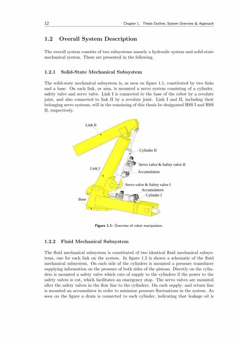
The solid-state mechanical subsystem is, as seen on figure 1.1, constituted by two linksand a base. On each link, or arm, is mounted a servo system consisting of a cylinder,safety valve and servo valve. Link I is connected to the base of the robot by a revolutejoint, and also connected to link II by a revolute joint. Link I and II, including theirbelonging servo systems, will in the remaining of this thesis be designated HSS I and HSSII, respectively.
Cylinder II
Cylinder I
Accumulators
Accumulators
Link I
Link II
Servo valve & Safety valve I
Servo valve & Safety valve II
Base
Figure 1.1: Overview of robot manipulator.
1.2.2 Fluid Mechanical Subsystem
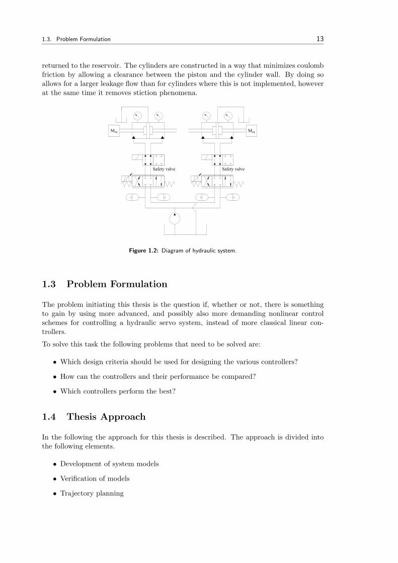
The fluid mechanical subsystem is constituted of two identical fluid mechanical subsys-tems, one for each link on the system. In figure 1.2 is shown a schematic of the fluidmechanical subsystem. On each side of the cylinders is mounted a pressure transducersupplying information on the pressure of both sides of the pistons. Directly on the cylin-ders is mounted a safety valve which cuts of supply to the cylinders if the power to thesafety valves is cut, which facilitates an emergency stop. The servo valves are mountedafter the safety valves in the flow line to the cylinders. On each supply- and return lineis mounted an accumulator in order to minimize pressure fluctuations in the system. Asseen on the figure a drain is connected to each cylinder, indicating that leakage oil is
1.3. Problem Formulation 13
returned to the reservoir. The cylinders are constructed in a way that minimizes coulombfriction by allowing a clearance between the piston and the cylinder wall. By doing soallows for a larger leakage flow than for cylinders where this is not implemented, howeverat the same time it removes stiction phenomena.
Safety valve Safety valve
MeqMeq
Figure 1.2: Diagram of hydraulic system.
1.3 Problem Formulation
The problem initiating this thesis is the question if, whether or not, there is somethingto gain by using more advanced, and possibly also more demanding nonlinear controlschemes for controlling a hydraulic servo system, instead of more classical linear con-trollers.
To solve this task the following problems that need to be solved are:
• Which design criteria should be used for designing the various controllers?
• How can the controllers and their performance be compared?
• Which controllers perform the best?
1.4 Thesis Approach
In the following the approach for this thesis is described. The approach is divided intothe following elements.
• Development of system models
• Verification of models
• Trajectory planning
14 Chapter 1. Thesis Outline, System Overview & Approach
• Establishment of linear controllers
• Establishment of nonlinear controllers
• Comparison of controllers
• Conclusions
In the following, the above listed elements will be briefly described.
1.4.1 Development of System Models
In order to develop and test the various controllers in this thesis, a nonlinear and linearmodel are developed. The nonlinear model for test of controllers, and the linear modelwhich is to be used for linear control design.
1.4.2 Verification of Models
In order to insure the validity of the nonlinear model outputs, this is compared withtransducer outputs from the physical system, and the nonlinear model is tuned to fitthis. The outputs from the nonlinear and linear models is then compared in order tovalidate the linear model near an operating point.
1.4.3 Establishment of Linear Controllers
As basis for comparison of controllers, a series of classical linear controllers are establish-ment. Furthermore some extensions to these controllers are made.
1.4.4 Establishment of Nonlinear Controllers
A series of nonlinear controllers in the form of various adaptive and learning controllersare establishment.
1.4.5 Comparison of Controllers
After having implemented the controllers on the nonlinear model, and in some cases on thephysical system, a comparison of the controllers will be made on the basis of performance,equipment needed in the form of transducers, and robustness towards disturbances.
1.5 Evaluation Criteria
In the following a list of evaluation criteria is set up and subsequently elaborated.
• Tracking performance
• Number of sensors needed
• Robustness towards disturbances

1.6. Summary 15
1.5.1 Tracking Performance
The tracking performance of each controller will be tested on the nonlinear model and forsome controllers implemented on the physical system. In order to evaluate the trackingperformance the system is to follow a a certain trajectory, either in actuator space, or forthe tool center point (TCP). The difference between the desired trajectory and the actualtrajectory followed by the HSS’s is then evaluated, by observing the rms tracking errorand the peak tracking error. By doing so the controllers ability to handle time varyingreferences is evaluated.
1.5.2 Number of Transducers Needed
Depending on the complexity of the controllers, a varying amount of transducers areneeded in order to secure the necessary amount of feedback signals from the HSS makingthe controller in question more expensive and at the same time also more prone to errorsin the form of transducer failure. This hopefully is countered by increased controllerperformance.
1.5.3 Robustness Towards Disturbances
When the HSS’s is in operational mode a number of disturbance input to the system is tobe expected, and therefore a crucial parameter in the evaluation of the controllers is theirrobustness towards such disturbances. In order to test this robustness each controller is,on the nonlinear model in simulink, subjected to mass step at a given point in time ofthe trajectory, and the ability to reject the disturbance is then evaluated.
1.5.4 Final Conclusions
Based on the comparisons of the various controllers a conclusion is made stating whichcontrollers are the most suited for this type hydraulic servo system.
1.6 Summary
In this chapter the thesis outline and a system description has been given. Further a prob-lem formulation has been setup, and an approach for how to solve the problem formulationhas been given. The tasks for solving the problem formulation are various modeling workand verification, trajectory planning, establishment of linear controllers, establishment ofnonlinear controllers, and finally a comparison of the established controllers followed byconclusions made from this thesis.

Part I
System Modeling & TrajectoryPlanning
17

Chapter 2Dynamic Modelof RobotManipulator
Contents
2.1 Solid-State Mechanical Sub-system . . . . . . . . . . . . . 19
2.2 Fluid Mechanical Subsystem . 20
2.3 Model Verification . . . . . . . 20
2.4 Summary . . . . . . . . . . . . 23
In this chapter the non-linear dynamic model of the robot manipulator is accounted for.Here the overall considerations regarding the kinematics and kinetics of the robot manipu-lator are described, and a more detailed derivation of the model are found in appendix A.Finally, the model verification will be carried out.
2.1 Solid-State Mechanical Subsystem
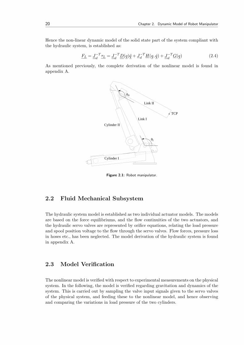
The solid state part of the model is derived as a two degree of freedom system. The flexiblebehavior of the system is neglected in the model, and the system is hence considered asconsisting of completely rigid bodies. The kinematics of the system is derived based onthe joint angles (illustrated in figure 2.1):
q = [θI θII ]T (2.1)
The solid state part of the model is derived in joint space by use of the Newton-Eulerformulation:
τ = [τLI τLII ]T = D(q)q + H(q, q) + G(q) (2.2)
Here the joint load torques are related to the forces applied from the hydraulic system(via the cylinder pistons), by the drive jacobian J
d, which yields:
τL = JTdFL (2.3)
19
20 Chapter 2. Dynamic Model of Robot Manipulator
Hence the non-linear dynamic model of the solid state part of the system compliant withthe hydraulic system, is established as:
FL = J−Td
τL = J−Td
D(q)q + J−Td H(q, q) + J−T
dG(q) (2.4)
As mentioned previously, the complete derivation of the nonlinear model is found inappendix A.
θII
θI
TCPLink I
Link II
Cylinder II
Cylinder I
Figure 2.1: Robot manipulator.
2.2 Fluid Mechanical Subsystem
The hydraulic system model is established as two individual actuator models. The modelsare based on the force equilibriums, and the flow continuities of the two actuators, andthe hydraulic servo valves are represented by orifice equations, relating the load pressureand spool position voltage to the flow through the servo valves. Flow forces, pressure lossin hoses etc., has been neglected. The model derivation of the hydraulic system is foundin appendix A.
2.3 Model Verification
The nonlinear model is verified with respect to experimental measurements on the physicalsystem. In the following, the model is verified regarding gravitation and dynamics of thesystem. This is carried out by sampling the valve input signals given to the servo valvesof the physical system, and feeding these to the nonlinear model, and hence observingand comparing the variations in load pressure of the two cylinders.
2.3. Model Verification 21
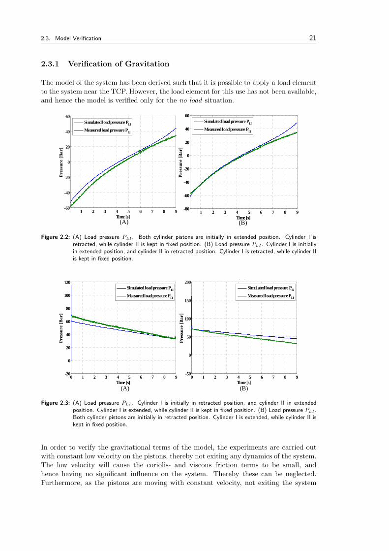
2.3.1 Verification of Gravitation
The model of the system has been derived such that it is possible to apply a load elementto the system near the TCP. However, the load element for this use has not been available,and hence the model is verified only for the no load situation.
(A) (B)
1 2 3 4 5 6 7 8 9-60
-40
-20
0
20
40
60
Time [s]
Pres
sure
[Bar
]
Simulated load pressure PLI
Measured load pressure PLI
1 2 3 4 5 6 7 8 9-80
-60
-40
-20
0
20
40
60
Time [s]
Pres
sure
[Bar
]
Simulated load pressure PLI
Measured load pressure PLI
Figure 2.2: (A) Load pressure PLI . Both cylinder pistons are initially in extended position. Cylinder I isretracted, while cylinder II is kept in fixed position. (B) Load pressure PLI . Cylinder I is initiallyin extended position, and cylinder II in retracted position. Cylinder I is retracted, while cylinder IIis kept in fixed position.
(A) (B)
(A) (B)
1 2 3 4 5 6 7 8 9-60
-40
-20
0
20
40
60
Time [s]
Pres
sure
[Bar
]
Simulated load pressure PLI
Measured load pressure PLI
NE
1 2 3 4 5 6 7 8 9-80
-60
-40
-20
0
20
40
60
Time [s]
Pres
sure
[Bar
]
Simulated load pressure PLI
Measured load pressure PLI
grav_TOP_I_NED_II_I_NED
_I_Ograv_NED_I_NED_II_I_O
P
0 1 2 3 4 5 6 7 8 9-20
0
20
40
60
80
100
120
Time [s]
Pres
sure
[Bar
]
Simulated load pressure PLI
Measured load pressure PLI
0 1 2 3 4 5 6 7 8 9-50
0
50
100
150
200
Time [s]
Pres
sure
[Bar
]
Simulated load pressure PLI
Measured load pressure PLI
Figure 2.3: (A) Load pressure PLI . Cylinder I is initially in retracted position, and cylinder II in extendedposition. Cylinder I is extended, while cylinder II is kept in fixed position. (B) Load pressure PLI .Both cylinder pistons are initially in retracted position. Cylinder I is extended, while cylinder II iskept in fixed position.
In order to verify the gravitational terms of the model, the experiments are carried outwith constant low velocity on the pistons, thereby not exiting any dynamics of the system.The low velocity will cause the coriolis- and viscous friction terms to be small, andhence having no significant influence on the system. Thereby these can be neglected.Furthermore, as the pistons are moving with constant velocity, not exiting the system
22 Chapter 2. Dynamic Model of Robot Manipulator
dynamics, the gravitational terms and coulomb friction can be verified by evaluating theload pressures of the cylinders.
From figures 2.2 and 2.3 it is found that the static terms of link I has been modeledsufficiently accurate, compared to the physical system. However, from figures A.16 andA.17 of appendix A (verification plots for link II), it is found that this is less accuratethan that of the verification for link I. This is assumed to be due to inaccuracies in themodeling regarding masses lengths and so on. However, it is found that the model is asufficiently accurate rendering of the physical system regarding gravitation.
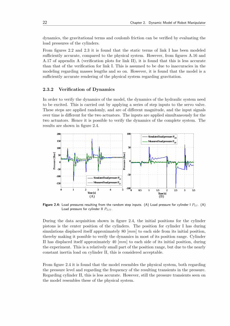
2.3.2 Verification of Dynamics
In order to verify the dynamics of the model, the dynamics of the hydraulic system needto be excited. This is carried out by applying a series of step inputs to the servo valve.These steps are applied randomly, and are of different magnitude, and the input signalsover time is different for the two actuators. The inputs are applied simultaneously for thetwo actuators. Hence it is possible to verify the dynamics of the complete system. Theresults are shown in figure 2.4.
(A) (B)
0 1 2 3 4 5
-150
-100
-50
0
50
100
150
200
Time [s]
Pres
sure
[Bar
]
Simulated load pressure PLI
Measured load pressure PLI
0 0.5 1 1.5 2 2.5 3 3.5-100
-50
0
50
100
Time [s]
Pres
sure
[Bar
]
Simulated load pressure PLII
Measured load pressure PLII
Figure 2.4: Load pressures resulting from the random step inputs. (A) Load pressure for cylinder I PLI . (A)Load pressure for cylinder II PLII .
During the data acquisition shown in figure 2.4, the initial positions for the cylinderpistons is the center position of the cylinders. The position for cylinder I has duringsimulations displaced itself approximately 80 [mm] to each side from its initial position,thereby making it possible to verify the dynamics in most of its position range. CylinderII has displaced itself approximately 40 [mm] to each side of its initial position, duringthe experiment. This is a relatively small part of the position range, but due to the nearlyconstant inertia load on cylinder II, this is considered acceptable.
From figure 2.4 it is found that the model resembles the physical system, both regardingthe pressure level and regarding the frequency of the resulting transients in the pressure.Regarding cylinder II, this is less accurate. However, still the pressure transients seen onthe model resembles these of the physical system.
2.4. Summary 23
From the dynamic verification, it is found that the model is sufficiently accurate in re-semblance to the physical system, implying that the model can be used in the design ofvarious control systems. Hence the model is considered verified.
2.4 Summary
In the above, a dynamic model of the robot manipulator, both solid state and fluid me-chanical, has been established. The developed model was subsequent tested, by compari-son of pressure data from the physical system, regarding both dynamics and gravitation.It was found that the model proved adequately accurate for the development and testingof controllers.

Chapter 3Linear Model ofRobotManipulator
Contents
3.1 Linear Model . . . . . . . . . . 25
3.2 Verification of Linear Model . 26
3.3 Summary . . . . . . . . . . . . 27
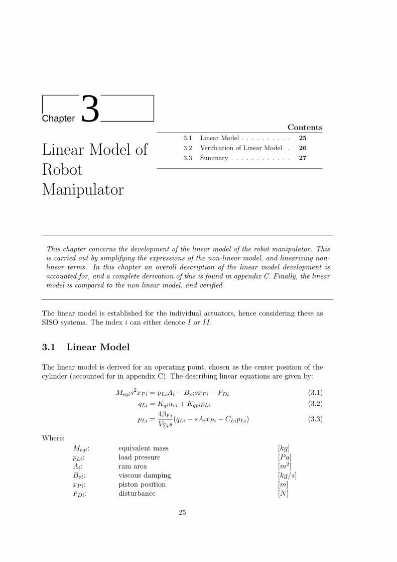
This chapter concerns the development of the linear model of the robot manipulator. Thisis carried out by simplifying the expressions of the non-linear model, and linearizing non-linear terms. In this chapter an overall description of the linear model development isaccounted for, and a complete derivation of this is found in appendix C. Finally, the linearmodel is compared to the non-linear model, and verified.
The linear model is established for the individual actuators, hence considering these asSISO systems. The index i can either denote I or II.
3.1 Linear Model
The linear model is derived for an operating point, chosen as the center position of thecylinder (accounted for in appendix C). The describing linear equations are given by:
Meqis2xPi = pLiAi −BvisxPi − FDi (3.1)qLi = Kqiuvi + KqpipLi (3.2)
pLi =4βFi
VΣis(qLi − sAixPi − CLipLi) (3.3)
Where:Meqi: equivalent mass [kg]pLi: load pressure [Pa]Ai: ram area [m2]Bvi: viscous damping [kg/s]xPi: piston position [m]FDi: disturbance [N ]
25
26 Chapter 3. Linear Model of Robot Manipulator
qLi: load flow [m3/s]βFi: bulk modulus [Pa]VΣi: total volume of cylinder chambers and hoses [m3]CLi: internal leakage coefficient [ms/s/Pa]
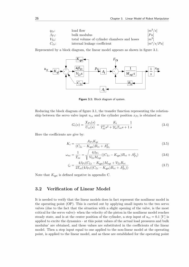
Represented by a block diagram, the linear model appears as shown in figure 3.1.
+-+
sV i
Fi
Σ
β4iA
LiC
+- sMeqi
1s1
viB
PixLipqiKviu -
DiFqpiK
-
iA
Figure 3.1: Block diagram of system.
Reducing the block diagram of figure 3.1, the transfer function representing the relation-ship between the servo valve input uvi and the cylinder position xPi is obtained as:
Gi(s) =XPi(s)Uvi(s)
=Ki
T 2nis
2 + 2ζiTnis + 11s
(3.4)
Here the coefficients are give by:
Ki =APiKqi
(CLi −Kqpi)Bvi + A2Pi
(3.5)
ωni =1
Tni=
√4βFi
VΣiMeqi((CLi −Kqpi)Bvi + A2
Pi) (3.6)
ζi =4βFi(CLi −Kqpi)Meqi + VΣiBvi
2Tni(4βFi((CLi −Kqpi)Bvi + A2Pi))
(3.7)
Note that Kqpi is defined negative in appendix C.
3.2 Verification of Linear Model
It is needed to verify that the linear models does in fact represent the nonlinear model inthe operating point (OP). This is carried out by applying small inputs to the two servovalves (due to the fact that the situation with a slight opening of the valve, is the mostcritical for the servo valve)- when the velocity of the piston in the nonlinear model reachessteady state, and is at the center position of the cylinder, a step input of uvi = 0.1 [V ] isapplied to excite the dynamics - at this point values of the actual load pressures and bulkmodulus’ are obtained, and these values are substituted in the coefficients of the linearmodel. Then a step input equal to one applied to the non-linear model at the operatingpoint, is applied to the linear model, and as these are established for the operating point
3.3. Summary 27
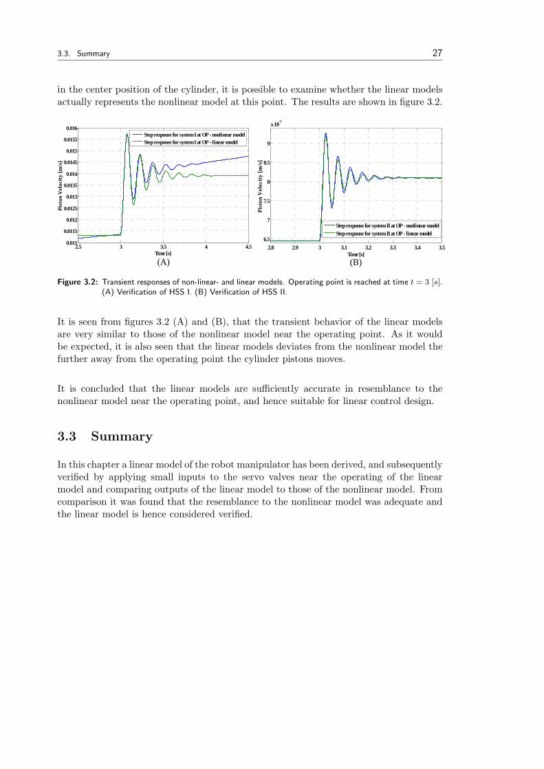
in the center position of the cylinder, it is possible to examine whether the linear modelsactually represents the nonlinear model at this point. The results are shown in figure 3.2.
2.5 3 3.5 4 4.50.011
0.0115
0.012
0.0125
0.013
0.0135
0.014
0.0145
0.015
0.0155
0.016
Time [s]
Pist
on V
eloc
ity [m
/s]
Step response for system I at OP - nonlinear modelStep response for system I at OP - linear model
2.8 2.9 3 3.1 3.2 3.3 3.4 3.56.5
7
7.5
8
8.5
9
x 10-3
Time [s]Pi
ston
Vel
ocity
[m/s
]
Step response for system II at OP - nonlinear modelStep response for system II at OP - linear model
(A) (B)
Figure 3.2: Transient responses of non-linear- and linear models. Operating point is reached at time t = 3 [s].(A) Verification of HSS I. (B) Verification of HSS II.
It is seen from figures 3.2 (A) and (B), that the transient behavior of the linear modelsare very similar to those of the nonlinear model near the operating point. As it wouldbe expected, it is also seen that the linear models deviates from the nonlinear model thefurther away from the operating point the cylinder pistons moves.
It is concluded that the linear models are sufficiently accurate in resemblance to thenonlinear model near the operating point, and hence suitable for linear control design.
3.3 Summary
In this chapter a linear model of the robot manipulator has been derived, and subsequentlyverified by applying small inputs to the servo valves near the operating of the linearmodel and comparing outputs of the linear model to those of the nonlinear model. Fromcomparison it was found that the resemblance to the nonlinear model was adequate andthe linear model is hence considered verified.

Chapter 4TrajectoryPlanning
Contents
4.1 Introduction . . . . . . . . . . 29
4.2 General Trajectory Boundaries 30
4.3 Trajectory Generation . . . . . 32
4.4 Trajectory Profiles (RECT) . . 33
4.5 Trajectory Profiles (IOT) . . . 37
4.6 Necessary Pressure & Flow . . 38
4.7 Summary . . . . . . . . . . . . 40
In this chapter the planning of the trajectory will be carried out. This involves the shape ofthe trajectory for the tool center point, ensuring that the system is loaded in a proper wayto be able to evaluate the performance of the control systems. The shape of the trajectorywill be based on the wanted positions, velocities and accelerations/decelerations experiencedby the system when the trajectory is executed.
4.1 Introduction
In order to evaluate the performance of the controllers applied in this thesis, the tra-jectories must be planned in such a way, that the robot manipulator is properly loadedregarding power consumption, thereby meaning regarding necessary flow and load pres-sure for the individual actuators. It has, by the project group, been decided to applytwo trajectories from which the performance of the controllers will be evaluated. Heretwo scenarios are used - a scenario concerning robot control, where the tool center point(henceforward designated TCP) of the robot manipulator is to track a specified trajectory,and a scenario concerning servo control where the actuators are to follow a specified tra-jectory regardless of the resulting TCP trajectory - the chosen scenarios are for the robotcontrol scenario a rectangular trajectory, and for the servo control scenario a trajectorywhere actuators are to retract and extend within a specified period of time. Hencefor-ward these trajectories are designated RECT for the rectangular trajectory, and IOT forthe in/out trajectory. In this chapter, the boundaries for these trajectories are defined,and within these the position, velocity and acceleration profiles are established (note thatTCP-coordinates are denoted xD, yD).
29
30 Chapter 4. Trajectory Planning
4.2 General Trajectory Boundaries
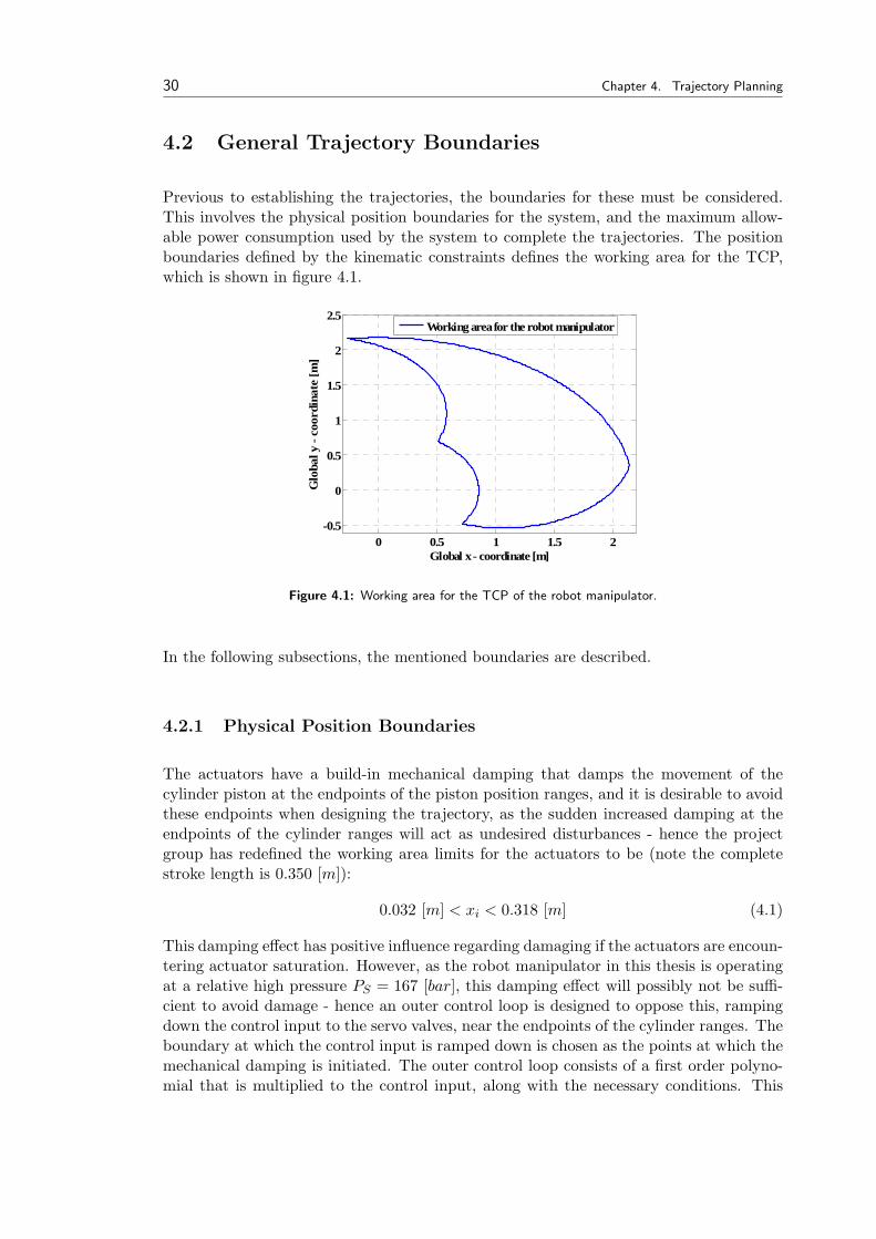
Previous to establishing the trajectories, the boundaries for these must be considered.This involves the physical position boundaries for the system, and the maximum allow-able power consumption used by the system to complete the trajectories. The positionboundaries defined by the kinematic constraints defines the working area for the TCP,which is shown in figure 4.1.
0 0.5 1 1.5 2-0.5
0
0.5
1
1.5
2
2.5
Global x - coordinate [m]
Glo
bal y
- co
ordi
nate
[m]
Working area for the robot manipulator
Figure 4.1: Working area for the TCP of the robot manipulator.
In the following subsections, the mentioned boundaries are described.
4.2.1 Physical Position Boundaries
The actuators have a build-in mechanical damping that damps the movement of thecylinder piston at the endpoints of the piston position ranges, and it is desirable to avoidthese endpoints when designing the trajectory, as the sudden increased damping at theendpoints of the cylinder ranges will act as undesired disturbances - hence the projectgroup has redefined the working area limits for the actuators to be (note the completestroke length is 0.350 [m]):
0.032 [m] < xi < 0.318 [m] (4.1)
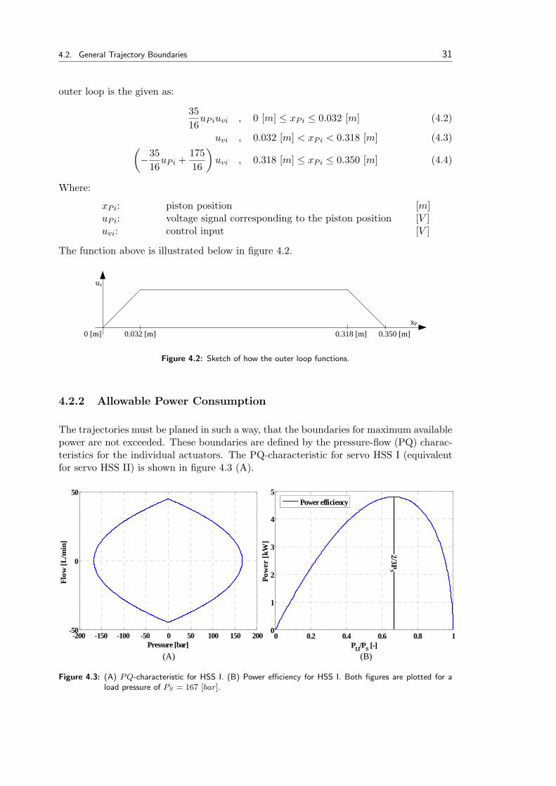
This damping effect has positive influence regarding damaging if the actuators are encoun-tering actuator saturation. However, as the robot manipulator in this thesis is operatingat a relative high pressure PS = 167 [bar], this damping effect will possibly not be suffi-cient to avoid damage - hence an outer control loop is designed to oppose this, rampingdown the control input to the servo valves, near the endpoints of the cylinder ranges. Theboundary at which the control input is ramped down is chosen as the points at which themechanical damping is initiated. The outer control loop consists of a first order polyno-mial that is multiplied to the control input, along with the necessary conditions. This
4.2. General Trajectory Boundaries 31
outer loop is the given as:
3516
uPiuvi , 0 [m] ≤ xPi ≤ 0.032 [m] (4.2)
uvi , 0.032 [m] < xPi < 0.318 [m] (4.3)(−35
16uPi +
17516
)uvi , 0.318 [m] ≤ xPi ≤ 0.350 [m] (4.4)
Where:
xPi: piston position [m]uPi: voltage signal corresponding to the piston position [V ]uvi: control input [V ]
The function above is illustrated below in figure 4.2.
0 [m] 0.350 [m]0.032 [m] 0.318 [m]
uv
xP
Figure 4.2: Sketch of how the outer loop functions.
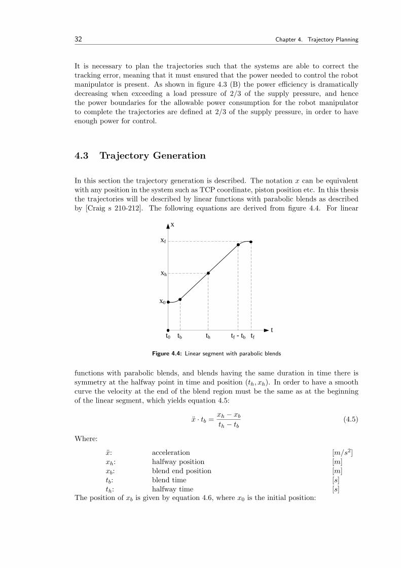
4.2.2 Allowable Power Consumption
The trajectories must be planed in such a way, that the boundaries for maximum availablepower are not exceeded. These boundaries are defined by the pressure-flow (PQ) charac-teristics for the individual actuators. The PQ-characteristic for servo HSS I (equivalentfor servo HSS II) is shown in figure 4.3 (A).
0 0.2 0.4 0.6 0.8 10
1
2
3
4
5
PLI/PS [-]
Pow
er [k
W]
Power efficiency
2/3PS
-200 -150 -100 -50 0 50 100 150 200-50
0
50
Pressure [bar]
Flow
[L/m
in]
(A) (B)
Figure 4.3: (A) PQ-characteristic for HSS I. (B) Power efficiency for HSS I. Both figures are plotted for aload pressure of PS = 167 [bar].
32 Chapter 4. Trajectory Planning
It is necessary to plan the trajectories such that the systems are able to correct thetracking error, meaning that it must ensured that the power needed to control the robotmanipulator is present. As shown in figure 4.3 (B) the power efficiency is dramaticallydecreasing when exceeding a load pressure of 2/3 of the supply pressure, and hencethe power boundaries for the allowable power consumption for the robot manipulatorto complete the trajectories are defined at 2/3 of the supply pressure, in order to haveenough power for control.
4.3 Trajectory Generation
In this section the trajectory generation is described. The notation x can be equivalentwith any position in the system such as TCP coordinate, piston position etc. In this thesisthe trajectories will be described by linear functions with parabolic blends as describedby [Craig s 210-212]. The following equations are derived from figure 4.4. For linear
t
x
x0
xf
t0 tb tf - tb tf
xh
th
Figure 4.4: Linear segment with parabolic blends
functions with parabolic blends, and blends having the same duration in time there issymmetry at the halfway point in time and position (th, xh). In order to have a smoothcurve the velocity at the end of the blend region must be the same as at the beginningof the linear segment, which yields equation 4.5:
x · tb =xh − xb
th − tb(4.5)
Where:
x: acceleration [m/s2]xh: halfway position [m]xb: blend end position [m]tb: blend time [s]th: halfway time [s]
The position of xb is given by equation 4.6, where x0 is the initial position:
4.4. Trajectory Profiles (RECT) 33
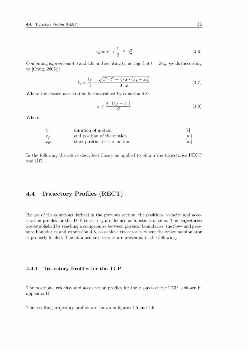
xb = x0 +12· x · t2b (4.6)
Combining expressions 4.5 and 4.6, and isolating tb, noting that t = 2·th, yields (accordingto [Craig, 2005]):
tb =tf2−√
x2 · t2 − 4 · x · (xf − x0)2 · x
(4.7)
Where the chosen acceleration is constrained by equation 4.8:
x ≥4 · (xf − x0)
t2(4.8)
Where:
t: duration of motion [s]xf : end position of the motion [m]x0: start position of the motion [m]
In the following the above described theory as applied to obtain the trajectories RECTand IOT.
4.4 Trajectory Profiles (RECT)
By use of the equations derived in the previous section, the position-, velocity and acce-leration profiles for the TCP-trajectory are defined as functions of time. The trajectoriesare established by reaching a compromise between physical boundaries, the flow- and pres-sure boundaries and expression 4.8, to achieve trajectories where the robot manipulatoris properly loaded. The obtained trajectories are presented in the following.
4.4.1 Trajectory Profiles for the TCP
The position-, velocity- and acceleration profiles for the xD-axis of the TCP is shown inappendix D.
The resulting trajectory profiles are shown in figures 4.5 and 4.6.
34 Chapter 4. Trajectory Planning
(A) (B) (C)
0 0.5 1 1.5 2 2.5 3 3.5-10
-5
0
5
10
Time [s]
Acc
eler
atio
n [m
/s2 ]
xD - acceleration profile
0 0.5 1 1.5 2 2.5 3 3.5-3
-2
-1
0
1
2
3
Time [s]
Vel
ocity
[m/s
]
xD - velocity profile
0 0.5 1 1.5 2 2.5 3 3.51.1
1.2
1.3
1.4
1.5
1.6
Time [s]
Posi
tion
[m]
xD - position profile
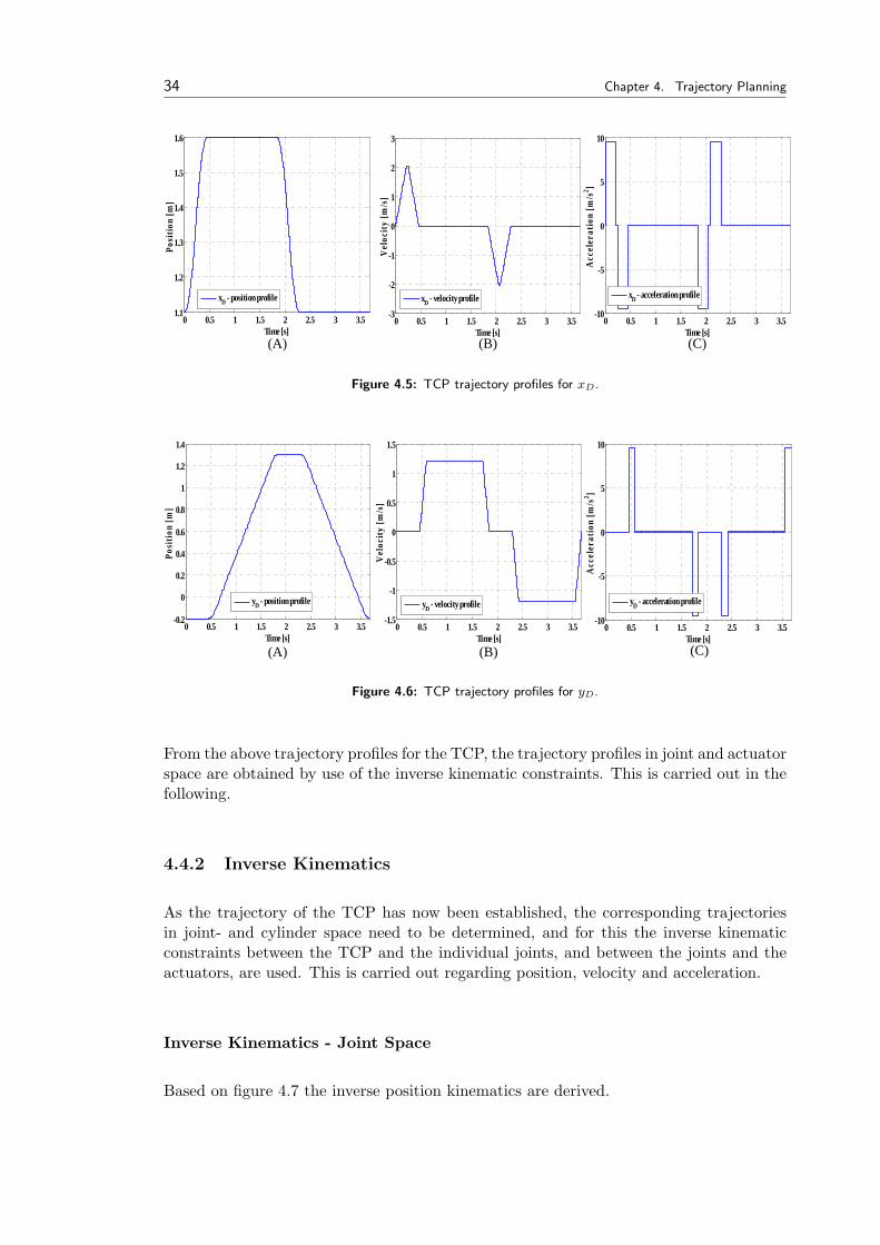
Figure 4.5: TCP trajectory profiles for xD.
(A) (B) (C)
0 0.5 1 1.5 2 2.5 3 3.5-10
-5
0
5
10
Time [s]
Acc
eler
atio
n [m
/s2 ]
yD - acceleration profile
0 0.5 1 1.5 2 2.5 3 3.5-1.5
-1
-0.5
0
0.5
1
1.5
Time [s]
Vel
ocity
[m/s
]
yD - velocity profile
0 0.5 1 1.5 2 2.5 3 3.5-0.2
0
0.2
0.4
0.6
0.8
1
1.2
1.4
Time [s]
Posi
tion
[m]
yD - position profile
Figure 4.6: TCP trajectory profiles for yD.
From the above trajectory profiles for the TCP, the trajectory profiles in joint and actuatorspace are obtained by use of the inverse kinematic constraints. This is carried out in thefollowing.
4.4.2 Inverse Kinematics
As the trajectory of the TCP has now been established, the corresponding trajectoriesin joint- and cylinder space need to be determined, and for this the inverse kinematicconstraints between the TCP and the individual joints, and between the joints and theactuators, are used. This is carried out regarding position, velocity and acceleration.
Inverse Kinematics - Joint Space
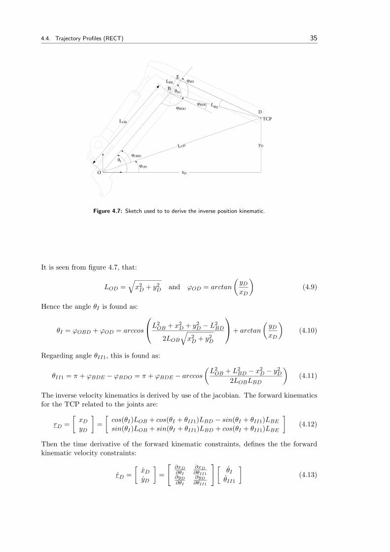
Based on figure 4.7 the inverse position kinematics are derived.
4.4. Trajectory Profiles (RECT) 35
O
B
E
A
yI
L EPφ
LA
E
φEA
B
θII1
TCP
xD
yD
D
LOD
LBDφBDE
E
φBDO
φBD
φOBD
φOD
θI
LOB
LBE
Figure 4.7: Sketch used to to derive the inverse position kinematic.
It is seen from figure 4.7, that:
LOD =√
x2D + y2
D and ϕOD = arctan
(yD
xD
)(4.9)
Hence the angle θI is found as:
θI = ϕOBD + ϕOD = arccos
L2OB + x2
D + y2D − L2
BD
2LOB
√x2
D + y2D
+ arctan
(yD
xD
)(4.10)
Regarding angle θII1, this is found as:
θII1 = π + ϕBDE − ϕBDO = π + ϕBDE − arccos
(L2
OB + L2BD − x2
D − y2D
2LOBLBD
)(4.11)
The inverse velocity kinematics is derived by use of the jacobian. The forward kinematicsfor the TCP related to the joints are:
rD =[
xD
yD
]=[
cos(θI)LOB + cos(θI + θII1)LBD − sin(θI + θII1)LBE
sin(θI)LOB + sin(θI + θII1)LBD + cos(θI + θII1)LBE
](4.12)
Then the time derivative of the forward kinematic constraints, defines the the forwardkinematic velocity constraints:
rD =[
xD
yD
]=
[∂xD∂θI
∂xD∂θII1
∂yD∂θI
∂yD∂θII1
] [θI
θII1
](4.13)
36 Chapter 4. Trajectory Planning
Hence the velocity of the joint angles are:[θI
θII1
]=
[∂xD∂θI
∂xD∂θII1
∂yD∂θI
∂yD∂θII1
]−1 [xD
yD
](4.14)
The inverse acceleration kinematics is determined as the time derivative of the inversevelocity kinematics, which yields:
[θI
θII1
]=
ddt
(∂xD∂θI
)ddt
(∂xD∂θII1
)ddt
(∂yD∂θI
)ddt
(∂yD∂θII1
) −1 [xD
yD
](4.15)
Inverse Kinematics - Actuator Space
The kinematic constraints relating the joint angles, angular velocities and angular accel-erations to the linear positions, velocities and accelerations in actuator space can be foundin appendix A.1.1 (note that θII1 = θII and θII1 = θII). Combining these constraints,the inverse kinematic relations between the TCP and the actuators are established.
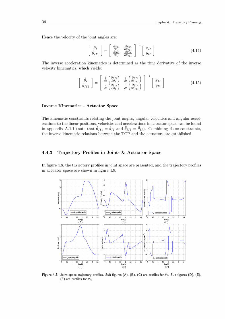
4.4.3 Trajectory Profiles in Joint- & Actuator Space
In figure 4.8, the trajectory profiles in joint space are presented, and the trajectory profilesin actuator space are shown in figure 4.9.
(A) (B) (C)
(C) (E) (F)
0 0.5 1 1.5 2 2.5 3 3.5-3
-2
-1
0
1
2
3
Time [s]
Vel
ocity
[rad
/s]
θII - velocity profile
0 0.5 1 1.5 2 2.5 3 3.5-1.5
-1
-0.5
0
0.5
1
1.5
2
Time [s]
Vel
ocity
[rad
/s]
θI - velocity profile
0 0.5 1 1.5 2 2.5 3 3.5-2.5
-2
-1.5
-1
Time [s]
Posi
tion
[rad
]
θII - position profile
0 0.5 1 1.5 2 2.5 3 3.5
0.8
1
1.2
1.4
1.6
Time [s]
Posi
tion
[rad
]
θI - position profile
0 0.5 1 1.5 2 2.5 3 3.5-10
-5
0
5
10
Time [s]
Acc
eler
atio
n [r
ad/s2 ]
θI - acceleration profile
0 0.5 1 1.5 2 2.5 3 3.5-15
-10
-5
0
5
10
15
Time [s]
Acc
eler
atio
n [r
ad/s2 ]
θII - acceleration profile
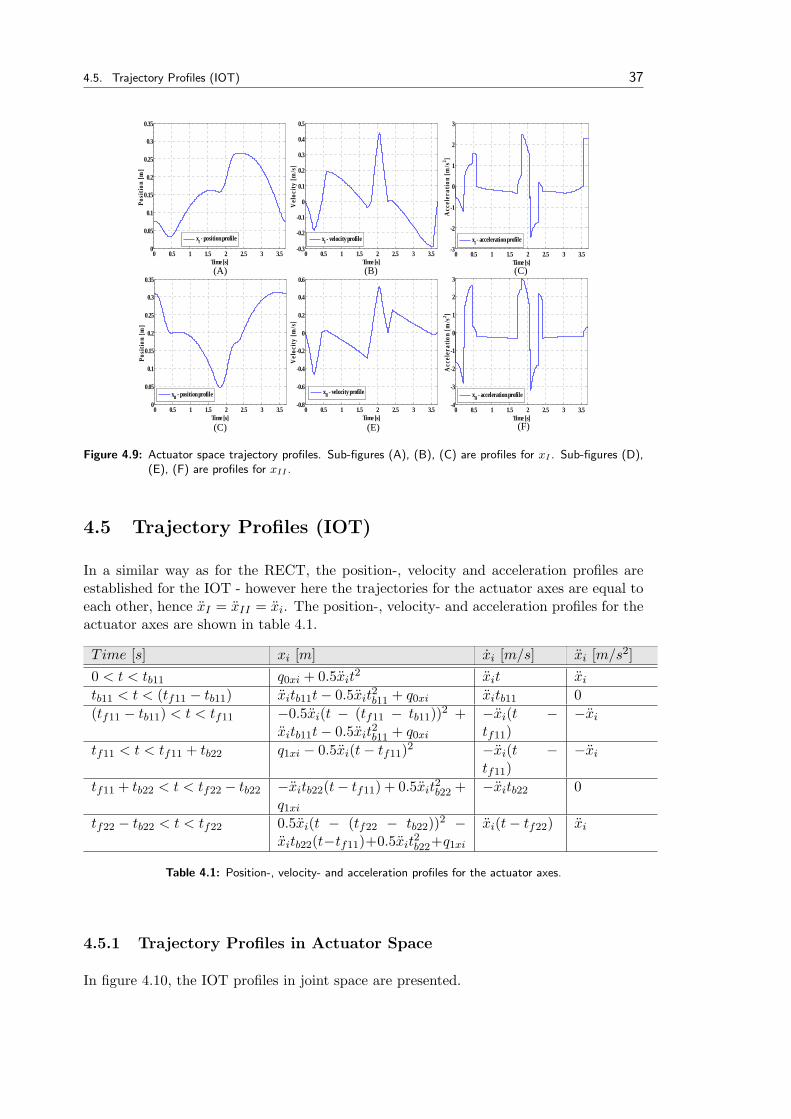
Figure 4.8: Joint space trajectory profiles. Sub-figures (A), (B), (C) are profiles for θI . Sub-figures (D), (E),(F) are profiles for θII .
4.5. Trajectory Profiles (IOT) 37
(A) (B) (C)
(C) (E) (F)
0 0.5 1 1.5 2 2.5 3 3.5-0.3
-0.2
-0.1
0
0.1
0.2
0.3
0.4
0.5
Time [s]
Vel
ocity
[m/s
]
xI - velocity profile
0 0.5 1 1.5 2 2.5 3 3.50
0.05
0.1
0.15
0.2
0.25
0.3
0.35
Time [s]
Posi
tion
[m]
xII - position profile
0 0.5 1 1.5 2 2.5 3 3.50
0.05
0.1
0.15
0.2
0.25
0.3
0.35
Time [s]
Posi
tion
[m]
xI - position profile
0 0.5 1 1.5 2 2.5 3 3.5-0.8
-0.6
-0.4
-0.2
0
0.2
0.4
0.6
Time [s]
Vel
ocity
[m/s
]
xII - velocity profile
0 0.5 1 1.5 2 2.5 3 3.5-3
-2
-1
0
1
2
3
Time [s]
Acc
eler
atio
n [m
/s2 ]
xI - acceleration profile
0 0.5 1 1.5 2 2.5 3 3.5-4
-3
-2
-1
0
1
2
3
Time [s]
Acc
eler
atio
n [m
/s2 ]
xII - acceleration profile
Figure 4.9: Actuator space trajectory profiles. Sub-figures (A), (B), (C) are profiles for xI . Sub-figures (D),(E), (F) are profiles for xII .
4.5 Trajectory Profiles (IOT)
In a similar way as for the RECT, the position-, velocity and acceleration profiles areestablished for the IOT - however here the trajectories for the actuator axes are equal toeach other, hence xI = xII = xi. The position-, velocity- and acceleration profiles for theactuator axes are shown in table 4.1.
Time [s] xi [m] xi [m/s] xi [m/s2]0 < t < tb11 q0xi + 0.5xit
2 xit xi
tb11 < t < (tf11 − tb11) xitb11t− 0.5xit2b11 + q0xi xitb11 0
(tf11 − tb11) < t < tf11 −0.5xi(t − (tf11 − tb11))2 +xitb11t− 0.5xit
2b11 + q0xi
−xi(t −tf11)
−xi
tf11 < t < tf11 + tb22 q1xi − 0.5xi(t− tf11)2 −xi(t −tf11)
−xi
tf11 + tb22 < t < tf22 − tb22 −xitb22(t− tf11) + 0.5xit2b22 +
q1xi
−xitb22 0
tf22 − tb22 < t < tf22 0.5xi(t − (tf22 − tb22))2 −xitb22(t−tf11)+0.5xit
2b22+q1xi
xi(t− tf22) xi
Table 4.1: Position-, velocity- and acceleration profiles for the actuator axes.
4.5.1 Trajectory Profiles in Actuator Space
In figure 4.10, the IOT profiles in joint space are presented.
38 Chapter 4. Trajectory Planning
(A) (B) (C)
0 0.5 1 1.5 2 2.50
0.05
0.1
0.15
0.2
0.25
0.3
0.35
Time [s]
Posi
tion
[m]
xI/xII - position profile
0 0.5 1 1.5 2 2.5-0.4
-0.3
-0.2
-0.1
0
0.1
0.2
0.3
Time [s]
Vel
ocity
[m/s
]
xI/xII - velocity profile
0 0.5 1 1.5 2 2.5-1.5
-1
-0.5
0
0.5
1
1.5
Time [s]
Acc
eler
atio
n [m
/s2 ]
xI/xII - acceleration profile
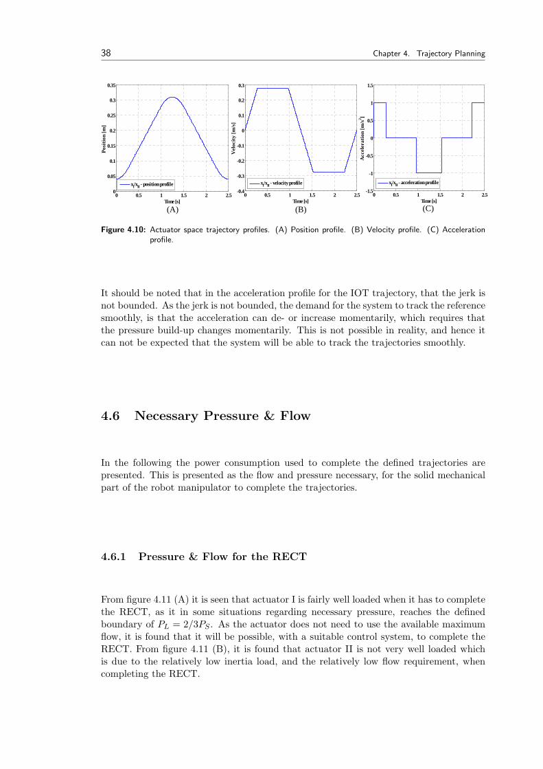
Figure 4.10: Actuator space trajectory profiles. (A) Position profile. (B) Velocity profile. (C) Accelerationprofile.
It should be noted that in the acceleration profile for the IOT trajectory, that the jerk isnot bounded. As the jerk is not bounded, the demand for the system to track the referencesmoothly, is that the acceleration can de- or increase momentarily, which requires thatthe pressure build-up changes momentarily. This is not possible in reality, and hence itcan not be expected that the system will be able to track the trajectories smoothly.
4.6 Necessary Pressure & Flow
In the following the power consumption used to complete the defined trajectories arepresented. This is presented as the flow and pressure necessary, for the solid mechanicalpart of the robot manipulator to complete the trajectories.
4.6.1 Pressure & Flow for the RECT
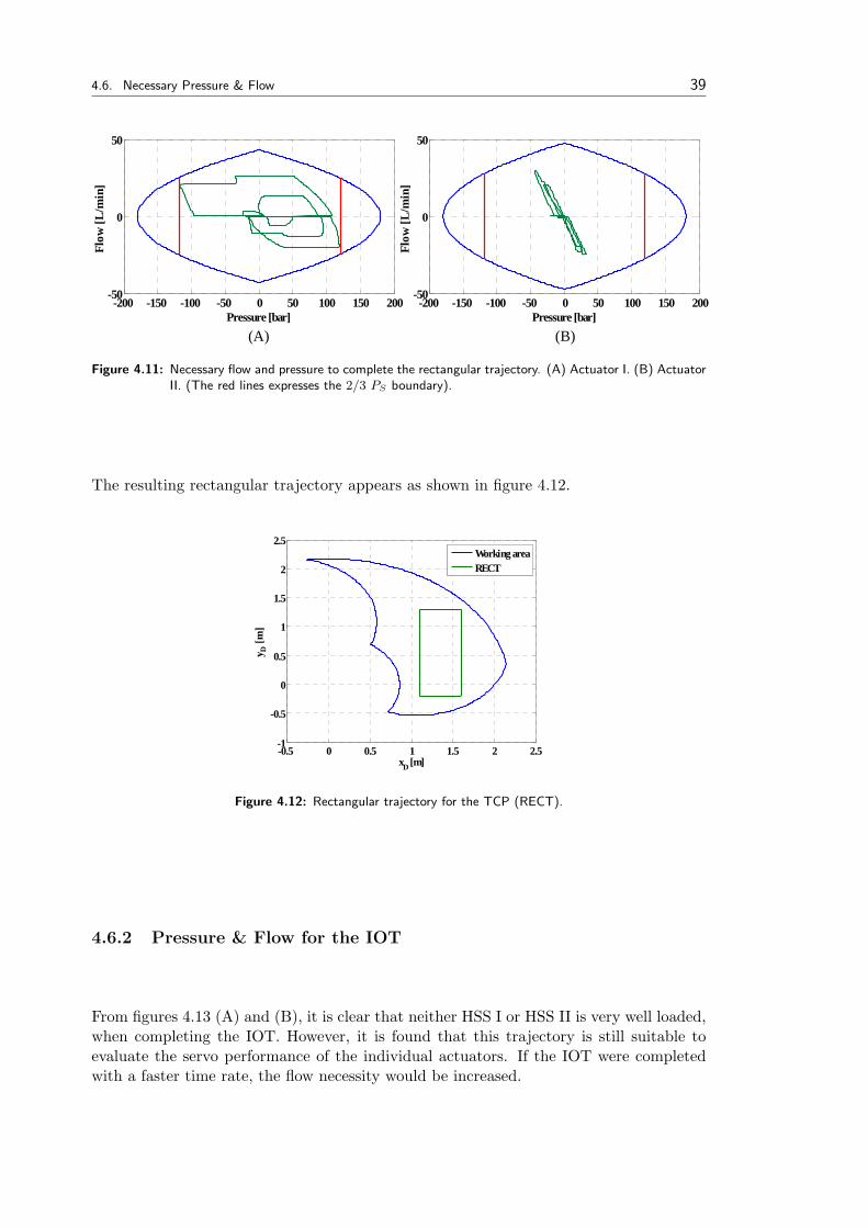
From figure 4.11 (A) it is seen that actuator I is fairly well loaded when it has to completethe RECT, as it in some situations regarding necessary pressure, reaches the definedboundary of PL = 2/3PS . As the actuator does not need to use the available maximumflow, it is found that it will be possible, with a suitable control system, to complete theRECT. From figure 4.11 (B), it is found that actuator II is not very well loaded whichis due to the relatively low inertia load, and the relatively low flow requirement, whencompleting the RECT.
4.6. Necessary Pressure & Flow 39
-200 -150 -100 -50 0 50 100 150 200-50
0
50
Pressure [bar]
Flow
[L/m
in]
-200 -150 -100 -50 0 50 100 150 200-50
0
50
Pressure [bar]
Flow
[L/m
in]
(A) (B)
Figure 4.11: Necessary flow and pressure to complete the rectangular trajectory. (A) Actuator I. (B) ActuatorII. (The red lines expresses the 2/3 PS boundary).
The resulting rectangular trajectory appears as shown in figure 4.12.
-0.5 0 0.5 1 1.5 2 2.5-1
-0.5
0
0.5
1
1.5
2
2.5
xD [m]
y D [m
]
Working areaRECT
Figure 4.12: Rectangular trajectory for the TCP (RECT).
4.6.2 Pressure & Flow for the IOT
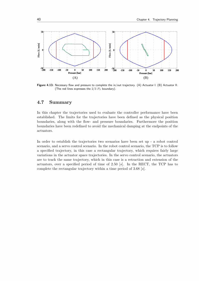
From figures 4.13 (A) and (B), it is clear that neither HSS I or HSS II is very well loaded,when completing the IOT. However, it is found that this trajectory is still suitable toevaluate the servo performance of the individual actuators. If the IOT were completedwith a faster time rate, the flow necessity would be increased.
40 Chapter 4. Trajectory Planning
-200 -150 -100 -50 0 50 100 150 200-50
0
50
Pressure [bar]
Flow
[L/m
in]
-200 -150 -100 -50 0 50 100 150 200-50
0
50
Pressure [bar]
Flow
[L/m
in]
(A) (B)
Figure 4.13: Necessary flow and pressure to complete the in/out trajectory. (A) Actuator I. (B) Actuator II.(The red lines expresses the 2/3 PS boundary).
4.7 Summary
In this chapter the trajectories used to evaluate the controller performance have beenestablished. The limits for the trajectories have been defined as the physical positionboundaries, along with the flow- and pressure boundaries. Furthermore the positionboundaries have been redefined to avoid the mechanical damping at the endpoints of theactuators.
In order to establish the trajectories two scenarios have been set up - a robot controlscenario, and a servo control scenario. In the robot control scenario, the TCP is to followa specified trajectory, in this case a rectangular trajectory, which requires fairly largevariations in the actuator space trajectories. In the servo control scenario, the actuatorsare to track the same trajectory, which in this case is a retraction and extension of theactuators, over a specified period of time of 2.50 [s]. In the RECT, the TCP has tocomplete the rectangular trajectory within a time period of 3.68 [s].
Part II
Linear Control Schemes
41

Chapter 5Classic LinearControl
Contents
5.1 Introduction . . . . . . . . . . 43
5.2 Proportional Control (P) . . . 45
5.3 Proportional Integral Control(PI) . . . . . . . . . . . . . . . 45
5.4 Proportional Lead Compensator 46
5.5 Proportional Lag Compensator 46
5.6 Proportional Lag-Lead Com-pensator . . . . . . . . . . . . 47
5.7 Simulation Results . . . . . . . 48
5.8 Summary . . . . . . . . . . . . 49
In this chapter classic linear controllers/compensators are developed and implemented onthe nonlinear model. The control types chosen to be tested in this chapter are a proportionalcontroller, a proportional + integral controller, a Lead compensator, a Lag compensatorand a Lag-Lead compensator.
5.1 Introduction
As mentioned in the meta text, this chapter concerns the development of classical linearcontrollers/compensators using position feedback. The controller development will beperformed by use of linear control theory applied on the SISO transfer functions estab-lished in chapter 3. The nomenclature of this chapter, not previously defined, is givenbelow.
KPi: proportional gain [−]KPIi: proportional gain [−]Kci: proportional gain [−]TPIi: time constant [s]Tleadi: time constant [s]Tlagi: time constant [s]αi: scaling factor [−]βi: scaling factor [−]γleadi: scaling factor [−]γlagi: scaling factor [−]
5.1.1 Design Specifications
In order to facilitate the design and comparison of the chosen linear controllers, designspecifications are setup in the following. First and foremost the system must remain stable
43
44 Chapter 5. Classic Linear Control
for all chosen controllers, and accompanying parameters, which is done by ensuring thatthe phase and gain margins (henceforward designated PM and GM, respectively), as aminimum, are always positive. However to ensure a certain clearance, it is desirable tohave GM > 6− 8 [dB] and PM > 45 − 60[Rasmussen, 1996]. Furthermore it is, sincethe actuators are to follow the specified trajectories, desired to have an error as small aspossible.
5.1.2 Design Approach
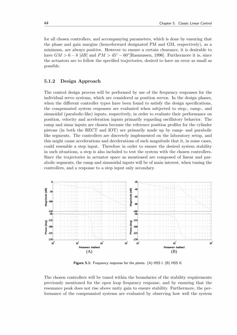
The control design process will be performed by use of the frequency responses for theindividual servo systems, which are considered as position servos. In the design phases,when the different controller types have been found to satisfy the design specifications,the compensated system responses are evaluated when subjected to step-, ramp-, andsinusoidal (parabolic-like) inputs, respectively, in order to evaluate their performance onposition, velocity and acceleration inputs primarily regarding oscillatory behavior. Theramp and sinus inputs are chosen because the reference position profiles for the cylinderpistons (in both the RECT and IOT) are primarily made up by ramp- and paraboliclike segments. The controllers are discretely implemented on the laboratory setup, andthis might cause accelerations and decelerations of such magnitude that it, in some cases,could resemble a step input. Therefore in order to ensure the desired system stabilityin such situations, a step is also included to test the system with the chosen controllers.Since the trajectories in actuator space as mentioned are composed of linear and par-abolic segments, the ramp and sinusoidal inputs will be of main interest, when tuning thecontrollers, and a response to a step input only secondary.
(A) (B)
-150
-100
-50
0
Mag
nitu
de (d
B)
100
101
102
103
-270
-225
-180
-135
-90
Phas
e (d
eg)
Frequency (rad/sec)
-100
-80
-60
-40
-20
Mag
nitu
de (d
B)
101
102
103
-270
-225
-180
-135
-90
Phas
e (d
eg)
Frequency (rad/sec)
Figure 5.1: Frequency response for the plants. (A) HSS I. (B) HSS II.
The chosen controllers will be tuned within the boundaries of the stability requirementspreviously mentioned for the open loop frequency response, and by ensuring that theresonance peak does not rise above unity gain to ensure stability. Furthermore, the per-formance of the compensated systems are evaluated by observing how well the system
5.2. Proportional Control (P) 45
tracks the step, ramp and sinusoidal inputs, and possibly subsequently adjusted.
The controllers established in this chapter are especially suited for regulator problemswith constant references, but has poor performance regarding position servo problemswith trajectory tracking (varying references). Efforts to compensate for this are takenin the following chapter. The frequency responses for the uncompensated systems areshown in figure 5.1.
The natural frequencies and damping ratios for the uncompensated systems are:
ωnI = 39.68 [rad/s] , ωnII = 133.01 [rad/s] (5.1)ζnI = 0.11 [−] , ζnII = 0.12 [−] (5.2)
5.2 Proportional Control (P)
The first controller to be implemented is a proportional (P) controller which has thepurpose of speeding up the transient response of the system. The proportional gainis tuned until a reasonable compromise between step, ramp and sinusoidal response isobtained. Due to the fact that the system is a type 1 system, there will be a steady stateerror for ramp and sinusoidal inputs, when utilizing a proportional controller. Applying aproportional controller to a system only affects the magnitude of the frequency response,and the phase remains unaltered. When the proportional gain is increased for HSS I andII both the gain margin and phase margin is minimized until the compensated systemsatisfies the design specifications. The frequency response for the compensated systemare shown in appendix E.
The margins obtained for the tuning of the proportional controller for HSS I and II are:
GMI = 7.50 [dB] ∧ PMI = 88.90 [] (5.3)GMII = 7.89 [dB] ∧ PMII = 88.60 [] (5.4)
5.3 Proportional Integral Control (PI)
In order to compensate for the steady state error on the ramp input, when using aproportional controller, an integral term is applied to controller. The structure for thePI controller is:
Gc(s) = KPIiTPIis + 1
TPIis(5.5)
It is seen that applying a PI controller to a HSS increases the system type by 1, so thecompensated system becomes a type 2 system. It must be taken into account when ap-plying a PI controller to a type 1 system, that the DC-phase becomes −180 [o]. Hence inorder to avoid instability of the system, one must choose the position of the zero of thePI controller at a relatively low frequency assuring that no low frequent dynamics causesinstability of the system.

46 Chapter 5. Classic Linear Control
Like for the proportional controller, the PI controller is tuned observing the phase andgain margin of the frequency response. As mentioned above the PI compensated HSSis a type 2 system with an initial phase of −180 [] - the zero enables the possibility ofadjusting the PM - hence it is possible to adjust the compensated system to meet thedesign specifications regarding GM and PM. The gains and the time constants of the PIcontrollers of the two compensated systems are tuned to meet the following margins:
GMI = 7.96 [dB] ∧ PMI = 62.40 [] (5.6)GMII = 6.37 [dB] ∧ PMII = 67.60 [] (5.7)
It is noted that when applying a PI controller, integrator anti wind up also must beimplemented. The anti wind up is briefly accounted for in appendix G.
5.4 Proportional Lead Compensator
The motivation for applying a lead compensator is to increase the bandwidth of thecompensated system and hence increase the speed of the response. The basic structureof a lead compensator is given by:
Gc(s) = KciTleadis + 1
αiTleadis + 1; αi < 1 (5.8)
The lead compensator is implemented in the forward path of the HSS in cascade withthe plant, and is essentially a PD controller. The zero and pole of the lead compensatoris placed near the resonance peak in order to add phase lead here. Here the zero isplaced in the low frequency region and the pole in the high frequency region. The leadcompensator speeds up the response due to the added phase lead - however, due to therelatively poor damped system, little effect is obtained by using the lead compensator.Furthermore the zero and pole has been placed, and the gain designed in such a way,that the performance specifications are met regarding GM and PM, and the frequencyresponses of the compensators and compensated systems are found in appendix E. Theachieved margins for the compensated systems are:
GMI = 7.15 [dB] ∧ PMI = 91.40 [deg] (5.9)GMII = 7.90 [dB] ∧ PMII = 91.70 [deg] (5.10)
5.5 Proportional Lag Compensator
In this section a lag compensator is established. The motivation for applying a lagcompensator is to decrease the steady state velocity error. The basic structure of a lagcompensator is given by:
Gc(s) = KciTlagis + 1
βiTlagis + 1; βi > 1 (5.11)
The lag controller is applied with both the pole and zero are placed in the low frequencyregion, such that the phase contribution of the compensator approximately does not in-
5.6. Proportional Lag-Lead Compensator 47
fluence the phase near the resonance peak. By doing so, it is avoided to add additionalnegative phase to the already poorly damped system. Then by subsequently adjustingthe compensator gain, increased gain at lower frequencies is achieved, reducing the steadystate error. However, the placement of a pole in the low frequency region reduces thebandwidth and hence the speed of the transient response. On the other hand, this en-ables the possibility of increasing the gain further than it would be possible, if the lagcompensator was not introduced.As the lag compensator (and the lead compensator) does not introduce any additionalfree integrators to the compensated system, the system type remains a type 1, whichyields a static velocity error - it is not possible in any way to alter the system to a type2 system by using only a lag compensator, but the steady state velocity error will bereduced due to the possibility of increasing the gain further. The frequency responses ofthe compensators and compensated systems are found in appendix E.
The achieved margins for the lag compensated systems are:
GMI = 7.74 [dB] ∧ PMI = 65.50 [deg] (5.12)GMII = 7.18 [dB] ∧ PMII = 82.70 [deg] (5.13)
5.6 Proportional Lag-Lead Compensator
In this section a lag-lead compensator is established. Implementing this type of com-pensator is motivated by the possibility for achieving the advantages of lead- and lagcompensators regarding speed of the transient response and the reduction of the steadystate error, respectively. Essentially, the lag-lead compensator consists of a lead and alag compensator placed in cascade with each other and the plant, hence the structure ofthe lag-lead compensator is:
Gc(s) = KciTlagis + 1
γlagiTlagis + 1Tleadis + 1
γleadiTleadis + 1; γleadi < 1 < γlagi (5.14)
The lag part of this compensator is placed in the low frequency region in a way similar tothe lag compensator in order to increase the gain at lower frequencies. The lag compen-sator is placed near the resonance peak in order to add phase in this frequency area. Asfor the previous mentioned compensators, the frequency responses of the compensatorsand compensated systems are found in appendix E.
The margins achieved by applying lag-lead compensators to the systems are:
GMI = 7.00 [dB] ∧ PMI = 66.90 [deg] (5.15)GMII = 7.04 [dB] ∧ PMII = 67.60 [deg] (5.16)
In the following the simulation results for the systems implemented with the describedcontrollers are presented. The controller parameters designed for the above controllersare found in appendix F.
48 Chapter 5. Classic Linear Control
5.7 Simulation Results
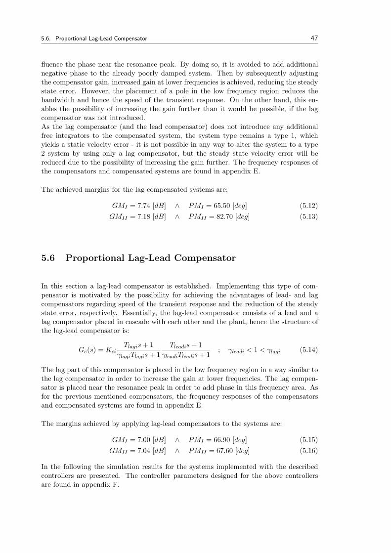
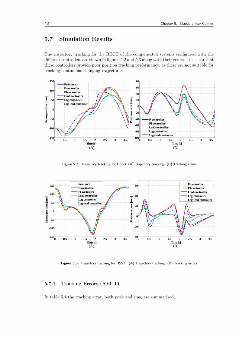
The trajectory tracking for the RECT of the compensated systems configured with thedifferent controllers are shown in figures 5.2 and 5.3 along with their errors. It is clear thatthese controllers provide poor position tracking performance, as these are not suitable fortracking continuous changing trajectories.
(A) (B)
0 0.5 1 1.5 2 2.5 3 3.5-150
-100
-50
0
50
100
150
Time [s]
Pist
on p
ositi
on [m
m]
ReferenceP-controllerPI-controllerLead-controllerLag-controllerLag-lead-controller
0 0.5 1 1.5 2 2.5 3 3.5-100
-80
-60
-40
-20
0
20
40
60
80
Time [s]
Posi
tion
erro
r [m
m]
P-controllerPI-controllerLead-controllerLag-controllerLag-lead-controller
Figure 5.2: Trajectory tracking for HSS I. (A) Trajectory tracking. (B) Tracking errors
(A) (B)
0 0.5 1 1.5 2 2.5 3 3.5-150
-100
-50
0
50
100
150
Time [s]
Pist
on p
ositi
on [m
m]
ReferenceP-controllerPI-controllerLead-controllerLag-controllerLag-lead-controller
0 0.5 1 1.5 2 2.5 3 3.5-40
-20
0
20
40
60
Time [s]
Posi
tion
erro
r [m
m]
P-controllerPI-controllerLead-controllerLag-controllerLag-lead-controller
Figure 5.3: Trajectory tracking for HSS II. (A) Trajectory tracking. (B) Tracking errors
5.7.1 Tracking Errors (RECT)
In table 5.1 the tracking error, both peak and rms, are summarized.
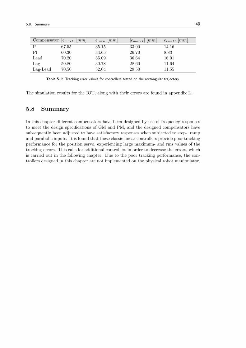
5.8. Summary 49
Compensator |emaxI | [mm] ermsI [mm] |emaxII | [mm] ermsII [mm]P 67.55 35.15 33.90 14.16PI 60.30 34.65 26.70 8.83Lead 70.20 35.09 36.64 16.01Lag 50.80 30.78 28.60 11.64Lag-Lead 70.50 32.04 29.50 11.55
Table 5.1: Tracking error values for controllers tested on the rectangular trajectory.
The simulation results for the IOT, along with their errors are found in appendix L.
5.8 Summary
In this chapter different compensators have been designed by use of frequency responsesto meet the design specifications of GM and PM, and the designed compensators havesubsequently been adjusted to have satisfactory responses when subjected to step-, rampand parabolic inputs. It is found that these classic linear controllers provide poor trackingperformance for the position servo, experiencing large maximum- and rms values of thetracking errors. This calls for additional controllers in order to decrease the errors, whichis carried out in the following chapter. Due to the poor tracking performance, the con-trollers designed in this chapter are not implemented on the physical robot manipulator.

Chapter 6Linear ControlExtensions
Contents
6.1 Introduction . . . . . . . . . . 51
6.2 Velocity Feedforward Com-pensation . . . . . . . . . . . . 51
6.3 Simulation Results - VFCP . . 55
6.4 Simulation Results - VFCA . . 57
6.5 Experimental Results . . . . . 58
6.6 Summary . . . . . . . . . . . . 59
This chapter serves as an extension to chapter 5 and the classical linear feedback control.Here velocity feedforward compensators are introduced, both with passive and active gainsin the feedforward loops, and their effects are evaluated.
6.1 Introduction
The controllers designed previously are especially suited for regulator problems, and havepoor performance regarding the position servo problems of this thesis, when tracking atrajectory where the reference is continuously changing with time. An effort that canbe made to achieve improved performance is to implement a velocity feedforward com-pensation (henceforward designated VFC) in combination with the previously designedcontrollers. In the following the index i is omitted.
The nomenclature of this chapter, not previously defined, is shown below.
K: system gain [−]Tn: time constant [s]ζ: damping ratio [−]FD: disturbance [N ]
6.2 Velocity Feedforward Compensation
The general idea of implementing this type of compensation is to feed forward the idealservo valve gain, and from knowledge of the system and of the velocity trajectory, it ispossible to establish this feed forward control signal. As the desired displacement flow isproportional to the velocity of the piston, based on information of the relationship be-tween the spool position of the servo valve, the velocity of the piston, and piston velocity
51
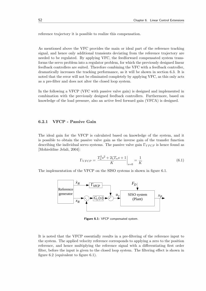
52 Chapter 6. Linear Control Extensions
reference trajectory it is possible to realize this compensation.
As mentioned above the VFC provides the main or ideal part of the reference trackingsignal, and hence only additional transients deviating from the reference trajectory areneeded to be regulated. By applying VFC, the feedforward compensated system trans-forms the servo problem into a regulator problem, for which the previously designed linearfeedback controllers are suited. Therefore combining the VFC with a feedback controller,dramatically increases the tracking performance, as it will be shown in section 6.3. It isnoted that the error will not be eliminated completely by applying VFC, as this only actsas a pre-filter and does not alter the closed loop system.
In the following a VFCP (VFC with passive valve gain) is designed and implemented incombination with the previously designed feedback controllers. Furthermore, based onknowledge of the load pressure, also an active feed forward gain (VFCA) is designed.
6.2.1 VFCP - Passive Gain
The ideal gain for the VFCP is calculated based on knowledge of the system, and itis possible to obtain the passive valve gain as the inverse gain of the transfer functiondescribing the individual servo systems. The passive valve gain ΓV FCP is hence found as[Mohieddine Jelali, 2004]:
ΓV FCP =T 2
ns2 + 2ζTns + 1K
∣∣∣∣s=0
=1K
(6.1)
The implementation of the VFCP on the SISO systems is shown in figure 6.1.
VFCPΓ
vu SISO system(Plant)
Px+++-
Referencegenerator
DFRx&
Rx )(sGc
Figure 6.1: VFCP compensated system.
It is noted that the VFCP essentially results in a pre-filtering of the reference input tothe system. The applied velocity reference corresponds to applying a zero to the positionreference, and hence multiplying the reference signal with a differentiating first orderfilter, before the input is given to the closed loop system. The filtering effect is shown infigure 6.2 (equivalent to figure 6.1).
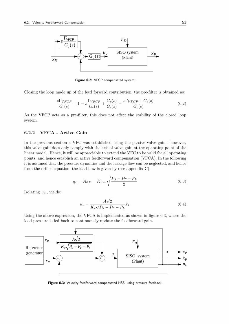
6.2. Velocity Feedforward Compensation 53
)(sGs
c
VFCPΓ
vu SISO system(Plant)
Px+-
DF
Rx )(sGc+
Figure 6.2: VFCP compensated system.
Closing the loop made up of the feed forward contribution, the pre-filter is obtained as:
sΓV FCP
Gc(s)+ 1 = s
ΓV FCP
Gc(s)+
Gc(s)Gc(s)
=sΓV FCP + Gc(s)
Gc(s)(6.2)
As the VFCP acts as a pre-filter, this does not affect the stability of the closed loopsystem.
6.2.2 VFCA - Active Gain
In the previous section a VFC was established using the passive valve gain - however,this valve gain does only comply with the actual valve gain at the operating point of thelinear model. Hence, it will be appreciable to extend the VFC to be valid for all operatingpoints, and hence establish an active feedforward compensation (VFCA). In the followingit is assumed that the pressure dynamics and the leakage flow can be neglected, and hencefrom the orifice equation, the load flow is given by (see appendix C):
qL = AxP = Kvuv
√PS − PT − PL
2(6.3)
Isolating uvi, yields:
uv =A√
2Kv
√PS − PT − PL
xP (6.4)
Using the above expression, the VFCA is implemented as shown in figure 6.3, where theload pressure is fed back to continuously update the feedforward gain.
LTSv PPPKA
−−
2
Px&vu SISO system
(Plant)
Px
Lp+++-
Referencegenerator
DFRx&
Rx
Figure 6.3: Velocity feedforward compensated HSS, using pressure feedback.
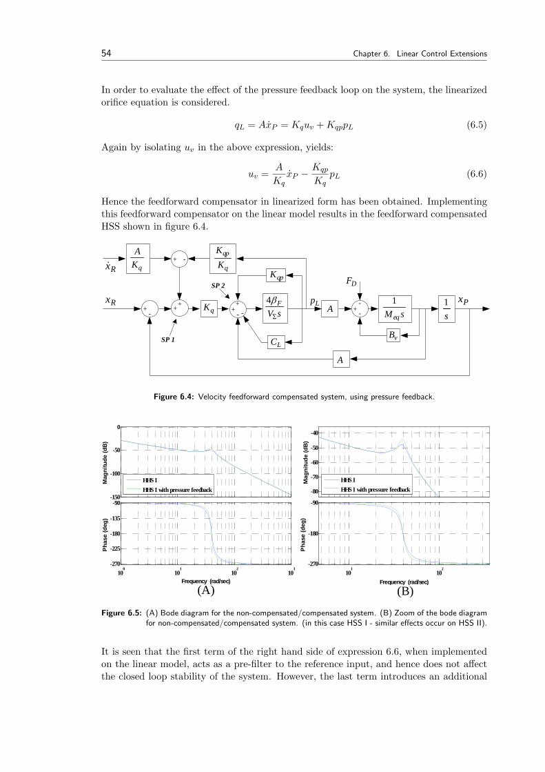
54 Chapter 6. Linear Control Extensions
In order to evaluate the effect of the pressure feedback loop on the system, the linearizedorifice equation is considered.
qL = AxP = Kquv + KqppL (6.5)
Again by isolating uv in the above expression, yields:
uv =A
KqxP −
Kqp
KqpL (6.6)
Hence the feedforward compensator in linearized form has been obtained. Implementingthis feedforward compensator on the linear model results in the feedforward compensatedHSS shown in figure 6.4.
+-+
sVF
Σ
β4A
LC
+ - sMeq
1
s1
vB
PxLpRx
uiK
-
DF
Loop 3
Summati
Summation point 3
feedback 1
feedba
qpK
-
A
+--
sV i
Fi
Σ
β4PiA +
vieqi BsM +1
s1 PixApp
qiKviu -
DiFLiqpi CK +
PiA
+--
)(44
LiqpiFii
PiFiCKsV
A++Σ β
β+
vieqi BsM +1
s1 Pix
qiKviu -
DiF
PiA
++-
+
+ -Rx& q
qp
KK
qK
qKA
SP 1
SP 2
Figure 6.4: Velocity feedforward compensated system, using pressure feedback.
(A) (B)
-150
-100
-50
0
Mag
nitu
de (d
B)
100
101
102
103
-270
-225
-180
-135
-90
Phas
e (d
eg)
Frequency (rad/sec)
HHS IHHS I with pressure feedback -80
-70
-60
-50
-40
Mag
nitu
de (d
B)
101
102
-270
-180
-90
Pha
se (d
eg)
Frequency (rad/sec)
HHS IHHS I with pressure feedback
Figure 6.5: (A) Bode diagram for the non-compensated/compensated system. (B) Zoom of the bode diagramfor non-compensated/compensated system. (in this case HSS I - similar effects occur on HSS II).
It is seen that the first term of the right hand side of expression 6.6, when implementedon the linear model, acts as a pre-filter to the reference input, and hence does not affectthe closed loop stability of the system. However, the last term introduces an additional
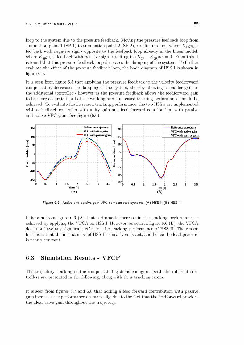
6.3. Simulation Results - VFCP 55
loop to the system due to the pressure feedback. Moving the pressure feedback loop fromsummation point 1 (SP 1) to summation point 2 (SP 2), results in a loop where KqppL isfed back with negative sign - opposite to the feedback loop already in the linear model,where KqppL is fed back with positive sign, resulting in (Kqp −Kqp)pL = 0. From this itis found that this pressure feedback loop decreases the damping of the system. To furtherevaluate the effect of the pressure feedback loop, the bode diagram of HSS I is shown infigure 6.5.
It is seen from figure 6.5 that applying the pressure feedback to the velocity feedforwardcompensator, decreases the damping of the system, thereby allowing a smaller gain tothe additional controller - however as the pressure feedback allows the feedforward gainto be more accurate in all of the working area, increased tracking performance should beachieved. To evaluate the increased tracking performance, the two HSS’s are implementedwith a feedback controller with unity gain and feed forward contribution, with passiveand active VFC gain. See figure (6.6).
(A) (B)
0 0.5 1 1.5 2 2.5 3 3.5-150
-100
-50
0
50
100
150
Time [s]
Pist
on p
ositi
on [m
m]
Reference trajectoryVFC with ative gainVFC with passive gain
0 0.5 1 1.5 2 2.5 3 3.5-150
-100
-50
0
50
100
150
200
Time [s]
Pist
on p
ositi
on [m
m]
Reference trajectoryVFC with active gainVFC with passive gain
Figure 6.6: Active and passive gain VFC compensated systems. (A) HSS I. (B) HSS II.
It is seen from figure 6.6 (A) that a dramatic increase in the tracking performance isachieved by applying the VFCA on HSS I. However, as seen in figure 6.6 (B), the VFCAdoes not have any significant effect on the tracking performance of HSS II. The reasonfor this is that the inertia mass of HSS II is nearly constant, and hence the load pressureis nearly constant.
6.3 Simulation Results - VFCP
The trajectory tracking of the compensated systems configured with the different con-trollers are presented in the following, along with their tracking errors.
It is seen from figures 6.7 and 6.8 that adding a feed forward contribution with passivegain increases the performance dramatically, due to the fact that the feedforward providesthe ideal valve gain throughout the trajectory.
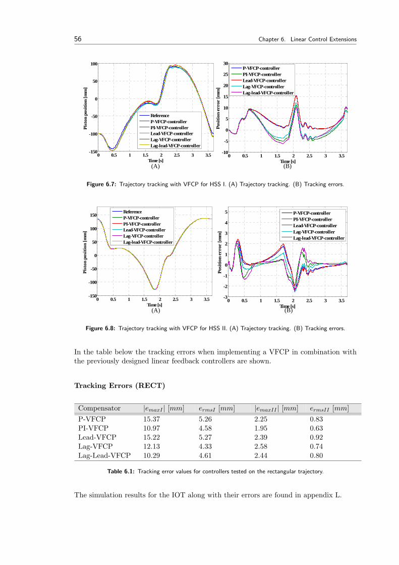
56 Chapter 6. Linear Control Extensions
(A) (B)
0 0.5 1 1.5 2 2.5 3 3.5-150
-100
-50
0
50
100
Time [s]
Pist
on p
ositi
on [m
m]
ReferenceP-VFCP-controllerPI-VFCP-controllerLead-VFCP-controllerLag-VFCP-controllerLag-lead-VFCP-controller
0 0.5 1 1.5 2 2.5 3 3.5-10
-5
0
5
10
15
20
25
30
Time [s]
Posi
tion
erro
r [m
m]
P-VFCP-controllerPI-VFCP-controllerLead-VFCP-controllerLag-VFCP-controllerLag-lead-VFCP-controller
Figure 6.7: Trajectory tracking with VFCP for HSS I. (A) Trajectory tracking. (B) Tracking errors.
(A) (B)
(A) (B)
0 0.5 1 1.5 2 2.5 3 3.5-150
-100
-50
0
50
100
Time [s]
Pist
on p
ositi
on [m
m]
ReferenceP-VFCP-controllerPI-VFCP-controllerLead-VFCP-controllerLag-VFCP-controllerLag-lead-VFCP-controller
0 0.5 1 1.5 2 2.5 3 3.5-150
-100
-50
0
50
100
150
Time [s]
Pist
on p
ositi
on [m
m]
ReferenceP-VFCP-controllerPI-VFCP-controllerLead-VFCP-controllerLag-VFCP-controllerLag-lead-VFCP-controller
0 0.5 1 1.5 2 2.5 3 3.5-10
-5
0
5
10
15
20
25
30
Time [s]
Posi
tion
erro
r [m
m]
P-VFCP-controllerPI-VFCP-controllerLead-VFCP-controllerLag-VFCP-controllerLag-lead-VFCP-controller
0 0.5 1 1.5 2 2.5 3 3.5-3
-2
-1
0
1
2
3
4
5
Time [s]
Posi
tion
erro
r [m
m]
P-VFCP-controllerPI-VFCP-controllerLead-VFCP-controllerLag-VFCP-controllerLag-lead-VFCP-controller
Figure 6.8: Trajectory tracking with VFCP for HSS II. (A) Trajectory tracking. (B) Tracking errors.
In the table below the tracking errors when implementing a VFCP in combination withthe previously designed linear feedback controllers are shown.
Tracking Errors (RECT)
Compensator |emaxI | [mm] ermsI [mm] |emaxII | [mm] ermsII [mm]P-VFCP 15.37 5.26 2.25 0.83PI-VFCP 10.97 4.58 1.95 0.63Lead-VFCP 15.22 5.27 2.39 0.92Lag-VFCP 12.13 4.33 2.58 0.74Lag-Lead-VFCP 10.29 4.61 2.44 0.80
Table 6.1: Tracking error values for controllers tested on the rectangular trajectory.
The simulation results for the IOT along with their errors are found in appendix L.
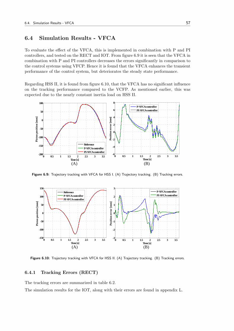
6.4. Simulation Results - VFCA 57
6.4 Simulation Results - VFCA
To evaluate the effect of the VFCA, this is implemented in combination with P and PIcontrollers, and tested on the RECT and IOT. From figure 6.9 it is seen that the VFCA incombination with P and PI controllers decreases the errors significantly in comparison tothe control systems using VFCP. Hence it is found that the VFCA enhances the transientperformance of the control system, but deteriorates the steady state performance.
Regarding HSS II, it is found from figure 6.10, that the VFCA has no significant influenceon the tracking performance compared to the VCFP. As mentioned earlier, this wasexpected due to the nearly constant inertia load on HSS II.
(A) (B)
0 0.5 1 1.5 2 2.5 3 3.5-200
-150
-100
-50
0
50
100
Time [s]
Pist
on p
ositi
on [m
m]
ReferenceP-VFCA-controllerPI-VFCA-controller
0 0.5 1 1.5 2 2.5 3 3.5-6
-4
-2
0
2
4
6
8
Time [s]
Posi
tion
erro
r [m
m]
P-VFCA-controllerPI-VFCA-controller
Figure 6.9: Trajectory tracking with VFCA for HSS I. (A) Trajectory tracking. (B) Tracking errors.
(A) (B)
0 0.5 1 1.5 2 2.5 3 3.5-150
-100
-50
0
50
100
150
Time [s]
Pist
on p
ositi
on [m
m]
ReferenceP-VFCA-controllerPI-VFCA-controller
0 0.5 1 1.5 2 2.5 3 3.5-3
-2
-1
0
1
2
3
Time [s]
Posi
tion
erro
r [m
m]
P-VFCA-controllerPI-VFCA-controller
Figure 6.10: Trajectory tracking with VFCA for HSS II. (A) Trajectory tracking. (B) Tracking errors.
6.4.1 Tracking Errors (RECT)
The tracking errors are summarized in table 6.2.
The simulation results for the IOT, along with their errors are found in appendix L.
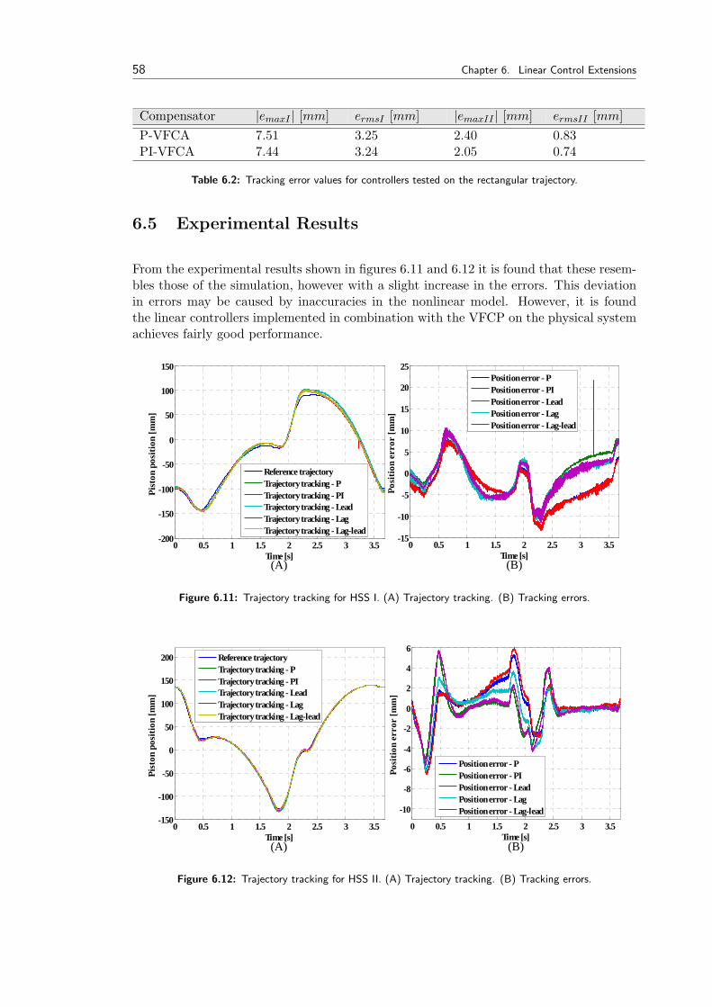
58 Chapter 6. Linear Control Extensions
Compensator |emaxI | [mm] ermsI [mm] |emaxII | [mm] ermsII [mm]P-VFCA 7.51 3.25 2.40 0.83PI-VFCA 7.44 3.24 2.05 0.74
Table 6.2: Tracking error values for controllers tested on the rectangular trajectory.
6.5 Experimental Results
From the experimental results shown in figures 6.11 and 6.12 it is found that these resem-bles those of the simulation, however with a slight increase in the errors. This deviationin errors may be caused by inaccuracies in the nonlinear model. However, it is foundthe linear controllers implemented in combination with the VFCP on the physical systemachieves fairly good performance.
(A) (B)
0 0.5 1 1.5 2 2.5 3 3.5-200
-150
-100
-50
0
50
100
150
Time [s]
Pist
on p
ositi
on [m
m]
Reference trajectoryTrajectory tracking - PTrajectory tracking - PITrajectory tracking - LeadTrajectory tracking - LagTrajectory tracking - Lag-lead
0 0.5 1 1.5 2 2.5 3 3.5-15
-10
-5
0
5
10
15
20
25
Time [s]
Posi
tion
erro
r [m
m]
Position error - PPosition error - PIPosition error - LeadPosition error - LagPosition error - Lag-lead
Figure 6.11: Trajectory tracking for HSS I. (A) Trajectory tracking. (B) Tracking errors.
(A) (B)
0 0.5 1 1.5 2 2.5 3 3.5-150
-100
-50
0
50
100
150
200
Time [s]
Pist
on p
ositi
on [m
m]
Reference trajectoryTrajectory tracking - PTrajectory tracking - PITrajectory tracking - LeadTrajectory tracking - LagTrajectory tracking - Lag-lead
0 0.5 1 1.5 2 2.5 3 3.5
-10
-8
-6
-4
-2
0
2
4
6
Time [s]
Posi
tion
erro
r [m
m]
Position error - PPosition error - PIPosition error - LeadPosition error - LagPosition error - Lag-lead
Figure 6.12: Trajectory tracking for HSS II. (A) Trajectory tracking. (B) Tracking errors.
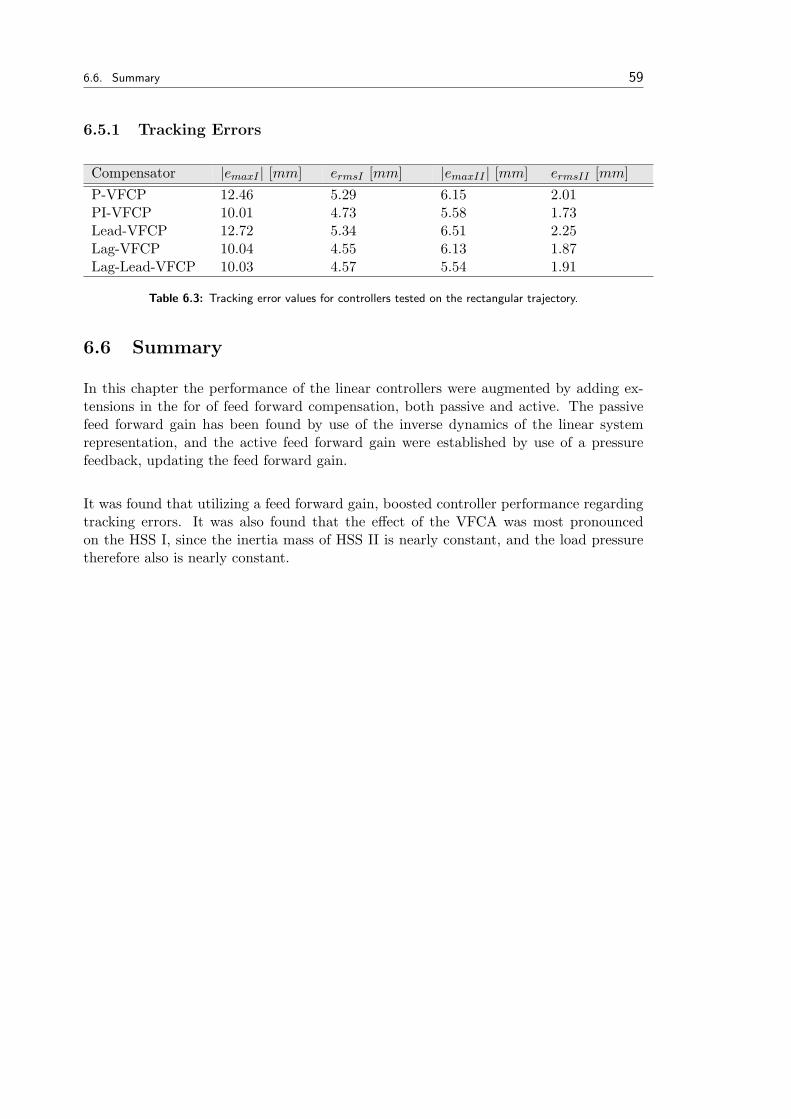
6.6. Summary 59
6.5.1 Tracking Errors
Compensator |emaxI | [mm] ermsI [mm] |emaxII | [mm] ermsII [mm]P-VFCP 12.46 5.29 6.15 2.01PI-VFCP 10.01 4.73 5.58 1.73Lead-VFCP 12.72 5.34 6.51 2.25Lag-VFCP 10.04 4.55 6.13 1.87Lag-Lead-VFCP 10.03 4.57 5.54 1.91
Table 6.3: Tracking error values for controllers tested on the rectangular trajectory.
6.6 Summary
In this chapter the performance of the linear controllers were augmented by adding ex-tensions in the for of feed forward compensation, both passive and active. The passivefeed forward gain has been found by use of the inverse dynamics of the linear systemrepresentation, and the active feed forward gain were established by use of a pressurefeedback, updating the feed forward gain.
It was found that utilizing a feed forward gain, boosted controller performance regardingtracking errors. It was also found that the effect of the VFCA was most pronouncedon the HSS I, since the inertia mass of HSS II is nearly constant, and the load pressuretherefore also is nearly constant.

Chapter 7Linear ControlDesign in StateSpace
Contents
7.1 Introduction . . . . . . . . . . 61
7.2 State Space Model Represen-tation . . . . . . . . . . . . . . 62
7.3 State Controllability . . . . . . 62
7.4 Compensation by Pole Assign-ment . . . . . . . . . . . . . . 63
7.5 Simulation Results . . . . . . . 65
7.6 Summary . . . . . . . . . . . . 67
In this chapter a compensator is developed based on a state space representation of thelinear system. More specifically a state feedback gain compensator is developed using thepole assignment technique, in order to achieve certain system specifications. Furthermorea modification is made to this compensator regarding feedforward contribution.
7.1 Introduction
The pole assignment technique could be advantageous to use in the compensator design,for a compensator usable for trajectory tracking. The general idea of applying this methodis to alter the properties of the system, by displacing the poles of the uncompensatedsystem to desired locations of the compensated system. As the servo systems are poorlydamped, and have slow transient response due to the free integrator, this method mightprove usable, and will be used in this chapter. The nomenclature of this chapter is givenbelow (not notations introduced previously).
xi: state vector [−]xi: time derivative of state vector [−]Ai: system matrix [−]Bi: input matrix [−]Ci: output matrix [−]y: output [−]x1, x2, x3: states [−]K: state feedback gain matrix [−]k1, k2, k3: elements of the state feedback gain matrix [−]
61
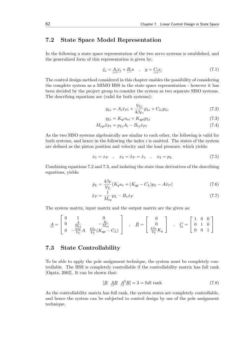
62 Chapter 7. Linear Control Design in State Space
7.2 State Space Model Representation
In the following a state space representation of the two servo systems is established, andthe generalized form of this representation is given by:
xi = Aixi + Biu , y = Cixi (7.1)
The control design method considered in this chapter enables the possibility of consideringthe complete system as a MIMO HSS in the state space representation - however it hasbeen decided by the project group to consider the system as two separate SISO systems.The describing equations are (valid for both systems):
qLi = AixPi +VΣi
4βFipLi + CLipLi (7.2)
qLi = Kqiuvi + KqpipLi (7.3)MeqixPi = pLiAi −BvixPi (7.4)
As the two SISO systems algebraically are similar to each other, the following is valid forboth systems, and hence in the following the index i is omitted. The states of the systemare defined as the piston position and velocity and the load pressure, which yields:
x1 = xP , x2 = xP = x1 , x3 = pL (7.5)
Combining equations 7.2 and 7.3, and isolating the state time derivatives of the describingequations, yields:
pL =4βF
VΣ(Kquv + (Kqp − CL)pL −AxP ) (7.6)
xP =1
MeqpL −BvxP (7.7)
The system matrix, input matrix and the output matrix are the given as:
A =
0 1 00 A
Meq− Bv
Meq
0 −4βFVΣ
A 4βFVΣ
(Kqp − CL)
, B =
00
4βFVΣ
Kq
, C =
1 0 00 1 00 0 1
7.3 State Controllability
To be able to apply the pole assignment technique, the system must be completely con-trollable. The HSS is completely controllable if the controllability matrix has full rank[Ogata, 2002]. It can be shown that:
[B AB A2B] = 3 = full rank (7.8)
As the controllability matrix has full rank, the system states are completely controllable,and hence the system can be subjected to control design by use of the pole assignmenttechnique.
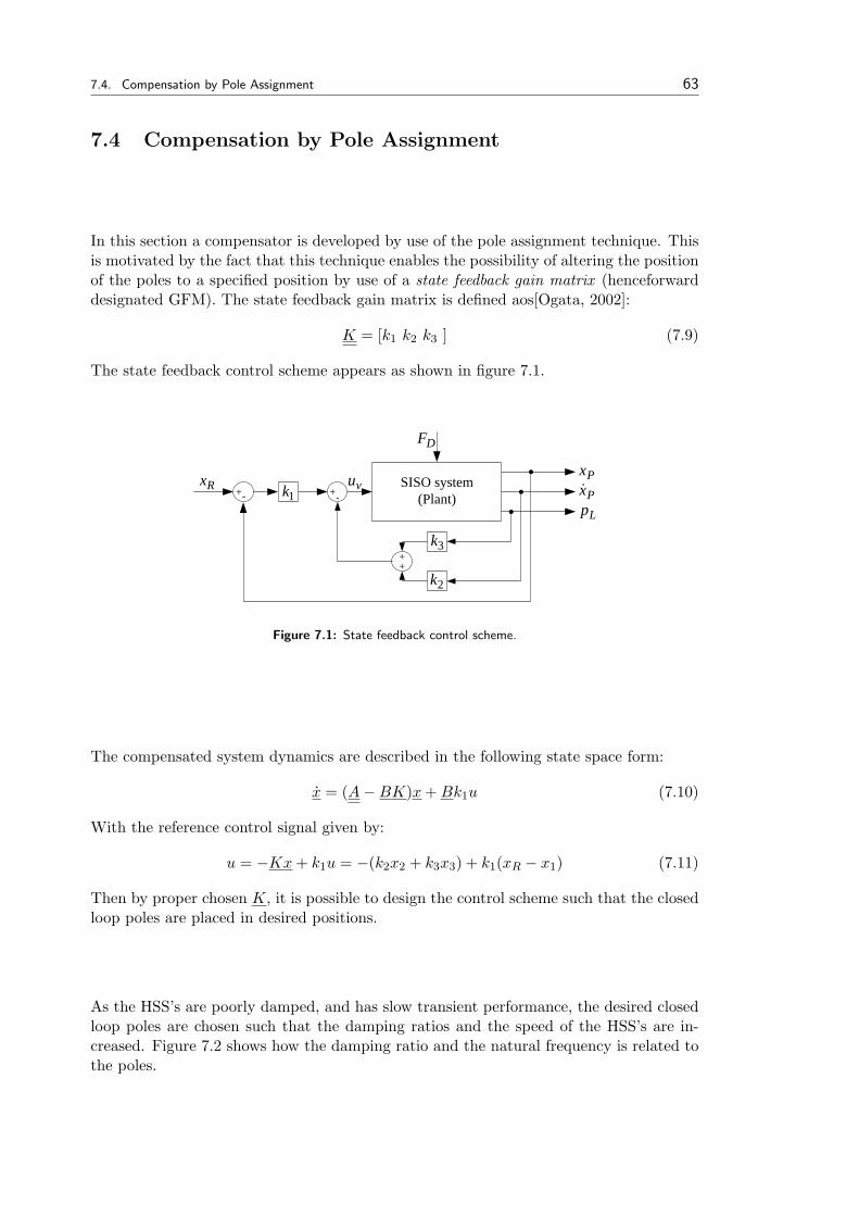
7.4. Compensation by Pole Assignment 63
7.4 Compensation by Pole Assignment
In this section a compensator is developed by use of the pole assignment technique. Thisis motivated by the fact that this technique enables the possibility of altering the positionof the poles to a specified position by use of a state feedback gain matrix (henceforwarddesignated GFM). The state feedback gain matrix is defined aos[Ogata, 2002]:
K = [k1 k2 k3 ] (7.9)
The state feedback control scheme appears as shown in figure 7.1.
Px&vu SISO system(Plant)
Px
Lp+-+-
DF
Rx1k
2k
3k++
Figure 7.1: State feedback control scheme.
The compensated system dynamics are described in the following state space form:
x = (A−BK)x + Bk1u (7.10)
With the reference control signal given by:
u = −Kx + k1u = −(k2x2 + k3x3) + k1(xR − x1) (7.11)
Then by proper chosen K, it is possible to design the control scheme such that the closedloop poles are placed in desired positions.
As the HSS’s are poorly damped, and has slow transient performance, the desired closedloop poles are chosen such that the damping ratios and the speed of the HSS’s are in-creased. Figure 7.2 shows how the damping ratio and the natural frequency is related tothe poles.
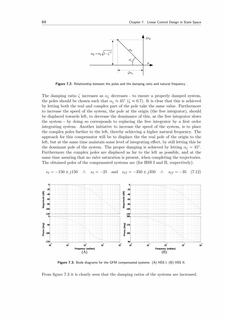
64 Chapter 7. Linear Control Design in State Space
21 ζωω −= nd
nζω
nω
σ
djω
ζα
Figure 7.2: Relationship between the poles and the damping ratio and natural frequency .
The damping ratio ζ increases as αζ decreases - to ensure a properly damped system,the poles should be chosen such that αζ ≈ 45 (ζ ≈ 0.7). It is clear that this is achievedby letting both the real and complex part of the pole take the same value. Furthermoreto increase the speed of the system, the pole at the origin (the free integrator), shouldbe displaced towards left, to decrease the dominance of this, as the free integrator slowsthe system - by doing so corresponds to replacing the free integrator by a first orderintegrating system. Another initiative to increase the speed of the system, is to placethe complex poles further to the left, thereby achieving a higher natural frequency. Theapproach for this compensator will be to displace the the real pole of the origin to theleft, but at the same time maintain some level of integrating effect, by still letting this bethe dominant pole of the system. The proper damping is achieved by letting αζ = 45.Furthermore the complex poles are displaced as far to the left as possible, and at thesame time assuring that no valve saturation is present, when completing the trajectories.The obtained poles of the compensated systems are (for HSS I and II, respectively):
sI = −150± j150 ∧ sI = −25 and sII = −350± j350 ∧ sII = −35 (7.12)
(A) (B)
-120
-100
-80
-60
-40
-20
0
Mag
nitu
de (d
B)
100
101
102
103
104
-270
-180
-90
0
Phas
e (d
eg)
Frequency (rad/sec)
-120
-100
-80
-60
-40
-20
0
Mag
nitu
de (d
B)
100
101
102
103
104
90
180
270
360
Phas
e (d
eg)
Frequency (rad/sec)
Figure 7.3: Bode diagrams for the GFM compensated systems. (A) HSS I. (B) HSS II.
From figure 7.3 it is clearly seen that the damping ratios of the systems are increased.
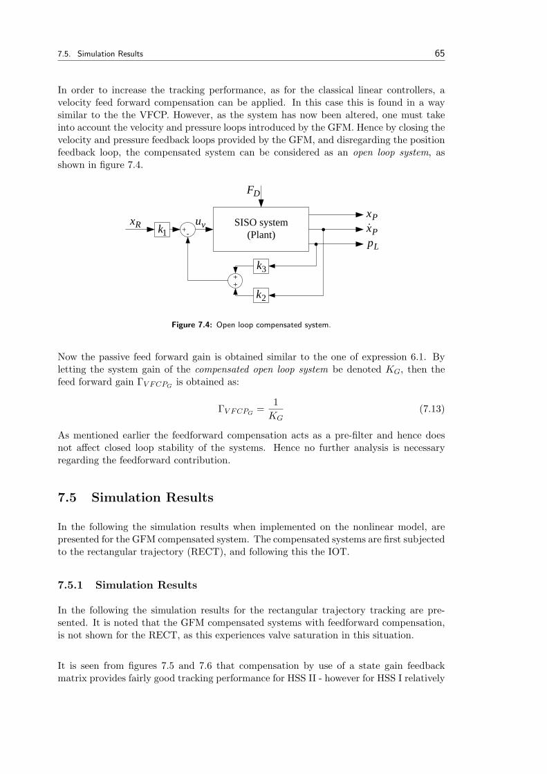
7.5. Simulation Results 65
In order to increase the tracking performance, as for the classical linear controllers, avelocity feed forward compensation can be applied. In this case this is found in a waysimilar to the the VFCP. However, as the system has now been altered, one must takeinto account the velocity and pressure loops introduced by the GFM. Hence by closing thevelocity and pressure feedback loops provided by the GFM, and disregarding the positionfeedback loop, the compensated system can be considered as an open loop system, asshown in figure 7.4.
Px&vu SISO system(Plant)
Px
Lp+-
DF
Rx1k
2k
3k++
Figure 7.4: Open loop compensated system.
Now the passive feed forward gain is obtained similar to the one of expression 6.1. Byletting the system gain of the compensated open loop system be denoted KG, then thefeed forward gain ΓV FCPG
is obtained as:
ΓV FCPG=
1KG
(7.13)
As mentioned earlier the feedforward compensation acts as a pre-filter and hence doesnot affect closed loop stability of the systems. Hence no further analysis is necessaryregarding the feedforward contribution.
7.5 Simulation Results
In the following the simulation results when implemented on the nonlinear model, arepresented for the GFM compensated system. The compensated systems are first subjectedto the rectangular trajectory (RECT), and following this the IOT.
7.5.1 Simulation Results
In the following the simulation results for the rectangular trajectory tracking are pre-sented. It is noted that the GFM compensated systems with feedforward compensation,is not shown for the RECT, as this experiences valve saturation in this situation.
It is seen from figures 7.5 and 7.6 that compensation by use of a state gain feedbackmatrix provides fairly good tracking performance for HSS II - however for HSS I relatively
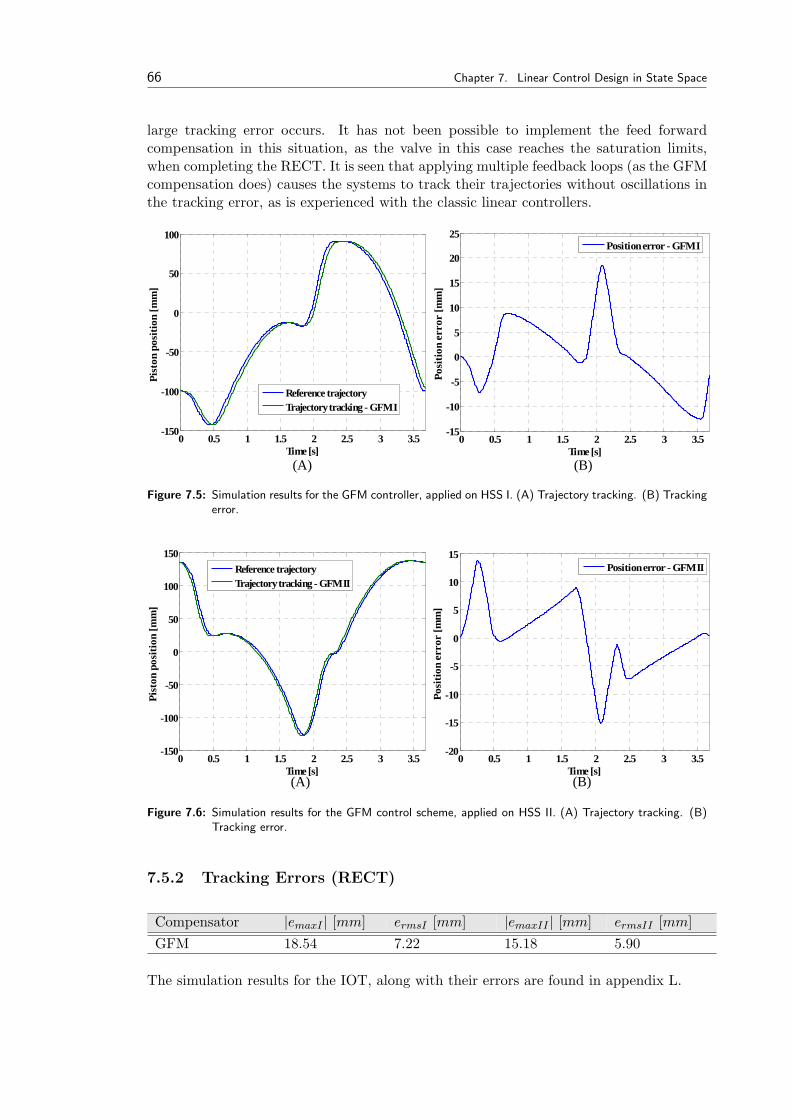
66 Chapter 7. Linear Control Design in State Space
large tracking error occurs. It has not been possible to implement the feed forwardcompensation in this situation, as the valve in this case reaches the saturation limits,when completing the RECT. It is seen that applying multiple feedback loops (as the GFMcompensation does) causes the systems to track their trajectories without oscillations inthe tracking error, as is experienced with the classic linear controllers.
(A) (B)
0 0.5 1 1.5 2 2.5 3 3.5-150
-100
-50
0
50
100
Time [s]
Pist
on p
ositi
on [m
m]
Reference trajectoryTrajectory tracking - GFM I
0 0.5 1 1.5 2 2.5 3 3.5-15
-10
-5
0
5
10
15
20
25
Time [s]Po
sitio
n er
ror
[mm
]
Position error - GFM I
Figure 7.5: Simulation results for the GFM controller, applied on HSS I. (A) Trajectory tracking. (B) Trackingerror.
(A) (B)
0 0.5 1 1.5 2 2.5 3 3.5-150
-100
-50
0
50
100
150
Time [s]
Pist
on p
ositi
on [m
m]
Reference trajectoryTrajectory tracking - GFM II
0 0.5 1 1.5 2 2.5 3 3.5-20
-15
-10
-5
0
5
10
15
Time [s]
Posi
tion
erro
r [m
m]
Position error - GFM II
Figure 7.6: Simulation results for the GFM control scheme, applied on HSS II. (A) Trajectory tracking. (B)Tracking error.
7.5.2 Tracking Errors (RECT)
Compensator |emaxI | [mm] ermsI [mm] |emaxII | [mm] ermsII [mm]GFM 18.54 7.22 15.18 5.90
The simulation results for the IOT, along with their errors are found in appendix L.
7.6. Summary 67
7.6 Summary
In this chapter state space representation is utilized for controller development. Hereboth a state feedback gain compensator and an augmentation of the same compensator byapplying feed forward contributions is developed by use of the pole placement technique.The augmented state feedback gain compensator could unfortunately not be tested onthe system using RECT, as this caused valve saturation. However, the augmented statefeedback gain compensator could be tested for the system using IOT, which yielded adramatically increased tracking performance compared to the pure GFM compensatedsystem.

Part III
Advanced Control Schemes
69

Chapter 8SimplifiedActuator Model
This chapter concerns the establishment of a simplified actuator model, suitable for use inthe development of the adaptive control schemes. This simplified model will be based onthe existing model of the hydraulic actuators.
Before initiating the process of establishing the adaptive control laws, a simplified modelused to represent the system is determined - this will be carried out considering the indi-vidual servo systems, hence the simplified model is established as a SISO system.
In general, hydraulic systems include various time variant parameters, which are difficultto describe. To be able to establish the adaptive controllers, as for the linear controllers,a mathematical model is needed. In this case, it is desirable to have a simplified lowerorder model, rather than having a complex relative high order model as that used in thelinear control design. In order to establish this simplified lower order model, the followingassumptions are made:
• The forces applied by the load pressure is strictly larger than the inertia load andthe friction forces counteracting this - hence the force equilibrium is omitted in thesimplified model
• The hydraulic oil is infinitely stiff - hence the pressure dynamics are omitted
Due to the less accurate simplified model based on the above mentioned assumption, themodeling error has increased compared to the linear model obtained previously - hencein the simplified model, a modeling error which is considered unknown, is introduced.
To provide further justification for using the simplified model in the control design, thepreviously obtained linear actuator model representation is considered:
GPi(s) =Ki
(T 2nis
2 + 2ζiTnis + 1)s=
Ki(1
ω2ni
s2 + 2ζi1
ωnis + 1
)s
(8.1)
71
72
It is seen that for large values of the natural frequency and damping ratio, which occursfor small values of the equivalent mass, it is reasonable to consider the dynamic model asconsisting of the system gain and the pure integrator - hence, as mentioned before, whenassuming that the forces applied by the load pressure is strictly larger than the inertiaload, this is a valid simplification.
It is assumed that the stiffness of the hydraulic oil is infinite, thereby neglecting thepressure dynamics. When also neglecting the inertia load, the friction forces, and whenalso omitting the leakage flow, the describing equations for the actuators are reduced to:
QL = Kviuvi
√PS − PT − sign(uvi)PLi
2, QL = AisxPi ⇒ (8.2)
AisxPi = Kviuvi
√PS − PT − sign(uvi)PLi
2⇒ (8.3)
xPi
uvi=
Kvi
√PS−PT−sign(uvi)PLi
2
Ai
1s
(8.4)
Hence the simplified dynamic model is given by:
Gsi =Γp
swhere, Γp =
Kvi
√PS−PT−sign(uvi)PLi
2
Ai=
Kvi
√PS − PT − sign(uvi)PLi√
2Ai
(8.5)
Rewriting the dynamic model to express the valve input, introducing the modeling error ν(due to the neglected terms following from the made assumptions), the simplified dynamicmodel is given by:
Γ(t)xP (t) + ν(t) = u(t) where, Γ(t) =1Γp
(8.6)
This simplified model is a time variant function, representing the individual servo systems,thereby meaning a hydraulic cylinder and a servo valve.
Chapter 9AdaptiveControl Schemes
Contents
9.1 Introduction . . . . . . . . . . 73
9.2 Robust Model Based Con-troller (RMC) . . . . . . . . . 74
9.3 Adaptive Inverse DynamicsController (AIDC) . . . . . . . 77
9.4 Modified Adaptive InverseDynamics Controller (MAIDC) 80
9.5 Augmented Adaptive Con-troller (AAC) . . . . . . . . . 81
9.6 Modified Augmented Adap-tive Controller (MAAC) . . . . 84
9.7 RAIDC & RAAC . . . . . . . 86
9.8 Parameters for Adaptive Con-trol Schemes . . . . . . . . . . 88
9.9 Simulation Results . . . . . . . 89
9.10 Experimental Results . . . . . 92
9.11 Summary . . . . . . . . . . . . 94
This chapter concerns the establishment and implementation of adaptive control schemes.First a derivation of a Robust Model based Controller (RMC) control law is carried out,which will form the base for the adaptive control laws. Hereafter the adaptive control lawsare chosen and proved stable, and finally these are implemented and tested in simulationsand in experiments.
9.1 Introduction
The adaptive control schemes developed and implemented in this chapter, based on thesimplified model are:
• Adaptive Inverse Dynamics Controller (AIDC)
• Modified Adaptive Inverse Dynamics Controller (MAIDC)
• Augmented Adaptive Controller (AAC)
• Modified Augmented Adaptive Controller (MAAC)
• Robust Adaptive Inverse Dynamics Controller (RAIDC)
• Robust Augmented Adaptive Controller (RAIDC)
The approach will be to establish a control law that will enable the closed loop systemto track a position reference, when assuming non varying system states, and thereby no
73

74 Chapter 9. Adaptive Control Schemes
parameter variation (Robust Model based Controller)[Andersen, 1996]. In reality this isnot the case, as parameters will vary, and to take these variations into account, adaptionlaws are introduced, enabling the possibility of updating the control parameters contin-uously over time, increasing the tracking performance. In each of these adaptive controlschemes it will be necessary to prove that the chosen control law will cause the closedloop system to remain stable, and that the position error will converge to zero. For thestability proofs Lyapunov theory is used.
In the following (t) and the index i is omitted for reasons of clarity. Furthermore vectornotation is omitted.
9.2 Robust Model Based Controller (RMC)
In this thesis the adaptive control scheme will basically be constituted by two elements- a gain in the feedforward path of the closed loop system stabilizing the error trackingsystem, and a feedforward contribution using the inverse dynamic expression in the feed-forward loop, which as previously mentioned will provide the necessary valve input fortrajectory tracking, and thereby increase tracking performance.
The robust control scheme is suggested as[Andersen, 1996]:
Γ(xR − kpe) + ν = u (9.1)
With the Γ and ν representing the control parameter estimates. This control scheme ismotivated by the fact that it can be shown that, in the ideal case with known parametersand no disturbances, the system error dynamics will converge to zero, as time goes toinfinity, which is found from the following. The simplified model and ideal case controllaw is given by:
ΓxP + ν = u ; Γ(xR − kpe) + ν = u ; e = xP − xR (9.2)
From the above expressions, the closed loop dynamics is given by:
ΓxP + ν = Γ(xR − kpe) + ν (9.3)ΓxP + ν = ΓxR − Γkpe + ν (9.4)
Γ(xP − xR) = −Γkpe (9.5)Γe + Γkpe = 0 (9.6)
e + kpe = 0 (9.7)
It is found that the error dynamics will converge to zero as time goes to infinity, andthereby the closed loop system is asymptotically stable (for proper values of kp).
In reality however, the ideal case with known parameters an no disturbances does notoccur, and hence it is needed to show that the closed loop system with estimated controlparameters Γ and ν are stable, which is shown in the following. The closed loop control
9.2. Robust Model Based Controller (RMC) 75
system with estimated control parameters is given by:
ΓxP + ν = Γ(xR − kpe) + ν (9.8)(9.9)
Subtracting ΓxR on both sides, yields:
ΓxP + ν − ΓxR = Γ(xR − kpe) + ν − ΓxR (9.10)
Γe + ν = ΓxR − Γkpe + ν − ΓxR (9.11)
Γe = (Γ− Γ)xR − Γkpe + ν − ν (9.12)
Defining the error estimates Γ = Γ− Γ and ν = ν − ν[Slotine E J-J, 1991], yields:
Γe = ΓxR − Γkpe + ν (9.13)
Γe− Γe = ΓxR − Γkpe + ν (9.14)
Γe + Γkpe = ΓxR + Γe + ν (9.15)
Γ(e + kpe) = ΓxR + ΓxP − ΓxR + ν (9.16)
Γ(e + kpe) = ΓxP + ν (9.17)
e + kpe = Γ−1ΓxP + Γ−1ν (9.18)
Using e = xP − xR, yields:
e + kpe = Γ−1Γe + Γ−1ΓxR + Γ−1ν (9.19)
e− Γ−1Γe + kpe = Γ−1ΓxR + Γ−1ν (9.20)
e(1− Γ−1Γ) + kpe = Γ−1ΓxR + Γ−1ν (9.21)
Using Γ = Γ− Γ ⇒ Γ = Γ− Γ ⇒ Γ−1Γ = 1− Γ−1Γ, yields:
eΓ−1Γ + kpe = Γ−1ΓxR + Γ−1ν (9.22)
e + ΓΓ−1kpe = ΓΓ−1Γ−1ΓxR + ΓΓ−1Γ−1ν (9.23)
e + ΓΓ−1kpe = Γ−1ΓxR + Γ−1ν (9.24)
e + ΓΓ−1kpe = Γ−1(ΓxR + ν) (9.25)
Addition of kpe on both sides yields:
e + kpe + ΓΓ−1kpe = Γ−1(ΓxR + ν) + kpe (9.26)
e + kpe = Γ−1(ΓxR + ν) + kpe− ΓΓ−1kpe (9.27)
e + kpe = Γ−1(ΓxR + ν) + (1− ΓΓ−1)kpe (9.28)
Defining ξ = Γ−1(ΓxR + ν) + (1− ΓΓ−1)kpe, yields:
e + kpe = ξ (9.29)
76 Chapter 9. Adaptive Control Schemes
It is seen that the above expression represents a linear differential equation given by:
se + kpe = ξ (9.30)(s + kp)e = ξ (9.31)
e
ξ=
1s + kp
= h(s) ⇒ h(t) = e−kpt (9.32)
The function norm in appendix H.5 is used to give h(s) a bound. The function normsays that for any fixed p ∈ [1,∞], if f : <n → < belongs to Lp if
∫∞0 |f(t)|pdt < ∞. This
means that if ‖h(s)‖∞ has a finite positive value, then h(s) is bounded (according to thefunction norm). This yields:
‖h(s)‖∞ =∫ ∞
0|e−kpt|dt =
1kp
(9.33)
From the above it is then found that h(s) is bounded since ‖h(s)‖∞ < ∞. It is notpossible to conclude whether ξ is bounded - however by using the truncated L∞ norm, ξcan be given a bound in some limited time interval 0 < t < T , where T < ∞. Then forzero initial conditions it is possible to give the error a bound as[Andersen, 1996]:
‖e‖T∞ ≤ 1kp‖ξ‖T∞ (9.34)
Defining α1 = ‖Γ−1(ΓxR + ν)‖T∞ and α2 = ‖(1− ΓΓ−1)kp‖T∞, expression 9.34 is writtenas:
‖e‖T∞ ≤ 1kp
α1 +1kp
α2‖e‖T∞ ⇒ (9.35)
‖e‖T∞ ≤1kp
α1
1− 1kp
α2(9.36)
To ensure that e is bounded (e ∈ L∞), the right hand side of expression 9.36 must havea finite value, which implies that:
1kp
α2 < 1 (9.37)
1kp‖(1− ΓΓ−1)kp‖T∞ < 1 (9.38)
‖1− ΓΓ−1‖T∞ < 1 (9.39)
Using expression 8.5 and disregarding sign(uvi), yields:
1− ΓΓ−1 = 1− ΓKvi
√Ps − PT − PLi√
2Ai
< 1 (9.40)
The estimate Γ is chosen as:
Γ =√
2Ai
Kvi
√Ps − PT
(9.41)
9.3. Adaptive Inverse Dynamics Controller (AIDC) 77
Substituting into expression 9.40, yields:
1−√
2Ai
Kvi
√Ps − PT
Kvi
√Ps − PT − PLi√
2Ai
< 1 (9.42)
1−√
Ps − PT − PLi√Ps − PT
< 1 (9.43)
As the trajectories are planned such that the necessary supply pressure does not exceedPLi = 2/3Ps in order to have have enough power for control, the inequality of expression9.43 will always be satisfied. Then the robustness of the controller is assured if thefollowing conditions are satisfied[Andersen, 1996].
Γ(t) exists , kp > 0 , ‖1− ΓΓ−1‖T∞ < 1 (9.44)e = 0 for t = 0 , xR is bounded , ν is bounded (9.45)
If these conditions are satisfied, then the system is stable, with:
‖e‖T∞ ≤1kp
α1
1− 1kp
α2(9.46)
It has now been shown that the suggested control law implemented in the system is stable,and this control law will form the base of the following adaptive control schemes.
9.3 Adaptive Inverse Dynamics Controller (AIDC)
The AIDC is derived based on the RMC control law, and in addition to this an adaptionlaw is added, which will adapt the estimated control parameters continuously over time toachieve increased tracking performance. The stability for this set of differential equationswhich constitutes the control- and adaption laws, is proved by use of Lyapunov theory.By use of the simplified model and the control law, the closed loop system is given by:
ΓxP + ν = Γ(xR − kpe) + ν (9.47)
Subtracting ΓxR on both sides yields:
ΓxP + ν − ΓxR = Γ(xR − kpe) + ν − ΓxR (9.48)
Γe + ν = Γ(xR − kpe) + ν − ΓxR (9.49)
Using the error estimates Γ = Γ− Γ and ν = ν − ν, yields:
Γe = Γ(xR − kpe) + ν − ΓxR (9.50)
Γe = Γ(xR − kpe) + Γ(xR − kpe) + ν − ΓxR (9.51)
Γe = Γ(xR − kpe) + ΓxR − Γkpe + ν − ΓxR (9.52)
Γe = Γ(xR − kpe)− Γkpe + ν (9.53)
Γe + Γkpe = Γ(xR − kpe) + ν (9.54)
Γ(e + kpe) = Γ(xR − kpe) + ν (9.55)
78 Chapter 9. Adaptive Control Schemes
The following vectors are defined:
Y =[
xR − kpe 1]
and a =[
Γν
](9.56)
Substituting these vectors into expression (9.55), the system is rewritten to:
Γ(e + kpe) = Y a (9.57)
e + kpe = Γ−1Y a (9.58)
e = −kpe + Γ−1Y a (9.59)
Written by use of the laplace transform, this yields:
e + kpe = Γ−1Y a (9.60)
e(s + kp) = Γ−1Y a (9.61)
e =1
s + kpΓ−1Y a (9.62)
From lemma I in appendix H.2 it is seen, that the adaption parameters will adapt suchthat e → 0 for t →∞, if the adaption law is chosen as:
˙a = −γY T e ; γ > 0 (9.63)
Here γ is the adaption gain. In the following, the stability of the AIDC will be shownusing Lyapunov theory.
9.3.1 Stability Proof (AIDC)
The Lyapunov candidate is chosen to be[Andersen, 1996]:
V (e, a) =12e2 +
12γ−1Γ−1aT a (9.64)
Taking the time derivative yields:
V (e, a) = ee +12γ−1(Γ−1aT a + 2Γ−1aT ˙a) (9.65)
Substituting the error dynamics (expression 9.59), yields:
V (e, a) = (−kpe + Γ−1Y a)e +12γ−1(Γ−1aT a + 2Γ−1aT ˙a) (9.66)
= −kpe2 + Γ−1Y ae +
12γ−1Γ−1aT a + γ−1Γ−1aT ˙a (9.67)
Assuming that ‖Γ‖ << ‖ ˙a‖, yields:
V (e, a) = −kpe2 + Γ−1Y ae + γ−1Γ−1aT ˙a (9.68)
9.3. Adaptive Inverse Dynamics Controller (AIDC) 79
Using that Y a = aT Y T , yields:
V (e, a) = −kpe2 + Γ−1aT (Y T e + γ−1 ˙a) (9.69)
Substituting the adaption law, yields:
V (e, a) = −kpe2 + Γ−1aT (Y T e + γ−1(−γY T e)) (9.70)
= −kpe2 + Γ−1aT (Y T e− γ−1γY T e) (9.71)
= −kpe2 + Γ−1aT (Y T e− Y T e) (9.72)
= −kpe2 ⇒ (9.73)
V (e, a) = −kpe2 ≤ 0 (9.74)
It is seen that V (e, a) is negative semi-definite as the inequality is satisfied, independentof the value of a. This indicates that e ∈ L2∩L∞ and a ∈ L∞. Then by considering 9.59,and noting that xR, a and Γ are bounded, it is found that e is bounded and e ∈ L∞. Thefollowing can now be stated:
V (e, a) > 0 ; V (e, a) ≤ 0 ; (e, a) 6= 0 (9.75)
According to the Lyapunov-like lemma in appendix H.4, if 9.75 is satisfied, and V (e, a)is uniformly continuous, then e → 0 for t →∞. Barbalats lemma (appendix H.3) states,that a sufficient condition for a differentiable function to be uniformly continuous, is thatits derivative is bounded. This means that it is needed to show that V (e, a) is bounded.Taking the time derivative of V (e, a), yields:
V (e, a) = −2kpee (9.76)
From the above expression it is seen, that as e and e are bounded, then V (e, a) is bounded,and hence V (e, a) is uniformly continuous, according to Barbalats lemma. It can then,according to the Lyapunov-like lemma, be concluded that e → 0 as t →∞, yielding thate is asymptotically stable.
The control- and adaption laws of the AIDC can now formally be written, noting that˙a = ˙a, when considering a as a true slow varying parameter.
AIDC control law:
Γ(xR − kpe) + ν = u ; e = xP − xR ; kp > 0 (9.77)
AIDC adaption law:
˙a = ˙a = −γY T e =
[˙Γ˙ν
]=[−γ1(xR − kpe)e
−γ2e
]; γ1, γ2 > 0 (9.78)
80 Chapter 9. Adaptive Control Schemes
9.4 Modified Adaptive Inverse Dynamics Controller (MAIDC)
The MAIDC is similar to the AIDC, but with a modified adaption law - instead of onlyhaving the integral part, also a proportional part is added to the adaption law. Themodel and control law is, as for the AIDC:
ΓxP + ν = u and Γ(xR − kpe) + ν = u ; e = xP − xR (9.79)
And the modified adaption law is given by[Hansen, 1997]:
˙a = −γY T e− αd
dt(Y T e) ; γ, α > 0 (9.80)
9.4.1 Stability Proof (MAIDC)
The Lyapunov candidate is chosen as[Hansen, 1997]:
V (e, I) =12e2 +
12γΓ−1IT I (9.81)
Where I =∫
(Y T e)dt. Taking the time derivative and assuming that ‖Γ‖ << ‖ ˙a‖, yields:
V (e, I) = ee + γΓ−1IT I (9.82)
Substituting the error dynamics (expression (9.59)), yields:
V (e, I) = (−kpe + Γ−1Y a)e + γΓ−1IT I (9.83)
= −kpe2 + Γ−1Y ae + γΓ−1IT I (9.84)
= −kpe2 + Γ−1IT a + γΓ−1IT I (9.85)
Using the modified adaption law:
˙a = −γY T e− αd
dt(Y T e) (9.86)
= −γI − αI ⇒ (9.87)
a = −γI − αI ⇒ (9.88)
I = γ−1(−a− αI) (9.89)
And inserting, yields:
V (e, I) = −kpe2 + Γ−1IT a + γΓ−1IT γ−1(−a− αI) (9.90)
= −kpe2 + Γ−1IT a + Γ−1IT (−a− αI) (9.91)
= −kpe2 + Γ−1IT a− Γ−1IT a− αΓ−1IT I (9.92)
= −kpe2 − αΓ−1IT I (9.93)
= −(kpe2 + αΓ−1IT I) (9.94)
The terms e2 and IT I will always be positive, and as Γ is positive it is found that V (e, I) isnegative semi-definite, for positive values of kp and α. As V (e, I) is negative semi-definite
9.5. Augmented Adaptive Controller (AAC) 81
and V (e, I) > 0, it is found that e and I are bounded. Furthermore, by consideringexpression 9.59 it is found that e is bounded and e ∈ L∞. Then if V (e, I) is uniformlycontinuous, e → 0 for t →∞ (Lyapunov-like lemma, appendix H.4), and e will hence beasymptotically stable. Taking the time derivative of V (e, I), yields:
V (e, I) = −2kpee− 2αΓ−1IT I (9.95)
Substituting ˙a = −γI − αI ⇒ I = −γI/α− ˙a/α, yields:
V (e, I) = −2kpee− 2αΓ−1IT (−γI/α− ˙a/α) (9.96)
= −2kpee− 2Γ−1IT (−γI − ˙a) (9.97)
As e, e and I are found to be bounded, and as ˙a is bounded, it is found that V (e, I) isbounded, and consequently that V (e, I) is uniformly continuous. From the Lyapunov-likelemma it is found that e → 0 for t →∞. The control- and adaption laws of the MAIDCare formally written as shown below.
MAIDC control law:
Γ(xR − kpe) + ν = u ; e = xP − xR ; kp > 0 (9.98)
MAIDC adaption law:
˙a = ˙a =
[˙Γ˙ν
]=[−γ1(xR − kpe)e− α1
ddt((xR − kpe)e)
−γ2e− α2ddte
]; γ1, γ2, α1, α2 > 0
9.5 Augmented Adaptive Controller (AAC)
The AAC control scheme is similar to that of the AIDC, however in the AAC an additionalproportional+integral term is added in the control law - the motivation for applying thiscontrol scheme is an initiative to decrease the error further than that of the AIDC. Thecontrol law is given by[Andersen, 1996]:
Γ(xR − kpe) + ν − kPI x = u ; x = e + kp
∫ t
0e(τ)dτ ; e = xP − xR (9.99)
First it is shown that this control structure will in fact cause the error to converge tozero, when the control parameters are known (as also carried out for the RMC controllaw used for the AIDC and MAIDC). Using the simplified model, and the AAC control

82 Chapter 9. Adaptive Control Schemes
scheme with known parameters, the closed loop dynamics is given by:
ΓxP + ν = Γ(xR − kpe) + ν − kPI x (9.100)ΓxP + ν = ΓxR − Γkpe + ν − kPI x (9.101)
ΓxP = ΓxR − Γkpe− kPI x (9.102)ΓxP − ΓxR + Γkpe = −kPI x (9.103)
Using the expression for x, yields:
Γ(e + kpe) = −kPI x (9.104)Γ ˙x = −kPI x (9.105)
Γ ˙x + kPI x = 0 (9.106)
The chosen Lyapunov candidate is[Andersen, 1996]:
V (x) =12Γx2 (9.107)
Taking the time derivative, yields:
V (x) = Γx ˙x (9.108)
Substituting ˙x = −Γ−1kPI x, yields:
V (x) = Γx(−Γ−1kPI x) (9.109)
V (x) = −kPI x2 (9.110)
V (x) ≤ 0 (9.111)
It is seen that V (x) is negative semi definite, and as V (x) > 0 it is found that x isbounded and x ∈ L2 ∩L∞. From this it follows by considering expression (9.106), that ˙xis bounded and ˙x ∈ L∞. Then if V (x) is uniformly continuous, x → 0 for t → 0. Takingthe time derivative of V (x), yields:
V (x) = −2kPI x ˙x (9.112)
As x and ˙x are bounded, V (x) is bounded, and hence V (x) is uniformly continuous.According to the Lyapunov-like lemma, this implies that x → 0 for t →∞. This however,does not imply whether e converges to zero, only that x does - to determine whether edoes in fact converge to zero the expression for x is considered. Taking the time derivativeand the laplace transform, yields:
sx = se + kPIe (9.113)sx = (s + kPI)e ⇒ (9.114)
e =s
s + kPIx (9.115)
From the above expression it is found that for positive values of kPI and if x → 0 fort → ∞ (which is the case), then e is stable and e → 0 for t → ∞. From this it is foundthat the error will in fact converge to zero with an additional PI term in the control law.
9.5. Augmented Adaptive Controller (AAC) 83
As mentioned earlier there is not perfect knowledge of the control law parameters, and itis now shown that the e is asymptotically stable when using the adaption law to estimatethe control parameters.
9.5.1 Stability Proof (AAC)
The control law is given by:
Γ(xR − kpe) + ν − kPI x =[
xR − kpe 1] [ Γ
ν
]− kPI x = Y a− kPI x = u (9.116)
With the adaption law[Andersen, 1996]:
˙a = −γY T x (9.117)
The Lyapunov-like candidate is chosen as[Andersen, 1996]:
V (x, a) =12Γx2 +
12γ−1aT a (9.118)
Taking the time derivative, yields:
V (x, a) =12Γx2 + Γx ˙x + γ−1aT ˙a (9.119)
Using:
Γ ˙x = Γe + Γkpe = u− ν − ΓxR + Γkpe (9.120)
Yields:
V (x, a) =12Γx2 + x(u− ν − ΓxR + Γkpe) + γ−1aT ˙a (9.121)
Assuming ‖Γ‖ << ‖ ˙a‖, gives:
V (x, a) = x(u− ν − ΓxR + Γkpe) + γ−1aT ˙a (9.122)
= x(u− ν − Γ(xR + kpe)) + γ−1aT ˙a (9.123)
Using the control law:
Γ(xR − kpe) + ν − kPI x = u (9.124)
And substituting, gives:
V (x, a) = x(u− ν − Γ(xR + kpe)) + γ−1aT ˙a (9.125)
= x((Γ(xR − kpe) + ν − kPI x)− ν − Γ(xR + kpe)) + γ−1aT ˙a (9.126)
= x(Γ(xR − kpe) + ν − kPI x) + γ−1aT ˙a (9.127)
= x(Y a− kPI x) + γ−1aT ˙a (9.128)
84 Chapter 9. Adaptive Control Schemes
Using the adaption law, and assuming that a is a slow varying parameter:
˙a = ˙a = −γY T x (9.129)
Yields:
V (x, a) = x(Y a− kPI x) + γ−1aT ˙a (9.130)
= x(Y a− kPI x) + γ−1aT (−γY T x) (9.131)
= x(Y a− kPI x)− aT Y T x (9.132)
Using that aT Y T = Y a, yields:
V (x, a) = x(Y a− kPI x)− Y ax (9.133)
= Y ax− kPI x2 − Y ax (9.134)
= −kPI x2 (9.135)
It is seen that V (x, a) is negative semi-definite. As expression 9.135 is identical to expres-sion 9.110, then using the same argumentation it can be shown that x → 0 for t → ∞,hence e → 0 for t → ∞. Thereby it is found that the e is asymptotically stable. TheAAC can now formally be written as:
AAC control law:
Γ(xR − kpe) + ν − kPI x = u ; e = xP − xR ; kp, kPI > 0 (9.136)
AAC adaption law:
˙a = ˙a =
[˙Γ˙ν
]=[−γ1(xR − kpe)x
−γ2x
]; γ1, γ2 > 0 (9.137)
Where:
x = e + kp
∫ t
0e(τ)dτ (9.138)
9.6 Modified Augmented Adaptive Controller (MAAC)
The MAAC is similar to the AAC but instead of using only integral terms in the adaptionlaw, also a proportional term is added (as also done in the MAIDC). The control law andbelonging adaption law is given as[Andersen, 1996]:
Γ(xR − kpe) + ν − kPI x = u ; x = e + Kp
∫ t
0e(τ)dτ ; e = xP − xR (9.139)
9.6. Modified Augmented Adaptive Controller (MAAC) 85
˙a = −γY T x− αd
dt(Y T x) ; γ, α > 0 (9.140)
To ensure that this control law is stable with the modified adaption law, again Lyapunovtheory is used. Previous to the stability proof, ˙x is obtained by use of the simplifiedclosed loop system.
ΓxP + ν = Γ(xR − kpe) + ν − kPI x (9.141)
Subtracting ΓxR on both sides, yields:
ΓxP + ν − ΓxR = Γ(xR − kpe) + ν − kPI x− ΓxR (9.142)
Γe + ν = Γ(xR − kpe) + ν − kPI x− ΓxR (9.143)
Γe = Γ(xR − kpe) + ν − kPI x− ΓxR (9.144)(9.145)
Using Γ = Γ + Γ, yields:
Γe = Γ(xR − kpe) + Γ(xR − kpe) + ν − kPI x− ΓxR (9.146)
Γe = Γ(xR − kpe) + ΓxR − Γkpe + ν − kPI x− ΓxR (9.147)
Γe = Γ(xR − kpe)− Γkpe + ν − kPI x (9.148)
Γe + Γkpe = Γ(xR − kpe) + ν − kPI x (9.149)Γe + Γkpe = Y a− kPI x (9.150)
Using that ˙x = e + kpe, yields:
Γ ˙x = Y a− kPI x (9.151)˙x = Γ−1Y a− Γ−1kPI x (9.152)
The error dynamics has now been derived using the closed loop dynamics, and the stabilityproof can be carried out.
9.6.1 Stability Proof (MAAC)
The Lyapunov candidate is chosen as[Hansen, 1997]:
V (x, I) =12x2 +
12γΓ−1IT I (9.153)
Where I =∫
(Y T x)dt. Taking the time derivative and assuming that ‖Γ‖ << ‖ ˙a‖, yields:
V (x, I) = ˙xx + γΓ−1IT I (9.154)
Substituting the expression 9.151, yields:
V (x, I) = (Γ−1Y a− Γ−1kPI x)x + γΓ−1IT I (9.155)
= Γ−1Y ax− Γ−1kPI x2 + γΓ−1IT I (9.156)
86 Chapter 9. Adaptive Control Schemes
Using the modified adaption law:
˙a = −γY T x− αd
dt(Y T x) = −γI − αI ⇒ (9.157)
a = −γI − αI ⇒ I = γ−1(−a− αI) (9.158)
And inserting, yields:
V (x, I) = Γ−1Y ax− Γ−1kPI x2 + γΓ−1IT I (9.159)
= Γ−1Y ax− Γ−1kPI x2 + γΓ−1IT (γ−1(−a− αI)) (9.160)
= Γ−1Y ax− Γ−1kPI x2 − Γ−1IT a− αΓ−1IT I (9.161)
= Γ−1Y ax− Γ−1kPI x2 − Γ−1Y ax− αΓ−1IT I (9.162)
= −Γ−1kPI x2 − αΓ−1IT I (9.163)
= −Γ−1(kPI x2 + αIT I) ≤ 0 (9.164)
It is seen that V (x, I) is negative semi-definite, and as V (x, I) > 0, then according tothe Lyapunov-like lemma, if V (x, I) is uniformly continuous, x will converge to zero astime goes to infinity. The argumentation that V (x, I) is uniformly continuous is similarto that of the MAIDC, and it is found that x → 0 for t → ∞, and consequently thate → 0 for t → ∞. Thereby it is found that e is asymptotically stable. The control- andadaption laws of the MAAC are given as shown below.
MAAC control law:
Γ(xR − kpe) + ν − kPI x = u ; e = xP − xR ; kp, kPI > 0 (9.165)
MAAC adaption law:
˙a = ˙a =
[˙Γ˙ν
]=[−γ1(xR − kpe)x− α1
ddt((xR − kpe)x)
−γ2x− α2ddt x
]; γ1, γ2, α1, α2 > 0
Where:
x = e + kp
∫ t
0e(τ)dτ (9.166)
9.7 RAIDC & RAAC
In this section robust versions of the adaption law of the AIDC and AAC are presented(Robust Adaptive Inverse Dynamics Controller and Robust Augmented Adaptive Con-troller).
These adaption laws are accounted for, but not proved by Lyapunov theory as the pre-vious controllers presented in this chapter. For stability proofs, there is referred to
9.7. RAIDC & RAAC 87
[Andersen, 1996].
The AIDC and AAC adaption laws consists of pure integral parts, and it was assumedthat the system could be represented by the simplified first order model - however, thesystem is of higher order which introduces dynamics that is not taken into account in thesimplified model, and hence un-modeled high frequency dynamics might cause instabilityto the physical system. Furthermore, on the physical robot manipulator, the controlschemes are implemented in a discrete way, using feedback signals containing some levelof noise. This may also cause instability in the system if for example the adaption lawadapts the control parameters using signals overlayed with noise. The mentioned elementsacts as disturbances to the system, which calls for robust versions of the adaption laws,enabling the control schemes to cope with these disturbances.
In the robust adaption laws, instead of letting these consist of pure integral terms, a firstorder integrating system is put instead of the integrator. This corresponds to applying afirst order filter in the adaption law, enabling the possibility to avoid these disturbancesto some extend, making the parameter adaption more robust. As this is equivalent toapplying a feedback loop in the adaption law, this ensures that the adapted parametersremain bounded provided that the input signals to the adaption algorithm are bounded.
It is noted that the adaption laws for the AIDC and AAC are similar to each other,and hence the following robust adaption law goes for both control schemes, seen from analgebraic point of view. The robust adaption laws are given by[Andersen, 1996]:
˙a = ˙a = −σa− γY T e ; γ, σ > 0 (9.167)
From the following, it is found that the σa term in the above expression does correspondto applying a first order filter to the adaption algorithm, instead of a pure integrator.Laplace transforming, yields:
as = −σa− γY T e (9.168)
as + σa = −γY T e (9.169)
(s + σ)a = −γY T e (9.170)
a = − γ
s + σY T e (9.171)
(9.172)
It is seen that including the σa term does have a filter effect in the adaption algorithm,with filter time constant determined by σ.
The RAIDC- and RAAC control schemes are given in the following:
88 Chapter 9. Adaptive Control Schemes
RAIDC control law:
Γ(xR − kpe) + ν = u ; e = xP − xR ; kp > 0 (9.173)
RAIDC adaption law:
˙a = ˙a =
[˙Γ˙ν
]=[−σγ1
∫t((xR − kpe)e)dt− γ1(xR − kpe)e
−σγ2
∫t(e)dt− γ2e
]; σ, γ1, γ2 > 0 (9.174)
RAAC control law:
Γ(xR − kpe) + ν − kPI x = u ; e = xP − xR ; kp, kPI > 0 (9.175)
RAAC adaption law:
˙a = ˙a =
[˙Γ˙ν
]=[−σγ1
∫t((xR − kpe)x)dt− γ1(xR − kpe)x
−σγ2
∫t(x)dt− γ2x
]; σ, γ1, γ2 > 0
(9.176)
Where:
x = e + kp
∫ t
0e(τ)dτ (9.177)
9.8 Parameters for Adaptive Control Schemes
In the following the control parameters obtained, when implementing the MAIDC- andMAAC schemes, will be presented. The AIDC-, AAC, RAIDC and RAAC control schemesare presented in appendix I. When implementing the adaptive control schemes, it is nec-essary to consider the initial values of the adapted parameters and in particular Γ - in thecase of large deviations in the initial value of Γ compared to Γ, the parameter adaptionmight experience large transient periods, as this may not be able to adapt the parameterswith sufficient speed. However, by using proper initial values of the adaption parame-ters, close to the actual values of these parameters, the transient period of the parameteradaption will be decreased.
The parameters used during simulations are presented in appendix J. It is noted thatthese has been found by trial and error, as no method for this purpose is available.

9.9. Simulation Results 89
9.9 Simulation Results
In the following the simulation results for the MAIDC and the MAAC are presented.
From figures 9.1 and 9.5 it is found that the MAIDC and MAAC when implemented onHSS I increases tracking performance compared to the classic linear controllers, especiallywhen completing the parabolic-like segments of the trajectory. From figures 9.2 and 9.6no visible improvement is found, compared to the classic linear controllers - however,from table 9.1 it is clear that both maximum- and RMS errors are decreased comparedto the classic linear controllers.
It is found from figures 9.3, 9.4, 9.7, 9.8, that when choosing proper initial values for theadapted parameters and properly tuned controller parameters, the adapted parametersΓi are able to track fluctuations in the Γi to some extend.
9.9.1 MAIDC
(A) (B)
0 0.5 1 1.5 2 2.5 3 3.5-150
-100
-50
0
50
100
Time [s]
Pist
on p
ositi
on [m
m]
Reference trajectoryTrajectory tracking - MAIDC I
0 0.5 1 1.5 2 2.5 3 3.5-6
-4
-2
0
2
4
Time [s]
Posi
tion
erro
r [m
m]
Position error - MAIDC I
Figure 9.1: MAIDC scheme implemented on HSS I. (A) Trajectory tracking. (B) Tracking error.
(A) (B)
0 0.5 1 1.5 2 2.5 3 3.5-150
-100
-50
0
50
100
150
Time [s]
Pist
on p
ositi
on [m
m]
Reference trajectoryTrajectory tracking - MAIDC II
0 0.5 1 1.5 2 2.5 3 3.5-1.5
-1
-0.5
0
0.5
1
1.5
Time [s]
Posi
tion
erro
r [m
m]
Position error - MAIDC II
Figure 9.2: MAIDC scheme implemented on HSS II. (A) Trajectory tracking. (B) Tracking error.
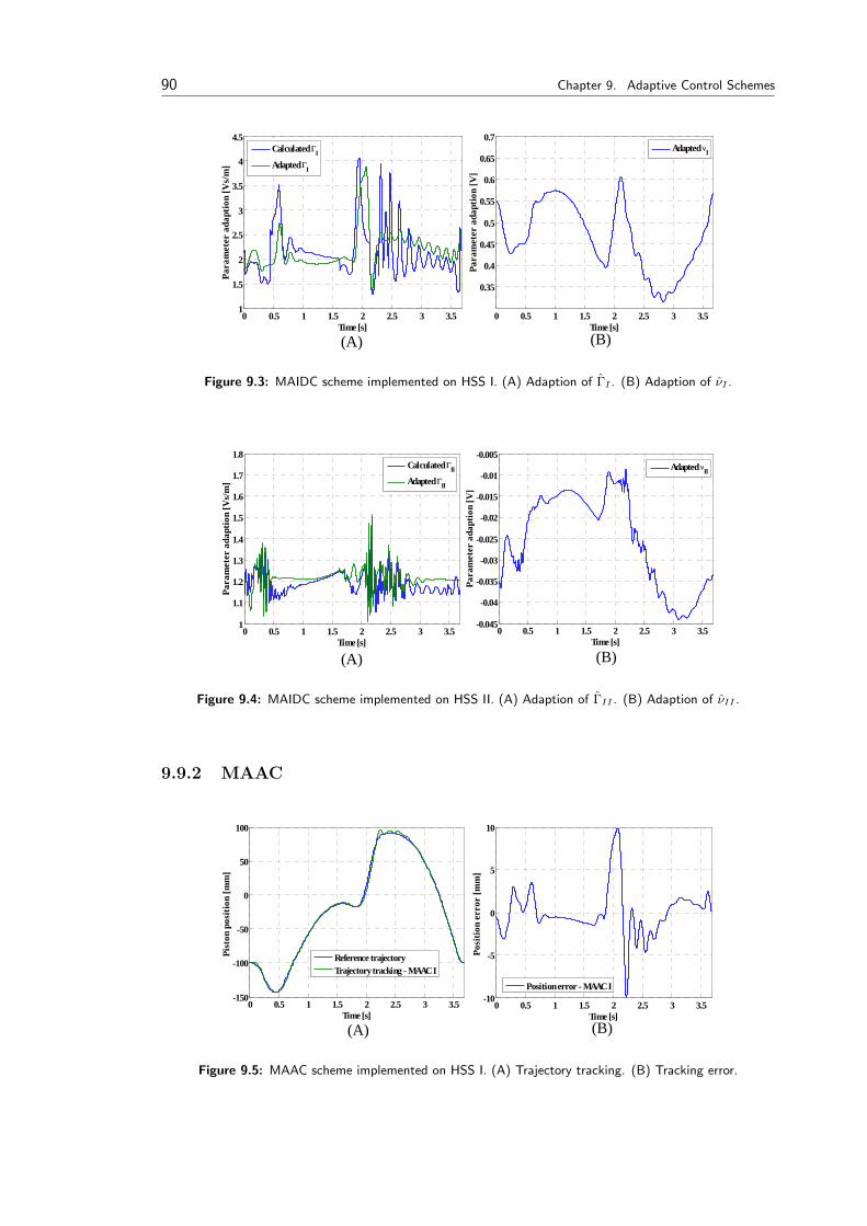
90 Chapter 9. Adaptive Control Schemes
(A) (B)0 0.5 1 1.5 2 2.5 3 3.5
1
1.5
2
2.5
3
3.5
4
4.5
Time [s]
Para
met
er a
dapt
ion
[Vs/
m]
Calculated ΓI
Adapted ΓI
0 0.5 1 1.5 2 2.5 3 3.5
0.35
0.4
0.45
0.5
0.55
0.6
0.65
0.7
Time [s]
Para
met
er a
dapt
ion
[V]
Adapted νI
Figure 9.3: MAIDC scheme implemented on HSS I. (A) Adaption of ΓI . (B) Adaption of νI .
(A) (B)
0 0.5 1 1.5 2 2.5 3 3.51
1.1
1.2
1.3
1.4
1.5
1.6
1.7
1.8
Time [s]
Para
met
er a
dapt
ion
[Vs/
m]
Calculated ΓII
Adapted ΓII
0 0.5 1 1.5 2 2.5 3 3.5-0.045
-0.04
-0.035
-0.03
-0.025
-0.02
-0.015
-0.01
-0.005
Time [s]
Para
met
er a
dapt
ion
[V]
Adapted νII
Figure 9.4: MAIDC scheme implemented on HSS II. (A) Adaption of ΓII . (B) Adaption of νII .
9.9.2 MAAC
(A) (B)0 0.5 1 1.5 2 2.5 3 3.5
-150
-100
-50
0
50
100
Time [s]
Pist
on p
ositi
on [m
m]
Reference trajectoryTrajectory tracking - MAAC I
0 0.5 1 1.5 2 2.5 3 3.5-10
-5
0
5
10
Time [s]
Posi
tion
erro
r [m
m]
Position error - MAAC I
Figure 9.5: MAAC scheme implemented on HSS I. (A) Trajectory tracking. (B) Tracking error.
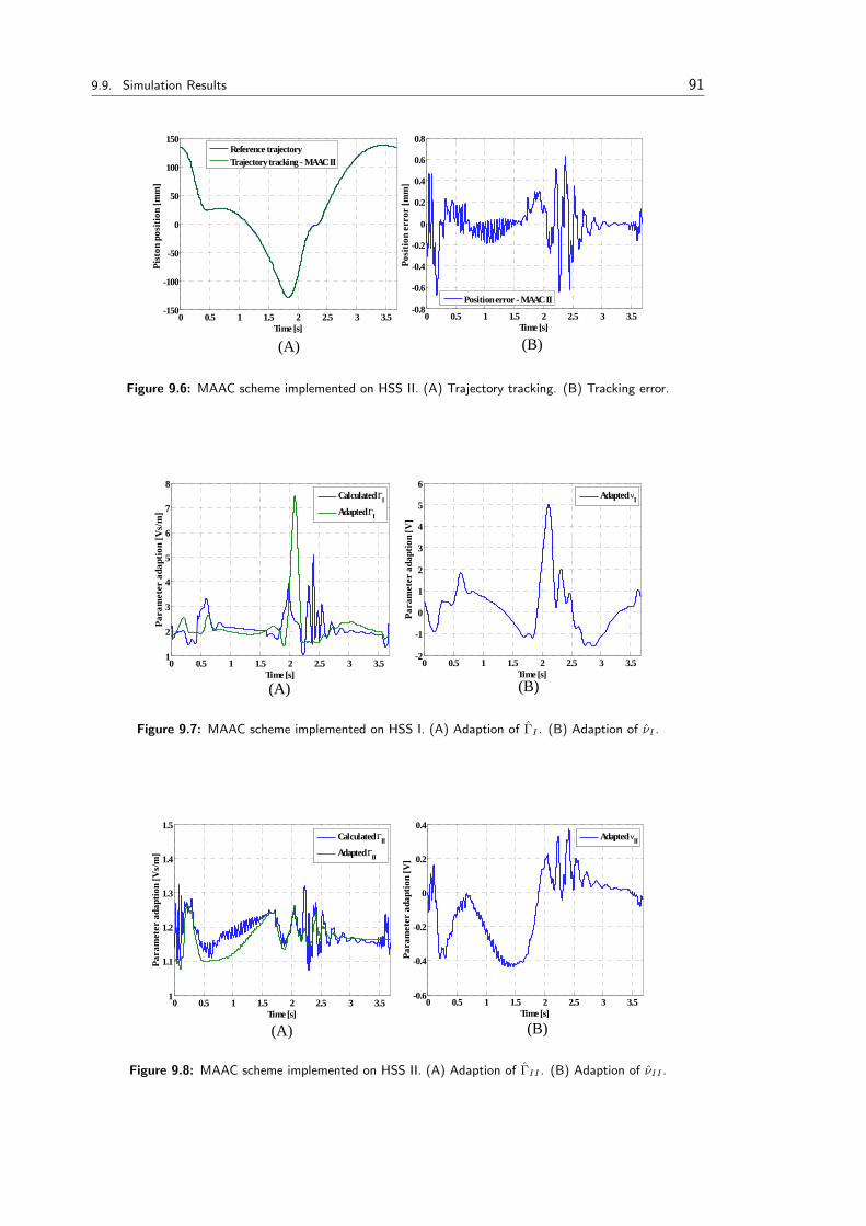
9.9. Simulation Results 91
(A) (B)
0 0.5 1 1.5 2 2.5 3 3.5-150
-100
-50
0
50
100
150
Time [s]
Pist
on p
ositi
on [m
m]
Reference trajectoryTrajectory tracking - MAAC II
0 0.5 1 1.5 2 2.5 3 3.5-0.8
-0.6
-0.4
-0.2
0
0.2
0.4
0.6
0.8
Time [s]
Posi
tion
erro
r [m
m]
Position error - MAAC II
Figure 9.6: MAAC scheme implemented on HSS II. (A) Trajectory tracking. (B) Tracking error.
(A) (B)0 0.5 1 1.5 2 2.5 3 3.5
1
2
3
4
5
6
7
8
Time [s]
Para
met
er a
dapt
ion
[Vs/
m]
Calculated ΓI
Adapted ΓI
0 0.5 1 1.5 2 2.5 3 3.5-2
-1
0
1
2
3
4
5
6
Time [s]
Para
met
er a
dapt
ion
[V]
Adapted νI
Figure 9.7: MAAC scheme implemented on HSS I. (A) Adaption of ΓI . (B) Adaption of νI .
(A) (B)
0 0.5 1 1.5 2 2.5 3 3.51
1.1
1.2
1.3
1.4
1.5
Time [s]
Para
met
er a
dapt
ion
[Vs/
m]
Calculated ΓII
Adapted ΓII
0 0.5 1 1.5 2 2.5 3 3.5-0.6
-0.4
-0.2
0
0.2
0.4
Time [s]
Para
met
er a
dapt
ion
[V]
Adapted νII
Figure 9.8: MAAC scheme implemented on HSS II. (A) Adaption of ΓII . (B) Adaption of νII .
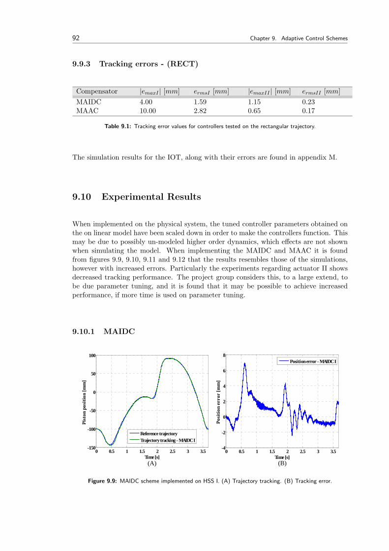
92 Chapter 9. Adaptive Control Schemes
9.9.3 Tracking errors - (RECT)
Compensator |emaxI | [mm] ermsI [mm] |emaxII | [mm] ermsII [mm]MAIDC 4.00 1.59 1.15 0.23MAAC 10.00 2.82 0.65 0.17
Table 9.1: Tracking error values for controllers tested on the rectangular trajectory.
The simulation results for the IOT, along with their errors are found in appendix M.
9.10 Experimental Results
When implemented on the physical system, the tuned controller parameters obtained onthe on linear model have been scaled down in order to make the controllers function. Thismay be due to possibly un-modeled higher order dynamics, which effects are not shownwhen simulating the model. When implementing the MAIDC and MAAC it is foundfrom figures 9.9, 9.10, 9.11 and 9.12 that the results resembles those of the simulations,however with increased errors. Particularly the experiments regarding actuator II showsdecreased tracking performance. The project group considers this, to a large extend, tobe due parameter tuning, and it is found that it may be possible to achieve increasedperformance, if more time is used on parameter tuning.
9.10.1 MAIDC
(A) (B)
0 0.5 1 1.5 2 2.5 3 3.5-150
-100
-50
0
50
100
Time [s]
Pist
on p
ositi
on [m
m]
Reference trajectoryTrajectory tracking - MAIDC I
0 0.5 1 1.5 2 2.5 3 3.5-4
-2
0
2
4
6
8
Time [s]
Posi
tion
erro
r [m
m]
Position error - MAIDC I
Figure 9.9: MAIDC scheme implemented on HSS I. (A) Trajectory tracking. (B) Tracking error.
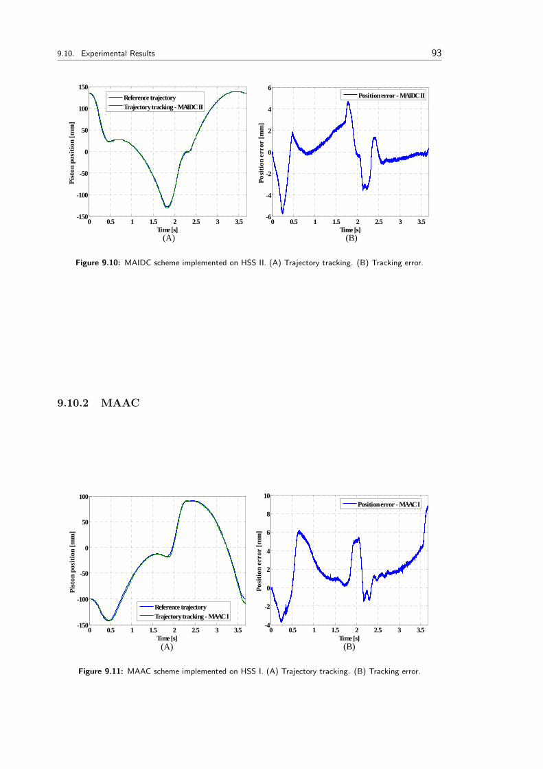
9.10. Experimental Results 93
(A) (B)
0 0.5 1 1.5 2 2.5 3 3.5-150
-100
-50
0
50
100
150
Time [s]
Pist
on p
ositi
on [m
m]
Reference trajectoryTrajectory tracking - MAIDC II
0 0.5 1 1.5 2 2.5 3 3.5-6
-4
-2
0
2
4
6
Time [s]
Posi
tion
erro
r [m
m]
Position error - MAIDC II
Figure 9.10: MAIDC scheme implemented on HSS II. (A) Trajectory tracking. (B) Tracking error.
9.10.2 MAAC
(A) (B)
0 0.5 1 1.5 2 2.5 3 3.5-150
-100
-50
0
50
100
Time [s]
Pist
on p
ositi
on [m
m]
Reference trajectoryTrajectory tracking - MAAC I
0 0.5 1 1.5 2 2.5 3 3.5-4
-2
0
2
4
6
8
10
Time [s]
Posi
tion
erro
r [m
m]
Position error - MAAC I
Figure 9.11: MAAC scheme implemented on HSS I. (A) Trajectory tracking. (B) Tracking error.
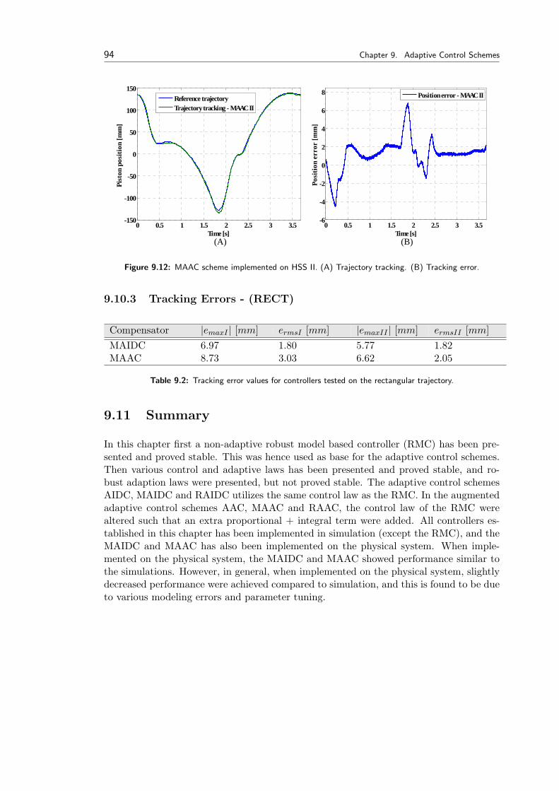
94 Chapter 9. Adaptive Control Schemes
(A) (B)
0 0.5 1 1.5 2 2.5 3 3.5-150
-100
-50
0
50
100
150
Time [s]
Pist
on p
ositi
on [m
m]
Reference trajectoryTrajectory tracking - MAAC II
0 0.5 1 1.5 2 2.5 3 3.5-6
-4
-2
0
2
4
6
8
Time [s]
Posi
tion
erro
r [m
m]
Position error - MAAC II
Figure 9.12: MAAC scheme implemented on HSS II. (A) Trajectory tracking. (B) Tracking error.
9.10.3 Tracking Errors - (RECT)
Compensator |emaxI | [mm] ermsI [mm] |emaxII | [mm] ermsII [mm]MAIDC 6.97 1.80 5.77 1.82MAAC 8.73 3.03 6.62 2.05
Table 9.2: Tracking error values for controllers tested on the rectangular trajectory.
9.11 Summary
In this chapter first a non-adaptive robust model based controller (RMC) has been pre-sented and proved stable. This was hence used as base for the adaptive control schemes.Then various control and adaptive laws has been presented and proved stable, and ro-bust adaption laws were presented, but not proved stable. The adaptive control schemesAIDC, MAIDC and RAIDC utilizes the same control law as the RMC. In the augmentedadaptive control schemes AAC, MAAC and RAAC, the control law of the RMC werealtered such that an extra proportional + integral term were added. All controllers es-tablished in this chapter has been implemented in simulation (except the RMC), and theMAIDC and MAAC has also been implemented on the physical system. When imple-mented on the physical system, the MAIDC and MAAC showed performance similar tothe simulations. However, in general, when implemented on the physical system, slightlydecreased performance were achieved compared to simulation, and this is found to be dueto various modeling errors and parameter tuning.
Chapter 10Adaptive RobustControl Scheme(ARC)
Contents
10.1 Introduction . . . . . . . . . . 95
10.2 Model used in Design Phase . 95
10.3 Control Design . . . . . . . . . 98
10.4 Stability Proof (ARC) . . . . . 105
10.5 Summary . . . . . . . . . . . . 106
This chapter concerns the establishment of an adaptive robust controller (ARC) suitableto take into account the effect of various uncertainties, disturbances etc.
10.1 Introduction
On the physical system, both parametric uncertainties such as varying inertia load, vari-ations of bulk modulus due to temperature changes and varying pressure, and uncertainnon-linearities, such as external disturbances, un-modeled leakage and friction, occurs. Inthe design phase of this ARC, an initiative to compensate for these uncertainties is carriedout. The controller established is a modified version of an ARC, called a discontinuousprojection based adaptive robust controller[Yao et al., 2001]. The controller is establishedbased on the complete hydraulic actuator model, and the design approach used is partlyadaptive backstepping control design. In the following the index i is omitted.
10.2 Model used in Design Phase
In the model used in the design phase, proposed by [Yao et al., 2001], the servo valvedynamics is described by a third order system, where the complex conjugated poles aresufficiently fast to be neglected. However, for the servo valves implemented on the phys-ical system object for this thesis, the servo valve dynamics is approximated by a secondsystem, constituted by poles sufficiently fast to be neglected in the control design phase.In order to avoid redoing the proof developed by [Yao et al., 2001], it is assumed that thefirst order dynamics for the servo valve is present.
95
96 Chapter 10. Adaptive Robust Control Scheme (ARC)
In the treatment of the ARC controller, the inertia load dynamics of the system is de-scribed by equation 10.1, where f(t, xP , xP ) represents the external disturbances andun-modeled friction forces.
MeqxP = PLA− bxP − FC(xP ) + f(t, xP , xP ) (10.1)
The actuator dynamics is described by equation 10.2:
Vt
4βFPL = −AxP − CLPL + QL (10.2)
The load flow QL is given by 10.3:
QL = Cdwxv
√PS − sign(xv)PL
ρ(10.3)
The relation between the spool valve displacement and the input voltage is given byequation 10.4.
τvxv = −xv + Kvuv (10.4)
As seen from equation 10.4 the spool valve / input voltage relation is described by a firstorder system where τv and Kv is the servo valve time constant and gain, respectively.When implementing the controller for simulation purposes numerical errors may ariseaccording to [Yao et al., 2001], and in order to minimize this phenomena scaling factorsare used to scale the valve opening and the load pressure, by xv = xv
Sc4and PL = PL
Sc3,
respectively. By including the scaling factors and rewriting the system equations theequations take the form of 10.5:
xP =ASc3
Meq
(PL −
b
ASc3xP −
FC(xP )ASc3
)+ d(t, xP , xP ) (10.5)
˙PL =4βF
Vt
Sc4√Sc3
Cdw√ρ
(− A
Sc4
√Sc3
√ρ
CdwxP −
√Sc3
Sc4
√ρ
CdwCLPL + g3(PL, xv)xv
)˙xv = − 1
τvx4 +
Kv
Sc4τvuv
Where, d = 1Meq
f(t, xP , xP ), g3(PL, xv) =√
PS − sign(xv)PL and PS = PSSc3
. The systemis now formulated in state space, with the states defined as:
x1 = xP , x2 = xP , x3 = PL , x4 = xv (10.6)
Hence the state space representation of the system, is given as:
x1 = x2 (10.7)
x2 =ASc3
m(x3 − bx2 − FC) + d(t, x1, x2)
x3 =4βF
Vt
Sc4√Sc3
Cdw√ρ
[−Ax2 − CLx3 + g3x4]
(10.8)

10.2. Model used in Design Phase 97
x4 = − 1τv
x4 +Kv
τvuv
Where:
b =1
ASc3b , FC =
1ASc3
FC , A =1
Sc4
√Sc3
√ρ
CdwA , (10.9)
CL =√
Sc3
Sc4
√ρ
CdwCL , Kv =
1Sc4
Kv (10.10)
In order to reduce parametric uncertainties of bulk modlus βF , the inertia load Meq andthe nominal value of the disturbance d (henceforward designated dn), the state spaceequations in 10.7 are linearized and parameterized. The unknown parameter set θ =[θ1, θ2, θ3]T is defined as:
θ1 =ASc3
m, θ2 = dn , θ3 =
4βF
Vt
Sc4√Sc3
Cdw√ρ
(10.11)
The state space equations resulting from the linearization, parameterization and definingd = d(t, x1, x2)− dn, is given by:
x1 = x2 (10.12)
x2 = θ1(x3 − bx2 − FC(x2)) + θ2 + d(t, x1, x2) (10.13)x3 = θ3[−Ax2 − CLx3 + g3(x3, x4)x4] (10.14)
x4 = − 1τv
x4 +Kv
τvu (10.15)
It is assumed that the bounds of 10.16 holds true.
θ ∈ Ωθ = θ : θmin < θ < θmax (10.16)
| d(t, x1, x2) |≤ δd(x1, x2, t)
where: θmin = [θ1min, θ2min, θ3min]T , θmax = [θ1max, θ2max, θ3max]T and δd(t, x1, x2) areknown. The adaption law proposed by [Yao et al., 2001], is given by:
˙θ = Projθ(Γτ) (10.17)
where Γ > 0 describes a constant diagonal matrix, τ is an adaption function and Proj isa discontinuous projection given by:
Projθ(•) =
0 if θi = θimax and • > 00 if θi = θimin and • < 0
• otherwise
(10.18)
Here θ is the estimate of θ, and θ is the estimation error given by θ = θ − θ. Bounds onthe projection Projθ are given by (according to [Yao et al., 2001]):
θ ∈ Ωθ = θ : θmin ≤ θ ≤ θmax (10.19)
θT (Γ−1Projθ(Γτ)− τ) ≤ 0, ∀τ (10.20)
98 Chapter 10. Adaptive Robust Control Scheme (ARC)
The parts of x2 and x3 that can be calculated are given by ˆx2 and ˆx3, respectively, andgiven by expressions 10.21.
ˆx2 = θ1(x3 − bx2 − FC(x2)) + θ2 (10.21)ˆx3 = θ3[−Ax2 − CLx3 + g3(x3, x4)x4]
10.3 Control Design
In the following the control design will be accounted for. This is carried out accordingto [Yao et al., 2001]. The control design is carried out in three steps - first a Lyapunovfunction is established for the first two states x1 and x2 directly. Following this, Lyapunovfunctions are established first, and the control laws are thus found in a way similar tothe backstpping design approach[Yao et al., 2001]. In the following, notations (•) will beomitted.
10.3.1 Step 1
The error dynamics denoted by z2 is given by equation 10.22:
z2 = e1 + kpe1 (10.22)
Where e1 = x1 − x1R is the tracking position error. x1 is the actual position, x1R is thedesired position and kp is a positive feedback gain. Defining x2eq = x1R − kpe1, the errordynamics is rewritten as:
z2 = x2 − x2eq (10.23)
Laplace transforming equation 10.22 yields,
z2 = e1 + kpe1
z2 = e1s + kpe1
z2 = e1(s + kp)e1(s)z2(s)
=1
s + kp(10.24)
Since 10.24 is a stable transfer function, then if the input z2 is bounded the output e1
will also be bounded. Hence if the input converges to zero the output will also convergeto zero as time goes to infinity. Then in the following the objective will be to make z2
become as small as possible, in order to make the error e1 as small as possible.
Differentiating 10.23 and substituting equation 10.13, yields:
z2 = x2 − x2eq = θ1(x3 − bx2 − FC) + θ2 + d− x2eq , x2eq = x1R − kpe1 (10.25)
A virtual control law α making z2 small can be chosen for x3 (according to [Yao et al., 2001]),
10.3. Control Design 99
and is given by 10.26:
α2(x1, x2, θ1, θ2, t) = α2a + α2s = α2a + α2s1 + α2s2 (10.26)
Where:
α2a = bx2 + FC +1
θ1
(x2eq − θ2) , α2s1 = −k2s1z2 , α2s2 = − h2
2θ1minε2z2 (10.27)
For a more detailed description of the elements of the control law in expression 10.26, seeappendix N.1.
Defining the input discrepancy between x3 and the control function α2 by z3 = x3 − α2,and substituting into expression 10.25, yields:
z2 = θ1(x3 − bx2 − FC) + θ2 + d− x2eq
= θ1x3 − θ1bx2 − θ1FC + θ2 + d− x2eq
= θ1(z3 + α2)− θ1bx2 − θ1FC + θ2 + d− x2eq
= θ1(z3 + α2a + α2s)− θ1bx2 − θ1FC + θ2 + d− x2eq
= θ1z3 + θ1α2s + θ1(α2a − bx2 − FC) + θ2 + d− x2eq (10.28)
Noting that θ = θ − θ ⇒ θ = θ − θ, yields:
z2 = θ1z3 + θ1α2s + θ1(α2a − bx2 − FC)− θ1(α2a − bx2 − FC) + θ2 + d− x2eq
(10.29)
Knowing that α2a is given as α2a = bx2 + FC + 1θ1
(x2eq − θ2), yields:
z2 = θ1z3 + θ1α2s + θ1(1
θ1
(x2eq − θ2))− θ1(α2a − bx2 − FC) + θ2 + d− x2eq
= θ1z3 + θ1α2s − θ2 − θ1(α2a − bx2 − FC) + θ2 + d (10.30)
Knowing that α2s = α2s1 + α2s2 where α2s1 = −k2s1z2, yields:
z2 = θ1z3 + θ1(α2s2 − k2s1z2)− θ2 − θ1(α2a − bx2 − FC) + θ2 + d
(10.31)
The following vector is defined:
φ2 =
α2a − x2 − FC
10
(10.32)
Then z2 can be written as:
z2 = θ1z3 + θ1α2s2 − θ1k2s1z2 − θT φ2 + d (10.33)
100 Chapter 10. Adaptive Robust Control Scheme (ARC)
Now a positive semi-definite Lyapunov function V2 is defined.
V2 =12w2z
22 ; w2 > 0 (10.34)
With the time derivative:
V2(z2) = w2z2z2 (10.35)
Substituting expression 10.28, yields:
V2 = w2z2z2
= w2z2(θ1z3 + θ1α2s2 − θ1k2s1z2 − θT φ2 + d) (10.36)
= w2θ1z2z3 + w2z2(θ1α2s2 − θT φ2 + d)− w2θ1k2s1z22 (10.37)
The above Lyapunov function is in itself not proved stable, but as it will be shown in thefollowing, by establishing an overall Lyapunov function composed of the above expressionand Lyapunov functions for the remaining states, it is possible to proof stability. Hencethis step has been completed, and step 2 can be initiated.
10.3.2 Step 2
In this step a virtual control law for α3 is developed for QL such that x3 tracks thecontrol function α2 developed in Step 1. Like the control function α2 in Step 1 thecontrol function α3 also consists of two parts as shown in equation 10.38, and is chosenaccording to [Yao et al., 2001]:
α3(x3, θ, t) = α3a + α3s (10.38)
The time derivative of 10.38, is given by:
α2 = α2c + α2u
=∂α2
∂x1x2 +
∂α2
∂x2x2 +
∂α2
∂θ
˙θ +
∂α2
∂t(10.39)
=∂α2
∂x1x2 +
∂α2
∂x2
ˆx2 −∂α2
∂x2
˜x2 +∂α2
∂θ
˙θ +
∂α2
∂t(10.40)
Here α2c is the calculable part and α2u is the incalculable part due to various uncertainties.Hence these are obtained as:
α2c =∂α2
∂x1x2 +
∂α2
∂x2
ˆx2 +∂α2
∂t(10.41)
α2u =∂α2
∂x2(−˜x2) +
∂α2
∂θ
˙θ =
∂α2
∂x2θ1[−(x3 − bx2 − FC)− θ2 + d] +
∂α2
∂θ
˙θ (10.42)
In the following an initiative to deal with the incalculable part α2u, is taken. Taking thetime derivative of the previously defined z3 = x3 − α2, yields:
z3 = x3 − α2 (10.43)
10.3. Control Design 101
Substituting the state equation x3 = PL, yields:
z3 = θ3(−Ax2 − CLx3 + g3x4)− α2c − α2u (10.44)= θ3(−Ax2 − CLx3 + QL)− α2c − α2u (10.45)
Defining z4 = QL − α3 ⇒ QL = z4 + α3, and substituting, yields:
z3 = θ3(−Ax2 − CLx3 + z4 + α3)− α2c − α2u (10.46)= θ3z4 + θ3(−Ax2 − CLx3 + α3)− α2c − α2u (10.47)
Now the Lyapunov candidate, regarding the third state equation, is established. TheLyapunov candidate is chosen as [Yao et al., 2001]:
V3 = V2 +12w3z
23 ; w3 > 0 (10.48)
Taking the time derivative, yields:
V3 = θ1w2z2z3 + V2|α2 + w3z3 (10.49)
Here V2|α2 denotes V2 under the condition that x3 = α3, which yields z3 = 0. Substitutingthe expression for z3, yields:
V3 = θ1w2z2z3 + V2|α2 + w3z3
(θ3z4 + θ3(−Ax2 − CLx3 + α3)− α2c − α2u
)(10.50)
= θ3w3z3z4 + V2|α2 + w3z3
(w2
w3θ1z2 + θ3(−Ax2 − CLx3 + α3)− α2c − α2u
)Substituting the expression for α2u, yields:
V3 = θ3w3z3z4 + V2|α2 + w3z3(w2
w3θ1z2 + θ3(−Ax2 − CLx3 + α3)− α2c (10.51)
− ∂α2
∂x2(−(x3 − bx2 − FC)θ1 − θ2 + d) +
∂α2
∂θ
˙θ)
= θ3w3z3z4 + V2|α2 + w3z3θ3α3 + w3z3(w2
w3θ1z2 + θ3(−Ax2 − CLx3)− α2c
− ∂α2
∂x2(−(x3 − bx2 − FC)θ1 − θ2 + d) +
∂α2
∂θ
˙θ)
Using the error estimate θ = θ − θ ⇒ θ = θ − θ, yields:
V3 = θ3w3z3z4 + V2|α2 + w3z3θ3α3 + w3z3(w2
w3θ1z2 + θ3(−Ax2 − CLx3) (10.52)
− w2
w3θ1z2 − θ3(−Ax2 − CLx3)− α2c −
∂α2
∂x2(−(x3 − bx2 − FC)θ1 − θ2 + d) +
∂α2
∂θ
˙θ)
Considering the third term of the right hand side of the above expression, and using thatα3 = α3a + α3s, yields:
w3z3θ3α3 = w3z3θ3α3s + w3z3θ3α3a (10.53)

102 Chapter 10. Adaptive Robust Control Scheme (ARC)
Using that θ = θ − θ, gives:
w3z3θ3α3 = w3z3θ3α3s + w3z3θ3α3a − w3z3θ3α3a (10.54)
Substituting into equation 10.52, yields:
V3 = θ3w3z3z4 + V2|α2 + w3z3θ3α3s + w3z3(w2
w3θ1z2 + θ3(−Ax2 − CLx3 + α3a)
− w2
w3θ1z2 − θ3(−Ax2 − CLx3 − α3a)− α2c −
∂α2
∂x2(−(x3 − bx2 − FC)θ1 − θ2
+ d) +∂α2
∂θ
˙θ) (10.55)
Defining the expression:
α3e =w2
w3θ1z2 + θ3(−Ax2 − CLx3)− α2c (10.56)
And the vector:
φ3 =
w2w3
z2 − ∂α2∂x2
(−(x3 − bx2 − FC)−∂α2
∂x2
−Ax2 − CLx3 + α3a
(10.57)
Then expression 10.55 can be written as:
V3 = θ3w3z3z4 + V2|α2 + w3z3θ3α3s (10.58)
+ w3z3
(θ3α3a + α3e − θT φ3 −
∂α2
∂x2d− ∂α2
∂θ
˙θ
)The control law α3 is chosen as[Yao et al., 2001]:
α3 = α3a + α3s = α3a + α3s1 + α3s2 where, (10.59)
α3a = − 1
θ3
α3e , α3s1 = −K3s1z3 , α3s1 = − 12θ3min
h3z3
The coefficients of the above control law is accounted for according to [Yao et al., 2001],and are given in appendix N.2. Substituting into expression 10.58, yields:
V3 = θ3w3z3z4 + V2|α2 + w3z3
(θ3α3s2 − θT φ3 −
∂α2
∂x2d
)− θ3w3K3s1z
23 − w3z3
∂α2
∂θ
˙θ
(10.60)
The second step of the control design has now been completed, and the third step can becarried out.
10.3.3 Step 3
In this step, the control law for the valve input uv is established. This is carried outsuch that QL tracks the control law established in step 2, and can be carried out by step2, where the control law was determined based on the time derivative of the Lyapunov
10.3. Control Design 103
candidate. However, as QL contains sign(x4), QL is not continuous at x4 = 0, and henceis not differentiable. However, according to [Yao et al., 2001], it is possible to proceed thecontrol design by noting that QL is differentiable anywhere except at the singular pointof x4 = 0 and is continuous anywhere.
Similar to the previous step, the positive semi-definite Lyapunov candidate is chosenas[Yao et al., 2001]:
V4 = V3 +12w4z
24 ; w4 > 0 (10.61)
Taking the time derivative, yields:
V4 = θ3w3z3z4 + V3|α3 + w4z4z4 (10.62)
Using that:
z4 = QL − α3 ⇒ z4 = ˙QL − α3 (10.63)
And substituting into 10.62, yields:
V4 = θ3w3z3z4 + V3|α3 + w4z4( ˙QL − α3) (10.64)
= V3|α3 + w4z4(θ3w3
w4z3 + ˙QL − α3) (10.65)
The time derivative of the control law α3 is determined as:
α3 = α3c + α3u (10.66)
Where α3c and α3u are the calculable and the incalculable parts, respectively.
α3c =∂α3
∂x1x2 +
∂α3
∂x2
˙x2 +∂α3
∂x3
˙x3 +∂α3
∂t(10.67)
α3u =∂α3
∂x2(−(x3 − bx2 − FC)θ1 − θ2 + d)− ∂α3
∂x3(−Ax2 − CLx3 + g3x4)θ3 (10.68)
+∂α3
∂θ
˙θ)
Substituting expressions 10.66 and 10.68 into expression 10.65, and using that ˙QL =∂g3
∂x3x3x4 + g3x4, yields:
V4 = V3|α3 + w4z4(θ3w3
w4z3 +
∂g3
∂x3x3x4 + g3x4 − α3c −
∂α3
∂x2(−(x3 − bx2 − FC)θ1
− θ2 + d)− ∂α3
∂x3(−Ax2 − CLx3 + g3x4)θ3 +
∂α3
∂θ
˙θ)) (10.69)
Substituting the third state equation x3 into the above expression gives:
V4 = V3|α3 + w4z4(θ3w3
w4z3 +
∂g3
∂x3θ3(−Ax2 − CLx3 + g3x4)x4 + g3x4 (10.70)

104 Chapter 10. Adaptive Robust Control Scheme (ARC)
Continued ⇒
− α3c −∂α3
∂x2(−(x3 − bx2 − FC)θ1 − θ2 + d)
− ∂α3
∂x3(−Ax2 − CLx3 + g3x4)θ3 +
∂α3
∂θ
˙θ))
Using that θ = θ − θ, and inserting the expression for x4 yields:
V4 = V3|α3 + w4z4(θ3w3
w4z3 +
∂g3
∂x3θ3(−Ax2 − CLx3 + g3x4)x4 − θ3
w3
w4z3 (10.71)
− ∂g3
∂x3θ3(−Ax2 − CLx3 + g3x4)x4 + g3(−
1τv
x4 +Kv
τvu)− α3c −
∂α3
∂x2(−(x3 − bx2
− FC)θ1 − θ2 + d)− ∂α3
∂x3(−Ax2 − CLx3 + g3x4)θ3 +
∂α3
∂θ
˙θ))
Defining expressions:
α4e = θ3w3
w4z3 − g3
1τv
x4 +∂g3
∂x3
˙x3x4 + α4e (10.72)
φ4 =
−∂α3∂x2
(−(x3 − bx2 − FC)−∂α3
∂x2w3w4
z3 − ( ∂g3
∂x3x4 − ∂α3
∂x3)Ax2 − CLx3 + QL
(10.73)
And noting the expression for ˙x3, expression 10.71 is written as:
V4 = V3|α3 + w4z4(g3Kv
τvu + α4e − θφ4 +
∂α3
∂x2d− ∂α3
∂θ
˙θ)
The control law for uv is now chosen according to [Yao et al., 2001], as:
uv(x, θ, t) = ua + us = ua + us1 + us2 (10.74)
Where:
ua = − τv
Kvg3α4e , us1 = −K4s1z4 , us2 = − τv
2Kvg3ε4h4z4 (10.75)
The constants of the above expression is presented in appendix N.3. Substituting expres-sion 10.60 into expression 10.74, yields:
V4 = w2z2
(θ1α2s2 − θT φ2 + d
)− θ1w2K2s1z
22 (10.76)
+ w3z3
(θ3α3s2 − θT φ3 −
∂α2
∂x2d
)− θ3w3K3s1z
23
+ w4z4(g3Kv
τvus2 − θT φ4 +
∂α3
∂x2d)− w4K4s1z
24
− (w3z3∂α2
∂θ
˙θ + w4z4
∂α3
∂θ
˙θ)
10.4. Stability Proof (ARC) 105
10.4 Stability Proof (ARC)
According to theorem 1 of appendix N.4, if the adaption law is chosen as:
τ =4∑
j=2
wjzjφj (10.77)
Then expression 10.76 can, according to [Yao et al., 2001], be rewritten to:
V4 ≤ −4∑
j=2
wjkjz2j − θT τ (10.78)
The following new Lyapunov function is defined:
Vθ = V4 +12θT Γ−1θ (10.79)
Taking the time derivative, yields:
Vθ = V4 + θT Γ−1 ˙θ (10.80)
Considering θ a slow varying parameter, then ˙θ = ˙
θ. This gives:
Vθ = V4 + θT Γ−1 ˙θ (10.81)
Substituting expression 10.78, yields:
Vθ ≤ −4∑
j=2
wjkjz2j − θT τ + θT Γ−1 ˙
θ (10.82)
Using the projection bound of expression 10.20 and noting the adaption law of expression10.17, yields:
θT (Γ−1Projθ(Γτ)− τ) ≤ 0 (10.83)
θT (Γ−1 ˙θ − τ) ≤ 0 (10.84)
θT Γ−1 ˙θ − θT τ ≤ 0 (10.85)
θT Γ−1 ˙θ ≤ θT τ (10.86)
Substituting into expression 10.82, yields:
Vθ ≤ −4∑
j=2
wjkjz2j (10.87)
As wj and kj are positive constants, it is found that expression 10.87, which containsV2, V3 and V4, is negative semi-definite, indicating that z2, z3 and z4 are bounded asVθ > 0. Then according to the Lyapunov-like lemma of appendix H.4, if Vθ is uniformly
106 Chapter 10. Adaptive Robust Control Scheme (ARC)
continuous, z2, z3, z4 → 0 for t →∞. Taking the time derivative of Vθ, yields:
Vθ = −2(w2k2z2z2 + w3k3z3z3 + w4k4z4z4) (10.88)
In the above it was found that z2, z3, z4 are bounded, and according to [Yao et al., 2001]it can be shown that z2, z3 and z4 are bounded. Hence it is found that Vθ is bounded, andVθ is uniformly continuous. Then according to the Lyapunov-like lemma z2, z3, z4 → 0for t → 0. From the above, and noting expression 10.22, it is found that e → 0 for t → 0.The control- and adaption laws are summarized below.
ARC control law:
uv = ua + us (10.89)
Where the terms ua and us are synthesized as shown in the derivation.
ARC adaption law:
˙θ = Γτ ; Γ > 0 (10.90)
Where:
Γτ =
0 if θi = θimax and Γτ > 00 if θi = θimin and Γτ < 0Γτ else
(10.91)
And:
τ =4∑
j=2
wjzjφj = w2z2φ2 + w3z3φ3 + w4z4φ4 (10.92)
Due to the significant amount of parameters in the ARC, it has not been possible toobtain reasonable tracking performance in simulations within the time frame of this thesis.However, the project group will attempt to achieve reasonable results in order to presentthese at the thesis evaluation.
10.5 Summary
In this chapter an adaptive robust controller has been derived and proved stable, basedon the theory of [Yao et al., 2001]. However, due to difficulties in the tuning phase,which were caused by the significant amount of unknown controller parameters, it hasnot been possible to obtain reasonable tracking performance within the time frame of thisthesis. An initiative to improve performance of the ARC will be made in order to presentreasonable result to the thesis evaluation.
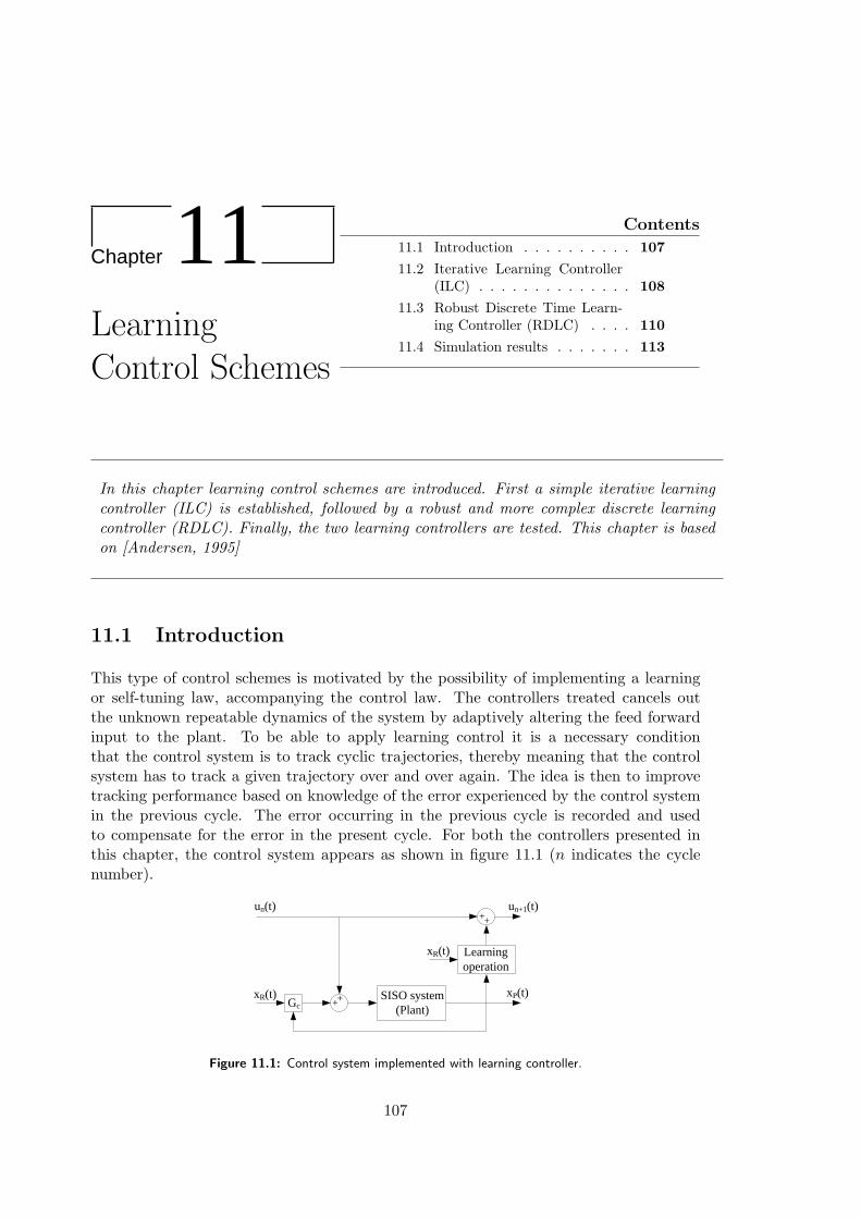
Chapter 11LearningControl Schemes
Contents
11.1 Introduction . . . . . . . . . . 107
11.2 Iterative Learning Controller(ILC) . . . . . . . . . . . . . . 108
11.3 Robust Discrete Time Learn-ing Controller (RDLC) . . . . 110
11.4 Simulation results . . . . . . . 113
In this chapter learning control schemes are introduced. First a simple iterative learningcontroller (ILC) is established, followed by a robust and more complex discrete learningcontroller (RDLC). Finally, the two learning controllers are tested. This chapter is basedon [Andersen, 1995]
11.1 Introduction
This type of control schemes is motivated by the possibility of implementing a learningor self-tuning law, accompanying the control law. The controllers treated cancels outthe unknown repeatable dynamics of the system by adaptively altering the feed forwardinput to the plant. To be able to apply learning control it is a necessary conditionthat the control system is to track cyclic trajectories, thereby meaning that the controlsystem has to track a given trajectory over and over again. The idea is then to improvetracking performance based on knowledge of the error experienced by the control systemin the previous cycle. The error occurring in the previous cycle is recorded and usedto compensate for the error in the present cycle. For both the controllers presented inthis chapter, the control system appears as shown in figure 11.1 (n indicates the cyclenumber).
Gc ++ SISO system(Plant)
Learning operation
++un(t) un+1(t)
xR(t) xP(t)
xR(t)
Figure 11.1: Control system implemented with learning controller.
107
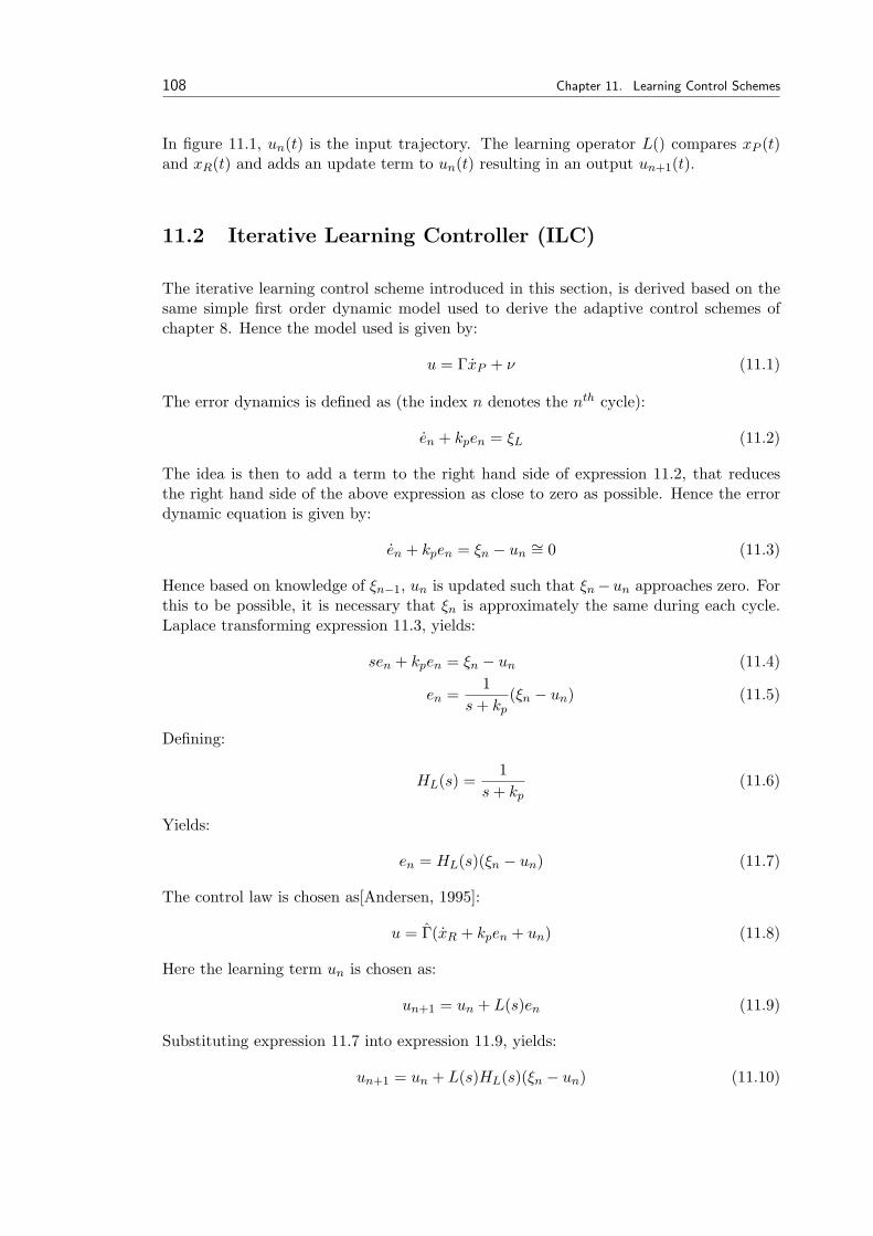
108 Chapter 11. Learning Control Schemes
In figure 11.1, un(t) is the input trajectory. The learning operator L() compares xP (t)and xR(t) and adds an update term to un(t) resulting in an output un+1(t).
11.2 Iterative Learning Controller (ILC)
The iterative learning control scheme introduced in this section, is derived based on thesame simple first order dynamic model used to derive the adaptive control schemes ofchapter 8. Hence the model used is given by:
u = ΓxP + ν (11.1)
The error dynamics is defined as (the index n denotes the nth cycle):
en + kpen = ξL (11.2)
The idea is then to add a term to the right hand side of expression 11.2, that reducesthe right hand side of the above expression as close to zero as possible. Hence the errordynamic equation is given by:
en + kpen = ξn − un∼= 0 (11.3)
Hence based on knowledge of ξn−1, un is updated such that ξn−un approaches zero. Forthis to be possible, it is necessary that ξn is approximately the same during each cycle.Laplace transforming expression 11.3, yields:
sen + kpen = ξn − un (11.4)
en =1
s + kp(ξn − un) (11.5)
Defining:
HL(s) =1
s + kp(11.6)
Yields:
en = HL(s)(ξn − un) (11.7)
The control law is chosen as[Andersen, 1995]:
u = Γ(xR + kpen + un) (11.8)
Here the learning term un is chosen as:
un+1 = un + L(s)en (11.9)
Substituting expression 11.7 into expression 11.9, yields:
un+1 = un + L(s)HL(s)(ξn − un) (11.10)
11.2. Iterative Learning Controller (ILC) 109
Defining CL1 = L(s)HL(s), yields:
un+1 = un + CL1(ξn − un) (11.11)= CL1ξn + un(1− CL1) (11.12)
(11.13)
Letting u0 = 0, expression 11.11 can be written as:
un =n∑
i=1
((1− CL1)n−iCL1)ξn (11.14)
Subtracting ξn on both sides of expression 11.14, gives:
un − ξn =n∑
i=1
((1− CL1)n−iCL1)ξn − ξn (11.15)
= (n∑
i=1
((1− CL1)n−iCL1)− 1)ξn (11.16)
Defining CL2 = 1− CL1, yields:
un − ξn = (n∑
i=1
(Cn−iL2 CL1)− 1)ξn (11.17)
= (n∑
i=1
(Cn−iL2 (1− CL2))− 1)ξn (11.18)
It is possible to write∑n
i=1(Cn−iL2 (1−CL2)) = 1−Cn
L2. Substituting into expression 11.17,yields:
un − ξn = ((1− CnL2)− 1)ξn (11.19)
= −CnL2ξn (11.20)
Substituting CL2 = 1− CL1, yields:
un − ξn = −CnL2ξn (11.21)
= −(1− CL1)nξn (11.22)
Applying the L2 norm, yields:
‖un − ξn‖2 ≤ ‖ − (1− CL1)n‖2‖ξn‖2 (11.23)
From expression 11.23, it is found that for un to converge to ξn, the following must besatisfied, noting that n represents the number of cycles, and hence always will be 0 ≤ n:
‖ − (1− CL1)‖2 ≤ 1 for ‖ − (1− CL1)n‖2 → 0 (11.24)
110 Chapter 11. Learning Control Schemes
Now choosing the learning operator L(s) to L(s) = s + (kp − µ)[Andersen, 1995], yields:
1− CL1 = 1− L(s)HL(s) = 1− s + (kp − µ)s + kp
(11.25)
=s + kp
s + kp− s + (kp − µ)
s + kp(11.26)
=s + kp − s− kp + µ
s + kp(11.27)
=µ
s + kp(11.28)
Taking the L2 norm (according to appendix H.7), yields:
‖1− CL1‖2 =∥∥∥∥ µ
s + kp
∥∥∥∥2
= maxω∈<
∣∣∣∣ µ
jω + kp
∣∣∣∣ = µ
kp(11.29)
Hence it is found that for ‖(1−CL1)‖2 ≤ 1 to be satisfied, the following must be satisfied:
0 < µ < kp (11.30)
Hence by satisfying expression 11.30, it is found that un will approach ξn as the number ofcycles progresses. From this it follows that the error will approach zero. Now the control-and learning update law can be written as shown below (here the learning update law isdisplaced one cycle back).
ILC control law:
u = Γ(xR + kpe + un) (11.31)
ILC learning update law:
un = un−1 + L(s)en−1 = un−1 + (s + (kp − µ))en−1 (11.32)
11.3 Robust Discrete Time Learning Controller (RDLC)
The controller presented in this section is a robust discrete time learning controller fornon-linear time varying systems as the type described by the state space equations ofexpressions 11.33.
xn(t) = f(xn((t), t) + B(xn((t), t)un(t) + ωn(t) (11.33)yn(t) = g(xn((t), t)
First there will be a motivation (according to [Andersen, 2004a]) for using the later pro-posed more general learning control law, following a presentation of the proposed controland learning laws proposed for the system at hand.
11.3. Robust Discrete Time Learning Controller (RDLC) 111
In the following a motivation for the later proposed learning control law is given. This isbased on the same simplified model, used in the previous section (expression 11.1). Thesimplified model is rewritten to the following form:
xP (t) = Γ−1(t)u(t)− Γ−1(t)ν(t) (11.34)
It is seen that −Γ−1(t)ν(t) is equivalent to the state error, and will in the following bedenoted φ(t). Denoting the nth work cycle, yields (in the following the subscript P isomitted):
xn(t) = Γ−1n (t)un(t) + φn(t) (11.35)
By utilizing Taylor expansion the output xn at time t + ∆t can be described as:
xn(t + ∆t) = xn(t) + xn(t)∆t = xn(t) + [Γ−1n (t)un(t) + φn(t)]∆t (11.36)
The subsequent work cycle is denoted by n + 1 and an expression for the input is foundas:
xn+1(t + ∆t) = xn+1(t) + xn+1(t)∆t = xn+1(t) + [Γ−1n+1(t)un+1(t) + φn+1(t)]∆t (11.37)
By substituting xn+1(t + ∆t) with xd(t + ∆t) the input signal un+1(t) which causesxn+1(t + ∆t) to approach xR(t + ∆t) can be found if φ(t) is known. This is carried outin the following. Substituting xn+1(t + ∆t) with xR(t + ∆t), yields (xR represents thedesired, or reference position):
xR(t + ∆t) = xn+1(t) + xn+1(t)∆t = xn+1(t) + [Γ−1n+1(t)un+1(t) + φn+1(t)]∆t (11.38)
If the variation of φ(t) between two cycles is ignored, meaning that φn(t) = φn+1(t),thenφn+1(t) can be eliminated from equation 11.38, and an expression for φ(t) is subsequentlyderived by isolating in equation 11.36.
xn(t + ∆t) = xn(t) + [Γ−1n (t)un(t) + φn(t)]∆t ⇒
xn(t + ∆t)− xn(t)− Γ−1n (t)un(t)∆t = φn(t)∆t ⇒
xn(t + ∆t)∆t
− xn(t)∆t
− Γ−1n (t)un(t) = φn(t) (11.39)
Inserting equation 11.39 into equation 11.38, yields:
xR(t + ∆t) = xn+1(t) + [Γ−1n+1(t)un+1(t) +
xn(t + ∆t)∆t
− xn(t)∆t
(11.40)
− Γ−1n (t)un(t)]∆t
= xn+1(t) + Γ−1n+1(t)un+1(t)∆t + xn(t + ∆t)− xn(t) (11.41)
− Γ−1n (t)un(t)∆t ⇒
xR(t + ∆t)− xn(t + ∆t) = xn+1(t)− xn(t) + [Γ−1n+1(t)un+1(t)− Γ−1
n (t)un(t)]∆t (11.42)
Equation 11.42 can, by isolating un+1(t) and ignoring the variation of Γ between the
112 Chapter 11. Learning Control Schemes
cycles, be turned into a learning algorithm given by:
xR(t + ∆t)− xn(t + ∆t) = xn+1(t)− xn(t) + [Γ−1un+1(t)− Γ−1un(t)]∆t ⇒ (11.43)
xR(t + ∆t)− xn(t + ∆t)− xn+1(t) + xn(t)∆t
= [Γ−1un+1(t)− Γ−1un(t)] (11.44)
Isolating un+1(t) yields the motivational learning update law:
un+1(t) = un(t) + Γ[xR(t + ∆t)− xn(t + ∆t)]− [xn+1(t)− xn(t)]
∆t(11.45)
A more general form of the learning law is proposed in equation 11.46[Andersen, 2004a]:
un+1(t) = (1− γ)un(t) + γu0(t) + L(xn(t), t)[xR(t + ∆t)− xn(t + ∆t)]− [xn+1(t)− xn(t)]
∆t(11.46)
Where, L : Rm × [0, T ] → Rr×m is bounded, and the term γ is can be used to preventinput wandering at initial conditions and also function as a bias. The term L(xn(t), t) isa learning operator which in this thesis is considered constant. If the system described inequation 11.33 uses the learning law of equation 11.46, and satisfies assumptions (A1)−(A5) listed in appendix K, then (according to [Andersen, 2004a]) given an obtainable xR,and if:
‖(1− γ)I − Ln(g(x(t), t)1
∆t
∫ t+∆t
tgx(x, t)B(x, t)dτ‖ ≤ ρ < 1 (11.47)
And if the initial state error is bounded, then as n approaches infinity, the error betweenun and uR is bounded,that is ‖xR(0)− xn(0)‖ ≤ bx0.
As the number of work cycles approaches infinity, then the error between un and uR arebounded.
Where ∀(x, t) ∈ <n × [0, T ].
By choosing a small ∆t the theorem of equation 11.47 is reduced to equation 11.48:
‖(1− γ)I − Ln(g(x(t), t)gx(x, t)B(x, t)dτ‖ ≤ ρ < 1 (11.48)
Where ∀(x, t) ∈ <n × [0, T ].
The chosen control law is given as 11.49[Andersen, 2004a]:
u = Γ(t)(x(t)− kP (xR(t)− x(t))) + uL (11.49)
where uL is the learning term.
A modified version of the learning law given in equation 11.46 is given by equation11.50[Andersen, 2004a].
uLn+1(t) = uL
n(t) + L(t)[xR(t + ∆t)− xk(t + ∆t)]− [xk+1(t)− xk(t)]
∆t(11.50)
where the learning operator L(t) represents Γ.
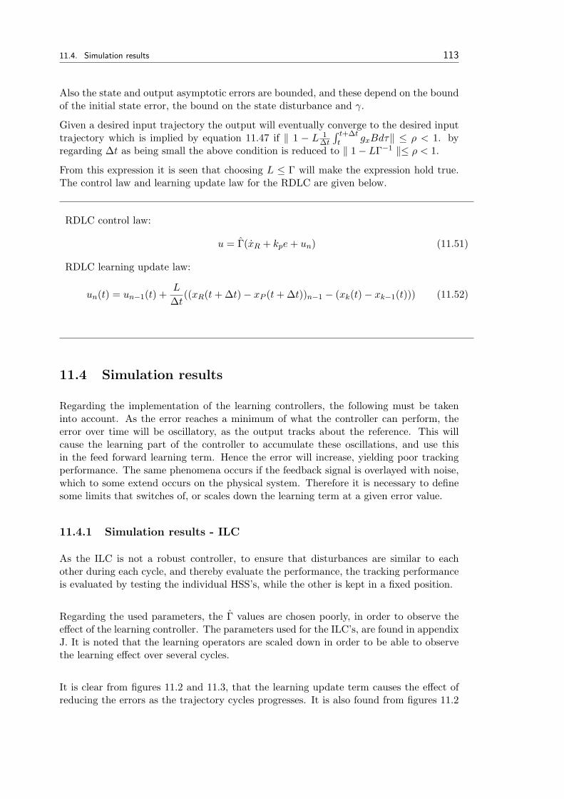
11.4. Simulation results 113
Also the state and output asymptotic errors are bounded, and these depend on the boundof the initial state error, the bound on the state disturbance and γ.
Given a desired input trajectory the output will eventually converge to the desired inputtrajectory which is implied by equation 11.47 if ‖ 1 − L 1
∆t
∫ t+∆tt gxBdτ‖ ≤ ρ < 1. by
regarding ∆t as being small the above condition is reduced to ‖ 1− LΓ−1 ‖≤ ρ < 1.
From this expression it is seen that choosing L ≤ Γ will make the expression hold true.The control law and learning update law for the RDLC are given below.
RDLC control law:
u = Γ(xR + kpe + un) (11.51)
RDLC learning update law:
un(t) = un−1(t) +L
∆t((xR(t + ∆t)− xP (t + ∆t))n−1 − (xk(t)− xk−1(t))) (11.52)
11.4 Simulation results
Regarding the implementation of the learning controllers, the following must be takeninto account. As the error reaches a minimum of what the controller can perform, theerror over time will be oscillatory, as the output tracks about the reference. This willcause the learning part of the controller to accumulate these oscillations, and use thisin the feed forward learning term. Hence the error will increase, yielding poor trackingperformance. The same phenomena occurs if the feedback signal is overlayed with noise,which to some extend occurs on the physical system. Therefore it is necessary to definesome limits that switches of, or scales down the learning term at a given error value.
11.4.1 Simulation results - ILC
As the ILC is not a robust controller, to ensure that disturbances are similar to eachother during each cycle, and thereby evaluate the performance, the tracking performanceis evaluated by testing the individual HSS’s, while the other is kept in a fixed position.
Regarding the used parameters, the Γ values are chosen poorly, in order to observe theeffect of the learning controller. The parameters used for the ILC’s, are found in appendixJ. It is noted that the learning operators are scaled down in order to be able to observethe learning effect over several cycles.
It is clear from figures 11.2 and 11.3, that the learning update term causes the effect ofreducing the errors as the trajectory cycles progresses. It is also found from figures 11.2
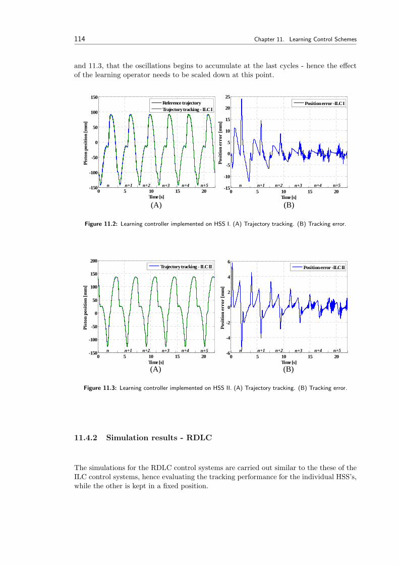
114 Chapter 11. Learning Control Schemes
and 11.3, that the oscillations begins to accumulate at the last cycles - hence the effectof the learning operator needs to be scaled down at this point.
(B)
0 5 10 15 20-150
-100
-50
0
50
100
150
Time [s]
Pist
on p
ositi
on [m
m]
Reference trajectoryTrajectory tracking - ILC I
(A)
n n+1 n+2 n+3 n+4 n+50 5 10 15 20
-15
-10
-5
0
5
10
15
20
25
Time [s]
Posi
tion
erro
r [m
m]
Position error -ILC I
n n+1 n+2 n+3 n+4 n+5
Figure 11.2: Learning controller implemented on HSS I. (A) Trajectory tracking. (B) Tracking error.
(A) (B)
0 5 10 15 20-150
-100
-50
0
50
100
150
200
Time [s]
Pist
on p
ositi
on [m
m]
Trajectory tracking - ILC II
n n+1 n+2 n+3 n+4 n+50 5 10 15 20
-6
-4
-2
0
2
4
6
Time [s]
Posi
tion
erro
r [m
m]
Position error -ILC II
n n+1 n+2 n+3 n+4 n+5
Figure 11.3: Learning controller implemented on HSS II. (A) Trajectory tracking. (B) Tracking error.
11.4.2 Simulation results - RDLC
The simulations for the RDLC control systems are carried out similar to the these of theILC control systems, hence evaluating the tracking performance for the individual HSS’s,while the other is kept in a fixed position.
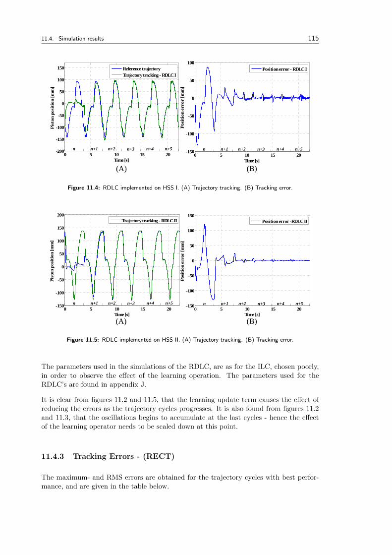
11.4. Simulation results 115
(B)(A)
0 5 10 15 20-150
-100
-50
0
50
100
Time [s]
Posi
tion
erro
r [m
m]
Position error - RDLC I
n n+1 n+2 n+3 n+4 n+50 5 10 15 20
-200
-150
-100
-50
0
50
100
150
Time [s]
Pist
on p
ositi
on [m
m]
Reference trajectoryTrajectory tracking - RDLC I
n n+1 n+2 n+3 n+4 n+5
Figure 11.4: RDLC implemented on HSS I. (A) Trajectory tracking. (B) Tracking error.
(A) (B)
0 5 10 15 20-150
-100
-50
0
50
100
150
200
Time [s]
Pist
on p
ositi
on [m
m]
Trajectory tracking - RDLC II
0 5 10 15 20-150
-100
-50
0
50
100
150
Time [s]
Posi
tion
erro
r [m
m]
Position error -RDLC II
n n+1 n+2 n+3 n+4 n+5 n n+1 n+2 n+3 n+4 n+5
Figure 11.5: RDLC implemented on HSS II. (A) Trajectory tracking. (B) Tracking error.
The parameters used in the simulations of the RDLC, are as for the ILC, chosen poorly,in order to observe the effect of the learning operation. The parameters used for theRDLC’s are found in appendix J.
It is clear from figures 11.2 and 11.5, that the learning update term causes the effect ofreducing the errors as the trajectory cycles progresses. It is also found from figures 11.2and 11.3, that the oscillations begins to accumulate at the last cycles - hence the effectof the learning operator needs to be scaled down at this point.
11.4.3 Tracking Errors - (RECT)
The maximum- and RMS errors are obtained for the trajectory cycles with best perfor-mance, and are given in the table below.
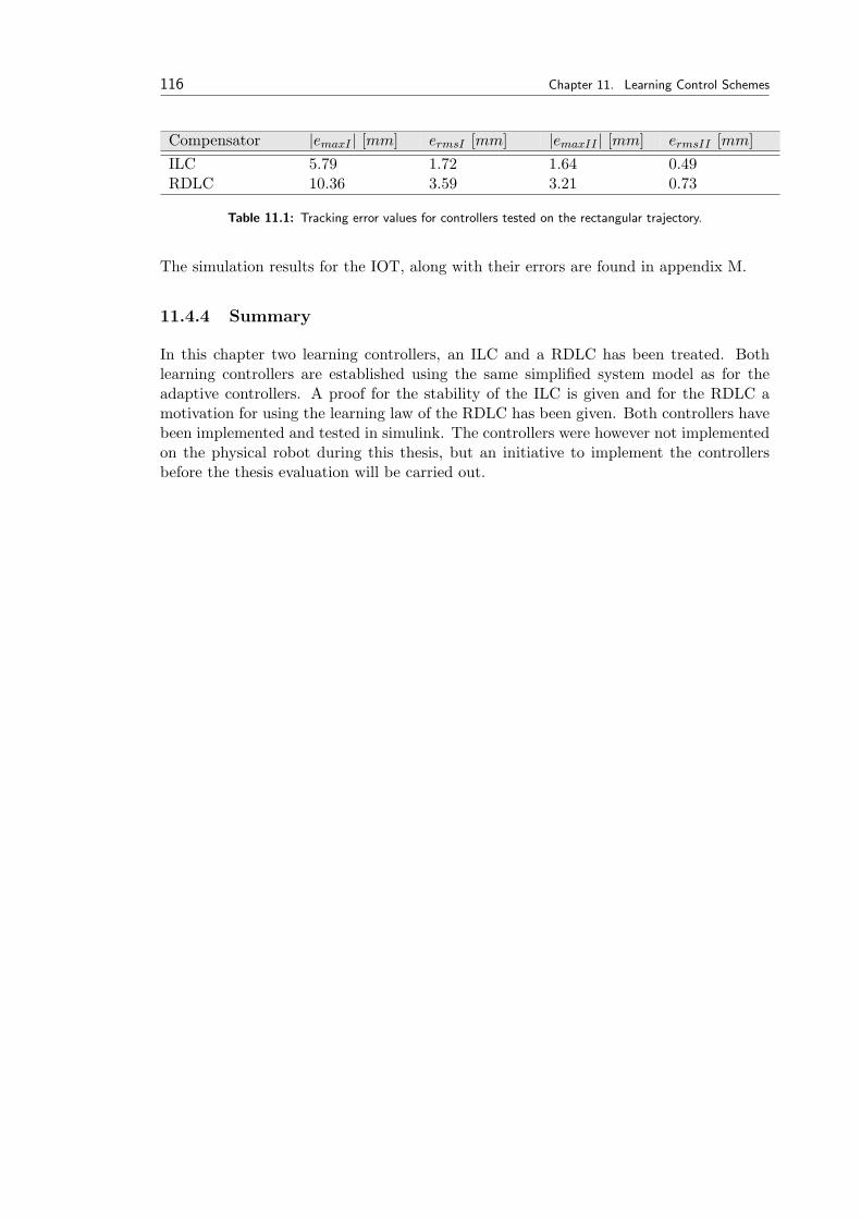
116 Chapter 11. Learning Control Schemes
Compensator |emaxI | [mm] ermsI [mm] |emaxII | [mm] ermsII [mm]ILC 5.79 1.72 1.64 0.49RDLC 10.36 3.59 3.21 0.73
Table 11.1: Tracking error values for controllers tested on the rectangular trajectory.
The simulation results for the IOT, along with their errors are found in appendix M.
11.4.4 Summary
In this chapter two learning controllers, an ILC and a RDLC has been treated. Bothlearning controllers are established using the same simplified system model as for theadaptive controllers. A proof for the stability of the ILC is given and for the RDLC amotivation for using the learning law of the RDLC has been given. Both controllers havebeen implemented and tested in simulink. The controllers were however not implementedon the physical robot during this thesis, but an initiative to implement the controllersbefore the thesis evaluation will be carried out.
Part IV
Comparison of Control Schemes &Conclusions
117

Chapter 12Comparison ofControllers
Contents
12.1 Robustness . . . . . . . . . . . 119
12.2 Linear Controllers . . . . . . . 120
12.3 Adaptive Controllers . . . . . 123
12.4 Learning Controllers . . . . . . 124
This chapter treats the comparison of the controllers in order to estimate which controllersyield the best performance when implemented on a hydraulic servo application as the servorobot in this thesis.
In order to estimate the performance of the various controllers, a set of evaluation criteriawas setup in chapter 1. These where the maximum RMS error, maximum peak error androbustness towards disturbances.
Even though some of the controllers in the following will perform worse then others, itmay still be justifiable to use them on a hydraulic servo robot, depending on the taskthat the robot is to perform. This means that the performance of the controllers mightvary with the job that the robot is to carry out.
12.1 Robustness
As mentioned in section 1.5.3 the robustness of the controllers will also be investigated.The analysis of the robustness is carried out in order to be able to evaluate how robustthe control systems tested in the thesis, are towards disturbances. In order to provideproper disturbances to the control systems, it will be appreciable to be able to apply adisturbance that excites all of the system dynamics. To do this an additional load isapplied to the system at a given point of time during the trajectory - this is applied as astep to the mass of link II at the center of mass of this. Due to the sudden increase in theload, the pressure dynamics will be affected, hence affecting all of the hydraulic system.This analysis is carried only for the RECT, as this is the trajectory that provides thehighest demands for the system. The applied mass will be 50 [kg], and will be applied attime t = 1 [s] for all control systems. This analysis will be carried out for the linear con-trollers with VFCP and VFCA, for the AIDC, MAIDC, RAIDC, AAC, MAAC, RAAC,and for the learning controllers ILC and RDLC. Regarding the learning controllers, the
119
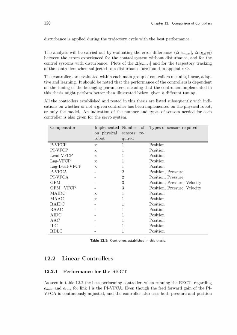
120 Chapter 12. Comparison of Controllers
disturbance is applied during the trajectory cycle with the best performance.
The analysis will be carried out by evaluating the error differences (∆|emaxi|, ∆eRMSi)between the errors experienced for the control system without disturbance, and for thecontrol systems with disturbance. Plots of the ∆|emaxi| and for the trajectory trackingof the controllers when subjected to a disturbance, are found in appendix O.
The controllers are evaluated within each main group of controllers meaning linear, adap-tive and learning. It should be noted that the performance of the controllers is dependenton the tuning of the belonging parameters, meaning that the controllers implemented inthis thesis might perform better than illustrated below, given a different tuning.
All the controllers established and tested in this thesis are listed subsequently with indi-cations on whether or not a given controller has been implemented on the physical robot,or only the model. An indication of the number and types of sensors needed for eachcontroller is also given for the servo system.
Compensator Implementedon physicalrobot
Number ofsensors re-quired
Types of sensors required
P-VFCP x 1 PositionPI-VFCP x 1 PositionLead-VFCP x 1 PositionLag-VFCP x 1 PositionLag-Lead-VFCP x 1 PositionP-VFCA - 2 Position, PressurePI-VFCA - 2 Position, PressureGFM - 3 Position, Pressure, VelocityGFM+VFCP - 3 Position, Pressure, VelocityMAIDC x 1 PositionMAAC x 1 PositionRAIDC - 1 PositionRAAC - 1 PositionAIDC - 1 PositionAAC - 1 PositionILC - 1 PositionRDLC - 1 Position
Table 12.1: Controllers established in this thesis.
12.2 Linear Controllers
12.2.1 Performance for the RECT
As seen in table 12.2 the best performing controller, when running the RECT, regardingemax and erms for link I is the PI-VFCA. Even though the feed forward gain of the PI-VFCA is continuously adjusted, and the controller also uses both pressure and position
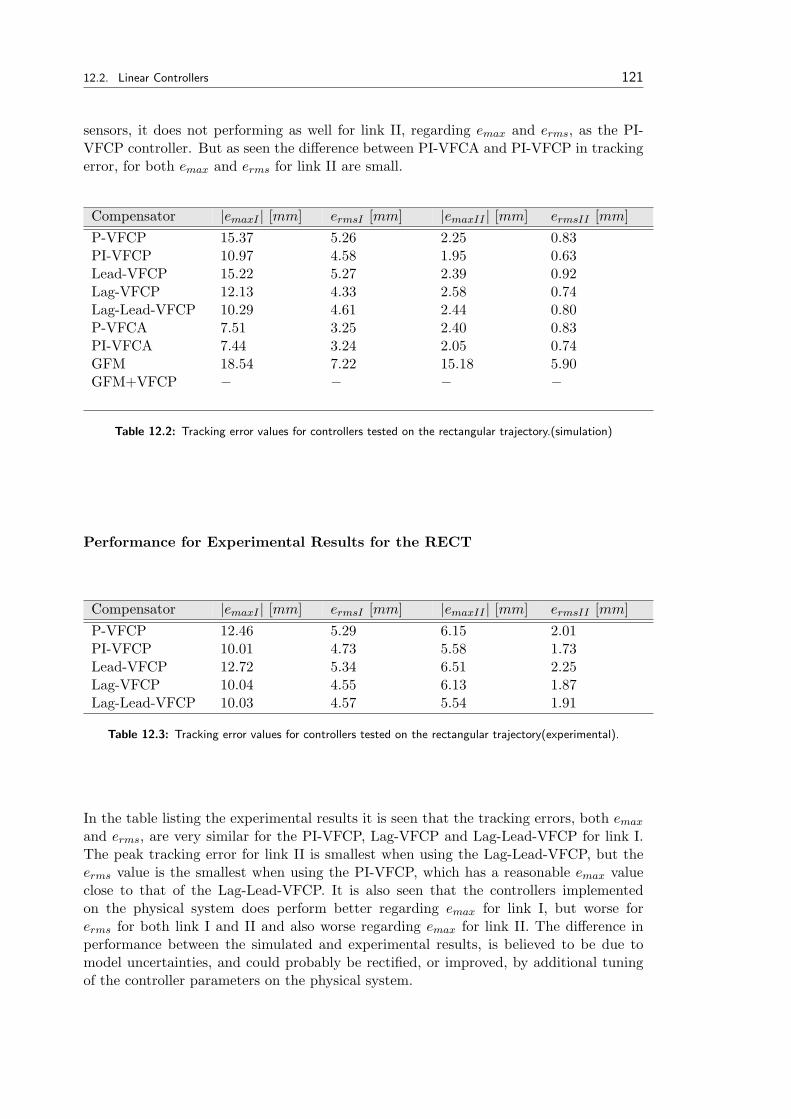
12.2. Linear Controllers 121
sensors, it does not performing as well for link II, regarding emax and erms, as the PI-VFCP controller. But as seen the difference between PI-VFCA and PI-VFCP in trackingerror, for both emax and erms for link II are small.
Compensator |emaxI | [mm] ermsI [mm] |emaxII | [mm] ermsII [mm]P-VFCP 15.37 5.26 2.25 0.83PI-VFCP 10.97 4.58 1.95 0.63Lead-VFCP 15.22 5.27 2.39 0.92Lag-VFCP 12.13 4.33 2.58 0.74Lag-Lead-VFCP 10.29 4.61 2.44 0.80P-VFCA 7.51 3.25 2.40 0.83PI-VFCA 7.44 3.24 2.05 0.74GFM 18.54 7.22 15.18 5.90GFM+VFCP − − − −
Table 12.2: Tracking error values for controllers tested on the rectangular trajectory.(simulation)
Performance for Experimental Results for the RECT
Compensator |emaxI | [mm] ermsI [mm] |emaxII | [mm] ermsII [mm]P-VFCP 12.46 5.29 6.15 2.01PI-VFCP 10.01 4.73 5.58 1.73Lead-VFCP 12.72 5.34 6.51 2.25Lag-VFCP 10.04 4.55 6.13 1.87Lag-Lead-VFCP 10.03 4.57 5.54 1.91
Table 12.3: Tracking error values for controllers tested on the rectangular trajectory(experimental).
In the table listing the experimental results it is seen that the tracking errors, both emax
and erms, are very similar for the PI-VFCP, Lag-VFCP and Lag-Lead-VFCP for link I.The peak tracking error for link II is smallest when using the Lag-Lead-VFCP, but theerms value is the smallest when using the PI-VFCP, which has a reasonable emax valueclose to that of the Lag-Lead-VFCP. It is also seen that the controllers implementedon the physical system does perform better regarding emax for link I, but worse forerms for both link I and II and also worse regarding emax for link II. The difference inperformance between the simulated and experimental results, is believed to be due tomodel uncertainties, and could probably be rectified, or improved, by additional tuningof the controller parameters on the physical system.
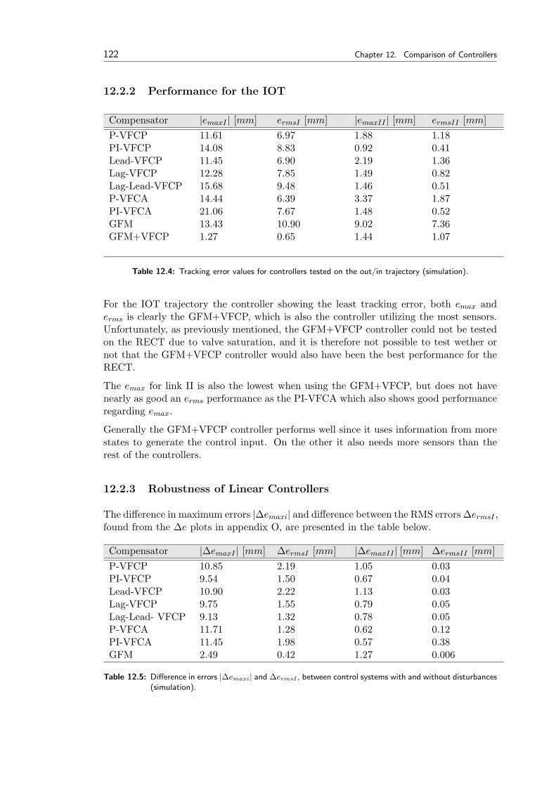
122 Chapter 12. Comparison of Controllers
12.2.2 Performance for the IOT
Compensator |emaxI | [mm] ermsI [mm] |emaxII | [mm] ermsII [mm]P-VFCP 11.61 6.97 1.88 1.18PI-VFCP 14.08 8.83 0.92 0.41Lead-VFCP 11.45 6.90 2.19 1.36Lag-VFCP 12.28 7.85 1.49 0.82Lag-Lead-VFCP 15.68 9.48 1.46 0.51P-VFCA 14.44 6.39 3.37 1.87PI-VFCA 21.06 7.67 1.48 0.52GFM 13.43 10.90 9.02 7.36GFM+VFCP 1.27 0.65 1.44 1.07
Table 12.4: Tracking error values for controllers tested on the out/in trajectory (simulation).
For the IOT trajectory the controller showing the least tracking error, both emax anderms is clearly the GFM+VFCP, which is also the controller utilizing the most sensors.Unfortunately, as previously mentioned, the GFM+VFCP controller could not be testedon the RECT due to valve saturation, and it is therefore not possible to test wether ornot that the GFM+VFCP controller would also have been the best performance for theRECT.
The emax for link II is also the lowest when using the GFM+VFCP, but does not havenearly as good an erms performance as the PI-VFCA which also shows good performanceregarding emax.
Generally the GFM+VFCP controller performs well since it uses information from morestates to generate the control input. On the other it also needs more sensors than therest of the controllers.
12.2.3 Robustness of Linear Controllers
The difference in maximum errors |∆emaxi| and difference between the RMS errors ∆ermsI ,found from the ∆e plots in appendix O, are presented in the table below.
Compensator |∆emaxI | [mm] ∆ermsI [mm] |∆emaxII | [mm] ∆ermsII [mm]P-VFCP 10.85 2.19 1.05 0.03PI-VFCP 9.54 1.50 0.67 0.04Lead-VFCP 10.90 2.22 1.13 0.03Lag-VFCP 9.75 1.55 0.79 0.05Lag-Lead- VFCP 9.13 1.32 0.78 0.05P-VFCA 11.71 1.28 0.62 0.12PI-VFCA 11.45 1.98 0.57 0.38GFM 2.49 0.42 1.27 0.006
Table 12.5: Difference in errors |∆emaxi| and ∆ermsI , between control systems with and without disturbances(simulation).
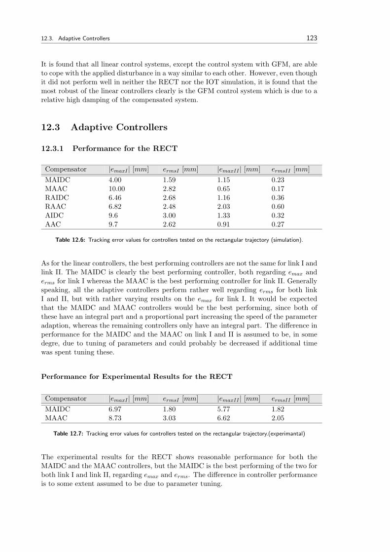
12.3. Adaptive Controllers 123
It is found that all linear control systems, except the control system with GFM, are ableto cope with the applied disturbance in a way similar to each other. However, even thoughit did not perform well in neither the RECT nor the IOT simulation, it is found that themost robust of the linear controllers clearly is the GFM control system which is due to arelative high damping of the compensated system.
12.3 Adaptive Controllers
12.3.1 Performance for the RECT
Compensator |emaxI | [mm] ermsI [mm] |emaxII | [mm] ermsII [mm]MAIDC 4.00 1.59 1.15 0.23MAAC 10.00 2.82 0.65 0.17RAIDC 6.46 2.68 1.16 0.36RAAC 6.82 2.48 2.03 0.60AIDC 9.6 3.00 1.33 0.32AAC 9.7 2.62 0.91 0.27
Table 12.6: Tracking error values for controllers tested on the rectangular trajectory (simulation).
As for the linear controllers, the best performing controllers are not the same for link I andlink II. The MAIDC is clearly the best performing controller, both regarding emax anderms for link I whereas the MAAC is the best performing controller for link II. Generallyspeaking, all the adaptive controllers perform rather well regarding erms for both linkI and II, but with rather varying results on the emax for link I. It would be expectedthat the MAIDC and MAAC controllers would be the best performing, since both ofthese have an integral part and a proportional part increasing the speed of the parameteradaption, whereas the remaining controllers only have an integral part. The difference inperformance for the MAIDC and the MAAC on link I and II is assumed to be, in somedegre, due to tuning of parameters and could probably be decreased if additional timewas spent tuning these.
Performance for Experimental Results for the RECT
Compensator |emaxI | [mm] ermsI [mm] |emaxII | [mm] ermsII [mm]MAIDC 6.97 1.80 5.77 1.82MAAC 8.73 3.03 6.62 2.05
Table 12.7: Tracking error values for controllers tested on the rectangular trajectory.(experimantal)
The experimental results for the RECT shows reasonable performance for both theMAIDC and the MAAC controllers, but the MAIDC is the best performing of the two forboth link I and link II, regarding emax and erms. The difference in controller performanceis to some extent assumed to be due to parameter tuning.
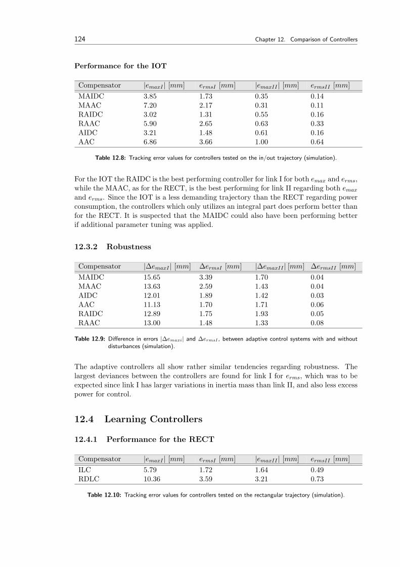
124 Chapter 12. Comparison of Controllers
Performance for the IOT
Compensator |emaxI | [mm] ermsI [mm] |emaxII | [mm] ermsII [mm]MAIDC 3.85 1.73 0.35 0.14MAAC 7.20 2.17 0.31 0.11RAIDC 3.02 1.31 0.55 0.16RAAC 5.90 2.65 0.63 0.33AIDC 3.21 1.48 0.61 0.16AAC 6.86 3.66 1.00 0.64
Table 12.8: Tracking error values for controllers tested on the in/out trajectory (simulation).
For the IOT the RAIDC is the best performing controller for link I for both emax and erms,while the MAAC, as for the RECT, is the best performing for link II regarding both emax
and erms. Since the IOT is a less demanding trajectory than the RECT regarding powerconsumption, the controllers which only utilizes an integral part does perform better thanfor the RECT. It is suspected that the MAIDC could also have been performing betterif additional parameter tuning was applied.
12.3.2 Robustness
Compensator |∆emaxI | [mm] ∆ermsI [mm] |∆emaxII | [mm] ∆ermsII [mm]MAIDC 15.65 3.39 1.70 0.04MAAC 13.63 2.59 1.43 0.04AIDC 12.01 1.89 1.42 0.03AAC 11.13 1.70 1.71 0.06RAIDC 12.89 1.75 1.93 0.05RAAC 13.00 1.48 1.33 0.08
Table 12.9: Difference in errors |∆emaxi| and ∆ermsI , between adaptive control systems with and withoutdisturbances (simulation).
The adaptive controllers all show rather similar tendencies regarding robustness. Thelargest deviances between the controllers are found for link I for erms, which was to beexpected since link I has larger variations in inertia mass than link II, and also less excesspower for control.
12.4 Learning Controllers
12.4.1 Performance for the RECT
Compensator |emaxI | [mm] ermsI [mm] |emaxII | [mm] ermsII [mm]ILC 5.79 1.72 1.64 0.49RDLC 10.36 3.59 3.21 0.73
Table 12.10: Tracking error values for controllers tested on the rectangular trajectory (simulation).
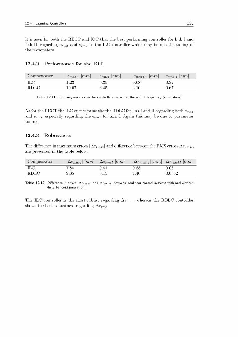
12.4. Learning Controllers 125
It is seen for both the RECT and IOT that the best performing controller for link I andlink II, regarding emax and erms, is the ILC controller which may be due the tuning ofthe parameters.
12.4.2 Performance for the IOT
Compensator |emaxI | [mm] ermsI [mm] |emaxII | [mm] ermsII [mm]ILC 1.23 0.35 0.68 0.32RDLC 10.07 3.45 3.10 0.67
Table 12.11: Tracking error values for controllers tested on the in/out trajectory (simulation).
As for the RECT the ILC outperforms the the RDLC for link I and II regarding both emax
and erms, especially regarding the emax for link I. Again this may be due to parametertuning.
12.4.3 Robustness
The difference in maximum errors |∆emaxi| and difference between the RMS errors ∆ermsI ,are presented in the table below.
Compensator |∆emaxI | [mm] ∆ermsI [mm] |∆emaxII | [mm] ∆ermsII [mm]ILC 7.88 0.81 0.88 0.03RDLC 9.65 0.15 1.40 0.0002
Table 12.12: Difference in errors |∆emaxi| and ∆ermsI , between nonlinear control systems with and withoutdisturbances.(simulation)
The ILC controller is the most robust regarding ∆emax, whereas the RDLC controllershows the best robustness regarding ∆erms.

Chapter 13Conclusions & Perspectives
This thesis have been initiated in order to investigate the performances of an array ofcontrollers, linear and non-linear, on an electro hydraulic servo system realized by anelectro hydraulic robot manipulator, in order to decide which of the tested controllerswere the most suited for implementation on such a system. The controllers investigatedwere classical linear controllers, linear controllers with extensions, adaptive, and learningcontrollers. The thesis has been divided into four parts were the tasks and outcome ofeach part is summarized subsequently.
Part I
In order to simulate the behavior of the electro hydraulic robot manipulator and test thecontrollers a dynamic non-linear model of the electro hydraulic robot manipulator hasbeen established, both for the solid state and fluid mechanical parts of the overall system.The model has then subsequently been tested, by comparison of pressure data from thephysical system, regarding both dynamics and gravitation, which has proved the modelto be adequately accurate for the design and testing of controllers.
The non-linear model has then been linearized and a linear model of the robot manipulatorhas been developed. The linear model has been verified by applying small inputs to theservo valves near the operating point of the linear model and afterwards comparing theoutputs of the linear model to those of the nonlinear model. From this comparisonthe linear model has been found sufficiently accurate, and has therefore been used fordevelopment of the linear controllers.
In order to have a common testing scenario for evaluating the performances of the con-trollers developed in the thesis, trajectories have been established. The limits for thetrajectories have been set up as the physical system boundaries, taking into account themechanical damping at the actuator endpoints in order to avoid undesired system behav-ior. Furthermore flow and pressure boundaries for the hydraulic part of the system havebeen taken into account. Two trajectory scenarios have been set up - a robot controlscenario, and a servo control scenario. In the robot control scenario the tool center pointis to track a rectangular trajectory which requires fairly large variations in the actuator
127
128 Chapter 13. Conclusions & Perspectives
space trajectories over a specified period of time. In the servo control scenario both actu-ators are to track the same trajectory, which is constituted by a retraction and extensionof the actuators, also over a specified period of time.
part II
As a base of comparison different linear controllers have been designed by use of frequencyresponses to meet the design specifications of GM and PM, and the designed compensatorshave subsequently been adjusted to have satisfactory responses when subjected to step-,ramp and parabolic inputs. It has been found that the classical linear controllers providedpoor tracking performance for both trajectories, resulting in large rms and peak trackingerrors. In order to augment the performance of the classical controllers, extensions hasbeen added in the form of feed forward compensation, both passive and active. Thepassive feed forward gain has been found by use of the inverse dynamics of the linearsystem representation, and the active feed forward gain has been established by use ofpressure feedback, updating the feed forward gain. It has been found that adding a feedforward gain boosted the performance of the controllers regarding tracking performance.It has also been found that the effect of adding the active feed forward gain was mostpronounced on the HSS I, since this part of the system has the largest variations in inertiamass and thereby also the largest fluctuations in load pressure. As the inertia mass forHSS II is almost constant, resulting in nearly constant load pressure rendering the activefeed forward gain nearly constant, and therefore without any noteworthy difference fromthe passive feed forward gain.
By use of state space representation and pole placement two versions of a controller havebeen developed - one with state feedback gain matrix, and an augmented version withfeed forward contributions. The augmented state feedback gain compensator could unfor-tunately not be tested on the system using the rectangular trajectory, as this caused valvesaturation. However, the augmented state feedback gain compensator could be tested forthe system using IOT, which yielded a dramatically increased tracking performance incomparison with the controller without feed forward contributions.
Part III
A non-adaptive robust model based controller (RMC) has been presented and proved sta-ble forming the base of for the adaptive control schemes AIDC, MAIDC and RAIDC whichutilizes the same control law as the RMC, but uses adaption laws in order to continuouslyadapt the parameters of the control law. The augmented adaptive control schemes AAC,MAAC and RAAC uses an altered control law, where an extra proportional + integrationterm has been added. All adaptive control schemes have been implemented and tested insimulink, and the MAIDC and MAAC have also been implemented on the physical robotmanipulator. Also an adaptive robust controller has been established and proved stable,based on the theory of [Yao et al., 2001]. It has however not been possible to obtainreasonable tracking performance for this controller within the time frame of this thesisdue to difficulties in the tuning phase. An initiative will however be made to improvethe performance of the ARC in order to present reasonable results at the thesis evaluation.
129
Furthermore in this part, two learning controllers, an ILC and a RDLC, have been estab-lished. Both learning controllers have been established using the same simplified systemmodel as for the adaptive controllers, and were both tested on the in simulation. Thecontrollers were however not implemented on the physical robot during this thesis, butan initiative to implement the controllers before the thesis evaluation will be carried out.
The controller parameters used in this part have all been found by trial and error, asno method for this task is available. The adaptive controllers all provided good trackingperformance in simulation and when implemented on the physical system (For thoseimplemented there). The learning function of the learning controllers has been foundto perform reasonable, and it has been found that these controllers reduces trackingerrors significantly as the trajectory cycles progresses. For the nonlinear controllers it isfound that these may achieve even better tracking performance, if more time is spend onparameter tuning.
Part IV
In this part controllers have been evaluated by performance and robustness, but alsothe number of sensors necessary for implementing the controllers were taken into con-sideration. The controllers have been grouped into three categories - linear, adaptiveand learning controllers, and within each category the controller performance has beentested on the rectangular- and in/out trajectories, and subsequently the robustness of thecontrollers has been tested by giving a mass step to the system at a given time duringthe rectangular trajectory. The peak and rms errors have then been compared to thepeak and rms errors without the disturbance input, and ∆ peak- and rms values havebeen found as an indicator of the robustness of the given compensated system towardsdisturbance in the form of a mass step.
It has been found that the performance of the controllers varied with the trajectory, andto which actuator they were applied, meaning that controllers showing good performancefor one trajectory and actuator, could show a rather different performance for the othertrajectory and actuator.
Performance of Controllers
Linear Controllers
It has been found that the best performing linear controller running the rectangulartrajectory for actuator I was the PI-VFCA with a peak tracking error of 7.44 [mm] andan rms error of 3.24 [mm]. The best performing linear controller for actuator II was thePI-VFCP with peak and rms errors of 1.95 [mm] 0.63 [mm] respectively. However, thedifference in tracking error both rms and peak between the PI-VFCP and the PI-VFCAfor link II was found to be rather small with differences of peak and rms error of 0.1 [mm]and 0.11 [mm], respectively.
When running the in/out trajectory in simulation, it has been found that the GFM+VFCPwas the best performing linear controller for actuator I, with peak and rms errors of1.27 [mm] 0.65 [mm], respectively. Unfortunately this controller could not be tested
130 Chapter 13. Conclusions & Perspectives
for the RECT due to servo valve saturation. For actuator II the best performing con-troller was the PI-VFCP with peak and rms tracking errors of 0.92 [mm] and 0.41 [mm],respectively.
Of the linear controllers implemented on the physical system the best performance re-garding peak error for actuator I, has been obtained with the PI-VFCP with an error of10.01 [mm], whereas the best rms error performance was obtained with the Lag-VFCP,with an rms error of 4.55 [mm]. It was also noted that the difference in peak and rms er-rors for the PI-VFCP, Lag-VFCP and Lag-Lead-VFCP was rather small with the biggestdifferences being between PI-VFCP and Lag-VFCP, with differences in peak and rmserrors of 0.03 [mm] and 0.18 [mm] respectively.
The peak tracking error for acuator II has been found to be smallest when using theLag-Lead-VFCP, but the rms value is the smallest when using the PI-VFCP, which alsohas a peak value close to that of the Lag-Lead-VFCP. It is also seen that the controllersimplemented on the physical system does perform better regarding peak error for actuatorI, but generally worse regarding rms errors for both actuator I and II, and also worseregarding peak error for actuator II.
Adaptive Controllers
The adaptive controller performing the best for actuator I, running the rectangular tra-jectory, has been found to be the MAIDC with peak and rms errors of 4 [mm] and1.59 [mm], respectively, and for actuator II the best performing controller is the MAACwith peak and rms errors of 0.65 [mm] 0.17 [mm], respectively. It was also noted thatthe difference in peak and rms error, for link II, using the MAIDC and MAAC was only0.5 [mm] and 0.06 [mm] respectively.
The controller performance when running the in/out trajectory was found to be best forlink I and II when utilizing the RAIDC and MAAC controllers respectively.
When implemented on the physical system the MAIDC performed the best for bothactuator I and II with peak and rms errors of 6.97 [mm] and 1.80 [mm], respectively, foractuator I and 5.77 [mm] 1.82 [mm] respectively for actuator II.
Learning Controllers
The best performing learning controller for both the rectangular- and in/out trajectories,for both actuator I and II, was found to be the ILC. For the RECT the peak and rmserrors for actuator I was 5.79 [mm] and 1.72 [mm], and for actuator II the peak andrms values was 1.64 [mm] 0.49 [mm] respectively. When running the IOT the peak andrms errors for actuator I was 1.23 [mm] and 0.35 [mm], and the peak and rms values foractuator II was 0.68 [mm] 0.32 [mm] respectively. The Difference in tracking performancebetween the ILC and RDLC, is assumed to be partially due to the parameter tuning foreach of the controllers.
131
Robustness
The most robust of the tested controllers proved to be the GFM controller, which is due tothe relative high damping of the compensated system. The remaining controllers showedrather similar tendencies regarding the robustness. Also it was noted that the adaptivecontrollers in general did not yield good robustness compared to the linear controllers,which is thought to be due to the parameter adaption not being fast enough, which wasto be expected since the adaptive controllers are not meant for fast changing parametervariations.
The different tuning of the controller parameters makes the comparison difficult, sincesome of the controllers probably would be able to perform rather different given a bettertuning. However, it can be concluded that the performance of the tested controllers varieswith the trajectory, and also according to which of the actuators the controller is imple-mented on. Therefore the task of the servo system should be considered before choosinga controller, since this can make the difference on whether or not a given controller willyield a reasonable performance. It is also concluded that one of the best all-round per-forming controllers is the MAIDC, which provide reasonable good tracking performancefor both the rectangular- and in/out trajectory in simulation and also for the rectangulartrajectory, when implemented on the physical system.
Perspectives
During this thesis it was found that the tuning of the controller parameters naturally hasgreat influence on the behavior of the compensated systems. For the linear controllers thisdid not pose a problem since it was possible to analyze the behavior of the compensatedsystem and tune the parameters accordingly. For the non-linear controllers, it did howeverpose a problem since the non-linear controllers generally had more parameters which aredifficult to determine, since no method for this is available. Because of this it was ratherdifficult to obtain consistent results, and the tuning also proved to be rather cumbersomefor some of the controllers. It was also noted that some of the non-linear controllersmight have performed better given a different tuning. Hence it might prove prudentto utilize optimization techniques for tuning of the parameters, and thus maybe obtainbetter controller performance, and a better basis of comparison of the controllers, sincethis process might help tuning the parameters to values closer to their optimal values.

Chapter 14Abstract
This master thesis concerns the development and implementation of an array of con-trollers both linear and non-linear in order to investigate if there is something to gain byusing more advanced control schemes instead of simple and linear schemes on an electrohydraulic servo system implemented by an hydraulic robot manipulator. It should benoted that this is considered mainly as a position servo.
In order to develop, test and tune the various controllers, a non-linear dynamic model ofthe hydraulic robot manipulator has been developed and verified by comparing pressureand position data for the physical robot manipulator, and the non-linear dynamic model.Afterwards the non-linear model has been linearized in order to obtain a linear modelfor tuning and analyzing the linear controllers. The linear model has been verified bycomparison to the nonlinear model in a region near the operating point of the linearmodel.
Using the linear model for parameter tuning an array of linear controllers were developed,all including a feed forward gain contribution. Two versions of the feed forward gain havebeen tested, one with passive gain and one with an active gain utilizing the load pressureof the system. The controllers were added to the system yielding a compensated systemwhich has been tuned by using frequency responses.
For establishment and testing of the more advanced non-linear controllers a simplifiedversion of the linear model has been derived describing only a simplified version of theactuator dynamics of the system, since this was found to be the dominant part of thesystem. A term taking into account the modeling error, due to the simplification of thesystem, has also been added and the simplified system is ultimately given by a gain, anintegrator, and the modeling error term.
Utilizing the simplified linear model, an array of adaptive controllers have been developedand proved stable. The adaptive controllers have been implemented on the non-linearmodel and the system behavior for the compensated systems have been simulated, andselected controllers have been implemented and tested on the physical system. Also twolearning controllers have been developed, using the simplified linear model, and imple-mented and tested in the non-linear model.
The controllers treated in this thesis have been compared on peak and rms errors regard-ing the tracking of selected trajectories. It has been found that the performance of the
133
134 Chapter 14. Abstract
controllers to a wide extent varied depending on the chosen trajectory, indicating the im-portance to take into account the specific use of the hydraulic servo system when choosinga control strategy. Performance wise the comparisons showed reasonable performance forsome controllers in both the linear, adaptive and learning category and it was seen thatone of the best performing controllers for a specific trajectory was a state feedback gainmatrix controller with an added feed forward gain. The controller with the best over-all performance has been found to be a Modified Adaptive Inverse Dynamic Controller(MAIDC) which performed well on all tested trajectories, and also when implemented onthe physical robot manipulator.
The robustness of the controllers have also been tested, by giving a disturbance input tothe top link of the robot manipulator in the form of a mass step. The different tuningof the controller parameters made the comparison difficult, since some of the controllersprobably would be able to perform rather different given a better tuning. However, it canbe concluded that the performance of the tested controllers varies with the trajectory,and also according to which of the actuators the controller is implemented on. Thereforethe task of the servo system should be considered before choosing a controller, sincethis can make the difference on whether or not a given controller will yield a reasonableperformance.
Bibliography
[Andersen, 2003a] Andersen, T.O., H.-M. (2003a). Fluid Power Systems, Modelling andAnalysis, 2nd edition. Institute of Energy Technology and Institute of MechanicalEngineering, Aalborg Universitet.
[Andersen, 2004a] Andersen, T.O., H.-M. (2004a). Discrete Learning Control ApplicationTo Hydraulic Actuators. Institute of Energy Technology and Institute of MechanicalEngineering, Aalborg Universitet.
[Andersen, 2004b] Andersen, J.A., L.-J. (2004b). Advanced control of hydraulic servosystems. Institut for Energiteknik, Aalborg Universitet. Master thesis.
[Andersen, 1995] Andersen, T. O. (1995). Robust Control, Discrete Learning Control:Strategy, Convergence and Robustness. Instituttet for Styreteknik, Danmarks TekniskeUniversitet. Rapport nr. S95.51.
[Andersen, 1996] Andersen, T. O. (1996). Adaptive Control of Hydraulic Actuators andMultivariable Hydraulic Systems. Control Engineering Institute Technical Universityof Denmark.
[Andersen, 2003b] Andersen, T. O. (2003b). Applied Nonlinear Control, Norms and Ma-trix Measures, Lyapunov Theory, Hyperstability. Institut for Energiteknik, AalborgUniversitet.
[Craig, 2005] Craig, J. (2005). Introduction to robotics - Mechanics and Control. PrenticeHall, third edition. ISBN: 0-13-123629-6.
[Hansen, 1997] Hansen, P. E. (1997). Autonomous and Adaptive Control of Hydraulic Ac-tuator Systems. Department of Control and Engineering Design, Technical Universityof Denmark. PhD Dissertation.
[Mohieddine Jelali, 2004] Mohieddine Jelali, A. K. (2004). Hydraulic servo systems.Springer, - edition. ISBN 1-85233-692-7.
[Ogata, 2002] Ogata, K. (2002). Modern Control Engineering. Prentice Hall, fourthedition edition. ISBN: 0-13-043245-8.
[Rasmussen, 1996] Rasmussen, W. (1996). Hydraulik Stabi. Teknisk Forlag A/S, - edition.ISBN 87-571-1325-4.
135
136 Bibliography
[Slotine E J-J, 1991] Slotine E J-J, L. W. (1991). Applied Nonlinear Control. Prentice-Hall, Inc. New Jersey. ISBN: 0-13-040890-5.
[Yao et al., 2001] Yao, B., Bu, F., and Chui, G. T. (2001). Non-linear adaptive robustcontrol of electro-hydraulic systems driven by double-rod actuators. International Jour-nal of Control. ISSN 0020-7179.

Part V
Appendix
137

Appendix ADynamic Model
In this appendix, the kinematics and kinetics of the robot manipulator will be described.First the necessary kinematic constraints will be derived, followed by kinetic derivations.Finally, the dynamic model will be formulated mathematically, and the inertia, coriolis andgravitational are presented graphically. Values for characteristic lengths, masses, inertiaetc. are given according to [Andersen, 2004b]
A.1 Kinematics
In this section necessary kinematic constraints for the model development is derived. Thisincludes kinematic relations between the cylinder positions and joint angles, definition oflengths on cylinders and kinematic relations between the joint angles and the overallrobot structure.
A.1.1 Kinematic Constraints Between Joint Angles & Cylinder Posi-tions
From figure A.1 it is seen that the angle θI is found as:
θI = ϕI − ϕO + ϕOQ ⇒ ϕI = θI + ϕO − ϕOQ (A.1)
The relationship between the joint angle θI and the total length of cylinder I and pistonI, xI , is found as:
ϕI = arccos
(L2
OQ + L2HO − x2
I
2LOQLHO
)(A.2)
From the above expression, xI is determined as:
xI =√
L2OQ + L2
HO − 2LOQLHOcos(ϕI) (A.3)
139
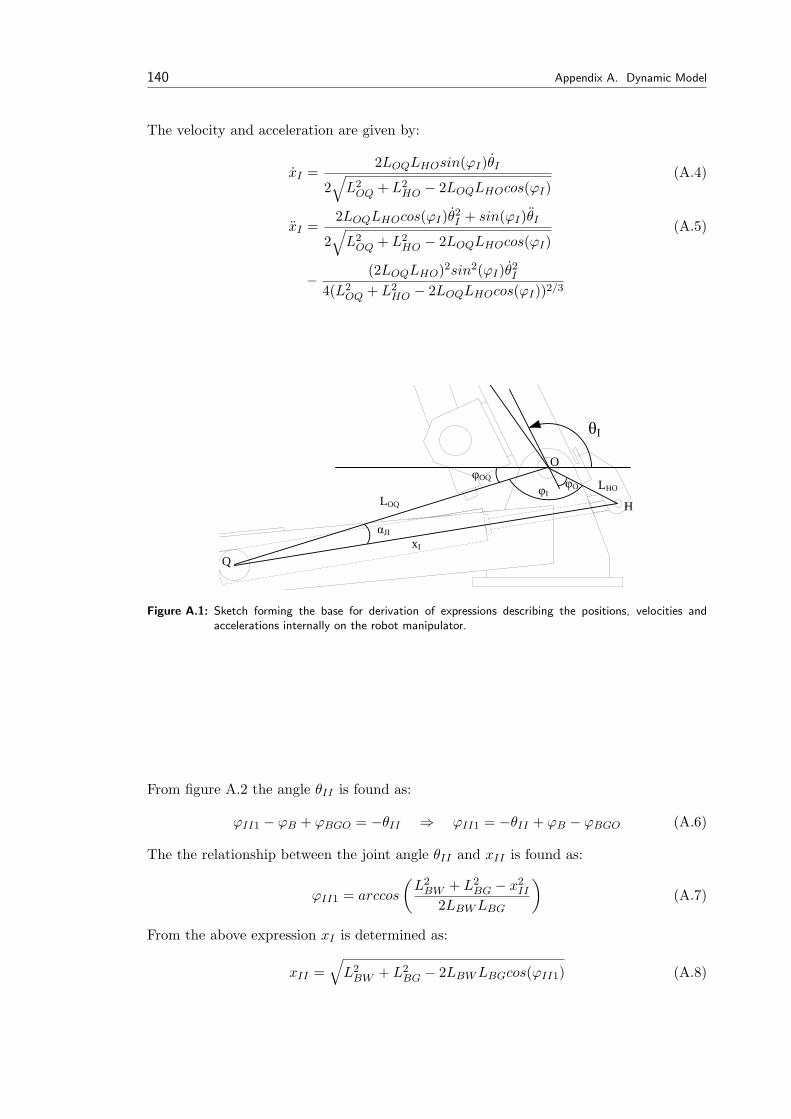
140 Appendix A. Dynamic Model
The velocity and acceleration are given by:
xI =2LOQLHOsin(ϕI)θI
2√
L2OQ + L2
HO − 2LOQLHOcos(ϕI)(A.4)
xI =2LOQLHOcos(ϕI)θ2
I + sin(ϕI)θI
2√
L2OQ + L2
HO − 2LOQLHOcos(ϕI)(A.5)
−(2LOQLHO)2sin2(ϕI)θ2
I
4(L2OQ + L2
HO − 2LOQLHOcos(ϕI))2/3
θII
θI
TCPR
LHO
LOQ
xI
φOφI
φOQ
αJI
Q
H
O
Figure A.1: Sketch forming the base for derivation of expressions describing the positions, velocities andaccelerations internally on the robot manipulator.
From figure A.2 the angle θII is found as:
ϕII1 − ϕB + ϕBGO = −θII ⇒ ϕII1 = −θII + ϕB − ϕBGO (A.6)
The the relationship between the joint angle θII and xII is found as:
ϕII1 = arccos
(L2
BW + L2BG − x2
II
2LBW LBG
)(A.7)
From the above expression xI is determined as:
xII =√
L2BW + L2
BG − 2LBW LBGcos(ϕII1) (A.8)
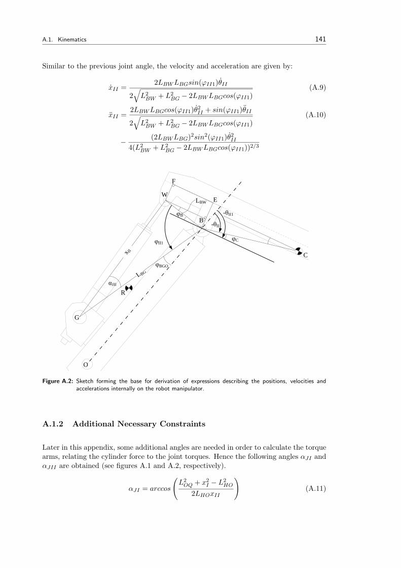
A.1. Kinematics 141
Similar to the previous joint angle, the velocity and acceleration are given by:
xII =2LBW LBGsin(ϕII1)θII
2√
L2BW + L2
BG − 2LBW LBGcos(ϕII1)(A.9)
xII =2LBW LBGcos(ϕII1)θ2
II + sin(ϕII1)θII
2√
L2BW + L2
BG − 2LBW LBGcos(ϕII1)(A.10)
−(2LBW LBG)2sin2(ϕII1)θ2
II
4(L2BW + L2
BG − 2LBW LBGcos(ϕII1))2/3
C
G
O
B
R
E
A
yI
L EPφ
LA
E
φEA
B
LBG
-θII
W
φBGO
φB
φC
LBW
x II
φII1
-θII1
E
F
D
αJII
Figure A.2: Sketch forming the base for derivation of expressions describing the positions, velocities andaccelerations internally on the robot manipulator.
A.1.2 Additional Necessary Constraints
Later in this appendix, some additional angles are needed in order to calculate the torquearms, relating the cylinder force to the joint torques. Hence the following angles αJI andαJII are obtained (see figures A.1 and A.2, respectively).
αJI = arccos
(L2
OQ + x2I − L2
HO
2LHOxII
)(A.11)
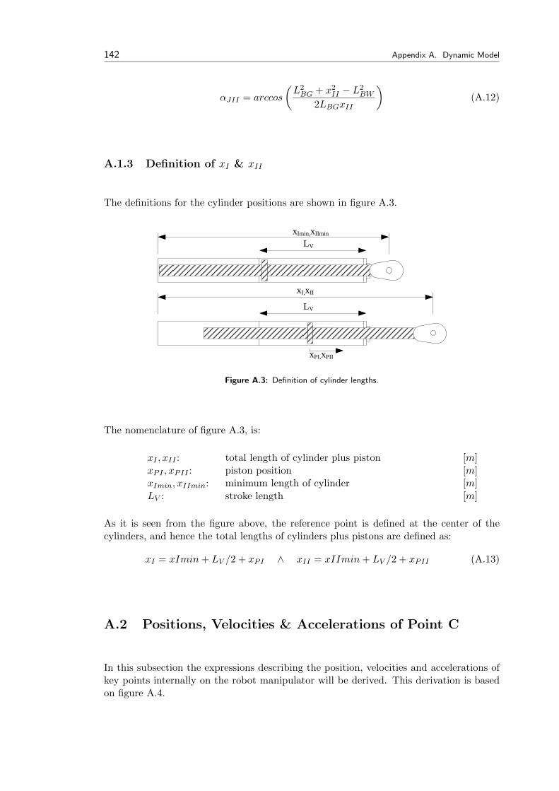
142 Appendix A. Dynamic Model
αJII = arccos
(L2
BG + x2II − L2
BW
2LBGxII
)(A.12)
A.1.3 Definition of xI & xII
The definitions for the cylinder positions are shown in figure A.3.
E
A
yI
L EPφ
LA
E
φEA
B
LV
xImin,xIImin
LV
xPI,xPII
xI,xII
Figure A.3: Definition of cylinder lengths.
The nomenclature of figure A.3, is:
xI , xII : total length of cylinder plus piston [m]xPI , xPII : piston position [m]xImin, xIImin: minimum length of cylinder [m]LV : stroke length [m]
As it is seen from the figure above, the reference point is defined at the center of thecylinders, and hence the total lengths of cylinders plus pistons are defined as:
xI = xImin + LV /2 + xPI ∧ xII = xIImin + LV /2 + xPII (A.13)
A.2 Positions, Velocities & Accelerations of Point C
In this subsection the expressions describing the position, velocities and accelerations ofkey points internally on the robot manipulator will be derived. This derivation is basedon figure A.4.
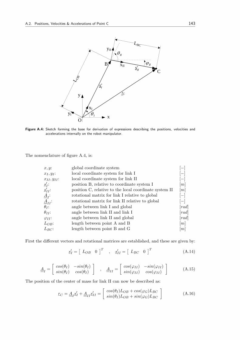
A.2. Positions, Velocities & Accelerations of Point C 143
y
xyI
xI
yII
xII
O
BC
L OB
LBC
'sI
'sII
Cr
IIθ
Iθ
IIϕ
Figure A.4: Sketch forming the base for derivation of expressions describing the positions, velocities andaccelerations internally on the robot manipulator.
The nomenclature of figure A.4, is:
x, y: global coordinate system [−]xI , yI : local coordinate system for link I [−]xII , yII : local coordinate system for link II [−]s′I : position B, relative to coordinate system I [m]s′II : position C, relative to the local coordinate system II [m]A
I: rotational matrix for link I relative to global [−]
AII
: rotational matrix for link II relative to global [−]θI : angle between link I and global [rad]θII : angle between link II and link I [rad]ϕII : angle between link II and global [rad]LOB: length between point A and B [m]LBC : length between point B and G [m]
First the different vectors and rotational matrices are established, and these are given by:
s′I =[
LOB 0]T
, s′II =[
LBC 0]T (A.14)
AI
=[
cos(θI) −sin(θI)sin(θI) cos(θI)
], A
II=[
cos(ϕII) −sin(ϕII)sin(ϕII) cos(ϕII)
](A.15)
The position of the center of mass for link II can now be described as:
rC = AIs′I + A
IIs′II =
[cos(θI)LOB + cos(ϕG)LBC
sin(θI)LOB + sin(ϕG)LBC
](A.16)

144 Appendix A. Dynamic Model
Taking the first time derivative of expression A.16, yields the velocity vector:
rC =[−sin(θI)θILOB − sin(ϕII)ϕIILBC
cos(θI)θILOB + cos(ϕII)ϕIILBC
](A.17)
And the second time derivative of expression A.16, yields the acceleration vector:
rC =[−cos(θI)θ2
ILOB − sin(θI)θILOB − cos(ϕII)ϕ2IILBC − sin(ϕII)ϕIILBC
−sin(θI)θ2ILOB + cos(θI)θILOB − sin(ϕII)ϕ2
IILBC + cos(ϕII)ϕIILBC
](A.18)
A.3 Force & Torque Equilibriums for Link I
The kinetic diagram for link I is shown in figure A.5.
L OB
L OR
x
y
BRBx
RBy
LIIτ
x
y
ROx
ROyLIτ
MIg
R
RI xM &&
RIRJ θ&&
RI yM &&
OO
R
B
φOBR
φI
θI
Link I
Figure A.5: Kinetic diagram for link I.
From figure A.5, the following force and torque equilibrium equations can be established:∑FIx = ROx + RBx = MI xR (A.19)∑FIy = ROy + RBy −MIg = MI yR (A.20)
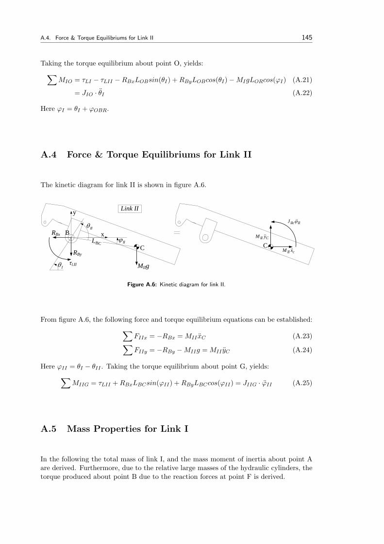
A.4. Force & Torque Equilibriums for Link II 145
Taking the torque equilibrium about point O, yields:∑MIO = τLI − τLII −RBxLOBsin(θI) + RByLOBcos(θI)−MIgLORcos(ϕI) (A.21)
= JIO · θI (A.22)
Here ϕI = θI + ϕOBR.
A.4 Force & Torque Equilibriums for Link II
The kinetic diagram for link II is shown in figure A.6.
C
x
y
BLBC
IIθ
IIϕ
Iθ MIIg
RBx
RBy
τLII
CcII xM &&
CII yM &&
IIIIcJ ϕ&&
Link II
Figure A.6: Kinetic diagram for link II.
From figure A.6, the following force and torque equilibrium equations can be established:∑FIIx = −RBx = MII xC (A.23)∑FIIy = −RBy −MIIg = MII yC (A.24)
Here ϕII = θI − θII . Taking the torque equilibrium about point G, yields:∑MIIG = τLII + RBxLBCsin(ϕII) + RByLBCcos(ϕII) = JIIG · ϕII (A.25)
A.5 Mass Properties for Link I
In the following the total mass of link I, and the mass moment of inertia about point Aare derived. Furthermore, due to the relative large masses of the hydraulic cylinders, thetorque produced about point B due to the reaction forces at point F is derived.
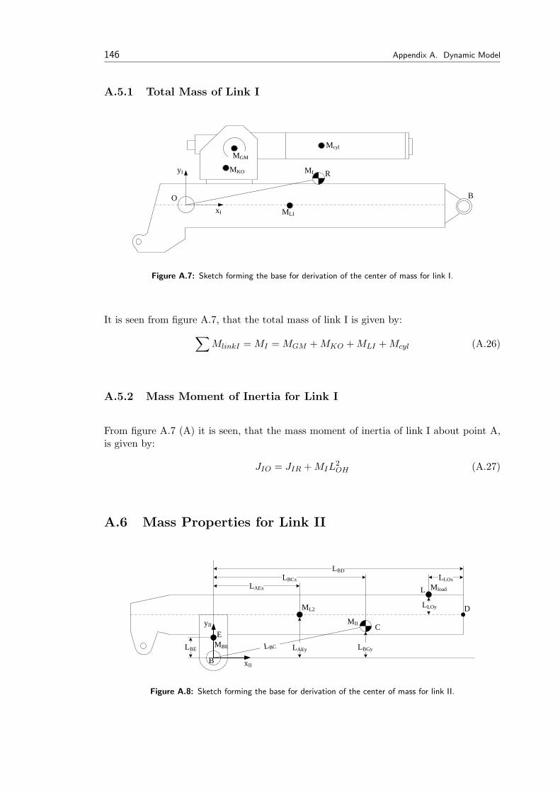
146 Appendix A. Dynamic Model
A.5.1 Total Mass of Link I
MGM
O B
RMKO
Mcyl
MLIxI
yI MI
Figure A.7: Sketch forming the base for derivation of the center of mass for link I.
It is seen from figure A.7, that the total mass of link I is given by:∑MlinkI = MI = MGM + MKO + MLI + Mcyl (A.26)
A.5.2 Mass Moment of Inertia for Link I
From figure A.7 (A) it is seen, that the mass moment of inertia of link I about point A,is given by:
JIO = JIR + MIL2OH (A.27)
A.6 Mass Properties for Link II
LAEx
C
MBE
xII
yII
ML2
Mload
LBCx
LBE LAEy LBGy
LBD
B
LBC
E
L
DLLOy
LLOx
MII
Figure A.8: Sketch forming the base for derivation of the center of mass for link II.
A.6. Mass Properties for Link II 147
A.6.1 Center of Mass for Link II
The total mass of link II is given by:∑MlinkII = MII = ML2 + Mload + MBE (A.28)
(A.29)
Due to the fact that load can vary, the position of the center of mass can vary, and hencean expression for this position is described. Related to the local coordinate system forlink II (xII , yII), the position of the center of mass is for the xII -position:∑
MlinkIILBCx = MIILBCx = ML2LAEx + Mload(LBD − LLOX) (A.30)
LBCx =ML2LAEx + Mload(LBD − LLOX)
MII(A.31)
And for the yII -position:∑MlinkIILBCy = MIILBCy = ML2LAEy + Mload(LAEy + LLOy) + MBELBE (A.32)
LBCy =ML2LAEy + Mload(LAEy + LLOy) + MBELBE
MII(A.33)
The length between point B and G is then given by:
LBC =√
L2BCx + L2
BCy (A.34)
In the expressions above, the nomenclature is:
LBCx: length from point B to point G (x-direction) 0.353 / 0.632 [m]LBCy: length from point B to point G (y-direction) 0.130 / 0.213 [m]LBC : length from point B to point G 0.376 / 0.667 [m]LAEx: length from point B to point K (x-direction) 0.420 [m]LAEy: length from point B to point K (y-direction) 0.142 [m]LBD: length from point B to point N 1.080 [m]LLOx: length from point L to point N 0.200 [m]LLOy: length from point K to point L 0.145 [m]LBE : length from point B to point J 0.071 [m]MBE : mass of bearing housing at point B 7.800 [kg]ML2: mass of link II 38.000 [kg]Mload: mass of load 0.000 / 50 [kg]MII : total mass of link II 45.800 / 95.800 [kg]
The above values has been obtained from [Andersen, 2004b]
A.6.2 Mass Moment of Inertia for Link II
The mass moment of inertia about point B is given by:
JCIIC = JC
L2 + JCAEx + JC
load (A.35)
148 Appendix A. Dynamic Model
Using the parallel axis theorem to find the mass moment of inertia about point G, yields:
JBIIC = JC
IIC + MIIL2BC (A.36)
A.7 Formulating the Describing Equations in Joint Space
In the following, the model will be established in cylinder space by use of the describingequations derived in the previous sections of the present appendix.
To be able to sustain the overview, the describing equations are presented again.
xG = −cos(θI)θ2ILOB − sin(θI)θILOB − cos(ϕII)ϕ2
IILBC − sin(ϕII)ϕIILBC (A.37)
yG = −sin(θI)θ2ILOB + cos(θI)θILOB − sin(ϕII)ϕ2
IILBC + cos(ϕII)ϕIILBC (A.38)
τLI = JIAθI + τLII + RBxLOBsin(θI)−RByLOBcos(θI) + MIgLORcos(ϕI) (A.39)τLII = JIIGϕII −RBxLBCsin(ϕII)−RByLBCcos(ϕII) (A.40)RBx = −MII xG (A.41)RBy = −MIIg −MII yG (A.42)
The model is expressed by use of the Newton-Euler formulation, given by:
τL = [τLI τLII ]T = D(q)q + H(q, q) + G(q) (A.43)
Substituting the above equations and substituting ϕII = θI − θII , the Newton-Euler for-mulation is obtained. The elements of D(q), H(q, q) and G(q) are found on the appendedCD, in the Maple file Newton Euler Joint Space.
A.8 Formulating the Describing Equations in Actuator Space
In this section the dynamic equations are formulated in actuator space. Expression A.43are related to the linear forces provided by the hydraulic actuators by the drive jacobianJ
d, yielding:
τL = JTdFL (A.44)
Where:
τL = [τLI τLII ]T , FL = [FLI FLII ]T , JTd
=[
LOQsin(αJI) 00 −LBGsin(αJII)
]
A.8. Formulating the Describing Equations in Actuator Space 149
Hence the non-linear dynamic model of the solid state part of the system compliant withthe hydraulic system, is established as:
FL = J−Td
τL = J−Td
D(q)q + J−Td H(q, q) + J−T
dG(q) (A.45)
The Jd
transpose provides the torque arms, and hence the perpendicular distance fromthe cylinder line of action, to the joints, relating the cylinder forces to the joint torques.In order to express equation B.3 in terms of the cylinder positions, the definition of thedrive jacobian is used:
xP = Jdq (A.46)
The piston velocities xP and accelerations xP , are obtained as:
xP = Jdq , xP = J
dq + J
dq (A.47)
Isolating the last expression above, yields:
Jdq = J
dq − xP (A.48)
q = J−1d
xP − J−1d
Jdq (A.49)
Substituting the expression for q, yields:
FL = J−Td
D(q)(J−1d
xP − J−1d
Jdq) + J−T
d H(q, q)J−1d
+ J−Td
G(q) (A.50)
= J−Td
D(q)J−1d
xP + (J−Td H(q, q)J−1
d− J−T
dD(q)J−1
dJ
dq) + J−T
dG(q) (A.51)
Hence the cylinder forces are expressed in terms of the piston velocities and accelerations.The inertia-, coriolis and gravitational terms are then given in actuator space, as:
MxP
(q) =[
MxP 11(q) MxP 12(q)MxP 21(q) MxP 22(q)
]= J−T
dD(q)J−1
d(A.52)
VxP
(q, q) =[
VxP 11(q) VxP 12(q)VxP 21(q) VxP 22(q)
]= (J−T
d H(q, q)J−1d− J−T
dD(q)J−1
dJ
dJ−1
d) (A.53)
GxP
(q) =[
GxP 1(q)GxP 2(q)
]= J−T
dG(q) (A.54)
By substituting expressions q, q and q, the formulation in actuator space is obtained as:
FL = MxP
(xP )xP + VxP
(xP , xP ) + GxP(xP )xP (A.55)
The model is now formulated in actuator space. However, friction phenomenons arepresent, hence coulomb and viscous friction elements are added, acting in the oppositedirection of the cylinder force, which yields:
FL = MxP
(xP )xP + VxP
(xP , xP ) + GxP(xP ) + BT
v xP + F Tc sign(xP ) (A.56)
The inertia, coriolis and gravitational terms are shown in figures A.9, A.10, A.11, A.12and A.13, respectively.
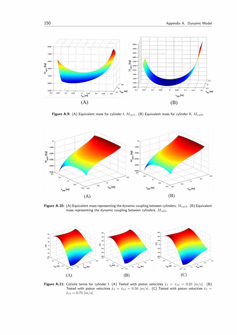
150 Appendix A. Dynamic Model
Figure A.9: (A) Equivalent mass for cylinder I, Meq11. (B) Equivalent mass for cylinder II, Meq22.
Figure A.10: (A) Equivalent mass representing the dynamic coupling between cylinders, Meq12. (B) Equivalentmass representing the dynamic coupling between cylinders, Meq21.
Figure A.11: Coriolis terms for cylinder I. (A) Tested with piston velocities xI = xII = 0.25 [m/s]. (B)Tested with piston velocities xI = xII = 0.50 [m/s]. (C) Tested with piston velocities xI =xII = 0.75 [m/s]
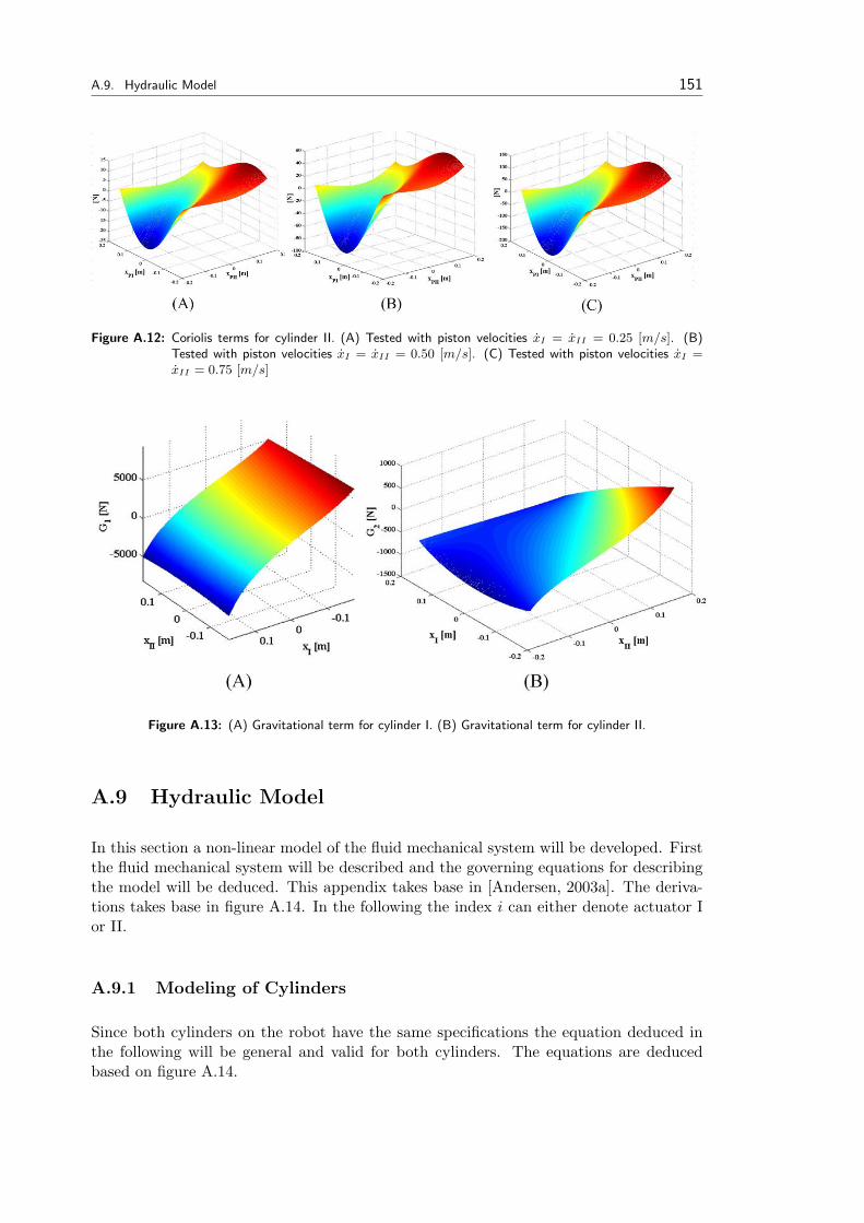
A.9. Hydraulic Model 151
Figure A.12: Coriolis terms for cylinder II. (A) Tested with piston velocities xI = xII = 0.25 [m/s]. (B)Tested with piston velocities xI = xII = 0.50 [m/s]. (C) Tested with piston velocities xI =xII = 0.75 [m/s]
Figure A.13: (A) Gravitational term for cylinder I. (B) Gravitational term for cylinder II.
A.9 Hydraulic Model
In this section a non-linear model of the fluid mechanical system will be developed. Firstthe fluid mechanical system will be described and the governing equations for describingthe model will be deduced. This appendix takes base in [Andersen, 2003a]. The deriva-tions takes base in figure A.14. In the following the index i can either denote actuator Ior II.
A.9.1 Modeling of Cylinders
Since both cylinders on the robot have the same specifications the equation deduced inthe following will be general and valid for both cylinders. The equations are deducedbased on figure A.14.
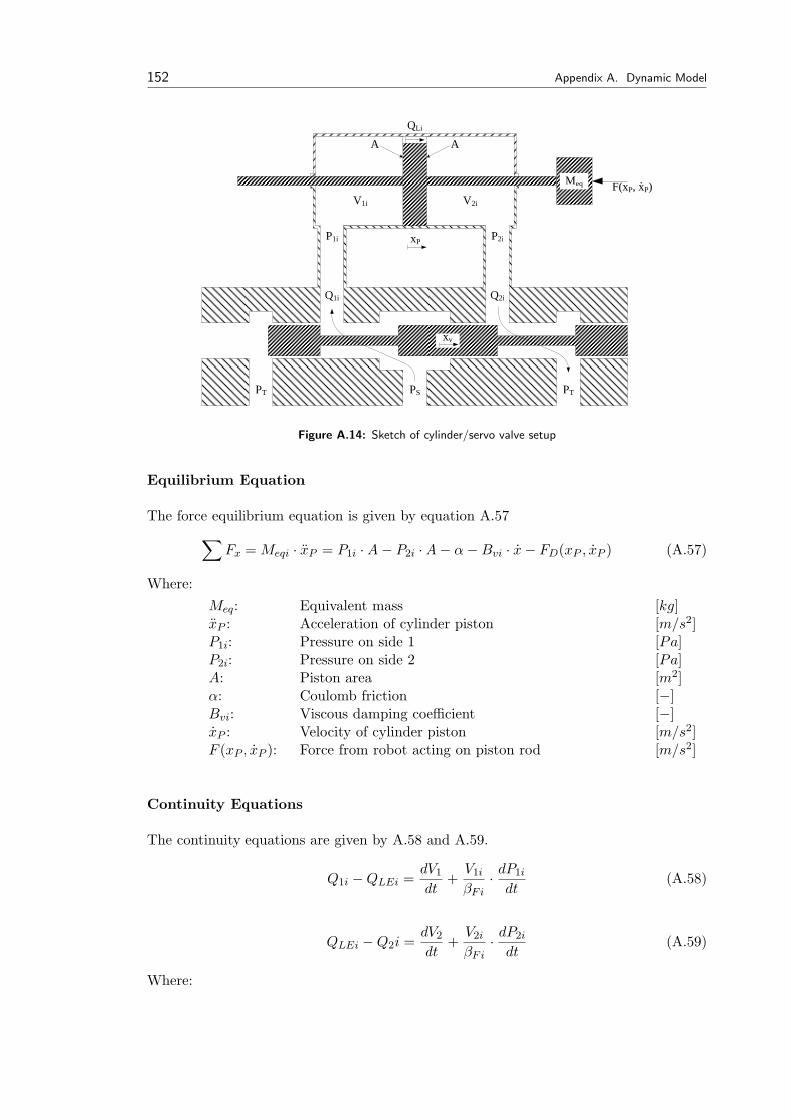
152 Appendix A. Dynamic Model
Q1i Q2i
PT PTPS
P1i P2i
A A
V1i
xP
Meq
V2i
xv
F(xP, xP).
QLi
Figure A.14: Sketch of cylinder/servo valve setup
Equilibrium Equation
The force equilibrium equation is given by equation A.57∑Fx = Meqi · xP = P1i ·A− P2i ·A− α−Bvi · x− FD(xP , xP ) (A.57)
Where:Meq: Equivalent mass [kg]xP : Acceleration of cylinder piston [m/s2]P1i: Pressure on side 1 [Pa]P2i: Pressure on side 2 [Pa]A: Piston area [m2]α: Coulomb friction [−]Bvi: Viscous damping coefficient [−]xP : Velocity of cylinder piston [m/s2]F (xP , xP ): Force from robot acting on piston rod [m/s2]
Continuity Equations
The continuity equations are given by A.58 and A.59.
Q1i −QLEi =dV1
dt+
V1i
βFi· dP1i
dt(A.58)
QLEi −Q2i =dV2
dt+
V2i
βFi· dP2i
dt(A.59)
Where:
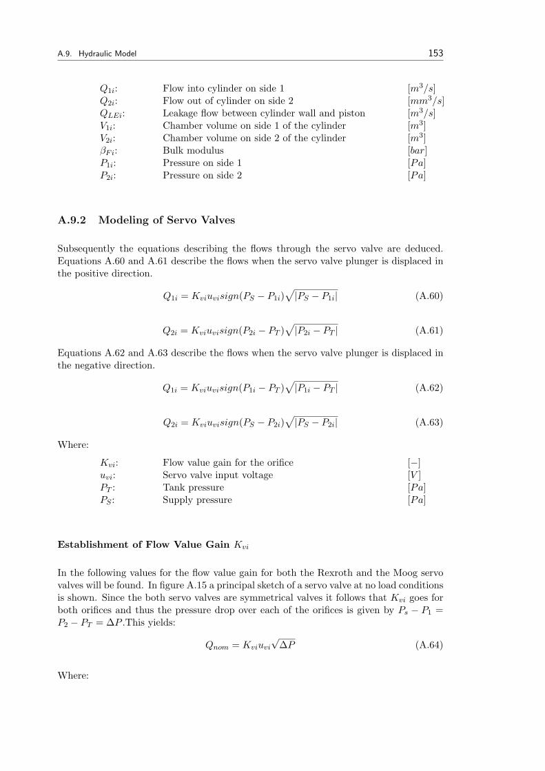
A.9. Hydraulic Model 153
Q1i: Flow into cylinder on side 1 [m3/s]Q2i: Flow out of cylinder on side 2 [mm3/s]QLEi: Leakage flow between cylinder wall and piston [m3/s]V1i: Chamber volume on side 1 of the cylinder [m3]V2i: Chamber volume on side 2 of the cylinder [m3]βFi: Bulk modulus [bar]P1i: Pressure on side 1 [Pa]P2i: Pressure on side 2 [Pa]
A.9.2 Modeling of Servo Valves
Subsequently the equations describing the flows through the servo valve are deduced.Equations A.60 and A.61 describe the flows when the servo valve plunger is displaced inthe positive direction.
Q1i = Kviuvisign(PS − P1i)√|PS − P1i| (A.60)
Q2i = Kviuvisign(P2i − PT )√|P2i − PT | (A.61)
Equations A.62 and A.63 describe the flows when the servo valve plunger is displaced inthe negative direction.
Q1i = Kviuvisign(P1i − PT )√|P1i − PT | (A.62)
Q2i = Kviuvisign(PS − P2i)√|PS − P2i| (A.63)
Where:
Kvi: Flow value gain for the orifice [−]uvi: Servo valve input voltage [V ]PT : Tank pressure [Pa]PS : Supply pressure [Pa]
Establishment of Flow Value Gain Kvi
In the following values for the flow value gain for both the Rexroth and the Moog servovalves will be found. In figure A.15 a principal sketch of a servo valve at no load conditionsis shown. Since the both servo valves are symmetrical valves it follows that Kvi goes forboth orifices and thus the pressure drop over each of the orifices is given by Ps − P1 =P2 − PT = ∆P .This yields:
Qnom = Kviuvi
√∆P (A.64)
Where:
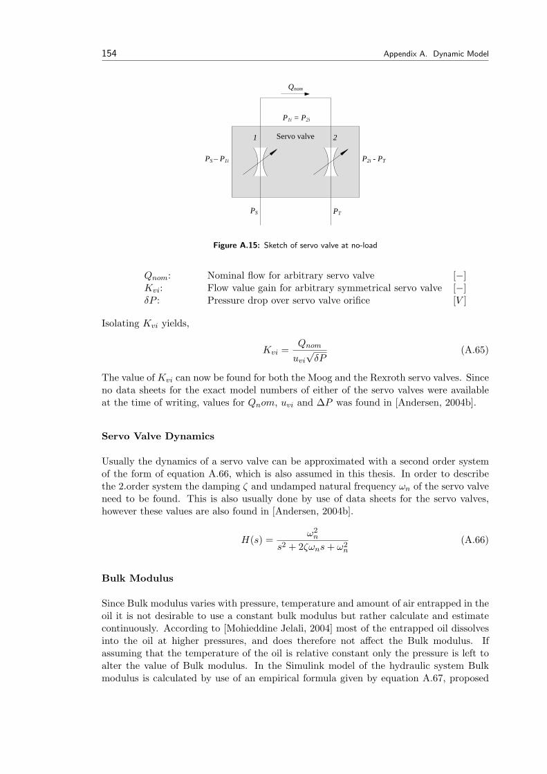
154 Appendix A. Dynamic Model
Servo valve
PS PT
P1i = P2i
1 2
PS – P1i P2i - PT
Qnom
Figure A.15: Sketch of servo valve at no-load
Qnom: Nominal flow for arbitrary servo valve [−]Kvi: Flow value gain for arbitrary symmetrical servo valve [−]δP : Pressure drop over servo valve orifice [V ]
Isolating Kvi yields,
Kvi =Qnom
uvi
√δP
(A.65)
The value of Kvi can now be found for both the Moog and the Rexroth servo valves. Sinceno data sheets for the exact model numbers of either of the servo valves were availableat the time of writing, values for Qnom, uvi and ∆P was found in [Andersen, 2004b].
Servo Valve Dynamics
Usually the dynamics of a servo valve can be approximated with a second order systemof the form of equation A.66, which is also assumed in this thesis. In order to describethe 2.order system the damping ζ and undamped natural frequency ωn of the servo valveneed to be found. This is also usually done by use of data sheets for the servo valves,however these values are also found in [Andersen, 2004b].
H(s) =ω2
n
s2 + 2ζωns + ω2n
(A.66)
Bulk Modulus
Since Bulk modulus varies with pressure, temperature and amount of air entrapped in theoil it is not desirable to use a constant bulk modulus but rather calculate and estimatecontinuously. According to [Mohieddine Jelali, 2004] most of the entrapped oil dissolvesinto the oil at higher pressures, and does therefore not affect the Bulk modulus. Ifassuming that the temperature of the oil is relative constant only the pressure is left toalter the value of Bulk modulus. In the Simulink model of the hydraulic system Bulkmodulus is calculated by use of an empirical formula given by equation A.67, proposed

A.10. Additional Verification Plots for the Nonlinear Model 155
in [Mohieddine Jelali, 2004].
E′(p) = a1Emaxlog(a2p
pmax+ a3) (A.67)
Where a1 = 0.5, a2 = 90, and a3 = 3 are empirical values, and the maximum value ofbulk modulus and the pressure are given as Emax and pmax, respectively.
A.10 Additional Verification Plots for the Nonlinear Model
In the following, addition verification plots for the nonlinear model is shown. Here thegravitation for link II is shown.
(A) (B)
0 1 2 3 4 5 6 7 8 95
10
15
20
25
30
Time [s]
Pres
sure
[Bar
]
Simulated load pressure PLII
Measured load pressure PLII
0 1 2 3 4 5 6 7 8 9-10
0
10
20
30
40
50
Time [s]
Pres
sure
[Bar
]
Simulated load pressure PLII
Measured load pressure PLII
Figure A.16: (A) Load pressure PLII . Both cylinder pistons are initially in retracted position. Cylinder II isextended, while cylinder I is kept in fixed position. (B) Load pressure PLII . Cylinder I is initiallyin extended position, and cylinder II in retracted position. Cylinder II is extended, while cylinderI is kept in fixed position.
(A) (B)
0 1 2 3 4 5 6 7 8 9-20
-10
0
10
20
30
40
Time [s]
Pres
sure
[Bar
]
Simulated load pressure PLII
Measured load pressure PLII
0 1 2 3 4 5 6 7 8 9-20
-15
-10
-5
0
5
10
15
20
Time [s]
Pres
sure
[Bar
]
Simulated load pressure PLII
Measured load pressure PLII
Figure A.17: (A) Load pressure PLII . Cylinder I is initially in retracted position, and cylinder II in extendedposition. Cylinder II is retracted, while cylinder I is kept in fixed position. (B) Load pressurePLKII . Both cylinder pistons are initially in extended position. Cylinder II is retracted, whilecylinder I is kept in fixed position.
It is found from figures A.16 and A.17, that the data acquisition for the pressures ofcylinder two is quite noisy. However, it is still possible to verify that the pressure levels,
156 Appendix A. Dynamic Model
and variations are similar when comparing the simulated and measured load pressuresfor cylinder II. Hence it is found that the part of the model concerning gravitation oncylinder II, is a sufficiently accurate rendering of the physical system.

Appendix BSimulink Modelof the RobotManipulator
Contents
A.1 Kinematics . . . . . . . . . . . 139
A.2 Positions, Velocities & Accel-erations of Point C . . . . . . 142
A.3 Force & Torque Equilibriumsfor Link I . . . . . . . . . . . . 144
A.4 Force & Torque Equilibriumsfor Link II . . . . . . . . . . . 145
A.5 Mass Properties for Link I . . 145
A.6 Mass Properties for Link II . . 146
A.7 Formulating the DescribingEquations in Joint Space . . . 148
A.8 Formulating the DescribingEquations in Actuator Space . 148
A.9 Hydraulic Model . . . . . . . . 151
A.10 Additional Verification Plotsfor the Nonlinear Model . . . . 155
In this appendix, the simulink model of the robot manipulator is presented, along with itslimitations.
The overall model of the system is shown in figure B.1.
time
Step2
Step1
Robot dynamics
P_LI
P_LII
x_I
x_dI
P_LI
x_PI
x_PII
P_LII
x_dII
x_II
Hydraulic dynamics
x_1
x_1,d
u_1
u_2
x_2,d
x_2
P_L1
P_L2
Clock
Figure B.1: Simulink model of the system.
157
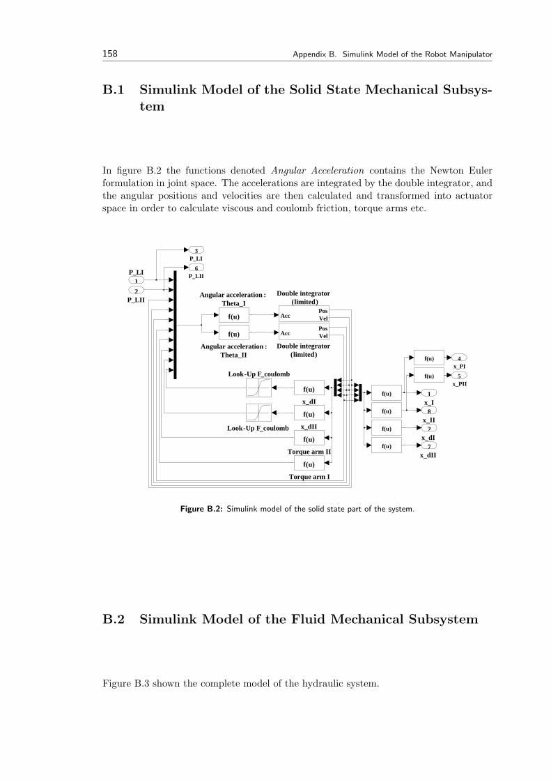
158 Appendix B. Simulink Model of the Robot Manipulator
B.1 Simulink Model of the Solid State Mechanical Subsys-tem
In figure B.2 the functions denoted Angular Acceleration contains the Newton Eulerformulation in joint space. The accelerations are integrated by the double integrator, andthe angular positions and velocities are then calculated and transformed into actuatorspace in order to calculate viscous and coulomb friction, torque arms etc.
x_II8
x_dII 7
P_LII 6
x_PII5
x_PI4
P_LI 3
x_dI 2
x_I1
x_dII
f(u)
x_dI
f(u)
Torque arm II
f(u)
Torque arm I
f(u)
Look-Up F_coulomb
Look-Up F_coulomb f(u)
f(u)
f(u)
f(u)
f(u)
f(u)
Double integrator (limited)
AccPosVel
Double integrator (limited)
AccPosVel
Angular acceleration : Theta_I
f(u)
Angular acceleration :Theta_II
f(u)
P_LII2
P_LI1
Figure B.2: Simulink model of the solid state part of the system.
B.2 Simulink Model of the Fluid Mechanical Subsystem
Figure B.3 shown the complete model of the hydraulic system.

B.2. Simulink Model of the Fluid Mechanical Subsystem 159
P_LII2
P_LI1
Valve for actuator II
u_vII
P_1II
P_2II
Q _1II
Q _2II
Valve for actuator I
P_1I
P_2I
u_vI
Q _1I
Q _2I
Continuity II
Q _1II
Q _2II
x_II
x_II,d
P_LII
P_1II
P_2II
Continuity I
Q _1I
Q _2I
x_I
x_I,d
P_1I
P_2I
P_L1
x_II6
x_II,d5
u_vII4
u_vI3
x_I,d2
x_I1
Figure B.3: Simulink model of the hydraulic part of the system.
The flow continuities and orifice equations are implemented in simulink as shown in figuresB.4, B.5 and B.6.
Q_2I2
Q_1I1
P_T
P_T
P_S
P_S
Servo Valve Dynamics
u_1 x_v1
f(u)
f(u)
f(u)
f(u) f(u)
f(u)
u_vI3
P_2I2
P_1I1
Figure B.4: Simulink model of servo valve.
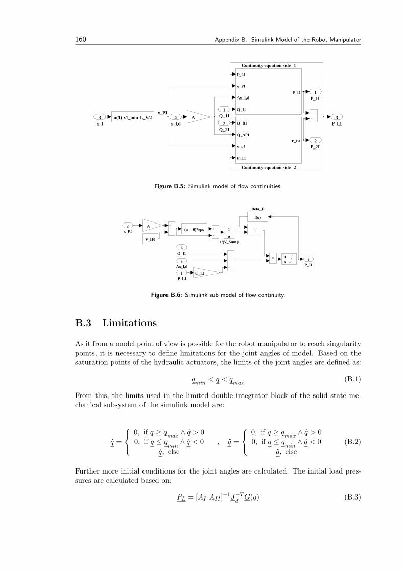
160 Appendix B. Simulink Model of the Robot Manipulator
x_PI
P_L13
P_2I 2
P_1I 1
u(1)-x1_min-L_V/2 A
Continuity equation side 2
Q _B1
Q _AP1
x_p1
P_L1
P_B1
Continuity equation side 1
P_LI
x_PI
Ax_1,d
Q _I1
P_I1
x_I,d4
x_I3
Q_2I2
Q_1I1
Figure B.5: Simulink model of flow continuities.
P_I11
A
1s
V_I10
C_LI
Beta_F
f(u)
1/(V_Sum )
1
u
(u==0)*eps
Q_I14
Ax_I,d3
x_PI2
P_LI1
Figure B.6: Simulink sub model of flow continuity.
B.3 Limitations
As it from a model point of view is possible for the robot manipulator to reach singularitypoints, it is necessary to define limitations for the joint angles of model. Based on thesaturation points of the hydraulic actuators, the limits of the joint angles are defined as:
qmin
< q < qmax
(B.1)
From this, the limits used in the limited double integrator block of the solid state me-chanical subsystem of the simulink model are:
q =
0, if q ≥ q
max∧ q > 0
0, if q ≤ qmin
∧ q < 0q, else
, q =
0, if q ≥ q
max∧ q > 0
0, if q ≤ qmin
∧ q < 0q, else
(B.2)
Further more initial conditions for the joint angles are calculated. The initial load pres-sures are calculated based on:
PL = [AI AII ]−1J−Td
G(q) (B.3)
Appendix CLinear Model ofRobotManipulator
Contents
B.1 Simulink Model of the SolidState Mechanical Subsystem . 158
B.2 Simulink Model of the FluidMechanical Subsystem . . . . 158
B.3 Limitations . . . . . . . . . . . 160
This appendix concerns the derivation of the linear SISO representation of the nonlineardynamic model of the robot manipulator. The linear SISO model is derived for use in thedevelopment of classical linear SISO controllers applied on the individual servo loops.
C.1 Linearized & Reduced Describing Dynamic Equations
To be able to establish the linear models, the describing dynamic equations are simplifiedand linearized for a defined point of operation for the two servo loops, and following fromthis a block diagram and hence a transfer function can be established. Furthermore it isnoticed that as the servo loops are similar to each other, both of the linear models arealgebraically equal to each other, and hence the indices are i = I ∨ i = II.
The assumptions used in this derivation are:
• The servo valves are constructed with ideal zero-lap spools
• Possible leakage flow in servo valves can be disregarded
• Supply pressure is constant
• Tank pressure is constant
Furthermore due to the high frequency of the servo valves compared to the frequency ofthe solid state part of the system, this is disregarded in the linear model as these are lessdominating for the dynamic behavior.
161
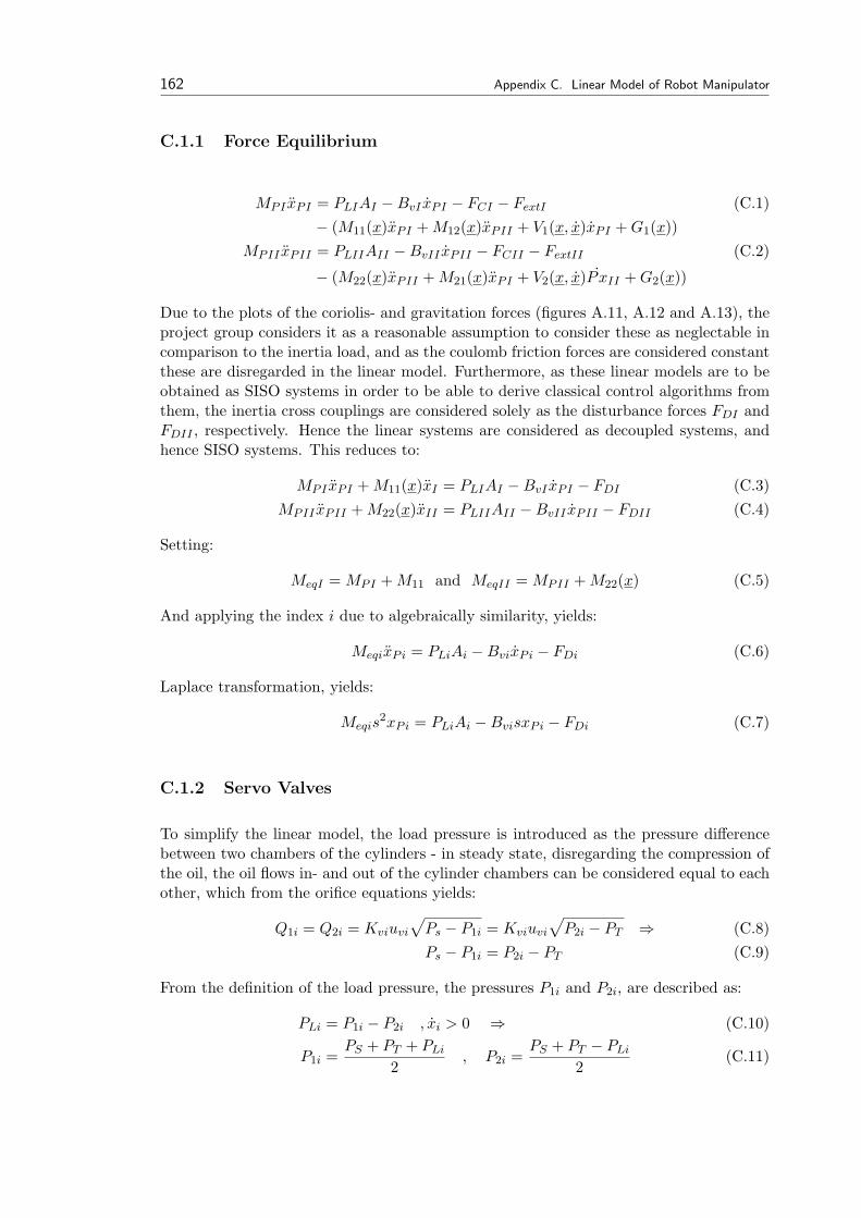
162 Appendix C. Linear Model of Robot Manipulator
C.1.1 Force Equilibrium
MPI xPI = PLIAI −BvI xPI − FCI − FextI (C.1)− (M11(x)xPI + M12(x)xPII + V1(x, x)xPI + G1(x))
MPII xPII = PLIIAII −BvII xPII − FCII − FextII (C.2)
− (M22(x)xPII + M21(x)xPI + V2(x, x)P xII + G2(x))
Due to the plots of the coriolis- and gravitation forces (figures A.11, A.12 and A.13), theproject group considers it as a reasonable assumption to consider these as neglectable incomparison to the inertia load, and as the coulomb friction forces are considered constantthese are disregarded in the linear model. Furthermore, as these linear models are to beobtained as SISO systems in order to be able to derive classical control algorithms fromthem, the inertia cross couplings are considered solely as the disturbance forces FDI andFDII , respectively. Hence the linear systems are considered as decoupled systems, andhence SISO systems. This reduces to:
MPI xPI + M11(x)xI = PLIAI −BvI xPI − FDI (C.3)MPII xPII + M22(x)xII = PLIIAII −BvII xPII − FDII (C.4)
Setting:
MeqI = MPI + M11 and MeqII = MPII + M22(x) (C.5)
And applying the index i due to algebraically similarity, yields:
MeqixPi = PLiAi −BvixPi − FDi (C.6)
Laplace transformation, yields:
Meqis2xPi = PLiAi −BvisxPi − FDi (C.7)
C.1.2 Servo Valves
To simplify the linear model, the load pressure is introduced as the pressure differencebetween two chambers of the cylinders - in steady state, disregarding the compression ofthe oil, the oil flows in- and out of the cylinder chambers can be considered equal to eachother, which from the orifice equations yields:
Q1i = Q2i = Kviuvi
√Ps − P1i = Kviuvi
√P2i − PT ⇒ (C.8)
Ps − P1i = P2i − PT (C.9)
From the definition of the load pressure, the pressures P1i and P2i, are described as:
PLi = P1i − P2i , xi > 0 ⇒ (C.10)
P1i =PS + PT + PLi
2, P2i =
PS + PT − PLi
2(C.11)
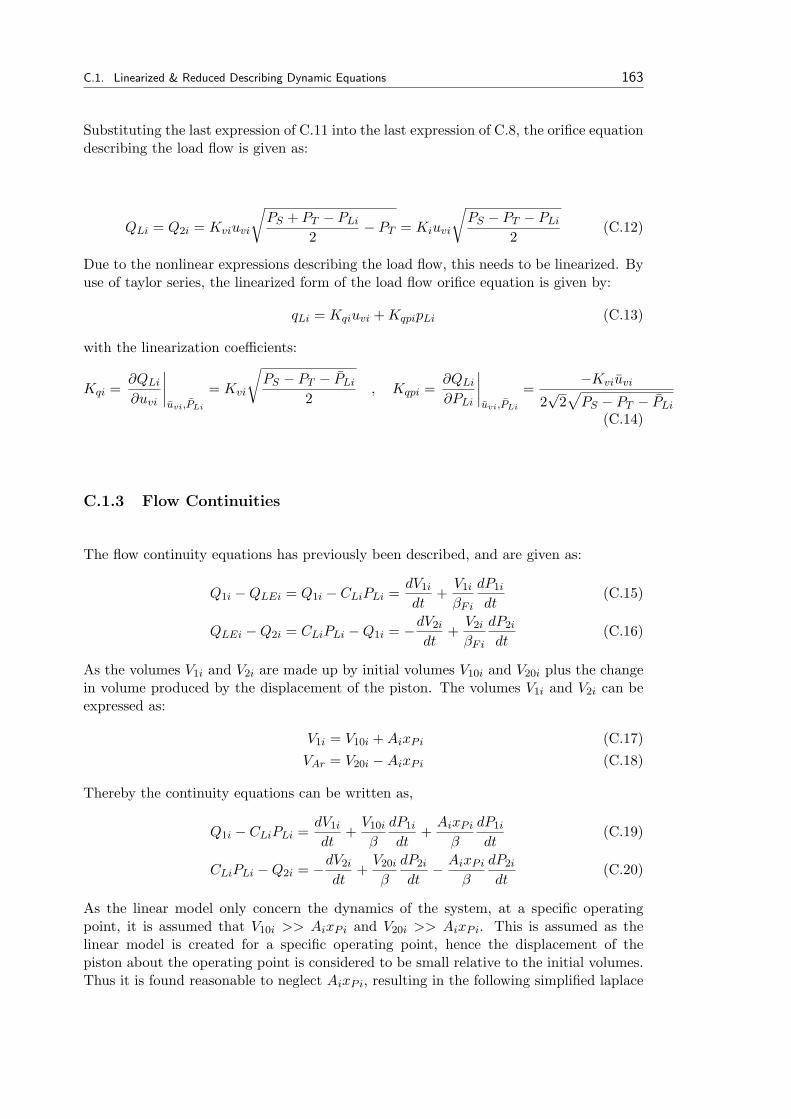
C.1. Linearized & Reduced Describing Dynamic Equations 163
Substituting the last expression of C.11 into the last expression of C.8, the orifice equationdescribing the load flow is given as:
QLi = Q2i = Kviuvi
√PS + PT − PLi
2− PT = Kiuvi
√PS − PT − PLi
2(C.12)
Due to the nonlinear expressions describing the load flow, this needs to be linearized. Byuse of taylor series, the linearized form of the load flow orifice equation is given by:
qLi = Kqiuvi + KqpipLi (C.13)
with the linearization coefficients:
Kqi =∂QLi
∂uvi
∣∣∣∣uvi,PLi
= Kvi
√PS − PT − PLi
2, Kqpi =
∂QLi
∂PLi
∣∣∣∣uvi,PLi
=−Kviuvi
2√
2√
PS − PT − PLi
(C.14)
C.1.3 Flow Continuities
The flow continuity equations has previously been described, and are given as:
Q1i −QLEi = Q1i − CLiPLi =dV1i
dt+
V1i
βFi
dP1i
dt(C.15)
QLEi −Q2i = CLiPLi −Q1i = −dV2i
dt+
V2i
βFi
dP2i
dt(C.16)
As the volumes V1i and V2i are made up by initial volumes V10i and V20i plus the changein volume produced by the displacement of the piston. The volumes V1i and V2i can beexpressed as:
V1i = V10i + AixPi (C.17)VAr = V20i −AixPi (C.18)
Thereby the continuity equations can be written as,
Q1i − CLiPLi =dV1i
dt+
V10i
β
dP1i
dt+
AixPi
β
dP1i
dt(C.19)
CLiPLi −Q2i = −dV2i
dt+
V20i
β
dP2i
dt− AixPi
β
dP2i
dt(C.20)
As the linear model only concern the dynamics of the system, at a specific operatingpoint, it is assumed that V10i >> AixPi and V20i >> AixPi. This is assumed as thelinear model is created for a specific operating point, hence the displacement of thepiston about the operating point is considered to be small relative to the initial volumes.Thus it is found reasonable to neglect AixPi, resulting in the following simplified laplace
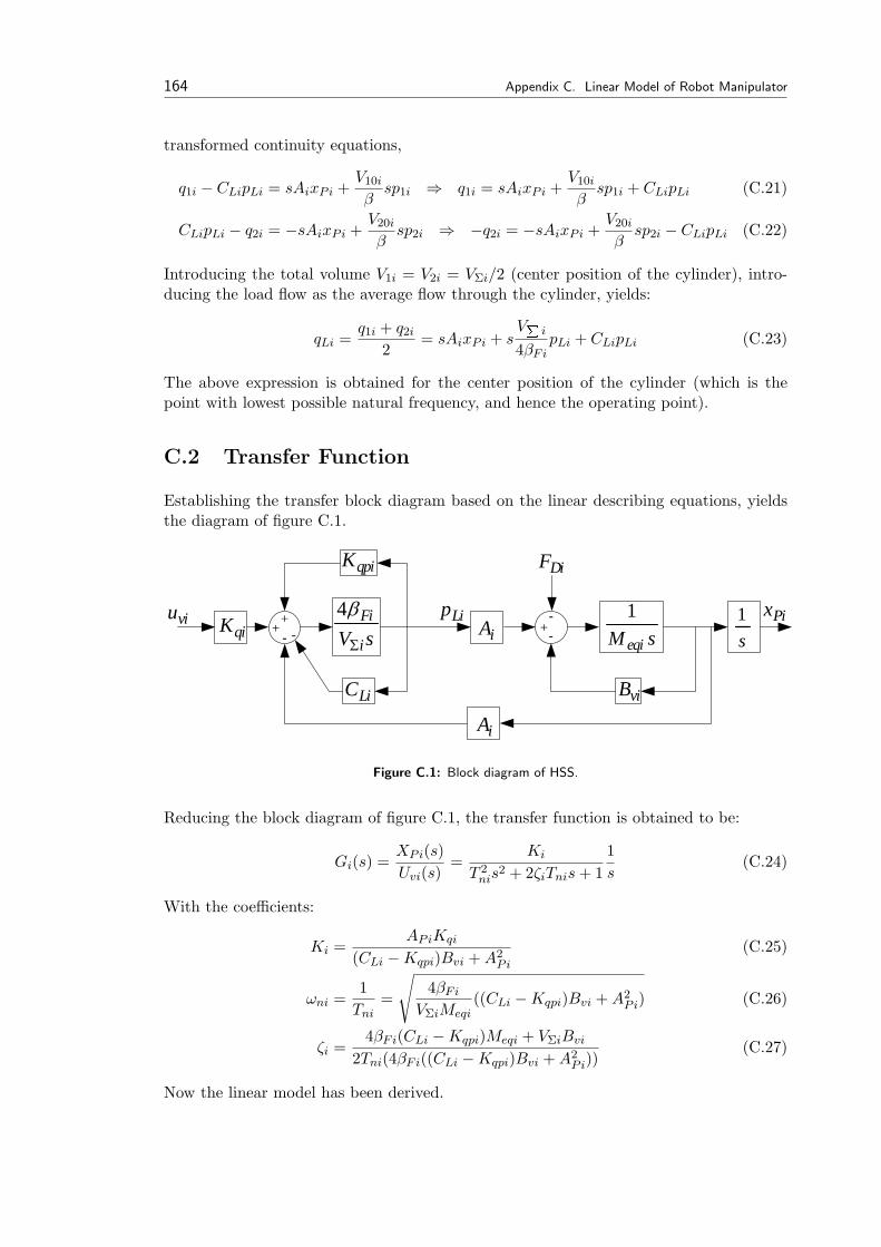
164 Appendix C. Linear Model of Robot Manipulator
transformed continuity equations,
q1i − CLipLi = sAixPi +V10i
βsp1i ⇒ q1i = sAixPi +
V10i
βsp1i + CLipLi (C.21)
CLipLi − q2i = −sAixPi +V20i
βsp2i ⇒ −q2i = −sAixPi +
V20i
βsp2i − CLipLi (C.22)
Introducing the total volume V1i = V2i = VΣi/2 (center position of the cylinder), intro-ducing the load flow as the average flow through the cylinder, yields:
qLi =q1i + q2i
2= sAixPi + s
VP i
4βFipLi + CLipLi (C.23)
The above expression is obtained for the center position of the cylinder (which is thepoint with lowest possible natural frequency, and hence the operating point).
C.2 Transfer Function
Establishing the transfer block diagram based on the linear describing equations, yieldsthe diagram of figure C.1.
+-+
sV i
Fi
Σ
β4iA
LiC
+- sMeqi
1s1
viB
PixLipqiKviu -
DiFqpiK
-
iA
Figure C.1: Block diagram of HSS.
Reducing the block diagram of figure C.1, the transfer function is obtained to be:
Gi(s) =XPi(s)Uvi(s)
=Ki
T 2nis
2 + 2ζiTnis + 11s
(C.24)
With the coefficients:
Ki =APiKqi
(CLi −Kqpi)Bvi + A2Pi
(C.25)
ωni =1
Tni=
√4βFi
VΣiMeqi((CLi −Kqpi)Bvi + A2
Pi) (C.26)
ζi =4βFi(CLi −Kqpi)Meqi + VΣiBvi
2Tni(4βFi((CLi −Kqpi)Bvi + A2Pi))
(C.27)
Now the linear model has been derived.

C.3. Assessment of Operating Point 165
C.3 Assessment of Operating Point
Regarding an operating point for which the linear models must be valid, a critical pointof operation must be chosen - regarding the cylinders the critical point of operation iswhere the lowest possible natural frequency occurs, which for symmetric actuators is atthe center position. Due to the symmetry of the cylinders, this critical point occurs atthe center stroke position.
-90
-80
-70
-60
-50
-40
Mag
nitu
de (d
B)
101
102
-225
-180
-135
-90
Phas
e (d
eg)
Bode Diagram
Frequency (rad/sec)
uvI=0.01 [V]
uvI=2 [V]
uvI=4 [V]
uvI=6 [V]
uvI=8 [V]
uvI=10 [V]
Indsæt egenfrekvensplot
(A) (B)Figure C.2: Bode diagram of HSS I with different values for the input voltage at the operating point.
Regarding an operating point for the servo valves, the damping ratio of the transfer func-tion is examined via its bode diagram, when varying the input signal in the linearizationcoefficients - it is seen from the bode diagram in figure C.2, that the critical point of op-eration is when the spool of the servo valve is slightly opened, due to the poor dampingratio.

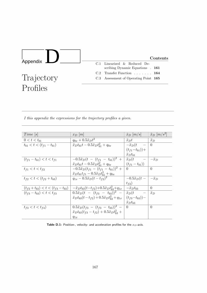
Appendix DTrajectoryProfiles
Contents
C.1 Linearized & Reduced De-scribing Dynamic Equations . 161
C.2 Transfer Function . . . . . . . 164
C.3 Assessment of Operating Point 165
I this appendix the expressions for the trajectory profiles a given.
Time [s] xD [m] xD [m/s] xD [m/s2]0 < t < tb1 q0x + 0.5xDt2 xDt xD
tb1 < t < (tf1 − tb1) xDtb1t− 0.5xDt2b1 + q0x −xD(t −(tf1−tb1))+xDtb1
0
(tf1 − tb1) < t < tf1 −0.5xD(t − (tf1 − tb1))2 +xDtb1t− 0.5xDt2b1 + q0x
xD(t −(tf1 − tb1))
−xD
tf1 < t < tf2 −0.5xD(tf1 − (tf1 − tb1))2 +xDtb1tf1 − 0.5xDt2b1 + q0x
0 0
tf2 < t < (tf2 + tb3) q1x − 0.5xD(t− tf2)2 −0.5xD(t −tf2)
−xD
(tf2 + tb3) < t < (tf3 − tb3) −xDtb3(t−tf2)+0.5xDt2b3+q1x −xDtb3 0(tf3 − tb3) < t < tf3 0.5xD(t − (tf3 − tb3))2 −
xDtb3(t− tf2)+0.5xDt2b3 + q1x
xD(t −(tf3−tb3))−xDtb3
xD
tf3 < t < tf4) 0.5xD(tf3 − (tf3 − tb3))2 −xDtb3(tf3 − tf2) + 0.5xDt2b3 +q1x
0 0
Table D.1: Position-, velocity- and acceleration profiles for the xD-axis.
167
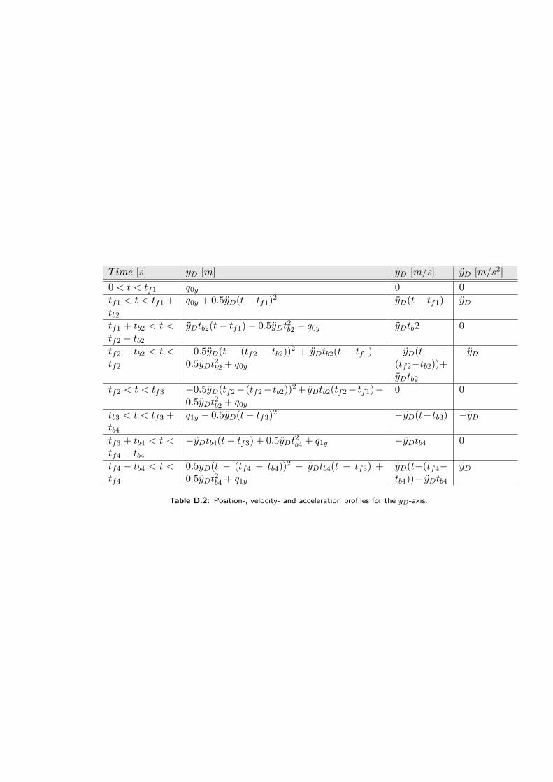
Time [s] yD [m] yD [m/s] yD [m/s2]0 < t < tf1 q0y 0 0tf1 < t < tf1 +tb2
q0y + 0.5yD(t− tf1)2 yD(t− tf1) yD
tf1 + tb2 < t <tf2 − tb2
yDtb2(t− tf1)− 0.5yDt2b2 + q0y yDtb2 0
tf2 − tb2 < t <tf2
−0.5yD(t − (tf2 − tb2))2 + yDtb2(t − tf1) −0.5yDt2b2 + q0y
−yD(t −(tf2−tb2))+yDtb2
−yD
tf2 < t < tf3 −0.5yD(tf2− (tf2− tb2))2 + yDtb2(tf2− tf1)−0.5yDt2b2 + q0y
0 0
tb3 < t < tf3 +tb4
q1y − 0.5yD(t− tf3)2 −yD(t−tb3) −yD
tf3 + tb4 < t <tf4 − tb4
−yDtb4(t− tf3) + 0.5yDt2b4 + q1y −yDtb4 0
tf4 − tb4 < t <tf4
0.5yD(t − (tf4 − tb4))2 − yDtb4(t − tf3) +0.5yDt2b4 + q1y
yD(t−(tf4−tb4))− yDtb4
yD
Table D.2: Position-, velocity- and acceleration profiles for the yD-axis.
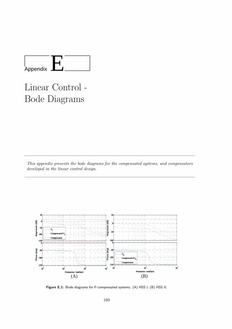
Appendix ELinear Control -Bode Diagrams
This appendix presents the bode diagrams for the compensated systems, and compensatorsdeveloped in the linear control design.
(A) (B)
-150
-100
-50
0
50
Mag
nitu
de (d
B)
100
101
102
103
-270
-180
-90
0
Phas
e (d
eg)
Frequency (rad/sec)
GI
Compensated GI
Compensator-100
-50
0
50
Mag
nitu
de (d
B)
101
102
103
-270
-180
-90
0
Pha
se (d
eg)
Frequency (rad/sec)
GII
Compensated GII
Compensator
Figure E.1: Bode diagrams for P-compensated systems. (A) HSS I. (B) HSS II.
169
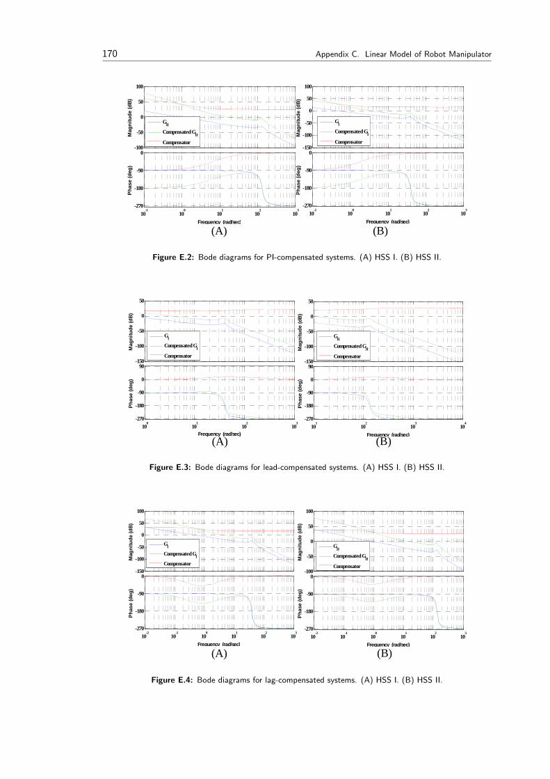
170 Appendix C. Linear Model of Robot Manipulator
(A) (B)
-100
-50
0
50
100
Mag
nitu
de (d
B)
10-1
100
101
102
103
-270
-180
-90
0
Phas
e (d
eg)
Frequency (rad/sec)
GII
Compensated GII
Compensator-150
-100
-50
0
50
100
Mag
nitu
de (d
B)
10-1
100
101
102
103
-270
-180
-90
0
Phas
e (d
eg)
Frequency (rad/sec)
GI
Compensated GI
Compensator
Figure E.2: Bode diagrams for PI-compensated systems. (A) HSS I. (B) HSS II.
(A) (B)
-150
-100
-50
0
50
Mag
nitu
de (d
B)
100
101
102
103
-270
-180
-90
0
90
Phas
e (d
eg)
Frequency (rad/sec)
GI
Compensated GI
Compensator-150
-100
-50
0
50M
agni
tude
(dB
)
101
102
103
104
-270
-180
-90
0
90
Pha
se (d
eg)
Frequency (rad/sec)
GII
Compensated GII
Compensator
Figure E.3: Bode diagrams for lead-compensated systems. (A) HSS I. (B) HSS II.
(A) (B)
-150
-100
-50
0
50
100
Mag
nitu
de (d
B)
10-2
10-1
100
101
102
103
-270
-180
-90
0
Phas
e (d
eg)
Frequency (rad/sec)
GI
Compensated GI
Compensator-100
-50
0
50
100
Mag
nitu
de (d
B)
10-2
10-1
100
101
102
103
-270
-180
-90
0
Pha
se (d
eg)
Frequency (rad/sec)
GII
Compensated GII
Compensator
Figure E.4: Bode diagrams for lag-compensated systems. (A) HSS I. (B) HSS II.
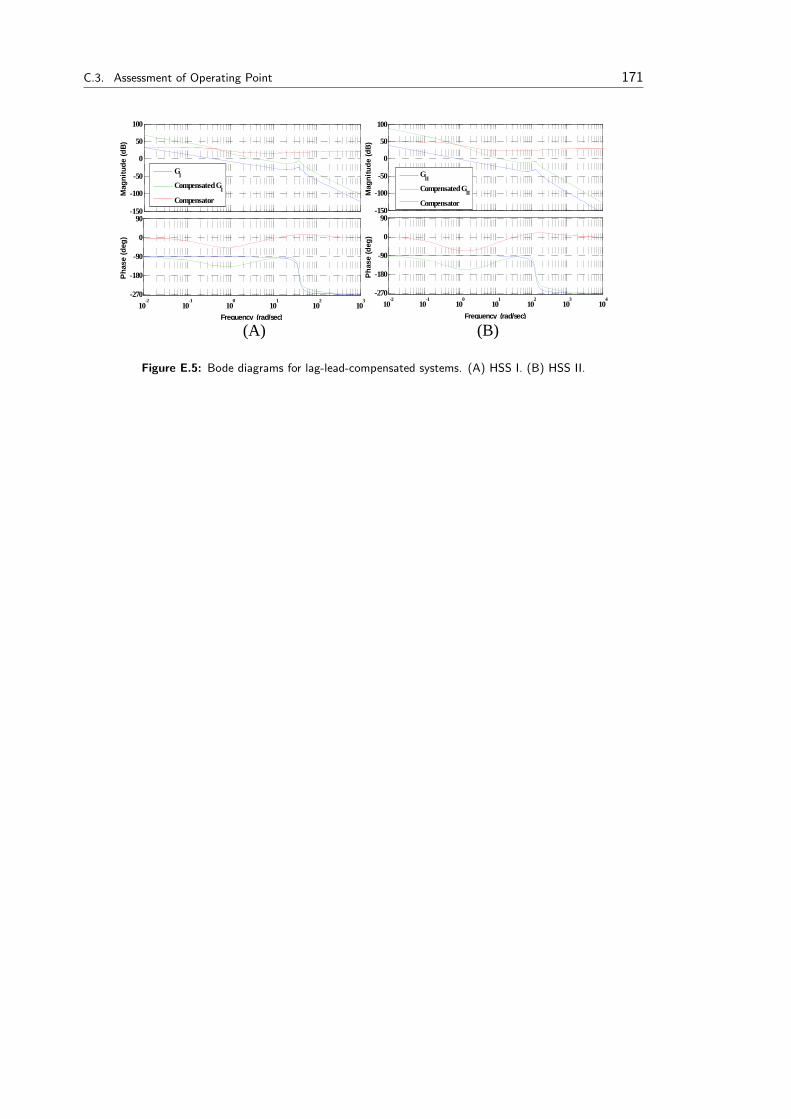
C.3. Assessment of Operating Point 171
(A) (B)
-150
-100
-50
0
50
100M
agni
tude
(dB)
10-2
10-1
100
101
102
103
-270
-180
-90
0
90
Pha
se (d
eg)
Frequency (rad/sec)
GI
Compensated GI
Compensator-150
-100
-50
0
50
100
Mag
nitu
de (d
B)
10-2
10-1
100
101
102
103
104
-270
-180
-90
0
90
Phas
e (d
eg)
Frequency (rad/sec)
GII
Compensated GII
Compensator
Figure E.5: Bode diagrams for lag-lead-compensated systems. (A) HSS I. (B) HSS II.

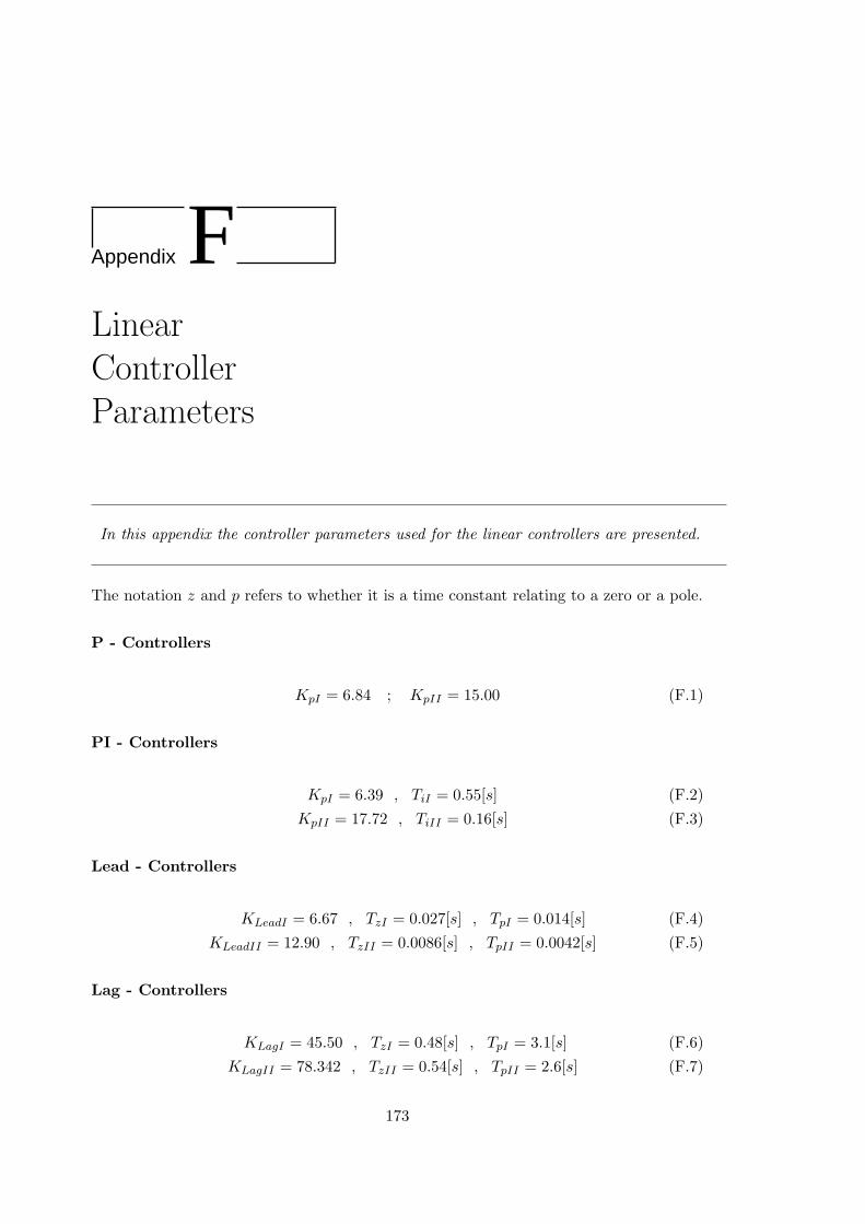
Appendix FLinearControllerParameters
In this appendix the controller parameters used for the linear controllers are presented.
The notation z and p refers to whether it is a time constant relating to a zero or a pole.
P - Controllers
KpI = 6.84 ; KpII = 15.00 (F.1)
PI - Controllers
KpI = 6.39 , TiI = 0.55[s] (F.2)KpII = 17.72 , TiII = 0.16[s] (F.3)
Lead - Controllers
KLeadI = 6.67 , TzI = 0.027[s] , TpI = 0.014[s] (F.4)KLeadII = 12.90 , TzII = 0.0086[s] , TpII = 0.0042[s] (F.5)
Lag - Controllers
KLagI = 45.50 , TzI = 0.48[s] , TpI = 3.1[s] (F.6)KLagII = 78.342 , TzII = 0.54[s] , TpII = 2.6[s] (F.7)
173
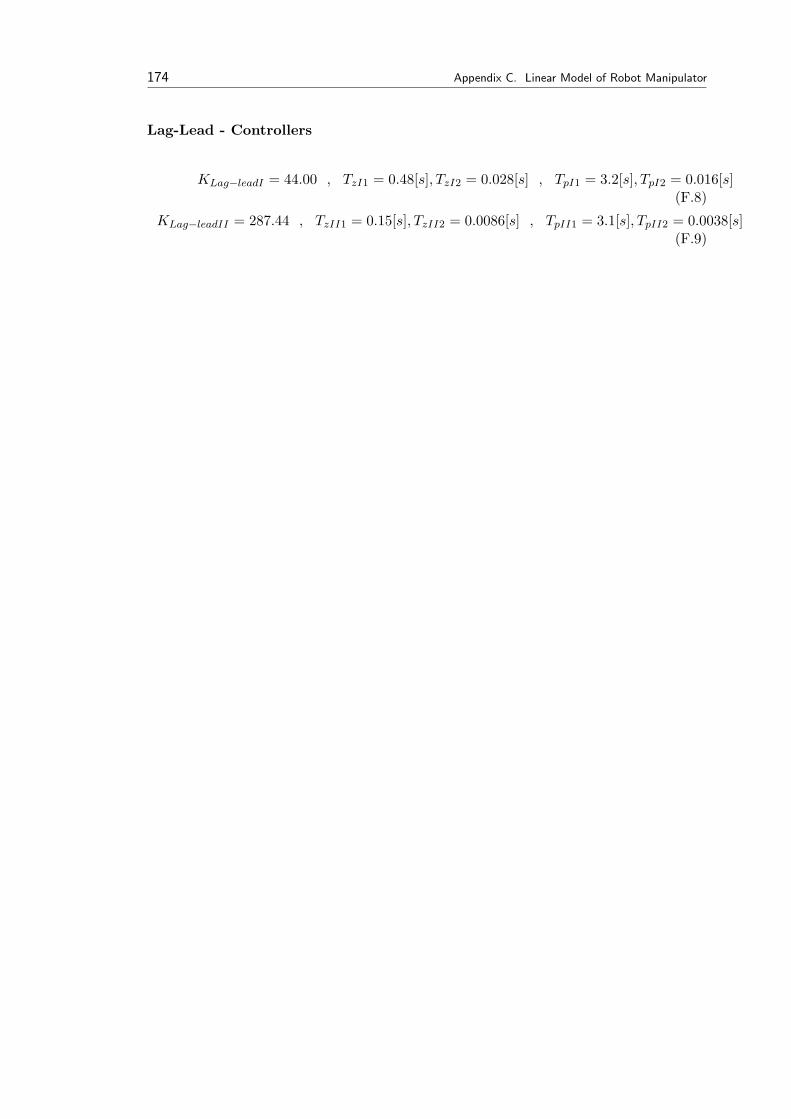
174 Appendix C. Linear Model of Robot Manipulator
Lag-Lead - Controllers
KLag−leadI = 44.00 , TzI1 = 0.48[s], TzI2 = 0.028[s] , TpI1 = 3.2[s], TpI2 = 0.016[s](F.8)
KLag−leadII = 287.44 , TzII1 = 0.15[s], TzII2 = 0.0086[s] , TpII1 = 3.1[s], TpII2 = 0.0038[s](F.9)
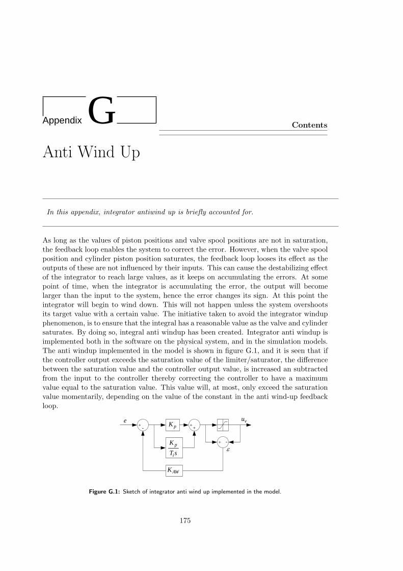
Appendix GAnti Wind Up
Contents
In this appendix, integrator antiwind up is briefly accounted for.
As long as the values of piston positions and valve spool positions are not in saturation,the feedback loop enables the system to correct the error. However, when the valve spoolposition and cylinder piston position saturates, the feedback loop looses its effect as theoutputs of these are not influenced by their inputs. This can cause the destabilizing effectof the integrator to reach large values, as it keeps on accumulating the errors. At somepoint of time, when the integrator is accumulating the error, the output will becomelarger than the input to the system, hence the error changes its sign. At this point theintegrator will begin to wind down. This will not happen unless the system overshootsits target value with a certain value. The initiative taken to avoid the integrator windupphenomenon, is to ensure that the integral has a reasonable value as the valve and cylindersaturates. By doing so, integral anti windup has been created. Integrator anti windup isimplemented both in the software on the physical system, and in the simulation models.The anti windup implemented in the model is shown in figure G.1, and it is seen that ifthe controller output exceeds the saturation value of the limiter/saturator, the differencebetween the saturation value and the controller output value, is increased an subtractedfrom the input to the controller thereby correcting the controller to have a maximumvalue equal to the saturation value. This value will, at most, only exceed the saturationvalue momentarily, depending on the value of the constant in the anti wind-up feedbackloop.
++-+ pK
sTK
i
p -+
AWK
ε
e vu
Figure G.1: Sketch of integrator anti wind up implemented in the model.
175


Appendix HLemmas,Theorems &Norms
This appendix presents the theorems, lemmas and function norms used in the stabilityproofs of the adaptive controllers.
H.1 Lyapunov’s Stability Theorem
If there exists a function V : <n → < which is positive definite, and if its derivative alongdxdt = f(x) is negative semi-definite, then the solution x = 0 is stable. If dV
dt is negativedefinite, then the solution is asymptotically stable. V is then referred to as a Lyapunovfunction for dx
dt = f(x).
H.2 Lemma I
(This lemma has been taken directly from [Slotine E J-J, 1991])
Consider two signals e and φ related by the following dynamic equation:
e(t) = H(s)(kφT (t)v(t)) (H.1)
Where:
e(t): scalar output signal [−]H(s): strictly positive real transfer function [−]k: unknown constant with known sign [−]φ(t): m× 1 vector function of time [−]v(t): measurable m× 1 vector [−]
177
178 Appendix H. Lemmas, Theorems & Norms
If the vector φ varies according to:
φ = −sign(k)γev(t) (H.2)
with γ being a positive constant, then e(t) and φ(t) are globally bounded. Furthermoreif v(t) is bounded, then:
e → 0 for t →∞ (H.3)
H.3 Lemma II - Barbalats Lemma
If g is a real function of a real variable t, defined and uniformly continuous for t ≥ 0, andif the limit of the integral: ∫ t
0g(τ)dτ (H.4)
Exists for t →∞ and is a finite number, then:
limt→∞
g(t) = 0 (H.5)
Remark: A consequence of Barbalats Lemma is that if g ∈ L2 and dgdt is bounded, then:
limt→∞
g(t) = 0 (H.6)
Uniform Continuity
A sufficient condition for a differentiable function to be uniformly continuous is that itsderivative is bounded.
H.4 Lemma III - Lyapunov-like Lemma
If a scalar function V (x, t) satisfies the following conditions:
• V (x, t) is lower bounded
• V (x, t) is negative semi-definite
• V (x, t) is uniformly continuous
Then:
V (x, t) → 0 for t →∞ (H.7)
H.5. Function Norms 179
H.5 Function Norms
(Taken directly from [Andersen, 2003b])
For any fixed p ∈ [1,∞], if f : <n → < belongs to Lp if∫∞0 |f(t)|pdt < ∞. The associated
norm is:
‖fp‖ =(∫ ∞
0|f(t)|pdt
) 1p
=1kp
(H.8)
In addition to the class of functions in Lp, this extended space also includes truncatedfunctions of the form:
fT (t) =
f(t) t ≤ T0 t > T
(H.9)
Such that:
‖fT ‖p < ∞ ; ∀T (H.10)
H.6 Induced Matrix Norms
(Taken directly from [Andersen, 2003b])
For a matrix A ∈ <n×n a norm can be defined by,
‖A‖p= supx 6=0
‖Ax‖p
‖x‖p, ∀x ∈ <n (H.11)
The norm is called the induced (matrix) norm of A corresponding to the vector norm‖x‖p. For the induced norm it can be shown that,
‖AB‖p ≤ ‖A‖p · ‖B‖p, ∀A, B ∈ <n×n (H.12)
‖Ax‖p ≤ ‖A‖p · ‖x‖p, ∀A ∈ <n×n, x ∈ <n (H.13)
For p = 2 the induced norm can be given as ‖A‖2 =√
maxiλi(AT A).
H.7 Gain of Linear Operators
(Taken directly from [Andersen, 2003b])
Let H be a causal operator H : f → g. The Lp gain of H is denoted ‖H‖p and is definedas the smalles value of γ such that:
‖g‖p = ‖Hf‖p ≤ γ‖f‖p + β ∀f ∈ Lp (H.14)

180 Appendix H. Lemmas, Theorems & Norms
Consider the convolution-type operator H : f → g given by,
g(t) =∫ ∞
−∞h(t− τ)f(τ)dτ ∀t ∈ < (H.15)
Then for p = 2 the L2 gain is given by:
‖H‖2 = maxω∈<
|h(jω)| (H.16)
Where h(s) is the laplace transform of the impulse response of H. For p = ∞ the L∞ isgiven by:
‖H‖∞ =∫ ∞
0|h(t)|dt (H.17)
Having defined the Lp spaces the following lemma is useful in analysing the input-outputproporties of systems with exponentially stable transfer functions.
Lemma 1: (Desoer & Vidyasagar)
Let the transfer function H(s) be exponentially stable and strictly proper. Then f ∈ L2
implies that g = H · f ∈ L2 ∩ L∞, g ∈ L2, g is continuous, and g → 0 as t → ∞. If, inaddition f → 0 as t →∞, then g → 0.
H.8 Normed Spaces
(Taken directly from [Andersen, 2003b])
A normed space is a vector space V with a given norm. A norm on a vector space Vis a rule which, given any x ∈ V , specifies a real number ‖x‖, such that,
(a) ‖x‖ > 0 if x 6= 0, and ‖0‖ = 0;(b) ‖ax‖ = |a| · ‖x‖ for any x ∈ V and any scalar a;(c) ‖x + y‖ ≤ ‖x‖+ ‖y‖ for any x, y ∈ V (the triangle inequality);
A normed vector space is called real or complex according to whether the underlyingvector space V is real or complex. Subsequent only norms defined on <n are considered.
Examples of norms which satisfy the axioms of the norm are,
‖x‖1=n∑
i=1
|xi| (H.18)
H.8. Normed Spaces 181
‖x‖p=
(n∑
i=1
|xi|p)1/p
(H.19)
‖x‖∞= maxi|xi| (H.20)
‖x‖2 is the usual Euclidean of x.
An important result is that all norms are equivalent in the sense that there exist positivenumbers κ1 and κ2 such that,
κ1‖x‖a ≤ ‖x‖b ≤ κ2‖x‖a,∀x ∈ <n (H.21)
This means that any norm can be used to show boundedness or convergence. Hence,often the symbol ‖ · ‖ is used without specifying exactly which norm is meant.

Appendix ISimulationResults forAIDC, AAC,RAIDC &RAAC
Contents
H.1 Lyapunov’s Stability Theorem 177
H.2 Lemma I . . . . . . . . . . . . 177
H.3 Lemma II - Barbalats Lemma 178
H.4 Lemma III - Lyapunov-likeLemma . . . . . . . . . . . . . 178
H.5 Function Norms . . . . . . . . 179
H.6 Induced Matrix Norms . . . . 179
H.7 Gain of Linear Operators . . . 179
H.8 Normed Spaces . . . . . . . . . 180
In this appendix the simulation results for the AIDC, AAC, RAIDC and AAC schemes arepresented. These are presented for the rectangular trajectory, and the plots when simulatedon the in/out trajectory are found on the appended CD.
183
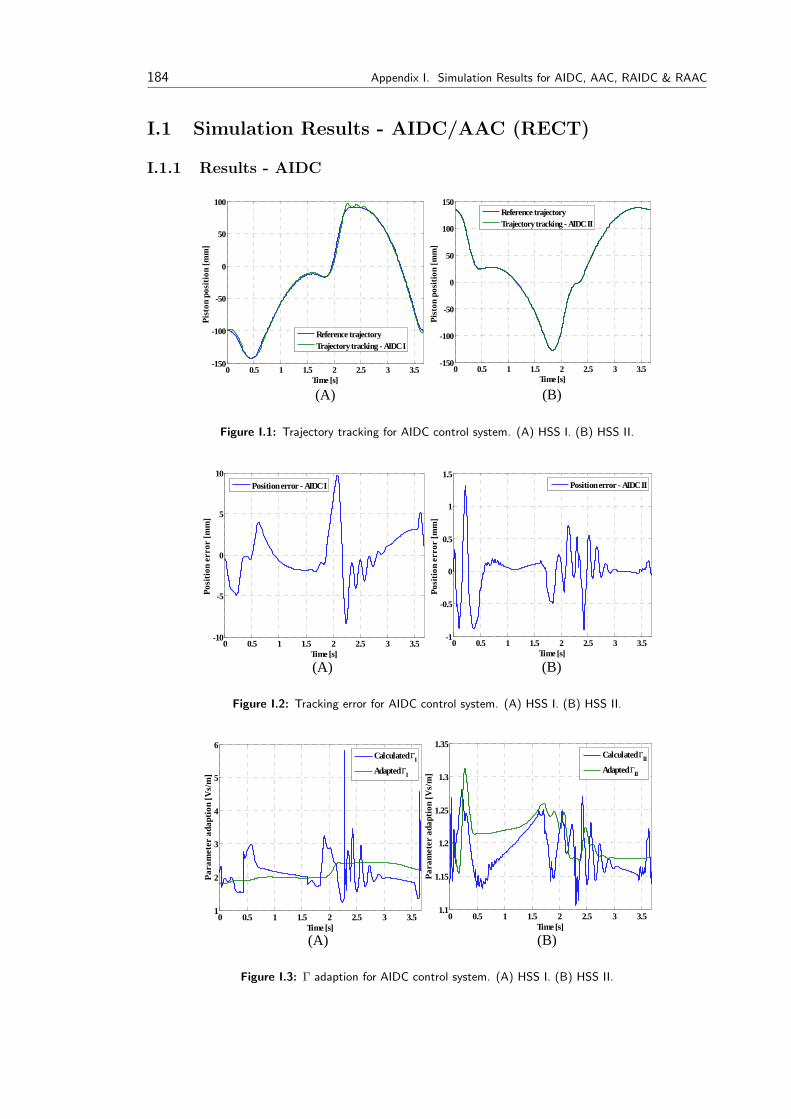
184 Appendix I. Simulation Results for AIDC, AAC, RAIDC & RAAC
I.1 Simulation Results - AIDC/AAC (RECT)
I.1.1 Results - AIDC
(A) (B)
0 0.5 1 1.5 2 2.5 3 3.5-150
-100
-50
0
50
100
Time [s]
Pist
on p
ositi
on [m
m]
Reference trajectoryTrajectory tracking - AIDC I
0 0.5 1 1.5 2 2.5 3 3.5-150
-100
-50
0
50
100
150
Time [s]
Pist
on p
ositi
on [m
m]
Reference trajectoryTrajectory tracking - AIDC II
Figure I.1: Trajectory tracking for AIDC control system. (A) HSS I. (B) HSS II.
0 0.5 1 1.5 2 2.5 3 3.5-10
-5
0
5
10
Time [s]
Posi
tion
erro
r [m
m]
Position error - AIDC I
0 0.5 1 1.5 2 2.5 3 3.5-1
-0.5
0
0.5
1
1.5
Time [s]
Posi
tion
erro
r [m
m]
Position error - AIDC II
(A) (B)
Figure I.2: Tracking error for AIDC control system. (A) HSS I. (B) HSS II.
0 0.5 1 1.5 2 2.5 3 3.51
2
3
4
5
6
Time [s]
Para
met
er a
dapt
ion
[Vs/
m]
Calculated ΓI
Adapted ΓI
0 0.5 1 1.5 2 2.5 3 3.51.1
1.15
1.2
1.25
1.3
1.35
Time [s]
Para
met
er a
dapt
ion
[Vs/
m]
Calculated ΓII
Adapted ΓII
(A) (B)
Figure I.3: Γ adaption for AIDC control system. (A) HSS I. (B) HSS II.
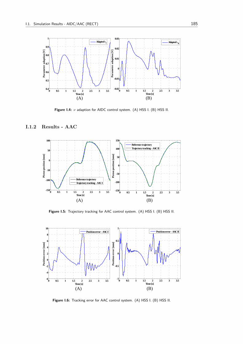
I.1. Simulation Results - AIDC/AAC (RECT) 185
0 0.5 1 1.5 2 2.5 3 3.50.4
0.5
0.6
0.7
0.8
0.9
1
Time [s]
Para
met
er a
dapt
ion
[V]
Adapted νI
0 0.5 1 1.5 2 2.5 3 3.5-0.02
-0.01
0
0.01
0.02
0.03
Time [s]
Para
met
er a
dapt
ion
[V]
Adapted νII
(A) (B)
Figure I.4: ν adaption for AIDC control system. (A) HSS I. (B) HSS II.
I.1.2 Results - AAC
(A) (B)
0 0.5 1 1.5 2 2.5 3 3.5-150
-100
-50
0
50
100
Time [s]
Pist
on p
ositi
on [m
m]
Reference trajectoryTrajectory tracking - AAC I
0 0.5 1 1.5 2 2.5 3 3.5-150
-100
-50
0
50
100
150
Time [s]
Pist
on p
ositi
on [m
m]
Reference trajectoryTrajectory tracking - AAC II
Figure I.5: Trajectory tracking for AAC control system. (A) HSS I. (B) HSS II.
(A) (B)
0 0.5 1 1.5 2 2.5 3 3.5-6
-4
-2
0
2
4
6
8
10
Time [s]
Posi
tion
erro
r [m
m]
Position error - AAC I
0 0.5 1 1.5 2 2.5 3 3.5-1
-0.5
0
0.5
1
Time [s]
Posi
tion
erro
r [m
m]
Position error - AAC II
Figure I.6: Tracking error for AAC control system. (A) HSS I. (B) HSS II.
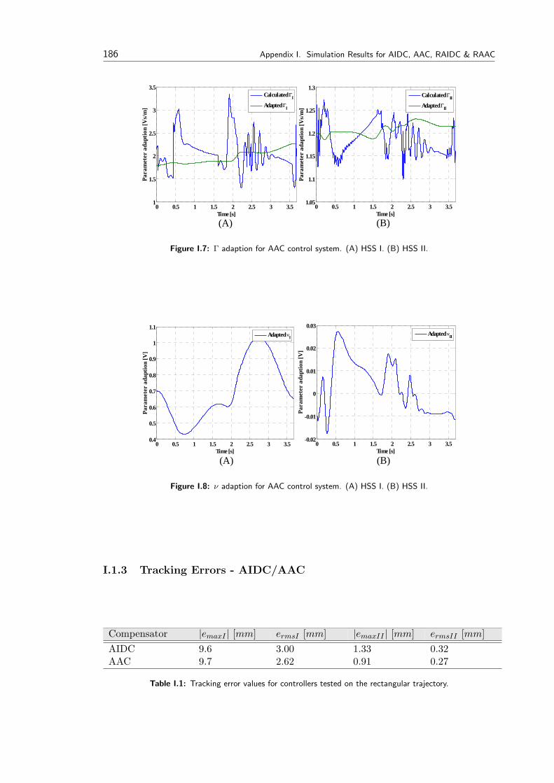
186 Appendix I. Simulation Results for AIDC, AAC, RAIDC & RAAC
(A) (B)
0 0.5 1 1.5 2 2.5 3 3.51
1.5
2
2.5
3
3.5
Time [s]
Para
met
er a
dapt
ion
[Vs/
m]
Calculated ΓI
Adapted ΓI
0 0.5 1 1.5 2 2.5 3 3.51.05
1.1
1.15
1.2
1.25
1.3
Time [s]
Para
met
er a
dapt
ion
[Vs/
m]
Calculated ΓII
Adapted ΓII
Figure I.7: Γ adaption for AAC control system. (A) HSS I. (B) HSS II.
0 0.5 1 1.5 2 2.5 3 3.5-0.02
-0.01
0
0.01
0.02
0.03
Time [s]
Para
met
er a
dapt
ion
[V]
Adapted νII
(A) (B)
0 0.5 1 1.5 2 2.5 3 3.50.4
0.5
0.6
0.7
0.8
0.9
1
1.1
Time [s]
Para
met
er a
dapt
ion
[V]
Adapted νI
Figure I.8: ν adaption for AAC control system. (A) HSS I. (B) HSS II.
I.1.3 Tracking Errors - AIDC/AAC
Compensator |emaxI | [mm] ermsI [mm] |emaxII | [mm] ermsII [mm]AIDC 9.6 3.00 1.33 0.32AAC 9.7 2.62 0.91 0.27
Table I.1: Tracking error values for controllers tested on the rectangular trajectory.
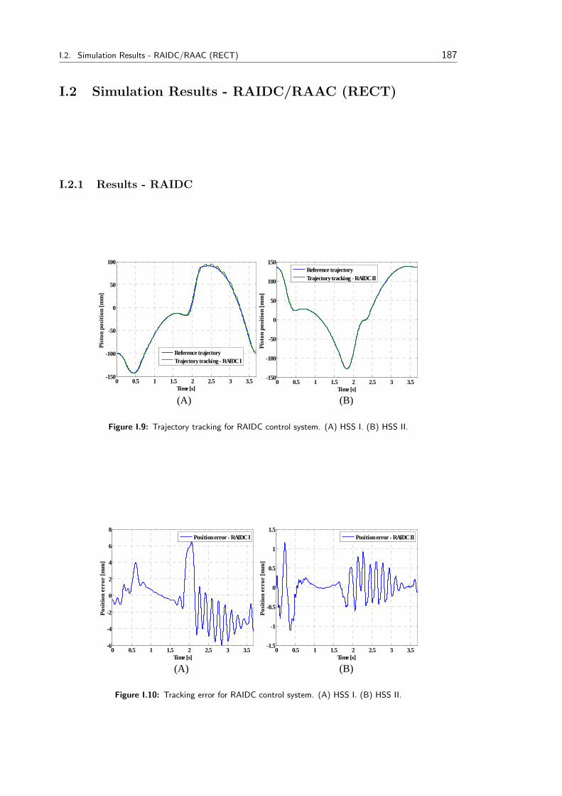
I.2. Simulation Results - RAIDC/RAAC (RECT) 187
I.2 Simulation Results - RAIDC/RAAC (RECT)
I.2.1 Results - RAIDC
(A) (B)
0 0.5 1 1.5 2 2.5 3 3.5-150
-100
-50
0
50
100
Time [s]
Pist
on p
ositi
on [m
m]
Reference trajectoryTrajectory tracking - RAIDC I
0 0.5 1 1.5 2 2.5 3 3.5-150
-100
-50
0
50
100
150
Time [s]
Pist
on p
ositi
on [m
m]
Reference trajectoryTrajectory tracking - RAIDC II
Figure I.9: Trajectory tracking for RAIDC control system. (A) HSS I. (B) HSS II.
(A) (B)
0 0.5 1 1.5 2 2.5 3 3.5-6
-4
-2
0
2
4
6
8
Time [s]
Posi
tion
erro
r [m
m]
Position error - RAIDC I
0 0.5 1 1.5 2 2.5 3 3.5-1.5
-1
-0.5
0
0.5
1
1.5
Time [s]
Posi
tion
erro
r [m
m]
Position error - RAIDC II
Figure I.10: Tracking error for RAIDC control system. (A) HSS I. (B) HSS II.
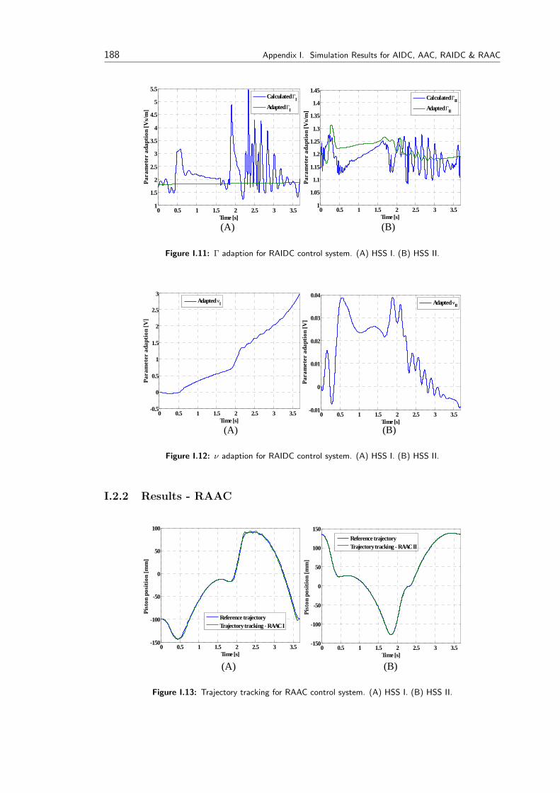
188 Appendix I. Simulation Results for AIDC, AAC, RAIDC & RAAC
(A) (B)
0 0.5 1 1.5 2 2.5 3 3.51
1.5
2
2.5
3
3.5
4
4.5
5
5.5
Time [s]
Para
met
er a
dapt
ion
[Vs/
m]
Calculated ΓI
Adapted ΓI
0 0.5 1 1.5 2 2.5 3 3.51
1.05
1.1
1.15
1.2
1.25
1.3
1.35
1.4
1.45
Time [s]
Para
met
er a
dapt
ion
[Vs/
m]
Calculated ΓII
Adapted ΓII
Figure I.11: Γ adaption for RAIDC control system. (A) HSS I. (B) HSS II.
(A) (B)
0 0.5 1 1.5 2 2.5 3 3.5-0.5
0
0.5
1
1.5
2
2.5
3
Time [s]
Para
met
er a
dapt
ion
[V]
Adapted νI
0 0.5 1 1.5 2 2.5 3 3.5-0.01
0
0.01
0.02
0.03
0.04
Time [s]
Para
met
er a
dapt
ion
[V]
Adapted νII
Figure I.12: ν adaption for RAIDC control system. (A) HSS I. (B) HSS II.
I.2.2 Results - RAAC
(A) (B)
0 0.5 1 1.5 2 2.5 3 3.5-150
-100
-50
0
50
100
Time [s]
Pist
on p
ositi
on [m
m]
Reference trajectoryTrajectory tracking - RAAC I
0 0.5 1 1.5 2 2.5 3 3.5-150
-100
-50
0
50
100
150
Time [s]
Pist
on p
ositi
on [m
m]
Reference trajectoryTrajectory tracking - RAAC II
Figure I.13: Trajectory tracking for RAAC control system. (A) HSS I. (B) HSS II.
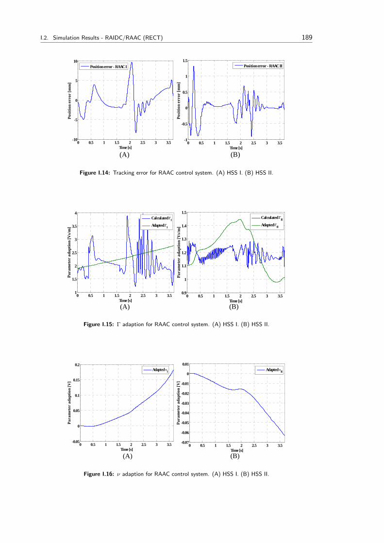
I.2. Simulation Results - RAIDC/RAAC (RECT) 189
(A) (B)
0 0.5 1 1.5 2 2.5 3 3.5-10
-5
0
5
10
Time [s]
Posi
tion
erro
r [m
m]
Position error - RAAC I
0 0.5 1 1.5 2 2.5 3 3.5-1
-0.5
0
0.5
1
1.5
Time [s]
Posi
tion
erro
r [m
m]
Position error - RAAC II
Figure I.14: Tracking error for RAAC control system. (A) HSS I. (B) HSS II.
(A) (B)
0 0.5 1 1.5 2 2.5 3 3.51
1.5
2
2.5
3
3.5
4
Time [s]
Para
met
er a
dapt
ion
[Vs/
m]
Calculated ΓI
Adapted ΓI
0 0.5 1 1.5 2 2.5 3 3.50.9
1
1.1
1.2
1.3
1.4
1.5
Time [s]
Para
met
er a
dapt
ion
[Vs/
m]
Calculated ΓII
Adapted ΓII
Figure I.15: Γ adaption for RAAC control system. (A) HSS I. (B) HSS II.
(A) (B)
0 0.5 1 1.5 2 2.5 3 3.5-0.05
0
0.05
0.1
0.15
0.2
Time [s]
Para
met
er a
dapt
ion
[V]
Adapted νI
0 0.5 1 1.5 2 2.5 3 3.5-0.07
-0.06
-0.05
-0.04
-0.03
-0.02
-0.01
0
0.01
Time [s]
Para
met
er a
dapt
ion
[V]
Adapted νII
Figure I.16: ν adaption for RAAC control system. (A) HSS I. (B) HSS II.
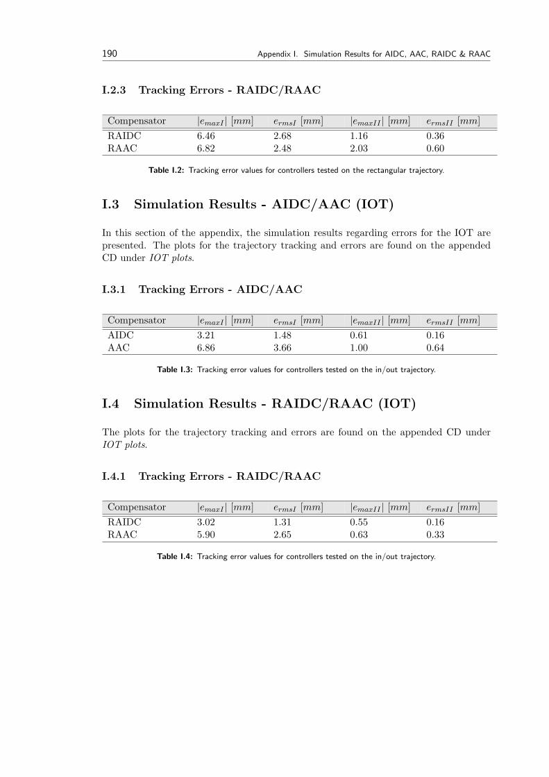
190 Appendix I. Simulation Results for AIDC, AAC, RAIDC & RAAC
I.2.3 Tracking Errors - RAIDC/RAAC
Compensator |emaxI | [mm] ermsI [mm] |emaxII | [mm] ermsII [mm]RAIDC 6.46 2.68 1.16 0.36RAAC 6.82 2.48 2.03 0.60
Table I.2: Tracking error values for controllers tested on the rectangular trajectory.
I.3 Simulation Results - AIDC/AAC (IOT)
In this section of the appendix, the simulation results regarding errors for the IOT arepresented. The plots for the trajectory tracking and errors are found on the appendedCD under IOT plots.
I.3.1 Tracking Errors - AIDC/AAC
Compensator |emaxI | [mm] ermsI [mm] |emaxII | [mm] ermsII [mm]AIDC 3.21 1.48 0.61 0.16AAC 6.86 3.66 1.00 0.64
Table I.3: Tracking error values for controllers tested on the in/out trajectory.
I.4 Simulation Results - RAIDC/RAAC (IOT)
The plots for the trajectory tracking and errors are found on the appended CD underIOT plots.
I.4.1 Tracking Errors - RAIDC/RAAC
Compensator |emaxI | [mm] ermsI [mm] |emaxII | [mm] ermsII [mm]RAIDC 3.02 1.31 0.55 0.16RAAC 5.90 2.65 0.63 0.33
Table I.4: Tracking error values for controllers tested on the in/out trajectory.
Appendix JControllerParameters -NonlinearControllers
Contents
I.1 Simulation Results - AID-C/AAC (RECT) . . . . . . . . 184
I.2 Simulation Results - RAID-C/RAAC (RECT) . . . . . . . 187
I.3 Simulation Results - AID-C/AAC (IOT) . . . . . . . . . 190
I.4 Simulation Results - RAID-C/RAAC (IOT) . . . . . . . . 190
In this appendix the parameters for the adaptive and learning controllers used during sim-ulation are presented. Controller parameters for the AIDC, AAC, RAIDC and AAC arefound on the appended CD.
J.1 Control Parameters used for MAIDC/MAAC
J.1.1 Control Parameters used for the RECT - MAIDC/MAAC
The control parameters used for the MAIDC and MAAC, when completing the rectan-gular trajectory are presented in table J.1.
191
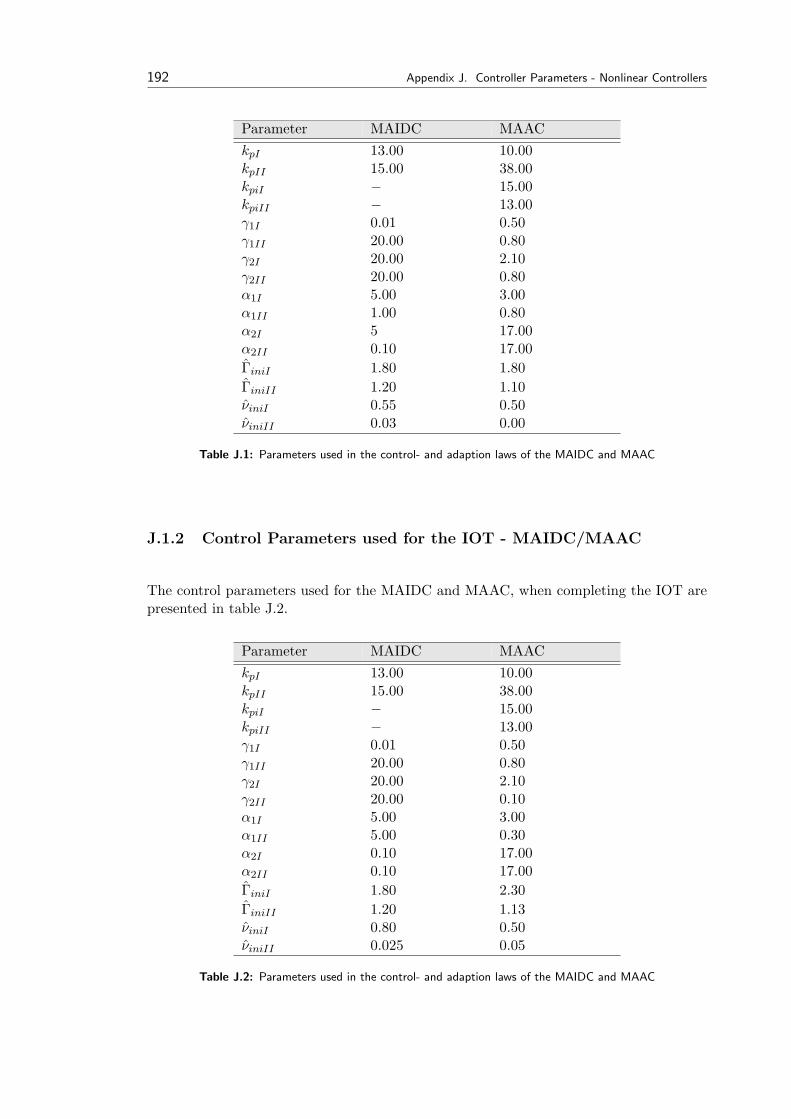
192 Appendix J. Controller Parameters - Nonlinear Controllers
Parameter MAIDC MAACkpI 13.00 10.00kpII 15.00 38.00kpiI − 15.00kpiII − 13.00γ1I 0.01 0.50γ1II 20.00 0.80γ2I 20.00 2.10γ2II 20.00 0.80α1I 5.00 3.00α1II 1.00 0.80α2I 5 17.00α2II 0.10 17.00ΓiniI 1.80 1.80ΓiniII 1.20 1.10νiniI 0.55 0.50νiniII 0.03 0.00
Table J.1: Parameters used in the control- and adaption laws of the MAIDC and MAAC
J.1.2 Control Parameters used for the IOT - MAIDC/MAAC
The control parameters used for the MAIDC and MAAC, when completing the IOT arepresented in table J.2.
Parameter MAIDC MAACkpI 13.00 10.00kpII 15.00 38.00kpiI − 15.00kpiII − 13.00γ1I 0.01 0.50γ1II 20.00 0.80γ2I 20.00 2.10γ2II 20.00 0.10α1I 5.00 3.00α1II 5.00 0.30α2I 0.10 17.00α2II 0.10 17.00ΓiniI 1.80 2.30ΓiniII 1.20 1.13νiniI 0.80 0.50νiniII 0.025 0.05
Table J.2: Parameters used in the control- and adaption laws of the MAIDC and MAAC
J.2. Control Parameters used for ILC/RDLC 193
J.2 Control Parameters used for ILC/RDLC
The control parameters used for the ILC and RDLC aresimilar for both trajectories.
J.2.1 Control Parameters used for ILC
ΓI = 1 , kpI = 20 , µI = 10 (J.1)
ΓII = 1 , kpII = 20 , µII = 5 (J.2)
J.2.2 Control Parameters used for RDLC
ΓI = 1 , kpI = 1 , LI = 0.011 (J.3)
ΓII = 1 , kpII = 1 , LII = 0.011 (J.4)
Here ∆t = 1/2000 [s].

Appendix KAppendix forthe RDLC
Contents
J.1 Control Parameters used forMAIDC/MAAC . . . . . . . . 191
J.2 Control Parameters used forILC/RDLC . . . . . . . . . . . 193
This appendix presents the bounds and assumptions used for the RDLC. This is takendirectly from [Andersen, 2004a].
In the following the desired trajectory is denoted xd, whereas the desired trajectory inthis thesis is denoted xR.
K.1 Bounds & Assumptions
The following has been scanned directly from [Andersen, 2004a].
195
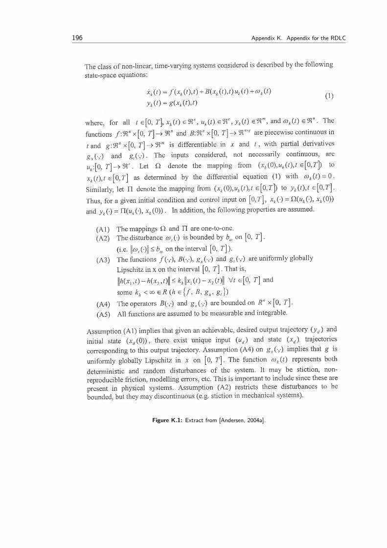
196 Appendix K. Appendix for the RDLC
Figure K.1: Extract from [Andersen, 2004a].

Appendix LSimulationResults for theIOT - LinearControllers
Contents
K.1 Bounds & Assumptions . . . . 195
In this appendix the simulation results for linear controllers tested on the IOT are pre-sented.
L.1 Simulation Results - Classic Linear Controllers
As shown in figures L.1 and L.2, it is clear that the tracking performance is similar tothose of the RECT, despite the lesser demanding trajectory.
(A) (B)
0 0.5 1 1.5 2 2.5-200
-150
-100
-50
0
50
100
150
200
Time [s]
Pist
on p
ositi
on [m
m]
ReferenceP-controllerPI-controllerLead-controllerLag-controllerLag-lead-controller
0 0.5 1 1.5 2 2.5-150
-100
-50
0
50
100
Time [s]
Posi
tion
erro
r [m
m]
P-controllerPI-controllerLead-controllerLag-controllerLag-lead-controller
Figure L.1: (A) Trajectory position tracking, for the nonlinear model cylinder I. (B) Position tracking errorsfor the nonlinear model, cylinder I.
197
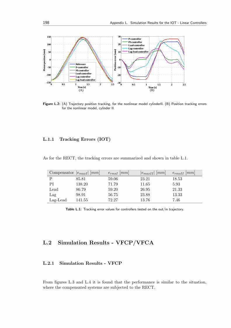
198 Appendix L. Simulation Results for the IOT - Linear Controllers
(A) (B)
0 0.5 1 1.5 2 2.5-150
-100
-50
0
50
100
150
Time [s]
Pist
on p
ositi
on [m
m]
ReferenceP-controllerPI-controllerLead-controllerLag-controllerLag-lead-controller
0 0.5 1 1.5 2 2.5-30
-20
-10
0
10
20
30
Time [s]
Posi
tion
erro
r [m
m]
P-controllerPI-controllerLead-controllerLag-controllerLag-lead-controller
Figure L.2: (A) Trajectory position tracking, for the nonlinear model cylinderII. (B) Position tracking errorsfor the nonlinear model, cylinder II.
L.1.1 Tracking Errors (IOT)
As for the RECT, the tracking errors are summarized and shown in table L.1.
Compensator |emaxI | [mm] ermsI [mm] |emaxII | [mm] ermsII [mm]P 85.81 59.06 23.21 18.53PI 138.20 71.79 11.65 5.93Lead 86.79 59.20 26.95 21.33Lag 98.91 56.75 23.88 13.33Lag-Lead 141.55 72.27 13.76 7.46
Table L.1: Tracking error values for controllers tested on the out/in trajectory.
L.2 Simulation Results - VFCP/VFCA
L.2.1 Simulation Results - VFCP
From figures L.3 and L.4 it is found that the performance is similar to the situation,where the compensated systems are subjected to the RECT.
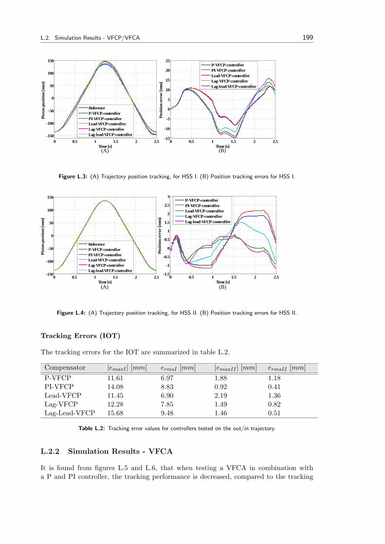
L.2. Simulation Results - VFCP/VFCA 199
(A) (B)
0 0.5 1 1.5 2 2.5-150
-100
-50
0
50
100
150
Time [s]
Pist
on p
ositi
on [m
m]
ReferenceP-VFCP-controllerPI-VFCP-controllerLead-VFCP-controllerLag-VFCP-controllerLag-lead-VFCP-controller
0 0.5 1 1.5 2 2.5-15
-10
-5
0
5
10
15
20
25
Time [s]
Posi
tion
erro
r [m
m]
P-VFCP-controllerPI-VFCP-controllerLead-VFCP-controllerLag-VFCP-controllerLag-lead-VFCP-controller
Figure L.3: (A) Trajectory position tracking, for HSS I. (B) Position tracking errors for HSS I.
(A) (B)
0 0.5 1 1.5 2 2.5-150
-100
-50
0
50
100
150
Time [s]
Pist
on p
ositi
on [m
m]
ReferenceP-VFCP-controllerPI-VFCP-controllerLead-VFCP-controllerLag-VFCP-controllerLag-lead-VFCP-controller
0 0.5 1 1.5 2 2.5-1.5
-1
-0.5
0
0.5
1
1.5
2
2.5
3
Time [s]
Posi
tion
erro
r [m
m]
P-VFCP-controllerPI-VFCP-controllerLead-VFCP-controllerLag-VFCP-controllerLag-lead-VFCP-controller
Figure L.4: (A) Trajectory position tracking, for HSS II. (B) Position tracking errors for HSS II.
Tracking Errors (IOT)
The tracking errors for the IOT are summarized in table L.2.
Compensator |emaxI | [mm] ermsI [mm] |emaxII | [mm] ermsII [mm]P-VFCP 11.61 6.97 1.88 1.18PI-VFCP 14.08 8.83 0.92 0.41Lead-VFCP 11.45 6.90 2.19 1.36Lag-VFCP 12.28 7.85 1.49 0.82Lag-Lead-VFCP 15.68 9.48 1.46 0.51
Table L.2: Tracking error values for controllers tested on the out/in trajectory.
L.2.2 Simulation Results - VFCA
It is found from figures L.5 and L.6, that when testing a VFCA in combination witha P and PI controller, the tracking performance is decreased, compared to the tracking
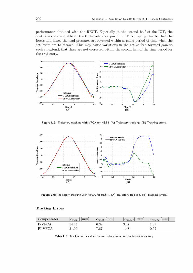
200 Appendix L. Simulation Results for the IOT - Linear Controllers
performance obtained with the RECT. Especially in the second half of the IOT, thecontrollers are not able to track the reference position. This may by due to that theforces and hence the load pressures are reversed within as short period of time when theactuators are to retract. This may cause variations in the active feed forward gain tosuch an extend, that these are not corrected within the second half of the time period forthe trajectory.
(A) (B)
0 0.5 1 1.5 2 2.5-200
-150
-100
-50
0
50
100
150
Time [s]
Pist
on p
ositi
on [m
m]
ReferenceP-VFCA-controllerPI-VFCA-controller
0 0.5 1 1.5 2 2.5-15
-10
-5
0
5
10
15
20
25
Time [s]
Posi
tion
erro
r [m
m]
P-VFCA-controllerPI-VFCA-controller
Figure L.5: Trajectory tracking with VFCA for HSS I. (A) Trajectory tracking. (B) Tracking errors.
(A) (B)
0 0.5 1 1.5 2 2.5-150
-100
-50
0
50
100
150
Time [s]
Pist
on p
ositi
on [m
m]
ReferenceP-VFCA-controllerPI-VFCA-controller
0 0.5 1 1.5 2 2.5-1.5
-1
-0.5
0
0.5
1
1.5
2
2.5
3
3.5
Time [s]
Posi
tion
erro
r [m
m]
P-VFCA-controllerPI-VFCA-controller
Figure L.6: Trajectory tracking with VFCA for HSS II. (A) Trajectory tracking. (B) Tracking errors.
Tracking Errors
Compensator |emaxI | [mm] ermsI [mm] |emaxII | [mm] ermsII [mm]P-VFCA 14.44 6.39 3.37 1.87PI-VFCA 21.06 7.67 1.48 0.52
Table L.3: Tracking error values for controllers tested on the in/out trajectory.
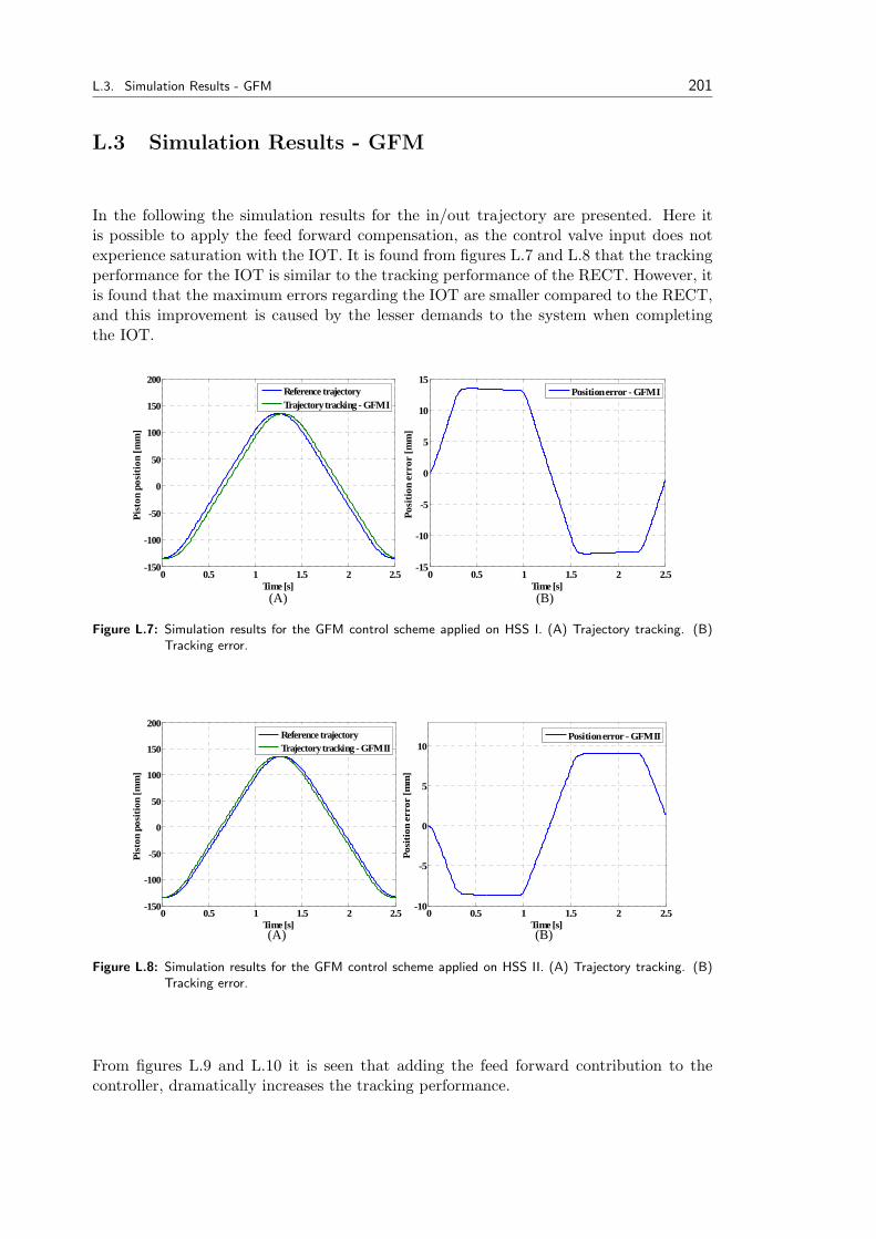
L.3. Simulation Results - GFM 201
L.3 Simulation Results - GFM
In the following the simulation results for the in/out trajectory are presented. Here itis possible to apply the feed forward compensation, as the control valve input does notexperience saturation with the IOT. It is found from figures L.7 and L.8 that the trackingperformance for the IOT is similar to the tracking performance of the RECT. However, itis found that the maximum errors regarding the IOT are smaller compared to the RECT,and this improvement is caused by the lesser demands to the system when completingthe IOT.
(A) (B)
(A) (B)
0 0.5 1 1.5 2 2.5-150
-100
-50
0
50
100
150
200
Time [s]
Pist
on p
ositi
on [m
m]
Reference trajectoryTrajectory tracking - GFM I
0 0.5 1 1.5 2 2.5-150
-100
-50
0
50
100
150
200
Time [s]
Pist
on p
ositi
on [m
m]
Reference trajectoryTrajectory tracking - GFM II
0 0.5 1 1.5 2 2.5-15
-10
-5
0
5
10
15
Time [s]
Posi
tion
erro
r [m
m]
Position error - GFM I
0 0.5 1 1.5 2 2.5-10
-5
0
5
10
Time [s]
Posi
tion
erro
r [m
m]
Position error - GFM IIFigure L.7: Simulation results for the GFM control scheme applied on HSS I. (A) Trajectory tracking. (B)
Tracking error.
(A) (B)
0 0.5 1 1.5 2 2.5-150
-100
-50
0
50
100
150
200
Time [s]
Pist
on p
ositi
on [m
m]
Reference trajectoryTrajectory tracking - GFM II
0 0.5 1 1.5 2 2.5-10
-5
0
5
10
Time [s]
Posi
tion
erro
r [m
m]
Position error - GFM II
Figure L.8: Simulation results for the GFM control scheme applied on HSS II. (A) Trajectory tracking. (B)Tracking error.
From figures L.9 and L.10 it is seen that adding the feed forward contribution to thecontroller, dramatically increases the tracking performance.
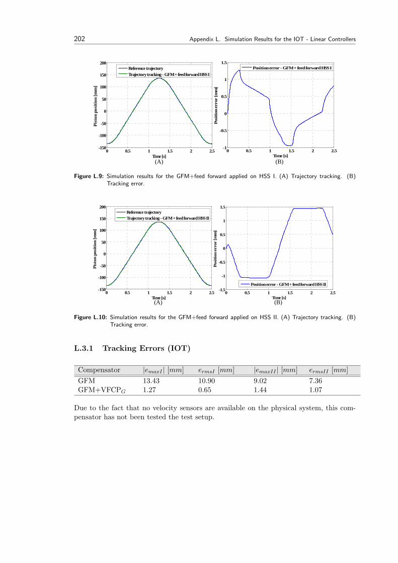
202 Appendix L. Simulation Results for the IOT - Linear Controllers
(A) (B)
0 0.5 1 1.5 2 2.5-1
-0.5
0
0.5
1
1.5
Time [s]
Posi
tion
erro
r [m
m]
Position error - GFM + feed forward HSS I
0 0.5 1 1.5 2 2.5-150
-100
-50
0
50
100
150
200
Time [s]
Pist
on p
ositi
on [m
m]
Reference trajectoryTrajectory tracking - GFM + feed forward HSS I
Figure L.9: Simulation results for the GFM+feed forward applied on HSS I. (A) Trajectory tracking. (B)Tracking error.
(A) (B)
(A) (B)
0 0.5 1 1.5 2 2.5-1.5
-1
-0.5
0
0.5
1
1.5
Time [s]
Posi
tion
erro
r [m
m]
Position error - GFM + feed forward HSS II
0 0.5 1 1.5 2 2.5-1
-0.5
0
0.5
1
1.5
Time [s]
Posi
tion
erro
r [m
m]
Position error - GFM + feed forward HSS I
0 0.5 1 1.5 2 2.5-150
-100
-50
0
50
100
150
200
Time [s]
Pist
on p
ositi
on [m
m]
Reference trajectoryTrajectory tracking - GFM + feed forward HSS II
0 0.5 1 1.5 2 2.5-150
-100
-50
0
50
100
150
200
Time [s]
Pist
on p
ositi
on [m
m]
Reference trajectoryTrajectory tracking - GFM + feed forward HSS I
Figure L.10: Simulation results for the GFM+feed forward applied on HSS II. (A) Trajectory tracking. (B)Tracking error.
L.3.1 Tracking Errors (IOT)
Compensator |emaxI | [mm] ermsI [mm] |emaxII | [mm] ermsII [mm]GFM 13.43 10.90 9.02 7.36GFM+VFCPG 1.27 0.65 1.44 1.07
Due to the fact that no velocity sensors are available on the physical system, this com-pensator has not been tested the test setup.

Appendix MSimulationResults for theIOT - NonlinearControllers
Contents
L.1 Simulation Results - ClassicLinear Controllers . . . . . . . 197
L.2 Simulation Results -VFCP/VFCA . . . . . . . . . 198
L.3 Simulation Results - GFM . . 201
In this appendix the simulation results for linear controllers tested on the IOT are pre-sented.
The simulation results for the IOT, along with their errors are found in appendix M.
M.1 Simulation Results - Adaptive Controllers
In the following the simulation results for the MAIDC and the MAAC are presented.
It is found from figures M.1, M.2, M.5 and M.6, that when using MAIDC- and MAACschemes to complete the IOT, tracking performance is similar to completing the RECT -however, with an increase in the tracking performance.
Regarding the parameter adaption, it is found from figures M.3, M.4, M.7 and M.8, thatthe adapted parameters Γi experiences increased tracking of the calculated Γi, along theramp-like segments of the IOT.
203
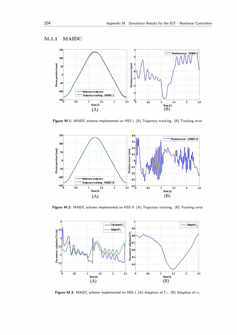
204 Appendix M. Simulation Results for the IOT - Nonlinear Controllers
M.1.1 MAIDC
(A) (B)0 0.5 1 1.5 2 2.5
-4
-3
-2
-1
0
1
2
3
Time [s]
Posi
tion
erro
r [m
m]
Position error - MAIDC I
0 0.5 1 1.5 2 2.5-150
-100
-50
0
50
100
150
Time [s]
Pist
on p
ositi
on [m
m]
Reference trajectoryTrajectory tracking - MAIDC I
Figure M.1: MAIDC scheme implemented on HSS I. (A) Trajectory tracking. (B) Tracking error.
(A) (B)
0 0.5 1 1.5 2 2.5-0.4
-0.3
-0.2
-0.1
0
0.1
0.2
0.3
0.4
Time [s]
Posi
tion
erro
r [m
m]
Position error - MAIDC II
0 0.5 1 1.5 2 2.5-150
-100
-50
0
50
100
150
Time [s]
Pist
on p
ositi
on [m
m]
Reference trajectoryTrajectory tracking - MAIDC II
Figure M.2: MAIDC scheme implemented on HSS II. (A) Trajectory tracking. (B) Tracking error.
(A) (B)
0 0.5 1 1.5 2 2.5
0.4
0.5
0.6
0.7
0.8
0.9
1
Time [s]
Para
met
er a
dapt
ion
[V]
Adapted νI
0 0.5 1 1.5 2 2.51
1.5
2
2.5
3
3.5
4
Time [s]
Para
met
er a
dapt
ion
[Vs/
m]
Calculated ΓI
Adapted ΓI
Figure M.3: MAIDC scheme implemented on HSS I. (A) Adaption of ΓI . (B) Adaption of νI .
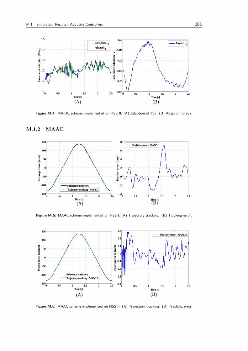
M.1. Simulation Results - Adaptive Controllers 205
(A) (B)
0 0.5 1 1.5 2 2.5-0.035
-0.03
-0.025
-0.02
-0.015
-0.01
Time [s]
Para
met
er a
dapt
ion
[V]
Adapted νII
0 0.5 1 1.5 2 2.51
1.1
1.2
1.3
1.4
1.5
Time [s]
Para
met
er a
dapt
ion
[Vs/
m]
Calculated ΓII
Adapted ΓII
Figure M.4: MAIDC scheme implemented on HSS II. (A) Adaption of ΓII . (B) Adaption of νII .
M.1.2 MAAC
(A) (B)0 0.5 1 1.5 2 2.5
-150
-100
-50
0
50
100
150
Time [s]
Pist
on p
ositi
on [m
m]
Reference trajectoryTrajectory tracking - MAAC I
0 0.5 1 1.5 2 2.5-4
-2
0
2
4
6
8
Time [s]
Posi
tion
erro
r [m
m]
Position error - MAAC I
Figure M.5: MAAC scheme implemented on HSS I. (A) Trajectory tracking. (B) Tracking error.
(A) (B)
0 0.5 1 1.5 2 2.5-150
-100
-50
0
50
100
150
Time [s]
Pist
on p
ositi
on [m
m]
Reference trajectoryTrajectory tracking - MAAC II
0 0.5 1 1.5 2 2.5-0.4
-0.3
-0.2
-0.1
0
0.1
0.2
0.3
Time [s]
Posi
tion
erro
r [m
m]
Position error - MAAC II
Figure M.6: MAAC scheme implemented on HSS II. (A) Trajectory tracking. (B) Tracking error.
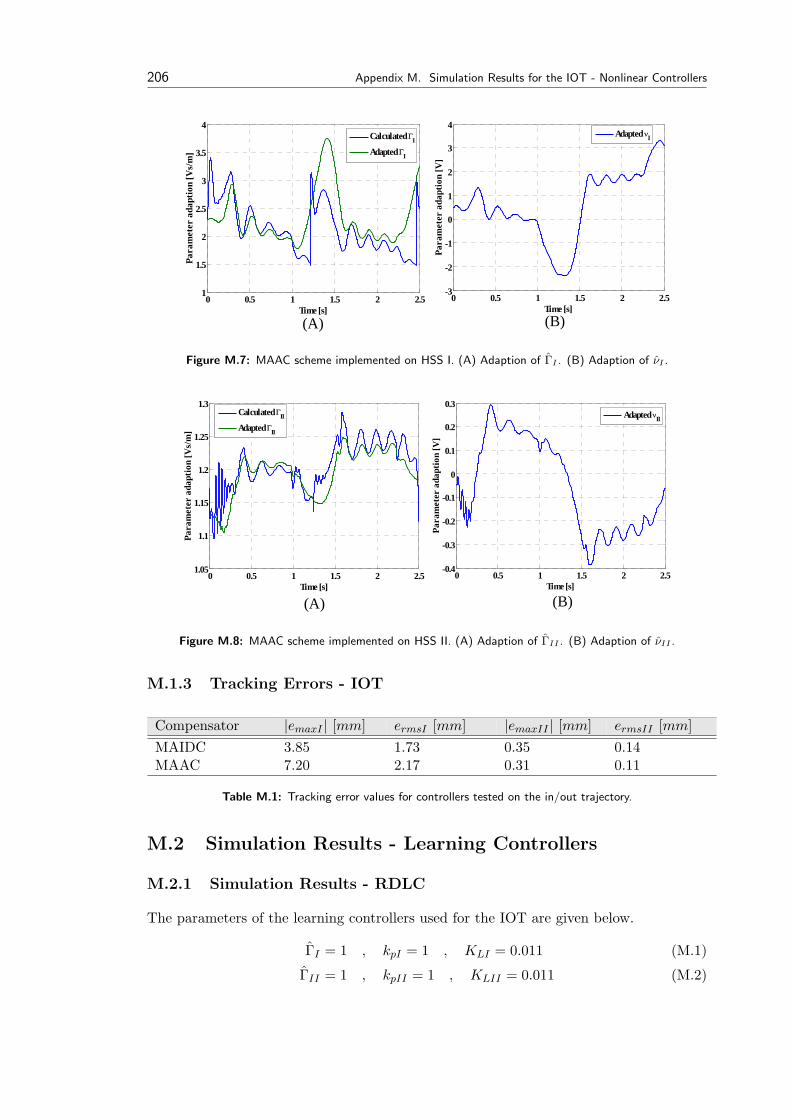
206 Appendix M. Simulation Results for the IOT - Nonlinear Controllers
(A) (B)0 0.5 1 1.5 2 2.5
1
1.5
2
2.5
3
3.5
4
Time [s]
Para
met
er a
dapt
ion
[Vs/
m]
Calculated ΓI
Adapted ΓI
0 0.5 1 1.5 2 2.5-3
-2
-1
0
1
2
3
4
Time [s]
Para
met
er a
dapt
ion
[V]
Adapted νI
Figure M.7: MAAC scheme implemented on HSS I. (A) Adaption of ΓI . (B) Adaption of νI .
(A) (B)
0 0.5 1 1.5 2 2.51.05
1.1
1.15
1.2
1.25
1.3
Time [s]
Para
met
er a
dapt
ion
[Vs/
m]
Calculated ΓII
Adapted ΓII
0 0.5 1 1.5 2 2.5-0.4
-0.3
-0.2
-0.1
0
0.1
0.2
0.3
Time [s]
Para
met
er a
dapt
ion
[V]
Adapted νII
Figure M.8: MAAC scheme implemented on HSS II. (A) Adaption of ΓII . (B) Adaption of νII .
M.1.3 Tracking Errors - IOT
Compensator |emaxI | [mm] ermsI [mm] |emaxII | [mm] ermsII [mm]MAIDC 3.85 1.73 0.35 0.14MAAC 7.20 2.17 0.31 0.11
Table M.1: Tracking error values for controllers tested on the in/out trajectory.
M.2 Simulation Results - Learning Controllers
M.2.1 Simulation Results - RDLC
The parameters of the learning controllers used for the IOT are given below.
ΓI = 1 , kpI = 1 , KLI = 0.011 (M.1)
ΓII = 1 , kpII = 1 , KLII = 0.011 (M.2)
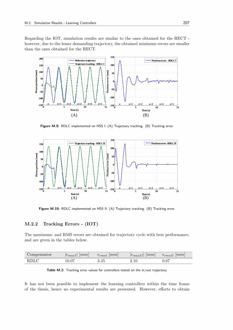
M.2. Simulation Results - Learning Controllers 207
Regarding the IOT, simulation results are similar to the ones obtained for the RECT -however, due to the lesser demanding trajectory, the obtained minimum errors are smallerthan the ones obtained for the RECT.
(B)(A)
0 5 10 15-150
-100
-50
0
50
100
150
Time [s]Po
sitio
n er
ror
[mm
]
Position error - RDLC I
n n+1 n+2 n+3 n+4 n+50 5 10 15
-150
-100
-50
0
50
100
150
200
Time [s]
Pist
on p
ositi
on [m
m]
Reference trajectoryTrajectory tracking - RDLC I
n n+1 n+2 n+3 n+4 n+5
Figure M.9: RDLC implemented on HSS I. (A) Trajectory tracking. (B) Tracking error.
(A) (B)
0 5 10 15-150
-100
-50
0
50
100
150
Time [s]
Pist
on p
ositi
on [m
m]
Trajectory tracking - RDLC II
n n+1 n+2 n+3 n+4 n+50 5 10 15
-150
-100
-50
0
50
100
150
Time [s]
Posi
tion
erro
r [m
m]
Position error -RDLC II
n n+1 n+2 n+3 n+4 n+5
Figure M.10: RDLC implemented on HSS II. (A) Trajectory tracking. (B) Tracking error.
M.2.2 Tracking Errors - (IOT)
The maximum- and RMS errors are obtained for trajectory cycle with best performance,and are given in the tables below.
Compensator |emaxI | [mm] ermsI [mm] |emaxII | [mm] ermsII [mm]RDLC 10.07 3.45 3.10 0.67
Table M.2: Tracking error values for controllers tested on the in/out trajectory.
It has not been possible to implement the learning controllers within the time frameof the thesis, hence no experimental results are presented. However, efforts to obtain
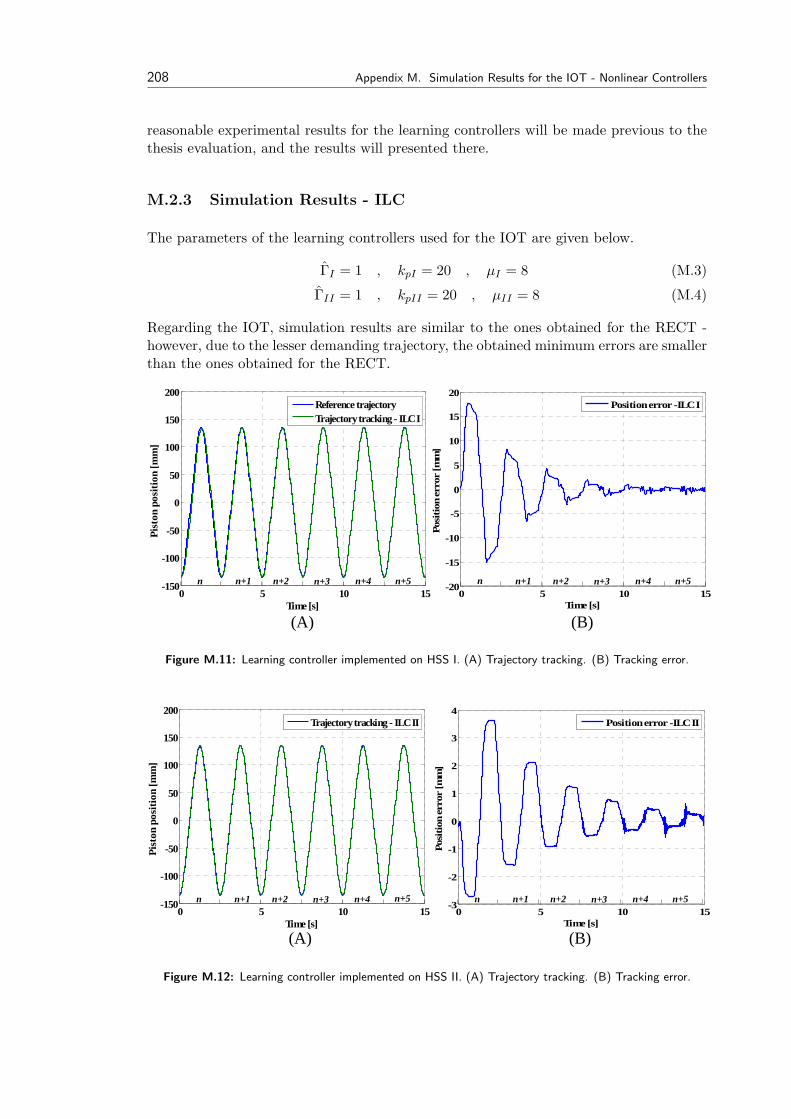
208 Appendix M. Simulation Results for the IOT - Nonlinear Controllers
reasonable experimental results for the learning controllers will be made previous to thethesis evaluation, and the results will presented there.
M.2.3 Simulation Results - ILC
The parameters of the learning controllers used for the IOT are given below.
ΓI = 1 , kpI = 20 , µI = 8 (M.3)
ΓII = 1 , kpII = 20 , µII = 8 (M.4)
Regarding the IOT, simulation results are similar to the ones obtained for the RECT -however, due to the lesser demanding trajectory, the obtained minimum errors are smallerthan the ones obtained for the RECT.
(A) (B)
0 5 10 15-150
-100
-50
0
50
100
150
200
Time [s]
Pist
on p
ositi
on [m
m]
Reference trajectoryTrajectory tracking - ILC I
n n+1 n+2 n+3 n+4 n+50 5 10 15
-20
-15
-10
-5
0
5
10
15
20
Time [s]
Posi
tion
erro
r [m
m]
Position error -ILC I
n+1 n+2 n+3 n+4 n+5n
Figure M.11: Learning controller implemented on HSS I. (A) Trajectory tracking. (B) Tracking error.
(A) (B)
0 5 10 15-150
-100
-50
0
50
100
150
200
Time [s]
Pist
on p
ositi
on [m
m]
Trajectory tracking - ILC II
n n+1 n+2 n+3 n+4 n+50 5 10 15
-3
-2
-1
0
1
2
3
4
Time [s]
Posi
tion
erro
r [m
m]
Position error -ILC II
n n+1 n+2 n+3 n+4 n+5
Figure M.12: Learning controller implemented on HSS II. (A) Trajectory tracking. (B) Tracking error.
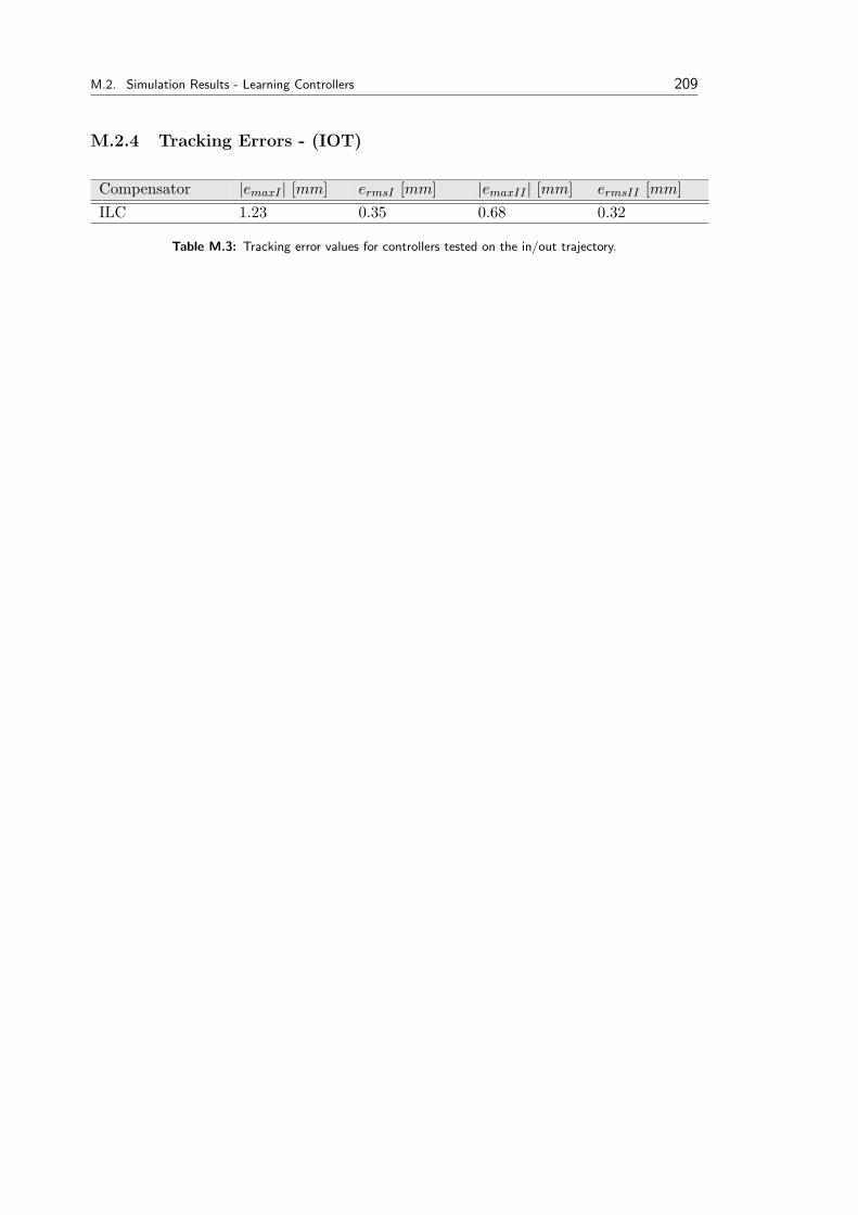
M.2. Simulation Results - Learning Controllers 209
M.2.4 Tracking Errors - (IOT)
Compensator |emaxI | [mm] ermsI [mm] |emaxII | [mm] ermsII [mm]ILC 1.23 0.35 0.68 0.32
Table M.3: Tracking error values for controllers tested on the in/out trajectory.

Appendix NControl Laws forARC
Contents
M.1 Simulation Results - AdaptiveControllers . . . . . . . . . . . 203
M.2 Simulation Results - LearningControllers . . . . . . . . . . . 206
This appendix presents the elements of the control laws for the ARC. This is taken directlyfrom [Yao et al., 2001].
N.1 Control Law α2
The following has been scanned directly from [Yao et al., 2001]. The following two figures(N.1, N.2 and N.3) are coherent.
Figure N.1: Extract from [Yao et al., 2001].
211
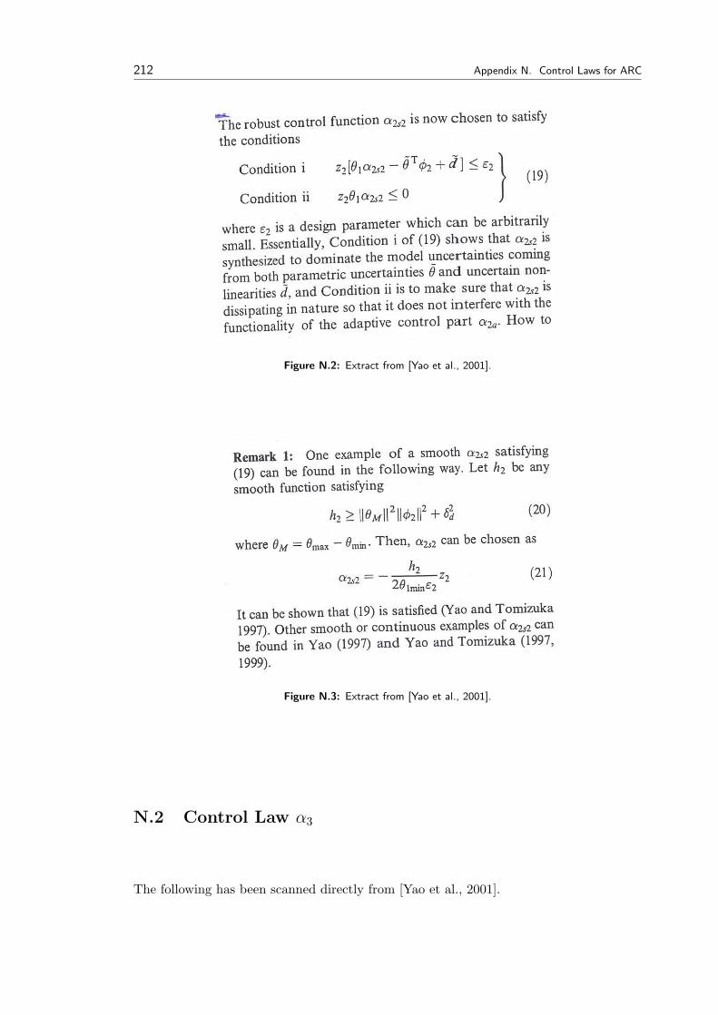
212 Appendix N. Control Laws for ARC
Figure N.2: Extract from [Yao et al., 2001].
Figure N.3: Extract from [Yao et al., 2001].
N.2 Control Law α3
The following has been scanned directly from [Yao et al., 2001].
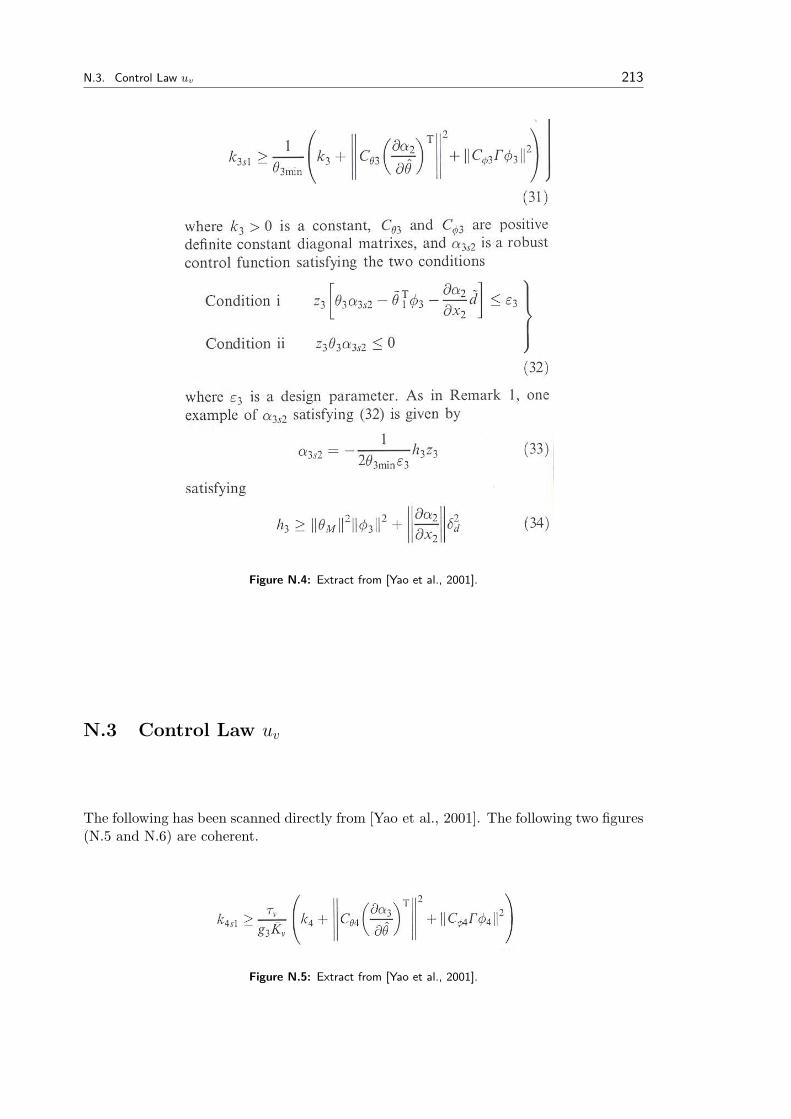
N.3. Control Law uv 213
Figure N.4: Extract from [Yao et al., 2001].
N.3 Control Law uv
The following has been scanned directly from [Yao et al., 2001]. The following two figures(N.5 and N.6) are coherent.
Figure N.5: Extract from [Yao et al., 2001].
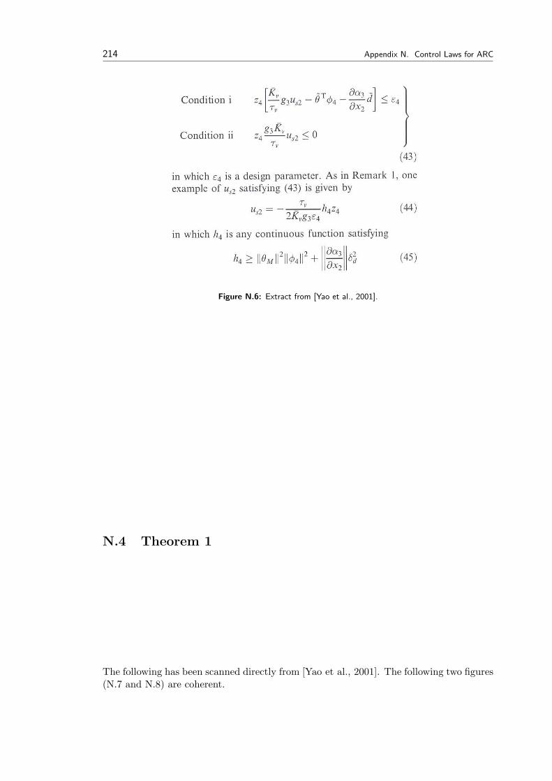
214 Appendix N. Control Laws for ARC
Figure N.6: Extract from [Yao et al., 2001].
N.4 Theorem 1
The following has been scanned directly from [Yao et al., 2001]. The following two figures(N.7 and N.8) are coherent.
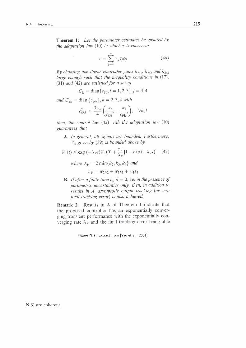
N.4. Theorem 1 215
Figure N.7: Extract from [Yao et al., 2001].
N.6) are coherent.
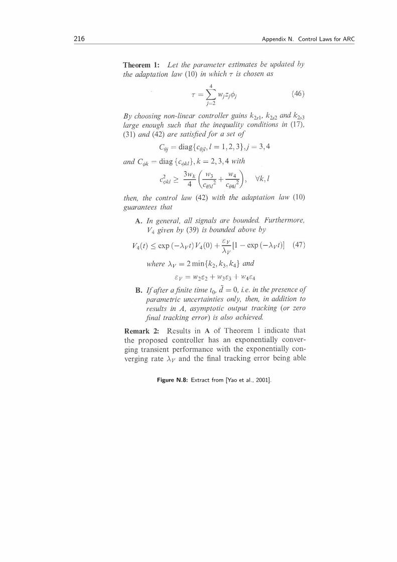
216 Appendix N. Control Laws for ARC
Figure N.8: Extract from [Yao et al., 2001].

Appendix ORobustnessanalysis
Contents
N.1 Control Law α2 . . . . . . . . 211
N.2 Control Law α3 . . . . . . . . 212
N.3 Control Law uv . . . . . . . . 213
N.4 Theorem 1 . . . . . . . . . . . 214
This appendix is a supplement to the chapter concerning the robustness of the control sys-tems. Here the trajectory tracking of the control systems, when subjected to a disturbance,are presented.
O.1 ∆ Error Plots for Linear Controllers
(A) (B)
0 0.5 1 1.5 2 2.5 3 3.50
2
4
6
8
10
12
Time [s]
Δ p
ositi
on e
rror
[mm
]
Δ position error - HSS I
0 0.5 1 1.5 2 2.5 3 3.5
0
0.2
0.4
0.6
0.8
1
1.2
Time [s]
Δ p
ositi
on e
rror
[mm
]
Δ position error - HSS II
Figure O.1: Difference in error between P control system, with and without disturbance. (A) HSS I. (B) HSSII.
217
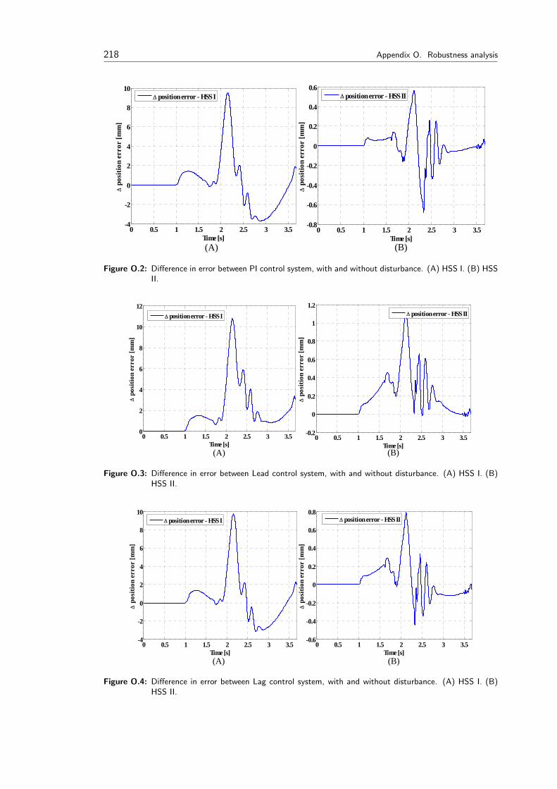
218 Appendix O. Robustness analysis
(A) (B)
0 0.5 1 1.5 2 2.5 3 3.5-4
-2
0
2
4
6
8
10
Time [s]
Δ p
ositi
on e
rror
[mm
]
Δ position error - HSS I
0 0.5 1 1.5 2 2.5 3 3.5-0.8
-0.6
-0.4
-0.2
0
0.2
0.4
0.6
Time [s]
Δ p
ositi
on e
rror
[mm
]
Δ position error - HSS II
Figure O.2: Difference in error between PI control system, with and without disturbance. (A) HSS I. (B) HSSII.
(A) (B)
0 0.5 1 1.5 2 2.5 3 3.50
2
4
6
8
10
12
Time [s]
Δ p
ositi
on e
rror
[mm
]
Δ position error - HSS I
0 0.5 1 1.5 2 2.5 3 3.5-0.2
0
0.2
0.4
0.6
0.8
1
1.2
Time [s]
Δ p
ositi
on e
rror
[mm
]
Δ position error - HSS II
Figure O.3: Difference in error between Lead control system, with and without disturbance. (A) HSS I. (B)HSS II.
(A) (B)
0 0.5 1 1.5 2 2.5 3 3.5-4
-2
0
2
4
6
8
10
Time [s]
Δ p
ositi
on e
rror
[mm
]
Δ position error - HSS I
0 0.5 1 1.5 2 2.5 3 3.5-0.6
-0.4
-0.2
0
0.2
0.4
0.6
0.8
Time [s]
Δ p
ositi
on e
rror
[mm
]
Δ position error - HSS II
Figure O.4: Difference in error between Lag control system, with and without disturbance. (A) HSS I. (B)HSS II.
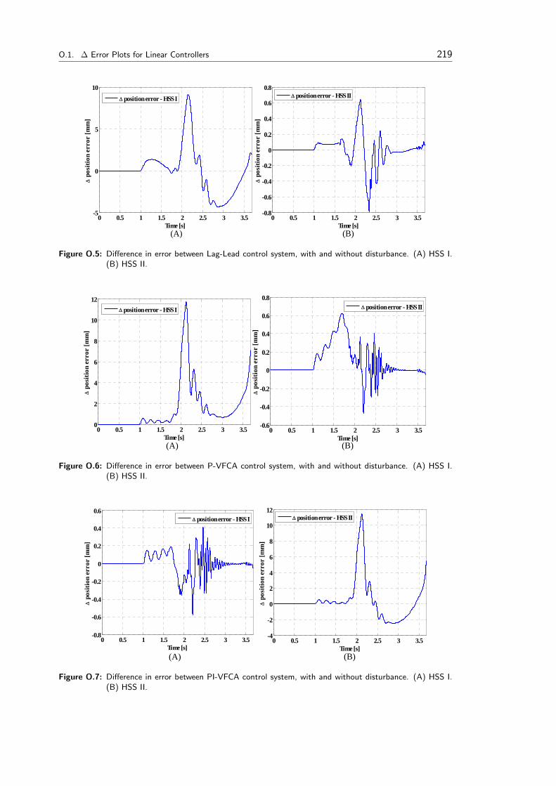
O.1. ∆ Error Plots for Linear Controllers 219
(A) (B)
0 0.5 1 1.5 2 2.5 3 3.5-5
0
5
10
Time [s]
Δ p
ositi
on e
rror
[mm
]
Δ position error - HSS I
0 0.5 1 1.5 2 2.5 3 3.5-0.8
-0.6
-0.4
-0.2
0
0.2
0.4
0.6
0.8
Time [s]
Δ p
ositi
on e
rror
[mm
]
Δ position error - HSS II
Figure O.5: Difference in error between Lag-Lead control system, with and without disturbance. (A) HSS I.(B) HSS II.
(A) (B)
0 0.5 1 1.5 2 2.5 3 3.5-0.6
-0.4
-0.2
0
0.2
0.4
0.6
0.8
Time [s]
Δ p
ositi
on e
rror
[mm
]
Δ position error - HSS II
0 0.5 1 1.5 2 2.5 3 3.50
2
4
6
8
10
12
Time [s]
Δ p
ositi
on e
rror
[mm
]
Δ position error - HSS I
Figure O.6: Difference in error between P-VFCA control system, with and without disturbance. (A) HSS I.(B) HSS II.
(A) (B)
0 0.5 1 1.5 2 2.5 3 3.5-0.8
-0.6
-0.4
-0.2
0
0.2
0.4
0.6
Time [s]
Δ p
ositi
on e
rror
[mm
]
Δ position error - HSS I
0 0.5 1 1.5 2 2.5 3 3.5-4
-2
0
2
4
6
8
10
12
Time [s]
Δ p
ositi
on e
rror
[mm
]
Δ position error - HSS II
Figure O.7: Difference in error between PI-VFCA control system, with and without disturbance. (A) HSS I.(B) HSS II.
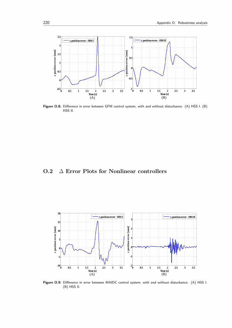
220 Appendix O. Robustness analysis
(A) (B)
0 0.5 1 1.5 2 2.5 3 3.5-0.5
0
0.5
1
1.5
2
2.5
Time [s]
Δ p
ositi
on e
rror
[mm
]
Δ position error - HSS I
0 0.5 1 1.5 2 2.5 3 3.5-1
-0.5
0
0.5
1
1.5
Time [s]
Δ p
ositi
on e
rror
[mm
]
Δ position error - HSS II
Figure O.8: Difference in error between GFM control system, with and without disturbance. (A) HSS I. (B)HSS II.
O.2 ∆ Error Plots for Nonlinear controllers
(A) (B)
0 0.5 1 1.5 2 2.5 3 3.5-10
-5
0
5
10
15
20
Time [s]
Δ p
ositi
on e
rror
[mm
]
Δ position error - HSS I
0 0.5 1 1.5 2 2.5 3 3.5-2
-1
0
1
2
3
Time [s]
Δ p
ositi
on e
rror
[mm
]
Δ position error - HSS II
Figure O.9: Difference in error between MAIDC control system, with and without disturbance. (A) HSS I.(B) HSS II.

O.2. ∆ Error Plots for Nonlinear controllers 221
(A) (B)
0 0.5 1 1.5 2 2.5 3 3.5-15
-10
-5
0
5
10
15
Time [s]
Δ p
ositi
on e
rror
[mm
]
Δ position error - HSS I
0 0.5 1 1.5 2 2.5 3 3.5-1.5
-1
-0.5
0
0.5
1
Time [s]
Δ p
ositi
on e
rror
[mm
]
Δ position error - HSS II
Figure O.10: Difference in error between MAAC control system, with and without disturbance. (A) HSS I.(B) HSS II.
(A) (B)
0 0.5 1 1.5 2 2.5 3 3.5-1.5
-1
-0.5
0
0.5
1
Time [s]
Δ p
ositi
on e
rror
[mm
]
Δ position error - HSS II
0 0.5 1 1.5 2 2.5 3 3.5-10
-5
0
5
10
15
Time [s]
Δ p
ositi
on e
rror
[mm
]
Δ position error - HSS I
Figure O.11: Difference in error between AIDC control system, with and without disturbance. (A) HSS I. (B)HSS II.
(A) (B)
0 0.5 1 1.5 2 2.5 3 3.5-6
-4
-2
0
2
4
6
8
10
12
Time [s]
Δ p
ositi
on e
rror
[mm
]
Δ position error - HSS I
0 0.5 1 1.5 2 2.5 3 3.5-2
-1.5
-1
-0.5
0
0.5
1
Time [s]
Δ p
ositi
on e
rror
[mm
]
Δ position error - HSS II
Figure O.12: Difference in error between AAC control system, with and without disturbance. (A) HSS I. (B)HSS II.
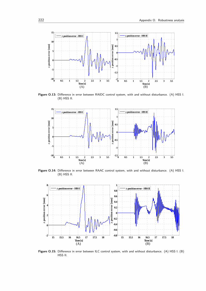
222 Appendix O. Robustness analysis
(A) (B)
0 0.5 1 1.5 2 2.5 3 3.5-2
-1.5
-1
-0.5
0
0.5
1
1.5
Time [s]
Δ p
ositi
on e
rror
[mm
]
Δ position error - HSS II
0 0.5 1 1.5 2 2.5 3 3.5-10
-5
0
5
10
15
Time [s]
Δ p
ositi
on e
rror
[mm
]
Δ position error - HSS I
Figure O.13: Difference in error between RAIDC control system, with and without disturbance. (A) HSS I.(B) HSS II.
(A) (B)
0 0.5 1 1.5 2 2.5 3 3.5-10
-5
0
5
10
15
Time [s]
Δ p
ositi
on e
rror
[mm
]
Δ position error - HSS I
0 0.5 1 1.5 2 2.5 3 3.5-1.5
-1
-0.5
0
0.5
1
1.5
Time [s]
Δ p
ositi
on e
rror
[mm
]
Δ position error - HSS II
Figure O.14: Difference in error between RAAC control system, with and without disturbance. (A) HSS I.(B) HSS II.
(A) (B)
15 15.5 16 16.5 17 17.5 18-2
0
2
4
6
8
Time [s]
Δ p
ositi
on e
rror
[mm
]
Δ position error - HSS I
15 15.5 16 16.5 17 17.5 18-0.8
-0.6
-0.4
-0.2
0
0.2
0.4
0.6
0.8
1
Time [s]
Δ p
ositi
on e
rror
[mm
]
Δ position error - HSS II
Figure O.15: Difference in error between ILC control system, with and without disturbance. (A) HSS I. (B)HSS II.
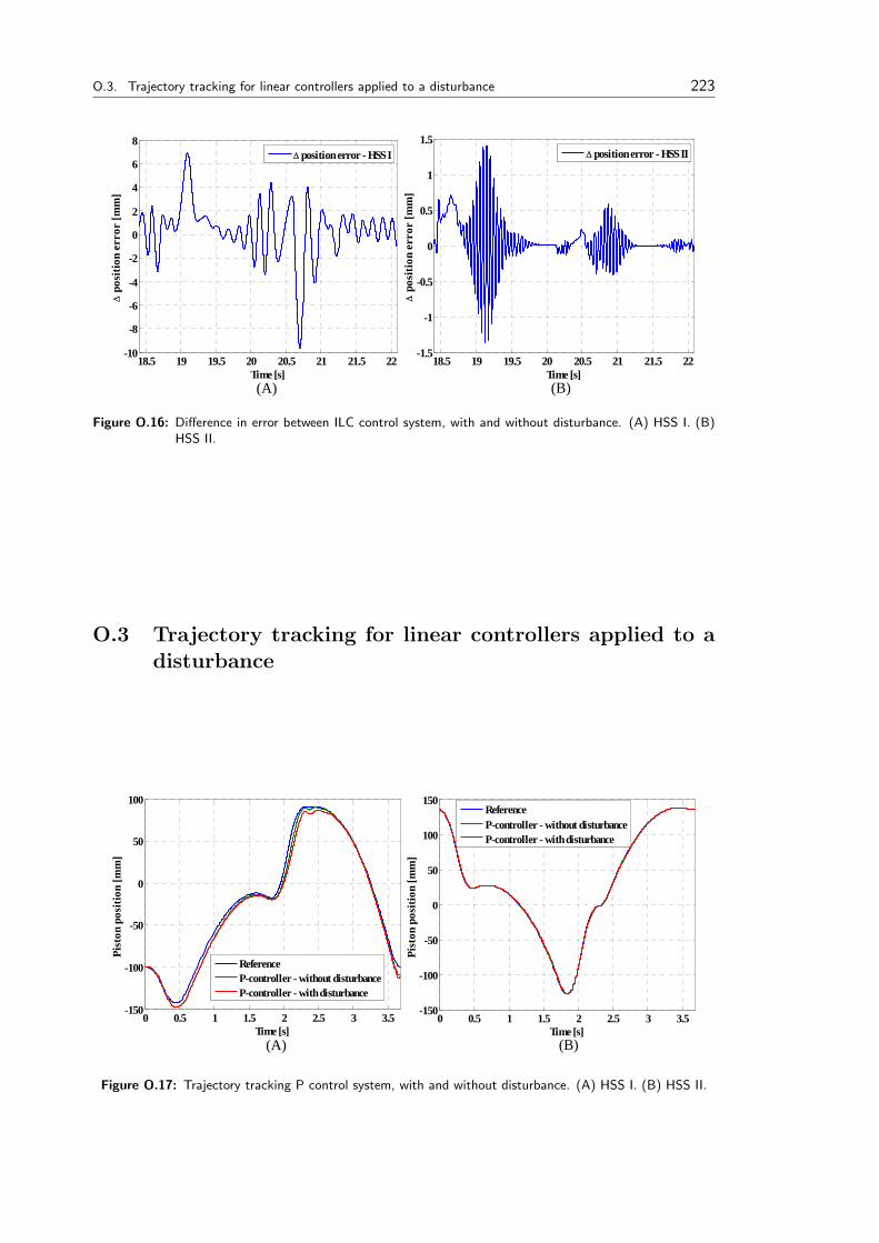
O.3. Trajectory tracking for linear controllers applied to a disturbance 223
(A) (B)
18.5 19 19.5 20 20.5 21 21.5 22-10
-8
-6
-4
-2
0
2
4
6
8
Time [s]
Δ p
ositi
on e
rror
[mm
]
Δ position error - HSS I
18.5 19 19.5 20 20.5 21 21.5 22-1.5
-1
-0.5
0
0.5
1
1.5
Time [s]
Δ p
ositi
on e
rror
[mm
]
Δ position error - HSS II
Figure O.16: Difference in error between ILC control system, with and without disturbance. (A) HSS I. (B)HSS II.
O.3 Trajectory tracking for linear controllers applied to adisturbance
(A) (B)
0 0.5 1 1.5 2 2.5 3 3.5-150
-100
-50
0
50
100
Time [s]
Pist
on p
ositi
on [m
m]
ReferenceP-controller - without disturbanceP-controller - with disturbance
0 0.5 1 1.5 2 2.5 3 3.5-150
-100
-50
0
50
100
150
Time [s]
Pist
on p
ositi
on [m
m]
ReferenceP-controller - without disturbanceP-controller - with disturbance
Figure O.17: Trajectory tracking P control system, with and without disturbance. (A) HSS I. (B) HSS II.
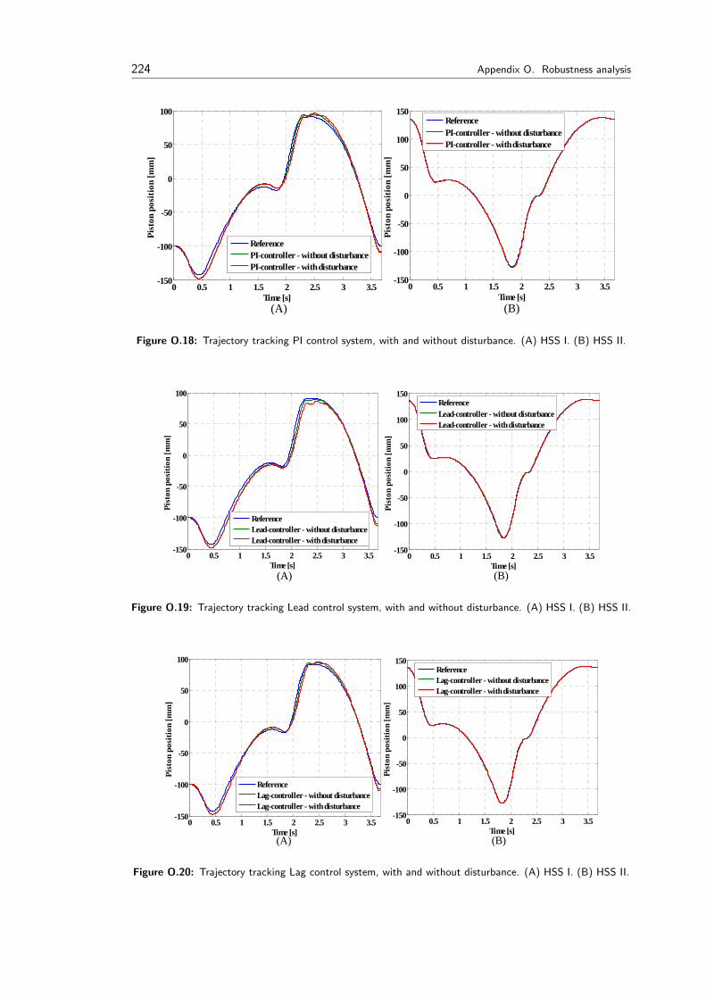
224 Appendix O. Robustness analysis
(A) (B)
0 0.5 1 1.5 2 2.5 3 3.5-150
-100
-50
0
50
100
Time [s]
Pist
on p
ositi
on [m
m]
ReferencePI-controller - without disturbancePI-controller - with disturbance
0 0.5 1 1.5 2 2.5 3 3.5-150
-100
-50
0
50
100
150
Time [s]
Pist
on p
ositi
on [m
m]
ReferencePI-controller - without disturbancePI-controller - with disturbance
Figure O.18: Trajectory tracking PI control system, with and without disturbance. (A) HSS I. (B) HSS II.
(A) (B)
0 0.5 1 1.5 2 2.5 3 3.5-150
-100
-50
0
50
100
Time [s]
Pist
on p
ositi
on [m
m]
ReferenceLead-controller - without disturbanceLead-controller - with disturbance
0 0.5 1 1.5 2 2.5 3 3.5-150
-100
-50
0
50
100
150
Time [s]
Pist
on p
ositi
on [m
m]
ReferenceLead-controller - without disturbanceLead-controller - with disturbance
Figure O.19: Trajectory tracking Lead control system, with and without disturbance. (A) HSS I. (B) HSS II.
(A) (B)
0 0.5 1 1.5 2 2.5 3 3.5-150
-100
-50
0
50
100
Time [s]
Pist
on p
ositi
on [m
m]
ReferenceLag-controller - without disturbanceLag-controller - with disturbance
0 0.5 1 1.5 2 2.5 3 3.5-150
-100
-50
0
50
100
150
Time [s]
Pist
on p
ositi
on [m
m]
ReferenceLag-controller - without disturbanceLag-controller - with disturbance
Figure O.20: Trajectory tracking Lag control system, with and without disturbance. (A) HSS I. (B) HSS II.
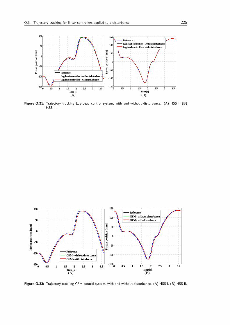
O.3. Trajectory tracking for linear controllers applied to a disturbance 225
(A) (B)
0 0.5 1 1.5 2 2.5 3 3.5-150
-100
-50
0
50
100
Time [s]
Pist
on p
ositi
on [m
m]
ReferenceLag-lead-controller - without disturbanceLag-lead-controller - with disturbance
0 0.5 1 1.5 2 2.5 3 3.5-150
-100
-50
0
50
100
150
Time [s]
Pist
on p
ositi
on [m
m]
ReferenceLag-lead-controller - without disturbanceLag-lead-controller - with disturbance
Figure O.21: Trajectory tracking Lag-Lead control system, with and without disturbance. (A) HSS I. (B)HSS II.
(A) (B)
0 0.5 1 1.5 2 2.5 3 3.5-150
-100
-50
0
50
100
Time [s]
Pist
on p
ositi
on [m
m]
ReferenceGFM - without disturbanceGFM - with disturbance
0 0.5 1 1.5 2 2.5 3 3.5-150
-100
-50
0
50
100
150
Time [s]
Pist
on p
ositi
on [m
m]
ReferenceGFM - without disturbanceGFM - with disturbance
Figure O.22: Trajectory tracking GFM control system, with and without disturbance. (A) HSS I. (B) HSS II.
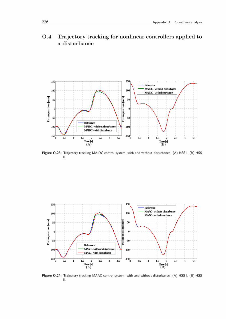
226 Appendix O. Robustness analysis
O.4 Trajectory tracking for nonlinear controllers applied toa disturbance
(A) (B)
0 0.5 1 1.5 2 2.5 3 3.5-150
-100
-50
0
50
100
150
Time [s]
Pist
on p
ositi
on [m
m]
ReferenceMAIDC - without disturbanceMAIDC - with disturbance
0 0.5 1 1.5 2 2.5 3 3.5-150
-100
-50
0
50
100
150
Time [s]
Pist
on p
ositi
on [m
m]
ReferenceMAIDC - without disturbanceMAIDC - with disturbance
Figure O.23: Trajectory tracking MAIDC control system, with and without disturbance. (A) HSS I. (B) HSSII.
(A) (B)
0 0.5 1 1.5 2 2.5 3 3.5-150
-100
-50
0
50
100
150
Time [s]
Pist
on p
ositi
on [m
m]
ReferenceMAAC - without disturbanceMAAC - with disturbance
0 0.5 1 1.5 2 2.5 3 3.5-150
-100
-50
0
50
100
150
Time [s]
Pist
on p
ositi
on [m
m]
ReferenceMAAC - without disturbanceMAAC - with disturbance
Figure O.24: Trajectory tracking MAAC control system, with and without disturbance. (A) HSS I. (B) HSSII.
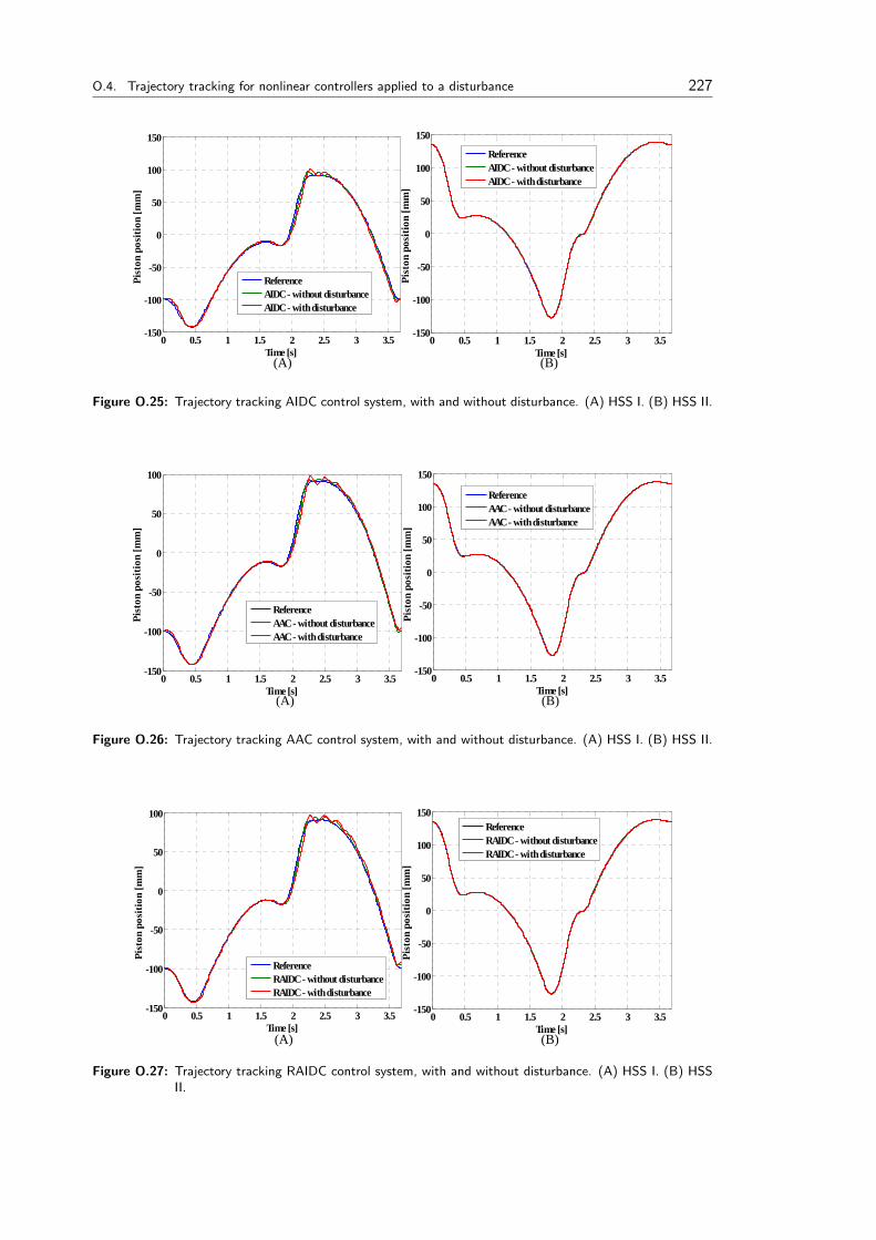
O.4. Trajectory tracking for nonlinear controllers applied to a disturbance 227
(A) (B)
0 0.5 1 1.5 2 2.5 3 3.5-150
-100
-50
0
50
100
150
Time [s]
Pist
on p
ositi
on [m
m]
ReferenceAIDC - without disturbanceAIDC - with disturbance
0 0.5 1 1.5 2 2.5 3 3.5-150
-100
-50
0
50
100
150
Time [s]
Pist
on p
ositi
on [m
m]
ReferenceAIDC - without disturbanceAIDC - with disturbance
Figure O.25: Trajectory tracking AIDC control system, with and without disturbance. (A) HSS I. (B) HSS II.
(A) (B)
0 0.5 1 1.5 2 2.5 3 3.5-150
-100
-50
0
50
100
Time [s]
Pist
on p
ositi
on [m
m]
ReferenceAAC - without disturbanceAAC - with disturbance
0 0.5 1 1.5 2 2.5 3 3.5-150
-100
-50
0
50
100
150
Time [s]
Pist
on p
ositi
on [m
m]
ReferenceAAC - without disturbanceAAC - with disturbance
Figure O.26: Trajectory tracking AAC control system, with and without disturbance. (A) HSS I. (B) HSS II.
(A) (B)
0 0.5 1 1.5 2 2.5 3 3.5-150
-100
-50
0
50
100
150
Time [s]
Pist
on p
ositi
on [m
m]
ReferenceRAIDC - without disturbanceRAIDC - with disturbance
0 0.5 1 1.5 2 2.5 3 3.5-150
-100
-50
0
50
100
Time [s]
Pist
on p
ositi
on [m
m]
ReferenceRAIDC - without disturbanceRAIDC - with disturbance
Figure O.27: Trajectory tracking RAIDC control system, with and without disturbance. (A) HSS I. (B) HSSII.
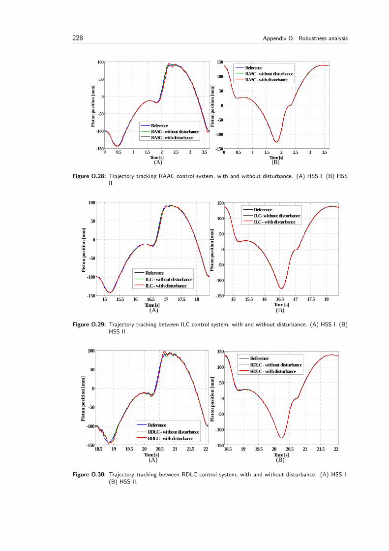
228 Appendix O. Robustness analysis
(A) (B)
0 0.5 1 1.5 2 2.5 3 3.5-150
-100
-50
0
50
100
Time [s]
Pist
on p
ositi
on [m
m]
ReferenceRAAC - without disturbanceRAAC - with disturbance
0 0.5 1 1.5 2 2.5 3 3.5-150
-100
-50
0
50
100
150
Time [s]
Pist
on p
ositi
on [m
m]
ReferenceRAAC - without disturbanceRAAC - with disturbance
Figure O.28: Trajectory tracking RAAC control system, with and without disturbance. (A) HSS I. (B) HSSII.
(A) (B)
15 15.5 16 16.5 17 17.5 18-150
-100
-50
0
50
100
Time [s]
Pist
on p
ositi
on [m
m]
ReferenceILC - without disturbanceILC - with disturbance
15 15.5 16 16.5 17 17.5 18-150
-100
-50
0
50
100
150
Time [s]
Pist
on p
ositi
on [m
m]
ReferenceILC- without disturbanceILC - with disturbance
Figure O.29: Trajectory tracking between ILC control system, with and without disturbance. (A) HSS I. (B)HSS II.
(A) (B)
18.5 19 19.5 20 20.5 21 21.5 22-150
-100
-50
0
50
100
Time [s]
Pist
on p
ositi
on [m
m]
ReferenceRDLC - without disturbanceRDLC - with disturbance
18.5 19 19.5 20 20.5 21 21.5 22-150
-100
-50
0
50
100
150
Time [s]
Pist
on p
ositi
on [m
m]
ReferenceRDLC - without disturbanceRDLC - with disturbance
Figure O.30: Trajectory tracking between RDLC control system, with and without disturbance. (A) HSS I.(B) HSS II.
Appendix PLaboratorySetup
Contents
O.1 ∆ Error Plots for Linear Con-trollers . . . . . . . . . . . . . 217
O.2 ∆ Error Plots for Nonlinearcontrollers . . . . . . . . . . . 220
O.3 Trajectory tracking for linearcontrollers applied to a distur-bance . . . . . . . . . . . . . . 223
O.4 Trajectory tracking for non-linear controllers applied to adisturbance . . . . . . . . . . . 226
In this appendix the laboratory equipment used for implementing and testing the controllersfrom the thesis is described
In the following is listed all the laboratory equipment used during this thesis along withand indication of where the belonging data sheets may be found. Afterwards a moredetailed description of selected components are given along with a diagram showing thecoupling of the various components.
• One servo valve, Moog, E760-942, El05(Data sheet on CD (not specific valve))
• One servo valve, Rexroth, 4WS 2 EE 10-40(Data sheet on CD(not specific valve))
• Two safety valves, Rexroth, 4 WE 6 Y51/AG24NZ4(No data sheet available)
• Two cylinders, Rexroth, STC 0331-10/, WLP350 17126, H05001(No data sheetavailable)
• Four pressure transducers, HBM P4A(Data sheet on CD)
• Two position transducers, Messotron WLP 350(Data sheet on CD)
• One pressure transducer amplifier, (No data sheet available)
• Two position transducer amplifiers, HBM, MVD2555(Data sheet on CD)
• One servo valve amplifier, Moog, Moog servo amp(No data sheet available)
• One servo valve amplifier, Rexroth, VT 1610(No data sheet available)
• Two DC power supplies(No data sheet available)
• One PC with DSP and DAQ card(No data sheet available)
• One DSP interface(No data sheet available)
229
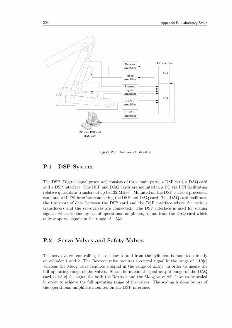
230 Appendix P. Laboratory Setup
DSP interface
HBM 1
Amplifier
HBM 2
Amplifier
D/A
A/D
Rexroot
Amplifier
Moog
Amplifier
Pressure
Signals
Amplifier
PC with DSP and
DAQ card
Figure P.1: Overview of lab setup
P.1 DSP System
The DSP (Digital signal processor) consists of three main parts, a DSP card, a DAQ cardand a DSP interface. The DSP and DAQ cards are mounted in a PC via PCI facilitatingrelative quick data transfers of up to 132[MB/s]. Mounted on the DSP is also a processor,ram, and a BITSI interface connecting the DSP and DAQ card. The DAQ card facilitatesthe transport of data between the DSP card and the DSP interface where the varioustransducers and the servovalves are connected. The DSP interface is used for scalingsignals, which is done by use of operational amplifiers, to and from the DAQ card whichonly supports signals in the range of ±5[v].
P.2 Servo Valves and Safety Valves
The servo valves controlling the oil flow to and from the cylinders is mounted directlyon cylinder 1 and 2. The Rexroot valve requires a control signal in the range of ±10[v]whereas the Moog valve requires a signal in the range of ±15[v] in order to insure thefull operating range of the valves. Since the maximal signal output range of the DAQcard is ±5[v] the signal for both the Rexroot and the Moog valve will have to be scaledin order to achieve the full operating range of the valves. The scaling is done by use ofthe operational amplifiers mounted on the DSP interface.
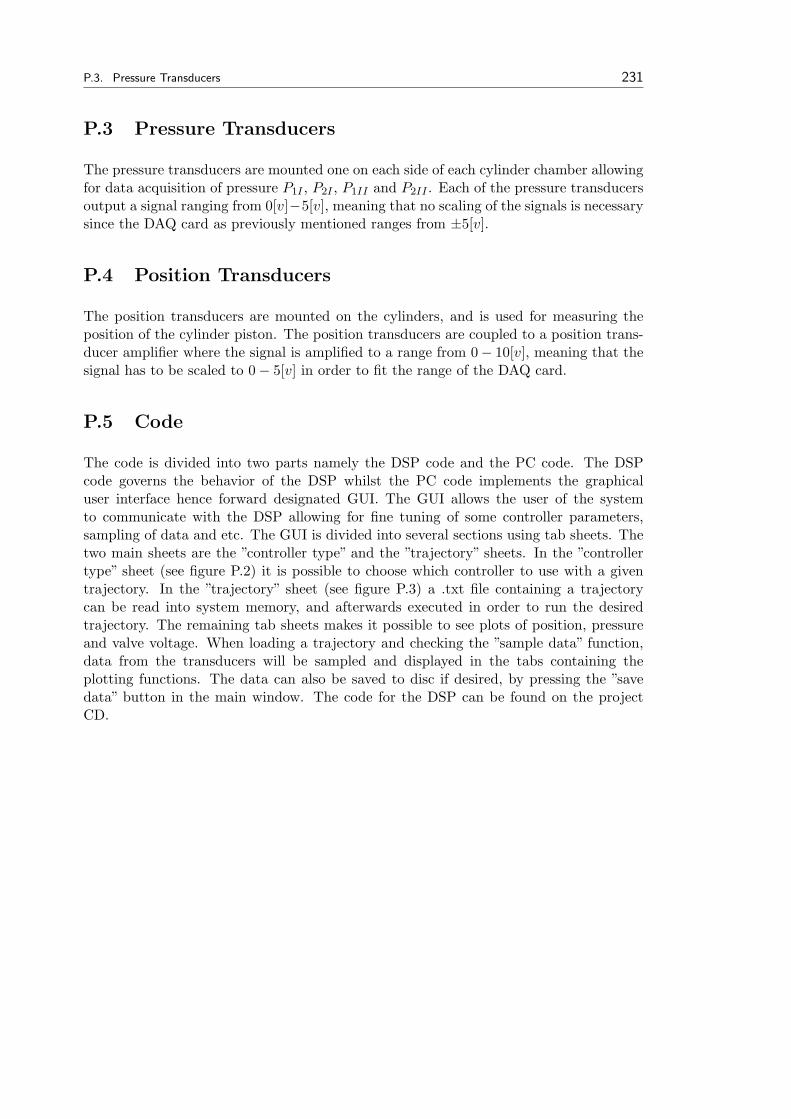
P.3. Pressure Transducers 231
P.3 Pressure Transducers
The pressure transducers are mounted one on each side of each cylinder chamber allowingfor data acquisition of pressure P1I , P2I , P1II and P2II . Each of the pressure transducersoutput a signal ranging from 0[v]−5[v], meaning that no scaling of the signals is necessarysince the DAQ card as previously mentioned ranges from ±5[v].
P.4 Position Transducers
The position transducers are mounted on the cylinders, and is used for measuring theposition of the cylinder piston. The position transducers are coupled to a position trans-ducer amplifier where the signal is amplified to a range from 0− 10[v], meaning that thesignal has to be scaled to 0− 5[v] in order to fit the range of the DAQ card.
P.5 Code
The code is divided into two parts namely the DSP code and the PC code. The DSPcode governs the behavior of the DSP whilst the PC code implements the graphicaluser interface hence forward designated GUI. The GUI allows the user of the systemto communicate with the DSP allowing for fine tuning of some controller parameters,sampling of data and etc. The GUI is divided into several sections using tab sheets. Thetwo main sheets are the ”controller type” and the ”trajectory” sheets. In the ”controllertype” sheet (see figure P.2) it is possible to choose which controller to use with a giventrajectory. In the ”trajectory” sheet (see figure P.3) a .txt file containing a trajectorycan be read into system memory, and afterwards executed in order to run the desiredtrajectory. The remaining tab sheets makes it possible to see plots of position, pressureand valve voltage. When loading a trajectory and checking the ”sample data” function,data from the transducers will be sampled and displayed in the tabs containing theplotting functions. The data can also be saved to disc if desired, by pressing the ”savedata” button in the main window. The code for the DSP can be found on the projectCD.
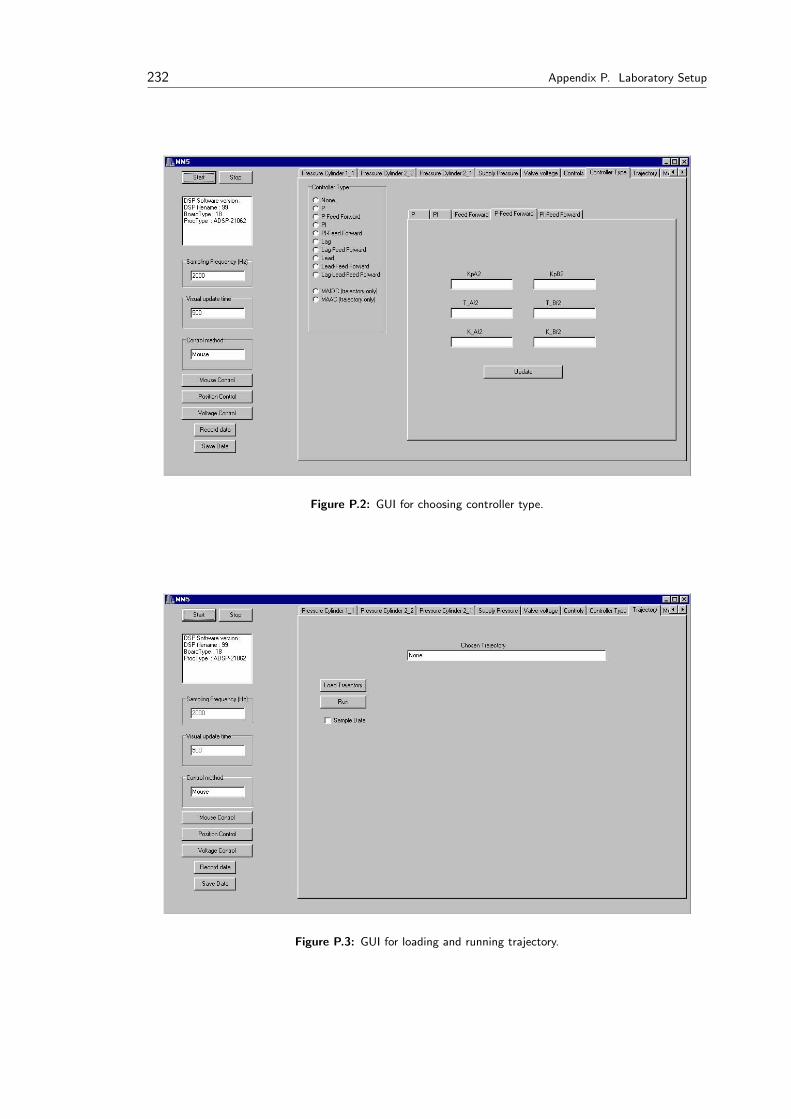
232 Appendix P. Laboratory Setup
Figure P.2: GUI for choosing controller type.
Figure P.3: GUI for loading and running trajectory.