a comprehensive framework for testing database-centric
TRANSCRIPT

A COMPREHENSIVE FRAMEWORK FOR
TESTING DATABASE-CENTRIC SOFTWARE
APPLICATIONS
by
Gregory M. Kapfhammer
Bachelor of Science, Allegheny College,
Department of Computer Science, 1999,
Master of Science, University of Pittsburgh,
Department of Computer Science, 2004
Submitted to the Graduate Faculty of
the Department of Computer Science in partial fulfillment
of the requirements for the degree of
Doctor of Philosophy
University of Pittsburgh
2007

UNIVERSITY OF PITTSBURGH
DEPARTMENT OF COMPUTER SCIENCE
This dissertation was presented
by
Gregory M. Kapfhammer
It was defended on
April 19, 2007
and approved by
Dr. Mary Lou Soffa, University of Virginia, Department of Computer Science
Dr. Bruce Childers, University of Pittsburgh, Department of Computer Science
Dr. Panos Chrysanthis, University of Pittsburgh, Department of Computer Science
Dr. Jeffrey Voas, SAIC
Dissertation Director: Dr. Mary Lou Soffa, University of Virginia, Department of Computer Science
ii

Copyright c© by Gregory M. Kapfhammer
2007
iii

A COMPREHENSIVE FRAMEWORK FOR TESTING DATABASE-CENTRIC
SOFTWARE APPLICATIONS
Gregory M. Kapfhammer, PhD
University of Pittsburgh, 2007
The database is a critical component of many modern software applications. Recent reports indicate that
the vast majority of database use occurs from within an application program. Indeed, database-centric
applications have been implemented to create digital libraries, scientific data repositories, and electronic
commerce applications. However, a database-centric application is very different from a traditional software
system because it interacts with a database that has a complex state and structure. This dissertation
formulates a comprehensive framework to address the challenges that are associated with the efficient and
effective testing of database-centric applications. The database-aware approach to testing includes: (i) a
fault model, (ii) several unified representations of a program’s database interactions, (iii) a family of test
adequacy criteria, (iv) a test coverage monitoring component, and (v) tools for reducing and re-ordering a
test suite during regression testing.
This dissertation analyzes the worst-case time complexity of every important testing algorithm. This
analysis is complemented by experiments that measure the efficiency and effectiveness of the database-
aware testing techniques. Each tool is evaluated by using it to test six database-centric applications. The
experiments show that the database-aware representations can be constructed with moderate time and space
overhead. The adequacy criteria call for test suites to cover 20% more requirements than traditional criteria
and this ensures the accurate assessment of test suite quality. It is possible to enumerate data flow-based
test requirements in less than one minute and coverage tree path requirements are normally identified in
no more than ten seconds. The experimental results also indicate that the coverage monitor can insert
instrumentation probes into all six of the applications in fewer than ten seconds. Although instrumentation
may moderately increase the static space overhead of an application, the coverage monitoring techniques
only increase testing time by 55% on average. A coverage tree often can be stored in less than five seconds
even though the coverage report may consume up to twenty-five megabytes of storage. The regression tester
usually reduces or prioritizes a test suite in under five seconds. The experiments also demonstrate that the
modified test suite is frequently more streamlined than the initial tests.
iv

TABLE OF CONTENTS
PREFACE . . . . . . . . . . . . . . . . . . . . . . . . . . . . . . . . . . . . . . . . . . . . . . . . . . . xviii
1.0 INTRODUCTION . . . . . . . . . . . . . . . . . . . . . . . . . . . . . . . . . . . . . . . . . . . 1
1.1 THE RISE OF THE DATABASE . . . . . . . . . . . . . . . . . . . . . . . . . . . . . . . . . 1
1.2 OVERVIEW OF THE RESEARCH CONTRIBUTIONS . . . . . . . . . . . . . . . . . . . . 2
1.2.1 Technical Contributions . . . . . . . . . . . . . . . . . . . . . . . . . . . . . . . . . . 2
1.2.2 A New Perspective on Software Testing . . . . . . . . . . . . . . . . . . . . . . . . . 4
1.3 OVERVIEW OF THE DATABASE-AWARE TESTING FRAMEWORK . . . . . . . . . . 4
1.4 ORGANIZATION OF THE DISSERTATION . . . . . . . . . . . . . . . . . . . . . . . . . . 6
2.0 BACKGROUND . . . . . . . . . . . . . . . . . . . . . . . . . . . . . . . . . . . . . . . . . . . . 7
2.1 INTRODUCTION . . . . . . . . . . . . . . . . . . . . . . . . . . . . . . . . . . . . . . . . . 7
2.2 RELATIONAL DATABASES . . . . . . . . . . . . . . . . . . . . . . . . . . . . . . . . . . . 7
2.3 OVERVIEW OF DATABASE-CENTRIC APPLICATIONS . . . . . . . . . . . . . . . . . . 8
2.4 TRADITIONAL PROGRAM REPRESENTATIONS FOR TESTING . . . . . . . . . . . . 11
2.5 TRADITIONAL EXECUTION-BASED SOFTWARE TESTING . . . . . . . . . . . . . . . 14
2.5.1 Preliminaries . . . . . . . . . . . . . . . . . . . . . . . . . . . . . . . . . . . . . . . . 14
2.5.2 Model of Execution-Based Software Testing . . . . . . . . . . . . . . . . . . . . . . . 15
2.5.3 Test Adequacy Criteria . . . . . . . . . . . . . . . . . . . . . . . . . . . . . . . . . . 17
2.5.4 Test Coverage Monitoring . . . . . . . . . . . . . . . . . . . . . . . . . . . . . . . . . 19
2.5.5 Test Suite Reduction . . . . . . . . . . . . . . . . . . . . . . . . . . . . . . . . . . . . 20
2.5.6 Test Suite Prioritization . . . . . . . . . . . . . . . . . . . . . . . . . . . . . . . . . . 21
2.5.7 Discussion of the Testing Model . . . . . . . . . . . . . . . . . . . . . . . . . . . . . . 22
2.6 TESTING DATABASE-CENTRIC APPLICATIONS . . . . . . . . . . . . . . . . . . . . . . 22
2.7 CONCLUSION . . . . . . . . . . . . . . . . . . . . . . . . . . . . . . . . . . . . . . . . . . . 25
3.0 IMPLEMENTATION AND EVALUATION OF THE TESTING FRAMEWORK . . 26
3.1 INTRODUCTION . . . . . . . . . . . . . . . . . . . . . . . . . . . . . . . . . . . . . . . . . 26
3.2 OVERVIEW . . . . . . . . . . . . . . . . . . . . . . . . . . . . . . . . . . . . . . . . . . . . 26
3.3 HIGHLIGHTS OF THE DATABASE-AWARE TESTING FRAMEWORK . . . . . . . . . 27
v

3.4 LIMITATIONS OF THE APPROACH . . . . . . . . . . . . . . . . . . . . . . . . . . . . . . 27
3.5 CHARACTERIZING THE CASE STUDY APPLICATIONS . . . . . . . . . . . . . . . . . 30
3.5.1 High Level Description . . . . . . . . . . . . . . . . . . . . . . . . . . . . . . . . . . . 30
3.5.2 Relational Schemas . . . . . . . . . . . . . . . . . . . . . . . . . . . . . . . . . . . . . 36
3.5.3 Detailed Characterization . . . . . . . . . . . . . . . . . . . . . . . . . . . . . . . . . 38
3.5.3.1 Test Suites . . . . . . . . . . . . . . . . . . . . . . . . . . . . . . . . . . . . 38
3.5.3.2 Database Interactions . . . . . . . . . . . . . . . . . . . . . . . . . . . . . . 41
3.6 DESIGN OF THE EXPERIMENTS . . . . . . . . . . . . . . . . . . . . . . . . . . . . . . . 41
3.7 THREATS TO VALIDITY . . . . . . . . . . . . . . . . . . . . . . . . . . . . . . . . . . . . 42
3.8 CONCLUSION . . . . . . . . . . . . . . . . . . . . . . . . . . . . . . . . . . . . . . . . . . . 43
4.0 FAMILY OF TEST ADEQUACY CRITERIA . . . . . . . . . . . . . . . . . . . . . . . . . 44
4.1 INTRODUCTION . . . . . . . . . . . . . . . . . . . . . . . . . . . . . . . . . . . . . . . . . 44
4.2 DATABASE INTERACTION FAULT MODEL . . . . . . . . . . . . . . . . . . . . . . . . . 44
4.2.1 Type (1-c) and (2-v) Defects . . . . . . . . . . . . . . . . . . . . . . . . . . . . . . . 45
4.2.2 Type (1-v) and (2-c) Defects . . . . . . . . . . . . . . . . . . . . . . . . . . . . . . . 48
4.3 DATABASE-AWARE TEST ADEQUACY CRITERIA . . . . . . . . . . . . . . . . . . . . . 48
4.3.1 Traditional Definition-Use Associations . . . . . . . . . . . . . . . . . . . . . . . . . . 48
4.3.2 Test Adequacy for Database-Centric Applications . . . . . . . . . . . . . . . . . . . . 49
4.3.3 Subsumption of the Test Adequacy Criteria . . . . . . . . . . . . . . . . . . . . . . . 51
4.3.4 Suitability of the Test Adequacy Criteria . . . . . . . . . . . . . . . . . . . . . . . . 52
4.3.5 Comparison to Traditional Adequacy Criteria . . . . . . . . . . . . . . . . . . . . . . 53
4.4 CONCLUSION . . . . . . . . . . . . . . . . . . . . . . . . . . . . . . . . . . . . . . . . . . . 55
5.0 TEST ADEQUACY COMPONENT . . . . . . . . . . . . . . . . . . . . . . . . . . . . . . . 56
5.1 INTRODUCTION . . . . . . . . . . . . . . . . . . . . . . . . . . . . . . . . . . . . . . . . . 56
5.2 OVERVIEW OF THE TEST ADEQUACY COMPONENT . . . . . . . . . . . . . . . . . . 56
5.3 REPRESENTING THE PROGRAM UNDER TEST . . . . . . . . . . . . . . . . . . . . . . 57
5.4 ANALYZING A DATABASE INTERACTION . . . . . . . . . . . . . . . . . . . . . . . . . 58
5.4.1 Overview of the Analysis . . . . . . . . . . . . . . . . . . . . . . . . . . . . . . . . . . 58
5.4.2 Representing a Database’s State and Structure . . . . . . . . . . . . . . . . . . . . . 60
5.4.3 Representing a Database Interaction . . . . . . . . . . . . . . . . . . . . . . . . . . . 61
5.4.4 Generating Relational Database Entities . . . . . . . . . . . . . . . . . . . . . . . . . 65
5.4.4.1 Databases . . . . . . . . . . . . . . . . . . . . . . . . . . . . . . . . . . . . . 67
5.4.4.2 Relations . . . . . . . . . . . . . . . . . . . . . . . . . . . . . . . . . . . . . 68
5.4.4.3 Attributes, Records, and Attribute Values . . . . . . . . . . . . . . . . . . . 68
5.4.5 Enumerating Unique Names for Database Entities . . . . . . . . . . . . . . . . . . . 70
5.5 CONSTRUCTING A DATABASE-AWARE REPRESENTATION . . . . . . . . . . . . . . 74
vi

5.6 IMPLEMENTATION OF THE TEST ADEQUACY COMPONENT . . . . . . . . . . . . . 80
5.7 EXPERIMENT GOALS AND DESIGN . . . . . . . . . . . . . . . . . . . . . . . . . . . . . 83
5.8 KEY INSIGHTS FROM THE EXPERIMENTS . . . . . . . . . . . . . . . . . . . . . . . . . 85
5.9 ANALYSIS OF THE EXPERIMENTAL RESULTS . . . . . . . . . . . . . . . . . . . . . . 85
5.9.1 Number of Test Requirements . . . . . . . . . . . . . . . . . . . . . . . . . . . . . . . 85
5.9.2 Time Overhead . . . . . . . . . . . . . . . . . . . . . . . . . . . . . . . . . . . . . . . 86
5.9.3 Space Overhead . . . . . . . . . . . . . . . . . . . . . . . . . . . . . . . . . . . . . . . 87
5.10 THREATS TO VALIDITY . . . . . . . . . . . . . . . . . . . . . . . . . . . . . . . . . . . . 88
5.11 CONCLUSION . . . . . . . . . . . . . . . . . . . . . . . . . . . . . . . . . . . . . . . . . . . 89
6.0 FOUNDATIONS OF TEST COVERAGE MONITORING . . . . . . . . . . . . . . . . . 91
6.1 INTRODUCTION . . . . . . . . . . . . . . . . . . . . . . . . . . . . . . . . . . . . . . . . . 91
6.2 OVERVIEW OF THE COVERAGE MONITORING PROCESS . . . . . . . . . . . . . . . 91
6.3 TEST COVERAGE MONITORING CHALLENGES . . . . . . . . . . . . . . . . . . . . . . 93
6.3.1 Location of the Instrumentation . . . . . . . . . . . . . . . . . . . . . . . . . . . . . 93
6.3.2 Types of Instrumentation . . . . . . . . . . . . . . . . . . . . . . . . . . . . . . . . . 94
6.3.3 Format of the Test Coverage Results . . . . . . . . . . . . . . . . . . . . . . . . . . . 99
6.4 DATABASE-AWARE TEST COVERAGE MONITORING TREES . . . . . . . . . . . . . 101
6.4.1 Overview . . . . . . . . . . . . . . . . . . . . . . . . . . . . . . . . . . . . . . . . . . 101
6.4.2 Traditional Trees . . . . . . . . . . . . . . . . . . . . . . . . . . . . . . . . . . . . . . 103
6.4.2.1 Dynamic Call Trees . . . . . . . . . . . . . . . . . . . . . . . . . . . . . . . 103
6.4.2.2 Calling Context Trees . . . . . . . . . . . . . . . . . . . . . . . . . . . . . . 104
6.4.3 Database-Aware Trees . . . . . . . . . . . . . . . . . . . . . . . . . . . . . . . . . . . 110
6.4.3.1 Instrumentation to Monitor a Database Use . . . . . . . . . . . . . . . . . . 110
6.4.3.2 Instrumentation to Monitor a Database Definition . . . . . . . . . . . . . . 115
6.4.3.3 Worst-Case Time Complexity . . . . . . . . . . . . . . . . . . . . . . . . . . 117
6.4.4 Inserting the Database-Aware Instrumentation . . . . . . . . . . . . . . . . . . . . . 123
6.5 CALCULATING TEST ADEQUACY . . . . . . . . . . . . . . . . . . . . . . . . . . . . . . 124
6.5.1 Representing Database-Aware Test Suites . . . . . . . . . . . . . . . . . . . . . . . . 124
6.5.2 Calculating Data Flow-Based Adequacy . . . . . . . . . . . . . . . . . . . . . . . . . 126
6.6 CONCLUSION . . . . . . . . . . . . . . . . . . . . . . . . . . . . . . . . . . . . . . . . . . . 127
7.0 TEST COVERAGE MONITORING COMPONENT . . . . . . . . . . . . . . . . . . . . 128
7.1 INTRODUCTION . . . . . . . . . . . . . . . . . . . . . . . . . . . . . . . . . . . . . . . . . 128
7.2 OVERVIEW OF THE COVERAGE MONITORING COMPONENT . . . . . . . . . . . . . 128
7.3 IMPLEMENTATION OF THE COVERAGE MONITOR . . . . . . . . . . . . . . . . . . . 130
7.3.1 Instrumentation . . . . . . . . . . . . . . . . . . . . . . . . . . . . . . . . . . . . . . . 130
7.3.2 Tree Format and Storage . . . . . . . . . . . . . . . . . . . . . . . . . . . . . . . . . 131
vii

7.4 EXPERIMENT GOALS AND DESIGN . . . . . . . . . . . . . . . . . . . . . . . . . . . . . 132
7.5 KEY INSIGHTS FROM THE EXPERIMENTS . . . . . . . . . . . . . . . . . . . . . . . . . 133
7.6 ANALYSIS OF THE EXPERIMENTAL RESULTS . . . . . . . . . . . . . . . . . . . . . . 134
7.6.1 Instrumentation . . . . . . . . . . . . . . . . . . . . . . . . . . . . . . . . . . . . . . . 134
7.6.1.1 Instrumentation Time Overhead . . . . . . . . . . . . . . . . . . . . . . . . 135
7.6.1.2 Instrumentation Space Overhead . . . . . . . . . . . . . . . . . . . . . . . . 135
7.6.2 Test Suite Execution Time . . . . . . . . . . . . . . . . . . . . . . . . . . . . . . . . 138
7.6.2.1 Static and Dynamic Instrumentation Costs . . . . . . . . . . . . . . . . . . 139
7.6.2.2 Varying Database Interaction Granularity . . . . . . . . . . . . . . . . . . . 141
7.6.2.3 Storage Time for the TCM Tree . . . . . . . . . . . . . . . . . . . . . . . . 142
7.6.3 Tree Space Overhead . . . . . . . . . . . . . . . . . . . . . . . . . . . . . . . . . . . . 144
7.6.3.1 Nodes and Edges in the TCM Tree . . . . . . . . . . . . . . . . . . . . . . . 146
7.6.3.2 Memory and Filesystem Size of the TCM Tree . . . . . . . . . . . . . . . . 148
7.6.4 Detailed Tree Characterization . . . . . . . . . . . . . . . . . . . . . . . . . . . . . . 150
7.6.4.1 Height of the TCM Tree . . . . . . . . . . . . . . . . . . . . . . . . . . . . . 152
7.6.4.2 Node Out Degree . . . . . . . . . . . . . . . . . . . . . . . . . . . . . . . . . 152
7.6.4.3 Node Replication Counts . . . . . . . . . . . . . . . . . . . . . . . . . . . . 154
7.7 THREATS TO VALIDITY . . . . . . . . . . . . . . . . . . . . . . . . . . . . . . . . . . . . 156
7.8 CONCLUSION . . . . . . . . . . . . . . . . . . . . . . . . . . . . . . . . . . . . . . . . . . . 158
8.0 REGRESSION TESTING . . . . . . . . . . . . . . . . . . . . . . . . . . . . . . . . . . . . . . 159
8.1 INTRODUCTION . . . . . . . . . . . . . . . . . . . . . . . . . . . . . . . . . . . . . . . . . 159
8.2 OVERVIEW OF REGRESSION TESTING . . . . . . . . . . . . . . . . . . . . . . . . . . . 160
8.3 THE BENEFITS OF REGRESSION TESTING . . . . . . . . . . . . . . . . . . . . . . . . 161
8.4 USING DATABASE-AWARE COVERAGE TREES . . . . . . . . . . . . . . . . . . . . . . 166
8.5 DATABASE-AWARE REGRESSION TESTING . . . . . . . . . . . . . . . . . . . . . . . . 171
8.6 EVALUATING THE EFFECTIVENESS OF A TEST SUITE . . . . . . . . . . . . . . . . . 176
8.7 IMPLEMENTATION OF THE REGRESSION TESTING COMPONENT . . . . . . . . . . 181
8.8 EXPERIMENT GOALS AND DESIGN . . . . . . . . . . . . . . . . . . . . . . . . . . . . . 181
8.9 KEYS INSIGHTS FROM THE EXPERIMENTS . . . . . . . . . . . . . . . . . . . . . . . . 185
8.10 ANALYSIS OF THE EXPERIMENTAL RESULTS . . . . . . . . . . . . . . . . . . . . . . 186
8.10.1 Coverage Information . . . . . . . . . . . . . . . . . . . . . . . . . . . . . . . . . . . 186
8.10.2 Test Reduction . . . . . . . . . . . . . . . . . . . . . . . . . . . . . . . . . . . . . . . 192
8.10.2.1 Efficiency . . . . . . . . . . . . . . . . . . . . . . . . . . . . . . . . . . . . . 192
8.10.2.2 Test Suite Size . . . . . . . . . . . . . . . . . . . . . . . . . . . . . . . . . . 192
8.10.2.3 Reductions in Testing Time . . . . . . . . . . . . . . . . . . . . . . . . . . . 194
8.10.2.4 Coverage Preservation . . . . . . . . . . . . . . . . . . . . . . . . . . . . . . 197
viii

8.10.3 Test Prioritization . . . . . . . . . . . . . . . . . . . . . . . . . . . . . . . . . . . . . 201
8.11 THREATS TO VALIDITY . . . . . . . . . . . . . . . . . . . . . . . . . . . . . . . . . . . . 203
8.12 CONCLUSION . . . . . . . . . . . . . . . . . . . . . . . . . . . . . . . . . . . . . . . . . . . 204
9.0 CONCLUSIONS AND FUTURE WORK . . . . . . . . . . . . . . . . . . . . . . . . . . . . 205
9.1 SUMMARY OF THE CONTRIBUTIONS . . . . . . . . . . . . . . . . . . . . . . . . . . . . 205
9.2 KEY INSIGHTS FROM THE EXPERIMENTS . . . . . . . . . . . . . . . . . . . . . . . . . 208
9.3 FUTURE WORK . . . . . . . . . . . . . . . . . . . . . . . . . . . . . . . . . . . . . . . . . 210
9.3.1 Enhancing the Techniques . . . . . . . . . . . . . . . . . . . . . . . . . . . . . . . . . 210
9.3.2 New Database-Aware Testing Techniques . . . . . . . . . . . . . . . . . . . . . . . . 214
9.3.3 Further Empirical Evaluation . . . . . . . . . . . . . . . . . . . . . . . . . . . . . . . 215
9.3.4 Additional Environmental Factors . . . . . . . . . . . . . . . . . . . . . . . . . . . . 217
9.3.5 Improving Traditional Software Testing and Analysis . . . . . . . . . . . . . . . . . . 218
APPENDIX A. SUMMARY OF THE NOTATION . . . . . . . . . . . . . . . . . . . . . . . . 220
APPENDIX B. CASE STUDY APPLICATIONS . . . . . . . . . . . . . . . . . . . . . . . . . 228
APPENDIX C. EXPERIMENT DETAILS . . . . . . . . . . . . . . . . . . . . . . . . . . . . . . 239
BIBLIOGRAPHY . . . . . . . . . . . . . . . . . . . . . . . . . . . . . . . . . . . . . . . . . . . . . . 241
ix

LIST OF TABLES
2.1 The Faults Detected by a Test Suite. . . . . . . . . . . . . . . . . . . . . . . . . . . . . . . . 21
3.1 High Level Description of the RM, FF, and PI Case Study Applications. . . . . . . . . . . . . 31
3.2 High Level Description of the TM, ST, and GB Case Study Applications. . . . . . . . . . . . . 31
3.3 Average Method Cyclomatic Complexity Measurements. . . . . . . . . . . . . . . . . . . . . 35
3.4 Characterization of the Test Suites. . . . . . . . . . . . . . . . . . . . . . . . . . . . . . . . . 38
3.5 Number of Test Cases and Oracle Executions. . . . . . . . . . . . . . . . . . . . . . . . . . . 40
3.6 Database Interactions in the Case Study Applications. . . . . . . . . . . . . . . . . . . . . . . 40
4.1 The Edges Covered by a Test Case. . . . . . . . . . . . . . . . . . . . . . . . . . . . . . . . . 54
4.2 The Def-Use Associations Covered by a Test Case. . . . . . . . . . . . . . . . . . . . . . . . . 55
5.1 Test Adequacy Pairings for the Measurement of T R. . . . . . . . . . . . . . . . . . . . . . . 83
5.2 Test Adequacy Pairings for the Measurement of T and S. . . . . . . . . . . . . . . . . . . . . 83
5.3 Characteristics of the mp3cd Case Study Application. . . . . . . . . . . . . . . . . . . . . . . 84
5.4 Percent Increase in the Number of Test Requirements. . . . . . . . . . . . . . . . . . . . . . . 85
5.5 Percent Increase in the Time Overhead. . . . . . . . . . . . . . . . . . . . . . . . . . . . . . . 88
5.6 Percent Increase in the Space Overhead for Nodes. . . . . . . . . . . . . . . . . . . . . . . . . 88
5.7 Percent Increase in the Space Overhead for Edges. . . . . . . . . . . . . . . . . . . . . . . . . 89
6.1 High Level Comparison of the Different Types of Coverage Monitoring Trees. . . . . . . . . . 100
6.2 Summary of the Time Complexities for the Instrumentation Probes. . . . . . . . . . . . . . . 122
7.1 Average Static Size Across All Instrumented Case Study Applications. . . . . . . . . . . . . 136
7.2 Size of the Test Coverage Monitoring Probes. . . . . . . . . . . . . . . . . . . . . . . . . . . . 136
7.3 Percent Increase in Testing Time when Static Instrumentation Generates a CCT. . . . . . . 138
7.4 Average Test Coverage Monitoring Time Across All Case Study Applications. . . . . . . . . 139
7.5 Average TCM Time Across All Applications when Granularity is Varied. . . . . . . . . . . . 141
7.6 Average TCM Tree Storage Time Across All Case Study Applications. . . . . . . . . . . . . 144
7.7 Average Number of Nodes in the TCM Tree Across All Applications. . . . . . . . . . . . . . 148
7.8 Memory Sizes of the Test Coverage Monitoring Trees (bytes). . . . . . . . . . . . . . . . . . . 150
7.9 Height of the Test Coverage Monitoring Trees. . . . . . . . . . . . . . . . . . . . . . . . . . . 154
x

8.1 Test Suite Execution Time. . . . . . . . . . . . . . . . . . . . . . . . . . . . . . . . . . . . . . 162
8.2 Test Requirement Coverage for a Test Suite. . . . . . . . . . . . . . . . . . . . . . . . . . . . 162
8.3 Test Coverage Effectiveness. . . . . . . . . . . . . . . . . . . . . . . . . . . . . . . . . . . . . 162
8.4 Summary of the Linear Regression Analysis. . . . . . . . . . . . . . . . . . . . . . . . . . . . 165
8.5 Examples of Paths in a Test Coverage Tree. . . . . . . . . . . . . . . . . . . . . . . . . . . . 167
8.6 The Cost and Coverage of a Test Suite. . . . . . . . . . . . . . . . . . . . . . . . . . . . . . . 174
8.7 Summary of the Worst-Case Time Complexities. . . . . . . . . . . . . . . . . . . . . . . . . . 176
8.8 Comparing Test Suite Reductions. . . . . . . . . . . . . . . . . . . . . . . . . . . . . . . . . . 179
8.9 Test Suite Execution Time With and Without Database Server Restarts. . . . . . . . . . . . 184
8.10 Reduction Factors for the Size of a Test Suite. . . . . . . . . . . . . . . . . . . . . . . . . . . 193
8.11 Summary of the Abbreviations Used to Describe the Reduction Techniques. . . . . . . . . . 194
8.12 Summary of the Abbreviations Used to Describe the Prioritization Techniques. . . . . . . . . 200
A1 Relational Databases. . . . . . . . . . . . . . . . . . . . . . . . . . . . . . . . . . . . . . . . . 220
A2 Traditional Program Representation. . . . . . . . . . . . . . . . . . . . . . . . . . . . . . . . 221
A3 Characterizing a Database-Centric Application. . . . . . . . . . . . . . . . . . . . . . . . . . 221
A4 Database Entity Sets. . . . . . . . . . . . . . . . . . . . . . . . . . . . . . . . . . . . . . . . . 221
A5 Database-Aware Test Adequacy Criteria. . . . . . . . . . . . . . . . . . . . . . . . . . . . . . 222
A6 Database-Centric Applications. . . . . . . . . . . . . . . . . . . . . . . . . . . . . . . . . . . . 222
A7 Enumerating the Sets of Database Entities. . . . . . . . . . . . . . . . . . . . . . . . . . . . . 223
A8 The Database-Aware Test Adequacy Component. . . . . . . . . . . . . . . . . . . . . . . . . 223
A9 Database-Aware Test Coverage Monitoring Trees. . . . . . . . . . . . . . . . . . . . . . . . . 224
A10 Instrumentation to Create the Database-Aware TCM Trees. . . . . . . . . . . . . . . . . . . 224
A11 Relational Difference Operators. . . . . . . . . . . . . . . . . . . . . . . . . . . . . . . . . . . 225
A12 Worst-Case Complexity of the Database-Aware Instrumentation. . . . . . . . . . . . . . . . . 225
A13 Database-Aware Test Suites. . . . . . . . . . . . . . . . . . . . . . . . . . . . . . . . . . . . . 225
A14 Describing the Test Coverage Monitor. . . . . . . . . . . . . . . . . . . . . . . . . . . . . . . 226
A15 Paths in the Test Coverage Monitoring Tree. . . . . . . . . . . . . . . . . . . . . . . . . . . . 226
A16 Database-Aware Regression Testing. . . . . . . . . . . . . . . . . . . . . . . . . . . . . . . . . 227
A17 Evaluating a Test Suite Prioritization. . . . . . . . . . . . . . . . . . . . . . . . . . . . . . . . 227
A18 Evaluating a Test Suite Reduction. . . . . . . . . . . . . . . . . . . . . . . . . . . . . . . . . 227
B1 Reminder (RM) Case Study Application. . . . . . . . . . . . . . . . . . . . . . . . . . . . . . . 228
B2 FindFile (FF) Case Study Application. . . . . . . . . . . . . . . . . . . . . . . . . . . . . . . 228
B3 Pithy (PI) Case Study Application. . . . . . . . . . . . . . . . . . . . . . . . . . . . . . . . . 229
B4 StudentTracker (ST) Case Study Application. . . . . . . . . . . . . . . . . . . . . . . . . . . 229
B5 TransactionManager (TM) Case Study Application. . . . . . . . . . . . . . . . . . . . . . . . 230
B6 GradeBook (GB) Case Study Application. . . . . . . . . . . . . . . . . . . . . . . . . . . . . . 230
xi
B7 Test Suite for Reminder. . . . . . . . . . . . . . . . . . . . . . . . . . . . . . . . . . . . . . . 231
B8 Test Suite for FindFile. . . . . . . . . . . . . . . . . . . . . . . . . . . . . . . . . . . . . . . 231
B9 Test Suite for Pithy. . . . . . . . . . . . . . . . . . . . . . . . . . . . . . . . . . . . . . . . . 232
B10 Test Suite for StudentTracker. . . . . . . . . . . . . . . . . . . . . . . . . . . . . . . . . . . 233
B11 Test Suite for TransactionManager. . . . . . . . . . . . . . . . . . . . . . . . . . . . . . . . . 234
B12 Test Suite for GradeBook. . . . . . . . . . . . . . . . . . . . . . . . . . . . . . . . . . . . . . . 235
C1 Estimated Data Type Sizes for a 32-bit Java Virtual Machine. . . . . . . . . . . . . . . . . . 239
C2 Metrics Used During the Evaluation of the Test Coverage Monitor. . . . . . . . . . . . . . . 240
C3 Exercise (EX) Case Study Application. . . . . . . . . . . . . . . . . . . . . . . . . . . . . . . 240
C4 Using the Traditional Coverage Tree for (a) GradeBook and (b) TransactionManager. . . . . 240
xii

LIST OF FIGURES
1.1 A Defect in a Real World Database-Centric Application. . . . . . . . . . . . . . . . . . . . . 2
2.1 General Form of the SQL DML Operations. . . . . . . . . . . . . . . . . . . . . . . . . . . . 8
2.2 High Level View of a Database-Centric Application. . . . . . . . . . . . . . . . . . . . . . . . 9
2.3 SQL DDL Statements Used to Create the (a) UserInfo and (b) Account Relations. . . . . . . 10
2.4 An Instance of the Relational Database Schema in the TM Application. . . . . . . . . . . . . 10
2.5 Specific Examples of the SQL DML Operations. . . . . . . . . . . . . . . . . . . . . . . . . . 11
2.6 Code Segment of a Traditional Program. . . . . . . . . . . . . . . . . . . . . . . . . . . . . . 12
2.7 A Traditional Control Flow Graph. . . . . . . . . . . . . . . . . . . . . . . . . . . . . . . . . 13
2.8 A Control Flow Graph of an Iteration Construct. . . . . . . . . . . . . . . . . . . . . . . . . 13
2.9 Execution-Based Software Testing Model for Traditional Programs. . . . . . . . . . . . . . . 16
2.10 Intuitive Example of a Control Flow Graph. . . . . . . . . . . . . . . . . . . . . . . . . . . . 17
2.11 Calculating Test Case Adequacy. . . . . . . . . . . . . . . . . . . . . . . . . . . . . . . . . . . 18
2.12 The Iterative Process of Test Coverage Monitoring. . . . . . . . . . . . . . . . . . . . . . . . 19
2.13 A Test Suite that is a Candidate for Reduction. . . . . . . . . . . . . . . . . . . . . . . . . . 20
3.1 Execution-Based Software Testing Model for Database-Centric Applications. . . . . . . . . . 28
3.2 Classification Scheme for Database-Centric Applications. . . . . . . . . . . . . . . . . . . . . 29
3.3 Cyclomatic Complexity of a Simple Method. . . . . . . . . . . . . . . . . . . . . . . . . . . . 32
3.4 Cyclomatic Complexity of a Method with Conditional Logic. . . . . . . . . . . . . . . . . . . 33
3.5 Cyclomatic Complexity of a Method with Conditional Logic and Iteration. . . . . . . . . . . 33
3.6 Cyclomatic Complexity of a Method. . . . . . . . . . . . . . . . . . . . . . . . . . . . . . . . 34
3.7 Relational Schema for Reminder. . . . . . . . . . . . . . . . . . . . . . . . . . . . . . . . . . . 36
3.8 Relational Schema for FindFile. . . . . . . . . . . . . . . . . . . . . . . . . . . . . . . . . . . 37
3.9 Relational Schema for Pithy. . . . . . . . . . . . . . . . . . . . . . . . . . . . . . . . . . . . . 37
3.10 Relational Schema for StudentTracker. . . . . . . . . . . . . . . . . . . . . . . . . . . . . . . 37
3.11 Relational Schema for TransactionManager. . . . . . . . . . . . . . . . . . . . . . . . . . . . 37
3.12 Relational Schema for GradeBook. . . . . . . . . . . . . . . . . . . . . . . . . . . . . . . . . . 39
3.13 Using the Java Database Connectivity Interface to Perform a Database Interaction. . . . . . 41
xiii

4.1 Summary of the Program Defects that Violate Database Integrity. . . . . . . . . . . . . . . . 45
4.2 The Natural Language Specifications for the (a) removeAccount and (b) transfer Methods. 46
4.3 A Type (1-c) Defect in the removeAccount Method. . . . . . . . . . . . . . . . . . . . . . . . 47
4.4 A Type (2-v) Defect in the removeAccount Method. . . . . . . . . . . . . . . . . . . . . . . . 47
4.5 A Correct Implementation of the transfer Method. . . . . . . . . . . . . . . . . . . . . . . . 47
4.6 Database Interaction Types for the SQL DML Operations. . . . . . . . . . . . . . . . . . . . 49
4.7 Database Interactions at Multiple Levels of Granularity. . . . . . . . . . . . . . . . . . . . . . 50
4.8 The Subsumption Hierarchy for the Database-Aware Test Criteria. . . . . . . . . . . . . . . . 52
4.9 A removeAccount Method with Incorrect Error Checking. . . . . . . . . . . . . . . . . . . . 53
5.1 High Level Architecture of the Test Adequacy Component. . . . . . . . . . . . . . . . . . . . 57
5.2 Connecting the Intraprocedural CFGs. . . . . . . . . . . . . . . . . . . . . . . . . . . . . . . 58
5.3 A Partial Interprocedural CFG for the TM Database-Centric Application. . . . . . . . . . . . 59
5.4 The Process of Database Interaction Analysis. . . . . . . . . . . . . . . . . . . . . . . . . . . 60
5.5 Value Duplication in a Relational Database. . . . . . . . . . . . . . . . . . . . . . . . . . . . 61
5.6 Context Stacks for Duplicate Attribute Values. . . . . . . . . . . . . . . . . . . . . . . . . . . 62
5.7 The DI-FSM for a Dynamic Interaction Point. . . . . . . . . . . . . . . . . . . . . . . . . . . 63
5.8 The DI-FSM for the getAccountBalance Method. . . . . . . . . . . . . . . . . . . . . . . . . 63
5.9 The Implementation of the getAccountBalance Method. . . . . . . . . . . . . . . . . . . . . 63
5.10 The DI-FSM for the lockAccount Method. . . . . . . . . . . . . . . . . . . . . . . . . . . . . 64
5.11 The Implementation of the lockAccount Method. . . . . . . . . . . . . . . . . . . . . . . . . 64
5.12 Inputs and Output of a Generation Function. . . . . . . . . . . . . . . . . . . . . . . . . . . . 65
5.13 A DI-FSM with Unknown Attributes. . . . . . . . . . . . . . . . . . . . . . . . . . . . . . . . 66
5.14 A DI-FSM with Unknown Relations. . . . . . . . . . . . . . . . . . . . . . . . . . . . . . . . 66
5.15 A DI-FSM with Unknown Attributes and Relations. . . . . . . . . . . . . . . . . . . . . . . . 66
5.16 The GENR(Fr, Df , λ) Function for the select Statement. . . . . . . . . . . . . . . . . . . . . 68
5.17 The GENR(Fr, Df , λ) Function for the update, insert, and delete Statements. . . . . . . . 69
5.18 The GENA(Fr , relj , λ) Function for the select Statement. . . . . . . . . . . . . . . . . . . . 69
5.19 The GENA(Fr , relj , λ) Function for the insert and delete Statements. . . . . . . . . . . . . 69
5.20 The GENA(Fr , relj , λ) Function for the update Statement. . . . . . . . . . . . . . . . . . . 70
5.21 The EnumerateDatabases Algorithm. . . . . . . . . . . . . . . . . . . . . . . . . . . . . . . . 71
5.22 The EnumerateRelations Algorithm. . . . . . . . . . . . . . . . . . . . . . . . . . . . . . . . . 72
5.23 The EnumerateAttributes Algorithm. . . . . . . . . . . . . . . . . . . . . . . . . . . . . . . . 72
5.24 The EnumerateRecords Algorithm. . . . . . . . . . . . . . . . . . . . . . . . . . . . . . . . . . 73
5.25 The EnumerateAttributeValues Algorithm. . . . . . . . . . . . . . . . . . . . . . . . . . . . . 73
5.26 The Order of Algorithm Invocation when Constructing the Database-Aware Representation. 75
5.27 A Database Interaction Graph. . . . . . . . . . . . . . . . . . . . . . . . . . . . . . . . . . . . 76
xiv

5.28 The CreateRepresentation Algorithm. . . . . . . . . . . . . . . . . . . . . . . . . . . . . . . . 77
5.29 The CreateDIG Algorithm. . . . . . . . . . . . . . . . . . . . . . . . . . . . . . . . . . . . . . 78
5.30 The CreateDIGNodes Algorithm. . . . . . . . . . . . . . . . . . . . . . . . . . . . . . . . . . . 79
5.31 The CreateDICFG Algorithm. . . . . . . . . . . . . . . . . . . . . . . . . . . . . . . . . . . . 80
5.32 Before the Execution of CreateDICFG. . . . . . . . . . . . . . . . . . . . . . . . . . . . . . . 81
5.33 After the Execution of CreateDICFG. . . . . . . . . . . . . . . . . . . . . . . . . . . . . . . . 81
5.34 A DI-CFG for the lockAccount Operation. . . . . . . . . . . . . . . . . . . . . . . . . . . . . 82
5.35 Number of Def-Use and Database Interaction Associations for (a) TM and (b) mp3cd. . . . . . 86
5.36 Time Required to Enumerate Test Requirements for (a) TM and (b) mp3cd. . . . . . . . . . . 87
5.37 Average Space Overhead for (a) TM and (b) mp3cd. . . . . . . . . . . . . . . . . . . . . . . . . 90
6.1 Overview of the Test Coverage Monitoring Process. . . . . . . . . . . . . . . . . . . . . . . . 92
6.2 The Execution Environment for a Database-Centric Application. . . . . . . . . . . . . . . . . 94
6.3 Instrumentation for Database-Aware Test Coverage Monitoring. . . . . . . . . . . . . . . . . 95
6.4 Syntax for the SQL select in (a) MySQL, (b) PostreSQL, (c) HSQLDB, and (d) Oracle. . . 96
6.5 The Matching Records from the SQL select Statement. . . . . . . . . . . . . . . . . . . . . . 96
6.6 Support for a Single Iteration of the Result Set. . . . . . . . . . . . . . . . . . . . . . . . . . 97
6.7 A Database Relation (a) Before and (b) After a delete Statement. . . . . . . . . . . . . . . 98
6.8 A Coverage Monitoring Tree that Offers Full Context for the Test Coverage Results. . . . . . 99
6.9 Categorization of the Test Coverage Monitoring Trees. . . . . . . . . . . . . . . . . . . . . . 101
6.10 Examples of the Traditional (a) Dynamic and (b) Calling Context Trees. . . . . . . . . . . . 102
6.11 The InitializeTCMTree Algorithm. . . . . . . . . . . . . . . . . . . . . . . . . . . . . . . . . . 105
6.12 The Before Algorithm for the Dynamic Call Tree. . . . . . . . . . . . . . . . . . . . . . . . . 105
6.13 The After Algorithm for the Dynamic Call Tree. . . . . . . . . . . . . . . . . . . . . . . . . . 105
6.14 The EquivalentAncestor Algorithm for the Calling Context Tree. . . . . . . . . . . . . . . . . 107
6.15 Using the EquivalentAncestor Algorithm. . . . . . . . . . . . . . . . . . . . . . . . . . . . . . 107
6.16 The Before Algorithm for the Calling Context Tree. . . . . . . . . . . . . . . . . . . . . . . . 108
6.17 The After Algorithm for the Calling Context Tree. . . . . . . . . . . . . . . . . . . . . . . . . 108
6.18 The (a) CCT with Back Edges and (b) Corresponding Active Back Edge Stack. . . . . . . . 109
6.19 The Structure of a Database-Aware TCM Tree. . . . . . . . . . . . . . . . . . . . . . . . . . 110
6.20 The Function that Maps Relations to Attributes. . . . . . . . . . . . . . . . . . . . . . . . . . 111
6.21 The Function that Maps Relations to Records. . . . . . . . . . . . . . . . . . . . . . . . . . . 111
6.22 Example of the Functions that Analyze a Result Set. . . . . . . . . . . . . . . . . . . . . . . 113
6.23 The BeforeDatabaseUse Algorithm. . . . . . . . . . . . . . . . . . . . . . . . . . . . . . . . . 114
6.24 The AfterDatabaseUse Algorithm. . . . . . . . . . . . . . . . . . . . . . . . . . . . . . . . . . 114
6.25 Example of the Database-Aware Difference Operators for the update Statement. . . . . . . 118
6.26 Example of the Database-Aware Difference Operators for the insert Statement. . . . . . . . 118
xv

6.27 Example of the Database-Aware Difference Operators for the delete Statement. . . . . . . . 119
6.28 An Additional Example of the Database-Aware Difference Operators. . . . . . . . . . . . . . 119
6.29 The BeforeDatabaseDefine Algorithm. . . . . . . . . . . . . . . . . . . . . . . . . . . . . . . . 120
6.30 The AfterDatabaseDefine Algorithm. . . . . . . . . . . . . . . . . . . . . . . . . . . . . . . . 120
6.31 (a) Before and (b) After the Introduction of the Database-Aware Instrumentation. . . . . . . 123
6.32 Connecting the CFGs for Adjacent Test Cases. . . . . . . . . . . . . . . . . . . . . . . . . . . 124
6.33 Connecting a Test Case to a Method Under Test. . . . . . . . . . . . . . . . . . . . . . . . . 125
6.34 A Partial Interprocedural Control Flow Graph for a Test Suite. . . . . . . . . . . . . . . . . 126
7.1 Different Configurations of the Test Coverage Monitoring Component. . . . . . . . . . . . . . 129
7.2 AspectJ Pointcuts and Advice for the Before Instrumentation Probe. . . . . . . . . . . . . . 130
7.3 Overview of the Dynamic Instrumentation Process. . . . . . . . . . . . . . . . . . . . . . . . 131
7.4 Static Instrumentation Time. . . . . . . . . . . . . . . . . . . . . . . . . . . . . . . . . . . . . 135
7.5 Size of the Statically Instrumented Applications. . . . . . . . . . . . . . . . . . . . . . . . . . 137
7.6 Test Coverage Monitoring Time with Static and Dynamic Instrumentation. . . . . . . . . . . 140
7.7 Test Coverage Monitoring Time at Different Database Interaction Levels. . . . . . . . . . . . 143
7.8 Time Required to Store the Test Coverage Monitoring Trees. . . . . . . . . . . . . . . . . . . 145
7.9 Number of Nodes in the Test Coverage Monitoring Trees. . . . . . . . . . . . . . . . . . . . . 147
7.10 Number of Edges in the Test Coverage Monitoring Trees. . . . . . . . . . . . . . . . . . . . . 149
7.11 Compressed and Uncompressed Size of the TCM Trees. . . . . . . . . . . . . . . . . . . . . . 151
7.12 The Height Algorithm for a Test Coverage Monitoring Tree. . . . . . . . . . . . . . . . . . . 153
7.13 The Replication Algorithm for a Test Coverage Monitoring Tree. . . . . . . . . . . . . . . . . 153
7.14 Node Out Degree of the CCT Test Coverage Monitoring Trees. . . . . . . . . . . . . . . . . . 155
7.15 Node Out Degree of the DCT Test Coverage Monitoring Trees. . . . . . . . . . . . . . . . . . 155
7.16 ECDFs of the Node Out Degree for the Pithy TCM Trees. . . . . . . . . . . . . . . . . . . . 155
7.17 Node Replication of the CCT Test Coverage Monitoring Trees. . . . . . . . . . . . . . . . . . 157
7.18 Node Replication of the DCT Test Coverage Monitoring Trees. . . . . . . . . . . . . . . . . . 157
7.19 ECDFs of the Node Replication Count for the Pithy TCM Trees. . . . . . . . . . . . . . . . 157
8.1 Overview of the Database-Aware Regression Testing Process. . . . . . . . . . . . . . . . . . . 160
8.2 Coverage Effectiveness of Regression Test Prioritizations. . . . . . . . . . . . . . . . . . . . . 161
8.3 Executing the Database-Aware Test Oracle. . . . . . . . . . . . . . . . . . . . . . . . . . . . 163
8.4 Test Suite Execution Times for Reduced Test Suites. . . . . . . . . . . . . . . . . . . . . . . 164
8.5 Trends in Testing Time for Reduced Test Suites. . . . . . . . . . . . . . . . . . . . . . . . . . 166
8.6 The IsEqual Algorithm for the Coverage Tree Paths. . . . . . . . . . . . . . . . . . . . . . . . 168
8.7 The IsSuperPath Algorithm for the Coverage Tree Paths. . . . . . . . . . . . . . . . . . . . . 170
8.8 The IsContainingPath Algorithm for the Coverage Tree Paths. . . . . . . . . . . . . . . . . . 170
8.9 The KeepMaximalUnique Algorithm for the Coverage Tree Paths. . . . . . . . . . . . . . . . 170
xvi

8.10 Classifying our Approaches to Regression Testing. . . . . . . . . . . . . . . . . . . . . . . . . 171
8.11 The GreedyReductionWithOverlap (GRO) Algorithm. . . . . . . . . . . . . . . . . . . . . . . 172
8.12 The GreedyPrioritizationWithOverlap (GPO) Algorithm. . . . . . . . . . . . . . . . . . . . . 172
8.13 The GreedyReductionWithoutOverlap (GR) Algorithm. . . . . . . . . . . . . . . . . . . . . . 172
8.14 The GreedyPrioritizationWithoutOverlap (GP) Algorithm. . . . . . . . . . . . . . . . . . . . 175
8.15 The ReverseReduction (RVR) Algorithm. . . . . . . . . . . . . . . . . . . . . . . . . . . . . . 175
8.16 The ReversePrioritization (RVP) Algorithm. . . . . . . . . . . . . . . . . . . . . . . . . . . . 175
8.17 The RandomReduction (RAR) Algorithm. . . . . . . . . . . . . . . . . . . . . . . . . . . . . . 175
8.18 The RandomPrioritization (RAP) Algorithm. . . . . . . . . . . . . . . . . . . . . . . . . . . . 175
8.19 The Cumulative Coverage of a Test Suite. . . . . . . . . . . . . . . . . . . . . . . . . . . . . . 177
8.20 Different Configurations of the Regression Testing Component. . . . . . . . . . . . . . . . . . 180
8.21 ECDFs for Test Case Execution Time. . . . . . . . . . . . . . . . . . . . . . . . . . . . . . . 182
8.22 Test Path Enumeration Time. . . . . . . . . . . . . . . . . . . . . . . . . . . . . . . . . . . . 187
8.23 Number of Test Requirements. . . . . . . . . . . . . . . . . . . . . . . . . . . . . . . . . . . . 188
8.24 Coverage Relationships. . . . . . . . . . . . . . . . . . . . . . . . . . . . . . . . . . . . . . . . 190
8.25 ECDFs for Pithy’s Coverage Relationships. . . . . . . . . . . . . . . . . . . . . . . . . . . . . 190
8.26 Reduction Factor for Test Suite Execution Time (Relation and Attribute). . . . . . . . . . . 195
8.27 Reduction Factor for Test Suite Execution Time (Record and Attribute Value). . . . . . . . 196
8.28 Preservation Factor for Test Suite Coverage (Relation and Attribute). . . . . . . . . . . . . . 198
8.29 Preservation Factor for Test Suite Coverage (Record and Attribute Value). . . . . . . . . . . 199
8.30 Coverage Effectiveness for the StudentTracker Application. . . . . . . . . . . . . . . . . . . 201
8.31 Coverage Effectiveness for the GradeBook Application. . . . . . . . . . . . . . . . . . . . . . . 202
8.32 Visualizing the Cumulative Coverage of Student and GradeBook. . . . . . . . . . . . . . . . 203
9.1 The Enhanced Test Coverage Monitoring Tree. . . . . . . . . . . . . . . . . . . . . . . . . . . 211
9.2 (a) Conflicting Test Cases and (b) a Test Conflict Graph. . . . . . . . . . . . . . . . . . . . . 212
9.3 Example of a Tuple Space-Based Application. . . . . . . . . . . . . . . . . . . . . . . . . . . 217
B1 Bytecode of the FindFile Constructor Before Instrumentation. . . . . . . . . . . . . . . . . 236
B2 Bytecode of the FindFile Constructor After Instrumentation. . . . . . . . . . . . . . . . . . 237
B3 An Example of a Database-Aware Test Case and Oracle. . . . . . . . . . . . . . . . . . . . . 238
xvii
PREFACE
So now, come back to your God! Act on theprinciples of love and justice, and alwayslive in confident dependence on your God.Hosea 12:6 (New Living Translation)
xviii
1.0 INTRODUCTION
1.1 THE RISE OF THE DATABASE
Modern day academic institutions, corporations, and individuals are producing information at an amazing
rate. Recent studies estimate that approximately five exabytes (1018 bytes) of new information were stored in
print, film, magnetic, and optical storage media during the year 2002 [Lyman and Varian, 2003]. Additional
results from the same study demonstrate that ninety-two percent of new information was stored on magnetic
media such as the traditional hard drive. In an attempt to ensure that it is convenient and efficient to insert,
retrieve, and remove information, data managers frequently place data into a structured collection called a
database. In 1997, Knight Ridder’s DIALOG was the world’s largest database because it used seven terabytes
of storage. In 2002, the Stanford Linear Accelerator Center maintained the world’s largest database that
contained approximately 500 terabytes of valuable experiment data [Lyman and Varian, 2003]. Since the
year 2005, it is common for many academic and industrial organizations to store hundreds of megabytes,
terabytes, and even petabytes of critical data in databases [Becla and Wang, 2005, Hicks, 2003].
A database is only useful for storing information if people can correctly and efficiently (i) query, update,
and remove existing data and (ii) insert new data. To this end, software developers frequently implement a
database-centric application – a program that interacts with the complex state and structure of database(s). 1
Database-centric applications have been implemented to create electronic journals [Marchionini and Maurer,
1995], scientific data repositories [Moore et al., 1998, Stolte et al., 2003], warehouses of aerial, satellite,
and topographic images [Barclay et al., 2000], electronic commerce applications [Halfond and Orso, 2005],
and national science digital libraries [Janee and Frew, 2002, Lagoze et al., 2002]. Since a database-centric
application uses a program to query and modify the database, there is a direct relationship between the
quality of the data in the database and the correctness of the program that interacts with the database.
If the program in a database-centric application contains defects, corruption of the important data within
the database could occur. Software testing is a valuable technique that can be used to establish confidence
in the correctness of, and isolate defects within, database-centric applications. In recent years, traditional
approaches to program and database testing focused on independently testing the program and the databases
that constitute a database-centric application. There is a relative dearth of techniques that address the
testing of a database-centric application by testing the program’s interaction with the databases.
1This dissertation uses the term “database-centric application.” Other terms that have been used in the literature include“database-driven application,” “database application,” and “database system.”
1
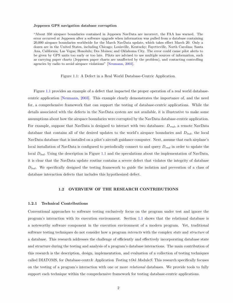
Jeppesen GPS navigation database corruption
“About 350 airspace boundaries contained in Jeppesen NavData are incorrect, the FAA has warned. Theerror occurred at Jeppesen after a software upgrade when information was pulled from a database containing20,000 airspace boundaries worldwide for the March NavData update, which takes effect March 20. Only adozen are in the United States, including Chicago; Louisville, Kentucky; Fayetteville, North Carolina; SantaAna, California; Las Vegas; Honolulu; Des Moines; and Oklahoma City. The error could cause pilot alerts tobe given by GPS units too early or too late. Pilots are advised to use multiple sources of information, suchas carrying paper charts (Jeppesen paper charts are unaffected by the problem), and contacting controllingagencies by radio to avoid airspace violations” [Neumann, 2003].
Figure 1.1: A Defect in a Real World Database-Centric Application.
Figure 1.1 provides an example of a defect that impacted the proper operation of a real world database-
centric application [Neumann, 2003]. This example clearly demonstrates the importance of, and the need
for, a comprehensive framework that can support the testing of database-centric applications. While the
details associated with the defects in the NavData system are not available, it is illustrative to make some
assumptions about how the airspace boundaries were corrupted by the NavData database-centric application.
For example, suppose that NavData is designed to interact with two databases: Drnd, a remote NavData
database that contains all of the desired updates to the world’s airspace boundaries and Dlnd, the local
NavData database that is installed on a pilot’s aircraft guidance computer. Next, assume that each airplane’s
local installation of NavData is configured to periodically connect to and query Drnd in order to update the
local Dlnd. Using the description in Figure 1.1 and the speculations about the implementation of NavData,
it is clear that the NavData update routine contains a severe defect that violates the integrity of database
Dlnd. We specifically designed the testing framework to guide the isolation and prevention of a class of
database interaction defects that includes this hypothesized defect.
1.2 OVERVIEW OF THE RESEARCH CONTRIBUTIONS
1.2.1 Technical Contributions
Conventional approaches to software testing exclusively focus on the program under test and ignore the
program’s interaction with its execution environment. Section 1.1 shows that the relational database is
a noteworthy software component in the execution environment of a modern program. Yet, traditional
software testing techniques do not consider how a program interacts with the complex state and structure of
a database. This research addresses the challenge of efficiently and effectively incorporating database state
and structure during the testing and analysis of a program’s database interactions. The main contribution of
this research is the description, design, implementation, and evaluation of a collection of testing techniques
called DIATOMS, for Database-centrIc Application Testing tOol ModuleS. This research specifically focuses
on the testing of a program’s interaction with one or more relational databases. We provide tools to fully
support each technique within the comprehensive framework for testing database-centric applications.
2

The foundation of each testing technique is a model of the faults that could occur when a program
interacts with a relational database. The framework includes a database-aware test adequacy component
that identifies the test requirements that must be covered in order to adequately test an application. A test
coverage monitoring technique instruments the application under test and records how the program interacts
with the databases during test suite execution. DIATOMS also provides database-aware test suite reduction
and prioritization components that support regression testing. The approach to test suite reduction discovers
and removes the redundant test cases within a test suite. The prioritization scheme re-orders the tests in
an attempt to improve test suite effectiveness. We provide a worst-case analysis of the performance of every
key algorithm within DIATOMS. We also empirically evaluate each of the techniques by testing several real
world case study applications. In summary, the technical contributions of this research include:
1. Fault Model: Conventional fault models only consider how defects in the input and structure of a
program might lead to a failure. We provide a fault model that explains how a program’s interactions
can violate the integrity of a relational database. The model describes four types of program defects that
could compromise data quality.
2. Database-Aware Representations: Traditional program representations focus on control and data
flow within the program and do not show how a program interacts with a database. We develop database-
aware finite state machines, control flow graphs, and call trees in order to statically and dynamically
represent the structure and behavior of a database-centric application.
3. Test Adequacy Criteria: Current program-based adequacy criteria do not evaluate how well a test
suite exercises the database interactions. DIATOMS enumerates test requirements by using data flow
analysis algorithms that operate on a database-aware control flow graph. We also furnish a subsumption
hierarchy that organizes the database-aware adequacy criteria according to their strength.
4. Test Coverage Monitoring: Existing test coverage monitoring schemes do not record how a program
interacts with its databases during test suite execution. The coverage monitor instruments the program
under test with statements that capture the database interactions. The component stores coverage results
in a manner that minimizes storage overhead while preserving all of the necessary coverage information.
5. Test Suite Reduction: The execution of a test for a database-centric application involves costly ma-
nipulations of the state of the database. Therefore, the removal of the redundant tests can significantly
decrease the overall testing time. However, traditional test suite reduction schemes remove a test if it
redundantly covers program-based test requirements. Our approach to test suite reduction deletes a test
case from the test suite if it performs unnecessary database interactions.
6. Test Suite Prioritization: Conventional approaches to test suite prioritization re-order a test suite
according to its ability to cover program-based test requirements. Our database-aware prioritizer cre-
ates test case orderings that cover the database interactions at the fastest rate possible. This type of
prioritization is more likely to reveal database interaction faults earlier in the testing process.
3

1.2.2 A New Perspective on Software Testing
A program executes in an environment that might contain components such as an operating system, database,
file system, graphical user interface, wireless sensor network, distributed system middleware, and/or virtual
machine. Since a modern software application often interacts with a diverse execution environment in a
complicated and unpredictable manner, there is a clear need for techniques that test an application, an
application’s execution environment, and the interaction between the software application and its environ-
ment. This research shows how to perform environment-aware testing for a specific environmental factor –
the relational database. However, the concepts, terminology, tool implementations, and experiment designs
provided by this research can serve as the foundation for testing techniques that focus on other software
components in the execution environment.
1.3 OVERVIEW OF THE DATABASE-AWARE TESTING FRAMEWORK
We designed, implemented, and tested each of the database-aware techniques with great attention to detail.
We used hundreds of unit and integration tests to demonstrate the correctness of each testing tool. For
example, the coverage monitoring component contains over one hundred test cases. The four test suites for
this component comprise 2282 non-commented source statements (NCSS) while the eighteen classes in the
tool itself only contain 1326 NCSS. Furthermore, all of the source code contains extensive documentation.
We successfully applied the techniques to the testing and analysis of small and moderate size case study
applications. The following goals guided the implementation of the presented testing techniques:
1. Comprehensive and Customized: DIATOMS establishes a conceptual foundation that supports the
design and implementation of testing techniques for each of the important stages in the software testing life
cycle for database-centric applications. We customized the comprehensive suite of techniques provided
by DIATOMS in order to handle the inherent challenges associated with the testing and analysis of
database-centric applications.
2. Practical and Applicable: DIATOMS is useful for practicing software engineers. Unlike some existing
program testing techniques (e.g., [Addy and Sitaraman, 1999, Doong and Frankl, 1994, Sitaraman et al.,
1993]), DIATOMS does not require knowledge of formal specification or architectural description lan-
guages. DIATOMS does not force testers to write descriptions of the state and/or structure of the
databases and the program, as required in [Willmor and Embury, 2006]. DIATOMS also utilizes soft-
ware testing tools (e.g., [Hightower, 2001, Jeffries, 1999]) that are already accepted by practicing software
developers.
3. Highly Automated: The tools within DIATOMS automate the testing process whenever possible.
Unlike prior approaches to testing (e.g., [Barbey et al., 1996, Chays et al., 2000, MacColl et al., 1998,
Richardson et al., 1992]), DIATOMS does not require the tester to manually specify the test require-
ments. DIATOMS can monitor test coverage and report test results in an automated fashion. The
4
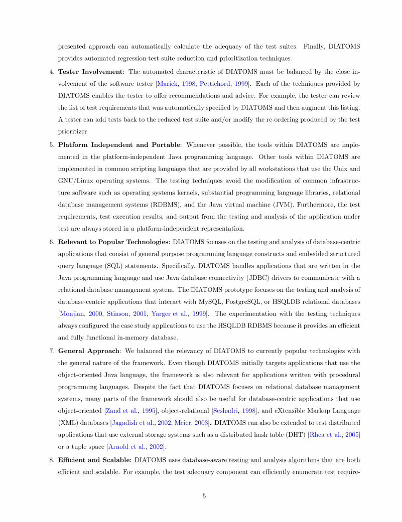
presented approach can automatically calculate the adequacy of the test suites. Finally, DIATOMS
provides automated regression test suite reduction and prioritization techniques.
4. Tester Involvement: The automated characteristic of DIATOMS must be balanced by the close in-
volvement of the software tester [Marick, 1998, Pettichord, 1999]. Each of the techniques provided by
DIATOMS enables the tester to offer recommendations and advice. For example, the tester can review
the list of test requirements that was automatically specified by DIATOMS and then augment this listing.
A tester can add tests back to the reduced test suite and/or modify the re-ordering produced by the test
prioritizer.
5. Platform Independent and Portable: Whenever possible, the tools within DIATOMS are imple-
mented in the platform-independent Java programming language. Other tools within DIATOMS are
implemented in common scripting languages that are provided by all workstations that use the Unix and
GNU/Linux operating systems. The testing techniques avoid the modification of common infrastruc-
ture software such as operating systems kernels, substantial programming language libraries, relational
database management systems (RDBMS), and the Java virtual machine (JVM). Furthermore, the test
requirements, test execution results, and output from the testing and analysis of the application under
test are always stored in a platform-independent representation.
6. Relevant to Popular Technologies: DIATOMS focuses on the testing and analysis of database-centric
applications that consist of general purpose programming language constructs and embedded structured
query language (SQL) statements. Specifically, DIATOMS handles applications that are written in the
Java programming language and use Java database connectivity (JDBC) drivers to communicate with a
relational database management system. The DIATOMS prototype focuses on the testing and analysis of
database-centric applications that interact with MySQL, PostgreSQL, or HSQLDB relational databases
[Monjian, 2000, Stinson, 2001, Yarger et al., 1999]. The experimentation with the testing techniques
always configured the case study applications to use the HSQLDB RDBMS because it provides an efficient
and fully functional in-memory database.
7. General Approach: We balanced the relevancy of DIATOMS to currently popular technologies with
the general nature of the framework. Even though DIATOMS initially targets applications that use the
object-oriented Java language, the framework is also relevant for applications written with procedural
programming languages. Despite the fact that DIATOMS focuses on relational database management
systems, many parts of the framework should also be useful for database-centric applications that use
object-oriented [Zand et al., 1995], object-relational [Seshadri, 1998], and eXtensible Markup Language
(XML) databases [Jagadish et al., 2002, Meier, 2003]. DIATOMS can also be extended to test distributed
applications that use external storage systems such as a distributed hash table (DHT) [Rhea et al., 2005]
or a tuple space [Arnold et al., 2002].
8. Efficient and Scalable: DIATOMS uses database-aware testing and analysis algorithms that are both
efficient and scalable. For example, the test adequacy component can efficiently enumerate test require-
5

ments and the test coverage monitoring technique records coverage information with low time and space
overheads. Furthermore, the regression testing component was able to efficiently identify a modified
test suite that was more effective than the original tests. The experimental results show that the tech-
niques provided by DIATOMS are applicable to both small and medium-scale programs that interact
with databases. Although additional experimentation is certainly required, the results suggest that the
majority of DIATOMS can also be used to test large-scale database-centric applications.
1.4 ORGANIZATION OF THE DISSERTATION
Chapter 2 presents a model of execution-based software testing and reviews the related work. Chapter 3
provides an overview of the testing framework, discusses the experimental design used in the evaluation of the
testing techniques, and examines each case study application. Chapter 4 introduces a family of database-
aware test adequacy criteria. In this chapter, we explore the subsumption hierarchy that formalizes the
relationship between each criterion in the test adequacy family. The fourth chapter also shows that traditional
data flow-based test adequacy criteria are not sufficient because they only focus on program variables and
they disregard the entities within the relational database. Chapter 5 describes and empirically evaluates
a database-aware test adequacy component that determines how well a test suite exercises the program’s
interactions with the relational databases. Chapter 6 discusses the database-aware test coverage monitoring
(TCM) technique. This chapter explains how we instrument an application in order to support the creation
of coverage reports that contain details about all of the program’s database interactions.
Chapter 7 introduces the database-aware TCM component and shows how we insert the monitoring
instrumentation. In this chapter we empirically evaluate the costs that are associated with program instru-
mentation and the process of test coverage monitoring. Chapter 8 presents a database-aware approach to
test suite reduction that identifies and removes the tests that redundantly cover the program’s database
interactions. This chapter also describes test suite prioritization techniques that use test coverage informa-
tion to re-order the tests in an attempt to maximize the potential for finding defects earlier in the testing
process. Chapter 9 reviews the contributions of this research and identifies promising areas for future work.
Appendix A summarizes the notation conventions that we use throughout this dissertation. Appendix B
describes each case study application that we employ during experimentation. This appendix contains in-
formation about the size and structure of the programs and their test suites. Finally, Appendix C furnishes
additional tables of data and examples that support our discussion of the experiment results.
6

2.0 BACKGROUND
2.1 INTRODUCTION
Since this research describes and evaluates a comprehensive framework for testing database-centric software
applications, this chapter reviews the relevant database and software testing concepts. We also examine the
related research and the shortcomings of existing techniques. In particular, this chapter provides:
1. A description of the relational database model, the relational database management system, and the
structured query language (SQL) (Section 2.2).
2. The intuitive definition of a database-centric software application that supports the formal characteriza-
tion that is developed in Chapter 4 (Section 2.3).
3. The definition of a graph and tree-based representation of a traditional program that can be enhanced
to represent database-centric applications (Section 2.4).
4. A discussion of the relevant software testing concepts and terminology and the description of an execution-
based software testing model (Section 2.5).
5. A review of the research that is related to the testing and analysis of database-centric software applications
(Section 2.6).
2.2 RELATIONAL DATABASES
This research focuses on the testing and analysis of database-centric applications that interact with relational
databases. Our concentration on relational databases is due to the frequent use of relational databases in
database-centric applications [Barclay et al., 2000, Stolte et al., 2003]. Furthermore, there are techniques
that transform semi-structured data into structured data that then can be stored in a relational database
[Laender et al., 2002, Ribeiro-Neto et al., 1999]. Finally, the relational database is also capable of stor-
ing data that uses a non-relational representation [Khan and Rao, 2001, Kleoptissner, 1995], A relational
database management system (RDBMS) is a set of procedures that are used to access, update, and modify a
collection of structured data called a database [Codd, 1970, 1979, Silberschatz et al., 2006]. The fundamental
concept in the relational data model is a relation. A relational database is a set of relations where a relation
of attributes A1, . . . , Az, with domains M1, . . . , Mz, is a subset of M1× . . .×Mz. That is, a relation is simply
7

select A1, A2, . . . , Az
from rel1, rel2, . . . , relwwhere P
(a)
delete from reljwhere P
(b)
insert into relj(A1, A2, . . . , Az)values(v1, v2, . . . , vz)
(c)
update reljset Al = F (A′
l)where P
(d)
P contains sub-predicates Vφ < Vψ
< ∈ <,≤, >,≥, 6=, in,between, like
Vφ ∈ A1, A2, . . . , Az
Figure 2.1: General Form of the SQL DML Operations.
a set of records. Each record in a relation is an ordered set of attribute values. Finally, a relational database
schema describes the logical design of the relations in the database and a relational database instance is a
populated example of the schema [Chamberlin, 1976, Codd, 1970, 1979, Silberschatz et al., 2006].
This research directly focuses on the SQL data manipulation language (DML) operations of select, up-
date, insert, and delete and also considers SQL statements that combine these commands in an appropriate
fashion. Since Chapter 4’s family of test adequacy criteria uses data flow information, the chosen model
of the structured query language contains the features of the SQL 1999 standard that are most relevant
to the flow of data in a database-centric application (c.f. Section 3.4 for a clarification of this assertion
and a review of the testing framework’s main limitations). This research relies upon the description of the
SQL operations provided by Figure 2.1. Parts (a), (b), and (d) of Figure 2.1 contain a reference to logical
predicate P that includes sub-predicates of the form Vφ < Vψ with < ∈ <,≤, >,≥, 6=, in,between, like
and Vφ is any attribute from the set A1, A2, . . . , Az. The sub-predicates in P are connected by a logical
operator such as and or or. The variable Vψ is defined in a fashion similar to Vφ; however, Vψ can also be
an arbitrary string, a pattern description, or the result of the execution of a nested select query. Also, the
v1, . . . , vz in Figure 2.1(c) represent the specific attribute values that are inserted into relation relj . Table A1
in Appendix A summarizes the notation conventions that we use to describe relational databases.
2.3 OVERVIEW OF DATABASE-CENTRIC APPLICATIONS
A program is an organized collection of algorithms that manipulates data structures in an attempt to
solve a problem [Wirth, 1976]. Intuitively, a database-centric application consists of a relational database
management system, one or more relational databases, and a program that interacts with the databases
through the management system. Figure 2.2 shows an example of a database-centric application and some
8

1D eD
P m
RDBMS
update
insert
deleteselect
Figure 2.2: High Level View of a Database-Centric Application.
of the canonical operations that the program can use to interact with the databases D1, . . . , De. In this
example, program P uses method m to submit structured query language statements to the RDBMS that
processes the SQL, performs the requested query and/or database manipulation, and returns any results
back to the program. The program in Figure 2.2 uses the SQL data manipulation language statements in
order to view and modify the state of the database.
This research uses a transaction manager database-centric application to make the discussion in subse-
quent chapters more concrete. The transaction manager is also one of the case study applications that we use
in the empirical studies and describe in more detail in Chapter 3 (for brevity, we will refer to this application as
TM throughout the remainder of this dissertation).1 TM performs an unlimited number of banking transactions
with an account once an appropriate personal identification number (PIN) has been provided. Supported
operations include the capability to deposit or withdraw money, transfer money from one account to an-
other, and check the balance of an existing account. The TM application interacts with a Bank database that
consists of the UserInfo and Account relations. The UserInfo relation contains the card number, pin number,
user name, and acct lock attributes while the Account relation includes the id, acct name, user name, bal-
ance, and card number attributes. Figure 2.3 provides the data definition language (DDL) statements used
to create the UserInfo and Account relations. This discussion assumes that TM is implemented in Java and
it interacts with a Java-based relational database. The Web site http://www.hsqldb.org/ describes the
RDBMS and specifies the subset of SQL that it supports.
1This research adheres to the following typographic conventions: relational database entities are in italics (e.g., UserInfo
and card number), structured query language keywords are in bold (e.g., select and foreign key), and program variables arein typewriter font (e.g., transfer and id).
9

create table UserInfo (card number int not null identity, pin number intnot null, user name varchar(50) not null, acct lock int)
(a)
create table Account (id int not null identity, account name var-char(50) not null, user name varchar(50) not null, balance int default’0’, card number int not null, foreign key(card number) references User-Info(card number));
(b)
Figure 2.3: SQL DDL Statements Used to Create the (a) UserInfo and (b) Account Relations.
K K
1
2
3
4
0
0
0
0 3
2
11
2
3
4
5
Primary Checking
Primary Checking
Primary Checking
Primary Checking
Robert Roos
Brian Zorman
Brian Zorman 2
4
Geoffrey Arnold
41601
32142
45322
56471
1000
1200
2350
4500
125Geoffrey Arnold
UserInfo Account
Marcus Bittman
user_name acct_lockcard_number pin_number card_numberacct_name user_nameid balance1 ... *
Marcus Bittman
Secondary Checking
Brian Zorman
Robert Roos
Figure 2.4: An Instance of the Relational Database Schema in the TM Application.
Figure 2.4 shows an example instance of the relational schema for the Bank database. The UserInfo
relation uses the card number attribute as a key that uniquely identifies each of the users while the id
attribute is the key in the Account relation. In Figure 2.3, the SQL identity keyword declares that an
attribute is a key. In Figure 2.4, the “K” above an attribute denotes a key. The UserInfo relation contains
four records and the Account relation contains five records.2 A foreign key constraint requires that every
card number in Account is associated with a card number in the UserInfo relation. Figure 2.3(b) shows that
this constraint is specified in DDL by using the foreign key and references key words. Furthermore, there
is a one-to-many relationship between the card number attribute in UserInfo and the Account relation’s
card number attribute. A single user of TM can access one or more accounts (e.g., user “Brian Zorman”
maintains primary and a secondary checking accounts).
Figure 2.5 provides a specific example of the general SQL DML statements that were described by
Figure 2.1. Intuitively, a select operation allows the program to issue a query that requests certain data
items from the database. The insert operation places new data in the database while the update and
delete operations respectively change and remove existing data. If the program submits incorrect select,
update, insert, and delete operations it will communicate incorrect data to P ’s method m and/or corrupt
the data within one of the databases D1, . . . , De. For example, suppose that an account accumulates interest
at a higher rate if the balance is above $10, 000. The SQL select statement in Figure 2.5(a) incorrectly
identifies all accounts that have a balance greater than $1, 000. If a program submits this defective select
2In the literature, the terms “relation” and “table” are used interchangeably. The words “record” and “tuple” also have thesame intuitive meaning. This research always use the terms relation and record.
10

select account name, user namefrom Accountwhere balance > 1000
(a)
delete from Accountwhere card number = 2
(b)
insert into Accountvalues(-10, “Primary Checking”,
“Robert S. Roos”, 1800, 1)
(c)
update UserInfoset acct lock = 1where card number = 5
(d)
Figure 2.5: Specific Examples of the SQL DML Operations.
to the database, all of the accounts with a balance greater than $1, 000 will accrue interest even though
this violates the banking policy. If the program provides the wrong card number during the execution of
the delete and update statements of Figure 2.5(b) and Figure 2.5(d) this would also corrupt the state of
the database. When a program executes the SQL insert statement in Figure 2.5(c), this would incorrectly
modify the database to include an Account record with an id of -10. Ultimately, faults in the program’s
interaction with the database can lead to the defective behavior of the entire application.
2.4 TRADITIONAL PROGRAM REPRESENTATIONS FOR TESTING
Software testing and analysis tools use a program representation to statically and dynamically model the
structure and behavior of an application. The chosen program representation has an impact upon all software
testing activities. For the purposes of analysis and testing, a specific operation within a program or an
entire program can be represented as a control flow graph (CFG). A control flow graph provides a static
representation of all of the possible ways that a program could execute. Intuitively, a control flow graph for
a single program method is a set of nodes and edges, where a node is an executable program entity (e.g., a
source code statement or a method) and an edge is a transfer of control from one program entity to another.
An intraprocedural CFG is a graph representation for a single program operation while an interprocedural
CFG statically represents the flow of control between the program’s methods [Harrold and Soffa, 1994,
Sinha et al., 2001]. A call tree offers a dynamic view of the program under test since it shows which source
code elements were actually executed during testing and it can store data about input parameters and
program variable state [Ammons et al., 1997]. Yet, the traditional control flow graph and call tree do not
contain nodes or edges that explicitly represent how a program interacts with a relational database.
G = 〈N , E〉 denotes a control flow graph G for program P ’s method m. N represents the set of CFG
nodes and E denotes the set of CFG edges. Each control flow graph G contains the nodes entry, exit ∈ N
that demarcate the entry and exit points of the graph. We define the dynamic call tree (DCT) in a fashion
analogous to the CFG, except for the restrictions that it (i) has a single distinguished node, the root, that
marks the initial testing operation and (ii) does not contain any cycles. The path 〈Nρ, . . . , Nφ〉 represents
11

1 import java . lang .Math ;2 public c lass Kinet ic3 4 public stat ic St r ing computeVelocity ( int k ine t i c , int mass )5 6 int ve l o c i ty squa r ed , v e l o c i t y ;7 S t r ingBu f f e r f i n a l v e l o c i t y = new St r ingBu f f e r ( ) ;8 i f ( mass != 0 )9
10 v e l o c i t y s qua r ed = 2 ∗ ( k i n e t i c / mass ) ;11 v e l o c i t y = ( int )Math . sq r t ( v e l o c i t y s qua r ed ) ;12 f i n a l v e l o c i t y . append ( v e l o c i t y ) ;13 14 else
15 16 f i n a l v e l o c i t y . append ( ”Undefined” ) ;17 18 return f i n a l v e l o c i t y . t oS t r ing ( ) ;19 20
Figure 2.6: Code Segment of a Traditional Program.
one way to traverse the CFG from arbitrary node Nρ to node Nφ. Finally, a complete path is a sequence of
nodes in a CFG that starts at the entry node and ends at the exit node. A path in a CFG represents one
way that a method could be executed. A DCT path records a sequence of method calls that were actually
executed during testing. For a CFG edge (Nρ, Nφ), the notation succ(Nρ) denotes the successor(s) of Nρ,
or in this example Nφ. For the same CFG edge, the notation pred(Nφ) is the predecessor(s) of Nφ and for
this example edge it corresponds to Nρ. Table A2 in Appendix A summarizes the notation that describes
these traditional program representations.
There are many different graph-based and tree-based representations for programs. Harrold and Rother-
mel survey a number of static graph-based representations and the algorithms and tool support used to
construct these representations [Harrold and Rothermel, 1995, 1996]. For example, the class control flow
graph (CCFG) represents the static control flow among the methods within a specific class and therefore
provides a limited interprocedural representation of a program [Harrold and Rothermel, 1994, 1996]. Am-
mons et al. describe the calling context tree (CCT) that depicts the execution of a method in the historical
context of the methods that were executed before and after this method [Ammons et al., 1997]. The chosen
representation for the program under test influences the test adequacy criteria that are subsequently used to
measure the quality of existing test suites and support the implementation of new tests. Furthermore, the
program representation also impacts regression testing activities such as test suite reduction and prioritiza-
tion. Program analysis framework such as Aristotle [Harrold and Rothermel, 1995], Soot [Vallee-Rai et al.,
1999], or AspectJ [Elrad et al., 2001, Kiczales et al., 2001a] create conventional graph and tree-based repre-
sentations. This research demonstrates that we can also use these frameworks to produce database-aware
models of an application’s static structure and dynamic behavior.
In order to make the discussion of the traditional graph-based program representations more concrete,
Figure 2.6 provides a Java class called Kinetic that contains a static method called computeVelocity
12

PSfrag replacements
N6
enter computeVelocity
enter computeVelocity
N6
N6
N7
N7
N8
N8
N10
N8
N16
N10
N11
N11
N12
N12N18
N16
N18 N18
exit computeVelocityexit computeVelocity
succ(N8) = N10, N16 and pred(N18) = N12, N16
Figure 2.7: A Traditional Control Flow Graph.
PSfrag replacements
N6
enter computeVelocity
enter computeVelocity
N6
N6
N7
N7
N8
N8
N10
N8
N16
N10
N11
N11
N12
N12
N18
N16
N18
N18
exit computeVelocity
exit computeVelocity
N6
N1
N1
N2
N2
N3
N3
N1
N1
N4
N4
N5
N5
Figure 2.8: A Control Flow Graph of an Iteration Construct.
13
[Paul, 1996]. Since Kinetic does not interact with a relational database, we classify it as a traditional
program and not as a database-centric application. The computeVelocity operation calculates the velocity of
an object based upon its kinetic energy and its mass. This method uses the knowledge that the kinetic energy
of an object, K, is defined as K = 12mv2. Figure 2.7 shows the control flow graph for the computeVelocity
method. The path 〈entrycv, N6, N7, N8, N16, N18, exitcv〉 represents a complete path in this example CFG
and 〈N6, N7, N8〉 is a path from node N6 to node N8. Inspection of the CFG in Figure 2.7 reveals that
succ(N8) = N10, N16 and pred(N18) = N12, N16. A dynamic call tree for computeVelocity includes all
of the nodes that were actually executed during the testing of the method. Even though computeVelocity
does not contain any iteration constructs like a for, while, or do while loop, Figure 2.8 shows that it is
also possible to represent iteration in a CFG. In this while loop node N2 and N3 are executed until the
condition that is tested in node N1 is false and then nodes N4 and N5 are executed. Our testing techniques
use tree and graph-based representations that fully model iteration, recursion, method calls, and database
interactions.
2.5 TRADITIONAL EXECUTION-BASED SOFTWARE TESTING
2.5.1 Preliminaries
Conventional software testing techniques focus on the source code and specification of a program and ignore
the important database component of the database-centric application depicted in Figure 2.2. Even though
most program-based software testing techniques are not directly applicable to the testing of a database-
centric application, these approaches offer a conceptual foundation for this research. Any approach to
testing database-centric applications must address many of the same fundamental testing challenges that
traditional testing techniques already consider. It is important to observe that the testing of traditional
programs is challenging because the domain of program inputs is so large that it is not possible to test with
every input and there are too many possible program execution paths to test [Kaner et al., 1993]. Indeed,
Young and Taylor have noted that every software testing technique must involve some trade-off between
accuracy and computational cost because the presence (or lack thereof) of defects within a program is an
undecidable property [Young and Taylor, 1989]. The theoretical limitations of testing clearly indicate that
it is impossible to propose and implement a software testing framework that is completely accurate and
applicable to arbitrary database-centric applications.
The IEEE standard defines a failure as the external, incorrect behavior of a program [IEEE, 1996].
Traditionally, the anomalous behavior of a program is observed when incorrect output is produced or a
runtime failure occurs. Furthermore, the IEEE standard defines a fault (alternatively known as a defect) as
a collection of program source code statements that causes a failure. Finally, an error is a mistake made
by a programmer during the implementation of a software system [IEEE, 1996].3 One purpose of software
3While these definitions are standard in the software engineering and software testing research community, they are differentthan those that are normally used in the fault-tolerant computing community. For example, this community defines a fault asthe underlying phenomenon that causes an error. Furthermore, an error is recognized as a deviation in the system state fromthe correct state. For more details, please refer to [Jalote, 1998].
14

testing is to reveal software faults in order to ensure that they do not manifest themselves as runtime failures.
Another goal of software testing is to establish an overall confidence in the quality of the program under
test. Even though database-centric applications are tested for the same reasons, the terminology used to
describe traditional testing techniques must be revised and extended in order to correctly explain the testing
of this new class of applications. In the context of database-centric applications, faults could exist within
the program, the data within the relational databases, or the interactions between the program and the
databases. Moreover, a fault might only manifest itself as a failure when both the program and the database
are in a certain anomalous state.
This research focuses on execution-based software testing techniques. It is also possible to perform
non-execution-based software testing through the usage of software inspections [Fagan, 1976]. All execution-
based testing techniques are either program-based, specification-based, or combined [Zhu et al., 1997]. This
research uses program-based (alternatively known as structural or white-box) testing approaches that rely
upon the program’s source code in order to create and evaluate a test suite [Zhu et al., 1997]. It is important
for the described testing techniques to have source code access because it is the program’s source code
that reveals how the application interacts with the databases.4 Unlike traditional program-based testing
methodologies, the presented testing approach considers one or more of the following: (i) the source code
of the program, (ii) the relational schema, (iii) the current instance of the relational schema, and (iv) the
manner in which the program interacts with the relational databases. Several of the testing techniques
presented in this research, including test coverage monitoring and test suite reduction and prioritization, can
be configured to operate without source code access.
2.5.2 Model of Execution-Based Software Testing
Figure 2.9 provides a model of execution-based software testing. In the subsequent sections of this chapter,
we describe each of these stages in light of traditional software testing techniques. This model is only one
valid and useful view of software testing. Our model of software testing takes as input a program under test
P , a test suite T , and a test adequacy criterion C. Even though we assume that P is tested with a provided
test suite, Chapter 9 explains that there are no inherent limitations within the framework that would prevent
the inclusion of an automated test generation technique. The formulation of a test adequacy criterion C is a
function of the chosen representation for P and a specific understanding of the “good” qualities that a test
suite should possess. The test adequacy component analyzes P in light of the chosen C and constructs a
listing of the test requirements that must be covered before the entire test suite can be judged as completely
adequate.
Even though manual testing is possible, this research focuses on the automated execution of test suites.
During test suite execution, the test coverage monitoring technique records information about the behavior
4Throughout this research, the definition of the term source code includes any description of a software application that isfully executable. In the context of database-centric applications written in the Java programming language, Java bytecodes arean example of a type of source code.
15

(P)Application Under Test
(C)Test Adequacy Criterion
1 )adeq(T
Adequacy Measurements
adeq(Tn )R R1R 2
Test Results
n
Regression Testing
Test SuitePrioritization
TT T2 n 1
Prioritized Test Suite
T2T1
Test SuiteReduction
Test CaseRequirements
Test Suite
(T)
Test Adequacy
Test Execution
Tn
Reduced Test Suite
Component
MonitoringTest Coverage
PSfrag replacements
N6
enter computeVelocity
enter computeVelocity
N6
N6
N7
N7
N8
N8
N10
N8
N16
N10
N11
N11
N12
N12
N18
N16
N18
N18
exit computeVelocity
exit computeVelocity
N6
N1
N1
N2
N2
N3
N3
N1
N1
N4
N4
N5
N5
Figure 2.9: Execution-Based Software Testing Model for Traditional Programs.
16

4
6
1def(x)
2use(x)use(y)
def(y)
3use(x)
use(x)use(y)def(x)
use(x)use(y)def(y)
use(x)use(y)
exitm
5
use(y)
menter
FT
PSfrag replacements
N6
enter computeVelocity
enter computeVelocity
N6
N6
N7
N7
N8
N8
N10
N8
N16
N10
N11
N11
N12
N12
N18
N16
N18
N18
exit computeVelocity
exit computeVelocity
N6
N1
N1
N2
N2
N3
N3
N1
N1
N4
N4
N5
N5
Figure 2.10: Intuitive Example of a Control Flow Graph.
of the test suite and the program under test. The test coverage monitor identifies which test requirements
were covered during testing and then calculates an adequacy measurement for each test case, as depicted in
Figure 2.9. Finally, regression testing is an important software maintenance activity that attempts to ensure
that the addition of new functionality and/or the removal of program faults does not negatively impact the
correctness of P . Approaches to test suite reduction identify a subset of the entire test suite that can still
adequately test the program. Traditional test suite prioritization techniques normally re-order the execution
of the test suite so that the rate of test requirement coverage or the potential for fault detection is maximized.
2.5.3 Test Adequacy Criteria
Test adequacy criteria embody certain characteristics of test case “quality” or “goodness.” Test adequacy
criteria can be viewed in light of a program’s control flow graph, and the program paths and variable values
that must be exercised. Intuitively, if a test adequacy criterion Cα requires the exercising of more path and
variable value combinations than criterion Cβ , it is “stronger” than Cβ . More formally, a test adequacy
criterion Cα subsumes a test adequacy criterion Cβ if every test suite that satisfies Cα also satisfies Cβ
[Clarke et al., 1985, Rapps and Weyuker, 1985]. Two adequacy criteria Cα and Cβ are equivalent if Cα
subsumes Cβ and vice versa. Finally, a test adequacy criterion Cα strictly subsumes criterion Cβ if and only
if Cα subsumes Cβ and Cβ does not subsume Cα [Clarke et al., 1985, Rapps and Weyuker, 1985].
Some software test adequacy criteria are based upon the control flow graph of a program under test.
Control flow-based criteria solely attempt to ensure that a test suite covers certain source code locations
with the rationale that a fault will not manifest itself in a failure unless it is executed [Morell, 1990, Voas,
1992]. While several control flow-based adequacy criterion are relatively easy to satisfy (e.g., all-nodes or
statement coverage), others are so strong that it is generally not possible for a test suite to test P and satisfy
17

m1
Ti
COV? COV?
m2
Test Requirements Test Requirements
R4
R1R2R3
RequirementR1
Requirement
R2R3
R5R4
R6
m m1 2
PSfrag replacements
N6
enter computeVelocity
enter computeVelocity
N6
N6
N7
N7
N8
N8
N10
N8
N16
N10
N11
N11
N12
N12
N18
N16
N18
N18
exit computeVelocity
exit computeVelocity
N6
N1
N1
N2
N2
N3
N3
N1
N1
N4
N4
N5
N5
Figure 2.11: Calculating Test Case Adequacy.
the criterion (i.e., all-paths coverage). For example, the all-nodes criterion requires a test suite to cover all of
the nodes in the control flow graph of the method under test and the all-edges criterion forces the coverage of
the CFG edges. Some control flow-based adequacy criteria focus on the control structure of a program and
the value of the variables that are used in conditional logic predicates. Since this research does not specifically
develop control flow-based test criteria, we omit a discussion of criteria such as condition-decision coverage
(CDC) and multiple-condition decision coverage (MCDC) [Jones and Harrold, 2003].
If the tests cause the definition of a program variable and then never use this variable, it is not possible
for the test suite to reveal the program’s defective variable definitions. Data flow-based test adequacy criteria
require coverage of the control flow graph by forcing the execution of program paths that involve the definition
and subsequent use of program variables. For a standard program, the occurrence of a variable on the left
hand side of an assignment statement is a definition of this variable (e.g., int a = 0; defines the variable
a). The occurrence of a variable on the right hand side of an assignment statement is a computation-use
(or c-use) of this variable (e.g., int a = b++; includes a c-use of the variable b). Finally, when a variable
appears in the predicate of a conditional logic statement or an iteration construct is a predicate-use (or p-use)
of the variable [Frankl and Weyuker, 1988, Rapps and Weyuker, 1982] (e.g., if(flag)... has a p-use of
the boolean variable flag).
A def-c-use association includes a node that defines a program variable and a node that subsequently
c-uses the same variable. Furthermore, a def-p-use association corresponds to a node that causes the def-
inition of a variable and the later p-use of the variable at another CFG node [Frankl and Weyuker, 1988,
Rapps and Weyuker, 1982]. A def-use association contains the node that defines a program variable and
the node that subsequently defines or uses the same variable (i.e., the def-use association does not distin-
guish between a p-use or a c-use) [Hutchins et al., 1994]. A def-use association for variable var is a triple
〈Ndef , Nuse, var〉 where Ndef defines variable var and Nuse uses this variable. Figure 2.10 provides an
example of a control flow graph that includes a total of sixteen def-use associations such as 〈N1, N4, x〉.
18

(C)Test Adequacy Criterion
Cumulative Adequacy Table
Test RequirementsResidual
(P)
Test Requirements
Program Instrumenter
Program Under Test
Program Under TestInstrumented
Test Suite Execution
Covered
PSfrag replacements
N6
enter computeVelocity
enter computeVelocity
N6
N6
N7
N7
N8
N8
N10
N8
N16
N10
N11
N11
N12
N12
N18
N16
N18
N18
exit computeVelocity
exit computeVelocity
N6
N1
N1
N2
N2
N3
N3
N1
N1
N4
N4
N5
N5
Figure 2.12: The Iterative Process of Test Coverage Monitoring.
In [Rapps and Weyuker, 1982], the authors propose a family of test adequacy criteria based upon the
data flow information in a program. Among their test adequacy measures, the all-uses data flow adequacy
criterion requires a test suite to cover all of the def-c-use and def-p-use associations in a program. The all-
uses criterion is commonly used as the basis for data flow testing. Alternatively, the all-DUs test adequacy
criterion requires the coverage of def-use associations [Hutchins et al., 1994]. Due to the fact that data
flow-based test adequacy criteria track the flow of data within a program, they are particularly well-suited
to serve as a foundation for the adequacy criteria that support the testing of database-centric applications
[Kapfhammer and Soffa, 2003] (this assertion is further explored and justified in Chapter 4).
2.5.4 Test Coverage Monitoring
If test suites are provided with the program under test, it is important to measure the adequacy of these tests
in order to decide if the program under test is being tested “thoroughly.” If the all-nodes criterion is selected
to measure the adequacy of a T used to test the computeVelocity method in Figure 2.6, then the test
coverage monitor (TCM) must determine whether the nodes enter cv, n6, n7, n8, n10, n11, n12, n16, n18, exitcv
were executed during testing. Alternatively, if C is the all-uses test adequacy criterion, then the test
coverage monitor would record whether or not the test suite causes the execution of the def-c-use and def-p-
use associations within computeVelocity. Line 11 of computeVelocity contains a definition of the variable
velocity and lines 12 contains a computation-use of velocity. The TCM component would include this
def-use association in the listing of test requirements subject to monitoring. Once the coverage of test
requirements is known, we can calculate the adequacy of a test case as the ratio between the test’s covered
test requirements and the total number of requirements. Figure 2.11 shows a test case Ti that tests two
methods m1 and m2. This test yields an adequacy of 50% for its testing of m1, an adequacy of 67% for m2,
and a cumulative adequacy of 60% for both of the methods. These adequacy scores are calculated under the
assumption that there are a total of ten unique requirements for Ti to cover and the test is able to cover six
of them overall.
19

PSfrag replacements
N6
enter computeVelocity
enter computeVelocity
N6
N6
N7
N7
N8
N8
N10
N8
N16
N10
N11
N11
N12
N12
N18
N16
N18
N18
exit computeVelocity
exit computeVelocity
N6
N1
N1
N2
N2
N3
N3
N1
N1
N4
N4
N5
N5
Set of Requirements
R1
Set of Requirements
R2
Set of Requirements
R3
Set of Requirements
R4
Set of Requirements
R5
Set of Requirements
R6
Set of Requirements
R7
R1
T1
R1
T2
R2
T2
R2
T8
R3
T3
R3
T4
R3
T7
R3
T8
R3
T11
R3
T12
R4
T1
R4
T2
R4
T3
R4
T5
R4
T9
R4
T10
R4
T11
R5
T5
R5
T6
R6
T9
R6
T10
R7
T6
R7
T7
R7
T10
Rj → Ti means that requirement Rj is covered by test Ti
Figure 2.13: A Test Suite that is a Candidate for Reduction.
Test coverage monitoring techniques frequently require instrumentation of the test suite and/or the
program under test in order to report which test requirements are covered during the execution of T . Among
other goals, the instrumentation must efficiently monitor test coverage without changing the semantics of the
program and the test suite. Pavlopoulou and Young have proposed, designed, and implemented a residual
test adequacy evaluator that instruments the program under test and calculates the adequacy of the test suites
used during development [Pavlopoulou and Young, 1999]. Figure 2.12 provides a high level depiction of this
test adequacy evaluation tool for Java programs (many other test coverage monitoring techniques would
adhere to a similar architecture). The residual coverage tool described by these authors can also measure
the coverage of test requirements after a software system is deployed and it is being used in the field. This
test coverage monitoring tool provides the ability to incrementally remove the test coverage probes placed in
the program under test after the associated test requirements have been exercised [Pavlopoulou and Young,
1999]. More recently, Misurda et al. presented the Jazz test coverage monitoring technique that records
information about the execution of edges, nodes, and def-use associations [Misurda et al., 2005]. The Jazz
structural testing tool uses a modified Jikes Research Virtual Machine (RVM) to introduce and remove
instrumentation in a demand-driven fashion.
2.5.5 Test Suite Reduction
A test suite can consist of test cases that overlap in their coverage of test requirements. Figure 2.13 shows
how seven separate test requirements are covered by twelve unique test cases. In this tree, a directed edge
from a requirement Rj to a test case Ti indicates that Rj is covered by Ti (or, that Ti covers Rj). For
example, an edge between a requirement R2 and a test case T8 indicates that R2 is covered by T8 or T8
covers R2. The test coverage monitor establishes the covered by relationship, as described in Section 2.5.4.
Since the test suite in Figure 2.13 contains a significant amount of overlap in test requirement coverage, it
20

Test Case Faults
f1 f2 f3 f4 f5
T1 X
T2 X
T3 X X
T4 X X
T5 X
Table 2.1: The Faults Detected by a Test Suite.
is a candidate for reduction. Test suite reduction techniques identify a potentially smaller set of tests that
cover the same requirements as the initial test suite. We can use reduction during regression testing if it is
too expensive to execute the complete test suite. Inspection of Figure 2.13 reveals that we could execute a
reduced test suite consisting of T2, T3, T6, andT9 instead of the original twelve test cases and still cover all of
the seven requirements. Recently developed reduction algorithms attempt to maximize both coverage and
defect detection rates while still decreasing the size of the test suite [Black et al., 2004].
Harrold et al. present a test suite reduction technique that is formulated in terms of a heuristic solution
to the hitting set problem [Harrold et al., 1993]. Their approach creates a mapping from each test case
to the test requirement(s) that it covers and it uses a custom heuristic for finding a reduced test suite.
McMaster and Memon apply the algorithm of [Harrold et al., 1993] to a mapping from test cases to test
requirements that are extracted from an earlier execution of the test suite [McMaster and Memon, 2005].
These authors argue that reduction should be performed whenever test cases produce the same call stacks
during test execution. The standard technique of Harrold et al. is often applied after performing a static
analysis of the program under test in order to locate the test requirements. In contrast, the approach of
McMaster and Memon uses low overhead instrumentation to identify the call stacks that arise during testing
[McMaster and Memon, 2005].
2.5.6 Test Suite Prioritization
Test prioritization schemes typically create a single re-ordering of the test suite that can be executed after
many subsequent changes to the program under test [Do et al., 2004, Rothermel et al., 2001]. Test case
prioritization techniques re-order the execution of a test suite in an attempt to ensure that (i) defects are
revealed earlier in the test execution phase and/or (ii) the tests cover the requirements as rapidly as possible.
If testing must be terminated early, a re-ordered test suite can also be more effective at finding faults than
one that was not prioritized [Rothermel et al., 2001]. Normally, a software tester is not aware of the defect
locations within the program under test. However, to make this discussion more concrete, suppose that
program P is tested with test suite T and a priori knowledge of the faults within P is available. Table 2.1
shows an example of a simple test suite and the faults that each test can reveal. In this example, there
21

are five faults that are revealed by certain test cases. In this test suite, some tests isolate more faults than
other test cases. In particular, tests T3 and T4 are able to reveal more of the faults within the program
under test than the other test cases. Intuitively, it would be better if these two test cases were executed
before the other tests within the suite. Over the entire execution of the test suite, the test suite ordering
σ1 = 〈T1, T2, T3, T4, T5〉 yields a smaller weighted average percentage of isolated defects than the ordering
σ2 = 〈T3, T4, T1, T2, T5〉 (i.e., σ2 detects faults faster than σ1).
Since the existence of a priori knowledge about the location of faults within the program under test
is unlikely, regression test suite prioritization algorithms must use a proxy for this complete knowledge.
Current regression test suite prioritization algorithms are motivated by the empirical investigations of the
effectiveness of test adequacy criteria which indicate that tests that are not highly adequate are often less
likely to reveal program defects [Harder et al., 2003, Hutchins et al., 1994]. In light of the correlation between
low adequacy test suites and the decreased potential to reveal a defect [Hutchins et al., 1994], a prioritization
algorithm might chose to execute highly adequate tests before those with lower adequacy. Of course, since
highly adequate tests are not guaranteed to always reveal the most defects, prioritization schemes can still
fail to produce an optimal ordering of the tests [Hutchins et al., 1994, Rummel et al., 2005]. Yet, reports
of industrial experience suggest that prioritization is both a cost-effective and valuable testing technique
[Srivastava and Thiagarajan, 2002]. Recently developed prioritization techniques are time-aware because
they generate test suite orderings that rapidly cover code while always terminating after a specified period
of time [Walcott et al., 2006].
2.5.7 Discussion of the Testing Model
In the execution-based testing model of Figure 2.9, one testing technique produces output that is then used
as the input to another technique. For example, the test suite executor and the test coverage monitor
generate test results and adequacy measurements that are used by the approaches to regression testing.
The output of a reduction or prioritization algorithm is a new test suite that can be used during future
executions of the suite. Figure 2.9 also presents a model of execution-based software testing that contains
cycles. Execution-based testing terminates when the adequacy of the test suite exceeds a pre-defined level,
the testers determine that they have established sufficient confidence in the correctness of the program, or
the testing budget has been exhausted [Zhu et al., 1997]. This research provides an execution-based testing
framework where (i) interoperable modules produce input and output that is meaningful to all of the other
components and (ii) testing can be repeated until an established termination condition has been met.
2.6 TESTING DATABASE-CENTRIC APPLICATIONS
While a significant amount of research has focused on the testing and analysis of programs, there is a relative
dearth of work that specifically examines the testing of database-centric applications. We distinguish the
presented research from the following related work because it provides a comprehensive testing framework
22

and a suite of automated tools that can be applied to a wide range of database-centric applications. Our
research also represents the most complete evaluation of the efficiency and effectiveness of approaches to
database-aware testing. When we compare our empirical evaluations to those in prior work, it is also clear
that we used the largest number of case study applications during experimentation. This research was
initially motivated by the observation that even simple software applications have complicated and ever-
changing operating environments that increase the number of interfaces and the interface interactions that
must be tested [Whittaker and Voas, 2000]. These authors point out that device drivers, operating systems,
and databases are all aspects of a software system’s environment that are often ignored during testing.
However, they do not propose and evaluate specific techniques that support the software testing process.
Even though Jin and Offutt highlight test adequacy criteria that incorporate a program’s interaction with
its environment [Jin and Offutt, 1998], these authors do not specifically address the challenges associated
with test adequacy criteria for database-centric applications. Dauo et al. use data flow information to support
the regression testing of database-centric applications. However, their exploration of data flow issues does
not include either a representation for a database-centric application or a complete description of a database
interaction association [Daou et al., 2001]. Another coverage criterion measures the adequacy of SQL select
queries in light of a database that has already been populated with data [Suarez-Cabal and Tuya, 2004].
This approach can automatically calculate the coverage of a single query, identify a subset of the database
that will yield the same level of coverage as the initial database, and provide guidance that might increase
database coverage. However, this scheme focuses on the select statement and it does not consider the
program that submits the queries to the relational database. Finally, Halfond and Orso present an adequacy
criterion that is complementary to our family of data flow-based criteria [Halfond and Orso, 2006]. Their
command-form coverage criterion ensures that a test suite causes the program under test to submit as many
of the viable SQL commands as is possible. That is, they use static analysis to identify all of the SQL
commands that the program could submit and then determine how many of these statements are actually
generated during testing.
Chan and Cheung propose a technique that tests database-centric applications that are written in a
general purpose programming languages, such as Java, C, or C++, and include embedded structured query
language statements that are designed to interact with a relational database [Chan and Cheung, 1999a,b].
This approach transforms the embedded SQL statements within a database-centric application into gen-
eral purpose programming language constructs. In [Chan and Cheung, 1999a], the authors provide C code
segments that describe the selection, projection, union, difference, and cartesian product operators that
form the relational algebra and thus heavily influence the structured query language. Once the embedded
SQL statements within the program under test have been transformed into general purpose programming
language constructs, it is possible to apply traditional control flow-based criteria to the problem of testing
programs that interact with one or more relational databases. However, their focus on the control flow of a
program ignores important information about the flow of data between the program and the databases.
23
Chays et al. and Chays and Deng describe several challenges associated with testing database-centric
applications and propose the AGENDA tool suite as a solution to some of these challenges [Chays et al.,
2000, Chays and Deng, 2003, Chays et al., 2002]. In [Chays et al., 2000], the authors propose a partially
automatable software testing technique, inspired by the category-partition method [Ostrand and Balcer,
1988], that attempts to determine if a program behaves according to specification. When provided with the
relational schema of the databases used by the application under test and a description of the categories
and choices for the attributes required by the relational tables, the AGENDA tool can generate meaningful
test databases [Chays and Deng, 2003, Chays et al., 2002]. AGENDA also provides a number of database
testing heuristics, such as “determine the impact of using attribute boundary values” or “determine the
impact of null attribute values” that can enable the tester to gain insights into the behavior of a program
when it interacts with a database that contains “interesting” states [Chays et al., 2000, Chays and Deng,
2003, Chays et al., 2002]. Deng et al. have also extended AGENDA to support the testing of database
transaction concurrency by using a data flow analysis to determine database transaction schedules that
may reveal program faults [Deng et al., 2003]. It is important to observe that the current prototype of the
AGENDA framework is designed to support the testing of database-centric applications that contain a single
query [Chays et al., 2004]. This testing scheme is limited since the majority of database-centric applications
contain many database interactions (in fact, Chapter 3 reveals that each of our case study applications has
between 5 and 45 database interactions).
Neufeld et al. and Zhang et al. describe approaches that are similar to [Chays et al., 2000,
Chays and Deng, 2003, Chays et al., 2002] because they generate database states using knowledge of the con-
straints in the relational schema [Neufeld et al., 1993, Zhang et al., 2001]. Yet, neither of these approaches
explicitly provides a framework to support common testing activities like those depicted in Figure 2.9. While
Gray et al. generate test databases that satisfy the constraints in the relational schema, their approach fo-
cuses on the rapid generation of large random data sets that support performance testing [Gray et al., 1994].
Instead of handling the generation of test databases, Slutz addresses the issues associated with automatically
creating the statements that support the querying and manipulation of relational databases [Slutz, 1998].
This approach generates database query and manipulation statements outside of the context of a program
that interacts with a database. Willmor and Embury also describe an automated test data generation scheme
that can produce test data when given a predicate logic condition that describes the desired database state
[Willmor and Embury, 2006].
Haftmann et al. present a regression test prioritization scheme that re-orders a test suite in an attempt
to avoid RDBMS restarts [Haftmann et al., 2005a]. Their approach executes the test suite without database
restarts and observes whether or not each test case passes. A test ordering conflict is recorded in a database
if the exclusion of a restart between the two tests causes the otherwise passing tests to fail [Haftmann et al.,
2005a]. These authors also describe prioritization heuristics that re-order a test suite in an attempt to avoid
the test conflicts that were stored within the conflict database. Haftmann et al. have extended their basic
24

technique to support the parallel execution of the test suite on a cluster of testing computers [Haftmann et al.,
2005b]. None of their prioritization approaches use either static or dynamic analysis to observe how the test
cases interact with specific relational database entities. As such, these prioritizers must coarsely identify the
test conflicts through an examination of the test results. Furthermore, Haftmann et al. focus on improving the
efficiency of regression testing and do not propose techniques to create more effective prioritizations. Finally,
Willmor and Embury propose a regression test selection technique that can identify a subset of a test suite
to use during subsequent rounds of testing [Willmor and Embury, 2005]. Their approach is similar to the
presented reduction technique but it could exhibit limited reductions and performance concerns because it
performs a conservative static analysis of the entire database-centric application.
2.7 CONCLUSION
This chapter reviews the data management and software testing concepts underlying our comprehensive
testing framework. This chapter intuitively defines a database-centric application that we subsequently
refine in Chapter 4. This chapter also provides a model for execution-based software testing that Chapter 3
extends to support the testing of a database-centric application. This testing model include components that
measure test adequacy, monitor test coverage, and perform regression testing. Chapters 4 and 5 introduce
a family of data flow-based test adequacy criteria that focuses on a program’s database interactions. We
present database-aware approaches for test coverage monitoring and regression testing in Chapter 6 through
Chapter 8. Finally, this chapter examines the strengths and weaknesses of existing approaches to testing
programs that interact with databases. The review of the related research clearly demonstrates that there
is a need for a comprehensive framework that tests database-centric applications.
25

3.0 IMPLEMENTATION AND EVALUATION OF THE TESTING FRAMEWORK
3.1 INTRODUCTION
This chapter provides an overview of our framework for testing database-centric applications. We also
describe the (i) case study applications that were tested with the database-aware framework, (ii) design of
the experiments to evaluate the efficiency and effectiveness of the testing techniques, and (iii) high level
threats to experiment validity. In summary, this chapter includes:
1. An overview of a framework for testing database-centric applications (Sections 3.2, 3.3, and 3.4).
2. A detailed examination of the case study applications that were used during experimentation and an
overview of the design of the experiments used in subsequent chapters (Sections 3.5 and 3.6).
3. An analysis of the threats to the validity of the experiments and a presentation of the steps that were
taken to control these threats (Section 3.7).
3.2 OVERVIEW
This chapter serves as the central location for the (i) survey of the database-aware testing framework, (ii)
detailed characterization of the case study applications that we use during the empirical evaluation of the
testing techniques, and (iii) overview of the experiment design that we employ throughout the entire process
of experimentation. In particular, Section 3.3 explains the inputs and outputs of every testing tool and it
shows the connection points between each of the components. This type of discussion contextualizes the
testing techniques and demonstrates how each component contributes to the complete framework. We also
clarify how database-aware testing is similar to and different from traditional testing schemes.
There are no well-established metrics that we can use to characterize a database-centric application
according to its static and dynamic complexity. Therefore, Section 3.5 reports the value of traditional
complexity metrics such as the (i) number of non-commented source statements (NCSS) and (ii) method
level cyclomatic complexity number (CCN). Calculating NCSS and CCN allows us to compare our case study
applications to those that were used in prior empirical studies. We also complement the discussion of these
traditional complexity metrics with a review of the structure of the each application’s relational database.
Furthermore, we examine the (i) size and structure of each test suite and (ii) testing strategies that each
application uses to verify the correctness of the program’s database interactions. Since many of the following
26

chapters contain the results from experiments with the testing components, Sections 3.6 and 3.7 review the
general design that governs all of our experimentation. Structuring the dissertation in this manner avoids
the need to repeatedly explain how we configured the execution environment and controlled the factors that
could compromise the validity of our experimental results.
3.3 HIGHLIGHTS OF THE DATABASE-AWARE TESTING FRAMEWORK
Figure 3.1 describes our model for the execution-based testing of a database-centric application. This
framework differs from the one that was presented in Chapter 2 because it accepts the following additional
inputs: (i) a relational database management system, (ii) the state of one or more databases, and (iii) the
relational schema that describes the organization of the databases. Each of the provided testing techniques
is database-aware because it considers the state and structure of the relational databases. For example, the
test adequacy component produces test case requirements called database interaction associations. These
associations require the test suites to define and use the entities within the databases (e.g., the relations,
records, attributes, and attribute values that are a part of the database’s state and structure). Each test case
populates the database with some initial state, executes one or more of the methods under test, and then
invokes an oracle that compares an expected database state to the actual state that the method produced.
The test executor also manipulates the state of the databases and could restart the RDBMS in order to
ensure that the tests execute correctly.
The test execution phase outputs test results that contain (i) the outcome of executing each test case
and (ii) portions of database state that support the debugging process. The database-aware test coverage
monitor can construct multiple types of test coverage monitoring trees that record how the program and
the test suite define and use the databases. The coverage monitoring trees contain nodes and edges that
represent the program’s interaction with the databases. The test coverage monitor (TCM) efficiently inspects
the state of the relational database in order to create these database-aware trees. We use the TCM trees to
produce adequacy measurements that reflect how well the test suite actually defines and uses the database at
multiple levels of interaction granularity. Finally, the regression test prioritization and reduction techniques
use the database-aware test coverage monitoring tree and the test adequacy measurements to re-order and
reduce the test suite. The test reduction algorithm identifies a potentially smaller test suite that still covers
the same set of database-aware test requirements. The prioritizer can re-order the test suite so that the tests
maximize their potential for finding database interaction defects as early as is possible.
3.4 LIMITATIONS OF THE APPROACH
Figure 3.2 depicts a classification scheme for database-centric applications that extends the classification pro-
posed in [Chan and Cheung, 1999a,b]. Every database-centric application must interact with its databases
using either an “Embedded” or an “Interface” approach. In the “Embedded” approach that is normally asso-
27

(P)Application Under Test
(C)Test Adequacy Criterion
1 )adeq(T
Adequacy Measurements
adeq(Tn )R R1R 2
Test Results
n
Regression Testing
Test SuitePrioritization
TT T2 n 1
Prioritized Test Suite
T2T1
Test SuiteReduction
RDBMS
Relational Schema
Test CaseRequirements
Test Suite
(T)
Test Adequacy
Test Execution
Tn
Reduced Test Suite
Databases
Component
MonitoringTest Coverage
PSfrag replacements
N6
enter computeVelocity
enter computeVelocity
N6
N6
N7
N7
N8
N8
N10
N8
N16
N10
N11
N11
N12
N12
N18
N16
N18
N18
exit computeVelocity
exit computeVelocity
N6
N1
N1
N2
N2
N3
N3
N1
N1
N4
N4
N5
N5
Figure 3.1: Execution-Based Software Testing Model for Database-Centric Applications.
28

Interface
Interaction Approach
Embedded
Program Location
Inside DBMS Outside DBMS
Database−Centric Applications
PSfrag replacements
N6
enter computeVelocity
enter computeVelocity
N6
N6
N7
N7
N8
N8
N10
N8
N16
N10
N11
N11
N12
N12
N18
N16
N18
N18
exit computeVelocity
exit computeVelocity
N6
N1
N1
N2
N2
N3
N3
N1
N1
N4
N4
N5
N5
Figure 3.2: Classification Scheme for Database-Centric Applications.
ciated with the use of languages such as SQLJ, the program component contains embedded SQL statements
that are transformed during a pre-compilation phase [Silberschatz et al., 2006]. Alternatively, a database-
centric application that adheres to the “Interface” approach uses a database connectivity driver that can
submit SQL statements to and return results from the database. Finally, the program component of a
database-centric application can either exist inside or outside of the database management system. If a
database-centric application consists of stored procedures that the RDBMS executes, then this program
exists inside of the database management system. A program is located outside of the RDBMS if it interacts
with the database through a standard interface like JDBC.
In Figure 3.2, a leaf from the “Interaction Approach” subtree can be paired with a leaf from the “Pro-
gram Location” subtree, yielding four different possible configurations of a database-centric application:
Embedded-Inside, Embedded-Outside, Interface-Inside, and Interface-Outside. The framework focuses on
the testing and analysis of database-centric applications that adhere to the Interface-Outside architecture
and it does not contain support for the analysis of applications that use stored procedures or triggers.
Even though this research focuses on the Interface-Outside configuration of a database-centric application,
Chapter 9 explains how we could extend the framework to test other types of applications. These current
restrictions are not inherent limitations of the individual testing components. Instead, we view this as evi-
dence of the need for new program analysis frameworks that support the (i) control and data flow analysis
and (ii) instrumentation of programs written in languages such as SQLJ or PL/SQL. If program analysis
techniques existed for these languages, then it would be possible to enumerate test requirements, monitor
coverage, and perform regression testing.
Since many current relational database management systems restrict or do not support the definition
of virtual relations with create view [Silberschatz et al., 2006], the framework does not analyze database-
centric applications that use the create view statement. The database-aware testing framework does not
support the testing of concurrent applications that use transactions. As such, the test adequacy component
does not consider database transactions during the creation of the representation and the enumeration of
test requirements. We further assume that each application executes a database interaction under an auto-
commit directive that treats each SQL command as an indivisible unit of work. However, each of the
aforementioned limitations does not impact the empirical results that we present because none of the case
study application use these features of SQL. Chapter 9 describes the steps that must be taken to improve
the framework so that it supports these facets of the structured query language.
29

Since all of the testing techniques are based on the state and structure of a database-centric application,
they are not properly suited for detecting omission faults (c.f. Sections 4.2 and 4.3 for a justification of
this assertion). The testing framework does not focus on finding the defects within P that incorrectly
manipulate or display a program variable whose value is the result of a correct database interaction. For
example, the testing tools will not highlight a fault where P correctly submits a select statement to retrieve
the value of attribute Al and then incorrectly updates the graphical user interface (GUI) by producing a label
that indicates it is the value of attribute Al′ . The combination of adequacy criteria that consider program
variables, database entities, and GUI elements will support the identification of this type of defect.
3.5 CHARACTERIZING THE CASE STUDY APPLICATIONS
3.5.1 High Level Description
We empirically evaluated each testing technique in Figure 3.1 by using it to test and analyze one or more of
the six case study applications.1 Each command line-based application is organized into a single Java package
with a varying number of classes and methods. All of the database-centric applications include a build system
written with the Apache Ant framework. The test suite for each case study application uses the DBUnit 2.1
extension of the popular JUnit 3.8.1 testing framework. Every application interacts with either a 1.7.3 or
a 1.8.0 HSQLDB in-memory relational database that executes within the same Java virtual machine as the
application itself. Since the case study applications use the standard Java database connectivity (JDBC)
interface, it is possible to configure the programs to use other databases such as MySQL [Yarger et al., 1999]
or PostreSQL [Monjian, 2000]. This section also characterizes each case study application according to the
number of classes, methods, and non-commented source code statements (NCSS) it contains. Tables 3.1 and
3.2 provide a high level description of each case study application by reporting the average number of classes,
methods, and NCSS per program, class, and method. In these two tables the term “method” refers to any
executable code body within the program and thus includes the test cases.
For each method mk with Gk = 〈Nk, Ek〉 we also calculated its cyclomatic complexity number (CCN)
v(Gk) = |Ek| − |Nk|+ |Bk| [McCabe and Butler, 1989]. We use Bk ⊂ Nk to denote the set of non-executable
nodes within a method’s CFG. Since the nodes entryk, exitk ∈ Nk (i.e., the nodes that demarcate a CFG’s
entry and exit points) are the only non-executable nodes in our CFG, we always have |Bk| = 2 in the equation
for v(Gk). The CCN is the maximum number of linearly independent paths through the CFG of a method
mk [McCabe and Butler, 1989]. Figure 3.3 shows that v(Gk) = 1 for a method mk that contains a single
straight-line code segment. Figure 3.4 reveals that v(Gk) = 2 when Gk contains a single conditional logic
statement. Adding the edge (N4, N1) to the CFG of Figure 3.4 increases the CCN by one, as demonstrated in
Figure 3.5. Finally, Figure 3.6 shows the calculation of v(Gk) for a CFG that uses iteration and conditional
logic constructs to form a Gk with five linearly independent paths. Table A3 in Appendix A summarizes
this chapter’s use of notation.
1Unless specified otherwise, Gregory M. Kapfhammer implemented each case study application. The author also implementedthe test suite for each case study application.
30

Name Classes Methods NCSS Per
Reminder (RM) 9 55.0 548.0 Program
6.11 60.89 Class
9.96 Method
FindFile (FF) 5 49.0 558.0 Program
9.8 111.6 Class
11.39 Method
Pithy (PI) 11 73.0 579.0 Program
6.64 52.64 Class
7.93 Method
Table 3.1: High Level Description of the RM, FF, and PI Case Study Applications.
Name Classes Methods NCSS Per
StudentTracker (ST) 9 72.0 620.0 Program
8.0 68.89 Class
8.61 Method
TransactionManager (TM) 6 87.0 748.0 Program
14.5 124.67 Class
8.6 Method
GradeBook (GB) 10 147.0 1455.0 Program
14.7 145.5 Class
9.9 Method
Table 3.2: High Level Description of the TM, ST, and GB Case Study Applications.
31

PSfrag replacements
N6
enter computeVelocity
enter computeVelocity
N6
N6
N7
N7
N8
N8
N10
N8
N16
N10
N11
N11
N12
N12
N18
N16
N18
N18
exit computeVelocity
exit computeVelocity
N6
N1
N1
N2
N2
N3
N3
N1
N1
N4
N4
N5
N5
Id : cfgstraight.ladot, v1.12006/09/0922 : 09 : 38gkapfhamExp
Revision : 1.1
N6
enterk
enterk
N1
N1
exitk
exitk
v(Gk) = |Ek| − |Nk|+ |Bk|
= 2− 3 + 2
= 1
Figure 3.3: Cyclomatic Complexity of a Simple Method.
Higher values for v(Gk) reveal that there are more paths that must be tested and this could suggest that
the method mk is more “complex” than a method mk′ with a lower v(Gk′ ) [Shepperd, 1988]. Table 3.3 reports
the average cyclomatic complexity across all methods within P . It is crucial to observe that calculating the
CCN for a traditional CFG does not take into account the method’s interaction with a relational database.
Therefore, the reported CCN values represent a lower bound on the “complexity” of the methods within
the program under test and they should only be used as a rough characterization of application complexity.
Chapter 9 identifies the development of a complexity metric for database-centric applications as an area for
future research.
Table 3.1 shows that Reminder (RM) is the smallest case study application with a total of 548 NCSS.
This application provides methods such as addEvent and getCurrentCriticalEvents that store events
including birthdays and appointments and then generate reminders for these events. The methods in RM have
an average CCN of 2.09 and Table B1 in Appendix B provides additional details about the RM application.
Table 3.1 indicates that FindFile (FF) is the second smallest case study application with 558 NCSS. FF is
an enhanced version of the file system searching application called FindFile that is available for download
at http://www.hsqldb.org/. FF contains methods such as listFiles, removeFiles, and fillFileNames
that have an average CCN of 2.02. Table B2 in Appendix B offers additional information about the FF
application. The cyclomatic complexity numbers for RM and FF suggest that these programs have “simple”
methods if their database interactions are not taken into account.
The Pithy (PI) case study application contains 579 NCSS, as noted in Table 3.1. Pithy is an extended
implementation of an example program available from http://uk.builder.com/. This application stores
and generates quotations with methods such as addQuote and getQuote. Similar to RM and FF, the PI case
study application has an average CCN of 2.05. Table B3 in Appendix B includes additional details about the
32

PSfrag replacements
N6
enter computeVelocity
enter computeVelocity
N6
N6
N7
N7
N8
N8
N10
N8
N16
N10
N11
N11
N12
N12
N18
N16
N18
N18
exit computeVelocity
exit computeVelocity
N6
N1
N1
N2
N2
N3
N3
N1
N1
N4
N4
N5
N5
Id : cfgstraight.ladot, v1.12006/09/0922 : 09 : 38gkapfhamExp
Revision : 1.1
N6
enterk
enterk
N1
N1
N2
N1N3
N2N4 N3
N4N4
exitkexitk
v(Gk) = |Ek| − |Nk|+ |Bk|
= 6− 6 + 2
= 2
Figure 3.4: Cyclomatic Complexity of a Method with Conditional Logic.
PSfrag replacements
N6
enter computeVelocity
enter computeVelocity
N6
N6
N7
N7
N8
N8
N10
N8
N16
N10
N11
N11
N12
N12
N18
N16
N18
N18
exit computeVelocity
exit computeVelocity
N6
N1
N1
N2
N2
N3
N3
N1
N1
N4
N4
N5
N5
Id : cfgstraight.ladot, v1.12006/09/0922 : 09 : 38gkapfhamExp
Revision : 1.1
N6
enterk
enterk
N1
N1
N2
N1
N3
N2
N4
N3N4
N4
N1
N4
exitkexitk
v(Gk) = |Ek| − |Nk|+ |Bk|
= 7− 6 + 2
= 3
Figure 3.5: Cyclomatic Complexity of a Method with Conditional Logic and Iteration.
33

PSfrag replacements
N6
enter computeVelocity
enter computeVelocity
N6
N6
N7
N7
N8
N8
N10
N8
N16
N10
N11
N11
N12
N12
N18
N16
N18
N18
exit computeVelocity
exit computeVelocity
N6
N1
N1
N2
N2
N3
N3
N1
N1
N4
N4
N5
N5
Id : cfgstraight.ladot, v1.12006/09/0922 : 09 : 38gkapfhamExp
Revision : 1.1
N6
enterk
enterk
N1
N1
N2
N2
N3
N2
N4
N3
N5
N5
N9
N5
N6
N6
N7
N7
N5
N7
N12
N4N8
N8
N9N8
N10
N9
N11
N10
N11
N11
N12
N12
exitk
exitk
v(Gk) = |Ek| − |Nk|+ |Bk|
= 17− 14 + 2
= 5
π1 = 〈enterk, N1, N2, N3, N5, N6, N7, N12, exitk〉
π2 = 〈enterk, N1, N2, N3, N5, N6, N7, N5, N6, N7, N12, exitk〉
π3 = 〈enterk, N1, N2, N3, N5, N9, N11, N12, exitk〉
π4 = 〈enterk, N1, N2, N4, N8, N9, N11, N12, exitk〉
π5 = 〈enterk, N1, N2, N4, N8, N10, N11, N12, exitk〉
Figure 3.6: Cyclomatic Complexity of a Method.
34

Application Average Method CCN
RM 2.09
FF 2.02
PI 2.05
ST 1.65
TM 2.21
GB 2.60
Table 3.3: Average Method Cyclomatic Complexity Measurements.
classes and methods in PI. Table 3.2 reveals that the StudentTracker (ST) case study application contains
620 NCSS and is the third largest application. This application uses methods such as insertStudent and
getAllStudents to track administrative information about college students. The average method CCN for
ST is 1.65 even though the application contains more executable source statements than RM, FF, or PI. This is
due to the fact that several methods within ST consist of straight-line code segments that reduce the average
method CCN. Table B4 in Appendix B provides more information about the StudentTracker application.
As described in Chapter 2, the TransactionManager (TM) application interacts with the Bank database.
At 748 NCSS, TransactionManager is the second largest case study application. It furnishes methods
such as removeAccount, removeUser, transfer, withdraw, and deposit. The average method cyclomatic
complexity number of TM is 2.21 and thus it is slightly more complex than the smaller applications. Table B5
in Appendix B offers additional information about TM. Table 3.2 shows that GradeBook (GB) is the largest
case study application with 1455 NCSS. This application provides 147 methods that include getExams,
addLab, and getFinalProjectScore. GB exhibits the largest average method CCN with a value of 2.60.
Even though GB’s average CCN is not significantly larger than the average CCNs of the other case study
applications, it does have many methods with cyclomatic complexities of 5 through 14. In contrast, the
CCNs for the other applications normally range from 1 to 5. Table B6 in Appendix B provides more details
concerning GB.
The data in Table 3.1, Table 3.2, and Table B1 through Table B6 in Appendix B indicate that all of the
applications have relatively small method code bodies that range in average size from 7.93 to 11.39 NCSS.
The largest applications, GB and TM, also have the most methods per class (14.5 and 14.7 methods per class,
respectively). In contrast, the smaller applications such as RM and PI only have an average of 6.11 and
6.64 methods per class. While descriptive statistics do not reveal anything about the quality of the source
code documentation, the tables in Appendix B demonstrate that most of the methods contain JavaDoc
comments. The “Classes” column in the tables from Appendix B denotes the number of inner classes that
are declared within the specified class. The chosen case study applications do not use inner classes and thus
this column always contains zeros. However, the presented framework supports the testing and analysis of
database-centric applications that use any of the major features of Java (e.g., static methods and variables,
inner classes, iteration, and recursion).
35

Reminder
Id (INTEGER)
Event_Name (VarChar)
Month (int)
Day (int)
Year (int)
Month_Trigger (int)
Day_Trigger (int)
PSfrag replacements
N6
enter computeVelocity
enter computeVelocity
N6
N6
N7
N7
N8
N8
N10
N8
N16
N10
N11
N11
N12
N12
N18
N16
N18
N18
exit computeVelocity
exit computeVelocity
N6
N1
N1
N2
N2
N3
N3
N1
N1
N4
N4
N5
N5
Id : TestMonitorConfiguration.java, v1.62006/03/2016 : 52 : 21gkapfhamExp
Revision : 1.6
N1 : T1, T2, T3, T4, T5
N1 : T1, T2, T3, T4, T5
N2 : T3, T5
N1 : T1, T2, T3, T4, T5
N3 : T1, T2, T4
N2 : T3, T5
N4 : T3, T5
N4 : T3, T5
N5 : T3, T5
N5 : T3, T5
N11 : T1, T2, T3, T4, T5
N11 : T1, T2, T3, T4, T5
N12 : T1, T2, T3, T4, T5
N6 : T1, T2, T4
N7 : T1, T2
N3 : T1, T2, T4
N6 : T1, T2, T4
N5 : T3, T5
N4 : T3, T5
N7 : T1, T2
N11 : T1, T2, T3, T4, T5
N8 : T4
N9 : T4
N6 : T1, T2, T4
N8 : T4
N9 : T4
N10 : T4
N10 : T4
N11 : T1, T2, T3, T4, T5
N10 : T4
N9 : T4
N12 : T1, T2, T3, T4, T5
Figure 3.7: Relational Schema for Reminder.
3.5.2 Relational Schemas
The test coverage monitoring component described in Chapter 6 includes a technique that records the
SQL data definition language statements that construct the relations within an application’s database.
The component also contains a tool that can automatically visualize each relational schema. This section
provides a graphical depiction of the relational schema that is used by each case study application. Figure 3.7
describes the relational schema for the Reminder case study application. The Reminder relation contains
seven attributes that are either of type Integer, int, or Varchar. Integer and int correspond to the
same variable type and the Java language-based HSQLDB uses the java.lang.Integer data type to store
these attributes. Attributes of type Varchar store variable length character data and HSQLDB internally
represents them as java.lang.String variables. Figure 3.8 shows the relational schema for FindFile’s
database. The Files relation contains two Varchar attributes called Path and Name. Even though this
database has a simple schema, FF was incorporated into the experiments because it provides functionality
that scans a file system to extract and store path and file name information. Therefore, FindFile can
automatically create very large databases that support the evaluation of a testing technique’s scalability.
Figure 3.9 provides the relational schema for Pithy’s database. The id attribute is a unique identifica-
tion number for each quotation and the pith attribute stores a Varchar-based textual representation of a
quotation. The category attribute is also of type Varchar and it classifies the quotation into one or more user-
defined categories. The experiments include the Pithy application because it comes with a large pre-defined
database of quotations. Figure 3.10 reveals that StudentTracker also interacts with a simple database that
contains the Student relation with the Id and Name attributes of type Varchar. The TransactionManager
application uses two tables called Account and UserInfo, as depicted in Figure 3.11 and previously described
in Chapter 2. The experiments use the ST and TM applications because they contain methods that have
sequences of database interactions. For example, the transfer method within TM follows the execution of
a select statement with two update statements. Therefore, the correct operation of the updates depends
upon the correctness of the select.
36

FILES
PATH (VARCHAR)
NAME (VARCHAR)
PSfrag replacements
N6
enter computeVelocity
enter computeVelocity
N6
N6
N7
N7
N8
N8
N10
N8
N16
N10
N11
N11
N12
N12
N18
N16
N18
N18
exit computeVelocity
exit computeVelocity
N6
N1
N1
N2
N2
N3
N3
N1
N1
N4
N4
N5
N5
Id : TestMonitorConfiguration.java, v1.62006/03/2016 : 52 : 21gkapfhamExp
Revision : 1.6
N1 : T1, T2, T3, T4, T5
N1 : T1, T2, T3, T4, T5
N2 : T3, T5
N1 : T1, T2, T3, T4, T5
N3 : T1, T2, T4
N2 : T3, T5
N4 : T3, T5
N4 : T3, T5
N5 : T3, T5
N5 : T3, T5
N11 : T1, T2, T3, T4, T5
N11 : T1, T2, T3, T4, T5
N12 : T1, T2, T3, T4, T5
N6 : T1, T2, T4
N7 : T1, T2
N3 : T1, T2, T4
N6 : T1, T2, T4
N5 : T3, T5
N4 : T3, T5
N7 : T1, T2
N11 : T1, T2, T3, T4, T5
N8 : T4
N9 : T4
N6 : T1, T2, T4
N8 : T4
N9 : T4
N10 : T4
N10 : T4
N11 : T1, T2, T3, T4, T5
N10 : T4
N9 : T4
N12 : T1, T2, T3, T4, T5
Figure 3.8: Relational Schema for FindFile.
PithyRemarks
id (INTEGER)
category (VARCHAR)
pith (VARCHAR)
PSfrag replacements
N6
enter computeVelocity
enter computeVelocity
N6
N6
N7
N7
N8
N8
N10
N8
N16
N10
N11
N11
N12
N12
N18
N16
N18
N18
exit computeVelocity
exit computeVelocity
N6
N1
N1
N2
N2
N3
N3
N1
N1
N4
N4
N5
N5
Id : TestMonitorConfiguration.java, v1.62006/03/2016 : 52 : 21gkapfhamExp
Revision : 1.6
N1 : T1, T2, T3, T4, T5
N1 : T1, T2, T3, T4, T5
N2 : T3, T5
N1 : T1, T2, T3, T4, T5
N3 : T1, T2, T4
N2 : T3, T5
N4 : T3, T5
N4 : T3, T5
N5 : T3, T5
N5 : T3, T5
N11 : T1, T2, T3, T4, T5
N11 : T1, T2, T3, T4, T5
N12 : T1, T2, T3, T4, T5
N6 : T1, T2, T4
N7 : T1, T2
N3 : T1, T2, T4
N6 : T1, T2, T4
N5 : T3, T5
N4 : T3, T5
N7 : T1, T2
N11 : T1, T2, T3, T4, T5
N8 : T4
N9 : T4
N6 : T1, T2, T4
N8 : T4
N9 : T4
N10 : T4
N10 : T4
N11 : T1, T2, T3, T4, T5
N10 : T4
N9 : T4
N12 : T1, T2, T3, T4, T5
Figure 3.9: Relational Schema for Pithy.
Student
Id (INTEGER)
Name (VarChar)
PSfrag replacements
N6
enter computeVelocity
enter computeVelocity
N6
N6
N7
N7
N8
N8
N10
N8
N16
N10
N11
N11
N12
N12
N18
N16
N18
N18
exit computeVelocity
exit computeVelocity
N6
N1
N1
N2
N2
N3
N3
N1
N1
N4
N4
N5
N5
Id : TestMonitorConfiguration.java, v1.62006/03/2016 : 52 : 21gkapfhamExp
Revision : 1.6
N1 : T1, T2, T3, T4, T5
N1 : T1, T2, T3, T4, T5
N2 : T3, T5
N1 : T1, T2, T3, T4, T5
N3 : T1, T2, T4
N2 : T3, T5
N4 : T3, T5
N4 : T3, T5
N5 : T3, T5
N5 : T3, T5
N11 : T1, T2, T3, T4, T5
N11 : T1, T2, T3, T4, T5
N12 : T1, T2, T3, T4, T5
N6 : T1, T2, T4
N7 : T1, T2
N3 : T1, T2, T4
N6 : T1, T2, T4
N5 : T3, T5
N4 : T3, T5
N7 : T1, T2
N11 : T1, T2, T3, T4, T5
N8 : T4
N9 : T4
N6 : T1, T2, T4
N8 : T4
N9 : T4
N10 : T4
N10 : T4
N11 : T1, T2, T3, T4, T5
N10 : T4
N9 : T4
N12 : T1, T2, T3, T4, T5
Figure 3.10: Relational Schema for StudentTracker.
UserInfo
card_number (int)
pin_number (int)
user_name (varchar)
acct_lock (int)
Account
id (int)
account_name (varchar)
user_name (varchar)
balance (int)
card_number (int)
FOREIGN (KEY)
PSfrag replacements
N6
enter computeVelocity
enter computeVelocity
N6
N6
N7
N7
N8
N8
N10
N8
N16
N10
N11
N11
N12
N12
N18
N16
N18
N18
exit computeVelocity
exit computeVelocity
N6
N1
N1
N2
N2
N3
N3
N1
N1
N4
N4
N5
N5
Id : TestMonitorConfiguration.java, v1.62006/03/2016 : 52 : 21gkapfhamExp
Revision : 1.6
N1 : T1, T2, T3, T4, T5
N1 : T1, T2, T3, T4, T5
N2 : T3, T5
N1 : T1, T2, T3, T4, T5
N3 : T1, T2, T4
N2 : T3, T5
N4 : T3, T5
N4 : T3, T5
N5 : T3, T5
N5 : T3, T5
N11 : T1, T2, T3, T4, T5
N11 : T1, T2, T3, T4, T5
N12 : T1, T2, T3, T4, T5
N6 : T1, T2, T4
N7 : T1, T2
N3 : T1, T2, T4
N6 : T1, T2, T4
N5 : T3, T5
N4 : T3, T5
N7 : T1, T2
N11 : T1, T2, T3, T4, T5
N8 : T4
N9 : T4
N6 : T1, T2, T4
N8 : T4
N9 : T4
N10 : T4
N10 : T4
N11 : T1, T2, T3, T4, T5
N10 : T4
N9 : T4
N12 : T1, T2, T3, T4, T5
Figure 3.11: Relational Schema for TransactionManager.
37

Application Test NCSS / Total NCSS
RM 227/548 = 50.5%
FF 330/558 = 59.1%
PI 203/579 = 35.1%
ST 365/620 = 58.9%
TM 355/748 = 47.5%
GB 769/1455 = 52.8%
Table 3.4: Characterization of the Test Suites.
Figure 3.12 explains the structure of the nine relations that are subject to interaction by the GradeBook
application. We used GB to empirically evaluate the testing techniques because it interacts with a moderate
size database that contains thirty-three attributes of varying type. The Master table uses the Integer and
Decimal attribute types to describe how different class scores contribute to the final grade in a college-level
science course. The HSQLDB database stores a Decimal attribute with the Java type java.math.BigDecimal
that provides immutable and arbitrary-precision signed decimal numbers. For example, if GradeBook stores
.2 within the FinalProject attribute this indicates that 20% of the course grade is associated with the grade
on the final project. The source code of GradeBook also contains checks to ensure that the values of Master’s
attributes sum to 1.0.
The Student relation uses Integer and Varchar attributes to store identification and contact information
about each student in the class. Finally, the ExamMaster relation stores the description of each examination
that was given during the course and the ExamScores relation persists the examination scores for each
student. The GradeBook application does not create a foreign key constraint from the ExamId attribute
in the ExamScores relation to ExamMaster’s ExamId. Instead, GradeBook uses Java methods to enforce
the constraint that each score in ExamScores corresponds with a unique examination in ExamMaster. The
remaining tables such as LabMaster and LabScores are defined analogously to ExamMaster and ExamScores.
These characteristics of GradeBook’s implementation demonstrate the importance of testing the interactions
between the program and the relational database. As noted in Chapter 9, we intend to investigate the reverse
engineering of program-enforced integrity constraints as part of future research.
3.5.3 Detailed Characterization
3.5.3.1 Test Suites The test suite for each application is organized into one or more Java classes. The
test executor recognizes the methods with names beginning with the word “test” as individual test cases.
A single test class (e.g., TestReminder for RM) also contains many methods that support the testing process.
Support methods such as getDataSet, getConnection, setUp, and tearDown are required by the JUnit and
DBUnit testing frameworks. Table 3.4 shows that the test code (e.g., both the support and “test” methods)
is often a significant portion of the application’s entire code base. Across all of the case study applications,
the test suite code comprises 50.65% of the total NCSS. Table 3.5 characterizes the size of each test suite
according to the number of test cases and oracle execution locations. These results indicate that the largest
38

HomeworkScores
HomeworkId (INTEGER)
StudentId (INTEGER)
EarnedPoints (INTEGER)
LabScores
LabId (INTEGER)
StudentId (INTEGER)
EarnedPoints (INTEGER)
FinalProjectScores
StudentId (INTEGER)
EarnedPoints (INTEGER)
ExamMaster
ExamId (INTEGER)
Name (VarChar)
TotalPoints (INTEGER)
Curve (INTEGER)
ExamScores
ExamId (INTEGER)
StudentID (INTEGER)
EarnedPoints (INTEGER)
Master
Id (INTEGER)
Participation (DECIMAL)
ExamOne (DECIMAL)
ExamTwo (DECIMAL)
ExamThree (DECIMAL)
Laboratory (DECIMAL)
Homework (DECIMAL)
FinalProject (DECIMAL)
Student
Id (INTEGER)
FirstName (VarChar)
LastName (VarChar)
Email (VarChar)
HomeworkMaster
HomeworkId (INTEGER)
Name (VARCHAR)
TotalPoints (INTEGER)
LabMaster
LabId (INTEGER)
Name (VARCHAR)
TotalPoints (INTEGER)
PSfrag replacements
N6
enter computeVelocity
enter computeVelocity
N6
N6
N7
N7
N8
N8
N10
N8
N16
N10
N11
N11
N12
N12
N18
N16
N18
N18
exit computeVelocity
exit computeVelocity
N6
N1
N1
N2
N2
N3
N3
N1
N1
N4
N4
N5
N5
Id : TestMonitorConfiguration.java, v1.62006/03/2016 : 52 : 21gkapfhamExp
Revision : 1.6
N1 : T1, T2, T3, T4, T5
N1 : T1, T2, T3, T4, T5
N2 : T3, T5
N1 : T1, T2, T3, T4, T5
N3 : T1, T2, T4
N2 : T3, T5
N4 : T3, T5
N4 : T3, T5
N5 : T3, T5
N5 : T3, T5
N11 : T1, T2, T3, T4, T5
N11 : T1, T2, T3, T4, T5
N12 : T1, T2, T3, T4, T5
N6 : T1, T2, T4
N7 : T1, T2
N3 : T1, T2, T4
N6 : T1, T2, T4
N5 : T3, T5
N4 : T3, T5
N7 : T1, T2
N11 : T1, T2, T3, T4, T5
N8 : T4
N9 : T4
N6 : T1, T2, T4
N8 : T4
N9 : T4
N10 : T4
N10 : T4
N11 : T1, T2, T3, T4, T5
N10 : T4
N9 : T4
N12 : T1, T2, T3, T4, T5
Figure 3.12: Relational Schema for GradeBook.
39

Application Num of Test Cases Num of Oracle Exec Avg Oracle Exec Per Test
RM 13 25 1.9
FF 16 80 5.0
PI 15 34 2.3
ST 25 59 2.4
TM 27 91 3.4
GB 51 91 1.8
Table 3.5: Number of Test Cases and Oracle Executions.
Application Num of executeUpdate Calls Num of executeQuery Calls Total
RM 3 4 7
FF 3 4 7
PI 3 2 5
ST 4 3 7
TM 36 9 45
GB 11 23 34
Table 3.6: Database Interactions in the Case Study Applications.
number of test cases is 91 (TM and GB) and the smallest number of tests is 25 (RM). Across all case study
applications, the average size of a test suite is approximately 63 tests.
Table 3.5 also reveals that the average number of oracles per test case ranges between 1.8 (GB) and 5 (FF).
The test suite for FindFile exhibits a high number of oracle executions per test because the tests often check
the correctness of the file names that are stored within the database on a per file name basis. GradeBook
shows the smallest number of oracle executions per test because it has the most test cases. Moreover, each
GB test case contains only one or two oracle executions that compare the expected and actual states of
entire database relations. Table B7 through Table B12 in Appendix B provide the name of each test case
and the Java class in which it is located. These tables show that many test suites contain test cases such
as testDatabaseServerIsRunning and testMakeDatabaseConnection. This is due to the fact that the
correctness of the methods that start and connect to the RDBMS is crucial to the proper operation of the
entire application.
Some case study applications have a dedicated Java class that is responsible for creating the relations in
the database (e.g., the GradeBookCreator class in the GB application creates all of the tables described in
Section 3.5.2) and this class is often tested with its own test cases. Analysis of the case study applications also
reveals that many of their test suites contain tests that perform a single operation repeatedly. For example,
the testDoesNotStartServerAgain method in TestFindFile starts the database server and then checks
to ensure that the server does not start again after multiple invocations of the RDBMS startup methods.
Furthermore, the testInsertAndRemoveStudentIterativeSmall test case for ST uses program methods
to iteratively insert information about a student and then delete all records of information pertaining to
the same student. This test determines if the ST application always assigns unique identification numbers
40

Program and Test Suite
Java Virtual Machine
Operating System
Database Manager
Java Virtual Machine
Operating System
executeUpdate or executeQuery
PSfrag replacements
N6
enter computeVelocity
enter computeVelocity
N6
N6
N7
N7
N8
N8
N10
N8
N16
N10
N11
N11
N12
N12
N18
N16
N18
N18
exit computeVelocity
exit computeVelocity
N6
N1
N1
N2
N2
N3
N3
N1
N1
N4
N4
N5
N5
Figure 3.13: Using the Java Database Connectivity Interface to Perform a Database Interaction.
to all of the students. Further examination indicates that some tests use program methods to add data
to the database and then execute a database-aware oracle (e.g., testAddOnePithyRemark in PI). Other
tests use program methods to insert data, delete data records, and then finally execute an oracle (e.g.,
testInsertAndRemoveStudent in ST). Finally, some test cases directly modify the state of the database
using DBUnit primitives, execute methods within the program under test, and then execute an oracle to
inspect the database state (e.g., testGetAccountBalance in TM). When considered cumulatively, the tests
for the case study applications represent a wide range of different testing strategies.
3.5.3.2 Database Interactions As depicted in Figure 3.13, the case study applications interact with
their relational database through the use of the executeUpdate and executeQuery methods that are pro-
vided by HSQLDB’s implementation of the java.sql.Statement interface. The executeUpdate method
submits SQL data manipulation statements such as update, insert, and delete. The same method can
also submit SQL data definition statements such as create table and drop table. For example, FF uses
executeUpdate to submit the statement drop table files. The executeQuery method always submits a
SQL select command. The java.sql.Statement interface also provides other interaction methods, such as
execute, that can send an arbitrary SQL command to the database. However, the selected case study appli-
cations do not use these alternative database interaction methods. Table 3.6 categorizes all of the database
interactions within the applications. This table shows that the smaller case study applications have the least
interactions while the largest applications, TM and GB, also have the most interactions. It is critical to note
that the case study applications express their database interactions as java.lang.Strings that can only
be partially characterized through static analysis (e.g., the database interaction might be dependent upon
user input or data values stored in external files). When examined as a whole, the case study applications
contain a wide range of database interactions that vary according to their static structure and use of the
Java database connectivity interface.
3.6 DESIGN OF THE EXPERIMENTS
The overarching goal of the experiments is to measure the efficiency and effectiveness of the testing techniques
presented by this research. Chapter 4 through Chapter 8 describe the specific experiment design that
41

supports the evaluation of each phase of the software testing life cycle. We implemented the entire testing
framework in the Java, Mathematica, and tcsh programming languages. The implementation also includes
a substantial test suite for each of the approaches to testing. Chapter 4 describes the initial experiments
that were conducted on a GNU/Linux workstation with kernel 2.4.18-14smp, LinuxThreads 0.10, dual 1
GHz Pentium III Xeon processors, 512 MB of main memory, and a SCSI disk subsystem. The subsequent
experiments described in Chapter 6 through Chapter 8 were performed on a GNU/Linux workstation with
kernel 2.6.11-1.1369, Native POSIX Thread Library (NPTL) version 2.3.5, a dual core 3.0 GHz Pentium
IV processor, 2 GB of main memory, and 1 MB of L1 processor cache. This workstation used a Serial
ATA connection to the hard drive and we enabled CPU hyper-threading in order to support thread-level
parallelism on the processor. All of the experiments use a JVM version 1.5.0 that was configured to operate
in Java HotSpotTMclient mode. The maximum size of the JVM heap varied depending upon the memory
demands of the experiment. Subsequent chapters explain the remaining details about the experiment design
and the evaluation metrics.
3.7 THREATS TO VALIDITY
The experiments described in this research are subject to validity threats. Internal threats to validity are those
factors that have the potential to impact the measured variables defined in Chapter 4 through Chapter 8.
One internal validity threat is associated with defects in the prototype of the database-aware testing tools.
Defects within any of the testing techniques would impact the experiment results. This threat is controlled
by the implementation and frequent execution of a regression test suite for the entire testing framework.
Furthermore, we applied the prototype to smaller known examples, and we manually checked the correct-
ness of these results. We also controlled this threat by incorporating tools and Java class libraries that
are frequently used by software testing researchers and practitioners (e.g., JUnit [Do et al., 2004], DBUnit
[Dallaway, 2002], and Soot [Vallee-Rai et al., 2000]). Since we have repeatedly used these tools without
experiencing errors or anomalous results, we have a confidence in their correctness and we judge that they
did not negatively impact the validity of our empirical studies. The efficiency of each testing technique was
measured by Java programming language instrumentation that inserted profiling statements into the source
code of the testing techniques. To ensure that the profilers yielded accurate timings, we measured the wall
clock time for the execution of a testing tool and compared this to the time that was calculated by the
profiler. In order to prevent inappropriate variations in the time overhead, we used the same workstation
for all experiments within a chapter and we prevented external user logins to this workstation during the
empirical analysis.
External threats to validity are factors that limit the ability to generalize the experimental results.
Since the empirical studies described by this research use a limited number of case study applications, we
cannot claim that these results are guaranteed to generalize to other database-centric applications. However,
Section 3.5 shows that the experiments use six small to moderate size applications that vary in terms of their
42

NCSS, cyclomatic complexity, test suite structure, and type of database interaction. We also configured each
case study application to interact with the real world HSQLDB RDBMS that is used in current applications
such as OpenOffice and Mathematica. Another threat to external validity is related to the size of the selected
case study applications and their test suites. If we compare our case study applications to those that were
used in other studies by [Tonella, 2004] (mean size of 607.5), [McMinn and Holcombe, 2005] (mean size of
119.2), [Harrold et al., 1993] (mean size of 33.6), and the Siemens application suite [Rothermel et al., 2001]
(mean size 354.4), the average size of our programs and test suites (mean size 571) is comparable to the
size of the other applications. Since both Tonella, McMinn and Holcombe, and Harrold et al. report a lines
of code (LOC) size metric instead of an NCSS metric, it is possible that our case study applications have
a larger static size than those programs used in prior experimentation. Finally, the case study applications
in these previous studies do not interact with a relational database. The last threat to external validity is
that the author of this dissertation implemented and tested each case study application. We implemented
our own applications because the software testing research community has not established a repository of
database-centric applications.
3.8 CONCLUSION
This chapter offers a brief overview of our comprehensive framework for testing database-centric applications.
Subsequent chapters will provide more details about the test adequacy component and our approaches to
test coverage monitoring, and test suite reduction and prioritization. This chapter examines the case study
applications that we used to empirically evaluate the testing techniques described in Chapter 4 through
Chapter 8. We report the number of classes, methods, and non-commented source statements in each of
the case study applications. This chapter includes a definition of cyclomatic complexity and a summary of
the average cyclomatic complexity across all of the methods within an application. We also examine the
test suite and the relational schema for each database-centric application. For each test suite we report the
number of tests and we characterize the tests according to their static structure and dynamic behavior. We
graphically depict each relational schema and explain how the programs use the JDBC interface to submit
SQL statements to the database. This chapter concludes with a high level review of the experiment design
and a discussion of the steps we took to address the threats to the validity of our experiments.
43

4.0 FAMILY OF TEST ADEQUACY CRITERIA
4.1 INTRODUCTION
This chapter describes a fault model for database-centric applications and a family of database-aware test
adequacy criteria. The fault model describes how a program can violate the integrity of a relational database.
We also explain why our data flow-based adequacy criteria support the isolation of faults that violate database
integrity. Finally, we compare our database-aware criteria to traditional adequacy criteria that solely focus
on program variables. In particular, this chapter offers:
1. A fault model that describes the interaction patterns that frequently lead to the violation of relational
database integrity (Section 4.2).
2. The definition of a family of test adequacy criteria for database-centric applications that extends the
traditional data flow-based all-DUs criterion (Sections 4.3.1 and 4.3.2).
3. The presentation of a subsumption hierarchy that characterizes the relative strength of each database-
aware test adequacy criterion (Section 4.3.3).
4. The discussion of the suitability of the test adequacy criteria and a comparison to traditional structural
adequacy metrics (Section 4.3.4 and 4.3.5).
4.2 DATABASE INTERACTION FAULT MODEL
We define a database-centric application A = 〈P, 〈D1, . . . , De〉, 〈S1, . . . , Se〉〉 to consist of a program P and
databases D1, . . . , De that are specified by relational schemas S1, . . . , Se. Our testing framework ensures
that the tests for A can isolate the type of interaction faults that are commonly found in a database-centric
application. Accuracy, relevancy, completeness, and consistency are commonly associated with the quality of
the data that is stored in a database [Motro, 1989, Strong et al., 1997, Wand and Wang, 1996]. The testing
framework’s fault model uses the conception of database integrity initially proposed in [Motro, 1989]. This
research views the integrity of A’s databases as a function of the validity and completeness of the data that is
stored in each database. We specify the correct behavior of method mk’s interaction with database Df from
the perspective of the expected database state, denoted Dx. The fault model assumes that the relational
database is in a valid state before the execution of method mk. If Df = Dx after executing mk, then we
know that method mk performed as anticipated. If the expected and actual database states are not equal,
then this demonstrates that there is a defect within mk that violates the integrity of the database.
44
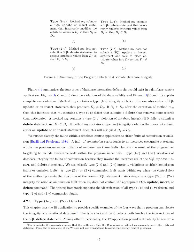
Type (1-v): Method mk submitsa SQL update or insert state-ment that incorrectly modifies theattribute values in Df so that Df 6=Dx.
(a)
Type (1-c): Method mk submitsa SQL delete statement that incor-rectly removes attribute values fromDf so that Df ⊂ Dx.
(b)
Type (2-v): Method mk does notsubmit a SQL delete statement toremove attribute values from Df sothat Df ⊃ Dx.
(c)
Type (2-c): Method mk does notsubmit a SQL update or insertstatement and fails to place at-tribute values into Df so that Df 6=Dx.
(d)
Figure 4.1: Summary of the Program Defects that Violate Database Integrity.
Figure 4.1 summarizes the four types of database interaction defects that could exist in a database-centric
application. Figure 4.1(a) and (c) describe violations of database validity and Figure 4.1(b) and (d) explain
completeness violations. Method mk contains a type (1-v) integrity violation if it executes either a SQL
update or an insert statement that produces Df 6= Dx. If Df ⊂ Dx after the execution of method mk,
then this indicates that mk contains a type (1-c) defect that submits a delete that removes more records
than anticipated. A method mk contains a type (2-v) violation of database integrity if it fails to submit a
delete statement and Df ⊃ Dx. If method mk contains a type (2-c) integrity violation that does not submit
either an update or an insert statement, then this will also yield Df 6= Dx.
We further classify the faults within a database-centric application as either faults of commission or omis-
sion [Basili and Perricone, 1984]. A fault of commission corresponds to an incorrect executable statement
within the program under test. Faults of omission are those faults that are the result of the programmer
forgetting to include executable code within the program under test. Type (1-c) and (1-v) violations of
database integrity are faults of commission because they involve the incorrect use of the SQL update, in-
sert, and delete statements. We also classify type (2-c) and (2-v) integrity violations as either commission
faults or omission faults. A type (2-c) or (2-v) commission fault exists within mk when the control flow
of the method prevents the execution of the correct SQL statement. We categorize a type (2-c) or (2-v)
integrity violation as an omission fault when mk does not contain the appropriate SQL update, insert, or
delete command. The testing framework supports the identification of all type (1-c) and (1-v) defects and
type (2-c) and (2-v) commission faults.
4.2.1 Type (1-c) and (2-v) Defects
This chapter uses the TM application to provide specific examples of the four ways that a program can violate
the integrity of a relational database.1 The type (1-c) and (2-v) defects both involve the incorrect use of
the SQL delete statement. Among other functionality, the TM application provides the ability to remove a
1For simplicity, this research assumes that the methods within the TM application will not concurrently access the relationaldatabase. Thus, the source code of the TM does not use transactions to avoid concurrency control problems.
45

The removeAccount(int id) operation should completely remove theuser account that is specified by the provided id. If the removal ofthe account from the Account relation results in an TM user that nolonger maintains any accounts in the TM application, any additionaluser information should also be removed from the UserInfo relation.
(a)
The transfer(int source id, int dest id, double balance) op-eration should withdraw balance dollars from the account specifiedby source id, deposit this amount into the account specified bydest id, and return true to signal success. If the account associ-ated with the source id has a balance that is less than the specifiedbalance, then the transfer must not occur and the operation shouldreturn false.
(b)
Figure 4.2: The Natural Language Specifications for the (a) removeAccount and (b) transfer Methods.
specified account. Since it uses a SQL delete statement, the removeAccount method could contain either
a (1-c) or a (2-v) defect. The natural language specification for the removeAccount method is provided in
Figure 4.2(a). Figure 4.3 shows a defective implementation of the removeAccount operation in the Java
programming language.2 In this method, line 4 constructs a structured query language statement that is
supposed to remove the specified account from the Account relation. Since this line erroneously builds a
where clause that compares the card number attribute to the provided id parameter instead of using the
id attribute, the database interaction on line 6 is faulty. If we call removeAccount(2) with the input state
shown in Figure 2.4, then the method from Figure 4.3 incorrectly removes both of the accounts that are
owned by user “Brian Zorman” instead of deleting the account with an id of 2. This operation contains a
type (1-c) defect that violates the completeness of the relational database.
Figure 4.4 provides another implementation of removeAccount that resolves the defect that exists in
the operation from Figure 4.3. However, this method still does not correctly implement Figure 4.2(a)’s
specification for the removeAccount method. Lines 4 and 6 of this method correctly build the String
removeAcct and interact with the database. However, the method lacks an additional interaction to delete
the information from the UserInfo relation when the user removes his or her last account from the Account
relation (for the purposes of discussion, we assume that the RDBMS either could not be or was not config-
ured to automatically handle the referential integrity constraint between the two relations). Therefore, the
removeAccount method in Figure 4.4 contains a type (2-v) defect that violates the validity of TM’s database.
We classify this defect as a fault of omission because the program source code does not contain a database
interaction to remove attribute values from the UserInfo relation.
2In the method listing in Figure 4.3 and all subsequent source code listing, the variable connect corresponds to the alreadyinitialized connection to the Bank database.
46

1 public boolean removeAccount( int id ) throws SQLException2 3 boolean completed = f a l se ;4 S t r ing removeAcct = ‘‘ de l e t e from Account where card number = ’’ + id ;5 Statement removeStmt = connect . c reateStatement ( ) ;6 int removeAccountResult = removeStmt . executeUpdate ( removeAcct ) ;7 i f ( removeAccountResult == 1 )8 9 completed = true ;
10 11 return completed ;12
Figure 4.3: A Type (1-c) Defect in the removeAccount Method.
1 public boolean removeAccount( int id ) throws SQLException2 3 boolean completed = f a l se ;4 S t r ing removeAcct = ‘‘ de l e t e from Account where id = ’’ + id ;5 Statement removeStmt = connect . c reateStatement ( ) ;6 int removeAccountResult = removeStmt . executeUpdate ( removeAcct ) ;7 i f ( removeAccountResult == 1 )8 9 completed = true ;
10 11 return completed ;12
Figure 4.4: A Type (2-v) Defect in the removeAccount Method.
1 public boolean t r a n s f e r ( int source u id , int dest u id ,2 double amount ) throws SQLException3 4 boolean completed = f a l se ;5 S t r ing qs = ‘‘ s e l e c t id , ba lance from Account ; ’’ ;6 Statement stmt = connect . c reateStatement ( ) ;7 Resu l tSet r s = stmt . executeQuery ( qs ) ;8 while ( r s . next ( ) )9
10 int id = r s . g e t In t ( ‘‘ id ’’ ) ;11 double balance = r s . getDouble ( ‘‘ba lance’’ ) ;12 i f ( id == source u id && amount <= balance )13 14 St r ing qu withdraw = ‘‘update Account s e t ba lance = balance−’’ +15 amount + ‘‘ where id = ‘‘ + source u id + ‘‘ ; ’’ ;16 Statement update withdraw = connect . c reateStatement ( ) ;17 int r e su l t w i thdraw = update withdraw . executeUpdate ( qu withdraw ) ;1819 St r ing qu depo s i t = ‘‘update Account s e t ba lance = balance+’’ +20 amount + ‘‘ where id = ‘‘ + de s t u id + ‘‘ ; ’’ ;21 Statement update depos i t = connect . c reateStatement ( ) ;22 int r e s u l t d ep o s i t = update depos i t . executeUpdate ( qu depo s i t ) ;2324 i f ( r e su l t w i thdraw == 1 && r e s u l t d ep o s i t == 1 )25 completed = true ;26 27 28 return completed ;29
Figure 4.5: A Correct Implementation of the transfer Method.
47
4.2.2 Type (1-v) and (2-c) Defects
The type (1-v) and (2-c) defects both involve the incorrect use of either the SQL update or insert statements.
We use the transfer method to provide an example of the improper modification or deletion of data
that already exists in a relational database. Figure 4.5 shows a correct implementation of the transfer
method that is specified by the natural language description provided in Figure 4.2(b). Suppose that the
SQL update statement constructed on lines 14 and 15 made reference to dest id instead of source id.
Furthermore, suppose that the SQL update statement created on lines 19 and 20 referenced source id
instead of dest id. If this hypothesized defect exists within the transfer method, the transfer operation
will withdraw money from the account associated with dest id and deposit amount dollars into the account
associated with source id. This hypothesized modification to transfer creates a type (1-v) violation of
database validity because it places incorrect balances into TM’s Bank database.
Suppose we replace the second condition of the if statement on line 12 in Figure 4.5 with the condition
amount >= balance. If the transfer operation contained this hypothesized defect, the transfer will not
occur even if account source id contained sufficient funds. In this circumstance, the balance attribute values
for the two accounts will not be properly modified. This potential modification to transfer introduces a
type (2-c) violation of database completeness. This is due to the fact that transfer fails to place appropriate
values for balance inside of the Account relation. This type (2-c) violation is also a fault of commission because
incorrect conditional logic prevents the method under test from executing a correct database interaction.
4.3 DATABASE-AWARE TEST ADEQUACY CRITERIA
4.3.1 Traditional Definition-Use Associations
Throughout the discussion of our family of data flow-based test adequacy criteria for database-centric ap-
plications, we adhere to the notation initially proposed in [Rapps and Weyuker, 1985]. We focus on the
definition of intraprocedural definition-use associations for CFG Gk = 〈Nk, Ek〉. A definition clear path
πvar = 〈Nρ, . . . , Nφ〉 for variable var is a path in Gk such that (i) Nρ contains a definition of var, (ii) Nφ
contains a use of var, and (iii) none of the nodes Nρ+1, . . . , Nφ contain a subsequent definition of var. We
say that node Nρ contains a reaching definition for the use of var at Nφ if there exists a definition clear
path πvar = 〈Nρ, . . . , Nφ〉. We define RD(Gk, Nφ, var) as the set of nodes that contain reaching definitions
for the use of the variable var at Nφ. We define the def-use association as a triple 〈Ndef , Nuse, var〉 such
that Ndef ∈ RD(Gk, Nuse, var). As initially defined in Chapter 2, a complete path is a sequence of nodes
in a method’s control flow graph that starts at the CFG’s entry node and ends at its exit node. A test
case Ti covers a def-use association if it executes a complete path πvar that has a definition clear sub-path
from node Ndef to Nuse. For more details about traditional data flow-based test adequacy criteria, refer to
[Rapps and Weyuker, 1985, Zhu et al., 1997]. Table A5 in Appendix A reviews the notation that we use to
define the def-use association.
48
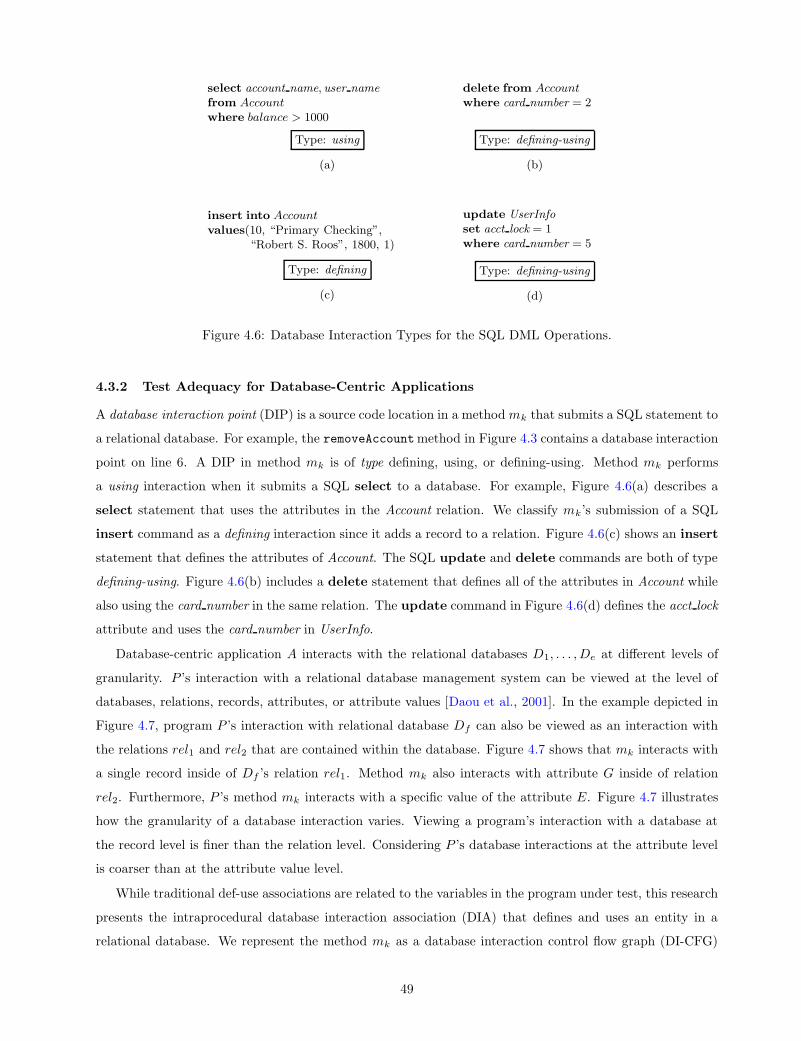
select account name, user namefrom Accountwhere balance > 1000
Type: using
(a)
delete from Accountwhere card number = 2
Type: defining-using
(b)
insert into Accountvalues(10, “Primary Checking”,
“Robert S. Roos”, 1800, 1)
Type: defining
(c)
update UserInfoset acct lock = 1where card number = 5
Type: defining-using
(d)
Figure 4.6: Database Interaction Types for the SQL DML Operations.
4.3.2 Test Adequacy for Database-Centric Applications
A database interaction point (DIP) is a source code location in a method mk that submits a SQL statement to
a relational database. For example, the removeAccountmethod in Figure 4.3 contains a database interaction
point on line 6. A DIP in method mk is of type defining, using, or defining-using. Method mk performs
a using interaction when it submits a SQL select to a database. For example, Figure 4.6(a) describes a
select statement that uses the attributes in the Account relation. We classify mk’s submission of a SQL
insert command as a defining interaction since it adds a record to a relation. Figure 4.6(c) shows an insert
statement that defines the attributes of Account. The SQL update and delete commands are both of type
defining-using. Figure 4.6(b) includes a delete statement that defines all of the attributes in Account while
also using the card number in the same relation. The update command in Figure 4.6(d) defines the acct lock
attribute and uses the card number in UserInfo.
Database-centric application A interacts with the relational databases D1, . . . , De at different levels of
granularity. P ’s interaction with a relational database management system can be viewed at the level of
databases, relations, records, attributes, or attribute values [Daou et al., 2001]. In the example depicted in
Figure 4.7, program P ’s interaction with relational database Df can also be viewed as an interaction with
the relations rel1 and rel2 that are contained within the database. Figure 4.7 shows that mk interacts with
a single record inside of Df ’s relation rel1. Method mk also interacts with attribute G inside of relation
rel2. Furthermore, P ’s method mk interacts with a specific value of the attribute E. Figure 4.7 illustrates
how the granularity of a database interaction varies. Viewing a program’s interaction with a database at
the record level is finer than the relation level. Considering P ’s database interactions at the attribute level
is coarser than at the attribute value level.
While traditional def-use associations are related to the variables in the program under test, this research
presents the intraprocedural database interaction association (DIA) that defines and uses an entity in a
relational database. We represent the method mk as a database interaction control flow graph (DI-CFG)
49

D
P
rel
rel
f
1
2
A B C D
E F G H
km
PSfrag replacements
N6
enter computeVelocity
enter computeVelocity
N6
N6
N7
N7
N8
N8
N10
N8
N16
N10
N11
N11
N12
N12
N18
N16
N18
N18
exit computeVelocity
exit computeVelocity
N6
N1
N1
N2
N2
N3
N3
N1
N1
N4
N4
N5
N5
Figure 4.7: Database Interactions at Multiple Levels of Granularity.
GDI(k) = 〈NDI(k), EDI(k)〉. We define NDI(k) as a set of nodes that contains definitions and uses of both
database entities and program variables. The set EDI(k) contains the set of edges that transfer control
between the nodes in NDI(k). Chapter 5 explains the structure of GDI(k) and the steps that the adequacy
component takes to automatically generate a method’s DI-CFG. We define D(GDI(k)) as the set of database
names that are subject to interaction in the method mk. We respectively define R(GDI(k)), A(GDI(k)),
Rc(GDI(k)), and Av(GDI(k)) as the sets of relation, attribute, record, and attribute value names. Chapter 5
discusses the techniques that we use to analyze A and enumerate these sets of relational database entities.
A database interaction association is a triple 〈Ndef , Nuse, varDB〉 where the definition of relational database
entity varDB happens in node Ndef and a use occurs in node Nuse. However, each database interaction
association is defined for a relational database entity varDB that is a member of one of the sets D(GDI(k)),
R(GDI(k)), A(GDI(k)), Rc(GDI(k)), Av(GDI(k)). The data flow analyzer described in Chapter 5 performs
reaching definitions analysis in order to identify the DIAs within the DI-CFG GDI(k).
While the database interaction association is similar to a traditional def-use association, it does have addi-
tional semantics that are different from a def-use association for a program variable. When Ndef corresponds
to the execution of a SQL delete statement, the semantics of a DIA differ from the traditional understand-
ing of a def-use association. For example, the database interaction association 〈Ndef , Nuse, varDB〉 with
varDB ∈ Rc(GDI(k)) requires the definition and use of a record that is stored within a specific relation
of a database. If Ndef corresponds to the execution of the SQL delete statement, then mk removes the
record varDB from the database and it is no longer available for use. Therefore, the all-record-DUs and
all-attribute-value-DUs test adequacy criteria allow the use of varDB on node Nuse to correspond to the
use of a phantom record, or a record that once existed in a previous state of the database but was removed
during testing. The existence of phantom records (and analogously, phantom attribute values) forces the test
coverage monitoring component to observe the program’s manipulation of the relational database and retain
information about the deleted records. However, the use of phantom records requires a test suite to execute
operations that remove records from a database and then verify that the records are no longer available.
50
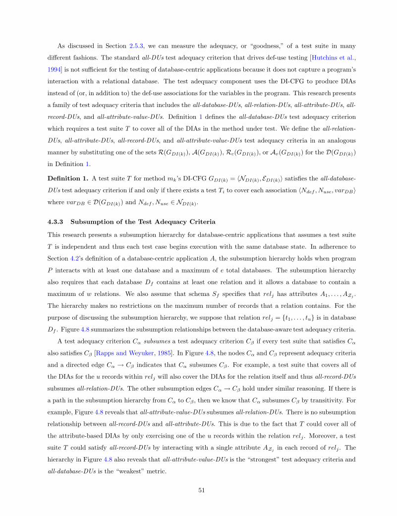
As discussed in Section 2.5.3, we can measure the adequacy, or “goodness,” of a test suite in many
different fashions. The standard all-DUs test adequacy criterion that drives def-use testing [Hutchins et al.,
1994] is not sufficient for the testing of database-centric applications because it does not capture a program’s
interaction with a relational database. The test adequacy component uses the DI-CFG to produce DIAs
instead of (or, in addition to) the def-use associations for the variables in the program. This research presents
a family of test adequacy criteria that includes the all-database-DUs, all-relation-DUs, all-attribute-DUs, all-
record-DUs, and all-attribute-value-DUs. Definition 1 defines the all-database-DUs test adequacy criterion
which requires a test suite T to cover all of the DIAs in the method under test. We define the all-relation-
DUs, all-attribute-DUs, all-record-DUs, and all-attribute-value-DUs test adequacy criteria in an analogous
manner by substituting one of the sets R(GDI(k)), A(GDI(k)), Rc(GDI(k)), or Av(GDI(k)) for the D(GDI(k))
in Definition 1.
Definition 1. A test suite T for method mk’s DI-CFG GDI(k) = 〈NDI(k), EDI(k)〉 satisfies the all-database-
DUs test adequacy criterion if and only if there exists a test Ti to cover each association 〈Ndef , Nuse, varDB〉
where varDB ∈ D(GDI(k)) and Ndef , Nuse ∈ NDI(k).
4.3.3 Subsumption of the Test Adequacy Criteria
This research presents a subsumption hierarchy for database-centric applications that assumes a test suite
T is independent and thus each test case begins execution with the same database state. In adherence to
Section 4.2’s definition of a database-centric application A, the subsumption hierarchy holds when program
P interacts with at least one database and a maximum of e total databases. The subsumption hierarchy
also requires that each database Df contains at least one relation and it allows a database to contain a
maximum of w relations. We also assume that schema Sf specifies that relj has attributes A1, . . . , AZj.
The hierarchy makes no restrictions on the maximum number of records that a relation contains. For the
purpose of discussing the subsumption hierarchy, we suppose that relation relj = t1, . . . , tu is in database
Df . Figure 4.8 summarizes the subsumption relationships between the database-aware test adequacy criteria.
A test adequacy criterion Cα subsumes a test adequacy criterion Cβ if every test suite that satisfies Cα
also satisfies Cβ [Rapps and Weyuker, 1985]. In Figure 4.8, the nodes Cα and Cβ represent adequacy criteria
and a directed edge Cα → Cβ indicates that Cα subsumes Cβ . For example, a test suite that covers all of
the DIAs for the u records within relj will also cover the DIAs for the relation itself and thus all-record-DUs
subsumes all-relation-DUs. The other subsumption edges Cα → Cβ hold under similar reasoning. If there is
a path in the subsumption hierarchy from Cα to Cβ , then we know that Cα subsumes Cβ by transitivity. For
example, Figure 4.8 reveals that all-attribute-value-DUs subsumes all-relation-DUs. There is no subsumption
relationship between all-record-DUs and all-attribute-DUs. This is due to the fact that T could cover all of
the attribute-based DIAs by only exercising one of the u records within the relation relj . Moreover, a test
suite T could satisfy all-record-DUs by interacting with a single attribute AZjin each record of relj . The
hierarchy in Figure 4.8 also reveals that all-attribute-value-DUs is the “strongest” test adequacy criteria and
all-database-DUs is the “weakest” metric.
51

all−attribute−value−DUs
all−record−DUs all−attribute−DUs
all−relation−DUs
all−database−DUs
PSfrag replacements
N6
enter computeVelocity
enter computeVelocity
N6
N6
N7
N7
N8
N8
N10
N8
N16
N10
N11
N11
N12
N12
N18
N16
N18
N18
exit computeVelocity
exit computeVelocity
N6
N1
N1
N2
N2
N3
N3
N1
N1
N4
N4
N5
N5
Figure 4.8: The Subsumption Hierarchy for the Database-Aware Test Criteria.
4.3.4 Suitability of the Test Adequacy Criteria
A test is more likely to reveal database interaction points that cause type (1-c) and (1-v) violations if it
first executes a program operation that incorrectly modifies the database and then it subsequently uses
the database. For example, a test case for the defective removeAccount operation listed in Figure 4.3
would expose the program defect on line 4 if it first executed removeAccount(2). Next, the test could call a
listAccounts operation to verify that the account with id = 2 was not in the database and all other accounts
(in particular, the one where id = 3 and card number = 2) were still inside of the Account relation. The test
could also use an oracle to directly access the state of the database and reveal the defect in removeAccount.
By requiring the coverage of database interaction associations, the presented family of test adequacy criteria
can determine whether or not the provided tests are well suited to revealing type (1-c) and (1-v) defects.
The test adequacy criteria also evaluate the capability of a test suite to isolate type (2-c) and (2-v)
commission faults. This is due to the fact that the component assigns low adequacy scores to the test cases
that do not execute the program’s database interactions. Methods that are only tested by low adequacy tests
are more likely to contain latent type (2-c) and (2-v) commission defects. We do not focus on the creation of
adequacy criteria to support the isolation of type (2-c) and (2-v) omission defects that fail to update, insert,
and delete data values. This is due to the fact that structural adequacy criteria, like the family proposed
by this research, are not well suited to revealing omission faults [Marick, 1999, 2000]. The data flow-based
test adequacy criteria will not yield any test requirements for methods that contain type (2-c) and (2-v)
omission faults because the database interactions do not exist within the source code. Chapter 9 observes that
database-aware versions of existing approaches to (i) code inspection (e.g., [Shull et al., 2001]), (ii) black-box
testing (e.g., [Ostrand and Balcer, 1988]), and/or (iii) automatic defect isolation (e.g, [Hovemeyer and Pugh,
2004]) could be more appropriate for identifying omission faults [Marick, 2000].
52

1 public boolean removeAccount( int id ) throws SQLException2 3 boolean completed = f a l se ;4 S t r ing removeAcct = ‘‘ de l e t e from Account where id = ’’ + id ;5 Statement removeStmt = connect . c reateStatement ( ) ;6 int removeAccountResult = removeStmt . executeUpdate ( removeAcct ) ;7 S t r ing s e l e c tAcc t = ‘‘ s e l e c t ∗ from Account where ’’ +8 ‘‘ba lance =’’ + id ;9 Statement s e l e c tS tmt = connect . c reateStatement ( ) ;
10 Resu l tSet se lectAccountResu l t = se l e c tS tmt .11 executeQuery ( s e l e c tAcc t ) ;12 i f ( removeAccountResult == 1 && ! se lectAccountResu l t . next ( ) )13 14 completed = true ;15 16 return completed ;17
Figure 4.9: A removeAccount Method with Incorrect Error Checking.
4.3.5 Comparison to Traditional Adequacy Criteria
Figure 4.9 contains a faulty implementation of the removeAccount method that incorrectly determines if the
desired rows were removed from the Account relation (i.e., lines 7 and 8 should contain ‘‘select * from
Account where id = ’’ + id; instead of ‘‘select * from Account where balance = ’’ + id;). Yet,
test adequacy criteria based upon control flow and data flow information, such as all-nodes, all-edges, and
all-DUs, will indicate that a test for this method is highly adequate and they will not focus a tester’s attention
on this incorrect implementation of removeAccount. This is due to the fact that these criteria exclusively
focus on the control flow within the program’s source code and the data flow between program variables.
For example, the all-nodes (or, statement coverage) criterion requires a test case to execute all of the source
code statements within the removeAccount method in Figure 4.9. Furthermore, the all-edges (or, branch
coverage) criterion stipulates that a test execute all of the transfers of control between removeAccount’s
statements [Zhu et al., 1997]. The all-DUs adequacy criterion requires the tests to cover the definition-use
associations for all of the program variables in removeAccount.
If a test case calls removeAccount(2), then it will cover all of the nodes in the method. Table 4.1
shows that the same test case will also cover 87.5% of the edges within the method under test. This table
represents an edge in the method under test as (Nρ, Nφ) when there is a transfer of control from node Nρ to
Nφ (for source code statements that span lines ρ and φ we represent this as node Nρ:φ). Table 4.1 reveals
that the test does not cover the edge (N12, N16) because removeAccount(2) executes the if statement’s
body. However, the execution of an additional test that calls removeAccount(-4) will cover the edge
(N12, N16) and yield 100% coverage for the test suite. Finally, Table 4.2 demonstrates that a test’s invocation
of removeAccount(2) will afford 100% coverage of the def-use associations within this method. Thus,
traditional adequacy criteria will classify a test suite for this method as highly adequate even though it does
not reveal the defect.
When a test invokes removeAccount(2) this will cause the execution of line 6 and line 11 without
guaranteeing that the delete on line 6 removes the record with id = 2 and the select on line 11 contains
53

Edge Covered?
(N3, N4) X
(N4, N5) X
(N6, N7:8) X
(N7:8, N9) X
(N9, N10:11) X
(N10:11, N12) X
(N12, N14) X
(N12, N16) ×
Ti calls removeAccount(2) for 87.5% all-edges coverage.
Table 4.1: The Edges Covered by a Test Case.
the appropriate where clause. Even though both all-nodes and all-edges require a test case to execute the
database interactions on line 6 and line 11, these criteria do not ensure that removeAccount interacts with
the correct entities in the relational database. The definition of the String variable selectAcct on line 9
and the use on line 11 forms a definition-use association for the variable selectAcct. The all-DUs criterion
judges a test as adequate if it creates paths from the entrance to the exit of removeAccount that cover all
of the def-use associations for all of the program variables like selectAcct. Since all-DUs ignores the state
of the database, most tests for removeAccount will be highly adequate with respect to all-DUs and exhibit
low adequacy when evaluated by the database-aware test adequacy criteria.
Suppose that we use the database-aware test adequacy criteria to measure the quality of TM’s test suite
with the all-record-DUs adequacy criterion. The component will evaluate removeAccount’s tests with respect
to their ability to define and then subsequently use the records in the Account relation. Since lines 4 and 8
of Figure 4.9 use the method parameter id to define removeAcct and selectAcct, a static analysis will not
reveal the records that the method uses. Therefore, the all-record-DUs test adequacy criterion conservatively
requires the definition and use of all of the records in the Account relation. A test that causes removeAccount
to define the record where id = 2 will not be able to use this record. This is because the select statement
executed on line 11 incorrectly references the balance attribute instead of id.3 A select statement that is
executed with the clause where balance = 2 will not use any records of the Account relation depicted in
Figure 2.4 because all accounts currently have balances greater than $125.00. The inability to define and
use the records in the Account relation will yield low adequacy scores for removeAccount’s tests. These low
scores will focus attention on this method during testing and increase the potential for revealing the defective
database interaction on line 11.
3Since the database interaction on line 6 of removeAccount does remove the record from the Account relation where id = 2,the all-record-DUs criterion actually requires the use of a phantom record, as discussed in Section 4.3.2.
54

Def-Use Association Covered?
〈N3, N16, completed〉 X
〈N3, N14, completed〉 X
〈N4, N6, removeAcct〉 X
〈N5, N6, removeStmt〉 X
〈N6, N16, removeAccountResult〉 X
〈N7:8, N10:11, selectAccount〉 X
〈N9, N10:11, selectStmt〉 X
〈N10:11, N12, selectStmt〉 X
Ti calls removeAccount(2) for 100% all-DUs coverage.
Table 4.2: The Def-Use Associations Covered by a Test Case.
4.4 CONCLUSION
This chapter defines a database-centric application A that consists of a program P , relational databases
D1, . . . , De, and relational schemas S1, . . . , Se. We discuss a database interaction fault model and the type
(1-c), (1-v), (2-c), (2-v) defects that could violate the completeness and validity of A’s databases. We also
classify database interaction faults as faults of commission or omission. This chapter presents a family of
database-aware test adequacy criteria that are uniquely suited for the isolation of all type (1-c) and (1-v)
defects and type (2-c) and (2-v) commission faults. We furnish a subsumption hierarchy that organizes the
test adequacy criteria according to their strength. This hierarchy reveals that all-attribute-value-DUs is the
strongest adequacy criterion and all-database-DUs is the weakest. This chapter concludes by comparing our
database-aware test adequacy criteria to traditional structural test adequacy metrics. For example, we use
a defective removeAccount method to demonstrate that the traditional all-nodes, all-edges, and all-DUs will
assign a high adequacy score to a simple test suite. We also show that a database-aware criterion such as
all-record-DUs increases the potential for revealing faulty database interactions by assigning low adequacy
values to the same tests. Chapter 5 shows how the test adequacy component automatically creates the
DI-CFGs and performs the data flow analysis to identify the DIAs. Finally, Chapters 6 through 8 explain
an alternative type of test requirement that focuses on the behavior of the program during testing.
55

5.0 TEST ADEQUACY COMPONENT
5.1 INTRODUCTION
This chapter describes a test adequacy component that analyzes a database-centric application and generates
a set of database interaction associations (DIAs). As discussed in Chapter 4, these DIAs are the requirements
that state how an application must be tested in order to achieve a confidence in the correctness of the database
interactions. The testing techniques in Chapters 6 through 8 can use these requirements to guide the effective
testing of a database-centric application. In summary, this chapter provides:
1. A high level overview of the techniques within the test adequacy component (Section 5.2).
2. An interprocedural program representation that supports the identification of test requirements (Sec-
tion 5.3).
3. A model for a database interaction and the algorithms that enumerate database entities (Section 5.4).
4. A representation for a database-centric application that describes a program’s interaction with relational
database entities at multiple levels of granularity (Section 5.5).
5. An empirical examination of the time and space overhead incurred during the generation of intraprocedu-
ral database interaction associations for two case study applications (Section 5.7 through Section 5.10).
6. A review of the test adequacy component’s implementation and a concluding discussion (Section 5.6 and
Section 5.11).
5.2 OVERVIEW OF THE TEST ADEQUACY COMPONENT
Figure 5.1 depicts the high level architecture of the test adequacy component. This component analyzes
program P in light of database-aware test adequacy criterion C and produces a set of database interaction
associations. The test adequacy criterion C is one of the database-aware criterion that we presented in
Chapter 4. The first stage produces an interprocedural control flow graph (ICFG) for program P . Next,
the database interaction analyzer uses the ICFG in order to identify the database interaction points (DIPs)
within the program under test. These DIPs send a SQL select, update, insert, or delete statement to the
database. However, the SQL command might not be fully specified in the source code of the method under
test. Many database-centric applications contain database interactions that send a SQL command whose
elements are specified during program execution. Furthermore, a method often contains one or more control
flow paths that lead to a single database interaction point.
56

P, C
Representation Constructor
ICFG
Database Interaction Analyzer
Database-Aware Representation Constructor
Database Entities
Database
Database Interaction ICFG (DI-ICFG)
Data Flow Analyzer
Database Interaction Associations
PSfrag replacements
N6
enter computeVelocity
enter computeVelocity
N6
N6
N7
N7
N8
N8
N10
N8
N16
N10
N11
N11
N12
N12
N18
N16
N18
N18
exit computeVelocity
exit computeVelocity
N6
N1
N1
N2
N2
N3
N3
N1
N1
N4
N4
N5
N5
Figure 5.1: High Level Architecture of the Test Adequacy Component.
The adequacy component includes a database interaction analyzer that models each DIP as a database
interaction finite state machine (DI-FSM). The DI-FSM models all of the possible SQL statements that
program P could submit to a database at a particular DIP. The database interaction analyzer correctly
handles (i) SQL commands that are not statically specified and (ii) interaction points that exist on multiple
paths of the ICFG. We consult a DI-FSM during the enumeration of the set of database entities that are
subject to interaction at a DIP. Next, we use the set of database entities and the ICFG to construct a
database interaction interprocedural control flow graph (DI-ICFG). The DI-ICFG includes nodes and edges
that represent a program’s interaction with a relational database. The data flow analyzer uses the DI-ICFG
to generate the database interaction associations. The test adequacy component can leverage traditional
data flow analysis algorithms that were designed for program variables (e.g., [Duesterwald et al., 1996]) since
we designed the DI-ICFG to fully model the program’s definition and use of the database.
5.3 REPRESENTING THE PROGRAM UNDER TEST
In order to support the enumeration of test requirements, the test adequacy component represents a database-
centric application A = 〈P, 〈D1, . . . , De〉, 〈S1, . . . , Se〉〉 as an interprocedural control flow graph. The follow-
ing Definition 2 defines the interprocedural control flow graph GP that traditionally represents program
P . Figure 5.1 shows that the component initially constructs an ICFG for P with the goal of subsequently
creating a DI-ICFG that fully describes the interactions between P and the D1, . . . , De within A. The tra-
ditional ICFG contains all of the CFGs for each of P ’s methods and the edges that connect these graphs.
Each CFG Gj can have call mk and return mk nodes that respectively demarcate the call to and the return
from another method mk. Figure 5.2 demonstrates how the CFGs for methods mj and mk are connected
when the CFG for mj contains an invocation of the method mk. In an attempt to preserve the simplicity
of the CFGs, Figures 5.2 and 5.3 use nodes with the label “. . .” to represent other nodes within Gj and Gk.
Definition 2 and Figure 5.2 reveal that GP provides an edge that connects the call node in Gj to the enter
node in Gk. The ICFG also includes an edge from the exit node in Gk to the return node in Gj . Table A6
in Appendix A more fully describes the notation for the ICFG representation of program P .
57

PSfrag replacements
N6
enter computeVelocity
enter computeVelocity
N6
N6
N7
N7
N8
N8
N10
N8
N16
N10
N11
N11
N12
N12
N18
N16
N18
N18
exit computeVelocity
exit computeVelocity
N6
N1
N1
N2
N2
N3
N3
N1
N1
N4
N4
N5
N5
Id : icfgsimple.ladot, v1.22006/08/0115 : 58 : 34gkapfhamExp
Revision : 1.2
enter mj
. . .
call mk
enter mk
. . .
enter mj
enter mj
. . .
∈ Ej
. . .
call mk
∈ Ej
call mk
enter mk
∈ EP
enter mk
. . .
∈ Ek
. . .
exit mk
∈ Ek
∈ Ek
exit mk
return mk
∈ EP
∈ EP
return mk
. . .
∈ Ej
. . .exit mj
∈ Ej
∈ Ej
∈ Ej
∈ Ej
exit mj
Figure 5.2: Connecting the Intraprocedural CFGs.
Definition 2. An program interprocedural control flow graph GP = 〈ΓP , EP 〉 consists of the set of intrapro-
cedural control flow graphs ΓP and the set of edges EP . For each method mk in P , there exists a Gk ∈ ΓP .
For any method mj that invokes method mk there exists (i) CFGs Gj , Gk ∈ ΓP with call mk, return mk ∈ Nj
and enter mk, exit mk ∈ Nk and (ii) edges (call mk, enter mk), (exit mk, return mk) ∈ EP .
Figure 5.3 provides part of the ICFG for the TM case study application and the getAccountBalance
method in Figure 5.9. We simplified this ICFG by including nodes of the form call mk to represent method
invocations that were not expanded. For example, we did not add the full CFG for the inputPin method
after the node call inputPin. However, Figure 5.3 does contain the CFG for the getAccountBalancemethod.
We use the line numbers in getAccountBalance’s source code listing to number the nodes within this CFG.
For example, the node N6 corresponds to line 6 of Figure 5.9 where getAccountBalance submits a SQL
select statement to the Bank database. It is important to observe that the traditional ICFG in Figure 5.3
does not contain nodes that capture the program’s interaction with the database entities.
5.4 ANALYZING A DATABASE INTERACTION
5.4.1 Overview of the Analysis
Figure 5.4 offers a high level overview of the database interaction analysis that we perform and Section 5.4.2
reviews the common terms and notation that we use throughout our discussion of the process depicted
in this figure. First, the test adequacy component models a database interaction using the interprocedural
control flow graph and any statically available information from the database interaction point. The database
interaction modeling component creates a database interaction finite state machine, as further discussed in
Section 5.4.3. Figure 5.4 reveals that the generation functions described in Section 5.4.4 use this DI-FSM
to enumerate the sets of database entities. Section 5.5 explains how we use these sets of database entities
58

PSfrag replacements
N6
enter computeVelocity
enter computeVelocity
N6
N6
N7
N7
N8
N8
N10
N8
N16
N10
N11
N11
N12
N12
N18
N16
N18
N18
exit computeVelocity
exit computeVelocity
N6
N1
N1
N2
N2
N3
N3
N1
N1
N4
N4
N5
N5
N6
enter P
enter P
call main
call main
enter main
enter main
enter main
. . .
. . .
call inputCardNumber
call inputCardNumber
call inputPin
call inputCardNumber
call handleError
call handleError
call inputCardNumber
call inputPin
call handleError
call handleError
call inputPin
call inputPin
call inputOperation
call inputOperation
call getAccountBalance
call getAccountBalance
call promptAgain
call inputOperation
call lockAccount
call lockAccount
call promptAgain
call promptAgain
call inputOperation
call promptAgain
. . .
call getAccountBalance
enter getAccountBalance
enter getAccountBalance
N3
N3
N4
N4
N5
N5
N6
N6
N7
N7
N10
N10
N12
N12
N15
N10
N15
N15
exit getAccountBalance
exit getAccountBalance
return getAccountBalance
return lockAccount
. . .
return getAccountBalance
call promptAgain
. . .
exit main
exit main
return main
return main
exit P
exit P
. . .
exit main
enter lockAccount
enter lockAccount
. . .
. . .
exit lockAccount
exit lockAccount
return lockAccount
return lockAccountexit main
Figure 5.3: A Partial Interprocedural CFG for the TM Database-Centric Application.
59

ICFG
Database Interaction Modeling
DIP
DI-FSM Generation Functions Database Entity Sets
PSfrag replacements
N6
enter computeVelocity
enter computeVelocity
N6
N6
N7
N7
N8
N8
N10
N8
N16
N10
N11
N11
N12
N12
N18
N16
N18
N18
exit computeVelocity
exit computeVelocity
N6
N1
N1
N2
N2
N3
N3
N1
N1
N4
N4
N5
N5
N6
enter P
enter P
call main
call main
enter main
enter main
enter main
. . .
. . .
call inputCardNumber
call inputCardNumber
call inputPin
call inputCardNumber
call handleError
call handleError
call inputCardNumber
call inputPin
call handleError
call handleError
call inputPin
call inputPin
call inputOperation
call inputOperation
call getAccountBalance
call getAccountBalance
call promptAgain
call inputOperation
call lockAccount
call lockAccount
call promptAgain
call promptAgain
call inputOperation
call promptAgain
. . .
call getAccountBalance
enter getAccountBalance
enter getAccountBalance
N3
N3
N4
N4
N5
N5
N6
N6
N7
N7
N10
N10
N12
N12
N15
N10
N15
N15
exit getAccountBalance
exit getAccountBalance
return getAccountBalance
return lockAccount
. . .
return getAccountBalance
call promptAgain
. . .
exit main
exit main
return main
return main
exit P
exit P
. . .
exit main
enter lockAccount
enter lockAccount
. . .
. . .
exit lockAccount
exit lockAccount
return lockAccount
return lockAccount
exit mainFigure 5.4: The Process of Database Interaction Analysis.
to (i) automatically generate a database-aware control flow graph and (ii) perform a data flow analysis that
enumerates the test requirements. Tables A7 and A8 in Appendix A summarize the notation that we develop
in the remainder of this chapter.
5.4.2 Representing a Database’s State and Structure
Method mk’s control flow graph Gk = 〈Nk, Ek〉 can contain one or more database interaction points, each
of which corresponds to a database interaction node Nr ∈ Nk. The source code in Figure 5.9 has a DIP
on line 6 (i.e., “ResultSet rs = stmt.executeQuery(qs)”) and the method listing in Figure 5.11 contains
a DIP on line 7 (i.e., “int result lock = update lock.executeUpdate(qu lck)”). The test adequacy
component analyzes the state and structure of the relational databases in order to enumerate unique names
for the database entities that are subject to interaction at node Nr. Suppose that program P interacts with
database Df at node Nr. We view database Df as a set of relations so that Df = rel1, . . . , relw and we
define a relation relj = t1, . . . , tu as a set of records. Each record is an ordered set of attribute values
such that tk = 〈tk [1], . . . , tk[q]〉. We use the notation tk[l] to denote the value of the lth attribute of the
kth record in a specified relation. In order to differentiate between the name of a database entity and its
contents, we use the functions name(Df ), name(C, relj), and name(C, tk) to respectively return the unique
names of the database Df , the relation relj in database Df , and relj ’s record tk. For example, relj is a set
of records while name(C, relj) is the unique name of the relation. The name function uses a context stack
C to record the complete context for a database entity.
A relational database Df can contain duplicate values in different database records. The adequacy
component uses the context stack C to ensure that name returns a unique identifier for duplicate attribute
values. At the attribute value level, two cases of entity value duplication are relevant: (i) the same attribute
contains the same value in one or more records or (ii) two different attributes contain the same value in
one or more records. Figure 5.5 shows a relation relj where certain attributes have the same value as
the attribute value tk[l] (the same attribute values are represented by cells that have a darkened border).
In circumstance (i), the record tk′ has the same value for attribute Al as record tk (i.e., tk[l] = tk′ [l]).
However, Figures 5.6(a) and 5.6(b) show that tk[l] and tk′ [l] have different context stacks and thus name
can return unique identifiers for each attribute value (i.e., name(C, tk[l]) 6= name(C, tk′ [l]) even though
tk[l] = tk′ [l]). In case (ii), the attribute Al′ contains the same value as the attribute Al in the record tk (i.e.,
tk[l] = tk[l′]). Since Figures 5.6(a) and 5.6(c) reveal that tk[l] and tk[l
′] have different context stacks, name
60

2A1A qA1t
kt
lA
jrel
lA
k ~k [l ]
......
...... ...
...
tk
...
ot
tk~
tt tk [l] [l]
PSfrag replacements
N6
enter computeVelocity
enter computeVelocity
N6
N6
N7
N7
N8
N8
N10
N8
N16
N10
N11
N11
N12
N12
N18
N16
N18
N18
exit computeVelocity
exit computeVelocity
N6
N1
N1
N2
N2
N3
N3
N1
N1
N4
N4
N5
N5
N6
enter P
enter P
call main
call main
enter main
enter main
enter main
. . .
. . .
call inputCardNumber
call inputCardNumber
call inputPin
call inputCardNumber
call handleError
call handleError
call inputCardNumber
call inputPin
call handleError
call handleError
call inputPin
call inputPin
call inputOperation
call inputOperation
call getAccountBalance
call getAccountBalance
call promptAgain
call inputOperation
call lockAccount
call lockAccount
call promptAgain
call promptAgain
call inputOperation
call promptAgain
. . .
call getAccountBalance
enter getAccountBalance
enter getAccountBalance
N3
N3
N4
N4
N5
N5
N6
N6
N7
N7
N10
N10
N12
N12
N15
N10
N15
N15
exit getAccountBalance
exit getAccountBalance
return getAccountBalance
return lockAccount
. . .
return getAccountBalance
call promptAgain
. . .
exit main
exit main
return main
return main
exit P
exit P
. . .
exit main
enter lockAccount
enter lockAccount
. . .
. . .
exit lockAccount
exit lockAccount
return lockAccount
return lockAccount
exit main
Value Duplication: tk[l] = tk′ [l] and tk[l] = tl[l′]
Figure 5.5: Value Duplication in a Relational Database.
can return unique identifiers for these duplicate attribute values (i.e., name(C, tk[l]) 6= name(C, tk[l′]) even
though tk[l] = tk[l′]). The test adequacy component also uses the context stack C and the name function to
accommodate value duplication at the relation, attribute, and record levels.
5.4.3 Representing a Database Interaction
The adequacy component produces a database interaction finite state machine to model the interaction at
a single CFG node Nr. According to the following Definition 3, Fr contains the set of internal states Q
and the set of final states Qf ⊆ Q. The DI-FSM begins the processing of input string s at the initial state
q0 ∈ Q. The transition function δ : Q×Σ→ Q allows Fr to move from state q ∈ Q to state q′ ∈ Q whenever
γ is the current symbol in s and δ(q, γ) = q′ is a transition. We know that CFG node Nr can submit a SQL
string s to the database if and only if Fr terminates in a final state q ∈ Qf when it processes input s.
Definition 3. A database interaction node Nr is represented by a database interaction finite state machine
Fr = 〈Q, Qf , q0, δ, Σ〉 where Q is a non-empty set of internal states, Qf ⊆ Q is the set of final states, q0 ∈ Q
is the start state, δ : Q× Σ→ Q is the transition function, and Σ is the input alphabet.
Fr’s input alphabet Σ consists of all the terminals in the SQL grammar (e.g., select, where, attribute
Az , relation relj , etc.) and additional symbols µ, R, A, and O. The symbol µ denotes an unknown input and
a transition uses µ to indicate that this aspect of the database interaction is not statically detectable. Fr uses
the additional symbols R, A, and O to respectively denote the relation, attribute, and operation inputs and
to provide semantic meaning to the other transitions. The transitions δ(q, q′) = relj and δ(q, q′) = R show
that relj is a recognized relation in the databases. The transitions δ(q, q′) = Al and δ(q, q′) = A indicate
that Al is a valid database attribute. If op ∈ select,update, insert,delete and Fr has the transitions
δ(q, q′) = op and δ(q, q′) = O, then this reveals that op is a correct SQL operation. For brevity, we call the
transition δ(q, q′) = R an R−transition and define the µ, A and O-transitions analogously. The component
adds the R, A, O−transitions to Fr using a context-free language (CFL) reachability algorithm that “parses”
61

PSfrag replacements
N6
enter computeVelocity
enter computeVelocity
N6
N6
N7
N7
N8
N8
N10
N8
N16
N10
N11
N11
N12
N12
N18
N16
N18
N18
exit computeVelocity
exit computeVelocity
N6
N1
N1
N2
N2
N3
N3
N1
N1
N4
N4
N5
N5
N6
enter P
enter P
call main
call main
enter main
enter main
enter main
. . .
. . .
call inputCardNumber
call inputCardNumber
call inputPin
call inputCardNumber
call handleError
call handleError
call inputCardNumber
call inputPin
call handleError
call handleError
call inputPin
call inputPin
call inputOperation
call inputOperation
call getAccountBalance
call getAccountBalance
call promptAgain
call inputOperation
call lockAccount
call lockAccount
call promptAgain
call promptAgain
call inputOperation
call promptAgain
. . .
call getAccountBalance
enter getAccountBalance
enter getAccountBalance
N3
N3
N4
N4
N5
N5
N6
N6
N7
N7
N10
N10
N12
N12
N15
N10
N15
N15
exit getAccountBalance
exit getAccountBalance
return getAccountBalance
return lockAccount
. . .
return getAccountBalance
call promptAgain
. . .
exit main
exit main
return main
return main
exit P
exit P
. . .
exit main
enter lockAccount
enter lockAccount
. . .
. . .
exit lockAccount
exit lockAccount
return lockAccount
return lockAccount
exit mainAl
tk
relj
Df
tk[l]
(a)
PSfrag replacements
N6
enter computeVelocity
enter computeVelocity
N6
N6
N7
N7
N8
N8
N10
N8
N16
N10
N11
N11
N12
N12
N18
N16
N18
N18
exit computeVelocity
exit computeVelocity
N6
N1
N1
N2
N2
N3
N3
N1
N1
N4
N4
N5
N5
N6
enter P
enter P
call main
call main
enter main
enter main
enter main
. . .
. . .
call inputCardNumber
call inputCardNumber
call inputPin
call inputCardNumber
call handleError
call handleError
call inputCardNumber
call inputPin
call handleError
call handleError
call inputPin
call inputPin
call inputOperation
call inputOperation
call getAccountBalance
call getAccountBalance
call promptAgain
call inputOperation
call lockAccount
call lockAccount
call promptAgain
call promptAgain
call inputOperation
call promptAgain
. . .
call getAccountBalance
enter getAccountBalance
enter getAccountBalance
N3
N3
N4
N4
N5
N5
N6
N6
N7
N7
N10
N10
N12
N12
N15
N10
N15
N15
exit getAccountBalance
exit getAccountBalance
return getAccountBalance
return lockAccount
. . .
return getAccountBalance
call promptAgain
. . .
exit main
exit main
return main
return main
exit P
exit P
. . .
exit main
enter lockAccount
enter lockAccount
. . .
. . .
exit lockAccount
exit lockAccount
return lockAccount
return lockAccount
exit mainAl
tk′
relj
Df
tk′ [l]
(b)
PSfrag replacements
N6
enter computeVelocity
enter computeVelocity
N6
N6
N7
N7
N8
N8
N10
N8
N16
N10
N11
N11
N12
N12
N18
N16
N18
N18
exit computeVelocity
exit computeVelocity
N6
N1
N1
N2
N2
N3
N3
N1
N1
N4
N4
N5
N5
N6
enter P
enter P
call main
call main
enter main
enter main
enter main
. . .
. . .
call inputCardNumber
call inputCardNumber
call inputPin
call inputCardNumber
call handleError
call handleError
call inputCardNumber
call inputPin
call handleError
call handleError
call inputPin
call inputPin
call inputOperation
call inputOperation
call getAccountBalance
call getAccountBalance
call promptAgain
call inputOperation
call lockAccount
call lockAccount
call promptAgain
call promptAgain
call inputOperation
call promptAgain
. . .
call getAccountBalance
enter getAccountBalance
enter getAccountBalance
N3
N3
N4
N4
N5
N5
N6
N6
N7
N7
N10
N10
N12
N12
N15
N10
N15
N15
exit getAccountBalance
exit getAccountBalance
return getAccountBalance
return lockAccount
. . .
return getAccountBalance
call promptAgain
. . .
exit main
exit main
return main
return main
exit P
exit P
. . .
exit main
enter lockAccount
enter lockAccount
. . .
. . .
exit lockAccount
exit lockAccount
return lockAccount
return lockAccount
exit main
Id : fsmdynamic.ladot, v1.22006/08/0302 : 48 : 33gkapfhamExp
Revision : 1.2Al′
tk
relj
Df
tk[l′]
(c)
Figure 5.6: Context Stacks for Duplicate Attribute Values.
the finite state machine with a parser for the SQL grammar [Melski and Reps, 1997, Reps et al., 1995]. In
this chapter, all figures that depict DI-FSMs use a bold node to indicate a final state and a dashed edge to
represent the R, A, O−transitions that the CFL reachability algorithm adds.
The following Definition 4 classifies Fr’s database interaction as static, partially dynamic, or dynamic.
If P ’s source code fully specifies the interaction, then Nr performs a static interaction and the compo-
nent creates an Fr that does not contain any µ−transitions. If P does not statically specify a portion of
the database interaction, then the component produces a partially dynamic Fr that contains at least one
µ−transition. The component generates a dynamic DI-FSM if the database interaction at Nr is specified at
run-time. Definition 4 classifies Fr as dynamic when it only contains two states qo, q′ ∈ Q, q′ ∈ Qf , and the
single transition δ(q0, µ) = q′. Since the dynamic DI-FSM in Figure 5.7 accepts any SQL string, the test
adequacy component must conservatively assume that Nr interacts with all of the attribute values in all of
the databases.
Definition 4. A database interaction represented by Fr = 〈Q, Qf , q0, δ, Σ〉 is (i) static if (∀q, q′ ∈
Q) (δ(q, µ) 6= q′), (ii) partially dynamic if (∀q, q′ ∈ Q) (∃δ(q, µ) = q′), or (iii) dynamic if |Q| = 2, |Qf | = 1,
q0, q′ ∈ Q, q′ ∈ Qf , and δ(q0, µ) = q′.
Figure 5.8 provides the DI-FSM for line 4 of the getAccountBalancemethod in Figure 5.9. This DI-FSM
consists of five states with q0 ∈ Q as the initial state and q5 ∈ Q as the final state. The O-transition in this
DI-FSM identifies select as a valid SQL operation. The DI-FSM uses two A-transitions to reveal that id and
balance are attributes. Figure 5.8 also contains an R-transition to show that Account is a correct relation.
Since the declaration of String qs completely defines the database interaction on line 6 of Figure 5.9,
the static Fr in Figure 5.8 does not have any µ-transitions. The test adequacy component can precisely
enumerate the database entities used by getAccountBalance because the DI-FSM is static.
The partially dynamic DI-FSM in Figure 5.10 models the database interaction on lines 5 and 6 of
Figure 5.11. The O−transition in the DI-FSM indicates that update is a correct SQL operation. The
A−transitions reveal that acct lock and card number are attributes in the Bank database. The R−transition
62

PSfrag replacements
N6
enter computeVelocity
enter computeVelocity
N6
N6
N7
N7
N8
N8
N10
N8
N16
N10
N11
N11
N12
N12
N18
N16
N18
N18
exit computeVelocity
exit computeVelocity
N6
N1
N1
N2
N2
N3
N3
N1
N1
N4
N4
N5
N5
N6
enter P
enter P
call main
call main
enter main
enter main
enter main
. . .
. . .
call inputCardNumber
call inputCardNumber
call inputPin
call inputCardNumber
call handleError
call handleError
call inputCardNumber
call inputPin
call handleError
call handleError
call inputPin
call inputPin
call inputOperation
call inputOperation
call getAccountBalance
call getAccountBalance
call promptAgain
call inputOperation
call lockAccount
call lockAccount
call promptAgain
call promptAgain
call inputOperation
call promptAgain
. . .
call getAccountBalance
enter getAccountBalance
enter getAccountBalance
N3
N3
N4
N4
N5
N5
N6
N6
N7
N7
N10
N10
N12
N12
N15
N10
N15
N15
exit getAccountBalance
exit getAccountBalance
return getAccountBalance
return lockAccount
. . .
return getAccountBalance
call promptAgain
. . .
exit main
exit main
return main
return main
exit P
exit P
. . .
exit main
enter lockAccount
enter lockAccount
. . .
. . .
exit lockAccount
exit lockAccount
return lockAccount
return lockAccount
exit main
Id : fsmdynamic.ladot, v1.12006/07/1320 : 05 : 55gkapfhamExp
Revision : 1.1
q0
q′
q0
q0 q′µ
Figure 5.7: The DI-FSM for a Dynamic Interaction Point.
PSfrag replacements
N6
enter computeVelocity
enter computeVelocity
N6
N6
N7
N7
N8
N8
N10
N8
N16
N10
N11
N11
N12
N12
N18
N16
N18
N18
exit computeVelocity
exit computeVelocity
N6
N1
N1
N2
N2
N3
N3
N1
N1
N4
N4
N5
N5
N6
enter P
enter P
call main
call main
enter main
enter main
enter main
. . .
. . .
call inputCardNumber
call inputCardNumber
call inputPin
call inputCardNumber
call handleError
call handleError
call inputCardNumber
call inputPin
call handleError
call handleError
call inputPin
call inputPin
call inputOperation
call inputOperation
call getAccountBalance
call getAccountBalance
call promptAgain
call inputOperation
call lockAccount
call lockAccount
call promptAgain
call promptAgain
call inputOperation
call promptAgain
. . .
call getAccountBalance
enter getAccountBalance
enter getAccountBalance
N3
N3
N4
N4
N5
N5
N6
N6
N7
N7
N10
N10
N12
N12
N15
N10
N15
N15
exit getAccountBalance
exit getAccountBalance
return getAccountBalance
return lockAccount
. . .
return getAccountBalance
call promptAgain
. . .
exit main
exit main
return main
return main
exit P
exit P
. . .
exit main
enter lockAccount
enter lockAccount
. . .
. . .
exit lockAccount
exit lockAccount
return lockAccount
return lockAccount
exit main
Id : fsmgab.ladot, v1.62006/07/1417 : 39 : 41gkapfhamExp
Revision : 1.6
q0
q1
q2
q3
q4
q5
q0
q1
q2
q3
q4
q5
q0
q0
q1
select
q0
q1
O
q1
q2
idq1
q2
A
q2
q3
balanceq2
q3
AA
q3
q4
from
q4
q5
Account
q4
q5
R
Fr is static
Figure 5.8: The DI-FSM for the getAccountBalance Method.
1 public double getAccountBalance( int uid ) throws SQLException2 3 double balance = −1.0;4 S t r ing qs = ‘‘ s e l e c t id , ba lance from Account ; ’’ ;5 Statement stmt = connect . c reateStatement ( ) ;6 Resu l tSet r s = stmt . executeQuery ( qs ) ;7 while ( r s . next ( ) )9
10 i f ( r s . g e t In t ( ‘‘ id ’’) == uid )11 12 ba lance = r s . getDouble ( ‘‘ba lance’’ ) ;13 14 15 return balance ;16
Figure 5.9: The Implementation of the getAccountBalance Method.
63

PSfrag replacements
N6
enter computeVelocity
enter computeVelocity
N6
N6
N7
N7
N8
N8
N10
N8
N16
N10
N11
N11
N12
N12
N18
N16
N18
N18
exit computeVelocity
exit computeVelocity
N6
N1
N1
N2
N2
N3
N3
N1
N1
N4
N4
N5
N5
N6
enter P
enter P
call main
call main
enter main
enter main
enter main
. . .
. . .
call inputCardNumber
call inputCardNumber
call inputPin
call inputCardNumber
call handleError
call handleError
call inputCardNumber
call inputPin
call handleError
call handleError
call inputPin
call inputPin
call inputOperation
call inputOperation
call getAccountBalance
call getAccountBalance
call promptAgain
call inputOperation
call lockAccount
call lockAccount
call promptAgain
call promptAgain
call inputOperation
call promptAgain
. . .
call getAccountBalance
enter getAccountBalance
enter getAccountBalance
N3
N3
N4
N4
N5
N5
N6
N6
N7
N7
N10
N10
N12
N12
N15
N10
N15
N15
exit getAccountBalance
exit getAccountBalance
return getAccountBalance
return lockAccount
. . .
return getAccountBalance
call promptAgain
. . .
exit main
exit main
return main
return main
exit P
exit P
. . .
exit main
enter lockAccount
enter lockAccount
. . .
. . .
exit lockAccount
exit lockAccount
return lockAccount
return lockAccount
exit main
Id : fsmla.ladot, v1.22006/08/0314 : 51 : 54gkapfhamExp
Revision : 1.2
q0
q1
q2
q3
q4
q5
q6
q7
q8
q9
q10
q0
q1
q2
q3
q4
q5
q6
q7
q8
q9
q10
q10
q0
q0
q1
update
q0
q1
O
q1
q2
UserInfo
q1
q2
R
q2
q3
set
q3
q4
acct lock
q3
q4
A
q4
q5
=
q5
q6
1
q6
q7
where
q7
q8
card number
q7
q8
A
q8
q9
==
q9
q10
µ
q9
q10
Aq9
q10
A
A
A
Fr is partially dynamic
Figure 5.10: The DI-FSM for the lockAccount Method.
1 public boolean lockAccount( int c n ) throws SQLException2 3 boolean completed = f a l se ;4 S t r ing qu l ck = ‘‘update User In fo s e t a cc t l o ck=1’’ +5 ‘‘ where card number=’’ + c n + ‘‘ ; ’’ ;6 Statement update lock = m connect . c reateStatement ( ) ;7 int r e s u l t l o c k = update lock . executeUpdate ( qu l ck ) ;8 i f ( r e s u l t l o c k == 1 )9
10 completed = true ;11 12 return completed ;13
Figure 5.11: The Implementation of the lockAccount Method.
64

DI-FSM
Generation FunctionDatabase State and Structure
Generation Limit
Database Entities
PSfrag replacements
N6
enter computeVelocity
enter computeVelocity
N6
N6
N7
N7
N8
N8
N10
N8
N16
N10
N11
N11
N12
N12
N18
N16
N18
N18
exit computeVelocity
exit computeVelocity
N6
N1
N1
N2
N2
N3
N3
N1
N1
N4
N4
N5
N5
N6
enter P
enter P
call main
call main
enter main
enter main
enter main
. . .
. . .
call inputCardNumber
call inputCardNumber
call inputPin
call inputCardNumber
call handleError
call handleError
call inputCardNumber
call inputPin
call handleError
call handleError
call inputPin
call inputPin
call inputOperation
call inputOperation
call getAccountBalance
call getAccountBalance
call promptAgain
call inputOperation
call lockAccount
call lockAccount
call promptAgain
call promptAgain
call inputOperation
call promptAgain
. . .
call getAccountBalance
enter getAccountBalance
enter getAccountBalance
N3
N3
N4
N4
N5
N5
N6
N6
N7
N7
N10
N10
N12
N12
N15
N10
N15
N15
exit getAccountBalance
exit getAccountBalance
return getAccountBalance
return lockAccount
. . .
return getAccountBalance
call promptAgain
. . .
exit main
exit main
return main
return main
exit P
exit P
. . .
exit main
enter lockAccount
enter lockAccount
. . .
. . .
exit lockAccount
exit lockAccount
return lockAccount
return lockAccount
exit main
Figure 5.12: Inputs and Output of a Generation Function.
in the DI-FSM also shows that lockAccount interacts with the UserInfo relation. We classify the DI-FSM
in Figure 5.10 as partially dynamic because it contains a µ-transition. The component creates the transition
δ(q9, µ) = q10 because the lockAccount method uses the c n parameter to define the where clause. During
the analysis of the lockAccount method, the adequacy component conservatively enumerates all of the
database entities in the UserInfo relation.
The test adequacy component constructs a DI-FSM like the ones provided in Figure 5.13 through Fig-
ure 5.15 whenever P uses an iteration or recursion construct to assemble the SQL string that it submits to
the database. We create the DI-FSM in Figure 5.13 because P iteratively constructs a listing of attributes
to select from relation relj . The component produces the DI-FSM in Figure 5.14 since P uses iteration
to create the list of relations. We make Figure 5.15’s DI-FSM when P uses iteration to designate both
the attributes and the relations. We classify the DI-FSMs in Figure 5.13 through Figure 5.15 as partially
dynamic because they contain one or more µ-transitions. Even though we focus the discussion on the select
statement, the adequacy component uses similarly defined techniques to create DI-FSMs for the update,
insert, and delete commands.
5.4.4 Generating Relational Database Entities
The adequacy component uses generation functions to conservatively identify the database entities that are
subject to interaction at node Nr. Figure 5.12 shows that a generation function analyzes both the DI-FSM
associated with a database interaction point and the current state of the relational database. The output of
a generation function is a set of entities that are (i) part of either the databases’ state or structure and (ii)
subject to interaction at the specified DIP. We present generation functions for the five levels of database
interaction granularity (e.g., the database, relation, attribute, record, and attribute value levels). For real
world database-centric applications, the generation functions can return a prohibitively large number of
database entities. This is due to the fact that the state of a database is practically infinite [Chays et al.,
2000].
We use the parameter λ in order to limit the number of generated database entities and thus ensure that it
is practical to enumerate database-aware test requirements. Suppose that a generation function GEN returns
65

PSfrag replacements
N6
enter computeVelocity
enter computeVelocity
N6
N6
N7
N7
N8
N8
N10
N8
N16
N10
N11
N11
N12
N12
N18
N16
N18
N18
exit computeVelocity
exit computeVelocity
N6
N1
N1
N2
N2
N3
N3
N1
N1
N4
N4
N5
N5
N6
enter P
enter P
call main
call main
enter main
enter main
enter main
. . .
. . .
call inputCardNumber
call inputCardNumber
call inputPin
call inputCardNumber
call handleError
call handleError
call inputCardNumber
call inputPin
call handleError
call handleError
call inputPin
call inputPin
call inputOperation
call inputOperation
call getAccountBalance
call getAccountBalance
call promptAgain
call inputOperation
call lockAccount
call lockAccount
call promptAgain
call promptAgain
call inputOperation
call promptAgain
. . .
call getAccountBalance
enter getAccountBalance
enter getAccountBalance
N3
N3
N4
N4
N5
N5
N6
N6
N7
N7
N10
N10
N12
N12
N15
N10
N15
N15
exit getAccountBalance
exit getAccountBalance
return getAccountBalance
return lockAccount
. . .
return getAccountBalance
call promptAgain
. . .
exit main
exit main
return main
return main
exit P
exit P
. . .
exit main
enter lockAccount
enter lockAccount
. . .
. . .
exit lockAccount
exit lockAccount
return lockAccount
return lockAccount
exit main
Id : fsmla.ladot, v1.22006/08/0314 : 51 : 54gkapfhamExp
Revision : 1.2
q0
q1
q2
q3
q4
q0
q1
q2
q3
q4
q5
q5
q6
q7
q8
q9
q10
q10
q0
q0
q1
selectq0
q1
O
q1
q2
µ
q1
q2
A
q2
q1 ,q2
q3
from
q3
q4
reljq3 q4R
Figure 5.13: A DI-FSM with Unknown Attributes.
PSfrag replacements
N6
enter computeVelocity
enter computeVelocity
N6
N6
N7
N7
N8
N8
N10
N8
N16
N10
N11
N11
N12
N12
N18
N16
N18
N18
exit computeVelocity
exit computeVelocity
N6
N1
N1
N2
N2
N3
N3
N1
N1
N4
N4
N5
N5
N6
enter P
enter P
call main
call main
enter main
enter main
enter main
. . .
. . .
call inputCardNumber
call inputCardNumber
call inputPin
call inputCardNumber
call handleError
call handleError
call inputCardNumber
call inputPin
call handleError
call handleError
call inputPin
call inputPin
call inputOperation
call inputOperation
call getAccountBalance
call getAccountBalance
call promptAgain
call inputOperation
call lockAccount
call lockAccount
call promptAgain
call promptAgain
call inputOperation
call promptAgain
. . .
call getAccountBalance
enter getAccountBalance
enter getAccountBalance
N3
N3
N4
N4
N5
N5
N6
N6
N7
N7
N10
N10
N12
N12
N15
N10
N15
N15
exit getAccountBalance
exit getAccountBalance
return getAccountBalance
return lockAccount
. . .
return getAccountBalance
call promptAgain
. . .
exit main
exit main
return main
return main
exit P
exit P
. . .
exit main
enter lockAccount
enter lockAccount
. . .
. . .
exit lockAccount
exit lockAccount
return lockAccount
return lockAccount
exit main
Id : fsmla.ladot, v1.22006/08/0314 : 51 : 54gkapfhamExp
Revision : 1.2
q0
q1
q2
q3
q4
q0
q1
q2
q3
q4
q5
q5
q6
q7
q8
q9
q10
q10
q0
q0
q1
selectq0
q1
O
q1
q2
Alq1
q2
A
q4
q3
,
q2
q3
from
q3
q4
µq3 q4R
Figure 5.14: A DI-FSM with Unknown Relations.
PSfrag replacements
N6
enter computeVelocity
enter computeVelocity
N6
N6
N7
N7
N8
N8
N10
N8
N16
N10
N11
N11
N12
N12
N18
N16
N18
N18
exit computeVelocity
exit computeVelocity
N6
N1
N1
N2
N2
N3
N3
N1
N1
N4
N4
N5
N5
N6
enter P
enter P
call main
call main
enter main
enter main
enter main
. . .
. . .
call inputCardNumber
call inputCardNumber
call inputPin
call inputCardNumber
call handleError
call handleError
call inputCardNumber
call inputPin
call handleError
call handleError
call inputPin
call inputPin
call inputOperation
call inputOperation
call getAccountBalance
call getAccountBalance
call promptAgain
call inputOperation
call lockAccount
call lockAccount
call promptAgain
call promptAgain
call inputOperation
call promptAgain
. . .
call getAccountBalance
enter getAccountBalance
enter getAccountBalance
N3
N3
N4
N4
N5
N5
N6
N6
N7
N7
N10
N10
N12
N12
N15
N10
N15
N15
exit getAccountBalance
exit getAccountBalance
return getAccountBalance
return lockAccount
. . .
return getAccountBalance
call promptAgain
. . .
exit main
exit main
return main
return main
exit P
exit P
. . .
exit main
enter lockAccount
enter lockAccount
. . .
. . .
exit lockAccount
exit lockAccount
return lockAccount
return lockAccount
exit main
Id : fsmla.ladot, v1.22006/08/0314 : 51 : 54gkapfhamExp
Revision : 1.2
q0
q1
q2
q3
q4
q0
q1
q2
q3
q4
q5
q5
q6
q7
q8
q9
q10
q10
q0
q0
q1
selectq0
q1
O
q1
q2
µ
q1
q2
A
q4
q3
,
q2
q1
,,
q2
q3
from
q3
q4
µµq3 q4R
Figure 5.15: A DI-FSM with Unknown Attributes and Relations.
66

w database entities and we have GEN =λ d1, . . . , dw. We use the =λ operator to indicate that GEN
returns all w database entities when λ ≥ w and one of the(wλ
)sets of λ entities when λ < w. For example,
suppose that the UserInfo relation contains five records of data when the adequacy component invokes the
GEN function. Since UserInfo has four attributes, this mean that GEN could return up to twenty attribute
values. However, if we set λ = 10, then GEN may return any ten of the twenty attribute values that are
in the UserInfo relation. Throughout our discussion of the generation functions, we also assume that any
statically specified fragment of a SQL statement adheres to the format described in Figure 2.1.
5.4.4.1 Databases The test adequacy component uses the GEND function to discover the databases
that are subject to interaction at node Nr. All Java programs that connect to relational databases must use
one of the getConnection methods that the java.sql.DriverManager class provides. Since the connection
variable var can be defined at one or more nodes within P ’s ICFG GP , we use reaching definitions analysis
to identify all of var’s definition nodes that reach the use at Nr. If node Nr uses the database connection
variable var, then Equation (5.1) provides the generation function GEND(GP , Nr, var, λ) that returns the
databases with which node Nr interacts. This equation uses Dρ to denote the set of databases to which
reaching definition node Nρ could bind connection variable var. If the database Df is statically specified at
Nρ, then Dρ = Df. We conservatively assume that Nr connects to any of the databases if Nρ specifies the
database at run-time and thus Dρ = D1, . . . , De.
GEND(GP , Nr, var, λ) =λ
⋃
Nρ∈RD(GP ,Nr,var)
Dρ (5.1)
Since GEND must identify the set RD(GP , Nr, var) for connection variable var, we know that the worst-
case time complexity of GEND is O(Υ×Ψ×Ω+λ) where Equation (5.2) through Equation (5.4) respectively
define Υ, Ψ, and Ω. In the time complexity for GEND the term Υ×Ψ × Ω corresponds to the worst-case
time complexity for the computation of RD(GP , Nr, var) in a demand-driven fashion [Duesterwald et al.,
1996]. Equation (5.2) uses caller(mj , mk) to denote the set of nodes call mj ∈ Nk for the CFGs Gj , Gk ∈ ΓP .
Therefore, Υ is the maximum number of calls to the same method within one of P ’s methods. Equation (5.3)
uses define(Nk) to denote the set of nodes that contain definitions of program variables and thus Ψ is the
maximum number of variable definitions within one of P ’s methods. Equation (5.4) defines Ω as the total
number of nodes in all of the control flow graphs. Finally, the λ term in GEND ’s time complexity corresponds
to the use of Equation (5.1) to iteratively create the set Dρ and return at most λ databases.
Υ = max |caller(mj , mk)| : Gj , Gk ∈ ΓP (5.2)
Ψ = max |define(Nk)| : Gk = 〈Nk, Ek〉 ∈ ΓP (5.3)
Ω =∑
Gk=〈Nk,Ek〉∈ΓP
|Nk| (5.4)
67

PSfrag replacements
N6
enter computeVelocity
enter computeVelocity
N6
N6
N7
N7
N8
N8
N10
N8
N16
N10
N11
N11
N12
N12
N18
N16
N18
N18
exit computeVelocity
exit computeVelocity
N6
N1
N1
N2
N2
N3
N3
N1
N1
N4
N4
N5
N5
N6
enter P
enter P
call main
call main
enter main
enter main
enter main
. . .
. . .
call inputCardNumber
call inputCardNumber
call inputPin
call inputCardNumber
call handleError
call handleError
call inputCardNumber
call inputPin
call handleError
call handleError
call inputPin
call inputPin
call inputOperation
call inputOperation
call getAccountBalance
call getAccountBalance
call promptAgain
call inputOperation
call lockAccount
call lockAccount
call promptAgain
call promptAgain
call inputOperation
call promptAgain
. . .
call getAccountBalance
enter getAccountBalance
enter getAccountBalance
N3
N3
N4
N4
N5
N5
N6
N6
N7
N7
N10
N10
N12
N12
N15
N10
N15
N15
exit getAccountBalance
exit getAccountBalance
return getAccountBalance
return lockAccount
. . .
return getAccountBalance
call promptAgain
. . .
exit main
exit main
return main
return main
exit P
exit P
. . .
exit main
enter lockAccount
enter lockAccount
. . .
. . .
exit lockAccount
exit lockAccount
return lockAccount
return lockAccount
exit main
Id : fsmdynamic.ladot, v1.22006/08/0302 : 48 : 33gkapfhamExp
Revision : 1.2
Fr
Df
λ
rel1, . . . , relw
Fr
Df
λ
GENR
GENR
select
=λ rel1, . . . , relw or rel1, . . . , relWf
Figure 5.16: The GENR(Fr, Df , λ) Function for the select Statement.
5.4.4.2 Relations Figure 5.16 shows the input and output when the GENR(Fr, Df , λ) function enu-
merates up to λ relations that are used in a select statement. This figure reveals that GENR(Fr , Df , λ) =λ
rel1, . . . , relw or rel1, . . . , relWf. GENR returns rel1, . . . , relw when Fr does not contain the tran-
sitions δ(q, R) = q′ and δ(q, µ) = q′ for q, q′ ∈ Q (i.e., the select statement fully specifies its relations)
and these w relations are inside of the database Df . In this circumstance, GENR outputs each relation
relj ∈ rel1, . . . , relw when δ(q, relj) = q′ and δ(q, R) = q′. Figure 5.16 uses Wf to denote the total
number of relations in database Df . If there exists states q, q′ ∈ Q with δ(q, R) = q′ and δ(q, µ) = q′ (i.e.,
the select command has one or more unspecified relations), then GENR outputs rel1, . . . , relWf. GENR
also returns rel1, . . . , relWf when the DI-FSM Fr specifies the relations rel1, . . . , relw but these relations
are not inside of Df .
GENR conservatively produces this output when GEND returns Df and Fr does not reveal anything
about Nr’s interaction with the relations in this database. If we take the output of a relation relj as the
basic operation, then we know that GENR has a worst-case time complexity of O(λ). The other generation
functions GENA, GENRc, and GENAv
also have the same time complexity. Figure 5.17 shows the input and
output for the GENR function that handles the update, insert, and delete statements. Since these SQL
commands only interact with a single relation, GENR returns relj when the relation is statically specified
in Fr. Like the GENR for the SQL select, this generation function also returns rel1, . . . , relWf whenever
(i) Fr contains one or more µ-transitions for the relation or (ii) the specified relation is not in Df .
5.4.4.3 Attributes, Records, and Attribute Values Figure 5.18 reveals that the GENA function
returns two different outputs depending upon the structure of Fr and the relation relj . If Fr does not
contain δ(q, A) = q′ and δ(q, µ) = q′ for q, q′ ∈ Q (i.e., the select statement fully specifies its attributes)
and these z attributes are inside of the relation relj , then GENA returns A1, . . . , Az. If Fr has one or
more µ-transitions that have an A-transition decoration, then we assume that Nr interacts with all of the
Zj attributes in relj and GENA returns A1, . . . , AZj. GENA also returns this set when Fr specifies an
interaction with A1, . . . , Az and these attributes are not inside of the input relation relj .
68

PSfrag replacements
N6
enter computeVelocity
enter computeVelocity
N6
N6
N7
N7
N8
N8
N10
N8
N16
N10
N11
N11
N12
N12
N18
N16
N18
N18
exit computeVelocity
exit computeVelocity
N6
N1
N1
N2
N2
N3
N3
N1
N1
N4
N4
N5
N5
N6
enter P
enter P
call main
call main
enter main
enter main
enter main
. . .
. . .
call inputCardNumber
call inputCardNumber
call inputPin
call inputCardNumber
call handleError
call handleError
call inputCardNumber
call inputPin
call handleError
call handleError
call inputPin
call inputPin
call inputOperation
call inputOperation
call getAccountBalance
call getAccountBalance
call promptAgain
call inputOperation
call lockAccount
call lockAccount
call promptAgain
call promptAgain
call inputOperation
call promptAgain
. . .
call getAccountBalance
enter getAccountBalance
enter getAccountBalance
N3
N3
N4
N4
N5
N5
N6
N6
N7
N7
N10
N10
N12
N12
N15
N10
N15
N15
exit getAccountBalance
exit getAccountBalance
return getAccountBalance
return lockAccount
. . .
return getAccountBalance
call promptAgain
. . .
exit main
exit main
return main
return main
exit P
exit P
. . .
exit main
enter lockAccount
enter lockAccount
. . .
. . .
exit lockAccount
exit lockAccount
return lockAccount
return lockAccount
exit main
Id : fsmdynamic.ladot, v1.22006/08/0302 : 48 : 33gkapfhamExp
Revision : 1.2
Fr
Df
λ
rel1, . . . , relw
Fr
Df
λ
GENR
GENR
select
=λ relj or rel1, . . . , relWf
Figure 5.17: The GENR(Fr, Df , λ) Function for the update, insert, and delete Statements.
PSfrag replacements
N6
enter computeVelocity
enter computeVelocity
N6
N6
N7
N7
N8
N8
N10
N8
N16
N10
N11
N11
N12
N12
N18
N16
N18
N18
exit computeVelocity
exit computeVelocity
N6
N1
N1
N2
N2
N3
N3
N1
N1
N4
N4
N5
N5
N6
enter P
enter P
call main
call main
enter main
enter main
enter main
. . .
. . .
call inputCardNumber
call inputCardNumber
call inputPin
call inputCardNumber
call handleError
call handleError
call inputCardNumber
call inputPin
call handleError
call handleError
call inputPin
call inputPin
call inputOperation
call inputOperation
call getAccountBalance
call getAccountBalance
call promptAgain
call inputOperation
call lockAccount
call lockAccount
call promptAgain
call promptAgain
call inputOperation
call promptAgain
. . .
call getAccountBalance
enter getAccountBalance
enter getAccountBalance
N3
N3
N4
N4
N5
N5
N6
N6
N7
N7
N10
N10
N12
N12
N15
N10
N15
N15
exit getAccountBalance
exit getAccountBalance
return getAccountBalance
return lockAccount
. . .
return getAccountBalance
call promptAgain
. . .
exit main
exit main
return main
return main
exit P
exit P
. . .
exit main
enter lockAccount
enter lockAccount
. . .
. . .
exit lockAccount
exit lockAccount
return lockAccount
return lockAccount
exit main
Id : fsmdynamic.ladot, v1.22006/08/0302 : 48 : 33gkapfhamExp
Revision : 1.2
Fr
relj
λ
A1, . . . , Az
Fr
relj
λ
GENA =λ A1, . . . , Az or A1, . . . , AZj
Figure 5.18: The GENA(Fr, relj , λ) Function for the select Statement.
PSfrag replacements
N6
enter computeVelocity
enter computeVelocity
N6
N6
N7
N7
N8
N8
N10
N8
N16
N10
N11
N11
N12
N12
N18
N16
N18
N18
exit computeVelocity
exit computeVelocity
N6
N1
N1
N2
N2
N3
N3
N1
N1
N4
N4
N5
N5
N6
enter P
enter P
call main
call main
enter main
enter main
enter main
. . .
. . .
call inputCardNumber
call inputCardNumber
call inputPin
call inputCardNumber
call handleError
call handleError
call inputCardNumber
call inputPin
call handleError
call handleError
call inputPin
call inputPin
call inputOperation
call inputOperation
call getAccountBalance
call getAccountBalance
call promptAgain
call inputOperation
call lockAccount
call lockAccount
call promptAgain
call promptAgain
call inputOperation
call promptAgain
. . .
call getAccountBalance
enter getAccountBalance
enter getAccountBalance
N3
N3
N4
N4
N5
N5
N6
N6
N7
N7
N10
N10
N12
N12
N15
N10
N15
N15
exit getAccountBalance
exit getAccountBalance
return getAccountBalance
return lockAccount
. . .
return getAccountBalance
call promptAgain
. . .
exit main
exit main
return main
return main
exit P
exit P
. . .
exit main
enter lockAccount
enter lockAccount
. . .
. . .
exit lockAccount
exit lockAccount
return lockAccount
return lockAccount
exit main
Id : fsmdynamic.ladot, v1.22006/08/0302 : 48 : 33gkapfhamExp
Revision : 1.2
Fr
relj
λ
A1, . . . , Az
Fr
relj
λ
GENA =λ A1, . . . , AZj
Figure 5.19: The GENA(Fr, relj , λ) Function for the insert and delete Statements.
69

PSfrag replacements
N6
enter computeVelocity
enter computeVelocity
N6
N6
N7
N7
N8
N8
N10
N8
N16
N10
N11
N11
N12
N12
N18
N16
N18
N18
exit computeVelocity
exit computeVelocity
N6
N1
N1
N2
N2
N3
N3
N1
N1
N4
N4
N5
N5
N6
enter P
enter P
call main
call main
enter main
enter main
enter main
. . .
. . .
call inputCardNumber
call inputCardNumber
call inputPin
call inputCardNumber
call handleError
call handleError
call inputCardNumber
call inputPin
call handleError
call handleError
call inputPin
call inputPin
call inputOperation
call inputOperation
call getAccountBalance
call getAccountBalance
call promptAgain
call inputOperation
call lockAccount
call lockAccount
call promptAgain
call promptAgain
call inputOperation
call promptAgain
. . .
call getAccountBalance
enter getAccountBalance
enter getAccountBalance
N3
N3
N4
N4
N5
N5
N6
N6
N7
N7
N10
N10
N12
N12
N15
N10
N15
N15
exit getAccountBalance
exit getAccountBalance
return getAccountBalance
return lockAccount
. . .
return getAccountBalance
call promptAgain
. . .
exit main
exit main
return main
return main
exit P
exit P
. . .
exit main
enter lockAccount
enter lockAccount
. . .
. . .
exit lockAccount
exit lockAccount
return lockAccount
return lockAccount
exit main
Id : fsmdynamic.ladot, v1.22006/08/0302 : 48 : 33gkapfhamExp
Revision : 1.2
Fr
relj
λ
A1, . . . , Az
Fr
relj
λ
GENA =λ Al, Al′ or A1, . . . , AZj
Figure 5.20: The GENA(Fr, relj , λ) Function for the update Statement.
Figure 5.19 reveals that the GENA function for the SQL insert and delete statements always returns
A1, . . . , AZj. This is due to the fact that the insert and delete statements always interact with all of the
attributes in the relation relj , regardless of whether or not there exists states q, q′ ∈ Q with δ(q, A) = q′ and
δ(q, µ) = q′. Figure 5.20 shows the output of the GENA function for the SQL update statement. GENA
returns Al, Al′ when these attributes are statically specified in Fr and relj contains these attributes. We
conservatively return A1, . . . , AZj when Fr has one or more dynamic attribute transitions or the specified
Al and Al′ are not contained in relation relj . We also provide GENRcand GENAv
generation functions
that analyze the state of the input relation and record, respectively. Since these two functions focus on the
state of the database, they do not need to examine the Fr that models the SQL statement. The function
GENRc(relj , λ) inspects the state of relation relj = t1, . . . , tu and returns (i) one of the
(uλ
)sets of
records when λ < u or (ii) all u records when λ ≥ u. Finally, GENAv(tk, λ) examines the state of record
tk = 〈tk[1], . . . , tk[z]〉 and outputs (i) one of the(zλ
)sets of attribute values when λ < z or (ii) all z attribute
values when λ ≥ z.
5.4.5 Enumerating Unique Names for Database Entities
The test adequacy component invokes enumeration algorithms like EnumerateDatabases and EnumerateRe-
lations. These algorithms use the (i) name function, (iii) context stack, and (i) generation functions in
order to enumerate a set of unique database entity names that are involved in the interaction at node Nr.
Figure 5.21 contains the EnumerateDatabases algorithm that returns the set of database names denoted D.
Line 1 initializes D to the empty set. After GEND performs a reaching definitions analysis on GP , the
algorithm adds the name of each Df into the set D. Our characterization of the worst-case time complexity
of EnumerateDatabases and the other enumeration algorithms assumes the prior invocation of the GEN
functions and the caching of their output.1 If we take line 3 as the basic operation, then we know that Enu-
merateDatabases has a worst-case time complexity of O(|GEND |). We use the notation |GEND | to stand
1Our implementation of the adequacy component caches the output of a GEN function for specific inputs. This techniquereduces time overhead at the cost of increasing space overhead. The worst-case time complexity of every enumeration algorithmwould increase by one or more factors of λ if we assumed that the algorithms do not use caching. These additional factor(s)corresponds to the repeated invocation of GEN during the use of the CreateRepresentation algorithm in Figure 5.28.
70
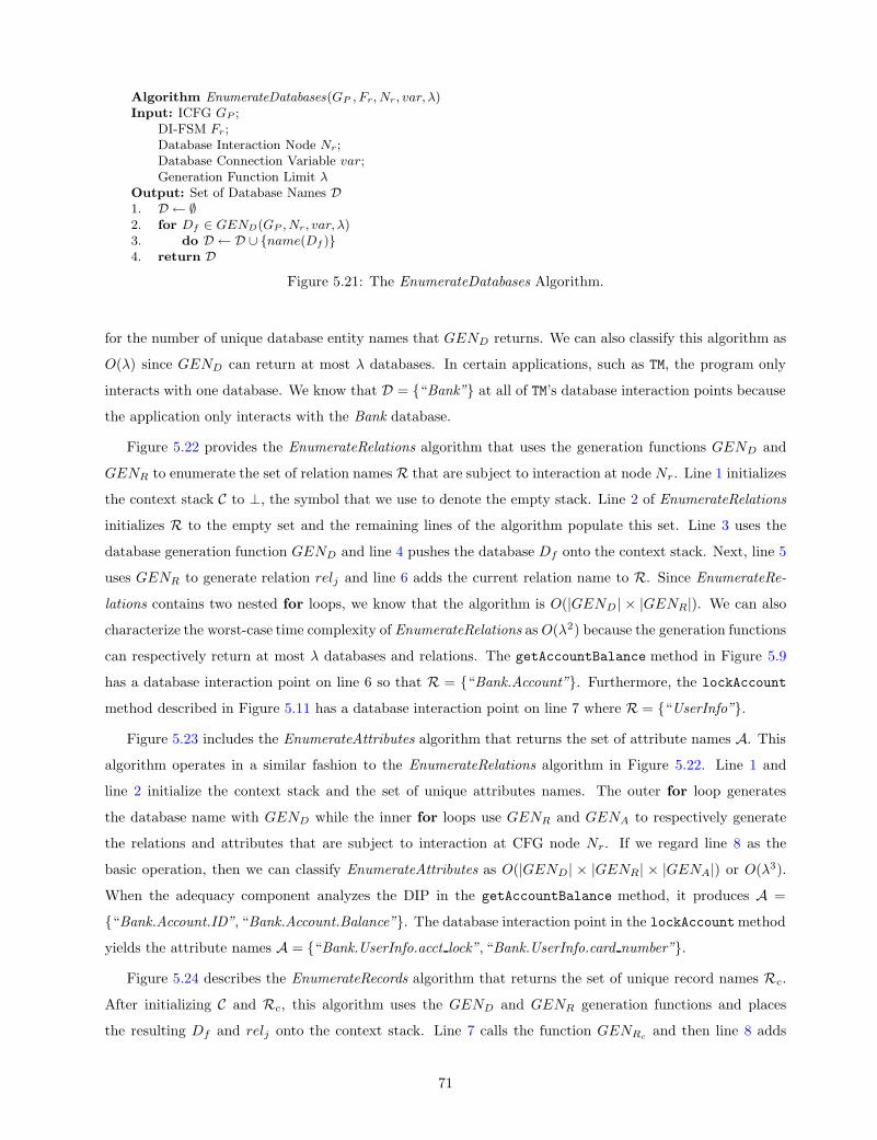
Algorithm EnumerateDatabases(GP , Fr, Nr, var, λ)Input: ICFG GP ;
DI-FSM Fr;Database Interaction Node Nr;Database Connection Variable var;Generation Function Limit λ
Output: Set of Database Names D1. D ← ∅2. for Df ∈ GEND(GP , Nr, var, λ)3. do D ← D ∪ name(Df )4. return D
Figure 5.21: The EnumerateDatabases Algorithm.
for the number of unique database entity names that GEND returns. We can also classify this algorithm as
O(λ) since GEND can return at most λ databases. In certain applications, such as TM, the program only
interacts with one database. We know that D = “Bank” at all of TM’s database interaction points because
the application only interacts with the Bank database.
Figure 5.22 provides the EnumerateRelations algorithm that uses the generation functions GEND and
GENR to enumerate the set of relation names R that are subject to interaction at node Nr. Line 1 initializes
the context stack C to ⊥, the symbol that we use to denote the empty stack. Line 2 of EnumerateRelations
initializes R to the empty set and the remaining lines of the algorithm populate this set. Line 3 uses the
database generation function GEND and line 4 pushes the database Df onto the context stack. Next, line 5
uses GENR to generate relation relj and line 6 adds the current relation name to R. Since EnumerateRe-
lations contains two nested for loops, we know that the algorithm is O(|GEND | × |GENR|). We can also
characterize the worst-case time complexity of EnumerateRelations as O(λ2) because the generation functions
can respectively return at most λ databases and relations. The getAccountBalance method in Figure 5.9
has a database interaction point on line 6 so that R = “Bank.Account”. Furthermore, the lockAccount
method described in Figure 5.11 has a database interaction point on line 7 where R = “UserInfo”.
Figure 5.23 includes the EnumerateAttributes algorithm that returns the set of attribute names A. This
algorithm operates in a similar fashion to the EnumerateRelations algorithm in Figure 5.22. Line 1 and
line 2 initialize the context stack and the set of unique attributes names. The outer for loop generates
the database name with GEND while the inner for loops use GENR and GENA to respectively generate
the relations and attributes that are subject to interaction at CFG node Nr. If we regard line 8 as the
basic operation, then we can classify EnumerateAttributes as O(|GEND | × |GENR| × |GENA|) or O(λ3).
When the adequacy component analyzes the DIP in the getAccountBalance method, it produces A =
“Bank.Account.ID”, “Bank.Account.Balance”. The database interaction point in the lockAccountmethod
yields the attribute names A = “Bank.UserInfo.acct lock”, “Bank.UserInfo.card number”.
Figure 5.24 describes the EnumerateRecords algorithm that returns the set of unique record names Rc.
After initializing C and Rc, this algorithm uses the GEND and GENR generation functions and places
the resulting Df and relj onto the context stack. Line 7 calls the function GENRcand then line 8 adds
71

Algorithm EnumerateRelations(GP , Fr, Nr, var, λ)Input: ICFG GP ;
DI-FSM Fr;Database Interaction Node Nr;Database Connection Variable var;Generation Function Limit λ
Output: Set of Relation Names R1. C ←⊥2. R← ∅3. for Df ∈ GEND(GP , Nr, var, λ)4. do C.push(Df )5. for relj ∈ GENR(Fr, λ)6. do R← R ∪ name(C, relj)7. C.pop()8. return R
Figure 5.22: The EnumerateRelations Algorithm.
Algorithm EnumerateAttributes(GP , Fr, Nr, var, λ)Input: ICFG GP ;
DI-FSM Fr;Database Interaction Node Nr;Database Connection Variable var;Generation Function Limit λ
Output: Set of Attribute Names A1. C ←⊥2. A ← ∅3. for Df ∈ GEND(GP , Nr, var, λ)4. do C.push(Df )5. for relj ∈ GENR(Fr, λ)6. do C.push(relj)7. for Al ∈ GENA(Fr, λ)8. do A ← A ∪ name(C, Al)9. C.pop()10. C.pop()11. return A
Figure 5.23: The EnumerateAttributes Algorithm.
72

Algorithm EnumerateRecords(GP , Fr, Nr, var, λ)Input: ICFG GP ;
DI-FSM Fr;Database Interaction Node Nr;Database Connection Variable var;Generation Function Limit λ
Output: Set of Record Names Rc
1. C ←⊥2. Rc ← ∅3. for Df ∈ GEND(GP , Nr, var, λ)4. do C.push(Df )5. for relj ∈ GENR(Fr, λ)6. do C.push(relj)7. for tk ∈ GENRc (relj , λ)8. do Rc ←Rc ∪ name(C, tk)9. C.pop()10. C.pop()11. return Rc
Figure 5.24: The EnumerateRecords Algorithm.
Algorithm EnumerateAttributeValues(GP , Fr, Nr, var, λ)Input: ICFG GP ;
DI-FSM Fr;Database Interaction Node Nr;Database Connection Variable var;Generation Function Limit λ
Output: Set of Attribute Value Names Av
1. C ←⊥2. Av ← ∅3. for Df ∈ GEND(GP , Nr, var, λ)4. do C.push(Df )5. for relj ∈ GENR(Fr, λ)6. do C.push(relj)7. for tk ∈ GENRc (relj , λ)8. do C.push(tk)9. for Al ∈ GENA(Fr, λ)10. do C.push(Al)11. for tk[l] ∈ GENAv (tk, λ)12. do Av ← Av ∪ name(C, tk[l])13. C.pop()14. C.pop()15. C.pop()16. C.pop()17. return Av
Figure 5.25: The EnumerateAttributeValues Algorithm.
73

each tk into the set Rc. If line 8 is the basic operation, then we classify EnumerateRecords as O(|GEND | ×
|GENR|×|GENRc|) or O(λ3). If we use the instance of the relational schema provided in Figure 2.4, then the
DIP in getAccountBalancemethod producesRc = name(C, 〈1, . . . , 1000, 1〉), . . . , name(C, 〈5, . . . , 125, 4〉).
Since the DIP in the lockAccount method depends upon the input to the operation, EnumerateRecords
conservatively outputs all of the records inside of the UserInfo relation. If we knew that card number = 1
during the execution of this method (i.e., because lockAccount was invoked so that the formal parameter
c n = 1), EnumerateRecords would return Rc = name(C, 〈1, 32142, . . . , 0〉).
Figure 5.25 provides the EnumerateAttributeValues algorithm that returns Av , the set of unique names
for attribute values. Line 3 through line 9 iteratively invoke the GEND, GENR, GENRc, and GENA
generation functions and respectively push Df , relj , tk, and Al onto the context stack C. The function
GENAvinspects the state of record tk and returns an attribute value tk[l]. Line 12 of EnumerateAt-
tributeValues adds tk[l] to Av. If line 12 is the basic operation, then we know that this algorithm is
O(|GEND | × |GENR| × |GENRc| × |GENA| × |GENAv
|) or O(λ5). When the adequacy component an-
alyzes the instance of the relational schema provided in Figure 2.4 and the DIP in the getAccountBalance
method, this yields Av = name(C, 1), name(C, 1000), . . . , name(C, 5), name(C, 125). The input-dependent
database interaction point in lockAccount forces EnumerateAttributeValues to return all of the attribute
values within the records of the UserInfo relation.
The enumeration algorithms in Figure 5.21 through Figure 5.25 return a set of database entity names for
a single interaction point. For example, the output of the EnumerateRecords algorithm returns Rc, the set
of record names for a single interaction point Nr. Yet, Section 4.3.2 explains that the database-aware test
adequacy criteria focus on the database interaction association 〈Ndef , Nuse, varDB〉 where relational database
entity varDB is an element of one of the sets D(Gk), R(Gk), A(Gk), Rc(Gk), or Av(Gk). To this end,
Equation (5.5) defines D(Gk), the set of database names that are subject to interaction in the method mk.
This equation uses D(Nr) to denote the set of databases with which node Nr ∈ Nk interacts. Equation (5.5)
shows that we enumerate the set D(Gk) through the iterative invocation of EnumerateDatabases algorithm
for each database interaction point in the method. We define the sets R(Gk), A(Gk), Rc(Gk), and Av(Gk)
in an analogous fashion.
D(Gk) =⋃
Nr∈Nk
D(Nr) (5.5)
5.5 CONSTRUCTING A DATABASE-AWARE REPRESENTATION
The database interaction control flow graph is an extended CFG that contains transfers of control to the
nodes from one or more database interaction graphs (DIGs). A DIG represents a database interaction point
at a single level of interaction granularity and multiple DIGs can exist within a DI-CFG. While the code
examples in Figures 5.9 and 5.11 indicate that DIPs occur in assignment statements, the predicate of a
conditional logic statement can also perform a database interaction. In order to preserve the semantics of a
74
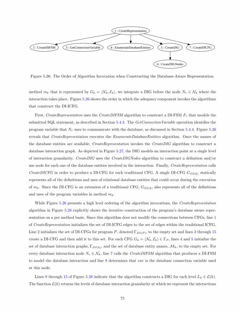
1 : CreateRepresentation
2 : CreateDIFSM 3 : GetConnectionVariable 4 : EnumerateDatabaseEntities 5 : CreateDIG 7 : CreateDICFG
6 : CreateDIGNodes
PSfrag replacements
N6
enter computeVelocity
enter computeVelocity
N6
N6
N7
N7
N8
N8
N10
N8
N16
N10
N11
N11
N12
N12
N18
N16
N18
N18
exit computeVelocity
exit computeVelocity
N6
N1
N1
N2
N2
N3
N3
N1
N1
N4
N4
N5
N5
N6
enter P
enter P
call main
call main
enter main
enter main
enter main
. . .
. . .
call inputCardNumber
call inputCardNumber
call inputPin
call inputCardNumber
call handleError
call handleError
call inputCardNumber
call inputPin
call handleError
call handleError
call inputPin
call inputPin
call inputOperation
call inputOperation
call getAccountBalance
call getAccountBalance
call promptAgain
call inputOperation
call lockAccount
call lockAccount
call promptAgain
call promptAgain
call inputOperation
call promptAgain
. . .
call getAccountBalance
enter getAccountBalance
enter getAccountBalance
N3
N3
N4
N4
N5
N5
N6
N6
N7
N7
N10
N10
N12
N12
N15
N10
N15
N15
exit getAccountBalance
exit getAccountBalance
return getAccountBalance
return lockAccount
. . .
return getAccountBalance
call promptAgain
. . .
exit main
exit main
return main
return main
exit P
exit P
. . .
exit main
enter lockAccount
enter lockAccount
. . .
. . .
exit lockAccount
exit lockAccount
return lockAccount
return lockAccount
exit main
Figure 5.26: The Order of Algorithm Invocation when Constructing the Database-Aware Representation.
method mk that is represented by Gk = 〈Nk, Ek〉, we integrate a DIG before the node Nr ∈ Nk where the
interaction takes place. Figure 5.26 shows the order in which the adequacy component invokes the algorithms
that construct the DI-ICFG.
First, CreateRepresentation uses the CreateDIFSM algorithm to construct a DI-FSM Fr that models the
submitted SQL statement, as described in Section 5.4.3. The GetConnectionVariable operation identifies the
program variable that Nr uses to communicate with the database, as discussed in Section 5.4.4. Figure 5.26
reveals that CreateRepresentation executes the EnumerateDatabaseEntities algorithm. Once the names of
the database entities are available, CreateRepresentation invokes the CreateDIG algorithm to construct a
database interaction graph. As depicted in Figure 5.27, the DIG models an interaction point at a single level
of interaction granularity. CreateDIG uses the CreateDIGNodes algorithm to construct a definition and/or
use node for each one of the database entities involved in the interaction. Finally, CreateRepresentation calls
CreateDICFG in order to produce a DI-CFG for each traditional CFG. A single DI-CFG GDI(k) statically
represents all of the definitions and uses of relational database entities that could occur during the execution
of mk. Since the DI-CFG is an extension of a traditional CFG, GDI(k) also represents all of the definitions
and uses of the program variables in method mk.
While Figure 5.26 presents a high level ordering of the algorithm invocations, the CreateRepresentation
algorithm in Figure 5.28 explicitly shows the iterative construction of the program’s database aware repre-
sentation on a per method basis. Since this algorithm does not modify the connections between CFGs, line 1
of CreateRepresentation initializes the set of DI-ICFG edges to the set of edges within the traditional ICFG.
Line 2 initializes the set of DI-CFGs for program P , denoted ΓDI(P ), to the empty set and lines 3 through 15
create a DI-CFG and then add it to this set. For each CFG Gk = 〈Nk, Ek〉 ∈ ΓP , lines 4 and 5 initialize the
set of database interaction graphs, ΓDI(k), and the set of database entity names,Mk, to the empty set. For
every database interaction node Nr ∈ Nk, line 7 calls the CreateDIFSM algorithm that produces a DI-FSM
to model the database interaction and line 8 determines that var is the database connection variable used
at this node.
Lines 9 through 15 of Figure 5.28 indicate that the algorithm constructs a DIG for each level Lk ∈ L(k).
The function L(k) returns the levels of database interaction granularity at which we represent the interactions
75

PSfrag replacements
N6
enter computeVelocity
enter computeVelocity
N6
N6
N7
N7
N8
N8
N10
N8
N16
N10
N11
N11
N12
N12
N18
N16
N18
N18
exit computeVelocity
exit computeVelocity
N6
N1
N1
N2
N2
N3
N3
N1
N1
N4
N4
N5
N5
N6
enter P
enter P
call main
call main
enter main
enter main
enter main
. . .
. . .
call inputCardNumber
call inputCardNumber
call inputPin
call inputCardNumber
call handleError
call handleError
call inputCardNumber
call inputPin
call handleError
call handleError
call inputPin
call inputPin
call inputOperation
call inputOperation
call getAccountBalance
call getAccountBalance
call promptAgain
call inputOperation
call lockAccount
call lockAccount
call promptAgain
call promptAgain
call inputOperation
call promptAgain
. . .
call getAccountBalance
enter getAccountBalance
enter getAccountBalance
N3
N3
N4
N4
N5
N5
N6
N6
N7
N7
N10
N10
N12
N12
N15
N10
N15
N15
exit getAccountBalance
exit getAccountBalance
return getAccountBalance
return lockAccount
. . .
return getAccountBalance
call promptAgain
. . .
exit main
exit main
return main
return main
exit P
exit P
. . .
exit main
enter lockAccount
enter lockAccount
. . .
. . .
exit lockAccount
exit lockAccount
return lockAccount
return lockAccount
exit main
Id : icfgsimple.ladot, v1.22006/08/0115 : 58 : 34gkapfhamExp
Revision : 1.2
〈enterr,A〉 〈enterr,A〉
〈Bank.Account.id,use〉 〈Bank.Account.id,use〉
〈Bank.Account.balance,use〉 〈Bank.Account.balance,use〉
〈exitr,A〉〈exitr,A〉
Mr = Bank.Account.id, Bank.Account.balance and Lk = A
Figure 5.27: A Database Interaction Graph.
in method mk. To this end, we require that L(k) ⊆ D,R,A,Rc,Av and we assume that the tester specifies
L(k). If D ∈ L(k), then CreateRepresentation must construct a DIG to model a method mk’s interaction
with a relational database at the database level. Line 10 calls the EnumerateDatabaseEntities algorithm that
subsequently invokes the appropriate enumeration algorithm as specified by the value of Lk. For example, if
Lk = A, then the EnumerateDatabaseEntities operation invokes the EnumerateAttributes algorithm. Line 11
stores this set of database entity names, Mr, in the set of names for the entire method mk, denoted Mk.
A call to the CreateDIG algorithm yields the DIG GLkr that the CreateRepresentation algorithm places into
ΓDI(k), mk’s set of DIGs.
After the DIGs have been constructed for all interaction points and interaction levels, the CreateDICFG
algorithm integrates the DIGs into the CFG Gk in order to produce the DI-CFG GDI(k). Line 14 of
Figure 5.28 shows that the CreateDICFG algorithm uses the traditional CFG, the set of DIGs, and the set
of database entity names in order to produce the DI-CFG called GDI(k). The worst-case time complexity
of CreateRepresentation is O(|ΓP | × Nmax × Lmax) where ΓP is the set of P ’s CFGs and Equations (5.6)
and (5.7) define Nmax and Lmax, respectively. We use Nmax to denote the maximum number of database
interaction points within the CFG of a single method. Equation (5.7) uses Lmax to stand for the maximum
number of interaction levels that were chosen to represent the DIGs for an individual method.
Nmax = max
∣∣∣∣∣⋃
Nr∈Nk
Nr
∣∣∣∣∣ : Gk = 〈Nk, Ek〉 ∈ ΓP (5.6)
Lmax = max |L(k)| : Gk ∈ ΓP (5.7)
Figure 5.29 provides the CreateDIG algorithm that constructs a DIG Gr = 〈Nr, Er, Nr〉 for a database
interaction node Nr. A DIG contains a set of nodes Nr, a set of edges Er, and the database interaction
node whose interaction it represents. Lines 1 and 2 of CreateDIG initialize these sets of nodes and edges
76

Algorithm CreateRepresentation(GP ,L, λ)Input: ICFG GP = 〈ΓP , EP 〉;
Levels of DIP Representation L;Generation Function Limit λ
Output: DI-ICFG GDI(P ) = 〈ΓDI(P ), EDI(P )〉1. EDI(P ) ← EP
2. ΓDI(P ) ← ∅3. for Gk = 〈Nk, Ek〉 ∈ ΓP
4. do ΓDI(k) ← ∅5. Mk ← ∅6. for Nr ∈ Nk
7. do Fr ← CreateDIFSM(GP , Nr)8. var← GetConnectionVariable(Nr)9. for Lk ∈ L(k)10. do Mr ← EnumerateDatabaseEntities(Fr, var, λ, Lk)11. Mk ←Mk ∪Mr
12. GLkr ← CreateDIG(Mr, Nr, Fr, Lk)
13. ΓDI(k) ← ΓDI(k) ∪ GLkr
14. GDI(k) ← CreateDICFG(Gk, ΓDI(k),Mk)15. ΓDI(P ) ← ΓDI(P ) ∪ GDI(k)16. return 〈ΓDI(P ), EDI(P )〉
Figure 5.28: The CreateRepresentation Algorithm.
to the empty set. The entry and exit points of a DIG Gr are demarcated by the nodes 〈entryr, Lk〉 and
〈exitr, Lk〉. These nodes contain the annotation Lk to indicate that Gr represents the database interaction at
the granularity level Lk. The nested for loops in CreateDIG iteratively construct a straight-line code segment
that connects all of the database entities d ∈ Mr. Line 4 shows that we initialize the current node Np to the
entry node and line 6 calls the CreateDIGNodes algorithm that returns a tuple of DIG nodes, denoted Nd.
Line 8 of Figure 5.29 adds DIG node Nd into the set Nr and line 9 places the edge (Np, Nd) into the set Er.
After handling every database entity d ∈ Mr, the algorithm connects the last node Np to the exit node of Gr
and returns the DIG to the CreateRepresentation algorithm. Figure 5.27 shows the DIG that we create for the
DI-FSM from Figure 5.8, the set of database entity namesMr = Bank.Account.id, Bank.Account.balance
and the granularity marker Lk = A. We know that |Nd| ∈ 1, 2 because CreateDIGNodes can return either
(i) one definition node, (ii) one use node, or (iii) one definition and one use node. Since |Nd| is a always a
small constant, we have that CreateDIG is O(|Mr |).
Figure 5.30 describes the CreateDIGNodes algorithm that returns a tuple of DIG nodes, Nd, when
provided with a DI-FSM Fr and a single database entity d. This algorithm uses ] as the union operator
for tuples. If Fr models a DIP that is defining or using, then this algorithm returns a tuple with a single
node of the form 〈d, op〉 where op ∈ def ,use. If Fr models a database interaction that is defining-using,
then CreateDIGNodes returns a tuple Nd = 〈〈d,use〉, 〈d,def〉〉. We place d’s use node before the definition
node in order to ensure that the database interaction associations span the DIGs of a DI-CFG. The Used
operation on line 2 inspects the DI-FSM Fr in order to determine whether the DIP defines or uses d. If
we have δ(q, select) = q′ and δ(q, O) = q′ for q, q′ ∈ Q, then Used returns true. The Used operation also
returns true when δ(q, A) = q′ and δ(q, d) = q′ and d exists in the where clause of either a SQL delete
77

Algorithm CreateDIG(Mr , Nr, Fr, Lk)Input: Set of Database Entity Names Mr;
Database Interaction Node Nr;Database Interaction FSM Fr;Database Interaction Granularity Lk;
Output: Database Interaction Graph Gr = 〈Nr, Er, Nr〉1. Nr ← ∅2. Er ← ∅3. Nr ← Nr ∪ 〈entryr, Lk〉, 〈exitr, Lk〉4. Np ← 〈entryr, Lk〉5. for d ∈Mr
6. do Nd ← CreateDIGNodes(Fr, d)7. for Nd ∈ Nd
8. do Nr ← Nr ∪ Nd9. Er ← Er ∪ (Np, Nd)10. Np ← Nd
11. Er ← Er ∪ (Np, 〈exitr, Lk〉)12. return 〈Nr, Er, Nr〉
Figure 5.29: The CreateDIG Algorithm.
or an update statement. The Defined method also examines Fr and it operates in an analogous fashion
to Used. If we assume that the execution time of Defined and Used is bounded by a small constant, then
CreateDIGNodes is a O(1) algorithm.
Figure 5.31 gives the CreateDICFG algorithm that produces a DI-CFG GDI(k) = 〈NDI(k), EDI(k)〉 from
a traditional CFG Gk, the set of DIGs ΓDI(k), and the set of database entity names Mk. Lines 1 and 2
initialize the set of nodes and edges in the DI-CFG to the nodes and edges within the CFG. The Create-
DICFG algorithm iteratively removes and adds edges to EDI(k), while only adding nodes to NDI(k). Lines 3
and 4 initialize the nodes Nl and Ncr to null. We use Nl to denote the last node in a DIG and Ncr points
to the current database interaction node Nr. Line 5 calls the DefineTemporaries operation that adds nodes
to NDI(k). These nodes define temporary variables that we initialize to the value of method mk’s formal pa-
rameters [Duesterwald et al., 1996]. DefineTemporaries also treats the entities within the relational database
as global variables and inserts temporary variables to represent these data elements.
The CreateRepresentation algorithm orders the DIGs within ΓDI(k) so that Gr and Gr′ are adjacent when
they represent the same Nr at different levels of granularity. When we encounter the node Nr for the first
time, lines 12 through 14 remove the edge (Np, Nr) from EDI(k) for each node Np ∈ pred(Nr). After we
disconnect the predecessor node Np from Nr, we create a new edge (Np, entryr) for the node entryr ∈ Nr.
Next, line 15 sets node Nl to the exit node of the current Gr so that the algorithm can integrate subsequent
DIGs (for the same Nr) after this DIG. Line 16 sets Ncr to Nr in order to indicate that Nr is the current
database interaction node under analysis. If Ncr 6= Nr and Nl 6= null (i.e., we have encountered DIGs for
a new Nr and there is a residual Nl from the previous execution of the for loop on line 6), then line 11
connects the last node Nl to Ncr. If Gr is not the first DIG under analysis for a given Nr, then CreateDICFG
executes lines 18 though 19 so that it can connect the exit node of the previous DIG to the entry node of
the current DIG. Finally, line 20 connects the exit node of the last DIG to the last interaction node.
78
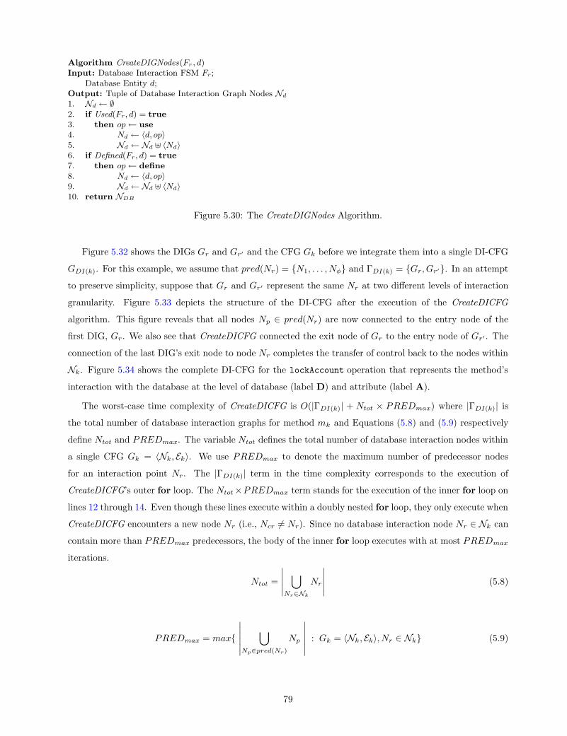
Algorithm CreateDIGNodes(Fr , d)Input: Database Interaction FSM Fr;
Database Entity d;Output: Tuple of Database Interaction Graph Nodes Nd
1. Nd ← ∅2. if Used(Fr, d) = true3. then op← use4. Nd ← 〈d, op〉5. Nd ← Nd ] 〈Nd〉6. if Defined(Fr, d) = true7. then op← define8. Nd ← 〈d, op〉9. Nd ← Nd ] 〈Nd〉10. return NDB
Figure 5.30: The CreateDIGNodes Algorithm.
Figure 5.32 shows the DIGs Gr and Gr′ and the CFG Gk before we integrate them into a single DI-CFG
GDI(k). For this example, we assume that pred(Nr) = N1, . . . , Nφ and ΓDI(k) = Gr, Gr′. In an attempt
to preserve simplicity, suppose that Gr and Gr′ represent the same Nr at two different levels of interaction
granularity. Figure 5.33 depicts the structure of the DI-CFG after the execution of the CreateDICFG
algorithm. This figure reveals that all nodes Np ∈ pred(Nr) are now connected to the entry node of the
first DIG, Gr. We also see that CreateDICFG connected the exit node of Gr to the entry node of Gr′ . The
connection of the last DIG’s exit node to node Nr completes the transfer of control back to the nodes within
Nk. Figure 5.34 shows the complete DI-CFG for the lockAccount operation that represents the method’s
interaction with the database at the level of database (label D) and attribute (label A).
The worst-case time complexity of CreateDICFG is O(|ΓDI(k)| + Ntot × PREDmax) where |ΓDI(k)| is
the total number of database interaction graphs for method mk and Equations (5.8) and (5.9) respectively
define Ntot and PREDmax. The variable Ntot defines the total number of database interaction nodes within
a single CFG Gk = 〈Nk, Ek〉. We use PREDmax to denote the maximum number of predecessor nodes
for an interaction point Nr. The |ΓDI(k)| term in the time complexity corresponds to the execution of
CreateDICFG’s outer for loop. The Ntot×PREDmax term stands for the execution of the inner for loop on
lines 12 through 14. Even though these lines execute within a doubly nested for loop, they only execute when
CreateDICFG encounters a new node Nr (i.e., Ncr 6= Nr). Since no database interaction node Nr ∈ Nk can
contain more than PREDmax predecessors, the body of the inner for loop executes with at most PREDmax
iterations.
Ntot =
∣∣∣∣∣⋃
Nr∈Nk
Nr
∣∣∣∣∣ (5.8)
PREDmax = max
∣∣∣∣∣∣⋃
Np∈pred(Nr)
Np
∣∣∣∣∣∣: Gk = 〈Nk , Ek〉, Nr ∈ Nk (5.9)
79

Algorithm CreateDICFG(Gk , ΓDI(k),M)Input: Traditional CFG Gk = 〈Nk, Ek〉;
Set of Database Interaction Graphs ΓDI(k);Set of Database Entities Mk
Output: DI-CFG GDI(k) = 〈NDI(k), EDI(k)〉1. NDI(k) ← Nk
2. EDI(k) ← Ek
3. Nl ← null4. Ncr ← null5. DefineTemporaries(Gk,Mk)6. for Gr = 〈Nr, Er, Nr, Lr〉 ∈ ΓDI(k)
7. do NDI(k) ← NDI(k) ∪Nr
8. EDI(k) ← EDI(k) ∪ Er
9. if Ncr 6= Nr
10. then if Nl 6= null11. then EDI(k) ← EDI(k) ∪ (Nl, Ncr)12. for Np ∈ pred(Nr)13. do EDI(k) ← EDI(k) − (Np, Nr)14. EDI(k) ← EDI(k) ∪ (Np, entryr)15. Nl ← exitr
16. Ncr ← Nr
17. else18. EDI(k) ← EDI(k) ∪ (Nl, entryr)19. Nl ← exitr
20. EDI(k) ← EDI(k) ∪ (Nl, Ncr)21. return 〈NDI(k), EDI(k)〉
Figure 5.31: The CreateDICFG Algorithm.
5.6 IMPLEMENTATION OF THE TEST ADEQUACY COMPONENT
The implementation of the adequacy component uses the Soot 1.2.5 program analysis framework. During the
analysis of the methods in a database-centric application, we use the three address code intermediate repre-
sentation called Jimple [Vallee-Rai et al., 1999, 2000]. Since a database-centric application frequently uses
the exception handling constructs of the Java programming language, we use a Soot CFG that conservatively
models the flow of exceptions across method boundaries. We also use Soot’s points-to analysis techniques
in order to (i) identify the heap objects to which a reference variable can point, (ii) resolve the potential
destination(s) of all polymorphic method dispatches, and (iii) create the interprocedural control flow graph
[Berndl et al., 2003, Lhotak and Hendren, 2003]. It is possible to extend the test adequacy component by in-
corporating recent demand-driven points-to analysis techniques [Sridharan et al., 2005, Sridharan and Bodik,
2006].
We employ the Java String Analyzer (JSA) to generate a DI-FSM for each DIP in a database-centric
application [Christensen et al., 2003]. The adequacy component uses the HSQLDB parser to perform CFL
reachability and to annotate a DI-FSM with the R, A, O−transitions. The current implementation supports
the integration of parsers that handle different SQL dialects. The adequacy component also uses Soot to im-
plement the DI-ICFG creation algorithms described in Section 5.5. Using Soot, the test adequacy component
performs an exhaustive intraprocedural data flow analysis in order to enumerate the def-use and database
80
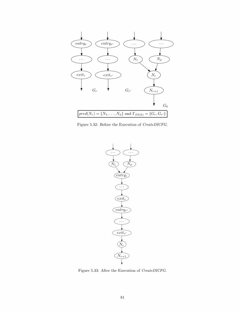
PSfrag replacements
N6
enter computeVelocity
enter computeVelocity
N6
N6
N7
N7
N8
N8
N10
N8
N16
N10
N11
N11
N12
N12
N18
N16
N18
N18
exit computeVelocity
exit computeVelocity
N6
N1
N1
N2
N2
N3
N3
N1
N1
N4
N4
N5
N5
N6
enter P
enter P
call main
call main
enter main
enter main
enter main
. . .
. . .
call inputCardNumber
call inputCardNumber
call inputPin
call inputCardNumber
call handleError
call handleError
call inputCardNumber
call inputPin
call handleError
call handleError
call inputPin
call inputPin
call inputOperation
call inputOperation
call getAccountBalance
call getAccountBalance
call promptAgain
call inputOperation
call lockAccount
call lockAccount
call promptAgain
call promptAgain
call inputOperation
call promptAgain
. . .
call getAccountBalance
enter getAccountBalance
enter getAccountBalance
N3
N3
N4
N4
N5
N5
N6
N6
N7
N7
N10
N10
N12
N12
N15
N10
N15
N15
exit getAccountBalance
exit getAccountBalance
return getAccountBalance
return lockAccount
. . .
return getAccountBalance
call promptAgain
. . .
exit main
exit main
return main
return main
exit P
exit P
. . .
exit main
enter lockAccount
enter lockAccount
. . .
. . .
exit lockAccount
exit lockAccount
return lockAccount
return lockAccount
exit main
Id : cfgiter.ladot, v1.12006/07/1220 : 28 : 13gkapfhamExp
Revision : 1.1
N6
entryr
entryr
. . .
. . .
exitr
exitr
Gr
. . .
exitr
entryr′
entryr′
. . .
. . .
exitr′
exitr′
Gr′
. . .
exitr′
. . .
. . .
. . .
N1
. . .
Nφ
N1
Nr
Nφ
Nr
Nr
Nr+1
Nr+1
Gk
. . .
exitr′
pred(Nr) = N1, . . . , Nφ and ΓDI(k) = Gr, Gr′
Figure 5.32: Before the Execution of CreateDICFG.
PSfrag replacements
N6
enter computeVelocity
enter computeVelocity
N6
N6
N7
N7
N8
N8
N10
N8
N16
N10
N11
N11
N12
N12
N18
N16
N18
N18
exit computeVelocity
exit computeVelocity
N6
N1
N1
N2
N2
N3
N3
N1
N1
N4
N4
N5
N5
N6
enter P
enter P
call main
call main
enter main
enter main
enter main
. . .
. . .
call inputCardNumber
call inputCardNumber
call inputPin
call inputCardNumber
call handleError
call handleError
call inputCardNumber
call inputPin
call handleError
call handleError
call inputPin
call inputPin
call inputOperation
call inputOperation
call getAccountBalance
call getAccountBalance
call promptAgain
call inputOperation
call lockAccount
call lockAccount
call promptAgain
call promptAgain
call inputOperation
call promptAgain
. . .
call getAccountBalance
enter getAccountBalance
enter getAccountBalance
N3
N3
N4
N4
N5
N5
N6
N6
N7
N7
N10
N10
N12
N12
N15
N10
N15
N15
exit getAccountBalance
exit getAccountBalance
return getAccountBalance
return lockAccount
. . .
return getAccountBalance
call promptAgain
. . .
exit main
exit main
return main
return main
exit P
exit P
. . .
exit main
enter lockAccount
enter lockAccount
. . .
. . .
exit lockAccount
exit lockAccount
return lockAccount
return lockAccount
exit main
Id : cfgiter.ladot, v1.12006/07/1220 : 28 : 13gkapfhamExp
Revision : 1.1
entryr
. . .
N1
Nφ
exitr
entryr
. . .
. . .
exitr
exitr
entryr′
entryr′
. . .
. . .
exitr′
exitr′
Nr
. . .
. . .
. . .
N1
. . .
Nφ
N1
entryr
Nφ
entryr
Nr
Nr+1Nr+1
Figure 5.33: After the Execution of CreateDICFG.
81

exit Gr1
<temp2,use>
<temp2,define>
exit lockAccount
exit
entry entry
update_lock = m_connect.createStatement()
G G
G
r2
r 2
r 1
temp1 = parameter0:c_n
qu_lck = "update UserInfo ..." + temp1 + ";"
temp3 = LocalDatabaseEntity1:acct_lock
temp2 = LocalDatabaseEntity0:Bank
lockAccountentry
temp4 = LocalDatabaseEntity2:card_number
completed = false
result_lock = update_lock.executeUpdate(qu_lck)
<temp4, use>
if(result_lock == 1)
DA
<temp3, define>
completed = true
return completed
PSfrag replacements
N6
enter computeVelocity
enter computeVelocity
N6
N6
N7
N7
N8
N8
N10
N8
N16
N10
N11
N11
N12
N12
N18
N16
N18
N18
exit computeVelocity
exit computeVelocity
N6
N1
N1
N2
N2
N3
N3
N1
N1
N4
N4
N5
N5
N6
enter P
enter P
call main
call main
enter main
enter main
enter main
. . .
. . .
call inputCardNumber
call inputCardNumber
call inputPin
call inputCardNumber
call handleError
call handleError
call inputCardNumber
call inputPin
call handleError
call handleError
call inputPin
call inputPin
call inputOperation
call inputOperation
call getAccountBalance
call getAccountBalance
call promptAgain
call inputOperation
call lockAccount
call lockAccount
call promptAgain
call promptAgain
call inputOperation
call promptAgain
. . .
call getAccountBalance
enter getAccountBalance
enter getAccountBalance
N3
N3
N4
N4
N5
N5
N6
N6
N7
N7
N10
N10
N12
N12
N15
N10
N15
N15
exit getAccountBalance
exit getAccountBalance
return getAccountBalance
return lockAccount
. . .
return getAccountBalance
call promptAgain
. . .
exit main
exit main
return main
return main
exit P
exit P
. . .
exit main
enter lockAccount
enter lockAccount
. . .
. . .
exit lockAccount
exit lockAccount
return lockAccount
return lockAccount
exit main
Figure 5.34: A DI-CFG for the lockAccount Operation.
82
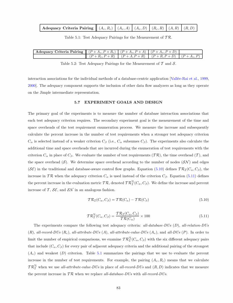
Adequacy Criteria Pairing (Av , Rc) (Av , A) (Av , D) (Rc, R) (A, R) (R, D)
Table 5.1: Test Adequacy Pairings for the Measurement of T R.
Adequacy Criteria Pairing (P + Av, P + Rc) (P + Av, P + A) (P + Av, P + D)
(P + Rc, P + R) (P + A,P + R) (P + R, P + D) (P + Av, P )
Table 5.2: Test Adequacy Pairings for the Measurement of T and S.
interaction associations for the individual methods of a database-centric application [Vallee-Rai et al., 1999,
2000]. The adequacy component supports the inclusion of other data flow analyzers as long as they operate
on the Jimple intermediate representation.
5.7 EXPERIMENT GOALS AND DESIGN
The primary goal of the experiments is to measure the number of database interaction associations that
each test adequacy criterion requires. The secondary experiment goal is the measurement of the time and
space overheads of the test requirement enumeration process. We measure the increase and subsequently
calculate the percent increase in the number of test requirements when a stronger test adequacy criterion
Cα is selected instead of a weaker criterion Cβ (i.e., Cα subsumes Cβ). The experiments also calculate the
additional time and space overheads that are incurred during the enumeration of test requirements with the
criterion Cα in place of Cβ . We evaluate the number of test requirements (T R), the time overhead (T ), and
the space overhead (S). We determine space overhead according to the number of nodes (SN ) and edges
(SE) in the traditional and database-aware control flow graphs. Equation (5.10) defines T RI(Cα, Cβ), the
increase in T R when the adequacy criterion Cα is used instead of the criterion Cβ . Equation (5.11) defines
the percent increase in the evaluation metric T R, denoted T R%I (Cα, Cβ). We define the increase and percent
increase of T , SE , and SN in an analogous fashion.
T RI(Cα, Cβ) = T R(Cα)− T R(Cβ) (5.10)
T R%I (Cα, Cβ) =
T RI(Cα, Cβ)
T R(Cα)× 100 (5.11)
The experiments compare the following test adequacy criteria: all-database-DUs (D), all-relation-DUs
(R), all-record-DUs (Rc), all-attribute-DUs (A), all-attribute-value-DUs (Av), and all-DUs (P ). In order to
limit the number of empirical comparisons, we examine T R%I (Cα, Cβ) with the six different adequacy pairs
that include (Cα, Cβ) for every pair of adjacent adequacy criteria and the additional pairing of the strongest
(Av) and weakest (D) criterion. Table 5.1 summarizes the pairings that we use to evaluate the percent
increase in the number of test requirements. For example, the pairing (Av , Rc) means that we calculate
T R%I when we use all-attribute-value-DUs in place of all-record-DUs and (R, D) indicates that we measure
the percent increase in T R when we replace all-database-DUs with all-record-DUs.
83

NCSS # Methods # Rels Total # Attrs # Attrs Per Rel
mp3cd 2913 452 7 25 3.6
Table 5.3: Characteristics of the mp3cd Case Study Application.
A single execution of the test adequacy component can list test requirements for one or more adequacy
criteria. For example, a tester can use the adequacy component to enumerate the test requirements necessi-
tated by the all-DUs, all-database-DUs, and all-record-DUs criteria. We record the time and space overhead
required to analyze application A in light of all-DUs criterion and one of the database-aware test adequacy
criterion. During the evaluation of time and space overhead, we analyze the percent increase in T and S
for seven different adequacy pairings, as described in Table 5.2. This table uses the notation P + Av to
indicate that we measure the time overhead incurred during the enumeration of traditional def-use associ-
ations and attribute value DIAs. For example, T %I (P + Av , P + D) denotes the percent increase in time
overhead when we enumerate test requirements for the all-attribute-value-DUs and all-DUs criteria instead
of the all-database-DUs and all-DUs criteria.
We use the test adequacy component to identify the test requirements and to calculate T R. We compute
the time overhead metric T with a profiling tool and we measure the space overhead metrics SN and SE
by counting the number of nodes and edges in the CFGs and the DI-CFGs, respectively. We conducted
all of these experiments on the GNU/Linux workstation with kernel 2.4.18-14smp, dual 1 GHz Pentium III
Xeon processors, 512 MB of main memory, and a SCSI disk subsystem. We executed the test adequacy
component in five separate trials for each case study application and each test adequacy criterion. Since
the time overhead metric varied across each trial, we calculate arithmetic means and standard deviations
for T (the T R, SN , and SE metrics did not vary across the separate trials). We design the bar charts in
Figure 5.36 to use an error bar to represent one standard deviation from the arithmetic mean of the time
overheads. Since the standard deviation for T was insignificant, the diamonds at the top of the bars in
Figure 5.36 indicate that no visible error bar could be produced.
The experiments applied the adequacy component to two subjects: TransactionManager and mp3cd.
The mp3cd subject manages a local collection of MP3 files and it is available for download at
http://mp3cdbrowser.sourceforge.net/mp3cd/. We do not use mp3cd in subsequent experiments and
we did not discuss it in Chapter 3 because this application does not have a test suite. However, Chapter 3
provides more details about the TM case study application. mp3cd contains 2913 non-commented source state-
ments, not including its JDBC driver. This application also uses the Java bytecode of an MP3 manipulation
utility. The MP3 manipulation bytecodes and the complete mp3cd application required the analysis of 453
methods. mp3cd interacts with a relational database that contains seven relations named Album, Altr, Aral,
Artist, Cd, Track, and Version. Table 5.3 summarizes the characteristics of the mp3cd case study application.
In future work we will use the test adequacy component to analyze other database-centric applications.
84

T R%I (R, D) (Rc, R) (A, R) (Av , Rc) (Av , A) (Av , D)
TM 4.9 49.3 61.6 60.0 47.2 80.7
mp3cd 49.0 49.2 72.4 71.1 46.8 92.5
Table 5.4: Percent Increase in the Number of Test Requirements.
5.8 KEY INSIGHTS FROM THE EXPERIMENTS
Section 5.9 furnishes a detailed review of the experimental results. This section summarizes the key insights
from the experiments that we introduced in Section 5.7. We identify the following high level trends in the
empirical results.
1. Number of Test Requirements
a. The database-aware test requirements constitute between 10 and 20% of the total number of data
flow-based test requirements.
b. The number of DIAs increases by almost 50% when we use the state-based all-record-DUs adequacy
criterion instead of the structure-based all-relation-DUs.
2. Time Overhead
a. We can enumerate the test requirements for small and moderate size applications in less than forty
seconds. Across multiple executions, this analysis exhibits little variation in time overhead.
b. Enumerating test requirements at the finest level of database interaction granularity never increases
analysis time by more than 15% over the base line configuration.
3. Space Overhead
a. Moderate size applications exhibit a 25% increase in the number of CFG nodes and edges when we
include the database interactions at the attribute value level instead of the database level.
b. For small database states, the use of the state-based all-record-DUs instead of the structure-based
all-relation-DUs only increases the number of CFG nodes and edges by 5%.
5.9 ANALYSIS OF THE EXPERIMENTAL RESULTS
5.9.1 Number of Test Requirements
Table 5.4 shows the percent increase in the number of test requirements for different test adequacy criteria
pairs and Figure 5.35 depicts the number of def-use and database interaction associations for both case study
applications. Since all-DUs does not have a subsumption relationship with any of the database-aware criteria,
Table 5.4 does not display any percent increases for a criteria pair involving all-DUs. Figure 5.35 shows that
all-DUs produces a significantly greater number of test requirements than any of the database aware criteria.
This is due to the fact that TM and mp3cd both interact with databases that have relatively few relations and
85

D R Rc A Av PAdequacy Criteria
500
1000
1500
2000
Number
of
Associations
D R Rc A Av P
39 41 81 107203
1910
PSfrag replacements
N6
enter computeVelocity
enter computeVelocity
N6
N6
N7
N7
N8
N8
N10
N8
N16
N10
N11
N11
N12
N12
N18
N16
N18
N18
exit computeVelocity
exit computeVelocity
N6
N1
N1
N2
N2
N3
N3
N1
N1
N4
N4
N5
N5
N6
enter P
enter P
call main
call main
enter main
enter main
enter main
. . .
. . .
call inputCardNumber
call inputCardNumber
call inputPin
call inputCardNumber
call handleError
call handleError
call inputCardNumber
call inputPin
call handleError
call handleError
call inputPin
call inputPin
call inputOperation
call inputOperation
call getAccountBalance
call getAccountBalance
call promptAgain
call inputOperation
call lockAccount
call lockAccount
call promptAgain
call promptAgain
call inputOperation
call promptAgain
. . .
call getAccountBalance
enter getAccountBalance
enter getAccountBalance
N3
N3
N4
N4
N5
N5
N6
N6
N7
N7
N10
N10
N12
N12
N15
N10
N15
N15
exit getAccountBalance
exit getAccountBalance
return getAccountBalance
return lockAccount
. . .
return getAccountBalance
call promptAgain
. . .
exit main
exit main
return main
return main
exit P
exit P
. . .
exit main
enter lockAccount
enter lockAccount
. . .
. . .
exit lockAccount
exit lockAccount
return lockAccount
return lockAccount
exit main
(a)
D R Rc A Av PAdequacy Criteria
2000
4000
6000
8000
10000
Number
of
Associations
D R Rc A Av P
132 259 510940
1768
8718
PSfrag replacements
N6
enter computeVelocity
enter computeVelocity
N6
N6
N7
N7
N8
N8
N10
N8
N16
N10
N11
N11
N12
N12
N18
N16
N18
N18
exit computeVelocity
exit computeVelocity
N6
N1
N1
N2
N2
N3
N3
N1
N1
N4
N4
N5
N5
N6
enter P
enter P
call main
call main
enter main
enter main
enter main
. . .
. . .
call inputCardNumber
call inputCardNumber
call inputPin
call inputCardNumber
call handleError
call handleError
call inputCardNumber
call inputPin
call handleError
call handleError
call inputPin
call inputPin
call inputOperation
call inputOperation
call getAccountBalance
call getAccountBalance
call promptAgain
call inputOperation
call lockAccount
call lockAccount
call promptAgain
call promptAgain
call inputOperation
call promptAgain
. . .
call getAccountBalance
enter getAccountBalance
enter getAccountBalance
N3
N3
N4
N4
N5
N5
N6
N6
N7
N7
N10
N10
N12
N12
N15
N10
N15
N15
exit getAccountBalance
exit getAccountBalance
return getAccountBalance
return lockAccount
. . .
return getAccountBalance
call promptAgain
. . .
exit main
exit main
return main
return main
exit P
exit P
. . .
exit main
enter lockAccount
enter lockAccount
. . .
. . .
exit lockAccount
exit lockAccount
return lockAccount
return lockAccount
exit main
(b)
Figure 5.35: Number of Def-Use and Database Interaction Associations for (a) TM and (b) mp3cd.
records. Since Figure 5.35 reveals that mp3cd always produces a greater number of test requirements than
TM, it is clear that mp3cd is a larger application that could be more difficult to test adequately. T R%I (R, D)
is 49% for mp3cd and only 4.9% for TM because mp3cd has seven relations and TM only has two. When we use
the state-based all-record-DUs instead of all-relation-DUs, this yields an almost 50% increase in T R. These
results quantitatively demonstrate that it is more difficult for a test suite to satisfy the adequacy criteria
that consider the definition and use of the databases’ state.
Even though both case study applications yield larger T R%I values for (Av , Rc) than (Av , A), the rela-
tionship between these percent increases could change as the number of records within the database increases
(the DI-CFGs in this study represented interactions with a small number of records). TM’s 80.7% and mp3cd’s
92.5% values for T R%I (Av , D) demonstrate that the strongest criterion requires test suites to cover a con-
siderably greater number of database interaction associations than the weakest criterion. The results in
Figure 5.35 also show that TM’s 203 attribute value DIAs represent 9.6% of the total number of def-use
and database interaction associations. mp3cd’s 1768 attribute value DIAs correspond to 16.8% of the total
number of variable and database entity associations. These results provide quantitative evidence that the
database-aware test adequacy criteria require test suites to exercise additional associations that traditional
def-use testing would neglect.
5.9.2 Time Overhead
Table 5.5 shows the percent increase in the time overhead for different test adequacy criteria pairs. Figure 5.36
depicts the time that was required to enumerate the traditional def-use associations (e.g., label P ) and all of
the associations for the program variables and the database entities at a single level of interaction granularity
(e.g., label P +D). These graphs show that no execution of the data flow analyzer took more than thirty-nine
seconds. Since the the standard deviation for T was always less than .08 seconds for TM and .46 seconds
for mp3cd, it is clear that the time overhead measurement demonstrated little variation across experiment
trials. The time overhead results in Figure 5.36 indicate that the complete data flow analysis of mp3cd always
takes longer than the same analysis of TM. For example, the all-DUs criterion requires 37.72 seconds of time
86
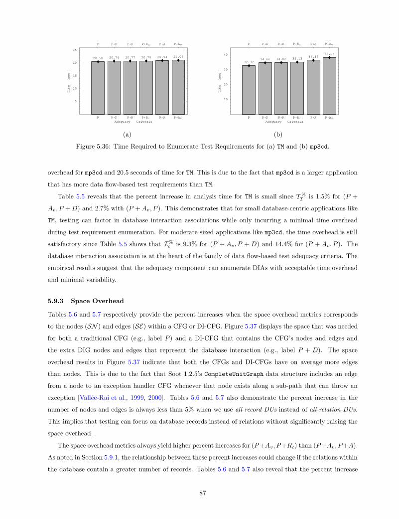
P P+D P+R P+Rc P+A P+AvAdequacy Criteria
5
10
15
20
25
Time
HsecL
P P+D P+R P+Rc P+A P+Av
20.50 20.74 20.77 20.78 20.94 21.06
PSfrag replacements
N6
enter computeVelocity
enter computeVelocity
N6
N6
N7
N7
N8
N8
N10
N8
N16
N10
N11
N11
N12
N12
N18
N16
N18
N18
exit computeVelocity
exit computeVelocity
N6
N1
N1
N2
N2
N3
N3
N1
N1
N4
N4
N5
N5
N6
enter P
enter P
call main
call main
enter main
enter main
enter main
. . .
. . .
call inputCardNumber
call inputCardNumber
call inputPin
call inputCardNumber
call handleError
call handleError
call inputCardNumber
call inputPin
call handleError
call handleError
call inputPin
call inputPin
call inputOperation
call inputOperation
call getAccountBalance
call getAccountBalance
call promptAgain
call inputOperation
call lockAccount
call lockAccount
call promptAgain
call promptAgain
call inputOperation
call promptAgain
. . .
call getAccountBalance
enter getAccountBalance
enter getAccountBalance
N3
N3
N4
N4
N5
N5
N6
N6
N7
N7
N10
N10
N12
N12
N15
N10
N15
N15
exit getAccountBalance
exit getAccountBalance
return getAccountBalance
return lockAccount
. . .
return getAccountBalance
call promptAgain
. . .
exit main
exit main
return main
return main
exit P
exit P
. . .
exit main
enter lockAccount
enter lockAccount
. . .
. . .
exit lockAccount
exit lockAccount
return lockAccount
return lockAccount
exit main
(a)
P P+D P+R P+Rc P+A P+AvAdequacy Criteria
10
20
30
40
Time
HsecL
P P+D P+R P+Rc P+A P+Av
32.7234.66 34.82 35.13
36.3738.23
PSfrag replacements
N6
enter computeVelocity
enter computeVelocity
N6
N6
N7
N7
N8
N8
N10
N8
N16
N10
N11
N11
N12
N12
N18
N16
N18
N18
exit computeVelocity
exit computeVelocity
N6
N1
N1
N2
N2
N3
N3
N1
N1
N4
N4
N5
N5
N6
enter P
enter P
call main
call main
enter main
enter main
enter main
. . .
. . .
call inputCardNumber
call inputCardNumber
call inputPin
call inputCardNumber
call handleError
call handleError
call inputCardNumber
call inputPin
call handleError
call handleError
call inputPin
call inputPin
call inputOperation
call inputOperation
call getAccountBalance
call getAccountBalance
call promptAgain
call inputOperation
call lockAccount
call lockAccount
call promptAgain
call promptAgain
call inputOperation
call promptAgain
. . .
call getAccountBalance
enter getAccountBalance
enter getAccountBalance
N3
N3
N4
N4
N5
N5
N6
N6
N7
N7
N10
N10
N12
N12
N15
N10
N15
N15
exit getAccountBalance
exit getAccountBalance
return getAccountBalance
return lockAccount
. . .
return getAccountBalance
call promptAgain
. . .
exit main
exit main
return main
return main
exit P
exit P
. . .
exit main
enter lockAccount
enter lockAccount
. . .
. . .
exit lockAccount
exit lockAccount
return lockAccount
return lockAccount
exit main
(b)
Figure 5.36: Time Required to Enumerate Test Requirements for (a) TM and (b) mp3cd.
overhead for mp3cd and 20.5 seconds of time for TM. This is due to the fact that mp3cd is a larger application
that has more data flow-based test requirements than TM.
Table 5.5 reveals that the percent increase in analysis time for TM is small since T %I is 1.5% for (P +
Av , P + D) and 2.7% with (P + Av, P ). This demonstrates that for small database-centric applications like
TM, testing can factor in database interaction associations while only incurring a minimal time overhead
during test requirement enumeration. For moderate sized applications like mp3cd, the time overhead is still
satisfactory since Table 5.5 shows that T %I is 9.3% for (P + Av , P + D) and 14.4% for (P + Av , P ). The
database interaction association is at the heart of the family of data flow-based test adequacy criteria. The
empirical results suggest that the adequacy component can enumerate DIAs with acceptable time overhead
and minimal variability.
5.9.3 Space Overhead
Tables 5.6 and 5.7 respectively provide the percent increases when the space overhead metrics corresponds
to the nodes (SN ) and edges (SE) within a CFG or DI-CFG. Figure 5.37 displays the space that was needed
for both a traditional CFG (e.g., label P ) and a DI-CFG that contains the CFG’s nodes and edges and
the extra DIG nodes and edges that represent the database interaction (e.g., label P + D). The space
overhead results in Figure 5.37 indicate that both the CFGs and DI-CFGs have on average more edges
than nodes. This is due to the fact that Soot 1.2.5’s CompleteUnitGraph data structure includes an edge
from a node to an exception handler CFG whenever that node exists along a sub-path that can throw an
exception [Vallee-Rai et al., 1999, 2000]. Tables 5.6 and 5.7 also demonstrate the percent increase in the
number of nodes and edges is always less than 5% when we use all-record-DUs instead of all-relation-DUs.
This implies that testing can focus on database records instead of relations without significantly raising the
space overhead.
The space overhead metrics always yield higher percent increases for (P +Av, P +Rc) than (P +Av, P +A).
As noted in Section 5.9.1, the relationship between these percent increases could change if the relations within
the database contain a greater number of records. Tables 5.6 and 5.7 also reveal that the percent increase
87

T %I (P + R, P + D) (P + Rc, P + R) (P + A, P + R)
TM .1 .04 .8
mp3cd .5 .8 4.3
T %I (P + Av, P + Rc) (P + Av, P + A) (P + Av, P + D) (P + Av, P )
TM 1.3 .6 1.5 2.7
mp3cd 8.1 4.9 9.3 14.4
Table 5.5: Percent Increase in the Time Overhead.
SN%I (P + R, P + D) (P + Rc, P + R) (P + A, P + R)
TM .6 2.5 4.3
mp3cd 2.0 3.8 9.5
SN%I (P + Av, P + Rc) (P + Av, P + A) (P + Av, P + D) (P + Av, P )
TM 7.5 5.8 10.4 12.2
mp3cd 15.5 10.2 20.4 21.6
Table 5.6: Percent Increase in the Space Overhead for Nodes.
in the number of nodes and edges is less than 23% for mp3 and 11% for TM when the weakest database aware
criterion (D) is replaced with the strongest criterion (Av). For smaller applications like TM the experimental
results suggest that the DI-CFGs will create less than a 13% increase in the number of nodes and edges when
we use all-attribute-value-DUs and all-DUs instead of just all-DUs. The results also indicate that moderate
size applications such as mp3cd will incur no more than a 24% increase in the number of nodes and edges
when we evaluate the adequacy of a test suite at the P + Av level rather than the P level. In summary, the
experiments quantitatively confirm that the control flow graph can represent a program’s interaction with a
relational database in an acceptable amount of space.
5.10 THREATS TO VALIDITY
The experiments described in this chapter are subject to validity threats and Chapter 3 explains the steps
that we took to control these threats during experimentation. We also took additional steps to handle
the threats that are specific to experimentation with the test adequacy component. Internal threats to
validity are those factors that have the potential to impact the measured variables defined in Section 5.7.
One internal validity threat is related to defects in the test adequacy component. These defects could
compromise the correctness of the (i) control flow graphs, (ii) sets of database entities, or (iii) database
interaction associations. We controlled this threat by visualizing all of the DI-CFGs and checking them to
ensure correctness. For example, we verified that each database interaction graph was a straight line code
88

SE%I (P + R, P + D) (P + Rc, P + R) (P + A, P + R)
TM 0.0 2.4 4.2
mp3cd 2.1 4.4 10.5
SE%I (P + Av, P + Rc) (P + Av, P + A) (P + Av, P + D) (P + Av, P )
TM 7.4 5.7 9.7 11.4
mp3cd 16.7 11.0 22.1 23.8
Table 5.7: Percent Increase in the Space Overhead for Edges.
segment that was placed at the correct database interaction location within the DI-CFG. We also selected
database interaction points and checked that the interaction analyzer produced a correct set of database
entities. Finally, we inspected the sets of database interaction associations for methods in order to guarantee
that the data flow analyzer worked properly.
Construct validity is related to the appropriateness of the evaluation metrics described in Section 5.7.
Even though T R does not directly measure the effectiveness of a test adequacy criterion with respect to its
ability to isolate defects, it is still useful in an evaluation of the test adequacy component because it reveals
the relative difficulty of satisfying an adequacy criterion. The measurement of space overhead by calculating
the number of nodes and edges in a control flow graph is not directly tied to the consumption of bytes of
memory and thus not as useful to software testing practitioners. Yet, if S was the number of bytes used
by the in-memory or on-disk representation of a database-centric application, then these values could be
dependent upon the choice of the file system, operating system, and Java virtual machine. The number of
CFG nodes and edges are also established metrics for measuring the size of graphs [Tip and Palsberg, 2000].
The experiments did not measure the costs associated with all aspects of the test adequacy component.
Since our research is not directly related to the construction of interprocedural CFGs, we did not focus on
the time consumed by the points-to analysis and the CFG construction technique. Moreover, these static
analysis techniques have been studied extensively by previous research efforts [Lhotak and Hendren, 2003,
2006]. Our experiments did not concentrate on measuring the cost of DI-FSM creation since other researchers
have provided preliminary insights into the performance of this process [Christensen et al., 2003]. Yet, this
chapter provides a detailed analytical evaluation of the worst-case time complexity of each key algorithm
within the test adequacy component. We judge that the time complexity analysis serves as the foundation
for future empirical evaluations of these techniques.
5.11 CONCLUSION
This chapter explains the test adequacy component that (i) constructs a database-aware program repre-
sentation, (ii) analyzes database interaction points, and (iii) lists the test requirements. We describe the
89

5 10 15 20Node and Edge Count
P+Av
P+A
P+Rc
P+R
P+D
PAdequacy
Criteria
P+Av
P+A
P+Rc
P+R
P+D
P
17.5
16.5
16.2
15.8
15.8
15.5
17.2
16.2
15.9
15.5
15.4
15.1
Edges
Nodes
PSfrag replacements
N6
enter computeVelocity
enter computeVelocity
N6
N6
N7
N7
N8
N8
N10
N8
N16
N10
N11
N11
N12
N12
N18
N16
N18
N18
exit computeVelocity
exit computeVelocity
N6
N1
N1
N2
N2
N3
N3
N1
N1
N4
N4
N5
N5
N6
enter P
enter P
call main
call main
enter main
enter main
enter main
. . .
. . .
call inputCardNumber
call inputCardNumber
call inputPin
call inputCardNumber
call handleError
call handleError
call inputCardNumber
call inputPin
call handleError
call handleError
call inputPin
call inputPin
call inputOperation
call inputOperation
call getAccountBalance
call getAccountBalance
call promptAgain
call inputOperation
call lockAccount
call lockAccount
call promptAgain
call promptAgain
call inputOperation
call promptAgain
. . .
call getAccountBalance
enter getAccountBalance
enter getAccountBalance
N3
N3
N4
N4
N5
N5
N6
N6
N7
N7
N10
N10
N12
N12
N15
N10
N15
N15
exit getAccountBalance
exit getAccountBalance
return getAccountBalance
return lockAccount
. . .
return getAccountBalance
call promptAgain
. . .
exit main
exit main
return main
return main
exit P
exit P
. . .
exit main
enter lockAccount
enter lockAccount
. . .
. . .
exit lockAccount
exit lockAccount
return lockAccount
return lockAccount
exit main
(a)
5 10 15 20 25 30 35Node and Edge Count
P+Av
P+A
P+Rc
P+R
P+D
P
Adequacy
Criteria
P+Av
P+A
P+Rc
P+R
P+D
P
29.8
26.5
24.8
23.7
23.2
22.7
24.5
22.0
20.7
19.9
19.5
19.2
Edges
Nodes
PSfrag replacements
N6
enter computeVelocity
enter computeVelocity
N6
N6
N7
N7
N8
N8
N10
N8
N16
N10
N11
N11
N12
N12
N18
N16
N18
N18
exit computeVelocity
exit computeVelocity
N6
N1
N1
N2
N2
N3
N3
N1
N1
N4
N4
N5
N5
N6
enter P
enter P
call main
call main
enter main
enter main
enter main
. . .
. . .
call inputCardNumber
call inputCardNumber
call inputPin
call inputCardNumber
call handleError
call handleError
call inputCardNumber
call inputPin
call handleError
call handleError
call inputPin
call inputPin
call inputOperation
call inputOperation
call getAccountBalance
call getAccountBalance
call promptAgain
call inputOperation
call lockAccount
call lockAccount
call promptAgain
call promptAgain
call inputOperation
call promptAgain
. . .
call getAccountBalance
enter getAccountBalance
enter getAccountBalance
N3
N3
N4
N4
N5
N5
N6
N6
N7
N7
N10
N10
N12
N12
N15
N10
N15
N15
exit getAccountBalance
exit getAccountBalance
return getAccountBalance
return lockAccount
. . .
return getAccountBalance
call promptAgain
. . .
exit main
exit main
return main
return main
exit P
exit P
. . .
exit main
enter lockAccount
enter lockAccount
. . .
. . .
exit lockAccount
exit lockAccount
return lockAccount
return lockAccount
exit main
(b)
Figure 5.37: Average Space Overhead for (a) TM and (b) mp3cd.
database interaction finite state machine (DI-FSM) that models a single database interaction point and we
explain how to use a DI-FSM to enumerate database entities. We also show how to transform a traditional
interprocedural control flow graph (ICFG) into a database interaction interprocedural control flow graph (DI-
ICFG). This chapter examines the implementation of the test adequacy component and it provides empirical
evidence that it is possible to enumerate database-aware test requirements with acceptable time and space
overhead. Further experimentation with larger case study applications will serve to confirm the scalability
of enumerating database interaction associations (DIAs). The experiments suggest that our database-aware
adequacy criteria obligate test suites to cover test requirements that traditional def-use testing would over-
look. In summary, this chapter shows that the test adequacy component is promising and thus warrants
further empirical investigation.
90

6.0 FOUNDATIONS OF TEST COVERAGE MONITORING
6.1 INTRODUCTION
This chapter presents a database-aware test coverage monitoring technique. We identify and address the
major challenges associated with monitoring a test suite’s coverage of a database-centric application. We
encounter these challenges during the (i) instrumentation of a database-centric application, (ii) creation
and storage of the coverage results, and (iii) calculation of test suite adequacy. This chapter describes the
database-aware test coverage monitoring (TCM) trees that represent a test suite’s coverage. We also discuss
the algorithms that construct the TCM trees and show how to use these trees to calculate the adequacy of
a test suite. In particular, this chapter furnishes:
1. A high level overview of the test coverage monitoring process (Section 6.2).
2. A discussion of the challenges associated with test coverage monitoring (Section 6.3).
3. The description of the TCM trees and the monitoring instrumentation that records coverage information
in a database-aware fashion (Section 6.4).
4. An interprocedural representation for a test suite that supports the calculation of test adequacy (Sec-
tion 6.5.1).
5. A technique for calculating test suite adequacy according to the family of data flow-based adequacy
criteria described in Chapter 4 (Section 6.5.2).
6.2 OVERVIEW OF THE COVERAGE MONITORING PROCESS
The overarching goal of test coverage monitoring is to record the requirements that the test suite covers during
testing. Since we focus on database-aware test requirements, our test coverage monitor stores information
about the definition and use of relational database entities. Figure 6.1 depicts the process of test coverage
monitoring. This diagram shows that the instrumentation phase accepts adequacy criteria (e.g., all-record-
DUs and all-database-DUs), a test suite, and the program under test. We instrument the program under
test by placing probes at key locations within the control flow graph. These probes execute payloads that
record information about the coverage of the test requirements [Misurda et al., 2005]. For example, suppose
that method mk contains a database interaction that submits a SQL select statement to the database. A
database-aware test coverage monitor inserts a probe after the execution of the select statement in order
to inspect the records that match the database query. Since the tests for a database-centric application
91
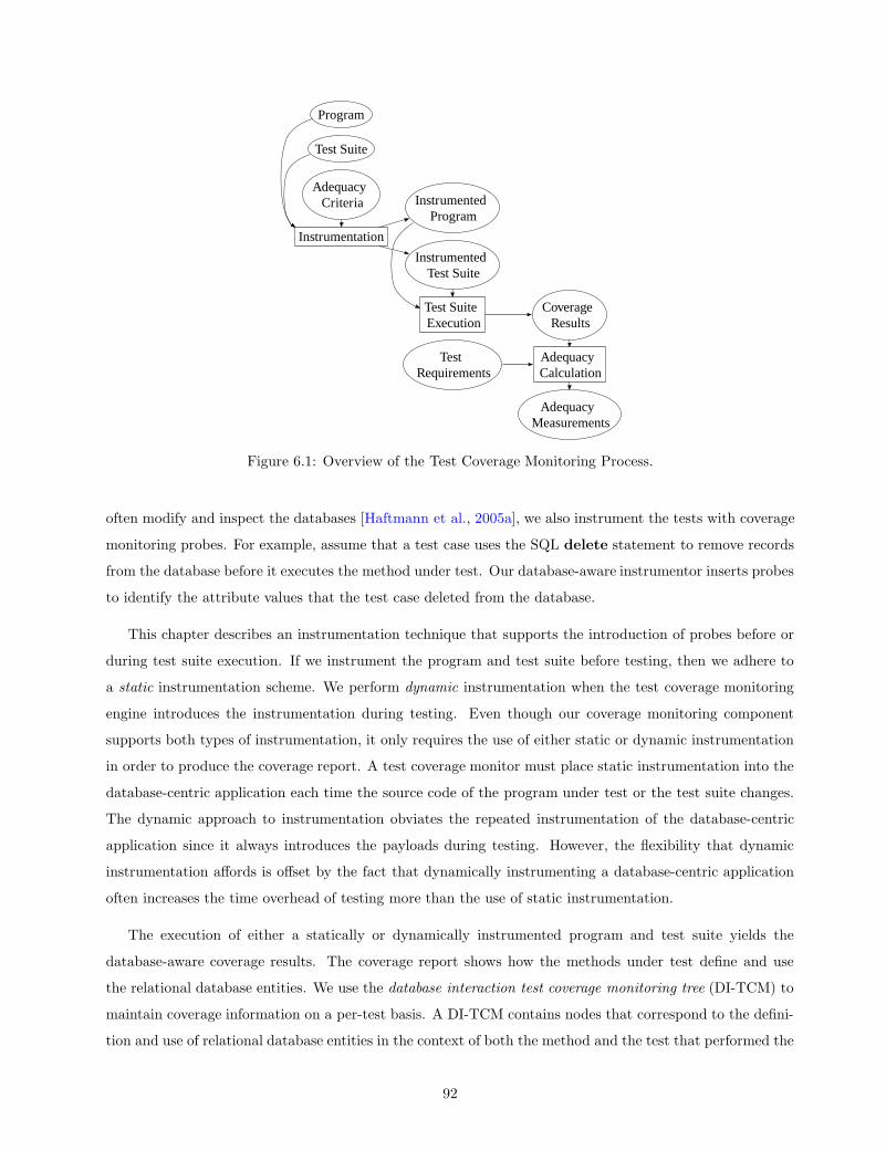
Program
Instrumentation
Test Suite
Adequacy Criteria Instrumented
Program
Test Suite Execution
Instrumented Test Suite
Coverage Results
Adequacy Calculation
Test Requirements
Adequacy Measurements
PSfrag replacements
N6
enter computeVelocity
enter computeVelocity
N6
N6
N7
N7
N8
N8
N10
N8
N16
N10
N11
N11
N12
N12
N18
N16
N18
N18
exit computeVelocity
exit computeVelocity
N6
N1
N1
N2
N2
N3
N3
N1
N1
N4
N4
N5
N5
N6
enter P
enter P
call main
call main
enter main
enter main
enter main
. . .
. . .
call inputCardNumber
call inputCardNumber
call inputPin
call inputCardNumber
call handleError
call handleError
call inputCardNumber
call inputPin
call handleError
call handleError
call inputPin
call inputPin
call inputOperation
call inputOperation
call getAccountBalance
call getAccountBalance
call promptAgain
call inputOperation
call lockAccount
call lockAccount
call promptAgain
call promptAgain
call inputOperation
call promptAgain
. . .
call getAccountBalance
enter getAccountBalance
enter getAccountBalance
N3
N3
N4
N4
N5
N5
N6
N6
N7
N7
N10
N10
N12
N12
N15
N10
N15
N15
exit getAccountBalance
exit getAccountBalance
return getAccountBalance
return lockAccount
. . .
return getAccountBalance
call promptAgain
. . .
exit main
exit main
return main
return main
exit P
exit P
. . .
exit main
enter lockAccount
enter lockAccount
. . .
. . .
exit lockAccount
exit lockAccount
return lockAccount
return lockAccount
exit main
Figure 6.1: Overview of the Test Coverage Monitoring Process.
often modify and inspect the databases [Haftmann et al., 2005a], we also instrument the tests with coverage
monitoring probes. For example, assume that a test case uses the SQL delete statement to remove records
from the database before it executes the method under test. Our database-aware instrumentor inserts probes
to identify the attribute values that the test case deleted from the database.
This chapter describes an instrumentation technique that supports the introduction of probes before or
during test suite execution. If we instrument the program and test suite before testing, then we adhere to
a static instrumentation scheme. We perform dynamic instrumentation when the test coverage monitoring
engine introduces the instrumentation during testing. Even though our coverage monitoring component
supports both types of instrumentation, it only requires the use of either static or dynamic instrumentation
in order to produce the coverage report. A test coverage monitor must place static instrumentation into the
database-centric application each time the source code of the program under test or the test suite changes.
The dynamic approach to instrumentation obviates the repeated instrumentation of the database-centric
application since it always introduces the payloads during testing. However, the flexibility that dynamic
instrumentation affords is offset by the fact that dynamically instrumenting a database-centric application
often increases the time overhead of testing more than the use of static instrumentation.
The execution of either a statically or dynamically instrumented program and test suite yields the
database-aware coverage results. The coverage report shows how the methods under test define and use
the relational database entities. We use the database interaction test coverage monitoring tree (DI-TCM) to
maintain coverage information on a per-test basis. A DI-TCM contains nodes that correspond to the defini-
tion and use of relational database entities in the context of both the method and the test that performed the
92

database interaction. Since the size of a DI-TCM can be prohibitively large, we also leverage compression
algorithms in order to reduce the size of the coverage report. When we have the coverage results and the
test requirements for a test case, we can calculate the adequacy of this test. The adequacy of a test case is
simply the number of covered test requirements divided by the total number of requirements.
6.3 TEST COVERAGE MONITORING CHALLENGES
6.3.1 Location of the Instrumentation
The majority of traditional test coverage monitoring frameworks place instrumentation probes into the pro-
gram under test through the use of either static instrumentation or Java virtual machine (JVM)-based
techniques [Misurda et al., 2005, Pavlopoulou and Young, 1999, Tikir and Hollingsworth, 2002]. It is chal-
lenging to develop a database-aware instrumentation approach because the coverage monitor must place
the probes in the appropriate locations within the program, the test suite, and/or the execution environ-
ment. We use the different execution environments for a Java database-centric application, as depicted in
Figure 6.2, to illustrate these challenges with a concrete example. In the context of applications written in
Java, we must accommodate the wide variety of Java virtual machines, JDBC drivers, database managers,
and operating systems that exist in an application’s execution environment. As noted in Chapter 3, we
assume that the program and the test suite interact with the database manager through a Java database
connectivity driver. Prior monitoring techniques place the instrumentation probes in the (i) program and
the test suite (e.g., [Misurda et al., 2005]), (ii) JDBC driver (e.g., [Bloom, 2006]), (iii) relational database
management system (e.g., [Chays et al., 2004]), or (iv) operating system (OS) (e.g., [Engel and Freisleben,
2005, Tamches and Miller, 1999]). Figure 6.2(a) shows a program and a test suite that execute on a Java
virtual machine and interact with a Java-based RDBMS. We configured the case study applications to exe-
cute in this manner, as discussed in Chapter 3. Finally, Figure 6.2(b) describes an application that interacts
with a native database manager that directly executes on the operating system instead of using a JVM.
The coverage monitor cannot place instrumentation into the relational database management system
because we want the monitoring technique to function properly for all of the database management systems
that provide a JDBC interface. Since the testing framework does not require a database-centric applica-
tion to execute on specific operating system(s), it is not practical to monitor coverage by instrumenting
the OS. Moreover, OS-based instrumentation is unlikely to reveal how the JVM executes the test suite.
For example, instrumentation in the operating system can capture system calls but it will not normally
be able to monitor method invocations within the program and the test suite. The JDBC Web site at
http://developers.sun.com/product/jdbc/drivers/ reveals that there are currently over two hundred
different JDBC driver implementations. A JDBC driver could be written in Java or in a combination of
the Java, C, and C++ programming languages. If the JDBC driver is partially written in C and/or C++,
then it must use the Java Native Interface (JNI) to make its functionality accessible to the database-centric
application that uses Java. The testing framework does not stipulate that the database-centric application
93

Program and Test Suite
Java Virtual Machine
Operating System
Database Manager
Java Virtual Machine
Operating System
JDBC Driver
PSfrag replacements
N6
enter computeVelocity
enter computeVelocity
N6
N6
N7
N7
N8
N8
N10
N8
N16
N10
N11
N11
N12
N12
N18
N16
N18
N18
exit computeVelocity
exit computeVelocity
N6
N1
N1
N2
N2
N3
N3
N1
N1
N4
N4
N5
N5
N6
enter P
enter P
call main
call main
enter main
enter main
enter main
. . .
. . .
call inputCardNumber
call inputCardNumber
call inputPin
call inputCardNumber
call handleError
call handleError
call inputCardNumber
call inputPin
call handleError
call handleError
call inputPin
call inputPin
call inputOperation
call inputOperation
call getAccountBalance
call getAccountBalance
call promptAgain
call inputOperation
call lockAccount
call lockAccount
call promptAgain
call promptAgain
call inputOperation
call promptAgain
. . .
call getAccountBalance
enter getAccountBalance
enter getAccountBalance
N3
N3
N4
N4
N5
N5
N6
N6
N7
N7
N10
N10
N12
N12
N15
N10
N15
N15
exit getAccountBalance
exit getAccountBalance
return getAccountBalance
return lockAccount
. . .
return getAccountBalance
call promptAgain
. . .
exit main
exit main
return main
return main
exit P
exit P
. . .
exit main
enter lockAccount
enter lockAccount
. . .
. . .
exit lockAccount
exit lockAccount
return lockAccount
return lockAccount
exit main
(a)
Program and Test Suite
Java Virtual Machine
Operating System
Database Manager
Operating System
JDBC Driver
PSfrag replacements
N6
enter computeVelocity
enter computeVelocity
N6
N6
N7
N7
N8
N8
N10
N8
N16
N10
N11
N11
N12
N12
N18
N16
N18
N18
exit computeVelocity
exit computeVelocity
N6
N1
N1
N2
N2
N3
N3
N1
N1
N4
N4
N5
N5
N6
enter P
enter P
call main
call main
enter main
enter main
enter main
. . .
. . .
call inputCardNumber
call inputCardNumber
call inputPin
call inputCardNumber
call handleError
call handleError
call inputCardNumber
call inputPin
call handleError
call handleError
call inputPin
call inputPin
call inputOperation
call inputOperation
call getAccountBalance
call getAccountBalance
call promptAgain
call inputOperation
call lockAccount
call lockAccount
call promptAgain
call promptAgain
call inputOperation
call promptAgain
. . .
call getAccountBalance
enter getAccountBalance
enter getAccountBalance
N3
N3
N4
N4
N5
N5
N6
N6
N7
N7
N10
N10
N12
N12
N15
N10
N15
N15
exit getAccountBalance
exit getAccountBalance
return getAccountBalance
return lockAccount
. . .
return getAccountBalance
call promptAgain
. . .
exit main
exit main
return main
return main
exit P
exit P
. . .
exit main
enter lockAccount
enter lockAccount
. . .
. . .
exit lockAccount
exit lockAccount
return lockAccount
return lockAccount
exit main
(b)
Figure 6.2: The Execution Environment for a Database-Centric Application.
use a particular JDBC driver. Without a general and automated technique for instrumenting an arbitrary
JDBC driver, it is unrealistic for the coverage monitor to record database interactions by placing probes into
all of the currently available JDBC drivers.
Our database-aware testing framework does not assume that the program and the test suite execute on
a certain Java virtual machine. For example, the program and the tests might use the Sun HotSpotTMJVM
or the Jikes Research Virtual Machine (RVM) [Alpern et al., 2005]. The wide variety of JVMs indicates that
it is challenging to dynamically introduce the test coverage monitoring instrumentation with the JVM that
runs the test suite. In light of our analysis of the potential instrumentation locations, we implemented static
and dynamic instrumentation techniques that only modify the program and the test suite. Since a tester
does not always have access to an application’s source code, it is also preferable if the test coverage monitor
can statically instrument Java bytecode. To this end, we designed the TCM component so that it can
operate on Java source code, bytecode, or a combination of both types of program representations. Finally,
our dynamic instrumentation technique operates on well-established interfaces that exist in all Java virtual
machines (the current implementation performs load-time instrumentation using the JVM class loader).
6.3.2 Types of Instrumentation
Instrumenting a traditional program requires the placement of probes at control flow graph locations that (i)
execute CFG nodes and edges, (ii) define and use program variables, and/or (iii) invoke program methods
[Misurda et al., 2005, Pavlopoulou and Young, 1999, Tikir and Hollingsworth, 2002]. The payload of a tra-
ditional probe simply marks an entity within a control flow graph as covered if a test causes the execution of
this entity. For example, a probe that monitors the coverage of CFG nodes executes a payload to record the
fact that a node was executed during testing. In contrast, database-aware instrumentation must intercept
database interactions and efficiently analyze the state and structure of the databases that are subject to
94

Test Coverage Monitoring Instrumentation
Interaction Location Interaction Type
Program Test Suite Defining Using Defining-Using
PSfrag replacements
N6
enter computeVelocity
enter computeVelocity
N6
N6
N7
N7
N8
N8
N10
N8
N16
N10
N11
N11
N12
N12
N18
N16
N18
N18
exit computeVelocity
exit computeVelocity
N6
N1
N1
N2
N2
N3
N3
N1
N1
N4
N4
N5
N5
N6
enter P
enter P
call main
call main
enter main
enter main
enter main
. . .
. . .
call inputCardNumber
call inputCardNumber
call inputPin
call inputCardNumber
call handleError
call handleError
call inputCardNumber
call inputPin
call handleError
call handleError
call inputPin
call inputPin
call inputOperation
call inputOperation
call getAccountBalance
call getAccountBalance
call promptAgain
call inputOperation
call lockAccount
call lockAccount
call promptAgain
call promptAgain
call inputOperation
call promptAgain
. . .
call getAccountBalance
enter getAccountBalance
enter getAccountBalance
N3
N3
N4
N4
N5
N5
N6
N6
N7
N7
N10
N10
N12
N12
N15
N10
N15
N15
exit getAccountBalance
exit getAccountBalance
return getAccountBalance
return lockAccount
. . .
return getAccountBalance
call promptAgain
. . .
exit main
exit main
return main
return main
exit P
exit P
. . .
exit main
enter lockAccount
enter lockAccount
. . .
. . .
exit lockAccount
exit lockAccount
return lockAccount
return lockAccount
exit main
Figure 6.3: Instrumentation for Database-Aware Test Coverage Monitoring.
interaction. For example, the coverage instrumentation for the SQL delete statement examines the state of
the relational database in order to determine which records were removed.
Figure 6.3 categorizes the types of instrumentation that we use to monitor the coverage of the test
suites for a database-centric application. This diagram shows that the location of a database interaction is
either in the program or the test suite. A database-centric application maintains a significant amount of
external state and the tests for a database-centric application frequently change the state of the database
[Haftmann et al., 2005a]. For example, a test for the removeAccount method in the TransactionManager
application might need to add accounts into the database before executing the method under test. Since
the test suite for a database-centric application directly modifies the state of the database, the test coverage
monitor places additional instrumentation into the tests. The coverage monitoring instrumentation must
also handle database interactions that are either of type defining, using, or defining-using (c.f. Section 4.3.2
for a discussion of these types of interactions).
Similar to [Christensen et al., 2003, Halfond and Orso, 2005], we focus on the testing and analysis of
database-centric applications that interact with a database by submitting SQL strings. Since our testing
framework does not restrict which relational database management system controls the program’s access
to the databases, the program of a database-centric application might interact with the databases that
are managed by a MySQL, PostreSQL, HSQLDB, or Oracle RDBMS. It is challenging to instrument a
database-centric application for coverage monitoring because different RDBMS support different dialects of
the structured query language. Figure 6.4 provides four SQL select statements that extract records tbegin
through tend from the relation relj = t1, . . . , tu. We use the notation recbegin and recend to respectively
denote the numerical index to records tbegin and tend, as depicted in Figure 6.5. The SQL select for the
Oracle RDBMS uses the rownum variable to bound the records in the select’s result set while the MySQL,
PostreSQL, and HSQLDB statements use the limit and/or offset keywords. Our test coverage monitor
supports the testing of programs that use different RDBMS because the instrumentation limits the parsing
of the SQL strings to the syntactical elements that all SQL dialects have in common.
It is also challenging to perform database-aware coverage monitoring because the probes must examine
the state and structure of the database without inadvertently introducing defects into the program. Since
95

select A1, A2, . . . , Az
from relj limit recbegin , recend
(a)
select A1, A2, . . . , Az
from relj limit recend offset recbegin
(b)
select A1, A2, . . . , Az
from relj limit recbegin recend
(c)
select A1, A2, . . . , Az from relj
where rownum ≥ recbegin and rownum ≤ recend
(d)
Figure 6.4: Syntax for the SQL select in (a) MySQL, (b) PostreSQL, (c) HSQLDB, and (d) Oracle.
PSfrag replacements
N6
enter computeVelocity
enter computeVelocity
N6
N6
N7
N7
N8
N8
N10
N8
N16
N10
N11
N11
N12
N12
N18
N16
N18
N18
exit computeVelocity
exit computeVelocity
N6
N1
N1
N2
N2
N3
N3
N1
N1
N4
N4
N5
N5
N6
enter P
enter P
call main
call main
enter main
enter main
enter main
. . .
. . .
call inputCardNumber
call inputCardNumber
call inputPin
call inputCardNumber
call handleError
call handleError
call inputCardNumber
call inputPin
call handleError
call handleError
call inputPin
call inputPin
call inputOperation
call inputOperation
call getAccountBalance
call getAccountBalance
call promptAgain
call inputOperation
call lockAccount
call lockAccount
call promptAgain
call promptAgain
call inputOperation
call promptAgain
. . .
call getAccountBalance
enter getAccountBalance
enter getAccountBalance
N3
N3
N4
N4
N5
N5
N6
N6
N7
N7
N10
N10
N12
N12
N15
N10
N15
N15
exit getAccountBalance
exit getAccountBalance
return getAccountBalance
return lockAccount
. . .
return getAccountBalance
call promptAgain
. . .
exit main
exit main
return main
return main
exit P
exit P
. . .
exit main
enter lockAccount
enter lockAccount
. . .
. . .
exit lockAccount
exit lockAccount
return lockAccount
return lockAccount
exit main
t1
. . .X tbegin
X . . .
X tend
. . .
. . .
tu
Figure 6.5: The Matching Records from the SQL select Statement.
96
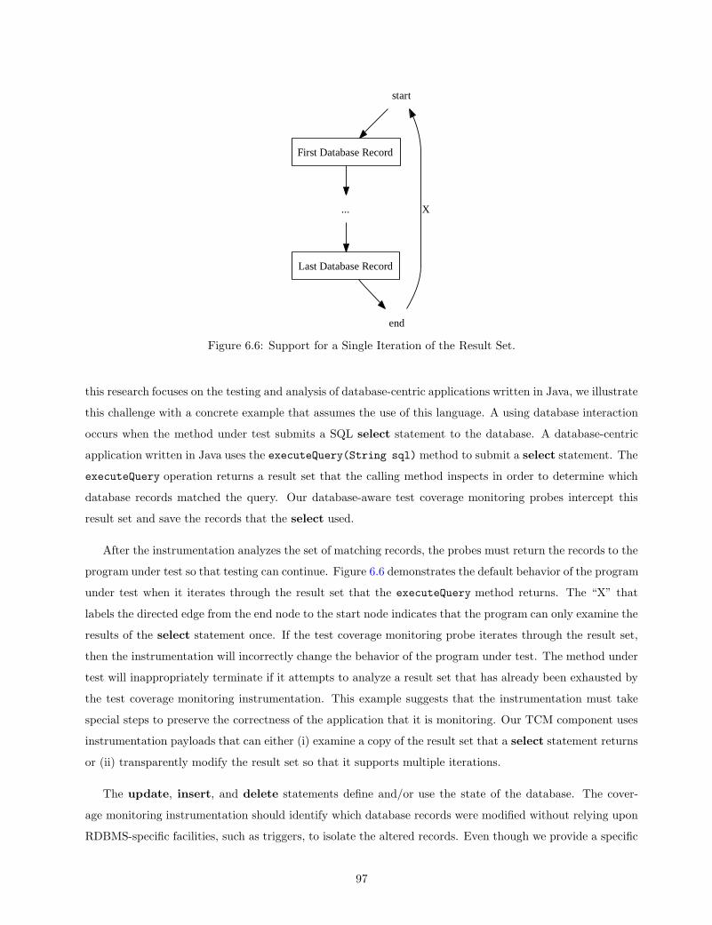
start
First Database Record
...
Last Database Record
end
X
PSfrag replacements
N6
enter computeVelocity
enter computeVelocity
N6
N6
N7
N7
N8
N8
N10
N8
N16
N10
N11
N11
N12
N12
N18
N16
N18
N18
exit computeVelocity
exit computeVelocity
N6
N1
N1
N2
N2
N3
N3
N1
N1
N4
N4
N5
N5
N6
enter P
enter P
call main
call main
enter main
enter main
enter main
. . .
. . .
call inputCardNumber
call inputCardNumber
call inputPin
call inputCardNumber
call handleError
call handleError
call inputCardNumber
call inputPin
call handleError
call handleError
call inputPin
call inputPin
call inputOperation
call inputOperation
call getAccountBalance
call getAccountBalance
call promptAgain
call inputOperation
call lockAccount
call lockAccount
call promptAgain
call promptAgain
call inputOperation
call promptAgain
. . .
call getAccountBalance
enter getAccountBalance
enter getAccountBalance
N3
N3
N4
N4
N5
N5
N6
N6
N7
N7
N10
N10
N12
N12
N15
N10
N15
N15
exit getAccountBalance
exit getAccountBalance
return getAccountBalance
return lockAccount
. . .
return getAccountBalance
call promptAgain
. . .
exit main
exit main
return main
return main
exit P
exit P
. . .
exit main
enter lockAccount
enter lockAccount
. . .
. . .
exit lockAccount
exit lockAccount
return lockAccount
return lockAccount
exit mainFigure 6.6: Support for a Single Iteration of the Result Set.
this research focuses on the testing and analysis of database-centric applications written in Java, we illustrate
this challenge with a concrete example that assumes the use of this language. A using database interaction
occurs when the method under test submits a SQL select statement to the database. A database-centric
application written in Java uses the executeQuery(String sql) method to submit a select statement. The
executeQuery operation returns a result set that the calling method inspects in order to determine which
database records matched the query. Our database-aware test coverage monitoring probes intercept this
result set and save the records that the select used.
After the instrumentation analyzes the set of matching records, the probes must return the records to the
program under test so that testing can continue. Figure 6.6 demonstrates the default behavior of the program
under test when it iterates through the result set that the executeQuery method returns. The “X” that
labels the directed edge from the end node to the start node indicates that the program can only examine the
results of the select statement once. If the test coverage monitoring probe iterates through the result set,
then the instrumentation will incorrectly change the behavior of the program under test. The method under
test will inappropriately terminate if it attempts to analyze a result set that has already been exhausted by
the test coverage monitoring instrumentation. This example suggests that the instrumentation must take
special steps to preserve the correctness of the application that it is monitoring. Our TCM component uses
instrumentation payloads that can either (i) examine a copy of the result set that a select statement returns
or (ii) transparently modify the result set so that it supports multiple iterations.
The update, insert, and delete statements define and/or use the state of the database. The cover-
age monitoring instrumentation should identify which database records were modified without relying upon
RDBMS-specific facilities, such as triggers, to isolate the altered records. Even though we provide a specific
97

PSfrag replacements
N6
enter computeVelocity
enter computeVelocity
N6
N6
N7
N7
N8
N8
N10
N8
N16
N10
N11
N11
N12
N12
N18
N16
N18
N18
exit computeVelocity
exit computeVelocity
N6
N1
N1
N2
N2
N3
N3
N1
N1
N4
N4
N5
N5
N6
enter P
enter P
call main
call main
enter main
enter main
enter main
. . .
. . .
call inputCardNumber
call inputCardNumber
call inputPin
call inputCardNumber
call handleError
call handleError
call inputCardNumber
call inputPin
call handleError
call handleError
call inputPin
call inputPin
call inputOperation
call inputOperation
call getAccountBalance
call getAccountBalance
call promptAgain
call inputOperation
call lockAccount
call lockAccount
call promptAgain
call promptAgain
call inputOperation
call promptAgain
. . .
call getAccountBalance
enter getAccountBalance
enter getAccountBalance
N3
N3
N4
N4
N5
N5
N6
N6
N7
N7
N10
N10
N12
N12
N15
N10
N15
N15
exit getAccountBalance
exit getAccountBalance
return getAccountBalance
return lockAccount
. . .
return getAccountBalance
call promptAgain
. . .
exit main
exit main
return main
return main
exit P
exit P
. . .
exit main
enter lockAccount
enter lockAccount
. . .
. . .
exit lockAccount
exit lockAccount
return lockAccount
return lockAccount
exit main
t1
t2
t3
. . .
tu−2
tu−1
tu
(a)
PSfrag replacements
N6
enter computeVelocity
enter computeVelocity
N6
N6
N7
N7
N8
N8
N10
N8
N16
N10
N11
N11
N12
N12
N18
N16
N18
N18
exit computeVelocity
exit computeVelocity
N6
N1
N1
N2
N2
N3
N3
N1
N1
N4
N4
N5
N5
N6
enter P
enter P
call main
call main
enter main
enter main
enter main
. . .
. . .
call inputCardNumber
call inputCardNumber
call inputPin
call inputCardNumber
call handleError
call handleError
call inputCardNumber
call inputPin
call handleError
call handleError
call inputPin
call inputPin
call inputOperation
call inputOperation
call getAccountBalance
call getAccountBalance
call promptAgain
call inputOperation
call lockAccount
call lockAccount
call promptAgain
call promptAgain
call inputOperation
call promptAgain
. . .
call getAccountBalance
enter getAccountBalance
enter getAccountBalance
N3
N3
N4
N4
N5
N5
N6
N6
N7
N7
N10
N10
N12
N12
N15
N10
N15
N15
exit getAccountBalance
exit getAccountBalance
return getAccountBalance
return lockAccount
. . .
return getAccountBalance
call promptAgain
. . .
exit main
exit main
return main
return main
exit P
exit P
. . .
exit main
enter lockAccount
enter lockAccount
. . .
. . .
exit lockAccount
exit lockAccount
return lockAccount
return lockAccount
exit main
t1
t2
× t3
. . .
tu−2
× tu−1
tu
(b)
Figure 6.7: A Database Relation (a) Before and (b) After a delete Statement.
example of this challenge in the context of the SQL delete statement, we also confront similar instrumenta-
tion challenges when we handle the update and insert statements. Since different RDBMS vary the syntax
of the SQL delete statement, we use instrumentation that minimizes the parsing of the delete when it
determines which record(s) will be removed. To this end, the coverage monitoring probes preserve a snap-
shot of the relevant database state before and after the database interaction occurs. These probes execute a
payload that first determines which relation is being defined and then use a SQL select statement to record
the current state of this relation. Figure 6.7 shows the state of a relation relj = t1, . . . , tu before and after
the execution of a SQL delete statement. This diagram reveals that the delete removed records t3 and
tu−1 from relation relj . For this example, the probe will add an entry to the coverage report to indicate that
the delete defined the records t3 and tu−1. In order to minimize space overhead, we designed the coverage
monitoring probe to only maintain the state of the relation that the program is currently defining. Once
the RDBMS finishes executing the delete statement and the instrumentation records the final state of the
database, the probe uses efficient relational difference operators to determine which records were deleted.
We must take into account several additional considerations when we develop the database-aware instru-
mentation technique. Our primary concern is to ensure that the payloads always preserve the correctness
of the database-centric application. Our secondary goal is to control the time and space overhead of the
instrumentation payloads. The previous discussion reveals that the coverage monitoring instrumentation for
a database-centric application often requires the parsing of SQL strings. Whenever possible, the instrumen-
tation payloads use efficient context-insensitive parsing techniques. Since the monitoring of a single database
interaction requires the execution of two probes (i.e., Before and After instrumentation, as discussed in Sec-
tion 6.4), we designed the payload at each probe to execute with minimal time overhead. The tester can also
decrease the cost of the instrumentation by configuring the probes to store less execution context or record
the database interactions at a coarser level of granularity.
98

PSfrag replacements
N6
enter computeVelocity
enter computeVelocity
N6
N6
N7
N7
N8
N8
N10
N8
N16
N10
N11
N11
N12
N12
N18
N16
N18
N18
exit computeVelocity
exit computeVelocity
N6
N1
N1
N2
N2
N3
N3
N1
N1
N4
N4
N5
N5
N6
enter P
enter P
call main
call main
enter main
enter main
enter main
. . .
. . .
call inputCardNumber
call inputCardNumber
call inputPin
call inputCardNumber
call handleError
call handleError
call inputCardNumber
call inputPin
call handleError
call handleError
call inputPin
call inputPin
call inputOperation
call inputOperation
call getAccountBalance
call getAccountBalance
call promptAgain
call inputOperation
call lockAccount
call lockAccount
call promptAgain
call promptAgain
call inputOperation
call promptAgain
. . .
call getAccountBalance
enter getAccountBalance
enter getAccountBalance
N3
N3
N4
N4
N5
N5
N6
N6
N7
N7
N10
N10
N12
N12
N15
N10
N15
N15
exit getAccountBalance
exit getAccountBalance
return getAccountBalance
return lockAccount
. . .
return getAccountBalance
call promptAgain
. . .
exit main
exit main
return main
return main
exit P
exit P
. . .
exit main
enter lockAccount
enter lockAccount
. . .
. . .
exit lockAccount
exit lockAccount
return lockAccount
return lockAccount
exit main
Ti
TiTi
mk
mk
mk
mkmk
Df
Df
Nr1
Nr1Nr1
relj′
relj
relj
mk′
mk′
mk′
Df ′
Df
DfDf
T
T
Tj
T
Tj
Tj
relj
relj
relj
Tj
Nr2
Nr2
Nr3
Nr3
Figure 6.8: A Coverage Monitoring Tree that Offers Full Context for the Test Coverage Results.
In order to reduce the space overhead, the test coverage monitor must release any database state that it
does not need to store in the coverage report. For example, the payload for a SQL delete statement should
relinquish the storage that it uses to maintain the temporary before and after database snapshots. However,
the allocation and de-allocation of memory could impact the performance and behavior of the program
under test. For example, increasing the use of a JVM’s garbage collector (GC) can impact the performance
of the program under test [Blackburn et al., 2004, Brecht et al., 2006, Xian et al., 2006]. In the context of a
Java database-centric application (and any others that use automatic memory management), the allocation
and de-allocation of memory by the coverage monitoring instrumentation should not noticeably impact the
behavior of the GC subsystem. To this end, we designed the coverage report so that the tester can trade-off
the pressure that a tree places on the memory subsystem with the level of detail that the tree provides.
6.3.3 Format of the Test Coverage Results
The test coverage monitor must record coverage information in the appropriate context in order to permit
the calculation of test adequacy. For example, the instrumentation payload should store the definition of
a relational database entity in the context of the method that performed the database interaction. When
test case Ti tests method mk, the coverage report needs to reflect the fact that this test causes mk to
define and/or use certain database entities. Yet, the majority of test coverage monitoring tools, such as
Clover [Kessis et al., 2005], Jazz [Misurda et al., 2005], and Emma [Roubtsov, 2005], keep coverage results
99

Tree Database Aware? Testing Context Probe Time Overhead Tree Space Overhead
CCT × Partial Low - Moderate Low
DCT × Full Low Moderate - High
DI-CCT X Partial Moderate Moderate
DI-DCT X Full Moderate High
Database Aware? ∈ ×, XContext ∈ Partial, FullProbe Time Overhead ∈ Low, Moderate, HighTree Space Overhead ∈ Low, Moderate, High
Table 6.1: High Level Comparison of the Different Types of Coverage Monitoring Trees.
on a per-test suite basis. This approach only supports the calculation of adequacy for an entire test suite
and it hampers the efficiency of many prioritization techniques [Walcott et al., 2006]. The preservation of
testing context also enables debuggers and automatic fault localization tools to more efficiently and effectively
isolate defective program and/or database locations [Jones and Harrold, 2005]. Our database-aware coverage
monitor always preserves enough testing context to ensure the correct calculation of adequacy in a per-test
and per-test suite fashion. It is challenging to devise different types of coverage reports that balance the
benefits of full context with the time and space overheads that come with storing additional coverage context.
Our coverage monitor achieves this balance by allowing the tester to select different types of TCM trees.
Figure 6.8 provides an example of a coverage report that could be produced by the TCM component
described in Chapter 7. For simplicity, we assume that a test suite T contains two tests Ti and Tj . We use
edges of the form T → Ti and Ti → mk to respectively indicate that test suite T calls test Ti and Ti invokes
method mk. The bold edges Nr1 → Df and Df → relj demonstrate that database interaction point Nr1
interacts with database Df and relation relj . This coverage report fully contextualizes T ’s testing of methods
mk and mk′ . In order to preserve the simplicity of the example, this tree does not distinguish between the
definition and use of an entity in the database (the database-aware TCM trees that Section 6.4.3 describes
make a distinction between nodes that define and use the relational database entities). This tree-based
report reveals that the first execution of test Ti calls method mk two times and both invocations of this
method execute database interaction point Nr1 .
The tree also shows that Ti’s initial call to mk interacts with relation relj and the subsequent call
manipulates a different relation relj′ . The coverage report indicates that test case Tj tests method mk′ and
causes the execution of the database interaction at node Nr2 . The coverage results demonstrate that (i)
the first call to method mk′ does not yield any database interactions and (ii) the subsequent recursive call
interacts with relation relj in the database Df ′ . Since the coverage monitoring tree preserves execution and
database interaction context, it is clear that methods mk and mk′ interact with different relations during
testing. Figure 6.8 shows that this execution of test suite T calls the test case Ti two times. The tree reveals
that the third invocation of method mk during the second run of Ti causes an interaction with relj at the
point Nr3 .
100

Test Coverage Monitoring Trees
Tree Type Node Type
Dynamic Call Tree Context Calling Tree Method Method and Database
PSfrag replacements
N6
enter computeVelocity
enter computeVelocity
N6
N6
N7
N7
N8
N8
N10
N8
N16
N10
N11
N11
N12
N12
N18
N16
N18
N18
exit computeVelocity
exit computeVelocity
N6
N1
N1
N2
N2
N3
N3
N1
N1
N4
N4
N5
N5
N6
enter P
enter P
call main
call main
enter main
enter main
enter main
. . .
. . .
call inputCardNumber
call inputCardNumber
call inputPin
call inputCardNumber
call handleError
call handleError
call inputCardNumber
call inputPin
call handleError
call handleError
call inputPin
call inputPin
call inputOperation
call inputOperation
call getAccountBalance
call getAccountBalance
call promptAgain
call inputOperation
call lockAccount
call lockAccount
call promptAgain
call promptAgain
call inputOperation
call promptAgain
. . .
call getAccountBalance
enter getAccountBalance
enter getAccountBalance
N3
N3
N4
N4
N5
N5
N6
N6
N7
N7
N10
N10
N12
N12
N15
N10
N15
N15
exit getAccountBalance
exit getAccountBalance
return getAccountBalance
return lockAccount
. . .
return getAccountBalance
call promptAgain
. . .
exit main
exit main
return main
return main
exit P
exit P
. . .
exit main
enter lockAccount
enter lockAccount
. . .
. . .
exit lockAccount
exit lockAccount
return lockAccount
return lockAccount
exit main
Figure 6.9: Categorization of the Test Coverage Monitoring Trees.
We must consider several additional constraints when we implement the database-aware coverage mon-
itoring component. Debugging and fault localization techniques should be able to analyze the coverage
results in order to determine what happened during testing. For example, it might be useful to enumerate
all of the failing tests that cause a method to interact with a specific record in a certain database. We can
improve the process of debugging a database-centric application if it is possible to use the coverage report
to automatically determine which methods do not interact with a database. Since it might be expensive to
identify the data flow-based test requirements for some database-centric applications, the coverage results
must support the efficient calculation of alternative forms of test adequacy. For example, McMaster and
Memon propose a call stack-based coverage metric that avoids data flow analysis by efficiently creating test
requirements from the observed behavior of the test suite [McMaster and Memon, 2005]. We have designed
the coverage trees so that they can support the calculation of data flow-based adequacy (c.f. Section 6.5) or
database-aware call stack coverage (c.f. Chapter 8). Since our coverage monitor stores details about the state
and structure of a relational database, the coverage report can become very large. Therefore, we maintain
the coverage results in a highly compressible format.
6.4 DATABASE-AWARE TEST COVERAGE MONITORING TREES
6.4.1 Overview
A database interaction at node Nr always occurs through the invocation of a method such as executeQuery
or executeUpdate. Therefore, we construct a coverage report by using instrumentation that operates before
and after the execution of a method. Table 6.1 compares the types of trees that we use to store the coverage
information. The test coverage monitor can construct either a dynamic call tree (DCT) or a calling context
tree (CCT). The DCT records the complete execution context while incurring low TCM probe overhead and
moderate to high tree space overhead. Alternatively, the CCT provides less execution context and low tree
space overheads at the expense of slightly increasing the execution time of the probes. Since both the CCT
and the DCT do not record a program’s interaction with a relational database, they are not directly suited
101

B B
G
G
G
H
I
H
A
C F
D E
PSfrag replacements
N6
enter computeVelocity
enter computeVelocity
N6
N6
N7
N7
N8
N8
N10
N8
N16
N10
N11
N11
N12
N12
N18
N16
N18
N18
exit computeVelocity
exit computeVelocity
N6
N1
N1
N2
N2
N3
N3
N1
N1
N4
N4
N5
N5
N6
enter P
enter P
call main
call main
enter main
enter main
enter main
. . .
. . .
call inputCardNumber
call inputCardNumber
call inputPin
call inputCardNumber
call handleError
call handleError
call inputCardNumber
call inputPin
call handleError
call handleError
call inputPin
call inputPin
call inputOperation
call inputOperation
call getAccountBalance
call getAccountBalance
call promptAgain
call inputOperation
call lockAccount
call lockAccount
call promptAgain
call promptAgain
call inputOperation
call promptAgain
. . .
call getAccountBalance
enter getAccountBalance
enter getAccountBalance
N3
N3
N4
N4
N5
N5
N6
N6
N7
N7
N10
N10
N12
N12
N15
N10
N15
N15
exit getAccountBalance
exit getAccountBalance
return getAccountBalance
return lockAccount
. . .
return getAccountBalance
call promptAgain
. . .
exit main
exit main
return main
return main
exit P
exit P
. . .
exit main
enter lockAccount
enter lockAccount
. . .
. . .
exit lockAccount
exit lockAccount
return lockAccount
return lockAccount
exit main
Number of Nodes = 13, Number of Edges = 12
(a)
B
G
H
I
A
C F
D E
PSfrag replacements
N6
enter computeVelocity
enter computeVelocity
N6
N6
N7
N7
N8
N8
N10
N8
N16
N10
N11
N11
N12
N12
N18
N16
N18
N18
exit computeVelocity
exit computeVelocity
N6
N1
N1
N2
N2
N3
N3
N1
N1
N4
N4
N5
N5
N6
enter P
enter P
call main
call main
enter main
enter main
enter main
. . .
. . .
call inputCardNumber
call inputCardNumber
call inputPin
call inputCardNumber
call handleError
call handleError
call inputCardNumber
call inputPin
call handleError
call handleError
call inputPin
call inputPin
call inputOperation
call inputOperation
call getAccountBalance
call getAccountBalance
call promptAgain
call inputOperation
call lockAccount
call lockAccount
call promptAgain
call promptAgain
call inputOperation
call promptAgain
. . .
call getAccountBalance
enter getAccountBalance
enter getAccountBalance
N3
N3
N4
N4
N5
N5
N6
N6
N7
N7
N10
N10
N12
N12
N15
N10
N15
N15
exit getAccountBalance
exit getAccountBalance
return getAccountBalance
return lockAccount
. . .
return getAccountBalance
call promptAgain
. . .
exit main
exit main
return main
return main
exit P
exit P
. . .
exit main
enter lockAccount
enter lockAccount
. . .
. . .
exit lockAccount
exit lockAccount
return lockAccount
return lockAccount
exit main
Number of Nodes = 9, Number of Edges = 10
(b)
Figure 6.10: Examples of the Traditional (a) Dynamic and (b) Calling Context Trees.
102

to maintaining the coverage of the tests for a database-centric application. To this end, Table 6.1 shows
that the TCM component can also produce a database interaction DCT and CCT (i.e., the DI-DCT and
DI-CCT) that could incur additional time and space overhead because they are database-aware.
Figure 6.9 shows that the nodes in a traditional TCM trees always represent method calls (i.e., the “Node
Type” subtree contains the leaf node “Method”). The database-aware trees contain nodes that correspond
to either a method call or the interaction with a relational database entity (i.e., “Method and Database” is
a child of the “Node Type”). Since the DCT includes a node to represent each method and test case that is
invoked during the testing process, it preserves the full testing context in a manner that can be used during
debugging and fault localization. Even though the CCT coalesces certain nodes in order to minimize space
overhead, it still preserves all unique method call and database interaction contexts. Figure 6.10 provides an
example of a DCT with thirteen nodes and twelve edges. In this tree a node with the label “A” corresponds
to the invocation of the method A and the edge A → B indicates that method A invokes method B. The
existence of the two DCT edges A → B reveals that method A repeatedly invokes method B.
In the example from Figure 6.10, the dynamic call tree represents the recursive invocation of method
G by chaining together edges of the form G → G. The CCT in Figure 6.10(b) coalesces the DCT nodes
and yields a 30.7% reduction in the number of nodes and a 16.6% decrease in the number of edges. For
example, the CCT combines the two B nodes in the DCT into a single node. The CCT also coalesces nodes
and introduces back edges when a method calls itself recursively (e.g., the DCT path G → G → G) or a
method is repeatedly executed (e.g., the DCT path H→ I→ H). Figure 6.10(b) shows that we depict a CCT
back edge with a dashed line.1 Section 6.4.2 provides a formal definition of the traditional DCT and CCT
and Section 6.4.3 explains how we enhance these trees so that they can store the details about a program’s
database interactions. Section 6.4.4 reveals how the TCM component modifies the control flow graph of
a database-centric application in order to introduce the instrumentation that generates the trees. Finally,
Section 6.5 describes how we traverse the coverage trees in order to identify the covered test requirements
and calculate test suite adequacy.
6.4.2 Traditional Trees
6.4.2.1 Dynamic Call Trees Throughout the remainder of this research, we use τ to denote any type
of TCM tree and we use τdct and τcct to respectively stand for a dynamic call tree and a calling context tree.
Table A9 summarizes the notation that we use to describe the test coverage monitoring trees. Definition 5
defines the dynamic call tree τdct = 〈Nτ , Eτ , Na, N0〉. We use Nτ as the set of tree nodes and Eτ as the set
of edges. The node Na ∈ Nτ is the active node that the instrumentation payload references when it makes
modifications to τdct. We use the notation in(Nρ) and out(Nρ) to respectively refer to the in-degree and
out-degree of a node Nρ. For example, if the edges (Nφ1, Nρ), (Nφ2
, Nρ), and (Nρ, Nφ3) exist in τdct, then
we know that in(Nρ) = 2 and out(Nρ) = 1. The following Definition 5 requires τdct to have a distinguished
1The introduction of one or more back edges into a CCT forms cycle(s). Even though a CCT is not strictly a tree, the treeedges are distinguishable from the back edges [Ammons et al., 1997]. Section 6.4.2 examines this issue in more detail.
103

node N0, the root, such that τdct does not contain any edges of the form (Nφ, N0) (i.e., in(N0) = 0). For all
nodes Nφ ∈ Nτ−N0, Definition 5 requires in(Nφ) = 1 (i.e., every node except the root must have a unique
parent). The dynamic call tree preserves full testing context at the expense of having unbounded depth and
breadth [Ammons et al., 1997]. The DCT has unbounded depth because it fully represents recursion and it
has unbounded breadth since it completely represents iterative method invocation.
Definition 5. A dynamic call tree τdct is a four tuple 〈Nτ , Eτ , Na, N0〉 where Nτ is a set of nodes, Eτ is
a set of edges, Na ∈ Nτ is the active node, and N0 ∈ Nτ is the root with in(N0) = 0. For all nodes
Nφ ∈ Nτ − N0, we require in(Nφ) = 1.
Figure 6.11 describes the InitializeTCMTree algorithm that creates a tree τ with the root N0. We
invoke this algorithm at the start of test suite execution. InitializeTCMTree operates on any of the TCM
trees that we describe in Section 6.4.2 and Section 6.4.3. Line 1 stores the root in the set Nτ and line 2
initializes Eτ to the empty set. Finally, InitializeTCMTree makes N0 the active node and returns τ so that
the instrumentation payloads can use it during the remainder of test coverage monitoring. We construct a
test coverage monitoring tree by executing instrumentation payloads before and after a method invocation
or a database interaction. We use the Before and After instrumentation payloads to respectively modify τdct
before and after the execution of the structural entity σ. In a conventional control flow graph Gk = 〈Nk, Ek〉,
σ corresponds to the method invocation node call mj ∈ Nk or the database interaction node Nr ∈ Nk.
Figure 6.12 provides the Before instrumentation payload for the traditional dynamic call tree. Intuitively,
the Before instrumentation adds a new node to the tree as a child of the active node and then returns the
updated TCM tree. Line 1 adds the node σ to the set of tree nodes and line 2 adds the edge (Na, σ) to the
set of tree edges. After line 3 updates the active node Na to refer to the recently added node σ, the Before
payload returns the modified DCT. Figure 6.13 provides the After algorithm that modifies τdct by updating
the tree to show that the program is returning from the current method. This algorithm uses the operation
parent(Na) to retrieve the node Np when we have (Np, Na) ∈ Eτ . The Before and After algorithms for
the DCT have a O(1) worst-case time complexity. However, these instrumentation payloads yield large test
coverage monitoring trees because they frequently store duplicate nodes within the tree.
6.4.2.2 Calling Context Trees The following Definition 6 defines the CCT τcct = 〈τdct, EF , EB,NB〉.
Since the CCT contains a DCT, it still incorporates the sets of nodes and edges, a root, and an active node.
In addition to the standard components of a DCT, the calling context tree contains EF , the set of forward
edges, EB , the set of back edges, and NB , the set of nodes that receive a back edge. We say that Nρ receives
a back edge when (Nφ, Nρ) ∈ EB. Even though τcct is not strictly a tree, we can distinguish the back edges
in EB from the other edges in Eτ . Any node Nρ ∈ NB that receives a back edge also maintains an active
back edge stack Bρ. The active back edge stack enables the After instrumentation to properly update Na
if a single node receives multiple back edges. When the CCT’s Before instrumentation adds the back edge
(Nφ, Nρ) to τcct, it also executes Bρ.push(Nφ). If Nφ is at the top of Bρ, then τcct’s active node should point
104

Algorithm InitializeTCMTree(N0)Input: Root of the Tree N0
Output: Test Coverage Monitoring Tree τ1. Nτ ← N02. Eτ ← ∅3. Na ← N0
4. return 〈Nτ , Eτ , Na, N0〉
Figure 6.11: The InitializeTCMTree Algorithm.
Algorithm Before(τdct, σ)Input: Dynamic Call Tree τdct = 〈Nτ , Eτ , Na, N0〉;
Structural Entity σOutput: Updated Dynamic Call Tree τdct = 〈Nτ , Eτ , Na, N0〉1. Nτ ← Nτ ∪ σ2. Eτ ← Eτ ∪ (Na, σ)3. Na ← σ4. return 〈Nτ , Eτ , Na, N0〉
Figure 6.12: The Before Algorithm for the Dynamic Call Tree.
Algorithm After(τdct)Input: Dynamic Call Tree τdct = 〈Nτ , Eτ , Na, N0〉Output: Updated Dynamic Call Tree τdct = 〈Nτ , Eτ , Na, N0〉1. Na ← parent(Na)2. return 〈Nτ , Eτ , Na, N0〉
Figure 6.13: The After Algorithm for the Dynamic Call Tree.
105
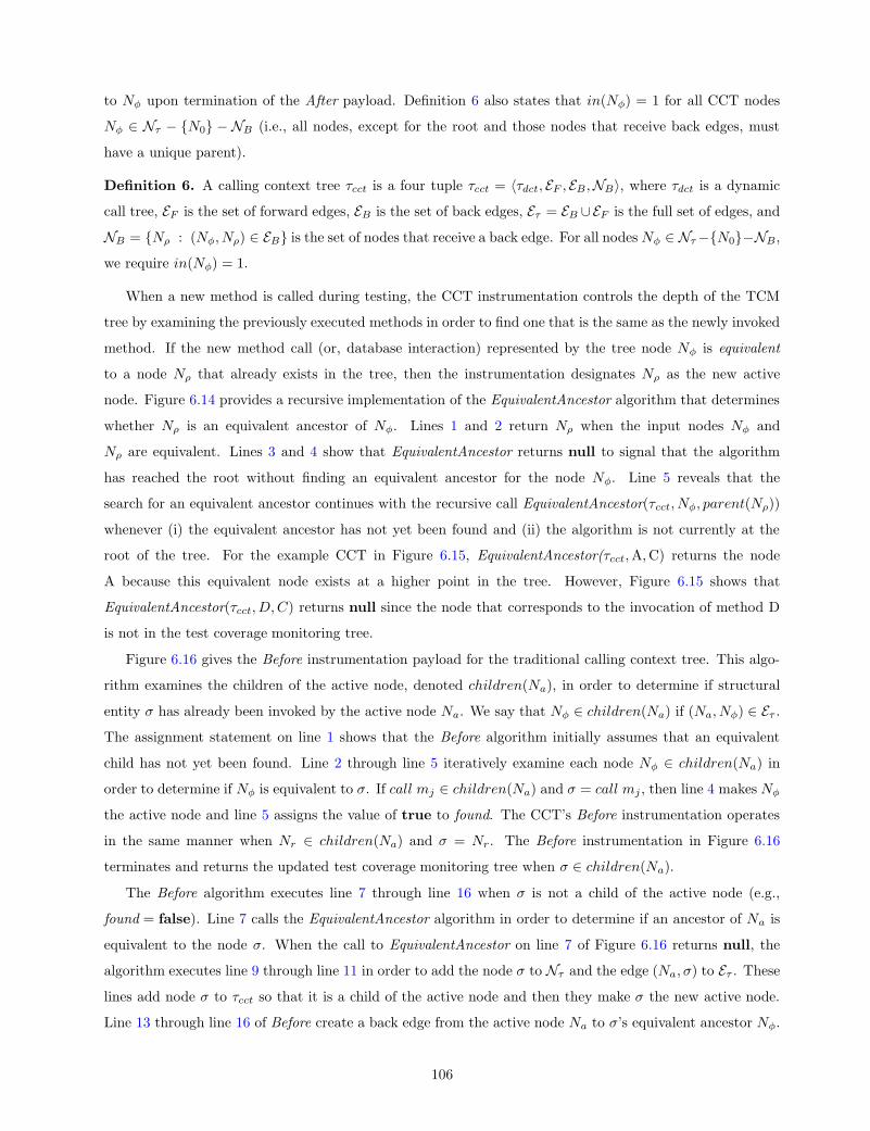
to Nφ upon termination of the After payload. Definition 6 also states that in(Nφ) = 1 for all CCT nodes
Nφ ∈ Nτ − N0 − NB (i.e., all nodes, except for the root and those nodes that receive back edges, must
have a unique parent).
Definition 6. A calling context tree τcct is a four tuple τcct = 〈τdct, EF , EB ,NB〉, where τdct is a dynamic
call tree, EF is the set of forward edges, EB is the set of back edges, Eτ = EB ∪EF is the full set of edges, and
NB = Nρ : (Nφ, Nρ) ∈ EB is the set of nodes that receive a back edge. For all nodes Nφ ∈ Nτ−N0−NB,
we require in(Nφ) = 1.
When a new method is called during testing, the CCT instrumentation controls the depth of the TCM
tree by examining the previously executed methods in order to find one that is the same as the newly invoked
method. If the new method call (or, database interaction) represented by the tree node Nφ is equivalent
to a node Nρ that already exists in the tree, then the instrumentation designates Nρ as the new active
node. Figure 6.14 provides a recursive implementation of the EquivalentAncestor algorithm that determines
whether Nρ is an equivalent ancestor of Nφ. Lines 1 and 2 return Nρ when the input nodes Nφ and
Nρ are equivalent. Lines 3 and 4 show that EquivalentAncestor returns null to signal that the algorithm
has reached the root without finding an equivalent ancestor for the node Nφ. Line 5 reveals that the
search for an equivalent ancestor continues with the recursive call EquivalentAncestor(τcct, Nφ, parent(Nρ))
whenever (i) the equivalent ancestor has not yet been found and (ii) the algorithm is not currently at the
root of the tree. For the example CCT in Figure 6.15, EquivalentAncestor(τcct, A, C) returns the node
A because this equivalent node exists at a higher point in the tree. However, Figure 6.15 shows that
EquivalentAncestor(τcct, D, C) returns null since the node that corresponds to the invocation of method D
is not in the test coverage monitoring tree.
Figure 6.16 gives the Before instrumentation payload for the traditional calling context tree. This algo-
rithm examines the children of the active node, denoted children(Na), in order to determine if structural
entity σ has already been invoked by the active node Na. We say that Nφ ∈ children(Na) if (Na, Nφ) ∈ Eτ .
The assignment statement on line 1 shows that the Before algorithm initially assumes that an equivalent
child has not yet been found. Line 2 through line 5 iteratively examine each node Nφ ∈ children(Na) in
order to determine if Nφ is equivalent to σ. If call mj ∈ children(Na) and σ = call mj , then line 4 makes Nφ
the active node and line 5 assigns the value of true to found. The CCT’s Before instrumentation operates
in the same manner when Nr ∈ children(Na) and σ = Nr. The Before instrumentation in Figure 6.16
terminates and returns the updated test coverage monitoring tree when σ ∈ children(Na).
The Before algorithm executes line 7 through line 16 when σ is not a child of the active node (e.g.,
found = false). Line 7 calls the EquivalentAncestor algorithm in order to determine if an ancestor of Na is
equivalent to the node σ. When the call to EquivalentAncestor on line 7 of Figure 6.16 returns null, the
algorithm executes line 9 through line 11 in order to add the node σ to Nτ and the edge (Na, σ) to Eτ . These
lines add node σ to τcct so that it is a child of the active node and then they make σ the new active node.
Line 13 through line 16 of Before create a back edge from the active node Na to σ’s equivalent ancestor Nφ.
106

Algorithm EquivalentAncestor(τcct , Nφ, Nρ)Input: Calling Context Tree τcct = 〈τdct, EF , EB,NB〉;
Calling Context Tree Nodes Nφ and Nρ
Output: Equivalent Ancestor Node Nρ
1. if Nφ = Nρ
2. then return Nρ
3. if Nρ = N0
4. then return null5. return EquivalentAncestor(τcct, Nφ, parent(Nρ))
Figure 6.14: The EquivalentAncestor Algorithm for the Calling Context Tree.
A
B D
C E
PSfrag replacements
N6
enter computeVelocity
enter computeVelocity
N6
N6
N7
N7
N8
N8
N10
N8
N16
N10
N11
N11
N12
N12
N18
N16
N18
N18
exit computeVelocity
exit computeVelocity
N6
N1
N1
N2
N2
N3
N3
N1
N1
N4
N4
N5
N5
N6
enter P
enter P
call main
call main
enter main
enter main
enter main
. . .
. . .
call inputCardNumber
call inputCardNumber
call inputPin
call inputCardNumber
call handleError
call handleError
call inputCardNumber
call inputPin
call handleError
call handleError
call inputPin
call inputPin
call inputOperation
call inputOperation
call getAccountBalance
call getAccountBalance
call promptAgain
call inputOperation
call lockAccount
call lockAccount
call promptAgain
call promptAgain
call inputOperation
call promptAgain
. . .
call getAccountBalance
enter getAccountBalance
enter getAccountBalance
N3
N3
N4
N4
N5
N5
N6
N6
N7
N7
N10
N10
N12
N12
N15
N10
N15
N15
exit getAccountBalance
exit getAccountBalance
return getAccountBalance
return lockAccount
. . .
return getAccountBalance
call promptAgain
. . .
exit main
exit main
return main
return main
exit P
exit P
. . .
exit main
enter lockAccount
enter lockAccount
. . .
. . .
exit lockAccount
exit lockAccount
return lockAccount
return lockAccount
exit main
EquivalentAncestor(τcct, A, C)=A
EquivalentAncestor(τcct, D, C)=null
Figure 6.15: Using the EquivalentAncestor Algorithm.
107

Algorithm Before(τcct, σ)Input: Calling Context Tree τcct = 〈τdct, EF , EB,NB〉;
Structural Entity σOutput: Updated Calling Context Tree τcct = 〈τdct, EF , EB,NB〉1. found ← false2. for Nφ ∈ children(Na)3. do if Nφ = σ4. then Na ← Nφ
5. found← true6. if found = false7. then Nφ ← EquivalentAncestor(τ, σ, parent(σ))8. if Nφ = null9. then Nτ ← Nτ ∪ σ10. Eτ ← Eτ ∪ (Na, σ)11. Na ← σ12. else13. Eτ ← Eτ ∪ (Na, Nφ)14. EB ← EB ∪ (Na, Nφ)15. Bφ.push(Na)16. Na ← Nφ
17. return 〈τdct, EF , EB ,NB〉
Figure 6.16: The Before Algorithm for the Calling Context Tree.
Algorithm After(τcct)Input: Calling Context Tree τcct = 〈τdct, EF , EB,NB〉Output: Updated Calling Context Tree τcct = 〈τdct, EF , EB,NB〉1. if Ba.size() > 02. then Na ← Ba.pop()3. else4. Na ← parent(Na)5. return 〈τdct, EF , EB ,NB〉
Figure 6.17: The After Algorithm for the Calling Context Tree.
108

A
B D
C E
PSfrag replacements
N6
enter computeVelocity
enter computeVelocity
N6
N6
N7
N7
N8
N8
N10
N8
N16
N10
N11
N11
N12
N12
N18
N16
N18
N18
exit computeVelocity
exit computeVelocity
N6
N1
N1
N2
N2
N3
N3
N1
N1
N4
N4
N5
N5
N6
enter P
enter P
call main
call main
enter main
enter main
enter main
. . .
. . .
call inputCardNumber
call inputCardNumber
call inputPin
call inputCardNumber
call handleError
call handleError
call inputCardNumber
call inputPin
call handleError
call handleError
call inputPin
call inputPin
call inputOperation
call inputOperation
call getAccountBalance
call getAccountBalance
call promptAgain
call inputOperation
call lockAccount
call lockAccount
call promptAgain
call promptAgain
call inputOperation
call promptAgain
. . .
call getAccountBalance
enter getAccountBalance
enter getAccountBalance
N3
N3
N4
N4
N5
N5
N6
N6
N7
N7
N10
N10
N12
N12
N15
N10
N15
N15
exit getAccountBalance
exit getAccountBalance
return getAccountBalance
return lockAccount
. . .
return getAccountBalance
call promptAgain
. . .
exit main
exit main
return main
return main
exit P
exit P
. . .
exit main
enter lockAccount
enter lockAccount
. . .
. . .
exit lockAccount
exit lockAccount
return lockAccount
return lockAccount
exit main
(a)
E
C
PSfrag replacements
N6
enter computeVelocity
enter computeVelocity
N6
N6
N7
N7
N8
N8
N10
N8
N16
N10
N11
N11
N12
N12
N18
N16
N18
N18
exit computeVelocity
exit computeVelocity
N6
N1
N1
N2
N2
N3
N3
N1
N1
N4
N4
N5
N5
N6
enter P
enter P
call main
call main
enter main
enter main
enter main
. . .
. . .
call inputCardNumber
call inputCardNumber
call inputPin
call inputCardNumber
call handleError
call handleError
call inputCardNumber
call inputPin
call handleError
call handleError
call inputPin
call inputPin
call inputOperation
call inputOperation
call getAccountBalance
call getAccountBalance
call promptAgain
call inputOperation
call lockAccount
call lockAccount
call promptAgain
call promptAgain
call inputOperation
call promptAgain
. . .
call getAccountBalance
enter getAccountBalance
enter getAccountBalance
N3
N3
N4
N4
N5
N5
N6
N6
N7
N7
N10
N10
N12
N12
N15
N10
N15
N15
exit getAccountBalance
exit getAccountBalance
return getAccountBalance
return lockAccount
. . .
return getAccountBalance
call promptAgain
. . .
exit main
exit main
return main
return main
exit P
exit P
. . .
exit main
enter lockAccount
enter lockAccount
. . .
. . .
exit lockAccount
exit lockAccount
return lockAccount
return lockAccount
exit main
(b)
Dynamic Call Chain: A → B → C → A → D → E → A
Figure 6.18: The (a) CCT with Back Edges and (b) Corresponding Active Back Edge Stack.
We also push the node Na onto Nφ’s active back edge stack Bφ and establish Nφ as the new active node.
Figure 6.18 illustrates how the the Before instrumentation manipulates the active back edge stack and adds
in the back edges. This figure shows a simple CCT and the active back edge stack after the execution of the
method call chain A → B → C → A → D → E → A during testing. Since E is at the top of BA, the After
instrumentation in Figure 6.17 will make node E the active node when it re-traces the back edge (E,A) (i.e.,
BA ensures that After follows the back edge (E,A) before it re-traces the edge (C,A)).
If we assume that line 8 through line 16 of Before execute in constant time, then the Before instru-
mentation payload in Figure 6.16 has a worst-case time complexity of O(|children(Na)| + depth(Na)). We
recursively define the depth function so that depth(N0) = 0 and depth(Nφ) = 1 + depth(parent(Nφ)). The
term |children(Na)| corresponds to the execution of line 2 through line 5. This worst-case time complexity
holds when line 1 through line 4 of Figure 6.14 execute in constant time and the EquivalentAncestor al-
gorithm is recursively invoked depth(Na) + 1 times. The worst-case behavior of EquivalentAncestor occurs
when the root is equivalent to σ, or τcct does not contain an equivalent ancestor for σ. Even though the
time overhead associated with executing Before is greater for the CCT than for the DCT, the CCT’s Before
instrumentation yields smaller TCM trees that have bounded breadth and depth [Ammons et al., 1997].
The CCT has bounded depth because it coalesces nodes and uses back edges when methods are recursively
invoked during testing (e.g., line 13 through line 16 in Figure 6.16). The CCT has bounded breadth since
it coalesces nodes when testing causes the iterative invocation of methods (e.g., line 2 through line 5 of
Figure 6.16). Like the DCT’s instrumentation, the After payload for a CCT is also O(1).
109

Test Case
Method Invocation
Database Interaction Point
Database
Relation
Attribute Record
Attribute Value
PSfrag replacements
N6
enter computeVelocity
enter computeVelocity
N6
N6
N7
N7
N8
N8
N10
N8
N16
N10
N11
N11
N12
N12
N18
N16
N18
N18
exit computeVelocity
exit computeVelocity
N6
N1
N1
N2
N2
N3
N3
N1
N1
N4
N4
N5
N5
N6
enter P
enter P
call main
call main
enter main
enter main
enter main
. . .
. . .
call inputCardNumber
call inputCardNumber
call inputPin
call inputCardNumber
call handleError
call handleError
call inputCardNumber
call inputPin
call handleError
call handleError
call inputPin
call inputPin
call inputOperation
call inputOperation
call getAccountBalance
call getAccountBalance
call promptAgain
call inputOperation
call lockAccount
call lockAccount
call promptAgain
call promptAgain
call inputOperation
call promptAgain
. . .
call getAccountBalance
enter getAccountBalance
enter getAccountBalance
N3
N3
N4
N4
N5
N5
N6
N6
N7
N7
N10
N10
N12
N12
N15
N10
N15
N15
exit getAccountBalance
exit getAccountBalance
return getAccountBalance
return lockAccount
. . .
return getAccountBalance
call promptAgain
. . .
exit main
exit main
return main
return main
exit P
exit P
. . .
exit main
enter lockAccount
enter lockAccount
. . .
. . .
exit lockAccount
exit lockAccount
return lockAccount
return lockAccount
exit main
Figure 6.19: The Structure of a Database-Aware TCM Tree.
6.4.3 Database-Aware Trees
The traditional Before and After instrumentation from Section 6.4.2 does not include functionality to observe
a database interaction and update the TCM tree. The test coverage monitor also creates a database inter-
action dynamic call tree (DI-DCT) or a database interaction calling context tree (DI-CCT). These database-
aware trees still respectively adhere to Definitions 5 and 6. However, the nodes within a DI-DCT or DI-CCT
correspond to a (i) method invocation, (ii) definition of a database entity, or (iii) use of a database entity.
The instrumentation can insert database entity nodes into the tree at all levels of interaction granularity, as
described in Figure 6.19.
Following the convention that we established in Figure 6.8, we use bold edges to connect two database
entity nodes. If a node Nφ ∈ Nτ has the database interaction node Nr ∈ Nτ as its ancestor, then Nφ must
correspond to the definition or use of a database entity. Figure 6.19 reveals that a database node must
have an interaction node as its parent and a relation node is always a child of a database node. Figure 6.19
also shows that we place attribute value nodes below the record that contains the attribute value and the
attribute nodes are children of the containing relation. We structure a TCM tree in this manner because it
ensures the correct calculation of database-aware adequacy for each test and the entire test suite. Table A10
summarizes the notation that we use to describe the database-aware instrumentation.
6.4.3.1 Instrumentation to Monitor a Database Use Figure 6.23 provides the BeforeDatabaseUse
instrumentation payload. The test coverage monitor executes this payload before the use of a database by
either a program or a test suite. The program uses the database when it executes a SQL select statement.
110

PSfrag replacements
N6
enter computeVelocity
enter computeVelocity
N6
N6
N7
N7
N8
N8
N10
N8
N16
N10
N11
N11
N12
N12
N18
N16
N18
N18
exit computeVelocity
exit computeVelocity
N6
N1
N1
N2
N2
N3
N3
N1
N1
N4
N4
N5
N5
N6
enter P
enter P
call main
call main
enter main
enter main
enter main
. . .
. . .
call inputCardNumber
call inputCardNumber
call inputPin
call inputCardNumber
call handleError
call handleError
call inputCardNumber
call inputPin
call handleError
call handleError
call inputPin
call inputPin
call inputOperation
call inputOperation
call getAccountBalance
call getAccountBalance
call promptAgain
call inputOperation
call lockAccount
call lockAccount
call promptAgain
call promptAgain
call inputOperation
call promptAgain
. . .
call getAccountBalance
enter getAccountBalance
enter getAccountBalance
N3
N3
N4
N4
N5
N5
N6
N6
N7
N7
N10
N10
N12
N12
N15
N10
N15
N15
exit getAccountBalance
exit getAccountBalance
return getAccountBalance
return lockAccount
. . .
return getAccountBalance
call promptAgain
. . .
exit main
exit main
return main
return main
exit P
exit P
. . .
exit main
enter lockAccount
enter lockAccount
. . .
. . .
exit lockAccount
exit lockAccount
return lockAccount
return lockAccount
exit main
Id : fsmdynamic.ladot, v1.22006/08/0302 : 48 : 33gkapfhamExp
Revision : 1.2
S
relj
Al : Al ∈ attr(S) ∧ Al ∈ attr(relj)S
relj
HR:A Al : Al ∈ attr(S) ∧ Al ∈ attr(relj)
Figure 6.20: The Function that Maps Relations to Attributes.
PSfrag replacements
N6
enter computeVelocity
enter computeVelocity
N6
N6
N7
N7
N8
N8
N10
N8
N16
N10
N11
N11
N12
N12
N18
N16
N18
N18
exit computeVelocity
exit computeVelocity
N6
N1
N1
N2
N2
N3
N3
N1
N1
N4
N4
N5
N5
N6
enter P
enter P
call main
call main
enter main
enter main
enter main
. . .
. . .
call inputCardNumber
call inputCardNumber
call inputPin
call inputCardNumber
call handleError
call handleError
call inputCardNumber
call inputPin
call handleError
call handleError
call inputPin
call inputPin
call inputOperation
call inputOperation
call getAccountBalance
call getAccountBalance
call promptAgain
call inputOperation
call lockAccount
call lockAccount
call promptAgain
call promptAgain
call inputOperation
call promptAgain
. . .
call getAccountBalance
enter getAccountBalance
enter getAccountBalance
N3
N3
N4
N4
N5
N5
N6
N6
N7
N7
N10
N10
N12
N12
N15
N10
N15
N15
exit getAccountBalance
exit getAccountBalance
return getAccountBalance
return lockAccount
. . .
return getAccountBalance
call promptAgain
. . .
exit main
exit main
return main
return main
exit P
exit P
. . .
exit main
enter lockAccount
enter lockAccount
. . .
. . .
exit lockAccount
exit lockAccount
return lockAccount
return lockAccount
exit main
Id : fsmdynamic.ladot, v1.22006/08/0302 : 48 : 33gkapfhamExp
Revision : 1.2
S
relj
tk : tk ∈ S ∧ tk ∈ reljS
relj
HR:Rc tk : Al ∈ HR:A(S, relj) ∧ tk[l] ∈ relj ∧ tk[l] ∈ S
Figure 6.21: The Function that Maps Relations to Records.
A test suite uses the database when it executes an oracle to compare the actual and expected database
states. Figure B3 of Appendix B provides a test case that uses a database-aware test oracle to compare
the expected and actual state of the HomeworkMaster relation in the GradeBook database. Figure 6.23
shows that BeforeDatabaseUse returns the test coverage monitoring tree that Before(τ, Nr) outputs. The
call to Before(τ, Nr) places node Nr into the TCM tree and establishes this node as the parent for all of the
database entity nodes that the instrumentation subsequently adds. The database-aware payloads invoke the
appropriate Before and After instrumentation algorithms based upon the type of the TCM tree τ . If τ is a
DCT, then BeforeDatabaseUse runs the Before instrumentation given in Figure 6.12. Alternatively, if τ is a
CCT, then line 1 of Figure 6.23 executes the Before algorithm from Figure 6.16.
Figure 6.24 furnishes the AfterDatabaseUse instrumentation that determines how a SQL select statement
uses the database. Since a select can specify attributes from multiple relations, its result set S can contain
records whose attribute values are derived from one or more relations in the database. For example, the SQL
statement “select Al, Al from relj , relj where P” will yield a result set S that mixes attribute values from
relations relj and relj (for the purpose of illustration, we assume that Al is an attribute of relj , relation relj
contains Al, and P is an arbitrary predicate whose form we defined in Figure 2.1 of Chapter 2). In order
to support the correct calculation of database-aware test adequacy, the instrumentation must determine
the containing record and relation for each attribute value in the result set. For example, if relation relj
contains attribute Al and S includes an attribute value from Al, then the TCM tree must have the edge
(〈relj ,use〉, 〈Al,use〉) in order to indicate that this relation and attribute were used during testing.
AfterDatabaseUse uses the functions HR:A and HR:Rc, as respectively defined by Figure 6.20 and Fig-
ure 6.21, to identify the attributes and records that S contains. Figure 6.20 shows that HR:A returns the set
111

of all attributes Al that exist in both the result set S and the specified relation relj . We use the notation
attr(S) and attr(relj) to denote the set of attributes that are associated with S and relj , respectively. Fig-
ure 6.21 reveals that HR:Rcoutputs the set of records tk that have an attribute value tk[l] inside of both the
result set S and the relation relj . Figure 6.22 provides an example of the input and output of the functions
HR:A and HR:Rc. The execution of the SQL select statement in Figure 6.22 yields the result set S that
contains two records. In this example, HR:A(S, relj) outputs Al because this is the only attribute that is
in both the input result set and the relation. HR:A(S, relj) does not return the attribute Al because this
attribute exists in the relation relj . The function HR:Rc(S, relj) returns t1, t3 since the attribute values
from these records in relj are also in S. HR:Rc(S, relj) does not output the record t2 since it is not in S.
Figure 6.22 confirms that the functions HR:A and HR:Rcoperate in an analogous fashion when they analyze
the result set S and the relation relj .
The AfterDatabaseUse(τ, Nr,S,L) payload in Figure 6.24 analyzes result set S in order to updates tree
τ after the execution of the database interaction at node Nr. The input function L(τ) returns the levels
of database interaction granularity at which we represent node Nr’s interaction. Following the convention
established in Chapter 5, we require that L(τ) ⊆ D,R,A,Rc,Av. If D ∈ L(τ), then the database-aware
payloads must include nodes to represent the definition and/or use of the database. When Av ∈ L(τ)
these payloads create TCM trees with nodes that represent an interaction at the attribute value level.
AfterDatabaseUse uses GetDatabase to determine which database is subject to interaction at Nr.
Since HR:A and HR:Rcaccept a relation as one of the two inputs, the AfterDatabaseUse payload also uses
the relations(S) operation to determine which relations have records in the specified result set. Figure 6.22
shows that relations(S) = relj , relj for the example SQL select statement. The test coverage monitor uses
the Java class java.sql.ResultSetMetaData to implement HR:A, HR:Rc, attr(S), and relations(S). For ex-
ample, this Java class provides methods such as getTableName and getColumnName. The getTableName(int
l) method returns the relation relj that contains the attribute Al and getColumnName(int l) returns the
fully qualified name for attribute Al. The test coverage monitor determines the output of attr(relj) by
consulting the relational schema for the current database.
Line 1 of Figure 6.24 initializes the variable op to use since the AfterDatabaseUse payload analyzes
a database interaction point that submits a select statement. If D ∈ L(τ), then line 4 creates node
ND = 〈Df , op〉 and line 5 executes Before(τ, ND). If a tester specifies that τ should contain relation nodes
(i.e., R ∈ L(τ)), then line 7 through line 9 iteratively create node NR = 〈relj , op〉 and add it to the TCM
tree for each relation relj ∈ relations(S). Figure 6.19 shows that the test coverage monitor places attribute
nodes below the relation node NR. Thus, AfterDatabaseUse executes line 10 through 14 in order to iteratively
place node NA = 〈Al, op〉 into τ for each attribute Al ∈ HR:A(S, relj). The use of HR:A ensures that the
parent of NA is the node for the relation relj that specifies attribute Al (i.e., node NR).
When Rc ∈ L(τ), line 16 through line 18 call Before(τ, NRc) in order to place a node NRc
= 〈tk, op〉
into τ for each record tk in the current relation relj . We use the function HR:Rcin order to guarantee
112

PSfrag replacements
N6
enter computeVelocity
enter computeVelocity
N6
N6
N7
N7
N8
N8
N10
N8
N16
N10
N11
N11
N12
N12
N18
N16
N18
N18
exit computeVelocity
exit computeVelocity
N6
N1
N1
N2
N2
N3
N3
N1
N1
N4
N4
N5
N5
N6
enter P
enter P
call main
call main
enter main
enter main
enter main
. . .
. . .
call inputCardNumber
call inputCardNumber
call inputPin
call inputCardNumber
call handleError
call handleError
call inputCardNumber
call inputPin
call handleError
call handleError
call inputPin
call inputPin
call inputOperation
call inputOperation
call getAccountBalance
call getAccountBalance
call promptAgain
call inputOperation
call lockAccount
call lockAccount
call promptAgain
call promptAgain
call inputOperation
call promptAgain
. . .
call getAccountBalance
enter getAccountBalance
enter getAccountBalance
N3
N3
N4
N4
N5
N5
N6
N6
N7
N7
N10
N10
N12
N12
N15
N10
N15
N15
exit getAccountBalance
exit getAccountBalance
return getAccountBalance
return lockAccount
. . .
return getAccountBalance
call promptAgain
. . .
exit main
exit main
return main
return main
exit P
exit P
. . .
exit main
enter lockAccount
enter lockAccount
. . .
. . .
exit lockAccount
exit lockAccount
return lockAccount
return lockAccount
exit main
t1
t2
t3
. . .
tu−2
tu−1
tu
. . .
Al
. . .
t1
1
. . .
Al
. . .
t1
t2
t3
. . . Al
1
2
3
. . .. . .
relj
PSfrag replacements
N6
enter computeVelocity
enter computeVelocity
N6
N6
N7
N7
N8
N8
N10
N8
N16
N10
N11
N11
N12
N12
N18
N16
N18
N18
exit computeVelocity
exit computeVelocity
N6
N1
N1
N2
N2
N3
N3
N1
N1
N4
N4
N5
N5
N6
enter P
enter P
call main
call main
enter main
enter main
enter main
. . .
. . .
call inputCardNumber
call inputCardNumber
call inputPin
call inputCardNumber
call handleError
call handleError
call inputCardNumber
call inputPin
call handleError
call handleError
call inputPin
call inputPin
call inputOperation
call inputOperation
call getAccountBalance
call getAccountBalance
call promptAgain
call inputOperation
call lockAccount
call lockAccount
call promptAgain
call promptAgain
call inputOperation
call promptAgain
. . .
call getAccountBalance
enter getAccountBalance
enter getAccountBalance
N3
N3
N4
N4
N5
N5
N6
N6
N7
N7
N10
N10
N12
N12
N15
N10
N15
N15
exit getAccountBalance
exit getAccountBalance
return getAccountBalance
return lockAccount
. . .
return getAccountBalance
call promptAgain
. . .
exit main
exit main
return main
return main
exit P
exit P
. . .
exit main
enter lockAccount
enter lockAccount
. . .
. . .
exit lockAccount
exit lockAccount
return lockAccount
return lockAccount
exit main
t1
t2
t3
t4
. . . Al
A
B
C
D
. . .. . .
relj
PSfrag replacements
N6
enter computeVelocity
enter computeVelocity
N6
N6
N7
N7
N8
N8
N10
N8
N16
N10
N11
N11
N12
N12
N18
N16
N18
N18
exit computeVelocity
exit computeVelocity
N6
N1
N1
N2
N2
N3
N3
N1
N1
N4
N4
N5
N5
N6
enter P
enter P
call main
call main
enter main
enter main
enter main
. . .
. . .
call inputCardNumber
call inputCardNumber
call inputPin
call inputCardNumber
call handleError
call handleError
call inputCardNumber
call inputPin
call handleError
call handleError
call inputPin
call inputPin
call inputOperation
call inputOperation
call getAccountBalance
call getAccountBalance
call promptAgain
call inputOperation
call lockAccount
call lockAccount
call promptAgain
call promptAgain
call inputOperation
call promptAgain
. . .
call getAccountBalance
enter getAccountBalance
enter getAccountBalance
N3
N3
N4
N4
N5
N5
N6
N6
N7
N7
N10
N10
N12
N12
N15
N10
N15
N15
exit getAccountBalance
exit getAccountBalance
return getAccountBalance
return lockAccount
. . .
return getAccountBalance
call promptAgain
. . .
exit main
exit main
return main
return main
exit P
exit P
. . .
exit main
enter lockAccount
enter lockAccount
. . .
. . .
exit lockAccount
exit lockAccount
return lockAccount
return lockAccount
exit main
Al
1
3
Al
A
D
S
select Al, Al
from relj , relj
where P
relations(S) = relj , relj
HR:A(S, relj) = Al
HR:Rc(S, relj) = t1, t3
HR:A(S, relj) = Al
HR:Rc(S, relj) = t1, t4
Figure 6.22: Example of the Functions that Analyze a Result Set.
113

Algorithm BeforeDatabaseUse(τ, Nr)Input: Test Coverage Monitoring Tree τ ;
Database Interaction Point Nr
Output: Updated Test Coverage Monitoring Tree τ1. return Before(τ, Nr)
Figure 6.23: The BeforeDatabaseUse Algorithm.
Algorithm AfterDatabaseUse(τ, Nr,S,L)Input: Test Coverage Monitoring Tree τ ;
Database Interaction Point Nr;Database Interaction Result Set S;Levels for Representing a Database Interaction L
Output: Updated Test Coverage Monitoring Tree τ1. op← use2. Df ←GetDatabase(Nr )3. if D ∈ L(τ )4. then ND ← 〈Df , op〉5. Before(τ, ND)6. if R ∈ L(τ )7. then for relj ∈ relations(S)8. do NR ← 〈relj , op〉9. Before(τ, NR)10. if A ∈ L(τ )11. then for Al ∈ HR:A(S, relj)12. do NA ← 〈Al, op〉13. Before(τ, NA)14. After(τ )15. if Rc ∈ L(τ )16. then for tk ∈ HR:Rc(S, relj)17. do NRc ← 〈tk, op〉18. Before(τ, NRc )19. if Av ∈ L(τ )20. then for Al ∈ HR:A(S, relj)21. do NAv ← 〈tk[l], op〉22. Before(τ, NAv )23. After(τ )24. After(τ )25. After(τ )26. After(τ )27. After(τ )28. return τ
Figure 6.24: The AfterDatabaseUse Algorithm.
114

that an edge (NR, RRc) ∈ Eτ corresponds to the use of a record tk that (i) exists in the relation relj and
(ii) has one or more attribute values tk[l] in the result set S. Line 20 through line 23 of AfterDatabaseUse
invoke Before(τ, NAv) and After(τ) to insert node NAv
into the TCM tree for each attribute value tk[l] in
the current record. The instrumentation always follows a call to Before(τ, NAv) with an immediate call to
After(τ) because the attribute value nodes are leaves of the test coverage monitoring tree (i.e., out(NAv) = 0
for all attribute value nodes NAv). The AfterDatabaseUse instrumentation orders all of the calls to the Before
and After probes so that the coverage monitoring tree adheres to the structure prescribed by Figure 6.19.
6.4.3.2 Instrumentation to Monitor a Database Definition Figure 6.29’s BeforeDatabaseDefine
algorithm uses the GetRelation(Nr) operation to parse the SQL command that Nr submits to the RDBMS.
The GetDatabase and GetRelation operations use a regular expression-based parser to identify these syntac-
tical elements in the intercepted SQL statement. After GetRelation parses the intercepted SQL statement
and identifies relj as the relation subject to definition, it executes a select to extract relj ’s state. Once
this payload has stored relj , it returns the output of Before(τ, Nr) and passes control back to the program
under test. The AfterDatabaseDefine algorithm in Figure 6.30 extracts the state of the same relation after
the program under test executes a SQL update, insert, or delete command.
We use the symmetric relational difference (SRD) operator⊗
Rcto determine the difference between
relation relj (i.e., the relation before the execution of the interaction at Nr) and relj′ (i.e., the rela-
tion after the execution of the defining interaction). If there is a need to discern the difference between
the database record tk in the relations relj and relj′ , then we use the symmetric attribute value differ-
ence (SAVD) operator⊗
Av. The TCM component uses the difference operators because they enable the
instrumentation to accurately identify changes in a relation without relying upon RDBMS-specific func-
tions such as triggers. Previously developed data change detection techniques (e.g., [Chawathe et al., 1996,
Chawathe and Garcia-Molina, 1997, Labio and Garcia-Molina, 1996]) do not support test coverage moni-
toring because of their (i) focus on non-relational data or (ii) use of lossy compression algorithms. Since
the change detectors described in [Chawathe et al., 1996, Chawathe and Garcia-Molina, 1997] operate on
rooted trees with node labels, they do not fit our use of the relational data model. We could not use the
relational differencing system developed in [Labio and Garcia-Molina, 1996] because this approach uses lossy
compression to handle database snapshots that do not fit into memory. Since this scheme can overlook a
database modification, it might yield an incorrect coverage report and thus lead to improper test adequacy
measurements. To this end, the test coverage monitoring framework uses a database-aware extension of the
Myers difference algorithm in the implementation of the SRD and SAVD operators [Myers, 1986].
The following Equation (6.1) defines the⊗
Rcoperator that considers the contents of the records in two
database relations relj and relj′ and returns those records whose contents differ. We use \Rcto denote the
set difference operator that outputs the records that vary in the two input relations. Equation (6.2) defines
the⊗
Avoperator that examines two database records tk and tk′ in order to return the attribute values that
115

differ. The symbol \Avstands for the set difference operator that isolates the attribute values that are not the
same in the two input records. The SRD and SAVD operators allow the AfterDatabaseDefine instrumentation
payload to precisely determine how the database interaction changes the state of the database. Table A11
in Appendix A reviews the meaning and purpose of the relational difference operators.
relj⊗
Rc
relj′ = (relj \Rcrelj′ ) ∪ (relj′ \Rc
relj) (6.1)
tk ∈ relj⊗
Av
tk′ ∈ relj′ = (tk \Avtk′) ∪ (tk′ \Av
tk) (6.2)
Figure 6.25 shows the output of the SRD and SAVD operators when an update statement defines the
database. In this example, the update changes the value of t2[2] from 3 to 4. The SRD operator differs
from the traditional symmetric difference operator because it uses \Rcinstead of the set theoretic difference
operator \ (i.e., \Rcoutputs a record tk instead of the contents of the record 〈tk[1], . . . , tk[q]〉). Figure 6.25
reveals that relj \Rcrelj′ returns t2 instead of 〈t2[1], t2[2]〉, as returned by the set difference operator. After
the SRD operator isolates t2 as the modified record, we use⊗
Avto find t2[2], the specific attribute value
that was modified by the update statement. Unlike the traditional symmetric difference operator, the SAVD
operator identifies the modified attribute value instead of the different values of tk[l] in the two relations. For
this example, the symmetric difference of tk ∈ relj and tk ∈ relj′ would return (t2[2], 3), (t2[2], 4) instead
of determining that t2[2] was the only modified attribute value.
Figure 6.26 explains how the database-aware difference operators determine which record a SQL insert
statement adds to the database. In this example, the SRD operator returns t4 ∈ relj′ because this record
does not exist in relation relj . Since the insert statement places tk into the database, the SAVD operator
must return all of the attribute values within this record. The example in Figure 6.27 demonstrates that the
database-aware difference operators can also identify the record and attribute values that are removed from
relation relj by a SQL delete statement. Finally, Figure 6.28 shows that we can use the SRD and SAVD
operators determine how a SQL statement defines multiple locations within a relation. In this example, a
SQL update changes t1[2] to 22 and t2[1] to 3. The update also modifies both of the attribute values in
record t3. Figure 6.28 reveals that the use of the⊗
Avoperator for each record tk ∈ relj
⊗Rc
relj′ finds
each attribute value that the SQL statement defined.
Line 1 of Figure 6.30 initializes the variable op to define since the AfterDatabaseDefine analyzes an
interaction that submits a SQL update, insert, or delete statement. Line 2 determines that Nr interacts
with database Df and line 3 stores the state of the defined relation in relation relj′ . If D ∈ L(τ), then
line 5 creates the node ND = 〈Df , op〉 and line 6 calls Before(τ, ND). If a tester specifies that τ should
contain nodes concerning the definition of relations (i.e., R ∈ L(τ)), then line 8 through line 9 iteratively
construct node Nr = 〈relj , op〉 and place it in the TCM tree (the coverage monitoring framework ensures
that AfterDatabaseDefine has access to the relj that BeforeDatabaseDefine stored). Line 10 initializes the
116

set Adef to the empty set. We use this set to store all of the attributes that are subject to definition at node
Nr. AfterDatabaseDefine identifies each Al ∈ Adef through the iterative application of⊗
Rcand
⊗Av
on
line 12 through line 21.
If Rc ∈ L(τ), then line 12 applies the SRD operator to the relations relj and relj′ . Lines 13 and 14 of
Figure 6.30 create node NRc= 〈tk, op〉 and place it into the tree by calling Before(τ, NRc
). If Av ∈ L(τ),
then AfterDatabaseDefine uses the SAVD operator to determine which attribute values tk[l] were defined by
the SQL statement. Line 17 through line 20 construct the defining node NAv= 〈tk[l], op〉 and use calls to
Before and After to put this node into τ . These lines of the payload also add Al to Adef for each attribute
value tk[l]. The repeated execution of line 18 for the same attribute Al does not change the contents of Adef
since it is a set. Finally, line 22 through line 26 insert each the attribute definition node NA = 〈Al, op〉 so
that parent(NA) = NR. The AfterDatabaseDefine payload must also execute line 12 through line 21 when
A ∈ L(τ) because the instrumentation can only identify Adef by applying the SRD and SAVD operators. This
is due to the fact that the defined attributes can vary for each record tk ∈ relj⊗
Rcrelj′ (e.g., Figure 6.28
reveals that attribute A1 is defined in t1 and both attribute A1 and A2 are defined in t2).
6.4.3.3 Worst-Case Time Complexity We characterize the worst-case time complexity of Before-
DatabaseUse, AfterDatabaseUse, BeforeDatabaseDefine, and AfterDatabaseDefine in this chapter and we
empirically evaluate the performance of the coverage monitor in Chapter 7. Table A12 summarizes the
notation that we develop in this section. Since a database-aware instrumentation probe always requires the
execution of Before and After, we consider a call to one of these traditional probes as the basic operation
(we do not incorporate the time complexity of the DCT and CCT creation probes in the complexities that
we develop here). For simplicity, these worst-case time complexities assume a fixed database Df (relaxing
this assumption simply requires that we redefine each time complexity variable as the maximum across all
databases). Our worst-case analysis of each database-aware algorithm also assumes that the TCM tree τ will
represent each database interaction at all levels of granularity (i.e., L(τ) = D,R,A,Rc,Av). We classify
the BeforeDatabaseUse algorithm in Figure 6.23 as O(1) because it simply invokes the Before instrumentation
probe that also has a constant worst-case time complexity.
Figure 6.24 shows that the execution time of AfterDatabaseUse depends upon the time overhead of the
relations operation and the HR:A and HR:Rcfunctions. Since we implement each of these operations using a
hash table, we assume that their worst-case time complexity is O(1). The AfterDatabaseUse instrumentation
probe is O(Wf×MR:A+Wf×MR:A×MR:Rc) whereWf stands for the total number of relations in database
Df , as previously defined in Chapter 5.2 The following Equation (6.3) definesMR:A, the maximum number
of attributes in both the relation relj and the result set S. The maximal value ofMR:A occurs when the SQL
select statement requests all of the attributes from a relation in database Df . The time complexity term
Wf ×MR:A corresponds to the iterative execution of line 7 through line 14 in Figure 6.24. The following
2Simplification of this time complexity yields O((Wf ×MR:A) + (1 +MR:Rc)). We do not use this time complexity in ourdiscussion of AfterDatabaseUse because it does not closely adhere to the probe’s structure.
117

PSfrag replacements
N6
enter computeVelocity
enter computeVelocity
N6
N6
N7
N7
N8
N8
N10
N8
N16
N10
N11
N11
N12
N12
N18
N16
N18
N18
exit computeVelocity
exit computeVelocity
N6
N1
N1
N2
N2
N3
N3
N1
N1
N4
N4
N5
N5
N6
enter P
enter P
call main
call main
enter main
enter main
enter main
. . .
. . .
call inputCardNumber
call inputCardNumber
call inputPin
call inputCardNumber
call handleError
call handleError
call inputCardNumber
call inputPin
call handleError
call handleError
call inputPin
call inputPin
call inputOperation
call inputOperation
call getAccountBalance
call getAccountBalance
call promptAgain
call inputOperation
call lockAccount
call lockAccount
call promptAgain
call promptAgain
call inputOperation
call promptAgain
. . .
call getAccountBalance
enter getAccountBalance
enter getAccountBalance
N3
N3
N4
N4
N5
N5
N6
N6
N7
N7
N10
N10
N12
N12
N15
N10
N15
N15
exit getAccountBalance
exit getAccountBalance
return getAccountBalance
return lockAccount
. . .
return getAccountBalance
call promptAgain
. . .
exit main
exit main
return main
return main
exit P
exit P
. . .
exit main
enter lockAccount
enter lockAccount
. . .
. . .
exit lockAccount
exit lockAccount
return lockAccount
return lockAccount
exit main
t1
t2
t3
A1
1
2
3
A2
2
2 3
3 4
relj
PSfrag replacements
N6
enter computeVelocity
enter computeVelocity
N6
N6
N7
N7
N8
N8
N10
N8
N16
N10
N11
N11
N12
N12
N18
N16
N18
N18
exit computeVelocity
exit computeVelocity
N6
N1
N1
N2
N2
N3
N3
N1
N1
N4
N4
N5
N5
N6
enter P
enter P
call main
call main
enter main
enter main
enter main
. . .
. . .
call inputCardNumber
call inputCardNumber
call inputPin
call inputCardNumber
call handleError
call handleError
call inputCardNumber
call inputPin
call handleError
call handleError
call inputPin
call inputPin
call inputOperation
call inputOperation
call getAccountBalance
call getAccountBalance
call promptAgain
call inputOperation
call lockAccount
call lockAccount
call promptAgain
call promptAgain
call inputOperation
call promptAgain
. . .
call getAccountBalance
enter getAccountBalance
enter getAccountBalance
N3
N3
N4
N4
N5
N5
N6
N6
N7
N7
N10
N10
N12
N12
N15
N10
N15
N15
exit getAccountBalance
exit getAccountBalance
return getAccountBalance
return lockAccount
. . .
return getAccountBalance
call promptAgain
. . .
exit main
exit main
return main
return main
exit P
exit P
. . .
exit main
enter lockAccount
enter lockAccount
. . .
. . .
exit lockAccount
exit lockAccount
return lockAccount
return lockAccount
exit main
t1
t2
t3
A1
1
2
3
A2
2
2
4 4
4
relj′
relj⊗
Rc
relj′ = (relj \Rcrelj′ ) ∪ (relj′ \Rc
relj)
= t2 ∪ t2
= t2
t2 ∈ relj⊗
Av
t2 ∈ relj′ = t2[2]
Figure 6.25: Example of the Database-Aware Difference Operators for the update Statement.
PSfrag replacements
N6
enter computeVelocity
enter computeVelocity
N6
N6
N7
N7
N8
N8
N10
N8
N16
N10
N11
N11
N12
N12
N18
N16
N18
N18
exit computeVelocity
exit computeVelocity
N6
N1
N1
N2
N2
N3
N3
N1
N1
N4
N4
N5
N5
N6
enter P
enter P
call main
call main
enter main
enter main
enter main
. . .
. . .
call inputCardNumber
call inputCardNumber
call inputPin
call inputCardNumber
call handleError
call handleError
call inputCardNumber
call inputPin
call handleError
call handleError
call inputPin
call inputPin
call inputOperation
call inputOperation
call getAccountBalance
call getAccountBalance
call promptAgain
call inputOperation
call lockAccount
call lockAccount
call promptAgain
call promptAgain
call inputOperation
call promptAgain
. . .
call getAccountBalance
enter getAccountBalance
enter getAccountBalance
N3
N3
N4
N4
N5
N5
N6
N6
N7
N7
N10
N10
N12
N12
N15
N10
N15
N15
exit getAccountBalance
exit getAccountBalance
return getAccountBalance
return lockAccount
. . .
return getAccountBalance
call promptAgain
. . .
exit main
exit main
return main
return main
exit P
exit P
. . .
exit main
enter lockAccount
enter lockAccount
. . .
. . .
exit lockAccount
exit lockAccount
return lockAccount
return lockAccount
exit main
t1
t2
t3
A1
1
2
3
A2
2
2 3
3 4
relj
PSfrag replacements
N6
enter computeVelocity
enter computeVelocity
N6
N6
N7
N7
N8
N8
N10
N8
N16
N10
N11
N11
N12
N12
N18
N16
N18
N18
exit computeVelocity
exit computeVelocity
N6
N1
N1
N2
N2
N3
N3
N1
N1
N4
N4
N5
N5
N6
enter P
enter P
call main
call main
enter main
enter main
enter main
. . .
. . .
call inputCardNumber
call inputCardNumber
call inputPin
call inputCardNumber
call handleError
call handleError
call inputCardNumber
call inputPin
call handleError
call handleError
call inputPin
call inputPin
call inputOperation
call inputOperation
call getAccountBalance
call getAccountBalance
call promptAgain
call inputOperation
call lockAccount
call lockAccount
call promptAgain
call promptAgain
call inputOperation
call promptAgain
. . .
call getAccountBalance
enter getAccountBalance
enter getAccountBalance
N3
N3
N4
N4
N5
N5
N6
N6
N7
N7
N10
N10
N12
N12
N15
N10
N15
N15
exit getAccountBalance
exit getAccountBalance
return getAccountBalance
return lockAccount
. . .
return getAccountBalance
call promptAgain
. . .
exit main
exit main
return main
return main
exit P
exit P
. . .
exit main
enter lockAccount
enter lockAccount
. . .
. . .
exit lockAccount
exit lockAccount
return lockAccount
return lockAccount
exit main
t1
t2
t3
t4
A1
1
2
3
4
A2
2
2 3
3 4
4 5
relj′
relj⊗
Rc
relj′ = (relj \Rcrelj′ ) ∪ (relj′ \Rc
relj)
= ∅ ∪ t4
= t4
t4 ∈ relj⊗
Av
t4 ∈ relj′ = t4[1], t4[2]
Figure 6.26: Example of the Database-Aware Difference Operators for the insert Statement.
118

PSfrag replacements
N6
enter computeVelocity
enter computeVelocity
N6
N6
N7
N7
N8
N8
N10
N8
N16
N10
N11
N11
N12
N12
N18
N16
N18
N18
exit computeVelocity
exit computeVelocity
N6
N1
N1
N2
N2
N3
N3
N1
N1
N4
N4
N5
N5
N6
enter P
enter P
call main
call main
enter main
enter main
enter main
. . .
. . .
call inputCardNumber
call inputCardNumber
call inputPin
call inputCardNumber
call handleError
call handleError
call inputCardNumber
call inputPin
call handleError
call handleError
call inputPin
call inputPin
call inputOperation
call inputOperation
call getAccountBalance
call getAccountBalance
call promptAgain
call inputOperation
call lockAccount
call lockAccount
call promptAgain
call promptAgain
call inputOperation
call promptAgain
. . .
call getAccountBalance
enter getAccountBalance
enter getAccountBalance
N3
N3
N4
N4
N5
N5
N6
N6
N7
N7
N10
N10
N12
N12
N15
N10
N15
N15
exit getAccountBalance
exit getAccountBalance
return getAccountBalance
return lockAccount
. . .
return getAccountBalance
call promptAgain
. . .
exit main
exit main
return main
return main
exit P
exit P
. . .
exit main
enter lockAccount
enter lockAccount
. . .
. . .
exit lockAccount
exit lockAccount
return lockAccount
return lockAccount
exit main
t1
t2
t3
A1
1
2
3
A2
2
2 3
3 4
relj
PSfrag replacements
N6
enter computeVelocity
enter computeVelocity
N6
N6
N7
N7
N8
N8
N10
N8
N16
N10
N11
N11
N12
N12
N18
N16
N18
N18
exit computeVelocity
exit computeVelocity
N6
N1
N1
N2
N2
N3
N3
N1
N1
N4
N4
N5
N5
N6
enter P
enter P
call main
call main
enter main
enter main
enter main
. . .
. . .
call inputCardNumber
call inputCardNumber
call inputPin
call inputCardNumber
call handleError
call handleError
call inputCardNumber
call inputPin
call handleError
call handleError
call inputPin
call inputPin
call inputOperation
call inputOperation
call getAccountBalance
call getAccountBalance
call promptAgain
call inputOperation
call lockAccount
call lockAccount
call promptAgain
call promptAgain
call inputOperation
call promptAgain
. . .
call getAccountBalance
enter getAccountBalance
enter getAccountBalance
N3
N3
N4
N4
N5
N5
N6
N6
N7
N7
N10
N10
N12
N12
N15
N10
N15
N15
exit getAccountBalance
exit getAccountBalance
return getAccountBalance
return lockAccount
. . .
return getAccountBalance
call promptAgain
. . .
exit main
exit main
return main
return main
exit P
exit P
. . .
exit main
enter lockAccount
enter lockAccount
. . .
. . .
exit lockAccount
exit lockAccount
return lockAccount
return lockAccount
exit main
t1
t3
A1
1
3
A2
2
4
relj′
relj⊗
Rc
relj′ = (relj \Rcrelj′ ) ∪ (relj′ \Rc
relj)
= t2 ∪ ∅
= t2
t2 ∈ relj⊗
Av
t2 ∈ relj′ = t2[1], t2[2]
Figure 6.27: Example of the Database-Aware Difference Operators for the delete Statement.
PSfrag replacements
N6
enter computeVelocity
enter computeVelocity
N6
N6
N7
N7
N8
N8
N10
N8
N16
N10
N11
N11
N12
N12
N18
N16
N18
N18
exit computeVelocity
exit computeVelocity
N6
N1
N1
N2
N2
N3
N3
N1
N1
N4
N4
N5
N5
N6
enter P
enter P
call main
call main
enter main
enter main
enter main
. . .
. . .
call inputCardNumber
call inputCardNumber
call inputPin
call inputCardNumber
call handleError
call handleError
call inputCardNumber
call inputPin
call handleError
call handleError
call inputPin
call inputPin
call inputOperation
call inputOperation
call getAccountBalance
call getAccountBalance
call promptAgain
call inputOperation
call lockAccount
call lockAccount
call promptAgain
call promptAgain
call inputOperation
call promptAgain
. . .
call getAccountBalance
enter getAccountBalance
enter getAccountBalance
N3
N3
N4
N4
N5
N5
N6
N6
N7
N7
N10
N10
N12
N12
N15
N10
N15
N15
exit getAccountBalance
exit getAccountBalance
return getAccountBalance
return lockAccount
. . .
return getAccountBalance
call promptAgain
. . .
exit main
exit main
return main
return main
exit P
exit P
. . .
exit main
enter lockAccount
enter lockAccount
. . .
. . .
exit lockAccount
exit lockAccount
return lockAccount
return lockAccount
exit main
t1
t2
t3
A1
1
2
3
A2
2
2 3
3 4
relj
PSfrag replacements
N6
enter computeVelocity
enter computeVelocity
N6
N6
N7
N7
N8
N8
N10
N8
N16
N10
N11
N11
N12
N12
N18
N16
N18
N18
exit computeVelocity
exit computeVelocity
N6
N1
N1
N2
N2
N3
N3
N1
N1
N4
N4
N5
N5
N6
enter P
enter P
call main
call main
enter main
enter main
enter main
. . .
. . .
call inputCardNumber
call inputCardNumber
call inputPin
call inputCardNumber
call handleError
call handleError
call inputCardNumber
call inputPin
call handleError
call handleError
call inputPin
call inputPin
call inputOperation
call inputOperation
call getAccountBalance
call getAccountBalance
call promptAgain
call inputOperation
call lockAccount
call lockAccount
call promptAgain
call promptAgain
call inputOperation
call promptAgain
. . .
call getAccountBalance
enter getAccountBalance
enter getAccountBalance
N3
N3
N4
N4
N5
N5
N6
N6
N7
N7
N10
N10
N12
N12
N15
N10
N15
N15
exit getAccountBalance
exit getAccountBalance
return getAccountBalance
return lockAccount
. . .
return getAccountBalance
call promptAgain
. . .
exit main
exit main
return main
return main
exit P
exit P
. . .
exit main
enter lockAccount
enter lockAccount
. . .
. . .
exit lockAccount
exit lockAccount
return lockAccount
return lockAccount
exit main
t1
t2
t3
A1
1
3
4
A2
22
33
44
relj′
relj⊗
Rc
relj′ = (relj \Rcrelj′ ) ∪ (relj′ \Rc
relj)
= t1, t2, t3 ∪ t1, t2, t3
= t1, t2, t3
t1 ∈ relj⊗
Av
t1 ∈ relj′ = t1[2]
t2 ∈ relj⊗
Av
t2 ∈ relj′ = t2[1]
t3 ∈ relj⊗
Av
t3 ∈ relj′ = t3[1], t3[2]
Figure 6.28: An Additional Example of the Database-Aware Difference Operators.
119

Algorithm BeforeDatabaseDefine(τ, Nr)Input: Test Coverage Monitoring Tree τ ;
Database Interaction Point Nr
Output: Updated Test Coverage Monitoring Tree τ1. relj ←GetRelation(Nr)2. return Before(τ, Nr)
Figure 6.29: The BeforeDatabaseDefine Algorithm.
Algorithm AfterDatabaseDefine(τ, Nr,L)Input: Test Coverage Monitoring Tree τ ;
Database Interaction Point Nr;Levels for Representing a Database Interaction L
Output: Updated Test Coverage Monitoring Tree τ1. op← define2. Df ←GetDatabase(Nr )3. relj′ ←GetRelation(Nr)4. if D ∈ L(τ )5. then ND ← 〈Df , op〉6. Before(τ, ND)7. if R ∈ L(τ )8. then NR ← 〈relj , op〉9. Before(τ, NR)10. Adef ← ∅11. if Rc ∈ L(τ ) ∨A ∈ L(τ )12. then for tk ∈ (relj
N
Rcrelj′)
13. do NRc ← 〈tk, op〉14. Before(τ, NRc)15. if Av ∈ L(τ ) ∨A ∈ L(τ )16. then for tk[l] ∈ (tk ∈ relj
N
Avtk ∈ relj′)
17. do NAv ← 〈tk[l], op〉18. Adef ← Adef ∪ Al19. Before(τ, NAv )20. After(τ )21. After(τ )22. if A ∈ L(τ )23. then for Al ∈ Adef
24. do NA ← 〈Al, op〉25. Before(τ, NA)26. After(τ )27. After(τ )28. After(τ )29. After(τ )30. return τ
Figure 6.30: The AfterDatabaseDefine Algorithm.
120

Equation (6.4) defines MR:Rc, the maximum number of records that have an attribute value in both relj
and S. The variable MR:Rctakes on its greatest value when the select’s where clause predicate matches
every record in the specified relation. The time complexity termWf ×MR:A×MR:Rcrefers to the iterative
execution of line 16 through line 23 for each relj ∈ relation(S).
MR:A = max |HR:A(S, relj)| : relj ∈ relations(S) (6.3)
MR:Rc= max |HR:Rc
(S, relj)| : relj ∈ relations(S) (6.4)
The BeforeDatabaseDefine instrumentation probe in Figure 6.29 has a worst-case time complexity of
O(tmax) where tmax = max |relj | : relj ∈ Df is the maximum number of records in the database
Df . For the derivation of this time complexity, we take the return of an individual database record as
the basic operation. We characterize BeforeDatabaseDefine in this manner because the instrumentation
calls GetRelation(Nr) in order to extract the state of the relation that is subject to interaction at node
Nr. Figure 6.30 shows that the execution time of AfterDatabaseDefine depends on the time overhead of
the SRD and SAVD operators. Our derivation of the time complexity for⊗
Rcand
⊗Av
leverages the
prior analytical evaluation of the Myers difference algorithm upon which we base our operators [Myers,
1986]. Using the notation that we established in Chapter 5, our analysis assumes that relj = t1, . . . , tu,
relj′ = t1, . . . , tu′, and each tk = 〈tk[1], . . . , tk[q]〉 (i.e., relj and relj′ are respectively of length u and u′
and all of the records in relj and relj′ are of length q). The SRD(j, j ′) term defined in Equation (6.5) is the
worst-case time complexity for the execution of relj⊗
Rcrelj′ on line 12 of AfterDatabaseDefine. We use the
notation Λ(j, j′) to denote the length of the longest common subsequence (LCS) between relations relj and
relj′ . For more details about the computation of Λ(j, j ′), please refer to [Hirschberg, 1977, Ullman et al.,
1976]. Equation (6.5) reveals that the worst-case time complexity of the SRD operator is a function of the
sum of the lengths of relj and relj′ (i.e., u + u′) and the length of the LCS for the relations (i.e., Λ(j, j ′)).3
SRD(j, j′) = 2× (u + u′)× (u + u′ − Λ(j, j′)) (6.5)
The SAVD(k, j, j′) term defined in Equation (6.6) is the worst-case time complexity of the SAVD operator
that AfterDatabaseDefine executes on line 16 of Figure 6.30. The notation Λ(k, j, j ′) stands for the length
of the LCS between records tk ∈ relj and tk ∈ relj′ . The following Equation (6.6) is not the same as
Equation (6.5) because we (i) apply the SRD operator to relations of different lengths and (ii) always use
the SAVD operator to difference two records of the same length (the records have identical lengths because
they come from the before and after snapshots of the same relation). The worst-case analysis of⊗
Rcand
⊗Av
reveals that these operators will perform well when the (i) input relations and records are small and (ii)
size of the longest common subsequence is large (these performance trends have also been confirmed in prior
empirical studies [Miller and Myers, 1985, Myers, 1986]). We judge that condition (i) will frequently hold for⊗
Rcbecause testers often use small relations during the testing of a database-centric application. Condition
3Since differencing algorithms are not the focus of this chapter, we do not present the derivation of Equation (6.5) andEquation (6.6). A more thorough treatment of the worst-case time complexity for the Myers difference algorithm is availablein [Myers, 1986].
121

Instrumentation Algorithm Worst-Case Time Complexity
Before (DCT) O(1)
After (DCT) O(1)
Before (CCT) O(|children(Na)|+ depth(Na))
After (CCT) O(1)
BeforeDatabaseUse O(1)
AfterDatabaseUse O(Wf ×MR:A +Wf ×MR:A ×MR:Rc)
BeforeDatabaseDefine O(tmax)
AfterDatabaseDefine O(SRD(j, j ′) + |Amax|+ |⊗
Rc| × SAVD(k, j, j′)× |
⊗Av|)
Table 6.2: Summary of the Time Complexities for the Instrumentation Probes.
(i) will also hold for⊗
Avbecause many databases have a small to moderate number of attributes per relation.
Since the SQL insert statement only modifies a single record in a relation, this suggests that condition (ii)
is true for both the SRD and SAVD operators. It is possible that an update or delete statement could
remove many of the records from relation relj and yield large values for Λ(j, j ′) and Λ(k, j, j′). However, an
examination of the behavior of our case study applications suggests that most tests cause the program to
update or delete a small number of records.
SAVD(k, j, j′) = 4q × (2q − Λ(k, j, j ′)) (6.6)
We categorize the AfterDatabaseDefine instrumentation as O(SRD(j, j ′) + |Amax| + |⊗
Rc| ×
SAVD(k, j, j′) × |⊗
Av|) where Equation (6.5) and Equation (6.6) respectively define SRD(j, j ′) and
SAVD(k, j, j′). We use |⊗
Rc| to denote the cardinality of the set that results from executing relj
⊗Rc
relj′
and we define |⊗
Av| in a similar manner. This time complexity corresponds to the circumstance when
AfterDatabaseDefine (i) applies the SRD operator to relations relj and relj′ (line 12), (ii) uses the SAVD
operator for each tk ∈ (relj⊗
Rcrelj′ ) (line 16 through line 20), and (iii) iteratively invokes Before and After
for each Al ∈ Adef (line 23 through line 26). The |Amax| term in the time complexity for AfterDatabaseDe-
fine refers to the iterative execution of line 24 through line 26 for each attribute Al ∈ Adef . We define
Amax as the maximum number of attributes that differ in the relations relj and relj′ . Amax takes on its
greatest value when the SQL statement defines all of the attributes in relation relj . Therefore, the value of
Amax depends upon the structure of the SQL update, insert, or define that Nr submits to the database.
Table 6.2 reviews the worst-case time complexity for each of the instrumentation probes that this chapter
describes. This table suggests that (i) it is more costly to create a CCT than it is to produce a DCT and
(ii) the construction of a DI-CCT will incur a greater time overhead than the creation of a DI-DCT. These
worst-case time complexities also indicate that it is less time consuming to create a traditional TCM than
it is to make a database-aware tree.
122
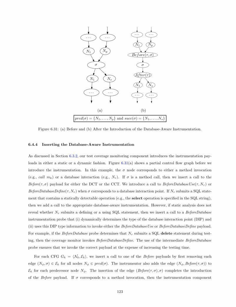
PSfrag replacements
N6
enter computeVelocity
enter computeVelocity
N6
N6
N7
N7
N8
N8
N10
N8
N16
N10
N11
N11
N12
N12
N18
N16
N18
N18
exit computeVelocity
exit computeVelocity
N6
N1
N1
N2
N2
N3
N3
N1
N1
N4
N4
N5
N5
N6
enter P
enter P
call main
call main
enter main
enter main
enter main
. . .
. . .
call inputCardNumber
call inputCardNumber
call inputPin
call inputCardNumber
call handleError
call handleError
call inputCardNumber
call inputPin
call handleError
call handleError
call inputPin
call inputPin
call inputOperation
call inputOperation
call getAccountBalance
call getAccountBalance
call promptAgain
call inputOperation
call lockAccount
call lockAccount
call promptAgain
call promptAgain
call inputOperation
call promptAgain
. . .
call getAccountBalance
enter getAccountBalance
enter getAccountBalance
N3
N3
N4
N4
N5
N5
N6
N6
N7
N7
N10
N10
N12
N12
N15
N10
N15
N15
exit getAccountBalance
exit getAccountBalance
return getAccountBalance
return lockAccount
. . .
return getAccountBalance
call promptAgain
. . .
exit main
exit main
return main
return main
exit P
exit P
. . .
exit main
enter lockAccount
enter lockAccount
. . .
. . .
exit lockAccount
exit lockAccount
return lockAccount
return lockAccount
exit main
Id : cfgiter.ladot, v1.12006/07/1220 : 28 : 13gkapfhamExp
Revision : 1.1
N6
. . .
. . .
. . .
. . .. . .
. . .. . .N1
N1
N1Np
σ
Np
σ
σ
σ
Ns
Ns
(a)
PSfrag replacements
N6
enter computeVelocity
enter computeVelocity
N6
N6
N7
N7
N8
N8
N10
N8
N16
N10
N11
N11
N12
N12
N18
N16
N18
N18
exit computeVelocity
exit computeVelocity
N6
N1
N1
N2
N2
N3
N3
N1
N1
N4
N4
N5
N5
N6
enter P
enter P
call main
call main
enter main
enter main
enter main
. . .
. . .
call inputCardNumber
call inputCardNumber
call inputPin
call inputCardNumber
call handleError
call handleError
call inputCardNumber
call inputPin
call handleError
call handleError
call inputPin
call inputPin
call inputOperation
call inputOperation
call getAccountBalance
call getAccountBalance
call promptAgain
call inputOperation
call lockAccount
call lockAccount
call promptAgain
call promptAgain
call inputOperation
call promptAgain
. . .
call getAccountBalance
enter getAccountBalance
enter getAccountBalance
N3
N3
N4
N4
N5
N5
N6
N6
N7
N7
N10
N10
N12
N12
N15
N10
N15
N15
exit getAccountBalance
exit getAccountBalance
return getAccountBalance
return lockAccount
. . .
return getAccountBalance
call promptAgain
. . .
exit main
exit main
return main
return main
exit P
exit P
. . .
exit main
enter lockAccount
enter lockAccount
. . .
. . .
exit lockAccount
exit lockAccount
return lockAccount
return lockAccount
exit main
Id : cfgiter.ladot, v1.12006/07/1220 : 28 : 13gkapfhamExp
Revision : 1.1
N6
. . .
. . .
. . .
. . .. . .
. . .. . .
N1
N1
N1
Np
σNp
σ
σ
Ns
σ
NsNs
Before(τ, σ)
After(τ)
(b)
pred(σ) = N1, . . . , Np and succ(σ) = N1, . . . , Ns
Figure 6.31: (a) Before and (b) After the Introduction of the Database-Aware Instrumentation.
6.4.4 Inserting the Database-Aware Instrumentation
As discussed in Section 6.3.2, our test coverage monitoring component introduces the instrumentation pay-
loads in either a static or a dynamic fashion. Figure 6.31(a) shows a partial control flow graph before we
introduce the instrumentation. In this example, the σ node corresponds to either a method invocation
(e.g., call mk) or a database interaction (e.g., Nr). If σ is a method call, then we insert a call to the
Before(τ, σ) payload for either the DCT or the CCT. We introduce a call to BeforeDatabaseUse(τ, Nr) or
BeforeDatabaseDefine(τ, Nr) when σ corresponds to a database interaction point. If Nr submits a SQL state-
ment that contains a statically detectable operation (e.g., the select operation is specified in the SQL string),
then we add a call to the appropriate database-aware instrumentation. However, if static analysis does not
reveal whether Nr submits a defining or a using SQL statement, then we insert a call to a BeforeDatabase
instrumentation probe that (i) dynamically determines the type of the database interaction point (DIP) and
(ii) uses this DIP type information to invoke either the BeforeDatabaseUse or BeforeDatabaseDefine payload.
For example, if the BeforeDatabase probe determines that Nr submits a SQL delete statement during test-
ing, then the coverage monitor invokes BeforeDatabaseDefine. The use of the intermediate BeforeDatabase
probe ensures that we invoke the correct payload at the expense of increasing the testing time.
For each CFG Gk = 〈Nk, Ek〉, we insert a call to one of the Before payloads by first removing each
edge (Nφ, σ) ∈ Ek for all nodes Nφ ∈ pred(σ). The instrumentor also adds the edge (Nφ,Before(τ, σ)) to
Ek for each predecessor node Nφ. The insertion of the edge (Before(τ, σ), σ) completes the introduction
of the Before payload. If σ corresponds to a method invocation, then the instrumentation component
123

PSfrag replacements
N6
enter computeVelocity
enter computeVelocity
N6
N6
N7
N7
N8
N8
N10
N8
N16
N10
N11
N11
N12
N12
N18
N16
N18
N18
exit computeVelocity
exit computeVelocity
N6
N1
N1
N2
N2
N3
N3
N1
N1
N4
N4
N5
N5
N6
enter P
enter P
call main
call main
enter main
enter main
enter main
. . .
. . .
call inputCardNumber
call inputCardNumber
call inputPin
call inputCardNumber
call handleError
call handleError
call inputCardNumber
call inputPin
call handleError
call handleError
call inputPin
call inputPin
call inputOperation
call inputOperation
call getAccountBalance
call getAccountBalance
call promptAgain
call inputOperation
call lockAccount
call lockAccount
call promptAgain
call promptAgain
call inputOperation
call promptAgain
. . .
call getAccountBalance
enter getAccountBalance
enter getAccountBalance
N3
N3
N4
N4
N5
N5
N6
N6
N7
N7
N10
N10
N12
N12
N15
N10
N15
N15
exit getAccountBalance
exit getAccountBalance
return getAccountBalance
return lockAccount
. . .
return getAccountBalance
call promptAgain
. . .
exit main
exit main
return main
return main
exit P
exit P
. . .
exit main
enter lockAccount
enter lockAccount
. . .
. . .
exit lockAccount
exit lockAccount
return lockAccount
return lockAccount
exit main
Id : icfgconnecttwotests.ladot, v1.22006/07/3117 : 04 : 41gkapfhamExp
Revision : 1.2
call Ti
enter Ti
. . .
exit Ti
return Ti
call Tj
enter Tj
. . .
exit Tj
return Tj
call Ti
call Ti
enter Ti
∈ ET
enter Ti
. . .
∈ Ei
. . .
exit Ti
∈ Ei
∈ Ei
exit Ti
return Ti
∈ ET
∈ ET
return Ti
call Tj
∈ Eexec
call Tj
enter Tj
∈ ET
enter Tj
. . .
∈ Ej
. . .exit Tj
∈ Ej
∈ Ej
exit Tj
return Tj ∈ ET
∈ ET
return Tj
Figure 6.32: Connecting the CFGs for Adjacent Test Cases.
places a call to After(τ) in the control flow graph. We introduce the traditional After payload by first
removing the edge (σ, Nφ) ∈ Ek for each node Nφ ∈ succ(σ). Next, we add the edge (σ,After(τ)) and
introduce (After(τ), Nφ) for all nodes Nφ ∈ succ(σ). The instrumentor adds one of the AfterDatabaseUse,
AfterDatabaseDefine, or AfterDatabase instrumentation payloads into the control flow graph when σ is a
database interaction. We place a call to the appropriate After payload when the type of the database
interaction is statically detectable and we use the AfterDatabase instrumentation to dynamically dispatch to
the correct instrumentation otherwise. Figure 6.31(b) shows a control flow graph after the introduction of the
test coverage monitoring instrumentation. Even though this instrumented CFG contains probes to construct
a traditional TCM tree, the replacement of Before(τ, σ) and After(τ) with the equivalent database-aware
probes will support the creation of either a DI-DCT or a DI-CCT.
6.5 CALCULATING TEST ADEQUACY
6.5.1 Representing Database-Aware Test Suites
The test coverage monitor records coverage information so that we can calculate adequacy on either a per-test
or per-test suite basis. A test suite is a collection of test cases that invoke program operations and inspect
the results in order to determine if the methods performed correctly. Definition 7 defines a test suite T that
tests a database-centric application and Table A13 in Appendix A summarizes the notation developed in
this section. The notation ∆i = Ti(∆i−1) means that test case Ti was executed with input test state ∆i−1
and subsequently produced test state ∆i. Intuitively, the state of a database-centric application includes
the values of all of the program’s variables and the state of the databases with which the program interacts
during testing.
Definition 7. A test suite T is a triple 〈∆0, 〈T1, . . . , Tn〉, 〈∆1, . . . , ∆n〉〉, consisting of an initial test state, ∆0,
a test case sequence 〈T1, . . . , Tn〉 for state ∆0, and expected test states 〈∆1, . . . , ∆n〉 where ∆i = Ti(∆i−1)
for i = 1, . . . , n.
124
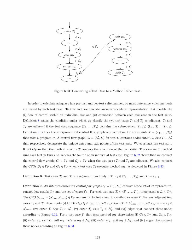
PSfrag replacements
N6
enter computeVelocity
enter computeVelocity
N6
N6
N7
N7
N8
N8
N10
N8
N16
N10
N11
N11
N12
N12
N18
N16
N18
N18
exit computeVelocity
exit computeVelocity
N6
N1
N1
N2
N2
N3
N3
N1
N1
N4
N4
N5
N5
N6
enter P
enter P
call main
call main
enter main
enter main
enter main
. . .
. . .
call inputCardNumber
call inputCardNumber
call inputPin
call inputCardNumber
call handleError
call handleError
call inputCardNumber
call inputPin
call handleError
call handleError
call inputPin
call inputPin
call inputOperation
call inputOperation
call getAccountBalance
call getAccountBalance
call promptAgain
call inputOperation
call lockAccount
call lockAccount
call promptAgain
call promptAgain
call inputOperation
call promptAgain
. . .
call getAccountBalance
enter getAccountBalance
enter getAccountBalance
N3
N3
N4
N4
N5
N5
N6
N6
N7
N7
N10
N10
N12
N12
N15
N10
N15
N15
exit getAccountBalance
exit getAccountBalance
return getAccountBalance
return lockAccount
. . .
return getAccountBalance
call promptAgain
. . .
exit main
exit main
return main
return main
exit P
exit P
. . .
exit main
enter lockAccount
enter lockAccount
. . .
. . .
exit lockAccount
exit lockAccount
return lockAccount
return lockAccount
exit main
Id : icfgtestcallsmethod.ladot, v1.32006/07/3118 : 57 : 52gkapfhamExp
Revision : 1.3
enter Ti
. . .
call mk
enter mk
. . .
exit mk
return mk
. . .
exit Ti
enter Ti
enter Ti
. . .
∈ Ei
. . .
call mk
∈ Ei
call mk
enter mk
∈ ET
enter mk
. . .
∈ Ek
. . .
exit mk
∈ Ek
∈ Ek
exit mkreturn mk
∈ ET
∈ ET
return mk
. . .
∈ Ei . . .
exit Ti
∈ Ei
∈ Ei
∈ Ei
∈ Ei
exit Ti
Figure 6.33: Connecting a Test Case to a Method Under Test.
In order to calculate adequacy in a per-test and per-test suite manner, we must determine which methods
are tested by each test case. To this end, we describe an interprocedural representation that models the
(i) flow of control within an individual test and (ii) connection between each test case in the test suite.
Definition 8 states the condition under which we classify the two test cases Ti and Tj as adjacent. Ti and
Tj are adjacent if the test case sequence 〈T1, . . . , Tn〉 contains the subsequence 〈Ti, Tj〉 (i.e., Ti = Tj−1).
Definition 9 defines the interprocedural control flow graph representation for a test suite T = 〈T1, . . . , Tn〉
that tests a program P . A control flow graph Gi = 〈Ni, Ei〉 for test Ti contains nodes enter Ti, exit Ti ∈ Ni
that respectively demarcate the unique entry and exit points of the test case. We construct the test suite
ICFG GT so that the method execute T controls the execution of the test suite. The execute T method
runs each test in turn and handles the failure of an individual test case. Figure 6.32 shows that we connect
the control flow graphs Gi ∈ ΓT and Gj ∈ ΓT when the test cases Ti and Tj are adjacent. We also connect
the CFGs Gi ∈ ΓT and Gk ∈ ΓP when a test case Ti executes method mk, as depicted in Figure 6.33.
Definition 8. Test cases Ti and Tj are adjacent if and only if Ti, Tj ∈ 〈T1, . . . , Tn〉 and Ti = Tj−1.
Definition 9. An interprocedural test control flow graph GT = 〈ΓT , ET 〉 consists of the set of intraprocedural
control flow graphs ΓT and the set of edges ET . For each test case Ti ∈ 〈T1, . . . , Tn〉, there exists a Gi ∈ ΓT .
The CFG Gexec = 〈Nexec, Eexec〉 ∈ ΓT represents the test execution method execute T . For any adjacent test
cases Ti and Tj there exists (i) CFGs Gi, Gj ∈ ΓT , (ii) call Ti, return Ti ∈ Nexec, (iii) call Tj , return Tj ∈
Nexec, (iv) enter Ti, exit Ti ∈ Ni, (v) enter Tj , exit Tj ∈ Nj , and (vi) edges that connect these nodes
according to Figure 6.32. For a test case Ti that tests method mk there exists (i) Gi ∈ ΓT and Gk ∈ ΓP ,
(ii) enter Ti, exit Ti, call mk, return mk ∈ Ni, (iii) enter mk, exit mk ∈ Nk, and (iv) edges that connect
these nodes according to Figure 6.33.
125

PSfrag replacements
N6
enter computeVelocity
enter computeVelocity
N6
N6
N7
N7
N8
N8
N10
N8
N16
N10
N11
N11
N12
N12
N18
N16
N18
N18
exit computeVelocity
exit computeVelocity
N6
N1
N1
N2
N2
N3
N3
N1
N1
N4
N4
N5
N5
N6
enter P
enter P
call main
call main
enter main
enter main
enter main
. . .
. . .
call inputCardNumber
call inputCardNumber
call inputPin
call inputCardNumber
call handleError
call handleError
call inputCardNumber
call inputPin
call handleError
call handleError
call inputPin
call inputPin
call inputOperation
call inputOperation
call getAccountBalance
call getAccountBalance
call promptAgain
call inputOperation
call lockAccount
call lockAccount
call promptAgain
call promptAgain
call inputOperation
call promptAgain
. . .
call getAccountBalance
enter getAccountBalance
enter getAccountBalance
N3
N3
N4
N4
N5
N5
N6
N6
N7
N7
N10
N10
N12
N12
N15
N10
N15
N15
exit getAccountBalance
exit getAccountBalance
return getAccountBalance
return lockAccount
. . .
return getAccountBalance
call promptAgain
. . .
exit main
exit main
return main
return main
exit P
exit P
. . .
exit main
enter lockAccount
enter lockAccount
. . .
. . .
exit lockAccount
exit lockAccount
return lockAccount
return lockAccount
exit main
Id : icfgtestbem.ladot, v1.22006/07/3118 : 58 : 05gkapfhamExp
Revision : 1.2
enter execute T = 〈T1, . . . , Tn〉
call T1
enter T1
. . .
exit T1
return T1
. . .
call Ti
enter Ti
. . .
Nθ : (∆x, ∆a)
Npass Ti
Nfail Ti
. . .
exit Ti
. . .
call Tn
enter Tn
. . .
exit Tn
return Tn
exit execute T = 〈T1, . . . , Tn〉
enter execute T = 〈T1, . . . , Tn〉
enter execute T = 〈T1, . . . , Tn〉
call T1
call T1
enter T1
enter T1
. . .
. . .
exit T1
exit T1
return T1
return T1
. . .
. . .
call Ti
call Ti
enter Ti
enter Ti
. . .
. . .
Nθ : (∆x, ∆a)
Nθ : (∆x, ∆a)
Npass Ti
Nθ : (∆x, ∆a)
Nfail Ti
Npass Ti
. . .
Nfail Ti
exit Ti
. . .
exit Ti
Npass Ti
Nfail Ti
exit Ti
. . .
. . .
call Tn
call Tn
enter Tn
enter Tn
. . .
. . .
exit Tn
exit Tn
return Tn
return Tn
exit execute T = 〈T1, . . . , Tn〉
. . .exit execute T = 〈T1, . . . , Tn〉 exit execute T = 〈T1, . . . , Tn〉
Figure 6.34: A Partial Interprocedural Control Flow Graph for a Test Suite.
Figure 6.34 depicts a partial ICFG for a test suite T = 〈T1, . . . , Tn〉. In an attempt to preserve simplicity,
this schematic uses nodes with the label “. . .” to denote arbitrary ICFG nodes and edges. Figure 6.34
shows that the CFG Gexec contains nodes that transfer control to each of the test cases. For example,
the edge (enter execute T = 〈T1, . . . , Tn〉, call T1) represents a transfer of control to test T1 and the edge
(return Tn, enter execute T = 〈T1, . . . , Tn〉) indicates the completion of both Tn and the termination of the
test execution method. Test case Ti’s CFG Gi = 〈Ni, Ei〉 contains zero or more test oracle execution nodes
Nθ ∈ Ni. The node Nθ corresponds to the execution of an oracle θ that compares the actual test state ∆a
to the expected test state ∆x. If ∆x = ∆a, then the test oracle returns true and the successor node Npass Ti
records the passing outcome of this test. If ∆x 6= ∆a, then the test oracle returns false and the successor
node Nfail Ti registers the failure of Ti. Figure 6.34 shows that the failure of the oracle at Nθ triggers the
termination of test case Ti and then the halt of the entire test suite T . Whenever Nθ returns true, test suite
execution continues until either all of the tests have correctly executed or an oracle failure is encountered.
6.5.2 Calculating Data Flow-Based Adequacy
Since a failing test case suggests that there is a defect in the program under test, we focus on calculating the
adequacy of a passing test case Ti and test suite T . Focusing on the calculation of adequacy for a passing
test suite is prudent because the failure of the program under test might prevent our instrumentation from
capturing all of the covered test requirements. We classify a test case Ti as passing if all oracle nodes Nθ ∈ Ni
return true for a test CFG Gi = 〈Ni, Ei〉. A test suite T = 〈T1, . . . , Tn〉 is passing if all of T ’s test cases are
also passing. The following Equation (6.7) provides the means for calculating adeq(Ti), the adequacy of a
126

test case Ti. This equation shows that the adequacy of a test case Ti is the number of covered requirements
divided by the total number of test requirements. This equation uses U(i) to denote the set of methods that
are tested by test case Ti. During the static analysis that enumerates U(i), the test adequacy component
follows the edges between adjacent test cases until it finds the CFG for Ti. For an interprocedural test CFG
GT = 〈ΓT , ET 〉, we know that Gk ∈ U(i) when call mk ∈ Ni for a test case CFG Gi ∈ ΓT . For example,
Figure 6.33 reveals that test case Ti tests method mk. Equation (6.7) uses υ(i, k) to denote the set of test
requirements that Ti covered during the testing of method mk and χ(k) to stand for the complete set of
requirements for mk.
adeq(Ti) =
∑Gk ∈ U(i) |υ(i, k)|
∑Gk ∈ U(i) |χ(k)|
(6.7)
We traverse a test coverage monitoring tree in order to identify υ(i, k). For example, suppose that we
test a database-centric application at the relation level (i.e., R ∈ L(τ)) and method mk contains a database
interaction association involving relation relj (i.e., 〈Ndef, Nuse, relj〉 ∈ χ(k)). If Ti tests method mk (i.e.,
Gk ∈ U(i)) and it causes mk to define and use relj , then we mark the database interaction association
〈Ndef, Nuse, relj〉 as covered. We know that the test covers this DIA if testing yields a TCM tree τ that
contains the nodes NR1= 〈relj ,def〉 and NR2
= 〈relj ,use〉 such that (i) call Ti is an ancestor of call mk
and (ii) call mk is an ancestor of nodes NR1and NR2
. In the context of data flow testing, we use the
database-aware test adequacy component described in Chapter 5 to enumerate χ(k). For an interprocedural
CFG GP = 〈ΓP , EP 〉, Equation (6.8) defines the adequacy of an entire test suite T as the number of covered
requirements divided by the total number of requirements over all methods Gk ∈ ΓP .
adeq(T ) =
∑Gk∈ΓP
|υ(k)|∑Gk∈ΓP
|χ(k)|(6.8)
6.6 CONCLUSION
This chapter presents a database-aware coverage monitoring technique. We explain why it is challenging to (i)
instrument a database-centric application and (ii) accurately and efficiently store the test coverage monitoring
results. This chapter also introduces the database interaction dynamic call tree (DI-DCT) and the database
interaction calling context tree (DI-CCT) and reveals how we use these trees to calculate the adequacy of a
test suite. In particular, we provide a formal definition of each test coverage monitoring tree and we describe
the instrumentation probes that construct a tree. We show how to insert database-aware instrumentation
probes before and after the execution of both a program method and a database interaction. Finally, we
explain how to use (i) an interprocedural representation of a program’s test suite and (ii) the TCM tree in
order to calculate adequacy on a per-test and per-test suite basis. Chapter 7 describes the implementation
of the database-aware test coverage monitoring component and presents empirical performance results for
this key element of our testing framework. Chapter 8 presents a regression testing technique that leverages
the output of the test coverage monitor.
127

7.0 TEST COVERAGE MONITORING COMPONENT
7.1 INTRODUCTION
This chapter describes the test coverage monitoring component that (i) instruments a database-centric
application and (ii) creates and stores a test coverage monitoring tree. We explain how the coverage monitor
uses aspect-oriented programming (AOP) techniques to statically and dynamically instrument the program
and the test suite. This chapter also shows how the monitoring component leverages existing compression
algorithms to reduce the size of the coverage report. The chapter describes the goals and design for an
experiment to measure the performance of our approach to database-aware test coverage monitoring. We
conducted experiments to measure the time required to statically instrument the case study applications.
We also performed experiments to identify the impact that the coverage monitoring instrumentation has
on the static size of each application. Finally, we empirically evaluated how different configurations of the
coverage monitor increase test suite execution time and we characterize the size and structure of the test
coverage monitoring trees. In summary, this chapter includes:
1. A high level overview of the different configurations of the database-aware test coverage monitor (Sec-
tion 7.2).
2. Details about the implementation of the instrumentation technique and the test coverage monitoring
trees (Section 7.3)
3. The design of an experiment to measure the performance of the coverage monitor, an overview of the
experimental results, and a discussion of the steps that we took to control the threats to experiment
validity (Sections 7.4, 7.5, and 7.7).
4. An empirical evaluation of the costs that are associated with instrumenting the program and the test
suite (Section 7.6.1) and monitoring coverage during test suite execution (Section 7.6.2).
5. An identification of the relationship between the size, structure, and compressibility of a TCM tree and
the configuration of the coverage monitoring component (Sections 7.6.3 and 7.6.4)
7.2 OVERVIEW OF THE COVERAGE MONITORING COMPONENT
Figure 7.1 depicts the different ways that we can configure the test coverage monitoring component. This
tree shows that we can introduce the instrumentation probes in either a dynamic or a static fashion, as
128

Configuration of the Test Coverage Monitor
Instrumentation Tree Format Tree Type Tree Storage
Static Dynamic
Source Code Bytecode
Binary XML Traditional Database-Aware
CCT DCT Interaction Level DI-DCT DI-CCT
Database Relation Attribute Record Attribute Value
Standard Compressed
PSfrag replacements
N6
enter computeVelocity
enter computeVelocity
N6
N6
N7
N7
N8
N8
N10
N8
N16
N10
N11
N11
N12
N12
N18
N16
N18
N18
exit computeVelocity
exit computeVelocity
N6
N1
N1
N2
N2
N3
N3
N1
N1
N4
N4
N5
N5
N6
enter P
enter P
call main
call main
enter main
enter main
enter main
. . .
. . .
call inputCardNumber
call inputCardNumber
call inputPin
call inputCardNumber
call handleError
call handleError
call inputCardNumber
call inputPin
call handleError
call handleError
call inputPin
call inputPin
call inputOperation
call inputOperation
call getAccountBalance
call getAccountBalance
call promptAgain
call inputOperation
call lockAccount
call lockAccount
call promptAgain
call promptAgain
call inputOperation
call promptAgain
. . .
call getAccountBalance
enter getAccountBalance
enter getAccountBalance
N3
N3
N4
N4
N5
N5
N6
N6
N7
N7
N10
N10
N12
N12
N15
N10
N15
N15
exit getAccountBalance
exit getAccountBalance
return getAccountBalance
return lockAccount
. . .
return getAccountBalance
call promptAgain
. . .
exit main
exit main
return main
return main
exit P
exit P
. . .
exit main
enter lockAccount
enter lockAccount
. . .
. . .
exit lockAccount
exit lockAccount
return lockAccount
return lockAccount
exit main
Figure 7.1: Different Configurations of the Test Coverage Monitoring Component.
discussed in Chapter 6. We use aspect-oriented programming (AOP) techniques and the AspectJ program-
ming language in order to place the TCM probes before and after method calls and database interaction
points [Elrad et al., 2001, Kiczales et al., 2001a]. Figure 7.1 shows that the use of AspectJ enables us to
statically insert the instrumentation into either the source code or the Java bytecode of the case study ap-
plications. The dynamic instrumentation technique always places the coverage monitoring probes into the
bytecode of a Java application. Our monitoring framework records coverage information in a TCM tree and
the component can store this tree in either a binary or an eXtensible Markup Language (XML) format.
Since we implemented the TCM component in the Java programming language, we use Java’s serialization
mechanism to store the trees in a binary format. The coverage monitor supports a binary format because
this representation may result in reduced storage requirements [Geer, 2005].
Our testing framework also maintains the TCM trees in XML because this text-based encoding enables
independence from execution environment factors such as the computer architecture, operating system, and
programming language [Ferragina et al., 2006, Lin et al., 2005]. Since XML uses markup tags to express the
structure of the TCM tree and the markup is repeated for each node, the trees often consume a significant
amount of storage. However, several recently developed compression algorithms can substantially reduce
the size of the trees that we encode in XML [Ferragina et al., 2006, Liefke and Suciu, 2000, Lin et al., 2005,
Ng et al., 2006]. It is also possible to store the XML-based trees in an XML database (e.g., TIMBER
[Jagadish et al., 2002]) and this would enable a tester to issue queries about the state and structure of the
tree during the debugging process [Lin et al., 2005, Shasha et al., 2002]. For example, the tester might wish
to determine which failing test case(s) interact with a certain relation or attribute in a database. Figure 7.1
shows that the coverage monitor can either produce a traditional tree (e.g., DCT or CCT) or a database-aware
tree (e.g., DI-DCT or DI-CCT). If the tree is database-aware, then we must also configure the monitoring
component to record coverage at a certain level of interaction granularity (e.g., relation or attribute value).
129

pointcut executeMethod(): chosenClass() && execution(* *(..));
(a)
pointcut chosenClass(): (within(gradebook.*) ||
within(org.hsqldb.sample.*) || within(reminder.*) ||
within(com.runstate.pithy.*) || within(student.*) ||
within(TransactionAgent.*));
(b)
before(): executeMethod() && if(monitorEnabled) < . . . >
(c)
Figure 7.2: AspectJ Pointcuts and Advice for the Before Instrumentation Probe.
7.3 IMPLEMENTATION OF THE COVERAGE MONITOR
7.3.1 Instrumentation
The AspectJ language supports the introduction of arbitrary code segments at certain join points within
a Java application. A join point is a well-defined location in the control flow graph of a program. For
example, AspectJ can identify join points related to the execution of (i) a method or a constructor, (ii) an
exception handler, or (iii) a reference to a field of an object. We use AspectJ to define pointcuts that identify
specific join points and the values that are available at these points. For example, Figure 7.2(a) describes
the executeMethod pointcut that is part of the coverage monitoring framework. The execution(* *(..))
portion of this pointcut indicates that we want AspectJ to monitor the execution of all the methods and
constructors that occur within chosenClass(). Figure 7.2(b) shows that we currently define chosenClass()
to include all of the case study applications that we described in Chapter 3. Figure 7.2(c) provides an example
of advice that will be executed when the executeMethod pointcut occurs during test suite execution. The
body of the advice for executeMethod can invoke the Before instrumentation probe that we defined in
Chapter 6. The test coverage monitor contains additional pointcuts and before and after advice that we
use to construct the DCT, CCT, DI-DCT, and DI-CCT. For more details about aspect-oriented programming
and the AspectJ language, please refer to [Elrad et al., 2001, Kiczales et al., 2001a].
A single execution of the static instrumentor can introduce the monitoring probes into one or more
case study applications. We say that the instrumentor operates in batch mode when it inserts TCM probes
into multiple applications during a single run. Since static instrumentation normally increases the size of an
application’s bytecode, the coverage monitoring framework incorporates compression algorithms such as Pack
[Pugh, 1999]. This compression technique is specifically designed to reduce the size of Java bytecodes and it is
now fully integrated into the Java 1.5 libraries and virtual machine. Bytecode compression techniques reduce
the cost of transmitting the statically instrumented application across a network or storing it on a file system.
Figure 7.3 provides an overview of the dynamic instrumentation process. Our goal is to correctly instrument
the program and the test suite with minimal time overhead. The static instrumentation technique places
130

Program and Test Suite ClassesDynamic Instrumentor
JVMTI or Class Loader
Instrumented Classes
Java Virtual Machine
PSfrag replacements
N6
enter computeVelocity
enter computeVelocity
N6
N6
N7
N7
N8
N8
N10
N8
N16
N10
N11
N11
N12
N12
N18
N16
N18
N18
exit computeVelocity
exit computeVelocity
N6
N1
N1
N2
N2
N3
N3
N1
N1
N4
N4
N5
N5
N6
enter P
enter P
call main
call main
enter main
enter main
enter main
. . .
. . .
call inputCardNumber
call inputCardNumber
call inputPin
call inputCardNumber
call handleError
call handleError
call inputCardNumber
call inputPin
call handleError
call handleError
call inputPin
call inputPin
call inputOperation
call inputOperation
call getAccountBalance
call getAccountBalance
call promptAgain
call inputOperation
call lockAccount
call lockAccount
call promptAgain
call promptAgain
call inputOperation
call promptAgain
. . .
call getAccountBalance
enter getAccountBalance
enter getAccountBalance
N3
N3
N4
N4
N5
N5
N6
N6
N7
N7
N10
N10
N12
N12
N15
N10
N15
N15
exit getAccountBalance
exit getAccountBalance
return getAccountBalance
return lockAccount
. . .
return getAccountBalance
call promptAgain
. . .
exit main
exit main
return main
return main
exit P
exit P
. . .
exit main
enter lockAccount
enter lockAccount
. . .
. . .
exit lockAccount
exit lockAccount
return lockAccount
return lockAccount
exit main
Figure 7.3: Overview of the Dynamic Instrumentation Process.
probes into the all of the classes of the program and the test suite. Currently, we use a load-time technique
to dynamically instrument the program and the tests on a per-class basis. Identifying the appropriate unit of
instrumentation is a trade-off between (i) instrumenting only those program units that are actually executed
during testing and (ii) minimizing the number of calls to the dynamic instrumentation module.
Relying on per-class instrumentation could inefficiently force the insertion of TCM probes into methods
that will never be used during test suite execution. However, our per-class instrumentation scheme is simple
and it greatly minimizes the number of separate invocations of the instrumentor. Per-class instrumentation
is also an efficient approach when the test suite invokes the majority of the methods within the case study
application. We judge that it is likely that the tests will execute most of the program’s methods since method
coverage is often used to measure the adequacy of a test suite [Zhu et al., 1997]. Figure 7.3 shows that the
current prototype uses either the Java Virtual Machine Tool Interface (JVMTI) or a custom Java class loader
to introduce the probes. Prior testing and analysis techniques frequently use one or both of these interfaces
(or, the JVMTI’s precursor, the JVM Profiler Interface) during the instrumentation or observation of a Java
program (e.g., [Binder, 2005, Dufour et al., 2003, Zhuang et al., 2006]). We will investigate the different
granularities at which we can introduce instrumentation in future work, as further discussed in Chapter 9.
We designed the dynamic instrumentor so that it only places probes in the classes that are a part of the
program and the test suite.
7.3.2 Tree Format and Storage
Since the test coverage monitoring trees record the behavior of the program during testing, they must be
stored in order to support debugging and/or automatic fault localization. We performed experiments to
determine how the encoding of a test coverage monitoring tree would impact the size of the trees. Our
preliminary experimental results suggested that the binary encoding was more compact than the text-based
XML representation for the same TCM tree. For example, a dynamic call tree that represents ten method
invocations was 1497 bytes when stored in a binary format and 9762 bytes in XML. For this simple TCM tree,
the XML encoding yields a file size that is 552% greater than the binary representation. The experimental
results in Section 7.6 suggest that the difference between the two representations is even more marked for
larger coverage monitoring trees. However, recent empirical results reveal that XML files often exhibit
better compressibility than binary files [Liefke and Suciu, 2000]. In fact, several of our experiments also
demonstrate that the XML-aware compression techniques yield an XML-based tree that is smaller than the
compressed version of the binary tree. Finally, recent XML compression algorithms create a compressed
format that enables a tester to query the compressed XML file without completely decompressing the tree
131

[Lin et al., 2005, Ferragina et al., 2006]. In an attempt to (i) reduce storage requirements and (ii) speed
up the network transmission of the coverage reports, we leverage traditional compression algorithms such
Gzip and Zip [Lelewer and Hirschberg, 1987, Morse, 2005] to compress the binary trees and we use XMill
[Liefke and Suciu, 2000] and XMLPPM [Cheney, 2001] to shrink the XML trees.1
7.4 EXPERIMENT GOALS AND DESIGN
The primary goal of the experiments is to measure the performance of the test coverage monitoring compo-
nent. Section 7.6 formally defines each evaluation metric and then describes the results from applying the
TCM component to each of the case study applications. We implemented the current version of the test
coverage monitor with the Java 1.5 and AspectJ 1.5 programming languages. Even though our implemen-
tation of the TCM component supports dynamic instrumentation with either the JVM tools interface or
a custom class loader, the experiments focus on measuring the performance of the class loading approach.
Since most Java virtual machines (e.g., the Sun JVM and the Jikes RVM) use the same type of class loader
interface, this choice ensures that our experimental results are more likely to generalize to other execution
environments. We also designed the experiment in this manner because our preliminary results revealed
that the “heavy weight” JVMTI introduced significant time overheads, in confirmation of prior results
[Popovici et al., 2002]. In future work we will also evaluate the performance of dynamic instrumentation
with the JVMTI and recent JVM-based techniques that dynamically introduce the instrumentation (e.g.,
[Bockisch et al., 2006, Golbeck and Kiczales, 2007]). We configured the static instrumentation technique to
operate on the bytecode of a case study application. In future research, we will evaluate the performance of
statically instrumenting the (i) Java source code and (ii) different combinations of source code and bytecode.
Since the time overhead metrics varied across each trial, we calculate arithmetic means and standard
deviations for all of these timings (the space overhead and tree characterization metrics did not vary across
trials). The standard deviation measures the amount of dispersion in the recorded data sets and higher
values for this descriptive statistic suggest that the data values are more dispersed. When we plot a bar
chart, we place a standard deviation error bar at the top of the bar and we use a diamond when the standard
deviation is small. We also use a box and whisker plot to visually compare the experiment results from
different configurations of the coverage monitor. Unless specified otherwise, the box spans the distance
between the 25% and 75% quantile and the whiskers extend to cover the non-outlying data points. The qth
quantile is the point at which q% of the recorded data points fall below and 1 − q% fall above a specific
data value. Our box and whisker plots represent data outliers with small square shaped points. We plot an
empirical cumulative distribution function (ECDF) to support further examination of a data set. An ECDF
gives the cumulative percentage of the recorded data set whose values fall below a specific value. For more
details about these statistical analysis and visualization techniques, please refer to [Dowdy et al., 2004].
1XMill and XMLPPM do not directly support the querying of a compressed XML file. We were not able to use thecompression techniques that provide this functionality (e.g., [Lin et al., 2005, Ferragina et al., 2006]) because they were notfreely distributed at the time of writing.
132
We performed all of the experiments on a GNU/Linux workstation with kernel 2.6.11-1.1369, a dual
core 3.0 GHz Pentium IV processor, 2 GB of main memory, and 1 MB of L1 processor cache. In order
to improve performance, we implemented portions of the TCM component in a multi-threaded fashion and
we configured the workstation to use the Native POSIX Thread Library (NPTL) version 2.3.5. We always
executed the static instrumentor in ten separate trials for each case study application. For each possible
configuration of the coverage monitor (c.f. Figure 7.1), we ran the test suite ten times. Section 7.6 provides
a definition of each evaluation metric and explains how we measured it during experimentation. Table C2
summarizes each of these metrics and Table A14 explains the additional notation that we use during the
discussion of the experimental results.
7.5 KEY INSIGHTS FROM THE EXPERIMENTS
The experimental results in Section 7.6 complement Chapter 6’s analytical evaluation of the TCM instrumen-
tation probes. Due to the comprehensive nature of our empirical evaluation, we offer the following insights
from the experiments:
1. Static Instrumentation
a. Time Overhead: The static instrumentation technique requires less than six seconds to insert cov-
erage probes into a database-centric application. A batch approach to instrumentation can attach
the probes to six applications in less than nine seconds. Across all applications, the instrumentation
of a program and its test suite requires no more than five seconds.
b. Space Overhead: For all of the studied applications, static instrumentation increases the space
overhead by 420% on average. We judge that this increase is acceptable because it successfully
controls the time overhead of coverage monitoring.
2. Test Suite Execution
a. Type of Instrumentation: The use of statically introduced probes lengthens testing time by 12.5%
while dynamic instrumentation causes a 52% increase in test execution time.
b. Type of Coverage Tree: Calling context trees are less expensive to produce than the dynamic call
tree. Using static instrumentation to create a TCM tree respectively increases testing time by 12.5%
and 26.1% for the CCT and DCT.
c. Interaction Level: Using a CCT to record coverage at the finest level of database interaction gran-
ularity (e.g., attribute value) only increases testing time by 54%.
d. Storing the Coverage Tree: The time required for tree storage ranges from less than 200 milliseconds
for the binary CCT to three seconds for the XML-based DCT.
3. Test Coverage Trees
a. Number of Nodes and Edges: The CCT has node and edge counts that range from 144 at the
program level to 22992 at the level of attribute values. The number of DCT nodes ranges from a
minimum of 433 to a maximum of 87538.
133

b. Memory Size: The in-memory size of the TCM trees ranges from 423 KB to almost 24 MB. Small
TCM trees place little, if any, pressure on the memory subsystem of the JVM while the largest trees
require an increase in heap storage space.
c. File System Size: The XML encoding yields TCM trees that are larger than the binary encoding
of the same tree. Yet, XML-aware compression algorithms can considerably reduce the size of the
coverage report.
d. Tree Characterization: The coverage trees are normally “short” and “bushy,” in confirmation of pre-
vious empirical studies [Ammons et al., 1997]. A DI-CCT at the finest level of database interaction
granularity often consumes less space overhead than a traditional DCT.
7.6 ANALYSIS OF THE EXPERIMENTAL RESULTS
7.6.1 Instrumentation
The static instrumentor can insert the coverage monitoring probes into one or more applications. We measure
Tinstr(A), the time required to statically instrument the applications in the set A. For example, if A = FF,
then the TCM component will introduce the probes into the FindFile case study application. Alternatively,
if A′ = FF, GB, TM, then the instrumentation module operates in batch mode and places probes into the
FindFile, GradeBook, and TransactionManager applications. We report the increase and percent increase
in Tinstr when we perform static instrumentation with the application set A′ instead of A and A ⊂ A′.
Equation (7.1) defines the increase in Tinstr when we replace the application set A with A′. Equation (7.2)
defines the percent increase in evaluation metric Tinstr , denoted T %Iinstr(A
′,A). We compute the time overhead
metrics Tinstr with the operating system-based timer /usr/bin/time.
T Iinstr(A′,A) = Tinstr(A
′)− Tinstr(A) (7.1)
T %Iinstr(A
′,A) =T Iinstr(A
′,A)
Tinstr(A)× 100 (7.2)
We use Ts and As to denote a test suite and an application that were statically instrumented and we say
that Td and Ad are tests and an application that we dynamically instrument. We evaluate S(A) and S(As),
the respective size of an application A before and after static instrumentation. Finally, we report S(A, c)
and S(As, c) the size of applications A and As when compressed with compression technique c. Currently,
our framework can compress Java bytecodes using Zip [Lelewer and Hirschberg, 1987], Gzip [Morse, 2005],
and Pack [Pugh, 1999]. We also compute the increase and percent increase in space overhead associated
with the static instrumentation, respectively denoted SI (As, A) and S%I(As, A) (we use equations similar to
Equations (7.1) and (7.2) in order to calculate these values). Since dynamic instrumentation occurs during
test suite execution, we do not explicitly measure the increase in space overhead that results from inserting
the instrumentation probes.2
2The Sun JVM that we used during experimentation does not include facilities to report the in-memory size of Java bytecodeor the native code that results from just-in-time (JIT) compilation. As discussed in Chapter 9, we will explore the use of theJikes RVM and the experiment design developed in [Zhang and Krintz, 2005] in order to measure S(Ad).
134

FF PI RM ST TM GB AllApplication
2
4
6
8
10
Static
Instrumentation
Time
HsecL
FF PI RM ST TM GB All
4.391 4.404 4.396 4.394
5.1695.583
8.687
PSfrag replacements
N6
enter computeVelocity
enter computeVelocity
N6
N6
N7
N7
N8
N8
N10
N8
N16
N10
N11
N11
N12
N12
N18
N16
N18
N18
exit computeVelocity
exit computeVelocity
N6
N1
N1
N2
N2
N3
N3
N1
N1
N4
N4
N5
N5
N6
enter P
enter P
call main
call main
enter main
enter main
enter main
. . .
. . .
call inputCardNumber
call inputCardNumber
call inputPin
call inputCardNumber
call handleError
call handleError
call inputCardNumber
call inputPin
call handleError
call handleError
call inputPin
call inputPin
call inputOperation
call inputOperation
call getAccountBalance
call getAccountBalance
call promptAgain
call inputOperation
call lockAccount
call lockAccount
call promptAgain
call promptAgain
call inputOperation
call promptAgain
. . .
call getAccountBalance
enter getAccountBalance
enter getAccountBalance
N3
N3
N4
N4
N5
N5
N6
N6
N7
N7
N10
N10
N12
N12
N15
N10
N15
N15
exit getAccountBalance
exit getAccountBalance
return getAccountBalance
return lockAccount
. . .
return getAccountBalance
call promptAgain
. . .
exit main
exit main
return main
return main
exit P
exit P
. . .
exit main
enter lockAccount
enter lockAccount
. . .
. . .
exit lockAccount
exit lockAccount
return lockAccount
return lockAccount
exit main
Figure 7.4: Static Instrumentation Time.
7.6.1.1 Instrumentation Time Overhead Figure 7.4 presents the time overhead associated with the
static instrumentation of the case study applications. The results show that Tinstr is never more than
approximately 4.5 seconds and the instrumentation process exhibits little variability. For example, ten
executions of the instrumentor on the ST application yielded a mean instrumentation time of 4.4 seconds
with a standard deviation of .04 seconds. Figure 7.4 also provides the static instrumentation time results for
the larger case study applications (i.e., TM and GB) and a batch execution of the instrumentor. For the box
labeled “All,” we configured the static instrumentation technique to introduce probes into all of the case study
applications. Our experiments reveal that the instrumentation of a larger application (e.g., GB) incurs one
additional second of time overhead when compared to instrumenting a smaller application (e.g., FF). Since
we can instrument all of the case study applications is 9 seconds or less, the results in Figure 7.4 also suggest
that we can efficiently instrument more than one application with a single run of the instrumentor. If we take
A = ST andA′ as the set of all applications, then we know that T %Iinstr(A
′,A) = 97% for the instrumentation
of six applications instead of one. Across all of the case study applications, static instrumentation takes 4.72
seconds on average. In summary, we judge that our approach to static instrumentation introduces the
instrumentation probes with minimal time overhead.
7.6.1.2 Instrumentation Space Overhead We use As to denote the statically instrumented version of
an application A. As includes additional bytecode instructions at the boundaries of all method invocations
and database interactions. The static instrumentor also outputs an archive that contains the bytecode of
the coverage monitoring probes. In preparation for a call to the Before probe, the instrumentation must (i)
store the contents of the program stack in local variables, (ii) check to ensure that coverage monitoring is
enabled, (iii) load the probe, and (iv) invoke the probe. The instrumentor also adds additional bytecode
instructions to handle any exceptions that might be thrown by a coverage monitoring probe (e.g., we use
exception handlers to manage the problems that occur when the storage of the TCM trees exceeds the space
available for file storage). We disassembled each of the case study applications in order to discern how
many additional instructions were needed to use the test coverage monitoring probes. For example, the
135

Compression Technique Before Instr (bytes) After Instr (bytes)
None 29275 887609
Zip 15623 41351
Gzip 10624 35594
Pack 5699 34497
Table 7.1: Average Static Size Across All Instrumented Case Study Applications.
Compression Technique Probe Size (bytes)
None 119205
Zip 40017
Gzip 34982
Pack 35277
Table 7.2: Size of the Test Coverage Monitoring Probes.
constructor for the org.hsqldb.sample.FindFile class contains three bytecode instructions in the initial
version of FindFile and twenty-seven after static instrumentation (Figures B1 and B2 in Appendix B provide
the bytecode for this constructor). A noteworthy design choice of the AspectJ compiler is that it accepts
an increase in static application size for a reduction in execution time by always using additional bytecode
operations instead of Java’s reflection mechanism [Hilsdale and Hugunin, 2004, Kiczales et al., 2001b]. We
attribute the marked increase in the number of bytecode instructions, and thus the S(As) metric, to this
design choice. Section 7.6.2 offers further investigation of this trade-off between time and space overhead.
Figure 7.5 presents the size of each case study application before and after the introduction of the calls to
the instrumentation probes. In these graphs, the bar grouping with the label “ZIP” corresponds to the size
of a traditional Java archive (JAR) file that contains the application’s bytecodes. The “GZIP” and “PACK”
labels refer to the size of A or As after we applied the Gzip and Pack compression algorithms. Since Java
applications are normally distributed in archives, we only report the size of the uncompressed bytecodes in
the summary results of Tables 7.1 and 7.2. The graphs in Figure 7.5 reveal that statically inserting the in-
strumentation probes increases the space overhead of the case study applications. For example, Figure 7.5(f)
shows that S(GBs) = 75782 bytes and S(GB) = 25084 bytes such that S%I (GBs, GB) = 202% when we use the
Zip compression algorithm. Figure 7.5(b) indicates that the FindFile case study application has the small-
est bytecodes since S(FF) = 10748. This graph also shows that the size of FindFile’s bytecode increases to
33304 bytes after we insert the calls to the TCM probes so that S%I(FFs, FF) = 209%.
Table 7.1 shows the average size, across all case study applications, of the bytecodes before and after
the execution of the static instrumentor. These results reveal that the Pack compression algorithm is the
most effective at controlling the increase in the space overhead of an instrumented application. Using Pack
136

ZIP GZIP PACKCompression Technique HRM L
10000
20000
30000
40000
50000
Application
Size
Hbytes
L ZIP GZIP PACK
14137
9883
4916
40997
34715 34237
A As
PSfrag replacements
N6
enter computeVelocity
enter computeVelocity
N6
N6
N7
N7
N8
N8
N10
N8
N16
N10
N11
N11
N12
N12
N18
N16
N18
N18
exit computeVelocity
exit computeVelocity
N6
N1
N1
N2
N2
N3
N3
N1
N1
N4
N4
N5
N5
N6
enter P
enter P
call main
call main
enter main
enter main
enter main
. . .
. . .
call inputCardNumber
call inputCardNumber
call inputPin
call inputCardNumber
call handleError
call handleError
call inputCardNumber
call inputPin
call handleError
call handleError
call inputPin
call inputPin
call inputOperation
call inputOperation
call getAccountBalance
call getAccountBalance
call promptAgain
call inputOperation
call lockAccount
call lockAccount
call promptAgain
call promptAgain
call inputOperation
call promptAgain
. . .
call getAccountBalance
enter getAccountBalance
enter getAccountBalance
N3
N3
N4
N4
N5
N5
N6
N6
N7
N7
N10
N10
N12
N12
N15
N10
N15
N15
exit getAccountBalance
exit getAccountBalance
return getAccountBalance
return lockAccount
. . .
return getAccountBalance
call promptAgain
. . .
exit main
exit main
return main
return main
exit P
exit P
. . .
exit main
enter lockAccount
enter lockAccount
. . .
. . .
exit lockAccount
exit lockAccount
return lockAccount
return lockAccount
exit main
(a)
ZIP GZIP PACKCompression Technique HFF L
10000
20000
30000
40000
Application
Size
Hbytes
L ZIP GZIP PACK
107488413
4382
3330430362 30117
A As
PSfrag replacements
N6
enter computeVelocity
enter computeVelocity
N6
N6
N7
N7
N8
N8
N10
N8
N16
N10
N11
N11
N12
N12
N18
N16
N18
N18
exit computeVelocity
exit computeVelocity
N6
N1
N1
N2
N2
N3
N3
N1
N1
N4
N4
N5
N5
N6
enter P
enter P
call main
call main
enter main
enter main
enter main
. . .
. . .
call inputCardNumber
call inputCardNumber
call inputPin
call inputCardNumber
call handleError
call handleError
call inputCardNumber
call inputPin
call handleError
call handleError
call inputPin
call inputPin
call inputOperation
call inputOperation
call getAccountBalance
call getAccountBalance
call promptAgain
call inputOperation
call lockAccount
call lockAccount
call promptAgain
call promptAgain
call inputOperation
call promptAgain
. . .
call getAccountBalance
enter getAccountBalance
enter getAccountBalance
N3
N3
N4
N4
N5
N5
N6
N6
N7
N7
N10
N10
N12
N12
N15
N10
N15
N15
exit getAccountBalance
exit getAccountBalance
return getAccountBalance
return lockAccount
. . .
return getAccountBalance
call promptAgain
. . .
exit main
exit main
return main
return main
exit P
exit P
. . .
exit main
enter lockAccount
enter lockAccount
. . .
. . .
exit lockAccount
exit lockAccount
return lockAccount
return lockAccount
exit main
(b)
ZIP GZIP PACKCompression Technique HPI L
10000
20000
30000
40000
50000
Application
Size
Hbytes
L ZIP GZIP PACK
15823
10507
5241
43116
35005 34495
A As
PSfrag replacements
N6
enter computeVelocity
enter computeVelocity
N6
N6
N7
N7
N8
N8
N10
N8
N16
N10
N11
N11
N12
N12
N18
N16
N18
N18
exit computeVelocity
exit computeVelocity
N6
N1
N1
N2
N2
N3
N3
N1
N1
N4
N4
N5
N5
N6
enter P
enter P
call main
call main
enter main
enter main
enter main
. . .
. . .
call inputCardNumber
call inputCardNumber
call inputPin
call inputCardNumber
call handleError
call handleError
call inputCardNumber
call inputPin
call handleError
call handleError
call inputPin
call inputPin
call inputOperation
call inputOperation
call getAccountBalance
call getAccountBalance
call promptAgain
call inputOperation
call lockAccount
call lockAccount
call promptAgain
call promptAgain
call inputOperation
call promptAgain
. . .
call getAccountBalance
enter getAccountBalance
enter getAccountBalance
N3
N3
N4
N4
N5
N5
N6
N6
N7
N7
N10
N10
N12
N12
N15
N10
N15
N15
exit getAccountBalance
exit getAccountBalance
return getAccountBalance
return lockAccount
. . .
return getAccountBalance
call promptAgain
. . .
exit main
exit main
return main
return main
exit P
exit P
. . .
exit main
enter lockAccount
enter lockAccount
. . .
. . .
exit lockAccount
exit lockAccount
return lockAccount
return lockAccount
exit main
(c)
ZIP GZIP PACKCompression Technique HST L
10000
20000
30000
40000
50000
Application
Size
Hbytes
L ZIP GZIP PACK
13366
9469
4568
40326
33987 33602
A As
PSfrag replacements
N6
enter computeVelocity
enter computeVelocity
N6
N6
N7
N7
N8
N8
N10
N8
N16
N10
N11
N11
N12
N12
N18
N16
N18
N18
exit computeVelocity
exit computeVelocity
N6
N1
N1
N2
N2
N3
N3
N1
N1
N4
N4
N5
N5
N6
enter P
enter P
call main
call main
enter main
enter main
enter main
. . .
. . .
call inputCardNumber
call inputCardNumber
call inputPin
call inputCardNumber
call handleError
call handleError
call inputCardNumber
call inputPin
call handleError
call handleError
call inputPin
call inputPin
call inputOperation
call inputOperation
call getAccountBalance
call getAccountBalance
call promptAgain
call inputOperation
call lockAccount
call lockAccount
call promptAgain
call promptAgain
call inputOperation
call promptAgain
. . .
call getAccountBalance
enter getAccountBalance
enter getAccountBalance
N3
N3
N4
N4
N5
N5
N6
N6
N7
N7
N10
N10
N12
N12
N15
N10
N15
N15
exit getAccountBalance
exit getAccountBalance
return getAccountBalance
return lockAccount
. . .
return getAccountBalance
call promptAgain
. . .
exit main
exit main
return main
return main
exit P
exit P
. . .
exit main
enter lockAccount
enter lockAccount
. . .
. . .
exit lockAccount
exit lockAccount
return lockAccount
return lockAccount
exit main
(d)
ZIP GZIP PACKCompression Technique HTM L
10000
20000
30000
40000
50000
Application
Size
Hbytes
L ZIP GZIP PACK
1458211424
6058
4888745730 45650
A As
PSfrag replacements
N6
enter computeVelocity
enter computeVelocity
N6
N6
N7
N7
N8
N8
N10
N8
N16
N10
N11
N11
N12
N12
N18
N16
N18
N18
exit computeVelocity
exit computeVelocity
N6
N1
N1
N2
N2
N3
N3
N1
N1
N4
N4
N5
N5
N6
enter P
enter P
call main
call main
enter main
enter main
enter main
. . .
. . .
call inputCardNumber
call inputCardNumber
call inputPin
call inputCardNumber
call handleError
call handleError
call inputCardNumber
call inputPin
call handleError
call handleError
call inputPin
call inputPin
call inputOperation
call inputOperation
call getAccountBalance
call getAccountBalance
call promptAgain
call inputOperation
call lockAccount
call lockAccount
call promptAgain
call promptAgain
call inputOperation
call promptAgain
. . .
call getAccountBalance
enter getAccountBalance
enter getAccountBalance
N3
N3
N4
N4
N5
N5
N6
N6
N7
N7
N10
N10
N12
N12
N15
N10
N15
N15
exit getAccountBalance
exit getAccountBalance
return getAccountBalance
return lockAccount
. . .
return getAccountBalance
call promptAgain
. . .
exit main
exit main
return main
return main
exit P
exit P
. . .
exit main
enter lockAccount
enter lockAccount
. . .
. . .
exit lockAccount
exit lockAccount
return lockAccount
return lockAccount
exit main
(e)
ZIP GZIP PACKCompression Technique HGB L
20000
40000
60000
80000
Application
Size
Hbytes
L ZIP GZIP PACK
2508419419
9034
75782
68456 68475
A As
PSfrag replacements
N6
enter computeVelocity
enter computeVelocity
N6
N6
N7
N7
N8
N8
N10
N8
N16
N10
N11
N11
N12
N12
N18
N16
N18
N18
exit computeVelocity
exit computeVelocity
N6
N1
N1
N2
N2
N3
N3
N1
N1
N4
N4
N5
N5
N6
enter P
enter P
call main
call main
enter main
enter main
enter main
. . .
. . .
call inputCardNumber
call inputCardNumber
call inputPin
call inputCardNumber
call handleError
call handleError
call inputCardNumber
call inputPin
call handleError
call handleError
call inputPin
call inputPin
call inputOperation
call inputOperation
call getAccountBalance
call getAccountBalance
call promptAgain
call inputOperation
call lockAccount
call lockAccount
call promptAgain
call promptAgain
call inputOperation
call promptAgain
. . .
call getAccountBalance
enter getAccountBalance
enter getAccountBalance
N3
N3
N4
N4
N5
N5
N6
N6
N7
N7
N10
N10
N12
N12
N15
N10
N15
N15
exit getAccountBalance
exit getAccountBalance
return getAccountBalance
return lockAccount
. . .
return getAccountBalance
call promptAgain
. . .
exit main
exit main
return main
return main
exit P
exit P
. . .
exit main
enter lockAccount
enter lockAccount
. . .
. . .
exit lockAccount
exit lockAccount
return lockAccount
return lockAccount
exit main
(f)
Figure 7.5: Size of the Statically Instrumented Applications.
137

Application T %Iexec(〈Ts, As, τcct〉, 〈T, A〉)
PI 18.45
ST 14.75
TM 15.67
GB 9.9
Table 7.3: Percent Increase in Testing Time when Static Instrumentation Generates a CCT.
compression instead of no compression yields a 96% reduction in the size of the instrumented applications.
We also observe that the Pack compressor reduces the bytecode size of the non-instrumented applications by
80.5%. This result suggest that statically instrumented applications are more compressible than those that
were not instrumented. The difference in these reduction percentages is due to the fact that As repetitively
uses the same bytecode instructions when it invokes the TCM probes.
Table 7.2 gives the size of the compressed archive that contains the test coverage monitoring probes.
Since we do not have to customize the probes for a specific database-centric application, the Java virtual
machine always consults these probes when an application invokes any instrumentation. Our experiment
results demonstrate that the Gzip and Pack algorithms are best suited for reducing the size of the coverage
monitoring probes. Employing either Gzip or Pack instead of no compression leads to a 70% reduction in
the static size of the instrumentation probes. If we consider the use of Zip compression and the overall size
of an instrumented application (i.e., the compressed size of As plus the compressed size of the probes), then
the use of static TCM instrumentation increases space overhead by 420% on average across all applications.
However, the results in Section 7.6.2 suggest that the noticeable increase in space overhead is acceptable
because it supports efficient test coverage monitoring.
7.6.2 Test Suite Execution Time
We conducted experiments to measure Texec(T, A), the time required to test application A with test suite
T . Since Texec(T, A) corresponds to the execution of T and A without any test coverage monitoring instru-
mentation, we use this metric to establish a base line for testing time. Following the notation established in
Chapter 6, we define L ∈ L(τ) as the level of database interaction granularity at which the TCM compo-
nent will record coverage information. We use L(τ) = P,D,R,A,Rc,Av and we take P as the coverage
marker that causes the creation of a traditional coverage tree (e.g., a DCT or a CCT). The use of any marker
L ∈ L(τ) \ P leads to the construction of a database-aware TCM tree (e.g., a DI-DCT or a DI-CCT).
We measure Texec(Ts, As, τ), the time required to perform testing and generate the TCM tree τ during the
execution of the statically instrumented program and test suite (we define Texec(Td, Ad, τ) in an analogous
fashion). As in Chapter 6, we use τcct and τdct to differentiate between the calling context and dynamic
TCM trees that the coverage monitor generates. We compute Texec with the operating system-based timer
/usr/bin/time.
138

Instrumentation Technique Tree Type TCM Time (sec) Percent Increase (%)
Static CCT 7.44 12.5
Static DCT 8.35 26.1
Dynamic CCT 10.17 53.0
Dynamic DCT 11.0 66.0
Normal Average Testing Time: 6.62 sec
Table 7.4: Average Test Coverage Monitoring Time Across All Case Study Applications.
In order to compare the performance of the TCM component when we vary the type of instrumentation
and the TCM tree, we calculate the increase and percent increase when we perform testing with statically
introduced probes instead of no instrumentation. We also report the increase and percent increase in testing
time when we use dynamically inserted probes rather than using no instrumentation. For a fixed instru-
mentation technique, we use equations similar to Equations (7.1) and (7.2) to calculate the increase and
percent increase in test suite execution time when a finer interaction granularity L′ is used instead of L (e.g.,
L′ = Av and L = D). Since the test coverage monitor stores the TCM tree after executing the tests, we
measure Tstore(T, A, τ), the time required to maintain application A’s coverage tree τ .
7.6.2.1 Static and Dynamic Instrumentation Costs For the experiments that measured Texec, we
initially configured the TCM component to generate a traditional TCM tree (e.g., L = P) and we stored
all of the trees in the binary representation. During these experiments we systematically varied the type
of tree (e.g., DCT or CCT) and the type of instrumentation (e.g., static or dynamic). The “Norm” label
in Figure 7.6 refers to the testing time for a case study application when we did not monitor coverage.
The labels “Sta” or “Dyn” respectively refer to the use of static or dynamic instrumentation. Figure 7.6(a)
and Figure 7.6(b) reveal that static test coverage monitoring does not introduce a noticeable time overhead
for the small case study applications like RM and FF. For example, we observe that Texec(T, FF) = 6.41
seconds and Texec(Ts, FFs, τcct) = 6.90 seconds and this represents a percent increase in testing time of only
7.57%. The results in Figure 7.6(a) and Figure 7.6(b) also suggest that there is little difference in the
time overhead required to create a CCT or a DCT. However, the experiments indicate that even the small
applications do demonstrate an increase in testing time when we use dynamic instrumentation instead of
statically introducing the probes. For example, Figure 7.6(a) shows that Texec(Ts, RMs, τcct) = 6.52 seconds
and Texec(Td, RMd, τcct) = 8.96 seconds and this corresponds to a 37.44% increase in test suite execution time.
The experimental results in Figure 7.6 suggest that the larger case study applications (e.g., PI, ST, TM,
and GB) do exhibit a difference in testing time when the statically introduced instrumentation creates a CCT.
However, Table 7.3 shows that the value for T %Iexec(〈Ts, As, τcct〉, 〈T, A〉) ranges between 9% and 19% for these
applications. Figure 7.6 also reveals that the flexibility afforded by dynamic instrumentation increases testing
time of the larger applications from 6 seconds to approximately 12 seconds. For applications such as GB,
139

Norm Sta -CCT Sta -DCT Dyn -CCT Dyn -DCTInstrumentation Technique - Tree Type H RM L
2
4
6
8
10
12
TCM
Time
HsecL
Norm Sta -CCT Sta -DCT Dyn -CCT Dyn -DCT
6.0416.519 6.569
8.96 9.015
PSfrag replacements
N6
enter computeVelocity
enter computeVelocity
N6
N6
N7
N7
N8
N8
N10
N8
N16
N10
N11
N11
N12
N12
N18
N16
N18
N18
exit computeVelocity
exit computeVelocity
N6
N1
N1
N2
N2
N3
N3
N1
N1
N4
N4
N5
N5
N6
enter P
enter P
call main
call main
enter main
enter main
enter main
. . .
. . .
call inputCardNumber
call inputCardNumber
call inputPin
call inputCardNumber
call handleError
call handleError
call inputCardNumber
call inputPin
call handleError
call handleError
call inputPin
call inputPin
call inputOperation
call inputOperation
call getAccountBalance
call getAccountBalance
call promptAgain
call inputOperation
call lockAccount
call lockAccount
call promptAgain
call promptAgain
call inputOperation
call promptAgain
. . .
call getAccountBalance
enter getAccountBalance
enter getAccountBalance
N3
N3
N4
N4
N5
N5
N6
N6
N7
N7
N10
N10
N12
N12
N15
N10
N15
N15
exit getAccountBalance
exit getAccountBalance
return getAccountBalance
return lockAccount
. . .
return getAccountBalance
call promptAgain
. . .
exit main
exit main
return main
return main
exit P
exit P
. . .
exit main
enter lockAccount
enter lockAccount
. . .
. . .
exit lockAccount
exit lockAccount
return lockAccount
return lockAccount
exit main
(a)
Norm Sta -CCT Sta -DCT Dyn -CCT Dyn -DCTInstrumentation Technique - Tree Type H FF L
2
4
6
8
10
12
TCM
Time
HsecL
Norm Sta -CCT Sta -DCT Dyn -CCT Dyn -DCT
6.416.895 6.99
9.527 9.611
PSfrag replacements
N6
enter computeVelocity
enter computeVelocity
N6
N6
N7
N7
N8
N8
N10
N8
N16
N10
N11
N11
N12
N12
N18
N16
N18
N18
exit computeVelocity
exit computeVelocity
N6
N1
N1
N2
N2
N3
N3
N1
N1
N4
N4
N5
N5
N6
enter P
enter P
call main
call main
enter main
enter main
enter main
. . .
. . .
call inputCardNumber
call inputCardNumber
call inputPin
call inputCardNumber
call handleError
call handleError
call inputCardNumber
call inputPin
call handleError
call handleError
call inputPin
call inputPin
call inputOperation
call inputOperation
call getAccountBalance
call getAccountBalance
call promptAgain
call inputOperation
call lockAccount
call lockAccount
call promptAgain
call promptAgain
call inputOperation
call promptAgain
. . .
call getAccountBalance
enter getAccountBalance
enter getAccountBalance
N3
N3
N4
N4
N5
N5
N6
N6
N7
N7
N10
N10
N12
N12
N15
N10
N15
N15
exit getAccountBalance
exit getAccountBalance
return getAccountBalance
return lockAccount
. . .
return getAccountBalance
call promptAgain
. . .
exit main
exit main
return main
return main
exit P
exit P
. . .
exit main
enter lockAccount
enter lockAccount
. . .
. . .
exit lockAccount
exit lockAccount
return lockAccount
return lockAccount
exit main
(b)
Norm Sta -CCT Sta -DCT Dyn -CCT Dyn -DCTInstrumentation Technique - Tree Type H PI L
2
4
6
8
10
12
14
16
TCM
Time
HsecL
Norm Sta -CCT Sta -DCT Dyn -CCT Dyn -DCT
6.421
7.606
10.5419.902
12.632
PSfrag replacements
N6
enter computeVelocity
enter computeVelocity
N6
N6
N7
N7
N8
N8
N10
N8
N16
N10
N11
N11
N12
N12
N18
N16
N18
N18
exit computeVelocity
exit computeVelocity
N6
N1
N1
N2
N2
N3
N3
N1
N1
N4
N4
N5
N5
N6
enter P
enter P
call main
call main
enter main
enter main
enter main
. . .
. . .
call inputCardNumber
call inputCardNumber
call inputPin
call inputCardNumber
call handleError
call handleError
call inputCardNumber
call inputPin
call handleError
call handleError
call inputPin
call inputPin
call inputOperation
call inputOperation
call getAccountBalance
call getAccountBalance
call promptAgain
call inputOperation
call lockAccount
call lockAccount
call promptAgain
call promptAgain
call inputOperation
call promptAgain
. . .
call getAccountBalance
enter getAccountBalance
enter getAccountBalance
N3
N3
N4
N4
N5
N5
N6
N6
N7
N7
N10
N10
N12
N12
N15
N10
N15
N15
exit getAccountBalance
exit getAccountBalance
return getAccountBalance
return lockAccount
. . .
return getAccountBalance
call promptAgain
. . .
exit main
exit main
return main
return main
exit P
exit P
. . .
exit main
enter lockAccount
enter lockAccount
. . .
. . .
exit lockAccount
exit lockAccount
return lockAccount
return lockAccount
exit main
(c)
Norm Sta -CCT Sta -DCT Dyn -CCT Dyn -DCTInstrumentation Technique - Tree Type H ST L
2
4
6
8
10
12
14
TCM
Time
HsecL
Norm Sta -CCT Sta -DCT Dyn -CCT Dyn -DCT
6.955
7.981
9.158
10.324
11.431
PSfrag replacements
N6
enter computeVelocity
enter computeVelocity
N6
N6
N7
N7
N8
N8
N10
N8
N16
N10
N11
N11
N12
N12
N18
N16
N18
N18
exit computeVelocity
exit computeVelocity
N6
N1
N1
N2
N2
N3
N3
N1
N1
N4
N4
N5
N5
N6
enter P
enter P
call main
call main
enter main
enter main
enter main
. . .
. . .
call inputCardNumber
call inputCardNumber
call inputPin
call inputCardNumber
call handleError
call handleError
call inputCardNumber
call inputPin
call handleError
call handleError
call inputPin
call inputPin
call inputOperation
call inputOperation
call getAccountBalance
call getAccountBalance
call promptAgain
call inputOperation
call lockAccount
call lockAccount
call promptAgain
call promptAgain
call inputOperation
call promptAgain
. . .
call getAccountBalance
enter getAccountBalance
enter getAccountBalance
N3
N3
N4
N4
N5
N5
N6
N6
N7
N7
N10
N10
N12
N12
N15
N10
N15
N15
exit getAccountBalance
exit getAccountBalance
return getAccountBalance
return lockAccount
. . .
return getAccountBalance
call promptAgain
. . .
exit main
exit main
return main
return main
exit P
exit P
. . .
exit main
enter lockAccount
enter lockAccount
. . .
. . .
exit lockAccount
exit lockAccount
return lockAccount
return lockAccount
exit main
(d)
Norm Sta -CCT Sta -DCT Dyn -CCT Dyn -DCTInstrumentation Technique - Tree Type H TM L
2
4
6
8
10
12
14
TCM
Time
HsecL
Norm Sta -CCT Sta -DCT Dyn -CCT Dyn -DCT
6.933
8.02
8.796
11.24511.916
PSfrag replacements
N6
enter computeVelocity
enter computeVelocity
N6
N6
N7
N7
N8
N8
N10
N8
N16
N10
N11
N11
N12
N12
N18
N16
N18
N18
exit computeVelocity
exit computeVelocity
N6
N1
N1
N2
N2
N3
N3
N1
N1
N4
N4
N5
N5
N6
enter P
enter P
call main
call main
enter main
enter main
enter main
. . .
. . .
call inputCardNumber
call inputCardNumber
call inputPin
call inputCardNumber
call handleError
call handleError
call inputCardNumber
call inputPin
call handleError
call handleError
call inputPin
call inputPin
call inputOperation
call inputOperation
call getAccountBalance
call getAccountBalance
call promptAgain
call inputOperation
call lockAccount
call lockAccount
call promptAgain
call promptAgain
call inputOperation
call promptAgain
. . .
call getAccountBalance
enter getAccountBalance
enter getAccountBalance
N3
N3
N4
N4
N5
N5
N6
N6
N7
N7
N10
N10
N12
N12
N15
N10
N15
N15
exit getAccountBalance
exit getAccountBalance
return getAccountBalance
return lockAccount
. . .
return getAccountBalance
call promptAgain
. . .
exit main
exit main
return main
return main
exit P
exit P
. . .
exit main
enter lockAccount
enter lockAccount
. . .
. . .
exit lockAccount
exit lockAccount
return lockAccount
return lockAccount
exit main
(e)
Norm Sta -CCT Sta -DCT Dyn -CCT Dyn -DCTInstrumentation Technique - Tree Type H GB L
2
4
6
8
10
12
14
TCM
Time
HsecL
Norm Sta -CCT Sta -DCT Dyn -CCT Dyn -DCT
6.9397.626
8.026
11.08411.435
PSfrag replacements
N6
enter computeVelocity
enter computeVelocity
N6
N6
N7
N7
N8
N8
N10
N8
N16
N10
N11
N11
N12
N12
N18
N16
N18
N18
exit computeVelocity
exit computeVelocity
N6
N1
N1
N2
N2
N3
N3
N1
N1
N4
N4
N5
N5
N6
enter P
enter P
call main
call main
enter main
enter main
enter main
. . .
. . .
call inputCardNumber
call inputCardNumber
call inputPin
call inputCardNumber
call handleError
call handleError
call inputCardNumber
call inputPin
call handleError
call handleError
call inputPin
call inputPin
call inputOperation
call inputOperation
call getAccountBalance
call getAccountBalance
call promptAgain
call inputOperation
call lockAccount
call lockAccount
call promptAgain
call promptAgain
call inputOperation
call promptAgain
. . .
call getAccountBalance
enter getAccountBalance
enter getAccountBalance
N3
N3
N4
N4
N5
N5
N6
N6
N7
N7
N10
N10
N12
N12
N15
N10
N15
N15
exit getAccountBalance
exit getAccountBalance
return getAccountBalance
return lockAccount
. . .
return getAccountBalance
call promptAgain
. . .
exit main
exit main
return main
return main
exit P
exit P
. . .
exit main
enter lockAccount
enter lockAccount
. . .
. . .
exit lockAccount
exit lockAccount
return lockAccount
return lockAccount
exit main
(f)
Figure 7.6: Test Coverage Monitoring Time with Static and Dynamic Instrumentation.
140

CCT Interaction Level TCM Time (sec) Percent Increase (%)
Program 7.44 12.39
Database 7.51 13.44
Relation 7.56 14.20
Attribute 8.91 34.59
Record 8.90 34.44
Attribute Value 10.14 53.17
Normal Average Testing Time: 6.62 sec
Table 7.5: Average TCM Time Across All Applications when Granularity is Varied.
we observe an acceptable percent increase in testing time since T %Iexec(〈Td, GBd, τcct〉, 〈T, GB〉) = 59.28% and
T %Iexec(〈Td, GBd, τcct〉, 〈Ts, GBs, τcct〉) = 45.34%. We also note that the graphs in Figure 7.6(d) - (f) demonstrate
a “stair step” trend in testing time as the horizontal axis transitions from normal testing to dynamic testing
with the DCT. These results indicate that, for many database-centric applications, normal testing will incur
the least time overhead and dynamic testing that produces a DI-DCT will require the most test execution
time.
Interestingly, Figure 7.6(c) shows that the PI application exhibits higher time overheads for the static
DCT configuration than the dynamic CCT approach to coverage monitoring. We attribute this to the fact
that the PI test suite has tests that repeatedly executed a method (e.g., testMultipleAddIterativeLarge).3
This type of testing behavior causes the TCM component to perform many more updates to τdct than to τcct
and this increases the time that it must devote to node creation and tree maintenance. For the PI case study
application, the time for coverage tree manipulation dominates the time needed to dynamically introduce
the instrumentation probes. This experimental outcome reveals that the use of the CCT to record coverage
information can result in better performance for applications that frequently use iteration during testing.
Even though the majority of our programs do not heavily rely upon recursive methods, we anticipate similar
performance results for this type of database-centric application. Finally, Table 7.4 shows that normal
testing time, across all case study applications, is 6.62 seconds. This table points out that our coverage
monitoring techniques increase testing time by approximately 12% to 66%, depending upon the technique
and tree type used by the TCM component. When L = P, we judge that our approach to test coverage
monitoring demonstrates time overheads that are comparable to other TCM schemes (e.g., [Misurda et al.,
2005, Pavlopoulou and Young, 1999, Tikir and Hollingsworth, 2002]).
7.6.2.2 Varying Database Interaction Granularity We conducted experiments in order to ascertain
how the variation of database interaction granularity would impact the time overhead of testing. For these
3The tests for other case study applications such as ST and TM also use iteration constructs. However, none of theseapplications exhibit such a pronounced use of iteration during testing.
141

experiments, we always used static instrumentation and we stored all of the trees in the binary representation.
These experiments also focused on the use of the CCT to record coverage information. As shown on the
horizontal axis of the graphs in Figure 7.7, we executed the test coverage monitor for all applications and
all levels of database interaction granularity (e.g., L = P through L = Av). For several applications such
as RM, FF, and GB, we observe that there is only a small increase in test coverage monitoring time when
we vary the database interaction level. For example, the value of T %Iexec(〈Ts, As, τcct,Av〉, 〈Ts, As, τcct,P〉)
is less than 6% for RM, FF, and GB. This is due to the fact that a test case for these applications normally
interacts with a minimal number of entities in the relational database. In light of the fact that GB is the
largest application in terms of non-commented source statements (NCSS), it is clear that we cannot predict
test coverage monitoring time by solely focusing on the static size of the source code.
Figure 7.7(c) and (d) demonstrate that the PI and ST applications exhibit a marked increase in test-
ing time as the database interaction granularity transitions from the program to the attribute value level.
Testing time increases because both PI and ST iteratively interact with a large portion of the relational
database and this type of testing behavior necessitates the insertion of more nodes into the TCM tree. PI
shows a more noticeable increase at the attribute value level than ST because it interacts with a relation
that has three attributes while ST’s relation only contains two attributes (see Figures 3.9 and 3.10 in Sec-
tion 3.5.2 for a description of the relational schema for the databases that PI and ST respectively use).
Even though Texec(Ts, As, τcct,Av) is 13.40 for PI and 10.95 for ST, the coarser levels of database interac-
tion (e.g., database and relation) only introduce minimal testing time overhead. Figure 7.7(e) reveals that
Texec(Ts, TMs, τcct,A) > Texec(Ts, TMs, τcct,Rc) because TM interacts with a relation that normally contains
more attributes that records during test suite execution. Table 7.5 provides the average value of Texec across
all case study applications when we varied the database interaction granularity. These results indicate that
we can efficiently monitor coverage at all levels of interaction if we use static instrumentation to construct
a database-aware calling context tree. For example, coverage monitoring at the relation level only incurs a
14.20% increase in testing time and the TCM component can record coverage at the attribute value level
with a 53.17% increase in time overhead.
7.6.2.3 Storage Time for the TCM Tree Since the TCM component must store the test coverage
tree after the completion of testing, we also performed experiments to measure Tstore(T, A, τ). During these
experiments we always used static instrumentation. Employing either static or dynamic instrumentation
yielded similar results because the TCM component that stores the coverage trees is not subject to in-
strumentation. In an attempt to establish a performance baseline, we configured the TCM component to
produce τ when L = P. We also investigated the variation in tree storage time when the test coverage
monitor generated either a CCT or a DCT in the binary or XML representation. Table 7.6 provides the
average TCM tree storage time across all of the case study applications. The results in this table sug-
gest that the coverage monitor can store the binary tree in less time than the XML tree. For example,
T binstore(T, A, τcct) = 144.9 milliseconds and T xmlstore(T, A, τcct) = 408.17 milliseconds. Figure 7.8 records the
142

P D Rl A Rc AvDatabase Interaction Level H RM L
2
4
6
8
10
TCM
Time
HsecL
P D Rl A Rc Av
6.519 6.51 6.515 6.669 6.618 6.774
PSfrag replacements
N6
enter computeVelocity
enter computeVelocity
N6
N6
N7
N7
N8
N8
N10
N8
N16
N10
N11
N11
N12
N12
N18
N16
N18
N18
exit computeVelocity
exit computeVelocity
N6
N1
N1
N2
N2
N3
N3
N1
N1
N4
N4
N5
N5
N6
enter P
enter P
call main
call main
enter main
enter main
enter main
. . .
. . .
call inputCardNumber
call inputCardNumber
call inputPin
call inputCardNumber
call handleError
call handleError
call inputCardNumber
call inputPin
call handleError
call handleError
call inputPin
call inputPin
call inputOperation
call inputOperation
call getAccountBalance
call getAccountBalance
call promptAgain
call inputOperation
call lockAccount
call lockAccount
call promptAgain
call promptAgain
call inputOperation
call promptAgain
. . .
call getAccountBalance
enter getAccountBalance
enter getAccountBalance
N3
N3
N4
N4
N5
N5
N6
N6
N7
N7
N10
N10
N12
N12
N15
N10
N15
N15
exit getAccountBalance
exit getAccountBalance
return getAccountBalance
return lockAccount
. . .
return getAccountBalance
call promptAgain
. . .
exit main
exit main
return main
return main
exit P
exit P
. . .
exit main
enter lockAccount
enter lockAccount
. . .
. . .
exit lockAccount
exit lockAccount
return lockAccount
return lockAccount
exit main
(a)
P D Rl A Rc AvDatabase Interaction Level H FF L
2
4
6
8
10
TCM
Time
HsecL
P D Rl A Rc Av
6.895 6.893 6.928 7.14 7.138 7.242
PSfrag replacements
N6
enter computeVelocity
enter computeVelocity
N6
N6
N7
N7
N8
N8
N10
N8
N16
N10
N11
N11
N12
N12
N18
N16
N18
N18
exit computeVelocity
exit computeVelocity
N6
N1
N1
N2
N2
N3
N3
N1
N1
N4
N4
N5
N5
N6
enter P
enter P
call main
call main
enter main
enter main
enter main
. . .
. . .
call inputCardNumber
call inputCardNumber
call inputPin
call inputCardNumber
call handleError
call handleError
call inputCardNumber
call inputPin
call handleError
call handleError
call inputPin
call inputPin
call inputOperation
call inputOperation
call getAccountBalance
call getAccountBalance
call promptAgain
call inputOperation
call lockAccount
call lockAccount
call promptAgain
call promptAgain
call inputOperation
call promptAgain
. . .
call getAccountBalance
enter getAccountBalance
enter getAccountBalance
N3
N3
N4
N4
N5
N5
N6
N6
N7
N7
N10
N10
N12
N12
N15
N10
N15
N15
exit getAccountBalance
exit getAccountBalance
return getAccountBalance
return lockAccount
. . .
return getAccountBalance
call promptAgain
. . .
exit main
exit main
return main
return main
exit P
exit P
. . .
exit main
enter lockAccount
enter lockAccount
. . .
. . .
exit lockAccount
exit lockAccount
return lockAccount
return lockAccount
exit main
(b)
P D Rl A Rc AvDatabase Interaction Level H PI L
2
4
6
8
10
12
14
16
TCM
Time
HsecL
P D Rl A Rc Av
7.606 7.619 7.655
8.9559.317
13.393
PSfrag replacements
N6
enter computeVelocity
enter computeVelocity
N6
N6
N7
N7
N8
N8
N10
N8
N16
N10
N11
N11
N12
N12
N18
N16
N18
N18
exit computeVelocity
exit computeVelocity
N6
N1
N1
N2
N2
N3
N3
N1
N1
N4
N4
N5
N5
N6
enter P
enter P
call main
call main
enter main
enter main
enter main
. . .
. . .
call inputCardNumber
call inputCardNumber
call inputPin
call inputCardNumber
call handleError
call handleError
call inputCardNumber
call inputPin
call handleError
call handleError
call inputPin
call inputPin
call inputOperation
call inputOperation
call getAccountBalance
call getAccountBalance
call promptAgain
call inputOperation
call lockAccount
call lockAccount
call promptAgain
call promptAgain
call inputOperation
call promptAgain
. . .
call getAccountBalance
enter getAccountBalance
enter getAccountBalance
N3
N3
N4
N4
N5
N5
N6
N6
N7
N7
N10
N10
N12
N12
N15
N10
N15
N15
exit getAccountBalance
exit getAccountBalance
return getAccountBalance
return lockAccount
. . .
return getAccountBalance
call promptAgain
. . .
exit main
exit main
return main
return main
exit P
exit P
. . .
exit main
enter lockAccount
enter lockAccount
. . .
. . .
exit lockAccount
exit lockAccount
return lockAccount
return lockAccount
exit main
(c)
P D Rl A Rc AvDatabase Interaction Level H ST L
2
4
6
8
10
12
14
TCM
Time
HsecL
P D Rl A Rc Av
7.981 8.1 8.18
9.74 9.941
10.945
PSfrag replacements
N6
enter computeVelocity
enter computeVelocity
N6
N6
N7
N7
N8
N8
N10
N8
N16
N10
N11
N11
N12
N12
N18
N16
N18
N18
exit computeVelocity
exit computeVelocity
N6
N1
N1
N2
N2
N3
N3
N1
N1
N4
N4
N5
N5
N6
enter P
enter P
call main
call main
enter main
enter main
enter main
. . .
. . .
call inputCardNumber
call inputCardNumber
call inputPin
call inputCardNumber
call handleError
call handleError
call inputCardNumber
call inputPin
call handleError
call handleError
call inputPin
call inputPin
call inputOperation
call inputOperation
call getAccountBalance
call getAccountBalance
call promptAgain
call inputOperation
call lockAccount
call lockAccount
call promptAgain
call promptAgain
call inputOperation
call promptAgain
. . .
call getAccountBalance
enter getAccountBalance
enter getAccountBalance
N3
N3
N4
N4
N5
N5
N6
N6
N7
N7
N10
N10
N12
N12
N15
N10
N15
N15
exit getAccountBalance
exit getAccountBalance
return getAccountBalance
return lockAccount
. . .
return getAccountBalance
call promptAgain
. . .
exit main
exit main
return main
return main
exit P
exit P
. . .
exit main
enter lockAccount
enter lockAccount
. . .
. . .
exit lockAccount
exit lockAccount
return lockAccount
return lockAccount
exit main
(d)
P D Rl A Rc AvDatabase Interaction Level H TM L
2.5
5
7.5
10
12.5
15
17.5
TCM
Time
HsecL
P D Rl A Rc Av
8.02 8.246 8.406
13.16512.547
14.437
PSfrag replacements
N6
enter computeVelocity
enter computeVelocity
N6
N6
N7
N7
N8
N8
N10
N8
N16
N10
N11
N11
N12
N12
N18
N16
N18
N18
exit computeVelocity
exit computeVelocity
N6
N1
N1
N2
N2
N3
N3
N1
N1
N4
N4
N5
N5
N6
enter P
enter P
call main
call main
enter main
enter main
enter main
. . .
. . .
call inputCardNumber
call inputCardNumber
call inputPin
call inputCardNumber
call handleError
call handleError
call inputCardNumber
call inputPin
call handleError
call handleError
call inputPin
call inputPin
call inputOperation
call inputOperation
call getAccountBalance
call getAccountBalance
call promptAgain
call inputOperation
call lockAccount
call lockAccount
call promptAgain
call promptAgain
call inputOperation
call promptAgain
. . .
call getAccountBalance
enter getAccountBalance
enter getAccountBalance
N3
N3
N4
N4
N5
N5
N6
N6
N7
N7
N10
N10
N12
N12
N15
N10
N15
N15
exit getAccountBalance
exit getAccountBalance
return getAccountBalance
return lockAccount
. . .
return getAccountBalance
call promptAgain
. . .
exit main
exit main
return main
return main
exit P
exit P
. . .
exit main
enter lockAccount
enter lockAccount
. . .
. . .
exit lockAccount
exit lockAccount
return lockAccount
return lockAccount
exit main
(e)
P D Rl A Rc AvDatabase Interaction Level H GB L
2
4
6
8
10
TCM
Time
HsecL
P D Rl A Rc Av
7.626 7.662 7.655 7.817 7.819 8.028
PSfrag replacements
N6
enter computeVelocity
enter computeVelocity
N6
N6
N7
N7
N8
N8
N10
N8
N16
N10
N11
N11
N12
N12
N18
N16
N18
N18
exit computeVelocity
exit computeVelocity
N6
N1
N1
N2
N2
N3
N3
N1
N1
N4
N4
N5
N5
N6
enter P
enter P
call main
call main
enter main
enter main
enter main
. . .
. . .
call inputCardNumber
call inputCardNumber
call inputPin
call inputCardNumber
call handleError
call handleError
call inputCardNumber
call inputPin
call handleError
call handleError
call inputPin
call inputPin
call inputOperation
call inputOperation
call getAccountBalance
call getAccountBalance
call promptAgain
call inputOperation
call lockAccount
call lockAccount
call promptAgain
call promptAgain
call inputOperation
call promptAgain
. . .
call getAccountBalance
enter getAccountBalance
enter getAccountBalance
N3
N3
N4
N4
N5
N5
N6
N6
N7
N7
N10
N10
N12
N12
N15
N10
N15
N15
exit getAccountBalance
exit getAccountBalance
return getAccountBalance
return lockAccount
. . .
return getAccountBalance
call promptAgain
. . .
exit main
exit main
return main
return main
exit P
exit P
. . .
exit main
enter lockAccount
enter lockAccount
. . .
. . .
exit lockAccount
exit lockAccount
return lockAccount
return lockAccount
exit main
(f)
Figure 7.7: Test Coverage Monitoring Time at Different Database Interaction Levels.
143

Tree Type Tree Representation Tree Storage Time (msec)
CCT Binary 144.9
DCT Binary 1011.72
CCT XML 408.17
DCT XML 2569.22
Table 7.6: Average TCM Tree Storage Time Across All Case Study Applications.
number of milliseconds that were required to store the TCM tree in the four different configurations (i.e.,
CCT-Bin, DCT-Bin, CCT-XML, and DCT-XML). Figure 7.8(a), (b), and (f) exhibit an increase in Tstore
as we transition from CCT-Bin to DCT-XML on the horizontal axis. This is due to the fact that the test
suites for RM, FF, and GB do not make heavy use of either iteration or recursion and thus the CCT probes do
not enable a significant reduction in either the tree size or Tstore. For this type of case study application,
the chosen representation has a greater impact upon tree storage time than the type of the TCM tree. We
also observe that Tstore is less than one second for RM and FF and below two seconds for GB.
The PI, ST, and TM case study applications use iteration constructs during testing (as discussed in
Section 7.6.2.1, the tests for PI use more iteration than the tests for any other application). When the
TCM component records the coverage with τcct instead of τdct, it coalesces nodes and reduces the overall size
of the tree. This characteristic of the CCT yields binary and XML TCM trees that are significantly smaller
than their DCT counterparts. For example, Figure 7.8(e) demonstrates that T xmlstore(T, TM, τcct) = 577.7
milliseconds while T binstore(T, TM, τcct) = 952 milliseconds. As anticipated, this trend is more pronounced
for the PI application such that T binstore(T, PI, τcct) = 248.3 milliseconds and T xmlstore(T, PI, τdct) = 2917.8
milliseconds. If an application or its tests makes frequent use of iteration and/or recursion, the experiments
reveal that the type of the tree will have a more pronounced influence on storage time than the tree encoding.
7.6.3 Tree Space Overhead
We used the test coverage monitor to create a TCM tree for each case study application and then we
calculated platform-independent and platform-dependent measures of tree space overhead. In support of
measurements that are independent of both the programming language and the execution environment, we
calculate SN (A, τ, L) and SE (A, τ, L), the respective number of nodes and edges in a TCM tree τ when it
represents the database interactions at level L. Since the dynamic call tree does not contain back edges,
we know that SE(A, τdct, L) = |Nτ | − 1. Equations (7.3) and (7.4) show that we calculate SE(A, τcct, L) by
counting the number of nodes and the number of back edges in the CCT. We determine the impact that the
database interaction granularity has on space overhead by reporting the increase and percent increase in the
number of nodes and edges when a marker L is replaced with one of finer granularity, L′ (e.g., L = Rl and
L′ = Rc).
SE (A, τcct, L) = |EF |+ |EB | (7.3)
= |Nτ | − 1 + |EB | (7.4)
144

CCT -Bin DCT -Bin CCT -XML DCT -XML
Instrumentation Technique - Tree Representation H RM L
100
200
300
400
500
Storage
Time
HmsecL
CCT -Bin DCT -Bin CCT -XML DCT -XML
104.6
166.2
233.8
460.1
PSfrag replacements
N6
enter computeVelocity
enter computeVelocity
N6
N6
N7
N7
N8
N8
N10
N8
N16
N10
N11
N11
N12
N12
N18
N16
N18
N18
exit computeVelocity
exit computeVelocity
N6
N1
N1
N2
N2
N3
N3
N1
N1
N4
N4
N5
N5
N6
enter P
enter P
call main
call main
enter main
enter main
enter main
. . .
. . .
call inputCardNumber
call inputCardNumber
call inputPin
call inputCardNumber
call handleError
call handleError
call inputCardNumber
call inputPin
call handleError
call handleError
call inputPin
call inputPin
call inputOperation
call inputOperation
call getAccountBalance
call getAccountBalance
call promptAgain
call inputOperation
call lockAccount
call lockAccount
call promptAgain
call promptAgain
call inputOperation
call promptAgain
. . .
call getAccountBalance
enter getAccountBalance
enter getAccountBalance
N3
N3
N4
N4
N5
N5
N6
N6
N7
N7
N10
N10
N12
N12
N15
N10
N15
N15
exit getAccountBalance
exit getAccountBalance
return getAccountBalance
return lockAccount
. . .
return getAccountBalance
call promptAgain
. . .
exit main
exit main
return main
return main
exit P
exit P
. . .
exit main
enter lockAccount
enter lockAccount
. . .
. . .
exit lockAccount
exit lockAccount
return lockAccount
return lockAccount
exit main
(a)
CCT -Bin DCT -Bin CCT -XML DCT -XML
Instrumentation Technique - Tree Representation H FF L
200
400
600
800
Storage
Time
HmsecL
CCT -Bin DCT -Bin CCT -XML DCT -XML
132.9
234.9
381.8
744.9
PSfrag replacements
N6
enter computeVelocity
enter computeVelocity
N6
N6
N7
N7
N8
N8
N10
N8
N16
N10
N11
N11
N12
N12
N18
N16
N18
N18
exit computeVelocity
exit computeVelocity
N6
N1
N1
N2
N2
N3
N3
N1
N1
N4
N4
N5
N5
N6
enter P
enter P
call main
call main
enter main
enter main
enter main
. . .
. . .
call inputCardNumber
call inputCardNumber
call inputPin
call inputCardNumber
call handleError
call handleError
call inputCardNumber
call inputPin
call handleError
call handleError
call inputPin
call inputPin
call inputOperation
call inputOperation
call getAccountBalance
call getAccountBalance
call promptAgain
call inputOperation
call lockAccount
call lockAccount
call promptAgain
call promptAgain
call inputOperation
call promptAgain
. . .
call getAccountBalance
enter getAccountBalance
enter getAccountBalance
N3
N3
N4
N4
N5
N5
N6
N6
N7
N7
N10
N10
N12
N12
N15
N10
N15
N15
exit getAccountBalance
exit getAccountBalance
return getAccountBalance
return lockAccount
. . .
return getAccountBalance
call promptAgain
. . .
exit main
exit main
return main
return main
exit P
exit P
. . .
exit main
enter lockAccount
enter lockAccount
. . .
. . .
exit lockAccount
exit lockAccount
return lockAccount
return lockAccount
exit main
(b)
CCT -Bin DCT -Bin CCT -XML DCT -XML
Instrumentation Technique - Tree Representation H PI L
2000
4000
6000
8000
Storage
Time
HmsecL
CCT -Bin DCT -Bin CCT -XML DCT -XML
109.3
2917.8
248.3
7063.7
PSfrag replacements
N6
enter computeVelocity
enter computeVelocity
N6
N6
N7
N7
N8
N8
N10
N8
N16
N10
N11
N11
N12
N12
N18
N16
N18
N18
exit computeVelocity
exit computeVelocity
N6
N1
N1
N2
N2
N3
N3
N1
N1
N4
N4
N5
N5
N6
enter P
enter P
call main
call main
enter main
enter main
enter main
. . .
. . .
call inputCardNumber
call inputCardNumber
call inputPin
call inputCardNumber
call handleError
call handleError
call inputCardNumber
call inputPin
call handleError
call handleError
call inputPin
call inputPin
call inputOperation
call inputOperation
call getAccountBalance
call getAccountBalance
call promptAgain
call inputOperation
call lockAccount
call lockAccount
call promptAgain
call promptAgain
call inputOperation
call promptAgain
. . .
call getAccountBalance
enter getAccountBalance
enter getAccountBalance
N3
N3
N4
N4
N5
N5
N6
N6
N7
N7
N10
N10
N12
N12
N15
N10
N15
N15
exit getAccountBalance
exit getAccountBalance
return getAccountBalance
return lockAccount
. . .
return getAccountBalance
call promptAgain
. . .
exit main
exit main
return main
return main
exit P
exit P
. . .
exit main
enter lockAccount
enter lockAccount
. . .
. . .
exit lockAccount
exit lockAccount
return lockAccount
return lockAccount
exit main
(c)
CCT -Bin DCT -Bin CCT -XML DCT -XML
Instrumentation Technique - Tree Representation H ST L500
1000
1500
2000
2500
3000
3500
Storage
Time
HmsecL
CCT -Bin DCT -Bin CCT -XML DCT -XML
133.9
1255.
384.
3145.
PSfrag replacements
N6
enter computeVelocity
enter computeVelocity
N6
N6
N7
N7
N8
N8
N10
N8
N16
N10
N11
N11
N12
N12
N18
N16
N18
N18
exit computeVelocity
exit computeVelocity
N6
N1
N1
N2
N2
N3
N3
N1
N1
N4
N4
N5
N5
N6
enter P
enter P
call main
call main
enter main
enter main
enter main
. . .
. . .
call inputCardNumber
call inputCardNumber
call inputPin
call inputCardNumber
call handleError
call handleError
call inputCardNumber
call inputPin
call handleError
call handleError
call inputPin
call inputPin
call inputOperation
call inputOperation
call getAccountBalance
call getAccountBalance
call promptAgain
call inputOperation
call lockAccount
call lockAccount
call promptAgain
call promptAgain
call inputOperation
call promptAgain
. . .
call getAccountBalance
enter getAccountBalance
enter getAccountBalance
N3
N3
N4
N4
N5
N5
N6
N6
N7
N7
N10
N10
N12
N12
N15
N10
N15
N15
exit getAccountBalance
exit getAccountBalance
return getAccountBalance
return lockAccount
. . .
return getAccountBalance
call promptAgain
. . .
exit main
exit main
return main
return main
exit P
exit P
. . .
exit main
enter lockAccount
enter lockAccount
. . .
. . .
exit lockAccount
exit lockAccount
return lockAccount
return lockAccount
exit main
(d)
CCT -Bin DCT -Bin CCT -XML DCT -XML
Instrumentation Technique - Tree Representation H TM L
500
1000
1500
2000
2500
Storage
Time
HmsecL
CCT -Bin DCT -Bin CCT -XML DCT -XML
195.1
952.
577.7
2522.5
PSfrag replacements
N6
enter computeVelocity
enter computeVelocity
N6
N6
N7
N7
N8
N8
N10
N8
N16
N10
N11
N11
N12
N12
N18
N16
N18
N18
exit computeVelocity
exit computeVelocity
N6
N1
N1
N2
N2
N3
N3
N1
N1
N4
N4
N5
N5
N6
enter P
enter P
call main
call main
enter main
enter main
enter main
. . .
. . .
call inputCardNumber
call inputCardNumber
call inputPin
call inputCardNumber
call handleError
call handleError
call inputCardNumber
call inputPin
call handleError
call handleError
call inputPin
call inputPin
call inputOperation
call inputOperation
call getAccountBalance
call getAccountBalance
call promptAgain
call inputOperation
call lockAccount
call lockAccount
call promptAgain
call promptAgain
call inputOperation
call promptAgain
. . .
call getAccountBalance
enter getAccountBalance
enter getAccountBalance
N3
N3
N4
N4
N5
N5
N6
N6
N7
N7
N10
N10
N12
N12
N15
N10
N15
N15
exit getAccountBalance
exit getAccountBalance
return getAccountBalance
return lockAccount
. . .
return getAccountBalance
call promptAgain
. . .
exit main
exit main
return main
return main
exit P
exit P
. . .
exit main
enter lockAccount
enter lockAccount
. . .
. . .
exit lockAccount
exit lockAccount
return lockAccount
return lockAccount
exit main
(e)
CCT -Bin DCT -Bin CCT -XML DCT -XML
Instrumentation Technique - Tree Representation H GB L250
500
750
1000
1250
1500
1750
Storage
Time
HmsecL
CCT -Bin DCT -Bin CCT -XML DCT -XML
193.5
544.4623.4
1479.1
PSfrag replacements
N6
enter computeVelocity
enter computeVelocity
N6
N6
N7
N7
N8
N8
N10
N8
N16
N10
N11
N11
N12
N12
N18
N16
N18
N18
exit computeVelocity
exit computeVelocity
N6
N1
N1
N2
N2
N3
N3
N1
N1
N4
N4
N5
N5
N6
enter P
enter P
call main
call main
enter main
enter main
enter main
. . .
. . .
call inputCardNumber
call inputCardNumber
call inputPin
call inputCardNumber
call handleError
call handleError
call inputCardNumber
call inputPin
call handleError
call handleError
call inputPin
call inputPin
call inputOperation
call inputOperation
call getAccountBalance
call getAccountBalance
call promptAgain
call inputOperation
call lockAccount
call lockAccount
call promptAgain
call promptAgain
call inputOperation
call promptAgain
. . .
call getAccountBalance
enter getAccountBalance
enter getAccountBalance
N3
N3
N4
N4
N5
N5
N6
N6
N7
N7
N10
N10
N12
N12
N15
N10
N15
N15
exit getAccountBalance
exit getAccountBalance
return getAccountBalance
return lockAccount
. . .
return getAccountBalance
call promptAgain
. . .
exit main
exit main
return main
return main
exit P
exit P
. . .
exit main
enter lockAccount
enter lockAccount
. . .
. . .
exit lockAccount
exit lockAccount
return lockAccount
return lockAccount
exit main
(f)
Figure 7.8: Time Required to Store the Test Coverage Monitoring Trees.
145

Since the size of the TCM tree can impact the performance of test suite execution (e.g., by increasing
pressure on the memory subsystem [Xian et al., 2006]), we determine the in-memory size of the test coverage
monitoring tree, denoted Smem(A, τ, L). We traverse the tree and use Roubtsov’s sizing technique in order
to calculate Smem [Roubtsov, 2003]. Our tools calculate the in-memory size of a TCM tree under the
assumption that the size of a tree node is the sum of the size of all of its data fields. Furthermore, we
also assume that the overall size of a TCM tree is the sum of the sizes of every individual tree node. Our
approach to in-memory sizing also requires the definition of the size of an instance of java.lang.Object
and each of the primitive data types supported by a Java virtual machine. We assume the use of a standard
32-bit JVM and we specify the size of the data types according to Table C1 in Appendix C. For example, we
adopt the convention that an int and a long respectively consume 4 and 8 bytes of memory. Following the
guidelines established in [Roubtsov, 2003], we ignore any memory alignment issues that only arise in specific
Java virtual machines and computer architectures. We judge that this assumption is reasonable because
these variations in the execution environment normally yield minor changes in the actual data type size.
Recent Java profilers also make the same simplifying assumptions and report the calculation of accurate
object sizes [Pearce et al., 2006].
We measure the size of the trees that the coverage monitor stores because we anticipate that testers will
preserve these trees in order to support debugging. To this end, we calculate Sbin(A, τ, L) and Sxml(A, τ, L),
the respective size of application A’s TCM tree τ when it is encoded in either the binary or the XML format.
We examine how a compression algorithm c can reduce the size of tree τ and we calculate Sbin(A, τ, L, c) and
Sxml(A, τ, L, c). Using Equations (7.5) and (7.6), we compute the reduction and percent reduction in the
evaluation metrics Sbin and Sxml when we apply compression technique c to τ . The TCM component uses
the standard Java serialization primitive to produce the binary tree and it uses the XStream serialization
tool to create the XML-based encoding [Schaible, 2006]. We evaluate the use of Zip [Lelewer and Hirschberg,
1987], Gzip [Morse, 2005], XMill [Liefke and Suciu, 2000] and XMLPPM [Cheney, 2001] to compress the test
coverage monitoring trees. We use the size reported by the file system in order to determine Sbin and Sxml.
SR(A, τ, L, c) = S(A, τ, L) − S(A, τ, L, c) (7.5)
S%R(A, τ, L, c) =SR(A, τ, L, c)
S(A, τ, L)× 100 (7.6)
7.6.3.1 Nodes and Edges in the TCM Tree During the experiments to characterize the structure of
the TCM tree, we always used the static instrumentation technique and we encoded the trees in the binary
format. Instead of calculating SN and SE for all levels of database interaction, we focused the experiments
on the program, relation, record, and attribute value levels. We selected these levels because (i) P provides
an appropriate base line for comparison, (ii) R represents a database interaction in a structural fashion, and
(iii) Rc and Av both record an interaction in a manner that incorporates database state. The graphs in
Figure 7.9 confirm the results that we found in the previous experiments. We see that the static size of a case
146

250 500 750 1000 1250 1500 1750Number of Nodes HRM L
Av
Rc
R
P
Database
Interaction
Av
Rc
R
P
1428
622
561
433
824
251
190
144
CCT DCT
PSfrag replacements
N6
enter computeVelocity
enter computeVelocity
N6
N6
N7
N7
N8
N8
N10
N8
N16
N10
N11
N11
N12
N12
N18
N16
N18
N18
exit computeVelocity
exit computeVelocity
N6
N1
N1
N2
N2
N3
N3
N1
N1
N4
N4
N5
N5
N6
enter P
enter P
call main
call main
enter main
enter main
enter main
. . .
. . .
call inputCardNumber
call inputCardNumber
call inputPin
call inputCardNumber
call handleError
call handleError
call inputCardNumber
call inputPin
call handleError
call handleError
call inputPin
call inputPin
call inputOperation
call inputOperation
call getAccountBalance
call getAccountBalance
call promptAgain
call inputOperation
call lockAccount
call lockAccount
call promptAgain
call promptAgain
call inputOperation
call promptAgain
. . .
call getAccountBalance
enter getAccountBalance
enter getAccountBalance
N3
N3
N4
N4
N5
N5
N6
N6
N7
N7
N10
N10
N12
N12
N15
N10
N15
N15
exit getAccountBalance
exit getAccountBalance
return getAccountBalance
return lockAccount
. . .
return getAccountBalance
call promptAgain
. . .
exit main
exit main
return main
return main
exit P
exit P
. . .
exit main
enter lockAccount
enter lockAccount
. . .
. . .
exit lockAccount
exit lockAccount
return lockAccount
return lockAccount
exit main
(a)
500 1000 1500 2000 2500Number of Nodes HFF L
Av
Rc
R
P
Database
Interaction
Av
Rc
R
P
2155
1491
1280
924
869
501
340
250
CCT DCT
PSfrag replacements
N6
enter computeVelocity
enter computeVelocity
N6
N6
N7
N7
N8
N8
N10
N8
N16
N10
N11
N11
N12
N12
N18
N16
N18
N18
exit computeVelocity
exit computeVelocity
N6
N1
N1
N2
N2
N3
N3
N1
N1
N4
N4
N5
N5
N6
enter P
enter P
call main
call main
enter main
enter main
enter main
. . .
. . .
call inputCardNumber
call inputCardNumber
call inputPin
call inputCardNumber
call handleError
call handleError
call inputCardNumber
call inputPin
call handleError
call handleError
call inputPin
call inputPin
call inputOperation
call inputOperation
call getAccountBalance
call getAccountBalance
call promptAgain
call inputOperation
call lockAccount
call lockAccount
call promptAgain
call promptAgain
call inputOperation
call promptAgain
. . .
call getAccountBalance
enter getAccountBalance
enter getAccountBalance
N3
N3
N4
N4
N5
N5
N6
N6
N7
N7
N10
N10
N12
N12
N15
N10
N15
N15
exit getAccountBalance
exit getAccountBalance
return getAccountBalance
return lockAccount
. . .
return getAccountBalance
call promptAgain
. . .
exit main
exit main
return main
return main
exit P
exit P
. . .
exit main
enter lockAccount
enter lockAccount
. . .
. . .
exit lockAccount
exit lockAccount
return lockAccount
return lockAccount
exit main
(b)
20000 40000 60000 80000 100000Number of Nodes HPI L
Av
Rc
R
P
Database
Interaction
Av
Rc
R
P
87538
26705
25423
22855
22992
1522
241
173
CCT DCT
PSfrag replacements
N6
enter computeVelocity
enter computeVelocity
N6
N6
N7
N7
N8
N8
N10
N8
N16
N10
N11
N11
N12
N12
N18
N16
N18
N18
exit computeVelocity
exit computeVelocity
N6
N1
N1
N2
N2
N3
N3
N1
N1
N4
N4
N5
N5
N6
enter P
enter P
call main
call main
enter main
enter main
enter main
. . .
. . .
call inputCardNumber
call inputCardNumber
call inputPin
call inputCardNumber
call handleError
call handleError
call inputCardNumber
call inputPin
call handleError
call handleError
call inputPin
call inputPin
call inputOperation
call inputOperation
call getAccountBalance
call getAccountBalance
call promptAgain
call inputOperation
call lockAccount
call lockAccount
call promptAgain
call promptAgain
call inputOperation
call promptAgain
. . .
call getAccountBalance
enter getAccountBalance
enter getAccountBalance
N3
N3
N4
N4
N5
N5
N6
N6
N7
N7
N10
N10
N12
N12
N15
N10
N15
N15
exit getAccountBalance
exit getAccountBalance
return getAccountBalance
return lockAccount
. . .
return getAccountBalance
call promptAgain
. . .
exit main
exit main
return main
return main
exit P
exit P
. . .
exit main
enter lockAccount
enter lockAccount
. . .
. . .
exit lockAccount
exit lockAccount
return lockAccount
return lockAccount
exit main
(c)
5000 10000 15000 20000 25000 30000Number of Nodes HST L
Av
Rc
R
P
Database
Interaction
Av
Rc
R
P
29379
18693
15897
8659
7655
3219
425
259
CCT DCT
PSfrag replacements
N6
enter computeVelocity
enter computeVelocity
N6
N6
N7
N7
N8
N8
N10
N8
N16
N10
N11
N11
N12
N12
N18
N16
N18
N18
exit computeVelocity
exit computeVelocity
N6
N1
N1
N2
N2
N3
N3
N1
N1
N4
N4
N5
N5
N6
enter P
enter P
call main
call main
enter main
enter main
enter main
. . .
. . .
call inputCardNumber
call inputCardNumber
call inputPin
call inputCardNumber
call handleError
call handleError
call inputCardNumber
call inputPin
call handleError
call handleError
call inputPin
call inputPin
call inputOperation
call inputOperation
call getAccountBalance
call getAccountBalance
call promptAgain
call inputOperation
call lockAccount
call lockAccount
call promptAgain
call promptAgain
call inputOperation
call promptAgain
. . .
call getAccountBalance
enter getAccountBalance
enter getAccountBalance
N3
N3
N4
N4
N5
N5
N6
N6
N7
N7
N10
N10
N12
N12
N15
N10
N15
N15
exit getAccountBalance
exit getAccountBalance
return getAccountBalance
return lockAccount
. . .
return getAccountBalance
call promptAgain
. . .
exit main
exit main
return main
return main
exit P
exit P
. . .
exit main
enter lockAccount
enter lockAccount
. . .
. . .
exit lockAccount
exit lockAccount
return lockAccount
return lockAccount
exit main
(d)
20000 40000 60000 80000Number of Nodes HTM L
Av
Rc
R
P
Database
Interaction
Av
Rc
R
P
66637
20282
15768
6670
6884
2067
1545
633
CCT DCT
PSfrag replacements
N6
enter computeVelocity
enter computeVelocity
N6
N6
N7
N7
N8
N8
N10
N8
N16
N10
N11
N11
N12
N12
N18
N16
N18
N18
exit computeVelocity
exit computeVelocity
N6
N1
N1
N2
N2
N3
N3
N1
N1
N4
N4
N5
N5
N6
enter P
enter P
call main
call main
enter main
enter main
enter main
. . .
. . .
call inputCardNumber
call inputCardNumber
call inputPin
call inputCardNumber
call handleError
call handleError
call inputCardNumber
call inputPin
call handleError
call handleError
call inputPin
call inputPin
call inputOperation
call inputOperation
call getAccountBalance
call getAccountBalance
call promptAgain
call inputOperation
call lockAccount
call lockAccount
call promptAgain
call promptAgain
call inputOperation
call promptAgain
. . .
call getAccountBalance
enter getAccountBalance
enter getAccountBalance
N3
N3
N4
N4
N5
N5
N6
N6
N7
N7
N10
N10
N12
N12
N15
N10
N15
N15
exit getAccountBalance
exit getAccountBalance
return getAccountBalance
return lockAccount
. . .
return getAccountBalance
call promptAgain
. . .
exit main
exit main
return main
return main
exit P
exit P
. . .
exit main
enter lockAccount
enter lockAccount
. . .
. . .
exit lockAccount
exit lockAccount
return lockAccount
return lockAccount
exit main
(e)
1000 2000 3000 4000 5000Number of Nodes HGB L
Av
Rc
R
P
Database
Interaction
Av
Rc
R
P
4991
3965
3740
3380
1774
967
757
589
CCT DCT
PSfrag replacements
N6
enter computeVelocity
enter computeVelocity
N6
N6
N7
N7
N8
N8
N10
N8
N16
N10
N11
N11
N12
N12
N18
N16
N18
N18
exit computeVelocity
exit computeVelocity
N6
N1
N1
N2
N2
N3
N3
N1
N1
N4
N4
N5
N5
N6
enter P
enter P
call main
call main
enter main
enter main
enter main
. . .
. . .
call inputCardNumber
call inputCardNumber
call inputPin
call inputCardNumber
call handleError
call handleError
call inputCardNumber
call inputPin
call handleError
call handleError
call inputPin
call inputPin
call inputOperation
call inputOperation
call getAccountBalance
call getAccountBalance
call promptAgain
call inputOperation
call lockAccount
call lockAccount
call promptAgain
call promptAgain
call inputOperation
call promptAgain
. . .
call getAccountBalance
enter getAccountBalance
enter getAccountBalance
N3
N3
N4
N4
N5
N5
N6
N6
N7
N7
N10
N10
N12
N12
N15
N10
N15
N15
exit getAccountBalance
exit getAccountBalance
return getAccountBalance
return lockAccount
. . .
return getAccountBalance
call promptAgain
. . .
exit main
exit main
return main
return main
exit P
exit P
. . .
exit main
enter lockAccount
enter lockAccount
. . .
. . .
exit lockAccount
exit lockAccount
return lockAccount
return lockAccount
exit main
(f)
Figure 7.9: Number of Nodes in the Test Coverage Monitoring Trees.
study application is not an appropriate predictor for the number of nodes in the TCM tree. For example,
Figure 7.9(c) and Figure 7.9(f) show that SN (PI, τdct,Av) = 87538 while SN (GB, τdct,Av) = 4991. Once
again, this trend is due to the fact that PI’s tests iteratively invoke many more methods than the GB’s tests.
Across all of the applications, the number of nodes in τcct ranges from a minimum of 144 at the program
level (e.g., RM) to a maximum of 22922 at the attribute value level (e.g., PI). The graphs in Figure 7.9 show
that the SN metric for τdct ranges from 433 nodes (e.g., RM) to 87538 nodes (e.g., PI). For the applications
that exhibit moderate to heavy use of either iteration (e.g., PI, ST, and TM) or recursion (e.g., FF), the
experiments reveal that there is a marked increase in the number of nodes when the TCM component
generates a DCT instead of a CCT. Table 7.7 reports the average number of TCM tree nodes across all of
the case study applications. We see that the DI-CCT can represent the database interactions at the finest
level of granularity (e.g., Av) and still use less nodes that a conventional DCT (e.g., P). We also observe
that the attribute value level DI-DCT is one order of magnitude larger than the comparable DI-CCT. When
space overhead must be controlled, these results suggest that a tester should only record coverage with a
dynamic call tree when the additional context is absolutely needed to support debugging.
FindFile is the only case study application that uses recursion during testing. Therefore, Figure 7.10
tracks SN (PI, τcct, L) for the four chosen database interaction levels. A label on the vertical axis of this
graph designates the type of tree (e.g., “C” or “D”) and the level (e.g., “P” or “Av”) and thus the label
“C-P” stands for a CCT at the program level. This figure shows that there is a constant number of back
147

Tree Type P R Rc Av
CCT 341 583 1421 6833
DCT 7154 10445 11960 32021
Table 7.7: Average Number of Nodes in the TCM Tree Across All Applications.
edges when we vary the level of database interaction. This is due to the fact that FF’s tests do not cause the
program under test to recursively perform a database interaction. As part of future empirical research, we
will study the number of back edges in the CCT of applications that recursively interact with a database.
7.6.3.2 Memory and Filesystem Size of the TCM Tree Table 7.8 reports the value of Smem for all
of the case study applications and each of the four chosen levels of database interaction. Our measurement
of the actual in-heap size of the TCM trees confirms the results in Section 7.6.3.1. This indicates that
the platform-independent measures of TCM tree size (e.g., SN and SE) are reliable measures of tree space
overhead. Table 7.8 shows that (i) the CCT is normally much smaller than the DCT and (ii) a fixed tree type
is smaller at the P level than at the Av level. Interestingly, FF’s TCM tree only consumes 679385 bytes of
heap space when the coverage monitor uses a DCT to record database interactions at the attribute value level.
This result suggests that it is possible to completely monitor the coverage of small scale database-centric
applications with a reasonable increase in JVM heap consumption.
The RM application yields the smallest DCT at the Av level (e.g., 433593 bytes), while PI creates the
largest attribute value DCT (e.g., 25313633 bytes). We found that TCM trees like the ones produced for RM
and FF placed little pressure on the JVM’s garbage collector and did not noticeably increase testing time.
In contrast, PI’s 24 MB coverage tree did introduce additional memory pressure and require both extra
invocations of the GC subsystem and a larger maximum heap. Chapter 9 explains that our future research
will assess the impact of the test coverage monitoring instrumentation upon the behavior of the garbage
collector. Finally, Table 7.8 shows that the TCM tree consumes an acceptable amount of space overhead
when we use the CCT to record coverage at the program, relation, and record levels. Excluding the Pithy
application, we observe that the record level CCT can represent all database interactions with no more than
697643 bytes.
Figure 7.11 provides the compressed and un-compressed file system sizes of the CCT and the DCT that
record coverage at the program level. We focus our analysis on the RM, ST, and PI case study applications
because Figure 7.9 and Table 7.8 reveal that their TCM trees can be roughly classified as small, medium,
and large in comparison to the other trees (note that this trend only holds for the CCT at the P level).
In future research, we will analyze the value of the Sbin and Sxml metrics for the relation, record, and
attribute value levels. Across these three applications and for both the binary and XML representation,
RM exhibits the smallest tree sizes and ST has the largest. For example, Figure 7.11(a) - (c) demonstrate
that Sbin(RM, τcct,P) = 22.5 KB, Sbin(ST, τcct,P) = 39.1 KB, and Sbin(PI, τcct,P) = 25.8 KB (the XML
148

500 1000 1500 2000 2500Number of Nodes HFF L
D - Av
C - Av
D - Rc
C - Rc
D-R
C-R
D-P
C-P
Database
Interaction
D - Av
C - Av
D - Rc
C - Rc
D-R
C-R
D-P
C-P
2154
953
1490
585
1279
424
923
334
Forward Backward
PSfrag replacements
N6
enter computeVelocity
enter computeVelocity
N6
N6
N7
N7
N8
N8
N10
N8
N16
N10
N11
N11
N12
N12
N18
N16
N18
N18
exit computeVelocity
exit computeVelocity
N6
N1
N1
N2
N2
N3
N3
N1
N1
N4
N4
N5
N5
N6
enter P
enter P
call main
call main
enter main
enter main
enter main
. . .
. . .
call inputCardNumber
call inputCardNumber
call inputPin
call inputCardNumber
call handleError
call handleError
call inputCardNumber
call inputPin
call handleError
call handleError
call inputPin
call inputPin
call inputOperation
call inputOperation
call getAccountBalance
call getAccountBalance
call promptAgain
call inputOperation
call lockAccount
call lockAccount
call promptAgain
call promptAgain
call inputOperation
call promptAgain
. . .
call getAccountBalance
enter getAccountBalance
enter getAccountBalance
N3
N3
N4
N4
N5
N5
N6
N6
N7
N7
N10
N10
N12
N12
N15
N10
N15
N15
exit getAccountBalance
exit getAccountBalance
return getAccountBalance
return lockAccount
. . .
return getAccountBalance
call promptAgain
. . .
exit main
exit main
return main
return main
exit P
exit P
. . .
exit main
enter lockAccount
enter lockAccount
. . .
. . .
exit lockAccount
exit lockAccount
return lockAccount
return lockAccount
exit main
Figure 7.10: Number of Edges in the Test Coverage Monitoring Trees.
representation yields an analogous trend). We attribute this result to the fact that PI invokes a small
number of methods during testing and thus its CCT can coalesce more nodes than the CCT for the ST
application. Since Figure 7.9 and Table 7.8 also evidence this same trend, we conclude that all of our space
overhead metrics (i.e., number of nodes, in-memory size, and file system size) produce corresponding results.
For the binary representation, Figure 7.11 indicates that the Gzip and Zip compression techniques offer a
significant size reduction for the TCM trees of every application. For example, S%Rbin (PI, τcct, Gzip) = 89.5%
and S%Rbin (PI, τdct, Gzip) = 95.2%. The results reveal that S%R
bin (A, τcct, c) is normally less than S%Rbin (A, τdct, c)
since the DCT frequently contains more duplicate node information than the CCT. During experimentation,
we also noted that the compression of τcct and τdct incurred no more than one or two seconds of time
overhead. Figure 7.11(d) - (f) show that the XML encoded TCM trees can be very large without the use of
compression. For example, Figure 7.11(f) illustrates that PI’s τdct consumes 25430 KB of storage when we
encode it in XML. In contrast, the same tree is 1264 KB when the TCM component stored it in a binary
format. We omit a more detailed discussion of the space overhead metrics for FF, TM, and GB because the
investigation of the TCM tree sizes for these case study applications yielded similar trends.
Figure 7.11 shows that the XMill compression technique is the most effective at reducing the size of the
XML-based TCM tree. We observe that XMill reduces the size of ST’s DCT from 9650 KB to 2.36 KB while
Gzip, Zip, and XMLPPM create a compressed tree of approximately 7.0 KB. Even though both types of
TCM trees and tree encodings demonstrate substantial compression ratios, our experiments also identified
an interesting trend concerning the compressibility of the binary and the XML representation. For example,
we note that Sxml(PI, τdct, XMill) = 2.36 KB while Gzip reduces the same XML-based tree to 4.89 KB. More
importantly, Figure 7.11 highlights the fact that Gzip only decreases the binary version of this tree to 3.59
KB. We see that the XML-aware technique yields a smaller TCM tree than the Gzip or Zip compression of
the same binary tree. This is due to the fact that the eXtensible Markup Language reveals information about
the structure of a TCM tree and XMill takes advantage of this meta-data to group similar nodes and improve
compressibility. Even though XMill’s reduction in absolute space overhead comes with a compression time of
four seconds and a decompression time of two seconds, we judge that the compressed XML encoding should
be considered if a tester will store a TCM tree on the file system or transmit it across a network.
149

P R Rc Av
CCT 52311 62899 92851 248375
DCT 158635 187881 217825 433593
Reminder
(a)
P R Rc Av
CCT 96115 116425 170119 272517
DCT 348645 428789 498967 679385
FindFile
(b)
P R Rc Av
CCT 60047 75489 2747971 8522835
DCT 4910199 5487383 8159165 25315633
Pithy
(c)
P R Rc Av
CCT 92913 130659 979027 2169569
DCT 3055397 4697137 5543397 8314685
StudentTracker
(d)
P R Rc Av
CCT 241067 449417 697643 2007231
DCT 2522271 4598789 6765835 19427555
TransactionManager
(e)
P R Rc Av
CCT 227611 266267 338743 557871
DCT 1350335 1432771 1509417 1785923
GradeBook
(f)
Table 7.8: Memory Sizes of the Test Coverage Monitoring Trees (bytes).
7.6.4 Detailed Tree Characterization
In order to better explain the results in Section 7.6.3, we took additional steps to characterize the test coverage
monitoring trees. Following [Ammons et al., 1997], we also calculated several metrics that characterize the
structure of the coverage monitoring trees in terms of tree height, node out degree, and node replication.
Equation (7.7) defines outavg(A, τ, L), the average out degree of a tree τ with the set of nodes Nτ . Since
the external nodes in τ can artificially reduce the measurement of the average node out degree, we define
Xτ = Nφ : out(Nφ) = 0 as the set of external nodes in τ . We use Equation (7.8) to calculate the average
out degree of the internal nodes in the coverage monitoring tree τ . Equations (7.7) and (7.8) both use L to
denote the level at which the TCM tree represents all of the database interactions. We also report outmax,
the maximum out degree of a TCM tree.
outavg(A, τ, L) =
∑Nφ∈Nτ
out(Nφ)
SN (A, τ, L)(7.7)
outavg(A, τ,Xτ , L) =
∑Nφ∈Nτ\Xτ
out(Nφ)
SN (A, τ, L)− |Xτ |(7.8)
Our tree characterization discussion always uses the depth function that we defined in Chapter 6 (i.e.,
depth(N0) = 0 and depth(Nφ) = 1 + depth(parent(Nφ))). Finally, we report the height(A, τ, L) of a tree
τ as the maximum depth for all of the external nodes Nφ ∈ Xτ . Figure 7.12 provides the Height(τ, Nφ)
algorithm that returns the height of tree τ when we call Height(τ, N0). Height correctly handles the back
150

10 20 30 40 50 60 70 80Tree Size H KB L
ZIP
GZIP
None
Compression
Technique
ZIP
GZIP
None
Binary Representation HRM L
4.79
4.44
67.3
2.83
2.48
22.5
CCT DCT
PSfrag replacements
N6
enter computeVelocity
enter computeVelocity
N6
N6
N7
N7
N8
N8
N10
N8
N16
N10
N11
N11
N12
N12
N18
N16
N18
N18
exit computeVelocity
exit computeVelocity
N6
N1
N1
N2
N2
N3
N3
N1
N1
N4
N4
N5
N5
N6
enter P
enter P
call main
call main
enter main
enter main
enter main
. . .
. . .
call inputCardNumber
call inputCardNumber
call inputPin
call inputCardNumber
call handleError
call handleError
call inputCardNumber
call inputPin
call handleError
call handleError
call inputPin
call inputPin
call inputOperation
call inputOperation
call getAccountBalance
call getAccountBalance
call promptAgain
call inputOperation
call lockAccount
call lockAccount
call promptAgain
call promptAgain
call inputOperation
call promptAgain
. . .
call getAccountBalance
enter getAccountBalance
enter getAccountBalance
N3
N3
N4
N4
N5
N5
N6
N6
N7
N7
N10
N10
N12
N12
N15
N10
N15
N15
exit getAccountBalance
exit getAccountBalance
return getAccountBalance
return lockAccount
. . .
return getAccountBalance
call promptAgain
. . .
exit main
exit main
return main
return main
exit P
exit P
. . .
exit main
enter lockAccount
enter lockAccount
. . .
. . .
exit lockAccount
exit lockAccount
return lockAccount
return lockAccount
exit main
(a)
250 500 750 1000 1250 1500 1750 2000Tree Size H KB L
ZIP
GZIP
None
Compression
Technique
ZIP
GZIP
None
Binary Representation HST L
55.35
54.53
1264.
3.94
3.59
39.1
CCT DCT
PSfrag replacements
N6
enter computeVelocity
enter computeVelocity
N6
N6
N7
N7
N8
N8
N10
N8
N16
N10
N11
N11
N12
N12
N18
N16
N18
N18
exit computeVelocity
exit computeVelocity
N6
N1
N1
N2
N2
N3
N3
N1
N1
N4
N4
N5
N5
N6
enter P
enter P
call main
call main
enter main
enter main
enter main
. . .
. . .
call inputCardNumber
call inputCardNumber
call inputPin
call inputCardNumber
call handleError
call handleError
call inputCardNumber
call inputPin
call handleError
call handleError
call inputPin
call inputPin
call inputOperation
call inputOperation
call getAccountBalance
call getAccountBalance
call promptAgain
call inputOperation
call lockAccount
call lockAccount
call promptAgain
call promptAgain
call inputOperation
call promptAgain
. . .
call getAccountBalance
enter getAccountBalance
enter getAccountBalance
N3
N3
N4
N4
N5
N5
N6
N6
N7
N7
N10
N10
N12
N12
N15
N10
N15
N15
exit getAccountBalance
exit getAccountBalance
return getAccountBalance
return lockAccount
. . .
return getAccountBalance
call promptAgain
. . .
exit main
exit main
return main
return main
exit P
exit P
. . .
exit main
enter lockAccount
enter lockAccount
. . .
. . .
exit lockAccount
exit lockAccount
return lockAccount
return lockAccount
exit main
(b)
500 1000 1500 2000 2500 3000Tree Size H KB L
ZIP
GZIP
None
Compression
Technique
ZIP
GZIP
None
Binary Representation HPI L
105.6
105.8
2206.
3.05
2.70
25.8
CCT DCT
PSfrag replacements
N6
enter computeVelocity
enter computeVelocity
N6
N6
N7
N7
N8
N8
N10
N8
N16
N10
N11
N11
N12
N12
N18
N16
N18
N18
exit computeVelocity
exit computeVelocity
N6
N1
N1
N2
N2
N3
N3
N1
N1
N4
N4
N5
N5
N6
enter P
enter P
call main
call main
enter main
enter main
enter main
. . .
. . .
call inputCardNumber
call inputCardNumber
call inputPin
call inputCardNumber
call handleError
call handleError
call inputCardNumber
call inputPin
call handleError
call handleError
call inputPin
call inputPin
call inputOperation
call inputOperation
call getAccountBalance
call getAccountBalance
call promptAgain
call inputOperation
call lockAccount
call lockAccount
call promptAgain
call promptAgain
call inputOperation
call promptAgain
. . .
call getAccountBalance
enter getAccountBalance
enter getAccountBalance
N3
N3
N4
N4
N5
N5
N6
N6
N7
N7
N10
N10
N12
N12
N15
N10
N15
N15
exit getAccountBalance
exit getAccountBalance
return getAccountBalance
return lockAccount
. . .
return getAccountBalance
call promptAgain
. . .
exit main
exit main
return main
return main
exit P
exit P
. . .
exit main
enter lockAccount
enter lockAccount
. . .
. . .
exit lockAccount
exit lockAccount
return lockAccount
return lockAccount
exit main
(c)
100 200 300 400 500 600Tree Size H KB L
XMLPPM
XMILL
ZIP
GZIP
None
Compression
Technique
XMLPPM
XMILL
ZIP
GZIP
None
XML Representation HRM L
10.777
2.6299
12.310
11.945
475.55
4.21
1.96
4.70
4.35
157.
CCT DCT
PSfrag replacements
N6
enter computeVelocity
enter computeVelocity
N6
N6
N7
N7
N8
N8
N10
N8
N16
N10
N11
N11
N12
N12
N18
N16
N18
N18
exit computeVelocity
exit computeVelocity
N6
N1
N1
N2
N2
N3
N3
N1
N1
N4
N4
N5
N5
N6
enter P
enter P
call main
call main
enter main
enter main
enter main
. . .
. . .
call inputCardNumber
call inputCardNumber
call inputPin
call inputCardNumber
call handleError
call handleError
call inputCardNumber
call inputPin
call handleError
call handleError
call inputPin
call inputPin
call inputOperation
call inputOperation
call getAccountBalance
call getAccountBalance
call promptAgain
call inputOperation
call lockAccount
call lockAccount
call promptAgain
call promptAgain
call inputOperation
call promptAgain
. . .
call getAccountBalance
enter getAccountBalance
enter getAccountBalance
N3
N3
N4
N4
N5
N5
N6
N6
N7
N7
N10
N10
N12
N12
N15
N10
N15
N15
exit getAccountBalance
exit getAccountBalance
return getAccountBalance
return lockAccount
. . .
return getAccountBalance
call promptAgain
. . .
exit main
exit main
return main
return main
exit P
exit P
. . .
exit main
enter lockAccount
enter lockAccount
. . .
. . .
exit lockAccount
exit lockAccount
return lockAccount
return lockAccount
exit main
(d)
2000 4000 6000 8000 10000 12000 14000Tree Size H KB L
XMLPPM
XMILL
ZIP
GZIP
None
Compression
Technique
XMLPPM
XMILL
ZIP
GZIP
None
XML Representation HST L
195.7
10.22
141.0
140.5
9650.
6.87
2.36
7.09
6.73
283.
CCT DCT
PSfrag replacements
N6
enter computeVelocity
enter computeVelocity
N6
N6
N7
N7
N8
N8
N10
N8
N16
N10
N11
N11
N12
N12
N18
N16
N18
N18
exit computeVelocity
exit computeVelocity
N6
N1
N1
N2
N2
N3
N3
N1
N1
N4
N4
N5
N5
N6
enter P
enter P
call main
call main
enter main
enter main
enter main
. . .
. . .
call inputCardNumber
call inputCardNumber
call inputPin
call inputCardNumber
call handleError
call handleError
call inputCardNumber
call inputPin
call handleError
call handleError
call inputPin
call inputPin
call inputOperation
call inputOperation
call getAccountBalance
call getAccountBalance
call promptAgain
call inputOperation
call lockAccount
call lockAccount
call promptAgain
call promptAgain
call inputOperation
call promptAgain
. . .
call getAccountBalance
enter getAccountBalance
enter getAccountBalance
N3
N3
N4
N4
N5
N5
N6
N6
N7
N7
N10
N10
N12
N12
N15
N10
N15
N15
exit getAccountBalance
exit getAccountBalance
return getAccountBalance
return lockAccount
. . .
return getAccountBalance
call promptAgain
. . .
exit main
exit main
return main
return main
exit P
exit P
. . .
exit main
enter lockAccount
enter lockAccount
. . .
. . .
exit lockAccount
exit lockAccount
return lockAccount
return lockAccount
exit main
(e)
5000 10000 15000 20000 25000 30000Tree Size H KB L
XMLPPM
XMILL
ZIP
GZIP
None
Compression
Technique
XMLPPM
XMILL
ZIP
GZIP
None
XML Representation HPI L
195.72
10.221
318.87
318.32
25430.
6.87
2.36
5.05
4.69
187.
CCT DCT
PSfrag replacements
N6
enter computeVelocity
enter computeVelocity
N6
N6
N7
N7
N8
N8
N10
N8
N16
N10
N11
N11
N12
N12
N18
N16
N18
N18
exit computeVelocity
exit computeVelocity
N6
N1
N1
N2
N2
N3
N3
N1
N1
N4
N4
N5
N5
N6
enter P
enter P
call main
call main
enter main
enter main
enter main
. . .
. . .
call inputCardNumber
call inputCardNumber
call inputPin
call inputCardNumber
call handleError
call handleError
call inputCardNumber
call inputPin
call handleError
call handleError
call inputPin
call inputPin
call inputOperation
call inputOperation
call getAccountBalance
call getAccountBalance
call promptAgain
call inputOperation
call lockAccount
call lockAccount
call promptAgain
call promptAgain
call inputOperation
call promptAgain
. . .
call getAccountBalance
enter getAccountBalance
enter getAccountBalance
N3
N3
N4
N4
N5
N5
N6
N6
N7
N7
N10
N10
N12
N12
N15
N10
N15
N15
exit getAccountBalance
exit getAccountBalance
return getAccountBalance
return lockAccount
. . .
return getAccountBalance
call promptAgain
. . .
exit main
exit main
return main
return main
exit P
exit P
. . .
exit main
enter lockAccount
enter lockAccount
. . .
. . .
exit lockAccount
exit lockAccount
return lockAccount
return lockAccount
exit main
(f)
Figure 7.11: Compressed and Uncompressed Size of the TCM Trees.
151

edges that can exist in the calling context tree by using the ContainsBackEdgeFrom operation to determine
if edge (Nφ, Nρ) ∈ EB . Since the dynamic call tree does not contain back edges, the ContainsBackEdgeFrom
operation always returns false when τ is a DCT.
A node Nφ in the TCM tree τ always corresponds to a method invocation, database interaction point,
or a relational database entity. The instrumentation probes that build the coverage monitoring trees can
introduce replicated nodes into τ and this increases the space consumption of a tree. For example, if tests Ti
and Tj both test method mk, then the tree node call mk will exist at two different locations within the tree.
Figure 7.13 provides the Replication algorithm that we use to determine the amount of node level replication
within a TCM tree. We call Replication(H, τ, N0) with an empty hash table H in order to determine the
replication count for each unique node in τ . This algorithm uses the hash table H to store key value pairs
of the form (Nφ, r) where Nφ is a unique tree node and r is the replication count for this node. We use
the Replication algorithm to populate H with a replication count for each unique node in τ and then we
calculate the average node replication, ravg , with Equation (7.9). In the analysis of the experimental results,
we use the notation ravg(A, τ, L) to stand for the average level of replication for a specific application A and
an interaction level L. Higher average replication counts offer one explanation for a coverage monitoring tree
that exhibits high values for the evaluation metrics Tstore, Smem, Sbin, and Sxml. Finally, we report rmax,
the maximum node replication count for a TCM tree.
ravg(H) =
∑
(Nφ,r)∈H
r
|H|(7.9)
7.6.4.1 Height of the TCM Tree Table 7.9 provides the height of the TCM tree for each of the case
study applications. We determined the height of a CCT and a DCT that maintains coverage information at
either the program, relation, record, or attribute value level (as such, each entry in Table 7.9 gives the tree
heights in the level order of P,Rl,Rc,Av). Even though Section 7.6.3 indicates that the testing of the PI
and GB applications yields very different TCM trees, this table shows that the trees have very similar heights.
We also see that the height of the DCT is often the same as the CCT (e.g., RM) or just slightly greater (e.g.,
FF). When the coverage monitor created a TCM tree at the Av level instead of P, this increased the tree
height by three or four additional nodes. For the calling context tree, we see that height(FF, τcct,P) = 5 and
height(FF, τcct,Av) = 9. If we consider the dynamic call tree, Table 7.9 shows that height(FF, τdct,P) = 6
and height(FF, τdct,Av) = 10. Since the TCM trees are so “bushy,” it is clear that the overall size of
a TCM tree is not heavily influenced by its height. Interestingly, this result corroborates the empirical
characterization of the procedural CCT that is reported in [Ammons et al., 1997].
7.6.4.2 Node Out Degree We focused the analysis of a TCM tree’s node out degree by excluding the
external nodes from our analysis. As part of future research, we will include the leaf nodes and identify how
this impacts the measured value of outavg(A, τ, L). Figure 7.14 through Figure 7.16 offer different views of
152
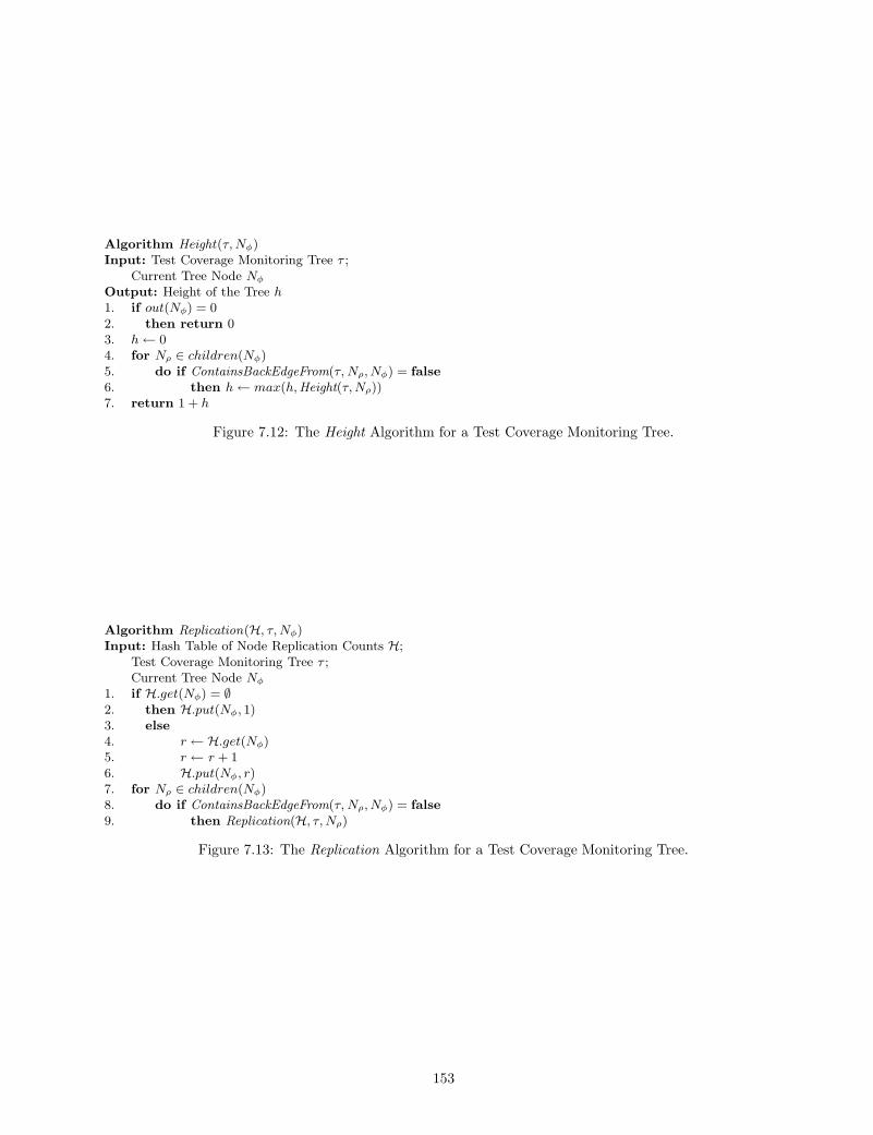
Algorithm Height(τ, Nφ)Input: Test Coverage Monitoring Tree τ ;
Current Tree Node Nφ
Output: Height of the Tree h1. if out(Nφ) = 02. then return 03. h← 04. for Nρ ∈ children(Nφ)5. do if ContainsBackEdgeFrom(τ, Nρ, Nφ) = false6. then h← max(h,Height(τ, Nρ))7. return 1 + h
Figure 7.12: The Height Algorithm for a Test Coverage Monitoring Tree.
Algorithm Replication(H, τ, Nφ)Input: Hash Table of Node Replication Counts H;
Test Coverage Monitoring Tree τ ;Current Tree Node Nφ
1. if H.get(Nφ) = ∅2. then H.put(Nφ, 1)3. else4. r← H.get(Nφ)5. r← r + 16. H.put(Nφ, r)7. for Nρ ∈ children(Nφ)8. do if ContainsBackEdgeFrom(τ, Nρ, Nφ) = false9. then Replication(H, τ, Nρ)
Figure 7.13: The Replication Algorithm for a Test Coverage Monitoring Tree.
153

Application CCT Height DCT Height
RM (6, 7, 8, 9) (6, 7, 8, 9)
FF (5, 7, 8, 9) (6, 8, 9, 10)
PI (6, 6, 7, 8) (6, 6, 7, 8)
ST (6, 7, 8, 9) (6, 7, 8, 9)
TM (5, 7, 8, 9) (5, 7, 8, 9)
GB (6, 7, 8, 9) (6, 7, 8, 9)
Data Format: (P,Rl,Rc,Av)
Table 7.9: Height of the Test Coverage Monitoring Trees.
the out(A, τ, L) metric for all of the database-centric applications. In particular, Figure 7.14 provides a box
and whisker plot of the node out degree for the six case study applications. The graphs demonstrate that
the out degree for a single node can be as low as one to five children and as great as 700 children. Across the
majority of the case study applications, many nodes have a substantial number of children and this result
suggests that the outavg(A, τ, L) does impact the size of the TCM tree. For example, the experiments reveal
that outavg(PI, τcct,P) = 3.25 with a standard deviation of 3.19 while outavg(PI, τcct,Av) = 16.01 and a
standard deviation of 34.8. This explains the result in Table 7.8 where PI’s CCT at the attribute value level
consumes 8522835 bytes of heap storage space
Figures 7.14 and 7.15 show that the DCT has a higher average node out degree than the CCT, for the
majority of the applications. Of course, we attribute this result to the fact that the CCT instrumentation
payloads can coalesce more nodes than the DCT probes. For example, we see that outmax(ST, τcct,P) = 6
and outmax(ST, τdct,P) = 25. However, for some applications (e.g., RM) there is little difference in the node
out degree when we compare τcct and τdct. Figure 7.14 also suggests that the CCT does an acceptable job at
controlling node out degree when we monitor coverage at finer levels of database interaction. The empirical
cumulative distribution function (ECDF) in Figure 7.16(a) reveals that almost 90% of the nodes in PI’s Av
level CCT have a node out degree of less than 50. However, the ECDFs in Figure 7.16 demonstrate that the
node out degree of a database-aware TCM tree can be as high as 700 children. Our empirical characterization
of the out(A, τ, L) further explains why testers should use the CCT to record the coverage of most types of
tests for database-centric applications.
7.6.4.3 Node Replication Counts It is desirable to produce a TCM tree that avoids replication in
all circumstances where the coalescing of a node does not destroy testing context. Figure 7.17 through
Figure 7.19 furnish different views of node level replication within the coverage trees for all six case study
applications. Specifically, Figures 7.17 and 7.18 demonstrate that the DCT has much high replication
than the CCT. For example, we see that rmax(FF, τcct,P) = 25 while rmax(FF, τdct,P) = 100 and FF’s
τdct has several outlying nodes with replication counts in the range of 50 to 100 nodes. Figures 7.17 and
154

P R Rc AvDatabase Interaction
5
10
15
20
25
Node
Out
Degree
Calling Context Tree H RM L
PSfrag replacements
N6
enter computeVelocity
enter computeVelocity
N6
N6
N7
N7
N8
N8
N10
N8
N16
N10
N11
N11
N12
N12
N18
N16
N18
N18
exit computeVelocity
exit computeVelocity
N6
N1
N1
N2
N2
N3
N3
N1
N1
N4
N4
N5
N5
N6
enter P
enter P
call main
call main
enter main
enter main
enter main
. . .
. . .
call inputCardNumber
call inputCardNumber
call inputPin
call inputCardNumber
call handleError
call handleError
call inputCardNumber
call inputPin
call handleError
call handleError
call inputPin
call inputPin
call inputOperation
call inputOperation
call getAccountBalance
call getAccountBalance
call promptAgain
call inputOperation
call lockAccount
call lockAccount
call promptAgain
call promptAgain
call inputOperation
call promptAgain
. . .
call getAccountBalance
enter getAccountBalance
enter getAccountBalance
N3
N3
N4
N4
N5
N5
N6
N6
N7
N7
N10
N10
N12
N12
N15
N10
N15
N15
exit getAccountBalance
exit getAccountBalance
return getAccountBalance
return lockAccount
. . .
return getAccountBalance
call promptAgain
. . .
exit main
exit main
return main
return main
exit P
exit P
. . .
exit main
enter lockAccount
enter lockAccount
. . .
. . .
exit lockAccount
exit lockAccount
return lockAccount
return lockAccount
exit main
(a)
P R Rc AvDatabase Interaction
5
10
15
20
25
Node
Out
Degree
Calling Context Tree H FF L
PSfrag replacements
N6
enter computeVelocity
enter computeVelocity
N6
N6
N7
N7
N8
N8
N10
N8
N16
N10
N11
N11
N12
N12
N18
N16
N18
N18
exit computeVelocity
exit computeVelocity
N6
N1
N1
N2
N2
N3
N3
N1
N1
N4
N4
N5
N5
N6
enter P
enter P
call main
call main
enter main
enter main
enter main
. . .
. . .
call inputCardNumber
call inputCardNumber
call inputPin
call inputCardNumber
call handleError
call handleError
call inputCardNumber
call inputPin
call handleError
call handleError
call inputPin
call inputPin
call inputOperation
call inputOperation
call getAccountBalance
call getAccountBalance
call promptAgain
call inputOperation
call lockAccount
call lockAccount
call promptAgain
call promptAgain
call inputOperation
call promptAgain
. . .
call getAccountBalance
enter getAccountBalance
enter getAccountBalance
N3
N3
N4
N4
N5
N5
N6
N6
N7
N7
N10
N10
N12
N12
N15
N10
N15
N15
exit getAccountBalance
exit getAccountBalance
return getAccountBalance
return lockAccount
. . .
return getAccountBalance
call promptAgain
. . .
exit main
exit main
return main
return main
exit P
exit P
. . .
exit main
enter lockAccount
enter lockAccount
. . .
. . .
exit lockAccount
exit lockAccount
return lockAccount
return lockAccount
exit main
(b)
P R Rc AvDatabase Interaction
0
50
100
150
200
Node
Out
Degree
Calling Context Tree H PI L
PSfrag replacements
N6
enter computeVelocity
enter computeVelocity
N6
N6
N7
N7
N8
N8
N10
N8
N16
N10
N11
N11
N12
N12
N18
N16
N18
N18
exit computeVelocity
exit computeVelocity
N6
N1
N1
N2
N2
N3
N3
N1
N1
N4
N4
N5
N5
N6
enter P
enter P
call main
call main
enter main
enter main
enter main
. . .
. . .
call inputCardNumber
call inputCardNumber
call inputPin
call inputCardNumber
call handleError
call handleError
call inputCardNumber
call inputPin
call handleError
call handleError
call inputPin
call inputPin
call inputOperation
call inputOperation
call getAccountBalance
call getAccountBalance
call promptAgain
call inputOperation
call lockAccount
call lockAccount
call promptAgain
call promptAgain
call inputOperation
call promptAgain
. . .
call getAccountBalance
enter getAccountBalance
enter getAccountBalance
N3
N3
N4
N4
N5
N5
N6
N6
N7
N7
N10
N10
N12
N12
N15
N10
N15
N15
exit getAccountBalance
exit getAccountBalance
return getAccountBalance
return lockAccount
. . .
return getAccountBalance
call promptAgain
. . .
exit main
exit main
return main
return main
exit P
exit P
. . .
exit main
enter lockAccount
enter lockAccount
. . .
. . .
exit lockAccount
exit lockAccount
return lockAccount
return lockAccount
exit main
(c)
P R Rc AvDatabase Interaction
2
4
6
8
10
12
14
Node
Out
Degree
Calling Context Tree H ST L
PSfrag replacements
N6
enter computeVelocity
enter computeVelocity
N6
N6
N7
N7
N8
N8
N10
N8
N16
N10
N11
N11
N12
N12
N18
N16
N18
N18
exit computeVelocity
exit computeVelocity
N6
N1
N1
N2
N2
N3
N3
N1
N1
N4
N4
N5
N5
N6
enter P
enter P
call main
call main
enter main
enter main
enter main
. . .
. . .
call inputCardNumber
call inputCardNumber
call inputPin
call inputCardNumber
call handleError
call handleError
call inputCardNumber
call inputPin
call handleError
call handleError
call inputPin
call inputPin
call inputOperation
call inputOperation
call getAccountBalance
call getAccountBalance
call promptAgain
call inputOperation
call lockAccount
call lockAccount
call promptAgain
call promptAgain
call inputOperation
call promptAgain
. . .
call getAccountBalance
enter getAccountBalance
enter getAccountBalance
N3
N3
N4
N4
N5
N5
N6
N6
N7
N7
N10
N10
N12
N12
N15
N10
N15
N15
exit getAccountBalance
exit getAccountBalance
return getAccountBalance
return lockAccount
. . .
return getAccountBalance
call promptAgain
. . .
exit main
exit main
return main
return main
exit P
exit P
. . .
exit main
enter lockAccount
enter lockAccount
. . .
. . .
exit lockAccount
exit lockAccount
return lockAccount
return lockAccount
exit main
(d)
P R Rc AvDatabase Interaction
10
20
30
40
50
Node
Out
Degree
Calling Context Tree H TM L
PSfrag replacements
N6
enter computeVelocity
enter computeVelocity
N6
N6
N7
N7
N8
N8
N10
N8
N16
N10
N11
N11
N12
N12
N18
N16
N18
N18
exit computeVelocity
exit computeVelocity
N6
N1
N1
N2
N2
N3
N3
N1
N1
N4
N4
N5
N5
N6
enter P
enter P
call main
call main
enter main
enter main
enter main
. . .
. . .
call inputCardNumber
call inputCardNumber
call inputPin
call inputCardNumber
call handleError
call handleError
call inputCardNumber
call inputPin
call handleError
call handleError
call inputPin
call inputPin
call inputOperation
call inputOperation
call getAccountBalance
call getAccountBalance
call promptAgain
call inputOperation
call lockAccount
call lockAccount
call promptAgain
call promptAgain
call inputOperation
call promptAgain
. . .
call getAccountBalance
enter getAccountBalance
enter getAccountBalance
N3
N3
N4
N4
N5
N5
N6
N6
N7
N7
N10
N10
N12
N12
N15
N10
N15
N15
exit getAccountBalance
exit getAccountBalance
return getAccountBalance
return lockAccount
. . .
return getAccountBalance
call promptAgain
. . .
exit main
exit main
return main
return main
exit P
exit P
. . .
exit main
enter lockAccount
enter lockAccount
. . .
. . .
exit lockAccount
exit lockAccount
return lockAccount
return lockAccount
exit main
(e)
P R Rc AvDatabase Interaction
5
10
15
20
25
Node
Out
Degree
Calling Context Tree H GB L
PSfrag replacements
N6
enter computeVelocity
enter computeVelocity
N6
N6
N7
N7
N8
N8
N10
N8
N16
N10
N11
N11
N12
N12
N18
N16
N18
N18
exit computeVelocity
exit computeVelocity
N6
N1
N1
N2
N2
N3
N3
N1
N1
N4
N4
N5
N5
N6
enter P
enter P
call main
call main
enter main
enter main
enter main
. . .
. . .
call inputCardNumber
call inputCardNumber
call inputPin
call inputCardNumber
call handleError
call handleError
call inputCardNumber
call inputPin
call handleError
call handleError
call inputPin
call inputPin
call inputOperation
call inputOperation
call getAccountBalance
call getAccountBalance
call promptAgain
call inputOperation
call lockAccount
call lockAccount
call promptAgain
call promptAgain
call inputOperation
call promptAgain
. . .
call getAccountBalance
enter getAccountBalance
enter getAccountBalance
N3
N3
N4
N4
N5
N5
N6
N6
N7
N7
N10
N10
N12
N12
N15
N10
N15
N15
exit getAccountBalance
exit getAccountBalance
return getAccountBalance
return lockAccount
. . .
return getAccountBalance
call promptAgain
. . .
exit main
exit main
return main
return main
exit P
exit P
. . .
exit main
enter lockAccount
enter lockAccount
. . .
. . .
exit lockAccount
exit lockAccount
return lockAccount
return lockAccount
exit main
(f)
Figure 7.14: Node Out Degree of the CCT Test Coverage Monitoring Trees.
P R Rc AvDatabase Interaction
5
10
15
20
25
Node
Out
Degree
Dynamic Call Tree H RM L
PSfrag replacements
N6
enter computeVelocity
enter computeVelocity
N6
N6
N7
N7
N8
N8
N10
N8
N16
N10
N11
N11
N12
N12
N18
N16
N18
N18
exit computeVelocity
exit computeVelocity
N6
N1
N1
N2
N2
N3
N3
N1
N1
N4
N4
N5
N5
N6
enter P
enter P
call main
call main
enter main
enter main
enter main
. . .
. . .
call inputCardNumber
call inputCardNumber
call inputPin
call inputCardNumber
call handleError
call handleError
call inputCardNumber
call inputPin
call handleError
call handleError
call inputPin
call inputPin
call inputOperation
call inputOperation
call getAccountBalance
call getAccountBalance
call promptAgain
call inputOperation
call lockAccount
call lockAccount
call promptAgain
call promptAgain
call inputOperation
call promptAgain
. . .
call getAccountBalance
enter getAccountBalance
enter getAccountBalance
N3
N3
N4
N4
N5
N5
N6
N6
N7
N7
N10
N10
N12
N12
N15
N10
N15
N15
exit getAccountBalance
exit getAccountBalance
return getAccountBalance
return lockAccount
. . .
return getAccountBalance
call promptAgain
. . .
exit main
exit main
return main
return main
exit P
exit P
. . .
exit main
enter lockAccount
enter lockAccount
. . .
. . .
exit lockAccount
exit lockAccount
return lockAccount
return lockAccount
exit main
(a)
P R Rc AvDatabase Interaction
5
10
15
20
25
Node
Out
Degree
Dynamic Call Tree H FF L
PSfrag replacements
N6
enter computeVelocity
enter computeVelocity
N6
N6
N7
N7
N8
N8
N10
N8
N16
N10
N11
N11
N12
N12
N18
N16
N18
N18
exit computeVelocity
exit computeVelocity
N6
N1
N1
N2
N2
N3
N3
N1
N1
N4
N4
N5
N5
N6
enter P
enter P
call main
call main
enter main
enter main
enter main
. . .
. . .
call inputCardNumber
call inputCardNumber
call inputPin
call inputCardNumber
call handleError
call handleError
call inputCardNumber
call inputPin
call handleError
call handleError
call inputPin
call inputPin
call inputOperation
call inputOperation
call getAccountBalance
call getAccountBalance
call promptAgain
call inputOperation
call lockAccount
call lockAccount
call promptAgain
call promptAgain
call inputOperation
call promptAgain
. . .
call getAccountBalance
enter getAccountBalance
enter getAccountBalance
N3
N3
N4
N4
N5
N5
N6
N6
N7
N7
N10
N10
N12
N12
N15
N10
N15
N15
exit getAccountBalance
exit getAccountBalance
return getAccountBalance
return lockAccount
. . .
return getAccountBalance
call promptAgain
. . .
exit main
exit main
return main
return main
exit P
exit P
. . .
exit main
enter lockAccount
enter lockAccount
. . .
. . .
exit lockAccount
exit lockAccount
return lockAccount
return lockAccount
exit main
(b)
P R Rc AvDatabase Interaction
10
20
30
40
50
Node
Out
Degree
Dynamic Call Tree H PI L
PSfrag replacements
N6
enter computeVelocity
enter computeVelocity
N6
N6
N7
N7
N8
N8
N10
N8
N16
N10
N11
N11
N12
N12
N18
N16
N18
N18
exit computeVelocity
exit computeVelocity
N6
N1
N1
N2
N2
N3
N3
N1
N1
N4
N4
N5
N5
N6
enter P
enter P
call main
call main
enter main
enter main
enter main
. . .
. . .
call inputCardNumber
call inputCardNumber
call inputPin
call inputCardNumber
call handleError
call handleError
call inputCardNumber
call inputPin
call handleError
call handleError
call inputPin
call inputPin
call inputOperation
call inputOperation
call getAccountBalance
call getAccountBalance
call promptAgain
call inputOperation
call lockAccount
call lockAccount
call promptAgain
call promptAgain
call inputOperation
call promptAgain
. . .
call getAccountBalance
enter getAccountBalance
enter getAccountBalance
N3
N3
N4
N4
N5
N5
N6
N6
N7
N7
N10
N10
N12
N12
N15
N10
N15
N15
exit getAccountBalance
exit getAccountBalance
return getAccountBalance
return lockAccount
. . .
return getAccountBalance
call promptAgain
. . .
exit main
exit main
return main
return main
exit P
exit P
. . .
exit main
enter lockAccount
enter lockAccount
. . .
. . .
exit lockAccount
exit lockAccount
return lockAccount
return lockAccount
exit main
(c)
P R Rc AvDatabase Interaction
5
10
15
20
25
30
Node
Out
Degree
Dynamic Call Tree H ST L
PSfrag replacements
N6
enter computeVelocity
enter computeVelocity
N6
N6
N7
N7
N8
N8
N10
N8
N16
N10
N11
N11
N12
N12
N18
N16
N18
N18
exit computeVelocity
exit computeVelocity
N6
N1
N1
N2
N2
N3
N3
N1
N1
N4
N4
N5
N5
N6
enter P
enter P
call main
call main
enter main
enter main
enter main
. . .
. . .
call inputCardNumber
call inputCardNumber
call inputPin
call inputCardNumber
call handleError
call handleError
call inputCardNumber
call inputPin
call handleError
call handleError
call inputPin
call inputPin
call inputOperation
call inputOperation
call getAccountBalance
call getAccountBalance
call promptAgain
call inputOperation
call lockAccount
call lockAccount
call promptAgain
call promptAgain
call inputOperation
call promptAgain
. . .
call getAccountBalance
enter getAccountBalance
enter getAccountBalance
N3
N3
N4
N4
N5
N5
N6
N6
N7
N7
N10
N10
N12
N12
N15
N10
N15
N15
exit getAccountBalance
exit getAccountBalance
return getAccountBalance
return lockAccount
. . .
return getAccountBalance
call promptAgain
. . .
exit main
exit main
return main
return main
exit P
exit P
. . .
exit main
enter lockAccount
enter lockAccount
. . .
. . .
exit lockAccount
exit lockAccount
return lockAccount
return lockAccount
exit main
(d)
P R Rc AvDatabase Interaction
20
40
60
80
100
120
140
Node
Out
Degree
Dynamic Call Tree H TM L
PSfrag replacements
N6
enter computeVelocity
enter computeVelocity
N6
N6
N7
N7
N8
N8
N10
N8
N16
N10
N11
N11
N12
N12
N18
N16
N18
N18
exit computeVelocity
exit computeVelocity
N6
N1
N1
N2
N2
N3
N3
N1
N1
N4
N4
N5
N5
N6
enter P
enter P
call main
call main
enter main
enter main
enter main
. . .
. . .
call inputCardNumber
call inputCardNumber
call inputPin
call inputCardNumber
call handleError
call handleError
call inputCardNumber
call inputPin
call handleError
call handleError
call inputPin
call inputPin
call inputOperation
call inputOperation
call getAccountBalance
call getAccountBalance
call promptAgain
call inputOperation
call lockAccount
call lockAccount
call promptAgain
call promptAgain
call inputOperation
call promptAgain
. . .
call getAccountBalance
enter getAccountBalance
enter getAccountBalance
N3
N3
N4
N4
N5
N5
N6
N6
N7
N7
N10
N10
N12
N12
N15
N10
N15
N15
exit getAccountBalance
exit getAccountBalance
return getAccountBalance
return lockAccount
. . .
return getAccountBalance
call promptAgain
. . .
exit main
exit main
return main
return main
exit P
exit P
. . .
exit main
enter lockAccount
enter lockAccount
. . .
. . .
exit lockAccount
exit lockAccount
return lockAccount
return lockAccount
exit main
(e)
P R Rc AvDatabase Interaction
5
10
15
20
25
Node
Out
Degree
Dynamic Call Tree H GB L
PSfrag replacements
N6
enter computeVelocity
enter computeVelocity
N6
N6
N7
N7
N8
N8
N10
N8
N16
N10
N11
N11
N12
N12
N18
N16
N18
N18
exit computeVelocity
exit computeVelocity
N6
N1
N1
N2
N2
N3
N3
N1
N1
N4
N4
N5
N5
N6
enter P
enter P
call main
call main
enter main
enter main
enter main
. . .
. . .
call inputCardNumber
call inputCardNumber
call inputPin
call inputCardNumber
call handleError
call handleError
call inputCardNumber
call inputPin
call handleError
call handleError
call inputPin
call inputPin
call inputOperation
call inputOperation
call getAccountBalance
call getAccountBalance
call promptAgain
call inputOperation
call lockAccount
call lockAccount
call promptAgain
call promptAgain
call inputOperation
call promptAgain
. . .
call getAccountBalance
enter getAccountBalance
enter getAccountBalance
N3
N3
N4
N4
N5
N5
N6
N6
N7
N7
N10
N10
N12
N12
N15
N10
N15
N15
exit getAccountBalance
exit getAccountBalance
return getAccountBalance
return lockAccount
. . .
return getAccountBalance
call promptAgain
. . .
exit main
exit main
return main
return main
exit P
exit P
. . .
exit main
enter lockAccount
enter lockAccount
. . .
. . .
exit lockAccount
exit lockAccount
return lockAccount
return lockAccount
exit main
(f)
Figure 7.15: Node Out Degree of the DCT Test Coverage Monitoring Trees.
0 50 100 150 200 250Node Out Degree
0.6
0.7
0.8
0.9
1
Empirical
CDF
CCT Av
PSfrag replacements
N6
enter computeVelocity
enter computeVelocity
N6
N6
N7
N7
N8
N8
N10
N8
N16
N10
N11
N11
N12
N12
N18
N16
N18
N18
exit computeVelocity
exit computeVelocity
N6
N1
N1
N2
N2
N3
N3
N1
N1
N4
N4
N5
N5
N6
enter P
enter P
call main
call main
enter main
enter main
enter main
. . .
. . .
call inputCardNumber
call inputCardNumber
call inputPin
call inputCardNumber
call handleError
call handleError
call inputCardNumber
call inputPin
call handleError
call handleError
call inputPin
call inputPin
call inputOperation
call inputOperation
call getAccountBalance
call getAccountBalance
call promptAgain
call inputOperation
call lockAccount
call lockAccount
call promptAgain
call promptAgain
call inputOperation
call promptAgain
. . .
call getAccountBalance
enter getAccountBalance
enter getAccountBalance
N3
N3
N4
N4
N5
N5
N6
N6
N7
N7
N10
N10
N12
N12
N15
N10
N15
N15
exit getAccountBalance
exit getAccountBalance
return getAccountBalance
return lockAccount
. . .
return getAccountBalance
call promptAgain
. . .
exit main
exit main
return main
return main
exit P
exit P
. . .
exit main
enter lockAccount
enter lockAccount
. . .
. . .
exit lockAccount
exit lockAccount
return lockAccount
return lockAccount
exit main
(a)
0 100 200 300 400 500 600 700Node Out Degree
0.9
0.92
0.94
0.96
0.98
1
Empirical
CDF
DCT R and Rc
PSfrag replacements
N6
enter computeVelocity
enter computeVelocity
N6
N6
N7
N7
N8
N8
N10
N8
N16
N10
N11
N11
N12
N12
N18
N16
N18
N18
exit computeVelocity
exit computeVelocity
N6
N1
N1
N2
N2
N3
N3
N1
N1
N4
N4
N5
N5
N6
enter P
enter P
call main
call main
enter main
enter main
enter main
. . .
. . .
call inputCardNumber
call inputCardNumber
call inputPin
call inputCardNumber
call handleError
call handleError
call inputCardNumber
call inputPin
call handleError
call handleError
call inputPin
call inputPin
call inputOperation
call inputOperation
call getAccountBalance
call getAccountBalance
call promptAgain
call inputOperation
call lockAccount
call lockAccount
call promptAgain
call promptAgain
call inputOperation
call promptAgain
. . .
call getAccountBalance
enter getAccountBalance
enter getAccountBalance
N3
N3
N4
N4
N5
N5
N6
N6
N7
N7
N10
N10
N12
N12
N15
N10
N15
N15
exit getAccountBalance
exit getAccountBalance
return getAccountBalance
return lockAccount
. . .
return getAccountBalance
call promptAgain
. . .
exit main
exit main
return main
return main
exit P
exit P
. . .
exit main
enter lockAccount
enter lockAccount
. . .
. . .
exit lockAccount
exit lockAccount
return lockAccount
return lockAccount
exit main
(b)
0 100 200 300 400 500 600 700Node Out Degree
0.85
0.875
0.9
0.925
0.95
0.975
1
Empirical
CDF
DCT Av
PSfrag replacements
N6
enter computeVelocity
enter computeVelocity
N6
N6
N7
N7
N8
N8
N10
N8
N16
N10
N11
N11
N12
N12
N18
N16
N18
N18
exit computeVelocity
exit computeVelocity
N6
N1
N1
N2
N2
N3
N3
N1
N1
N4
N4
N5
N5
N6
enter P
enter P
call main
call main
enter main
enter main
enter main
. . .
. . .
call inputCardNumber
call inputCardNumber
call inputPin
call inputCardNumber
call handleError
call handleError
call inputCardNumber
call inputPin
call handleError
call handleError
call inputPin
call inputPin
call inputOperation
call inputOperation
call getAccountBalance
call getAccountBalance
call promptAgain
call inputOperation
call lockAccount
call lockAccount
call promptAgain
call promptAgain
call inputOperation
call promptAgain
. . .
call getAccountBalance
enter getAccountBalance
enter getAccountBalance
N3
N3
N4
N4
N5
N5
N6
N6
N7
N7
N10
N10
N12
N12
N15
N10
N15
N15
exit getAccountBalance
exit getAccountBalance
return getAccountBalance
return lockAccount
. . .
return getAccountBalance
call promptAgain
. . .
exit main
exit main
return main
return main
exit P
exit P
. . .
exit main
enter lockAccount
enter lockAccount
. . .
. . .
exit lockAccount
exit lockAccount
return lockAccount
return lockAccount
exit main
(c)
Figure 7.16: ECDFs of the Node Out Degree for the Pithy TCM Trees.
155

7.18 also demonstrate that rmax(TM, τcct,P) = 25 and rmax(FF, τdct,P) > 200. Our analysis reveals that
ravg(FF, τcct,R) = 5.31 with a standard deviation of 7.37. However, we also found that the use of the
DCT at the same record level yielded ravg(FF, τcct,R) = 20.0 with with a standard deviation of 30.51. In
comparison to the DCT, these results clearly indicate that the CCT does a very good job at controlling the
maximum and average node replication counts.
For most applications, Figures 7.17 and 7.18 demonstrate that the CCT controls node replication well
when we transition from P to Av. Figure 7.17(e) shows that TM’s CCT has a maximum node out degree
of 70 while Figure 7.18(e) reveals that the corresponding DCT has node(s) with a replication count of
over 400. Figure 7.19 offers ECDFs that further characterize the node replication count for PI’s coverage
monitoring trees. The graph in Figure 7.19(a) indicates that 90% of the nodes in the Av-level CCT still
have a replication count less than 50. Yet, this same CCT has a small number of nodes that are replicated in
the tree 350 times. In comparison, the program level CCT for PI never has a replication count higher than
50. Figure 7.19(b) shows that this trend is more pronounced for the DI-DCT. While the majority of PI’s
nodes have a count less than 1000, a small percentage of nodes are replicated in the tree more than 5000
times. Our analysis suggests that it is difficult for either the CCT or the DCT to control replication at the
Av level. If it is desirable to control node replication, then we judge that the tester should rarely monitor
coverage at the level of attribute values. Since Section 7.6.2 indicates that coverage monitoring at Av never
increases testing time by more than six seconds, we judge that the high values for r are acceptable if this
type of information is needed for debugging.
7.7 THREATS TO VALIDITY
The experiments described in this chapter are subject to validity threats and Chapter 3 reveals the steps
that we took to control these threats during all of the experimentation for this dissertation. We also took
additional steps to handle the threats that are specific to experimentation with the coverage monitoring
component. Internal threats to validity are those factors that have the potential to impact the measured
variables defined in Sections 7.4 and 7.6. One internal validity threat is related to defects in the TCM
component. These defects could could compromise the correctness of the test coverage monitoring trees
and the final measurement of test suite adequacy. We controlled this threat by visualizing small TCM trees
and checking them to ensure correctness. We implemented an automated check to guarantee that the tree’s
active node points to the root (e.g., Na = N0) when the TCM component terminates. We automatically
ensure that the tree adheres to the structure described in Figure 6.19 of Chapter 6. We verify that the leaves
of a tree always correspond to either a method invocation or the correct level for the database interactions.
For example, if L = D, then there should be no attribute values in the tree and an external node must
always be either a method call or a database entity. The coverage monitor also ensures that a DCT does
not have any back edges. We judge that threats to construct validity were controlled since Sections 7.4 and
7.6 describe a wide range of evaluation metrics that are useful to both researchers and practitioners.
156

P R Rc AvDatabase Interaction
5
10
15
20
25
30
35
Replication
Count
Calling Context Tree H RM L
PSfrag replacements
N6
enter computeVelocity
enter computeVelocity
N6
N6
N7
N7
N8
N8
N10
N8
N16
N10
N11
N11
N12
N12
N18
N16
N18
N18
exit computeVelocity
exit computeVelocity
N6
N1
N1
N2
N2
N3
N3
N1
N1
N4
N4
N5
N5
N6
enter P
enter P
call main
call main
enter main
enter main
enter main
. . .
. . .
call inputCardNumber
call inputCardNumber
call inputPin
call inputCardNumber
call handleError
call handleError
call inputCardNumber
call inputPin
call handleError
call handleError
call inputPin
call inputPin
call inputOperation
call inputOperation
call getAccountBalance
call getAccountBalance
call promptAgain
call inputOperation
call lockAccount
call lockAccount
call promptAgain
call promptAgain
call inputOperation
call promptAgain
. . .
call getAccountBalance
enter getAccountBalance
enter getAccountBalance
N3
N3
N4
N4
N5
N5
N6
N6
N7
N7
N10
N10
N12
N12
N15
N10
N15
N15
exit getAccountBalance
exit getAccountBalance
return getAccountBalance
return lockAccount
. . .
return getAccountBalance
call promptAgain
. . .
exit main
exit main
return main
return main
exit P
exit P
. . .
exit main
enter lockAccount
enter lockAccount
. . .
. . .
exit lockAccount
exit lockAccount
return lockAccount
return lockAccount
exit main
(a)
P R Rc AvDatabase Interaction
5
10
15
20
25
30
35
Replication
Count
Calling Context Tree H FF L
PSfrag replacements
N6
enter computeVelocity
enter computeVelocity
N6
N6
N7
N7
N8
N8
N10
N8
N16
N10
N11
N11
N12
N12
N18
N16
N18
N18
exit computeVelocity
exit computeVelocity
N6
N1
N1
N2
N2
N3
N3
N1
N1
N4
N4
N5
N5
N6
enter P
enter P
call main
call main
enter main
enter main
enter main
. . .
. . .
call inputCardNumber
call inputCardNumber
call inputPin
call inputCardNumber
call handleError
call handleError
call inputCardNumber
call inputPin
call handleError
call handleError
call inputPin
call inputPin
call inputOperation
call inputOperation
call getAccountBalance
call getAccountBalance
call promptAgain
call inputOperation
call lockAccount
call lockAccount
call promptAgain
call promptAgain
call inputOperation
call promptAgain
. . .
call getAccountBalance
enter getAccountBalance
enter getAccountBalance
N3
N3
N4
N4
N5
N5
N6
N6
N7
N7
N10
N10
N12
N12
N15
N10
N15
N15
exit getAccountBalance
exit getAccountBalance
return getAccountBalance
return lockAccount
. . .
return getAccountBalance
call promptAgain
. . .
exit main
exit main
return main
return main
exit P
exit P
. . .
exit main
enter lockAccount
enter lockAccount
. . .
. . .
exit lockAccount
exit lockAccount
return lockAccount
return lockAccount
exit main
(b)
P R Rc AvDatabase Interaction
10
20
30
40
50
Replication
Count
Calling Context Tree H PI L
PSfrag replacements
N6
enter computeVelocity
enter computeVelocity
N6
N6
N7
N7
N8
N8
N10
N8
N16
N10
N11
N11
N12
N12
N18
N16
N18
N18
exit computeVelocity
exit computeVelocity
N6
N1
N1
N2
N2
N3
N3
N1
N1
N4
N4
N5
N5
N6
enter P
enter P
call main
call main
enter main
enter main
enter main
. . .
. . .
call inputCardNumber
call inputCardNumber
call inputPin
call inputCardNumber
call handleError
call handleError
call inputCardNumber
call inputPin
call handleError
call handleError
call inputPin
call inputPin
call inputOperation
call inputOperation
call getAccountBalance
call getAccountBalance
call promptAgain
call inputOperation
call lockAccount
call lockAccount
call promptAgain
call promptAgain
call inputOperation
call promptAgain
. . .
call getAccountBalance
enter getAccountBalance
enter getAccountBalance
N3
N3
N4
N4
N5
N5
N6
N6
N7
N7
N10
N10
N12
N12
N15
N10
N15
N15
exit getAccountBalance
exit getAccountBalance
return getAccountBalance
return lockAccount
. . .
return getAccountBalance
call promptAgain
. . .
exit main
exit main
return main
return main
exit P
exit P
. . .
exit main
enter lockAccount
enter lockAccount
. . .
. . .
exit lockAccount
exit lockAccount
return lockAccount
return lockAccount
exit main
(c)
P R Rc AvDatabase Interaction
10
20
30
40
50
Replication
Count
Calling Context Tree H ST L
PSfrag replacements
N6
enter computeVelocity
enter computeVelocity
N6
N6
N7
N7
N8
N8
N10
N8
N16
N10
N11
N11
N12
N12
N18
N16
N18
N18
exit computeVelocity
exit computeVelocity
N6
N1
N1
N2
N2
N3
N3
N1
N1
N4
N4
N5
N5
N6
enter P
enter P
call main
call main
enter main
enter main
enter main
. . .
. . .
call inputCardNumber
call inputCardNumber
call inputPin
call inputCardNumber
call handleError
call handleError
call inputCardNumber
call inputPin
call handleError
call handleError
call inputPin
call inputPin
call inputOperation
call inputOperation
call getAccountBalance
call getAccountBalance
call promptAgain
call inputOperation
call lockAccount
call lockAccount
call promptAgain
call promptAgain
call inputOperation
call promptAgain
. . .
call getAccountBalance
enter getAccountBalance
enter getAccountBalance
N3
N3
N4
N4
N5
N5
N6
N6
N7
N7
N10
N10
N12
N12
N15
N10
N15
N15
exit getAccountBalance
exit getAccountBalance
return getAccountBalance
return lockAccount
. . .
return getAccountBalance
call promptAgain
. . .
exit main
exit main
return main
return main
exit P
exit P
. . .
exit main
enter lockAccount
enter lockAccount
. . .
. . .
exit lockAccount
exit lockAccount
return lockAccount
return lockAccount
exit main
(d)
P R Rc AvDatabase Interaction
10
20
30
40
50
60
70
Replication
Count
Calling Context Tree H TM L
PSfrag replacements
N6
enter computeVelocity
enter computeVelocity
N6
N6
N7
N7
N8
N8
N10
N8
N16
N10
N11
N11
N12
N12
N18
N16
N18
N18
exit computeVelocity
exit computeVelocity
N6
N1
N1
N2
N2
N3
N3
N1
N1
N4
N4
N5
N5
N6
enter P
enter P
call main
call main
enter main
enter main
enter main
. . .
. . .
call inputCardNumber
call inputCardNumber
call inputPin
call inputCardNumber
call handleError
call handleError
call inputCardNumber
call inputPin
call handleError
call handleError
call inputPin
call inputPin
call inputOperation
call inputOperation
call getAccountBalance
call getAccountBalance
call promptAgain
call inputOperation
call lockAccount
call lockAccount
call promptAgain
call promptAgain
call inputOperation
call promptAgain
. . .
call getAccountBalance
enter getAccountBalance
enter getAccountBalance
N3
N3
N4
N4
N5
N5
N6
N6
N7
N7
N10
N10
N12
N12
N15
N10
N15
N15
exit getAccountBalance
exit getAccountBalance
return getAccountBalance
return lockAccount
. . .
return getAccountBalance
call promptAgain
. . .
exit main
exit main
return main
return main
exit P
exit P
. . .
exit main
enter lockAccount
enter lockAccount
. . .
. . .
exit lockAccount
exit lockAccount
return lockAccount
return lockAccount
exit main
(e)
P R Rc AvDatabase Interaction
5
10
15
20
25
30
35
Replication
Count
Calling Context Tree H GB L
PSfrag replacements
N6
enter computeVelocity
enter computeVelocity
N6
N6
N7
N7
N8
N8
N10
N8
N16
N10
N11
N11
N12
N12
N18
N16
N18
N18
exit computeVelocity
exit computeVelocity
N6
N1
N1
N2
N2
N3
N3
N1
N1
N4
N4
N5
N5
N6
enter P
enter P
call main
call main
enter main
enter main
enter main
. . .
. . .
call inputCardNumber
call inputCardNumber
call inputPin
call inputCardNumber
call handleError
call handleError
call inputCardNumber
call inputPin
call handleError
call handleError
call inputPin
call inputPin
call inputOperation
call inputOperation
call getAccountBalance
call getAccountBalance
call promptAgain
call inputOperation
call lockAccount
call lockAccount
call promptAgain
call promptAgain
call inputOperation
call promptAgain
. . .
call getAccountBalance
enter getAccountBalance
enter getAccountBalance
N3
N3
N4
N4
N5
N5
N6
N6
N7
N7
N10
N10
N12
N12
N15
N10
N15
N15
exit getAccountBalance
exit getAccountBalance
return getAccountBalance
return lockAccount
. . .
return getAccountBalance
call promptAgain
. . .
exit main
exit main
return main
return main
exit P
exit P
. . .
exit main
enter lockAccount
enter lockAccount
. . .
. . .
exit lockAccount
exit lockAccount
return lockAccount
return lockAccount
exit main
(f)
Figure 7.17: Node Replication of the CCT Test Coverage Monitoring Trees.
P R Rc AvDatabase Interaction
10
20
30
40
50
Replication
Count
Dynamic Call Tree H RM L
PSfrag replacements
N6
enter computeVelocity
enter computeVelocity
N6
N6
N7
N7
N8
N8
N10
N8
N16
N10
N11
N11
N12
N12
N18
N16
N18
N18
exit computeVelocity
exit computeVelocity
N6
N1
N1
N2
N2
N3
N3
N1
N1
N4
N4
N5
N5
N6
enter P
enter P
call main
call main
enter main
enter main
enter main
. . .
. . .
call inputCardNumber
call inputCardNumber
call inputPin
call inputCardNumber
call handleError
call handleError
call inputCardNumber
call inputPin
call handleError
call handleError
call inputPin
call inputPin
call inputOperation
call inputOperation
call getAccountBalance
call getAccountBalance
call promptAgain
call inputOperation
call lockAccount
call lockAccount
call promptAgain
call promptAgain
call inputOperation
call promptAgain
. . .
call getAccountBalance
enter getAccountBalance
enter getAccountBalance
N3
N3
N4
N4
N5
N5
N6
N6
N7
N7
N10
N10
N12
N12
N15
N10
N15
N15
exit getAccountBalance
exit getAccountBalance
return getAccountBalance
return lockAccount
. . .
return getAccountBalance
call promptAgain
. . .
exit main
exit main
return main
return main
exit P
exit P
. . .
exit main
enter lockAccount
enter lockAccount
. . .
. . .
exit lockAccount
exit lockAccount
return lockAccount
return lockAccount
exit main
(a)
P R Rc AvDatabase Interaction
20
40
60
80
100
120
140
Replication
Count
Dynamic Call Tree H FF L
PSfrag replacements
N6
enter computeVelocity
enter computeVelocity
N6
N6
N7
N7
N8
N8
N10
N8
N16
N10
N11
N11
N12
N12
N18
N16
N18
N18
exit computeVelocity
exit computeVelocity
N6
N1
N1
N2
N2
N3
N3
N1
N1
N4
N4
N5
N5
N6
enter P
enter P
call main
call main
enter main
enter main
enter main
. . .
. . .
call inputCardNumber
call inputCardNumber
call inputPin
call inputCardNumber
call handleError
call handleError
call inputCardNumber
call inputPin
call handleError
call handleError
call inputPin
call inputPin
call inputOperation
call inputOperation
call getAccountBalance
call getAccountBalance
call promptAgain
call inputOperation
call lockAccount
call lockAccount
call promptAgain
call promptAgain
call inputOperation
call promptAgain
. . .
call getAccountBalance
enter getAccountBalance
enter getAccountBalance
N3
N3
N4
N4
N5
N5
N6
N6
N7
N7
N10
N10
N12
N12
N15
N10
N15
N15
exit getAccountBalance
exit getAccountBalance
return getAccountBalance
return lockAccount
. . .
return getAccountBalance
call promptAgain
. . .
exit main
exit main
return main
return main
exit P
exit P
. . .
exit main
enter lockAccount
enter lockAccount
. . .
. . .
exit lockAccount
exit lockAccount
return lockAccount
return lockAccount
exit main
(b)
P R Rc AvDatabase Interaction
20
40
60
80
100
120
140
Replication
Count
Dynamic Call Tree H PI L
PSfrag replacements
N6
enter computeVelocity
enter computeVelocity
N6
N6
N7
N7
N8
N8
N10
N8
N16
N10
N11
N11
N12
N12
N18
N16
N18
N18
exit computeVelocity
exit computeVelocity
N6
N1
N1
N2
N2
N3
N3
N1
N1
N4
N4
N5
N5
N6
enter P
enter P
call main
call main
enter main
enter main
enter main
. . .
. . .
call inputCardNumber
call inputCardNumber
call inputPin
call inputCardNumber
call handleError
call handleError
call inputCardNumber
call inputPin
call handleError
call handleError
call inputPin
call inputPin
call inputOperation
call inputOperation
call getAccountBalance
call getAccountBalance
call promptAgain
call inputOperation
call lockAccount
call lockAccount
call promptAgain
call promptAgain
call inputOperation
call promptAgain
. . .
call getAccountBalance
enter getAccountBalance
enter getAccountBalance
N3
N3
N4
N4
N5
N5
N6
N6
N7
N7
N10
N10
N12
N12
N15
N10
N15
N15
exit getAccountBalance
exit getAccountBalance
return getAccountBalance
return lockAccount
. . .
return getAccountBalance
call promptAgain
. . .
exit main
exit main
return main
return main
exit P
exit P
. . .
exit main
enter lockAccount
enter lockAccount
. . .
. . .
exit lockAccount
exit lockAccount
return lockAccount
return lockAccount
exit main
(c)
P R Rc AvDatabase Interaction
500
1000
1500
2000
Replication
Count
Dynamic Call Tree H ST L
PSfrag replacements
N6
enter computeVelocity
enter computeVelocity
N6
N6
N7
N7
N8
N8
N10
N8
N16
N10
N11
N11
N12
N12
N18
N16
N18
N18
exit computeVelocity
exit computeVelocity
N6
N1
N1
N2
N2
N3
N3
N1
N1
N4
N4
N5
N5
N6
enter P
enter P
call main
call main
enter main
enter main
enter main
. . .
. . .
call inputCardNumber
call inputCardNumber
call inputPin
call inputCardNumber
call handleError
call handleError
call inputCardNumber
call inputPin
call handleError
call handleError
call inputPin
call inputPin
call inputOperation
call inputOperation
call getAccountBalance
call getAccountBalance
call promptAgain
call inputOperation
call lockAccount
call lockAccount
call promptAgain
call promptAgain
call inputOperation
call promptAgain
. . .
call getAccountBalance
enter getAccountBalance
enter getAccountBalance
N3
N3
N4
N4
N5
N5
N6
N6
N7
N7
N10
N10
N12
N12
N15
N10
N15
N15
exit getAccountBalance
exit getAccountBalance
return getAccountBalance
return lockAccount
. . .
return getAccountBalance
call promptAgain
. . .
exit main
exit main
return main
return main
exit P
exit P
. . .
exit main
enter lockAccount
enter lockAccount
. . .
. . .
exit lockAccount
exit lockAccount
return lockAccount
return lockAccount
exit main
(d)
P R Rc AvDatabase Interaction
100
200
300
400
Replication
Count
Dynamic Call Tree H TM L
PSfrag replacements
N6
enter computeVelocity
enter computeVelocity
N6
N6
N7
N7
N8
N8
N10
N8
N16
N10
N11
N11
N12
N12
N18
N16
N18
N18
exit computeVelocity
exit computeVelocity
N6
N1
N1
N2
N2
N3
N3
N1
N1
N4
N4
N5
N5
N6
enter P
enter P
call main
call main
enter main
enter main
enter main
. . .
. . .
call inputCardNumber
call inputCardNumber
call inputPin
call inputCardNumber
call handleError
call handleError
call inputCardNumber
call inputPin
call handleError
call handleError
call inputPin
call inputPin
call inputOperation
call inputOperation
call getAccountBalance
call getAccountBalance
call promptAgain
call inputOperation
call lockAccount
call lockAccount
call promptAgain
call promptAgain
call inputOperation
call promptAgain
. . .
call getAccountBalance
enter getAccountBalance
enter getAccountBalance
N3
N3
N4
N4
N5
N5
N6
N6
N7
N7
N10
N10
N12
N12
N15
N10
N15
N15
exit getAccountBalance
exit getAccountBalance
return getAccountBalance
return lockAccount
. . .
return getAccountBalance
call promptAgain
. . .
exit main
exit main
return main
return main
exit P
exit P
. . .
exit main
enter lockAccount
enter lockAccount
. . .
. . .
exit lockAccount
exit lockAccount
return lockAccount
return lockAccount
exit main
(e)
P R Rc AvDatabase Interaction
20
40
60
80
100
120
140
Replication
Count
Dynamic Call Tree H GB L
PSfrag replacements
N6
enter computeVelocity
enter computeVelocity
N6
N6
N7
N7
N8
N8
N10
N8
N16
N10
N11
N11
N12
N12
N18
N16
N18
N18
exit computeVelocity
exit computeVelocity
N6
N1
N1
N2
N2
N3
N3
N1
N1
N4
N4
N5
N5
N6
enter P
enter P
call main
call main
enter main
enter main
enter main
. . .
. . .
call inputCardNumber
call inputCardNumber
call inputPin
call inputCardNumber
call handleError
call handleError
call inputCardNumber
call inputPin
call handleError
call handleError
call inputPin
call inputPin
call inputOperation
call inputOperation
call getAccountBalance
call getAccountBalance
call promptAgain
call inputOperation
call lockAccount
call lockAccount
call promptAgain
call promptAgain
call inputOperation
call promptAgain
. . .
call getAccountBalance
enter getAccountBalance
enter getAccountBalance
N3
N3
N4
N4
N5
N5
N6
N6
N7
N7
N10
N10
N12
N12
N15
N10
N15
N15
exit getAccountBalance
exit getAccountBalance
return getAccountBalance
return lockAccount
. . .
return getAccountBalance
call promptAgain
. . .
exit main
exit main
return main
return main
exit P
exit P
. . .
exit main
enter lockAccount
enter lockAccount
. . .
. . .
exit lockAccount
exit lockAccount
return lockAccount
return lockAccount
exit main
(f)
Figure 7.18: Node Replication of the DCT Test Coverage Monitoring Trees.
0 50 100 150 200 250 300 350Node Replication Count
0.75
0.8
0.85
0.9
0.95
1
Empirical
CDF
CCT Av
PSfrag replacements
N6
enter computeVelocity
enter computeVelocity
N6
N6
N7
N7
N8
N8
N10
N8
N16
N10
N11
N11
N12
N12
N18
N16
N18
N18
exit computeVelocity
exit computeVelocity
N6
N1
N1
N2
N2
N3
N3
N1
N1
N4
N4
N5
N5
N6
enter P
enter P
call main
call main
enter main
enter main
enter main
. . .
. . .
call inputCardNumber
call inputCardNumber
call inputPin
call inputCardNumber
call handleError
call handleError
call inputCardNumber
call inputPin
call handleError
call handleError
call inputPin
call inputPin
call inputOperation
call inputOperation
call getAccountBalance
call getAccountBalance
call promptAgain
call inputOperation
call lockAccount
call lockAccount
call promptAgain
call promptAgain
call inputOperation
call promptAgain
. . .
call getAccountBalance
enter getAccountBalance
enter getAccountBalance
N3
N3
N4
N4
N5
N5
N6
N6
N7
N7
N10
N10
N12
N12
N15
N10
N15
N15
exit getAccountBalance
exit getAccountBalance
return getAccountBalance
return lockAccount
. . .
return getAccountBalance
call promptAgain
. . .
exit main
exit main
return main
return main
exit P
exit P
. . .
exit main
enter lockAccount
enter lockAccount
. . .
. . .
exit lockAccount
exit lockAccount
return lockAccount
return lockAccount
exit main
(a)
0 5000 10000 15000Node Replication Count
0.85
0.875
0.9
0.925
0.95
0.975
1
Empirical
CDF
DCT Av
PSfrag replacements
N6
enter computeVelocity
enter computeVelocity
N6
N6
N7
N7
N8
N8
N10
N8
N16
N10
N11
N11
N12
N12
N18
N16
N18
N18
exit computeVelocity
exit computeVelocity
N6
N1
N1
N2
N2
N3
N3
N1
N1
N4
N4
N5
N5
N6
enter P
enter P
call main
call main
enter main
enter main
enter main
. . .
. . .
call inputCardNumber
call inputCardNumber
call inputPin
call inputCardNumber
call handleError
call handleError
call inputCardNumber
call inputPin
call handleError
call handleError
call inputPin
call inputPin
call inputOperation
call inputOperation
call getAccountBalance
call getAccountBalance
call promptAgain
call inputOperation
call lockAccount
call lockAccount
call promptAgain
call promptAgain
call inputOperation
call promptAgain
. . .
call getAccountBalance
enter getAccountBalance
enter getAccountBalance
N3
N3
N4
N4
N5
N5
N6
N6
N7
N7
N10
N10
N12
N12
N15
N10
N15
N15
exit getAccountBalance
exit getAccountBalance
return getAccountBalance
return lockAccount
. . .
return getAccountBalance
call promptAgain
. . .
exit main
exit main
return main
return main
exit P
exit P
. . .
exit main
enter lockAccount
enter lockAccount
. . .
. . .
exit lockAccount
exit lockAccount
return lockAccount
return lockAccount
exit main
(b)
Figure 7.19: ECDFs of the Node Replication Count for the Pithy TCM Trees.
157
7.8 CONCLUSION
This chapter describes the design, implementation, and empirical evaluation of a component that performs
database-aware test coverage monitoring. We explain how to use aspect-oriented programming techniques
to introduce the TCM probes in either a static or a dynamic fashion. After discussing the goals and
design for an experiment to measure the performance of our approach to monitoring, we systematically
state each evaluation metric and analyze the experimental results. Since our technique does not use a
customized JVM to produce the reports, we judge that the experimental results establish an upper bound
on the costs associated with database-aware monitoring. We anticipate further reductions in test coverage
monitoring time if we use recently developed JVM-based techniques to introduce the instrumentation (e.g.,
[Bockisch et al., 2006, Golbeck and Kiczales, 2007]). The experiments furnish several key insights into the
fundamental performance trade-offs for the different configurations of the TCM component. For example,
we found that efficient coverage monitoring often requires the use of a static instrumentation technique that
increases the static space overhead of a database-centric application.
The experiment data suggests that a DI-CCT at the finest level of database interaction granularity often
consumes less space overhead than a traditional DCT. The empirical results also indicate that monitoring
coverage at the attribute value level has the potential to increase average node out degree and replication
counts in the TCM trees. We also discovered that the XML-based tree encoding has exceptional compress-
ibility and it often yields very small coverage reports. In general, we find that most configurations of the
TCM component yield acceptable time and space overheads for the chosen applications. Since our coverage
monitoring component builds traditional and database-aware TCM trees, it can also be used to support
regression test suite reduction techniques for normal programs [McMaster and Memon, 2005]. The TCM
trees can also serve as a vehicle for efficient time-aware test suite prioritization because they record coverage
information on a per-test basis [Walcott et al., 2006]. Chapter 8 explains how we use the DI-DCT and
DI-CCT to perform database-aware regression test suite reduction and prioritization.
158

8.0 REGRESSION TESTING
8.1 INTRODUCTION
This chapter introduces database-aware techniques for regression testing. It describes an approach to regres-
sion test suite reduction that efficiently identifies a smaller test suite that covers the same test requirements
as the original tests. We also present a method for regression test prioritization that re-orders a test suite so
that it rapidly covers the test requirements. These regression testing algorithms can improve the efficiency
and effectiveness of testing whenever it is possible to precisely determine which requirements are covered by
a test case. This chapter also demonstrates how to use a path in a database-aware coverage tree as a test
requirement that supports reduction and prioritization. We performed experiments to measure the efficiency
of the regression testing techniques and to identify how reduction and prioritization impact both testing
time and effectiveness. In summary, this chapter provides:
1. A high level overview of the regression testing process (Section 8.2).
2. A demonstration of the practical benefits of regression test suite reduction and prioritization (Section 8.3).
3. The algorithms that we use to identify test paths within a database-aware coverage tree and a discussion
of how these paths can be used as test requirements (Section 8.4).
4. The description of database-aware reduction and prioritization techniques that consider both the tests’
overlap in requirement coverage and the time overhead of an individual test (Section 8.5)
5. Metrics for evaluating the effectiveness of reduced and prioritized test suites (Section 8.6).
6. Details about the implementation of the database-aware regression testing component (Section 8.7).
7. The design of an experiment to measure the performance of the regression tester, a summary of the exper-
imental results, and an examination of the steps that we took to control experiment validity (Sections 8.8,
8.9, and 8.11).
8. An empirical evaluation of the costs associated with analyzing the coverage report and identifying a
reduced or prioritized test suite (Sections 8.10.2 and 8.10.3).
9. An experimental examination of the impact that the database-aware regression testing techniques have
on test suite execution time and effectiveness (Sections 8.10.2 and 8.10.3).
159

Begin Coverage Report End
Program or Database Changes
Program
Test Suite Execution
Reduction or Prioritization
Original Test Suite
Modified Test Suite
Testing Results
PSfrag replacements
N6
enter computeVelocity
enter computeVelocity
N6
N6
N7
N7
N8
N8
N10
N8
N16
N10
N11
N11
N12
N12
N18
N16
N18
N18
exit computeVelocity
exit computeVelocity
N6
N1
N1
N2
N2
N3
N3
N1
N1
N4
N4
N5
N5
N6
enter P
enter P
call main
call main
enter main
enter main
enter main
. . .
. . .
call inputCardNumber
call inputCardNumber
call inputPin
call inputCardNumber
call handleError
call handleError
call inputCardNumber
call inputPin
call handleError
call handleError
call inputPin
call inputPin
call inputOperation
call inputOperation
call getAccountBalance
call getAccountBalance
call promptAgain
call inputOperation
call lockAccount
call lockAccount
call promptAgain
call promptAgain
call inputOperation
call promptAgain
. . .
call getAccountBalance
enter getAccountBalance
enter getAccountBalance
N3
N3
N4
N4
N5
N5
N6
N6
N7
N7
N10
N10
N12
N12
N15
N10
N15
N15
exit getAccountBalance
exit getAccountBalance
return getAccountBalance
return lockAccount
. . .
return getAccountBalance
call promptAgain
. . .
exit main
exit main
return main
return main
exit P
exit P
. . .
exit main
enter lockAccount
enter lockAccount
. . .
. . .
exit lockAccount
exit lockAccount
return lockAccount
return lockAccount
exit main
Figure 8.1: Overview of the Database-Aware Regression Testing Process.
8.2 OVERVIEW OF REGRESSION TESTING
Figure 8.1 provides an overview of database-aware regression testing. Database-aware regression testing is
the process of executing a test suite whenever changes are made to the (i) program, (ii) state of the database,
or (iii) relational schema of the database. Regression testing ensures that the introduction of either a bug fix
or a new feature does not impact the correctness of the application. In the general regression testing (GRT)
model, we re-order or reduce the test suite and then use the modified test suite during many subsequent
rounds of regression testing [Rothermel et al., 2001]. The version specific regression testing (VSRT) model
suggests that the test suite should be re-ordered or reduced after each modification to the database-centric
application. Version specific approaches to regression testing are valuable because they always consider the
current state and structure of both the program and the database. However, version specific regression
testing requires efficient implementations of the (i) test requirement enumerator, (ii) test coverage monitor,
(iii) test adequacy calculator, and (iv) reduction and/or prioritization technique. Any regression testing
approach that can efficiently operate in a version specific fashion should also support general regression
testing. Therefore, we focus on version specific regression testing schemes.
Before reducing or prioritizing the test suite, we analyze the coverage report in order to determine how the
tests covered the requirements. Currently, the regression tester examines the database-aware test coverage
trees and uses a path in the tree as a test requirement. Our approach to reduction and prioritization can
properly operate as long as we can determine which requirements are covered by a test case. Therefore, the
regression tester can also reduce and/or prioritize tests with the database interaction associations (DIAs)
that are described in Chapter 4. Yet, the coverage tree paths still reveal how the test cases cause the
program to interact with both the methods under test and the entities in the relational database. This type
of requirement is particularly useful when a database-centric application contains many partially dynamic
and dynamic database interaction points. We judge that the tree-based requirement is ideal for our case
study applications since Chapter 3 reveals that they have few static database interactions and Chapter 7
demonstrates that the coverage monitor can efficiently create these trees during test execution. Using a
coverage tree path as a test requirement also avoids the need to repeatedly execute the data flow analyzer
in order to enumerate the DIAs after a change occurs in any part of the database-centric application. We
judge that the tree-based requirements are well suited for either version specific or general regression testing
and the DIAs are most useful in the GRT model.
160

0 5 10 15 20Time H sec L
0
1
2
3
4
5
Covered
Test
Reqs
Hcount
L T1 T2 T3
0 5 10 15 20Time H sec L
0
1
2
3
4
5
Covered
Test
Reqs
Hcount
L T1 T2 T3
PSfrag replacements
N6
enter computeVelocity
enter computeVelocity
N6
N6
N7
N7
N8
N8
N10
N8
N16
N10
N11
N11
N12
N12
N18
N16
N18
N18
exit computeVelocity
exit computeVelocity
N6
N1
N1
N2
N2
N3
N3
N1
N1
N4
N4
N5
N5
N6
enter P
enter P
call main
call main
enter main
enter main
enter main
. . .
. . .
call inputCardNumber
call inputCardNumber
call inputPin
call inputCardNumber
call handleError
call handleError
call inputCardNumber
call inputPin
call handleError
call handleError
call inputPin
call inputPin
call inputOperation
call inputOperation
call getAccountBalance
call getAccountBalance
call promptAgain
call inputOperation
call lockAccount
call lockAccount
call promptAgain
call promptAgain
call inputOperation
call promptAgain
. . .
call getAccountBalance
enter getAccountBalance
enter getAccountBalance
N3
N3
N4
N4
N5
N5
N6
N6
N7
N7
N10
N10
N12
N12
N15
N10
N15
N15
exit getAccountBalance
exit getAccountBalance
return getAccountBalance
return lockAccount
. . .
return getAccountBalance
call promptAgain
. . .
exit main
exit main
return main
return main
exit P
exit P
. . .
exit main
enter lockAccount
enter lockAccount
. . .
. . .
exit lockAccount
exit lockAccount
return lockAccount
return lockAccount
exit main
(a)
0 5 10 15 20Time H sec L
0
1
2
3
4
5
Covered
Test
Reqs
Hcount
L T1 T3 T2
0 5 10 15 20Time H sec L
0
1
2
3
4
5
Covered
Test
Reqs
Hcount
L T1 T3 T2
PSfrag replacements
N6
enter computeVelocity
enter computeVelocity
N6
N6
N7
N7
N8
N8
N10
N8
N16
N10
N11
N11
N12
N12
N18
N16
N18
N18
exit computeVelocity
exit computeVelocity
N6
N1
N1
N2
N2
N3
N3
N1
N1
N4
N4
N5
N5
N6
enter P
enter P
call main
call main
enter main
enter main
enter main
. . .
. . .
call inputCardNumber
call inputCardNumber
call inputPin
call inputCardNumber
call handleError
call handleError
call inputCardNumber
call inputPin
call handleError
call handleError
call inputPin
call inputPin
call inputOperation
call inputOperation
call getAccountBalance
call getAccountBalance
call promptAgain
call inputOperation
call lockAccount
call lockAccount
call promptAgain
call promptAgain
call inputOperation
call promptAgain
. . .
call getAccountBalance
enter getAccountBalance
enter getAccountBalance
N3
N3
N4
N4
N5
N5
N6
N6
N7
N7
N10
N10
N12
N12
N15
N10
N15
N15
exit getAccountBalance
exit getAccountBalance
return getAccountBalance
return lockAccount
. . .
return getAccountBalance
call promptAgain
. . .
exit main
exit main
return main
return main
exit P
exit P
. . .
exit main
enter lockAccount
enter lockAccount
. . .
. . .
exit lockAccount
exit lockAccount
return lockAccount
return lockAccount
exit main
(b)
0 5 10 15 20Time H sec L
0
1
2
3
4
5
Covered
Test
Reqs
Hcount
L T2 T1 T3
0 5 10 15 20Time H sec L
0
1
2
3
4
5
Covered
Test
Reqs
Hcount
L T2 T1 T3
PSfrag replacements
N6
enter computeVelocity
enter computeVelocity
N6
N6
N7
N7
N8
N8
N10
N8
N16
N10
N11
N11
N12
N12
N18
N16
N18
N18
exit computeVelocity
exit computeVelocity
N6
N1
N1
N2
N2
N3
N3
N1
N1
N4
N4
N5
N5
N6
enter P
enter P
call main
call main
enter main
enter main
enter main
. . .
. . .
call inputCardNumber
call inputCardNumber
call inputPin
call inputCardNumber
call handleError
call handleError
call inputCardNumber
call inputPin
call handleError
call handleError
call inputPin
call inputPin
call inputOperation
call inputOperation
call getAccountBalance
call getAccountBalance
call promptAgain
call inputOperation
call lockAccount
call lockAccount
call promptAgain
call promptAgain
call inputOperation
call promptAgain
. . .
call getAccountBalance
enter getAccountBalance
enter getAccountBalance
N3
N3
N4
N4
N5
N5
N6
N6
N7
N7
N10
N10
N12
N12
N15
N10
N15
N15
exit getAccountBalance
exit getAccountBalance
return getAccountBalance
return lockAccount
. . .
return getAccountBalance
call promptAgain
. . .
exit main
exit main
return main
return main
exit P
exit P
. . .
exit main
enter lockAccount
enter lockAccount
. . .
. . .
exit lockAccount
exit lockAccount
return lockAccount
return lockAccount
exit main
(c)
0 5 10 15 20Time H sec L
0
1
2
3
4
5
Covered
Test
Reqs
Hcount
L T2 T3 T1
0 5 10 15 20Time H sec L
0
1
2
3
4
5
Covered
Test
Reqs
Hcount
L T2 T3 T1
PSfrag replacements
N6
enter computeVelocity
enter computeVelocity
N6
N6
N7
N7
N8
N8
N10
N8
N16
N10
N11
N11
N12
N12
N18
N16
N18
N18
exit computeVelocity
exit computeVelocity
N6
N1
N1
N2
N2
N3
N3
N1
N1
N4
N4
N5
N5
N6
enter P
enter P
call main
call main
enter main
enter main
enter main
. . .
. . .
call inputCardNumber
call inputCardNumber
call inputPin
call inputCardNumber
call handleError
call handleError
call inputCardNumber
call inputPin
call handleError
call handleError
call inputPin
call inputPin
call inputOperation
call inputOperation
call getAccountBalance
call getAccountBalance
call promptAgain
call inputOperation
call lockAccount
call lockAccount
call promptAgain
call promptAgain
call inputOperation
call promptAgain
. . .
call getAccountBalance
enter getAccountBalance
enter getAccountBalance
N3
N3
N4
N4
N5
N5
N6
N6
N7
N7
N10
N10
N12
N12
N15
N10
N15
N15
exit getAccountBalance
exit getAccountBalance
return getAccountBalance
return lockAccount
. . .
return getAccountBalance
call promptAgain
. . .
exit main
exit main
return main
return main
exit P
exit P
. . .
exit main
enter lockAccount
enter lockAccount
. . .
. . .
exit lockAccount
exit lockAccount
return lockAccount
return lockAccount
exit main
(d)
0 5 10 15 20Time H sec L
0
1
2
3
4
5
Covered
Test
Reqs
Hcount
L T3 T1 T2
0 5 10 15 20Time H sec L
0
1
2
3
4
5
Covered
Test
Reqs
Hcount
L T3 T1 T2
PSfrag replacements
N6
enter computeVelocity
enter computeVelocity
N6
N6
N7
N7
N8
N8
N10
N8
N16
N10
N11
N11
N12
N12
N18
N16
N18
N18
exit computeVelocity
exit computeVelocity
N6
N1
N1
N2
N2
N3
N3
N1
N1
N4
N4
N5
N5
N6
enter P
enter P
call main
call main
enter main
enter main
enter main
. . .
. . .
call inputCardNumber
call inputCardNumber
call inputPin
call inputCardNumber
call handleError
call handleError
call inputCardNumber
call inputPin
call handleError
call handleError
call inputPin
call inputPin
call inputOperation
call inputOperation
call getAccountBalance
call getAccountBalance
call promptAgain
call inputOperation
call lockAccount
call lockAccount
call promptAgain
call promptAgain
call inputOperation
call promptAgain
. . .
call getAccountBalance
enter getAccountBalance
enter getAccountBalance
N3
N3
N4
N4
N5
N5
N6
N6
N7
N7
N10
N10
N12
N12
N15
N10
N15
N15
exit getAccountBalance
exit getAccountBalance
return getAccountBalance
return lockAccount
. . .
return getAccountBalance
call promptAgain
. . .
exit main
exit main
return main
return main
exit P
exit P
. . .
exit main
enter lockAccount
enter lockAccount
. . .
. . .
exit lockAccount
exit lockAccount
return lockAccount
return lockAccount
exit main
(e)
0 5 10 15 20Time H sec L
0
1
2
3
4
5
Covered
Test
Reqs
Hcount
L T3 T2 T1
0 5 10 15 20Time H sec L
0
1
2
3
4
5
Covered
Test
Reqs
Hcount
L T3 T2 T1
PSfrag replacements
N6
enter computeVelocity
enter computeVelocity
N6
N6
N7
N7
N8
N8
N10
N8
N16
N10
N11
N11
N12
N12
N18
N16
N18
N18
exit computeVelocity
exit computeVelocity
N6
N1
N1
N2
N2
N3
N3
N1
N1
N4
N4
N5
N5
N6
enter P
enter P
call main
call main
enter main
enter main
enter main
. . .
. . .
call inputCardNumber
call inputCardNumber
call inputPin
call inputCardNumber
call handleError
call handleError
call inputCardNumber
call inputPin
call handleError
call handleError
call inputPin
call inputPin
call inputOperation
call inputOperation
call getAccountBalance
call getAccountBalance
call promptAgain
call inputOperation
call lockAccount
call lockAccount
call promptAgain
call promptAgain
call inputOperation
call promptAgain
. . .
call getAccountBalance
enter getAccountBalance
enter getAccountBalance
N3
N3
N4
N4
N5
N5
N6
N6
N7
N7
N10
N10
N12
N12
N15
N10
N15
N15
exit getAccountBalance
exit getAccountBalance
return getAccountBalance
return lockAccount
. . .
return getAccountBalance
call promptAgain
. . .
exit main
exit main
return main
return main
exit P
exit P
. . .
exit main
enter lockAccount
enter lockAccount
. . .
. . .
exit lockAccount
exit lockAccount
return lockAccount
return lockAccount
exit main
(f)
Figure 8.2: Coverage Effectiveness of Regression Test Prioritizations.
The reduction and prioritization techniques analyze the original test suite and the per-test coverage
information in order to create a modified test suite. In the context of reduction, the primary goal is to
identify a subset of the original test cases that covers the same test requirements. Controlling the size of
the test suite in this manner can improve the efficiency of testing without compromising coverage or unduly
decreasing fault detection effectiveness. A prioritization algorithm re-orders a test suite so that it covers
test requirements and reveals faults more effectively than the initial ordering. We describe approaches to
reduction and prioritization that consider the tests’ overlap in coverage and the actual cost associated with
executing each test. Since overlap-aware regression testing requires a heuristic solution to the NP-complete
minimal set cover (MSC) problem [Garey and Johnson, 1979], we also propose reduction and prioritization
algorithms that ignore overlap in an attempt to improve efficiency. However, the overlap-aware reduction
and prioritization techniques employ the greedy approximation algorithm that is provably the best for MSC
[Feige, 1998, Vazirani, 2001] and the experiments also demonstrate that our approach is very efficient. Our
regression testing component differs from the schemes previously developed by [Do et al., 2004, Harrold et al.,
1993, Rothermel et al., 2001] because it (i) considers the actual cost of executing a test and (ii) uses test
requirements that incorporate details about a database interaction.
8.3 THE BENEFITS OF REGRESSION TESTING
Suppose that a test suite T = 〈T1, T2, T3〉 tests program P and covers a total of five test requirements. These
requirements might be (i) coverage tree paths, (ii) def-use and database interaction associations, or (iii) nodes
and edges in a control flow graph. Table 8.1 shows that test T2 takes ten seconds to execute while T1 and
T3 respectively consume five and four seconds during test suite execution. Even though this test suite only
161

Test Case Test Execution Time (sec)
T1 5
T2 10
T3 4
Total Testing Time = 19 seconds
Table 8.1: Test Suite Execution Time.
Test Case Requirements
R1 R2 R3 R4 R5
T1 X X
T2 X X X X
T3 X X X
Table 8.2: Test Requirement Coverage for a Test Suite.
Test Ordering Coverage Area Coverage Effectiveness
T1 T2 T3 36 .3798
T1 T3 T2 48 .5053
T2 T1 T3 36 .3798
T2 T3 T1 41 .4316
T3 T1 T2 55 .5789
T3 T2 T1 55 .5789
Ideal Coverage Area = 95
Table 8.3: Test Coverage Effectiveness.
162

Start
Act and Exp Relation j
j = j + 1
j < w
End
Database-Aware Test Oracle
true or false?
PSfrag replacements
N6
enter computeVelocity
enter computeVelocity
N6
N6
N7
N7
N8
N8
N10
N8
N16
N10
N11
N11
N12
N12
N18
N16
N18
N18
exit computeVelocity
exit computeVelocity
N6
N1
N1
N2
N2
N3
N3
N1
N1
N4
N4
N5
N5
N6
enter P
enter P
call main
call main
enter main
enter main
enter main
. . .
. . .
call inputCardNumber
call inputCardNumber
call inputPin
call inputCardNumber
call handleError
call handleError
call inputCardNumber
call inputPin
call handleError
call handleError
call inputPin
call inputPin
call inputOperation
call inputOperation
call getAccountBalance
call getAccountBalance
call promptAgain
call inputOperation
call lockAccount
call lockAccount
call promptAgain
call promptAgain
call inputOperation
call promptAgain
. . .
call getAccountBalance
enter getAccountBalance
enter getAccountBalance
N3
N3
N4
N4
N5
N5
N6
N6
N7
N7
N10
N10
N12
N12
N15
N10
N15
N15
exit getAccountBalance
exit getAccountBalance
return getAccountBalance
return lockAccount
. . .
return getAccountBalance
call promptAgain
. . .
exit main
exit main
return main
return main
exit P
exit P
. . .
exit main
enter lockAccount
enter lockAccount
. . .
. . .
exit lockAccount
exit lockAccount
return lockAccount
return lockAccount
exit main
Figure 8.3: Executing the Database-Aware Test Oracle.
executes for nineteen seconds, the tests for a database-centric application might consume more time if they
interact with large databases. Table 8.2 reveals that none of the test cases cover all of the test requirements.
As is the case for most real world test suites, there is an overlap in how the tests cover the requirements (e.g.,
all of the tests cover requirement R1). In this example, we assume that test T2 covers four requirements and
T3 and T1 cover three and two requirements, respectively. There are 3! = 3× 2× 1 = 6 different orderings
in which we could execute this simple test suite. In order to characterize the coverage effectiveness of a
test suite prioritization, Figure 8.2 plots the cumulative number of covered test requirements during the
execution of T . The shaded area under these coverage curves highlights the effectiveness of a test ordering
(i.e., a large shaded area suggests that an ordering is highly effective).
We construct a coverage function with the assumption that a requirement is marked as covered when
one of its covering test cases terminates. For example, Figure 8.2(a) shows that the execution of T1 leads
to the coverage of two test requirements (i.e., R1 and R2) after five seconds of test suite execution. This
figure also reveals that the cumulative coverage of the test suite increases to four when T2 terminates (i.e.,
T2 covers R3 and R5 after executing for ten seconds). A high coverage area indicates that the test ordering
covers the requirements faster than a test suite order with a low coverage area. Furthermore, an ideal test
suite would immediately cover all of the test requirements. Intuitively, we define the coverage effectiveness
of a prioritized test suite as the ratio between its coverage area and the coverage area of the ideal test suite
(c.f. Section 8.6 for a formal definition of this metric). According to this definition, a coverage effectiveness
value falls inclusively between 0 and 1 with higher values indicating a better test suite. Since high coverage
test cases are more likely to reveal program faults than those with low coverage [Frankl and Weiss, 1993,
Hutchins et al., 1994], it is sensible to re-order test suites in a manner that maximizes coverage effectiveness.
163

0 % 25 % 50 % 75 %Test Suite Reduction
5
10
15
20
25
Test
Execution
Time
HsecL
0 % 25 % 50 % 75 %Configuration: H 10,5,5 L
19.5364
16.383
13.8328
10.3104
PSfrag replacements
N6
enter computeVelocity
enter computeVelocity
N6
N6
N7
N7
N8
N8
N10
N8
N16
N10
N11
N11
N12
N12
N18
N16
N18
N18
exit computeVelocity
exit computeVelocity
N6
N1
N1
N2
N2
N3
N3
N1
N1
N4
N4
N5
N5
N6
enter P
enter P
call main
call main
enter main
enter main
enter main
. . .
. . .
call inputCardNumber
call inputCardNumber
call inputPin
call inputCardNumber
call handleError
call handleError
call inputCardNumber
call inputPin
call handleError
call handleError
call inputPin
call inputPin
call inputOperation
call inputOperation
call getAccountBalance
call getAccountBalance
call promptAgain
call inputOperation
call lockAccount
call lockAccount
call promptAgain
call promptAgain
call inputOperation
call promptAgain
. . .
call getAccountBalance
enter getAccountBalance
enter getAccountBalance
N3
N3
N4
N4
N5
N5
N6
N6
N7
N7
N10
N10
N12
N12
N15
N10
N15
N15
exit getAccountBalance
exit getAccountBalance
return getAccountBalance
return lockAccount
. . .
return getAccountBalance
call promptAgain
. . .
exit main
exit main
return main
return main
exit P
exit P
. . .
exit main
enter lockAccount
enter lockAccount
. . .
. . .
exit lockAccount
exit lockAccount
return lockAccount
return lockAccount
exit main
(a)
0 % 25 % 50 % 75 %Test Suite Reduction
10
20
30
40
Test
Execution
Time
HsecL
0 % 25 % 50 % 75 %Configuration: H 20,5,5 L
32.541
26.2522
19.9342
13.8374
PSfrag replacements
N6
enter computeVelocity
enter computeVelocity
N6
N6
N7
N7
N8
N8
N10
N8
N16
N10
N11
N11
N12
N12
N18
N16
N18
N18
exit computeVelocity
exit computeVelocity
N6
N1
N1
N2
N2
N3
N3
N1
N1
N4
N4
N5
N5
N6
enter P
enter P
call main
call main
enter main
enter main
enter main
. . .
. . .
call inputCardNumber
call inputCardNumber
call inputPin
call inputCardNumber
call handleError
call handleError
call inputCardNumber
call inputPin
call handleError
call handleError
call inputPin
call inputPin
call inputOperation
call inputOperation
call getAccountBalance
call getAccountBalance
call promptAgain
call inputOperation
call lockAccount
call lockAccount
call promptAgain
call promptAgain
call inputOperation
call promptAgain
. . .
call getAccountBalance
enter getAccountBalance
enter getAccountBalance
N3
N3
N4
N4
N5
N5
N6
N6
N7
N7
N10
N10
N12
N12
N15
N10
N15
N15
exit getAccountBalance
exit getAccountBalance
return getAccountBalance
return lockAccount
. . .
return getAccountBalance
call promptAgain
. . .
exit main
exit main
return main
return main
exit P
exit P
. . .
exit main
enter lockAccount
enter lockAccount
. . .
. . .
exit lockAccount
exit lockAccount
return lockAccount
return lockAccount
exit main
(b)
0 % 25 % 50 % 75 %Test Suite Reduction
5
10
15
20
25
30
Test
Execution
Time
HsecL
0 % 25 % 50 % 75 %Configuration: H 10,10,10 L
24.1278
20.245
16.016
11.6886
PSfrag replacements
N6
enter computeVelocity
enter computeVelocity
N6
N6
N7
N7
N8
N8
N10
N8
N16
N10
N11
N11
N12
N12
N18
N16
N18
N18
exit computeVelocity
exit computeVelocity
N6
N1
N1
N2
N2
N3
N3
N1
N1
N4
N4
N5
N5
N6
enter P
enter P
call main
call main
enter main
enter main
enter main
. . .
. . .
call inputCardNumber
call inputCardNumber
call inputPin
call inputCardNumber
call handleError
call handleError
call inputCardNumber
call inputPin
call handleError
call handleError
call inputPin
call inputPin
call inputOperation
call inputOperation
call getAccountBalance
call getAccountBalance
call promptAgain
call inputOperation
call lockAccount
call lockAccount
call promptAgain
call promptAgain
call inputOperation
call promptAgain
. . .
call getAccountBalance
enter getAccountBalance
enter getAccountBalance
N3
N3
N4
N4
N5
N5
N6
N6
N7
N7
N10
N10
N12
N12
N15
N10
N15
N15
exit getAccountBalance
exit getAccountBalance
return getAccountBalance
return lockAccount
. . .
return getAccountBalance
call promptAgain
. . .
exit main
exit main
return main
return main
exit P
exit P
. . .
exit main
enter lockAccount
enter lockAccount
. . .
. . .
exit lockAccount
exit lockAccount
return lockAccount
return lockAccount
exit main
(c)
0 % 25 % 50 % 75 %Test Suite Reduction
10
20
30
40
50
Test
Execution
Time
HsecL
0 % 25 % 50 % 75 %Configuration: H 20,10,10 L
44.9455
36.0165
26.2315
17.2105
PSfrag replacements
N6
enter computeVelocity
enter computeVelocity
N6
N6
N7
N7
N8
N8
N10
N8
N16
N10
N11
N11
N12
N12
N18
N16
N18
N18
exit computeVelocity
exit computeVelocity
N6
N1
N1
N2
N2
N3
N3
N1
N1
N4
N4
N5
N5
N6
enter P
enter P
call main
call main
enter main
enter main
enter main
. . .
. . .
call inputCardNumber
call inputCardNumber
call inputPin
call inputCardNumber
call handleError
call handleError
call inputCardNumber
call inputPin
call handleError
call handleError
call inputPin
call inputPin
call inputOperation
call inputOperation
call getAccountBalance
call getAccountBalance
call promptAgain
call inputOperation
call lockAccount
call lockAccount
call promptAgain
call promptAgain
call inputOperation
call promptAgain
. . .
call getAccountBalance
enter getAccountBalance
enter getAccountBalance
N3
N3
N4
N4
N5
N5
N6
N6
N7
N7
N10
N10
N12
N12
N15
N10
N15
N15
exit getAccountBalance
exit getAccountBalance
return getAccountBalance
return lockAccount
. . .
return getAccountBalance
call promptAgain
. . .
exit main
exit main
return main
return main
exit P
exit P
. . .
exit main
enter lockAccount
enter lockAccount
. . .
. . .
exit lockAccount
exit lockAccount
return lockAccount
return lockAccount
exit main
(d)
Figure 8.4: Test Suite Execution Times for Reduced Test Suites.
Figure 8.2 and Table 8.3 demonstrate that not all of T ’s prioritizations have the same coverage effec-
tiveness. In fact, the test suite ordering T = 〈T1, T2, T3〉 yields a coverage area of 36 and an effectiveness
value of only .3798. The results in Figure 8.2 and Table 8.3 also show that different test orderings can lead
to the same effectiveness value. For example, Table 8.3 indicates that the orderings T = 〈T1, T2, T3〉 and
T = 〈T2, T1, T3〉 have the same low coverage effectiveness. Visual inspection of the plots in Figures 8.2(e) and
(f) suggest that the test orderings T = 〈T3, T1, T2〉 and T = 〈T3, T2, T1〉 both cover the requirements faster
than any of the other orderings. Indeed, Table 8.3 shows that these orderings have a coverage effectiveness
of .5789. The high effectiveness of these two orderings is due to the fact that they initially execute test T3
and thus cover three requirements in only four seconds. Furthermore, Figure 8.2(f) exposes the fact that test
case T1 is redundant if it is executed after T3 and T2 (i.e., the coverage curve attains the maximum height of
five after executing for only 15 seconds). This example demonstrates that (i) prioritization can improve the
effectiveness of testing and (ii) a test suite can contain tests that redundantly cover the test requirements.
We conducted an empirical study with a real database-aware test suite in order to measure the practical
benefits of reduction. This test suite contains sixty tests that all perform the same operation. Following
the notation established in Chapter 2, we assume that a test interacts with a relational database that
contains w relations and each relation relj contains q attributes. Each test case is also configured to insert
u records into a relation and then repeatedly execute a database-aware test oracle for all w relations. As
depicted in Figure 8.3, the database-aware oracle compares the actual and expected state of each relation
164

Configuration α β R2
(10, 5, 5) 19.55 -12.09 .997
(20, 5, 5) 32.51 -24.97 .999
(10, 10, 10) 24.25 -16.62 .999
(20, 10, 10) 45.05 -37.20 .999
f(%) = α + β × %
Table 8.4: Summary of the Linear Regression Analysis.
relj , returning true when the states are the same and returning false otherwise. After each test case
performs the w× q×u attribute value comparisons, it removes the u records from each of the w relations. A
database-aware test suite of this nature models a testing process that performs many database interactions.
Table C3 in Appendix C provides additional information about this test suite.
We executed the test suite with four different reduction factors % ∈ 0, .25, .5, .75 (i.e., % = .5 corresponds
to a 50% reduction in the number of tests). In this circumstance, a 0% reduction executes all sixty test
cases and a 75% reduction runs fifteen tests. Since we performed this experiment with the sole purpose of
determining how reduction can impact the efficiency of testing, we randomly reduced the test suite to the
designated size. We also configured the database to execute in four different configurations that we describe
with the notation (w, u, q). For this study, we used databases in the configurations (10, 5, 5), (20, 5, 5),
(10, 10, 10), and (20, 10, 10). In these experiments, (10, 5, 5) corresponds to a small database containing
ten relations, each with five records and five attributes. The smallest database requires 250 attribute value
comparisons while the largest database, denoted (20, 10, 10), causes the test oracle to compare 2000 attribute
values. We ran each unique test suite and database configuration five times and we calculated arithmetic
means and standard deviations for testing time. For the bar charts in Figure 8.4, a diamond at the top of a
bar indicates a small standard deviation.
Figure 8.4 reveals that a 75% reduction in the number of test cases reduces testing time by 47 to 62%,
depending upon the size of the database. For example, Figure 8.4(a) shows that the execution of 15 test
cases requires 10 seconds of test execution time while the full test suite does not terminate until almost
twenty seconds have elapsed. Figure 8.4(d) reveals that the 75% reduction decreases testing time by almost
62% when the tests manipulate the (20, 10, 10) database. A test suite that interacts with a large database
benefits from reduction more than a suite for a small database since a single large database test is more
costly to run than a small database test. Moreover, the percent reduction in test suite size will normally be
higher than the percent reduction in testing time because the test suite executor must incur one time costs
associated with tasks such as connecting to the database. Even though the (20, 5, 5) and (10, 10, 10) tests
respectively perform 500 and 1000 comparisons, Figures 8.4(b) and (c) show that (20, 5, 5) exhibits higher
test execution times than (10, 10, 10). This trend is due to the fact it is more costly for the test executor
to load relj ’s actual and expected state than it is for the database-aware test oracle to compare additional
attribute values.
165

0 0.2 0.4 0.6 0.8 1Test Suite Reduction Factor
10
15
20
25
30
Test
Execution
Time
HsecL
H 20,5,5 LH 10,5,5 L
PSfrag replacements
N6
enter computeVelocity
enter computeVelocity
N6
N6
N7
N7
N8
N8
N10
N8
N16
N10
N11
N11
N12
N12
N18
N16
N18
N18
exit computeVelocity
exit computeVelocity
N6
N1
N1
N2
N2
N3
N3
N1
N1
N4
N4
N5
N5
N6
enter P
enter P
call main
call main
enter main
enter main
enter main
. . .
. . .
call inputCardNumber
call inputCardNumber
call inputPin
call inputCardNumber
call handleError
call handleError
call inputCardNumber
call inputPin
call handleError
call handleError
call inputPin
call inputPin
call inputOperation
call inputOperation
call getAccountBalance
call getAccountBalance
call promptAgain
call inputOperation
call lockAccount
call lockAccount
call promptAgain
call promptAgain
call inputOperation
call promptAgain
. . .
call getAccountBalance
enter getAccountBalance
enter getAccountBalance
N3
N3
N4
N4
N5
N5
N6
N6
N7
N7
N10
N10
N12
N12
N15
N10
N15
N15
exit getAccountBalance
exit getAccountBalance
return getAccountBalance
return lockAccount
. . .
return getAccountBalance
call promptAgain
. . .
exit main
exit main
return main
return main
exit P
exit P
. . .
exit main
enter lockAccount
enter lockAccount
. . .
. . .
exit lockAccount
exit lockAccount
return lockAccount
return lockAccount
exit main
(a)
0 0.2 0.4 0.6 0.8 1Test Suite Reduction Factor
10
15
20
25
30
35
40
45
Test
Execution
Time
HsecL
H 20,10,10 LH 10,10,10 L
PSfrag replacements
N6
enter computeVelocity
enter computeVelocity
N6
N6
N7
N7
N8
N8
N10
N8
N16
N10
N11
N11
N12
N12
N18
N16
N18
N18
exit computeVelocity
exit computeVelocity
N6
N1
N1
N2
N2
N3
N3
N1
N1
N4
N4
N5
N5
N6
enter P
enter P
call main
call main
enter main
enter main
enter main
. . .
. . .
call inputCardNumber
call inputCardNumber
call inputPin
call inputCardNumber
call handleError
call handleError
call inputCardNumber
call inputPin
call handleError
call handleError
call inputPin
call inputPin
call inputOperation
call inputOperation
call getAccountBalance
call getAccountBalance
call promptAgain
call inputOperation
call lockAccount
call lockAccount
call promptAgain
call promptAgain
call inputOperation
call promptAgain
. . .
call getAccountBalance
enter getAccountBalance
enter getAccountBalance
N3
N3
N4
N4
N5
N5
N6
N6
N7
N7
N10
N10
N12
N12
N15
N10
N15
N15
exit getAccountBalance
exit getAccountBalance
return getAccountBalance
return lockAccount
. . .
return getAccountBalance
call promptAgain
. . .
exit main
exit main
return main
return main
exit P
exit P
. . .
exit main
enter lockAccount
enter lockAccount
. . .
. . .
exit lockAccount
exit lockAccount
return lockAccount
return lockAccount
exit main
(b)
Figure 8.5: Trends in Testing Time for Reduced Test Suites.
We performed a linear regression analysis in order to confirm the aforementioned trends and to support
the prediction of testing time for percent reductions that we did not explicitly examine. We found a least
squares fit for the function f(%) = α + β × % where % ∈ [0, 1] is the reduction factor and α and β are the
linear coefficients of the model. We evaluated the quality of the linear model by calculating the coefficient of
determination, R2 ∈ [0, 1] (high R2 values suggest that the model is a good predictor for the observed values).
Table 8.4 summarizes the results from the regression analysis and Figure 8.5 plots the trends lines for the
four different database configurations. As anticipated, the trend line for (20, 10, 10) has the sharpest slope
while (10, 5, 5) exhibits the most gradual reduction in testing time. Figure 8.5 also indicates that the tests
require approximately seven seconds to (i) initialize the Java virtual machine and the in-memory database
server and (ii) create a database connection (we anticipate that this value would be lower if the application
connected to a previously started database server). Provided that a reduction technique can preserve the test
suite’s effectiveness, these empirical results suggest that reduction can significantly decrease testing time.
8.4 USING DATABASE-AWARE COVERAGE TREES
A database-aware test coverage monitoring tree τ reveals how the test suite T caused the program to interact
with the databases. As discussed in Section 8.2, we can use the paths in the TCM tree as a test requirement.
Previous approaches to regression testing used the coverage tree paths to reduce the test suites for procedural
C programs and GUI applications [McMaster and Memon, 2005, 2006]. Our techniques are distinguished
from prior work because the regression tester (i) handles paths from both the dynamic call tree (DCT)
and the calling context tree (CCT), (ii) uses coverage trees that represent database interactions, and (iii)
attempts to make reduction or prioritization more efficient by coalescing tree paths. In support of database-
aware regression testing, we denote Π(τ) as the multiset of paths in the coverage tree τ . We define Π(τ) as
a multiset because coverage trees like the DCT can contain the same path more than once. Table A15 in
Appendix A summarizes the notation that we use to describe the path-based test requirements.
166

Coverage Tree Path
π1 = 〈call m1, call m2, call m3, use Df 〉π2 = 〈call m1, call m2, call m3〉π3 = 〈call m1, call m3, call m4〉π4 = 〈call m2, call m3, use Df 〉
Table 8.5: Examples of Paths in a Test Coverage Tree.
Following the path notation established in Chapter 4, we define a path π ∈ Π(τ) as a sequence of nodes
such that π = 〈Nρ, . . . , Nφ〉. For a path π ∈ Π(τ), we require (i) Nρ = N0 (i.e., the first node in the path is the
root) and (ii) Nφ ∈ Xτ (i.e., the last node is a member of the external node set Xτ = Nφ : out(Nφ) = 0).
When π = 〈Nρ, . . . , Nφ〉 and |π| = m, we use the notation π[0] and π[m−1] to respectively reference nodes Nρ
and Nφ. Table 8.5 provides four concrete examples of simple coverage tree paths that we will use to support
the discussion in this section. In these paths, a node of the form call mk corresponds to the invocation of
method mk during testing and the node use Df represents an interaction point that executes a SQL select
command and thus uses the database Df . For the tree path π1 in Table 8.5, we see that π1[0] = call m1 and
π1[m− 1] = use Df . For any two test paths π and π′, we say that Nρ ∈ π and Nφ ∈ π′ are corresponding
nodes if π[j] = Nρ, π′[j′] = Nφ, and j = j′. For the coverage tree paths π1 and π4 in Table 8.5, we observe
that π1[0] = call m1 and π4[0] = call m2 are corresponding nodes.
Since our focus is on using a coverage tree path as a test requirement, we define Π(τ, Ti) as the multiset
of tree paths for the test case Ti. For a path π ∈ Π(τ, Ti), we require π to be a sequence of nodes such that
Nρ = call Ti and Nφ ∈ Xτ . We present several mechanisms for reducing the size of Π(τ, Ti) because the
worst-case running time of the reduction and prioritization techniques is bound by the number of test cases
and test requirements (c.f. Section 8.5 for the details concerning the time complexities of these algorithms).
To this end, we define Πυ(τ, Ti) ⊆ Π(τ, Ti) as the set of unique test paths for test case Ti. In support of
enumerating Πυ(τ, Ti), Figure 8.6 defines an algorithm for determining path equality. The IsEqual algorithm
always returns false if the two test coverage paths are of a different length. If the two paths are of the same
length and each node in π is equal to the corresponding node in π′, then IsEqual returns true.1 For
example, we see that π1 6= π2 because the paths are of different lengths and π2 6= π3 since π2[1] 6= π3[1] and
π2[2] 6= π3[2].
Even though Πυ(τ, Ti) does not contain more than one element for each equivalent test path, it can still
contain paths that are duplicative from the testing perspective. If path π includes all of the nodes in π ′
and some additional nodes, then we say that π is a super path of π′ and π′ is a sub-path of π. Intuitively, a
super path is stronger than all of its sub-paths because it always exercises the same methods and database
entities as each sub-path. We use = as the super path operator and we write π = π′ to indicate that π is a
1This chapter presents several brute-force path comparison operators that the regression tester uses to identify the testrequirements. Since these path-based operators are clearly related to traditional text processing techniques, it might be ben-eficial to enhance them by using time saving heuristics (e.g., [Ager et al., 2006, Boyer and Moore, 1977, Knuth et al., 1977,Salmela et al., 2006, Sunday, 1990]). Since text processing is not the focus of this research and the empirical results suggestthat our path enumeration techniques are efficient, we intend to pursue these enhancements as part of future work.
167

Algorithm IsEqual(π, π′)Input: Coverage Tree Paths π, π′
Output: Boolean Value for Path Equality1. if |π| 6= |π′|2. then return false3. else4. for Nφ ∈ π5. do for Nρ ∈ π′
6. do if Nφ 6= Nρ
7. then return false8. return true
Figure 8.6: The IsEqual Algorithm for the Coverage Tree Paths.
super path of π′. Figure 8.7 provides the IsSuperPath algorithm that returns true when π = π′ and false
when the super path relationship does not hold. Since a super path π always corresponds to a longer call
sequence than a sub-path π′, IsSuperPath returns false if π contains fewer nodes than π′. When |π| > |π′|,
IsSuperPath compares π[0, |π′|−1] to π′ using the IsEquals algorithm defined in Figure 8.6. For the example
paths π1 and π2 in Table 8.5, we observe that π1 = π2. However, IsSuperPath(π2, π1) = false because
|π2| < |π1|. IsSuperPath(π2, π3) also returns false since π2 and π3 correspond to different calling contexts.
Since the CCT instrumentation probes that we defined in Chapter 7 already coalesce the test paths
according to =, the super path operator will not reduce the size of Πυ(τcct, Ti). However, applying = to
Πυ(τdct, Ti) can reduce the number of test requirements and thus make regression testing more efficient.
If path π′ exists within path π, then we say that π is a containing path for π′ and we write π π′.
Figure 8.8 gives the IsContainingPath algorithm that returns true when π π′ and false when π 6 π′.
IsContainingPath examines all of the possible locations where π′ could “fit” into π and returns true if
a matching location is found. The algorithm returns false if it does not locate a matching region after
comparing each |π′| length sub-path in π to π′.
Suppose that we execute IsContainingPath(π1, π4) with the paths π1 and π4 from Table 8.5. For these
inputs, we see that j iteratively takes on the value of 0 and 1 since |π1| = 4 and |π4| = 3. The first iteration
of the for loop uses IsEqual in order to determine that π1[0, 2] 6= π4. Since the second iteration reveals that
π1[1, 3] = π4, the IsContainingPath algorithm returns true and thus we know that π1 π4. Coalescing tree
paths according to the path containment operator should reduce the number of test requirements. However,
decreasing the number of paths with may compromise the capability of the requirements to capture the
behavior of the program during testing. This is due to the fact that a containing path corresponds to a
different testing context when it exercises the same methods and database entities as the contained path.
For example, both π1 and π4 include an interaction with database Df after the prior execution of m1 and
m2. However, the containing path π1 uses Df in the context of successive calls to m1, m2, and m3 while π4
does not have the initial invocation of m1.
We refer to = and as path dominance operators and we use a to stand for either of these two operators.
We define Πµ(τ, Ti,a) ⊆ Πυ(τ, Ti) as the set of maximally unique test paths for the test Ti and the dominance
operator a. We say that π ∈ Πµ(τ, Ti,a) is maximally unique because it dominates all of the other unique test
168

paths under the dominance operator a. Figure 8.9 describes the KeepMaximalUnique algorithm that applies
a to Πυ(τ, Ti) in an attempt to reduce the number of test requirements. Intuitively, KeepMaximalUnique
compares each test path π ∈ Πυ(τ, Ti) to all of other test paths π′ that could dominate π according to a.
A test path π is only included in Πµ(τ, Ti) if KeepMaximalUnique demonstrates that it dominates all of
the other test paths. This algorithm uses Πη(τ, Ti) to store each of the test paths that it has previously
examined. For each new test path π ∈ Πυ(τ, Ti), KeepMaximalUnique places π into the set of examined
paths and then compares it to all of the other paths π′ that either have not yet been examined or have
already been proven to be maximally unique. The algorithm assumes that the current π is dominant and
uses a call to IsDominant to prove otherwise. The IsDominant algorithm invokes either the IsSuperPath or
IsContainingPath algorithm, depending upon the chosen dominance operator.
Suppose that a test case Ti covered each of the paths in Table 8.5. In this circumstance, we know that
Πυ(τ, Ti) includes all four of these test paths because each one is unique. However, the set Πµ(τ, Ti, =) =
π1, π3, π4 does not contain π2 because π1 = π2. The requirement set Πµ(τ, Ti,) = π1, π3 does not
contain either π2 or π4 because π1 π2 and π1 π4. This example clearly demonstrates that the use of
the KeepMaximalUnique algorithm can reduce the number of test requirements and thus decrease the time
that we must devote to either reduction or prioritization. Yet, there is a trade-off associated with applying
a since the execution of KeepMaximalUnique incurs an additional time overhead that might not yield a
commensurate decrease in the time consumed by the reduction or prioritization algorithm. Section 8.10
empirically investigates this trade-off by measuring the time overhead for enumerating the coverage tree
paths and creating the modified test suite.
Once we have identified Πµ(τ, Ti,a) for each test case Ti, we must apply Equation (8.1) in order to
identify the set of maximally unique test requirements for the entire test suite. If the tester forgoes the use
of KeepMaximalUnique, we can also identify Πυ(τ, T ) with Equation (8.2). The reduction and prioritization
algorithms described in Section 8.5 analyze how the test cases overlap in their coverage of the test paths in
either Πµ(τ, T,a) or Πυ(τ, T ). However, if there is a π ∈ Πµ(τ, Ti,a) and π′ ∈ Πµ(τ, T ′i ,a) such that π a π′,
the regression tester will not view this as an overlap in requirement coverage. For example, suppose that for
T = 〈Ti, Ti〉, Ti covers paths π1 and π2 and Ti covers π3 and π4. Coalescing these test paths according to
yields Πµ(τ, Ti,) = π1, Πµ(τ, Ti,) = π3, π4, and Πµ(τ, T,) = π1, π3, π4. Since we did not apply
to the entire test suite, the regression tester does not recognize that π1 π4 and this may increase the
time overhead for creating the modified test suite and/or lead to the removal of fewer tests from the initial
suite. In principle, we can extend the KeepMaximalUnique algorithm to operate on the entire test suite. We
reserve the study of this approach for future research.
Πµ(τ, T,a) =
n⋃
i=1
Πµ(τ, Ti,a) (8.1)
Πυ(τ, T ) =
n⋃
i=1
Πυ(τ, Ti) (8.2)
169

Algorithm IsSuperPath(π, π′)Input: Coverage Tree Paths π, π′
Output: Boolean Value for the Super Path Operator =
1. if |π| ≤ |π′|2. then return false3. return IsEqual(π[0, |π′| − 1], π′)
Figure 8.7: The IsSuperPath Algorithm for the Coverage Tree Paths.
Algorithm IsContainingPath(π, π′)Input: Coverage Tree Paths π, π′
Output: Boolean Value for the Containing Path Operator 1. if |π| ≤ |π′|2. then return false3. for j ∈ 0, . . . , |π| − |π′|4. do if IsEquals(π[j, j + |π′| − 1], π′) = true5. then return true6. return false
Figure 8.8: The IsContainingPath Algorithm for the Coverage Tree Paths.
Algorithm KeepMaximalUnique(Πυ(τ, Ti),a)Input: Set of Unique Test Paths Πυ(τ, Ti);
Path Dominance Operator aOutput: Set of Maximally Unique Test Paths Πµ(τ, Ti)1. Πµ(τ, Ti)← ∅2. Πη(τ, Ti)← ∅3. for π ∈ Πυ(τ, Ti)4. do Πη(τ, Ti)← Πη(τ, Ti) ∪ π5. dominant← true6. for π′ ∈ (Πυ(τ, Ti) \ Πη(τ, Ti)) ∪ Πµ(τ, Ti)7. do if IsDominant(π′, π,a) = true8. then dominant← false9. if dominant = true10. then Πµ(τ, Ti)← Πµ(τ, Ti) ∪ π11. return Πµ(τ, Ti)
Figure 8.9: The KeepMaximalUnique Algorithm for the Coverage Tree Paths.
170

Reduction or Prioritization Technique
Greedy Reverse Random
Overlap-Aware Not Overlap-Aware
PSfrag replacements
N6
enter computeVelocity
enter computeVelocity
N6
N6
N7
N7
N8
N8
N10
N8
N16
N10
N11
N11
N12
N12
N18
N16
N18
N18
exit computeVelocity
exit computeVelocity
N6
N1
N1
N2
N2
N3
N3
N1
N1
N4
N4
N5
N5
N6
enter P
enter P
call main
call main
enter main
enter main
enter main
. . .
. . .
call inputCardNumber
call inputCardNumber
call inputPin
call inputCardNumber
call handleError
call handleError
call inputCardNumber
call inputPin
call handleError
call handleError
call inputPin
call inputPin
call inputOperation
call inputOperation
call getAccountBalance
call getAccountBalance
call promptAgain
call inputOperation
call lockAccount
call lockAccount
call promptAgain
call promptAgain
call inputOperation
call promptAgain
. . .
call getAccountBalance
enter getAccountBalance
enter getAccountBalance
N3
N3
N4
N4
N5
N5
N6
N6
N7
N7
N10
N10
N12
N12
N15
N10
N15
N15
exit getAccountBalance
exit getAccountBalance
return getAccountBalance
return lockAccount
. . .
return getAccountBalance
call promptAgain
. . .
exit main
exit main
return main
return main
exit P
exit P
. . .
exit main
enter lockAccount
enter lockAccount
. . .
. . .
exit lockAccount
exit lockAccount
return lockAccount
return lockAccount
exit main
Figure 8.10: Classifying our Approaches to Regression Testing.
8.5 DATABASE-AWARE REGRESSION TESTING
Figure 8.10 shows that the regression testing component supports both test suite reduction and prioritization.
In particular, we furnish overlap-aware greedy techniques that are based on the approximation algorithm
for the minimal set cover problem [Feige, 1998, Vazirani, 2001]. Greedy reduction with overlap awareness
iteratively selects the most cost-effective test case for inclusion in the reduced test suite. During every
successive iteration, the overlap-aware greedy algorithm re-calculates the cost-effectiveness for each leftover
test according to how well it covers the remaining test requirements. This reduction technique terminates
when the reduced test suite covers all of the test requirements that the initial tests cover. Since this approach
to reduction leaves the excess tests in the initial test suite, the overlap-aware prioritization scheme identifies
a test re-ordering by repeatedly reducing the residual tests. The prioritizer’s invocation of the overlap-aware
reducer continues until the original suite of tests is empty.
Prioritization that is not overlap-aware re-orders the tests by sorting them according to a cost-effectiveness
metric [Rothermel et al., 2001, Rummel et al., 2005]. When provided with a target size for the reduced test
suite, the regression tester sorts the tests by cost-effectiveness and then selects test cases until the new test
suite reaches the size limit. The overlap-aware reduction and prioritization techniques have the potential
to identify a new test suite that is more effective than the suite that was created by ignoring the overlap
in requirement coverage. However, the algorithms that are based upon the greedy heuristic for minimal set
cover normally require more execution time than the techniques that disregard the overlap. Figure 8.10 also
indicates that the regression testing component reverses the initial tests in order to generate a prioritized
test suite [Walcott et al., 2006]. This scheme may be useful if a tester always adds new, and possibly more
effective, tests to the end of the test suite. Test reduction via reversal selects tests from the reversed test
suite until reaching the provided target size. We also employ random reduction and prioritization as a form
of experimental control [Do et al., 2004, Rothermel et al., 2001, Walcott et al., 2006].
Figure 8.11 provides the GreedyReductionWithOverlap (GRO) algorithm that produces the reduced test
suite Tr after repeatedly analyzing how each remaining test covers the requirements in Π(T ). Following the
notation established in Chapter 5, this algorithm uses ] as the union operator for tuples. GRO initializes Tr
171

Algorithm GreedyReductionWithOverlap(T, Π(T ))Input: Test Suite T = 〈T1, . . . , Tn〉;
Test Coverage Set Π(T )Output: Reduced Test Suite Tr
1. Tr ← ∅, Π(Tr)← ∅, T ← T2. while Π(Tr) 6= Π(T )3. do ϕ←∞4. Tϕ ← null5. for Ti ∈ T6. do if Π(Ti) \ Π(Tr) 6= ∅
7. then ϕi ←time(〈Ti〉)
|Π(Ti)\Π(Tr)|
8. if ϕi < ϕ9. then Tϕ ← Ti
10. ϕ← ϕi
11. else12. T ← T \ Ti
13. Tr ← Tr ] Tϕ
14. T ← T \ Tϕ
15. Π(Tr)← Π(Tr) ∪Π(Tϕ)16. T ← T \ Tr
17. return Tr
Figure 8.11: The GreedyReductionWithOverlap (GRO) Algorithm.
Algorithm GreedyPrioritizationWithOverlap(T, Π(T ))Input: Test Suite T = 〈T1, . . . , Tn〉;
Test Coverage Set Π(T )Output: Prioritized Test Suite Tp
1. Tp ← ∅, Π`(T )← Π(T )2. while T 6= ∅3. do Tr ← GreedyReductionWithOverlap(T, Π`(T ))4. Tp ← Tp ] Tr
5. Πl(T )← ∅6. for Ti ∈ T7. do Π`(T )← Π`(T ) ∪Π(Ti)8. return Tp
Figure 8.12: The GreedyPrioritizationWithOverlap (GPO) Algorithm.
Algorithm GreedyReductionWithoutOverlap(T, n∗, ϕ)Input: Test Suite T = 〈T1, . . . , Tn〉;
Test Suite Target Size n∗;Test Cost-Effectiveness Metric ϕ
Output: Reduced Test Suite Tr
1. T ← Sort(T, ϕ)2. Tr ← T [1, n∗]3. return Tr
Figure 8.13: The GreedyReductionWithoutOverlap (GR) Algorithm.
172

to the empty set and iteratively adds the most cost-effective test into the reduced test suite. Equation (8.4)
defines the greedy cost-effectiveness metric ϕi for test case Ti. This equation uses the time(〈Ti〉) function to
calculate the execution time of the singleton test tuple 〈Ti〉. More generally, we require time(〈T1, . . . , Tn〉)
to return the time overhead associated with executing all of the n tests in the input tuple. According to
Equation (8.4), ϕi is the average cost at which test case Ti covers the |Π(Ti) \Π(Tr)| requirements that are
not yet covered by Tr [Vazirani, 2001]. Therefore, each iteration of GRO’s outer while loop finds the test
case with the lowest cost-effectiveness value and places it into Tr.
ϕi =time(〈Ti〉)
|Π(Ti) \Π(Tr)|(8.3)
GRO initializes the temporary test suite T to contain all of T ’s tests and then selects test cases from T .
Line 2 of Figure 8.11 shows that GRO terminates when Π(Tr) = Π(T ). Line 5 through line 12 are responsible
for (i) identifying Tϕ, the next test that GRO will add to Tr, and (ii) removing any non-viable test Ti that
does not cover at least one of the un-covered requirements (i.e., Ti is non-viable when Π(Ti) \ Π(Tr) = ∅).
Lines 13 and 14 respectively place Tϕ into Tr and then remove this test from T so that it is not considered
during later executions of GRO’s outer while loop. Finally, line 15 augments Π(Tr) so that this set contains
Π(Tϕ), the set of requirements that Tϕ covers. Since we want GRO to support prioritization via successive
invocations of the reducer, line 16 updates T so that it no longer contains any of the tests in Tr. We know
that GreedyReductionWithOverlap is O(|Π(T )|× |T |) or O(m×n) because the algorithm contains a for loop
nested within a while loop [Rothermel et al., 2001, Vazirani, 2001].
Figure 8.12 contains the GreedyPrioritizationWithOverlap (GPO) algorithm that uses the GRO algo-
rithm to re-order test suite T according to its coverage of the requirements in Π(T ). GPO initializes the
prioritized test suite Tp to the empty set and uses Π`(T ) to store the live test requirements. We say that
a requirement is live as long as it is covered by a test case that remains in T after one or more calls to
GreedyReductionWithOverlap. Each invocation of GRO yields both (i) a new reduced Tr that we place in Tp
and (ii) a smaller number of residual tests in the original T . After each round of reduction, lines 5 through
7 reinitialize Π`(T ) to the empty set and insert all of the live requirements into this set. GPO uses the
newly populated Π`(T ) during the next call to GRO. Line 2 shows that the prioritization process continues
until T = ∅. The worst-case time complexity of GreedyPrioritizationWithOverlap is O(n × (m × n) + n2)
or O(n2 × (1 + m)). The n × (m × n) term in the time complexity stands for GPO’s repeated invocation
of GreedyReductionWithOverlap and the n2 term corresponds to the cost of iteratively populating Π`(T )
during each execution of the outer while loop. Since overlap-aware greedy prioritization must re-order the
entire test suite, it is more expensive than GRO in the worst case.
Figure 8.13 describes the GreedyReductionWithoutOverlap (GR) algorithm that reduces a test suite T
to the target size n∗ ∈ 0, . . . , n − 1. GR uses the cost-effectiveness metric ϕ when it sorts the tests in
T . For a test case Ti, we use one of the three definitions for ϕi: (i) time(〈Ti〉)|Π(Ti)|
, the ratio between the test’s
cost and coverage, (ii) time(〈Ti〉), the cost of the test and (iii) |Π(Ti)|, the number of requirements that
173

Test Case Test Cost Test Coverage Cost to Coverage Ratio
T1 1 5 1/5
T2 2 5 2/5
T3 2 6 2/6
(a)
Effectiveness Metric Test Case Order
Cost T1, T2, T3
Coverage T3.T1, T2
Ratio T1, T3, T2
(b)
Table 8.6: The Cost and Coverage of a Test Suite.
are covered by the test. When ϕi is either the cost to coverage ratio or the cost of each test, the GR
algorithm sorts T in ascending order. If ϕi is the coverage of a test case, then we sort the test suite in
descending order. Figure 8.13 shows that GR stores the output of Sort(T, ϕ) in T and then creates Tr so
that it contains T ’s first n∗ tests (i.e., we use the notation T [1, n∗] to denote the sub-tuple 〈T1, . . . , Tn∗〉).
Finally, Figure 8.14 demonstrates that GreedyPrioritizationWithoutOverlap (GP) returns the test suite that
results from sorting T according to ϕ. If we assume that the enumeration of T [1, n∗] occurs in linear time,
then GR is O(log2 n + n∗) and GP is O(log2 n). These time complexities both include a log2 n term because
they sort the input test suite T in order to respectively create Tr and Tp. The n∗ term in GR’s worst-case
time complexity corresponds to the execution of line 2 in Figure 8.13 (i.e., Tr ← T [1, n∗]).
Using GR to perform reduction requires the selection of the target size parameter n∗. When provided
with a testing time limit and the average time overhead of a test case, we could pick n∗ so that test execution
roughly fits into the time budget. In order to ensure a fair experimental comparison between GRO and GR,
we set n∗ = |Tr| after using GRO to identify Tr. The choice of ϕ can also change the ordering of the tests
in the modified test suite created by either GR or GP. For example, suppose that GP prioritizes test suite
T = 〈T1, T2, T3〉, as described in Table 8.6(a). Re-ordering T according to cost gives the initial ordering
〈T1, T2, T3〉 since T1 consumes one time unit and T2 and T3 both consume two time units (for this example,
we resolve ties by creating the order 〈Ti, Tk〉 when i < k or 〈Tk, Ti〉 if i > k). Prioritization according to
test requirement coverage yields the ordering 〈T3, T1, T2〉 because T3 covers six requirements and T1 and
T2 both cover five. Table 8.6(b) also shows that prioritization by the cost to coverage ratio creates the
ordering 〈T1, T3, T2〉. In contrast to GRO and GPO, the reduction and prioritization techniques that ignore
test coverage overlap may require the tuning of n∗ (GR) and ϕ (GR and GP) in order to ensure that the
modified test suite is both efficient and effective.
Figures 8.15 and 8.16 furnish the ReverseReduction (RVR) and ReversePrioritization (RVP) algorithms.
RVR and RVP differ from GR and GP in that they use Reverse instead of Sort. Since reversal of the test
tuple T [1, n∗] is O(n∗), we know that RVR is O(2n∗) and RVP is O(n). Figures 8.17 and 8.18 give the
RandomReduction (RAR) and RandomPrioritization (RAP) algorithms. These algorithms are different than
174

Algorithm GreedyPrioritizationWithoutOverlap(T, ϕ)Input: Test Suite T = 〈T1, . . . , Tn〉;
Test Cost-Effectiveness Metric ϕOutput: Prioritized Test Suite Tp
1. Tp ← Sort(T, ϕ)2. return Tp
Figure 8.14: The GreedyPrioritizationWithoutOverlap (GP) Algorithm.
Algorithm ReverseReduction(T, n∗)Input: Test Suite T = 〈T1, . . . , Tn〉;
Test Suite Target Size n∗
Output: Reduced Test Suite Tr
1. T ← T [1, n∗]2. Tr ← Reverse(T )3. return Tr
Figure 8.15: The ReverseReduction (RVR) Algorithm.
Algorithm ReversePrioritization(T )Input: Test Suite T = 〈T1, . . . , Tn〉Output: Prioritized Test Suite Tp
1. Tp ← Reverse(T )2. return Tp
Figure 8.16: The ReversePrioritization (RVP) Algorithm.
Algorithm RandomReduction(T, n∗)Input: Test Suite T = 〈T1, . . . , Tn〉;
Test Suite Target Size n∗
Output: Reduced Test Suite Tr
1. T ← T [1, n∗]2. Tr ← Shuffle(T )3. return Tr
Figure 8.17: The RandomReduction (RAR) Algorithm.
Algorithm RandomPrioritization(T )Input: Test Suite T = 〈T1, . . . , Tn〉Output: Prioritized Test Suite Tp
1. Tp ← Shuffle(T )2. return Tp
Figure 8.18: The RandomPrioritization (RAP) Algorithm.
175
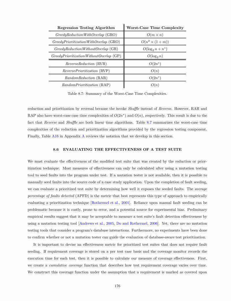
Regression Testing Algorithm Worst-Case Time Complexity
GreedyReductionWithOverlap (GRO) O(m × n)
GreedyPrioritizationWithOverlap (GRO) O(n2 × (1 + m))
GreedyReductionWithoutOverlap (GR) O(log2 n + n∗)
GreedyPrioritizationWithoutOverlap (GP) O(log2 n)
ReverseReduction (RVR) O(2n∗)
ReversePrioritization (RVP) O(n)
RandomReduction (RAR) O(2n∗)
RandomPrioritization (RAP) O(n)
Table 8.7: Summary of the Worst-Case Time Complexities.
reduction and prioritization by reversal because the invoke Shuffle instead of Reverse. However, RAR and
RAP also have worst-case case time complexities of O(2n∗) and O(n), respectively. This result is due to the
fact that Reverse and Shuffle are both linear time algorithms. Table 8.7 summarizes the worst-case time
complexities of the reduction and prioritization algorithms provided by the regression testing component.
Finally, Table A16 in Appendix A reviews the notation that we develop in this section.
8.6 EVALUATING THE EFFECTIVENESS OF A TEST SUITE
We must evaluate the effectiveness of the modified test suite that was created by the reduction or prior-
itization technique. Most measures of effectiveness can only be calculated after using a mutation testing
tool to seed faults into the program under test. If a mutation tester is not available, then it is possible to
manually seed faults into the source code of a case study application. Upon the completion of fault seeding,
we can evaluate a prioritized test suite by determining how well it exposes the seeded faults. The average
percentage of faults detected (APFD) is the metric that best represents this type of approach to empirically
evaluating a prioritization technique [Rothermel et al., 2001]. Reliance upon manual fault seeding can be
problematic because it is costly, prone to error, and a potential source for experimental bias. Preliminary
empirical results suggest that it may be acceptable to measure a test suite’s fault detection effectiveness by
using a mutation testing tool [Andrews et al., 2005, Do and Rothermel, 2006]. Yet, there are no mutation
testing tools that consider a program’s database interactions. Furthermore, no experiments have been done
to confirm whether or not a mutation tester can guide the evaluation of database-aware test prioritization.
It is important to devise an effectiveness metric for prioritized test suites that does not require fault
seeding. If requirement coverage is stored on a per test case basis and the coverage monitor records the
execution time for each test, then it is possible to calculate our measure of coverage effectiveness. First,
we create a cumulative coverage function that describes how test requirement coverage varies over time.
We construct this coverage function under the assumption that a requirement is marked as covered upon
176

Testing Time
. . .C
over
ed T
est R
eqs
PSfrag replacements
N6
enter computeVelocity
enter computeVelocity
N6
N6
N7
N7
N8
N8
N10
N8
N16
N10
N11
N11
N12
N12
N18
N16
N18
N18
exit computeVelocity
exit computeVelocity
N6
N1
N1
N2
N2
N3
N3
N1
N1
N4
N4
N5
N5
N6
enter P
enter P
call main
call main
enter main
enter main
enter main
. . .
. . .
call inputCardNumber
call inputCardNumber
call inputPin
call inputCardNumber
call handleError
call handleError
call inputCardNumber
call inputPin
call handleError
call handleError
call inputPin
call inputPin
call inputOperation
call inputOperation
call getAccountBalance
call getAccountBalance
call promptAgain
call inputOperation
call lockAccount
call lockAccount
call promptAgain
call promptAgain
call inputOperation
call promptAgain
. . .
call getAccountBalance
enter getAccountBalance
enter getAccountBalance
N3
N3
N4
N4
N5
N5
N6
N6
N7
N7
N10
N10
N12
N12
N15
N10
N15
N15
exit getAccountBalance
exit getAccountBalance
return getAccountBalance
return lockAccount
. . .
return getAccountBalance
call promptAgain
. . .
exit main
exit main
return main
return main
exit P
exit P
. . .
exit main
enter lockAccount
enter lockAccount
. . .
. . .
exit lockAccount
exit lockAccount
return lockAccount
return lockAccount
exit main
T1 Done Tn−1 Done
Tn Done
Cover Π(T1) Cover⋃n−1i=1 Π(Ti)
Cover Π(T )
Area∫ t(n)
0 κ(T, t)κ(T
,t)
(t)
Figure 8.19: The Cumulative Coverage of a Test Suite.
the completion of one of its covering tests. Integrating this function yields the coverage area of the test
suite. Intuitively, a large coverage area suggests that a particular re-ordering of a test suite is highly
effective. In support of an approach to comparing different prioritizations of the same test suite, we define
coverage effectiveness (CE) as the ratio between the re-ordered suite’s coverage area and the coverage area
of the ideal test suite. As mentioned in Section 8.3, an ideal test suite immediately covers all of the test
requirements. Since high coverage tests are more likely to reveal program faults than those with low coverage
[Hutchins et al., 1994], CE is an appropriate metric for characterizing a re-ordered test suite. Even though
CE and APFD are similar because they both calculate an area under a curve, CE obviates the need for fault
seeding. Therefore, CE is useful when manual fault seeding is too costly or mutation testing is not feasible.
We envisage the use of CE in conjunction with previously developed metrics such as APFD.
Equation (8.4) defines ξ(T, Tp) ∈ [0, 1], the coverage effectiveness of the prioritized test suite Tp that
was derived from T . Suppose that the regression tester creates Tp and Tp after applying two different
prioritization techniques to T . If ξ(T, Tp) > ξ(T, Tp), then we know that Tp is more coverage effective than
Tp. For this example, we would prefer the first approach to reduction instead of the second. The numerator
of Equation (8.4) is the integral of κ(Tp, t), the requirement coverage for test suite Tp at time t during test
suite execution. Equation (8.4)’s denominator is the integral of κ(T, t), the requirement coverage for the
ideal version of T . Calculating ξ(T, Tp) requires the integration of both the κ and κ functions in the closed
interval between 0 and t(n). Equation (8.5) defines t(n′) as the time required to execute the first n′ test
cases in T . For example, t(1) would return the time overhead for test T1 and t(n) calculates the running
time for the entire suite of n test cases. Finally, Equation (8.4) uses t to stand for a specific point in time
during testing.
ξ(T, Tp) =
∫ t(n)
0κ(Tp, t)∫ t(n)
0 κ(T, t)(8.4)
t(n′) =
n′∑
i=1
time(Ti) (8.5)
177

Since the ideal test suite immediately covers all of the test requirements, Equation (8.6) shows that
κ(T, t) is constant across all time inputs t for a specific test suite T . If T covers the requirements in the set
Π(T ), then κ(T, t) indicates that an ideal suite would cover all π ∈ Π(T ) right away. Finally, Equation (8.7)
defines the piecewise function κ(T, t) that describes the cumulative coverage of T at time t during testing.
We define κ(T, t) as an (n + 1)-part piecewise function when T = 〈T1, . . . , Tn〉. Equation (8.7) reveals that
κ(T, t) = 0 until the completion of test case T1 (i.e., t < t(1)). In the time period after the execution of
T1 and during the running of T2 (i.e., t ∈ [t(1), t(2))), the value of κ shows that T has covered a total
of |Π(T1)| test requirements. After running the first n − 1 tests, κ’s output indicates that T has covered∣∣∣⋃n−1i=1 Π(Ti)
∣∣∣ test requirements until the test executor completes the execution of the final test Tn (i.e.,
t ∈ [t(n − 1), t(n))). We define κ to maintain the maximum height of |Π(T )| for all time points t ≥ t(n).
Figure 8.19 graphically demonstrates how we construct the cumulative coverage function κ. Even though
our definition of ξ and κ leverages the notation for coverage tree paths, it is also possible to calculate
coverage efficiency according to the test suite’s coverage of other types of test requirements such as the
database interaction association. Table A17 in Appendix A reviews the notation that we develop during the
discussion of the coverage effectiveness for a test prioritization.
κ(T, t) =
∣∣∣∣∣n⋃
i=1
Π(Ti)
∣∣∣∣∣ (8.6)
κ(T, t) =
0 t < t(1)
|Π(T1)| t ∈ [t(1), t(2))
......∣∣∣
⋃n−1i=1 Π(Ti)
∣∣∣ t ∈ [t(n− 1), t(n))
|Π(T )| t ≥ t(n)
(8.7)
We can only use the previous formulation of coverage effectiveness when we evaluate the prioritization
of a test suite. This is due to the fact that different reduction techniques frequently create test suites that
vary in their reduction of the (i) number of tests, (ii) overall test suite execution time, and (iii) coverage of
the test requirements. To this end, we present two metrics for evaluating the efficiency of a reduced test
suite. Equation (8.8) defines %n(T, Tr) ∈ [0, 1], the reduction factor for test size (RFS) of the original test
suite T and reduced test suite Tr. Furthermore, Equation (8.9) defines %t(T, Tr) ∈ [0, 1], the reduction factor
for testing time (RFT). High values for RFS and RFT suggest that a reduced test suite is very efficient.
Suppose that the regression tester analyzes test suite T and creates two reduced test suites called Tr and
Tr. If %n(T, Tr) > %n(T, Tr) and %t(T, Tr) > %t(T, Tr), then we know that Tr is more efficient than Tr.
%n(T, Tr) =|T | − |Tr|
|T |(8.8)
%t(T, Tr) =time(T )− time(Tr)
time(T )(8.9)
178

νr νr Comparison
〈.4, .5, .8〉 〈.4, .5, .9〉 νr νr
〈.4, .5, 1〉 〈.4, .55, 1〉 νr νr
〈.6, .5, 1〉 〈.4, .5, 1〉 νr νr
〈.4, .5, 1〉 〈.55, .75, .9〉 νr ∼ νr
Table 8.8: Comparing Test Suite Reductions.
We must also evaluate the effectiveness of a reduced test suite. The majority of prior empirical research
calculates the decrease in fault detection effectiveness for a reduced test suite after seeding faults into the
program under test (e.g., [Jones and Harrold, 2003, McMaster and Memon, 2005]). We judge that it is
important to devise a measure of effectiveness that can be used instead of or in conjunction with a fault-
based measurement. To this end, Equation (8.10) defines the reduction factor for test requirements (RFR) as
%π(T, Tr) ∈ [0, 1]. Unlike the RFS and RFT metrics, we prefer low values for %π(T, Tr) because this indicates
that a reduced test suite Tr covers the majority of the requirements that the initial tests cover. To avoid
confusion during the empirical comparison of different reduction techniques, we define the preservation factor
for test requirements (PFR) as νπ(T, Tr) = 1− %π(T, Tr) such that νπ(T, Tr) ∈ [0, 1]. If a reduced test suite
has a high PFR factor, then we know that it covers most of the requirements that the original tests cover.
The overlap-aware greedy reduction algorithm that we defined in Section 8.5 (i.e., GRO) always creates a Tr
that covers all of the test requirements and thus νπ(T, Tr) = 1. However, the other reduction techniques (i.e.,
GR, RVR, and RAR) are not guaranteed to construct a test suite that covers all π ∈ Π(T ) and thus they
may yield values for νπ that are less than one. Even though we defined %π and νπ in the context of coverage
tree paths, we can also use these coverage effectiveness metrics in conjunction with reduction techniques that
use other types of test requirements (e.g., the database interaction associations).
%π(T, Tr) =|Π(T )| − |Π(Tr)|
|Π(T )|(8.10)
In order to facilitate the comparison between different approaches to reduction, we employ νr = 〈%n, %t, νπ〉
to organize the evaluation metrics for test suite Tr. Table 8.8 summarizes the four different evaluation tu-
ples that we use to explain the process of comparing different reduction algorithms. Suppose that two
different reduction techniques create Tr and Tr that are respectively characterized by the evaluation tuples
νr = 〈.4, .5, .8〉 and νr = 〈.4, .5, .9〉. In this example, we would prefer the νr configuration because it (i) has
the same values for %n and %t (i.e., the reduction factors for the number of tests and the overall testing time)
and (ii) preserves the coverage of more test requirements since νπ > νπ. If νr = 〈.4, .5, 1〉 and νr = 〈.4, .55, 1〉,
then we would prefer the reduced suite with νr because it fully preserves requirement coverage while yielding
a larger value for %t (i.e., .55 > .5). Next, suppose that νr = 〈.6, .5, 1〉 and νr = 〈.4, .5, 1〉. In this situation,
we would favor νr’s reduction algorithm since it yields the smallest test suite (i.e., %n > %n since .6 > .4).
This choice is sensible because it will control test execution time if there is an increase in the startup and
shutdown costs associated with running a test.
179
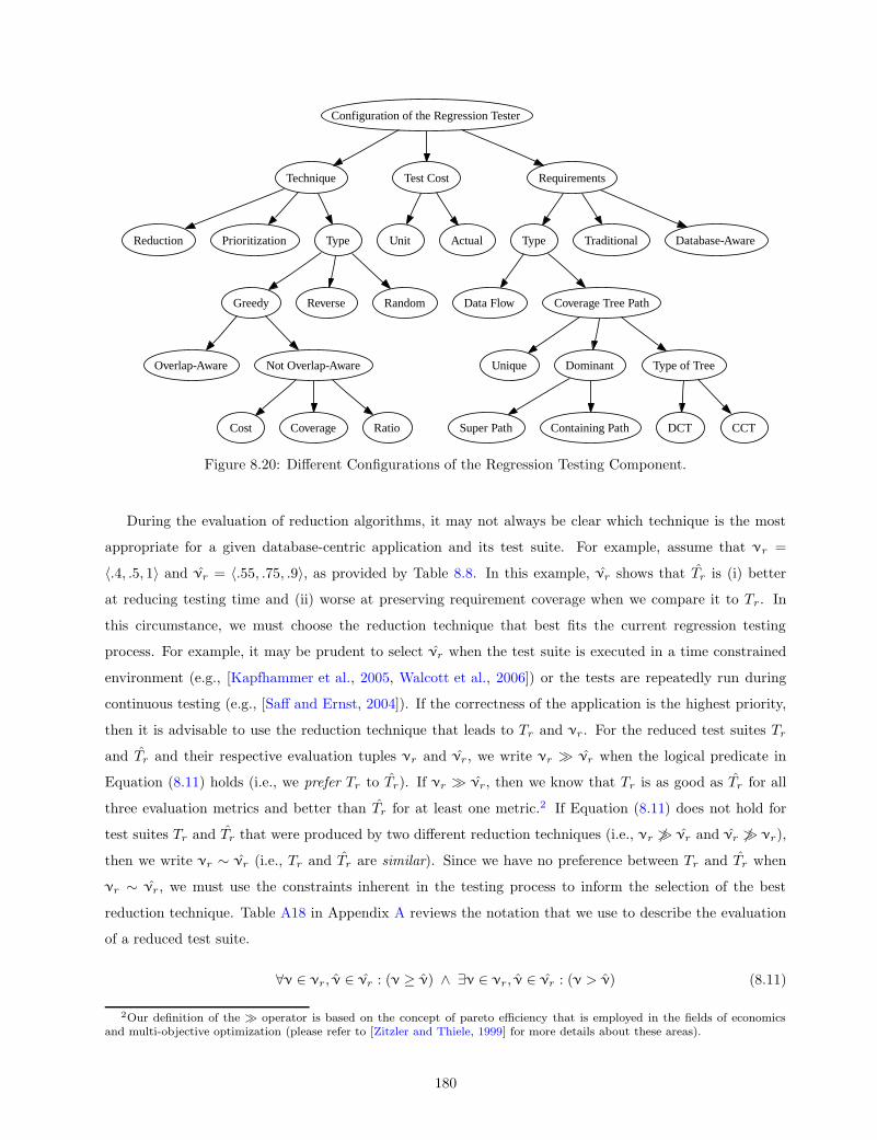
Type
Data Flow Coverage Tree Path
Configuration of the Regression Tester
Technique Test Cost Requirements
Reduction Prioritization Type
Greedy Reverse Random
Overlap-Aware Not Overlap-Aware
Cost Coverage Ratio
Unit Actual Traditional Database-Aware
Unique Dominant Type of Tree
Super Path Containing Path DCT CCT
PSfrag replacements
N6
enter computeVelocity
enter computeVelocity
N6
N6
N7
N7
N8
N8
N10
N8
N16
N10
N11
N11
N12
N12
N18
N16
N18
N18
exit computeVelocity
exit computeVelocity
N6
N1
N1
N2
N2
N3
N3
N1
N1
N4
N4
N5
N5
N6
enter P
enter P
call main
call main
enter main
enter main
enter main
. . .
. . .
call inputCardNumber
call inputCardNumber
call inputPin
call inputCardNumber
call handleError
call handleError
call inputCardNumber
call inputPin
call handleError
call handleError
call inputPin
call inputPin
call inputOperation
call inputOperation
call getAccountBalance
call getAccountBalance
call promptAgain
call inputOperation
call lockAccount
call lockAccount
call promptAgain
call promptAgain
call inputOperation
call promptAgain
. . .
call getAccountBalance
enter getAccountBalance
enter getAccountBalance
N3
N3
N4
N4
N5
N5
N6
N6
N7
N7
N10
N10
N12
N12
N15
N10
N15
N15
exit getAccountBalance
exit getAccountBalance
return getAccountBalance
return lockAccount
. . .
return getAccountBalance
call promptAgain
. . .
exit main
exit main
return main
return main
exit P
exit P
. . .
exit main
enter lockAccount
enter lockAccount
. . .
. . .
exit lockAccount
exit lockAccount
return lockAccount
return lockAccount
exit main
Figure 8.20: Different Configurations of the Regression Testing Component.
During the evaluation of reduction algorithms, it may not always be clear which technique is the most
appropriate for a given database-centric application and its test suite. For example, assume that νr =
〈.4, .5, 1〉 and νr = 〈.55, .75, .9〉, as provided by Table 8.8. In this example, νr shows that Tr is (i) better
at reducing testing time and (ii) worse at preserving requirement coverage when we compare it to Tr. In
this circumstance, we must choose the reduction technique that best fits the current regression testing
process. For example, it may be prudent to select νr when the test suite is executed in a time constrained
environment (e.g., [Kapfhammer et al., 2005, Walcott et al., 2006]) or the tests are repeatedly run during
continuous testing (e.g., [Saff and Ernst, 2004]). If the correctness of the application is the highest priority,
then it is advisable to use the reduction technique that leads to Tr and νr. For the reduced test suites Tr
and Tr and their respective evaluation tuples νr and νr, we write νr νr when the logical predicate in
Equation (8.11) holds (i.e., we prefer Tr to Tr). If νr νr, then we know that Tr is as good as Tr for all
three evaluation metrics and better than Tr for at least one metric.2 If Equation (8.11) does not hold for
test suites Tr and Tr that were produced by two different reduction techniques (i.e., νr 6 νr and νr 6 νr),
then we write νr ∼ νr (i.e., Tr and Tr are similar). Since we have no preference between Tr and Tr when
νr ∼ νr, we must use the constraints inherent in the testing process to inform the selection of the best
reduction technique. Table A18 in Appendix A reviews the notation that we use to describe the evaluation
of a reduced test suite.
∀ν ∈ νr, ν ∈ νr : (ν ≥ ν) ∧ ∃ν ∈ νr, ν ∈ νr : (ν > ν) (8.11)
2Our definition of the operator is based on the concept of pareto efficiency that is employed in the fields of economicsand multi-objective optimization (please refer to [Zitzler and Thiele, 1999] for more details about these areas).
180

8.7 IMPLEMENTATION OF THE REGRESSION TESTING COMPONENT
Figure 8.20 describes the different configurations of the regression testing component. Section 8.4 provides
a detailed discussion of the “Requirements” subtree and Section 8.5 examines the “Technique” subtree. We
implemented the regression testing component in the Java 1.5.0 programming language. For simplicity, we
convert a coverage tree path into a java.lang.String and we use the startsWith and contains methods
in the implementation of the path dominance operators. For example, the regression tester transforms the
tree paths π and π′ into strings s and s′. If we have π = π′ (i.e., π is a super path for π′), then we know
that s.startsWith(s′) returns true. Furthermore, if π π′ holds (i.e., π is a containing path for π′), then
we know that s.contains(s′) returns true.
Even though the empirical results in Section 8.10 suggest that the use of java.lang.String exhibits
acceptable performance, we intend to use more efficient string implementations (e.g., [Boldi and Vigna,
2005]) and text processing algorithms (e.g., [Sunday, 1990]) to further reduce the time overhead of test path
enumeration. Since the default JUnit and DBUnit test executors do not support reduction or prioritization,
we enhanced these tools to read external configurations. When prioritization is enabled, the test executor
ignores the default ordering of the tests and re-orders them before testing starts. If reduction is chosen,
then the test suite execution engine only runs a test if it is specified in the external configuration file. Even
though each configuration file is automatically generated by the regression testing component, the tester
may manually modify these configurations when necessary. Since our regression testing tools incorporate a
test’s actual running time, we enhanced the coverage monitor so that it (i) uses instrumentation probes to
time the execution of a test and (ii) stores this data in the coverage report.
8.8 EXPERIMENT GOALS AND DESIGN
We conducted experiments to measure the performance of the algorithms that (i) enumerate the tree-based
test requirements and (ii) reduce or prioritize the test suite. We also investigate how reduction and pri-
oritization impact the efficiency and effectiveness of regression testing (c.f. Section 8.6 for a discussion of
the primary evaluation metrics). We characterize each case study application in order to explain why the
efficiency and effectiveness of the algorithms vary across the different applications. Since the existence of
many long running test cases may limit the opportunities for reduction and/or prioritization [Elbaum et al.,
2001], we calculate the running time for each test case in a test suite. Furthermore, we measure how many
tests cover each individual test requirement because a test suite with a high overlap in requirement coverage
is more amenable to reduction. If a test suite is composed of many tests that create numerous tree paths
and there is a small number of test requirements, then it is likely that this suite is fit for reduction. Thus,
we count the number of tree paths that are created by each test case. Finally, we report how many unique
tree paths are covered by the entire test suite because the worst-case time complexity of GRO and GPO is
bound by both the number of test cases (i.e., |T | or n) and the number of requirements (i.e., |Π(T )| or m).
181

0 1000 2000 3000 4000 5000 6000 7000Test Suite Execution Time H msec L
0
0.2
0.4
0.6
0.8
1
Empirical
CDF
Reminder
PSfrag replacements
N6
enter computeVelocity
enter computeVelocity
N6
N6
N7
N7
N8
N8
N10
N8
N16
N10
N11
N11
N12
N12
N18
N16
N18
N18
exit computeVelocity
exit computeVelocity
N6
N1
N1
N2
N2
N3
N3
N1
N1
N4
N4
N5
N5
N6
enter P
enter P
call main
call main
enter main
enter main
enter main
. . .
. . .
call inputCardNumber
call inputCardNumber
call inputPin
call inputCardNumber
call handleError
call handleError
call inputCardNumber
call inputPin
call handleError
call handleError
call inputPin
call inputPin
call inputOperation
call inputOperation
call getAccountBalance
call getAccountBalance
call promptAgain
call inputOperation
call lockAccount
call lockAccount
call promptAgain
call promptAgain
call inputOperation
call promptAgain
. . .
call getAccountBalance
enter getAccountBalance
enter getAccountBalance
N3
N3
N4
N4
N5
N5
N6
N6
N7
N7
N10
N10
N12
N12
N15
N10
N15
N15
exit getAccountBalance
exit getAccountBalance
return getAccountBalance
return lockAccount
. . .
return getAccountBalance
call promptAgain
. . .
exit main
exit main
return main
return main
exit P
exit P
. . .
exit main
enter lockAccount
enter lockAccount
. . .
. . .
exit lockAccount
exit lockAccount
return lockAccount
return lockAccount
exit main
(a)
0 1000 2000 3000 4000 5000 6000 7000Test Suite Execution Time H msec L
0
0.2
0.4
0.6
0.8
1
Empirical
CDF
FindFile
PSfrag replacements
N6
enter computeVelocity
enter computeVelocity
N6
N6
N7
N7
N8
N8
N10
N8
N16
N10
N11
N11
N12
N12
N18
N16
N18
N18
exit computeVelocity
exit computeVelocity
N6
N1
N1
N2
N2
N3
N3
N1
N1
N4
N4
N5
N5
N6
enter P
enter P
call main
call main
enter main
enter main
enter main
. . .
. . .
call inputCardNumber
call inputCardNumber
call inputPin
call inputCardNumber
call handleError
call handleError
call inputCardNumber
call inputPin
call handleError
call handleError
call inputPin
call inputPin
call inputOperation
call inputOperation
call getAccountBalance
call getAccountBalance
call promptAgain
call inputOperation
call lockAccount
call lockAccount
call promptAgain
call promptAgain
call inputOperation
call promptAgain
. . .
call getAccountBalance
enter getAccountBalance
enter getAccountBalance
N3
N3
N4
N4
N5
N5
N6
N6
N7
N7
N10
N10
N12
N12
N15
N10
N15
N15
exit getAccountBalance
exit getAccountBalance
return getAccountBalance
return lockAccount
. . .
return getAccountBalance
call promptAgain
. . .
exit main
exit main
return main
return main
exit P
exit P
. . .
exit main
enter lockAccount
enter lockAccount
. . .
. . .
exit lockAccount
exit lockAccount
return lockAccount
return lockAccount
exit main
(b)
0 1000 2000 3000 4000 5000 6000 7000Test Suite Execution Time H msec L
0
0.2
0.4
0.6
0.8
1
Empirical
CDF
Pithy
PSfrag replacements
N6
enter computeVelocity
enter computeVelocity
N6
N6
N7
N7
N8
N8
N10
N8
N16
N10
N11
N11
N12
N12
N18
N16
N18
N18
exit computeVelocity
exit computeVelocity
N6
N1
N1
N2
N2
N3
N3
N1
N1
N4
N4
N5
N5
N6
enter P
enter P
call main
call main
enter main
enter main
enter main
. . .
. . .
call inputCardNumber
call inputCardNumber
call inputPin
call inputCardNumber
call handleError
call handleError
call inputCardNumber
call inputPin
call handleError
call handleError
call inputPin
call inputPin
call inputOperation
call inputOperation
call getAccountBalance
call getAccountBalance
call promptAgain
call inputOperation
call lockAccount
call lockAccount
call promptAgain
call promptAgain
call inputOperation
call promptAgain
. . .
call getAccountBalance
enter getAccountBalance
enter getAccountBalance
N3
N3
N4
N4
N5
N5
N6
N6
N7
N7
N10
N10
N12
N12
N15
N10
N15
N15
exit getAccountBalance
exit getAccountBalance
return getAccountBalance
return lockAccount
. . .
return getAccountBalance
call promptAgain
. . .
exit main
exit main
return main
return main
exit P
exit P
. . .
exit main
enter lockAccount
enter lockAccount
. . .
. . .
exit lockAccount
exit lockAccount
return lockAccount
return lockAccount
exit main
(c)
0 1000 2000 3000 4000 5000 6000 7000Test Suite Execution Time H msec L
0
0.2
0.4
0.6
0.8
1
Empirical
CDF
Student
PSfrag replacements
N6
enter computeVelocity
enter computeVelocity
N6
N6
N7
N7
N8
N8
N10
N8
N16
N10
N11
N11
N12
N12
N18
N16
N18
N18
exit computeVelocity
exit computeVelocity
N6
N1
N1
N2
N2
N3
N3
N1
N1
N4
N4
N5
N5
N6
enter P
enter P
call main
call main
enter main
enter main
enter main
. . .
. . .
call inputCardNumber
call inputCardNumber
call inputPin
call inputCardNumber
call handleError
call handleError
call inputCardNumber
call inputPin
call handleError
call handleError
call inputPin
call inputPin
call inputOperation
call inputOperation
call getAccountBalance
call getAccountBalance
call promptAgain
call inputOperation
call lockAccount
call lockAccount
call promptAgain
call promptAgain
call inputOperation
call promptAgain
. . .
call getAccountBalance
enter getAccountBalance
enter getAccountBalance
N3
N3
N4
N4
N5
N5
N6
N6
N7
N7
N10
N10
N12
N12
N15
N10
N15
N15
exit getAccountBalance
exit getAccountBalance
return getAccountBalance
return lockAccount
. . .
return getAccountBalance
call promptAgain
. . .
exit main
exit main
return main
return main
exit P
exit P
. . .
exit main
enter lockAccount
enter lockAccount
. . .
. . .
exit lockAccount
exit lockAccount
return lockAccount
return lockAccount
exit main
(d)
0 1000 2000 3000 4000 5000 6000 7000Test Suite Execution Time H msec L
0
0.2
0.4
0.6
0.8
1
Empirical
CDF
TransactionManager
PSfrag replacements
N6
enter computeVelocity
enter computeVelocity
N6
N6
N7
N7
N8
N8
N10
N8
N16
N10
N11
N11
N12
N12
N18
N16
N18
N18
exit computeVelocity
exit computeVelocity
N6
N1
N1
N2
N2
N3
N3
N1
N1
N4
N4
N5
N5
N6
enter P
enter P
call main
call main
enter main
enter main
enter main
. . .
. . .
call inputCardNumber
call inputCardNumber
call inputPin
call inputCardNumber
call handleError
call handleError
call inputCardNumber
call inputPin
call handleError
call handleError
call inputPin
call inputPin
call inputOperation
call inputOperation
call getAccountBalance
call getAccountBalance
call promptAgain
call inputOperation
call lockAccount
call lockAccount
call promptAgain
call promptAgain
call inputOperation
call promptAgain
. . .
call getAccountBalance
enter getAccountBalance
enter getAccountBalance
N3
N3
N4
N4
N5
N5
N6
N6
N7
N7
N10
N10
N12
N12
N15
N10
N15
N15
exit getAccountBalance
exit getAccountBalance
return getAccountBalance
return lockAccount
. . .
return getAccountBalance
call promptAgain
. . .
exit main
exit main
return main
return main
exit P
exit P
. . .
exit main
enter lockAccount
enter lockAccount
. . .
. . .
exit lockAccount
exit lockAccount
return lockAccount
return lockAccount
exit main
(e)
0 1000 2000 3000 4000 5000 6000 7000Test Suite Execution Time H msec L
0
0.2
0.4
0.6
0.8
1
Empirical
CDF
GradeBook
PSfrag replacements
N6
enter computeVelocity
enter computeVelocity
N6
N6
N7
N7
N8
N8
N10
N8
N16
N10
N11
N11
N12
N12
N18
N16
N18
N18
exit computeVelocity
exit computeVelocity
N6
N1
N1
N2
N2
N3
N3
N1
N1
N4
N4
N5
N5
N6
enter P
enter P
call main
call main
enter main
enter main
enter main
. . .
. . .
call inputCardNumber
call inputCardNumber
call inputPin
call inputCardNumber
call handleError
call handleError
call inputCardNumber
call inputPin
call handleError
call handleError
call inputPin
call inputPin
call inputOperation
call inputOperation
call getAccountBalance
call getAccountBalance
call promptAgain
call inputOperation
call lockAccount
call lockAccount
call promptAgain
call promptAgain
call inputOperation
call promptAgain
. . .
call getAccountBalance
enter getAccountBalance
enter getAccountBalance
N3
N3
N4
N4
N5
N5
N6
N6
N7
N7
N10
N10
N12
N12
N15
N10
N15
N15
exit getAccountBalance
exit getAccountBalance
return getAccountBalance
return lockAccount
. . .
return getAccountBalance
call promptAgain
. . .
exit main
exit main
return main
return main
exit P
exit P
. . .
exit main
enter lockAccount
enter lockAccount
. . .
. . .
exit lockAccount
exit lockAccount
return lockAccount
return lockAccount
exit main
(f)
Figure 8.21: ECDFs for Test Case Execution Time.
Figure 8.20 shows that the regression tester can reduce or re-order the test suite by incorporating either
the unit cost or the actual cost of running a test. Under the unit cost assumption, a regression testing
algorithm supposes that all of the test cases execute for the same amount of time. With the exception
of [Elbaum et al., 2001, Walcott et al., 2006], the majority of regression testing tools operate under the
unit cost assumption (e.g., [Jeffrey and Gupta, 2007, Harrold et al., 1993, McMaster and Memon, 2005,
Tallam and Gupta, 2005]). However, it is not advisable to make this assumption during the regression
testing of a database-centric application. When a test suite mixes database-aware test cases with those that
do not perform database interactions, the time overhead of the tests can vary by one or more orders of
magnitude. Figure 8.21 presents an empirical cumulative distribution function (ECDF) of test execution
time for the test suite of each case study application. As noted in Chapter 7, an ECDF gives the cumulative
percentage of the recorded data set whose values fall below a specific value. In these graphs, a sharply rising
ECDF indicates that most test cases are very fast. An ECDF curve that rises more gradually would suggest
that the test suite has a greater concentration of long running tests.
For brevity, our discussion of test case execution time focuses on the FF application (the other case
study applications demonstrate similar testing patterns). FindFile’s ECDF in Figure 8.21(b) reveals that
almost 90% of the test cases have execution times below 500 milliseconds and over 60% of tests run in under
200 milliseconds. We also observe that a small percentage of the tests run for almost six seconds. After
investigating the source code of FindFile’s test suite, we noted that the fast test cases perform few, if
any, database interactions. The more costly test cases execute many database-aware test oracles and often
interact with more than one of the database’s relations. Generally, the most expensive tests incur a high
time overhead because they ensure the correctness of the database server’s startup and shutdown routines
182

by starting and stopping the server. We anticipate that these costs would be much higher if FindFile
restarted a stand-alone RDBMS (e.g., MySQL [Yarger et al., 1999] or PostreSQL [Monjian, 2000]) instead
of the in-memory HSQLDB database management system. The graphs in Figure 8.21 demonstrate that all
of the test suites contain many tests that execute very quickly (i.e., in less than 100 milliseconds) and a few
tests that run for approximately five or six seconds. This evidence clearly suggests that there is a substantial
difference in the time overhead for the tests and thus motivates the use of the actual test execution time.
Since our test coverage monitor records the time overhead for running each test case, all of the experiments
use the actual test execution cost. In future work, we will examine how the unit cost assumption impacts
database-aware regression testing.
It is important to perform reduction and prioritization for our case study applications even though
Table 8.9 shows that all of the test suites execute in less than ten seconds. A testing time of ten seconds may
be too costly in certain software development processes, such as extreme programming, that promote a short
implementation and testing cycle and the frequent execution of very fast tests [Poole and Huisman, 2001]. If
a test suite is executed in a time sensitive environment (e.g., [Walcott et al., 2006]), the tests are run during
continuous testing (e.g., [Saff and Ernst, 2004]), or testing occurs in a resource constrained environment
(e.g., [Kapfhammer et al., 2005]), then it also may be too expensive to run all of the tests. Furthermore,
recent research suggests that the test executor should restart the RDBMS server after the execution of every
test case [Haftmann et al., 2005a]. This approach is useful because it is often difficult for a tester to ensure
that all of the tests restore the database state that they modified. For example, test execution may have
side effects if a test case modifies the state of the database and the RDBMS subsequently changes one or
more relations when it enforces integrity constraints or executes triggers.
We judge that it is not absolutely necessary to restart the server upon the completion of a test because
each of our test suites executes in an independent fashion. However, in light of the recommendations made
by [Haftmann et al., 2005a], we estimated the execution time of each test suite under the assumption that
the tests are non-independent and the executor repeatedly performs server restarts in order to purge the
database’s state. After studying the testing behavior of each case study application, we concluded that a
restart of the HSQLDB server takes approximately five seconds. Table 8.9 reveals that the execution of
a test suite with server restarts will consume between 32 and 43 seconds of testing time. Therefore, it is
important to perform reduction and/or prioritization if the (i) testing process dictates that tests must run
in a rapid fashion, (ii) testing occurs in an environment with time or resource constraints, and/or (iii) test
executor always restarts the RDBMS because the tests do not properly cleanse the database.
Figure 8.20 shows that the regression testing component can analyze both traditional and database-aware
DCTs and CCTs. The experiments use coverage trees that record database interactions at the relation,
attribute, record, and attribute value levels (e.g., Rl, A, Rc, and Av). We selected the Rl and A levels
since they focus on the structure of the database. Furthermore, we included the Rc and Av levels because
they represent a program’s interaction with the database’s state. We observe that the program and database
183

Application Without Restarts (sec) With Restarts (sec)
Reminder 6.164 32.053
FindFile 6.966 36.379
Pithy 8.243 52.864
StudentTracker 6.686 34.767
TransactionManager 8.211 42.697
GradeBook 7.576 39.395
Table 8.9: Test Suite Execution Time With and Without Database Server Restarts.
levels (e.g., P and D) yield equivalent coverage trees in our experiments. This is due to the fact that all of
the applications interact with one database. Since a database interaction point will only lead to a higher
number of test requirements if it interacts with more than one database entity, the P-level and D-level trees
always yield the same number of test requirements. For example, suppose that the database interaction point
Ir submits the SQL command select ∗ from relj . If node Nφ precedes Ir , then the P-level and D-level
coverage trees will respectively contain the path Nφ → Ir and Nφ → Ir → use(Df ).
For all of the applications except TM and GB, the D-level and Rl-level trees will always render the same
number of tree paths. This is due to the fact that all of the other case study applications use a database
that only contains one relation. In the context of the previous SQL statement, an Rl-level tree would still
lead to the single test path Nφ → Ir → use(Df ) → use(relj). However, assume that the database contains
relations relj and relj and Ir executes the command select ∗ from relj where relj .Al = relj .Al. In
this circumstance, the Rl-level tree contains the two test paths Nφ → Ir → use(Df ) → use(relj) and
Nφ → Ir → use(Df ) → use(relj). Since only TM and GB contain interaction patterns like the second SQL
statement, we omit both the P and D levels from the empirical study (i.e., for the other four applications, the
D and Rl levels would lead to the same experimental outcomes). For completeness, Table C4 in Appendix C
furnishes the results from enumerating the P-level test requirements for TM and GB.
We configured the test coverage monitor to create an XML-based coverage tree and we traverse this
tree during requirement enumeration. Since XML parsing is often the limiting factor in the performance of
an application [Nicola and John, 2003], we judge that this choice ensures that we characterize the worst-
case performance of our technique for enumerating the test paths. In fact, preliminary experiments suggest
that the use of a binary coverage tree may halve test path enumeration time when we analyze the largest
coverage trees. The experiments also focused on using the database-aware calling context tree (i.e., the DI-
CCT) instead of the DI-DCT because previous empirical studies (e.g., [McMaster and Memon, 2005, 2006])
used the traditional version of the CCT. Since the CCT instrumentation probes already coalesce tree paths
according to the super path operator, we time the enumeration of the set Πµ(τcct, T, =). We also apply the
containing path operator in order to measure the time consumed during the enumeration of Πµ(τcct, T,)
(c.f. Section 8.4 for a discussion of the enumeration algorithms and the path dominance operators).
Even though the case study applications are written in a fashion that allows the tests to start their own
instance of the HSQLDB server, we assume that every database-centric application connects to a previously
184

started database management system. We set up the reduction and prioritization algorithms so that they
analyze the coverage information in the set Πµ(τcct, Ti,a) for each test case Ti. In addition to using all of the
prioritization techniques that are listed in Table 8.7, we also report the effectiveness of the initial ordering
of the test suite. Since the GR, RVR, and RAR reduction techniques require a target size, we executed the
GRO algorithm first and then use the size of the resulting test suite as input to the other algorithms. As
an experimental control, we generated fifty randomly reduced and prioritized test suites. We calculate the
average value of each evaluation metric across all fifty of the test suites. In order to ensure a fair comparison,
we employed a uniformly distributed pseudo-random number generator to create fifty seeds. Throughout
the entire experimentation process, we used the first seed to initialize the pseudo-random number generator
that governs the creation of the first randomly reduced or re-ordered test suite (the second seed is used for
the second test suite and so forth). We judge that this design improves the repeatability of the experiments.
As part of future research, we intend to employ Walcott et al.’s approach to randomly generating a large
number of test suite orderings and reductions [Walcott et al., 2006].
Finally, we executed the (i) test requirement enumerator and (ii) reduction or prioritization algorithm in
five separate trials. Since the time overhead metrics varied across each trial, we calculate arithmetic means
and standard deviations for all of these timings (the metrics that characterize a case study application did not
vary across trials). As in Chapter 7, we use box and whisker plots and bar charts to visualize the empirical
results (c.f. Section 7.4 for a discussion of these approaches to data visualization). When we visualize a
time overhead, we create a bar chart so that the height of the bar corresponds to the arithmetic mean of the
measurements. We do not include error bars in the bar charts in Figure 8.22 because the standard deviations
were very small. We performed all of the experiments on a GNU/Linux workstation with kernel 2.6.11-1.1369,
Native POSIX Thread Library (NPTL) version 2.3.5, a dual core 3.0 GHz Pentium IV processor, 2 GB of
main memory, and 1 MB of L1 processor cache.
8.9 KEYS INSIGHTS FROM THE EXPERIMENTS
The experimental results in Section 8.10 complement the analytical evaluation of the regression testing
algorithms in Sections 8.4 and 8.5. Due to the comprehensive nature of the empirical analysis, we furnish
the following insights from the experiments:
1. Test Path Enumeration: It is often possible to enumerate the tree-based test paths in less than one
second. The enumeration process is the most expensive when we identify the paths in a coverage tree
that represents a database interaction at the attribute value level. In the majority of circumstances,
we can identify the tree paths in the Av-level DI-CCT in less than six seconds. We conclude that the
tree-based test requirement is suitable for both version specific and general regression testing.
2. Test Suite Reduction:
a. Effectiveness: The reduced test suites are between 30 and 80% smaller than the original test suite.
Across all of the case study applications, the GreedyReductionWithOverlap (GRO) algorithm yields
185
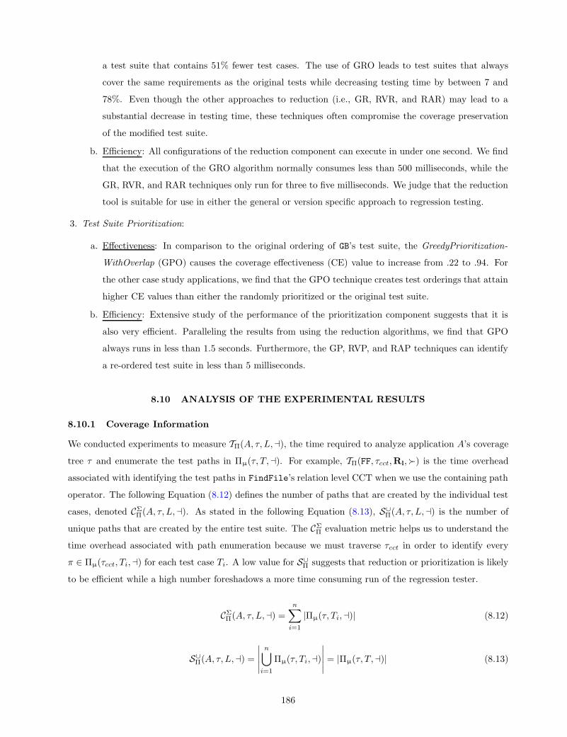
a test suite that contains 51% fewer test cases. The use of GRO leads to test suites that always
cover the same requirements as the original tests while decreasing testing time by between 7 and
78%. Even though the other approaches to reduction (i.e., GR, RVR, and RAR) may lead to a
substantial decrease in testing time, these techniques often compromise the coverage preservation
of the modified test suite.
b. Efficiency: All configurations of the reduction component can execute in under one second. We find
that the execution of the GRO algorithm normally consumes less than 500 milliseconds, while the
GR, RVR, and RAR techniques only run for three to five milliseconds. We judge that the reduction
tool is suitable for use in either the general or version specific approach to regression testing.
3. Test Suite Prioritization:
a. Effectiveness: In comparison to the original ordering of GB’s test suite, the GreedyPrioritization-
WithOverlap (GPO) causes the coverage effectiveness (CE) value to increase from .22 to .94. For
the other case study applications, we find that the GPO technique creates test orderings that attain
higher CE values than either the randomly prioritized or the original test suite.
b. Efficiency: Extensive study of the performance of the prioritization component suggests that it is
also very efficient. Paralleling the results from using the reduction algorithms, we find that GPO
always runs in less than 1.5 seconds. Furthermore, the GP, RVP, and RAP techniques can identify
a re-ordered test suite in less than 5 milliseconds.
8.10 ANALYSIS OF THE EXPERIMENTAL RESULTS
8.10.1 Coverage Information
We conducted experiments to measure TΠ(A, τ, L,a), the time required to analyze application A’s coverage
tree τ and enumerate the test paths in Πµ(τ, T,a). For example, TΠ(FF, τcct,Rl,) is the time overhead
associated with identifying the test paths in FindFile’s relation level CCT when we use the containing path
operator. The following Equation (8.12) defines the number of paths that are created by the individual test
cases, denoted CΣΠ(A, τ, L,a). As stated in the following Equation (8.13), S∪Π(A, τ, L,a) is the number of
unique paths that are created by the entire test suite. The CΣΠ evaluation metric helps us to understand the
time overhead associated with path enumeration because we must traverse τcct in order to identify every
π ∈ Πµ(τcct, Ti,a) for each test case Ti. A low value for S∪Π suggests that reduction or prioritization is likely
to be efficient while a high number foreshadows a more time consuming run of the regression tester.
CΣΠ(A, τ, L,a) =
n∑
i=1
|Πµ(τ, Ti,a)| (8.12)
S∪Π(A, τ, L,a) =
∣∣∣∣∣n⋃
i=1
Πµ(τ, Ti,a)
∣∣∣∣∣ = |Πµ(τ, T,a)| (8.13)
186

Super Contain
Dominance Operator HRM L50
100
150
200
250
300
350Enumeration
Time
Hmsec
LSuper Contain
59 59.4
103123.2
76.4 84.
201.8
282.4
Rl A Rc Av
PSfrag replacements
N6
enter computeVelocity
enter computeVelocity
N6
N6
N7
N7
N8
N8
N10
N8
N16
N10
N11
N11
N12
N12
N18
N16
N18
N18
exit computeVelocity
exit computeVelocity
N6
N1
N1
N2
N2
N3
N3
N1
N1
N4
N4
N5
N5
N6
enter P
enter P
call main
call main
enter main
enter main
enter main
. . .
. . .
call inputCardNumber
call inputCardNumber
call inputPin
call inputCardNumber
call handleError
call handleError
call inputCardNumber
call inputPin
call handleError
call handleError
call inputPin
call inputPin
call inputOperation
call inputOperation
call getAccountBalance
call getAccountBalance
call promptAgain
call inputOperation
call lockAccount
call lockAccount
call promptAgain
call promptAgain
call inputOperation
call promptAgain
. . .
call getAccountBalance
enter getAccountBalance
enter getAccountBalance
N3
N3
N4
N4
N5
N5
N6
N6
N7
N7
N10
N10
N12
N12
N15
N10
N15
N15
exit getAccountBalance
exit getAccountBalance
return getAccountBalance
return lockAccount
. . .
return getAccountBalance
call promptAgain
. . .
exit main
exit main
return main
return main
exit P
exit P
. . .
exit main
enter lockAccount
enter lockAccount
. . .
. . .
exit lockAccount
exit lockAccount
return lockAccount
return lockAccount
exit main
(a)
Super Contain
Dominance Operator HFF L
50
100
150
200
250
Enumeration
Time
Hmsec
L
Super Contain
89102
95
111.6
130.6
153.8159.4
202.2
Rl A Rc Av
PSfrag replacements
N6
enter computeVelocity
enter computeVelocity
N6
N6
N7
N7
N8
N8
N10
N8
N16
N10
N11
N11
N12
N12
N18
N16
N18
N18
exit computeVelocity
exit computeVelocity
N6
N1
N1
N2
N2
N3
N3
N1
N1
N4
N4
N5
N5
N6
enter P
enter P
call main
call main
enter main
enter main
enter main
. . .
. . .
call inputCardNumber
call inputCardNumber
call inputPin
call inputCardNumber
call handleError
call handleError
call inputCardNumber
call inputPin
call handleError
call handleError
call inputPin
call inputPin
call inputOperation
call inputOperation
call getAccountBalance
call getAccountBalance
call promptAgain
call inputOperation
call lockAccount
call lockAccount
call promptAgain
call promptAgain
call inputOperation
call promptAgain
. . .
call getAccountBalance
enter getAccountBalance
enter getAccountBalance
N3
N3
N4
N4
N5
N5
N6
N6
N7
N7
N10
N10
N12
N12
N15
N10
N15
N15
exit getAccountBalance
exit getAccountBalance
return getAccountBalance
return lockAccount
. . .
return getAccountBalance
call promptAgain
. . .
exit main
exit main
return main
return main
exit P
exit P
. . .
exit main
enter lockAccount
enter lockAccount
. . .
. . .
exit lockAccount
exit lockAccount
return lockAccount
return lockAccount
exit main
(b)
Super Contain
Dominance Operator HPI L1000
2000
3000
4000
5000
6000
7000
Enumeration
Time
Hmsec
L
Super Contain
89.4 96.882.2 94.8314.8
2964.
5719.6
12000
Rl A Rc Av
PSfrag replacements
N6
enter computeVelocity
enter computeVelocity
N6
N6
N7
N7
N8
N8
N10
N8
N16
N10
N11
N11
N12
N12
N18
N16
N18
N18
exit computeVelocity
exit computeVelocity
N6
N1
N1
N2
N2
N3
N3
N1
N1
N4
N4
N5
N5
N6
enter P
enter P
call main
call main
enter main
enter main
enter main
. . .
. . .
call inputCardNumber
call inputCardNumber
call inputPin
call inputCardNumber
call handleError
call handleError
call inputCardNumber
call inputPin
call handleError
call handleError
call inputPin
call inputPin
call inputOperation
call inputOperation
call getAccountBalance
call getAccountBalance
call promptAgain
call inputOperation
call lockAccount
call lockAccount
call promptAgain
call promptAgain
call inputOperation
call promptAgain
. . .
call getAccountBalance
enter getAccountBalance
enter getAccountBalance
N3
N3
N4
N4
N5
N5
N6
N6
N7
N7
N10
N10
N12
N12
N15
N10
N15
N15
exit getAccountBalance
exit getAccountBalance
return getAccountBalance
return lockAccount
. . .
return getAccountBalance
call promptAgain
. . .
exit main
exit main
return main
return main
exit P
exit P
. . .
exit main
enter lockAccount
enter lockAccount
. . .
. . .
exit lockAccount
exit lockAccount
return lockAccount
return lockAccount
exit main
(c)
Super Contain
Dominance Operator HST L
1000
2000
3000
4000
5000
Enumeration
Time
Hmsec
L
Super Contain
71.2 74.493 102.336.2
1556.4
588.4
4256.6
Rl A Rc Av
PSfrag replacements
N6
enter computeVelocity
enter computeVelocity
N6
N6
N7
N7
N8
N8
N10
N8
N16
N10
N11
N11
N12
N12
N18
N16
N18
N18
exit computeVelocity
exit computeVelocity
N6
N1
N1
N2
N2
N3
N3
N1
N1
N4
N4
N5
N5
N6
enter P
enter P
call main
call main
enter main
enter main
enter main
. . .
. . .
call inputCardNumber
call inputCardNumber
call inputPin
call inputCardNumber
call handleError
call handleError
call inputCardNumber
call inputPin
call handleError
call handleError
call inputPin
call inputPin
call inputOperation
call inputOperation
call getAccountBalance
call getAccountBalance
call promptAgain
call inputOperation
call lockAccount
call lockAccount
call promptAgain
call promptAgain
call inputOperation
call promptAgain
. . .
call getAccountBalance
enter getAccountBalance
enter getAccountBalance
N3
N3
N4
N4
N5
N5
N6
N6
N7
N7
N10
N10
N12
N12
N15
N10
N15
N15
exit getAccountBalance
exit getAccountBalance
return getAccountBalance
return lockAccount
. . .
return getAccountBalance
call promptAgain
. . .
exit main
exit main
return main
return main
exit P
exit P
. . .
exit main
enter lockAccount
enter lockAccount
. . .
. . .
exit lockAccount
exit lockAccount
return lockAccount
return lockAccount
exit main
(d)
Super Contain
Dominance Operator HTM L
500
1000
1500
2000
Enumeration
Time
Hmsec
LSuper Contain
167.6 194.4282.6
489.6
173. 220.
501.6
1833.4
Rl A Rc Av
PSfrag replacements
N6
enter computeVelocity
enter computeVelocity
N6
N6
N7
N7
N8
N8
N10
N8
N16
N10
N11
N11
N12
N12
N18
N16
N18
N18
exit computeVelocity
exit computeVelocity
N6
N1
N1
N2
N2
N3
N3
N1
N1
N4
N4
N5
N5
N6
enter P
enter P
call main
call main
enter main
enter main
enter main
. . .
. . .
call inputCardNumber
call inputCardNumber
call inputPin
call inputCardNumber
call handleError
call handleError
call inputCardNumber
call inputPin
call handleError
call handleError
call inputPin
call inputPin
call inputOperation
call inputOperation
call getAccountBalance
call getAccountBalance
call promptAgain
call inputOperation
call lockAccount
call lockAccount
call promptAgain
call promptAgain
call inputOperation
call promptAgain
. . .
call getAccountBalance
enter getAccountBalance
enter getAccountBalance
N3
N3
N4
N4
N5
N5
N6
N6
N7
N7
N10
N10
N12
N12
N15
N10
N15
N15
exit getAccountBalance
exit getAccountBalance
return getAccountBalance
return lockAccount
. . .
return getAccountBalance
call promptAgain
. . .
exit main
exit main
return main
return main
exit P
exit P
. . .
exit main
enter lockAccount
enter lockAccount
. . .
. . .
exit lockAccount
exit lockAccount
return lockAccount
return lockAccount
exit main
(e)
Super Contain
Dominance Operator HGB L50
100
150
200
250
300
350
Enumeration
Time
Hmsec
L
Super Contain
104.2118.8
149.6
177.4
146.6167.2
206.8
294.
Rl A Rc Av
PSfrag replacements
N6
enter computeVelocity
enter computeVelocity
N6
N6
N7
N7
N8
N8
N10
N8
N16
N10
N11
N11
N12
N12
N18
N16
N18
N18
exit computeVelocity
exit computeVelocity
N6
N1
N1
N2
N2
N3
N3
N1
N1
N4
N4
N5
N5
N6
enter P
enter P
call main
call main
enter main
enter main
enter main
. . .
. . .
call inputCardNumber
call inputCardNumber
call inputPin
call inputCardNumber
call handleError
call handleError
call inputCardNumber
call inputPin
call handleError
call handleError
call inputPin
call inputPin
call inputOperation
call inputOperation
call getAccountBalance
call getAccountBalance
call promptAgain
call inputOperation
call lockAccount
call lockAccount
call promptAgain
call promptAgain
call inputOperation
call promptAgain
. . .
call getAccountBalance
enter getAccountBalance
enter getAccountBalance
N3
N3
N4
N4
N5
N5
N6
N6
N7
N7
N10
N10
N12
N12
N15
N10
N15
N15
exit getAccountBalance
exit getAccountBalance
return getAccountBalance
return lockAccount
. . .
return getAccountBalance
call promptAgain
. . .
exit main
exit main
return main
return main
exit P
exit P
. . .
exit main
enter lockAccount
enter lockAccount
. . .
. . .
exit lockAccount
exit lockAccount
return lockAccount
return lockAccount
exit main
(f)
Figure 8.22: Test Path Enumeration Time.
Figure 8.22 provides the measurements of the time overhead associated with enumerating the test paths.
In many circumstances, it is possible to identify all of the paths in less than 100 milliseconds (e.g., when
we apply the super path operator to either the record or attribute level CCT for both FF and ST). In the
context of RM, FF, and GB, we complete the enumeration of the paths at any level of interaction in less
than one second. Across all of the case study applications, it is more costly to apply the containing path
operator than it is to just enumerate the super paths. This result is due to the fact that IsContainingPath
iteratively invokes IsEquals while IsSuperPath only calls IsEquals once. We identify two main trends in the
measurements for TΠ as we transition from Rl to Av: (i) the time overhead increases monotonically (e.g.,
FF, PI, and ST) or (ii) enumeration time varies in a “zig-zag” fashion (e.g., RM, TM, and GB). We attribute
the first trend to test suites that insert many records into the database during test execution. For example,
both FF and ST repeatedly add records to relations that only contain two attributes (i.e., FF interacts with
the Files relation and ST modifies the Student table). In contrast, the second empirical trend is due to the
fact that the tests place few records into the database and thus the number of paths is greater at the A level
than the Rc level. For example, many of RM’s test cases only place a few records into a Reminder relation
that contains seven attributes. Across all of the applications, we note that the values for TΠ are very often
similar at the levels of Rl, A, and Rc.
Some experiments reveal moderately high enumeration times when we applied the path containment
operator at the levels of record and attribute value (e.g., ST and TM). The results in Figure 8.22 also demon-
strate that the value of TΠ is always the highest for the Av-level coverage tree. Even though PI exhibits
187

Suite Case
Contain HRM L
200
400
600
800
Number
of
Paths
Hcount
L
Suite Case
196261
200
39
108
240
684
Suite Case
Super HRM L
200
400
600
800
Number
of
Paths
Hcount
L
Suite Case
196261
200
39
108
240
684
Rl A Rc Av
PSfrag replacements
N6
enter computeVelocity
enter computeVelocity
N6
N6
N7
N7
N8
N8
N10
N8
N16
N10
N11
N11
N12
N12
N18
N16
N18
N18
exit computeVelocity
exit computeVelocity
N6
N1
N1
N2
N2
N3
N3
N1
N1
N4
N4
N5
N5
N6
enter P
enter P
call main
call main
enter main
enter main
enter main
. . .
. . .
call inputCardNumber
call inputCardNumber
call inputPin
call inputCardNumber
call handleError
call handleError
call inputCardNumber
call inputPin
call handleError
call handleError
call inputPin
call inputPin
call inputOperation
call inputOperation
call getAccountBalance
call getAccountBalance
call promptAgain
call inputOperation
call lockAccount
call lockAccount
call promptAgain
call promptAgain
call inputOperation
call promptAgain
. . .
call getAccountBalance
enter getAccountBalance
enter getAccountBalance
N3
N3
N4
N4
N5
N5
N6
N6
N7
N7
N10
N10
N12
N12
N15
N10
N15
N15
exit getAccountBalance
exit getAccountBalance
return getAccountBalance
return lockAccount
. . .
return getAccountBalance
call promptAgain
. . .
exit main
exit main
return main
return main
exit P
exit P
. . .
exit main
enter lockAccount
enter lockAccount
. . .
. . .
exit lockAccount
exit lockAccount
return lockAccount
return lockAccount
exit main (a)
Suite Case
Contain HFF L
100
200
300
400
500
Number
of
Paths
Hcount
L
Suite Case
22
146
25
172
65
266
114
474
Suite Case
Super HFF L
100
200
300
400
500
Number
of
Paths
Hcount
L
Suite Case
22
157
25
183
65
277
114
485
Rl A Rc Av
PSfrag replacements
N6
enter computeVelocity
enter computeVelocity
N6
N6
N7
N7
N8
N8
N10
N8
N16
N10
N11
N11
N12
N12
N18
N16
N18
N18
exit computeVelocity
exit computeVelocity
N6
N1
N1
N2
N2
N3
N3
N1
N1
N4
N4
N5
N5
N6
enter P
enter P
call main
call main
enter main
enter main
enter main
. . .
. . .
call inputCardNumber
call inputCardNumber
call inputPin
call inputCardNumber
call handleError
call handleError
call inputCardNumber
call inputPin
call handleError
call handleError
call inputPin
call inputPin
call inputOperation
call inputOperation
call getAccountBalance
call getAccountBalance
call promptAgain
call inputOperation
call lockAccount
call lockAccount
call promptAgain
call promptAgain
call inputOperation
call promptAgain
. . .
call getAccountBalance
enter getAccountBalance
enter getAccountBalance
N3
N3
N4
N4
N5
N5
N6
N6
N7
N7
N10
N10
N12
N12
N15
N10
N15
N15
exit getAccountBalance
exit getAccountBalance
return getAccountBalance
return lockAccount
. . .
return getAccountBalance
call promptAgain
. . .
exit main
exit main
return main
return main
exit P
exit P
. . .
exit main
enter lockAccount
enter lockAccount
. . .
. . .
exit lockAccount
exit lockAccount
return lockAccount
return lockAccount
exit main (b)
Suite Case
Contain HPI L
5000
10000
15000
20000
25000
Number
of
Paths
Hcount
L
Suite Case
14 8018 1267101328
16470
21527
Suite Case
Super HTM L
5000
10000
15000
20000
25000
Number
of
Paths
Hcount
L
Suite Case
15 9119 1377111339
16470
21527
Rl A Rc Av
PSfrag replacements
N6
enter computeVelocity
enter computeVelocity
N6
N6
N7
N7
N8
N8
N10
N8
N16
N10
N11
N11
N12
N12
N18
N16
N18
N18
exit computeVelocity
exit computeVelocity
N6
N1
N1
N2
N2
N3
N3
N1
N1
N4
N4
N5
N5
N6
enter P
enter P
call main
call main
enter main
enter main
enter main
. . .
. . .
call inputCardNumber
call inputCardNumber
call inputPin
call inputCardNumber
call handleError
call handleError
call inputCardNumber
call inputPin
call handleError
call handleError
call inputPin
call inputPin
call inputOperation
call inputOperation
call getAccountBalance
call getAccountBalance
call promptAgain
call inputOperation
call lockAccount
call lockAccount
call promptAgain
call promptAgain
call inputOperation
call promptAgain
. . .
call getAccountBalance
enter getAccountBalance
enter getAccountBalance
N3
N3
N4
N4
N5
N5
N6
N6
N7
N7
N10
N10
N12
N12
N15
N10
N15
N15
exit getAccountBalance
exit getAccountBalance
return getAccountBalance
return lockAccount
. . .
return getAccountBalance
call promptAgain
. . .
exit main
exit main
return main
return main
exit P
exit P
. . .
exit main
enter lockAccount
enter lockAccount
. . .
. . .
exit lockAccount
exit lockAccount
return lockAccount
return lockAccount
exit main (c)
Suite Case
Contain HST L
1000
2000
3000
4000
5000
6000
Number
of
Paths
Hcount
LSuite Case
15 9022 139
1328
2813
2264
4913
Suite Case
Super HST L
1000
2000
3000
4000
5000
6000
Number
of
Paths
Hcount
L
Suite Case
15 9722 152
1330
2819
2268
4941
Rl A Rc Av
PSfrag replacements
N6
enter computeVelocity
enter computeVelocity
N6
N6
N7
N7
N8
N8
N10
N8
N16
N10
N11
N11
N12
N12
N18
N16
N18
N18
exit computeVelocity
exit computeVelocity
N6
N1
N1
N2
N2
N3
N3
N1
N1
N4
N4
N5
N5
N6
enter P
enter P
call main
call main
enter main
enter main
enter main
. . .
. . .
call inputCardNumber
call inputCardNumber
call inputPin
call inputCardNumber
call handleError
call handleError
call inputCardNumber
call inputPin
call handleError
call handleError
call inputPin
call inputPin
call inputOperation
call inputOperation
call getAccountBalance
call getAccountBalance
call promptAgain
call inputOperation
call lockAccount
call lockAccount
call promptAgain
call promptAgain
call inputOperation
call promptAgain
. . .
call getAccountBalance
enter getAccountBalance
enter getAccountBalance
N3
N3
N4
N4
N5
N5
N6
N6
N7
N7
N10
N10
N12
N12
N15
N10
N15
N15
exit getAccountBalance
exit getAccountBalance
return getAccountBalance
return lockAccount
. . .
return getAccountBalance
call promptAgain
. . .
exit main
exit main
return main
return main
exit P
exit P
. . .
exit main
enter lockAccount
enter lockAccount
. . .
. . .
exit lockAccount
exit lockAccount
return lockAccount
return lockAccount
exit main (d)
Suite Case
Contain HTM L
1000
2000
3000
4000
5000
6000
Number
of
Paths
Hcount
L
Suite Case
46
535
128
2051
113
603
989
4932
Suite Case
Super HTM L
1000
2000
3000
4000
5000
6000
Number
of
Paths
Hcount
L
Suite Case
46
535
128
2051
113
603
989
4932
Rl A Rc Av
PSfrag replacements
N6
enter computeVelocity
enter computeVelocity
N6
N6
N7
N7
N8
N8
N10
N8
N16
N10
N11
N11
N12
N12
N18
N16
N18
N18
exit computeVelocity
exit computeVelocity
N6
N1
N1
N2
N2
N3
N3
N1
N1
N4
N4
N5
N5
N6
enter P
enter P
call main
call main
enter main
enter main
enter main
. . .
. . .
call inputCardNumber
call inputCardNumber
call inputPin
call inputCardNumber
call handleError
call handleError
call inputCardNumber
call inputPin
call handleError
call handleError
call inputPin
call inputPin
call inputOperation
call inputOperation
call getAccountBalance
call getAccountBalance
call promptAgain
call inputOperation
call lockAccount
call lockAccount
call promptAgain
call promptAgain
call inputOperation
call promptAgain
. . .
call getAccountBalance
enter getAccountBalance
enter getAccountBalance
N3
N3
N4
N4
N5
N5
N6
N6
N7
N7
N10
N10
N12
N12
N15
N10
N15
N15
exit getAccountBalance
exit getAccountBalance
return getAccountBalance
return lockAccount
. . .
return getAccountBalance
call promptAgain
. . .
exit main
exit main
return main
return main
exit P
exit P
. . .
exit main
enter lockAccount
enter lockAccount
. . .
. . .
exit lockAccount
exit lockAccount
return lockAccount
return lockAccount
exit main (e)
Suite Case
Contain HGB L
200
400
600
800
1000
Number
of
Paths
Hcount
L
Suite Case
88
219
139
366
199
346
520
944
Suite Case
Super HGB L
200
400
600
800
1000
Number
of
Paths
Hcount
L
Suite Case
98
229
149
376
209
356
533
957
Rl A Rc Av
PSfrag replacements
N6
enter computeVelocity
enter computeVelocity
N6
N6
N7
N7
N8
N8
N10
N8
N16
N10
N11
N11
N12
N12
N18
N16
N18
N18
exit computeVelocity
exit computeVelocity
N6
N1
N1
N2
N2
N3
N3
N1
N1
N4
N4
N5
N5
N6
enter P
enter P
call main
call main
enter main
enter main
enter main
. . .
. . .
call inputCardNumber
call inputCardNumber
call inputPin
call inputCardNumber
call handleError
call handleError
call inputCardNumber
call inputPin
call handleError
call handleError
call inputPin
call inputPin
call inputOperation
call inputOperation
call getAccountBalance
call getAccountBalance
call promptAgain
call inputOperation
call lockAccount
call lockAccount
call promptAgain
call promptAgain
call inputOperation
call promptAgain
. . .
call getAccountBalance
enter getAccountBalance
enter getAccountBalance
N3
N3
N4
N4
N5
N5
N6
N6
N7
N7
N10
N10
N12
N12
N15
N10
N15
N15
exit getAccountBalance
exit getAccountBalance
return getAccountBalance
return lockAccount
. . .
return getAccountBalance
call promptAgain
. . .
exit main
exit main
return main
return main
exit P
exit P
. . .
exit main
enter lockAccount
enter lockAccount
. . .
. . .
exit lockAccount
exit lockAccount
return lockAccount
return lockAccount
exit main (f)
Figure 8.23: Number of Test Requirements.
188

enumeration times of less than one second at the A and Rc levels, TΠ is almost six seconds at the Av level
when we enumerate Πµ(Tcct, T, =). After profiling the path enumeration process, we determined that the
majority of this time was spent parsing and validating the 38 megabyte XML file that stored the coverage
results. However, applying the containing path operator to PI’s Av-level coverage tree caused TΠ to increase
to over one minute. In this configuration, the execution profiles of the path enumerator show that most of its
time was spent performing garbage collection and executing the IsContainingPath and IsEquals algorithms.
This result highlights the only circumstance in which the use of a naive text processing algorithm does
not support the efficient identification of the test requirements. Yet, the experimental results support the
conclusion that we can use the coverage tree path during both the general and version specific regression
testing of a database-centric application.
We also counted the number of test requirements that were enumerated for each application, as depicted
in Figure 8.23. Each pair of graphs shows the number of test requirements that we identified after applying
the super path (i.e., the top graph) and the containing path (i.e., the bottom graph) operators. In a single
graph, a bar group with the “Suite” label corresponds to the measurement of S∪Π. We use the “Case”
label for the evaluation metric CΣΠ . As discussed in Section 8.4, the containing path operator may reduce
the total number of test requirements if the test suite often performs the same series of operations in a
different context. The results in Figure 8.23 demonstrate that the containing path operator does not reduce
the number of test requirements for the RM and TM applications. The empirical results show that does
decrease the value of S∪Π for PI, ST, and GB. In fact, GB’s number of suite level test requirements dropped by
thirteen after we applied the operator. Section 8.10.2 investigates whether or not decreasing the number
of requirements shortens the time needed to reduce or prioritize GB’s test suite.
Classifying the case study applications according to the SΠ and CΠ metrics leads to three distinct groups
of applications with (i) less than one thousand (e.g., RM, FF, and GB), (ii) less than five thousand (e.g., ST
and TM), and (iii) greater than five thousand (e.g., PI) test requirements. This result suggests that reduction
and prioritization is likely to be the (i) most time consuming for PI and (ii) most efficient for RM, FF, and
GB. Across all of the applications, Figure 8.23(d) reveals that ST has the fewest requirements (i.e., fifteen
at the Rl level) and Figure 8.23(c) demonstrates that PI has the most (i.e., 16470 at the Av level). As
anticipated, an Av-level coverage tree yields more test paths than the corresponding Rl-level tree. We also
find that the value of S∪Π is normally much smaller than the corresponding value for CΣΠ . For example,
S∪Π(FF, τcct,Av, =) = 240 while CΣΠ(FF, τcct,Av, =) = 684. The decrease is even more dramatic for the TM
application: out of the 4932 test paths at the test case level, only 989 of these paths are unique. This
experimental trend indicates that there is a substantial overlap in the tests’ coverage of the requirements.
Thus, we judge that all of these test suites may be amenable to reduction. Section 8.10.2 studies whether
this overlap leads to a reduced test suite that exhibits a noticeable decrease in testing time.
As discussed in Section 8.4, Π(τ, Ti,a) is the set of test requirements that test Ti covers. For a test
suite T , we calculate the value of |Π(τ, Ti,a)| for all of the tests in order to characterize how they cover
189

Rl A Rc AvDatabase Interaction
20
40
60
80
100
T-
>R
Hcount
L Reminder
Rl A Rc AvDatabase Interaction
5
10
15
20
25
R-
>T
Hcount
L Reminder
PSfrag replacements
N6
enter computeVelocity
enter computeVelocity
N6
N6
N7
N7
N8
N8
N10
N8
N16
N10
N11
N11
N12
N12
N18
N16
N18
N18
exit computeVelocity
exit computeVelocity
N6
N1
N1
N2
N2
N3
N3
N1
N1
N4
N4
N5
N5
N6
enter P
enter P
call main
call main
enter main
enter main
enter main
. . .
. . .
call inputCardNumber
call inputCardNumber
call inputPin
call inputCardNumber
call handleError
call handleError
call inputCardNumber
call inputPin
call handleError
call handleError
call inputPin
call inputPin
call inputOperation
call inputOperation
call getAccountBalance
call getAccountBalance
call promptAgain
call inputOperation
call lockAccount
call lockAccount
call promptAgain
call promptAgain
call inputOperation
call promptAgain
. . .
call getAccountBalance
enter getAccountBalance
enter getAccountBalance
N3
N3
N4
N4
N5
N5
N6
N6
N7
N7
N10
N10
N12
N12
N15
N10
N15
N15
exit getAccountBalance
exit getAccountBalance
return getAccountBalance
return lockAccount
. . .
return getAccountBalance
call promptAgain
. . .
exit main
exit main
return main
return main
exit P
exit P
. . .
exit main
enter lockAccount
enter lockAccount
. . .
. . .
exit lockAccount
exit lockAccount
return lockAccount
return lockAccount
exit main
(a)
Rl A Rc AvDatabase Interaction
10
20
30
40
50
60
T-
>R
Hcount
L FindFile
Rl A Rc AvDatabase Interaction
5
10
15
20
25
R-
>T
Hcount
L FindFile
PSfrag replacements
N6
enter computeVelocity
enter computeVelocity
N6
N6
N7
N7
N8
N8
N10
N8
N16
N10
N11
N11
N12
N12
N18
N16
N18
N18
exit computeVelocity
exit computeVelocity
N6
N1
N1
N2
N2
N3
N3
N1
N1
N4
N4
N5
N5
N6
enter P
enter P
call main
call main
enter main
enter main
enter main
. . .
. . .
call inputCardNumber
call inputCardNumber
call inputPin
call inputCardNumber
call handleError
call handleError
call inputCardNumber
call inputPin
call handleError
call handleError
call inputPin
call inputPin
call inputOperation
call inputOperation
call getAccountBalance
call getAccountBalance
call promptAgain
call inputOperation
call lockAccount
call lockAccount
call promptAgain
call promptAgain
call inputOperation
call promptAgain
. . .
call getAccountBalance
enter getAccountBalance
enter getAccountBalance
N3
N3
N4
N4
N5
N5
N6
N6
N7
N7
N10
N10
N12
N12
N15
N10
N15
N15
exit getAccountBalance
exit getAccountBalance
return getAccountBalance
return lockAccount
. . .
return getAccountBalance
call promptAgain
. . .
exit main
exit main
return main
return main
exit P
exit P
. . .
exit main
enter lockAccount
enter lockAccount
. . .
. . .
exit lockAccount
exit lockAccount
return lockAccount
return lockAccount
exit main
(b)
Rl A Rc AvDatabase Interaction
500
1000
1500
2000
2500
3000
3500
4000
T-
>R
Hcount
L Pithy
Rl A Rc AvDatabase Interaction
5
10
15
20
25
R-
>T
Hcount
L Pithy
PSfrag replacements
N6
enter computeVelocity
enter computeVelocity
N6
N6
N7
N7
N8
N8
N10
N8
N16
N10
N11
N11
N12
N12
N18
N16
N18
N18
exit computeVelocity
exit computeVelocity
N6
N1
N1
N2
N2
N3
N3
N1
N1
N4
N4
N5
N5
N6
enter P
enter P
call main
call main
enter main
enter main
enter main
. . .
. . .
call inputCardNumber
call inputCardNumber
call inputPin
call inputCardNumber
call handleError
call handleError
call inputCardNumber
call inputPin
call handleError
call handleError
call inputPin
call inputPin
call inputOperation
call inputOperation
call getAccountBalance
call getAccountBalance
call promptAgain
call inputOperation
call lockAccount
call lockAccount
call promptAgain
call promptAgain
call inputOperation
call promptAgain
. . .
call getAccountBalance
enter getAccountBalance
enter getAccountBalance
N3
N3
N4
N4
N5
N5
N6
N6
N7
N7
N10
N10
N12
N12
N15
N10
N15
N15
exit getAccountBalance
exit getAccountBalance
return getAccountBalance
return lockAccount
. . .
return getAccountBalance
call promptAgain
. . .
exit main
exit main
return main
return main
exit P
exit P
. . .
exit main
enter lockAccount
enter lockAccount
. . .
. . .
exit lockAccount
exit lockAccount
return lockAccount
return lockAccount
exit main
(c)
Rl A Rc AvDatabase Interaction
50
100
150
200
T-
>R
Hcount
L StudentTracker
Rl A Rc AvDatabase Interaction
5
10
15
20
25
R-
>T
Hcount
L StudentTracker
PSfrag replacements
N6
enter computeVelocity
enter computeVelocity
N6
N6
N7
N7
N8
N8
N10
N8
N16
N10
N11
N11
N12
N12
N18
N16
N18
N18
exit computeVelocity
exit computeVelocity
N6
N1
N1
N2
N2
N3
N3
N1
N1
N4
N4
N5
N5
N6
enter P
enter P
call main
call main
enter main
enter main
enter main
. . .
. . .
call inputCardNumber
call inputCardNumber
call inputPin
call inputCardNumber
call handleError
call handleError
call inputCardNumber
call inputPin
call handleError
call handleError
call inputPin
call inputPin
call inputOperation
call inputOperation
call getAccountBalance
call getAccountBalance
call promptAgain
call inputOperation
call lockAccount
call lockAccount
call promptAgain
call promptAgain
call inputOperation
call promptAgain
. . .
call getAccountBalance
enter getAccountBalance
enter getAccountBalance
N3
N3
N4
N4
N5
N5
N6
N6
N7
N7
N10
N10
N12
N12
N15
N10
N15
N15
exit getAccountBalance
exit getAccountBalance
return getAccountBalance
return lockAccount
. . .
return getAccountBalance
call promptAgain
. . .
exit main
exit main
return main
return main
exit P
exit P
. . .
exit main
enter lockAccount
enter lockAccount
. . .
. . .
exit lockAccount
exit lockAccount
return lockAccount
return lockAccount
exit main
(d)
Rl A Rc AvDatabase Interaction
50
100
150
200
250
300
350
T-
>R
Hcount
L TransactionManager
Rl A Rc AvDatabase Interaction
5
10
15
20
25
30
35
R-
>T
Hcount
L TransactionManager
PSfrag replacements
N6
enter computeVelocity
enter computeVelocity
N6
N6
N7
N7
N8
N8
N10
N8
N16
N10
N11
N11
N12
N12
N18
N16
N18
N18
exit computeVelocity
exit computeVelocity
N6
N1
N1
N2
N2
N3
N3
N1
N1
N4
N4
N5
N5
N6
enter P
enter P
call main
call main
enter main
enter main
enter main
. . .
. . .
call inputCardNumber
call inputCardNumber
call inputPin
call inputCardNumber
call handleError
call handleError
call inputCardNumber
call inputPin
call handleError
call handleError
call inputPin
call inputPin
call inputOperation
call inputOperation
call getAccountBalance
call getAccountBalance
call promptAgain
call inputOperation
call lockAccount
call lockAccount
call promptAgain
call promptAgain
call inputOperation
call promptAgain
. . .
call getAccountBalance
enter getAccountBalance
enter getAccountBalance
N3
N3
N4
N4
N5
N5
N6
N6
N7
N7
N10
N10
N12
N12
N15
N10
N15
N15
exit getAccountBalance
exit getAccountBalance
return getAccountBalance
return lockAccount
. . .
return getAccountBalance
call promptAgain
. . .
exit main
exit main
return main
return main
exit P
exit P
. . .
exit main
enter lockAccount
enter lockAccount
. . .
. . .
exit lockAccount
exit lockAccount
return lockAccount
return lockAccount
exit main
(e)
Rl A Rc AvDatabase Interaction
20
40
60
80
T-
>R
Hcount
L GradeBook
Rl A Rc AvDatabase Interaction
5
10
15
20
25
R-
>T
Hcount
L GradeBook
PSfrag replacements
N6
enter computeVelocity
enter computeVelocity
N6
N6
N7
N7
N8
N8
N10
N8
N16
N10
N11
N11
N12
N12
N18
N16
N18
N18
exit computeVelocity
exit computeVelocity
N6
N1
N1
N2
N2
N3
N3
N1
N1
N4
N4
N5
N5
N6
enter P
enter P
call main
call main
enter main
enter main
enter main
. . .
. . .
call inputCardNumber
call inputCardNumber
call inputPin
call inputCardNumber
call handleError
call handleError
call inputCardNumber
call inputPin
call handleError
call handleError
call inputPin
call inputPin
call inputOperation
call inputOperation
call getAccountBalance
call getAccountBalance
call promptAgain
call inputOperation
call lockAccount
call lockAccount
call promptAgain
call promptAgain
call inputOperation
call promptAgain
. . .
call getAccountBalance
enter getAccountBalance
enter getAccountBalance
N3
N3
N4
N4
N5
N5
N6
N6
N7
N7
N10
N10
N12
N12
N15
N10
N15
N15
exit getAccountBalance
exit getAccountBalance
return getAccountBalance
return lockAccount
. . .
return getAccountBalance
call promptAgain
. . .
exit main
exit main
return main
return main
exit P
exit P
. . .
exit main
enter lockAccount
enter lockAccount
. . .
. . .
exit lockAccount
exit lockAccount
return lockAccount
return lockAccount
exit main
(f)
Figure 8.24: Coverage Relationships.
0 5 10 15 20R -> T H count L
0
0.2
0.4
0.6
0.8
1
Empirical
CDF
Attribute
PSfrag replacements
N6
enter computeVelocity
enter computeVelocity
N6
N6
N7
N7
N8
N8
N10
N8
N16
N10
N11
N11
N12
N12
N18
N16
N18
N18
exit computeVelocity
exit computeVelocity
N6
N1
N1
N2
N2
N3
N3
N1
N1
N4
N4
N5
N5
N6
enter P
enter P
call main
call main
enter main
enter main
enter main
. . .
. . .
call inputCardNumber
call inputCardNumber
call inputPin
call inputCardNumber
call handleError
call handleError
call inputCardNumber
call inputPin
call handleError
call handleError
call inputPin
call inputPin
call inputOperation
call inputOperation
call getAccountBalance
call getAccountBalance
call promptAgain
call inputOperation
call lockAccount
call lockAccount
call promptAgain
call promptAgain
call inputOperation
call promptAgain
. . .
call getAccountBalance
enter getAccountBalance
enter getAccountBalance
N3
N3
N4
N4
N5
N5
N6
N6
N7
N7
N10
N10
N12
N12
N15
N10
N15
N15
exit getAccountBalance
exit getAccountBalance
return getAccountBalance
return lockAccount
. . .
return getAccountBalance
call promptAgain
. . .
exit main
exit main
return main
return main
exit P
exit P
. . .
exit main
enter lockAccount
enter lockAccount
. . .
. . .
exit lockAccount
exit lockAccount
return lockAccount
return lockAccount
exit main
(a)
0 5 10 15 20R -> T H count L
0
0.2
0.4
0.6
0.8
1
Empirical
CDF
Record
PSfrag replacements
N6
enter computeVelocity
enter computeVelocity
N6
N6
N7
N7
N8
N8
N10
N8
N16
N10
N11
N11
N12
N12
N18
N16
N18
N18
exit computeVelocity
exit computeVelocity
N6
N1
N1
N2
N2
N3
N3
N1
N1
N4
N4
N5
N5
N6
enter P
enter P
call main
call main
enter main
enter main
enter main
. . .
. . .
call inputCardNumber
call inputCardNumber
call inputPin
call inputCardNumber
call handleError
call handleError
call inputCardNumber
call inputPin
call handleError
call handleError
call inputPin
call inputPin
call inputOperation
call inputOperation
call getAccountBalance
call getAccountBalance
call promptAgain
call inputOperation
call lockAccount
call lockAccount
call promptAgain
call promptAgain
call inputOperation
call promptAgain
. . .
call getAccountBalance
enter getAccountBalance
enter getAccountBalance
N3
N3
N4
N4
N5
N5
N6
N6
N7
N7
N10
N10
N12
N12
N15
N10
N15
N15
exit getAccountBalance
exit getAccountBalance
return getAccountBalance
return lockAccount
. . .
return getAccountBalance
call promptAgain
. . .
exit main
exit main
return main
return main
exit P
exit P
. . .
exit main
enter lockAccount
enter lockAccount
. . .
. . .
exit lockAccount
exit lockAccount
return lockAccount
return lockAccount
exit main
(b)
0 5 10 15 20R -> T H count L
0
0.2
0.4
0.6
0.8
1
Empirical
CDF
Attribute Value
PSfrag replacements
N6
enter computeVelocity
enter computeVelocity
N6
N6
N7
N7
N8
N8
N10
N8
N16
N10
N11
N11
N12
N12
N18
N16
N18
N18
exit computeVelocity
exit computeVelocity
N6
N1
N1
N2
N2
N3
N3
N1
N1
N4
N4
N5
N5
N6
enter P
enter P
call main
call main
enter main
enter main
enter main
. . .
. . .
call inputCardNumber
call inputCardNumber
call inputPin
call inputCardNumber
call handleError
call handleError
call inputCardNumber
call inputPin
call handleError
call handleError
call inputPin
call inputPin
call inputOperation
call inputOperation
call getAccountBalance
call getAccountBalance
call promptAgain
call inputOperation
call lockAccount
call lockAccount
call promptAgain
call promptAgain
call inputOperation
call promptAgain
. . .
call getAccountBalance
enter getAccountBalance
enter getAccountBalance
N3
N3
N4
N4
N5
N5
N6
N6
N7
N7
N10
N10
N12
N12
N15
N10
N15
N15
exit getAccountBalance
exit getAccountBalance
return getAccountBalance
return lockAccount
. . .
return getAccountBalance
call promptAgain
. . .
exit main
exit main
return main
return main
exit P
exit P
. . .
exit main
enter lockAccount
enter lockAccount
. . .
. . .
exit lockAccount
exit lockAccount
return lockAccount
return lockAccount
exit main
(c)
Figure 8.25: ECDFs for Pithy’s Coverage Relationships.
190

the requirements in Π(τ, T,a). A high average value for |Π(τ, Ti,a)| suggests that most tests cover many
requirements and thus there is a greater potential for an overlap in coverage. If there are many requirements
and the majority of the test cases cover a small number of requirements, then it is unlikely that the test
suite is fit for reduction. Equation (8.14) defines the set of test cases that cover the requirement π, denoted
T (τ, π,a). If a test suite has a high average value for |T (τ, π,a)|, then this indicates that a requirement is
often covered by many test cases. In this circumstance, the test suite may be a good candidate for reduction.
However, we observe that |Π(τ, Ti,a)| and |T (τ, π,a)| are only rough indicators for the (i) performance of
the reduction and prioritization algorithms and (ii) efficiency and effectiveness of the modified test suite (i.e.,
these evaluation metrics do not characterize the exact overlap in requirement coverage).
T (τ, π,a) = Ti : π ∈ Π(τ, Ti,a) (8.14)
Figure 8.24 depicts the coverage relationships that are evident in the test suite of every case study
application. Each pair of graphs shows the number of tests that cover a requirement (i.e., the top graph)
and the number of requirements that are covered by a test (i.e., the bottom graph). We organize the
horizontal axis of these graphs by an increase in the database interaction granularity. For these box and
whisker plots, the label “R→ T” corresponds to the |T (τ, π,a)|metric and “T → R” labels the measurements
for |Π(τ, Ti,a)|. Since the bar charts in Figure 8.23 only furnish summary results for the number of test
requirements (i.e., SΠ and CΠ), we judge that Figure 8.24’s “T → R” plots offer additional insight into a
test suite’s coverage relationships. In this study, we focus on the use of the super path operator (preliminary
results from applying the containing path operator suggest that the trends are similar). The PI, ST, and TM
applications all exhibit a sharp decrease in the average value of |T (τ, π,a)| as we transition from the Rl-level
to the Av-level coverage tree. However, the RM and FF applications display a gradual decrease in the same
evaluation metric. We attribute this dichotomy to the fact that the tests for RM and FF perform a variety of
modifications to the same small collection of data records. On the contrary, PI, ST, and TM have a test suite
that places a greater variety of records into the relational database.
We studied how these two different testing strategies impact the coverage relationships for a database-
centric application. For brevity, we focus our analysis on the Pithy case study application. The empirical
cumulative distribution function in Figure 8.25(a) reveals that recording coverage at the attribute level leads
to 60% of the tests requirements being covered by at least ten tests. Yet, Figures 8.25(b) and (c) demonstrate
that the record and attribute value trees result in approximately 75% of the requirements being covered by no
more than two tests. This trend clearly suggests that there is a trade-off associated with collecting coverage
information at a fine level of database interaction granularity. On one hand, this type of coverage report
more accurately captures the behavior of the program under test and may be more useful during testing and
debugging. However, the Av-level coverage tree drives down the value of |T (τ, π,a)| and thus it could limit
the potential for reduction. Nevertheless, if the tests for a database-centric application frequently insert
records that only differ in a few locations, the Av-level requirements may lead to a better reduction factor
than coverage tree paths at the Rc-level (c.f. Section 8.10.2.2 for a detailed explanation of this phenomenon).
191

The box and whisker plots in Figure 8.24 also reveal that an increase in database interaction granularity
causes the average value of |Π(τ, Ti,a)| to (i) stay the same (e.g., FF and GB), (ii) moderately increase (e.g.,
RM, ST, and TM), or (iii) grow sharply (e.g., PI). For applications in the first two categories, we anticipate
that reduction or prioritization with Av-level requirements will not consume significantly more time than
regression testing with the Rl-level coverage tree. Once again, the bottom plot in Figure 8.24(c) attests
to the fact that it may be expensive use the Av-level requirements to reduce or re-order Pithy’s test suite
(i.e., many of PI’s tests create numerous test paths and this leads to a total of 16470 unique requirements).
Finally, the top plot in Figure 8.24(f) reveals that GB’s average value for |T (τ, π,a)| is very low at all levels
of database interaction. Since this trend is not evident for the other case study applications, it affirms the
fact that GradeBook is likely to exhibit a smaller value for RFS than the other applications.
8.10.2 Test Reduction
8.10.2.1 Efficiency Extensive experimentation with the reduction tool demonstrates that efficient test
suite reduction is possible for all case study applications at all levels of database interaction. We find that
every configuration of the reduction component can identify the redundant test cases in less than one second.
In most circumstances, the GreedyReductionWithOverlap (GRO) technique can reduce the most challenging
test suites (i.e., those with the most tests and requirements) in less than 500 milliseconds. We observe that
reduction only requires one second of time overhead when we handle the Pithy case study application at
the attribute value level. This is a noteworthy result because PI has over 16000 Av-based test requirements,
as shown in Figure 8.23(c) in Section 8.10.1. The other approaches to test suite reduction (i.e., GR, RVR,
and RAR) always reduce the test suite in less than five milliseconds. These empirical trends indicate that
it is not necessary to apply the containing path operator in an attempt to (i) reduce the number of test
requirements and (ii) make reduction more efficient. We anticipate that the containing path operator may
be more useful during the regression testing of larger database-centric applications. Finally, we found that
each reduction technique exhibits little performance variability since the standard deviation across trials
was normally less than a few milliseconds. In light of these results, we anticipate that the performance of
the reduction component will favorably scale when we apply it to larger case study applications. These
experimental outcomes also suggest that the reduction algorithms are appropriate for use in the context of
both version specific and general regression testing.
8.10.2.2 Test Suite Size Table 8.10 provides the values of %n, the reduction factor for the size of the
test suite. We derived the values in this table by applying the GRO algorithm to the test suite for each
application. We use the notation %n(A, L) to denote the RFS value for the application A at database
interaction level L. If all of the test cases execute for a uniform time period, then %n roughly corresponds
to the reduction in testing time, denoted %t. However, Section 8.10.2.3 demonstrates that the value of %t
may be higher or lower than %n, depending upon the characteristics of the application and the tests. High
192

Application Relation Attribute Record Attribute Value All
RM (13) (7, .462) (7, .462) (10, .300) (9, .308) (8.25, .365)
FF (16) (7, .563) (7, .563) (11, .313) (11, .313) (9, .438)
PI (15) (6, .600) (6, .600) (8, .700) (7, .533) (6.75, .550)
ST (25) (5, .800) (5, .760) (11, .560) (10, .600) (7.75, .690)
TM (27) (14, .481) (14, .481) (15, .449) (14, .481) (14.25, .472)
GB (51) (33, .352) (33, .352) (33, .352) (32, .373) (32.75, .358)
All (24.5) (12, .510) (12.17, .503) (14.667, .401) (13.83, .435)
Data Format: (|Tr|, %n)
Table 8.10: Reduction Factors for the Size of a Test Suite.
values for %n serve to control testing time when the test executor must regularly restart the database server
in order to enforce test case independence. Overall, we observe that ST exhibits the best reduction factor
and GB has the worst, as generally predicted by our analysis in Section 8.10.1. That is, across all of the levels
of database interaction, Table 8.10 shows that ST has an average reduction factor of .69 and GB’s average
value for RFS is .3578. Across all of the applications, the average value of %n was .51 at the relation level
and .4354 at the attribute value level. In summary, we see that it is possible to decrease the size of the test
suite with the GRO technique.
The results in Table 8.10 reveal that the value of RFS is normally the highest at the relation level and
the lowest at the record level. The value of %n(A,Rl) is greater than %n at the other database interaction
levels because most applications only interact with a small number of relations. For example, ST uses the
Student relation and TM only stores data in UserInfo and Account. If testing occurs at the Rl level, then
there is a high overlap in requirement coverage and this leads to substantial reduction factors. Since GB has
the most relations, it exhibits the smallest value for %(A,Rl). It may be advisable to perform reduction at
the A level instead of the Rl level because the (i) reduction algorithms are efficient at both of these levels,
(ii) value of %n is comparable at the Rl and A levels, and (iii) attribute level coverage tree is normally better
at differentiating the behavior of the test cases.
Further analysis of the data in Table 8.10 also demonstrates a marked decreased in %n when we transition
from the attribute to the record level. Across all of the applications, we see that %n drops from .503 to .401
when GRO analyzes the Rc-level coverage tree instead of the A-level coverage report. This result suggests
the potential for reduction is limited if (i) the test cases often place different records into the database and
(ii) reduction is performed at the Rc level. Interestingly, the reduction factor increases when we perform the
analysis at the Av level rather than the Rc level. For example, Table 8.10 shows that the average value of
%n increases to .4354 when the reduction component analyzes the attribute value DI-CCT. We ascribe this
193

Abbreviation Meaning
GRC GreedyReductionWithoutOverlap - Cost
GRV GreedyReductionWithoutOverlap - Coverage
GRR GreedyReductionWithoutOverlap - Ratio
Table 8.11: Summary of the Abbreviations Used to Describe the Reduction Techniques.
empirical trend to the fact that the tests often insert records that only differ by a small number of attribute
values. The RFS value increases at the Av level because it is now possible to identify the commonalities
in the behavior of the tests as they interact with the state of the database. Since the reduction process is
efficient at both the levels of record and attribute value, it is sensible to perform reduction with the Av-level
requirements instead of the Rc-based tree paths.
8.10.2.3 Reductions in Testing Time Figures 8.26 and 8.27 present the values for the reduction factor
in testing time, denoted %t(A, L). We organized the bar charts so that Figure 8.26 provides the results for
the structure-based interaction levels (i.e., Rl and A) and Figure 8.27 furnishes the outcomes associated
with using the state-based levels (i.e., Rc and Av). Table 8.11 summarizes the abbreviations that we use in
the legends for all of the remaining bar charts in this chapter (c.f. Table 8.7 for a review of the abbreviations
that we previously defined). For example, GRC stand for the use of GreedyReductionWithoutOverlap in
combination with the cost-based ordering criterion. We also use the abbreviation GR to stand for any of
the greedy techniques listed in Table 8.11. The most notable trend in these empirical results is that GRO
consistently exhibits the worst value for %t across all of the applications. We see that GRO’s value for RFT
varies from a low of %t(RM,Rl) = .07 to a high of %t(GB,Av) = .78.
Interestingly, the empirical study demonstrates that GRO can substantially reduce testing time for GB
even though the %n values for this application never exceed .38. This result suggests that it is not sufficient
to evaluate a test suite reduction technique by only measuring how many tests are removed from the original
suite (yet, most empirical studies of reduction algorithms focus on the RFS metric [Jeffrey and Gupta, 2007,
Harrold et al., 1993, McMaster and Memon, 2005]). Furthermore, this outcome demonstrates the importance
of using the execution time of a test case during regression testing process. We also find that many of the
other reduction techniques (e.g., GR and RVR) frequently yield test suites with values for %t that range from
.8 to .98. Furthermore, we see that random reduction often leads to better reduction factors than GRO.
These results are due to the fact that GRO must continue to select test cases until all of the requirements
have been covered. In the context of applications like RM, this frequently compels GRO to select one or more
of the slow test cases. Since the other reduction schemes (e.g., GR and RVR) do not guarantee complete
coverage of the test requirements, they are not always forced to include slow tests in the modified suite.
However, Section 8.10.2.4 shows that GR’s higher value for %t is often accompanied by a poor preservation of
test suite coverage and thus these reduction techniques are likely to compromise fault detection effectiveness.
194

Rl A
Database Interaction HRM L
0.2
0.4
0.6
0.8
1
Reduction
Factor
-Time
Rl A
0.07 0.07
0.97 0.97
0.91 0.920.96 0.950.94 0.94
0.42 0.42
GRO GRC GRV GRR RVR RAR
PSfrag replacements
N6
enter computeVelocity
enter computeVelocity
N6
N6
N7
N7
N8
N8
N10
N8
N16
N10
N11
N11
N12
N12
N18
N16
N18
N18
exit computeVelocity
exit computeVelocity
N6
N1
N1
N2
N2
N3
N3
N1
N1
N4
N4
N5
N5
N6
enter P
enter P
call main
call main
enter main
enter main
enter main
. . .
. . .
call inputCardNumber
call inputCardNumber
call inputPin
call inputCardNumber
call handleError
call handleError
call inputCardNumber
call inputPin
call handleError
call handleError
call inputPin
call inputPin
call inputOperation
call inputOperation
call getAccountBalance
call getAccountBalance
call promptAgain
call inputOperation
call lockAccount
call lockAccount
call promptAgain
call promptAgain
call inputOperation
call promptAgain
. . .
call getAccountBalance
enter getAccountBalance
enter getAccountBalance
N3
N3
N4
N4
N5
N5
N6
N6
N7
N7
N10
N10
N12
N12
N15
N10
N15
N15
exit getAccountBalance
exit getAccountBalance
return getAccountBalance
return lockAccount
. . .
return getAccountBalance
call promptAgain
. . .
exit main
exit main
return main
return main
exit P
exit P
. . .
exit main
enter lockAccount
enter lockAccount
. . .
. . .
exit lockAccount
exit lockAccount
return lockAccount
return lockAccount
exit main
(a)
Rl A
Database Interaction HFF L
0.2
0.4
0.6
0.8
1
Reduction
Factor
-Time
Rl A
0.13 0.13
0.97 0.97
0.88 0.88
0.97 0.96
0.9 0.9
0.54 0.54
GRO GRC GRV GRR RVR RAR
PSfrag replacements
N6
enter computeVelocity
enter computeVelocity
N6
N6
N7
N7
N8
N8
N10
N8
N16
N10
N11
N11
N12
N12
N18
N16
N18
N18
exit computeVelocity
exit computeVelocity
N6
N1
N1
N2
N2
N3
N3
N1
N1
N4
N4
N5
N5
N6
enter P
enter P
call main
call main
enter main
enter main
enter main
. . .
. . .
call inputCardNumber
call inputCardNumber
call inputPin
call inputCardNumber
call handleError
call handleError
call inputCardNumber
call inputPin
call handleError
call handleError
call inputPin
call inputPin
call inputOperation
call inputOperation
call getAccountBalance
call getAccountBalance
call promptAgain
call inputOperation
call lockAccount
call lockAccount
call promptAgain
call promptAgain
call inputOperation
call promptAgain
. . .
call getAccountBalance
enter getAccountBalance
enter getAccountBalance
N3
N3
N4
N4
N5
N5
N6
N6
N7
N7
N10
N10
N12
N12
N15
N10
N15
N15
exit getAccountBalance
exit getAccountBalance
return getAccountBalance
return lockAccount
. . .
return getAccountBalance
call promptAgain
. . .
exit main
exit main
return main
return main
exit P
exit P
. . .
exit main
enter lockAccount
enter lockAccount
. . .
. . .
exit lockAccount
exit lockAccount
return lockAccount
return lockAccount
exit main
(b)
Rl A
Database Interaction HPI L
0.2
0.4
0.6
0.8
1
Reduction
Factor
-Time
Rl A
0.29 0.29
0.95 0.95
0.84 0.84
0.950.93
0.88 0.88
0.64 0.64
GRO GRC GRV GRR RVR RAR
PSfrag replacements
N6
enter computeVelocity
enter computeVelocity
N6
N6
N7
N7
N8
N8
N10
N8
N16
N10
N11
N11
N12
N12
N18
N16
N18
N18
exit computeVelocity
exit computeVelocity
N6
N1
N1
N2
N2
N3
N3
N1
N1
N4
N4
N5
N5
N6
enter P
enter P
call main
call main
enter main
enter main
enter main
. . .
. . .
call inputCardNumber
call inputCardNumber
call inputPin
call inputCardNumber
call handleError
call handleError
call inputCardNumber
call inputPin
call handleError
call handleError
call inputPin
call inputPin
call inputOperation
call inputOperation
call getAccountBalance
call getAccountBalance
call promptAgain
call inputOperation
call lockAccount
call lockAccount
call promptAgain
call promptAgain
call inputOperation
call promptAgain
. . .
call getAccountBalance
enter getAccountBalance
enter getAccountBalance
N3
N3
N4
N4
N5
N5
N6
N6
N7
N7
N10
N10
N12
N12
N15
N10
N15
N15
exit getAccountBalance
exit getAccountBalance
return getAccountBalance
return lockAccount
. . .
return getAccountBalance
call promptAgain
. . .
exit main
exit main
return main
return main
exit P
exit P
. . .
exit main
enter lockAccount
enter lockAccount
. . .
. . .
exit lockAccount
exit lockAccount
return lockAccount
return lockAccount
exit main
(c)
Rl A
Database Interaction HST L
0.2
0.4
0.6
0.8
1
Reduction
Factor
-Time
Rl A
0.19 0.18
0.99 0.990.980.95
0.99 0.990.96 0.96
0.8 0.79
GRO GRC GRV GRR RVR RAR
PSfrag replacements
N6
enter computeVelocity
enter computeVelocity
N6
N6
N7
N7
N8
N8
N10
N8
N16
N10
N11
N11
N12
N12
N18
N16
N18
N18
exit computeVelocity
exit computeVelocity
N6
N1
N1
N2
N2
N3
N3
N1
N1
N4
N4
N5
N5
N6
enter P
enter P
call main
call main
enter main
enter main
enter main
. . .
. . .
call inputCardNumber
call inputCardNumber
call inputPin
call inputCardNumber
call handleError
call handleError
call inputCardNumber
call inputPin
call handleError
call handleError
call inputPin
call inputPin
call inputOperation
call inputOperation
call getAccountBalance
call getAccountBalance
call promptAgain
call inputOperation
call lockAccount
call lockAccount
call promptAgain
call promptAgain
call inputOperation
call promptAgain
. . .
call getAccountBalance
enter getAccountBalance
enter getAccountBalance
N3
N3
N4
N4
N5
N5
N6
N6
N7
N7
N10
N10
N12
N12
N15
N10
N15
N15
exit getAccountBalance
exit getAccountBalance
return getAccountBalance
return lockAccount
. . .
return getAccountBalance
call promptAgain
. . .
exit main
exit main
return main
return main
exit P
exit P
. . .
exit main
enter lockAccount
enter lockAccount
. . .
. . .
exit lockAccount
exit lockAccount
return lockAccount
return lockAccount
exit main
(d)
Rl A
Database Interaction HTM L
0.2
0.4
0.6
0.8
1
Reduction
Factor
-Time
Rl A
0.23 0.23
0.95 0.95
0.880.86
0.94 0.94
0.14 0.14
0.52 0.52
GRO GRC GRV GRR RVR RAR
PSfrag replacements
N6
enter computeVelocity
enter computeVelocity
N6
N6
N7
N7
N8
N8
N10
N8
N16
N10
N11
N11
N12
N12
N18
N16
N18
N18
exit computeVelocity
exit computeVelocity
N6
N1
N1
N2
N2
N3
N3
N1
N1
N4
N4
N5
N5
N6
enter P
enter P
call main
call main
enter main
enter main
enter main
. . .
. . .
call inputCardNumber
call inputCardNumber
call inputPin
call inputCardNumber
call handleError
call handleError
call inputCardNumber
call inputPin
call handleError
call handleError
call inputPin
call inputPin
call inputOperation
call inputOperation
call getAccountBalance
call getAccountBalance
call promptAgain
call inputOperation
call lockAccount
call lockAccount
call promptAgain
call promptAgain
call inputOperation
call promptAgain
. . .
call getAccountBalance
enter getAccountBalance
enter getAccountBalance
N3
N3
N4
N4
N5
N5
N6
N6
N7
N7
N10
N10
N12
N12
N15
N10
N15
N15
exit getAccountBalance
exit getAccountBalance
return getAccountBalance
return lockAccount
. . .
return getAccountBalance
call promptAgain
. . .
exit main
exit main
return main
return main
exit P
exit P
. . .
exit main
enter lockAccount
enter lockAccount
. . .
. . .
exit lockAccount
exit lockAccount
return lockAccount
return lockAccount
exit main
(e)
Rl A
Database Interaction HGB L
0.2
0.4
0.6
0.8
1
Reduction
Factor
-Time
Rl A
0.78 0.78
0.94 0.94
0.06 0.06
0.81 0.810.79 0.79
0.36 0.36
GRO GRC GRV GRR RVR RAR
PSfrag replacements
N6
enter computeVelocity
enter computeVelocity
N6
N6
N7
N7
N8
N8
N10
N8
N16
N10
N11
N11
N12
N12
N18
N16
N18
N18
exit computeVelocity
exit computeVelocity
N6
N1
N1
N2
N2
N3
N3
N1
N1
N4
N4
N5
N5
N6
enter P
enter P
call main
call main
enter main
enter main
enter main
. . .
. . .
call inputCardNumber
call inputCardNumber
call inputPin
call inputCardNumber
call handleError
call handleError
call inputCardNumber
call inputPin
call handleError
call handleError
call inputPin
call inputPin
call inputOperation
call inputOperation
call getAccountBalance
call getAccountBalance
call promptAgain
call inputOperation
call lockAccount
call lockAccount
call promptAgain
call promptAgain
call inputOperation
call promptAgain
. . .
call getAccountBalance
enter getAccountBalance
enter getAccountBalance
N3
N3
N4
N4
N5
N5
N6
N6
N7
N7
N10
N10
N12
N12
N15
N10
N15
N15
exit getAccountBalance
exit getAccountBalance
return getAccountBalance
return lockAccount
. . .
return getAccountBalance
call promptAgain
. . .
exit main
exit main
return main
return main
exit P
exit P
. . .
exit main
enter lockAccount
enter lockAccount
. . .
. . .
exit lockAccount
exit lockAccount
return lockAccount
return lockAccount
exit main
(f)
Figure 8.26: Reduction Factor for Test Suite Execution Time (Relation and Attribute).
195

Rc AvDatabase Interaction HRM L
0.2
0.4
0.6
0.8
1
Reduction
Factor
-Time
Rc Av
0.04 0.05
0.94 0.95
0.9 0.910.93
0.910.92 0.93
0.2
0.32
GRO GRC GRV GRR RVR RAR
PSfrag replacements
N6
enter computeVelocity
enter computeVelocity
N6
N6
N7
N7
N8
N8
N10
N8
N16
N10
N11
N11
N12
N12
N18
N16
N18
N18
exit computeVelocity
exit computeVelocity
N6
N1
N1
N2
N2
N3
N3
N1
N1
N4
N4
N5
N5
N6
enter P
enter P
call main
call main
enter main
enter main
enter main
. . .
. . .
call inputCardNumber
call inputCardNumber
call inputPin
call inputCardNumber
call handleError
call handleError
call inputCardNumber
call inputPin
call handleError
call handleError
call inputPin
call inputPin
call inputOperation
call inputOperation
call getAccountBalance
call getAccountBalance
call promptAgain
call inputOperation
call lockAccount
call lockAccount
call promptAgain
call promptAgain
call inputOperation
call promptAgain
. . .
call getAccountBalance
enter getAccountBalance
enter getAccountBalance
N3
N3
N4
N4
N5
N5
N6
N6
N7
N7
N10
N10
N12
N12
N15
N10
N15
N15
exit getAccountBalance
exit getAccountBalance
return getAccountBalance
return lockAccount
. . .
return getAccountBalance
call promptAgain
. . .
exit main
exit main
return main
return main
exit P
exit P
. . .
exit main
enter lockAccount
enter lockAccount
. . .
. . .
exit lockAccount
exit lockAccount
return lockAccount
return lockAccount
exit main
(a)
Rc AvDatabase Interaction HFF L
0.2
0.4
0.6
0.8
1
Reduction
Factor
-Time
Rc Av
0.08 0.08
0.95 0.95
0.86 0.86
0.94 0.94
0.87 0.87
0.22 0.22
GRO GRC GRV GRR RVR RAR
PSfrag replacements
N6
enter computeVelocity
enter computeVelocity
N6
N6
N7
N7
N8
N8
N10
N8
N16
N10
N11
N11
N12
N12
N18
N16
N18
N18
exit computeVelocity
exit computeVelocity
N6
N1
N1
N2
N2
N3
N3
N1
N1
N4
N4
N5
N5
N6
enter P
enter P
call main
call main
enter main
enter main
enter main
. . .
. . .
call inputCardNumber
call inputCardNumber
call inputPin
call inputCardNumber
call handleError
call handleError
call inputCardNumber
call inputPin
call handleError
call handleError
call inputPin
call inputPin
call inputOperation
call inputOperation
call getAccountBalance
call getAccountBalance
call promptAgain
call inputOperation
call lockAccount
call lockAccount
call promptAgain
call promptAgain
call inputOperation
call promptAgain
. . .
call getAccountBalance
enter getAccountBalance
enter getAccountBalance
N3
N3
N4
N4
N5
N5
N6
N6
N7
N7
N10
N10
N12
N12
N15
N10
N15
N15
exit getAccountBalance
exit getAccountBalance
return getAccountBalance
return lockAccount
. . .
return getAccountBalance
call promptAgain
. . .
exit main
exit main
return main
return main
exit P
exit P
. . .
exit main
enter lockAccount
enter lockAccount
. . .
. . .
exit lockAccount
exit lockAccount
return lockAccount
return lockAccount
exit main
(b)
Rc AvDatabase Interaction HPI L
0.2
0.4
0.6
0.8
1
Reduction
Factor
-Time
Rc Av
0.150.18
0.92 0.93
0.750.77
0.750.77
0.830.87
0.5
0.55
GRO GRC GRV GRR RVR RAR
PSfrag replacements
N6
enter computeVelocity
enter computeVelocity
N6
N6
N7
N7
N8
N8
N10
N8
N16
N10
N11
N11
N12
N12
N18
N16
N18
N18
exit computeVelocity
exit computeVelocity
N6
N1
N1
N2
N2
N3
N3
N1
N1
N4
N4
N5
N5
N6
enter P
enter P
call main
call main
enter main
enter main
enter main
. . .
. . .
call inputCardNumber
call inputCardNumber
call inputPin
call inputCardNumber
call handleError
call handleError
call inputCardNumber
call inputPin
call handleError
call handleError
call inputPin
call inputPin
call inputOperation
call inputOperation
call getAccountBalance
call getAccountBalance
call promptAgain
call inputOperation
call lockAccount
call lockAccount
call promptAgain
call promptAgain
call inputOperation
call promptAgain
. . .
call getAccountBalance
enter getAccountBalance
enter getAccountBalance
N3
N3
N4
N4
N5
N5
N6
N6
N7
N7
N10
N10
N12
N12
N15
N10
N15
N15
exit getAccountBalance
exit getAccountBalance
return getAccountBalance
return lockAccount
. . .
return getAccountBalance
call promptAgain
. . .
exit main
exit main
return main
return main
exit P
exit P
. . .
exit main
enter lockAccount
enter lockAccount
. . .
. . .
exit lockAccount
exit lockAccount
return lockAccount
return lockAccount
exit main
(c)
Rc AvDatabase Interaction HST L
0.2
0.4
0.6
0.8
1
Reduction
Factor
-Time
Rc Av
0.13 0.13
0.98 0.98
0.87 0.870.87 0.87
0.12 0.12
0.560.59
GRO GRC GRV GRR RVR RAR
PSfrag replacements
N6
enter computeVelocity
enter computeVelocity
N6
N6
N7
N7
N8
N8
N10
N8
N16
N10
N11
N11
N12
N12
N18
N16
N18
N18
exit computeVelocity
exit computeVelocity
N6
N1
N1
N2
N2
N3
N3
N1
N1
N4
N4
N5
N5
N6
enter P
enter P
call main
call main
enter main
enter main
enter main
. . .
. . .
call inputCardNumber
call inputCardNumber
call inputPin
call inputCardNumber
call handleError
call handleError
call inputCardNumber
call inputPin
call handleError
call handleError
call inputPin
call inputPin
call inputOperation
call inputOperation
call getAccountBalance
call getAccountBalance
call promptAgain
call inputOperation
call lockAccount
call lockAccount
call promptAgain
call promptAgain
call inputOperation
call promptAgain
. . .
call getAccountBalance
enter getAccountBalance
enter getAccountBalance
N3
N3
N4
N4
N5
N5
N6
N6
N7
N7
N10
N10
N12
N12
N15
N10
N15
N15
exit getAccountBalance
exit getAccountBalance
return getAccountBalance
return lockAccount
. . .
return getAccountBalance
call promptAgain
. . .
exit main
exit main
return main
return main
exit P
exit P
. . .
exit main
enter lockAccount
enter lockAccount
. . .
. . .
exit lockAccount
exit lockAccount
return lockAccount
return lockAccount
exit main
(d)
Rc AvDatabase Interaction HTM L
0.2
0.4
0.6
0.8
1
Reduction
Factor
-Time
Rc Av
0.190.22
0.95 0.95
0.830.86
0.93 0.94
0.13 0.14
0.44
0.52
GRO GRC GRV GRR RVR RAR
PSfrag replacements
N6
enter computeVelocity
enter computeVelocity
N6
N6
N7
N7
N8
N8
N10
N8
N16
N10
N11
N11
N12
N12
N18
N16
N18
N18
exit computeVelocity
exit computeVelocity
N6
N1
N1
N2
N2
N3
N3
N1
N1
N4
N4
N5
N5
N6
enter P
enter P
call main
call main
enter main
enter main
enter main
. . .
. . .
call inputCardNumber
call inputCardNumber
call inputPin
call inputCardNumber
call handleError
call handleError
call inputCardNumber
call inputPin
call handleError
call handleError
call inputPin
call inputPin
call inputOperation
call inputOperation
call getAccountBalance
call getAccountBalance
call promptAgain
call inputOperation
call lockAccount
call lockAccount
call promptAgain
call promptAgain
call inputOperation
call promptAgain
. . .
call getAccountBalance
enter getAccountBalance
enter getAccountBalance
N3
N3
N4
N4
N5
N5
N6
N6
N7
N7
N10
N10
N12
N12
N15
N10
N15
N15
exit getAccountBalance
exit getAccountBalance
return getAccountBalance
return lockAccount
. . .
return getAccountBalance
call promptAgain
. . .
exit main
exit main
return main
return main
exit P
exit P
. . .
exit main
enter lockAccount
enter lockAccount
. . .
. . .
exit lockAccount
exit lockAccount
return lockAccount
return lockAccount
exit main
(e)
Rc AvDatabase Interaction HGB L
0.2
0.4
0.6
0.8
1
Reduction
Factor
-Time
Rc Av
0.78 0.78
0.94 0.94
0.06 0.06
0.81 0.810.79 0.79
0.360.39
GRO GRC GRV GRR RVR RAR
PSfrag replacements
N6
enter computeVelocity
enter computeVelocity
N6
N6
N7
N7
N8
N8
N10
N8
N16
N10
N11
N11
N12
N12
N18
N16
N18
N18
exit computeVelocity
exit computeVelocity
N6
N1
N1
N2
N2
N3
N3
N1
N1
N4
N4
N5
N5
N6
enter P
enter P
call main
call main
enter main
enter main
enter main
. . .
. . .
call inputCardNumber
call inputCardNumber
call inputPin
call inputCardNumber
call handleError
call handleError
call inputCardNumber
call inputPin
call handleError
call handleError
call inputPin
call inputPin
call inputOperation
call inputOperation
call getAccountBalance
call getAccountBalance
call promptAgain
call inputOperation
call lockAccount
call lockAccount
call promptAgain
call promptAgain
call inputOperation
call promptAgain
. . .
call getAccountBalance
enter getAccountBalance
enter getAccountBalance
N3
N3
N4
N4
N5
N5
N6
N6
N7
N7
N10
N10
N12
N12
N15
N10
N15
N15
exit getAccountBalance
exit getAccountBalance
return getAccountBalance
return lockAccount
. . .
return getAccountBalance
call promptAgain
. . .
exit main
exit main
return main
return main
exit P
exit P
. . .
exit main
enter lockAccount
enter lockAccount
. . .
. . .
exit lockAccount
exit lockAccount
return lockAccount
return lockAccount
exit main
(f)
Figure 8.27: Reduction Factor for Test Suite Execution Time (Record and Attribute Value).
196
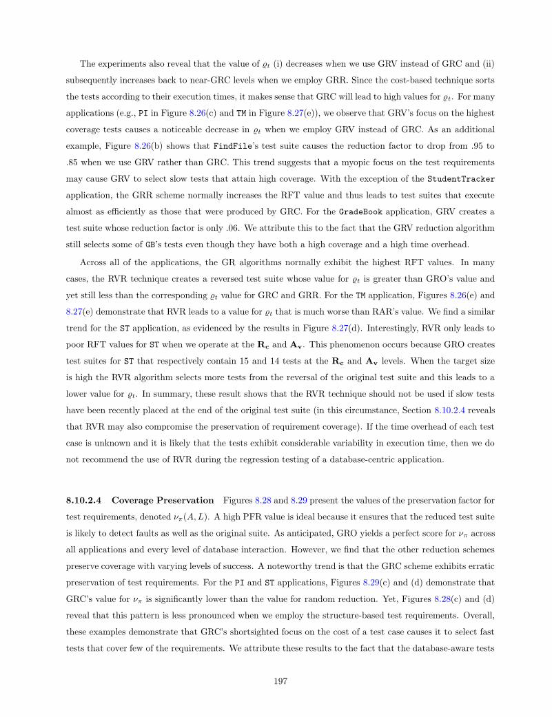
The experiments also reveal that the value of %t (i) decreases when we use GRV instead of GRC and (ii)
subsequently increases back to near-GRC levels when we employ GRR. Since the cost-based technique sorts
the tests according to their execution times, it makes sense that GRC will lead to high values for %t. For many
applications (e.g., PI in Figure 8.26(c) and TM in Figure 8.27(e)), we observe that GRV’s focus on the highest
coverage tests causes a noticeable decrease in %t when we employ GRV instead of GRC. As an additional
example, Figure 8.26(b) shows that FindFile’s test suite causes the reduction factor to drop from .95 to
.85 when we use GRV rather than GRC. This trend suggests that a myopic focus on the test requirements
may cause GRV to select slow tests that attain high coverage. With the exception of the StudentTracker
application, the GRR scheme normally increases the RFT value and thus leads to test suites that execute
almost as efficiently as those that were produced by GRC. For the GradeBook application, GRV creates a
test suite whose reduction factor is only .06. We attribute this to the fact that the GRV reduction algorithm
still selects some of GB’s tests even though they have both a high coverage and a high time overhead.
Across all of the applications, the GR algorithms normally exhibit the highest RFT values. In many
cases, the RVR technique creates a reversed test suite whose value for %t is greater than GRO’s value and
yet still less than the corresponding %t value for GRC and GRR. For the TM application, Figures 8.26(e) and
8.27(e) demonstrate that RVR leads to a value for %t that is much worse than RAR’s value. We find a similar
trend for the ST application, as evidenced by the results in Figure 8.27(d). Interestingly, RVR only leads to
poor RFT values for ST when we operate at the Rc and Av. This phenomenon occurs because GRO creates
test suites for ST that respectively contain 15 and 14 tests at the Rc and Av levels. When the target size
is high the RVR algorithm selects more tests from the reversal of the original test suite and this leads to a
lower value for %t. In summary, these result shows that the RVR technique should not be used if slow tests
have been recently placed at the end of the original test suite (in this circumstance, Section 8.10.2.4 reveals
that RVR may also compromise the preservation of requirement coverage). If the time overhead of each test
case is unknown and it is likely that the tests exhibit considerable variability in execution time, then we do
not recommend the use of RVR during the regression testing of a database-centric application.
8.10.2.4 Coverage Preservation Figures 8.28 and 8.29 present the values of the preservation factor for
test requirements, denoted νπ(A, L). A high PFR value is ideal because it ensures that the reduced test suite
is likely to detect faults as well as the original suite. As anticipated, GRO yields a perfect score for νπ across
all applications and every level of database interaction. However, we find that the other reduction schemes
preserve coverage with varying levels of success. A noteworthy trend is that the GRC scheme exhibits erratic
preservation of test requirements. For the PI and ST applications, Figures 8.29(c) and (d) demonstrate that
GRC’s value for νπ is significantly lower than the value for random reduction. Yet, Figures 8.28(c) and (d)
reveal that this pattern is less pronounced when we employ the structure-based test requirements. Overall,
these examples demonstrate that GRC’s shortsighted focus on the cost of a test case causes it to select fast
tests that cover few of the requirements. We attribute these results to the fact that the database-aware tests
197

Rl A
Database Interaction HRM L
0.2
0.4
0.6
0.8
1
Preservation
Factor
-Coverage
Rl A
1. 1.
0.84
0.750.740.77
0.84
0.79
0.89
0.97
0.770.79
GRO GRC GRV GRR RVR RAR
PSfrag replacements
N6
enter computeVelocity
enter computeVelocity
N6
N6
N7
N7
N8
N8
N10
N8
N16
N10
N11
N11
N12
N12
N18
N16
N18
N18
exit computeVelocity
exit computeVelocity
N6
N1
N1
N2
N2
N3
N3
N1
N1
N4
N4
N5
N5
N6
enter P
enter P
call main
call main
enter main
enter main
enter main
. . .
. . .
call inputCardNumber
call inputCardNumber
call inputPin
call inputCardNumber
call handleError
call handleError
call inputCardNumber
call inputPin
call handleError
call handleError
call inputPin
call inputPin
call inputOperation
call inputOperation
call getAccountBalance
call getAccountBalance
call promptAgain
call inputOperation
call lockAccount
call lockAccount
call promptAgain
call promptAgain
call inputOperation
call promptAgain
. . .
call getAccountBalance
enter getAccountBalance
enter getAccountBalance
N3
N3
N4
N4
N5
N5
N6
N6
N7
N7
N10
N10
N12
N12
N15
N10
N15
N15
exit getAccountBalance
exit getAccountBalance
return getAccountBalance
return lockAccount
. . .
return getAccountBalance
call promptAgain
. . .
exit main
exit main
return main
return main
exit P
exit P
. . .
exit main
enter lockAccount
enter lockAccount
. . .
. . .
exit lockAccount
exit lockAccount
return lockAccount
return lockAccount
exit main
(a)
Rl A
Database Interaction HFF L
0.2
0.4
0.6
0.8
1
Preservation
Factor
-Coverage
Rl A
1. 1.
0.820.8
0.770.8
0.82
0.68
0.820.84
0.8 0.81
GRO GRC GRV GRR RVR RAR
PSfrag replacements
N6
enter computeVelocity
enter computeVelocity
N6
N6
N7
N7
N8
N8
N10
N8
N16
N10
N11
N11
N12
N12
N18
N16
N18
N18
exit computeVelocity
exit computeVelocity
N6
N1
N1
N2
N2
N3
N3
N1
N1
N4
N4
N5
N5
N6
enter P
enter P
call main
call main
enter main
enter main
enter main
. . .
. . .
call inputCardNumber
call inputCardNumber
call inputPin
call inputCardNumber
call handleError
call handleError
call inputCardNumber
call inputPin
call handleError
call handleError
call inputPin
call inputPin
call inputOperation
call inputOperation
call getAccountBalance
call getAccountBalance
call promptAgain
call inputOperation
call lockAccount
call lockAccount
call promptAgain
call promptAgain
call inputOperation
call promptAgain
. . .
call getAccountBalance
enter getAccountBalance
enter getAccountBalance
N3
N3
N4
N4
N5
N5
N6
N6
N7
N7
N10
N10
N12
N12
N15
N10
N15
N15
exit getAccountBalance
exit getAccountBalance
return getAccountBalance
return lockAccount
. . .
return getAccountBalance
call promptAgain
. . .
exit main
exit main
return main
return main
exit P
exit P
. . .
exit main
enter lockAccount
enter lockAccount
. . .
. . .
exit lockAccount
exit lockAccount
return lockAccount
return lockAccount
exit main
(b)
Rl A
Database Interaction HPI L
0.2
0.4
0.6
0.8
1
Preservation
Factor
-Coverage
Rl A
1. 1.
0.930.95
0.6
0.68
0.93
0.68
0.870.89
0.72
0.78
GRO GRC GRV GRR RVR RAR
PSfrag replacements
N6
enter computeVelocity
enter computeVelocity
N6
N6
N7
N7
N8
N8
N10
N8
N16
N10
N11
N11
N12
N12
N18
N16
N18
N18
exit computeVelocity
exit computeVelocity
N6
N1
N1
N2
N2
N3
N3
N1
N1
N4
N4
N5
N5
N6
enter P
enter P
call main
call main
enter main
enter main
enter main
. . .
. . .
call inputCardNumber
call inputCardNumber
call inputPin
call inputCardNumber
call handleError
call handleError
call inputCardNumber
call inputPin
call handleError
call handleError
call inputPin
call inputPin
call inputOperation
call inputOperation
call getAccountBalance
call getAccountBalance
call promptAgain
call inputOperation
call lockAccount
call lockAccount
call promptAgain
call promptAgain
call inputOperation
call promptAgain
. . .
call getAccountBalance
enter getAccountBalance
enter getAccountBalance
N3
N3
N4
N4
N5
N5
N6
N6
N7
N7
N10
N10
N12
N12
N15
N10
N15
N15
exit getAccountBalance
exit getAccountBalance
return getAccountBalance
return lockAccount
. . .
return getAccountBalance
call promptAgain
. . .
exit main
exit main
return main
return main
exit P
exit P
. . .
exit main
enter lockAccount
enter lockAccount
. . .
. . .
exit lockAccount
exit lockAccount
return lockAccount
return lockAccount
exit main
(c)
Rl A
Database Interaction HST L
0.2
0.4
0.6
0.8
1
Preservation
Factor
-Coverage
Rl A
1. 1.
0.53
0.590.6
0.68
0.6
0.68
0.730.77
0.62
0.71
GRO GRC GRV GRR RVR RAR
PSfrag replacements
N6
enter computeVelocity
enter computeVelocity
N6
N6
N7
N7
N8
N8
N10
N8
N16
N10
N11
N11
N12
N12
N18
N16
N18
N18
exit computeVelocity
exit computeVelocity
N6
N1
N1
N2
N2
N3
N3
N1
N1
N4
N4
N5
N5
N6
enter P
enter P
call main
call main
enter main
enter main
enter main
. . .
. . .
call inputCardNumber
call inputCardNumber
call inputPin
call inputCardNumber
call handleError
call handleError
call inputCardNumber
call inputPin
call handleError
call handleError
call inputPin
call inputPin
call inputOperation
call inputOperation
call getAccountBalance
call getAccountBalance
call promptAgain
call inputOperation
call lockAccount
call lockAccount
call promptAgain
call promptAgain
call inputOperation
call promptAgain
. . .
call getAccountBalance
enter getAccountBalance
enter getAccountBalance
N3
N3
N4
N4
N5
N5
N6
N6
N7
N7
N10
N10
N12
N12
N15
N10
N15
N15
exit getAccountBalance
exit getAccountBalance
return getAccountBalance
return lockAccount
. . .
return getAccountBalance
call promptAgain
. . .
exit main
exit main
return main
return main
exit P
exit P
. . .
exit main
enter lockAccount
enter lockAccount
. . .
. . .
exit lockAccount
exit lockAccount
return lockAccount
return lockAccount
exit main
(d)
Rl A
Database Interaction HTM L
0.2
0.4
0.6
0.8
1
Preservation
Factor
-Coverage
Rl A
1. 1.
0.890.91
0.83
0.93
0.76
0.860.83
0.91
0.86
0.94
GRO GRC GRV GRR RVR RAR
PSfrag replacements
N6
enter computeVelocity
enter computeVelocity
N6
N6
N7
N7
N8
N8
N10
N8
N16
N10
N11
N11
N12
N12
N18
N16
N18
N18
exit computeVelocity
exit computeVelocity
N6
N1
N1
N2
N2
N3
N3
N1
N1
N4
N4
N5
N5
N6
enter P
enter P
call main
call main
enter main
enter main
enter main
. . .
. . .
call inputCardNumber
call inputCardNumber
call inputPin
call inputCardNumber
call handleError
call handleError
call inputCardNumber
call inputPin
call handleError
call handleError
call inputPin
call inputPin
call inputOperation
call inputOperation
call getAccountBalance
call getAccountBalance
call promptAgain
call inputOperation
call lockAccount
call lockAccount
call promptAgain
call promptAgain
call inputOperation
call promptAgain
. . .
call getAccountBalance
enter getAccountBalance
enter getAccountBalance
N3
N3
N4
N4
N5
N5
N6
N6
N7
N7
N10
N10
N12
N12
N15
N10
N15
N15
exit getAccountBalance
exit getAccountBalance
return getAccountBalance
return lockAccount
. . .
return getAccountBalance
call promptAgain
. . .
exit main
exit main
return main
return main
exit P
exit P
. . .
exit main
enter lockAccount
enter lockAccount
. . .
. . .
exit lockAccount
exit lockAccount
return lockAccount
return lockAccount
exit main
(e)
Rl A
Database Interaction HGB L
0.2
0.4
0.6
0.8
1
Preservation
Factor
-Coverage
Rl A
1. 1.
0.58
0.4
0.950.97
0.920.95
0.83 0.84
0.770.8
GRO GRC GRV GRR RVR RAR
PSfrag replacements
N6
enter computeVelocity
enter computeVelocity
N6
N6
N7
N7
N8
N8
N10
N8
N16
N10
N11
N11
N12
N12
N18
N16
N18
N18
exit computeVelocity
exit computeVelocity
N6
N1
N1
N2
N2
N3
N3
N1
N1
N4
N4
N5
N5
N6
enter P
enter P
call main
call main
enter main
enter main
enter main
. . .
. . .
call inputCardNumber
call inputCardNumber
call inputPin
call inputCardNumber
call handleError
call handleError
call inputCardNumber
call inputPin
call handleError
call handleError
call inputPin
call inputPin
call inputOperation
call inputOperation
call getAccountBalance
call getAccountBalance
call promptAgain
call inputOperation
call lockAccount
call lockAccount
call promptAgain
call promptAgain
call inputOperation
call promptAgain
. . .
call getAccountBalance
enter getAccountBalance
enter getAccountBalance
N3
N3
N4
N4
N5
N5
N6
N6
N7
N7
N10
N10
N12
N12
N15
N10
N15
N15
exit getAccountBalance
exit getAccountBalance
return getAccountBalance
return lockAccount
. . .
return getAccountBalance
call promptAgain
. . .
exit main
exit main
return main
return main
exit P
exit P
. . .
exit main
enter lockAccount
enter lockAccount
. . .
. . .
exit lockAccount
exit lockAccount
return lockAccount
return lockAccount
exit main
(f)
Figure 8.28: Preservation Factor for Test Suite Coverage (Relation and Attribute).
198

Rc AvDatabase Interaction HRM L
0.2
0.4
0.6
0.8
1
Preservation
Factor
-Coverage
Rc Av
1. 1.
0.90.88
0.92
0.980.95
0.980.970.94
0.880.85
GRO GRC GRV GRR RVR RAR
PSfrag replacements
N6
enter computeVelocity
enter computeVelocity
N6
N6
N7
N7
N8
N8
N10
N8
N16
N10
N11
N11
N12
N12
N18
N16
N18
N18
exit computeVelocity
exit computeVelocity
N6
N1
N1
N2
N2
N3
N3
N1
N1
N4
N4
N5
N5
N6
enter P
enter P
call main
call main
enter main
enter main
enter main
. . .
. . .
call inputCardNumber
call inputCardNumber
call inputPin
call inputCardNumber
call handleError
call handleError
call inputCardNumber
call inputPin
call handleError
call handleError
call inputPin
call inputPin
call inputOperation
call inputOperation
call getAccountBalance
call getAccountBalance
call promptAgain
call inputOperation
call lockAccount
call lockAccount
call promptAgain
call promptAgain
call inputOperation
call promptAgain
. . .
call getAccountBalance
enter getAccountBalance
enter getAccountBalance
N3
N3
N4
N4
N5
N5
N6
N6
N7
N7
N10
N10
N12
N12
N15
N10
N15
N15
exit getAccountBalance
exit getAccountBalance
return getAccountBalance
return lockAccount
. . .
return getAccountBalance
call promptAgain
. . .
exit main
exit main
return main
return main
exit P
exit P
. . .
exit main
enter lockAccount
enter lockAccount
. . .
. . .
exit lockAccount
exit lockAccount
return lockAccount
return lockAccount
exit main
(a)
Rc AvDatabase Interaction HFF L
0.2
0.4
0.6
0.8
1
Preservation
Factor
-Coverage
Rc Av
1. 1.
0.58 0.57
0.920.96
0.58 0.580.580.56
0.83 0.83
GRO GRC GRV GRR RVR RAR
PSfrag replacements
N6
enter computeVelocity
enter computeVelocity
N6
N6
N7
N7
N8
N8
N10
N8
N16
N10
N11
N11
N12
N12
N18
N16
N18
N18
exit computeVelocity
exit computeVelocity
N6
N1
N1
N2
N2
N3
N3
N1
N1
N4
N4
N5
N5
N6
enter P
enter P
call main
call main
enter main
enter main
enter main
. . .
. . .
call inputCardNumber
call inputCardNumber
call inputPin
call inputCardNumber
call handleError
call handleError
call inputCardNumber
call inputPin
call handleError
call handleError
call inputPin
call inputPin
call inputOperation
call inputOperation
call getAccountBalance
call getAccountBalance
call promptAgain
call inputOperation
call lockAccount
call lockAccount
call promptAgain
call promptAgain
call inputOperation
call promptAgain
. . .
call getAccountBalance
enter getAccountBalance
enter getAccountBalance
N3
N3
N4
N4
N5
N5
N6
N6
N7
N7
N10
N10
N12
N12
N15
N10
N15
N15
exit getAccountBalance
exit getAccountBalance
return getAccountBalance
return lockAccount
. . .
return getAccountBalance
call promptAgain
. . .
exit main
exit main
return main
return main
exit P
exit P
. . .
exit main
enter lockAccount
enter lockAccount
. . .
. . .
exit lockAccount
exit lockAccount
return lockAccount
return lockAccount
exit main
(b)
Rc AvDatabase Interaction HPI L
0.2
0.4
0.6
0.8
1
Preservation
Factor
-Coverage
Rc Av
1. 1.
0.11
0.01
0.99 1.0.99 1.
0.72
0.67
0.72
0.56
GRO GRC GRV GRR RVR RAR
PSfrag replacements
N6
enter computeVelocity
enter computeVelocity
N6
N6
N7
N7
N8
N8
N10
N8
N16
N10
N11
N11
N12
N12
N18
N16
N18
N18
exit computeVelocity
exit computeVelocity
N6
N1
N1
N2
N2
N3
N3
N1
N1
N4
N4
N5
N5
N6
enter P
enter P
call main
call main
enter main
enter main
enter main
. . .
. . .
call inputCardNumber
call inputCardNumber
call inputPin
call inputCardNumber
call handleError
call handleError
call inputCardNumber
call inputPin
call handleError
call handleError
call inputPin
call inputPin
call inputOperation
call inputOperation
call getAccountBalance
call getAccountBalance
call promptAgain
call inputOperation
call lockAccount
call lockAccount
call promptAgain
call promptAgain
call inputOperation
call promptAgain
. . .
call getAccountBalance
enter getAccountBalance
enter getAccountBalance
N3
N3
N4
N4
N5
N5
N6
N6
N7
N7
N10
N10
N12
N12
N15
N10
N15
N15
exit getAccountBalance
exit getAccountBalance
return getAccountBalance
return lockAccount
. . .
return getAccountBalance
call promptAgain
. . .
exit main
exit main
return main
return main
exit P
exit P
. . .
exit main
enter lockAccount
enter lockAccount
. . .
. . .
exit lockAccount
exit lockAccount
return lockAccount
return lockAccount
exit main
(c)
Rc AvDatabase Interaction HST L
0.2
0.4
0.6
0.8
1
Preservation
Factor
-Coverage
Rc Av
1. 1.
0.060.04
0.98 0.980.98 0.98
0.65 0.660.62
0.59
GRO GRC GRV GRR RVR RAR
PSfrag replacements
N6
enter computeVelocity
enter computeVelocity
N6
N6
N7
N7
N8
N8
N10
N8
N16
N10
N11
N11
N12
N12
N18
N16
N18
N18
exit computeVelocity
exit computeVelocity
N6
N1
N1
N2
N2
N3
N3
N1
N1
N4
N4
N5
N5
N6
enter P
enter P
call main
call main
enter main
enter main
enter main
. . .
. . .
call inputCardNumber
call inputCardNumber
call inputPin
call inputCardNumber
call handleError
call handleError
call inputCardNumber
call inputPin
call handleError
call handleError
call inputPin
call inputPin
call inputOperation
call inputOperation
call getAccountBalance
call getAccountBalance
call promptAgain
call inputOperation
call lockAccount
call lockAccount
call promptAgain
call promptAgain
call inputOperation
call promptAgain
. . .
call getAccountBalance
enter getAccountBalance
enter getAccountBalance
N3
N3
N4
N4
N5
N5
N6
N6
N7
N7
N10
N10
N12
N12
N15
N10
N15
N15
exit getAccountBalance
exit getAccountBalance
return getAccountBalance
return lockAccount
. . .
return getAccountBalance
call promptAgain
. . .
exit main
exit main
return main
return main
exit P
exit P
. . .
exit main
enter lockAccount
enter lockAccount
. . .
. . .
exit lockAccount
exit lockAccount
return lockAccount
return lockAccount
exit main
(d)
Rc AvDatabase Interaction HTM L
0.2
0.4
0.6
0.8
1
Preservation
Factor
-Coverage
Rc Av
1. 1.
0.72
0.41
0.94
0.99
0.88
0.96
0.670.64
0.690.66
GRO GRC GRV GRR RVR RAR
PSfrag replacements
N6
enter computeVelocity
enter computeVelocity
N6
N6
N7
N7
N8
N8
N10
N8
N16
N10
N11
N11
N12
N12
N18
N16
N18
N18
exit computeVelocity
exit computeVelocity
N6
N1
N1
N2
N2
N3
N3
N1
N1
N4
N4
N5
N5
N6
enter P
enter P
call main
call main
enter main
enter main
enter main
. . .
. . .
call inputCardNumber
call inputCardNumber
call inputPin
call inputCardNumber
call handleError
call handleError
call inputCardNumber
call inputPin
call handleError
call handleError
call inputPin
call inputPin
call inputOperation
call inputOperation
call getAccountBalance
call getAccountBalance
call promptAgain
call inputOperation
call lockAccount
call lockAccount
call promptAgain
call promptAgain
call inputOperation
call promptAgain
. . .
call getAccountBalance
enter getAccountBalance
enter getAccountBalance
N3
N3
N4
N4
N5
N5
N6
N6
N7
N7
N10
N10
N12
N12
N15
N10
N15
N15
exit getAccountBalance
exit getAccountBalance
return getAccountBalance
return lockAccount
. . .
return getAccountBalance
call promptAgain
. . .
exit main
exit main
return main
return main
exit P
exit P
. . .
exit main
enter lockAccount
enter lockAccount
. . .
. . .
exit lockAccount
exit lockAccount
return lockAccount
return lockAccount
exit main
(e)
Rc AvDatabase Interaction HGB L
0.2
0.4
0.6
0.8
1
Preservation
Factor
-Coverage
Rc Av
1. 1.
0.3
0.09
0.98 0.990.96
0.98
0.910.94
0.71 0.72
GRO GRC GRV GRR RVR RAR
PSfrag replacements
N6
enter computeVelocity
enter computeVelocity
N6
N6
N7
N7
N8
N8
N10
N8
N16
N10
N11
N11
N12
N12
N18
N16
N18
N18
exit computeVelocity
exit computeVelocity
N6
N1
N1
N2
N2
N3
N3
N1
N1
N4
N4
N5
N5
N6
enter P
enter P
call main
call main
enter main
enter main
enter main
. . .
. . .
call inputCardNumber
call inputCardNumber
call inputPin
call inputCardNumber
call handleError
call handleError
call inputCardNumber
call inputPin
call handleError
call handleError
call inputPin
call inputPin
call inputOperation
call inputOperation
call getAccountBalance
call getAccountBalance
call promptAgain
call inputOperation
call lockAccount
call lockAccount
call promptAgain
call promptAgain
call inputOperation
call promptAgain
. . .
call getAccountBalance
enter getAccountBalance
enter getAccountBalance
N3
N3
N4
N4
N5
N5
N6
N6
N7
N7
N10
N10
N12
N12
N15
N10
N15
N15
exit getAccountBalance
exit getAccountBalance
return getAccountBalance
return lockAccount
. . .
return getAccountBalance
call promptAgain
. . .
exit main
exit main
return main
return main
exit P
exit P
. . .
exit main
enter lockAccount
enter lockAccount
. . .
. . .
exit lockAccount
exit lockAccount
return lockAccount
return lockAccount
exit main
(f)
Figure 8.29: Preservation Factor for Test Suite Coverage (Record and Attribute Value).
199

Abbreviation Meaning
GPC GreedyPrioritizationWithoutOverlap - Cost
GPV GreedyPrioritizationWithoutOverlap - Coverage
GPR GreedyPrioritizationWithoutOverlap - Ratio
ORP OriginalPrioritization
Table 8.12: Summary of the Abbreviations Used to Describe the Prioritization Techniques.
create most of the coverage tree paths when we record coverage at the Rc or Av levels. Therefore, GRC
includes the low coverage tests that do not interact with the database when it picks the fast test cases. In
general, we observe that GRC is not well suited to reducing database-aware test suites because there is often
an inverse relationship between testing time and requirement coverage.
The empirical study also suggests that it may also be misleading to exclusively focus on the coverage of
the test requirements. For example, Figure 8.28(c) shows that GRV creates a reduced test suite for Pithy
that has a lower PFR value than GRC, GRR, and RVR. For example, we see that νπ drops from .93 to .6
when we use GRV instead of GRC. Further study of the reduced test suite reveals that the highest coverage
tests have longer running times. The inclusion of these tests in the reduced test suite eventually prevents
GRV from including other tests that cumulatively cover more requirements in less time. For PI, we observe
that the use of GRR increases the value of νπ to near-GRO levels. However, Figure 8.28(e) demonstrates
that using GRR may still lead to a decrease in PFR that severely compromises coverage. In fact, the use
of the Rl-level requirements for TM leads to preservation factors that are worse than those that we see for
random reduction. Therefore, ratio-based sorting of the test cases is not guaranteed to preserve coverage
better than the other greedy techniques that ignore overlap.
In conclusion, we often find that one or more of GRC, GRV, GRR, or RVR exhibit coverage preservation
values that are worse than the corresponding values for the randomly reduced test suite. For example,
Figure 8.29(b) indicates that three reduction techniques lead to νπ values that are worse than random. In
particular, the use of GRC, GRR, or RVR to reduce FF’s test suite leads to νπ = .58 even though random
reduction exhibits a νπ value of .83. If small to moderate reductions are acceptable and coverage preservation
is important, then we recommend the use of GreedyReductionWithOverlap. We advocate the use of GRO
because the empirical results demonstrate that ignoring the overlap in the tests’ coverage may cause the GR
algorithms to improvidently include tests within the reduced suite. Even though GRO may lead to reduction
factors that are smaller than GR and RVR, we judge that it is an appropriate choice if variations in coverage
preservation are not desirable.
If we adopt the notion of preference under the operator, as defined in Section 8.6, then it is clear that
there are few configurations of the reduction component that regularly identify reduced test suites that are
both efficient and effective. For brevity, we focus on a specific example to illustrate the main point. If we
consider the reduced test suites for ST at the Rc level, then GRO and GRC are respectively described by the
evaluation tuples νr = 〈.56, .13, 1.0〉 and νr = 〈.56, .99, .04〉. Following the definition of in Equation (8.11),
200

Rl A
Database Interaction HST L
0.2
0.4
0.6
0.8
1
Coverage
Effectiveness
Rl A
0.940.96
0.98 0.98
0.850.87
0.98 0.98
0.85 0.850.850.88
0.750.77
GPO GPC GPV GPR RVP ORP RAP
PSfrag replacements
N6
enter computeVelocity
enter computeVelocity
N6
N6
N7
N7
N8
N8
N10
N8
N16
N10
N11
N11
N12
N12
N18
N16
N18
N18
exit computeVelocity
exit computeVelocity
N6
N1
N1
N2
N2
N3
N3
N1
N1
N4
N4
N5
N5
N6
enter P
enter P
call main
call main
enter main
enter main
enter main
. . .
. . .
call inputCardNumber
call inputCardNumber
call inputPin
call inputCardNumber
call handleError
call handleError
call inputCardNumber
call inputPin
call handleError
call handleError
call inputPin
call inputPin
call inputOperation
call inputOperation
call getAccountBalance
call getAccountBalance
call promptAgain
call inputOperation
call lockAccount
call lockAccount
call promptAgain
call promptAgain
call inputOperation
call promptAgain
. . .
call getAccountBalance
enter getAccountBalance
enter getAccountBalance
N3
N3
N4
N4
N5
N5
N6
N6
N7
N7
N10
N10
N12
N12
N15
N10
N15
N15
exit getAccountBalance
exit getAccountBalance
return getAccountBalance
return lockAccount
. . .
return getAccountBalance
call promptAgain
. . .
exit main
exit main
return main
return main
exit P
exit P
. . .
exit main
enter lockAccount
enter lockAccount
. . .
. . .
exit lockAccount
exit lockAccount
return lockAccount
return lockAccount
exit main
(a)
Rc AvDatabase Interaction HST L
0.2
0.4
0.6
0.8
1
Coverage
Effectiveness
Rc Av
0.97 0.97
0.88 0.89
0.96 0.960.96 0.96
0.64 0.65
0.93 0.93
0.64 0.64
GPO GPC GPV GPR RVP ORP RAP
PSfrag replacements
N6
enter computeVelocity
enter computeVelocity
N6
N6
N7
N7
N8
N8
N10
N8
N16
N10
N11
N11
N12
N12
N18
N16
N18
N18
exit computeVelocity
exit computeVelocity
N6
N1
N1
N2
N2
N3
N3
N1
N1
N4
N4
N5
N5
N6
enter P
enter P
call main
call main
enter main
enter main
enter main
. . .
. . .
call inputCardNumber
call inputCardNumber
call inputPin
call inputCardNumber
call handleError
call handleError
call inputCardNumber
call inputPin
call handleError
call handleError
call inputPin
call inputPin
call inputOperation
call inputOperation
call getAccountBalance
call getAccountBalance
call promptAgain
call inputOperation
call lockAccount
call lockAccount
call promptAgain
call promptAgain
call inputOperation
call promptAgain
. . .
call getAccountBalance
enter getAccountBalance
enter getAccountBalance
N3
N3
N4
N4
N5
N5
N6
N6
N7
N7
N10
N10
N12
N12
N15
N10
N15
N15
exit getAccountBalance
exit getAccountBalance
return getAccountBalance
return lockAccount
. . .
return getAccountBalance
call promptAgain
. . .
exit main
exit main
return main
return main
exit P
exit P
. . .
exit main
enter lockAccount
enter lockAccount
. . .
. . .
exit lockAccount
exit lockAccount
return lockAccount
return lockAccount
exit main
(b)
Figure 8.30: Coverage Effectiveness for the StudentTracker Application.
we see that νr 6 νr and νr 6 νr and thus νr ∼ νr (i.e., νr and νr describe approaches to reduction that
are similar according to the evaluation metrics stated in Section 8.6). In this circumstance, the correct choice
for the regression testing of ST is dictated by the testing process. Severe time constraints would suggest the
use of GRC, while the overlap-aware GRO technique would be preferred when coverage preservation is more
important. As part of future work, we intend to exhaustively compare the different reductions with the
operator.
8.10.3 Test Prioritization
We also conducted an empirical study in order to determine how prioritization impacts the coverage effec-
tiveness (CE) of a test suite (c.f. Section 8.6 for a definition of the CE metric). Paralleling the results in
Section 8.10.2.1, the experiments reveal that the prioritization component is also efficient for the chosen ap-
plications. We selected the StudentTracker and GradeBook applications for further analysis because these
case studies (i) respectively represent the best and the worst values for %n and (ii) support a discussion of
the most relevant experimental trends. Table 8.12 summarizes the abbreviations that we use to describe the
different approaches to prioritization (c.f. Table 8.7 for a review of the abbreviations that were previously
defined). For example, GPR stands for the use of GreedyPrioritizationWithoutOverlap in conjunction with
the ratio-based ordering criterion.
Figure 8.30 presents the coverage effectiveness value, denoted ξ, for the ST application. Since ST exhibits
high values for %n, it is evident that there are many redundant tests in the original test suite. Therefore,
we anticipate that many of the prioritization techniques should yield high CE values. Indeed, Figure 8.30
reveals that all of the greedy techniques create test suites with ξ values greater than .85. For this application,
we see that GPC and GPR have CE values of .98 and GPO has a CE value of .94. Furthermore, Figure 8.30
demonstrates that most of the prioritization algorithms, with the exception of RVP at the Rc and Av levels,
perform much better than random prioritization. Since ST’s tests have a substantial amount of overlap,
201

Rl A
Database Interaction HGB L
0.2
0.4
0.6
0.8
1
Coverage
Effectiveness
Rl A
0.96 0.960.93 0.92
0.820.86
0.94 0.94
0.8 0.81
0.360.38
0.60.63
GPO GPC GPV GPR RVP ORP RAP
PSfrag replacements
N6
enter computeVelocity
enter computeVelocity
N6
N6
N7
N7
N8
N8
N10
N8
N16
N10
N11
N11
N12
N12
N18
N16
N18
N18
exit computeVelocity
exit computeVelocity
N6
N1
N1
N2
N2
N3
N3
N1
N1
N4
N4
N5
N5
N6
enter P
enter P
call main
call main
enter main
enter main
enter main
. . .
. . .
call inputCardNumber
call inputCardNumber
call inputPin
call inputCardNumber
call handleError
call handleError
call inputCardNumber
call inputPin
call handleError
call handleError
call inputPin
call inputPin
call inputOperation
call inputOperation
call getAccountBalance
call getAccountBalance
call promptAgain
call inputOperation
call lockAccount
call lockAccount
call promptAgain
call promptAgain
call inputOperation
call promptAgain
. . .
call getAccountBalance
enter getAccountBalance
enter getAccountBalance
N3
N3
N4
N4
N5
N5
N6
N6
N7
N7
N10
N10
N12
N12
N15
N10
N15
N15
exit getAccountBalance
exit getAccountBalance
return getAccountBalance
return lockAccount
. . .
return getAccountBalance
call promptAgain
. . .
exit main
exit main
return main
return main
exit P
exit P
. . .
exit main
enter lockAccount
enter lockAccount
. . .
. . .
exit lockAccount
exit lockAccount
return lockAccount
return lockAccount
exit main
(a)
Rc AvDatabase Interaction HGB L
0.2
0.4
0.6
0.8
1
Coverage
Effectiveness
Rc Av
0.94 0.94
0.88 0.870.870.9
0.93 0.93
0.840.86
0.22 0.22
0.55 0.56
GPO GPC GPV GPR RVP ORP RAP
PSfrag replacements
N6
enter computeVelocity
enter computeVelocity
N6
N6
N7
N7
N8
N8
N10
N8
N16
N10
N11
N11
N12
N12
N18
N16
N18
N18
exit computeVelocity
exit computeVelocity
N6
N1
N1
N2
N2
N3
N3
N1
N1
N4
N4
N5
N5
N6
enter P
enter P
call main
call main
enter main
enter main
enter main
. . .
. . .
call inputCardNumber
call inputCardNumber
call inputPin
call inputCardNumber
call handleError
call handleError
call inputCardNumber
call inputPin
call handleError
call handleError
call inputPin
call inputPin
call inputOperation
call inputOperation
call getAccountBalance
call getAccountBalance
call promptAgain
call inputOperation
call lockAccount
call lockAccount
call promptAgain
call promptAgain
call inputOperation
call promptAgain
. . .
call getAccountBalance
enter getAccountBalance
enter getAccountBalance
N3
N3
N4
N4
N5
N5
N6
N6
N7
N7
N10
N10
N12
N12
N15
N10
N15
N15
exit getAccountBalance
exit getAccountBalance
return getAccountBalance
return lockAccount
. . .
return getAccountBalance
call promptAgain
. . .
exit main
exit main
return main
return main
exit P
exit P
. . .
exit main
enter lockAccount
enter lockAccount
. . .
. . .
exit lockAccount
exit lockAccount
return lockAccount
return lockAccount
exit main
(b)
Figure 8.31: Coverage Effectiveness for the GradeBook Application.
we also notice that the original ordering of the test suite attains high values for ξ (e.g., ξ = .93 when we
represent the database interactions at the Rc and Av levels).
Figure 8.31 provides the CE values for the GradeBook case study application. GB’s low values for %n attest
to the fact that the test suite for this application does not include many tests that redundantly cover the
requirements. The bottom box and whisker plot in Figure 8.24(f) also reveals that there is a wide variation
in how many requirements are covered by a single test case. Therefore, we judge that it is more difficult to
identify a prioritization that will rapidly cover GB’s test requirements. In contrast to the empirical outcomes
associated with prioritizing ST’s test suite, we observe that applying GPO to GB’s test suite always leads to
the highest value of ξ. At the Rc and Av levels, Figure 8.31(b) shows that GPO creates test suites with
ξ = .94. In comparison, we notice that the GP generated test orderings have CE values that are less than
GPO’s corresponding CE value by between .01 and .07 units. Since higher CE values suggest that the tests
are more likely to reveal faults earlier in the testing process, we recommend the use of GPO during the
prioritization of tests for a database-centric application that exhibits coverage patterns similar to the ones
found in GB’s test suite.
The results in Figure 8.31 also point out that random prioritization attains CE values that are much better
than the original ordering of the test suite. Furthermore, we also find that the CE value for GPO is much
higher than the corresponding CE value for ORP. In an attempt to better understand these experimental
outcomes, Figure 8.32 furnishes a plot of κ for the GPO and ORP techniques (c.f. Section 8.6 for a detailed
discussion of κ). For the ST application, Figures 8.32(a) and (b) show that both GPO and ORP have a κ
function that grows very rapidly. For GB, Figures 8.32(c) and (d) reveal that there is a distinct difference
between the κ function for GPO and ORP. Interestingly, this result corroborates a recent discovery concerning
the ways in which the re-ordering of a traditional test suite may impact the value of the average percentage
of faults detected (APFD) metric [Do et al., 2004].
202

0 2000 4000 6000Time H ms L
0
500
1000
1500
2000
Covered
Test
Reqs
Hcount
L
StudentTracker - GRO - Attribute Value
0 2000 4000 6000Time H ms L
0
500
1000
1500
2000
Covered
Test
Reqs
Hcount
L
StudentTracker - GRO - Attribute Value
PSfrag replacements
N6
enter computeVelocity
enter computeVelocity
N6
N6
N7
N7
N8
N8
N10
N8
N16
N10
N11
N11
N12
N12
N18
N16
N18
N18
exit computeVelocity
exit computeVelocity
N6
N1
N1
N2
N2
N3
N3
N1
N1
N4
N4
N5
N5
N6
enter P
enter P
call main
call main
enter main
enter main
enter main
. . .
. . .
call inputCardNumber
call inputCardNumber
call inputPin
call inputCardNumber
call handleError
call handleError
call inputCardNumber
call inputPin
call handleError
call handleError
call inputPin
call inputPin
call inputOperation
call inputOperation
call getAccountBalance
call getAccountBalance
call promptAgain
call inputOperation
call lockAccount
call lockAccount
call promptAgain
call promptAgain
call inputOperation
call promptAgain
. . .
call getAccountBalance
enter getAccountBalance
enter getAccountBalance
N3
N3
N4
N4
N5
N5
N6
N6
N7
N7
N10
N10
N12
N12
N15
N10
N15
N15
exit getAccountBalance
exit getAccountBalance
return getAccountBalance
return lockAccount
. . .
return getAccountBalance
call promptAgain
. . .
exit main
exit main
return main
return main
exit P
exit P
. . .
exit main
enter lockAccount
enter lockAccount
. . .
. . .
exit lockAccount
exit lockAccount
return lockAccount
return lockAccount
exit main
(a)
0 2000 4000 6000Time H ms L
0
500
1000
1500
2000
Covered
Test
Reqs
Hcount
L
StudentTracker - ORP - Attribute Value
0 2000 4000 6000Time H ms L
0
500
1000
1500
2000
Covered
Test
Reqs
Hcount
L
StudentTracker - ORP - Attribute Value
PSfrag replacements
N6
enter computeVelocity
enter computeVelocity
N6
N6
N7
N7
N8
N8
N10
N8
N16
N10
N11
N11
N12
N12
N18
N16
N18
N18
exit computeVelocity
exit computeVelocity
N6
N1
N1
N2
N2
N3
N3
N1
N1
N4
N4
N5
N5
N6
enter P
enter P
call main
call main
enter main
enter main
enter main
. . .
. . .
call inputCardNumber
call inputCardNumber
call inputPin
call inputCardNumber
call handleError
call handleError
call inputCardNumber
call inputPin
call handleError
call handleError
call inputPin
call inputPin
call inputOperation
call inputOperation
call getAccountBalance
call getAccountBalance
call promptAgain
call inputOperation
call lockAccount
call lockAccount
call promptAgain
call promptAgain
call inputOperation
call promptAgain
. . .
call getAccountBalance
enter getAccountBalance
enter getAccountBalance
N3
N3
N4
N4
N5
N5
N6
N6
N7
N7
N10
N10
N12
N12
N15
N10
N15
N15
exit getAccountBalance
exit getAccountBalance
return getAccountBalance
return lockAccount
. . .
return getAccountBalance
call promptAgain
. . .
exit main
exit main
return main
return main
exit P
exit P
. . .
exit main
enter lockAccount
enter lockAccount
. . .
. . .
exit lockAccount
exit lockAccount
return lockAccount
return lockAccount
exit main
(b)
0 2000 4000 6000 8000Time H ms L
0
100
200
300
400
500
Covered
Test
Reqs
Hcount
L
GradeBook - GRO - Attribute Value
0 2000 4000 6000 8000Time H ms L
0
100
200
300
400
500
Covered
Test
Reqs
Hcount
L
GradeBook - GRO - Attribute Value
PSfrag replacements
N6
enter computeVelocity
enter computeVelocity
N6
N6
N7
N7
N8
N8
N10
N8
N16
N10
N11
N11
N12
N12
N18
N16
N18
N18
exit computeVelocity
exit computeVelocity
N6
N1
N1
N2
N2
N3
N3
N1
N1
N4
N4
N5
N5
N6
enter P
enter P
call main
call main
enter main
enter main
enter main
. . .
. . .
call inputCardNumber
call inputCardNumber
call inputPin
call inputCardNumber
call handleError
call handleError
call inputCardNumber
call inputPin
call handleError
call handleError
call inputPin
call inputPin
call inputOperation
call inputOperation
call getAccountBalance
call getAccountBalance
call promptAgain
call inputOperation
call lockAccount
call lockAccount
call promptAgain
call promptAgain
call inputOperation
call promptAgain
. . .
call getAccountBalance
enter getAccountBalance
enter getAccountBalance
N3
N3
N4
N4
N5
N5
N6
N6
N7
N7
N10
N10
N12
N12
N15
N10
N15
N15
exit getAccountBalance
exit getAccountBalance
return getAccountBalance
return lockAccount
. . .
return getAccountBalance
call promptAgain
. . .
exit main
exit main
return main
return main
exit P
exit P
. . .
exit main
enter lockAccount
enter lockAccount
. . .
. . .
exit lockAccount
exit lockAccount
return lockAccount
return lockAccount
exit main
(c)
0 2000 4000 6000 8000Time H ms L
0
100
200
300
400
500
Covered
Test
Reqs
Hcount
L
GradeBook - ORP - Attribute Value
0 2000 4000 6000 8000Time H ms L
0
100
200
300
400
500
Covered
Test
Reqs
Hcount
L
GradeBook - ORP - Attribute Value
PSfrag replacements
N6
enter computeVelocity
enter computeVelocity
N6
N6
N7
N7
N8
N8
N10
N8
N16
N10
N11
N11
N12
N12
N18
N16
N18
N18
exit computeVelocity
exit computeVelocity
N6
N1
N1
N2
N2
N3
N3
N1
N1
N4
N4
N5
N5
N6
enter P
enter P
call main
call main
enter main
enter main
enter main
. . .
. . .
call inputCardNumber
call inputCardNumber
call inputPin
call inputCardNumber
call handleError
call handleError
call inputCardNumber
call inputPin
call handleError
call handleError
call inputPin
call inputPin
call inputOperation
call inputOperation
call getAccountBalance
call getAccountBalance
call promptAgain
call inputOperation
call lockAccount
call lockAccount
call promptAgain
call promptAgain
call inputOperation
call promptAgain
. . .
call getAccountBalance
enter getAccountBalance
enter getAccountBalance
N3
N3
N4
N4
N5
N5
N6
N6
N7
N7
N10
N10
N12
N12
N15
N10
N15
N15
exit getAccountBalance
exit getAccountBalance
return getAccountBalance
return lockAccount
. . .
return getAccountBalance
call promptAgain
. . .
exit main
exit main
return main
return main
exit P
exit P
. . .
exit main
enter lockAccount
enter lockAccount
. . .
. . .
exit lockAccount
exit lockAccount
return lockAccount
return lockAccount
exit main
(d)
Figure 8.32: Visualizing the Cumulative Coverage of Student and GradeBook.
Following the commentary of Do et al., we postulate that this trend is due to the fact that testers regularly
place the newest tests at the end of the test suite. Since the new tests often cover (i) many portions of the
database that were not covered by the previous tests and (ii) some database regions that were touched by
the earlier test cases, it may be advantageous to use random prioritization in an attempt to spread the high
coverage tests throughout the entire suite. If the test cases exhibit a relatively minor overlap in coverage
and/or there is significant variation in the total number of requirements covered by a test, then it is always
advisable to use one of the prioritization algorithms. That is, it would be better to use random prioritization
than it would be to simply execute the tests in their original ordering. Yet, since the performance study
shows that GPO is efficient for the chosen applications, we advocate the use of the overlap-aware greedy
algorithm if it is important to achieve the highest possible value for the coverage effectiveness metric.
8.11 THREATS TO VALIDITY
The experiments that we describe in this chapter are subject to validity threats. Chapter 3 discusses the
steps that we took to control these threats throughout the experimentation process. We also took additional
steps to handle the threats that are specific to experimentation with the regression testing component.
Internal threats to validity are those factors that have the potential to impact the measured variables
defined in Sections 8.6 and 8.10. The primary threat to internal validity is the existence of a defect in
the regression testing tool. We controlled this threat by performing an extensive series of correctness tests
203
for the techniques that (i) enumerate the test paths and (ii) reduce or prioritize the test suite. During
the testing of the path enumerator, we generated the set of test requirements for small DCTs and CCTs
that were both traditional and database-aware. After enumeration, we verified that each set contained the
proper test paths. We confirmed that the reduction and prioritization algorithms were properly working
by applying them to small instances of the minimal set cover problem. During this process, we tracked the
number of algorithm iterations and we ensured that this count never exceeded the known worst-case. Finally,
we manually added redundant test cases to the test suite for each case study application. After applying
the reduction algorithm, we verified that the reduced test suite did not contain the unnecessary tests. We
judge that threats to construct validity were controlled since Sections 8.6 and 8.10 present a wide range of
evaluation metrics that are useful to both researchers and practitioners.
8.12 CONCLUSION
This chapter describes the design, implementation, and empirical evaluation of our approach to database-
aware regression testing. We provide a high level overview of the regression testing process and we develop
examples to demonstrate the practical benefits of reducing or re-ordering the test suite. This chapter also
introduces the algorithms that (i) enumerate the coverage tree-based test requirements and (ii) perform
database-aware reduction and prioritization. We present approaches to regression testing that consider both
the tests’ overlap in coverage and the time overhead to execute a test case. This chapter also explains how
to evaluate a reduced or prioritized test suite without resorting to the use of a fault seeding mechanism.
In particular, we introduce the notion of coverage effectiveness and we show how to construct a cumulative
coverage function for a test suite. Finally, we discuss the relevant details associated with the implementation
of the regression testing component.
After discussing the goals and design for an experiment to measure the performance of our regression
testing techniques, we systematically state each evaluation metric and analyze the experimental results. The
enumeration of coverage tree paths is efficient enough to support the identification of this type of requirement
in a version specific approach to regression testing. In the context of the largest case study application (i.e.,
GradeBook), we can enumerate the test paths at any level of database interaction in less than 300 milliseconds.
In general, we find that some case study applications yield less than one thousand path-based requirements
while others create more than ten thousand requirements. The empirical results suggest that most test
suites exhibit a moderate overlap in requirement coverage. Yet, for several applications (e.g., Pithy), we
also observe that many Av-level test requirements are only covered by one or two test cases. Considerable
experimentation with the reduction and prioritization components indicates that it is possible to efficiently
create a modified test suite for each of the selected case study applications. Across all of the applications,
we also discover that GreedyReductionWithOverlap (GRO) identifies test suites that are 51% smaller than
the original test suite. Finally, the empirical study reveals that GreedyPrioritizationWithOverlap (GPO) can
re-order the test suite in a manner that improves coverage effectiveness.
204

9.0 CONCLUSIONS AND FUTURE WORK
This chapter summarizes the contributions of this research. We also review the key insights from the
experimental results. It suggests future work that includes enhancing the presented database-aware testing
techniques. We propose several new approaches to testing database-centric applications that leverage the
current framework. This chapter reveals other ways that we can use the research’s conceptual foundation in
order to test a program’s interaction with additional environmental factors such as an eXtensible markup
language (XML) database or a distributed system middleware. We also discuss ways to use the database-
aware tools and techniques in order to test and analyze conventional software applications. In summary, this
chapter provides:
1. A review of the contributions of this dissertation (Section 9.1).
2. A high level summary of the empirical results (Section 9.2).
3. A detailed discussion of future work that leverages the concepts, techniques, and tools developed by this
research (Section 9.3).
9.1 SUMMARY OF THE CONTRIBUTIONS
The database is a ubiquitous technology that many academic institutions, corporations, and individuals use to
manage data. However, a database is only useful for storing information if users can correctly and efficiently
(i) query, update, and remove existing data and (ii) insert new data. To this end, software developers
often implement database-centric applications that interact with one or more relational databases. Indeed,
Silberschatz et al. observe that “practically all use of databases occurs from within application programs”
[Silberschatz et al., 2006, pg. 311]. A database-centric application is very different from a traditional software
system because it interacts with a database that has a complex state and structure. To the best of our
knowledge, this dissertation formulates the first comprehensive framework to address the challenges that are
associated with the efficient and effective testing of database-centric applications. The main contribution of
this research is the description, design, implementation, and evaluation of a collection of testing techniques
called DIATOMS, for Database-centrIc Application Testing tOol ModuleS. We developed tools to fully
support each technique within the comprehensive framework for testing database-centric applications. The
contributions of this research include:
205

1. Fault Model: The database-aware fault model explains how a program’s database interactions could
violate the integrity of a relational database. We focus on program interactions that could negatively
impact the validity and completeness of the database [Motro, 1989]. The type (1-c) and (2-v) defects
involve the incorrect use of the SQL delete statement. If a program contains a type (1-v) or (2-c) defect,
then it submits an incorrect SQL update or insert statement to the database. We further classify
database interaction faults as either commission or omission defects. A fault of commission corresponds
to an incorrect executable statement in the program. A programmer introduces an omission fault when
he/she forgets to include important executable code segments in the program. The database-aware
testing framework supports the identification of all type (1-c) and (1-v) defects and type (2-c) and (2-v)
commission faults.
2. Database-Aware Representations:
a. Control Flow Graphs: Many database-centric applications use the Java Database Connectivity
(JDBC) interface to submit structured query language (SQL) statements to a relational database.
Even though a traditional control flow graph (CFG) contains a node for each database interaction in
a program, it does not statically model what takes place during the execution of the SQL command.
The database interaction interprocedural control flow graph (DI-ICFG) contain nodes and edges
that characterize how the program defines and uses the state and structure of the database.
b. Finite State Machines: The test adequacy component automatically generates a database interaction
finite state machine (DI-FSM) to model each program location that submits a SQL command to the
database. We use the DI-FSMs to model the SQL select, update, insert, and delete statements
that are constructed by the program during testing. We consult the DI-FSMs in order to (i)
determine which database entities are subject to interaction at a given CFG node and (ii) create a
DI-CFG from a conventional CFG.
c. Call Trees: The traditional dynamic call tree (DCT) and calling context tree (CCT) represent the
sequence of method invocations that occur during testing. We describe coverage trees that reveal
how the program interacts with the database during testing (e.g., the DI-DCT and DI-CCT). A
database-aware tree supports both the calculation of coverage and the process of regression testing.
3. Data Flow-Based Test Adequacy Criteria:
a. Comprehensive Family: The conventional def-use association is the foundation for data flow-based
testing because it models a program’s definition and use of variables. This research presents the
database interaction association (DIA) that reveals how the program defines and uses a relational
database entity. We describe a family of database-aware test adequacy criteria that include the
structure-based all-relation-DUs and the state-based all-attribute-value-DUs. For example, the all-
relation-DUs criterion requires a test suite to cover all of the DIAs in the program that involve the
definition and use of the relations in one of the databases.
206

b. Subsumption Hierarchy: This research furnishes a subsumption hierarchy to organize the database-
aware test adequacy criteria according to their strength. The hierarchy shows that all-attribute-
value-DUs is the most difficult adequacy criterion for a test suite to fulfill. We also demonstrate
that all-database-DUs is the weakest criterion. The hierarchy reveals that there is no subsumption
relationship between all-attribute-DUs and all-record-DUs.
4. Test Coverage Monitoring: In order to record a database interaction in the appropriate execution
context, we use the DI-DCT and the DI-CCT. We formally describe these database-aware trees and we
explain how to automatically insert probes that can produce a tree-based coverage report during test
execution. The instrumentation probes intercept the SQL statement that performs a database interaction.
After analyzing the SQL command, these probes efficiently inspect the relevant portions of a database’s
state and structure. Finally, the instrumentation inserts nodes and edges into the DI-DCT and DI-CCT in
order to record all of the pertinent information about a database interaction. The coverage monitor uses
either static or dynamic instrumentation to transparently construct these coverage trees during testing.
5. Regression Testing: The database-aware regression tester minimizes or re-orders a test suite by using
reduction and prioritization techniques. We describe regression testing algorithms that are applicable
whenever it is possible to accurately determine which test requirements are covered by a test case. Our
regression tester can consider both the tests’ overlap in requirement coverage and the time overhead
for an individual test. We also furnish algorithms that improve the efficiency of regression testing by
ignoring the overlap in requirement coverage. Even though the regression tester currently uses a path
in the database-aware coverage tree as a test requirement, we can also configure it to use the database
interaction association. Finally, we describe several new approaches to evaluating the efficiency and
effectiveness of either a prioritized or a reduced test suite.
6. Comprehensive Evaluation:
a. Worst-Case Time Complexity: We characterize the worst-case complexity of the key algorithms in
the comprehensive testing framework. For example, we analyze the algorithms that (i) construct
the database-aware representation, (ii) record coverage information, and (iii) prioritize and reduce a
test suite. We provide formal statements of each algorithm in order to support the time complexity
analysis.
b. Case Study Applications: During the empirical evaluation of the testing techniques, we primarily
use six database-centric applications that were written in Java. We offer a detailed characteri-
zation of each application by examining the size and structure of both the source code and the
relational database. The applications range in size from 548 to 1455 non-commented source state-
ments (NCSS). The database for each application contains between one and nine relations. The
applications use various techniques to submit a wide variety of SQL select, update, insert, and
delete statements. Each case study application has a test suite with test cases that employ many
different testing strategies.
207
c. Tool Implementation Details: We implemented and tested each component in the database-aware
testing framework. We provide pertinent implementation details about the components that calcu-
late test requirements, monitor coverage, and perform regression testing. For example, we explain
how to use aspect-oriented programming (AOP) and the AspectJ language in order to implement
a coverage monitor. These details about the tools demonstrate the practicality of our testing tech-
niques and ensure that other researchers can reproduce our experimental results.
d. Experiment Design: We fully detail the execution environment and the tool versions that we used
during experimentation. We also describe the internal, external, and construct threats that could
compromise experiment validity and we explain how we addressed these threats. The chapters
employ several visualization techniques in order to explain the empirical results. Finally, we furnish
one page summaries that highlight the important insights from each experiment.
9.2 KEY INSIGHTS FROM THE EXPERIMENTS
In order to complement and confirm our analytical evaluation of algorithm performance, we conducted exper-
iments to measure the efficiency and effectiveness of each database-aware testing technique. We calculated
different types of time and space overheads in order to evaluate efficiency. The measurements of effectiveness
were different for each of the testing components. Noteworthy insights from the experimental results include:
1. Data Flow-Based Test Adequacy:
a. Effectiveness: The data flow-based test requirements for a database-centric application include
both the def-use and database interaction associations. The experiments show that the database-
aware test requirements constitute between 10 and 20% of the total number of requirements. This
result suggests that the database-aware test adequacy criteria call for test suites to cover additional
requirements that conventional test criteria ignore.
b. Efficiency: For small and moderate size applications, our data flow analysis algorithm normally
enumerates the database-aware test requirements in less than one minute. The experiments also
show that the inclusion of database interactions in a program’s control flow graph never incurs more
than a 25% increase in the number of nodes and edges.
2. Coverage Monitoring:
a. Effectiveness: Manual and automated inspections of the coverage reports indicate that the coverage
monitor correctly records information concerning program behavior and database interaction. A
comparison of the test suite’s output before and after the insertion of coverage instrumentation
shows that our techniques preserve the syntax and semantics of the program and the tests.
b. Efficiency
i. Instrumentation: Our static instrumentation technique requires less than six seconds to insert
coverage probes into a database-centric application. The batch approach to instrumentation
208

attaches the probes to all six of the applications in less than nine seconds. The dynamic
instrumentation scheme incurs moderate overheads (e.g., a 50% increase in testing time) when
it introduces the instrumentation during test suite execution. The experiments reveal that the
use of static instrumentation increases space overhead by 420% on average. We judge that this
is acceptable because it supports efficient coverage monitoring.
ii. Test Suite Execution: Using static instrumentation to record coverage at coarse levels of
database interaction granularity (e.g., the database and relation levels) increases the testing
time by less than 15% across all applications. On average, coverage monitoring at the finest
level of granularity (e.g., the attribute value level) leads to a 54% increase in testing time
overhead.
iii. Coverage Reports: The size of the in-memory representation of the coverage results range
from 400 kilobytes to almost 25 megabytes. The size of this tree-based coverage report ranges
from 400 to 88000 nodes, depending upon the static structure and dynamic behavior of the
application under test. Even though these reports are large, on average they can be stored
in less than three seconds. We found that efficient compression algorithms successfully reduce
the size of a coverage report by at least one order of magnitude. The results also show that
a DI-CCT at the finest level of database interaction granularity consumes less space overhead
than a traditional dynamic call tree.
3. Regression Testing:
a. Characterizing the Test Suites: The test suites contain many tests that rapidly execute and a few
tests that execute for several seconds. Tests consume a significant amount of execution time if they
(i) interact with many portions of the database and/or (ii) restart the database server.
b. Test Path Enumeration: It is often possible to enumerate the tree-based test paths in less than one
second. Test path enumeration is the most expensive when we identify the paths in a coverage tree
that represents a database interaction at the attribute value level. We conclude that the tree-based
test requirement is suitable for both version specific and general regression testing.
c. Test Suite Reduction:
i. Effectiveness: The reduced test suites are between 30 and 80% smaller than the original test
suite. Across all of the case study applications, the GreedyReductionWithOverlap (GRO) algo-
rithm yields a test suite that contains 51% fewer test cases. The use of GRO leads to test suites
that always cover the same requirements as the original tests while decreasing test execution
time by between 7 and 78%. These results indicate that the reduction component can identify
a modified test suite that is more streamlined that the original suite.
ii. Efficiency: All configurations of the regression testing component can execute in under one
second. We find that the execution of the GRO algorithm normally consumes less than 500
milliseconds, while the GR, RVR, and RAR techniques only run for three to five milliseconds.
209

The experimental results suggest that the reduction technique should scale favorably when it is
applied to larger case study applications. We conclude that the reduction component is ideal
for use in either a version specific or a general regression testing model.
d. Test Suite Prioritization:
i. Effectiveness: In comparison to the original ordering of GB’s test suite, the GreedyPrioritiza-
tionWithOverlap (GPO) causes the coverage effectiveness (CE) value to increase from .22 to .94.
For the other case study applications, we find that the GPO technique creates test orderings
that attain higher CE values than a randomly prioritized suite.
ii. Efficiency: Extensive study of the performance of the prioritization component suggests that
it is very efficient. Paralleling the results from using the reduction algorithms, we find that
GPO always runs in less than 1.5 seconds. Furthermore, the GP, RVP, and RAP techniques
can identify a re-ordered test suite in less than 5 milliseconds.
9.3 FUTURE WORK
This section suggests several areas for future research. It is possible to enhance the testing techniques so
that they handle other types of database interactions. We can also employ the comprehensive framework
during the development of new database-aware testing techniques. For example, we could use the coverage
trees during automatic fault localization and the simplification of a database state that is failure-inducing. A
tree-based coverage report supports this type of debugging because it can record the (i) execution context of
a faulty interaction and (ii) state of the database that existed before the program’s failure. The experiments
also suggest several new avenues for research that empirically investigates the trade-offs in the efficiency
and effectiveness of testing. The database-aware testing techniques provide a foundation for new tools that
test a program’s interaction with other environmental factors. Finally, this research reveals several ways to
improve traditional testing schemes.
9.3.1 Enhancing the Techniques
1. Fault Model: Some database-centric applications use programmer defined transactions so that con-
current database interactions operate correctly. However, our fault model is not tailored for multi-
threaded applications that use transactions. Future work should extend the fault model to include the
three canonical concurrency control problems known as lost update, inconsistent read, and dirty read
[Weikum and Vossen, 2002].
2. Test Adequacy: Extending the fault model to incorporate concurrency necessitates the improvement
of the test adequacy criteria. Future research should also explore new approaches to enumerating
the database interaction associations. Currently, the adequacy component identifies intraprocedural
test requirements. Further research could explore the use of interprocedural data flow analysis (e.g.,
[Harrold and Soffa, 1994]).
210

Test Suite
Passing Test Case Failing Test Case
CCT Sub Tree DCT Sub Tree
PSfrag replacements
N6
enter computeVelocity
enter computeVelocity
N6
N6
N7
N7
N8
N8
N10
N8
N16
N10
N11
N11
N12
N12
N18
N16
N18
N18
exit computeVelocity
exit computeVelocity
N6
N1
N1
N2
N2
N3
N3
N1
N1
N4
N4
N5
N5
N6
enter P
enter P
call main
call main
enter main
enter main
enter main
. . .
. . .
call inputCardNumber
call inputCardNumber
call inputPin
call inputCardNumber
call handleError
call handleError
call inputCardNumber
call inputPin
call handleError
call handleError
call inputPin
call inputPin
call inputOperation
call inputOperation
call getAccountBalance
call getAccountBalance
call promptAgain
call inputOperation
call lockAccount
call lockAccount
call promptAgain
call promptAgain
call inputOperation
call promptAgain
. . .
call getAccountBalance
enter getAccountBalance
enter getAccountBalance
N3
N3
N4
N4
N5
N5
N6
N6
N7
N7
N10
N10
N12
N12
N15
N10
N15
N15
exit getAccountBalance
exit getAccountBalance
return getAccountBalance
return lockAccount
. . .
return getAccountBalance
call promptAgain
. . .
exit main
exit main
return main
return main
exit P
exit P
. . .
exit main
enter lockAccount
enter lockAccount
. . .
. . .
exit lockAccount
exit lockAccount
return lockAccount
return lockAccount
exit main
Figure 9.1: The Enhanced Test Coverage Monitoring Tree.
3. Test Coverage Monitoring
a. Enhanced Coverage Trees: The dynamic call tree incurs high space overhead because it provides full
test execution context. The calling context tree decreases space overhead by coalescing tree nodes
and thus offering a partial context. Future research should investigate a hybrid call tree (HCT)
that balances the strengths and weaknesses of the DCT and the CCT. This HCT could contain a
mixture of CCT and DCT subtrees. If test histories are available, then the HCT could use a DCT
to represent the coverage for the tests that execute any of the methods that previously failed. The
instrumentation probes for the HCT could create CCT subtrees for all of the tests that execute non-
failing methods. As shown in Figure 9.1, the HCT could selectively provide additional execution
context for those tests that are most likely to reveal faults and thus lead to better support for
the debugging process. In principle, the HCT is similar to the incremental call tree described by
[Bernat and Miller, 2006]. However, we intend to use the HCT to test and debug database-centric
and object-oriented applications and their approach is primarily designed for profiling procedural C
programs.
b. Alternative Forms of Interaction: The test coverage monitor (TCM) currently records any database
interaction that occurs through the standard JDBC interface. Recent JDBC drivers include new
functionality that allows the program to update the database through the result set. Some RDBMS
also allow the definition of views that combine the pre-defined relations in order to create a virtual
relation. However, using the SQL create view statement to define a virtual relation forces the
RDBMS to maintain the view when either (i) the underlying relations change or (ii) the state of the
view is directly updated. Many RDBMS support the definition of referential integrity constraints
that create a referencing relationship between two relations. The use of the SQL references keyword
compels the RDBMS to update the state of the referencing relation when the referenced one changes.
Finally, most RDBMS allow the specification of a trigger that executes when a certain event occurs.
Upon the satisfaction of the trigger’s event condition, the database executes a list of actions that
may change the state or structure of the relations. Even though our case study applications do
211

define
use
PSfrag replacements
N6
enter computeVelocity
enter computeVelocity
N6
N6
N7
N7
N8
N8
N10
N8
N16
N10
N11
N11
N12
N12
N18
N16
N18
N18
exit computeVelocity
exit computeVelocity
N6
N1
N1
N2
N2
N3
N3
N1
N1
N4
N4
N5
N5
N6
enter P
enter P
call main
call main
enter main
enter main
enter main
. . .
. . .
call inputCardNumber
call inputCardNumber
call inputPin
call inputCardNumber
call handleError
call handleError
call inputCardNumber
call inputPin
call handleError
call handleError
call inputPin
call inputPin
call inputOperation
call inputOperation
call getAccountBalance
call getAccountBalance
call promptAgain
call inputOperation
call lockAccount
call lockAccount
call promptAgain
call promptAgain
call inputOperation
call promptAgain
. . .
call getAccountBalance
enter getAccountBalance
enter getAccountBalance
N3
N3
N4
N4
N5
N5
N6
N6
N7
N7
N10
N10
N12
N12
N15
N10
N15
N15
exit getAccountBalance
exit getAccountBalance
return getAccountBalance
return lockAccount
. . .
return getAccountBalance
call promptAgain
. . .
exit main
exit main
return main
return main
exit P
exit P
. . .
exit main
enter lockAccount
enter lockAccount
. . .
. . .
exit lockAccount
exit lockAccount
return lockAccount
return lockAccount
exit main
Id : fsmdynamic.ladot, v1.22006/08/0302 : 48 : 33gkapfhamExp
Revision : 1.2
T1
T2
T1
T2
relj
(a)
conflicts
PSfrag replacements
N6
enter computeVelocity
enter computeVelocity
N6
N6
N7
N7
N8
N8
N10
N8
N16
N10
N11
N11
N12
N12
N18
N16
N18
N18
exit computeVelocity
exit computeVelocity
N6
N1
N1
N2
N2
N3
N3
N1
N1
N4
N4
N5
N5
N6
enter P
enter P
call main
call main
enter main
enter main
enter main
. . .
. . .
call inputCardNumber
call inputCardNumber
call inputPin
call inputCardNumber
call handleError
call handleError
call inputCardNumber
call inputPin
call handleError
call handleError
call inputPin
call inputPin
call inputOperation
call inputOperation
call getAccountBalance
call getAccountBalance
call promptAgain
call inputOperation
call lockAccount
call lockAccount
call promptAgain
call promptAgain
call inputOperation
call promptAgain
. . .
call getAccountBalance
enter getAccountBalance
enter getAccountBalance
N3
N3
N4
N4
N5
N5
N6
N6
N7
N7
N10
N10
N12
N12
N15
N10
N15
N15
exit getAccountBalance
exit getAccountBalance
return getAccountBalance
return lockAccount
. . .
return getAccountBalance
call promptAgain
. . .
exit main
exit main
return main
return main
exit P
exit P
. . .
exit main
enter lockAccount
enter lockAccount
. . .
. . .
exit lockAccount
exit lockAccount
return lockAccount
return lockAccount
exit main
Id : fsmdynamic.ladot, v1.22006/08/0302 : 48 : 33gkapfhamExp
Revision : 1.2
T1
T2
T2 T1
(b)
Figure 9.2: (a) Conflicting Test Cases and (b) a Test Conflict Graph.
not use these features of JDBC and SQL, future research should enhance the coverage monitor to
efficiently capture all of these database interactions. Improving the TCM component in this manner
will result in more accurate coverage reports and better support for any testing technique that uses
coverage information (e.g., regression test suite reduction or prioritization).
c. New Instrumentation Granularities: Currently, we perform static instrumentation on all of the
loaded classes in the program and the test suite. If static instrumentation occurs frequently and
we can preserve information about source code modification, then it would be possible to selectively
instrument only those methods that were last changed. The coverage monitor dynamically inserts
instrumentation on a per-class basis. However, this approach might be inefficient for classes that
contain methods that are rarely used during testing. To this end, future work should enhance the
dynamic instrumentor so that it inserts probes on a per-method basis. Improving the static and
dynamic instrumentation techniques in these ways will reduce the cost of inserting the coverage
probes and ensure that coverage monitoring is scalable for larger database-centric applications.
d. Optimizing the Instrumentation: We currently rely upon the Java virtual machine (JVM) to dy-
namically optimize the instrumented programs and we do not perform any static optimization.
However, recent research has empirically demonstrated that it can be beneficial to statically and
dynamically optimize an instrumented program [Luk et al., 2005, Yang et al., 2006]. Future work
can use the Soot program analysis framework [Vallee-Rai et al., 1999, 2000] in order to apply static
optimizations such as method inlining, constant propagation, and the removal of partially redun-
dant expressions. Further research should also examine whether or not the adaptive optimizations
provided by the Jikes RVM [Alpern et al., 2005] can further reduce testing time.
4. Regression Testing:
a. Avoiding RDBMS Restarts: Sometimes the tests for a database-centric application are not indepen-
dent (i.e., one or more tests do not clear the database state that they created during execution).
In this circumstance, test independence must be imposed by clearing out the state of the database
and/or restarting the entire database management system. Forcing test independence in this fashion
normally leads to a significant increase in testing time. Recent prioritization schemes use heuristics
that re-order a test suite in a fashion that avoids some RDBMS restarts [Haftmann et al., 2005a].
212

We can reduce testing time by using the static and dynamic details about a database interaction
as generated by the adequacy and coverage monitoring components. Information about how the
tests define and use the database can be leveraged to create a test conflict graph. As depicted in
Figure 9.2(a), two test cases would conflict if they define and use the same part of the database.
Future research could identify new prioritization(s) by applying topological sorting algorithms (e.g.,
[Cormen et al., 2001]) to a test conflict graph like the one in Figure 9.2(b). If we monitor how test
conflicts change during regression testing, we can also use more efficient online topological sorting
algorithms (e.g., [Pearce and Kelly, 2006]) that create test prioritizations without re-analyzing the
entire conflict graph. We will investigate how these re-orderings improve the efficiency of testing by
avoiding RDBMS restarts.
b. Time-Aware Testing: Testing database-centric applications is often time consuming because a
database interaction normally involves costly remote method invocations and data transfers. Time-
aware regression testing techniques (e.g., [Elbaum et al., 2001, Walcott et al., 2006]) are applicable
in this domain since many database-aware test suites should terminate after a pre-defined time
interval [Haftmann et al., 2005a]. Future research must leverage database-aware test requirements
during the generation of a time sensitive prioritization. Since it is often expensive to produce a
time-aware re-ordering or reduction of the tests [Walcott et al., 2006], future work must investigate
efficient approaches that heuristically solve the underlying NP-complete problems. For example, we
can investigate the use of efficient solvers for the 0/1 knapsack problem (e.g., dynamic program-
ming, branch and bound, and the core algorithm [Kellerer et al., 2004]) when we perform time-aware
reduction. In circumstances when regression testing must be timely but a specific time limit is un-
known (or, undesirable), we will use multi-objective optimization techniques [Zitzler and Thiele,
1999]. This approach will find the test suite re-ordering(s) and/or reduction(s) that are the most
effective at minimizing the test execution time and maximizing the coverage of the test requirements.
c. Alternative Techniques for Regression Testing: There are several other approaches to reduction and
prioritization that focus on modifying the test suite for a traditional program. For example, the
HGS reduction scheme analyzes the test coverage information and initially selects all of the tests
that cover a single requirement [Harrold et al., 1993]. In the next iteration, HGS examines all of the
requirements that are covered by two tests and it selects the test case with the greatest coverage. The
HGS reduction procedure continues to select test cases until it obtains a minimized suite that covers
all of the requirements. An alternative approach reduces a test suite by analyzing a concept lattice
that represents the coverage information [Tallam and Gupta, 2005]. The lattice-based approach
exploits information concerning the (i) requirements that a test case covers and (ii) tests that cover
a specific requirement. A recently developed reduction method retains a test case if it is redundant
according to a primary adequacy criteria and yet still relevant with regard to secondary and tertiary
criteria [Jeffrey and Gupta, 2007]. Finally, [Rothermel et al., 2002] suggest that it may be possible
213

to reduce testing time by joining together test cases that interact with similar regions of the program.
We intend to enhance these regression testing algorithms so that they use test requirements such as
the (i) paths in the database-aware coverage tree and (ii) database interaction association.
9.3.2 New Database-Aware Testing Techniques
1. Automated Debugging: Traditional approaches to automatic fault localization identify the source
code location that is most likely to contain a program defect [Jones and Harrold, 2005]. Future work
should develop fault localizers that use test execution histories (e.g., information about the passing and
failing test cases) in order to find defective database interactions. These techniques should also discover
which syntactic elements of a SQL command have the highest probability of containing the fault. A
comprehensive approach to database-aware automatic debugging must also consider how the state of
the database causes a program failure. To this end, future work must devise database-aware delta
debuggers [Zeller and Hildebrandt, 2002], that can simplify the failure-inducing database state. Our
research suggests that it is often valuable to view a database interaction at different levels of granularity
(e.g., the structure-based relation level or the state-based record level). Hierarchical delta debuggers
(e.g., [Misherghi and Su, 2006]) hold particular promise for efficiently simplifying database state because
we can customize them to intelligently view the database at different granularity levels.
2. Mutation Testing: A mutation adequacy criterion ensures that a test suite can reveal the types of
defects that are normally inserted into a program by competent programmers [DeMillo et al., 1988].
This type of testing technique uses mutation operators that make small modifications to the source code
of the program under test. The majority of approaches to mutation testing exclusively focus on control
structures, program variables, and object-oriented features (e.g., [Ma et al., 2002, Offutt et al., 2001]).
A recently developed tool mutates a SQL statement that is statically specified outside the context of an
executable program [Tuya et al., 2007]. Future research should leverage the static and dynamic analysis
techniques provided by the test adequacy and coverage monitoring components. We can use the current
framework in order to identify the SQL statements that the program submits during testing. After
mutating all of the recorded SQL commands using the technique from [Tuya et al., 2007], we can execute
the program with a mutant database interaction (we say that the tests kill a mutant if they differentiate
the faulty interaction from the original SQL statement). Finally, we can calculate mutation coverage as
the ratio between the number of killed mutants and the total number of mutants [Zhu et al., 1997].
3. Reverse Engineering: Database designers can define relationships among the attributes in a database
by specifying integrity constraints in the relational schema. Since software engineers often cannot change
the relational schema of a large database, new integrity constraints are frequently encoded in the pro-
gram’s methods. However, a database-centric applications becomes difficult to test, maintain, and un-
derstand if the constraints are dispersed throughout the schema and the source code. Future work should
develop reverse engineering techniques that observe the database state before and after an interaction in
214

order to detect implicit constraints that are not expressed in the schema. A reverse engineered constraint
could be included in a new version of the schema after it was verified by a database administrator. Dy-
namic invariant detection techniques (e.g., [Ernst et al., 2001, 2006]) can analyze the database state that
was extracted from the coverage report in order to identify the program enforced integrity constraints.
4. Performance Testing and Analysis: The primary focus of our testing framework is to establish a
confidence in the correctness of a program’s database interactions. Even though the majority of tra-
ditional testing techniques do not consider performance [Vokolos and Weyuker, 1998], future research
should investigate the creation of approaches to database-aware performance testing. Performance test-
ing tools will assist software developers in designing high performance queries and selecting the most
efficient database configuration in the context of a specific database-centric application. We will ex-
tend the test execution component to support the encoding of test oracles about the response time of a
database interaction. For example, a performance oracle might specify that a test case fails whenever
one or more database interactions exceed a specified time threshold. Future work must enhance the test
coverage monitoring trees so that they can record information about the performance of each database
interaction. A performance-aware regression tester could re-order a test suite so that it is better at
finding performance defects earlier in the testing process. A performance-aware prioritization would first
execute those test cases that cover the performance sensitive methods (e.g., those methods that contain
database interactions, file system calls, or the invocation of remote procedures).
5. Other Testing and Analysis Techniques: This research reports the cyclomatic complexity of each
case study application. Prior research proposed various complexity metrics that only apply to traditional
software applications [Cherniavsky and Smith, 1991, Weyuker, 1988]. Future work should extend these
criteria to include details about the relational schema (e.g., the number of relations and the average
number of attributes per relation) and the state of the database (e.g., the average number of records per
relation). Other previous research scans the source code of a program in an attempt to find locations that
match pre-defined bug patterns [Hovemeyer and Pugh, 2004, Reimer et al., 2004]. New fault detectors
could verify that a database interaction point never submits a SQL statement that references entities
that are not inside of the database. Future research can also use static analyzers to verify that all SQL
operators and keywords are spelled correctly. These tools could ensure that the program does not attempt
to submit a SQL select with the executeUpdate method or one of the update, insert, and delete
statements with executeQuery. Finally, we will develop automated test data generation algorithms that
create values for both the (i) parameters to the method under test and (ii) entities within the relational
database.
9.3.3 Further Empirical Evaluation
Future work must empirically evaluate each of the new testing techniques that were described in Section 9.3.2.
Yet, it is also valuable to pursue further empirical studies with the current version of the testing framework.
215

1. Additional Case Study Applications: We intend to evaluate the testing techniques with new case
study applications. Future experiments should vary the size of the database in an attempt to more
accurately characterize the scalability of each testing tool. We will use applications like FindFile to
conduct the scalability experiments since it is easy to modify the size of the database for this type of
program. None of the current case study applications come with historical details about defects, revisions,
or testing outcomes. We plan on creating a publicly accessible repository of database-centric applications
that other researchers can use during the evaluation of their database-aware testing techniques. This
repository will contain the source code of the tests and the application, details about the relational
schema, sample instances of the database, and additional versioning information.
2. Performance of the Instrumentation: Many previous empirical studies have measured how in-
strumentation increases the time overhead of testing and program execution (e.g., [Luk et al., 2005,
Misurda et al., 2005]). To the best of our knowledge, no prior research has investigated the impact
that the instrumentation has on the (i) behavior of the memory subsystem and (ii) memory footprint
of the program and the tests. This type of empirical study is particularly important in the context of
instrumentation for database-centric applications because the probes must allocate and de-allocate por-
tions of the database. An experiment of this nature will also clarify whether it is possible to perform
database-aware test coverage monitoring in memory constrained environments such as those discussed
in [Kapfhammer et al., 2005]. We intend to use recently developed memory profilers (e.g., [Pearce et al.,
2006, Rojemo and Runciman, 1996]) in order to characterize the behavior of the JVM’s garbage col-
lector and determine how instrumentation impacts space overhead. Using the scheme developed by
[Camesi et al., 2006], future work will also examine how the instrumentation changes the CPU consump-
tion of a database-centric application. We plan to conduct similar empirical studies so that we can
measure the performance of instrumentation for traditional programs.
3. Effectiveness of Regression Testing: The empirical evaluation of the database-aware regression tester
primarily focused on measuring the (i) efficiency of the technique itself, (ii) coverage effectiveness of the
prioritized test suite, and (iii) reduction in testing time. Even though the value of regression testing
has been extensively studied for traditional programs (e.g., [Do et al., 2004, Rothermel et al., 2001, 2002,
Rummel et al., 2005]), future research must determine how reduction and prioritization impact the fault
detection effectiveness of regression testing for database-centric applications. Since there is preliminary
evidence that mutation testing techniques can be used to create seeded faults (e.g., [Andrews et al., 2005,
Do and Rothermel, 2006]), we will use our proposed database-aware mutation tester to enumerate faulty
database interactions. After seeding these faults into the case study applications, we will determine how
reduction and prioritization impact the test suite’s ability to detect defects. This empirical study will
also attempt to identify the trade-offs that are associated with the efficiency and effectiveness of the
database-aware regression testing techniques.
216
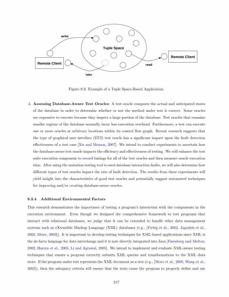
Tuple Space
read
take
write
Remote Client
Remote Client
PSfrag replacements
N6
enter computeVelocity
enter computeVelocity
N6
N6
N7
N7
N8
N8
N10
N8
N16
N10
N11
N11
N12
N12
N18
N16
N18
N18
exit computeVelocity
exit computeVelocity
N6
N1
N1
N2
N2
N3
N3
N1
N1
N4
N4
N5
N5
N6
enter P
enter P
call main
call main
enter main
enter main
enter main
. . .
. . .
call inputCardNumber
call inputCardNumber
call inputPin
call inputCardNumber
call handleError
call handleError
call inputCardNumber
call inputPin
call handleError
call handleError
call inputPin
call inputPin
call inputOperation
call inputOperation
call getAccountBalance
call getAccountBalance
call promptAgain
call inputOperation
call lockAccount
call lockAccount
call promptAgain
call promptAgain
call inputOperation
call promptAgain
. . .
call getAccountBalance
enter getAccountBalance
enter getAccountBalance
N3
N3
N4
N4
N5
N5
N6
N6
N7
N7
N10
N10
N12
N12
N15
N10
N15
N15
exit getAccountBalance
exit getAccountBalance
return getAccountBalance
return lockAccount
. . .
return getAccountBalance
call promptAgain
. . .
exit main
exit main
return main
return main
exit P
exit P
. . .
exit main
enter lockAccount
enter lockAccount
. . .
. . .
exit lockAccount
exit lockAccount
return lockAccount
return lockAccount
exit main
Figure 9.3: Example of a Tuple Space-Based Application.
4. Assessing Database-Aware Test Oracles: A test oracle compares the actual and anticipated states
of the database in order to determine whether or not the method under test is correct. Some oracles
are expensive to execute because they inspect a large portion of the database. Test oracles that examine
smaller regions of the database normally incur less execution overhead. Furthermore, a test can execute
one or more oracles at arbitrary locations within its control flow graph. Recent research suggests that
the type of graphical user interface (GUI) test oracle has a significant impact upon the fault detection
effectiveness of a test case [Xie and Memon, 2007]. We intend to conduct experiments to ascertain how
the database-aware test oracle impacts the efficiency and effectiveness of testing. We will enhance the test
suite execution component to record timings for all of the test oracles and then measure oracle execution
time. After using the mutation testing tool to seed database interaction faults, we will also determine how
different types of test oracles impact the rate of fault detection. The results from these experiments will
yield insight into the characteristics of good test oracles and potentially suggest automated techniques
for improving and/or creating database-aware oracles.
9.3.4 Additional Environmental Factors
This research demonstrates the importance of testing a program’s interaction with the components in the
execution environment. Even though we designed the comprehensive framework to test programs that
interact with relational databases, we judge that it can be extended to handle other data management
systems such as eXtensible Markup Language (XML) databases (e.g., [Fiebig et al., 2002, Jagadish et al.,
2002, Meier, 2003]). It is important to develop testing techniques for XML-based applications since XML is
the de-facto language for data interchange and it is now directly integrated into Java [Eisenberg and Melton,
2002, Harren et al., 2005, Li and Agrawal, 2005]. We intend to implement and evaluate XML-aware testing
techniques that ensure a program correctly submits XML queries and transformations to the XML data
store. If the program under test represents the XML document as a tree (e.g., [Moro et al., 2005, Wang et al.,
2003]), then the adequacy criteria will ensure that the tests cause the program to properly define and use
217

the nodes in the tree. We will enhanced event-based test adequacy criteria that were developed for graphical
user interfaces (e.g., [Memon et al., 2001]) in order to test XML programs that process XML parsing events
(e.g., [Megginson, 2001]).
Future research should also enhance the testing framework to handle distributed applications that interact
with data repositories such as distributed hash tables (DHTs) (e.g., [Rhea et al., 2005]) and tuple spaces
(e.g., [Arnold et al., 2002, Murphy et al., 2006]). A DHT furnishes a hash table-like interface with put
and get methods that remotely transfer data in a distributed system. As depicted in Figure 9.3, a tuple
space is another type of distributed system middleware that supports data storage and transfer through
methods such as write, take, and read. It is important to test programs that interact with DHTs and
tuple spaces because these components are widely used to implement peer-to-peer and distributed systems
that support scientific and ubiquitous computing (e.g., [Chawathe et al., 2005, Noble and Zlateva, 2001,
Rhea et al., 2005, Zorman et al., 2002]). Since the DHT and the tuple space both provide an interface that
focuses on the definition and use of remote data, it is possible to adapt our data flow-based testing techniques
to handle this new domain. Future research can extend previous test adequacy criteria for parallel shared
memory programs (e.g., [Yang et al., 1998]) in order to support coverage monitoring and regression testing
for programs that interact with DHTs and tuple spaces.
9.3.5 Improving Traditional Software Testing and Analysis
Even though our framework focuses on testing database-centric applications, it can also be used to test
conventional software systems. This type of future research is feasible because our testing framework correctly
operates in both database-aware and traditional configurations. For example, our test coverage monitor
constructs traditional CCTs and DCTs and the regression testing techniques reduce and/or re-order any
test suite for which coverage results are known. Furthermore, our testing techniques support the full range
of features in Java and they interoperate with popular testing tools such as JUnit. Prior work in regression
testing focused on using call stacks to reduce the test suite for either a procedural program written in C or a
GUI program written in Java [McMaster and Memon, 2005, 2006]. We intend to use the coverage monitoring
and regression testing components to perform traditional call stack-based reduction and prioritization for
object-oriented Java programs. These empirical studies will use the conventional Java programs and JUnit
test suites in the software-artifact infrastructure repository (SIR) [Do et al., 2005].
The calling context tree was initially proposed and empirically evaluated in the context of procedural
programs [Ammons et al., 1997]. In future research, we will use our framework to characterize the dynamic
call tree and the calling context tree for a wide variety of object-oriented programs. We plan to focus our
empirical studies on determining how long it takes to create and store the DCT and CCT for object-oriented
programs. These studies will calculate the size of the DCT and CCT in order to determine the space overhead
associated with storing the trees for testing and fault localization purposes. We can also compare the size and
structure of object-oriented control flow graphs and dynamic call trees. A comprehensive empirical study
218
of object-oriented call trees is relevant to traditional software engineering because the CCT and the DCT
are a central component of several profilers and debuggers (e.g., [Dmitriev, 2004]). The tool support and
the experiment results are also useful for improving dynamic optimization since many JVMs use context-
sensitive information about methods calls in order to guide inlining decisions [Hazelwood and Grove, 2003,
Zhuang et al., 2006]. To the best of our knowledge, these proposed future research ideas represent the first
attempt to investigate call tree-based approaches to the testing and analysis of object-oriented programs.
219
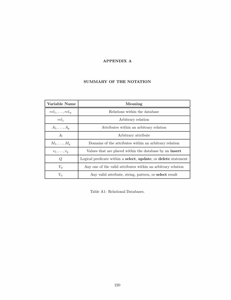
APPENDIX A
SUMMARY OF THE NOTATION
Variable Name Meaning
rel1, . . . , relw Relations within the database
relj Arbitrary relation
A1, . . . , Aq Attributes within an arbitrary relation
Al Arbitrary attribute
M1, . . . , Mq Domains of the attributes within an arbitrary relation
v1, . . . , vq Values that are placed within the database by an insert
Q Logical predicate within a select, update, or delete statement
Vφ Any one of the valid attributes within an arbitrary relation
Vψ Any valid attribute, string, pattern, or select result
Table A1: Relational Databases.
220

Variable Name Meaning
G Control flow graph for a method
N Set of control flow graph nodes
E Set of control flow graph edges
Nρ, Nτ Arbitrary nodes within a control flow graph
〈Nρ, . . . , Nτ 〉 Arbitrary path within a control flow graph
succ(Nρ) Successor of node Nρ
pred(Nτ ) Predecessor of node Nτ
Table A2: Traditional Program Representation.
Variable Name Meaning
Gk Control flow graph for method mk
Nk Set of control flow graph nodes
Ek Set of control flow graph edges
Bk Set of non-executable nodes with a method’s CFG
v(Gk) Cyclomatic complexity number for a CFG Gk
Table A3: Characterizing a Database-Centric Application.
Set Name Meaning
GDI(k) Database interaction CFG for method mk
D(GDI(k)) Set of database interactions
R(GDI(k)) Set of relation interactions
A(GDI(k)) Set of attribute interactions
Rc(GDI(k)) Set of record interactions
Av(GDI(k)) Set of attribute value interactions
Table A4: Database Entity Sets.
221

Variable Name Meaning
〈Ndef , Nuse, var〉 Def-use association for program variable var
πvar Complete path that covers a def-use association
GDI(k) Database interaction control flow graph for a method
NDI(k) Set of DI-CFG nodes
EDI(k) Set of DI-CFG edges
〈Ndef , Nuse, varDB〉 Database interaction association for database entity varDB
Cα, Cβ Arbitrary test adequacy criteria
Table A5: Database-Aware Test Adequacy Criteria.
Variable Name Meaning
A A database-centric application
P Program component of a database-centric application
m Method within the program component
D1, . . . , De Relational databases of a database-centric application
Df Arbitrary relational database
tk Record within a database relation
tk Record within a database relation
tk[l] Attribute value within a specific record
S1, . . . , Se Schemas of the relational databases
Sf Arbitrary relational schema
GP Interprocedural control flow graph for program P
ΓP Set of control flow graphs in GP
EP Set of control flow graphs edges in GP
Gj Intraprocedural control flow graph for program method mj
Table A6: Database-Centric Applications.
222
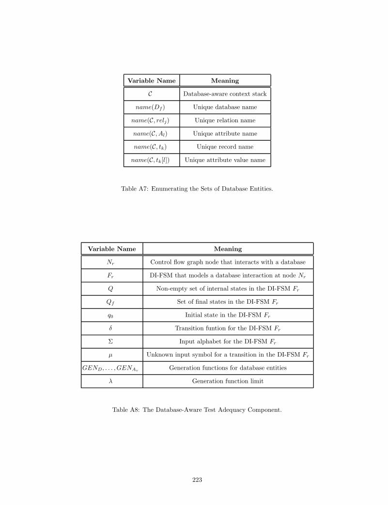
Variable Name Meaning
C Database-aware context stack
name(Df ) Unique database name
name(C, relj) Unique relation name
name(C, Al) Unique attribute name
name(C, tk) Unique record name
name(C, tk[l]) Unique attribute value name
Table A7: Enumerating the Sets of Database Entities.
Variable Name Meaning
Nr Control flow graph node that interacts with a database
Fr DI-FSM that models a database interaction at node Nr
Q Non-empty set of internal states in the DI-FSM Fr
Qf Set of final states in the DI-FSM Fr
q0 Initial state in the DI-FSM Fr
δ Transition funtion for the DI-FSM Fr
Σ Input alphabet for the DI-FSM Fr
µ Unknown input symbol for a transition in the DI-FSM Fr
GEND, . . . , GENAvGeneration functions for database entities
λ Generation function limit
Table A8: The Database-Aware Test Adequacy Component.
223

Variable Name Meaning
Nr CFG node that performs a databse interaction
in(Nρ) In degree of a CFG node
out(Nρ) Out degree of a CFG node
τ Test coverage monitoring tree
τdct Dynamic test coverage monitoring tree
τcct Calling context test coverage monitoring tree
Nτ Set of TCM tree nodes
Eτ Set of TCM tree edges
Na Active node in a TCM tree
N0 Root node in a TCM tree
EF Set of forward edges in a CCT
EB Set of back edges in a CCT
NB Set of nodes that receive a back edge in a CCT
Bφ Active back edge stack for a CCT node Nφ
σ Program or database entity to place into a TCM tree
Table A9: Database-Aware Test Coverage Monitoring Trees.
Variable Name Meaning
HR:A Function that maps relations to attributes
HR:RcFunction that maps relations to attributes
Al and Al Attributes in a relation
relj and relj Relations in a database
S Result set that arises from a SQL select
attr(S) The set of attributes associated with result set S
relations(S) The set of relations associated with result set S
attr(relj) The set of attributes associated with relation relj
L(τ) Levels of database interaction for a TCM tree
Table A10: Instrumentation to Create the Database-Aware TCM Trees.
224

Operator Name Meaning
⊗Rc
Symmetric relational difference operator
⊗Av
Symmetric attribute value difference operator
\RcRelational difference operator at the record level
\AvRelational difference operator at the attribute value level
Table A11: Relational Difference Operators.
Variable Name Meaning
Wf Total number of relations in database Df
tmax Maximum number of records in the database Df
MR:A Maximum number of attributes in both relj and S
MR:RcMaximum number of records that have an attribute value in both relj and S
Λ(j, j′) Length of the longest common subsequence (LCS) between relj and relj′
Amax Maximum number of attributes that differ in relj and relj′
Table A12: Worst-Case Complexity of the Database-Aware Instrumentation.
Variable Name Meaning
T Test suite for a database-centric application
Ti Arbitrary test case within T
∆0 Initial test state
∆i Test state produced by test Ti
GT Interprocedural control flow graph for test suite T
ΓT Set of control flow graphs in GT
ET Set of control flow graphs edges in GT
Nθ Node that executes test oracle θ
∆x Expected test state for test oracle θ
∆a Actual test state for test oracle θ
Table A13: Database-Aware Test Suites.
225

Variable Name Meaning
A,A′ Sets of applications to statically instrument
Ts, As Statically instrumented test suite and application
Td, Ad Dynamically instrumentated test suite and application
L Database interaction level during test coverage monitoring
c Arbitrary compression technique for a program or a TCM tree
Xτ Set of external nodes in a TCM tree
H Hash table that stores the replication counts for a TCM tree
Table A14: Describing the Test Coverage Monitor.
Variable Name Meaning
Π(τ) Multiset of paths in the coverage tree τ
π, π′ Arbitrary paths in the coverage tree τ
Π(τ, Ti) Multiset of tree paths for test case Ti
Πυ(τ, Ti) Set of unique tree paths for test case Ti
= Super path operator for coverage tree paths
Containing path operator for coverage tree paths
a Containing path operator for coverage tree paths
Πµ(τ, Ti,a) Set of maximally unique tree paths for test case Ti
Πη(τ, Ti) Set of previously examined coverage tree paths for Ti
Πυ(τ, T ) Set of unique tree paths for test suite T
Πµ(τ, T,a) Set of maximally unique tree paths for test suite T
Table A15: Paths in the Test Coverage Monitoring Tree.
226

Variable Name Meaning
T, T Original test suites
Tr Reduced test suite
Tp Prioritized test suite
ϕi Cost-effectiveness metric for test case Ti
time(〈Ti〉) Time required to executed test Ti
n∗ Target size for the reduced test suite
Table A16: Database-Aware Regression Testing.
Variable Name Meaning
ξ(T, Tp) Coverage effectiveness of the Tp derived from T
κ(T, t) Cummulative coverage of test suite T at time t
κ(T, t) Cummulative coverage of the ideal test suite T at time t
t(n′) The running time for the first n′ tests in T
Table A17: Evaluating a Test Suite Prioritization.
Variable Name Meaning
%n(T, Tr) Reduction factor for the size of a test suite
%t(T, Tr) Reduction factor for the time to run a test suite
%π(T, Tr) Reduction factor for the number of covered test requirements
νπ(T, Tr) Preservation factor for the number of covered test requirements
νr Tuple that contains the evaluation metrics for Tr
ν Specific value for an evaluation metric in νr
Table A18: Evaluating a Test Suite Reduction.
227

APPENDIX B
CASE STUDY APPLICATIONS
Number NCSS Methods Classes Javadocs Class
1 91 15 0 15 reminder.ReminderCreator
2 22 0 0 1 reminder.ReminderConstants
3 31 6 0 6 reminder.TestBeforeAllTests
4 5 2 0 1 reminder.ReminderDataException
5 23 4 0 5 reminder.TestReminderCreator
6 62 7 0 8 reminder.Reminder
7 223 15 0 15 reminder.TestReminder
8 18 2 0 0 reminder.AllTests
9 14 4 0 1 reminder.DatabaseDescription
Table B1: Reminder (RM) Case Study Application.
Number NCSS Methods Classes Javadocs Class
1 8 1 0 0 org.hsqldb.sample.FindFileDatabaseCreator
2 10 1 0 1 org.hsqldb.sample.DatabaseExport
3 330 25 0 23 org.hsqldb.sample.TestFindFile
4 14 4 0 1 org.hsqldb.sample.DatabaseDescription
5 161 18 0 16 org.hsqldb.sample.FindFile
Table B2: FindFile (FF) Case Study Application.
228

Number NCSS Methods Classes Javadocs Class
1 80 12 0 13 com.runstate.pithy.PithyCreator
2 31 6 0 6 com.runstate.pithy.TestBeforeAllTests
3 23 4 0 5 com.runstate.pithy.TestPithyCreator
4 84 10 0 0 com.runstate.pithy.PithyDBHSQLDB
5 20 7 0 0 com.runstate.pithy.Pith
6 95 4 0 1 com.runstate.pithy.PithyCommand
7 6 5 0 0 com.runstate.pithy.PithyDB
8 18 2 0 0 com.runstate.pithy.AllTests
9 14 4 0 1 com.runstate.pithy.DatabaseDescription
10 131 18 0 11 com.runstate.pithy.TestPithy
11 5 1 0 1 com.runstate.pithy.Pithy
Table B3: Pithy (PI) Case Study Application.
Number NCSS Methods Classes Javadocs Class
1 31 6 0 6 student.TestBeforeAllTests
2 37 6 0 7 student.TestStudentCreator
3 5 2 0 1 student.StudentDataException
4 91 15 0 15 student.StudentCreator
5 69 11 0 11 student.Student
6 18 2 0 0 student.AllTests
7 14 4 0 1 student.DatabaseDescription
8 17 0 0 1 student.StudentConstants
9 279 26 0 7 student.TestStudent
Table B4: StudentTracker (ST) Case Study Application.
229

Number NCSS Methods Classes Javadocs Class
1 337 33 0 10 TransactionAgent.TestMySQLDatabaseAgent
2 263 27 0 22 TransactionAgent.MySQLDatabaseAgent
3 11 10 0 1 TransactionAgent.DatabaseAgent
4 78 11 0 12 TransactionAgent.TransactionAgentCreator
5 18 2 0 0 TransactionAgent.AllTests
6 14 4 0 1 TransactionAgent.DatabaseDescription
Table B5: TransactionManager (TM) Case Study Application.
Number NCSS Methods Classes Javadocs Class
1 197 40 0 41 gradebook.GradeBookCreator
2 34 6 0 6 gradebook.TestBeforeAllTests
3 602 39 0 37 gradebook.TestGradeBook
4 329 29 0 30 gradebook.GradeBook
5 22 4 0 5 gradebook.TestGradeBookCreator
6 19 2 0 0 gradebook.AllTests
7 5 2 0 1 gradebook.GradeBookDataException
8 14 4 0 1 gradebook.DatabaseDescription
9 114 21 0 22 gradebook.TestGradeBookCreatorWithFullDataSet
10 51 0 0 1 gradebook.GradeBookConstants
Table B6: GradeBook (GB) Case Study Application.
230

Location Name
TestBeforeAllTests.java testDatabaseServerIsRunning()
TestBeforeAllTests.java testDoesNotStartServerAgain()
TestReminderCreator.java testMakeDatabaseConnection()
TestReminder.java testGetEmptyEvents()
TestReminder.java testAddReminderOneReminder()
TestReminder.java testAddReminderOneReminderNewNamesAndDate()
TestReminder.java testAddReminderMultipleReminders()
TestReminder.java testAddReminderMultipleRemindersCriitcalMonths()
TestReminder.java testAddReminderMultipleRemindersCriticalDays()
TestReminder.java testAddReminderMultipleRemindersGetEventInfo()
TestReminder.java testAddReminderMultipleRemindersDeleteEvent()
TestReminder.java testAddReminderMultipleRemindersFullEventList()
Table B7: Test Suite for Reminder.
Location Name
TestFindFile.java testDatabaseServerIsRunning()
TestFindFile.java testDoesNotStartServerAgain()
TestFindFile.java testMakeDatabaseConnection()
TestFindFile.java testFindFilePopulateWithLocalDirectoryFiveFiles()
TestFindFile.java testFindFilePopulateWithLocalDirectoryFiveFilesRemove15()
TestFindFile.java testFindFilePopulateWithLocalDirectoryFiveFilesRemove234()
TestFindFile.java testFindFilePopulateWithLocalDirectoryFiveFilesUpdate1()
TestFindFile.java testFindFilePopulateWithLocalDirectoryFiveFilesUpdate2()
TestFindFile.java testFindFilePopulateWithLocalDirectoryFiveFilesUpdate345()
TestFindFile.java testFindFilePopulateWithLocalDirectoryFiveFiles1()
TestFindFile.java testFindFilePopulateWithLocalDirectoryFiveFiles2()
TestFindFile.java testFindFilePopulateWithLocalDirectoryFiveFiles3()
TestFindFile.java testFindFilePopulateWithLocalDirectoryFiveFiles4()
TestFindFile.java testFindFilePopulateWithLocalDirectoryFiveFiles5()
TestFindFile.java testFindFilePopulateWithLocalDirectoryTenFiles()
TestFindFile.java testFindFilePopulateWithLocalEmptyDirectory()
Table B8: Test Suite for FindFile.
231

Location Name
TestBeforeAllTests.java testDatabaseServerIsRunning()
TestBeforeAllTests.java testDoesNotStartServerAgain()
TestPithyCreator.java testMakeDatabaseConnection()
TestPithy.java testNoInitialPithyRemarks()
TestPithy.java testAddOnePithyRemark()
TestPithy.java testAddManyPithyRemarks()
TestPithy.java testAddManyPithyRemarksCheckCategory()
TestPithy.java testAdd()
TestPithy.java testAddIterativeSmallValue()
TestPithy.java testAddIterativeMediumValue()
TestPithy.java testAddIterativeLargeValue()
TestPithy.java testMultipleAdd()
TestPithy.java testMultipleAddIterativeSmall()
TestPithy.java testMultipleAddIterativeMedium()
TestPithy.java testMultipleAddIterativeLarge()
Table B9: Test Suite for Pithy.
232

Location Name
TestBeforeAllTests.java testDatabaseServerIsRunning()
TestBeforeAllTests.java testDoesNotStartServerAgain()
TestStudentCreator.java testMakeDatabaseConnectionSmall()
TestStudentCreator.java testMakeDatabaseConnectionMedium()
TestStudentCreator.java testMakeDatabaseConnectionLarge()
TestStudent.java testInsertSingleStudent()
TestStudent.java testInsertSingleStudentIterativeSmall()
TestStudent.java testInsertAndRemoveStudent()
TestStudent.java testInsertAndRemoveStudentIterativeSmall()
TestStudent.java testInsertAndRemoveStudentIterativeMedium()
TestStudent.java testInsertAndRemoveStudentIterativeLarge()
TestStudent.java testInsertAndRemoveMultipleStudents()
TestStudent.java testInsertAndRemoveMultipleStudentsDoNotRemove()
TestStudent.java testInsertAndUpdateStudentExampleTwoTimes()
TestStudent.java testInsertAndUpdateStudentExampleSmall()
TestStudent.java testInsertAndUpdateStudentExampleMedium()
TestStudent.java testInsertAndUpdateStudentExampleLarge()
TestStudent.java testRemoveStudentFromEmptyDatabase()
TestStudent.java testRemoveStudentFromEmptyDatabaseCheckIndividualStudents()
TestStudent.java testInsertSingleStudentGetSingleStudent()
TestStudent.java testInsertSingleStudentGetSingleStudentPerformRepeatedly10()
TestStudent.java testInsertSingleStudentGetSingleStudentPerformRepeatedly50()
TestStudent.java testInsertSingleStudentGetSingleStudentPerformRepeatedly100()
TestStudent.java testInsertMultipleStudentGetMultipleStudentsDirectly()
TestStudent.java testInsertAndUpdateExampleDirectRemove()
Table B10: Test Suite for StudentTracker.
233

Location Name
TestMySQLDatabaseAgent.java testDatabaseServerIsRunning()
TestMySQLDatabaseAgent.java testDoesNotStartServerAgain()
TestMySQLDatabaseAgent.java testMakeDatabaseConnection()
TestMySQLDatabaseAgent.java testBasicTestFramework()
TestMySQLDatabaseAgent.java testMakeDatabaseConnectionRepeatedly10()
TestMySQLDatabaseAgent.java testCreateDefaultBankState()
TestMySQLDatabaseAgent.java testRemoveAccountNotPossibleInitialState()
TestMySQLDatabaseAgent.java testRemoveAccountTwiceDoesNotWorkCorrectly()
TestMySQLDatabaseAgent.java testRemoveDifferentAccountNumberTwice()
TestMySQLDatabaseAgent.java testRemoveASingleUser()
TestMySQLDatabaseAgent.java testVerifySingleUser()
TestMySQLDatabaseAgent.java testVerifySingleUserRepeatedlyTenTimes()
TestMySQLDatabaseAgent.java testAccountExistsSingleAccount()
TestMySQLDatabaseAgent.java testAccountExistsSingleAccountRepeatedly()
TestMySQLDatabaseAgent.java testGetAccountBalance()
TestMySQLDatabaseAgent.java testGetAccountBalanceRepeatedly()
TestMySQLDatabaseAgent.java testGetAccountBalanceAndThenWithdraw()
TestMySQLDatabaseAgent.java testGetAccountBalanceWithdrawRepeatedly()
TestMySQLDatabaseAgent.java testDepositForSingleUser()
TestMySQLDatabaseAgent.java testAccountTransfer()
TestMySQLDatabaseAgent.java testAccountTransferMultipleTimes()
TestMySQLDatabaseAgent.java testLockTwoAccounts()
TestMySQLDatabaseAgent.java testLockUnlockLockTwoAcctsRepeatedlySmall()
TestMySQLDatabaseAgent.java testDeleteAccounts()
TestMySQLDatabaseAgent.java testDeleteAccountsRepeatedSmall()
TestMySQLDatabaseAgent.java testDeleteAccountsRepeatedMedium()
TestMySQLDatabaseAgent.java testDeleteAccountsRepeatedLarge()
Table B11: Test Suite for TransactionManager.
234

Location Name
TestBeforeAllTests.java testDatabaseServerIsRunning()TestBeforeAllTests.java testDoesNotStartServerAgain()
TestGradeBookCreator.java testMakeDatabaseConnection()TestGradeBookCreatorWithFullDataSet.java testCreateMasterTable()TestGradeBookCreatorWithFullDataSet.java testDropMasterNotPossible()TestGradeBookCreatorWithFullDataSet.java testCreateStudentTable()TestGradeBookCreatorWithFullDataSet.java testDropStudentNotPossible()TestGradeBookCreatorWithFullDataSet.java testCreateExamMasterTable()TestGradeBookCreatorWithFullDataSet.java testDropExamMasterNotPossible()TestGradeBookCreatorWithFullDataSet.java testCreateExamScoresTable()TestGradeBookCreatorWithFullDataSet.java testDropExamScoresNotPossible()TestGradeBookCreatorWithFullDataSet.java testCreateLabMasterTable()TestGradeBookCreatorWithFullDataSet.java testDropLabMasterNotPossible()TestGradeBookCreatorWithFullDataSet.java testCreateLabScoresTable()TestGradeBookCreatorWithFullDataSet.java testDropLabScoresNotPossible()TestGradeBookCreatorWithFullDataSet.java testCreateHomeworkMasterTable()TestGradeBookCreatorWithFullDataSet.java testDropHomeworkMasterNotPossible()TestGradeBookCreatorWithFullDataSet.java testCreateHomeworkScoresTable()TestGradeBookCreatorWithFullDataSet.java testDropHomeworkScoresNotPossible()TestGradeBookCreatorWithFullDataSet.java testCreateFinalProjectScoresTable()TestGradeBookCreatorWithFullDataSet.java testDropFinalProjScoresNotPoss()
TestGradeBook.java testDatabaseServerIsRunning()TestGradeBook.java testDoesNotStartServerAgain()TestGradeBook.java testPopulateMasterTableWrongPercentages()TestGradeBook.java testPopulateMasterTable()TestGradeBook.java testAddNullStudentNotPossible()TestGradeBook.java testAddEmptyStringStudentNotPossible()TestGradeBook.java testAddStudent()TestGradeBook.java testAddExamNegativeNotPossible()TestGradeBook.java testAddExamNullNotPossible()TestGradeBook.java testAddExamsToExamMasterTable()TestGradeBook.java testAddExamsToExamMasterTableIncludeCurves()TestGradeBook.java testAddExamScoreSecondNegativeNotPossible()TestGradeBook.java testAddExamScoreFirstNegativeNotPossible()TestGradeBook.java testAddExamScoresToExamScoresTable()TestGradeBook.java testCorrectAverageExamScores()TestGradeBook.java testAddLabScoreSecondNegativeNotPossible()TestGradeBook.java testAddLabScoreFirstNegativeNotPossible()TestGradeBook.java testAddLabScoresToLabScoresTable()TestGradeBook.java testCorrectAverageLabScores()TestGradeBook.java testAddHomeworkScoreSecondNegativeNotPossible()TestGradeBook.java testAddHomeworkScoreFirstNegativeNotPossible()TestGradeBook.java testAddHomeworkScoresToHomeworkScoresTable()TestGradeBook.java testAddFinalProjectScoreSecondNegativeNotPossible()TestGradeBook.java testAddFinalProjectScoreFirstNegativeNotPossible()TestGradeBook.java testAddFinalProjectScoresToLabScoresTable()TestGradeBook.java testCalculateFinalGrade()TestGradeBook.java testGetExamIdsAndExamFinalGrade()TestGradeBook.java testCalculateLaboratoryFinalGrade()TestGradeBook.java testCalculateHomeworkFinalGrade()TestGradeBook.java testCalculateFinalProjectFinalGrade()
Table B12: Test Suite for GradeBook.
235

public org.hsqldb.sample.FindFile();
Code:
0: aload_0
1: invokespecial #1; //Method java/lang/Object."<init>":()V
4: return
Figure B1: Bytecode of the FindFile Constructor Before Instrumentation.
236

public org.hsqldb.sample.FindFile();
Code:
0: aload_0
1: invokespecial #59; //Method java/lang/Object."<init>":()V
// Method diatoms/monitor/TraceMonitorTestCoverage.ajc$if_0:()Z
4: invokestatic #385;
7: ifeq 25
// Method diatoms/monitor/TraceMonitorTestCoverage.ajc$if_1:()Z
10: invokestatic #382;
13: ifne 25
// Method diatoms/monitor/TraceMonitorTestCoverage.aspectOf:()
// Ldiatoms/monitor/TraceMonitorTestCoverage;
16: invokestatic #373;
// Field ajc$tjp_0:Lorg/aspectj/lang/JoinPoint$StaticPart;
19: getstatic #375;
// Method diatoms/monitor/TraceMonitorTestCoverage.ajc$
// before$diatoms_monitor_TraceMonitorTestCoverage$1$5a83f1be:
// (Lorg/aspectj/lang/JoinPoint$StaticPart;)V
22: invokevirtual #379;
25: goto 52
28: astore_1
// Method diatoms/monitor/TraceMonitorTestCoverage.ajc$if_2:()Z
29: invokestatic #394;
32: ifeq 50
// Method diatoms/monitor/TraceMonitorTestCoverage.ajc$if_3:()Z
35: invokestatic #391;
38: ifne 50
// Method diatoms/monitor/TraceMonitorTestCoverage.aspectOf:()
// Ldiatoms/monitor/TraceMonitorTestCoverage;
41: invokestatic #373;
// Field ajc$tjp_0:Lorg/aspectj/lang/JoinPoint$StaticPart;
44: getstatic #375;
// Method diatoms/monitor/TraceMonitorTestCoverage.ajc$after$
// diatoms_monitor_TraceMonitorTestCoverage$2$5a83f1be:
// (Lorg/aspectj/lang/JoinPoint$StaticPart;)V
47: invokevirtual #388;
50: aload_1
51: athrow
// Method diatoms/monitor/TraceMonitorTestCoverage.ajc$if_2:()Z
52: invokestatic #394;
55: ifeq 73
// Method diatoms/monitor/TraceMonitorTestCoverage.ajc$if_3:()Z
58: invokestatic #391;
61: ifne 73
// Method diatoms/monitor/TraceMonitorTestCoverage.aspectOf:()
// Ldiatoms/monitor/TraceMonitorTestCoverage;
64: invokestatic #373;
// Field ajc$tjp_0:Lorg/aspectj/lang/JoinPoint$StaticPart;
67: getstatic #375;
// Method diatoms/monitor/TraceMonitorTestCoverage.ajc$after$
// diatoms_monitor_TraceMonitorTestCoverage$2$5a83f1be:
// (Lorg/aspectj/lang/JoinPoint$StaticPart;)V
70: invokevirtual #388;
73: return
Figure B2: Bytecode of the FindFile Constructor After Instrumentation.
237

1 public void testAddHomeworkScoresToHomeworkScoresTable ( )2 3 try
4 5 // add the three standard exams with t h e i r6 // standard point t o t a l s7 testGradeBook . addHomework( ”HomeworkOne” , 1 0 ) ;8 testGradeBook . addHomework( ”HomeworkTwo” , 2 0 ) ;9 testGradeBook . addHomework( ”HomeworkThree” , 3 0 ) ;
10 // create the expected Exam MASTER from the XML11 IDataSet expectedDatabaseStateFir s t = getDataSet ( ) ;12 ITable expectedHomeworkMasterTable =13 expectedDatabaseStateFir s t .14 getTable ( GradeBookConstants .HOMEWORKMASTER) ;15 // create the actua l Scores Table from the database16 IDataSet ac tua lDataba s eS tat eF ir s t =17 getConnection ( ) . c reateDataSet ( ) ;18 ITable actualHomeworkMasterTable =19 ac tua lDataba s eS ta t eFi r s t .20 getTable ( GradeBookConstants .HOMEWORKMASTER) ;21 // expected should be equa l to actua l in terms22 // of both the number of rows and the data23 As s e r t i on . a s s e r tEqua l s ( expectedHomeworkMasterTable ,24 actualHomeworkMasterTable ) ;25 26 // in order to preserve s imp l i c i t y , the except ion handling27 // code was removed28
Figure B3: An Example of a Database-Aware Test Case and Oracle.
238

APPENDIX C
EXPERIMENT DETAILS
Data Type Size of the Type (bytes)
long 8
int 4
double 8
float 8
short 2
char 2
byte 1
boolean 1
java.lang.Object (shell) 8
java.lang.Object (reference) 4
Table C1: Estimated Data Type Sizes for a 32-bit Java Virtual Machine.
239

Variable Name Meaning
Tinstr Static instrumentation time
S Static size of an application
Texec Test coverage monitoring time
T binstore Time required for storing a TCM tree in binary
T xmlstore Time required for storing a TCM tree in XML
SN Number of nodes in a TCM tree
Smem In memory size of a TCM tree
Sbin File system size of a TCM tree in binary
Sxml File system size of a TCM tree in XML
outavg Average node out degree of a TCM tree
rmax, ravg Maximum and average node replication count in a TCM tree
Table C2: Metrics Used During the Evaluation of the Test Coverage Monitor.
Number NCSS Functions Classes Javadocs Class
1 8 1 0 0 exercise.ExerciseDatabaseCreator
2 187 70 0 10 exercise.TestExercise
3 167 14 0 14 exercise.Exercise
4 10 1 0 1 exercise.DatabaseExport
5 14 4 0 1 exercise.DatabaseDescription
Table C3: Exercise (EX) Case Study Application.
Dominance Operator (a) Enumeration Time (ms) Path Count (Suite) Path Count (Case)
Super Path (=) 104 90 221
Containing Path () 118 80 211
(a)
Dominance Operator (a) Enumeration Time (ms) Path Count (Suite) Path Count (Case)
Super Path (=) 154 46 535
Containing Path () 195 46 535
(b)
Table C4: Using the Traditional Coverage Tree for (a) GradeBook and (b) TransactionManager.
240

BIBLIOGRAPHY
E. Addy and M. Sitaraman. Formal specification of COTS-based software. In Symposium on SoftwareReuseability, May 1999.
M. S. Ager, O. Danvy, and H. K. Rohde. Fast partial evaluation of pattern matching in strings. ACMTransactions on Programming Languages and Systems, 28(4):696–714, 2006.
B. Alpern, S. Augart, S. Blackburn, M. Butrico, A. Cocchi, P. Cheng, J. Dolby, S. Fink, D. Grove, M. Hind,K. McKinley, M. Mergen, J. Moss, T. Ngo, V. Sarkar, and M. Trapp. The Jikes research virtual machineproject: Buliding an open-source research community. IBM Systems Journal, 44(2), 2005.
G. Ammons, T. Ball, and J. R. Larus. Exploiting hardware performance counters with flow and context sen-sitive profiling. In Proceedings of the Conference on Programming Language Design and Implementation,pages 85–96, New York, NY, USA, 1997. ACM Press.
J. H. Andrews, L. C. Briand, and Y. Labiche. Is mutation an appropriate tool for testing experiments? InProceedings of 27th ACM/IEEE International Conference on Software Engineering, pages 402–411, NewYork, NY, USA, 2005.
G. C. Arnold, G. M. Kapfhammer, and R. S. Roos. Implementation and analysis of a JavaSpace supportedby a relational database. In Proceedings of the 8th International Conference on Parallel and DistributedProcessing Techniques and Applications, Las Vegas, Nevada, June 2002.
S. Barbey, D. Buchs, and C. Praire. A theory of specification-based testing for object-oriented software. InProceedings of the 2nd European Dependable Computing Conference, Taormina, Italy, 1996.
T. Barclay, J. Gray, and D. Slutz. Microsoft TerraServer: a spatial data warehouse. In Proceedings of theACM SIGMOD International Conference on Management of Data, pages 307–318. ACM Press, 2000.
V. R. Basili and B. T. Perricone. Software errors and complexity: an empirical investigation. Communicationsof the ACM, 27(1):42–52, 1984.
J. Becla and D. L. Wang. Lessons learned from managing a petabyte. In Proceedings of the Conference onInnovative Data Systems Research, pages 70–83, 2005.
A. R. Bernat and B. P. Miller. Incremental call-path profiling. Concurrency and Computation: Practice andExperience, 2006. Published Online October 24, 2006.
M. Berndl, O. Lhotak, F. Qian, L. Hendren, and N. Umanee. Points-to analysis using BDDs. In Proceedingsof the ACM SIGPLAN Conference on Programming Language Design and Implementation, pages 103–114.ACM Press, 2003.
W. Binder. Portable, efficient, and accurate sampling profiling for Java-based middleware. In Proceedings ofthe 5th International Workshop on Software Engineering and Middleware, pages 46–53, New York, NY,USA, 2005. ACM Press.
241

J. Black, E. Melachrinoudis, and D. Kaeli. Bi-criteria models for all-uses test suite reduction. In Proceedingsof the 26th International Conference on Software Engineering, pages 106–115, Washington, DC, USA,2004. IEEE Computer Society.
S. M. Blackburn, P. Cheng, and K. S. McKinley. Myths and realities: the performance impact of garbagecollection. In Proceedings of the Joint International Conference on Measurement and Modeling of ComputerSystems, pages 25–36, New York, NY, USA, 2004. ACM Press.
R. Bloom. Debugging JDBC with a logging driver. Java Developer’s Journal, April 2006.
C. Bockisch, M. Arnold, T. Dinkelaker, and M. Mezini. Adapting virtual machine techniques for seam-less aspect support. In Proceedings of the 21st Annual ACM SIGPLAN Conference on Object-OrientedProgramming Languages, Systems, and Applications, pages 109–124, New York, NY, USA, 2006. ACMPress.
P. Boldi and S. Vigna. Mutable strings in Java: design, implementation and lightweight text-search algo-rithms. Science of Computer Programming, 54(1):3–23, 2005.
R. S. Boyer and J. S. Moore. A fast string searching algorithm. Communications of the ACM, 20(10):762–772, 1977.
T. Brecht, E. Arjomandi, C. Li, and H. Pham. Controlling garbage collection and heap growth to reducethe execution time of Java applications. ACM Transactions on Programming Languages and Systems, 28(5):908–941, 2006.
A. Camesi, J. Hulaas, and W. Binder. Continuous bytecode instruction counting for CPU consumption esti-mation. In Proceedings of the Third International Conference on the Quantitative Evaluation of Systems,pages 19–30, Washington, DC, USA, 2006. IEEE Computer Society.
D. D. Chamberlin. Relational data-base management systems. ACM Computing Surveys, 8(1):43–66, 1976.
M.-Y. Chan and S.-C. Cheung. Applying white box testing to database applications. Technical ReportHKUST-CS9901, Hong Kong University of Science and Technology, Department of Computer Science,February 1999a.
M.-Y. Chan and S.-C. Cheung. Testing database applications with SQL semantics. In Proceedings of the2nd International Symposium on Cooperative Database Systems for Advanced Applications, pages 363–374,March 1999b.
S. S. Chawathe and H. Garcia-Molina. Meaningful change detection in structured data. In Proceedings ofthe ACM SIGMOD International Conference on Management of Data, pages 26–37, New York, NY, USA,1997. ACM Press.
S. S. Chawathe, A. Rajaraman, H. Garcia-Molina, and J. Widom. Change detection in hierarchically struc-tured information. In Proceedings of the ACM SIGMOD International Conference on Management ofData, pages 493–504, New York, NY, USA, 1996. ACM Press.
Y. Chawathe, S. Ramabhadran, S. Ratnasamy, A. LaMarca, S. Shenker, and J. Hellerstein. A case studyin building layered DHT applications. In Proceedings of the Conference on Applications, Technologies,Architectures, and Protocols for Computer Communications, pages 97–108, New York, NY, USA, 2005.ACM Press.
D. Chays, S. Dan, P. G. Frankl, F. I. Vokolos, and E. J. Weyuker. A framework for testing databaseapplications. In Proceedings of the 7th International Symposium on Software Testing and Analysis, pages147–157, August 2000.
D. Chays and Y. Deng. Demonstration of AGENDA tool set for testing relational database applications. InProceedings of the International Conference on Software Engineering, pages 802–803, May 2003.
242

D. Chays, Y. Deng, P. G. Frankl, S. Dan, F. I. Vokolos, and E. J. Weyuker. AGENDA: A test generatorfor relational database applications. Technical Report TR-CIS-2002-04, Department of Computer andInformation Sciences, Polytechnic University, Brooklyn, NY, August 2002.
D. Chays, Y. Deng, P. G. Frankl, S. Dan, F. I. Vokolos, and E. J. Weyuker. An AGENDA for testingrelational database applications. Software Testing, Verification, and Reliability, 14(1):17–44, 2004.
J. Cheney. Compressing XML with multiplexed hierarchical PPM models. In Proceedings of the DataCompression Conference, page 163, Washington, DC, USA, 2001. IEEE Computer Society.
J. C. Cherniavsky and C. H. Smith. On Weyuker’s axioms for software complexity measures. IEEE Trans-actions on Software Engineering, 17(6):636–638, 1991.
A. S. Christensen, A. Møller, and M. I. Schwartzbach. Precise analysis of string expressions. In Proceedingsof the 10th International Static Analysis Symposium, volume 2694 of LNCS, pages 1–18. Springer-Verlag,June 2003.
L. A. Clarke, A. Podgurski, D. J. Richardson, and S. J. Zeil. A comparison of data flow path selectioncriteria. In Proceedings of the 8th International Conference on Software Engineering, pages 244–251.IEEE Computer Society Press, 1985.
E. F. Codd. A relational model of data for large shared data banks. Communications of the ACM, 13(6):377–387, 1970.
E. F. Codd. Extending the database relational model to capture more meaning. ACM Transactions onDatabase Systems, 4(4):397–434, 1979.
T. H. Cormen, C. E. Leiserson, R. L. Rivest, and C. Stein. Introduction to algorithms. MIT Press, Cambridge,MA, USA, 2001.
R. Dallaway. Unit testing database code. 2002. http://www.dallaway.com/acad/dbunit.html.
B. Daou, R. A. Haraty, and N. Mansour. Regression testing of database applications. In Proceedings of theACM Symposium on Applied Computing, pages 285–289. ACM Press, 2001.
R. DeMillo, D. Guindi, W. McCracken, A. Offutt, and K. King. An extended overview of the Mothrasoftware testing environment. In Proceedings of the ACM SIGSOFT Second Symposium on SoftwareTesting, Analysis, and Verficiation, pages 142–151, July 1988.
Y. Deng, P. Frankl, and Z. Chen. Testing database transaction concurrency. In Proceedings of the 18thInternational Conference on Automated Software Engineering, Montreal, Canada, October 2003.
M. Dmitriev. Profiling Java applications using code hotswapping and dynamic call graph revelation. InProceedings of the 4th International Workshop on Software and Performance, pages 139–150, New York,NY, USA, 2004. ACM Press.
H. Do, S. G. Elbaum, and G. Rothermel. Supporting controlled experimentation with testing techniques:An infrastructure and its potential impact. Empirical Software Engineering: An International Journal,10(4):405–435, 2005.
H. Do and G. Rothermel. On the use of mutation faults in empirical assessments of test case prioritizationtechniques. IEEE Transactions on Software Engineering, 32(9), 2006.
H. Do, G. Rothermel, and A. Kinneer. Empirical studies of test case prioritization in a JUnit testingenvironment. In Proceedings of the 15th International Symposium on Software Reliability Engineering,pages 113–124, Washington, DC, USA, 2004. IEEE Computer Society.
243

R.-K. Doong and P. G. Frankl. The ASTOOT approach to testing object-oriented programs. ACM Trans-actions on Software Engineering and Methodology, 3(2):101–130, April 1994.
S. Dowdy, S. Wearden, and D. Chilko. Statistics for Research. Wiley-Interscience, third edition, 2004.
E. Duesterwald, R. Gupta, and M. L. Soffa. A demand-driven analyzer for data flow testing at the integrationlevel. In Proceedings of the 18th International Conference on Software Engineering, pages 575–584, 1996.
B. Dufour, K. Driesen, L. Hendren, and C. Verbrugge. Dynamic metrics for Java. In Proceedings of the18th ACM SIGPLAN Conference on Object-Oriented Programing, Systems, Languages, and Applications,pages 149–168, New York, NY, USA, 2003. ACM Press.
A. Eisenberg and J. Melton. An early look at XQuery. SIGMOD Record, 31(4):113–120, 2002.
S. G. Elbaum, A. G. Malishevsky, and G. Rothermel. Incorporating varying test costs and fault severities intotest case prioritization. In International Conference on Software Engineering, pages 329–338, Washington,DC, USA, 2001. IEEE Computer Society.
T. Elrad, R. E. Filman, and A. Bader. Aspect-oriented programming: An introduction. Communications ofthe ACM, 44(10):59–65, October 2001.
M. Engel and B. Freisleben. Supporting autonomic computing functionality via dynamic operating systemkernel aspects. In Proceedings of the 4th International Conference on Aspect-Oriented Software Develop-ment, pages 51–62, New York, NY, USA, 2005. ACM Press.
M. D. Ernst, J. Cockrell, W. G. Griswold, and D. Notkin. Dynamically discovering likely program invariantsto support program evolution. IEEE Transactions on Software Engineering, 27(2):99–123, Feb. 2001.
M. D. Ernst, J. H. Perkins, P. J. Guo, S. McCamant, C. Pacheco, M. S. Tschantz, and C. Xiao. The Daikonsystem for dynamic detection of likely invariants. Science of Computer Programming, 2006.
M. Fagan. Design and code inspections to reduce errors in program development. IBM Systems Journal, 15(3):182–211, 1976.
U. Feige. A threshold of ln n for approximating set cover. Journal of the ACM, 45(4):634–652, 1998.
P. Ferragina, F. Luccio, G. Manzini, and S. Muthukrishnan. Compressing and searching XML data via twozips. In Proceedings of the 15th International Conference on the World Wide Web, pages 751–760, NewYork, NY, USA, 2006. ACM Press.
T. Fiebig, S. Helmer, C.-C. Kanne, G. Moerkotte, J. Neumann, R. Schiele, and T. Westmann. Anatomy ofa native XML base management system. The VLDB Journal, 11(4):292–314, 2002.
P. G. Frankl and S. Weiss. An experimental comparison of the effectiveness of branch testing and data flowtesting. IEEE Transactions on Software Engineering, 19(8):774–787, August 1993.
P. G. Frankl and E. J. Weyuker. An applicable family of data flow testing criteria. IEEE Transactions onSoftware Engineering, 14(10):1483–1498, October 1988.
M. R. Garey and D. S. Johnson. Computers and Intractability: A Guide to the Theory of NP-Completeness.W. H. Freeman & Co., New York, NY, USA, 1979.
D. Geer. Will binary XML speed network traffic? IEEE Computer, 38(4):16–18, 2005.
R. M. Golbeck and G. Kiczales. A machine code model for efficient advice dispatch. In Proceedings of the 1stWorkshop on Virtual Machines and Intermediate Languages for Emerging Modularization Mechanisms,page 2, New York, NY, USA, 2007. ACM Press.
244
J. Gray, P. Sundaresan, S. Englert, K. Baclawski, and P. J. Weinberger. Quickly generating billion-recordsynthetic databases. In Proceedings of the ACM SIGMOD International Conference on Management ofData, pages 243–252. ACM Press, 1994.
F. Haftmann, D. Kossmann, and A. Kreutz. Efficient regression tests for database applications. In Proceedingsof the Conference on Innovative Data Systems Research, pages 95–106, 2005a.
F. Haftmann, D. Kossmann, and E. Lo. Parallel execution of test runs for database application systems.In Proceedings of the 31st International Conference on Very Large Data Bases, pages 589–600. VLDBEndowment, 2005b.
W. G. Halfond and A. Orso. Combining Static Analysis and Runtime Monitoring to Counter SQL-InjectionAttacks. In Proceedings of the Third International ICSE Workshop on Dynamic Analysis, St. Louis, MO,USA, May 2005.
W. G. J. Halfond and A. Orso. Command-form coverage for testing database applications. In Proceedings ofthe 21st IEEE International Conference on Automated Software Engineering, pages 69–80, Washington,DC, USA, 2006. IEEE Computer Society.
M. Harder, J. Mellen, and M. D. Ernst. Improving test suites via operational abstraction. In Proceedings ofthe 24th International Conference on Software Engineering, pages 60–71, 2003.
M. Harren, M. Raghavachari, O. Shmueli, M. G. Burke, R. Bordawekar, I. Pechtchanski, and V. Sarkar. XJ:facilitating XML processing in Java. In Proceedings of the 14th International Conference on World WideWeb, pages 278–287, New York, NY, USA, 2005. ACM Press.
M. J. Harrold, R. Gupta, and M. L. Soffa. A methodology for controlling the size of a test suite. ACMTransactions on Software Engineering and Methodology, 2(3):270–285, 1993.
M. J. Harrold and G. Rothermel. Performing data flow testing on classes. In Proceedings of the 2nd ACMSIGSOFT Symposium on Foundations of Software Engineering, pages 154–163. ACM Press, 1994.
M. J. Harrold and G. Rothermel. Aristotle: A system for research on and developement of program-analysis-based tools. Technical Report OSU-CISRC-3/97-TR17, The Ohio State University, Departmentof Computer and Information Science, March 1995.
M. J. Harrold and G. Rothermel. A coherent family of analyzable graphical representations for object-oriented software. Technical Report Technical Report OSU-CISRC-11/96-TR60, Department of Computerand Information Sciences, Ohio State University, November 1996.
M. J. Harrold and M. L. Soffa. Efficient computation of interprocedural definition-use chains. ACM Trans-actions on Programming Languages and Systems, 16(2):175–204, 1994.
K. Hazelwood and D. Grove. Adaptive online context-sensitive inlining. In Proceedings of the InternationalSymposium on Code Generation and Optimization, pages 253–264, Washington, DC, USA, 2003. IEEEComputer Society.
M. Hicks. Survey: Biggest databases approach 30 terabytes. eWeek Enterprise News and Reviews, November2003. http://www.eweek.com/.
R. Hightower. Java Tools for Extreme Programming: Mastering Open Source Tools, Including Ant, JUnit,and Cactus. John Wiley and Sons, Inc., New York, NY, 2001.
E. Hilsdale and J. Hugunin. Advice weaving in AspectJ. In Proceedings of the 3rd International Conferenceon Aspect-Oriented Software Development, pages 26–35, New York, NY, USA, 2004. ACM Press.
D. S. Hirschberg. Algorithms for the longest common subsequence problem. Journal of the ACM, 24(4):664–675, 1977.
245
D. Hovemeyer and W. Pugh. Finding bugs is easy. ACM SIGPLAN Notices, 39(12):92–106, 2004.
M. Hutchins, H. Foster, T. Goradia, and T. Ostrand. Experiments of the effectiveness of dataflow- andcontrolflow-based test adequacy criteria. In Proceedings of the 16th International Conference on SoftwareEngineering, pages 191–200. IEEE Computer Society Press, 1994.
IEEE. IEEE Standard Glossary of Software Engineering Terminology. ANSI/IEEE Std 610.12-1990, 1996.
H. V. Jagadish, S. Al-Khalifa, A. Chapman, L. V. S. Lakshmanan, A. Nierman, S. Paparizos, J. M. Patel,D. Srivastava, N. Wiwatwattana, Y. Wu, and C. Yu. TIMBER: A native XML database. The VLDBJournal, 11(4):274–291, 2002.
P. Jalote. Fault Tolerance in Distributed Systems. PTR Prentice Hall, Upper Saddle River, New Jersey,1998.
G. Janee and J. Frew. The ADEPT digital library architecture. In Proceedings of the Second ACM/IEEE-CSJoint Conference on Digital Libraries, pages 342–350. ACM Press, 2002.
D. Jeffrey and N. Gupta. Improving fault detection capability by selectively retaining test cases during testsuite reduction. IEEE Transactions on Software Engineering, 33(2):108–123, 2007.
R. E. Jeffries. Extreme testing. Software Testing and Quality Engineering, March/April 1999.
Z. Jin and A. J. Offutt. Coupling-based criteria for integration testing. Software Testing, Verification &Reliability, 8(3):133–154, 1998.
J. A. Jones and M. J. Harrold. Test-suite reduction and prioritization for modified condition/decisioncoverage. IEEE Transactions on Software Engineering, 29(3):195–209, 2003.
J. A. Jones and M. J. Harrold. Empirical evaluation of the tarantula automatic fault-localization technique.In Proceedings of the 20th IEEE/ACM international Conference on Automated Software Engineering,pages 273–282, New York, NY, USA, 2005. ACM Press.
C. Kaner, J. Falk, and H. Q. Hguyen. Testing Computer Software. International Thompson Computer Press,London, UK, 1993.
G. M. Kapfhammer and M. L. Soffa. A family of test adequacy criteria for database-driven applications. InProceedings of the 9th European Software Engineering Conference and the 11th ACM SIGSOFT Symposiumon Foundations of Software Engineering. ACM Press, 2003.
G. M. Kapfhammer, M. L. Soffa, and D. Mosse. Testing in resource constrained execution environments. InProceedings of the 20th IEEE/ACM International Conference on Automated Software Engineering, pages418–422, New York, NY, USA, 2005. ACM Press.
H. Kellerer, U. Pferschy, and D. Pisinger. Knapsack Problems. Springer, Berlin, Germany, 2004.
M. Kessis, Y. Ledru, and G. Vandome. Experiences in coverage testing of a Java middleware. In Proc. of5th International Workshop on Software Engineering and Middleware, pages 39–45, New York, NY, USA,2005.
L. Khan and Y. Rao. A performance evaluation of storing XML data in relational database managementsystems. In Proceeding of the Third International Workshop on Web Information and Data Management,pages 31–38. ACM Press, 2001.
G. Kiczales, E. Hillsdale, J. Hugunin, M. Kersten, J. Palm, and W. Griswold. Getting started with AspectJ.Communications of the ACM, 44(10):59–65, October 2001a.
246

G. Kiczales, E. Hilsdale, J. Hugunin, M. Kersten, J. Palm, and W. G. Griswold. An overview of AspectJ.In European Conference on Object-Oriented Programming, pages 327–353, 2001b.
C. Kleoptissner. Enterprise objects framework: a second generation object-relational enabler. In Proceedingsof the ACM SIGMOD International Conference on Management of Data, pages 455–459. ACM Press,1995.
D. E. Knuth, J. H. M. Jr., and V. R. Pratt. Fast pattern matching in strings. SIAM Journal on Computing,6(2):323–350, 1977.
W. Labio and H. Garcia-Molina. Efficient snapshot differential algorithms for data warehousing. In Pro-ceedings of the 22th International Conference on Very Large Data Bases, pages 63–74, San Francisco, CA,USA, 1996. Morgan Kaufmann Publishers Inc.
A. H. F. Laender, B. Ribeiro-Neto, and A. S. da Silva. DEByE - data extraction by example. Data andKnowledge Engineering, 40(2):121–154, 2002.
C. Lagoze, W. Arms, S. Gan, D. Hillmann, C. Ingram, D. Krafft, R. Marisa, J. Phipps, J. Saylor, C. Terrizzi,W. Hoehn, D. Millman, J. Allan, S. Guzman-Lara, and T. Kalt. Core services in the architecture of thenational science digital library (NSDL). In Proceedings of the Second ACM/IEEE-CS Joint Conferenceon Digital Libraries, pages 201–209. ACM Press, 2002.
D. A. Lelewer and D. S. Hirschberg. Data compression. ACM Compututing Surveys, 19(3):261–296, 1987.
O. Lhotak and L. Hendren. Scaling Java points-to analysis using Spark. In G. Hedin, editor, 12th Inter-national Conference on Compiler Construction, volume 2622 of LNCS, pages 153–169, Warsaw, Poland,April 2003. Springer.
O. Lhotak and L. Hendren. Context-sensitive points-to analysis: is it worth it? In A. Mycroft and A. Zeller,editors, Compiler Construction, 15th International Conference, volume 3923 of LNCS, pages 47–64, Vi-enna, March 2006. Springer.
X. Li and G. Agrawal. Efficient evaluation of XQuery over streaming data. In Proceedings of the 31stInternational Conference on Very Large Data Bases, pages 265–276. VLDB Endowment, 2005.
H. Liefke and D. Suciu. XMill: an efficient compressor for XML data. In Proceedings of the ACM SIGMODInternational Conference on Management of Data, pages 153–164, New York, NY, USA, 2000. ACM Press.
Y. Lin, Y. Zhang, Q. Li, and J. Yang. Supporting efficient query processing on compressed XML files. InProceedings of the ACM Symposium on Applied Computing, pages 660–665, New York, NY, USA, 2005.ACM Press.
C.-K. Luk, R. Cohn, R. Muth, H. Patil, A. Klauser, G. Lowney, S. Wallace, V. J. Reddi, and K. Hazelwood.Pin: building customized program analysis tools with dynamic instrumentation. In Proceedings of theACM SIGPLAN Conference on Programming Language Design and Implementation, pages 190–200, NewYork, NY, USA, 2005. ACM Press.
P. Lyman and H. R. Varian. How much information? http://www.sims.berkeley.edu/how-much-info-2003,accessed January 12, 2007, 2003.
Y.-S. Ma, Y.-R. Kwon, and J. Offutt. Inter-class mutation operators for Java. In Proceedings of the TwelfthInternational Symposium on Software Reliability Engineering, November 2002.
I. MacColl, L. Murray, P. Strooper, and D. Carrington. Specification-based class testing: A case study. InProceedings of the International Conference on Formal Engineering Methods, 1998.
G. Marchionini and H. Maurer. The roles of digital libraries in teaching and learning. Communications ofthe ACM, 38(4):67–75, 1995.
247

B. Marick. When should a test be automated? In Proceedings of the 11th International Quality WeekConference, San Francisco, CA, May, 26–29 1998.
B. Marick. How to misuse code coverage. In Proceedings of the 16th Interational Conference on TestingComputer Software, June 1999. http://www.testing.com/writings/coverage.pdf.
B. Marick. Faults of omission. Software Testing and Quality Engineering, January 2000.http://www.testing.com/writings/omissions.pdf.
T. J. McCabe and C. W. Butler. Design complexity measurement and testing. Commununications of theACM, 32(12):1415–1425, 1989.
S. McMaster and A. M. Memon. Call stack coverage for test suite reduction. In Proceedings of the 21stIEEE International Conference on Software Maintenance, pages 539–548, Washington, DC, USA, 2005.IEEE Computer Society.
S. McMaster and A. M. Memon. Call stack coverage for GUI test-suite reduction. In Proceedings of the17th IEEE International Symposium on Software Reliability Engineering. IEEE Computer Society Press,November 2006.
P. McMinn and M. Holcombe. Evolutionary testing of state-based programs. In Proceedings of the Conferenceon Genetic and Evolutionary Computation, pages 1013–1020, 2005.
D. Megginson. SAX: A simple API for XML. Technical report, Megginson Technologies, 2001.
W. Meier. eXist: An open source native XML database. In Proceedings of the Workshop on Web, Web-Services, and Database Systems, pages 169–183, London, UK, 2003. Springer-Verlag.
D. Melski and T. Reps. Interconvertbility of set constraints and context-free language reachability. InProceedings of the ACM SIGPLAN Symposium on Partial Evaluation and Semantics-based Program Ma-nipulation, pages 74–89, New York, NY, USA, 1997. ACM Press.
A. M. Memon, M. L. Soffa, and M. E. Pollock. Coverage criteria for GUI testing. In Proceedings of the 9thInternational Symposium on the Foundations of Software Engineering, September 2001.
W. Miller and E. W. Myers. A file comparison program. Software: Practice and Experience, 15(11):1025–1040, 1985.
G. Misherghi and Z. Su. HDD: hierarchical delta debugging. In Proceeding of the 28th International Con-ference on Software Engineering, pages 142–151, New York, NY, USA, 2006. ACM Press.
J. Misurda, J. A. Clause, J. L. Reed, B. R. Childers, and M. L. Soffa. Demand-driven structural testing withdynamic instrumentation. In Proceedings of the 27th international conference on Software engineering,pages 156–165, New York, NY, USA, 2005. ACM Press.
B. Monjian. PostegreSQL. Addison-Wesley, 2000.
R. Moore, T. A. Prince, and M. Ellisman. Data-intensive computing and digital libraries. Communicationsof the ACM, 41(11):56–62, 1998.
L. J. Morell. A theory of fault-based testing. IEEE Transactions on Software Engineering, 16(8):844–857,1990.
M. M. Moro, Z. Vagena, and V. J. Tsotras. Tree-pattern queries on a lightweight XML processor. In Proceed-ings of the 31st International Conference on Very Large Data Bases, pages 205–216. VLDB Endowment,2005.
K. G. Morse. Compression tools compared. Linux Journal, 2005(137):3, 2005.
248

A. Motro. Integrity = validity + completeness. ACM Transactions on Database Systems, 14(4):480–502,1989.
A. L. Murphy, G. P. Picco, and G.-C. Roman. LIME: A coordination model and middleware supportingmobility of hosts and agents. ACM Transactions on Software Engineering and Methodology, 15(3):279–328,2006.
E. W. Myers. An O(ND) difference algorithm and its variations. Algorithmica, 1(2):251–266, 1986.
A. Neufeld, G. Moerkotte, and P. C. Lockemann. Generating consistent test data: Restricting the searchspace by a generator formula. VLDB Journal, 2:173–213, 1993.
P. G. Neumann. Risks to the public in computers and related systems. SIGSOFT Software EngineeringNotes, 28(4):6–10, 2003.
W. Ng, W.-Y. Lam, and J. Cheng. Comparative analysis of XML compression technologies. World WideWeb Journal, 9(1):5–33, 2006.
M. Nicola and J. John. XML parsing: a threat to database performance. In Proceedings of the TwelfthInternational Conference on Information and Knowledge Management, pages 175–178, New York, NY,USA, 2003. ACM Press.
M. S. Noble and S. Zlateva. Scientific computation with JavaSpaces. In Proceedings of the 9th InternationalConference on High Performance Computing and Networking, June 2001.
J. Offutt, R. Alexander, Y. Wu, Q. Xiao, and C. Hutchinson. A fault model for subtype inheritance andpolymorphism. In Proceedings of the Twelfth International Symposium on Software Reliability Engineering,pages 84–95, November 2001.
T. Ostrand and M. J. Balcer. The category-partition method for specifying and generating functional tests.Communications of the ACM, 31(6):676–686, June 1988.
A. S. Paul. SAGE: A static metric for testability under the PIE model. Technical Report 96-5, AlleghenyCollege, Department of Computer Science, 1996.
C. Pavlopoulou and M. Young. Residual test coverage monitoring. In Proceedings of the 21st InternationalConference on Software Engineering, pages 277–284. IEEE Computer Society Press, 1999.
D. J. Pearce and P. H. J. Kelly. A dynamic topological sort algorithm for directed acyclic graphs. Journalof Experimental Algorithmics, 11:1.7, 2006.
D. J. Pearce, M. Webster, R. Berry, and P. H. J. Kelly. Profiling with AspectJ. Software: Practice andExperience, 2006. Early Access Article Provided Online.
B. Pettichord. Seven steps to test automation success. In Proceedings of the International Conference onSoftware Testing, Analysis, and Review, San Jose, CA, November 1999.
C. Poole and J. W. Huisman. Using extreme programming in a maintenance environment. IEEE Software,18(6):42–50, 2001.
A. Popovici, T. Gross, and G. Alonso. Dynamic weaving for aspect-oriented programming. In Proceedingsof the 1st International Conference on Aspect-Oriented Software Development, pages 141–147, New York,NY, USA, 2002. ACM Press.
W. Pugh. Compressing Java class files. In Proceedings of the ACM SIGPLAN Conference on ProgrammingLanguage Design and Implementation, pages 247–258, New York, NY, USA, 1999. ACM Press.
249

S. Rapps and E. J. Weyuker. Data flow analysis techniques for test data selection. In Proceedings of the 6thInternational Conference on Software Engineering, pages 272–278. IEEE Computer Society Press, 1982.
S. Rapps and E. J. Weyuker. Selecting software test data using data flow information. IEEE Transactionson Software Engineering, 11(4), April 1985.
D. Reimer, E. Schonberg, K. Srinivas, H. Srinivasan, B. Alpern, R. D. Johnson, A. Kershenbaum, andL. Koved. SABER: smart analysis based error reduction. In Proceedings of the ACM SIGSOFT Inter-national Symposium on Software Testing and Analysis, pages 243–251, New York, NY, USA, 2004. ACMPress.
T. Reps, S. Horwitz, and M. Sagiv. Precise interprocedural dataflow analysis via graph reachability. InProceedings of the 22nd ACM SIGPLAN-SIGACT Symposium on Principles of Programming Languages,pages 49–61, New York, NY, USA, 1995. ACM Press.
S. Rhea, B. Godfrey, B. Karp, J. Kubiatowicz, S. Ratnasamy, S. Shenker, I. Stoica, and H. Yu. OpenDHT:a public DHT service and its uses. In Proceedings of the ACM Conference on Applications, Technologies,Architectures, and Protocols for Computer Communications, pages 73–84, New York, NY, USA, 2005.ACM Press.
B. Ribeiro-Neto, A. H. F. Laender, and A. S. da Silva. Extracting semi-structured data through examples.In Proceedings of the Eighth International Conference on Information and Knowledge Management, pages94–101. ACM Press, 1999.
D. J. Richardson, S. Aha, and T. O’Malley. Specification-based test oracles for reactive systems. In Proceed-ings of the 14th International Conference on Software Engineering, May 1992.
N. Rojemo and C. Runciman. Lag, drag, void and use: heap profiling and space-efficient compilation revis-ited. In Proceedings of the First ACM SIGPLAN International Conference on Functional programming,pages 34–41, New York, NY, USA, 1996. ACM Press.
G. Rothermel, S. Elbaum, A. Malishevsky, P. Kallakuri, and B. Davia. The impact of test suite granularityon the cost-effectiveness of regression testing. In Proceedings of the 24th International Conference onSoftware Engineering, pages 130–140, New York, NY, USA, 2002. ACM Press.
G. Rothermel, R. J. Untch, and C. Chu. Prioritizing test cases for regression testing. IEEE Transactions onSoftware Engineering, 27(10):929–948, 2001.
V. Roubtsov. Sizeof for Java: Object sizing revisited. JavaWorld, December 2003.
V. Roubtsov. Emma: a free java code coverage tool. http://emma.sourceforge.net/index.html, March2005.
M. Rummel, G. M. Kapfhammer, and A. Thall. Towards the priotiziation of regression test suites with dataflow information. In Proceedings of the 20th Symposium on Applied Computing, Santa Fe, New Mexico,March 2005. ACM Press.
D. Saff and M. D. Ernst. An experimental evaluation of continuous testing during development. In Proceedingsof the ACM SIGSOFT International Symposium on Software Testing and Analysis, pages 76–85, New York,NY, USA, 2004.
L. Salmela, J. Tarhio, and J. Kytojoki. Multipattern string matching with q-grams. Journal of ExperimentalAlgorithmics, 11:1.1, 2006.
J. Schaible. Xstream: XML-based object serialization. http://xstream.codehaus.org/, November 2006.
P. Seshadri. Enhanced abstract data types in object-relational databases. The VLDB Journal, 7(3):130–140,1998.
250

D. Shasha, J. T. L. Wang, and R. Giugno. Algorithmics and applications of tree and graph searching. InProceedings of the 21st ACM SIGMOD-SIGACT-SIGART Symposium on Principles of Database Systems,pages 39–52, New York, NY, USA, 2002. ACM Press.
M. Shepperd. A critique of cyclomatic complexity as a software metric. Software Engineering Journal, 3(2):30–36, 1988.
F. Shull, I. Rus, and V. Basili. Improving software inspections by using reading techniques. In Proceedingsof the 23rd International Conference on Software Engineering, pages 726–727. IEEE Computer Society,2001.
A. Silberschatz, H. F. Korth, and S. Sudarshan. Database System Concepts. McGraw-Hill Companies, Inc.,New York, NY, 5th edition, 2006.
S. Sinha, M. J. Harrold, and G. Rothermel. Interprocedural control dependence. ACM Transactions onSoftware Engineering and Methodology, 10(2):209–254, 2001.
M. Sitaraman, L. R. Welch, and D. E. Harms. On specification of reusable software components. InternationalJournal of Software Engineering and Knowledge Engineering, 3(2):207–229, June 1993.
D. R. Slutz. Massive stochastic testing of SQL. In Proceedings of 24th International Conference on VeryLarge Data Bases, pages 618–622, 1998.
M. Sridharan and R. Bodik. Refinement-based context-sensitive points-to analysis for Java. In Proceedingsof the 2006 ACM SIGPLAN Conference on Programming Language Design and Implementation, pages387–400, New York, NY, USA, 2006. ACM Press.
M. Sridharan, D. Gopan, L. Shan, and R. Bodik. Demand-driven points-to analysis for Java. In Proceed-ings of the 20th ACM SIGPLAN Conference on Object-Oriented Programming, Systems, Languages, andApplications, pages 59–76, New York, NY, USA, 2005. ACM Press.
A. Srivastava and J. Thiagarajan. Effectively prioritizing tests in development environment. In Proceedingsof the International Symposium on Software Testing and Analysis, pages 97–106. ACM Press, 2002.
B. Stinson. PostreSQL Essential Reference. New Riders Publishing, 2001.
E. Stolte, C. von Praun, G. Alonso, and T. Gross. Scientific data repositories: designing for a moving target.In Proceedings of the ACM SIGMOD International Conference on Management of Data, pages 349–360.ACM Press, 2003.
D. M. Strong, Y. W. Lee, and R. Y. Wang. Data quality in context. Communications of the ACM, 40(5):103–110, 1997.
M. J. Suarez-Cabal and J. Tuya. Using an SQL coverage measurement for testing database applications. InProceedings of the 12th ACM SIGSOFT International Symposium on Foundations of Software Engineering,pages 253–262, New York, NY, USA, 2004. ACM Press.
D. M. Sunday. A very fast substring search algorithm. Communications of the ACM, 33(8):132–142, 1990.
S. Tallam and N. Gupta. A concept analysis inspired greedy algorithm for test suite minimization. In The6th ACM SIGPLAN-SIGSOFT Workshop on Program Analysis for Software Tools and Engineering, pages35–42, New York, NY, USA, 2005. ACM Press.
A. Tamches and B. P. Miller. Using dynamic kernel instrumentation for kernel and application tuning.International Journal of High Performance Computing Applications, 13(3):263–276, 1999.
M. M. Tikir and J. K. Hollingsworth. Efficient instrumentation for code coverage testing. In Proceedings ofthe International Symposium on Software Testing and Analysis, pages 86–96. ACM Press, 2002.
251

F. Tip and J. Palsberg. Scalable propagation-based call graph construction algorithms. In Proceedings ofthe 15th ACM SIGPLAN Conference on Object-Oriented Programming, Systems, Languages, and Appli-cations, pages 281–293, New York, NY, USA, 2000. ACM Press.
P. Tonella. Evolutionary testing of classes. In Proceedings of the ACM SIGSOFT International Symposiumon Software Testing and Analysis, pages 119–128, 2004.
J. Tuya, M. J. Suarez-Cabaal, and C. de La Riva. Mutating database queries. Information and SoftwareTechnology, 49(4):398–417, 2007.
J. D. Ullman, A. V. Aho, and D. S. Hirschberg. Bounds on the complexity of the longest common subsequenceproblem. Journal of the ACM, 23(1):1–12, 1976.
R. Vallee-Rai, E. Gagnon, L. J. Hendren, P. Lam, P. Pominville, and V. Sundaresan. Optimizing Java byte-code using the Soot framework: Is it feasible? In 9th International Conference on Compiler Construction,pages 18–34, 2000.
R. Vallee-Rai, L. Hendren, V. Sundaresan, P. Lam, E. Gagnon, and P. Co. Soot - a Java optimizationframework. In Proceedings of the IBM Centers for Advanced Studies Conference, pages 125–135, 1999.
V. V. Vazirani. Approximation algorithms. Springer-Verlag New York, Inc., New York, NY, USA, 2001.
J. M. Voas. PIE: a dynamic failure-based technique. IEEE Transactions on Software Engineering, 18(8):717–735, 1992.
F. I. Vokolos and E. J. Weyuker. Performance testing of software systems. In Proceedings of the 1stInternational Workshop on Software and Performance, pages 80–87, New York, NY, USA, 1998. ACMPress.
K. R. Walcott, G. M. Kapfhammer, R. S. Roos, and M. L. Soffa. Time-aware test suite prioritization. InProceedings of the International Symposium on Software Testing and Analysis, New York, NY, USA, July2006.
Y. Wand and R. Y. Wang. Anchoring data quality dimensions in ontological foundations. Communicationsof the ACM, 39(11):86–95, 1996.
H. Wang, S. Park, W. Fan, and P. S. Yu. ViST: a dynamic index method for querying XML data by treestructures. In Proceedings of the ACM SIGMOD International Conference on Management of Data, pages110–121, New York, NY, USA, 2003. ACM Press.
G. Weikum and G. Vossen. Transactional Information Systems. Morgan Kaufmann, 2002.
E. J. Weyuker. Evaluating software complexity measures. IEEE Transactions on Software Engineering, 14(9):1357–1365, 1988.
J. A. Whittaker and J. Voas. Toward a more reliable theory of software reliability. IEEE Computer, 32(12):36–42, December 2000.
D. Willmor and S. M. Embury. A safe regression test selection technique for database-driven applications. InProceedings of the 21st IEEE International Conference on Software Maintenance, pages 421–430, Wash-ington, DC, USA, 2005. IEEE Computer Society.
D. Willmor and S. M. Embury. An intensional approach to the specification of test cases for databaseapplications. In Proceeding of the 28th International Conference on Software Engineering, pages 102–111,New York, NY, USA, 2006. ACM Press.
N. Wirth. Algorithms + Data Structures = Programs. Prentice-Hall, Englewood Cliffs, New Jersey, 1976.
252

F. Xian, W. Srisa-an, and H. Jiang. Investigating throughput degradation behavior of Java applicationservers: a view from inside a virtual machine. In Proceedings of the 4th International Symposium onPrinciples and Practice of Programming in Java, pages 40–49, New York, NY, USA, 2006. ACM Press.
Q. Xie and A. M. Memon. Designing and comparing automated test oracles for GUI-based software appli-cations. ACM Transactions on Software Engineering and Methodology, 16(1):4, 2007.
C.-S. D. Yang, A. L. Souter, and L. L. Pollock. All-du-path coverage for parallel programs. In Proceedingsof the ACM SIGSOFT International Symposium on Software Testing and Analysis, pages 153–162, NewYork, NY, USA, 1998. ACM Press.
J. Yang, S. Zhou, and M. L. Soffa. Dimension: An instrumentation tool for virtual execution environments.In Proceedings of the 2nd International Conference on Virtual Execution Environments, pages 122–132,New York, NY, USA, 2006. ACM Press.
R. J. Yarger, G. Reese, and T. King. MySQL and mSQL. O’Reilly and Associates, Sebastopol, CA, 1999.
M. Young and R. N. Taylor. Rethinking the taxonomy of fault detection techniques. In Proceedings of the11th International Conference on Software Engineering, pages 53–62. ACM Press, 1989.
M. Zand, V. Collins, and D. Caviness. A survey of current object-oriented databases. SIGMIS Database, 26(1):14–29, 1995.
A. Zeller and R. Hildebrandt. Simplifying and isolating failure-inducing input. IEEE Transactions onSoftware Engineering, 28(2):183–200, 2002.
J. Zhang, C. Xu, and S. Cheung. Automatic generation of database instances for whitebox testing. InProceedings of the 25th Annual International Computer Software and Applications Conference, October2001.
L. Zhang and C. Krintz. The design, implementation, and evaluation of adaptive code unloading for resource-constrained devices. ACM Transactions on Architecture and Code Optimization, 2(2):131–164, 2005.
H. Zhu, P. A. V. Hall, and J. H. R. May. Software unit test coverage and adequacy. ACM ComputingSurveys, 29(4):366–427, 1997.
X. Zhuang, M. J. Serrano, H. W. Cain, and J.-D. Choi. Accurate, efficient, and adaptive calling con-text profiling. In Proceedings of the ACM SIGPLAN Conference on Programming Language Design andImplementation, pages 263–271, New York, NY, USA, 2006. ACM Press.
E. Zitzler and L. Thiele. Multi-objective evolutionary algorithms: a comparative case study and the strengthpareto approach. IEEE Transactions on Evolutionary Computation, 3(4):257–271, 1999.
B. Zorman, G. M. Kapfhammer, and R. S. Roos. Creation and analysis of a JavaSpace-based geneticalgorithm. In In 8th International Conference on Parallel and Distributed Processing Techniques andApplications, Las Vegas, NV, June 2002.
253