a computer model for fatigue crack growth from rough surfaces

International Journal of Fatigue 22 (2000) 619–630www.elsevier.com/locate/ijfatigue

A computer model for fatigue crack growth from rough surfaces

Scott Andrews, Huseyin Sehitoglu*

Department of Mechanical and Industrial Engineering, University of Illinois, Urbana, IL 61801, USA

Received 28 February 1999; received in revised form 8 August 1999; accepted 7 January 2000

Abstract

The effects of roughness characteristics of machined surfaces on fatigue life were determined using a series of computer simula-tions. The random surfaces were generated with a wide variation of asperity heights, distance between asperities, asperity radii,and initial crack sizes to account for the presence of intrinsic defects. The growth rates of multiple cracks were determined as afunction of stress amplitude and crack length accounting for local stress fields from the asperities, crack closure effects, and crackinteraction. The fatigue life was governed by the number of cycles for the first crack to reach a critical length. The simulationswere repeatedly conducted to test the effects of the average asperity height, the standard deviation of the asperity heights, the lengthof the sample, and the material constants. Results showed that fatigue life was a strong function of average asperity heights whenthe average height exceeded 0.1µm. The role of the standard deviation of the asperity heights was evaluated, and when its magnitudeapproached the average asperity height considerable scatter in fatigue lives became evident. The crack growth constants weresystematically varied in the simulations, with suitable normalization of results. Finally, the model was applied to ground and roughmilled 4340 steel with satisfactory predictions of fatigue lives. 2000 Elsevier Science Ltd. All rights reserved.

Keywords:Fatigue; Surface roughness; Crack growth

1. Introduction

Despite considerable advances in understandingfatigue over the last 30 years, the role of surface rough-ness from first principles is poorly understood. Often thepractitioners of fatigue technology seek to find a system-atic method for handling the effects of surface rough-ness, including the variability observed in lifetimes, but asystematic procedure has not been developed. This paperattempts to develop such a procedure using the conceptsof fatigue crack growth, as influenced by crack closure,from surfaces and is only concerned with the role ofgeometry on fatigue crack growth. Changes in surfacechemistry, surface hardness, and residual stresses due toprocessing are outside the scope of the current work.Before the model is presented, a brief review of theliterature is given.

Early studies [1,2] predicted the changes in the fatiguelimit when roughness was differentiated by the machin-

* Corresponding author. Tel.:+1-217-333-1176; fax:+1-217-244-6534.

E-mail address:[email protected] (H. Sehitoglu).

0142-1123/00/$ - see front matter 2000 Elsevier Science Ltd. All rights reserved.PII: S0142-1123 (00)00018-9

ing method used, such as forging, grinding, machining,and polishing. Depending on the surface conditions thefatigue lives could vary within an order of magnitude.These studies, however, have limited predictive capa-bility for different materials and roughness valuesbecause each category has a wide range of interpretation.In addition, the surface characteristics, such as hardnessand chemistry, change as a result of the machining pro-cess. Thus, comparing the roughness of a forged objectto a cast object can cause misleading results. Whilechanges in roughness affect the fatigue life, the effect ishard to separate from the changes in surface chemistryand structure. The Lipson curves [3], which provide aload (stress) factor depending on the surface conditions,have been published for some time, but they should onlybe used to capture qualitative trends. The Lipsonapproach uses the fatigue notch factor,Kf, whichdepends on the theoretical stress concentration factor,material hardness (or strength), and notch size. Althoughthis approach is useful as a first approximation, a bettermodel that encompasses the detailed characteristics ofthe surfaces and the fatigue crack growth behavior isexpected to capture the lifetimes over a broad range ofconditions.

620 S. Andrews, H. Sehitoglu / International Journal of Fatigue 22 (2000) 619–630

Nomenclature

r average asperity tip radiusrSD standard deviation of asperity tip radiiri asperity tip radius ofith asperitysy yield strengthl mean of a log-normal distribution in the logarithmic domainz standard deviation of a log-normal distribution in the logarithmic domainA constant used in crack closure equationsArSD standard deviation of distance between asperity tipsAr average distance between asperity tipsa width of notch at datum lineB constant used in crack closure equationsb distance between notch tipsbi distance betweenith and ith+1 crackC material constant in the Paris lawc notch depthc average asperity heightci height of ith asperitycSD standard deviation of asperity heightsD constant used in crack closure equationsdl/dN crack growth rate: change in crack length/cycleE Young’s modulusF constant used in crack closure equationsFI correction factor for crack interaction effectsFIL correction factor for long crack interaction effectsFIS correction factor for short crack interaction effectsf(ci) log-normal probability distribution functionh distance between cracksH plastic modulusKt stress concentration factorDKeff effective stress intensity factor rangeL sample lengthl crack lengthl0 average initial crack lengthl0i initial crack length ofith crackl0SD standard deviation of initial crack lengthslcrit critical crack lengthl i crack length of ith crackl t transition lengthm exponent in Paris lawNf total fatigue lifen number of asperities in the sample lengthR stress ratioSmin/Smax

Smax maximum applied stressSmin minimum applied stressSopen crack opening stressSstable

open crack opening stress (at largel)DS range of applied stress:Smax2Smin

xi horizontal position of an individual crackU effective stress ratio

621S. Andrews, H. Sehitoglu / International Journal of Fatigue 22 (2000) 619–630

Noll and Erickson [4] compiled generalized stress-lifediagrams for various surface finishes in carbon (0.2%–0.9%) and alloy (3.5% Ni, Cr–Ni, and 4130) steels.These finishes were classified as ground, machined, hotrolled, and forged. At high stresses the lives of allsamples were approximately the same, but at lowstresses the fatigue lives diverged significantly. At stressamplitudes near 80% of yield strength, a ground finishedcomponent exhibited a fatigue life 20 times longer thana forged component. Siebel and Gaier [5] also attemptedto generalize the effects of surface roughness. Using themaximum surface depth to characterize the surfaceroughness, they developed a surface fatigue factor func-tion for annealed and tempered steels. This factor, whichranged from 0.7 to 1.0, was defined as the ratio of thefatigue life of a specimen with finite surface roughnessto that of the polished case. Maiya and Busch [6] exam-ined Type 304 stainless steel at 593°C. They concludedthat the fatigue life was described byNf~R20.21, whereNf is the total fatigue life andR is the rms roughnessmeasured in microns. Also, Wareing and Vaughan [7]examined three surface finishes with grooves rangingfrom ,0.1µm to 4µm in Type 316 stainless steel. Theyconcluded that the fourfold reduction in fatigue liferesulted from a difference in nucleation sites and theresulting shape of the cracks as they interacted with eachother. Additional research conducted by Starkey and Irv-ing [8] examined the effects of microshrinkage pores andgraphite nodules in cast iron on fatigue life. The defectsfound in cast iron were exposed during machining andwere approximately 50µm in diameter for the nodulesand 50 to 500µm in length for the pores. They con-cluded that the graphite nodules had little effect onfatigue life because the majority of failure cracks wereinitiated at pores. When examining other surface irregu-larities, such as pits, Starkey and Irving found a slightreduction in fatigue life. On the other hand, Wood et al.[9] found fatigue life to be insensitive to differences insurface finishes up to 5µm in Type 316 stainless steelwhen tested at 600°C. Gungor and Edwards [10] alsotested four different surface finishes and found littleeffect on small fatigue crack growth rates as well. How-ever, they concluded that the particles introduced intothe surface by forging were the preferred nucleation sitesinstead of the specimen surface. Lee and Nam [11] con-sidered Type 304 stainless steel with three surface fin-ishes. By examining large and small grain specimens atroom temperature and 600°C, they concluded that sur-face roughness was a significant factor in fatigue lifewhen the initiation sites were extrinsic, i.e. on the speci-men surface. However, as temperature increased, theeffect diminished because the cracks nucleated on intrin-sic sites, such as grain boundaries, due to strain concen-trations in these locations. Fluck [12] examined theeffects of roughness and the effects of the direction ofthe scratches. He found that polishing extended the life

of the specimens that had circumferential scratches up totenfold. However, longitudinal scratches had little effect,even if they were large. He also found that the scatterof the test results was greater at low stresses except forthe lathe-formed and superfinished specimens.

In this study, a numerical approach was adopted.Analysis of the influence of roughness on the fatiguelife was accomplished by studying the behavior of crackgrowth in the vicinity of asperities. The asperities aretreated as micronotches. Initially a random surface wasgenerated using a symbolic algebra program(Mathematica, Wolfram Research). At the tip of eachvalley, an initial crack was assumed to be present. Thispremise is reasonable in view of the presence of intrinsicdefects. Using fatigue crack growth laws in conjunctionwith crack closure, crack interaction, and notch stressfield effects, the growth rate of each crack was determ-ined as a function of crack length. By integrating thegrowth rate, the number of cycles for each crack to reacha critical length was computed. The fatigue life was lim-ited by the first crack to reach this critical length. Thesimulation was repeatedly conducted to test for theeffects of sample length, the variation in average asperityheight, the standard deviation of asperity height, and thematerial constants on fatigue life. Finally, the resultswere applied to predict lifetimes in 4340 steel with roughmilled and ground surfaces with average asperity heightsof 0.5 µm and 20µm, respectively.

The purpose of this research was fourfold:

1. to generate surfaces with prescribed characteristicsand describe the surfaces mathematically.

2. to incorporate the concepts for crack growth fromnotches and plasticity induced crack closure into acrack growth prediction model.

3. to establish a systematic procedure for determiningthe fatigue life for a random, rough surface underMode I loading as a function of surface andmaterial variables.

4. to verify the validity of the model by applying it tothe fatigue life prediction of 4340 steel with roughmilled and ground surfaces.

2. Surface generation

2.1. Creation of asperity characteristics

The first step in the simulations was to identify theessential parameters and generate a surface profile. Thedefinitions of the various parameters for a random sur-face are shown schematically in Fig. 1. Using a symboliccomputer language (Mathematica from WolframResearch), the surface was created as a series of alternat-ing notches and peaks. Each of these two types of


Fig. 1. Definitions of various surface parameters.

asperities was characterized by three values: horizontalposition (xi), asperity height (ci), and tip radius (ri).Every notch also had an initial crack length (l0i) associa-ted with it. The sample length, denoted asL, representedthe surface length being analyzed.

The first asperity was considered to have a horizontalposition of zero (x1=0). To arrive at the horizontal pos-ition of each subsequent asperity, a random distance wasadded to the horizontal position of the last asperity. Thestatistical variations ofci, l0i, ri, andxi followed a log-normal distribution. Examples of this distribution withvarious means and standard deviations are shown in Fig.2 and are discussed further below.

Furthermore, the formulas for constructing a log-nor-mal distribution of the asperity heights are given as Eqs.(1)–(3) below. In Eq. (1),f(ci) is the probability densityfunction, which is the probability of the random numberfalling in the infinitesimal region betweenci andci+dci.By integrating this function between two limits, theprobability of the random number selected for the heightof a specific asperity,ci, falling within these two boundscould be found. The probability was determined usingthe mean asperity height,c, and the standard deviationof the asperity heights,cSD. For a log-normal distri-bution, the mean and standard deviation were converted

Fig. 2. Examples of log-normal distributions.

to the log domain before being used directly as shownin Eqs. (2) and (3). In Eqs. (2) and (3), the log-normaldistribution, therefore, was defined by a log domainmean value,l, and a log domain standard deviation,z.

f(ci)51

cizÎ2pexpF2

12Sln ci−l

z D2G (1)

z25ln S11c2

SD

c2 D (2)

l5ln(c)212z2 (3)

In Fig. 2, the solid line represents a log-normal distri-bution with a mean of 1µm and a standard deviationof 0.2 µm. The evenly dashed line shows the effects ofchanging the mean and leaving the standard deviationconstant: the curve is shifted to the right, but its shapeis not distorted. The unevenly dashed line shows theeffects of changing the standard deviation while leavingthe mean constant. The random samples chosen fromthis distribution would not be as concentrated as in thesolid distribution. The examples shown are for theasperity height, but any of the random variables can begenerated analogously.

When the horizontal position of an asperity exceededthe sampling length,xi.L, and an even number ofasperities existed, the iterative process was stopped.These horizontal positions were then stored in a vector:(x1 x2 x3 … xn). The total number of asperities, n, wasdefined by the number of horizontal positions generated.From another log-normal distribution,n asperity heightswere selected as explained previously and stored inanother vector: (c1 c2 c3 … cn). The type of distributionused was the same as that used to generate the horizontalpositions (Eq. (1)), but the mean and standard deviationvalues were different. Next, the tip radii were generatedby selecting n random numbers from yet another log-normal distribution. The same was also done for theinitial crack lengths. The tip radii and the initial cracklengths were stored in two vectors: (r1 r2 r3 … rn) and(l01 l02 l03 … l0n), respectively.

Finally, these vectors were combined into matrices foreasier manipulation of the information relevant to thenotches and peaks. To generate the matrices, each listbecame a column vector in the matrix. Each row con-tained information relating to one asperity. From thislarge matrix, two smaller matrices were formed. Onematrix contained information for notches, and the othercontained information for peaks.

Consequently, the matrix for notch informationextracted all odd numbered rows. Since each of thenotches should have a negative height, the positiveasperity heights were negated when the new matrix wasformed. A similar process formed the matrix for the peak


information. However, since no cracks were initiated atpeaks in the simulation, the initial crack lengths for theseasperities were discarded. Asperity heights should havebeen positive for each peak, so the heights were notnegated. Selecting odd rows to be notches and even rowsto be peaks guaranteed that exactly one peak followedand preceded each valley and vice versa.

The purpose of manipulating vectors in this way wasto reduce programming complexity and to ensure thatexactly one peak lay between every two notches. Oneadvantage of the symbolic programming language in thissimulation was the relative ease with which these matr-ices could be manipulated. To extract the informationfrom an array in a standard procedural language wouldhave required a much more elaborate design of nestedlooping each time the information was needed.

To better understand the effects of surface parameters,example cases are shown in Figs. 4 and 5. In the figuresx represents the length along the surface, andz representsthe height of the surface. Fig. 3(a) and (b) show theeffects of increasing the average asperity height and sca-ling the standard deviation appropriately. All other para-meters were the same for each case. The surface in Fig.3(b) was rougher because each asperity was a greater

Fig. 3. (a) Surface profile for small average asperity height; (b) Sur-face profile for large average asperity height.

distance from the datum line. In Fig. 4(a) and (b), thestandard deviation of the asperity heights was varied.Both cases had an average asperity height of 1.0µm,but the surface in Fig. 4(b) had a much wider range ofasperity heights. Numerous other cases were consideredin this paper and the effect of these changes on fatiguewill be illustrated.

2.2. Interpolation of the surface

Upon knowing the asperity characteristics such asaverage asperity height, the remainder of the surfacebetween asperities was produced. The asperity tips wereconsidered as arcs of circles with radii specified in thematrices of asperity information. Angles were foundsuch that the two arcs could be connected by a mutuallytangent line. By plotting only these portions of the arcsand then adding more points along a connecting line, theoutline of the surface could be seen as illustrated in Fig.5(a). The large points are the arcs of the circles thatdefine the tip curvature, and the connecting points areshown by smaller dots.

A series of cubic curves (via Mathematica’s Interp-

Fig. 4. (a) Surface profile for small standard deviation of asperityheight; (b) Surface profile for large standard deviation of asperityheight.


Fig. 5. (a) Interpolation of surface points to define a random surface;(b) Surface function after interpolation.

olation command) were used to fit successive points onthe surface as shown in Fig. 5(b). In all cases, the func-tions produced a logical surface for characterization. Themodel is not highly sensitive to the particular method ofinterpolation. Only the asperity width is calculated basedon the interpolation, and, as will be seen in later sections,the width is only used in the ratio of asperity height toasperity width. Since the width is much greater than theheight for all cases considered, exact calculation of thewidth is not crucial.

3. Modeling of fatigue crack growth

3.1. Crack growth behavior

Once the surface and crack locations have been estab-lished, the growth rates were computed using the para-meters obtained by examination of the random surface.To calculate the fatigue life, the crack growth rates foreach crack were found using fracture mechanics con-cepts. The growth rate was found using the Paris equ-ation dl/dN=C(DKeff)m, where dl/dN is the crack growth

rate andDKeff is the effective stress intensity factor.DKeff was used as the driving force and accounted forplasticity induced crack closure effects. The governingequations are given as Eqs. (4) and (5). The crack inter-action factors,FIS and FIL, and the stress concentrationfactor,Kt will be described in more detail later. For smallcracks less than the transition length, the influence of thenotch is apparent. Once the crack grows past the tran-sition length,lt, the effective crack length includes thenotch height,c.

Short crack:DKeff5FISU KtDSÎpl l#l t (4)

Long crack:DKeff5FILU DSÎp(l+c) l$l t (5)

In Eq. (4) the short crack stress intensity range isgiven. This equation includes the stress concentrationfactor of the notch depicted asKt and described in Sec-tion 3.3. In Eq. (5) the long crack stress intensity rangeincorporates the crack length including the notch size.U is the effective stress ratio defined asU=(12Sopen/Smax)/12R) whereSopen/Smax is the fractionof the maximum applied stress required to open thecrack. TheSopen/Smax will be described in detail in Sec-tion 3.2. The termDS is the range of the applied (remote)stress. The crack interaction factors are given in twoterms. The first,FIS, denotes short cracks, and thesecond,FIL, denotes long cracks. These terms will bedescribed in Section 3.4.

Once the surface was generated, cracks were initiatedfrom each valley on the surface. From the above equa-tions, the corresponding crack growth behavior can bedetermined for any given notch and crack. The initiallength of each crack was a random value stored in thematrix for notch information. The growth rates for eachof these cracks were then integrated to find functions forthe length of each crack at any given time. These func-tions were solved to determine when each crack wouldreach lcrit, the critical length, which was defined as 5mm. By taking the shortest of these lives, the simulatedlife of the material could be found. In the strictest sense,the critical length is arbitrary so the following casesexamined must be considered case studies. However,this length was chosen to be sufficiently large that thecrack reaching the critical length is growing much fasterthan the growth rates during the initial cycles. Therefore,most of the fatigue life occurs when the cracks are muchsmaller than the critical length. Thus, the choice of thecritical length is not nearly as important as the crackparameters.

3.2. Crack closure

As a crack grows from a notch, it undergoes transientchanges because crack opening stress increases. Formore information concerning crack closure and how it


is influenced by notches, the reader is referred to theoverview paper by Sehitoglu et al. [13]. For Mode Iloading, cracks can only propagate when they are com-pletely open, so a correction factor was introduced in thedefinition of DKeff.

The correction factor used was based on a finiteelement analysis by Sun [14] and was described brieflyby Sehitoglu et al. [13]. The equation forSopen/Smax isgiven in Eq. (6).A, B, D, andF are constants dependingon the R ratio, the stress concentration factor, and thecrack length.Sopen/Smax evolves with normalized cracklength and yield stress,sy, in a nonlinear fashion.Sopen/Smax is shown for theR=21 case at two maximumstress levels in Fig. 6. For very small crack sizes, theSopen/Smax ratio is equal to theR ratio, i.e. the crack opensat minimum load. As the crack length increases,Sopen/Smax approachesSstable

open/Smax. As illustrated in Fig. 6,this occurs whenl/c exceeds 2. The evolution of theSopen/Smax is strongly dependent on the applied stress. Asthe applied stress with respect to yield stress increases,the crack opening stresses are lowered. This concept isthoroughly explained in [13]. The simulations shown inFig. 6 are for the case whenH/E=0.01, plane stress, andR=21 conditions. The ratio of plastic modulus to elasticmodulus isH/E. For results atH/E ratios, the reader isreferred to the early work of Sehitoglu [13].

Sopen

Smax5HSstable

open

Smax2FASSmax

syD1BGexpF −l/c

(Smax/sy)DGJ(1 (6)

2F)1FR

The Sstableopen/Smax value (independent of the notchKt is

given in Eq. (7).

Sstableopen

Smax

50.9510.13R2(0.7020.30R)Smax

sy

(7)

The coefficients appearing in Eq. (6) are functions ofKt

andR values.

Fig. 6. l/c vs. Sopen/Smax for a semi-circular notch (Kt=3). R=21.

A521.13821.138R1(0.16310.163R)Kt (8)

B50.90210.507R1(0.08910.164)Kt (9)

D53.40012.575R20.125RKt (10)

Finally, the termF is given by Eq. (11).

F5exp(21063l/c) (11)

3.3. Stress concentration factor

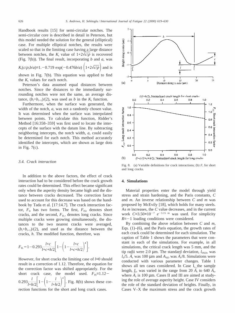
Since the stress concentration factor,Kt, enters Eqs.(4), (5), (8)–(10), its determination in the presence ofmultiple notches will be considered next. The idealizedgeometry is shown in Fig. 7(a). The notch width andnotch spacing are denoted as a and b, respectively. Thenotch depth and tip radius are once again symbolized byc andr. Unlike the simulated surface, the idealized sur-face has constant semi-circular notch depth and spacing.This idealization was used to obtain the initial functionfor the stress concentration factor, which was then modi-fied to account for the non-uniformity of the notch spac-ings and depths as described below.

First, a function forKt was derived by using Peterson

Fig. 7. (a) Idealized geometry used for findingKt; (b) NormalizedKt

curve; (c) Location of surface intercepts used to find notch widths.


Handbook results [15] for semi-circular notches. Thesemi-circular core is described in detail in Peterson, butthis model needed the solution for the general (elliptical)case. For multiple elliptical notches, the results werescaled so that in the limiting case having a large distancebetween notches, theKt value of 1+2√c/r is recovered(Fig. 7(b)). The final result, incorporatingb anda, was

Kt(c/r,b/a)=1.20.719 exp(20.476b/a) S1+2√c/rD and is

shown in Fig. 7(b). This equation was applied to findthe Kt values for each notch.

Peterson’s data assumed equal distances betweennotches. Since the distances to the immediately sur-rounding notches were not the same, an average dis-tance, (bi+bi−1)/(2), was used asb in the Kt function.

Furthermore, when the surface was generated, thewidth of the notch,a, was not a randomly chosen value.It was determined when the surface was interpolatedbetween points. To calculate this function, Ridder’sMethod [16:358–359] was first used to locate the inter-cepts of the surface with the datum line. By subtractingneighboring intercepts, the notch width,a, could easilybe determined for each notch. This method accuratelyidentified the intercepts, which are shown as large dotsin Fig. 7(c).

3.4. Crack interaction

In addition to the above factors, the effect of crackinteraction had to be considered before the crack growthrates could be determined. This effect became significantonly when the asperity density became high and the dis-tance between cracks decreased. The correction factorused to account for this decrease was based on the hand-book by Tada et al. [17:14.7]. The crack interaction fac-tor, FI, has two forms. The first,FIS, denotes shortcracks, and the second,FIL, denotes long cracks. Sincemultiple cracks were growing simultaneously, the dis-tances to the two nearest cracks were averaged,(bi+bi−1)/(2), and used as the distance between thecracks,h. The modified function, therefore, was

FIL5120.293l+c

l+c+h/2F12S12l+c

l+c+h/2D4G.

However, for short cracks the limiting case ofl=0 shouldresult in a correction of 1.12. Therefore, the equation forthe correction factor was shifted appropriately. For theshort crack case, the model used.FIS=1.122

0.293l

l+h/2F12S12l

l+h/2D4G. Fig. 8(b) shows these cor-

rection functions for the short and long crack cases.

Fig. 8. (a) Variable definitions for crack interactions; (b)Fi for shortand long cracks.

4. Simulations

Material properties enter the model through yieldstress and strain hardening, and the Paris constants,Cand m. An inverse relationship betweenC and m wasproposed by McEvily [18], which holds for many steels.As m increases, theC value decreases, and in the currentwork C=3.50×1027 e23.15 m was used. For simplicityR=21 loading conditions were considered.

By combining the above relation betweenC and m,Eqs. (1)–(6), and the Paris equation, the growth rates ofeach crack could be determined for each simulation. Thecaption of Table 1 shows the parameters that were con-stant in each of the simulations. For example, in allsimulations, the critical crack length was 5 mm, and thetip radii were 2.0µm. The standard deviation,l0SD, wasl0/5. Ar was 100µm andASD wasAr/8. Simulations wereconducted with various parameter changes. Table 1shows all ten cases considered. In Case I, the samplelength,L, was varied in the range from 20Ar to 640 Ar,whereAr is 100µm. Cases II and III are aimed at study-ing the role of average asperity height. Case IV considersthe role of the standard deviation of heights. Finally, inCases V–X the maximum stress and the crack growth


Table 1Quantities varied within the simulations. In all simulationsr=2.0 µm, rSD=2r, Ar=100 µm, ArSD=Ar/8, l0SD=l0/5, lcrit=5 mm, andR=21

Case L c (µm) cSD l0(µm) Smax(MPa) m sy (MPa)

I 20 Ar–640 Ar 1.0 c/5 0.1 300 3 400II 40 Ar 0.004–65.5 c/5 0.1 300 3 400III 40 Ar 0.004–65.5 c/5 0.1 400 3 400IV 40 Ar 1.0 c/5–5 c 1.0 300 3 400V 40 Ar 10 c/5 0.1 300 2–7 400VI 40 Ar 10 c/5 0.1 400 2–7 400VII 40 Ar 10 c/5 0.1 500 2–7 400VIII 40 Ar 10 c/5 0.1 300 2–7 800IX 40 Ar 10 c/5 0.1 400 2–7 800X 40 Ar 10 c/5 0.1 500 2–7 800

exponent,m were varied for different stresses. For eachcase, 10 simulations were conducted. Because the sur-faces generated differ for the same set of parameters, thefatigue life in these 10 simulations were not identical.Thus, knowledge of the surface parameters does not leadto exact knowledge of the fatigue life. However, as willbe shown, the distribution in fatigue lives sensitivityonly becomes significant if the standard deviation of theasperity height becomes large.

As mentioned previously in Case I, the sample lengthwas varied from 20Ar to 640Ar. SinceAr was held con-stant at 100µm, its range was from 2.0 mm to 64 mm,which corresponded to 10 cracks and 320 cracks,respectively. The simulation was repeated 10 times foreach sample length, with the lengths being doubled dur-ing each increment, as shown in Fig. 9. This figure illus-trates that the fatigue lives were insensitive to changesin L/Ar. Although the valueL/Ar=20 was sufficient tocapture the role of the sample length,L/Ar=40 was usedin all later simulations to help ensure a sufficient sam-ple length.

Next, the average asperity height,c, was varied from

Fig. 9. Effects of sample length on fatigue life under Case I con-ditions (see Table 1).

0.004 µm to 65.5µm under Case II and Case III con-ditions. Cases II and III had maximum stress levels of300 MPa and 400 MPa, respectively. Ten simulationswere conducted for each asperity height, as shown inFig. 10. In all three casesL/Ar=40. The results showedthat for rough surfaces, wherec.0.1 µm, the fatiguelives were strongly dependent on thec value. Forc ,0.1µm, the sensitivity ofc on Nf diminished. Below thislimit, the initial crack length (0.1µm in all cases) domi-nated the asperity heights and, therefore, did not signifi-cantly affect the fatigue lives. The increased stress levelsdid not alter the shape of thec versusNf curve.

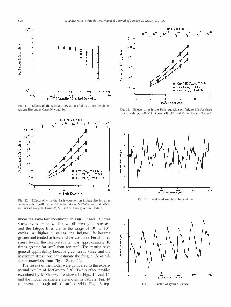
In Case IV conditions, as shown in Fig. 11, theasperity height standard deviation,cSD was varied from0.02 c to 5 c. Fig. 11 shows that whencSD/c,0.1 thelives are invariant to this ratio. WhencSD/c.0.1 the scat-ter in lives is apparent. In addition, the increased vari-ance tends to decrease the average fatigue life.

Finally, m, the exponent in the Paris equation, wasvaried from 2 to 7 in Fig. 12. TheC coefficient in theParis equation was changed according to the value ofm.For high m values, there was a larger variation in life

Fig. 10. Effects of average roughness for Case II and Case III (SeeTable 1).


Fig. 11. Effects of the standard deviation of the asperity height onfatigue life under Case IV conditions.

Fig. 12. Effects ofm in the Paris equation on fatigue life for threestress levels.sy=400 MPa.DK is in units of MPA√m, anda da/dN isin units of m/cycle. Cases V, VI, and VII are given in Table 1.

under the same test conditions. In Figs. 12 and 13, threestress levels are shown for two different yield stresses,and the fatigue lives are in the range of 103 to 1011

cycles. At higherm values, the fatigue life becamegreater and tended to have a wider variation. For all threestress levels, the relative scatter was approximately 10times greater form=7 than for m=2. The results havegeneral applicability because given anm value and themaximum stress, one can estimate the fatigue life of dif-ferent materials from Figs. 12 and 13.

The results of the model were compared to the experi-mental results of McGreevy [19]. Two surface profilesexamined by McGreevy are shown in Figs. 14 and 15,and the model parameters are shown in Table 2. Fig. 14represents a rough milled surface while Fig. 15 rep-

Fig. 13. Effects ofm in the Paris equation on fatigue life for threestress levels.sy=800 MPa. Cases VIII, IX, and X are given in Table 1.

Fig. 14. Profile of rough milled surface.

Fig. 15. Profile of ground surface.


Table 2Model parameters for the experimental comparison

lcritCase L c (µm) cSD m C sy (MPa) r (µm) rSD Ar (µm) ArSD l0/c l0SD R(mm)

Rough milled 20Ar 0.5 c/5 2.54 1.8×1028 1725 2.0 2r 200 Ar/8 0.01 l0/5 5 0.1Ground 40Ar 20 c/5 2.54 1.8×1028 1725 2.0 2r 250 Ar/8 0.1 l0/5 5 0.1

resents a ground surface. The parameters used wereobtained from McGreevy’s profilometer measurementsof his samples. Unfortunately, exact measurements ofthe initial crack length and tip radius could not beobtained due to the limited resolution of the profilom-eter. Therefore, these quantities had to be estimated. Thecrack growth exponent,m, of 2.54 was obtained fromresearch on 4340 steel by Ritchie [20]. Fig. 16 comparesthe model presented in this paper to the fatigue livesfrom McGreevy [19]. We note the scatter in experi-mental lives, especially for the ground “surface finish”case. The fact that both the rough milled and groundsurface cases are predicted supports the validity of themodel. The polished and fine milled specimens fromMcGreevy [19] fractured predominantly from inclusions.Therefore, the model was only applicable to the roughmilled and ground data.

5. Conclusions

The work supports the following conclusions:

1. Fatigue life strongly depends on surface roughnesswhen the average asperity heights exceed the intrinsicdefects in the material, i.e.c.l0. Whenc falls belowl0, the effect of surface roughness decreases as theintrinsic defects (i.e.l0) limit the lifetime.

2. When the standard deviation of the asperity heights,cSD, approach the magnitude of the asperity height,c, the variation in fatigue lives increases andapproaches an order of magnitude. The average

Fig. 16. Comparison of model to experiemental data for 4340 steel.

fatigue life decreases with increasing standard devi-ation in asperity heights,cSD.

3. Normalization of crack growth rates withCSmmax aids

in the presentation of crack growth results frommicro-notches under different maximum stress con-ditions. The results show that the crack growth ratesfrom the notches increase rapidly with increasingcrack length, reach a maximum in some cases, andapproach a steady state level whenl/c exceeds 0.5.

4. In most of the conditions studied, the fatigue lifeexceeded 105 cycles. In this life regime, the fatiguelives increased systematically with increasing valueof m and with increasing magnitude of yield stress.

5. Based on the simulations, the sample length adoptedin the simulations had no major influence on thefatigue lives when the sample length/distance betweenthe asperities exceeded 20. In some of the simula-tions, this ratio was taken as high as 700, but theinfluence on the results was not significant.

6. Comparison of the model to experimental data of4340 steel with ground (c=15 µm) and rough milled(c=0.75µm) surfaces showed good correlation despitethe large experimental scatter in lives.

Acknowledgements

This work is supported by the Fracture Control Pro-gram (FCP), College of Engineering, University of Illi-nois, Urbana, IL. We are grateful to Dr. T. McGreevyfor providing us with his roughness and life data for4340 steels. Initial portions of the work were fundedwith an NSF–REU grant.

References

[1] Moore HF, Kommers JB. An investigation of the fatigue of met-als. University of Illinois Engineering Experiment Station Bull-etin 1921;124.

[2] Thomas WN. Effect of scratches and of various workshop fin-ishes upon the fatigue strength of steel. Engng 1923;116:449–85.

[3] Lipson C, Juvinall RC. Handbook of stress and strength. NewYork: Macmillan Company, 1963.

[4] Noll GC, Erickson GC. Allowable stresses for steel members offinite life. Proc Soc Exp Stress Analy 1948;5(2):132–43.

[5] Siebel E, Gaier M. Influence of surface roughness on the fatiguestrength of steels and non-ferrous alloys. Engineers Digest


1957;18:109–112. (Translation from VDI Zeitschrift1956;98(30):1715–1723).

[6] Maiya PS, Busch DE. Effect of surface roughness on low-cyclefatigue behavior of type 304 stainless steel. Metallurgical TransA 1975;6:1761–74.

[7] Wareing J, Vaughan HG. Influence of surface finish on low-cyclefatigue characteristics of type 316 stainless steel at 400°C. MetalSci 1979;13:1–7.

[8] Starkey MS, Irving PE. A comparison of the fatigue strength ofmachined and as-cast surfaces of SG iron. Int J Fatigue1982;4:17–24.

[9] Wood DS, Wynn J, Baldwin AB, O’Riordan P. Somecreep/fatigue properties of type 316 steel at 625°C. Fatigue EngngMat Struct 1980;3:39–57.

[10] Gungor S, Edwards L. Effect of surface texture on the initiationand propagation of small fatigue cracks in a forged 6082 alumi-num alloy. Mat Sci Engng A: Struct Mat: Properties, Microstruc-ture and Processing 1993;160A:17–24.

[11] Lee JM, Nam SW. Effect of crack initiation mode on low cyclefatigue life of type 304 stainless steel with surface roughness.Mat Lett 1990;10:223–30.

[12] Fluck PG. The influence of surface roughness on the fatigue lifeand scatter of test results of two steels. Proc Am Soc Testing Mat1951;51:584–92.

[13] Sehitoglu H, Gall K, Garcı´a A. Recent advances in fatigue crackgrowth modeling. Int J Fract 1996;80:165–92.

[14] Sun W. Finite element simulations of fatigue crack growth andclosure. PhD thesis, University of Illinois, Urbana-Champaign,IL, 1991.

[15] Peterson RE. Stress concentration factors. New York: John Wileyand Sons, 1974.

[16] Press W, Teukolsky S, Vetterling W, Flannery B. Numericalrecipes in C: the art of scientific computing. 2nd ed. Cambridge:Cambridge University Press, 1992.

[17] Tada H, Paris P, Irwin G. The stress analysis of cracks handbook.2nd ed St. Louis: Del Research Corporation, 1985.

[18] McEvily AJ. On the quantitative analysis on fatigue crack propa-gation. In: Lankford J, Davidson DL, Morris WL, Wei RP, edi-tors. Fatigue mechanisms: advances in quantitative measurementof physical damage, ASTM STP 881. American Society for Test-ing and Materials, 1983:283–312.

[19] McGreevy T. The competing roles of microstructure and flawsize on the fatigue limit of metals. PhD thesis, University of Illi-nois, Urbana-Champaign, IL, 1998.

[20] Ritchie RO. Near-threshold fatigue crack propagation in ultra-high strength steel: influence of load ratio and cyclic strength. JEngng Mat Tech 1977;195–204.

a computer model for fatigue crack growth from rough surfaces

Documents