a continuous plate-tectonic model using geophysical data ... · model differ only slightly from...
TRANSCRIPT

GEOPHYSICAL JOURNAL INTERNATIONAL, 133, 379–389, 1998 1
A continuous plate-tectonic model using geophysical datato estimate plate margin widths, with a seismicity basedexampleCaroline Dumoulin1, David Bercovici2, Pal WesselDepartment of Geology & Geophysics, School of Ocean and Earth Science and Technology, University of Hawaii,Honolulu, 96822, USA
Summary
A continuous kinematic model of present day plate motions is developed which 1) provides more realisticmodels of plate shapes than employed in the original work of Bercovici & Wessel [1994]; and 2) providesa means whereby geophysical data on intraplate deformation is used to estimate plate margin widths forall plates. A given plate’s shape function (which is unity within the plate, zero outside the plate) canbe represented by analytic functions so long as the distance from a point inside the plate to the plate’sboundary can be expressed as a single valued function of azimuth (i.e., a single-valued polar function). Toallow sufficient realism to the plate boundaries, without the excessive smoothing used by Bercovici andWessel, the plates are divided along pseudoboundaries; the boundaries of plate sections are then simpleenough to be modelled as single-valued polar functions. Moreover, the pseudoboundaries have little or noeffect on the final results. The plate shape function for each plate also includes a plate margin functionwhich can be constrained by geophysical data on intraplate deformation. We demonstrate how this marginfunction can be determined by using, as an example data set, the global seismicity distribution for shallow(depths less than 29km) earthquakes of magnitude greater than 4. Robust estimation techniques are usedto determine the width of seismicity distributions along plate boundaries; these widths are then turned intoplate-margin functions, i.e., analytic functions of the azimuthual polar coordinate (the same azimuth ofwhich the distance to the plate boundary is a single-valued function). The model is used to investigatethe effects of “realistic” finite-margin widths on the Earth’s present-day vorticity (i.e., strike-slip shear)and divergence fields as well as the kinetic energies of the toroidal (strike-slip and spin) and poloidal(divergent and convergent) flow fields. The divergence and vorticity fields are far more well defined thanfor the standard discontinuous plate model and distinctly show the influence of diffuse plate boundariessuch as the north-east boundary of the Eurasian plate. The toroidal and poloidal kinetic energies of thismodel differ only slightly from those of the standard plate model; the differences, however, are systematicand indicate the greater proportion of spin kinetic energy in the continuous plate model.
Short title: The continuous model of plate tectonics
Keywords: Plate-tectonics; plate boundaries; intraplate deformation, toroidal-poloidal partitioning.
1Now at the Department of Geology, Ecole Normale Superieure, 24 Rue Lhomond, Paris, 75005 FRANCE2Author to whom correspondence should be addressed.

GEOPHYSICAL JOURNAL INTERNATIONAL, 133, 379–389, 1998 2
1 IntroductionThe theories of mantle dynamics and plate tectonics arefundamentally incompatible; the former employs contin-uum physics while the latter assumes that plates moveas rigid bodies and thereby have infinitesimally thin mar-gins. This disparity hampers efforts to couple plate andmantle theories, causing two problems in particular. First,the discontinuity between plates causes plate traction onthe mantle to be infinite [Hager & O’Connell, 1981].Second, the same discontinuity renders the vorticity (strike-slip shear) and divergence (which represents sources andsinks of mass in the lithosphere) fields to be comprisedof unphysical and mathematically intractable singular-ites [Bercovici & Wessel, 1994; Bercovici, 1995a]. TheEarth’s plates are for the most part not discontinuous; i.e.,intraplate deformation is common and many plate mar-gins have significant widths. Thus, efforts to understandhow plates are coupled to or generated from mantle flowshould not seek to achieve discontinuous plates; suchplates are abstractions based on the simple assumptionsof the standard plate model, and are therefore unrealis-tic as well as unrealizable. However, the actual continu-ity of plates needs to be assessed, and then incorporatedinto a global plate model; the resulting model would bemore compatible with mantle flow models, and representa more realistic goal for plate generation theories.
To this end, we here extend the continuous kinematicplate model of Bercovici & Wessel [1994], which intro-duced finite margin widths into a global model of platemotions. In particular, we use analytically continuous(i.e., infinitely differentiable) functions to describe bothplate geometry and plate-margin width. In this paper, themathematical model of the plate geometries is consider-ably refined to prevent the excessive smoothing of plateboundaries used by Bercovici & Wessel [1994]. More-over, we demonstrate how geophysical data on intraplatedeformation can be incorporated into the model to con-strain plate margin widths; for purposes of demonstra-tion, we use, as an example data set, the global seismicitydistribution. This leads to a marked improvement overthe ad hoc constant margin width assumed in the stan-dard plate model, or in the simple model of Bercovici andWessel [1994]. We refer to this seismicity based applica-tion of the model as the SEISMAR (seismicity-inferredmargin-width) plate model. The SEISMAR model ofcontinuous plate motions introduced here is a basic ex-ample of how data on intraplate deformation can be in-corporated into a global plate-tectonic model.
In this paper, we will first present the theoretical modelfor representing plate shapes and, in particular, developthe necessary improvements to facilitate more realisticplate boundaries. We will then discuss how margin widthis determined, for example, from global seismicity. Fi-nally, we will examine the implications of the resultingseismicity-based SEISMAR model on global velocity, inparticular the associated deformation fields (vorticity and
divergence) and kinetic energy partitioning between toroidaland poloidal parts.
2 Plate shapes and boundariesThe analysis of how to represent the shape of a tectonicplate with an analytically continuous function is discussedin detail in Bercovici & Wessel [1994]. We will here re-view the more salient points of the theory and explain indetail when we have differed from or improved on thatearlier work.
The horizontal velocity field of the Earth’s surface,given the motion of
�tectonic plates can be written in a
single equation:
�������� � � ������������� ����� (1)
where � is the position vector of a point on the surface ofthe Earth, at longitude
�and latitude � , and ��� and �
�are
the angular velocity vector and shape function of the �! #"plate, respectively. The angular velocities of the present-day plates is determined from the NUVEL-1A Pacific-plate-fixed Euler poles [DeMets et al. 1994] added toestimates of the instantaneous Pacific-hotspot pole fromPollitz’s [1988] joint inversion of North American andPacific plate motions. The shape function �
�is defined
to be 1 within the plate, and 0 outside the plate. Forthe standard plate model, �
�has a discontinuous transi-
tion from 1 to 0, whereas the transition is continuous andsmooth (i.e., infinitely differentiable) in the continuousmodel. The procedure for determining �
�in the continu-
ous model requires several steps as discussed below [seealso Bercovici & Wessel, 1994].
2.1 Plate boundary filtering.To make the model of the tectonic plates analyticallycontinuous, the plate boundaries must be smoothed atleast slightly to remove minor discontinuities (e.g., ridge-transform offsets). This is necessary to allow the bound-ary to be modelled as a mathematically single valuedfunction (see next subsection below). In Bercovici &Wessel [1994], smoothing was performed until each plateboundary could be represented as a single-valued polarfunction in which the polar origin was at some point in-side the plate. To that end, a very large filter width (7000kmGaussian full-width; see Bercovici & Wessel [1994]) wasnecessary so that the most non-circular plates (e.g., nearlyhorse-shoe shaped ones such as the Austro-Indian plate)could be sufficiently rounded out. Invariably, each re-sulting smoothed plates became a crude first order rep-resentation of the original plate, and smaller plates, suchas the Cocos plate (with its lopsided hour-glass shape),
GEOPHYSICAL JOURNAL INTERNATIONAL, 133, 379–389, 1998 3
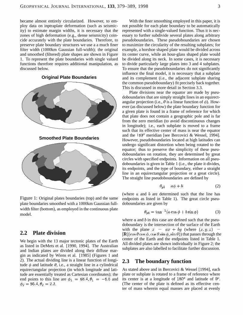
became almost entirely circularized. However, to em-ploy data on inptraplate deformation (such as seismic-ity) to estimate margin widths, it is necessary that thezones of high deformation (e.g., dense seismicity) coin-cide accurately with the plate boundaries. Therefore, topreserve plate boundary structures we use a a much finerfilter width (1000km Gaussian full-width); the originaland smoothed (filtered) plate shapes are shown in Figure1. To represent the plate boundaries with single valuedfunctions therefore requires additional manipulation, asdiscussed below.
Original Plate Boundaries
Smoothed Plate Boundaries
Figure 1: Original plates boundaries (top) and the sameplate boundaries smoothed with a 1000km Gaussian full-width filter (bottom), as employed in the continuous platemodel.
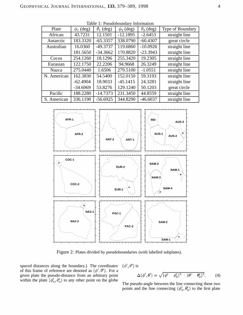
2.2 Plate divisionWe begin with the 13 major tectonic plates of the Earthas listed in DeMets et al. [1990, 1994]. The Australianand Indian plates are divided along their diffuse mar-gin as indicated by Wiens et al. [1985] (Figures 1 and2). The actual dividing line is a linear function of longi-tude
�and latitude � , i.e., a straight line in a cylindrical
equirectangular projection (in which longitude and lati-tude are essentially treated as Cartesian coordinates); theend points to this line are
� � � ������� ��� � � � ����� and�� ��� ��� ��� � �� � � .
With the finer smoothing employed in this paper, it isnot possible for each plate boundary to be automaticallyrepresented with a single-valued function. Thus it is nec-essary to further subdivide several plates along arbitrarypseudoboundaries. These pseudoboundaries are chosento maximize the circularity of the resulting subplates; forexample, a horshoe shaped plate would be divided acrossits center curve, while an hour-glass shaped plate wouldbe divided along its neck. In some cases, it is necessaryto divide particularly large plates into 3 and 4 subplates.To ensure that the pseudoboundaries do not significantlyinfluence the final model, it is necessary that a subplateand its complement (i.e., the adjacent subplate sharingthe common pseudoboundary) fit precisely back together.This is discussed in more detail in Section 3.3.
Plate divisions near the equator are made by pseu-doboundaries that are simply straight lines in an equirect-angular projection (i.e., � is a linear function of
�). How-
ever (as discussed below) the plate boundary function fora given plate is found in a frame of reference for whichthat plate does not contain a geographic pole and is farfrom the zero meridian (to avoid discontinuous changesin longitude); i.e., each subplate is moved to a framesuch that its effective center of mass is near the equatorand the ����� meridian [see Bercovici & Wessel, 1994].However, pseudoboundaries located at high latitudes canundergo significant distortion when being rotated to theequator; thus to preserve the simplicity of these pseu-doboundaries on rotation, they are determined by greatcircles with specified endpoints. Information on all pseu-doboundaries is given in Table 1 (i.e., the plate it divides,its endpoints, and the type of boundary, either a straightline in an equirectangular projection or a great circle).The straight line pseudoboundaries are defined by����� ���
����
(2)
(where � and�
are determined such that the line hasendpoints as listed in Table 1). The great circle pseu-doboundaries are given by����� ������ "! � � �$#&%�' � ��� '�()
� � (3)
where � and�
in this case are defined such that the pseu-doboundary is the intersection of the surface of the Earthwith the plane * � �,+ �-�/.
(where
�+ � . � * � �0 � 0
�#&%�' � #&%�' � � #&%�' � '/() � � '/() ��� ) that passes through the
center of the Earth and the endpoints listed in Table 1.All divided plates are shown individually in Figure 2; thesubplates are also labelled to facilitate further discussion.
2.3 The boundary functionAs stated above and in Bercovici & Wessel [1994], eachplate or subplate is rotated to a frame of reference whereits center is at a longitude of ���1� and latitude of
�1�.
(The center of the plate is defined as its effective cen-ter of mass wherein equal masses are placed at evenly
GEOPHYSICAL JOURNAL INTERNATIONAL, 133, 379–389, 1998 4
Table 1: Pseudoboundary InformationPlate
� � (deg) � � (deg)� � (deg) � � (deg) Type of Boundary
African 43.7231 12.1501 -12.1895 -2.6453 straight lineAntarctic 183.3320 -65.3357 338.0790 -60.4307 great circleAustralian 16.0360 -49.3737 119.6860 -10.0926 straight line
181.5650 -34.3662 170.8820 -23.3943 straight lineCocos 254.1260 18.1296 255.3420 19.2305 straight line
Eurasian 122.1750 22.2206 94.9668 26.3249 straight lineNazca 275.0440 1.6506 279.5100 -1.0551 straight line
N. American 162.3830 54.5400 152.0150 59.3193 straight line-62.4904 18.9033 -45.1415 24.3281 straight line-34.6069 53.8276 129.1240 50.1203 great circle
Pacific 188.2280 -14.7373 231.3450 44.8559 straight lineS. American 336.1190 -56.6925 344.8290 -46.6037 straight line
AFR-1
AFR-2
ANT-1ANT-2
IND
AUS-1AUS-2
AUS-3
COC-1
COC-2
EUR-1
EUR-2NAM-1
NAM-4
NAM-2
NAM-3
NAZ-1
NAZ-2
PAC-1
PAC-2
SAM-1
SAM-2
Figure 2: Plates divided by pseudoboundaries (with labelled subplates).
spaced distances along the boundary.) The coordinatesof this frame of reference are denoted as
����� ��� � � . For agiven plate the pseudo-distance from an arbitrary pointwithin the plate
������ ��� �� � to any other point on the globe
����� ��� � � is� ��� � ��� � � ������ � � � �
� � � � � � � � � �� � � � (4)
The pseudo-angle between the line connecting these twopoints and the line connecting
��� �� ��� �� � to the first plate
GEOPHYSICAL JOURNAL INTERNATIONAL, 133, 379–389, 1998 5
boundary data point
��� �� � ��� �� � � is
� ������ ! � � � � � � ��� � � � ���� � ���� ! ��� � ���� � � ��� �
� � � � ��� (5)
(The terms ‘pseudo-distance’ and ‘pseudo-angle’ are usedbecause these quantities treat � � and
� �as if they were
Cartesian coordinates; see Bercovici & Wessel [1994].)An arbitrary boundary point
��� �� ����� � has pseudo-distance� � � � ��� � � ���
�� � . In order to make the plate shape ana-
lytically continuous,� � must be expressed as a single-
valued function of � ; this function� �
� � � is called theplate-boundary function. Achieving a single-valued
� �� � �
requires a prudent choice of the polar origin
��� �� ��� �� � .
Here, the optimum
��� �� ��� �� � yields the smallest maximum
value of0 � ��� � 0 since this would be zero for the ideal
circular boundary while a multivalued� � � � would have
singularities in its slope. The optimum values of
� �� and� �� are found numerically for all 25 plates and/or sub-
plates. Since most plates and subplates are, to first order,elliptically shaped, most of the
��� �� ��� �� � are near
� ��� � � � .
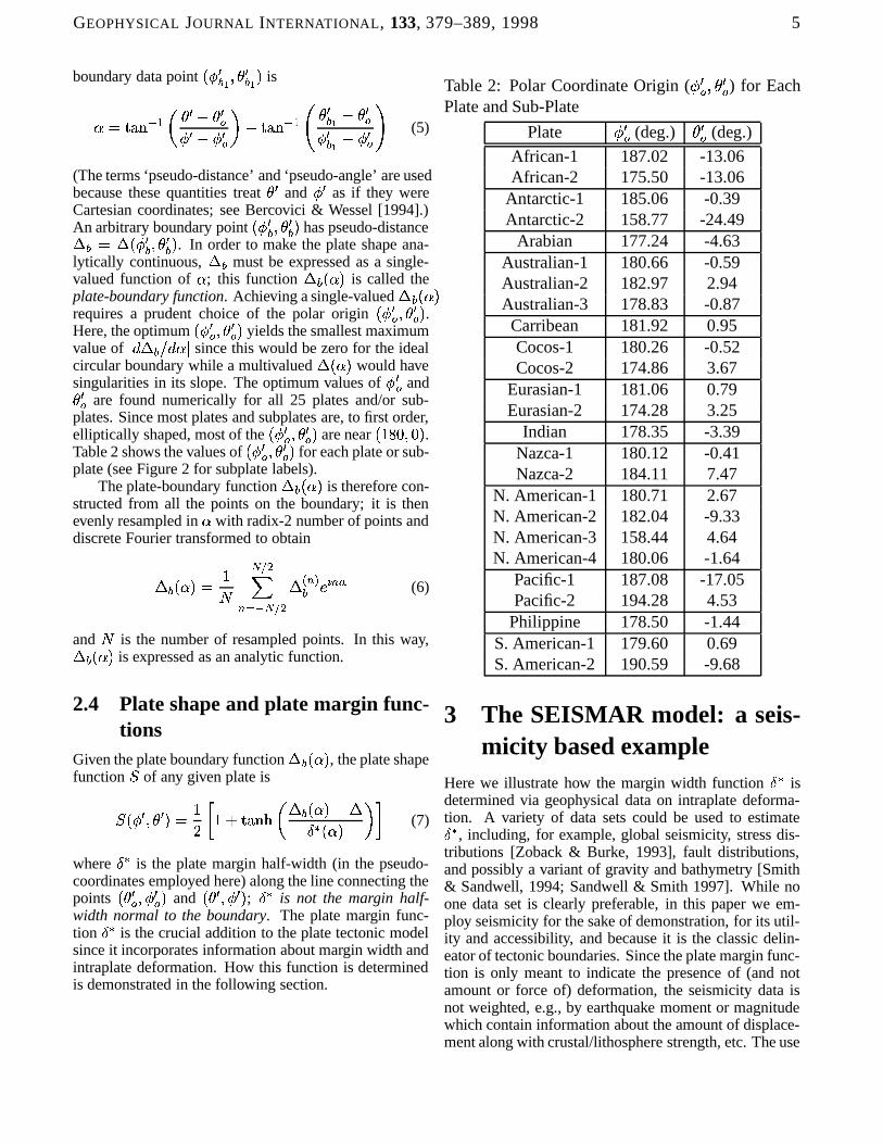
Table 2 shows the values of
��� �� ��� �� � for each plate or sub-
plate (see Figure 2 for subplate labels).The plate-boundary function
� �� � � is therefore con-
structed from all the points on the boundary; it is thenevenly resampled in � with radix-2 number of points anddiscrete Fourier transformed to obtain
� �� � � � � � ��� ! � � ��� ������ � ��� (6)
and�
is the number of resampled points. In this way,� �� � � is expressed as an analytic function.
2.4 Plate shape and plate margin func-tions
Given the plate boundary function� �
� � � , the plate shapefunction � of any given plate is
���� � ��� � � � ��� � ���� �� � � � � � � � ���� � � � �! (7)
where� �
is the plate margin half-width (in the pseudo-coordinates employed here) along the line connecting thepoints
� � �� � � � � � and
� � � � � � � ; � � is not the margin half-width normal to the boundary. The plate margin func-tion
� �is the crucial addition to the plate tectonic model
since it incorporates information about margin width andintraplate deformation. How this function is determinedis demonstrated in the following section.
Table 2: Polar Coordinate Origin (� � ��" � �� ) for Each
Plate and Sub-Plate
Plate� � � (deg.) �
�� (deg.)
African-1 187.02 -13.06African-2 175.50 -13.06
Antarctic-1 185.06 -0.39Antarctic-2 158.77 -24.49
Arabian 177.24 -4.63Australian-1 180.66 -0.59Australian-2 182.97 2.94Australian-3 178.83 -0.87
Carribean 181.92 0.95Cocos-1 180.26 -0.52Cocos-2 174.86 3.67
Eurasian-1 181.06 0.79Eurasian-2 174.28 3.25
Indian 178.35 -3.39Nazca-1 180.12 -0.41Nazca-2 184.11 7.47
N. American-1 180.71 2.67N. American-2 182.04 -9.33N. American-3 158.44 4.64N. American-4 180.06 -1.64
Pacific-1 187.08 -17.05Pacific-2 194.28 4.53
Philippine 178.50 -1.44S. American-1 179.60 0.69S. American-2 190.59 -9.68
3 The SEISMAR model: a seis-micity based example
Here we illustrate how the margin width function� �
isdetermined via geophysical data on intraplate deforma-tion. A variety of data sets could be used to estimate� �
, including, for example, global seismicity, stress dis-tributions [Zoback & Burke, 1993], fault distributions,and possibly a variant of gravity and bathymetry [Smith& Sandwell, 1994; Sandwell & Smith 1997]. While noone data set is clearly preferable, in this paper we em-ploy seismicity for the sake of demonstration, for its util-ity and accessibility, and because it is the classic delin-eator of tectonic boundaries. Since the plate margin func-tion is only meant to indicate the presence of (and notamount or force of) deformation, the seismicity data isnot weighted, e.g., by earthquake moment or magnitudewhich contain information about the amount of displace-ment along with crustal/lithosphere strength, etc. The use

GEOPHYSICAL JOURNAL INTERNATIONAL, 133, 379–389, 1998 6
of geologically recent seismicity data of course gives avery current estimate of plate margin structure and thusis relevant for models (e.g., mantle flow models) whichneed to employ instantaneous motion. We discuss belowhow the data are chosen, used and manipulated in orderto yield the plate margin function
� �. We refer to the
resulting seismicity based application as the SEISMAR(seismicity-inferred margin-width) plate model.
3.1 The seismicity dataWe use seismicity data for the period from 1928 to 1990in the June 1992 version of the Global Hypocenter DataBase. While earthquake locations are less reliable priorto 1960, we choose to have a large data set to facilitateresolution of plate margins (i.e., to minimize gaps in seis-micity along plate boundaries). Certain constraints, how-ever, are placed on the chosen earthquakes. First, we al-low only earthquakes whose focal depth is less than orequal to 29 km; this is done because indeterminant focaldepths are, by default, asigned a value of 30 km [F. Duen-nebier, pers. comm, 1996]. Earthquakes deeper than30km are eliminated as they are less representative ofplate boundary deformation and interactions (and are li-able to be influenced by deep earthquakes which are wellremoved from plate boundaries). We also choose onlyearthquakes with magnitude greater than 4 (given thatsmall earthquakes have poorly determined locations). Inthe end, we obtain the locations of 24,721 earthquakes(Figure 3). However, when necessary we delete intraplateearthquakes that are clearly unrelated to plate deforma-tion (e.g., earthquakes on Hawaii which are primarilyfrom landslides and volcanic activity).
Figure 3: Global seismicity distribution used to deter-mine plate margin widths.
3.2 Determination of margin widthsFor a given plate we consider only the subset of the seis-micity data which includes 1) earthquakes on the plateitself, and 2) earthquakes outside the plate but within� ��� ��� of the plate boundary (and not including earth-quakes associated with other plate boundaries). We then
calculate the position of each earthquake in terms of thepseudo-distance
�and angle � .
We next divide the given plate into wedges of equalangular extent
� and bin the seismicity data on eachwedge (Figure 4). Thus the number of earthquakes
�����at pseudo-distance
�and a given � is in fact the number
of earthquakes at�
between � � � � � and � � � � �(Figure 4). If
�����versus
�at the given � had a nor-
mal (Gaussian) distribution centered at� � � � , then
the margin half-width would be the Gaussian half-width(i.e., � � times the standard deviation) of the distribution.However, given the scatter and occurence of outliers inthe actual data, we employ robust estimation techniques[Rousseeuw & Leroy, 1987] and define the margin widthas the minimum width of the window (in the units ofpseudo-distance) which contains 50% of the earthquakes(again, in the wedge centered on � ). (This step is consid-erably facilitated if one first sorts the earthquake locationin each wedge in order of increasing
�.) By finding this
width for each � we build the raw margin function� �� � � �
(deemed raw as it still requires some additional process-ing, as discussed below).
The chosen wedge size � differs between plates be-
cause, for example, the � for a small plate is larger than
that for a big plate since the smaller plate is likely to havefewer earthquakes along its boundary. In general we usebetween 60 and 70 wedges for the bigger plates, and 20to 30 for the smaller ones. Moreover, we can only cal-culate a margin width in a wedge if it has more than 4earthquakes. If there are fewer than 4 earthquakes in thewedge we assume the margin width is the average of thewidths of the two surrounding wedges.
To determine the confidence in the inferred marginwidth, we also record the total number of earthquakes oneach wedge
� � � . We then smooth the function� �� � � �
by a Gaussian filter that is weighted by � � � ; in this
way values of� �� that have higher confidence are more
strongly weighted. (The Gaussian filter is arbitrarily cho-sen to have a half-width that is � � ). Therefore, oursmoothed margin width at the � #" value of � is� � � � � � ���� � �� � � � � � � � ! � ��� ! ��� ��� ������ � ���
�� � � � � ! � ��� ! ��� � � ������ � � � (8)
However, the pseudoboundaries (where some plates aredivided) must be left intact so the parts of a plate willfit back together again along the boundary as tightly aspossible. The calculation of the margin widths for thepseudoboundaries is discussed below.
As with the boundary function� �
� � � , the marginfunction can be put into an analytic form with discreteFourier transforms, though since
� �is defined only on
wedges and not each boundary point, it is defined (usu-ally resampled to radix 2 points) at fewer values of � .

GEOPHYSICAL JOURNAL INTERNATIONAL, 133, 379–389, 1998 7
(φ'0 ,θ'0)
α−dα/2
α+dα/2
d
δ
2δ0∗
pseudoboundary
fm
∗
Figure 4: Sketch illustrating the determination of mar-gin width along the true boundary and pseudoboundaryof a single subplate, in this case the northern Pacificplate (Pacific-1; see Figure 2). On the true boundary, theoblique margin width at angle � is determined by bin-ning the seismicity within a wedge between � � � � �and � � � � � (upper left); the margin is then the narrow-est region which contains 50% of the earthquakes in thatwedge (the shaded region, which is exaggerated for thesake of clarity). The margin width of the pseudobound-ary (lower right) is found by measuring, along a line ofconstant � , the width of a box-car function
���centered
on the boundary (long shaded region). The figure, how-ever, is over-simplified and should only be considered il-lustrative; in particular,
� �is defined in the original co-
ordinate frame
��� ����� , while the measurements of marginwidth are done in the rotated frame
����� ��� � � . See text forfurther discussion.
3.3 Pseudoboundary margin widthsThe creation of pseudoboundaries has no (or negligible)effect on the final model of plate kinematics as long asthe effects of these boundaries’ margins essentially can-cel each other once all the subplates are pieced back to-gether again. The shape functions of a subplate and itscomplement (i.e., the adjacent suplate sharing the pseu-doboundary) should add to unity on the pseudobound-ary. As a simple example, the 1-D hyperbolic-tangentstep function (centered at + ��+ � and of margin width
�)
and it’s mirror image add to unity:
�� � ���� � � + � + �� � � �
� � ���� �� � + � + �� � � (9)
But these functions only add to unity as long as they eachhave the same margin width. Moreover, since comple-mentary subplates have the same Euler pole, there is nodifferential motion across their pseudoboundary and thusthe pseudoboundary has little or no effect on strain-rate,vorticity and divergence fields.
However, the actual description of margin widths onpseudoboundaries is not as precise or as simple as im-plied by (9) given that the boundaries are arbitrary curveson a spherical surface, and the margin widths are mea-sured from completely different points on a subplate andits complement.
To make a subplate and its complement fit as tightlyas possible along a pseudoboundary the definition of themargin must be precise. The margin width must havea consistent mathematical definition that is frame invari-ant (in particular, independent of the frame of referenceof the subplate in which the margin width is measured).Thus, it is best to have an exact mathematical descriptionof the margin in the original spherical coordinates
�and� . For precision we delineate the margin region of the
plate with a top-hat or box car function centered alongthe pseudoboundary, representing, say, a distribution offictional earthquakes (see Figure 4); i.e., this function is1 inside and 0 outside the margin region. Since a pseu-doboundary curve is given by the single valued function����� ��� � (see equations (2) and (3)), the margin region istherefore defined by the function��� ��� ����� � �
� � '��� � � � � � ����� ��� �� ��� � � � ���
(10)
where� ��� � is the margin half-width measured in the North-
South direction. For simplicity, we prescribe the marginto have a constant half-width
normal to the boundary
(see Figure 4) and thus� ��� � � �� ����� � � � (11)
(i.e.,� �
if the boundary at that particular
�is tan-
gent to an East-West line; and� �
if the boundaryapproaches a North-South tangent; see also Bercovici &Wessel [1994]). With this definition, the margin widthmeasured from the centers of two adjacent subplates willbe derived from the same formula.
With the margin region for a given plate’s pseudobound-ary defined in the (
�, � ) coordinate system, we need to
measure the width of the region in the rotated polar coor-dinate system (
�, � ). For a given constant- � line (that in-
tersects the pseudoboundary) the values of���
are calcu-lated for increasing
�(using in (10) the
�and � uniquely
corresponding to the given�
and � ). The margin half-width along this constant � line is thus� � � �
� � � ��� � � � � � � (12)
GEOPHYSICAL JOURNAL INTERNATIONAL, 133, 379–389, 1998 8
where� � � � and
� � ���are, respectively, the minimum
and maximum�
for which� � � . (Precise measure-
ment of� �
may require many incremental steps in�
toproperly resolve the margin region, sometimes as manyas 50,000 steps.) This is done for a sufficient number of� along the pseudoboundary (typically about 20 values).In this way we obtain a sampling of the function
� � � � �along the pseudoboundary. This sampling is appended tothe filtered sampling of
� � � � � along the true boundaries(with seismicity data) to yield a complete margin func-tion
� � � � � for� � � � ��� . Incorporation of the total
margin function for each plate into the associated plateshape function (see equation (7)) comprises the essentialpart of the SEISMAR plate model.
Figure 5 shows an example of the seismically in-ferred margin width for a plate with considerable vari-ability in its margin structure, i.e., the Eurasian plate.Where the concentration of earthquakes is dense the mar-gin width is relatively narrow and well defined. However,where earthquakes are poorly concentrated, the marginwidth is appropriately broad (e.g., the north-east marginof the Eurasian plate).
4 Results of the SEISMARModel
4.1 Divergence and Vorticity FieldsThe Earth’s plate motions can be divided linearly intopoloidal and toroidal parts [Hager & O’Connell, 1978,1979]. Poloidal flow represents divergent motion (ridgesand subduction zones) and thus reflects upwelling anddownwelling in the mantle. Toroidal motion representspurely horizontal rotational motion as exists in the spin ofplates and strike-slip shear. Poloidal motion is typical ofconvective flow. However, the issue of how and why thepurely horizontal and dissipative toroidal motion is gen-erated in the plate-mantle system remains a fundamen-tal, yet largely unresolved, aspect of our understandingof how plate tectonics is linked to mantle convection [seeBercovici, 1993, 1995a,b, 1996, 1997; Zhong & Gurnis,1995a,b, 1996].
In this section we show how the SEISMAR modelresolves the poloidal and toroidal parts of the Earth’spresent-day plate motions. In particular, we will exam-ine the horizontal divergence and vertical vorticity of theplate motions which are the most detailed manifestationsof the poloidal and toroidal fields. In the standard platemodel divergence and vorticity are essentially impossi-ble to resolve as they are singularities (due to the as-sumption of zero margin width). However, in the con-tinuous plate model, and the SEISMAR model in thispaper, these quantities are quite resolvable and containconsiderable detail about deformation of the Earth’s sur-face. Although this model also has certain drawbacks
and artifacts it gives us the first quantitative estimate ofthe Earth’s surface divergence and vorticity fields.
4.1.1 Theoretical background
The two-dimensional velocity on the surface of a spherecan be expressed with a Helmholtz representation:������� � � � �
�� � (13)
where � is the horizontal gradient, � is the poloidal po-tential, is the toroidal stream function, and
�� is the unitvector in the radial direction. Horizontal divergence is
� ���� ����� � � (14)
while radial or vertical vorticity is
����� ��� �� � � � ��� � � (15)
Divergence and vorticity are thus also representative ofthe poloidal and toroidal fields, respectively. However,since the divergence and vorticity involve gradients of �and , they enhance the finer small-scale features andthus permit a more detailed description of the poloidaland toroidal fields.
To calculate the divergence and vorticity fields di-rectly we would simply find the appropriate horizontalgradients of the surface velocity field. This is possiblein the continuous plate model, but not so in the standardplate model. In the continuous plate model we wouldobtain (from substituting (1) into (14) and (15)):
� � � � � ���� �� ��� ��
� � � � �� �� #&%�' � � �
���
(16)
��� � � � �� � ��� �� �� � � �
� ��� ��
� � � � �� �� #&%�' � � �
���
(17)
where
� �� �� � �
� �� �� #&%�'
�� � �
� �� '/()
� � #&%�' � � � �� �� '�( � (18)
� �� �� � �
� �� �� #&%�'
�� � �
� �� '/()
� � '�() � � � �� �� #&%�' � (19)
� �� �� � � �
� �� #&%�'
� � � �� �� '�()
�(20)
and �� � �
� �� �� � � �
� �� � � �
� �� � . Since the plate margins for
the continuous plate model are of finite width, the var-ious derivatives of �
�are calculable. Moreover, since�
and � � are scalars they are invariants and thus weneed only determine them for each individual plate orsubplate in the plate’s specific plate-centered reference

GEOPHYSICAL JOURNAL INTERNATIONAL, 133, 379–389, 1998 9
320˚ 0˚ 40˚ 80˚ 120˚ 160˚-20˚ -20˚
0˚ 0˚
20˚ 20˚
40˚40˚
60˚60˚
80˚80˚
Figure 5: The seismically inferred margin width for the Eurasian plate, superimposed on the local seismicitydistribution. The plot shows the shape function � for the entire Eurasian plate; however, only values between
� � � � and� � are given a single gray shade while all other values are white.
frame
��� � ��� � � . Both divergence and vorticity involvederivatives of each plate’s shape function � with respectto
� �and � � ;these take the form of
� �� ��� ��� � � � '���#�� � � � � � �� � � ��� ������ �� � � � �� � � � ��� ��� � ��� �� � � � � � � � � � � � � ��� � �
(21)
where ��� � � � , � ! � ���and we use Fourier transforms
of� � and
� �to evaluate their derivatives with respect to� . Although these derivatives are susceptible to Gibbs ef-
fects, such effects can be reduced with modest Gaussianfiltering in the Fourier domain [see Bercovici & Wessel,1994]. We then simply use the value of
�or � � at the
point
��� � ��� � � for the divergence and vorticity of the as-sociated point
��� ����� . The�
and � � for all the platesare then added together to yield the total divergence andvorticity fields.
For the standard plate model the shape function �is essentially constructed from discontinuous step func-tions and therefore derivatives of � do not exist (i.e., theyare singularities). One can however determine the diver-gence and vorticity from the velocity field without takinggradients of � . This method involves vector-spherical-harmonic transforms [see O’Connell et al., 1991] andyields the spherical harmonic transform of
�and � � , not
the physical quantities themselves. Using this methodone finds that the spherical harmonic transforms of
�
and ��� are
��� � � � ����� ��� ���� � � (22)
� � � � � ����� � ��� ���� � �� � � � (23)
where � is the solid angle, and � �!�� is the complex con-jugate of the normalized spherical harmonic � �� of de-gree " and order
�. In this way divergence and vorticity
can be calcluated from the expansions
� � #� � ��� ��� ! � ��� � � �� (24)
����� #� � ��� ��� ! � � � � � �� � (25)
where $ is the maximum " used.
4.1.2 Field representations
The divergence and vorticity fields for the standard dis-continuous plate model (using (22)–(25) with $ � ���
;O’Connell, pers. comm., 1992) are shown in Figure 6.Even though the vector spherical harmonic transformsfrom which these are derived do not directly involve sin-gularities, the divergence and vorticity fields for this modelare intrinsically singular. This causes the excessive ring-ing or Gibbs phenomenon extant in both fields. More-over, the magnitudes of
�and � � depend on $ , i.e.,
where the spherical harmonic series is truncated. Someof the broader true features are discernible in the diver-gence and vorticity fields, such as the East Pacific Rise,and the Southeast Indian Ridge. However, the Gibbs ef-fect obscures any finer or more complex features, suchas those around the Philippine plate. Finally, it is worthnoting for the sake of later comparison that the diver-gence field has the largest amplitude feature which oc-curs the along East Pacific Rise. The maximum vortic-ity is about 80% of the maximum divergence and oc-curs on the southwest side of the Philippine plate (though
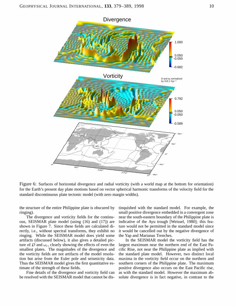
GEOPHYSICAL JOURNAL INTERNATIONAL, 133, 379–389, 1998 10
-0.682
-0.0500.050
1.000
-0.589
-0.0500.050
0.792
D and ωr normalized by 319.1 Gyr -1
Divergence
Vorticity
0˚90˚
180˚270˚
0˚-90˚
-45˚
0˚
45˚
90˚
Figure 6: Surfaces of horizontal divergence and radial vorticity (with a world map at the bottom for orientation)for the Earth’s present day plate motions based on vector spherical harmonic transforms of the velocity field for thestandard discontinuous plate tectonic model (with zero margin widths).
the structure of the entire Philippine plate is obscured byringing).
The divergence and vorticity fields for the continu-ous, SEISMAR plate model (using (16) and (17)) areshown in Figure 7. Since these fields are calculated di-rectly, i.e., without spectral transforms, they exhibit noringing. While the SEISMAR model does yield someartifacts (discussed below), it also gives a detailed pic-ture of
�and � � , clearly showing the effects of even the
smallest plates. The magnitudes of the divergence andthe vorticity fields are not artifacts of the model resolu-tion but arise from the Euler pole and seismicity data.Thus the SEISMAR model gives the first quantitative es-timate of the strength of these fields.
Fine details of the divergence and vorticity field canbe resolved with the SEISMAR model that cannot be dis-
tinquished with the standard model. For example, thesmall positive divergence embedded in a convergent zonenear the south-eastern boundary of the Philippine plate isindicative of the Ayu trough [Weissel, 1980]; this fea-ture would not be permitted in the standard model sinceit would be cancelled out by the negative divergence ofthe Yap and Marianas Trenches.
In the SEISMAR model the vorticity field has thelargest maximum near the northern end of the East Pa-cific Rise, not near the Philippine plate as implied withthe standard plate model. However, two distinct localmaxima in the vorticity field occur on the northern andsouthern corners of the Philippine plate. The maximumpositive divergence also occurs on the East Pacific rise,as with the standard model. However the maximum ab-solute divergence is in fact negative, in contrast to the
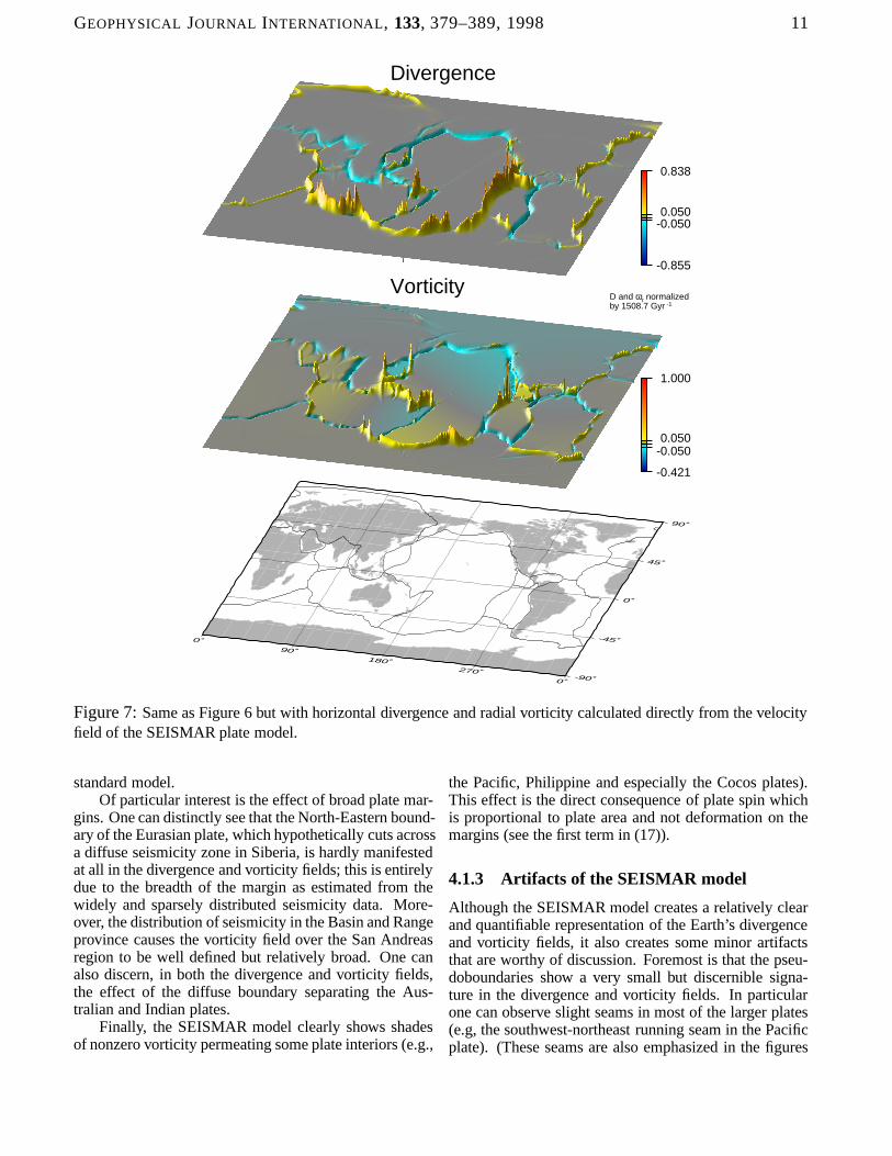
GEOPHYSICAL JOURNAL INTERNATIONAL, 133, 379–389, 1998 11
-0.855
-0.0500.050
0.838
-0.421
-0.0500.050
1.000
D and ωr normalizedby 1508.7 Gyr -1
Divergence
Vorticity
0˚90˚
180˚270˚
0˚-90˚
-45˚
0˚
45˚
90˚
Figure 7: Same as Figure 6 but with horizontal divergence and radial vorticity calculated directly from the velocityfield of the SEISMAR plate model.
standard model.Of particular interest is the effect of broad plate mar-
gins. One can distinctly see that the North-Eastern bound-ary of the Eurasian plate, which hypothetically cuts acrossa diffuse seismicity zone in Siberia, is hardly manifestedat all in the divergence and vorticity fields; this is entirelydue to the breadth of the margin as estimated from thewidely and sparsely distributed seismicity data. More-over, the distribution of seismicity in the Basin and Rangeprovince causes the vorticity field over the San Andreasregion to be well defined but relatively broad. One canalso discern, in both the divergence and vorticity fields,the effect of the diffuse boundary separating the Aus-tralian and Indian plates.
Finally, the SEISMAR model clearly shows shadesof nonzero vorticity permeating some plate interiors (e.g.,
the Pacific, Philippine and especially the Cocos plates).This effect is the direct consequence of plate spin whichis proportional to plate area and not deformation on themargins (see the first term in (17)).
4.1.3 Artifacts of the SEISMAR model
Although the SEISMAR model creates a relatively clearand quantifiable representation of the Earth’s divergenceand vorticity fields, it also creates some minor artifactsthat are worthy of discussion. Foremost is that the pseu-doboundaries show a very small but discernible signa-ture in the divergence and vorticity fields. In particularone can observe slight seams in most of the larger plates(e.g, the southwest-northeast running seam in the Pacificplate). (These seams are also emphasized in the figures

GEOPHYSICAL JOURNAL INTERNATIONAL, 133, 379–389, 1998 12
due to the false illumination projected from the south-west). In the plate interiors these seams are not strongenough to register outside the narrow zero-centered grayrange (i.e,. less than 5% of the maximum) of the colorscale in Figures 6 and 7; however, they do manifest them-selves more distinctly where they intersect a true bound-ary. Although these artifacts are second-order at worst,they demonstrate that there is room for improvement inthe continuous plate model, or in the application of seis-micity in the SEISMAR model. While considerable carewas taken to accurately resolve the pseudoboundaries (sothat sections of a divided plate would fit cleanly togetheragain) there are still some problems. First, pseudobound-aries (both the boundary distance and margin width) arenot sampled by two adjacent plates from the same coor-dinate system; thus the boundary shape and width are notmeasured at the same points or from the same angles bytwo complementary plates. This scheme for sampling thepseudoboundaries might be made more exact in futurestudies. Alternatively, it may be possible to essentiallyapply a high-pass filter to the divergence and vorticityfield; i.e., permit only values with absolute values greaterthan some minimum and thus effectively exclude most ofthe effects of the pseudoboundaries. This latter methodis arbitrary at best and thus not entirely satisfactory.
Another artifact of the SEISMAR model is evidentin the spikes and ringing in the divergence and vortic-ity fields along (i.e., parallel to) the margins. This un-doubtedly comes about because of the often highly os-cillatory nature of the margin width function
� � � � � formany plates. This in itself likely reflects the sparse cover-age of seismicity data on certain plate boundaries, and/ordiffuse boundaries. Even with smoothing weighted byconfidence (i.e., number of earthquakes, e.g., from (8)),the resolution of
� �in � is still relatively coarse in or-
der to permit more than 4 earthquakes per wedge of theplate; this can cause significant variation from one al-pha to the next which becomes manifest as spikes andsome secondary ringing of
�and � � along the bound-
aries. Again, these artifacts might be reduced by moreaggressive filtering, or by using more data on plate mar-gin widths (e.g., other data sets with additional resolutionof plate boundaries).
4.2 Power spectra and kinetic energypartitioning
The kinetic energies of toroidal and poloidal motions aremostly dependent on the bulk size and shape of the largerplates, and not extensively on the margin width. Thus oneshould expect that the toroidal and poloidal kinetic ener-gies, their power spectra and their ratio should differ littlefrom one plate model to the next. We therefore examinethe effect (or lack of effect) the SEISMAR model hason the various characteristics of the toroidal and poloidalkinetic energies (as well as the power spectra of the di-
vergence and vorticity field).The spherical harmonic kinetic energy spectrum is
defined as the kinetic energy for each spherical harmonicdegree " ; the poloidal and toroidal energy spectra (perunit mass and divided by
� �) are, respectively,
������ " � � � " � " � �
� ��� ! � ��� � � �� � (26)
������ " � � � " � " � �
� ��� ! � � � � � �� � � (27)
Figure 8 (top two frames) shows these spectra and theirratios for both the standard discontinuous plate modeland the SEISMAR model. One can see that the SEIS-MAR model has little effect on the amplitude and shapeof this spectrum, as expected. The ratio of the energies�����
� " � � ��� � � " � is also shown in the same figure andthis emphasizes some minor differences between the twomodels. The ratio for both models is greater than unityonly in the " � mode, which represents the amountof net lithospheric spin. The ratio is noticeably larger at" � for the SEISMAR model than the standard model.Moreover, the local peak in the ratio at " ��� in thestandard model is not present in the SEISMAR model.These differences may reflect the use of finite margins inthe SEISMAR model because, for example, with morediffuse margins the SEISMAR model gives relative moreweight to spin kinetic energy in the toroidal field (whichdepends on plate area not on margin structure).
For the standard plate model the total poloidal andtoroidal kinetic energies, and their ratio are
���� � � � �(rad/Gyr)
�,��� � � � ��� (rad/Gyr)
�and
��� � � ����� �� ��� � . For the SEISMAR model��� � ���� � (rad/Gyr)
�,��� � � � � � (rad/Gyr)
�and
��� � � ����� � � �����. The
SEISMAR poloidal energy is 6% and the toroidal energy3% lower than those for the standard model, while the en-ergy ratio is higher for the SEISMAR model. While thesedifferences between the models are subtle, they are sys-tematic and thus likely reflect the reduction in energy as-sociated with deformation on margins in the SEISMARmodel, and thus a higher proportion of spin energy in theSEISMAR toroidal field.
A perhaps more revealing power spectra involves thesquared amplitude of divergence and vorticity at eachspherical harmonic degree, i.e.,
� �� � � ��� ! � ��� � � �� � (28)
� �� � � ��� ! � � � � � �� � � (29)
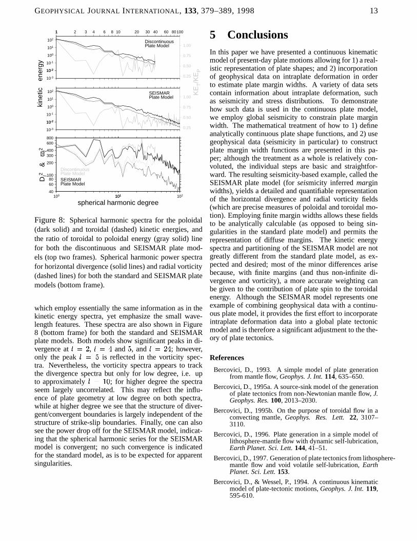
GEOPHYSICAL JOURNAL INTERNATIONAL, 133, 379–389, 1998 13
0.25
0.50
0.75
1.00
KE
T/K
EP
10-3
10-210-2
10-1
100
101
102en
ergy
11 2 3 4 6 8 10 20 30 40 60 80100
Discontinuous Plate Model
0.25
0.50
0.75
1.00
10-3
10-210-2
10-1
100
101
102
kine
tic SEISMAR Plate Model
40
6080
100
200
300400
600800
Dl2
&
ωl2
100 101101 102
spherical harmonic degree
DiscontinuousPlate ModelSEISMARPlate Model
Figure 8: Spherical harmonic spectra for the poloidal(dark solid) and toroidal (dashed) kinetic energies, andthe ratio of toroidal to poloidal energy (gray solid) linefor both the discontinuous and SEISMAR plate mod-els (top two frames). Spherical harmonic power spectrafor horizontal divergence (solid lines) and radial vorticity(dashed lines) for both the standard and SEISMAR platemodels (bottom frame).
which employ essentially the same information as in thekinetic energy spectra, yet emphasize the small wave-length features. These spectra are also shown in Figure8 (bottom frame) for both the standard and SEISMARplate models. Both models show significant peaks in di-vergence at " � � , " � �
and � , and " � � � ; however,only the peak " � � is reflected in the vorticity spec-tra. Nevertheless, the vorticity spectra appears to trackthe divergence spectra but only for low degree, i.e. upto approximately " � � ; for higher degree the spectraseem largely uncorrelated. This may reflect the influ-ence of plate geometry at low degree on both spectra,while at higher degree we see that the structure of diver-gent/convergent boundaries is largely independent of thestructure of strike-slip boundaries. Finally, one can alsosee the power drop off for the SEISMAR model, indicat-ing that the spherical harmonic series for the SEISMARmodel is convergent; no such convergence is indicatedfor the standard model, as is to be expected for apparentsingularities.
5 ConclusionsIn this paper we have presented a continuous kinematicmodel of present-day plate motions allowing for 1) a real-istic representation of plate shapes; and 2) incorporationof geophysical data on intraplate deformation in orderto estimate plate margin widths. A variety of data setscontain information about intraplate deformation, suchas seismicity and stress distributions. To demonstratehow such data is used in the continuous plate model,we employ global seismicity to constrain plate marginwidth. The mathematical treatment of how to 1) defineanalytically continuous plate shape functions, and 2) usegeophysical data (seismicity in particular) to constructplate margin width functions are presented in this pa-per; although the treatment as a whole is relatively con-voluted, the individual steps are basic and straightfor-ward. The resulting seismicity-based example, called theSEISMAR plate model (for seismicity inferred marginwidths), yields a detailed and quantifiable representationof the horizontal divergence and radial vorticity fields(which are precise measures of poloidal and toroidal mo-tion). Employing finite margin widths allows these fieldsto be analytically calculable (as opposed to being sin-gularities in the standard plate model) and permits therepresentation of diffuse margins. The kinetic energyspectra and partitioning of the SEISMAR model are notgreatly different from the standard plate model, as ex-pected and desired; most of the minor differences arisebecause, with finite margins (and thus non-infinite di-vergence and vorticity), a more accurate weighting canbe given to the contribution of plate spin to the toroidalenergy. Although the SEISMAR model represents oneexample of combining geophysical data with a continu-ous plate model, it provides the first effort to incorporateintraplate deformation data into a global plate tectonicmodel and is therefore a significant adjustment to the the-ory of plate tectonics.
References
Bercovici, D., 1993. A simple model of plate generationfrom mantle flow, Geophys. J. Int. 114, 635–650.
Bercovici, D., 1995a. A source-sink model of the generationof plate tectonics from non-Newtonian mantle flow, J.Geophys. Res. 100, 2013–2030.
Bercovici, D., 1995b. On the purpose of toroidal flow in aconvecting mantle, Geophys. Res. Lett. 22, 3107–3110.
Bercovici, D., 1996. Plate generation in a simple model oflithosphere-mantle flow with dynamic self-lubrication,Earth Planet. Sci. Lett. 144, 41–51.
Bercovici, D., 1997. Generation of plate tectonics from lithosphere-mantle flow and void volatile self-lubrication, EarthPlanet. Sci. Lett. 153.
Bercovici, D., & Wessel, P., 1994. A continuous kinematicmodel of plate-tectonic motions, Geophys. J. Int. 119,595-610.

GEOPHYSICAL JOURNAL INTERNATIONAL, 133, 379–389, 1998 14
DeMets, C., Gordon, R.G., Argus, D.F. & Stein, S., 1990.Current plate motions, Geophys J. Int., 101 425–478.
DeMets, C., Gordon, R.G., Argus, D.F., Stein, S., 1994. Ef-fect of recent revisions to the geomagnetic reversal timescale on estimates of current plate motions, Geophys.Res. Lett. 21, 2191-2194.
Hager, B.H., & O’Connell, R.J., 1978. Subduction zonedip angles and flow driven by plate motion, Tectono-physics, 50, 111–133.
Hager, B.H., & O’Connell, R.J., 1979. Kinematic modelsof large-scale flow in the Earth’s mantle, J. Geophys.Res., 84, 1031–1048.
Hager, B.H., & O’Connell, R.J., 1981. A simple global modelof plate dynamics and mantle convection, J. Geophys.Res., 86, 4843–4867.
O’Connell, R.J., Gable, C.W., & Hager, B.H., 1991. Toroidal-poloidal partitioning of lithospheric plate motion, inGlacial Isostasy, Sea Level and Mantle Rheology, editedby R. Sabadini and K. Lambeck, pp. 535–551, KluwerAcademic, Norwell, Mass.
Pollitz, F.F., 1988. Episodic North American and Pacificplate motions, Tectonics, 7, 711–726.
Rousseeuw, P.J. & Leroy, A.M., 1987. Robust Regressionand Outlier Detection, Wiley.
Sandwell, D.T. & Smith, W.H.F., 1997. Marine gravity anomalyfrom Geosat and ERS-1 satellite altimetry, J. Geophys.Res., 102, 10,039–10054.
Smith, W.H.F. & Sandwell, D.T., 1994. Bathymetric predic-tion from dense satellite altimetry and sparse shipboardbathymetry J. Geophys. Res., 99, 21,903-21,824.
Weissel, J.K., 1980. Evidence for Eocene oceanic crust in theCelebes Basin, in The Tectonic and Geologic Evolu-tion of Southeast Asian Seas and Islands, D.E. Hayes,ed., Geophysical Monograph 23, American Geophysi-cal Union, Washington DC, 37–47.
Wiens, D.A., DeMets, C., Gordon, R.G., Stein, S., Argus,D., Engeln, J.F., Lundgren, P., Quible, D., Stein, C.,Weinstein, S., & Woods, D.F., 1985. A diffuse plateboundary model for Indian ocean tectonics, Geophys.Res. Lett. 12, 429-432.
Zhong, S. & Gurnis, M. 1995a. Mantle convection withplates and mobile, faulted plate margins, Science 267,838–843.
Zhong,S. & Gurnis, M. 1995b. Towards a realistic simulationof plate margins in mantle convection, Geophys. Res.Lett. 22, 981–984.
Zhong, S. & Gurnis, M., 1996. Interaction of weak faults andnon-Newtonian rheology produces plate tectonics in a3D model of mantle flow, Nature 267, 838–843.
Zoback, M.L. & Burke, K., 1993. Lithospheric stress pat-terns: A global view, EOS Trans. AGU 74, 609-618.