a continuous surface tension force formulation for diﬀuse-interface...

Journal of Computational Physics 204 (2005) 784–804

www.elsevier.com/locate/jcp

A continuous surface tension force formulation fordiffuse-interface models

Junseok Kim *

Department of Mathematics, 103 Multipurpose Science and Technology Building, University of California, Irvine, CA 92697-3875, USA

Received 25 March 2004; received in revised form 14 October 2004; accepted 19 October 2004

Available online 30 November 2004

Abstract

We present a new surface tension force formulation for a diffuse-interface model, which is derived for incompress-

ible, immiscible Navier–Stokes equations separated by free interfaces. The classical infinitely thin boundary of separa-

tion between the two immiscible fluids is replaced by a transition region of small but finite width, across which the

composition of the one of two fluids changes continuously. Various versions of diffuse-interface methods have been

used successfully for the numerical simulations of two phase fluid flows. These methods are robust, efficient, and capa-

ble of computing interface singularities such as merging and pinching off. But prior studies used modified surface ten-

sion force formulations, therefore it is not straightforward to calculate pressure field because pressure includes the

gradient terms resulting from the modified surface tension term. The new formulation allows us to calculate the pressure

field directly from the governing equations. Computational results showing the accuracy and effectiveness of the method

are given for a drop deformation and Rayleigh capillary instability.

� 2004 Elsevier Inc. All rights reserved.

Keywords: Continuum surface tension; Diffuse-interface; Phase field

1. Introduction

In this paper, we derive a new surface tension force formulation for a diffuse-interface model of incom-

pressible, immiscible two-phase flow. The basic idea underlying the new formulation is to replace level set

based surface tension formulation [7] by an equivalent phase field form. The diffuse-interface method (see

the review paper [2] for the development and application of this model for both single-component and

0021-9991/$ - see front matter � 2004 Elsevier Inc. All rights reserved.

doi:10.1016/j.jcp.2004.10.032

* Tel.: +1 949 250 8993.

E-mail address: [email protected].

URL: http://www.math.uci.edu/~jskim.

mailto:[email protected].

J. Kim / Journal of Computational Physics 204 (2005) 784–804 785

binary fluids) is getting the growing popularity in solving multiphase fluid flows especially when the inter-

face undergoes extreme topological changes, e.g., merging or pinching off (see [4,17], and the references

therein). In this method, we introduce an order parameter c, which is a mass fraction of one of two phases.

The advantages of this approach are: (1) topology changes without difficulties; interfaces can either

merge or break up and no extra coding is required; (2) the composition field c has physical meaningsnot only on the interface but also in the bulk phases. Therefore, this method can be applied to many phys-

ical phase states such as miscible, immiscible, partially miscible, lamellar phases, to name a few. Fig. 1

shows evolution of the randomly oriented lamellar structure of block copolymers under steady shear flow

[16]; (3) it can be naturally extended to multicomponent systems (more than two components, e.g., ternary

system) and three space dimensions with straightforward manner [18]. Fig. 2 shows time sequence of two

droplets leaving interfaces under surface tension forces. This system consists of three immiscible, density

matched fluids, i.e., top and bottom fluid (I), middle fluid (II), and two droplets (III) between interfaces.

Surface tension between fluid I and III are greater than the other ones.The continuum surface force (CSF) formulation [6] is widely used in modeling surface tension force of

two phase fluid flows in volume-of-fluid (VOF) [10,11,26,32], level set method [7], and diffuse-interface

method [4,9]. In the CSF computational model, the surface tension is converted into a form of volume force

and the resulting force is proportional to the product of the interface gradient and the surface curvature.

The effects of surface tension are consequently included in the computational model through an external

forcing term added to the momentum equation.

In a level set method [7], the governing equation for the fluid velocity, u and the pressure, p can be writ-

ten as

qð/Þðut þ u � ruÞ ¼ �rp þr � ð2gð/ÞDÞ � rjð/Þdð/Þr/þ qð/Þg, ð1Þ
where q, g, D = ($u + $uT)/2, r, j, d, and g are the density, the viscosity, the deformation tensor, the sur-
face tension coefficient, the curvature, the Dirac delta function, and the gravity, respectively. The level set

function is denoted as / and it is taken positive in one phase and negative in the other phase. Therefore, the

Fig. 1. Evolution of the lamellar structure under shear flow.

Fig. 2. Evolution of two droplets leaving interfaces under surface tension forces.

786 J. Kim / Journal of Computational Physics 204 (2005) 784–804

interface of two fluids is the zero level set of /. Also, / is initialized to be the signed normal distance from

the interface. For simplicity of presentation, here we focus on density (which is taken to be 1) and viscosity

matched case. In the last example, we will present a bubble rising in the water to validate our scheme to the

case having large density and viscosity ratios. Then Eq. (1) becomes

ut þ u � ru ¼ �rp þ gDu� rjð/Þdð/Þr/:

In a diffuse-interface method [4,9], the governing equation can be written as

ut þ u � ru ¼ �rp þ gDuþ Fi, for i ¼ 1,2, or 3: ð2Þ
Here
F1 ¼ r�ar � ðjrcj2I �rc�rcÞ, ð3Þ

F2 ¼ra�lrc, ð4Þ

F3 ¼ � ra�crl, ð5Þ

where a is given in Eq. (14), � is a small positive parameter, I is the unit tensor dij, l is a chemical potential,

which is defined as

l ¼ F 0ðcÞ � �2Dc, ð6Þ

where F ðcÞ ¼ 14c2ð1� cÞ2. The term $c � $c is the usual tensor product, i.e. ðrc�rcÞij ¼ oc

oxiocoxj. In [15,19–

22,27], surface tension formulation F1 is used. In [3,9,12,34], F2 is used. F3 is used in [13,14,17]. In this

paper, we propose a new surface tension force formulation, F4.

F4 ¼ �rr � rcjrcj

� ��ajrcj2 rc

jrcj , ð7Þ

where r � rcjrcj

� �, �aj$cj2, and rc

jrcj correspond to j(/), d(/), and $/ in Eq. (1), respectively. This new formu-

lation idea is from the level set formulation.

The curvature of each level set is

j ¼ r � rcjrcj

� �¼ 1

jrcj Dc�rrc :rcjrcj �

rcjrcj

� �, ð8Þ

where the operator �:� is defined as A : B ¼P

ijaijbij. Therefore the Eqs. (3)–(5) can be rewritten as

F1 ¼ r�ar � ðjrcj2I �rc�rcÞ ¼ r�a �Dcrcþ 1

2rjrcj2

� �

¼ F4 � ra� rrc :rcjrcj �

rcjrcj

� �rc� 1

2rjrcj2

� �, ð9Þ

F2 ¼ra�lrc ¼ �ra�jjrcjrcþ ra

f ðcÞ�

� �rrc :rcjrcj �

rcjrcj

� �rc

¼ F4 þ raf ðcÞ�


rcjrcj

� �rc, ð10Þ

F3 ¼ � ra�crl ¼ ra

�ðlrc�rðclÞÞ ¼ F4 þ ra

f ðcÞ�


rcjrcj

� �rc� ra

�rðclÞ: ð11Þ


The previous numerical studies [3,9,12–15,19–22,27,34] with F1, F2, or F3 did not calculate pressure field

explicitly. It is evident from the above equations (9)–(11) that why previous works did not calculate pres-

sure field explicitly. It is partly due to the fact that all the pure gradient terms are absorbed in the pressure in

the formulations F1, F2, or F3.

Calculation of pressure field is important in some situations. For example, a circular hydraulic jump isformed when a vertical liquid jet impinges on a horizontal surface and spreads out radially on the surface.

In a study [35], they found that the pressure deviation from the hydrostatic equilibrium around the hydrau-

lic jump is essential for the structure formation and that the surface tension plays an important role for the

establishment of the pressure deviation.

For another example, let us consider a biomedical simulation which is one of the most important appli-

cations of computational fluid dynamics. The growth of the vascularized tumor depends vitally on the

nutrient transfer rate, the level of nutrient in the blood, and the blood pressure in the new capillaries.

The phase-field model for the sharp interfaced model [36] of a tumor growth can be written as

u� ��Du ¼ ��lrp � Fsf , ð12Þ
where �� is a constant, �l is cell mobility, and Fsf is a surface tension force. The authors in the paper [36]
tested the pressure field with the new surface tension force F4 and found a good agreement with the results

from the sharp interface model. The pressure field plays a key role in explaining the rate of nutrient transfer,

and hence the rate of growth of the tumor [36].

Here, we view the diffuse-interface model as a computational method. The most significant computa-tional advantage of this method is that explicit tracking of the interface is unnecessary. Note that only

the 1/2 level set of the concentration field is physically relevant as interface locations unlike most other

diffuse-interface models. This proposed diffuse-interface model is a hybrid method which combines a

level set type surface tension force formulation and a concentration relaxation by a diffuse-interface

model.

The main purpose of this paper is to introduce a new surface tension force formulation in diffuse-inter-

face models. The novel feature of this new formulation is that it permits the explicit calculation of pressure

field from the governing equations. The contents of this paper are: in Section 2 we discretize the new surfacetension force formulation. In Section 4 we present numerical experiments to validate our new surface ten-

sion formulation. The experiments are simulations of 2 dimensional drop, 3 dimensional drop under shear

flow, and axisymmetric thread breakup under capillary force. In Section 5, conclusions are given.

2. Discretization of the surface tension force formulation

In this section, we derive a discretization of the new surface tension force and for simplicity, we present itin 2D and 3D case is a straightforward extension. Let the surface tension formulation (7) be rewritten as

F4 ¼ �r�ar � rcjrcj

� �jrcjrc: ð13Þ

We want the concentration field, c, to be locally equilibrium state during evolution. To match the surface

tension of the sharp interface model, a must satisfy

�aZ 1

�1ðceqx Þ

2dx ¼ 1, ð14Þ

where ceqðx,yÞ ¼ ½1þ tanhðx=ð2ffiffiffi2

p�ÞÞ�=2 is an equilibrium composition profile in the infinite domain when

the chemical potential is given as Eq. (6) [14] and it is a good approximation in the finite domain. Therefore

from Eq. (14), we get a ¼ 6ffiffiffi2

p.


Let a computational domain be partitioned in Cartesian geometry into a uniform mesh with mesh

spacing h. The center of each cell, Xij, is located at (xi,yj) = ((i � 0.5)h,(j � 0.5)h) for i = 1, . . ., M and

j = 1, . . ., N. M and N are the numbers of cells in x and y-directions, respectively. The cell vertices are

located at ðxiþ12,yjþ1

2Þ ¼ ðih,jhÞ. Vertex-centered normal vectors are obtained by differentiating the phase

field in the four surrounding cells. For example, the normal vector at the top right vertex of cell Xij isgiven by

niþ12,jþ1

2¼ nxiþ1

2,jþ1

2,ny

iþ12,jþ1

2

� �¼ ciþ1,j þ ciþ1,jþ1 � cij � ci,jþ1

2h,ci,jþ1 þ ciþ1,jþ1 � cij � ciþ1,j

2h

� �:

The curvature (8) is calculated at cell centers from the vertex-centered normals and is given by

jðcijÞ ¼ rd �n

jnj

� �ij

¼ 1

2h

nxiþ1

2,jþ1

2

þ nyiþ1

2,jþ1

2

jniþ12,jþ1

2j þ

nxiþ1

2,j�1

2

� nyiþ1

2,j�1

2

jniþ12,j�1

2j �

nxi�1

2,jþ1

2

� nyi�1

2,jþ1

2

jni�12,jþ1

2j �

nxi�1

2,j�1

2

þ nyi�1

2,j�1

2

jni�12,j�1

2j

!,

where $dÆ is a finite difference approximation to the divergence operator. And the cell-centered normal is the

average of vertex normals,

rdcij ¼ niþ12,jþ1

2þ niþ1

2,j�1

2þ ni�1

2,jþ1

2þ ni�1

2,j�1

2

� �=4,

where $d is a finite difference approximation to the gradient operator. Therefore, the discretization of the

proposed surface tension force formulation F4 is

F4ðcijÞ ¼ �r�ard �n

jnj

� �ij

jrdcijjrdcij:

3. Numerical experiment without flow

Let us consider equilibrium of a drop placed within another fluid. Let the drop composition be defined as

cðx,yÞ ¼ 1

21þ tanh

1�ffiffiffiffiffiffiffiffiffiffiffiffiffiffix2 þ y2

p2ffiffiffi2

p�

!: ð15Þ

We define the interface location to be the position of the level set c = 0.5. Fig. 3(a) shows composition

field (15) of an unit circle along with the interface (solid line).

In equilibrium state of a droplet, velocity vanishes (u ” 0) and therefore the governing Eq. (2) reduces to

Eq. (16) and therefore pressure gradient should balance surface tension force.

rp ¼ �r�a r � rcjrcj

� �jrcjrc

� �: ð16Þ

We solve Eq. (17) numerically by taking divergence operator to Eq. (16) with r = 1, 256 · 256 mesh,

computational domain X = [�4,4] · [�4,4], and � = 0.03.

Dp ¼ �r�ar � r � rcjrcj

� �jrcjrc

� �, ð17Þ

where we discretize Dp by

Ddpiþ12,jþ1

2¼ ðpi�1

2,jþ3

2þ piþ1

2,jþ3

2þ piþ3

2,jþ3

2þ pi�1

2,jþ1

2� 8piþ1

2,jþ1

2þ piþ3

2,jþ1

2þ pi�1

2,j�1

2þ piþ1

2,j�1

2þ piþ3

2,j�1

2Þ=ð3h2Þ:

0

1

2

00.511.52

0

0.2

0.4

0.6

0.8

1

(a)

0 0.5 1

0

0.5

1 1.0

1.0

1.0

1.0

3.0

3.0

0.3

3.0

5.0

5.0

5.0

5.0

0.7

7.0

7.0

7.0

9.0

9.0

9.0

9.0

(b)

Fig. 3. (a) Composition field along with contour plot c(x,y) = 0.5. (b) Contour plots of pressure field.


From Laplace�s formulation we can obtain the theoretical prediction of the pressure-jump inside an infi-

nite cylinder as Dptheor = r/R, where r is surface tension coefficient and R is the cylinder radius. Fig. 3(b)

shows isocontour of the pressure field at (p = 0.1, 0.3, 0.5, 0.7, 0.9) along with composition (solid circles) atc = 0.1 and 0.9. Pressure changes within interface region and Laplace�s law is well verified.

Fig. 4(a) shows numerically calculated curvature around interface region along with the exact one, ��,defined by $ Æ ($c/j$cj) on the ellipsoid x2

4þ y2 ¼ 1 (solid line). Fig. 4(b) shows contour plots (dotted lines)

of the pressure field around the ellipsoid x2

4þ y2 ¼ 1 (solid line).

4. Numerical experiments with flow

In this section we present 2D, 3D, and axisymmetric flow simulations to demonstrate the flexibility and

accuracy of the new surface tension formulation. For completeness, we describe numerical solution proce-

dure for 2D. 3D is straightforward extension and axisymmetric case is given in detail in [15]. The nondi-

mensional governing equations, Navier–Stokes–Cahn–Hilliard equations (NSCH), are

r � u ¼ 0, ð18Þ

ut þ u � ru ¼ �rp þ 1

Rer � ½gðcÞðruþruTÞ� � �a

Wer � rc

jrcj

� �jrcjrc, ð19Þ

ct þ u � rc ¼ 1

Per � ðMðcÞrlÞ, ð20Þ

l ¼ f ðcÞ � CDc, ð21Þ
where the dimensionless parameters are Reynolds number, Re = q*V*L*/g*, Weber number,
We ¼ q�L�V 2�=r, Cahn number, C = �2/l*, and diffusional Peclet number, Pe = L*V*/(M*l*). The values

with lower * are characteristic values of corresponding ones. M(c) is a composition dependent mobility

and is defined by M(c) = c(1 � c) [8].

0 1 2 3

0

2

0

0.5

1

1.5

2

2.5

3

3.5

4

4.5

(a)

0 1 2 3

0

1

2

3

2.0

1.0

1.00

0

0

1.0

1.0

1.0

2.0

2.0

2.0

5.0

5.0

5.0

6.0

6.0

7.0

(b)

Fig. 4. (a) Numerically calculated curvature around interface region along with the exact one �� on the ellipsoid x2


(b) Contour plots (dotted line) of pressure field around the ellipsoid x2



4.1. Numerical procedure

Our strategy for solving the system (18)–(21) is a fractional step scheme having two parts: first we solve

the momentum and composition equations (19)–(21) without strictly enforcing the incompressibility con-

straint (18), then we approximately project the resulting velocity field onto the space of discretely diver-

gence-free vector fields [5].The discrete velocity field unij and composition field cnij are located at cell centers. The pressure p

n�12

iþ12,jþ1

2

is

located at cell corners. The notation unij is used to represent an approximation to u(xi,yj,tn), where tn = nDt

and Dt is a time step. Likewise, pn�1

2

iþ12,jþ1

2

is an approximation to pðxi þ h2,yj þ h

2,tn � Dt

2Þ.

The time-stepping procedure is based on the Crank–Nicholson type method. At the beginning of each

time step, given un� 1,un, cn� 1, cn, and pn�12, we want to find un+1, cn+1, and pnþ

12 which solve the following

second-order temporal discretization of the equation of motion:

unþ1 � un

Dt¼ �rdpnþ

12 þ 1

2Rerd � gðcnþ1Þ½rdu

nþ1 þ ðrdunþ1ÞT� þ 1

2Rerd � gðcnÞ½rdu

n þ ðrdunÞT�

þ Fnþ12 � ðu � rduÞnþ

12,

cnþ1 � cn

Dt¼ 1

Perd � ðMðcnþ1

2Þrdlnþ1

2Þ � ðu � rdcÞnþ12, ð22Þ

lnþ12 ¼ 1

2½f ðcnÞ þ f ðcnþ1Þ� � C

2Ddðcn þ cnþ1Þ, ð23Þ

where Fnþ12 is the surface tension force term and the updated flow field satisfies the incompressibility

condition

rd � unþ1 ¼ 0:


The outline of the main procedures in one time step is as follows.

Step 1. Initialize c0 to be the locally equilibrated composition profile and u0 to be the divergence-free veloc-

ity field.

Step 2. The half time values unþ12 and cnþ

12 are calculated using an extrapolation from previous values, i.e.,

unþ12 ¼ ð3un � un�1Þ=2 and cnþ

12 ¼ ð3cn � cn�1Þ=2. With these half time values, we calculate

ðu � rdcÞnþ12 by using a second order ENO scheme [28].

Step 3. Update the composition field cn to cn+1 by solving the discrete Cahn–Hilliard (CH) Eqs. (22) and

(23). Details of this step, which use a nonlinear multigrid method and a second order accurate dis-

cretization in time and space, are presented in Section 4.1.1. Once cn+1 is obtained, we compute

cnþ12 ¼ ðcnþ cnþ1Þ=2 and g(cn+1).

Step 4. Compute ðu � rduÞnþ12 by using a second order ENO scheme and Fnþ1

2 with cnþ12.

Step 5. We solve

u� � un

Dt¼ �rdpn�

12 þ 1

2Rerd � gðcnþ1Þ½rdu

� þ ðrdu�ÞT� þ 1

2Rerd � gðcnÞ½rdu

n þ ðrdunÞT�

þ Fnþ12 � ðu � rduÞnþ

12 ð24Þ

using a multigrid method for the intermediate velocity u* without strictly enforcing the incompress-

ibility constraint.

Step 6. Project u* onto the space of discretely divergence-free vector fields and get the velocity un+1, i.e.,

u* = un+1 + Dt$d/, where / satisfies Dd/ ¼ rd � u��un

Dt .

Step 7. Update pressure, pnþ12 ¼ pn�

12 þ /. These complete one time step.

4.1.1. Cahn–Hilliard equation with advection – a nonlinear multigrid method

In this section, we describe a nonlinear full approximation storage (FAS) multigrid method to solve the

nonlinear discrete system (22) and (23) at the implicit time level. The nonlinearity is treated using one step

of Newton�s iteration and a pointwise Gauss–Seidel relaxation scheme is used as the smoother in the mul-

tigrid method. See the reference text [33] for additional details and background. The algorithm of the non-

linear multigrid method for solving the discrete CH system is:

First, let us rewrite Eqs. (22) and (23) as follows.

NSOðcnþ1,lnþ12Þ ¼ ð/n,wnÞ,

where

NSOðcnþ1,lnþ12Þ ¼ cnþ1

Dt� 1

Perd � ðMðcnþ1

2Þrdlnþ1

2Þ,lnþ12 � 1

2f ðcnþ1Þ þ C

2Ddcnþ1

� �
and the source term is ð/n,wnÞ ¼ ðcnDt � ðu � rdcÞnþ
12, 1

2f ðcnÞ � C

2DdcnÞ.

In the following description of one FAS cycle, we assume a sequence of grids Xk (Xk� 1 is coarser than Xk

by factor 2). Given the number m of pre- and post-smoothing relaxation sweeps, an iteration step for the

nonlinear multigrid method using the V-cycle is formally written as follows [33]:

4.1.1.1. FAS multigrid cycle.n o � �
cmþ1k ,l
mþ12

k ¼ FAScycle k,cnk ,cmk ,l

m�12

k ,NSOk,/nk ,w

nk ,m :

That is, cmk ,lm�1

2

k

n oand cmþ1

k ,lmþ1

2

k

n oare the approximations of cn+1(xi,yj) and lnþ1

2ðxi,yjÞ before and after

an FAScycle. Now, define the FAScycle.


(1) Presmoothing

�cmk ,�lm�1

2

k

n o¼ SMOOTHm cnk ,c

mk ,l

m�12

k ,NSOk,/nk ,w

nk

� �,

which means performing m smoothing steps with the initial approximations cmk , lm�1

2

k , cnk , source terms /nk , w

nk ,

and SMOOTH relaxation operator to get the approximations �cmk , �lm�1

2

k : One SMOOTH relaxation operator

step consists of solving the system (27) and (28) given below by 2 · 2 matrix inversion for each i and j. Here,

we derive the smoothing operator in two dimensions. Rewriting Eq. (22), we get

cnþ1ij

DtþM

nþ12

iþ12,j þM

nþ12

i�12,j þM

nþ12

i,jþ12

þMnþ1

2

i,j�12

h2Pelnþ1

2ij ¼ /n

ij þM

nþ12

iþ12,jl

nþ12

iþ1,j þMnþ1

2

i�12,jl

nþ12

i�1,j þMnþ1

2

i,jþ12

lnþ1

2

i,jþ1 þMnþ1

2

i,j�12

lnþ1

2

i,j�1

h2Pe:

ð25Þ
Since f ðcnþ1
ij Þ is nonlinear with respect to cnþ1ij , we linearize f ðcnþ1

ij Þ at cmij , i.e.,

f ðcnþ1ij Þ � f ðcmijÞ þ

df ðcmijÞdc

ðcnþ1ij � cmijÞ:

After substitution of this into (23), we get

� 2C

h2þdf ðcmijÞ2dc

� �cnþ1ij þ l

nþ12

ij ¼ wnij þ

1

2f ðcmijÞ �

df ðcmijÞ2dc

cmij �C

2h2ðcnþ1

iþ1,j þ cnþ1i�1,j þ cnþ1

i,jþ1 þ cnþ1i,j�1Þ: ð26Þ

Next, we replace cnþ1kl and l

nþ12

kl in the Eqs. (25) and (26) with �cmkl and �lm�1

2

kl if k 6 i and l 6 j, otherwise with

cmkl and lm�1

2

kl , i.e.,

�cmijDt

þM

m�12

iþ12,j þM

m�12

i�12,j þM

m�12

i,jþ12

þMm�1

2

i,j�12

h2Pe�lm�1

2ij ¼ /n

ij þM

m�12

iþ12,jl

m�12

iþ1,j þMm�1

2

i�12,j�l

m�12

i�1,j þMm�1

2

i,jþ12

lm�1

2

i,jþ1 þMm�1

2

i,j�12

�lm�1

2

i,j�1

h2Pe,

ð27Þ

where Mm�1

2

iþ12,j ¼ Mððcmij þ cmiþ1,j þ cnij þ cniþ1,jÞ=4Þ and the other terms are similarly defined.

� 2C

h2þdf ðcmijÞ2dc

� ��cmij þ �l

m�12

ij ¼ wnij þ

1

2f ðcmijÞ �

df ðcmijÞ2dc

cmij �C

2h2ðcmiþ1,j þ �cmi�1,j þ cmi,jþ1 þ �cmi,j�1Þ: ð28Þ

(2) Compute the defect

ð�dm1 k,

�dm2 kÞ ¼ ð/n

k ,wnkÞ �NSOkð�cmk ,�l

m�12

k Þ: ð29Þ
(3) Restrict the defect and �cmk ,�l
m�12

k

n o
ð�dm
1 k�1,�dm2 k�1Þ ¼ Ik�1

k ð�dm1 k,

�dm2 kÞ,ð�d

mk 1,�l

m�12

k�1 Þ ¼ Ik�1k ð�cmk ,�l

m�12

k Þ:
The restriction operator Ik�1
k maps k-level functions to (k � 1)-level functions.

dk�1ðxi,yjÞ ¼ Ik�1k dkðxi,yjÞ ¼

1

4½dkðxi�1

2,yj�1

2Þ þ dkðxi�1

2,yjþ1

2Þ þ dkðxiþ1

2,yj�1

2Þ þ dkðxiþ1

2,yjþ1

2Þ�:

(4) Compute the right-hand side

ð/nk�1,w

nk�1Þ ¼ ð�dm

1 k�1,�dm2 k�1Þ þNSOk�1ð�cmk�1,�l

m�12

k�1 Þ:
(5) Compute an approximate solution cmk�1,l
m�12

k�1

n oof the coarse grid equation on Xk� 1, i.e.

NSOk�1ðcmk�1,lm�1

2

k�1 Þ ¼ ð/nk�1,w

nk�1Þ: ð30Þ


If k = 1, we explicitly invert a 2 · 2 matrix to obtain the solution. If k > 1, we solve (30) by performing a

FAS k-grid cycle using �cmk�1,�lm�1

2

k�1

n oas an initial approximation:

1n o

1� �

cmk�1,lm�

2

k�1 ¼ FAScycle k � 1,cnk�1,�cmk�1,�l

m�2

k�1 ,NSOk�1,/nk�1,w

nk�1,m :

(6) Compute the coarse grid correction (CGC):

vm1k�1 ¼ cmk�1 � �cmk�1, vm�1

2

2k�1 ¼ lm�1

2

k�1 � �lm�1

2

k�1 :

(7) Interpolate the correction: vm1k ¼ Ikk�1vm1k�1, v

m�12

2k ¼ Ikk�1vm�1

2

2k�1:Here, the coarse values are simply transferred to the four nearby fine grid points, i.e.

vkðxi,yjÞ ¼ Ikk�1vk�1ðxi,yjÞ ¼ vk�1ðxiþ12,yjþ1

2Þ for i and j odd-numbered integers.

(8) Compute the corrected approximation on Xk

cm,after CGCk ¼ �cmk þ vk1m, l

m�12,after CGC

k ¼ �lm�1

2

k þ vm�1

2

2k :

(9) Postsmoothing

cmþ1k ,l

mþ12

k

n o¼ SMOOTHm cnk ,c

m,after CGCk ,l

m�12,after CGC

k ,NSOk,/nk ,w

nk

� �:

This completes the description of a nonlinear FAScycle.

We find that convergence of the multigrid method can be achieved with time steps that depend very

weakly on the spatial grid size. In particular, convergence is obtained if Dt � h. We define the convergence

criterion as a discrete l2-norm of the difference between mth and (m + 1)th-iterations becomes less than a

tolerance, 10�7. That is,

kcmþ1 � cmk 6 10�7, where kck ¼ h

ffiffiffiffiffiffiffiffiffiffiffiffiffiXM,Nij

c2ij

vuut :

The typical number of iterations with the tolerance for the solver to converge is two or three V(1,1)-

cycles. For more detailed analysis and notations, see the paper [17]. One should note that there are a couple

of differences between the previous paper [17] and this work. First, treatment of nonlinear term, in the pre-

vious one, we used a Taylor series expansion, but in this work, we use analytic derivatives. Second, we use a

concentration dependent variable mobility here, which was taken as constant in the previous paper. Thelocal mode Fourier analysis for the relaxation step can be done in a similar way as being done in the paper

[17].

4.2. Numerical experiments and validation

In this section, we validate our scheme by verifying the second-order convergence, spurious currents,

capillary wave, three dimensional drop deformation in a shear flow, Rayleigh-capillary instability, and a

rising bubble problem with high density and viscosity ratios.

4.2.1. Convergence test

To obtain an estimate of the rate of convergence, we perform a number of simulations for a sample

initial problem on a set of increasingly finer grids. The initial concentration field is

Table

l2-norm

Case

u

v


cðx,yÞ ¼ 1� 1

2tanh

y � 0:25

2ffiffiffi2

p�

� �þ tanh

0:75� y

2ffiffiffi2

p�

� �� ð31Þ

and initial velocity field is a double shear layer taken from [5]

uðx,yÞ ¼tanhð30ðy � 0:25ÞÞ for y 6 0:5,

tanhð30ð0:75� yÞÞ for y > 0:5,

�vðx,yÞ ¼ 0:05 sinð2pxÞ,

on a square domain, [0,1] · [0,1]. Thus, the initial flow field consists of a horizontal shear layer of finite

thickness, perturbed by a small amplitude vertical velocity. The numerical solutions are computed on

the uniform grids, Dx = Dy = h = 1/2n for n = 5, 6, 7, 8, and 9. For each case, the convergence is measured

at time t = 0.25 with the uniform time steps, Dt = 0.25h. The viscosity g is constant and Re = 100, Pe = 10,

and We = 100. For the interface parameter �, we want to have smaller � as the grid size h is refined. One

possible choice is � = O(hk), where k satisfy the condition, 0 < k 6 1. Note that k cannot be greater thanone because we also want to have a finite number of grid points across interface to accurately calculate sur-

face tension term. For the convergence test, we choose k = 1/2, i.e., � ¼ 0:02ffiffiffiffiffiffiffiffi32h

p.

In our formulation of the method for the NSCH equation, since a cell centered grid is used, we define the

error to be the discrete l2-norm of the difference between that grid and the average of the next finer grid cells

covering it:

eh=h2ij

¼def uhij � uh22i,2j

þ uh22i�1,2j

þ uh22i,2j�1

þ uh22i�1,2j�1

� �=4:

The rate of convergence is defined as the ratio of successive errors:

log2ðkeh=h2k=keh

2=h4kÞ:

In Table 1, the errors and rates of convergence are shown for the velocity components u and v, respec-

tively. Observe that these quantities converge with second order accuracy.

Also in Fig. 5, the time evolution is shown with mesh size 128 · 128. In Fig. 6, we plot the interface loca-

tion on the lower half of the domain with dotted line (32 · 32), dashed line (64 · 64), and solid line

(128 · 128). The convergence of the results under grid refinement is evident.

4.2.2. Numerical results on spurious currents

Spurious or parasite currents are described in [30] as vortices ‘‘in the neighborhood of interface despite

the absence of any external forcing.’’ They are observed with many surface tension simulation methods

including the CSF method. In this section, we test our new surface tension formulation with the similar

test problem in [25]. The computational domain is 1 · 1 and the time step is Dt = 10�5. The boundary

conditions are zero velocity at the top and bottom walls, and periodicity in x-direction. Initially, a cir-

cular drop is centered at (0.5,0.5), with radius a = 0.25 and surface tension coefficient r = 0.357. Bothfluids have equal density, 4, and viscosity, 1. The initial velocity field is zero. The exact solution is zero

1

of the errors and convergence rates for velocity (u,v)

32–64 Rate 64–128 Rate 128–256 Rate 256–512

3.5081e�3 1.89 9.4397e�4 1.99 2.3771e�4 1.95 6.1579e�5

1.0145e�4 1.72 3.0805e�5 1.92 8.1282e�6 1.97 2.0742e�6

Fig. 5. Evolution of interface from the initial condition (31) with � = 0.01. The times are t = 0, 0.5, 1.5, 2.5, and 5.

0 0.1 0.2 0.3 0.4 0.5 0.6 0.7 0.8 0.9 10

0.05

0.1

0.15

0.2

0.25

0.3

0.35

0.4

0.45

0.5

Fig. 6. The interface location on the lower half of the domain. Dotted line 32 · 32, dashed line 64 · 64, and solid line 128 · 128.


velocity for all time. In dimensionless terms, the relevant parameter is the Ohnesorge number

Oh ¼ g=ffiffiffiffiffiffiffiffirqa

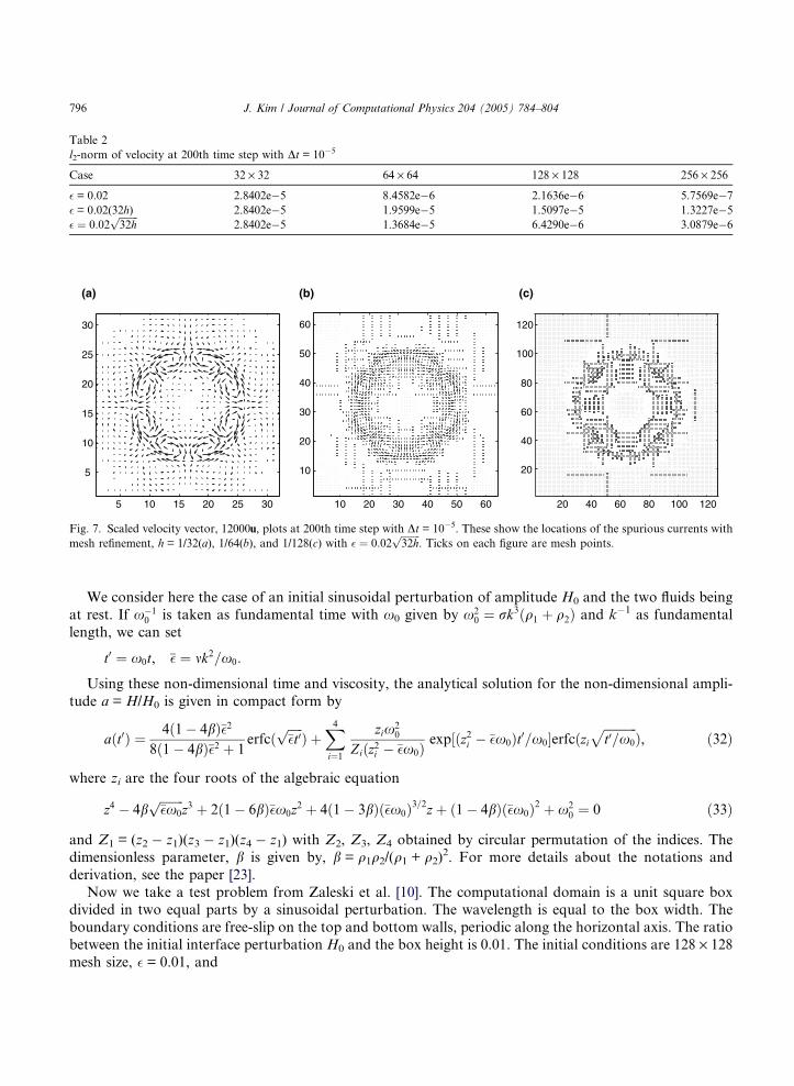
p � 1:6737.Table 2 shows three convergence cases of the spurious currents as we refine the mesh size. The first case

(� = 0.02) shows almost second order convergence of the spurious velocity when we fix � with refining mesh

size. The second case (� = 0.02(32h)) shows minor decreases as we refine the mesh. This is due to the fact

that the number of grid points across interface is linearly proportional to �. Therefore, we have same num-

ber of grid points across the interface but more grid points tangentially to the interface. The third case

ð� ¼ 0:02ffiffiffiffiffiffiffiffi32h

pÞ shows a linear convergence of the spurious currents. This case is between two extreme

cases, i.e., the first and the third ones. It does refine interface thickness as the mesh size refines, but com-

pared to fixed � the convergence rate reduces from second to first order.In Fig. 7, scaled velocity vector, 12000u, plots at 200th time step with Dt = 10�5 are shown. These show

the locations of the spurious currents with mesh refinement, h = 1/32(a), 1/64(b), and 1/128(c) with

� ¼ 0:02ffiffiffiffiffiffiffiffi32h

p. The convergence of the spurious currents is evident as we refine the mesh size h and interface

parameter �.

4.2.3. Capillary wave

Another important test for the surface tension force is the comparison with the solution of the damped

oscillations of a capillary wave. As shown by Prosperetti [23], an analytical solution exists for the initial-value problem in the case of the small-amplitude waves on the interface between two superposed viscous

fluids, provided the fluids have the same dynamic viscosity.

5 10 15 20 25 30

5

10

15

20

25

30

(a)

10 20 30 40 50 60

10

20

30

40

50

60

(b)

20 40 60 80 100 120

20

40

60

80

100

120

(c)

Fig. 7. Scaled velocity vector, 12000u, plots at 200th time step with Dt = 10�5. These show the locations of the spurious currents with

mesh refinement, h = 1/32(a), 1/64(b), and 1/128(c) with � ¼ 0:02ffiffiffiffiffiffiffiffi32h

p. Ticks on each figure are mesh points.

Table 2

l2-norm of velocity at 200th time step with Dt = 10�5

Case 32 · 32 64 · 64 128 · 128 256 · 256

� = 0.02 2.8402e�5 8.4582e�6 2.1636e�6 5.7569e�7

� = 0.02(32h) 2.8402e�5 1.9599e�5 1.5097e�5 1.3227e�5

� ¼ 0:02ffiffiffiffiffiffiffiffi32h

p2.8402e�5 1.3684e�5 6.4290e�6 3.0879e�6


We consider here the case of an initial sinusoidal perturbation of amplitude H0 and the two fluids being

at rest. If x�10 is taken as fundamental time with x0 given by x2

0 ¼ rk3ðq1 þ q2Þ and k�1 as fundamental

length, we can set

t0 ¼ x0t, �� ¼ mk2=x0:

Using these non-dimensional time and viscosity, the analytical solution for the non-dimensional ampli-

tude a = H/H0 is given in compact form by

aðt0Þ ¼ 4ð1� 4bÞ��28ð1� 4bÞ��2 þ 1

erfcðffiffiffiffiffi��t0

pÞ þ

X4i¼1

zix20

Ziðz2i � ��x0Þexp½ðz2i � ��x0Þt0=x0�erfcðzi

ffiffiffiffiffiffiffiffiffiffiffit0=x0

pÞ, ð32Þ

where zi are the four roots of the algebraic equation

z4 � 4bffiffiffiffiffiffiffiffi��x0

pz3 þ 2ð1� 6bÞ��x0z2 þ 4ð1� 3bÞð��x0Þ3=2zþ ð1� 4bÞð��x0Þ2 þ x2

0 ¼ 0 ð33Þ

and Z1 = (z2 � z1)(z3 � z1)(z4 � z1) with Z2, Z3, Z4 obtained by circular permutation of the indices. The

dimensionless parameter, b is given by, b = q1q2/(q1 + q2)2. For more details about the notations and

derivation, see the paper [23].

Now we take a test problem from Zaleski et al. [10]. The computational domain is a unit square boxdivided in two equal parts by a sinusoidal perturbation. The wavelength is equal to the box width. The

boundary conditions are free-slip on the top and bottom walls, periodic along the horizontal axis. The ratio

between the initial interface perturbation H0 and the box height is 0.01. The initial conditions are 128 · 128

mesh size, � = 0.01, and

Fig. 8.

initial-


cðx,yÞ ¼ 1

21� tanh

y � 0:5� 0:01 cosð2pxÞ2ffiffiffi2

p�

� �,

uðx,yÞ ¼ vðx,yÞ ¼ 0:

Let Oh ¼ 1=ffiffiffiffiffiffiffiffiffiffi3000

p, the non-dimensional viscosity �� ¼ mk2=x0 � 6:472 10�2, frequency x0 = 6.778, and

the two fluid densities are the same.

Fig. 8 shows the evolution of the amplitude with time for the numerical solution (circles) and the initial-

value analytical solution (solid line). The numerical results with surface tension formulations (F1, F2, and

F4) are identical within the tolerance, 10�7. But the numerical calculation blows up in finite time with the

formulation F3 because the chemical potential is not smooth. At early times there is excellent agreement

between the theory and simulation. The results slightly deviate when nonlinearity becomes dominant at

later times.

In [10], the error is a function of the grid size h and of the initial wave amplitude H0. They have studiedhow varying the grid size h and the ratio h/H0 influences the convergence toward the analytical solution

with a VOF method. When h/H0 is much larger than 1, the wave amplitude is no longer resolved by the

grid and the numerical results diverge. For sufficiently small h, typically from 1282 to 5122, there may be

convergence but at a sublinear rate.

4.2.4. Three dimensional drop deformation in a shear flow

We consider a 3D spherical drop in a shear flow. This is a classical problem that was solved analytically

for sharp interfaces and small deformations in the creeping flow approximation by Taylor [31]. The drop

0 5 10 15 20 25

0

0.002

0.004

0.006

0.008

0.01 simulationtheory

Time evolution of the amplitude of a capillary wave. The theoretical curve (solid line) is obtained from the exact solution to the

value problem in the linearized Navier–Stokes equations.


will assume the shape of an ellipsoid with a deformation that depends on the capillary number and the vis-

cosity ratio.

Taylor [31] found that, when deformation due to the externally imposed shear flow and interfacial relax-

ation balance one another, the deformation parameter D = (l � s)/(l + s) is related to the capillary number

Ca ¼ g _ca=r, where _c is the local shear rate, g is the viscosity of the ambient fluid, a (see Fig. 9(a)) is the dropradius, and r is the surface tension as

D ¼ 19kþ 16

16kþ 16Ca, ð34Þ

where l, s (see Fig. 9(b)) and k denote the longest and shortest axes of the ellipsoid in the shear gra-dient plane, and the viscosity ratio, respectively. Now we perform 3D simulations with a mesh size

128 · 64 · 128 and a computational domain X = [�4,4] · [�2,2] · [�4,4]. The initial conditions are

cðx,y,zÞ ¼ 1

21þ tanh

1�ffiffiffiffiffiffiffiffiffiffiffiffiffiffiffiffiffiffiffiffiffiffiffiffix2 þ y2 þ z2

p2ffiffiffi2

p�

!,

uðx,y,zÞ ¼ z, vðx,y,zÞ ¼ wðx,y,zÞ ¼ 0, ð35Þ

_c ¼ 1, k = 1, g = 1, � = 0.04 and time step Dt = 0.005 are used.

Fig. 10 shows cross-sectional slice in the x–z plane through the center of the drop for steady-state solu-

tion (Ca = 0.3) in simple shear along with velocity field. Table 3 shows comparison of Taylor deformationnumber D obtained by numerical simulations with linear theory. It can be seen that the numerical results

are in good agreement with the analytic expression (34).

4.2.5. Axisymmetric immiscible two phase flow: Rayleigh-instability

Surface tension causes the fluid to have as little surface area as possible for a given volume. A long slen-

der column of liquid reduce its surface area by breaking up into a series of small droplets, which have less

surface area than the cylinder. This effect is known as the ‘‘Rayleigh instability’’ [24].

We will consider a long cylindrical thread of a viscous fluid 1, the viscosity and density of which aredenoted by gi and qi, respectively, in an infinite mass of another viscous fluid 2 of viscosity go and qo. Inthe unperturbed state, the interface has a perfectly cylindrical shape with a circular cross-section of radius

a

x

yz

(a)

l

s

(b)

Fig. 9. (a) Schematic of a drop. (b) Schematic of scalar measures of deformation.

Fig. 10. Cross-sectional slice in the x–z plane through the center of the drop for steady-state solution (Ca = 0.3) in simple shear along

with velocity field.

Table 3

Comparison of Taylor deformation number D with linear theory

Case Ca = 0.1 Ca = 0.2 Ca = 0.3

Numerical simulation 0.1143 0.2188 0.3124

Linear theory 0.1094 0.2137 0.3281


a. In this simulation, an initially cosinusoidal perturbation with an amplitude a0 to the thread radius a is

given by

RðzÞ ¼ aþ a0 cosðkzÞ:
In Fig. 11, these parameters are shown schematically. The domain is axisymmetric and the bottom
boundary is the axis of symmetry.

The initial concentration field and velocity fields are given by

c0ðr,zÞ ¼ 0:5 1� tanhr � 0:5� 0:05 cosðzÞ

2ffiffiffi2

p�

� �� ,

u0ðr,zÞ ¼ w0ðr,zÞ ¼ 0

0 1 2 3 4 5 60

0.5

1

1.5

→↑rz

Fluid 1, ρi , η

i

Fluid 2, ρo , η

o

R

↑

↓a↑

↓

α0↑↓

Fig. 11. Schematic of a cylindrical thread of viscous fluid 1 embedded in another viscous fluid 2.


on a domain, X = {(r,z)j0 6 r 6 p and 0 6 z 6 2p}. In this computation we use the parameters: a = 0.5,

a(0) = 0.05, k = 1, � = 0.02, Re = 0.32, We = 0.032, Pe = 1, and viscosity ratio b = 1. Mesh size 128 · 256

and time step Dt = 0.001 are used. For more detailed description and numerical solution, see [15].

An example of the long time evolution of the interface profile is shown in Fig. 12. In the early states

(t = 0.125 and 3.125) the surface contour has only one minimum at exactly z = p. As the time increases,nonlinearities become important and the initially cosinusoidal shape of the interface changes to a more

complex form. The zone of the minimum moves symmetrically off the center (z = p), giving rise to a satellite

drop.

In Fig. 13, we plot the c = 0.5 contours overlaid with (a) vorticity field and (b) pressure contour lines

(higher value in the middle of the thread) at time t = 3.125. Positive and negative vorticities are given by

solid and dotted curves, respectively. In Fig. 13(b), the pressure field is high in the center of the thread,

which forces fluid to move to symmetrically off the center.

Fig. 12. Time evolution leading to multiple pinch-offs is shown (from top to bottom and left to right). The dimensionless times are at

t = 0.125, 3.125, 4.0, 4.25, 4.375, and 6.375. Viscosity ratio is 1, � = 0.02, Pe = 1, Re = 0.32, and We = 0.032.

(a) (b)

Fig. 13. The c = 0.5 contours overlaid with (a) vorticity field and (b) pressure field at time t = 3.125.


In Fig. 14, we plot the c = 0.5 contours overlaid with (a) vorticity field and (b) pressure contour lines at

time t = 4.0. In Fig. 14(a), as two minima in the thread develop, the surface tension force produces oppo-

sitely signed vortex rings along the interface. This opposite vorticities becomes associated with thread

breakup into droplets. This also can be seen from pressure field in Fig. 14(b). Two maxima of pressure field

in the off-center positions force the thin thread in the middle to recover to the center, resulting in a satellitedroplet.

4.2.6. High density and viscosity ratios variable density and viscosity case

We compute the rise of a gas bubble in liquid to validate the code�s capability for simulating high density

and viscosity ratio case. The bubble radius R, the densities of air and water are qair and qwater, respectively.The viscosities are gair and gwater.

The nondimensional momentum equations (19) are changed into the following Eqs. (36) to account var-

iable density and viscosity.

ut þ u � ru ¼ � 1

qrp þ 1

qRer � ðgðcÞðruþruTÞÞ � �a

qBr � rc

jrcj

� �jrcjrcþ g, ð36Þ

where Bond number B = 4qwatergR2/r and Re ¼ ð2RÞ3=2 ffiffiffi

gp

qwater=gwater, and g represents a unit gravitational

force. The nondimensional variable density and viscosity are defined as

qðcÞ ¼ ðqaircþ qwaterð1� cÞÞ=qwater, gðcÞ ¼ ðgaircþ gwaterð1� cÞÞ=gwater:

Fig. 15 shows evolution of a rising bubble with Re = 100, B = 200, grid 128 · 256, h = p/128, � = 0.015,

density ratio qwater/qair = 1000, and viscosity ratio gwater/gair = 100. The result with diffuse-interface model

qualitatively compares well to the results from level set method [29].

5. Discussion and conclusion

A new surface tension force formulation for diffuse-interface models has been derived for incompress-

ible, immiscible Navier–Stokes equations separated by an interface. The new formulation allows us to cal-

culate pressure field directly from the governing equations. Numerical experiments have been presented to

demonstrate the accuracy and effectiveness of the method. The results showed that the method is promisingin the numerical simulation of two-phase fluid flows.

(a) (b)

Fig. 14. The c = 0.5 contours overlaid with (a) vorticity field and (b) pressure field at time t = 4.0.

5 10 15 20 25 30

5

10

15

20

25

30

0 10 20 30 40 50 600

10

20

30

40

50

60

0 20 40 60 80 100 1200

20

40

60

80

100

120

Fig. 16. Adaptive mesh refinement.

Fig. 15. Evolution of rising bubble with Re = 100, B = 200, grid 128 · 256, h = p/128, � = 0.015, density ratio qwater/qair = 1000, and

viscosity ratio gwater/gair = 100. Time increases from left to right (t = 0, 2.1, 3.0, 3.9, and 5.1).


In the future, we would like to incorporate adaptive mesh refinement method into the diffuse-inter-

face method. When we solve fluid flow problems with moving interfaces numerically, high grid resolu-

tion is needed to adequately solve the equations. However, there are often also large portions of the

domain where high levels of refinement are not needed; using a highly refined mesh in these regions

represents a waste of computational effort. By locally refining the mesh only where needed, Adaptive

Mesh Refinement (AMR) allows concentration of effort where it is needed, allowing better resolution

of the problem. Fig. 16 illustrates this concept. We recursively refine the mesh around the interface

to resolve interfacial area and put most of computational load on that region. Currently, we are devel-oping AMR diffuse-interface model for an incompressible two-phase fluid flow system using the adap-

tive framework [1] from ‘‘The Center for Computational Sciences and Engineering at Lawrence

Berkeley National Laboratory’’.

Acknowledgements

The author thanks his advisor, John Lowengrub, for intellectual and financial support. This work wassupported by the National Science Foundation, Division of Mathematical Sciences and the Department of


Energy, Basic Energy Sciences Division. The author acknowledges the support of the Network and Aca-

demic Computing Services (NACS) at the University of California, Irvine.

References

[1] A.S. Almgren, J.B. Bell, P. Colella, L.H. Howell, M.L. Welcome, A conservative adaptive projection method for the variable

density incompressible Navier–Stokes equations, J. Comput. Phys. 142 (1998) 1–46.

[2] D.M. Anderson, G.B. McFadden, A.A. Wheeler, Diffuse-interface methods in fluid mechanics, Ann. Rev. Fluid Mech. 30 (1998)

139–165.

[3] F. Boyer, A theoretical and numerical model for the study of incompressible mixture flows, Comput. Fluids 31 (2002) 41–68.

[4] V.E. Badalassi, H.D. Ceniceros, S. Banerjee, Computation of multiphase systems with phase field models, J. Comput. Phys. 190

(2003) 371–397.

[5] J. Bell, P. Collela, H. Glaz, A second-order projection method for the incompressible Navier–Stokes equations, J. Comput. Phys.

85 (2) (1989) 257–283.

[6] J.U. Brackbill, D.B. Kothe, C. Zemach, A continuum method for modeling surface tension, J. Comput. Phys. 100 (1992) 335–354.

[7] Y.C. Chang, T.Y. Hou, B. Merriman, S. Osher, A level set formulation of eulerian interface capturing methods for

incompressible fluid flows, J. Comput. Phys. 124 (1996) 449–464.

[8] J.W. Cahn, J.E. Taylor, Surface motion by surface diffusion, Acta Metall. 42 (1994) 1045–1063.

[9] R. Chella, J. Vinals, Mixing of a two-phase fluid by cavity flow, Phys. Rev. E 53 (1996) 3832–3840.

[10] D. Gueyffier, Jie Li, Ali Nadim, R. Scardovelli, S. Zaleski, Volume-of-fluid interface tracking with smoothed surface stress

methods for three-dimensional flows, J. Comput. Phys. 152 (1999) 423–456.

[11] D. Gao, N.B. Morley, V. Dhir, Numerical simulation of wavy falling film flow using VOF method, J. Comput. Phys. 192 (2003)

624–642.

[12] M.E. Gurtin, D. Polignone, J. Vinals, Two-phase binary fluids and immiscible fluids described by an order parameter, Math.

Models Meth. Appl. Sci. 6 (6) (1996) 815–831.

[13] D. Jacqmin, Calculation of two-phase Navier–Stokes flows using phase-field modeling, J. Comput. Phys. 155 (1999) 96–127.

[14] D. Jacqmin, Contact-line dynamics of a diffuse fluid interface, J. Fluid Mech. 402 (2000) 57–88.

[15] Junseok Kim, A diffuse-interface model for axisymmetric immiscible two-phase flow, Appl. Math. Comput. 160 (2005) 589–606.

[16] H. Kodama, M. Doi, Shear-induced instability of the lamellar phase of a block copolymer, Macromolecules 29 (1996) 2652–2658.

[17] Junseok Kim, Kyungkeun Kang, J. Lowengrub, Conservative multigrid methods for Cahn–Hilliard fluids, J. Comput. Phys. 193

(2004) 511–543.

[18] Junseok Kim and John Lowengrub, Ternary Cahn–Hilliard fluids, submitted for publication.

[19] H.Y. Lee, J.S. Lowengrub, J. Goodman, Modeling pinchoff and reconnection in a Hele–Shaw cell. I. The models and their

calibration, Phys. Fluids 14 (2) (2002) 492–513.

[20] H.Y. Lee, J.S. Lowengrub, J. Goodman, Modeling pinchoff and reconnection in a Hele–Shaw cell. II. Analysis and simulation in

the nonlinear regime, Phys. Fluids 14 (2) (2002) 514–545.

[21] Chun Liu, Jie Shen, A phase field model for the mixture of two incompressible fluids and its approximation by a Fourier-spectral

method, Physica D 179 (2003) 211–228.

[22] J.S. Lowengrub, L. Truskinovsky, Quasi-incompressible Cahn–Hilliard fluids and topological transitions, Proc. R. Soc. Lond. A

454 (1998) 2617–2654.

[23] A. Prosperetti, Motion of two superposed viscous fluids, Phys. Fluids 24 (1981) 1217–1223.

[24] W.S. Rayleigh, On the instability of jets, Proc. London Math. Soc. 10 (1878) 4–13.

[25] Y.Y. Renardy, M. Renardy, PROST: a parabolic reconstruction of surface tension for the volume-of-fluid method, J. Comput.

Phys. 183 (2002) 400–421.

[26] Y.Y. Renardy, M. Renardy, V. Cristini, A new volume-of-fluid formation for surfactants and simulations of drop deformation

under shear at a low viscosity ratio, Eur. J. Mech. B/Fluids 21 (2002) 49–59.

[27] V.N. Starovoitov, Model of the motion of a two-component liquid with allowance of capillary forces, J. Appl. Mech. Techn. Phys.

35 (1994) 891–897.

[28] C.W. Shu, S. Osher, Efficient implementation of essentially non-oscillatory shock capturing schemes II, J. Comput. Phys. 83

(1989) 32–78.

[29] M. Sussman, P. Smereka, S. Osher, A level set approach for computing solutions to incompressible two-phase flow, J. Comput.

Phys. 114 (1994) 146–159.

[30] R. Scardovelli, S. Zaleski, Direct numerical simulation of free surface and interfacial flow, Annu. Rev. Fluid Mech. 31 (1999) 567–

603.

[31] G.I. Taylor, The deformation of emulsions in definable fields of flows, Proc. R. Soc. Lond. A 146 (1934) 501–523.


[32] Hao Tang, L.C. Wrobel, Z. Fan, Tracking of immiscible interfaces in multiple-material mixing processes, Comp. Mater. Sci. 29

(2004) 103–118.

[33] U. Trottenberg, C. Oosterlee, A. Schuller, Multigrid, Academic Press, New York, 2001.

[34] M. Verschueren, F.N. Van De Vosse, H.E.H. Heijer, Diffuse-interface modelling of thermocapillary flow instabilities in a Hele–

Shaw cell, J. Fluid Mech. 434 (2001) 153–166.

[35] K. Yokoi, Feng Xiao, Mechanism of structure formation in circular hydraulic jumps: numerical studies of strongly deformed free-

surface shallow flows, Physica D 161 (2002) 202–219.

[36] X. Zheng, S.M. Wise, V. Cristini, Nonlinear simulation of tumor nectrosis, neo-vascularization and tissue invasion via an adaptive

finite-element/level-set method, Bull. Math. Biol., in press.

a continuous surface tension force formulation for diﬀuse-interface...

Documents