A Control Reduced Primal Interior Point Method

for a Class of Control Constrained Optimal

Control Problems∗

Martin Weiser Tobias Ganzler Anton Schiela

June 3, 2008

Abstract

A primal interior point method for control constrained optimal con-trol problems with PDE constraints is considered. Pointwise eliminationof the control leads to a homotopy in the remaining state and dual vari-ables, which is addressed by a short step pathfollowing method. The al-gorithm is applied to the continuous, infinite dimensional problem, wherediscretization is performed only in the innermost loop when solving linearequations. The a priori elimination of the least regular control permits toobtain the required accuracy with comparatively coarse meshes. Conver-gence of the method and discretization errors are studied, and the methodis illustrated at two numerical examples.

AMS MSC 2000: 90C51, 65N15, 49M15

Keywords: interior point methods in function space, optimal control,finite elements, discretization error

1 Introduction

Optimal control problems with PDE constraints are not only very importantin practical applications, but also very expensive to solve numerically. Inde-pendently of where discretization is located in an algorithm, at the outermostloop as in direct methods or at the innermost loop as in function space ori-ented methods, the resulting finite dimensional equations are quite large. Thisis particularly true if highly local features of the solution need to be representedaccurately, which requires fine meshes and thus leads to large finite dimensionalsubproblems.

In control constrained optimization problems such local features arise at theboundaries of active sets, where the control exhibits kinks or even jumps in

∗Supported by the DFG Research Center Matheon ”Mathematics for key technologies”in Berlin. The original publication is available at www.springerlink.com (DOI 10.1007/s10589-007-

9088-y, http://www.springerlink.com/content/t0n5827m2634lql6/?p=e598839a7e094eaf9bb37c35bd364212&pi=0).

1

2

bang-bang control problems. Unfortunately, the boundaries of active sets arein general not grid-aligned. This leads to error estimates of O(h) for piecewiseconstant and O(h3/2) for piecewise linear control discretizations [1, 4, 15]. Forthe faithful representation of an approximate solution up to a requested accu-racy, massive mesh refinement along the boundaries of active sets is necessary— see e.g. [22] and Fig. 5. In certain situations, the need for refinement canbe alleviated by a special postprocessing procedure [12], which results in anapproximation order of O(h2).

As a different approach to alleviate the need for mesh refinement, Hinze [10]suggests to eliminate the control u analytically from the optimality system bycomputing it from the dual variable λ. For a certain class of optimal controlproblems, this is a simple pointwise calculation. The resulting variables thathave to be discretized, the state y and dual variable λ, are comparatively smoothacross boundaries of active sets. For this reason, a rather coarse mesh is suf-ficient, and a control error of order O(h2) is obtained. The approach leads toa nonsmooth equation that has to be solved. For this purpose, semismoothNewton methods are an appropriate choice. Local superlinear convergence hasbeen shown, e.g., in [11, 18, 9].

A popular alternative to semismooth Newton methods are interior pointmethods, which substitute the nonsmooth problem by a homotopy of smoothones. Both primal and primal-dual adaptive function space oriented linearlyconvergent interior-point methods for optimal control problems have been de-veloped, analyzed and applied in [21, 20, 22, 14]. Superlinear convergence hasbeen obtained recently in [19] by means of an intermediate smoothing stepclosely related to the current setting.

These methods rely on approximating the control in a finite dimensionalspace and hence need to refine the mesh substantially, which impedes theircomputational efficiency. The abovementioned idea of eliminating the controlcan also be applied to primal interior point methods, which is addressed inthis paper. Compared to the interior point methods above, the necessity ofmesh refinement is decreased to a similar amount as reported in [10]. A furtheradvantage is the superlinear convergence, which is shown in the companionarticle [17].

The remainder of the paper is organized as follows: The elimination of thecontrol from the optimality system and its interior point regularization is de-scribed in Section 2, where also convergence of the central path is stated. Sec-tion 3 is devoted to linear convergence of a short step pathfollowing method,whereas discretization error estimates are given in Section 4. Finally, numericalexamples illustrate the method in Section 5.

3

2 Elimination of controls

For ease of presentation we restrict the discussion to the simple elliptic optimalcontrol problem

miny∈H1

0 ,u∈L2

12‖y − yd‖2L2 +

α

2‖u‖2L2 subject to Ly = u, −1 ≤ u ≤ 1 (1)

on some domain Ω ⊂ Rd, d ≤ 3. yd ∈ L2 is the desired state, and α > 0 isa fixed regularization parameter. Ly = − div(a(x)∇y) + b(x)y with symmetrica(x) ∈ Rd×d uniformly positive definite and b(x) ∈ R uniformly positive is asecond order elliptic differential operator. With S : H−1 → H1

0 we denote thesymmetric positive definite solution operator for the state equation.

Since H3-regularity is needed in § 4 in order to derive discretization errorestimates for quadratic finite elements, we assume a ∈ C1,1(Ω), b ∈ C0,1(Ω),and ∂Ω ∈ C3.

We do emphasize, however, that the following discretization concept can bedirectly extended to more complex and nonlinear control constrained problemsas long as (i) the control constraints are defined pointwise and (ii) the derivativeof the objective function w.r.t. the control is an invertible Nemyckii operator ofu.

For problem (1) the first order necessary conditions state the existence ofLagrange multipliers λ ∈ H1

0 and η, η ∈ L2, such that

y − yd + Lλ = 0αu− λ− η + η = 0 (2)

Ly − u = 0 (3)〈η, u+ 1〉 = 〈η, 1− u〉 = 0 (4)

u+ 1, 1− u, η, η ≥ 0. (5)

On the one hand, it is now possible to use (2), (4), and (5) in order toeliminate

u = u(λ) = max(−1,min(λ/α, 1)), (6)

which results in the nonsmooth system

y − yd + Lλ = 0Ly − u(λ) = 0.

This well known formulation is used by [10] to construct a discretization scheme,where only y and λ are actually discretized and u is pointwisely computed fromλ.

For later use we notice that the nonsmooth system may be reformulatedequivalently as

u = u(S(yd − Su)),

where the iteration variable u can be discretized implicitly in terms of discreteapproximate solutions of S(yd − Su).

4

On the other hand, primal-dual interior point methods substitute (4) by theregularized equations

η(u+ 1) = η(1− u) = µ a.e. (7)

u+ 1, 1− u > 0

for µ > 0 and thus define the central path µ 7→ (y, u, λ, η, η). This approachhas been analyzed and justified in [20, 22]. Using (7) to eliminate the Lagrangemultipliers η and η results in the primal interior point method given by

y − yd + Lλ = 0

αu− λ− µ

u+ 1+

µ

1− u= 0 (8)

Ly − u = 0u+ 1, 1− u > 0. (9)

These are just the first order necessary conditions for the logarithmic barrierreformulation of (1),

min12‖y−yd‖2L2 +

α

2‖u‖2L2 +µ‖ log(u+1)+log(1−u)‖L1 subject to Ly = u.

Existence and convergence of the central path defined by primal interior pointmethods for control constrained problems has been established in [14], alongwith convergence of a function space oriented pathfollowing method.

Again, we can use (8) and (9) in order to eliminate u = u(λ). Instead ofthe L2-projection (6) we need to solve a scalar cubic equation in every point inspace. As before, we obtain the equation system

y − yd + Lλ = 0Ly − u(λ;µ) = 0,

which is, however, smooth. Its unique solvability is a consequence of the follow-ing Lemma.

Lemma 2.1. For any µ > 0, λ ∈ R, there is exactly one u(λ;µ) ∈]− 1, 1[ thatsatisfies (8). Moreover, u(λ;µ) is twice continuously differentiable with respectto λ, and

0 ≤ u′(λ;µ) ≤ 1α+ 2µ

and |u′′(λ;µ)| ≤ min

(1√µα3

,8µ2

).

Proof. The left hand side of (8) as a function of u ∈] − 1, 1[ is continuous,monotonically increasing and tends to ±∞ for u → ±1. Therefore, by theintermediate value theorem, equation (8) has a root u(λ) for each λ ∈ R. Bystrict monotonicity this root is unique.

5

As for the derivatives, we apply the implicit function theorem to (8) andobtain (

α+µ

(u(λ;µ) + 1)2+

µ

(1− u(λ;µ))2

)u′(λ;µ)− 1 = 0,

which gives the first order bound. A second application of the implicit functiontheorem gives(− µ

(u(λ;µ) + 1)3+

µ

(1− u(λ;µ))3

)u′(λ;µ)2

+(α+

µ

(u(λ;µ) + 1)2+

µ

(1− u(λ;µ))2

)u′′(λ;µ) = 0

which yields

u′′(λ;µ) = µ(u(λ;µ) + 1)−3 − (1− u(λ;µ))−3(α+ µ

(u(λ;µ)+1)2 + µ(1−u(λ;µ))2

)3 .

For the case u(λ;µ) ≤ 0 we infer

|u′′(λ;µ)| ≤ µ (u(λ;µ) + 1)−3(α+ µ

(u(λ;µ)+1)2 + µ(1−u(λ;µ))2

)3

≤ µ(α(u(λ;µ) + 1) +

µ

u(λ;µ) + 1

)−3

≤ µ

max(2√αµ, µ/2)3

= min

(1√µα3

,8µ2

).

Due to symmetry, this bound is also valid for u(λ;µ) > 0.

Remark 2.2. Special care has to be taken for the numerically stable evaluationof u(λ). A naive implementation may lead to numerical instabilities for certainranges of α, λ, and µ.

We define v = (y, λ) and the homotopy

F (v;µ) =[y − yd + LλLy − u(λ;µ)

]= 0, (10)

which in turn defines the central path v(µ).

Theorem 2.3. For each µ > 0 there is a corresponding unique v(µ) ∈ H10 ×H1

0

satisfying (10). v(µ) is a continuously differentiable path with ‖v′(µ)‖H1 ≤ c√µ

for some generic constant c independent of µ. Moreover, the estimate

‖v(µ)− v(σµ)‖H1 ≤ c(1−√σ)√µ (11)

holds. In particular, v(µ) converges to the solution v(0) of (1) at a rate of

‖v(µ)− v(0)‖H1 ≤ c√µ. (12)

6

Proof. This result is a direct consequence of [14]. Alternatively, existence ofcentral path solutions for µ > 0 can be shown directly by applying Schauder’sfixed point theorem to u = u(S(Su − yd)). Continuous differentiability of thepath results from the implicit function theorem. The necessary invertibility of∂vF (v;µ) is shown in Lemma 3.3. Integrating the slope of the central path overthe interval [σµ, µ] yields the estimate (11). Setting σ = 0 we obtain (12).

3 A pathfollowing method

This section is devoted to the analysis of a pathfollowing method for solving (10),which employs an inexact Newton corrector. The exact Newton correction ∆vk

defined by the Newton equation

∂vF (vk;µk)∆vk = −F (vk;µk)

is numerically unavailable due to discretization and iteration errors. Thus, weresort to inexact Newton methods, where an inner residual rk remains whencomputing the numerically available inexact Newton correction δvk by

∂vF (vk;µk)δvk = −F (vk;µk) + rk. (13)

Algorithm 3.1.select µ0 > 0, δ > 0, 0 < σ < 1, and v0 with ‖v0 − v(µ0)‖H1 ≤ ρ√µFor k = 0, . . .

µk+1 = σµk

solve (13) for δvk with a relative tolerance of ‖δvk −∆vk‖H1 ≤ δ‖∆vk‖H1

vk+1 = vk + δvk

Remark 3.2. Algorithm 3.1 is clearly conceptual due to its simplicity. How-ever, using a reliable error estimator and adaptive mesh refinement to satisfythe accuracy requirement ‖δvk −∆vk‖H1 ≤ δ‖∆vk‖H1 , it can actually be im-plemented. Details on the implementation of this approach can be found in[16].

In the remainder of the section we show that for suitable choice of δ, σ, and ρthis algorithm is well defined and computes iterates that converge to the solutionv(0). First we derive a Lipschitz constant for the derivative of F , which governsthe convergence speed of the exact Newton method.

Lemma 3.3. There is a constant ω = ω(αmax, µmax), such that

‖∂vF (v;µ)−1(∂vF (v;µ)− ∂vF (v, µ))(v − v)‖H1 ≤ ω

(α+ 2µ)√µα3‖v − v‖2H1

holds for all α ∈]0, αmax] and µ ∈]0, µmax].

Proof. First we note that

∂vF (v;µ) =[I LL −u′(λ)

].

7

By Lemma 2.1 and the Sobolev embedding H1 ⊂ L4 for d ≤ 3 we have

‖(∂vF (v;µ)− ∂vF (v, µ))(v − v)‖L2 = ‖(u′(λ)− u′(λ))(λ− λ)‖L2

≤ 1√µα3‖(λ− λ)2‖L2

=1√µα3‖λ− λ‖2L4

≤ 1√µα3‖λ− λ‖2H1 .

Next we note that ∂vF (v;µ) : (H10 )2 → (H−1)2 satisfies the assumptions of

the saddle point Lemma given by [3, Lemma B.1]. In particular, u′(λ) is apositive semidefinite and bounded Nemyckii operator. We obtain a constant γindependent of α and µ, such that

‖∂vF (v;µ)−1(∂vF (v;µ)− ∂vF (v, µ))(v − v)‖H1

≤ 4 max(

1γ,

1γ2(α+ 2µ)

)‖(∂vF (v;µ)− ∂vF (v, µ))(v − v)‖L2

≤ 4√µα3

max(

1γ,

1γ2(α+ 2µ)

)‖λ− λ‖2H1 .

Since α+2µ is bounded by αmax+2µmax, the claim is verified for ω = max((αmax+2µmax)/γ, γ−2).

Now we are ready to formulate the main result of this section, which takesinto account the inexactness of the Newton steps.

Theorem 3.4. With the constant c defined in Theorem 2.3, assume that

ρ =

√α5

10ω, (1−

√σ) ≤ ρ

c, σ ≥ 1

2, δ ≤

√σ

4, (14)

and ‖v0− v(µ0)‖H1 ≤ ρ√µ0. Then the iterates defined by Algorithm 3.1 are all

well defined and converge linearly towards the limit point v(0). More precisely,

‖vk − v(µk)‖H1 ≤ ρ√µk and ‖vk − v(0)‖H1 ≤ c

õk (15)

with some generic constant c.

Proof. By induction, assume that (15) holds for some k. Using (11) in Theo-rem 2.3 we derive

‖vk − v(µk+1)‖H1 ≤ ‖vk − v(µk)‖H1 + ‖v(µk)− v(µk+1)‖H1

=(ρ+ c(1−

√σ))√

µk.

8

By the refined Newton-Mysovskii theorem (cf. [6, Thm. 2.3]), one exact Newtonstep for µ = µk+1 yields

‖vk + ∆vk − v(µk+1)‖H1 ≤ ω

2√µk+1α5

‖vk − v(µk+1)‖2H1

≤ ω

2√σµkα5

(ρ+ c(1−

√σ))2µk

=ω

2σ√α5

(ρ+ c(1−

√σ))2√

µk+1.

The length of the exact Newton correction is bounded by

‖∆vk‖H1 ≤ ‖v(µk+1)− vk −∆vk‖H1 + ‖v(µk+1)− vk‖H1

≤ ω

2σ√α5

(ρ+ c(1−

√σ))2√

µk+1 +(ρ+ c(1−

√σ))√

µk.

Using the assumptions (14) from right to left, we can now estimate the error ofthe next iterate vk+1 = vk + δvk obtained by an inexact Newton correction δvk

as

‖vk+1 − v(µk+1)‖H1

≤[

(1 + δ)ω2σ√α5

(ρ+ c(1−

√σ))2 +

δ√σ

(ρ+ c(1−

√σ))]√

µk+1

≤[

5ω8σ√α5

(ρ+ c(1−

√σ))2 +

14(ρ+ c(1−

√σ))]√

µk+1

≤[

5ω4√α5

(ρ+ c(1−

√σ))2 +

14(ρ+ c(1−

√σ))]√

µk+1

≤[

5ω4√α5

(2ρ)2 +14

(2ρ)]√

µk+1

=[

5ω√α5ρ+

12

]ρ√µk+1

= ρ√µk+1,

which completes the induction.

Remark 3.5. Exploiting strong strict complementarity of the solution, localsuperlinear convergence of a similar short step pathfollowing method can beshown [17].

4 Finite element discretization

The advantage of eliminating the control pointwise is apparent when it comesto discretize the variables. Remember that Algorithm 3.1 requires the solutionof (13) up to a relative (discretization) error of ‖δvk −∆vk‖H1 ≤ δ‖∆vk‖H1 .

9

We consider finite element discretizations on a sequence of uniformly shape-regular and quasi-uniform triangulations Th of Ω with maximal element size h,thus we assume that there exists a constant c, such that hmin ≥ ch. On Th wedefine for p = 1, 2 the ansatz space V ph = φ ∈ (H1

0 (Ω))2|∀T ∈ Th : φ|T ∈ P2p

of piecewise linear and piecewise quadratic functions, respectively. With Ih :C0(Ω)→ V ph we denote the Lagrange interpolation operator with interpolationpoints at the vertices of Th for p = 1, and at vertices and edge midpoints of Thfor p = 2, respectively.

Since the accuracy of the numerical integration used for assembling 〈u, φ〉turns out to be crucial, it is considered separately from the finite element dis-cretization. We interpret the numerical integration as exact integration of aprojection Phu of u. The discrete approximation Fh : V ph → (V ph )∗ is thendefined by

〈Fh(vh), (φ1, φ2)〉 = 〈yh− yd +Lλh, φ1〉+ 〈Lyh−Phu(λh), φ2〉 ∀(φ1, φ2) ∈ V ph .

With Sh : H−1 → V ph , z 7→ ζ, we denote the solution operator of the discretizedproblem

〈Lζ − z, φ〉 = 0 ∀φ ∈ V phwith exact integration. For a triangulation T we denote by

‖v‖H2,T := ‖v‖H1(Ω) +∑T∈T‖v‖H2(T )

the piecewise H2-norm and by H2T the corresponding Sobolev space.

Lemma 4.1. Assume that yd ∈ H1. Then there exists a constant c < ∞independent of µ, such that the central path solutions (y, λ) satisfy the followingregularity conditions:

‖y‖H2 ≤ c, ‖λ‖H3 ≤ c.

Moreover, for λ ∈ W 1,4(Ω) ∩H2T (Ω) the following regularity estimates hold for

u(λ;µ):

‖u(λ;µ)‖L2 ≤ c, ‖u(λ;µ)‖H1 ≤ c‖λ‖H1

‖u(λ;µ)‖H2,T ≤ c‖λ‖H2,T +c√µ‖λ‖2W 1,4 .

Proof. We denote by c a generic constant which is independent of µ. Since|u| ≤ 1 by construction, ‖u(λ)‖L2 ≤

√|Ω| is immediately clear. By standard

regularity results for elliptic PDEs (see e.g. [8]) we have ‖y‖H2 ≤ c‖u‖L2 ≤c and ‖λ‖H3 ≤ c‖y − yd‖H1 ≤ c. Lemma 2.1 and ∇u = u′(λ)∇λ imply‖u‖H1 ≤ 1

α‖λ‖H1 ≤ c. Concerning the H2-estimate for u we compute ∇2u =u′′(λ)(∇λ,∇λ) + u′(λ)∇2λ and conclude

‖u‖H2,T ≤ c‖u′′‖∞‖λ‖2W 1,4 + ‖u′‖∞‖λ‖H2,T ,

which yields the assertion.

10

In the following subsection, we derive discretization error estimates basedon certain accuracy assumptions imposed on Ph, whereas the next subsection isdevoted to the question how to realize an integration scheme that satisfies theseassumptions.

4.1 Error estimates

First we collect some immediate results of standard finite element theory.

Lemma 4.2. The following estimates hold for p = 1, 2:

‖Sz‖Hm ≤ c‖z‖Hm−2 for m = 1, 2, 3 (16)‖(Sh − S)z‖H1 ≤ chp‖z‖Hp−1 (17)

‖(Sh − S)z‖L2 ≤ chp+1‖z‖Hp−1 (18)

‖(ShSh − SS)z‖L2 ≤ chp+1‖z‖H1 (19)‖Shz‖H2,T ≤ c‖z‖H1 (20)

Proof. The regularity result (16) holds for sufficiently smooth ∂Ω (see e.g. [8]).For (17) and (18) we refer to [5, Thms. 3.2.2 and 3.2.5]. As for (19) we estimate

‖(ShSh − SS)z‖L2 ≤ ‖Sh(Sh − S)z‖L2 + ‖(Sh − S)Sz‖L2

≤ c‖(Sh − S)z‖L2 + chp+1‖Sz‖Hp−1

≤ chp+1‖z‖Hp−1 + chp+1‖z‖L2

≤ chp+1‖z‖H1 .

Concerning (20), we only need to consider the case p = 2, and we first noticethat Sz ∈ H3. Thus the Lagrange interpolate IhSz of Sz corresponding to thequadratic finite elements satisfies the error estimates (cf. [5, Thm. 3.1.6])

‖IhSz − Sz‖H2,T ≤ ch‖Sz‖H3 ≤ ch‖z‖H1

‖IhSz − Sz‖H1 ≤ ch2‖Sz‖H3 ≤ h2c‖z‖H1 ,

and by (17) we obtain

‖IhSz − Shz‖H1 ≤ ‖IhSz − Sz‖H1 + ‖Shz − Sz‖H1 ≤ ch2‖z‖H1 .

Now we may use an inverse inequality ‖vh‖H2,T ≤ ch‖vh‖H1∀vh ∈ V 2

h (cf. [5,Thm. 3.2.6]) to obtain

‖Shz‖H2,T ≤ ‖IhSz − Shz‖H2,T + ‖IhSz − Sz‖H2,T + ‖Sz‖H2,T

≤ c(1 + h)‖z‖H1 .

Lemma 4.3. Consider a quasi-uniform family of triangulations Th of Ω, letp = 1, 2, z ∈ Hp+1(Ω), zh ∈ V ph (Ω) and assume

‖z − zh‖H1 ≤ chp‖z‖Hp+1 . (21)

11

Then the following discrete Sobolev inequalitiy holds with c independent of h:

‖zh‖W 1,4 ≤ c‖z‖Hp+1 . (22)

Proof. We use the triangle inequality to obtain

‖zh‖W 1,4(Ω) ≤ ‖z‖W 1,4(Ω) + ‖Ihz − z‖W 1,4(Ω) + ‖zh − Ihz‖W 1,4(Ω).

Thus we may estimate on each triangle (cf. [5, Thm. 3.1.6]):

‖Ihz − z‖W 1,4(T ) ≤ chp+d(1/4−1/2)‖z‖Hp+1(T ).

Moreover, an inverse inequality (cf. [5, Thm. 3.2.6]) applied to the grid functionzh − Ihz yields

‖zh − Ihz‖W 1,4(T ) ≤ chd(1/4−1/2)‖zh − Ihz‖H1(T )

≤ ch−d/4(‖zh − z‖H1(T ) + ‖z − Ihz‖H1(T )

),

where d is the spatial dimension. Using the estimate

‖z − Ihz‖H1(T ) ≤ hp‖z − Ihz‖Hp+1(T )

we obtain together:

‖zh‖W 1,4(T ) ≤ ‖z‖W 1,4(T ) + chp−d/4‖z‖Hp+1(T ) + ch−d/4‖zh − z‖H1(T )

To sum up over all triangles we use the following relations in lq-spaces:

‖v1 + v2‖l4 ≤ ‖v1‖l4 + ‖v2‖l4 ≤ ‖v1‖l4 + ‖v2‖l2 ,

insert v1 := (‖z‖W 1,4(T ))T∈Thand v2 := (chp−d/4‖z‖Hp+1(T ) + ch−d/4‖zh −

z‖H1(T ))T∈Thand obtain (since p− d/4 > 0):

‖zh‖W 1,4(Ω) ≤ ‖z‖W 1,4(Ω) + chp−d/4‖z‖Hp+1(Ω) + ch−d/4‖zh − z‖H1(Ω)

≤ ‖z‖W 1,4(Ω) + chp−d/4‖z‖Hp+1(Ω) + chp−d/4‖z‖Hp+1(Ω)

≤ ‖z‖W 1,4(Ω) + c‖z‖Hp+1(Ω).

Here we used the estimate

h−d/4min ‖zh − z‖H1(Ω) ≤ ch−d/4‖zh − z‖H1(Ω)

and thus quasi-uniformity of the triangulation. Finally, the Sobolev embeddingHp+1(Ω) →W 1,4(Ω) yields:

‖zh‖W 1,4 ≤ c‖z‖Hp+1 .

12

Lemma 4.4. Let c denote some generic constant independent of µ, u, h, andv. If the linear projector Ph satisfies

‖Phu− u‖H−1 ≤ chp√µ‖u‖H2,T , (23)

then there is a discrete central path solution vh ∈ V ph with associated controluh = u(λh), such that for both linear (p = 1) and quadratic (p = 2) finiteelements the error estimates

‖vh − v(µ)‖H1 ≤ chp

‖uh − u(µ)‖L2 ≤ chp

hold.

Proof. (i) Existence of vh. The set M = u ∈ L2 : |u| ≤ 1 a.e. is nonempty,closed, convex, and bounded, and the mapping

T : L2 → L2, u 7→ u(λh(yh(Phu)− yd)) = u(−Sh(ShPhu− yd))

is a compact operator that maps M into itself. By the Schauder fixed-pointtheorem (cf. [23, Theorem 2.A]) T has a fixed point uh = u(−Sh(ShPhu− yd))and corresponding finite element solutions vh = (yh, λh), such that Fh(vh) = 0.(ii) Inexact integration of uh. Define λh := −Sh(yh−yd) and λ := −S(yh−yd).Since yh − yd ∈ H1, it follows that λ ∈ Hp+1 and by Lemma 4.3:

‖λh − λ‖H1 ≤ chp‖λ‖Hp+1 ⇒ ‖λh‖W 1,4 ≤ c, ‖λh‖H2,T ≤ c

and thus by Lemma 4.1

‖uh‖H2,T ≤ c1√µ.

Assumption (23) yields

‖Sh(Phuh − uh)‖H1 ≤ c‖Phuh − uh‖H−1

≤ chp√µ‖uh‖H2,T ≤ chp.(24)

(iii) L2 error estimates for uh. First we note that

λ(u) = αu− µ

u+ 1+

µ

1− uobtained from (8) is monotonically increasing with λ′(u) ≥ α + µ, and holdsfor both the exact central path solution as well as for any discrete solutionλh = −Sh(ShPhu− yd). We adapt the proof given in [10] to the present settingand estimate

(α+ µ)‖u− uh‖2L2 ≤ 〈λ(u)− λ(uh), u− uh〉= 〈−S(Su− yd) + Sh(ShPhuh − yd), u− uh〉= 〈−SSu+ Syd + ShShPhuh − Shyd, u− uh〉= 〈(ShSh − SS)u, u− uh〉+ 〈ShSh(uh − u), u− uh〉︸ ︷︷ ︸

≤0

+ 〈ShSh(Phuh − uh), u− uh〉+ 〈(S − Sh)yd, u− uh〉.

13

Dividing by ‖u− uh‖L2 we obtain by (24)

(α+ µ)‖u− uh‖L2 ≤ ‖(ShSh − SS)u‖L2 + ‖ShSh(Ph − I)uh)‖L2 + ‖(S − Sh)yd‖L2

≤ chp+1‖u‖H1 + chp√µ‖uh‖H2,T + chp+1‖yd‖H1

≤ chp.

(iv) H1 error estimates for yh and λh. Equipped with the estimate ‖u−uh‖L2 ≤chp we obtain by standard error estimates for finite element solutions and (24)

‖y − yh‖H1 ≤ ‖Su− Suh‖H1 + ‖Suh − Shuh‖H1 + ‖Shuh − ShPhuh‖H1

≤ c‖u− uh‖L2 + chp‖uh‖Hp−1 + chp√µ‖uh‖H2,T

≤ chp

and

‖λ− λh‖H1 ≤ ‖S(y − yh)‖H1 + ‖(Sh − S)yh‖H1

≤ chp + chp‖yh‖Hp−1

≤ chp.

Corollary 4.5. If (23) holds, Algorithm 3.1 computes discrete central pathsolutions vh ∈ V ph with associated control uh with distance to the solution v(0)of (1) bounded by

‖vh − v(0)‖H1 ≤ chp

‖uh − u(0)‖L2 ≤ chp.

Proof. For µ > 0, Theorem 3.4 requires discrete solutions vh with ‖vh−v(µ)‖H1 ≤ρ√µ, which is satisfied for

chp ≤ ρ√µ (25)

by Lemma 4.4. Using the coarsest possible discretization, i.e. choosing h(µ) orequivalently µ(h) such that equality holds in (25), we obtain

‖vh − v(0)‖H1 ≤ ‖vh − v(µ)‖H1 + ‖v(µ)− v(0)‖H1 ≤ chp

by Theorem 2.3.

Remark 4.6. Higher order results ‖uh − u(0)‖L2 ≤ chp+1−ε can be obtainedby using more accurate numerical integration and superconvergence propertiesof the central path (cf. [16, 17]), if a strong strict complementarity assumptionholds for the solution v(0) .

14

4.2 Numerical integration schemes

We will now analyse a simple possibility to construct an interpolation operatorPh that satisfies (23). Since we only have regularity in the norm ‖ · ‖H2,T , wedefine Ph = Ph,h as a piecewise linear interpolation on sub-triangles with sizeh ≤ h, that are aligned to the finite-element grid. By standard interpolationtheory we obtain the error estimate

‖Phu− u‖L2 ≤ ch2‖u‖H2,T ,

thus we have to chooseh2 := chp

õ. (26)

By (25) we know that hp = cρ√µ holds during Algorithm 3.1. Inserting this

into (26) yieldsh2 := ch2p,

and henceh = chp.

Thus, in the case of linear finite elements we may use a fixed subdivision ofthe finite element grid to interpolate uh, but in the case of quadratic finite ele-ments we have to introduce finer and finer subgrids for assembling uh sufficientlyaccurate.

Taking the considerations above into account, the computational effort forevaluating the integrals during the assembly phase up to the required accuracyis a significant part of the overall computational work. In contrast, controldiscretization approaches can work with fixed, standard quadrature rules, butrequire a significantly finer mesh in order to achieve the same accuracy. There-fore, their computational complexity for assembly is comparable to the controlreduced method, but their effort for solution of the resulting large systems isconsiderably greater. Furthermore, their memory requirement for storing finemeshes and the associated data is much greater.

Remark 4.7. In actual computation with quadratic finite elements one willchoose the accuracy of the integration adaptively. If the boundary ∂ΩA of theactive set ΩA of u is not too complex, the additional computational effort forsuch an adaptive integration will be bounded by a fixed factor, since sharp bendsin uh are to be expected in the vicinity of ∂ΩA only. Moreover, the contributionof this region to the overall error will be small, due to its shrinking size.

5 Numerical examples

This section is devoted to demonstrate the method at some illustrative examples.

15

00.2

0.40.6

0.81

00.2

0.40.6

0.81

0.8

1

1.2

1.4

1.6

1.8

2

2.2

00.2

0.40.6

0.81

00.2

0.40.6

0.81

−6

−4

−2

0

2

4

6

x 10−3

00.2

0.40.6

0.81

00.2

0.40.6

0.81

−6

−4

−2

0

2

4

6

00.2

0.40.6

0.81

00.2

0.40.6

0.81

0.8

1

1.2

1.4

1.6

1.8

2

2.2

00.2

0.40.6

0.81

00.2

0.40.6

0.81

−8

−6

−4

−2

0

2

4

6

8

x 10−3

00.2

0.40.6

0.81

00.2

0.40.6

0.81

−6

−4

−2

0

2

4

6

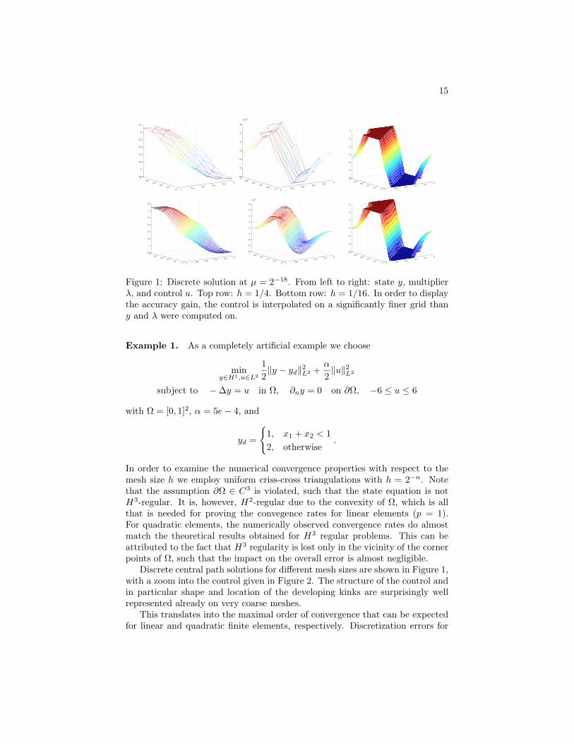
Figure 1: Discrete solution at µ = 2−18. From left to right: state y, multiplierλ, and control u. Top row: h = 1/4. Bottom row: h = 1/16. In order to displaythe accuracy gain, the control is interpolated on a significantly finer grid thany and λ were computed on.

Example 1. As a completely artificial example we choose

miny∈H1,u∈L2

12‖y − yd‖2L2 +

α

2‖u‖2L2

subject to −∆y = u in Ω, ∂ny = 0 on ∂Ω, −6 ≤ u ≤ 6

with Ω = [0, 1]2, α = 5e− 4, and

yd =

1, x1 + x2 < 12, otherwise

.

In order to examine the numerical convergence properties with respect to themesh size h we employ uniform criss-cross triangulations with h = 2−n. Notethat the assumption ∂Ω ∈ C3 is violated, such that the state equation is notH3-regular. It is, however, H2-regular due to the convexity of Ω, which is allthat is needed for proving the convegence rates for linear elements (p = 1).For quadratic elements, the numerically observed convergence rates do almostmatch the theoretical results obtained for H3 regular problems. This can beattributed to the fact that H3 regularity is lost only in the vicinity of the cornerpoints of Ω, such that the impact on the overall error is almost negligible.

Discrete central path solutions for different mesh sizes are shown in Figure 1,with a zoom into the control given in Figure 2. The structure of the control andin particular shape and location of the developing kinks are surprisingly wellrepresented already on very coarse meshes.

This translates into the maximal order of convergence that can be expectedfor linear and quadratic finite elements, respectively. Discretization errors for

16

state y and multiplier λ, both in ‖ · ‖H1 and ‖ · ‖L2 , are given in Figure 3.Note that the quadratic and cubic convergence order of λ in L2 for linear andquadratic elements, respectively, translates directly into the same order of con-vergence for u in L2.

Figure 2: Zoom of control for µ = 2−18. Left: h = 1/4. Right: h = 1/16.

1e-05

0.0001

0.001

0.01

0.1

1

2 4 8 16 32 64

State/H1Multiplier/H1

State/L2Multiplier/L2 1e-06

1e-05

0.0001

0.001

0.01

0.1

1

2 4 8 16 32

State/H1Multiplier/H1

State/L2Multiplier/L2

Figure 3: Convergence rates for linear (left) and quadratic (right) finite elementsat different values of µ = 2−8, 2−13, 2−15.

Example 2. This problem taken from [22] is a drastically simplified bench-mark problem for applicator development in regional hyperthermia treatment,a cancer therapy that aims at heating deeply seated tumors by microwave radi-ation in order to make it more susceptible to an accompanying radio or chemotherapy [7]. The governing PDE is the stationary bio-heat-transfer equation [13]

−∇(κ∇y) + (y − 37)w = σu in Ω∂ny = 0 on ∂Ω

for the temperature y on the relevant part Ω of the human body. Our benchmarkproblem is based on a problem considered in [2, Section 4], where a detaileddescription of the material parameters can be found.

17

Tumor

Figure 4: Cross section Ω of the pelvic region with different tissue types (left)and optimal state (right).

The control u, assumed to be freely adjustable within the bounds 0 ≤ u ≤umax, is the energy absorption of the tissue and is directly related to the am-plitude of the time harmonic electric field generated by the microwave gener-ator. We set umax := 106 V 2/m2. The thermal effect of perfusion w witharterial blood of 37C from different regions of the body is accounted for by theHelmholtz term. We aim at a therapeutical temperature

yd =

45 in Ωt37 in Ω\Ωt

that affects only the tumor tissue Ωt ⊂ Ω (see Fig. 4). For this example, theregularization parameter α has been set to 10−12.

As can be expected, the optimal control just deposits almost all the energyinto the tumor region and almost nothing outside. The very small value of αleads to a very thin band of steep increase in the control, which is, however, notaligned to the coarse grid.

The intent of this example is not to numerically verify the theoretical conver-gence rates for h → 0, but to illustrate the efficiency of the method for rathercoarse meshes. In particular, here we are not interested in the loss of evenH2-regularity due to the nonconvex polygonal domain Ω.

The problem has been solved numerically by a primal-dual function spaceoriented interior point method as described in [21, 22]. The discretized controlneeds to represent the ‘discontinuity’ of the solution with sufficient accuracy,such that massive grid refinement occurs along the boundaries of the active sets(see Fig. 5, left). The finest computational grid contained about 40000 triangles,most of them concentrated along the control ’discontinuity’.

We also solved this problem with the control reduced primal interior pointmethod, however on a much coarser grid with about 2500 triangles. Then thecontrol was computed via (8) on a uniformly refined grid (see Fig. 5, right),which yielded a comparable result with much less computational effort.

18

Figure 5: Mesh refinement and discrete control for the primal dual approachwith piecewise constant control discretization (left) and for the control reducedprimal approach (right) computed on a coarse grid.

19

Conclusion

A novel discretization scheme for primal interior point methods applied to PDEconstrained optimization problems has been presented. Pointwise eliminationof the control, which is the least regular variable, enables high accuracy withcomparatively coarse meshes.

References

[1] N. Arada, E. Casas, and F. Troltzsch. Error estimates for the numericalapproximation of a semilinear elliptic control problem. Comput. Optim.Appl., 23:201–229, 2002.

[2] F.A. Bornemann. An adaptive multilevel approach to parabolic equationsIII. 2D error estimation and multilevel preconditioning. IMPACT Comput.Sci. Engrg., 4:1–45, 1992.

[3] D. Braess and C. Blomer. A multigrid method for a parameter dependentproblem in solid mechanics. Numer. Math., 57:747–761, 1990.

[4] E. Casas and F. Troltzsch. Error estimates for linear-quadratic ellipticcontrol problems. In V. Barbu et al., editor, Analysis and Optimization ofDifferential Systems, pages 89–100. Kluwer, 2003.

[5] P.G. Ciarlet. The finite element method for elliptic problems. North-Holland, 1987.

[6] P. Deuflhard. Newton Methods for Nonlinear Problems. Affine Invari-ance and Adaptive Algorithms, volume 35 of Computational Mathematics.Springer, 2004.

[7] P. Deuflhard, M. Seebaß, D. Stalling, R. Beck, and H.-C. Hege. Hyperther-mia Treatment Planning in Clinical Cancer Therapy: Modelling, Simula-tion and Visualization. In A. Sydow, editor, Proc. of the 15th IMACS WorldCongress 1997 on Scientific Computation: Modelling and Applied Mathe-matics, volume 3, pages 9–17. Wissenschaft und Technik Verlag, 1997.

[8] D. Gilbarg and N.S. Trudinger. Elliptic Partial Differential Equations ofSecond Order. Springer, 1977.

[9] M. Hintermuller, K. Ito, and K Kunisch. The primal-dual active set strat-egy as a semi-smooth Newton method. SIAM J. Optim., 13:865–888, 2002.

[10] M. Hinze. A variational discretization concept in control constrained op-timization: the linear-quadratic case. Comput. Optim. Appl., 30:45–63,2005.

[11] B. Kummer. Generalized Newton and NCP-methods: convergence, reg-ularity and actions. Discussiones Mathematicae - Differential Inclusions,20(2):209–244, 2000.

20

[12] C. Meyer and A. Rosch. Superconvergence properties of optimal controlproblems. SIAM J. Control Optim., 43(3):970–985, 2004.

[13] H.H. Pennes. Analysis of tissue and arterial blood temperatures in theresting human forearm. J. Appl. Phys., 1:93–122, 1948.

[14] U. Prufert, F. Troltzsch, and M. Weiser. The convergence of an interiorpoint method for an elliptic control problem with mixed control-state con-straints. Comput. Optim. Appl., to appear.

[15] A. Rosch. Error estimates for linear-quadratic control problems with con-trol constraints. Optim. Meth. Softw., 21(1):121–134, 2006.

[16] A. Schiela. The Control Reduced Interior Point Method. doctoral thesis,Freie Universitat Berlin, Dept. Math. and Comp. Sci., 2006.

[17] A. Schiela and M. Weiser. Superlinear convergence of the control reducedinterior point method for PDE constrained optimization. Comput. Optim.Appl., to appear.

[18] M. Ulbrich. Nonsmooth Newton-like Methods for Variational Inequalitiesand Constrained Optimization Problems in Function Spaces. Habilitationthesis, Fakultat fur Mathematik, Technische Universitat Munchen, 2002.

[19] M. Ulbrich and S. Ulbrich. Primal-dual interior point methods for PDE-constrained optimization. Technical report, TU Darmstadt, 2006.

[20] M. Weiser. Interior point methods in function space. SIAM J. ControlOptim., 44(5):1766–1786, 2005.

[21] M. Weiser and P. Deuflhard. Inexact central path following algorithms foroptimal control problems. SIAM J. Control Optim., to appear.

[22] M. Weiser and A. Schiela. Function space interior point methods for PDEconstrained optimization. PAMM, 4(1):43–46, 2004.

[23] E. Zeidler. Nonlinear Functional Analysis and its Applications, volume I.Springer, New York, 1986.