A DEEP PROPER MOTION CATALOG WITHIN THE SLOAN DIGITAL SKY SURVEY FOOTPRINT.II. THE WHITE DWARF LUMINOSITY FUNCTION

Jeffrey A. Munn1, Hugh C. Harris

1, Ted von Hippel

2, Mukremin Kilic

3, James W. Liebert

4, Kurtis A. Williams

5,

Steven DeGennaro6, Elizabeth Jeffery

7, Kyra Dame

3, A. Gianninas

3, and Warren R. Brown

8

1 US Naval Observatory, Flagstaff Station, 10391 W. Naval Observatory Road, Flagstaff, AZ 86005-8521, USA; jam@nofs.navy.mil2 Center for Space and Atmospheric Research, Embry-Riddle Aeronautical University, Daytona Beach, FL 32114-3900, USA

3 University of Oklahoma, Homer L. Dodge Department of Physics and Astronomy, 440 W. Brooks Street, Norman, OK 73019, USA4 University of Arizona, Steward Observatory, Tucson, AZ 85721, USA

5 Department of Physics and Astronomy, Texas A&M University–Commerce, P.O. Box 3011, Commerce, TX 75429, USA6 Department of Astronomy, University of Texas at Austin, 1 University Station C1400, Austin, TX 78712-0259, USA

7 BYU Department of Physics and Astronomy, N283 ESC, Provo, UT 84602, USA8 Smithsonian Astrophysical Observatory, 60 Garden Street, Cambridge, MA 02138, USA

Received 2016 September 11; revised 2016 October 25; accepted 2016 October 25; published 2016 December 19

ABSTRACT

A catalog of 8472 white dwarf (WD) candidates is presented, selected using reduced proper motions from the deepproper motion catalog of Munn et al. Candidates are selected in the magnitude range < <r16 21.5 over 980square degrees, and < <r16 21.3 over an additional 1276 square degrees, within the Sloan Digital Sky Survey(SDSS) imaging footprint. Distances, bolometric luminosities, and atmospheric compositions are derived by fittingSDSS ugriz photometry to pure hydrogen and helium model atmospheres (assuming surface gravities =glog 8).The disk white dwarf luminosity function (WDLF) is constructed using a sample of 2839 stars with

< <M5.5 17bol , with statistically significant numbers of stars cooler than the turnover in the luminosity function.The WDLF for the halo is also constructed, using a sample of 135 halo WDs with < <M5 16bol . We find spacedensities of disk and halo WDs in the solar neighborhood of ´ - -5.5 0.1 10 pc3 3 and ´ - -3.5 0.7 10 pc5 3,respectively. We resolve the bump in the disk WDLF due to the onset of fully convective envelopes in WDs, andsee indications of it in the halo WDLF as well.

Key words: stars: luminosity function, mass function – white dwarfs

Supporting material: data behind figures, machine-readable tables

1. INTRODUCTION

White dwarfs (WDs) are the endpoint of stellar evolution forstars lighter than 8–10M☉ (Williams et al. 2009; García-Berro& Oswalt 2016), or greater than 97% of Galactic stars. As thedirect remnants of earlier star formation, WDs are an importanttool in studying the evolution of our Galaxy. The basicobservable when studying star formation history with WDs isthe distribution of WDs in luminosity, or the luminosity function(LF; see García-Berro & Oswalt 2016 for a recent review of boththe observational and theoretical work on the white dwarfluminosity function (WDLF)). In particular, for a given stellarpopulation, the location and shape of the peak and turnover inthe LF at the faint end can be used to constrain the age of thatpopulation (Liebert et al. 1979; Winget et al. 1987).

The bright end ( M 13bol ) of the WDLF is populated by hotWDs whose optical colors are distinct from other stellarpopulations, allowing clean samples of hot WDs to be foundbased on photometry alone. Thus, even the earliest LFs for hotWDs contained hundreds of stars, including those producedfrom the Palomar–Green (Green 1980; Fleming et al. 1986;Liebert et al. 2005; Bergeron et al. 2011) and Kiso (Ishidaet al. 1982; Wegner & Darling 1994; Limoges & Bergeron 2010)ultraviolet excess surveys. LFs generated from modern large-scale spectroscopic surveys have been based on samples ofthousands of hot WDs, including those from the Sloan DigitalSky Survey (SDSS; Hu et al. 2007; DeGennaro et al. 2008;Krzesinski et al. 2009) and the Anglo-Australian 2dF QSORedshift Survey (Vennes et al. 2002, 2005). Thus, the bright endof the WDLF is defined with high statistical significance.

The majority of WDs, however, are fainter, with colorsindistinguishable from subdwarfs, making their selection usingphotometry alone impossible. The first study to resolve thepeak of the LF and obtain samples of WDs fainter than theturnover was Liebert et al. (1988), based on a sample of 43 coolWDs selected from the Luyten Half-Second Catalog (Luy-ten 1979) to have >M 13v (and later reanalyzed withadditional spectroscopy and photometry by Leggettet al. 1998). Subsequent proper-motion-based studies hadsimilar sample sizes (Evans 1992; Oswalt et al. 1996; Knoxet al. 1999). The first major increase in sample size was that ofHarris et al. (2006, hereafter H06), which used SDSS (Fukugitaet al. 1996; Gunn et al. 1998, 2006; York et al. 2000)photometry and proper motions from a combined catalog(Munn et al. 2004, 2008) of SDSS and USNO-B (Monetet al. 2003) astrometry to generate a sample of 6000 reduced-proper-motion (RPM)-selected WDs.(Rowell & Hambly(2011, hereafter RH11) similarly used RPMs to select10,000 WDs from the SuperCOSMOS sky survey (Hamblyet al. 2001a, 2001b, 2001c). Both surveys provide a Galacticdisk WDLF with high statistical significance in the luminosityrange < <M6 15bol , and clearly define the peak of the diskWDLF at ~M 15bol . However, neither provides many starsfainter than the turnover, with only 4 stars in H06 and 48 inRH11 with >M 15.5bol (in their > -v 30 km stan

1 samples).Both surveys are dependent on the classic Schmidt telescopephotographic surveys for one or both epochs, and thus arelimited to the depth of the photographic surveys, ~r 19.5. Ahydrogen atmosphere WD one magnitude fainter than theturnover has ~M 16r , which at a faint limit of ~r 19.5

The Astronomical Journal, 153:10 (19pp), 2017 January doi:10.3847/1538-3881/153/1/10© 2016. The American Astronomical Society. All rights reserved.

1

corresponds to only 50pc. Thus the small surveyed volumeseverely limits the number of WDs detectable past the turnover.RH11 detected more such WDs as their sky coverage is nearlysix times as great as that for H06 (roughly 30,000 deg2 forRH11 versus 5300 deg2 for H06). Both papers also present aLF for clean samples of Galactic halo WDs, definedkinematically by requiring > -v 200 km stan

1. H06 detect only18 such halo WDs, while RH11 with their greater sky coveragedetect 93. The sample sizes of halo WDs are limited by themuch smaller density of halo stars within the solar neighbor-hood. The RH11 sample is by far the largest sample of haloWD candidates to date. Note that, unlike many of the othersamples discussed above, most of the WDs in the H06 andRH11 samples lack spectroscopic confirmation, though con-tamination by non-WDs is thought to be both understood andsmall (Kilic et al. 2006, 2010a).

Recent work has concentrated on producing nearly completesamples of WDs in the local volume. LFs have been producedusing WDs within 20 (Giammichele et al. 2012), 25 (Holberget al. 2016), and 40pc (Limoges et al. 2015; Torres & Garcia-Berro 2016) of the Sun, with sample sizes of 147, 232, and 501WDs, respectively. The 40pc LF has 22 stars fainter than theturnover ( >M 15.5bol ). No halo WDs were found in any of thesamples, with three possible candidates in the 40pc sample.

In order to address the paucity of both disk WDs fainter thanthe turnover and halo WDs in our earlier work in H06, in 2009we started a survey to re-observe parts of the SDSS imagingfootprint, obtaining a second epoch that, combined with SDSSastrometry, would yield proper motions roughly two magni-tudes fainter than that obtainable using the Schmidt surveys(Munn et al. 2014). This paper presents a catalog of WDcandidates selected from that survey, and the resultant disk andhalo WDLFs. Individual objects with additional follow-upobservations have been presented in previous papers (Kilicet al. 2010b; Dame et al. 2016). Section 2 describes the sampleselection. Section 3 describes the fitting of atmospheric modelsto SDSS photometry to derive distances, effective tempera-tures, and bolometric luminosities for the sample WDs.Section 4 presents the LFs, Section 5 presents the catalog,and Section 6 summarizes our results.

2. SAMPLE SELECTION

2.1. Sky Coverage

The WD sample is drawn from the deep proper motionsurvey of Munn et al. (2014, hereafter M2014). This paper usesonly the data considered “good” from the survey, whichincludes 1089 square degrees of sky observed with the 90primeprime focus wide-field imager on the Steward Observatory Bok90 inch telescope (Williams et al. 2004), and an additional1521 square degrees of sky observed with the Array Camera onthe U.S. Naval Observatory, Flagstaff Station, 1.3 m telescope.The Bok and 1.3 m data are 90% complete to r = 22.3 and r =21.3, respectively.

We define the term field throughout this paper as the area ofsky covered by a single CCD within a single observationin M2014. Data quality naturally varies between individualobservations, due to differences in seeing, image depth, etc. Dataquality can also vary between different fields within individualobservations, primarily due to the varying PSF across the largefield-of-views of the Bok and 1.3 m telescopes; collimating fast,large field-of-view telescopes is not easy, and both telescopes

suffered from collimation issues at times during the survey. Wethus treat each field as a separate survey, in terms of rejecting baddata, modeling the data quality, and selecting candidate WDs.Each field images an area of sky covered by multiple SDSS

scans, which typically were taken on different nights. Thus, theepoch difference between the Bok/1.3 m and SDSS data canvary for different objects within a field. We limit our survey tofields whose minimum epoch difference is at least 3.5 yr, so as toprovide well measured proper motions; this reduces the areacoverage by 4.2%. A number of fields in both the Bok and 1.3 msurveys are suspect, for a variety of reasons: they appear not toobtain the depth estimated in the catalog; the image quality ispoor, primarily due to poor collimation; or they have a muchlarger number of candidate high proper motion candidate starsthan expected, indicating problems with either the image qualityor astrometric calibration. These fields are excluded from thesample, and are listed in Table 1; this reduces the area coverageby a further 0.8%. Image quality in the corners of the ArrayCamera on the 1.3 m begins to deteriorate, and we find a higherincidence of false proper motions in the catalog in the cornersbased on visual inspection. Thus we include only objectsdetected within a 0.68 degree radius of the camera center for the1.3 m data, reducing the sky coverage of the 1.3 m data by12.0%. We further exclude areas of sky affected by bright stars,as specified using the bright star masks given in M2014 (whichare derived from those of Blanton et al. 2005), for an additionalreduction in area coverage of 2.0%. The sky coverage of thefinal sample includes 980 square degrees from the Bok survey,and 1276 square degrees from the 1.3 m survey.

2.2. Clean Star Sample

We start with a clean sample of SDSS stars in the r bandwithin our fields, by requiring (1) that they pass the set ofcriteria suggested on the SDSS DR7 Web site for defining aclean sample of point sources in the r band;9 and (2) that theynot be considered a moving object within a single SDSSobservation (e.g., an asteroid), according to the criteria adoptedfor the SDSS Moving Object Catalog10 (Ivezić et al. 2002). TheBok sample is limited to stars with < <r16 21.5, while the1.3 m sample is limited to stars with < <r16 21.3. This

Table 1Excluded Fields

Nighta obsIDb ccdsc

53888 16 1, 2, 3, 453888 17 1, 2, 3, 453888 18 1, 2, 3, 454245 13 1, 2, 3, 354245 14 1, 2, 3, 4

Notes.a MJD number of the night the observation was obtained in M2014.Corresponds to the night column in the Observation Schema (Table 2)in M2014.b Observation number in M2014, unique within a given night. Corresponds tothe obsID column in the Observation Schema (Table 2) in M2014.c List of CCDs for this observation whose data were suspect, and thusexcluded.

(This table is available in its entirety in machine-readable form.)

9 http://www.sdss.org/dr7/products/catalogs/flags.html10 http://www.astro.washington.edu/users/ivezic/sdssmoc/sdssmoc1.html

2

The Astronomical Journal, 153:10 (19pp), 2017 January Munn et al.

defines the complete stellar sample from which the WDcandidates will be selected.

While the proper motion of each candidate WD will bevisually verified, we wish to define a relatively clean sample ofstars with reliably measured proper motions via a set of cutsthat reject well-defined regions of parameter space with a highcontamination rate of false high proper motion objects. To thisend, we adopt the following cuts:

1. Objects must be detected by SExtractor in the Bok/1.3 msurveys, and not be flagged as truncated or havingincomplete or corrupted aperture data (or, for the 1.3 m,being saturated). Many of the objects detected byDAOPHOT but not SExtractor are located in the extendedPSF of nearby bright stars and have unreliable centroids.

2. Objects must have a reliable DAOPHOT PSF fit in theBok/1.3 m surveys, as indicated by the number ofiterations required to converge on a solution( < <0 nIter 10). The DAOPHOT centroids are used tomeasure the proper motion, and thus the proper motionfor objects whose PSF fits failed to converge ( =nIter 10)are unreliable. The first two cuts, which are a measure ofthe depth of M2014, reject 3.9% and 6.8% of the Bok and1.3 m survey objects, respectively.

3. Objects must not have a nearby neighbor, whoseoverlapping PSF could adversely affect the measuredcentroids. For the 1.3 m, objects with a neighbor withinfour arcseconds are rejected. For the Bok survey, objectswith a neighbor within + - r3.0 0.5 23 n( ) arcsecondsare rejected, where rn is the r magnitude of the nearbyneighbor. This cut rejects a further 3.2% and 2.2% of theBok and 1.3 m survey objects, respectively.

4. Objects that are not a one-to-one match between SDSSand the Bok/1.3 m surveys, or whose difference in SDSSand Bok/1.3 m r magnitude exceeds 0.5 mag, arerejected. The majority of these are blends and mis-matches. This rejects 0.3% of the remaining objects.

These cuts reject the bulk of objects with unreliable propermotion measurements, while allowing us to define the effect onour sample completeness to allow later correction. The surveycompleteness after application of these cuts is shown inFigure 1.

2.3. RPM Selection

We select our WD candidates from stars with at least 3.5σproper motions. The proper motion errors are magnitudedependent, as well as varying between fields. Thus, stars ineach field, which we are already treating as separate samples,are further divided into magnitude bins 0.1 mag wide in r(hereafter referred to as subsamples). We calculate the meanproper motion error in each magnitude bin, scaled to theminimum epoch difference in its field, and then smooth theseestimates by fitting, for each field separately, the scaled meanproper motion error versus r magnitude to the function

s = +m-a 10 1r b0.6 ( )( )

where r is the magnitude at the center of the magnitude bin andsm is the scaled mean proper motion error in that bin. Eachmagnitude bin is then treated as a separate subsample, wherethe proper motion error for that bin is conservatively adopted tobe the proper motion error, scaled to the minimum epochdifference in the field, estimated from the fit for the faint r limitof the bin. The initial 3.5σ proper motion sample is thencomprised of all stars with proper motions greater than 3.5times the estimated scaled proper motion error in theirsubsamples. The distribution of subsamples in scaled propermotion error versus r magnitude is displayed in Figures 2and 3, which gives an indication of the dependence of scaledproper motion error on r magnitude, and the variation in thatdependency across different fields.A common tool used to isolate cool WDs is RPM (Luyten

1922a, 1922b), defined (here in the SDSS g band) as

m= + + = + -H g M v5 log 5 5 log 3.379, 2g g tan ( )

where μ is the proper motion in arcsec year−1 and vtan is thetangential velocity in -km s 1. Proper motion serves as a proxyfor the unknown distance, as stars with similar kinematics willhave similar proper motions at a given distance. Since WDsare typically five to seven magnitudes less luminous thansubdwarfs of the same color, they are cleanly separated fromsubdwarfs in RPM versus color diagrams. This technique wasused by both H06 and RH11 (as well as numerous other studiescited in the Introduction). Kilic et al. (2006, 2010a) obtainedfollow-up spectroscopy for candidate cool WDs selected from

Figure 1. Survey completeness vs. r magnitude, after applying the cutsdiscussed in the text. The solid line is for the Bok survey, and the dotted line isfor the 1.3 m survey.

Figure 2. Distribution of subsamples in proper motion error, scaled to theminimum epoch difference within their fields, vs. r magnitude, for the Boksurvey.

3

The Astronomical Journal, 153:10 (19pp), 2017 January Munn et al.

the Hg versus g− i diagram for the H06 sample, and found aclean separation between WDs and subdwarfs with acontamination rate of only a few percent. Our sample willuse the same selection technique, as well as the samephotometric catalog (SDSS), and thus their results are directlyapplicable to our work.

The RPM diagram (Hg versus g− i) for our 3.5σ propermotion sample is displayed in Figure 4. In the high-densityportion of the diagram, density contours are plotted (number ofstars per bin, where each bin is 0.1 mag in Hg by 0.1 mag ing− i). Outside the lowest density contour, individual stars areplotted. The evolutionary tracks for model WDs (detailedbelow) of different kinematics are overlain to indicate theexpected location of WDs within the RPM diagram. Objectsbelow the -30 km s 1 WD evolutionary tracks are almostexclusively expected to be WDs, with the exception of somecontamination from subdwarfs at the reddest end of theevolutionary tracks for WDs with < -v 40 km stan

1

( - ~g i 2, ~H 22g ). M2014 estimate a contamination rateof objects with errant proper motions of 1.5%. However, withinthe WD region of the RPM diagram, we expect a much largercontamination rate, as a 1.5% contamination rate for the farmore numerous subdwarfs can scatter a large number ofsubdwarfs with errant proper motions into the WD region.Thus, all candidate WDs with > -v 20 km stan

1 (i.e., objectsbelow the > -v 20 km stan

1 WD evolutionary tracks inFigure 4) have been examined by eye on the SDSS r images,the M2014 images, and for brighter objects, on the SpaceTelescope Science Institute’s Digitized Sky Survey scans of thephotographic sky survey plates from the Palomar OschinSchmidt and UK Schmidt telescopes. Of the 12,158 candidates,3087 have errant proper motions, most due to unresolvedblends with neighboring stars or image defects. While this is a25% contamination rate among the WD candidates, it is only2.1% of the 3.5σ proper motion sample in the same colorrange, and is thus consistent with the estimate of thecontamination rate in M2014. The WD candidates with visuallydetermined errant proper motions are not plotted in Figure 4.The remaining 9071 candidate WD candidates with

> -v 20 km stan1 and visually confirmed proper motions are

plotted in Figure 4, and comprise our RPM-selected sampleused throughout the rest of the paper.

3. FITS TO MODEL WDS

We derive estimates for the distances, bolometric luminos-ities, effective temperatures, and atmospheric compositions forour WD candidates by fitting the SDSS photometry to the latestonline set of synthetic absolute magnitudes for model WDsfrom P. Bergeron, G. Fontaine, P. Tremblay, and P. M.Kowalski11 (BFTK; Holberg & Bergeron 2006; Kowalski &Saumon 2006; Bergeron et al. 2011; Tremblay et al. 2011). It isnot possible to distinguish between models with differentsurface gravities based on broad-band photometry alone(Bergeron et al. 1997). Spectroscopic studies of WDs show astrong peak in the distribution of mass at around 0.65–0.70M☉(depending on the details of the samples under study),corresponding to ~glog 8, with one σ dispersions in massof about 0.16–0.20M☉ (Bergeron et al. 2001; Giammicheleet al. 2012; Limoges et al. 2015). Thus, lacking surface gravitydiscriminators, we assume =glog 8 in our fits. Eachcandidate is fit to both the pure hydrogen and pure heliumatmosphere =glog 8 model grids using variance-weightedleast-squares. Individual magnitudes that do not meet thecriteria on the SDSS DR7 Web site for clean point sources inthat filter (as used above in defining our r-limited stellarsample) are not used in the fit. We also do not use individualSDSS asinh12 magnitudes fainter than 24.02, 24.50, 24.19,23.74, and 22.20 in u, g, r, i, and z, respectively, whichcorresponds to requiring roughly a 2σ detection in each filter.The SDSS photometry is corrected to the Hubble SpaceTelescope flux scale, which the BFTK models use, by addingzero point offsets of −0.0424, 0.0023, 0.0032, 0.0160, and0.0276 to the u, g, r, i, and z magnitudes, respectively (Holberg& Bergeron 2006). Errors are estimated using the c + 1min

2

confidence boundaries in the least-squares fits. To these areadded in quadrature an estimate of the errors due to an assumed0.3 dex scatter in logg (corresponding to a scatter in mass of~ M0.18 ☉), derived by refitting using =glog 7.7 and

=glog 8.3 models. The uncertainty in logg is the dominantsource of error for the bolometric luminosities and distances,leading to typical errors in the bolometric luminosities of0.4–0.5 mag.We correct for interstellar extinction using the three-

dimensional reddening maps of Green et al. (2015), whichprovide the cumulative reddening at equally spaced distancemoduli. The reddening for each star is obtained by linearlyinterpolating the median reddening profile along the star’ssightline. Over half of our stars lie at distances less than theminimum distances along their sightlines considered to bereliable. In these cases, we linearly interpolate between anassumed zero reddening at zero distance and the first reliablereddening measurement along the sightline. Reddening isconverted to extinction values in each filter using the

-A E B Vb ( ) values from Table6 of Schlafly & Finkbeiner(2011), assuming an RV = 3.1 reddening law (Fitzpatrick 1999;Schlafly & Finkbeiner 2011). Since SDSS targeted areas of lowGalactic extinction, the extinction corrections are small andhave little effect on the derived distances. The median and 90thpercentile extinction in r for our > -v 40 km stan

1 sample are0.02 and 0.06, respectively.

Figure 3. Same as Figure 2, except for the 1.3 m survey.

11 http://www.astro.umontreal.ca/~bergeron/CoolingModels, with modelslast updated 2011 October 17.12 http://www.sdss.org/dr12/algorithms/magnitudes/

4

The Astronomical Journal, 153:10 (19pp), 2017 January Munn et al.

Each model fit is inspected by eye. Poor fits with obviousexcess flux in the i and z passbands are refit without the i and zphotometry, under the assumption that the candidate WD hasan unresolved M dwarf companion (Raymond et al. 2003;Kleinman et al. 2004; Smolčić et al. 2004). If this yields anacceptable fit, the new fit is used. 1.3% of the sample was fit inthis way.

A fit is considered acceptable if there is at least a 1% chanceof obtaining its cn

2 value, and at least three SDSS magnitudeswere used in the fit. A sample fit is shown in Figure 5, forwhich the hydrogen atmosphere model fit is consideredacceptable while the helium atmosphere model fit is consideredunacceptable. Of the 9071 RPM-selected candidates, 599, or7%, did not have an acceptable fit for either the hydrogen orhelium atmosphere model fits. The final WD candidate sampleconsists of the 8472 RPM-selected candidates with at least oneacceptable fit. For a given star, if only the hydrogen or heliumfit is acceptable, then that atmospheric model is consideredpreferred and is used in subsequent analyses. For stars forwhich both the hydrogen and helium atmosphere models yieldacceptable fits, both fits are used, weighted by the expectedprobability of each star having a hydrogen or heliumatmosphere, described below.

Figure 6 displays the fraction of stars (with > -v 40 km stan1

to avoid subdwarf contamination) for which the hydrogenor helium model fits are preferred as a function of g− i. Of

stars with - < -g i 0.2, corresponding to roughly>T 10,500 Keff , 82% have a preferred model. For the

remaining stars without a preferred model in this color range,we weight the hydrogen and helium atmosphere model fitsassuming the same ratio of helium to hydrogen atmosphereWDs in a given color bin as derived from stars in that bin withpreferred models. Since the derived bolometric luminosities ofWDs differ depending on whether the hydrogen or heliumatmosphere model fits are used, the observed ratio of hydrogento helium model atmospheres WDs must be adjusted to accountfor the difference in the maximum survey volume over whicheach star can be observed for the different model atmospheres.Calculation of the maximum survey volume is describedbelow. Figure 7 displays the resultant helium fraction againstTeff for stars with >T 10,500 Keff (based on the same sample ofstars, kinematic cuts, and Galactic model used to derive ourpreferred disk LF, described in detail below). The decrease inhelium fraction from ~T 11,000 Keff to ~T 150,000 Keff isconsistent with similar trends seen in the 20 pc local volumesample of Giammichele et al. (2012, GBD12) and 40 pc localvolume sample of Limoges et al. (2015), though our results aremore consistent with the overall higher helium fraction of the20 pc sample. For stars hotter than =T 15,000 Keff , we find ahelium fraction of 15%, consistent with the estimate of ∼9% byBergeron et al. (2011) using the Palomar–Green survey (Greenet al. 1986).

Figure 4. Reduced proper motion diagram for our 3.5σ proper motion sample. In the high-density portion of the diagram, density contours are plotted (number of starsper bin, where each bin is 0.1 mag in Hg by 0.1 mag in g − i). Outside the lowest density contour, individual stars are plotted. Evolutionary tracks for model WDs withdifferent kinematics are plotted to indicate the expected position of WDs within the diagram. Solid lines are pure hydrogen atmosphere WDs, while dashed lines arepure helium atmosphere WDs. The red, magenta, cyan, and blue tracks are for WDs with tangential velocities of 20, 30, 40, and 150 -km s 1, respectively. Almost allobjects below the = -v 30 km stan

1 evolutionary tracks are expected to be WDs.

5

The Astronomical Journal, 153:10 (19pp), 2017 January Munn et al.

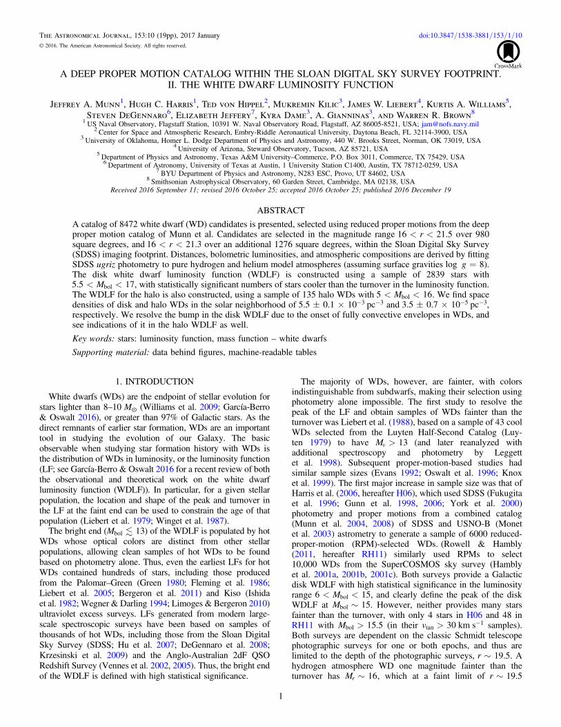
For stars with - > -g i 0.2, most stars lack a preferredmodel. In this color range, we adopt the helium fraction versusTeff results of GBD12, based on their 20 pc local volumesample. Figure 8 displays our adopted model for heliumfraction versus g− i, used to weight the hydrogen and heliumatmosphere model fits for stars that lack a preferred atmo-spheric model. Our results and those of GBD12 do notsmoothly meet at the border between the two ( - = -g i 0.2).The dashed line in the - < - <g i0.2 0.0 bin indicates theactual GBD12 results in that color range. We have chosen toinflate the helium fraction in that bin to provide a smooth matchbetween the two data sets. The difference is certainly within theerror in the estimate of the true helium fraction in that colorrange, and has negligible impact on the resultant LFs.

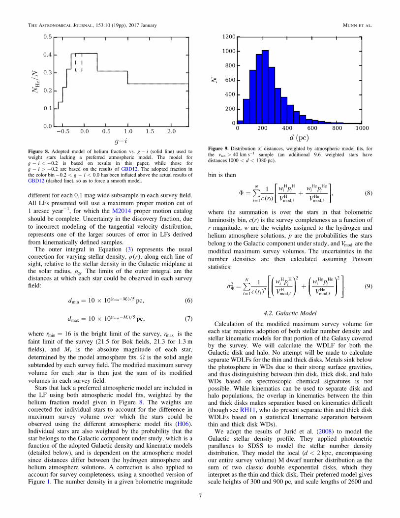
Figure 9 shows the distribution of distances, weighted byatmospheric model fits, for the > -v 40 km stan

1 sample (thereare an additional 9.6 weighted stars with distances <1000<d 1380 pc). The median distance is 220pc, while 95% of

the stars have <d 500 pc.

4. THE WHITE DWARF LUMINOSITY FUNCTION

4.1. Method

The WDLF is derived using a modification of the V1 maxmethod (Schmidt 1968), where Vmax is the maximum surveyvolume over which each object is detectable. Our WD sample iskinematically defined, dependent both on tangential velocitylimits used to separate different Galactic populations, as well asproper motion limits that vary both between different fields andwith magnitude within each field. We use the modifiedmaximum survey volume of Lam et al. (2015,hereafter LRH15) as the density estimator, which accounts forvarying kinematic limits along independent lines of sight.Reproducing their Equation (12), the modified maximum surveyvolume, calculated for each survey object independently in eachsurveyfield, is

⎡⎣⎢

⎤⎦⎥ò ò

rr

= WVr

r P v r dv dr, . 3d

d

a r

b r

mod2

tan tanmin

max ( ) ( ) ( )☉ ( )

( )

The inner integral, referred to as the discovery fraction χ, is theinstantaneous fraction of objects that could be observed due tothe kinematic cuts. P v r,tan( ) is the tangential velocity (vtan )distribution, which can vary with distance, r, along each line ofsight. The limits of the integral can also vary with distance,being a combination of the tangential velocity and propermotion cuts, and are (Equations (15) and (16) from LRH15)

m=a r v r rmax , 0.00474 , 4min min( ) [ ( ) ] ( )

m=b r v rmin , 0.00474 . 5max max( ) [ ] ( )

While the tangential velocity limits, vmin and vmax (in -km s 1),as well as the maximum proper motion cut, mmax (inmas year−1), are constant, the minimum proper cut, m ,min is

Figure 5. Sample white dwarf atmosphere model fit. The filled circles witherror bars display the dereddened SDSS photometry (order ugriz), while theopen circles and diamonds display the best-fitting pure hydrogen and purehelium atmosphere model fits, respectively. For this star, the hydrogenatmosphere model fit is considered acceptable while the helium atmospheremodel fit is considered unacceptable.

Figure 6. Fraction of stars (with > -v 40 km stan1) for which either the pure

hydrogen atmosphere model (blue histogram) or pure helium atmospheremodel (red histogram) fits are considered preferred.

Figure 7. Upper panel: Counts of stars with preferred atmospheric models vs.Teff . The solid line is for all stars, while the dotted line is for stars with apreferred helium atmosphere model. Lower panel: Fraction of stars with apreferred helium atmosphere model vs. Teff .

6

The Astronomical Journal, 153:10 (19pp), 2017 January Munn et al.

different for each 0.1 mag wide subsample in each survey field.All LFs presented will use a maximum proper motion cut of1arcsec year−1, for which the M2014 proper motion catalogshould be complete. Uncertainty in the discovery fraction, dueto incorrect modeling of the tangential velocity distribution,represents one of the larger sources of error in LFs derivedfrom kinematically defined samples.

The outer integral in Equation (3) represents the usualcorrection for varying stellar density, r r( ), along each line ofsight, relative to the stellar density in the Galactic midplane atthe solar radius, r☉. The limits of the outer integral are thedistances at which each star could be observed in each surveyfield:

= ´ -d 10 10 pc, 6r Mmin

5rmin ( )( )

= ´ -d 10 10 pc, 7r Mmax

5rmax ( )( )

where =r 16min is the bright limit of the survey, rmax is thefaint limit of the survey (21.5 for Bok fields, 21.3 for 1.3 mfields), and Mr is the absolute magnitude of each star,determined by the model atmosphere fits. Ω is the solid anglesubtended by each survey field. The modified maximum surveyvolume for each star is then just the sum of its modifiedvolumes in each survey field.

Stars that lack a preferred atmospheric model are included inthe LF using both atmospheric model fits, weighted by thehelium fraction model given in Figure 8. The weights arecorrected for individual stars to account for the difference inmaximum survey volume over which the stars could beobserved using the different atmospheric model fits (H06).Individual stars are also weighted by the probability that thestar belongs to the Galactic component under study, which is afunction of the adopted Galactic density and kinematic models(detailed below), and is dependent on the atmospheric modelsince distances differ between the hydrogen atmosphere andhelium atmosphere solutions. A correction is also applied toaccount for survey completeness, using a smoothed version ofFigure 1. The number density in a given bolometric magnitude

bin is then

⎡⎣⎢⎢

⎤⎦⎥⎥åF = +

= c r

w p

V

w p

V

1, 8

i

N

i

i i

i

i i

i1

H H

mod,H

He He

mod,He( )

( )

where the summation is over the stars in that bolometricluminosity bin, c(r) is the survey completeness as a function ofr magnitude, w are the weights assigned to the hydrogen andhelium atmosphere solutions, p are the probabilities the starsbelong to the Galactic component under study, andVmod are themodified maximum survey volumes. The uncertainties in thenumber densities are then calculated assuming Poissonstatistics:

⎡⎣⎢⎢

⎛⎝⎜⎜

⎞⎠⎟⎟

⎛⎝⎜⎜

⎞⎠⎟⎟

⎤⎦⎥⎥ås = +F

= c r

w p

V

w p

V

1. 9

i

N

i

i i

i

i i

i

2

12

H H

mod,H

2 He He

mod,He

2

( )( )

4.2. Galactic Model

Calculation of the modified maximum survey volume foreach star requires adoption of both stellar number density andstellar kinematic models for that portion of the Galaxy coveredby the survey. We will calculate the WDLF for both theGalactic disk and halo. No attempt will be made to calculateseparate WDLFs for the thin and thick disks. Metals sink belowthe photosphere in WDs due to their strong surface gravities,and thus distinguishing between thin disk, thick disk, and haloWDs based on spectroscopic chemical signatures is notpossible. While kinematics can be used to separate disk andhalo populations, the overlap in kinematics between the thinand thick disks makes separation based on kinematics difficult(though see RH11, who do present separate thin and thick diskWDLFs based on a statistical kinematic separation betweenthin and thick disk WDs).We adopt the results of Jurić et al. (2008) to model the

Galactic stellar density profile. They applied photometricparallaxes to SDSS to model the stellar number densitydistribution. They model the local ( <d 2 kpc, encompassingour entire survey volume) M dwarf number distribution as thesum of two classic double exponential disks, which theyinterpret as the thin and thick disk. Their preferred model givesscale heights of 300 and 900 pc, and scale lengths of 2600 and

Figure 8. Adopted model of helium fraction vs. g − i (solid line) used toweight stars lacking a preferred atmospheric model. The model for- < -g i 0.2 is based on results in this paper, while those for- > -g i 0.2 are based on the results of GBD12. The adopted fraction in

the color bin- < - <g i0.2 0.0 has been inflated above the actual results ofGBD12 (dashed line), so as to force a smooth model.

Figure 9. Distribution of distances, weighted by atmospheric model fits, forthe > -v 40 km stan

1 sample (an additional 9.6 weighted stars havedistances < <d1000 1380 pc).

7

The Astronomical Journal, 153:10 (19pp), 2017 January Munn et al.

3600 pc, for the thin and thick disks, respectively, with a localthick-to-thin disk normalization of 12%. We use the sum oftheir disk profiles as a single “disk” density profile. Using starsnear the main sequence turn-off, they model the Galactic haloas an oblate radial power law, with axis ratio 0.64, radialpower-law index −2.77, and local halo-to-thin disk normal-ization of 0.51%.

To model the kinematics of the disk, we use the results ofFuchs et al. (2009, hereafter F09). They combine photometricparallaxes and proper motions to measure the first and secondmoments of the velocity distribution of SDSS M dwarfs ineight slices in height above the Galactic plane, z, from< <z0 800 pc (encompassing the vast majority of our WDs).

We thus model the velocity ellipsoid as eight three-dimensionalGaussians, with the first and second moments as measured

by F09, each Gaussian centered on the F09 slices( =z 50 pc, 150 pc ,..., 750 pc). Discovery fractions are thenobtained by linearly interpolating between the discoveryfractions obtained from the bounding slices. A single velocityellipsoid is adopted for the Galactic halo, based on the resultsfor the inner halo from Carollo et al. (2010), with dispersions(s s sf, ,v v vR z) of (150, 95, 85) -km s 1, and a mean rotationconsistent with zero. The velocity ellipsoids in Galacticcylindrical coordinates are projected onto the tangent planefollowing Murray (1983).Figure 10 plots the expected contribution of halo stars to our

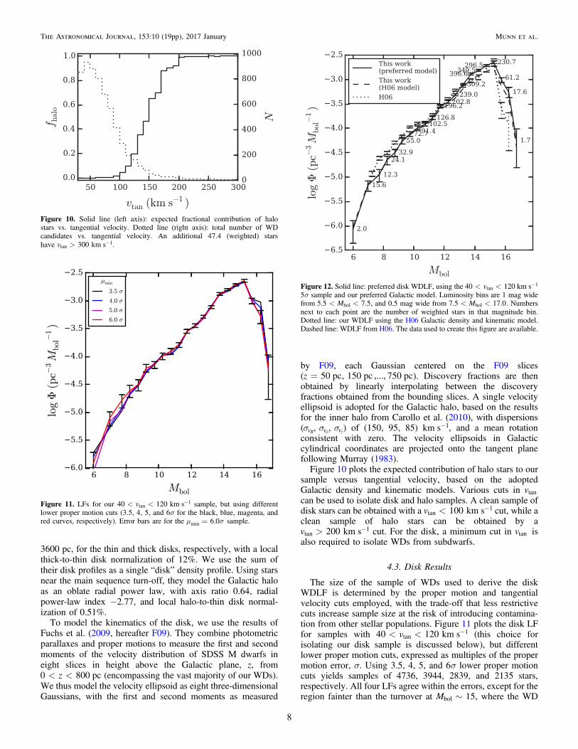
sample versus tangential velocity, based on the adoptedGalactic density and kinematic models. Various cuts in vtancan be used to isolate disk and halo samples. A clean sample ofdisk stars can be obtained with a < -v 100 km stan

1 cut, while aclean sample of halo stars can be obtained by a

> -v 200 km stan1 cut. For the disk, a minimum cut in vtan is

also required to isolate WDs from subdwarfs.

4.3. Disk Results

The size of the sample of WDs used to derive the diskWDLF is determined by the proper motion and tangentialvelocity cuts employed, with the trade-off that less restrictivecuts increase sample size at the risk of introducing contamina-tion from other stellar populations. Figure 11 plots the disk LFfor samples with < < -v40 120 km stan

1 (this choice forisolating our disk sample is discussed below), but differentlower proper motion cuts, expressed as multiples of the propermotion error, σ. Using 3.5, 4, 5, and 6σ lower proper motioncuts yields samples of 4736, 3944, 2839, and 2135 stars,respectively. All four LFs agree within the errors, except for theregion fainter than the turnover at ~M 15bol , where the WD

Figure 10. Solid line (left axis): expected fractional contribution of halostars vs. tangential velocity. Dotted line (right axis): total number of WDcandidates vs. tangential velocity. An additional 47.4 (weighted) starshave > -v 300 km stan

1.

Figure 11. LFs for our < < -v40 120 km stan1 sample, but using different

lower proper motion cuts (3.5, 4, 5, and 6σ for the black, blue, magenta, andred curves, respectively). Error bars are for the m s= 6.0min sample.

Figure 12. Solid line: preferred disk WDLF, using the < < -v40 120 km stan1

5σ sample and our preferred Galactic model. Luminosity bins are 1 mag widefrom < <M5.5 7.5bol , and 0.5 mag wide from < <M7.5 17.0bol . Numbersnext to each point are the number of weighted stars in that magnitude bin.Dotted line: our WDLF using the H06 Galactic density and kinematic model.Dashed line: WDLF from H06. The data used to create this figure are available.

8

The Astronomical Journal, 153:10 (19pp), 2017 January Munn et al.

density in the 3.5 and 4σ samples are elevated relative to the 5and 6σ samples. This is likely due to the scattering ofsubdwarfs with large proper motion errors into the WD regionof the RPM diagram. Since we are particularly interested in thefaint end of the LF, we will conservatively adopt the s5 samplefor our preferred disk sample.

Referring to Figure 4, a clean separation from subdwarfsis obtained by requiring > -v 40 km stan

1. Our preferreddisk WDLF is based on the s5 sample of stars with

< < -v40 120 km stan1, which does introduce a small

expected contamination from halo stars at the highest vtan , inexchange for a larger sample (see Figure 10). The resultant diskLF is displayed in Figure 12, along with the preferred LF fromH06 (their Figure 4). Luminosity bins are 1 mag wide from

< <M5.5 7.5bol , and 0.5 mag wide from < <M7.5 17.0bol .Our LF agrees reasonably well with the H06 model in theregion M11 15bol . The dip in the LF at ~M 11bol firstseen by H06 and confirmed by RH11 is less strong in ourpreferred LF, though it is more evident in the LF from the 3.5and 4σ samples (see Figure 11). Brighter than ~M 10bol , H06obtain densities roughly 30% higher than our values. Thedifference between our and the H06’s LFs is partly due to thedifferent Galactic models used to correct for variations in theGalactic density profile and velocity ellipsoid. This is indicatedin the figure by plotting the LF using our preferred sample ofdisk stars, but calculated using the H06 Galactic density andkinematic models. The shape of our modified LF agrees betterwith the H06 LF brighter than the turnover, though with anoverall offset of roughly 20%. The primary difference betweenthe models as it impacts the LF is the scale height of the thindisk. H06 used a single-component disk with a scale height of250 pc, versus the Jurić et al. (2008) value of 300 pc, which weadopted for our thin disk component (see Figure 6 in H06 forthe impact of varying the disk scale height on their LF). Note

that H06 measured a scale height of -+340 pc70

100 , but adopted250 pc for better comparison with earlier studies. Integratingour LF yields a total WD space density in the solarneighborhood of ´ - -5.5 0.1 10 pc3 3, versus the H06 valueof ´ - -4.6 0.5 10 pc3 3. Our space density using the H06Galactic model is ´ - -4.4 0.1 10 pc3 3, in good agreementwith the H06 value.Our WD sample and the H06 WD sample share many of the

same stars, though they were selected from different propermotion catalogs, and those stars in common use the same SDSSphotometry for the WD atmosphere model fits, thus they arenot entirely independent. This is particularly true at the brighterend of the LF; 67% of our preferred disk WD sample with

<M 12bol are also in the H06 sample, while only 16% of oursample with >M 12bol are in the H06 sample. The overlap isless for the 3.5σ sample, where 55% of the stars with

<M 12bol are in the H06 sample, and only 11% of stars with>M 12bol .

Figure 13 again displays our preferred disk LF, but nowcompared to the sum of the thin and thick disk LFs from RH11(their Figure 18). The RH11 LF has been scaled up by a factorof 2.00 to match our LF in the region < <M9 15.5bol ,consistent with their estimated incompleteness of up to 50%.The agreement in the shape of the LFs is better than with theH06 LF. RH11 used a two-component disk model, with thinand thick disk scale heights of 250pc and 1500pc,respectively, and derived fractional thin disk, thick disk, andhalo contributions to the local WD density of 0.79, 0.16, and0.05, respectively. Using our data with the RH11 Galacticmodel makes for a somewhat poorer agreement with theRH11 LF.The y-axis error bars in our LFs reflect only the Poisson

errors, and do not account for other potential sources of error.For example, at the faint end of the LF, the distribution of WDmasses is poorly constrained, as the spectra are featureless andso one must rely on parallaxes, which are not available for mostknown WDs fainter than the turnover. This leads to typical

Figure 13. Solid line: preferred disk WDLF, using the < < -v40 120 km stan1

5σ sample and our preferred Galactic model (same as in Figure 12). Dottedline: our WDLF using the RH11 Galactic density and kinematic model. Dashedline: WDLF from RH11, scaled up by a factor of 2.00. The data used to createthis figure are available.

Figure 14. Solid line: preferred disk WDLF (same as Figures 12 and 13).Dashed line: disk WDLF from a Monte Carlo simulation assuming a Gaussiandispersion in surface gravity of s = 0.3glog .

9

The Astronomical Journal, 153:10 (19pp), 2017 January Munn et al.

errors in the bolometric luminosities of around 0.5 mag,comparable to the size of the bins in our LF. We examine theimpact on the LF of the large uncertainties in bolometricluminosities by performing a Monte Carlo simulation, in which100 stars are generated for each star in our preferred disk LF,where Mbol for each simulated star is drawn from a Gaussiandistribution centered on the measured Mbol with a dispersion inMbol corresponding to a dispersion in surface gravity ofs = 0.3glog . Figure 14 compares our preferred disk LF with theLF derived from the Monte Carlo simulation. An increase inthe density in the luminosity bins beyond the turnover can beseen, as the sharp decline in the LF results, for each luminositybin, in more stars being scattered in from the adjacent brighterbin than are scattered out into the adjacent fainter bin.

Figure 15 displays the disk LF, but with 0.2 mag wide binsrather than 0.5 mag (limited to >M 9bol , as there are too fewstars brighter than that limit to support the finer binning). Wesee the same sharp rise just before the peak ( ~M 14.6bol ) thatH06 saw (see their Figure 9), though now with considerablygreater statistical significance. The rise also occurs about0.2 mag brighter than in H06. H06 interpreted this feature asdue to the delay in cooling that occurs when the hydrogenenvelope becomes fully convective, breaking into the thermalreservoir of the degenerate core and leading to the release ofexcess thermal energy (Fontaine et al. 2001).

The sensitivity of the LF to the adopted Galactic model isdisplayed in Figure 16, where the ratio of our LFs using theH06 and RH11 models to the LF using our preferred model isgiven. The differences are as large as 30%. The dominant

contributor to the differences is the different values used for thethin disk scale height.Correction for the discovery fraction presents one of the

larger sources of uncertainty in deriving the WDLF fromkinematically defined samples. Figure 17 displays the meandiscovery fraction versus Mbol for our preferred disk sampleusing three different Galactic models: our preferred model(black curve), the H06 model (red curve), and the RH11 model

Figure 15. Preferred disk LF with 0.2 mag wide bins (solid line, with numbers indicating the number of weighted stars in each bin), compared to LF with 0.5 magwide bins (dotted line). The data used to create this figure are available.

Figure 16. Effect on the disk LF of different Galactic density and kinematicmodels. Colored lines indicate the ratio of the LF using alternate Galacticmodels to our preferred LF. The dots indicate the size of the Poisson errors inour preferred LF.

10

The Astronomical Journal, 153:10 (19pp), 2017 January Munn et al.

(blue curve). The discovery fraction increases at fainterbolometric magnitudes because intrinsically fainter stars areon average nearer than the brighter stars, and thus have a higherexpected proper motion. The discovery fraction averaged overthe entire sample for our preferred Galactic model is 0.36, thusa large correction is required. The sensitivity of the discoveryfraction to the adopted model can be seen by comparing thecurves for the different models. The H06 model yieldsdiscovery fractions typically 15% higher than ours, thoughup to 30% higher at the faint end of the LF. H06 used a singlevelocity ellipsoid for their disk, whose dispersion is larger thanthe F09 values used in our preferred kinematic model for

z 350 pc∣ ∣ . This leads to a higher discovery fraction,particularly at the faint end of the LF, where stars in oursample are much closer than at the bright end. RH11 used asingle velocity ellipsoid for each of their thin and thick diskcomponents. This yields a discovery fraction that agrees betterwith our preferred model, being 5% higher at the bright end,though rising to 15% at the faint end. For a given sample ofstars, a higher discovery fraction yields a smaller normalizationcorrection and thereby a lower luminosity density.

The accuracy of the correction for the discovery fraction canbe assessed by comparing LFs using different cuts in vtan . Thisis done in Figure 18, where the ratios of the LFs using vtan cutsof < < -v40 100 km stan

1, < < -v40 140 km stan1, and

< < -v30 120 km stan1 to our preferred LF with <40

< -v 120 km stan1 are plotted. Also plotted are the Poisson

errors in our preferred LF, to allow comparison of the differentsources of errors. The large difference between the

< < -v30 120 km stan1 and preferred LFs for >M 15bol is

due to subdwarf contamination. Excluding that contaminatedregion, the models vary by typically 5%–10%, comparable tothe Poisson errors.Fainter than the turnover ( >M 15bol ) we find a higher

density of stars than either H06 or RH11, though again theerror bars on all three LFs are likely underestimates of theactual errors, and thus the differences are only of order 2–3σ. Inraw counts, we have 230.7 weighted stars in the peak bin of theLF, < <M15 15.5bol , versus 31 in H06 and 213 in RH11. For

>M 15.5bol , we have 80.5 stars, versus 4 in H06 and 48in RH11. Lacking spectroscopic confirmation, some contam-ination from subdwarfs cannot be completely ruled out, thoughwe expect the contamination to be small with the conservative

Figure 17. Mean discovery fraction, χ, vs. Mbol for our preferred disk WDsample ( < < -v40 120 km stan

1), using different Galactic kinematic anddensity models. Luminosity bins are the same as in Figure 12.

Figure 18. Effect on the disk LF of different cuts in vtan . Colored lines indicatethe ratio of the LF using alternate vtan cuts to our preferred LF( < < -v40 120 km stan

1). The dots indicate the size of the Poisson errors inour preferred LF.

Figure 19. Difference in bolometric magnitude between the hydrogen andhelium model fits vs. the bolometric magnitude using the hydrogen model fitfor stars in our preferred disk LF.

Figure 20. Fraction of stars in our preferred disk sample whose fit to either thepure hydrogen atmosphere model (blue histogram) or pure helium atmospheremodel (red histogram) is considered preferred as a function of bolometricluminosity.

11

The Astronomical Journal, 153:10 (19pp), 2017 January Munn et al.

tangential velocity and proper motion cuts we adopted. Usingfollow-up spectroscopy, Kilic et al. (2010a) found only onesubdwarf among the 75 WD candidates with >M 14.6bol and

> -v 30 km stan1 in the H06 sample (they find a considerably

higher contamination rate for the > -v 20 km stan1 sample).

While we use a different proper motion catalog than H06, withonly two epochs versus six in H06 and thus a higher risk oferrant proper motions, we used a similar vetting procedure asH06 to confirm our proper motions, and thus we expect theirresults to be largely applicable to our sample.

Previous studies, including both H06 and RH11, haveemphasized the impact of the unknown atmospheric composition

of the stars on the LF fainter than the turnover. Figure 19displays the difference in bolometric magnitude derived from thehydrogen and helium atmosphere model fits versus bolometricmagnitude derived from the hydrogen model fits. While thedifference is large for intrinsically brighter WDs ( M 12bol ,

T 9600 Keff ), optical colors allow a determination of theappropriate atmospheric composition for most of these stars dueto the strong Balmer lines in DAWDs. This is seen in Figure 20,which shows the fraction of stars in our disk sample that have apreferred atmospheric model fit, using the same binning inbolometric luminosity as used in our disk LFs. From

M12 15.5bol , just past the peak of the LF, most stars lacka preferred model; however, the difference in bolometricmagnitude is less than 0.1 mag, and thus has little impact onthe LF. Beyond the turnover ( >M 15.5bol ), the magnitudedifferences exceed 0.1 mag and increase as the intrinsicluminosity decreases. Most stars in this luminosity range lacka preferred atmospheric model (the high fraction of stars with apreferred model in the faintest bin in Figure 20 has littlestatistical significance, as there are only 1.7 weighted stars in thisbin), and thus the uncertainty in the atmospheric compositionsignificantly impacts the region of the LF cooler than theturnover. This impact is indicated in Figure 21, where we plotthe fainter end of the LF with different assumed helium fractionsfor stars which lack a preferred atmospheric model. Ourpreferred model uses the helium fraction model of GDB12 inthis luminosity range, which has a helium fraction of 24% forstars fainter than the turnover. Also plotted are the LFs of H06and RH11, which both assumed helium fractions of 50%.Regardless of what helium fraction we adopt, we still find ahigher density of stars beyond the turnover than either H06or RH11.Additional data can help distinguish between atmospheric

models for cooler WDs. The onset of collisionally inducedabsorption by hydrogen molecules in hydrogen atmosphereWDs cooler than about 4500K causes infrared colors tobecome bluer with decreasing temperature, and begins to affectoptical colors below about 4000K, while helium atmosphere

Figure 21. Effect of different models for the ratio of hydrogen to heliumatmosphere stars for those stars lacking a preferred atmospheric model. Solidline: our preferred model. Dashed line: 100/0 H/He split. Dash-dotted line:50/50 H/He split. Dotted line: 0/100 H/He split. Red line: H06LF. Blueline: RH11LF.

Figure 22. Optical color–color plot for our preferred disk sample with>M 16bol . Stars plotted in cyan and magenta have preferred hydrogen and

helium atmospheres, respectively. The blue and red lines are the WD coolingtracks for pure hydrogen and helium atmosphere WDs, with pointscorresponding to Teff of 4500, 4000, and 3500K indicated (temperaturedecreases with increasing g − r for both models).

Figure 23. Optical-infrared color–color plot of our preferred disk sample with>M 15.5bol , for those stars with infrared photometry from D16. Stars plotted

in cyan, magenta, and yellow were classified as hydrogen, helium, and mixedatmosphere WDs by D16, respectively; however, those classified as heliumatmosphere WDs should be considered to not have a preferred fit (see text). Theblue and red lines are the WD cooling tracks for pure hydrogen and heliumatmosphere WDs, respectively, with points corresponding to Teff of 4500, 4000,and 3500K indicated (temperature decreases with increasing J − H for thehelium model, but decreases with decreasing J − H for the hydrogen model).

12

The Astronomical Journal, 153:10 (19pp), 2017 January Munn et al.

WDs of the same temperature have optical and infrared energydistributions similar to blackbodies. Thus the addition ofinfrared data, or higher quality optical data, can helpdistinguish between atmosphere models for WDs beyond theturnover. Figure 22 plots g−r versus r−i for stars with

>M 16bol ( T 3870eff ), with hydrogen and helium atmos-phere evolutionary tracks overplotted. Stars with preferredhydrogen and helium atmosphere models are plotted in cyanand magenta, respectively. At ~T 3500eff , the hydrogen andhelium atmosphere evolutionary tracks separate by about 0.2mag in r−i. For these stars in our sample the SDSSphotometric error is of the order of 0.1 mag, and thusdistinguishing between atmosphere models is not possible formost of them. Deeper photometry may help, though it would

require that other sources of error, such as in the extinctiondetermination or atmosphere models themselves, be understoodat the few percent level. Much better leverage is obtained byadding infrared data. (Dame et al. 2016, hereafter D16)obtained J and H photometry for 40 cool WDs selected fromour survey, and fit hydrogen and helium atmosphere models tothe combined infrared and SDSS photometry. Figure 23 plotstheir infrared colors for 11 stars with >M 15.5bol in oursurvey, again with hydrogen and helium atmosphere modelcooling tracks overplotted. Three of the stars were classified byD16 as pure hydrogen atmosphere WDs, indicated in cyan inFigure 23. One was classified as having a mixed hydrogen andhelium atmosphere (yellow in the figure). The remaining sevenwere classified as having pure helium atmospheres (magenta inthe figure); however, D16 state that for those objects, thedifferences between the hydrogen and helium atmospheremodel fits are small. We thus consider those classified ashelium atmosphere WDs to be better considered as not having apreferred atmosphere composition. The overall impression ofFigure 23 is that it is consistent with our high adopted fractionof hydrogen atmosphere WDs past the turnover, and thatclearly more accurate infrared photometry has the potential toallow unambiguous classification of atmospheric compositionfor stars cooler than ~T 4000 Keff .Kilic et al. (2010a) specifically addressed the problem of

unknown atmospheric composition of cool WDs by obtainingfollow-up JHK photometry of most of the H06 WD samplewith >M 14.6bol . They find 48%, 35%, and 17% of theirsample of 126 cool WDs have pure hydrogen, pure helium, andmixed hydrogen/helium atmospheres, respectively. Theyfound no pure helium atmosphere WDs cooler than 4500K( ~M 15.3bol ), and mostly mixed atmospheres cooler than4000K ( ~M 15.9bol ). Their results thus support the low

Figure 24. LFs for our < < -v200 500 km stan1 halo sample, but using

different lower proper motion cuts (3.5, 4, 5, and 6σ for the black, blue,magenta, and red curves, respectively). Error bars are for the m s= 6.0minsample.

Figure 25. Effect on the halo LF of different cuts in vtan . Colored lines indicatethe ratio of the LF using alternate vtan cuts to our preferred LF( < < -v200 500 km stan

1). The dots indicate the size of the Poisson errorsin our preferred LF.

Figure 26. Solid line: WDLF for our preferred halo sample ( < <v200 tan-500 km s 1, m s> 3.5 ). Luminosity bins are 1 mag wide from <5.0

<M 16.0bol . Numbers next to each point are the number of weighted starsin that magnitude bin. Dashed line: halo WDLF from H06. The data used tocreate this figure are available.

13

The Astronomical Journal, 153:10 (19pp), 2017 January Munn et al.

fraction of helium WDs we’ve adopted (see also Gianninaset al. 2015).

A larger source of bias in interpreting the WDLF turnover isthe unknown mass of most faint WDs. Few intrinsically faintWDs have parallax measurements. Gianninas et al. (2015)obtained parallaxes for 54 cool WDs, and all 6 of their ultracoolWDs ( <T 4000 Keff ) have masses less than 0.4M☉, versus the

typical mass for hotter WDs of ~ M0.6 ☉ assumed in ouranalysis. A 4000K pure hydrogen atmosphere WD with amass of 0.3M☉ is ∼0.7 mag brighter than a 0.6M☉ WD of thesame temperature and atmospheric composition. Clearly Gaiawill assist greatly in resolving this issue.

4.4. Halo Results

It is typical to isolate halo stars by limiting the sample ofstars to those with > -v 200 km stan

1. This is consistent withthe expected halo fraction versus vtan curve in Figure 10, andwe adopt it for this work. We also require < -v 500 km stan

1 toremove unbound stars from the sample (e.g., Piffl et al. 2014derive a local Galactic escape velocity of -

+ -533 km s4154 1); this

removes only 4.5 weighted stars. Figure 24 plots the halo LFfor the sample of stars with < < -v200 500 km stan

1 fordifferent lower proper motion limits. Using 3.5, 4, 5, and 6σlower proper motion cuts yields samples of 135, 124, 107, and94 stars, respectively. All four LFs agree within the errors.Since there is no apparent significant contamination in thelarger 3.5σ sample, we adopt it as our preferred halo sample.Figure 25 displays the ratio of LFs using vtan cuts of

< < -v160 500 km stan1 and < < -v240 500 km stan

1 to

Figure 27. Solid line: WDLF for our preferred halo sample ( < <v200 tan-500 km s 1, m s> 3.5 , same as in Figure 26). Dashed line: halo WDLF

from RH11, scaled up by a factor of 2.00. The data used to create this figure areavailable.

Figure 28. Preferred halo LF with 0.5 mag wide bins (solid line, with numbersindicating the number of weighted stars in each bin), compared to LF with 1.0mag wide bins (dotted line). The data used to create this figure are available.

Figure 29. Mean discovery fraction, χ, vs. Mbol for our preferred halo WDsample, using different Galactic kinematic and density models. Luminositybins are the same as in Figure 26.

Figure 30. Effect on the halo LF of different Galactic density and kinematicmodels. Colored lines indicate the ratio of the LF using alternate Galacticmodels to our preferred LF. The brightest two bins of the LF have beenexcluded due to small number statistics.

14

The Astronomical Journal, 153:10 (19pp), 2017 January Munn et al.

Table 2WD Candidates

ObjIDa Nightb ObsIDc CCDd α (deg) δ (deg) u g r

587722952767242621 54245 49 3 236.693017 −0.011476 24.958 0.797 22.821 0.141 21.143 0.049587722952768225477 55333 18 3 239.010919 −0.122741 19.522 0.029 19.441 0.016 19.728 0.020587722952768618871 55333 18 4 239.853096 −0.156805 20.463 0.048 20.026 0.020 20.092 0.029587722952768684170 53890 12 1 240.033640 −0.144565 19.146 0.025 18.661 0.015 18.617 0.016587722952769667554 53890 14 1 242.285879 −0.075495 22.284 0.195 21.205 0.035 20.823 0.037

Used in Fitsh

i z ma -mas year 1( )e md -mas year 1( ) mcutf Compg u g r i z DOFi

20.520 0.047 20.003 0.115 −43.7 7.4 −60.5 7.6 6.74 0.923 0 1 1 1 1 219.906 0.033 20.135 0.135 −30.8 4.0 2.5 3.4 5.37 0.909 1 1 1 1 1 320.216 0.038 20.318 0.142 −1.5 3.7 −40.1 4.1 7.01 0.906 1 1 1 1 1 318.657 0.015 18.740 0.040 −33.9 3.6 28.1 3.5 8.36 0.932 1 1 1 1 1 320.688 0.049 21.117 0.268 26.2 7.2 −28.6 7.2 4.04 0.925 1 1 1 1 0 2

Hydrogen Atmospherej Helium Atmospherej

c2 Teff (K) d (pc) Mbol -E B V( ) c2 Teff (K) d (pc) Mbol -E B V( )

25.92 K K K K K K K 2.65 3500 53 66.0 14.3 16.440 0.471 0.0102.54 22470 738 534.0 120.5 8.254 0.539 0.131 12.04 K K K K K K K2.02 12692 725 414.2 85.6 10.774 0.544 0.126 20.86 K K K K K K K2.08 8790 224 147.3 33.0 12.388 0.529 0.043 14.13 K K K K K K K2.15 6197 162 227.4 44.9 13.921 0.469 0.063 1.95 6232 182 229.0 47.9 13.924 0.482 0.063

Notes. Positions and ugriz photometry are from the SDSS Data Release 7. Proper motions are from M2014.a Unique identifier in SDSS Data Release 7. Corresponds to the objID column of Table 4 of M2014.b MJD number of the night the observation was obtained in M2014. Corresponds to the Night column in both Table 6 in this paper as well as Table 2 of M2014.c Observation number in M2014, unique within a given night. Corresponds to the ObsID column in both Table 6 in this paper as well as Table 2 of M2014.d CCD on which the object was detected in M2014. Corresponds to the CCD column of Table 6.e a dcos˙ ( ).f Total proper motion expressed as a multiple of the estimated proper motion error in its subsample.g Correction factor for survey completeness.h 1 if magnitude was used in model fits, 0 if not used.i Degrees of freedom in model fits.j c2 values are listed for all model atmosphere fits. The fit parameters are listed only if the fit is considered acceptable.

(This table is available in its entirety in machine-readable form.)

15

TheAstronomicalJournal,153:10

(19pp),2017

JanuaryMunnetal.

our preferred LF with < < -v200 500 km stan1. Some con-

tamination from the disk is apparent in the lower> -v 160 km stan

1 cut.Our preferred halo sample (m s> 3.5 , < <v200 tan

-500 km s 1) contains 135 stars, versus 18 and 93 with> -v 200 km stan

1 for H06 and RH11, respectively. Figures 26and 27 display our preferred halo LF, along with those of H06( > -v 200 km stan

1 LF from their Figure 10) and RH11 (theirFigure 18), respectively. The RH11 LF has been scaled up bythe same factor of 2.00 that we used to scale up their disk LF.The turnover of the halo LF remains undetected, and willrequire deeper surveys to define. The H06 LF agrees with ourswithin their error bars. We find a total space density of haloWDs of ´ -3.5 0.7 10 5, consistent with H06ʼs value of´ - -4 10 pc5 3. RH11 find a larger overall density. Within

the luminosity range of their LF with the best statistics,< <M5 12bol , their WD density is on average 40% larger

than ours (after scaling to match the disk LFs).With finer binning, we see the bump due to the onset of fully

convective envelopes in the halo LF, just as we saw in the diskLF (Figure 15). Figure 28 displays the halo LF with 0.5 magwide bins. The rise occurs at the same luminosity as in the diskLF, though not as well defined due to the smaller number ofstars.

Figure 29 displays the mean discovery fraction for ourpreferred halo WD sample, using different Galactic models.The discovery fraction averaged over the entire sample for ourpreferred model is 0.55. Similarly to the disk LF, the discoveryfraction thus requires a large correction to the halo LF. It ismuch less sensitive to the Galactic kinematic model than the

disk discovery fraction is. H06 used the halo velocity ellipsoidfrom Morrison et al. (1990), with dispersions (svR

, sfv , svz) of(133, 98, 94) -km s 1 and a rotation velocity relative to the Sunof - -206 km s 1. RH11 used the halo velocity ellipsoid fromChiba & Beers (2000), with dispersions (svR

, sfv , svz) of (141,106, 94) -km s 1 and a rotation velocity relative to the Sun of- -199 km s 1. We use the inner halo velocity ellipsoid fromCarollo et al. (2010), with dispersions (svR

, sfv , svz) of (150, 95,85) -km s 1 and a rotation velocity relative to the Sun of- -232 km s 1. Differences between the models of order 10%yield differences in the discovery fraction of only about 1%,and with no significant trends with bolometric luminosity.The halo LF is also far less sensitive to the choice of Galactic

density model than the disk LF is. This is primarily due to thefact that the halo density varies little over the local volumesurveyed. Figure 30 displays the ratio of our LFs using the H06and RH11 models to the LF using our preferred model. H06and RH11 both assumed the halo density is constant over thesurvey volume. This has the effect of lowering their halodensities by roughly 5% compared to the Jurić et al. (2008)halo density model we adopted, smaller than the Poisson errorsin any of our LFs. There is a slight trend in the modeldifferences with luminosity, of the order of 2%.

5. CATALOG

Table 2 lists our catalog of 8472 WD candidates withm s> 3.5 , > -v 20 km stan

1, and an acceptable fit to either thepure hydrogen or pure helium atmosphere models. Theminimum cut in vtan is based on location within the RPM

Table 3WD Candidates in Preferred Disk Sample (m > < < -v5.0, 40 120 km stan

1)

Hydrogen Atmosphereb Helium Atmosphereb

ObjIDa Weightc Probd V pcmod3( ) χe Weightc Probd V pcmod

3( ) χe

587722952768225477 1.000 0.997 2330815.4 0.327 0.000 K K K587722952768618871 1.000 0.998 1834089.7 0.343 0.000 K K K587722952772092251 0.685 1.000 763030.9 0.364 0.315 1.000 780805.3 0.363587722953304309938 0.000 K K K 1.000 1.000 1334854.9 0.354587722953305882673 1.000 0.988 1949106.5 0.340 0.000 K K K

Notes.a Unique identifier in SDSS Data Release 7.b Values are listed only if atmospheric model has an acceptable fit.c Weight assigned to this atmospheric model.d Probability star belongs to the targeted Galactic component.e Discovery fraction.

(This table is available in its entirety in machine-readable form.)

Table 4WD Candidates in Contaminated Disk Sample (m > < < -v3.5, 30 120 km stan

1)

Hydrogen Atmosphere Helium Atmosphere

ObjID Weight Prob V pcmod3( ) χ Weight Prob V pcmod

3( ) χ

587722952768225477 1.000 0.997 5557623.6 0.436 0.000 K K K587722952768618871 1.000 0.998 4048229.7 0.461 0.000 K K K587722952768684170 1.000 1.000 2551750.7 0.483 0.000 K K K587722952769667554 0.686 1.000 1179623.6 0.507 0.314 1.000 1201655.7 0.507587722952771568497 1.000 1.000 3030914.2 0.476 0.000 K K K

(This table is available in its entirety in machine-readable form.)

16

The Astronomical Journal, 153:10 (19pp), 2017 January Munn et al.

diagram (Figure 4), not the actual model fits. Thus, there aresome objects in the catalog for which the atmospheric modelfits yield tangential velocities of less than -20 km s 1. Positionsand ugriz magnitudes are listed from SDSS Data Release 7, andproper motions from M2014. While c2 values from both thehydrogen and helium atmosphere model fits are listed for allcandidates, the actual fitted parameters are listed only for thosefits deemed acceptable.

Tables 3–5 give the data necessary to construct LFs for threedifferent samples: (1) our preferred disk sample, with m s> 5and < < -v40 120 km s ;tan

1 (2) a disk sample with m s> 3.5and < < -v30 120 km stan

1, which yields a considerablylarger sample size than our preferred disk sample but doessuffer from contamination by subdwarfs at the faint end of theLF; and (3) our preferred halo sample, with m s> 3.5 and

< < -v200 500 km stan1. Only stars contained within each

sample are listed in the respective tables. The data given foreach candidate WD include the modified maximum surveyvolumes, discovery fractions, and probabilities that the starbelongs to the targeted Galactic component, assuming bothhydrogen and helium atmospheres, as well as the weightsassigned to the hydrogen and helium atmosphere fits. Allvalues use our preferred Galactic model. Our LFs thus may bereproduced, or modified with different binning, hydrogen/helium atmosphere model weights, and likelihoods of belong-ing to different Galactic populations. Table 6 lists each surveyfield, with the complete information required to calculate LFsusing different vtan and proper motion cuts than were used inthe paper, including the coordinates of each field center, thesolid angle they cover on the sky, and the minimum propermotion cuts in each of their 0.1 mag wide r bins.

6. SUMMARY

We have presented an RPM-selected sample of 8472 WDcandidates from a deep proper motion catalog, covering 2256square degrees of sky to faint r limits of 21.3–21.5. SDSSugriz photometry has been fit to pure hydrogen and heliumatmosphere model WDs to derive distances, bolometricluminosities, effective temperatures, and atmospheric compo-sitions. The disk WDLF has been presented, with statisticallysignificant samples of stars cooler than the LF turnover, aregion of the LF particularly important in applying the WDLFto the determination of the age of the disk. That determinationremains hampered by the unknown atmospheric compositionand masses of most stars fainter than the turnover, and likelywon’t be resolved until Gaia parallaxes for significantsamples of faint WDs are available. The halo WDLF hasalso been presented, based on a sample of 135 stars. Both thedisk and halo WDLFs have been compared to those of H06and RH11, which are similar in technique, the portion of theLF studied, and sample size. The shape of the disk LF is inbroad agreement with both H06 and RH11 brighter than theturnover. We find a higher density of WDs fainter than theturnover, though only at the 2–3σ level. Our halo WDLFagrees with the H06 LF within their errors, but the RH11 LFgives densities about 40% larger (after scaling to match ourdisk LFs). The turnover in the halo WDLF remainsundetected. We detect with high statistical significance thebump in the disk LF due to the onset of fully convectiveenvelopes in WDs, a feature first seen by H06, and seeindications of it in the halo LF as well.While these are the largest samples to date of disk WDs

fainter than the turnover, as well as of halo WDs, the imminent

Table 5WD Candidates in Preferred Halo Sample (m > < < -v3.5, 200 500 km stan

1)

Hydrogen Atmosphere Helium Atmosphere

ObjID Weight Prob V pcmod3( ) χ Weight Prob V pcmod

3( ) χ

587722982832734535 0.907 1.000 184188380.0 0.502 0.093 1.000 173244465.4 0.504587722982836928948 1.000 1.000 130084347.1 0.515 0.000 K K K587722983357087771 1.000 1.000 89714036.8 0.532 0.000 K K K587722983890354441 0.000 1.000 196251208.9 0.500 0.084 1.000 164044409.2 0.506587722983900512884 0.773 1.000 376128.8 0.566 0.227 1.000 348782.2 0.564

(This table is available in its entirety in machine-readable form.)

Table 6Survey Fields

sm -mas year 1( )c

Nighta ObsIDb CCD α (deg) δ (deg) W deg2( ) 16.0 16.1 16.2 16.3 16.4 16.5 16.6

53737 27 1 118.203423 28.214987 0.170 27.35 27.35 27.35 27.36 27.36 27.36 27.3653737 27 2 118.203423 28.214987 0.159 23.65 23.65 23.65 23.65 23.66 23.66 23.6653737 27 3 118.203423 28.214987 0.168 11.61 11.61 11.61 11.61 11.61 11.62 11.6253737 27 4 118.203423 28.214987 0.182 18.08 18.08 18.08 18.08 18.08 18.08 18.0853740 151 1 29.481613 14.290259 0.168 7.27 7.27 7.28 7.28 7.28 7.28 7.28

Notes. There are an additional 48 columns specifying the proper motion errors in fainter bins.a MJD number of the night the observation was obtained in M2014. Corresponds to the night column in Table 2 of M2014.b Observation number in M2014, unique within a given night. Corresponds to the obsID column in Table 2 of M2014.c Error in proper motion for each 0.1 mag wide r bin (i.e., subsample), used to set the minimum proper motion in that bin. Each column is marked with the brighter rlimit for that bin. The last two bins for 1.3 m fields will not contain data, as they are beyond the survey limits for the 1.3 m.

(This table is available in its entirety in machine-readable form.)

17

The Astronomical Journal, 153:10 (19pp), 2017 January Munn et al.

release of the the Panoramic Survey Telescope and RapidResponse System 3pi survey data will allow for both deeperand much larger samples, with improved photometric accuracythat should help in distinguishing between hydrogen andhelium atmosphere WDs for those WDs cooler than theturnover in the disk LF. In about a year we anticipate therevolution in WD research that the Gaia Data Release 2 willoffer, and in just a few years the second revolution that theLarge Synoptic Survey Telescope will deliver. In a field thathas long been challenged by insufficiently small samples, thenext few years are going to be rewarding.

We thank N. Rowell and N. C. Hambly for providing us withthe data for their luminosity functions. We also thank thereferee, E. García-Berro, for helpful suggestions. This materialis based on work supported by the National Science Foundationunder grant AST 06-07480. M.K., K.D., and A.G. gratefullyacknowledge the support of the NSF and NASA under grantsAST-1312678 and NNX14AF65G. K.W. gratefully acknowl-edges the support of the NFS under grant AST-0602288.

Funding for the SDSS and SDSS-II has been provided by theAlfred P. Sloan Foundation, the Participating Institutions, theNational Science Foundation, the U.S. Department of Energy,the National Aeronautics and Space Administration, theJapanese Monbukagakusho, the Max Planck Society, and theHigher Education Funding Council for England. The SDSSWeb Site is http://www.sdss.org/. The SDSS is managed bythe Astrophysical Research Consortium for the ParticipatingInstitutions. The Participating Institutions are the AmericanMuseum of Natural History, Astrophysical Institute Potsdam,University of Basel, University of Cambridge, Case WesternReserve University, University of Chicago, Drexel University,Fermilab, the Institute for Advanced Study, the JapanParticipation Group, Johns Hopkins University, the JointInstitute for Nuclear Astrophysics, the Kavli Institute forParticle Astrophysics and Cosmology, the Korean ScientistGroup, the Chinese Academy of Sciences (LAMOST), LosAlamos National Laboratory, the Max-Planck-Institute forAstronomy (MPIA), the Max-Planck-Institute for Astrophysics(MPA), New Mexico State University, Ohio State University,University of Pittsburgh, University of Portsmouth, PrincetonUniversity, the United States Naval Observatory, and theUniversity of Washington.

The Digitized Sky Surveys were produced at the SpaceTelescope Science Institute under U.S. Government grant NAGW-2166. The images of these surveys are based on photo-graphic data obtained using the Oschin Schmidt Telescope onPalomar Mountain and the UK Schmidt Telescope. The plateswere processed into the present compressed digital form withthe permission of these institutions.

Facilities: Bok(90prime), USNO:1.3m(Array Camera).Software: Astropy (Astropy Collaboration et al. 2013),

Image Reduction and Analysis Facility (IRAF; Tody 1986,1993)13, DS9, SExtractor (Bertin & Arnouts 1996), DAO-PHOT II (Stetson 1987).

REFERENCES

Astropy Collaboration, Robitaille, T. P., Tollerud, E. J., et al. 2013, A&A,558, A33

Bergeron, P., Leggett, S. K., & Ruiz, M. T. 2001, ApJS, 133, 413Bergeron, P., Ruiz, M. T., & Leggett, S. K. 1997, ApJS, 108, 339Bergeron, P., Wesemael, F., Dufour, P., et al. 2011, ApJ, 737, 28Bertin, E., & Arnouts, S. 1996, A&AS, 117, 393Blanton, M. R., Schlegel, D. J., Strauss, M. A., et al. 2005, AJ, 129, 2562Carollo, D., Beers, T. C., Chiba, M., et al. 2010, ApJ, 712, 692Chiba, M., & Beers, T. C. 2000, AJ, 119, 2843Dame, K., Gianninas, A., Kilic, M., et al. 2016, MNRAS, 463, 2453DeGennaro, S., Hippel, T., Winget, D. E., et al. 2008, AJ, 135, 1Evans, D. W. 1992, MNRAS, 255, 521Fitzpatrick, E. L. 1999, PASP, 111, 63Fleming, T. A., Liebert, J., & Green, R. F. 1986, ApJ, 308, 176Fontaine, G., Brassard, P., & Bergeron, P. 2001, PASP, 113, 409Fuchs, B., Dettbarn, C., Rix, H., et al. 2009, AJ, 137, 4149Fukugita, M., Ichikawa, T., Gunn, J. E., et al. 1996, AJ, 111, 1748García-Berro, E., & Oswalt, T. D. 2016, NewAR, 72, 1Giammichele, N., Bergeron, P., & Dufour, P. 2012, ApJS, 199, 29Gianninas, A., Curd, B., Thorstensen, J. R., et al. 2015, MNRAS, 449, 3966Green, G. M., Schlafly, E. F., Finkbeiner, D. P., et al. 2015, ApJ, 810, 25Green, R. F. 1980, ApJ, 238, 685Green, R. F., Schmidt, M., & Liebert, J. 1986, ApJS, 61, 305Gunn, J. E., Carr, M., Rockosi, C., et al. 1998, AJ, 116, 3040Gunn, J. E., Siegmund, W. A., Mannery, E. J., et al. 2006, AJ, 131, 2332Hambly, N. C., Davenhall, A. C., Irwin, M. J., & MacGillivray, H. T. 2001a,

MNRAS, 326, 1315Hambly, N. C., Irwin, M. J., & MacGillivray, H. T. 2001b, MNRAS, 326, 1295Hambly, N. C., MacGillivray, H. T., Read, M. A., et al. 2001c, MNRAS,

326, 1279Harris, H. C., Munn, J. A., Kilic, M., et al. 2006, AJ, 131, 571Holberg, J. B., & Bergeron, P. 2006, AJ, 132, 1221Holberg, J. B., Oswalt, T. D., Sion, E. M., & McCook, G. P. 2016, MNRAS,

462, 2295Hu, Q., Wu, C., & Wu, X.-B. 2007, A&A, 466, 627Ishida, K., Mikami, T., Noguchi, T., & Maehara, H. 1982, PASJ, 34, 381Ivezić, Ž., Jurić, M., Lupton, R. H., Tabachnik, S., & Quinn, T. 2002, Proc.

SPIE, 4836, 98Jurić, M., Ivezić, Ž., Brooks, A., et al. 2008, ApJ, 673, 864Kilic, M., Leggett, S. K., Tremblay, P.-E., et al. 2010a, ApJS, 190, 77Kilic, M., Munn, J. A., Harris, H. C., et al. 2006, AJ, 131, 582Kilic, M., Munn, J. A., Williams, K. A., et al. 2010b, ApJL, 715, L21Kleinman, S. J., Harris, H. C., Eisenstein, D. J., et al. 2004, ApJ, 607, 426Knox, R. A., Hawkins, M. R. S., & Hambly, N. C. 1999, MNRAS, 306, 736Kowalski, P. M., & Saumon, D. 2006, ApJL, 651, L137Krzesinski, J., Kleinman, S. J., Nitta, A., et al. 2009, A&A, 508, 339Lam, M. C., Rowell, N., & Hambly, N. C. 2015, MNRAS, 450, 4098Leggett, S. K., Ruiz, M. T., & Bergeron, P. 1998, ApJ, 497, 294Liebert, J., Bergeron, P., & Holberg, J. B. 2005, ApJS, 156, 47Liebert, J., Dahn, C. C., Gresham, M., & Strittmatter, P. A. 1979, ApJ,

233, 226Liebert, J., Dahn, C. C., & Monet, D. G. 1988, ApJ, 332, 891Limoges, M.-M., & Bergeron, P. 2010, ApJ, 714, 1037Limoges, M.-M., Bergeron, P., & Lépine, S. 2015, ApJS, 219, 19Luyten, W. J. 1922a, LicOB, 10, 135Luyten, W. J. 1922b, PASP, 34, 156Luyten, W. J. 1979, The LHS Catalogue (2nd ed.; Minneapolis: Univ.

Minnesota)Monet, D. G., Levine, S. E., Canzian, B., et al. 2003, AJ, 125, 984Morrison, H. L., Flynn, C., & Freeman, K. C. 1990, AJ, 100, 1191Munn, J. A., Harris, H. C., von Hippel, T., et al. 2014, AJ, 148, 132Munn, J. A., Monet, D. G., Levine, S. E., et al. 2004, AJ, 127, 3034Munn, J. A., Monet, D. G., Levine, S. E., et al. 2008, AJ, 136, 895Murray, C. A. 1983, Vectorial Astrometry (Abingdon: Taylor and Francis)Oswalt, T. D., Smyth, J. A., Wood, M. A., & Hintzen, P. 1996, Natur,

382, 692Piffl, T., Scannapieco, C., Binney, J., et al. 2014, A&A, 562, A91Raymond, S. N., Szkody, P., Hawley, S. L., et al. 2003, AJ, 125, 2621Rowell, N., & Hambly, N. C. 2011, MNRAS, 417, 93Schlafly, E. F., & Finkbeiner, D. P. 2011, ApJ, 737, 103Schmidt, M. 1968, ApJ, 151, 393Smolčić, V., Ivezić, Z., Knapp, G. R., et al. 2004, ApJL, 615, L141Stetson, P. B. 1987, PASP, 99, 191Tody, D. 1986, Proc. SPIE, 627, 733

13 IRAF is distributed by the National Optical Astronomy Observatories,which are operated by the Association of Universities for Research inAstronomy, Inc., under cooperative agreement with the National ScienceFoundation.

18

The Astronomical Journal, 153:10 (19pp), 2017 January Munn et al.

Tody, D. 1993, in ASP Conf. Ser. 52, Astronomical Data Analysis Softwareand Systems II, ed. R. J. Hanisch, R. J. V. Brissenden, & J. Barnes (SanFrancisco, CA: ASP), 173

Torres, S., & Garcia-Berro, E. 2016, A&A, 588, A35Tremblay, P. E., Bergeron, P., & Gianninas, A. 2011, ApJ, 730, 128Vennes, S., Kawka, A., Croom, S. M., et al. 2005, in ASSL 332, White Dwarfs:

Cosmological and Galactic Probes, ed. E. M. Sion, S. Vennes, &H. L. Shipman (Dordrecht: Springer), 49

Vennes, S., Smith, R. J., Boyle, B. J., et al. 2002, MNRAS, 335, 673

Wegner, G., & Darling, G. W. 1994, in ASPC 57, Stellar and CircumstellarAstrophysics, ed. G. Wallerstein & A. Noriega-Crespo (San Francisco, CA:ASP), 178

Williams, G. G., Olszewski, E., Lesser, M. P., & Burge, J. H. 2004, Proc. SPIE,5492, 787

Williams, K. A., Bolte, M., & Koester, D. 2009, ApJ, 693, 355Winget, D. E., Hansen, C. J., Liebert, J., et al. 1987, ApJL, 315, L77York, D. G., Adelman, J., Anderson, J. E., Jr., et al. 2000, AJ, 120,

1579

19

The Astronomical Journal, 153:10 (19pp), 2017 January Munn et al.