math3216 ocean surface waves notes: weeks 9–10web.maths.unsw.edu.au/~alexg/notes_waves.pdf · 2...

MATH3216 Ocean Surface Waves Notes: weeks 9–10

Contents

1 Waves in a Non-Rotating Reference Frame 71.1 Surface Gravity Waves . . . . . . . . . . . . . . . . . . . . . . . . . . . . . . . . . . 7

1.1.1 The Navier-Stokes Equation . . . . . . . . . . . . . . . . . . . . . . . . . . . 71.1.2 Boundaries Conditions . . . . . . . . . . . . . . . . . . . . . . . . . . . . . . 81.1.3 The Laplace Equation . . . . . . . . . . . . . . . . . . . . . . . . . . . . . . 91.1.4 Solutions . . . . . . . . . . . . . . . . . . . . . . . . . . . . . . . . . . . . . 91.1.5 Dispersion Relation . . . . . . . . . . . . . . . . . . . . . . . . . . . . . . . 10

1.2 Linear Isotropic Dispersion . . . . . . . . . . . . . . . . . . . . . . . . . . . . . . . 101.2.1 An Introduction to Group Velocity . . . . . . . . . . . . . . . . . . . . . . . 101.2.2 Deep Water (Short Wave) Approximation . . . . . . . . . . . . . . . . . . . 111.2.3 Shallow Water (Long Wave) Approximation . . . . . . . . . . . . . . . . . . 12

1.3 Particle Paths . . . . . . . . . . . . . . . . . . . . . . . . . . . . . . . . . . . . . . . 131.4 Wave Conservation . . . . . . . . . . . . . . . . . . . . . . . . . . . . . . . . . . . . 15

1.4.1 Conservation I . . . . . . . . . . . . . . . . . . . . . . . . . . . . . . . . . . 151.4.2 Conservation II . . . . . . . . . . . . . . . . . . . . . . . . . . . . . . . . . . 161.4.3 Linear Bottom Slope . . . . . . . . . . . . . . . . . . . . . . . . . . . . . . . 17

2 Shallow Water Waves in a Rotating Reference Frame 212.1 Poincare (gravity-inertia) waves . . . . . . . . . . . . . . . . . . . . . . . . . . . . . 21

2.1.1 Dispersion Relation . . . . . . . . . . . . . . . . . . . . . . . . . . . . . . . 222.1.2 Horizontal Particle Paths . . . . . . . . . . . . . . . . . . . . . . . . . . . . 232.1.3 Phase Speed and Group Velocity . . . . . . . . . . . . . . . . . . . . . . . . 24

2.2 Kelvin Waves . . . . . . . . . . . . . . . . . . . . . . . . . . . . . . . . . . . . . . . 242.3 Rossby Waves . . . . . . . . . . . . . . . . . . . . . . . . . . . . . . . . . . . . . . . 26

2.3.1 The Beta Plane . . . . . . . . . . . . . . . . . . . . . . . . . . . . . . . . . . 262.3.2 Governing Equation . . . . . . . . . . . . . . . . . . . . . . . . . . . . . . . 272.3.3 Dispersion Relation . . . . . . . . . . . . . . . . . . . . . . . . . . . . . . . 282.3.4 Group Velocity . . . . . . . . . . . . . . . . . . . . . . . . . . . . . . . . . . 29

3 Waves and the El Nino-Southern Oscillation 313.1 What is ENSO? . . . . . . . . . . . . . . . . . . . . . . . . . . . . . . . . . . . . . . 32

3.1.1 The “Normal” State . . . . . . . . . . . . . . . . . . . . . . . . . . . . . . . 323.1.2 The Bjerknes Feedback . . . . . . . . . . . . . . . . . . . . . . . . . . . . . 33

3.2 Equatorial Wave Dynamics . . . . . . . . . . . . . . . . . . . . . . . . . . . . . . . 333.2.1 The Equatorial Beta Plane . . . . . . . . . . . . . . . . . . . . . . . . . . . 333.2.2 The Equatorial Kelvin Wave . . . . . . . . . . . . . . . . . . . . . . . . . . 343.2.3 The Equatorial Rossby Wave . . . . . . . . . . . . . . . . . . . . . . . . . . 35

3.3 Explaining ENSO Periodicity . . . . . . . . . . . . . . . . . . . . . . . . . . . . . . 363.3.1 The Delayed Action Oscillator . . . . . . . . . . . . . . . . . . . . . . . . . 37

3

4 CONTENTS

Introduction

References for these notes are:

• Gill, A. E. 1982. Atmosphere-Ocean Dynamics. Vol. 30 of International Geophysics Series.Academic Press, 662pp + xv.

• Pedlosky, J. 1987. Geophysical Fluid Dynamics, 2nd Edition. Springer, 710pp + xiv.

• Lighthill, J. 1978. Waves in Fluids. Cambridge University Press, 504pp + xv.

• Clarke, A. J. 2008. Dynamics of El Nino & the Southern Oscillation. Academic Press, 308+ xv.

• Philander, S. G. 1991. El Nino, La Nina, and the Southern Oscillation. Vol. 46 of theInternational Geophysics Series. Academic Press, 293 + xi.

5

6 CONTENTS

Chapter 1

Waves in a Non-RotatingReference Frame

1.1 Surface Gravity Waves

1.1.1 The Navier-Stokes Equation

We wish to find an expression that will accurately describe the disturbed (with a small perturba-tion) free surface depicted in figure 1.1. We begin with the rotational, compressible Navier-Stokesequation and continuity equation

∂ρv∂t

+ v · (∇ρv) + 2Ω× ρv = g −∇p+ µ∇2ρv (1.1)

∂ρ

∂t+∇ · ρv = 0 (1.2)

where ρ is density, v = (u, v, w) is the velocity, ∇ = ( ∂∂x ,

∂∂y ,

∂∂z ) is the differential operator,

2Ω = (0, f∗, f) is the intertial term, g = (0, 0,−g) is gravity, p is pressure, and µ is the viscosity.If we now make some assumptions.

• Constant density, ρ = ρ0. This means that ∂ρ∂t = 0 and density may be taken out to the LHS

of the differential operators as a constant.

• Inviscid flow, µ = 0. The molecular friction, on large scales, can reasonably be set to zero.

• For the moment, we will assume that the earth’s rotation is unimportant, Ω = 0.

• The products of perturbation quantities are small, in other words, non-linear term is unim-portant, v · ∇v = 0.

• Hydrostatic pressure, ∂p∂z = −gρ0 – particularly as we are assuming a uniform density, it is

quite reasonable to assume that the pressure is proportional to the depth.

z = −H

z = η(x, y, t)z

Figure 1.1: The shaded region is the (constant depth) ocean floor, the dashed line indicates meansea level and the solid line represents the free surface. H is distance from mean sea level to theocean floor, and η(x, y, t) is the deviation of the free surface from mean sea level.

7

8 CHAPTER 1. WAVES IN A NON-ROTATING REFERENCE FRAME

Now, we integrate the pressure from the surface to a depth z, assuming that the pressurevanishes, p = 0 at the surface z = η.

p = −∫ z

η

gρ0dz (1.3)

=∫ 0

z

gρ0Dz +∫ η

0

gρ0dz (1.4)

= −gρ0z + gρ0η (1.5)= p0 + p′ (1.6)

⇒ p′ = ρ0gη at z = η (1.7)

We can see that the first pressure term in equation (1.5) is proportional to z regardless of horizontalposition, and we call this term the equilibrium pressure, p0, because this is the pressure if the systemwere unperturbed. The second term on the other hand, is dependent on η, the deviation of the freesurface height from mean sea-level. We call this term the perturbation pressure p′. Our continuityand momentum equation therefore become

∇ · v = 0 (1.8)

ρ0∂u

∂t= −∂p

′

∂x(1.9)

ρ0∂v

∂t= −∂p

′

∂y(1.10)

ρ0∂w

∂t= −∂p

′

∂z(1.11)

1.1.2 Boundaries Conditions

We state that the vertical velocity must be zero at the ocean bottom (since the ocean bottom isassumed to be a constant depth and impermiable).

w = 0 at z = −H (1.12)

The free surface boundary condition is a little more tricky. We say that a particle in the freesurface will stay there. Using the material derivative1 and noting that2 ∂z

∂t = 0, ∂η∂z = 0 ∂z

∂x = 0,∂z∂z = 1 and ∂z

∂y = 0.

D(z − η)Dt

= 0 at z = η (1.13)

or in other words∂η

∂t+ u

∂η

∂x+ v

∂η

∂y= w at z = η (1.14)

which, for small perturbations, we can ignore the multplicative terms, and equation (1.14) reducesto

w =∂η

∂tat z = η (1.15)

Since the perturbations are small, we relax this restriction by saying that this applies at z = 0rather than z = η in order to make it easier to solve for, without introducing a large error.

w =∂η

∂tat z = 0 (1.16)

This approximation is known as the rigid lid approximation.

1Recall that the material derivative: DDt

= ∂∂t

+ v · ∇, follows a particle of fluid, while the inertial expression

measures the fluid passing a point in space. Note that some authors use ddt

to denote the material derivative.2It is extremely important to note that w = Dz

Dt. This is a statement about the rate of change of position of a

water parcel whose position depends on time. Since z 6= z(t), then it follows that ∂z∂t

= 0. What this is saying isthat our vertical coordinate does not have a time dependency. This is a subtle, but important distinction to make.

1.1. SURFACE GRAVITY WAVES 9

1.1.3 The Laplace Equation

We now take the derivative with respect to x of equation (1.9), y of equation (1.10) and z ofequation (1.11). Adding them all together, and using operator commutation, we end up with aLaplacian equation, recognising the portion of the equation that is identically zero – see equa-tion (1.8)

ρ0∂

∂t

(∂u

∂x+∂v

∂y+∂w

∂z

)=∂2p′

∂x2+∂2p′

∂y2+∂2p′

∂z2(1.17)

∇2p′ = 0 (1.18)

Note that ∇2 ≡ ∇ · ∇.

1.1.4 Solutions

There are many possible solutions to this equation, however, we only consider the instance wherethe solution p′ varies sinusoidally. Interestingly, this does not really restrict us, as Fourier’s the-orem means that we can describe an arbitrary disturbance with a superposition of sinusoids. Inparticular, a long crested, travelling wave has the form

η = η0 cos(k · x− ωt) (1.19)or

η = <η0e

iΦ

(1.20)

where η0 is the amplitude, k is the x component of the wavenumber, l is the y component of thewavenumber and ω is the angular frequency. We also define the wavenumber vector and the phase

k = (k, l) (1.21)

Φ = kx+ ly − ωt = k · x− ωt (1.22)

where x = (x, y) We also define the magnitude of the wavenumber, κ.

κ2 = k2 + l2 (1.23)

This quantity is the magnitude of the wavenumber in the direction of propagation, while k and lare the wavenumber in the x and y directions respectively3. Therefore, the wavelength is 2π/κ.The phase velocity (that is, the velocity of lines of constant Φ) and phase speed are, respectivelyare

c =(ωk,ω

l

)(1.24)

c =ω

|κ|. (1.25)

Since we have assumed that p′ = ρ0gη in equation (1.5), we can substitute our solution, equa-tion (1.19) into the Laplacian, equation (1.18), and get the following relation.

∂2p′

∂z2− κ2p′ = 0 (1.26)

Solutions to this equation must be a sum of exponentials or hyperbolics.

p′ = Aeκz +Beκz (1.27)or p′ = A cosh(κz) +B sinh(κz) (1.28)or p′ = A cosh[κ(z +B)] (1.29)

where A and B are constants. In order to satisfy the bottom boundary condition, the mostsuitable expression is the last, equation (1.29). Our bottom boundary condition, equation (1.12),in combination with the vertical accelleration expression, equation (1.11), it is trivial to see that

3If an observer was measuring the wavelength in the x direction, they would find it to be 2π/k and similarly2π/l in the y direction, while in the direction of propagation, they would find it to be 2π/κ.


∂p′

∂z = 0 at z = −H. Also recall that sinh(φ) = 0 uniquely for φ = 0. Substituting this boundarycondition into equation (1.29) and solve for B, we see that

∂p′

∂z= Aκ sinh[κ(z +B)]

0 = Aκ sinh[κ(−H +B)] at z = −H⇒ B = H (1.30)

Now we wish to find A by recalling our surface boundary condition, equation (1.16).

∂2p′

∂z2− κ2p′ = 0

κ2A cosh[κ(0 +H)] = κ2ρ0g at z = 0

⇒ A =ρ0g

cosh(κH)(1.31)

Therefore, our solution has the form

p′ =ρ0gη0 cos(k · x− ωt) cosh[κ(z +H)]

cosh(κH)(1.32)

Substituting this equation into equation (1.11) we get the vertical velocity

w =κgη0 sin(k · x− ωt) sinh[κ(z +H)]

ω cosh(κH)(1.33)

1.1.5 Dispersion Relation

It remains to satisfy equation (1.16). Taking the time derivative of our assumed solution for η,equation (1.19), and stating our expression for the vertical velocity, equation (1.33) at z = 0.

∂η

∂t= ωη0 sin(k · x− ωt) (1.34)

w =κgη0 sin(k · x− ωt) sinh(κH)

ω cosh(κH)at z = 0 (1.35)

Now subsituting into equation (1.16), we find our dispersion relation.

ωη0 sin(k · x− ωt) =κgη0 sin(k · x− ωt) sinh(κH)

ω cosh(κH)(1.36)

⇒ ω2 = gκsinh(κH)cosh(κH)

ω2 = gκ tanh(κH) (1.37)

1.2 Linear Isotropic Dispersion

In the coming sections, we will investigate the disperion properties of linear surface gravity waves(recall from the previous section that we have assumed that the non-linear terms are small andtherefore unimportant) in which the phase speed, c = ω/κ, is invariant with direction. Here, webriefly review what exactly a dispersion relation is and what the consequences are for waves weobserve in the ocean. We can see from the dispersion relation in equation (1.37) that the onlything that the frequency is independent of direction, but depends only on the wavenumber. Waveswith this property are known as dispersive waves (the reason for this will become clear soon). Con-versely, waves that do not have a wave speed dependent on wavenumber are called non-dispersive.

1.2.1 An Introduction to Group Velocity

In the real world we never have a purely sinusoidal perturbation, but instead, we describe per-turbations as a superposition of many sinusoids. Since dispersive waves have varying phase speed

1.2. LINEAR ISOTROPIC DISPERSION 11

z

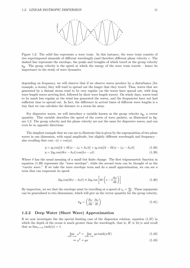
Figure 1.2: The solid line represents a wave train. In this instance, the wave train consists oftwo superimposed sinusoids of different wavelength (and therefore different phase velocity c. Thedashed line represents the envelope, the peaks and troughts of which travel at the group velocitycg. The group velocity is the speed at which the energy of the wave train travels – hence itsimportance in the study of wave dynamics.

depending on frequency, we will observe that if we observe waves produce by a disturbance (forexample, a storm) they will tend to spread out the longer that they travel. Thus, waves that aregenerated by a distant storm tend to be very regular (as the waves have spread out, with longwave length waves arriving first, followed by short wave length waves). On windy days, waves tendto be much less regular as the wind has generated the waves, and the frequencies have not hadsufficient time to spread out. In fact, the difference in arrival times of different wave lengths is away that we can calculate the distance to a storm far away.

For dispersive waves, we will introduce a variable known as the group velocity cg, a vectorquantity. This variable describes the speed of the crests of wave packets, as illustrated in fig-ure 1.2. The group velocity and the phase velocity are not the same for dispersive waves, and caneven be in opposite directions.

The simplest example that we can use to illustrate this is given by the superposition of two planewaves in one dimension, with equal amplitude, but slightly different wavelength and frequency –also recalling that cos(−φ) = cos(φ).

η = η0 cos[(k + δk)x− (ω + δω)t] + η0 cos[(k − δk)x− (ω − δω)t] (1.38)η = 2η0 cos(δkx− δωt) cos(kx− ωt) (1.39)

Where δ has the usual meaning of a small but finite change. The first trigonometric function inequation (1.39) represents the “wave envelope”, while the second term can be thought of as the“carrier wave.” If we take the wave envelope term and do a small approximation, we can see aterm that can respresent its speed.

2η0 cos(δkx− δωt) ≈ 2η0 cos[δk

(x− t

dωdk

)](1.40)

By inspection, we see that the envelope must be travelling at a speed of cg = dωdk . These arguments

can be generalised to two dimensions, which will give us the vector quantity for the group velocity.

cg =(∂ω

∂k,∂ω

∂l

)(1.41)

1.2.2 Deep Water (Short Wave) Approximation

If we now investigate the the special limiting case of the dispersion relation, equation (1.37) inwhich the depth of the ocean is much greater than the wavelength, that is, H 2π/κ and recallthat as limφ→∞ tanh(φ) = 1.

limκH→∞

ω2 = limκH→∞

gκ tanh(κH) (1.42)

⇒ ω2 = gκ (1.43)


This also allows us to approximate our expression for the phase speed.

c2 =g

κ(1.44)

Note that in this limit, the phase speed is still dependent on the wavenumber, and is thereforedispersive.

We also have an expression for the perturbation pressure, p′ in equation (1.32), recalling thatcosh(φ+ ψ) = cosh(φ) cosh(ψ) + sinh(φ) sinh(ψ), sinh(φ)

cosh(φ) = tanh(φ) and sinh(φ) + cosh(φ) = eφ.

p′ = ρ0gη0 cos(k · x− ωt)eκz (1.45)

Notice that the depth of the ocean, H does not appear in any of the equations. This is becausethese waves do not feel the effects of the bottom (hence the name deep water wave). Anothervery important thing to note as a consequence of this, is the depth dependence of the perturba-tion pressure (the exponential term). This means that the wave attenuates proportionally to thewavelength. We can do a simple calculation to find the e-folding depth (e−1 ∼ 0.37), which givesus a measure of the depth of influence of a surface wave.

e−1 = eκz

−1 = κz

z = − λ

2π(1.46)

where λ is the wavelength. If we use similar arguments, except setting e−π, noting that e−π ∼ 0.04,we can see that the influence of the surface wave on the subsurface is up to a depth of approxi-mately half a wavelength (that is, at a depth that is equal to half a wavelength, the perturbationpressure is only ∼ 4% the perturbation pressure at the surface).

Now, we can also find the group velocity using the dispersion relation, equation (1.43). Weassume that the medium is isotropic (that is, k = l) and as such, the phase velocity will beindependent of direction (for brevity we only consider k, but the result applies equally to l).

cg =∂ω

∂k

=√g∂

∂k(k)

12

=12

√g

k(1.47)

⇒ cg =12c (1.48)

A typical short wave has a period 2πω−1 = 10s, and thus it has a wavelength 2πκ−1 = 105m,an e-folding depth of 25m and a phase speed of c = 15ms−1.

1.2.3 Shallow Water (Long Wave) Approximation

On the other hand, the other limiting case is where H 2π/κ, where the effects of the bottomare very important. Opposite to the short wave approximation, we take the limiting case in whichthe depth of the ocean is much shorter than the wavelength, and recall that limφ→0 tanh(φ) = φ.

limκH→0

ω2 = limκH→0

gκ tanh(κH) (1.49)

⇒ ω2 = gκ2H (1.50)

We can find our phase speed from this.c2 = gH (1.51)

Importantly, note that these waves are non-dispersive, as there is no dependence of the velocityon the wave number – thus, the velocity of the wave energy is the same as the phase velocity.

1.3. PARTICLE PATHS 13

Z0 = 0

X = X0, Y = Y0

η0eκZ0

η0

Z0

Figure 1.3: This shows the decreasing radius of circular particle paths with depth. The verticledotted line indicates X0 and Y0, while horizontal dotted line indicates Z0 = 0, the mean sea surfaceheight. The solid lines are the particle paths of particles with mean position (X0, Y0, Z0), whilethe dashed line is the envelope of decreasing particle path radii.

The speed of these waves is also highly influenced by the bottom depth, with waves travelling inshallow water (for example, the continental shelf, where a typical speed might be 20ms−1) muchslower than in deep water (for example, the open ocean, where a typical speed might be 200ms−1).

We can now also find our perturbation pressure, recalling that tanh(0) = 0 and cosh(0) = 1.We need to bear in mind that κz ' 0 since we are assuming that κ−1 H and by definitionz ≤ H (see figure 1.1).

p′ = ρ0gη0 cos(k · x− ωt) (1.52)

Importantly, and contrasted to the deep water waves, the pressure perturbation of the shallowwater waves does not attenuate with depth.

1.3 Particle Paths

Recall our continuity and momentum equations (1.8) – (1.11). For convenience, we rewrite themomentum equations in a compact form.

∂v∂t

= − 1ρ0∇p′ (1.53)

We have, up until now, discussed two kinds of velocities, phase velocity c (which is the propagationof waves with a constant Φ) and group velocity cg (which is the propagation of the energy of “wavetrains”). Neither of these velocities is indicative of the velocity of a particle floating in the water(for example, a bottle on the surface of the ocean, or perhaps a phytoplankton).

For illustrative purposes, we will go through in detail the way that we find the particle pathsfor the deep water approximation derived in section 1.2.2. We begin by finding the velocityby substituting the equation for the perturbation pressure, equation (1.45) into the momentumequation, taking the spatial derivatives of the perturbation pressure and integrating with respectto time to find the velocity v.

u =gη0k

ωcos(k · x− ωt)eκz (1.54)

v =gη0l

ωcos(k · x− ωt)eκz (1.55)

w = −gη0κω

sin(k · x− ωt)eκz (1.56)

While the velocity tells us how fast the particles might be travelling, what we really want to knowis their position. If we take a Lagrangian perspective and track the position of individual particles,X = (X,Y, Z) labelling them as X0 = (X0, Y0, Z0), where we define X0 as the initial particleposition (which cooincidentally, turns out to be the mean position). We are now ready to define


Z0

Z0 = 0

c

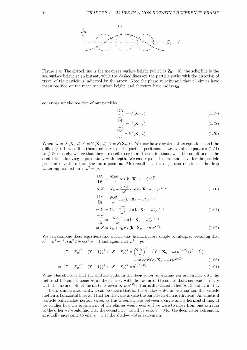
Figure 1.4: The dotted line is the mean sea surface height (which is Z0 = 0), the solid line is thesea surface height at an instant, while the dashed lines are the particle paths with the direction oftravel of the particle is indicated by the arrow. Note the phase velocity and that all circles havemean position on the mean sea surface height, and therefore have radius η0.

equations for the position of our particles.

DXDt

= U(X0, t) (1.57)

DYDt

= V (X0, t) (1.58)

DZDt

= W (X0, t) (1.59)

Where X = X(X0, t), Y = Y (X0, t), Z = Z(X0, t). We now have a system of six equations, and thedifficulty is how to link them and solve for the particle positions. If we examine equations (1.54)to (1.56) closely, we see that they are oscillatory in all three directions, with the amplitude of theoscillations decaying exponentially with depth. We can exploit this fact and solve for the particlepaths as deviations from the mean position. Also recall that the dispersion relation in the deepwater approximation is ω2 = gκ.

DXDt

=gη0k

ωcos(k ·X0 − ωt)eκZ0

⇒ X = X0 −gη0k

ω2sin(k ·X0 − ωt)eκZ0 (1.60)

DYDt

=gη0l

ωcos(k ·X0 − ωt)eκZ0

⇒ Y = Y0 −gη0l

ω2sin(k ·X0 − ωt)eκZ0 (1.61)

DZDt

= −gη0κω

sin(k ·X0 − ωt)eκZ0

⇒ Z = Z0 + η0 cos(k ·X0 − ωt)eκZ0 (1.62)

We can combine these equations into a form that is much more simple to interpret, recalling thatκ2 = k2 + l2, sin2 φ+ cos2 φ = 1 and again that ω2 = gκ.

(X −X0)2 + (Y − Y0)2 + (Z − Z0)2 =(gη0ω2

)2

sin2(k ·X0 − ωt)e2κZ0(k2 + l2)

+ η20 cos2(k ·X0 − ωt)e2κZ0 (1.63)

⇒ (X −X0)2 + (Y − Y0)2 + (Z − Z0)2 =η20e

2κZ0 (1.64)

What this shows is that the particle paths in the deep water approximation are circles, with theradius of the circles being η0 at the surface, with the radius of the circles decaying exponentiallywith the mean depth of the particle, given by η0eκZ0 . This is illustrated in figure 1.3 and figure 1.4.

Using similar arguments, it can be shown that for the shallow water approximation, the particlemotion is horizontal lines and that for the general case the particle motion is elliptical. An ellipticalparticle path makes perfect sense, as this is somewhere between a circle and a horizontal line. Ifwe condier how the eccentricity of the ellipses would evolve if we were to move from one extremato the other we would find that the eccentricity would be zero, ε = 0 for the deep water extremum,gradually increasing to one, ε = 1 at the shallow water extremum.

1.4. WAVE CONSERVATION 15

1.4 Wave Conservation

Now that we have examined waves in the deep ocean, and waves in a uniformly shallow ocean. Thisbegs the question, what if the ocean is not uniformly deep, but gradually becomes more shallow(for example, waves going from the deep ocean to the continental shelf)?

1.4.1 Conservation I

For brevity, we will restrict the following discussion to two dimensions, however, it can be reason-ably easily generalised to three dimensions. We begin by recalling the complex form of notation.

η = η0eiΦ (1.65)

Where Φ = Φ(x, t) is the phase parameter defined in equation (1.22). If we now allow the wavenum-ber and frequency to vary slowly that is k = k(x, t) and ω = ω(x, t). Next, we note some helpfulrelations.

k ≡ ∂Φ∂x

(1.66)

ω ≡ −∂Φ∂t

(1.67)

If we also allow slow variations in the amplitude, we get the following solution for the surfaceheight.

η(x, t) = η0(x, t)eiΦ(x,t) (1.68)

Now, if we cross differentiate equations (1.66) and (1.67), recalling the dispersoin relation in equa-tion (1.50) and add them together, we get the following relation.

∂k

∂t+∂ω

∂x= 0 (1.69)

Furthermore, if we recall the definition of the group velocity in equation (1.41) and exploit thechain rule.

∂k

∂t+∂ω

∂x=∂k

∂t+∂ω

∂k

∂k

∂x

=∂k

∂t+ cg

∂k

∂x

⇒ DkDt

= 0 (1.70)

where DkDt ≡

∂k∂t +cg ∂k

∂x which is a Lagrangian representation, but instead of following a fluid parcel,we are following the local wave energy. If we use the shallow water approximation and recall thedispersion relation in equation (1.50) and is ω2 = gHk2 in two dimensions only. Also recall thephase velocity in equation (1.51), which is c2 = gH. Now, recall the group velocity, defined inequation (1.41), and we see that the phase speed is the same as the group velocity.

cg =∂ω

∂k

=√gH

⇒ cg = c (1.71)

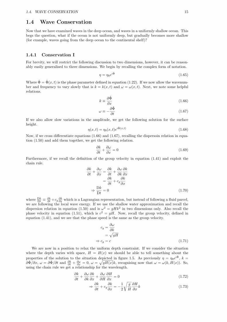
We are now in a position to relax the uniform depth constraint. If we consider the situationwhere the depth varies with space, H = H(x) we should be able to tell something about theproperties of the solution to the situation depicted in figure 1.5. As previously η = η0e

iΦ, k =∂Φ/∂x, ω = ∂Φ/∂t and ∂k

∂t + ∂ω∂x = 0, ω =

√gH(x)k, recognising now that ω = ω(k,H(x)). So,

using the chain rule we get a relationship for the wavelength.

∂k

∂t+∂ω

∂k

∂k

∂x+∂ω

∂H

∂H

∂x= 0 (1.72)

⇒ ∂k

∂t+ cg

∂k

∂x= −1

2

√g

H

∂H

∂xk (1.73)


z

x

z = −H(x)

Figure 1.5: This diagram shows the situation where the depth H (the shaded region indicates thebottom) varies with x with a free surface (solid line). The dotted line idicates the average the meansurface. Note that the shape of the free surface is indicative only, see the text for the solution.

Furthermore, application of the chain rule to ∂ω∂t , (noting that ∂H

∂t = 0 and ∂k∂t = −∂ω

∂x ) resultsin a similar expresson for ω.

∂ω

∂t+ cg

∂ω

∂x= 0 (1.74)

We can investigate the steady state solution of these equations without having to go to thetrouble of attempting to derive some explicit solution. When we say a steady state solution, weare assuming that all time derivative terms are zero ( ∂

∂t ≡ 0). In the present example, this wouldbe a good assumption to make if you were observing waves coming onshore on a relatively windlessday (a strong wind will provide a non-trivial forcing, which means that ∂

∂t 6= 0).

There are three main things that we can easily see from these equations.

1. cg ∂k∂x = − 1

2

√gH

∂H∂x k by equation (1.73). As the depth of the ocean is decreasing with

increasing x, thus, ∂H∂x < 0. Therefore, we see that the wavenumber must increase with

increasing x. Since the wavelength is reciprocal to the wavenumber, the wavelength mustshorten as the waves travel.

2. ∂ω∂t = 0 ⇒ ∂ω

∂x = 0 by equation (1.74). This means that as the travelling waves get closer toshore (with decreasing H), the frequency of the waves will not change.

3. cg =√gH implies that the wave velocity will decrease as the wave progresses.

1.4.2 Conservation II

Recall from the shallow water approximation that the perturbation pressure, p′, is independent ofdepth and is proportional to the sea surface height, η – cf. equations (1.7) and (1.52). Thus, thehorizontal velocity is independent of depth (i.e. the velocity at any horizontal point is the same atall depths). We shall now exploit this fact, along with continuity, equation (1.8) to find solutionsfor a situtation where we have a non-uniform depth.

Let us first restate the horizontal equations of motion and the continuity equation.

∂u

∂t= − 1

ρ0

∂p′

∂x

= −g ∂η∂x

∂v

∂t= − 1

ρ0

∂p′

∂z

= −g ∂η∂z

∇ · v = 0

Next, we need to state our boundary conditions. We assume for our surface boundary condition,that the vertical velocity at the surface is the same as the rate of change of sea surface height – cf.


equation (1.14) and the discussion on the surface boundary condition in section 1.1.4.

w =∂η

∂tat z = 0 (1.75)

For our bottom boundary condition, we state that there can be no flow normal to the bottom.Now, recall from vector calculus that the normal vector of a surface is described by its gradientwhen the surface has been given implicitly as a set of points F (x, y, z) = 0. The surface of theocean floor is described by z = −H(x, y) or alternatively, z +H(x, y) = 0. Thus its normal vectoris given by n = ∇(z +H) = (∂H

∂x ,∂H∂y , 1). Also recall from vector calculus that the dot product of

two vectors describes how aligned they are (i.e. orthogonal vectors have a zero dot product). Ifwe want to ensure that there is no normal flow (which is a reasonable condition to impose as theocean floor is impermiable), we take the dot product of the velocity and the normal vector andwe can see that this must be zero. This is really the same boundary condition as what we haveused previously, except we must make its mathematical description more general, as previouslythe normal vector for the bottom was always vertically aligned – cf. equation (1.12).

v · n = 0 at z = −H(x, y) (1.76)⇒ v · ∇(z +H) = 0 at z = −H(x, y) (1.77)

⇒ u∂H

∂x+ v

∂H

∂y+ w = 0 at z = −H(x, y) (1.78)

If we now depth integrate the continuity and exploit the fact that our bottom boundary equationgives us an expression for the vertical velocity at z = −H, we get a neat differential equation.Remember that both u and v are independent of z, and our surface boundary condition, equa-tion (1.75). ∫ 0

−H

∂u

∂x+∂v

∂y+∂w

∂zdz = 0 (1.79)∫ 0

−H

∂u

∂x+∂v

∂yDz +

∫ 0

−H

∂w

∂zdz = 0 (1.80)[

0−−H(∂u

∂x+∂v

∂y

)]+ [w(0)− w(−H)] = 0 (1.81)[

H

(∂u

∂x+∂v

∂y

)]+[∂η

∂t+u∂H

∂x+ v

∂H

∂y

]= 0 (1.82)

⇒ ∂η

∂t+

∂

∂x(Hu) +

∂

∂y(Hy) = 0 (1.83)

We get from equation (1.82) to equation (1.83) by use of the chain rule. Now, if we differentiateequation (1.83) with respect to t and then recall our horizontal equations of motion stated earlierin this section, we come up with a single equation for the free surface. We are assuming operatorcommutation and we remember that H is independent of time.

∂2η

∂t2+

∂

∂x

(H∂u

∂t

)+

∂

∂y

(H∂v

∂t

)= 0 (1.84)

1g

∂2η

∂t2+

∂

∂x

(H∂η

∂x

)+

∂

∂y

(H∂η

∂y

)= 0 (1.85)

The major implicit assumption in all of the above is that the vertical accelleration much smallerthan gravity ∂w

∂t g. This means that the relationship we have now derived will not hold forsteep slopes as continuity will dictate that ∂w

∂t ∼ g.

1.4.3 Linear Bottom Slope

Let us consider a two dimensional system (in x and z) where we have a bottom slope described byH = H(x). Let us now assume that our solution is a simple harmonic time dependent solution.

η = Z(x)e−iωt (1.86)


Substituing this into equation (1.85), we get an ordinary differential equation for Z(x).

−ω2

gZ − d

dx

(H

dZdx

)= 0 (1.87)

This is now an ordinary differential equation with a variable coefficient H. We can get exactanalytic solutions for certain forms of H. One of those forms is where H linearly increases with x,see figure 1.6. We will now investigate this form.

H = αx where α > 0 (1.88)

Recall that α cannot be too large as we have assumed that the vertical accelleration must be muchsmaller than gravity, dw

dt g. Thus, equation (1.87) becomes

ddx

(x

dZdx

)+ω2

gαZ = 0. (1.89)

This equation has an exact solution.

Z(x) = AJ0

(2ω√

x

gα

)+BY0

(2ω√

x

gα

)(1.90)

Where J0 is the Bessel function of the first kind of order 0 and Y0 is the Bessel function4 of thesecond kind of order 0 and A & B are constants of integration. Now recall that the Bessel functionof the second kind, Y0(x) → −∞ as x→ 0. We require a non-singular solution at that point, thus,we must set B = 0. Now our solution is finite and we have a form for Z.

Z(x) = AJ0

(2ω√

x

gα

)(1.91)

⇒ η(x, t) = AJ0

(2ω√

x

gα

)e−iωt (1.92)

Now, if we wish to find the associated velocity, we need to recall from section 1.4.2 that

∂u

∂t= −g ∂η

∂x(1.93)

Similarly to the surface height, we assume a particular form, and subsitute into equation (1.93) tofind our solution for u(x, t). We also need to recall that DJ0(x)

Dx = −J1(x).

u(x, t) = U(x)e−iωt (1.94)

⇒ −iωU = −gA2ω√

1gα

12√xJ0

(2ω√

x

gα

)(1.95)

U(x) = Ai

√g

αx−

12 J1

(2ω√

x

gα

)(1.96)

⇒ u(x, t) = Ai

√g

αx−

12 J1

(2ω√

x

gα

)e−iωt (1.97)

While this may seem like a complicated result, we can use it in relatively simple ways to tell usinformation about the amplitude of waves near the coast where the coast is reasonably straightand the sea floor is gently sloping, similarly to the situation described in figure 1.6.

Given a measured amplitude of η = ηL at the edge of the sloping topography, x = L, wecan relatively simply find an expression that tells us the amplitude of the sea surface waves for

4Recall that Jn(x) =P∞

m=0(−1)m

m!Γ(m+n+1)

`x2

´2m+nand Yn(x) =

Jn(x) cos(nπ)−J−n(x)

sin(nπ)where Γ is the generalised

factorial function (to include non-ingeters). These definitions of Bessel functions are included for completeness andwe do not need to overly concern ourselves with their exact form – however, we will rely on their properties to gatherinformation about constants of integration as well as properties of solutions.


x = 0 x = L

ηη = +ηL

η = −ηL

Figure 1.6: Schematic of a linear bottom slope. We can find an exact solution for the waveamplitude in this situation.

0 ≤ x ≤ L. We substitute this into equation (1.90) to solve for A.

Z(L) = ηL (1.98)

⇒ ηL = AJ0

(2ω

√L

gα

)(1.99)

⇒ η(x, t) = ηL

J0

(2ω√

xgα

)J0

(2ω√

Lgα

)e−iωt (1.100)

The maximum amplification of the wave is going to occur at x = 0 is going to be Z(0) = ηL

J0

“2ω

qL

gα

” .

Thus, if we look at the amplification factor at x = 0 as this will give us an idea about the signfi-cance of this amplification.

An example: Let’s plug in some reasonable numbers and see what we find. Say L = 10km=104m, α = 0.1 (this represents a decrease in depth of 1m for every 10m horizontally), g = 10ms−2

and let the period T , be in hours, such that the frequency is given by ω = 2π60×60T .

2ω

√L

gα=

2× 2π3600T

√104

10× 0.1(1.101)

∼ 13T

(1.102)

If we choose a long period wave (low frequency) wave with a period of about 12 hours, we getJ0

(136

)' 0.999. This indicates that the amplification is insignificant as the amplitude at x = 0 is

virtually the same as that at x = L.

Next, if we choose a short period (high frequency) wave with a period of about 10 minutes(= 1/6 hour), we find that J0(2) ' 0.224. Thus the amplitude of the wave at the shore, x = 0, is

10.224 ' 4.5 times greater than at the edge of the slope, x = L.

Chapter 2

Shallow Water Waves in aRotating Reference Frame

The effects of rotation are not significant for many classes of water waves. However, for manyaspects of global climate, planetary scale waves that are affected by the Earth’s rotation are veryimportant. In this chapter we will build on the theory that we have developed in the previouschapter by relaxing the assumption that the effects of rotation are unimportant.

We will examine a number of types of important planetary scale waves. In the next chapter,we will examine how some of these waves play an extremely important role in one of the mostglobally dominant climatic features, the El Nino-Southern Oscillation.

2.1 Poincare (gravity-inertia) waves

Thus far in our discussion on waves, we have ignored the effects of rotation, and indeed, we havenot even specified the form of rotation (see section 1.1.1). To breifly recap, the rotation vector,Ω = 1

2 (0, f∗, f) has two components: a horizontal component and a vertical component. For thevast majority of problems (including those considered here), we can ignore the horizontal compo-nent, f∗ = 0. The vertical component is the familiar coriolis parameter, f = 2Ω sin(φ), where φ isthe latitude and Ω is the Earth’s angular velocity.

If we now remove the irrotational assumption, which is true for waves with period O(hours),we arrive at new equations of motion.

∂u

∂t− fv = −g ∂η

∂x(2.1)

∂v

∂t+ fu = −g ∂η

∂y(2.2)

p = ρg(η − z) (2.3)

We now assume that the velocity is of the form u(x, y, t) = F (x, y)e−iωt and v(x, y, t) = G(x, y)e−iωt

and substitute this into the equations for the horizontal velocities.

−iωu− fv = −g ∂η∂x

(2.4)

−iωv + fu = −g ∂η∂y

(2.5)

The equations are now in a relatively easy form to solve for the velocities by cross substitution.

u = g−iω ∂η

∂x + f ∂η∂y

ω2 − f2(2.6)

v = −giω ∂η

∂y + f ∂η∂x

ω2 − f2(2.7)

21

22 CHAPTER 2. SHALLOW WATER WAVES IN A ROTATING REFERENCE FRAME

κ

ω

f

Figure 2.1: The dispersion relation, ω2 = f2 + gHκ2, for Poincare waves (a.k.a. inertia-gravitywaves). Note that the frequency has a lower bound, being ω2 > f2.

If we now assume that these waves do not have a large meridional extent, we can consider φ tobe constant and therefore f to be constant when taking spatial derivatives. We also assume thatthe frequency does not change significantly with space and we may also consider this a constant.Finally, we also assume that the time dependent portion of the sea surface height, η has the forme−iωt.

Combining these assumptions with the results from the previous chapter, recalling the conti-nuity equation for shallow water waves with an arbitrary bathymetry (but not allowing it to gettoo steep), equation (1.83). For completeness, we restate equation (1.83) first.

∂η

∂t+

∂

∂x(Hu) +

∂

∂y(Hy) = 0 (2.8)

−iωη +g

ω2 − f2

∂

∂x

[H

(−iω ∂η

∂x+ f

∂η

∂y

)]− ∂

∂y

[H

(iω∂η

∂y+ f

∂η

∂x

)]= 0 (2.9)

If we now assume a uniform depth (i.e. constant H), we end up with a much easier expression tosolve.

−iωη +gH

ω2 − f2

[(−iω ∂

2η

∂x2+ f

∂2η

∂x∂y

)−(iω∂2η

∂y2+ f

∂2η

∂y∂x

)]= 0 (2.10)

−iωη +gH

ω2 − f2

[−iω ∂

2η

∂x2− iω

∂2η

∂y2

]= 0 (2.11)

ω2 − f2

gHη +

∂2η

∂x2+∂2η

∂y2= 0 (2.12)


By inspection of equation (2.12), we can see that η(x, y, t) = η0ei(k·x−ωt) is a solution to this

equation on the condition that

−(k2 + l2) +ω2 − f2

gH= 0 (2.13)

⇒ ω2 = f2 + gHκ2. (2.14)

Recall that κ2 = k2 + l2. We reach this dispersion relation by simply substituting our solution intothe partial differential equation in equation (2.12) and then dividing through by η.

We can see by inspection of relation (2.14) that ω must always be greater than the coriolisparameter (aka, the inertial frequency), ω2 > f2. The dispersion relation is show in figure 2.1.

We can see that for small f or large k (i.e. k2 f2

gH ), this class of waves becomes the normal,surface gravity wave in the shallow water limit, described in section 1.2.3.

2.1. POINCARE (GRAVITY-INERTIA) WAVES 23

x

y

a

b

(u, v)

Figure 2.2: The time evolution of the horizontal velocity asssociated with a Poincare wave takethe form of an ellipse with the length a = η0gωk

ω2−f2 being the major axis and b = η0gfkω2−f2 being the

minor axis.

2.1.2 Horizontal Particle Paths

Let us now substitute the solution for sea surface height, η(x, y, t) = η0ei(kx+ly−ωt), into the

expressions for velocity, equations (2.6) and (2.7).

u = gωk + ilf

ω2 − f2η (2.15)

v = g−ωl + ifk

ω2 − f2η (2.16)

To keep things simple, lets now assume that we have a wave propagating in the x directiononly (i.e. l = 0). We also follow the convention that the physical solution is the real part of theresultant complex expression, recalling that eix = cos(x) + i sin(x).

u = <g

ωk

ω2 − f2η0 [cos(kx− ωt) + i sin(kx− ωt)]

(2.17)

⇒ u =η0gωk

ω2 − f2cos(kx− ωt) (2.18)

v = <g

ifk

ω2 − f2η0 [cos(kx− ωt) + i sin(kx− ωt)]

(2.19)

⇒ v = − η0gfk

ω2 − f2sin(kx− ωt) (2.20)

We can thus see that there is a component of the velocity which is perpendicular in the horizontalto the direction of travel of the wave. If we square the velocities and add them together, recallingthat cos2(x) + sin2(x) = 1, we get a parametric equation in the form of an ellipse.

u2(ω2 − f2)2

η20g

2ω2k2+v2(ω2 − f2)2

η20g

2f2k2= 1 (2.21)

u2

a2+v2

b2= 1 (2.22)

We can see that the major axis of the ellipse (which is in the x direction) has a length of a = η0gωkω2−f2

ad a minor axis in the y direction of b = η0gfkω2−f2 and is shown schamatically in figure 2.2.

Notice that

a

b=ω

f(2.23)

⇒ b ' a for ω ' f (2.24)⇒ b ' 0 for ω f. (2.25)


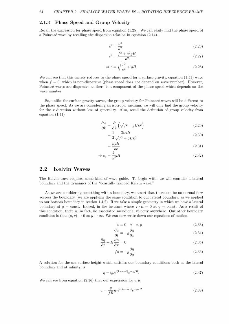
2.1.3 Phase Speed and Group Velocity

Recall the expression for phase speed from equation (1.25). We can easily find the phase speed ofa Poincare wave by recalling the dispersion relation in equation (2.14).

c2 =ω2

κ2(2.26)

c2 =f2 + κ2gH

κ2(2.27)

⇒ c =

√f2

κ2+ gH (2.28)

We can see that this merely reduces to the phase speed for a surface gravity, equation (1.51) wavewhen f = 0, which is non-dispersive (phase speed does not depend on wave number). However,Poincare waves are dispersive as there is a component of the phase speed which depends on thewave number!

So, unlike the surface gravity waves, the group velocity for Poincare waves will be different tothe phase speed. As we are considering an isotropic medium, we will only find the group velocityfor the x direction without loss of generality. Also, recall the definition of group velocity fromequation (1.41)

∂ω

∂k=

∂

∂k

(√f2 + gHk2

)(2.29)

=12

2kgH√f2 + gHk2

(2.30)

=kgH

kc(2.31)

⇒ cg =k

ωgH (2.32)

2.2 Kelvin Waves

The Kelvin wave requires some kind of wave guide. To begin with, we will consider a lateralboundary and the dynamics of the “coastally trapped Kelvin wave.”

As we are considering something with a boundary, we assert that there can be no normal flowaccross the boundary (we are applying the same condition to our lateral boundary, as we appliedto our bottom boundary in section 1.4.2). If we take a simple geometry in which we have a lateralboundary at y = const. Indeed, in the instance where v · n = 0 at y = const. As a result ofthis condition, there is, in fact, no associated meridional velocity anywhere. Our other boundarycondition is that (u, v) → 0 as y →∞. We can now write down our equations of motion.

v ≡ 0 ∀ x, y (2.33)∂u

∂t= −g ∂η

∂x(2.34)

∂η

∂t+H

∂u

∂x= 0 (2.35)

fu = −g ∂η∂y. (2.36)

A solution for the sea surface height which satisfies our boundary conditions both at the lateralboundary and at infinity, is

η = η0ei(kx−ωt)e−y/R. (2.37)

We can see from equation (2.36) that our expression for u is:

u =g

fRη0e

i(kx−ωt)e−y/R (2.38)

2.2. KELVIN WAVES 25

(a)f > 0 (b)f < 0

x

y

c

decaying η

x

y

c

decaying η

Figure 2.3: For both subfigures, dashed lines represent travelling wave crests with the direction oftravel indicated. (a) A Kelvin wave travelling eastward along a southern boundary in the northernhemisphere; (b) A Kelvin wave travelling along a southern boundary in the southern hemisphere.

Using the other two equations, we get two expressions which allows us to solve for R.

ω = fRk (2.39)

ω =gHk

fR(2.40)

⇒ R2 =gH

f2(2.41)

We should recognise |R| as being the Rossby radius of deformation, the length scale for whichrotation becomes important. Due to the fact that our expression for R is a square, it therefore hastwo roots. If we now substitute the positive root of R into equation (2.39), we find the dispersionrelation.

ω =√gHk (2.42)

From the dispersion relation, we find the phase velocity. We begin, however, by using equa-tion (2.39) – the reason for which will become obvious soon.

c =ω

k= fR (2.43)

=√gH (2.44)

The most obvious thing of note about the phase velocity is that the Kelvin wave is non-dispersive. There is, however, something of equal importance that is somewhat more subtle. SinceR appears as a square, it thus has two roots. The sign of the root of R that we choose dependson the situation. We always want η to decay to zero far away from the boundary, and eitherthe positive or negative root of R should be chosen to satisfy this boundary condition. Notefrom the expression for phase velocity in equation (2.43) that it is the combination of the signs ofR and f that dictates the direction of propagation. To illustrate, we will now look at two examples.

Example – easterly propagating wave in the northern hemisphere: see figure 2.3(a). For thisexample, we should choose the positive root of R to ensure that the sea surface height decays farfrom the boundary. Thus, since both f and R are positive, c is also positive.

Example – westerly propagating wave in the southern hemisphere: see figure 2.3(b). For thisexample, we should choose the positive root of R to ensure that the sea surface height decays farfrom the boundary. Since we have f < 0 and R > 0, we thus have c < 0.

To generalise this discussion, we note that an observer following a Kelvin wave will alwayshave the boundary on their right in the northern hemisphere and on their left in the southernhemisphere. Thus, at meridional boundaries, Kelvin waves travel poleward at an eastern bound-ary and equatorward at a western boundary. Furthermore, if we had an enclosed basin entirely inthe northern hemisphere, Kelvin waves would always travel anti-clockwise around the boundaries.Conversely, in the southern hemisphere, they would always travel clockwise.


f

φ-90 -60 -30 0 30 60 90

2Ω

−2Ω

Figure 2.4: The f plane (solid line) is shown with a beta plane (dashed line) centred at 45. Notehow the beta plane closely approximates the f plane between 30 and 60, however, particularlyat high latitudes, rapidly diverges from the f plane.

2.3 Rossby Waves

Rossby waves owe their existance to the conservation of potential vorticity. As you will recall fromprevious lectures, vorticity is conserved (see notes on planetary vorticity and vortex stretching).There are two instances where these dynamics will become important, one is when we have a largemeridional extent (and are no longer able to assume that f is locally constant). The other is overvariations in bottom topography.

In order to begin our discussion on Rossby waves, we must first investigate the beta planeapproximation.

2.3.1 The Beta Plane

Recall that the coriolis parameter is

f = 2Ωcos(φ). (2.45)

where Ω is the angular speed of rotation of the earth and φ is the latitude. Recalling that y = reφwhere re is the earth’s radius, we can rewrite this expression as a variation from a particularlatitude.

f = 2Ω sin(φo + y/re) (2.46)

We can now do a Taylor expansion about this point, only taking the first two terms.

f ' 2Ω sin(φ0) + 2Ωy

recos(φ0) (2.47)

' f0 + βy (2.48)

We can see that f0 = 2Ω sin(φ0), and β = 2Ωcos(φ0)/re. The beta plane is illustrated in figure 2.4,and as can be seen, it is not valid at high latitudes, where the rate of change of the gradient of fis fast (i.e. D2f

Dφ2 is large).

At mid-latitudes, the beta plane approximation is valid only if βy is small compared with f0. Ifthe meridional length scale is L, then βL f0. There is a form of the beta plane which is valid atthe equator and is important for equatorial wave dynamics, however, we will cover this in chapter 3.

2.3. ROSSBY WAVES 27

2.3.2 Governing Equation

Let us now restate the equations of motion with a constant depth, H.

∂u

∂t− fv = −g ∂η

∂x(2.49)

∂v

∂t+ fu = −g ∂η

∂y(2.50)

∂η

∂t+H

(∂u

∂x+∂v

∂y

)= 0 (2.51)

As usual, we assume that the solution for sea surface height and our horizontal velocities are ofthe form F (x, y)e−iωt. Next, we substitute this into the three equations of motion.

−iωu− fv = −g ∂η∂x

(2.52)

−iωv + fu = −g ∂η∂y

(2.53)

−iωη +H

(∂u

∂x+∂v

∂y

)= 0 (2.54)

In order to solve for these three variables, we start by rearranging equation (2.52) in terms of uand equation (2.53) in terms of η and then taking its derivative with respect to y.

u =fv

iω− g

iω

∂η

∂x(2.55)

η =H

iω

(∂u

∂x+∂v

∂y

)⇒ ∂η

∂y=H

iω

(∂2u

∂y∂x+∂2v

∂y2

)(2.56)

Now, we are able to substitute equations (2.55) and (2.56) into equation (2.53) and rearrange.

−iωv − f

iω

(fv − g

∂η

∂y

)= −gH

iω

(∂2u

∂x∂y+

∂v

∂y2

)(ω2 − f2)v + gH

∂2v

∂y2= −g

(f∂η

∂x+H

∂2u

∂x∂y

)(2.57)

In order to simplify this equation, we need to do some heavy algebra.

We begin by taking the derivative with respect to y of equation (2.52) and with respect to x ofequation (2.53). First, we must note that using the beta plane approximation from equation (2.48)and the product rule, ∂

∂y (fv) = f0∂v∂y + βv + βy ∂v

∂y = f ∂v∂y + βv.

−iω ∂u∂y− f

∂v

∂y+ βv = −g ∂2η

∂y∂x(2.58)

−iω ∂v∂x

+ f∂u

∂x= −g ∂2η

∂x∂y(2.59)

Next we subtract equation (2.58) from equaton (2.59) and assume operator commutation.

−iω(∂v

∂x− ∂u

∂y

)+ f

(∂u

∂x+∂v

∂y

)+ βv = 0 (2.60)

Recognising that we have seen the second bracketed term before, we then substitute equation (2.54)into equation (2.60).

−iω(∂v

∂x− ∂u

∂y

)+fiω

Hη + βv = 0

iω

H

(fη +H

∂u

∂y

)= iω

∂v

∂x− βv (2.61)


Next, we differentiate this last equation with respect the x, and then multiply both sides by−gH/iω.

−g(f∂η

∂x+H

∂2u

∂x∂y

)= −gH ∂2v

∂x2+gHβ

iω

∂v

∂x(2.62)

Notice that the left hand side of this equation is exactly the right hand side of equation (2.57), theequation that we have set out to simplify. We are now able to eliminate η from these equations.

−iω(ω2 − f2

gHv +

∂2v

∂x2+∂2v

∂y2

)+ β

∂v

∂x= 0 (2.63)

Note, that with a little more manipulation, and setting β = 0 and f = f0 we can regain equa-tion (2.12), our governing equation for Poincare and Kelvin waves. This is nice, as it gives usconfidence in our result.

Let us now consider waves that are very low frequency waves, ω2 f2. We can then furthersimplify equation (2.63) using this approximation. Let us also replace all f2 terms with f2

0 byassuming that f0βy f2

0 and (βy)2 f20 , which is not unreasonable for mid-latitudes, as we

have stated in section 2.3.1 that the beta plane approximation is only valid for small values of βycompared to f0.

−iω(∂2v

∂x2+∂2v

∂y2− f2

0

gHv

)+ β

∂v

∂x= 0 (2.64)


As usual, we seek solutions of the form v = Aei(kx+ly−ωt). We now substitute this into equa-tion (2.64) to find the dispersion relation.

−iω(−k2 − l2 − f2

0

gH

)+ ikβ = 0 (2.65)

⇒ ω =−kβ

κ2 +R−2(2.66)

We recognise R2 = gHf2 as the Rossby radius and κ2 = k2 + l2. Let us now look at the phase

velocity, c = (cx, cy), in the x direction – cf. equation (1.24).

cx =ω

k

⇒ cx =−β

κ2 +R−2(2.67)

Note that the phase velocity in the x direction is always negative. As we take east to be our posi-tive x direction, we can therefore deduce that Rossby waves always travel in a westward direction.

The interesting properties of a Rossby wave do not finish there. We can rewrite the dispersionrelation, equation (2.66) to describe a circle1 in (k, l) space.

k2 +kβ

ω+ l2 +R−2 = 0 (2.68)[

k2 +2kβ2ω

+(β

2ω

)2]

+ l2 +R−2 =(β

2ω

)2

(2.69)

[k +

β

2ω

]2+ l2 =

(β

2ω

)2

− 1R2

(2.70)

This dispersion relation thus describes a cicrle in (k, l) space centred on (−β/2ω, 0) with radius√(β/2ω)2 −R−2. This relation is shown in figure 2.5. For this relation to exist, the radius of the

1recall, the form of a circle, centred on x0, y0 with radius r is (x− x0)2 + (y − y0)2 = r2

2.3. ROSSBY WAVES 29

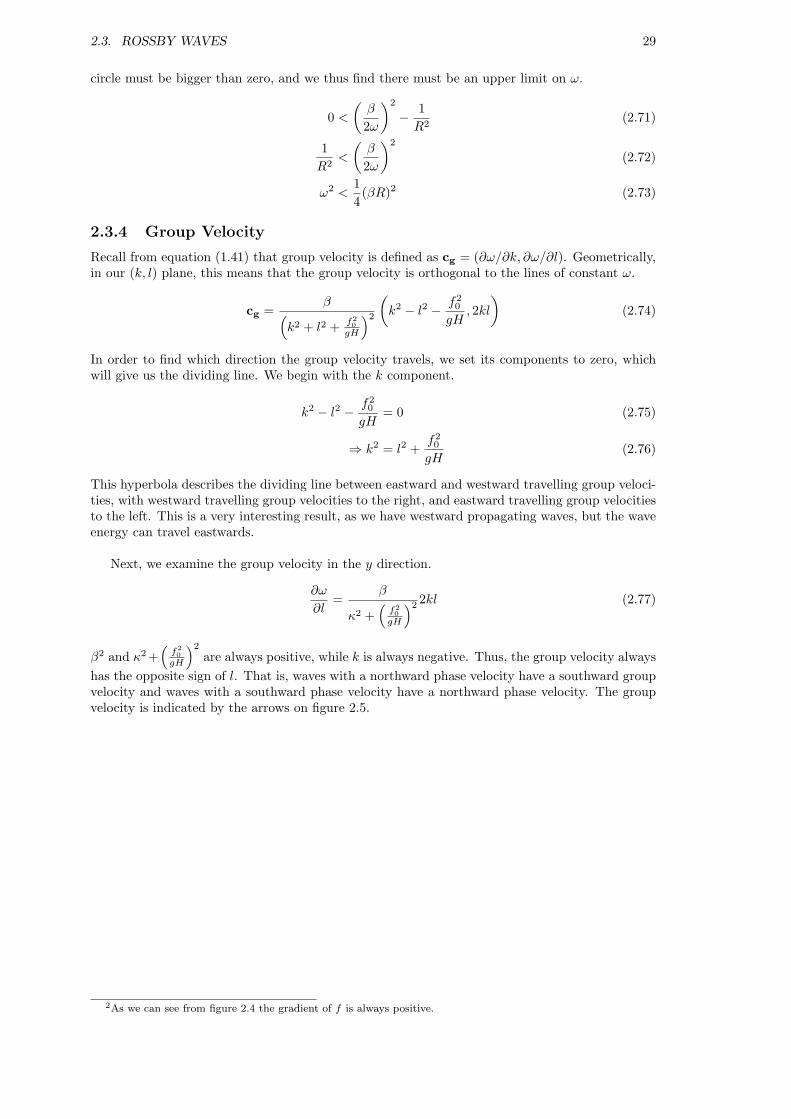
circle must be bigger than zero, and we thus find there must be an upper limit on ω.

0 <(β

2ω

)2

− 1R2

(2.71)

1R2

<

(β

2ω

)2

(2.72)

ω2 <14(βR)2 (2.73)

2.3.4 Group Velocity

Recall from equation (1.41) that group velocity is defined as cg = (∂ω/∂k, ∂ω/∂l). Geometrically,in our (k, l) plane, this means that the group velocity is orthogonal to the lines of constant ω.

cg =β(

k2 + l2 + f20

gH

)2

(k2 − l2 − f2

0

gH, 2kl

)(2.74)

In order to find which direction the group velocity travels, we set its components to zero, whichwill give us the dividing line. We begin with the k component.

k2 − l2 − f20

gH= 0 (2.75)

⇒ k2 = l2 +f20

gH(2.76)

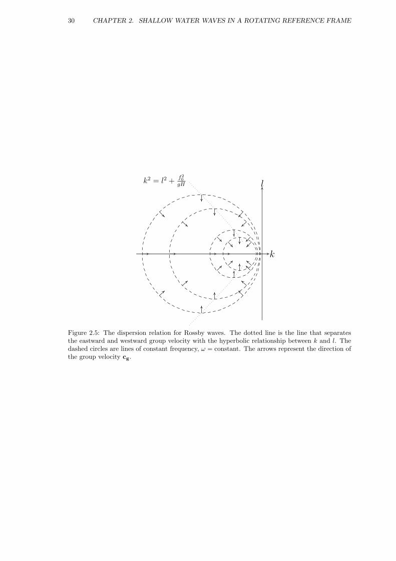
This hyperbola describes the dividing line between eastward and westward travelling group veloci-ties, with westward travelling group velocities to the right, and eastward travelling group velocitiesto the left. This is a very interesting result, as we have westward propagating waves, but the waveenergy can travel eastwards.

Next, we examine the group velocity in the y direction.

∂ω

∂l=

β

κ2 +(

f20

gH

)2 2kl (2.77)

β2 and κ2 +(

f20

gH

)2

are always positive, while k is always negative. Thus, the group velocity alwayshas the opposite sign of l. That is, waves with a northward phase velocity have a southward groupvelocity and waves with a southward phase velocity have a northward phase velocity. The groupvelocity is indicated by the arrows on figure 2.5.

2As we can see from figure 2.4 the gradient of f is always positive.


k

lk2 = l2 +f20

gH

Figure 2.5: The dispersion relation for Rossby waves. The dotted line is the line that separatesthe eastward and westward group velocity with the hyperbolic relationship between k and l. Thedashed circles are lines of constant frequency, ω = constant. The arrows represent the direction ofthe group velocity cg.

Chapter 3

Waves and the El Nino-SouthernOscillation

Why would one want to study ENSO? ENSO is the most dominant interannual climate signalon Earth. Both ENSO warm (aka El Nino) and cold (aka La Nina) events have major economicand social impacts on people. ENSO warm events can cause droughts in the western Pacific fromIndia to Indonesia to Australia. In the eastern Pacific, one of the most productive fisheries in theworld, have very poor years. It is not just those who live in the shadow of the Pacific ocean whoare affected. ENSO “teleconnections” have been shown to affect the amount of snowfall in NorthAmerica as well as the number of Atlantic hurricanes in a given season to name only a couple. Amap of ENSO relationships are shown in figure 3.1.

(a) ENSO warm events (b) ENSO cold events

Figure 3.1: Illustrative map of ENSO regional relationships. Images courtesy of NOAA.

As it turns out, equatorial wave dynamics plays an extremely important role in the dynamicsof ENSO, and holds the key to unlocking the mystery of ENSO. In this chapter, we will applywhat we have learned so far about wave dynamics to this important topic in climate science. It isan area where wave dynamics has taught us so much, but at the same time, still has much to tellus. ENSO is a very active area of research, and is exteremly complex. Presented here is a simpleexplanation of a very complex process.

31

32 CHAPTER 3. WAVES AND THE EL NINO-SOUTHERN OSCILLATION

3.1 What is ENSO?

ENSO warm and cold events1 refer to changes in the average temperatures of particular parts ofthe sea surface temperature of the tropical Pacific. The reason for these changes in average SST,and the concequences of these changes are what is of most interest to us.

3.1.1 The “Normal” State

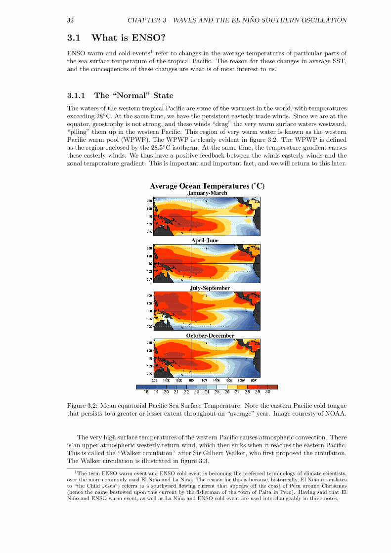
The waters of the western tropical Pacific are some of the warmest in the world, with temperaturesexceeding 28C. At the same time, we have the persistent easterly trade winds. Since we are at theequator, geostrophy is not strong, and these winds “drag” the very warm surface waters westward,“piling” them up in the western Pacific. This region of very warm water is known as the westernPacific warm pool (WPWP). The WPWP is clearly evident in figure 3.2. The WPWP is definedas the region enclosed by the 28.5C isotherm. At the same time, the temperature gradient causesthese easterly winds. We thus have a positive feedback between the winds easterly winds and thezonal temperature gradient. This is important and important fact, and we will return to this later.

Figure 3.2: Mean equatorial Pacific Sea Surface Temperature. Note the eastern Pacific cold tonguethat persists to a greater or lesser extent throughout an “average” year. Image couresty of NOAA.

The very high surface temperatures of the western Pacific causes atmospheric convection. Thereis an upper atmospheric westerly return wind, which then sinks when it reaches the eastern Pacific.This is called the “Walker circulation” after Sir Gilbert Walker, who first proposed the circulation.The Walker circulation is illustrated in figure 3.3.

1The term ENSO warm event and ENSO cold event is becoming the preferred terminology of climate scientists,over the more commonly used El Nino and La Nina. The reason for this is because, historically, El Nino (translatesto “the Child Jesus”) referrs to a southward flowing current that appears off the coast of Peru around Christmas(hence the name bestowed upon this current by the fisherman of the town of Paita in Peru). Having said that ElNino and ENSO warm event, as well as La Nina and ENSO cold event are used interchangeably in these notes.

3.2. EQUATORIAL WAVE DYNAMICS 33

Figure 3.3: An illustrative “normal” sea surface temperature, thermocline depth and atmosphericconvection and tradewind pattern. Image courtesy of NOAA.

The water along the equator, travelling from east to west, causes deep water in the easternPacific to be upwelled. It is this cold, nutrient rich water, which makes the eastern Pacific fishinggrounds so fertile and productive. This cold, upwelled water joins the movement of surface waterwestward, slowly warming as it goes. This cold water is referred to as the “eastern Pacific coldtongue.” This is evident in figure 3.2.

3.1.2 The Bjerknes Feedback

The situation described in the previous section involves a very closely coupled atmosphere-oceaninteraction. Even a slight perturbation to this system, under favourable circumstances, can causea negative feedback loop. A slackening of the trade winds, weakens the zonal equatorial temper-ature gradient, which in turn weakens the easterly winds, which in turn slackens the tradewindsfurther, and so on and so forth. This feedback is called the Bjerkens feedback after the scientistJacob Bjernes, who first proposed this feedback in 1969 to describe how ENSO warm events areinstigated and grow.

Obviously, there must be some sort of “turnabout” mechanism at work, otherwise, we wouldbe in a constantly increasing El Nino. It was not for nearly another 20 years before a viablemechanism was proposed. In order to understand this mechanism, we must apply what we havelearned about waves to the equator.

3.2 Equatorial Wave Dynamics

3.2.1 The Equatorial Beta Plane

The equator tends to act as a wave guide, due to the fact that the sign of f changes. This waveguide tends to “trap” waves between approximately 7S and 7N (although, this depends some-what on the type of wave we are considering).

Recalling equation (2.48), for the beta plane approximation, we note that f0 = 0 at the equator.If we look at figure 2.4, we see however, that the beta plane should be a good approximation there,even though in the vicinity of the equator f0 6 βy, in the vicinity of the equator, the beta planeapproximation is still appropriate.

f = βy (3.1)


(a) El Nino (b) La Nina

Figure 3.4: Illustrative sea surface temperature, thermocline depth and atmospheric convection andtradewind pattern. Compare these images with the “normal” case in figure 3.3. Images courtesyof NOAA.

Another important thing to note in the vicinity of the equator, is that the normal expression forour Rossby radius of deformation, (see section 2.3.3) does not hold (as it has f in the denominator,and at the equator, would be infinite). Instead, we use the equatorial Rossby radius of deformation,Re.

R2e =

√gH

β≡ c

β(3.2)

In the equatorial beta plane, we can now state our equations of motion for a constant depthocean.

∂u

∂t− βyv = −g ∂η

∂x(3.3)

∂v

∂t+ βyu = −g ∂η

∂y(3.4)

∂η

∂t+H

(∂u

∂x+∂v

∂y

)= 0 (3.5)

3.2.2 The Equatorial Kelvin Wave

The equatorial Kelvin wave is so called, because it very closely resembles the coastally trappedKelvin wave disucssed in section 2.2. The main difference is that instead of havnig a solid bound-ary on one side, with exponential decay far away, the equator acts as a wave guide and we haveexponetial decay at y → ±∞.

Our decay length scale, instead of being the Rossby radius of deformation, R, like in thecoastally trapped Kelvin wave, is instead the equatorial Rossby Radius of deformation, Re.

η = η0e−y2/2Re cos(kx− ωt) (3.6)

u =√

g

He−y2/2Re cos(kx− ωt) (3.7)

v = 0 (3.8)

The dispersion relation for the equatorial Kelvin wave is the same as for the coastally trappedKelvin wave.

ω = kc (3.9)

Kelvin waves tend to travel very fast, with a typical speed being 2.8ms−1. With this speed, itwould take roughly two months for a Kelvin wave generated off the coast of New Guinea to reachthe coast of South America.

3.2. EQUATORIAL WAVE DYNAMICS 35

x

y

EQ

c

c

decaying η

decaying η

Figure 3.5: The equatorial Kelvin wave. The dashed lines represent wave crests, the phase velocityis indicated and is always eastward. The equator, EQ, is indicated and is equivalent to y = 0.The sea surface height anomaly η decays away from the equator, scaling like the equatorial Rossbyradius of deformation, Re. All particle motion is in the x direction (not shown).

3.2.3 The Equatorial Rossby Wave

If we recall our original equation for Rossby waves, equation (2.63), and seek solutions of the formei(kx−ωt). We begin by restating that equation for brevity, and remembering that f = βy.

−iω(ω2 − f2

gHv +

∂2v

∂x2+∂2v

∂y2

)+ β

∂v

∂x= 0 (3.10)

−iω(ω2

gHv − (βy)2

gHv − k2v +

∂2v

∂y2

)+ ikβv = 0 (3.11)

∂2v

∂y2+(ω2

gH− (βy)2

gH− k2 − kβ

ω

)v = 0 (3.12)

It turns out that there is a solution to such an equation.

v = Dn (ξ) cos(kx− ωt) (3.13)

Dn(ξ) = 2−n/2eξ2/2Hn(ξ) is the Hermite function (sometimes also known as the parabolic cylinderfunction), Hn(ξ) is the nth Hermite polynomial2 and ξ = y/Re. The Hermite function shouldbe familiar to the physicists amongst you, as it is a solution to the Schrodinger equation for aharmonic oscillator in quantum mechanics. The first six Hermite functions are shown in figure 3.6.We can, with some effort (that we shall not concern ourselves with here), also find expressions forthe zonal velocity, u and sea surface height, η.

u = i√

2βei(kx−ωt)

[√nDn−1(ξ)ω + ck

+√n+ 1Dn+1(ξ)ω − ck

](3.14)

η = −√

2βei(kx−ωt)

[√nDn−1(ξ)ω + ck

+√n+ 1Dn+1(ξ)ω − ck

](3.15)

Note that the meridional velocity (v) is proportional to the Hermite function, and so is symmetricfor even n, and anti-symmetric for odd n. Conversely the zonal velocity u, and the sea surface

2Not to be confused with H, the depth of the ocean. The Hermite polynomial is defined as Hn(ξ) =

(−1)neξ2 Dn

Dξn e−ξ2. As with the Bessel function considered in section 1.4.3, we will not be needing to concern

ourselves too much with the Hermite polynomial, but we will be exploiting some of its properties. For reference,the first 6 Hermite polynomials (starting with n = 0) are H0 = 1, H1 = 2ξ, H2 = 4ξ2 − 2, H3 = 8ξ3 − 12ξ,

H4 = 16ξ4 − 48ξ2 + 12 and H5 = 32ξ5 − 160ξ3 + 120ξ. Another couple of handy identites are DHnDξ

= 2nHn−1 and

ξHn = nHn−1 + 0.5Hn+1


(a) Even Hermite Functions (b) Odd Hermite Functions

Figure 3.6: Scaled Hermite functions from n = 0 to n = 5. These are only indicative, and thenumbers on the axes have no physically based meaning.

height, η are linear combinations of symmetric Hermite functions for odd n and linear combinationsof anti-symmetric Hermite functions for even n.

The corresponding dispersion relation is.

ω2

gH− k2 − βk

ω= (2n+ 1)

β√gH

(3.16)

Note that there are two solutions for each n ≥ 1 as this dispersion relation is quadratic in ω. Ifwe assume that the term βk

ω is small (i.e. large ω, for high frequency), then we get a dispersionrelation for equatorially trapped Poincare waves.

ω2 ' (2n+ 1)β√gH + k2gH (3.17)

This dispersion relation corresponds to relatively high frequency waves and is the upper branchesof the dispersion relation in figure 3.7. Equatorially trapped Poincare waves are unimportant inENSO dynamics and we will not consider them further.

The other branch assumes low frequency, and that ω2

gH is small.

ω ' − βk√gH

k2√gH + (2n+ 1)β

(3.18)

Note, that as with the Rossby wave discussed in section 2.3, the only direction of propagation iswestward.

The case of n = 0 is a special case, and is often referred to as the mixed Poincare-Rossby (ormixed gravity-planetary or Yanai) wave. This wave is also not important in the study of ENSO,and will not be considered here. The dispersion relation for all four types of equatorial waves(Kelvin, n = −1; mixed, n = 0; Poincare, n ≥ 1; and Rossby, n ≥ 1) is shown in figure 3.7.

3.3 Explaining ENSO Periodicity

Armed with our knowledge of eastward propagating equatorial Kelvin waves and westward prop-agating equatorially trapped Rossby waves, we are now ready to investigate the “turnabout”mechanism discussed in section 3.1.2. Firstly, we introduce the various “Nino” regions, shown infigure 3.8.

3.3. EXPLAINING ENSO PERIODICITY 37

Figure 3.7: Dispersion diagram for equatorially trapped waves, including the first two Poincare(intertia-gravity) waves, the first two Rossby (planetary) waves, the equatorially trapped Kelvinwave and the mixed gravity-Rossby wave (also sometimes known as a Yanai wave).

Figure 3.8: A map indicating the Nino 1, 2, 3 and 3-4 regions. Note that there are also Nino 5 and6 regions, but these are not commonly used and omitted in this map. Image courtesy of NOAA.

3.3.1 The Delayed Action Oscillator

In order to understand the Delayed Action Oscillator (DAO), we must firstly recall the definitionof the western Pacific warm pool (WPWP) in section 3.1.1. As an ENSO warm event is devloping,the eastern edge of the WPWP creeps eastward, altering the region of atmospheric convection,and also affecting the surface winds. Due to this fact, the DAO considers that the region of mostimportance (that is, the region of strongest atmosphere-ocean coupling) is the central-western Pa-cific (approximately, around the date-line).

We wish to establish a function that describes this anomalous displacement of the eastern edgeof the WPWP, which is defined as the 28.5C isotherm, between 4S and 4N. We begin by denotingits anomalous displacement.

x = x(t) (3.19)

The anomalous displacement must be caused by anomalous currents, which we denote as u′, whichis a linear combination of three parts u′1, u

′2 and u′3.

DxDt

= u′(t) ≡ u′1(t) + u′2(t) + u′3(t) (3.20)


The first part, u′1 is essentially proportional to the local anomalous zonal wind stress. As metionedabove, a small displacement of the eastern edge of the WPWP will cause atmospheric deep convec-tion to shift eastward, which causes anomalous westerly winds (see figure 3.4(a)) and anomalouswesterly ocean surface currents.

u′1(t) = ax(t) (3.21)

This essentially describes the Bjerknes feedback, and if this were the end of the story, we wouldhave an exponentially growing function. Thus, there must be some negative feedback mechanismsthat cause the turnabout.

The negative feedback is a result of the anomalous westerly winds generating equatorial Rossbywaves, which propagate westward, reflect at the western boundary and return as eastward propa-gating equatorial Kelvin waves. The returning Kelvin waves arrive back in the central-west Pacificsome time, ∆ later. These Kelvin waves generate westward surface currents, which act to returnthe WPWP edge westward, providing the necessary negative feedback to cause a turnaround.

u′2(t) = −bx(t−∆) (3.22)

Due to the fact that ∆, the return time of the Kelvin wave, is related to the distance that theKelvin wave must travel (and therefore the edge of the WPWP), some more complex DAO theoriesinclude this effect and make ∆ = ∆(x), which introduces a non-linearity. We will not consider thiscase.

The third anomalous velocity u′3 results from the generation of eastward propagating Kelvinwaves by the same winds that generated the Rossby waves. Most versions of the DAO theory,however, states that the reflection of the Kelvin waves at the eastern boundary is unimportant, oris qualitatively the same effect as for u′2 and is incorporated in this effect.

u′3 = 0 (3.23)

We now have a differential equation.

DxDt

= ax− bx(t−∆) (3.24)

This equation has a solution of the form

x(t) = Aeσt cos(ωt). (3.25)

As it turns out, if we use some realistic numbers for a, b and ∆ we can get a solution whichmatches the periodicity of ENSO reasonably well (given the simplicity of this model), with os-cillations between ENSO warm, cold and normal states. By varying ∆, we can find some veryinteresting properties. For instance, if we make ∆ sufficiently large, we get solutions where theinstability grows large before the negative feedback has enough time to provide the turnabout, andwe have a permanent El Nino.

Conversely, if ∆ is small, the negative feed back reacts quickly, and the instability does nothave time to grow and we are in a permanent “normal” state. This is of critical importance inunderstanding why ENSO is unique to the Pacific, and does not occur in the Atlantic or the Indianoceans. In order for the instability to grow, we require the tropical section of an ocean to have aminimum width.

math3216 ocean surface waves notes: weeks 9–10web.maths.unsw.edu.au/~alexg/notes_waves.pdf · 2...

Documents