A Dependent LP-rounding Approach for the k-MedianProblem

Moses Charikar1 and Shi Li1

Department of computer science, Princeton University, Princeton NJ 08540, USA

Abstract. In this paper, we revisit the classical k-median problem: Given npoints in a metric space, select k centers so as to minimize the sum of distancesof points to their closest center. Using the standard LP relaxation for k-median,we give an efficient algorithm to construct a probability distribution on sets of kcenters that matches the marginals specified by the optimal LP solution. Our al-gorithm draws inspiration from clustering and randomized rounding approachesthat have been used previously for k-median and the closely related facility lo-cation problem, although ensuring that we choose at most k centers requires acareful dependent rounding procedure.Analyzing the approximation ratio of our algorithm presents significant techni-cal difficulties: we are able to show an upper bound of 3.25. While this is worsethan the current best known 3 + ϵ guarantee of [2], our approach is interestingbecause: (1) The random choice of the k centers given by the algorithm keepsthe marginal distributions and satisfies the negative correlation, leading to 3.25approximation algorithms for some generalizations of the k-median problem, in-cluding the k-UFL problem introduced in [8], (2) our algorithm runs in O(k3n2)time compared to the O(n8) time required by the local search algorithm of [2]to guarantee a 3.25 approximation, and (3) our approach has the potential to beatthe decade old bound of 3 + ϵ for k-median by a suitable instantiation of variousparameters in the algorithm.We also give a 34-approximation for the knapsack median problem, which greatlyimproves the approximation constant in [11]. Besides the improved approxima-tion ratio, both our algorithm and analysis are simple, compared to [11]. Usingthe same technique, we also give a 9-approximation for matroid median problemintroduced in [9], improving on their 16-approximation.

1 Introduction

In this paper, we present a novel LP rounding algorithm for the metric k-median prob-lem which achieves approximation ratio 3.25. For the k-median problem, we are givena finite metric space (F ∪ C, d) and an integer k ≥ 1, where F is a set of facility loca-tions and C is a set of clients. Our goal is to select k facilities to open, such that the totalconnection cost for all clients in C is minimized, where the connection cost of a clientis its distance to its nearest open facility. When F = C = X , the set of points with thesame nearest open facility is known as a cluster and thus the sum measures how well Xcan be partitioned into k clusters. The k-median problem has numerous applications,starting from clustering to data mining [3], to assigning efficient sources of supplies tominimize the transportation cost([10, 13]).

The problem is NP-hard and has received a lot of attention. The first constant factorapproximation is due to [5]. Based on LP rounding, their algorithm produces a 6 2

3 -approximation. The best known approximation algorithm is the local search algorithmgiven by [2]. They showed that if there is a solution F ′, where any p swaps of thecenters can not improve the solution, then F ′ is a 3 + 2/p approximation. This leads toa 3 + ϵ approximation in n2/ϵ running time. Jain, Mahdian and Saberi [7] proved thatthe k-median problem is 1 + 2/e ≈ 1.736-hard to approximate.

Our algorithm (like several previous ones) is based on the following natural LPrelaxation:

LP(1) min∑

i∈F,j∈C d(i, j)xi,j s.t.∑i∈F

xi,j = 1, ∀j ∈ C; xi,j ≤ yi, ∀i ∈ F , j ∈ C;∑i∈F

yi ≤ k; xi,j , yi ∈ [0, 1], ∀i ∈ F , j ∈ C

It is known that the LP has an integrality gap of 2. On the positive side, [1] showed thatthe integrality gap is at most 3 by giving an exponential time rounding algorithm thatrequires to solve maximum independent set.

Very recently, Kumar [11] gave a (large) constant-factor approximation algorithmfor a generalization of the k-median problem, which is called knapsack median prob-lem. In this problem, each facility i ∈ F has an opening cost fi and we are given abudget M . The goal is to open a set of facilities such that their total opening cost isat most M , and minimize the total connection cost of all clients. When M = k andfi = 1 for all facilities i ∈ F , the problem is k-median problem.

Another generalization of the k-median problem is the matroid-median problem,introduced by Krishnaswamy et al. [9]. In the problem, the set of open facilities has toform an independent set of some given matroid. [9] gave a 16-approximation for thisproblem, assuming there is a separation oracle for the matroid polytope.

1.1 Our results

We give a simple and efficient rounding procedure. Given a LP solution, we open aset of k facilities from some distribution and connect each client j to its nearest openfacility, such that the expected connection cost of j is at most 3.25 times its fractionalconnection cost. This leads to a 3.25 approximation for the k-median algorithm. Thoughthe provable approximation ratio is worse than that of the current best algorithm, webelieve the algorithm (and particularly our approach) is interesting for the followingreasons:

Firstly, our algorithm is more efficient than the 3+ ϵ-approximation algorithm withthe same approximation guarantee. The bottleneck of our algorithm is solving the LP.Using Young’s (1 + ϵ)-approximation for the k-median LP [15] (for ϵ = O(1/k)),we get a running time of O(k3n2). By comparison, the local search algorithm of [2]requires O(n8) time to achieve a 3.25 approximation.

Secondly, our approach has the potential to beat the decade old 3+ϵ-approximationalgorithm for k-median. In spite of the simplicity of our algorithm, we are unable to

exploit its full potential due to technical difficulties in the analysis. Our upper boundof 3.25 is not tight. The algorithm has some parameters which we have instantiated forease of analysis. It is possible that the algorithm with these specific choices gives an ap-proximation ratio strictly better than 3; further there is additional room for improvementby making a judicious choice of algorithm parameters.

The distribution of solutions produced by the algorithm has two nice properties thatmake it applicable for some variants of the k-median problem: (1) The probability thata facility i is open is exactly yi, and (2) The events that facilities are open are negativelyrelated. Consequently, the algorithm can be easily extended to solve the k-median prob-lem with facility costs and the k-median problem with multiple types of facilities, bothintroduced in [8]. The techniques of this paper yield a factor 3.25 algorithm for the twogeneralizations.

Based on our techniques for the k-median problem, we give a 34-approximation al-gorithm for the knapsack median problem, which greatly improves the constant approx-imation given by [11].(The constant was 2700.) Besides the improved approximationratio, both our algorithm and analysis are simpler compared to those in [11]. Followingthe same line of the algorithm, we can give a 9-approximation for the matroid-medianproblem, improving on the 16-approximation in [9].

2 The approximation algorithm for the k-median problem

Our algorithm is inspired by the 6 23 -approximation for k-median by [5] and the clus-

tered rounding approach of Chudak and Shmoys [6] for facility location as well as theanalysis of the 1.5-approximation for UFL problem by [4]. In particular, we are ableto save the additive factor of 4 that is lost at the beginning of the 6 2

3 -approximationalgorithm by [5], using some ideas from the rounding approaches for facility location.

We first give with a high level overview of the algorithm. A simple way to matchthe marginals given by the LP solution is to interpret the yi variables as probabilities ofopening facilities and sample independently for each i. This has the problem that withconstant probability, a client j could have no facility opened close to j. In order to ad-dress this, we group fractional facilities into bundles, each containing a total fractionalof between 1/2 and 1. At most one facility is opened in each bundle and the probabilitythat some facility in a bundle is picked is exactly the volume, i.e. the sum of yi valuesfor the bundle.

Creating bundles reduces the uncertainty of the sampling process. E.g. if the facil-ities in a bundle of volume 1/2 are sampled independently, with probability e−1/2 inthe worst case, no facility will be open; while sampling the bundle as a single entityreduces the probability to 1/2. The idea of creating bundles alone does not reduce theapproximation ratio to a constant, since still with some non-zero probability, no nearbyfacilities are open.

In order to ensure that clients always have an open facility within expected dis-tance comparable to their LP contribution, we pair the bundles. Each pair now has atleast a total fraction of 1 facility and we ensure that the rounding procedure alwayspicks one facility in each pair. The randomized rounding procedure makes independentchoices for each pair of bundles and for fractional facilities that are not in any bundle.

This produces k facilities in expectation. We get exactly k by replacing the indepen-dent rounding by a dependent rounding procedure with negative correlation propertiesso that our analysis need only consider the independent rounding procedure. One finaldetail: In order to obtain a faster running time, we use a procedure that yields an approx-imately optimal LP solution with at most (1+ ϵ)k fractional facilities. Setting ϵ = δ/k,and applying our dependent rounding approach, we get at most k facilities with highprobability with a small additive loss in the guarantee.

Now we proceed to give more details. We solve LP(1) to obtain a fractional solution(x, y). By splitting one facility into many if necessary, we can assume xi,j ∈ 0, yi.We remove all facilities i from C that have yi = 0. Let Fj = i ∈ F : xi,j > 0. So,instead of using x and y, we shall use (y, Fj |j ∈ C) to denote a solution.

For a subset of facilities F ′ ⊆ F , define vol(F ′) =∑

i∈F ′ yi to be the volume ofF ′. So, vol(Fj) = 1,∀j ∈ C. W.L.O.G, we assume vol(F) = k. Denote by d(j,F ′) theaverage distance from j to F ′ w.r.t weights y, i.e, d(j,F ′) =

∑i∈F ′ yid(j, i)/vol(F ′).

Unless otherwise stated, d(j, ∅) = 0. Define dav(j) =∑

i∈Fjyid(i, j) to be the con-

nection cost of j in the fractional solution. For a client j, let B(j, r) denote the set offacilities that have distance strictly smaller than r to j.

Our rounding algorithm consists of 4 phases, which we now describe.

2.1 Filtering phase

We begin our algorithm with a filtering phase, where we select a subset C′ ⊆ C ofclients. C′ has two properties: (1) The clients in C′ are far away from each other. Withthis property, we can guarantee that each client in C′ can be assigned an exclusive setof facilities with large volume. (2) A client in C\C′ is close to some client in C′, so thatits connection cost is bounded in terms of the connection cost of its neighbour in C′.So, C′ captures the connection requirements of C and also has a nice structure. Afterthis filtering phase, our algorithm is independent of the clients in C\C′. Following is thefiltering phase.

Initially, C′ = ∅, C′′ = C. At each step, we select the client j ∈ C′′ with theminimum dav(j), breaking ties arbitrarily, add j to C′ and remove j and all j′s thatd(j, j′) ≤ 4dav(j

′) from C′′. This operation is repeated until C′′ = ∅.

Lemma 1. The following statements hold:

1. For any j, j′ ∈ C′, j = j′, d(j, j′) > 4max dav(j), dav(j′);2. For any j′ ∈ C\C′, there is a client j ∈ C′ such that dav(j) ≤ dav(j

′), d(j, j′) ≤4dav(j

′).

Proof. Consider two different clients j, j′ ∈ C′. W.L.O.G, assume j is added to C′ first.So, dav(j) ≤ dav(j

′). Since j′ is not removed from C′′, we have d(j, j′) > 4dav(j′) =

4max dav(j), dav(j′).Now we prove the second statement. Since j′ is not in C′, it must be removed from

C′′ when some j is added to C′. Since j was picked instead of j′, dav(j) ≤ dav(j′);

since j′ was removed from C′′, d(j, j′) ≤ 4dav(j′).

2.2 Bundling phase

Since clients in C′ are far away from each other, each client j ∈ C′ can be assigned a setof facilities with large volume. To be more specific, for a client j ∈ C′, we define a setUj as follows. Let Rj = 1

2 minj′∈C′,j′ =j d(j, j′) be half the distance of j to its nearest

neighbour in C′, and F ′j = Fj ∩ B(j, 1.5Rj) to be the set of facilities that serve j and

are at most 1.5Rj away.1 A facility i which belongs to at least one F ′j is claimed by the

nearest j ∈ C′ such that i ∈ F ′j , breaking ties arbitrarily. Then, Uj ⊆ Fj is the set of

facilities claimed by j.

Lemma 2. The following two statements are true:(1) 1/2 ≤ vol(Uj) ≤ 1, ∀j ∈ C′, and (2) Uj ∩ Uj′ = ∅, ∀j, j′ ∈ C′, j = j′.

Proof. Statement 2 is trivial; we only consider the first one. Since Uj ⊆ F ′j ⊆ Fj , we

have vol(Uj) ≤ vol(Fj) = 1. For a client j ∈ C′, the closest client j′ ∈ C′\ j to j hasd(j, j′) > 4dav(j) by lemma 1. So, Rj > 2dav(j) and the facilities in Fj that are atmost 2dav(j) away must be claimed by j. The set of these facilities has volume at least1− dav(j)/(2dav(j)) = 1/2. Thus, vol(Uj) ≥ 1/2.

The sets Uj’s are called bundles. Each bundle Uj is treated as a single entity inthe sense that at most 1 facility from it is open, and the probability that 1 facility isopen is exactly vol(Uj). From this point, a bundle Uj can be viewed as a single facilitywith y = vol(Uj), except that it does not have a fixed position. We will use the phrase“opening the bundle Uj” the operation that opens 1 facility randomly from Uj , withprobabilities yi/vol(Uj).

2.3 Matching phase

Next, we construct a matching M over the bundles (or equivalently, over C′). If twobundles Uj and Uj′ are matched, we sample them using a joint distribution. Since eachbundle has volume at least 1/2, we can choose a distribution such that with probability1, at least 1 bundle is open.

We construct the matching M using a greedy algorithm. While there are at least 2unmatched clients in C′, we choose the closest pair of unmatched clients j, j′ ∈ C′ andmatch them.

2.4 Sampling phase

Following is our sampling phase.

1 It is worthwhile to mention the motivation behind the choice of the scalar 1.5 in the definitionof F ′

j . If we were only aiming at a constant approximation ratio smaller than 4, we couldreplace 1.5 with 1, in which case the analysis is simpler. On the other hand, we believe thatchanging 1.5 to ∞ would give the best approximation, in which case the algorithm also seemscleaner (since F ′

j = Fj). However, if the scalar were ∞, the algorithm is hard to analyze dueto some technical reasons. So, the scalar 1.5 is selected so that we don’t lose too much in theapproximation ratio and yet the analysis is still manageable.

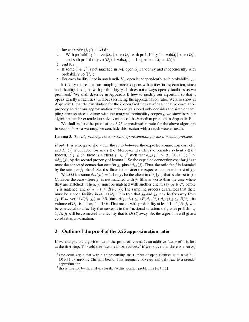
1: for each pair (j, j′) ∈ M do2: With probability 1− vol(Uj′), open Uj ; with probability 1− vol(Uj), open Uj′ ;

and with probability vol(Uj) + vol(Uj′)− 1, open both Uj and Uj′ ;3: end for4: If some j ∈ C′ is not matched in M, open Uj randomly and independently with

probability vol(Uj);5: For each facility i not in any bundle Uj , open it independently with probability yi.

It is easy to see that our sampling process opens k facilities in expectation, sinceeach facility i is open with probability yi. It does not always open k facilities as wepromised.2 We shall describe in Appendix B how to modify our algorithm so that itopens exactly k facilities, without sacrificing the approximation ratio. We also show inAppendix B that the distribution for the k open facilities satisfies a negative correlationproperty so that our approximation ratio analysis need only consider the simpler sam-pling process above. Along with the marginal probability property, we show how ouralgorithm can be extended to solve variants of the k-median problem in Appendix B.

We shall outline the proof of the 3.25 approximation ratio for the above algorithmin section 3. As a warmup, we conclude this section with a much weaker result:

Lemma 3. The algorithm gives a constant approximation for the k-median problem.

Proof. It is enough to show that the ratio between the expected connection cost of jand dav(j) is bounded, for any j ∈ C. Moreover, it suffices to consider a client j ∈ C′.Indeed, if j /∈ C′, there is a client j1 ∈ C′ such that dav(j1) ≤ dav(j), d(j, j1) ≤4dav(j), by the second property of lemma 1. So the expected connection cost for j is atmost the expected connection cost for j1 plus 4dav(j). Thus, the ratio for j is boundedby the ratio for j1 plus 4. So, it suffices to consider the expected connection cost of j1.

W.L.O.G, assume dav(j1) = 1. Let j2 be the client in C′\ j1 that is closest to j1.Consider the case where j1 is not matched with j2 (this is worse than the case wherethey are matched). Then, j2 must be matched with another client, say j3 ∈ C′, beforej1 is matched, and d(j2, j3) ≤ d(j1, j2). The sampling process guarantees that theremust be a open facility in Uj2 ∪ Uj3 . It is true that j2 and j3 may be far away fromj1. However, if d(j1, j2) = 2R (thus, d(j1, j3) ≤ 4R, dav(j2), dav(j3) ≤ R/2), thevolume of Uj1 is at least 1− 1/R. That means with probability at least 1− 1/R, j1 willbe connected to a facility that serves it in the fractional solution; only with probability1/R, j1 will be connected to a facility that is O(R) away. So, the algorithm will give aconstant approximation.

3 Outline of the proof of the 3.25 approximation ratio

If we analyze the algorithm as in the proof of lemma 3, an additive factor of 4 is lostat the first step. This additive factor can be avoided,3 if we notice that there is a set Fj

2 One could argue that with high probability, the number of open facilities is at most k +O(

√k) by applying Chernoff bound. This argument, however, can only lead to a pseudo-

approximation.3 this is inspired by the analysis for the facility location problem in [6, 4, 12].

of facilities of volume 1 around j. Hopefully with some probability, some facility in Fj

is open. It is not hard to show that this probability is at least 1 − 1/e. So, only withprobability 1/e, we are going to pay the additive factor of 4. Even if there are no openfacilities in Fj , the facilities in Fj1 and Fj2 can help to reduce the constant.

A natural style of analysis is: focus on a set of “potential facilities”, and considerthe expected distance between j and the closest open facility in this set. An obviouscandidate for the potential set is Fj ∪ Fj1 ∪ Fj2 ∪ Fj3 . However, we are unable toanalyze this complicated system.

Instead, we will consider a different potential set. Observing that Uj1 ,Uj2 ,Uj3 aredisjoint, the potential set Fj ∪ Uj1 ∪ Uj2 ∪ Uj3 is much more tractable. Even with thissimplified potential set, we still have to consider the intersection between Fj and eachof Uj1 , Uj2 and Uj3 . Furthermore, we tried hard to reduce the approximation ratio at thecost of complicating the analysis(recall the argument about the choice of the scalar 1.5).With the potential set Fj ∪ Uj1 ∪ Uj2 ∪ Uj3 , we can only prove a worse approximationratio. To reduce it to 3.25, different potential sets are considered for different bottleneckcases.

W.L.O.G, we can assume j ∈ C′, since we can think of the case j ∈ C′ as j ∈ C′

and there is another client j1 ∈ C′ with d(j, j1) = 0. We also assume dav(j) = 1. Letj1 ∈ C′ be the client such that dav(j1) ≤ dav(j) = 1, d(j, j1) ≤ 4dav(j) = 4. Let j2be the closest client in C′\ j1 to j1, thus d(j1, j2) = 2Rj1 . Then, either j1 is matchedwith j2, or j2 is matched with a different client j3 ∈ C′, in which case we will haved(j2, j3) ≤ d(j1, j2) = 2Rj1 . We only consider the second case. Readers can verifythis is indeed the bottleneck case.

For the ease of notation, define 2R := d(j1, j2) = 2Rj1 , 2R′ := d(j2, j3) ≤

2R, d1 := d(j, j1), d2 := d(j, j2) and d3 := d(j, j3).At the top level, we divide the analysis into two cases : the case 2 ≤ d1 ≤ 4 and the

case 0 ≤ d1 ≤ 2(Notice that we assumed dav(j) = 1 and thus 0 ≤ d1 ≤ 4). For sometechnical reason, we can not include the whole set Fj in the potential set for the case2 ≤ d1 ≤ 4. Instead we only include a subset F ′

j (notice that j /∈ C′ and thus F ′j was

not defined before). F ′j is defined as Fj ∩B(j, d1).

The case 2 ≤ d1 ≤ 4 is further divided into 2 sub-cases : F ′j ∩ F ′

j1⊆ Uj1 and

F ′j ∩ F ′

j1⊆ Uj1 . Thus, we will have 3 cases :

1. 2 ≤ d1 ≤ 4,F ′j ∩ F ′

j1⊆ Uj1 . In this case, we consider the potential set F ′′ =

F ′j ∪F ′

j1∪ Uj2 ∪ Uj3 . Notice that F ′

j = Fj ∩B(j, d1), F ′j1

= Fj1 ∩B(j1, 1.5R).In Appendix C.1, we show that the expected connection cost of j in this case isbounded by 3.243.

2. 2 ≤ d1 ≤ 4,F ′j ∩ F ′

j1⊆ Uj1 . In this case, some facility i in F ′

j ∩ F ′j1

must beclaimed by some client j′ = j1. Since d(j, i) ≤ d1, d(j1, i) ≤ 1.5R, we have

d(j, j′) ≤ d(j, i) + d(j′, i) ≤ d(j, i) + d(j1, i) ≤ d1 + 1.5R.

If j′ /∈ j2, j3, we can include Uj′ in the potential set and thus the potential set isF ′′ = F ′

j ∪ F ′j1

∪ Uj2 ∪ Uj3 ∪ Uj′ . If j ∈ j2, j3, then we know j and j2, j3 areclose. So, we either have a “larger” potential set, or small distances between j andj2, j3. Intuitively, this case is unlikely to be the bottleneck case. In Appendix C.2,we prove that the expected connection cost of j in this case is bounded by 3.189.

3. 0 ≤ d1 ≤ 2. In this case, we consider the potential set F ′′ = Fj ∪Uj1 ∪Uj2 ∪Uj3 .In Appendix C.3, we show that the expected connection cost of j in this case isbounded by 3.25.

3.1 Running time of the algorithm

Let’s now analyze the running time of our algorithm in terms of n = |F ∪ C|. Thebottleneck of the algorithm is solving the LP. Indeed, generating the set C′, creatingbundles and constructing the matching M all take time O(n2). Then new samplingalgorithm takes time O(n) and computing the nearest open facility for all the clientstakes time O(n2). Thus, the total time to round a fractional solution is O(n2).

To solve the LP, we use the (1 + ϵ) approximation algorithm for the fractional k-median problem in [15]. The algorithm gives a fractional solution which opens (1 +ϵ)k facilities with connection cost at most 1 + ϵ times the fractional optimal in timeO(kn2 ln(n/ϵ)/ϵ2). To apply it here, we set ϵ = δ/k for some small constant δ. Then,our rounding procedure will open k facilities with probability 1− δ and k+1 facilitieswith probability δ. The expected connection cost of the integral solution is at most3.25(1 + δ/k) times the fractional optimal. Conditioned on the rounding procedureopening k facilities, the expected connection cost is at most 3.25(1 + δ/k)/(1 − δ) ≤3.25(1 +O(δ)) times the optimal fractional value.

Theorem 1. For any δ > 0, there is a 3.25(1 + δ)-approximation algorithm for k-median problem that runs in O

((1/δ2)k3n2

)time.

3.2 Generalization of the algorithm to variants of k-median problems

The distribution of k open facilities that our algorithm produces has two good proper-ties. First, the probability that a facility i is open is exactly yi. Second, the events thatfacilities are open are negatively correlated, as stated in Lemma 10. The two propertiesallow our algorithm to be extended to some variants of the k-median problem, whichthe local search algorithm seems hard to apply to.

The first variant is a common generalization of the k-median problem and the UFLproblem introduced in [8]. In the generalized problem, we have both upper bound onthe number of facilities we can open and facility costs. For this problem, the LP is thesame as LP(1), except that the objective function contains a term for the opening cost.After solving the LP, we can use our rounding procedure to get an integral solution. Theexpected opening cost of the integral solution is exactly the fractional opening cost inthe LP solution, while the expected connection cost is at most 3.25 times the fractionalconnection cost.

Another generalization introduced in [8] is the k-median problem with multipletypes of facilities. Suppose we have t types of facilities, and the total number of thet types of facilities we can open is at most k so that each client is connected to onefacility of each type. The goal is to minimize the total connection cost. Our techniquesyield a 3.25 approximation for this problem as well. We first solve the natural LP forthis problem and then round t instances of the k-median problem separately. We canagain use the dependence rounding technique described in Appendix B to guarantee thecardinality constraint.

4 Approximation algorithms for knapsack-median problem andmatroid-median problem

The LP for Knapsack-median problem is the same as LP (1), except that we change thecardinality constraint

∑i∈F yi ≤ k to the knapsack constraint

∑i∈F fiyi ≤ M .

As showed in [11], the LP has unbounded integrality gap. To amend this, we do thesame trick as in [11]. Suppose we know the optimal cost OPT for the knapsack medianproblem. For a client j, let Lj be its connection cost. Then, for some other client j′, itsconnection cost is at least max 0, Lj − d(j, j′). This suggests∑

j′∈C

max0, Lj − d(j, j′) ≤ OPT. (1)

Thus, knowing OPT, we can get an upper bound Lj on the connection cost of j: Lj

is the largest number such that the above inequality is true. We solve the LP with theadditional constraint that xi,j = 0 if d(i, j) > Lj . Then, the LP solution, denotedby LP, must be at most OPT. By binary searching, we find the minimum OPT sothat LP ≤ OPT. Let

(x(1), y(1)

)be the fractional solution given by the LP. We use

LPj = dav(j) =∑

i∈F d(i, j)x(1)i,j to denote the contribution of the client j to LP.

Then we select a set of filtered clients C′ as we did in the algorithm for the k-median problem. For a client j ∈ C, let π(j) be a client j′ ∈ C′ such that dav(j′) ≤dav(j), d(j, j

′) ≤ 4dav(j). Notice that for a client j ∈ C′, we have π(j) = j. This time,we can not save the additive factor of 4; instead, we move the connection demand oneach client j /∈ C′ to π(j). For a client j′ ∈ C′, let wj′ =

∣∣π−1(j′)∣∣ be its connection

demand. Let LP(1) =∑

j′∈C′,i∈F wj′xi,j′d(i, j′) =

∑j′∈C′ wj′dav(j

′) be the cost of

the solution(x(1), y(1)

)to the new instance. For a client j ∈ C, let LP(1)

j = dav(π(j))

be the contribution of j to LP(1). (The amount wj′dav(j′) is evenly spread among the

wj′ clients in π−1(j′).) Since LPj = dav(j) ≤ dav(j) ≤ LP(1)j , we have LP(1) ≤ LP.

For any client j ∈ C′, let 2Rj = minj′∈C′,j′ =j d(j, j′), if vol(B(j, Rj)) ≤ 1;

otherwise let Rj be the smallest number such that vol(B(j, Rj)) = 1. (vol(S) is definedas∑

i∈S y(1)i .) Let Bj = B(j, Rj) for the ease of notation. If vol(Bj) = 1, we call Bj a

full ball; otherwise, we call Bj a partial ball. Notice that we always have vol(Bj) ≥ 1/2.Notice that Rj ≤ Lj since x

(1)i,j = 0 for all facilities i with di,j > Lj .

We find a matching M over the partial balls as in Section 2: while there are at least2 unmatched partial balls, match the two balls Bj and Bj′ with the smallest d(j, j′).

Consider the following LP.

LP(2) min∑

j′∈C′ wj′

(∑i∈Bj′

d(i, j′)yi +(1−

∑i∈Bj

yi

)Rj′

)s.t.∑

i∈Bj′

yi = 1, ∀j′ ∈ C′, Bj′ full;∑i∈Bj′

yi ≤ 1, ∀j′ ∈ C′, Bj′ partial;

∑i∈Bj

yi +∑i∈Bj′

yi ≥ 1, ∀(Bj , Bj′) ∈ M;∑i∈F

fiyi ≤ M ;

yi ≥ 0, ∀i ∈ F

Let y(2) be an optimal basic solution of LP (2) and let LP(2) be the value of LP(2).For a client j ∈ C with π(j) = j′, let LP(2)

j =∑

i∈Bj′d(i, j′)yi+

(1−

∑i∈Bj′

yi

)Rj′

be the contribution of j to LP(2). Then we prove

Lemma 4. LP(2) ≤ LP(1).

Proof. It is easy to see that y(1) is a valid solution for LP(2). By slightly abusing thenotation, we can think of LP(2) is the cost of y(1) to LP(2). We compare the contributionof each client j ∈ C with π(j) = j′ to LP(2) and to LP(1). If Bj′ is a full ball, j′

contributes the same to LP(2) and as to LP(1). If Bj′ is a partial ball, j′ contributes∑i∈Fj′

d(i, j′)y(1)i to LP(1) and

∑i∈Bj′

d(i, j′)y(1)i + (1−

∑i∈Bj′

y(1)i )Rj′ to LP(2).

Since Bj′ = B(j′, Rj′) ⊆ Fj′ and vol(Fj′) = 1, the contribution of j′ to LP(2) is atmost that to LP(1). So, LP(2) ≤ LP(1).

Notice that LP(2) only contains y-variables. We show that any basic solution y∗ ofLP(2) is almost integral. In particular, we prove the following lemma in Appendix A.

Lemma 5. Any basic solution y∗ of LP(2) contains at most 2 fractional values. More-over, if it contains 2 fractional values y∗i , y

∗i′ , then y∗i + y∗i′ = 1 and either there exists

some j ∈ C′ such that i, i′ ∈ Bj or there exists a pair (Bj , Bj′) ∈ M such thati ∈ Bj , i

′ ∈ Bj′ .

Let y(3) be the integral solutin obtained from y(2) as follows. If y(2) contains atmost 1 fractional value, we zero-out the fractional value. If y(2) contains 2 fractionalvalues y(2)i , y

(2)i′ , let y(3)i = 1, y

(3)i′ = 0 if fi ≤ fi′ and let y(3)i = 0, y

(3)i′ = 1 otherwise.

Notice that since y(2)i + y

(2)i′ = 1, this modification does not increase the budget. Let

SOL be the cost of the solution y(3) to the original instance.We leave the proof of the following lemma to Appendix A.

Lemma 6.∑

i∈B(j′,5Rj′ )y(2)i ≥ 1 and

∑i∈B(j′,5Rj′ )

y(3)i ≥ 1. i.e, there is an open

facility (possibly two facilities whose opening fractions sum up to 1) inside B(j′, 5Rj′)in both the solution y(2) and the solution y(3).

Lemma 7. SOL ≤ 34OPT.

Proof. Let i be the facility that y(2)i

> 0, y(3)

i= 0, if it exists; let j be the client that

i ∈ Bj .Now, we focus on a client j ∈ C with π(j) = j′. Then, d(j, j′) ≤ 4dav(j) = 4LPj .

Assume that j′ = j. Then, to obtain y(3), we did not move or remove an open facilityfrom Bj′ . In other words, for every i ∈ Bj′ , y

(3)i ≥ y

(2)i . In this case, we show

SOLj′ ≤∑i∈Bj′

d(i, j′)y(2)i + (1−

∑i∈Bj′

y(2)i )× 5Rj′ .

If there is no open facility in Bj′ in y(3), then there is also no open facility in Bj′ iny(2). Then, by Lemma 6, SOLj′ = 5Rj′ = right-side. Otherwise, there is exactly one

open facility in Bj′ in y(3). In this case, SOLj′ =∑

i∈Bj′d(j′, i)y

(3)i ≤ right-side

since y(3)i ≥ y

(2)i and d(i, j′) ≤ 5Rj′ for every i ∈ Bj′ .

Observing that the right side of the inequality is at most 5LP(2)j , we have SOLj ≤

4LPj + SOLj′ ≤ 4LPj + 5LP(2)j .

Now assume that j′ = j. Since there is an open facility in B(j′, 5Rj′) by Lemma 6,we have SOLj ≤ 4LPj +5Rj′ . Consider the set π−1(j′) of clients. Notice that we haveRj′ ≤ Lj′ since x(1)

i,j′ = 0 for facilities i such that d(i, j′) > Lj′ . Also by Inequality (1),we have

∑j∈π−1(j′)(Rj′−d(j, j′)) ≤

∑j∈π−1(j′)(Lj′−d(j, j′)) ≤ OPT. Then, since

d(j, j′) ≤ 4LPj for every j ∈ π−1(j′), we have∑j∈π−1(j′)

SOLj ≤∑j

(4LPj + 5Rj′) ≤ 4∑j

LPj + 5∑j

Rj′

≤ 4∑j

LPj + 5(OPT+

∑j

d(j, j′))≤ 24

∑j

LPj + 5OPT,

where the sums are all over clients j ∈ π−1(j′). Summing up all clients j ∈ C, we have

SOL =∑j∈C

SOLj =∑

j /∈π−1(j)

SOLj +∑

j∈π−1(j)

SOLj

≤∑

j /∈π−1(j)

(4LPj + 5LP(2)j ) + 24

∑j∈π−1(j)

LPj + 5OPT

≤ 24∑j∈C

LPj + 5∑j∈C

LP(2)j + 5OPT ≤ 24LP+ 5LP(2) + 5OPT ≤ 34OPT,

where the last inequality follows from the fact that LP(2) ≤ LP(1) ≤ LP ≤ SOL. Thus,we proved

Theorem 2. There is an efficient 34-approximation algorithm for the knapsack-medianproblem.

It is not hard to change our algorithm so that it works for the matroid median prob-lem. The analysis for the matroid median problem is simpler, since y(2) will already bean integral solution. We leave the proof of the following theorem to Appendix A.

Theorem 3. There is an efficient 9-approximation algorithm for the matroid medianproblem, assuming there is an efficient oracle for the input matroid.

References

1. Aaron Archer, Ranjithkumar Rajagopalan, and David B. Shmoys. Lagrangian relaxation forthe k-median problem: new insights and continuity properties. In In Proceedings of the 11thAnnual European Symposium on Algorithms, pages 31–42, 2003.

2. Vijay Arya, Naveen Garg, Rohit Khandekar, Adam Meyerson, Kamesh Munagala, andVinayaka Pandit. Local search heuristic for k-median and facility location problems. InProceedings of the thirty-third annual ACM symposium on Theory of computing, STOC ’01,pages 21–29, New York, NY, USA, 2001. ACM.

3. P. S. Bradley, Usama M. Fayyad, and O. L. Mangasarian. Mathematical programming fordata mining: Formulations and challenges. INFORMS Journal on Computing, 11:217–238,1998.

4. Jaroslaw Byrka. An optimal bifactor approximation algorithm for the metric uncapacitatedfacility location problem. In APPROX ’07/RANDOM ’07: Proceedings of the 10th Interna-tional Workshop on Approximation and the 11th International Workshop on Randomization,and Combinatorial Optimization. Algorithms and Techniques, pages 29–43, Berlin, Heidel-berg, 2007. Springer-Verlag.

5. Moses Charikar, Sudipto Guha, Eva Tardos, and David B. Shmoys. A constant-factor ap-proximation algorithm for the k-median problem (extended abstract). In Proceedings of thethirty-first annual ACM symposium on Theory of computing, STOC ’99, pages 1–10, NewYork, NY, USA, 1999. ACM.

6. Fabian A. Chudak and David B. Shmoys. Improved approximation algorithms for the unca-pacitated facility location problem. SIAM J. Comput., 33(1):1–25, 2004.

7. Kamal Jain, Mohammad Mahdian, and Amin Saberi. A new greedy approach for facilitylocation problems. In Proceedings of the thiry-fourth annual ACM symposium on Theory ofcomputing, STOC ’02, pages 731–740, New York, NY, USA, 2002. ACM.

8. Kamal Jain and Vijay V. Vazirani. Approximation algorithms for metric facility locationand k-median problems using the primal-dual schema and lagrangian relaxation. J. ACM,48(2):274–296, 2001.

9. Ravishankar Krishnaswamy, Amit Kumar, Viswanath Nagarajan, Yogish Sabharwal, andBarna Saha. The matroid median problem. In In Proceedings of ACM-SIAM Symposiumon Discrete Algorithms, pages 1117–1130, 2011.

10. A. A. Kuehn and M. J. Hamburger. A heuristic program for locating warehouses. 9(9):643–666, July 1963.

11. Amit Kumar. Constant factor approximation algorithm for the knapsack median problem.In Proceedings of the Twenty-Third Annual ACM-SIAM Symposium on Discrete Algorithms,SODA ’12, pages 824–832. SIAM, 2012.

12. Shi Li. A 1.488-approximation algorithm for the uncapacitated facility location problem. InIn Proceeding of the 38th International Colloquium on Automata, Languages and Program-ming, 2011.

13. A.S Manne. Plant location under economies-of-scale-decentralization and computation. InManagment Science, 1964.

14. A. Srinivasan. Distributions on level-sets with applications to approximation algorithms. InProceedings of the 42nd IEEE symposium on Foundations of Computer Science, FOCS ’01,pages 588–, Washington, DC, USA, 2001. IEEE Computer Society.

15. Neal E. Young. K-medians, facility location, and the chernoff-wald bound. In Proceedingsof the eleventh annual ACM-SIAM symposium on Discrete algorithms, SODA ’00, pages86–95, Philadelphia, PA, USA, 2000. Society for Industrial and Applied Mathematics.

A Proofs omitted from Section 4

Proof (of Lemma 5). Focus on an independent set of tight constraints defining y∗. We make sure that ify∗i = 0, then the constraint yi = 0 is in the independent set. Any tight constraint other than the knapsackconstraint and the constraints yi = 0 is defined by a set S, which is either Bj for some j ∈ C ′ or Bj ∪Bj′

for some (Bj , Bj′) ∈ M. The constraint for S is∑

i∈S yi = 1. Let S be the set of subsets S whosecorrespondent constraint is in the independent set.

We show that sets in S are disjoint. This is not true only if there is some pair (Bj , Bj′) ∈ M such thatBj ∈ S, Bj ∪Bj′ ∈ S . However, this would imply that yi = 0 for every i ∈ Bj′ . Thus, the two constraintsfor Bj and Bj ∪Bj′ are not independent. Thus, sets in S are disjoint.

Consider the matrix A defined by the set of tight constraints, where each rows represent constraints andcolumns represent variables. Focus on set S∗ of columns (facilities) correspondent to the fractional valuesin y∗. Then, the sub-matrix AY ∗ defined by Y ∗ must have rank |Y ∗|. Also, if some S ∈ S contains elementsin S∗, it must contain at least 2 elements in S∗. Noticing that sets in S are disjoint, if |S∗| ≥ 3, the rankof AY ∗ can be at most ⌊|S∗|/2⌋ + 1 < |S∗|. Thus, |S∗| ≤ 2. If |S∗| = 2, then there must be a set S ∈ Scontaining S∗. This implies that the two fractional value y∗i , y

∗i′ satisfies y∗i + y∗i′ = 1 and either i, i′ ∈ Bj

for some j ∈ mC ′, or i ∈ Bj , i′ ∈ Bj′ for some (Bj , Bj′) ∈ M.

Proof (of Lemma 6). Focus on the solution y(2). Consider the nearest neighbour j2 of j′ in C′. If Bj′ is afull ball, then there is an open facility inside Bj′ = B(j′, Rj′); we assume Bj′ is a partial ball and thusd(j′, j2) = 2Rj′ , Rj2 ≤ Rj′ . If Bj2 is a full ball, there is an open facility in Bj2 ⊆ B(j′, 2Rj′ + Rj2) ⊆B(j′, 3Rj′). We assume Bj2 is a partial ball. If Bj′ is matched with Bj3 , then there is an open facility insideBj′ ∪ Bj2 ⊆ B(j′, 3Rj′). Otherwise, assume Bj2 is matched with Bj3 for some j3 ∈ C′. By the matchingrule, d(j2, j3) ≤ d(j′, j2) = 2R′. In this case, there is an open facility inside Bj2 ∪Bj3 ⊆ B(j′, 5Rj′ .

Now we prove the lemma for the solution y(3). If y(2) contains 2 fractional facilities, then to obtainy(3), we moved 1 fractional facility within some ball Bj , or moved 1 fractional facility from Bj to Bj′ forsome (Bj , Bj′) ∈ M. It is easy to check that the argument for y(2) also works for y(3). If y(2) contains 1fractional open facility, then after removing this facility, we still have that every full ball contains an openfacility and every pair of matched partial balls contains an open facility. Thus, in the solution y(3), there isan open facility inside B(j′, 5Rj′).

Proof (sketch of Theorem 3). We follow the same line of the algorithm for the knapsack median problem,except that we change the knapsack constraint (in LP (1) and LP (2)) to the constraints∑

i∈S

yi ≤ rH(S), ∀S ⊆ F ,

where H is the given matroid, and rH(S) is the rank function of H. We shall show that the basic solutiony(2) for LP 2 is already an integral solution. This is true since the polytope of the LP is the intersection of amatroid polytope and a polytope given by a laminar system of constraints. By the same argument as in theproof of lemma 3.2 in [9], y(2) is an integral solution, i.e, we have y(3) = y(2). Then, following the sameproof of Lemma 7, we can show that SOLj ≤ 4LPj + 5LP

(2)j for every j ∈ C, which immediately implies

an 9-approximation for the matroid median problem.

B Handling the cardinality constraint

In this section, we show how to modify our algorithm so that it opens exactly k facilities. The main ideais to apply the technique of dependent rounding. For each pair of matched bundles, we have a 0-1 variable

indicating whether there are 2 or 1 open facilities in the pair of bundles. For the unmatched bundle andeach facility that is not in any bundle, we have a 0-1 variable indicating whether the facility or the bundleis open. In the algorithm described in section 2, these indicator variables are generated independently. Theexpected sum of these indicator variables is k − |M|. To make sure that we open exactly k facilities, weneed to guarantee that the sum is always k − |M|. To achieve this, we can, for example, use the tree-baseddependent rounding procedure introduced in [14]. After the indicator variables are determined, we sampleseparately each pair of bundles and the unmatched bundle .

Let us define some notations here. We are given n real numbers x1, x2, · · · , xn with 0 ≤ xi ≤ 1 forevery i and m =

∑ni=1 xi is an integer. We use the random process in [14] to select exactly m elements

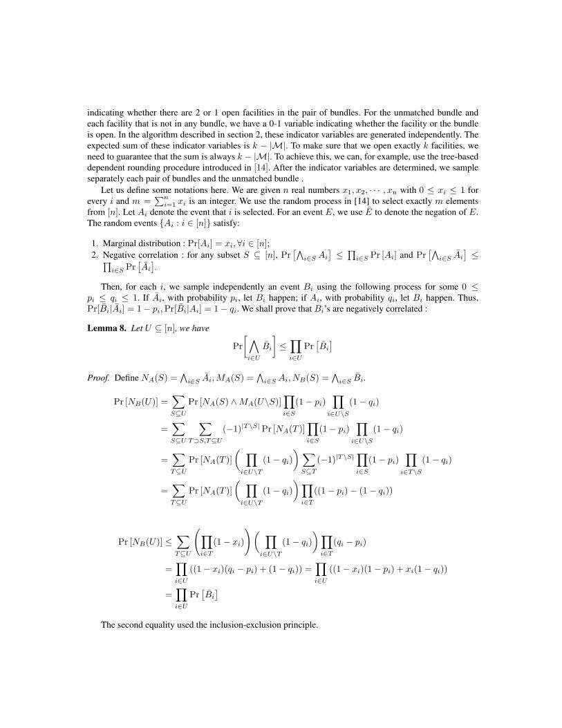
from [n]. Let Ai denote the event that i is selected. For an event E, we use E to denote the negation of E.The random events Ai : i ∈ [n] satisfy:

1. Marginal distribution : Pr[Ai] = xi, ∀i ∈ [n];2. Negative correlation : for any subset S ⊆ [n], Pr

[∧i∈S Ai

]≤∏

i∈S Pr [Ai] and Pr[∧

i∈S Ai

]≤∏

i∈S Pr[Ai

].

Then, for each i, we sample independently an event Bi using the following process for some 0 ≤pi ≤ qi ≤ 1. If Ai, with probability pi, let Bi happen; if Ai, with probability qi, let Bi happen. Thus,Pr[Bi|Ai] = 1− pi,Pr[Bi|Ai] = 1− qi. We shall prove that Bi’s are negatively correlated :

Lemma 8. Let U ⊆ [n], we have

Pr

[∧i∈U

Bi

]≤∏i∈U

Pr[Bi

]Proof. Define NA(S) =

∧i∈S Ai,MA(S) =

∧i∈S Ai, NB(S) =

∧i∈S Bi.

Pr [NB(U)] =∑S⊆U

Pr [NA(S) ∧MA(U\S)]∏i∈S

(1− pi)∏

i∈U\S

(1− qi)

=∑S⊆U

∑T⊃S,T⊆U

(−1)|T\S| Pr [NA(T )]∏i∈S

(1− pi)∏

i∈U\S

(1− qi)

=∑T⊆U

Pr [NA(T )]

( ∏i∈U\T

(1− qi)

)∑S⊆T

(−1)|T\S|∏i∈S

(1− pi)∏

i∈T\S

(1− qi)

=∑T⊆U

Pr [NA(T )]

( ∏i∈U\T

(1− qi)

)∏i∈T

((1− pi)− (1− qi))

Pr [NB(U)] ≤∑T⊆U

(∏i∈T

(1− xi)

)( ∏i∈U\T

(1− qi)

)∏i∈T

(qi − pi)

=∏i∈U

((1− xi)(qi − pi) + (1− qi)) =∏i∈U

((1− xi)(1− pi) + xi(1− qi))

=∏i∈U

Pr[Bi

]The second equality used the inclusion-exclusion principle.

We are ready to apply the above lemma to our approximation algorithm. In the new algorithm, wesample the indicator variables using the dependence rounding procedure. So, we can guarantee that exactlyk facilities are open. Then, we show that the expected connection cost for a client u does not increase :

Lemma 9. The approximation ratio of the algorithm using the dependence rounding procedure is at mostthat of the original algorithm (i.e, the algorithm described in section 2).

Proof. For the ease of description, we assume that every facility is in some bundle and all the bundles arematched. For a client u, we order the facilities in the ascending order of distances to u. Let z1, z2, · · · , ztbe the order. Then, u is connected to the first open facility in the order, and thue

Expected connection cost of u =

t∑s=1

Pr[the first s facilities are not open] (d(u, zs+1)− d(u, zs))

It suffices to show that for every s, the probability Pnew that the first s facilities are not open in the newalgorithm is at most the correspondent probability Pold in the old algorithm. For a pair i of bundles, let Ai

be the variable indicating whether the pair i contains 2 or 1 open facility. Let Bi denote the event that thefirst s facilities that are in in bundle i are not open. Notice that in the new algorithm, Bi is independent ofAj |j = i∩Bj |j = i under the condition Ai (Ai as well). It’s easy to see that Pr

[Bi|Ai

]≥ Pr

[Bi|Ai

].

Since Pnew = Pr[∧

i Bi

]and Pold =

∏i Pr[Bi], we have Pnew ≤ Pold, by lemma 8. Thus, the

expected connection cost of any facility in the new algorithm is at most its expected connection cost in theoriginal algorithm.

Lemma 10. The distribution of the k open facilities generated by our new algorithm satisfy the followingnegative correlation. Let T be a subset of facilities. We have

Pr

[∧z∈T

z

]≤∏z∈T

Pr[z], Pr

[∧z∈T

z

]≤∏z∈T

Pr[z]

where z also denotes the event that facility z is open, and z is the negation of z.

Proof. We only prove the second inequality; the proof for the first is symmetric. Again, for the ease ofdescription, assume all facilities are in a pair of matched bundles. For a pair i of bundles, let Bi be the event

that facilities in T that are in pair i are not open. Again, by lemma 8, we have Pr

[∧i Bi

]≤∏

i Pr[Bi

].

It’s easy to see that Pr[Bi] ≤∏

z Pr[z], where the product is over all z’s which are in T and are in pair i.Thus, we proved the lemma.

C Proof of the 3.25 approximation ratio

We now start the long journey of bounding the expected connection cost, denoted by E, of a client j withdav(j) = 1. Before dispatching the analysis into the 3 cases, we outline our main techniques for the analysis.When analyzing each case, we will focus on a set of potential facilities F ′′ and a set C′′ of clients. C′′ willbe either j, j1, j2, j3 (Section C.1 and C.3) or j, j1, j2, j3, j′ (Section C.2). Each facility in F ′′ servesat least 1 client in C′′. In the analysis, we only focus on the sub-metric induced by F ′′ ∪ C′′. Using similarargument as we proved lemma 10, we may assume the minimum dependence between the facilities in F ′′.To be more specific, we assume

1. Facilities in F ′′ that are not claimed by any facility in C′′ were sampled independently in the algorithm.We call these facilities individual facilities.

2. If j′ ∈ C′′, Uj′ and Uj1 are not matched in M(We know Uj2 and Uj3 are matched).

With these conditions, we prove the following lemma.

Lemma 11. Consider a set G ⊆ F ′′ of individual facilities. We have

1. The probability that G contains at least 1 open facility is at least 1− e−vol(G).2. Under the condition that there is at least 1 open facility in G, the expected distance between j and the

closest open facility in G is at most d(j,G).

Proof. The probability that no facility in G is open is at most∏i∈G

(1− yi) ≤∏i∈G

e−yi = e−vol(G)

This implies the first statement.For the second statement, we sort all facilities in G according the non-decreasing distances to j. Let the

order be i1, i2, · · · , im. Then, the expected distance between j and the closest open facility in G is(m∑t=1

(t−1∏s=1

(1− yis)

)yitd(j, it)

)/(1−

m∏t=1

(1− yit)

)

Compare the coefficients for d(j, ia) and d(j, ib) for some a < b in the above quantity. The ratio of the

two coefficients isyiayib

/b−1∏t=a

(1 − yit) ≥ yiayib

. Compared to d(j,G) =∑m

t=1 yitd(j, it)/vol(G), the above

quantity puts relatively more weights on smaller distances. Thus, the expected distance between j and theclosest open facility in G is at most d(j,G).

In the analysis for each case, the potential set F ′′ is split into disjoint “atoms” I1, I2, · · · , IM . Eachatom is either a sub bundle (i.e a subset of a bundle) or a set of individual facilities. Typically, an atom is aregion in the Venn diagram of some sets (for example, in subsection C.1, we consider the Venn diagram ofsets F ′

j ,F ′j1,Uj1 ,Uj2 ,Uj3). An atom contains facilities with the same “characterization”, so that averaging

the locations of the facilities in the same atom will still give a valid instance, from the view of F ′′ ∪ C′′.Given a order o of the facilities in F ′′, the value of o, denoted by val(o), is defined as the connection cost

from j to the first open facility in o. It is easy to see that E = E(val(o)), if o is the order where facilities aresorted according to the increasing distances to j. Also, for every order o, E ≤ E(val(o)). In our analysis,we only consider the orders where the facilities in the same atom are consecutive and are sorted optimally.Thus, each atom is equivalent to a single facility at the weighted averaging location of the facilities in theatom, by the first statement of lemma 11(if the atom is a sub bundle, we can also average the locations). Theequivalent facility has y value vol(It) if It is a sub-bundle and 1 − e−vol(It) if It is an atom of individualfacilities, by the second statement of 11.

At each step, we maintain a partial order p. A partial order p is an order (S1,S2, · · · Sm), whereS1,S2, · · · ,Sm forms a partitioning for the atoms I1, I2, · · · , IM. The value of p, denoted by val(p),is the distance between j and the closest open atom (notice that each atom is already replaced by a facility)in St, where St is the first set in p containing an open atom. Initially, the partial order p contains only 1 setI1, I2, · · · , IM and E(val(p)) = E. In each step, we may refine the partial order p by splitting some setSi into smaller subsets and replace Si with some order of these subsets; or we may merge some atoms insome set St into 1 atom. Both operations can only increase E(val(p)).

Now, we shall consider the 3 cases one by one. Let’s recall some notations here. d1 = d(j, j1), d2 =d(j, j2), d3 = d(j, j3), 2R = 2Rj1 = d(j1, j2), 2R

′ = 2Rj2 = d(j2, j3),F ′j = Fj ∩ B(j, d1),F ′

j1=

Fj1 ∩B(j1, 1.5R).

C.1 The case 2 ≤ d1 ≤ 4,F ′j ∩ F ′

j1⊆ Uj1

In this subsection, we consider the case 2 ≤ d1 ≤ 4,F ′j ∩ F ′

j1⊆ Uj1 . The potential set to be considered is

F ′′ = F ′j ∪ F ′

j1∪ Uj2 ∪ Uj3 .

Essentially, we would like to show that figure C.1 is the worst instance in this case. Notice that we arenot using the facilities in Fj2\Uj2 . The expected connection cost of j in this case is

e−34

(3

4· 4 + 1

4

(1− e−

14

)× 8 +

1

4e−

14 · 1

2· 12 + 1

4e−

14 · 1

2· 22)

= e−34

(5 + 2.25e−

14

)< 3.19

At some point, we relaxed the objective function. e−3/4(5 + 2.25e−3/16

)< 3.243 is the upper bound

we can prove.The idea is showing that W.L.O.G, we can assume F ′

j ∪F ′j1

and Uj2 ∪Uj3 are disjoint. Then, under thecondition that no facility is open in F ′

j ∪F ′j1

, the expected connection cost of j is at most (1/2)(d1+2R)+(1/2)(d1 +2.5R) = d1 +3.25R. Then, by using d1 +3.25R as a “backup” value, we can ignore j2 and j3.

4 8

03/43/4

1/4

4 4

1/2

1/2

1

28j j1 j3j2

Fig. C.1. The worst case for 2 ≤ d1 ≤ 4,F ′j ∩F ′

j1 ⊆ Uj1 . The 3 solid rectangles represent the facilities claimed by j1,j2 and j3; the 3 dash rectangles represent the facilities serving j1, j2 and j3. 1/4 fractional facility at j1 is serving j.

Initially, an atom is a region in the Venn diagram of the following 5 sets : F ′j ,F ′

j1,Uj1 ,Uj2 ,Uj3 . We first

consider the partial order p =(F ′

j ∪ F ′j1,Uj2\(F ′

j ∪ F ′j1),Uj3\(F ′

j ∪ F ′j1)).

Let E3 be the expected value of p under the condition that no atom in F ′j ∪F ′

j1∪Uj2 is open. We prove

Lemma 12. If d2 + 0.5R′ ≥ d1, E3 ≤ d2 + 2.5R′.

Proof. Under the condition that no atom in F ′j∪F ′

j1∪Uj2 is open, there is exactly 1 open atom in Uj3\(F ′

j∪F ′

j1). Thus, E3 = d(j,Uj3\(F ′

j ∪ F ′j1)). Since d(j3,Fj3) ≤ Rj3/2 and d(j3,Fj3\Uj3) ≥ Rj3 , we have

d(j3,Uj3) ≤ Rj3/2 ≤ R′/2.Uj3 ∩ (F ′

j ∪ F ′j1) contains 2 components : Uj3 ∩ F ′

j ,Uj3 ∩ (F ′j1\F ′

j). If the average distance from j3to each of the 2 components is at least R′/2, then d(j3,Uj3\(F ′

j ∪ F ′j1)) is at most R′/2 and thus E3 is at

most d2 + 2R′ + R′/2 ≤ d2 + 2.5R′. So, it suffices to consider the case where at least 1 component hasaverage distance strictly smaller than R′/2 to j3.

If d(j3,Uj3 ∩ F ′j) < R′/2, then since d(j,Uj3 ∩ F ′

j) ≤ d1(recall that F ′j = Fj ∩ B(j, d1)), we have

d(j, j3) ≤ d1 +R′/2. Since d(j3,Uj3\F ′j) ≤ 1.5R′, we have E3 ≤ d1 +R′/2 + 1.5R′ ≤ d2 + 2.5R′.

If d(j3,Uj3 ∩ (F ′j1\Fj)) < R′/2, then since d(j1,Uj3 ∩ (F ′

j1\Fj)) ≤ 1.5R, we have d(j1, j3) <

1.5R+R′/2 ≤ 2R, which contradicts the fact that the closest neighbor of j1 in C′\ j1 has distance 2R.

Let β2 = vol(Uj2\(F ′j ∪ F ′

j1)), b2 = d(j2,Uj2\(F ′

j ∪ F ′j1)), and E2 be the expected value of p under

the condition that no atom in F ′j ∪ F ′

j1is open.

Lemma 13. E2 ≤ d1 + 3.25R.

Proof. Under the condition that no atom in F ′j ∪ F ′

j1is open, there is at least 1 open atom in (Uj2 ∪

Uj3)\(F ′j ∪F ′

j1). We first try to connect j to Uj2\(F ′

j ∪F ′j1); if this fails, we connect j to Uj3\(F ′

j ∪F ′j1).

E2 is the expected connection cost.If d2 + 0.5R′ ≤ d1, then d(j,Uj2\(F ′

j ∪ F ′j1)) ≤ d2 + 1.5R′ ≤ d1 + R and d(j,Uj3\(F ′

j ∪ F ′j1)) ≤

d2 + 2R′ + 1.5R′ ≤ d1 + 3R. Clearly in this case, E2 ≤ max d1 +R, d1 + 3R = d1 + 3R. So, weassume d2 + 0.5R′ > d1. Thus, by lemma 12, E3 ≤ d2 + 2.5R′.

Let θ = vol(Uj2 ∩ (F ′j ∪ F ′

j1)), t = d(j2,Uj2 ∩ (F ′

j ∪ F ′j1)). Then

E2 ≤ β2

1− θ(d2 + b2) +

1− θ − β

1− θE3

≤ β2

1− θ

(d2 +

R′/2− θt− (1− θ − β2)R′

β2

)+

1− θ − β2

1− θ(d2 + 2.5R′)

≤ d2 +R′/2− θt

1− θ+

1− θ − β2

1− θ1.5R′ ≤ d2 +

R′/2− θt

1− θ+

(R′/2− θt)/R′

1− θ1.5R′

= d2 + 2.5R′/2− θt

1− θ

If t ≥ R′/2, then E2 ≤ d2 + 2.5R′/2 ≤ d1 + 2R+ 1.25R′ ≤ d1 + 3.25R.Thus, we can assume that t < R′/2. This implies either d(j2,Uj2 ∩ F ′

j) < R′/2 or d(j2,Uj2 ∩(F ′

j1\F ′

j)) < R′/2. d(j2,Uj2 ∩ (F ′j1\F ′

j)) < R′/2 implies

d(j1, j2) ≤ d(j2,Uj2 ∩ (F ′j1\F

′j)) + d(j1,Uj2 ∩ (F ′

j1\F′j)) < R′/2 + 1.5R ≤ 2R,

contradicting d(j1, j2) = 2R. So, we only need to consider the case d(j2,Uj2 ∩ F ′j) ≤ R′/2. In this

case, d2 ≤ d(j,Uj2 ∩ F ′j) + d(j2,Uj2 ∩ F ′

j) ≤ d1 + R′/2. Then, d(j,Uj2\(F ′j ∪ F ′

j1)) ≤ d1 + R′/2 +

1.5R′ ≤ d1 + 2R′ and d(j,Uj3\(F ′j ∪ F ′

j1)) = E3 ≤ d2 + 2.5R′ ≤ d1 + 3R′. Thus, we have E2 ≤

max d1 + 2R′, d1 + 3R′ ≤ d1 + 3.25R.

By lemma 13, we can replace the order p by(F ′

j ∪ F ′j1, d1 + 3.25R

). That is, connect j to the closest

open atom in F ′j ∪ F ′

j1, if it exists; otherwise use d1 + 3.25R as the value of p. By merging many atoms

into one, we can redefine atoms as regions in the Venn diagram of the sets F ′j ,F ′

j1,Uj1 . This means that we

can ignore j2 and j3 from now on.Now, we refine the order p to

(F ′

j\F ′j1,F ′

j ∩ F ′j1,Uj1\(F ′

j ∪ F ′j1),F ′

j1\Uj1 , d1 + 3.25R

).

Define α = vol(F ′j\Uj1), a = d(j,F ′

j\Uj1), α1 = vol(F ′j ∩F ′

j1), a1 = d(j1,F ′

j ∩F ′j1), a′1 = d(j,F ′

j ∩F ′

j1), β1 = vol(Uj1\F ′

j). Define b1 = d(j1,Uj1\F ′j), γ = vol(F ′

j1\Uj1), c = d(j1,F ′

j1\Uj1). Define

s = dav(j1). See figure C.2 for illustration.Let E1 be the expected value of p under the condition that the atom F ′

j\F ′j1

is not open.

E1 = α1a′1 + β1(d1 + b1) + (1− α1 − β1)(1− e−γ)(d1 + c) + (1− α1 − β1)e

−γ(d1 + 3.25R)

= α1a′1 + (1− α1)d1 + β1b1 + (1− α1 − β1)

((1− e−γ)c+ 3.25e−γR

)

F ′j1

Uj1F ′j

j j1

F ′j\Uj1 Uj1\F ′

j

F ′j ∩ Uj1

α a1a′1a

α1

F ′j1\Uj1

γ

β1b1

c

Fig. C.2. The definition of variables

Let E = E(val(p)), then E = (1− e−α)a+ e−αE1.Consider the following optimization problem :

PROBLEM(1) max E = (1− e−α)a+ e−αE1, where

E1 = α1a′1 + (1− α1)d1 + β1b1 + (1− α1 − β1)

((1− e−γ)c+ 3.25e−γR

)s.t

αa+ α1a′1 + (1− α− α1)d1 ≤ 1 a′1 ≤ d1 2 ≤ d1 ≤ 4

α+ α1 ≤ 1 s ≤ 1 a1 + a′1 ≥ d1

α1a1 + β1b1 + γc+ (1− α1 − β1 − γ)1.5R ≤ s b1 ≤ 1.5R R ≤ c ≤ 1.5R

α1 + β1 + γ ≤ 1 R ≤ 16/3 s ≤ R/2

We need to mention constraint R ≤ 16/3. To see this, define θ = vol(Fj ∩ Fj1), l = d(j,Fj\Fj1).Then R ≤ d1 + l(assuming vol(Uj1) < 1). If l > d1/(d1 − 1), then θ ≥ 1− 1/l = 1/d1 and

dav(j1) ≥ θ(d1 − d(j,Fj ∩ Fj1)) = θ

(d1 −

1− (1− θ)l

θ

)> θd1 − 1 + (1− θ)d1/(d1 − 1)

≥ (1/d1)d1 − 1 + (1− 1/d1)d1/(d1 − 1) = 1

which leads to a contradiction. The last inequality above used that d1 ≥ d1/(d1 − 1). Since 2 ≤ d1 ≤ 4,R ≤ d1 + d1/(d1 − 1) ≤ 4 + 4/3 = 16/3.

In subsection D.1, we prove that value of optimization problem 1 is at most 3.243.

C.2 The case 2 ≤ d1 ≤ 4,F ′j ∩ F ′

j1⊆ Uj1

We only sketch the analysis for this case F ′j ∩ F ′

j1⊆ Uj1 , since the techniques are exactly the same as the

previous case. As we already showed, there is a client j′ ∈ C′, j′ = j1 with d(j, j′) ≤ d1 +1.5R. There aretwo cases.

1. j′ ∈ j2, j3.In this case, we know j2(or j3) is close to j, compared to the previous case, where d(j, j2) couldbe d1 + 2R. With this gain, we can consider a smaller potential set : F ′

j ∪ Uj1 ∪ Uj2 ∪ Uj3 . Usingsimilar argument, we can first show that E2 ≤ d1 + 1.5R + 2.5R/2 = d1 + 2.75R and then proveE ≤ e−3/4(4 + 2.75) < 3.189.

2. j′ /∈ j2, j3.In this case, we know that there is a client j′ ∈ C′ other than j1, j2, j3 that is close to j. We can use F ′

j∪Uj1 ∪Uj′ ∪Uj2 ∪Uj3 as the potential set. We consider the order F ′

j ,Uj1\F ′j ,Uj′\F ′

j ,Uj2\F ′j ,Uj3\F ′

j .Similarly, let E2 be the expected connection cost under the condition that no facilities in F ′

j ∪ Uj1 isopen. We can first show that E2 ≤ d1+(1/2)1.5R+(1/2)3.25R = d1+2.375R, i.e the maximum valueis achieved when F ′

j∪Uj1 and Uj′∪Uj2∪Uj3 are disjoint. Then, we can prove E ≤ e−3/4 (4 + 2.375) =

6.375e−3/4 < 3.02.

C.3 The case 0 ≤ d1 ≤ 2

In this case, we use the potential set F ′′ = Fj ∪ Uj1 ∪ Uj2 ∪ Uj3 .We show that the worst instance in this case is give by figure C.3. Notice that we are not using the

facilities in FF2\FU2 . The expected connection cost for j is upper bounded by(1− 1

R

)· 0 + 1

R(1− e−1/R) ·R+

1

Re−1/R · 1

2· 2R+

1

Re−1/R · 1

2· 4.5R = 1 + 2.25e−1/R

As R tends to ∞, the above upper bound tends to 3.25.

01/2

1/2

1

j3j2

R

j, j1

1/R

R

1− 1/R

2R 2R R/2

Fig. C.3. The worst instance for 0 ≤ d1 ≤ 2.

The proof is similar to the proof in subsection C.1. We first show that in the worst case, Fj ∪ Uj1

and Uj2 ∪ Uj3 are disjoint. Then, under the condition that no facilities are open in Fj ∪ Uj1 , the expectedconnection cost of j is at most d1 + 3.25R.

An atom is a region in the Venn diagram of sets Fj ,Uj1 ,Uj2 ,Uj3 . The partial order p we first consideris (Fj ,Uj1\Fj ,Uj2\Fj ,Uj3\Fj). Similar to the first case, define E3 to be the expected value of p under thecondition that there is no open atom in Fj ∪ Uj1 ∪ Uj2 is open.

Define α3 = vol(Fj ∩ Uj3), a3 = d(j3,Fj ∩ Uj3), a′3 = d(j,Fj ∩ Uj3), β3 = vol(Uj3\Fj), b3 =

d(j3,Uj3\Fj).

Lemma 14. If α3 ≤ 1/2 and a′3 ≤ d2 + 1.5R′, then E3 ≤ d2 + 2.5R.

Proof. Under the condition that there is no open atom in Fj ∪ Uj1 ∪ Uj2 , the atom Uj3\Fj is open. Thus,E3 = d(j,Uj3\Fj).

Let R′′ = Rj3 and thus R′′ ≤ R′, dav(j3) ≤ R′′/2, and

b3 ≤ R′′/2− α3a3 − (1− α3 − β3)R′′

β3≤ R′′/2− α3a3 − (1− α3 − β3)R

′′ + (1− α3 − β3)R′′

β3 + (1− α3 − β3)

=R′′/2− α3a3

1− α3≤ R′/2− α3a3

1− α3

where the second inequality used the fact that R′′/2−α3a3

1−α3≤ R′′/2

1−1/2 = R′′

Since 1− α3

1−α3≥ 0, d3 ≤ d2 + 2R′ and d3 − a3 ≤ a′3,

E3 ≤ d3 +R′/2− α3a3

1− α3≤ d3 + (d2 + 2R′ − d3) +

R′/2− α3(a3 + d2 + 2R′ − d3)

1− α3

≤ d2 + 2R′ +R′/2− α3(d2 + 2R′ − a′3)

1− α3≤ d2 + 2R′ +

R′/2− α3R′/2

1− α3= d2 + 2.5R′

Define α2 = vol(Fj ∩ Uj2), a2 = d(j2,Fj ∩ Uj2), a′2 = d(j,Fj ∩ Uj2), β2 = vol(Uj2\Fj), b2 =

d(j2,Uj2\Fj). Let E2 be the expected value of p under the condition that no atom in Fj ∪ Uj1 is open. Weshow

Lemma 15. If α3 ≤ 1/2, a′2 ≤ d1 + 1.5R and α2 ≤ 2/7, then E2 ≤ d1 + 3.25R.

Proof. We first consider the case a′3 > d2 + 1.5R′(assuming α3 > 0). Consider the balls B(j1, R)and B(j2, R

′). The two balls are disjoint and each has volume at least 1/2 and thus the union of thetwo balls has volume at least 1. Since there are facilities in Fj that are a′3 away from j, we have a′3 ≤max d1 +R, d2 +R′. According to the assumption a′3 > d2 + 1.5R′, we get d2 + 1.5R′ < d1 + R. Inthis case E2 ≤ maxd2+1.5R′, d2+2R′+1.5R′ = d2+3.5R′ < d1+R+2R′ ≤ d1+3R ≤ d1+3.25R.

Now we can assume a′3 ≤ d2 + 1.5R′. By lemma 14, E3 ≤ d2 + 2.5R′. So,

E2 ≤ β2

1− α2

(d2 +

R′/2− α2a2 − (1− α2 − β2)R′

β2

)+

1− α2 − β2

1− α2(d2 + 2.5R′)

= d2 +R′/2− α2a2

1− α2+

1− α2 − β2

1− α21.5R′ ≤ d2 +

R′/2− α2a21− α2

+(R′/2− α2a2)/R

′

1− α21.5R′

= d2 + 2.5R′/2− α2a2

1− α2≤ d2 + 2.5

R/2− α2a21− α2

Since d2 ≤ d1 + 2R, 1− 2.5α2

1−α2≥ 0 and d2 − a2 ≤ a′2, we have

E2 ≤ d2 + (d1 + 2R− d2) + 2.5R/2− α2(a2 + d1 + 2R− d2)

1− α2

≤ d1 + 2R+ 2.5R/2− α2(d1 + 2R− a′2)

1− α2

≤ d1 + 2R+ 2.5R/2 = d1 + 3.25R

At this time, we assume α3 ≤ 1/2, a′2 ≤ d1 + 1.5R and α2 ≤ 2/7. We shall consider the other missingcases later. By lemma 15, we can change p to (Fj ,Uj1\Fj , d1 + 3.25R). We redefine atoms as regions inthe Venn diagram of the 2 sets Fj ,Uj1 . From now on, we can forget about j2 and j3. Let E be the expectedvalue of p.

Define α = vol(Fj\Uj1) and a = d(j,Fj\Uj1), α1 = vol(Fj ∩ Uj1), a′1 = d(j,Fj ∩ Uj1), a1 =

d(j1,Fj ∩ Uj1). Define β1 = vol(Uj1\Fj), b1 = d(j1,Uj1\Fj). Define s = dav(j1). These definitions arethe same as the definitions in subsection C.1(see figure C.2).

We prove

Lemma 16. If α3 ≤ 1/2, a′2 ≤ d1 + 1.5R and α2 ≤ 2/7, E ≤ 3.25.

Proof. By lemma 15, we can consider the following maximization problem :

PROBLEM(2)

max E =

(1− e−α)a+ e−αα1a

′1 + T a ≤ a′1

α1a′1 + (1− e−α)(1− α1)a+ T a′1 ≤ a

T = e−αβ1(d1+b1)+e−α(1−α1−β1)(d1+3.25R) = e−α(1−α1)d1+e−α (β1b1 + 3.25(1− α1 − β1)R)

s.t.

α+ α1 = 1 αa+ α1a′1 = 1 α1 + β1 ≤ 1 α1a1 + β1b1 + (1− α1 − β1)R ≤ 1

d1 ≤ 2 a′1 + a1 ≥ d1 b1 ≤ 1.5R d1 + a ≥ R

It is not hard to see that E = E(val(p)). All the constraints are straight forward except the last one: d1 + a ≥ R. This is true if we assume facilities in B(j1, R) are all claimed by j1 (since otherwisevol(Uj1) = 1 and we can prove that the expected connection cost of j is at most d1 + 1 ≤ 3) and Fj\Uj1 isnot empty (otherwise, we also have vol(Uj1) = 1).

We shall prove in subsection D.2 that the above optimization problem has value 3.25.

Now we remove the 3 assumptions : α3 ≤ 1/2, a′2 ≤ d1 + 1.5R and α2 ≤ 7/2. We consider the 3conditions separately.

1. α3 > 1/2. Notice that all we need for lemma 16 is that E2 ≤ d1 + 3.25R. So, we can assumeE2 > d1+3.25R. By α3 > 1/2, we get α2 < 1/2 and d(j,Uj2\Fj) ≤ d1+2R+ R/2

1−α2≤ d1+3R. Then

since d1 + 3.25R < E2 ≤ max d(j,Uj2), E3 ≤ max d1 + 3R,E3, we have E3 > d1 + 3.25R.We also have R ≥ 2dav(j1) ≥ 2(1− d1).It is not hard to prove that

E3 ≤

1α3

+ R/21−α3

1/2 < α3 ≤ 2/31α3

+ 3R− Rα3

2/3 < α3 ≤ 1

For a fixed R, E3 ≤ max 2 +R, 1.5 + 1.5R, 1 + 2R = max 2 +R, 1 + 2R. If R ≥ 1, thenE3 ≤ 1 + 2R ≤ 3.25R, contradicting the assumption that E3 > d1 + 3.25R. So, R < 1 and thusd1 + 3.25R < 2 + R < 3. Notice that if we consider the order (Uj1 ,Uj2 ,Uj3), we can get an upperbound d1 + 3.25dav(j1) ≤ d1 + 1.625R for the expected connection cost of j. Now d1 + 1.625R ≤d1 + 3.25R < 3. So, the expected connection cost of j is at most 3 in this case.

2. a′2 ≥ d1 + 1.5R. In this case, we have dmin(j1,Fj1\Fj) ≥ d1 + 1.5R − d1 = 1.5R, since otherwisesome facilities in Fj1\Fj should be claimed by j, leading to a contradiction. Thus, Uj1 ⊆ Fj , andα1a1 + (1− α1)1.5R ≤ s, where s = dav(j1). Since R ≥ 2s, we have α1 ≥ 2/3, α ≤ 1/3.Since E2 ≤ max d1 + 2R+ 1.5R,E3 ≤ d1 + 4.5R. We can consider the order (Fj , d1 + 4.5R).Then,

If a ≤ a′1, then

E = (1− e−α)a+ e−αα1a′1 + e−α(1− α1)(d1 + 4.5R)

≤ (1− e−α)a+ e−αα1a′1 + e−α(1− α1)d1 + 1.5e−αR

:= (1− e−α)a+ e−αα1a′1 + T

If a > a′1, then

E ≤ α1a′1 + (1− e−α)(1− α1)a+ e−α(1− α1)d1 + 1.5e−αR

= α1a′1 + (1− e−α)(1− α1)a+ T

We have the following constraints :

α+ α1 = 1 αa+ α1a′1 = 1 α1a1 + (1− α1)1.5R ≤ 1 d1 ≤ 2

a′1 + a1 ≥ d1 α ≤ 1/3 d1 + a ≥ R

Let’s compare the above maximization problem with problem (2) with restriction β1 = b1 = 0. We cansee that the two sets of constraints are almost the same, except that the constraint α1a1+(1−α1)1.5R ≤1, which is stronger than the correspondent constraint α1a1 + (1 − α1)R ≤ 1 in problem (2), andthe above optimization problem has one more constraint α ≤ 1/3. Thus the constraints of the aboveproblem are stronger than that of problem (2).Let’s compare the two objective functions. They are only different in the definition of T . In the aboveproblem, the value of T is e−α(1− α1)d1 + 1.5R, which is at most the correspondent value e−α(1−α1)d1 + 3.25e−αR. Thus the above problem has value at most that of problem (2), which is 3.25.

3. α2 ≥ 2/7, a′2 < d1 + 1.5R. Again, we can assume E2 > d1 + 3.25R.If 2/7 ≤ α2 ≤ 1/2, it’s not hard to see that E2 ≤ a′2 + 1/2

1−α22.5R. If α1 ≥ 0.1, we consider

the order(Fj ∩ Uj1 ,Uj1\Fj ,Fj ∩ Uj2 , a

′2 +

1/21−α2

2.5R)

. Notice that we do not use the facilities inFj\(Uj1 ∪ Uj2). Define β1 = vol(Uj1\Fj), b1 = d(j1,Uj1\Fj), then

E ≤ α1a′1 + β1(d1 + b1) + (1− α1 − β1)α2a

′2 + (1− α1 − β1)(1− α2)

(a′2 +

1/2

1− α22.5R

)= α1a

′1 + β1(d1 + b1) + (1− α1 − β1)(a

′2 + 1.25R)

Consider the following optimization problem :

PROBLEM(3) max E = α1a′1 + β1(d1 + b1) + (1− α1 − β1)(a

′2 + 1.25R) s.t.

αa+ α1a′1 + α2a

′2 ≤ 1 α1a1 + β1b1 + (1− α1 − β1)R ≤ s a′2 +

1/2

1− α22.5R ≥ d1 + 3.25R

2/7 ≤ α2 ≤ 1/2 α+ α1 + α2 = 1 s ≤ min R/2, 1

In subsection D.3, we show that E ≤ 3.5, and E ≤ 3.21 if we have α1 ≥ 0.1. If α1 ≤ 0.1, we considerthe order

(Fj\(Uj1 ∪ Uj2),Fj ∩ Uj1 ,Uj1\Fj ,Fj ∩ Uj2 , a

′2 +

1/21−α2

2.5R)

. Then,

E ≤ (1− e−α)a+ e−α (α1a′1 + β1(d1 + b1) + (1− α1 − β1)(a

′2 + 1.25R)) ≤ (1− e−α)a+3.5e−α

We have α = 1− α1 − α2 ≥ 1− 1/2− 0.1 = 0.4 and a ≤ 1/α. So,

E ≤ (1− e−α)(1/α) + 3.5e−α ≤ (1− e−0.4)/0.4 + 3.5e−0.4 ≤ 3.18.

If 1/2 ≤ α2 ≤ 1, we have d1+3.25R < E2 ≤ a′2+(α2 − 1/2)R

α2+2.5R. Thus d1+b1 ≤ d1+1.5R ≤

a′2 + 1.25R.Consider the order p =

(Fj ∩ Uj1 ,Uj1\Fj ,Uj2\Fj , a

′2 +

(α2−1/2)Rα2

+ 2.5R)

, we have

E = α1a′1 + β1(d1 + b1) + (1− α1 − β1)α2a

′2 + (1− α1 − β1)(1− α2)

(a′2 +

(α2 − 1/2)R

α2+ 2.5R

)= α1a

′1 + β1(d1 + b1) + (1− α1 − β1)

(a′2 + (1− α2)

(3.5− 0.5

α2

)R

)≤ α1a

′1 + β1(d1 + b1) + (1− α1 − β1) (a

′2 + 1.25R)

≤ α1a′1 +

(1− α1 −

s− α1a1R

)d1 +

s− α1a1R

(a′2 + 1.25R)

= α1a′1 + (1− α1)d1 +

s− α1a1R

(a′2 − d1) + 1.25(s− α1a1)

≤ α1a′1 + (1/2− α1)d1 +

1

2a′2 + 1.25

The third inequality used d1 + b1 ≤ a′2 + 1.25R and α1a1 + β1b1 + (1 − α1 − β1)R ≤ s. The righthand side is maximized only if b1 = 0 and β1 = 1− α1 − (s− α1a1)/R.Since α1a

′1 +

12a

′2 ≤ α1a

′1 + α2a

′2 ≤ 1, (1/2− α1)d1 ≤ 1, we have E ≤ 1 + 1 + 1.25 ≤ 3.25.

D Solving optimization problems

In this section, we solve the optimization problems mentioned before. The domain over which we need tofind a maximum point is a closed body Ω, and the function f over Ω is continuous.

The technique we shall use is finding all local maxima using local adjustments. That is, for every x ∈ Ωwhich does not satisfy some condition, we can change it locally to x′ ∈ Ω such that x′ satisfies the conditionand f(x′) ≥ f(x), then we only need to consider the points in Ω that satisfy the condition.

In some cases, we may break the closed body Ω into two bodies according to a given function g : onebody Ω1 with g(x) ≥ 0 and the other body Ω2 with g(x) < 0. We will find local maxima in Ω1 andΩ2 separately. Ω2 is not closed; it has an open boundary g(x) < 0. Since the function f is continuousand the boundary g(x) = 0 is already considered in Ω1, we do not need to consider the local maxima atthe boundary g(x) = 0 when dealing with Ω2. If we can apply some local adjustment to move the pointsarbitrarily close to the boundary g(x) = 0, then we can ignore these points. In this case, we say that thelocal adjustment “hits the open boundary”.

All the variables in the following optimization problem are non-negative real numbers.

D.1 Optimization problem (1)

PROBLEM (1) max E = (1− e−α)a+ e−αE1, where

E1 = α1a′1 + (1− α1)d1 + β1b1 + (1− α1 − β1)

((1− e−γ)c+ 3.25e−γR

)s.t αa+ α1a

′1 + (1− α− α1)d1 ≤ 1 a′1 ≤ d1 2 ≤ d1 ≤ 4

α+ α1 ≤ 1 s ≤ R/2 a1 + a′1 ≥ d1

α1a1 + β1b1 + γc+ (1− α1 − β1 − γ)1.5R ≤ s b1 ≤ 1.5R R ≤ c ≤ 1.5R

α1 + β1 + γ ≤ 1 R ≤ 16/3 s ≤ 1

We prove that the above maximization problem has value at most 2.423.Notice that decreasing a1 does not change E, since it is independent of a1. We can decrease a1 until

d1 = a1+a′1, which comes before a1 = 0 due to the constraint a′1 ≤ d1. Thus, we can assume a′1+a1 = d1.We can also assume α1a1 + β1b1 + γc+ (1− α1 − β1 − γ)1.5R = s.

We first prove

Lemma 17. For fixed α, α1, a, a1, d1,

E1 ≤ d1 − α1a1 + (1− α1a1)(1 + 2.25e−3(1−α1a1)/16

)Proof. We fix α, α1, a, a1, d1 and apply local adjustments on the other variables.

If c > R, we can decrease c and γ so that γc+ (1−α− β1 − γ)1.5R does not change. i.e, we decreasec by ϵ and decrease γ by γ

1.5R−cϵ. The increment of E is e−α(1− α1 − β1) times

−(1− e−γ)ϵ+ e−γ γϵ

1.5R− c((d1 + 3.25R)− (d1 + c)) ≥ (e−γ − 1 + 4.5γe−γ)ϵ ≥ 0

So, we can decease c to R, which comes before γ becomes 0. Thus,

E1 = d1 − α1a1 + β1b1 + (1− α1 − β1)(1 + 2.25e−γ)R

If b1 > 0 and b = R, we decrease b1 by ϵ, decrease β1 by β1ϵ/(R− b1) and increase γ by βϵ/(R− b1)so that β1 + γ and β1b1 + γc do not change. (If b1 > R, we increase β1 and decrease γ). The increment ofE1 will be

dE1 = −β1ϵ−β1ϵ

R− b1b1 +

β1ϵ

R− b1(1 + 2.25e−γ)R− β1ϵ

R− b1(1− α1 − β1)e

−γ2.25R

=βϵ

R− b1

(−(R− b1)− b1 + (1 + 2.25e−γ)R− 2.25(1− α1 − β1)e

−γR)

=βϵ

R− b12.25(α1 + β1)e

−γR ≥ 0

So, we can decrease b1 to 0 or R. If b1 = R, we can change decrease β1 and increase γ so that E1 willonly increase, until β1 = 0. In this case, we can assume b1 = 0. So, we always have b1 = 0.

E1 = d1 − α1a1 + (1− α1 − β1)(1 + 2.25e−γ)R

Now, if α1 + β1 + γ < 1, decrease β1 by ϵ, increase γ by 3ϵ, so that γR+(1−α1 − β1 − γ)1.5R doesnot change. The increment of E1 will be

dE1 =(1 + 2.25e−γ

)Rϵ− (1−α1 − β1)(2.25e

−γR× 3ϵ) = (1+ 2.25e−γ − 6.75(1−α1 − β1)e−γ)Rϵ

Since α1a1 + γR+ (1− α1 − β1 − γ)1.5R = s ≤ R/2, we have α1 + β1 ≥ 1/2, α1 + β1 + γ ≥ 2/3.Denoting z = α1 + β1, then 1/2 ≤ z ≤ 1 and γ ≥ 2/3− z.

dE1 =(1 + 2.25e−γ − 6.75(1− z)e−γ

)Rϵ = (1− 4.5e−γ + 6.75ze−γ)

If z ≥ 2/3, then dE1 ≥ 0; otherwise,

dE1 ≥ (1− 2.25(2− 3z)e−(2/3−z))Rϵ ≥(1− 2.25× (2− 3× 1/2)e1/2−2/3

)Rϵ

= (1− 1.125e−1/6)Rϵ ≥ 0

Thus, the above operation can only increase E1, even if we don’t have β ≥ 0. We now remove thecondition that β ≥ 0 and apply the operation until α1 + β1 + γ = 1. So, we have α1 + β1 + γ = 1 andα1a1 + γR = s, s ≤ 1. Then, γ = (s− α1a1)/R and

E1 = d1 − α1a1 − γR(1 + 2.25e−(s−α1a1)/R) ≤ d1 − α1a1 + (s− α1a1)(1 + 2.25e−3(s−α1a1)/16)

Let z = s − α1a1 and thus 0 ≤ z ≤ 1. z(1 + 2.25e−3z/16) is an increasing function of z; indeed, thederivative of the function to z is (1 + 2.25e−3z/16)− 2.25ze−3z/16 × 3/16 ≥ 0. Thus

E1 ≤ d1 − α1a1 + (1− α1a1)(1 + 2.25e−3(1−α1a1)/16)

This concludes the proof.

It suffices to solve the following optimization problem :

max E = (1− e−α)a+ e−α(d1 − α1a1 + (1− α1a1)

(1 + 2.25e−3(1−α1a1)/16

))s.t.

αa− α1a1 + (1− α)d1 ≤ 1 2 ≤ d1 ≤ 4 α+ α1 ≤ 1 a1 ≤ d1

where the first constraint is from αa+ α1a′1 + (1− α− α1)d1 ≤ 1 and a′1 = d1 − a1.

We can increase a until αa− α1a1 + (1− α)d1 = 1.If we decrease a by (1− α)ϵ and increase d by αϵ, the increment of E is

dE = −(1− e−α)(1− α)ϵ+ e−ααϵ = (e−α + α− 1)ϵ ≥ 0

We can apply the operation until a = 0 or d1 = 4. We have two cases :

1. a = 0.In this case, a1 = ((1− α)d1 − 1)/α1 and thus 1− α1a1 = 2− (1− α)d1. So,

E = e−α(1 + αd1) + e−α(2− (1− α)d1)(1 + 2.25e−3(2−(1−α)d1)/16)

subject to (1− α)d1 ≥ 1, 2 ≤ d1 ≤ 4, α ≤ 1, (1− α− α1)d1 ≤ 1.If we increase α by ϵ, the increment of E will be

dE = −e−αϵ(1 + αd1 + (2− (1− α)d1)

(1 + 2.25e−3(2−(1−α)d1)/16

))+ e−αd1ϵ

+ e−α(d1ϵ(1 + 2.25e−3(2−(1−α)d1)/16

)− (2− (1− α)d1)(27/64)e

−3(2−(1−α)d1)/16ϵ)

≥ −e−αϵ(1 + αd1 + 1 + 2.25e−3/16) + e−αd1ϵ+ e−α(d1ϵ(1 + 2.25e−3/16)− (27/64)e−3/16ϵ)

= e−αϵ(−2− 2.25e−3/16 + (2 + 2.25e−3/16 − α)d1 − (27/64)e−3/16

)≥ e−αϵ

(−2− 2.25e−3/16 + (2 + 2.25e−3/16 − 1)× 2− (27/64)e−3/16

)≥ 1.8e−3/16e−αϵ ≥ 0

So, we can increase α until (1− α)d1 = 1, i.e d1 = 1/(1− α), 1/2 ≤ α ≤ 3/4. So,

E = e−α

(1 +

α

1− α

)+ e−α(1 + 2.25e−3/16) = e−α

(1

1− α+ 1 + 2.25e−3/16

)dE

dα= e−α

(1

(1− α)2− 1

1− α− 1− 2.25e−3/16

)There is a α ∈ [1/2, 3/4] such that the differential is 0, but it corresponds to a local minimum. So,

E ≤ max

e−1/2

(1

1− 1/2+ 1 + 2.25e−3/16

), e−3/4

(1

1− 3/4+ 1 + 2.25e−3/16

)< 3.243

2. d1 = 4.In this case, a = (1− 4(1− α) + α1a1)/α.

E =1− e−α

α(1− 4(1− α) + α1a1) + (4− α1a1)e

−α + e−α(1− α1a1)(1 + 2.25e−3(1−α1a1)/16)

subject to a1 ≤ 4, α1a1 ≥ (3− 4α), α+ α1 ≤ 1.Notice that a1α1 appears as a whole in the right side hand. Decrease a1α1 by ϵ, the increment of E willbe

dE = −1− e−α

αϵ+ e−αϵ+ e−α(1 + 2.25e−3(1−α1a1)/16)ϵ− e−α(1− α1a1)(27/64)e

−3(1−α1a1)/16

≥ −1− e−α

αϵ+ e−α

(2 + 1.8e−3(1−α1a1)/16

)ϵ ≥ −1− e−α

αϵ+ 3e−αϵ

=ϵ

α(3αe−α + e−α − 1) ≥ ϵ

αmin

3× 0× e−0 + e−0 − 1, 3e−1 + e−1 − 1

≥ 0

So, we can assume α1a1 = max 0, 3− 4α.If α ≥ 3/4, then α1a1 = 0,

E =1− e−α

α(4α− 3) + e−α(4 + 1 + 2.25e−3/16) = 4− 3

1− e−α

α+ e−α(1 + 2.25e−3/16)

≤ 4− 31− e−3/4

3/4+ e−3/4(1 + 2.25e−3/16) = e−3/4(5 + 2.25e−3/16) < 3.243

If α ≤ 3/4, then α1a1 = 3− 4α.

E = (1 + 4α)e−α + e−α(4α− 2)(1 + 2.25e−3(4α−2)/16)

≤ (1 + 4× 3/4)e−3/4 + e−3/4(4× 3/4− 2)(1 + 2.25e−3(4×3/4−2)/16) = e−3/4(5 + 2.25e−3/16)

< 3.243

D.2 Optimization problem (2)

PROBLEM (2)

max E =

(1− e−α)a+ e−αα1a

′1 + T a ≤ a′1

α1a′1 + (1− e−α)(1− α1)a+ T a′1 ≤ a

T = e−α(1− α1)d1 + e−α (β1b1 + 3.25(1− α1 − β1)R)

s.t.

α+ α1 = 1 αa+ α1a′1 = 1 α1 + β1 ≤ 1 α1a1 + β1b1 + (1− α1 − β1)R ≤ 1

d1 ≤ 2 a′1 + a1 ≥ d1 b1 ≤ 1.5R d1 + a ≥ R

We prove that the above optimization problem has value 3.25.Notice that

E = min(1− e−αa+ e−αα1a

′1, α1a

′1 + (1− e−α)(1− α1)a

+ T

That is, when a ≤ a′1, the first quantity is smaller and when a > a′1, the second quantity is smaller.

W.L.O.G, we can assume b1 = 0. Indeed, if b1 ≥ R, we can decrease β to 0 and since b1 ≤ 1.5R ≤3.25R, the value of the objective function can only increase. So, assume b1 ≤ R. In this case, we candecrease b1 by ϵ and β1 by β1ϵ/(R− b1), the increment of E is e−α times

−β1ϵ−β1ϵ

R− b1b1 +

β1ϵ

R− b13.25R =

β1ϵ

R− b1(−R+ b1 − b1 + 3.25R) = 2.25

β1ϵ

R− b1R ≥ 0

Thus, we can assume b1 = 0. T = e−α(1− α1)d1 + 3.25e−α(1− α1 − β1)R.Since (1 − α1 − β1)R appears as a whole, we can decrease β1 and decrease R so that (1 − α1 − β1)

does not change. The operation does not make any constraint invalid. Thus, we can assume β1 = 0.Up to now, the problem becomes

max E =

(1− e−α)a+ e−αα1a

′1 + T a ≤ a′1

α1a′1 + (1− e−α)(1− α1)a+ T a′1 ≤ a

T = e−α(1− α1)d1 + 3.25e−α(1− α1)R, s.t.

α+ α1 = 1 αa+ α1a′1 = 1 α1a1 + (1− α1)R ≤ 1

d1 ≤ 2 a′1 + a1 ≥ d1 d1 + a ≥ R

We first solve the problem for d1 = 2.

Lemma 18. If d1 = 2, E ≤ 3.185.

Proof. For the above optimization problem, we remove the condition d1 + a ≥ R and relax the objectivefunction to E = (1 − e−α)a + e−αα1a

′1 + T . The two operations can only increase the value of E,

(recall that E was min (1− e−α)a+ e−αα1a′1, α1a

′1 + (1− e−α)(1− α1a1)a + T ). We can increase

R until α1a1 + (1 − α1)R = 1. Thus T = 2e−α(1 − α1) + 3.25e−α(1 − α1a1). We decrease a1 untila1 = max 0, 2− a′1.

1. If a1 = 2− a′1.

E = (1− e−α)a+ e−αα1a′1 + 2e−α(1− α1) + 3.25e−α(1− α1a1)

= (1− e−α)a+ 2e−α − e−αα1a1 + 3.25e−α(1− α1a1)

subject toα+ α1 = 1, αa+ α1(2− a1) = 1, α1a1 ≤ 1, a1 ≤ 2

The maximum point falls into 1 of the following 3 cases :(a) a = 1/α, a1 = 2

E = (1− e−α)/α+ 2e−α − 2α1e−α + 3.25e−α(1− 2α1)

=1− e−α

α+ e−α(8.5α− 3.25) ≤ 1 + 4.25e−1 < 2.57

(b) a = 0, a1 = 2− 1/α1, α1 ≥ 1/2

E = 2e−α − 2α1e−α + e−α + 3.25e−α(2− 2α1) = e−α(1 + 8.5α) ≤ e−1/2(1 + 8.5× 1/2) < 3.185

(c) a = (1− 2α1)/α, a1 = 0, α1 ≤ 1/2

E = (1− e−α)(2− 1/α) + 2e−α + 3.25e−α = 2− (1− e−α)/α+ 3.25e−α

≤ 2− (1− e−1/2)/(1/2) + 3.25e−1/2 < 5.25e−1/2 < 3.185

2. a1 = 0 and a′1 > 2.

E = (1− e−α)a+ e−αα1a′1 + 2e−α(1− α1) + 3.25e−α

subject toα+ α1 = 1, αa+ α1a

′1 = 1, a′1 > 2

Increase a by α1ϵ and decrease a′1 by αϵ, the increment of E will be

dE = (1− e−α)α1ϵ− e−αα1αϵ = α1ϵ(1− e−α − e−αα) ≥ 0

Thus, we can increase a and decrease a′1 until we hit the open boundary a′1 > 2.

So, we already considered the case d1 = 2 and we can change the condition d1 ≤ 2 to d1 < 2.The optimization problem now is :

max E =

(1− e−α)a+ e−αα1a

′1 + T a ≤ a′1

α1a′1 + (1− e−α)(1− α1)a+ T a′1 ≤ a

T = e−α(1− α1)d1 + 3.25e−α(1− α1)R, s.t.

α+ α1 = 1 αa+ α1a′1 = 1 α1a1 + (1− α1)R ≤ 1

d1 < 2 a′1 + a1 ≥ d1 d1 + a ≥ R

We can decrease a1 until a1 = max 0, d1 − a1. This will not violate any constraint above, and doesnot change the objective function, since it is independent of a1. If a1 = 0 and a′1 > d1, we can increase d1until a′1 = d1 or we hit the open boundary d1 = 2.

Thus, we can assume we have a1 + a′1 = d1.Up to now, the objective function becomes

max E =

(1− e−α)a+ e−αα1(d1 − a1) + T a ≤ d1 − a1

α1(d1 − a1) + (1− e−α)(1− α1)a+ T d1 − a1 < a

where T = e−α(1− α1)d1 + 3.25e−α(1− α1)R, s.t.

α+ α1 = 1 αa+ α1(d1 − a1) = 1 a1 ≤ d1 < 2 α1a1 + (1− α1)R ≤ 1 d1 + a ≥ R

If α1a1 + (1 − α1)R < 1, we can increase d1, a1 and R at the same rate. It is easy to see that this canonly increase E. We can do this until α1a1 + (1− α1)R = 1 or we hit the open boundary d = 2.

So, R = (1− α1a1)/(1− α1) and T = e−α(1− α1)d1 + 3.25e−α(1− α1a1).Depending the whether a ≤ d1 − a1, we have 2 cases.

1. a ≤ d1 − a1. In this case

E = (1− e−α)a+ e−αα1(d1 − a1) + e−α(1− α1)d1 + 3.25e−α(1− α1a1)

= (1− e−α)a+ e−α(d1 − α1a1) + 3.25e−α(1− α1a1)

Constraints are

α+ α1 = 1 αa+ α1(d1 − a1) = 1 a+ a1 ≤ d1 < 2, α1a1 ≤ 1,1− α1a11− α1

≤ d1 + a

If we decrease d1 and a1 by ϵ, the increment of E will be

dE = e−α(−1 + α1 + 3.25α1) = e−α(4.25α1 − 1) = e−α(3.25− 4.25α)

We have two cases :(a) α ≤ 3.25/4.25. We can decrease d1 and a1 at the same rate until a1 = 0 or 1−α1a1

1−α1= d1 + a.

i. a1 = 0. In this case,E = (1− e−α)a+ e−αd1 + 3.25e−α

subject to

α ≤ 3.25/4.25, αa+ (1− α)d1 = 1, a ≤ d1 < 2, 1 ≤ (d1 + a)α,

The second and the fourth constraints imply d1 = 0 or α ≥ 1/2. If d1 = 0 then a = 0, whichcontradicts αa+ (1− α)d1 = 1. Thus, α ≥ 1/2.For a fixed α, E is a linear function of a and d. Since e−α/(1 − α) ≥ (1 − e−α)/α, we candecrease a and increase d1 so that αa + (1 − α)d1 does not change E only increases. E ismaximized when a = 0 and d = 1/(1− α). In this case,

E = e−α/(1− α) + 3.25e−α ≤ e−1/2/(1− 1/2) + 3.25e−1/2 = 5.25e−1/2 < 3.185

ii. 1−α1a1

1−α1= d1 + a, a1 > 0. In this case,

a =2− d12α

, a1 = d1 −d1

2(1− α),

2− d12

≤ α < 1/2, d1 < 2

E = (1− e−α)2− d12α

+ e−α(d1/2 + αd1) + 3.25e−α (1− (1/2− α)d1)

For a fixed α, we should either maximize d1 or minimize d1. Thus, either we hit the openboundary d1 = 2 or d1 = 2−2α. So, we only consider d1 = 2−2α. In this case, 0 < α ≤ 1/2,and

E = (1− e−α) + e−α(1− α+ 2α− 2α2) + 3.25e−α(1− (1/2− α)(2− 2α))

= 1 + e−αα(10.75− 8.5α)

The maximum is achieved at α = 1/2 and E ≤ 1 + 3.25e−1/2 < 2.972.(b) α ≥ 3.25/4.25. We can increase d1 to a1 until we hit the open boundary d1 = 2.

2. a > d1 − a1

E = α1(d1 − a1) + (1− e−α)(1− α1)a+ e−α(1− α1)d1 + 3.25e−α(1− α1a1)

The constraints are

α+ α1 = 1, αa+ α1(d1 − a1) = 1, a1 ≤ d12,

α1a1 ≤ 1,1− α1a11− α1

≤ d1 + a, a+ a1 > d1

Again, depending on the value of α, we may choose to decrease or increase d1 and a1.

(a) α ≤ 3.25/4.25. We can decrease d1 and a1 at the same rate until a1 = 0 or (1 − α1a1) =(d1 + a)(1− α1).

i. a1 = 0. E = (1− α)d1 + (1− e−α)αa+ e−ααd1 + 3.25e−α subject to

αa+ (1− α)d1 = 1, d1 < 2, 1 ≤ (d1 + a)α, a > d1, α ≤ 3.25/4.25

By the first and the third constraint, either d1 = 0 or α ≥ 1/2.If d1 = 0, a = 1/α, E = (1− e−α) + 3.25e−α = 1 + 2.25e−α ≤ 3.25.Now, consider the case α ≥ 1/2. The third constraint is always true. For a fixed α, E is a linearfunction of a and d1. We should either maximize d or maximize a. If we need to maximize d1,we will hit the open boundary a = d1. So, suppose we need to maximize a. Thus, we haved1 = 0 and a = 1/α, 0 ≤ α ≤ 3.25/4.25 and E = 1−e−α+3.25e−α = 1+2.25e−α ≤ 3.25.

ii. 1− α1a1 = (d1 + a)(1− α1), a1 > 0. In this case,

E = α1(d1 − a1) + (1− e−α)(1− α1)a+ e−α(1− α1)d1 + 3.25e−α(1− α1a1)

The constraints are

α+ α1 = 1, αa+ α1(d1 − a1) = 1, 0 < a1 ≤ d1 < 2

α1a1 ≤ 1,1− α1a11− α1

= d1 + a, a+ a1 > d1

So, we have

a =2− d12α

, a1 = d1 −d1

2(1− α), α < min

1/2,

2− d12

, d1 < 2

E =d12

+ (1− e−α)2− d1

2+ e−ααd1 + 3.25e−α (1− (1/2− α)d1)

For a fixed α, we should either maximize d1 or minimize d1. If we want to maximize d1, wewill hit the open boundary α = (2 − d1)/2. If we want to minimize d1, we will have d1 = 0,in which case E = 1− e−α + 3.25e−α = 1 + 2.25e−α ≤ 3.25.

(b) α > 3.25/4.25. We can increase d1 and a1 until we hit the open boundary d1 = 2.

D.3 Optimization problem 3

PROBLEM (3) max E = α1a′1 + β1(d1 + b1) + (1− α1 − β1)(a

′2 + 1.25R) s.t.

αa+ α1a′1 + α2a

′2 ≤ 1 α1a1 + β1b1 + (1− α1 − β1)R ≤ s a′2 +

1/2

1− α22.5R ≥ d1 + 3.25R

2/7 ≤ α2 ≤ 1/2 α+ α1 + α2 = 1 s ≤ min R/2, 1b1 ≤ 1.5R

We want to show that E ≤ 3.5, and E ≤ 3.21 if α1 ≥ 0.1.a′2 + 1.25R = a′2 + 2.5R− 1.25R ≥ a′2 +

1/21−α2

2.5R− 1.25R ≥ d1 + 3.25R− 1.25R = d1 + 2R.If b1 ≥ R, we can decrease β until β = 0. If b1 < R, we can decrease b1 by ϵ and decrease β by

β1ϵ/(R− b1) until b1 = 0.Thus, we can assume b1 = 0, β1 ≥ 1− α1 − (s− α1a1)/R. Then

E ≤ α1a′1 + (1− α1 − (s− α1a1)/R)d1 +

s− α1a1R

(a′2 + 1.25R)

= α1a′1 + (1− α1)d1 +

s− α1a1R

(a′2 − d1) + 1.25(s− α1a1)

≤ α1a′1 + (1− α1)d1 +

1

2(a′2 − d1) + 1.25s

subject to

αa+ α1a′1 + α2a

′2 ≤ 1 a′2 +

1/2

1− α25s ≥ d1 + 6.5s 2/7 ≤ α2 ≤ 1/2 α+ α1 + α2 = 1 s ≤ 1

If α1 ≥ 1/2, then decrease d1 to 0,

E ≤ α1a′1 +

1

2a′2 + 1.25s ≤ α1a

′1 + (1/2)a′2

α1a′1 + α2a′2+ 1.25 ≤ 1/2

2/7+ 1.25 = 3

If α1 ≤ 1/2, increase d1 until a′2 − d1 =(6.5− 5/2

1−α2

)s.

E ≤ α1a′1 + (1− α1)d1 +

(4.5− 5/4

1− α2

)s

subject to α1a′1 + α2d1 + α2

(6.5− 5/2

1−α2

)s ≤ 1.

Comparing the ratio of the coefficients, we have

α1

α1= 1;

1− α1

α2≤ 3.5;

4.5− (5/4)/(1− α2)

α2(6.5− (5/2)(1− α2))≤ 2.75

6/7< 3.21

So E ≤ 3.5. If α1 ≥ 0.1, 1−α1

α2≤ 3.15 and thus E ≤ 3.21.