a dichotomy for regular expression membership testingieee-focs.org/focs-2017-papers/3464a307.pdf ·...
TRANSCRIPT
A Dichotomy for Regular Expression Membership Testing
Karl Bringmann
Max Planck Institute for InformaticsSaarbrucken Informatics Campus
Saarbrucken, GermanyEmail: [email protected]
Allan Grønlund†Computer Science
Aarhus University,Aarhus, Denmark
Email: [email protected]
Kasper Green Larsen†Computer ScienceAarhus UniversityAarhus, Denmark
Email: [email protected]
Abstract—We study regular expression membership testing:Given a regular expression of size m and a string of size n,decide whether the string is in the language described by theregular expression. Its classic O(nm) algorithm is one of thebig success stories of the 70s, which allowed pattern matchingto develop into the standard tool that it is today.
Many special cases of pattern matching have been studiedthat can be solved faster than in quadratic time. However, asystematic study of tractable cases was made possible onlyrecently, with the first conditional lower bounds reportedby Backurs and Indyk [FOCS’16]. Restricted to any “type”of homogeneous regular expressions of depth 2 or 3, theyeither presented a near-linear time algorithm or a quadraticconditional lower bound, with one exception known as theWord Break problem.
In this paper we complete their work as follows:• We present two almost-linear time algorithms that gener-
alize all known almost-linear time algorithms for specialcases of regular expression membership testing.
• We classify all types, except for the Word Break problem,into almost-linear time or quadratic time assuming theStrong Exponential Time Hypothesis. This extends theclassification from depth 2 and 3 to any constant depth.
• For the Word Break problem we give an improvedO(nm1/3 + m) algorithm. Surprisingly, we also provea matching conditional lower bound for combinatorialalgorithms. This establishes Word Break as the onlyintermediate problem.
In total, we prove matching upper and lower bounds forany type of bounded-depth homogeneous regular expressions,which yields a full dichotomy for regular expression member-ship testing.
Keywords-regular expressions; pattern matching; algo-rithms; computational complexity; conditional hardness; im-proved upper bounds;
I. INTRODUCTION
A regular expression is a term involving an alphabet Σand the operations concatenation ◦, union |, Kleene’s star �,
and Kleene’s plus +, see Section II. In regular expression
membership testing, we are given a regular expression R and
a string s and want to decide whether s is in the language
described by R. In regular expression pattern matching, we
†Supported by the Center for Massive Data Algorithmics, a Center ofthe Danish National Research Foundation, grant DNRF84. KGL is alsosupported by a Villum Young Investigator grant and an AUFF starting grant.
instead want to decide whether any substring of s is in the
language described by R. A big success story of the 70s was
to show that both problems have O(nm) time algorithms [1],
where n is the length of the string s and m is the size
of R. This quite efficient running time, coupled with the
great expressiveness of regular expressions, made pattern
matching the standard tool that it is today.
Despite the efficient running time of O(nm), it would
be desirable to have even faster algorithms. A large body
of work in the pattern matching community was devoted to
this goal, improving the running time by logarithmic factors
[2], [3] and even to near-linear for certain special cases [4],
[5], [6].
A systematic study of the complexity of various special
cases of pattern matching and membership testing was made
possible by the recent advances in the field of conditional
lower bounds, where tight running time lower bounds are
obtained via fine-grained reductions from certain core prob-
lems like satisfiability, all-pairs-shortest-paths, or 3SUM
(see, e.g., [7], [8], [9], [10]). Many of these conditional
lower bounds are based on the Strong Exponential Time
Hypothesis (SETH) [11] which asserts that k-satisfiability
has no O(2(1−ε)n) time algorithm for any ε > 0 and all
k ≥ 3.
The first conditional lower bounds for pattern match-
ing problems were presented by Backurs and Indyk [12].
Viewing a regular expression as a tree where the inner
nodes are labeled by ◦, |, �, and + and the leaves are
labeled by alphabet symbols, they call a regular expression
homogeneous of type t ∈ {◦, |, �,+}d if in each level iof the tree all inner nodes have type ti, and the depth of
the tree is at most d. Note that leaves may appear in any
level, and the degrees are unbounded. This gives rise to
natural restrictions t-pattern matching and t-membership,
where we require the regular expression to be homogeneous
of type t. The main result of Backurs and Indyk [12] is
a characterization of t-pattern matching for all types t of
depth d ≤ 3: For each such problem they either design a
near-linear time algorithm or show a quadratic lower bound
based on SETH. We observed that the results by Backurs
and Indyk actually even yield a classification for all t, not
only for depth d ≤ 3. This is not explicitly stated in [12],
58th Annual IEEE Symposium on Foundations of Computer Science
0272-5428/17 $31.00 © 2017 IEEE
DOI 10.1109/FOCS.2017.36
307

so for completeness we prove it in this paper, see the full
version [13]. This closes the case for t-pattern matching.
For t-membership, Backurs and Indyk also prove a clas-
sification into near-linear time and “SETH-hard” for depth
d ≤ 3, with the only exception being +|◦-membership. The
latter problem is also known as the Word Break problem,
since it can be rephrased as follows: Given a string s and
a dictionary D, can s be split into words contained in D?
Indeed, a regular expression of type ◦ represents a string,
so a regular expression of type |◦ represents a dictionary,
and type +|◦ then asks whether a given string can be split
into dictionary words. Word Break is a well known interview
and programming competition question [14] and a simplified
version of a word segmentation problem from Natural Lan-
guage Processing [15]. A relatively easy algorithm solves the
Word Break problem in randomized time O(nm1/2 + m),which Backurs and Indyk improved to randomized time
O(nm1/2−1/18 + m). Thus, the Word Break problem is
the only studied special case of membership testing (or
pattern matching) for which no near-linear time algorithm
or quadratic time hardness is known. In particular, no other
special case is “intermediate”, i.e., in between near-linear
and quadratic running time. Besides the status of Word
Break, Backurs and Indyk also leave open a classification
for d > 3.
A. Our Results
In this paper, we complete the dichotomy started by
Backurs and Indyk [12] to a full dichotomy for any depth
d. In particular, we (conditionally) establish Word Break
as the only intermediate problem for (bounded-depth ho-
mogeneous) regular expression membership testing. More
precisely, our results are as follows.
Word Break Problem: We carefully study the only
depth-3 problem left unclassified by Backurs and Indyk.
Here we improve Backurs and Indyk’s O(nm1/2−1/18+m)randomized algorithm to a deterministic O(nm1/3 + m)algorithm.
Theorem 1. The Word Break problem can be solved in timeO(n(m logm)1/3 +m).
We remark that often running times of the form O(n√m)
stem from a tradeoff of two approaches to a problem.
Analogously, our time O(nm1/3+m) stems from trading off
three approaches. Moreover, our algorithm uses Fast Fourier
Transform to efficiently compute Boolean convolutions by
multiplication of big numbers.
Very surprisingly, we also prove a matching conditional
lower bound. Our result only holds for combinatorial algo-
rithms, which is a notion without agreed upon definition,
intuitively meaning that we forbid unpractical algorithms
such as fast matrix multiplication. We use the following
hypothesis. Recall that the k-Clique problem has a trivial
O(nk) time algorithm, an O(nk/ lgk n) combinatorial algo-
rithm [16], and all known faster algorithms use fast matrix
multiplication [17], [18].
Conjecture 1. For all k ≥ 3, any combinatorial algorithmfor k-Clique takes time nk−o(1).
In a conditional lower bound for context-free grammar
parsing, Abboud et al. [19] recently used a similar hypoth-
esis, which we prove to be equivalent to Conjecture 1. See
the full version [13]. We provide a (combinatorial) reduction
from k-Clique to the Word Break problem showing:
Theorem 2. Assuming Conjecture 1, the Word Break prob-lem has no combinatorial algorithm in time (nm1/3−ε+m)for any ε > 0.
This is a surprising result for multiple reasons. First,
nm1/3 is a very uncommon time complexity, specifically
we are not aware of any other problem where the fastest
known algorithm has this running time. Second, it shows
that the Word Break problem is an intermediate problem
for t-membership, as it is neither solvable in almost-linear
time nor does it need quadratic time. Our results below show
that the Word Break problem is, in fact, the only intermediate
problem for t-membership, which is quite fascinating.
As mentioned, our new upper bound relies on the Fast
Fourier Transform and may be considered as not combina-
torial. On the other hand, while fast matrix multiplication
is often considered impractical, Fast Fourier Transform and
Boolean convolution have very efficient implementations. In
other words, restricted to algorithms avoiding fast matrixmultiplication our bounds are tight. We leave it as an
open problem to prove a matching lower bound without
the assumptions of “combinatorial” or “avoiding fast matrix
multiplication”.
Related to this question, note that the currently fastest
algorithm for 4-Clique is based on fast rectangular matrix
multiplication and runs in time O(n3.256689) [18], [20]. If
this bound is close to optimal, then we can still establish
Word Break as an intermediate problem (without any re-
striction to combinatorial algorithms).
Theorem 3. For any δ > 0, if 4-Clique has no O(n3+δ)algorithm, then Word Break has no O(n1+δ/3) algorithmfor n = m.
We remark that this situation of having matching con-
ditional lower bounds only for combinatorial algorithms
is not uncommon, see, e.g., Sliding Window Hamming
Distance [21].
New Almost-Linear Time Algorithms: We establish two
more types for which the membership problem is in almost-
linear time.
Theorem 4. There is a deterministic O(n) + O(m) al-gorithm for | + ◦+-membership and an expected time
308
n1+o(1) + O(m) algorithm for | + ◦|-membership. Thesealgorithms also work for t-membership for any subsequencet of |+ ◦+ or |+ ◦|, respectively.
This generalizes all previously known almost-linear time
algorithms for any t-membership problem, as all such types
t are proper subsequences of | + ◦+ or | + ◦|. Moreover,
no further generalization of our algorithms is possible, as
shown below.
New Hardness Results: We prove SETH-based lower
bounds for t-membership for types +| ◦+, +| ◦ |, and |+ |◦.Theorem 5. For types +| ◦+, +| ◦ |, and |+ |◦ membershiptakes time (nm)1−o(1) unless SETH fails.
Due to lack of space these proofs can only be found in
the full version [13].
Dichotomy: We complement the classification for t-membership started by Backurs and Indyk for d ≤ 3 to give
a complete dichotomy for all types t. To this end, we first
establish the following simplification rules.
Lemma 1. For any type t, applying any of the follow-ing rules yields a type t′ such that t-membership and t′-membership are equivalent under linear-time reductions:
1) replace any substring pp, for any p ∈ {◦, |, �,+}, byp,
2) replace any substring +|+ by +|,3) replace prefix r� by r+ for any r ∈ {+, |}∗.
We say that t-membership simplifies if one of these rulesapplies. Applying these rules in any order will eventuallylead to an unsimplifiable type.
We show the following dichotomy. Note that we do not
have to consider simplifying types, as they are equivalent to
some unsimplifiable type.
Theorem 6. For any t ∈ {◦, |, �,+}∗ one of the followingholds:• t-membership simplifies,• t is a subsequence of | + ◦+ or | + ◦|, and thus t-
membership is in almost-linear time (by Theorem 4),• t = +|◦, and thus t-membership is the Word Break
problem taking time (nm1/3+m)1±o(1) (by Theorems 1and 2, assuming Conjecture 1), or
• t-membership takes time (nm)1−o(1), assuming SETH.
This yields a complete dichotomy for any constant depth
d. We discussed the algorithmic results and the results
for Word Break before. Regarding the hardness results,
Backurs and Indyk [12] gave SETH-hardness proofs for t-membership on types ◦�, ◦|◦, ◦ + ◦, ◦|+, and ◦ + |. We
provide further SETH-hardness for types +| ◦+, +| ◦ |, and
|+ |◦. To get from these (hard) core types to all remaining
hard types, we would like to argue that all hard types contain
one of the core types as a subsequence and thus are at least as
hard. However, arguing about subsequences fails in general,
since the definition of “homogeneous with type t” does not
allow to leave out layers. This makes it necessary to proceed
in a more ad-hoc way.
In summary, we provide matching upper and lower bounds
for any type of bounded-depth homogeneous regular expres-
sions, which yields a full dichotomy for the membership
problem.
II. PRELIMINARIES
A regular expression is a tree with leaves labelled by
symbols in an alphabet Σ and inner nodes labelled by ◦(at least one child), | (at least one child), + (exactly one
child), or � (exactly one child).1 The size of a regular
expression is the number of tree nodes, and its depth is
the length of the longest root-to-leaf path. The language
described by a regular expression is recursively defined as
follows. A leaf v labelled by c ∈ Σ describes the language
L(v) := {c}, consisting of one word of length 1. Consider
an inner node v with children v1, . . . , v�. If v is labelled
by ◦ then it describes the language {s1 . . . s� | s1 ∈L(v1), . . . , sk ∈ L(v�)}, i.e., all concatenations of strings in
the children’s languages. If v is labelled by | then it describes
the language L(v) := L(v1) ∪ . . . L(v�). If v is labelled +,
then its degree � must be 1 and it describes the language
L(v) := {s1 . . . sk | k ≥ 1 and s1, . . . , sk ∈ L(v1)}, and if
v is labelled � then the same statement holds with “k ≥ 1”
replaced by “k ≥ 0”. we say that a string s matches a regular
expression R if s is in the language described by R.
We use the following definition given in [12]. We
let {◦, |, �,+}∗ be the set of all finite sequences over
{◦, |, �,+}; we also call this the set of types. For any
t ∈ {◦, |, �,+}∗ we denote its length by |t| and its i-th entry
by ti. We say that a regular expression is homogeneous oftype t if it has depth at most |t|+1 (i.e., any inner node has
level in {1, . . . , |t|}), and for any i, any inner node in level
i is labelled by ti. We also say that the type of any inner
node at level i is ti. This does not restrict the appearance of
leaves in any level.
Definition 1. A linear-time reduction from t-membershipto t′-membership is an algorithm that, given a regularexpression R of type t and length m and a string s of lengthn, in total time O(n+m) outputs a regular expression R′
of type t′ and size O(m), and a string s′ of length O(n)such that s matches R if and only if s′ matches R′.
The Strong Exponential Time Hypothesis (SETH) was
introduced by Impagliazzo, Paturi, and Zane [22] and is
defined as follows.
1All our algorithms work in the general case where ◦ and | may havedegree 1. For the conditional lower bounds, it may be unnatural to allowdegree 1 for these operations. If we restrict to degrees at least 2, it ispossible to adapt our proofs to prove the same results, but this is tediousand we think that the required changes would be obscuring the overallpoint.
309
Conjecture 2. For no ε > 0, k-SAT on N variables can besolved in time O(2(1−ε)N ) for all k ≥ 3.
Very often it is easier to show SETH-hardness based on
the intermediate problem Orthogonal Vectors (OV): Given
two sets of d-dimensinal vectors A,B ⊆ {0, 1}d with |A| =|B| = n, determine if there exist vectors a ∈ A, b ∈ Bsuch that
∑di=1 a[i] · b[i] = 0. The following OV-conjecture
follows from SETH [23].
Conjecture 3. For any ε > 0 there is no algorithm for OVthat runs in time O(n2−εpoly(d)).
To start off the proof for the dichotomy, we have the
following hardness results from [12].
Theorem 7. For any type t among ◦�, ◦|◦, ◦+ ◦, ◦|+, and◦+|, any algorithm for t-membership takes time (nm)1−o(1)
unless SETH fails.
III. CONDITIONAL LOWER BOUND FOR WORD BREAK
In this section we prove our conditional lower bounds for
the Word Break problem, Theorems 2 and 3. Both theorems
follow from the following reduction.
Theorem 8. For any k ≥ 4, given a k-Clique instanceon n vertices, we can construct an equivalent Word Breakinstance on a string of length O(nk−1) and a dictionary Dof total size ‖D‖ =
∑d∈D |d| = O(n3). The reduction is
combinatorial and runs in linear time in the output size.
First lets us see why this implies Theorems 2 and 3.
Proof of Theorem 2: Suppose for the sake of contradic-
tion that Word Break can be solved combinatorially in time
O(nm1/3−ε+m). Then our reduction yields a combinatorial
algorithm for k-Clique in time O(nk−1 · (n3)1/3−ε) =O(nk−3ε), contradicting Conjecture 1.
Proof of Theorem 3: Assuming that 4-Clique has no
O(n3+δ) algorithm for some δ > 0, we want to show that
Word Break has no O(n1+δ/3) algorithm for n = m.
Setting k = 4 in the above reduction yields a string and a
dictionary, both of size O(n3) (which can be padded to the
same size). Thus, an O(n1+δ/3) algorithm for Word Break
with n = m would yield an O(n3+δ) algorithm for 4-Clique,
contradicting the assumption.
It remains to prove Theorem 8. Let G = (V,E) be an
n-node graph on which we want to determine whether there
is a k-clique. The main idea of our reduction is to construct
a gadget that for any (k − 2)-clique S ⊂ V can determine
whether there are two nodes u, v ∈ V \S such that (u, v) ∈E and both u and v are connected to all nodes in S, i.e.,
S ∪ {u, v} forms a k-clique in G. For intuition, we first
present a simplified version of our gadgets and then show
how to modify them to obtain the final reduction.
Simplified Neighborhood Gadget: Given a (k − 2)-clique S, the purpose of our first gadget is to test whether
there is a node u ∈ V that is connected to all nodes
in S. Assume the nodes in V are denoted v1, . . . , vn.
The alphabet Σ over which we construct strings has a
symbol i for each vi. Furthermore, we assume Σ has special
symbols # and $. The simplified neighborhood gadget for
S = {vi1 , . . . , vik−2} has the text T being
$123 · · ·n#i1#123 · · ·n#i2#123 · · ·#ik−2#123 · · ·n$
and the dictionary D contains for every edge (vi, vj) ∈ E,
the string:
i(i+ 1) · · ·n#j#123 · · · (i− 2)(i− 1)
and for every node vi, the two strings
$123 · · · (i− 2)(i− 1) i(i+ 1) · · ·n$
The idea of the above construction is as follows: Assume we
want to break T into words. The crucial observation is that to
match T using D, we have to start with $123 · · · (i−2)(i−1)for some node vi. The only way we can possibly match
the following part i(i+ 1) · · ·n#i1# is if D has the string
i(i+1) · · ·n#i1#123 · · · (i− 2)(i− 1). But this is the case
if and only if (vi, vi1) ∈ E, i.e. vi is a neighbor of vi1 .
If indeed this is the case, we have now matched the prefix
#i1#123 · · · (i−2)(i−1) of the next block. This means that
we can still only use strings starting with i(i+ 1) · · · from
D. Repeating this argument for all vij ∈ S, we conclude
that we can break T into words from D if and only if there
is some node vi that is a neighbor of every node vij ∈ S.
Simplified k-Clique Gadget: With our neighborhood
gadget in mind, we now describe the main ideas of our
gadget that for a given (k − 2)-clique S can test whether
there are two nodes vi, vj such that (vi, vj) ∈ E and vi and
vj are both connected to all nodes of S, i.e., S ∪ {vi, vj}forms a k-clique.
Let TS denote the text used in the neighborhood gadget
for S, i.e.
$123 · · ·n#i1#123 · · ·n#i2#123 · · ·#ik−2#123 · · ·n$
Our k-clique gadget for S has the following text T :
TSγTS
where γ is a special symbol in Σ. The dictionary D has the
strings mentioned in the neighborhood gadget, as well as the
string
i(i+ 1) · · ·n$γ$123 · · · (j − 1)
for every edge (vi, vj) ∈ E. The idea of this gadget is as
follows: Assume we want to break T into words. We have
to start using the dictionary string $123 · · · (i− 1) for some
node vi. For such a candidate node vi, we can match the
prefix
$123 · · ·n#i1#123 · · ·n#i2#123 · · ·n# · · ·n#ik−2#
310
of TSγTS if and only if vi is a neighbor of every node in S.
Furthermore, the only way to match this prefix (if we start
with $123 · · · (i− 1)) covers precisely the part:
$123 · · ·n#i1#123 · · ·n#i2 · · ·#ik−2#123 · · · (i−2)(i−1)
Thus if we want to also match the γ, we can only use strings
i(i+ 1) · · ·n$γ$123 · · · (j − 1)
for an edge (vi, vj) ∈ E. Finally, by the second neigh-
borhood gadget, we can match the whole string TSγTS if
and only if there are some nodes vi, vj such that vi is a
neighbor of every node in S (we can match the first TS),
and (vi, vj) ∈ E (we can match the γ) and vj is a neighbor
of every node in S (we can match the second TS), i.e.,
S ∪ {vi, vj} forms a k-clique.
Combining it all: The above gadget allows us to test
for a given (k − 2)-clique S whether there are some two
nodes vi and vj we can add to S to get a k-clique. Thus,
our next step is to find a way to combine such gadgets for
all the (k − 2)-cliques in the input graph. The challenge is
to compute an OR over all of them, i.e. testing whether at
least one can be extended to a k-clique. For this, our idea is
to replace every symbol in the above constructions with 3
symbols and then carefully concatenate the gadgets. When
we start matching the string T against the dictionary, we
are matching against the first symbol of the first (k − 2)-clique gadget, i.e. we start at an offset of zero. We want to
add strings to the dictionary that always allow us to match
a clique gadget if we have an offset of zero. These strings
will then leave us at offset zero in the next gadget. Next, we
will add a string that allow us to change from offset zero to
offset one. We will then ensure that if we have an offset of
one when starting to match a (k− 2)-clique gadget, we can
only match it if that clique can be extended to a k-clique. If
so, we ensure that we will start at an offset of two in the next
gadget. Next, we will also add strings to the dictionary that
allow us to match any gadget if we start at an offset of two,
and these strings will ensure we continue to have an offset
of two. Finally, we append symbols at the end of the text
that can only be matched if we have an offset of two after
matching the last gadget. To summarize: Any breaking of Tinto words will start by using an offset of zero and simply
skipping over (k − 2)-cliques that cannot be extended to a
k-clique. Then once a proper (k−2)-clique is found, a string
of the dictionary is used to change the start offset from zero
to one. Finally, the clique is matched and leaves us at an
offset of two, after which the remaining string is matched
while maintaining the offset of two.
We now give the final details of the reduction. Let G =(V,E) be the n-node input graph to k-clique. We do as
follows:
1) Start by iterating over every set of (k − 2) nodes Sin G. For each such set of nodes, test whether they
form a (k− 2)-clique in O(k2) time. Add each found
(k − 2)-clique S to a list L.
2) Let α, β, γ, μ,# and $ be special symbols in the
alphabet. For a string T = t1t2t3 · · · tm, let
[T ](0)α,β = αt1βαt2β · · ·αtmβ
and
[T ](1)α,β = t1βαt2βαt3β · · ·αtmβα
For each node vi ∈ V , add the following two strings
to the dictionary D:
[$123 · · · (i− 2)(i− 1)](1)α,β [i(i+ 1) · · ·n](1)α,β
3) For each edge (vi, vj) ∈ E, add the following two
strings to the dictionary:
[i(i+ 1) · · ·n#j#123 · · · (i− 2)(i− 1)](1)α,β
and
[i(i+ 1) · · ·n$γ$123 · · · (j − 1)](1)α,β
4) For each symbol σ amongst {1, . . . , n, $,#, γ, μ}, add
the following two string to D:
ασβ βασ
Intuitively, the first of these strings is used for skipping
a gadget if we have an offset of zero, and the second
is used for skipping a gadget if we have an offset of
two.
5) Also add the three strings
αμβα $βαμ βμμ
to the dictionary. The first is intuitively used for
changing from an offset of zero to an offset of one
(begin matching a clique gadget), the second is used
for changing from an offset of one to an offset of two
in case a clique gadget could be matched, and the last
string is used for matching the end of T if an offset
of two has been achieved.
6) We are finally ready to describe the text T . For a
(k − 2)-clique S = {vi1 , . . . , vik−2}, let TS be the
neighborhood gadget from above, i.e.
$123 · · ·n#i1#123 · · ·n#i2# · · ·#ik−2#123 · · ·n$For each S ∈ L (in some arbitrary order), we append
the string:
[μTSγTSμ](0)α,β
to the text T . Finally, once all these strings have been
appended, append another two μ’s to T . That is, the
text T is:
T :=(◦S∈L[μTSγTSμ]
(0)α,β
)μμ
We want to show that the text T can be broken into words
from the dictionary D iff there is a k-clique in the input
311
graph. Assume first there is a k-clique S in G = (V,E).Let S′ be an arbitrary subset of k − 2 nodes from S.
Since these form a (k − 2)-clique, it follows that T has
the substring [μTS′γTS′μ](0)α,β . To match T using D, do as
follows: For each S′′ preceeding S′ in L, keep using the
strings ασβ from step 4 above to match. This allows us to
match everything preceeding [μTS′γTS′μ](0)α,β in T . Then use
the string αμβα to match the beginning of [μTS′γTS′μ](0)α,β .
Now let vi and vj be the two nodes in S \ S′. Use the
string [$123 · · · (i− 2)(i− 1)](1)α,β to match the next part of
[μTS′γTS′μ](0)α,β . Then since S is a k-clique, we have the
string [i(i + 1) · · ·n#h#123 · · · (i − 2)(i − 1)](1)α,β in the
dictionary for every vh ∈ S′. Use these strings for each
vh ∈ S′. Again, since S is a k-clique, we also have the
edge (vi, vj) ∈ E. Thus we can use the string
[i(i+ 1) · · ·n$γ$123 · · · (j − 1)](1)α,β
to match across the γ in [μTS′γTS′μ](0)α,β . We then re-
peat the argument for vj and repeatedly use the strings
[j(j + 1) · · ·n#h#123 · · · (j − 2)(j − 1)](1)α,β to match the
second TS′ . We finish by using the string [j(j+1) · · ·n](1)α,β
followed by using $βαμ. We are now at an offset where
we can repeatedly use βασ to match across all remaining
[μTS′′γTS′′μ](0)α,β . Finally, we can finish the match by using
βμμ after the last substring [μTS′′γTS′′μ](0)α,β .
For the other direction, assume it is possible to break
T into words from D. By construction, the last word used
has to be βμμ. Now follow the matching backwards until
a string not of the form βασ was used. This must happend
eventually since T starts with α. We are now at a position in
T where the suffix can be matched by repeatedly using βασ,
and then ending with βμμ. By construction, T has ασ just
before this suffix for some σ ∈ {1, . . . , n, $,#, γ, μ}. The
only string in D that could match this without being of the
form βασ is the one string $βαμ. It follows that we must
be at the end of some substring [μTS′γTS′μ](0)α,β and used
$βαμ for matching the last μ. To match the preceeding n in
the last TS′ , we must have used a string [j(j + 1) · · ·n](1)α,β
for some vj . The only strings that can be used preceeding
this are strings of the form [j(j + 1) · · ·n#h#123 · · · (j −2)(j − 1)]
(1)α,β . Since we have matched T , it follows that
(vj , vh) is in E for every vh ∈ S′. Having traced back
the match across the last TS′ in [μTS′γTS′μ](0)α,β , let vi be
the node such that the string [i(i + 1) · · ·n$γ$123 · · · (j −1)]
(1)α,β was used to match the γ. It follows that we must
have (vi, vj) ∈ E. Tracing the matching through the first
TS′ in [μTS′γTS′μ](0)α,β , we conclude that we must also have
(vi, vh) ∈ E for every vh ∈ S′. This establishes that S′ ∪{vi, vj} forms a k-clique in G.
Finishing the proof: From the input graph G, we
constructed the Word Break instance in time O(nk−2k2)
plus the time needed to output the text and the dictionary.
For every edge (vi, vj) ∈ E, we added two strings to D,
both of length O(n). Furthermore, D had two O(n) length
strings for each node vi ∈ V and another O(n) strings
of constant length. Thus the total length of the strings in
D is M = O(|E|n + n) = O(n3). The text T has the
substring [μTS′γTS′μ](0)α,β for every (k − 2)-clique S. Thus
T has length N = O(nk−1) (assuming k is constant). The
entire reduction takes O(nk−1 + n3) time for constant k.
This finishes the reduction and proves Theorem 8.
IV. ALGORITHM FOR WORD BREAK
In this section we present an O(nm1/3+m) algorithm for
the Word Break problem, proving Theorem 1. Our algorithm
uses many ideas of the randomized O(nm1/2−1/18 + m)algorithm by Backurs and Indyk [12], in fact, it can be seen
as a cleaner execution of their main ideas. Recall that in
the Word Break Problem we are given a set of strings D ={d1, . . . , dk} (the dictionary) and a string s (the text) and
we want to decide whether s can be (D-)partitioned, i.e.,
whether we can write s = s1 . . . sr such that si ∈ D for all
i. We denote the length of s by n and the total size of Dby m := ‖D‖ := ∑k
i=1 |di|.We say that we can (D-)jump from j to i if the substring
s[j+1..i] is in D. Note that if s[1..j] can be partitioned and
we can jump from j to i then also s[1..i] can be partitioned.
Moreover, s[1..i] can be partitioned if and only if there exists
0 ≤ j < i such that s[1..j] can be partitioned and we can
jump from j to i. For any power of two q ≥ 1, we let
Dq := {d ∈ D | q ≤ |d| < 2q}.In the algorithm we want to compute the set T of all
indices i such that s[1..i] can be partitioned (where 0 ∈ T ,
since the empty string can be partitioned). The trivial O(nm)algorithm computes T ∩{0, . . . , i} one by one, by checking
for each i whether for some string d in the dictionary we
have s[i−|d|+1..i] = d and i−|d| ∈ T , since then we can
extend the existing partitioning of s[1..i− |d|] by the string
d to a partitioning of s.
In our algorithm, when we have computed the set T ∩{0, . . . , x}, we want to compute all possible “jumps” from
a point before x to a point after x using dictionary words
with length in [q, 2q) (for any power of two q). This gives
rise to the following query problem.
Lemma 2. On dictionary D and string s, consider thefollowing queries:• Jump-Query: Given a power of two q ≥ 1, an index x
in s, and a set S ⊆ {x− 2q + 1, . . . , x}, compute theset of all x < i ≤ x + 2q such that we can Dq-jumpfrom some j ∈ S to i.
We can preprocess D, s in time O(n logm + m) suchthat queries of the above form can be answered in timeO(min{q2,√qm log q}), where m is the total size of D andn = |s|.
312
Before we prove that jump-queries can be answered in
the claimed running time, let us show that this implies an
O(nm1/3+m)-time algorithm for the Word Break problem.
Proof of Theorem 1: The algorithm works as follows.
After initializing T := {0}, we iterate over x = 0, . . . , n−1.
For any x, and any power of two q ≤ n dividing x, define
S := T∩{x−2q+1, . . . , x}. Solve a jump-query on (q, x, S)to obtain a set R ⊆ {x+ 1..x+ 2q}, and set T := T ∪R.
To show correctness of the resulting set T , we have to
show that i ∈ {0, . . . , n} is in T if and only if s[1..i] can be
partitioned. Note that whenever we add i to T then s[1..i]can be partitioned, since this only happens when there is a
jump to i from some j ∈ T , j < i, which inductively yields
a partitioning of s[1..i]. For the other direction, we have
to show that whenever s[1..i] can be partitioned then we
eventually add i to T . This is trivially true for the empty
string (i = 0). For any i > 0 such that s[1..i] can be
partitioned, consider any 0 ≤ j < i such that s[1..j] can
be partitioned and we can jump from j to i. Round down
i − j to a power of two q, and consider any multiple x of
q with j ≤ x < i. Inductively, we correctly have j ∈ T .
Moreover, this holds already in iteration x, since after this
time we only add indices larger than x to T . Consider the
jump-query for q, x, and S := T ∩ {x − 2q + 1, . . . , x}in the above algorithm. In this query, we have j ∈ S and
we can jump from j to i, so by correctness of Lemma 2
the returned set R contains i. Hence, we add i to T , and
correctness follows.
For the running time, since there are O(n/q) multiples
of 1 ≤ q ≤ n in {0, . . . , n − 1}, there are O(n/q)invocations of the query algorithm with power of two q ≤ n.
Thus, the total time of all queries is up to constant factors
bounded by∑logn
�=0n2�· min
{(2�)2,
√2�m log(2�)
}= n ·
∑logn�=0 min
{2�,
√m�/2�
}. We split the sum at a point �∗
where 2�∗= Θ((m logm)1/3) and use the first term for
smaller � and the second for larger. Using∑b
i=a 2i = O(2b)
and∑b
i=a
√i/2i = O(
√a/2a), we obtain the upper bound
≤ n · ∑�∗
�=0 2� + n · ∑logn
�=�∗+1
√m�/2� = O
(n2�
∗+
n√m�∗/2�∗
)= O
(n(m logm)1/3
), since �∗ = O(logm)
by choice of 2�∗
= Θ((m logm)1/3). Together with the
preprocessing time O(n logm+m) of Lemma 2, we obtain
the desired running time O(n(m logm)1/3 +m).It remains to design an algorithm for jump-queries. We
present two methods, one with query time O(q2) and one
with query time O(√qm log q). The combined algorithm,
where we first run the preprocessing of both methods, and
then for each query run the method with the better guarantee
on the query time, proves Lemma 2.
A. Jump-Queries in Time O(q2)
The dictionary matching algorithm by Aho and Cora-
sick [6] yields the following statement.
Lemma 3. Given a set of strings D′, in time O(‖D′‖) onecan build a data structure allowing the following queries.Given a string s′ of length n′, we compute the set Z of allsubstrings of s′ that are contained in D′, in time O(n′ +|Z|) ≤ O(n′2).
With this lemma, we design an algorithm for jump-queries
as follows. In the preprocessing, we simply build the data
structure of the above lemma for each Dq , in total time
O(m).For a jump-query (q, x, S), we run the query of the above
lemma on the substring s[x − 2q + 1..x + 2q] of s. This
yields all pairs (j, i), x − 2q < j < i ≤ x + 2q, such
that we can Dq-jump from j to i. Iterating over these pairs
and checking whether j ∈ S gives a simple algorithm for
solving the jump-query. The running time is O(q2), since
the query of Lemma 3 runs in time quadratic in the length
of the substring s[x− 2q + 1..x+ 2q].
B. Jump-Queries in Time O(√qm log q)
The second algorithm for jump-queries is more involved.
Note that if q > m then Dq = ∅ and the jump-query is
trivial. Hence, we may assume q ≤ m, in addition to q ≤ n.
Preprocessing: We denote the reverse of a string d by
drev, and let Drevq := {drev | d ∈ Dq}. We build a trie Tq for
each Drevq . Recall that a trie on a set of strings is a rooted
tree with each edge labeled by an alphabet symbol, such that
if we orient edges away from the root then no node has two
outgoing edges with the same labels. We say that a node vin the trie spells the word that is formed by concatenating
all symbols on the path from the root to v. The set of strings
spelled by the nodes in Tq is exactly the set of all prefixes
of strings in Drevq . Finally, we say that the nodes spelling
strings in Drevq are marked. We further annotate the trie Tq
by storing for each node v the lowest marked ancestor mv .
In the preprocessing we also run the algorithm of the
following lemma.
Lemma 4. The following problem can be solved in total timeO(n logm+m). For each power of two q ≤ min{n,m} andeach index i in string s, compute the minimal j = j(i) suchthat s[j..i] is a suffix of a string in Dq . Furthermore, computethe node v(q, i) in Tq spelling the string s[j(i)..i]
rev.
Note that the second part of the problem is well-defined:
Tq stores the reversed strings Drevq , so for each suffix x of
a string in Dq there is a node in Tq spelling xrev.
Proof: First note that the problem decomposes over q.
Indeed, if we solve the problem for each q in time O(‖Dq‖+n), then over all q the total time is O(m+n logm), as the Dq
partition D and there are O(logm) powers of two q ≤ m.
Thus, fix a power of two q ≤ min{n,m}. It is natural to
reverse all involved strings, i.e., we instead want to compute
for each i the maximal j such that srev[i..j] is a prefix of a
string in Drevq .
313
Recall that a suffix tree is a compressed trie containing
all suffixes of a given string s′. In particular, “compressed”
means that if the trie would contain a path of degree 1 nodes,
labeled by the symbols of a substring s′[i..j], then this path
is replaced by an edge, which is succinctly labeled by the
pair (i, j). We call each node of the uncompressed trie a
position in the compressed trie, in other words, a position
in a compressed trie is either one of its nodes or a pair
(e, k), where e is one of the edges, labeled by (i, j), and
i < k < j. A position p is an ancestor of a position p′
if the corresponding nodes in the uncompressed tries have
this relation, i.e., if we can reach p from p′ by going up
the uncompressed trie. It is well-known that suffix trees
have linear size and can be computed in linear time [24].
In particular, iterating over all nodes of a suffix tree takes
linear time, while iterating over all positions can take up to
quadratic time (as each of the n suffixes may give rise to
Ω(n) positions on average).
We compute a suffix tree S of srev. Now we determine
for each node v in Tq the position pv in S spelling the
same string as v, if it exists. This task is easily solved by
simultaneously traversing Tq and S, for each edge in Tqmaking a corresponding move in S, if possible. During this
procedure, we store for each node in S the corresponding
node in Tq , if it exists. Moreover, for each edge e in Swe store (if it exists) the pair (v, k), where k is the lowest
position (e, k) corresponding to some node in Tq , and v is
the corresponding node in Tq . Note that this procedure runs
in time O(‖Dq‖), as we can charge all operations to nodes
in Tq .
Since S is a suffix tree of srev, each leaf u of S cor-
responds to some suffix srev[i..n] of srev. With the above
annotations of S, iterating over all nodes in S we can
determine for each leaf u the lowest ancestor position pof u corresponding to some node v in Tq . It is easy to see
that the string spelled by v is the longest prefix shared by
srev[i..n] and any string in Drevq . In other words, denoting by
� the length of the string spelled by v (which is the depth
of v in Tq), the index j := i + � − 1 is maximal such that
srev[i..j] is a prefix of a string in Drevq . Undoing the reversing,
j′ := n + 1 − j is minimal such that s[j′..n + 1 − i] is a
suffix of a string in Dq . Hence, setting v(q, n+ 1− i) := vsolves the problem.
This second part of this algorithm performs one iteration
over all nodes in S , taking time O(n), while we charged the
first part to the nodes in Tq , taking time linear in the size of
Dq . In total over all q, we thus obtain the desired running
time O(n logm+m).
For each Tq , we also compute a maximal packing of
paths with many marked nodes, as is made precise in the
following lemma. Recall that in the trie T ′ for dictionary
D′ the marked nodes are the ones spelling the strings in D′.
Lemma 5. Given any trie T and a parameter λ, a λ-packing
is a family B of pairwise disjoint subsets of V (T ) such that(1) each B ∈ B is a directed path in T , i.e., it is a pathfrom some node rB to some descendant vB of rB , (2) rBand vB are marked for any B ∈ B, and (3) each B ∈ Bcontains exactly λ marked nodes.
In time O(|V (T )|) we can compute a maximal (i.e., non-extendable) λ-packing.
Proof: We initialize B = ∅. We perform a depth first
search on T , remembering the number �v of marked nodes
on the path from the root to the current node v. When v is a
leaf and �v < λ, then v is not contained in any directed path
containing λ marked nodes, so we can backtrack. When we
reach a node v with �v = λ, then from the path from the
root to v we delete the (possibly empty) prefix of unmarked
nodes to obtain a new set B that we add to B. Then we
restart the algorithm on all unvisited subtrees of the path
from the root to v. Correctness is immediate.
For any power of two q ≤ min{n,m}, we set λq :=(mq log q
)1/2and compute a λq-packing Bq of Tq , in total
time O(m). In Tq , we annotate the highest node rB of each
path B ∈ B as being the root of B. This concludes the
preprocessing.
Query Algorithm: Consider a jump-query (q, x, S) as
in Lemma 2. For any B ∈ B let dBrev be the string spelled
by the root rB of B in Tq , and let πB = (u1, . . . , uk) be
the path from the root of T to the root rB of B (note that
the labels of πB form dBrev). We set SB := {1 ≤ i ≤
k | ui is marked}, which is the set containing the length of
any prefix of dBrev (corresponding to a suffix of dB) that is
contained in Drevq , as the marked nodes in Tq correspond to
the strings in Drevq .
As the first part of the query algorithm, we compute the
sumsets S + SB := {i+ j | i ∈ S, j ∈ SB} for all B ∈ B.
Now consider any x < i ≤ x+ 2q. By the preprocessing
(Lemma 4), we know the minimal j such that s[j..i] is a
suffix of some d ∈ Dq , and we know the node v := v(q, i)in Tq spelling s[j..i]
rev. The path σ from the root to v in Tq
spells the reverse of s[j..i]. It follows that the strings d ∈ Dq
such that s[i − |d| + 1..i] = d correspond to the marked
nodes on σ. To solve the jump-query (for i) it would thus
be sufficient to check for each marked node u on σ whether
for the depth j of u we have i − j ∈ S, as then we can
Dq-jump from i − j to j and have i − j ∈ S. Note that
we can efficiently enumerate the marked nodes on σ, since
each node in Tq is annotated with its lowest marked ancestor.
However, there may be up to Ω(q) marked nodes on σ, so
this method would again result in running time Θ(q) for
each i, or Θ(q2) in total.
Hence, we change this procedure as follows. Starting in
v = v(q, i), we repeatedly go the lowest marked ancestor
and check whether it gives rise to a partitioning of s[1..i],until we reach the root rB of some B ∈ B. Note that by
maximality of B we can visit less than λq marked ancestors
314
before we meet any node of some B ∈ B, and it takes less
than λq more steps to lowest marked ancestors to reach the
root rB . Thus, this part of the query algorithm takes time
O(λq). Observe that the remainder of the path σ equals πB .
We thus can make use of the sumset S+SB as follows. The
sumset S + SB contains i if and only if for some 1 ≤ j ≤|πB | we have i− j ∈ S and we can Dq-jump from i− j to
i. Hence, we simply need to check whether i ∈ S + SB to
finish the jump-query for i.Running Time: As argued above, the second part of the
query algorithm takes time O(λq) for each i, which yields
O(q · λq) in total.
For the first part of computing the sumsets, first note that
Dq contains at most m/q strings, since its total size is at
most m and each string has length at least q. Thus, the total
number of marked nodes in Tq is at most m/q. As each
B ∈ B contains exactly λq marked nodes, we have
|B| ≤ m/(q · λq). (1)
For each B ∈ B we compute a sumset S + SB . Note
that S and SB both live in universes of size O(q), since
S ⊆ {x − 2q + 1, . . . , x} by definition of jump-queries,
and all strings in Dq have length less than 2q and thus
|SB | ⊆ {1, . . . , 2q}. After translation, we can even as-
sume that S, SB ⊆ {1, . . . , O(q)}. It is well-known that
computing the sumset of X,Y ⊆ {1, . . . , U} is equivalent
to computing the Boolean convolution of their indicator
vectors of length U . The latter in turn can be reduced
to multiplication of O(U logU)-bit numbers, by padding
every bit of an indicator vector with O(logU) zero bits
and concatenating all padded bits. Since multiplication is in
linear time on the Word RAM, this yields an O(U logU)algorithm for sumset computation. Hence, performing a
sumset computation S + SB can be performed in time
O(q log q). Over all B ∈ B, we obtain a running time of
O(|B| · q log q) = O((m log q)/λq), by the bound (1).
Summing up both parts of the query algorithm yields
running time O(q ·λq +(m log q)/λq). Note that our choice
of λq =(mq log q
)1/2minimizes this time bound and yields
the desired query time O(√qm log q). This finishes the proof
of Lemma 2.
V. ALMOST-LINEAR TIME ALGORITHMS
In this section we prove the second part of Theorem 4, i.e.
we present our expected n1+o(1)+O(m) time algorithm for
|+ ◦|-membership. Due to lack of space, our O(n)+O(m)time algorithm for |+◦+-membership can be found only in
the full version [13].
A. Almost-linear Time for |+ ◦|For a given length-n string T and length-m regular ex-
pression R of type |+◦|, over an alphabet Σ, let R1, . . . , Rk
denote the regular expressions of type ◦| such that R =R+
1 |R+2 | · · · |R+
k |σ1| · · · |σj . Here the σj’s are characters
from Σ (recall that in the definition of homogenous regular
expressions we allow leaves in any depth, so we can have
the single characters σi in R). Since the σi’s are trivial to
handle, we ignore them in the remainder.
For convenience, we index the characters of T by
T [0], . . . , T [n−1]. For R to match T , it must be the case that
R+i matches T for some index i. Letting �i be the number
of ◦’s in Ri, we define Si,j ⊆ Σ for j = 0, . . . , �i as the set
of characters from Σ such that
Ri = (|σ∈Si,0σ) ◦ (|σ∈Si,1σ) ◦ · · · ◦ (|σ∈Si,�iσ).
Note that if a leaf appears in the |-level, then the set Si,j is
simply a singleton set.
We observe that T matches R+i iff (�i+1) divides |T | = n
and T [j] ∈ Si,j mod(�i+1) for all j = 0, . . . , n − 1. In other
words, if (�i +1) divides n and we define sets T �ij ⊆ Σ for
j = 0, . . . , �i, such that
T �ij =
n/(�i+1)−1⋃h=0
{T [h(�i + 1) + j]},
then we see that T matches R+i iff Tj ⊆ Si,j for j =
0, . . . , �i.Note that the sets T �i
j depend only on T and �i, i.e.
the number of ◦’s in Ri. We therefore start by partitioning
the expressions Ri into groups having the same number of
◦’s � = �i. This takes time O(m). We can immediately
discard all groups where (� + 1) does not divide n. The
crucial property we will use is that an integer n can have no
more than 2O(lgn/ lg lgn) distinct divisors [25], so we have
to consider at most 2O(lgn/ lg lgn) groups.
Now let Ri1 , . . . , Rik be the regular expressions in a
group, i.e., � = �i1 = �i2 = · · · = �ik . By a linear
scan through T , we compute in O(n) time the sets T �j for
j = 0, . . . , �. We store the sets in a hash table for expected
constant time lookups, and we store the sizes |T �j |. We then
check whether there is an Rih such that T �j ⊆ Sih,j for
all j. This is done by examining each Rih in turn. For
each such expression, we check whether T �j ⊆ Sih,j for
all j. For one Sih,j , this is done by taking each character
of Sih,j and testing for membership in T �j . From this, we
can compute |T �j ∩ Sih,j |. We conclude that T �
j ⊆ Sih,j iff
|T �j ∩ Sih,j | = |T �
j |.All the membership testings, summed over the entire
execution of the algorithm, take expected O(m) time as we
make at most one query per symbol of the input regular
expression. Computing the sets T �j for each divisor (�+ 1)
of n takes n2O(lgn/ lg lgn) time. Thus, we conclude that
| + ◦|-membership testing can be solved in expected time
n1+o(1) +O(m).Sub-types: We argue that the above algorithm also
solves any type t where t is a subsequence of | + ◦|. Type
+ ◦ | simply corresponds to the case of just one Ri and is
thus handled by our algorithm above. Moreover, since there
315
is only one Ri and thus only one divisor �i+1, the running
time of our algorithm improves to O(n+m). Type | ◦ | can
be solved by first discarding all Ri with �i = n − 1 and
then running the above algorithm. Again this leaves only
one value of �i and thus the above algorithm runs in time
O(n + m). The type | + | corresponds to the case where
each �i = 0 and is thus also handled by the above algorithm.
Again the running time becomes O(n+m) as there is only
one value of �i. Type | + ◦ is the case where all sets Si,j
are singleton sets and is thus also handled by the above
algorithm. However, this type is also a subsequence of |+◦+and using the algorithm developed in the next section, we
get a faster algorithm for |+ ◦ than using the one above.
Type ||, |◦, |+ are trivial. Type +| corresponds to the case
of just one Ri having �i = 0 and is thus solved in O(n+m)time using our algorithm. Type +◦ corresponds to just one
Ri and only singleton sets Si,j and thus is also solved in
O(n +m) time by the above algorithm. The type ◦| is the
special case of | ◦ | in which there is only one set Ri and
is thus also solved in O(n +m) time. Types with just one
operator are trivial.
VI. DICHOTOMY
In this section we prove Theorem 6, i.e., we show that the
remaining results in this paper yield a complete dichotomy.
We first provide a proof of Lemma 1.
Proof of Lemma 1: Let t ∈ {◦, |, �,+}∗ and let R be a
homogeneous regular expression of type t. For each claimed
simplification rule (from t to some type t′) we show that
there is an easy transformation of R into a regular expression
R′ which is homogeneous of type t′ and describes the
same language as R (except for rule 3, where the language
is slightly changed by removing the empty string). This
transformation can be performed in linear time. Together
with a similar transformation in the opposite direction, this
yields an equivalence of t-membership and t′-membership
under linear-time reductions.
(1) Suppose that t contains a substring pp, say ti =ti+1 = p ∈ {◦, |, �,+}, and denote by t′ the simplified
type, resulting from t by deleting the entry ti+1. In R, for
any node on level i put a direct edge to any descendant
in level i + 2 and then delete all internal nodes in level
i+1. This yields a regular expression R′ of type t′. For any
p ∈ {◦, |, �,+} it is easy to see that both regular expressions
descibe the same language. In particular, this follows from
the facts (E�)� = E� for any regular expression E (and
similarly for +) and (E1,1 ◦ . . . ◦E1,k(1)) ◦ . . . ◦ (E�,1 ◦ . . . ◦E�,k(�)) = E1,1◦ . . .◦E1,k(1)◦ . . .◦E�,1◦ . . .◦E�,k(�) for any
regular expressions Ei,j (and similarly for |). This yields a
linear-time reduction from t-membership to t′-membership.
For the opposite direction, if the i-th layer is labeled pthen we may introduce a new layer between i − 1 and icontaining only degree 1 nodes, labelled by p. This means
we replace E� by (E�)�, and similarly for +. For ◦ and |
the degree 1 vertices are not visible in the written form of
regular expressions2.
(2) For any regular expressions E1, . . . , Ek, the expres-
sion((E+
1 )| . . . |(E+k )
)+describes the same language as(
E1| . . . |Ek
)+. Thus, the inner +-operation is redundant
and can be removed. Specifically, for a homogeneous regular
expression of type t with ti, ti+1, ti+2 = +|+ we may
contract all edges between layer i+ 1 and i+ 2 to obtain a
homogeneous regular expression R′ of type t′ describing the
same language as R. This yields a linear-time reduction from
t-membership to t′-membership. For the opposite direction,
we may introduce a redundant +-layer below any +|-layers
without changing the language.
(3) Note that for any regular expression E we can check in
linear time whether it describes the empty string, by a simple
recursive algorithm: No leaf describes the empty string. Any
�-node describes the empty string. A +-node describes the
empty string if its child does so. A |-node describes the
empty string if at least one of its children does so. A ◦-node describes the empty string if all of its children do so.
Perform this recursive algorithm to decide whether the root
describes the empty string.
Now suppose that t has prefix r� for some r ∈ {+, |}∗,and denote by t′ the type where we replaced the prefix r�by r+. Let R be homogeneous of type t, and s a string
for which we want to decide whether it is described by R.
If s is the empty string, then as described above we can
solve the instance in linear time. Otherwise, we adapt R by
labeling any internal node in layer |r| + 1 by +, obtaining
a homogeneous regular expression R′ of type t′. Then Rdescribes s if and only R′ describes s. Indeed, since � allows
more strings than +, R describes a superset of R′. Moreover,
if R describes s, then we trace the definitions of | and + as
follows. We initialize node v as the root and string x as s. If
the current vertex v is labelled |, then the language of v is the
union over the children’s languages, so the current string xis contained in the language of at least one child v′, and we
recursively trace (v′, x). If v is labelled +, then we can write
x as a concatenation x1 . . . xk for some k ≥ 1 and all xi in
the language of the child v′ of v. Note that we may remove
all x� which equal the empty string. For each remaining
x� we trace (v′, x�). Running this traceback procedure until
layer |r|+1 yields trace calls (vi, xi) such that vi describes
xi for all i, and the xi partition s. Since by construction
each xi is non-empty, xi is still in the language of vi if we
relabel vi by +. This shows that s is also described by R′,where we relabeled each node in layer |r|+ 1 by +.
Finally, applying these rules eventually leads to an unsim-
plifiable type, since rules 1 and 2 reduce the length of the
type and rule 3 reduces the number of �-operations. Thus,
2This is the only place where we need to use degree 1 vertices; all otherproofs in this paper also work with the additional requirement that each |-or ◦-node has degree at least 2 (cf. footnote 1 on page 3).
316
each rule reduces the sum of these two non-negative integers.
Lemma 6. For types t, t′, there is a linear-time reductionfrom t′-membership to t-membership if one of the followingsufficient conditions holds:
1) t′ is a prefix of t,2) we may obtain t from the sequence t′ by inserting a |
at any position,3) we may obtain t from the sequence t′ by replacing a
� by +�, or4) t′ starts with ◦ and we may obtain t from the sequence
t′ by prepending a +.
Proof: (1) The definition of “homogeneous with type
t” does not restrict the appearance of leaves in any level.
Thus, any homogeneous regular expression of type t′ (i.e.,
the prefix) can be seen as a homogeneous regular expression
of type t (i.e., the longer string) where all leaves appear in
levels at most |t′|+ 1.
(2) Let t be obtained from t′ by inserting a | at position i.Consider any homogeneous regular expression R′ of type t′.Viewed as a tree, in R we subdivide any edge from a node in
layer i− 1 to a node in layer i, and mark the newly created
nodes by |. This yields a regular expression R of type t.Since a | with degree 1 is trivial, the language described by
R is the same as for R′.3
(3) Let R′ be a homogeneous regular expression of type
t′ with t′i = �. Subdivide any edge in R′ from a node in
layer i − 1 to an internal node in layer i, and label the
newly created nodes by +. This yields a regular expression
R of type t. (Note that by this construction any leaf of
R′ in layer i stays a leaf of R in layer i.) Consider any
newly created node v with child u. Since u is an internal
node, it is labeled by � and (its subtree) represents a regular
expression E�. The newly created node v thus represents the
regular expression (E�)+. Using the fact (E�)+ = E� for
any regular expression E, it follows that R and R′ describe
the same language.
(4) Let R′ = E1 ◦ . . . ◦ Ek be a homogeneous regular
expression of type t′. Let s′ be the input string for which
we want to know whether it matches R′, and let x be a
fresh symbol not occuring in s′. We construct the expression
R := (x◦E1 ◦ . . .◦Ek ◦x)+ and the string s := xs′x. Note
that R is homogeneous of type t. Moreover, there are exactly
two occurences of x in s, and thus s matches R if and only
if s′ matches E1 ◦ . . . ◦ Ek = R′.
Proof Sketch of Theorem 6: We refer to the full version
3An alternative to using |-nodes of degree 1 is as follows: Let x be afresh symbol, not occuring in the input string s′ for which we want to knowwhether it matches R′. For each newly created node v by the subdivisionprocess, add a new leaf node �v marked by x and connect it to v. Thisagain yields a regular expression of type t. Since x is a fresh symbol, thenewly added leaves cannot match any symbol in s′, and thus s′ matchesR′ if and only if s′ matches R.
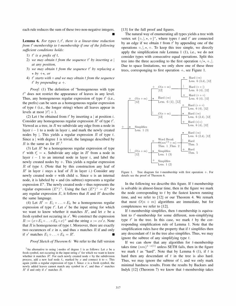
[13] for the full proof and figures.The natural way of enumerating all types yields a tree with
vertex set {◦, |, �,+}∗, where types t and t′ are connected
by an edge if we obtain t from t′ by appending one of the
operations ◦, |, �,+. To keep this tree simple, we directly
apply the simplification rule Lemma 1 (1), i.e., we do not
consider types with consecutive equal operations. Split this
tree into the three according to the first operation ◦/�,+, |.Due to space limitations, we only show one of these three
trees, corresponging to first operation +, see Figure 1.
+ �
|
◦
Simplifies
O(n+m) Simplifies
Simplifies
Lem. 1 (3)
Lem. 1 (2)
Word BreakΘ(nm1/3 +m)Thm. 1 ,Thm. 2
Hard (◦�)Lem. 6 (2,4), [12]
Hard
HardThm. 5
Thm. 5
�
◦
+
�
+
|
O(n+m) Hard (◦�)Lem. 6 (4), [12]
O(n+m)
O(n+m)
|
+
�
Hard (◦+ ◦)
Hard (◦�)
Hard (◦|+)
Lem. 6 (4), [12]
Lem. 6 (2,4), [12]
Lem. 6 (4), [12]
Hard (◦�)
Hard (◦+ |)
Hard (◦+ ◦)
Lem. 6 (3,4), [12]
Lem. 6 (4), [12]
�
◦
�
+
◦[12]
[12]
Lem. 1 (3)
Lem. 6 (4), [12]
|
[12]
[12]
Figure 1. Tree diagram for t-membership with first operation +. Fordetails see the proof of Theorem 6.
In the following we describe this figure. If t-membership
is solvable in almost-linear time, then in the figure we mark
the node corresponding to t by the fastest known running
time, and we refer to [12] or our Theorem 4. We remark
that most O(n + m) algorithms are immediate, but for
completeness we refer to [12].If t-membership simplifies, then t-membership is equiva-
lent to t′-membership for some different, non-simplifying
type t′ in the tree. In this case, we mark t by the cor-
responding simplification rule of Lemma 1. Note that the
simplification rules have the property that if t simplifies then
any descendant of t in the tree also simplifies. Thus, we may
ignore the subtree of any simplifying type t.If we can show that any algorithm for t-membership
takes time (nm)1−o(1) unless SETH fails, then in the figure
we mark t as “hard”. Note that by Lemma 6 (1), if t is
hard then any descendant of t in the tree is also hard.
Thus, we may ignore the subtree of t, and we only mark
minimal hardness results. From the results by Backurs and
Indyk [12] (Theorem 7) we know that t-membership takes
317
time (nm)1−o(1) under SETH for the types ◦�, ◦|◦, ◦ + ◦,◦|+, and ◦ + |. In the full version of this paper, we add
hardness for the types +|◦+, +|◦|, and |+|◦. If there is such
a direct hardness proof of t-membership, then in the figure
we refer to the corresponding theorem. In all other minimal
hard cases, there is a combination of the reduction rules,
Lemma 6 (2–4), resulting in a type t′ such that hardness of
t′-membership follows from Theorem 7 and t′-membership
has a linear time reduction to t-membership. In this case, in
the figure we additionally mark the node corresponding to
t by t′. E.g., | ◦ |�-membership contains ◦�-membership as
a special case (since by Lemma 6 (2) we may remove any
| operations) and ◦�-membership is hard by Theorem 7, so
we mark the node corresponding to | ◦ |� by “hard ◦�”.
It is easy to check that our Figure 1 indeed enumerates all
cases starting with + and thus contains all maximal algo-
rithmic results and minimal hardness results. The claimed
dichotomy of Theorem 6 now follows by inspecting the
figure, as well as the two remaining figures that can be found
in the full version.
REFERENCES
[1] K. Thompson, “Programming techniques: Regular expressionsearch algorithm,” Commun. ACM, vol. 11, no. 6, pp. 419–422, Jun. 1968.
[2] G. Myers, “A four russians algorithm for regular expressionpattern matching,” J. ACM, vol. 39, no. 2, pp. 432–448, Apr.1992.
[3] P. Bille and M. Thorup, “Faster regular expression matching,”in 36th International Colloquium on Automata, Languagesand Programming, 2009, pp. 171–182.
[4] D. E. Knuth, J. H. Morris, and V. R. Pratt, “Fast patternmatching in strings,” SIAM Journal on Computing, vol. 6,pp. 323–350, 1977.
[5] R. Cole and R. Hariharan, “Verifying candidate matchesin sparse and wildcard matching,” in 34th Annual ACMSymposium on Theory of Computing, 2002, pp. 592–601.
[6] A. V. Aho and M. J. Corasick, “Efficient string matching: Anaid to bibliographic search,” Commun. ACM, vol. 18, no. 6,pp. 333–340, Jun. 1975.
[7] A. Gajentaan and M. H. Overmars, “On a class of O(N2)problems in computational geometry,” Comput. Geom. TheoryAppl., vol. 5, no. 3, pp. 165–185, Oct. 1995.
[8] V. V. Williams and R. Williams, “Subcubic equivalencesbetween path, matrix and triangle problems,” in 51st AnnualIEEE Symposium on Foundations of Computer Science, 2010,pp. 645–654.
[9] A. Abboud and V. V. Williams, “Popular conjectures implystrong lower bounds for dynamic problems,” in P55th AnnualIEEE Symposium on Foundations of Computer Science, 2014,pp. 434–443.
[10] M. Patrascu and R. Williams, “On the possibility of faster satalgorithms,” in 21st Annual ACM-SIAM Symposium on Dis-crete Algorithms, 2010, pp. 1065–1075. [Online]. Available:http://dl.acm.org/citation.cfm?id=1873601.1873687
[11] R. Impagliazzo and R. Paturi, “On the complexity of k-sat,” J.Computer and System Sciences, vol. 62, no. 2, pp. 367–375,Mar. 2001.
[12] A. Backurs and P. Indyk, “Which regular expression patternsare hard to match?” in 57th Annual IEEE Symposium onFoundations of Computer Science, 2016.
[13] K. Bringmann, A. Grønlund, and K. G. Larsen, “Adichotomy for regular expression membership testing,”CoRR, vol. abs/1611.00918, 2016. [Online]. Available:http://arxiv.org/abs/1611.00918
[14] D. Tunkelang, “Retiring a great interview problem,”2011, http://thenoisychannel.com/2011/08/08/retiring-a-great-interview-problem.
[15] P. Norvig, “Natural language corpus data,” in Beautiful Data.The Stories Behind Elegant Data Solutions, 2009.
[16] V. Vassilevska, “Efficient algorithms for clique problems,” Inf.Process. Lett., vol. 109, no. 4, pp. 254–257, Jan. 2009.
[17] J. Nesetril and S. Poljak, “On the complexity of the subgraphproblem,” Commentationes Math. Universitatis Carolinae,vol. 026, no. 2, pp. 415–419, 1985.
[18] F. Eisenbrand and F. Grandoni, “On the complexity of fixedparameter clique and dominating set,” Theoretical ComputerScience, vol. 326, no. 1, pp. 57–67, 2004.
[19] A. Abboud, A. Backurs, and V. Vassilevska Williams, “If thecurrent clique algorithms are optimal, so is Valiant’s parser,”in 56th Annual IEEE Symposium on Foundations of ComputerScience, 2015.
[20] F. L. Gall, “Faster algorithms for rectangular matrix multipli-cation,” in 53rd Annual IEEE Symposium on Foundations ofComputer Science, 2012, pp. 514–523.
[21] R. Clifford, “Matrix multiplication and pattern matchingunder hamming norm.”
[22] R. Impagliazzo, R. Paturi, and F. Zane, “Which problems havestrongly exponential complexity?” J. Computer and SystemSciences, vol. 63, no. 4, pp. 512–530, 2001.
[23] R. Williams, “A new algorithm for optimal 2-constraint satis-faction and its implications,” Theoretical Computer Science,vol. 348, no. 2, pp. 357–365, Dec. 2005.
[24] P. Weiner, “Linear pattern matching algorithms,” in 14thAnnual Symposium on Switching and Automata Theory, 1973,pp. 1–11.
[25] S. Wigert, “Sur l’ordre de grandeur du nombre des diviseursd’un entier,” Ark. Math. Astron. Fys., vol. 3, pp. 113–140,1906-07.
318