a disjunctive positive refinement of model elimination and its application to subsumption deletion
TRANSCRIPT

Journal of Automated Reasoning 19: 205–262, 1997. 205c© 1997 Kluwer Academic Publishers. Printed in the Netherlands.
A Disjunctive Positive Refinement of ModelElimination and Its Application to SubsumptionDeletion
PETER BAUMGARTNER1? and STEFAN BRUNING21Universitat Koblenz, Institut fur Informatik, Rheinau 1, 56075 Koblenz, Germany.e-mail: [email protected] Hochschule Darmstadt, Fachbereich Informatik, Intellektik, Alexanderstr. 10, 64283Darmstadt, Germany.e-mail: [email protected]
(Received: 9 September 1996)
Abstract. The Model Elimination (ME) calculus is a refutationally complete, goal-oriented calculusfor first-order clause logic. In this article, we introduce a new variant called disjunctive positiveME (DPME); it improves on Plaisted’s positive refinement of ME in that reduction steps areallowed only with positive literals stemming from clauses having at least two positive literals (so-called disjunctive clauses). DPME is motivated by its application to various kinds of subsumptiondeletion: in order to apply subsumption deletion in ME equally successful as in resolution, itis crucial to employ a version of ME that minimizes ancestor context (i.e., the necessary A-literals to find a refutation). DPME meets this demand. We describe several variants of ME withsubsumption, the most important ones being ME with backward and forward subsumption and theT∗-Context Check. We compare their pruning power, also taking into consideration the well-knownregularity restriction. All proofs are supplied. The practicability of our approach is demonstratedwith experiments.
Key words: theorem proving, model elimination, subsumption.
1. Introduction
The past four decades of research in the field of automated deduction havebrought forth several exceptionally successful proof systems for first-order logicsuch as OTTER (Wos et al., 1990), MKRP (Blasius et al., 1981), and SETHEO(Letz et al., 1992).
In many cases, their success is based on the high inference rates that areachieved using modern computers. Often one can obtain thousands (even millions(Van de Riet, 1993)) of true first-order inferences per second. In most cases,however, the problem is not speed but control. While searching for a proof of atheorem, a machine is mostly unable, unlike human beings, to distinguish betweenrelevant and irrelevant information. Since the amount of irrelevant information
? Supported by the DFG within the ‘Schwerpunktprogramm Deduktion’ under grant FU 263/2-2.
VTEX (Ju) PIPS No.: 139899 MATHKAPJARSWB1.tex; 15/08/1997; 11:41; v.7; p.1

206 PETER BAUMGARTNER AND STEFAN BRUNING
naturally overwhelms the relevant part, it is impossible, even with the highestinference rates, to examine the whole search space.
Therefore, one of the main goals in the field of automated deduction is toaugment calculi with the possibility to reduce search spaces as much as possible.
Basically, a calculus has to cope with two different kinds of redundancy. First,information can be redundant because of its logical form such that it can beremoved without loss of logical information. Second, information can be redun-dant because it cannot contribute to a successful derivation. Such informationcan be removed without affecting the satisfiability of the respective formula.
In this paper, we study the problem of avoiding logical redundancies duringModel Elimination (ME) derivations (e.g., see (Loveland, 1986; Letz et al., 1992;Letz et al., 1994; Baumgartner and Furbach, 1994a) for descriptions of ME cal-culi). A lot of work done in the field of automated deduction to avoid logicalredundancies has been carried out in the context of resolution. In resolution-based systems this kind of redundancy is traditionally handled by mechanismsthat remove tautological and subsumed clauses (e.g., see (Chang and Lee, 1973;Loveland, 1978)). One distinguishes two basic kinds of subsumption: forwardsubsumption discards newly generated clauses that are subsumed by alreadyexisting clauses, whereas backward subsumption removes old clauses that aresubsumed by new ones. In (Overbeek and Wos, 1989) it was shown that althoughsubsumption tests can be rather expensive, these mechanisms are very effectiveto prevent logical redundancy.
Unfortunately, such reduction mechanisms are not applicable in a straight-forward manner in model-elimination-like calculi. This is because ME, which –like PROLOG – performs a top-down backward-chaining proof search, does notenumerate derivable clauses but tries to find a proof by enumerating derivations.Needed, therefore, are mechanisms that prevent logically redundant derivations.Within this context, one has to distinguish two basic approaches. The first (andmore investigated) one is based on the fact that many subderivations are simi-lar and therefore sometimes interchangeable. Mechanisms that make use of thisfact are factorization (Fronhofer, 1985), lemma handling (Fronhofer and Cafer-ra, 1988), caching (Astrachan and Stickel, 1992), and the foothold refinement(Spencer, 1994).
In what follows we shall pursue the second basic approach, which aims atavoiding a derivation if the possibility to extend it to a refutation would implythe same possibility for a different and (one hopes) smaller derivation.
There already exist some techniques following this general approach. Popularones are the identical ancestor check and its generalization, regularity, which aresuccessfully used in several theorem provers (e.g., see (Stickel, 1988; Letz et al.,1992)). These refinements prune a derivation if some literal is identical to one ofits ancestors. Other restrictions on ME to prevent redundant derivations are cut-freeness and subsumption-freeness (Letz, 1993) (which can be seen as restrictedversions of tautology and subsumption deletion in resolution-based systems). The
JARSWB1.tex; 15/08/1997; 11:41; v.7; p.2

MODEL ELIMINATION AND SUBSUMPTION DELETION 207
first one ensures that tableaux do not contain tautological tableau clauses. Thelatter one demands that no tableau clause is properly subsumed by some clauseof the input set.
A further possibility to avoid redundant derivations, which is mostly neglectedin connection with top-down backward-chaining calculi, is the use of subsump-tion. As shown in (Besnard, 1989; Bol et al., 1991), SLD-resolution, which canbe seen as a restricted variant of ME, can be combined with a technique thatcompares (via subsumption) sets of open goals.? Whenever the set of open goalsafter applying a sequence of inference steps d1, . . . , dn is subsumed by some for-mer set of open goals (that is, the set of open goals after some dj with j < n),the last inference step, dn, can be withdrawn.
Unfortunately, a straightforward application of this kind of forward subsump-tion to ME preserves completeness only when Horn clause sets are considered.Roughly speaking, this is due to the fact that ancestor goals, which may becomeimportant to perform reduction steps, are ignored. Hence, a first step to retaincompleteness would be to compare entire ME tableaux. However, it becomesclear immediately that without further refinements, such a proceeding would be(rather) useless: An ME tableau Tn generated after a sequence D = d1, . . . , dnof inference steps usually contains more ancestor goals than the tableau Tj gen-erated by d1, . . . , dj , where j < n. Since every ancestor of an open goal is apotential candidate for the application of a reduction step, one cannot prune Dunless, roughly speaking, each of the ‘additional’ ancestors in Tn (or generaliza-tions of these ancestors) also occurs in Tj in the corresponding tableau branches.This, however, is very rarely the case.
In this article, we propose two approaches to overcome this problem. Bothof them provide criteria that allow us to identify ancestor goals (i.e., A-literalsin Loveland’s terminology) that can be safely ignored as potential candidates forthe application of reduction steps. Hence, in case these criteria tell us that, forinstance, none of the ancestors in Tn is necessary for the application of reductionsteps, we can safely prune D if the set of open goals of Tj subsumes the set ofopen goals of Tn.
The first and more important approach is based on the positive refinement forME. This refinement restricts reduction steps to those that use a positive ancestorgoal (Plaisted, 1990) and therefore allows one to ignore all negative ancestors.However, one can do better. In Section 3, we prove that it is additionally possible(without losing completeness) to ignore positive ancestors that originate fromHorn clauses. Thus, the sole ancestors that have to be taken into account bya subsumption-based pruning technique are non-negated literals that stem fromnon-Horn clauses (called disjunctive clauses). We further show that it is – at leastpartially – possible to overcome the problem of the incompatibility of the positiverefinement with regularity (see (Plaisted, 1990)). To this end, we introduce the
? Note that, in terms of resolution, the set of open goals is in fact a resolvent.
JARSWB1.tex; 15/08/1997; 11:41; v.7; p.3
208 PETER BAUMGARTNER AND STEFAN BRUNING
concept of blockwise regularity and prove that this restricted form of regularityand the (extended) positive refinement can be safely combined.
The second approach is to predetermine which ancestors of a goal G cannotbe used for reduction steps in order to solve G. This is achieved by the conceptof reachability originally proposed in (Neugebauer, 1992) (in a different context).Roughly speaking, the idea is as follows: in a preprocessing step it is determinedwhich literals are reachable from G, that is, which literals (modulo additionalsubstitutions) may occur as subgoals of G. Then, one can safely ignore anyancestor A of G in case no literal, which can be made complementary to A (viaunification), is reachable from G.
With these two approaches at hand, we define several pruning techniquesbased on subsumption for ME. Besides a generalized version of the aforemen-tioned variant of forward subsumption we also introduce backward subsumption,which, similar to the concept of backward subsumption in resolution-based cal-culi, prunes a derivation D1 if it is subsumed (in the above sense) by a derivationD2 which is generated after D1 in the course of the deduction process (Section 4).
Furthermore, we propose a variant of forward subsumption that compares onlyone open goal with one of its ancestor goals, rather than comparing sets of literals(‘T-Context Check’, Section 5). Roughly speaking, the idea is to prune a deriva-tion if some open goal is an instance of one of its ancestor goals. Clearly, such aprocedure preserves completeness only if variable dependencies with other goalsare taken into account. The resulting pruning technique is (if Horn clause sets areconsidered) a true generalization of the loop check proposed in (Besnard, 1989)and of the aforementioned identical ancestor check. Further, we shall illustrate inSection 4 that it does not suffer from one main problem of other subsumption-based techniques, namely, a dependence of the employed search strategy.
Finally, it is worth emphasizing that the techniques proposed in this articleallow more than reduction in the search space. Additionally they make it possibleto detect that formulas cannot be proven. This is particularly interesting forapplications where false conjectures or incorrect theorems have to be identified.Note that many other techniques, for instance factorization or the use of lemmata,do not help to solve this problem.
The article is structured as follows. In Section 2 we provide some basic defi-nitions to make this paper self-contained. Section 3 is devoted to the introductionof the positive refinement and its generalization, the so-called disjunctive positiverefinement. There, the completeness of ME in combination with the disjunctivepositive refinement is proved. In Section 4 and Section 5 we introduce the afore-mentioned subsumption-based pruning techniques. We discuss their relation aswell as their connection to other known refinements of ME. In Section 6 we illus-trate the usefulness of our techniques by presenting some experimental data. InSection 7 and Section 8 we discuss our results and point out some future researchperspectives. Figure 13 in Section 7 is a graphical summary of our results; it mightbe a good idea to occasionally have a look at it for orientation during reading.
JARSWB1.tex; 15/08/1997; 11:41; v.7; p.4

MODEL ELIMINATION AND SUBSUMPTION DELETION 209
2. Preliminaries
In what follows, we assume the reader to be familiar with the basic concepts offirst-order logic. A clause is a multiset? of literals {|L1, . . . , Ln|}, considered as adisjunction and therefore usually written as L1∨· · ·∨Ln. As usual, the variablesoccurring in clauses are considered implicitly as being universally quantified,and a clause set is taken as a conjunction of clauses. A clause is Horn iff itcontains at most one positive literal. A non-negative clause contains at least onepositive literal. A definite clause is a clause containing exactly one positive literal.A negative literal in a definite clause is called body literal. Let Ld denote thecomplement of a literal L. Two literals L and K are complementary if Ld = K.The set of variables occurring in an expression E is denoted by var(E).
Throughout this paper, we consider a variant of ME that uses so-calledME tableaux as basic proof objects (e.g., see (Letz et al., 1992; Letz et al.,1994)), rather than ME chains (Loveland, 1986). An alternate, and equally usable,approach would have been to follow (Baumgartner and Furbach, 1993) and viewME as a transformation on branch sets.
DEFINITION 1 (Literal tree). A literal tree is a pair (t, λ) consisting of anordered tree t and a labeling function λ assigning literals or multisets of lit-erals to the non-root nodes of t. The successor sequence of a node N in anordered tree t is the sequence of nodes with immediate predecessor N , in theorder given by t.
DEFINITION 2 (Tableau). A (clausal) tableau T of a set of clauses S is a literaltree (t, λ) in which, for every maximal successor sequence N1, . . . ,Nn in tlabeled with literals K1, . . . ,Kn, respectively, there is a substitution σ and aclause {|L1, . . . , Ln|} ∈ S with Ki = Liσ for every 1 6 i 6 n. {|K1, . . . ,Kn|} iscalled a tableau clause and the elements of a tableau clause are called tableauliterals.
A tableau is called model elimination tableau (ME tableau) if each inner nodeN labeled with a literal L has a leaf node N ′ among its immediate successornodes that is labeled with the literal Ld.
Let Tδ denote the tableau that is obtained from a tableau T by application ofthe substitution δ to all literals of T . Furthermore, given a tableau T containingsome node N , we often denote the literal attached to N in T by L(N,T ).
DEFINITION 3 (Branch, Open and Closed Tableau, Open Goal, Frontier). Abranch of a tableau T is a sequence N1, . . . ,Nn of nodes in T such that N1
is the root of T , Ni is the immediate predecessor of Ni+1 for 1 6 i < n, andNn is a leaf of T . The leaf of a branch b is denoted by leaf(b). A branch is? The use of multisets instead of sets facilitates the lifting of derivations from the ground level
to the general level.
JARSWB1.tex; 15/08/1997; 11:41; v.7; p.5

210 PETER BAUMGARTNER AND STEFAN BRUNING
complementary if the labels of N1, . . . ,Nn contain some literal L and its com-plement Ld. To distinguish the simple presence of a complementary branch andthe detection of this fact, we allow branches to be labeled as either open orclosed. A tableau is closed if each of its branches is closed; otherwise it is open.Let OB(T ) denote the set of open branches of T .
Given a branch N1, . . . ,Nn in a ME tableau T , we call Ni an ancestor(node) of Nj iff i < j. Correspondingly we call L(Ni, T ) an ancestor (literal)of L(Nj , T ) iff i < j.
Let b be an open branch of a ME tableau T . If L is the label of the leaf nodeof b, then L is called an open goal of T . Further, the set of leaf nodes in T thatare labeled with open goals is called the frontier of T .
The motivation to distinguish between complementary and closed tableaubranches will be given after the ME calculus has been defined. Given a branchN1, . . . ,Nn, we sometimes say that Ni dominates Nj if i < j.
THEOREM 4 ((Letz, 1993)). Let S be a clause set. S is unsatisfiable iff thereexists a closed ME tableau of S.
Note 1 (Loveland’s Model Elimination). The original model elimination cal-culus (Loveland, 1968; Loveland, 1978) uses chains as the primary data structure.A chain is a finite sequence of literals a1b1 · · · anbn where each ai stands for asequence of literals written in brackets, that is, ai = [ai,1] · · · [ai,ki ], and each bistands for a sequence of literals bi = bi,1 · · · bi,li .
The chains used in Loveland’s ME can be simulated by certain literal treeswhere every inner node lies on one single branch of the literal tree. Such aliteral tree equals a tableau T whose closed branches are omitted: The literalscontained in the sequences a1, . . . , an (the so-called A-literals) correspond toancestor literals of open goals in T whereas the literals contained in b1, . . . , bn(the so-called B-literals) correspond to the open goals in T .
Figure 1 gives an idea of the transformation (see (Baumgartner and Furbach,1993) for a more detailed treatment).
In our terminology, Loveland’s model elimination is fixed to a computationrule where always some longest branch in the corresponding tableaux is selectedfor extension or reduction step. In fact, the possibility to use any longest branchis mirrored by using ordering rules for extension clauses. For ease of presentationwe dispense with the chain notation and formulate our calculi within a tableauxsetting.
Based on the above definitions we now introduce the inference steps of ME. Theirpurpose is to allow for systematical construction of ME tableaux. Throughoutthe following definitions, let S be a set of input clauses.
DEFINITION 5 (Initialization step). Let N be the root of a one-node tree. Selecta new variant {|L1, . . . , Ln|} of a clause C ∈ S, attach n new successor nodes
JARSWB1.tex; 15/08/1997; 11:41; v.7; p.6

MODEL ELIMINATION AND SUBSUMPTION DELETION 211
Figure 1. Mapping of chains to literal trees.
to N (called top-nodes), and label them with L1, . . . , Ln (called top-literals),respectively. C is called top-clause.
DEFINITION 6 (Extension step). Select a leaf node N of an open branch labeledwith literal L. Let C ′ = {|L1, . . . , Ln|} be a new variant of a clause C ∈ S suchthat there exists an MGU σ and a literal Li ∈ C ′ with Ldσ = Liσ. Then attach nnew successor nodes N1, . . . ,Nn to N , label them with L1, . . . , Ln, respectively,and apply σ to all tableau literals. Finally, the new branch with leaf node Ni ismarked as closed.
We call Ni an extension node, and each element of {N1, . . . ,Nn} − {Ni} anonextension node. A literal attached to an extension node is called extensionliteral, otherwise nonextension literal.
DEFINITION 7 (Reduction step from node N ′ to node N ). Select a leaf nodeN ′ of an open branch b labeled with literal L′. If there is a dominating node Non b labeled with literal L such that there exists a MGU σ with L′σ = Ldσ, thenapply σ to all tableau literals and mark b as closed.
Note that as an immediate consequence of these definitions we have that a branchis closed only if it is complementary (but not necessarily vice versa).
DEFINITION 8 (Model Elimination). A sequence of T1, . . . , Tn of ME tableauxis called a ME derivation for a clause set S (called the set of input clauses) ifT1 is obtained by an initialization step, and for 1 < i 6 n, Ti is obtained byone single application of a reduction step or an extension step to some node inTi−1. Furthermore, each clause used in an extension step has to be a variant ofan element of S. A ME derivation is called a ME refutation if it generates aclosed tableau.
JARSWB1.tex; 15/08/1997; 11:41; v.7; p.7
212 PETER BAUMGARTNER AND STEFAN BRUNING
It turns out to be practical to confuse a derivation (i.e., a sequence of tableaux)with the process generating it. We thus write d1, . . . , dn instead of T1, . . . , Tn,where dis denotes the used instances of the respective inference rules to obtainthe Tis.
Let L be an open goal attached to a node N in a ME tableau T . A MEsubderivation D for N (or L) is a sequence of derivation steps where the firstelement of D selects N and each further element selects a descendant of N . Dis called a ME subrefutation if after applying D to T , each branch containing Nis closed.
We simply say (sub)derivation instead of ME (sub)derivation and (sub)refu-tation instead of ME (sub)refutation.
A derivation D is called unrestricted if the substitution used to apply theelements of D need not be MGUs.
Now we can motivate the explicit marking of a closed branch (as opposed tothe state of being a complementary branch): first, it is natural in view of a proofprocedure to make the detection of a complementary branch explicit; second, itfacilitates the definition of the disjunctive positive variant of ME below; third,(a technical motivation) the lifting of derivations from the ground level to thegeneral level is less complicated, because otherwise reduction steps at the generallevel become necessary that do not have a counterpart at the ground level; fourth,if the distinction were not made, it would be mandatory to check the selectedbranch for complementarity because a complementary (and hence closed) branchcannot be selected for a derivation step.
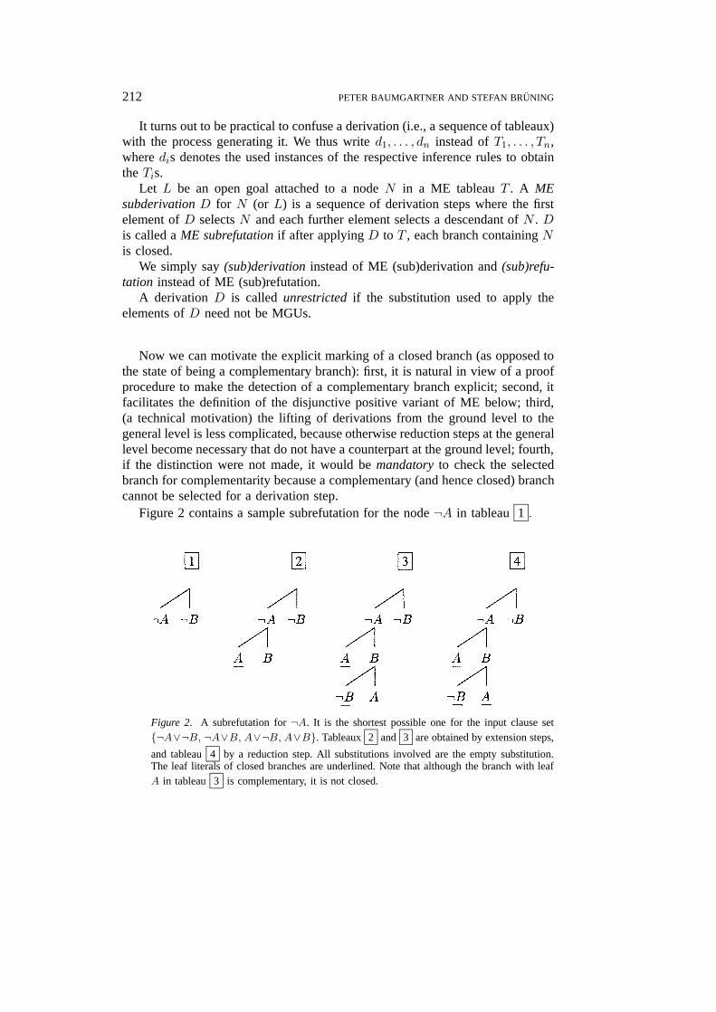
Figure 2 contains a sample subrefutation for the node ¬A in tableau 1 .
Figure 2. A subrefutation for ¬A. It is the shortest possible one for the input clause set{¬A∨¬B, ¬A∨B, A∨¬B, A∨B}. Tableaux 2 and 3 are obtained by extension steps,
and tableau 4 by a reduction step. All substitutions involved are the empty substitution.The leaf literals of closed branches are underlined. Note that although the branch with leafA in tableau 3 is complementary, it is not closed.
JARSWB1.tex; 15/08/1997; 11:41; v.7; p.8

MODEL ELIMINATION AND SUBSUMPTION DELETION 213
THEOREM 9 ((Letz, 1993)). Given any ME tableau T of a clause set S, there isa ME derivation of S generating a tableau T ′ such that T is an instance of T ′.?
DEFINITION 10 ((Local) computation rule). A computation rule r is a mappingassigning to each open tableau T a leaf node N in T that is labeled with an opengoal. N is called the node selected by r. Alternatively, we often say that theliteral attached to N is selected by r.
A derivation via a computation rule r is a derivation d1, . . . , dn such that forall 1 6 i < n, di+1 is applied to the node selected by r in the tableau generatedby d1, . . . , di.
We call a computation rule r local if every derivation d1, d2, . . . , generatedvia r satisfies the following property: whenever a node N is selected for theapplication of a derivation step di, then a sibling node N ′ of N is selected fora derivation step dj with j > i only in case each branch containing N has beenclosed previously. Further, we require local computation rules to be stable undersubstitution; that is, a node is selected in a tableau T by r if and only if it isalso selected in Tσ for every substitution σ.
For instance, a computation rule that always selects the ‘leftmost’ open branchis local. Likewise, always selecting a longest open branch is also local.
PROPOSITION 11 ((Letz, 1993)). Any closed ME tableau for a set of groundclauses can be constructed with any possible computation rule.
3. A Disjunctive Positive Refinement of Model Elimination
In this section we introduce a disjunctive positive refinement of ME. This is astrengthening of the positive refinement of (Plaisted, 1990). Let us first motivateit by its application to subsumption deletion.
When attempting to define a subsumption relation among ME tableaux, onesoon recognizes that the situation is more complicated than in resolution. Toexplain this, let us take the view of a ME tableau as a generalized clause, whoseliterals are the tableau’s leaf literals (thus, we are talking about the ‘frontier’ in thesense of Definition 3). The ancestor literals then can be thought of as additionalliteral lists attached to the clause literals (see (Baumgartner and Furbach, 1993)for a more detailed treatment). Clauses as used in resolution then can be seen asfrontiers of ME tableaux.
In order to adapt the notion of subsumption of resolution?? to ME, a first ideais to apply subsumption among tableaux frontiers to discard subsumed tableaux.This approach is appealing because no ancestor context needs to be examined.
? A tableau T is an instance of another tableau T ′ iff there is a substitution σ such T ′σ = T .?? Recall that a clause C subsumes a clause D iff for some substitution σ we have Cσ ⊆ D,
where a clause is a multiset of literals.
JARSWB1.tex; 15/08/1997; 11:41; v.7; p.9
214 PETER BAUMGARTNER AND STEFAN BRUNING
Unfortunately, completeness is lost then, because some ancestor context presentonly in the discarded tableaux might be necessary to complete the proof. Thus,ancestor context has to be obeyed for the subsumption check. On the other hand,if the whole ancestor context for every literal is obeyed, chances are low to applysubsumption successfully very often.
To overcome these problems, we propose to use a variant of ME that mini-mizes ancestor literals. In (Plaisted, 1990) D. Plaisted has shown that it sufficesfor completeness to keep only positive literals as ancestors. With this calculusa larger subsumption relation can be defined, since only the positive ancestorliterals have to be obeyed for the subsumption test. We further improve on thisby restricting ancestor context to those positive literals that stem from disjunctiveclauses.? For example, if a leaf literal A is extended with the clause B ∨ ¬A,then both ordinary ME and Plaisted’s positive refinement will keep B in theancestor context (and thus allowing reduction steps to B) of the subrefutation ofB, while in our positive disjunctive refinement it will not be kept. These casesoccur every time when a definite clause is used with a body literal as entry point.As a positive example consider C ∨ B ∨ ¬A; after an extension step to A bothC and B have to be kept for reduction steps in the subrefutations of C and B.??
Since only these positive disjunctive literals are needed to get a completecalculus, it is thus sufficient to restrict subsumption to use these literals only. Adetailed treatment of this can be found in Section 4.
In the following we shall formally introduce the positive disjunctive refine-ment and prove its completeness.
3.1. DEFINITION OF THE DISJUNCTIVE POSITIVE REFINEMENT
As indicated above, the information whether a certain literal stems from a positivedisjunctive clause is crucial. The next definition accounts for this formally.
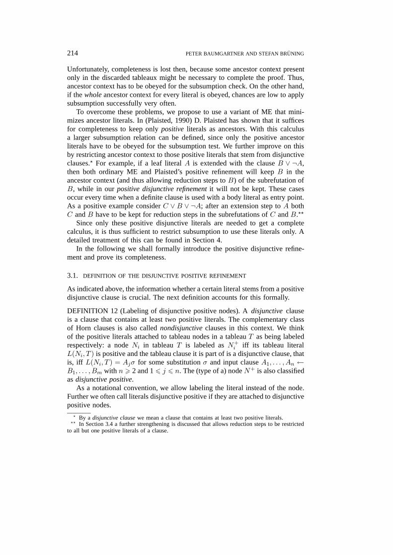
DEFINITION 12 (Labeling of disjunctive positive nodes). A disjunctive clauseis a clause that contains at least two positive literals. The complementary classof Horn clauses is also called nondisjunctive clauses in this context. We thinkof the positive literals attached to tableau nodes in a tableau T as being labeledrespectively: a node Ni in tableau T is labeled as N+
i iff its tableau literalL(Ni, T ) is positive and the tableau clause it is part of is a disjunctive clause, thatis, iff L(Ni, T ) = Ajσ for some substitution σ and input clause A1, . . . , An ←B1, . . . , Bm with n > 2 and 1 6 j 6 n. The (type of a) node N+ is also classifiedas disjunctive positive.
As a notational convention, we allow labeling the literal instead of the node.Further we often call literals disjunctive positive if they are attached to disjunctivepositive nodes.? By a disjunctive clause we mean a clause that contains at least two positive literals.?? In Section 3.4 a further strengthening is discussed that allows reduction steps to be restricted
to all but one positive literals of a clause.
JARSWB1.tex; 15/08/1997; 11:41; v.7; p.10

MODEL ELIMINATION AND SUBSUMPTION DELETION 215
We can now define the disjunctive positive refinement.
DEFINITION 13 (Disjunctive positive refinement). In the following let N be anopen goal node in a tableau T . Suppose a computation rule r as given.
We are going to define a restricted version of ‘reduction step’ (see Defini-tion 7): if N ′ is selected in T by r and if there is a dominating positive dis-junctive node N+ of N ′ on the same branch and if there exists an MGU σ withL(N ′, T )σ = L(N+, T )dσ, then apply σ to all tableau literals. Such reductionsteps are called disjunctive positive reduction steps (via r).
The definition of extension step (Definition 6) via r remains unchanged. Inparticular, the type of the extension node is understood to be disregarded: bothdisjunctive positive and nondisjunctive positive nodes have to be extended. Asin the disjunctive positive reduction step, only extension of a selected node isallowed.
Finally, the notion of derivation (Definition 8) is adapted to incorporate thesechanges, and we shall speak of disjunctive positive derivations and refutations.The calculus is termed disjunctive positive refinement of ME (DPME).
Figure 3 contains a sample refutation.
Note 2 (Extra literals). Since the nondisjunctive positive literals and the neg-ative literals of a branch cannot be subject to reduction steps, it would in a strictsense not be necessary to store them along a refutation. Nevertheless, it may beadvisable to do so. One reason is that, occasionally, allowing (ordinary) reductionsteps helps to find a refutation more quickly. For instance, in Figure 3, tableau3 , the branch ending in A could immediately be closed by an (ordinary) reduc-
tion step (see Figure 2). Indeed, a respective strategy for the restart version of
Figure 3. A subrefutation for ¬A. It is the shortest possible one for the input clause set{¬A∨¬B, ¬A∨B, A∨¬B, A∨B}. Tableaux 2 , 3 , and 4 are obtained by extension
steps. Note that the node A in tableau 3 cannot be closed by a disjunctive positive reduction
step, but the node ¬B in 4 can. A similar subrefutation exists for ¬B.
JARSWB1.tex; 15/08/1997; 11:41; v.7; p.11
216 PETER BAUMGARTNER AND STEFAN BRUNING
ME (see Section 3.2 below) turned out to be essential in practice (Baumgartnerand Furbach, 1994b).
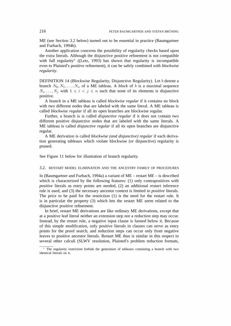
Another application concerns the possibility of regularity checks based uponthe extra literals. Although the disjunctive positive refinement is not compatiblewith full regularity? ((Letz, 1993) has shown that regularity is incompatibleeven to Plaisted’s positive refinement), it can be safely combined with blockwiseregularity.
DEFINITION 14 (Blockwise Regularity, Disjunctive Regularity). Let b denote abranch N0,N1, . . . ,Nn of a ME tableau. A block of b is a maximal sequenceNi, . . . ,Nj with 1 6 i < j 6 n such that none of its elements is disjunctivepositive.
A branch in a ME tableau is called blockwise regular if it contains no blockwith two different nodes that are labeled with the same literal. A ME tableau iscalled blockwise regular if all its open branches are blockwise regular.
Further, a branch is is called disjunctive regular if it does not contain twodifferent positive disjunctive nodes that are labeled with the same literals. AME tableau is called disjunctive regular if all its open branches are disjunctiveregular.
A ME derivation is called blockwise (and disjunctive) regular if each deriva-tion generating tableaux which violate blockwise (or disjunctive) regularity ispruned.
See Figure 11 below for illustration of branch regularity.
3.2. RESTART MODEL ELIMINATION AND THE ANCESTRY FAMILY OF PROCEDURES
In (Baumgartner and Furbach, 1994a) a variant of ME – restart ME – is describedwhich is characterized by the following features: (1) only contrapositives withpositive literals as entry points are needed, (2) an additional restart inferencerule is used, and (3) the necessary ancestor context is limited to positive literals.The price to be paid for the restriction (1) is the need for the restart rule. Itis in particular the property (3) which lets the restart ME seem related to thedisjunctive positive refinement.
In brief, restart ME derivations are like ordinary ME derivations, except thatat a positive leaf literal neither an extension step nor a reduction step may occur.Instead, by the restart rule, a negative input clause is fanned below it. Becauseof this simple modification, only positive literals in clauses can serve as entrypoints for the proof search, and reduction steps can occur only from negativeleaves to positive ancestor literals. Restart ME thus is similar in this respect toseveral other calculi (SLWV resolution, Plaisted’s problem reduction formats,
? The regularity restriction forbids the generation of tableaux containing a branch with twoidentical literals on it.
JARSWB1.tex; 15/08/1997; 11:41; v.7; p.12

MODEL ELIMINATION AND SUBSUMPTION DELETION 217
and Loveland’s near-Horn Prolog variants). These calculi differ with respect tothe required ancestor context, the number of contrapositives, and the definition ofthe restart rule. Very systematic expositions of these calculi along this parameterspace are given in (Loveland and Reed, 1995; Reed and Loveland, 1992).
Since the main idea is the same in all of these calculi, it suffices for ourpurposes to consider restart ME only. The link between restart ME and thedisjunctive positive refinement has been explicated in (Mayr, 1995). In that paper,Mayr discovered independently from us the possibility of restricting reductionsteps to disjunctive positive literals. His result was obtained as a by-product ofthe completeness proof there. That proof proceeds by transforming a given restartME refutation into an ordinary ME refutation in such a way that the absence ofreduction steps to nondisjunctive positive literals (which is a property of restartME) carries over to the transformed proof.
Below, we shall give another, more direct proof. It is similar to that of restartME. This suggests imposing restrictions defined for restart ME also on disjunc-tive positive ME. Indeed, blockwise regularity holds for both calculi. However,while the analogue to disjunctive regularity – a ‘global’ regularity w.r.t. all pos-itive literals in a branch – is compatible with restart ME, the situation is moreinvolved for disjunctive regularity. Since we found neither a respective proof nora counterexample, this problem remains open.
Another feature of restart ME is the possibility to introduce a selection func-tion. A selection function is a function that maps a clause to one of its positiveliterals. Now, in restart ME, extension steps can be restricted in such a way thatonly the selected literal may be used as extension literal. It soon becomes obviousthat for disjunctive positive model elimination, at least the negative literals of aclause must be selected as well. But, unfortunately, even such relaxed selectionfunctions cause incompleteness. The canonical counterexample consists of theclauses {¬A, A∨B, ¬B ∨¬C, A∨C} and a selection function that selects Ain both positive clauses. Then no refutation exists.
Another calculus with improved ancestor step handling is Spencer’s footholdrefinement (Spencer, 1994). The motivation is to avoid duplicate proofs, andthe idea is to prune a (sub)refutation if there exists a (sub)refutation that usesthe same clauses, but with different entry points for extension steps and that issmaller in a specific well-founded ordering on tableaux. This ordering is basedon an ordering on the literals of the clauses. More specifically, a derivation canbe pruned if some branch in the current tableaux violates a specific conditionthat depends from the ordering of the literals in the input clauses.
As an important difference with our DPME, we emphasize that the footholdrefinement takes the whole branch under construction into account for determin-ing whether a derivation can be pruned, whereas our refinement works purely‘locally’ by looking at the positive literals of disjunctive clauses only. Interesting,the foothold refinement can take advantage of full regularity.
JARSWB1.tex; 15/08/1997; 11:41; v.7; p.13

218 PETER BAUMGARTNER AND STEFAN BRUNING
3.3. SOUNDNESS AND COMPLETENESS
While soundness of the disjunctive positive refinement follows immediately fromthe soundness of ordinary ME, completeness is harder to establish.
THEOREM 15 (Completeness). Let S be an unsatisfiable clause set and r be acomputation rule. Then there exists a blockwise regular disjunctive positive MErefutation via r of S with some negative clause from S as top-clause.
The proof of the theorem proceeds by assuming a set Sg of ground instancesof clauses of S that is unsatisfiable. Such a set exists according to the Skolem-Herbrand-Lowenheim theorem (see, e.g., (Gallier, 1987) for a proof). Withoutloss of generality we can think of Sg as being minimal unsatisfiable. Furthermore,Sg must contain a negative clause G (because otherwise Sg would be satisfiable).Then by ground completeness (which is to be proven below) a refutation on theground level with top-clause G exists. However, this proof does not give usthe claimed independence of the computation rule. A respective result (for theground case) was proven explicitly in (Baumgartner, 1994). This proof works forany set of inference rules that work ‘locally’, that is, only one single branch isaffected by the inference rules. Since this applies in our case, we can take therespective result for our calculus as granted.
The lifting to the first-order case can be carried out by using standard tech-niques. See (Baumgartner et al., 1995) for a lifting proof for ME. In particular,independence of the computation rule is an easy consequence from the result forthe ground level (because if a refutation at the first-order level via some compu-tation rule r would not be possible, it would neither be possible at the groundlevel, where corresponding nodes are selected).
Ground completeness reads as follows:
LEMMA 16 (Ground completeness of DPME). Let S be a minimal unsatisfiableground clause set, and G ∈ S. Then there exists a blockwise regular DPMErefutation of S with top-clause G.
We shall briefly summarize the proof idea, introduce two lemmas, and thenturn to the proof of Lemma 16. Informally, the proof is by splitting the non-Horn clause set into clause sets that are ‘more Horn,’ assuming by the inductionhypotheses ME refutations of these sets, and then assembling these refutationsinto the desired disjunctive positive ME refutation. The base case in the inductionproof deals with Horn clause sets.
Reduction steps come in when assembling back the splitted refutations. Forexample, suppose that disjunctive clause A ∨ B ← C is split into A ← C andB. The respective refutations R1 with clause A← C and R2 with clause B areassembled by replacing in R1 the clause A ← C with A ∨ B ← C, and thenappending R2 in order to close the leaves ending in B. Here, reduction stepscome in by replacing extension steps in R2 with B by respective reduction steps.
JARSWB1.tex; 15/08/1997; 11:41; v.7; p.14

MODEL ELIMINATION AND SUBSUMPTION DELETION 219
This proof construction gives also an idea why the blockwise regularity carriesover from the regularity of the base case (Horn case). However, the disjunctiveregularity is more complicated. Since we found neither a respective proof nor acounterexample, this problem must remain open.
Now we turn to two lemmas. As mentioned, the base case consists of Hornsets. The respective result reads as follows.
LEMMA 17 (Ground completeness for Horn clause sets without reduction steps).Let S be a minimal unsatisfiable ground Horn clause set and G ∈ S be a (notnecessarily negative) clause. Then there exists a blockwise regular ME refutationof S with top-clause G where no reduction step is applied.
It is well known that ME is complete for Horn clause sets without reductionsteps for negative top-clauses. In fact, the result follows immediately from thecompleteness of ME for general clause sets and the simple observation thatreduction steps are not possible at all in that special case. However, the situationis different if any (not necessarily negative) clause is allowed as a top-clause,because the simple syntactic argument is no longer valid. Thus, Lemma 17 isnontrivial.
A completeness result similar to Lemma 17 has been proven in (Antoniouand Langetepe, 1994) in the context of SLD-resolution. However, they do notconsider regularity. Thus, we need a new proof.
Unfortunately, we cannot demand a stronger version of regularity which alsoconsiders already closed branches. This difference is crucial for Lemma 17.Consider, for instance, the Horn clause set
{A, ¬A ∨B, ¬B ∨ ¬A}
and select A as top-clause. Both existing refutations without reduction stepshave to violate the full regularity restriction. Nevertheless, regularity w.r.t. openbranches holds.
Proof of Lemma 17. If G is a negative clause, we shall rely on earlier com-pleteness proofs (e.g., (Baumgartner, 1994)). Thus, suppose from now on thatG is a definite clause. By the completeness theorem from (Baumgartner, 1994),we know that there exists a ME refutation R of S with top-clause G. Now weproceed in two stages: we shall show (1) how possibly applied reduction steps inR can be transformed away, yielding R′, and then (2) how regularity violationsin R′ can be eliminated.
Ad (1): Let TR be the closed tableau generated by R, and let B be the multisetof closed branches of TR. The top clause can be written as G = A ∨ ¬G1 ∨· · · ∨ ¬Gn. Let RA be the subrefutation of A. For syntactical reasons, reductionsteps can occur only in RA. Let BA ⊆ B be the multiset of branches generatedby RA. Also for syntactical reasons, every branch in b ∈ BA is of the form
JARSWB1.tex; 15/08/1997; 11:41; v.7; p.15

220 PETER BAUMGARTNER AND STEFAN BRUNING
b = K1, . . . ,Ki,Ki+1, . . . ,Km, where m > 1, i > 1, K1, . . . ,Ki (K1 ≡ A)are positive literals and Ki+1 is a negative literal. Furthermore, b is closed by areduction step if and only if Km is a negative literal, and in this case Km
d = Kj
for some j ∈ {1, . . . , i}. In words, reduction steps can occur only from negativeto positive literals, the latter of which are all in the prefix of the branch beingclosed.
Next, we locate the reduction step to a ‘bottommost’ positive literal, becausethis is the one to be transformed away. In this transformation new reduction stepswill possibly be introduced, but each of them reduces to a dominating node. Thisgives us the termination of the procedure.
For the formal treatment we define for a branch b ∈ BA in the form abovethe functions fb : {|K1, . . . ,Ki|} 7→ {0, 1}? and, based on this, the function f .
fb(K) =
{1 if b is closed by a reduction step to K,
0 else,
f(b) = fb(Ki), . . . , fb(K1).
Thus, f(b) maps b to a sequence of 0s and 1s, containing at most one occurrenceof 1 (depending on whether b is closed by a reduction step or not). The ‘reverse’ordering of indices is motivated by the way branches are to be compared: fortwo branches b1, b2 ∈ BA we define b1 ≺ b2 iff b1 is strictly smaller in the lexi-cographical extension of the usual ordering ‘<’ on naturals. Informally, branchesget smaller as reduction steps are applied to more ‘topmost’ literals. The ordering‘≺’ is extended to branch multisets by defining B′ < B iff F (B′A) ≺≺ F (BA),where F (BA) = {|f(b) | b ∈ BA|} and ‘≺≺’ denotes the multiset extension of‘≺’. When we write R′ < R for (sub)refutations we mean the correspondinggenerated multisets of branches.
It is well known that with ‘<’ being well founded, so is ‘≺’ and ‘≺≺’. Thus,we can apply well-founded induction.
Base case: Every element in F (BA) is a sequence 0, . . . , 0. In other words,the subrefutation RA is constructed without any reduction step. Since, if at all,reduction steps can occur only in RA, R does not contain reduction steps either.Thus the result holds.
Induction step: As the induction hypothesis, suppose the result to hold for allrefutations R′ with R′ < R.F (BA) contains an element f(b) = fb(Ki), . . . , fb(K1) for some branch b ∈
BA that is not a sequence of 0s, that is, fb(Kj) = 1 for some j ∈ {1, . . . , i}. Byconstruction of tableaux, Kj is contained in an input clause
C = Kj ∨ c,
? To be precise, in the domain of fb we mean the occurrences, that is, the nodes, but not thelabels.
JARSWB1.tex; 15/08/1997; 11:41; v.7; p.16
MODEL ELIMINATION AND SUBSUMPTION DELETION 221
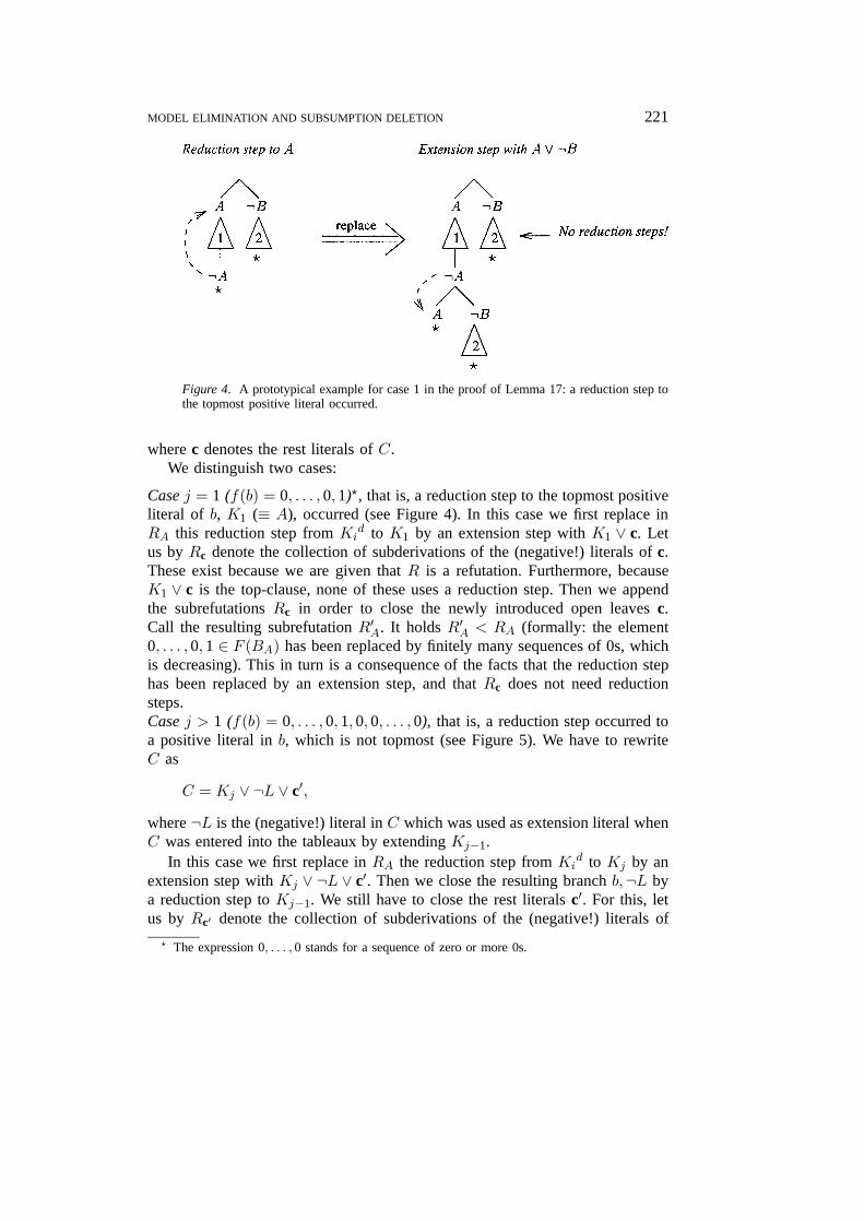
Figure 4. A prototypical example for case 1 in the proof of Lemma 17: a reduction step tothe topmost positive literal occurred.
where c denotes the rest literals of C.We distinguish two cases:
Case j = 1 (f(b) = 0, . . . , 0, 1)?, that is, a reduction step to the topmost positiveliteral of b, K1 (≡ A), occurred (see Figure 4). In this case we first replace inRA this reduction step from Ki
d to K1 by an extension step with K1 ∨ c. Letus by Rc denote the collection of subderivations of the (negative!) literals of c.These exist because we are given that R is a refutation. Furthermore, becauseK1 ∨ c is the top-clause, none of these uses a reduction step. Then we appendthe subrefutations Rc in order to close the newly introduced open leaves c.Call the resulting subrefutation R′A. It holds R′A < RA (formally: the element0, . . . , 0, 1 ∈ F (BA) has been replaced by finitely many sequences of 0s, whichis decreasing). This in turn is a consequence of the facts that the reduction stephas been replaced by an extension step, and that Rc does not need reductionsteps.Case j > 1 (f(b) = 0, . . . , 0, 1, 0, 0, . . . , 0), that is, a reduction step occurred toa positive literal in b, which is not topmost (see Figure 5). We have to rewriteC as
C = Kj ∨ ¬L ∨ c′,
where ¬L is the (negative!) literal in C which was used as extension literal whenC was entered into the tableaux by extending Kj−1.
In this case we first replace in RA the reduction step from Kid to Kj by an
extension step with Kj ∨ ¬L ∨ c′. Then we close the resulting branch b,¬L bya reduction step to Kj−1. We still have to close the rest literals c′. For this, letus by Rc′ denote the collection of subderivations of the (negative!) literals of
? The expression 0, . . . , 0 stands for a sequence of zero or more 0s.
JARSWB1.tex; 15/08/1997; 11:41; v.7; p.17

222 PETER BAUMGARTNER AND STEFAN BRUNING
Figure 5. A prototypical example for case 2 in the proof of lemma 17: a reduction stepoccurred to a positive literal which is not topmost.
c′. These exist because we are given that R is a refutation. Furthermore, anyreduction steps used therein must reduce to a predecessor node of Kj . Next, weappend the subrefutations Rc′ in order to close the newly introduced open leafsc. Call the resulting subrefutation R′A. It holds R′A < RA (formally: the elementf(b) = 0, . . . , 0, 1, 0, 0, . . . , 0 ∈ F (BA) has been replaced by (a) a sequence of0s, stemming from the extension step, and (b) a sequence 0, . . . , 0, 0, 1, 0, . . . , 0 ≺0, . . . , 0, 1, 0, 0, . . . , 0 stemming from the reduction step from ¬L, and (c) bysome sequences stemming from the subrefutationsRc′ , each of them being strictlysmaller w.r.t. ≺ than f(b)).
This concludes the case analysis. Note that in both cases we have obtainedR′A < RA. Let us denote by R′ the refutation that is obtained from R by replacingRA with R′A. It follows, by definition, that R′ < R. Hence we can apply theinduction hypothesis to R′, which concludes the proof of (1).
Ad (2): Having achieved the property (1), (2) is now rather easy. The proof is byinduction on the number N of violations of the blockwise regularity restrictionin a refutation R without reduction steps. If N = 0, we are done; otherwise Rcontains a tableau with open branch b = K1, . . . ,Km which is to be extendedin the course of the refutation to an open branch b′ = K1, . . . ,Km, . . . ,Km.Now, since no reduction steps are applied, we can safely delete from R thesubderivation that leads from b to b′, and use b instead of b′ in the subrefutation
JARSWB1.tex; 15/08/1997; 11:41; v.7; p.18

MODEL ELIMINATION AND SUBSUMPTION DELETION 223
of (the open leaf of) b′. This decreases N by one, and we can apply the inductionhypothesis.
Before we turn to the proof of the main lemma (Lemma 16), we need onemore lemma.
LEMMA 18. Suppose a ground clause set
S = {G, A1, . . . , An ← B1, . . . , Bm} ∪ S ′ (n > 2, m > 0)
is minimal unsatisfiable. Then, for some i, 1 6 i 6 n, the set
Si = {G, A1, . . . , Ai−1, Ai+1, . . . , An ← B1, . . . , Bm} ∪ S ′
is unsatisfiable, and furthermore Si \ {G} is satisfiable.Proof. Clearly, Si is unsatisfiable (for every i), because otherwise a model
for Si would be a model for S.Let I be a model for S \ {G}. Such a model exists because S is minimal
unsatisfiable. It holds that I is a model for A1, . . . , An ← B1, . . . , Bm (becausethis clause is contained in S). We distinguish two cases.
Case 1: I is a model for some Aj (j ∈ {1, . . . , n}). But then, I is a model forA1, . . . , Ai−1, Ai+1, . . . , An ← B1, . . . , Bm, where
i :=
{2 if j = 1,
1 else.
Thus, I is a model for Si \ {G}Case 2: It is not the case that I is a model for some Aj; in other words, Aj isfalse in I for all j = 1, . . . , n. Since I is a model for A1, . . . , An ← B1, . . . , Bm,it must be that I is a model for some body literal Bk. But then, I is a modelfor, say, A1, . . . , An−1 ← B1, . . . , Bm; that is, we set i := n. Thus, also in thiscase we have that I is a model for Si \ {G}.
Now for the general case.
Proof of Lemma 16. Some terminology is introduced. If we speak of ‘replac-ing a clause C in a derivation by a clause C ∨D,’ we mean the derivation thatresults when using the clause C ∨D in place of C in extension steps. Also, ifL ∈ C is used as extension literal, then L must be used as extension literal inC ∨D as well.
By a ‘derivation of a clause C’ we mean a derivation that generates a tableauwith frontier C.
Let k(S) denote the number of occurrences of positive literals in S minus thenumber of definite clauses in S (k(S) is related to the well-known excess literal
JARSWB1.tex; 15/08/1997; 11:41; v.7; p.19
224 PETER BAUMGARTNER AND STEFAN BRUNING
parameter). Below, we shall make use of the obvious fact that S ′ ⊂ S impliesk(S ′) 6 k(S).
Now we prove the claim by induction on k(S).
Induction start (k(S) = 0): S must be a set of Horn clauses. Apply Lemma 17.
Induction step (k(S) > 0): As the induction hypothesis, suppose the result tohold for minimal unsatisfiable ground clause sets S ′ with k(S ′) < k(S).
Since k(S) > 0, S must contain a disjunctive clause
D = A1, . . . , An ← B1, . . . , Bm
with n > 2. If several such disjunctive clauses exist, select for D one that isdifferent from G. We distinguish two cases.
Case 1. G ≡ D; that is, the selected disjunctive clause is the desired top-clause(and S \ {G} is a Horn clause set due to the mentioned preference in selectingD).
D′ = A1, . . . , An−1 ← B1, . . . , Bm.
Clearly, SD′ := (S \ {D}) ∪ {D′} is unsatisfiable (because otherwise, a modelfor SD′ would be a model for S). Furthermore, SD′ \{D′} is satisfiable, becauseotherwise S would not be minimal unsatisfiable. Hence, if we select a minimalunsatisfiable subset S ′D′ ⊆ SD′ it must be that D′ ∈ S ′D′ .
With k(S ′D′) 6 k(SD′) = k(S) − 1 < k(S), we can apply the inductionhypothesis to S ′D′ and obtain a refutation RD′ of S ′D′ (and thus also of SD′) withtop clause D′.
Let SAn := (S \ {D}) ∪ {An}. By the same line of reasoning as for SD′we can find a minimal unsatisfiable subset S ′An ⊆ SAn , and it must be thatAn ∈ S ′An . Similarly, k(S ′An) 6 k(SAn) = k(S) − (n− 1) < k(S), and we canapply the induction hypothesis to S ′An and obtain a refutation RAn of S ′An (andthus also of SAn) with top clause An.
Now replace in RD′ every occurrence of the clause D′ by D. This gives usa derivation RD from the input set S. RD is a derivation of, say, k occurrencesof the disjunctive positive literal An.
Now append k times the refutation RAn to RD in order to obtain subrefuta-tions for every occurrence of An in the tableau generated by RD. Call this newrefutation R. Since RAn might possibly contain extension steps with An, R is arefutation of S ∪ {An}. In order to turn R into a refutation of S alone, replaceevery extension step with An in the appended refutations RAn by a reductionstep to An. This is possible because An is the top-clause in RAn and hence canbe accessed. Further, these reduction steps are in accordance with the disjunctivepositive refinement, because An stems from a disjunctive positive clause. Theresulting refutation is a desired disjunctive positive ME refutation of S. Further-more, since RD′ and RAn can be assumed by the induction hypothesis to be
JARSWB1.tex; 15/08/1997; 11:41; v.7; p.20

MODEL ELIMINATION AND SUBSUMPTION DELETION 225
blockwise regular, and the construction of the final refutation keeps the blockstructure of its constituents, the final refutation must be blockwise regular, too.
Case 2:G 6≡ D; that is, the selected non-Horn clause is different from the desiredtop-clause. According to Lemma 18 there exists an appropriate literal Ai (1 6i 6 n) to be deleted from D. More formally, we can define
Di = A1, . . . , Ai−1, Ai+1, . . . , An ← B1, . . . , Bm
in such a way that SDi := (S \ {D}) ∪ {Di} is unsatisfiable and SDi \ {G}is satisfiable. Further, as for SD′ above, SDi is unsatisfiable and SDi \ {Di} issatisfiable. Hence, if we select a minimal unsatisfiable subset S ′Di ⊆ SDi it mustbe that G ∈ S ′Di and Di ∈ S ′Di .
With k(S ′Di) 6 k(SDi) = k(S) − 1 < k(S), we can apply the inductionhypothesis to S ′Di and obtain a refutation RDi of S ′Di (and thus also of SDi)with top clause G.
Let SAi := (S \ {D}) ∪ {Ai}. As in the previous case for An, there exists arefutation RAi of S ′Ai with top clause Ai, where S ′Ai is defined analogously toS ′An above.
The rest of the proof is literally the same as for the previous case, except thatD′ is replaced by Di and An is replaced by Ai.
3.4. A NONOBVIOUS REFINEMENT
We turn to a further strengthening of the disjunctive positive refinement, whichcame to our attention by a reviewer’s conjecture. This concerns the possibility tofurther restrict the necessary ancestor context to all but one disjunctive positiveliterals of a clause.
The advantages of such a result are twofold: first, it reduces without anychange to the Horn case, where reduction steps are unnecessary. Second, the sub-sumption relation among tableaux (see the next section) can further be extended.Clearly, there is tradeoff in using the restriction, as refutations tend to get longer.This tradeoff should be evaluated theoretically and/or empirically. This is notsubject of the present paper; instead we shall derive a completeness result only.
We first modify the framework now and then prove the completeness.
DEFINITION 19 (Labeling rule for disjunctive clauses). A labeling rule l is amapping assigning to every disjunctive clause D = (A1, . . . , An ← B1, . . . , Bm)a multiset
l(D) = {|A1, . . . , Ai−1, Ai+i, . . . , An|} for some i, 1 6 i 6 n.
The literal Ai is called discarded from D (by l) , and l(D) is also called themultiset of literals selected in D (by l). We require any labeling rule to be stableunder instantiation?; in other words, l(Dσ) = (l(D))σ for any substitution σ.? This property is needed for lifting purposes; it guarantees that the labeling restriction for
ground clauses has a counterpart on the first-order level.
JARSWB1.tex; 15/08/1997; 11:41; v.7; p.21
226 PETER BAUMGARTNER AND STEFAN BRUNING
We usually attach a ‘+’ mark to all but one positive literals in disjunctiveclauses in order to indicate the labeling rule in effect, as in A+
1 , A2, A+3 ← B.
Definition 12 on labeling nodes with a ‘+’ is changed in the following way: anode Ni in tableau T is labeled as N+
i iff its tableau literal L(Ni, T ) is positiveand stems from a respectively labeled input clause, that is, iff L(Ni, T ) = Ajσfor some substitution σ and input clause A1, . . . , An ← B1, . . . , Bm with Aj ∈l(A1, . . . , An ← B1, . . . , Bm).
The calculus restricted disjunctive positive refinement of model elimination(RDPME) consists of the same inference rules as DPME (Definition 13), howeverwith the labeling of positive literals carried out according to some given labelingrule as just defined.
Note that RDPME is strictly weaker than DPME (i.e., any RDPME derivationis also a DPME refutation, but not necessarily vice versa), because in RDPME noteach positive literal of a disjunctive clause can potentially be used for reductionsteps.
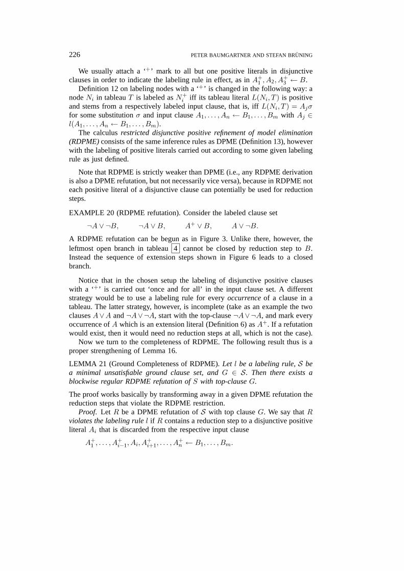
EXAMPLE 20 (RDPME refutation). Consider the labeled clause set
¬A ∨ ¬B, ¬A ∨B, A+ ∨B, A ∨ ¬B.A RDPME refutation can be begun as in Figure 3. Unlike there, however, theleftmost open branch in tableau 4 cannot be closed by reduction step to B.Instead the sequence of extension steps shown in Figure 6 leads to a closedbranch.
Notice that in the chosen setup the labeling of disjunctive positive clauseswith a ‘+’ is carried out ‘once and for all’ in the input clause set. A differentstrategy would be to use a labeling rule for every occurrence of a clause in atableau. The latter strategy, however, is incomplete (take as an example the twoclauses A∨A and ¬A∨¬A, start with the top-clause ¬A∨¬A, and mark everyoccurrence of A which is an extension literal (Definition 6) as A+. If a refutationwould exist, then it would need no reduction steps at all, which is not the case).
Now we turn to the completeness of RDPME. The following result thus is aproper strengthening of Lemma 16.
LEMMA 21 (Ground Completeness of RDPME). Let l be a labeling rule, S bea minimal unsatisfiable ground clause set, and G ∈ S. Then there exists ablockwise regular RDPME refutation of S with top-clause G.
The proof works basically by transforming away in a given DPME refutation thereduction steps that violate the RDPME restriction.
Proof. Let R be a DPME refutation of S with top clause G. We say that Rviolates the labeling rule l if R contains a reduction step to a disjunctive positiveliteral Ai that is discarded from the respective input clause
A+1 , . . . , A
+i−1, Ai, A
+i+1, . . . , A
+n ← B1, . . . , Bm.
JARSWB1.tex; 15/08/1997; 11:41; v.7; p.22

MODEL ELIMINATION AND SUBSUMPTION DELETION 227
Figure 6. Continuing the derivation in Figure 3 in the RDPME setup. Tableau 7 can becontinued to a refutation (but not the shortest possible one).
Let NR be the total number of violations of the labeling rule l in R.The proof is by well-founded induction on pairs (k(S),NR), compared lex-
icographically, where k(S) is as in the proof of Lemma 16), and NR refers tosome refutation R of S with top clause G (such a refutation exists by Lemma 16).
Induction start 1, k(S) = 0: S must be a set of Horn clauses. By Lemma 17 noreduction steps are carried out, which trivially coincides with the reduction stepsrestrictions of RDPME.
Induction start 2, NR = 0: Also trivial, NR = 0 means nothing but that R is inaccordance with the restrictions of RDPME.
Induction step, k(S) > 0 and NR > 0: As the induction hypothesis, suppose theresult to hold for minimal unsatisfiable ground clause sets S ′, admitting DPMErefutation R′, such that (k(S ′),NR′) < (k(S),NR).
Let R be a DPME refutation of S with top-clause G. Since NR > 0, thereexists an input clause
D = (A+1 , . . . , A
+i−1, Ai, A
+i+1, . . . , A
+n ← B1, . . . , Bm)
for some i (1 6 i 6 n),
JARSWB1.tex; 15/08/1997; 11:41; v.7; p.23

228 PETER BAUMGARTNER AND STEFAN BRUNING
with n > 2 such that R contains a reduction step to Ai, thus violating the labelingrestriction. Without loss of generality assume that i = 2 (this makes the indexhandling a bit simpler). Define
DA1 = A1,
DA2 = (A2, A+3 , . . . , A
+n ← B1, . . . , Bm)
and the unsatisfiable sets
SA1 = (S \ {D}) ∪ {DA1},SA2 = (S \ {D}) ∪ {DA2}.
Since S is minimal unsatisfiable, every minimal unsatisfiable subset of SAj(j ∈ {1, 2}) contains DAj . Since k(SAj ) < k(S), there exists by the inductionhypothesis a RDPME refutation RAj of SAj with top-clause DAj . Notice thatby the induction hypothesis no reduction step in RA2 to A2 can occur, becauseA2 is discarded from D by l (since S is minimal unsatisfiable, S cannot containthe clause DA2 , and hence the extension of the labeling rule l to the clause DA2
can be done as suggested).Now replace in RA2 the initialization step and every extension step with DA2
by a corresponding one with D; i.e., add back A1 to DA2 . This gives a derivationfrom S of, say, p branches with open goal A+
1 . Each of these can be closed byappending the refutation RA1 p times. Finally, in order to turn this refutationof S ∪ {A1} into a refutation of S alone, every extension step with unit clauseA1 carried out in one of the appended refutations RA1 has to be replaced by areduction step to A+
1 . Let R′ be the resulting refutation.Next, delete from R′ the subrefutation below the top-literal A2, and let R′′
be the resulting derivation with single open goal A2.Now recall that R contains a reduction step to A2 violating the labeling rule.
The reduction step must clearly be carried from a leaf labeled with ¬A2. Hencewe can delete this reduction step and append the derivation R′′ instead, wherethe initialization step in R′′ is replaced by an extension step with D and literalA2 as extension literal.
By this, a refutation, say R′′′, of S results that contains at least one lessviolation of the labeling rule than R. In other words, (k(S),NR′′′ ) < (k(S),NR)and we can apply the induction hypothesis, which gives us the desired RDPMErefutation.
As the construction in the proof shows, we potentially need reduction stepsto all positive unit clauses temporarily split off in the induction step. RDPMEcannot be strengthened in a straightforward way toward discarding more than oneliteral in disjunctive clauses for reduction steps. The canonical counterexampleto such a strengthening consists of the clauses
¬A, ¬B ∨ ¬B, ¬C ∨ ¬C, A+ ∨B ∨ C.
JARSWB1.tex; 15/08/1997; 11:41; v.7; p.24

MODEL ELIMINATION AND SUBSUMPTION DELETION 229
Notice that in the last clause only one positive literal is labeled. Although unsat-isfiable, there exists no RDPME refutation with, say, top-clause ¬A. From theviewpoint of the previous proof, the transformation given there runs into a circle.
4. Backward and Forward Subsumption for Model Elimination
In this section we shall refine ME in such a way that it can take advantage ofthe subsumption deletion techniques that have been applied so successfully inthe resolution paradigm.
As described in the introduction, it is crucial in the ME case to define thesubsumption relation among tableaux in such a way that as few ancestor literalsas possible have to be considered. To assure that subsumption deletion based onsuch a subsumption relation is complete, a version of ME has to be used thatis complete when reduction steps are restricted to just that considered ancestorcontext. To this end, we defined in Section 3 the ‘disjunctive positive refinement’of ME.
We shall consider both forward subsumption and backward subsumption. Ata superficial level one might think that both of them are quite similar and easilyincorporated into any reasonable calculus. While this might be true for resolutionsystems, it is not for ME, at least if the ‘usual’ definition of refutation is used.Let us explain this now in more detail.
It is more straightforward to incorporate into ME a concept of forward sub-sumption than backward subsumption. For forward subsumption, the definitionof ‘derivation’ (Definition 8) can be extended to forbid the derivation of a tableauT if some prefix of this derivation generates a tableau T ′ that subsumes T (w.r.t.some subsumption relation to be defined). Such an approach has already beenconsidered in (Loveland, 1978).
Usually,? derivations are constructed in ME proof procedures by nondeter-ministically guessing the inference steps and backtracking on failure. Forwardsubsumption is straightforwardly incorporated into such a regime by setting upa failure in case a forward subsumption applies. However, this requires storingtableaux explicitly – which is usually not done, for instance, in SETHEO andPTTP-based procedures.
Now, backward subsumption is dual to forward subsumption. A first attemptto define backward subsumption within the given framework is to say that tableauT backward subsumes a tableau T ′ in a derivation D iff T (strictly) subsumes T ′
and T ′ was generated in D prior to T . The information that can be gained froma concrete backward subsumption case can be expressed as follows: ‘if T cannotbe extended to a refutation, then also T ′ cannot be extended to a refutation’. Interms of a proof procedure, this means that failure to prove T should immediatelybacktrack to the tableau before T ′ and explore an alternative to T ′. In addition
? For instance, in SETHEO and the whole class of PTTP theorem provers.
JARSWB1.tex; 15/08/1997; 11:41; v.7; p.25

230 PETER BAUMGARTNER AND STEFAN BRUNING
to explicitly store tableaux, this requires manipulating the backtracking schemein depth.
We shall not elaborate on the practicability of such an approach. Insteadwe shall return to the calculus level and propose a new notion of derivationwthich supports our needs. More precisely, instead of guessing the ‘next’ tableauwe shall explicitly generate all possible successor tableaux. By this we changeME from an enumeration procedure of derivations into a saturation procedurefor formulas. This is the approach of resolution, and, as there, it allows us toconveniently express backward subsumption as a simple deletion operation.
A general subsumption concept that is related to ours is defined in (Letz etal., 1994). As we do, they consider explicitly generated tableaux. Unlike ourapproach, which enumerates these tableaux sequentially, they generate AND/OR
search trees whose nodes are labeled with tableaux. They define a notion ofsubsumption deletion that allows one to give up a tableau if it is (not necessarilystrictly) subsumed by a competitive tableau in the search tree. Our approachdiffers from that w.r.t. the following aspects, First, they do not restrict the ancestorcontext for the subsumption test; they even do not consider permutations for this.Thus, subsumption will apply only rarely. Second, as they themselves note, theirapproach is incomplete. Our work can be seen to solve open issues in their workby identifying several technicalities needed to obtain a complete calculus. In ourterminology, their calculus is incomplete at least for the reason that they do notuse the strict version of the subsumption test for backward subsumption.
4.1. DEFINITION OF MODEL ELIMINATION WITH SUBSUMPTION
DEFINITION 22 (Subsumption). Let T be a tableau and b = N1, . . . ,Nn be abranch of T . Define the disjunctive positive ancestor context of b, anc+(b), as
anc+(b) = {|Li | Ni is a disjunctive positive node, labeled with Li,i = 1, . . . , n|}.
Thus we simply collect the disjunctive positive literals.Let b1 and b2 be branches of tableaux T1 and T2, respectively. We say that b1
is an ancestor extension of b2, b1 > b2, iff
leaf(b1) = leaf(b2) and anc+(b1) ⊇ anc+(b2).
In words, b1 is an ancestor extension of b2 iff the leaves are equal and b1 has atleast the disjunctive positive ancestor context of b2.
Extending to branch sets, we say that a branch set B1 is an ancestor extensionof a branch set B2, B1 > B2, iff there exists a bijective function f from B1 intoB2 such that b > f(b) for every b ∈ B1. Thus, in particular, subsumption isbased on comparing multisets of goal literals.
We intend to generalize to tableaux. In the sequel let T, T1, T2 denote tableaux,and let δ denote a substitution.
JARSWB1.tex; 15/08/1997; 11:41; v.7; p.26

MODEL ELIMINATION AND SUBSUMPTION DELETION 231
We say that T1 is more general by δ than T2 iff? OB(T1δ) > OB(T2); T1 ismore general than T2 iff T1 is more general than T2 by some substitution δ. Notethat this relation is reflexive and transitive, but not antisymmetric, and hence apreorder.
We say that T1 strictly δ-subsumes T2, T1 �δ T2 iff OB(T1δ) > B2 for somesubset B2 ⊂ OB(T2). Furthermore, T1 strictly subsumes T2, T1 � T2, iff thereexists a substitution δ such that T1 �δ T2. In words, T1 strictly subsumes T2 if bysome substitution the open branches of T1 are an ancestor extension of some ofthe open branches of T2. We note that as a consequence of the well-foundednessof strict multiset inclusion, strict subsumption is also well founded.
Finally, we say that T1 subsumes T2, T1 � T2, iff T1 � T2 or T1 is moregeneral than T2. Note that this is a slight abuse of notation, since the ‘moregeneral’ relation is not an equivalence relation, not even if no substitutions areinvolved.
EXAMPLE 23. Figure 7 depicts some tableaux and subsumption relations amongthem.
Tableaux 1 strictly subsumes tableaux 2 (and hence also subsumes) by virtue of the
empty substitution ε because the branch (q(x), p(x))ε in 1 is an ancestor extension of
the branch p(x) in 2 . Tableau 2 subsumes (but not strictly subsumes) 3 by means
of the substitution {x← f(x)}. Notice that the positive ancestor literal p(x) in tableau
3 is irrelevant for subsumption, because it does not stem from a disjunctive clause.
Tableau 3 does not subsume tableau 4 because of the disjunctive positive ancestor
context in tableau 4 ; neither does 4 subsume 3 (because of the extra literal r(x)
in 4 ).
Figure 7. Subsumption relations among some tableaux.
DEFINITION 24 (Model Elimination with Subsumption (MES)). Let r be a com-putation rule. For brevity of notation we define T `Infer,r T
′ iff the tableau T ′
can be obtained from the tableau T by one single application of one of the infer-ence rule extension step or reduction step of the disjunctive positive refinement(Definition 13) to the goal node selected by r in T .
We define the binary relations ‘`Infer,r’ and ‘`Delete’ on sets of tableaux asfollows: S `Infer,r S
′ (resp. S `Delete S′) if S′ is obtained from S by one single
? Recall that OB(T ) denotes the set of open branches in T (see Definition 3).
JARSWB1.tex; 15/08/1997; 11:41; v.7; p.27

232 PETER BAUMGARTNER AND STEFAN BRUNING
application of the following respective inference rules (also called derivationrules from now on).
Infer:S ∪ {T}
S ∪ {T, T ′} {If T `Infer,r T′,
Delete:S ∪ {T, T ′}S ∪ {T} {If T � T ′.
The calculus forward and backward subsumption ME (MES) consists of thederivation rules Infer and Delete; the calculus forward subsumption ME consistsof the derivation rule Infer only.
A derivation (w.r.t. one of these calculi) for a clause set S, top-clause setG ⊆ S and computation rule r is a sequence
S = (S0, S1, . . . , Sn, . . .)
of sets of tableaux of S, where
1. S0 = {TG | G ∈ G, TG is an initial tableau for G}, and2. for i > 0, either Si−1 `Infer,r Si or Si−1 `Delete Si (‘backward subsumption’ –
only for the forward and backward variant).
Finally, a refutation of a clause set S is a derivation for S such that one of itselements contains a closed tableau.
In words: beginning with a set of initial tableaux, we generate new tableaux bymeans of the traditional inference rules, and we also allow to delete a previouslyderived tableau, provided that it is strictly subsumed in the current proof state. Bythis backward subsumption deletion we avoid further exploration of the subsumedtableau. It is important to use the strict version of subsumption here in order toavoid infinite loops. Forward subsumption is covered by a certain property offair derivations (see Definition 25 below). Informally, it says that a tableau neednot be generated in presence of a subsuming tableau.
In the traditional definition of derivation (Definition 8) the transition fromone tableau to the next can be thought of as a nondeterministic guess. In the newframework we shall use a fairness condition instead. Roughly, fairness means thatno application of an Infer derivation rule is deferred infinitely long. Fairness isimportant because it entails that ‘enough’ tableaux will be generated; in particular,a closed tableau will be generated after finitely many steps for unsatisfiable clausesets.
Our definition of fairness is an adaptation of standard definitions in the term-rewriting literature (see, e.g., (Bachmair, 1991)).
DEFINITION 25 (Limit, Fairness). Let S = (S0, S1, . . . , Sn, . . .) be a derivationfor some clause set S. The limit of S is defined as
S∞ :=⋃
(i>0)
⋂(j>i)
Sj .
JARSWB1.tex; 15/08/1997; 11:41; v.7; p.28

MODEL ELIMINATION AND SUBSUMPTION DELETION 233
The elements of S∞ are also called the persisting tableaux of S.The derivation S is called fair iff S is a refutation or else, whenever S∞ `Infer,r
S∞ ∪ {T ′}, then for some k > 0 and some T ∈ Sk we have T � T ′.
The first item in (Definition 24) guarantees in conjunction with fairness thatevery clause given from the goal set G is tried as a top clause; when instantiatedwith all negative clauses from S, this corresponds to the result for ‘traditional’ME, which states that if a refutation exists at all, then also a refutation withnegative clause as top-clause exists.
The fairness condition, proper, means that it is sufficient to generate a newtableau from the persisting tableaux? only if it is not subsumed in some stageof the derivation (provided S is not a refutation). Since this case includes thepossibility of discarding a tableau in favor of a subsuming previously derivedtableau, we have a case of forward subsumption. Note further that we need notinsist on strict subsumption here.
The presence of a computation rule is most important in the fairness condition.It is sufficient to consider inferences to the selected branch only, but not to allbranches of a tableau.
Our notion of fairness enables the use of a ‘delete as many tableaux as pos-sible’ strategy in implementations, since a tableau once shown to be subsumedwill be subsumed in all subsequent stages and thus need not persist.
EXAMPLE 26. (1) Consider the clause set
(1) p(a) ← p(y)
(2) p(a) ← r(z)
(3) r(c) ←(4) ← p(x), q(x).
Suppose a computation rule that selects the bottommost leftmost goal. It follows afair derivation for the top-clause (4). Since this example is Horn and all ancestorliterals are negative and thus irrelevant, it suffices to depict the frontiers of thetableaux as clauses instead of the tableaux themselves. For instance, for thetableaux 2 in Figure 2 we would write B ∨¬B. The clause sets in parenthesesneed not be built as the generated tableau in these steps are subsumed. Theselected literal in each step is underlined.
S0 = {¬p(x) ∨ ¬q(x)} Initial tableau with (4),
S1 = {¬p(x) ∨ ¬q(x),¬p(y) ∨ ¬q(a)} By extension with (1),
(S2 = {¬p(x) ∨ ¬q(x),¬p(y) ∨ ¬q(a),¬p(y) ∨ ¬q(a)}) By extension with (1),
? Informally, these are the tableaux generated eventually and never deleted afterwards.
JARSWB1.tex; 15/08/1997; 11:41; v.7; p.29

234 PETER BAUMGARTNER AND STEFAN BRUNING
S2 = {¬p(x) ∨ ¬q(x),¬p(y) ∨ ¬q(a),¬r(z) ∨ ¬q(a)} By extension with (2),
S3 = {¬p(x) ∨ ¬q(x),¬p(y) ∨ ¬q(a),¬q(a)} By extension with (3),
S4 = {¬p(x) ∨ ¬q(x),
¬q(a)} By deletion of ¬p(y) ∨ ¬q(a),
(S5 = {¬p(x) ∨ ¬q(x),¬q(a),¬p(y) ∨ ¬q(a)}) By extension with (1). Unnecessary, because
the new tableau is subsumed by ¬p(y) ∨¬q(a) ∈ S1,
(S5 = {¬p(x) ∨ ¬q(x),¬q(a),¬r(z) ∨ ¬q(a)}) By extension with (2). Unnecessary, because
the new tableau is subsumed by ¬r(z) ∨¬q(a) ∈ S2.
Thus, the derivation is finite and ends in S4.
(2) Consider the clause set
(1) x = x ←(2) y = x ← x = y(3) x = z ← x = y, y = z(4) f(x) = f(y) ← x = y(5) p(x, y) ← x = x′, p(x′, y)(6) p(x, y) ← y = y′, p(x, y′)
(7) ← x = f(y), p(z, y).
Of course, clauses (1)–(6) are an axiom set for the theory of equality in thepresence of a predicate symbol p and a function symbol f . Certainly, there arebetter ways to handle equality, but this example should indicate that part of theimprovements achieved for inference rules for equality, notably paramodulation(Robinson and Wos, 1969), can be obtained as instances of subsumption.
When started with the top-clause (7) and equipped with the same computationrule as above, our subsumption prover stops after six inferences and (correct-ly) reports failure, while other ME provers (PROTEIN – a PTTP prover, andSETHEO, Version 3.3) loop on this example.
The MES derivation starts with the initial tableau? ¬(x = f(y)) ∨ ¬p(z, y)for (7). The key inference is the extension of ¬(x = f(y)) ∨ ¬p(z, y) with? Again, since we deal with a Horn example, we identify a tableau with its frontier.
JARSWB1.tex; 15/08/1997; 11:41; v.7; p.30

MODEL ELIMINATION AND SUBSUMPTION DELETION 235
the reflexivity clause (1), giving the tableau ¬p(z, y). As a result of fairness,this inference must be carried out eventually, and the resulting tableau ¬p(z, y)subsumes the initial tableau and all other tableaux generated from it (except¬p(z, y), of course). Hence the derivation is finite. More generally, such anargumentation is applicable in situations where resolving X = X against aclause of the form ¬(s = t) ∨R does not alter R.
Subsumption is a concept strong enough to to generalize some well-known refine-ments of ME. For instance, blockwise regularity is covered? by forward andbackward subsumption in the case of a local computation rule (see Theorem 41below).
Another well-known refinement of ME is factorization (Loveland, 1978). Thefactorization inference rule allows one to close a branch b iff leaf(b) is identicalto a left sibling node of some ancestor node of leaf(b). It is allowed to applysome (most general) substitution to achieve this condition. An important specialcase is that the two literals in question are identical without application of asubstitution.?? In ME proof procedures, a folklore-like heuristics (already usedin (Stickel, 1988)) allows in this case to close the branch b without need forbacktracking. Backward subsumption explains why this step is correct: supposea tableau T ′ is obtained from a tableau T by factorization with empty substitution.Then it is easy to see that T ′ � T . Hence, T can be deleted in a fair derivationwithout affecting completeness; this corresponds to nonbacktracking over thisinference step in backtracking procedures.
4.2. SOUNDNESS AND COMPLETENESS
Since ordinary ME is sound, the disjunctive positive refinement of the precedingsection must be sound, too (because the latter case is more restricted). But then,MES must be sound, too, because it is more restricted (i.e., whenever a tableaucan be constructed in MES, it can also be constructed in the disjunctive positiverefinement). Altogether, this sketch convinces us of the soundness of the calculus.Thus, we now turn to completeness.
Completeness reads as follows.
THEOREM 27 (Completeness). Let r be a computation rule. Let S be an unsat-isfiable clause set, and let
S = (S0, S1, . . . , Sn, . . .)
be a fair MES derivation for S with top-clause set G, where G is the set ofnegative clauses from S. Then for some q > 0, Sq contains a closed tableau; inother words, S is a refutation.? We say that a refinement R1 covers another refinement R2 iff in each case where R2 can be
applied, R1 can be applied, too.?? This option is included in Loveland’s original definition of ME (Loveland, 1978).
JARSWB1.tex; 15/08/1997; 11:41; v.7; p.31

236 PETER BAUMGARTNER AND STEFAN BRUNING
Before we can prove this theorem, we find it helpful to introduce some nota-tion and lemmas. Unless otherwise noted, for the rest of this section we shallrefer to the disjunctive positive refinement of ME (Definition 13), and r willalways denote a given computation rule.
Let D = d0, . . . , dm be a derivation via r, generating a tableau Tn. We call Dpromising iff D can be extended to a refutation, that is, iff a refutation d0, . . . , dm,dm+1, . . . , dn via r exists, for some n > m. In this case we shall restrict allpossible refutations to those of minimal length. Hence, suppose without loss ofgenerality n to be minimal, and define steps(D) := n−m as the minimal numberof inference steps necessary to extend D to a refutation; obviously, steps(D) = 0iff D is a refutation. The value steps(D) will be of central importance below,since it is the measure to be decreased in the induction step. It is important thatsteps(D) not depend on the computation rule r. Indeed, this independence is aconsequence of the proof of the independence of the computation rule. For thisproof (see (Baumgartner, 1994)) one needs only to switch inference steps of agiven derivations, but never to delete or add some.
The previous definitions are also applicable to Tm, and in this case it is under-stood that Tm is generated by some appropriate derivation that is left implicit.
Now, let S be a set of tableaux and T be a tableau. We say that S is minimalfor T iff T is promising and for every promising tableau T ′ ∈ S we havesteps(T ) 6 steps(T ′). Note that according to this definition, T ∈ S does notnecessarily hold.
We start with two lemmas.
LEMMA 28. Let T ′ be a promising tableau, and let D be a derivation generatinga tableau T that is more general than T ′. Then T is promising, and furthermoresteps(T ) 6 steps(T ′).
Proof. In the sequel, we use the term ‘subrefutation of a tableau T ’ to meanthe concatenation of the subrefutations of the nodes of the frontier of T .
We are given that T ′ is promising, which means that there exists a subrefu-tation of T ′.
By definition of ‘more general’ we find a substitution δ such that for everyopen branch in T ′ there is exactly one open branch in Tδ (and these are all theopen branches of Tδ). Furthermore, two corresponding branches b ∈ Tδ andb′ ∈ T ′ have the same leaf literals, and anc+(b) ⊇ anc+(b′). Hence, the existingsubrefutation of the leaf of b′ can also be applied to the leaf of b. If this is donefor every such branch b′ ∈ T ′, we finally arrive at a subrefutation of Tδ, and itholds steps(Tδ) = steps(T ′). However, since anc+(b) ⊃ anc+(b′) might holdin some cases, reduction steps could be enabled in the refutation of Tδ that haveno counterpart in T ′. Hence, even steps(Tδ) < steps(T ′) is possible.
We have to show the claim for T , but not for Tδ. We can do so by lifting thesubrefutation of Tδ to a subrefutation of T . For this we need a lifting theoremfor ME derivations. There exist several such results; the lifting theorem needed
JARSWB1.tex; 15/08/1997; 11:41; v.7; p.32

MODEL ELIMINATION AND SUBSUMPTION DELETION 237
in our case can be proven with methods developed in (Baumgartner et al., 1995).Notably, lifting does not change the number of inference steps that gives ussteps(T ) 6 steps(T ′).
LEMMA 29. Let T ′ be a promising open tableau, and let D be a derivationgenerating a tableau T with T � T ′. Then T is promising, and furthermoresteps(T ) < steps(T ′).
Proof. The proof is very similar to that of the preceding lemma. The majordifference is that we now have a one-to-one correspondence between the openbranches B of Tδ and a strict subset B′ of the open branches of T ′. Thus, we canapply the subrefutations of the leafs of the branches of B′ to their correspondingbranches B. This process gives us a subrefutation of Tδ. Again using a liftingtheorem. we obtain a subrefutation of T with the same number of inference steps.Since T ′ contains strictly more open branches than T , the subrefutation of T ′
needs strictly more inference steps than that of T , or, equivalently, steps(T ) <steps(T ′).
The next lemma is central.
LEMMA 30. Let S = (S0, S1, . . . , Sn, . . .) be a fair derivation that is not arefutation (i.e., the empty tableau is never generated). If Sk is minimal for Tkand steps(Tk) > 0, there exists an index l > 0 and a tableau Tl ∈ Sl such thatSl is minimal for Tl and steps(Tl) < steps(Tk).
Proof. By definition of minimality, Tk is promising. Since steps(Tk) > 0 atleast one inference step has to be applied to extend Tk to a refutation. Let
Tk `Infer T′ (1)
be such an inference step. It holds steps(T ′) = steps(Tk)− 1 < steps(Tk) (*).Now we distinguish two cases:
1. Tk ∈⋃
(i>k)
⋂(j>i) Sj . That is, Tk is generated at some point > k and then
never deleted afterwards. But then also
Tk ∈⋃
(i>0)
⋂(j>i)
Sj (= S∞)
because this is a superset. From this and Equation 1 it follows S∞ `Infer,rS∞∪{T ′}. But then, by fairness, there exists an index l > 0 and tableau T ∈ Slsuch that (a) T � T ′ or (b) T is more general than T ′. In case (a), if T is closedwe have steps(T ) = 0 (< steps(Tk)) or otherwise T is open. But then, byLemma 29, T can be extended to a refutation such that steps(T ) < steps(T ′),and together with (*) above we conclude steps(T ) < steps(Tk). In case (b) weapply Lemma 28 and conclude that T can be extended to a refutation such thatsteps(T ) 6 steps(T ′), which also gives us steps(T ) < steps(Tk).
JARSWB1.tex; 15/08/1997; 11:41; v.7; p.33

238 PETER BAUMGARTNER AND STEFAN BRUNING
2. Tk /∈ ⋃(i>k)
⋂(j>i) Sj . That is, for some l > k + 1 we have Tk ∈ Sl−1 and
Tk /∈ Sl. In other words, Tk is deleted. This step can be done only by backwardsubsumption pruning, i.e.
(Sl−1 =) Sl ∪ {Tk} `Delete Sl.
By definition of Delete there exists a tableau T ∈ Sl with T � Tk. By Lem-ma 29, T can be extended to a refutation such that steps(T ) < steps(Tk). Thisconcludes the second case.
Now, in both cases, we have shown that there exists a tableau T ∈ Sl suchthat steps(T ) < steps(Tk). Either Sl is already minimal for T (and in this casedefine Tl := T ), or otherwise Sl is minimal for some different Tl ∈ Sl (and inthis case even steps(Tl) < steps(T ) holds). Thus, in any case we can find atableau Tl as claimed.
Now we can proof our main theorem.
Proof of Theorem 27. By the completeness theorem for the disjunctive posi-tive refinement (Theorem 15) there exists a refutation of S with some negativeclause G ∈ S as top-clause. Without loss of generality assume that among allnegative clauses for which a refutation exists, G is chosen minimal w.r.t. thelength of the shortest possible refutation.
We are given that the top-clause set G used for S consists of all negativeclauses from S. Hence, by the definition of derivation, TG ∈ S0, where TG is aninitial tableau for G. Further, by the choice of G we have in present terminologythat TG is promising, TG > 0, and S0 is minimal for TG.
Now suppose, to the contrary of the theorem, that S is not a refutation. Butthen, by repeatedly applying Lemma 30, starting with S0 and T0 = TG, we canfind an infinite chain steps(T0) > steps(T1) > · · · > steps(Tn) > · · · > 0,which is impossible. Hence, S is the refutation as claimed.
5. A Context Check for Model Elimination
An interesting alternative to the techniques presented in the preceding sectionare so-called context checks, which were originally proposed in (Besnard, 1989)and further developed in (Bol et al., 1991) in the context of SLD-resolution.Context checks are based on forward subsumption; but instead of comparing twomultisets of open goals, the idea is to prune a derivation if a subrefutation foronly one open goal would constitute a subrefutation for one of its ancestor goals.Hence, such pruning techniques can be interpreted as loop-checking mechanisms.
Clearly, in order to prune a derivation, one cannot concentrate on one opengoal and its ancestors. Additionally, variable dependencies with other open goalshave to be taken into account.
JARSWB1.tex; 15/08/1997; 11:41; v.7; p.34

MODEL ELIMINATION AND SUBSUMPTION DELETION 239
Figure 8. Tableaux for Example 31.
EXAMPLE 31. For illustration, consider the following clause set.
(1) r(a) ←(2) p(f 5(b)), q(a) ←(3) p(z) ← p(f(z))(4) q(a) ← p(y)(5) ← q(x), r(x).
The task is to find an ME refutation of the (non-Horn) clause set with top-clause(5). After an initialization and one extension step with clause (4), we get thetableau depicted in Figure 8 on the left. One further extension step applied to theopen goal ¬p(y) results in the tableau shown on the right. Now, it is quite easy tosee that the last extension step is redundant: Every subrefutation R for ¬p(f(y))immediately constitutes a subrefutation for ¬p(y) (via an additional substitution){y\f(y)}. This is because, from positive refinement, we know that none of theancestors of ¬p(f(y)) is needed for the application of reduction steps. Further,since the variable y does not occur in other open goals, the application of R to¬p(y) does not affect the possibility to find an overall refutation.?
To define a loop check that shows the desired behavior, we first have to explainwhat it means to undo derivation steps. Intuitively speaking, the derivation stepsapplied to a node N (and its successors) are undone by cutting away all successornodes of N (and removing the substitutions that are due to the correspondingderivation steps).
DEFINITION 32. Let D = d1, . . . , dn be a derivation generating a tableau T ,and N be an inner node of an open branch in T . Then, let
D′ = d′l1 , . . . , d′r1, d′l2 , . . . , d
′r2, . . . , d′lk , . . . , d
′rk
be a derivation such that? Clearly, the use of forward-subsumption (as defined previously) also prunes this derivation.
However, there are examples that show that none of these ‘variants’ of forward-subsumption isstrictly stronger than the other.
JARSWB1.tex; 15/08/1997; 11:41; v.7; p.35
240 PETER BAUMGARTNER AND STEFAN BRUNING
− 1 6 l1 6 r1 < l2 6 r2 < · · · < lk 6 rk 6 n,− the sequence dl1 , . . . , dr1 , dl2 , . . . , dr2 , . . . , dlk , . . . , drk contains all ele-
ments of D but the derivation steps applied to N (and its descendants),and
− for each j ∈ ⋃ki=1{li, . . . , ri}, d′j equals dj except that d′j might use a
different MGU.
We call the tableau T ′ generated by D′ the tableau emerging from T by undoingthe derivation steps applied to N and its descendants.
Note 3. For derivations using a local computation rule (see Definition 10),T ′ is the tableau generated after di for some i < n. This is because such acomputation rule, after having selected a node N to apply a derivation step,does not select another node occurring in the same successor sequence until eachbranch containing N is closed. In view of an implementation this is obviouslyuseful: In the course of a derivation, one merely has to memorize the sequenceS of tableaux generated during the current derivation. Then, the tableau thatemerges by undoing the derivation steps applied to some node N is simply theelement of S that was modified by a derivation step applied to N .
With this definition we are now able to introduce the so-called T-ContextCheck.? Following (Bol et al., 1991), where loop checks are defined as sets ofderivations fulfilling certain criteria,??, we define the T-Context Check as theset of all ME derivations which can be pruned because, roughly speaking, agoal is subsumed by one of its ancestor goals. Clearly, as discussed above, wehave to take care of disjunctive positive ancestors. Further, variable dependenciesbetween the goals under consideration and other open goals and their disjunctivepositive ancestors have to be taken into account.
DEFINITION 33 (T-Context Check). Let D be a ME derivation generating atableau T which contains an open branch b with leaf node Nl. Let Na be anancestor of Nl such that neither Nl nor Na or any of its descendants which areancestors of Nl is disjunctive positive. Further, let T ′ be the tableau emergingfrom T by undoing all derivation steps applied to Na and its descendants, let S′ ={|G1, . . . , Gm,Na|} be the frontier of T ′, and let A1, . . . , Ak be the disjunctivepositive ancestors of nodes in S′.D belongs to the Tableau Context Check (T-Context Check for short) iff there
exists a substitution θ such that L(Ai, T′)θ = L(Ai, T ) for all i ∈ {1, . . . , k},
L(Gi, T′)θ = L(Gi, T ) for all i ∈ {1, . . . ,m}, and L(Na, T
′)θ = L(Nl, T ).? The T-Context Check constitutes a proper generalization of the Context Check proposed in
(Besnard, 1989) which is, when Horn clause sets are considered, a generalization of the IdenticalAncestor Check.?? More formally, a loop check is a computable set L of connection tableau derivations such
that for every derivation D ∈ L each variant of D is contained in L, too (i.e., L is closed undervariants).
JARSWB1.tex; 15/08/1997; 11:41; v.7; p.36

MODEL ELIMINATION AND SUBSUMPTION DELETION 241
EXAMPLE 34. We continue Example 31. In terms of Definition 33, let T bethe tableau shown in Figure 8 on the right-hand side. Further, let Na and Nl bethe nodes in T labeled with the literals ¬p(y) and ¬p(f(y)), respectively. Then,the tableau T ′ that emerges from T by undoing all derivation steps applied toNa and its successors is the tableau depicted in Figure 8 on the left. We getk = 0, m = 1, L(G1, T
′) = ¬r(a), L(Na, T′) = ¬p(y), L(G1, T ) = ¬r(a), and
L(Nl, T ) = ¬p(f(y)).Now we can conclude that the derivation generating T belongs to the T-
Context Check because no node in T is disjunctive positive and for θ = {y\f(y)}we have L(G1, T
′)θ = L(G1, T ) and L(Na, T′)θ = L(Nl, T ).
We now have to prove that the T-Context Check preserves completeness. Thisholds in combination with blockwise regularity.
THEOREM 35. The completeness of blockwise regular ME is preserved even ifeach derivation belonging to the T-Context Check is pruned.
Proof. Let D be a derivation belonging to the T-Context Check. If D cannotbe completed to a refutation by a sequence D′ = d1, . . . , dn of inference steps, itis obviously correct to prune D. Otherwise we have to prove that there is a tableauthat is smaller than T (that is, it can be generated with fewer derivation steps thanT ) and can be extended to a closed tableau by a derivation of length n′ wheren′ 6 n. Since this closed tableau can be built using an arbitrary computation rule(see Proposition 11) we do not have to take particular computation rules intoaccount.
We can assume, from the disjunctive positive refinement of ME, that reductionsteps in D′ use neither the literal attached to Nl nor the literals attached toNa or its successors that are ancestors of Nl. Let σ be the composition ofsubstitutions needed for D′, and let dk1 , . . . , dkr (1 6 k1 < k2 < · · · < kr 6 n)be the inference steps in D′ that are applied to elements of S′ − {Na} ∪ {Nl}.Furthermore, let d′k1
, . . . , d′kr be an (unrestricted) sequence of derivation steps,where d′k1
equals dk1 but uses the substitution θσ and, for i ∈ {2, . . . , r}, d′kiequals dki but uses the substitution σ.
Since L(Ai, T′)θ = L(Ai, T ) for all i ∈ {1, . . . , k} and L(Gi, T
′)θ =L(Gi, T ) for all i ∈ {1, . . . ,m}, it is guaranteed that (i) for each open goalattached to a node N ∈ S′ − {Na}, L(N,T ′θ) = L(N,T ) and that (ii) for eachdisjunctive positive ancestor N of an open goal in T ′θ, L(N,T ′θ) = L(N,T ).Since, furthermore, L(Na, T
′)θ = L(Nl, T ) holds, it is easy to see that the unre-stricted derivation d′k1
, . . . , d′kr closes the tableau T ′ (which obviously can be builtwith fewer derivation steps than T ). But then there also exists a sequence of infer-ence steps d′′k1
, . . . , d′′kr that closes T ′ (note that r 6 n), where for i ∈ {1, . . . , r},d′′ki equals d′ki but uses a more general substitution (this can be proven by alemma that is similar to Lemma 8.1 in (Lloyd, 1987); for instance, see (Bruning,1994)).
JARSWB1.tex; 15/08/1997; 11:41; v.7; p.37

242 PETER BAUMGARTNER AND STEFAN BRUNING
It is, however, easy to recognize that the tableau T1 generated by D, d′′k1, . . . ,
d′′kr might violate blockwise regularity. But this does not impose any problems:Suppose some open branch b in T1 violates blockwise regularity because somenode K1 and its descendant K2 occurring in the same block of b are labeledwith the same literal. Let ρ be the composition of substitutions needed to applythe derivation steps in D, d′′k1
, . . . , d′′kr . Then it is obviously possible to applyan unrestricted subrefutation to K1 that equals the subrefutation for K2 exceptthat each of the involved derivation steps uses the substitution ρ. Let T2 bethe resulting tableau. With the same argumentation as above, we can infer thatthere exists a (restricted) refutation that generates a tableau T3 such that T2 is aninstance of T3.
Note 4. The T-Context Check is compatible with disjunctive regularity, too(note, however, that we do not know whether disjunctive regular ME is complete).To prove this, we assume that (speaking in terms used in the above proof) D,D′
does not violate disjunctive regularity. Then it is easy to see that D, d′k1, . . . , d′kr
cannot violate disjunctive regularity, too, since the latter (unrestricted) derivationgenerates a tableau that equals the one generated by D,D′ except that somebranches are ‘shortened’ (recall that d′k1
uses the substitution θσ). But then,D′ = D, d′′k1
, . . . , d′′kr cannot violate disjunctive regularity, too, since the tableaugenerated by D, d′k1
, . . . , d′kr is an instance of the tableau generated by D′′.
An interesting aspect of mechanisms for avoiding redundancies is their (in)de-pendence of the employed search strategy (see also (Bruning, 1994)). In whatfollows we shall illustrate that the success of forward subsumption in fact dependson this relationship whereas the T-Context Check prunes a derivation regardlessof the order in which the involved derivation steps are performed.
EXAMPLE 36. Consider the following clause set.
(1) q(x, y) ← s(x, y)(2) p(z, a) ← l(z)(3) l(c) ← p(c, b)(4) ← p(u, v), q(u,w).
A ME derivation of this clause set is depicted in Figure 9. First, an initializa-tion step is performed with top-clause (4). Afterwards, extension steps are applied
Figure 9. Tableaux for Example 36.
JARSWB1.tex; 15/08/1997; 11:41; v.7; p.38

MODEL ELIMINATION AND SUBSUMPTION DELETION 243
with clause (2), clause (1), and clause (3), respectively. This derivation is prunedby the T-Context Check: Let Nl be the node labeled with ¬p(c, b), and let Na
be its ancestor labeled with ¬p(c, a). In terms of Definition 33 we get k = 0,m = 1, L(G1, T
′) = ¬s(u,w), L(G1, T ) = ¬s(c, w), L(Na, T′) = ¬p(u, v),
and L(Nl, T ) = ¬p(c, b). Further, T contains no disjunctive positive literals. Ifwe select θ = {u\c, v\b}, all conditions of Definition 33 are met.
On the other hand, it easy to verify that the derivation does not allow theapplication of forward subsumption. This becomes possible if the third extensionstep is performed before the second one (then we get the multiset of open goals{|¬p(c, b),¬q(c, w)|}, which is subsumed by the multiset of open goals after theinitialization step). Hence, the success of forward subsumption in fact dependson the search strategy used.
However, for an important class of computation rules, namely, the local ones,it is possible to show that each derivation belonging to the T-Context Check isalso pruned by the use of forward subsumption.
THEOREM 37. Let D = d1, . . . , dn be a derivation generated by using a localcomputation rule, and let Ti denote the tableau generated by d1, . . . , di, for1 6 i 6 n. If D belongs to the T-Context Check, then for some 1 6 j < n,Tj � Tn.
The proof of this theorem uses ideas found in (Bol et al., 1991), where asimilar theorem is proved in the context of SLD-resolution.
Proof. Speaking in terms of Definition 33, let T ′ be the tableau emerging fromTn by undoing the derivation steps applied to Na and its successors. Since weassume a local computation rule, r say, T ′ is the tableau generated by d1, . . . , difor some 1 6 i < n; hence, T ′ = Ti. Further, we know that there is a mostgeneral substitution τ such that L(Na, Ti)τ = L(Nl, Tn).
In the sequel, let θl denote the substitution used for dl (1 6 l 6 n), and letLG = {L(G1, Ti), . . . , L(Gm, Ti)} and LA = {L(A1, Ti), . . . , L(Ak, Ti)}.
We first show that for each variable x that occurs in L(Na, Ti) and someelement of LG ∪LA, xθi+1 . . . θn = xτ . To this end, recall that the definition ofthe T-Context Check implies that
(L(Na, Ti)τ, LAθi+1 . . . θn, LGθi+1 . . . θn)
must be an instance of (L(Na, Ti), LA, LG), say (L(Na, Ti)ρ,LAρ,LGρ). Clearly
xρ =
{xτ for x ∈ var(L(Na, Ti))
xθi+1 . . . θn for x ∈ var(LG ∪ LA).
Hence, for x ∈ var(L(Na, Ti)) ∩ var(LG ∪ LA), xτ = xθi+1 . . . θn. (?)
Now, let S be the elements of {G1, . . . , Gm} that are selected before Na
by r during D, and let R = {G1, . . . , Gm} − S. Since r is local, we know
JARSWB1.tex; 15/08/1997; 11:41; v.7; p.39

244 PETER BAUMGARTNER AND STEFAN BRUNING
that complete subrefutations of the elements of S are found before the branchcontaining Na is considered. Hence, there exist some j (i 6 j < n) such thatthe tableau Tj generated by d1, . . . , dj has the frontier R ∪ {Na}. To prove thetheorem we show that Tj � Tn. This is achieved by proving that there is asubstitution σ such that
(i) L(Na, Ti)θi+1 . . . θjσ = L(Na, Tj)σ = L(Nl, Tn) = L(Na, Ti)τ .(ii) for each elementG ∈ R∪{A1, . . . , Ak}, L(G,Ti)θi+1 . . . θjσ = L(G,Tj)σ =
L(G,Tn) = L(G,Ti)θi+1 . . . θn.
Taking Definition 22 into account, one easily sees that if σ exists, there is foreach open branch in Tjσ some open branch in Tn with the same open goal andthe same set of disjunctive positive ancestors. Hence, we have Tj � Tn.
Let F = R∪{A1, . . . , Ak}∪ {Na}. Then, let L(Fi) and L(Fj) be the sets ofliterals attached to the elements of F in Ti and Tj , respectively. Further, let L(S)be the set of literals attached to the elements of S and their positive disjunctiveancestors in Ti.
We define σ as follows.
xσ =
x if x 6∈ var(L(Fj))
xθj+1 . . . θn if x ∈ var(L(Fj))− var(L(Na, Ti))
xτ if x ∈ var(L(Fj)) ∩ var(L(Na, Ti))
Now we prove that using this definition of σ, (i) and (ii) are valid.
Proof of (i): Let x ∈ var(L(Na, Ti)). Then we obviously have x ∈ var(L(Fi)).We show that xτ = xθi+1 . . . θjσ.
If x ∈ var(L(Fj)), no substitution was applied to x during the subrefutationsof the elements of S. Hence, xθi+1 . . . θj = x, and therefore xθi+1 . . . θjσ =xσ = xτ . Otherwise, if x 6∈ var(L(Fj)), then xθi+1 . . . θj 6= x; hence, x ∈var(L(S)) must hold. According to (?) we therefore know that xθi+1 . . . θn =xτ . Moreover, for every y ∈ var(xθi+1 . . . θj), either (a) y ∈ var(L(S)) or (b)y was in introduced during the subrefutations of the elements of S.
In case (b) we obviously have y 6∈ var(L(Fi)) and therefore y 6∈ var(L(Na,Ti)). Then, the definition of σ gives us yσ = yθj+1 . . . θn because y ∈ var(L(Fj)):
y ∈ var(xθi+1 . . . θj) ⊆ var(L(Na, Ti)θi+1 . . . θj)
= var(L(Na, Tj)) ⊆ var(L(Fj)).
In case (a) we have either (a1) y ∈ var(L(Na, Ti) or (a2) y 6∈ var(L(Na, Ti).In the first case (a1) we know, due to (?) (and because y ∈ var(L(Fj))) thatyσ = yτ = yθi+1 . . . θn = yθj+1 . . . θn. In the second case (a2) we also getyσ = yθj+1 . . . θn.
Summarizing the cases (a) and (b), we get xθi+1 . . . θjσ = xθi+1 . . . θn = xτ .
Proof of (ii): Let L(R) denote the set of literals attached to the nodes of R ∪{A1, . . . , Ak} in Ti, and let y ∈ var(L(R)θi+1 . . . θj). We have to prove that
JARSWB1.tex; 15/08/1997; 11:41; v.7; p.40

MODEL ELIMINATION AND SUBSUMPTION DELETION 245
yσ = yθj+1 . . . θn holds. To this end, let x be some variable in var(L(R)) suchthat y ∈ var(xθi+1 . . . θj). Now we distinguish two cases.
If x 6∈ var(L(S)), then obviously x = xθi+1 . . . θj = y, and therefore y ∈var(L(R)). If x 6∈ var(L(Na, Ti) the definition of σ implies yσ = yθj+1 . . . θn.Otherwise we know (again, from (?)) that
yσ = yτ = yθi+1 . . . θn = yθj+1 . . . θn.
If x ∈ var(L(S)), then, again, either y ∈ var(L(S)) or y 6∈ var(L(S)).In the latter case we have y 6∈ var(L(Na, Ti)), and the definition of σ impliesthe desired result (note that we assumed that y ∈ var(L(R)θi+1 . . . θj); hence,y ∈ var(L(Fj))). In the former case we again distinguish two cases: If y 6∈var(L(Na, Ti)), we can apply the definition of σ. Otherwise, if y ∈var(L(Na,Ti))we know that yθi+1 . . . θj = y (because y appears in var(L(R)θi+1 . . . θj)), andfrom (?) we have yσ = yτ = yθi+1 . . . θn = yθj+1 . . . θn, which is the desiredresult.
We have seen that the T-Context Check is compatible with blockwise and dis-junctive regularity. In what follows we prove that the T-Context Check is even –at least partially – able to prevent derivations violating blockwise regularity onits own.
That this cannot be achieved in general is illustrated by the next example.Afterwards we show, however, that each derivation that violates a restrictedversion of blockwise regularity belongs to the T-Context Check.
EXAMPLE 38. Consider a clause set containing the following clauses.
(1) p(a) ← q(a)(2) p(a) ← p(x), q(b)(3) ← p(a).
Suppose that after selecting clause (3) for an initialization step, a derivation Dproceeds by applying two extension steps selecting the open goals ¬p(a) and¬p(x) and the clauses (2) and (1), respectively. The corresponding tableaux areshown in Figure 10. Clearly, the rightmost tableau T violates blockwise regularity.It is, however, easy to verify that T does not belong to the T-Context Check.
For a restricted version of blockwise regularity given in the following defini-tion, we can prove the desired result.
DEFINITION 39 (Weak Blockwise Regularity). A branch is weakly blockwiseregular if its leaf node N belongs to a block N1, . . . ,Nk,N and the label of Nis different from the label of Ni, for all 1 6 i 6 k.
A tableau is weakly blockwise regular if all of its open branches are weaklyblockwise regular.
JARSWB1.tex; 15/08/1997; 11:41; v.7; p.41

246 PETER BAUMGARTNER AND STEFAN BRUNING
Figure 10. Tableaux for Example 38.
Figure 11. Contrasting the disjunctive, the blockwise (Definition 14), and the weak blockwise(Definition 39) regularity properties of branches. The characterizing nodes for failure ofregularity are typeset in boldface. Notice that in the leftmost branch the two occurrences ofp(b) do not preclude blockwise regularity, since they occur in different blocks.
Thus, unlike the stronger version of blockwise regularity (Definition 14), theweak version does not insist that branches remain blockwise regular as they arefurther extended and thus instantiated in the course of the derivation. (Figure 11contains an example contrasting all versions of regularity defined so far). Theweak version form of regularity equals the identical ancestor pruning rule as itis defined in (Poole and Goebel, 1985). Stickel (Stickel, 1984) considers bothversions in the context of ME, concluding that the weak version often is sufficientin practice, and it is of linear complexity, whereas the stronger version is ofquadratic complexity.
THEOREM 40. Every derivation generating a tableau that is not weakly block-wise regular is pruned by the T-Context Check.
JARSWB1.tex; 15/08/1997; 11:41; v.7; p.42

MODEL ELIMINATION AND SUBSUMPTION DELETION 247
Proof. Suppose a derivation D generates a tableaux T that is not weaklyblockwise regular. Then, T contains some open goal Ll that is identical to oneof its ancestors La. Further the nodes labeled with Ll and La, Nl and Na say,occur in the same block. Hence, neither Nl nor Na nor any node that is adescendant of Na and a successor of Nl is disjunctive positive.
Now, let T ′ be the tableau emerging from T by removing the derivation stepsapplied to Na and its descendants, let S′ = {|G1, . . . , Gm,Na|} be the frontierof T ′, and let σ′ be the composition of substitutions needed to generate T ′.Obviously, σ′ is more general than the substitution σ that is the composition ofsubstitutions needed to build T . Hence there is a substitution θ such that σ′θ = σ.
Then we know that L(Na, T′)θ = L(Nl, T ), L(Gi, T
′)θ = L(Gi, T ) for all1 6 i 6 m, and L(Ai, T
′)θ = L(Ai, T ) for all 1 6 i 6 k, where A1, . . . , Ak arethe disjunctive positive nodes occurring on open branches in T ′. But this meansthat D belongs to the T-Context Check.
With Theorem 37 we could now conclude that each tableau that was generatedusing a local computation rule and that violates weak blockwise regularity canbe deleted by the use of forward subsumption. But one can do better. In thefollowing theorem we show that when local computation rules are considered,each tableau that violates full blockwise regularity is deleted by subsumption.
THEOREM 41. Let T be a tableau generated by a MES derivation S that uses alocal computation rule. If T is not blockwise regular, there exists a fair derivationsuch that T is subsumed by some tableau in S∞.
Proof. Suppose a tableau T generated by a subsumption ME derivation vio-lates blockwise regularity. Then there exist two nodes, N1 and N2 say, in oneblock of T such that N1 is an ancestor of N2 and L(N1, T ) = L(N2, T ). If N2
is a leaf node of T we immediately can conclude the desired result by applyingTheorem 37 and Theorem 40 since we assume a local computation rule.
Otherwise, let d1, . . . , dn be the sequence of derivation steps applied to N2
and its successors in order to generate T . Since N1 and N2 belong to the sameblock, and L(N1, T ) = L(N2, T ) it is obviously possible to apply a sequenceof (unrestricted) derivation steps d′1, . . . , d
′n directly to N1, where d′i equals di
except that d′i uses the substitution σ that is the composition of all substitutionsused to generate T . Let T ′ denote the resulting tableau. Since a local computationrule is assumed (derivation steps can only be applied to N1 and its successorsuntil each branch containing N1 is closed), it is easy to see that T ′ � T musthold.
Then, there also exists a tableau T ′′ that is more general than T ′ and that isgenerated by applying a derivation d′′1 , . . . , d
′′n to N1, where d′′i equals d′i but uses
an MGU (note that the application of such a derivation is possible because weassume local computation rules to be stable under substitution). Clearly, T ′′θ � Tholds for some substitution θ.
JARSWB1.tex; 15/08/1997; 11:41; v.7; p.43

248 PETER BAUMGARTNER AND STEFAN BRUNING
Unfortunately, it is not clear that T ′′ is contained in S∞ because its generationmight be pruned. We can show, however, that in this case there exists anothertableau in S∞ that subsumes T . Let T ′′i be the tableau generated after d′′i for1 6 i 6 n. Suppose T ′′i is subsumed by some other tableau Ti ∈ S∞. If i = n,Ti immediately also subsumes T , and we are done.
If i < n, we distinguish two cases. Let OBi be some subset of OB(T ′′i )− bwhere b is the branch to which d′′i+1 is applied. If OB(Tiθ) > OBi for somesubstitution θ (case 1), then Ti also subsumes T , and we are done. Otherwise(case 2), it is possible to apply a derivation step d to T that corresponds to theapplication of d′′i+1 to T ′′i . The resulting tableau Ti+1 obviously subsumes thetableau T ′′i+1. If Ti+1 is not persistent, it is pruned by some other tableau Tx. Butthis tableau Tx also subsumes T ′′i+1. Hence, in all cases we know either that T issubsumed by some persistent tableau or that T ′′i+1 is subsumed by some persistenttableau. In the latter case we can iterate our argumentation for i + 1, i + 2, . . .until we find a persistent tableau that subsumes T ′′n (note that T ′n = T ).
Note, however, that this theorem does not imply that an additional check thatdiscards nonregular tableaux would be useless. The fairness condition of MESguarantees only that the subsuming tableau is generated at some point during aderivation. Hence, it might not be possible to subsume T immediately after itsgeneration (and, therefore, further tableaux might be built from T ). Instead itcould be removed immediately by an additional check for blockwise regularity.
5.1. REACHABILITY ANALYSIS
The disjunctive positive refinement, in fact, considerably reduces the number ofliterals that are needed for reduction steps during ME derivations. However, thereare situations where even disjunctive positive ancestor literals can be ignored.
EXAMPLE 42. Consider the following clause set.
(1) r(a) ←(2) q(a) ← p(f 5(b))(3) p(f(z)) ← p(z)(4) q(a), p(y) ←(5) ← q(x), r(x).
The task is to find a refutation of the above clause set with top-clause (5).Applying an initialization step and an extension step that uses clause (4) resultsin the tableau depicted in Figure 12 on the left-hand side. A further extension stepapplied to the open goal p(y) gives the tableau T , which is shown on the right.Unfortunately we now cannot apply the same arguments as in Example 31 inorder to prune the derivation, because p(y) is disjunctive positive. However, it iseasy to verify that no open goal generated during a subrefutation for p(f(y)) canbe made complementary to p(y). If we take the disjunctive positive refinement
JARSWB1.tex; 15/08/1997; 11:41; v.7; p.44

MODEL ELIMINATION AND SUBSUMPTION DELETION 249
Figure 12. Tableaux for Example 42.
into account, none of the ancestors in T is relevant for the application of reductionsteps; hence the derivation can be pruned.
To identify the ancestor literals that might be used by a reduction step, we usethe concept of reachability originally proposed in (Neugebauer, 1992).? Intuitive-ly speaking, a literal L is reachable from a literal K if L may occur as subgoalof K.
DEFINITION 43 (Reachability, Relevance). Let K be a literal and S a clauseset. The set of literals that are reachable from K (in S) is defined inductively.
− K is reachable.− If a literal L is reachable and there exists a literal L′ contained in a clauseC ∈ S such that Ld and L′ are weakly unifiable, then all literals in C−{|L′|}are reachable, too.
− No other literals are reachable.
We call a node N in a tableau T relevant if the label of N can be madecomplementary to a literal that is reachable from some open goal in T .
Clearly, if for some open goalG there is no literal reachable from G that can bemade complementary to a disjunctive positive ancestorG′ of G, then (an instanceof) G′ definitely cannot be used for a reduction step during a subrefutation for G.Thus, reachability is a useful means to check which ancestor literals may becomerelevant to find a subrefutation for an open goal. In a similar form it has beensuccessfully used in (Sutcliffe, 1992b) to detect goals whose subrefutations canbe found by exclusively applying Horn clause techniques (experimental resultsare reported in (Sutcliffe, 1992a)).
EXAMPLE 44. We continue Example 42. The literals reachable from the literalp(f(z)) of clause (3) are the literals q(a) in clause (2), ¬r(x), and the literalp(f(z)) itself. Hence, we learn that during a subrefutation of p(f(y)) (in thetableau depicted in Figure 12 on the right-hand side) no open goal can be made
? Similar concepts have been studied in (Bibel and Buchberger, 1985) and (Sutcliffe, 1992b).
JARSWB1.tex; 15/08/1997; 11:41; v.7; p.45

250 PETER BAUMGARTNER AND STEFAN BRUNING
complementary to (an instance of) p(y). Therefore, no ancestor in the tableau isneeded for the application of reduction steps, and the derivation can be pruned.
Summarizing, we can define a variant of the T-Context Check, called T∗-Context Check, whose definition equals Definition 33 except that the term ‘dis-junctive positive’ is replaced by ‘disjunctive positive and relevant.’?
COROLLARY 45. The completeness of blockwise regular ME is preserved evenif each derivation belonging to the T∗-Context Check is pruned.
Note 5. We did not claim that the completeness of blockwise and disjunctiveregular ME is preserved by the T∗-Context Check (this is of interest only ifdisjunctive regular ME is complete). This is the case only if we restrict disjunctiveregularity as follows: After an application of the T∗-Context Check, the irrelevantdisjunctive positive literals contained in the considered branch must not be usedto check disjunctive regularity.
Note 6. Given a clause set S, most of the work needed to examine whethersome literal L is reachable from another literal K can be shifted into a prepro-cessing step. One has to build up a table containing one row and one columnfor each literal in the clause set. An entry of this table is set to 1 if the literalcorresponding to the column is reachable from the literal corresponding to therow, otherwise to 0.
At runtime, given an instanceKσ of a literalK in S, there are two possibilitiesto check whether another literal L is reachable from Kσ. The first (and lessprecise) possibility is to ignore the substitution σ and to look up the table entryfor K and L. If one does not wish to neglect σ, one has to check (by inspectingthe table) whether L is reachable from a literal K ′, where K ′ occurs in a clauseC that contains a further literal L′ that is weakly unifiable with Kdσ.
6. Experimental Results
Model Elimination with Subsumption. The ME calculus with forward and back-ward subsumption (MES) of Section 4 is implemented in our prover called‘The Mission’ (Theorem proving by Model Elimination with Subsumption).The Mission features general theory handling as described in (Baumgartner,1996), lemmas, factorization and a built-in weak blockwise regularity check. Asdiscussed previously, the subsumption mechanism covers blockwise regularity.Nevertheless, we have also a built-in weak blockwise regularity check in orderto relate the pruning power of subsumption to the more easily implementable? The T∗-Context Check is a proper generalization of a loop check proposed in (Bruning, 1993).
The loop check presented there augments the Context Check of (Besnard, 1989) by a reachabilityanalysis but does not make use of the positive refinement of ME.
JARSWB1.tex; 15/08/1997; 11:41; v.7; p.46

MODEL ELIMINATION AND SUBSUMPTION DELETION 251
(and widely used) special case of the identical ancestor pruning mechanism.To explore the power of subsumption proper, we employ neither lemmas norfactorization in the examples below.
The Mission was designed as an experimental device for examining the use ofsubsumption in connection with model elimination. Hence, the main requirementwas flexibility, not performance. Therefore, it was written as a Meta-Interpreterin Prolog (about 2,000 lines). Given the need for a sound unification, we usedECRC’s Eclipse-Prolog. To speed retrieval of candidates for subsumption checks,we employed term indexing (Graf, 1994), written in C. Nevertheless, our impres-sion is that the implementation could be speeded up significantly by using animplementation language that supports destructive data manipulation better thanProlog. Hence the runtimes given below should not be read as the ultimate resultsfor ME with subsumption.
One interesting feature of the Meta-Interpreter approach is that it allows oneto guide the search better than usual PTTP-approaches. More specifically, weemploy a weighting function that selects among all tableaux in storage the lightestone, and applies all possible inferences to some selected branch in that tableau.A fairly good (and fair!) strategy is to select a minimal tableau w.r.t. the sumof ‘depth’ (i.e., the length of a longest branch) and ‘width’ (i.e., length of thefrontier). This function was used throughout all our experiments.
In the construction of the tableaux sets, we trace for each tableau the historyof its generation. That is, if a new tableau is stored, we keep the informationfrom which tableau it was generated and by what kind of inference. Thus, foreach tableau we have a list of its predecessors that lead to its generation. Thislist not only is useful for printing a trace at the end, but also supports a heuristicfor forward subsumption: it turned out (empirically) that, without losing toomany successful subsumption checks, it suffices to restrict the check whether atableau T is subsumed by some already stored tableau to the predecessors of T .This is plausible because tableaux not being in this predecessor relation are oftendeveloped to tableaux which are not similar enough for a successful subsumptioncheck. A notable exception is the examples in Table I labeled with ‘−’.
Tables I and II summarize the experimental results for various provers. Theexamples run are almost the same as for the T-Context Check prover below. Theexamples run were all taken from the TPTP library (Sutcliffe et al., 1994).
Column 1 in Table I contains the problem name. If it is marked with a star(‘∗’), we have chosen a clause different from the clause labeled as ‘theorem’ inthe TPTP library, because otherwise a proof would not exist.? Columns 2 and 3contain the results for plain disjunctive positive ME without any refinements (butreduction steps are allowed to non-disjunctive nodes as well). In column 4 and 5weak blockwise regularity was used. Columns 6, 7, and 8 list the results for thedisjunctive positive refinement of ME with subsumption with the heuristics and? This is because the respective clause sets are not minimal unsatisfiable sets. Hence, it is not
guaranteed that a proof can be found for arbitrary chosen (negative) top-clause.
JARSWB1.tex; 15/08/1997; 11:41; v.7; p.47

252 PETER BAUMGARTNER AND STEFAN BRUNING
tableaux selection function as described above. Since The Mission enumeratestableaux, much as resolution provers enumerate clauses, we found it interestingto compare The Mission to a resolution prover running in a setting coming closeto MES as far as possible. Columns 9, 10, and 11 contain the results for thewell-known OTTER prover (version 3.0). We chose the set of support (SOS)strategy, where the SOS consisted of the top-clause(s) used for The Mission. Itis well known that this strategy is complete, provided that the rest clause set (i.e.,without query) is satisfiable.
The first group of examples (up to the borderline) are Horn clause sets. Weare interested in those for the following reason: recall that for Horn clause setsno reduction steps are necessary, and hence ancestor nodes are not required inME. In this case, the enumerated tableaux can thus be seen as clauses by simplytaking the frontiers and forgetting the ancestor nodes. But then, MES enumeratesthe same clauses as a resolution derivation, provided that the SOS strategy isused and the SOS comprises the same top-clause(s). It has to be obeyed thatthe top-clause is negative, because otherwise resolvents among the SOS clauseswould be possible, which would have no counterpart in MES. For the samereason, resolution behaves different for non-Horn input sets.
Let us comment on the results in Table I. When comparing DPME with DPMEwith weak blockwise regularity pruning, it is confirmed as expected that weakblockwise regularity considerably cuts the number of inferences to find a proof.Since it is cheap to implement, runtimes improve roughly to the same degree.On the other hand, the forward and backward subsumption proper are not thatcheap to implement. It is thus not surprising that runtimes can easily get longer.This is demonstrated by the GRP031-2 example, which needs almost the sameinferences with and without subsumption, but the time increases from 1.9 to 5.8seconds. However, we are optimistic that we can improve on the runtime resultsby a more clever implementation.
The result for MES show that in almost all cases the number of inferencesdecreases considerably when subsumption is used. Hence, the weak blockwiseregularity check does not cover the subsumption deletion to a large degree. Inthe best case (MSC002-1, ‘Blind hand problem’), subsumption deletion helpedto reduce the inference number to less than a tenth. In other cases, we had toabort due to memory overflow when not using subsumption. However, thereare examples where subsumption deletion is counterproductive (MSC006-1 andothers not mentioned in Table I). To explain this phenomenon, we point out thatfor the subsumption test only disjunctive positive ancestor literals are considered,whereas reduction steps are allowed to any literal along a branch? (cf. Note 2).Hence, it might happen that a tableau containing important ancestor context isprevented from further expansion because of subsumption. We consider this ananomaly.
? Optional reduction steps help to find a refutation more quickly in almost all examples.
JARSWB1.tex; 15/08/1997; 11:41; v.7; p.48
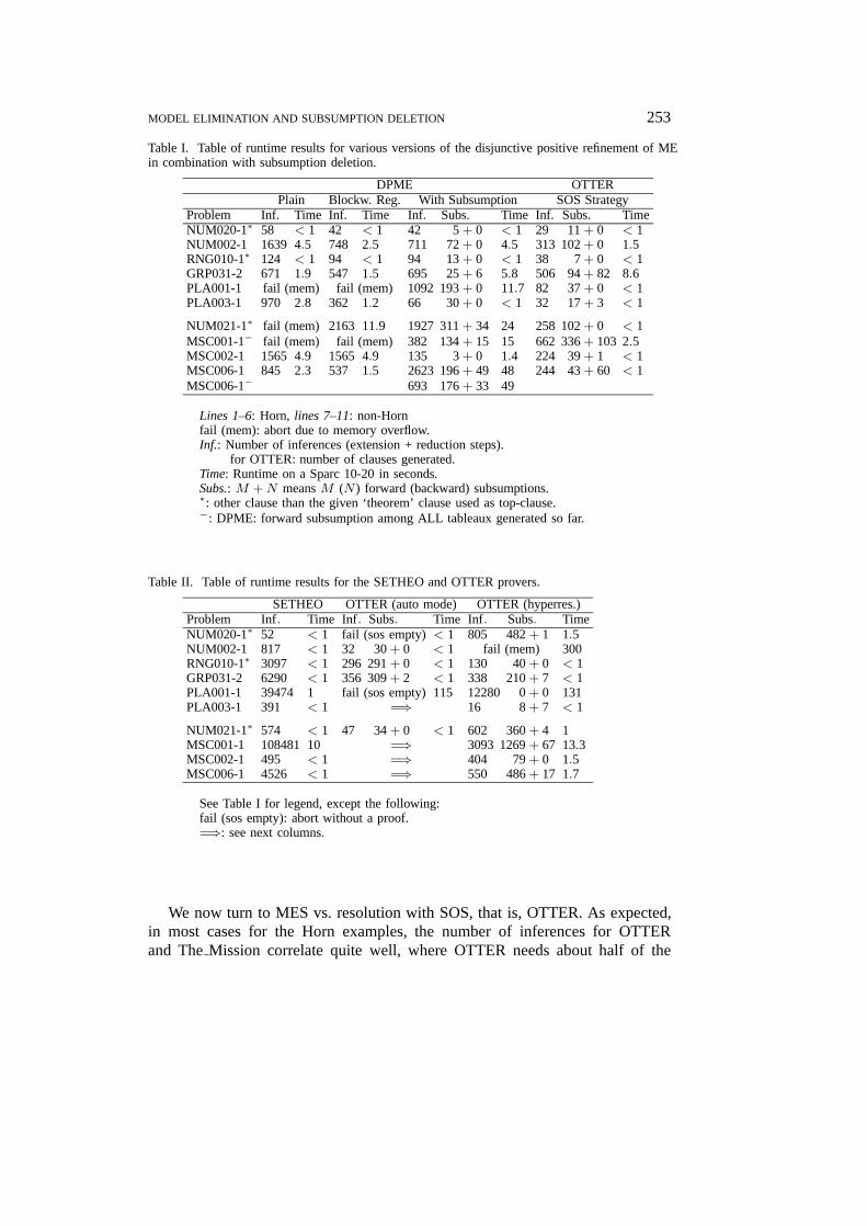
MODEL ELIMINATION AND SUBSUMPTION DELETION 253
Table I. Table of runtime results for various versions of the disjunctive positive refinement of MEin combination with subsumption deletion.
DPME OTTERPlain Blockw. Reg. With Subsumption SOS Strategy
Problem Inf. Time Inf. Time Inf. Subs. Time Inf. Subs. TimeNUM020-1∗ 58 < 1 42 < 1 42 5 + 0 < 1 29 11 + 0 < 1NUM002-1 1639 4.5 748 2.5 711 72 + 0 4.5 313 102 + 0 1.5RNG010-1∗ 124 < 1 94 < 1 94 13 + 0 < 1 38 7 + 0 < 1GRP031-2 671 1.9 547 1.5 695 25 + 6 5.8 506 94 + 82 8.6PLA001-1 fail (mem) fail (mem) 1092 193 + 0 11.7 82 37 + 0 < 1PLA003-1 970 2.8 362 1.2 66 30 + 0 < 1 32 17 + 3 < 1
NUM021-1∗ fail (mem) 2163 11.9 1927 311 + 34 24 258 102 + 0 < 1MSC001-1− fail (mem) fail (mem) 382 134 + 15 15 662 336 + 103 2.5MSC002-1 1565 4.9 1565 4.9 135 3 + 0 1.4 224 39 + 1 < 1MSC006-1 845 2.3 537 1.5 2623 196 + 49 48 244 43 + 60 < 1MSC006-1− 693 176 + 33 49
Lines 1–6: Horn, lines 7–11: non-Hornfail (mem): abort due to memory overflow.Inf.: Number of inferences (extension + reduction steps).
for OTTER: number of clauses generated.Time: Runtime on a Sparc 10-20 in seconds.Subs.: M +N means M (N) forward (backward) subsumptions.∗: other clause than the given ‘theorem’ clause used as top-clause.−: DPME: forward subsumption among ALL tableaux generated so far.
Table II. Table of runtime results for the SETHEO and OTTER provers.
SETHEO OTTER (auto mode) OTTER (hyperres.)Problem Inf. Time Inf. Subs. Time Inf. Subs. TimeNUM020-1∗ 52 < 1 fail (sos empty) < 1 805 482 + 1 1.5NUM002-1 817 < 1 32 30 + 0 < 1 fail (mem) 300RNG010-1∗ 3097 < 1 296 291 + 0 < 1 130 40 + 0 < 1GRP031-2 6290 < 1 356 309 + 2 < 1 338 210 + 7 < 1PLA001-1 39474 1 fail (sos empty) 115 12280 0 + 0 131PLA003-1 391 < 1 =⇒ 16 8 + 7 < 1
NUM021-1∗ 574 < 1 47 34 + 0 < 1 602 360 + 4 1MSC001-1 108481 10 =⇒ 3093 1269 + 67 13.3MSC002-1 495 < 1 =⇒ 404 79 + 0 1.5MSC006-1 4526 < 1 =⇒ 550 486 + 17 1.7
See Table I for legend, except the following:fail (sos empty): abort without a proof.=⇒: see next columns.
We now turn to MES vs. resolution with SOS, that is, OTTER. As expected,in most cases for the Horn examples, the number of inferences for OTTERand The Mission correlate quite well, where OTTER needs about half of the
JARSWB1.tex; 15/08/1997; 11:41; v.7; p.49

254 PETER BAUMGARTNER AND STEFAN BRUNING
inferences of The Mission to find the proof. We attribute this result to a moresophisticated selection of the ‘next’ clause to be processed. For non-Horn inputclause sets there are examples where MES needs fewer inferences than doesOTTER. We consider this as an advantage of MES. Finally, Table II contain thedata for SETHEO (Letz et al., 1992), a high inference rate model eliminationprover, and OTTER.
We used version 3.2. of SETHEO in standard flag setting. This setting includesclause set preprocessing (reordering) and employs regularity, subsumption, andtautology constraints. We switched off ‘folding up’ (a generalized form of fac-torization), since it did not improve the results significantly.
Since SETHEO enumerates derivation by iterative deepening (w.r.t. tableaudepth), and all but the very last tried derivation is without success, a huge num-ber of inferences (extension plus reduction steps) results. In the extreme case(MSC001-1−) about 300 times as many inferences were necessary.
When run in ‘auto’ mode, OTTER analyzes the input clause set and determinesinference rules and strategies by itself (columns 4, 5, and 6 in Table II). TheNUM, RNG, and GRP examples contain equality. OTTER chooses an efficientcompletion-based equality handling and thus has no difficulties, if it finds a proof(see NUM020-1).
An interesting case is PLA001-1, a planning problem due to D. Plaisted.OTTER chooses hyperresolution, which, however, does not result in a proof. Thisfailure is probably because of an incomplete automatically determined weightingfunction. When OTTER is set to hyperresolution manually, a proof can be found,although this example is better suited for more goal-oriented calculi like ME.
To conclude, we think that subsumption is a promising direction to improveModel Elimination–based theorem proving.T-Context Check. The T-Context Check has been integrated into a prototypicalimplementation of DPME. This proof system additionally allows for checking(full) blockwise regularity in order to relate the pruning power of the T-ContextCheck to the one of blockwise regularity. Since the main purpose of our investi-gations was to explore the usefulness of the T-Context Check rather than to builta high-performance system, we used Prolog as the programming language. Afurther simplification resulted from the fact that we restricted our proof systemto local computation rules. This strategy allowed us (as mentioned in note 3) toimplement the T-Context Check in a straightforward way.
Table III summarizes the results. All of them were computed on a Sun SPARC-station 20. The first column contains the names of the used problems. Theyinclude almost all of those that were used for the experiments with The Mission;the additional ones were also taken from the TPTP library (Sutcliffe et al., 1994).The second column indicates the applied search strategy. We found it interestingto employ two different (widely used) search strategies: ‘d’ stands for the usageof an iterative deepening search strategy iterating over the depth of the generatedtableaux, whereas ‘l’ means that the search strategy iterates over the length of
JARSWB1.tex; 15/08/1997; 11:41; v.7; p.50

MODEL ELIMINATION AND SUBSUMPTION DELETION 255
Table III. Table of results for an implementation of DPME in combination with the T-ContextCheck.
Block. Reg. only plus T-Context CheckProblem M. Limit Inf. Time Inf. Time PrunedNUM020-1 l 9 176489 205.1 96219 111.1 4418
d 4 9382 6.0 2447 1.6 45NUM021-1 l 8 47096 77.9 31780 51.6 1409
d 4 10787 8.7 2883 2.3 29NUM002-1 l 7∗ 16897 19.0 16897 19.6 0
d 3∗ 649 0.6 649 0.6 0RNG010-1 l 6 23958 42.7 22978 41.2 220
d 4 35853 63.6 35853 64.4 0GRP031-2 l 7∗ 1871 1.6 1871 1.8 0
d 3∗ 2716 1.9 2716 2.0 0GRP040-3 l 5 10866 25.1 9917 23.2 27
d 3 248168 159.9 246759 158.7 101PLA001-1 l 12∗ >500000 >600 39803 89.9 9409
d 7∗ 6031 7.2 1709 2.3 130PLA003-1 l 7∗ 343 0.8 127 0.3 18
d 7∗ 658 1.0 197 0.3 18COL005-1 l 8 79406 75.1 61491 59.8 13
d 4 248168 156.1 246759 158.1 101LCL105-1 l 14 72257 143.1 69435 140.1 639
d 5 76845 165.9 66700 145.0 810LCL038-1 l 20 131020 254.7 115180 245.8 2106
d 7 >250000 >600 86551 107.7 3598MSC001-1 l 10 12873 38.9 7406 22.6 42
d 6∗ 4911 5.7 2469 3.0 21MSC002-1 l 11∗ 5771 12.7 1625 3.8 20
d 6∗ 777 0.9 244 0.3 6SET012-2 l 7 22764 77.6 22716 77.7 62
d 5 28200 21.5 28200 21.6 0CAT001-1 l 7 103720 278.0 103514 283.7 25
d 4 715823 745.5 715823 754.0 0CAT015-3 l 5 23556 54.5 17644 39.5 366
d 4 >500000 >600 345555 205.7 605
the derivation. The third column contains the maximal tableaux-depth/derivation-length explored by our prover. An additional ‘*’ indicates that a proof was foundat the given limit. The results generated without using the T-Context Check aregiven in the fourth and fifth column. The sixth and seventh column show thecorresponding numbers produced by applying the T-Context Check additionally.Finally, the last column of the table lists the number of derivations that werepruned by the T-Context Check. During our experiments, we always used onlythe given ‘theorem’ clauses (that is, the clauses marked as ‘theorem’ in the TPTPlibrary) as top-clauses, but no other negative clauses.?
? This implies that the results concerning NUM020-1, NUM021-1, and RNG010-1 in Tables Iand III cannot be compared. If another negative clause is used as top-clause, the proofs for these
JARSWB1.tex; 15/08/1997; 11:41; v.7; p.51

256 PETER BAUMGARTNER AND STEFAN BRUNING
To comment on our results, there are some examples that obviously benefitfrom the use of the T-Context Check. For instance, this is the case for PLA001-1 or MSC002-1 were proofs can be found with considerably fewer inferencesteps and time (for comparison, see also the number of inference steps used bySETHEO in Table II). In other cases, where a proof could not be found (withinthe given inference/depth limits) the number of inference steps is reduced to alarge extent (e.g., see NUM020-1 or LCL038-1). These results demonstrate thatblockwise regularity is in many cases not able to cover the T-Context Check.Clearly, there are also examples where the T-Context Check is not very useful;however, the runtime results show that the additional computational overheadwas negligible in all cases.
Summarizing, these experiments demonstrate that a weak variant of subsump-tion deletion (namely, the T-Context Check) can be useful for reducing both infer-ence steps and proof time. A comparison of Tables I and III, however, showsthat the pruning power of subsumption deletion as used in The Mission is in factstronger than the one of the T-Context Check (e.g., see PLA001-1 or MSC002-1).Therefore, it might be interesting to improve the implementation of The Missionto reduce the computational requirements for (full) subsumption deletion. Addi-tionally, it might be worthwhile to think about something ‘between’ the T-ContextCheck and subsumption deletion, that is, an extension of the T-Context Checkthat retains its simplicity (in view of an efficient implementation) and coversmore of the cases where subsumption deletion can be applied successfully.
7. Discussion
In this article we successfully adapted the notion of subsumption known fromresolution-based approaches to Model Elimination. It soon became clear that anapproach comparing entire Model Elimination tableaux by subsumption wouldbe useless. On the other hand, completeness is lost if only the open goals oftableaux without their ancestors (i.e., the frontiers are taken into account).
To overcome these problems, we first introduced a variant of Model Elimi-nation that minimizes ancestor literals. In (Plaisted, 1990), D. Plaisted showedthat it suffices to keep only positive literals as ancestors. This approach obvious-ly allows one to define a larger subsumption relation because only the positiveancestors contained in tableaux have to be obeyed for the subsumption tests. Wefurther improved on this by restricting the ancestor context even more, namelyto those positive literals that stem from disjunctive clauses.? This allows one toignore all positive ancestors that stem from definite clauses. The resulting cal-
theorems can be found fast (0.1, 6.1, and 0.5 seconds, respectively) with the proof system containingthe T-Context Check.? In Section 3.4 we showed that even further restriction to all but one positive literal of a clause
is still complete.
JARSWB1.tex; 15/08/1997; 11:41; v.7; p.52

MODEL ELIMINATION AND SUBSUMPTION DELETION 257
culus, the so-called disjunctive positive refinement of Model Elimination, wasproved to be sound and complete.
With this refinement of Model Elimination at hand, we defined a calculus thatintegrates forward and backward subsumption. This required a new organizationof the proof process: instead of constructing one tableau by nondeterministicallyguessing the inference steps and backtracking on failure, all tableaux that canbe built are stored explicitly. By this we changed Model Elimination from anenumeration procedure into a saturation procedure that allows one to delete allgenerated tableaux that are subsumed by some other generated tableau. It wasproven that using a fair selection strategy, this new calculus, called subsumptionModel Elimination, is sound and complete.
As an alternative to subsumption Model Elimination, we proposed a variantof forward subsumption that, instead of comparing entire frontiers (together withtheir disjunctive positive ancestors), aims at pruning a derivation if a subrefuta-tion for only one open goal would constitute a subrefutation for one of its ances-tors. We proved that the use of the resulting pruning technique, the T-ContextCheck, does not affect completeness of disjunctive positive Model Elimination.Further, we showed that the T-Context Check is an instance of forward sub-sumption (as used in subsumption Model Elimination) in case local computationrules are employed. We also related an important refinement, namely, regularity,to the context check and the use of subsumption. We were able to prove thatweak blockwise regularity is an instance of the T-Context Check and that eachtableau that violates blockwise regularity? is deleted by the use of subsumption.Finally, we proposed a refinement of the T-Context Check which allows one toignore even some of the positive disjunctive ancestors in a tableau by applyinga reachability analysis.
The relations between the investigated refinements of Model Elimination aredepicted in Figure 13. There are three top elements, namely, the forward andbackward subsumption, the blockwise regularity and T∗-Context check, and thedisjunctive and blockwise regular refinement. According to the semantics of the“→’ notation, these are the most restrictive, and hence most attractive, variants.The completeness of the disjunctive and blockwise regular refinement is stillopen. The remaining two variants are incomparable w.r.t. pruning power, butthey both are complete. These are the main results of this paper. These calculiare radically different: the one enumerates tableaux, and the other enumeratesderivations. Hence, we do not prefer the one to the other, and we conclude thatboth of them are interesting.
To illustrate the potential of the proposed refinements, we presented com-prehensive experimental results confirming that, in many cases, search spacesare considerably reduced. In particular, our experiments show that subsumptiondeletion in many cases allows to concentrate on only a few tableaux which can? Recall Definitions 14 and 39 for the difference between blockwise and weak blockwise
regularity.
JARSWB1.tex; 15/08/1997; 11:41; v.7; p.53

258 PETER BAUMGARTNER AND STEFAN BRUNING
Figure 13. Relating the ‘pruning power’ of the various refinements. A relationship ‘A→ B’means that whenever a derivation is pruned by the refinement A, it is also pruned bythe refinement B. Either this relation holds trivially, and in this case the link remainsundecorated, or else the respective result from the text is cited. For trivial links a respectivecompleteness result is stated at the more restrictive refinements, which entail completenessof the refinements below them.
be built with only a few inference steps. Further, the runtimes given in Table IIIshow that weaker variants of subsumption deletion can be implemented veryeasily without resulting in high computational overheads.
Subsumption deletion, however, not only aims at reducing search spaces tofind proofs more easily. Additionally, it is sometimes quite useful to detect that atheorem cannot be proven. In fact, it has been shown in (Bol et al., 1991) that (arestricted variant of) the T-Context Check prunes every infinite Model Elimina-tion derivation of various natural classes of clause sets without function symbols.These classes include Horn-clause sets that do not introduce new variables duringa derivation (the so-called nvi clause sets), and Horn-clause sets that allow atmost one recursive call per clause (the so-called recursion-restricted Horn-clausesets that, for example, include all Horn-clause sets of which all rules have abody with at most one literal).? These results are relevant for the non-Horn case,too, since it happens quite frequently that a subproblem occurring during thederivation from a non-Horn clause set can be proved by using only extension? To achieve the completeness result, one has to assume a selection function that selects the
recursive literal last.
JARSWB1.tex; 15/08/1997; 11:41; v.7; p.54

MODEL ELIMINATION AND SUBSUMPTION DELETION 259
steps because of its structure and the use of the disjunctive positive refinement(and, therefore, this subproblem ‘behaves’ like a Horn clause set).
From Theorem 37 such results can be immediately applied to subsumptionModel Elimination if local computation rules are used. Further, it might be pos-sible to prove much stronger results for subsumption Model Elimination, since(as depicted in Figure 13) the pruning power of forward and backward subsump-tion is stronger than the one of the T-Context Check. This point can be nicelyillustrated by the second clause set (‘equality’) given in Example 26. As we haveshown there, the satisfiability of this clause set can be decided by subsumptionModel Elimination. This is not the case for ordinary Model Elimination augment-ed by the T-Context Check. The T-Context Check allows one only to (roughly)halve the number of applied inference steps but is not able to prune every infinitederivation.
8. Future Work
Equality. As always, much remains to be done. In Example 26 we identified, asan instance of subsumption deletion, situations where extension steps with theequality axioms are unnecessary. It can be expected that the ME calculus withparamodulation can benefit from this observation by identifying correspondingsituations, where paramodulation steps are unnecessary (in particular, with thecumbersome functional reflexive axioms).
Extended Subsumption. It is possible to extend the backward subsumption rule.Suppose in a fair derivation T subsumes T ′. Backward subsumption can beextended to delete not only T , but also all tableaux that are generated from T ,except for T ′. In order to be complete, forward subsumption has to be restrictedto preceding tableaux. This calculus has to be defined formally.
Instantiations. A problem that we have not tackled in this paper is the abilityto take into account instantiations of open goals which are caused by furtherderivation steps. Even if some tableau T does not subsume another tableau T ′,this might be the case if substitutions are considered that are applied to T ′
by additional extension or reduction steps. In fact, it has been illustrated in(Bruning, 1994) that taking such additional instantiations into account can resultin a considerable strengthening of the pruning power.
EXAMPLE 46. Consider a clause set containing the following clauses.
(1) q(a) ← r(b)(2) q(c) ← p(a), q(z)(3) p(y) ← q(c)(4) ← p(x), q(x).
Suppose that, after clause (4) o is selected for an initialization step, a derivationD proceeds by applying three extension steps selecting the open goals ¬p(x),
JARSWB1.tex; 15/08/1997; 11:41; v.7; p.55

260 PETER BAUMGARTNER AND STEFAN BRUNING
¬q(c) and ¬q(z) and the clauses (3), (2), and (1), respectively. The generatedsequence of multisets of open goals is
(a) {|¬p(x),¬q(x)|},(b) {|¬q(c),¬q(x)|},(c) {|¬p(a),¬q(z),¬q(x)|},(d) {|¬p(a),¬r(b),¬q(x)|}.
Since none of these multisets subsumes another one, subsumption is not applica-ble (furthermore, the tableau generated by this derivation is not simply subsumedby another tableau that can be constructed by applying different extension steps).However, the variable z occurring in multiset (c) is instantiated to a by the lastextension step. This instantiated multiset is subsumed by multiset (a). Thus, sub-refutations for the goals in (c) that use this last extension step can be directlyapplied to the elements of (a). Hence, D is redundant.
It can be shown that a refined version of the T-Context Check, which allows forconsidering additional substitutions, is able to prune every derivation that violatesfull blockwise regularity. Recall that this is not the case for the T-Context Checkas defined in Section 5.Answer Computing. In (Baumgartner et al., 1995) the restart model eliminationcalculus is used for computing answers. It is demonstrated there that computingan answer for a given problem can be much harder than finding only a refutation(i.e., proving that an answer exists). It would be interesting to investigate thecalculi presented here w.r.t. answer computing.
ACKNOWLEDGMENTS
Thanks to M. Kuhn and B. Thomas who implemented The Mission prover. Fur-ther, we thank A. de Waal for carefully reading a previous version of this paper.Last, but not least, we thank the referees who carefully read the paper and pointedus to numerous improvements.
References
Antoniou, G. and Langetepe, E.: Applying SLD-resolution to a class of non-Horn logic programs,Bulletin of the IGPL 2(2) (1994), 231–243.
Astrachan, O. L. and Stickel, M. E.: Caching and lemmaizing in model elimination theorem provers,in D. Kapur (ed.), Proc. Conf. Automated Deduction, Vol. 607 Lecture Notes in ArtificialIntelligence, Springer, 1992, pp. 224–238.
Bachmair, L.: Canonical Equational Proofs, Progress in Theoretical Computer Science, Birkhauser,1991.
Baumgartner, P.: Refinements of theory model elimination and a variant without contrapositives,in A. G. Cohn (ed.), 11th European Conference on Artificial Intelligence, ECAI 94, Wiley,1994. (Long version in: Research Report 8/93, University of Koblenz, Institute for ComputerScience, Koblenz, Germany).
Baumgartner, P.: Linear and unit-resulting refutations for Horn theories, J. Automated Reasoning16(3) (1996), 241–319.
JARSWB1.tex; 15/08/1997; 11:41; v.7; p.56

MODEL ELIMINATION AND SUBSUMPTION DELETION 261
Baumgartner, P. and Furbach, U.: Consolution as a framework for comparing calculi, J. SymbolicComputation 16(5) (1993).
Baumgartner, P. and Furbach, U.: Model elimination without contrapositives and its application toPTTP, J. Automated Reasoning 13 (1994), 339–359. Short version in: Proceedings of CADE-12, Springer LNAI 814, 1994, pp. 87–101.
Baumgartner, P. and Furbach, U.: PROTEIN: A PROver with a Theory Extension Interface,in A. Bundy (ed.), Automated Deduction – CADE-12, Vol. 814 Lecture Notes inArtificial Intelligence, Springer, 1994, pp. 769–773. Available on the WWW, URLhttp://www.uni-koblenz.de/ag-ki/Systems/PROTEIN/.
Baumgartner, P., Furbach, U. and Stolzenburg, F.: Model elimination, logic programming andcomputing answers, in 14th Int. Joint Conference on Artificial Intelligence (IJCAI 95), Vol. 1,1995. (Long version in Research Report 1/95, University of Koblenz, Germany. To appear inArtificial Intelligence).
Besnard, P.: On Infinite Loops in Logic Programming, Technical Report 488, IRISA, Rennes,France, 1989.
Bibel, W. and Buchberger, B.: Towards a connection machine for logical inference, Future Gener-ations Computer Systems Journal 1(3) (1985), 177–188.
Blasius, K., Eisinger, N., Siekmann, J., Smolka, G., Herold, A. and Walther, C.: The Markgraf Karlrefutation procedure, in International Joint Conference on Artificial Intelligence, Los Altos, CA.Morgan Kaufmann, 1981, pp. 511–518.
Bol, R. N., Apt, K. R. and Klop, J. W.: An analysis of loop checking mechanisms for logicprogramming, J. Theoret. Computer Science 86 (1991), 35–79.
Bruning, S.: On loop detection in connection calculi, in G. Gottlob, A. Leitsch, and D. Mundici(eds), Proc. Kurt Godel Colloquium, Springer, 1993, pp. 144–151.
Bruning, S.: Techniques for avoiding redundancy in theorem proving based on the connectionmethod, PhD Thesis, TH Darmstadt, 1994.
Chang, C. L. and Lee, R. C.-T: Symbolic Logic and Mechanical Theorem Proving, Academic Press,New York, 1973.
Fronhofer, B.: On refinements of the connection method, in J. Demetrovics, G. Katona, and A. Salo-maa (eds), Algebra, Combinatorics and Logic in Computer Science, North Holland, 1985,pp. 391–401.
Fronhofer, B. and Caferra, R.: Memorization of literals: An enhancement of the connection method,Technical report, Institut fur Informatik, Technische Universitat Munchen, 1988.
Gallier, J.: Logic for Computer Science: Foundations of Automatic Theorem Proving, Wiley, 1987.Graf, P.: Extended path-indexing, in Automated Deduction – CADE 12, Vol. 814 Lecture Notes in
Artifical Intelligence, Springer, 1994.Letz, R.: First-order calculi and proof procedures for automated deduction, PhD Thesis, TH Darm-
stadt, 1993.Letz, R., Mayr, K. and Goller, Ch.: Controlled integrations of the cut rule into connection tableau
calculi, J. Automated Reasoning 13(3) (1994), 297–338. Special Issue on Automated Reasoningwith Analytic Tableaux.
Letz, R., Schumann, J., Bayerl, S. and Bibel, W.: SETHEO: A high-performance theorem prover,J. Automated Reasoning 8(2) (1992), 183–212.
Lloyd, J. W: Foundations of Logic Programming, 2nd edition, Springer, 1987.Loveland, D.: Mechanical theorem proving by model elimination, JACM 15(2) (1968).Loveland, D.: Automated Theorem Proving - A Logical Basis, North Holland, 1978.Loveland, D. W.: Mechanical theorem proving by model elimination, J. ACM 15 (1986), 236–251.Loveland, D. W. and Reed, D. W.: Near-Horn Prolog and the ancestry family of proof procedures,
Annals of Mathematics and Artificial Intelligence 14 (1995).Mayr, K.: Link deletion in model elimination, in R. Hahnle, P. Baumgartner and J. Posegga (eds),
Theorem Proving with Analytic Tableaux and Related Methods, Vol. 918 Lecture Notes inArtificial Intelligence, Springer, 1995, pp. 169–184.
Neugebauer, G.: From Horn clauses to first order logic: A graceful ascent, Technical Report AIDA–92–21, FG Intellektik, FB Informatik, TH Darmstadt, 1992.
JARSWB1.tex; 15/08/1997; 11:41; v.7; p.57

262 PETER BAUMGARTNER AND STEFAN BRUNING
Overbeek, R. and Wos, L.: Subsumption, a sometimes undervalued procedure, in J.-L. Lassez andG. Plotkin (eds), Festschrift for J. A. Robinson, MIT Press, 1991, pp. 3–40.
Plaisted, D.: A sequent-style model elimination strategy and a positive refinement, J. AutomatedReasoning 4(6) (1990), 389–402.
Poole, D. and Goebel, R.: On eliminating loops in Prolog, Sigplan Notices 20(8) (1985), 38–40.Reed, D. W. and Loveland, D. W.: A comparison of three Prolog extensions, J. Logic Programming
12(1) (1992), 25–50.Robinson, G. A. and Wos, L.: Paramodulation and theorem proving in first-order theories with
equality, in R. Meltzer and D. Mitchie (eds), Machine Intelligence 4, Edinburgh UniversityPress, 1969, pp. 135–150.
Spencer, B.: Avoiding duplicate proofs with the foothold refinement, Annals of Math. and ArtificialIntelligence 12 (1994), 117–140.
Stickel, M. E.: A Prolog technology theorem prover, New Generation Computing 2(4) (1984),371–383.
Stickel, M.: A Prolog technology theorem prover: Implementation by an extended Prolog compiler,J. Automated Reasoning 4 (1988), 353–380.
Sutcliffe, G.: A linear deduction system with integrated semantic guidance, PhD Thesis, Universityof Western Australia, 1992.
Sutcliffe, G.: Linear-input subset analysis, in D. Kapur (ed.), Proceedings of the Conference onAutomated Deduction, Springer, 1992, pp. 268–280.
Sutcliffe, G., Suttner, Ch. and Yemenis, T.: The TPTP problem library, in A. Bundy (ed.), Proc.Conf. on Automated Deduction, Vol. 814 Lecture Notes in Artificial Intelligence, Springer,1994, pp. 252–266.
van de Riet, R. P.: An overview and appraisal of the fifth generation computer system project,Future Generation Computer Systems Journal 9 (1993), 83–103.
Wos, L., Winker, S., McCune, W., Overbeek, R., Lusk, E. and Stevens, R.: Automated reason-ing contributes to mathematics and logic, in M. E. Stickel (ed.), Proc. Conf. on AutomatedDeduction, Springer, 1990, pp. 485–499.
JARSWB1.tex; 15/08/1997; 11:41; v.7; p.58